ANALYSIS OFRESULTS,

FORECASTINGAND CORPORATE PLANNING

1985 DISCUSSION PAPER PROGRAM

Presented May 8-11, 1985 Boca Raton, Florida .

CASUALTYACTUARIAL SOCIETY ORGAhVZED 1914

ANALYSIS OF RESULTS, FORECASTING AND CORPORATE PLANNING

These papers have been prepared in response to a call for papers by the Casualty Actuarial Society to provide discussion material for its Spring meeting, May 8-11, 1985, in Boca Raton, Florida.

Actuaries have been becoming increasingly involved in all aspects of corporate planning and are often called upon to explain results to people without technical or insurance backgrounds. It is hoped that these papers will serve as the basis for a stimulating discussion at the Spring meeting while estab- lishing a foundation for further research in these areas.

Committee on Continuing Education

NOTICE

The Casualty Actuarial Society is not responsible for statements or opinions expressed in the papers in this publication. These papers have not been reviewed by theCAS Committee on Review of Papers.

TABLE OF CONTENTS

Title

Corporate Planning-An Approach for an Emerging Company IreneK.Bass&LarryD.Carr

Crum and Forster Personal Insurance

Branch Office Profit Measurement for Property - Liability Insurers Robert P. Butsic

Fireman’s Fund Insurance Companics

A Formal Approach to Catastrophe Risk Assessment and Management Karen M. Clark

Commercial Union Insurance Companies

Measuring the Impact of Unreported Premiums on a Reinsurers’ Financial Results DouglasJ. Collins

Tillinghast, Nelson & Warren, Inc.

Bank Accounts as aToo for Retrospective Analysisof Experience on Long-Tail Coverages Claudia S. Forde and

W. James MacCinnitie Tillinghast, Nelson &Warren, Inc.

Page

5-24

2.5-61

62- 103

104- 125

126-139

Title

I Projections of Surplus for Underwriting Strategy William R. Gillam

North American Reinsurance

Interaction ofTotal Return Pricing and Asset Management in a Property/Casualty Company . . . Owen M. Gleeson

General Reinsurance Corporation

Page

140- 171

l72- 194

An Econometric Model of Private Passenger Liability Underwriting Results RichardM. Jaeger and

Christopher J Wachter 195-219

Insurance Services Office, Inc.

Contingency Margins in Rate Calculations Steven G. Lchmann State Farm Mutual Automobile Insurance Company

220-242

Budget Variances in Insurance Company Operations George M. Levine

National Council on Compensation Insurance

243-267

B Pricing, Planning and Monitoring of Results: An Integrated View . Stephen P. Lowe 268-286

Tillinghast, Nelson&Warren, Inc.

Title

The Cash Flow of a Retrospective

Page

Rating Plan Glenn Meyers The University of Iowa

287-310

Application of Principles, Philosophies and Procedures of Corporate Planning to Insurance Companies Mary Lou O’Neil 311-331

New .Jersey Department of Insurance

Measuring Division Operating Profitability DavidSkumick

Argonaut Insurance Company 332-342

q Actuarial Aspects of Financial Reporting Lee M. Smith

Ernst & Whinney 343-372

4 Projecting Calendar Period IBNR and Known Loss Using Reserve Study Results Edward W. Weissner and 373-424

ArthurJ. Beaudoin Prudential Reinsurance Company

TITLE: CORPORATE PLANNING -- AN APPROACH FOR AN EMERGING COMPANY

AUTHORS: Irene K. Bass is Vice President of the U.S. Fire Insurance Company and Actuarial Department head for Crum and Forster Personal Insurance. Prior to joining Crum and Forster, Miss Bass held positions at Commercial Union and Hanseco. She is a Fellow of the Casualty Actuarial Society and a Member of the American Academy of Actuaries. She holds a B.A. in German from Bowling Green State University and an M.S. in mathematics from Northeastern University.

Larry D. Car-r is Senior Vice President and Chief Financial Officer of the U.S. Fire Insurance Company with responsibility for the Underwritina. Actuarial, and Financial and- Planning areas of Crum aid Forster Personal Insurance . He serves as a member of the Board of Directors and Executive Committee of the U. S. Fire Insurance Company. Mr. Carr had extensive experience, at Allstate Insurance Company prior to joining CFPI in 1983. He holds a B.S. in finance from the University of Illinois.

ABSTRACT: A major property-casualty insurance group recently created a separate profit center for personal lines, thereby signaling a new emphasis on these lines. Since the group had been a carrier with primary emphasis on commercial business, the planning process at the personal lines profit center became similar to that of an emerging company: there was little relevant history available to use in order to plan effectively for a very different future.

Because planning at insurance companies is too often separated from field operations -- the very people who must make the plan happen -- we installed a process that is operationally driven.

We therefore developed an approach to premium and loss planning which did not rely on a simple projection of last year's results. The major benefit of this planning process is its lack of dependence on historical information and its explanation of current results in terms of specific components of the plan. We offer to share and discuss this approach to personal lines planning.

-j-

INTRODUCTION

Not too long ago, our insurance group reorganized and created, along

with several commercial lines profit centers, a separate profit

center for personal lines. Traditionally, the group's personal lines

volume was a relatively minor part of its total business,

representing about one-fourth of total premium. As such, there was

no special attention paid to it in the corporate planning process.

The profit center's new management, with its singular responsibility

for personal lines, initiated a planning process with five basic

goals in mind:

1. To build an operationally driven planning system from which the

financial plan would follow

2. To isolate measurements which are controlled -- or at least

influenced -- by line management

3. To insure commitment to the planning process by involving field

management in selecting planned levels of performance

To create a plan optimal for personal lines which would work in

an environment where the historical results would not necessarily

be an accurate predictor of the future

To blend the annual operating and financial plans into the profit

center's strategic plan.

-6

Although the personal lines volume is substantial, this new profit

center is an emerging company in the sense that the past will

probably not be representative of the future. It is also an emerging

company in terms of appointment of agents separately from the

remainder of the corporation, planned growth within the American

agency system, and independently defined goals, objectives, and

marketing strategies.

This paper is intended to illustrate a premium and loss planning

process for a personal lines company in a changing or emerging

environment. Expense planning is an important phase of all planning,

but the scope of this paper will be limited to premiums and losses

only. Our planning process is fairly straightforward in terms of the

mathematical concepts employed. It is not simply a matter of

determining last year's results and then making some estimates for

the coming year. Rather, each component of the premium is analyzed

down to the basic elements, beginning with number of agents and

ending with premium. Likewise, losses are analyzed in their

elementary components of frequency and severity.

In this paper we first offer some background on the difficulties of

planning for an emerging company and obtaining the proper source data

to do a zero-base analysis. Then we discuss the premium and loss

planning methods. Finally, we evaluate what was accomplished in the

planning process.

-7-

BACKGROUND

The operational plan is segmented into three separate but connected

pieces:

- Agent Plan

- Production/Premium Plan

- Losses Plan

These represent the major planning decision areas in which baseline

values and the impact of operational changes must be established.

Charts of the detailed statistical flow are contained in Exhibits

3-5. Once a conceptual understanding of this flow is achieved, four

things are required to plan:

1. Base Data -- the explicit values of the variables in the

equations to get from number of agents to premiums to incurred

losses.

2. Operational Plans -- the expected changes in operating

philosophy, approach, and execution. This information is based

on the continuing analysis of programs and their results and on

management's evaluation of areas where current performance

requires improvement.

3. Quantification of Plans -- the specific numerical ramifications

of operational plans. If operational plans are carefully

-8-

prepared within a structured framework and are based on objective

evaluation of data, this quantification is often completed in the

operational analysis process. If not, basic analysis to quantify

operational changes is required. This is a critical step in that

it allows management to see whether planned activity will achieve

desired results. This is the fundamental reason for planning.

4. External or Extraordinary Factors -- the impact of any

anticipated changes in external factors. These factors must also

be isolated and considered. Extraordinary weather-related claim

volume in the historical data is an example of this kind of

influence.

The planning model -- composed of the variables in the planning

equations and the equations themselves -- is fundamentally important

in that it allows for measuring the impact of planned actions on

operating results.

Because this profit center is a personal lines operation emerging

from a predominantly commercial lines environment, it is not

surprising that the kind of data we sought was not available from

readily accessible sources. Therefore, the acquisition of base data

was the most difficult part of the process and certainly the most

time-consuming. Annual Statement and Insurance Expense Exhibit data

do not provide sufficient detail for an operationally driven plan.

New and renewal production, frequency, and severity data just do not

exist in these sources. At our company, it also required compromises

regarding the desired breakdown of data by line of business.

-9-

It became obvious that ideal information was not to be found, so we

settled on the following compromise prioritization.

1. Necessary data would become available over time, so the most

important aspect was the integrity of the statistical flow. When

a source of net written premium by desired line of business did

not have a companion policy count report, we chose a summary

level that preserved the desired statistical flow. More

important than planning by ideal product line, it was essential

to begin installing the operational discipline, involving field

management in the planning process, and planning in a fundamental

step-by-step method that would permit isolating the sources of

variance from plan.

2. Because of the need to focus on markets, results, constraints,

and opportunities on a state-by-state basis, higher levels of

product summarization were accepted than was desired. For

example, homeowners was handled as one line rather than

separating it into owner, renter, and condo business.

3. When all else failed and source data was not to be found, prior

experience, judgment, and estimates were often used.

We often used sources for purposes other than their original intent.

Agent counts were developed from a monthly report used to check

validity of mailing lists. New business production and renewal

ratios were derived by an elaborate manipulation of in-force policy

counts and cancellation activity. New business and renewal premiums

-lO-

were generated from reports originally prepared to measure processing

through the underwriting department. Claim counts -- and,

ultimately, frequency and severity -- were completed using claim

department workload reports.

STATISTICAL MODEL

The premium planning process is outlined on Exhibits 1-4. Loss

planning is outlined on Exhibit 5.

Agents

The process begins with the agent plan and develops into premium on a

line of business basis.

Because of the radically changing environment in the company, we

could not begin with last year's premiums and project forward. We

knew we would be cancelling personal lines contracts for many agents

who were commercial lines oriented and appointing new agents for

personal lines only. Since this activity is part of regional

management's objectives, it made sense to involve them in the

quantification of the number of active agents and to have this item

become a measurable variable in the plan. This is an example of

field management involvement and of the isolation of measurements

that are controlled or influenced by them.

-ll-

Production

Average number of new policies per agent was calculated by line of

business from prior years, and an estimate for the ensuing year was

based on several assumptions. This number would be very different

from prior years because now we would be dealing with agents who are

primarily personal lines agents and who would use our company as a

major market, Agency management would be directed at personal lines

only, and major changes in pricing would shift our competitive

position.

By multiplying average number of agents by number of new policies we

obtained the total number of new policies issued for each line

(Exhibit 1). But renewals also had to be calculated. The prior

year's policies (which become available for renewal this year) were

multiplied by a renewal ratio to obtain the number of renewal

policies issued (Exhibit 2). Careful analysis of the renewal ratio

was necessary since the expected termination of some agents and the

planned re-underwriting programs would most likely cause this ratio

to drop. At the same time, improved policy service and changes in

the mix of business would tend to increase the renewal ratio.

Premium

The next step starts with number of policies issued and ends with

the net written premium (Exhibit 3). New policies must be handled

separately from renewal policies when estimating the average written

premium by line of business. New business, given the thrust to

-12-

appoint primarily personal lines agents and to penetrate a different

market sector, should have a significantly different average premium

from prior period business that will be renewing. For example, an

effort to write many more homes of high value will cause the average

premium to be much higher.

Even the average renewal premium might be very different from prior

years. If, as in the prior example, an effort to penetrate the high-

value homeowners market is coupled with competitive pricing in that

segment, changes in homeowners relativity curves may greatly increase

the premiums charged for low-valued dwellings. Re-underwriting and a

campaign to insure to value may also increase these averages. In our

plan, field management input along with information from the pricing

actuaries was needed to quantify this variable.

Gross written premium is obtained by multiplying the number of

policies issued by the average premium separately for new and renewal

policies (Exhibit 3). Endorsement premium is loaded by means of a

factor and the remainder of the steps leading to net written premium

are straightforward.

Earned premium and policies in force are important by-products of the

statistical flow (Exhibit 4). Neither is planned directly: they flow

from the numbers being generated by the internal relationships of the

model. By developing a historical relationship between formula

earned premium (l/24 of current month's written premium plus l/12 of

prior eleven months' written, plus l/24 of twelfth prior month's

written) and actual monthly earned premium, a clear pattern should

-13-

develop which will establish an appropriate relationship between

formula and actual earned premium (Exhibit 4).

At this point in the flow, developing the earned premium involves

only selecting an appropriate earned premium compensating factor and

doing the arithmetic. Policies in force (new and renewal separately)

are arrived at by accumulating all of the policies that could be in

force from the prior 12 months' policies issued and applying an

appropriate termination rate.

Losses

Once the premium plan is complete, the generation of incurred losses

essentially flows out of a continuation of the logic. Policies in

force become the base against which frequency ratios (new business

separately from renewals) are applied to arrive at claim counts

(Exhibit 5). It is important that the assumptions about changes in

the agency force, market focus, and underwriting rules be carried

through to frequency selection. Otherwise, loss ratios will be

distorted.

Claim counts can then be multiplied by an appropriate severity to

arrive at losses (Exhibit 5). A number of different approaches are

possible here but, essentially, historical levels are modified to

reflect expected changes in average claim costs due to inflation,

changes in mix of business, limits, deductible, etc. The

effectiveness of the claims department must also be reflected. IBNR

reserve changes can then be added to incurred losses before arriving

at the final loss ratio.

-14-

It is important to recognize that the various operational action

plans are quantified in very different ways in the development of the

plan. A careful evaluation of the loss ratio will help insure that

the impact of various operational plans is consistently assessed in

determining both premium-related and loss-related base data,

EVALUATIOH

A number of legitimate questions seem obvious. With all the

compromises in data, did the process really accomplish anything? Was

the cost in time and effort appropriate in the completely manual

environment? In short, was it worth the effort? Our answer is an

unequivocal, "Yes," because several very important baselines were

established, as discussed below.

1. A base of information was developed.

2. Management became more in touch with the company's expected

results more quickly than it would have without the planning

process.

3. An operationally based planning process was installed. Accepting

that the first plan would be the worst, we decided it was

important to install the process in order to begin its evolution.

We could not have waited another year to begin establishing those

disciplines and thought processes.

-15-

4. The planning process clearly established the relationship between

functional management and results. Operational actions -- the

changes, refinements, and corrections -- are necessary if results

are to change.

5. A set of performance benchmarks were established. They could

have been established in a number of other less time-consuming

ways. But the advantage of this approach is that when actual net

written premiums or incurred losses are different from plan, the

source of the difference can be specifically identified and

evaluated. From an informed perspective, management can then

decide to accept the variance or take action to correct it.

CONCEPTUAL MODEL

Critical questions to ask in an operationally based planning process

include:

Market Direction -- Will there be any changes in products, geographic

focus, or target market segments? Will there be changes in the

relationship with agents such as new profit-sharing agreements,

increased or decreased leverage, or an agency force restructuring?

All of these areas could impact assumptions about agents,

productivity, renewal trends, average premium, retention, losses, and

expenses.

-16-

Pricing Philosophy -- Are there going to be changes in price,

competitiveness, or rating schemes to attract certain risks? These

will also impact nearly all parts of the statistical flow.

Underwriting Approach -- Will any changes occur in underwriting rules

which could impact production and average premiums as well as losses?

Changes in emphasis on policy limits, deductibles, or sale of

optional coverages should also be carried thrbugh to the numbers

selected. It. is important to evaluate the impact of past

underwriting decisions that could be "cycling through" their period

of impact, e.g., a re-underwriting program begun in the middle of the

prior year.

Level of Service -- Strong correlations exist between retention and .

the level of policyholder/claim service. What will be the impact of

anticipated changes in level of service whi&h should be considered in

developing renewal and retention levels and changes?

Claims Handling Practices -- How will opening and closing practices,

different emphasis on case reserve adequacy, clearing backlogs, etc.,

influence both frequency and severity measurements?

Once a consensus on these five areas is achieved, only one conceptual

step remains: environmental issues need to be examined. Inflation,

unemployment, housing starts and car sales, trends in miles driven,

gasoline prices, and so on, all impact key planning variables. So,

too, do the actions of competitors, regulators, and legislators as

-17-

their collective modifications of the environment influence the

effectiveness of our actions.

At this point, the truly difficult part of planning is finished. The

remaining work involves, simply, a translation of these operational

and environmental conclusions into statistical impact. It is at this

point that the planner needs extraordinary discipline. There will be

times when, after all the work is completed, the results are

unsatisfactory -- management can't live with the bottom line.

An easy way to correct this situation is simply to change a number.

If this happens, the entire planning process is invalidated and

displeasure with planned performance quickly becomes dismay over

actual results. When unacceptable results are projected in the

planning process, only two valid actions can be taken. First, the

translation of concepts to numbers should be rechecked. Any mistakes

should be corrected and the numbers recalculated. If this does not

correct the problem of unacceptable results, management must return

to its basic assumptions about operations and modify them to achieve

acceptable results.

Only in this way is it possible to arrive at financial plans based on

sound operating decisions. Only with this detailed approach can the

future sources of variance be isolated and corrected.

-18-

Discussion Questions

1. If results are different from plan, does this method allow one to

identify the cause of the variation? Does it pinpoint the cause

sufficiently for management to take proper corrective action?

2. Is this approach adaptable to planning in the commercial lines

environment?

3. Is an operationally focused, detailed plan really needed in the

insurance industry?

4. What sort of controls are necessary to insure the integrity of

the plan?

5. Will this approach be effective for an emerging company or does

it require an established company "culture"?

-19-

Exhibit 1

NEW PRODUCTION

-_--m-e--- -- I I ; Average # Of Agents i L---- ------ -J

X

I Average Policies Per Agent , I I ---------------’

Prepared by line of business

-2o-

Exhibit 2

RENEWAL PRODUCTION

---------------------- t 7

Prior Year I 1 New Policies Issued 1 I i I ---------------------- J

+

1 t

------------------------. I

t Prior Year

, Renewal Policies Issued I .------------------------

Renewal Policies Issued

Prepared by line of business

-21-

PREMIUM Exhibit 3

X _--------- e-m I I New I 1 Average Premium I _-_--- -----

X -_---- --------

f I

Renewal I Average Premium I

----- -7----

Endorsements

7--- ---- -- “7

[Cancellation Ratio: t I

------_-a I f Reinsurance Ratio I I ----_ T------!

Prepared by line of business

-22-

EARNED PREMIUM AND

POLICIES IN FORCE*

1 I

I *'Formula" Earned I

12 Month Moving Policies Issued I

X X

r- --------w

t Earned Premium I

I I !

Compensating , I I -----_-_

r- --------I iPolicies in Ibrce/i , Policies Issued

Retention Ratio 1 c I m-m- ---.4

Prepared by line of business

*Policies in force calculated separately for new and renewal

-23-

LOSSES Exhibit 5

1 Policies In Force 1

X r------------, I Proportion of Coverages I

I (auto only)** I - ----- I

+

-__-__

Coverages in Force

X --- FFrequency 7 I ------I

X l- -----l I Severity I i-----J

I IBNR I I

/Total Losses 1

Earned Premiu

&I Loss Ratio

Prepared by Line of Business **Prepared by Coverage for Auto

-24-

BRANCH OFFICE PROFIT &BASIJREMENT FOR PROPERTY-LIABILITY INSURERS

Robert P. Butsic

Biographical Sketch

Current employer is Fireman's Fund Insurance Co.; prior affiliation was with CNA Insurance from 1969-1979. Earned BA in Mathematics in 1967 and MBA (Finance) in 1978, both from the University of Chicago. Associate in Society of Actuaries, 1975; Member of American Academy of Actuaries. Wrote papers for previous CAS Call Paper programs in 1979 ("Risk and Return for Property-Casualty Insurers") and 1981 ("The Effect of Inflation on Losses and Premiums for Property-Liability Insurers").

Abstract

Effective measurement of financial performance for individual branch offices is hindered by two major problems. The first is an appropriate definition of profit; this is addressed through an economic-value accounting method which minimizes distortions due to the timing of income recognition. Return on equity is the basic profitability gauge used to compare results between profit centers. The second problem is that, in comparing results between branches, different levels of risk will produce an uneven chance of error in measuring true performance vs. reported results. This problem is addressed through techniques which equalize systematic risk (by implying an equity value) and non-systematic risk (through internal reinsurance), for each branch. To develop the internal reinsurance concept, a Poisson claim frequency and a Pareto claim severity model is constructed. Finally, in order to recognize the credibility of each profit center's actual experience, a canpromise is made to the equal-variance prin- ciple. The analysis concludes that branch office profit measurement is best served when the branch network has minimal variation in size and product mix.

-25-

BRANCH OFFICE PROFIT MEASUREMENT FOR PROPERTY-LIABILITY INSURERS

-26-

The insurance industry is presently becoming less regulated, creating an

increasingly competitive long-term environment. To effectively meet the

challenge posed by this new climate, insurers must strengthen their marketing and

get closer to the consumer. Consequently, a strong branch office network is

needed in order to cope with the variety and complexity of local conditions.

A major factor in the development of a viable branch office organization is the

principle that each branch is completely responsible for Its own contribution to

corporate profits. Hence, the profit center concept. Given the objective to

drive corporate profits from the sub-units which are held accountable, an

appropriate tool for measuring performance must be used.

The purpose of this paper, then, is to outline a general approach for measuring

the performance of individual profit centers comprising a property-casualty

company. The methods presented here could apply to line of business or regional

definitions of “profit center”, but it dll be most useful to think of a profit

center as a branch office.

The paper focuses on the aspects of profit measurement and presents methods

which equalize both systematic and purely random variation in profit center

results. Other Important aspects of profit measurement, including the accounting

treatment, are developed in lesser detail. Many of the thoughts presented here

have wolved wer time at the writer’s own company and are now being brought to a

practical application In its management reports.

-27-

PROFIT I%- NT IW PEOPERlY-CA!XJALT’f INSRAIKE

Corporate Profitability

Before addressing the profitability measurement of individual profit centers one

must first define an appropriate yardstick for the corporation as a whole. For

this important concept we will choose return on equity, or ROE for short. This

measure is commonly used for other industries, and represents the return to an

investor in the corporation (for further background on this topic, see references

141, 181 and [lol).

Although ROE is a simple concept, it must be carefully defined. The accounting

conventions used must be suitable for performance measurement over a reasonable

time frame such as a month, quarter or year. Stated differently, management

reports should encourage behavior which will tend to maximize the value of the

firm.

The return on equity measure can be separated into two components: net income

(the numerator> and equity (the denominator).

Net income must reflect, to the extent possible, the current impact of all future

transactions related to the premium earned in the current period. This means

that:

1. Accident-period accounting is used, with all losses, premiums,

expenses and dividends continually being restated as better

estimates of their ultimate values become known.

-2%

2. All future investment income earned on cash flows arising from

the current period must be recognized in the period. The usual

device for collapsing an income stream is net present value.

3. The future cash flows are taken to present value using a market

interest rate, and not the portfolfo rate. It should be noted

that the appropriate rate for corporate performance measurement

may differ from that for profit centers, due to the separation of

responsibility for investment and underwriting risk.

Equity, in a similar fashion, must be adjusted to reflect the above timing of

income:

1. All assets must be evaluated at market prices and all liabilities

must be discounted to present value (i.e., the market price in a

portfolio reinsurance transaction).

2. Otherwise, normal GAAP accounting for equity should be used.

The preceding concepts attempt to recognize what is bown in the accounting

literature (see Lev [SJ) a8 economic income -- the anticipated consequences of

current decisions are directly reflected in current earnings. The notion of

economic income can be further explained by a numerical example. Assume that a

miniature “company” is formed under the following circumstances:

1. An annual policy of $100 is written on January 1, 1985.

-29-

2. A single claim of $68.20 occurs on January 1, 1985 and is paid

over three years, as indicated in the following cash flow

schedule.

3. Cash transactions occur on January 1 of each year; the last loss

payment occurs in 1987.

4. Cash is invested at a yield of 10% per year.

5. All cash flows are certain.

6. There are no income taxes applicable.

7. Capital of $50 cash (initial equity) is available on December 31,

1984.

8. Expenses of $35 are paid on January 1, 1985.

The cash flows are shown below:

Cash Flow Schedule

Premium Losses

l/l/85 L/1/85 l/1/86 l/1/87 Total Present Value - - -

100 100 100 0 -44 -24.2 -68.2 -60

Expenses -35 -35 -35 Total 65 -44 -24.2 -3.2 5

Here we see that the value of the policy to us at the time the premium was

written is $5.00. Under economic-value accounting, the balance sheet would look

like:

-3o-

Balance Sheet: Econanic Value

1984 1985 1986 1987 12/31 l/l 12/31 111 12131 -iTi- ---- -

Assets 50.00 115.00 126.50 82.50 90.75 66.55 Loss Reserve 0 60.00 66*00 22.00 24.20 0 Eiquity 50.00 55.00 60.50 60.50 66.55 66.55 - Pres. Value (l/1/85) 50.00 55.00 55.00 55.00 55.00 55.00

The loss reserve here equals the present value of unpaid losses. Notice that

beginning l/1/85, the present value of equity is always $55.00, because no addi-

tional income is generated by the future cash flows arising from the insurance

operation (as opposed to re-investment of equity):

Income Statement: Economic Value

Underwriting Gain Investment Income - Loss Reserves Net Income - Insurance Operation

Investment Income - Equity

Net Income - Total

1985 1986 Total

-1 .oo -2.20 -3.20 6.00 2.20 8.20

5.00 0 5.00

5.50 6.05 11.55

10.50 6.05 16.55

This tabulation clearly shows that all income arising from the policy is recorded -

in 1985, when the premium is earned. For comparison, the traditional accounting

method would give the following balance sheet end income statement:

-31-

Balance Sheet: Traditional Accounting

Assets

1984 1985 12/31

1986 1987 l/l 12/31 PI_ l/l 12131 -iT

50.00 115.00 --

126.50 82.50 90.75 66.55 Loss Reserve 0 68.20 68.20 24.20 24.20 0 Equity 50.00 46.80 58.30 58.30 66.55 66.55 - Pres. Value (l/1/85) 50.00 46.80 53.00 53.00 55.00 55.00

Income Statement: Traditional Accounting

1985 1986 Underwriting Gain

- - -3.20 0

Investment Income - Loss Reserves 6.82 2.42 Net Income - Insurance Operation 3.62 2.42

Investment Income - Equity 4.68 5.83

Net Income - Total 8.30 8.25

Total -3.20

9.24 6.04

10.51

16.55

Notice that by the end of 1986 (a moment before the last cash transaction on

l/1/87) the accumulated equity is equivalent under either accounting method.

However, the timing of income recognition differs dramatically.

The preceding example illustrates some fundamental ideas which can be developed

more fully. The first is the concept of the total profit margin, or TPM. In

economic valuation, the issuance of the $100 policy created an instant “profit”

of $5; we are indifferent to selling the policy or accepting $5 in cash. This

total profit brought to present value is 5% of premium, hence a 5% total profit

margin.

The second is the economic return on equity. We started with $50 of equity and

one year later the economic value of the mini-enterprise is $60.50, yielding a

21% ROE.

-32-

More compactly, the ROE can bs represented by

(1) 1 + R = (1 + I)(1 + km),

where R denotes the (economic) return on equity, i the market (riskless) interest

rate, k the premium divided by initial equity, and m the total profit margin. To

verify the preceding example, we get 1 + R = l.l[l + 2C.0511 = 1.21.

Although traditional accounting may provide a reasonable means of aggregate

performance measurement for an insurer under conditions of stable growth,

interest rates and product mix, It can fail miserably at the individual profit

center level due to more severe timing distortions of income recognition (for

example, individual case reserve changes on prior period losses can be dramatic

for a single branch).

-33-

?RODUCT LINR PROFIT HMSIPPIIENT

Raving established the economic return on equity evaluation approach as a viable

aggregate profitability measurement, its application must be extended to

individual product lines.

Relative Risk

Although ROE is a good profit measure, there are problems associated with its use

in comparing insurance (and other types of) companies or product lines. These

difficulties arise because the amount of risk associated with an ROE measure

varies significantly by line of business. For example, given the option of

buying stock in a medical malpractice insurer with an expected ROE of 20% or in a

personal lines company of the same size having a 15% ROE, it is unclear what

choice to make. The medical malpractice insurer would be considered to have a

riskier return. The returns must be adjusted to equalize risk between various

types of coverage.

Here risk means systematic or process risk, which cannot be reduced (relative to

premium) by increasing the number of individual exposures. Examples of

systematic risk for property-liability insurance include:

1. uncertainty of ultimate losses due to length of time from

occurrence to final settlement,

2. uncertainty of ultimate loss due to future costs (inflation) being

higher than anticipated in pricing, and

-34-

3. uncertainty of loss costs arising fran lopfrequency events, such

as in municipal bond or nuclear reactor coverages.

Further discussion of systematic risk can be found in references 121, (41 and

[PI. Also, Appendix I provides a more rigorous treatment of this topic, showing

the difference between systematic and non-systematic (random) risk.

To adjust the ROE measure for risk, consider Equation (1) with the ROE and TPM as

random variables:

(2) 1+fi= (1 + I)(1 + kg,.

Here "m" denote8 a random variable. ‘l’he interest rate, being riSkleSS, is not a

randaa variable. Also, the premium/equity ratio k is a constant since it repre-

sents a known quantity. The variance and standard deviation of the ROE are given

by

(3a) Var(5 - (1 + 1)’ k* Va& and

(3b) a6 - (1 + I) kU(%.

In order to proceed further, the ROE risk will be defined es being equal to its

standard deviation. Thf8 is commonly used in financial theory (see Sharpe [ql,

for example) aid has the intuitively appealing and important property that it IS

independent of the scale of operation: two companies identical in all other

respects but size will have the same risk, measured in terms of variation fran

-35-

expected ROE. This definition is equivalent to that of systematic risk, which,

being independent of the number of exposures, is constant for e particular

product line, regardless of size.

For two different product lines (denoted by subscripts) one cBn equate the ROE

risk using (3b);

(ha) m+ - O(i2>-- klC(gl) = kg CC:,), or

(4b) O-Cm”, )/ ci(G,) = k2/kl.

’ In other words, two product lines have ident ical ROE risk when their

premium/equity ratios are inversely proportional to their respective measures of

systematic risk.

Risk Equalization

How do we measure systematic risk for property-liability lines of business?

Unfortunately, there is no objective way to measure some of the risk components,

such as the uncertainty of low-frequency events. Nevertheless, even a

judgemental approach is better than to assume that all lines have equal risk.

A suggested method for subjectively balancing risk for various product lines is:

-36-

1. Select a product line, say Commercial Multiple Peril, with an

average perceived risk. Assign to it an arbitrary premium/equity

ratio in the neighborhood of the long-term industry average

premium/equity ratio for all lines; e.g., 2.5-to-l.

2. Select another line, compare it to the standard line (CMP) and set

a premium/equity ratio at which you would be indifferent to writing

this line compared to the standard line. For example, Fire (having

a fast loss payout and a relatively complete pricing data base) at

a b-to-1 premium/equity ratio might be considered equally risky as

CMP at 2.5-to-l.

3. Repeat the process for all applicable product lines. Of course,

the method can be extended to sublines or even new types of

insurance.

This procedure, or one which actually attempts to measure the relative systematic

risk (see Pairley [l]), will produce imputed equity values for each line based

upon the respective premiums written. The aggregate all-lines imputed equity

need not equal the "actual" equity reported externally, since our intent is to

measure relative profitability between lines without having to be concerned about

their different absolute levels of risk.

Returning to the earlierquandary (medical melpractice et 20% ROE vs. personal

lines at 15% ROE), suppose that the medical malpractice ROE arises from a 5% TPM

having e standard deviation of 3X, while the personal lines TPM is 2% with a

standard deviation of 1%. The intereet rate is 10%.

-37-

Applying Equstion (2), the medical malpractice premium/equity ratio is 1.818 and

the personal lines ratio is 2.273. Equation (3b) gives a 6% medical malpractice

ROE standard deviation and a 2.5% value for personal lines. To equalize the ROE

risk, we increase the personal lines premium/equity ratio to 2.273(6/2.5) = 5.455

(conversely, we could decrease the malpractice premium/equity ratio by a factor

of 2.5/6), yielding an ROE standard deviation of 6%. However, the expected

personal lines ROE now increases to l.l[l + 5.455(.02)] - 1 = 22%. Therefore the

personal lines return would be superior to that of the medical malpractice

insurer.

The preceding calculations are summarized in the following table:

Before Equalization After Equalization

E(g) a(r;;> k E(ii) 6, k E(ii) a&

Medical Malpractice 5.0% 3.0% 1.82 20.0% 6.0% 1.82 20.0% 6.0%

Personal Lines 2.0 1.0 2.27 15.0 2.5 5.45 22.0 6.0

-38-

?ROFIT CSRTKRPSKEQIJIVALEXE

Raving developed the basis for equalizing systematic risk between product lines,

it ie nov possible to apply the method to a composite of various lines, namely

the profit center.

Systematic Risk Epuivalence Between Profit Centers

For the ccrmposite of two (or more) lines, there is an additional element vhich

tends to increase systematic risk - correlation betveen total profit margins.

Suppose that the implied equity for each line has been determined to equalize the

respective ROE risk. Let fl and f2 represent the respective proportions of the

total (fl + fq - 1) implied equity for each line, p the correlation coefficient

between il and z2, and the subscript t the results for the branch total. The

variance of the branch ROE is

(5) Var(Q = Var(Zl)[l - 2(1-fJ)flf21.

Appendix I derives this result. Notice that Var$) - Var( ii;) eince the ROE risk

has been equalized.

The following numerical example illustrates the preceding result:

Line(i) Premium -II_ ki Equity 1 EG, Gi, 1 E&i) 4,)

1 100 4.0 25 1.5% 1.0% 16.60% 4.4%

2 150 2.0 75 4.0% 2‘0% 18.80% 4.4%

Total 250 2.5 100 3.0% 1.6% 18.25% 4.4% 1.3% 3.5%

e

1 0

-39-

Notice that the standard deviation of the ROE for this branch will be reduced

(down to 3.5%) if the lines have total profit margins which are not fully

correlated.

Several observation8 can be made from the analysis so far:

1. To the extent that lines within a profit center are not perfectly correlated

in their TPM's, the overall ROE risk is reduced.

2. For a given correlation structure, the profit: center ROE risk reduction is a

function of the line mix.

3. Maximum risk reduction is attained when the line mix is such that the implied

equity amount 18 equal for each line (i.e., fl - f2 In Equation (5)).

For comparing results between two different profit centers, the theoretically

correct procedure would adjust the implied equity for each branch due to risk

reduction from line mix. However, this would be a formidable computational task

due to the large size of the relevant correlation matrix and the difficulty of

estimating the line correlation coefficients fran empirical data. A more

practical approach is to assume that the line mix among branches is such that

there will be a negligible variation in ROE risk due to intercorrelation.

Non-Systematic Risk: Poisson-Pareto Model

We have now reached the point where each profit center can be evaluated on the

basi8 of its own ROE given the equalization of systematic risk. Ideally, we

vould like to remove all sources of chance variation, systematic or otherwfse, in

-4o-

order to ascertain whether the masured result is the “true”, or inherent

result. However, as discussed earlier, systematic risk by it8 very nature 18

difficult to reduce since it is independent of the size of operation (loss ratio

reinsurance would work somewhat, but at the expense of a lower return). On the

other hand, non-systematic (or NS) risk can be trimmed more readily thrcugh

internal reinsurance. Increasing the number of exposure8 will also reduce NS

risk, but in practice the size of a profit center is severely constrained.

A major source of random risk for a profit center is large losses due to single

occurrences. Here we define a large loss as arising fran a single insured, to

distinguish natural (i.e., IS0 serial-number) catastrophes, which will be treated

later.

For a network of profit centers, the NS risk arieing fraa large claims can be

formulated readily using some simplifying assumptions:

1. A large loss is denoted by the random variable 2 9 r, where r is a reference

point above which we are willing to establish an internal excess 1088

refnsurance pool. Losses below r are assumed to be fixed in number and

amount, and do not contribute to the variance of total losses for the profit

center. For eimplicity of presentation we will henceforth sssume that these

losses are eero.

2. All individual losses arise fr(~~ a single product line and have the same size

distribution; however, the expected number Ni of large losses varies by

branch I.

-41-

3. The rumber of large losses gi has the Poisson distribution with parameter Ni.

4. The lose amount “x has the Pareto distribution, with parameter a (Patrik[‘l]

discusses the applicability of this assumption). Other functions, such as

the log-normal, are less computationally tractable, beside8 being unsuitable

for fitting the tail of loss size distributions. Basically, the 2 parameter

indicates the “tail thickness” of the loss size distribution: the higher the

value of a, the less likely a loss will occur at a higher level relative to a

lower level. Empirical evidence indicates that 2 varies between about 1.5

and 3, with low values for liability lines and high values for property

coverages. Appendix II gives more detail regarding the Pareto distribution.

5. All losses have the 8ame payment pattern. Thus, the present value of the

1013s g can be represented by dx”, where d is a constant.

6. The total premium for the profit center is collected when written and is

proportional to the expected losses. Since the average loss size is the same

for all branches, the premium, denoted by PNi, is proportional to the

expected number of large losses.

7. There are no expenses, only losses and premiums.

m total VahS of all loeses in a particular branch i is (subscript i removed

for clarity)

(6) g-f,+<+ . ..+$.

-42-

where the number of losses G is also a randan variable with expectation N.

Because s is a compound Poisson distribution it has mean and variance (see

Appendix 111 for derivation):

(7a) E(Z) - NE& - Nra/(a-1) and

(7b) Var(3 - NE(ji2) + N2C - Nr2a/(a-2) + N2C,

where C - Cov(ji,,iij) 18 the covariance between two Separate losses zk and i$*

The total profit margin for the profit center is

(8) ii = (PN - d$)/PN.

The variance of the TPM is, from (7b) and (81,

(9) Var(m”) -$[ E(r) + “3.

Notice that as N becomes infinite, the variance of the branch TPM is proportional

to the covariance of individual losses; i.e., only systematic risk is present.

This result is consistent with the basis for selection of the implied

premium/equity ratios for different product lines. However , in the large loss

model here, we have assumed a single line and therefore the covariance C is the

8ame for all branches as is the premium/equity ratio. Consequently, equating the

ROE risk for two branches implies that E(“x2)/N must be the same for the branches.

Because the loss size distribution is the same for all profit centers, but the

expected number of lOS8eS N may vary (in fact, N defines the size of the branch),

the siee of loss dietrfbution must be transformed 80 that the second moment E(z2)

can vary by branch. The common mechanism for achieving this goal is excess

refnsurance.

-43-

To do this, we select a retention br > r , where b is a scaling factor. Now let

Y = g for r i x” ( br and 7 - br for z > br. In other words, the loss is

“stopped” at a value of br. For this protect ion, we charge the branch an amount

8uCh that its expected total losses remain equal to N?(g). As shown in

Appendix II, the expected portion of a Single loss retained in the interval r to

br is

(10) (l-b’-a)E(ii’> = (l-blma) ar/(a-1),

and the expected ceded amount above br 18

(11) blVaE(X”) - blsa ar/(a-1).

Also shown in Appendix II, under the Pareto distribution, the second moment of

the retained loss size becomes

(12a) E(T2) = r2(a - 2b2-a )/(a-2) for a $ 2,

(12b) E(F2) = r2[1 + 2 In(b)] for a = 2.

To determine the relative retentions which will equalize the NS risk for two

branches, set E(?12)/Nl = K(F2’)/N2, where the 8ubScriptS denote the respective

branches. Letting K - N2/Nl be the ratio of the expected number of losses for

the tvo branches, Equation (12) can be solved to produce the relationship between

retentions bl and b2:

1 - (13a) b2 - [Kb12-a - a(K-1)/21 2-a for a # 2,

( 13b) b2 - blKe(K-1)/2 for a - 2.

-44-

The Frequency Problem

The above results have some interesting implications. Fran Equation (7b) we see

that the non-systematic component of the variance of total losses is NE(X*2) with

no reinsurance protection. With excess reinsurance protection and a >2, the non-

systematic variance ranges from NE[F21 - Nr2 when b - 1, to NE[q2] = NE[z21

- Nr2 a/(a-2) when b is infinite. Thus, the non-systematic variance can only be

reduced by a factor of (a-2)/a.

However, the NS variance needs to bs reduced by a ratio of N1/N2 if N2 > N1.

Consequently, when a is large (indicating a thin-tall loss size distribution),

the wce88 reinsurance program will be insufficient. One way to further reduce

variance is to stop the number of large claims in addition to (or instead of)

limiting individual loss amounts.

To further illustrate this point, we can separate the total NS loss variance into

frequency and severity components. The frequency component is obtained by

setting the loss equal to its expected value; the severity caaponent arises frao

fixing the number of losses. This decomposition is derived in Appendix III with

the following result for the Poisson-Pareto mdel:

Frequency Severity

a(a-2) 1 -

(a-l12 (a-112

Total

1

For example, if a - 4, an excess reinsurance program can only reduce the NS

variance by 50%. Thus the maximum spread of branch sizes is 2-to-l for risk

equalization. However, since the frequency cauponent of the variance is 89% of

-45

the total, it 16 possible to allow up to a g-to-1 range of branch sizes by

holding the number of claims at the expected value while allowing unlimited loss

sizes.

Notice that if a <2, then the NS variance is infinite, but can be made finite

with excess reinsurance. In this case the retention scaling factors bi can be

determined for any range of branch sizes.

Numerical Example

To illustrate the NS variance-equalizing choice of retentions, suppose that the

lower limit r of the loss size distribution is $50,000 and the branch sizes range

from 10 to 80 expected large losses. The following table shows two (of many

possible) sets of equivalent retentions for three different values of a:

Equal-Variance Retentions (1.000's)

Branch Size (Exp. No. of Losses)

10 1.5 2:0 3.0

50 100 50 100 50 100 20 78 216 82 165 100 40 153 580 224 440 80 378 1,838 1,656 3,312

For a - 3, it is not possible to find equal-variance retentions beyond a range of

3-to-1 in branch sizes. Notice that the range of retention amounts can be

greater than the range of branch sires if that range is large enough. Another

observation is that, if a >2, setting the lowest retention above r further

reduces the range of branch sizes which will equalize NS variance. In the

example, when a = 3 and the lowest retention Is 100,000 (instead of 50,000), the

maximum range is 1.5-to-l.

-46-

The Credibility Problem

We have determined that the excess loss approach will equalize NS variance across

branches provided that a is low enough or the spread of branch sizes is narrow

enough. If not, limiting the number of losses will ba required. But for now,

assume that the excess method works. The preceding analysis has indicated that

various sets of retentions will equalize variance. How do we choose the right

set?

On one hand, we would like to minimize the NS variance for a particular branch.

On the other hand, we would like to measure the true performance of each profit

center to the extent that It differs frw the average of all branches. This is

the classical credibility problem.

Using the mDde1 developed in the preceding section, we can specify the problem

more precisely. For a branch i, let Ni represent the true (but unknown) number

of large losses (greater than r). Let Gi be the estimate of the true number.

Recall that 5 is assumed to be the same for all branches, so that the expected

loss size is identical by profit center.

Above the retention br, the reinsurance cost to the branch is

(14) iii bl-* E(i;)

when f is a Pareto variable (from Equation (11)).

-47-

With no reinsurance, the expected true branch total loss cost is Nip. Hence,

the expected cost below the retention br is, from Equation (10)

(15) N,(l-b’-‘)E(jt),

and total expected cost is

A

(16) [No + (~Q-N~) b 1-a ]E(ji).

The error introduced by the reinsurance program is the expected total cost with

reinsurance (Equation (16)) minus the true expected total losses of N~E(~).

Therefore the error for branch I is

(17)

Since

h(Ni)

error

dii-Ni)b ‘-’ E(z).

Ni is an unknown parameter, it has a prior probability distribution. L,et

denote the prior distribution. We want to minimize the variance of the

in this process as a function of b. Thus we integrate the square of

equation (17) over all possible values of the parameter Ni:

J 0

(18) EV(b) = (~i-Ni~2h(Ni)b2-2a E2(;)dNi. 0

Bayesian credibility methods can be used to determine the ii which will minimize

the error variance for a fixed b. Since Ni :ls assumed to be a Poisson variable,

a Gamma distribution could be used as the conjugate prior distribution (see

Mayerson [6] for further information). Developing the optimal Gi estimate is an

important practical problem, and needed for pricing internal reinsurance, but

will be left for subsequent analysis.

-4%

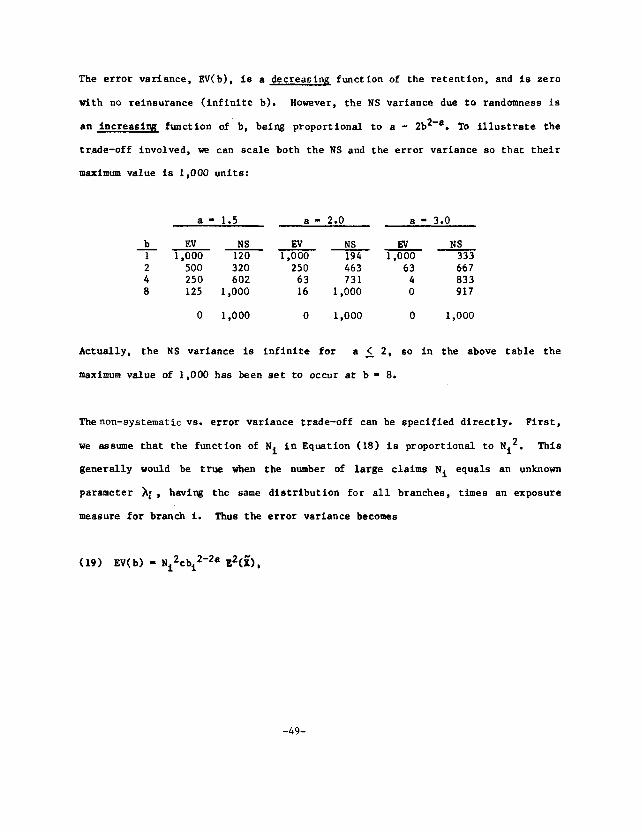
The error variance, 2X(b), is a decreasix function of the retention, and is zero

with no reinsurance (infinite b). However, the NS variance due to randomness is

an increasiqq function of b, being proportional to a - 2b2’a. To illustrate the

trade-off involved, we can scale both the NS and the error variance so that their

maximum value is 1,000 units:

a - 1.5 a- 2.0 a = 3.0

b Ev NS Ev NS Ev NS 1 ------ 120 194 333 1,000 1,000 1,000

2 500 320 250 463 63 667 4 250 602 63 731 4 833 8 125 1,000 16 1,000 0 917

0 1,000 0 1,000 0 1,000

Actually, the NS variance is infinite for a I 2, so in the above table the

maximum value of 1,000 has been set to occur at b - 8.

Thenon-systematic vs. error variance trade-off can be specified directly. First,

we assume that the function of Ni in Equation (18) is proportional to Ni2. This

generally would be true when the number of large claims Ni equals an unknown

parameter hi , having the same distribution for all branches, times an exposure

measure for branch I. Thus the error variance becomes

(19) EV( b) = Ni2cbi 2-2a E2(5,

-49-

where c is a constant, equal for all branches. Next, assume that we are willing

to trade v units of NS variance for one unit of error variance. This condition

produces an objective function Ti which is a linear combination of the NS

variance NiE(g2) and Equation (19):

(20) Ti = Nir2(a - 2bi1-a>/(a-2) + vcNi2bi2-2a r2a2/(a-1)2*

By setting the derivative with respect to bi equal to zero, the optimal bi

minimizing Ti is

(21) bi* = [Nivca2/(a-l)]1'a.

This result implies that b2/bl = (N2/Nl)'la = K1la, a more elegant form compared

to Equation (13).

The objective function Ti may be thought of as a "credibility-weighted" NS

variance. Therefore the ratio Ti/Ni2 is equivalent to the NS variance ratio

E("x2)/Ni In Equation (9). However, we no longer want to equalize the NS variance

across branches since doing so would not give proper weight to each profit

center's true result based upon Ni. Instead of equalizing ROE variance by branch

we minimize the z!!!!i of the individual branch credibility-weighted ROE

variances. Since the Ti for each branch are independent, separately minimizing

each of them (by choosing the bi*) minimizes the sum of the branch variances.

Equation (21) can be used to establish a set of retentions without directly

specifying the v and c parameters. We merely choose (judgementally), for the

smallest branch, a retention which would provide a reasonable balance between NS

-5o-

variance reduction and credibility of actual losses incurred. Retentions for the

remaining branches are then determined easily.

Catastrophe Losses

Natural catastrophe losses are inherently unpredictable at the profit center

level due to their low frequency and high severity (empirical evidence indicates

an a value near 1 .O) . Even at the corporate level, these losses have a high

variance. Consequently, there is almost no information regarding the true

catastrophe loss expectation in a profit center’s own experience for a single

year. Since there is virtually no credibility in branch experience and the

variance of catastrophe losses is high, it is necessary to remove variance,

rather than to equalize it.

A reasonable method of handling catastrophe losses is to charge each profit

center dth its annual aggregate catastrophe loss expectation, as a percentage of

earned premium. All actual catastrophe losses incurred are absorbed by the

internal reinsurance pool. Notice that this protection is an extreme form of

reinsurance since the variance of losses charged to the profit center is zero.

-51-

SUMMARY

A workable approach to measuring profits in property-liability insurance is the

return on equity concept, mith income defined such that timing differences are

minimal. For measuring profits at the branch office level, it is important to

equalize the ROE variance between branches. Otherwise the effect of measurement

error is not uniform by profit center and a haphazard incentive system may

result.

The preceding analysis has showo, in general terms, how both the systematic and

non-systematic risk components can be equalized for profit centers. However,

when the credibility of branch results is considered, some equalization of non-

systematic risk must be forgone. Based upon the complexity of the risk-

equalizing problem, a key observation emerges: As the range of branch sizes

expands, the difficulty of equitably measuring profit center results increases

dramatically. Also, the difficulty is compounded if the branches have widely

varying product mixes.

Practical applications of these risk-equalizing and profit-measuring techniques

will require additional, more specific assumptions and much empirical work.

Appendix IV provides an example of a profit center income statement which might

arise from these efforts.

-52-

APPENDIX I: SYSTEMATIC RISK

Aesume that a product line has N identically distributed exposures with profit

margins 9 for I - 1 to N. For simplicity, let each exposure have a premium of

one unit. The profit margin for the line is

(1.1) G - (zq)/N,

where the limits of summation are 1 to N. The variance of the line profit margin

ia

(1.2) Var(% = Var[@&)/N]

= [NV2 + (N2 - N)lV2]/N2 - V2[ 6 + (1-8)/N]

where V2 - Var(&) and x is the correlation coefficient between two different zi

and G 3' As the number of exposures becomes infinite, Var(& - IV*. This is

called systematic risk because it cannot ba reduced by the law of large

numbers. The remainder of the profit margin variance, (1 - $ )V2/N, becomes

smaller as N increases. This portion is called the non-systematic, or

diversifiable risk; i.e., adding more exposures to a portfolio will reduce

overall variance. The classical risk theory model assumes that t - 0.

-53-

Variance of KOE for Combination of Two Product Lines

For two separate product lines, denoted by subscripts 1 and 2, the return on

equity for a composite of the two lines is

(1.3) & - (1 + I)(1 + k&).

The composite pramium/equity ratio kt equals flkl + f2k2 and the composite TPM is

iig - (fLk& + f2k2;2)/kt. Thus

(1.4) ii, - (1 + I)(1 + flkl;l + f2k2g2).

Now assume that each line has an infinite number of exposures so that only

eytematic risk is present. The variance of $ is

(1.5) Var(4) - (1 + i)2[f12k12Var(m”l) + f22k22Var(G2;) + 2flf2klk2Cov(m”l,~2)]

- (1 + i)2k12[f12Var(gl) + f22Var(gl) + 2flf2 pVar(m”l)l

- (1 + i)2k12Var(~l)[(fl + f2>2 - 2flf2(1-p)l

- Var(Zl)[l - 2flf2(1-P >I.

Here e is the correlation coefficient between gl and G. Notice that

k12Var(;,) - k22Var(g2) by definition of the premium/equity ratios.

-54-

APPENDIX II: Tm PARETO DISTRIBUTION

The Pareto distribution in its simplest form is useful for fitting the tails of

loss size distrfbutions. Its cumulative function is

(2.1) F(x) - 1 - (r/x)’ (where a 2 1 and x 2 r)

with a density

(2.2) f(x) - araxma-l.

The mean and second moment are

I W

(2.3) r - xf(x)dx - ar/(a-1) t

(2.4) pl - a2/(a-2).

Notice that the mean is infinite if a ( 1 and the variance ( /~,-p’) is infinite

if a A2. The expected portion of loss in the interval fran r to br is

(2.5) ar(l-b”*)/(a-11, and

the remaining segment of expected loss above br Is

(2.6) s m xf(x)dx - arbl-*/(a-l).

br

-55-

The second moment of loss limited to a retention br is

(2.7) lrr2f(x)dx + /ir’f(x)dx - r2(, - 2b2’a)/(a-2) for a # 2,

= ??[I + 2*ln(b)l for a - 2.

-56-

APPENDIX III: RANDOM SUMS

A common stochastic model for the claim-generating process is the random sum.

This is discussed at length in probability theory (see Feller [3]). The total

value of all losses occurring in a fixed time period is

(3.1) ZN = ii1 + it2 +... + g+

where the random variables %i are identically distributed and the number of

claims N is also a random variable independent of any gi. Usually the zi are

assumed to be independent of each other, but we will assume that correlation

exists. The conditional expectation of the random sum given a fixed number of

claims N is

(3.2) E($+IN) - E( f?i) - NH5 1: I

The unconditional expectation is therefore

(3.3) dN) - zNE(;;)f(N) - E(z) E(g),

where f(N) is the density function of N.

The conditional second moment, given a fixed N is

(3.4) E(Z&'fN) - E[ igi2 +c ?$,j - NE(g2> + (N2 - N)E(g&)

i=l i#i

for i# j. The unconditional second moment becomes

-57-

(3.5) E(sN2) - c [NE(jr2) + (N2 - N)E(ji&)jf(N)

= E($E(!?) + [E(ij2) - E(G)] [Cov(?i,jf$ + E2(c)l

since COV(~~,~,) = E(z x" ) 1' rl

- E($)E(ji$. The variance of the random sum is

(3.6) Var($) - E(sN2) - E2(gN)

I g(i)Var(?) + E2(z)Var& + [Var($ + E*(G) - E(~)lCov(~f.~~)t

after some manipulation of terms. If g is a Poisson variable, then

Var(% - E(G) and (3.6) simplifies to

(3.7) Var(ZN) = E($E(s2) + E2(kov(:&).

Letting the premium charge to cover the aggregate losses be PE(N), and

letting e represent the correlation coefficient between zi and x" j' the variance

of the loss ratio becomes

(3.8) Var[$/PE($] - Var($)/P2E2(g) = 1

p2

E&) + eVar(Si) .

E& 1 Frequency vs. Severfty Components of Variance

Bquation (3.6) can be separated Into distinct frequency and severity components

by alternately fixing g ad z at their respective means (variances of the fixed

variables are zero):

-5%

(3.9) V[S”jf - E(g)] = E2&Var& (Frequency Variance)

(3.10) V[$$ = E(E)] - E($Var&) + [E2($ - E(z)]pVar(x) (Severity Variance)

When f - 0, the sum of the frequency and severity variances equals the total

variance Var(gN:,). For a Poisson G and a zero covariance between claim amounts,

we fird that the ratios of the variance components to the total variance are a

sole function of the loss size distribution:

(3.11) Frequency Ratio: a

E(ji2)

Severity Ratio: Va& .

E(“x2)

-59-

APPENDIX IV: PROFIT CENTER INCOME STATEMENT

Illustrative Example

Branch A: Second Quarter 1985 ($1,000'~)

Premium Written $1,150 8.2 Growth X Premium Earned 1,000 5.4 Growth %

Gross Losses 650 65.0 Excess Losses -45 -4.5 Reinsurance Charge 40 4.0 Catastrophe Charge 25 2.5 Net Losses 670 67.0

Before internal reinsurance Amount recovered For excess reinsurance Gross losses exclude catastrophes

Allocated Loss Expense

Commissions Taxes and Fees

Home Office Overhead Exp.

Underwriting Result

Total Profit

Return on Equity

Branch Overhead Expense 65

-60

25

-

50

150 30

95

5.0

15.0 3.0

9.5 6.5

Actual branch costs Allocated as a fixed I of earned

premium

-6.0

2.5

15.5

After income tax

Implied; based on required equity

Amount x* Comments

*of premium earned, except for premium

-6O-

REFERENCES

1.

2.

3.

4.

5.

6.

7.

Fairley, William B., "Investment Income and Profit Margins in Property- Liability Insurance: Theory and Empirical Results," The Bell Journal of Economics, X (Spring, 19791, 192-210.

Fama, Eugene P., and Miller, Merton H. The Theory of Finance, Hinsdale, Il.: Dryden Press, 1972.

Feller, Willfam, An Introduction to Probability Theory and Its Applications, Vol. I., New York: John Wiley 5 Sons, Inc., 1968.

Rahane, Yehuda, "The Theory of Insurance Risk Premiums--A Re-examination in the Light of Recent Developments in Capital Market Theory," The ASTIN Bulletin, Vol. 10, Part 2, 223-239.

hv, Baruch, Financial Statement Analysis: A New Approach, Englewood Cliffs, N.J.: Prentice-Hall, 1974.

Mayerson, Allen L., A Bayesian View of Credibility," Proceedings of the Casualty Actuarial Society, LI, 85-104.

Patrik, Gary, "Estimating Casualty Insurance Loss Amount Distributions," Proceedings of the Actuarial Society, LXVII, 57-109.

8. Plotkin, Irving ?I., Rates of Return in the Property and Liability Insurance Industry: 1955-1967, Cambridge: Arthur D. Little, Inc., 1969.

9. Shaxpe, William R., Portfolio Theory and Capital Markets, New York: McGraw-R%ll, 1970.

10. Wllllams, C. Arthur, Jr., "Regulating Property and Liability Insurance Rates Through Excess Profits Statutes," Journal of Risk and Insurance, L, No. 3, 445-472.

-61-

A FORMAL APPROACH TO CATASTROPHE RISK ASSESSMENT ANJI MANAGEMENT

Karen M. Clark

The author is a Research Associate for Commercial Union Insurance Company where she has worked on pricing and reinsurance issues as well as catastrophe risk assessment. She holds an M.B.A. and an M.A. in Economics from Boston University.

ABSTRACT

Insurers paid $1.9 billion on property claims arising from catastrophes in 1983. Researchers have estimated that annual Insured catastrophe losses could exceed $14 billion. Certainly, the financial implications for the insurance industry of losses of this magnitude would be severe; even industry losses much smaller in magnitude could cause financial difficulties for insurers who are heavily exposed to the risk of catastrophic losses.

The quantification of exposures to catastrophes, and the estimation of expected and probable maximum losses on these exposures pose problems for actuaries. This paper presents a methodology based on Monte Carlo simulation for estimating the probability distributions of property losses from catastrophes and discusses the uses of the probability distributions in management decision-making and planning.

-62-

INTRODUCTION

There were 33 named catastrophes in 1982, and they resulted in an

estimated $1.5 billion of insured property damage. Most of these

catastrophes were natural disasters such as hurricanes, tornadoes,

winter storms, and floods. In 1983, hurricane Alicia caused over $675

million of insured losses; the December storms caused insured damage of

$510 milli0n.l

Hurricane Alicia barely rated a three on a severity scale ranging from

one to five, and destruction from hurricanes increases exponentially

with increasing severity. A hurricane that rated a four hit New York

and New England in 1938; 600 people died and wind speeds of 183 mph

caused hundreds of millions of dollars of damage.

If this storm were to strike again, dollar losses to the insurance

industry could amount to six billion given the current insured property

values on Long Island and along the New England coast. Estimates of the

dollar damages that will result if a major earthquake occurs in Northern

or Southern California are even larger in magnitude.

A very severe hurricane or earthquake would produce a year of

catastrophic loss experience lying in the upper tail of the probability

distribution of annual losses from catastrophes, and it is the opinion

of the author that the 1982 catastrophe loss figure lies in the lower

end of this distribution. However, the determination of the shape and

the estimation of the parameters that describe this distribution are

-63-

tasks that are not easily performed by standard actuarial methodologies.

Yet since insurers need the knowledge of their exposures to catastrophes

and the probability distributions of annual catastrophic losses to make

pricing, marketing, and reinsurance decisions, the estimation of the

distribution and the expected and probable maximum losses pose problems

for actuaries.

Standard statistical approaches to estimation involve the use of

historical data to forecast future values of variables. However, models

based on time series of past catastrophe losses are not appropriate for

estimating future losses. Catastrophes are rare events so that the

actual loss data are sparse and their accuracy is questionable; average

recurrence intervals are long so that many exogenous variables change in

the time periods between occurrences. In particular, changing

population distributions, changing building codes, and changing building

repair costs alter the annual catastrophe loss distribution.

Since most catastrophes are caused by natural hazards and since most

natural hazards have associated with them geographical frequency and

severity patterns, the population distribution impacts the damage

producing potentials of these hazards. A natural disaster results when

a natural hazard occurs in a populated area. Changing population

patterns necessarily alter the probability distribution of catastrophic

losses. Since the average recurrence intervals of natural hazards in

any particular area are long, patterns of insured property values may

vary between occurrences to an extent that damage figures of historical

occurrences have no predictive power. For example, if hurricane Alicia

-64-

had struck in 1950, dollar damages would have been significantly lower

even after adjustment for inflation because of the smaller number of

insured residential and commercial structures in the Houston area at

that time.

It is primarily the influence of the geographic population distribution

that renders time series models inadequate although changing building

codes also alter the loss producing potentials of natural hazards. As

time passes, building materials and designs change, and new structures

become more or less vulnerable to particular natural hazards than the

old structures. Of course, changes in building repair costs also affect

the dollar damages that will result from catastrophes.

The above issues do not render the estimation problem intractable, but

they do produce a need for an alternative methodology to approaches

which employ historical catastrophe losses adjusted for inflation to

approximate the probability distribution of losses. Even models which

adjust these losses for population shifts can give only very rough

approximations of expected and probable maximum losses.

This paper presents a methodology based on Monte Carlo simulation, and

it focuses on property damage from natural disasters. Part I discusses

Monte Carlo simulation and the natural hazard simulation model. A

windstorm example is employed to illustrate the approach. Part II

outlines the ways in which management may use the model and its output

for decision-making and strategy formulation. It discusses how

knowledge of the probability distribution of property losses due to

-65-

catastrophes enables management to make risk versus return trade-offs in

marketing, pricing, and reinsurance decisions.

PART I: ESTIMATING THE PROBABILITY DISTRIBUTION OF CATASTROPHE LOSSES

Monte Carlo Simulation

Dramatic decreases in computing costs have led to the increased use of

computer simulation in the analysis of a wide variety of problems. Many

of these problems involve solutions that are difficult to obtain

analytically. For example, computer simulation may be employed to

evaluate complex integrals or to determine one or more attributes of

complex systems. Law and Kelton state that "Most complex, real-world

systems . . . cannot be accurately desertbed by a mathematical model which

can be evaluated analytically. Thus, a simulation is often the only

type of investigation possible." [8, p.81

The simulation approach is very basically the development of computer

programs that describe the particular system under study. All of the

system variables and their interrelationships are included. A high

speed computer then "simulates" the activity of the system and outputs

the measures of interest.

Simulation models may be deterministic or stochastic. Monte Carlo

simulation models are stochastic models with random variables from

-66-

stable probability distributions; they are static, i.e. not time

dependent, models.

A Monte Carlo simulation model is an excellent tool for performing

sensitivity analyses of the system of interest. Alternative values of

input variables may be given; the system may be resimulated and new

output produced. This type of simulation may be employed to analyze a

variety of insurance related problems. Arata described five areas in

which actuaries msy employ the simulation approach; one of these is the

pricing of difficult or catastrophic exposures. [I]

The Natural Hazard Simulation Model

The natural hazard simulation model is a model of the natural disaster

"system". As stated in the introduction, models based on historical

catastrophe losses are not appropriate for forecasting future losses,

Standard statistical approaches are found lacking for three reasons.

First, since the losses are caused by rare events, there is not much

historical loss data available and those that are available are

imprecise. Parameters estimated from the historical loss distribution

will be subject to much uncertainty because of the small sample size.

Secondly, the shape of the distribution itself is not clearly

discernible. Finally, the distribution is not stable since many factors

that influence it change with time.

-67-

The Monte Carlo model described below simulates natural hazards so that

the primary variables are meteorological or geophysical in nature.

These variables are random variables that have stable probability

distributions, and although the historical data on these variables are

sparse as are the loss data, their probability distributions may be

supplemented with the knowledge of authoritative meteorologists and

geophysicists.

This is, therefore, a stochastic yet stable system. The variables that

change with time, i.e. the geographic distribution of exposure units,

the insured property values, and the building construction types, are

inputs into the model and the probability distribution of losses from

natural hazards given these inputs is the model output. These inputs

may be changed to see how the loss distribution is altered.

The model variables may also be classified as frequency or severity

variables. The frequency variables indicate the expected number of

occurrences of the particular events within a given time period.

Severity variables represent the physical components of natural hazards

and they do not have a time dimension. Severity variables account for a

hazard's force, size, and duration.

A year of natural disasters is simulated thousands of times to generate

the probability distribution of annual losses. For each model iteration

and for each natural hazard, the following is performed:

-6%

1. The annual number of occurrences is generated from the

frequency distribution.

2. The exact location of each occurrence is generated.

3. For each occurrence, values for the force and size are

generated from the severity distributions.

4. The movement of the event across the affected area is

simulated, and dollar damages are calculated and accumulated.

The average of all iterations is the model-generated expected loss

estimate; a higher percentile loss is the probable maximum loss

estimate,

A Windstorm Example

A model of the hurricane hazard has been developed, and this model will

be used to illustrate the Monte Carlo simulation approach. Exhibit 1 is

a flowchart of the computer model.

All of the storm data used in the development of the model were obtained

from the U.S. Department of Commerce. The data had been collected and

analyzed by various agencies of the National Weather Service, and they

included seventy-nine years of history spanning the period from 1900 to

1978. Complete and accurate data were available for most of the

hurricanes that struck the U.S in this time period.

-69-

EXHIBIT 1

MODEL FLOWCHART

GENERATE ANNUAL NUMBER OF HURRICANE OCCURRENCES I

r- .._... T .__-- . .

For each zip code in affected area,-- CALCULATE WIND SPEED

(dependent on distance from eye and hours since landfall) -__________I

.i+l CALCULATE DAMAGE FACTOR

I---‘ --__._--_ -.L- -.-- .--.

APPLY TO EXPOSURES .--:

DAMAGE FACTOR AND VULNERABILITY FACTOR - ..- .__. I

I. -.

1 Go to next iteration ]

-7o-

A hurricane is a closed atmospheric circulation which develops over

tropical waters and in which winds move counterclockwise around a center

of pressure lower than the surrounding area. It is a severe tropical

storm in which the center of pressure is less than or equal to 29 (in.)

which causes sustainable wind speeds of 74 mph or more. One hundred and

twenty-eight hurricanes either approached and bypassed or entered the

U.S. during the sample period.

Referring back to exhibit 1, the first step of the model is the

generation of the annual number of landfalling hurricanes. Table 1

shows the numbers of years in which the number of occurrences was 0, 1,

2, and so on. The exhibited data fit a Poisson distribution with mean

and variance equal to 1.8, and the model generates the annual frequency

from this distribution.

Table 1 --

ANNIJAL NUMBER OF HURRICANES LANDFALLING IN U.S 1900-1978

No. storms Observed per year occurrence

0 25 1 25 2 14 3 8 4 5 5 1 6 1

-71-

The next step of the model is the determination of the landfall location

of each storm. Hurricanes enter the U.S. from the Gulf and East Coasts.

The map in exhibit 2 shows the U.S. coastline from Texas to Maine

divided into thirty-one smoothed 100 nautical mile segments. 2 The

number of hurricanes that entered through each segment during the sample

period is also shown.

The numbers seem to indicate that there are variations in locational

frequencies. In this case, it would not be appropriate to generate the

landfall location from a distribution which assigns equal probabilities

to all values, i.e. a uniform distribution. However, the limited amount

of data precludes one from ascertaining statistically whether there are

true frequency differences or whether the variations are caused by

randomness within the small samples.

The actual number of storm occurrences within each segment is not

employed by the model to develop the relative frequency distribution.

It is not clear, first of all, if 100 nautical mile segments are the

appropriate lengths of coastline to use for the calculations.

Additionally, although several segments are completely free of

historical storm occurrences, it is not clear that the probability of

hurricane landfall is zero in these areas.

The relative frequency may be estimated by correlating it with another

variable for which the value is known or may be estimated for each

segment. Alternatively, the causal relationship between a variable(s)

and the frequency of landfall may be employed if such a relationship

2The coastline is smoothed for irregularities such as inlets and bays.

-72-

Exhibit 2 --

HURRiCANES ENTERING THE U.S. 1900-1978

-73-

exists. Of course, if one knew all of the conditions favoring landfall,

one could assign probabilities based on the existence or absence of

these conditions at each coastal location.

The way in which hurricanes are formed as well as the process by which

energy is supplied to the circulating winds determine the likely paths

of these storms. To illustrate, "hurricanes obtain kinetic energy from

latent heat from the condensation and precipitation of water vapor.

Therefore, hurricanes develop over warm tropical ocean areas where

evaporation rates are very high and vast quantities of water vapor are

stored in the atmosphere. The general movement of air over most of the

Tropics is from the east while in higher latitudes it is usually from

the west. Consequently, most hurricanes move initially to the west and

may drift slightly northward. However, aa they continue to drift toward

higher latitudes, they come under the influence of westerly winds and

recurve to the east" [4, p.3). Wind patterns, therefore, provide an

explanation for the lower frequencies at higher latitudes.

To derive the model locational frequency distribution, the following

approach was adopted. First, the hurricane data were supplemented with

data on all tropical storms. Tropical storms are closed atmospheric

circulations with less intense winds than those of hurricanes. The

assumption here is that the atmospheric conditions that favor the

occurrence of a tropical storm are the same conditions that favor the

occurrence of a hurricane. The additional data eliminate the problem of

long coastal segments with no historical occurrences.

--I&

Next, the raw data on numbers of occurrences were smoothed using a

procedure that was selected on the basis of its ability to capture

turning points in the data while smoothing slight variations. The

coastline was redivided into 50 nautical mile segments, and the number

of occurrences for each segment was set equal to the weighted average of

11 successive data points centered on that segment. The smoothed

frequency values are obtained as follows:

where Ci = the number of historical hurricane

occurrences for the ith segment

Fi = the smoothed frequency value for the ith

segment

Wn - -300, ,252, .140, ‘028, -.O4. -.03

for n = 0, $1, 22, 23, -+4, 25, respectively

This is the preferred smoothing procedure in climatological analyses

because the weighting scheme maintains the frequency and phase angle of

the original series of numbers. The endpoints of the series were

approximated so that each segment of the coast was assigned a relative

-75-

frequency. The landfall location of each storm is generated from the

thus derived locational frequency distribution.

Step three of the model is the generation of values for the severity

variables. There are four primary variables which account for hurricane

severity . These variables are: the minimum central pressure, the

radius of maximum winds, the forward speed, and the wind inflow angle.

Central pressure (po) is defined as the sea-level pressure at the

hurricane center or eye. This variable is the most important for

computing hurricane windspeeds, and it is a universally accepted index

of hurricane intensity. All else being equal, the square of the wind

speed varies directly with op (ap = p,-p,) where p, is the peripheral

pressure, i.e. the sea level pressure at the periphery of the storm.

The radius of maximum winds (R) is the radial distance from the

hurricane center to the band of strongest winds. Forward speed (T)

refers to the rate of translation of the hurricane center from one

geographical point to another. Track direction (A) is the path of

forward movement along which the hurricane is traveling and is measured

clockwise from north.

The empirical data on each severity variable cannot be fit to standard

theoretical distributions as were the annual frequency data. There

appears to be a geographical hurricane severity pattern as there was a

locational frequency pattern so that the probability density functions

of the severity variables vary by location, and there are not enough

-76-

data points at each location to estimate these functions. Additionally,

the available data indicate that the severity variables are not

independent. Linear correlation coefficients are positive between most

pairs of variables. However, it is not possible to test the

significance of the correlation coefficients unless it is assumed that

pairs of variables form bivariate normal distributions.

If the variables are not independent, their correlations must be

explicitly formulated within the model since the correlations will

impact the variance of the model output, i.e. the estimated hurricane

loss distribution.

The strongest correlations seem to be between the severity variables and

latitude. In general, as latitude increases, average hurricane severity

decreases as does frequency. When a hurricane moves over cooler waters,

its primary source of energy is reduced so that the intensity of

circulation decreases in the absence of outside forces. "The reasons

for the increase in central pressure3 from south to north include: the

inability of hurricanes to carry their warm, moist, tropical atmosphere

into temperate latitudes and the entrance of colder and drier air at low

levels, which . . . decreases the amount of energy available to the

storm." [7, p.391

The data, however, indicate a more direct relationship between severity

and latitude than that between frequency and latitude, and the

mathematical expressions which describe the relationships between the

hurricane severity components and latitude were estimated and employed

3Central pressure is inversely related to severity so that high central pressures result in less severe storms.

-77-

by the simulation model in the following manner: Given the latitude and

longitude coordinates of the landfall location, the latitude coordinate

is entered into the equations to obtain initial values of the severity

variables. Stochastic elements are added to the initial values and the

sums become the simulated values. The stochastic elements are generated

from the distribution of the error term for each equation.

Linear transformations of exponential, power, hyperbolic, and other

special functions were fit to the empirical data for each severity

variable using the ordinary least squares estimation procedure. Simple

linear equations provided the best fits of the relationships between R

and latitude and T and latitude.

Exhibit 3 shows a plot of the latitude, radius of maximum winds pairs

for the 128 hurricanes in the data sample. Exhibit 4 shows the linear

regression residuals plotted against latitude. Although the dispersion

of the residuals is wide, i.e. the standard deviation is 10.10, the

errors are distributed normally with expected value equal to zero. This

statistical distribution is employed to generate the values e i for the

following equation:

RI = a + b(Li) + ed

where Ri = the ith simulated value for R

Li = the latitude coordinate for the ith hurricane

a,b are the estimated regression coefficients

-78-

8 1

L 2 88 t tt

tt t t tt tt t&t

tt tt t t t2 t&t n t&2 tt 8

2t2ttt ttt t22 8 3t3 tt t

2 t t3t 25 t 2 8 et:

t t&2 8 tt2 tt t 1: t t t 2:

t

3

t

t

8

~TI‘l'TJD~ (degrees)

-79-

Exhibit 4

A LATF'UDE'7rS. LIV2P.R RFXPXSSION RESIDUATS ( R - R )

20,oo 2sdo 30,oo 35m 4om 45.00 50,oo

+-----t---------t------+-----------t-------t----t

3oAo t

22.00 t

14&o t

6100 t

-2*oo t

-1om t

-18,oo t

-26,oo t

8

8 8

8 8

88 88 888 8 8 8 8 8 8 8 8 t&t 8 32tt 2

823 tt 882 2: 8

82 t&t t: 2: 3St

8 883: 32 8 8 tt3 8 82 ttt 88

8 8 8 ztt 888 8

8 :

8

8

2 8

8

8

8

8

----t-------t-------~---~---t-----

20*00 25,oo 3om 35,oo 40*00 45.00 !io,oo

IATlYJD!3 (degrees)

-8O-

The distribution of the simulated values of R is then bounded by

meteorological estimates of lowest and highest possible values.

The strength of the linear relationship between latitude and forward

speed is even greater than that between latitude and the radius of

maximum winds as shown by exhibit 5. However, the regression residuals

shown in exhibit 6 seem to be heteroskedastic, i.e. the variance of the

residuals increases with latitude. A basic assumption of the linear

regression model is that the distribution of the error term has a

constant variance, and the violation of this assumption leads to least

squares estimators that are not efficient, i.e. minimum variance, or

asymtotically efficient.

For the simulation model, it is also important that the distribution of

the error term from which values are generated is stable for all values

of latitude. If this is not the case, the simulated values of the

particular variable will not form probability distributions that match

the true underlying distributions, and the model-generated probability

distribution of losses will not provide an accurate estimate of the true

probability distribution of losses.

Corrections for heteroskedasticity were made by assuming that the

variance of the error term is proportional to latitude. The

re-estimated regression equation residuals are shown in exhibit 7; they

form a normal distribution with mean equal to zero and standard

deviation equal to 4.9.

-81-

Exhibit 5 --

L'+?ITUDEVS. FDRWARTI S!?E'YD

20.00 2sm 3om 35.00 40.00 45.00 !io,oa

rim t

6!Loo t

55100 t

45.00 t

35.00 t

25.00 t

1Mo t

5.00 t

1

8

8 cc

t t 1 cl

cc 3 t 1 2

t 1 t 1: 4: u3 2 cc t

t: m::2:tt a c233c:u2cbc2c $5514: 1 :232 Cl 2l 1 n2 3:

8

20.00 a*00 30.00 3540 40100 45m 50.00

LATITUDE kleg-rees)

-82-

Bhibit 6

20&o 25.00 30,oo 35do 40&o 45m 5om

+-+-----+-----) ---_ -+---+----+ 30.00 t

22,OQ t

<E+ - I

E! 14*00 t 1

1 1

4: 2 cc Cl:

11122u22 5431112 112c2 1 1

12W3 213 1 #3tl5$2 cc 1

1122 1 cc: 12c: cc 2 1

1: 1

1

1

1:

2

-26,OO t

t----t ~+w--..+-+*--+--+

20*00 25.00 3om 35.00 4om 45m 50.00

I~..AT~I’~JY (degrees)

-83-

Exhibit 7

LATITUDE VS. LIElEAR RXWSSIOV R=YKKlALS ( T - $ ) AFT% CDRR??IO1! WR !FF%OS'(.~AspICITy

20100 25.00 30,oo 35.00 40,w 45.w so*00

t ----+--+---+ I---- +---t-t m*w t

22,w t

14,w t

6.00 t

-2.00 t

-10,w t

-18*W t

1 1

1 1: 1 cc: 1 1 t: 1

24 Cl 122 t 124222 22ti2 22 1113t3 1

112 4 1323 :::::

$1 12 1 1

1 1

1 1 t

1 4: 1 1 1 12 cc

1 1

1

t--4----t----i-----4----t----t

2o*w 2500 30.00 35,w 40106 45,w 50,w

IATITIDE (degrees)

-84-

Although hurricane central pressure and track direction are both

correlated with latitude, the relationships between p, and latitude and

A and latitude were more difficult to estimate statistically. For these

variables, the simulated values are generated from the empirical

distributions. Outliers are first removed so that the simulated values

for each coastal location are within the lower and upper bounds that

have been developed by meteorologists.

The movement of the storm is next simulated by the computer model, and

the property damage inflicted by the circulating winds is calculated for

each geographic location. The particular geographical unit for which

the damages are accumulated is determined by the model input. Insured

property values are input along with the construction types and ages of

the insured buildings and locational information such as zipcodes and

counties. Wind speeds and dollar damages are calculated for each

zipcode, but the damages may be accumulated by larger units to provide

more meaningful output.

The dollar damages are calculated by applying damage and vulnerability

factors to the dollar amounts of liability. The damage factors are

based on the results of engineering studies of the relationship between

wind speeds and structural damage. The vulnerability factors account

for the variability in inflicted damage due to construction type and

age. The dollar damages are accumulated by the selected geographical

units.

-85

:’

.

Two thousand years of hurricane experience are simulated by the model.

These two thousand model iterations provide a complete probability

distribution of annual hurricane losses from which the expected loss and

probable maximum loss estimates are derived.

Exhibit 8 shows the expected losses as well as the 80%. 90%, 95%, and

99% confidence level losses calculated as the 80th, 90th, 95th. and 99th

percentile losses, respectively, for a given geographical distribution

of exposures. These conf.idence level losses may be interpreted in two

ways. A given confidence level loss shows the loss amount for which the

probability of experiencing losses above that amount is 1.0 minus the

particular confidence level. For the loss distribution in exhibit 8 the

probability of experiencing losses above $10 million is .20. The

confidence level loss also shows the loss amount for which losses

greater than that amount will be experienced on average once in every

l.O/(l.O - confidence level) years. Again, from exhibit 8 losses

greater than $10 million will be experienced once in every five years on

average. The loss distribution is highly skewed with a median value

which is much below the mean and a high proportion of zero values.

The model output provides management with information that may be used

in the formulation of pricing, marketing, and reinsurance strategies.

Before the uses of the model output are discussed, the next section will

summarize the Monte Carlo simulation approach.

-86-

EXP- ComIDm LEvm LoGsEs LIABlLITIES Loss 80% 90% 95% 99%

7,170,753,024 9,011,808 10,003,715 24,179',636 44,827,623 117,946,980

-87-

Summary of the Methodology

The Monte Carlo simulation approach to the estimation of the probability

distribution of catastrophe losses involves %he development of models to

simulate catastrophes. Each model is developed around the probability

distributions of the random variables of the loss-producing “system.”

Ideally, the model builder will have an a priori theory on the shape of

the probability distribution underlying each random variable. For the

results of the Monte Carlo simulation to be valid, the underlying model

assumptions must be true. The empirical distribution formed by the raw

data may be compared to standard statistical distributions using

appropriate goodness-of-fit tests, and if the data do fit a well-known

probability distribution, the moments of the distribution may be

estimated and employed by the simulation model. In the windstorm

example, the Poisson distribution was used to generate the annual number

of hurricanes.

Alternatively, the expressions which describe the relationships between

model variables may be estimated and employed by the model to generate

simulated values of variables. This approach was adopted for some of

the hurricane severity components.

Finally, the empirical distribution may be employed for the generation

of values for a particular model variable. This procedure, however has

a few drawbacks. First, since the sample is a collection of random

-88-

data, a different sample could yield a very different empirical

distribution. Secondly, the generation of random variables from an

empirical distribution precludes the possibility of generating a value

of the variable outside of the observed range, and the observed range

may not include all possible values of the variable. Finally, the

generation of values from empirical distributions is, in general, less

efficient from the standpoint of computing time than the generation of

values from theoretical distributions. Nevertheless, in some cases

generation from the empirical distribution is either necessary or

preferred for various reasons, and in these cases, the empirical

distribution can be programmed into the model.

The testimony of experts may be employed along with the statistical data

to build the model. Physical scientists who have studied extensively the

phenomena of interest can provide information on the ranges of possible

values of particular variables as well as on the most likely value or

values. This information may enable the model builder to substitute

theoretical distributions for empirical distributions, to identify

outliers in the data, and/or to determine appropriate points at which to

bound the probability distributions.

Once the model is built, i.e. the important variables have been

identified and their probability distributions and interrelationships

have been programmed into the computer, the system is simulated many

times to provide a range of all possible annual loss amounts. There is

no standard formula that gives the number of model iterations necessary

to produce output with a given level of precision for this type of Monte

-89-

Carlo simulation model. The necessary number of iterations is

endogenous, i.e. model-dependent.

Given that the variable of interest is annual dollar losses from

catastrophes, one hopes to derive accurate estimates of annual expected

losses and maximum probable losses. Assuming that the model has been

specified correctly, the expected loss estimate will converge to the

true expected loss and the model generated loss distribution will

converge to the true loss distribution as the number of iterations

increases. Very basically,

4 E(X) = lim

IJ+- z Xi

1=, n

where E(X) = expected annual loss

xi = annual loss from ith model iteration

and,

F(X) = lim F,(X) n---

where F(X) = the distribution function of annual losses

F,(X) = distribution function of n model generated annual loss figures.

-9o-

The larger the variance of the probability distribution of annual

losses, the larger the value of n needed to produce loss estimates with

a given level of precision. The variability of the model generated

annual losses is determined by the variability of the model variables,

i.e. the frequency and severity variables, and their correlations. If

the model variables are positively correlated, the variance of the loss

distribution will be greater than it would be in the absence of this

correlation.

Although there is no straightforward procedure for calculating the value

of n needed for specified precision levels, there are a few procedures

that may be employed to develop confidence intervals for E(X) if certain

assumptions are made. These procedures will not be discussed here, and

the interested reader is referred to Chapter 8 of Law and Kelton. [9]

The recommendation of this author is to perform at least 1000 model

iterations if possible. This should not present a problem given the low

costs of computing time on high speed computers; however, development

time may be well spent on writing efficient computer programs that

minimize the computing time, particularly if the model is to be run

frequently. If each iteration is still expensive, certain variance

reduction techniques may be employed to reduce the number of Iterations

needed to reach convergence. The model builder may perform tests to see

how quickly the loss distribution is converging. Iterations may be

performed in groups of 100 so that the changes in the loss distribution

may be monitored. A stable loss distribution indicates that convergence

has been reached.

-Yl-

Validation of simulation models often presents a problem if there are no

historical data on the variable that the model is designed to measure.

In the case of natural hazard simulation models, the historical data are

sparse. Past occurrences may be simulated, nevertheless, if the

geographical distribution of exposures that is input to the model

corresponds precisely to the geographical distribution of exposures that

existed at the time of the occurrence. Insured values, construction

types, and ages of exposure units should also match precisely. Values

for the variables which account for the severity components of the

hazard are input to the model, the model is simulated, and the

model-generated loss estimate is output. This estimate is compared to

actual dollar damages to test the validity of the model and its

underlying assumptions.

There are several advantages of the simulation approach. First of all,

it is able to capture the effects on the loss distribution of changes in

variables Over time. Secondly, this estimation procedure provides

management with a complete picture of the probability distribution of

losses rather than just estimates of expected and probable maximum

losses. And finally, the Monte Carlo simulation approach provides a

framework for performing sensitivity analyses and "what-if" studies.

The model uses will be described in the following sections.

-YZ-

PART II: MANAGING RXPOSURE TO CATASTROPHES -- -

A methodology for estimating the probability distribution of annual

catastrophe losses given a particular geographical distribution of

exposures was described and illustrated in Part I. Knowledge of the

probability distribution of losses enables insurers to manage their

exposures to catastrophes. With respect to these exposures, management

has several options:

1. Write no business in catastrophe prone areas.

2. Exclude coverage for losses caused by natural hazards.

3. Plan to recover losses after a catastrophe occurs by

retrospective pricing.

4. Spread property business so that it is not concentrated in

catastrophe prone areas.

5. Add loadings to premiums and build up reserves to cover

catastrophe losses when they occur.

6. Reinsure property business.

Option 1 does not present a very viable strategy since most areas of the

continental U.S. are prone to natural disasters of at least one type.

-93-

For example, the Gulf and East Coast states are prone to hurricanes

while the Great Plains and Midwestern states are highly prone to

tornadoes. Earthquakes are natural hazards with the greatest damage

producing potential in California, Nevada, Washington, and parts of

Indiana, Missouri, Tennessee, Arkansas, South Carolina, and

Massachusetts. [3]

Option 2 may also not be feasible. If an industry-wide attempt is made

to exclude coverage for losses resulting from a particular hazard,

legislation may be passed to prevent effective exclusion. Recent

legislation in California concerning concurrent causation is a case in

point. On the other hand, if a single company or group of companies

attempt to exclude coverage, business will certainly be lost to

competitors who do provide coverage unless the policy premiums are

reduced sufficiently.

The insurance industry has traditionally priced its products

retrospectively since expected costs are estimated from past costs.

Policy premiums are determined by the most recent historical loss

experience so that larger than expected losses in year t will lead to

higher prices in year t+l. As long aa the individual firm's loss

experience is better than or equal to the industry average, the firm may

set premiums in relation to its own loss experience (in the absence of

regulatory barriers.) However, if the individual firm's loss experience

is worse than the industry average, competition will force the firm to

price below its costs.

-94-

Retrospective pricing cannot be used to recover losses from

catastrophes. If an individual firm experiences a disproportionate

share of total industry losses from the occurrence of a catastrophic

event in year t, competition will prevent the firm from increasing its

rates enough to recover all of its losses in year t+l. Additionally,

the industry as a whole is prevented from increasing rates dramatically

after the occurrence of a catastrophe by the threat of new entry.

The barriers to entry into the insurance industry are high enough to

allow retrospective pricing of normal insurance covers; however, a

financial need of existing firms to raise prices by a significant amount

would provide a competitive advantage for new entrants that are free of

the financial burden.

Accordingly, option 3 is an inferior strategy as were options 1 and 2.

The last three alternatives, however, are all viable strategic options,

and each one will be discussed in turn under the headings of marketing,

pricing, and reinsurance.

Marketing

The windstorm simulation model output as illustrated in exhibit 8 shows

the probability distribution of annual countrywide losses from the

hurricane hazard. For marketing purposes, however, it may be more

useful to divide the country into zones so that the specific areas of

high windstorm risk are clearly identifiable.

-95-

The computer model may be designed to accumulate dollar damages by

state, by county, or by any other geographical configuration. Exhibit 9

shows the state of Louisiana divided into eight zones. The dollars of

liability, i.e. exposure, the expected loss, and various confidence

level losses' are shown for each zone. The loss figures show clearly

that the higher risk areas are the coastal zones. The hurricane is at

maximum force just as it crosses overland; as it travels inland, the

storm dissipates because of the elimination of its primary energy source

i.e. kinetic energy derived from the sea, and because of frictional

effects.

Because all natural hazards have associated with them geographical

frequency and severity patterns, they will produce gradations of damage

or pockets of high risk and low risk. Management will want to avoid

concentrations of property exposures in high risk areas, and the model

output enables the development of marketing plans that are based on the

long term profit potentials of various markets.

Property business in high risk areas may be very profitable in years of

no natural hazard occurrences. As years pass and no catastrophes occur,

insurers may begin to compete for the business in a high risk area. The

competition may drive the profits as well as the catastrophe loading to

zero so that there are no resources available to cover the catastrophic

losses when they occur. Knowledge of the probability distributions of

losses from natural hazards in these areas enables insurers to resist

the temptation to write business based on the very recent loss

experience in these areas.

41t is interesting to note that for small geographic areas, the confidence level losses may be zero since the frequencies of hurricances in specific

locations are low. -96

Exhibit 9

m

LWIS 1 LOUIS 2 LWIS 3 LaJIS 4 LOUIS s LOUIS 6 LOLUS 7 1WIS 0

Louisiana Windstorm Zones

90417112. 256512. 9210113* 25540,

56674660 * 94066, 50672900. 71042. 79796656* e-09&5 I

176149551. 231604, 4Ob4471be 47590, 33114740. 16552,

80% 90%

0, 276770 t 0. 12932, 01 31306. 0. 0. 0, 0, 0. 0, 0, 0. 0. 0,

level lossf?.s

95% 99%

1947396, 4930375. 213693, 537371. 653101. 2098500 t 2340B8, 1722377, 547837. 2021005. 598346, 6823092e 193227. 1309985*

5991. 772270.

-97-

The natural hazard simulation model is an excellent tool for evaluating

the exposure to natural hazards resulting from alternative marketing

plans. If marketing plans alter the geographic distribution of

exposures, the alternative distributions of exposures may be input to

the model and new loss distributions generated.

Pricing

The model-generated expected loss figures may be used to calculate

appropriate catastrophe premium loadings. The loadings may be expressed

as percentages of insured values by dividing the expected loss figures

by the dollars of liability for each of the established zones, i.e. the

geographical units into which the country is divided.

Theoretically, if an insurer establishes a reserve for catastrophe

losses and makes annual contributions equal to the annual expected

losses, the insurer will break even with respect to catastrophe losses

over the long run. The model-generated output enables management to

fine tune the catastrophe loadings in particular locations. Presumably,

premiums charged in catastrophe prone areas include loadings for

catastrophe losses, but these loadings may be subjective and may not

correspond closely with expected catastrophe losses. Since the model

can be programmed to accumulate dollar damages by any geographical

configuration, expected loss estimates may be derived for any unit of

area, and premiums that are in line with costs may be established.

-98-

Clearly, competitive factors dictate the amount of freedom that

management has to set prices. If demand is very elastic, small

increases in price will lead to large decreases in market share. Price

changes may be tempered to result in the desired distribution of premium

volume.

An additional caveat is that pricing in accordance with expected loss

does not eliminate the risk of large losses since it is possible that

catastrophes will occur when the loss fund is at a level that is not

sufficient to cover all of the losses. The losses could then lead to

financial difficulties for the insurer. Insurers may, however, transfer

part or all of this risk through reinsurance agreements.

Reinsurance

To evaluate alternative reinsurance proposals, management needs the

following:

1. An estimate of the probability distribution of losses for

which the reinsurance contracts are to provide cover.

2. Knowledge of the reinsurance market and the types of contracts

that are available.

3. A methodology for performing risk versus return trade-offs and

obtaining preference orderings.

-99-

Part I of this paper provided a methodology for estimating the

probability distribution of property losses from catastrophes. From the

cumulative distribution function, one may determine the probability of

experiencing losses in excess of any dollar amount.

There are two broad categories of reinsurance contracts: proportional

and nonproportional. Each type of treaty performs certain functions for

the reinsured. Proportional or quota share treaties provide capacity

and financing as well as reductions in the variance of the loss

distribution. Non proportional or excess-of-loss treaties provide

catastrophe and stop loss covers.

Borch [2] has shown that the "most efficient" reinsurance contract from

the viewpoint of the ceding company is the stop loss contract. The type

of treaty leads to the greatest reduction in variance for a given price

if the premium paid to the reinsurer is proportional to the expected

loss of the ceded portfolio and not to its variance. From the viewpoint

of the reinsurer, the quota share treaty that gives a ceded portfolio

with the same expected loss is superior because the variance of the

ceded portfolio will be smaller.

In general, the reinsurer will charge a premium that compensates for the

variability as well as the expected loss of the ceded portfolio.

Accordingly, the premium will be lower for a quota share treaty that

gives the reinsurer a portfolio with the same expected loss as the

excess-of-loss treaty. The specific premium that the reinsurer will

-lOO-

charge for a particular contract depends on the risk profile of the

company.

The estimated probability distribution of losses shows the benefits that

will be derived from particular reinsurance agreements, and these

benefits may be compared to the costs. The reinsuring company w-ill rank

order the alternatives that are available in the reinsurance market

using its own risk profile. The derivation of the risk profile relies

on utility theory and will not be discussed here.

The pricing, marketing, and reinsurance decisions are not independent

and as such should be evaluated simultaneously in the planning process.

Obviously, pricing policies impact marketing plans which influence the

geographical distribution of property exposures. This is a two-way

relationship since marketing decisions also impact pricing decisions.

The geographical distribution of property exposures will affect the

probability distribution of catastrophe losses which in turn will

influence the price of reinsurance since the reinsurer will demand a

higher premium to cover exposures in high risk areas. Finally, the

reinsurance covers influence the loss distribution and change the

expected losses which drive the catastrophe loadings. The diagram below

illustrates the decision triangle.

-101-

Summary

Catastrophic events can affect significantly the results of property and

casualty insurance companies. Since the losses resulting from the

occurrences of catastrophes could affect adversely the financial

condition of a company, management must plan for these events. The

first part of this paper described an estimation methodology based on

Monte Carlo simulation. A windstorm example illustrated the approach

and its primary advantages. These advantages are: It estimates the

full probability distribution of losses, it captures the effects on this

distribution of changes in population patterns, building codes, and

repair costs, and it may be used to perform sensitivity analyses. The

second part of the paper outlined how knowledge of the probability

distribution of losses enables management to evaluate the effects on the

probabilities of severe losses of alternative marketing, pricing, and

reinsurance strategies.

-102-

REFERENCES

[l] Arata, David A. "Computer Simulation and the Actuary: A Study in Realizable Potential", Proceedings of the Casulaty Actuarial

Society, Volume LXVIII, 1981.

[Z] Borch, Karl. The Mathematical Theory of Insurance, Lexington: D.C. Heath and Company, 1974.

[3] Conning & Company. Natural Catastrophes, Exposures and Reinsurance October, 1983.

[4] Cry, George W. "Tropical Cyclones of the North Atlantic Ocean,,, U.S. Department of Commerce, Weather Bureau, Technical Paper No. 55.

[5] Friedman, Don G. Computer Simulation in Natural Hazard Assessment, University of Colorado: Program on Technology, Environment and Man, Monograph $NSF-RA-E-15-002, 1975.

[6] Haggerty, Alfred G. "Earthquake Insurance Sales Nearing Limit,,, National Underwriter, June 29, 1984.

[7] Ho, Francis P., Schwerdt, Richard W. and Goodyear, Hugo V. "Some Climatological Characteristics of Hurricanes and Tropical Storms, Gulf and East Coast of the United States," U.S. Department of Commerce, National Weather Service, NOAA Technical Report HW515, May 1975.

IS] Insurance Information Institute. Insurance Facts, 1983.

[9] Law, Aver111 M. and Kelton, W. David. Simulation Modeling and Analysis, New York: McGraw-Hill, 1982.

[lo] Rubinstein, Reuben Y. Simulation and the Monte Carlo Method, New York: John Wiley & Sons, 1981.

[ll] Schwerdt, Richard W., Ho, Francis P. and Watkins, Roger R. "Meteorological Criteria for Standard Project Hurricane and Probable Maximum Hurricane Windfields, Gulf and East Coasts of the United States,,, U.S. Department of Commerce, National Oceans and Atmospheric Administration, NOAA Technical Report NWS 23, September 1979.

-103-

TITLE: MEASURING THE IMPACT OF UNREPORTED PREMIUMS ON A REINSURERS' FINANCIAL RESULTS

AUTHOR: Douglas J. Collins

Mr. Collins is a Vice President of Tillinghast, Nelson & Warren, Inc. He is a graduate of Rensselaer Polytechnic Institute, with a Bachelor of Science degree in mathematics. He became a Fellow of the Casualty Actuarial Society and a member of the American Academy of Actuaries in 1977. He has served on the Examination Committee of the C.A.S.

ABSTRACT: A reinsurers' financial results are materially influenced by unreported premiums, and the losses and expenses related to these premiums. When un- reported premiums and losses are estimated using underwriting year experience, an approximation is required to separate premiums earned and losses incurred before the reserve date from those earned and incurred after the reserve date. This paper presents a technique for approximating the earned portion of unreported premiums. It also demonstrates that financial results can vary significantly depending on the treatment of the earned and unearned portion of unreported premiums. A series of examples based on hypothetical data are used to show alternative estimates of underwriting income.

- 104-

MEASURING THE IMPACT OF UNREPORTED PREMIUMS

ON A REINSURERS' FINANCIAL RESULTS

INTRODUCTION

The analysis of reinsurers' financial results is complicated by the

fact that both premiums and losses are subject to significant

reporting lags. A further complication is the difficulty in

quantifying the earned portion of unreported premiums. Reinsurers do

not generally have sufficient information to calculate this quantity

exactly. Thus, accounting practices vary as to the methodology for

reflecting unreported premiums in financial statements.

This paper will present a technique for approximating unreported

earned premiums. Several examples will then be reviewed in which

calculations of unreported (IBNR) loss reserves are a function of

expected losses. These examples will provide a comparison of ultimate

loss estimates using alternative measures of unreported premiums in

the expected loss calculation. The financial impact of the various

assumptions will then be reviewed.

We will focus on the use of underwriting year experience to measure

financial results. While accident year loss reserve estimates are

required for Schedule P of the statutory annual statement, the use of

accident year data has several disadvantages that can create problems

for a reinsurer seeking to accurately measure its financial position.

-10%

Accident year loss estimates are usually compared to premiums reported

and earned during the accident year. Due to premium reporting lags,

this comparison does not match premiums and losses from the same

policies. Thus, accident year loss ratios do not always provide a

meaningful measure of underwriting results. Another disadvantage is

that reinsurers can not always identify the proper accident year of a

claim payment or reserve, since this information may not be supplied

by ceding carriers. Despite these problems, an estimated accident

year allocation of statistics is often the basis for reinsurers' loss

reserves, due to the reporting requirements for Schedule P. However,

if loss reserves are to be matched with an appropriate measure of

unreported premiums, a supplement to calendar-accident year statistics

is required.

A policy year type exposure period is used quite often by reinsurers

since it provides an appropriate matching of premiums and losses, and

also provides the data needed for calculating unreported premiums.

Reinsurers usually use the term underwriting or contract year, rather

than policy year, to reflect the difference between reinsurance and

primary insurance contracts. Since some reinsurance contracts cover

underlying policies written throughout the contract period (i.e., they

cover the reinsured's policy year), an underwriting year normally

includes parts of three accident years (or more if policy terms exceed

twelve months). For example, a reinsurance contract written on July

1, 1983 might cover underlying policies written through June 30, 1984

which would cover losses occurring through June 30, 1985. All of the

premiums and losses from this contract would be included in under-

writing year 1983.

-106-

The measurement of unreported premium reserves can be accomplished by

multiplicative projection techniques using historical underwriting

year premium development patterns. This unreported premium may

include the following components.

1. Premiums which have been written with effective dates prior

to the reserve date, but which have not yet been reported.

These premiums have an unearned and an earned portion. The

earned but not reported premium is often referred to as

EBNR.

2. Premiums which will be written with effective dates after

the reserve date but within the exposure period being

projected. For example, policies written after 6/30/84,

which might be included in a projection of ultimate premiums

for underwriting year 1984 as of 6/30/84.

The following section will describe a simple procedure for estimating

the component portions of an unreported premium reserve.

UNREPORTED PREMIUM RESERVES

Exhibit 1 shows the underlying data for Sebago Re, a hypothetical

growing young reinsurance company. We project that Sebago Re will

ultimately collect premiums of $15 million for underwriting years 1980

to 1984. As of 6/30/84, they have collected written premiums of $9

million. Thus, their total unreported premiums are $6 million. Of

-107-

course, the portion of these unreported premiums that will be written

with effective dates after 6/30/84, should not influence Sebago Re's

6/30/84 financial statement. The first task is to estimate this

portion. The assumption that policies are written uniformly

throughout the year is usually not appropriate for a reinsurer, but

the exact distribution of policy effective dates for underwriting year

1984 is unknown. As an estimate Sebago Re could sample the

distribution of premiums by effective month in prior underwriting

years. Such an analysis would typically produce a premium

distribution such as the following:

Policy Effective Portion of Month Premiums Written

January - March 57% April - June 18 July - September 21 October - December

ioi-

Assuming that this is the distribution that Sebago Re finds, then 25%

of the ultimate premium for underwriting year 1984, or $1.25 million,

has not yet been written.

The remaining $4.75 million of unreported premium contains an earned

and an unearned portion. Calculating these portions exactly would

require that Sebago Re know the ultimate premium for each policy that

it has written with an effective date of 6/30/84 or prior. Based on

each policy's coverage provisions, Sebago Re could then estimate the

earned portion. However, it is not usually feasible for a reinsurer

to calculate reasonable ultimate premiums for each policy. As an

alternative, the earned portion can be estimated on an aggregate

basis.

-108-

The earning of premium on a reinsurance contract can follow different

patterns, depending on the type of contract. The determining factor

is the provision for coverage of losses. The following are common

types of coverage found in reinsurance.

1.

2.

3.

4.

Occurrence - The reinsured is indemnified for a defined

share of all claims occurring during the reinsurance

contract period.

Claims-made - The reinsured is indemnified for a defined

share of all claims reported to it during the reinsurance

contract period.

Claims-paid - The reinsured is indemnified for a defined

share of all claims paid during the reinsurance contract

period.

Risks attaching - The reinsured is indemnified for a

defined share of all claims occurring on policies that it

writes during the reinsurance contract period.

Premiums are usually earned on a pro rata basis over the policy term

for types 1 through 3 above. The underlying assumption is that the

occurrence, reporting, and payment of losses are evenly distributed

throughout the year. For type 4, if the policies written by the

reinsured are earned on a pro-rata basis, the reinsurer's contract

would be earned according to the parallelogram rule. That is, the

earning of premium on a twelve month reinsurance contract would take

-109-

24 months, as the underlying policies are written and earned. If the

reinsured's policies include coverage on a risks-attaching basis, the

premium earning would be extended further. For simplicity we will

assume that Sebago Re's policies are earned either by the pro-rata or

parellelogram rules. A sampling of the contract provisions could

easily be used to determine premium volumes written by contract type.

Preferably, reserving data should be segregated so that ultimate

premiums and losses are projected separately for each type. In order

to simulate a mixed book of business for this example, we will combine

the two types into one calculation.

Exhibit 2, Sheet 2, shows the earning patterns that would result from

the pro-rata and parallelogram rules. In both cases we have assumed

that all policy terms are twelve months. Assuming that 50% of Sebago

Re's business is in each type, their average earning pattern is shown

in column (4). On Sheet 1 of Exhibit 2, the earning pattern is

combined with Sebago Re's monthly distribution of policy effective

dates to calculate a weighted average earned factor for each

underwriting year. These factors represent the earned portion of

ultimate written premiums for each underwriting year as of 6/30/84.

Averages could be calculated for any other reserving date using a

similar procedure.

The top half of Exhibit 3 derives the earned portion of the unreported

premium. We now have the following measures of premiums for Sebago

Re.

-llO-

1.

2.

3.

4.

5.

6.

7.

8.

9.

Reported written premium as of 6/30/84

Reported earned premium as of 6/30/84

Reported unearned premium as of 6/30,'84 (l-2)

Ultimate written premium

Portion of 4. written after 6/30,'84

Adjusted ultimate written premium (4-5)

6/30/84 earned ultimate premium

Unreported earned premium (7-2)

Unreported unearned premium (6-7-3)

$ 9,000,000

7,950,ooo

1,050,000

15,000,000

1,250,OOO

13,750,000

10,395,700

2,445,700

2,304,300

Thus, policies written through 6/30/84 are estimated to ultimately

bring in premiums of $13,750,000. Of this total $10,395,700

represents exposure that has been earned as of 6/30/84. The remaining

$3,354,300 is unearned at that date. The $6 million of unreported

premium consists of: $2,445,700 earned, $2,304,300 unearned, and

$1,250,000 unwritten. The results of these calculations are sensitive

to the hypothetical amounts of written, earned, and ultimate premiums.

The selected figures are believed to be reasonable, but the breakdown

of unreported premiums will vary significantly among reinsurers and at

different points in time.

IBNR RESERVES

In order to complete the example (and Exhibit 3) we need to calculate

Sebago Re's IBNR reserves. We have selected a technique described by

-lll-

Bornhuetter and Fergusonl that is well suited to long-tailed lines

such as reinsurance. For this technique, two parameters are required

to calculate the IBNR reserve: an initial expected loss ratio and an

expected loss reporting pattern. The IBNR reserve is equal to the

product of expected ultimate losses and the expected percentage

unreported as of the reserve date.

As shown on Exhibit 1, reported losses to date total approximately

$4.3 million. Applying appropriate development factors to these

losses would indicate an ultimate loss level of $14 million. However,

due to the large development factors the resulting ultimate loss

ratios are not consistent with our expectations. The

Bornhuetter-Ferguson technique might be chosen in this case to

reduce the inconsistency. There are four alternative premium bases

that could be used in this calculation.

Ultimate Reserves

Exhibit 4 shows a reserve calculation based on projected ultimate

premiums. The initial expected loss ratios in Column 3 will be used

in each example that follows. Their selection may be assumed to have

been based on reasonable actuarial judgments. The loss reporting

pattern is based on the development factors shown with the underlying

data (e.g., in Column (5): 83.33% = 1.00 t 1.20). The estimated

ultimate losses Column (10) reflect the combination of actual reported

losses and expected unreported (IBNR) losses.

1 Bornhuetter, R. L. and Ferguson, R. W. "The Actuary and IBNR". Proceedings of the Casualty Actuarial Society, LIX, 1972, p. 181.

-112-

This calculation results in an overstated IBNR reserve since it

reflects premiums written and losses incurred after 6/30/84. It is

shown for comparison with the projections of underlying data in

Exhibit 1.

Adjusted Ultimate Reserves

Exhibit 5 includes an adjustment of underwriting year 1984 premiums to

reflect only those written as of 6/30/84. The expected percentage of

losses reported for 1984 is also adjusted to reflect writings as of

6/30/84. That is, since only 75% of the ultimate premiums have been

written as of June, the indicated percent reported is divided by .75.

The purpose of matching the reporting pattern and premium adjustments

is to maintain the same expected reported losses. Note that Column

(7) will remain unchanged in each example.

This example still results in an overstated IBNR since it reflects

premiums earned and losses incurred after 6/30/84. However, it does

provide a meaningful estimate of Sebago Re's financial position after

all of its current underwriting commitments have run off.

Ultimate Earned Reserves

The 6/30/84 ultimate earned premiums derived in Exhibit 3 are used as

the base to calculate IBNR on Exhibit 6. The loss reporting pattern

requires adjustment for underwriting years 1982 to 1984 to reflect the

difference between ultimate earned and ultimate written premium. This

adjustment is similar to that described above. In this case, the

percent reported is divided by the ratio of ultimate earned premiums

to ultimate written premiums. Thus, the percentage reported for

-113-

underwriting year 1984 is 2.00% t ($973,000 t $5,000,000), or 10.28%.

The other percentages in Column (5) are calculated similarly.

Theoretically, this example provides IBNR reserves reflecting

exposures earned and incurred prior to 6/30/84. In this respect, it

would be the appropriate figure for Sebago Re to carry in its

statutory financial statements.

Current Earned Reserves

Exhibit 7 shows a reserve calculation based on the reported earned

premiums as of 6/30/84. The initial expected loss ratios and the loss

reporting pattern are the same as before, with similar adjustments to

the reporting pattern.

The calculation on Exhibit 7 results in an understated IBNR because it

does not reflect losses relating to premiums that are earned but

unbooked as of 6/30/84. Sebago Re might use this IBNR in their

financial statements assuming that the understatement of liabilities

would be offset by an understatement of assets. This assumption

requires that the unreported premium is equal to the unreported losses

and expenses relating to that premium. In times of poor underwriting

results, the unbooked liability will exceed the unbooked asset. The

extent of this shortfall for Sebago Re is estimated on Exhibit 3.

Returning to the lower portion of E:xhibit 3, we have assumed that

expenses associated with unreported premiums will average 30%. This

figure is intended to include only those expenses, such as

commissions, brokerage, and taxes, that would be directly incurred as

-114-

a result of receiving the premium. The net additional liability in

Column (11) is actually the combination of one asset and three

liabilities: unreported written premium, unreported unearned premium,

and loss and expense liabilities associated with the unreported earned

premium. This net liability represents the difference between

financial results calculated on a current earned basis and financial

results calculated on an ultimate earned basis.

A comparison of inception to date underwriting results under three

alternative IBNR calculations is shown below. The premiums and losses

are from Exhibits 5-7; the total expense ratio is assumed to be 35%.

Premiums

Underwriting Expenses

Ultimate Losses

Underwriting Profit

Combined Ratio

Adjusted Ultimate Current Ultimate Earned Earned

$13,750,000 $10,395,700 $7,950,000

4,812,500 3,638,495 2,782,500

13,006,666 9,652,696 7,261,666

(4,069,166) (2,895,491) (2,094,166)

129.6% 127.9% 126.3%

This comparison indicates the impact of poor underwriting results on

these calculations. The range of combined ratios spans 3.3%.

However, the underwriting loss varies by almost $2 million, which

would be 10% to 20% of surplus, assuming that Sebago Re is a small

reinsurer with surplus of $10 million to $20 million.

The same comparison for a reinsurer with more acceptable underwriting

results would have a smaller range. If Sebago Re's reported losses

-115-

and IBNR are reduced by 25%, the underwriting results would be as

follows.

Ad justed Ultimate Current Ultimate Earned Earned

Ultimate Losses $9,755,000 $7,239,522 $5,446,250

Underwriting Profit (817,500) (482,317) (278,750)

Combined Ratio 105.9% 104.6% 103.5%

The combined ratio swing is reduced to 2.4%, and the underwriting loss

range is only $538,750, or 2.7% to 5.4% of the surplus assumptions

mentioned above. However, this difference could still be material,

especially to a reinsurer that writes at a more typical premium to

surplus ratio of 1:l or higher.

If further improvements in underwriting results were assumed, the

range would continue to decline. A reinsurer that writes consistently

at a 100% combined ratio would have zero underwriting profit using

each method. Thus, the unreported premium would have no impact on the

income or surplus of such a reinsurer. Reinsurers writing below 100%

would be understating income and surplus by ignoring unreported

premiums.

CONCLUSIONS

Loss reserves are intended to reflect all occurrences prior to the

reserve date. When underwriting year data is used in reserving, an

approximation is required to estimate the portion of each year's

losses that have occurred. Similarly, an approximation of the

-116-

unreported premium reserve is required, to determine the amount that

is earned prior to the reserve date. We have seen that financial

estimates which exclude the unreported premium and those which include

the unearned premium can differ materially from estimates based on the

ultimate earned.

The alternative of using accident year data may reduce the uncertainty

concerning losses which occur prior to the reserve date. However,

calendar-accident year data provides no means for calculating

unreported premiums, and also can produce distorted measures of loss

ratios due to mismatching of premiums and losses.

It should be noted that if financial results are measured over a

complete underwriting cycle, the impact of unreported premiums is less

severe than at the peaks and troughs. However, the impact will almost

always be material.

-117-

Exhibit 1

SEBAGD RE

UNDERLY LNG DATA

Estimated Earned Uritten Ultimte

Premiums Preeiuss Development Written Underwriting As of As of Factor to Premiurs

Year 6/30/84 6/30/B) Ultieate (3) x (4) ___-----_----_ -----------_-- -------------- -------------- -^------------

(1) (2) (31 (4) (5)

1980 $1,0009000 Slr000,000 1.000 s 1,000~000 1981 2r000,000 2~000~000 1,000 2r000t000 1902 2r450~000 2?500,000 1,200 3r000~000 1983 2?1001000 2Y500,000 1,600 4~000,000 1984 400r000 ttOOOlOOO 5,000 5,000,000

Total 7,950,ooo 9r000,000 15~000,000

Estimated Estimated Incurred Ultimate Ultimte

Losses Develoment Incurred Loss Underwritind As of Factor to Losses Ratio

Year b/30/84 Ultirate (6) x (7) (8) / (51 -------------- -----------_-- -______------- _----__--____- ____--____--__

(1) (6) (7) (6) (9)

1980 $ 583,333 1.200 * 700~000 ,700 1981 17333,333 1.500 2?000~000 1,000 1982 1,200,000 2.000 2r400rOOO ,900 1983 1,100,000 4,000 4,400,000 l*lOO 1984 901000 50.000 4t500r000 ,900

Total 4?306?666 141000,000 ,933

-118-

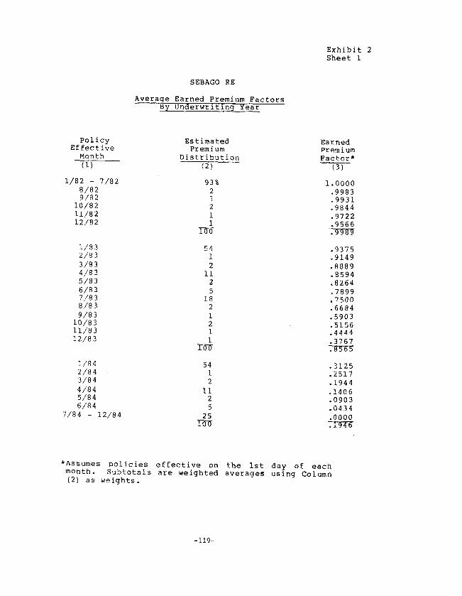
Exhibit 2 Sheet 1

Policy Estimated Effective

Earned Fremium Premium

Month Distribution Factor* (11 (2) (3)

l/82 - 7/82 8/82 9/82

lo/82 11/82 12/82

l/83 2/83 3/83 4,'83 5,'83 6/83 7/83 8,'83 9/83

lo/83 11,'83 12,'83

l/84 2/84 3/84 4/84 S/84 6,'84

7/84 - 12/84

SEBAGO RE

Average Earned Premium Factors By Underwriting Year

93% 2 1 2 1

-A 54

1 2

I.1 2

185 2 1

54 1 2

11 2 5

3%

1.0000 .9983

9931 :9844 .9722 .9566

m

-9375 -9149 .8889 .8594 .8264 . 7899 7500

:6684 .5903

5156 14444 .3767 T-R-!35

3125 :2517 . 1944 .1406 .0903 .0434 .oooo -TfTx

*;z;zes policies effecti,ve on the 1st day of each . Subtotals are welghted averages using Column

(2) as weights.

-119-

Exhibit 2 Sheet 2

NO. of Months From Policy

Effective Date (1)

2 3 4

65 7 8

1: 11 12

13 14 15 16 17 18 19 20

22’ 23 24

SEBAGO RE

Earned Premium Factors

Pro-Rata Parallelogram Earning Earning*

(2) (3)

.0833 1667

:2500 .3333 .4167

5000 :5833 .6667 -7500 -8333 .9167

1.0000

1.0000 1.0000 1.0000 1.0000 1.0000 1.0000 1.0000 1.0000 1.0000 1.0000 1.0000 1.0000

.0035

.0139

.0313

.0556

.0868

.:L250

.f701

.2222

.2813

.3472

.4201 . 5000

.0434

.0903

.1406

.1944

.2517 3125

:3767 4444

:5156 -5903 .6684 .7500

.5799 .7899

.6528 .8264

.7188 .8594

.7778 .8889

.8299 .9149

.8750 .9375 -9132 .9566 -9444 .9722 .9688 -9844

9861 :9965

9931 19983

1.0000 1.0000

Average [(2,'U',' + 2.0

*Assumes underlying policies are evenly distributed throughout the year. Figures are calculated by the following formula:

Earned Factor = M2 + 288, for M( 12

= l- [(24 - M)2 + 2881, for M > 12

Where M = Number of months from policy effective date.

-120-

Exhibit 3

SERAGO RE

CALCULATION OF NET ADDITIONAL LIABILITY

b/30/84 Underuritin3 Ultimte Earned

Year Premium Factor _____-__-__--- ---__-_------- ------__-__--

(1) (2) (3)

1980 $ 1t0001000 1 ,oooo 1981 2~000,000 1,0000 1982 310001000 .9989 1983 4,000~000 e8565 1984 5,0001000 ,1946

Totzl 1510001000

6/30/84

Ultimate Earned Premium

(2) x (3) - --------------

14)

0 lr000,000 2r000~000 21996,700 3~426~000

9731000

10,395,700

6130184 6/30/84 Unreported

Reported Earned Earned Premim Preaium (4) - (5)

^--_---------- ________-____-

(5) 16)

~1?000~000 5 0 2Y000~000 0 2f450rooo 5469 700 2,100~000 1,326~000

400r000 573,000

71950,000 21445r700

AddItional Initial Unreported Unreported

Underwritin3 Emense Emected Expenses Losses Year fidtio Lobs HAti (6) x (7) (6) :.: (8)

-------------- r------------- -------------- __-_____----__ ---__-_-----__

‘(1) (7) (8) (9) (101

1980 +30 ,800 s 0 s 0 1981 .30 ,850 0 0 1982 ,30 * 900 164,010 492,030 1983 ,30 i+ooo 397,800 1 r326rOOO 1984 130 1.000 171r900 573,000

Total 733,710 2~391~030

Net Additiunal

Llabilitv (9)+(101-(b)

------ -_--..---

(11)

1 0 0

109,340 397~800 171r900

6791040

Exhibit 4

SEBAGO RE

Ultimate Written Premium Basis

Frujected Ultimate Cusses !JSIII~~ Bumhuetter-Ferduson Techniaue Dn Incurred Losses

a,> UP 6/30/84

Initial Initial Expected Expected Percentage

Underurltin* Ultiadte Ewected Losses -----------------------------

Year Prer1un Loss Ratio (2) x (3) Reported Unrerurted -------------- -------------_ __----________ -------------- ----------____ ______________

!1) (21

0 1r000,000 2r000J000 3,000,000 4r000,000 59000?000

15r000~000

(3)

,800 ,850 ,900

1~000 1,000

(4)

1980 1881 1982 1983 1984

b 8001000 lr700r000 2,700,OOO 4r000~000 5r0007000

(5) (6)

83,33 16.67 66,67 33.33 50.00 50.00 25,OO 75.00

2.00 98.00

Total 14,200,OOO

Expected Reported

Losses (41 j: (5)

!li (7)

1980 S 665r667 1981 lr1331333 1982 i~350rooo 1983 1r000,000 1984 100I000

Total 4r250~000

.--

Actual Rerorted

Losses

Expected Unreported

Losses (4) i: (6)

-------------- ---------_-- (8) (9)

P 583~333 s 133,333 113331333 566,667 1,200f000 lr350r000 1~100~000 3r00or000

90rooo 4~900r000

4~306,666 9r9501OOO

--

Estimated Estimated Ultimate Ultimate

Losses Loss Ratio (8) t (9) (10) / (2)

-------------- -_ - - - - - - - - - - - -

(10) (11)

$ 716,666 ,717 1~900,000 ,950 2,550fOOO ,850 4r1001000 1,025 ~?990rooo ,998

14~256,666 ,950

-122-

Exhibit 5

SEBAGO RE

Adjusted Ultimate bitten Preriua Rasis

Projected Ultiwte LIJSS~S Usi~is Brtrnhuetter-Ferauson Techniaue On Incurred Losses

as of 6/30/84

Initial Adjusted Initial Expected Exrected Percentage

Underuritins Ul tinate Expected Losses """"""""""*"""""""""~""""""""

Year Premium Loss Ratio (2) x (3) Reported Unreported -"-""""""""""" """"""""""""-- ___________"_" ___""""___"""" __"""""""""""" """""-""""""""

(1) 12) (3) (4) (5) (6)

1980 B 1,000~000 ,800 $ 800 I 000 83.33 16.67 1981 21000~000 ,850 lr700~000 66.67 33.33 1982 3,000~000 ,900 2,700,000 50.00 50,oo 1983 4r000~000 1,000 4r000~000 25.00 75.00 1984 3r75oYoOo 1.000 3,750,ooo 2,67 97.33

Total 13J750,000 12~950~000

Expected Reported

Underwriting Losses Year (4) x IS)

““““““““---““” “-““““““-““““”

(I) (7)

1980 S 6669667 1981 1~133,333 1982 lt350Y000 1983 1~000,000 1984 100,000

Total 4,250,000

nctual Reported

Losses ---""""""""""" _

(8)

Expected Unreported

Losses (41 x (61

(9)

S 583,333 $ 133,333 19333,333 5669667 1,200,000 1,350,000 lrIOOIOOO 3,000r000

90,000 37 650,000

4~306,666 8r700iOOO

Estimated Estimated Ul tiaate Ultimate

Losses Loss Ratio (8) t (9) (10) / (2)

“““““““““““““” I”““““““““““”

(IO) (11)

s 716~666 ,717 11900,000 ,950 2r550,OOO ,850 4~100,000 1,025 3Y740,OOO *997

13~006r666 ,946

-123-

Exhibit 6

SEFAGO RE

UltirAe Earned Premium Basis

Projected Ultimate Losses Using Bornhuetter-Fer3ue.m Technieue On Incur rwd Losses

JS @C 6/30/04

Initial Ultimate Initial Expected Expected Percentcdr

Underwritins Earned Exrec ted Losses ---__--__--___-___-__________

Year Frenium Loss Ratio (2) x (3) Reported Unreported __------------ __------------ -------------- ----------_--- ---__--------_ __-__-________

(1) (2) (3) (4) (5) (4)

1980 6 1r0007000 ,800 1 800~000 83.33 lb.b7 1981 2r0009000 ,850 lr700r000 66*6? 33.33 1982 2~996,700 ,900 2~6971030 5O.Ob 49,94 l?Bf 3,426rOOO 1.000 3~426,000 29~19 70,81 1984 973rooo 1,000 9731000 10.28 89.72

Total 10,395r700 9r596,030

Expected Ewrcted RePorted Actual Unreported

Underuritins Losses Herorted Losses Yea;. (4) x (5) Losses (4) x (6)

-------------- ---------_---- -------_----_- ----___---__--

(1) (7) (8) (9)

Estimated Estimated Ultimate Ultimate

Losses Loss Ratio (8) t (9) (10) / (2)

------------ ------------_- -- (10) (11)

1980 B 6661667 $ 5839333 4 133,333 S 716~666 ,717 1981 19133,333 19333,333 566P667 11900,000 ,950 1982 1,350r000 lr200,000 lf347PO30 2~547,030 ,850 1983 lr0009000 1~100~000 2~426~000 3~526~000 1,029 1984 100,000 90rooo 873~000 963rOOO ,990

Total 4.2509000 4v3Obrbbb 5~346~030 9y452,&?6 ,929

-124-

Exhibit 7

SEBAGO HE

Reported Earned Presiur Basis

Pro.iected Ultimtr Lorises Usin Burnhuetter-Ferduson Techniaue On Incurred Losses

JS of b/30/84

Initial Reported 10itial Expected Ewacted Percentatie

UnderwritinS Earned Expected Losses --_-----------------*--------

Year Fweiua Loss Ratio (2) x (3) Reported Unreported ------------_- -------I------ ----_-___-___- ______---_-___ -------------- --------------

(If 12) (3) (4) (5) (6)

1980 %1,000,000 D 800 0 800,000 83.33 16.67 1981 2r0009000 ,850 1,70or000 66.67 33.33 1982 2r4501000 ,900 2~205rOOO 61 r22 38.78 1983 2,100,000 l*OOO 2r1001000 47,62 52.38 1984 400,000 1.000 400r000 25.00 75.00

Total 7r950rooo 7~205rOOO

Expected Expected Estimated Reported Actual Unreported Ultiaate

Underuritins Losses Reported Losses Losses Year (4) x (5) Losses (4) x (6) (8) t (9)

-------------- -------------- -------------- -------------- --------------

(1) (7) (8; (9) (10)

Estimatcti Ultirate

Loss Ratio (10) / (2)

--------------

(11)

1980 4 666,667 4 583,333 4 1331333 4 716,666 ,717 1981 lt133r333 113339333 566r667 lr900r000 ,950 1982 i,350~000 1,200,000 8551000 2~055~000 ,839 1983 1,000?000 1~100l000 11100~000 2t200r000 1.048 1984 100,000 90,000 300,000 390,000 ,975

Total 4r2501000 4r306~666 2t955rOOO 79261~666 ,913

-125-

TITLE: BANX ACCOUNTS AS A TOOL FOR RETROSPECTIVE ANALYSIS OF EXPERIENCE ON LONG-TAIL COVERAGES

AUTHORS: Claudia S. Forde

MS . Forde is a Consulting Actuary for Tillinghast, Nelson & Warren, Inc. Her eight years of experience in the casualty actuarial field include four years with Tilling- hast and over four years with a major personal lines writer. Ms. Forde received her ACAS in 1983 and is a Member of the American Academy of Actuaries. She holds a B.S. degree in Mathematics from Emory University.

W. James MacGinnitie

Mr. MacGinnitie is the Managing Principal of the Casualty Division of Tillinghast, Nelson & Warren, Inc. He has twenty-three years of experience in actuarial work inclu- ding ten at Tillinghast. Immediately prior to joining Tillinghast, Mr. MacGinnitie was Director of the Master of Actuarial Science Program at the University of Michi- gan's Graduate School of Business Administration. He is a Past President of the CAS, a Fellow of the CAS and a Fellow of the Society of Actuaries.

ABSTRACT: This paper presents a model for the retrospective analy- sis of experience on long-tail coverages. The model chosen is a "bank account" model which considers separ- ately the profitability of each exposure period. The model treats premium income and interest earnings as bank account deposits, and loss payments, expense payments and interest charges as withdrawals.

The exposure period results are calculated on three different bases: traditional underwriting profit/loss, net operating result at current value, and net operating result at exposure period value. Results are also dis- played graphically for an effective presentation of the profitability/unprofitability of the exposure period.

A model of this type is a valuable tool for communicating financial results to management and others in an effec- tive and straightforward manner. It is particularly helpful in the evaluation of long-tail lines of business.

-126-

RANX ACCOUNTS AS A TOOL FOR RETROSPECTIVE AXALYSIS OF EXPERIEtZiCE OH LONG-TAIL COVERAGES

As interest rates have risen and claim settlement patterns have

lengthened, actuaries have increasingly been called upon to take the

time value of money into account when evaluating profitability. When

analyzing historic results, this sometimes requires assumed rates of

return and payment patterns, because actual historic data is not read-

ily available. Where the data is available, however, it is possible to

produce an analysis which can be communicated to management and other

interested parties in an effective and straightforward manner.

The model chosen is a "bank account". It considers each exposure

period as a separate bank account. The account receives an initial

deposit (premiums collected less expenses) which is reduced by with-

drawals (loss and loss expense payments), increased by interest earned

and reduced by interest charges when the balance goes negative.

The model will seem straightforward, even simple, to anyone who has

mastered compound interest. It is presented here only because of its

utility in communicating results, particularly to important but less

experienced audiences.

By looking at each exposure period separately, the model enables us to

estimate profit or loss individually by exposure period. It provides a

hindsight look at what an appropriate rate level would have been in

each exposure period. The bank account model is particularly helpful

-127-

in evaluating long tail lines. The attached exhibits show the appli-

cation of the model to the medical malpractice line of business.

In long tail lines such as medical malpractice, investment income is a

crucial variable in the ultimate profitability or unprofitability of

the insurance enterprise. Care should be taken in the selection of

interest rates for the bank account model. The over or understatement

of investment income can obviously have a distortive effect on the

exposure period results. In the example which is attached, we have

used actual portfolio average rates of return for those calendar years

in which this information was available to us (1974 through 1983) and

one-year Treasury Bill rates as a reasonable approximation of available

rates of return for the earlier years (1959 through 1973).

Although real world considerations introduce complexities to this

simple illustration, the basic concepts are still applicable. Expenses

include unallocated loss adjustment expenses in addition to taxes,

underwriting and acquisition expenses, if any. No Federal income tax

implications have been considered. However, consideration has been

given to the interest charge which is made when the exposure period or

report period account balance turns negative. This charge represents

interest income lost because the particular exposure period account is

overdrawn and "borrowing from the bank." In the case of a multi-

line/state company, the bank represents one of three sources of funds:

surplus, profits from other states or lines of business, or future

policy years (i.e., other "bank accounts"). For a one-line, one-state

company, there are only two sources of funds: surplus and future

-128-

income. Obviously, the borrowing of funds from the future to pay the

loeees of the past implies both that those funds will not be available

to pay future losses and that the expected interest return on those

funds (which may be anticipated in the premium structure) will not be

collected.

Beneath the account's annual transactions is shown a Summary of

Results. This 8ummary consolidates the transaction8 over time and also

includes the unpaid loss liability for the account, both reported and

estimated unreported.

In the Summary of Results table, results are shown on three different

bases. The first is traditional underwriting profit/loss, which is

simply the amount of funds available for losses, less loss and allo-

cated loss adjustment expenses paid and remaining to be paid. This

measure does not consider any investment income.

The second measure reflects imputed investment income received through

the evaluation date (including the charge for borrowing if the balance

is negative), as well as discount on unpaid losses and loss expenses at

some assumed rate and payment pattern. This is shown as the net oper-

ating result at 12/31/83 value.

The third measure is the net operating result at the middle of the

initial exposure period. If negative, it is the additional amount

which, if it had been in the account at the time that premiums were

collected, would have resulted in no net gain or loss after all claims

-129-

were paid. If the account is profitab1.e. it represents the "profit at

issue".

In order to clarify how the bank account analogy works, we can review

Exhibit I, which shows the 1964 policy year account for Employers

Insurance of Wausau physicians and surgeons professional liability

business in New York. The initial deposit (premium paid) in 1964 was

S4,325,000. This was reduced for expenses of $700,000, resulting in

the initial balance of $3,625,000. It should be noted that, although

this amount is shown as the balance at January 1, 1964, the interest

calculation in the initial calendar year assumes that this amount is

not available until July 1.

Withdrawals (loss and allocated expense payments) for calendar year

1964 were $31,000, while interest income on the average fund at the

rate of 3.89% yielded $69,000. In subsequent years, withdrawals (loss

and allocated expense payments) increase sharply, exceeding the

interest income earned and reducing the account balance dramatically.

In 1971 the withdrawal exceeds the account balance making the balance

as of January 1, 1972 $-282,000. From this point on, the account is

charged, rather than credited, with interest. In calendar years

1972-1983, loss and expense payments total $4,643,000 and imputed

interest charged is $3,312,000, creating an account balance of

$-8,237,OOO on January 1, 1984.

The Summary of Results shows an underwriting loss of $6,836,000, which

is $4,325,000 of premium income, less $700,000 of expense, $9,615,000

of paid loss and allocated expense, and $846,000 of unpaid loss and

-130-

allocated expense (of which $676,000 is reported and $171,000 is

unreported). The net operating result valued at 12/31/83 is a loss of

$8.862.000. This reflects discount, at the rate of 128, on the unpaid

loss and allocated 1088 expense, in the amount of $221,000. The net

operating result at 1964 value is a 1088 of $2,851,000, which is to say

that Employers needed $2,851.000 of additional funds at the time that

premiums were being collected in 1964 in order to come out with a

breakeven result when the last claim is paid.

The bank account information can also be shown in graphical format, as

displayed on Exhibit II. The Solid line shown as "Available Funds"

represents premium income, reduced by expenses, then augmented by

interest income. The dashed line represents paid losses and allocated

loss adjustment expenses, while the dotted line shows reported losses

and allocated expenses (paid plus case basis reserves). The available

funds line stops at the point at which paid losses and allocated loss

adjustment expenses exceed available funds. We have included a

"dollar8 per doctor" scale on the right-hand side of the graph, as well

as reported loss and allocated expense information (not included in the

bank account on Exhibit I), to enhance the value of the graph as a

communications tool.

Where a good series of historical data is available, it is possible to

prepare separate accounts for each exposure period. Accident years or

policy years can be used, with appropriate adjustments in the computa-

tion of interest earned in the initial year. If the experience has

been consistently profitable or unprofitable, the cumulative communi-

-131-

zative impact of a series of graphs can be quite effective. It is also

easy to produce exhibits which account for an entire period of years to

illustrate the cumulative experience. Exhibit 111 shows the cumulative

experience of fifteen and one-half years of medical malpractice writ-

ings and Exhibit IV shows the same experience graphically. In Exhibits

III and IV, no interest was charged on the cumulative balance after it

turned negative. (Interested readers can obtain the complete set of

bank accounts and graphs which underlie these cumulative exhibits from

the authors.)

There are a number of simplifications in the present model, as des-

cribed earlier, which could be removed for a more in-depth analysis.

Expenses could be spread over time rather than charged to the initial

calendar year. Consideration could be given to Federal income taxes.

Finally, there are numerous adjustments that could be made to the

method of allocating investment income. Investment year methods, for

example, could keep track of funds by year originally received, and

could reflect the actual term structure and reinvestment results. In

this regard, our life insurance colleagues have already investigated

several methodologies for handling the complex accounting and

allocation procedures. Consistency in the choice of either new money

yields or embedded yields is obviously desirable.

The advantages of the bank account model for presenting exposure period

experience are mainly in the area of better communication. It provides

an effective way of looking at past underwriting results which is part-

icularly helpful when explaining results to non-actuaries or the non-

-132-

financially sophisticated. We have found it particularly useful in the

medical malpractice field, where specialty companies formed in the

middle 1970's are cash rich but still need regular rate increases

because of the long term trend in pure premiums on the order of 20% per

annum. These rate increases must be decided upon by boards of

directors composed primarily of medical professionals with little

insurance or financial expertise. It has also been useful in dealing

with arguments advanced by the plaintiff's bar, generally to the effect

that investment income has been inadequately taken into account.

The bank account model is not without its disadvantages as well.

Although it is a valuable tool in explaining financial results to the

non-sophisticated, it should not be used in place of actuarial anal-

ysis. It can in fact be a dangerous weapon in the hands of someone

unfamiliar with its limitations. Chief among its limitations is the

fact that the bank account model can not be used to make rates prospec-

tively, nor to set adequate reserves. It is, however, a very useful

method for analyzing and communicating financial results by exposure

period.

We have programmed the model in APL, but it could be easily undertaken

in spreadsheet software as well. Contributions to the development of

the model were also made by Jim Hurley, Dean Anderson, and Terry

Biscoglia. The data used in the attached exhibits was provided by

Employers Insurance of Wausau.

-133-

Exhibit I Sheet 1

NEU YORK PHYSICIANS AND SURGEONS

EMPLOYERS INSURANCE OF YAUSAU

1964 POLICY YEAR

(soool

PREHIUtl INCOME = S 4325 LESS EXPENSES(A) - 700

AVAILABLE FOR LOSSES(B) = $ 3625

CA++tttAR Bijl#CF&J I

---------- ---__-____ (1) (2)

1964 s 3625

YE i 967

ifs6i 3748

1968 3355

1969 2863

li9oSP 25371 ‘1995: -1503 -282

1974 -2117 1975 -2563 1976 -3411 1977 -3879 1978 -4226

1979 -4693

:w -5054 -5534

:EE I$;;$

1984 -8237

TOTAL

UITH-

1 RAYALS

( HTS)(B) ----------

(3)

s

3

it

6;;

916 1654

860 1176

478

319 679 266 119 213

8 9615

SUfiliARY -------

Rf!%N%, flj#lE% 1 --------- ----------

(4) (5)

7.28 182

6.94 4.90 93 5.01 -44 7.54 -136

-286

13,;: -405 -637

OF RESULTS -- -----em

FUNDS AVAILABLE FOR LOSSES PAID LOSS AND ALLOCATED LAE UNPAID LOSS AND ALLOCATED LAE

REPORTED UNREPORTED(F)

UNPAID LOSS AND ALAE DISCOUNTED AT 12X UNDERWRITING PROFIT/LOSS INTEREST INCOME/LOSS NET OPERATING RESULT AT 12/31/83 VALUE NET OF’ERATING RESULT AT 1964 VALUE

8 -2247

8 3625

9E

% 625

-6836 -2247 -8862 -2851

-134-

Exhibit I Sheet 2

Notes to Exhibit I, Sheet 1

(a) Expenses include administrative and unallocated loss adjust- ment expenses. Employers Insurance of Wausau figures have been extracted from figures they have provided to the New York Insurance Department (Exhibit IA).

(b) Includes allocated loss adjustment expense.

(c) In the initial year, the balance is only available for a half-year.

(d) Yields for calendar years 1959-1973 are based on one-year Treasury bill yield rates. Yields for subsequent years are the actual calendar year yields achieved by Employers Insurance of Wausau, as defined by net investment gain or loss (including realized capital gain or loss) divided by mean total assets.

(e) Assumes all transactions occur uniformly throughout the year.

(f) Provision for unreported losses is based on the projected ultimate pure premiums developed in Part I of the Medical Malpractice Insurance Association of New York June 1984 physicians and surgeons professional liability rate filing.

-13%

12

8

4

0

NEW YORK PHYSICIf3NS F1ND SURGEONS EMPLOYERS INSURflNCE OF WFIUSRU 1964 POLICY YERR

#I /* */>

,t* -----.N--/ /-- -1

#-- r’

/ l - /A

, ,*

. /

1

:

A / 0 AVFIILRBLE FUNDS

U PRID LOSSES *#

-- m- I

I’ I

: / I

1’

: /

// VFILUED FIT THE END OF YEFIR- I I I I I I I I I I I I

3 5 7 9 11 13 15 17 19 21 23 25

600

E -500 s

Ei -4moc

iii! -3m 0 CE a -2003

00

-100 !! P tT

-0 : l-4

.

Exhibit III &li?etl

caldar .-j-F

Preluiun w=!?z-

LossaId Ilmxm Intereet Interest hurls at ArAFl F&id(c) Cash Flow(d) Yield(e) Incundf) Year-Em3

(4) (5) -G-r -0 -0

1959 $2,442 $544 $ 76 $ 1,822 4.71% .9 42 $ 1,864 1960 2,895 642 183 2,070 3.55 104 4,038 1961 3,269 610 499 2,160 2.89 149 6,347 1962 3,790 655 633 2,502 3.10 238 9,087 1963 4,121 671 825 2,625 3.41 359 12,071

1964 1965 1966 1967 1968

4,325 4,428

x2 8:948

700 1,491 2,134 3.89 701 1,884 1,843 4.23 769 3,385 850 5.34 910 3,547 1,449 4.94

1,359 4,306 3,283 5.78

519 674

E 1,370

14,724 17,241 19,057 21,503 26,156

1969 11,939 1,657 4,778 5,504 7.28 2,164 33,824 1970 18,964 2,297 8,204 8,463 6.94 2,707 44,994 1971 33,256 3,060 7,130 23,066 4.90 2,811 70,871 1972 38,760 3,989 13,410 21,361 5.01 4,160 96,392 1973 36,903 4,157 19,297 13,449 7.54 8,008 117,849

1974 1975 1976 1977 1978

18,594 3,524 25,108 30,162 25,990 30,976 42,904

(10,038) 13205, zo;

(30:976) (42,904)

5.47 6,536 114,347 5.68 5,810 89,995 5.53 4,385 68,390 5.63 3,073 40,487 5.72 1,137 (1,280)

1979 1980 1981 1982 1983

51,930 48,044 39,460 37,372 30,383

Ef92i (39:%0) (37,372) (30,383)

5.88 0 (53,210) 6.55 0 (101,254) 6.89 0 (140,714) 7.36 0 (178,086) 8.26 0 (208,469)

aployers InswanceofWausau -ial R~~u.l.t33 for lblicy Years 1959 - 1974(a)

at 12/31/83 cxm)

Loss an3 ALAI?, Case Reserve @ 12/31/83 $ 76,583

Loss an3 AIAE IBNR @ 12/31/83 (g) 109,894

Total Unpaid ?&es ard AIAE @ 12/31/83 $186,477

unpaid Loss ti AIAE Discount& at 12% $101,997

-137-

Exhibit III Sheet 2

Notes to Exhibit III, 8heet 1

(a) Based on Employers' experience for policy years 1959-1974. Policy year 1974 is a partial writings from l/1/74 - 6/30/74.

policy year, reflecting

(b) Expenses include administrative and unallocated loss adjust- ment expenses. Employers' figures have been extracted from figures they have provided to the New York Insurance Department (Exhibit la).

(c) Includes allocated loss adjustment expense.

(d) Insurance Cash Flow [Column (5) = Columns (p)-(3)-(4)].

(e) Yields for calendar years 1959-1973 are based on one-year Treasury bill yield rates. Yields for subsequent years are the actual calendar year yields achieved by Employers, as defined by net investment gain or loss (including realized capital gain or loss) divided by mean total assets.

(f) Assumes all transactions occur uniformly throughout the year.

(g) Provision for unreported losses is based on the projected ultimate pure premiums developed in Part I of the Medical Malpractice Insurance Association of New York June 1984 physicians and surgeons professional liability rate filing.

-13s

NEW YORK PHYSICIflNS flND SURGEONS EMPLOYERS INSURANCE OF WRUSAU

POLICY YEARS 1959-1974 COMBINED

-225 i I I I I I I

59 63 67 71 75 79 83

RS OF YEfV? END XX

Projections of Surplus for Underwriting Strategy

William R. Gillam

Mr. Gillam is an Actuarial Associate at North American Reinsurance. His previous experience was at Prudential Reinsurance and Insurance Services Office. He has an M.S. from Rutgers University (1976) and a B.A. frQn Wesleyan University (1971), both in mathematics. He became an Associate of the CAS in 1982.

Abstract

The paper presents a specific modeling approach to the projection of surplus.

The model uses assumptions on growth, underwriting results, underwriting cash flow, interest and tax to simulate the operating results of an insurance company. Investible assets are incremented by cash flow at-d surplus by after tax income on an iterative basis for the years of the projection.

Results of several possible underwriting strategies of a multi-line canpany are compared according to several financial tests.

The vehicle for this model is an APL program, whose specifications are part of the paper.

It is hoped that the value of a model will be evidenced by this exposition. In addition, some of the canponents of this particular model may be useful in themselves, and conclusions I have made at least thought provoking.

William R. Gillam

-140-

Projections of Surplus for Underwriting Strategy

William R. Gillam

I. Need for a Projection of Insurance Company Surplus

Of course, anyone connected with the management of an insurance company

would like to be able to predict inccme or surplus for the years of the

foreseeable future. This is more than just wishing for a crystal

ball; good estimates of future incane may be necessary for several

purposes. Among then are the following:

1. Part of a valuation

2. Planning for management

3. Reports to stockholders or a parent canpany

4. An aid to underwriting strategy

This paper is primarily about the last, although the methods presented

have been used for iten 3. and could easily be used for 1. OK 2..

I have included an example of the prediction of surplus for a fictitious

multiline canpany, and some conclusions about underwriting strategies the

canpany may adopt. The input data for this company is hypothetical, but

the cash flow patterns resemble those of a casually oriented reinsurer,

an example which should best exhibit the distortions inherent in statutory

accounting.

Specifications of the program are liSted in III and hard copies of programs

and outputs appear in Exhibits C and D.

-141-

Projections of Surplus for Underwriting Strategy

II. Need for a Canputer Model

I probably need not defend the use of modeling to the actuarial comnunity.

Power and flexibility to handle a variety of situations are a primary

consideration. Ease of use and modification should also characterize a

god model. APL, which I have used for this particular model, allows

satisfaction of both criteria. This model could also probably be

executed on a spread sheet package such as LOTUS l-2-3, although the

reader will have to write his/her own.

Another advantage of a model which is not so obvious is that it forces

the creator to be more aware of each of his assumptions, its effect, or

whether it is even necessary. In my model, future growth, underwriting

results, interest rates, and transaction cash flow patterns will be

ass&. The ccmputer does the accounting. The computer is no better

at predicting the future than the user, but for testing the effect of

varying some selection of input parameters while holding others fixed,

it excels.

-142-

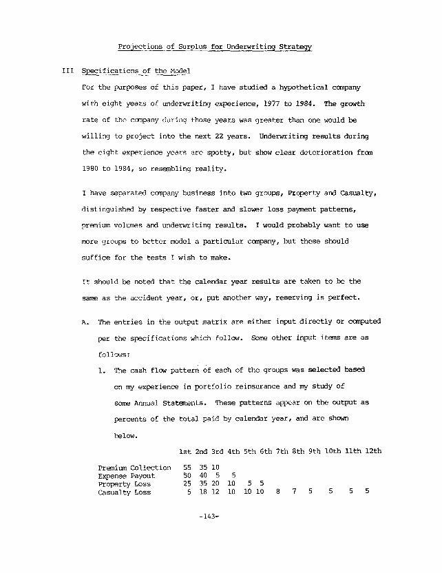
Projections of Surplus for Underwriting Strategy

III Specifications of the Model

For the purposes of this paper, I have studied a hypothetical canpany

with eight years of underwriting experience, 1977 to 1984. Thegrowth

rate of the company during those years was greater than one would be

willing to project into the next 22 years. Underwriting results during

the eight experience years are spotty, but show clear deterioration fran

1980 to 1984, so resembling reality.

I have separated company business into two groups, Property and Casualty,

distinguished by respective faster and slower loss payment patterns,

premium volumes and underwriting results. I would probably want to use

more groups to better model a particular canpany, but these should

suffice for the tests I wish to make.

It should be noted that the calendar year results are taken to be the

same as the accident year, OK, put another way, reserving is perfect.

A. The entries in the output matrix are either input directly OK canputed

per the specifications which follow. Some other input items are as

follows:

1. The cash flow pattern of each of the groups was selected based

on my experience in portfolio reinsurance and my study of

some Annual Statements. These patterns appear on the output as

percents of the total paid by calendar year, and are shm

below.

1st 2nd 3rd 4th 5th 6th 7th 8th 9th 10th 11th 12th

Premium Collection 55 35 10 Expense Payout 50 40 5 5 property Loss 25 35 20 10 5 5 Casualty Loss 5 18 12 10 10 10 8 7 5 5 5 5

-143-

Projections of Surplus for Underwriting Strategy

2. Surplus and investible assets fior 1984, $100 and $300 thousand

respectively. For the purposes of this paper "assets" will mean

investible assets, unless otherwise noted.

3. Effective interest rates by year. I selected +lO% by year,

starting 1985. For a cyclical pattern, I selected a ten year

cycle, which starting i n 1984 is

11, 10, 10, 8, 8, 8, 9, 10, 11, 12%

4. Tax rate of 46%, ignori ng any surtax exemptions.

5. An arbitrary portion (20%) of investment income was designated

tax fK@Z. This could be due to tax free bonds and/or the 85%

dividends received deduction. In practice, it would be adjusted

to better fit a company's results and investment portfolio

strategy.

6. A provision for a tax loss carry forward of seven years and a paid

tax recovery of three.

B. Itens 1 thru 9 are calculated separately for each group as follows:

1. Preinims Written These are entered exactly for

PWi , yew i (presumably) historic years and

as annual growth factors for years

to ba projected.

2. Accident Year Loss Ratio

LRi

These are input as a ratio to

premium earned.

-144-

3.

4.

6.

7.

8.

9.

Projections of Surplus for Underwriting Stratew

Expense Ratio

ERi

Prmium Earned

PEi= OcPWi+(i-d) PW

These are ratios to premium written,

as entered.

These are entered for historic years

i-i and calculated for the years of the

Where cl projection, based on an average preniun

x, PEj-PWj-1 earnings pattern. OLZ

P, PWj”PWj- 1.

Premium Collected This is a sum of the respective percents

of the present and four prior years'

Expense Incurred Extension of premium written by expense

Ei = ERi l PWi ratio.

Expanse paid

EX; = 5 EF:, l E 1ci-j A sm of respective portions of present

and fOuK pKiOK years' iIK!IIKKed expenses.

EF;: ikJpJ ewpen* payrw+ +C+W Losses Incurred Extension of prenim earned by loss ratio.

Li = LR; l PEi Losses @d A sum of respective portions of present

Lpi : $zILFj * Li+;-j and 14 prior years' losses incurred.

Items 10 and 11 are calculated for all groups canbined.

10. Underwriting Profit Pmnim earned less losses

UizPE~-CLi+Ei) and expense incurred.

-145-

Projections of Surplus for Underwriting Strategy

11. Underwriting Cash Flow Premimn collected less loss

UCi=PCi-(EXitLPi) and expensepaid.

Items 12 thru 20 are calculated sequentially by year for total business,

starting at a selected "last historic" year.

12. Investment Incane

Ii=(A;-,+o.s UC;I%Ri

Whete Ai is the Qhtitia\

e$$ec+k to&z

13. Gross Operating Incane

GI; = U;+I;

14. Taxable Income

Tli = Ui + Bfi

15. Effective Taxable Inccste

ATI;

(see A’? L)

16. Tax Paid

TPi =TRxATI;

17. Dividends or other

decrements to inccme.

Di

Extension of prior year's ending

invested assets plus one half

of underwriting cash flow by rate of

interest.

Total underwriting profit and investment

income.

Underwriting profit plus taxable

portion of investment income.

This is adjusted incane on which tax is

actually paid, after loss carry forward

or prior paid tax recovery.

Per input tax rate on effective

taxable income.

As input

-146-

Projections of Surplus for Underwriting Strategy

18. Ehding Investible Assets Previous year ending assets plus

Ai=Ai_,+u~i+Ti-(TPicDi~ U/W cash flow and investment

inccme minus tax paid and dividends.

19. mding Surplus Previous surplus plus U/W and

S;=Si-,+U;+I;-(TPi +D;) investment profit minus tax and

dividends paid.

20. Discounted Surplus At a rate l/l0 greater than the

rate of interest income, to reflect

an arbitrary preniun for risk.

21. GAAP Adjust+ Surplus Ending surplus fran 19. plus 15% of an

Si + Q~S i PWS-PE~ approximation for the unearned premium i

reserve, this being cumulative

written less earned premium.

-147-

IV Comparison of Some Underwriting Scenarios

A. General characteristics of the projection.

These ccmnnents pertain to the information graphed in Exhibit A. Each

scenario 1 through 6 is a canbination of growth vs. no growth in

premium volume and underwriting results which remain poor, improve,

or follow a cyclical pattern.

1. Flat writing, retain high loss and expense ratios.

Probably a worst case result for underwriting would be continued

writing at a combined ratio almost as high as the worst year,

1984, and not increase volune. The ultimate combined ratios are

106 and 115% for Property and Casualty respectively.

Surplus and assets both increase steadily and iaunediately, at

a reasonable rate which is, however, less than the 11% target

rate of discount.

The ratio of prenilrms written to prior surplus drops steadily to

less than 1.1 in 1995, so a canpany in such a position could

pay substantial dividends or expect a takeover by a capital

hungry purchaser.

The leverage ratio (assets-surplus) + surplus also drops

steadily, again indicating unused capital. (Investible assets

minus surplus is used as a sanewhat imperfect measure of

liabilities).

Statutory and @AP surpus are parallel after a year or so.

-148-

Projections of Surplus for Underwriting Strategy

2. Flat writing, decreasing loss ratio.

This may be an actual short-term goal of some insurance company

management. The ultimate combined ratios I have projected are

102 and 108% for Property and Casualty respectively, which may

be as good as we can hope for.

The increase in surplus is steady and immediate as for Scenario 1,

but the rate of increase flirts with 11% for more than 10 years.

After 1997, discounted surplus drops consistently as returns to

equity become more and more disappointing.

The premiums written to surplus ratio drops precipitously as

does the leverage ratio (Assets-Surplus) + Surplus. This is

very inefficient use of capital, and the same counts as for

Scenario 1 apply.

3. Growth, retaining high loss and expense ratio.

What would happen if a company continues to chase cash flow by

increasing volume at the expense of effecting any underwriting

control?

Surplus and assets both eventually increase, but surplus

does decrease for a year after the particularly poor 1984

underwriting year. It is not until 1990 that surplus increases

at a rate greater than the target 11%.

-149-

Projections of Surplus for Underwriting Strategy

The test ratio Written Premium + Prior Surplus is high, especially

in 1986, but remains less than three. This would not be the case

for much higher growth rates than the selected +8% for Casualty

and +6% for Property.

The leverage ratio (Assets-Surplus) + Surplus remains fairly

constant and as such seems within control, although this favor-

able appearance may be a distortion due to my approximation for

liabilities.

Surplus increases at a rate greater than 11% after 1989, but GAAP

surplus is already growing faster than +ll% in 1987.

4. Steady growth, decreasing loss ratio.

This would be an ideal situation. Recovery fran the exceptional

1984 year really only begins in 1986, but after this growth

and vital signs all appear good. The leverage ratio steadily

decreases and a payment of dividends would be in order.

Sanehow, I feel we do not need to spend much time admiring this

scenario.

5. Growth, with cyclical underwriting results.

Surplus and GAAP surplus increase unevenly, as might be expected.

Premiums to surplus is almost three in 1986, caning off the bad

underwriting year 1984. Our leverage ratio is worst in 1987.

-150-

Projections of SUKplUS for Undenhlriting Strategy

After this year, most vital signs are under control and surplus

increases at a rate alternating above and below the target 11%.

In general, we observe a 2-3 year lag for financial results

following underwriting results.

6. Growth, with cyclical underwriting results, which lag a

cyclical pattern of interest rates by two years.

This may or may not resemble reality, and I have included it

for curiosity's sake. My comments are nearly the same as those

for Scenario 5 above, except results are worse due to lesser

investment income. It is interesting that surplus discounted

along rates which follow the fluctuations (plus the premium)

remains significantly worse than discounted surplus in the case

of a uniform 10% rate, seen in Scenario 5. This may be the

result of continuing to write to a high combined ratio when

interest rates are falling, just as in current industry results.

B. Some comparisons of the projections.

These comparisons are graphed in Exhibit B.

1. Flat premium writings with improving underwriting vs. growth at

expense of continued high loss ratio, ‘AZ. vs. A3.

Writing to a lower loss and expense ratio at the expense of

growth has some bad characteristics mentioned above, but the

-151-

Projections of Surplus for Underwriting Strategy

effect on statutory surplus iS quite desirable. In this case,

the strategy produces higher surplus for 15 years than that for

continued growth'at a high combined ratio.

This comparison holds even for GAAP adjusted surplus, which

recognizes equity in the unearned premium for emissions paid

but not yet earned, so the regulatory strategem of curtailment of

premium writings for too rapidly growing companies may make n-ore

sense than it seems, at least if underwriting results improve.

2. Flat premium writings, no improvement in underwriting vs.

growth with no improvement in underwriting, Al. vs. A3.

Even when the curtailment of premium writings does not result

in better underwriting, statutory surplus will be better in

the case of no growth than in the case of growth for sane eight

years. The effect is not great, but it even OCCUKS in GAAP

surplus for five years.

The retention of a high leverage ratio in the growth case

ultimately leads to greater incana, but with a significant

time delay if underwriting results are poor.

The effect on statutory surplus of no growth, even if underwriting

does not improve, may still justify regulatory procedure.

-152-

PKOjeCtiOnS Of Surplus fOK UnderWriting strategy

3. Growth with poor loss and expense ratio vs. growth with cyclical

underwriting results, A3. vs. A5.

Surplus may be expected to vary more if underwriting results are

cyclical than if they are steady. So it is here, where the

surplus under cyclical underwriting snakes around the surplus of

the steady case.

It may be Observed fran the graph that the surplus fran the

cyclical underwriting case averages higher than that for the

stable scenario. This is in spite of the fact that the prsmium

weighted 20 year average loss and expense ratios for the cyclical

case, 80.1 and 31.4%, are higher than those in the steady state,

80.0 and 31.1. I would be a little hesitant to recanmend this as

a strategy, but if positive cash flow can be maximized at time

preceding high interest rates, the cycle may make economic sense.

-153-

Projections of Surplus for Underwriting Strategy

V Conclusions

The following conclusions are based on a fairly simple canputer model and

a set of assumptions which may not be fully justified, so are open to

debate. I hope: 1. the shortcomings of the model are minimized when

comparing results of different ingoing strategies under the same assun@ions,

and; 2. a debate is actually opened, resulting in improved modeling

techniques. It may be the case the conclusions of my KeSeaKCh are no more

than what is ccennon knowledge of financial planners, but even at that, the

viability of a model will have been demonstrated.

A. Conservative underwriting, even at the expense of growth, results

in higher incare than growth with continued poor underwriting. This

is even true for GAAP adjusted surplus.

B. There is a need fOK other than a statutory approach for measurement of

results. i$' Simple proxy fOK a CAAP adjustment Suggests even CAAP may

hide the true picture. I believe discounting reserves and better

monitoring of cash flow would be parts of such an approach, as well as

a true GAAP adjustment.

C. A cyclical underwriting pattern may have desirable effect on ultimate

inccme. This is especially true, of course, if cash flow can be timed

to take full advantage of changes in interest rates. It is also known

that the UndeKwritiKKJ cycle may well have adverse effects on down

years' financial results, which this model shows lag poor underwriting

years by l-3 years. Management may find reporting such results undesirable,

even when there need be no cause for alarm.

-154-

EXHIBIT A, p.1

1. FLAT WRITINGS CONTtNlJED POOR LOSS RATIO

1600 l-

1400 -

1200 -

1090 -

800

600

400

200

0 1984 85 86 82 88 89 90 91 92 93 94 95 96 97 98 99 2000 01 02 03 CM

EXHIBIT A, p.2

2. FLAT WRITINGS, IMPROVING LOSS RATIO

1600 r

1400

1200 t

01 ’ ’ ’ ’ ’ ’ ’ ’ ’ ’ ’ I ’ I I I I I I ,

1984 85 86 87 88 89 90 91 92 93 94 95 96 97 98 99 2000 01 02 03 it.4

EXHIBIT A, p.3

3. GROWTH, RETAIN HIGH LOSS RATIO

1600

1000 -

800 -

600-

200 -

o-“““““““““” 1984 85 86 87 88 89 90 91 92 93 94 95 96 97 98 99 2000 01 02 03 04

1400

1000

400

200

EXHlBlT A, p.4

4. GROWTH, IMPROVING LOSS RATIO

0’ ’ ’ ’ ’ ’ ’ ’ ’ ’ ’ ’ ’ ’ ’ ’ ’ ’ ’ ’ I 1984 85 86 87 88 89 90 91 92 93 94 95 96 97 98 99 2000 01 02 03 04

EXHIBIT A, p.5

5. CYCLICAL UNDERWRITING RESULTS

1984 85 86 87 88 89 90 91 92 93 94 95 96 97 98 99 2000 01 02 03 04

EXHIBIT A, p.6

1600

1400

1000

600

400

200

6. CYCLICAL UNDERWRITING, FOLLOWING INTEREST CHANGES

0““““““” “‘1’1,

1984 85 86 87- 88 89 90 91 92 93 94 95 96 97 98 99 2000 01 02 03 04

EXHIBIT B. p.1

SURPLUS COMPARISON

2. Fiat Writings, Improving Loss Ratio

3. Growth, Reta:: High Loss Ratio

800

700

600

500

400

300

200

100

0 1964 66 86 87 88 89 90 91 92 93 94 95 96 97 98 99 2000 01 02 03 04

EXHIBIT B. p.2

800

600

500

400

300

200

100

0

GAAP SURPLUS COMPARISON

2. Flat Writings, improving Loss Ratio

3. Growth, Reta:: High Loss Ratio

1984 85 86 87 88 89 90 91 92 93 94 95 96 97 98 99 2000 01 02 03 04

EXHIBITS B, p.3

SURPLUS COMPARISON

1. Flat Writings, High Loss Ratio

3. Growth, H& Loss Ratio

1984 65 86 87 88 89 SO 91 92 93 94 95 96 97 98 992ooO 01 02 03 04

EXHIBIT B, p.4

800

700

600

500

400

300

200

100

0

SURPLUS COMPARISON

3. Growth, High Loss Ratio

5. Cyclical Uncl%vIriting Results

1984 85 86 87 88 89 90 91 92 93 94 95 96 97 98 99 2000 01 02 03 04

EXHIHIT c, P, 1

VWASTERSP[‘j]7

v ~ASTERS~;STRT;~SC;t.tA~~S;LAG;AL~HA;~.G;R~TES;SA;S5;LOCAL;AttFG;T:~R

Cl3 ‘ENTER STARTING ‘YEAR OF U/W RESULTS’

C21 STRTtfl -1

L31 ‘ENTER THE HATEIX OF GROUPS” HISTORIC ARD F’KOJECTED Ut~tDERWPITItIG RESULTS’

L41 ATHIS SHOULD BE 1’4 THE FORM GPOUPS~~X,‘RS, WITH FOUR ROWS FOR WRT F’REM, L/F, E/P, EFi!n *REM

c51 AGROUF-5 RRE CHARACTERIZED BY COLLECTIOtt ANI; PAYOUT LAG F’ITTERttS AS NELL AS THE PAAfkETER5 I>! THE ASCaVE J ROW5

C63 *YRS SHOULD DE 10, 20, OR 30, THE NUMbER UF GROUPS IS VARIAbLE WITttTN REASOH,

171 RWRT PREW YAY APPEAR AS FACTORS FOR ANI~IUAL IRCREASE, STARTING AT PcEti YEAR It4 THE PRGJEPTIOt<

CFJI SERND PREY NEED DE ENTERED FOR HtSTORIC YE&R5 ONLY, THE REST WILL HE CALCULATED,

c91 BSCtU

II101 ‘ENTER A GWSy25 MATRIX OF 5 COLLECT LAGSId = EXFENSE F’A’YGUT LAGS, ‘,,~I, 15 LOS5 PAYOUT L AG:. FOR EACH GROUI”

Cl11 LAG&O

r.123 ‘ENTER THE RESPECTIVE NAMES OF THE GROUPS IH MOTES, AS /GPl/GY?/ ,,ETC’

, Cl31 NAtiESc(\fj)ROWNAMES~

-,ClSl ‘ENTER YEAR AT WHICH ENDING ASSETS AND SURPLUS WILL BE IWITIALIZED’

c;[ls] STHIS WOULD PRESUWADLY DE THE LATEST YEAR OF HISTORICAL DATA

Cl63 ANFG,.O

Cl73 ‘ENTER ENDING (XNVESTIBLE) ASSETS FOR THAT TEAR’

Cl83 SQt-IJ Cl91 ‘ENTER ENbLNG SURPLUS FOR THAT YEAR’

c201 sstu r.213 ‘ENTER TWO ROW MATRIX OF INTEREST RATES (AS DECIHALS) AttD PAID DTVIDEND AMOUNTS BY CALENPAR ‘YEPIH’

[22] *THESE SWOULD BE EFFECTIVE OR COMPOUNDED RATES

C231 C243 E251 C263 L-271 C283 C293 c303 c313 C323

v

RQTEStfl

‘ENTER THE TAX RATE AS A DECIMAL’

TXRtn

‘ENTER THE DECIMAL PORTXON OF INVESTYENT INCOME WHICH IS TAX FREE’

ALPHAcl-f,

‘ENTER A NAME FOR THE GLOBAL VARIQBLE IH YHICH THE TOTAL SURPLUS PROJECTION MATRIX WILL BE STORED’

‘AFTER ENTERINC,YOU SHOULD DELIBERATELY TURN TO THE TOP OF A NEW PAGE’

GLOWALt~

LOCALtRATES SURPROJ RGtLAG CASH BSC

RGLGDAL,‘+LOCAL’

EXHIBIT C, P, 2

P Zt1 CASH S;M;N;c-tEP;YRS.EP;R~TE;I;lEM;Y;EPFjSZ;G

El3 c23 t31 c43 II51 r.61 c71 C81 c91 Cl01 El11 Cl21 Cl31 El41

I Cl51 g Cl61 ‘i” Cl71

Cl83 Cl93 c201 E211 E223 C233 c241 E253 C261 C271 C281 C291 c301 E311 t321 c331 c341 c351 C363 c371 C381 r391 c401

RCMN SPRslNG PARTIALLY GROUN FROM THE FOREHEaD OF G, VEHTER

SI IS AN fiRRAY OF J COLLECT LAGS, 5 EXPENSE P&TOUT LIGS, LLND l’j LOSS PIYOUT LbGS FOR Es?LCH CATEGORY

18 IS CM, LRRLY WITH ROUS FOR WY, L/R, E/R, EP, c) COLVYN FDR EACH YELIR, LHD PLINES FOR E&C” GROUP

Yt((Gt(lt~~)),ll,~t-l~~~)~O ~~tL0,5+~+10 7Ci 1 2 3 i1tsti 1 2 3 il Nt0

TOP;NCHt1

SFIRST FILL IN WRITTEN PREM USING /)NNUI)L INCRE15ES

T~Mt(~E~~O)/~E~t(\~)x~CN;lil~lO YCt~;l;TE~]t7Cl~;~;(-lt~/TEM)]~X\Y~N;~;TEM]

SFOLLOWING 15 THE EXTENTION OF ECIRNED PREY USING HISTORIC ERND TO WRTN RITIO EPF

YRSEPtt/(D[N;4;]#G)

WZPtYRS%P+D[N;);]

EPFt(t/6[N;4;(~~~YRSEF)]-~[N;~;(-~~~7RSEF)])~t/~[~~;4;(~~~7RSEF)]-~[l~;~;(-~~~7RSE~)]

SEbYRHED FREWIUY

~C~~;4;lt~~~~~~C~ilil~+~l-~~~~xO~-l~~~~;l;l YCN;4; \YRSEP]MEF

SPREYIIJX COLLECTED . . ~C~~5,lt+f~~~“~~,~~~~x~-O~~~-l~~~~~54*~~;l~~,x~t~‘;l;l

REXPENSES INCURRED

~C~i6ilt~C~ililx’~C~~i3il~lOO SEXFENSES P&ID

~C~;7i1t+#~~\~~~,~1~~~~-0~1~-1~d~~4545~~C~~i3~~,x~C”;6;1 RLOSSES INCURRED

~C~~8ilt~C~i4i3x~C~~~ri2il~lOO SLOSSES PaID

~C~i9ilt+~~~~~~.,~~~~X(-O,I~-l~~~~4iO~~C~~~;l~~,x~~~~;8;l t(N(G)/TOP

SUNDERWRITING PROFIT

‘C;l0;lt’~Ci4il-t/C2l’~‘Ci 6 8 ;I RUNDERWRITING CLSH FLOW

~Cillilt~C~5il-~Ci7ilt~C~9~1 ItO

LF:ICItl

1 FRINTC ‘f

et(I<GJ/LF

Zt+/‘l

~[2;3tlOOx+f~~8 4 i3 ~C3;ltlOOx+f~C6 4 ;I

EXHIBIT C, P, 3

VSURFROJ[O]v

v CCR SURPROJ UW;IND;TI;LCF

Cl1 SPROGRIIU I[IEVISED BY R, GILLAY WITM ENCOUR.QGBWENT @ND TECHNICaL ClbVXCE FROM J, STCINPIRD

c21 SFROGRllM LOOPS TWRU CLLANDAR YEBRS, INCREYENTING SURPLUS BY IIlCOYE LESS TPX &ND DXVIDEblnS

r.33 CC(lO 0 +ruw1+u* c41 XNDCIWCG-STRT

C51 CC18;INDltSfi tI63 cc19 20 ;INDltSS II71 CC2l;~N~]c~~tO,l5x-/+/cCi 4 ;\IHDl C83 SINITIOLIZE LOSS C(\RRY FORUPIRD

t93 LCFtO [lo] LOOF;INDclt4Dt~

Cl13 SINVESTMENT INCOME

El21 ~C22ix~~lt~~~l8ix~~-lltG,~X~~ll~I~~~]~X~~lix~~l A[133 sGRG55 OPERCITING INCOME

T Cl41 C[13;1~4D]c+/C~10 12 ;IND] [ 153 STAXhBLE INCOME

t163 TItC[14j IND]+C~~t); XNK~]+RLPHaxC[12; IND]

[I73 SEFFECTIVE INCOME ON WHICH TI:< IS PAID, fiFTER LOSS CCiRRY FORUIRD OR PREVIOUSLY PAIb TAX RECOVERY

Cl81 C~~5iIN~~eETIc((O~TIt~~~LCF)xTx~O)t(O~TI~-t~~~~C~~~;~I~~-~])xTY~~ [19] (ITAX FQID

c201 CC16;IND]+TXRxETI

c211 LCFc--7)(-lfLCF)tLCFeOL(((LCF ,-lfLCF)tlI)xTILO)+(LCF,((T~-ETI)+-l+LCF))xTI(() [223 SDIVIDEHDS OR OTHER DETRIMENTS TO INCOWE

C231 CCl7;IND]tR[2;IND]

i-243 SENI~ING INVESTED ASSETS

t251 ~Cl8i~~~lc~~18i~~~~-llt~t/~~ll 12 ;~NDl1-+/CE16 17 ;x*Dl [2&] ,Y,ENDING SURPLUS

c271 ~C19ix~~]t~t19ix~D-llt(t/cCiO 12 ;xHDl)-+/CC16 17 ;Xl.JD] [28] RDISCOUNTED SURPLUS

t293 C[20;I~lD]eC[19;IND]4x/l+l.lxR[~;~(IND-~t~FG-STRT)] [30] SGLlF LDJUSTED SURPLUS

c313 ~C2li~~~l~~Cl9ix~~ltO,l5x-/+/cC1 4 iIIND1

1321 s(INDI(-l~pUW))/LOOP

c331 PRINTP C

v

EXHIBIT c, P, 4

v P PRIHTC LjII

Cl1 11+-l

c21 22P” c31 ((L(~~O-F~~WE~CP;I)C~)~’ ‘),NIYES[P;]

c43 PLHS:IItII+1

CSI 22P’ ’ C61 (‘YE&R ‘1, 10 0 ~~~R~t(lOx~~)t\lO c71 ’ ’ C81 ROYTITLES,(11 4 p’ ‘)I 10 0 r~cP;;(10x~~)+~101 c91 22?’ ’ Cl03 t~xxcL’0*5+*+10~/PLns Cl11 ‘COLLECTION FRCTORS; ‘F 6 2 tstaCpi3 r.123 ‘EXPENSE PLYOUT FWTORS: ‘f b 2 tstswCP;l

Lc133 ‘LOSS PllYOUT FWZTORS: ‘r b 2 tlOWCPi3 10 10 P’ ’

0

VPRXNTP[n]v

II PRINTP PR

Cl1 42r” L21 (641’ ‘),‘TOTLL’

c31 22P’ ’ t41 Kc-1 C51 CIR: KtlI+l Cbl ( ‘YEIR ‘)I 10 0 tSTRTt(lOxx)t\lO L71 ’ ’ L83 XX\RWTTLS,(21 4 p’ ‘)f 10 0 r~RCi(lOxx)t~103 co1 32~’ ’ Cl01 i~~cl-O~St~-ltr~~ftlO~/~~~

V

,979 ‘980 1981 1984 19Bb

,500oo 76

,,OOZ t.50000

45000 4,700

114000 LO9814

-9000 -4514

,996

150000 76 30

80000

,060O

105000

57600

58

2,885

2s

36765

c 70000

9400

90000 7,250

3000

92250 20000

29302

29‘00

31410

i70bJ 2,075

110*00 70 28

L25000 75

1x0000 78 JO

127000 126250

150000 80

150000 78 10

150000 148000

28 11500* 117750

35000 32290 86210 65060 -6250 L9600

30 140000 140500

45000 41390

LL2000 92321

-170*0 6709

107000 lOJ250

30800

7,900 28973

51083 *30*

25193

39000 36510 99060 79298

-11060 10442

45000 ,,2OO

117000 103312 -12000

288

I989 IPIO

150000 150000 76 10 ::

150000 LSWOO 150000 150000

,sooo 45000 ,500O 4fOOO

11,040 114000 t14050 114150

-9000 -9000 -9050 -91s0

,992 l99, ,993

150000 76

150000 76

150000 76

1s0000 76 30

*soooo *50000

45000 45000

11,000 ,*,ooo

-9000 -9000

150000 76

30 *soooo ,soooo

45000 45000

,,,ooo *,4000

-9000 -9000

30 *soooo *Jo000

45000 45000

11,000 114000

-9000 -9000

JO isoooo *?,0000

,500O ,500o

l,,OOO 114000 -9000 -9000

150000 ,500o 45000

l,,OOO 114000

4SOOb 45000

11,000 if3455

-9000 -0w

*PI*

150000 76 JO

1s0000 ,s0090

,500o 4sooo

,,,ooo 114000

-9000 -9000

45000 11,000 1,,000

-9000 -9000 -9000

,999 2000

,50000 150000 76 76

150000 76 30

,soooo 150000

,500o ,500o

,140oo ,140oo -9000 -9000

150000 76 SO

150000 1J0000

,woo ,500o

11,000 11,000

-9000

1’*0000 76 30

150000

1soooo 76 50

150000

150000 1f0000 76 7b

30 L1*000

30 30 1~0000 lJOOO0

30 *tx*oo 130000

45000 45000

lsooDo *soooo ,500o 45000 45000 4sooo

114000 11,000 11,000 11,000

-9000 -9000 -9000 -9000

lJo*oo 45000 ,500o

150000 ,sooo ,500o

f L4000 ll,OOO

-9000 ‘9000

lJooo* 4sooo ,sooo

*,4000 114000

-9000 -9000

114000 11,000

-9o*o

11,000 114000

-9000 ‘9000

0.55 0.15 0.10 0.00 0.00 0.59 0.40 0.05 0.05 0.00 0.25 0.35 0.20 0.10 0.0s 0.05 0,oo 0.00 0.00 0.00 o,oo 0100 0.00 0.00 0.00

-169-

Exhibit D. p-2

1977

20000 120

20 15000 1,000

,000 2000

lBOO0 900

-7000 0100

,907

90000 85 30

90000 90000 27000 27180 76500 60477

-13500 234,

1970

40000 105

25 33000 29000 10000

6600 34650

497, -11650

17428

1988

90000 85 30

90000 90000 27000 27045

65265 -13500

-2310

1997 ,998

90000 90000 05 85 30 30

90000 90000 90000 90000 27000 27000 27000 27000 76500 76500 76500 76500

-13500 -13500 -13500 -13500

lPB0

70000 80 30

60000 60000 21000 16200 48000 14676 -9000 29124

1990

90000 85 30

90000 PQQOD 27000 27000 76500 71263

-13500 X263

2000

9OQOO 85 30

90000 90000 27000 27000

76500 -13500 -13500

*PO*

7QQOO 85 30

70000 68000 21000 20025 JPSOO 21092

-10500 26883

,991

85 30

POOOO 90000 27000 27000 76500 71435

-11500 -10435

2*0*

85 30

90000 90000 27000 27000 76500 76500

-13500 -13500

,982

75000 87 10

72000 72750 225QQ 21325 62640 28377

-12.140 23048

1992

90000 85 50

90000 90000 27000 27000 76500 74799

-13500 -1,799

2QP2

90000 85 JO

90000 90000 27000 27000 76500

-13500 -13500

1984 1985

90000 90000 9: 00 33 11

85000 90000 85000 89000 29700 27900 26945 28195 78200 79200 4,934 49327

-22900 -17100 **12* 11478

,999

90000 85 10

90000 90000 27000 27000 76500 76288

-13500 -13288

1995

90000 05 30

90000 90000 27000 27000 76500 76720

'13500 '13720

90000 85 30

90000 90000 27000 27000 76500

-1350!l -135*0

90000 85 30

27QQO

0.55 0.35 0.10 0.00 Q*OQ 0.50 0.40 0.05 0.05 0.00 0.05 0.18 a.12 0.10 0.10 0.10 0.08 0.07 0.0s 0.05 0.05 0.05 0.00 0.00 0.00

1986

90000 05 IO

90000 90000 27000 27385 76500 55395

-13500 722,

,996

90000 05 30

90000 90000 27000 2700* 7650" 76635

-13.500 -13dIS

90000 05 30

90000 90000 27000 27000 76500 76500

-13500 -1,500

-170-

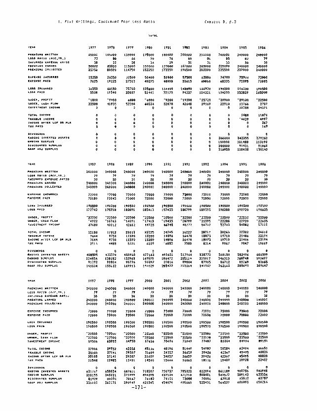
I. Flat Writrngs, Continued Poor Loss Ratso Exhlblt D, P.3

1978 ,979 IPBO

,*5000 130000 I71000 80 66 70

197,

61000 73 30

JOQQQ 35750

IS250 7625

36550 5338

32 28 34 83000 223000 130000 80300 lL4730 I?2250

26250 32500 JO400 19223 27313 40273

66150 75700 103600 19340 33037 51441

‘1800 22588

0

0 0 0 0

-9400 6800 -boo0 41935 32200 bQ514

0 0 0

0 0 0 0 0 0 0 P 0 0 0 0

0 0 0 0 0 0 0 0 0 0 0 0 Q b 0

,987 19bB 1989 1990

24bObb 79 JO

240000 210000

72000 72180

240000 240000 240000 79 79 79 JO 30 30

24ObOO Z,OdQO 240000 24OQPO 240000 24OOOb

f2000 72000 72000 72045 72000 72000

1905bb 190500 190500 lPO5OQ 172742 178718 18289, 183413

-22300 -4922 37680

15180 7644 ,644 3316

17812 2b112 22225 2,219 26222 2821, 30263 32382 34618 9750 1,590 *X2*0 ,489) 16478 18073 19710 21406 23194 9750 1,390 13280 14896 16478 18073 19710 21406 23194 4483 3331 6109 'b852 7588 8s14 906, Pb4, lo669

0 408503 12,834

91292 141804

0 0 0 433510 435968 477163 138182 L32961 169079

9,024 907,* 9039, 155132 ,*99*3 186029

1917

2,OObO 79 JO

*,0000 24OOOb

72000 72000

,998 1999 2000

240000 24OOQQ 24OObO 79 79 79 30 30 JO

240000 2,oooo 2,OObQ 21ObOb 24OPW 240000

72000 72000 72000 72000 72000 72000

L9b500 190500 19OSOO i90500 1905bO 19OSQO

198, 1982

,*Lwoo 200000 76 BO 29 31

177000 m7000 173230 190500

51*00 57500 48998 53615

134400 148890 72175 94237

-9200 -19390 52078 42648

0 0

0 0 0 0 0 0 0 0

0 0 0 0 0 0 0 0 0 0

1984

210000 81 31

205000 203500

240000 83 33

223QQO 225500

1985

240000 82 JO

240000 237000

1986

24bboo 79 30

240000 24bboo

63800 7,700 729(t~ 72000 60010 68133 7259s 72085

166920 1902DP L96200 1903QO 11432, 114235 152839 1b5208

-25720 29169

D

-39900 22PlO

Q

0 0 0 0

-29100 11766 30388

1488 -4629

0 0

-22500 2707

34371

1,871 6997

367 169

0 379263 113190

9lb68 L30140

0 3OQQQO 100000 100000 116950

0 342155 101488

91431 If8438

,991 1992 1993 1994 1995

240000 79 30

240000 240000

I996

24bOOO 79 30

z,oooo 240000

240000 240000 240000 240000

:i 10 79 JO 79 79 JO 2,OOOQ 24ObOO 24ObOO 2,bbbO 240000 240000 24OOOb 2,bObb

72000 72000 72bbO 72000 72000 72Obb

190506 1 Mom* f905bO 187435 188799 189595

72000 72000

72000 72000

1?0300 190500 190288 190720

72000 72000

*9o?joo 190635

0 0 P ,9,*21 5,796, 540180 186472 205114 24b213

8981b 89004 86712 203122 222064

0 538772 225017

87965 DIP67 263161

0 0 582496 606309 7.68748 29269,

85269 8,665 283698 309647

zoo, 2002

240000 240000 71 79 30 30

2,OOQQ 240000 2,oooo 240000

72800 72000 72000 72000

190500 1905bb lPO3OQ 190500

‘22~00 -22500 -22500 -22500

70696 73949

48196 5,4,9 34037 :3**59 34037 36659 156bb 16863

2003 2004

2,bbOO 77 JO

2,POOO 240000

72000 72000 72000 72000 72000 72000

190500 190500

-22500 -22300

81084

190500 190500

,905oo ,905Ob

-225po -22Soo

8W94

62494 45495 41495 20928

0 902755 589143

65832 Wb(193

-22300 -22800 -22500 -22300 ‘225bb -22soo

62052 64758 67636

39552 42258 43116 271,l 29307 31609 27111 2930, 31609 ,248s 13481 14s40

58384 42367

54907 39426 39426 18136

,2367 194EP

63883: 68,611 0 71820, 0 750737 0 785322 0 82209: 86,‘89 0

34522, 373999 404393 437124 47,710 50848, 3,,377 80090 78167 76182 7,131 72088 fObb6 6,918

362171 19OP49 42L54J ,3,0,, 488666 525.31 56452, -171-

Title: INTERACTION OF TOTAL RETURN PRICING AND ASSET I&Q&AGE- LMENT IN A PROPERTY/CASUALTY COMPANY

Author: Owen M. Gleeson

Biography: Currently Assistant Vice President and Actuary at General Reinsurance Corporation; previously employ- ed at USFG Corporation in a variety of capacities including Actuary in Corporate Actuarial Department and Vice President -- Financial Planning. Member of the Casualty Actuarial Society (ACAS-1975; FCAS-1978) and American Academy of Actuaries (1978). Education: BA, MS and PhD in Mathematics - St. Louis University.

Abstract: This paper proposes to show that it is not possible for a property-casualty company to price on a total return basis and achieve the targeted return without the aid of a detailed flow of funds statement. It is demonstrated that, for a company to achieve a targeted total rate of return, it is imperative that a company position itself so that funds can be invested at the assumed rate. As part of the demonstration an example of a hypothetical company is presented and the flow of funds constructed and analyzed. Projections of proforma statements of sources and uses of funds are employed to show that a company so situated must pay for "old losses" with "new money." Data is presented suggesting that many companies in the industry are positioned in a simi- lar fashion. The cause of the problem is identified and a tentative solution offered. Additional data is com- piled from Annual Statements of a sample of companies indicating that assets maturing in a given year are insufficient to meet current payments on losses in- curred in prior years. Finally, solutions to some of the problems in the area of planning and forecasting are suggested.

-172-

1. Introduction

Changes in the economic structure of the United States over

the past two decades have had significant impact on all segments of

the financial services industry. Some segments have been quicker to

react than othersand,even within a given segment, such as the prop-

erty- casualty insurance business, the response to the changing con-

ditions has shown a wide variation.

In order to operate in an environment characterized by sharp

changes it is necessary that the management of an enterprise be

able to react to the unpredictable events, One such event is the

sharp fluctuations in investment rates. Effective response to any

one of a range of events requires a degree of sophistication in plan-

ning that is unprecedented in the industry. Of course part of the

planning process is the objective analysis of the current financial

condition of the company and the identification of the opportunities

and constraints.

The intention of this note is to examine the problems that can

occur in the situation in which interest rates move up for a number

of years and in which the maturity of assets significantly exceeds

the maturity of liabilities. Foremost among the problems is the lack

of flexibility to respond to changes, and in particular the diffi-

culty in implementing a strategy of pricing on a total return basis.

It will be seen that a program such as this can only be effectively

carried out when the planning process involves the functions of

pricing, planning and investment. In addition to the discipline

and coordination that is required it is also necessary that the

proper tools be available to analyze the current situation and to

-17%

control the process of implementing the operational plan. The tool

that will be examined here is the Statement of Sources and Uses

of Funds both on actual and proforma bases.

It is conventional to construct Statements of Sources and Uses

of Funds by starting with accounting statements, the income state-

ments and the balance sheet, and construct the flow of funds state-

ment through a series of adjustments. This can be a cumbersome

process and will not be employed in this presentation. In the highly

simplified example that follows, it is very easy to calculate the in-

flow and outflow of funds directly and for this reason the exposition

will dispense with the distracting intermediate steps.

The example constructed here hypothesizes a highly idealized

economic scenario rather than drawing on past data. Motivation for

this approach stems from a desire to focus on the structure of the

situation and to keep details simple enough so that the reader does

not become bogged down in nuances that are beside the point. It

will also obviate the need for parenthetical explanations of random

and nonrandom deviations from the norms in actual economic events.

Of course no business operates in the world of contrived ex-

amples but rather in world in which deviations from the expected

are to the anticipated. Therefore at the conclusion of this paper

some space will be devoted to examination of the range of results

that might obtain and in particular, how the actuary can play a

significant role in quantifying risks associated with given strategies.

In spite of the fact that the following analysis focuses on a

situation in which a company is using total return pricing in deter-

mining strategy, this focus should not be construed as necessarily

-174-

recommending this methodology. Nor should the problems that will

be brought to light be interpreted as arguments against the use of

this technique. Approaches to the conduct of the business of a

given company will depend upon its situation and circumstances as

well as the attitude of management towards required results.

2. Financial Profile of Hypothetical Company

As indicated in the introduction,the example which will be con-

structed will be very simple so that the model does not become en-

meshed in unnecessary detail.

A. History of Premiums and Losses

Written Earned(l) Incurred Year Premiums Premiums Lasses(2)

1980 140,000

1981 150,000 145,000 116,000

1982 160,000 155,000 124,000

1983 170,000 165,000 132,000

1984 180,000 175,000 140,000

(1) Earned Premiums = (l/2) (Prior year's written premiums) +

(1/2)(Current year's written premiums).

(2) The ratio for losses and loss adjustment expense is

assumed to be 80% in each year.

-175-

8. Assumptions

1. Payout on Incurred Losses

The payout rate on accident year losses is given by

the schedule:

Calendar Year Percent

Current 40%

1st Following 30%

2nd Following 15%

3rd Following 10%

4th Following 5%

2. Expense Components

Category Percent

Commission 15%

Premium Tax 3%

General Expense 8%

3. Agent's Balances

The assumption made here is that there is a delay of

about 36 days i.e., l/10 of a year in the remittance

of premiums by agents to the company.

4. Dividends

The companys anticipates paying dividends to stockholde

in the amount of $5,000 during 1985.

C. Balance Sheet

To the history and assumptions above is appended the

additional supposition that the ratio of premium to

surplus at year end 1984 is 3 to 1. The following

simplified balance sheet results.

rs

-176-

Balance Sheet

Assets Liabilities

Bonds $282,700 Loss Reserves $148,000(2)

Agents Balances 15,300(l) Unearned Premium 90,000(3'

$298,000 Surplus 60,000

$298,000

(1) 15,300 = (l/10) (1 - .15)(180,000)

(2) 148,000 = 1.60) (140,000)+(.30) (132,000)+(.15)(124,000)+

f.05) (116,000)

(3) 90,000 = %(lSO,OOO)

D. Asset Maturity Schedule

The following maturity schedule has not been constructed

in a way that is intended to mirror a profile of the industry

or any company within the industry. Varying levels of cash

flow, widely fluctuating interest rates and other economic

events over the recent past have been such that the yield

by duration of an actual company would not show the smooth-

ness of progression presented in the example. The only

aspect of the maturity schedule which is similar to that of

the industry is that the average maturity of the assets is

greater than the average maturity of liabilities.

-177-

Year

1985

1986

1987

1988

1989

1990

1991

1992

1993

1994

Amount

28,270

28,270

28,270

28,270

28,270

28,270

28,270

28,270

28,270

28,270

282,700

Yield Rate

-0533

-0667

.0711

.0733

-0747

.0756

-0762

-0767

.0770

.0773

Yield

1,507

1,886

2,010

2,072

2,112

2,137

2,154

2,168

2,177

2,185

20,408

The invested assets are assumed to be bonds and it is further

assumed that the bonds are carried at par value. As a result if the

company chooses to liquidate the bonds in a period of high interest

rates it will suffer an accounting loss and a decrement to its statu-

tory surplus.

3. Planning in a Vacuum

Now suppose that the company embarks on its planning process

for the upcoming year (1985) and finds that the current and projected

rates for year range from 8 to 12 percent depending upon maturity

of the assets. Its targeted return on equity is 15%. Another fac-

tor entering into the analysis are that the company wishes to con-

tinue to write at approximately a 3:l ratio. The company does not

feel constrained to selecting early maturities and hence assumes

that funds can be invested at the maximum rate of 12%. It has

adopted a philosophy of total return pricing and so seeks the loss

-178-

ratio that will result in the 15% return on equity. The analysis

that follows is, by itself, neither unusual nor unreasonable.

Losses will be paid out as indicated in Section 2 and the funds

invested at 12% so that the discount factor is -8414. This naturally

is obtained as: (.40)/(1.12)+ t- (.30)/(1.12]3'2 + (.15)/(1.12]5/2

+ (.10]/(1.12)7/2 i- (.05)/(1.12)g'2 = .8414

The ratio of premiums to surplus for the company is 3 to 1 so

that the profit as related to surplus is 3 times that of the profit

margin in each dollar of premium. In addition to the income from

premiums, the company is earning investment income on the assets

equal to the surplus. The rate of return on these assets will be

assumed to be the same as that of the portfolioas a whole. There-

fore, the target loss ratio is the solution to the equation [l-

(.8414 X LR + -2611 X 3 + .0722 = .15 and is 84.87% which will be

rounded to 85%. At this point, it will be assumed that the company

is satisfied with a target combined of 111% which will produce an

economic return on equity of 15% although both statutory accounting

and GAAP results will be poorer than this due to the lag in the

earning of investment income and that fact that loss reserves are

not discounted. The question that will now be investigated is whether this tar-

get can be achieved given the constraints and financial condition of

the company. To answer this it is necessary to turn to a proforma

statement of sources and applications of funds for the year 1985.

4. Sources and Applications of Funds

With the exception of newly formed companies, each property-

casualty company is, to a certain extent, constrained by the past

-179-

in its ability to react to new situations. The most significant

constraints in the context of the problem under discussion is the

requirement to pay losses in the current and future years which are

the result of coverages issued in past years and the results of the

investment policies of those years. Because of this it is necessary

to start with a study of the application of funds. It is assumed

that the company writes premiums in the amount of 190,000 in 1985 so

that the earned premium figure is 185,000. The incurred losses for

1985 will be (+)(180,000) f.80) + (f)(l90,000) t-85) = 152,750.

Application of funds is calculated as follows:

Paid Losses 141,100(1)

Paid Expenses 20,900(2)

Dividends 5,000

167,000

(1) 141,100 = t-40) (152,750) + C-30) (140,000) + t.15) (132,000)

+ (.lO) (124,000) + f.05) (116,000)

(2) 20,900 = (.ll) (190,000)

Note that commissions are not included in paid expenses but

that this will not cause a problem in that the inflow of paid pre-

mium will be net of commissions.

Sources of funds include not only those from continuing opera-

tions but also from maturing assets. These will be projected

separately then totaled,

-180-

Inflow from Operations:

Paid Premiums

Investment Income

$160,650 (l)

22,309 (2)

$182,959

(1) 160,650 = 15,300 + (g/10) t.85) (190,000)

(2) 22,309 = 20,408 - (l/2) t.05333 (28,270) + (l/21 f.12) (28,270)

+ l/2(15,959) (.12)

When funds from maturing assets are added to the inflow/outflow

difference the total funds available for investment at 12% amounts

to 44,229 = 182,959 - 167,000 f 28,270. It is assumed here that the

company will not liquidate bonds maturing in 1986 and following be-

cause of the fact that they were purchased in a time when interest

rates were lower than the current level and hence sale at market

would cause a decrement to surplus.

It can now be seen that, given this last listed constraint and

the prior history of the company, it is not possible to implement

the strategy of writing at a combined ratio of 111% and obtaining

at 15% return on equity. The reason for this of course is that

for the strategy to be successful an amount equal to the losses in-

curred on the premiums written in 1985 must be invested at the new

money rate of 12% as indicated in Section 3. But this amount is

157,250 and the funds available for investment at 12% total only

44,229 for a shortfall of 113,021.

An estimate of the difference between statement and market

value is developed in Appendix A. This Appendix also presents

some evidence of the magnitude of the decline in bond prices over

the last 25 years and the industry condition with respect to differ-

-181-

ence in the market/statement values of bonds.

Appendix B is devoted to the study of a sample of property-

casualty companies with a view towards determining the relation

between maturing assets and demands on funds resulting from prior

commitments.

5. Analysis of Achieved Results

The funds assigned to the 1985 losses can be segregated into

two portions, first the funds newly invested at 12% and secondly

funds from the incoming portfolio. As an expedient it will be

assumed that the rate on the required additional funds will be that

of the average of the portfolio, that is 7.43% = (20,408 - 1,507)/

(282,700 - 28,270). This gives a weighted rate of the portfolio

supporting the losses incurred in 1985 of approximately 8.71% where

[(44,229) t.12) + t-0743) (113,021)1/157,250 = 8.71%.

The discount factor using this rate of return is -879 so that

the return on premiums written during 1985 is actually 1 - [ t.879)

t.85) + .261 = 1 -1.0072 =--0072, that is a slight loss rather than

the anticipated gain. This results in a return on equity of approxi-

mately 5.1% rather than the originally targeted 15%.

The company would not only fail to achieve the targeted rate

of return on equity but may not even obtain a sufficient addition

to surplus to maintain a 3 to 1 ratio. In this example the harm is

not great as shown in the following analysis.

-182-

Surplus (12/31/84): 60,000

Income Statement

Earned Premiums 185,000

Incurred Losses 152,750

Expenses 49,400

Underwriting Gain -17,150

Investment Income 22,309

Net Income 5,159

Dividends 5,000

Surplus (12/31/85) 60,159

Premium to Surplus Ratio = 190,000/60,159 = 3.158

Although the company only increases its premium to surplus ratio

slightly and no real problem is generated, it would be easy to con-

struct a situation in which the resulting decline in surplus came

as a great shock to the company and caused real difficulties. Un-

pleasant surprises should not befall companies with access to a

reasonably accurate financial planning model -- other than those

resulting from overly optimistic assumptions.

6. Solutions

There are many actions that a company might take in the effort

to avoid the pitfalls demonstrated in the previous example. Only

two will be suggested here -- one dealing with revision of asset

management and the other dealing with a more effective use of a

sources and applications of funds statement.

The problem presented here resulted from a mismatch of liabilities

and assets combined withashift to higher rates. Volatility of in-

terest rates has now become a fact of life and it is incumbent on

-183-

those charged with the successful conduct of the affairs of a com-

pany to recognize the need to accomodate this aspect of the economic

environment in the planning. In order to respond to challenges and

changes a company must maintain a significant degree of flexibility

and this includes flexibility in the assets that it manages. It is

tempting to reach for the last few basis points by going further

out on the yield curve but, as can be seen from this example, this

causes a loss of ability to respond to changing conditions and to

take advantage of new opportunities.

One observation that should be made is that, all things being

equal, newly capitalized companies have an advantage over older

companies with ill-positioned assets. The latter are forced to

make the choice between, on the one hand, realizing losses by

selling assets resulting in a weakening of the statutory balance

sheet and, on the other hand, paying for "old losses" with "new

money." This situation will allow the new companies to be more

competitive and still receive an acceptable economic return. However,

in the case where the older companies have followed a program of

matching assets and liabilities this threat should not be a concern.

Another action that the company in this example might have

taken centers on the use of a more realistic interest rate. In this

situation the company was positioned in such a way that it could not

invest the new money fully at the 12% rate. The analysis indicated

that rate available for the assets to be matched with the losses in-

curred in 1985 was 8.71%. This information could be used as input

into the pricing policy to determine that target loss ratio. As

seen previously the discount factor was .879 so that the target

-184-

loss ratio could be determined from the equation

(1 - t.879 X LR + .26)] X 3 + .0722 = .lS

The solution is LR = .812 which is rounded to 81% with a com-

bined ratio of 107%.

7. The Actuary's Role

Important items of the analysis is the example include the

level of loss reserves and the payout on losses. Both of these have

been used without reference to the variation experienced in each.

The actuary is particularly well suited to provide management with

estimates of the variation in these elements and thereby play a

vital role in analyzing the current position of the company, its

constaints and its range of opportunities.

Pricing also is substantially within the purview of the actuary

and when a company prices on the base of total return it is abso-

lutely essential that the company have not only a good estimate of

the ultimate cost but also reasonably accurate projections of the

cash flows associated with premiums, losses, expenses and investment

income. For many actuaries this is already part and parcel of their

work and for othersanextension of their current functions.

These are but two of the obvious applications of the actuary's

expertise in the areas of implementing the use of proforma sources

and application of funds statements and total return pricing. In

addition the actuary is particularly well suited to the assessment

of risk associated with various strategies and to the application

of optimization techniques to determine the best strategies.

-185-

8. Summary and Conclusion

The example presented in this paper has been shown to be re-

presentative of many companies in the insurance industry -- at least

in the aspect of the mismatch between liabilities and assets. Diffi-

culties of planning and strategy determination have been explored

with particular reference to total return pricing. It has been

shown that, to put it very simply, a company cannot fully take ad-

vantage of high interest rates and apply these to its pricing if

the funds generated cannot be entirely invested at the prevailing

rates. Better analysis and planning can be achieved through the

use of proforma statements of the source and application of funds.

In a rapidly changing environment a company needs to remain

flexible. Deployment of assets in such a way that reduces the

range of use of these assets can be detrimental to a company. In

particular the purchase of bonds with extremely distant maturities

in order to take advantage of the additional yield commits a com-

pany to holding these securities to maturity in the event that in-

terest rates rise and under the circumstances where a company cannot

afford the reduction in stated worth resulting from sale. This

limited study would suggest that companies should invest in bonds

with shorter maturities. It is still an open question as to whether

pure asset/liability matching is necessary.

There are many who feel that the long uptrend in interest rates

is in the process of being reversed. This does not mean that the

concepts explored in this paper will not apply in this event. A

substantial portion of the bonds owned by property casualty insurance

companies were purchased at a time when r.stes were extremely low

-186-

by today's standards. A cessation of increase in interest rates

will not provide an immediate solution to the problem of bonds with

statement values in excess of market values. Nor will a small de-

crease in the level of interest rates. Therefore, if companies are

constrained not to sell bonds at a loss because of the resulting

capacity problem, they should find proforma statements of sources

and applications of funds of vital use in planning -- at least for

the next few years.

Finally, it should be clear that the planning, pricing and in-

vestment functions cannot operate independently in the current en-

vironment if a company hopes to achieve satisfactory results. A

process of coordination and control must be introduced that brings

together the different skills so that the parties involved not only

have a thorough understanding of the impact of their actions on

the company but also so that they work together towards objectives

which are mutually consistent.

-187-

Appendix A - Book/Market Differential in Bond Holdings

The company is holding a portfolio of bonds on which the coupon

yield is less than that currently available according to the hypothe-

sized economic scenario. The long general decline in the bond mar-

ket over the past 25 years resulting from the increase in interest

rates is well known and graphically illustrated in Figure 1.

Figure 1

This coupled with the industry practice of investing long al-

though the liabilities are fairly short has lea to a condition in

the industry where the market values of bonds are substantially

below the statement value. For a number of years First Boston

Corporation has issued a study on this important aspect of property

casualty insurers' financial condition. Part of the 1984 study

which exemplifies the magnitude of the problem is reproduced on

the following page.

-188-

Table I

Property-Gsualty lnsurancc operatmns Statutory Surplus Adjusted For Unrealized F!md Losses

The Welationshlp of Writings to Surplus, 12/31/83 IS in miil~onsi

1983 12/31/83 Premiums Statuto~

Property-Casualty 12/31/83 oorxi PortfolIo "Adjusted"

12/31/83 sury I u* llnreat IZC 8 ~ColulNl 2 Less

72% Of col. 5)

Aetna Life 8 Casualty $ 4,416 ,$1.645 $6,158 $4.985 $1,173 $800 dubb 1,241 401 1,376 1,211 165 282 CIG-iA 3,535 1,314 5,161 4,333 828 718 COntinental 2,401 936 3,311 2,841 470 598 Genera1 Re 902 836 2,462 2.180 282 633 Kemp3 858 354 853 718 13s 257 Ohio Casualty 843 426 994 793 2Ul 281 h-ogressive 245 95 234 232 2 93 SAFE03 888 494 928 916 485 St. Paul 1,744 783 2.785 2,457

3:fi 547

TrZlVeletS 2,945 1,057 4.708 3.587 1.121 250 USFSC 1,989 779 2.151 1,993 158 665

Total smmm SYm Weighted Average

2.7x 5.5x 3.1 4.4 2.7 6.9 2.6 4.0 1.1 1.4 2.4 3.3 2.0 3.0 2.6 2.6 1.8 1.8 2.2 3.2 2.8 II.8 2.6 3.0

2.4x 3.9X

Source: The First Boston Corporation

It has been asserted earlier that the hypothetical company

would suffer a decrement to surplus if forced to sell bonds. As

is the case with other sections of this highly idealized situation,

determination of the amount will depend on assumptions and methods

which greatly simplify the situation. However, the results are

acceptably accurate for the purposes of example and planning. The

redemption value of the bond and the statement value are assumed

to be equal with the statement value having been given earlier in

the Asset Maturity schedule. Yields also have been given so

that all that is needed for a rough estimate of the market value of

the bonds is the currently prevailing interest rates by maturity.

The data is given on the following page.

-189-

Years to Maturity

1

2

4

5

6

7

8

9

10

Redemption Value

28,270

28,270

28,270

28,270

28,270

28,270

28,270

28,270

28,270

28,270

Yield

1,507

1,886

2,010

2,072

2,112

2,137

2,154

2,168

2,177

2,185

Current Rate

8.00%

10.00%

10.67%

11.00%

11.20%

11.33%

11.43%

11.50%

11.56%

11.60%

The method used here to estimate the market value of the bonds

is the yield-to-maturity method. Then the present value of the

bond -- all things being equal -- is given by the formula,

Present Value = (Redemption Value) /(I + rjn + (Annual Yield) a;;I r

where r is the yield to maturity, n represents the number of years

to maturity and the coupons are assumed to be paid annually. For

example, the bonds maturing in 5 years have a present value of

(28,270)/(1.112)5 + (2,112) afl .1112 which equals 16,626 + 7,767 =

24,393 so that sale of the bonds would result in a decrease in sur-

plus of $3,877. The results of this method of estimating the market

value of the bonds versus the statement value of the bonds is given

on the following page.

-L90-

Year of Maturity

1985

1986

1987

1988

1989

1990

1991

1992

1993

1994

Statement Value

28,270

28,270

28,270

28,270

28,270

28,270

28,270

28,270

28,270

28,270

282,700

Market Value

27,571

26,637

25,796

25,051

24,393

23,803

23,264

22,794

22,358

21,984

243,651

Discount

699

1,633

2,474

3,219

3,877

4,467

5,006

5,476

5,912

6,286

39,049

The statedsurplus of the company under study is 60,000 with

premiums writings of 180,000 for a 3 to 1 ratio. If the surplus is

adjusted to reflect market value of bonds, the adjusted surplus is

20,951 with a resultant ratio of approximately 8.59 to 1.

This ratio is considerably higher than most of the ratios in

Column (8) of the table reproduced from the study conducted by

David Seifer. The difference is due in part to methodology. The

reader should note that the "Adjusted Surplus" in the study is ob-

tained by subtracting 72% of the unrealized bond losses from the

stated surplus thereby reflecting the potential impact of capital

gains tax. If the unrealized losses had not been reduced by 28%

the ratios of premiums to adjusted surplus would have been sub-

stantially higher with the weighted average rising to 5.2 from 3.9

as calculated in the table.

-191-

Use of yield to maturity has some drawbacks that have brQen

covered in the book "Inside the Yield Book" by Sidney Homer and

Martin Leibowitz. However, the technique produces a useful approx-

imation which can be of great value in assessing the projected con-

dition of a company under a variety of scenarios associated with

a range of economic events and strategies.

-192-

Appendix B - Maturing Assets versus Paid Losses from Prior Years: An Industry Sample

The example constructed in this paper presents a picture of a

company with maturing assets far lower than those needed to meet

the obligations of the past. Specifically, the losses from 1984

and prior that are projected to be paid in 1985 amount to 80,000

while the maturing assets show only 28,270. This results in a

ratio of paid losses from prior years to funds from maturing assets

of about 2.8 to 1.

The reader might ask whether this is a strawman or whether

this is somehow representative of industry conditions. Some data

has been drawn from the Annual Statements of eight companies to ex-

amine this question. The companies were selected randomly and

include not only stock and mutual companies but companies of vary-

ing size, Column (1) is the amount of losses and loss adjustment

expense paid in 1983 from accident years 1982 and prior. The

figures were compiled using Schedules 0 and P from the 1982 and

1983 Annual Statements. Column (2) is the amount of funds avail-

able to the companies from assets held at year end 1982 and maturing

in 1983. The data was obtained using Schedule D-Part 1A and Lines

6.1 and 6.2 of Page 2(Assets) -- Cash and Short-term Investments,

respectively.

-193-

Company

A

B

C

D

E

F

G

H

(1) (2) Paid in 1983 * Assets Maturing*

on 1982 and prior in 1983

1,024,315 239,396

672,908 246,958

644,214 210,042

409,654 120,245

348,573 44,276

210,204 28,003

10,410 3,027

3,522 3,250

3,323,800 895,197

(3)

(l)/(2)

4.28

2.73

3.07

3.41

7.87

7.51

3.44

1.08

3.71

4.17

(4)

(2)/(l)

.234

.367

.326

.294

.127

.133

.291

.923

. 269 (w)

.240(u)

*Figures in thousands (WI - weighted (u) - unweighted

This exhibit is certainly not to be construed as representing

an exhaustive study of industry conditions but rather to show that

the hypothetical example is not totally at odds with prevailing con-

ditions. As a matter of fact, if the exhibit is truly representative,

then the hypothetical company is in somewhat better shape -- at least

in terms of the ability to pay for old losses with maturing assets.

One interpretation of Column (4) is that the sample companies

are only able to cover about 27% of obligations from prior years

through use of maturing assets. This means that 73% of the obliga-

tions coming due must be met through the use of new funds. The

figures for the hypothetical company are 35% and 65% respectively.

-194-

AN ECONOMETRIC MODEL OF PRIVATE PASSENGER

LIABILITY UNDERWRITING RESULTS

Richard M. Jaeger and Christopher J. Wachter

Richard Jaeger is currently Actuarial Director in the Actuarial Development Department of Insurance Services Office. He is a Fellow in the Casualty Actuarial Society and a Member of the American Academy of Actuaries. He is serving on the CAS Syllabus and Examination Committees. He holds a BA degree in Mathemetics from Boston College and an MS degree in Mathematics from the University of Notre Dame.

Christopher Wachter is currently Senior Actuarial Assistant in the Actuarial Development Department of Insurance Services Offices. His responsibilities include econometric modeling. He received his BS degree In Actuarial Science from Lebanon Valley College in 1983 and is currently pursuing associateship.

This paper presents an econometric model of private passenger liability underwriting results. The model, fitted on data from 1954 to 1983, is used to forecast results from 1984, 1985 and 1986. Premiums, losses, and expenses are modelled separately, with the loss model based on two sub-models (severity and traffic accidents). The paper covers the process of model building from initial a priori analysis, through forecasting. The paper also attempts to provide a general framework useful in the modeling of other lines.

-195-

PURPOSE

Our objective in undertaking the research presented here was to forecast industry

combined ratios for private passenger automobile liability. while actuaries have

always been concerned with trending, projecting and forecasting there is little in

the actuarial literature on forecasting industry results. Some of the papers in the

actuarial literature (Alff and Nikstad, James, Lommele and Sturgis) are listed in the

Bibliography of this paper. Although such forecasting may be several steps removed

from the actuary's day-to-day work, senior executives, insurance regulators and

financial analysts are all interested in what the results will be. The actuary has

the training and experience to help. A secondary objective of this paper is to

indicate a general approach that can be used to model other lines of insurance as

well.

ORGANIZATION OF THE PAPER

This paper follows a chronological format showing the development of the model from

initial a priori analysis through forecasting. The presented models, therefore,

appear after the section on the model fitting process and before the section on a -

posteriori analysis. The paper contains two appendices and a brief bibliography.

The appendices contain a glossary of useful econometric terms. a list of data

sources, and graphs displaying the fit of the presented models.

A PRIORI ANALYSIS

The importance of a priori analysis cannot be overemphasized. In an ideal, perfectly

efficient world the researcher will analyze the situation to be modeled or

-196-

forecasted, determine the relevant forces, select the appropriate variables, specify

the form of the mathematical relationship, indicate the signs (and perhaps the

magnitudes) of each variable in the relationship, and only then test the hypothesis

against the data. In the real world one tries to follow this approach while coping

with disappointing test results, new ideas that come to mind after the first results,

and the nagging question - where can the model be improved?

It is important to use the data to test the a priori hypothesis, rather than to

search for a model which fits the data well, and then derive an aposteriori

"hypothesis" from the model. We want assurance that it is a good model, not just

that a good fit results from much trial and error. We, of course, want the model to

fit well & addition fo agreeing with the a priori hypothesis.

This is especially important when there is limited data, Everyone is familiar with

the inadvisability of explaining the variation in ten data points by using ten

independent variables, or even six independent variables. The same effect can occur

when the best-fitting model is chosen after testing too many sets of variables using

several model forms, even if all of the variables and forms are reasonable.

There are ways to mitigate this problem. One way is to use part of the data for

fitting and another part for testing. Any partition that is expected to yield the

sams model on the subsets could be used. Some possibilities are first and third

quarters separate from second and fourth quarters, seasonally adjusted as necessary;

a geographical partition, by state or region; and stock companies separate from

mutual companies. Another way is ex post testing in which we try to forecast the

latest points after fitting to the data excluding those points.

-197-

The first assurance, however, of having a good model comes from the model's agreement

with a priori analysis. A priori analysis provides an intuitively reasonable

explanation of the actual situation. Steps to improve the model should be governed

by attempts to improve the a priori analysis. This insures that the resultant model

will be sound on a conceptual basis.

As stated earlier the purpose of the model is to forecast combined ratios. We

decided early, however, not to model the combined ratios directly, but to model the

losses and premiums separately and even to attempt to decompose losses and premiums

into separate factors. We attempted to model losses as volume times frequency times

swerity and premiums as expected losses times a "pricing factor."

One reason for this approach is to reduce the problem to relatively bite-size pieces,

each with a more manageable number of possible causal factors. Another reason is to

make more efficient use of relatively few data points. Separating losses from

premiums creates, in effect, twice as many points .as using just the combined ratios.

The most important reason, however, for decomposition is to guide efforts to improve

the model. If the premium model behaves better than the loss model, then attention

can be directed to the loss model. If frequency is the loss factor showing the most

unusual behavior, then frequency can be investigated before the other factors. A

related reason is that it is easier to confirm whether a proposed improvement has the

expected effect on the proper component.

One consideration in the a priori analysis is that the model is primarily intended

for forecasting rather than explanation of the changes in the historical period. The

independent variables selected should be easily forecastable or already forecasted in

a satisfactory way.

-198-

Losses

The initially selected form of decomposition for incurred losses was volume times

frequency times severity. At this point there were two ways of proceeding. Ckre way

was to seek sources of standard insurance data for each element in the decomposition,

such as, earned car-years for volume, and incurred or paid claim frequency for

frequency. Each element could then be modeled separately. The other way was to

build a precise decomposition from a reasonable starting point. An example of such a

decomposition is to start with the number of registered vehicles (VRCAR) for volume

and then, using the number of traffic accideuts (TRAPACC), define frequency as

TRAFACC/VRCAR and severity as incurred losses/TRAFACC. Both VRCAR and TRAPACC are

forecasted by Data Resources, Inc.- (DRI). Severity would have to be modeled.

The advantages of the first way arise from the fact that the elements in the

decomposition are standard insurance concepts.

. Prior knowledge of these concepts can be applied directly to the analysis.

If the elements have already been modeled, then much of the work is already

done.

. If there are strong judgmental reasons to expect particular changes in the

elements, these judgmental values can be used directly in the model to

obtain a forecast.

The advantages of the second way are:

The decomposition is precise, that is, the product of the factors exactly

equals the variable of interest. There is no need to adjust the product for

-199-

such differences as absolute scale (because of using a subset of industry

data) or paid rather than incurred data.

If there is a reasonable starting point that is already modeled or

forecasted, then part of the work is already done.

We chose the second approach to decomposition because of the above advantages plus a

very practical additional advantage. We wanted to have at least 20 years of data for

modeling, so that several underwriting cycles and a variety of economic conditions

would be present in the data. TRAFACC was available back to 1950 and VRCAR even

farther back. Insurance time series for a decomposition would have been more

difficult to obtain for a comparable length of time.

This second approach still leaves open the possibility of comparing elements of the

decomposition to available insurance time series for reasonableness.

Early work with the decomposition based on VRCAR and TRAFACC led to the conclusion

that TRAFACC showed very anomalous behavior, described more fully later in the paper.

Frequency

A number of factors were identified that might influence frequency. The principle of

simplicity and the 80-20 rule were applied. (Keep it simple, and 80% of the effect

comes from 20% of the causes.) Factors expected to have considerable effect were

demographic shifts (notably changes in the proportion of young drivers), changes in

the incidence of reporting traffic accidents (as repair costs go up while reporting

thresholds tend to remain fixed), and energy crises (gas shortages). Selection of

the first factor was influenced by work that had been done on other automobile

-2oo-

insurance frequency data. The ratio of population aged 16-28 to the number of

vehicle drivers licenses was selected to represent the demographic shift. A

CPI-based measure of automobile repair costs, BODYWORK, was selected as a variable

corresponding to the second factor. Eventually, it was decided to represent energy

crises by the variable vehicle miles traveled (VXTCAR). and to recast the

decomposition as losses equals accidents times severity, where TRAFACC is modeled as

VWTCAR times some factor. This is equivalent to substituting VMTCAR for VRCAR in the

initial loss decomposition.

Severity

Inflation should be the major force driving the loss severity model. loss severity

is a combination of bodily injury and property damage severities. To represent

inflation we created an index that is a weighted sum of various CPI component indices

expected to be related to automobile liability severity. The weights were

judgmentally selected in the a priori stage, with the expectation that the exact

weighting would not be critical.

Social inflation, as distinct from the purely economic underlying inflation, may also

be a factor. We expected that social inflation would be reflected in the fitted

quantitative relationship between severity and economic inflation, and therefore did

not represent it by a separate variable.

Small cars sre likely to provide less protection to occupants in an accident. They

may also tend to be damaged more severely. To represent the proportion of small cars

to total cars, we selected the ratio of foreign new car sales to total new cars

sales. We realized, however, that a possible future refinement would use this ratio

averaged over several years.

-2Ol-

It is possible that the introduction and subsequent modification of no-fault laws

affected severity. We did not expect a strong effect, however, and did not attempt

to represent this factor in the model.

Premiums

Premiums may be influenced by a large number of factors. Some of the factors are

exposure volume, inflation, recent loss experience, recent profitability,

competition, supply and demand, capacity, investment yields and the future expected

value of several of these factors. We finally selected several variables that

represent reasonably distinct factors. The number of vehicle registrations was

selected to represent exposure volume. The CNP deflator was selected to represent

inflation. The incurred losses of the current year and the prior year were selected

to represent the ratemaking process, recent profitability, and management's

expectation of future losses. Real surplus (using the GNP deflator) was selected to

represent supply and capacity and as a proxy for competition. These variables should

be positively related to premiums, except for real surplus. A high real surplus

should have a downward effect on premiums due to over-capacity and consequent

increased competition.

We intended to model written premiums as above and to produce earned premiums by a

simple linear model using the current year and prior year written premiums.

Expenses

The expense ratio should be inversely related to deflated written premium, since

there are fixed expenses which do not vary with written premiums. We used written

-202-

premiums deflated by the GNP deflator to model the expense ratio and obtained a

reasonable model.

Model Form

The final stage in a priori analysis is selection of the model form. The selection

of model form is significant, but is somewhat less important than the earlier stages

of a priori analysis. We selected a logarithmic form for the written premium and

severity models for the following reasons:

1. We expected a multiplicative relationship between the component independent

variables.

2. The coefficients are elasticities, rather than absolute magnitudes. The

effect of a 1% change in an independent variable is the coefficient times

1%. Thus, the relative contribution of each component variable can be

easily determined.

3. Inflation-sensitive time-series are transformed from an exponential form to

a linear form.

4. Heteroscedasticity is minimized, since inflation will not cause residuals

to grow as large with time if a logarithmic form is used.

5. The fit is more robust, since outliers tend to have less of an effect on

parameter estimation.

-203-

This completes the initial a priori analysis and prepares us for fitting and testing

actual models.

THE MODEL FITTING PROCESS

The first stage in the model fitting process is the selection of data. Ideally, data

should come from recognized and reliable sources, and be available for a significant

length of time. We used insurance premium, loss, expense and surplus data from A.M.

Best's Aggregates and Averages, and various economic time series from DRI's data

banks.

The second stage in the model fitting process was to splice data together. Prior to

1974, for example, auto liability was not split into private passenger liability and

commercial automobile liability. We applied a splicing factor of 0.89 to the

pre-1974 automobile liability data (stock and mutual only) to extend backwards the

1974-83 private passenger liability data (stock, mutual and reciprocal). The

splicing factor was based on the observed ratios from 1974 to 1983 which were very

stable and averaged 0.89. The advantage to splicing is that we are able to use 30

years of data (1954-83) rather than only 10 years (1974-83).

The third step in our model fitting was to handle a problem variable, TRAFACC.

TRAFACC is a time-series which measures reported traffic accidents. It is also a

variable whose definition has changed over the historical period. Prior to 1968, the

ratio of TRAFACC to highway fatalities is remarkably stable, indicating that TRAFACC

for that period may have been defined by multiplying highway fatalities by a

constant. We decided, therefore, to model TRAFACC over the period 1968 to 1983, and

use the fitted values produced by the model over the full period 1954 to 1983 in

-204-

place of the original TRAFACC series. We later decided, when a reasonable severity

model had been fitted, to create a final series representing traffic accidents called

TRAFACC', because of the problems noted above with TRAFACC. We felt that a

reasonable model for severity would be better than incurred losses divided by fitted

TRAFACC, and therefore would probably create a more accurate decomposition.

The fourth stage in the model fitting process was to decompose the incurred losses

into severity and traffic accidents. We defined severity as incurred losses divided

by fitted TRAFACC (described in the previous paragraph). We selected a deflator

judgmentally, and chose a variable to proxy for small cars (the proportion of

imported car sales to total car sales) to model severity. The resulting model fit

reasonably well, and we therefore tentatively accepted the severity model.

The fifth stage in our model fitting process was to use the fitted values generated

by the severity model to create TRAFACC'. We defined TRAFACC' as incurred losses

divided by fitted severity. We modeled TRAFACC' using the same variables that we had

used to model TRAFACC, and decided tentatively to accept the traffic accident model.

Multiplying the two models (severity and TRAFACC') we were able to construct our

incurred loss model.

After fitting the loss series, we fixed our attention on the premiums. We selected

several variables based on our a priori analysis corresponding to incurred losses,

capacity, volume, inflation, investment yields and recent profitability. We looked

at the relationship between changes in written premiums and changes in potential

explanatory variables at various lags to determine a reasonable lag structure. We

determined, for example, that change in surplus lagged two years was related to

change in written premiums more strongly than if it were lagged 0, 1, 3, or 4 years.

-205-

We fitted a preliminary model, and decided to discard some variables which did not

appear significant (had t-statistics of less than 2). We fitted a second model,

checked for and corrected for multicollinearity (the independent variables should

behave independently of each other, and not show strong correlation), and tentatively

accepted the premium model.

After tentatively accepting the premium and loss models, we tested the models to

determine if they were acceptable. There were four final tests:

We determined that the final models agreed with our a priori analysis.

Specifically, we checked the coefficient of every independent variable and

confirmed that each coefficient had the expected sign and had reasonable

magnitude.

We determined that the model’s error was acceptable (standard errors of

2.3% for premiums and 2.9% for losses) and that each dependent variable was

statistically significant at the 5% Level (as determined by the

t-statistic).

We performed an ex-post test. An ex-post test involves fitting the model

over a shorter historical period (we used 1954-80) and then "forecasting"

the latest values (1981-83) using actual values for the independent (input)

variables. The ex-post forecast errors were deemed acceptable, and are

summarized below:

EX-POST ERRORS*

1981 1982 1983

Premium Model

-2.85% +1.92X +0.66%

Loss Model

+1.72% -0.17% +2.79%

We analyzed the residuals (errors) of the models for violations of least

Correction needed (if any)

1.

square assumptions.

Potential Violation

There are outliers. A dummy variable was incorporated into the severity model for a 1974 outlier.

2. The residuals are correlated. Autocorrelation corrections were implemented as deemed appropriate.

3. The variance of the residuals is not constant. (heteroscedasticity)

The residuals were examined, and no indication of heteroscedasticity was found.

4. The independent variables are strongly correlated. (multicollinearity)

Multicolliearity was found in an early premium model and corrected for. Whatever multicollinearity remains does not appear substantial based on the observed correlations between the independent variables.

5. The relationship between dependent and independent variables is unstable.

Ex-post testing shows stable parameter estimation. When the models were refitted over the period 1954-80, the parameters did not substantially change from the model fitted over 1954-83.

On the basis of these four tests, we decided to accept the premium and loss models.

* Error = (Actual-Forecasted)/Actual

THE MODELS

The private passenger liability models are as follows:

1. Written premiums

Log (NPWt) = 0.664 Log ((A~+ At-,)/2) + 1.315 Log (VRCAR~)

- .115 Log (Surplust-2 /PGNP~-~) + .884 Log (PCNP$ + .573 AR1

Where: *

NPW = Net premiums written VRCAR = Vehicle Registrations (in thousands) PGNP = GNP deflator (1972 = 1.000) Surplus = Surplus (in thousands) A = Incurred Losses/ (VRCAR x PGNP) AR1 = Autoregressive term of order I.

t-statistics are 6.77, 18.08, -3.02, 27.24 and 3.27, respectively, for the five coefficients.

The model has a normalized standard error of 2.3%.

2. Incurred Losses

Incurred Losses equal TRAFACC' times severity

TRAFACC'DTRAFACC~~. VMTCARt (.4575+.4933 YOUTl$ + .0812 BODYWORRJ

VDLt

Where:

TRAFACC,8 = Number of traffic accident8 in 1978 (original TRAFACC series)

VMTCAR = Vehicle miles traveled by cars

YOUTH = Population aged 16-28

VDL = Vehicle Drivers Licenses

BODYWORK - CPI for auto bodywork (prior to 1978, CPI for auto repair and maintenance)

Note: all variables are normalized to 1.000 in 1978 except for TRAFACC' and TRAFACC78.

t-statistics are 3.131, 3.301 and 5.301 for the three coefficients.

Log (SEVERITYt)=.7321 Log (DEFLAlQRJ+.l008 Log (PROPJ-.0955 Dummyt

+ 6.3108 + .9419 AR1

Where:

DEFLATOR = .35 MEDCARE + .35 WAGE + .20 BODYWORK + .10 PC

MEDCARE = .67 CPIU for Hospitals (CPIU for Hospital Rooms before 1978) + .28 CPIU for Physician's Services + .05 CPIU for Medical Commodities. (All components indexed to 1.000 in 1978)

WAGE = Average Hourly Earning Index for Production Workers (1978 = 1.000)

PC = Implicit Price Deflator for Personal Consumption Expenditures (1978 = 1.000)

PROP = Foreign New Car Sales/Total New Car Sales

DUMMY = 1 in 1974, 0 otherwise

t-statistics are 8.96, 3.94, - 3.70, 64.34 and 12.20 for the five coefficients.

The incurred loss model has a normalized standard error of 2.9%.

-208-

3. Expense Ratio and Earned Premium

EPt = .668 WPt + -336 WPt 1

Log(RR,) = 2.458 - -240 Log(NPWt/PGNPt) + 1.096ARl - .690AR2

A POSTERIOR1 ANALYSIS

After the model fitting stage is completed, the a posteriori analysis stage begins. _

The function of aposterlori analysis is to examine the accepted model and attempt to

explain any unusual features of the model. This is useful, because possible

refinements to the model are identified for future research. It fs important to

realize that model building is an on-going process and that models should be

monitored and updated as additional data becomes available.

We have identified three unusual features in our model:

1. The elasticity of VRCAR, a volume measure, is greater than one in the

premium model.

2. The elasticity of DEFLATOR, an inflation measure, is less than one in the

loss model.

3. The lag structure of the incurred losses in the premium model is shorter

than might be expected.

Possible explanations for these features (which represent deviations from what might

be expected) are:

-209-

1. A rise in the proportion of insured vehicles over the historical period

(1954-83) would impact the elasticity of VRCAR.

2. The "real" severity may be declining somewhat due to safer automobiles and

roads.

3. The incurred loss term may combine two separate components: expected

losses (ILt) and "fast-track" experience (ILt-1). If this is, in fact,

the case, a longer distributed lag structure (using ILts2 and even further

back) for the "expected loss" component may be more appropriate.

This aposteriori analysis could serve as an input to the a priori analysis stage of

future model-building efforts. We feel that the present models are sound and useful

for forecasting, but that the a posteriori analysis indicates some areas for future -

research.

FORECASTS

After the analysis, model fitting and testing, the model can be used. The model has

two main applications: explanation and forecasting. To the extent the model

explains the mechanisms underlying industry written premiums and incurred losses,

alternative "what-if" scenarios can be devised and forecasts made for these

scenarios. Three potentially interesting scenarios are:

1. The banks enter the insurance industry injecting significant amounts of

capital.

2. The campaign against drunk driving significantly reduces accident

frequency.

-210-

3. Inflation surges upward again.

The actual scenario design and forecasts based on alternative scenarios are beyond

the scope of this paper. Cur forecasts, based on insurance data through 1983 and on

DRI control scenario forecasts (using the July 1984 forecast) are as follows:

1984 1985 1986

Written Premiums 24,763,224 26.048.890 28.039.674 Earned Premiums 24,391,568 25,721,102 27.482.929 Incurred Losses 21,080,953 22,606,582 24.082.622 Loss Ratio 0.864 0.875 0.876 Expense Ratio 0.246 0.239 0.233 Dividend Ratio (selected) 0.01 0.01 0.01 Combined Ratio 1.120 1.124 1.119

FUTURE RESEARCH

The research to develop these models has raised some questions for further

investigation. Potential topics for research include:

1. Incorporating investment yield into the current premium model. There are

many investment yield statistics, and also a variety of time frames to

select (current yield, recent yield, expected yield, and embedded yield). In

addition, it is possible that investment yield may be significant over a

small subset of the historical period.

2. Incorporating changes in the proportion of insured motorists in the total

driving population. The chief problem is to locate a source of data over

the historical period.

3. Incorporating a variable representing Increased safety of roads and

automobiles. The major task is to find a valid time series which can proxy

-211-

for automobile safety, and which is available over the entire historical

periot;"

4. Selecting other measures to proxy for industry price competition.

The authors will, as time permits, research th&e areas further, and would welcome

the insights, suggestions and research of other people involved in this area of

actuarial/econometric research.

-212-

APPENDIX A - GLOSSARY

Autocorrelation: The correlation between residuals and the residuals lagged a certain number of periods, called the order. An assumptfon of least squares regression is that autocorrelation is not present.

Autoregressive Term: A term (in a model equation) used to correct for autocorrelation when the analysis of the residuals of a model indicate the presence of autocorrelation. In this paper ARi denotes an autoregressive term of order I.

Decomposition:

Dummy Variable:

The breaking of a problem into smaller, more easily handled problems. The solutions to the small problems are combined to form a solution to the overall problem.

A variable that takes on two values, 0 and 1. The dummy variable is used to account for abnormal real world conditions (energy crises, price controls, wars, etc.) or to remove the effects of obvious outliers.

Elasticity: A measure of the relationship between two variables.

Heteroscedasticity: Heteroscedasticity exists when the variance of model’s residuals is not constant over the entire range of data. Least squares regression assumes heteroscedasticity does not exist.

Lag: The length of time between the effect on an Independent variable and the effect on the dependent variable. If several lags of an independent variable are combined into are term, we say that the term represents a distributed lag structure.

Multicollinearity: The degree of correlation between the independent variables. Least squares regression assumes that the independent variables are independent of each other.

Normalized Standard The standard deviation of the error of a model expressed as a Error: proportion of the dependent variable.

Gutlier: A data point that is questionsble due to an abnormally large deviation from its expected value. Outliers bias regression results, sometimes quite substantially.

Proxy: A variable used as a measure for something that is not readily quantifiable.

Residual : The difference between an actual observation and the expected value of that observation based upon model.

Robustness : The degree to which a model is stable and unresponsive to outliers.

-213-

Splicing:

T-statistic:

The combination of two similar time series covering

differing time periods into a unified series.

The ratio of a coefficient to the standard error of that

coefficient. Generally a T-statistic with absolute value greater than 2 indicates a significant relationship between an independent variable and the dependent variable.

-214-

APPENDIX B - Sources of Data

Insurance data was obtained from A.M. Best's Aggregates and Averages.

The following time series were obtained from stock, mutual and reciprocal companies combined:

Net premiums written, Net premiums earned, Incurred losses, Expense ratio, Surplus.

Economic data and forecasts were obtained from Data Resources, Inc. The following time series were obtained:

Primary source: Bureau of the Census Population aged 16 through 28

Primary source: Bureau of Economic Analysis, Department of Commerce Cross national product deflator, Personal consumption deflator, Retail sales, imported passenger cars, Retail sales, new cars.

Primary source:

Primary source:

Primary source:

Bureau of Labor Statistics, Department of Labor Index of average hourly earnings of non-farm production workers, Consumer Price Indices: Auto bodywork, Auto repair

and maintenance, hospital and other medical services, hospital room, medical commodities, physicians services.

Federal Highway Administration, Department of Transportation Vehicle driver licenses (estimated), vehicle miles traveled-passenger cars, vehicle registrations - automobiles.

Insurance Information Institute Traffic accidents.

-215-

FITTED VS. ACTUAL COMBINED RATIOS

\ \

I.175 +

\‘ \

l.laa + \

: I.fl75 +

\ \

I.mx + \ \

1:125 : \ \ \

i.clm + \ \ \

R.975 l \

\ \

n;95!a l

\ - --_I ----+--+ ---+--+-+--+-+--+--+--+--+--+-+--+--+---+--+--+,-+ -+-+-+ --.--d-P--

513 59 67 61 62 63 64 65 66 67 68 69 -It? 71 72 73. 74 75 76 ll 78 19 88 81 82 03

YEAR

NOTE: Solid lines connect actual combined ratios, Dashed lines connect fitted combined ratios.

RELATIVE ERRORS - PREMIUM MODEL

\‘ Ja.94 +

\‘ \

. l l

t \ l +

\‘

* * l

l l t + t

m.@m +

\ *

\ * *

:

-Q.?a2 + \ t \ + t *

l

l

i 4.96 * t

\ ~~~~-+~-+~+~t-*---+---+-*-+~+~*~I~~-+-+-+-+-+---*--+---+- -WV

51 51 49 fit 42 41 64 45 hA 41 6’3 67 78 71 72 73 74 75 76 l-l 18 73 BB 81 82 63

YEAR

Relative Error - Actual Minus Fitted Actual

\ \

a.“14 l \

RELATIVE ERRORS-LOSS MODEL

l

i \ \ l

I:R? + +

\ * \ . *

\ \ l * * l

ri:aq l * &

\ * * \ *

\ t

\ t t -q:a2 + : *

* \ * t5 \ *

-m:ci4 + \ l + \ \ \

-a.m4 + \ \ + \ \

-a.ru + -----------c--+---+---+--+---+ --+-~~+-~+--+--+--+---+--+---+--+---+--+-+-+-+--+-+ -+-+-+-ma----

cl!7 59 401 61 62 4? 44 b5 66 47 6.7 b9 7-a 71 72 73 .14 75 76 77 38 79 80 81 02 83

YEAR

Relative Rrror = Actual Minus Fitted Actual

BIBLIOGRAPHY

Alff, Gregory N. and Nikstad, James R. "A Model of General Liability Net Written Premiums," PCAS LXIX, pp. 30-45.

Armstrong, J. Scott. Long Range Forecasting, New York: John Wiley & Sons, 1978.

James, Kaye D. "Underwriting Cycles in the Property-Casualty Insurance Industry," Inflation Implications For Property-Casualty Insurance, 1981 CAS Discussion Paper Program

Lomele, Jan A. and Sturgis, Robert W. "An Econometric Model of Workmen's Compensation," PCAS LXI, pp. 170-189.

-219-

CONTINGENCY MARGINS IN RATE CALCULATIONS

Steven G. Lehmann

The author is a 1970 graduate of the University of Illinois with a Bachelor of Science degree in Actuarial Science. He is a Fellow of the CAS (1979), a Fellow of the Society of Actuaries (1974) and a Member of the Amercian Academy of Actuaries. He is Vice-Chairman of the Education (Syllabus) Committee of the CAS. He is employed as an Actuary for the State Farm Mutual Automobile Insurance Company, Bloomington, Illinois.

Abstract

Most insurance rating laws require consideration of “a reasonable margin for underwriting profit and contingencies" as one of the factors in establishing insurance rates. The purpose of this paper is to examine the contingency margin. A "contingency" is defined to be an uncertain, unexpected or unforeseen event. Evidence of the existence of "contingencies" can be seen by examination of industry underwriting results over the last 30 years. These results show a consistent shortfall between the anticipated, or target, underwriting results and the actual results. A practical example of how the contingency provision may be calculated for a hypothetical company is discussed in detail. Other methods of calculating the contingency margin are also discussed. In conclusion, for a variety of reasons, contingencies do occur and result in significant shortfalls between expected and actual results. It is essential that anyone undertaking a determination of insurance rates take this factor into account as part of the ratemaking process.

- 220-

CONTINGENCY MARGINS IN RATE CALCULATIONS

- 221-

I. INTRODUCTION

Actuaries are directed by most state insurance laws to carefully consider

“a reasonable margin for underwriting profit and contingencies” as one of the

factors in establishing insurance rates. This paper has been written with the sole

purpose of investigating the “contingency” element. Historically, the term has been

given limited attention, being taken by many as merely part of the “profit” factor.

Actually it encompasses a host of events which must be recognized by the ratemaker

if he/she is to establish adequate insurance rates.

The discussion of “contingencies” in this paper will be entirely in the context

of the profit and contingency margin to be considered in establishing insurance

rates.

II. DEFINITION

A contingency may be defined as an uncertain, unexpected, or unforeseen event.

In the insurance context, we are specifically concerned with events which impact, or

may impact, an insurance company’s underwriting results. These events do not occur

with predictable regularity, yet do occur from time to time and have resulted in

consistent shortfalls between the target underwriting profit allowance in the rates

and the actual results.

The following are examples of things which would be included in this definition

of a contingency:

Adverse court decisions

Legislative changes

Dramatic increase in inflation

Regulatory delay or reduction of the rate filing

Inadequate residual market rates

Catastrophic events not sufficiently recognized in the normal ratemaking process

-222 -

The general definition of contingency which many courts agree upon is that it

is something that may or may not happen. Butler vs. Attwood, C.A. Mich, 369F 2d

811. One court has interpreted “contingency” as implying the possibility of

happening and as something that may or may not happen, not something that cannot

happen. Commissioner of Corporations and Taxation vs. Bullard, 46 N. E. 2d 557, 313

Mass. 72.

A legitimate case could be made for including investment risk in the definition

of a contingency. However, in this paper, I will restrict the definition to

contingencies which affect the underwriting results.

Another possible example of a contingency might be the downward pressure on

rates caused by competition and other market forces. A company may have an

indicated rate need of 10X, but implement only 5% due to competitive pressure. The

problem with including this as a “contingency” is that for any particular filing,

the ratemaker will know whether or not such competitive adjustments are necessary.

Therefore it would not seem to be a contingency at the time of the filing.

Using the above definition one might ask if it is possible to have a “negative

contingency”, i.e. an improvement in the results brought about by positive

unforeseen events? The answer is that while this is theoretically possible, it is

extremely unlikely to occur in practice. Despite the best intentions of the

ratemaker or the rate approving regulators, there are just too many forces at work

keeping premiums at the lowest possible levels. In addition, while it is possible

for a court to interpret policy language in a more restrictive sense than was

-223 -

drafted and priced, this is a pretty remote possibility, and unlikely to be brought

into court in the first place, Most court cases involve situations where a more

liberal interpretation of the policy contract is sought.

III. EVOLUTION OF THE CONTINGENCY MARGIN

Despite the importance of the margin for underwriting profit and contingencies,

there is very little literature dealing directly with the contingency margin. The

recent NAIC Investment Income Task Force Report speculates that the contingency

provision began as a catastrophe allowance, and cites the 3% conflagration allowance

which was to be added to the 5% profit provision in the original “1921 Standard

Profit Formula”. This conflagration allowance was subsequently reduced to 1% and,

according to the report, has now been eliminated in most cases.

However, it is clear that as early as 1934, some actuaries recognized the need

for a contingency margin in the rates. In a paper published in the Proceedings of

the Casualty Actuarial Society 1, James Cahill described the need for a contingency

loading in Norkers’ Compensation Insurance. The purpose was to ensure that, over a

period of years, there would be neither an underwriting loss nor an underwriting

profit. The mechanics of the calculation dealt with a comparison between target and

actual results over a period of years. The contingency provision was subject to a

maximum of 5% and a minimum of 0%.

Little mention of the provision was made for the next several years and the

procedure was apparently discontinued after the war due to technical problems with

the calculation formula.

1”Contingency Loading - New York Workmen’s Compensation Insurance” James M. Cahill. PCAS Vol. XXVI, Part 1, 1939.

- 224-

A recent paper by Mike Walters on Homeowners Insurance Ratemaking discusses

the need for an “extra contingency loading“ in the profit and contingency factor for

the catastrophe hazard because

“no amount of actuarial smoothing or averaging of past loss data for prospective ratemaking purposes has any influence on the inherent risk of loss. Since profit is essentially a reward for risk taking, increased risk can be reflected in the profit provision independently of the average loss provision however calculated, i.e. through either long term averaging or no averaging.”

Most recently, contingency provisions have been discussed in the NAIC

Investment Income Task Force Report and in the Advisory Committee Report to that

Task Force. Further discussion of issues raised in these reports will be taken up

in a later section of this paper. The Florida Insurance Department has issued a

rule regarding the contingency provision in Florida automobile insurance rates.

This rule will be discussed in Section V.

IV. INDUSTRY RESULTS--TEE SHORTFALL PROBLEM

Evidence of the existence of “contingencies” can be seen by an examination of

industry results over the last 30 years. Attached Exhibit I shows the underwriting

results for the Property-Casualty Lines, all insurance companies combined. As can

be seen from this Exhibit, for the latest ten year period (1971-1980), the industry

had a statutory underwriting loss of 0.1X, despite a target profit provision in the

rates during that period of approximately 5%. Similarly, the underwriting results

over the entire 30 year period aggregate to +0.3%, again despite a target of 5%.

ZHomeowners Insurance Ratemaking, Michael A. Walters, PCAS Volume LXI, 1974 p.28.

- 225-

The above results are calculated on a statutory accounting basis. The Advisory

Committee to the NAIC Investment Income Task Force recalculated the latest 10 year

results using the Generally Accepted Accounting Principles (GAAP) basis on page 70

of the Appendices to their Report. The result was an underwriting loss of -0.7% as

compared to the -0.1% statutory underwriting loss. Thus the adjustment to a GAAP

basis has little effect on the shortfall in underwriting results.

Examination of Massachusetts results provides further insight. The attached

Exhibit II is a comparison of the target underwriting profit with actual

underwriting results for private passenger automobile insurance in the State of

Massachusetts from 1978 to 1983. Over the six year period, actual results have been

consistently worse than the target underwriting results. For the entire period, the

actual underwriting profit was 6.1% worse than the target underwriting profit.

Similarly, Exhibit III is a comparison of the permissible loss ratio to the actual

loss ratio for workers' compensation insurance in Massachusetts from 1971 to 1980.

Again, the shortfall is consistent, and averages over 14% for the ten year period.

Plotkin in his statement Lo the NAIC InvesLment Income Task Force cites Workers'

Compensation experience in Minnesota demonstrating the shortfall

phenomenon3.

V. THE FLORIDA INSURANCE DEPARTMENT RULE

The Florida Insurance Department has recently issued a rule dealing directly

with the contingency provision in automobile insurance rates. The rule states:

-IReport of the Advisory Committee to the NAIC Task Force on Profitability and and Investment Income, Volume II. Statement by Irving H. Plotkin, page 3.

-226 -

"All provisions for contingencies shall be derived utilizing reasonable actuarial techniques, and appropriate supporting material shall be included in the rate filing. Provisions for contingencies greater than 1.5% of premium are prima facie excessive and unreasonable until actuarially supported by clear and convincing evidence. Provisions for contingencies shall be added to the underwriting profit allowance, as determined under subsection (7) of this rule, in order to produce the percentage factor included in the rate filing for profit and contingencies."

As can be seen, this rule provides for a provision for contingencies in the

rate calculated using "reasonable actuarial techniques". We shall next examine some

reasonable methods of making this calculation. It is significant tha! the rule

makes it clear that the contingency margin is a separate, identifiable element to be

added to the underwriting profit allowance in determining the combined margin for

"profit and contingencies".

VI. MEASUREMENT

How do you measure the "unmeasurable"? Some may argue that measurement of the

contingency factor is impossible because, by their very nature, contingencies are

events which are not susceptible to treatment in the normal ratemaking

approach--&hings you cannot plan for. This school of thought would suggest that

rather than measure the contingency element, you should add some reasonable safety

loading into the rates to take care of the various adverse contingencies which may

occur. Of course, this brings you right back to the question of what is

reasonable.

One measure of the contingency factor can be derived by examining the industry

results cited in Section IV of this paper. For example, based on the Massachusetts

private passenger data, a contingency factor of 6.1% is indicated. The countrywide,

all industry results indicate a contingency factor of approximately 5%.

- 227-

Another approach would be to examine individual company results to determine a

reasonable contingency provision. A practical example will illustrate this

calculation.

In this example, we will compare the average anticipated, or target., provision

for underwriting profit plus contingencies in the implemented rates with the average

underwriting profit actually realized. As shown in Exhibit IV, over the last 10

years, the hypothetical XYZ Company had an average target provision for underwriting

profit and contingencies of 2.4% in t-he state of Florida. Please note that the

target has been adjusted for differences between the profit and contingency

provision in the indicated rates as calculated by the XYZ Company, and the profit

and contingency provision implicit in the rate changes actually implemented. For

example, in 1975 the company implemented a smaller increase than was indicated. The

target underwriting profit has therefore been reduced Lo account for this.

Of course, it may be that the reason that the XYZ Company implemented a smaller

rate increase than indicated was that it planned some management action, such as

reducing expenses, which the company felt would allow it to realize its filed target

profit provision even with the reduced rate change. However, for the purpose of

this example, it is assumed that no major changes in company operations were

contemplated or implemented and that the lower rate change was selected for

competitive reasons only.

As summarized in Exhibits IV and V, for the latest 10 years the company had an

average profit/contingency target of +2.4% and actually realized +0.2%. The

indicated contingency factor for the XYZ Company is therefore 2.2%.

- 228 -

A number of issues arise from the calculation. For example:

(1) What experience period should be used? The experience period

selected should be long enough to eliminate short term fluctuations

in the results from year to year. In this example a lo-12 year

period is recommended (roughly two underwriting cycles).

(2

(3)

Should the actual results be before or after policyholder

dividends? It has been argued that policyholder dividends are the

result of voluntary action by Lhe company, and not the result of

any "contingency" or unforeseen event. On the other hand the

dividend may have been "uncertain or unexpected" by the ratemaker at

the time of the rate calculations and therefore fall within the

definition of a contingency. Also, the exclusion of dividends would

tend to "bias" the company's results downwards, i.e. dividends would

reduce the profit in good years, with no compensating increase in

the results during bad years. Dividends may also be paid in order to

comply with excess profits statutes and therefore, perhaps, should be

treated in the same fashion as excess profits refunds (see item (4)

below). This example has been calculated before dividends.

Should the calculation be made based on an arithmetic average of

the 10 year resulLs or should the average be weighted by the premium

volume in each year? Of course, for a growing company the use of a

weighted average would place more emphasis on the most current

periods results. It seems inappropriate to give additional weight

(or lesser weight for a company with declining business) to a

contingency which occurred last year as compared to one which

occurred five years ago. The better approach would therefore seem to

be an ""weighted or arithmetic average.

-229-

Should the calculations be adjusted for any “excess profits” refunds?

The Florida “excess profits” st.atute requires insurers who earn a

profit during the test period in excess of the filed profit and

contingencies provision, plus 52, to refund such “excess profits” to

policyholders. I have constructed a simple example, Exhibit VI, of

how an excess profits provision might work for the ABC Company which

had fluctuating results over a 12 year period. Please note that over

the 12 year period, the results average out, before adjustment, to

exactly the 0% t arget . As can be seen, the effect of the excess

profits statute is to reduce the actual underwriting results to

-0.3%. (For simplicity, a one year test period for application of

the excess profits test has been assumed). Thus even though the rates

were, on the average, correct in producing the target profit

provision, the company actually realizes a lesser result due to

excess profits refunds. Failure to adjust for excess profits refunds

would bias the results downward.

An interesting point is raised with regard to thi.s excess profits

adjustment . If, in the above example, the excess profits adjustment

causes the profit and contingency margin in the rates to be increased

from 0% to 0.32, this adjustment will result in moving the excess

profits “threshold” up from 5.0% to 5.3X, presumably resulting in

slightly less in excess profits refunds than was originally

contemplated. Thus, it may be argued that such an excess profits

adjustment is not appropriate.

The flaw in this argument is that if such an adjustment is made to

the contingency provision, the rates would be increased by 0.3%, in

effect raising the entire chart by 0.3%. Yes, the threshold is

raised by 0.3%, but so is each year’s actual profit, all other

-230 -

things being equal. To put it another way, if a 0.3% contingency

margin had been built into the rates for the entire 12 year period,

the net result would be that the 0% target would, in fact, have been

exactly achieved, no more and no less, after payment of the excess

profits refunds.

(5) Should Florida or countrywide data be used? Most companies would not

have sufficient data on a statewide basis to be credible. This

would, of necessity, require a countrywide calculation. Where

sufficient, credible data exists on a state basis, it should be

reviewed along with the countrywide data in determining a reasonable

contingency provision.

(6) Should the target profil. be tested against calendar year results,

accident year results or policy year results? In theory, the most

accurate test would be a policy year. However, when the test is made

over a sufficiently long period of time, any of the three bases

should yield similar results. Calendar year results are usually the

most readily available and have been used in the example. Please note

that if a rate filing with a revised profit/contingency provision is

made during the year, the profit target for the year should be

pro-rated based on earned premium in order to test against calendar

year results.

VII. MEASUREMENT--ANOTHER APPROACH

The previous section examined approaches for determining the indicated

contingency provision by comparing actual results with target results. Another

approach, which has been particularly favored by European actuaries, is to apply

-231 -

risk theory principles to analyze the “probability of ruin” for an insurance

company. Contingency margins (“safety loadings”) are then derived in order to

minimize the probability that the company will become insolvent due to adverse

underwriting results.

Although a detailed discussion of these techniques is beyond the scope of this

paper, they do provide additional evidence of the need for a contingency margin in

insurance rates.

A special case occurs in states which limit the maximum profit an insurance

company may realize via excess profits statutes. The following describes a

calculation of an additional contingency margin for these circumstances.

Indicated Loading for the Capping of Profits

Assume that underwriting profits are normally distributed wit.h Mean,& and

Standard Deviation Cf. If profits are limited to/ +A Q-, then the following

loadings are needed to ensure the capped profits still average/over the long run.

dt

where

- 232-

which can be evaluated from Tables of the Standardized Normal Distribution.

SettingA (j- = .050, the following values are derived for the necessary loading.

6 Loading

.050 .004

.I00 .020

.I50 .038

.200 .057

Thus, it may be seen that when profits are capped through an excess profits

statute, an additional contingency loading is needed. This contingency loading

varies with the standard deviation of the underwriting results. This loading is in

addition to the normal contingency loading since it assumes that actual results vary

around the mean/( , which typically is less than the target underwriting profit.

Applying this calculation to the ABC Company results previously referred to

(Exhibit VI, page 2) gives an indicated additional contingency loading of

approximately 0.4%. Of course, if the excess profits statute uses a rolling three

year average for the test period, as does Florida's, underwriting results would have

to be grouped in performing this calculation. This would tend to reduce the needed

excess profits contingency loading somewhat.

VIII. THE NAIC INVESTMENT INCOME TASK FORCE REPORT

The NAIC Investment Income Task Force Report was adopted by the National

Association of Insurance Commissioners in June of 1984. This report contains

several references to the contingency margin in rate calculations.

On page 7 it is stated that:

"An important point to make in connection with target returns based upon relative risk is that the total risk of the enterprise is reflected in the target. No additional provision for contingencies is necessary."

-233 -

There are several problems with this rather simplistic view. Basically, this

statement says that somehow you should take the contingency provision into account

when you select the target, and since the target is selected using the relat.ive risk

of the enterprise, it will automatically be taken into account. Unfortunately

there is no generally accepted method of determining the relative risk of the

enterprise or the insurance industry. The Task Force Report acknowledged this on

page 7 where it stated:

“All of the techniques reviewed by the task force were subject to question and gave divergent views of the relative risk of the industry .‘I

Even if you were to somehow determine the relative risk of the enterprise,

this only accounts for the variation in earnings from year to year and not a

consistent shortfall between the target and the actual results. The Task Force

Report notes this problem later on in the Report and suggests that.

“If the estimate of losses and expenses is a priori biased one way or another, the method used to estimate losses and expense should be changed to remove that bias.”

In effect, this would require an additional loading in the losses and expenses

for shortfall bias. While such an approach would be feasible, it seems more

appropriate to include this directly in the rates through the contingency loading.

The Report also suggests on page 25 that although the “shortfall” between

target results and actual results has been significant, the indicated ral.es have

been calculated using a 5% profit allowance, but lesser rates have been implemented.

Discussion of this point was included in Section VI. Section VI also presents a

method for adjusting the target for differences between the indicated rates and the

rates actually implemented. Finally, this statement is inconsistent with the

Massachusetts data, cited in Section IV where the industry did, in fact, implement

the indicated rat-es, yet the shortfall still occurred.

- 234 -

In Vol. II of the “Report of the Advisory Committee to the NAIC Task Force on

Profitability and Investment Income”, Messrs. Hunter and Wilson discuss the

contingency question on page 99. They suggest that target results might differ from

actual results because a company might loosen its underwriting rules or become less

efficient. The obvious flaw in this reasoning is that the industry as a whole

couldn’t “loosen its underwriting rules”, so this fails to account for the industry

shortfall demonstrated earlier in Section IV of this paper. It is also difficult to

conceive of an individual company loosening its underwriting practices indefinitely

over time. The efficiency problem also seems unrealistic. In a competitive

industry, there is every incentive to increase efficiency and therefore become more

profitable. If there were a question about a company’s efficiency, this could be

evaluated by comparing the company’s expense ratio during the test period to see if

there is any consistent trend.

IX. CONCLUSION

Any thorough study of industry results over the last 30 years will document the

existence of a shortfall between anticipated underwriting results and the actual

results. For a variety of reasons, contingencies do occur and produce these

shortfalls. It is essential that anyone undertaking a determination of insurance

rates take this factor into account as part of the ratemaking process.

- 235 -

Exhibit I

Year Earned Premium

Underwriting Gain or Loss

1951 $ 6,928 $ 216.6 1952 7,765 418.8 1953 8,738 627.9 1954 9,214 715.8 1955 9,672 543.3 1956 10,271 66.4 1957 11,116 -143.5 1958 11,863 175.6 1959 12,884 380 .O 1960 13,914 422 .O 1961 14,590 439.3 1962 15,331 316.3 1963 15,835 -175.6 1964 16,999 -338.3 1965 18,415 -363.4

Source:

Combined Property-Casualty Lines

Underwriting Results

1951-1980

(Amounts in Millions)

% Year --

Earned Premium

Underwriting Gain or Loss %

3.1 1966 $20,272 $ 343.7 1.7 5.4 1967 21,975 156.7 0.7 7.2 1968 23,895 - 173.6 -0.7 7.8 1969 26,571 - 506.8 -1.9 5.6 1970 31,164 93.4 0.3 0.6 1971 33,867 1409.1 4.2

-1.3 1972 37,561 1793.9 4.8 1.5 1973 40,838 778.2 1.9 2.9 1974 43,665 -1893.2 -4.3 3.0 1975 47,829 -3623.6 -7.6 3.0 1976 57,119 -1571.9 -2.8 2.1 1977 68,823 1883 .O 2.7

-1.1 1978 78,686 2508.4 3.2 -2.0 1979 86,855 - 25.7 -0.0 -2.0 1980 93,676 -1743.1 -1.9

Earned Underwriting Premium Gain or Loss %

Totals: 1951-1960 $102,365 $ 3,422.9 3.3 1961-1970 205,047 - 208.3 -0.1 1971-1980 588,919 - 484.9 -0.1

Grand Total 896,331 2,729.7 0.3

Best's Aggregates and Averages, Property-Casualty, 1952-1981 Editions, Stock, Mutual and since 1970 Reciprocal Companies Combined, Statutory Basis, Before Dividends to Policyholders.

-236-

Exhibit II

Massachusetts Private Passenger Automobile insurance

Comparison of Target Underwriting Profit with Actual Underwriting Results

1978-1983

Target Actual Underwriting Underwriting

Policy Year Profit Profit Shortfall

1978 +0.2x - 2.5% - 2.7%

1979 -2.5% -13.7% -11.3%

1980 (Remand) -1.9% - 9.6% - 7.8%

1981 -2.0% -12.9% -11.0%

1982 -2.3% - 7.5% - 5.3%

1983 -7.7% - 6.3% + 1.4%

Six Year Average -2.7% - 8.8% - 6.1%

Source: Massachusetts Automobile Rating Bureau Underwriting Results.

- 237 -

Exhibit III

Massachusetts Workers' Compensation Insurance

Comparison of Permissible Loss Ratio to Actual Loss Ratio During Policy Year

(1)

Policy Year

a. 1971

b. 1972

C. 1973

d. 1974

e. 1975

f. 1976

g. 1977

h. 1978

. 1. 1979

1. 1980

(2)

Permissible Loss Ratio

.640

.640

.640

.640

.622

.610

.610

.666

.685

.733

(3)

Actual Loss Ratio

.632

.708

.740

.771

,754

.792

.773

.906

.916

.903

(4)

(2) - (3) Loss Ratio Deficiency

+.008

-.068

-.lOO

-.131

-.132

-.182

-.163

-.240

-.231

-.I70

-238 -

Exhibit IV

XYZ Company

Profit and Contingency Target

Profit and Contingency Year Target Comments

1973 5.0%

1974 5.0%

1975 2.8% Implemented smaller increase than indicated. Pro-rata effect on profit/contingency targeL = -2.2%, so pro-rated target = 2.8%.

1976 5.0%

1977 5.0%

1978 5.0%

1979 2.8%

1980 2.0%

1981 -2.0%

1982 -7.0% Implemented smaller increase than indicated. Pro- . rated target is lowered to -7.0%.

Average 2.4%

Financial needs change; underwriting profit/ contingency target changes from 5.0% to 2.0%. Pro-rated target for the year is 2.8%.

Implemented smaller increase than indicated. Pro-rated target is lowered from +2.0% to -2.0%.

-239-

Exhibit V

Year

1973

1974

1975

1976

1977

1978

1979

1980

1981

1982

Average

XYZ Company

Ten Year Profit Summary

Florida

Earned Premium (000)

$101,914

103,378

122,749

156,129

179,952

198,501

218,112

247,362

289,560

349,103

Adjusted Profit or Loss* $ (000) %

-11,547

-17,349

-18,895

14,017

60,907

53,352

14,750

- 6,422

-49,203

-40,366

-11.3

-16.8

-15.4

9.0

33.8

26.9

6.8

- 2.6

-17.0

-11.6

+ 0.2

*Profit or Loss is before policyholder dividends and after excess profits refunds.

-240-

Exhibit VI Page 1

ABC COMPANY

Target Underwriting Profit --- 0%

12 Year Average Underwriting Profit --- 0% (without Excess Profit Adjustment)

12 Year Average Underwriting Profit --- -0.3% (with Excess Profit Adjustment)

+

"i

+7

+fj Excess Profits Threshold

+-j ------------------------------------------------------

ACTUAL +4

UNDERh'RITING t3

PROFIT t2 . .

OR +I

LOSS 0

12 3 4 5 6 7 a 9 10 11 12 Year -1

-2

3

4

-5

-6

-7

9

NOTE: See page 2 for actual numbers

- 241-

Exhibit VI Page 2

ABC COMPANY

Year

1

2

3

4

5

6

7

8

9

10

11

12

Average 0.0% -0.3%

Underwriting Profit or Loss

Before Excess Profits After Excess Profits Adjustment Adjustment

3% 3%

6% 5%

8% 5%

1% 1%

-2% -2%

-7% -1%

1% 1%

2% 2%

2% 2%

-4% -4%

-6% -6%

-4% -4%

- 242-

TITLE: BUDGET VARIANCES IN INSURANCE COMPANY OPERATIONS

AUTHOR: Hr. George M. Levine

Mr. Levine is employed by the National Council on Compensation Insurance. He received his B.S. degree from the University of Pennsylvania's Wharton School, with a double major in Actuarial Science and Accounting. George received his ACAS in 1982 and is a member of the American Academy of Actuaries.

ABSTRACT:

This paper attempts to provide the actuary with a methodology for monitoring the price and quantity of insurance for budgeting purposes. The paper discusses and defines cost accounting concepts and relates them to casualty actuarial work. The technique entitled "Analysis of Budget Variances" is applied to budgeted figures and actual results displayed on a net income statement prepared using the contribution method of allocating expenses. Although this process is shown to have applications for the assignment of responsibility for budget variances, its main contribution is to provide a separation of the variances of components of the net income statement into their price and quantity variances.

-243 -

The need for explaining variances from budgeted results is a concern for

casualty actuaries in insurance companies. Often, the method of presentation is the

determination of an "indication," which shows the rate change necessary to balance

the actual historical loss ratio with the expected, or budgeted, loss ratio.

The "indicated rate change" evaluates the price adequacy of the insurance

product. However, the economic equation, "Price times Quantity equals Revenue,"

implies that only one half of the total revenue component of the net income statement

is being examined by the indication. A technique is needed which evaluates the

variances of the actual results from those expected for both the price of insurance

(rates) and the quantity of insurance written (exposures).

This paper presents a methodology for monitoring these elements through the

application of the cost accounting technique "Analysis of Budget Variances."

THE COST ACCOUNTANT ANB THB ACTUARY

Cost accounting has been defined as "ways of accumulating historical costs

and tracing them to units of output and to departments, primarily for purposes of

providing the inventory valuations used in balance sheets and income statements."'

In some ways, the role of the cost accountant is performed by the actuary. The

reserving actuary accumulates losses (historical costs) and traces them to premiums

(units of output) and to departments, providing reserve evaluations (inventory

valuations) for the balance sheet and the income statement. Similarly, the pricing

actuary accumulates incurred losses (historical costs) and traces them to premiums

(units of output), providing the proper rate evaluation for the future balance sheet

and net income statement.

-244-

The reserving and pricing actuaries may discover that cost accounting

techniques, however, are not appropriate for their actuarial work. Due to the

elements of risk and uncertainty inherent in insurance, historical loss patterns and

loss costs are only considered the best estimates of loss reserves and pure premiums

after appropriate actuarial analyses. Also, regulatory constraints in various

jurisdictions, such as legislation or judicial decisions which prohibit recoupment,

preclude a pure historical cost accounting analysis as a basis for ratemaking.

In an insurance company, actuaries often perform other duties besides those

responsibilities of the pricing or reserving actuary. Before the beginning of a

fiscal period, actuaries may participate in the corporate planning of budgeted goals

for the forthcoming period. After the close of the period, a system of measurement

is necessary to evaluate the performance of the respective departments in attaining

their goals.

The "Analysis of Budget Variances" can be adapted to the planning

activities of a casualty insurance company. Although other firms, such as

manufacturing concerns, use this technique primarily to assign responsibility to

various departments for variances from budgeted goals, its primary value for

corporate management of an insurance company is the separation of the variances of

expense components into price and quantity variances. This analysis provides the

corporate planning actuary with a more detailed evaluation of a company's expense

allocation system, which could be of value to the pricing actuary as well.

-245 -

COST ACCOUNTING TERMINOLOGY

Before presenting examples of the budget analysis, some cost accounting

terminology must be introduced.

Expense Allocation--The Contribution Method

The contribution method for the allocation of expenses is introduced in

Roger Wade's paper "Expense in Ratemaking and Pricing."' This method of expense

allocation separates and classifies the different expense components of the net

income statement by product and line of business, as opposed to the traditional full

absorption method of expense classification which details expenses by function.

A net income statement, prepared using both methods of expense allocation,

is shown in Appendix A. Wade implies that the primary value of the contribution

method is to evaluate alternate policies in a marginal situation through the

maximization of the line of business contribution margin. 3 Another benefit of this

expense allocation is an explicit separation of fixed and variable costs for expense

analysis purposes. This cost component division is necessary to analyze budget

variances.

The Budget

A budget is defined as a "detailed plan showing how resources will be

acquired and used over some specific time interval," 4 representing "a plan for the

future expressed in formal quantitative terms.lti5

-246 -

The pricing actuary recognizes the permissible or expected loss ratio as

the budgeted expected losses as a percentage of one dollar of premium. The indicated

rate change that the pricing actuary develops is a budget analysis of the adequacy of

rates; the budgeted expenses (and profit)6 are the complement of the expected loss

ratio, while the actual incurred losses adjust the budget for the purposes of

balancing the anticipated premium collected from the budgeted rates with the

expected losses and budgeted expenses. Because losses are the most volatile portion

of the premium dollar, the actuary maintains the other expenses as the budgeted

fraction of the premium dollar, and shows how the historic adjusted losses compare

with the budgeted losses.

For the underwriter, the budget is often expressed as total dollars of

premium to be written at a future time. If the pricing actuary has accepted

responsibility for the pricing budget, then the underwriter provides recommendations

regarding the quantity of insurance to be written. This budgeted quantity, expressed

as units of exposure, is obtained by dividing the total dollars of budgeted premium

by the budgeted rate.

Standard Costs

A standard cost is defined as "the budgeted cost for one unit of

product."7 Different standard costs can have different measurement bases, with the

appropriate base depending on the expense item being examined. For the total premium

dollar, flie standard cost base is the exposure unit, chosen as a medium which should

vary with the hazard of loss, but is practical and preferably already in use.’

-247-

The exposure unit, however, may not be the medium that varies most

directly with the level of expenses incurred. For example, a more appropriate

standard cost measure to analyze the budget variances for salary might be number of

hours worked rather than exposure units. Therefore, in the example shown in Appendix

B, hours worked is the salary standard cost base applied due to accuracy

considerations, although for practical purposes the exposure unit may be substituted.

Overhead Costs

Overhead costs, which are also known as indirect costs for an insurance

company, are all costs not directly associated with the selling costs of an

insurance product. Appendix A shows that overhead costs can be classified as

variable overhead costs, such as product promotion, underwriting, marketing or

actuarial, or fixed overhead costs, such as administration, marketing management,

and building and maintenance.

THE ANALYSIS OF BUDGET VARIANCES

With the cost accounting terminology introduced, the “Analysis of Budget

Variances" technique is presented.

Budget Variances--Variable Expenses

The total variance of actual results from expected results for variable

expenses can be divided into price and quantity variances. Although cost accounting

textbooks present this concept in terms of manufacturing companies, 9 this paper

adapts the technique for a service industry such as insurance. The following

-248-

example introduces an analysis method for the variable expenses through the loss

component, which is the most significant cost that varies directly with the earned

premium of an insurance company.

Example

Insurance Company Management (ICM) has outlined a Master Budget for the

year 1984. Based on discussions with the Underwriting Department, $1,400 of premium

is planned to be written on January 1, 1984. The Actuarial Department, basing its

recommendation on the rate indication, has budgeted a "standard price" for the rate

at $1.00 per exposure. The actuaries have also agreed that the standard cost for

losses, or expected loss ratio, for the 1,400 planned exposures ($1,400 : $1.00 per

exposure) is $.650, which will allow budgeted losses of $910.

After the close of the year, 1984 calendar year results show that 1,200

exposures were written at $.833 per exposure, for $1,000 of written and earned

premium. The incurred losses have been posted at $700 for the year. The results

follow:

Exhibit I Total Variance Comparison

Earned Premium

(1) (2) Master Budget Actual Results

$1,400 $1,000 Incurred Losses Variable Gross Profit

910 700 $ 490 $ 300

* The following notation is used throughout the paper:

U designates an Unfavorable Variance F designates a Favorable Variance

(3) Variance*

$400 u 210 F

$190 u

-249 -

The "flexible budget" has been developed by cost accountants to provide

more information than the information presented in Exhibit I. Exhibit II presents

the flexible budget, shown as Column (3) of Exhibit II, and several variable cost

variances for the earned premium and incurred losses of this example. The foundation

for the flexible budget, the concept of "standard exposures," is presented below.

Once this concept is understood, the remaining variances are formulas which can be

plugged to measure the price and quantity variances. Appendix C contains a graph of

the variances.

Exhibit II Analysis of Variable Cost Variances

(1) (2) (3) (4) Flexible Budget: Master Budget:

Actual Exposures Actual Exposures Standard Exposures Original Exposures at Actual Prices at Standard Prices at Standard Prices At Standard Prices

Premium

$1,000 $1,200 $1,000 $1,400 =1,200 Exposures =1,200 Exposures =l,OOO Exposures =1,400 Exposures @$.833/Exposure @l.OO/Exposure @$l.OO/Exposure

Price Variance Quantity Variance Budget Adjustment Variance =$200 U- ~300 F = $400 u

/ Flexible Budget Variance = $0

Overall Variable Cost Variance = $400 U

Losses

$700 $780 $650 $910 =1,200 Exposures =1,200 Exposures =l,OOO Exposures =1,400 Exposures @$.583/Exposure @.650/Exposure - 465O/Exposure @$.650/Exposure

Price Variance Quantity-Variance Budget Adjustment'Variance = $260F =$80 Fd$l30 U

Flexible Budget-Variance = $50 U

- 250-

Standard ExpoSureS - Exhibit II

Originally, 1,400 exposures have been budgeted through the master budget to

be written at $1.00 per exposure. However, since $1,000 of premium is the final

amount of premium written, the expected number of written exposures associated with

the actual premium, at the original budgeted price of $1.00, is 1,000 exposures (not

1,400). Restated, one would expect that the number of exposures written would have

been 1,000, if the original budgeted price of $1.00 had been actually charged for

the $1,000 of premium actually written. Therefore, the concept of "standard

exposures” gives the budget some flexibility, because the quantity of standard

exposures adjusts to the level of premium actually written.

The formula for standard exposures shows the flexibility:

Standard Exposures = Actual Premium i Standard Price

In this example,

(1)

1,000 Standard = $1,000 of Actual i $1.00 per Exposure, Exposures Written Premium the Budgeted Rate

The original, master budgeted quantity of 1,400 exposures can be considered

an original, independent assessment of the quantity to be written, while 1,000

exposures is the flexible budget's standard quantity, dependent on the actual premium

written.

-251-

Price Variance - Exhibit II

The general formula for the price variance is:

Price Variance = Actual Exposures x (Actual Price - Standard Price) (2)

The specific formulas for premium and losses are as follows:

Price Variance = Actual Exposures x (Actual Changed Rate - Budgeted Rate) (2a) for Premiums

and

Price Variance = Actual Exposures x (Actual Loss Ratio - Expected Loss Ratio) (2b) for Losses

The price variance, therefore, is the revenue variance due to the

difference in actual and expected prices (or costs) while holding the quantity

constant at the level of actual quantity written.

Quantity Variance - Exhibit II

The general formula for the quantity variance is:

Quantity Variance = Standard Price x (Actual Exposures - Standard Exposures) (3)

The specific formulas for premium and losses are as follows:

Quantity Variance = Budgeted Rate x (Actual Exposures - Standard Exposures) (34 for Premiums

Quantity Variance = Expected Loss Ratio x (Actual Exposures - Standard Exposures) (3b) for Losses

The quantity variance, likewise, is the revenue variance due to the

difference in actual and standard quantity while holding the price (or cost) constant

at the price (or cost) level originally budgeted.

Budget Adjustment Variance - Exhibit II

The general formula for the budget adjustment variance is:

(4) Budget Adjustment = Standard Price x (Standard Exposures - Original Exposures) Variance

-252 -

This variance is the revenue variance due to the difference in the standard

quantity, flexibly adjusted for actual premium written, and the original budgeted

quantity, while holding the price (or cost) constant at the price (or cost) level

originally budgeted. It is also the difference between the flexible budget's revenue

components and the master budget's revenue components.

The specific formulas for premiums and losses are as follows:

Budget Adjustment = Budgeted Rate x (Standard Exposures - Original Exposures) Variance for Premiums

Budget Adjustment = Expected Loss x (Standard Exposures - Original Exposures) Variance for Ratio

Losses

(4a)

(4b)

Flexible Budget Variance - Exhibit II

The flexible budget variance is the net effect of the price and quantity

variances, obtained as follows:

Flexible Budget = Price Variance + Quantity Variance (5) Variance (2) 13)

Overall Variable Cost Variance - Exhibit II

The overall variable cost variance is as follows:

Overall Variable = Flexible Budget + Budget Adjustment (6) Cost Variance Variance Variance

(5) (4)

-253 -

Uses of the Flexible Budget

The flexible budget is a budget tailored to actual results, built to a

level using standard costs. The flexible budget, column (3), is the primary

benchmark for performance appraisal, while the budget adjustment variance, which

reflects the master budget, can be considered a measure of the effectiveness of the

operation. ICM's failure to reach the attainable level of $1,400 of premium written,

targeted by the master budget, shows ineffective operation. The extent of the

ineffectiveness of the operation is indicated through the $400 unfavorable budget

adjustment variance for the premium. However, once the actual level of premium

written is accepted, the efficiency of the operation may be considered favorable as

indicated by the favorable quantity variance ($200) associated with the premium.

Exhibit II shows that the flexible budget concept for variable costs can be

adapted for revenue, although cost accounting textbooks do not display revenue in

this manner. Due to the nature of the flexible budget, price and quantity variances

for premium will always net to zero. This fact does not render that exercise

useless, as the variable gross profit variances, obtained by subtracting the loss

variance from the premium variance, may be a valuable tool in explaining results to

non-actuaries.

The separation of the flexible budget variance into price and quantity

variances can offer additional insight into cash-flow underwriting practices.

Cash-flow underwriting, through the Analysis of Budget Variances, is considered

profitable when a favorable quantity variance, with its guaranteed positive variable

gross profit, combines with an attractive investment environment to compel the profit

seeker to overlook the unfavorable price variance which is likely to occur. Exhibit

II shows that the $80 favorable price variance for losses could not overcome the $200

-254-

unfavorable price variance associated with the premium, which was necessary in order

to attract the additional business.

The separation of the flexible budget variance into price and quantity

components does not imply the absence of a price and volume relationship. Economic

theory, through the ideas of supply, demand and elasticities, demonstrates that the

price and quantity of a product are related. The flexible budget is a method to

measure the sensitivity of the price and volume trade-offs, which Wade discusses in

his paper. 10

As explained above, the assignment of responsibilities for the price and

quantity variances is the primary use of this system for manufacturing firms.

Although the assignment of responsibility for some expenses may be realistic, the

applicability of the responsibility assignment for the loss component of the price

variance is questionable. First, an unfavorable variance may not necessarily be

"bad" . , reserve strengthening may produce an unfavorable variance but be warranted.

Secondly, the multitude of forces that impact incurred losses, such as claims

awarding, loss control, and reserving practices, obviate the assignability of a

variance to one certain department or person. For the loss component of the price

variance, its complex nature compels a more detailed investigation into its nature

before the assignment of responsibility.

Pure Price Variance

Exhibit II shows the price variance as the difference between columns (1)

and (2). The price variance, in addition, can be divided into two more variances.

Exhibit III presents the price variances of Exhibit II, separated into additional

variances. Appendix D contains a graph of these variances.

-255-

Exhibit III Analysis of Price Variance

(1) (2) (3) (4) (Actual ExpoSUreS (Actual Exposures

minus minus Flexible Budget: Standard Exposures) Standard Exposures) Standard Exposures Standard Exposures

at Actual Prices at Standard Prices at Actual Prices at Standard Prices

Premium

$167 $200 $833 $1,000 =(1,200-1,000)x$.833 =(1,200-1,000)x$1.00 =1,000x$.833 =1,000x$1.00

Joint Price-Ouantitv Pure Price Variance Variance=$33 U -

Overall Price Variance =$200 u

Losses

$117 $130 $583 $650 =(1,200-1,000)x$.583 =(1,200-1,000)x$.650 =l,OO

Joint Price-Quantity Pure Price Variance Variance=$li F -

Overall-Price Variance =$80 F

(2), is:

The general formula for the price variance, as stated in formula

Price Variance = Actual Exposures x (Actual Price - Standard Price) (2)

A pure price variance can be calculated as follows:

Pure Price Variance = Standard Exposures x (Actual Price - Standard Price) (7)

A joint price-quantity variance is defined as:

Joint Price-Quantity =

c

Actual Variance Exposures

(8)

The sum of formulas (7) and (8) equal the price variance,

formula (2), which is apparent from the formulas.

-256-

The pure price variance, therefore, is the revenue variance due to the

difference in actual and expected prices (or costs), while holding the quantity

constant at the level of expected quantity written. This variance is more pure

than the price variance, which holds the quantity at the level of actual quantity

written.

This additional procedure may be unnecessary, as the overall price

variance is a method of recognizing that the actual exposures written will impact

the price of a product through supply and demand elasticities.

The remaining specific formulas for premium and losses, which produce

Exhibit III, are as follows:

Pure Price Variance = Standard Exposures x for Premium I

Actual Charged Rate - Budgeted 3

(?a) Rate

Pure Price Variance = Standard Exposures x Actual Loss Ratio -

f

Expected 3

(7b) For Losses Loss Ratio

Joint Price-Quantity = I

Actual Exposures -

\t

x Actual Charged - Budgeted (8a) Variance for Premium Standard Exposures Rate Rate I

Joint Price-Quantity =

f

Actual Exposures - - Expected Loss 3

(8b) Variance for Losses Standard Exposures Ratio

Budget Variances--Fixed Expenses

The fixed costs are budgeted and monitored through a different analysis of

variance technique than the procedure described for the variable costs. The specific

technique, called fixed-overhead application, requires the development of a

fixed-overhead rate which will be used to monitor the fixed costs throughout the

budget period. This rate is computed by dividing the budgeted dollar level of fixed

costs by the best measure of capacity over the budget period. This measure is called

the denominator level. 11

-257 -

One insurance definition of capacity is "the total premium volume a single

multiple-line insurer can write for all lines of insurance." 12 As long as a

Kenney-type rule of the ratio of net written premium to policyholders' surplus is

followed, the choice for an appropriate denominator level is facilitated.

Example

1(31's master budget for 1984 includes $140 of fixed costs. Corporate

management has chosen to adhere to the Kenney rule, which states that capacity equals

twice the level of policyholders' surplus. 13 At December 31, 1983, policyholders'

surplus is $1,750, producing a denominator level of $3,500. The fixed overhead rate

is set at .04($140 : $3,500) per dollar of capacity.

On December 31, 1984, the net income statement shows $150 of fixed costs

were incurred, and $1,000 of premium was written. Exhibit IV shows the Fixed Costs

Analysis of Budget Variances.

-258 -

Exhibit IV Fixed Costs Analysis of Budget Variances

(1) (2) (3) Actual Fixed Flexible Budget Fixed Overhead Costs Incurred Based on Premium Applied

$150 $140 $100 (same regardless of volume level)

Spending Variance** Denominator Variance =$lO u =$40 u

Underapplied Overhead = $50 u

*Since $1,400 of premium was allowed in the master budget for $3,500 of capacity, then $1,000 of "good output" of premium actually written produces standard capacity of $2,500 (($1,000 : $1,400) x $3,500 = $2,500).

**The spending variance is the budget variance.

Uses of Fixed-Overhead Analysis

The fixed costs variance analysis does not have an explicit quantity

variance, as fixed costs are presumed to be constant over a range of volume levels.

Column (2) is called a flexible budget because the $140 was selected as the best

flexible measure of fixed costs over that range of volume levels.

The denominator variance, which replaces the quantity variance for fixed

costs analysis purposes, is an approximate measure of the efficiency of production.

This firm has been inefficient in its production, as the amount of premium actually

written is on the low end of the range of volume levels.

Wade warns that one of the potential misapplications of the contribution

method of allocation of expenses is in the treatment of the fixed costs. 14 The

contribution method is an appropriate technique to compare alternate policies in a

marginal situation only when fixed costs truly remain "fixed" over the analysis

period.

-259-

The spending variance, and the causes for its balance, should be examined

to discover the true reason for any observed changes in fixed costs. Although Wade

indicates that changes in the volume of business can affect the level of fixed costs,

other factors such as inflation or poor cost estimation methods can produce

unanticipated fixed cost differences.

Committed fixed costs, including depreciation, real estate taxes, and

insurance,15 are likely to be independent of short-term changes in volume. For

example, an unanticipated increase in property tax assessments could produce an

unfavorable spending variance, but would not likely be produced due to a change in

volume. Discretionary costs, which are budgeted fixed costs due to short-term

decisions, are more likely to be incurred due to growth reasons. Here, a recent

surge in premium writings might encourage a company to undertake a management

development program which it might not have afforded in the absence of the change in

volume.

These above examples illustrate that the contribution method of allocation

of expenses is not rendered an inappropriate comparison measure of alternatives, if

the fixed-overhead budget analysis reveals that the variances occurred for reasons

other than expanding capacity.

- 260-

This paper has presented a technique which can evaluate the variances of

the actual results from those expected for all the components of the net income

statement. Price and quantity variances, which can be produced for the premium and

variable cost components, may have some applications for the assignment of

responsibilty. The fixed costs analysis provides a more detailed evaluation of a

company's expense allocation system, which could be of value to the pricing actuary

as well as the corporate planning actuary.

-261-

APPENDIX A Net Income Statement Comparison 16

Full Absorption Method

Earned Premiums Incurred Losses Loss Adjustment Expenses Incurred Commissions Incurred Other Acquisition Expenses Incurred General Expenses Incurred Taxes, Licenses and Fees Incurred

Net Income

$100 s 30 $ 24

; 2: S 6

Contribution Method

Earned Premiums Loss and Loss Adjustment Expenses Incurred $130

(Variable Cost of Goods Sold) Variable Gross Profit

Commissions Incurred $ 24 Other Acquisition Expenses Incurred $ 28 Premium Taxes s 5 Other Variable Costs Associated with Product $ 2

(10% of General Expenses) Variable Profit (Distribution Contribution Margin)

Variable Overhead Expenses* $ 10 (50% of General Expenses)

Line of Business Contribution Margin Fixed Overhead Expenses** S 8

(40% of General Expenses) Other Taxes $1

Line of Business Profit/Net Income

$200

s 12

$200

$ 70

$ 31

$ 21

s 12

* Indirect Costs - Variable and Not Directly Associated with Product. ** Indirect Costs - Fixed and Not Directly Associated with Product.

-262 _

APPENDIX B

This Appendix contains examples of standard cost bases other than exposure

units to measure variable cost budget variances.

Examples--Hourly Wages and Number of Policies

A data processing department of an insurer has a clerical staff which is

paid an hourly wage. In order to monitor the budget for clerical salaries, a

standard cost system based on hourly wages is maintained.

This same insurer is also concerned with the General Expenses of the Other

Underwriting Expenses shown on Part 1 of the Investment Income Exhibit. In

particular, Items 3 through 17 are the itemized expenses to be monitored. All of

these expenses have been deemed variable overhead by this insurer. The clerical

salaries, to be examined in another standard cost base, are removed from these

expenses. The standard cost for this group of expenses is number of policies

written.

For 1984, the clerical salaries are budgeted for $100,000, composed of

20,000 hours at $5.00 per hour. The Other Underwriting Expenses are budgeted for

$150,000, with 500 policies planned at a cost of $300 per policy. Budgeted earned

premium for 1984 is $l,OOO,OOO.

Actual 1984 results show that 480 policies were written and $900,000 of

earned premium was posted. Union negotiations have raised the clerical hourly wage

to $5.20, and 17,000 hours have been worked by the clerical staff. The Other

Underwriting Expenses actually incurred total $139,200.

-263-

Exhibits B-I and B-II show the Analysis of Budget Variances for clerical

salaries and Other Underwriting Expenses, respectively.

Exhibit B-I

Salaries: Analysis of Budget Variances

(1) (2) (3) (4) Flexible Budget: Master Budget:

Actual Exposures Actual Exposures Standard Exposures Original Exposures at Actual Prices at Standard Prices at Standard Prices at Standard Prices

$88,400 $85,000 $90,000 =17,000 hours =17,000 hours =18,000* hours at @$5.20 per hour @$5.00 per hour @$5.00 per hour

Price Variance Efficiency Variance =$3,400 u =$5,000 F

$100,000 =$20,000 hours at @$5.00 per hour

Flexible Budget Variance = 2,600 F

Budget Adjustment Variance = $10,000 F

*18,000 hours = $1 of clerical salaries allowed for $10 of earned premium ("good output"), so $900,000 of earned premium allows $90,000 of clerical salaries, and $90,000 ‘r $5.00 per hour = 18,000 hours.

Exhibit B-II Other Underwriting Expenses: Analysis of Budget Variances

(1) (2) (3) (4) Flexible Budget: Master Budget:

Actual Exposures Actual Exposures Standard Exposures Original Exposures at Actual Prices at Standard Prices at Standard Prices at Standard Prices

$139,200 $144,000 $135,000 $150,000 =480 policies =480 policies =45O* policies =500 policies at $290 per policy at $300 per policy at $300 per policy at $300 per policy

Price Variance Efficiency Variance =$4,800 U =$9,000 F

Flexible Budget Variance Budget Adjustment = 4,200 U Variance = $15,000 F

"450 policies = $15 of Other Underwriting Expenses allowed for $100 of earned premium (“good output"), so $900,000 earned premium allows $135,000 of Other Underwriting Expenses as a standard cost, and $135,000 : $300 per policy = 450 policies.

-264-

LOSSES

800

600

APPENDIX C

Graph of Variable Cost Variances

Quantity Variance = $130 U

/

a- --

'r Budget

. Adjustment 'Variance

'7kPrice \ = $260 F

200

EXPOSURES

x = Actual Losses Point of $700 o = Standard Losses Point of $650

APPENDIX D

Graph Illustrating Pure Price Variance

.650

.583

Quantity Variance \ (200 x $.650

= $130 U) +l \I

U

3 Fl

EXPOSURES

-266 -

1.

2.

3.

4.

5.

6.

7.

8.

9.

10.

11.

12.

13.

14.

15.

16.

FOOTNOTES

Charles T. Horngren, Cost Accounting: A Managerial Emphasis, 4th ed. (Englewood Cliffs, NJ: Prentice-Hall, Inc., 1977), p.4. Much of the general techniques for this paper are found in chapters 7 through 10 of this reference.

Roger C. Wade, "Expense Analysis in Ratemaking and Pricing," PCAS Vol. LX, 1973.

Ibid., p.1.

Ray H. Garrison, Managerial Accountinq, 3rd ed. (Plano, Texas: Business Publications, Inc., 1982), p. 288. Additional material for this paper, very similar to Horngren's, was gathered in chapters 8-10.

Ibid.

Explicit considerations for investment income and underwriting profit can embellish this method, but are ignored for the purposes of this paper.

Garrison, p-347.

Paul Dorweiler, 'lNotes on Exposures and Premium Bases," PCAS Vol. LVIII, 1971, p.60.

See Footnotes [l] and [4].

Wade, p.6.

Horngren, p.265

Robert I. Mehr, 'lInsurance Capacity: Issues and Perspectives," Issues in Insurance, Volume 1 (Malvern, PA: American Institute for Property and Liability Underwriters, 1981), p.318.

Ibid., p.321

Wade, p.9.

Garrison, p.154.

This example was based on Wade's of p.5.

- 267 -

TITLE: PRICING, PLANNING AND MONITORING OF RESULTS: AN INTEGRATED VIEW

AUTHOR: Stephen P. Lowe

Mr. Lowe is a Vice President and Principal of Tillinghast, Nelson & Warren, Inc. in Hartford, Connecticut. He holds a Bachelor of Science degree in Mathematics from Union College, and is currently pursuing a Master of Arts Degree in Economics at Trinity College.

Mr. Lowe is a Fellow of the Casualty Actuarial Society and a Member of the American Academy of Actuaries. He is a past president of the Casualty Actuaries of New England.

ABSTRACT: The paper discusses current approaches to financial planning, and argues that planning and monitoring of results can be improved by inte- grating them with the pricing process. Traditional insurance accounting information is rejected as not being meaningful. In its stead the author argues that products should be priced, planned and monitored either on an issue year or an exposure year basis.

-268-

Most major property/casualty insurance Companies (and many of the

smaller ones) are now actively engaged in business planning. The

centerpiece of this activity is a financial forecast of operating

results over some future time horizon, usually ranging from one to

five years.

Inputs to the financial forecast include estimates of future premium

growth based on market analyses and production objectives; pro-

jections of future loss ratios reflecting actuarial, claim and under-

writing input; as well as expense assumptions based on fairly

detailed budgets and staffing projections. As a final step the

investment and tax areas overlay their projections onto the under-

lying forecast of the insurance area.

These efforts are by no means the only type of planning activity that

takes place at most companies, In addition to the financial planning

described above, a great deal of operational planning is underway.

Marketing, claim, underwriting, and investment are all devising

strategies and operational plans designed to accomplish their

objectives.

Operational planning is important; however, the unfortunate truth is

that it usually takes a back seat to financial planning where the

focus is on results.

-269 -

Once the financial plan has been constructed, it is then used as a

benchmark against which actual results are measured. At most

companies considerable effort is expended in the analysis of planned

versus actual results, particularly in explaining significant

variances between actual and plan (especially adverse variances).

CURRENT APPROACHES TO PLANNING & MONITORING OF RESULTS

The proper construction of a property/casualty financial planning

exercise is the key to its success. Unfortunately, at many companies

the construction is not well conceived, and suffers as a result. The

defects in the construction of the financial planning exercise

usually stem from the historical traditions of the property/casualty

industry and fall into two main (but related) categories:

l An overemphasis on calendar year accounting results

0 Separation of underwriting results from investment results

This situation creates a straightjacket for any analysis, severely

limiting its effectiveness. Management is focusing on the wrong

numbers, configured in the wrong manner for intelligent

decision-making.

Calendar year accounting results are not a meaningful measure of an

insurer's profitability. This is true whether these results are

-270 -

presented on a statutory or a GAAP basis; and also whether or not the

reserves are discounted or undiscounted.

Calendar year results reflect the change in the inventory of

accumulated profits and losses on all past policies issued.

l They are distorted by changing reserve margins on past

issues.

l They reflect current investment income on cash flows

generated by current and prior issues, with all funds

commingled.

l Investment income derived from the insurance cash flow is

often commingled with investment income on retained surplus.

l Underwriting results on current business are almost entirely

an estimate.

Data configured in this manner is largely useless in assessing the

current profitability (or unprofitability) of products being sold.

The discussion above also implies that attempts to forecast calendar

year results directly are doomed to failure.

-271-

Related to the problem of reliance on calendar year results is the

traditional separation of underwriting and investment income.

Interest rates have been high enough for long enough that almost

everyone has developed an appreciation for the time value of money

(although I am still surprised to hear of underwriters who do not

consider deferred premium plans to be a form of price cutting).

However, this appreciation has not extended to the traditional income

statement.

Consider the following two cash flows:

(a) (b)

$+loo -30

-30

-20

-15

-10

-5

Cash flows (a) and (b) are both insurance products with combined

ratios of llO%, but with distinctly different cash flow

characteristics. Cash flow (a) is attractive only when interest

rates exceed 26%. On the other hand, cash flow (b) is attractive if

interest rates are above 7%.

- 272 -

Clearly the traditional underwriting result, which is the same for

both products, does not tell us enough to compare their performance.

By the underwriting results standard both products are losers. Yet

in reality, if interest rates are 10% (and stay at 10%) one product

is actually a winner.

And if interest rates are lo%, what is the magnitude of our true loss

on product (a) and gain on product (b)?

At a 10% interest rate, cash flow (a) has a net present value of

$-5.35, while cash flow (b) has a net present value of $+4.99.

Regardless of the accounting treatment (and ignoring taxes) these are

the true economic profits on these two transactions, given the ----- ---

interest rate.

At least for internal management purposes, we should be measuring our

performance in a manner that more directly reflects this fact.

MACRO-PRICING

As the title of this paper suggests, the author believes that

effective planning can only be accomplished by integrating financial

planning with pricing. Before proceeding further, it is necessary to

define pricing in this context. To do so, a distinction must be

drawn between macro-pricing and micro-pricing of property/casualty

insurance products.

-273-

Micro-pricing is concerned with individual rates for specific states,

classes, territories and coverage limits. This activity is tra-

ditional at large companies and at the bureaus, where armies led by

actuaries wage warfare with insurance departments using the rate

filing as their weaponry.

In contrast, macro-pricing is concerned with the overall cash flow

characteristics of a product line, and the resulting return on equity

that it produces. This kind of activity needs to be done by all

companies, regardless of whether they make their own rates or rely on

IS0 or NCCI.

Macro-pricing takes as its starting point, the aggregate ratemaking

statistics for the product. This includes exposure, premium, loss

and expense data, configured to reflect both the timing as well as

the amount of each item.

Using traditional pricing techniques (loss development, trend, etc.),

coupled with a cash-flow model it is possible to calculate the

overall premi,um revenue necessary during some future period, to

produce any desired rate of return. This is the essence of

macro-pricing:- the calculation produces an indication of future rate

level need for the product line as a whole.

-274 -

The macro-pricing indication is the benchmark by which micro-pricing

decisions are measured. In fact, an operational planning issue

becomes the design of a strategy to obtain via the individual

micro-pricing decisions the overall macro-pricing objective.

Alternatively, if the macro-pricing objective is unattainable (due to

market or regulatory constraints) the company might consider with-

drawing the product from the market, altering the product, or

curtailing the growth in its sales.

Inevitably, when the subject of rates of return arise the con-

versation turns to the question of what constitutes an adequate

return. It is argued that total return pricing is an exercise in

futility, without an answer to this question. A further impediment

to total return pricing is the question of how much capital is

required to support the line.

I will offer no answers to these related questions.

However, I would argue that the lack of concrete answers to these

questions doesn't mean that we ought to reject the thought process

embedded in them. Finance and economics strongly suggest that this

is the right way to look at things. The supply of answers to these

questions will not increase until it is spurred by a rise in the

demand for them.

-275

MONITORING OF RESULTS

In order to analyze the results for a product and measure its

profitability, either historically or currently, it is necessary to

accumulate all of the associated premium, loss, and expense

transactions together in an orderly and consistent manner.

Fundamentally, there are only two approaches to accomplish this

objective.

0 Accumulate all transactions that relate to a particular

exposure period.

0 Accumulate all transactions that relate to a particular set

of contracts, such as those issued during a set time

interval.

The reader should recognize that for traditional applications, and at

least for losses, these two approaches are synonymous with accident

period and policy period (and if the policies are annual we have the

traditional accident year and policy year.) I have utilized the

exposure and issue terminology to imply a more generalized concept,

capable of handling specialized products without a traditional policy

term, and also to emphasize that the approach applies not only to

losses, but also to exposures, premiums, and expenses.

- 276 -

~11 insurance transactions are assignable or allocable both to an

issue period and an exposure period.

0 Losses and allocated loss adjustment expenses are directly

assignable to both issue and exposure period.

0 Premiums, commissions, state premium taxes, and other excise

taxes that are a direct function of premium are directly

assignable to issue periods; they are traditionally allocated

pro-rata over the term of the exposure.

0 All other expenses are overhead, and must be allocated in

some reasonable manner both to issue periods and exposure

periods.

Ideally, all allocations of costs should be based on functional cost

and time studies. What is more important is that the methods of

allocation be consistent, particularly with pricing assumptions.

Exhibit I diagrams the traditional configuration of issue year versus

exposure year for contracts with an annual term. (Note that both the

policy year and the accident year are conceptualized as

parallelograms). Each approach has advantages and disadvantages,

most notably:

-277 -

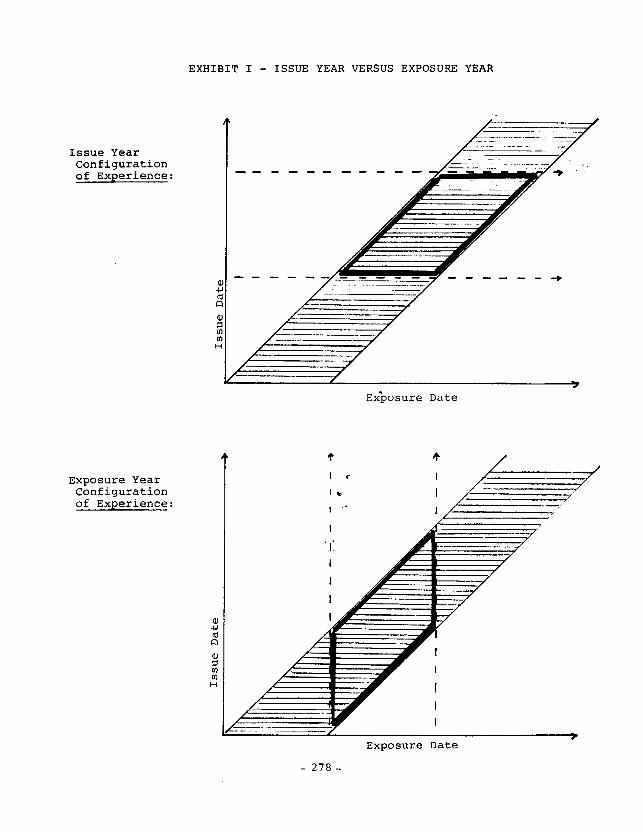
EXHIBIT I - ISSUE YEAR VERSUS EXPOSURE YEAR

Issue Year Configuration of Experience:

Exposure Year Configuration of Experience:

-----w---w

Ex>osure Date

Exposure Date

- 278 -

l Exposure year loss data matures more quickly than issue year

loss data, hence its greater acceptance in ratemaking.

l Premiums, commissions and taxes are easier to assign to issue

year, because all transactions associated with a given policy

are assigned to the same issue year. Correct allocation to

exposure year requires systems efforts not always easy to

obtain. Individual transactions must be split between

exposure periods: the pro-ration is intuitively simple, but

quickly becomes very complex in the real world of

endorsements, audit adjustments and error corrections.

a Policies are priced at the time of their issue. Similarly,

production goals are established by issue period. The issue

year approach has the advantage of relating directly to these

and other related marketing decisions and objectives.

FOK this last reason, the author prefers the issue year approach for

planning and monitoring of results.

INVESTMENT INCOME

In discussing the allocation of transactions to issue year and

exposure year, some readers may have noted that al'location of

investment income was absent from the discussion.

-279-

This was intentional, not because investment income is not important,

but instead because the author does not believe that actual invest-

ment income should be utilized in pricing, planning and monitoring of

property/casualty insurance results.

Instead, the investment department should .quarantee to the insurance

area spot and forward interest‘ rates to be used in the pricing

process. These rates should be used in the pricing of the product.

Investment income for the insurance area should be based on these

rates, as if they were actually the rates being earned.

In other words, the insurance operation ought to loan its available

cash to the investment operation at negotiated, fixed, and guaranteed

rates. In essence the investment department should "pay" for the

cash flow that it obtains from the insurance area.

The performance of the investment area should be based on its ability

to earn investment returns in excess of that which it is paying for

the funds that it has obtained. The investment department becomes a

true banking operation.

Some might argue that the artificial book-keeping entries required to

accomplish what I am describing are not worth the effort. I would

disagree. The approach I am suggesting may be the only way to

-280-

establish the missing dialogue between the two areas about such

topics as durations and the risks associated with mis-matching

maturities.

This approach will also facilitate meaningful consideration of

investment income in the pricing of these products.

The rates guaranteed to the insurance area should be at OK near

market interest rates, with any differences reflecting risk margins.

They should be the rates that management is willing to concede to the

buyer in the pricing of a product. For example, the pricing of

alternative payment plans should use these rates, so that the seller

is indifferent to the payment plan selected.

The concession of market interest rates in the pricing of the product

does not imply a reduction in the overall target profit margin of the

product. It merely causes that profit margin to be consolidated into

a single number, rather than being split between an underwriting and

an investment component.

Consolidating the profit margin into a single number is critical to

the pricing process. The decision to reduce the profit margin to

meet competitive pressures -becomes an explicit one, and not an

implicit one based on the amount of an indicated rate increase "left

on the table".

- 281-

A FINANCIAL PLANNING SYSTEM

Financial planning, including macro-pricing requires a specialized

management information system to house both actual and projected

experience. The system should consist of one OK more databases

capable of sorting and summarizing the various data elements in a

variety of ways.

Exhibit II displays such a system in schematic form. The system

consists of three inter-related databases:

0 An insurance database containing actual and projected

exposures, premiums, losses and expenses, for each product

line.

l An investment database containing actual and projected assets

by type (taxable bond, tax-exempt bond, common stock, etc.)

and maturity.

l A financial database containing traditional balance sheet and

income statement items.

These three databases would interact: actual and forecast results

from one database would serve as input to the others.

-282-

EXHIBIT II - A COMPREHENSIVE PLANNING SYSm

Exposures Issue Date Premium By: Exposure Date Losses Calendar Date

Investment Database

Assets by: Type

Financial Database

Traditional Balance

Incane Statment

- 283-

The insurance financial planning function (including macro-pricing

and monitoring) is housed entirely within the uppermost database in

Exhibit II. The analysis of actual results, and the forecast of

future results would be by issue year OK exposure year, (OK both),

depending on the specific design of the forecasting model for the

line. (For major lines, it may be desirable to maintain greater than

annual detail, e.g., issue guarter and/or exposure quarter).

The main objective of the planning exercise is the generation of the

insurance cash flow, which is the principal input to the investment

department for investment planning purposes. The investment

department's plan involves the selection of a maturity profile

appropriate to the cash flow forecast.

Both the investment and insurance areas can generate accrual

forecasts in addition to cash flows. These can be fed into the

financial database that produces forecasts of traditional accounting

results. While ancillary to the first two steps, this last step is

probably necessary, at least for tax planning purposes.

Given these three databases and modern database management techniques

reports in a near-infinite variety of formats can be generated.

Those reports should be designed to support either the macro-pricing,

financial planning OK monitoring of the line.

- 284 -

SUMMARY

In any business, decisions must be supported by adequate management

information. The financial planning exercise is the support tool by

which management assesses the current and future prospects of each

product being sold by the company. It is imperative that the

financial planning exercise be well defined, and reflect the true

economics of the enterprise. Decisions should not be driven by

either statutory OK GAAP reporting requirements, either in their

current OK future forms. These requirements should, instead, be

viewed on a constraint that must be satisfied. (Admittedly, an

important constraint, but nonetheless a constraint).

Pricing, financial planning and reserving all involve forecasts of

future transactions of the insurance company (hence they are all

actuarial). Differences between the forecasts stem from timing

differences. None of the differences suggest that the fundamental

approaches to each forecast should be different.

- 285 -

The author has argued that pricing and financial planning should be

performed on an issue year, or alternatively on an exposure year

basis. Forecasts should be made that reflect both the timing and the

amount of future cash flows. Within the insurance operation,

investment income should be based on simple, fixed interest rate

assumptions consistent with those used in pricing the product.

Finally, the monitoring of insurance results should not be on the

basis of calendar year accounting results. Rather, comparisons

between actual and planned results should be maintained by issue

period or exposure period.

-286-

THE CASH FLOW OF A RETROSPECTlVF RATING PLAN

by

Glenn Meyers

Glenn Meyers is en associate professor ITI the lkpartment of Statistics and Actuarial Science at the University ot lowa. He holds a Ph.D. in Mathematics from SUNY at Albany, M.A. In Md%hematics from Oakland University, and B.S. from Alma College in Mathematics and Physics.. Glenn ir a Fellow of the Casualty Actuarial Society. He currently serves the 9% on the Committee on Theory of Risk, the Committ:ee on RevjeLl ot Papers and the Examination Cammittee. Previous paper-5 include: “An Anal.ysis of Retrospective Hating;’ “The Calculation of Aggregate Loss Distributions from Claim Severity and Claim Count Dislzributions” (with Philip Heckman) ; “Parameter Uncertainty in the Co1 lective Risk Model” (with Nathaniel Schenker) and “Empirical Bayesian Credibility in Workers’ Compensation Classif ication Ratemaking. 1(

Abstract With current methodology, the parameterc of a retrospective rating plan are calculated to place the plan in balance on an underwriting basis. Thus paper provides a way of cai.c~\lati~.)g the present value of the retrospect j ve premium. Using this methodology, one can compare the expected prc3fitability of various retrospective ratinq plans on a dicounted or operating basis. This includes paid loss retros. It is al50 possible to determine ,the parameters of a Plan that will yield a predetermined operating profit,

- 287 -

1 Introduction A.- --_._-_._-_ __--

In recent years, the state of the property er~d c:asual ty

insurance industry could be characterized br three highs:

high combined ratios; high interest rates; and 6, high degrc:?e

of competition. Insurance company managers ~ncw that a great

deal of investment income can he made by writing inmrwncp.

and they are willi.nq tn lower prices in order to do this.

The luestion to be asked, tt,en, is t-row mlcch c-an t-ates be

lowered in ovder to stil.1 maintain an accc’ptahl~, overall

prof i t? It should be nnted that in prnct-ice. act*.taries do

not heve complete control of the pricjng procures.

Underwriting and marketing pE’rsonna1 have con~.iderable

i n put . If actuaries do not calculatE the cont’rjbution of

investment income to the prof ltabil ity of a line of

insckrancc, someone else wi 11. And the resul tinq

“cal.culation” may amount to no more than A reacfion to

competitive pres5ure5.

The suestlon is not whether to USE? investment income in the

calulation of rates. Instead the question 1~. &z to use

inve5tfrtent Income jr, the calccclatlon of ratcz.

This paper considers the effec:t c,f invertmrnt income II)

choosing the parametfrs of a ret.rospective rating plan. l%Jith

current methodologyr the parameters of a re>trospect Ive

ratinq plan are ctioseri to place ttte plan in balanre on a

nonllnal, or underwr1 t i. ng ba51 E. Py *his we mPdn that. t:he

-288-

expected retrospective premium is equal to the c.um of +:he

losses, e::pen~e~ and the anticipated protit. However it is

possible for different plans to have the same P:<pec::ted

premium and have different cash flows.

For examp 1 e, a plan wi.th a no maximum will have premium

floulng in as long as losses devel.op, while r7 plan with a

low maximum WI 11 stop producing premium as the insured

breaks the maxim~~m. Not all insureds will break the maxim~.ur~~

but there wil.1, on average. be a faster prcmlc~m flow hecause

of the hiqher basj c and the increased numbcjr of xnsurrds who

do break t:he ma:: j rrt~~m.

Other factors, such as the 1.~155 conversion factor and the

minimum premium factor will also affect the c8s.h flow of a

retrospective rati.ng plan.

Thic paper ~111 provide a way of c:alculating the preseilf:

value of the retrc!rpective premium. U51ng this me+hodol,c?yy,

one can compare the profitability of various retrospective

rating plans on a discounted or operating has~c. Thic

includes paid 1.0s~ retr‘ns. It is al.so F-?orsible to cra.l~~~late

parameters of a plan that will yieJ.d A F:)rt-determined

operating profit.

- 289 -

The principal tool urjed will be the poller-tlvc risk modej.

Excess pure premiums will be calculated for the insurc>d at

various stager of development. One can t hr-)n r:a1c.11 I,ate the

e,:pected rset:pospective premium at each stage, is n d C.I b ? a I. 1.1 t h E”

present value of the re?rospective premium.

This technique will enable the insurer to uffer s. standard

incurred loss retro which is competitive rulth a paid JOSE.

retro. This could help relj e’ve somr nf the pressure +hat the

Internal Revenue Service js plutting on paid 10s.~; rPtrc>c. I r,

addition it will. become possible to properly price P ret.r.l!

with loss development factors. T h 1 ~5 w 1 I I rr, I n 1 rr, 1 z 6.; t t IF’ 2. I :‘F’

of retrospective adjustments as tome passes.

We begin by first defining ?,i-1.e parameterc of a retrorpc=ctive

ratinq plan.

-290,- .,

.f The Parameters Defined CL __--- ..,._ __ - ----.-- -_ ,.--

The retrospective premium. F?, for an l.nsclr~.~t:l I.5 91vF.T: tW tt3P

follou~ir~g formula .

Many retrc>spectlvp ratting plans c: 1 a 1 n, 4rnOl IO t

over a speci ficd loss I imi t sha I. I. bt-J ,\ce(.( to 1. ~~1~~1 ate? the

retrospective prrvlium. In ftiir r:a5.F?r ttic c;!pE’C+erl lncc

resultinq from fhi=. provision ntctst, be added tc) t:he

retrospective premium. T~I s amo~..cnt is rkntrtt-ed bu E..

L. represents the actual losc.c-1s rnct\rrvd under the plant,

- 291-

In nrder to i::eep this paper as siiimp1.e as po~.;sx.ble, we to i 1 1

not consider t:tte vffer:t of 10s~: limit:s and premit.tm ta:.:es

unt i I the end of 4 he paper” We stial 1 alsc:~ ~gnur~ +he rr~~,n~m~rr~

premium. This results in a cimpljfied formula for the

retrospective premium.

- 292 -

has been to pay an amount totaling less than the standard

premium in inctal. lrrtents.

Wc~ ~111 be t:ollawlng a single hypothetical insured

thrtx.lqhor..tt this paper - The loss and expe~jse infor*mati,on tr::r

thi5 insured is qjven in the follr.iwinq table.

Expected Incurred Losses 100Q0)pIL3 Expected Los5 Adj. ExP. 1 c3000B Other Expensar ...r5l.@lJ Total 1157500

The expv(:ted Incurred losses fc.:w esdc:h retrc:)spec:+ive

adJcistment period are qiven in the f’ 0 1 1 c:w i ng t a t3 1 e.

- 293-

In order to talc-:ulate the average retrospective prcmlum, one

needs to have tables of e::c~‘r,r; pure’ prerltiumc: wh j c.11

correspond to each retrnspec-five ad jt.\strrrc2nt. Thc.:se t ahIf

are provtded in Exhibit I. 5 he Heckman-Plcyev.5 ~1 1 rnri t h&l. 111.15

used to generate these tables. While +tle IT~F-‘I.I~: for this

algorithm could be provided. it- c;eem% just 3% c:as’-J tcr c75C~IIlIC’

the tables are given.

These tables provide excess pure:’ prcmicmz for J 055 amounts

in increments of 10000. Linear intczbrpol <::tiol> can be tused to

calculate excess pure premjcrms for 105s amot.tr1t5. t hat arc’ not

a multiple of 10000.

The average retrospective premium is c:aIcr.~la~~~d in the>

following nmnner3. Detj ne the effective rr,a::jm~nr t.o t)rr esL{al

to (G - E)/c:, and let X be the RKC~E;S pC,re ~~mr~jwr~ for

losses over the effective rrta::imti.~~~. Then ttlcl average>

retrospective premium ir qiven by:

A5 an example, ar,s.ume II = 232450, G ::: JSWXl00. c =: 1 . 1 1 and

El: L 1 = 1000000. Then the effective rrm:.:~mc!rn := 1152Z’Cl. Yq

linear interpolation on Exhibit I !9Q month::.), we find

x = 131’77’ir and E.TRl = llEJ30B.

-294 -

3. The Standard Incurred Loss Retro ---_--_l_-,____.

We first calculate the expected underwrlti.ng profit for 27.

standard incurred lass retrn. We need unIy consi tier the

seventh (final ) retrnspective adjue,tment ior this

cdl culat ion.

Tab 1. E! 3

Pasi c 232450 1.c.f. 1.1 Has i rr11..1m 15 0DQ00 EC RI &I Ye, maths. 1 lE175l30 lL.055 & Espense 115 7500 Underwriting Profit 300Q0

This plan was designed to yield approximately the 2.5X

underwriting profit that is budgeted in standard Work~~rs’

Compensation rate f i 1 ings.

Next we calculate the espec:ted operating profit for the S~ITIR

plan assuming an effective annual interest. rate of 8%. That

is to 5ay9 for rxanfple, that a payment due in three mnrlthF;

is discounted at A rate of l.0817)‘25. A depaz i t Ix-cm i um c:) f

960000 is to be payable in sii: qusrterly installments ot

160000. The present value of the deposit Pr.emi~.ur~ i,s 935416.

Addit ional amounts of premium drue to retrospectj vo

adjustments r7re z\ssumed to be paid three months aftsr the

calculation of the retrospective premj.um.

-295-

Table 4

Basic 232450 1.c.f. 1.1. Masimum 1500000 Depos i t 96012900 ET RI @ 18 mths. 1078380

d 30 mths. 1155720 a 42 mth5. 1173210 @ 54 mths. t 179480 @ 66 mths. 11 H2340 @ 78 mths. 1185200 @ 90 mths. 1187500

P. V. Retro Premi<lm 1103720 P.V. Los5 & Expense 942000 Operating Pi-of i t 141720

In this example we see that the standard rating method

yields an operatinq profit of nearly 12% of the ultimate

average retrospective premium. This is fine if the

competition will allow it. If not, the insuranc:e company

management must decide what open-ating profit to seek.

Suppose they decide tu seek: an cxperatins profit of 100000.

Perhaps there is a vaque notion that an underwriting Profit

of 30000 already anticipat.es a certain ama~rnt of investment

income, and ir; not appropriate for an operatinq profit.

Anyway, the question becomes one nt selecting the basic

premium that yields the desired operating profit. Th15 can

be done by repeating the talc-ulaf.ions of T’able 4 on a trial

and error basis, although a numerical method mc4y yield the

desired solution more quirk ly4. The results or this process

are in the followIns Table.

-296 -

Table 5

Basic 1.c.f. Max imum Deposit ECRI @ 18 mths.

@ 30 mths. a 42 mths. a 54 mths. 61 66 mths. a 78 mttis. 61 90 mths.

P. V. R&r0 Premium P.V. 1~0s~ C Expense Operating Profit

167150 1.1

1.500000 960000

1024100 1106410 1125210 1131970 1135050 1138140 1140620 1062000

96’2000 100000

Having demonstrated how to select the basic premium whic::h

yields a predetermined operating profit, it should he

pointed out that it is possible to fix the basic premium and

select the loss conversion factor which yields a

predetermined operating profit.

Certain other cash flow provisions of a retrospective rating

plan are often subject to negntiation between insurer and

insured. Thus it seems appropriate that we show how to

properly account for them.

-297 -

4. Retro Development Fact=-+

An optional provision of most retrc)spec.tive rating plans is

to adjust the incurred 105ses tn their ultirrcatc value by

means of a 1055 (or retro) development factor. An advantage

to the insured is that the retrospective premium 15 close to

its ultimate value at the first retrospective adjustrrwnt. A

disadvantage is that the insured must pay the premium

sooner. To uvercome this disadvantage, the insurer can offer

to lower either the basic premium or the loss conversion

factor.

In the following table we consider the latter option. The

deposit premium is to be paid in installments as before.

Al though several retrospective adjustments are made, the

contribution of the later ad.jc.tstments is assumed to be

negligible. The final table of excess pure premictmr

(evaluated at 90 months) was. used to calcxrlat~:~ the average

retrospective premium at the first adjustment.

Table 6

Pd 5 i c: 147150 1.c.f. 1.07-75 Max i mum 1500000 Deposit 960000 EC RI d 18 mths. 1127730 P. V. Retro Premium 1062000 P.V. L-05-s & Expense 96200@ Operat ins Profit 100000

The results of this calculation should be direct19

comparable with the previous c:alc:ulat,:ion (Table 5). The

introduction of retro development factors c:auspd about a

- 298 -

1.1% decrease in the averi3qe retrospective premium on 4

nominal basis.

The accuracy of this calculat:ic?n depends i.rpon our abil. ity to

calculate the proper loss development factors. Even if we

get the correct overall loss development factcn-5, change5 In

the shape of the aggrasate loss di5tributiorl over time will

affect the averi3ge retrospective premium. The ac.ithnr

suspects that the result, over time, will be ;:I thinker tail

for the aggregate loss distribution, a tlighcl- e::ce~s ~L!YP

premium and a slight decrease in the average retrospective

premium. l~osses which are revalued upward wi 11 be l.imi tsd by

the maximum premium, while lorses which arc,! valued downward

wi 1 I. be unaffected. A full treatment of this effect i5

beyond the 5cope of this paper.

- 299 -

5. Paid Loss Retros

A very popular rating plan in recent years has been the so

cal led “paid loss retro. ’ While thca details of the f lnancial

transactions may vary, a typical plan could work as follc)ws.

A basic premium is paid, po5e.i bly in instal Imcnts. T h E!

retrospective premium based on paid losses is continuously

paid from a special fund set up hy the? insured. At some

point in time, ~~s~~ally 54 months after the fsffacrtive date,

the plan switches over to an ordinary incurred loss retro.

The continuous; adjustment of the retrnspective prc:)mil.krn

presents a technic-al problem. Thr?re is always the

possibility that the insured will break tt~e ma::~mcrm nn paid

losses before the 54 month swi tchover. Thi$, cm.\l.d, in

theory, require daily tabl.er ot excess pure premiums. I n

practice, the possibility of breaking the rrmximicm before

the switchover is considered remote, and is ignored in thr:,

followiny calc,ulations. The average retrr:,spec:tive prtmium

can then be estimated using ordinary 1.0s~ payout patterns.

The effect of this rimplifyinq assumptic!n wlould be to

overstate the average retrospective premium hefnre the

switchover. It will. be c::orrected at +he 54 month adjLr<-ltmcnt.

The end result wil 1 be to overst.ate the prcsrrtt valcrc~ of ttle

average retraspective premium by the amount of interest

earned on the exce55 pure prerf~1um hefore the E.utj tctiover.

This shot.!ld be a negligibile amcmnt..

-300 -

Let us a55urw that our hypothetical insured i.s e:cpect:ed ,ko

have Paid 800000 in losses by the switchover time, and that

the present value of therf:! payments i= 720000. tet 1.15 slso

assume that the basic: premii\m ic pai cl on the ef fecti.vs? datr

of the plan. The following table describes the plan in

deta i 1 .

Table 7

Basic 215170 1.c.f. 1.1 Max i mum 1500000 ElPaid RI 1095170 EC R1 i3 54 mths. 1167130

3 66 mths. 1170050 @ 78 mths. 1 172980 li) 90 mths. 1175320

P.V. EL’Paid RI 1007170 P.V. Retro Premium 1 (at2000 P.V. Loss t Expense 962000 Operating Profit 100vI00

The results of thi.s calculation should be direc:tly

comparable tcj the straight incurred loss retro (Table 5) -

The paid loss provision caused about: a X% increase in the

average retrospective premium on a nominal basis.

-301-

5. Excess Loss f’remium and Tax Multiplier

We did not consider the excess loss premium or the ta::

multiplier in the above calcula?:ions. The in+e!n+: was to keep

the discussion as simple as possible. We now show how to

modify the calculation to +:ake these into arcount.

On the premium side of the calculation, the c,nlr ad.jrlrtmr;!nt

needed to handle the loss limit is to input a I~mlterl claim

severity distribution into the Heckman-Meyers algorithm. No

adjustment is needed on the loss and expense side. Make note

that the present value of the unlimited losses 15 still

used.

A wrinkle in the above adjustment occurs when the e):c:ess

layer is reinsured and one want:s to incorporate the cost of

reinsurance in the pricing. In this case one:’ takes the ci~~m

of the present val~te of the limited 105s.~~. and the cost nf

the reinsurance. This SLIITI is used in place of the prrse>nt

value of the unlimited losses. A not:@ of caut:ion: the pa!Acut

pattern for 1 imited losses is faster than ttlat of c~nlirrt~tecl

1055es.

Premium taxes are paid on the basis of Written premit.url. 1:) n e

should note that retrospective adjtlstments Are alru

adjustments in written premi tur,. The prezent val t.,E’ of ttic>

premium taxes can be c:alculated by usjlng tt~e average

retrO5peCtiVe premium dt each adJLrstmcnt.

- 302 -

The following question should he asked at this point. Do we

really need to have separate factors in the retrospective

rating plan for excess losses and premium taw~5?

Tax multipliers are not used in guaranteed cost plans, 5’0

why use them for retrospective rating? Rates for other

guaranteed cost plans reflect premium taxes, and so could

the basic Premium and the loss canversion factor.

Skurni ck5 put the excess premium into the basic premium for

the California Table L., and there is no reason why this

could not be done for all retrospective rating plans.

What really matter5 is that the present value of the

retrospective premium is equal to the profit plus the

present value of the losses and expenses. This can be

accomplished by a proper selection of the basic premium and

the loss conversion factor. The result will be a simpler

formula for retrospective rating.

-303-

6. Conclusion_

This paper is written under the premise that an explicit

calculation of investment income is superior to the implicit

recognition of inve5tment income that 5ome say is in many

present rating formulas. We do not attempt to determine the

proper operating profit. This task belongs to insurance

company management and/or regulators. It does not belclng to

some ratemaking formula based on underwriting profit.

We have provided a methodology for finding the expected

operating profit for a retrospective rating plan. This

methodology is presently in use at a major insurance

company.

The author suspects that the more complicated versions of

retrospective rating, such as paid loss retros, arose

because the present plan does not allow for investment

income. Now that the various versions of retrospec:tive

rating can be rated on a comparable basis, it is hoped that

the more complicated versions will no longer be necessary.

Retrospective rating can be made simple.

- 304 -

7. Acknowledgments.

This paper is an outgrowth of a project which 1 directed

during my final year at CNA Insurance Companies. I worked

very closely with John Meeks and Steve Maguire in developing

the conceptual basis for what we called the “Account Pricing

System. ” Steve and Ron Swanstrom wrote a program which made

these ideas very workable in a production environment.

- 305 -

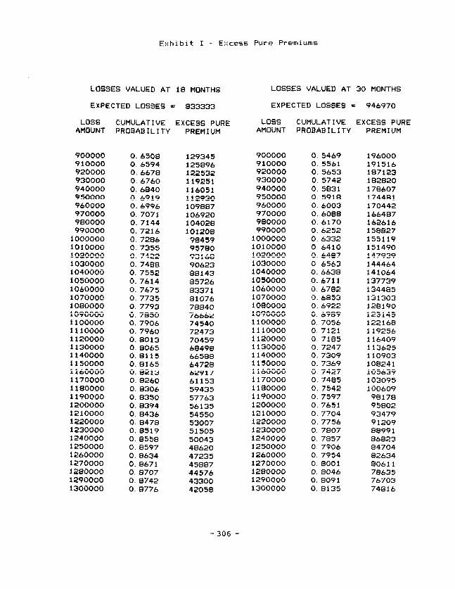
Exhibit I - E::cess Pure Prewiun~s

LOSSES VALUED AT 18 MONTHS

EXPECTED LOSSES = 833333

LOSS AMOUNT

CUMULATIVE EXCESS PURE PREMIUM PROBABILITY

900000 0. 6508 129345 910000 0. 6594 125896 920000 0. 6678 122532 930000 0. 6760 I I9251 940000 0. 6840 116051 950000 0.6919 112930 960000 0.6996 IO9887 970000 0.7071 106920 980000 0.7144 104028 9?0000 0. 7216 101208

i 000000 0. 7286 98459 1010000 0.7355 95780 1020000 0. 7422 93168 i 030000 0. 7408 90623 i 040000 0. 7552 88143 1050000 0. 7614 85726 1060000 0. 7675 a337 1 1070000 0.7735 81076 1080000 0. 7793 78840 i 090000 0. 7850 76662 1100000 0. 7906 74 540 1110000 0. 7960 72473 1120000 0. 8013 70459 i 130000 0. 8065 68490 1140000 0. a115 66588 1150000 0.8165 64728 1160000 0. 0213 62917 I 170000 0.8260 61153 1180000 0. 8306 59435 I 190000 0. 8350 57763 1200000 0. a394 56135 1210000 0. 8436 54550 1220000 0.8470 53007 1230000 0. 8519 51505 1240000 0. 8558 50043 1250000 0.8597 48620 1260000 0. 8634 47235 1270000 0.8671 45887 1280000 0. 8707 44576 1290000 0. 0742 43300 1300000 0. 8776 42058

- 306

LOSSES VALUED AT 30 MONTHS

EXPECTED LOSSES = 946970

LOSS AMOUNT

CUMULATIVE EXCESS PURE PROBABILITY PREMIUM

900000 0. 5469 196000 910000 0. 5561 191516 920000 0. 5653 187123 930000 0. 5742 182820 940000 0. 5831 170607 950000 0. 5918 174401 960000 0. 6003 170442 970000 0.6088 166407 980000 0. 6170 162616 990000 0.6252 158827

1000000 0. 6332 155119 1010000 0. 6410 151490 i 020000 0. 6487 I47939 1030000 0. 6563 144464 1040000 0. 6638 141064 1050000 0.6711 137739 i 060000 0.6782 134405 1070000 0. 6853 131303 1080000 0. 6922 128190 1090000 0. 6989 125145 I 100000 0. 7056 122168 1110000 0. 7121 119256 1120000 0. 7185 I 16409 i 130000 0. 7247 113625 I 140000 0.7309 I 10903 i 150000 0. 7369 108241 i 160000 0. 7427 105639 i 170000 0. 7485 103095 I 180000 0. 7542 100609 i 190000 0.7597 98178 1200000 0. 7651 95802 1210000 0. 7704 93479 1220000 0. 7756 91209 1230000 0. 7807 8899 1 1240000 0. 7857 86823 1250000 0. 7906 04704 1260000 0. 7954 82634 1270000 0.0001 80611 1280000 0. 904.5 78635 1290000 0.8091 76703 i 300000 0.8135 74816

LOSSES VALUED AT 42 MONTHS

EXPECTED LOSSES = 979610

LOSS AMOUNT

CUMULATIVE EXCESS PURE PROBABILITY PREMIUM

LOSS AMOUNT

CUMULATIVE EXCESS PURE PROBABILITY PREMIUM

900000 0. 5218 2 14600 900000 0. 5127 221641 910000 0. 5311 209865 9 10000 0. 5221 2ib815 920000 0. 5403 205223 920000 0. 5313 212081 930000 0. 5494 200672 930000 0. 5404 207440 940000 0. 5584 196210 940000 0. 5493 202888 950000 0. 5672 191838 950000 0. 5582 198426 960000 0. 5759 187553 960000 0. 5669 294051 970000 0. 5844 i 83355 970000 0. 5755 189763 9aoooo 0. 5928 17924 1 980000 0. 5840 185560 990000 0.6011 175211 990000 0. 5923 181442

1000000 0.6093 171263 i 000000 0.6005 i 77406 iOlOOOO 0.6173 16739b 1010000 0. 6086 i 73452 1020000 0.6252 163608 1020000 0. blbb 169578 1030000 0.6330 159899 1030000 3. 6244 165782 1040000 0. b40b 156267 i 040000 0. 6321 lb2065 1050000 0.6401 152711 i 050000 0. 6397 159423 106.0000 0. &555 149229 i 060000 0. t471 154857 1070000 O.&b27 145820 i 070000 0. 6544 1513b5 1080000 0.6698 142483 i 080000 0. bt;ib 147945 i 090000 0. b7b8 1392ib i 090000 0. b&8& 144596 I 100000 0. 6837 136019 1 I00000 0. 67% 141317 1110000 0.6904 132889 1110000 0. 6824 138106 i 120000 0. 6970 129826 1120000 0. bS91 134963 i 130000 0.7035 126829 1130000 0.6956 131887 i 140000 0.7099 123895 i i 40000 0. 7021 128875 1150000 0.7161 121025 1150000 0. 7084 125927 1160000 0. 7222 118216 11 boo00 0.7146 123042 1170000 0. 7282 1 i 5468 1170000 0. 7207 120218 i 180000 0.7341 112779 11a0000 0. 7266 117454 i 190000 0. 7399 110149 1190000 0. 7325 114749 i 200000 0.7455 107576 1200000 0. 7382 112103 1210000 0.752 1 105058 1210000 0. 7438 109513 1220000 0.7565 102596 1220000 0. 7494 106978 1230000 0.7618 100188 1230000 0. 7548 104499 1240000 0.7670 97832 1240000 0. 7601 102073 1250000 0.7722 95528 1250000 0. 7653 99700 1260000 0. 7772 93274 1260000 0.7704 97378 1270000 0.7821 91070 1270000 0. 7754 9510b 1280000 0.7869 88915 1280000 0.7803 92884 i 290000 0.7916 S6808 I290000 0. 7851 90711 1300000 0. 7962 84747 1300000 0. 7898 88585

LOSSES VALUED AT 54 MONTHS

EXPECTED L.OSSES = 986193

- 307 -

Exhibit I - E::ccss Purr! Premiums

LOSSES VALUED AT 66 NONTHS

EXPECTED LOSSES = 991080

LOSS AMOUNT

CUMULATIVE EXCESS PURE PROBABILITY PREMIUM

900000 0. 5086 910000 0. 5179 920000 0. 5271 930000 0. 5362 940000 0. 5452 950000 0. 5540 960000 0. 5628 970000 0. 5714 980000 0. 5799 990000 0. 5883

1000000 0. 5965 1010000 0. 6046 1020000 0. 6126 1030000 0. 6204 1040000 0.6282 i 050000 0. 6358 1060000 0. 6432 1070000 0. 6506 i 080000 0. 6578 1090000 0. 6649 1100000 0. 6718 1110000 0. 6787 1120000 0. 6854 I 130000 0. 6920 1140000 0. 6985 1150000 0.7048 116000cj 0. 7110 1170000 0.7172 11 a0000 0. 7232 i 190000 0. 7291 1200000 0. 7348 1210000 0. 7405 1220000 0. 7460 1230000 0.7515 1240000 0.756% 1250000 0.7621 1260000 0. 7672 1270000 0. 7723 12130000 0.7772 1290000 0. 7820 1300000 0. 7868

224922 220054 215279 210595 206002 201499 197083 192754 188510 184351 is0275 176280 172366 168531 164774 161094 157489 153951 150499 147112 143796 140548 137368 134255 131207 128223 125302 122443 119645 116906 114225 111601 109034 106522 104063 101658

99304 97001 94748 92544 90388

LOSSES VALUED AT 7B MONTHS

EXPECTED LOSSES = 9960 lb

LOSS CUMULATIVE EXCESS PURE AMOUNT PROBARILITY PREMIUM

900000 0. 5044 228254 910000 0. 5137 223345 920000 0. 5229 Zl8528 930000 0. 5320 213803 940000 0. 5410 209 168 950000 0. 5499 204622 960000 0. 5586 200165 970000 0. 5673 195795 980000 0. 5758 191510 990000 0. 5842 387310

1000000 0. 5924 193193 1010000 0. 6006 179158 1020000 0. 6086 175203 1030000 (3.6164 171328 1040000 0. 6242 lb7532 1 o5cJooo 0. 6318 163812 1060000 0. 6393 160167 1070000 0. 6467 156597 1080000 0. 6539 153100 i 09~000 0.6611 149675 1100000 0. 6681 146321 1110000 0. 6749 143036 1120000 ‘0. 6817 1’39818 1130000 0. 6883 13bbbP 1140000 0. 6948 i 33584 1150000 0.7012 130564 1160000 0. -7rj7:, 127607 1170000 0. 7136 124712 1180000 0 7197 121a79 1190000 0. 7256 119105 1200000 0 7314 116390 1210000 0. 7371 113732 1220000 0. 7427 111131 1230000 0. 7482 108585 1240000 0. 7536 106094 1250000 0. 7588 103656 1260000 0.7640 101270 1270000 0. 7691 98936 1280000 0.7741 96651 1290000 0 7789 94416 1300000 0. .7837 32229

- 308

LOSSES VALUED AT 90 MONTHS

EXPECTED LOSSES = 1000000

LOSS AMOUNT

CUMULATIVE EXCESS PURE PROBABILITY PRENI UM

900000 0. 5010 230957 910000 0.5103 226014 920000 0.5195 221163 930000 0. 5287 216405 940000 0. 5377 211736 950000 0. 5465 207 157 960000 0.5553 202667 970000 0. 5640 198263 980000 0. 5725 193945 990000 0. 5809 ia

1000000 0. 5892 !95562 1010000 0. 5973 131494 1020000 0. 6053 177508 1030000 0. 6132 173600 i 040000 0. 6210 169771 1050000 0. 6206 166020 1060000 0. 6362 162344 1070000 0. 6436 158742 1080000 0, 6508 155214 i 090000 0. 6580 151758 1100000 0. 6650 148373 1110000 0. 6719 145057 1120000 0. 6787 141810 I 130000 0. 6853 13P630 1140000 0. 6919 135516 1150000 0.6983 132467 1160000 0. 7046 129481 1170000 0. ‘7108 126558 1180000 0. 7168 123696 i 190000 0. 7228 120894 i 200000 0. 7286 118151 1210000 0.7344 115466 i 220000 0.7400 1 i 2337 1230000 0.7455 110265 1240000 0.7509 107747 1250000 0. 7562 I 05283 1260000 0. 7614 10287 1 i 270000 0. 7665 100511 1280000 0.7715 9820 1 i 290000 0. 7765 9594 1 1300000 0. 7813 93729

-309 -

Notes --

1. National Council on Compensation Insurance, Retrospective .------ ----- ,--- Rating Plan D.

2. Heckman, P. E. and Meyers, G.G. "The Calculation ot Aggregate Loss Distributions from Claim Severity and Claim Count Distributions," P&S LXX, 1983, p. 22.

3. Fiebrink, M. E. Discussion of "An Analysis of Retrospective Rating" (by Glenn Meyers), YsAs LXVIII, 1981, p. 113.

4. Eurden, R. L., Faires, J. D., and Reynolds, A. C. Numerical Analysis, 2nd Edition, Prindle, Wcber e( Schmidt, 1981, Ch. 2.

5. Skurnick, D. "The California Table I..," PM, LXI, 1974.

-310 -

Title: APPLICATION OF PRINCIPLES, PtlILOSWHIES AN3 PROCEWRES OF CORPORATE PLANNINGTO INSUfUWE COMPANIES

Author: Mary Lou O'Neil

Biography :

Abstract:

The author is the Chief Actuary for Property/Casualty and Life/Health Insurance at the New Jersey Department of Insurance and was previously Vice President and Assistant Actuary at the Prudential Property and Casualty Insurance Company. The author is a Fellow of the Casualty Actuarial Society, and a member of the American Academy of Actuaries and the Casualty Actuaries of New York. The author holds a B.S. in Mathematics and an M.A. in Statistics, both from The Pennsylvania State University. The author is a Contributing Editor to the Actuarial Review, a metier of the External Comnunications Comnittee, a member-e American Academy Comnittee on Property Liability Insurance; and a prior contributor to the Discussion Paper Program.

The purpose of this paper is to illustrate the need for development of unique applications of general corporate planning concepts to insurance companies. This is accomplished by briefly reviewing the principles, philosophies and procedures of corporate planning as applied to corporations in general, the unique aspects of insurers and the insurance business, and, finally presenting examples of the unique application of general corporate planning concepts to insurers.

I. INTRODUCTION AND PURPOSE

In researching the subjeot of corporate planning, I found a multitude of well

developed material providing detailed principles, philosophies and procedures of

corporate planning for corporate entities in general. Although these broad

concepts apply to insurers as corporate entities, insurers and their businesses

possess unique characteristics which require correspondingly unique applications

of these general concepts. The purpose of this paper is to demonstrate this need

by illustrating some of these unique applications in the context of the bmad

corporate planning concepts. This paper is, however, only a beginning in this

endeavor and is not intended to present a complete identification of all aspects

of the planning process unique to insurers.

II. CORPORATE PLANNING

As background for exploring the applicability of corporate planning

principles, philosophies and procedures to insurers, this section presents a brief

review of the principles, philosophies and procedures of corporate planning

currently applied to corporate entities in general.

A. Need for Planning

The first question often asked is why plan at all? Basically, business

planning parallels personal planning. In our everyday activity we anticipate the

outcomes of various actions so that we can select the action which will result in

the most desirable outcome. So too for business. Forecasts and plans are made to

illuminate today’s decisions -- to provide a process to make decisions now about

what action(s) to take in the future. 1

- 312 -

6. Definition of Planning and Planning Terminology

In reviewing many definitions of planning, I found that there were four comnon

elements to these definitions. These are:

'A company must determine its goals and objectives.

'Planning is a way to chart a path so that the company can achieve those goals.

'Planning involves decision making before a crisis occurs -- the future is anticipated and alternative courses of action are evaluated in a structured way.

'Planning is a multifaceted process involving the entire organization.

These elements were best encompassed in the following definition:

"Planning is an analytical process which encompasses an assessment of the future, the determination of desired objectives in the context of that future, the development of alternative courses of action to achieve such objectives, and the selection of a course (or courses) of action from among these altematives.VQ

For ease of reference plans may be classified into three categories: (1)

Subject area, referring to plans in terms of observable specs such as marketing

plans, financial plans and production plans, (2) Scope, referring to the range of

influence and amount of detail of the plans such as goals or policies and (3)

Time, referring to the duration of the plans (long-range, mid-range, short-range).

Certain coimron planning terms such as policies, strategies and tactics, overlap the

scope and time categories and may be distinguished as follows. Policies are

overall general guides to action or basic long term precepts of company

philosophy.3 Strategies, however, represent the overall plans of action set by

top management of the company4 while tactics are relatively short term plans set

by lower levels of management in an attempt to implement strategies.’

In developing corporate plans the organization first sets its long term

policies and strategies and then develops appropriate tactics and short range

-313 -

operational plans necessary to achieve these overall goals. This represents the

essence of the corporate planning process described in the next section.

C. The Corporate Planning Process

The corporate planning process is generally recognized to consist of the

following steps:

'Establish objectives or goals.

*Develop basic planning assumptions or premises.

'Identify alternative courses of action.

'Evaluate alternative courses of action.

'Implement the plan (select a course(s) of action).69 7, 8

‘Control9

For interested readers these steps are described in more detail below.

1. Establishment of Goals and Objectives

This stage of the process can be viewed narrowly by defining objectives so

that the only objective of any company is to make a pmfit. 10 Or fmm a

broader view, objectives are defined as long range desired states or outcomes

such as desired market shares 11 while goals are shorter range and are

considered to be milestones along the path toward achievement of objectives.

In this phase of the planning process management must first determine its

overall objectives and their translation into goals such as target profit and

then provide operational definitions of each goal and a way to measure progress

toward their achievement.12 This is probably the most important phase of the

planning process since it charts the cDmpany's long range course of activity

and is generally completed at the executive level.

2. Development of Planning Assumptions

In this phase the company must try to explicitly identify the universe of

conditions which may influence its operation or affect the achievement of

-314 -

objectives. These assumptions should reflect noncontrollable conditions such

as business cycles, semicontrollable conditions such as market share or

internal pricing policy, and controllable conditions such as whether to change

product line or pricing strategy. 13

3. Identification of Alternative Courses of Action

Based on the planning assumptions, the company then, forecasts its

expected results given no new actions are to be taken. This is generally

achieved using a system of linked together models, representing various aspects

of the firm such as the firm itself, supply, sales, consumers, conpetition,

envimmient and financial. Using variations of the original planning

assumptions, based on possible factors which may influence results, the company

can identify the results associated with different actions. me purpose of

this phase of ,the process is to identify the range of actions available to the

corrpany, the expected results associated with each, and an assessment of the

risk or margin of error inherent in each pmjection. 14

4. Evaluate Alternative Courses of Action

The company rmst evaluate its array of possible actions identified in

phase three in light of its moral policies, resources or other constraints to

action.15

5. Implement the Plan

Once the company has selected its course of action it must be translated

into specific policies, programs, procedures and practices by which the desired

objectives and goals may be achieved. 1' This stage is generally considered

the short range or operational phase of the process and is carried out by

managers thruout the organization. 17

6. Control

In order to assure achieving its selected plans, the company must

establish check points to indicate whether it is on course. This requires

continual monitoring and correction in the form of revised plans whenever

- 315-

significant deviations 0132ur.~~ In fact, the planning process may

appropriately be considered an iterative one -- continually changing as the

need arises. The required monitoring is most easily achieved via a management

information system designed to parallel the corporate planning model.

D. Organization for Planning

As noted above, certain aspects of the planning process are properly carried

out by top management -- setting objectives, policies and strategies, while others

are properly carried out by individual managers -- setting short term operational

goals. The key to success of the planning process is participation thruout the

organization. 19 The ideal organization for planning consists of an individual

corporate planner coordinating the plans of operational managers -- there is no

corporate planning department or specialized group of planners. 20

III. THE APPLICATION OF CORPORATE PLANNING TO INSURANCE COMPANIES

The preceding section presented an overview of corporate planning as it

currently relates to corporations in general. Several authors illustrate the need

to conform these basic concepts to individual industries and individual companies

within an industry using the results of a study of the motor freight industry from

which they found that regular long-range planning had little correlation with

profitability. They concluded that the reason for this was the regulated nature of

the industry -- markets, prices, and labor policies were stringently controlled

leaving only day-to-day operations to management control. Thus, these companies

could get by with ad hoc planning for acquisition or rate increases. The authors --

further point out that planning needs differ among different organizations and

among the various levels in an organization. For example, a young company may

require only a simple plan while a mature company in the same industry will need a

formal planning function, or a small high-tech firm may desparately need plans

- 316 -

while a large firm in a static industry may have less need. The planning needs of

any organization are individual and situational. 21

What does this mean for the role of planning for insurance companies? In order

to answer this question, the next sections identify the unique characteristics of

the insurance industry and its companies, and the consequent unique application of

general corporate planning concepts to insurers.

IV. UNIQUE CHARACTERISTICS OF THE INSURANCE INDUSTRY

The insurance industry shares many characteristics with other industries but is

also quite unique in many respects. Both types of characteristics are described

below.

Insurers are companies engaged in the sale of the product, insurance. They

share the characteristics of corporations in other industries such as a corporate

organizational structure including shareholders (stock coinpanies), board of

directors, and officers. However, at the same time, they differ greatly from

similar sized companies in other industries. The primary sources of these

differences are in the uniqueness of the insurance product and the significant role

of regulation on nearly all aspects of an insurer’s operation.

The insurance product differs frcm most products in two main ways, it is

intangible and its cost of production is unknown until, often times, long after its

sale. The intangible nature of the product likens insurers to other service

industries. However, the uncertainty with respect to product cost remains a

significant difference.

The other, and probably most important difference between insurers and other

corporate entities is close regulation of many aspects of the business. This

includes requirements for licensure to sell various insurance products, require-

ments to retain specified minimum capital and surplus, specification of the kinds

and amounts of investment holdings, limitations on the amount of business which may

-317 -

be sold, rules regarding to whom the business must be sold (such as mandatory

insurance or "take-all comers " laws and maximum premiun to surplus ratios), rules

regarding estimation of the final cost of the product, rules specifying the product

itself (such as mandatory contract language), price regulation, and, finally

limitation on rate of return. Because of these stringent guidelines the industry

is often compared to the utility industry. However, this comparison is defective

because that industry is provided a guaranteed rate of return in exchange for its

regulation while insurers are limited only in the maximum return they may earn with

no minimum.

In addition to regulation, insurers are set apart from other businesses because

of their unique jargon (e.g. frequency, severity, pure premium, etc.) and unique

accounting practices (e.g. deduction of pre-paid expenses and unpaid claims,

etc.).

Insurers further differ among themselves in their organizational structure

(stock vs. mutual), sales organization structure (direct writers, independent

agency system), product mix (personal, commercial, reinsurance, etc.), etc.

However, despite the constraints of regulation, there is intense cwnpetition,

particularly in property/casualty insurance. This competition is the result of the

maturity of the insurance product reflected in the saturation of the major

insurance markets (more than 90% of individuals are covered by life insurance and

more than 96% of workers are covered by group life and health insurance) and

relatively low growth (1 to 3% per year) in the number of insurable objects such as

people, cars, houses, businesses, etc., per year. 22

V. CORPORATE PLANNING -- AND ITS APPLICATION TO INSURANCE COMPANIES

The earlier sections of this paper presented a brief overview of corporate

planning -- its definition, its need, the process and its steps. This section

illustrates sane of the unique applications of general corporate planning concepts

-318 -

to insurance companies.

A. Need for Planning

Is planning needed at all by the insurance industry?

I believe that there is a role for planning in insurance companies. For

example, despite the constraints of regulation, there is a need for the firm to

establish its target profit or rate of return, to choose objectives such as market

dominance, market (or product) emphasis, geographic emphasis, prices, attitude

toward employees and clients, attitude toward social goals and insurance, and

reactions to changes in regulatory or legal climate, etc. Wherever there is room

for choice or change, there is room for planning.

Stated more strongly, insurance executives will be forced to reckon with

significant changes in the forseeable future requiring the ability to innovate and

respond quickly. 23 It is no longer possible to rely on the cyclical nature of

the business and operational strategies to pull them through. 24

B. Definition of Planning and Planning Terminology

Is the definition of planning provided in section II. B appropriate for

insurers? Is there any unique meaning of the common planning terminology for

insurers? What are the appropriate subject areas for insurer planning7 What

should the scope and planning horizon be? What should the level of detail of

planning be?

The appropriateness of the definition of planning may be ascertained by

examining each of the comaon elements of the various definitions of planning. The

first element requires a company to identify its goals and objectives. I believe

it is fundamental for insurers to identify goals and objectives particularly its

target rate of return -- otherwise the company has no direction. The second

element of the definition asserts that planning is a way for the company to chart

a path towards its objectives. Of course objectives are worthless if the

- 319-

organization cannot identify a way to achieve them -- insurer or not. Third,

planning is said to provide an opportunity to make decisions in advance. Insurers

can benefit from this insulated decision making as well as other corporate

entities. Finally, the definition identifies planning as a process. This would

be true regardless of the entity employing it. Thus, the definition of planning

applies to insurers without modification.

The categorization of plans into subject area, scope and time as well as the

terminology associated with these planning categories may be taken as generic and

hence applicable to insurers. Subject areas for insurance planning include, as

for corporations in general, marketing plans, financial plans, and production

plans.

The planning horizon will depend on the company's chosen lines of business and

areas of operation. In determining the planning horizon for a property/casualty

insurer it must be remembered that as of January 1 the results for the ensuing

year are largely already determined because the book of business which will create

those results has already been written. With restrictions on cancellations or

non-renewals, there is a long period of time between action and result for a

property/casualty insurer. Thus, the preparation of a one-year plan is a useful

exercise which will point out the work to be accomplished over a longer term, say

five years. 25 Thus, I believe there is an appropriate role for both short and

long term plans, each designed to meet the specific needs of the individual

organization. And, these two types of plans should be interdependent.

Plan scope can range from the broad statements of objectives to detailed plans

regarding every aspect of the business (number of claims in a given geographic

area in a given period of time for a given coverage, etc.) Planning must be done

in sufficient detail in order to provide a basis to monitor and control results.

There must be a balance between the detail used and the detail required or the

cost versus the benefit to the specific organization.

-320 -

C. The Planning Process - Establishing Objectives and Goals

Section II. C.l. defines and distinguishes objectives and goals for

corporations in general. What objectives and goals may be relevant to an

insurer? Who should set the objectives and goals. 3 What should be included in the

objectives and goals? What should the level of detail of the objectives and goals

be?

I believe that the objectives and goals relevant to an insurer, must certainly

parallel those of most corporations, in general, to make a profit and to survive,

and then, specifically, to the individual company, to gain certain market share,

etc. The detailed specification of these goals may take on a different

nomenclature due to the uniqueness of insurance jargon. For example, the goals of

controlling claim costs or improving renewal ratios parallel goals for other

businesses such as decrease production costs or maintain current customer

accounts. Objectives and goals could, as for corporations, be completed either by

top executives or by individual managers. I believe that the objective and goal

formulation phase of the planning process establishes the path of the organization

and, hence, should remain with top executives. Individual managers must be given

a framework within which to establish short term operational goals.

Objectives and goals can be broad statements of direction or specific

measurable achievements. I believe insurers have a need for both. Long range

policy statements and overall broad organizational goals provide the framework for

specific measurable goals to be completed by each manager.

The level of detail of objectives and goals should be sufficient to determine

whether or not the desired result has been achieved.

D. The Planning Process - Establishing Planning Assumptions

Section II. C.2. defines planning assunptions for coworations in general.

What should these assumptions include for insurers? Who should prepare the

assqtions?

-321-

Planning assumptions were defined to include all those conditions which may

confront the organization. For insurers, general conditions of importance include

inflation, interest rates, and regulatory and legislative changes. Dutter

enunerates six key forces which will confront insurers in the foreseeable future:

erratic swing in rates of inflation or interest, decline in attractiveness of

other business canbined with ease of entry to insurance, dramatic advances in ECP,

unbundling of commercial property/casualty, group life/health, and pensions, and

greater distribution efficiency. 26 Howland provides an extensive list of

external influences which must be considered, which is reproduced as Exhibit

I 27 . These fall into the category of noncontrollable forces.

Insurers should further enunerate controllable factors such as the number of

employees, its anticipated market share, product mix, geographic emphasis, etc.

These assumptions may take the form of nunerical projections (discussed below) of

new business sales, claim counts, etc., and provide the basis for input into the

ccnnpany's modeling system.

E. The Planning Process --Identification of Alternative Courses of Action

Section II. C.3. presented the process of identification of alternative

courses of action for corporations in general. What is the proper role for a

management information system in an insurance company? What aspects of the

insurance firm should be modeled?

As noted in Section II. C.3, corporations generally create models reflecting

various aspects of the firm. linked together to form an overall model. Hylas

states that for insurers, computer planning models may be used to systematize the

planning process, create "what if" analyses, measure the possible effects of

inflation on future earnings, evaluate the impact of state and other regulations,

evaluate the effect of recent court decisions, for tax planning, projecting cash

flow, structuring competitive rates, and determining the best mix of business.

He goes on to state that a successful planning model must be designed to meet

-322 -

the specific planning needs of the organization. There is no universal all

purpose planning model. He does, however, provide a simplified outline of the

basic elements which might be conmmn to most insurer modeling systems. These are

reproduced as Exhibit II.

He also asserts that the overall model consists of convenient submodels which

are unique to the individual company. His possible input/output variables for

each s&node1 are displayed on Exhibit III. The key to model design is to be sure

that the model meets the ‘user’s needs. 28 Verrengia concurs with these thoughts,

suggesting that for a medium size insurer models should focus on earned premiums,

loss ratios, profit and loss planning and ratemaking.

Hence, models are appropriate as well as useful tools as part of the planning

process. I believe canputerized models are key to the effectiveness of the

planning process.

F. The Planning Process -- Evaluation of Alternative Courses of Action

Section II. C.4, noted that corporations must evaluate alternative courses of

action in light of its constraints. Similarly, what criteria should be included

in the action selection process for insurers?

An insurer, which sells a product affected by the public interest, must

clearly identify its moral policies and first evaluate each action on this basis

discarding those which are unacceptable. Other constraints might include

available capital (premium to surplus ratio), maximum rate levels, or prohibited

underwriting standards. I believe that each insurer must develop its own criteria

for evaluation of its alternative actions. These criteria should be established

before they are needed, and should be consistent with the company's other policies

and philosophies. To the extent possible, the criteria should be objective and

measurable.

G. The Planning Process -- Implementation

- 323 -

Section II. C.5. discussed implementation of the planning process for

corporations in general. How should the plan be implemented by insurers?

This phase of the process refers to the implementation of the actions selected

in the previous phase and applies to insurers as well as corporations. Policies,

pmgrams, procedures and practices must be established to provide individual

managers with the actions which each must accomplish in order to achieve overall

goals.

H. The Planning Process -- Control

Section II. C.6. discussed the need for control of implemented plans for

corporations. What kind of analysis of results should be done, by whom, when?

How does the plan provide for control?

As noted for corporations in general, without control, there was basically no

reason to plan i.e. there would be no way for the company to know whether the

actions it implemented have put it on its desired course toward achievement of its

objectives or not. Reuter described the controlling process in his insurance

company as consisting of two items: an objective or standard which is clearly

stated in measurable terms and a timely assessment or measure of actual

performance or results. These two items are incorporated into control reports at

the individual manager level. 30

I believe that control includes both of Reuter’s items as well as a constant

monitoring of key variables via a management information system designed to

parallel the plan models, so that timely action may be taken in response to

deviations -- positive or negative.

I. The Planning Process -- Organization for Planning

Section II. D. discussed the proper organization for planning. Who should

plan? Should there be a Corporate Planning Department in insurance companies?

What should be the involvement of individual managers in the planning process?

-324 -

The planning process works best when the number of participants is as great as

possible. Certain forecasts can begin in the field, such as production, loss

ratio and development by line of business and then progress thru the organization.

Participation in the planning process should involve all of management via

specific measurable goals. Overall objectives, however, should be set by top

management.

VI. OVERALL GUIDELINES IN DESIGNING Ah' INSURER PLANNING SYSTEM

The preceding sections presented various concepts related to an effective

planning system. These are highlighted here,

'The company must develop a *plan"? i.e. choose a set of identifiable measurable actions designed to achieve certain identifiable measurable results not just a “forecast” which is merely a nunerical prediction of what results might be under one specific set of assumed actions.

'The planning process must balance detail with needs i.e. cost must be justified by benefits realized.

'The company must set overall objectives and policies. Executives should assume the responsibility of setting the company’s direction and make it well known throughout the organization.

'Those individuals responsible for results should also be responsible for the plans. Participation in the planning process should be as broad as possible. There should be no need for a separate corporate planning department or a separate group of V*planners9V.

'Plans should be structured so that the results are measurable and specific accountability should be assigned throughout the organization -- rewards should be tied to achievement of plan goals.

'The planning process should be a dynamic ongoing flexible activity responding to both favorable and unfavorable deviations as they arise.

-?25-

'The plan should include models and a management information system specifically structured for the individual insurer’s needs. Models and processes suitable for other firms should not be transplanted.

VII. SUMMARY AND CON&LLlSIONS

The preceding sections presented an overview of the planning process for

corporations in general and identified sane unique areas of application of the

process to insurers. This identification represents only a beginning. There is a

need to more fully develop these unique areas of application for insurers in

general and finally individual insurers must carry the process into their own

firms.

-326 -

Exhibit I

External Influences Influencing the Business Climate of Insurers31

I. For Property-Casualty Companies

*Extreme competition, especially for commercial business

-Cash-Plow underwriting

-Mandated subsidies in involuntary markets

*Growing company/agent computer interfacing

*Financial service marketing

.Multiple types of marketing outlets

*Nonrisk-bearing insurance services

*Loss of market share by independent agents

*Continued inflation in medical expenses and auto repairs

.Deterioration of smoke stack industries

*High energy costs

*Growth of self-insurance and captives

*Open competition and requirement of independent pricing

*Possible increased taxes

II. For Life and Health Companies

*Increasing medical expenses

*Investment-oriented life policies

*Agent retention

*Possible increased taxes

-32?-

Exhibit II

Basic Elements of An Insurance Planning Mode132

- 328 -

Exhibit III

Examples of Input/Output Variables for an Insurance Planning Mode133

amPuT “C*t*sLeS

-329 -

1.

2.

3.

4.

5.

6.

7.

8.

9.

10.

11.

12.

13.

14.

15.

16.

17.

18.

19.

20.

21.

22.

23.

Footnotes

John Argenti, Corporate Planning A Practical Guide (Homewood, Illinois: Dow Jones - Irwin, Inc., 19691, p. 204.

Brian W. Scott, Long-Range Planning in American Industry (American Management Association, 19651, p. 21.

George A. Steiner and John B. Miner, Management Policy and Strategy Text, Readings, and Cases (New York: Macmillan, 19771, p. 26-27.

Steiner, p. 19.

Steiner, p. 23-24.

William R. Osgood, Basics of Successful Business Planning (American Management Association, 19821, p. 20.

Scott, p.22.

Argenti, p. 17.

Russell L. Ackoff, A Concept of Corporate PlanniT (New York: John Wiley & Sons, Inc., 19701, p. 6.

Argenti, p. 28.

Ackoff, p. 24.

Leon Reinharth, H. Jack Shapiro, and Ernest A. Kallman, The Practice of Planning Strategic, Administrative, and Operational (New York, Van Nostrand Reinhold Company, 1981>, p. 31.

Osgood, p. 20-21.

Argenti, p. 110.

Argenti, p. 131-135.

Ackoff, p. 42.

David Oewan, Planning and Control for Managers (American Management Association Extension Institute, 19751, p. 4-5.

Reinharth, Shapiro, and Kallman, p. 38.

Ackoff, p. 129-131.

Argenti, p. 227.

Reinharth, Shapiro, and Kallman, p. 3-4.

William A. Sherden, "Stategic Planning: Do the Concepts Apply", Best's Review (October, 19831, 29.

Philip H. Dutter, Yuccessful Management in a Changing Environment”, Best's Review (December, 19831, 33-34.

-330 -

24. James E. Morey, nPlanning for Survival", Best's Review (September, 19831, 128.

25. Wilfred G. Howland, “Corporate Planning -- Prescription for Survival”, United States Banker (May, 19841, 121.

26. Dutter, p. 33-34.

27. Howland, p. 121.

28. Robert E. Hylas, "An Introduction to Planning Models for Insurance Companies”, Insurafxe Accounting and Statistical Proceedings, 1982, p. 624-626.

29. Robert A. Verrangia, “Computer Modeling/Planningn, Insurance Accounting and Statistical Association Proceedings, 1981, p. 469.

30. Robert E. Reuter, Torporate Planning", Insurance Accounting and Statistical Association Proceedings, 1981, p. 193.

31. Howland, p. 120.

32. Hylas, p. 626.

33. Hylas, p. 627.

-331 -

MEASURING DIVISION OPERATING PROFIT

by David Skurnick, FCAS

David Skurnick, FCAS 1970, (Chairman, Examination Committee 1980-81; Woodward Fondiller Prize 1975) MAAA, CPCU. Senior Vice President, Argonaut Insurance Company, formerly Associate Actuary, Insurance Company of North America 1968-73 and Actuary at California Inspection Rating Bureau 1973-75. B.S. in mathematics, University of Chicago 1963, M.A. University of California, Berkeley 1965, Ph.C. 1968.

ABSTRACT

We have developed a “Company Return” of operating results by division office and line. Company Return actuarially reflects loss development, retrospective rating plans, dividend plans, reinsurance, cash flow plans, and investment income. Losses are on an accident year basis. A retro accrual is deducted from the premium for retrospective returns paid or anticipated. A similar adjustment is made for dividends to policyholders. Large audits appearing in the wrong year are adjusted to the proper year. Reinsurance ceded is deducted from premiums and losses.

Division investment income is split into two components. Investment income reflecting the fact that losses are paid out over a period of time is handled by an incurred loss discount factor, which varies by line of business. The investment income gained or lost based on the speed with which the premium is collected is measured by a so-called Cash Collection Adjustment. Our top management uses the Company Return as the primary measure of division profitability.

- 332 -

MEASURING DWSION OPERATING PROFITABILITY

insurance companies traditionally measure their division office profitability in an

accounting sense. Premiums, losses, and expenses are shown on a calendar year basis.

Dividends to policyholders are either ignored or shown on a paid or declared basis.

Retrospective return reserves and IBNR reserves are calculated countrywide, then dis-

tributed to divisions using the “meat axe” method. No adjustment is made for investment

of unearned premiums or loss reserves. This accounting type report will accurately tie to

the company totals, but is inadequate for management of a division.

It is said than an actuary is content to be approximately right, while an accountant would

rather be exactly wrong. We have developed an “Argonaut Return” of operating results

by division office and line (Exhibit I). Argonaut Return actuarially reflects loss devel-

opment, retrospective rating plans, dividend plans, reinsurance, cash flow plans, and

investment income. Losses are on an accident year basis. A retro accrual is deducted

from the premium for retrospective returns paid or anticipated. A similar adjustment is

made for dividends to policyholders. Large audit premiums appearing in the wrong year

are adjusted to the proper year. Reinsurance ceded is deducted from premiums and

losses.

Division investment income is split into two components. Investment income reflecting

the fact that losses are paid out over a period of time is handled by an incurred loss dis-

count factor, which varies by line of business. The investment income gained or lost

based on the speed with which the premium is collected is measured by a so-called Cash

Collection Adjustment. Our top management uses the Argonaut Return as the primary

measure of division profitability.

-333-

The starting point is accident year loss development by line, by division office. An

example is shown in Exhibit 2. Since the investment income is explicitly credited to the

divisions, there is no cushion for adverse loss development. Therefore, loss development

factors must be fully adequate. We develop losses to IO years, with an additional factor

to a 20 year ultimate. This development also provides an IBNR balance by division,

which is used in internal calendar year reports.

In order to improve the accuracy of the loss development factors, we use a weighted

average of division LDF’s and countrywide (Total) LDF’s. (See Exhibit 3). A credibility

weighted LDF is selected, where credibility is:

2 = II of division claims in last 5 years \ 10,623

In the example shown, the division is large enough to receive full credibility.

An adjustment factor is used when it appears that the formula derived loss development

factors may not be appropriate. These adjustment factors are somewhat judgmental.

The most common reason for an adjustment would be a change in average severity, shown

in Exhibit 4.

For example, the 1984 adjustment was derived by comparing the average value at age I

(8761) with a projection based on the five prior values. These earlier values were in-

creased corresponding to a change in workers’ compensation benefits and trended for in-

flation, producing a projected I984 value of 86 12. Presumably the actual value is higher

than the projected value because the 1984 case reserves are stronger than they were

during the period used for deriving the LDF’s. Hence we adjust the 1984 LDF by a factor

of .983 (8612 i 8761).

-334 -

Another situation in which an LDF adjustment would be made would be a $I million

(policy limits) liability claim in a division with only $2 million of incurred liability loss,

for an immature accident year. We would reduce the LDF, since this large claim could

not develop adversely.

Adjusted Net Premium Earned, shown on line 7 of Exhibit I, is the amount we expect to

retain after after retrospective returns, dividends to policyholders, and reinsurance.

Line I of Exhibit I is the calendar year direct earned premium. Line 2, Audit Adjust-

ments, gives the actuary an opportunity to correct the premium for large final audits or

coding errors that have transferred premium from one year to another. The sum of lines

(I) and (2) corresponds more closely to the accident year losses than line (1) above.

The dividend accrual on line 4 of Exhibit I represents the dividends to policyholder paid

or anticipated, by accident year. In order to estimate this number, we compute dividends

paid and dividend reserves by policy year. The accrual (paid and reserve) for a more

recent year is estimated from the amounts paid in older years, taking into account

changes in the dividend plans used by the division. The accident year accrual rates are

weighted averages of the policy year accrual rates, based on the distribution of premiums

by policy month.

Retro accruals are handled in a similar fashion. Policy year tetro returns follow the

Berry method with individual input by division.1. The accident year retro accrual rate is

a weighted average of policy year retro accrual rates. The use of accident year retro

and dividend accrual ratios provides much more stobility than the use of calendar year

retro and dividend returns.

f C.H. Berry, “A Method for Setting Retro Reserves,”

-335-

Expenses shown are the same as the calendar year expenses done by the accountants.

Line I3 of Exhibit I shows an accident year underwriting profit or loss. However, in

today’s insurance world there are several reasons to take investment income into ac-

count. First, the true operating profit of a company is significantly due to its investment

income, especially as relates to casualty lines. Also, the division management has the

power to affect the rate at which premium is collected. In some cases, the full premium

may be collected at policy inception. Alternatively, the premium may be paid in monthly

or quarterly installments and the deposit percentage can vary. With cash flow retro

policies, a substantial percentage of the premium may be deferred until the first retro

adjustment. In a paid loss retro plan, the company collects only the retro basic and the

paid losses, with the reimbursement for loss reserves deferred to the fifth retro adjust-

ment or even later.

We decided to handle investment income,in two pieces. The investment income on the

loss reserves is measured prospectively by discounting incurred losses. We discount the

loss payment patterns for our various lines of business at an assumed interest rates. As a

result, workers’ compensation losses were discounted at 20% in most states. (We chose

to discount incurred loss rather than apportion interest to loss reserves in order to en-

courage prompt claims settlement. Also, we preferred to reflect estimated future in-

vestment income on the current accident year rather than actual current investment

income on past accident years.)

The investment income on the premium is measured by comparing the collected premium

to the earned premium. If the all-time collected premium is greater than the all-time

earned premium, the division receives interest on the difference, currently .9% per

-336 -

month. If the all-time collected premium is less than the earned premium, the division is

charged at the same rate.

The difference between the all-time collected premium and the all-time earned premium

equals the unearned premium reserve plus the dividend reserve plus the retrospective

returns minus the Agents’ Balances? Fortunately, our company calculates each of these

reserve balances by division, so the calculation of our Cash Collection Adjustment is

stroight-forward.

The Cash Collection Adjustment properly penalizes the divisions for lost investment

income when they sell cash flow policies. It also rewards them for prompt premium col-

lection or large deposits. A policy with a large anticipated retro or dividend return will

generate extra Cash Collection Adjustment, reflecting the period the company holds the

premium until the return is paid.

Not only is the Cash Collection Adjustment a part of Argonaut Return, but its display

also calls attention to the speed of collecting premium. It serves as a management

barometer of timely policy issuance, deposit adequacy, speed of audit adjustments, and

promptness of collections. One can see the improvement made by the Division shown in

Exhibit I, an improvement encouraged by the company’s use of the Cash Collection Ad-

justment.

Never before has division management had a greater opportunity to control their own

profitability. Divisions have enormous pricing flexibility as well as the ability to select

2 (Written) (Earned ) (Unearned (Premium) -

1 (Premium) = (Premium Reserve)

+ (Retro ) (Reserve)

+ (Dividend) (Reserve 1

(Written) _ (Collected) _ (Agents’ ) (Premium) (Premium ) - (Balances)

- 337-

or reject accounts. They also control the rate at which premium is collected and the

commission rates. It is essential that we have a measured of bottom line profit which is

stable and accurate. The Argonaut Return provides division management with a conven-

ient and realistic measurement of the operating profit of their business.

In the past, lacking a meaningful measure of operating income, management has not

always focused on the key items. A low expense rotio might be rewarded while a high

loss ratio was considered bad luck or a timing problem. The appearance of proper

management took priority over the substance of profitable results. The use of Argonaut

Return has helped us combine all the factors and work toward achieving profit for each

division, and thus for the entire company.

Dly-26

-338-

Argonaut Return Evaluated at 9/84

Division or Branch Name: Workers' Compensation

Calendar and Accident Year ($000) 1982 1983 1984(9 months)

1. Direct Premium Earned $38,056 128.5% $39 2.17 130 0% $33,000 143.4% 2. Final Audit Adjustment 1:326 414 -1,326 -5.8

- 3. Retro Accrual -1,699 5.7 -2;109 -7.0 -2;259 -9.8 4. Dividend Accrual -6,621 22.4 -8,137 -27.0 -6,135 -26.7 5. Adjusted Direct Earned Premium 29,736 100.4 30,297 100.4 23,280 101.2 6. Ceded Premium -126 -0.4 -129 -0.4 -268 -1.2 7. Adjusted Net Earned Premium 29,610 100.0 30,168 100.0 23,012 100.0

8. Direct AY Loss & ALAE 9. Ceded Loss & ALAE 0. Net AY Loss & ALAE 1. ULAE 2. Net Underwriting Expense 3. Adjusted Net Underwriting

Income

4. Loss Discount 5. Cash Collection Adjustment

6. Company Return

23,498 79.4 29,199 96.8 21,349 92.8 -564 -1.9 -701 -2.3 -512 -2.2

22,934 77.5 28,498 94.5 20,837 90.5 1,175 4.0 1,460 4.8 1,067 4.6 8,090 27.3 7,744 25.7 6,540 28.4

-2,589 -8.7 -7,534 -25.0

4,587 15.5 5,700 18.9 -1,034 -3.5 -602 -2.0

-5,432 -23.6

4,167 18.1 149 0.6

964 3.3 -2,436 -8.1 -1,116 -4.8

Exhibit 1

- 339 -

ACUWT YEAR LOSS DEVELOPMENT REPORT --AUCl'LINE:WCBXERS' (DMPDGRcION DIVISION NAME:

I nw. Ylncb,

rrrrc?J’F CALmCn I LOSS DEVELOPMENT. YEARS l IOOO.OMIllEDJ l. L”cIa

I LB-3

r.,... l^...._._ . . . -...--- I

mrewela past each accident year.

IBNR = Gross Ultimate Loss - Current Incurred Loss

Exhibit 2

-340-

ACC DIVISION acl.Rwm tJU-WTD* ADJIJ5XMR?T APRIED YEAR LDF FACIQR LW

1974 Liz 1.z 1.029 1.000 1.029 1975 1.060 1.060 1.060 1.000 1.060 1976 1.071 1.070 1.071 1.000 1.071 1977 1.075 1.061 1.075 1.000 1.075 1978 1.082 1.070 1.082 1.000 1.082 1979 1.075 1.067 1.075 1.000 1.075 1980 1.064 1.068 1.064 1.000 1.064 1981 1.071 1.072 1.071 1.000 1.071 1982 1.094 1.109 1.094 1.000 1.094 1983 1.174 1.174 1.174 0.961 1.128 1984 1.396 1.403 1.396 0.983 1.372

* 100.0% X DIVISION LDF + 0.0% x cKuwIRw1cE Ia?

Exhibit 3

-341 -

AVERAGE SEVERITY. EXCI IIDING M.O.‘r, CWP’r, & Ci.73’1 * NOTE 2

6 I 7 I 8 I 9 I ln ICLJRRENT

t i ~,.- -,--

1 9bl 5 , 1 5 i 5 . G6tj

8,164

Excludes from claim count and incurred loss --Medical only (M.O.) claims --Claims closed without payment (CWP) --Claims closed with zero loss payment, but

with allocated expense payment (CZPI

Exhibit 4

- 342 -

ACTUARIAL ASPECTS OF FINANCIAL REPORTING

Lee M. Smith

Tee X. Smi:h has a Bachelor’s degree in finance from Northern Iliinois Cniversity snd a ?laster ‘s degree in Economics from Trini:y College. He is a Fellow of the Casualty Actuarial Society and a Yember of the American Academy of Actuaries. He has served on C.&S Examination Connittees (Parts 3 and 8) and on the C%S Risk Classif;cation Comittee. He has been Chief Actuary for the State of Kichigan, 3irec:or of Planning a: Aetna Insurance Company, President 05 his ow consclting firm, and is currently a cocsulcant vith Er;ist & Kinney. He has taugh: actuarial science e: the Universities e i Connfctic~ut and Uichig2n.

Abstract

Fins~cLzl reports of proper:y;cas!Jalry insurance companies are notorious?? difficult to interFret. A major reason for this difficulty is that the actzariall~ generated elenents of those statements are usually not understood. Often they are not even identifiable.

By t k e iis* cf a fairly simple nodei, relationskips betvee:. ac:uarial analysis and financial statement fig-res can be displayed. Cnce the- sources of data i?. actuarial data bases and the flow of actuarial projec:ions in:0 financial s:atements are ider.tified a: the co-ceptual level, progress can be made toward financial reports with which non-actuaries can feel comforta’ble.

The firs: model illustrated Ls called deterministic because all growth, contingency, reporting, and payment patterns are uniform. The flow of information :o and fron: actuarial models is easily followed. Predictions czn Se inade with a his’> level of comfort.

The 5ecor.d model is labeled stochastic. This is to ciarify t-hat some of the uniformity :rom the first modei is relaxed. Grow:h rates, reporting Fattens, and payaent parterns are allowed to fluctuate in this model.

These models are used to identify and study the interrelationships between various actuarial projections and financial statements. Clearly, the actuarial elements of an ecterprise’s financial s:atements should be understood by as wide an audience

as possible. 8y the use of the simple models illustrated in the paper, the in:erreiationships between the rating, reserving, and financial retorting functions car. be examined and more fully appreciated. while the development of the se relationships can be a d-fficulc task in prac:ice, the increased level of .~r.derstazdrng is veil worth t’ne effor:.

-343-

ACTUARIAL. ASPECTS OF FINANCIAL REPORTING

Overview

Deterministic Model

Reconstructed Historical Financial Statement Loss Development Analysis Rate Analysis Projected Financial Statements DeterrAnistic Model Summary

Stochas:ic Yodel

Reconstructed Eistorical Financial Statement Loss 3evelopment Analysis Rate Analysis Projected Financial Statenen:s Stochastic Yodel Summary

Conclusion

- 344 -

ACTUARIAL ASPECTS OF FINANCING REPORTING

OVERVIEW

Casual:); actuaries are most often thought of as insurance professionals who perfora

ratemaking and reserve studies. While this may be a fairly accurate representation

in general, it abstracts away much of the essence of actuarial science. It also

leads to a sense of mystique about rate and reserve figures which is often

unwarranted.

Three key elements of casualty ac:uarial work are mathematics, economics, and

accounting. Seca-se casualtv , actuaries are in the forefront of :he stri;ggle to

evaluate the contingencies facing an insurer, they must be able to formulate

algorithms and fit Tarameters by i;h ich to predict losses. Not only mtist they

determine the likelihood of a loss and the amount of a loss from a given exposure,

the]; must also determine when the loss is likely :o become known by the insurer

and when it will be paid.

The mat5emacics involved tr. the evaic~atloz of casuj1:y con:inge~cles is forzida’ble.

The analysis includes fitting ctirves to frequency and severity distributions and

combining them to produce an expected loss distribution for a coverage at a point

ir. time. PredLcting losses at a dirferent point in :ime requires development

of a growth function. These mathematical aspects of actuarial science are the

ieast understood and most feared by non-actuaries.

A second itey elesent of actuarial work 1s economics. Particularly in their pricing

roie, actuaries are performing an economic function. Producing an “actuarially

correct” rate indication is an empty exercise if an inappropriate rate of return

- 345-

results. The rate of return will be ina??ropriate if elasticity of demand is

such that sales drop unacceptably. It will also be inappropriate if the rate

algcrithn xsed does net incorpora:e rate of ret’xr:. in an econoc<cal!y meaningful

manner.

The accounting function of the actGary is in many ways the most important. .A.?.

actuary’s math can be precise, but be applied to bad data. An algori:hm can be

properly applied to good data, but ::?e resu!: s can be misinterpreted or misutilized.

?Xlper effort applied to the accounting aspect cf actuarial science can assure

actuaria! calcviations are Frogerly applied and that the results are properly

:n:er?re:ed.

A 9ETERYISISTIC XODEL

1: iS the ?re@ise of this paper that a sajor reason financial sta:emen:s of

proper:y/casualtv insilrers are difficult to interpret and utilize FS that the

ac:zarial elenents Fmpac:ing the figures are not well ur.ders:ood by the preparers

ar,d -sers of tiose s:atements. In addition, :he fLr.anciaL s:atemer.ts into w:?Lch

i h e ac’“aT1B 1 elements are flowing are not always ,xnders:ood bv actuaries. A. s

1 aspects of financiai s:atenents

To Il?ustra:e the flow of actuarial elements into financial sta:ements, a very

sim?ie mode! is needed. If too many compllcatlng elements were introduced, the

relatlocshl?s -sou!r: ‘t,e ?:Efi.r.dlt :o crace. The idea is :o see how basic reserve

2r.e r;tes;; -T-z ;T;Cr:“TEE :zqac: ;3c are .zp;c:ec 5,,: f1nanc:;l st;te?len:s.

2econstructeo !!istsrLca! Financial S:a:ement

?‘erS.aFS t?.e report (not ordinarily prsduced) which .xould shed the most light 0~

the issue is a historical financ:al report in which loss figures are identified

-346 -

by acciden: ye.27. Calendar 1;ear Lnccrred losses are composed of payments and

TeseTve c’h!anaes 0~ losses frar.? a number of accident years. As such, they bury

the kev figures xhi:!i cas-al:! acrcaries use in reserve and rate conputaiions.

Exhibit 1A is aE example of a historical financial report in which losses are

SroXcn into acclden: year con?onents. The figures in this exhibit result from

a “derersizistic” insurance process. In other words, losses are reported and

paid acc0rlir.g :o aredetermined pat:er:s, and prenlue and loss levels grow at

predecerzlned :a:es.

.i nuder of s1rpliEying assunpticcs are made In order to illustrate the fundamental

relationships Ln ques:ion. The mode! cncpanv writes in one line in cne s:ate.

(Alternatively; all lines and states are aggregated for reporting, reserlring,

and rateaai:ir.$ ?ur?oses.) So reinsurance is asscmed or ceded. 411 transactions

are on a cash basis. Inves:rze:.: and :a:< rates are aggregated.

< 2 oegl~.n.~.-g le\-el of vrittez premium of $1 mClllor, is assured. Cnearned ~remi”r

IS assilned :0 he 50, Of written premium. Expenses are set at 25% of earned

pre!!Ecms. .G more re3liS:lC ap?raacli i;ould ‘have espezses as a functior of wri::er

and earned ;remiums, jut for illustrative purposes the relationships have been

aggregated into a single percentage.

Inc.2rred losses are set at i54: of earned premium. Paid losses, case reserves.

3rd iSSR reserves for a czie?lar-accident year combination are a Function of the

assvaed s 2 ‘.’ 0 2 : a ^ d rc~orting pat:err.s. Sec;iise the ~rccess is 8SSUwzi: to 5,

de:erzinisrLc, ISNR reserves are always accilrate.

-347 -

Underwriting cash flow is defined to be written premiums less paid losses less

expenses. Underwriting income is earned premiums less incurred losses less

expenses.

Written premium growth is a function of exposure growth, average premium growth,

and mix of business effect. Exposure growth reflects change in number of policies

written. Average premium growth reflects change in premium per exposure-resulting

from rate changes. Mix of business effect is change in premium resulting from

a change in demographic makeup of policyholders toward higher or lower rated

classifications. The assumed rate of growth for each growth type is, respectively,

IO%, 5%, 5%.

Incurred loss growth is a function of exposure growth, frequency growth, and

severity growth. Frequency represents the average number of claims per exposure

unit, and severity the average cost of a claim. The growth rates for these loss

elements are chosen to correspond with the growth rates for the premium elements.

The relationships chosen for this model produce a zero underwriting gain for each

year. Because of the predictability of events rates keep up with ldsses and

expenses. A z.ero underwriting gain is assumed to produce the target rate of return

for the model company.

Investment income is a function of beginning of year assets, underwriting cash

flow, and pre-:ax average investment return on assets. For simplicity, it is

assumed that full investment rate is earned on beginning of year assets while

half the rate is earned on underwriting cash flow.

- 348 -

Tax is defined to be 50% of underwriting profit plus 20% of investment income.

The lower rate on investment income assumes 60% of the income from the portfolio

is from non-taxable instruments.

End of year assets are defined as beginning of year assets plus underwriting cash

flow plus investment income less taxes. End of year liabilities are the sum of

unearned premium reserves, case reserves, and IBNR reserves. Surplus is the

difference between assets and liabilities. Change in surplus is after-tax

underwriting plus investment gain.

Discounted calendar year incurred losses represents the sum of past payments and

present value of future payments on accident years not fully paid. The present

vaues are computed from the payment schedules in Exhibit 1B. The discounted loss

reserve at any point in time is the present value of future payments on claims

from accident years with claims still outstanding.

Discounted liabilities are the sum of unearned premium reserve and discounted

loss reserves. Discounted surplus is the difference between assets and discounted

liabilities. GAAP adjustment is defined to be 20% of unearned premium reserve.

GAAP surplus is statutory surplus plus the GAAP adjustment. GAAP income is

underwriting gain plus investment income less taxes plus change in GAAP adjustment.

It should be noted that the fact that expenses were earlier made a function of

earned premium makes it unlikely that in a real company such an adjustment would

be needed to assure proper matching of income and expense.

This reconstructed historical financial statement, then, is the primary document

showing the relationship between actuarial analysis and financial reporting. By

- 349 -

decomposing calendar year losses into their accident year components we reveal

data used by actuaries in their deliberations. We are thus in a position to analyze

the flow from actuarial models to financial reports.

Loss Development Analysis

As was indicated above, reserve estimation is one of the areas most closely

identified with actuaries and their work. While very sophisticated procedures

have been developed by which to estimate ultimate liabilities as of a point in

time, the basic idea is quite simple. One must review liability estimates on

the books and formulate a model by which to adjust those liabilities to a “best

estimate” basis, assuming the booked figures are not determined to be appropriate.

The most common model for producing ultimate loss estimates is one which examines

groups of accidents for historical periods and evaluates patterns by which they

were paid, reported, and reserved. All other things being equal, these historical

patterns are assumed to continue into the relevant future.

Exhibit 1B builds a simple reserving data base from data in the reconstructed

historical financial statement. Loss figures are arranged by accident year and

calendar year in the traditional manner. Very simple reserve models often utilize

such data.

Because this is a deterministic model, the development patterns are totally stable.

Growth in paid and reported losses from one maturity point to the next is uniform

for each accident year. This is a function of the assumed uniform reporting and

payment patterns mentioned previously.

-350 -

Reserve estimation in such an environment is fairly routine, assuming no changes

can be anticipated. Because 1.4 times as many losses are always reported in two

years as were reported at one year maturity, it can be projected that the most

current year’s reported losses will be 40% higher next year. Likewise, it can

be assumed that paid loses on the most recent accident year will be three times

as high by next year.

Because loss reserving is always accurate in such a world, there is a one to one

relationship between the loss figures in financial statements and those in reserve

models. If such were not the case, incurred estimates for an accident year would

change from one calendar year to the next as new information leads to more refined

estimates. There would be a reserve table corresponding to each calendar year’s

financial statement, rather than a single table resulting from and feeding into

a five year financial statement.

The paid and reported development factors produced in this model can be used to

produce projected incremental future payments and reports by calendar year. We

can thus project how historical accident years will impact results of future

calendar years. Also, the projected payment schedule can be used to determine

the discounted value of an accident year’s loss payments at various points in

time. Some elements of the relationship between an actuarial reserve model and

a company’s final financial statements are now becoming more obvious.

Rate Analysis

Ultimate incurred loss estimates produced in the reserve model for a coverage

would flow into the rate level analysis for that coverage. They are often the

- 351 -

most critical component of a rate filing in terms of sensitivity of the rate

indication. A relationship is thus established between financial statements and

rate analyses.

Two critical relationships between rate analysis and financial statements involve

incurred losses and rate indications. The incurred losses should tie back to

financial statement figures. The rate indication, if implemented, would impact

future premium levels and thereby financial statement figures. Premium and expense

figures should be consistent with financial statement figures.

The rate model presented in Exhibit 1C is a simple one. The rate algorithm is

peripheral to illustrating relationships between actuarial analysis and financial

statements. The basic idea of any rate model, including this one, is that premiums

to be collected be sufficient to produce the proper rate of return for the insuring

entity. The historical figures should be consistent with those in other company

reports. Financial projections should account for expected impact of the rate

change, including an evaluation of demand elasticity.

Projected Financial Statements

Financial projections can be used for a variety of purposes. Examples are company

planning, merger and acquisition, and investment strategy. As a result, it is

important that these projections be as realistic as possible. They must also

be understandable to non-actuarial people using them.

Exhibit 1D provides key elements of pro jetted financial statements of a

property/casualty insurer. It reproduces the historical years 1980-84 and projects

results for the next five years. The primary addition to the projection model

-352-

relative to the historical model is the assumed flow through of the rate indication

in 1985. Since the rate change is zero and no elasticity is assumed, the

projections follow the historical figures.

The column headings in Exhibit 1D are identical to those in Exhibit 1A. Growth

assumptions after 1984 are the same as those prior to 1984 except that the rate

increase flows through written premium in 1985. Surplus continues to grow as

investment income flows through to surplus.

This company’s planning process is fairly simple. Budgets can be met by holding

expenses to 25% of earned premium. Evaluating the company for merger and

acquisition is also routine since net income and cash flow can be projected with

a high level of comfort. Similarly, investment strategy is simplified by the

fact that maturity of liabilities and taxable gains are so predictable.

Deterministic Model Summary

We have seen that when insurance contingencies are predictable and when complicating

elements are abstracted away , the relationships between actuarial models and

financial statements are fairly straightforward. As predictability of losses

decreases and complications increase, these relationships become more convoluted.

Nonetheless, by definition the financial statement figures of an insuring entity

must ultimately be tied back to their sources, which include actuarial data bases

and analyses.

A “STOCHASTIC” MODEL

Developing a risk theoretic model of the insurance process is beyond the scope

of this paper, and would add little to the understanding of the fundamental

-353 -

relationships between actuarial analyses and financial statement figures.

Notwithstanding this, however, there are some random and non-normal factors which

affect actuarial work and which lead to terminology which confuses non-actuaries.

This confusion can lead to misinterpretation of the results of actuarial studies

and misuse of the figures.

Reconstructed Historical Financial Statement

Exhibit ZA shows financial statement figures resulting from an insurance process

which does not have uniform growth rates, payment patterns, or reporting patterns.

To allow key relationships between the actuarial models and the financial statements

to be easily illustrated, distortions from a deterministic process have been

minimized. This model merely adds a few complicating elements and some terminology.

Actuaries often speak in terms of frequency, severity, and pure premiums. This

model allows growth in frequency and severity of claims to diverge from each other

and from premium growth. This leads to fluctuation in underwriting results.

This model also allows payment and reporting patterns to fluctuate from one year

to the next. This opens up the possibility of changes in ultimate incurred

estimates for an accident year from one calendar year to the next. Such changes

would lead to reconstructed reserve models for each calendar year’s development.

Written premium growth from one year to the next in this model is a function of

exposure growth, growth in average gross premium, and growth in mix of business.

For 1981 the respective growth rates u:ilized are 5%, lo%, and 5%. For 1982 through

1984 the growth rates are (5%, lo%, 5%); (5%, 5%, 5%); and (5%, lo%, 5%). Unearned

premium and expense ratios are as established in the deterministic model.

- 354 -

Growth in incurred losses is a function of exposure growth, frequency growth,

and severity growth. The respective growth rates assumed in 1981 are 5%, 5%,

and 10%. Growth rates for 1982 through 1984 are f5%, 5%, 10%); (5%, 5%, lo%),

and (5%, 5%, 10%). In 1984 an additional 5% growth factor is added.

Paid loss patterns are assumed to be uniform except for accident year 1981. The

payment pattern for 1981 by calendar year is .2, .2, .2, .2, .2. For other years

it is .l, .2, .3, .2, .2.

Reporting patterns and resulting case reserves are also uniform except for 1981.

The cumulative pattern for 1981 is .4, .6, .8, .9, 1.0. For other years it is

.5, .7, .8, .9, 1.0.

Other financial statement items are defined as they were in the previous model.

Loss Development Analysis

As was the case with the first model, the data base for loss development is

extracted from the reconstructed historical financial statements. In surveying

the development factors in Exhibit 2B we can see the impact of the non-uniform

reporting and payment patterns for accident year 1981. To simplify the analysis,

however, we have assumed that the reserve actuary for the entity was clever enough

to see that 1981 was distorted. As a result, incurred estimates for each accident

year as of each calendar year are the same.

The other aspects of’reserve analysis for this model are analogous to those of

the first model. Payments and reports are projected out and payments are discounted

as of each point in time to allow for the option of discounted liabilities.

-355-

Rate Analysis

Ratemaking also becomes more complicated when non-unifornity is introduced. Ue

see in Exhibit 2C that loss ratios fluctuate somewhat from year to year. The

interaction of the various growth assumptions has led to a slight upward trend

in loss ratio and the need for a rate increase. This rate increase will flow

into projected financial statements.

It is interesting to note that incurred losses for accident years 1983 and 1984

in the rate analysis are different than the corresponding figure in the financial

statements. The explanation for this is that the rating actuary used average

incurred development factors in projecting ultimate losses. The 1981 distortion

is thereby projected forward in the rate model. As a result, the loss figures

and rate indication are somewhat overstated.

Projected Financial Statements

Financial projections in this model are done under a greater degree of uncertainty.

Because historical patterns have not been uniform, prediction even under the cet

par assumption is more difficult. Even if future patterns can be assumed to follow

those of the past, an assumption must be made as to which of the past patterns

are likely to influence future figures. Exhibit 2D displays the financial

projections for the stochastic model.

The years 1980-1983 are reconstructed to eliminate the premium growth anomaly

in 1982. The rate of premium growth in 1985 is a function of exposure growth,

average premium groxh, mix of business growth, the rate increase, and zero

elasticity effect. Growth rates for 1986-1989 are functions of exposure, average

premium, and mix of business growth per the following: (5%, 102, 5%); (5%, lO%,

5%); (5%, lO%, 5%); (5%, lO%, 5%).

\ -356-

Incurred loss growth is a function of exposure growth, frequency growth, and

severity growth. The respective growth rates for 1985 are 5%, 5%, and 10%. For

1986-1989 the rates are: (5%, 5%, 10%); tsz, 5%, 10%); 15%, 5%, 10%); (5%, 5%,

10%).

Payment and reporting patterns are assumed to follow those of the historical

accident years excluding 1981. Resulting payments, case reserves, and IBNR reserves

therefore follow those patterns. Other elements of the projected financial

statement are produced analogously to those in the historical statements.

Stochastic Yodel Summary

While the “stochastic” model added some complications, simplifying assumptions

allow us to continue to trace relationships between actuarial analyses and financial

reports. The more these assumptions are relaxed, and the more operating

complexities added, the xore abstruse these relationships become. Nonetheless,

if complications are added incrementally, the relationships can cant inue to be

observed.

-357 -

This paper has attempted to build a bridge between actuarial models and financial

statement figures. Financial statements aggregate components of actuarial models.

As a result, many factors which could make use and interpretation of insurance

financial statements easier are not available for review. By explicitly identifyng

some of these factors reports can be produced which allow management to see and

evaluate elements which have influenced past and may influence future results.

The models in this paper identify a few key actuarial elements and show how they

interrelate with financial statement figures. The primary element allowing for

the analysis is the identification of accident year components of calendar year

figures. Actuaries use accident year data in producing many of the figures they

provide to management.

The models here deal with two systems of relationships. The calendar year system

is primarily composed of figures which show how much income was earned in a period

and which show as of a point in time the volume of assets and liabilities which

have arisen.

The key components of income are the premiums earned in a year, the losses which

accrue, the expenses which accrue, and the investment earnings which arise. Assets

and liabilities change based on the cash flow which arises and the future

obligations which accrue. Much of the actuary’s role involves a determination

as to how loss obligations accrue over time.

The accident year system provides data which is organized in such a manner as

to allow the actuary to estimate future losses based on patterns in which losses

-358-

on the books have arisen. There are two critical aspects to the loss estimation.

The first aspect involves production of financial statement figures which reflect

historical activity. Loss development analysis is used to estimate the extent

to which losses the company is liable for at some point will differ from losses

recognized by the company. Historical patterns of loss payment and loss reporting

are used to determine how booked loss figures are likely to change.

The second type of loss estimation involves projection of losses likely to arise

in future periods. This analysis is part of an actuary’s ratemaking activity.

Historical losses brought up to ultimate levels by development analysis are reviewed

and compared to exposure measures to determine the rate at which losses are

changing. This historical rate of change is used to predict future loss levels.

Because losses for property/casualty insurance cover-ages can vary in amount, it

is often helpful to review trends in numbers of claims separately from trends

in average claim size. These trends in frequency and severity, respectively,

can be combined into a pure premium trend which measures change in loss cost per

exposure unit.

The losses projected for future periods provide a basis for determining needed

rate level. They can also be used to project future financial results. This

process of developing losses to ultimate level and projecting them forward is

one of the major functions a casualty actuary plays in the process of producing

components of financial statements.

We have seen that actuarial methodology is conceptually related to financial

reporting. Demonstrating this for a large multi-line, multi-state insurer would

-359-

involve enormous effort, and might be challenged on a cost/benefit basis. Working

it through for a specialized entity like a one state malpractice carrier might

prove both enlightening and fruitful.

Expansion of the model to encompass credibility considerations, loss distribution

functions, changes in accident year incurred estimates by calendar year, reinsurance

programs, and similar items, while adding complication, would increase understanding

of the relationships. Only when actuaries can demonstrate how their data bases

and projections relate to other aspects of company reporting can they expect

non-actuaries to consistently and properly interpret financial statements of

property/casualty insurance companies. Improper interpretation of those statements

can lead to improper planning, improper marketing and underwriting decisions,

and improper investment strategies. It can also lead to unnecessarily strained

relationships with regulatory authorities.

-360-

Technical Appendix 1

Deterministic Model

Item

Direct Written Premium

Unearned Premium Reserve

Direct Earned Premium

Direct Expense

Paid Losses

Case Reserves

IBNR

Incurred Losses

U/W Cash Flow

Comment

The initial value is set at $1 million. Values for the years 1981-1984 are a function of the assumed growth rates in exposure, average premium, and mix of business. The growth rates are lo%, 5%, and 5%. Since the rate change is 0, these same growth rates persist in projected years 1985-1989.

This value is set at 50% of written premium.

This is defined to be written premium less change in unearned premium reserve.

This is set at 25% of earned premium.

Accident year paid losses in a calendar year are a function of ultimate incurred losses for the accident year and the assumed payment pattern. This model assumes 10% of ultimate losses are paid in the first year, 20% in the second, 30% in the third, and 20% in each of the fourth and fifth.

Case reserves for an accident year in a given calendar year are a function of ultimate accident year incurred losses, and the assumed reporting and payment patterns. At any point in time case reserves are reported losses less paid losses. The rpeortring pattern assumed is 50%, 20%, lo%, lo%, 10%. As an example, after two years an accident year will have 70% of its losses reported and 30% paid. The difference, 40%, is case reserves.

IBNR for an accident year in a given calendar year is the difference between ultimate amount for the year and the amount reported as of the calendar year. At the end of the second year, for example, 70% of ultimate losses are reported so 30% are incurred but not reported.

This model assumes the loss elements move in correspondence with the premium elements. As a result, a 75% loss ratio is maintained. Premiums and losses grow each year by (l.05)2(1.10).

Underwriting cash flow is defined as written premium less paid losses 1eSS expenses.

-361-

Deterministic Model--Continued

Item

U/W Gain

Investment Income

Tax

End of Year Assets

End of Year Liabilities

Surplus

Discounted Incurred Losses

Discounted Loss Reserves

Discounted Liabilities

Discounted Surplus

GAAP Adjustment

GAAP Surplus

GAAP Income

Beginning Exposure

Exposure Trends

Comment

Underwriting gain is defined as earned premium minus incurred loss minus expense.

Investment income is the earnings rate (10%) times the sum of beginning of year assets and half the underwriting cash flow.

Tax is the tax rate (50%) times the sum of underwriting gain and 40% of investment income.

End of year assets are beginning of year assets plus underwriting cash flow plus investment income less taxes.

End of year liabilities are the sum of the case reserves, IBNR, and unearned premium reserves.

Surplus is the difference between assets and liabilities. The change in surplus is the after-tax underwriting and investment gain.

Discounted incurred losses for an accident year in a particular calendar year represents the sum of past payments at that point in time plus the present value of future payments.

Discounted loss reserves in a calendar year are the sum of the present values of the payments remaining for each accident year.

Discounted liabilities are the sum of discounted loss reserves and unearned premium reserves.

Discounted surplus is the difference between assets and discounted liabilities.

The GAAP adjustment is defined to be 20% of the unearned premium reserve.

GAAP surplus is statutory surplus plus the GAAP adjustment.

GAAP income is statutory income plus change in GASP adjustment.

Initial exposure is set at 1,000 units.

Annual change in exposure can be 5% or 10%.

- 362 -

Deterministic Model--Continued

Item

Average Premium

Average Premium Trend

Mix of Business Trend

Comment

Initial average premium is set at $1,000.

Average premium may change at the rate of 5% or 10%.

The impact of changing mix of business is set at at unity at the beginning. Mix of business effect can be 5% or 10% per year. Thereafter the change can be a function of additional coverage being provided or a shift toward higher rated policyholders.

Frequency Trend Initial frequency is set at 10%. The change in frequency can be 5% or 10% per year.

Severity Trend Initial average claim size is set at $7,500. This can increase at rates of 5% or 10% per year.

-363 -

Technical Appendix 2

Stochastic Model

The income and balance sheet items in this model are defined in the same way as they are defined in the deterministic model. h’here this model differs is in the specification of a a couple of growth factors, reporting patterns, and payment patterns. To illustrate the impact of non-uniformity in some elements of the insurance process on the relationship of actuarial calculations to financial statement figures, some variations were introduced.

The first change from the uniformity of the first model is that the average premium growth rate for 1982 is reduced to zero. In 1983 it is increased so as to produce the same premium that year as was produced in the deterministic model. The second _ change is an additional 5% growth in losses for the 1984 accident year. The impact of these changes is most readily apparent in reviewing underwriting gain which

turns negative in 1982.

The other changes introduced in this model involve payment and reporting patterns. Accident year 1981 is given payment and reporting patterns which differ from those of the other years. The impact of this is best seen in the loss development tables which show loss development factors for 1981 which differ from those of other years at the first and second points.

This model best illustrates the type of situation faced by casualty actuaries performing their rating and reserving roles. When the various factors influencing loss amounts begin to vary the degree of mathematical and professional sophistication needed to project future losses increases. The casualty actuary must often look at inconclusive historical movements and attempt to build a model which best predicts the future therefrom.

-364-

.I 1.0

-365 -

, __-___

- 366-

- 367 -

-368 -

-369-

- 370 -

-371-

,,“OJ ,YW,b

-372-

TITLE: PROJECTING CALENDAR PERIOD IBNR AND KNOWN LOSS USING RESERVE STUDY RESULTS

AUTHORS: Edward W. Weissner Arthur J. Beaudoin

Edward W. Wei s5ner is currently an Actuarial Director with Prudent i al Reinsurance Company. His current interests include Reinsurance reserving, reinsurance database design, applications of mathematics and statistics to actuarial problems and presentation of results in a format that clearly def i nes any problems and suggests solutions. He holds a Ph.D (1970) in mathematical statistics from the University of North Carolina and is a Fellow of the Casualty Actuarial Society (1980).

Arthur J. Heaudoin is currently an Actuarial Assistant with Prudential Reinsurance Company. He has tackled assignments in reineurance reserving, reinsurance pricing and actuarial systems. He earned a Ph.D (1982) in philosophy from Northwestern University and is striving to become an FCAS.

ABSTRACT:

Periodically, our reinsurance company does a time consuming, indepth reserves study of each of its underwriting areas. These studies generate detailed information on exposure, market factors, report delay patterns, ultimate expected locus ratios, et cetera, f or each homogeneous group of contracts in the underwriting area. While these studies enable the company to periodically check the adequacy of ita resefve levels in each underwriting area, they, by themselves, do not yield

1) interim IDNR for each future calendar month until the next study,

21 projected futuf e calendar period IBNR and known ioss for company planninq based on our current book of business and future writings,

7 ,-\ ) a comparison of actual "future" calendar period known loss experience with projected “future” calendar period known loss experience,

41 t h e comparison in (3) by homogeneous, group of contracts and by accident period.

The purpose of this paper is to show how the detailed grow information from our reinsurance study is used by our company to address (1) - 14) above. It is hoped that in prer;enting our methodology the reader will be able to abstract general principles that will allow him to develop a similar system based on his reserve study and its output. The methodology to be discussed here is currently in use and programmed on an IEIM-F’C. A small teaching example is included.

- 373-

INTHODUCTION

The purpose of this paper is to show how the detailed

information from our rcinsurance reserve studies can be used to

determine the monthly change to IHNR for the interim months until

the next reserve study and determine the change to IBNK and the

known loss fcr future calendar periods of interest. It is hoped

that in presenting our methodology that the reader will be able

to "see how” to develop his own system based on his company's

reserving formulae and on the information contained in his

company's reserve studies.

Our relnsurance company does an indepth

reserve study of each of its underwrlting areas as often as

possible. Given our management’s committment to the production of

quality reserve analyses and our difficulties in obtaining useful

data from our system along with the usual problems in grouping

and analyzing reinsurance contracts, an individual study can take

three to four months. While the sire of a reserve study prevents

u s from doing more than one study a year for each underwriting

area, it follows, given the enormous effort Put into these

studies, that they do generate valuable detailed information on

exposure, mar 1. et factors, report delay patterns, ultimate

expected loss ratios, et cetera, for each homogeneous group of

contracts in the underwriting area. However, while these studies

enable the company to periodically check the adequacy of i t.5

reserve levels in each underwriting area, they, by themselves, do

not yield

- 374 -

1)

2)

3)

4)

For

the key

concerns

interim IBNR for each future calendar month until

the next study,

projected future calendar period IBNH and known

loss for company planning based on our current

book of business and future writings,

a comparison of actual “future” cdl endar

period known loss experience with projected “future”

calendar period known loss experience,

the comparison in (3) by homogeneous group of con-

tracts and by accident period.

some time we have been looking for a way to use much of

information in our latest reserve study to address the

in (1) to (4) above. In addition, management wanted us

to be able to generate results overnlght and to be able to run

vafyi ng senarios for (2) to 14) above. Of course the obvious

solution in light of today's information is to load all the

information from your latest reserve study into an IBM-F'C with a

hard disk and to program it to generate for each group the IHNR

and known loss figures you need to answer (1) to (4) above and

then to add up the results over all the groups. This is

precisely what we did. The inherant speed and storage capacity of

the IBM-FC makes it feasible to literally do all kinds of calcu-

lations for several hundred groups in a very short time.

We now present our methodology for extending a reserve study

into the future. Again, our purpose here is to show our system

in the hope that it will help the reader to see more clearly how

he could design a similar system for his company based on their

-375 -

reserve techniques and the information in their latest reserve

study.

While we focus on relnsurance for our examples we believe the

concepts are applicable to primary companies also.

F’LAN OF THE F’WEH

In presenting our methodology, we shall follow the following

format. First, we shall give a brief overview of our reserves

methodology and of the information found in our reserve studies.

Then, so we can illustrate our concepts later, we present the

"information" from a reserve study at Ex amp 1 e Rei nsurance

Company. This 1s followed by a discussion of how we extend the

results of a reserve study to obtain calendar period 18NR. Next ,

we address the determination of IBNR for future calendcir periods.

We will then be ready to discuss the calculation of expected

known 1 asses for current and future calendar periods. From

there we ,rave on to a brief discussion of the compar i son of

actual and e::peLted known loss by calendar period. This is

followed by 4 section on general issues which is followed by a

final section on implementation of this methodology on an IBM-PC.

We conclude with a list of references.

OVERVIEW OF A RESERVE STUDY

Before we can discuss how we would case the results of our

reserve study to project IFNR and known loss for future cdl endar

periods, we need to briefly review the essence of our reserve

- 376 -

method01 ogy and procedures. These have been discussed

extensively in John (1982), Patri): (1978), and Weissner (1981).

We begin each reserve study by sorting our contracts into

homogeneous groups. These groups can be based on coverage (cas-

ua1ty, marine, property, . ..). category type (working,

catastrophe, retro rated, . ..). pro rata or excess, line (automo-

bile, general liability, workers' compensation, fire, SMF, . ..).

retention, size of contract, . . . (see John (1982 p.129-130)).

For facultative business some of the typical groups could be

casualty certificates with low retentions, property certificate

with high retentions, et cetera. For treaty business some of the

typical groups could be property pro rata contracts, casualty

working contracts, crop hail contracts, funded covers, the large

AlX contract, the large DEF contract, et cetera. One of our

underwriting areas has over 70 distinctive and credible reserve

groups. More typically, an underwriting area has approximately

10 to 30 reserve groups.

Next, we develop the case reserve supplements (they can be

positive or negative) which will bring the known reserves

associated with each group to a level adequate to Pay the

ultimate liability. The analysis to do this is based on a review

Of the pet-tinent report period 105s development triangles.

Through an allocation rule based on the known outstanding

reset-ves by accident year, the case reserve supplements for each

group are assigned to individual accident years.

Simultaneously, we evaluate the “earned but unreported”

premium associated with each group. This is a very important

- 377 -

figure since it can be quite large for P reinsurer and since we

use full earned premium as a measure of exposure. Our evaluation

is based on the premium reporting practices of each contract. It

could also be developed by studying the premi urn development

triangles associated with collections of similarly sized contracts.

We also estimate the underlying distribution of the report

lags associated with the claims of each group. This is discussed

in detail in John (1982, p. 130-154), Wei ssner (1978), and

Wei ssner ( 1981, p.287-292). Generally, we have found that the

underlying distributions of report lags can be adequately des-

cribed by an e::ponential model, a Weibull model or a log normal

model. For our purposes here we need only know that a report lag

dlstributlon has been selected for each reserve group and that

given the distribution and its parameters, we can, for any

"accident month", say m, determlne the proportion of claims yet

to be reported relative to the lultlmate number. Sl nce this

pr-oportlon is the area under the report lag density and to the

right of the largest "observable" (not observed) report lag

relative to the evaluation date of the study, we will refer to It

as a "tail probability" and label it TPm

We are now almost ready to determine the IBNK for each group.

First, let US review our inputs. We have earned premiums by

calendar/accident year (these can be allocated to

calendar/accident month) along with a good estimate of earned

pt-emi urn which is “unreported”. Since a reinsurer has no good

measure of exposure li Ite car - years, most tend to use earned

prelni urn or written pren\ium as a general measure of exposure.

- 378 -

Since we use earned premium for exposure, it is important to us

to have a good estimate of our ultimate earned premium.

Of course, with shifts in rate adequacy even earned premium

can prove to be a poor exposure base. To overcome this, our

underwriters, based on review5 of prices, retentions, limits,

shar e5, and coverage, provde us with “market adjustment factors”,

labelled MAF’s. These factors record the shifts in rate adequacy

from year to year. More specifically, you select any year as a

base year and set the MAF for that year as 1. Also, you select a

"typical risk" and its price for that year. The MAF for any

other year is the price you got or would get for that "typical

r I cl- )' divided by the base year price. This definitxon implierj

that the factors can be above and below one. (If you selected

1980 as your base year, most reinsurers would be exhibitinq MAF

f actor5 below 1 that decrease by year through 1983 due to the so

called "soft marLet".)

Dividing the calendar/accident year earned premiums by the

respective MAF's we have a “better” exposure base. An example

may help. Assume you have ZZOCI of earned premium in 1980 and

t100 of earned premium in 1981. If a typical $1 risk in 1980

generated only 50 cents of premium in 1981, then the MAF for 1981

is .5 if 19BQ is the base year with MGF of 1. It follow!5 that

the exposure premium (earned premiums divided by HAF) for 1980 is

233 (200 divided by 1) and for 1981 is 700 (l!:W divided by .5).

Given the underlying pricing assumptions it appears that our

exposure premiums are a reasonable exposure base.

In addition to exposure premium by calendar/accident year, we

-379 -

also have loss experience by accident year. If we combine the

known losses with our case reserve supplements, then we can be

confident that our reserves for known losses are adequate to pay

ultimate losses.

WE. are now ready to evaluate the IBNR for each group. The

formula is discussed in detail in Wei s5ner (1981). Har1ca1ly

underlying our formula are two relationships. They are:

I BNF&

XLRp

where I HNHm

EF;,

MAFm

XLR P

LP TP, m P

(EF;, % tICiF,_ ) >: XLH P

x Tt&

( z IE(NR, + Lp ) % ( 2 (EF’,, % M&F, ))

m&p h=P

the IBNR for accident month m

earned premi urn for calendar/accident month m

the market adjustment factor for month m

the ultimate e::posure 1055 ratio for an

accident per-lad p of many months m (note

that this rat10 refers to “exposure

premium” and not premium. Hence the XLR is

not the same as the ultimate loss ratio)

the l.:nown losses set to ultimate pay out

for the accident period p

the proportlon of claims yet to be reported

for accident month m

a specific accident month

a specific accident period, usually 2 to 5

years in length, for which the XLHp is

assumed to be conctant. (see Wei saner

-380 -

(1981, P.276))

In reviewing the above formulas, it should become clear that

al 1 of variables are known for a period p except the XLR and the

IBNR. Since there are two relationships and two unknowns, simple

algebra yi el da solutions for the IBNR and XLR (see Wer ssner

(1981, p. 293-294 1) .

It follows from al 1 of the above that as a result of a

reserve study we have for each reserve group, either from inputs

or outputs, for each month

EP earned premi urns

MAF mari..et dd JuEtment factors

XLR ultimate exposure loss ratios

along with a distribution of report lags that can be used to

generate TF’. Also, though it was not mentioned above we usually

have A claim severity, labelled SW, which 1s by accident month

and which can be used Zo obtain IBNH counts by the obvious divi-

sion, that is

IRNF: Counts& = I BNR n % SEVhL

AN EXAMF’LE

Since the purpose of this paper is to show how we use the

results of a reserve study to project calendar period I HNR and

known loss, we thought it WOLII~ be best to i 1 lustrate the con-

cepts with an example. Since a realistic example would prove to

be unwieldly, we include a very simplified example that is com-

pletely artificial. None of the numbers are real; in Fact they

-381 -

were selected more for illustration than reality.

L-et us suppose that “Example Reinsurance C0mpXty” which

writes only domestic facultative business did a reserve study as

of 6/X1/84. Suppose that study followed the methods of the prior

section. Further , suppose the homogeneous reserve groups were

Fr oper ty , Casualty and Marine (remember we want to keep this

simple).

Exhibit 1 shows for each group the results (inputs and out-

puts by month) of that 6/X1/84 stctdy. For each variable the

values are given in vector notation with the 6/84 value as the

first component and the l/80 value as the last component. The

symbol e ’

an WL character, is the reshape character. When

you see something 1 i Ce 12 e

. 50 ) you can replace it with 12 .5’s.

She only exception to the vector notation is the LAG variable.

Here we store the general shape of report lag distribution (1 =

exponent i al , 2 = log normal, 3 = Weibull, . . . ) and its two pat-a-

meters.

According to e::hibit 1 the Property group parameters for

October, 1983 are:

EF = 46<10(:~

MAF = -75

XLR = .60

SW = JO

Al so the underlying report lag distribution is log normal (2,

with parameters 2.24 and .86.

Finally, for groups 1 i I:e Marine where there is zero earned

-382 -

premium in some months, we will put "filler" numbers in the other

variables just to keep the vectors consistent. This will be

useful later.

Exhibit 2 shows the IHNH and IBNR counts associated with each

group as of 6/30/84. These figures come directly from the

reserve study. They can also be regenerated by using the first

basic relationship.

IBNR, = ( EF& % MAF, ) x XLFi P

x TF;,

IDNH Count- = IBNH, 7. SW,

and then summing over the months in each year. If you WlSh to

verify these figures, let

TF;, = FrCLag 2 “b/84 - m” + .57

and the distribution functions be:

1) exponental : F(x) = 1 - e,:p (-t(>:-s))

2) 1 og normal : F(x) = ( (log >: - ml 7. v)

where the respective parameters are t,s and m, v?

EXTENDING THE RESULTS OF A KESEHVE STUDY

Once a reserve study is completed we would like to use the

results of that study to keep the IHNR current until the next

reserve study and to project IBNH and known losses for future

calendar periods. .&cording to our IHNR formula, if we can get

earned premium by calendar/accident month and by group, then we

-383 -

on1 y need to develop a rule for projecting market adjustment

factors, MAF’S, ultimate exposure loss ratios, XLR’s, and

severities, SEV’s, into the months after a study. This assumes,

of course, that our report lag distribution remains stable.

Let ‘5 assume that we can get earned premiums by month and

group, that the report lag distribution is stable and that for a

“few months” after a study the “most recent” values of MAF, XLR,

and SEV should be continued. This seems very plausible.

Exhibit 3 shows the values of our variables by group through

Y/30/84. Again, the value5 are in vector format except here the

1 ead values are for 9/84. Note that the first four values of

MAF , XLR, and SEV are the same; that is the latest three months

cat-t-y the b/84 value. All prior (for EF, too) values are as

they were in Exhibit 1. Also note that Example Re continues to

ha-/e zero earned premium for Marine.

Using our basic formula, we can now easily calculate the IBNR

a5 of Y/50/84 for Example Re. Exhibit 4 shows the IRNR as of

9/30/84; Exhibits 5-7 show the IBNR calccllation in detai 1 for

each group. Note that all the variable values below the dotted

line came directly from the reserve study. Only the 1 atest 3

months of MAF, XLR and SEV come from our projection rule of “no

change”. (We are still assuming the earned premiums are real,

actcta1 val Lle5. 1

Unfortunately, while We have the cLlmulative IBNR as of

9/30/84, we need the September calendar month change in IHNR. To

obtain it, we must subtract the August, 1984 cumulative IHNR from

the September cumulative IHNH. While this creates no pt-obl em

-384 -

mathemet i cdl 1 y , it does confuse some non-actuarial people who are

very comfortable with cdl endar month changes and very

uncomfortable with changes to cumulatives.

While it is indeed informative to see the cumulative IBNR

associated with a group of contracts as of a certain date split

by accident year or even by accident month as in Exhibits 5-7,

underwriters and management tend to be more interested with

calendar period results. They tend to focus on how much are we

writing this year and how much IBNH will be added?

We have found it to be much more productive to discuss the

change in IBNR for a calendar month and to show how it can be

divided into vat-i acts pieces due to current and past accident

months or years. We now introduce the formula for the cdl endar

mnnth increase to IHNR. The presentation underscores some basic

concepts that underwriters and management feel comfortable with;

the formula is, of cours.e, equivalent to taking the difference of

the cumulative IBNR as of the end of this month and that as of

the end of the prior month.

Before we develop the formula for the monthly increase to

IHNR, let us comment on notation. Further, let us restrict our

interest to a specific group. Clearly, the resulds for the nanth

are just the sum of the various group results.

For a specific accident month, m, let F be the proportion

of accident month, m, claims that will be reported, according to

the underlyinQ report lag distribution, in the calendar month of

i nter-est .

-385 - .

That is,

Fh = FrCLag = “calendar month of interest - m”3

= FrC”ca1. mon. - m” -,5 < Lag <"cdl. mon. -m” + -53

where all report lags are measured in months. It should be noted

that

F = TP n m--I - TFW

since the probability that a claim from accident month m will be

reported in this calendar month is the same as the probability

that a claim from this accident month m will be reported this

month or in the future less the probability that a claim from

this accident month m will be reported in the future. The second

probability in the difference is exactly TF,+,, ; the first

probability is equivalent to the probability that a claim from

the accident month just after'accident month m will be reported

in the future, i.e., TF,-, where "m-l" means just after m.

This formula for F, gives us an easy way to calculate it.

In discussing the formula we will also be interested in the

ultimate expected loss associated with an accident month m. In

general this ultimate loss would be the earned premium for the

period times the ultimate loss ratio for the period. Recall

however that in our reserve study earned premiums have been

converted to exposure earned premiums (EF % MAF) and the loss

ratio is an ultimate e::posure loss ratio. Hence,

Ultimate Expected Loss = (EFti % MAFti ) x XLH m 7

-386-

We now discuss the formula for a group. Let us separate the

discussion between prior accident months and the current accident

month. For the current month, the change (increase) to calendar

month IBNR due to it is the ultimate expected loss associated

with the exposure for the accident month less the expected losses

associated with the exposure for the accident month that should

have been reported. Since the expected reported losses equal the

ultimate expected loss times the expected proportion of losses to

be reported, FN , we have using the prior notation,

Change to IBNR n

= Ultimate Expected Loss

less Expected LossesmKeported

this Month

= Ultimate Expected Lossm-

Ultimate Expected Loss, x Percent Reported,

= C(EFYI, % MAF, ) x XLRp 3 -

C(EF- % MAF, ) x XLRe 1 x r,

For a prior accident month, the change to calendar month iBNR due

to it is simply a take down for the expected losses associated

with the specific prior accident month that should have been

reported. Observe that IBNR for the ultimate expected losses due

to this prior accident month would have been included in the

prior accident month's calendar month. Hence, as time moves on,

we need only reduce the IBNR associated with each prior accident

month based on expected reported losses. Following the above,

for a prior accident month m, we have:

- 387-

Change to IHNR- = - [(EF, % M"Fm. ) x XLR P

3 x F-

To clarify this formula let us return to our example. Exhi-

bits 8, 9, and 10 provide the details of the group calculations ~j

for the September, 1984 Monthly Increase to IBNR. Note that the

first four columns of Exhibit 8-10 are identical to the first

four columns of Exhibits 5-7 respectively. Also, in Exhibits 8-10

the fifth column contains the P values whereas in Exhibit 'J-7 the

fifth column contains the TF values. Note that successive dif-

ferences of the TF values yield the F values. Columns 6 and 7

show the current month expected increase to IHNR (the ultimate

loss due to the current month’s exposure) and the current month

expected decrease to IHNR (the expected reported losses due to

each accident month). Finally, column (8) contains each accident

month’s contribution to the monthly increase to IBNR. Column (9)

shows each accident year's contribution. Again, observe also

that all the parameterc- from the reserve study are enclosed by

the dotted lines.

We have found exhibits like this to be very useful in

discussing monthly IBNR. It is easy to see the increase in the

monthly IHNR due to the current month's new eyposure and the

decreases in the monthly IBNR due to the prior month’s

exposures. It is easy to see the “length of the tail" or the

number of prior months that still effect the IPNR. Further, for

groups like Marine, see Exhibit 10, the scheduled reduction of

IBNR due to expected loss patterns is clear to see.

Exhibit 11 summarizes the results of Exhibits E-10. These

-388 -

summaries of the monthly change to IBNR by group and by

contributing accident year seem to be more than adequate for

monthly reports.

Of tour 5e, some people will want to see both IBNR's - the

cumul at i ve IBNH as of month end and the change in IBNLH for the

month. Exhibits 12A and 128 do just that. In addition, they

show the year to date change to IBNR which is simply the sum of

the monthly changes to IHNR for each of this year's months to

date. A formula much like the monthly change to IHNH formula can

be developed to generate this figure directly.

Exhibit 13 contains a summary of the month’s IHNR for August

and September, 1984. From these you can verify that the monthly

formula is equivalent to taking the difference of the cumulative

ISNR figures.

The above methodology and computer sheets describe how we can

move the results of a reserve study forward in time to set

month1 y changes to IBNH. Of course, we have assumed that we

would receive earned premium each month by group and that for a

“few months” anyway we could extend our factors by using the

latest study factors. We'll discuss these assumptions in more

detai 1 later.

PHOJECTED IFNK FOR FUTURE CALENDAR PERIODS

As soon as the September, 1984 IBNH, both cumulative as of

?/30/84 and monthly change for September, has been reported to

the Comptroller, Management wants to know (l), how much more IBNH

-389 -

Will we have to book: by year end and (2) how much IHNF,’ will we

booi,. ne:.: t year. The f i t-st question is usual 1 y motivated by the

need to evaluate the year-end results early and often so

strategic planning can take place. The second question is

usually related to next year’s budget and planning process.

Sl nce our best information is contained in the most recent

reserve study parameters, it seems only natural to use these

pat-ameters with a rule for recent month’s parameters along with

some good estimates of earned premium for each group.

Let ‘5 tacI.le question one first. Here we must extend our

parameters another three months, i .e., to October, November and

Drcember 1984. We have already moved the MAF, XLR, and SEV for-

ward in time by assuming that July through September, 1984 have

the same values as June, 1984. Let’s continue this rule and

a~ss~qc, the June, 1984 value for M&F, XLR ) and SEV to the values

for Ortobet- through Decenlber 1754. (Of course, if there 1 s good

reason to lncl-ease or decrease valcter one should do it - more

later.) Further , let5 aswme the eairned premium projrctlons for

Octcber through December, 1984 are 55,750 and 27,583 per month

for the F’rc*perty and Casc~alty groups respectively.

Ex h i b i t 14 shows the recsrving pat-ameters we c-ha1 1 use to

n,al.~e o~tr year-end proJectIon. They are based on our rule for

movi rig parameters forward in time and on the study earned

premiums prior to 6/84, the actual earned premiums for 7/84 to

9184 and the projected earned premi urns for 10/84 to 12/84.

Again, the first component of each vector 1s 12/84.

1Jsi ng our IENR formulas, we oljtaln the pr-elected December,

- 390 -

1984 IBNR results. Exhibit 15 shows the results by group and by

accident year. Clearly the expected increase to IBNR over the

next three months (lo/84 to 12/84) is 120,960, that is 1,533,836

(the al 1 groups cumulative IBNH as of 12/84 - see Exhibit 15)

1 es.5 1,417,876 (the all groups cumulative IBNR as of 9/84 - 5ee

Exhibit 12). One could also ta1.e the difference of the respec-

tive year-to-date changes to IBNR, that 1s 491,986 less .%71,026.

To determine the change in IHNR for 198; we need to aqa1r-l

move OIlI- parameters forward in time. Let ‘5 assume that the

earned premiums for the next year are pt-ejected to be 33,175 and

24 8?‘= 1 --t per month respectively for the Casualty and Property

groups. Mar i ne continues to get zero earned premium. (If you

l.now your earned premium varlec- by season, you could enter the

seasonal 1 y ad just ed p!-OJeCted earned pr emictm. ) Let5 a150 a55ume

ti1at the XLR and SEV cdn -emdin at the 6184 val ue. Iiowever ,

litit’s assume that due to increases in prxcec,, the MAF values

In I 985 wf 11 be 20% higher than at the end of 1984. Ttils means

that 7184 - 12184 have the 4/84 MAF value but l/85 - 12/85 have

the 6/84 MAF value times 1.2 (a more realistic approach, given

that prices have suddenly jumped 20% in a month, would be to let

the MAF value in each successive mont.h be approi: i mate1 y 1 .a2

times the prior month PlAF brglnning with the l/US MAF.)

Exlrihlt lb chows the rescrvlng parameters through year-end

1985. They at-e based on the above rules for setting parameter

values. The vector begins, of cow-se, with the 12/85 value.

Again , usi ng our f ormul as, we obtain the projected December,

1985 IPNF? rcsul ts. E:xhibit 17 shows ttle resul tc- by group and

-391-

accident year. Clearly, the expected increase to 15NR for 1985 is

145,745, the all groups year to date IBNE Increase less the IHNFi

decrease, i.e., 874,225 - 740,480. You could also subtract the

al 1 group5 cumulative IBNR figures as of 12/85 and 12/El4 (see

Exhibit 15) i.e. , 1,684,581 - 1,538,836.

Clearly different rules to move the parameters forward in

time could have been used. Moreover, in doing projectlons, you

CC+y want to run various senat-ios. Hopefully, the above illus-

trates how projections can be developed.

EXF’ECTED t:NOWN LOSSES

In addltlon to current and future IENF: questions, manasement

al so has current and future known 10555 questions. More

z.p~clflc~lly, what does the latest reSer’,e study irr,ply about the

e.:pL’ctf.d l:nown losses for- tlge latest calendar months? Can we use

the expected I nown loss figures to monitor our actual experience?

What tl0e5 the reset-ve study imply about the expected calendar

per 1 od I.nown 1 osces for ne::t year or for the rest of the curr-ent

year?

Under certain regularity assumptions, the answers to these

que,st 1 on5 are already contalned in our e::hibits. In fact, if

/our lozces are reserved to ultimate on the day they are first

-eceived and you therefore i\ave no case development tc> consider,

.11e e:rpected known loss for a calendar pet-iod is exactly equal to

he “decrease” part of the IBNK’ for the calendar period. That

s , the c::pected 1 nccwn loss is precIseI y the e-::pected. reported

-392-

1 o5se5 for t h e calendar period. It follows then that the

expected known loss for the September, 1984 calendar month is

56 ,214 (5132 E::hibit 11, al 1 groups, the total in column 3) and

that the expected number of claims ie 781.2. The expected known

loss for the remaining three months of 1904 evaluated at 9/X)/84

is 177,112 which is the 12/1.1/84 year to date expected known loss

of 627 ,266 (see Exhibit 15, al 1 groups, the total in column 8)

less the 9/3’:)/84 year to date expected known loss of 4X),15 (see

Exhibit 11 , al 1 groups, the total In column B). The expected

number of claims is 1433 which is 8,710.7 less 6,260.7. Finally,

the expected !.nown loss for the 1985 calendar year is 748,480

which is the 12/31/85 year to date e::pected loss figure on

e::hibit 17 (see all groups, the total in column 8).

Of course, the no case development asr;ctmptlon 1s definitely

an unreallcitlc e5sumption. However, if one can assume that case

de.vel opmtznt patterns are stable and that new cl aims are entering

the 105s process a5 fast as old claims are being closed so that

the mi!.: of losses In various stages of development 1s Stationary,

then the expected known lo 51~s for a calendar period sti 11 equals

the expected reported losses for the calendar period.

To ce~? this we need to discuss a number of concepts. First,

the known 1 ass for a calendar period equals the development on

claims knorarn at the beginninq of the period (i.e., the change in

incurred o’ver the period) plus the value as observed at the end

Of t t-1 e period of all the newly reported claims in the period.

Since claims develop in this senario, the value of a new1 y

reportt,d claim at the end of the period is usual 1 y not it5

-393 -

ultimate value or value after development. If we restate the

known loss for a calendar period using ultimate values for new

claims, we have

Known Lo55 = Case development on old claims

+ Current value on new claim5

= Case development, for the period, on

old claims

+ Ultimate value on new claims

- Case development, all time, on new claims

Recall that the IBNR take down (decrease) for expected reported

losses in a calendar period is precisely the ultimate value of

the expected new claims in the period. If we can now show that

the case development on the old claims for the period is equal to

the fur!. case development over all time for the new claims, then

the calendar period Known Loss is exactly the "take down piece of

the monthly IHNR".

Let us now show that the case development for the calendar

period on the old claims is precisely the all time case develop-

ment on the newly reported claims. We are ar;suming, of course,

that the mix of claims is stationary. The following illustration

will be helpful in visualizing the concepts.

Assume that each calendar year we get $100 of new claims and

that the incurred pattern of development for every calendar year

as of each year-end is BlOO, *1X), 9110, '$100, 295, *95,... Then

as of the end of 1983 the report period incurred development

-394 -

pattern is:

Calendar Year 12 24 36 48 60 72

1978 100 130 110 100 95 95 1979 100 130 110 100 95 1980 100 130 110 100 1981 100 130 110 1982 100 130 1983 100

Now, given stable development and constant dollars of new claims

the incurred development triangle at the end of 1984 looks like

the prior triangle with one older row, i.e.,

Calendar Year 12 24 36 48 60 72 84

1978 100 130 110 100 95 95 95 1979 100 130 110 100 95 95 1980 100 130 110 100 95 1981 100 130 110 100 1982 100 130 110 1983 100 130 1984 100

It follows that the 1983 and 1984 legs of the report per i od

incurred development triangle are:

Calendar Year

12 24 36 48 6.0 72

1978 1979 1980 100 1981 110 100 1982 130 110 1983 100 130 1984 100

95 95 0 95 95 0 95 -5

-.lO -20 +30

El4 Calendar Losses (1984)

100 95 The calendar 1984 known losses are $93. Note however that the

$95 is precisely the ultimate payout on the $100 of new claim5

and that t_h_e ye_sr_ b_y ye_ac o_n_e yea_c develoemeef lo_zse_s_ ~oc~seon_d

ere-c-FZELY t-0 ?a2 GLl tQ!s deYelsK!est eat_t_ern- f.oc !a!? PEP. That

is, the development pattern for our $100 of losses is %lOO, 830,

- 395-

t-20, S-10, s-5, $0 on a change basis. Thus the 30, -20, -10, -

5, 0 is the development pattern for the individual year's case

development of old losses or for the all time cas@ development of

the new claims.

Thus, if you are willing to assume a level book of claims

with an homogeneous mix of development stages, we can use our

IHNR exhibits to estimate the known loss for a calendar period.

Of course, if you have an expanding book of claims, the suggested

procedure would probably misstate the known losses. 8ut even

in that case, the expected known losses for our exhibits might

serve as a useful guide until you can do something better.

MONITORING ACTUAL KNOWN LOSSES

Since all of our IFNR and known loss figures have been calcu-

lated at the group level (recall the groups are those of the

latest reserve study) and are avallable by accident year within

group, we have everything we need to monitor actual known loss

experience by calendar period. To compare actual versus expected

known loss experience for a calendar period, we could first make

a comparison at the total level. If a large difference existed,

we could do comparisons by group. When the group or groups that

generated the difference were found, we could do the comparisons

by accident year.

In making these comparisons where the expected known loss was

based on projected earned premiums, one should also compare the

actual earned permium to the projected earned premium. Since out-

-396 -

formulas use earned premiums as an exposure base, any big devia-

tion from the projected earned premiums can itself be the cau5e

of differences between actual and expected known loss.

SOME GENERAL ISSUES

Before concluding this paper, we would like to briefly

discuss some of the underlying, unstated assumptions that may

cause problems. The issues to be discussed include the alloca-

tion of earned premium to group, earned but unrecorded premium,

accident month versus calendar month earned premiums, extension

rules for the parameters, asbestos, and contract exclusions.

In this presentation we assQmed that the monthly earned

premiums received from the Comptroller could be split by group.

In our company the earned premiums are not split by group. The

comptroller delivers to us each month the calendar month earned

premium for each underwriting area. We then allocate this

premium to group based on the prior year's distribution,of earned

premium to group. To the extent that our mix of business is

constant this should be reasonable; if the underwriters decide to

change the mix of business by group, the allocation will be

incorrect. To monitor changes in the mix, we continually ask the

underwriters about their plans, about new big treaties, about

major cancellations, et cetera. Note that in our example the

Marine group had no earned premium since early 1983. Thus an

allocation for 1984 would assign zero to Marine. If the under-

writers were about to start writing Marine business again, we

-397-

would have to adjust our allocation ratios.

We also assumed here that the monthly earned premiums were

accident month earned premiums. Clearly the comptroller only has

cdl endar month earned premiums to give us. These can be quite

different concepts for a reinsurer since many premium5 are sent

to u5 after they are earned. This happens for instance on

working treaties which report activity after the quarter, on

retro-rated covers which could be sending us premi urn “on

schedule” ten years after the exposure, and on certificates with

audits. If we can assume that we “knew” that these earned but

unrecorded premi urns were coming , then our past accident months

have an estimate of earned but unrecorded premiums. If we re-

place the past accident months estimated earned but unrecorded

premi urn5 dollar for dollar with this calendar month’s contribu-

tions to the past accident months and then set up an earned but

unrecorded premium for this accident month to reflect the delays

in premium reporting, it seems to us that the increases and

decreases to this month’s calendar earned premium for earned but

unrecorded premiums offset each other, if you are writing a

constant premium volume. Hence, the comptroller's calendar month

earned premium is for all practical purposes equivalent to the

"full" accident month’5 earned premium.

Let us now discuss our extension rules for moving parameters

forward in time. In most of our presentation we either continued

the most recent value (i.e., the 6/04 value) or made an across

the groups change (i . e., the MAF in 1985 jumped by 20%). It

seems to us that within 5ix month5 of a study the continuation

-398 -

rule is best. If you want another rule you’re free to use it.

However in dealing with hundreds of groups we found that the

rules for extension should be kept simple, should be applied

uniformly to all groups and should- apply for several months.

While the updating of the parameters is difficult if it is

complex, the task is miniscule in comparison to the task of

getting underwriters to help you update the parameters group by

group.

Finally, we have found it necessary to treat some contract5

and issues outside the formula. We do not allow the earned

premium for large reserve transfers, funded covers, or certain

financial guarantee cover5 to enter the formula. The IBNR and

known loss for these are handled outside the formula. Further,

because of the issues, surrounding asbestos, and other mass action

claims, we handle the IBNR and known losses for them outside the

formula.

SYSTEMS IMPLEMENTATION OF THIS METHODOLOGY

In this section we include some comments that might help the

reader if he desires to develop a system like ours on a personal

computer. We will comment on our hardware, creation of the E-

database, changing the database, monthly runs for financial

results, output upt i on5 , and documentation.

Currently our system is programmed in APL and run on an

enhanced IEiM FC with 51% internal memory, a hard disk and two

d i 5 k dri ve5. Our system covers eight underwriting areas. The

- 399 -

largest has two cost centers with approximately seventy groups

per cost center. The smallest has one cost center with five

groups.

In creating the database of reserving parameters we decided

to set up one file for each group’s parameters. In fact, the

group parameters in exhibit 1 are copies of the group files. If

YOU can download these parameters from another system YOU can

save a lot of time. We load the parameters, including earned

premium, from a reserve study by hand. The parameters from the

reserve study of the largest underwriting area can be set up in

three days. Since we intend to update or extend these parameters

forward in time you must leave space in the files for growth. At

times, our need to hold up to 20 years of earned premi urns has

caused storage space problems. We store the data on disl.ettes

and keep the programs on the hard disk.

To update or extend the parameters each month we found that

we needed many options. We developed various extension rules,

i.e., repeat the prior factor, multiply the prior factor by a

se1 ected input , use a new factor that is being input, truncate

the prior three factors and update the file using one of the

abov* options for the next four factors, et cetera. Further, we

found that we needed to be able to chanye selected parameters in

selected groups. Sometimes a special review of certain large

contracts caused us to change the associated group parameters.

Rlso we found that we needed to store the reserving parameters

associated with future projections on separate disks from the so

called official parameters used for the monthly IHNH.

-400 -

To obtain the monthly change to IBNH we must obtain from the

comptroller the calendar month earned premium for each under-

writing area, then allocate it to group and then calculate. We

can do all the updating for a month for all the areas and run the

results in a day. Usually we set the programs to run over night.

We like to do that because then we can print the results by

group 9 by cost center, by treaty or facultative, et cetera. We

have various levels of print options depending on how much detail

we need. We also have a snapshot option that allows you to look

at the output of a group anytime.

In addition to the various print options mentioned above, we

have developed several parameter summaries for quick review of

the group inputs, and created several summary output report5 that

help u5 internally to quickly review the results. Also we have

begun to store for historical reference the group results and the

above summaries even though they can be recalculated. Management

likes quick responses to questions.

Finally a comment or two on documentation. Of course YOU

need to have documentation that explains how to run the system.

Hut you also need a way to keep track of all the extension rules

and changes that have been applied to the database. You neqd to

keep track of all the various copies of the database and their

reason for being. And you need a production record of all the

runs and their use. Finally, make two backup copies of your data

disks. If you only have one back up and two disk drives, a new

per son can erase your database and cau5e you to have to rel odd

the data.

-401-

CONCLUSION

In this paper we tried to show how we use detailed gt-OUP

informat ion from our reinsurance reserve study to determine

month1 y IBNR changes for interim months until the next reserve

study and determine the expected change to IBNR and the expected

known loss for future calendar periods of interest. Hopefully

YOU gained some insight into how you could do something similar

based on your reserve studies and reserves methodology. If 50,

our goal has been achieved.

REFERENCES

John, Russell T. (19821, "Keport Lag Distributions and IHNR," 1982 Casualty Loss Reserve Seminar Transcript, p.124-165.

F'atril:, Gary S. (1978), "An Actuarial Procedure for Estimating a Reinsurance Company's IBNR," F'roceedings of the Insurance Accounting and Statistical Association, ~01.1978, p.Zl-534.

Weissner, Edward W. (1978), "Estimation of the Distribution of Repot-t Lags By The Method of Maximum Likelihood," Froceedlng of the CAS, ~01.65, p.l-9.

Weissner, Edward W. (1?81), "Evaluation of IHNR on a Low Frequency Hook Where The Report Development F'attern is Still Incomplete," 1981 Casualty Loss Reserve Seminar Transcripts, p.273-294.

-402 -

EXHIBIT 1 EXAMPLE REINSURANCE COMPANY

Reserve Study as of June 30, 1984 Group Parameters

GROUP: PROPERTY EP = 54000,53000,52000,51000,50000,4900u,48000,4700~,4&Q0Q,4~C~00,44C~00,43Q~0,420C~Q,41

000,40000,39000,38000,37000,36CK~0,35CWIJ,~~ "4000,33000,32000,31000,3o000,2900o,20o0 0,27000,26000,25000,24000,23000,,L ~~000,21000,20000,19000,18000,17000,1600o,1~~00, 14000,13000,12000,11000,10000,9000,8000,701~0,600o,~o0o,4oc~0,3~o~,20o0,1C~C~~

MAF = (6~0.66),(12~C~.73),(12~0.81), (12~0.9), (12pl) XLR = ~18~o.6~,~24~o.55~,~12~0.~~ SEV = (54pm) LAG = 2 2.24 0.86

GROUP: CASUALTY EP = (19p24000),23000,22000,,21000,~ ~0000,19000,18000,17000,1600~,1~o~0,14c~c~~,130~~,120

~~,~~OOO,~OOOO,~OOQ,~OOO,~O~~,~~~~,SOCI~~,~O~~,~~OO,~OOO,~~OO,~~~~~~ MAF = (6pO.511, (12pO.64), (12pO.13). (24pl) XLR 5 (42po.9),112po) SEV = (42&'lC~OO),~12&'1) LAG = 1 0.02 o

GROUP: MARINE EP = (18~0) ,1000,2000,3000,4000, 50Q0,6000,7000,B000,9000,10O00,11000, (14p12000) ,110QO

,10000,9000,8000,7000,6000,5000,4000,30oo,2o00,1o00 MAF = (54Pl) XLR = (54~1.2) SEV = (18Pl), (36plOo) LAG = 1 0.05 0

1) ‘p’ can be defined as follows: ‘Jpb ’ means b,b,b,b,b. 2) In each vector of monthly parameters, the first component is 6184

and the final component is l/80.

-403 -

EXHIHIT 2 EXAMPLE REINSURANCE COMPANY

Cumulative IBNR as of June 30, 1984 by Group, by Accident ‘fear

GROUP : PROPERTY

ACC curl % CUM # YR IBNR I BNR 84 247,162 4,943.Z 83 179,535 3.590.7 82 41,236 824.7 81 10,617 212.3

80 1,698 34.0 TOTAL 480,249 9.605.0

CUMULATIVE IBNR

AS ClF:6/84

GROUF: CASUALTY

* CUMULATIVE IBNR * * AS OFa6/84 * + * ACC CUM 8 CUM # * YR IBNR I BNR * 84 239,459 239.5 + 83 319,344 319.3 + 82 156,903 156.9 * 81 35 506 7 35.5 * 80 0 0.0 + TOTAL 751,212 751.2

GROUP: MARINE GROUP: ALL

ACC CUM % CUM # YR I BNR IBNR 84 0 0.0 83 0 0.0 82 26,006 260.1 81 28,991 289.9 80 9,404 94.0

TOTAL 64,401 644.0

CUMULAT 1% I HNR

AS OF:6/84

* * * * + ACC * YR * 84 * 83 * 82 * 81 * 80 * TOTAL

CUMULATIVE IBNR

AS OF:6/84

CUM * I BNR

486,621 498,879 224,146

75,114 11,102

1,295,862

CUM # I BNR

5,182.7 3,910.o 1,241.7

537.8 128.0

11,000.2

-404-

EP =

NAF = XLR = SW = LAG =

EP =

MAF = XLR = SEV = LAG =

EP =

MAF = XLR = SEV = LAG =

1) 2)

EXHIBIT 3 EXAMPLE REINSURANCE COMPANY

Reserving Parameters ali of Sept 30, 1984 * Based on Reserve Study as of June 30, 1984

by Group GROUP: PROPERTY

54850,52182,53520,54OCK~, 53000,52000,51000,=i0000,49000,4800c7,47000,460c~0,450c)0,44 000,4300C1,42000,4 1000,40000,39000,38000,37000,36000,35000,340QO, 33C!i:)O, 32000,3 100 0,30CKK~,29CK10 ,28(10(, ,27QCKl, 26C%:iQ, "5QQO ,24000,230U0,22000,21000,20C~c~CS, lYOOO, 18CKK1, 170~30,16000,15000,14000,13000,120~:10,110(30,10~:~00,9000,8000,7~30c1,6000,5000,4000,30 00 , 21Jclt:B, 1 cjc)c) (9~C~.66),(12~C1.73),(12~Ci.E1),(12~C~.9),(12~1) (21~0.6),(24~0.55),(12~0.5) (57p50) 2 2.24 0.86

GROUP: CASUALTY 27142,25818,26480,119~24000~,23~0~,~ 72C~O0,21000,20000, 19000,18000,17000,16000,150 00,14000,13000,12000,11000,1~000,9000,80~0,7~00,6~00,~000,4000,3000,200C1,1000,~1 2poj (9PO.5 1),(12~0.64),(12~0.8),(24~1~ (45pJ.9) ,(lzpo) (45plooo),(12pl) 1 0.02 0

GROUP: MARINE ~21~0~,1000,2000,3000,4000,5000,6000,7000,8000,9~C~0,1C~000,110~0,~14~12000~,11000 ,10000,9000,8000,7000,6000,5000,4000,3000,2000,1000 (57Pl) (57P1.2) (21~1),(36~100) 1 0.05 0

‘p’ can be defined as follows: ‘5pb ’ means b,b,b,b,b. In each vector of monthly parameters, the first component is 9/84

and the final component is l/80. .-. 4 Extension rule: Parameters for months after 6/84 are set at the 4184 value

(i.e. NAF, XLR, SEV). Earned premiums after 6/84 at-e from the Comptroller.

-405-

EXHIBIT 4 EXAMPLE REINSURANCE COMPANY

Cumulative IBNH a5 of Sept 30, 1984 Based on Reserving F’arameters as of Sept 30, 1984 (see Exhibit 3)

by Group, by Accident Year

GFcIJI It’: F’WOPER T Y GROUP : CASIJALTY

ACC VR 84 83 82 81 80

TOTAL

CUPlULAT IVE 1E:NH

AS OF:9/84

curl is CUM # IBNR IBNR

336 517 6 730 7 . 138:3,0 2t767.8

33,546 670.9 8.956 179.1 1,466 29.3

518,89410,.377.9

tiRC)UF’: MAR I NE GROUP: ALL

ACC CUM f CUM # VR I BNR IBNR 84 0 0.0 83 0 0.0 82 22,384 223.8 81 34 953 - t 249.5 80 8,094 80.9

TOTAL 55 ) 430 554.3

CUMULATIVE IBNR

AS OF:9/84

x + * + * * 46 * * * * * * T

ACC CUM 0 CUM # VR IHNR I BNR 84 36 1 600 , 361.6 83 300 747 , 300.7 82 147,766 147.8 81 33,430 33.4 80 0 0.0

.OTAL 843 551 9 843.6

CUMULATIVE IHNR

AS OF:9/84

* * * * * ACC * VR * 84 * 83 * 82 * 81 * 80 it TOTAL

CUMULATIVE IHNR

AS OF:9184

CUM $ CUM # I HNR I HNR

698,137 7,092.3 439,137 3,068.S 203,696 1 ,042.S

67,347 462.1 9,559 110.2

1.417,876 11,775.7

-406 -

Exhibit 5

EXAMPLE REINSUHANCE COMPANY Cumulative IENR Calculation

Domestic Facultative - PROPERTY As of sept 30,1984

ACC MON EP MAF TP CUMULATIVE IBNH

ACCIDENT MONTH ACC [DENT YEAR (see Exhibit 4)

SEPT 84 54858 ----I .9992 AUG 84 52182 .9760

JULY a4 53520 .9233 JmET4

-_---- 54000 .856S

.66 . bOl3 _ 7863 MAY 94 APR 84 WAR 84 FEB 84 JAN 84 DEC 83 NW 83 DCT 83

SEPT 83 ALE 83

JULY 63 JUNE 83

MAY 83 APR 6: WAR 83 FEB 83 JAN S3 DEC 82 NW 82 OCT 82

SEPT 82 AUG 81

JULY 82 JUNE 82

MAY 82 APR 82 MAR 82 FEB 02 JAN 82 DEC 81 NW ai OCT 81

SEPT 81 AUG 81

JULY 81 JUNE 81

MAY El APR El MAR 81 FEE 81 JAN 81 DEC 80 NW SO OCT SO

SEPT 80 AUG 80

JULY SO JUNE SO

MAY 80 APR 80 MAR 80 FEE 80 JAN 80

53000 52000 51000 50000 49000 48000 47000 46OOCl 45000 44000 43000 42000 41000 40000 39000 38000 37000 36000 3ScJOO 34000 33000 32000 31000 ;ooclo 29000 28000 27000 26000 25000 24OClO 23000 22000 21000 2OClOO 19000 1eooo 17000 1anoo 1sooo 14000 13000 12000 11000 10000

9000 0000 7000 6000 5000 4000 3000 2000 1000

49832 46302 44921 42045 37884 33946

336537

Note: 1) 21

.66

.66

.66

.66

.73

.73 -73 .73

.bOO

. 600 600

: 600 -600 .600 . 400 .600

.7181 -6543 .5959 .?I429 .4951 -4522 .4136 -3790

.73 -73 .7x .81 .81 .8i .81 .81 .81 .81 .81 .81 .81 .81 .81 .90 .90 .90 .qo .90 .90 .90 .90 .90 .90 .90 .90

1.00 1.00 1.00 1.00 1.00 1.00 1.00 1.00 1.00 1.00 1.00 1.00

f 600 .600 .600 .600

550 : 550 .550 .550 .5so .550 .x50 .x50 .550 .550 .550 .550 .550 . 550 .550 .5so . sso .550 . 550 . 550

550 : 550 .550 .550 -500 .soo .500 .500 . !500 .500 -500 .soo . ‘JO0 .soo

500 : 500

.2718 2511

: 2324 .2155 .2000 .1860 .I731 .1614 . 1506 .1408 .1’17 .1234 .1157

1086 : 1020 .0960 -0904 * 0852 .oeoz .0758 .071b

0477 :0641 .0607 .0575

0546 :0!518 .0492 .0467 .0444 .0423 .0403 .0384 .0366 .0349 .0333 -0318 .0303 .0290 -0277 .02&S

30337 27086 24194 19534 17469 15639 14018 12590 11304 10169

9158 8256 7451 6729 6083 4545 4114 3726 3375 3059 2772 251: 2278 2065 1671 1695 1574 1249 1129 1020

919 828 744 660 598 534 475 421 371 267 233 201 173 146 122 100

79 61 43 28 13

Cal(b) = <Co1 (2) + Cal(3)) X Colt41 X Coi(5). TP is based on a log normai distribution with

parameters 2.24.0.86. It is defined as specified in the section .An Example .

138390

33546

A66

- 407 -

Exhibrt 6

EXAMPLE REINSURANCE COMPANY Cumulative IBNR Calculation

DamestIc Facultative - CASUALTY As of Sept 30.1984

ACC MON

SEPT a4 AUG 04

JULY a4 ?iJN?B4-

MAY 84 APR 84 MAR 84 FEB 84 JAN 84 DEC a3 NOV 83 OCT 83

SEPT 83 AU0 83

JULY 83 JUNE 8Z

WAY 83 APR a3 MAR 83 FEB 83 JAN a3 DEC I32 NOV 82 OCT 82

SEPT 82 ALE 82

JULY 62 JUNE 82

MAY 82 AFR 92 MAR a2 FEB 82 JAN 82 DEC 81 NOV I31 DC-r 61

SEPT 81 AUG 81

JULY El JUNE f31

MAY 81 AFR 81 MAR 81 FEB 81 JAN 81 DEC BO NOV 60 OCT SO

SEPT SO AUG 80

JULY 80 JUNE 60

MAY 60 AFR a0 MAR 80 FEB 80 JAN 80

Nate: 1) 21

-

CUMULATIVE IRNR EF MAF XLR TF ACCIDENT MONTH ACCIDENT YEAR

27142 .51 .900 I-. 9x10- 25818 -i

24OOO 24000 24000 24000 24000 24000 24OOO 24000 24OOO 24000 24000 24000 24000 24000 24000 24000 24000 24000 24000 23000 22000 2 1060 20000 19000 18000 17000 1 boo0 15000 14000 13000 12000 1 1 ow> 10000

9000 6000 7000 bOO0 5000 4000 3000 2000 1000

0 0 0 0 0 0 0 0 0 0 0 0

.900

.900

.900

.900

.900

.900

.900

.64

.64 64

:64 .80 .BO -80 .80 . 80 .ElO

60 :so -80 .80 .80 .BO

1.00 1.00 1.00 1.00 1.00 1.00 1.00 1.00 1.00 1.00 1.00 1.00 1.00 1.00 1.00 1.00 1.00 1.00 1.00 1.00 t * 00 1.00 1.00 1.00

.9OO

.900 -900 .900 .900 .900 .900 .900

900 : 900 .900 .9OO .900 -900 .900

900 : 900 .900 .900 .900 .900 .900 .900 .900

900 : 900 .900 .900 -900 -900 . 000 .ooo -000 .ooo . 000 -000 . 000 .ooo .ooo -000 . 000 . 000

.9704

.9512

.9324 .9139

8958 :a791 .a607 .a437 .B270 .BLOb .7945 .7788 .7634 .7483 .?334 -7189 .7047 .6907 -6771 . b637 -6505 .6;76 .625O .b126 .6005 .!SEb

5769 : 5655 .5543

5434 : 5326 .5220 .5117 .5016 .4916 .4819 .4724 .4630 .4538 .4449 .4360 .4274 .4190 .4107

4025 : 3946 .3B67 .3791 .3716 .3642 .3570 .3499 .3430 .3362 .3296 .3230

Co1 (6) = (Co1 (2) f Co1 (3)) X Co1 (4) X Co1 (5). TP is based on an exponential distribution with

parameters 0.02.0. It 1s defined am specified in the sectian ‘An Example .

47421 44215 44450 39490 38708 37941 37190 36454 35732 27910 27;57 26816 26285 25764 25254 24754 24264 23783 23312 22851 22398 175b4 16499 15469 14473 13511 12581 11683 lOBl6

9978 9169 8388 7635 5526 4966 4425 z903 3401 2917 2451 2002 1570 1154

754 370

0 0 0 0 0 0 0 0 0 0 0 0

(see Exhlblt 4) 361600

300747

147766

33438

0

- 408-

Exhibit 7

EXAMPLE REINSURANCE COMPANY Cumulative IBNR Calculation

Domestic Facultative - MARINE AS Of Sept 30.1984

ACC MON EF MAF XLR TP CUMULATIVE IBNR

ACCIDENT MONTH ACCIDENT YEAK

SEFT 84 0 1.00 1.200 1 AUG 84 0 1.00 1.200 ,

0

1.00

1.00

1.200 1

1.200 0

---~----me-

1.00

1.00

1.200 0

1.m-

1.00 1.200 0 1.00 I.200 0 1.00 1.200 0 1.00 1.200 0 1.00 1.200

9753 : 9277

8825 : 8395 .7985 .7596 .7225 .6B73 -6538 .6219 -5916

5627 :5353 .5092

4843 : 4607

4382 14169 .3965 .3772 .35BB .3413 .3247 .308B .2938 .2794 .2658 .2528 .2405 .2288 -2176 -2070 .1969 * 1873 .1782 .I695 .lblZ .l534

1459 : 1388 _ 1320

1256 :1194 .ll36 .1081

1028 : 0978 -0930 . OBBS .0842 .0801 .0762 .0724 .OhB9 .0655 .0623 . OS93

JULY 84

MAY 84 AFR

xNE84

04 MAR 84 FEB 84 JAN 84 EC 83 NOV 83 OCT 8:

SEPT 8; AUG 83

JULY 83 JUNE 83

MAY 83 AFR 83 MAR 8: FEB a3 JAN B? DEC 82 NO” 82 OCT 82

SEFT 82 AUG a2

JULY a2 JUNE 82

NAY 82 APR 82 MAR 82 FEB 82 JAN a2 DEC 81 NOV El OCT 81

SEPT 91 AUG 81

JULY 81 JUNE 81

MAY 81 AFR Bl MAR Bl FEB 81 JAN 81 DEC a0 NOV 90 OCT 80

SEFT a0 AUG 80

JULY 80 JUNE a0

NAY 80 AFR 80 MAR 80 FEB BO JAN 80

6 1.00 1.200 0 1.00 1.200 0 1.00 1.200 0 1.00 1.200 0 1.00 1.200 0 1.00 1.200

1000 1.00 1.200 2000 1.00 1.200 3000 1.00 1.200 4000 1.00 1.200 5000 1.00 1 . 2cio 6000 1.00 1.200 7000 1 . 00 1. ZOO 8000 1.00 1.200 9000 1.00 1.200

10000 1.00 1.200 l‘Ocl0 1.00 1.200 12000 1.00 1.200 12000 1.00 1.200 12000 1.00 1.200 12000 1.00 1.200 12000 1.00 1.200 12000 1.00 1.200 12000 1.00 1.200 12000 1.00 1.200 12000 1.00 1.200 12000 1.00 1.200 12000 1.00 1.200 12000 1.00 1.200 12000 1.00 1.200 12000 1.00 1.200 11000 1.00 1.200 10000 1.00 1.200

9000 1.00 1.200 BOO0 1.00 1.200 7000 I. 00 1.200 bClO0 1.00 1.200 5000 1.00 1.200 4000 1.00 1.200 3000 1.00 1.200 2000 1.00 1.200 1000 1.00 1.200

Note: 1) 21

CO1 (6) = (COl(2) + COl(3)) x Co114) x &l(5). TF ir based on an exponential distribution with

parameters O.O?,O. It is defined as specified in the section ‘An Example’.

0 0 0 0 0 0 0 0 0 0 0 0 0 0 0 0 0 0 0 0 0

(see Exhibit 4) 0

0

410 779

1112 1410 1677 1914 2124 2309 2471 2611 2732 2836 2697 2566 2441 2322 2208 2101 1998 1901 1808 1720 1636 1556 1480 1291 1116

956 BOB 672 548 43s 331 236 150

71

22384

24953

8094

-409-

EXAMPLE HEINSURfiNCE COMPANY Monthly Increase to IHNK Calculation

Domestic Facultatlve - PROPERTY For Sept , 1984

EP MAF XLR

CURRENT CALENDFIR MONTHLY I HNR MONTH EXFECTED INCREASE DllE TD

P ULTIMATE REF Oti TED ACC I’ION *cc YK LOSS LOSSES

SEF’T a4 54858 .66 . 6oo r -3~ 7 AUG 84 52lRZ .66 .600 I .0232 I

49871 39 0 1,)99 0 2568 0 3279 0 3za2 0 3-25 ” 2456 n 2b56 0 2;60 0 1884 0 lb59 0 I 458 0 1281 0 1126 0 990 0 872 cl 769 cl 678 0 599 0 530 0 470 0 544 0 205 0 271 0 241 0 214 0 191 0 17* 0 151 0 135 n 120 ” 107 ,:/ 95 0 76 0 68 0 60 I, 54 0 48 0 42 0 37 cl 33 0 29 0 2s 0 22 0 19 0 14 0 12 0 10 ,:> 9 0 7 0 b 0 5 0 4 0 3 0 2 0 1 0 1

49BJ2 - 1099 -2568 -3279 -3382

28328

MY 84 AFH a4 MAR 84 FEB 84 JAN a4 DEC a? NO” B? OCT a3

SEPT a3 AUG a3

JULY a3 JLJNE a3

Pint 8: AFR 8; MAR 8, FEEc 8; JAN 85 DEC 82 NW 82 OCT a2

SEF’T 81 AlJG a:

JULY a2 JUNF a:

MAY 82 ACH a2 MRR a2 FEH a2 J&N a2 DEC 81 NOV 81 OCT 61

SEFT a1 AUG a1

JULY a1 JUNE 81

MAY al AFH 81 MAR a1 FEH al JAN 61 DEC BO NOV 80 q CT 80

SEF’T 80 AUG 80

JULY aO JLINE 80

MCI-i a0 AFH a0 [*AR 80 FEH 80 JAN 80

.OZ46 ’

.OSll

.0280 I

.0x3

.0~28 I

:::z 1 .a170 .o1:4 .o141 I

.0128

.“I17 I

.olOB

. or:w9 I

.0091

.““a3

.“I177 I

.oo71

. OOb5

. 006 1

.OO56 I

. 0052

.I)048

.0045 I

. ou4:

. nor.9 I

.0036

.oo34 I

.0032

. oo:cl

.ooza I

.00x

.“I?24

. 0023

.0022 I

. 0020

. 00 19 I

. 00 1 E

.oo17 I

. 00 1 b

.0015

.a,“14 I

Note: II Co1 (6) = (Co1 (7, + Co1 (3)) X Co1 (4) (for current month only)

-5223 -29s -2656 -2360 -l&Z4 -1.659 -1458 -1281 -1lZ6

-990 -872 -7b9 -678 -599 -550 -470 -:44 -305 -271 -241

-12317

-2344

-214 -191 -170 -151 -115 -120 -107

-95 -76 -515 -68 -&j -54 -48 -42 -37 -35 -29 -25 -22 -19 -14 -12 - 10

-9 -7 -b -5 -4 -3 -2 -1 -1

-73

2) co1 (7) = co1 (6) x co1 (5).

-410-

Exhlblt 9

EXAMPLE REINSURANCE COWANY Monthly Increase to IHNR Calculat>on

Domestic Facultative - CASUALTY For Sat , 1984

ACC WON

CURRENT CALENDAR MONTH EXPECTED

EP M&F XLR P ULTIflATE FiEFOH EC LOSS LOSSES

SEPT 84 ALJG 84

JLJLY 34 JUNF a4

MAY a4 AF’R 84 MAR a4 FER 84 JFiN 84 DEC 8: NOV 83 OCT 83

SEF’T 83 ALJG 83

JULY 8: JUNE 83

MAY 83 APR 83 MAR 83 FEEt 85 JAN a3 DEC 82 NOV a2 OCT 82

SEPT a2 AUG 82

JULY a2 JUNE a2

MAY a2 APH a2 MAR 62 FEH 62 JAN 8’ DEC 61 NOV al OCT 81

SEPT 81 WE 81

JULY 81 JUNE 81

MAY 81 AF’R 81 MAR al FED al JF)N 81 DEC eO NOV 80 OCT 86

SEPT 80 AUG 80

JULY 90 JUNE 80

MAY a0 APR 86 Me* 80 FEB 80 JAN 80

27142 .51 .900 25818 .51 .966

l-.--y OlOCl 1 .“I96

u..Sb~; L -

2400” 24000 .51 -966 0181 I 2 40101) .51 . 960 :0177 24060 .51 .966 .0174 24663 .51 .91?6 .6170 2400” .b4 ,900 .01&7 24O<iC, .&4 ,900 .Olb4

24606 .64 , 906 24606

.01&l I

240”” 24006 2400* . 900 24000 .9”0 240616 .900

477 895 898 798 782 7&d 751 736 722

24000 .&4 246W .&4 24000 .&4 24060 . 80

.a0

. 86

16000 .a0 15°C:~” .a0 ! 4ocw . a0 13000 . 80 12000 1.0” 11600 I. IQ0 ,000” 1.00

9660 1.00 8000 1.00 7000 1.00 bOO0 1.00 5000 1. cm 461.K1 1.00 7001J 1 . 00 2600 1 . 00 loo* 1.0”

0 1 . “0 0 1.00 6 1.00 0 1.00 0 1.00 0 1.00 0 1.00 0 1.00 0 1.00 0 1.00 0 1.00 0 1.“”

.906 -900 .960 .900 . 900 .900 .906 .90” .960 .900 .900 .9oo .9ljO .900 .900 . 901-1 .909 .900 .900

.0154 [ 0151

:014e 0145

I

:O142 1 .0140 .0137 .01;4

I

. 0 13 1

.6129 I

0126 :0124 I

.o121 0119 I

:0117 .0114 I .0112 .OllO I .OlOB .OlOS . Cl 103 .OlOl i . 6099

0097 : 0095

I

.9”0

.90” -900 .960 .900 .960 .000 . 000 . 000 . 000 * 000 .oocl . 000 . 000 . 000

000 : 000 . 000

.6”94 -0092 .0090 I . ooea .OOBb . ilOB .06a3 I .0081 . ““B” .0078 I

.0077 I

2;;: 1 2

.0071 I :~“,t~ 1 . “067 .00&5 I

47898 0 0 il

: 0 0 0 0 I> 0 0 0 0 * 0 6 0 0 0 0 0 0 0 0 0 0 0 0 0 0 0 0 0 15 0 0 0 0 0 0 0 0 0 0 0 0 0 0 0 0 0 0 0 0 0

553 54” 531 5”” 510 900 490 480 471 462 452 355 333 312 292 275 254 236 218 262 185 169 154 112 100

a9 79 69 59 so 40 32 23 15

7 0 0 0 0 0 0 0 0 0 0 0 0

rate: 1) Co1 (6) = (Co1 (2) + Co1 13)) .i Co1 (4) (for current month only>. 2) Co1 (7) = Co1 tb) A Co1 (5).

MONTHLY IHNft INCRERSE DUE 713

ACC MON ACC Yk

47421 -El93 -898 -798 -762 -766 -751 -736 -722 -564 -553 -542 -531 -520 - 5 1 Cl -500 - 496 -4ao -471 -462 -452 -355 -333 -312 -292 -27; -254 -236 -219 -202 -185 -169 -154 -112 -100

-a9 -79 -69 -59 -50 -40 -32 -23 -15

-7 0 0 0 0 0 u 0 0 4 j 0 0 0

41074

-&67:

-29a5

-676

0

- 41?-

EXAMPLE REINSURANCE COMPANY Monthly Increase to IRNR Calculntlon

Domestic Facultative - MARINE For Sept , 1984

CURRENT CALENDAR MONTH EXPECTED

ACC MON EP MAF XLR F ULT INATE REC’UF:TED LOSSES

SEPT 84 0 I . 00 AUG 84 0 i.on

JULY 84 -- L. 00 JUNE 84 -+.- l.G-- 7.-z- .0430 ,

MAY 84 APR 84 MAH 84 FEH 84 JAN 84 DEC 83 NO” 8.3 CICT 83

SEPT 83 AUG 83

JULY 83 JUNE 8;

MAY 83 AFR 83 MAR 133 FEH ST JAN 53: DEC 82 NW 82 OCT 82

SEPT 82 FIUG 82

JULY 8’ JUNE 82

MAY 82 APR 82 MAR 92 FEE 82 JAN 82 DEC 81 NOV 81 OCT 81

SEPT 81 AUG 81

JULY 81 JUNE 81

MAY 81 APR 81 MAR 81 FEH 81 JAN El DEC EO NOV SO OCT SO

SEPT SO AUG 8”

JULY SO JUNE SO

MOY 80 APH SO MFIR SO FER 80 JAN 80

CJ 1.00 I. 200 0 1.00 1.200 0 1.00 I . 200 Cl 1.00 1 ,200

b 0 0 0 0

1000 2000 3'300 4000 5000 6000 ,000 8000 9000

10000 11000 12000 12000 12000 12000 I2000 12000 12000 12000 12000 12000 12000 i 2000 13000 12000 1 IO00 I0000

9000 8000 7000 6000 5000 4C’OO 3000 2000 1000

1 . 00 1.00 1.00 1.00 1.00 1.00 1. on 1.00 1 .oo I.00 1.00 1.00 1.00 1.00 1.00 1.00 1.00 1.00 1 . 00 1.00 1.00 1.00 1.00 1.00 1.00 1.00 1 . 00 1.00 1.00 1.00 1.00 1 .OO 1.00 1.00 1.00 1.00 1.00 1.00 1.00 1.00 1.00 1.00

I . 200 1.200 1.200 1.200 1 _ 200 1.200 1 .200 1 . 200 1.200 1.200 1.200 1. ZOO 1.200 1.200 1.200 1.200 1.200 1.200 I. 200 1.200 1.200 1.200 1.200 1.200 1.200 1.200 1.200 I . 200 1.200 1.200 1.200 1 . 200 1.200 1.200 1,200 I. 200 L.200 1.200 1.200 1.200 1.200 1,200 1.200

.0409 I

.0389

.0370 I

.0352

.0x5

.0319 .ozo3 1

.0289

.0274 I

.OZ.bi

.0248 I

.0236

.0225 I -0214 -0203 .019z .OlW .0175 I

.Olbb

.0158 I

.0151

.0143 I

.0136

.OIJO I

.0123

.0117 I

.0112

.01Ob I .oloL .0096 .0091

I

.0087

.0083 I 0079

: 0075 I

.0071

.OObS

.OOb4

.0061 i

.0058

.0055 I

. 0053

. oclso .0048 .0045 .0043 .0041 .0039

I .0037 I AmE; I

.0032

.0030 I

LOSS 0 0 0 0 0 0 0 0 0 0 0 0 0 0 0 0 0 0 0 0 0 0 0 0 0 0 0 0 0 0 0 0 0 0 0 0 0 0 0 0 0 0 0 0 0 0 0 0 0 0 0 0 0 0 0 0 0

0 0 0 0 0 0 0 0 0 0 0 0 0 0 0 0 0 0 0 0 0

21 40 57 72 86 98

109 118 127 134 140 145 178 132 125 119 113 108 102

97 9: 88 84 80 76 bb 57 49 41 34 28 22 17 12

8 4

Note: 1) co1 (6) = (CO1 (2) + co1 (3)) x cc.1 (4) (for current mooth only,. 21 Co1 (7) = Cal (6) X Co1 (5).

MONTHLY IBNR INCREASE DUE TO

ACC MON ACC YH

0 0 0 0 0 0 0 0 0 0 0 0 Ij 0 0 0 0 0 0 0 0 0 0

-21 -1148 -40 -57 -72 ‘86 -98

-109 -118 -127 -134 -140 -145 -138 -1279 - 132 -12s -119 -113 -109 -102

-97 -9: -BE -84 -80

-76 -66 -57 -49 -41 -34 -20 -22 -17 -12

-8 -4

-415

- 412 -

EXHIBIT 11 EXAMPLE REINSURANCE COMPANY

Monthly Increase to IBNH for September 1984 Based on Reserving Parameters as of Sept 30, 1984 (see Exhibit 3)

by Group, by Accident Year

PROPERTY

ACC $ IBNR S IBNR # IBNR # IBNR

YR INCREASE DECREASE INCR. DECR. 84 49,871 21,563 997.4 431.3 83 Cl 12,317 0. 0 246.3 a2 0 2,344 0 . 0 46.9 81 0 515 0. 0 10.3 80 0 73 0. 0 1.5

TOTAL 49,871 36 . 812 997.4 736.2

7 EXPECTED NET $ & # IBNR INCREASE Y

CAL MONTH = 1.5,(x59 261

GROUP : MARINE

ACC $ IBNR YR INCREASE 04 (3 83 0 02 0 81 0 00 0

TOTAL 0

~6 IBNR # IBNR # IHNR DECREASE INCR. DECR.

0 0. 0 0.0 0 0. 0 0. 0

1,148 0 . 0 11.5 1,279 0.0 12.8

415 0 . (3 4.1 2.842 0.0 20.4

EXPECTED NET * t # IBNR INCREASE CAL MONTH = -2,042 -28

ACC YR 84 83 u2 81 82,

TOTAL

CASUALTY

S IBNR INCREASE

47 898 1 0 0 0 cl

47,898

8 Imm # IBNR # IRNR DECREASE INCR. DECR.

6,023 47.9 6.8 6, 075 0.0 6.1 2,935 0. 0 3 . 0

674 0. ia 0 . 7 !-I 0.0 0.0

16,559 47.9 16.6

EXPECTED NET % P, # IBNR INCREASE CAL MONTH = 31 ,Z38

GROUP: ALL

31

ACC 8 IBNR S IBNR # IBNR # IRNR YR INCREASE DECREASE INCH. DECR. m

84 97 769 ) 28 ,387 1,045.x 438.1 r” - 83 0 18 393 ) 0. 0 252.4 * n2 0 6,477 0. 0 61.3 7 81 (:I 2,470 0. 0 23.0 c 80 0 48S 0. 0 5.6

TOTAL 97,769 56,214 1,045.Z 781.2

EXPECTED NET $ 8c # IBNR INCREASE CAL MONTH = 41,555 264

-413 -

- 414 -

- 415 -

EXAMPLE REINSIJRANCE COMPANY Calendar Month IBNR Summary

far August and September. 1984 Based on Reserving Parameters as of Sept 30, 1984

EXHIBIT 13

UNDERWRITING COST @MONTHLY QMONTHLY Z’QYEAR-TO-DATE *CUMULATIVE AREA CENTER NET EP INCREASE TO IBNR INCREASE TO IBNR IBNR CURR

-_--__-__--_--____-_----------------------------------------------------------------------------------------------- FOR: Auglmt 1984

FACULTATIVE ALL 78.000 38.253 329,471 11376.321 USS

FOR: Septorbw FACULTATIVE

1984 ALL 1,417.876 USS

l EXACT, OFFICIAL FIGURE Q NOT EXACT DUE TO ROUNDING > NOTE: DOES NOT EQUAL ACTUAL YTD TOTAL, UNLESS THE PARAMETERS CURRENTLY IN USE WERE EWPLOYED THROUGHOUT THIS YEAR THIS FORMULA EXCLUDES IBNR FOR: CASE RESERVE DEVELOPMENT

- 416-

EXHIBIT 14 EXAMPLE REINSURANCE COMPANY

Reservinq Parameters as of Dee 31, 1984 * Based on Reserve Study as of June 30, 1984

by Group GROUP: PROPERTY

EP s ~3~55750~,54858,52182,53520,54C~00,53000,52000,510~0,5000C~,49000,48000,47000,4600 ~,450Q0,44000,43000,42~00,40000,39000,3~~00,37000,36~~00,35000,34000,330~0, 32000,3,1000,30000,29000,2800C~,~ 37000,26000,25000,24000,i33000,22000,21000,20000,19 000,18000,17000,16000,15000,14000,13000,1200~~,11000,1~~C~00,90~~0,8000,7000,6000,50 00.4000.3000.2000.1000

MAF = ti~~0.6~,,~1i~0.7~,,~12~0.81~,~12~0.9~,~12~1~ XLR = (24~0.6),(24~0.55),(12~0.5) SW = (60~50) LA8 = 2 2.24 0.86

EP =

MAF = XLR = SEV - LAG =

GROUP: CASUALTY ~3~27583~,27142,25810,26480,~19~24000),23000,22C~00,2~000,20000,19000,18000,17000 ,16000,15000,14000,130Q0,12000,11000,10000,9000,8000,7000~6000,5000,4000,3000,20 00,1000,(12p0) (12~0'.51),(12~0.64),(12~0.8),(24pl) (48@.9),(12pO) (48p1000),(12(Jl) 1 0.02 0

EP =

MAF = XLR = SEV = LA8 =

GROUP: MARINE t24~0~,1000,2000,3000,4000,5ooo,6000,7000,8000,9000,10000,11000,~14~12~00~,11000 ,10000,9000,8000,7000,6000,5000,4000,3000,2000,1000 (6Opl) (60~1.2) (24pl),(36plOO) 1 0.05 0

1) 2)

‘p’ can be defined as follows: ‘!3Ab * means b,b,b,b,b. In each vector of monthly parameters, the first component is 12184

and the final component is l/80. *Extension rule: Parameters for months after 6/84 are set at the 6184 value

(i.e. MAF, XLR, SW). Earned premiums for July, Aug. Sept, 1984 are actual figures

from the Comptroller, and for Ott 1984 through Dee 1984 are based on Underwriter projections.

- 417 -

* IBNR DECREFSE

58.061 76.827 37.747

8.542 0

181,177

* IBNR DECR.

58.1 76.8 37.7

8.5 0.0

181.2

l

l l

l

I C)tt l YR I a4 t a3 l 82 l a1 l a0

l TOTAL

- 418 -

CALENDAR KNTH: v/a4

z IaNR * IBNI? * IBNR DECREASE INCR. DECR.

37,4tib 1.062.3 573.3 14.773 0.0 186.8

5.625 0.0 49.2 2.156 0.0 20.0

418 0.0 4.a 60.428 1.0.52.3 834. I

l

t

: l *

l

l

t I l

*

l

l

l

l

c

c *

*

*

*

1 I)

-419-

EXHIBIT 1%

EXAMPLE REINSURF)NCE CDMPCINY Projected ISNR Review as of Dee 31, 1984

Run at Sept 30. 1984 Based on Reserving Parameters as of Dee 31, 1984 (see Exhibit 141

by Group, by Wcident Year

CALENDAR MONTH IBNR SUMMARY FOR 12/84

UNDERWRITING COST AREA CENTER

@MONTHLY NET EP

@MONTHLY >@YEAR-TO-DCITE +CUMlJLATIVE INCREASE TO IBNR INCREASE TO IBNR IBNR CURR

FACULTATIVE ALL 83,333 38.929 491.986 1.53S.836 us*

i EXACT, OFFICIAL FIGURE C NOT EXACT DUE TO ROUNDING > NOTE: DOES NOT EQUAL ACTUAL YTD TOTAL, UNLESS THE PARAMETERS CURRENTLY IN USE WERE EMPLOYED THROUGHOUT THIS YE&R THIS FORMULFI EXCLUDES IBNH FOR1 CASE KESEHVE DEVELOPMENT

-420 -

EXAMPLE HEINSURANCE COMPANY Reserving Parameters as of Dee 31, 19854

Based on Reserve Study as of June 30, 1984 by Group

GROUP: PROPERTY

EXHIBIT 16

EP = (12p50175),(3~55750),54858, 52182,53520,54000,53OOO,!SZOOO, cJ1000,50000,49000,48000 ,47000,46000,45000,44000,43000,42000,41000,40000,39000,38000,37000,360~0,3~000,3 4000,33000,32000,31000,300000,, ~8000,27000,26000,25C~00,23000,22000,210 00,20000,19000,18000,17000,16000,1400~,13000,12~00,11000,1000~,90C~0,8000,7 000,6000,5000,4000,3000,2000,10C~0

MAF = 112~0.792), (12pO.663, (12~0.731, (12~0.81), (12,+0.9), (12pl) XLR = ~36~0.6),(24~0.55),(12po.5) SEV = (72pso) LAG = 2 2.24 0.06

GROUP: CASUALTY EP = ~12~24825~,~3~27583~,27142,25818,26480,~19~24000~,23000,22000,21000,20000,19000,

18000,17000,16000,15000,14000,13000,12000,11000~10000,9000,8000,7000,6000,5000,4 000,3000,2000,1000,(12&'0)

MAF = (12~0.612), (12pO.511, (12~0.64). (12~0.8). (24pl) XLR - (60~0.9),(12@0) SEV = (60~1000). (12pl) LAG = 1 0.02 0

GROUP : MARINE EP = (36~0),1000,2000,3000,40C~0 ,5000,6000,7000,8000,9000,100000,1100C~,~14~12000~,110QC~

,10000,9000,8000,7000,60uo,5oo0,5000,4000~3000,2000,1000 MAF = (12~1.21, (6Opl) XLR = (72p1.2) SEV = (3r ‘), (36~100) LAG = 1 0 5 0

1) 'P' -,n be defined as followslr ‘Spb’ means b,b,b,b,b. 2) In each vector of monthly parameters, the first component is 12/85

and the final component is l/80. -$ Extension rule: Parameters for months after 6184 are set at the 6184 value

(i.e. MAF, XLR, SEV). To reflect market rate increases, the MAF is multiplied by 1.20 beginning with l/85.

Earned premiums for July, Auq, Sept, 1984 are actual figures from the Comptroller, and for Ott 1984 through Dee 1985 are based on Underwriter projections.

-421-

F

l

t

l

-422 -

I lBNR * lSNR DECREWE INCR.

0 0.0 * 0.0 0 0.0

542 0.0 to4 0.0 196 0.0

L.342 0.0

1) IBNR l

DECR. l 0.0 l

0.0 l

0.0 l 5.4 *

6.0 l 2.0 l

‘3.4 l

t IBNR 1 IBNR * IBNR INCRE6aSE OECRERSE INCR.

0 0 0.0 84 0 0 0.0 83 0 0 0.0 82 0 8.693 0.0 931 0 9.690 0.0 RO 0 3,143 0. 0

TOTrx 0 21,526 0.0

* IBNR DECR.

0.0 0.0 0.0

m.9 96.9 31.4

215.3

CUM * lmm

0.0 0.0 0.0

105.7 117.9

38.2 261.8

-423 -

EXHISIT 17C

EXANPLE REINSURANCE COMPANY Projected IBNR Review as of Dee 31. 1985

Run at Sept 30. 1984 Blsed an Reserving Parameters as of Dee 31. 1905 (see Exhibit 16)

by Group, by Accident Year

CALENDAR MONTH ISNR SUMMARY FOR 12/85

UNDERWRITING COST SMONTHLY OIIONTHLY >BYEAR-TO-DATE *CUMULATIVE AREA CENTER NET EP INCREASE TO IBNR INCREASE TO ISNR ISNR CURR

-------------------------------------------------------------------------------------------------------------------

FACULTATIVE ALL 75 ) 000 12.146 145,745 1,684.582 us*

* EXACT, OFFICIAL FIGURE tf NOT EXACT DUE TO ROUNDING > NOTE: DOES NOT EQUAL ACTUAL YTD TOTAL, UNLESS THE PARAMETERS CURRENTLY IN USE WERE EMPLOYED THROUGHOUT THIS YEAR

’ THIS FORNULA EXCLUDES ISNR FOR: CASE HESERVE DEVELOPMENT

- 424 -