Potentials for planning support: a planning-conceptual approach
Upload
khangminh22Category
view
3download
0
Planning and Analysis of Energy Efficient Multi-RAT Networks:
The case of Addis Ababa City
A thesis submitted to the School of Graduate Studies in partial fulfillment of the
requirements for the degree of Masters of Science
On
Communication Engineering
By
Haftom G/Slassie
Under the Supervision of:
Dr. Yihenew Wondie
School of Electrical and Computer Engineering,
Addis Ababa Institute of Technology,
Addis Ababa University.
November 29, 2019
Addis Ababa, Ethiopia
Planning and analysis of Energy efficient Multi-RAT network: In the case of Addis Ababa city
i | P a g e
Abstract
Now a day’s wireless communication is one of the most active areas of technology
development. It enables customers to use communication services like telephony or internet
services at anytime and anywhere. A multitude of varying radio access technologies has been
developed in which they differ in their radio coverage, spectral efficiency, cell capacity, and
peak data rate. For a network operator different radio access technology may best be suited in
different parts of the network in terms of the radio environment, the expected traffic pattern,
and the anticipated services. But cooperating of multiple radio access technologies by
combining into a common network to allow network convergence and resource management
is the main concern for the operator.
On the other hand, energy is a scarce resource and becoming a main concern due to the
increasing demands on natural energy resources. Hence, implementation of energy efficient
communication networks has become the main research concern currently. Therefore, avoiding
of unnecessary energy consumptions by adopting sleep mode mechanisms is promising
solution as BSs consume the highest proportion of energy expenditure in cellular networks.
Sleep mode techniques aim to save energy by selectively turning off BSs during “off-peak”
hours.
This thesis deals with the procedure of how to carry out the Multi-RAT RNP for 2G, 3G, and
4G networks and reduce power consumption of the planned network without compromising
the expected service. All the required steps and methods of RNP for Multi-RATs including
GSM, UMTS & LTE like dimensioning, site selection for BS location, and radio resource
management strategies has been addressed. The RNP focuses specially on the coverage,
capacity dimensioning and frequency planning. Finally, minimizing of BSs energy
consumption by switching off selective BSs based on daily network traffic load is addressed.
Hence, the main aim of this thesis is planning of energy efficient Multi-RAT network for a
dense urban area and Addis Ababa city is used as a case study. The planning considers that one
site may have different access technologies with different configuration scenarios, depending
on the subscribers and other parameters due to the reason of GSM network is excellent for
coverage and mostly used for voice service, and UMTS & LTE have less coverage and mostly
used for data.
Keywords: GSM, UMTS, LTE, Coverage, Capacity, Energy Efficiency

Planning and analysis of Energy efficient Multi-RAT network: In the case of Addis Ababa city
ii | P a g e
Acknowledgment
It is with sincere gratitude that I thank my advisor, Dr. Yihenew Wondie for his critical
comments, persistent encouragement and advice on every of the steps during this thesis.
Besides my advisor, I would like to thank Dr. -Ing. Dereje Hailemariam for the insightful
comments and encouragement, but also for the question which incented me to widen my
research perspectives.
I would also like to thank my family: my parents, and my brothers and sisters for supporting
me throughout my study and my life to achieve my goals.
The last but not the list I would like to thank all my friends for your unconditional support
during happy and hard time, and my classmates for your unconstrained support and true
friendship.
Planning and analysis of Energy efficient Multi-RAT network: In the case of Addis Ababa city
iii | P a g e
Contents Abstract ....................................................................................................................................... i
Acknowledgment ....................................................................................................................... ii
Contents .................................................................................................................................... iii
List of Tables ............................................................................................................................. vi
List of figures ............................................................................................................................ vii
List of Acronyms ........................................................................................................................ ix
1. Chapter One: Introduction ................................................................................................. 1
1.1. Overview ..................................................................................................................... 1
1.2. Statement of the problem .......................................................................................... 2
1.3. Objectives .................................................................................................................... 3
1.3.1. General objective ................................................................................................. 3
1.3.2. Specific objectives ................................................................................................ 3
1.4. Literature Review ........................................................................................................ 4
1.5. Methodology ............................................................................................................... 5
1.6. Scope of the study ....................................................................................................... 6
1.7. Thesis Organization ..................................................................................................... 7
2. Chapter Two: Radio Access Technologies and Propagation Models ................................. 8
2.1 Introduction................................................................................................................. 8
2.2 Global System for Mobile (GSM) ................................................................................. 8
2.2.1 GSM architecture ................................................................................................. 8
2.2.2 Multiple access in GSM ........................................................................................ 9
2.2.3 GSM channels ...................................................................................................... 9
2.3 Universal Mobile Telecommunications System (UMTS) ........................................... 10
2.3.1 UMTS architecture ............................................................................................. 10
2.3.2 UMTS Operation Modes and Multiple Access ................................................... 11
2.3.3 Spread spectrum ................................................................................................ 12
2.4 Long Term Evolution (LTE) ........................................................................................ 13
2.4.1 Network Architecture of LTE.............................................................................. 13
2.4.2 LTE Channels ...................................................................................................... 14
2.4.2.1 Logical Channels: What to Transmit .............................................................. 15
2.4.2.2 Transport Channels: How to Transmit ........................................................... 16
2.4.2.3 Physical Channels: Actual Transmission ......................................................... 17
Planning and analysis of Energy efficient Multi-RAT network: In the case of Addis Ababa city
iv | P a g e
2.4.3 Multiple Access Technology............................................................................... 18
2.4.4 MIMO Technology ............................................................................................. 20
2.4.5 Adaptive Modulation and Coding (AMC) Schemes ........................................... 20
2.5 Propagation Models .................................................................................................. 21
2.5.1 Free Space Path Loss Model .............................................................................. 21
2.5.2 Okumura Model ................................................................................................. 23
2.5.3 Okumura-Hata Model ........................................................................................ 24
2.5.4 Cost-231 Hata Model ......................................................................................... 25
3. Chapter Three: Green Cellular Network Basics ................................................................ 26
3.1 Introduction............................................................................................................... 26
3.2 Energy use in Cellular Networks ............................................................................... 26
3.3 Energy Savings in Base Station .................................................................................. 27
3.3.1 Minimizing BS Energy Consumption .................................................................. 27
3.3.2 Energy-Aware Cooperative BS Power Management ......................................... 28
3.3.3 Using Renewable Energy Resources .................................................................. 29
3.3.4 Other Ways to Reduce BS Power Consumption ................................................ 30
4. Chapter Four: Energy Efficient Multi-RAT Radio Network Planning ................................ 31
4.1. Introduction............................................................................................................... 31
4.2. Radio Network Planning Criteria ............................................................................... 32
4.3. Site Survey and Selection .......................................................................................... 35
4.4. GSM Radio Network Planning ................................................................................... 35
4.4.1. GSM Coverage Planning ..................................................................................... 36
4.4.2. GSM Capacity Planning ...................................................................................... 45
4.5. UMTS Radio Network Planning ................................................................................. 48
4.5.1. UMTS Coverage Planning ................................................................................... 49
4.5.2. UMTS Capacity Planning .................................................................................... 58
4.6. LTE Radio Network Planning ..................................................................................... 60
4.6.1. Factors Affecting the LTE planning .................................................................... 61
4.6.2. Dimensioning of LTE Network............................................................................ 63
4.6.2.1. LTE network dimensioning inputs .............................................................. 63
4.6.2.2. LTE network dimensioning outputs ............................................................ 64
4.6.3. LTE Coverage Planning ....................................................................................... 64
4.6.4. LTE Capacity Planning ........................................................................................ 70
Planning and analysis of Energy efficient Multi-RAT network: In the case of Addis Ababa city
v | P a g e
4.7. Cell Sleep Mode ......................................................................................................... 76
4.7.1. Generation of the hexagonal eNBs topology .................................................... 78
4.7.2. Generation of the small cells or remote radio heads (RRHs) ............................ 79
4.7.3. Calculation of the Angle and antenna gain ........................................................ 80
4.7.4. Generation of UEs and the large-scale channel between UEs and eNBs .......... 80
5. Chapter Five: Results and Discussions .............................................................................. 82
5.1. Introduction............................................................................................................... 82
5.2. Setting simulation parameters in Atoll ..................................................................... 83
5.3. Analysis and Interpretation of Simulation Results .................................................... 84
5.3.1. Performance Evaluation of GSM Network ......................................................... 84
5.3.2. Performance Evaluation of UMTS Network ....................................................... 87
5.3.3. Performance Evaluation of LTE Network ........................................................... 90
5.3.4. The Overall Multi-RAT Network ......................................................................... 94
5.4. Comparison of Multi-RAT Networks ......................................................................... 95
5.4.1. Comparison of LTE and UMTS ............................................................................ 95
5.4.2. Comparison of LTE and GSM .............................................................................. 96
5.4.3. Comparison of UMTS and GSM ......................................................................... 97
5.5. Network layout Model of 4b Topology ..................................................................... 98
5.6. Impact of cell sleeping on coupling loss and SINR .................................................. 101
5.7. Performance analysis LTE network at sleep mode condition ................................. 102
5.8. Comparison of power consumption before and after sleep mode ........................ 105
6. Chapter Six: Conclusion and recommendation .............................................................. 107
6.1. Conclusion ............................................................................................................... 107
6.2. Recommendation .................................................................................................... 108
Bibliography ........................................................................................................................... 109
Appendix ................................................................................................................................ 114
Planning and analysis of Energy efficient Multi-RAT network: In the case of Addis Ababa city
vi | P a g e
List of Tables
Table 4.1: Common edge coverage probability and shadow fading margin .......................... 42
Table 4.2: GSM 900 MHz Radio Link Budget calculation ..................................................... 43
Table 4.3: Capacity planning input parameters and assumptions ............................................ 46
Table 4.4: Selected number of GSM sites for Addis Ababa city ............................................. 48
Table 4.5: Required Eb/No Values ........................................................................................... 51
Table 4.6: Link Budget Formula for UMTS ............................................................................ 55
Table 4.7: UMTS 2100MHz Radio Link Budget calculation for different services ............... 56
Table 4.8: Inputs for UMTS Traffic Model ............................................................................. 58
Table 4.9: UMTS cell load dimension result ........................................................................... 60
Table 4.10: Selected number of UMTS sites for Addis Ababa city ........................................ 60
Table 11: Maximum Uplink Capacity per Radio Channel ...................................................... 62
Table 4.12: Penetration losses and Standard deviation of slow fading based on clutter type
[49]. .......................................................................................................................................... 67
Table 4.13: LTE 1800MHz UL and DL Radio Link Budget ................................................... 68
Table 4.14: Traffic model and assumption of input parameters for capacity dimensioning ... 71
Table 4.15: Input parameters for UL and DL peak and average throughput per site .............. 73
Table 4.16: Input parameters for average throughput per site manipulation ........................... 73
Table 4.17: Selected number of LTE sites for Addis Ababa city ............................................ 75
Table 4.18: Total required number of Multi-RAT sites ........................................................... 75
Table 5.1: General Parameters used for simulation [58, 59] ................................................... 98
Table 5.2: Small Cell Related Parameters used for simulation [58, 59] .................................. 99
Table 5.3: Comparison of transmitted power for peak hour traffic and sleep mode ............. 106
Planning and analysis of Energy efficient Multi-RAT network: In the case of Addis Ababa city
vii | P a g e
List of figures
Figure 1.1: The overall block diagram of the methodology ...................................................... 5
Figure 2.1: GSM Network architecture ..................................................................................... 8
Figure 2.2: GSM channel ........................................................................................................... 9
Figure 2.3: UMTS Network Architecture ................................................................................ 10
Figure 2.4: LTE Network Architecture .................................................................................... 13
Figure 2.5: Logical to Transport Channel Mapping ................................................................ 15
Figure 2.6: Uplink and downlink physical channels ................................................................ 18
Figure 2.7: Frequency-time representation of an OFDM Signal ............................................. 19
Figure 2.8: Simplified MIMO structure ................................................................................... 20
Figure 3.1: Power consumption of a typical wireless cellular network ................................... 27
Figure 3.2: Cell zooming concepts a) Standard cell size b) Zoom in c) Zoom out ................. 28
Figure 3.3: Sleep mode concepts a) Standard cell size b) Neighboring cells zoom out to
compensate c) Neighboring cells remain in standard mode and use the CoMP ...................... 29
Figure 4.1: RAN evolution ...................................................................................................... 31
Figure 4.2: System model of Multi-RAT network planning.................................................... 34
Figure 4.3: Block diagram of link budget calculations ............................................................ 36
Figure 4.4: Lower tail of normal distribution curve ................................................................ 41
Figure 4.5: Comparison of single RAT site numbers with the existing ones .......................... 75
Figure 4.6: Daily traffic pattern of cellular system .................................................................. 77
Figure 5.1: Digital map of Addis Ababa .................................................................................. 83
Figure 5.2: Computational zone of the case study ................................................................... 84
Figure 5.3: a) GSM Coverage Prediction by Signal level b) Histogram ................................. 85
Figure 5.4: a) GSM Overlapping zone of transmitter b) Histogram ........................................ 86
Figure 5.5: a) GSM Coverage by C/ (I+N) Level and b) Histogram ....................................... 87
Figure 5.6: a) UMTS Coverage prediction by Signal level b) Histogram ............................... 88
Figure 5.7: a) UMTS Overlapping zone of transmitter b) Histogram ..................................... 89
Figure 5.8: a) UMTS Total Noise Level Analysis b) Histogram ............................................. 90
Figure 5.9: a) Coverage prediction by signal level b) Histogram ............................................ 91
Figure 5.10: a) Coverage prediction by overlapping zone b) Histogram ................................ 92
Figure 5.11: (a) Coverage analysis with C/ (I + N) (b) Histogram .......................................... 93
Figure 5.12: The Multi-RAT network (a) without prediction (b)with prediction ................... 94
Figure 5.13: Coverage comparison result of LTE and UMTS by signal level ........................ 95
Planning and analysis of Energy efficient Multi-RAT network: In the case of Addis Ababa city
viii | P a g e
Figure 5.14: Coverage comparison result of LTE and UMTS by overlapping zone ............... 95
Figure 5.15: Coverage comparison result of LTE and UMTS by total noise level analysis ... 96
Figure 5.16: Coverage comparison result of LTE and GSM by signal level ........................... 96
Figure 5.17: Coverage comparison result of LTE and GSM by overlapping zone ................. 97
Figure 5.18: Coverage comparison result of UMTS and GSM by signal level ....................... 97
Figure 5.19: Coverage comparison result of UMTS and GSM by overlapping zone .............. 98
Figure 5.20: Hexagonal network layouts for (a) standard mode (peak hour) (b) 50% sleep
mode (c) 75% sleep mode ...................................................................................................... 100
Figure 5.21: Impact of cell sleep mode on coupling loss ...................................................... 101
Figure 5.22: Impact of cell sleep mode on SINR................................................................... 102
Figure 5.23: With 50% sleep mode a) Coverage prediction by Signal level b) Histogram . 103
Figure 5.24: With 50% sleep mode a) Coverage prediction on overlapping zones b)
Histogram ............................................................................................................................... 104
Figure 5.25: With 50% sleep mode a) Coverage prediction by C/ (I+N) Level b) Histogram
................................................................................................................................................ 105
Planning and analysis of Energy efficient Multi-RAT network: In the case of Addis Ababa city
ix | P a g e
List of Acronyms
2G Second Generation
3G Third Generation
3GPP Third Generation Partnership Project
4G Fourth Generation
AMC Adaptive Modulation and Coding
AuC Authentication Center
BCCH Broadcast Control Channel
BCH Broadcast Channel
BSs Base Stations
CCCH Common Control Channel
CINR Carrier to Interference plus Noise Ratio
CoMP Coordinated Multipoint
CQI Channel Quality Indicator
DCCH Dedicated Control Channel
DCS Digital Cellular System
DFE Decision Feedback Equalizer
DFT Discrete Fourier Transform
DL Down Link
DL-SCH Downlink Shared Channel
DTCH Dedicated Traffic Channel
EIRP Effective isotropic radiated power
eNodeB Evolved Node B
EPC Evolved Packet Core
EPS Evolved Packet System
ETSI European Telecommunications Standard Institute
E-UTRAN Evolved Universal Terrestrial Radio Access Network
FDD Frequency Division Duplex
FDMA Frequency Division Multiple Access
FSPL Free Space Path Loss
GoS Grade of Service
GPRS Global Packet Radio Service
Planning and analysis of Energy efficient Multi-RAT network: In the case of Addis Ababa city
x | P a g e
GREEN Globally Resource- optimized & Energy-Efficient Networks
GSM Global System for Mobile communication
HetNet Conf 4b Heterogeneous Network Configuration 4b
HLR Home Location Register
HSDPA High Speed Downlink Packet Access
HSPA High Speed Packet Access
HSS Home Subscriber Server
HSUPA High Speed Uplink Packet Access
ICI Inter Carrier Interference
IP Internet Protocol
ISI Inter Symbol Interference
ITU International Telecommunications Union
LTE Long Term Evolution
MAC Medium Access Control
MAPL Maximum Allowed Path Loss
MCCH Multicast Control Channel
MCH Multicast Channel
MCS Modulation and Coding Scheme
MIMO Multiple Input- Multiple Output
MLSE Maximum Likelihood Sequence Estimation
MME Mobility Management Entity
MS Mobile Stations
MSC Mobile Switching Centers
MTCH Multicast Traffic Channel
NAS Non-Access Stratum
NSN Nokia Simense Network
OBF Overbooking factor
OFDMA Orthogonal Frequency Division Multiple Access
PAPR Peak to Average Power Ratio
PBCH Physical Broadcast Channel
PCCH Paging Control Channel
PCFICH Physical Control Format Indicator Channel
PCH Paging Channel
Planning and analysis of Energy efficient Multi-RAT network: In the case of Addis Ababa city
xi | P a g e
PCRF Policy and Charging Rules Function
PDCCH Physical Downlink Control Channel
PDN Packet Data Network
PDSCH Physical Downlink Shared Channel
PMCH Physical Multicast Channel
PRACH Physical Random-Access Channel
PS Packet Switching
PUCCH Physical Uplink Control Channel
PUSCH Physical Uplink Shared Channel
QAM Quadrature Amplitude Modulation
QoS Quality of service
QPSK Quadrature Phase Shift Keying
RAN Radio Access Network
RAT Radio Access Technology
RACH Random Access Channel
RB Resource Block
RLB Radio Link Budget
RLC Radio Link Control
RNP Radio Network Planning
RRC Radio Resource Control
RRHs Remote Radio Heads
RRM Radio Resource Management
RSCP Received Signal Code Power
RSRP Reference Signal Received Power
RSSI Received Signal Strength Indicator
RSRQ Reference Signal Received Quality
SC-FDMA Single Carrier FDMA
SINR Signal to Interference and Noise Ratio
SNR Signal to Noise Ratio
TCH Traffic Channel
TDD Time Division Duplex
TDMA Time Division Multiple Access
TMA Tower-Mounted Amplifiers
Planning and analysis of Energy efficient Multi-RAT network: In the case of Addis Ababa city
xii | P a g e
UE User Equipment
UL Up Link
UMTS Universal Mobile Telecommunications Systems
UTRAN Universal Terrestrial Radio Access Network
VLR Visitor Location Register
WCDMA Wideband Code Division Multiple Access
Planning and analysis of Energy efficient Multi-RAT network: In the case of Addis Ababa city
1 | P a g e
1. Chapter One: Introduction
1.1. Overview
A cellular network is a radio network laid overland through cells. Each cell includes a fixed
location transceiver which is known as the base station. Supporting a large number of users within
a limited spectrum is the main concept behind cellular networks. The network can support more
simultaneous users than would be possible without deploying the cellular system using the efficient
utilization of the spectrum over the network coverage area. Cellular systems accommodate very
large number of subscribers over a large geographic area within restricted frequency spectrum.
Generally, a cellular system mainly consists of mobile stations (MS) or user equipment (UE), base
stations (BS), and mobile switching centers (MSC) also known as the core network [1].
Radio Network planning is the most important part of the whole network design owing to its
proximity to mobile users. The main aim of the radio network planning is to provide a cost‐
effective solution for the radio network in terms of coverage, capacity and quality. The radio
access part of the wireless network is taken into account of essential importance in planning
because it is the direct physical radio connection between the mobile equipment (ME) and the core
part of the network. In order to fulfill the needs of the mobile services, the radio network should
offer adequate coverage and capacity. Multiple radio access technologies (Multi-RAT) provides a
cellular network to the users by incorporating GSM, UMTS, and LTE.
The radio network planning (RNP) process can be divided into different phases. Dimensioning is
the initial phase of network planning. It provides the primary estimate of the network part count in
addition of the capacity of those elements. The purpose of network dimensioning is to
predict/estimate the desired number of radio BSs required to support a specified traffic load in a
given area. Generally, dimensioning provides the first quick assessment of the probable wireless
network configuration [2].
The second phase is the main phase. A site survey will address the about to-be-covered area, and
the possible sites to set up the base stations will investigate. Once it supplemented all the data
related to the geographical properties the estimated traffic volumes at different points of the area
will be incorporated into a digital map, which consists of different pixels, each of which records
all the information about the selected site locations. Based on the propagation model, the link
Planning and analysis of Energy efficient Multi-RAT network: In the case of Addis Ababa city
2 | P a g e
budget will be calculated, which will help to define the cell range and coverage threshold. Antenna
gains, losses, receiver sensitivity, the fade margins are some important parameters which greatly
influence the link budget. Computer simulations will evaluate the different possibilities to build
up the radio network based on the digital map and the link budget results. The general objective
(goal) is to achieve or attain as much coverage as possible with the optimal capacity. Here,
coverage and the capacity planning are of essential importance in the whole radio network
planning. The coverage planning determines the service range, and the capacity planning
determines the number of to-be-used base stations and their respective capacities [3].
In the third phase, a constant adjustment will be made to ensure an optimal operation of the
network. Finally, the radio plan is ready to be deployed in the area to be covered and served so
that the performance of Multi-RAT network will proceed in terms of several parameters such as
coverage signal level, overlapping zone, throughput, and so on.
In addition, energy efficiency in information and communications technology and in cellular
mobile radio networks in particular, is a scarce resource and gaining importance not only with
regard to the ecological assessment. Reducing the energy consumption of cellular systems has
recently attracted the attention of network operators as energy costs make up a huge portion of
today's operational expenditure [2]. Hence, GREEN is one of the major initiatives taken in the
field of energy saving [4] because of its ability to enable for cellular growth while guarding against
increased environmental impact. The goal is to reduce energy consumption, without compromising
the offered Quality of Service (QoS), by deactivating the redundant BSs according to the native or
local traffic profile and depending on the required area coverage and cell energy efficiency. Energy
saving can also be achieved by adopting renewable energy resources or improving the design of
certain hardware to make it more energy-efficient.
1.2. Statement of the problem
In recent years the continuous demand on high data rate and multimedia services here in Addis
Ababa is growing exponentially, however; the service quality is far from being perfect in terms of
coverage and capacity. This is due to the coverage and capacity limitation in the existing network
of the city. In addition, currently power saving has become one of the biggest issues due to the
increasing demand on natural energy resources. To provide quality of data service with reduction
Planning and analysis of Energy efficient Multi-RAT network: In the case of Addis Ababa city
3 | P a g e
of network reconfiguration costs, RNP should be done by considering power source management
as on metric.
The problem which is going to address in this study is on the basis of the cellular network
infrastructures built in Addis Ababa, the existing cellular network coverage and its capacity
because of its limitation to fulfill advanced customer service requirements and also unnecessary
energy consumptions due to traffic load variation. Hence the study will address the problem of
Addis Ababa city cellular network on the basis of coverage, capacity, and QoS in addition to power
consumption by planning proper energy efficient Multi-RAT network.
1.3. Objectives
1.3.1. General objective
The general objective of this thesis is planning and analyzing of energy efficient Multi-RAT
network by taking Addis Ababa city as case study.
1.3.2. Specific objectives
The specific objectives to achieve the above general objective are:
▪ To assess basics of the three radio access technologies i.e. GSM, UMTS and LTE and also
energy consumption in cellular networks.
▪ To perform link budget calculation, defining a mathematical model for coverage and
capacity estimation of the three RAT network planning for Addis Ababa city.
▪ To model the network traffic, digital terrain model of the geographic structure, clutter
heights, clutter classes, population and environmental traffic of Addis Ababa city.
▪ To study cell sleep technique and traffic load variations in cellular system based on daily
hours.
▪ To simulate the planned network with the help of ATOLL network planning tool.
▪ To evaluate and discuss the performance of the planned network and saved energy based
on the obtained simulation results.
Planning and analysis of Energy efficient Multi-RAT network: In the case of Addis Ababa city
4 | P a g e
1.4. Literature Review
A lot of researches have been made on RNP and Energy Efficiency of the radio access parts of the
cellular system. Some of the recently published articles related to this work are reviewed as
follows:
Energy cost minimization in heterogeneous cellular networks with hybrid energy supplies which
is done by Bang Wang, Qiao Kong, and Qiang Yang [5]. They deal with energy cost minimization
in the green heterogeneous cellular network with hybrid energy supplies. Energy cost minimization
is discussed in both temporal optimization of resource allocation and spatial mobile traffic
distribution. They present a solution by combining optimization of the temporal green energy
allocation and spatial mobile traffic distribution by achieving spatial traffic balancing and temporal
green energy balancing. As a result, the proposed algorithm is more effective in terms of significant
cost reduction.
Yiming Sun [3] examines radio network planning for 2G and 3G. he deals with the procedure of
how to carry out the RNP for 2G and 3G systems. The general steps and methods for wireless RNP
are first addressed. Finally, the issue of RNP is discussed with special focus on the 2G and 3G
networks, as well as a comparison between 2G and 3G RNP processes.
Tibebu Mekonnen [6] studies dimensioning and planning of Multi-RAT radio network by taking
Bahir Dar City as case study. The thesis deals with the procedure of how to carry out the RNP for
2G, 3G and 4G systems for Bahir Dar city. He discussed RNP technologies including GSM,
UMTS, and LTE with a special focus on the coverage, capacity and frequency planning for
different clutter types.
A proactive approach for LTE RNP with green considerations which is developed by Wissam El-
Beaino, Ahmad M. El-Hajj, and Zaher Dawy [7] presents a proactive green RNP algorithm that
jointly optimizes BS locations and generates the BS on/off switching patterns based on the
changing traffic conditions. This algorithm results in significant energy saving by reducing active
BSs based on the daily traffic load variation.
Liang Zhang [8] introduced network capacity, coverage estimation and frequency planning of 3rd
Generation Partnership Project (3GPP) LTE. He investigated the capacity and coverage of LTE
based on average transmission data rate, peak transmission subscriber’s numbers supported by the
Planning and analysis of Energy efficient Multi-RAT network: In the case of Addis Ababa city
5 | P a g e
system data rate and different propagation models. He also studied the frequency planning of LTE.
The result addressed the interference limited coverage calculation, the traffic capacity calculation,
and radio frequency assignment. Generally, the study gives macroscopic dimension and valuable
estimation of the LTE system. Finally, the theoretical work of this thesis was implemented in
WRAP software and by using WRAP‟s capacity calculation and evaluation tools.
Oliver Blume, Harald Eckhardt, Siegfried Klein, Edgar Kuehn at al. [9] discussed energy savings
in mobile networks based on adaptation to traffic statistics: Deals with automatic switching off
unnecessary cells, modifying the radio topology, and reduced the radiated power with methods
such as bandwidth shrinking and cell micro-sleep. They use Self-Organizing Network (SON) for
proper selection of the appropriate energy saving mechanism and automatic collaborative
reconfiguration of cell parameters with the neighbor cells. As a result of the study introduction of
micro-sleep and dynamic spectrum reduction are suitable for short-term mechanism due to its
applicability at the local site, while switching of the entire sector is suited for long-term
mechanism.
In addition, there are also technical and periodic papers and journals which concern on the future
coexistence of 2G, 3G and 4G as well as energy efficient planning mechanisms. To the best of my
knowledge, it can be generalized that the existing works did not consider both power saving and
multi-service environment as part of the RNP. Hence, this thesis attempts to come up with an RNP
approach that considers a power saving technique as well as a multi-service environment which
carry out 2G, 3G and 4G systems.
1.5. Methodology
The methodology to be followed in order to achieve the objectives has different procedures.
Generally, the overall block diagram of the methodology is as shown in the figure below.
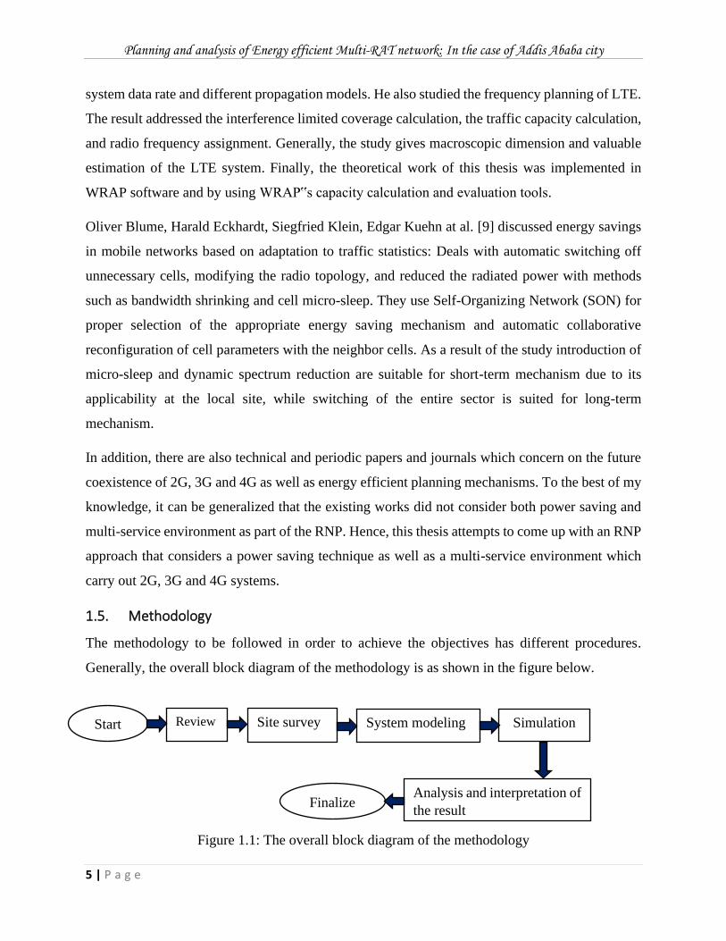
Figure 1.1: The overall block diagram of the methodology
Start Review Site survey System modeling Simulation
Analysis and interpretation of
the result Finalize
Planning and analysis of Energy efficient Multi-RAT network: In the case of Addis Ababa city
6 | P a g e
Literature review: Includes books on this area, different IEEE articles and journals, previous
studies on this subject specifically on radio network planning of each radio access technologies as
well as energy reduction of cellular system.
Site Survey: Making survey to collect data by using an existing cellular network and identify and
collect the customers current need and the problems occurred in the existing network service.
System modeling: Includes modeling of the selected study area network traffic, geographic digital
terrain model, clutter heights, clutter classes, population, and environmental traffic then design a
system which incorporates GSM, UMTS and LTE as a Multi-RAT network by considering
uniformly distribution of subscribers. In addition to this, cell sleeping technique on cellular system
and its impact on the network performance in terms of coverage, capacity and signal quality is
discussed.
Simulation: ATOLL network planning tool is used for modeling. In the modeling and planning
process, an actual data & scenario from Addis Ababa city will be used.
Analysis and Interpretation of the results: Include the conclusion and analysis of the planned
network and overall performance improvements based on the results.
1.6. Scope of the study
This study focuses mainly on the essentials of coverage and capacity analysis of Multi-RAT
networks and impact of cell sleep on the performance of planned network during low traffic load.
It addresses energy consumption reduction of cellular network by taking one mechanism from
Green network i.e. cell sleep mode technique in addition to detail coverage prediction and capacity
evaluation of Multi-RAT radio network by taking into account the actual morphology and
topography details. Additionally, it shows the performance variation of the planned network if
some BSs are in their sleep mode when the network traffic experiences low load and compare the
energy consumption of the network. It doesn’t address detailed of Green network modelling and
the process of how to sleep and wakeup the BSs based on the traffic load or what we call self-
organization network as well as the variation of the signal strength due to on off time of the BSs,
the core network dimensioning and the end-to-end service aspects such as IP backhaul and
microwave transmission.
Planning and analysis of Energy efficient Multi-RAT network: In the case of Addis Ababa city
7 | P a g e
1.7. Thesis Organization
This thesis consists of six Chapters. In the first Chapter the statement of problem, literature
reviews, objectives and approach with short introduction is presented. The second Chapter presents
the theoretical fundamentals and basics of RAT’s which includes GSM, UMTS and LTE in
addition to their features related to dimensioning work. Chapter three covers fundamentals and
basics of Green technology in addition to power consumption basics and energy saving techniques
in cellular system. In the fourth Chapter the main part of the thesis which is Multi-RAT network
with reduced power consumption is presented. This includes radio link budget, coverage and
capacity planning, selection of propagation models and calculation of site numbers based on
capacity and coverage planning for all RATs (GSM/UMTS/LTE). Additionally, a preliminary
study on cell sleep technique and its impact in the network performance and QoS is presented in
the fourth section. Chapter five presents Simulation result analysis and discussion of the of the
planned network and finally Chapter six concludes with summary of the entire thesis and discusses
possibilities of future research.
Planning and analysis of Energy efficient Multi-RAT network: In the case of Addis Ababa city
8 | P a g e
2. Chapter Two: Radio Access Technologies and Propagation Models
2.1 Introduction
In this section the general introduction and the overall architecture of radio access technologies
are discussed. The intended technologies for network planning are GSM, UMTS and LTE.
2.2 Global System for Mobile (GSM)
GSM is an associate open, digital cellular technology used for transmitting mobile voice and data
services. GSM is additionally spoken as 2G, as a result of it represents the second generation of
this technology, and it it’s definitely the foremost winning the most successful mobile
communication system. It was specified by European Telecommunications Standards Institute
(ETSI) and originally intended to be used only in Europe GSM, later on has evolved to be more or
less the first truly global standard for mobile communication. The basic GSM network uses the
900MHz frequency band, but there are also several derivatives, of which the two most important
are Digital Cellular System 1800 (DCS-1800; also known as GSM-1800) and PCS-1900 (GSM-
1900). The prime reason for the adding of GSM 1800 frequency band was the dearth of capacity
within the 900 MHz frequency band.
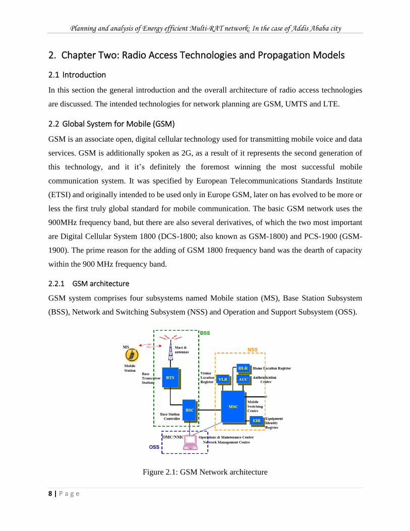
2.2.1 GSM architecture
GSM system comprises four subsystems named Mobile station (MS), Base Station Subsystem
(BSS), Network and Switching Subsystem (NSS) and Operation and Support Subsystem (OSS).
Figure 2.1: GSM Network architecture
Planning and analysis of Energy efficient Multi-RAT network: In the case of Addis Ababa city
9 | P a g e
2.2.2 Multiple access in GSM
The radio spectrum is a scarce resource. Therefore, the cellular systems use various mechanisms
to allow multiple users accessing the same radio spectrum at the same time. FDMA and TDMA
are the most common ones.
An FDMA system divides the available spectrum into several frequency channels. Each user is
allocated 2 channels, one for uplink and another for downlink communication. This allocation is
exclusive; no alternative user is allocated identical channels at the same time. Whereas in TDMA
system the entire available bandwidth is shared by single user at a time only for short periods. The
frequency channel is divided into timeslots so that it’s allocated periodically and other users can
use other time slots. Separate time slots are needed for the uplink and the downlink and also a slot
is equal to one timeslot on one frequency. GSM is based on TDMA technology, each frequency
channel is divided into several time slots and each user is allocated one (or more) slot(s).
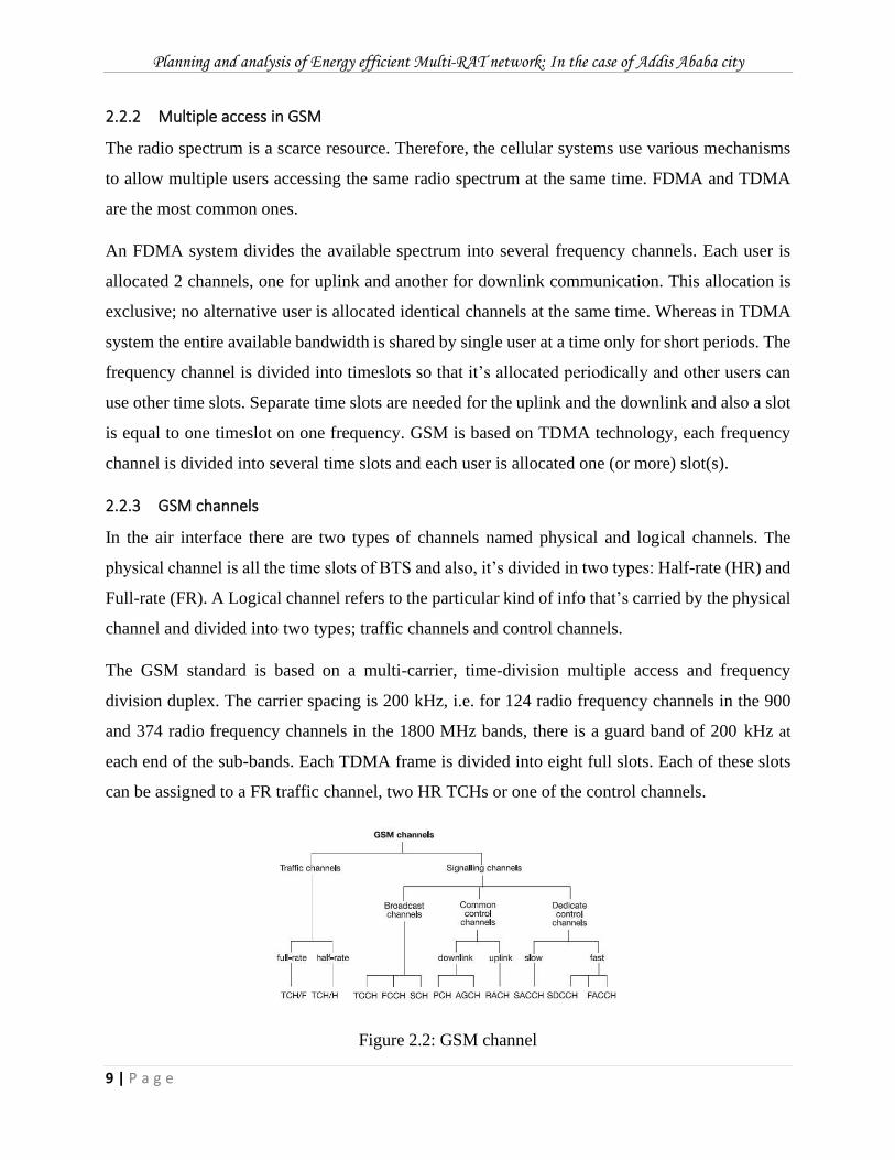
2.2.3 GSM channels
In the air interface there are two types of channels named physical and logical channels. The
physical channel is all the time slots of BTS and also, it’s divided in two types: Half-rate (HR) and
Full-rate (FR). A Logical channel refers to the particular kind of info that’s carried by the physical
channel and divided into two types; traffic channels and control channels.
The GSM standard is based on a multi-carrier, time-division multiple access and frequency
division duplex. The carrier spacing is 200 kHz, i.e. for 124 radio frequency channels in the 900
and 374 radio frequency channels in the 1800 MHz bands, there is a guard band of 200 kHz at
each end of the sub-bands. Each TDMA frame is divided into eight full slots. Each of these slots
can be assigned to a FR traffic channel, two HR TCHs or one of the control channels.
Figure 2.2: GSM channel
Planning and analysis of Energy efficient Multi-RAT network: In the case of Addis Ababa city
10 | P a g e
2.3 Universal Mobile Telecommunications System (UMTS)
The Universal Mobile Telecommunications System (UMTS) is the third generation (3G) mobile
telecommunication system by using the Wide-band Code Division Multiple Access (WCDMA) air
interface technology. It adopts a structure similar to the second generation (2G) mobile
telecommunication system, including the Radio Access Network (RAN) and the Core Network
(CN) [10]. The quality and delay requirement is much higher in UMTS networks as compared to
GSM networks. The bit rates are higher which means that a larger bandwidth of 5MHz is required
to support these higher bit rates. The possibility of offering subscriber variable bit rates and
bandwidth on demand is an attractive feature in UMTS networks [6].
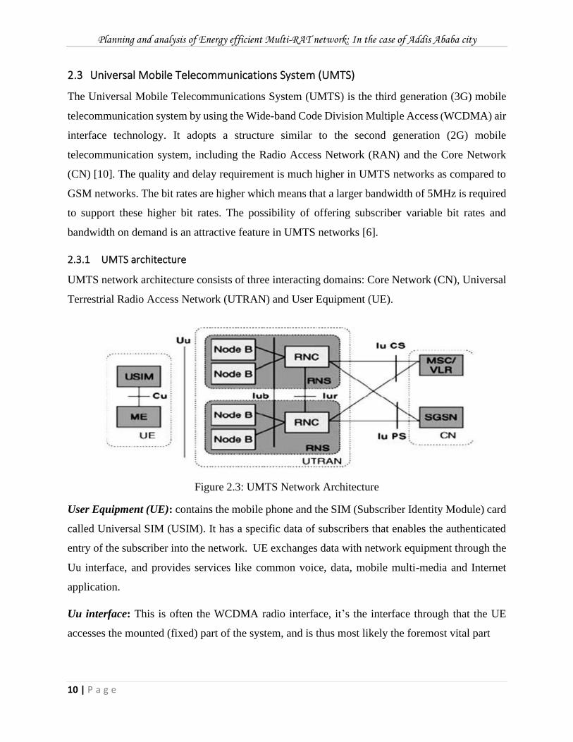
2.3.1 UMTS architecture
UMTS network architecture consists of three interacting domains: Core Network (CN), Universal
Terrestrial Radio Access Network (UTRAN) and User Equipment (UE).
Figure 2.3: UMTS Network Architecture
User Equipment (UE): contains the mobile phone and the SIM (Subscriber Identity Module) card
called Universal SIM (USIM). It has a specific data of subscribers that enables the authenticated
entry of the subscriber into the network. UE exchanges data with network equipment through the
Uu interface, and provides services like common voice, data, mobile multi-media and Internet
application.
Uu interface: This is often the WCDMA radio interface, it’s the interface through that the UE
accesses the mounted (fixed) part of the system, and is thus most likely the foremost vital part
Planning and analysis of Energy efficient Multi-RAT network: In the case of Addis Ababa city
11 | P a g e
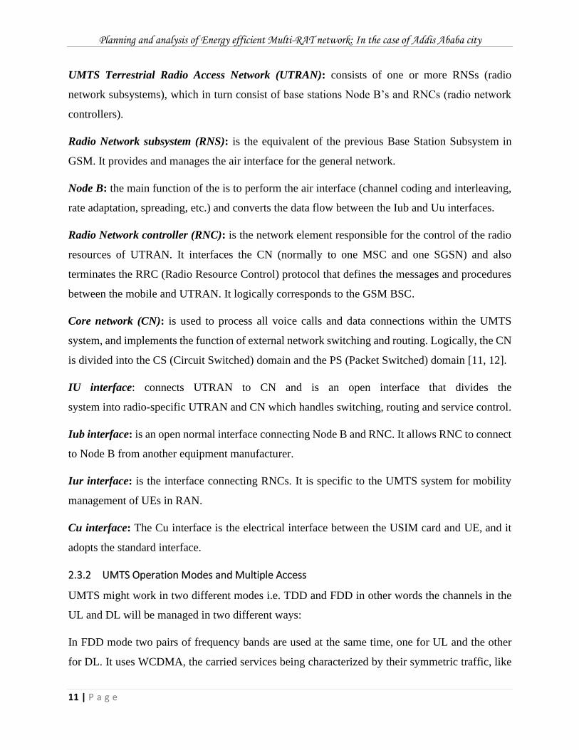
UMTS Terrestrial Radio Access Network (UTRAN): consists of one or more RNSs (radio
network subsystems), which in turn consist of base stations Node B’s and RNCs (radio network
controllers).
Radio Network subsystem (RNS): is the equivalent of the previous Base Station Subsystem in
GSM. It provides and manages the air interface for the general network.
Node B: the main function of the is to perform the air interface (channel coding and interleaving,
rate adaptation, spreading, etc.) and converts the data flow between the Iub and Uu interfaces.
Radio Network controller (RNC): is the network element responsible for the control of the radio
resources of UTRAN. It interfaces the CN (normally to one MSC and one SGSN) and also
terminates the RRC (Radio Resource Control) protocol that defines the messages and procedures
between the mobile and UTRAN. It logically corresponds to the GSM BSC.
Core network (CN): is used to process all voice calls and data connections within the UMTS
system, and implements the function of external network switching and routing. Logically, the CN
is divided into the CS (Circuit Switched) domain and the PS (Packet Switched) domain [11, 12].
IU interface: connects UTRAN to CN and is an open interface that divides the
system into radio-specific UTRAN and CN which handles switching, routing and service control.
Iub interface: is an open normal interface connecting Node B and RNC. It allows RNC to connect
to Node B from another equipment manufacturer.
Iur interface: is the interface connecting RNCs. It is specific to the UMTS system for mobility
management of UEs in RAN.
Cu interface: The Cu interface is the electrical interface between the USIM card and UE, and it
adopts the standard interface.
2.3.2 UMTS Operation Modes and Multiple Access
UMTS might work in two different modes i.e. TDD and FDD in other words the channels in the
UL and DL will be managed in two different ways:
In FDD mode two pairs of frequency bands are used at the same time, one for UL and the other
for DL. It uses WCDMA, the carried services being characterized by their symmetric traffic, like
Planning and analysis of Energy efficient Multi-RAT network: In the case of Addis Ababa city
12 | P a g e
voice. It will be used mainly in every kind of environment, particularly in macro and micro cells.
In the TDD mode, both UL and DL use the same frequency, through a scheme of Time Division -
Code Division Multiple Access (TD-CDMA) in unpaired bands, which will be advantageous to
handle services with uneven traffic, like Internet one. It will be used primarily in pico-cells (indoor)
or in hot-spot areas.
The wide BW of WCDMA provides an inherent performance gain over previous cellular systems,
since it reduces the attenuation (fading) of the radio network. It uses coherent demodulation in UL,
a feature that was not implemented in cellular CDMA systems.
WCDMA use BPSK (Binary phase-shift keying) and QPSK (Quadrature phase-shift keying) for
data modulations in uplink and downlink respectively [13].
2.3.3 Spread spectrum
Wideband Code Division Multiple Access (WCDMA) permits several subscribers to use an
identical frequency at the same time. In order to distinguish between the users, the information
undergoes a process known as spreading that is, the information is multiplied by a channelization
and scrambling code, hence WCDMA is referred to as a spread spectrum technology [6].
In WCDMA every user is appointed a unique code, which it uses to encode its information-bearing
signal. The receiver, knowing the code sequences of the user, decodes a received signal once
reception and recovers the first knowledge or information. scrambling codes (SC) and
channelization codes (CC) are the two categories of spreading codes. Each transmitter (cell in
downlink) is appointed completely different scrambling code and every information channel is
appointed different CC code.
The bandwidth of the code signal is chosen to be much larger than the bandwidth of the
information-bearing signal, hence, the encoding process spreads the spectrum of the signal.
Therefore, a spread-spectrum technique should perform two criteria:
▪ The transmission bandwidth must be much larger than the information bandwidth;
▪ The bandwidth must be statistically independent of the information signal.
The flexibility supported by WCDMA is achieved with the use of Orthogonal Variable Spreading
Factor (OVSF) codes for channelization of different users [13].
Planning and analysis of Energy efficient Multi-RAT network: In the case of Addis Ababa city
13 | P a g e
2.4 Long Term Evolution (LTE)
LTE network is developed by the 3GPP and also referred to as 4G wireless broadband technology.
This LTE technology is used to enable fast mobile Internet connection. It is a path followed to
achieve 4G speeds and a full IP technology used for the mobile broadband services for data transfer
and voice calls. Wireless operators are more and more increasing their LTE networks to own
advantage of additional extra efficiency, lower latency and additionally the power to manage ever-
increasing traffic load. The core technologies have rapt from circuit-switching to the all-IP evolved
packet core. Meanwhile, access has evolved from TDMA (Time Division Multiple Access) to
OFDMA (Orthogonal Frequency Division Multiple Access) as the need for higher data speeds and
volumes has increased [14]. All LTE devices got to support Multiple Input Multiple Output
(MIMO) transmissions, which permit the BS to transmit multiple data streams over the identical
carrier frequency simultaneously.
2.4.1 Network Architecture of LTE
3GPP identified in Release 8 that the architecture of LTE system is serving as a basis
architecture network of 4G Network. The LTE architecture includes the radio access network or
also called Evolved Universal Terrestrial Radio Access Network (E-UTRAN) and Evolved
Packet Core (EPC) network
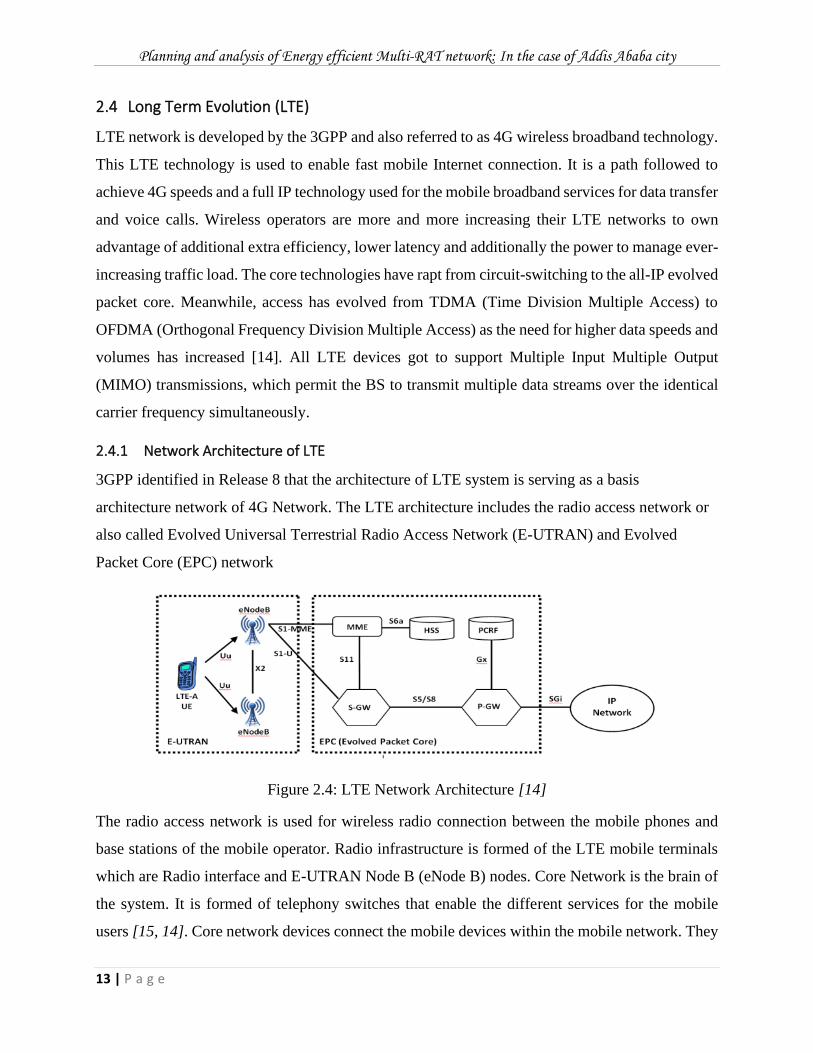
Figure 2.4: LTE Network Architecture [14]
The radio access network is used for wireless radio connection between the mobile phones and
base stations of the mobile operator. Radio infrastructure is formed of the LTE mobile terminals
which are Radio interface and E-UTRAN Node B (eNode B) nodes. Core Network is the brain of
the system. It is formed of telephony switches that enable the different services for the mobile
users [15, 14]. Core network devices connect the mobile devices within the mobile network. They
Planning and analysis of Energy efficient Multi-RAT network: In the case of Addis Ababa city
14 | P a g e
also connect the mobile network with the fixed telephony network and internet. The LTE core
network or Evolved Packet Core (EPC) is formed from the Mobility Management Entity (MME),
Serving Gateway (S-GW), Packet Data Network Gateway (P-GW), Home Subscriber Server
(HSS) and Policy and Charging Rules Function (PCRF).
LTE mobile terminals: LTE mobile terminals are the mobile phones and alternative devices that
support the LTE network. The LTE mobile station is also termed as User Equipment (UE).
eNodeB (eNB): eNB’s are situated all over the network of the mobile operator. They connect the
LTE mobile terminal via radio interface to the CN. The eNB’s are distributed throughout the
network’s coverage area.
MME: MME is that the central control node within the EPC network. It is responsible for mobility
and security signaling, tracking and paging of mobile terminals. It has a major role in registering
UE in a network, handling mobility functions between UE and core network, and creating and
keeping IP connectivity.
S-GW: transports the user traffic between the mobile terminals and external networks. It
additionally interconnects the radio access network with the EPC network. It acts as a router [6,
16], and forwards data between the base station and the packet data network (PDN) gateway.
P-GW: PDN Gateway connects the EPC network to the external networks. It routes traffic to and
from PDN networks. It is the highest-level mobility anchor in the system and is mainly in charge
of assigning and distributing the IP addresses for the UE.
HSS: is the database of all mobile users that includes all subscriber data. It is responsible for
authentication due to its ability to integrate the Authentication Center (AuC) which formulates
security keys and authentication vectors. It is also responsible for call and session setup.
PCRF: is node responsible for real-time policy rules and charging in EPC network. It makes
decisions on how to handle the services in terms of QoS, and provides information to the P-GW,
and if applicable also to the S-GW, so that appropriate bearers and policing can be set up.
2.4.2 LTE Channels
LTE adopts a hierarchical channel structure in order to efficiently support various QoS classes of
services. Channel types in LTE network are divided in to three categories. These channel types are
Planning and analysis of Energy efficient Multi-RAT network: In the case of Addis Ababa city
15 | P a g e
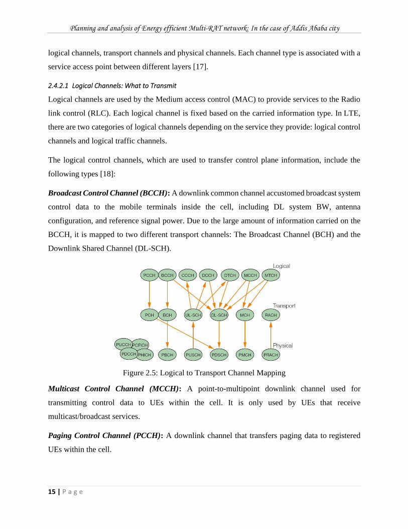
logical channels, transport channels and physical channels. Each channel type is associated with a
service access point between different layers [17].
2.4.2.1 Logical Channels: What to Transmit
Logical channels are used by the Medium access control (MAC) to provide services to the Radio
link control (RLC). Each logical channel is fixed based on the carried information type. In LTE,
there are two categories of logical channels depending on the service they provide: logical control
channels and logical traffic channels.
The logical control channels, which are used to transfer control plane information, include the
following types [18]:
Broadcast Control Channel (BCCH): A downlink common channel accustomed broadcast system
control data to the mobile terminals inside the cell, including DL system BW, antenna
configuration, and reference signal power. Due to the large amount of information carried on the
BCCH, it is mapped to two different transport channels: The Broadcast Channel (BCH) and the
Downlink Shared Channel (DL-SCH).
Figure 2.5: Logical to Transport Channel Mapping
Multicast Control Channel (MCCH): A point-to-multipoint downlink channel used for
transmitting control data to UEs within the cell. It is only used by UEs that receive
multicast/broadcast services.
Paging Control Channel (PCCH): A downlink channel that transfers paging data to registered
UEs within the cell.
Planning and analysis of Energy efficient Multi-RAT network: In the case of Addis Ababa city
16 | P a g e
Common Control Channel (CCCH): A bi-directional channel for transmitting control information
between the network and UEs when no Radio resource control (RRC) connection is available,
implying the UE is not attached to the network like within the idle state.
Dedicated Control Channel (DCCH): A point-to-point, bi-directional channel that transmits
dedicated control between a UE and the network. This channel is employed once the RRC
connection is obtainable, that is, the UE is attached to the network.
The logical traffic channels, which uses to transfer user plane information, include:
Dedicated Traffic Channel (DTCH): A point-to-point, bi-directional channel used between a
given UE and the network. It can exist in both uplink and downlink.
Multicast Traffic Channel (MTCH): A unidirectional, point-to-multipoint data channel that
transmits traffic information from the network to UEs. It is associated with the multicast/broadcast
service.
2.4.2.2 Transport Channels: How to Transmit
The transport channels are used to offer services to the MAC. A transport channel is actually
characterized by how and with what characteristics data is transferred over the radio interface, that
is, the channel coding scheme, the modulation scheme, and antenna mapping. Transport channels
are classified in to uplink and downlink channels [18, 19]. The downlink transport channels are
described below:
Downlink Shared Channel (DL-SCH): This channel will carry downlink signaling and traffic and
may have to be broadcast in the entire cell, given the nature of the data in this channel. It will also
support for both dynamic and semi-static resource allocation with the option to support for UE
discontinuous reception (DRX) to enable UE power saving and error control is supported in this
channel by means of Hybrid automatic repeat request (HARQ) and dynamic link adaptation by
varying the modulation coding and transmit power. Spectral efficiency can also be increased due
to the possibility of using beam forming antenna techniques. The channel also supports Multimedia
Broadcast Multicast Service (MBMS) transmissions.
Broadcast Channel (BCH): A downlink channel related to the BCCH logical channel and is
employed to broadcast system information over the entire coverage area of the cell. It has a fixed
Planning and analysis of Energy efficient Multi-RAT network: In the case of Addis Ababa city
17 | P a g e
and pre-defined transport format largely defined by the requirement to be broadcast in the entire
coverage area of the cell since the information carried by this channel contains system information.
Multicast Channel (MCH): The channel is associated with the multicast services from the upper
layers and as such there is a requirement to broadcast both control and user data over the entire
coverage area of the cell. It conjointly supports the Single Frequency Network as semi-static
resource allocation.
Paging Channel (PCH): Associated with the PCCH logical channel. It is mapped to dynamically
assign physical resources, and is needed for broadcast over the whole cell coverage area. It is
transmitted on the Physical Downlink Shared Channel (PDSCH), and supports UE discontinuous
reception.
The uplink transport channels include:
Uplink Shared Channel (UL-SCH): carries common and dedicated signaling as well as dedicated
traffic information. It supports the same features as the DL-SCH.
Random Access Channel (RACH): is a very specific transport channel and carries limited control
information during the very earliest stages of connection establishment. This is a common UL
channel so there’s the chance of collisions during UE transmission.
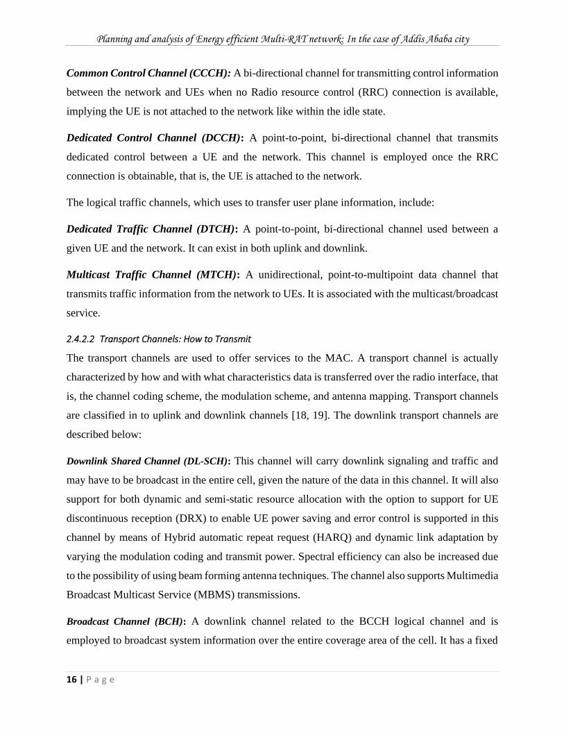
2.4.2.3 Physical Channels: Actual Transmission
The design of the LTE physical layer is heavily influenced by needs of high peak transmission rate
(100 Mbps DL or 50 Mbps UL), spectral efficiency, and multiple channel bandwidths (1.25-20
MHz). Each physical channel corresponds to a group of resource elements within the time-
frequency grid that carry info from higher layers. The basic entities that build a physical channel
are RE and RB. A RE is a single subcarrier over one OFDM symbol, and specifically this could
carry one (or two with spatial multiplexing) modulated symbol(s). A resource block (RB) is a
collection of RE and in the frequency domain this represents the littlest quanta of resources which
will be allocated. Physical channels are classified in to UL and DL channels.
Planning and analysis of Energy efficient Multi-RAT network: In the case of Addis Ababa city
18 | P a g e
Figure 2.6: Uplink and downlink physical channels [20]
2.4.3 Multiple Access Technology
LTE employs Orthogonal Frequency Division Multiple Access (OFDMA) for DL data
transmission and Single Carrier FDMA (SC-FDMA) for UL transmission. The OFDM signal is
often generated by using the Fast Fourier Transform (FFT). The available spectrum in an OFDM
system is divided into multiple, mutually orthogonal subcarriers. Each of those subcarriers are
modulated independently by a low data rate stream and might carry freelance or independent data
streams. The main reasons LTE chooses OFDM and SC-FDM as the basic transmission schemes
includes [21]: robustness to the multipath fading channel, high spectral efficiency, low-complexity
implementation, and the ability to provide versatile or flexible transmission bandwidths and
support advanced features like frequency-selective scheduling, MIMO transmission, and
interference coordination.
In the downlink, OFDM was selected as the air interface for LTE and also it is a specific form of
multicarrier modulation (MCM). In general, MCM is a parallel transmission technique that divides
a radio frequency channel into several, a lot of narrow-bandwidth subcarriers and transmits
information at the same time on every subcarrier. OFDM is well suited for high data rate systems
that operate in multipath environments as a result of its strength to delay spread. The cyclic
extension allows an OFDM system to operate in multipath channels while not the necessity for a
complex Decision Feedback Equalizer (DFE) or Maximum Likelihood Sequence Estimation
(MLSE) equalizer. As such, it’s simple to exploit frequency selectivity of the multipath channel
with low complexity receivers. This allows frequency-selective scheduling, as well as frequency
Planning and analysis of Energy efficient Multi-RAT network: In the case of Addis Ababa city
19 | P a g e
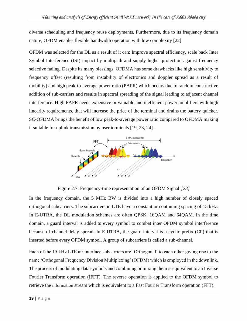
diverse scheduling and frequency reuse deployments. Furthermore, due to its frequency domain
nature, OFDM enables flexible bandwidth operation with low complexity [22].
OFDM was selected for the DL as a result of it can: Improve spectral efficiency, scale back Inter
Symbol Interference (ISI) impact by multipath and supply higher protection against frequency
selective fading. Despite its many blessings, OFDMA has some drawbacks like high sensitivity to
frequency offset (resulting from instability of electronics and doppler spread as a result of
mobility) and high peak-to-average power ratio (PAPR) which occurs due to random constructive
addition of sub-carriers and results in spectral spreading of the signal leading to adjacent channel
interference. High PAPR needs expensive or valuable and inefficient power amplifiers with high
linearity requirements, that will increase the price of the terminal and drains the battery quicker.
SC-OFDMA brings the benefit of low peak-to-average power ratio compared to OFDMA making
it suitable for uplink transmission by user terminals [19, 23, 24].
Figure 2.7: Frequency-time representation of an OFDM Signal [23]
In the frequency domain, the 5 MHz BW is divided into a high number of closely spaced
orthogonal subcarriers. The subcarriers in LTE have a constant or continuing spacing of 15 kHz.
In E-UTRA, the DL modulation schemes are often QPSK, 16QAM and 64QAM. In the time
domain, a guard interval is added to every symbol to combat inter OFDM symbol interference
because of channel delay spread. In E-UTRA, the guard interval is a cyclic prefix (CP) that is
inserted before every OFDM symbol. A group of subcarriers is called a sub-channel.
Each of the 15 kHz LTE air interface subcarriers are ‘Orthogonal’ to each other giving rise to the
name ‘Orthogonal Frequency Division Multiplexing’ (OFDM) which is employed in the downlink.
The process of modulating data symbols and combining or mixing them is equivalent to an Inverse
Fourier Transform operation (IFFT). The reverse operation is applied to the OFDM symbol to
retrieve the information stream which is equivalent to a Fast Fourier Transform operation (FFT).
Planning and analysis of Energy efficient Multi-RAT network: In the case of Addis Ababa city
20 | P a g e
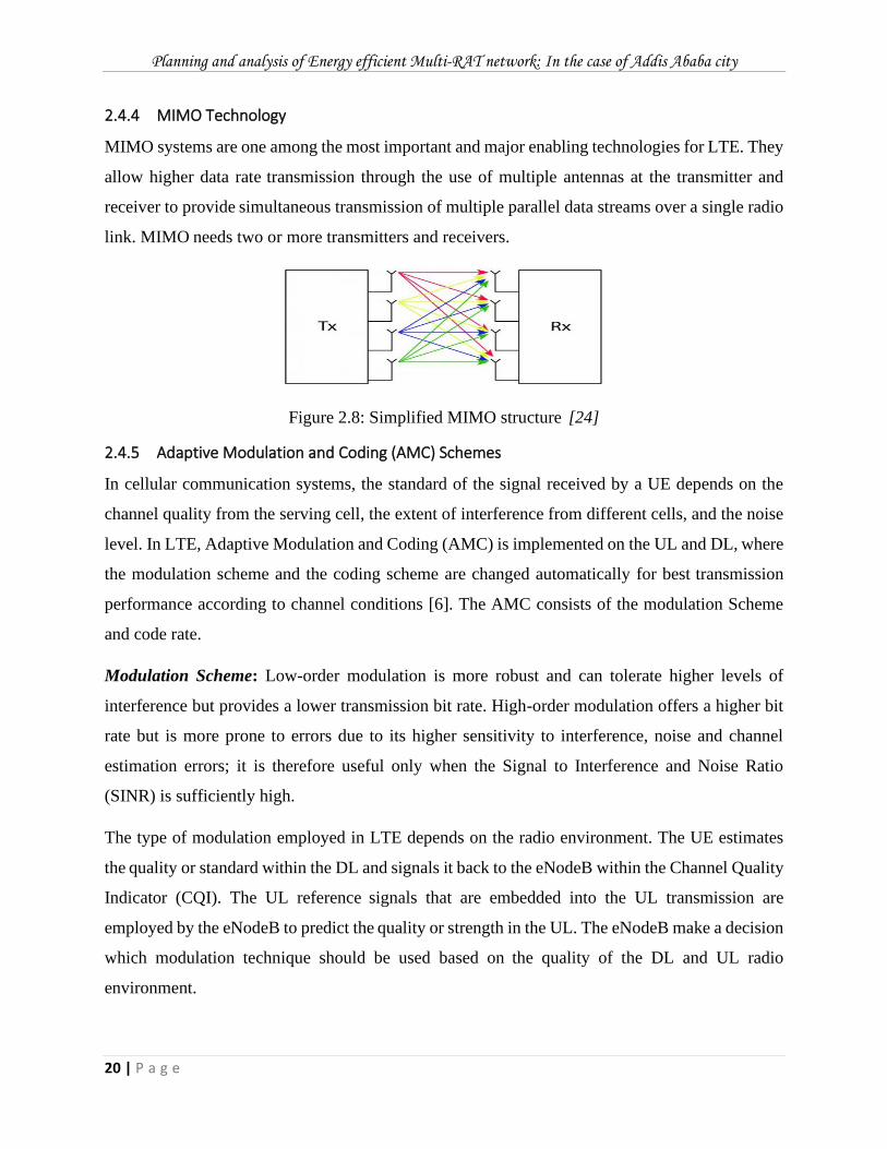
2.4.4 MIMO Technology
MIMO systems are one among the most important and major enabling technologies for LTE. They
allow higher data rate transmission through the use of multiple antennas at the transmitter and
receiver to provide simultaneous transmission of multiple parallel data streams over a single radio
link. MIMO needs two or more transmitters and receivers.
Figure 2.8: Simplified MIMO structure [24]
2.4.5 Adaptive Modulation and Coding (AMC) Schemes
In cellular communication systems, the standard of the signal received by a UE depends on the
channel quality from the serving cell, the extent of interference from different cells, and the noise
level. In LTE, Adaptive Modulation and Coding (AMC) is implemented on the UL and DL, where
the modulation scheme and the coding scheme are changed automatically for best transmission
performance according to channel conditions [6]. The AMC consists of the modulation Scheme
and code rate.
Modulation Scheme: Low-order modulation is more robust and can tolerate higher levels of
interference but provides a lower transmission bit rate. High-order modulation offers a higher bit
rate but is more prone to errors due to its higher sensitivity to interference, noise and channel
estimation errors; it is therefore useful only when the Signal to Interference and Noise Ratio
(SINR) is sufficiently high.
The type of modulation employed in LTE depends on the radio environment. The UE estimates
the quality or standard within the DL and signals it back to the eNodeB within the Channel Quality
Indicator (CQI). The UL reference signals that are embedded into the UL transmission are
employed by the eNodeB to predict the quality or strength in the UL. The eNodeB make a decision
which modulation technique should be used based on the quality of the DL and UL radio
environment.
Planning and analysis of Energy efficient Multi-RAT network: In the case of Addis Ababa city
21 | P a g e
Modulation techniques which supports by LTE in downlink and uplink are: 64 Quadrature
Amplitude Modulation (64 QAM) which uses 64 different quadrature and amplitude combinations
to carry 6 bits per symbol, 16 Quadrature Amplitude Modulation (16 QAM) which uses 16
different quadrature and amplitude combinations to carry 4 bits per symbol and Quadrature Phase
Shift Keying (QPSK) which used 4 different quadrature’s to send 2 bits per symbol [25, 26, 6].
Code rate: For a given modulation, the code rate are often chosen based on the radio link
conditions: a lower code rate are often utilized in poor channel conditions and a higher code rate
in the case of high SINR [8].
2.5 Propagation Models
In radio link budget calculation, the radio propagation model plays a key role. The coverage radius
of a base station is obtained based on the maximum propagation loss allowance in the link budget.
Therefore, Path loss models are important in the RF planning phase to be able to predict coverage
and link budget among other important performance parameters. These models are based on the
frequency band, type of deployment area (dense urban, urban, rural, suburban, etc.), and type of
application [27].
Radio propagation models are classified into two types: outdoor and indoor propagation models.
These two types of propagation models involve various factors. In an outdoor environment,
landforms and obstructions on the propagation path, in addition to buildings and trees should be
considered. Signals fade at varying rates in different environments. Propagation in free space gives
the lowest fade rate. The fading of signals is larger than free space when radio waves propagate in
open areas/suburban areas and fading rate is the largest in urban/dense urban areas. Indoor
propagation model features low RF transmits power, a short coverage distance and complicated
environmental changes [8, 28].
2.5.1 Free Space Path Loss Model
Free space loss describes the ideal situation, where the transmitter and receiver have line-of-sight
and no obstacles are around to create reflection, diffraction or scattering. In this ideal case the
attenuation of the radio wave signal is equivalent to the square of the distance from the transmitter.
When the signal has been transmitted in the free space towards the receiver antenna, the power
density S at the distance from the transmitter d can be written as [ [1, 29]:
Planning and analysis of Energy efficient Multi-RAT network: In the case of Addis Ababa city
22 | P a g e
𝑆 =𝑃𝑡𝐺𝑡
4𝜋𝑑2 (2.1)
Where Pt is the transmitted power and Gt is the gain of the transmitter antenna. The effective area
A of the receiver antenna, which affects the received power, can be expressed as
𝐴 =𝜆2 𝐺𝑟
4𝜋 (2.2)
Where 𝜆 is the wavelength and Gr is the gain of the receiver antenna. The received power density
can also be written as:
𝑆 =𝑃𝑟
𝐴 (2.3)
Combining these equations, previous the format for the received power is:
𝑃𝑟 = 𝑃𝑡𝐺𝑡𝑃𝑟 (𝜆
4𝜋𝑑)
2
(2.4)
The free space path loss is the ratio of transmitted and received power. Here is the equation in
simplified format, when the antenna gains are excluded:
𝐿 = (4𝜋𝑑
𝜆)
2
(2.5)
And the free space loss converted in decibels
𝐿𝑑𝐵 = 10𝑙𝑜𝑔10 (4𝜋𝑑
𝜆)
2
𝐿𝑑𝐵 = 20𝑙𝑜𝑔10 (4𝜋𝑑
𝜆)
𝐿𝑑𝐵 = 20𝑙𝑜𝑔10(4𝜋) + 20𝑙𝑜𝑔10(𝑑) − 20𝑙𝑜𝑔10(𝜆) (2.6)
Substituting 𝜆 = 0.3𝑓⁄ (in MHz) and rationalizing the equation produces the generic free space
path loss formula:
𝐿𝑑𝐵 = 20𝑙𝑜𝑔10(4𝜋) + 20𝑙𝑜𝑔10(𝑑) − 20𝑙𝑜𝑔10 (0.3𝑓⁄ )
𝐿𝑑𝐵 = 20𝑙𝑜𝑔10(𝑓) + 20𝑙𝑜𝑔10(𝑑) + 32.4 (2.7)
Where f is the frequency in MHz and d is the distance in km’s
Planning and analysis of Energy efficient Multi-RAT network: In the case of Addis Ababa city
23 | P a g e
In reality the radio wave propagation path is often a non-line-of-sight scenario with close obstacles
like buildings and trees. Therefore, the applicability of the free space propagation loss is limited
[1]. The received signal actually consists of several components, which have been travelling
through different paths facing reflection, diffraction and scattering. This result is named as
multipath and one component represents one propagation path. The different components, signal
vectors, are summarized as one signal considering the vector phases and amplitudes.
2.5.2 Okumura Model
Okumura model is one of the most commonly used models. Almost all the propagation models are
raised form of Okumura model. It can be used for frequencies up to 3000 MHz [27]. The model is
ideal and typical for using in cities with several urban structures however not several tall
obstruction structures. Okumura model was engineered into 3 modes which are urban, suburban
and open areas. The model for urban areas was engineered first and used as the baseline for others.
Clutter and terrain categories for open areas are; there are no tall trees or buildings in path, plot of
land cleared for 200-400m [30]. The path loss in Okumura model is expressed as follows.
𝐿𝑚(𝑑𝐵) = 𝐿𝐹(𝑑) + 𝐴𝑚𝑢(𝑓, 𝑑) − 𝐺(ℎ𝑡) − 𝐺(ℎ𝑟) − 𝐺𝐴𝑅𝐸𝐴 (2.8)
Where,
𝐿𝑚 = 𝑚𝑒𝑑𝑖𝑎𝑛 𝑜𝑓 𝑡ℎ𝑒 𝑝𝑎𝑡ℎ 𝑙𝑜𝑠𝑠
𝐿𝐹 = 𝑓𝑟𝑒𝑒 𝑠𝑝𝑎𝑐𝑒 𝑝𝑟𝑜𝑝𝑎𝑔𝑎𝑡𝑖𝑜𝑛 𝑝𝑎𝑡ℎ𝑙𝑜𝑠𝑠
𝐴𝑚𝑢 = 𝑚𝑒𝑑𝑖𝑎𝑛 𝑎𝑡𝑡𝑒𝑛𝑢𝑎𝑡𝑖𝑜𝑛 𝑟𝑒𝑙𝑎𝑡𝑖𝑣𝑒 𝑡𝑜 𝑓𝑟𝑒𝑒 𝑠𝑝𝑎𝑐𝑒
𝐺(ℎ𝑡) = 𝐵𝑆 𝑎𝑛𝑡𝑒𝑛𝑛𝑎 ℎ𝑒𝑖𝑔ℎ𝑡 𝑔𝑎𝑖𝑛 𝑓𝑎𝑐𝑡𝑜𝑟
= 20 log(ℎ𝑡 200⁄ ), 1000𝑚 > ℎ𝑡 > 30𝑚
𝐺(ℎ𝑟) = 𝑀𝑆 𝑎𝑛𝑡𝑒𝑛𝑛𝑎 ℎ𝑒𝑖𝑔ℎ𝑡 𝑔𝑎𝑖𝑛 𝑓𝑎𝑐𝑡𝑜𝑟
= 20 log(ℎ𝑡 3⁄ ), 10𝑚 > ℎ𝑡 > 3𝑚
𝐺𝐴𝑅𝐸𝐴 = 𝑔𝑎𝑖𝑛 𝑑𝑢𝑒 𝑡𝑜 𝑡𝑦𝑝𝑒 𝑜𝑓 𝑒𝑛𝑣𝑖𝑟𝑜𝑛𝑚𝑒𝑛𝑡 𝑔𝑖𝑣𝑒𝑛 𝑖𝑛 𝑠𝑢𝑏𝑢𝑟𝑏𝑎𝑛, 𝑢𝑟𝑏𝑎𝑛 𝑜𝑟 𝑜𝑝𝑒𝑛 𝑎𝑟𝑒𝑎𝑠
Planning and analysis of Energy efficient Multi-RAT network: In the case of Addis Ababa city
24 | P a g e
2.5.3 Okumura-Hata Model
The Okumura-Hata model is an empirical model, which suggests that it’s supported field
measurements. Okumura performed the field measurements in Japanese capital Tokyo and
published results in graphical format. HATA applied the measurement results into equations. The
model may be applied without correction factors for quasi smooth terrain (similar swish piece of
ground) in an urban or populated geographical area however in case of other terrain types
correction factors are required. The weakness of the Okumura-Hata model is that it doesn’t think
about reflections and shadowing.
The distance between transmitter and receiver can be around 100 km while the receiver height can
be 1 m to 10 m [1]. Generally, this model can be applied to the following scenario [25, 19, 6]:
▪ Frequency range 150–1500 MHz, extension 1500-3000 MHz
▪ Terrain morphologies (DU, U, SU, and RU)
▪ Mobile antenna height from 1 to 10 m
▪ BTS antenna height from 30 to 200 m
The path loss in Okumura-Hata model can be calculated as:
𝐿 = 𝐴 + 𝐵𝑙𝑜𝑔(𝑓) − 13.82 log(𝐻𝑏) − 𝑎(𝐻𝑚) + [44.9 − 6.55 log(𝐻𝑏)] log(𝑑) +
𝐿𝑜𝑡ℎ𝑒𝑟 (2.9)
Where, 𝑓 if the frequency (MHz)
𝐻𝑏 = base station antenna height (m)
𝐻𝑚 = the MS antenna height (m)
𝑎(𝐻𝑚) = the mobile antenna correction factor
𝑑 = the distance between the MS and BTS (km)
𝐿𝑜𝑡ℎ𝑒𝑟 = additional correction factor for area type correction with the of 3 for urban/dense
urban area.
The function 𝑎(𝐻𝑚) for urban/dense urban area is defined as:
𝑎(𝐻𝑚) = 3.2(log (11.75𝐻𝑚))2 − 4.79 (2.10)
Planning and analysis of Energy efficient Multi-RAT network: In the case of Addis Ababa city
25 | P a g e
For suburban and rural area, the function is defined as:
𝑎(𝐻𝑚) = [1.1 log(𝑓) − 0.7]𝐻𝑚 − (1.58𝑓 − 0.8) (2.11)
The parameters A and B are dependent on the frequency as follows:
𝐴 = {69.55, 𝑓 = 150 − 1500 𝑀𝐻𝑧46.30, 𝑓 = 1500 − 2000 𝑀𝐻𝑧
𝐵 = {26.16, 𝑓 = 150 − 1500 𝑀𝐻𝑧33.90, 𝑓 = 1500 − 2000 𝑀𝐻𝑧
2.5.4 Cost-231 Hata Model
Cost231-Hata Model is an extension of Hata’s model and designed for use in the frequency range
1500 MHz to 2.0 GHz. Four parameters are used for estimation of the propagation loss. These are
frequency f, distance d, base station antenna height 𝐻𝐵𝑆 and the height of the mobile antenna
𝐻𝑚𝑜𝑏𝑖𝑙𝑒 . The model can be expressed by the following formula [23]:
𝑇𝑜𝑡𝑎𝑙 = 𝐴 − 𝑎(𝐻𝑚) + 𝐶𝑚 (2.12)
Where,
𝐴 = 46.3 + 33.9 × log(𝑓) − log(𝐻𝐵𝑆) + [(44.9 − 6.55 × log(𝐻𝐵𝑆) × log(𝑑))
𝑓 is the working frequency of the system in MHz
𝐻𝐵𝑆 is height of the BS antenna in m
𝐻𝑚 is height of the mobile antenna in m
𝑑 is the distance between the terminal and BS in km
𝑎𝐻𝑚 is the terminal gain function. This function is related to the antenna height and
working frequency of the terminal and the environment.
𝑎𝐻𝑚 = 3.2[log (11.75)𝐻𝑚]2 − 4.79 (2.13)
𝐶𝑚 depends on the terrain type. The value of 𝐶𝑚 in the standard Cost231-Hata in large
cities (U and DU) is 3 and in medium sized cities is 0 [31].

Planning and analysis of Energy efficient Multi-RAT network: In the case of Addis Ababa city
26 | P a g e
3. Chapter Three: Green Cellular Network Basics
3.1 Introduction
Traditionally, mobile communication networks have been designed for maximum throughput and
maximum spectral efficiency while promising QoS to the user. With advent of new technologies
like 4G LTE and above technologies, speed and efficiency were enhanced. Consequently, the
growth rate of data traffic on mobile networks has been increasing and is expected to grow in the
coming years. There have been several reasons for the growing awareness of energy-efficient
wireless networks in the telecommunication community. Energy prices which imply electricity
bills have become a significant cost factor for mobile operators. The radio access part (includes
BS and antennas) of the cellular network is a major energy killer, which accounts from 50% up to
80% of the total energy [32]. Due to this reason improving the energy efficiency of base station
key components, such as power amplifiers and air conditioners, is of great importance for mobile
operators. The increase in energy consumption of mobile cellular networks has currently become
a priority not solely attributable to increase within the value of energy on the part of mobile
network operators but also because of its adverse effect on the environment due to global warming.
In order to reduce energy consumption, GREEN solution has been suggested [32, 33] [34].
GREEN is one of the major initiatives taken in field of energy saving. GREEN radio has been a
key enabler for cellular growth while guarding against increased environmental impact. There are
various distinctive approaches to reduce energy consumptions in a mobile cellular network. These
approaches include: Improving energy efficiency of hardware components, turning off
components selectively, optimizing energy efficiency of the radio transmission process, planning
and deploying heterogeneous cells and adopting renewable energy resources [4].
3.2 Energy use in Cellular Networks
Traditionally, the mobile terminals have been designed with energy efficiency in mind because of
their battery limitations. Furthermore, within a single base station the Power amplifiers (PAs) are
the dominating energy consumers [14]. Generally, the useful output power is only around 5% to
20% of the input power. Base stations are the key elements in energy consumption because they
consume relatively high energy as shown in Figure 3.1.
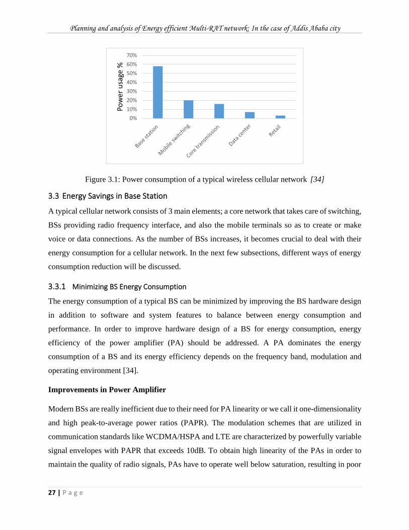
Planning and analysis of Energy efficient Multi-RAT network: In the case of Addis Ababa city
27 | P a g e
Figure 3.1: Power consumption of a typical wireless cellular network [34]
3.3 Energy Savings in Base Station
A typical cellular network consists of 3 main elements; a core network that takes care of switching,
BSs providing radio frequency interface, and also the mobile terminals so as to create or make
voice or data connections. As the number of BSs increases, it becomes crucial to deal with their
energy consumption for a cellular network. In the next few subsections, different ways of energy
consumption reduction will be discussed.
3.3.1 Minimizing BS Energy Consumption
The energy consumption of a typical BS can be minimized by improving the BS hardware design
in addition to software and system features to balance between energy consumption and
performance. In order to improve hardware design of a BS for energy consumption, energy
efficiency of the power amplifier (PA) should be addressed. A PA dominates the energy
consumption of a BS and its energy efficiency depends on the frequency band, modulation and
operating environment [34].
Improvements in Power Amplifier
Modern BSs are really inefficient due to their need for PA linearity or we call it one-dimensionality
and high peak-to-average power ratios (PAPR). The modulation schemes that are utilized in
communication standards like WCDMA/HSPA and LTE are characterized by powerfully variable
signal envelopes with PAPR that exceeds 10dB. To obtain high linearity of the PAs in order to
maintain the quality of radio signals, PAs have to operate well below saturation, resulting in poor
0%
10%
20%
30%
40%
50%
60%
70%
Pow
er u
sage
%
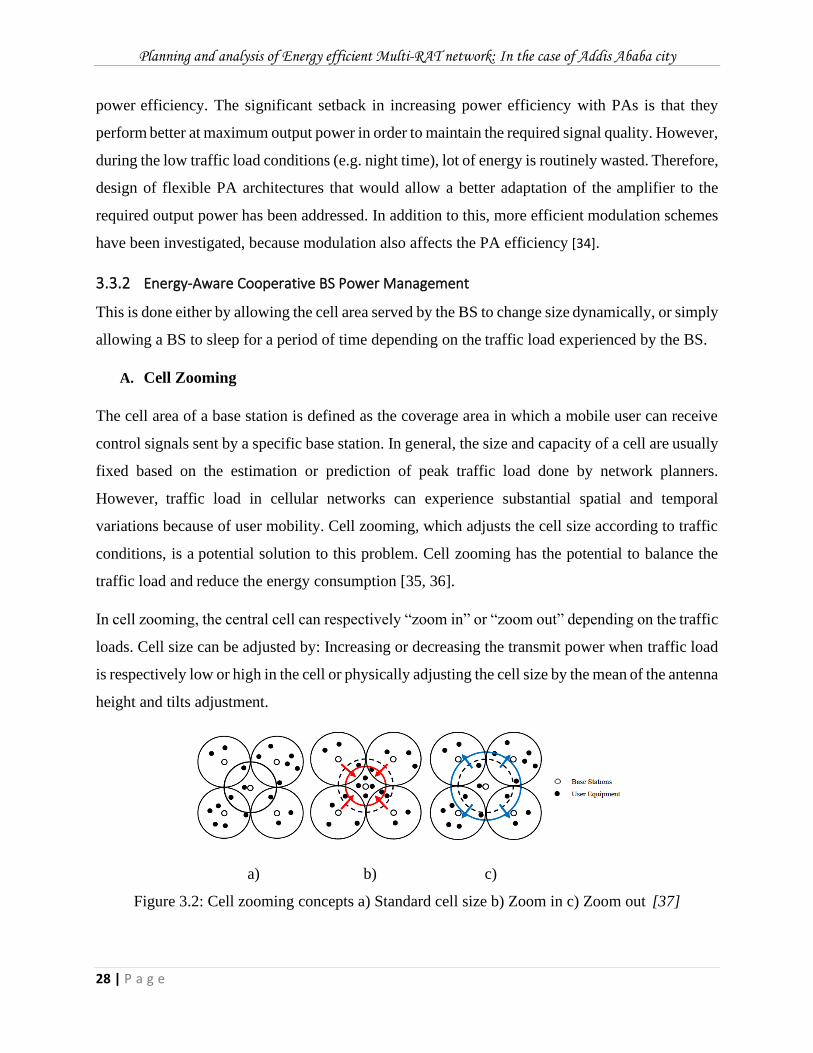
Planning and analysis of Energy efficient Multi-RAT network: In the case of Addis Ababa city
28 | P a g e
power efficiency. The significant setback in increasing power efficiency with PAs is that they
perform better at maximum output power in order to maintain the required signal quality. However,
during the low traffic load conditions (e.g. night time), lot of energy is routinely wasted. Therefore,
design of flexible PA architectures that would allow a better adaptation of the amplifier to the
required output power has been addressed. In addition to this, more efficient modulation schemes
have been investigated, because modulation also affects the PA efficiency [34].
3.3.2 Energy-Aware Cooperative BS Power Management
This is done either by allowing the cell area served by the BS to change size dynamically, or simply
allowing a BS to sleep for a period of time depending on the traffic load experienced by the BS.
A. Cell Zooming
The cell area of a base station is defined as the coverage area in which a mobile user can receive
control signals sent by a specific base station. In general, the size and capacity of a cell are usually
fixed based on the estimation or prediction of peak traffic load done by network planners.
However, traffic load in cellular networks can experience substantial spatial and temporal
variations because of user mobility. Cell zooming, which adjusts the cell size according to traffic
conditions, is a potential solution to this problem. Cell zooming has the potential to balance the
traffic load and reduce the energy consumption [35, 36].
In cell zooming, the central cell can respectively “zoom in” or “zoom out” depending on the traffic
loads. Cell size can be adjusted by: Increasing or decreasing the transmit power when traffic load
is respectively low or high in the cell or physically adjusting the cell size by the mean of the antenna
height and tilts adjustment.
a) b) c)
Figure 3.2: Cell zooming concepts a) Standard cell size b) Zoom in c) Zoom out [37]
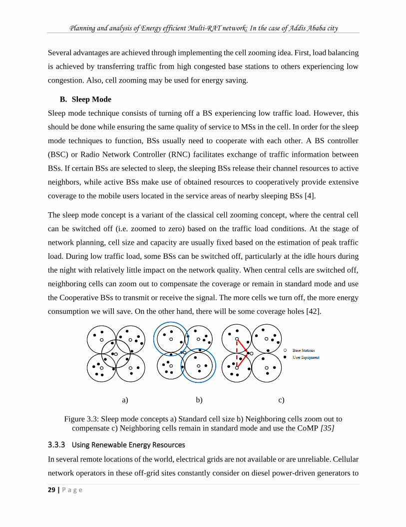
Planning and analysis of Energy efficient Multi-RAT network: In the case of Addis Ababa city
29 | P a g e
Several advantages are achieved through implementing the cell zooming idea. First, load balancing
is achieved by transferring traffic from high congested base stations to others experiencing low
congestion. Also, cell zooming may be used for energy saving.
B. Sleep Mode
Sleep mode technique consists of turning off a BS experiencing low traffic load. However, this
should be done while ensuring the same quality of service to MSs in the cell. In order for the sleep
mode techniques to function, BSs usually need to cooperate with each other. A BS controller
(BSC) or Radio Network Controller (RNC) facilitates exchange of traffic information between
BSs. If certain BSs are selected to sleep, the sleeping BSs release their channel resources to active
neighbors, while active BSs make use of obtained resources to cooperatively provide extensive
coverage to the mobile users located in the service areas of nearby sleeping BSs [4].
The sleep mode concept is a variant of the classical cell zooming concept, where the central cell
can be switched off (i.e. zoomed to zero) based on the traffic load conditions. At the stage of
network planning, cell size and capacity are usually fixed based on the estimation of peak traffic
load. During low traffic load, some BSs can be switched off, particularly at the idle hours during
the night with relatively little impact on the network quality. When central cells are switched off,
neighboring cells can zoom out to compensate the coverage or remain in standard mode and use
the Cooperative BSs to transmit or receive the signal. The more cells we turn off, the more energy
consumption we will save. On the other hand, there will be some coverage holes [42].
a) b) c)
Figure 3.3: Sleep mode concepts a) Standard cell size b) Neighboring cells zoom out to
compensate c) Neighboring cells remain in standard mode and use the CoMP [35]
3.3.3 Using Renewable Energy Resources
In several remote locations of the world, electrical grids are not available or are unreliable. Cellular
network operators in these off-grid sites constantly consider on diesel power-driven generators to

Planning and analysis of Energy efficient Multi-RAT network: In the case of Addis Ababa city
30 | P a g e
run BSs that isn’t only pricey, however conjointly generates CO2 emissions. In such places,
renewable energy resources such as sustainable biofuels, solar and wind energy seem to be more
viable options to reduce the overall network expenditure. In most cases a hybrid solution
combining of solar and wind is the most feasible for autonomous BTS site. For base station sites,
the renewable energy could be used for several reasons like: long distance to electricity grid,
unreliable grid and reduce amount of CO2 emission. In the design of base station site to be powered
by renewable energy the key factors to take in to account are the site and energy consumption of
BTS. The size of solar cell and wind turbine has to be defined based on that load and the available
solar and wind situation on the site location [34, 38].
3.3.4 Other Ways to Reduce BS Power Consumption
Since the energy consumption of the whole cellular network includes the summation of energy
utilized by each BS, reducing the quantity of BSs incorporates a direct impact on energy
consumption of a cellular network. However, efficient network design and finding an optimal
balance between cell size and BS capacity can be very challenging. Features like 2-way and 4-way
diversity, feeder less site, extended cell, low frequency band, 6-sector site and smart antenna can
be used to minimize the number of BS sites.
Another way to improve power efficiency of a BS is to bring some architectural changes to the
BS. Currently, the connection between the RF-transmitter and antenna is completed by long
coaxial cables that add nearly 3dB to the losses in power transmission and thus, low power RF-
cables should be used and RF-amplifier must to be near closer to the antenna. This will improve
the efficiency and reliability of the BS [35, 34, 39, 40].
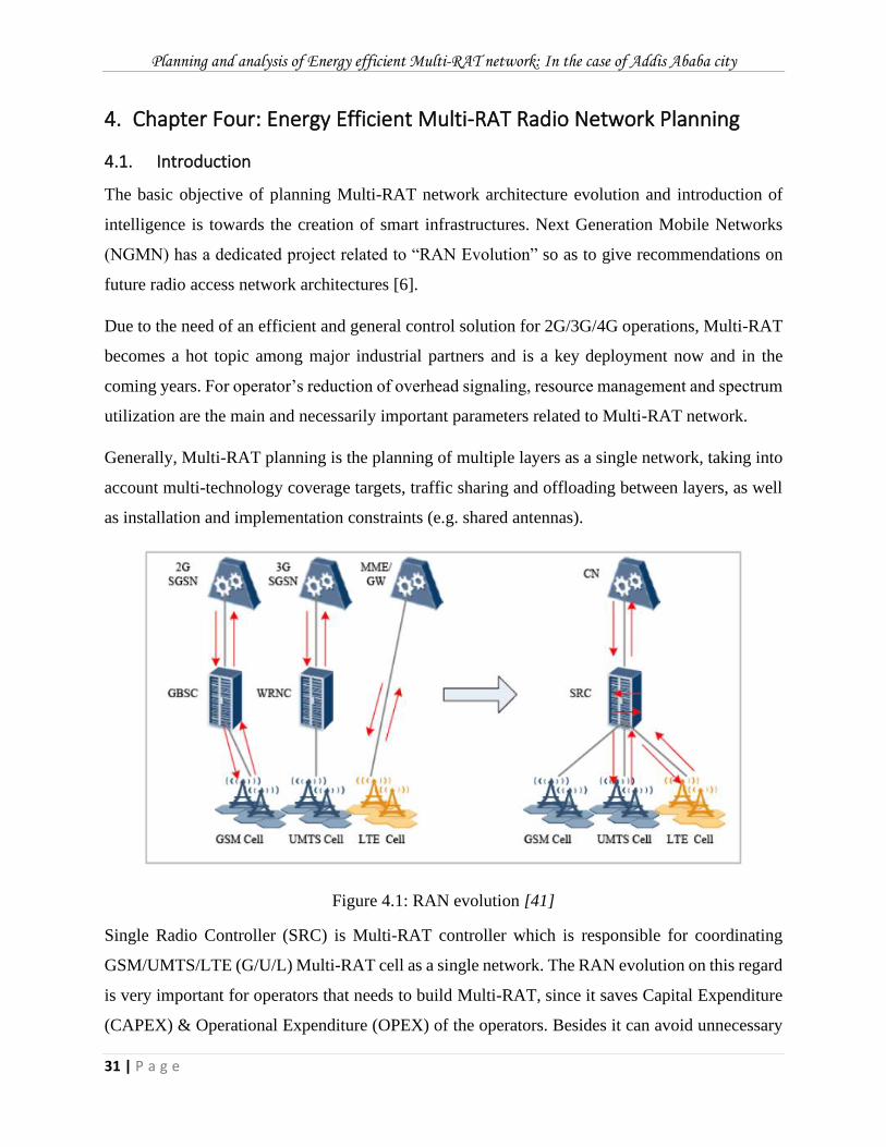
Planning and analysis of Energy efficient Multi-RAT network: In the case of Addis Ababa city
31 | P a g e
4. Chapter Four: Energy Efficient Multi-RAT Radio Network Planning
4.1. Introduction
The basic objective of planning Multi-RAT network architecture evolution and introduction of
intelligence is towards the creation of smart infrastructures. Next Generation Mobile Networks
(NGMN) has a dedicated project related to “RAN Evolution” so as to give recommendations on
future radio access network architectures [6].
Due to the need of an efficient and general control solution for 2G/3G/4G operations, Multi-RAT
becomes a hot topic among major industrial partners and is a key deployment now and in the
coming years. For operator’s reduction of overhead signaling, resource management and spectrum
utilization are the main and necessarily important parameters related to Multi-RAT network.
Generally, Multi-RAT planning is the planning of multiple layers as a single network, taking into
account multi-technology coverage targets, traffic sharing and offloading between layers, as well
as installation and implementation constraints (e.g. shared antennas).
Figure 4.1: RAN evolution [41]
Single Radio Controller (SRC) is Multi-RAT controller which is responsible for coordinating
GSM/UMTS/LTE (G/U/L) Multi-RAT cell as a single network. The RAN evolution on this regard
is very important for operators that needs to build Multi-RAT, since it saves Capital Expenditure
(CAPEX) & Operational Expenditure (OPEX) of the operators. Besides it can avoid unnecessary
Planning and analysis of Energy efficient Multi-RAT network: In the case of Addis Ababa city
32 | P a g e
resource usage by different controllers for signaling, handover and the like which can be controlled
by a single controller. The technological advancement on the basis of RAN evolution is a matter
of vendors to manufacture RAN equipment’s based on ITU & 3GPP standards, and this thesis is
focused on the planning part of Multi-RAT networks.
4.2. Radio Network Planning Criteria
Network coming up with may be a difficult method consisting of many phases. The final
target for the network coming up with method is to outline the network style, that is
then engineered as a cellular network. The basic requirements for the cellular network are to
meet coverage and quality targets. Coverage targets firstly mean the geographic area in which the
network is covering with an agreed location probability. The requirements also specify signal
strength values that need to be met inside different area types. The quality targets are related to
factors such as success of the call, call drop ratio, which should not exceed the agreed value and
the success ratio for the call setup and for handovers. With new wireless communication
technologies and therefore the increasing size of radio networks, the tasks of network planning and
resource optimization are becoming more and more challenging. This is because of the scarcity of
radio resources currently due to the increasing number of subscribers and many different types of
networks operating within the limited frequency spectrum. Secondly, deploying and operating a
large network is expensive and therefore requires careful network dimensioning to ensure high
resource utilization [3].
By doing a proper Network Planning and keeping the longer-term growth plan in mind we are able
to cut or reduce lots of problems that we have a tendency to could encounter within the future and
also reduce substantially the cost of optimization. On the other hand, a poorly planned network not
only leads to many network problems, it also increases the optimization costs and still may not
ensure the desired quality. A good plan should address the following issues: provision of required
capacity, optimum usage of the available frequency spectrum, minimum number of sites, provision
for easy and smooth expansion of the network in future & provision of adequate coverage of the
given area, for a minimum specified level of interference [3, 42, 43]. Generally, the detailed part
of radio network planning covers link budget calculation, coverage planning, capacity planning,
frequency planning, and parameter planning
Planning and analysis of Energy efficient Multi-RAT network: In the case of Addis Ababa city
33 | P a g e
a) Link budget calculation: Gives the loss in the signal strength on the path between the mobile
station antenna and BS antenna and should be done for both UL and DL communications [31].
b) Coverage Planning: Its objective is to find a minimum amount of cell sites with optimum
locations for producing the required coverage for the target area. Coverage regions, coverage
threshold values on per regions (outdoor, in-car, indoor), antenna (tower height limitations),
most well-linked antenna line system specifications, preferred BS specification & activities such
as propagation modeling, field strength predictions and measurements are the basic input data
for coverage planning section.
c) Capacity planning: is a very important process in the network rollout as it defines the number
of BS/NB’s/eNB’s required and their respective capacities. The number of transceivers
required is derived from capacity planning as it is directly associated with the frequency re-use
factor. BS antenna height is another factor because if the antenna height is too high then the
signal has to travel a greater distance, so the probability that the signal causes interference
becomes greater. Generally, there are three essential parameters required for capacity planning:
Estimated traffic, Average antenna height, and Frequency usage.
d) Frequency Planning: After site selection, assignment of the frequency channel for each cell
is done in a manner that causes minimal interference and maintains the desired quality.
Frequency allocation is based on the cell-to-cell channel to interference (C/I) ratio.
e) Parameter Planning: There is a parameter set for each cell that is used for network launch
and expansion. This set may include cell service area definitions, channel configurations,
handover and power control, adjacency definitions, and network specific parameters [43].
In this radio network planning GSM, UMTS and LTE are the multiple radio access technologies
which are taken in to account for planning as Multi-RAT network and the system model is shown
below.
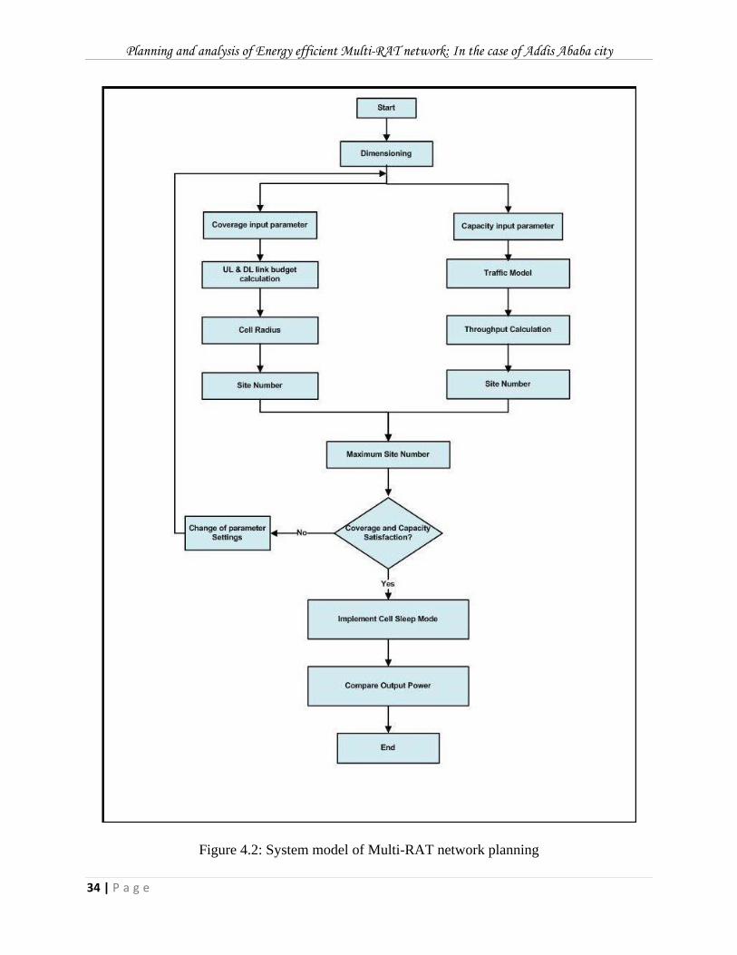
Planning and analysis of Energy efficient Multi-RAT network: In the case of Addis Ababa city
34 | P a g e
Figure 4.2: System model of Multi-RAT network planning
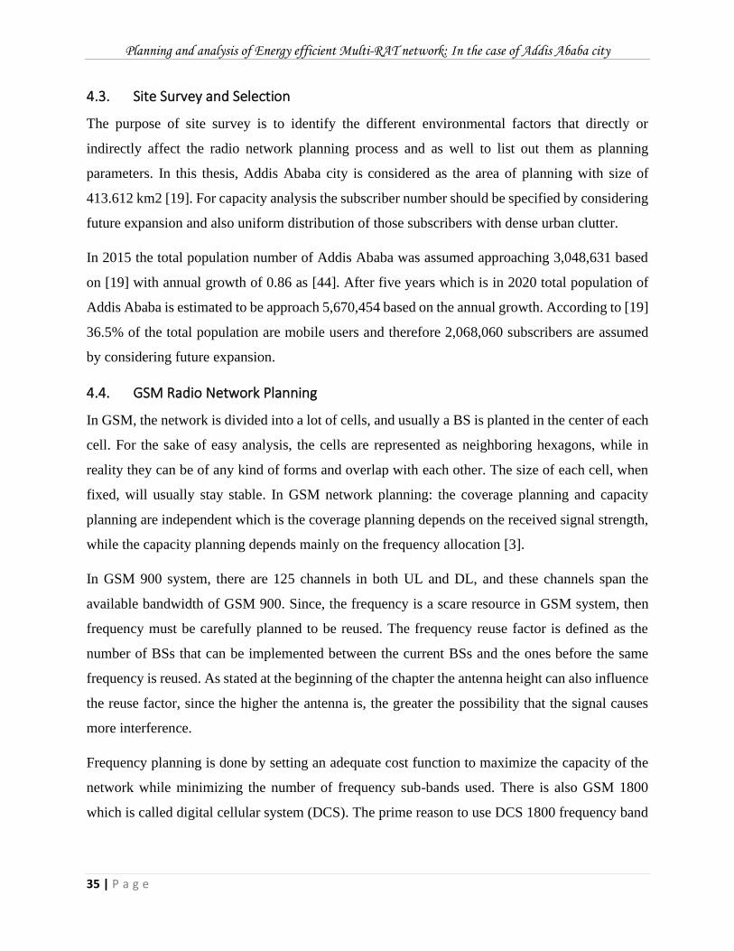
Planning and analysis of Energy efficient Multi-RAT network: In the case of Addis Ababa city
35 | P a g e
4.3. Site Survey and Selection
The purpose of site survey is to identify the different environmental factors that directly or
indirectly affect the radio network planning process and as well to list out them as planning
parameters. In this thesis, Addis Ababa city is considered as the area of planning with size of
413.612 km2 [19]. For capacity analysis the subscriber number should be specified by considering
future expansion and also uniform distribution of those subscribers with dense urban clutter.
In 2015 the total population number of Addis Ababa was assumed approaching 3,048,631 based
on [19] with annual growth of 0.86 as [44]. After five years which is in 2020 total population of
Addis Ababa is estimated to be approach 5,670,454 based on the annual growth. According to [19]
36.5% of the total population are mobile users and therefore 2,068,060 subscribers are assumed
by considering future expansion.
4.4. GSM Radio Network Planning
In GSM, the network is divided into a lot of cells, and usually a BS is planted in the center of each
cell. For the sake of easy analysis, the cells are represented as neighboring hexagons, while in
reality they can be of any kind of forms and overlap with each other. The size of each cell, when
fixed, will usually stay stable. In GSM network planning: the coverage planning and capacity
planning are independent which is the coverage planning depends on the received signal strength,
while the capacity planning depends mainly on the frequency allocation [3].
In GSM 900 system, there are 125 channels in both UL and DL, and these channels span the
available bandwidth of GSM 900. Since, the frequency is a scare resource in GSM system, then
frequency must be carefully planned to be reused. The frequency reuse factor is defined as the
number of BSs that can be implemented between the current BSs and the ones before the same
frequency is reused. As stated at the beginning of the chapter the antenna height can also influence
the reuse factor, since the higher the antenna is, the greater the possibility that the signal causes
more interference.
Frequency planning is done by setting an adequate cost function to maximize the capacity of the
network while minimizing the number of frequency sub-bands used. There is also GSM 1800
which is called digital cellular system (DCS). The prime reason to use DCS 1800 frequency band
Planning and analysis of Energy efficient Multi-RAT network: In the case of Addis Ababa city
36 | P a g e
was the lack of capacity in the 900 MHZ and can give solution on the issue of capacity, and used
to be deployed in most densely populated areas or large cities [3, 31, 44].
4.4.1. GSM Coverage Planning
As discussed in the first chapter dimensioning is the primary part of the planning phase. The
priority of the parameters also needed to be agreed besides the dimensioning parameters. The radio
network dimensioning parameters have an impact on each other and therefore it is important to
decide the emphasis in order to get an optimal dimensioning result within the agreed parameter
ranges [3, 44].
In this thesis macro cells with three sector sites which actually characterized by an outdoor antenna
are considered. When performing tasks related to coverage during network planning, link budget
calculation is an important step as mentioned above.
The main aim of radio link budget (RLB) is determining the cell coverage area by calculating UL
and DL path losses and then to balance the UL and DL powers. The links are calculated separately
and are different from the transmission powers. The Base Transceiver Station (BTS) transmission
power is higher than the MS transmission power and therefore the reception of the BTS needs to
have high sensitivity. To estimate the propagation loss between the transmitter and the receiver
radio wave propagation is the basic and required parameter.
Figure 4.3: Block diagram of link budget calculations
Planning and analysis of Energy efficient Multi-RAT network: In the case of Addis Ababa city
37 | P a g e
The GSM link budget parameters are classified into four types; these are system
parameter, transmitter parameters, receiver parameters, and margin reservation. Hence, the
formula of link budget is described as follows:
𝑀𝐴𝑃𝐿 = 𝑇𝑋 𝐸𝐼𝑅𝑃 + 𝑅𝑋 𝐺𝑎𝑖𝑛𝑠 − 𝑅𝑋 𝐿𝑜𝑠𝑠𝑒𝑠 − 𝑅𝑒𝑐𝑖𝑒𝑣𝑒𝑟 𝑆𝑒𝑛𝑠𝑖𝑡𝑖𝑣𝑖𝑡𝑦 − 𝑇𝑜𝑡𝑎𝑙 𝑚𝑎𝑟𝑔𝑖𝑛𝑠 (4.1)
Where, 𝑇𝑋 𝐸𝐼𝑅𝑃 = 𝑇𝑋 𝑝𝑜𝑤𝑒𝑟 + 𝑇𝑋 𝑎𝑛𝑡𝑒𝑛𝑛𝑎 𝑔𝑎𝑖𝑛 − 𝑏𝑜𝑑𝑦 𝑙𝑜𝑠𝑠
𝑇𝑜𝑡𝑎𝑙 𝑚𝑎𝑟𝑔𝑖𝑛𝑠 = 𝑠𝑙𝑜𝑤 𝑓𝑎𝑑𝑖𝑛𝑔 𝑚𝑎𝑟𝑔𝑖𝑛 + 𝑓𝑎𝑠𝑡 𝑓𝑎𝑑𝑖𝑛𝑔 𝑚𝑎𝑟𝑔𝑖𝑛 + 𝑖𝑛𝑡𝑒𝑟𝑓𝑒𝑟𝑒𝑛𝑐𝑒 𝑚𝑎𝑟𝑔𝑖𝑛
+ 𝑏𝑢𝑖𝑙𝑑𝑖𝑛𝑔 𝑜𝑟 𝑣𝑒ℎ𝑖𝑐𝑙𝑒 𝑝𝑒𝑛𝑒𝑡𝑟𝑎𝑡𝑖𝑜𝑛 𝑙𝑜𝑠𝑠
System parameters
Carrier frequency: Carrier frequency affects the transmission loss and radio waves of different
frequencies have different propagation models and different losses.
System bandwidth: In a GSM system, the receiver bandwidth is 200 kHz or 53dBHz
Data rate: The full rate of GSM voice service is 9.6 Kbit/s and the corresponding half rate is 4.8
Kbit/s.
Transmitter Parameters
Transmitter power: The MS transmission power is defined by the MS class in European
Telecommunications Standards Institute (ETSI) specifications. For MS class 4 (GSM 900) the
maximum TX power is 2W (33 dBm) and for class 1 (GSM 1800) 1W (30 dBm). BS TX power
depends on the BS type and vendor. The TX power is adjustable, which enables the link budget to
be balanced [44] but for this work it’s assumed to be 20 W (43 dBm).
Antenna gain: For MS, electronically small uni-pole antenna and planar inverted-F antennas
(PIFA) are always used and has a lower gain, of the order of 0dBi. The BS antenna gain can vary
from 8dBi to 21dBi depending upon the type of antenna being used (Omni directional versus
directional) and can be increased by using various techniques, such as antenna diversity [31, 44].
Body Loss: Body loss refers to the loss produced by the signal blockage and absorption when
hand-held mobile phones are near to the human body. It’s always taken 3dB and 0dB for the case
of voice service and data service using data card respectively [6].
Planning and analysis of Energy efficient Multi-RAT network: In the case of Addis Ababa city
38 | P a g e
Cable loss: Cable attenuation figures are usually quoted in loss (dB) per 100 m, obviously a longer
cable gives a higher loss and because of this the shortest possible route for the cable should be
used.
Connector losses: are usually gives a loss of around 0.1 dB, but depending on the cable
installations there can be several in one antenna line.
Receiver parameter
Noise spectral density: Spectral density of thermal noise is calculated as:
𝑆𝑝𝑒𝑐𝑡𝑟𝑎𝑙 𝑑𝑒𝑛𝑠𝑖𝑡𝑦 = 𝑘𝑇 = −174𝑑𝐵𝑚
𝐻𝑧 𝑖𝑛 𝑟𝑜𝑜𝑚 𝑡𝑒𝑚𝑝𝑟𝑎𝑡𝑢𝑟𝑒 (290𝑘) (4.2)
Where, k is Boltzmann constant, which equals 1.38 × 10⁻²³ 𝐽 𝑘⁄ and T is absolute temperature
(290k)
Noise power: Noise power Ni, also called thermal noise is produced by the thermal movement of
electrons.
𝑁𝑖 = 𝑘𝑇𝐵 (4.3)
Where, B is bandwidth
C/I required by TCH: Carrier-to-Interference ratio 𝐶 𝐼⁄ is the SNR requirement on the air
interface. In narrowband system, 𝐶 𝐼⁄ is the requirement of receiver base band demodulation
performance. The target value varies depending on the propagation environment, mobility speed,
and coding rate. According to the GSM protocol, 𝐶 𝐼⁄ should be greater than or equal to 9dB [6].
Noise figure: is a method to measure the noise added when a signal is pass through BS or/and MS
receiver. In the case of ideal receiver nose figure is F = 1 or 0dB. In actual situations, a receiver
has noise and the output noise power is greater than signal power. Thus, the SNR is worse and F
> 1. As defined in GSM protocol, the noise figure of a BS receiver is 8 dB and 10dB for MS
receiver.
Receiver sensitivity: is a measure of how well the receiver performs and is defined as the power
of the weakest signal the receiver can detect. In telecom system, receiver sensitivity is given by:
Planning and analysis of Energy efficient Multi-RAT network: In the case of Addis Ababa city
39 | P a g e
𝑅𝑒𝑐𝑒𝑖𝑣𝑒𝑟 𝑠𝑒𝑛𝑠𝑖𝑡𝑖𝑣𝑖𝑡𝑦 = 𝑛𝑜𝑖𝑠𝑒 𝑠𝑝𝑒𝑐𝑡𝑟𝑎𝑙 𝑑𝑒𝑛𝑠𝑖𝑡𝑦 (𝑑𝐵𝑚
𝐻𝑧) + 𝑏𝑎𝑛𝑑𝑤𝑖𝑑𝑡ℎ(𝑑𝐵𝐻𝑧) +
𝑛𝑜𝑖𝑠𝑒 𝑓𝑖𝑔𝑢𝑟𝑒 (𝑑𝐵) +𝐶
𝐼(𝑑𝐵) (4.4)
Or receiver sensitivity (Si): is solved from the following equation [44], where the input noise
power (Ni) is the product of three parameters: Boltzmann constant (k); temperature (T0) = 290K
and bandwidth (B) = 200 kHz (53 dB):
𝐹 =𝑆𝑖 𝑁𝑖⁄
𝑆0 𝑁0⁄=
𝑆𝑖(𝑘𝑇0𝐵)
𝐸0 𝑁0⁄ , 𝑁𝑖 = 𝑘𝑇0𝐵 (4.5)
Where, 𝑆𝑖 =𝐸𝑏
𝑁0𝐹𝑘𝑇0𝐵 (4.6)
BS sensitivity: The sensitivity of the base stations specified on the ETSI GSM recommendation
05.05 and the recommended value is -106 dBm. This is a general recommendation, however when
doing link budget calculations, the value given by the manufacturer (or measured value) should be
used. Based on ETSI recommendation 03.30 the value of energy per bit over noise density (𝐸𝑏 𝑁0⁄ )
is 7dB and using the Equation (4.6) the receiver sensitivity cab be calculated as:
𝑆𝑖 =𝐸𝑏
𝑁0𝐹𝑘𝑇0𝐵 = 8𝑑𝐵 + 7𝑑𝐵 + (290𝐾 × 1.38 × 10−23 𝐽 𝐾⁄ ) + 53𝑑𝐵
= 8𝑑𝐵 + 7𝑑𝐵 − 174𝑑𝐵𝑚 + 53𝑑𝐵𝑚 = −106𝑑𝐵𝑚
MS sensitivity: is also specified in the ETSI recommendation 05.05, where the receiver
sensitivity value for MS class 4 the recommended value is -102dBm. The MS sensitivity can also
be calculated using the information of receiver noise F and minimum Eb/N0 equation (4.6). The
minimum value of 𝐸𝑏 𝑁0⁄ is 9 dB, as defined in the ETSI recommendation 03.30. Therefore, the
receiver sensitivity of MS can be calculated as:
𝑆𝑖 =𝐸𝑏
𝑁0𝐹𝑘𝑇0𝐵 = 9𝑑𝐵 + 10𝑑𝐵 + (290𝐾 × 1.38 × 10−23 𝐽 𝐾⁄ ) + 53𝑑𝐵
= 9𝑑𝐵 + 10𝑑𝐵 − 174𝑑𝐵𝑚 + 53𝑑𝐵𝑚 = −102𝑑𝐵𝑚
The value of MS sensitivity given in these specifications is according to the class of mobile being
used. For MS class 4, which means GSM 900, the recommended value is -102 dBm.
Correspondingly for class 1, GSM 1800, the value is -100 dBm [6, 31, 44].
Planning and analysis of Energy efficient Multi-RAT network: In the case of Addis Ababa city
40 | P a g e
Interference degradation margin: describes the loss due to frequency reuse. Therefore, the
frequency reuse rate corresponds to the degradation margin value. The suggested value for the
interference degradation margin in an average suburban and rural area is 3dB according to the
ETSI recommendation 03.30. In the case of high frequency reuse in urban and dense urban areas
the degradation margin can have a value of 4-5dB.
Margin reservation
Slow fading margin / Shadow fading margin: also named as slow attenuation. It follows a
lognormal distribution in the calculation of radio coverage. To reach the specified coverage
probability, during network planning, certain power margin must be reserved for BS or MS
receivers to reduce the attenuation effect. Shadow fading standard deviation is related to
electromagnetic wave propagation environment. In urban and dense urban areas, the shadow
fading standard deviation is about 8 to 10 dB, in suburban and rural areas, the value range is 6 to
8 dB [6, 45, 46].
Coverage Probability: Coverage probability refers to the probability that the quality of
communication between terminals in radio coverage edge (or inside coverage) and the BS meet
the requirement. Coverage probability can also be classified into area coverage probability and
edge coverage probability.
a) Area coverage probability: is the percentage of area of the location where receiving signal
strength is greater than receiving threshold to the total area in a round region with radius R.
b) Edge Coverage Probability: is used to evaluate the reliability of communication links in
shadow fading environment. Edge coverage probability is an index determining the coverage
quality.
The 90% edge coverage probability corresponds to 95% area coverage probability and shadow
fading margin is 10.3dB [6]. To determine the location probability a distribution for the received
signal has to be defined. The slow fading variations in the average received signal level are
normally distributed, which is presented in Figure 4.4.
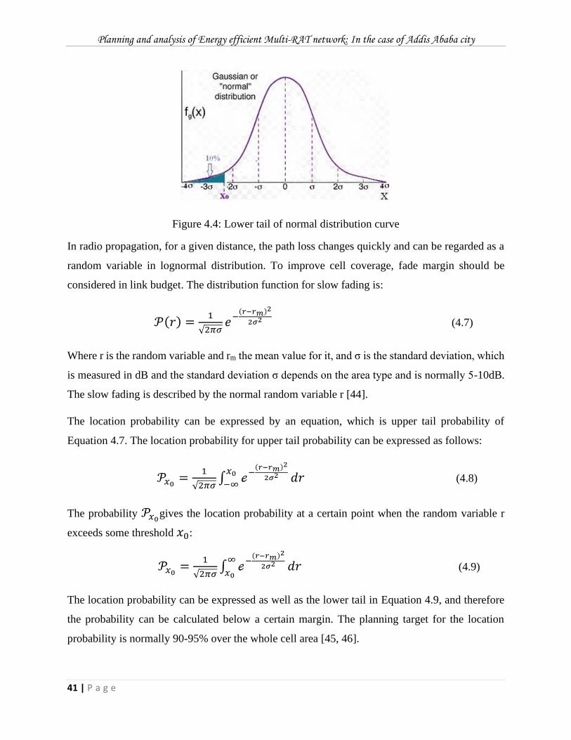
Planning and analysis of Energy efficient Multi-RAT network: In the case of Addis Ababa city
41 | P a g e
Figure 4.4: Lower tail of normal distribution curve
In radio propagation, for a given distance, the path loss changes quickly and can be regarded as a
random variable in lognormal distribution. To improve cell coverage, fade margin should be
considered in link budget. The distribution function for slow fading is:
𝒫(𝑟) =1
√2𝜋𝜎𝑒
−(𝑟−𝑟𝑚)2
2𝜎2 (4.7)
Where r is the random variable and rm the mean value for it, and σ is the standard deviation, which
is measured in dB and the standard deviation σ depends on the area type and is normally 5-10dB.
The slow fading is described by the normal random variable r [44].
The location probability can be expressed by an equation, which is upper tail probability of
Equation 4.7. The location probability for upper tail probability can be expressed as follows:
𝒫𝑥0=
1
√2𝜋𝜎∫ ℯ
−(𝑟−𝑟𝑚)2
2𝜎2𝑥0
−∞𝑑𝑟 (4.8)
The probability 𝒫𝑥0gives the location probability at a certain point when the random variable r
exceeds some threshold 𝑥0:
𝒫𝑥0=
1
√2𝜋𝜎∫ ℯ
−(𝑟−𝑟𝑚)2
2𝜎2∞
𝑥0𝑑𝑟 (4.9)
The location probability can be expressed as well as the lower tail in Equation 4.9, and therefore
the probability can be calculated below a certain margin. The planning target for the location
probability is normally 90-95% over the whole cell area [45, 46].
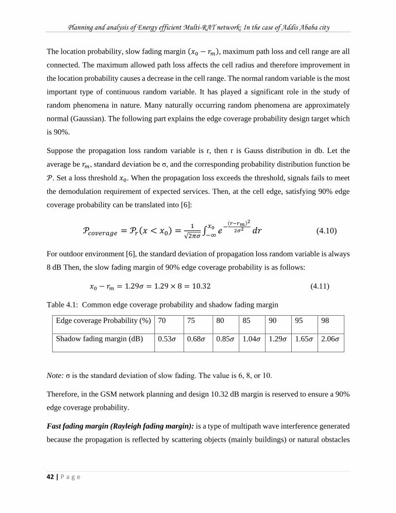
Planning and analysis of Energy efficient Multi-RAT network: In the case of Addis Ababa city
42 | P a g e
The location probability, slow fading margin (𝑥0 − 𝑟𝑚), maximum path loss and cell range are all
connected. The maximum allowed path loss affects the cell radius and therefore improvement in
the location probability causes a decrease in the cell range. The normal random variable is the most
important type of continuous random variable. It has played a significant role in the study of
random phenomena in nature. Many naturally occurring random phenomena are approximately
normal (Gaussian). The following part explains the edge coverage probability design target which
is 90%.
Suppose the propagation loss random variable is r, then r is Gauss distribution in db. Let the
average be 𝑟𝑚, standard deviation be σ, and the corresponding probability distribution function be
𝒫. Set a loss threshold 𝑥0. When the propagation loss exceeds the threshold, signals fails to meet
the demodulation requirement of expected services. Then, at the cell edge, satisfying 90% edge
coverage probability can be translated into [6]:
𝒫𝑐𝑜𝑣𝑒𝑟𝑎𝑔𝑒 = 𝒫𝑟(𝑥 < 𝑥0) =1
√2𝜋𝜎∫ ℯ
−(𝑟−𝑟𝑚)2
2𝜎2𝑥0
−∞𝑑𝑟 (4.10)
For outdoor environment [6], the standard deviation of propagation loss random variable is always
8 dB Then, the slow fading margin of 90% edge coverage probability is as follows:
𝑥0 − 𝑟𝑚 = 1.29𝜎 = 1.29 × 8 = 10.32 (4.11)
Table 4.1: Common edge coverage probability and shadow fading margin
Edge coverage Probability (%)
70 75 80 85 90 95 98
Shadow fading margin (dB)
0.53𝜎 0.68𝜎 0.85𝜎 1.04𝜎 1.29𝜎 1.65𝜎 2.06𝜎
Note: σ is the standard deviation of slow fading. The value is 6, 8, or 10.
Therefore, in the GSM network planning and design 10.32 dB margin is reserved to ensure a 90%
edge coverage probability.
Fast fading margin (Rayleigh fading margin): is a type of multipath wave interference generated
because the propagation is reflected by scattering objects (mainly buildings) or natural obstacles
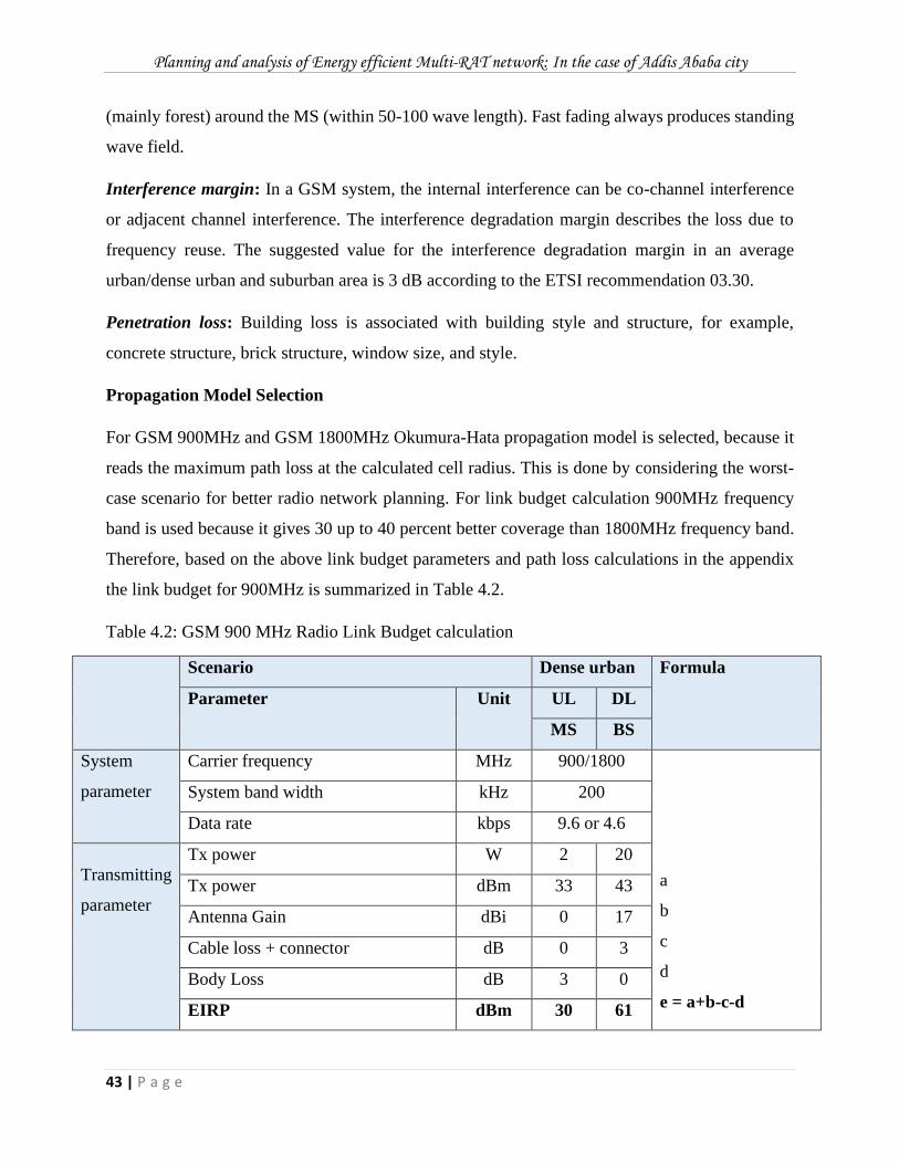
Planning and analysis of Energy efficient Multi-RAT network: In the case of Addis Ababa city
43 | P a g e
(mainly forest) around the MS (within 50-100 wave length). Fast fading always produces standing
wave field.
Interference margin: In a GSM system, the internal interference can be co-channel interference
or adjacent channel interference. The interference degradation margin describes the loss due to
frequency reuse. The suggested value for the interference degradation margin in an average
urban/dense urban and suburban area is 3 dB according to the ETSI recommendation 03.30.
Penetration loss: Building loss is associated with building style and structure, for example,
concrete structure, brick structure, window size, and style.
Propagation Model Selection
For GSM 900MHz and GSM 1800MHz Okumura-Hata propagation model is selected, because it
reads the maximum path loss at the calculated cell radius. This is done by considering the worst-
case scenario for better radio network planning. For link budget calculation 900MHz frequency
band is used because it gives 30 up to 40 percent better coverage than 1800MHz frequency band.
Therefore, based on the above link budget parameters and path loss calculations in the appendix
the link budget for 900MHz is summarized in Table 4.2.
Table 4.2: GSM 900 MHz Radio Link Budget calculation
Scenario Dense urban Formula
Parameter Unit UL DL
MS BS
System
parameter
Carrier frequency MHz 900/1800
a
b
c
d
e = a+b-c-d
System band width kHz 200
Data rate kbps 9.6 or 4.6
Transmitting
parameter
Tx power W 2 20
Tx power dBm 33 43
Antenna Gain dBi 0 17
Cable loss + connector dB 0 3
Body Loss dB 3 0
EIRP dBm 30 61
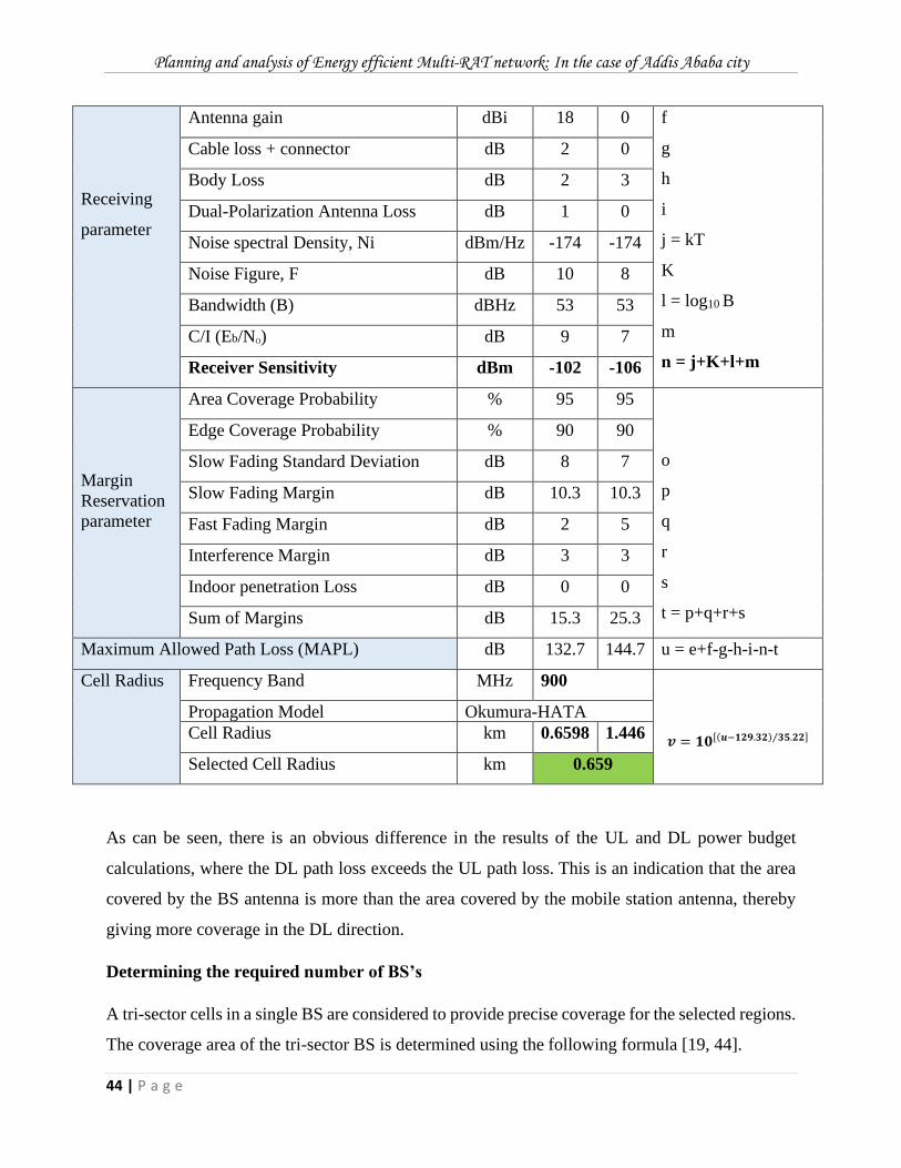
Planning and analysis of Energy efficient Multi-RAT network: In the case of Addis Ababa city
44 | P a g e
Receiving
parameter
Antenna gain dBi 18 0 f
g
h
i
j = kT
K
l = log10 B
m
n = j+K+l+m
Cable loss + connector dB 2 0
Body Loss dB 2 3
Dual-Polarization Antenna Loss dB 1 0
Noise spectral Density, Ni dBm/Hz -174 -174
Noise Figure, F dB 10 8
Bandwidth (B) dBHz 53 53
C/I (Eb/NO) dB 9 7
Receiver Sensitivity dBm -102 -106
Margin
Reservation
parameter
Area Coverage Probability % 95 95
o
p
q
r
s
t = p+q+r+s
Edge Coverage Probability % 90 90
Slow Fading Standard Deviation dB 8 7
Slow Fading Margin dB 10.3 10.3
Fast Fading Margin dB 2 5
Interference Margin dB 3 3
Indoor penetration Loss dB 0 0
Sum of Margins dB 15.3 25.3
Maximum Allowed Path Loss (MAPL) dB 132.7 144.7 u = e+f-g-h-i-n-t
Cell Radius
Frequency Band MHz 900
𝒗 = 𝟏𝟎[(𝒖−𝟏𝟐𝟗.𝟑𝟐) 𝟑𝟓.𝟐𝟐⁄ ]
Propagation Model Okumura-HATA
Cell Radius km 0.6598 1.446
Selected Cell Radius km 0.659
As can be seen, there is an obvious difference in the results of the UL and DL power budget
calculations, where the DL path loss exceeds the UL path loss. This is an indication that the area
covered by the BS antenna is more than the area covered by the mobile station antenna, thereby
giving more coverage in the DL direction.
Determining the required number of BS’s
A tri-sector cells in a single BS are considered to provide precise coverage for the selected regions.
The coverage area of the tri-sector BS is determined using the following formula [19, 44].
Planning and analysis of Energy efficient Multi-RAT network: In the case of Addis Ababa city
45 | P a g e
𝐴 =9√3
8𝑅2 = 1.95𝑅2 (4.12)
Where, A is maximum area covered by a single BS and
R is radius of single cell.
We can now predict the coverage per BS using above equation. Thus, the computed cell radius is
0.66 km2 for dense urban. Consequently, the coverage area of a single site would be 0.8494 km2.
Then, we can calculate the required number of BS using the equation [19]:
𝑅𝑒𝑞𝑢𝑖𝑟𝑒𝑑 𝑛𝑢𝑚𝑏𝑒𝑟 𝑜𝑓 𝑠𝑖𝑡𝑒𝑠 =𝐴𝑟𝑒𝑎 𝑡𝑜 𝑏𝑒 𝑐𝑜𝑣𝑒𝑟𝑒𝑑
𝑠𝑖𝑡𝑒 𝑐𝑜𝑣𝑒𝑟𝑎𝑔𝑒 𝑎𝑟𝑒𝑎 (4.13)
The city of Addis Ababa which is area to be covered is 413.612 km2 [19]. Therefore, a totally of
487 GSM 1800MHz BS’s are required for the entire area of Addis Ababa city by considering
uniform distribution of subscribers with dense urban area.
4.4.2. GSM Capacity Planning
Capacity dimensioning is a very important process in the network rollout as it defines the number
of BS required and their respective capacities. There are three essential parameters required for
capacity planning: estimated traffic, average antenna height and frequency usage.
Traffic estimation or modeling relays on theoretical estimates or assumptions, and on studies of
existing networks. Traffic within the network depends on the user communication rate and user
movement within the network. The user communication rate means that what quantity traffic is
generated by the subscriber and for how long. The estimated traffic in the network is given in terms
of ‘Erlangs’. One Erlang (1 Erl) is defined as the amount of traffic generated by the user when
he/she uses one traffic channel for one hour (this one hour is usually the busy hour of the network).
In this thesis it is assumed an average of two call per hour and the call lasts an average of 90
seconds per call and individual voice traffic intensity is calculated as:
𝐴𝑢 = 𝐻 × 𝜆 in Erlang (4.14)
Where: H is average holding time i.e. average duration of a call or time for which UE requires
service and 𝜆 is average arrival rate i.e. average number of UEs requesting service which is called
call request/time.
Another term that's oftentimes utilized in network planning is ‘Blocking’. Blocking describes the
situation when a user is trying to make a call and is not able to reach a dialed subscriber owing to
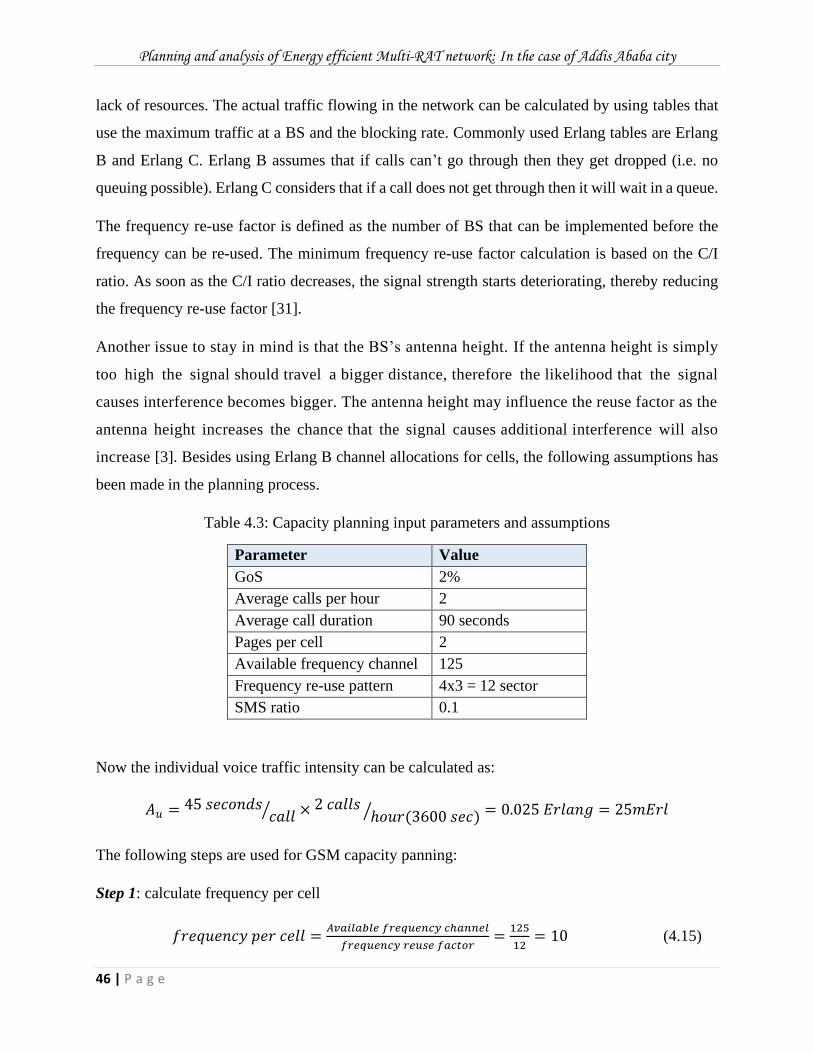
Planning and analysis of Energy efficient Multi-RAT network: In the case of Addis Ababa city
46 | P a g e
lack of resources. The actual traffic flowing in the network can be calculated by using tables that
use the maximum traffic at a BS and the blocking rate. Commonly used Erlang tables are Erlang
B and Erlang C. Erlang B assumes that if calls can’t go through then they get dropped (i.e. no
queuing possible). Erlang C considers that if a call does not get through then it will wait in a queue.
The frequency re-use factor is defined as the number of BS that can be implemented before the
frequency can be re-used. The minimum frequency re-use factor calculation is based on the C/I
ratio. As soon as the C/I ratio decreases, the signal strength starts deteriorating, thereby reducing
the frequency re-use factor [31].
Another issue to stay in mind is that the BS’s antenna height. If the antenna height is simply
too high the signal should travel a bigger distance, therefore the likelihood that the signal
causes interference becomes bigger. The antenna height may influence the reuse factor as the
antenna height increases the chance that the signal causes additional interference will also
increase [3]. Besides using Erlang B channel allocations for cells, the following assumptions has
been made in the planning process.
Table 4.3: Capacity planning input parameters and assumptions
Parameter Value
GoS 2%
Average calls per hour 2
Average call duration 90 seconds
Pages per cell 2
Available frequency channel 125
Frequency re-use pattern 4x3 = 12 sector
SMS ratio 0.1
Now the individual voice traffic intensity can be calculated as:
𝐴𝑢 = 45 𝑠𝑒𝑐𝑜𝑛𝑑𝑠𝑐𝑎𝑙𝑙⁄ × 2 𝑐𝑎𝑙𝑙𝑠
ℎ𝑜𝑢𝑟(3600 𝑠𝑒𝑐)⁄ = 0.025 𝐸𝑟𝑙𝑎𝑛𝑔 = 25𝑚𝐸𝑟𝑙
The following steps are used for GSM capacity panning:
Step 1: calculate frequency per cell
𝑓𝑟𝑒𝑞𝑢𝑒𝑛𝑐𝑦 𝑝𝑒𝑟 𝑐𝑒𝑙𝑙 =𝐴𝑣𝑎𝑖𝑙𝑎𝑏𝑙𝑒 𝑓𝑟𝑒𝑞𝑢𝑒𝑛𝑐𝑦 𝑐ℎ𝑎𝑛𝑛𝑒𝑙
𝑓𝑟𝑒𝑞𝑢𝑒𝑛𝑐𝑦 𝑟𝑒𝑢𝑠𝑒 𝑓𝑎𝑐𝑡𝑜𝑟=
125
12= 10 (4.15)
Planning and analysis of Energy efficient Multi-RAT network: In the case of Addis Ababa city
47 | P a g e
Step 2: calculate traffic channel per cell
As discussed in previous chapter GSM is TDMA based and contains 8 time slots. Out of the time
slots 2 are for control channel and then traffic channel per cell can be calculated as:
𝑇𝐶𝐻 𝑝𝑒𝑟 𝑐𝑒𝑙𝑙 = 𝑛𝑢𝑚𝑏𝑒𝑟 𝑜𝑓 𝑡𝑖𝑚𝑒 𝑠𝑙𝑜𝑡𝑠 × 𝑓𝑟𝑒𝑞𝑢𝑒𝑛𝑐𝑦 𝑝𝑒𝑟 𝑐𝑒𝑙𝑙 − 𝑐𝑜𝑛𝑡𝑟𝑜𝑙 𝑐ℎ𝑎𝑛𝑛𝑒𝑙 (4.16)
= 8 × 10 − 2 = 78 𝑇𝐶𝐻
Step 3: calculate number of subscribers per cell
First voice traffic intensity per cell is calculated and therefore from Erlang B table, 78 TCH with
GOS 2% implies 66.77 Erlangs per cell and using this value number of subscribers per cell can be
calculated as:
# 𝑜𝑓 𝑠𝑢𝑏/𝑐𝑒𝑙𝑙 =𝑣𝑜𝑖𝑐𝑒 𝑡𝑟𝑎𝑓𝑓𝑖𝑐 𝑖𝑛𝑡𝑒𝑛𝑠𝑖𝑡𝑦 𝑝𝑒𝑟 𝑐𝑒𝑙𝑙
𝐼𝑛𝑑𝑖𝑣𝑖𝑑𝑢𝑎𝑙 𝑣𝑜𝑖𝑐𝑒 𝑡𝑟𝑎𝑓𝑓𝑖𝑐 𝑖𝑛𝑡𝑒𝑛𝑠𝑖𝑡𝑦 (4.17)
=66.77
0.025= 2671
Step 4: calculate required number of cells
As we discuss in the beginning of the chapter 2,068,060 subscribers are considered and the number
of cells needed can be calculated as:
# 𝑜𝑓 𝑐𝑒𝑙𝑙𝑠 𝑟𝑒𝑞𝑢𝑖𝑟𝑒𝑑 =𝑇𝑜𝑡𝑎𝑙 # 𝑜𝑓 𝑠𝑢𝑏𝑠𝑐𝑟𝑖𝑏𝑒𝑟𝑠
𝑠𝑢𝑏𝑠𝑐𝑟𝑖𝑏𝑒𝑟𝑠 𝑝𝑒𝑟 𝑐𝑒𝑙𝑙 (4.18)
=2,068,060
2671= 775 𝑐𝑒𝑙𝑙𝑠
Step 5: calculate number of BS required
As discussed in the coverage planning session three sector cells in a single site is used in this thesis.
Therefore, the required number of sites can be calculated as:
𝑟𝑒𝑞𝑢𝑖𝑟𝑒𝑑 # 𝑜𝑓 𝑠𝑖𝑡𝑒𝑠 =𝑁𝑢𝑚𝑏𝑒𝑟 𝑜𝑓 𝑐𝑒𝑙𝑙𝑠
𝑠𝑒𝑐𝑡𝑜𝑟 𝑠𝑖𝑧𝑒=
775
3= 259 𝐵𝑆′𝑠 (4.19)
Therefore, based on capacity planning a total of GSM 900MHz 259 BS’s are needed to provide
the intended capacity.
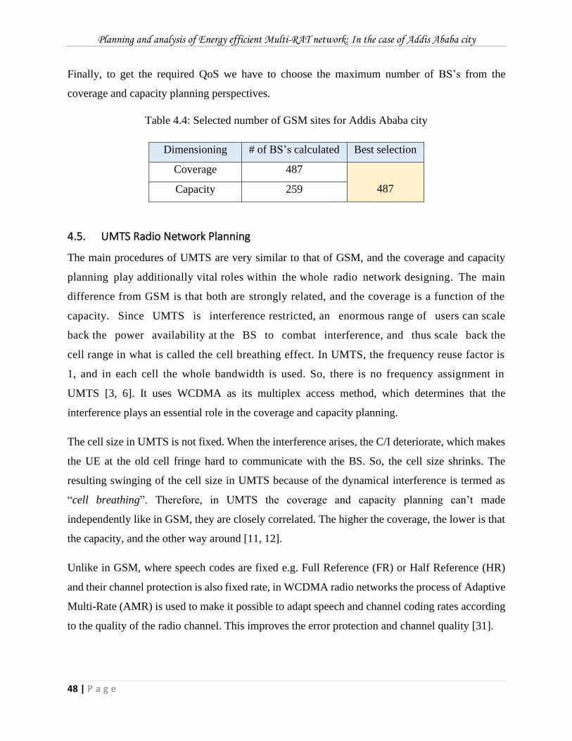
Planning and analysis of Energy efficient Multi-RAT network: In the case of Addis Ababa city
48 | P a g e
Finally, to get the required QoS we have to choose the maximum number of BS’s from the
coverage and capacity planning perspectives.
Table 4.4: Selected number of GSM sites for Addis Ababa city
Dimensioning # of BS’s calculated Best selection
Coverage 487
487 Capacity 259
4.5. UMTS Radio Network Planning
The main procedures of UMTS are very similar to that of GSM, and the coverage and capacity
planning play additionally vital roles within the whole radio network designing. The main
difference from GSM is that both are strongly related, and the coverage is a function of the
capacity. Since UMTS is interference restricted, an enormous range of users can scale
back the power availability at the BS to combat interference, and thus scale back the
cell range in what is called the cell breathing effect. In UMTS, the frequency reuse factor is
1, and in each cell the whole bandwidth is used. So, there is no frequency assignment in
UMTS [3, 6]. It uses WCDMA as its multiplex access method, which determines that the
interference plays an essential role in the coverage and capacity planning.
The cell size in UMTS is not fixed. When the interference arises, the C/I deteriorate, which makes
the UE at the old cell fringe hard to communicate with the BS. So, the cell size shrinks. The
resulting swinging of the cell size in UMTS because of the dynamical interference is termed as
“cell breathing”. Therefore, in UMTS the coverage and capacity planning can’t made
independently like in GSM, they are closely correlated. The higher the coverage, the lower is that
the capacity, and the other way around [11, 12].
Unlike in GSM, where speech codes are fixed e.g. Full Reference (FR) or Half Reference (HR)
and their channel protection is also fixed rate, in WCDMA radio networks the process of Adaptive
Multi-Rate (AMR) is used to make it possible to adapt speech and channel coding rates according
to the quality of the radio channel. This improves the error protection and channel quality [31].
Planning and analysis of Energy efficient Multi-RAT network: In the case of Addis Ababa city
49 | P a g e
The codec basically has one single integrated speech codec with eight source rates. This is
controlled by the radio resource management functions of the RAN. These eight source rates are
12.2, 10.20, 7.95, 7.40, 6.70, 5.90, 5.15 and 4.75 kbps. The process of AMR selection is based on
the channel quality measurements for which both the UE and BS are involved [31].
Once it is confirmed that the quality of a signal is bad, the number of speech codec bits is reduced,
thereby increasing the number of bits that can be used for error detection. The speech frames in
the AMR coder are of 20 ms, so if the sampling rate is 8000/s, 160 samples are processed. Thus,
the bit rate can be changed at each of these 160 samples through in-band signaling or through
dedicated channel (DCH). This process is known as link adaptation. Thus, by using AMR, speech,
coverage and quality performance can be improved [13, 47].
4.5.1. UMTS Coverage Planning
The link budget is performed as part of coverage dimensioning process to acquire the
maximum allowable path loss based on the given planning scenes. And the acquired maximum
path loss will be further used to calculate the maximum cell radius based on the radio propagation
model. In all these processes the final target is to estimate the number of required BS or NodeB to
cover the target coverage area [48].
Using the minimum cell radius, the area covered by the single NB can be calculated through the
hexagonal cellular layout. And as a final step, the number of NB required for the target coverage
area is estimated based on the coverage area of a single NB.
Link budget parameters
Based on the signal propagation path from the transmitting end to receiving end, there are two
paths, UL path, and a DL path. UMTS system could be UL or DL limited based on the system
loading. In a lightly loaded system, the UE transmit power sets a coverage limitation, therefore, it
is UL limited. In a heavily loaded system, the BS or NodeB transmit power limits the number of
user equipment it can serve, therefore it is DL limited. Therefore, initially typical UMTS network
is UL limiting or the UL is limiting link in terms of radio bearer coverage and later on a loaded
network becomes DL limiting [48].
Planning and analysis of Energy efficient Multi-RAT network: In the case of Addis Ababa city
50 | P a g e
The link budget calculation involves various link parameters associated with gains, losses and
design margins of the particular signal transmission path. As in [49] the major link parameters are
discussed below.
System parameter
Chip and information rates: The system chip rate is 3.84 Mchips/s whereas the information rate
depends upon the service. For speech the information rate is 12.2 kbps while for data services it
can be 64kbps, 128kbps, 384 kbps or High-Speed Packet Access (HSPA). The processing gain is
defined by the equation:
𝑃𝑟𝑜𝑐𝑒𝑠𝑠𝑖𝑛𝑔 𝐺𝑎𝑖𝑛 = 10 log𝑐ℎ𝑖𝑝 𝑟𝑎𝑡𝑒
𝑏𝑖𝑡𝑒 𝑟𝑎𝑡𝑒 (4.20)
UE velocity: is an important parameter as it impacts the UL and DL Eb/No requirements. The Eb/No
figures are based upon propagation models assuming 120 km/h and 3 km/h for vehicular and
pedestrian environments, respectively. These two UE velocities are used in the link budget as they
were deemed to provide the most challenging cases for planning. At 3 km/h the UE suffers
significantly from fast fading and therefore power control is required to track this fading
environment. At 120 km/h, power control is unable to track the fast fading, and therefore the Eb/No
value is now affected by the interleaving performance [11, 50, 51].
Transmitter parameters
UE maximum transmitting power (dBm): The maximum transmits power of the mobile station is
set by the UE power class. On any given network there exists different mobile equipment from
different power class. But usually voice-centric UE is class 3 or 4 and data-centric UE is class 3.
Therefore, in the link budget calculation, the transmit power parameter for the UL path is specified
as 21dBm for voice terminal while for data terminal it is specified as 24dBm and also 40dBm for
data terminals in which (>64kbps) [52]. However, the data terminal may have positive antenna
gain and some body loss but is assumed to have a net gain of 0dB.
NodeB’s transmitting power (dBm): The common pilot channel (CPICH) is used by the NodeB
to provide a reference to all mobile stations and aid the channel estimation at the terminals. For
this reason, the CPICH channel is used to define the maximum possible coverage of a particular
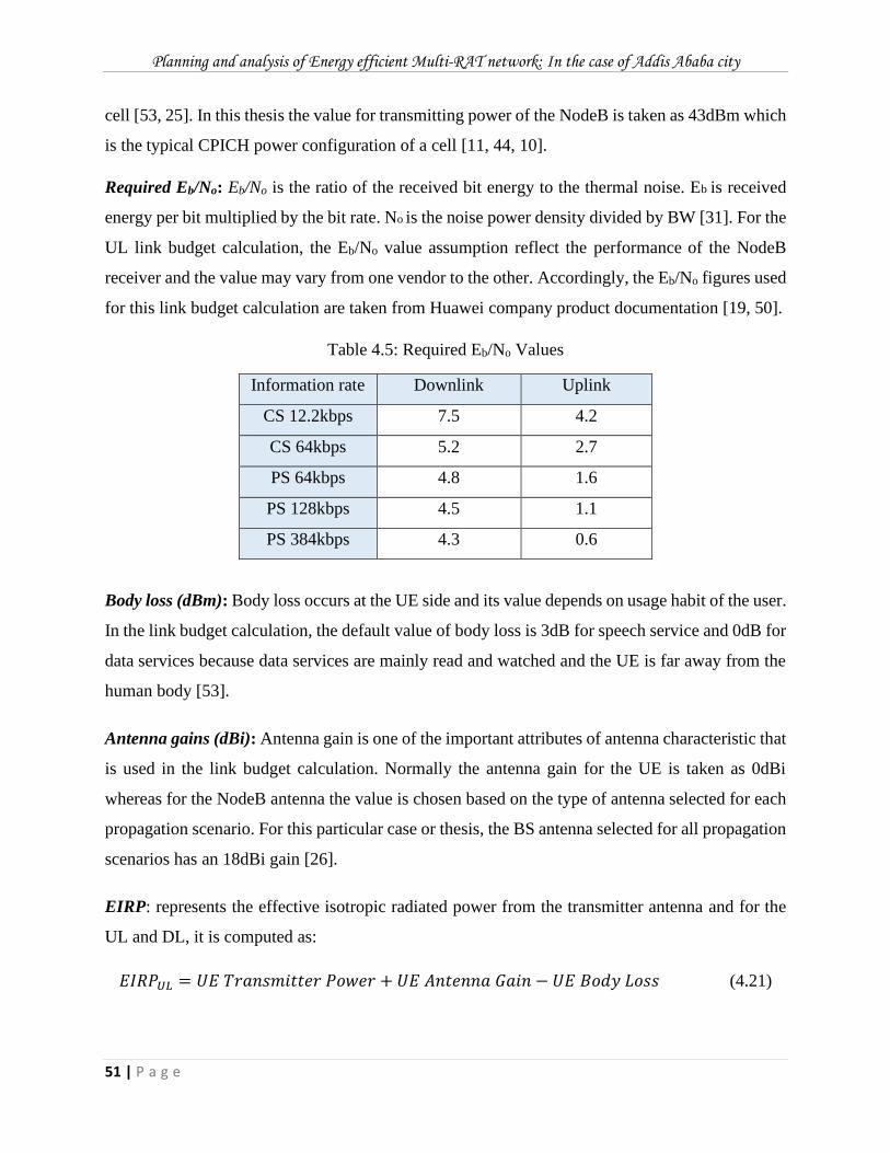
Planning and analysis of Energy efficient Multi-RAT network: In the case of Addis Ababa city
51 | P a g e
cell [53, 25]. In this thesis the value for transmitting power of the NodeB is taken as 43dBm which
is the typical CPICH power configuration of a cell [11, 44, 10].
Required Eb/No: Eb/No is the ratio of the received bit energy to the thermal noise. Eb is received
energy per bit multiplied by the bit rate. No is the noise power density divided by BW [31]. For the
UL link budget calculation, the Eb/No value assumption reflect the performance of the NodeB
receiver and the value may vary from one vendor to the other. Accordingly, the Eb/No figures used
for this link budget calculation are taken from Huawei company product documentation [19, 50].
Table 4.5: Required Eb/No Values
Information rate Downlink Uplink
CS 12.2kbps 7.5 4.2
CS 64kbps 5.2 2.7
PS 64kbps 4.8 1.6
PS 128kbps 4.5 1.1
PS 384kbps 4.3 0.6
Body loss (dBm): Body loss occurs at the UE side and its value depends on usage habit of the user.
In the link budget calculation, the default value of body loss is 3dB for speech service and 0dB for
data services because data services are mainly read and watched and the UE is far away from the
human body [53].
Antenna gains (dBi): Antenna gain is one of the important attributes of antenna characteristic that
is used in the link budget calculation. Normally the antenna gain for the UE is taken as 0dBi
whereas for the NodeB antenna the value is chosen based on the type of antenna selected for each
propagation scenario. For this particular case or thesis, the BS antenna selected for all propagation
scenarios has an 18dBi gain [26].
EIRP: represents the effective isotropic radiated power from the transmitter antenna and for the
UL and DL, it is computed as:
𝐸𝐼𝑅𝑃𝑈𝐿 = 𝑈𝐸 𝑇𝑟𝑎𝑛𝑠𝑚𝑖𝑡𝑡𝑒𝑟 𝑃𝑜𝑤𝑒𝑟 + 𝑈𝐸 𝐴𝑛𝑡𝑒𝑛𝑛𝑎 𝐺𝑎𝑖𝑛 − 𝑈𝐸 𝐵𝑜𝑑𝑦 𝐿𝑜𝑠𝑠 (4.21)
Planning and analysis of Energy efficient Multi-RAT network: In the case of Addis Ababa city
52 | P a g e
𝐸𝐼𝑅𝑃𝐷𝐿 = 𝑁𝑜𝑑𝑒𝐵 𝑇𝑟𝑎𝑛𝑠𝑚𝑖𝑡𝑡𝑒𝑟 𝑃𝑜𝑤𝑒𝑟 + 𝑁𝑜𝑑𝑒𝐵 𝐴𝑛𝑡𝑒𝑛𝑛𝑎 𝐺𝑎𝑖𝑛 − 𝐶𝑎𝑏𝑙𝑒 𝐿𝑜𝑠𝑠 −
𝐶𝑜𝑛𝑛𝑒𝑐𝑡𝑜𝑟 𝐿𝑜𝑠𝑠 (4.22)
Receiver parameters
The noise figures: Noise figure is an index used to evaluate whether noise performance of the
amplifier is good or not. It is expressed by Noise Figures (N) and defined as the ratio of input
Signal-to-Noise ratio (SNR) and output Signal-to-Noise ratio (SNR) of an amplifier.
Thermal noise spectral density: The thermal noise density is computed from the equation:
𝑁 = 𝐾𝑇 = −174𝑑𝐵𝑚/𝐻𝑧
Thermal noise power (Ni): The thermal noise density/power is computed from the equation:
𝑁𝑖 = 𝐾𝑇0𝐵
Where, k is Boltzmann constant, which equals 1.38 x 10⁻²³J/K, 𝑇0 is absolute temperature (𝑇0 =
290𝐾), and B is system bandwidth
𝐵𝑎𝑛𝑑𝑤𝑖𝑑𝑡ℎ 𝑝𝑒𝑟 𝑐ℎ𝑖𝑝 𝑟𝑎𝑡𝑒 = 3.84𝑀𝑐ℎ𝑖𝑝/𝑠 = 3.84 × 10⁶𝑐ℎ𝑖𝑝/𝑠
𝐵𝑑𝐵 𝑝𝑒𝑟 𝑐ℎ𝑖𝑝 𝑟𝑎𝑡𝑒 = 10 log(3.84 × 10⁶) = 65.84
𝑁𝑖 𝑐ℎ𝑖𝑝𝑟𝑎𝑡𝑒/𝑠 = 1.38 × 10−23 × 290,000 × 3.84 × 106 = 1.54 × 10⁻¹¹
𝑁𝑖(𝑑𝐵) = 10 log(𝐾𝑇0𝐵)
= −108.12 𝑑𝐵𝑚
Receiver noise power / Total effective noise power: The total effective noise at the receiver is
computed from the sum of the thermal noise power and the receiver noise figure.
𝑅𝑒𝑐𝑒𝑖𝑣𝑒𝑟 𝑁𝑜𝑖𝑠𝑒 𝑃𝑜𝑤𝑒𝑟 = 𝑇ℎ𝑒𝑟𝑚𝑎𝑙 𝑁𝑜𝑖𝑠𝑒 𝑃𝑜𝑤𝑒𝑟 + 𝑁𝑜𝑖𝑠𝑒 𝐹𝑖𝑔𝑢𝑟𝑒
Receiver sensitivity: measures how well the receiver performs and is defined as the power of the
weakest signal the receiver can detect. The receiver sensitivity is computed using the equation:
𝑅𝑒𝑐𝑒𝑖𝑣𝑒𝑟 𝑆𝑒𝑛𝑠𝑖𝑡𝑖𝑣𝑖𝑡𝑦 = 𝑅𝑒𝑐𝑒𝑖𝑣𝑒𝑟 𝑁𝑜𝑖𝑠𝑒 𝑝𝑜𝑤𝑒𝑟 +𝐸𝑏
𝑁0⁄ − 𝑃𝑟𝑜𝑐𝑒𝑠𝑠𝑖𝑛𝑔 𝐺𝑎𝑖𝑛 (4.23)
Other Margins and Gains
Loading Factor: The coverage and capacity of UMTS systems are closely related because of the
employment of constant frequency and sharing of power. As the cell load increases, additional
interference is generated within the system leading to reduced coverage area. The increase and

Planning and analysis of Energy efficient Multi-RAT network: In the case of Addis Ababa city
53 | P a g e
reduction in coverage area as a result of the loading is termed as cell breathing/shrinking and
should be taken under consideration when dimensioning the system.
Interference margin: The link budget includes an interference margin that is based upon the load
factor and is given by the following equation:
𝐼𝑛𝑡𝑒𝑟𝑓𝑒𝑟𝑒𝑛𝑐𝑒 𝑚𝑎𝑟𝑔𝑖𝑛 = 10𝑙𝑜𝑔 (1
1−𝑙𝑜𝑎𝑑 𝑓𝑎𝑐𝑡𝑜𝑟) (4.24)
As coverage is generally UL limited, the assumed UL loading will impact the cell ranges and site
density. It should also be noted that a percentage of the noise rise within a cell would be due to
interference from adjacent cells.
𝐿𝑜𝑎𝑑 𝑓𝑎𝑐𝑡𝑜𝑟 = 1 − [10−(𝑛𝑜𝑖𝑠𝑒 𝑟𝑖𝑠𝑒/10)] (4.25)
The value of load factor may vary from zero to 100%. But practically it is in the range 40-50%
[12, 11, 52]. Hence, the load factor is the ratio of actual load to the pole capacity and based on the
above equation, for a cell load of 50%, the interference margin is 3dB.
Slow fading / log-normal fading margin: Slow fading or shadowing is the variation in the local
mean of the received signal that is caused by terrain irregularity and is typically lognormally
distributed. In this design thesis, the standard deviation of shadowing is taken as 10 dB in a dense
urban propagation environment [6].
Fast fading margin / Power control headroom: Fast fading refers to the attenuation of the signals
due to multipath reflections and diffractions. The short-term average of fast fading can typically
be represented by a Rayleigh distribution. In slow moving environments, the UE’s closed-loop fast
power control can effectively compensate for fast fading. This would need applicable headroom
within the UE transmission power. Based on [50, 52] in thesis link budget calculation, 2-3 dB is
used for all propagation scenarios.
Soft Handover Gain: The soft handover phenomenon gives an additional gain against the fast
fading that takes place in the network. The soft handover phenomenon can give a better signal
quality for connection between UE & NodeB. Depending upon the degree of slow fading
correlation between BS, soft handover results in a reduction of the required slow fading margin.
In addition, soft handover provides gain against fast fading by reducing the required Eb/No. Typical

Planning and analysis of Energy efficient Multi-RAT network: In the case of Addis Ababa city
54 | P a g e
values for soft handover gain are 4dB, 3dB, and 2dB for dense urban, urban and suburban scenario
respectively [52].
Penetration loss: The in-building penetration losses are assumed to be dependent upon the
building construction. In all the propagation environment a mean penetration loss is assumed to
provide good indoor coverage for the outdoor macro cells. The value 20dB is assumed for dense
urban scenario [54].
Cable and Connector Losses: Cable and connector losses in the link budget attribute to the losses
in RF jumper cable that connects Remote Radio Unit (RRUs) of the BS to the antenna system. RF
jumpers transmit signals between a BS and an antenna system. The RF jumper comes with a
standard length of 2 m, 3m, 4 m, 6 m, and 10 m. For this design thesis 3m, standard length is
selected and accordingly, a cable loss of 0.5 dB is considered [54].
Link Budget Calculations
The fundamental principle remains the same as described in GSM link budget. However, in
WCDMA radio networks the link budget calculations need to be done individually for voice and
various data rates (e.g. 64 kbps, 128 kbps, 384 kbps & HSPA) for a certain load (50% in this thesis)
and for different applications.
This section presents the link budget templates for each radio bearer i.e. 12.2kbps speech, 64kbps
data, 128kbps data, 384kbps data and HSPA. The data service link budgets are presented for Low
Delay Constrained Data (LCD) services. It is assumed that the Unconstrained Delay Data (UDD)
services have identical link budgets i.e. there is no difference between the packet switched (PS)
and circuit switched (CS) radio bearer link budgets.
Maximum Allowed Path Loss (MAPL)
The Maximum Allowed Path Loss (MAPL) for each service and in every environment can be
computed for UL and DL load factors and are assumed based upon the traffic density expectation.
The transmitter EIRP and receiver sensitivities are calculated as the net gains and losses of the
radio link. Finally, the maximum allowed path loss is computed for both the UL and DL. The UL
is generally the limiting link in terms of radio bearer coverage. Nevertheless, the DL is checked to
verify this assumption.
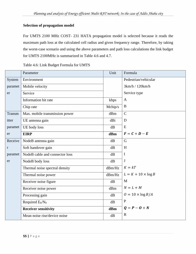
Planning and analysis of Energy efficient Multi-RAT network: In the case of Addis Ababa city
55 | P a g e
Selection of propagation model
For UMTS 2100 MHz COST- 231 HATA propagation model is selected because it reads the
maximum path loss at the calculated cell radius and given frequency range. Therefore, by taking
the worst-case scenario and using the above parameters and path loss calculations the link budget
for UMTS 2100MHz is summarized in Table 4.6 and 4.7.
Table 4.6: Link Budget Formula for UMTS
Parameter Unit Formula
System
paramet
er
Environment Pedestrian/vehicular
3km/h / 120km/h
Service type
A
B
Mobile velocity
Service
Information bit rate kbps
Chip rate Mchip/s
Transm
itter
paramet
er
Max. mobile transmission power dBm C
D
E
𝑭 = 𝑪 + 𝑫 − 𝑬
UE antenna gain dBi
UE body loss dB
EIRP dBm
Receive
r
paramet
er
NodeB antenna gain dB G
H
I
J
𝐾 = 𝑘𝑇
𝐿 = 𝐾 + 10 × log 𝐵
M
𝑁 = 𝐿 + 𝑀
𝑂 = 10 × log 𝐵/𝐴
P
𝑸 = 𝑷 − 𝑶 + 𝑵
R
Soft handover gain dB
NodeB cable and connector loss dB
NodeB body loss dB
Thermal noise spectral density dBm/Hz
Thermal noise power dBm/Hz
Receiver noise figure dB
Receiver noise power dBm
Processing gain dB
Required Eb/N0 dB
Receiver sensitivity dBm
Mean noise rise/device noise dB
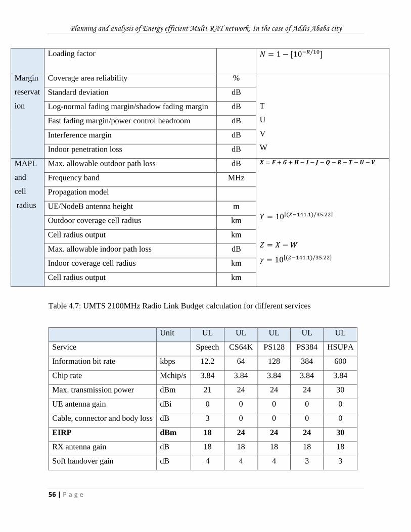
Planning and analysis of Energy efficient Multi-RAT network: In the case of Addis Ababa city
56 | P a g e
Loading factor 𝑁 = 1 − [10−𝑅/10]
Margin
reservat
ion
Coverage area reliability %
T
U
V
W
Standard deviation dB
Log-normal fading margin/shadow fading margin dB
Fast fading margin/power control headroom dB
Interference margin dB
Indoor penetration loss dB
MAPL
and
cell
radius
Max. allowable outdoor path loss dB 𝑿 = 𝑭 + 𝑮 + 𝑯 − 𝑰 − 𝑱 − 𝑸 − 𝑹 − 𝑻 − 𝑼 − 𝑽
𝑌 = 10[(𝑋−141.1)/35.22]
𝑍 = 𝑋 − 𝑊
𝛾 = 10[(𝑍−141.1)/35.22]
Frequency band MHz
Propagation model
UE/NodeB antenna height m
Outdoor coverage cell radius km
Cell radius output km
Max. allowable indoor path loss dB
Indoor coverage cell radius km
Cell radius output km
Table 4.7: UMTS 2100MHz Radio Link Budget calculation for different services
Unit UL UL UL UL UL
Service Speech CS64K PS128 PS384 HSUPA
Information bit rate kbps 12.2 64 128 384 600
Chip rate Mchip/s 3.84 3.84 3.84 3.84 3.84
Max. transmission power dBm 21 24 24 24 30
UE antenna gain dBi 0 0 0 0 0
Cable, connector and body loss dB 3 0 0 0 0
EIRP dBm 18 24 24 24 30
RX antenna gain dB 18 18 18 18 18
Soft handover gain dB 4 4 4 3 3
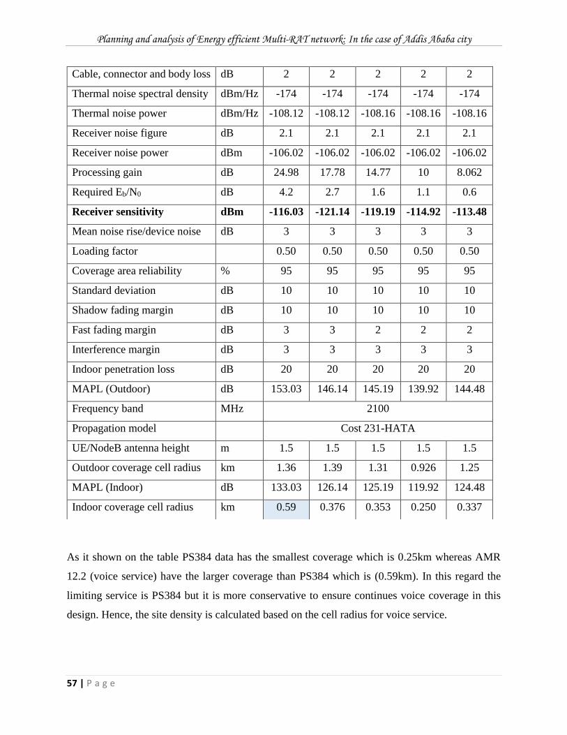
Planning and analysis of Energy efficient Multi-RAT network: In the case of Addis Ababa city
57 | P a g e
As it shown on the table PS384 data has the smallest coverage which is 0.25km whereas AMR
12.2 (voice service) have the larger coverage than PS384 which is (0.59km). In this regard the
limiting service is PS384 but it is more conservative to ensure continues voice coverage in this
design. Hence, the site density is calculated based on the cell radius for voice service.
Cable, connector and body loss dB 2 2 2 2 2
Thermal noise spectral density dBm/Hz -174 -174 -174 -174 -174
Thermal noise power dBm/Hz -108.12 -108.12 -108.16 -108.16 -108.16
Receiver noise figure dB 2.1 2.1 2.1 2.1 2.1
Receiver noise power dBm -106.02 -106.02 -106.02 -106.02 -106.02
Processing gain dB 24.98 17.78 14.77 10 8.062
Required Eb/N0 dB 4.2 2.7 1.6 1.1 0.6
Receiver sensitivity dBm -116.03 -121.14 -119.19 -114.92 -113.48
Mean noise rise/device noise dB 3 3 3 3 3
Loading factor 0.50 0.50 0.50 0.50 0.50
Coverage area reliability % 95 95 95 95 95
Standard deviation dB 10 10 10 10 10
Shadow fading margin dB 10 10 10 10 10
Fast fading margin dB 3 3 2 2 2
Interference margin dB 3 3 3 3 3
Indoor penetration loss dB 20 20 20 20 20
MAPL (Outdoor) dB 153.03 146.14 145.19 139.92 144.48
Frequency band MHz 2100
Propagation model Cost 231-HATA
UE/NodeB antenna height m 1.5 1.5 1.5 1.5 1.5
Outdoor coverage cell radius km 1.36 1.39 1.31 0.926 1.25
MAPL (Indoor) dB 133.03 126.14 125.19 119.92 124.48
Indoor coverage cell radius km 0.59 0.376 0.353 0.250 0.337
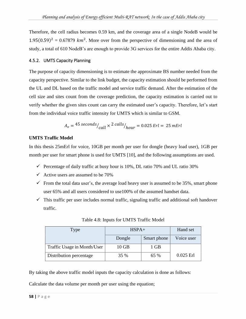
Planning and analysis of Energy efficient Multi-RAT network: In the case of Addis Ababa city
58 | P a g e
Therefore, the cell radius becomes 0.59 km, and the coverage area of a single NodeB would be
1.95(0.59)2 = 0.67879 𝑘𝑚2. More over from the perspective of dimensioning and the area of
study, a total of 610 NodeB’s are enough to provide 3G services for the entire Addis Ababa city.
4.5.2. UMTS Capacity Planning
The purpose of capacity dimensioning is to estimate the approximate BS number needed from the
capacity perspective. Similar to the link budget, the capacity estimation should be performed from
the UL and DL based on the traffic model and service traffic demand. After the estimation of the
cell size and sites count from the coverage prediction, the capacity estimation is carried out to
verify whether the given sites count can carry the estimated user’s capacity. Therefore, let’s start
from the individual voice traffic intensity for UMTS which is similar to GSM.
𝐴𝑣 = 45 𝑠𝑒𝑐𝑜𝑛𝑑𝑠𝑐𝑎𝑙𝑙⁄ × 2 𝑐𝑎𝑙𝑙𝑠
ℎ𝑜𝑢𝑟⁄ = 0.025 𝐸𝑟𝑙 = 25 𝑚𝐸𝑟𝑙
UMTS Traffic Model
In this thesis 25mErl for voice, 10GB per month per user for dongle (heavy load user), 1GB per
month per user for smart phone is used for UMTS [10], and the following assumptions are used.
✓ Percentage of daily traffic at busy hour is 10%, DL ratio 70% and UL ratio 30%
✓ Active users are assumed to be 70%
✓ From the total data user’s, the average load heavy user is assumed to be 35%, smart phone
user 65% and all users considered to use100% of the assumed handset data.
✓ This traffic per user includes normal traffic, signaling traffic and additional soft handover
traffic.
Table 4.8: Inputs for UMTS Traffic Model
Type HSPA+ Hand set
Dongle Smart phone Voice user
Traffic Usage in Month/User 10 GB 1 GB
0.025 Erl Distribution percentage 35 % 65 %
By taking the above traffic model inputs the capacity calculation is done as follows:
Calculate the data volume per month per user using the equation;
Planning and analysis of Energy efficient Multi-RAT network: In the case of Addis Ababa city
59 | P a g e
𝐷𝑎𝑡𝑎 𝑣𝑜𝑙𝑢𝑚𝑒/𝑚𝑜𝑛𝑡ℎ/𝑢𝑠𝑒𝑟 = ∑(𝑇𝑟𝑎𝑓𝑓𝑖𝑐 𝑢𝑠𝑎𝑔𝑒 𝑖𝑛 𝑚𝑜𝑛𝑡ℎ/𝑢𝑠𝑒𝑟 ×
𝑠𝑢𝑏𝑠𝑐𝑟𝑖𝑏𝑒𝑟𝑠 𝑑𝑖𝑠𝑡𝑟𝑖𝑏𝑢𝑡𝑖𝑜𝑛 %) (4.26)
= 10𝐺𝐵 × 35% + 1𝐺𝐵 × 65% = 4.15𝐺𝐵
Calculate HSPA throughput per user as:
𝐻𝑆𝑃𝐴 𝑝𝑒𝑟 𝑑𝑎𝑦 𝑝𝑒𝑟 𝑢𝑠𝑒𝑟 =𝐷𝑎𝑡𝑎 𝑣𝑜𝑙𝑢𝑚𝑒 𝑚𝑜𝑛𝑡ℎ 𝑢𝑠𝑒𝑟⁄⁄ ×8×1024×1024
30×24×3600 = 13.43 𝑘𝑏𝑝𝑠 (4.27)
Since the busy hour ratio is 10 %, HSPA/day/user @BH throughput value becomes
𝐻𝑆𝑃𝐴 𝑝𝑒𝑟 𝑑𝑎𝑦 𝑝𝑒𝑟 𝑢𝑠𝑒𝑟𝐵𝐻 = 13.43𝑘𝑏𝑝𝑠 × 0.1 = 1.343 𝑘𝑏𝑝𝑠
Calculate HSPA throughput per day per user @BH per active user by using the assumption of
active user ratio which is 70 %
𝐻𝑆𝑃𝐴 𝑝𝑒𝑟 𝑑𝑎𝑦 𝑝𝑒𝑟 𝑢𝑠𝑒𝑟 @𝐵𝐻 𝑝𝑒𝑟 𝑎𝑐𝑡𝑖𝑣𝑒 𝑢𝑠𝑒𝑟 = 1.343 × 0.7 = 0.940𝑘𝑏𝑝𝑠
Since the calculated individual voice traffic intensity is in Erlang, it should be converted to kbps
and calculate the total supported throughput
𝑉𝑜𝑙𝑢𝑚𝑒 𝑝𝑒𝑟 𝑢𝑠𝑒𝑟 @𝐵𝐻 = 𝐸𝑟𝑙 𝑝𝑒𝑟 𝑢𝑠𝑒𝑟@𝐵𝐻 × 3600 × 𝐴𝐹 × 𝑠𝑒𝑟𝑣𝑖𝑐𝑒 𝑟𝑎𝑡𝑒 (4.28)
Where, AF = Activity Factor with the value of 0.67, 1 and 0.9 for AMR12.2, CS64 and PS service
respectively. The value of service rate is also 12.2kbps and 64kbps for AMR12.2 and CS64
respectively.
𝑉𝑜𝑙𝑢𝑚𝑒 𝑝𝑒𝑟 𝑢𝑠𝑒𝑟 @𝐵𝐻 = 0.025 × 3600 × 1 × 64 = 5.76 𝑘𝑏𝑝𝑠
Therefore, we can calculate HSPA throughput per user for DL and UL using the assumption 70 %
DL ratio and 30 % UL ratio as:
𝐻𝑆𝑈𝑃𝐴 𝑡ℎ𝑟𝑜𝑢𝑔ℎ𝑝𝑢𝑡 𝑢𝑠𝑒𝑟⁄
= 𝑉𝑜𝑙𝑢𝑚𝑒 𝑝𝑒𝑟 𝑢𝑠𝑒𝑟 @𝐵𝐻 + 𝐻𝑆𝑃𝐴/𝑑𝑎𝑦/𝑢𝑠𝑒𝑟 @𝐵𝐻/𝑎𝑐𝑡𝑖𝑣𝑒 𝑢𝑠𝑒𝑟 × 0.3
= 5.76 + 0.94 × 0.3 = 6.042 𝑘𝑏𝑝𝑠
(4.29)
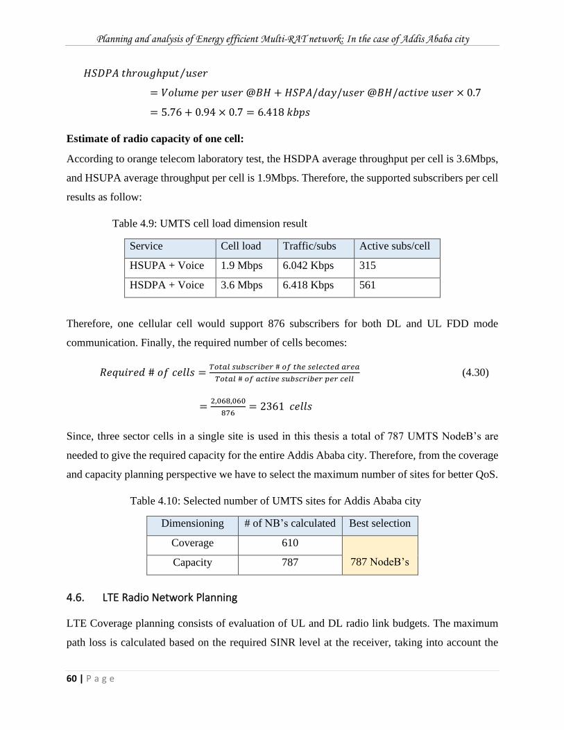
Planning and analysis of Energy efficient Multi-RAT network: In the case of Addis Ababa city
60 | P a g e
𝐻𝑆𝐷𝑃𝐴 𝑡ℎ𝑟𝑜𝑢𝑔ℎ𝑝𝑢𝑡 𝑢𝑠𝑒𝑟⁄
= 𝑉𝑜𝑙𝑢𝑚𝑒 𝑝𝑒𝑟 𝑢𝑠𝑒𝑟 @𝐵𝐻 + 𝐻𝑆𝑃𝐴/𝑑𝑎𝑦/𝑢𝑠𝑒𝑟 @𝐵𝐻/𝑎𝑐𝑡𝑖𝑣𝑒 𝑢𝑠𝑒𝑟 × 0.7
= 5.76 + 0.94 × 0.7 = 6.418 𝑘𝑏𝑝𝑠
Estimate of radio capacity of one cell:
According to orange telecom laboratory test, the HSDPA average throughput per cell is 3.6Mbps,
and HSUPA average throughput per cell is 1.9Mbps. Therefore, the supported subscribers per cell
results as follow:
Table 4.9: UMTS cell load dimension result
Service Cell load Traffic/subs Active subs/cell
HSUPA + Voice 1.9 Mbps 6.042 Kbps 315
HSDPA + Voice 3.6 Mbps 6.418 Kbps 561
Therefore, one cellular cell would support 876 subscribers for both DL and UL FDD mode
communication. Finally, the required number of cells becomes:
𝑅𝑒𝑞𝑢𝑖𝑟𝑒𝑑 # 𝑜𝑓 𝑐𝑒𝑙𝑙𝑠 =𝑇𝑜𝑡𝑎𝑙 𝑠𝑢𝑏𝑠𝑐𝑟𝑖𝑏𝑒𝑟 # 𝑜𝑓 𝑡ℎ𝑒 𝑠𝑒𝑙𝑒𝑐𝑡𝑒𝑑 𝑎𝑟𝑒𝑎
𝑇𝑜𝑡𝑎𝑙 # 𝑜𝑓 𝑎𝑐𝑡𝑖𝑣𝑒 𝑠𝑢𝑏𝑠𝑐𝑟𝑖𝑏𝑒𝑟 𝑝𝑒𝑟 𝑐𝑒𝑙𝑙 (4.30)
=2,068,060
876= 2361 𝑐𝑒𝑙𝑙𝑠
Since, three sector cells in a single site is used in this thesis a total of 787 UMTS NodeB’s are
needed to give the required capacity for the entire Addis Ababa city. Therefore, from the coverage
and capacity planning perspective we have to select the maximum number of sites for better QoS.
Table 4.10: Selected number of UMTS sites for Addis Ababa city
Dimensioning # of NB’s calculated Best selection
Coverage 610
787 NodeB’s Capacity 787
4.6. LTE Radio Network Planning
LTE Coverage planning consists of evaluation of UL and DL radio link budgets. The maximum
path loss is calculated based on the required SINR level at the receiver, taking into account the
Planning and analysis of Energy efficient Multi-RAT network: In the case of Addis Ababa city
61 | P a g e
extent of the interference caused by traffic. The radius of the cell is determined by considering
minimum of the maximum path losses in UL and DL directions and using a propagation model
appropriate to the deployment area. Radio link budget is that the most outstanding element of
coverage planning exercise as usual.
Capacity planning gives an estimate of the resources needed for supporting a specified offered
traffic with a certain level of QoS (e.g. throughput or blocking probability). Theoretical capacity
of the network is limited by the number of eNB installed in the network. Cell capacity in LTE is
impacted by several factors, which includes interference level, packet scheduler implementation
and supported modulation and coding schemes.
Link Budget offers the maximum allowed path loss and therefore the maximum vary of the cell,
whereas coverage planning takes into account the interference by providing a suitable model. LTE
conjointly exhibits soft capacity like 3G systems. Therefore, the rise in interference and noise by
increasing the number of users can decrease the cell coverage forcing the cell radius to become
smaller. In LTE, the most indicator of capacity is SINR distribution within the cell [25, 23, 17,
49].
4.6.1. Factors Affecting the LTE planning
LTE is design to support a single channel reuse pattern without resorting to tricks like spread
spectrum. When considering capacity planning, or general system planning, the followings are
some of the factors that should be taken in to account [19, 55].
Frequency Band: The chosen spectrum can have huge impact on the planning process since the
nominal radius of the LTE radio cell is depends on the frequency of operation. Generally speaking,
the lower the frequency, the larger the radio cell, the better the building penetration, the less
sensitive to atmospheric issues the system becomes.
Allocated Spectrum and Channel Bandwidth: The bands are regulated in terms of the allowed
operational BW. This is driven for the most part by the number of accessible spectrums in every
of the bands. Some of the bands do not allow the use of the narrow channels, while others prohibit
the use of the larger bandwidths. The amount of allocated spectrum can affect the overall network
capacity and also the individual sector capacity.
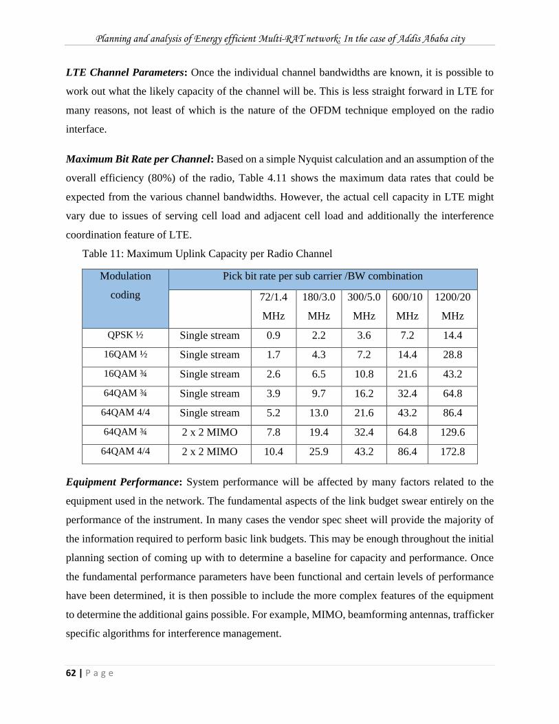
Planning and analysis of Energy efficient Multi-RAT network: In the case of Addis Ababa city
62 | P a g e
LTE Channel Parameters: Once the individual channel bandwidths are known, it is possible to
work out what the likely capacity of the channel will be. This is less straight forward in LTE for
many reasons, not least of which is the nature of the OFDM technique employed on the radio
interface.
Maximum Bit Rate per Channel: Based on a simple Nyquist calculation and an assumption of the
overall efficiency (80%) of the radio, Table 4.11 shows the maximum data rates that could be
expected from the various channel bandwidths. However, the actual cell capacity in LTE might
vary due to issues of serving cell load and adjacent cell load and additionally the interference
coordination feature of LTE.
Table 11: Maximum Uplink Capacity per Radio Channel
Modulation
coding
Pick bit rate per sub carrier /BW combination
72/1.4
MHz
180/3.0
MHz
300/5.0
MHz
600/10
MHz
1200/20
MHz
QPSK ½ Single stream 0.9 2.2 3.6 7.2 14.4
16QAM ½ Single stream 1.7 4.3 7.2 14.4 28.8
16QAM ¾ Single stream 2.6 6.5 10.8 21.6 43.2
64QAM ¾ Single stream 3.9 9.7 16.2 32.4 64.8
64QAM 4/4 Single stream 5.2 13.0 21.6 43.2 86.4
64QAM ¾ 2 x 2 MIMO 7.8 19.4 32.4 64.8 129.6
64QAM 4/4 2 x 2 MIMO 10.4 25.9 43.2 86.4 172.8
Equipment Performance: System performance will be affected by many factors related to the
equipment used in the network. The fundamental aspects of the link budget swear entirely on the
performance of the instrument. In many cases the vendor spec sheet will provide the majority of
the information required to perform basic link budgets. This may be enough throughout the initial
planning section of coming up with to determine a baseline for capacity and performance. Once
the fundamental performance parameters have been functional and certain levels of performance
have been determined, it is then possible to include the more complex features of the equipment
to determine the additional gains possible. For example, MIMO, beamforming antennas, trafficker
specific algorithms for interference management.
Planning and analysis of Energy efficient Multi-RAT network: In the case of Addis Ababa city
63 | P a g e
Population Demographic: The market research administration throughout the planning period can
make use of the area classifications mentioned on top of and conjointly the population
demographics. Analysis of typical demographic information can enable the planner to work out
doubtless range of subscribers in a very given location at totally different times of the day.
Data Throughput: Data rates available to mobile subscriber have been increasing steadily over
the last few years and will continue to do so, promoted by the additional capability of LTE.
However, the capacity of the radio sector is not unlimited and careful throughput must be applied
to the type of service sold to the subscriber. Of course, the best way to manage the traffic load in
the network is to support different service levels and manage the flow data using QoS mechanisms.
4.6.2. Dimensioning of LTE Network
Dimensioning is the initial phase of network planning as we discussed at the beginning. It provides
the primary estimate of the network part and their capacity. The purpose of dimensioning is to
estimate the needed number of radio BS’s required to support a specified traffic load in a specific
area with specific service to the cell edge users as we know.
4.6.2.1. LTE network dimensioning inputs
LTE dimensioning inputs are generally divided into 3 categories: Traffic, coverage and capacity
inputs. Traffic related inputs include average cell throughput, number of subscribers and demand
traffic for each user in busy hour. These parameters are the client needs to produce a particular
level of service. These inputs directly translate into QoS parameters. Besides this, cell edge
coverage probability is used in the dimensioning tool to determine the cell radius and thus the site.
Radio link budget is of central importance to coverage planning in LTE. Its inputs include
transmitter power, transmitter and receiver antenna systems, configuration antennas used,
conventional system gains and losses, cell loading that effect the value of interference margin and
propagation models. LTE can operate in conventional frequency bands of 900, 1800 and 2100MHz
as well as extended band of 2600MHz. Additionally, channel types (Pedestrian, Vehicular) and
geographical information is needed to start the coverage dimensioning exercise. Geographical
input information consists of area type information (Dense urban, Urban, Suburban, Rural, etc.…)
and its related parameters (penetration loss, shadowing margin, etc.…) and sizes of each area type
to be covered. Furthermore, needed coverage likelihood plays a significant role in determination
Planning and analysis of Energy efficient Multi-RAT network: In the case of Addis Ababa city
64 | P a g e
of cell radius. Even a minor modification in coverage likelihood causes an outsized variation in
cell radius.
Capacity dimensioning inputs provide the requirements, to be met by LTE network dimensioning
exercise. Capacity planning input gives the number of subscribers in the system, their demanded
services and subscriber usage level in the busy hour. Available spectrum and channel BW
employed by the LTE system are vital for LTE capacity planning. Traffic analysis and data rate to
support available services (voice, Data) are used to determine the number of subscribers supported
by a single cell and eventually the cell radius based on capacity evaluation.
4.6.2.2. LTE network dimensioning outputs
LTE dimension outputs are used to estimate the feasibility and cost of the network. These outputs
are further employed in detailed part of network planning. The main output of LTE dimensioning
is the size of the cell. Two values of cell radii are determined, one from coverage evaluation and
second from capacity evaluation. The minimum of the two numbers is taken as the final output.
Cell radius is then used to calculate the required number of eNB’s. Assuming a hexagonal cell
shape, number of sites can be determined by victimization easy pure mathematics. Capacities of
eNBs are obtained from capacity evaluation, along with the number of subscribers supported by
each cell. The input and output parameters of the LTE dimensioning tool is shown in Figure below.
4.6.3. LTE Coverage Planning
For LTE systems, the main goal of coverage planning is to estimate the coverage distance of an
eNB with parameter settings based on actual cell edge coverage requirements in order to meet
network size requirements. The first steps for the initial planning of a cellular network are the
selection of an adequate propagation model for the frequency range and type of region considered
[23].
LTE Link Budget
Coverage planning consists of analysis of DL and UL radio link budgets. The maximum path loss
is calculated based on service throughput defined by the cell edge user that required SINR level at
the receiver. The radius of the cell is determined by considering minimum of the maximum path
Planning and analysis of Energy efficient Multi-RAT network: In the case of Addis Ababa city
65 | P a g e
losses in UL and DL values and using a propagation model appropriate to the deployment area.
Radio Link Budget is that the most main component of coverage planning.
The Link budget considers many factors, such as building penetration loss, feeder loss, antenna
gain, and the interference margin of radio links to calculate all gains and losses that affect the final
cell coverage.
LTE Link budget Parameters
Effective Isotropic Radiated Power (EIRP): is used to express how much transmitted power is
radiated in the desired direction. It takes into account the losses in transmission cables and
connectors and includes the gain of the transmitter antenna as:
𝐸𝐼𝑅𝑃 = 𝑃𝑇𝑥 + 𝐺𝑇𝑥 − ∑ 𝑇𝑜𝑡𝑎𝑙 𝑡𝑟𝑎𝑛𝑠𝑚𝑖𝑠𝑠𝑖𝑜𝑛 𝑙𝑜𝑠𝑠𝑒𝑠 (4.31)
Where, 𝑃𝑇𝑥 is the transmitter power (dBm) and 𝐺𝑇𝑥 is the transmitter antenna gain (dBi)
eNB Output Power: This is one of the main factors that impact the link budget. In the link budget,
46 dBm output power per each branch of the MIMO 2×2 which means 2×40 watt is considered.
UE Maximum Total Transmitter Power: refers to the UE transmit power which depends on the
power class of the UE. Currently only one power class is defined in 3GPP TS 36.101; class 3 with
maximum transmitter power of 23dBm.
eNB Antenna Gain: The antenna gain is proportional to the antenna size, LTE band, and beam
width of the antenna patterns (horizontal and vertical). A large antenna with narrow beam width
provides a high gain while a short antenna with wider beam width provides less gain. The selection
of antenna gains and beam width depends on the clutter type and coverage requirement. The low
gain antenna (15–17dBi) can be used in dense urban and urban clutters while a high gain antenna
(18–20dBi) can be used in rural areas and highways to extend the RF coverage [23, 28, 55].
UE Antenna Gain: Based on the specifications of 3GPP, UE(s) are assumed to have an integral
antenna only with a gain of 0 dBi for each antenna port(s) [23].
Planning and analysis of Energy efficient Multi-RAT network: In the case of Addis Ababa city
66 | P a g e
Signal to interference noise ratio (SINR): SINR is the ratio of the average received modulated
carrier power to the sum of the average co-channel interference power and the noise power from
other sources. The UE is be able to identify new intra-frequency cells and perform the reference
signal received power (RSRP) and the reference signal received quality (RSRQ) measurements of
identified intra-frequency cells without an explicit intra-frequency neighbor list containing
Physical Cell Identity (PCI). SINR values are obtained from the system level simulation result and
it depends on the receiver design. Thus, SINR is a vendor specific parameter.
Noise Figure: It is a key factor to measure the receiver performance. It is defined as the ratio of
the input SINR at the input end to the output SINR at the output end of the receiver. The noise
figure depends on the bandwidth and the eNB capability. A typical value for the noise figure is
between 6 to 8 dB [26].
Thermal Noise: The thermal noise is a loss due to heat and can be formulated as:
𝑁 = 𝑘𝐵𝑇 (4.32)
Where,
✓ 𝑘 𝑖𝑠 𝐵𝑜𝑙𝑡𝑧𝑚𝑎𝑛 𝑐𝑜𝑛𝑠𝑡𝑎𝑛𝑡 = 1.38 × 10⁻²³ 𝐽 𝐾⁄
✓ 𝐵 𝑖𝑠 𝑏𝑎𝑛𝑑𝑤𝑖𝑑𝑡ℎ 𝑜𝑓 𝑡ℎ𝑒 𝑐ℎ𝑎𝑛𝑛𝑒𝑙 = 20𝑀𝐻𝑧
✓ 𝑇 𝑖𝑠 𝑎𝑏𝑠𝑜𝑙𝑢𝑡𝑒 𝑡𝑒𝑚𝑝𝑒𝑟𝑎𝑡𝑢𝑟𝑒 𝑎𝑡 290𝑘
Receiver sensitivity: The eNB receiver sensitivity is the signal level/threshold at which the RF
signal can be detected with a certain quality.
𝑅𝑒𝑐𝑒𝑖𝑣𝑒𝑟 𝑠𝑒𝑛𝑠𝑖𝑡𝑖𝑣𝑖𝑡𝑦 = 𝑁𝑜𝑖𝑠𝑒 𝑓𝑖𝑔𝑢𝑟𝑒 + 𝑆𝐼𝑁𝑅 + 𝑇ℎ𝑒𝑟𝑚𝑎𝑙 𝑁𝑜𝑖𝑠𝑒 (4.33)
Maximum Path Loss (LMAX): Maximum allowable attenuation of the radio wave traversing the air
interface excludes clutter data (e.g. penetration loses propagation data) is expresses as:
𝐿𝑀𝐴𝑋 = 𝑃𝑇𝑥 + 𝐺𝑇𝑥 − 𝐿𝑇𝑥 − 𝑆𝑅 + 𝐺𝑅𝑥 − 𝐿𝑅𝑥 + 𝐺𝑑𝑖𝑣 (4.34)
Where, 𝐿𝑀𝐴𝑋 is the maximum DL/UL loss (dB), 𝑃𝑇𝑥 is the transmitter power (dBm), 𝐺𝑇𝑥 /𝐺𝑅𝑥 is
the transmitting/receiving antenna gain (dBi), 𝐿𝑇𝑥 /𝐿𝑅𝑥 is the transmitter/receiver loss (dB), 𝑆𝑅 is
the receiver sensitivity (dBm) and 𝐺𝑑𝑖𝑣 is the diversity gain (dB).
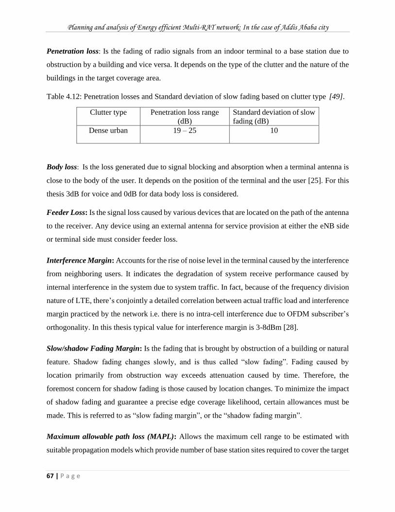
Planning and analysis of Energy efficient Multi-RAT network: In the case of Addis Ababa city
67 | P a g e
Penetration loss: Is the fading of radio signals from an indoor terminal to a base station due to
obstruction by a building and vice versa. It depends on the type of the clutter and the nature of the
buildings in the target coverage area.
Table 4.12: Penetration losses and Standard deviation of slow fading based on clutter type [49].
Clutter type Penetration loss range
(dB) Standard deviation of slow
fading (dB)
Dense urban 19 – 25
10
Body loss: Is the loss generated due to signal blocking and absorption when a terminal antenna is
close to the body of the user. It depends on the position of the terminal and the user [25]. For this
thesis 3dB for voice and 0dB for data body loss is considered.
Feeder Loss: Is the signal loss caused by various devices that are located on the path of the antenna
to the receiver. Any device using an external antenna for service provision at either the eNB side
or terminal side must consider feeder loss.
Interference Margin: Accounts for the rise of noise level in the terminal caused by the interference
from neighboring users. It indicates the degradation of system receive performance caused by
internal interference in the system due to system traffic. In fact, because of the frequency division
nature of LTE, there’s conjointly a detailed correlation between actual traffic load and interference
margin practiced by the network i.e. there is no intra-cell interference due to OFDM subscriber’s
orthogonality. In this thesis typical value for interference margin is 3-8dBm [28].
Slow/shadow Fading Margin: Is the fading that is brought by obstruction of a building or natural
feature. Shadow fading changes slowly, and is thus called “slow fading”. Fading caused by
location primarily from obstruction way exceeds attenuation caused by time. Therefore, the
foremost concern for shadow fading is those caused by location changes. To minimize the impact
of shadow fading and guarantee a precise edge coverage likelihood, certain allowances must be
made. This is referred to as “slow fading margin”, or the “shadow fading margin”.
Maximum allowable path loss (MAPL): Allows the maximum cell range to be estimated with
suitable propagation models which provide number of base station sites required to cover the target
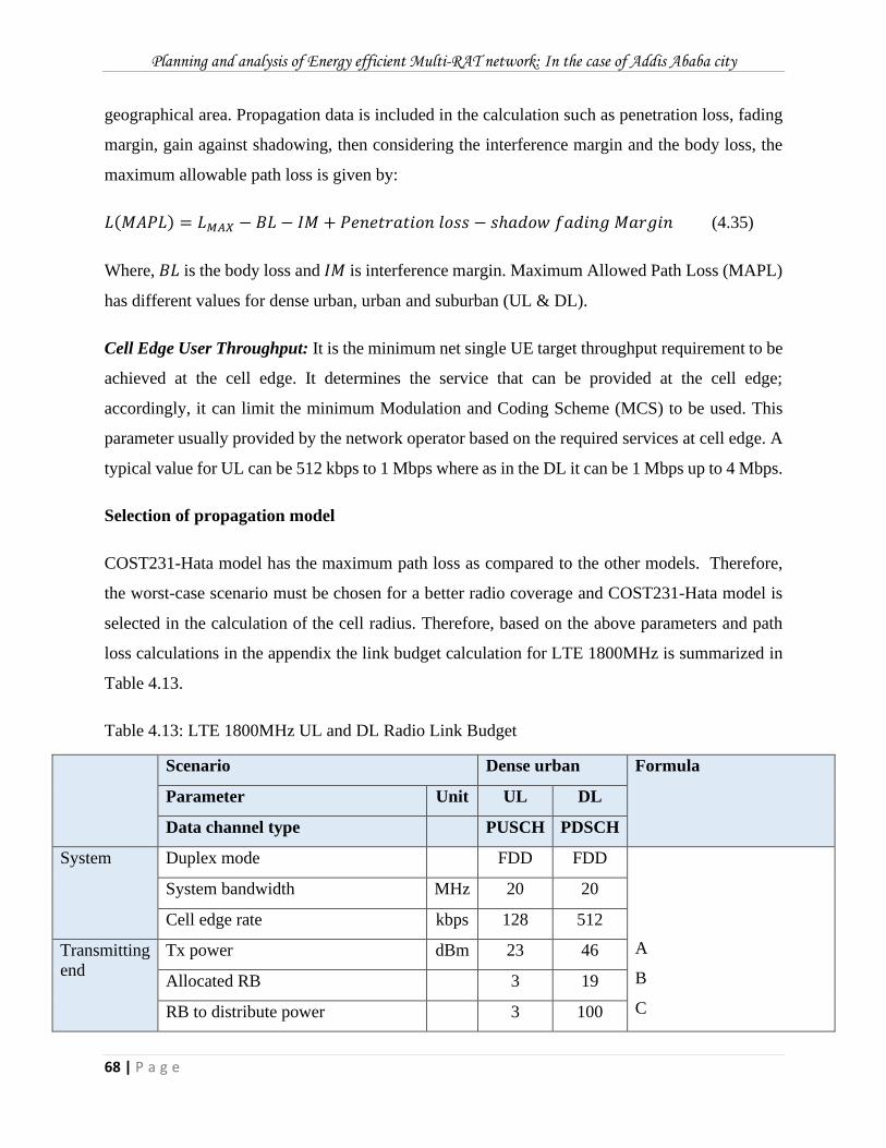
Planning and analysis of Energy efficient Multi-RAT network: In the case of Addis Ababa city
68 | P a g e
geographical area. Propagation data is included in the calculation such as penetration loss, fading
margin, gain against shadowing, then considering the interference margin and the body loss, the
maximum allowable path loss is given by:
𝐿(𝑀𝐴𝑃𝐿) = 𝐿𝑀𝐴𝑋 − 𝐵𝐿 − 𝐼𝑀 + 𝑃𝑒𝑛𝑒𝑡𝑟𝑎𝑡𝑖𝑜𝑛 𝑙𝑜𝑠𝑠 − 𝑠ℎ𝑎𝑑𝑜𝑤 𝑓𝑎𝑑𝑖𝑛𝑔 𝑀𝑎𝑟𝑔𝑖𝑛 (4.35)
Where, 𝐵𝐿 is the body loss and 𝐼𝑀 is interference margin. Maximum Allowed Path Loss (MAPL)
has different values for dense urban, urban and suburban (UL & DL).
Cell Edge User Throughput: It is the minimum net single UE target throughput requirement to be
achieved at the cell edge. It determines the service that can be provided at the cell edge;
accordingly, it can limit the minimum Modulation and Coding Scheme (MCS) to be used. This
parameter usually provided by the network operator based on the required services at cell edge. A
typical value for UL can be 512 kbps to 1 Mbps where as in the DL it can be 1 Mbps up to 4 Mbps.
Selection of propagation model
COST231-Hata model has the maximum path loss as compared to the other models. Therefore,
the worst-case scenario must be chosen for a better radio coverage and COST231-Hata model is
selected in the calculation of the cell radius. Therefore, based on the above parameters and path
loss calculations in the appendix the link budget calculation for LTE 1800MHz is summarized in
Table 4.13.
Table 4.13: LTE 1800MHz UL and DL Radio Link Budget Scenario Dense urban Formula
Parameter Unit UL DL
Data channel type PUSCH PDSCH
System Duplex mode FDD FDD
A
B
C
System bandwidth MHz 20 20
Cell edge rate kbps 128 512
Transmitting
end
Tx power dBm 23 46
Allocated RB 3 19
RB to distribute power 3 100
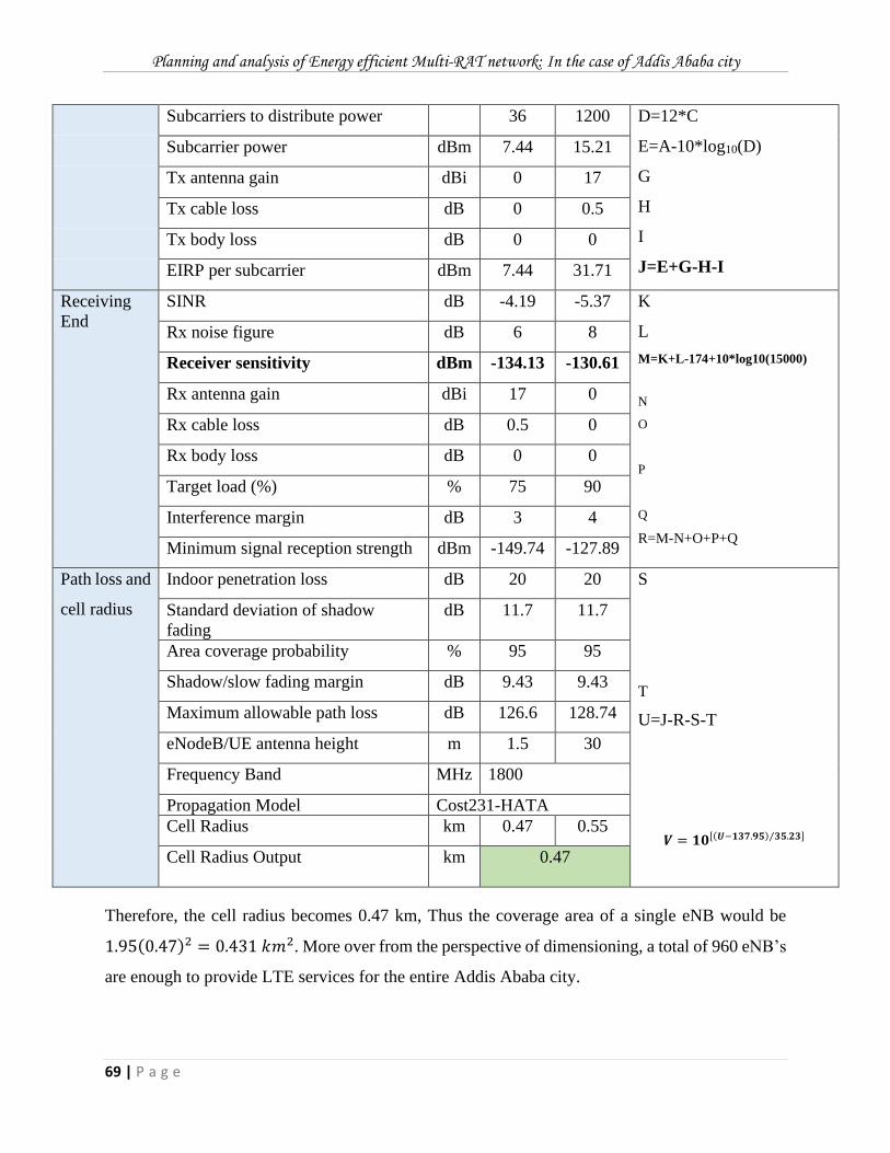
Planning and analysis of Energy efficient Multi-RAT network: In the case of Addis Ababa city
69 | P a g e
Subcarriers to distribute power 36 1200 D=12*C
E=A-10*log10(D)
G
H
I
J=E+G-H-I
Subcarrier power dBm 7.44 15.21
Tx antenna gain dBi 0 17
Tx cable loss dB 0 0.5
Tx body loss dB 0 0
EIRP per subcarrier dBm 7.44 31.71
Receiving
End
SINR dB -4.19 -5.37 K
L
M=K+L-174+10*log10(15000)
N
O
P
Q
R=M-N+O+P+Q
Rx noise figure dB 6 8
Receiver sensitivity dBm -134.13 -130.61
Rx antenna gain dBi 17 0
Rx cable loss dB 0.5 0
Rx body loss dB 0 0
Target load (%) % 75 90
Interference margin dB 3 4
Minimum signal reception strength dBm -149.74 -127.89
Path loss and
cell radius
Indoor penetration loss dB 20 20 S
T
U=J-R-S-T
𝑽 = 𝟏𝟎[(𝑼−𝟏𝟑𝟕.𝟗𝟓) 𝟑𝟓.𝟐𝟑⁄ ]
Standard deviation of shadow
fading
dB 11.7 11.7
Area coverage probability % 95 95
Shadow/slow fading margin dB 9.43 9.43
Maximum allowable path loss dB 126.6 128.74
eNodeB/UE antenna height m 1.5 30
Frequency Band MHz 1800
Propagation Model Cost231-HATA
Cell Radius km 0.47 0.55
Cell Radius Output km 0.47
Therefore, the cell radius becomes 0.47 km, Thus the coverage area of a single eNB would be
1.95(0.47)2 = 0.431 𝑘𝑚2. More over from the perspective of dimensioning, a total of 960 eNB’s
are enough to provide LTE services for the entire Addis Ababa city.
Planning and analysis of Energy efficient Multi-RAT network: In the case of Addis Ababa city
70 | P a g e
4.6.4. LTE Capacity Planning
Theoretical capacity of the network is limited by the number of eNBs installed in the network. In
LTE, the main indicator of capacity is the SINR distribution in the cell. The SINR distribution may
be directly mapped to the system capacity (data rate). Unlike thermal noise which may be
overcome by increasing SINR, co-channel interference can’t be countered by merely increasing
the carrier power of a transmitter. This is because an increase in carrier transmission power will
also increase the interference to the neighboring co-channel cells. Another type of interference in
LTE networks is adjacent channel interference which results from imperfect receiver filters and
allow nearby frequencies to interfere with the used frequency channel.
The subscriber density and subscriber traffic profile are the main requirements for capacity
dimensioning. The dimensioning method finds the maximum capacity that the target cell can
sustain momentarily, given the system load in the surrounding cells. It is improbable that all cells
in a system are fully loaded at the same time, as observed in real networks of different technologies
[23, 25]. Available spectrum and channel BW utilized by the LTE system also are vital for LTE
capacity planning.
Generally, the following steps are procedures for LTE Capacity Planning.
✓ Traffic model analysis: Specific customer requirements
✓ Throughput per subscriber: can be calculated by using traffic model and assumptions
✓ Network throughput per site: determined as three times of the sector throughput at BH.
✓ Number of subscribers per site: can be calculated as throughput per site / throughput per
user.
✓ Number of sites: Equals to total number of users / number of users per site
The daily traffic can be estimated as a percentage of the busy hour traffic in order to guarantee low
delays and reasonably good data rates. In this thesis design 10% of the daily traffic is assumed as
the busy hour traffic. Generally, the main purpose of traffic model is to describe the average
subscriber behavior during the most loaded day period (Busy Hour) and the capacity of site should
be based on busy hour as the traffic is not equally distributed during 24 hours [19].
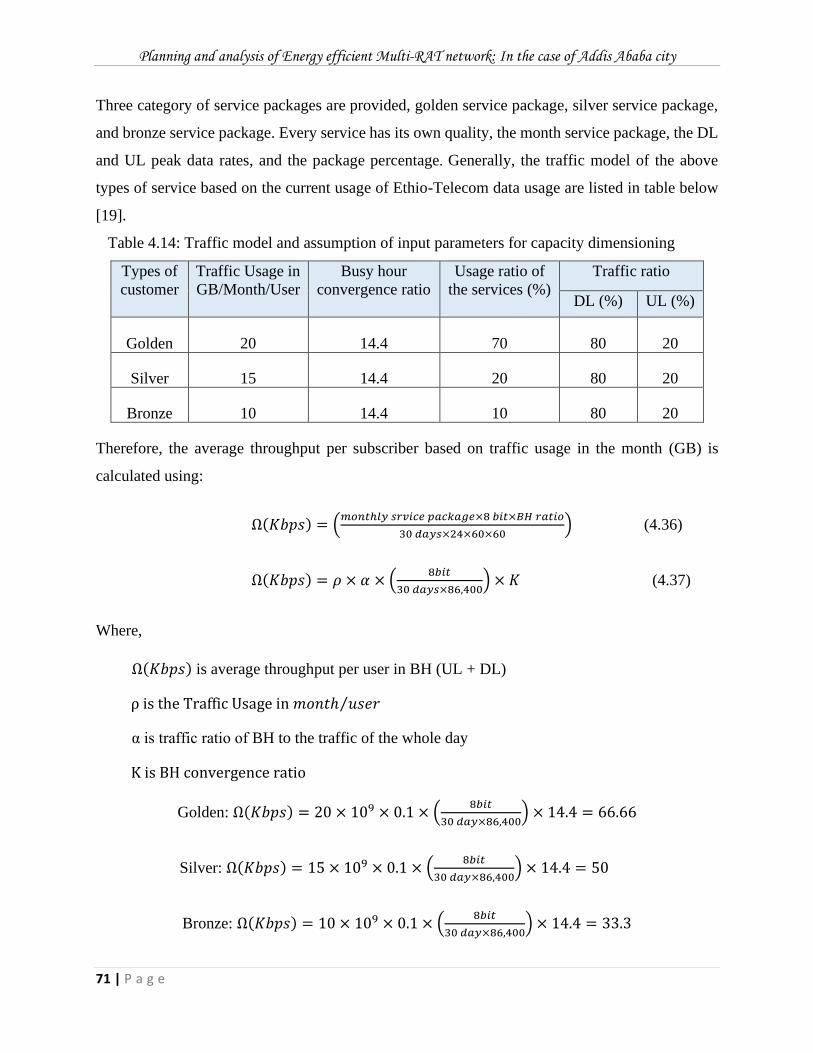
Planning and analysis of Energy efficient Multi-RAT network: In the case of Addis Ababa city
71 | P a g e
Three category of service packages are provided, golden service package, silver service package,
and bronze service package. Every service has its own quality, the month service package, the DL
and UL peak data rates, and the package percentage. Generally, the traffic model of the above
types of service based on the current usage of Ethio-Telecom data usage are listed in table below
[19].
Table 4.14: Traffic model and assumption of input parameters for capacity dimensioning Types of
customer Traffic Usage in
GB/Month/User Busy hour
convergence ratio Usage ratio of
the services (%) Traffic ratio
DL (%) UL (%)
Golden 20 14.4 70 80 20
Silver 15 14.4 20 80 20
Bronze 10 14.4 10 80 20
Therefore, the average throughput per subscriber based on traffic usage in the month (GB) is
calculated using:
Ω(𝐾𝑏𝑝𝑠) = (𝑚𝑜𝑛𝑡ℎ𝑙𝑦 𝑠𝑟𝑣𝑖𝑐𝑒 𝑝𝑎𝑐𝑘𝑎𝑔𝑒×8 𝑏𝑖𝑡×𝐵𝐻 𝑟𝑎𝑡𝑖𝑜
30 𝑑𝑎𝑦𝑠×24×60×60) (4.36)
Ω(𝐾𝑏𝑝𝑠) = 𝜌 × 𝛼 × (8𝑏𝑖𝑡
30 𝑑𝑎𝑦𝑠×86,400) × 𝐾 (4.37)
Where,
Ω(𝐾𝑏𝑝𝑠) is average throughput per user in BH (UL + DL)
ρ is the Traffic Usage in 𝑚𝑜𝑛𝑡ℎ 𝑢𝑠𝑒𝑟⁄
α is traffic ratio of BH to the traffic of the whole day
K is BH convergence ratio
Golden: Ω(𝐾𝑏𝑝𝑠) = 20 × 109 × 0.1 × (8𝑏𝑖𝑡
30 𝑑𝑎𝑦×86,400) × 14.4 = 66.66
Silver: Ω(𝐾𝑏𝑝𝑠) = 15 × 109 × 0.1 × (8𝑏𝑖𝑡
30 𝑑𝑎𝑦×86,400) × 14.4 = 50
Bronze: Ω(𝐾𝑏𝑝𝑠) = 10 × 109 × 0.1 × (8𝑏𝑖𝑡
30 𝑑𝑎𝑦×86,400) × 14.4 = 33.3
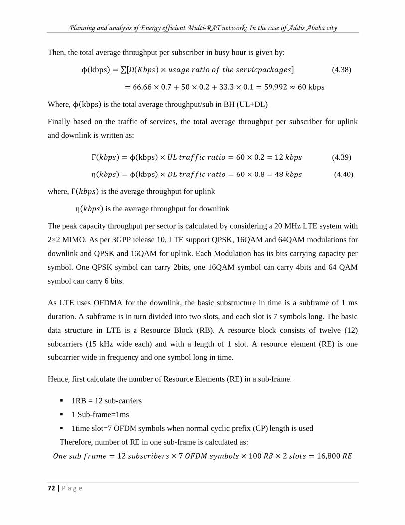
Planning and analysis of Energy efficient Multi-RAT network: In the case of Addis Ababa city
72 | P a g e
Then, the total average throughput per subscriber in busy hour is given by:
ϕ(kbps) = ∑[Ω(𝐾𝑏𝑝𝑠) × 𝑢𝑠𝑎𝑔𝑒 𝑟𝑎𝑡𝑖𝑜 𝑜𝑓 𝑡ℎ𝑒 𝑠𝑒𝑟𝑣𝑖𝑐𝑝𝑎𝑐𝑘𝑎𝑔𝑒𝑠] (4.38)
= 66.66 × 0.7 + 50 × 0.2 + 33.3 × 0.1 = 59.992 ≈ 60 kbps
Where, ϕ(kbps) is the total average throughput/sub in BH (UL+DL)
Finally based on the traffic of services, the total average throughput per subscriber for uplink
and downlink is written as:
Γ(𝑘𝑏𝑝𝑠) = ϕ(kbps) × 𝑈𝐿 𝑡𝑟𝑎𝑓𝑓𝑖𝑐 𝑟𝑎𝑡𝑖𝑜 = 60 × 0.2 = 12 𝑘𝑏𝑝𝑠 (4.39)
η(𝑘𝑏𝑝𝑠) = ϕ(kbps) × 𝐷𝐿 𝑡𝑟𝑎𝑓𝑓𝑖𝑐 𝑟𝑎𝑡𝑖𝑜 = 60 × 0.8 = 48 𝑘𝑏𝑝𝑠 (4.40)
where, Γ(𝑘𝑏𝑝𝑠) is the average throughput for uplink
η(𝑘𝑏𝑝𝑠) is the average throughput for downlink
The peak capacity throughput per sector is calculated by considering a 20 MHz LTE system with
2×2 MIMO. As per 3GPP release 10, LTE support QPSK, 16QAM and 64QAM modulations for
downlink and QPSK and 16QAM for uplink. Each Modulation has its bits carrying capacity per
symbol. One QPSK symbol can carry 2bits, one 16QAM symbol can carry 4bits and 64 QAM
symbol can carry 6 bits.
As LTE uses OFDMA for the downlink, the basic substructure in time is a subframe of 1 ms
duration. A subframe is in turn divided into two slots, and each slot is 7 symbols long. The basic
data structure in LTE is a Resource Block (RB). A resource block consists of twelve (12)
subcarriers (15 kHz wide each) and with a length of 1 slot. A resource element (RE) is one
subcarrier wide in frequency and one symbol long in time.
Hence, first calculate the number of Resource Elements (RE) in a sub-frame.
▪ 1RB = 12 sub-carriers
▪ 1 Sub-frame=1ms
▪ 1time slot=7 OFDM symbols when normal cyclic prefix (CP) length is used
Therefore, number of RE in one sub-frame is calculated as:
𝑂𝑛𝑒 𝑠𝑢𝑏 𝑓𝑟𝑎𝑚𝑒 = 12 𝑠𝑢𝑏𝑠𝑐𝑟𝑖𝑏𝑒𝑟𝑠 × 7 𝑂𝐹𝐷𝑀 𝑠𝑦𝑚𝑏𝑜𝑙𝑠 × 100 𝑅𝐵 × 2 𝑠𝑙𝑜𝑡𝑠 = 16,800 𝑅𝐸
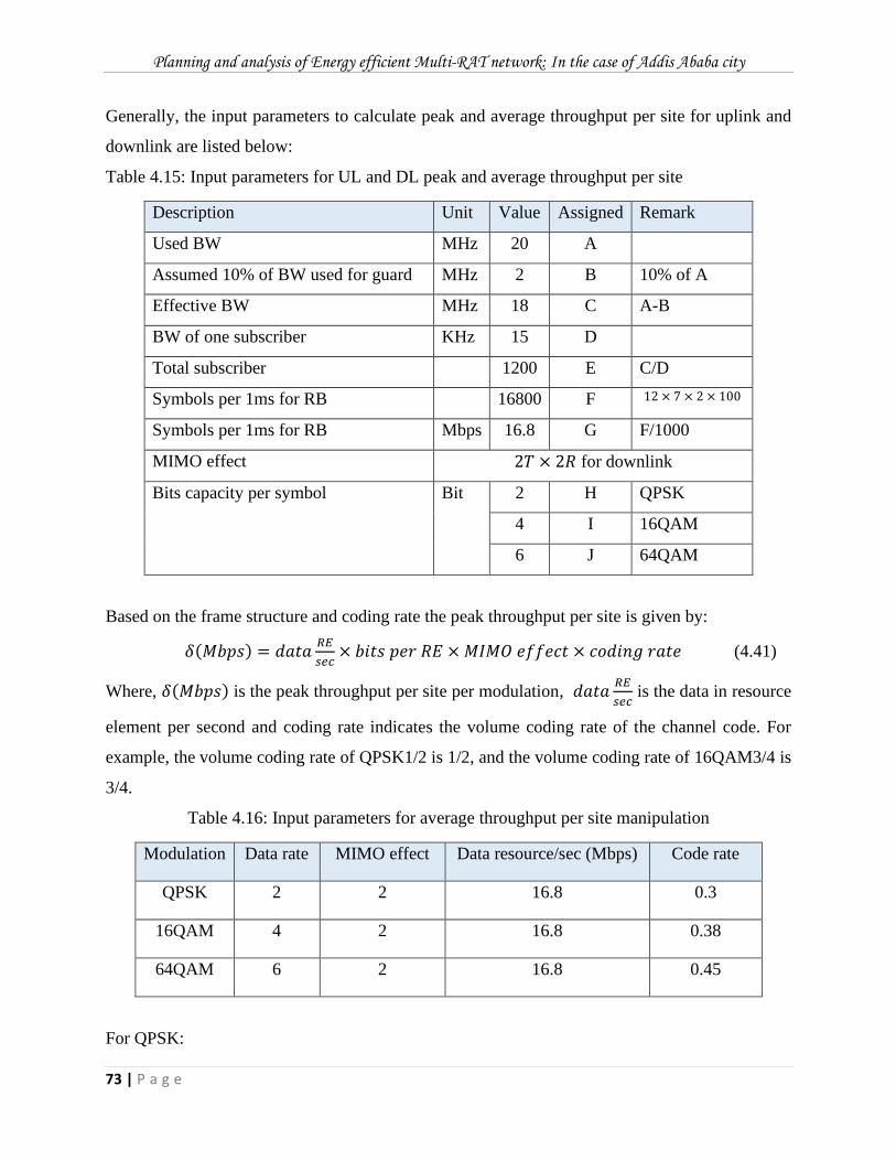
Planning and analysis of Energy efficient Multi-RAT network: In the case of Addis Ababa city
73 | P a g e
Generally, the input parameters to calculate peak and average throughput per site for uplink and
downlink are listed below:
Table 4.15: Input parameters for UL and DL peak and average throughput per site
Description Unit Value Assigned Remark
Used BW MHz 20 A
Assumed 10% of BW used for guard MHz 2 B 10% of A
Effective BW MHz 18 C A-B
BW of one subscriber KHz 15 D
Total subscriber 1200 E C/D
Symbols per 1ms for RB 16800 F 12 × 7 × 2 × 100
Symbols per 1ms for RB Mbps 16.8 G F/1000
MIMO effect 2𝑇 × 2𝑅 for downlink
Bits capacity per symbol Bit 2 H QPSK
4 I 16QAM
6 J 64QAM
Based on the frame structure and coding rate the peak throughput per site is given by:
𝛿(𝑀𝑏𝑝𝑠) = 𝑑𝑎𝑡𝑎𝑅𝐸
𝑠𝑒𝑐× 𝑏𝑖𝑡𝑠 𝑝𝑒𝑟 𝑅𝐸 × 𝑀𝐼𝑀𝑂 𝑒𝑓𝑓𝑒𝑐𝑡 × 𝑐𝑜𝑑𝑖𝑛𝑔 𝑟𝑎𝑡𝑒 (4.41)
Where, 𝛿(𝑀𝑏𝑝𝑠) is the peak throughput per site per modulation, 𝑑𝑎𝑡𝑎𝑅𝐸
𝑠𝑒𝑐 is the data in resource
element per second and coding rate indicates the volume coding rate of the channel code. For
example, the volume coding rate of QPSK1/2 is 1/2, and the volume coding rate of 16QAM3/4 is
3/4.
Table 4.16: Input parameters for average throughput per site manipulation
Modulation Data rate MIMO effect Data resource/sec (Mbps) Code rate
QPSK 2 2 16.8 0.3
16QAM 4 2 16.8 0.38
64QAM 6 2 16.8 0.45
For QPSK:
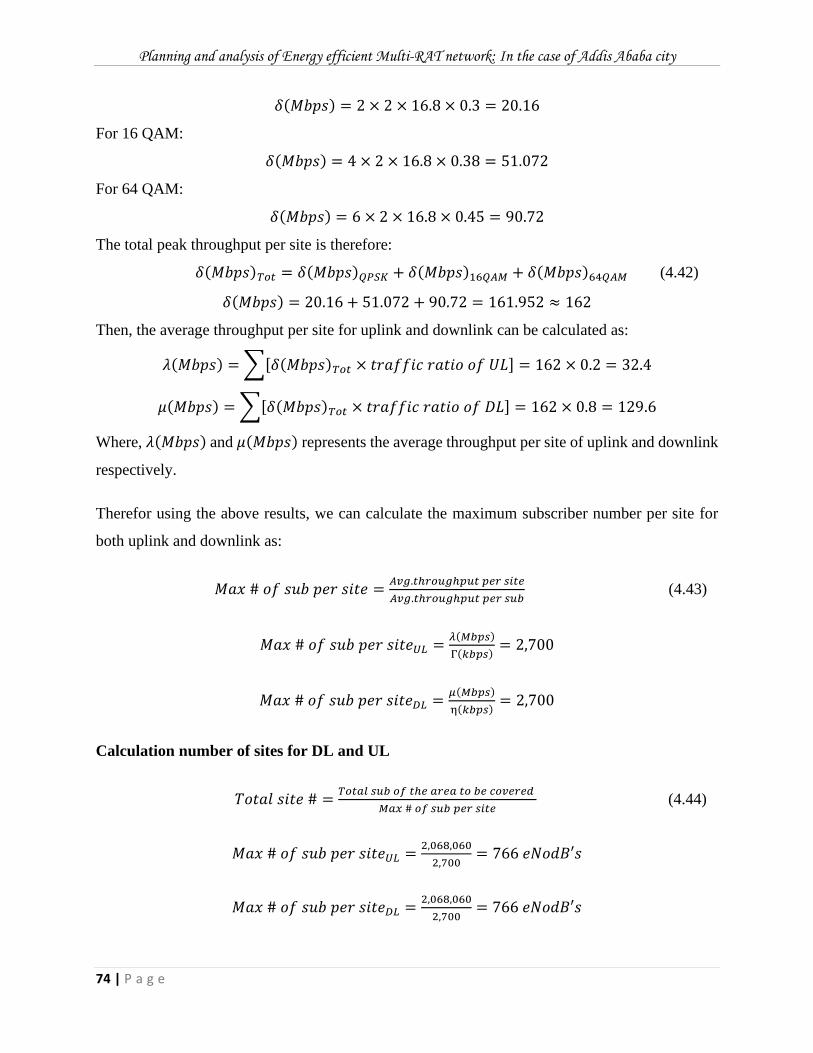
Planning and analysis of Energy efficient Multi-RAT network: In the case of Addis Ababa city
74 | P a g e
𝛿(𝑀𝑏𝑝𝑠) = 2 × 2 × 16.8 × 0.3 = 20.16
For 16 QAM:
𝛿(𝑀𝑏𝑝𝑠) = 4 × 2 × 16.8 × 0.38 = 51.072
For 64 QAM:
𝛿(𝑀𝑏𝑝𝑠) = 6 × 2 × 16.8 × 0.45 = 90.72
The total peak throughput per site is therefore:
𝛿(𝑀𝑏𝑝𝑠)𝑇𝑜𝑡 = 𝛿(𝑀𝑏𝑝𝑠)𝑄𝑃𝑆𝐾 + 𝛿(𝑀𝑏𝑝𝑠)16𝑄𝐴𝑀 + 𝛿(𝑀𝑏𝑝𝑠)64𝑄𝐴𝑀 (4.42)
𝛿(𝑀𝑏𝑝𝑠) = 20.16 + 51.072 + 90.72 = 161.952 ≈ 162
Then, the average throughput per site for uplink and downlink can be calculated as:
𝜆(𝑀𝑏𝑝𝑠) = ∑[𝛿(𝑀𝑏𝑝𝑠)𝑇𝑜𝑡 × 𝑡𝑟𝑎𝑓𝑓𝑖𝑐 𝑟𝑎𝑡𝑖𝑜 𝑜𝑓 𝑈𝐿] = 162 × 0.2 = 32.4
𝜇(𝑀𝑏𝑝𝑠) = ∑[𝛿(𝑀𝑏𝑝𝑠)𝑇𝑜𝑡 × 𝑡𝑟𝑎𝑓𝑓𝑖𝑐 𝑟𝑎𝑡𝑖𝑜 𝑜𝑓 𝐷𝐿] = 162 × 0.8 = 129.6
Where, 𝜆(𝑀𝑏𝑝𝑠) and 𝜇(𝑀𝑏𝑝𝑠) represents the average throughput per site of uplink and downlink
respectively.
Therefor using the above results, we can calculate the maximum subscriber number per site for
both uplink and downlink as:
𝑀𝑎𝑥 # 𝑜𝑓 𝑠𝑢𝑏 𝑝𝑒𝑟 𝑠𝑖𝑡𝑒 =𝐴𝑣𝑔.𝑡ℎ𝑟𝑜𝑢𝑔ℎ𝑝𝑢𝑡 𝑝𝑒𝑟 𝑠𝑖𝑡𝑒
𝐴𝑣𝑔.𝑡ℎ𝑟𝑜𝑢𝑔ℎ𝑝𝑢𝑡 𝑝𝑒𝑟 𝑠𝑢𝑏 (4.43)
𝑀𝑎𝑥 # 𝑜𝑓 𝑠𝑢𝑏 𝑝𝑒𝑟 𝑠𝑖𝑡𝑒𝑈𝐿 =𝜆(𝑀𝑏𝑝𝑠)
Γ(𝑘𝑏𝑝𝑠)= 2,700
𝑀𝑎𝑥 # 𝑜𝑓 𝑠𝑢𝑏 𝑝𝑒𝑟 𝑠𝑖𝑡𝑒𝐷𝐿 =𝜇(𝑀𝑏𝑝𝑠)
η(𝑘𝑏𝑝𝑠)= 2,700
Calculation number of sites for DL and UL
𝑇𝑜𝑡𝑎𝑙 𝑠𝑖𝑡𝑒 # =𝑇𝑜𝑡𝑎𝑙 𝑠𝑢𝑏 𝑜𝑓 𝑡ℎ𝑒 𝑎𝑟𝑒𝑎 𝑡𝑜 𝑏𝑒 𝑐𝑜𝑣𝑒𝑟𝑒𝑑
𝑀𝑎𝑥 # 𝑜𝑓 𝑠𝑢𝑏 𝑝𝑒𝑟 𝑠𝑖𝑡𝑒 (4.44)
𝑀𝑎𝑥 # 𝑜𝑓 𝑠𝑢𝑏 𝑝𝑒𝑟 𝑠𝑖𝑡𝑒𝑈𝐿 =2,068,060
2,700= 766 𝑒𝑁𝑜𝑑𝐵′𝑠
𝑀𝑎𝑥 # 𝑜𝑓 𝑠𝑢𝑏 𝑝𝑒𝑟 𝑠𝑖𝑡𝑒𝐷𝐿 =2,068,060
2,700= 766 𝑒𝑁𝑜𝑑𝐵′𝑠
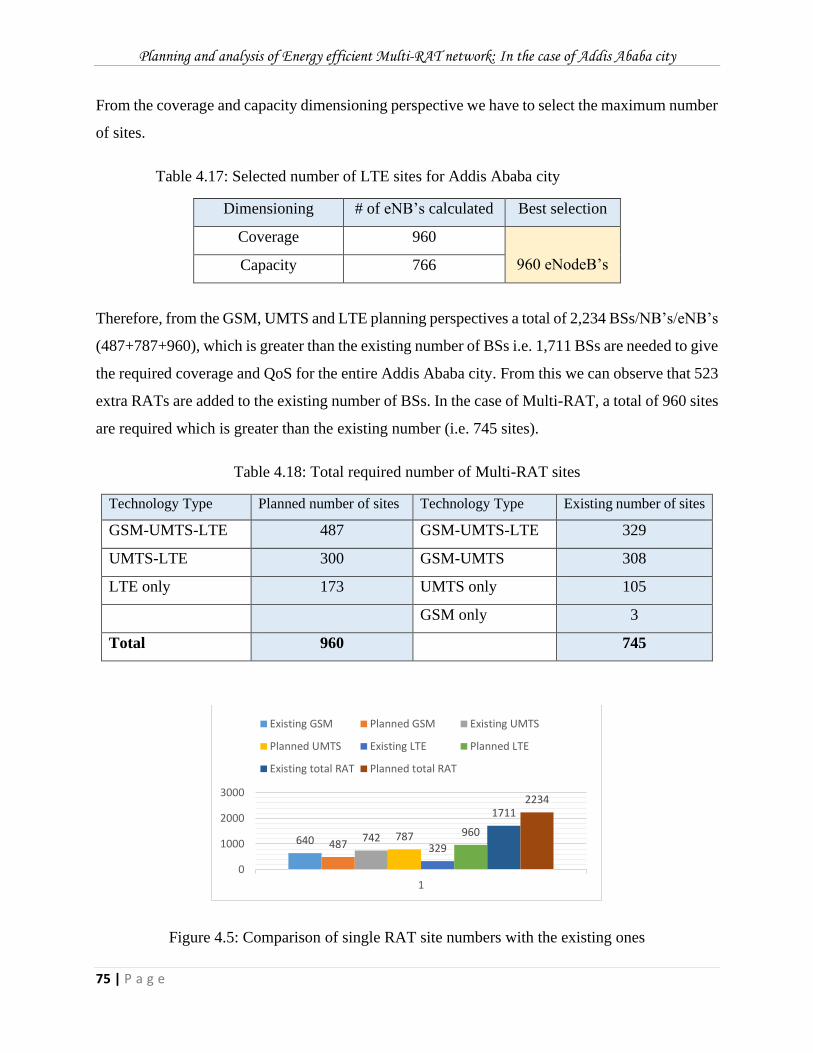
Planning and analysis of Energy efficient Multi-RAT network: In the case of Addis Ababa city
75 | P a g e
From the coverage and capacity dimensioning perspective we have to select the maximum number
of sites.
Table 4.17: Selected number of LTE sites for Addis Ababa city
Dimensioning # of eNB’s calculated Best selection
Coverage 960
960 eNodeB’s Capacity 766
Therefore, from the GSM, UMTS and LTE planning perspectives a total of 2,234 BSs/NB’s/eNB’s
(487+787+960), which is greater than the existing number of BSs i.e. 1,711 BSs are needed to give
the required coverage and QoS for the entire Addis Ababa city. From this we can observe that 523
extra RATs are added to the existing number of BSs. In the case of Multi-RAT, a total of 960 sites
are required which is greater than the existing number (i.e. 745 sites).
Table 4.18: Total required number of Multi-RAT sites
Technology Type Planned number of sites Technology Type Existing number of sites
GSM-UMTS-LTE 487 GSM-UMTS-LTE 329
UMTS-LTE 300 GSM-UMTS 308
LTE only 173 UMTS only 105
GSM only 3
Total 960 745
Figure 4.5: Comparison of single RAT site numbers with the existing ones
640 487742 787
329
960
17112234
0
1000
2000
3000
1
Existing GSM Planned GSM Existing UMTS
Planned UMTS Existing LTE Planned LTE
Existing total RAT Planned total RAT
Planning and analysis of Energy efficient Multi-RAT network: In the case of Addis Ababa city
76 | P a g e
4.7. Cell Sleep Mode
As discussed in the previous chapter cell sleep mode technique consists turning off a BSs
experiencing low traffic load. However, this should be done while ensuring the same quality of
service to mobile users in the cell by the stations that remain active and this is the main challenge
[4, 9]. A BS controller (BSC) facilitates exchange of traffic information between BSs. This
challenge occurs because at least a basic capacity over the whole coverage area of the cell or sector
that is being switched-off should maintain. Unnecessary energy consumptions, for example, air
conditioning under-loaded BSs, can be avoided by adopting such sleep mode mechanisms.
The sleep mode technique is based on current architecture, it has the advantage of being easier to
test and implement as no replacement of hardware is required, very helpful in the sense that it
targets and causes a reduction in the most energy consuming component, the BS and the
performance can be evaluated by computer simulation. In the other direction, implementing sleep
mode introduces some drawbacks in the total throughput of the system. Some of these drawbacks
include the duration of activation and deactivation of resources. This activation time normally
blocks new arrived mobile users or handovers. As a result, some upgrade has to be done in order
to reduce the activation time consequently reducing the blocking of mobile users and thus
achieving the required quality of service. A second known threat of sleep mode is the ping-pong
effect resulting in unnecessary on/off oscillations. This occurs when resources are activated or
deactivated several times, leading to a large signaling overhead [36].
Considering the facts mentioned above, the application of sleep modes of BS decreases the energy
consumption. BSs can be switched off when and where they are not necessary [56]. Furthermore,
interference between cells is also reduced since the radio emission is interrupted during sleep
modes. Generally, there are three requirements when BS sleep mode is applying:
1. Minimized the consumed energy.
2. Guarantee the availability of wireless access over the service area.
3. Minimize the perceived degradation of user experience.
Usually, the power consumption model of a BS consists of two parts [57]: The first part describes
the static power consumption, a power figure which is consumed already in an empty base station.
The second part is dynamic power consumption, which is depending on the load situation.
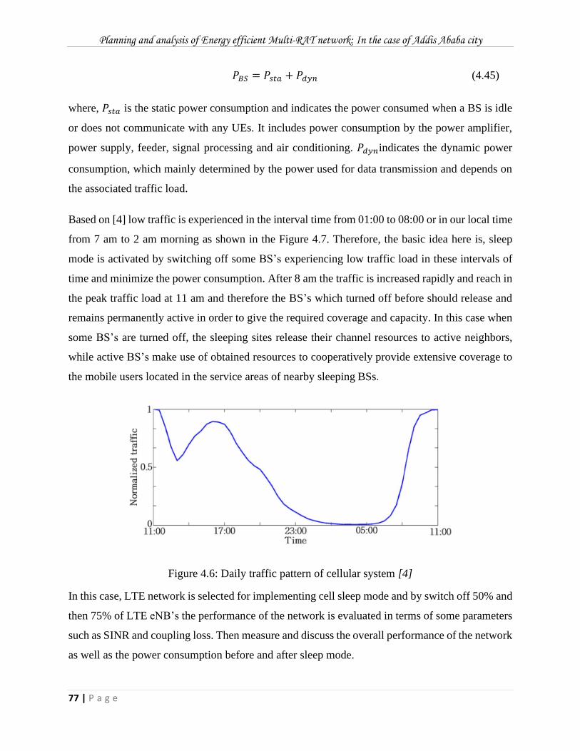
Planning and analysis of Energy efficient Multi-RAT network: In the case of Addis Ababa city
77 | P a g e
𝑃𝐵𝑆 = 𝑃𝑠𝑡𝑎 + 𝑃𝑑𝑦𝑛 (4.45)
where, 𝑃𝑠𝑡𝑎 is the static power consumption and indicates the power consumed when a BS is idle
or does not communicate with any UEs. It includes power consumption by the power amplifier,
power supply, feeder, signal processing and air conditioning. 𝑃𝑑𝑦𝑛indicates the dynamic power
consumption, which mainly determined by the power used for data transmission and depends on
the associated traffic load.
Based on [4] low traffic is experienced in the interval time from 01:00 to 08:00 or in our local time
from 7 am to 2 am morning as shown in the Figure 4.7. Therefore, the basic idea here is, sleep
mode is activated by switching off some BS’s experiencing low traffic load in these intervals of
time and minimize the power consumption. After 8 am the traffic is increased rapidly and reach in
the peak traffic load at 11 am and therefore the BS’s which turned off before should release and
remains permanently active in order to give the required coverage and capacity. In this case when
some BS’s are turned off, the sleeping sites release their channel resources to active neighbors,
while active BS’s make use of obtained resources to cooperatively provide extensive coverage to
the mobile users located in the service areas of nearby sleeping BSs.
Figure 4.6: Daily traffic pattern of cellular system [4]
In this case, LTE network is selected for implementing cell sleep mode and by switch off 50% and
then 75% of LTE eNB’s the performance of the network is evaluated in terms of some parameters
such as SINR and coupling loss. Then measure and discuss the overall performance of the network
as well as the power consumption before and after sleep mode.
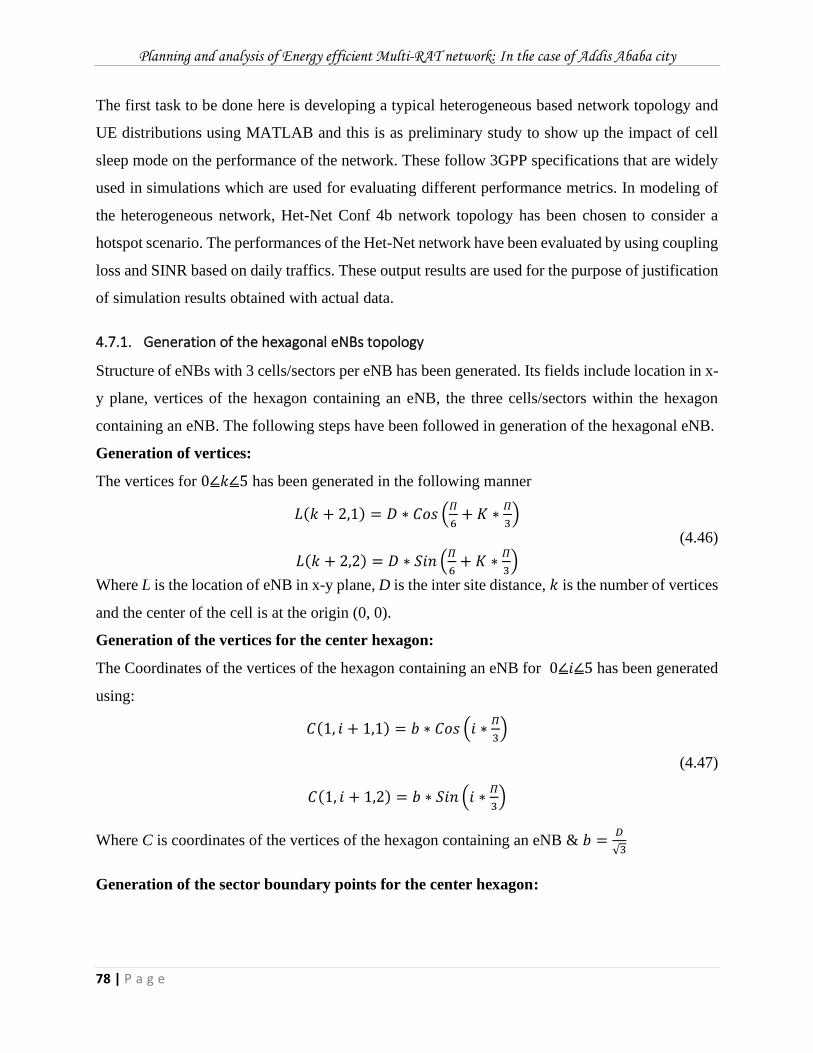
Planning and analysis of Energy efficient Multi-RAT network: In the case of Addis Ababa city
78 | P a g e
The first task to be done here is developing a typical heterogeneous based network topology and
UE distributions using MATLAB and this is as preliminary study to show up the impact of cell
sleep mode on the performance of the network. These follow 3GPP specifications that are widely
used in simulations which are used for evaluating different performance metrics. In modeling of
the heterogeneous network, Het-Net Conf 4b network topology has been chosen to consider a
hotspot scenario. The performances of the Het-Net network have been evaluated by using coupling
loss and SINR based on daily traffics. These output results are used for the purpose of justification
of simulation results obtained with actual data.
4.7.1. Generation of the hexagonal eNBs topology
Structure of eNBs with 3 cells/sectors per eNB has been generated. Its fields include location in x-
y plane, vertices of the hexagon containing an eNB, the three cells/sectors within the hexagon
containing an eNB. The following steps have been followed in generation of the hexagonal eNB.
Generation of vertices:
The vertices for 0⦤𝑘⦤5 has been generated in the following manner
𝐿(𝑘 + 2,1) = 𝐷 ∗ 𝐶𝑜𝑠 (𝛱
6+ 𝐾 ∗
𝛱
3)
(4.46)
𝐿(𝑘 + 2,2) = 𝐷 ∗ 𝑆𝑖𝑛 (𝛱
6+ 𝐾 ∗
𝛱
3)
Where L is the location of eNB in x-y plane, D is the inter site distance, 𝑘 is the number of vertices
and the center of the cell is at the origin (0, 0).
Generation of the vertices for the center hexagon:
The Coordinates of the vertices of the hexagon containing an eNB for 0⦤𝑖⦤5 has been generated
using:
𝐶(1, 𝑖 + 1,1) = 𝑏 ∗ 𝐶𝑜𝑠 (𝑖 ∗𝛱
3)
(4.47)
𝐶(1, 𝑖 + 1,2) = 𝑏 ∗ 𝑆𝑖𝑛 (𝑖 ∗𝛱
3)
Where C is coordinates of the vertices of the hexagon containing an eNB & 𝑏 =𝐷
√3
Generation of the sector boundary points for the center hexagon:
Planning and analysis of Energy efficient Multi-RAT network: In the case of Addis Ababa city
79 | P a g e
Assuming the three sectors within the hexagon containing an eNB are A, B & C, the coordinates
of the three sectors within the hexagon containing an eNB has been generated in the following
manner:
For Sector B and C boundary
𝑆(1,1,1) = 0
(4.48)
𝑆(1,1,2) = −𝑎
For Sector A and B boundary
𝑆(1,2,1) = −3 ⨉ 𝑏
4
(4.49)
𝑆(1,2,2) =𝑎
2
For Sector C and A boundary
𝑆(1,3,1) = 3⨉𝑏
4
(4.50)
𝑆(1,3,2) =𝑎
2
Where 𝑎 =𝐷
2
Generation of the vertices and sector boundary points for the other hexagons:
The vertices and sector boundary points for the remaining hexagons have been generated as
follows:
Generation of the vertices of the center hexagon for the remaining hexagons for 2⦤𝑘⦤𝑛
𝐶(𝐾, 𝑛, 1) = 𝐶(1, 𝑛, 1) + 𝐿(𝑘, 1) (4.51)
𝐶(𝐾, 𝑛, 2) = 𝐶(1, 𝑛, 2) + 𝐿(𝑘, 2) Where 𝑛 is number of eNBs
Generation of the sector boundary points for the center hexagon of the remaining hexagons for
1⦤𝑗⦤3
𝑆(𝐾, 𝑗, 1) = 𝑆(1, 𝑗, 1) + 𝐿(𝑘, 1) (4.52)
𝑆(𝐾, 𝑗, 2) = 𝑆(1, 𝑗, 2) + 𝐿(𝑘, 1)
4.7.2. Generation of the small cells or remote radio heads (RRHs)
The small cells or remote radio heads (RRHs) in each cell/sector as per a uniform distribution with
a minimum distance constraint from the base station in the cell/sector and other small cells has
been generated. The generated topology shows the sector, in which the given RRH is located, the
location of the RRH amongst associated sectors & finally the location of the RRH in the x-y plane.
Planning and analysis of Energy efficient Multi-RAT network: In the case of Addis Ababa city
80 | P a g e
4.7.3. Calculation of the Angle and antenna gain
The sector of the hexagon where the point falls given a point with coordinates 'p' and a hexagon
with center 'c' has been calculated as follows:
ɸ = 𝑎𝑡𝑎𝑛2(𝑒, 𝑓) (4.53)
Where,
𝑒 = 𝑝(2) − 𝑐(2)
𝑓 = 𝑝(1) − 𝑐(1)
ɸ is the azimuth angle of the point with respect to the hexagon center. For a given range value of
ɸ ( ɸ ≥𝛱
6 & ɸ ≤ 5⨉
𝛱
6 ) the sector in which the point falls is 1.
The combined gains of the horizontal (azimuth) sectorized and the vertical (elevation) antennas
for a given UE to all base cells/sectors have been calculated.
The horizontal antenna pattern used for each BS sectors is specified as
𝐴(Ѳ) = −𝑚𝑖𝑛 [12 (Ѳ
Ѳ3 𝑑𝐵 )
2
, 𝐴𝑚] (4.54)
Where, 𝐴(Ѳ) is the relative antenna gain (dB) in the direction Ѳ ,−1800 ≤ Ѳ ≤ 1800,
Ѳ3 𝑑𝐵 is 3 dB beam width &
𝐴𝑚 is the maximum attenuation
The vertical antenna pattern used for each BS sectors is specified as
𝐴𝑒(ɸ) = − min [12 (ɸ−ɸ𝑡𝑖𝑙𝑡
ɸ3𝑑𝐵 )
2
, 𝐴𝑚] (4.55)
Where, 𝐴𝑒(ɸ) is the relative antenna gain (dB) in the elevation direction ɸ,−900 ≤ ɸ ≤ 900,
ɸ3𝑑𝐵 is the elevation 3 dB value.
The combined Antenna gain (dB) is calculated as:
𝐴(Ѳ, ɸ) = − min[−( 𝐴(Ѳ) + 𝐴𝑒(ɸ)), 𝐴𝑚] (4.56)
4.7.4. Generation of UEs and the large-scale channel between UEs and eNBs
The UEs based on a clustered distribution over each cell/sector and a minimum distance constraint
from the base station and the small cells in that cell/sector have been generated. A certain fraction
of the UEs are clustered around the small cells.
Planning and analysis of Energy efficient Multi-RAT network: In the case of Addis Ababa city
81 | P a g e
The large-scale channel between UEs and base stations for the Het-Net conf 4b topology has been
generated. The path loss, shadow fading and sectorized antenna gains have been generated. They
are based on parameters specified in "Guidelines for evaluation of radio interface technologies for
IMT-Advanced" and 3GPP specifications. A certain percentage of UEs are assumed to be indoors.
The first simulation metric for the modeled system is the Coupling Loss (or the Link gain) and is
calculated as:
𝑃𝑅𝑥 − 𝑃𝑇𝑋 = 𝐴𝐺 − 𝑃𝐿 − 𝑆𝐹 (4.57)
Where, 𝑃𝑅𝑥 and 𝑃𝑇𝑋 are receiving and transmitting powers, 𝑃𝐿 and 𝑆𝐹 are the path loss and shadow
fading and also 𝐴𝐺 denotes the directional antenna gain that constitutes a sector. The path loss and
shadow fading vary with carrier frequency as discussed in the planning session, whether the UE is
indoor or outdoor and whether the UE link is LoS or NLoS. The links of most interest are the
coupling loss between the base station.
The second simulation metric for the modeled system is SINR (Geometry) in which an indication
of the overall performance of the cellular network.
𝑆𝐼𝑁𝑅 =𝑆𝑖𝑔𝑛𝑎𝑙
𝐼𝑛𝑡𝑒𝑟𝑓𝑒𝑟𝑒𝑛𝑐𝑒+𝑁𝑜𝑖𝑠𝑒 (4.58)
The noise is constant while the interference is an aggregate of all interfering base stations apart
from the serving base station.
Finally, the power consumption will be reduced while some BS’s are turned off when low traffic
load is experienced. During these times the total power consumption will calculate by adding
transmitting power of the remaining active sites.
Planning and analysis of Energy efficient Multi-RAT network: In the case of Addis Ababa city
82 | P a g e
5. Chapter Five: Results and Discussions
5.1. Introduction
In this chapter, the system model developed in Chapter 4 will be used for simulation using Atoll
network planning tool software as well as MATLAB & the results obtained from simulation will
be discussed.
Overview of ATOLL
ATOLL is a 64-bit multi-technology wireless network design and optimization platform. It is
scalable, flexible, and supports wireless operators throughout the network life cycle, from initial
design to densification and optimization. Atoll’s integration and automation features help
operators smoothly automate planning and optimization processes through flexible scripting and
service-oriented architecture (SOA) based mechanisms. Atoll supports a wide range of
implementation scenarios, from standalone to enterprise wide server-based configurations using
distributed and multi-threaded computing. It offers a series of coverage predictions which are
based on the predicted signal level from the best server and the predicted signal levels from other
cells (interference) at each pixel, i.e., carrier-to-interference-and-noise ratio, or C/(I+N).
In this thesis the atoll simulation environment is used to investigate the RAN nominal planning of
G/U/L networks. The Multi-RAT radio network planning simulation is intended to carry out the
link budget calculation, propagation modeling using the terrain model, coverage estimation and
capacity evaluation. The cell planning tools require digital map as one input which contains
information about, the land usage, about the height of obstacles and they should also contain so
called vector data.
On the other hand, the simulation results of the hexagonal grid layout with the eNBs at the center
and the location of the UEs for Heterogeneous Network Configurations is shown for different
traffic durations. Next, depending on the daily traffic, Sleep mode has been activated to study its
effect on coupling loss & SINR. The simulation results of above considered cases are obtained by
using MATLAB.
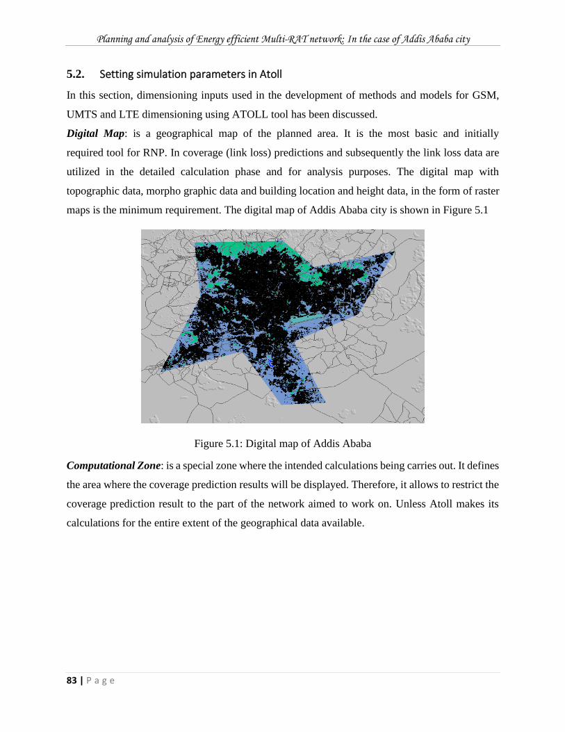
Planning and analysis of Energy efficient Multi-RAT network: In the case of Addis Ababa city
83 | P a g e
5.2. Setting simulation parameters in Atoll
In this section, dimensioning inputs used in the development of methods and models for GSM,
UMTS and LTE dimensioning using ATOLL tool has been discussed.
Digital Map: is a geographical map of the planned area. It is the most basic and initially
required tool for RNP. In coverage (link loss) predictions and subsequently the link loss data are
utilized in the detailed calculation phase and for analysis purposes. The digital map with
topographic data, morpho graphic data and building location and height data, in the form of raster
maps is the minimum requirement. The digital map of Addis Ababa city is shown in Figure 5.1
Figure 5.1: Digital map of Addis Ababa
Computational Zone: is a special zone where the intended calculations being carries out. It defines
the area where the coverage prediction results will be displayed. Therefore, it allows to restrict the
coverage prediction result to the part of the network aimed to work on. Unless Atoll makes its
calculations for the entire extent of the geographical data available.
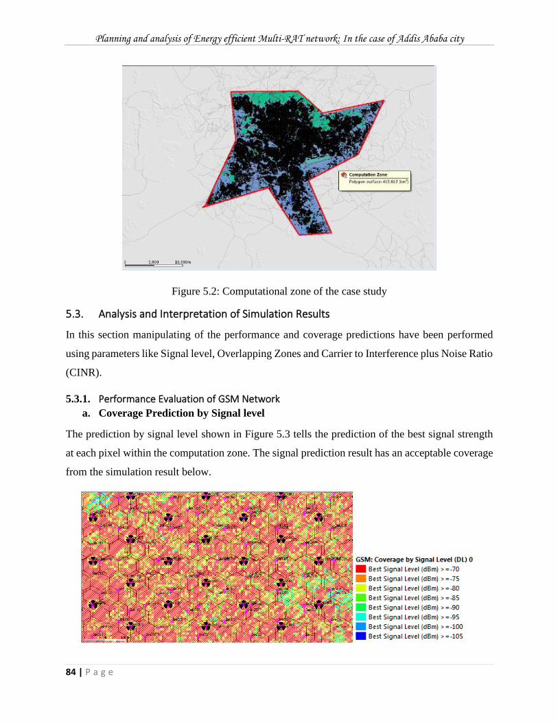
Planning and analysis of Energy efficient Multi-RAT network: In the case of Addis Ababa city
84 | P a g e
Figure 5.2: Computational zone of the case study
5.3. Analysis and Interpretation of Simulation Results
In this section manipulating of the performance and coverage predictions have been performed
using parameters like Signal level, Overlapping Zones and Carrier to Interference plus Noise Ratio
(CINR).
5.3.1. Performance Evaluation of GSM Network
a. Coverage Prediction by Signal level
The prediction by signal level shown in Figure 5.3 tells the prediction of the best signal strength
at each pixel within the computation zone. The signal prediction result has an acceptable coverage
from the simulation result below.
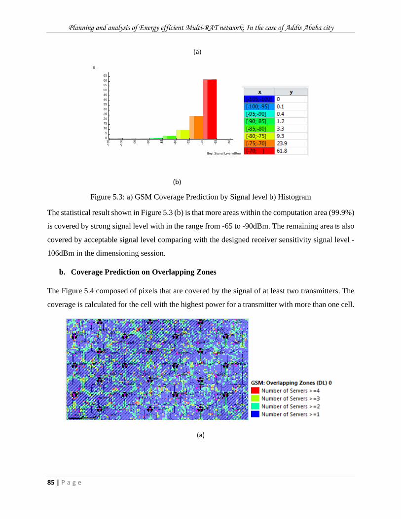
Planning and analysis of Energy efficient Multi-RAT network: In the case of Addis Ababa city
85 | P a g e
(a)
(b)
Figure 5.3: a) GSM Coverage Prediction by Signal level b) Histogram
The statistical result shown in Figure 5.3 (b) is that more areas within the computation area (99.9%)
is covered by strong signal level with in the range from -65 to -90dBm. The remaining area is also
covered by acceptable signal level comparing with the designed receiver sensitivity signal level -
106dBm in the dimensioning session.
b. Coverage Prediction on Overlapping Zones
The Figure 5.4 composed of pixels that are covered by the signal of at least two transmitters. The
coverage is calculated for the cell with the highest power for a transmitter with more than one cell.
(a)
%
0
5
10
15
20
25
30
35
40
45
50
55
60
65
-105
-100
-95
-90
-85
-80
-75
-70
-65
-60
Best Signal Level (dBm)
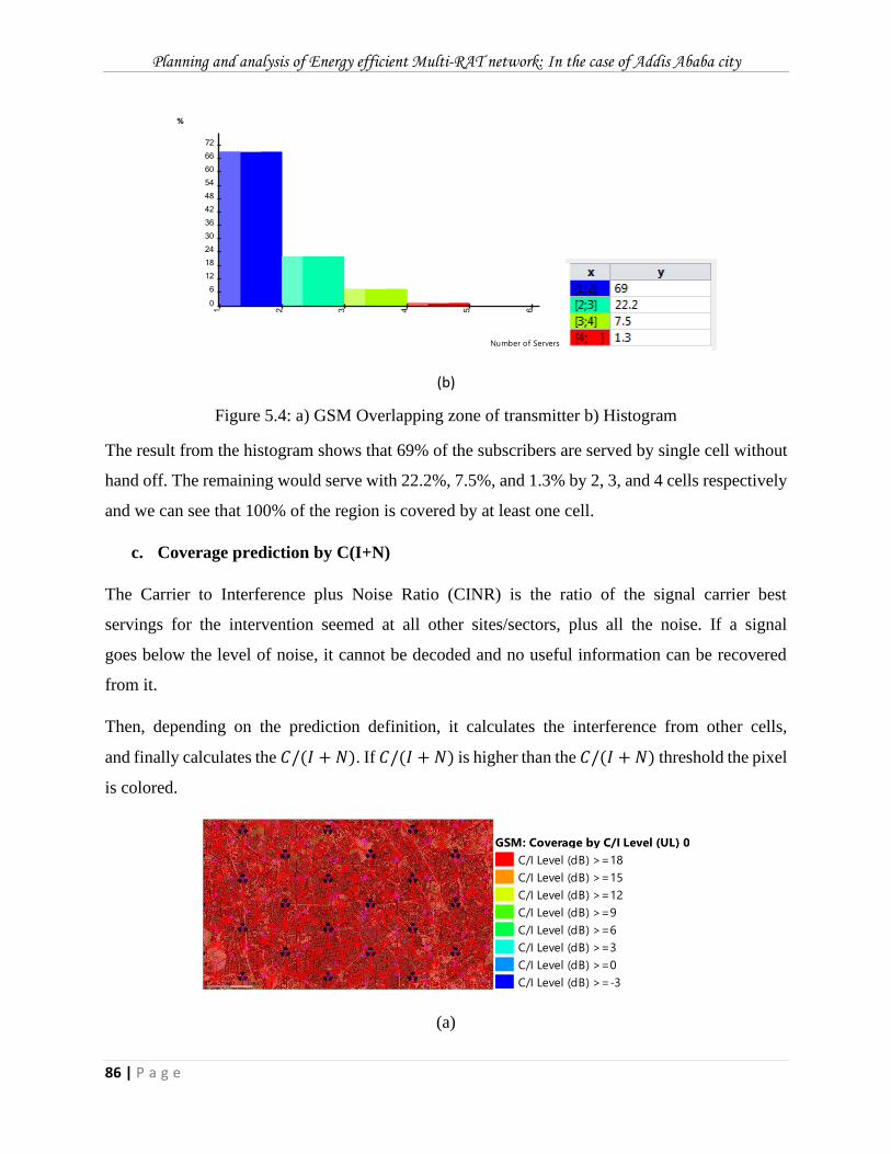
Planning and analysis of Energy efficient Multi-RAT network: In the case of Addis Ababa city
86 | P a g e
(b)
Figure 5.4: a) GSM Overlapping zone of transmitter b) Histogram
The result from the histogram shows that 69% of the subscribers are served by single cell without
hand off. The remaining would serve with 22.2%, 7.5%, and 1.3% by 2, 3, and 4 cells respectively
and we can see that 100% of the region is covered by at least one cell.
c. Coverage prediction by C(I+N)
The Carrier to Interference plus Noise Ratio (CINR) is the ratio of the signal carrier best
servings for the intervention seemed at all other sites/sectors, plus all the noise. If a signal
goes below the level of noise, it cannot be decoded and no useful information can be recovered
from it.
Then, depending on the prediction definition, it calculates the interference from other cells,
and finally calculates the 𝐶/(𝐼 + 𝑁). If 𝐶/(𝐼 + 𝑁) is higher than the 𝐶/(𝐼 + 𝑁) threshold the pixel
is colored.
(a)
%
0
6
12
18
24
30
36
42
48
54
60
66
72
1 2 3 4 5 6
Number of Servers
GSM: Coverage by C/I Level (UL) 0
C/I Level (dB) >=18
C/I Level (dB) >=15
C/I Level (dB) >=12
C/I Level (dB) >=9
C/I Level (dB) >=6
C/I Level (dB) >=3
C/I Level (dB) >=0
C/I Level (dB) >=-3
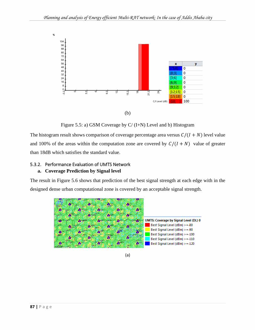
Planning and analysis of Energy efficient Multi-RAT network: In the case of Addis Ababa city
87 | P a g e
(b)
Figure 5.5: a) GSM Coverage by C/ (I+N) Level and b) Histogram
The histogram result shows comparison of coverage percentage area versus 𝐶/(𝐼 + 𝑁) level value
and 100% of the areas within the computation zone are covered by 𝐶/(𝐼 + 𝑁) value of greater
than 18dB which satisfies the standard value.
5.3.2. Performance Evaluation of UMTS Network
a. Coverage Prediction by Signal level
The result in Figure 5.6 shows that prediction of the best signal strength at each edge with in the
designed dense urban computational zone is covered by an acceptable signal strength.
(a)
%
0
8
16
24
32
40
48
56
64
72
80
88
96
104
-3.2 0
3.2 6
9.2 12
15.2 18
21.2 24
C/I Level (dB)
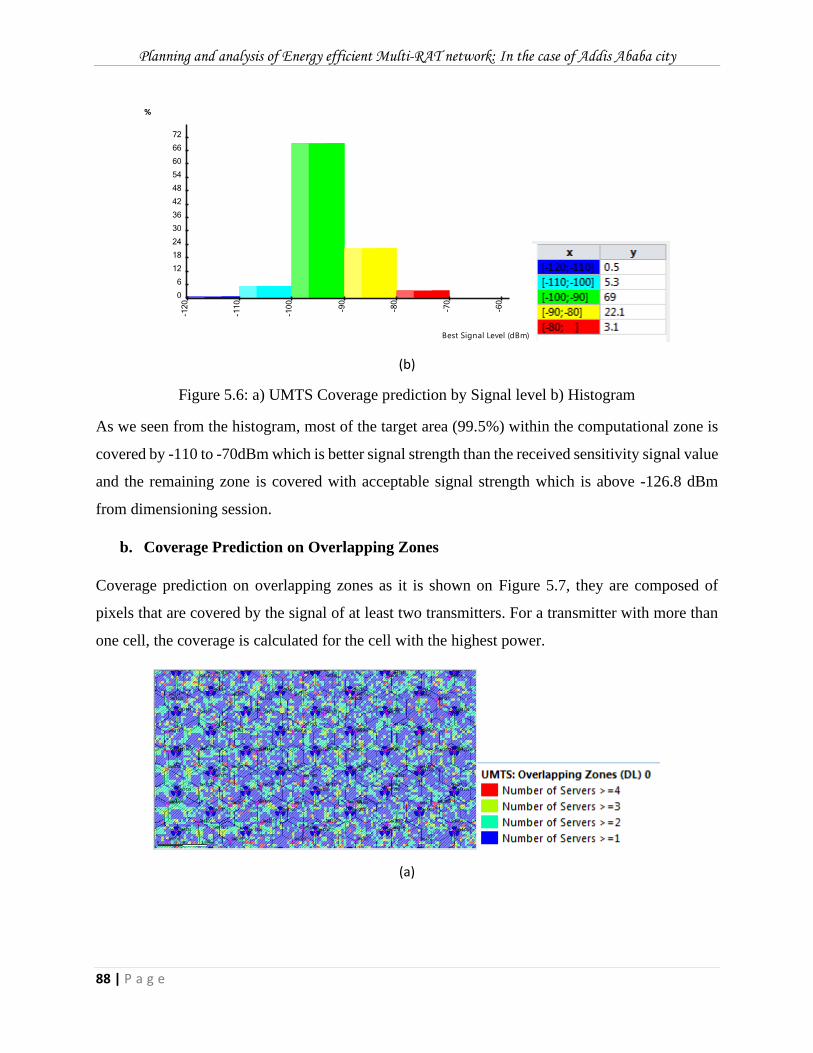
Planning and analysis of Energy efficient Multi-RAT network: In the case of Addis Ababa city
88 | P a g e
(b)
Figure 5.6: a) UMTS Coverage prediction by Signal level b) Histogram
As we seen from the histogram, most of the target area (99.5%) within the computational zone is
covered by -110 to -70dBm which is better signal strength than the received sensitivity signal value
and the remaining zone is covered with acceptable signal strength which is above -126.8 dBm
from dimensioning session.
b. Coverage Prediction on Overlapping Zones
Coverage prediction on overlapping zones as it is shown on Figure 5.7, they are composed of
pixels that are covered by the signal of at least two transmitters. For a transmitter with more than
one cell, the coverage is calculated for the cell with the highest power.
(a)
%
0
6
12
18
24
30
36
42
48
54
60
66
72
-120
-110
-100
-90
-80
-70
-60
Best Signal Level (dBm)
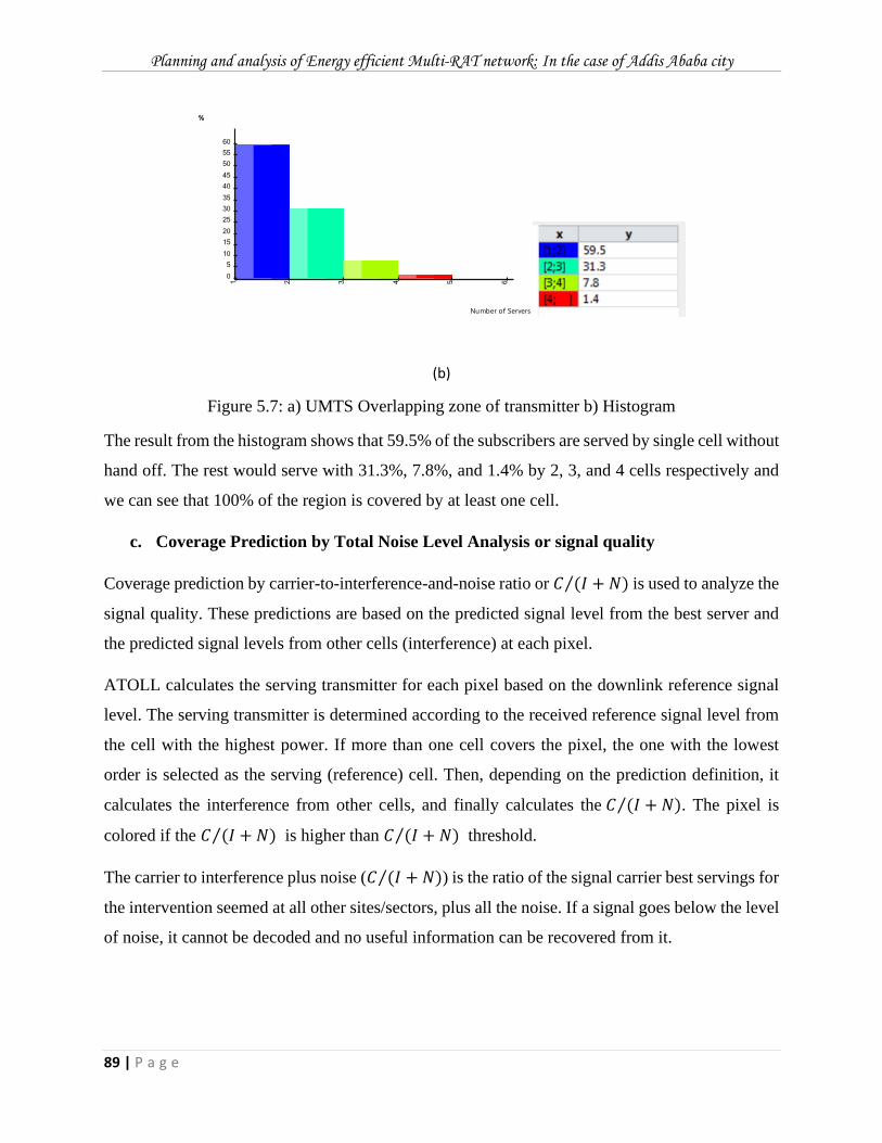
Planning and analysis of Energy efficient Multi-RAT network: In the case of Addis Ababa city
89 | P a g e
(b)
Figure 5.7: a) UMTS Overlapping zone of transmitter b) Histogram
The result from the histogram shows that 59.5% of the subscribers are served by single cell without
hand off. The rest would serve with 31.3%, 7.8%, and 1.4% by 2, 3, and 4 cells respectively and
we can see that 100% of the region is covered by at least one cell.
c. Coverage Prediction by Total Noise Level Analysis or signal quality
Coverage prediction by carrier-to-interference-and-noise ratio or 𝐶 (𝐼 + 𝑁)⁄ is used to analyze the
signal quality. These predictions are based on the predicted signal level from the best server and
the predicted signal levels from other cells (interference) at each pixel.
ATOLL calculates the serving transmitter for each pixel based on the downlink reference signal
level. The serving transmitter is determined according to the received reference signal level from
the cell with the highest power. If more than one cell covers the pixel, the one with the lowest
order is selected as the serving (reference) cell. Then, depending on the prediction definition, it
calculates the interference from other cells, and finally calculates the 𝐶 (𝐼 + 𝑁)⁄ . The pixel is
colored if the 𝐶 (𝐼 + 𝑁)⁄ is higher than 𝐶 (𝐼 + 𝑁)⁄ threshold.
The carrier to interference plus noise (𝐶 (𝐼 + 𝑁)⁄ ) is the ratio of the signal carrier best servings for
the intervention seemed at all other sites/sectors, plus all the noise. If a signal goes below the level
of noise, it cannot be decoded and no useful information can be recovered from it.
%
0
5
10
15
20
25
30
35
40
45
50
55
60
1 2 3 4 5 6
Number of Servers
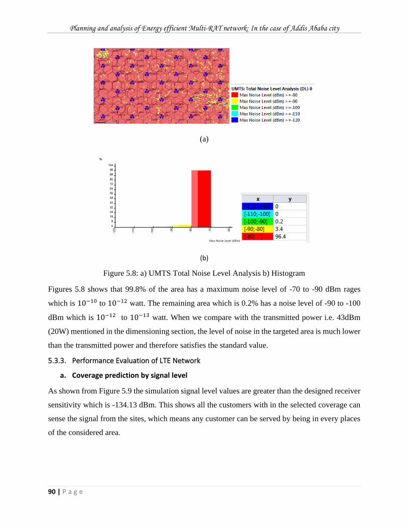
Planning and analysis of Energy efficient Multi-RAT network: In the case of Addis Ababa city
90 | P a g e
(a)
(b)
Figure 5.8: a) UMTS Total Noise Level Analysis b) Histogram
Figures 5.8 shows that 99.8% of the area has a maximum noise level of -70 to -90 dBm rages
which is 10−10 to 10−12 watt. The remaining area which is 0.2% has a noise level of -90 to -100
dBm which is 10−12 to 10−13 watt. When we compare with the transmitted power i.e. 43dBm
(20W) mentioned in the dimensioning section, the level of noise in the targeted area is much lower
than the transmitted power and therefore satisfies the standard value.
5.3.3. Performance Evaluation of LTE Network
a. Coverage prediction by signal level
As shown from Figure 5.9 the simulation signal level values are greater than the designed receiver
sensitivity which is -134.13 dBm. This shows all the customers with in the selected coverage can
sense the signal from the sites, which means any customer can be served by being in every places
of the considered area.
%
0
8
16
24
32
40
48
56
64
72
80
88
96
104
-120
-110
-100
-90
-80
-70
-60
Max Noise Level (dBm)
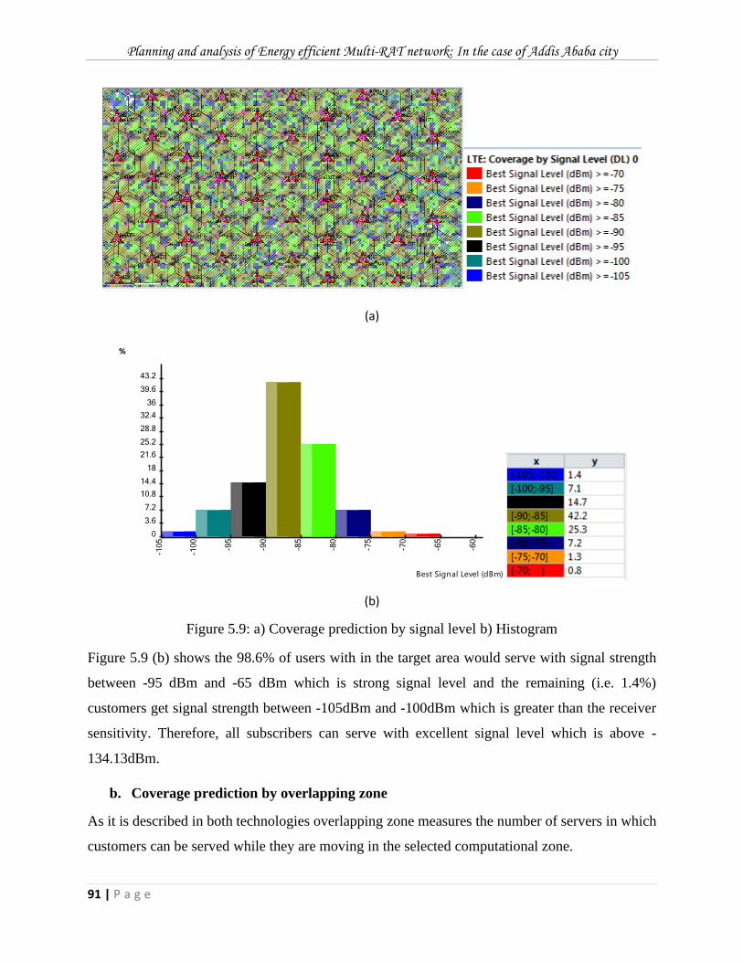
Planning and analysis of Energy efficient Multi-RAT network: In the case of Addis Ababa city
91 | P a g e
(a)
(b)
Figure 5.9: a) Coverage prediction by signal level b) Histogram
Figure 5.9 (b) shows the 98.6% of users with in the target area would serve with signal strength
between -95 dBm and -65 dBm which is strong signal level and the remaining (i.e. 1.4%)
customers get signal strength between -105dBm and -100dBm which is greater than the receiver
sensitivity. Therefore, all subscribers can serve with excellent signal level which is above -
134.13dBm.
b. Coverage prediction by overlapping zone
As it is described in both technologies overlapping zone measures the number of servers in which
customers can be served while they are moving in the selected computational zone.
%
0
3.6
7.2
10.8
14.4
18
21.6
25.2
28.8
32.4
36
39.6
43.2
-105
-100
-95
-90
-85
-80
-75
-70
-65
-60
Best Signal Level (dBm)
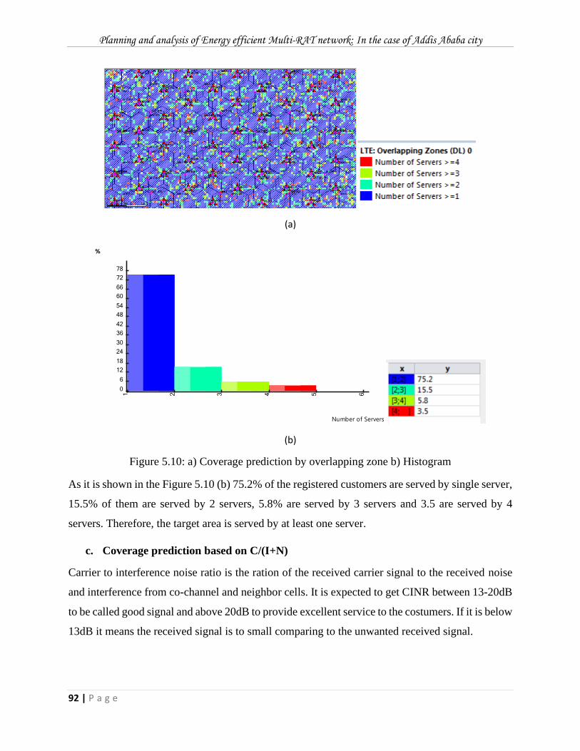
Planning and analysis of Energy efficient Multi-RAT network: In the case of Addis Ababa city
92 | P a g e
(a)
(b)
Figure 5.10: a) Coverage prediction by overlapping zone b) Histogram
As it is shown in the Figure 5.10 (b) 75.2% of the registered customers are served by single server,
15.5% of them are served by 2 servers, 5.8% are served by 3 servers and 3.5 are served by 4
servers. Therefore, the target area is served by at least one server.
c. Coverage prediction based on C/(I+N)
Carrier to interference noise ratio is the ration of the received carrier signal to the received noise
and interference from co-channel and neighbor cells. It is expected to get CINR between 13-20dB
to be called good signal and above 20dB to provide excellent service to the costumers. If it is below
13dB it means the received signal is to small comparing to the unwanted received signal.
%
0
6
12
18
24
30
36
42
48
54
60
66
72
78
1 2 3 4 5 6
Number of Servers
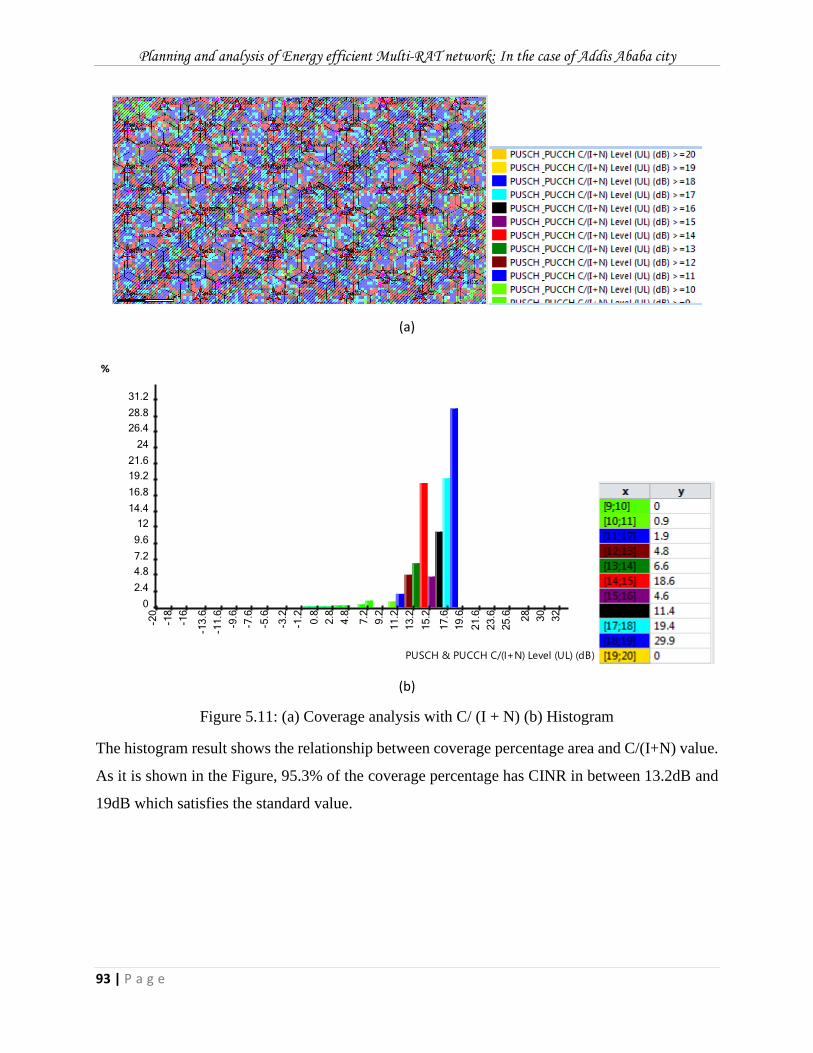
Planning and analysis of Energy efficient Multi-RAT network: In the case of Addis Ababa city
93 | P a g e
(a)
(b)
Figure 5.11: (a) Coverage analysis with C/ (I + N) (b) Histogram
The histogram result shows the relationship between coverage percentage area and C/(I+N) value.
As it is shown in the Figure, 95.3% of the coverage percentage has CINR in between 13.2dB and
19dB which satisfies the standard value.
%
0
2.4
4.8
7.2
9.6
12
14.4
16.8
19.2
21.6
24
26.4
28.8
31.2
-20
-18
-16
-13.6
-11.6
-9.6
-7.6
-5.6
-3.2
-1.2
0.8
2.8
4.8
7.2
9.2
11.2
13.2
15.2
17.6
19.6
21.6
23.6
25.6 28
30
32
PUSCH & PUCCH C/(I+N) Level (UL) (dB)
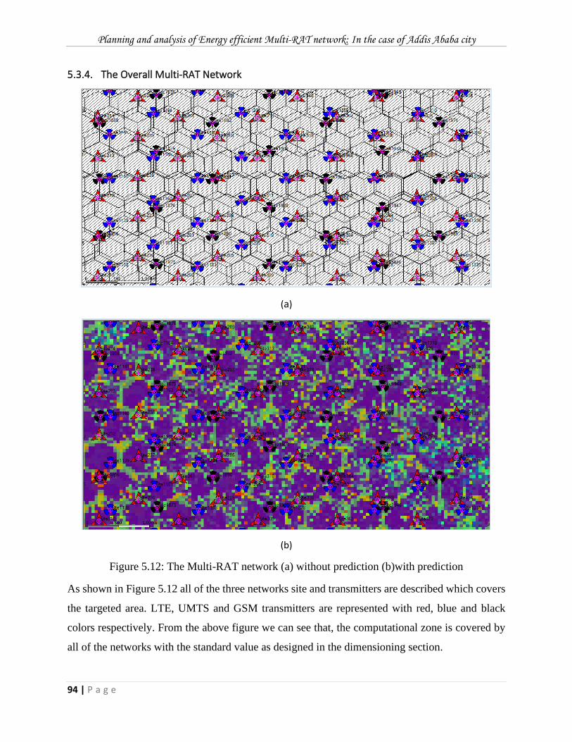
Planning and analysis of Energy efficient Multi-RAT network: In the case of Addis Ababa city
94 | P a g e
5.3.4. The Overall Multi-RAT Network
(a)
(b)
Figure 5.12: The Multi-RAT network (a) without prediction (b)with prediction
As shown in Figure 5.12 all of the three networks site and transmitters are described which covers
the targeted area. LTE, UMTS and GSM transmitters are represented with red, blue and black
colors respectively. From the above figure we can see that, the computational zone is covered by
all of the networks with the standard value as designed in the dimensioning section.
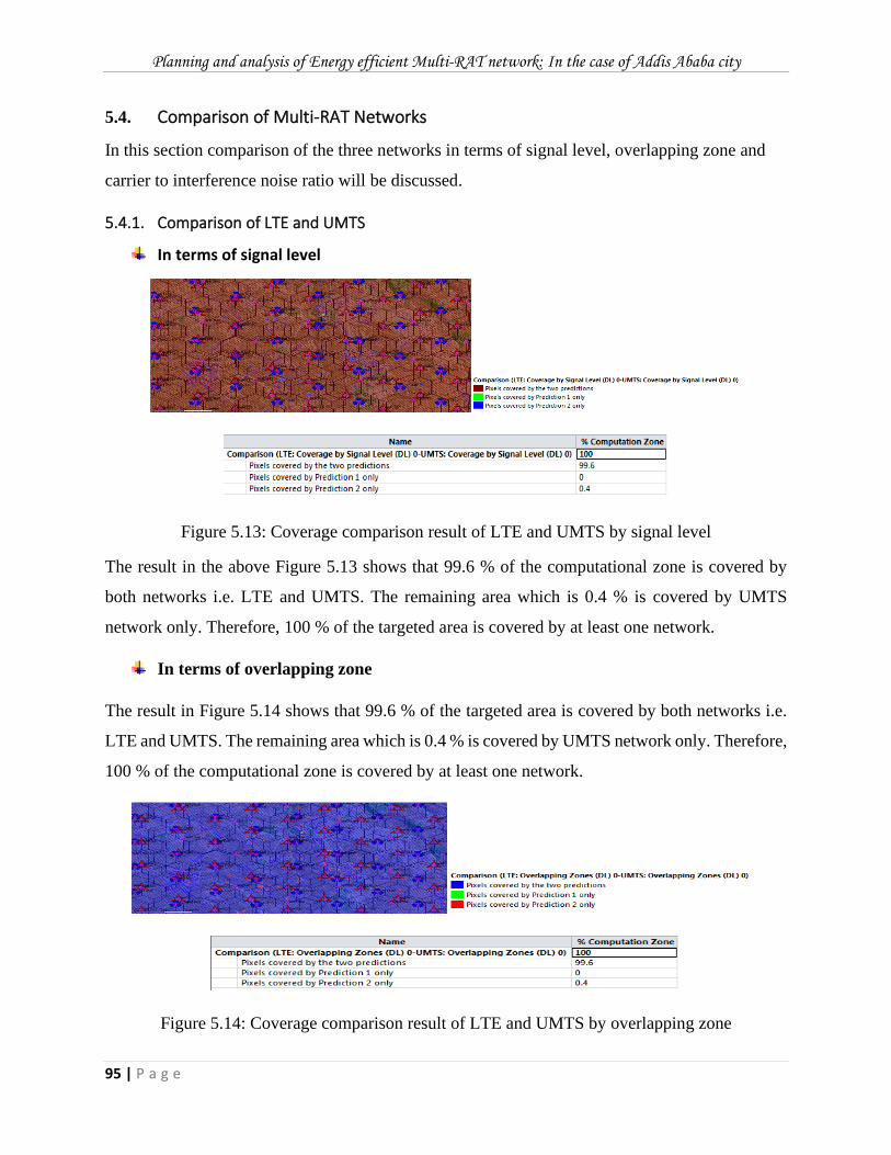
Planning and analysis of Energy efficient Multi-RAT network: In the case of Addis Ababa city
95 | P a g e
5.4. Comparison of Multi-RAT Networks
In this section comparison of the three networks in terms of signal level, overlapping zone and
carrier to interference noise ratio will be discussed.
5.4.1. Comparison of LTE and UMTS
In terms of signal level
Figure 5.13: Coverage comparison result of LTE and UMTS by signal level
The result in the above Figure 5.13 shows that 99.6 % of the computational zone is covered by
both networks i.e. LTE and UMTS. The remaining area which is 0.4 % is covered by UMTS
network only. Therefore, 100 % of the targeted area is covered by at least one network.
In terms of overlapping zone
The result in Figure 5.14 shows that 99.6 % of the targeted area is covered by both networks i.e.
LTE and UMTS. The remaining area which is 0.4 % is covered by UMTS network only. Therefore,
100 % of the computational zone is covered by at least one network.
Figure 5.14: Coverage comparison result of LTE and UMTS by overlapping zone
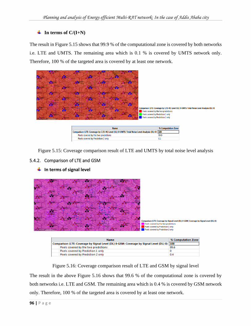
Planning and analysis of Energy efficient Multi-RAT network: In the case of Addis Ababa city
96 | P a g e
In terms of C/(I+N)
The result in Figure 5.15 shows that 99.9 % of the computational zone is covered by both networks
i.e. LTE and UMTS. The remaining area which is 0.1 % is covered by UMTS network only.
Therefore, 100 % of the targeted area is covered by at least one network.
Figure 5.15: Coverage comparison result of LTE and UMTS by total noise level analysis
5.4.2. Comparison of LTE and GSM
In terms of signal level
Figure 5.16: Coverage comparison result of LTE and GSM by signal level
The result in the above Figure 5.16 shows that 99.6 % of the computational zone is covered by
both networks i.e. LTE and GSM. The remaining area which is 0.4 % is covered by GSM network
only. Therefore, 100 % of the targeted area is covered by at least one network.
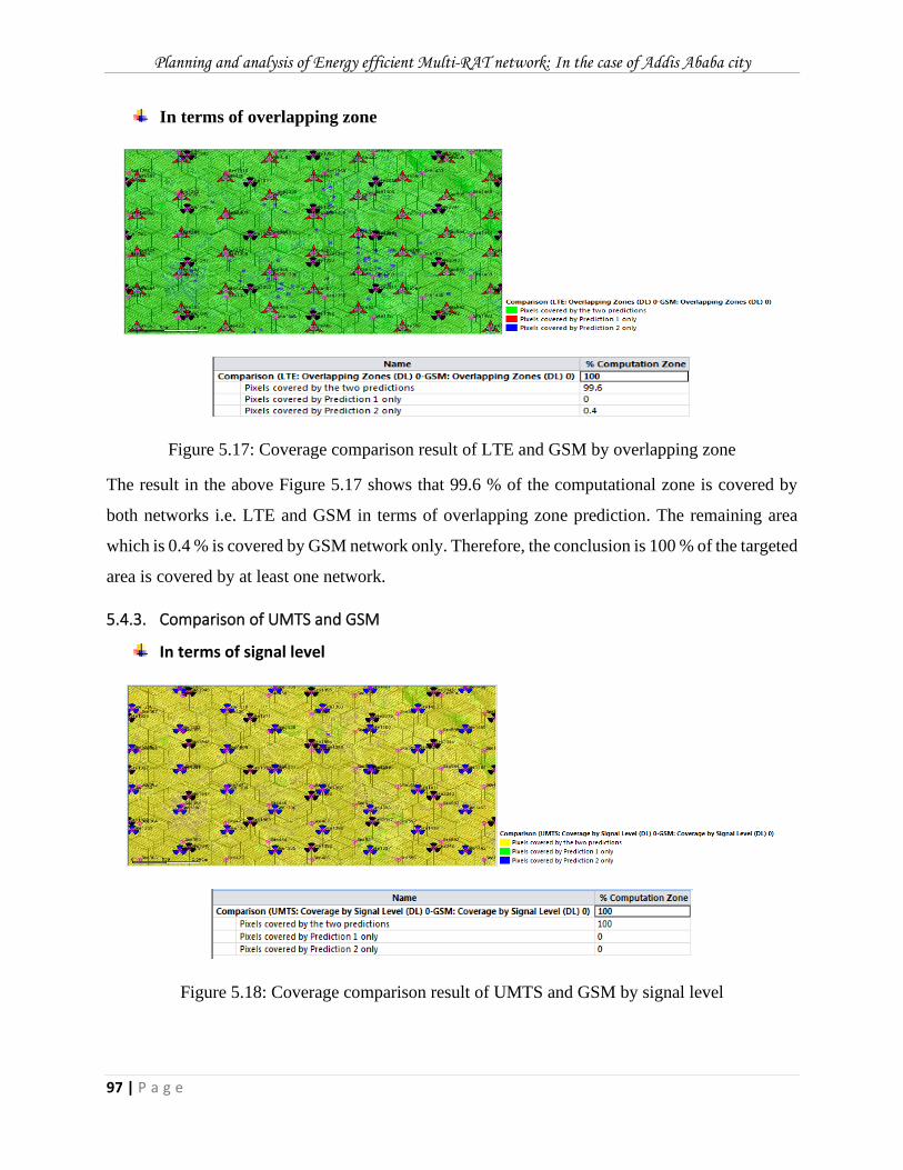
Planning and analysis of Energy efficient Multi-RAT network: In the case of Addis Ababa city
97 | P a g e
In terms of overlapping zone
Figure 5.17: Coverage comparison result of LTE and GSM by overlapping zone
The result in the above Figure 5.17 shows that 99.6 % of the computational zone is covered by
both networks i.e. LTE and GSM in terms of overlapping zone prediction. The remaining area
which is 0.4 % is covered by GSM network only. Therefore, the conclusion is 100 % of the targeted
area is covered by at least one network.
5.4.3. Comparison of UMTS and GSM
In terms of signal level
Figure 5.18: Coverage comparison result of UMTS and GSM by signal level
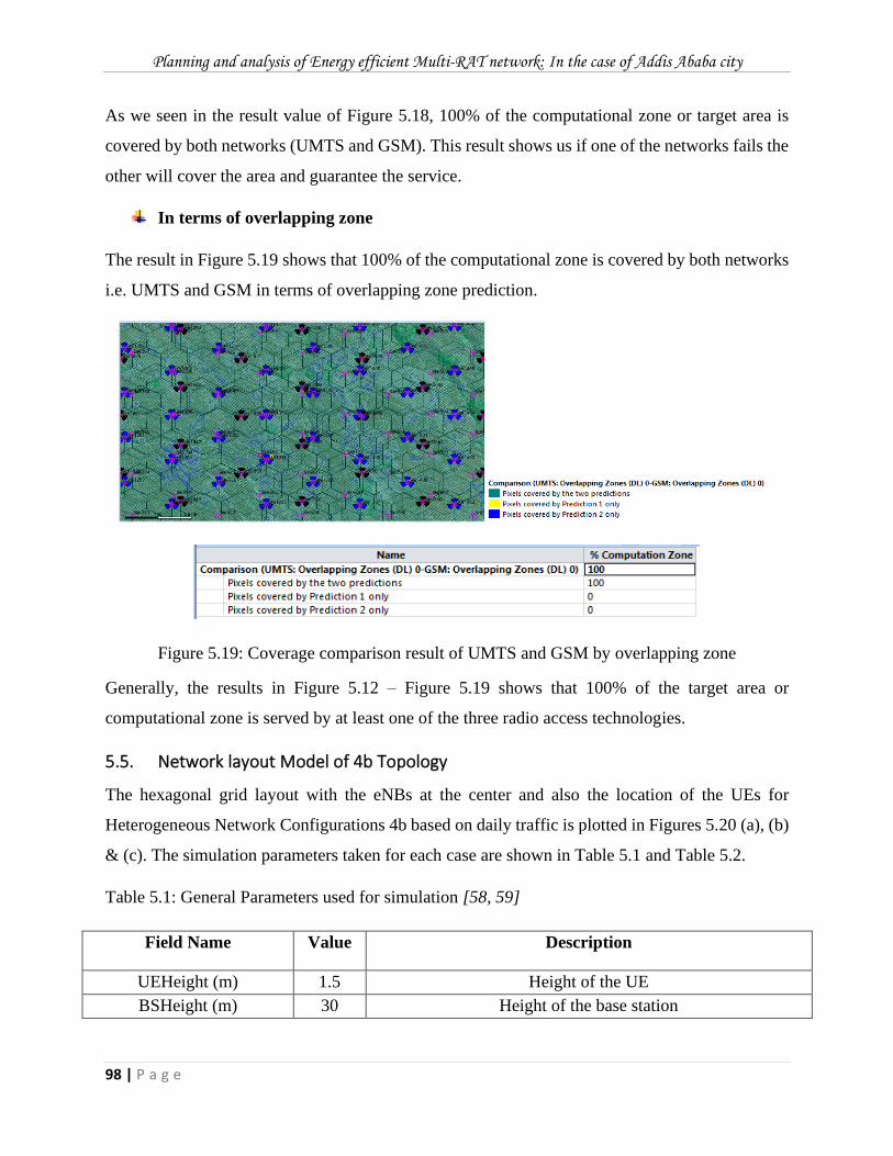
Planning and analysis of Energy efficient Multi-RAT network: In the case of Addis Ababa city
98 | P a g e
As we seen in the result value of Figure 5.18, 100% of the computational zone or target area is
covered by both networks (UMTS and GSM). This result shows us if one of the networks fails the
other will cover the area and guarantee the service.
In terms of overlapping zone
The result in Figure 5.19 shows that 100% of the computational zone is covered by both networks
i.e. UMTS and GSM in terms of overlapping zone prediction.
Figure 5.19: Coverage comparison result of UMTS and GSM by overlapping zone
Generally, the results in Figure 5.12 – Figure 5.19 shows that 100% of the target area or
computational zone is served by at least one of the three radio access technologies.
5.5. Network layout Model of 4b Topology
The hexagonal grid layout with the eNBs at the center and also the location of the UEs for
Heterogeneous Network Configurations 4b based on daily traffic is plotted in Figures 5.20 (a), (b)
& (c). The simulation parameters taken for each case are shown in Table 5.1 and Table 5.2.
Table 5.1: General Parameters used for simulation [58, 59]
Field Name Value Description
UEHeight (m) 1.5 Height of the UE
BSHeight (m) 30 Height of the base station

Planning and analysis of Energy efficient Multi-RAT network: In the case of Addis Ababa city
99 | P a g e
Table 5.2: Small Cell Related Parameters used for simulation [58, 59]
The impact of introducing cell sleeping on the coupling loss and received SINR is investigated for
heterogeneous network Conf 4b. As discussed in the above chapters low traffic period is
considered during 1a.m to 8a.m. In this interval of time, sleep mode is activated by switching 75%
of the cells which means 3 out of 4 cells can be switched of and 1 out of 4 cells remain permanently
InterSiteDist (m)
500 Distance between centers of two adjacent eNB hexagons
HandOverMargin (dB) 1
Handover margin
UENoiseFigure (dB) 7 UE noise figure
BandWidth (MHz) 20 System bandwidth
theta tilt (degrees) 102 Tilt of the Elevation antenna response
theta_3db (dB) 10 Half Power Beam width of the elevation antenna
phi_3db (dB) 70 Half Power Beam width of the azimuth antenna
SLL_h (dB) 25 Side lobe level suppression of azimuth antenna
SLL_v (dB) 20 Side lobe level suppression of elevation antenna
SLL (dB) 25 Side lobe level suppression of combined antenna
MinDistMacroUE(m) 35 Minimum distance between a macro base station and a UE
UEVel (km/h) 3 Velocity of the UE
Center Frequency (GHz) 2 Center frequency
TX Power (dBm) 46 Transmit power of the macro cell
BSAntennaGain (dB) 17 Maximum gain of the macro combined antenna
NumUEperCell 60 Number of UEs per cell
IndoorUEProb 0.8 Probability that a given UE in located indoors
Field Name Value Description
RRHHeight (m) 10 Height of the small cell
MinDistMacroRRH (m) 75 Minimum distance between a small cell and the macro
MinDistRRH (m) 40 Minimum distance between two small cells
MinDistRRHUE (m) 10 Minimum distance between a small cell and a UE
RRHAntenna Gain (dB) 5 Maximum gain of the combined antenna of the small cell
TxPower RRH (dBm) 30 Transmit power of the small cell
NumRRHper Macro 4 Number of small cells per sector
Rho 2/3 Fraction of UEs clustered around small cells
RRHRadius (m) 40 Radius of clustered UE locations
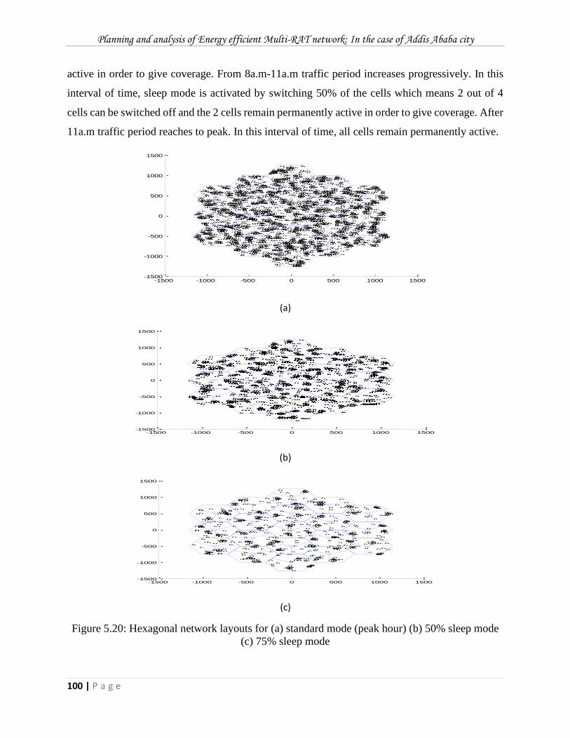
Planning and analysis of Energy efficient Multi-RAT network: In the case of Addis Ababa city
100 | P a g e
active in order to give coverage. From 8a.m-11a.m traffic period increases progressively. In this
interval of time, sleep mode is activated by switching 50% of the cells which means 2 out of 4
cells can be switched off and the 2 cells remain permanently active in order to give coverage. After
11a.m traffic period reaches to peak. In this interval of time, all cells remain permanently active.
(a)
(b)
(c)
Figure 5.20: Hexagonal network layouts for (a) standard mode (peak hour) (b) 50% sleep mode
(c) 75% sleep mode
-1500 -1000 -500 0 500 1000 1500-1500
-1000
-500
0
500
1000
1500
-1500 -1000 -500 0 500 1000 1500-1500
-1000
-500
0
500
1000
1500
-1500 -1000 -500 0 500 1000 1500-1500
-1000
-500
0
500
1000
1500
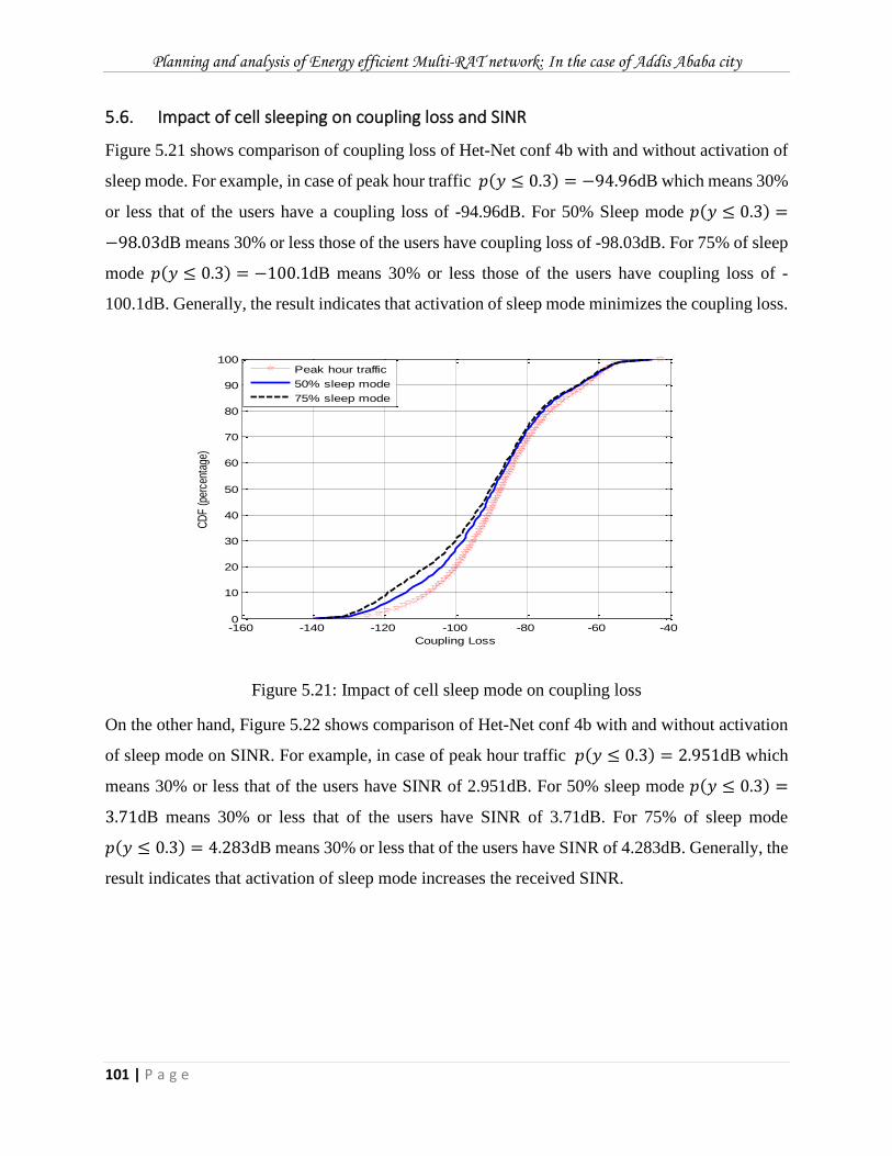
Planning and analysis of Energy efficient Multi-RAT network: In the case of Addis Ababa city
101 | P a g e
5.6. Impact of cell sleeping on coupling loss and SINR
Figure 5.21 shows comparison of coupling loss of Het-Net conf 4b with and without activation of
sleep mode. For example, in case of peak hour traffic 𝑝(𝑦 ≤ 0.3) = −94.96dB which means 30%
or less that of the users have a coupling loss of -94.96dB. For 50% Sleep mode 𝑝(𝑦 ≤ 0.3) =
−98.03dB means 30% or less those of the users have coupling loss of -98.03dB. For 75% of sleep
mode 𝑝(𝑦 ≤ 0.3) = −100.1dB means 30% or less those of the users have coupling loss of -
100.1dB. Generally, the result indicates that activation of sleep mode minimizes the coupling loss.
Figure 5.21: Impact of cell sleep mode on coupling loss
On the other hand, Figure 5.22 shows comparison of Het-Net conf 4b with and without activation
of sleep mode on SINR. For example, in case of peak hour traffic 𝑝(𝑦 ≤ 0.3) = 2.951dB which
means 30% or less that of the users have SINR of 2.951dB. For 50% sleep mode 𝑝(𝑦 ≤ 0.3) =
3.71dB means 30% or less that of the users have SINR of 3.71dB. For 75% of sleep mode
𝑝(𝑦 ≤ 0.3) = 4.283dB means 30% or less that of the users have SINR of 4.283dB. Generally, the
result indicates that activation of sleep mode increases the received SINR.
-160 -140 -120 -100 -80 -60 -400
10
20
30
40
50
60
70
80
90
100
Coupling Loss
CD
F (
perc
enta
ge)
Peak hour traffic
50% sleep mode
75% sleep mode
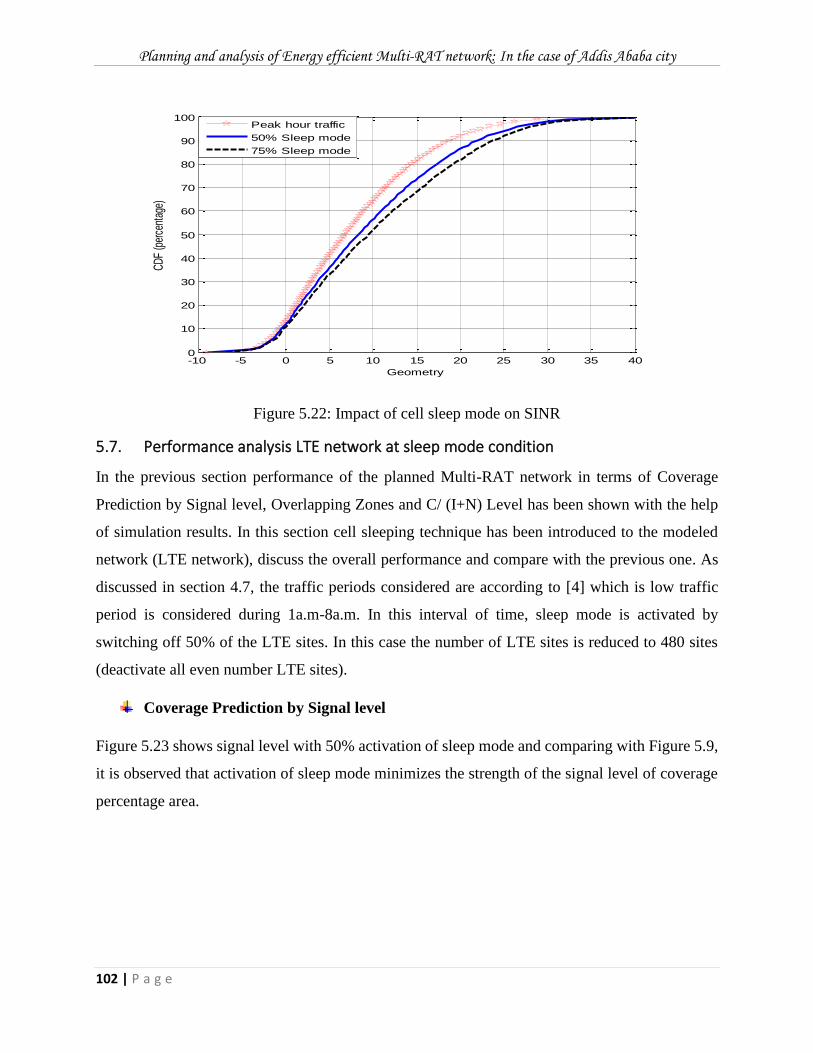
Planning and analysis of Energy efficient Multi-RAT network: In the case of Addis Ababa city
102 | P a g e
Figure 5.22: Impact of cell sleep mode on SINR
5.7. Performance analysis LTE network at sleep mode condition
In the previous section performance of the planned Multi-RAT network in terms of Coverage
Prediction by Signal level, Overlapping Zones and C/ (I+N) Level has been shown with the help
of simulation results. In this section cell sleeping technique has been introduced to the modeled
network (LTE network), discuss the overall performance and compare with the previous one. As
discussed in section 4.7, the traffic periods considered are according to [4] which is low traffic
period is considered during 1a.m-8a.m. In this interval of time, sleep mode is activated by
switching off 50% of the LTE sites. In this case the number of LTE sites is reduced to 480 sites
(deactivate all even number LTE sites).
Coverage Prediction by Signal level
Figure 5.23 shows signal level with 50% activation of sleep mode and comparing with Figure 5.9,
it is observed that activation of sleep mode minimizes the strength of the signal level of coverage
percentage area.
-10 -5 0 5 10 15 20 25 30 35 400
10
20
30
40
50
60
70
80
90
100
Geometry
CD
F (p
erce
ntag
e)
Peak hour traffic
50% Sleep mode
75% Sleep mode
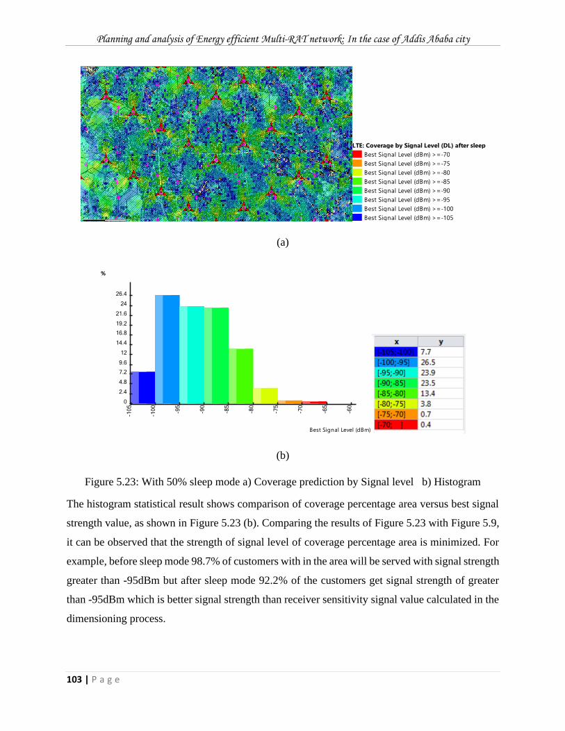
Planning and analysis of Energy efficient Multi-RAT network: In the case of Addis Ababa city
103 | P a g e
(a)
(b)
Figure 5.23: With 50% sleep mode a) Coverage prediction by Signal level b) Histogram
The histogram statistical result shows comparison of coverage percentage area versus best signal
strength value, as shown in Figure 5.23 (b). Comparing the results of Figure 5.23 with Figure 5.9,
it can be observed that the strength of signal level of coverage percentage area is minimized. For
example, before sleep mode 98.7% of customers with in the area will be served with signal strength
greater than -95dBm but after sleep mode 92.2% of the customers get signal strength of greater
than -95dBm which is better signal strength than receiver sensitivity signal value calculated in the
dimensioning process.
LTE: Coverage by Signal Level (DL) after sleep
Best Signal Level (dBm) >=-70
Best Signal Level (dBm) >=-75
Best Signal Level (dBm) >=-80
Best Signal Level (dBm) >=-85
Best Signal Level (dBm) >=-90
Best Signal Level (dBm) >=-95
Best Signal Level (dBm) >=-100
Best Signal Level (dBm) >=-105
%
0
2.4
4.8
7.2
9.6
12
14.4
16.8
19.2
21.6
24
26.4
-105
-100
-95
-90
-85
-80
-75
-70
-65
-60
Best Signal Level (dBm)
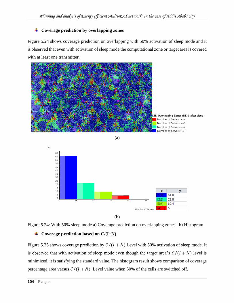
Planning and analysis of Energy efficient Multi-RAT network: In the case of Addis Ababa city
104 | P a g e
Coverage prediction by overlapping zones
Figure 5.24 shows coverage prediction on overlapping with 50% activation of sleep mode and it
is observed that even with activation of sleep mode the computational zone or target area is covered
with at least one transmitter.
(a)
(b)
Figure 5.24: With 50% sleep mode a) Coverage prediction on overlapping zones b) Histogram
Coverage prediction based on C/(I+N)
Figure 5.25 shows coverage prediction by 𝐶 (𝐼 + 𝑁)⁄ Level with 50% activation of sleep mode. It
is observed that with activation of sleep mode even though the target area’s 𝐶 (𝐼 + 𝑁)⁄ level is
minimized, it is satisfying the standard value. The histogram result shows comparison of coverage
percentage area versus 𝐶 (𝐼 + 𝑁)⁄ Level value when 50% of the cells are switched off.
LTE: Overlapping Zones (DL) 3 after sleep
Number of Servers >=4
Number of Servers >=3
Number of Servers >=2
Number of Servers >=1
%
0
5
10
15
20
25
30
35
40
45
50
55
60
65
1 2 3 4 5 6
Number of Servers

Planning and analysis of Energy efficient Multi-RAT network: In the case of Addis Ababa city
105 | P a g e
(a)
(b)
Figure 5.25: With 50% sleep mode a) Coverage prediction by C/ (I+N) Level b) Histogram
Comparing the results of Figure 5.25 with Figure 5.11, it can be observed that the 𝐶 (𝐼 + 𝑁)⁄ level
of coverage percentage area is minimized. For example, in peak hour traffic 96% of the coverage
percentage has CINR in between 13.2dB and 19.6dB but after 50% of the sites are switched off,
99.9% of the coverage percentage has CINR in between 11.2dBm and 13.2dBm which is reduced
value but it satisfies the standard value.
5.8. Comparison of power consumption before and after sleep mode
Transmitted Power consumption of the base station is calculated for peak hour traffic which means
before cell sleep mode and for low traffic load which means after applying cell sleep mode.
%
0
4.5
9
13.5
18
22.5
27
31.5
36
40.5
45
49.5
54
-20
-18
-16
-13.6
-11.6
-9.6
-7.6
-5.6
-3.2
-1.2
0.8
2.8
4.8
7.2
9.2
11.2
13.2
15.2
17.6
19.6
21.6
23.6
25.6 28
30
32
PUSCH & PUCCH C/(I+N) Level (UL) (dB)
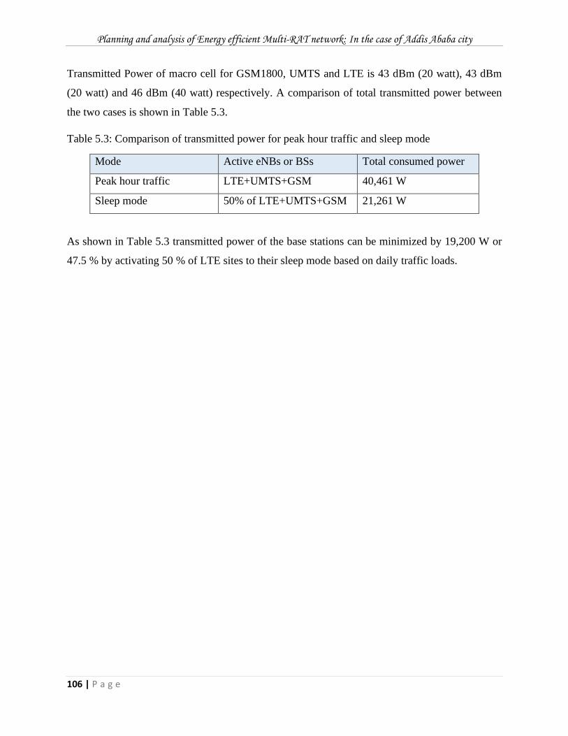
Planning and analysis of Energy efficient Multi-RAT network: In the case of Addis Ababa city
106 | P a g e
Transmitted Power of macro cell for GSM1800, UMTS and LTE is 43 dBm (20 watt), 43 dBm
(20 watt) and 46 dBm (40 watt) respectively. A comparison of total transmitted power between
the two cases is shown in Table 5.3.
Table 5.3: Comparison of transmitted power for peak hour traffic and sleep mode
Mode Active eNBs or BSs Total consumed power
Peak hour traffic LTE+UMTS+GSM 40,461 W
Sleep mode 50% of LTE+UMTS+GSM 21,261 W
As shown in Table 5.3 transmitted power of the base stations can be minimized by 19,200 W or
47.5 % by activating 50 % of LTE sites to their sleep mode based on daily traffic loads.
Planning and analysis of Energy efficient Multi-RAT network: In the case of Addis Ababa city
107 | P a g e
6. Chapter Six: Conclusion and Recommendation
6.1. Conclusion
In cellular system network RF planning is the basic foundation of a mobile communication
network. Hence, making a good planning at earlier stage will be a basic requirement for network
expansion and service update in the future. In addition to this energy usage in cellular system is
other issue over all the world due to high power consumption. Therefore, this study was done to
develop Multi-Rat network or tools and methods to be able to support multi-service radio network
dimensioning and planning for multi radio access technology besides techniques which help to
reduce energy consumption of cellular without compromising QoS for Addis Ababa city with the
area of 413.612 𝑘𝑚2 by considering dense urban clutter. The performance of the planned network
and results was modeled and analyzed using ATOLL network planning tool and MATLAB
software. Best signal level, overlapping zone and C(I+N) per each RAT are the selected
performance measuring parameters of the planned network and also coupling loss and SINR for
measuring the impact of energy reduction on the network performance.
From the coverage and capacity planning perspective of the Multi-RAT network 960 LTE eNB’s,
787 UMTS NB’s and 487 GSM BTS’s are obtained for Addis Ababa city. Since one Multi-Rat
site contains three radio access technologies, out of 960 LTE eNB’s and 787 UMTS NB’s the 487
can be shared or cohabited with GSM BTS’s. In addition to this 300 of LTE eNB’s can be shared
with the remaining 300 UMTS NB’s and finally the remaining 173 LTE eNB’s are located alone.
Therefore, a total of 960 sites are needed to cover the whole city.
In the case of energy efficiency, the result indicates that activation of sleep mode minimizes the
coupling loss but the SINR value will be increased as shown in the preliminary study results. In
this work sleep mode was activated by switching off 50% of LTE eNB’s as a case study during
1a.m up to 8a.m period and the transmitting power can be minimized by 47.5% during that period.
When sleep mode is activated, the performance of network is reduced in terms of coverage
prediction by signal strength, overlapping zones and C/ (I+N) comparing with performance of peak
hour traffic. But the network performance still satisfies the standard requirements while saving
large amount of transmitting power.
Planning and analysis of Energy efficient Multi-RAT network: In the case of Addis Ababa city
108 | P a g e
Generally, the investigations performed in this thesis work has shown that the performance of the
planned energy efficient Multi-Rat network satisfies the desired minimum standard requirements
even if sleep mode is activating during low traffic period and can save huge power consumption
of the cellular network.
6.2. Recommendation
There are several issues that can be addressed as a future work for this work. Some of the related
future works include:
✓ This study focused on the network planning of the radio access technologies by mainly
concentrated on coverage and capacity. One can further study the various features of these
technologies as well as the core network and microwave part.
✓ In this work only energy saving technique was considered as part of the RNP. This can be
extended by considering energy harvesting techniques as part of the RNP
✓ The analysis in this thesis was by manually switching off the base stations during low
traffic periods. Another future work that can be addressed is applying self-organization
technique in which the base station switch’s on and off by itself based on daily traffics.
✓ Beyond switching of individual cell modifying of the radio topology to different radio
configurations by comparing their capacity and radiated power. In this manner the when
there is a low traffic load the network is reconfigured to a topology with lower capacity
and radiated power.
Planning and analysis of Energy efficient Multi-RAT network: In the case of Addis Ababa city
109 | P a g e
Bibliography
[1] T. S. Rappaport, Wireless Communications Principles and Practice, 2nd ed ed., Prentice Hall
Communications Engineering and Emerging Technologies Series, 2001.
[2] R. L. Nils Anders Stefan Gustafsson, "System and Method for Radio Nework Planning with HSDPA
Analysis". United States Patent US 8,209,038 B2, 26 June 2012.
[3] Y. Sun, "Radio Network Planning for 2G and 3G," Munich University of Technology , 2004.
[4] Y. Z. M. Z. a. E. K.-N. Y. Jingjin Wu, "Energy-Efficient Base-Stations Sleep-Mode Techniques in Green
Cellular Networks: A Survey," IEEE Communication Surveys and Tutorials, vol. 17, no. 2, pp. 803-
826, 2015.
[5] Q. BangWang, "Energy Cost Minimization in Heterogeneous Cellular Networks with Hybrid Energy
Supplies," 29 August 2016.
[6] T. Mekonnen, "Dimensioning and Planning of Multi RAT Radio Network for Future Deployment in
Bahir Dar City," International Journal of Scientific & Engineering Research, 2016.
[7] A. M. E.-H. a. Z. D. Wissam El-Beaino, "A Proactive Approach for LTE Radio Network Planning With
Green Considerations," in 19th International Conference on Telecommunications, Beirut, 2012.
[8] L. Zhang, " Network Capacity, Coverage Estimation and Frequency Planning of 3GPP Long Term
Evolution," 2010.
[9] H. E. S. K. E. K. a. e. Oliver Blume, "Energy savings in mobile networks based on adaptation to
traffic statistics," Bell Labs Technical Journal , vol. 15, no. 2, pp. 77 - 94, 2010.
[10] L. Mitikie, "UMTS Coverage and Capacity Planning for the case of Bole Sub City in Addis Ababa,"
Addis Ababa, April, 2016 .
[11] J. Laiho, "RADIO NETWORK PLANNING AND OPTIMISATION FOR WCDMA," Helsinki University of
Technology Radio Laboratory Publications, July, 2002.
[12] J. Korhonen, Introduction to 3G Mobile Communications, Boston.London: ARTECH HOUSE, 2003.
[13] A. J. N. Serrador, "Optimisation of Cell Radius in UMTS-FDD Networks," December 2002.
[14] R. S. Rakesh Kumar Singh, "4G LTE Cellular Technology: Network Architecture and Mobile
Standards," International Journal of Emerging Research in Management &Technology, vol. 5, no.
12, December 2016.
[15] N. A. M. O. Magri Hicham, "4G System: Network Architecture and Performance," IJIRAE, vol. 2, no.
4, April, 2015.
Planning and analysis of Energy efficient Multi-RAT network: In the case of Addis Ababa city
110 | P a g e
[16] R. Nossenson, "Long-term Evolution Network Architecture," 2009 IEEE International Conference on
Microwaves, Communications, Antennas and Electronics Systems, 2009.
[17] C. C. C. L. Christopher Cox: Director, An Introduction to LTE, LTE-Advanced, SAE And 4G Mobile
Communications, UK: A John Wiley & Sons, Ltd, 2012.
[18] A. a. e. Ghosh, "Fundamental of LTE," Pearson Education, 2010.
[19] Z. Gurmu, "Long Term Evolution (LTE) Radio Network Dimensioning: Case of Addis Ababa City,"
June, 2015 .
[20] T. H. K. a. E. A, "Utran Long Term Evolution in 3GPP," 2006 IEEE 17th International Symposium on
Personal, Indoor and Mobile Radio communications, 2006.
[21] D. H. Zarrinkoub, Understanding LTE with Matlab from Mathematical Modeling to Simulation and
Prototyping, 1st ed, John Wiley & Sons, 2014.
[22] w. paper:, "LTE: The Future of Mobile Broadband Technology," Verizon Wireless, 2009.
[23] A. S. A. K. H. w. H. a. a. e. Abdullah Abdulwahab Mohammed Ghaleb, "LTE Network Planning and
Optimization," Taiz University Faculty of Engineering and IT Communication Department, 2014.
[24] T. D. Assefa, "QoS Performance of LTE Networks with Network Coding," M.S.thesis, Norwegian
University of Science and Technology, June 2015.
[25] M. A. E.-s. M. R. S. Ayman Elnashar, Design, Deployment & Performance of 4G LTE Networks: A
Practical Approach, John Wiley & Sons, Ltd, 2014.
[26] N. A. A. Abd-Elhamid M. Taha and Hossam S. Hassanein, LTE, LTE- Advanced, and WiMAX: towards
IMT-advanced networks, TOWARDS IMT-ADVANCED NETWORKS, A John Wiley & Sons, Ltd, 2002.
[27] H. K. M. T. S. R. U. Noman Shabbir, "Comparison of Radio Propagation Models for Long Term
Evolution (LTE) Network," International Journal of Next-Generation Networks (IJNGN) Vol.3, No.3,,
vol. 3, pp. 27-41, 07 September September, 2011.
[28] Z. I. S. H. a. S. F. M. M. Ahamed, "LTE network coverage prediction for multi-traffic users in an
urban area," in IEEE International Conference on Electro/Information Technology (EIT 2013), Rapid
City, SD, USA, 17 October 2013.
[29] M. S. a. A. Q. M. A. Hes-Shafi, "Analysis of Propagation Models for WiMAX at 3.5 GHz," Blekinge
Institute of Technology, Master's thesis of Science in Electrical Engineering, Karlskrona, Sweden,
September 2009.
[30] Y. Singh, "Comparison of Okumura, Hata and COST-231 Models on the Basis of Path Loss and Signal
Strength," International Journal of Computer Applications (0975 – 8887) , vol. 11, pp. 37-41,
December 2012.
Planning and analysis of Energy efficient Multi-RAT network: In the case of Addis Ababa city
111 | P a g e
[31] A. R. Mishra, "Fundamentals of Cellular Network Planning and Optimization 2G/2.5G/3G...
Evolution to 4G," John Wiley & Sons Ltd, 2004.
[32] R. R. P. B. V. a. R. D. Srudhi Lakshmi V., "Green Radio Technology for Energy Saving in Mobile
Towers," International Journal of Information and Electronics Engineering, vol. 3, no. 1, pp. 39-43,
Vol. 3, No. 1, January 2013.
[33] M. A. Deepa Palani, "ENERGY EFFICIENT SOLUTIONS FOR GREEN CELLULAR NETWORKS – A
SURVEY," International Journal of Electronics and Communication Engineering and Technology
(IJECET), vol. 9, no. 5, pp. 1-16, September-October 2018.
[34] H. B. a. V. K. B. Ziaul Hasan, "Green Cellular Networks: A Survey, Some Research Issues and
Challenges," IEEE, vol. 3, 24 Sep, 2011.
[35] S. K. A. Landou, "OPTIMIZATION OF 4G CELLULAR NETWORKS FOR THE REDUCTION OF ENERGY
CONSUMPTION," Masters Dissertation, UNIVERSITY OF BRASILIA Faculty of Technology, Brasilia,
August 2015.
[36] S. A.-N. L. B. a. F. S. Michel Nahas, "Reducing Energy Consumption in Cellular Networks by
Adjusting Transmitted Power of Base Stations," School of Engineering, Lebanese International
University (LIU), Lebanon .
[37] Y. W. J. G. a. Z. Y. Zhisheng Niu, "Cell Zooming for Cost-Efficient Green Cellular Networks," IEEE
Communications Magazine, pp. 74-79, November 2010.
[38] J.Louhi, "Energy Efficiency of Modern Cellular Base Stations," in INTELEC 07 - 29th International
Telecommunications Energy Conference, Rome, Italy, 2007.
[39] O. P. A. W. N. A. S. R. I. Y. Hani’ah Mahmudah, "Performance Analysis of Cell Zooming Based
Centralized Algorithm for Energy Efficient in Surabaya," EMITTER International Journal of
Engineering Technology , vol. 4, no. 2, pp. 324-343, December 2016.
[40] C. H. O. a. S. M. Shelly Salim, "Are Heterogeneous Cellular Networks Superior to Homogeneous
Ones?," International Federation for Information Processing, South Korea, pp. 61-68, 2012.
[41] L. Y. C. Q. L. P. D. A. G. Pingping Xing, "Multi-RAT network Architecture," Wireless World, WGC –
Communication Architectures and Technologies, November 2013.
[42] J. J. Tushar Saxena, "Review on 2G, 3G and 4G Radio Network Planning," International Journal of
Engineering, Business and Enterprise Applications (IJEBEA), pp. 84-89, 2013.
[43] J. S. J. RichaBudhiraja, "Mobile Radio Network Planning: A Survey," International Association of
Scientific Innovation and Research (IASIR), pp. 308-311, 2013.
[44] "Population of 2019.com," 2019. [Online]. Available: https://populationof2019.com/population-of-
addis-ababa-2019.html. [Accessed 04 February 2019].
Planning and analysis of Energy efficient Multi-RAT network: In the case of Addis Ababa city
112 | P a g e
[45] A. R. Mishra, ADVANCED CELLULAR NETWORK PLANNING AND OPTIMISATION 2G/2.5G/3G. . .
EVOLUTION TO 4G, John Wiley & Sons Ltd, 2007.
[46] Z. University, "GSM Basic Radio parameters".
[47] "Digital cellular telecommunications system (Phase 2+): Radio transmission and reception (GSM
05.05)," European Telecommunications Standards Institute (ETSI), March 1996.
[48] S. B. Mahato, "Performance Evaluation of Six-Sectored Configuration in Hexagonal WCDMA
(UMTS) Cellular Network Layout," Master of Science Thesis, LAPPEENRANTA UNIVERSITY OF
TECHNOLOGY, DEPARTMENT OF INFORMATION TECHNOLOGY, October, 2006.
[49] S. A. Benjamin Paul, "Code Planning of 3G UMTS Mobile Networks Using ATOLL Planning Tool,"
International Journal of Engineering Research & Technology (IJERT), vol. 1, no. 5, pp. 1-5, July -
2012.
[50] S. Abdul Basit, "Dimensioning of LTE Network Description of Models and Tool, Coverage and
Capacity Estimation of 3GPP Long Term Evolution radio interface," Masters Thesis submitted in
partial fulfillment of the requirements for the Degree of Masters of Science in Technology,
February, 2009.
[51] I. Siomina, "Radio Network Planning and Resource Optimization: Mathematical Models and
Algorithms for UMTS, WLANs, and Ad Hoc Networks," Link¨oping Studies in Science and
Technology, Dissertations No. 1116, Sweden, 2007.
[52] M. Eheduru, "Indoor Radio Measurement and Planning for UMTS/HSPDA with Antennas,"
University of Wisconsin Milwaukee UWM Digital Commons, Theses and Dissertations, May 2013.
[53] K. H. Jamal Khalab, "UTRAN Macro Link Budget," H3G CONFIDENTIAL, 2001.
[54] K. H. B. Marwa Elbagir Mohammed1, "LTE Radio Planning Using Atoll Radio Planning and
Optimization Software," International Journal of Science and Research (IJSR), vol. 3, no. 10,
October 2014.
[55] M. M. A. F. Martins, "3G Radio Network Planning for a Mobile Network Operator," Masters Thesis
in Electrical and Computer Engineering, December 2014.
[56] Huawei, "Long Term Evolution (LTE) Radio Access Network Planning Guide," Huawei Technology,
Co, Ltd, 2008.
[57] C. ZHANG, "Energy Efficient Cellular System Design with QoS Assurance," Stockholm, Sweden ,
October 2014.
[58] E. W. M. W. J. G. M. Z. Jingjin Wu, Writer, Performance Analysis of Green Cellular Networks with
Selective Base-Station Sleeping. [Performance]. Department of Electronic Engineering, City
University of Hong Kong, 83 Tat Chee Avenue, Kowloon, Hong Kong, 2017.

Planning and analysis of Energy efficient Multi-RAT network: In the case of Addis Ababa city
113 | P a g e
[59] ITU-R, "Detailed specifications of the terrestrial radio interfaces of International Mobile
Telecommunications-Advanced (IMT-Advanced)," Electronic Publisher, Geneva , 2018.
[60] T. Report, "3rd Generation Partnership Project; Technical Specification Group Radio Access
Network; Evolved Universal Terrestrial Radio Access (E-UTRA); Further advancements for E-UTRA
physical layer aspects (Release 9)," 3GPP TR 36.814 , 2017.
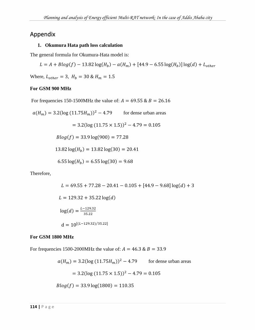
Planning and analysis of Energy efficient Multi-RAT network: In the case of Addis Ababa city
114 | P a g e
Appendix
1. Okumura Hata path loss calculation
The general formula for Okumura-Hata model is:
𝐿 = 𝐴 + 𝐵𝑙𝑜𝑔(𝑓) − 13.82 log(𝐻𝑏) − 𝑎(𝐻𝑚) + [44.9 − 6.55 log(𝐻𝑏)] log(𝑑) + 𝐿𝑜𝑡ℎ𝑒𝑟
Where, 𝐿𝑜𝑡ℎ𝑒𝑟 = 3, 𝐻𝑏 = 30 & 𝐻𝑚 = 1.5
For GSM 900 MHz
For frequencies 150-1500MHz the value of: 𝐴 = 69.55 & 𝐵 = 26.16
𝑎(𝐻𝑚) = 3.2(log (11.75𝐻𝑚))2 − 4.79 for dense urban areas
= 3.2(log (11.75 × 1.5))2 − 4.79 = 0.105
𝐵𝑙𝑜𝑔(𝑓) = 33.9 log(900) = 77.28
13.82 log(𝐻𝑏) = 13.82 log(30) = 20.41
6.55 log(𝐻𝑏) = 6.55 log(30) = 9.68
Therefore,
𝐿 = 69.55 + 77.28 − 20.41 − 0.105 + [44.9 − 9.68] log(𝑑) + 3
𝐿 = 129.32 + 35.22 log(𝑑)
log(𝑑) =𝐿−129.32
35.22
d = 10[(𝐿−129.32) 35.22]⁄
For GSM 1800 MHz
For frequencies 1500-2000MHz the value of: 𝐴 = 46.3 & 𝐵 = 33.9
𝑎(𝐻𝑚) = 3.2(log (11.75𝐻𝑚))2 − 4.79 for dense urban areas
= 3.2(log (11.75 × 1.5))2 − 4.79 = 0.105
𝐵𝑙𝑜𝑔(𝑓) = 33.9 log(1800) = 110.35
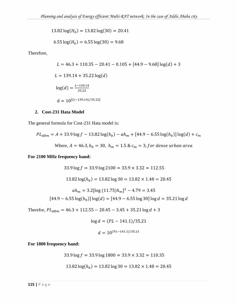
Planning and analysis of Energy efficient Multi-RAT network: In the case of Addis Ababa city
115 | P a g e
13.82 log(𝐻𝑏) = 13.82 log(30) = 20.41
6.55 log(𝐻𝑏) = 6.55 log(30) = 9.68
Therefore,
𝐿 = 46.3 + 110.35 − 20.41 − 0.105 + [44.9 − 9.68] log(𝑑) + 3
𝐿 = 139.14 + 35.22 log(𝑑)
log(𝑑) =𝐿−139.14
35.22
d = 10[(𝐿−139.14) 35.22]⁄
2. Cost-231 Hata Model
The general formula for Cost-231 Hata model is:
𝑃𝐿𝑑𝐵𝑚 = 𝐴 + 33.9 log 𝑓 − 13.82 log(ℎ𝑏) − 𝑎ℎ𝑚 + [44.9 − 6.55 log(ℎ𝑏)] log(𝑑) + 𝑐𝑚
Where, 𝐴 = 46.3, ℎ𝑏 = 30, ℎ𝑚 = 1.5 & 𝑐𝑚 = 3, 𝑓𝑜𝑟 𝑑𝑒𝑛𝑠𝑒 𝑢𝑟𝑏𝑎𝑛 𝑎𝑟𝑒𝑎
For 2100 MHz frequency band:
33.9 log 𝑓 = 33.9 log 2100 = 33.9 × 3.32 = 112.55
13.82 log(ℎ𝑏) = 13.82 log 30 = 13.82 × 1.48 = 20.45
𝑎ℎ𝑚 = 3.2[log (11.75)ℎ𝑚]2 − 4.79 = 3.45
[44.9 − 6.55 log(ℎ𝑏)] log(𝑑) = [44.9 − 6.55 log 30] log 𝑑 = 35.21 log 𝑑
Therefor, 𝑃𝐿𝑑𝐵𝑚 = 46.3 + 112.55 − 20.45 − 3.45 + 35.21 log 𝑑 + 3
log 𝑑 = (𝑃𝐿 − 141.1)/35.21
𝑑 = 10(𝑃𝐿−141.1)/35.21
For 1800 frequency band:
33.9 log 𝑓 = 33.9 log 1800 = 33.9 × 3.32 = 110.35
13.82 log(ℎ𝑏) = 13.82 log 30 = 13.82 × 1.48 = 20.45
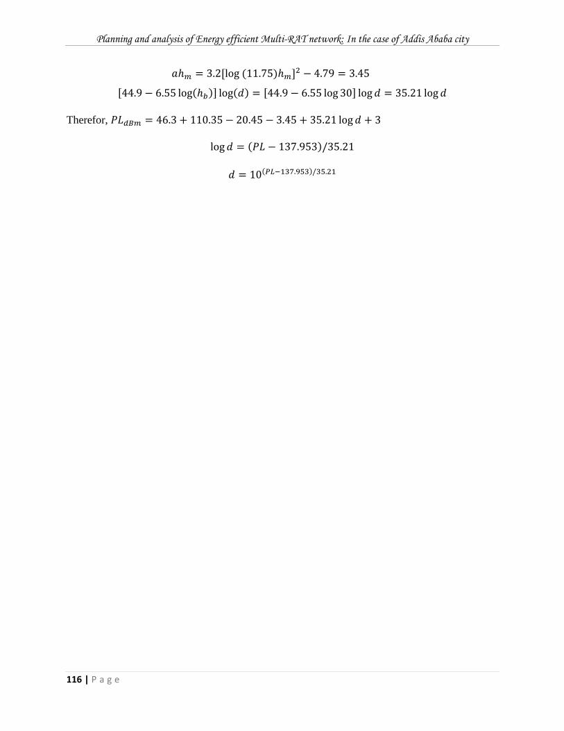
Planning and analysis of Energy efficient Multi-RAT network: In the case of Addis Ababa city
116 | P a g e
𝑎ℎ𝑚 = 3.2[log (11.75)ℎ𝑚]2 − 4.79 = 3.45
[44.9 − 6.55 log(ℎ𝑏)] log(𝑑) = [44.9 − 6.55 log 30] log 𝑑 = 35.21 log 𝑑
Therefor, 𝑃𝐿𝑑𝐵𝑚 = 46.3 + 110.35 − 20.45 − 3.45 + 35.21 log 𝑑 + 3
log 𝑑 = (𝑃𝐿 − 137.953)/35.21
𝑑 = 10(𝑃𝐿−137.953)/35.21
Copyright © 2022 FDOKUMEN