MUSE: Multimodal Separators for Efficient Route Planning in ...
32
HAL Id: hal-03402845 https://hal.archives-ouvertes.fr/hal-03402845 Submitted on 25 Oct 2021 HAL is a multi-disciplinary open access archive for the deposit and dissemination of sci- entific research documents, whether they are pub- lished or not. The documents may come from teaching and research institutions in France or abroad, or from public or private research centers. L’archive ouverte pluridisciplinaire HAL, est destinée au dépôt et à la diffusion de documents scientifiques de niveau recherche, publiés ou non, émanant des établissements d’enseignement et de recherche français ou étrangers, des laboratoires publics ou privés. MUSE: Multimodal Separators for Effcient Route Planning in Transportation Networks Mohamed Amine Falek, Cristel Pelsser, Sébastien Julien, Fabrice Theoleyre To cite this version: Mohamed Amine Falek, Cristel Pelsser, Sébastien Julien, Fabrice Theoleyre. MUSE: Multimodal Sep- arators for Effcient Route Planning in Transportation Networks. Transportation Science, INFORMS, 2021, 10.1287/xxxx.0000.0000. hal-03402845
-
Upload
khangminh22 -
Category
Documents
-
view
2 -
download
0
Transcript of MUSE: Multimodal Separators for Efficient Route Planning in ...

HAL Id: hal-03402845https://hal.archives-ouvertes.fr/hal-03402845
Submitted on 25 Oct 2021
HAL is a multi-disciplinary open accessarchive for the deposit and dissemination of sci-entific research documents, whether they are pub-lished or not. The documents may come fromteaching and research institutions in France orabroad, or from public or private research centers.
L’archive ouverte pluridisciplinaire HAL, estdestinée au dépôt et à la diffusion de documentsscientifiques de niveau recherche, publiés ou non,émanant des établissements d’enseignement et derecherche français ou étrangers, des laboratoirespublics ou privés.
MUSE: Multimodal Separators for Efficient RoutePlanning in Transportation Networks
Mohamed Amine Falek, Cristel Pelsser, Sébastien Julien, Fabrice Theoleyre
To cite this version:Mohamed Amine Falek, Cristel Pelsser, Sébastien Julien, Fabrice Theoleyre. MUSE: Multimodal Sep-arators for Efficient Route Planning in Transportation Networks. Transportation Science, INFORMS,2021, �10.1287/xxxx.0000.0000�. �hal-03402845�

TRANSPORTATION SCIENCEVol. 00, No. 0, Xxxxx 0000, pp. 000–000
issn 0041-1655 |eissn 1526-5447 |00 |0000 |0001
INFORMSdoi 10.1287/xxxx.0000.0000
© 0000 INFORMS
1
Authors are encouraged to submit new papers to INFORMS journals by means ofa style file template, which includes the journal title. However, use of a templatedoes not certify that the paper has been accepted for publication in the named jour-nal. INFORMS journal templates are for the exclusive purpose of submitting to anINFORMS journal and should not be used to distribute the papers in print or onlineor to submit the papers to another publication.
2
MUSE: Multimodal Separators for Efficient Route3
Planning in Transportation Networks4
Amine Mohamed Falek5
Technology & Strategy group, 4 rue de Dublin, 67300 Schiltigheim, France.6
[email protected] - [email protected]
Cristel Pelsser8
ICube Lab, CNRS/University of Strasbourg, Pole API, Boulevard Sebastien Brant, 67412 Illkirch, France.9
Sebastien Julien11
Technology & Strategy group, 4 rue de Dublin, 67300 Schiltigheim, France.12
Fabrice Theoleyre14
ICube Lab, CNRS/University of Strasbourg, Pole API, Boulevard Sebastien Brant, 67412 Illkirch, France.15
[email protected] http://www.theoleyre.eu16
Many algorithms compute shortest-path queries in mere microseconds on continental-scale networks. Mostsolutions are, however, tailored to either road or public transit networks in isolation. To fully exploit thetransportation infrastructure, multimodal algorithms are sought to compute shortest-paths combining var-ious modes of transportation. Nonetheless, current solutions still lack performance to efficiently handleinteractive queries under realistic network conditions where traffic jams, public transit cancelations, or delaysoften occur. We present MUSE, a new multimodal algorithm based on graph separators to compute shortesttravel time paths. It partitions the network into independent, smaller regions, enabling fast and scalablepreprocessing. The partition is common to all modes and independent of traffic conditions so that the pre-processing is only executed once. MUSE relies on a state automaton that describes the sequence of modes toconstrain the shortest path during the preprocessing and the online phase. The support of new sequences ofmobility modes only requires the preprocessing of the cliques, independently for each partition. We also aug-ment our algorithm with heuristics during the query phase to achieve further speedups with minimal effecton correctness. We provide experimental results on France’s multimodal network containing the pedestrian,road, bicycle, and public transit networks.
Key words : multimodal shortest path; graph separators, route planning; time-dependent graph
17
18
19
1. Introduction20
The well-being of the economy and even social infrastructure is highly reliant on an efficient trans-21
portation network. According to the U.S Department of Transportation (DOT 2015), 40% of all22
traveled passenger-kilometers consists of commuting. While commuting distances are increasing,23
average speeds are, however, decreasing due to steadily rising congestion. By 2015, the average24
commuter typically spent 40 hours stuck in traffic, costing $121 billion annually. For decades,25
personal-vehicle travel has been, and remains, the dominating trend: 105 million American com-26
muters rely mostly on driving while the remaining 32 million depend on all other transportation27
1

Falek et al.: MUSE: Multimodal Separators for Efficient Route Planning in Transportation Networks2 Transportation Science 00(0), pp. 000–000, © 0000 INFORMS
modes. Nevertheless, although accounting for only 5% of the overall commute trips, public transit28
is vital to alleviating congestion. The same report indicates that if public transit users in major29
metropolitan areas of the united states suddenly reverted to driving, congestion is estimated to30
increase by 24% and cost an additional $17 billion annually. Fortunately, over the past two decades,31
public transportation thrived with a registered 25% increase in public transit ridership. Enhanced32
access to information significantly improved transit networks and steered urban populations to33
consider better alternatives to their private cars.34
Multimodal algorithms are thereby of increasing importance for route planning to exploit the35
diversity of transportation infrastructure fully. A central problem to route planning is the ability to36
compute shortest paths efficiently. Most commonly, the shortest path denotes that which requires37
minimal travel time to reach the destination. In that regard, researchers accomplished significant38
progress, and as a result, the literature is abundant (Bast et al. 2016). Early algorithms such as39
Dijkstra’s (Dijkstra 1959) solve the one-to-many shortest path problem by greedily exploring the40
graph data structure that abstracts the transportation network. However, for large networks with41
up to several millions of vertices, Dijkstra’s algorithm becomes too slow for practical applications.42
Therefore, newer algorithms tend to split the problem into two parts (i) in a first offline phase,43
known as preprocessing, additional data is extracted from the graph based on some of its unique44
features, (ii) in a second online phase, known as the query, the preprocessed data is used to speed45
up a variant of Dijkstra’s algorithm. Ultimately, efficiency is measured as a tradeoff between query46
time, preprocessing time, and memory requirements.47
The 9th Dimacs Challenge (Demetrescu, Goldberg, and Johnson 2009) was a competition on the48
shortest path problem and renowned for the significant contribution it brought to the field of route49
planning in road networks. Algorithms such as Arc Flags (Hilger et al. 2009), Reach (Goldberg,50
Kaplan, and Werneck 2006), Transit Node Routing (Bast, Funke, and Matijevic 2006) and Highway51
Hierarchies (Delling et al. 2006) layed the foundations for modern algorithms.52
For instance, the commercial solution TomTom uses a variant of Arc Flags (Schilling 2012) and53
the Open Source Route Machine (OSRM) (Huber and Rust 2016) runs a faster version of Highway54
Hierarchies known as Contraction Hiearchies (Geisberger et al. 2008). Bast (2009) summarizes the55
key ingredients behind many algorithms that achieved speedups of several orders of magnitude.56
Techniques such as goal direction, contraction, and hierarchy stem from fundamental properties57
observed in road networks. For that reason, the same techniques proved to be much less effective58
when applied to public transit networks, which are time-dependent and lack hierarchy at the59
intracity level (Bast 2009).60
The time-expanded model (Pyrga et al. 2004, 2008) is an event-based graph used to model transit61
networks. Mainly, a single station is abstracted with many vertices, one for each event (arrival,62
departure, and transfer). Thereby, techniques such as bidirectional search become challenging:63
although the target station is known, the specific target vertex is not, and the backward search is64
not trivial. Another approach, the time-dependent model (Brodal and Jacob 2004) is more compact65
and treats each station as a unique vertex in the graph, consequently providing better performance.66
Nonetheless, the same speedup techniques applied to road networks are orders of magnitude lower67
when applied to transit networks, as Bauer et al. (Bauer, Delling, and Wagner 2011) experimentally68
show. Unlike road networks, transit networks are modeled according to timetable information69
(Muller-Hannemann et al. 2007). Instead of a graph structure, some of the fastest algorithms70
such as Round-Based Public Transit Routing (RAPTOR) (Delling, Pajor, and Werneck 2014) and71
Connection Scan Algorithm (CSA) (Dibbelt et al. 2013) operate directly on the timetable data.72
The structural differences between road and public transit networks represent the main challenge73
for efficient multimodal algorithms. Moreover, modal constraints, which are typically imposed by74
users, must be dealt with to compute the shortest path with a valid sequence of transportation75
types. We tackle this problem aiming for a practical solution with fast queries (few milliseconds)76
for interactive applications and fast preprocessing times (few minutes) to account for traffic, unex-77
pected congestion, and transit delays.78

Falek et al.: MUSE: Multimodal Separators for Efficient Route Planning in Transportation NetworksTransportation Science 00(0), pp. 000–000, © 0000 INFORMS 3
Customizable Route Planning (CRP) (Delling et al. 2011a) is a road network algorithm based79
on multilevel separators. Initially, the graph is partitioned, aiming to minimize the number of80
boundary vertices. Then, an overlay is constructed by computing full-cliques across all boundary81
vertices within each cell in the partition. Finally, during a query, bidirectional-Dijkstra is run on82
the query graph combining the source and target cells and the overlay, allowing to skip most of83
the vertices in the underlying graph.84
We detail here MUSE, a MUltimodal SEparators-based algorithm, extending CRP to handle85
the multimodal travel computation. By combining label constraints with a profile label correcting86
algorithm during preprocessing, we can efficiently handle modal constraints and time-dependency.87
Our main contributions are the following:88
• We present a multimodal graph partitioning approach, with a label correcting algorithm to89
compute multimodal time-dependent cliques efficiently;90
• We associate the multimodal graph to a labeled automaton to reduce the number of vertices in91
the product graph. It reduces the memory footprint and achieves faster preprocessing times;92
• We experimentally evaluate our algorithm on a country-scale network with different heuristics93
for faster queries.94
• We provide an open-source tool to construct multimodal networks and a unified dataset to serve95
as a benchmark for multimodal route planning algorithms.96
We first review in section 2 the relevant multimodal route planning algorithms. We then detail97
in section 3 the model we used to represent a realistic multimodal network. In section 4, we explain98
each stage of our solution. Mainly, we discuss partitioning in section 4.1, the process of computing99
a multimodal overlay in section 4.2, and the algorithm and heuristics used to answer queries in100
section 4.3. The experimental setup, the results, and associated discussion are available in section101
5. Finally, in section 6, we detail our conclusion and possible future work.102
2. Related Work103
Multimodality involves considering multiple transit networks. The public transit network is typi-104
cally modeled with a time-dependent graph (Brodal and Jacob 2004): an edge exists in the graph105
when a shuttle connects both vertices. Inversely, the road and other unrestricted networks (pedes-106
trian and bicycle) are time-independent: the graph structure remains unchanged for very long107
timescales.108
2.1. Road Networks109
Route planning in road networks involves computing a path that provides the shortest travel time.110
However, road congestion is very frequent, and travel duration may vary in time. Thus, Baum111
et al. (2016) compute a profile search, to compute the minimum travel time for all departure times112
of the day. They compute a multilevel partition of the graph, constructing an overlay. Then, the113
approach stores the clique matrix to compute the paths between the different border vertices in114
the overlay. The preprocessing has to be re-executed only for the affected cells in the partition to115
handle live traffic. MUSE extends this work to deal with multimodal networks.116
2.2. Public Transit networks117
Transit (Antsfeld and Walsh 2012) operates on a graph combining different public transit networks118
and evaluates the shortest path based on the associated risk of transfers (probability to miss119
one transfer and its impact on travel time) on a combination of transit networks. We believe,120
however, that true multimodal networks must combine both unrestricted networks such as road121
and pedestrian networks and schedule-based networks such as trains, trams, and buses. Otherwise,122
a classical time-dependent variant of Dijkstra’s algorithm (Bauer, Delling, and Wagner 2011) would123
suffice to solve the problem.124
Bast, Hertel, and Storandt (2016) exploit the natural hierarchy of local and long-distance trans-125
ports by partitioning the graph. Each stop is assigned to a cluster so that the number of inter-cluster126

Falek et al.: MUSE: Multimodal Separators for Efficient Route Planning in Transportation Networks4 Transportation Science 00(0), pp. 000–000, © 0000 INFORMS
edges is minimized. Then, an existing algorithm is executed to precompute the paths inside each127
cluster. Only the local transport connections are considered for clustering since long-distance trans-128
portation should rather interconnect the clusters. Delling et al. (2017) also partition the transit129
network to speed up the computation. They consider a hyper-graph where the vertices corre-130
spond to routes (bus/subway) and edges to stops. Typically, multiple public transport agencies131
are sparsely interconnected and would correspond to different partitions. Some routes are then132
precomputed in the overlay so that the query can only process the source and target clusters and133
these overlay routes. In MUSE, we also propose to partition the graph, but we consider rather134
multimodal networks.135
Cionini et al. (2017) exploit a Dynamic Timetable Model (DTM): the graph is updated when a136
delay is observed in the public transit network. In particular, DTM reduces the number of changes137
to apply to the graph when a timetable has to be modified. The authors only modify the graph138
structure to model the public transit network. Thus, a classical algorithm such as ALT (Goldberg139
and Harrelson 2005) may be directly applied to the modified graph to compute the shortest routes.140
2.3. Multimodal route planning141
Multimodal networks are usually modeled with labeled graph structures. Vertices belonging to the142
same modal network are marked with a similar label, and link edges (aka. connecting edges) are143
added to account for transfers from one mode to another. In that context, the shortest path problem144
comes with additional constraints that restrict the sequence of transportation during query time.145
Furthermore, path feasibility must be ensured: even if the private car is chosen as a valid means,146
the path is not feasible if it requires using the car after a bus ride.147
Minimizing the travel time may not be sufficient in multimodal networks: the number of trans-148
fers/modes or the price may also be considered. Three main approaches exist in the literature (Gian-149
nakopoulou, Paraskevopoulos, and Zaroliagis 2019):150
1. Scalar approaches: multiple metrics are transformed into a single objective, for instance, with a151
weighted sum. A transfer may typically be transformed into a time penalty to optimize the travel152
time uniquely. While such an approach reduces the complexity, combining different metrics is153
often reductive;154
2. Pareto sets: the algorithm keeps all the optimal paths for at least one criteria. This set may be155
quite large, and some heuristics exist to prune the less interesting elements;156
3. Label constrained shortest paths: the graph is explored while respecting a sequence of possible157
modes. These modes are often represented with a Finite State Automata.158
2.3.1. Scalar approaches: A few approaches handle only a single objective. Ulloa, Lehoux-159
Lebacque, and Roulland (2018) propose XTP, an iterative approach to merge the static road160
network and the public transit network. The shortest path is computed at each iteration from the161
previously reached bus stops to the next ones. While this approach works well for small networks162
(e.g., on a metropolitan scale), the complexity becomes intractable for large networks.163
The road network subgraph in a multimodal network is usually far bigger (and denser) than164
the public transit network. Access-Node Routing (ANR) (Delling, Pajor, and Wagner 2009) was165
designed to exploit this property. It borrows ideas from TNR (Bast, Funke, and Matijevic 2006) to166
perform table lookups on the road network and restrict the search on the public transit network.167
ANR pre-computes access-nodes, a set of vertices in the multimodal graph forming a boundary168
between the road and the public transit network. For each vertex in the road network, a profile-169
graph consisting of the shortest paths to all access-nodes is precomputed, requiring significant170
additional memory. An alternative technique, core-based ANR, hierarchically contracts the road171
network first. Subsequently, access-nodes are only evaluated for the core, i.e., the contracted graph,172
with significantly fewer vertices.173

Falek et al.: MUSE: Multimodal Separators for Efficient Route Planning in Transportation NetworksTransportation Science 00(0), pp. 000–000, © 0000 INFORMS 5
2.3.2. Pareto sets: User Constrained Contraction Hierarchies (UCCH) (Dibbelt, Pajor, and174
Wagner 2015) is a hierarchical technique originally designed for road networks. The main idea is175
to contract while preprocessing the graph vertices ordered by their measured importance. For each176
contracted vertex, a shortcut edge is inserted between its neighboring vertices and whose weight177
preserves the cost of the shortest path containing the contracted vertex. The algorithm solves178
queries by running a bidirectional Dijkstra, only scanning vertices with higher importance until179
the forward and the backward search meet. To separate modal constraints from preprocessing, the180
authors initially split all vertices into different sets based on their labels. They contract each set of181
vertices separately to make sure that all shortcut edges have a unique label. Thus, UCCH is scalable182
since it handles each mode of transport separately. However, travel times are often unpredictable183
in road networks. Thus, a weight change implies that the whole hierarchy has to be recomputed:184
routes may become suboptimal. We propose instead in MUSE to recompute the paths only for the185
geographical areas where the weight change occurred.186
Sauer, Wagner, and Zundorf (2020) propose to compute journeys in multimodal networks, with187
several bike-sharing operators. The operator-dependent variant introduces a new label identifying188
each operator which can only be changed at the specific bike-sharing stations. Handling labels189
allow the authors to compute Pareto sets, the bike operator being a criterion. The second variant190
expands the graph to execute any public transit algorithm: each operator corresponds to a layer.191
A pruning step helps to reduce the preprocessing time when different operators are far from each192
other.193
ULTRA (Baum et al. 2019) constructs the routes in a public transit network, with transfers194
using an unrestricted mode (e.g., walking or taxi). More precisely, ULTRA computes shortcuts195
in the transfer graph (with the unrestricted mode) to connect pairs of stops in the public transit196
network. ULTRA minimizes the number of shortcuts while still guaranteeing that Pareto-optimal197
journeys can be extracted. Giannakopoulou, Paraskevopoulos, and Zaroliagis (2019) also adopt a198
similar approach, extending the Dynamic Timetable Model: they update timetables when a delay is199
observed. The public transit network is modeled with a time expanded graph, and some additional200
arcs are inserted to connect two stations through an unrestricted mode (i.e., walking or driving).201
The authors group vertices in the graph to accelerate the computation. However, the unrestricted202
mode graph is considered static, while congestion may be frequent in urban environments. More-203
over, inserting additional arcs may be expensive in large graphs (e.g., for a whole country).204
2.3.3. Label constrained: State-Dependent ALT (SDALT) (Kirchler et al. 2011) adapts205
ALT (Goldberg and Harrelson 2005), a popular goal directed algorithm, for multimodal queries.206
The intuition is to speed up Dijkstra with a heuristic based on the triangle inequality observed in207
transportation networks. In essence, it computes during preprocessing a set of landmark vertices.208
Then, for each landmark, it constructs a constrained shortest-path tree to (and from) all other209
vertices in the graph. During query time, the preprocessed shortest path costs are used to assign a210
potential to each vertex representing the tentative distance to reach the target vertex. It relies on211
DRegLC (Barrett, Jacob, and Marathe 2000), a multimodal version of Dijkstra, constrained with212
predefined automata. The complexity of the automaton impacts both preprocessing and query213
times. The main drawback of this approach corresponds to its scalability: computing landmark214
distances becomes too costly for large graph instances.215
3. Model and Assumptions216
Transportation networks are usually modeled with graph structures for their intuitiveness and the217
extensive algorithmic toolbox of graph theory (Thomson and Richardson 1995). Mainly, we model218
a multimodal network using a labeled directed graph with time-dependent edge costs. It consists219
of multiple layers of unimodal networks that are interconnected via link edges.220
We detail in sections 3.1 through 3.4 each unimodal network followed by the process of computing221
link edges in section 3.5 to obtain the multimodal graph. For better readability, we summarize222
recurring notation in table 1. Following are definitions consistently used throughout the paper:223

Falek et al.: MUSE: Multimodal Separators for Efficient Route Planning in Transportation Networks6 Transportation Science 00(0), pp. 000–000, © 0000 INFORMS
Table 1 keywords and symbol definitions
notation definition
G(V,E) or G Directed graph with V vertices and E edges.G(V,E,Σ) or GΣ Directed graph, labeled with alphabet set Σ.Eroad ⊂E routes/streets that cars may takeEfoot ⊂E paths that pedestrians may takeC set of elementary connections between two public stations (with
their time schedule)V road ⊂ V crossroads that cars may takeV rentcar ⊂ V renting stations for shared vehiclesV park ⊂ V parking spots, where parking a car is authorizedV foot ⊂ V crossroads that pedestrians may takeV bike ⊂ V crossroads authorized for bikesV rentbike ⊂ V renting stations for shared bikesV stations ⊂ V stations of the public transit networkV platform ⊂ V platforms, each of them attached to a given stationspeedwalk ∈R average speed of pedestriansspeedbicycle ∈R average speed of bicyclesc, f , b, p modes: car, foot, (private or rental) bicycle, and publiccr and cs to denote when a car is rented and restoredbr and bs to denote when a bike is rented and restored
(v,w)∈E Directed edge from vertex v to w.c(v,w) The cost, represents travel time [s] of (v,w).c(v,w, τ) Time dependent cost of (v,w) at time τ .len(v,w) Physical length [m] of (v,w).lab(v,w) Label attached to (v,w).P = {v0, v1, .., vk} or Pv0vk A path is an ordered set of vertices vi ∈ V (G).c(P, τ) The cost of path P when departing at time τ .d(r, t, τ) The cost of the shortest path Prt departing at τ .word(P ) =∪k−1
i=0 lab(vi, vi+1) The sequence of edge labels associated to path P .
A= {S,Σ, δ, s0,F} Deterministic Finite Automaton (DFA) consists of a set of statesS and alphabet Σ, a transition function δ, an initial state s0,and a set of final states F . See section 4.2.
G(V ×,E×) or G× =GΣ×GA Product graph merging graph GΣ and graph automaton GA.⟨v, s⟩ ∈ V × Product vertex is a pair of vertex v ∈ V (GΣ) and a state s ∈
S(A).(⟨v, s⟩, ⟨w,s′⟩
)∈E× Product edge, requires a valid transition s′ ∈ δ(s, lab(v,w)).
A directed Graph G(V,E) consists of a set of vertices v ∈ V , and directed edges (v,w) ∈ E224
connecting vertices v,w ∈ V . A vertex is an abstraction of a physical entity in the network: an225
intersection of road segments in the road network or a public transit network station. Throughout226
the paper, all graphs are considered directed unless otherwise specified.227
The Edge Cost Function c(v,w, τ) (also written fvw(τ) in the literature) represents the time228
required to travel from vertex v to vertex w, when departing at time τ . This variable is referred229
to as the travel-time. This cost is a periodic positive piece-wise linear function f : Π→R+ where230
Π= [0, p]⊂ R with a period p ∈ N. If f is constant, then the edge belongs to a time-independent231
network such as the foot or bicycle networks; otherwise, the edge is said to be time-dependent.232
In public transportation, the period is typically one week, and the cost function is typically a233
non-continuous time function: the travel time increases suddenly when a bus/train leaves a specific234

Falek et al.: MUSE: Multimodal Separators for Efficient Route Planning in Transportation NetworksTransportation Science 00(0), pp. 000–000, © 0000 INFORMS 7
station. In road networks, the cost depends on the congestion and is rather a continuous time235
function. However, this cost is unknown a priori since making mid or long-term traffic forecasting236
is still an open problem (Chen et al. 2019).237
In any case, the FIFO property is maintained to ensure polynomial complexity (Kaufman and238
Smith 1993). Also known as the non-overtaking property, it holds that for all τ1, τ2 ∈Π such that239
τ1 ≤ τ2 then τ1 + f(τ1)≤ τ2 + f(τ2). In other words, waiting at a vertex never pays-off.240
A Path P = {v0, v1, .., vk}, also written Pv0vk , is an ordered sequence of vertices vi ∈ V . Its asso-241
ciated cost is recursively evaluated with the edge cost of its edges by c(v0, v1, τ)+ c({v1, .., vk}, τ +242
c(v0, v1, τ))when departing from v0 at time τ . For a query q(r, t, τ) with r, t ∈ V , our goal is to243
compute the shortest path P with the smallest cost denoted by d(r, t, τ).244
3.1. Road Network (private cars, taxis, and rental vehicles)245
Structurally, road networks consist of intersecting road segments. Each segment is characterized246
by its length and a specific speed-limit, which can be used to derive the cost function. In its graph247
representation, each edge (v,w) ∈ Eroad represents a road segment, and the vertices v,w ∈ V road248
mark the junction of two or more road segments.249
For a realistic model, though, dynamic traffic conditions must be taken into account as speed250
can unpredictably vary. Thus, we rely on speed measurements to construct the cost function. For251
each segment, we collect a set of speed values over a time window Π sampled at a fine-grained rate252
∆t (we detail our dataset in the experimental evaluation of section 5). Then, for each edge (v,w)253
we construct its speed profile as a piece-wise linear function fvw. During query time, we compute254
the cost c(v,w, τ1) of departing from v at time τ1 by evaluating the area under the speed-curve,255
adjusting the arrival time τ2 such that:∫ τ2
τ1fvwdt= len(v,w) where len(v,w) is the length of the256
edge. This is a trivial geometric computation considering the function is piecewise linear. Solving257
the integral for τ2, travel-time is given by c(v,w, τ1) = τ2− τ1.258
Moreover, getting onto or off of a car is only permissible where parking is possible. Hence, for259
each vertex belonging to a road segment where parking is authorized (typically excludes high-260
ways, tunnels, bridges, and sidewalks), we label it as a suitable parking spot v ∈ V park ⊂ V road.261
Furthermore, instead of restricting the road network to private driving only, we consider alter-262
native options, including rental vehicles and on-demand services such as Uber and taxis. While263
on-demand vehicles are typically accessible at every vertex v ∈ V park (we discuss the additional264
incurred waiting cost in section 5), rental vehicles are only available at rental stations. Thus, we265
add a vertex v ∈ V rentcar ⊂ V road for each rental station and insert an edge (v,w) ∈ E to connect266
the station to the closest junction w in the road network.267
3.2. Foot Network268
The foot network is represented by a time-independent graph (V foot,Efoot). Vertices V foot represent269
junctions and edges Efoot are added for each footpath including sidewalks, bridges, and stairs. The270
cost of an edge (v,w) is thereby a constant given by c(v,w) = len(v,w)/speedwalk where speedwalk271
represents the average pedestrian walking speed.272
3.3. Bicycle Network273
Similar to a foot network, the bicycle network is based on a time-independent graph G(V,E) where274
vertices V represent junctions and edges E depict either cycling lanes or road segments where275
biking is allowed (typically non-motorway road segments). The cost c(v,w) = len(v,w)/speedbicycle276
is evaluated based on average cycling speed speedbicycle.277
Besides private bicycles, bicycle-sharing systems are widespread in urban cities and are efficient278
for fast transfers between nearby public transit stations. Rental bicycles must, however, often be279
picked up and returned at specific locations (bicycle stations). Thus, we add a vertex v ∈ Vrentbike⊆V280
for each rental station and an edge (v,w) between the station and its closest junction in the bicycle281
network.282

Falek et al.: MUSE: Multimodal Separators for Efficient Route Planning in Transportation Networks8 Transportation Science 00(0), pp. 000–000, © 0000 INFORMS
Station A
vA
vA1
vA2
vA3
route 3
Station Broute 1route 2 v B1
vB
v B2
0
00
0
0
vA
vA3
Route
Meta station vertex
Platform vertex (3rd platform of station A)
(Generic) Transfer Edge
Connection Edge
Conditional Transfer Edge
Station of the public transit network
Figure 1 Time-dependent graph representing the public transit network
3.4. Public Transit Network283
The public transit network is based on a timetable T = (Z, V stations,C) which consists of a set of284
shuttle vehicles Z, a set of stations V stations, and a set of elementary connections C. An elementary285
connection is a 5-tuple c = {z, vd, va, td, ta} ∈ C and represents a unique shuttle z ∈ Z departing286
from a station vd ∈ V stations at time td and arriving at another station va ∈ V stations at time ta287
without a stop at any intermediate station.288
We define a trip as a sequence of elementary connections {c0, c1, .., ck} fulfilled by a single vehicle289
such that ∀i = 1,2, .., k, ci = {z ∈ Z, vd(i) ∈ V stations, va(i) ∈ V stations, td(i), ta(i)}, where vd(i) =290
va(i− 1). A trip typically denotes the itinerary of a single-vehicle scheduled at a particular time.291
We group multiple trips into a single route, which is time-independent and denotes a fixed ordered292
sequence of stations. To obtain the set of routes R, we iterate over all trips and extract for each293
of them, a route r= {vd(i)}i∈[0,k] ∪{va(k)} that we add to R iff r /∈R. We denote by Rsub(v)⊂R294
the subset of routes passing through station v ∈ V stations, that is ∀r ∈Rsub(v), v ∈ r.295
We have to model the transfers between different trips and routes to construct a realistic time-296
dependent graph G(V,E) from the timetable T . We proceed as follows:297
• ∀v ∈ V stations, ∀r ∈Rsub(v), we add a platform vertex vp ∈ V platforms, modeling the platform in298
the station for the corresponding route. Let us denote by fstation : (Vstations,Rsub(v))→ V platforms
299
the bijective function connecting each pair of station and route to its platform vertex.300
• if we know exactly the transfer time between two platforms, ∀v ∈ V stations, we add conditional301
transfer edges (vp, vp′) between platform vertices vp, vp′ ∈ V platforms of the same station, i.e.,302
fstation(vp) = fstation(vp′). Their cost is the transfer time (walking time) from one platform to303
another;304
• If the transfer time is not known exactly, we insert generic transfer edges. We compute the average305
walking time to go to a central point in the station, denoting a fixed transfer cost c(vp, fstation(vp))306
toward any other platform of the same station fstation(vp). As c(vp, fstation(vp)) includes the307
full transfer cost, ∀v′p ∈ V platforms|fstation(vp) = fstation(v′p), we add an edge (fstation(vp), v
′p) with308
c(fstation(vp), v′p) = 0 to preserve the connectivity: we consider that the transfer time has already309
been considered when the passenger arrives at the station vertex.310
These transfer edges are also used when a passenger exits the transit network.311
• ∀c ∈ C, we add a connection edge representing one ”edge” for each edge of a route followed312
by a collection of vehicles. A connection edge (vp, vp′) is inserted between the platform vertices313
vp ∈ V platforms and vp′ ∈ V platforms where ∃ci ∈ R|vp = vd(i) and vp′ = va(i) (a vehicle leaves314
vd(i) and arrives at va(i)). Its cost c(vp, vp′ , τ) = ta(i)− td(i) is time dependent, and depends315
on the timetable. It is worth noting that we consider non-multi-edge graphs: a connection edge316
is inserted between two consecutive platforms of a route. Since different routes correspond to317
different platforms, we have at most one edge between any pair of platforms (either a (conditional)318
transfer edge or a connection edge depending on whether the platforms correspond to the same319
station or not).320

Falek et al.: MUSE: Multimodal Separators for Efficient Route Planning in Transportation NetworksTransportation Science 00(0), pp. 000–000, © 0000 INFORMS 9
t
60 min
f v
travel-time
wai
ting
-tim
e
//
//
30 min
9h458h30
2v4
Figure 2 Piecewise linear function describing the cost of edge (vA2, vB1) from figure 1. Six trains are scheduled:four regular trains of 60 min travel-time and two fast trains of 30 min travel-time. Upon arriving to thestation at 8:30, the next shuttle is a regular train scheduled to depart at 9:45.
The resulting graph is illustrated in figure 1. A hypothetical journey may begin at station321
vA at τ = 8:30. There, we wait for the next train departing from the second platform (vertex322
vA2) towards station vB via route 2, reaching the first platform vB1. The cost function of edge323
(vA2, vB1) denoted fvA2,vB1is depicted in figure 2. The total cost for the traversal of (vA2, vB1) at324
t= τ = 8:30 is c(vA2, vB1, τ) = 135min, comprising both the waiting and the travel time. Because325
the slope dfvA2,vB1(t)/dt=−1, waiting time is given by the elapsed time between arrival and the326
next departure (8:30 → 9:45). Upon arriving to station vB at 10:45, we disembark on the platform327
denoted by vertex vB2 and proceed to transfer to another train traveling along route 3, costing us328
c(vB1, vB, τ + c(vA2, vB1, τ)
)additional time.329
3.5. Assembling the Multi-modal Network330
The multimodal network combines all of the road, foot, bicycle, and public transit networks within331
a single data structure: a labeled directed graph G(V,E,Σ). To distinguish the networks, we attach332
a unique label σ ∈ Σ = {c, f, b, rb, p} to each edge, where c, f , b, rb, and p stand for car, foot,333
(private) bicycle, rental bicycles, and public respectively. Let us denote by Gσ(Vσ,Eσ) the uni-modal334
graph labeled σ ∈ Σ. The vertex-set of the multi-modal graph G is given by V = ∪σ∈ΣVσ and its335
edge-set E = ∪σ∈ΣEσ ∪Elink where Elink contains the set of link edges allowing modal changes in336
G, such as taking a bus after a short walk, by linking the different uni-modal networks together.337
Intuitively, any transition from one network to another should be mediated via the foot network,338
as some walking is usually required for any modal change. Depending on the network however,339
transitions to and from the foot network are only allowed at specific locations, and thus, we select340
a subset of link vertices V σlink ⊆ V σ from each graph for the mode σ:341
Foot ↔ Road: The road network is accessible everywhere a car is allowed to park. Furthermore,342
rental vehicles are accessible at rental stations. Thus, all parking spots and rental stations are343
marked as link vertices V roadlink = V park ∪V rentcar.344
Foot ← Private Bicycle: Considering that bicycles can be used almost everywhere walking is345
possible (except on stairways, for instance), every vertex v ∈ V bike is a link vertex from which we346
can access the foot network. Thus, V bikelink = V bike.347
Foot ↔ Rental Bicycle: when renting a bicycle, we can ’enter’ and ’exit’ the bicycle mode only348
when entering a rental station. Thus, V rentbikelink = V rentbike, where V rentbike represents the rental349
stations only.350
We assume here that a bicycle can be returned to any rental station. If different companies are351
colocated, we should force the user to return its bike to the right rental station. To support such a352

Falek et al.: MUSE: Multimodal Separators for Efficient Route Planning in Transportation Networks10 Transportation Science 00(0), pp. 000–000, © 0000 INFORMS
feature, we would need to use a different label for each company, similarly to (Sauer, Wagner, and353
Zundorf 2020). The automaton would, in that case, introduce a new state denoting the company354
id to force to return the bicycle to the right location.355
Foot ↔ Public Transit: Public transit stations are accessible via station vertices. Hence,356
V stationslink = V stations.357
Then, for each vertex v ∈ V σ∈Σlink , we must compute the closest vertex w ∈ V foot in the foot network358
and add the link edges (v,w), (w,v)∈Elink. Additional labels are added to Σ as we label link edges359
according to the type of transfer:360
• link edges (v,w), (w,v)|v ∈ V foot∧w ∈ V rentbike are labeled with lab(v,w) = br and lab(w,v) = bs361
which imply renting and restoring the bike respectively.362
• link edges (v,w)|v ∈ V bike and w ∈ V foot are labeled with lab(v,w) = b. Indeed, we can only363
transition from the bike to the foot network (i.e., the bike is only available at the point of364
departure).365
• link edges (v,w), (w,v)|v ∈ V foot and w ∈ V rentcar denote transfers to car-rental stations, and are366
labeled with the labels cr and cs similarly to the bike-rental case.367
Relying on a brute force approach to compute link edges is costly: we have to scan the whole368
foot network to identify the closest foot-vertex for each vertex in the bicycle network, leading to a369
quadratic complexity of O(Vb×Vf ). A better approach relies on clustering the foot vertices using370
a 2d-tree (Bhatia et al. 2010) based on latitude and longitude, which is a suitable data structure371
for solving the nearest neighbor problem in logarithmic time.372
It is worth noting that this preprocessing is executed once, even if the traffic congestion evolves373
later: multimodal links are not time-dependent. Thus, the cost of a link edge c(v,w) is fixed and374
depends on the transfer type. It includes the required walking-time to transfer to or from the foot375
network and an additional cost to consider either parking-time, processing at a rental station, or376
for instance, the time it takes to secure a bicycle. Nonetheless, we must also ensure path feasibility.377
That is, if the private car (resp. bicycle) is left behind at some point during the trip in favor378
of using the bus, we would not be able to use our private car (resp. bicycle) again. Similarly, a379
scenario in which the private car is used after taking a train is not valid. However, the road network380
remains accessible via other means such as a taxi or from a rental station. Such constraints are381
not embedded within the graph but instead dealt with using an automaton, as detailed in the382
upcoming section.383
We may extend our multimodal graph to handle passengers carrying their private bikes on384
public transport. In that case, we would accept a direct transition between the bicycle and public385
networks. The link vertices correspond to the subway/bus stations that accept bicycles. The label386
associated with the link edges are different when transitioning from bicycles to the public network,387
and inversely. That way, we can force in the automaton the sequence bicycle→ public→ bicycle388
(cf. section 4.3).389
4. MUSE: The Algorithm390
We now detail MUSE, a speedup technique to Regular Language Constrained Dijkstra (DRegLC)391
based on graph separators to solve the multimodal shortest path problem. By dividing the multi-392
modal graph GΣ into multiple smaller regions, we can precompute an overlay graph H significantly393
smaller than GΣ and use it to compute queries much faster.394
MUSE runs in three stages:395
1. partitioning the graph: we partition the graph GΣ to split it into k cells {C0,C1, ..,Ck} so that396
we minimize the number of boundary vertices (section 4.1). Regardless of the time-dependent397
nature of GΣ, partitioning is run only once, as it only depends on the topology of the graph.398
2. computing the overlay: we compute for each cell a full clique, essentially adding a directed399
edge for each pair of boundary vertices (section 4.2). It is worth noting that the full clique has to400

Falek et al.: MUSE: Multimodal Separators for Efficient Route Planning in Transportation NetworksTransportation Science 00(0), pp. 000–000, © 0000 INFORMS 11
Multimodal Cell
Road
BikePublic
Foot
Cut Edges
wv
u x y
Figure 3 Multimodal graph partition with cut edges shown in bold segments. The multimodal cell spans acrossall unimodal networks. The vertices u, v, and w are boundary vertices and the shortest paths Puw andPvw share the subpath {x, y, ..w}.
be recomputed when the weights change. The overlay graph consists of all cliques and cut edges,401
i.e., edges connecting two different cells. The cliques are constrained by an automaton that402
defines the sequences of modes allowed by the user. Furthermore, considering that the graph403
contains time-dependent edges, the weight of clique edges can also, possibly, be time-dependent.404
Therefore, we run profile queries to compute the cost function of each clique edge. Even though405
profile queries are costly, cliques are independent, and the computations are parallelized, allowing406
to compute the whole overlay H for large instances in a few minutes only.407
3. solving queries: we compute the shortest path P = q(r, t, τ) by running DRegLC on the query408
graph Gq = Gr ∪ H ∪ Gt which consists of the subgraphs Gr and Gt, induced by the cells409
containing the source and target vertices r and t, respectively and the overlayH. We can improve410
query times with a goal-directed version of the algorithm called MUSE⋆. Better speed-ups are411
possible using heuristics (MUSESV ) with a tradeoff on correctness (section 4.3).412
4.1. Stage 1: Partitioning The Graph413
Planar graphs (i.e., graphs that can be drawn on a flat surface without any intersecting edges)414
belong to a class of sparse graphs with valuable topological properties. Most importantly, planar415
graphs can be partitioned in linear time with small separators (Djidjev 1982).416
Given an undirected graph G(V,E), a partition on G is a collection {C1,C2, ..,Ck} where each417
element Ci ⊆ V is referred to as a cell. Partitioning breaks apart the vertex-set V into k cells418
V =∪ki=1Ci with no overlap Ci∩Cj =∅|i = j. Most importantly, the goal is to compute a partition419
such that the number of boundary vertices is minimized. An edge (v,w) is a cut edge if both v and420
w are boundary vertices belonging to two different cells.421
Although not planar (due to overpasses and tunnels), road networks can also be efficiently422
partitioned (Eppstein and Goodrich 2008, Sanders and Schulz 2012). In a multimodal graph, the423
vast majority of the vertices belong to the road network. In fact, most foot and bicycle vertices424
are duplicates of road vertices (think of sidewalks along a road segment, for instance); therefore,425
partitioning remains viable.426
Computing ideal partitions is, however, NP-hard (Garey and Johnson 2002); thus, we recourse427
to approximations that have exhibited good results for transportation networks. METIS (Karypis428

Falek et al.: MUSE: Multimodal Separators for Efficient Route Planning in Transportation Networks12 Transportation Science 00(0), pp. 000–000, © 0000 INFORMS
and Kumar 1998) is a Multilevel Graph Partitioning algorithm that runs in three stages. The429
first, coarsening stage, aims to reduce the graph’s size by repeatedly merging neighboring vertices430
and collapsing edges. Each iteration i, produces a coarser graph Gi than its predecessor Gi−1.431
The second stage, partitioning, is run on the coarsest graph. Finally, during the uncoarsening and432
refining stage, the graph is expanded at each iteration i, and the partition is refined until the graph433
reaches its initial size.434
Setup: our objective is to minimize the overall number of boundary vertices, regardless of the435
number of incoming and outgoing cut edges at each cell. Therefore, we transform the directed436
labeled graph GΣ into an undirected graph G(V,E) without labels. Furthermore, considering that437
the public transit network is modeled as a time-dependent graph, the partitioning process might438
break apart the platform vertices of a single station across multiple cells. This would mean that the439
different platforms of a station would all be border vertices with many transfer edges, which would440
be suboptimal. To speed-up the partitioning, we contract all the platforms (V platforms) attached441
to the same station into a single vertex vs ∈ V station, corresponding to a station. We also keep an442
edge (vs, vs′)∈E if there exists at least one connection edge between any substation of vs and any443
substation of v′s (i.e., the two stations are connected by at least one route).444
Coarsening is an iterative process where pairs of vertices are contracted together to reduce the445
size of the graph. At each iteration i we obtain a coarser graph Gi(Vi,Ei), so that |Vi| < |Vi−1|.446
Initially, ∀v ∈G we attribute a size label s(v) = 1. Contracting two vertices v,w means replacing447
them with a new vertex x such that s(x) = s(v)+s(w). To contract multiple vertices simultaneously,448
a set of edges M ⊂Ei is selected, such that no two edges share the same vertex, also known as a449
matching. Thus, at each iteration, we compute the maximal matching, i.e., a matching such that450
no additional edge can be added, and contract all vertices v,w|(v,w) ∈M . Coarsening is halted451
when the size of the graph is sufficiently small. Most importantly, we must ensure that |Vi| ≥ k452
where k represents the number of desired cells in the partition.453
Partitioning: the coarsest graph Gc(Vc,Ec) can be partitioned using Breadth-First-Search (BFS)454
starting from a random vertex v ∈ Vc and growing a tree T ⊂ Vc until |T | ≃ 1/2|Vc|. To obtain k455
partitions, the initial partitions are then recursively partitioned log2(k) times. Kernighan and Lin456
(Kernighan and Lin 1970) use a heuristic to polish the partitioning by exchanging vertices between457
cells producing a smaller cut-size.458
Uncoarsening and Refining: at each iteration i, a less coarse graphGi is obtained by expanding459
Gi−1. For all vertices x∈ Vi−1, we expand x to obtain vertices v,w ∈ Vi, and assign them to the same460
cell x belonged to. Kernighan Lin’s heuristic is then run again to refine the partition. After the461
last iteration, we expand the station vertices to retrieve the public transit network and transform462
the undirected partitioned graph G back to the multimodal graph GΣ.463
We obtain a partitioned multimodal graph, as illustrated in figure 3, where each layer corresponds464
to a specific type of transportation. The cells of the partition are, therefore, multimodal cells with465
boundary vertices located in different layers.466
4.2. Stage 2: Computing The Overlay467
The partition produces a set of cells, where each cell Ci contains a set of boundary vertices V bi ⊂Ci.468
The overlay graphH(V H ,EH) of GΣ has the vertex-set V H =∪ki=1Vi
b which consists of all boundary469
vertices. The goal is to compute for each pair of boundary vertices v,w ∈ V bi belonging to the same470
cell Ci, a shortcut edge (v,w) denoting the shortest path Pvw.471
Computing all shortcuts within a cell produces a clique. It is worth noting that MUSE is naturally472
parallelizable. Indeed, each cell is independent, and the computation of the shortest paths for each473
clique can be executed on a different processor/core. After computing all cliques, the edge-set of474
the overlay EH =Ecut ∪ki=1 (v,w) | v,w ∈ V b
i consists of all edge cuts Ecut together with the clique475
edges. This explains why we minimize the number of boundary vertices when partitioning the476
graph. Computing a clique edge (v,w) requires, however, solving the two following problems:477

Falek et al.: MUSE: Multimodal Separators for Efficient Route Planning in Transportation NetworksTransportation Science 00(0), pp. 000–000, © 0000 INFORMS 13
• The shortest path Pvw between v and w is multimodal. Therefore, we must solve the Label478
Constrained Shortest Path Problem (Barrett, Jacob, and Marathe 2000) (LCSPP) to restrict479
the modal sequence of Pvw.480
• Edges can be time-dependent; hence, the cost of Pvw varies based on departure time. Therefore,481
we must compute the profile of (v,w) denoting its associated cost for all departure times.482
We solve both problems simultaneously using a label correcting algorithm, which produces a483
Constrained Profile Clique (CPC) for each cell in the partition. We first detail each problem484
separately, then delve into the details of the algorithm.485
Solving the LCSPP: Using formal languages, we can define modal constraints using regular486
expressions to prune prohibited edge transitions while computing clique edges. A regular expression487
defines a rule for combining a set of letters of an alphabet using the or, and, and kleene opera-488
tors. Moreover, any regular expression can be written in the form of a Deterministic finite-state489
automaton (DFA) (Bruggemann-Klein 1993). Formally, an DFA is a 5-tuple A = {S,Σ, δ, s0,F}490
which consists of a finite number of states S, an alphabet Σ, a transition function δ : S×Σ→ 2S,491
an initial state s0, and a set of accepting states F ⊆ S. Therefore, given a directed labeled graph492
GΣ and an DFA A, MUSE solves the LCSPP by computing a path in GΣ such that (i) its cost493
is minimum and (ii) the word obtained by concatenating its edge labels (sequence of modes) is494
accepted by A (i.e., it corresponds to an acceptable sequence of modes).495
Conveniently, A can be implemented as a directed labeled graph GA. Thus, we can solve the496
LCSPP with DRegLC (Barrett, Jacob, and Marathe 2000), a regular language constrained Dijkstra497
algorithm, deployed on the product graph G(V ×,E×) where V × are vertices and E× edges. The498
product graph G× = GΣ ×GA is a composition of the underlying graph GΣ and the automaton499
graph GA. A product vertex ⟨v, s⟩ ∈ V × is a pair of a vertex v ∈ V (GΣ) and a state s ∈ S(A).500
A product edge (⟨v, si⟩, ⟨w,sj⟩) ∈ E× is added iff there exists an edge (v,w) ∈ E(GΣ) such that501
si× lab(v,w)→ sj is a valid transition of δ ∈A.502
Computing a shortest path profile (Dp): In this section we use the term distance label of a503
vertex v, written l(v), to designate the tentative cost to reach v from a source vertex r (not to504
be confused with multimodal labels). In a unimodal time-dependent graph G, we call Dp a label505
correcting version of Dijkstra’s algorithm (Orda and Rom 1990) allowing to compute the profile506
function d∗(r, t) denoting the minimum travel time of the shortest path Prt for all departure times507
τ . The algorithm does not necessarily settle a vertex v after it is extracted from the queue because508
of time-dependency. Rather, it propagates its profile d∗(r, v) to its neighbors and potentially, re-509
inserts v into the queue (label correction) if d∗(r, v) is improved for some departure time τ .510
In that context, performing edge relaxations requires additional operations to manipulate func-511
tions rather than scalars. Therefore, we define the following operations:512
• evaluate: given a piece-wise linear function f and a time τ , evaluation returns f(τ) in O(log|f |).513
• link: given two edges (v,w) and (w,x) with cost functions f and g, respectively, linking returns514
the cost function f ∗ g = f + g ◦ (f + τ) of the path (v,w,x) with complexity O(|f |+ |g|). The515
operator ◦ designates the composition of two functions.516
• merge: given two parallel edges (v,w) and (v,w)′, with cost functions f and g, respectively,517
merging returns the cost function h=min(f, g), with minimal travel time from u to v for any518
time τ . That is, merge(f, g) =min{f(τ), g(τ) | ∀τ ∈Π} with complexity O(|f |+ |g|).519
Performing the merge operation, in particular, is computationally expensive because we have520
to compute all segment intersections of the input functions f and g. We use a line sweep algo-521
rithm (Bentley and Ottmann 1979) over the breakpoints of f and g. Computing intersections is a522
requirement because the merged functions are not necessarily homogeneous; that is, the slope of523
the piecewise linear functions f and g can be different, rendering the merge operation non-trivial.524
Figure 4 illustrates the outcome of the link and merge operations. In this example, we are merging525
(and linking) the cost function f of a road network edge with the cost function g of a public transit526

Falek et al.: MUSE: Multimodal Separators for Efficient Route Planning in Transportation Networks14 Transportation Science 00(0), pp. 000–000, © 0000 INFORMS
t
f
g
(a) cost functions fuv of a road network edge, andfvw of a public transit edge.
t
link(fuv, fvw)
merge(fuv, fvw)
(b) the resulting functions after linking or merg-ing fuv and fvw.
Figure 4 Illustrating the outcome of the linking and merging non-homogeneous edge cost functions f and g.
edge. As illustrated, the merged function in figure 4b contains breakpoints belonging to either f or527
g (for instance the first and last breakpoints) but also breakpoints corresponding to the segment-528
intersections of f and g. Furthermore, the resulting function has more breakpoints than either f529
or g, and thus, memory requirement becomes a concern after successive merge-operations.530
Nonetheless, merging can be avoided if one of the functions dominates the other; that is, if531
f ≥ g, then g is kept as the result of the merge. Similarly, explicit linking can be avoided if either532
function is constant. If both f and g are constant, linking is a trivial addition. If only one function533
is constant, we distinguish two cases: if f is constant, we simply translate all g segments upwards534
by the constant. If otherwise, g is constant, we additionally translate all f segments left by the535
constant. Only if f and g are non-constant functions, we scan their breakpoints and perform the536
link operation.537
Algorithm 1 details the steps of Dp, which is very analogous to the classic label setting Dijkstra538
algorithm with a few adaptations to handle vertex labels which are piecewise linear functions. At539
each iteration, the vertex v with the smallest key key(v) = d∗(r, v) (i.e., it has the highest priority)540
is extracted from the queue (line 4) and all of its neighboring vertices are scanned (line 7). For541
each outgoing edge (v,w), we compute the distance label l(w) = d∗(r, v) ∗ fvw (link operation)542
and check if it improves d∗(r,w) for some departure time. In that case, we update the distance543
label, with the merge operation: d∗(r,w) =merge(d∗(r,w), l(w)) and compute key(w) = d∗(r,w)544
(line 8-10). If w is scanned for the first time, we insert it into the queue; otherwise, we just update545
its key inside the queue (11-15). This whole process is repeated until a vertex v is extracted from546
the queue such that d∗(r, v)> d∗(r, t) holds (line 5). Therefore, the target’s distance label cannot547
be improved anymore, the algorithm is stopped, and d∗(r, t) is correct. Similarly, for a set of targets548
T , the same condition must hold for each t∈ T for the algorithm to stop.549
Constrained Profile Clique Algorithm (lcDpRegLC): Given a cell Ci, we have to compute the550
shortest path profiles from each boundary vertex v ∈ V bi toward all other boundary vertices. Since551
GΣ is a labeled graph, we must also ensure that all shortest paths abide by the regular language of552
automaton A. Let us call DpRegLC the regular language constrained version of Dp, which computes553
profiles of constrained shortest paths. Hence, one approach is to run DpRegLC , |V bi | × |S| times,554
from each product vertex ⟨v, s⟩ where v ∈ V bi and s ∈ S(A). In other words, the algorithm would555
compute a path from any boundary vertex: the path is possibly different for any state of the DFA.556
However, this approach is wasteful in terms of memory usage since all pairs of vertex v and state557
s of the DFA are always possible.558
Consider A5, the automaton shown in figure 5e. A vertex v whose label lab(v) = c (corresponds559
to the road network) is not compliant with the state s2 that corresponds to the public transit560
network. Besides, this state is only reachable from either itself or s1 (the foot network). Therefore,561
we design the automaton such that each state is attributed a unique label {f, c, b, p} designating a562
specific type of network. Hence, the product vertex ⟨v, s⟩ is valid only if lab(v) = lab(s). This way,563
we obtain a smaller set V ×bi of boundary vertices in the product graph.564

Falek et al.: MUSE: Multimodal Separators for Efficient Route Planning in Transportation NetworksTransportation Science 00(0), pp. 000–000, © 0000 INFORMS 15
Algorithm 1: Dp (Profile Dijkstra)
Input : graph G(V,E), source vertex r, set of target vertices TOutput: profile function d∗(r, t) for all t∈ T
1 d∗(r, v)≡∞ | ∀v ∈ V and scanned(v) = false;2 d∗(r, r)≡ 0, set key(r) = 0 and insert r into priority queue Q;
3 while Q not empty do4 extract vertex v with smallest key from Q;5 if d∗(r, v)>d∗(r, t)∀t∈ T then // stop when v cannot improve any target t∈ T
6 return7 foreach outgoing edge (v,w) do8 if d∗(r, v) ∗ fvw <d∗(r,w) then // (u,w) yields an improvement for some departure τ
9 d∗(r,w) =merge(d∗(r,w), d∗(r, v) ∗ fvw); // update profile of w
10 key(w) = d∗(r, v); // set key to global minimum of the profile function
11 if not scanned(w) then12 insert w into Q;13 scanned(w) = true;14 else15 update key(w) inside Q;16 end17 end
Moreover, instead of running DpRegLC a number of |V ×bi | times (once for each valid product565
boundary vertex), we are better off using a multiple source approach to compute the whole clique566
in a single run. To understand the appeal of using a multiple-source approach over multiple calls to567
the single-source shortest path algorithm, consider the diagram of figure 3. Vertices u, v, and w are568
boundary vertices belonging to the same cell and the edge (x, y) is common to both shortest paths569
Puw and Pvw. With a multiple source approach, each vertex is attributed one distance label for each570
source vertex. Hence, when scanning vertex y, we can update both d∗(u, y) and d∗(v, y) at once.571
This approach is favored when the set of source vertices are close to one another, increasing the572
likelihood of overlapping shortest paths. Thereby, particularly effective to compute our constrained573
cliques considering that boundary vertices are tightly packed in practice, outlining the boundary574
of the cell they belong to, as illustrated in figure 6b.575
We call our multiple-source algorithm lcDpRegLC , which stands for label-correcting Regular Lan-576
guage Constrained profile Dijkstra. As shown in Algorithm 2, lcDpRegLC takes as input the mul-577
timodal graph GΣ, the automaton A and a set of source vertices R. Since we are manipulating578
product vertices, the distance label of vertex ⟨v, s′⟩ with respect to a source vertex ⟨r, s⟩ is written579
dr,s∗ (v, s′).580
The first block (line 1-5) initializes, for each source vertex ⟨r, s⟩, its own distance label to581
dr,s∗ (r, s)≡ 0 and that of all other vertices dr,s∗ (v, s′)≡∞ (with respect to the source ⟨r, s⟩). Then,582
all source vertices are added to the queue. At each iteration, the vertex ⟨v, s′⟩ with the smallest583
key is extracted from the queue (line 7). Then, for each outgoing product edge (⟨v, s′⟩, ⟨w,s′′⟩)584
(line 8-9), we check if the distance label of ⟨w,s′′⟩ can be improved with respect to each source585
vertex ⟨r, s⟩. That is, if dr,s∗ (v, s′) ∗ fvw < dr,s∗ (w,s′′) holds for any departure time τ , then the edge586
is relaxed (line 13). In that case, we update the key key(w,s′′) to the smallest dr,s∗ (w,s′′) among587
all source vertices ⟨r, s⟩ and add ⟨w,s′′⟩ to the queue (line 16-19).588
To compute the clique of a cell Ci, we define the set of source vertices as the boundary vertices589
R = V bi . We also define a set of targets T = V b
i and stop the algorithm when the next extracted590
vertex ⟨v, s′⟩ respects rule key(v, s′)> dr,s∗ (t, s′′) for all targets ⟨t, s′′⟩ ∈ T ×S. This means that we591
cannot find a shorter path for the most distant boundary vertex.592

Falek et al.: MUSE: Multimodal Separators for Efficient Route Planning in Transportation Networks16 Transportation Science 00(0), pp. 000–000, © 0000 INFORMS
Algorithm 2: lcDpRegLC (label correcting DpRegLC)
Input : Graph G(V,E,Σ), Automaton A(S,Σ, δ, s0,F ), and Source set R⊆ VOutput: Constrained shortest path profiles dr,s∗ (v, s′) | ∀⟨r, s⟩ ∈R×S and ∀⟨v, s′⟩ ∈ V ×S
1 foreach source ⟨r, s⟩ ∈R×S do2 dr,s∗ (r, s)≡ 0; // set distance label of ⟨r, s⟩ to 0
3 dr,s∗ (v, s′)≡∞ | ∀⟨v, s′⟩ = ⟨r, s⟩; // set distance label of all other vertices to infinity
4 set key(r, s) = 0 and add ⟨r, s⟩ to priority queue Q;5 end
6 while Q not empty do7 extract product vertex ⟨v, s′⟩ with smallest key from Q;8 foreach outgoing edge (v,w) do9 foreach transition s′× lab(v,w)→ s′′ do
10 updated= false;11 foreach source ⟨r, s⟩ do // compute distance labels of ⟨w,s′′⟩ for each source ⟨r, s⟩12 if dr,s∗ (v, s′) ∗ fvw <dr,s∗ (w,s′′) then // relax product edge (⟨v, s′⟩, ⟨w,s′′⟩)13 dr,s∗ (w,s′′) =merge(dr,s∗ (w,s′′), dr,s∗ (v, s′) ∗ fvw);14 updated= true;15 end16 if updated then
// set key to the global minimum among all distance labels of ⟨w,s′′⟩17 key(w,s′′) =min{dr,s∗ (w,s′′) | ∀⟨r, s⟩ ∈R×S};18 add ⟨w,s′⟩ to Q if not in Q, otherwise update its key;19 end20 end21 end
4.3. Stage 3: Solving Queries593
During the online phase, MUSE solves a query q(r, t, τ) by running DRegLC on the query graph594
Gq = Gr ∪H ∪Gt which consists of the overlay H (precomputed in the previous stage) and the595
subgraphs Gr and Gt, induced by the cells containing the source and target vertices r and t,596
respectively. As Gq is significantly smaller than the original multimodal graph, MUSE computes the597
shortest path Prt(τ) fast enough for interactive queries. Algorithm 3 details the flow of execution.598
Nonetheless, knowing the target’s location allows for making informed decisions while searching599
for the shortest path. Instead of ”blindly” expanding from the source, the intuition behind goal600
direction is to use heuristics to guide the search by prioritizing vertices closer to the target. We601
call MUSE⋆ (pronounced ‘MUSE-star’) the goal directed version of the algorithm (analogous to602
A⋆ (Hart, Nilsson, and Raphael 1968)) which uses Euclidean distances to compute the potential603
function. The potential function π(v) of a vertex v represents an estimate of the remaining cost604
to reach the target vertex t. To guarantee correctness however, the potential function must be605
admissible, which means that it must underestimates the true cost, that is, π(v)≤ cost(Pvt) where606
Pvt denotes the shortest path between v and t.607
Another variant called MUSESV applies the same strategy but relies on the Sedgewick-Vitter608
heuristic (Sedgewick and Vitter 1986), which trades off correctness for the sake of speed. The609
potential function is evaluated as π(v) = α × dEuc(v, t) / Speedmax where dEuc(v, t) denotes the610
Euclidean distance between v and the target t, Speedmax the highest speed in the network and611
α a tuning parameter. Setting α> 1 may potentially overestimate the shortest path’s cost, which612
impacts correctness but results in a smaller search space overall.613

Falek et al.: MUSE: Multimodal Separators for Efficient Route Planning in Transportation NetworksTransportation Science 00(0), pp. 000–000, © 0000 INFORMS 17
Algorithm 3: MUSE (query algorithm)
Input : graph G(V,E,Σ), partition {C1,C2, ..,Ck}, overlay H, DFA A= {S,Σ, δ, s0,F},source r ∈ V , target t∈ V , departure time τ
Output: cost of shortest path Prt(τ)
1 Let Gq(V q,Eq) =Cr ∪H ∪Ct; // Gq is the query graph and Cr and Ct are the source andtarget subgraphs induced by their respective cells
2 d(v, s) =∞ | ∀⟨v, s⟩ ∈ V q ×S; // set distance label of all vertices to infinity
3 d(r, s0) = 0; // set distance label of source vertex to 0
4 add source ⟨r, s0⟩ to priority queue Q
5 while Q not empty do6 extract product vertex ⟨v, s⟩ with smallest key d(v, s) from Q;7 if v= t and s∈ F (A) then8 return d(v, s); // v is the target and s is a final state
9 foreach outgoing edge (v,w)∈Eq do10 foreach transition s× lab(v,w)→ s′ do11 if d(v, s)+ fvw(τ + d(v, s))<d(w,s′) then12 d(w,s′) = d(v, s)+ fvw(τ + d(v, s)); // relax the product edge (⟨v, s⟩, ⟨w,s′⟩)13 key(w,s′) = d(w,s′)+π(w);14 add ⟨w,s′⟩ to Q if not in Q, otherwise update its key;15 end16 end17 end
It is worth noting that different modes may be used inside the same cell. Indeed, Algorithm 3 does614
not restrict the number of time a specific re-enters a specific cell. Only the Finite State Automaton615
constrains the exploration and will possibly prevent re-using the same mode several times.616
4.4. Handling time-dependent weights and unpredictable evolutions617
In multimodal transportation, we cannot assume weights are static: the user decides according to618
the current network conditions. However, dynamic weights do not have the same meaning and are619
not handled similarly for all transportation modes.620
For Public Transit Networks, the weight of each edge is a non-continuous function: the travel621
time increases discretely after a station has been deserved, including the waiting time before the622
next vehicle’s arrival. Thus, merging two paths corresponds to merging the corresponding end-623
to-end cost functions (section 4.2). These linking and merging operations are expensive, but the624
weights are predictive and known a priori.625
For Foot and Bike Networks, we can safely neglect the variations. Thus, these modes don’t626
impact significantly the computation time.627
On the contrary, Road Networks also have time-dependent weights. However, these travel628
times for each road segment are highly complex to estimate accurately (Yang, Vereshchaka, and629
Dong 2018). Thus, we cannot update the routes with the linking - merging functions. We must630
rather recompute the routes for the road network, taking into account the new weights.631
Typically, UCCH (Dibbelt, Pajor, and Wagner 2015) considers each mode independently. Thus,632
only the road network mode has to be reprocessed. However, the routes have to be recomputed as633
soon as one of the routes becomes sub-optimal. MUSE has been rather designed to cope efficiently634
with this kind of situation: each cell is independent, and the routes have to be recomputed only635
for the cells which undergo a change.636

Falek et al.: MUSE: Multimodal Separators for Efficient Route Planning in Transportation Networks18 Transportation Science 00(0), pp. 000–000, © 0000 INFORMS
Table 2 Graph characteristics. For the road and bicycle networks, the stations column designates the numberof rental stations.
Transportation Network Vertices edges stations
Gidf Gfr Gidf Gfr Gidf Gfr
Foot (Gf ) 519,558 8,048,695 1,363,995 20,157,922 - -Road (Gr) 457,406 7,252,489 1,018,814 16,712,036 249 899Bicycle (Gb) 406,711 7,354,519 1,000,591 18,292,964 800 3,324Public Transit (Gp) 60,959 255,872 351,551 1,089,911 18,836 251,685
Foot-Road edges (Elinkr ) - - 44,270 431,470 - -
Foot-Bicycle edges (Elinkb ) - - 813,422 14,665,980 - -
Foot-Public edges (Elinkp ) - - 37,672 192,886 - -
Multimodal (GΣ) 1,444,634 22,911,575 4,630,315 71,543,169 - -
5. Experimental Evaluation637
We report in this section the performance evaluation of MUSE and its associated heuristic-based638
variants, namely MUSE⋆ and MUSESV . Furthermore, we evaluate State-Dependent ALT (SDALT)639
(Kirchler et al. 2011) on the same dataset to compare both algorithms. SDALT is a landmark-based640
approach applied to multimodal networks. Its preprocessing consists of computing all shortest641
paths in the network from and to a set of landmarks vertices, as described in section 2.3.3.642
Our experimental setup is fully available:643
1. a tool to transform OSM data into a directed graph with adjacency lists (Falek 2019);644
2. our dataset (GTFS, map, NFA, graph overlay) is available online (Falek 2021a). In particular,645
it can be reused to execute other algorithms in the same conditions;646
3. our implementation of our algorithms (Falek 2021b).647
5.1. Evaluation Setup648
We run all algorithms on two graph instances to assess scalability: the Ile-de-France region denoted649
Gidf and a country-size graph Gfr representing France. Table 2 summarizes the graph characteris-650
tics based on each transportation layer. The graphs were modeled by combining:651
1. a topological dataset from OpenstreetMap (Mooney, Minghini et al. 2017), an open-access652
dataset built through the effort of crowd-sensing and accessible via the GeoFabric (Geofabrik653
2019) online platform. We use it to construct the road, cycling, and pedestrian graphs. It consists654
of latitude and longitude coordinates denoting roads, parking spots, and even bicycle and car655
rental service stations.656
2. a General Transit Feed Specification (GTFS) dataset that represents the standard format used657
to encode public transit schedule information. For the Ile-de-France graph instance, we rely on658
the Ile-de-France mobilites (IdFm) dataset (Ile de France Mobilites 2020), an online platform659
providing up-to-date data in GTFS format combining train, RER, subway, tramways, and bus660
networks in the region. For France’s public transit network, we combine four GTFS datasets661
covering the whole country and obtained via the open-source platform Navitia (Navitia Open662
Data 2020).663
To model common use case multimodal trips, we define several automata (Fig. 5):664
A1 depicts the combination of walking and all types of public transportation.665
A2 depicts trips that rely on the private car only, for the whole trip;666
A3 extends A1 with faster transfers, using rental bicycles, mostly available in the city center at667
specific locations. An additional state s2 is reachable via link edges labeled br and bs to either rent668
or return the rental bicycle before pursuing the trip;669
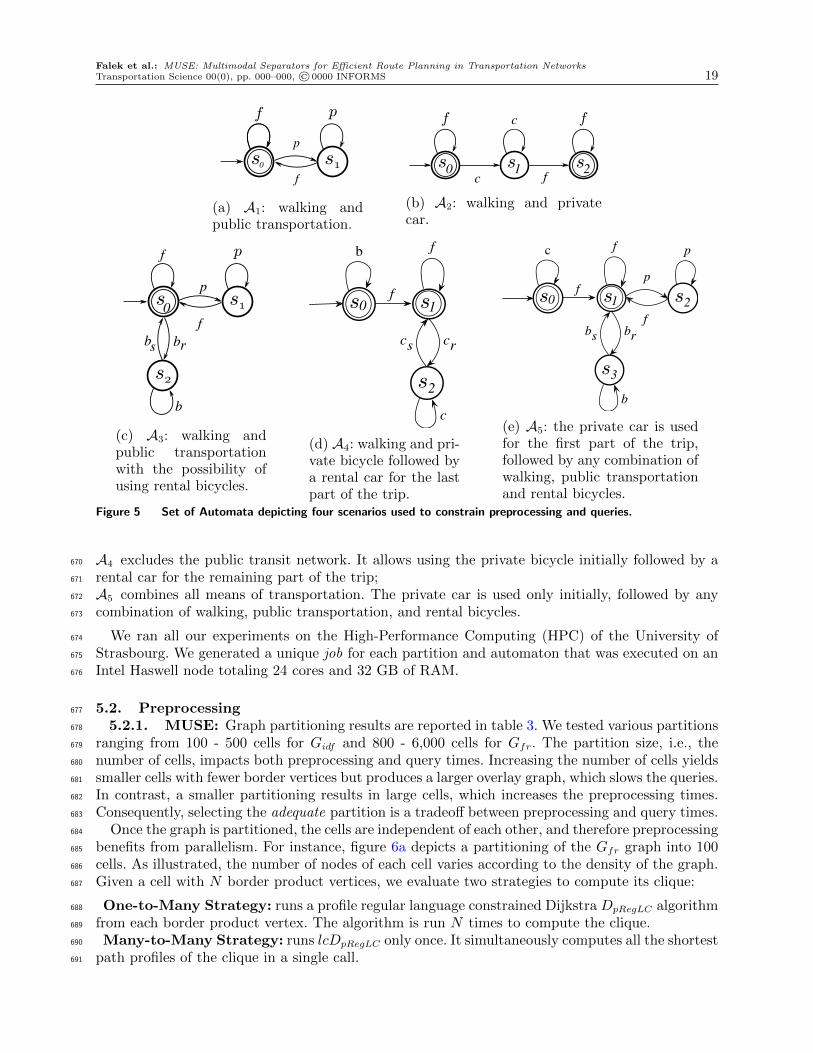
Falek et al.: MUSE: Multimodal Separators for Efficient Route Planning in Transportation NetworksTransportation Science 00(0), pp. 000–000, © 0000 INFORMS 19
s
0
s1
f p
ll
f
p0
(a) A1: walking andpublic transportation.
s
0
s
1
s
2
f fr
l l
r f1 20
c
c
(b) A2: walking and privatecar.
s1
p
ll
s2
b
s
0f
lb l
b
b brs
f
p
f
b
0
(c) A3: walking andpublic transportationwith the possibility ofusing rental bicycles.
c crs
c
f
b
s
0
s
1
s
2
f fr
l l
s3
p
ll
s4
b
lb l
b
0 1
s
0
s
1
s
2
f fr
l l
s3
p
ll
s4
b
lb l
b
2
s
0
s
1
s
2
f fr
l l
s3
p
ll
s4
b
lb l
b
f
(d) A4: walking and pri-vate bicycle followed bya rental car for the lastpart of the trip.
b brs
b
fp
f
c
s
0
s
1
s
2
f fr
l l
s3
p
ll
s4
b
lb l
b
0 1s
0
s
1
s
2
f fr
l l
s3
p
ll
s4
b
lb l
b
2
s
0
s
1
s
2
f fr
l l
s3
p
ll
s4
b
lb l
b
3
s
0
s
1
s
2
f fr
l l
s3
p
ll
s4
b
lb l
b
f p
(e) A5: the private car is usedfor the first part of the trip,followed by any combination ofwalking, public transportationand rental bicycles.
Figure 5 Set of Automata depicting four scenarios used to constrain preprocessing and queries.
A4 excludes the public transit network. It allows using the private bicycle initially followed by a670
rental car for the remaining part of the trip;671
A5 combines all means of transportation. The private car is used only initially, followed by any672
combination of walking, public transportation, and rental bicycles.673
We ran all our experiments on the High-Performance Computing (HPC) of the University of674
Strasbourg. We generated a unique job for each partition and automaton that was executed on an675
Intel Haswell node totaling 24 cores and 32 GB of RAM.676
5.2. Preprocessing677
5.2.1. MUSE: Graph partitioning results are reported in table 3. We tested various partitions678
ranging from 100 - 500 cells for Gidf and 800 - 6,000 cells for Gfr. The partition size, i.e., the679
number of cells, impacts both preprocessing and query times. Increasing the number of cells yields680
smaller cells with fewer border vertices but produces a larger overlay graph, which slows the queries.681
In contrast, a smaller partitioning results in large cells, which increases the preprocessing times.682
Consequently, selecting the adequate partition is a tradeoff between preprocessing and query times.683
Once the graph is partitioned, the cells are independent of each other, and therefore preprocessing684
benefits from parallelism. For instance, figure 6a depicts a partitioning of the Gfr graph into 100685
cells. As illustrated, the number of nodes of each cell varies according to the density of the graph.686
Given a cell with N border product vertices, we evaluate two strategies to compute its clique:687
One-to-Many Strategy: runs a profile regular language constrained Dijkstra DpRegLC algorithm688
from each border product vertex. The algorithm is run N times to compute the clique.689
Many-to-Many Strategy: runs lcDpRegLC only once. It simultaneously computes all the shortest690
path profiles of the clique in a single call.691

Falek et al.: MUSE: Multimodal Separators for Efficient Route Planning in Transportation Networks20 Transportation Science 00(0), pp. 000–000, © 0000 INFORMS
Table 3 Computational time for partitioning the graph with different number of cells and the associatednumber of border vertices.
Graph Number of cells # Border vertices Time [s]
min med max tot
100 124 239 428 24,518 1.023200 65 180 344 36,975 1.278
Gidf 300 52 159 407 49,102 1.474400 56 134 263 55,303 1.673500 29 122 308 63,081 1.874
800 13 91 317 94,897 16.4711,000 13 91 317 94,897 18.351
Gfr 2,000 3 67 331 141,104 19.7424,000 4 47 191 194,352 24.5986,000 2 38 183 239,639 33.366
(a) France multimodal network partition (b) boundary vertices of a single cellFigure 6 A multimodal partition of France separating the underlying graph into 100 cells. (a) Boundary vertices
belonging to the foot, bicycle, road and public transit networks are displayed in blue, green, red, andyellow dots, respectively. (b) boundary vertices of the area highlighted in red in figure (a)
Given that the graph’s density is not uniform, preprocessing time varies significantly (few mil-692
liseconds to seconds) from one cell to another within the same partition. Using the one-to-many693
strategy, we make the computation in parallel for each border vertex, i.e., we do not need to allo-694
cate all the border vertices of a cell to the same CPU. However, the one-to-many strategy does not695
leverage the fact that the shortest paths of a clique are likely to share common subpaths. Therefore,696
vertices that are shared by several shortest paths are processed several times.697
In contrast, the many-to-many strategy is more efficient as it simultaneously processes all the698
clique’s shortest paths. However, it prohibits load balancing because it allocates a whole cell to a699
single CPU. In terms of memory, the largest overlays we obtained are 289 MB and 3062 MB for700
Gidf and Gfr respectively.701
Figure 7 depicts the clique computation time distribution in the Ile-de-France region using the702
one-to-many (left) and many-to-many (right) strategies for each partition and automaton. As703

Falek et al.: MUSE: Multimodal Separators for Efficient Route Planning in Transportation NetworksTransportation Science 00(0), pp. 000–000, © 0000 INFORMS 21
Number of cells
(a) one-to-many algorithm (DpRegLC)
Number of cells
(b) many-to-many algorithm (lcDpRegLC)Figure 7 Computational time for the profile cliques of Gidf as a function of number of cells and automaton.
Number of cells
Figure 8 The preprocessing Gain Factor denoting the speedup of the many-to-many (lcDpRegLC) over the one-to-many (DpRegLC) strategy for each automaton and number of cells. The horizontal red line correspondsto a gain of 1 and imply no speedup.
expected, preprocessing time decreases when the number of cells increases. Furthermore, larger704
automata require more processing time (for instance, A5 compared to A1) because it increases the705
size of the product graph in addition to computing one shortest path for each available state. An706
interesting result is that lcDpRegLC is an order of magnitude faster compared to running DpRegLC707
multiple times. This confirms our previous hypothesis and shows that within a cell, there is indeed708
a significant number of shortest paths of the clique that do share common subpaths.709
For a clearer comparison, we compute the Preprocessing Gain Factor (PGF) for each clique,710
denoting the ratio of computation time using the one-to-many strategy to that of using the many-711
to-many strategy. The results are shown in figure 8 and suggest that the gain depends mainly on712
the type of automaton used to constrain the preprocessing. The gain is smaller on automata that713
rely, partially, on using the road network (A5) and smallest for automata that exclude the public714
transit network (A2 and A4). In our setup, the road and public transit networks are the dominating715
means of transportation; that is, if all means are allowed, the shortest path between two locations is716
comprised, mostly, of the road network and public transit edges (fastest alternatives). Furthermore,717
since the road network is much denser and larger than the public transit network, the shortest718

Falek et al.: MUSE: Multimodal Separators for Efficient Route Planning in Transportation Networks22 Transportation Science 00(0), pp. 000–000, © 0000 INFORMS
Figure 9 MUSE clique computation time for Ile-de-France based on the number of vertices contained in eachcell of the partition.
Figure 10 Distribution of 32 landmarks on the France graph based on the Avoid algorithm (Goldberg andHarrelson 2005).
paths that make up a clique overlap less when constrained by the road network compared to the719
public transit network. Hence, the gain factor is significant for automata A1 and A3.720
For a better insight, figure 9 shows the preprocessing time (using the many-to-many strategy)721
of each cell in the partition as a function of the cell size, i.e., the number of vertices inside the cell.722
Even for the worst-case scenario, the computation time is less than 30 sec and corresponds to a723
large cell of the 100-cell partition with 14000 vertices. The overall processing time is usually less724
than 5 min, even without considering the benefit of parallel computing.725
For the France region, we experimentally selected the partitions such that the cell sizes are726
equivalent to those of the Ile-de-France region, and therefore, preprocessing times are similar when727
one CPU is dedicated to each cell in both cases.728
5.2.2. SDALT: The multimodal goal-directed algorithm known as SDALT improves upon the729
A⋆ algorithm heuristics to achieve fast queries. SDALT relies on the triangle inequality principle730
(Goldberg and Harrelson 2005) to produce better bounds than Euclidean distances. To do so, it731
meticulously precomputes a small set of vertices L called landmarks spread across the network.732
Then, for each landmark l ∈L, it precomputes a forward and reverse constrained shortest path tree733
rooted at l. We implement SDALT as described in (Kirchler et al. 2011). Preprocessing consists of734
computing the landmark-set and their associated shortest-path trees.735

Falek et al.: MUSE: Multimodal Separators for Efficient Route Planning in Transportation NetworksTransportation Science 00(0), pp. 000–000, © 0000 INFORMS 23
Table 4 Preprocessing space and time of SDALT (computing landmark distances) based on 32 landmarks foreach automaton in the Ile-de-France region.
A1 A2 A3 A4 A5
space [MB] 634 450 611 438 423runtime [s] 64.92 83.54 79.92 108.04 106.07
Landmarks selection: we select 32 landmarks using the avoid algorithm (Goldberg and Har-736
relson 2005). The first landmark l0 ∈ L is chosen uniformly at random from the vertex-set Vf of737
the foot network. We compute all shortest paths from l0 to every other vertex v ∈ Vf . Note that738
the reverse shortest paths have the same cost as the foot network is bidirectional. Then, we pick739
a random vertex r ∈ Vf and compute the shortest path tree rooted at r, denoted Tr. For every740
other vertex v ∈ Vf , we compute its weight given by weight(v) = d(r, v)−max{d(l, v) | ∀l ∈L}. The741
weight of a vertex v consequently represents the error in the distance estimation for r when using742
the set of landmarks L, including v.743
To select a new landmark, we compute the size of every vertex v ∈ Vf . First we define the subtree744
Tv ⊂ Tr rooted at v. In particular, we set size(v) = 0 if Tv contains a landmark l ∈ L: v is useless745
since another landmark exists that is already well located. Otherwise, size(v) is evaluated as the746
sum of all the weights of the vertices in Tv. Finally, we select the vertex w greedily with the largest747
size, and we walk in its subtree Tw, traversing recursively, the child with the largest subtree until a748
leaf l is reached. That leaf l is then added to the set of landmarks L. This strategy produces good749
coverage landmarks that yield good lower bounds. This preprocessing phase is run only once.750
Landmark Distances: From each landmark l ∈L, we run DRegLC on the regular and the reverse751
multimodal graphs (we reverse the graph by inverting the direction of all its edges). Therefore,752
we obtain |L| forward and backward constrained shortest-path trees rooted at each landmark l,753
referred to as the landmark distances. In the original SDALT implementation (Kirchler et al. 2011),754
the authors defined four strategies to precompute landmark distances: standard, basic, advanced,755
and specific. Based on the author’s conclusions, the advanced strategy provides only mild speedups756
compared to the basic strategy and requires more memory as the number of calculated bounds is757
a factor |L| higher in the worst case. Hence, we favor the basic implementation, which uses DRegLC758
in conjunction with a single-state automaton with a loop transition labeled with all the allowed759
transportation modes.760
The computational time for selecting 32 landmarks using the Avoid algorithm was 29 seconds for761
Gidf and 8.75 minutes for Gfr. The additional preprocessing time and space required to compute762
landmark distances is summarized in table 4 for Gidf . However, SDALT is not scalable: computing763
all shortest paths between the 32 landmarks and all the vertices of the France graph proved to be764
impractical, even with the resources available on the HPC.765
5.3. Queries766
After precomputing an overlay graph will all the partitions and automata, we generate 10,000767
random queries q(r, t, τ) where r, t are the source and target vertices respectively, and τ is the768
departure time. We compare MUSE with both DRegLC (multimodal Regular Language Constrained769
Dijkstra (Barrett, Jacob, and Marathe 2000)) and SDALT (State-Dependent ALT (Kirchler et al.770
2011)) (Table 5). Figure 11a depicts the query times of MUSE compared to DRegLC on the Ile-de-771
France region, for all queries, regardless of the constraining automaton. MUSE achieves a speedup772
of almost two orders of magnitude over DRegLC .773
By organizing the queries according to their range (Euclidean distance between the source and774
the target), we observe that the speedup increases with the distance range (figure 11b). Indeed,775
the query time not only depends on the number of cells but also the location of the source and776
target vertices. Recalling that the query graph Gq =Gr ∪H ∪Gt combines the subgraphs Gr and777
Gt, induced by the cells containing the source and target vertices r and t, respectively and the778

Falek et al.: MUSE: Multimodal Separators for Efficient Route Planning in Transportation Networks24 Transportation Science 00(0), pp. 000–000, © 0000 INFORMS
Number of cells
(a) Query times distribution of DRegLC and MUSE for all automata.
0-5 5-20 20-50 50-100 100-150Distance Range [km]
10 1
100
101
102
Quer
y Ga
in F
acto
r
Partition Size100200
300400
500
(b) The Query Gain Factor represents the achieved speedup of MUSE over DRegLC for differentpartitions and query distance ranges (Euclidean distance).Figure 11 Performance comparison of DRegLC and MUSE on the Ile-de-France region graph.
overlay H, MUSE always explores Gr and Gt. Therefore, if the cells are large or if the source and779
target are either located inside the same cell or within adjacent cells, MUSE does not benefit from780
the overlay to skip over the rest of the graph. Hence, MUSE performs best for long-range queries,781
as shown in figure 11b.782
In contrast, figure 12 shows the query times distribution of all of DRegLC , SDALT, and MUSE for783
each automaton in the Ile-de-France region. We notice that the speedup of our own implementation784
of SDALT over DRegLC is very close to the original results published by Kirchler et al. MUSE785
is overall an order of magnitude faster than SDALT and achieves better stability across all the786
automata. By comparing the query times distribution of SDALT constrained by A1 and A5, we787
observe that the automaton’s complexity has a significant impact on the performance of SDALT.788
In contrast, MUSE is more robust to the modal constraints.789
MUSE can be augmented using any literature technique that does not require preprocessing790
to achieve further speedups during the query phase. Bi-directional search has been proved to be791
inefficient (and often results in speed-downs) on time-dependent graphs (Nannicini et al. 2008).792
Instead, we relied on goal direction to implement MUSE⋆ and MUSESV (Table 5), as already793
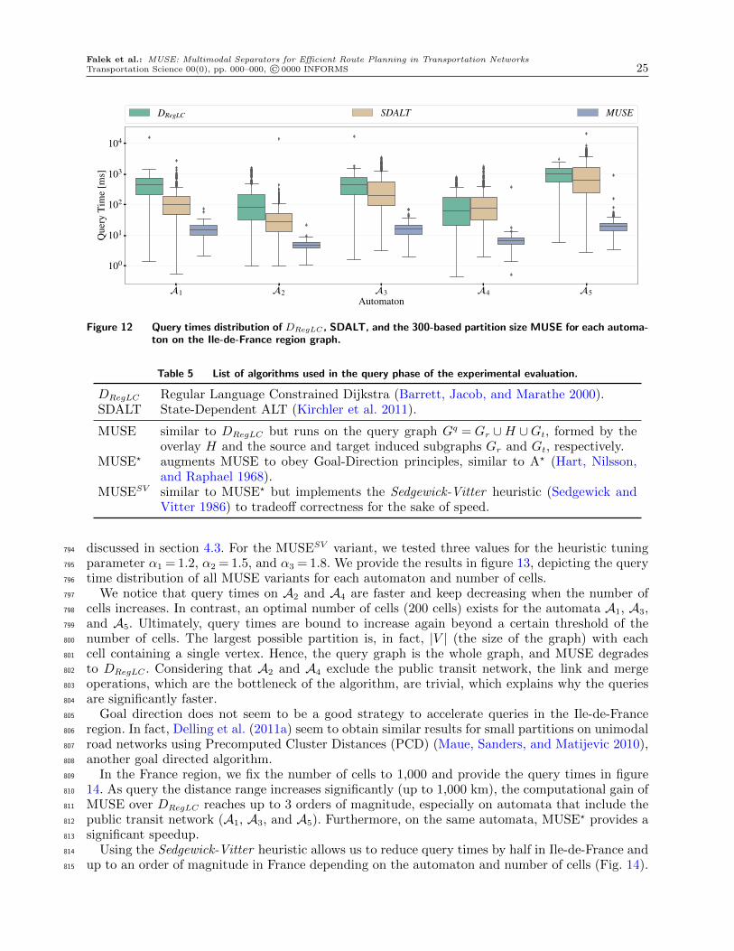
Falek et al.: MUSE: Multimodal Separators for Efficient Route Planning in Transportation NetworksTransportation Science 00(0), pp. 000–000, © 0000 INFORMS 25
1 2 3 4 5Automaton
100
101
102
103
104
Quer
y Ti
me [
ms]
DRegLC SDALT MUSE
Figure 12 Query times distribution of DRegLC , SDALT, and the 300-based partition size MUSE for each automa-ton on the Ile-de-France region graph.
Table 5 List of algorithms used in the query phase of the experimental evaluation.
DRegLC Regular Language Constrained Dijkstra (Barrett, Jacob, and Marathe 2000).SDALT State-Dependent ALT (Kirchler et al. 2011).
MUSE similar to DRegLC but runs on the query graph Gq = Gr ∪H ∪Gt, formed by theoverlay H and the source and target induced subgraphs Gr and Gt, respectively.
MUSE⋆ augments MUSE to obey Goal-Direction principles, similar to A⋆ (Hart, Nilsson,and Raphael 1968).
MUSESV similar to MUSE⋆ but implements the Sedgewick-Vitter heuristic (Sedgewick andVitter 1986) to tradeoff correctness for the sake of speed.
discussed in section 4.3. For the MUSESV variant, we tested three values for the heuristic tuning794
parameter α1 = 1.2, α2 = 1.5, and α3 = 1.8. We provide the results in figure 13, depicting the query795
time distribution of all MUSE variants for each automaton and number of cells.796
We notice that query times on A2 and A4 are faster and keep decreasing when the number of797
cells increases. In contrast, an optimal number of cells (200 cells) exists for the automata A1, A3,798
and A5. Ultimately, query times are bound to increase again beyond a certain threshold of the799
number of cells. The largest possible partition is, in fact, |V | (the size of the graph) with each800
cell containing a single vertex. Hence, the query graph is the whole graph, and MUSE degrades801
to DRegLC . Considering that A2 and A4 exclude the public transit network, the link and merge802
operations, which are the bottleneck of the algorithm, are trivial, which explains why the queries803
are significantly faster.804
Goal direction does not seem to be a good strategy to accelerate queries in the Ile-de-France805
region. In fact, Delling et al. (2011a) seem to obtain similar results for small partitions on unimodal806
road networks using Precomputed Cluster Distances (PCD) (Maue, Sanders, and Matijevic 2010),807
another goal directed algorithm.808
In the France region, we fix the number of cells to 1,000 and provide the query times in figure809
14. As query the distance range increases significantly (up to 1,000 km), the computational gain of810
MUSE over DRegLC reaches up to 3 orders of magnitude, especially on automata that include the811
public transit network (A1, A3, and A5). Furthermore, on the same automata, MUSE⋆ provides a812
significant speedup.813
Using the Sedgewick-Vitter heuristic allows us to reduce query times by half in Ile-de-France and814
up to an order of magnitude in France depending on the automaton and number of cells (Fig. 14).815

Falek et al.: MUSE: Multimodal Separators for Efficient Route Planning in Transportation Networks26 Transportation Science 00(0), pp. 000–000, © 0000 INFORMS
Number of cells
(a) Automaton A1
Number of cells
(b) Automaton A2
Number of cells
(c) Automaton A3
Number of cells
(d) Automaton A4
Number of cells
(e) Automaton A5
Figure 13 Query times distribution for the Ile-de-France region for each automaton of figure 5. Each plot depictsthe running times of MUSE, MUSE⋆, and MUSESV (with a heuristic factor of 1.2, 1.5, and 1.8) foreach number of cell of the preprocessing.
This is, however, at the cost of sacrificing the travel time correctness. We report in figure 15 the816
Travel Time Error (in minutes) for each MUSESV variant across all automata. MUSESV1.2 , the817
less aggressive overestimating variant, provides paths that are 99% of the time only a few seconds818
longer than the shortest paths. In the worst case, we measure a travel time error of 5 minutes.819
Interestingly, even MUSESV1.5 and MUSESV1.8 behave well if the automata do not allow using the820
public transit network (A2 and A4). Since the travel time function of public transit graph edges is821

Falek et al.: MUSE: Multimodal Separators for Efficient Route Planning in Transportation NetworksTransportation Science 00(0), pp. 000–000, © 0000 INFORMS 27
1 2 3 4 5Automaton
100
101
102
103
104
105
Quer
y Ti
me [
ms]
DRegLC
MUSEMUSEMUSE SV1.2
MUSE SV1.5
MUSE SV1.8
Figure 14 On the France region, we fix the number of cells to 1,000 cells and report the query times distributionof DRegLC versus MUSE and all of its variants, for each automaton.
1 2 3 4 5Automaton
10 1
100
101
102
Trav
el Ti
me E
rror [
min
]
MUSE SV1.2
MUSE SV1.5
MUSE SV1.8
(a) Ile-de-France region
1 2 3 4 5Automaton
10 2
10 1
100
101
102
Trav
el Ti
me E
rror [
min
]
MUSE SV1.2
MUSE SV1.5
MUSE SV1.8
(b) France regionFigure 15 Travel Time Error distribution on the Ile-de-France and France regions for each automaton based on
the heuristic factor setting of MUSESV .
non-continuous (figure 2), missing a connection results in a sudden increase of travel time, which822
explains the large errors observed on the remaining automata. Thus, this variant should be carefully823
exploited.824

Falek et al.: MUSE: Multimodal Separators for Efficient Route Planning in Transportation Networks28 Transportation Science 00(0), pp. 000–000, © 0000 INFORMS
6. Conclusion and Future Work825
We presented MUSE, a new approach to solve the multimodal shortest path problem via graph826
partitioning and finite state automaton. Its main advantage is scalability, as it splits large graph827
instances into several independent cells that can be processed in parallel. We also provide different828
strategies to improve the performance of both the preprocessing and the query phases. We achieve829
preprocessing and query times that are fast enough to process a cell and resolve a query in only830
a few milliseconds. Hence, MUSE is a viable solution for real-time multimodal route planning. We831
experimentally tested our implementation and achieved a speedup of up to two orders of magni-832
tude compared to DRegLC , the label constrained version of Dijkstra’s algorithm for multimodal833
networks. Using goal direction and heuristics, we further accelerate the queries and show that the834
obtained paths are, most of the time, only a few seconds longer than the shortest paths. We also835
validated the performance of MUSE against SDALT, a landmark-based goal-directed multimodal836
algorithm. MUSE is an order of magnitude faster than SDALT and proved more robust to varying837
modal constraints. Furthermore, SDALT could not be scaled to handle large graph instances such838
as France’s multimodal transportation network. A problem that MUSE circumvents using graph839
partitioning.840
The partitioning is critical for the performance of both the preprocessing and the query. We first841
tested our implementation of the PUNCH algorithm (Delling et al. 2011b) but switched later on842
to METIS, the general graph partitioning algorithm, which was more reliable and provided better843
results. Therefore, a formal analysis of graph partitioning algorithms tailored to transportation844
networks is essential to improve our current results. Furthermore, to improve query times, multilevel845
partitioning for multimodal graphs is an interesting next step. It allows skipping over most of the846
network using the overlay edges on the partition’s low level while reducing the search space in847
the source and target cells by exploring the high levels of the partition. During preprocessing, we848
also need to compute multimodal profile cliques. We observed that the merge and link operations849
are the bottleneck of lcDpRegLC due to a rapidly increasing number of breakpoints in the travel850
time functions. An interesting work perspective would be to rely on heuristics (Strasser 2017) to851
simplify these operations and evaluate the tradeoff between computational speed and impact on852
correctness. Finally, we considered here only a route computation that minimizes the travel time.853
Handling multiple criteria will require computing the cliques in each cell by maintaining Pareto854
sets. Then, the different Pareto sets will be explored during the query stage. While we conjecture855
that keeping a small number of solutions would be sufficient, we have to investigate how MUSE856
can support multiple criteria with an acceptable computation time and memory.857
References858
Antsfeld L, Walsh T, 2012 Finding multi-criteria optimal paths in multi-modal public transportation networks859
using the transit algorithm. ITS World Congress.860
Barrett C, Jacob R, Marathe M, 2000 Formal-language-constrained path problems. SIAM Journal on Com-861
puting 30(3):809–837, URL http://dx.doi.org/10.1137/S0097539798337716.862
Bast H, 2009 Car or public transport—two worlds. Efficient Algorithms, 355–367 (Springer), URL http:863
//dx.doi.org/10.1007/978-3-642-03456-5_24.864
Bast H, Delling D, Goldberg A, Muller-Hannemann M, Pajor T, Sanders P, Wagner D, Werneck RF, 2016865
Route planning in transportation networks. Algorithm engineering, 19–80 (Springer), URL http://dx.866
doi.org/10.1007/978-3-319-49487-6_2.867
Bast H, Funke S, Matijevic D, 2006 Ultrafast shortest-path queries via transit nodes. Ninth DIMACS Imple-868
mentation Challenge, 175–192, URL http://dx.doi.org/10.1090/dimacs/074/07.869
Bast H, Hertel M, Storandt S, 2016 Scalable transfer patterns. Proceedings of the Meeting on Algorithm Engi-870
neering and Experiments (ALENEX), 15–29, URL http://dx.doi.org/10.1137/1.9781611974317.871
2.872
Bauer R, Delling D, Wagner D, 2011 Experimental study of speed up techniques for timetable information873
systems. Networks 57(1):38–52, URL http://dx.doi.org/10.1002/net.20382.874

Falek et al.: MUSE: Multimodal Separators for Efficient Route Planning in Transportation NetworksTransportation Science 00(0), pp. 000–000, © 0000 INFORMS 29
Baum M, Buchhold V, Sauer J, Wagner D, Zundorf T, 2019 UnLimited TRAnsfers for Multi-Modal Route875
Planning: An Efficient Solution. Annual European Symposium on Algorithms (ESA), volume 144, 14:1–876
14:16, URL http://dx.doi.org/10.4230/LIPIcs.ESA.2019.14.877
Baum M, Dibbelt J, Pajor T, Wagner D, 2016 Dynamic time-dependent route planning in road net-878
works with user preferences. Experimental Algorithms, 33–49, URL http://dx.doi.org/10.1007/879
978-3-319-38851-9_3.880
Bentley JL, Ottmann TA, 1979 Algorithms for reporting and counting geometric intersections. IEEE Trans-881
actions on computers C-28(9):643–647, URL http://dx.doi.org/10.1109/TC.1979.1675432.882
Bhatia N, et al., 2010 Survey of nearest neighbor techniques. International Journal of Computer Science and883
Information Security 8(2).884
Brodal GS, Jacob R, 2004 Time-dependent networks as models to achieve fast exact time-table queries. Elec-885
tronic Notes in Theoretical Computer Science 92:3–15, URL http://dx.doi.org/10.1016/j.entcs.886
2003.12.019.887
Bruggemann-Klein A, 1993 Regular expressions into finite automata. Theoretical Computer Science888
120(2):197–213, URL http://dx.doi.org/10.1016/0304-3975(93)90287-4.889
Chen Y, Guizani M, Zhang Y, Wang L, Crespi N, Lee GM, Wu T, 2019 When traffic flow prediction and890
wireless big data analytics meet. IEEE Network 33(3):161–167, URL http://dx.doi.org/10.1109/891
MNET.2018.1800134.892
Cionini A, D’Angelo G, D’Emidio M, Frigioni D, Giannakopoulou K, Paraskevopoulos A, Zaroliagis C, 2017893
Engineering graph-based models for dynamic timetable information systems. Journal of Discrete Algo-894
rithms 46-47:40 – 58, URL http://dx.doi.org/https://doi.org/10.1016/j.jda.2017.09.001.895
Delling D, Dibbelt J, Pajor T, Zundorf T, 2017 Faster Transit Routing by Hyper Partitioning. D’Angelo G,896
Dollevoet T, eds., 17th Workshop on Algorithmic Approaches for Transportation Modelling, Optimiza-897
tion, and Systems (ATMOS 2017), volume 59, 8:1–8:14, URL http://dx.doi.org/10.4230/OASIcs.898
ATMOS.2017.8.899
Delling D, Goldberg AV, Pajor T, Werneck RF, 2011a Customizable route planning. International900
Symposium on Experimental Algorithms (SEA), 376–387, URL http://dx.doi.org/10.1007/901
978-3-642-20662-7_32.902
Delling D, Goldberg AV, Razenshteyn I, Werneck RF, 2011b Graph partitioning with natural cuts. Inter-903
national Parallel & Distributed Processing Symposium (IPDPS), 1135–1146 (IEEE), URL http:904
//dx.doi.org/10.1109/IPDPS.2011.108.905
Delling D, Pajor T, Wagner D, 2009 Accelerating multi-modal route planning by access-nodes. European906
Symposium on Algorithms, 587–598, URL http://dx.doi.org/10.1007/978-3-642-04128-0_53.907
Delling D, Pajor T, Werneck RF, 2014 Round-based public transit routing. Transportation Science 49(3):591–908
604, URL http://dx.doi.org/10.1287/trsc.2014.0534.909
Delling D, Sanders P, Schultes D, Wagner D, 2006 Highway hierarchies star. Ninth DIMACS Implementation910
Challenge, 141–174, URL http://dx.doi.org/10.1090/dimacs/074/06.911
Demetrescu C, Goldberg AV, Johnson DS, 2009 The Shortest Path Problem: Ninth Dimacs Implementation912
Challenge (American Mathematical Society), URL http://dx.doi.org/10.1090/dimacs/074.913
Dibbelt J, Pajor T, Strasser B, Wagner D, 2013 Intriguingly simple and fast transit routing. Interna-914
tional Symposium on Experimental Algorithms (SEA), 43–54, URL http://dx.doi.org/10.1007/915
978-3-642-38527-8_6.916
Dibbelt J, Pajor T, Wagner D, 2015 User-constrained multimodal route planning. Journal of Experimental917
Algorithmics (JEA) 19, URL http://dx.doi.org/10.1145/2699886.918
Dijkstra EW, 1959 A note on two problems in connexion with graphs. Numerische mathematik 1(1):269–271,919
URL http://dx.doi.org/10.1007/BF01386390.920
Djidjev HN, 1982 On the problem of partitioning planar graphs. SIAM Journal on Algebraic Discrete Methods921
3(2):229–240, URL http://dx.doi.org/10.1137/0603022.922
Falek et al.: MUSE: Multimodal Separators for Efficient Route Planning in Transportation Networks30 Transportation Science 00(0), pp. 000–000, © 0000 INFORMS
DOT U, 2015 Beyond traffic 2045: Trends and choices. Technical Report https://www.transportation.923
gov/sites/dot.gov/files/docs/BeyondTraffic_tagged_508_final.pdf, US Department of Trans-924
portation.925
Eppstein D, Goodrich MT, 2008 Studying (non-planar) road networks through an algorithmic lens. ACM926
SIGSPATIAL international conference on Advances in geographic information systems (ACM), URL927
http://dx.doi.org/10.1145/1463434.1463455.928
Falek A, 2019 osm-to-graph. https://github.com/aminefalek/osm-to-graph.929
Falek A, 2021a Muse: Multimodal separators for efficient route planning in transportation networks. Zenodo930
dataset, URL http://dx.doi.org/10.5281/zenodo.5276749.931
Falek A, 2021b Muse: Multimodal separators for efficient route planning in transportation networks. https:932
//github.com/aminefalek/muse.933
Garey MR, Johnson DS, 2002 Computers and intractability, volume 29 (W. H. Freeman & Co.).934
Geisberger R, Sanders P, Schultes D, Delling D, 2008 Contraction hierarchies: Faster and simpler hierarchical935
routing in road networks. International Workshop on Experimental and Efficient Algorithms (WEA),936
319–333, URL http://dx.doi.org/10.1007/978-3-540-68552-4_24.937
Geofabrik O, 2019 Openstreetmap data extract. URL https://download.geofabrik.de/europe/france/938
ile-de-france.html.939
Giannakopoulou K, Paraskevopoulos A, Zaroliagis C, 2019Multimodal dynamic journey-planning. Algorithms940
12(10):213, URL http://dx.doi.org/10.3390/a12100213.941
Goldberg AV, Harrelson C, 2005 Computing the shortest path: A* search meets graph theory. ACM-SIAM942
symposium on Discrete algorithms (SODA), 156–165.943
Goldberg AV, Kaplan H, Werneck RF, 2006 Reach for a*: Shortest path algorithms with preprocessing. Ninth944
DIMACS Implementation Challenge, 93–140, URL http://dx.doi.org/10.1090/dimacs/074/05.945
Hart PE, Nilsson NJ, Raphael B, 1968 A formal basis for the heuristic determination of minimum cost paths.946
IEEE Transactions on Systems Science and Cybernetics 4(2):100–107, URL http://dx.doi.org/10.947
1109/TSSC.1968.300136.948
Hilger M, Kohler E, Mohring RH, Schilling H, 2009 Fast point-to-point shortest path computations with949
arc-flags. Ninth DIMACS Implementation Challenge, volume 74, 41–72, URL http://dx.doi.org/10.950
1090/dimacs/074/03.951
Huber S, Rust C, 2016 Calculate travel time and distance with openstreetmap data using the open952
source routing machine (osrm). The Stata Journal 16(2):416–423, URL http://dx.doi.org/10.1177/953
1536867X1601600209.954
Ile de France Mobilites, 2020 Donnees offre de transport ile-de-france mobilites au format gtfs.955
https://data.iledefrance-mobilites.fr/explore/dataset/offre-horaires-tc-gtfs-idf/956
information/.957
Karypis G, Kumar V, 1998 A fast and high quality multilevel scheme for partitioning irregular958
graphs. SIAM Journal on scientific Computing 20(1):359–392, URL http://dx.doi.org/10.1137/959
S1064827595287997.960
Kaufman DE, Smith RL, 1993 Fastest paths in time-dependent networks for intelligent vehicle-highway sys-961
tems application. Journal of Intelligent Transportation Systems 1(1), URL http://dx.doi.org/10.962
1080/10248079308903779.963
Kernighan BW, Lin S, 1970 An efficient heuristic procedure for partitioning graphs. Bell system technical964
journal 49(2):291–307, URL http://dx.doi.org/10.1002/j.1538-7305.1970.tb01770.x.965
Kirchler D, Liberti L, Pajor T, Wolfler Calvo R, 2011 Unialt for regular language contrained shortest paths966
on a multi-modal transportation network. Workshop on Algorithmic Approaches for Transportation967
Modelling, Optimization, and Systems (ATMOS), URL http://dx.doi.org/10.4230/OASIcs.ATMOS.968
2011.64.969
Maue J, Sanders P, Matijevic D, 2010 Goal-directed shortest-path queries using precomputed cluster distances.970
Journal of Experimental Algorithmics (JEA) 14:3–2, URL http://dx.doi.org/10.1007/11764298_971
29.972

Falek et al.: MUSE: Multimodal Separators for Efficient Route Planning in Transportation NetworksTransportation Science 00(0), pp. 000–000, © 0000 INFORMS 31
Mooney P, Minghini M, et al., 2017 Mapping and the Citizen Sensor, chapter A review of OpenStreetMap973
data, 37–59 (Ubiquity Press), URL http://dx.doi.org/10.5334/bbf.c.974
Muller-Hannemann M, Schulz F, Wagner D, Zaroliagis C, 2007 Timetable information: Models and algo-975
rithms. Algorithmic Methods for Railway Optimization, 67–90, URL http://dx.doi.org/10.1007/976
978-3-540-74247-0_3.977
Nannicini G, Delling D, Liberti L, Schultes D, 2008 Bidirectional a* search for time-dependent fast paths.978
International Workshop on Experimental and Efficient Algorithms, 334–346, URL http://dx.doi.979
org/10.1007/978-3-540-68552-4_25.980
Navitia Open Data, 2020 France public transport data. https://navitia.opendatasoft.com/explore/981
?refine.geographicarea=France.982
Orda A, Rom R, 1990 Shortest-path and minimum-delay algorithms in networks with time-dependent983
edge-length. Journal of the ACM (JACM) 37(3):607–625, URL http://dx.doi.org/10.1145/79147.984
214078.985
Pyrga E, Schulz F, Wagner D, Zaroliagis C, 2008 Efficient models for timetable information in public trans-986
portation systems. Journal of Experimental Algorithmics (JEA) 12, URL http://dx.doi.org/10.987
1145/1227161.1227166.988
Pyrga E, Schulz F, Wagner D, Zaroliagis CD, 2004 Experimental comparison of shortest path approaches for989
timetable information. ALENEX/ANALC, 88–99 (Citeseer).990
Sanders P, Schulz C, 2012 Distributed evolutionary graph partitioning. Workshop on Algorithm Engineering991
and Experiments (ALENEX), 16–29 (SIAM), URL http://dx.doi.org/10.5555/2790265.2790267.992
Sauer J, Wagner D, Zundorf T, 2020 Faster Multi-Modal Route Planning With Bike Sharing Using ULTRA.993
18th International Symposium on Experimental Algorithms (SEA), volume 160, 16:1–16:14, URL http:994
//dx.doi.org/10.4230/LIPIcs.SEA.2020.16.995
Schilling H, 2012 Tomtom navigation–how mathematics help getting through traffic faster. International996
Symposium on Mathematical Programming (ISMP).997
Sedgewick R, Vitter JS, 1986 Shortest paths in euclidean graphs. Algorithmica 1:31–48, URL http://dx.998
doi.org/10.1007/BF01840435.999
Strasser B, 2017 Dynamic time-dependent routing in road networks through sampling. Workshop on Algo-1000
rithmic Approaches for Transportation Modelling, Optimization, and Systems (ATMOS), URL http:1001
//dx.doi.org/10.4230/OASIcs.ATMOS.2017.3.1002
Thomson RC, Richardson DE, 1995 A graph theory approach to road network generalisation. International1003
cartographic conference, 1871–1880.1004
Ulloa L, Lehoux-Lebacque V, Roulland F, 2018 Trip planning within a multimodal urban mobility. IET Intel-1005
ligent Transport Systems 12(2):87–92(5), URL http://dx.doi.org/10.1049/iet-its.2016.0265.1006
Yang F, Vereshchaka A, Dong W, 2018 Predicting and optimizing city-scale road traffic dynamics using1007
trajectories of individual vehicles. IEEE International Conference on Big Data (Big Data), 173–180,1008
URL http://dx.doi.org/10.1109/BigData.2018.8622356.1009