EsoReflex MUSE Tutorial - FTP Directory Listing - Eso.org

EUROPEAN SOUTHERN OBSERVATORYOrganisation Européenne pour des Recherches Astronomiques dans l’Hémisphère Austral

Europäische Organisation für astronomische Forschung in der südlichen Hemisphäre

VERY LARGE TELESCOPE

EsoReflex MUSE Tutorial

VLT-MAN-ESO-19540-6195

Issue 16.0

Date 2020-03-15

Prepared: L. Coccato, R. Palsa 2020-03-15. . . . . . . . . . . . . . . . . . . . . . . . . . . . . . . . . . . . . . . . . . . . . . . . . . . . . . . . . . . . . . . . . . . . . . . .Name Date Signature

Approved: W. Freudling. . . . . . . . . . . . . . . . . . . . . . . . . . . . . . . . . . . . . . . . . . . . . . . . . . . . . . . . . . . . . . . . . . . . . . . .Name Date Signature

Released: M. Sterzik. . . . . . . . . . . . . . . . . . . . . . . . . . . . . . . . . . . . . . . . . . . . . . . . . . . . . . . . . . . . . . . . . . . . . . . .Name Date Signature

This page was intentionally left blank

ESO EsoReflex MUSE TutorialDoc: VLT-MAN-ESO-19540-6195Issue: Issue 16.0Date: Date 2020-03-15Page: 3 of 59

Change record

Issue/Rev. Date Section/Parag. affected Reason/Initiation/Documents/Remarks1.0 05-12-2014 All First official release2.0 01-02-2015 1-3, 6 Improved text and more detailed explanations on the use

of the muse_exp_combine.xml workflow.3.0 01-04-2015 All Inclusion of exposure alignment in muse.xml;

Replacement of , muse_exp_combine.xml,now dedicated only to alignment and combination ofpre-reduced exposures (no raw or master calibrationframes needed). Installation instructionscompatible with the new install_esoreflexinstallation script.

4.0 15-04-2015 All Change labels from 1.0.2 to 1.0.3. Updated instructionsfor installation (Linux and Mac).

5.0 28-04-2015 All Change software version from 1.0.3 to 1.0.4.6.0 01-08-2015 All In sync with MUSE pipeline version 1.0.5 and Reflex 2.8.7.0 01-10-2015 5-7 In sync with MUSE pipeline version 1.2.

All Few typos corrected.8.0 01-10-2015 5-7 In sync with MUSE pipeline version 1.4.9.0 18-04-2016 2, 5, 9-10 In sync with MUSE pipeline version 1.6. Updated instructions

on how to use static response curve and provide user-definedsky masks.

10 01-03-2017 1, 6, 8 In line with pipeline version 2.0 and with the new layout:(creation of sky residual cubes and telluric correction strategy)

11 20-04-2018 6, 7 Adapted for Reflex 2.9. Inclusion of interactive alignmentprocedure.

12 14-12-2018 8 Added description about how to add a badpixeltable.13 26-02-2018 All Software package versions update.14 02-04-2019 All Software package versions update.

6.3 Added description about efficient cleaning of the Ramanline contamination

15 01-10-2019 6.4 Support for master calibrations16 01-05-2020 All In sync with reflex 2.11

This page was intentionally left blank


Contents

1 Introduction to Esoreflex 7

2 Software Installation 8

2.1 Installing Reflex workflows via macports . . . . . . . . . . . . . . . . . . . . . . . . . . . . 8

2.2 Installing Reflex workflows via rpm/yum/dnf . . . . . . . . . . . . . . . . . . . . . . . . . 8

2.3 Installing Reflex workflows via install_esoreflex . . . . . . . . . . . . . . . . . . . . . 9

2.4 System requirements . . . . . . . . . . . . . . . . . . . . . . . . . . . . . . . . . . . . . . . . 10

2.4.1 Hardware . . . . . . . . . . . . . . . . . . . . . . . . . . . . . . . . . . . . . . . . . . 10

2.5 JVM Memory set-up . . . . . . . . . . . . . . . . . . . . . . . . . . . . . . . . . . . . . . . . 11

2.5.1 Execution on machines with less than 64 GB of memory . . . . . . . . . . . . . . . . . 12

3 Quick Start: Reducing The Demo Data 13

4 Demo Data 17

4.1 Files in the demo datasets . . . . . . . . . . . . . . . . . . . . . . . . . . . . . . . . . . . . . . 17

4.2 Description of the different kinds of datasets . . . . . . . . . . . . . . . . . . . . . . . . . . . . 18

4.3 Selecting raw or master calibrations for a datasets . . . . . . . . . . . . . . . . . . . . . . . . . 19

5 About the main esoreflex canvas 21

5.1 Saving And Loading Workflows . . . . . . . . . . . . . . . . . . . . . . . . . . . . . . . . . . 21

5.2 Buttons . . . . . . . . . . . . . . . . . . . . . . . . . . . . . . . . . . . . . . . . . . . . . . . 21

5.3 Workflow States . . . . . . . . . . . . . . . . . . . . . . . . . . . . . . . . . . . . . . . . . . . 21

6 The MUSE Workflow 22

6.1 Workflow Canvas Parameters . . . . . . . . . . . . . . . . . . . . . . . . . . . . . . . . . . . 22

6.2 MUSE specific parameters: setting the data reduction strategy . . . . . . . . . . . . . . . . . . 23

6.3 Workflow Actors . . . . . . . . . . . . . . . . . . . . . . . . . . . . . . . . . . . . . . . . . . 27

6.3.1 Simple Actors . . . . . . . . . . . . . . . . . . . . . . . . . . . . . . . . . . . . . . . 27

6.3.2 Lazy Mode . . . . . . . . . . . . . . . . . . . . . . . . . . . . . . . . . . . . . . . . . 27

7 Reducing your own data 29

7.1 The esoreflex command . . . . . . . . . . . . . . . . . . . . . . . . . . . . . . . . . . . . 29


7.2 Launching the workflow . . . . . . . . . . . . . . . . . . . . . . . . . . . . . . . . . . . . . . 29

7.3 Workflow Steps . . . . . . . . . . . . . . . . . . . . . . . . . . . . . . . . . . . . . . . . . . . 31

7.3.1 Data Organisation And Selection . . . . . . . . . . . . . . . . . . . . . . . . . . . . . . 31

7.3.2 DataSetChooser . . . . . . . . . . . . . . . . . . . . . . . . . . . . . . . . . . . . . . . 32

7.3.3 The data reduction cascade and the workflow composite actors . . . . . . . . . . . . . . 33

7.3.4 Workflow products . . . . . . . . . . . . . . . . . . . . . . . . . . . . . . . . . . . . . 35

7.3.5 The ProductExplorer . . . . . . . . . . . . . . . . . . . . . . . . . . . . . . . . . . . . 36

8 Combination of multiple exposures 39

8.1 Automatic combination within the muse.xml workflow . . . . . . . . . . . . . . . . . . . . . 39

8.2 Automatic combination within the muse_exp_combine.xml workflow . . . . . . . . . . . 40

8.3 Interactive alignment of multiple exposures . . . . . . . . . . . . . . . . . . . . . . . . . . . . 42

9 Tips and tricks 46

9.1 Optimization of the automatic alignment . . . . . . . . . . . . . . . . . . . . . . . . . . . . . . 46

9.1.1 The algorithm in a nutshell . . . . . . . . . . . . . . . . . . . . . . . . . . . . . . . . . 46

9.1.2 Tips . . . . . . . . . . . . . . . . . . . . . . . . . . . . . . . . . . . . . . . . . . . . . 46

9.2 Optimization of the empty sky regions for sky background evaluation . . . . . . . . . . . . . . 47

9.3 Optimization of the sky removal via post-processing: the muse_zap workflow . . . . . . . . . . 48

9.4 Using user-supplied response curves and telluric correction . . . . . . . . . . . . . . . . . . . . 48

9.5 Masking bad pixels during combination of exposures . . . . . . . . . . . . . . . . . . . . . . . 49

9.6 Execution of the workflow on computers with limited Memory . . . . . . . . . . . . . . . . . . 50

9.7 Verification tools . . . . . . . . . . . . . . . . . . . . . . . . . . . . . . . . . . . . . . . . . . 51

9.7.1 Verification of the tracing solution . . . . . . . . . . . . . . . . . . . . . . . . . . . . . 51

9.7.2 Verification of the wavelength solution . . . . . . . . . . . . . . . . . . . . . . . . . . 53

9.8 Step by step product inspection . . . . . . . . . . . . . . . . . . . . . . . . . . . . . . . . . . . 54

10 Frequently Asked Questions 56


1 Introduction to Esoreflex

This document is a tutorial designed to enable the user to to reduce his/her data with the ESO pipeline run underan user-friendly environmet, called EsoReflex, concentrating on high-level issues such as data reductionquality and signal-to-noise (S/N) optimisation.

EsoReflex is the ESO Recipe Flexible Execution Workbench, an environment to run ESO VLT pipelineswhich employs a workflow engine to provide a real-time visual representation of a data reduction cascade,called a workflow, which can be easily understood by most astronomers. The basic philosophy and concepts ofReflex have been discussed by Freudling et al. (2013A&A...559A..96F). Please reference this article if you useReflex in a scientific publication.

Reflex and the data reduction workflows have been developed by ESO and instrument consortia and they arefully supported. If you have any issue, please contact [email protected] for further support.

A workflow accepts science and calibration data, as downloaded from the archive using the CalSelector tool1

(with associated raw calibrations) and organises them into DataSets, where each DataSet contains one scienceobject observation (possibly consisting of several science files) and all associated raw and static calibrationsrequired for a successful data reduction. The data organisation process is fully automatic, which is a majortime-saving feature provided by the software. The DataSets selected by the user for reduction are fed to theworkflow which executes the relevant pipeline recipes (or stages) in the correct order. Full control of the variousrecipe parameters is available within the workflow, and the workflow deals automatically with optional recipeinputs via built-in conditional branches. Additionally, the workflow stores the reduced final data products in alogically organised directory structure employing user-configurable file names.

The MUSE Reflex workflow is designed to process all the single target scientific exposures independently. Ittherefore produces reconstructed datacube, images, and reduced pixel table for all of them. It is also to design tocombine together exposures of the same object and the same instrument set-up, even from different ObservingBlocks. The exposures will be automatically aligned before combination, using reference bright objects in thefield of view.

The MUSE Reflex workflow handles both cases where sky exposures are present or not in the same OB ofthe target. In the latter case, the sky is evaluated in regions in the field of view where the target contributionis negligible. The most relevant parameters for the sky subtraction strategy can be specified directly in theReflex canvas.

Note: As for version 2.8, the muse workflow is able to process dataset with both raw and master calibrations.

The current MUSE esoreflex distribution contains also two additional workflows: muse_exp_combine.xml,which is dedicated only to the alignment and combination of already-processed reduced pixel tables (it does notprocess raw frames), and muse_zap, which is dedicated to the additional removal of sky residual lines.

In this document, we assume the user is already familiar with the recipes of the MUSE pipeline and theirparameters. For more information, we refer the reader to the MUSE pipeline manual available at:http://www.eso.org/sci/software/pipelines/ .

1http://www.eso.org/sci/archive/calselectorInfo.html

https://ui.adsabs.harvard.edu/abs/2013A%26A...559A..96F/abstract

mailto:[email protected]

http://www.eso.org/sci/software/pipelines/

http://www.eso.org/sci/archive/calselectorInfo.html


2 Software Installation

Esoreflex and the workflows can be installed in different ways: via package repositories, via theinstall_esoreflex script or manually installing the software tar files.

The recommended way is to use the package repositories if your operating system is supported. The macportsrepositories support macOS 10.11 to 10.14, while the rpm/yum repositories support Fedora 26 to 29, CentOS7, Scientific Linux 7. For any other operating system it is recommended to use the install_esoreflexscript.

The installation from package repository requires administrative privileges (typically granted via sudo), as itinstalls files in system-wide directories under the control of the package manager. If you want a local installation,or you do not have sudo privileges, or if you want to manage different installations on different directories, thenuse the install_esoreflex script. Note that the script installation requires that your system fulfill severalsoftware prerequisites, which might also need sudo privileges.

Reflex 2.10 needs java JDK 11 to be installed.

Please note that in case of major or minor (affecting the first two digit numbers) Reflex upgrades, the user shoulderase the $HOME/KeplerData, $HOME/.kepler directories if present, to prevent possible aborts (i.e. ahard crash) of the esoreflex process.

2.1 Installing Reflex workflows via macports

This method is supported for the macOS operating system. It is assumed that macports(http://www.macports.org) is installed. Please read the full documentation athttp://www.eso.org/sci/software/pipelines/installation/macports.html.

2.2 Installing Reflex workflows via rpm/yum/dnf

This method is supported for Fedora 26 to 29, CentOS 7, Scientific Linux 7 operating systems, and requiressudo rights. To install, please follow these steps

1. Configure the ESO repository (This step is only necessary if the ESO repository has not already beenpreviously configured).

• If you are running Fedora 26 or newer, run the following commands:

sudo dnf install dnf-plugins-coresudo dnf config-manager --add-repo=ftp://ftp.eso.org/pub/dfs/

pipelines/repositories/stable/fedora/esorepo.repo

• If you are running CentOS 7, run the following commands:

sudo yum install yum-utils ca-certificates yum-conf-repossudo yum install epel-releasesudo yum-config-manager --add-repo=ftp://ftp.eso.org/pub/dfs/

pipelines/repositories/stable/centos/esorepo.repo

http://www.macports.org

http://www.eso.org/sci/software/pipelines/installation/macports.html


• If you are running SL 7, run the following commands:

sudo yum install yum-utils ca-certificates yum-conf-repossudo yum install yum-conf-epelsudo yum-config-manager --add-repo=ftp://ftp.eso.org/pub/dfs/

pipelines/repositories/stable/sl/esorepo.repo

2. Install the pipelines

• The list of available top level packages for different instruments is given by:

sudo dnf list esopipe-\*-all # (Fedora 26 or newer)sudo yum list esopipe-\*-all # (CentOS 7, SL 7)

• To install an individual pipeline use the following (This example is for X-Shooter. Adjust the pack-age name to the instrument you require.):

sudo dnf install esopipe-xshoo-all # (Fedora 26 or newer)sudo yum install esopipe-xshoo-all # (CentOS 7, SL 7)

• To install all pipelines use:

sudo dnf install esopipe-\*-all # (Fedora 26 or newer)sudo yum install esopipe-\*-all # (CentOS 7, SL 7)

For further information, please read the full documentation athttp://www.eso.org/sci/software/pipelines/installation/rpm.html.

2.3 Installing Reflex workflows via install_esoreflex

This method is recommended for operating systems other than what indicated above, or if the user has no sudorights. Software dependencies are not fulfilled by the installation script, therefore the user has to install all theprerequisites before running the installation script.

The software pre-requisites for Reflex 2.11.0 may be found at:http://www.eso.org/sci/software/pipelines/reflex_workflows

To install the Reflex 2.11.0 software and demo data, please follow these instructions:

1. From any directory, download the installation script:

wget ftp://ftp.eso.org/pub/dfs/reflex/install_esoreflex

2. Make the installation script executable:

chmod u+x install_esoreflex

3. Execute the installation script:

http://www.eso.org/sci/software/pipelines/installation/rpm.html

http://www.eso.org/sci/software/pipelines/reflex_workflows


./install_esoreflex

and the script will ask you to specify three directories: the download directory <download_dir>, thesoftware installation directory <install_dir>, and the directory to be used to store the demo data<data_dir>. If you do not specify these directories, then the installation script will create them in thecurrent directory with default names.

4. Follow all the script instructions; you will be asked whether to use your Internet connecteion (recom-mended: yes), the pipelines and demo-datasets to install (note that the installation will remove all previ-ously installed pipelines that are found in the same installation directory).

5. To start Reflex, issue the command:

<install_dir>/bin/esoreflex

It may also be desirable to set up an alias command for starting the Reflex software, using the shell com-mand alias. Alternatively, the PATH variable can be updated to contain the <install_dir>/bindirectory.

2.4 System requirements

2.4.1 Hardware

The processing of MUSE data is very demanding in terms of computing resources. In particular, it requiresa machine with sufficient memory installed, and it is available only for 64-bit machines. The recommendedplatform is a powerful workstation with a recent 64-bit Linux system.

The recommended configuration of the target machine for creating the final data cube from a single MUSEobservation and the suggested set of calibrations is:

• 64 GB of memory

• 24 CPU cores (physical cores)2

• 4 TB of free disk space

• GCC 4.8.2 (or newer)

Scientific programs usually foreseen the creation of a datacube by merging multiple exposures taken at the sameposition. On average, the memory consumption grows linearly with the number of observations.

In the case of creation of mosaic, the size of the data cube may become really huge, and the required memorygrows accordingly.

2Using 24 CPUs is on average from 10% to 30% faster than using 12 CPUs (although the number of CPUs is doubled). Pleaseevaluate the costs/benefits of a 24 CPU system over a 12 CPU system.


By default, the workflow is set to use all the available cores (e.g. 24, in the configuration suggested above) andprocesses the data of the 24 MUSE IFUs in parallel. The serial or parallel execution of each recipe is set by thenifu recipe parameter3: a value of -1 will process the IFUs in parallel (fast, but memory demanding), a valueof 0 will process the IFUs in series (24 times slower, but less memory demanding). A value of 1 ≤ N ≤ 24 willprocess only the selected N−th IFU.

The execution of the recipes in parallel and the use of all the available cores can led to memory issues even fora 64 GB machine, if many calibration files are to be combined together. For example, the combination of 45flats or 45 arcs to generate the LSF_PROFILE requires more than 64 GB. A solution could be to instruct theworkflow to use only 12 cores. In this case, the workflow computes 2 groups of 12 IFUs in series, and the 12IFU in each group are processed in parallel; the execution times doubles, but memory demands are halved (atleast for those recipes that accept the nifu parameter).

This can be done by setting the following environmental variable OMP_NUM_THREADS. To do so, please pro-ceed as follows.

1. In the working directory type esoreflex -create-config muse.rc It will create a configura-tion file named muse.rc. Provide the full path of the esoreflex launch script if the command esoreflexis not in your PATH.

2. Edit the muse.rc configuration file and modify the value of the entry esoreflex.inherit-environmentfrom FALSE (default) to TRUE. Save the muse.rc file

3. Launch esoreflex with the command (single line):

$ env -i DISPLAY=:0 OMP_NUM_THREADS=N <full_path>/esoreflex \> -config \$PWD/muse.rc muse\& }

where N is the desired number of threads, and <full_path> is the full path of the esoreflex launchscript. In this way, esoreflex will be launched on a clean environment plus the variable OMP_NUM_THREADSthat regulates the number of cores to use.

Note that this is valid for Linux installations only, as there is no parallelization available for the MUSE pipelinein Mac OS.

For more information, please refer to the MUSE pipeline manual available athttp://www.eso.org/sci/software/pipelines/ .

2.5 JVM Memory set-up

The MUSE workflow need a sufficient amount of memory allocated to Reflex. The best way to set thememory allocation of Reflex is to run the reflex_set_memory script that is distributed with Reflexbefore starting Reflex. The recommended setting for MUSE is to leave the “Minimum amount of memory”

3This parameter is available only in the muse_bias, muse_flat, muse_wave, and muse_lsf, and muse_scibasic recipes. Otherrecipes, which are designed to combine all the available IFUs cannot be run in series.

http://www.eso.org/sci/software/pipelines/


unchanged, and set the “Maximum amount of memory” to 2000. Alternatively, the memory setting can be doneafter starting Reflex by clicking on "Tools – JVM Memory Settings" in the menu bar. Reflex needs to berestarted for this change to be applied.

2.5.1 Execution on machines with less than 64 GB of memory

The MUSE pipeline and the Reflex workflow can be still executed in less powerful machines, such as laptopswith 8GB of RAM, provided that the user restricts the wavelength range to short interval (e.g. 100 Å). Thisset-up, although still demanding in terms of computational time, allows the user to test the data reductionstrategy before having access to a more powerful machine and reduce the data on the full wavelength range.For example, it can be used to create sky masks, to find the best method and parameters for the sky subtractionin critical wavelength ranges, to calculate the coordinate offsets between different exposures, and much more.More information are in Section 9.6.


3 Quick Start: Reducing The Demo Data

For the user who is keen on starting reductions without being distracted by detailed documentation, we describethe steps to be performed to reduce the science data provided in the MUSE demo data set supplied with theesoreflex 2.11.0 release. By following these steps, the user should have enough information to performa reduction of his/her own data without any further reading:

1. First, type:

esoreflex -l

If the esoreflex executable is not in your path, then you have to provide the command with theexecutable full path <install_dir>/bin/esoreflex -l . For convenience, we will drop thereference to <install_dir>. A list with the available esoreflex workflows will appear, showingthe workflow names and their full path.

2. Open the MUSE by typing:

esoreflex muse&

Alternatively, you can type only the command esoreflex the empty canvas will appear (Figure 3.1)and you can select the workflow to open by clicking on File -> Open File. Note that the loadedworkflow will appear in a new window. The MUSE workflow is shown in Figure 3.2.

3. To aid in the visual tracking of the reduction cascade, it is advisable to use component (or actor) highlight-ing. Click on Tools -> Animate at Runtime, enter the number of milliseconds representing theanimation interval (100 ms is recommended), and click OK .

4. Change directories set-up. Under “Setup Directories” in the workflow canvas there are seven parametersthat specify important directories (green dots).

By default, the ROOT_DATA_DIR, which specifies the working directory within which the other directo-ries are organised. is set to your $HOME/reflex_data directory. All the temporary and final productsof the reduction will be organized under sub-directories of ROOT_DATA_DIR, therefore make sure thisparameter points to a location where there is enough disk space. To change ROOT_DATA_DIR, doubleclick on it and a pop-up window will appear allowing you to modify the directory string, which you mayeither edit directly, or use the Browse button to select the directory from a file browser. When you havefinished, click OK to save your changes.

Changing the value of RAW_DATA_DIR is the only necessary modification if you want to process dataother than the demo data

5. Click the button to start the workflow

6. The workflow will highlight the Data Organiser actor which recursively scans the raw data di-rectory (specified by the parameter RAW_DATA_DIR under “Setup Directories” in the workflow can-vas) and constructs the datasets. Note that the raw and static calibration data must be present either


in RAW_DATA_DIR or in CALIB_DATA_DIR, otherwise datasets may be incomplete and cannot beprocessed. However, if the same reference file was downloaded twice to different places this creates aproblem as esoreflex cannot decide which one to use.

7. The Data Set Chooser actor will be highlighted next and will display a “Select Datasets” window(see Figure 3.3) that lists the datasets along with the values of a selection of useful header keywords4. Thefirst column consists of a set of tick boxes which allow the user to select the datasets to be processed. Bydefault all complete datasets which have not yet been reduced will be selected. A full description of theoptions offered by the Data Set Chooser will be presented in Section 7.3.2.

8. Click the Continue button and watch the progress of the workflow by following the red highlightingof the actors. A window will show which dataset is currently being processed.

9. Once the reduction of all datasets has finished, a pop-up window called Product Explorer will appear,showing the datasets which have been reduced together with the list of final products. This actor allowsthe user to inspect the final data products, as well as to search and inspect the input data used to createany of the products of the workflow. Figure 3.4 shows the Product Explorer window. A full descriptionof the Product Explorer will be presented in Section 7.3.5.

10. After the workflow has finished, all the products from all the datasets can be found in a directory underEND_PRODUCTS_DIR named after the workflow start timestamp. Further subdirectories will be foundwith the name of each dataset.

Well done! You have successfully completed the quick start section and you should be able to use this knowledgeto reduce your own data. However, there are many interesting features of Reflex and the MUSE workflowthat merit a look at the rest of this tutorial.

Figure 3.1: The empty Reflex canvas.

4The keywords listed can be changed by double clicking on the DataOrganiser Actor and editing the list of keywords in the sec-ond line of the pop-up window. Alternatively, instead of double-clicking, you can press the right mouse button on the DataOrganiserActor and select Configure Actor to visualize the pop-up window.


Figure 3.2: The MUSE Reflex muse.wkf workflow.


Figure 3.3: The Select Dataset window.

Figure 3.4: The Product Explorer window.


4 Demo Data

4.1 Files in the demo datasets

A demo dataset is distributed together with the MUSE Reflexworkflow. It consists of several target exposures,off-set sky exposures, on-sky calibration frames (sky flats, standard star), and instrument calibration frames, raw(biases, flats, arcs...) and master (master bias, master flat...). In addition, the set of static calibrations includedin the pipeline distribution is needed for the reduction of the demo dataset.

Static calibrations for all the datasetsbadpix_table.fits BADPIX_TABLEextinct_table.fits EXTINCT_TABLEfilter_list.fits FILTER_LISTline_catalog.fits LINE_CATALOGsky_lines.fits SKY_LINESstd_flux_table.fits STD_FLUX_TABLEvignetting_mask.fits VIGNETTING_MASK

Dataset with master calibrationsFILE CATEGORYRaw science dataMUSE.2017-01-02T06:27:16.469.fits.fz OBJECTMUSE.2017-01-02T06:37:57.914.fits.fz SKYMUSE.2017-01-02T06:42:56.092.fits.fz OBJECTMaster calibrationsM.MUSE.2017-01-09T12:37:15.090.fits.fz TWILIGHT_CUBEM.MUSE.2017-01-09T12:51:24.606.fits.fz MASTER_BIASM.MUSE.2017-01-09T13:05:32.846.fits.fz MASTER_FLATM.MUSE.2017-01-09T13:10:38.540.fits.fz STD_RESPONSEM.MUSE.2017-01-09T13:12:11.910.fits.fz STD_TELLURICM.MUSE.2017-01-09T13:18:31.190.fits.fz TRACE_TABLEM.MUSE.2017-01-09T13:19:51.046.fits.fz WAVECAL_TABLEM.MUSE.2015-10-23T12:37:56.746.fits.fz LSF_PROFILEStatic calibrationsM.MUSE.2017-01-04T12:40:33.496.fits.fz ASTROMETRY_WCSM.MUSE.2017-01-04T12:51:19.510.fits.fz GEOMETRY_TABLEM.MUSE.2017-01-04T12:56:22.356.fits.fz LSF_PROFILEM.MUSE.2017-01-10T13:23:53.413.fits.fz ASTROMETRY_REFERENCE

Incomplete datasetFILE CATEGORYRaw science dataMUSE_WFM-NOAO_OBS039_0037.fits.fz OBJECT


Dataset with raw calibrationsFILE CATEGORYRaw science dataMUSE_WFM-NOAO_OBS173_0069.fits.fz OBJECTMUSE_WFM-NOAO_OBS173_0070.fits.fz SKYMUSE_WFM-NOAO_OBS173_0071.fits.fz OBJECTRaw calibrationsMUSE_CAL_BIAS173_0004.fits.fz BIASMUSE_CAL_BIAS173_0005.fits.fz BIASMUSE_CAL_BIAS173_0006.fits.fz BIASMUSE_CAL_BIAS173_0007.fits.fz BIASMUSE_CAL_BIAS173_0008.fits.fz BIASMUSE_WFM_FLAT172_0049.fits.fz FLAT,LAMPMUSE_WFM_FLAT172_0050.fits.fz FLAT,LAMPMUSE_WFM_FLAT172_0051.fits.fz FLAT,LAMPMUSE_WFM_FLAT172_0052.fits.fz FLAT,LAMPMUSE_WFM_FLAT172_0053.fits.fz FLAT,LAMPMUSE_WFM_SKYFLAT172_0001.fits.fz FLAT,SKYMUSE_WFM_SKYFLAT172_0002.fits.fz FLAT,SKYMUSE_WFM_SKYFLAT172_0003.fits.fz FLAT,SKYMUSE_WFM_SKYFLAT172_0004.fits.fz FLAT,SKYMUSE_WFM_SKYFLAT172_0005.fits.fz FLAT,SKYMUSE_WFM_STD172_0002.fits.fz STDMUSE_WFM_WAVE173_0001.fits.fz WAVEMUSE_WFM_WAVE173_0002.fits.fz WAVEMUSE_WFM_WAVE173_0003.fits.fz WAVEMUSE_WFM_WAVE173_0004.fits.fz WAVEMUSE_WFM_WAVE173_0005.fits.fz WAVEMUSE_WFM_WAVE173_0006.fits.fz WAVEMUSE_WFM_WAVE173_0007.fits.fz WAVEMUSE_WFM_WAVE173_0008.fits.fz WAVEMUSE_WFM_WAVE173_0009.fits.fz WAVETRACE_TABLE-06_ExtMode_Temp8p53.fits TRACE_TABLETRACE_TABLE-06_NomMode_Temp8p49.fits TRACE_TABLEStatic calibrationsastrometry_reference.fits ASTROMETRY_REFERENCEastrometry_wcs_wfm.fits ASTROMETRY_WCSgeometry_table_wfm.fits GEOMETRY_TABLEstd_response_wfm-n.fits STD_RESPONSE

4.2 Description of the different kinds of datasets

As specified in Section 3, Esoreflex uses a set of rules (so-called OCA rules) to group the files into datasets.There are two types of datasets. The first type contains only one science target exposure and it is named after


it. It also contains the calibrations (either raw or master) needed to reduce it. In the case of the demo data, thedatasets of this first type are:

• MUSE.2017-01-02T06:27:16.469.fits and MUSE.2017-01-02T06:42:56.092.fits. These datasets containone raw science and one raw sky exposures each, and the master calibrations needed to reduce them.

• MUSE.2017-01-02T06:42:56.092.fits. This dataset contains one raw science and one raw sky exposures,and the master calibrations needed to reduce them.

• MUSE_WFM-NOAO_OBS039_0037.fits. This dataset contains one raw science exposure, but it does notcontain all the needed calibrations to process it. It is therefore classified as incomplete and grayed out inthe Dataset Chooser.

• MUSE_WFM-NOAO_OBS173_0069.fits and MUSE_WFM-NOAO_OBS173_0071.fits. These datasetscontain one raw science and one raw sky exposures each, and the raw calibrations needed to reduce them.

The second type contains multiple science exposures that have the same HIERARCH ESO OBS TARG NAMEand HIERARCH ESO INS MODE header keywords. They are meant to be dithered exposures of the sametarget and the workflow combines them together to generate a single datacube. See Section 8.2 for instructionson how to change the rules that define the exposures to combine together.

In the case of the demo data, the datasets of this second type are:

• MUSE.2017-01-02T06:27:16.469.fits_combined_cubes. This dataset includes the MUSE.2017-01-02T06:27:16.469.fits and MUSE.2017-01-02T06:42:56.092.fits dataset. The two observations will be combinedtogether.

• MUSE_WFM-NOAO_OBS039_0037.fits_combined_cubes. This dataset is incomplete.

• MUSE_WFM-NOAO_OBS173_0069.fits_combined_cubes. This dataset includes the MUSE_WFM-NOAO_OBS173_0069.fits and MUSE_WFM-NOAO_OBS173_0071.fits datasets. The two observations will becombined together.

4.3 Selecting raw or master calibrations for a datasets

The MUSE workflow is capable of dealing with the presence of raw and master calibrations. For each scientificexposure, the general rule is to associate the calibration (either master or raw) that it is closer in time and use it.

In the case both master and raw calibrations are equally close in time to the science data, it is possible tospecify which calibrations one prefers to use. Before starting the workflow, one has to double click on the DataOrganizer and indicate a preference in the “Association preference” field.

The main application of this feature is the following. The user can download both master and raw calibrationsfrom the archive via CalSelector. In this case, the master calibrations downloaded from CalSelector are equallyclose in time to the science than the calibrations the workflow will generate from the raw files. In this case,the user can specify the preference to “MASTER CALIBRATIONS” and reduce only the science data. If theresults indicate an issue with the calibration, then the user can repeat the reduction with preference to “RAWCALIBRATIONS” and change the recipe parameters.


The only exceptions to this rule are the calibrations LSF_PROFILE, STD_RESPONSE, and STD_TELLURICfor which both master and raw calibrations are associated to the dataset, independently from the “Associationpreference” specified in the data organizer. The user has the possibility to decide which one to use by settingthe appropriate strategy configuration parameter (see Section 6.2).


5 About the main esoreflex canvas

5.1 Saving And Loading Workflows

In the course of your data reductions, it is likely that you will customise the workflow for various data sets, evenif this simply consists of editing the ROOT_DATA_DIR to a different value for each data set. Whenever youmodify a workflow in any way, you have the option of saving the modified version to an XML file using File-> Export As (which will also open a new workflow canvas corresponding to the saved file). The savedworkflow may be opened in subsequent esoreflex sessions using File -> Open. Saving the workflowin the default Kepler format (.kar) is only advised if you do not plan to use the workflow with another computer.

5.2 Buttons

At the top of the esoreflex canvas are a set of buttons which have the following functions:

• - Zoom in.

• - Reset the zoom to 100%.

• - Zoom the workflow to fit the current window size (Recommended).

• - Zoom out.

• - Run (or resume) the workflow.

• - Pause the workflow execution.

• - Stop the workflow execution.

The remainder of the buttons (not shown here) are not relevant to the workflow execution.

5.3 Workflow States

A workflow may only be in one of three states: executing, paused, or stopped. These states are indicated by the

yellow highlighting of the , , and buttons, respectively. A workflow is executed by clicking thebutton. Subsequently the workflow and any running pipeline recipe may be stopped immediately by clicking the

button, or the workflow may be paused by clicking the button which will allow the current actor/recipeto finish execution before the workflow is actually paused. After pausing, the workflow may be resumed by

clicking the button again.


6 The MUSE Workflow

The MUSE workflow canvas is organised into a number of areas. From top-left to top-right you will find generalworkflow instructions, directory parameters, and global parameters. In the middle row you will find five boxesdescribing the workflow general processing steps in order from left to right, and below this the workflow actorsthemselves are organised following the workflow general steps.

6.1 Workflow Canvas Parameters

The workflow canvas displays a number of parameters that may be set by the user. Under “Setup Directories” theuser is only required to set the RAW_DATA_DIR to the working directory for the dataset(s) to be reduced, which,by default, is set to the directory containing the demo data. The RAW_DATA_DIR is recursively scanned by theData Organiser actor for input raw data. The directory CALIB_DATA_DIR, which is by default within thepipeline installation directory, is also scanned by the Data Organiser actor to find any static calibrationsthat may be missing in your dataset(s). If required, the user may edit the directories BOOKKEEPING_DIR,LOGS_DIR, TMP_PRODUCTS_DIR, and END_PRODUCTS_DIR, which correspond to the directories wherebook-keeping files, logs, temporary products and end products are stored, respectively (see the Reflex UserManual for further details; [1]).

There is a mode of the Data Organiser that skips the built-in data organisation and uses instead the data or-ganisation provided by the CalSelector tool. To use this mode, click on Use CalSelector associationsin the Data Organiser properties and make sure that the input data directory contains the XML file down-loaded with the CalSelector archive request (note that this does not work for all instrument workflows).

Under the “Global Parameters” area of the workflow canvas, the user may set the FITS_VIEWER parameter tothe command used for running his/her favourite application for inspecting FITS files. Currently this is set bydefault to fv, but other applications, such as ds9, skycat and gaia for example, may be useful for inspectingimage data. Note that it is recommended to specify the full path to the visualization application (an alias willnot work).

By default the EraseDirs parameter is set to false, which means that no directories are cleaned beforeexecuting the workflow, and the recipe actors will work in Lazy Mode (see Section 6.3.2), reusing the previouspipeline recipe outputs if input files and parameters are the same as for the previous execution, which savesconsiderable processing time. Sometimes it is desirable to set the EraseDirs parameter to true, whichforces the workflow to recursively delete the contents of the directories specified by BOOKKEEPING_DIR,LOGS_DIR, and TMP_PRODUCTS_DIR. This is useful for keeping disk space usage to a minimum and willforce the workflow to fully re-reduce the data each time the workflow is run.

The parameter RecipeFailureMode controls the behaviour in case that a recipe fails. If set to Continue,the workflow will trigger the next recipes as usual, but without the output of the failing recipe, which in mostof the cases will lead to further failures of other recipes without the user actually being aware of it. This modemight be useful for unattended processing of large number of datasets. If set to Ask, a pop-up window will askwhether the workflow should stop or continue. This is the default. Alternatively, the Stop mode will stop theworkflow execution immediately.

The parameter ProductExplorerMode controls whether the ProductExplorer actor will show its win-dow or not. The possible values are Enabled, Triggered, and Disabled. Enabled opens the Product-


Explorer GUI at the end of the reduction of each individual dataset. Triggered (default and recommended)opens the ProductExplorer GUI when all the selected datasets have been reduced. Disabled does not displaythe ProductExplorer GUI.

6.2 MUSE specific parameters: setting the data reduction strategy

All the recipe parameters can be changed by configuring the associated RecipeExecuter actor. This can bedone by opening the various composite actors until the RecipeExecuter associated to the desired pipelinerecipe is visible. To open a composite actor, click on it with the mouse right button, and select "Open Actor".To configure the RecipeExecuter click on it with the mouse right button, and select “Configure Actor”. Alist of all recipe parameters will be available for editing. Press “Commit” to apply the changes.

In addition, the main Reflex canvas offers to the user a quick selection of some key parameters and options,which are relevant to select the appropriate strategy for the data reduction. They are located in the section “Datareduction strategy parameters” (Figure 6.1).

• Calibrations parameters.

– ComputeLSF. Valid entries are true or false. Default = false. It sets which parametrization ofthe instrumental Line Spread Function (LSF) to use during data reduction. This parametriza-tion is fundamental to construct reliable models of the sky emission lines. The frame tag for theLSF parametrization is LSF_PROFILE. A reliable parametrization requires 45 dedicated arc linesframes (DPR.TYPE = WAVE,LSF).If set to false, the workflow uses the parametrization associated to the dataset (either downloadedwith the dataset, or in the static calibration directory). With this option, the muse_lsf recipe withinthe Line Spread Function actor is not triggered.If set to true, the LSF is parametrized by the muse_lsf recipe from the dedicated raw arc calibrationsavailable in the dataset.Typically, the LSF_PROFILE calibration downloaded with the dataset contains a very good parametriza-tion of the instrumental line spread function profile.

– Telluric. It specifies which telluric correction strategy to adopt. Possible values are:

∗ 0 does not perform any telluric correction.∗ 1 (default) performs the telluric correction using the raw observations of the standard star ob-

served at twilight (if they are present in the dataset).∗ 2 Uses an user-provided file (e.g. master calibration) with the same structure of the STD_TELLURIC,

as produced by the muse_standard recipe. This is done even if raw observations of the standardstar are present in the dataset.

– Response. It specifies which strategy to adopt for the flux calibration (response curve). Possiblevalues are:

∗ 0 (default) performs the flux calibration using the raw observations of the standard star observedat twilight (if they are present in the dataset).

∗ 1 Uses an user-provided file (e.g. master calibration) containing the response curve (samestructure of the STD_RESPONSE, as produced by the muse_standard recipe). This is doneeven if raw observations of the standard star are present in the dataset.


Figure 6.1: The Data reduction strategic parameters section in the Reflex canvas. Top panel contains the fullview of the section. Central and Bottom panels contain the left and right zooms of the section, respectively.


Please consult Section Section 9.4 for more information .

• Wavelength range parameters. If you are interested in a restricted wavelength range it is possible tocreate the final datacube accordingly. The following parameters have an affect on the muse_create_sky,muse_astrometry, muse_scipost, and muse_exp_combine recipes.

– LamMin. Sets the minimum wavelength (in Å) to consider when reconstructing the datacube. Itcorresponds to the recipe parameter -lambdamin. Default: 4000.

– LamMax. Sets the maximum wavelength (in Å) to consider when reconstructing the datacube. Itcorresponds to the recipe parameter -lambdamax. Default: 10000.

The recipe muse_standard is not affected by LamMin and LamMax, because the change of the cor-responding -lambdamin and -lambdamax parameters can cause the recipe to fail. If you are us-ing on a computer with limited memory capabilities (see Section for hardware specifications 3.1) themuse_standard will fail in reconstructing the datacube and the workflow will crash. To avoid that, youcan remove the standard star observations from the dataset and use the master calibrations downloadedfrom the ESO archive via the CalSelector tool.

• Strategy for sky subtraction. The MUSE pipeline (and therefore the workflow) evaluates the sky tobe subtracted in two ways. If dedicated sky observations are present, the sky can be evaluated using aspecified fraction of spaxels in the reconstructed sky image. This fraction is specified by the SkyFr_1workflow parameter. Alternatively, the sky can be evaluated directly on the scientific frames, in regionswhere the contribution of the target is negligible. A specified fraction of spaxels in the reconstructedimage (the faintest spaxels) will be selected to create the sky spectrum. This fraction is specified by theSkyFr_2 workflow parameter.

The following parameters are relevant for the sky subtraction. Each dataset might require different values.

– Create Datacube with sky residual. If set to true, the workflow will create datacubes, reconstructedimage, and pixeltables of the dedicated sky exposures (if present in the dataset). These product aresaved in a directory nemed after the dataset they refer to, but with the suffix -SkyResidualCubesin the name, which is located in the reflex end product directory. It is advisable to set it to true if oneintend to remove residual sky lines with the ZAP tool (see Section 9.3).

– SkyFr_1. It corresponds to the recipe parameter -fraction in the muse_ create_sky recipe.This is relevant only if dedicated sky exposures are present in the dataset.

– SkyFr_2. It corresponds to the recipe parameter -skymodel_fraction in the muse_scipostrecipe. This is relevant if the sky has to be evaluated directly from the target exposure.

– SkyMethod. Method for sky subtraction. Valid entries are: “auto”, “model”, “subtract-model”,“simple”, and “none”. Default: auto. These values define the -skymethod parameter in themuse_scipost recipe, except for the “auto” mode (which is not recognized by muse_scipost).

∗ “none”, the sky background subtraction is not performed.∗ “subtract-model”, precalculated sky lines and continuum are subtracted (e.g. from dedicated

sky observations or static calibrations). We recommend to use this method if dedicated skyobservations are available.


∗ “model”, the sky is computed on a fraction of the field of view specified by the parameterSkyFr_2 and then subtracted. We recommend to use this method if the sky background needsto be evaluated from the target field of view.

∗ “simple”, the sky to be subtracted is created directly from the data, without regard to LSFvariations.

∗ “auto” If selected, the workflow will automatically set the SkyMethod variable to:· “subtract-model” if dedicated sky-observations are available for the scientific object in the

dataset.· “model” if dedicated sky-observations are not available for the scientific object in the

dataset.

If dedicated sky observations are present, good values could be SkyFr_1 = 0.75, SkyFr_2 = 0.2, andSkyMethod = subtract-model (the latter is automatically set if the “auto” mode is selected). If offset skyobservations are not present, the sky will be evaluated from a specified fraction of pixels in the target fieldof view; good values could be SkyFr_2 = 0.2 and SkyMethod = model (the latter is automatically set ifthe “auto” mode is selected); the parameter SkyFr_1 has no effect in this case.

Warning: if SkyMethod = model, SkyFr_2 cannot be 0, otherwise the recipe fails.

Warning: If dedicated sky observations are present, and if the SkyMethod is set to model, then the skycontinuum is evaluated from the dedicated sky observations, and the sky emission lines are computed fromthe science target. This strategy reduces systematic due to to variations of the intensity of the emissionlines between the sky and the target observations. It is recommended if there is a portion of the field ofview in the target exposure where the continuum of the targets is small (even if not zero), and the emissionlines from the target are negligible. Usually, this strategy gives better results than computing also the skycontinuum in the target exposure because the time variation of the sky continuum are smaller than that ofthe emission lines.

However, If an user wants to compute also the sky continuum in the target exposure (i.e., not using at allthe dedicated sky observations), then the suggested strategy is to remove the dedicated sky observationsfrom the dataset. In the Select Dataset window (Figure 3.3), highlight the desired dataset, click on InspectDataset, and deselect the sky exposures.

• Efficient cleaning of Raman emission lines contaminationObservations taken in Adaptive Optics mode (AO) exploit the Na laser to improve spatial resolution. Thelaser light is scattered by the atmosphere and contaminate the observations (Raman scattering). Thiscontamination shows up mainly as emission lines at 6485 Åand at 6827 Å which vary slowly across thefield, at about ±5 %.

The majority of this contamination removed during sky subtraction; However, for observations of nearlyempty fields, the MUSE pipeline provides a dedicated procedure to improve the correction of this con-tamination. To turn on this correction, the global parameter Use Raman lines correction has to be set toyes.

Note that this has effect only on NFM-AO-N, WFM-AO-N, and WFM-AO-E observation modes.

The correction is efficient only if large part of the field of view of the target is dominated by sky. Therefore,one has to set SkyMethod = model and use a high fraction of Sky_Fr (e.g., > 0.6).

For more information on how to fine-tune the Raman correction, please consult the pipeline manual(Section 6.5.4).


6.3 Workflow Actors

6.3.1 Simple Actors

Simple actors have workflow symbols that consist of a single (rather than multiple) green-blue rectangle. Theymay also have an icon within the rectangle to aid in their identification. The following actors are simple actors:

• - The DataOrganiser actor.

• - The DataSetChooser actor (inside a composite actor).

• - The FitsRouter actor Redirects files according to their categories.

• - The ProductRenamer actor.

• - The ProductExplorer actor (inside a composite actor).

Access to the parameters for a simple actor is achieved by right-clicking on the actor and selecting ConfigureActor. This will open an “Edit parameters” window. Note that the Product Renamer actor is a jythonscript (Java implementation of the Python interpreter) meant to be customised by the user (by double-clickingon it).

6.3.2 Lazy Mode

By default, all RecipeExecuter actors in a pipeline workflow are “Lazy Mode” enabled. This means thatwhen the workflow attempts to execute such an actor, the actor will check whether the relevant pipeline recipehas already been executed with the same input files and with the same recipe parameters. If this is the case,then the actor will not execute the pipeline recipe, and instead it will simply broadcast the previously generatedproducts to the output port. The purpose of the Lazy Mode is therefore to minimise any reprocessing of data byavoiding data re-reduction where it is not necessary.

One should note that the actor’s Lazy Mode depends on the contents of the directory specified by the parameterBOOKKEEPING_DIR and the relevant FITS file checksums. Any modification to the directory contents and/orthe file checksums will cause the corresponding actor to run the pipeline recipe again when executed, therebyre-reducing the input data.

The re-reduction of data at each execution may sometimes be desirable. To force a re-reduction of data forany single RecipeExecuter actor in the workflow, right-click the actor, select Configure Actor, and


uncheck the Lazy mode parameter tick-box in the “Edit parameters” window that is displayed. For many work-flows the RecipeExecuter actors are actually found inside the composite actors in the top level workflow.To access such embedded RecipeExecuter actors you will first need to open the sub-workflow by right-clicking on the composite actor and then selecting Open Actor.

To force the re-reduction of all data in a workflow (i.e. to disable Lazy mode for the whole workflow), you mustuncheck the Lazy mode for every single RecipeExecuter actor in the entire workflow. It is also possible tochange the name of the bookkeeping directory, instead of modifying any of the Lazy mode parameters. This willalso force a re-reduction of the given dataset(s). A new reduction will start (with the lazy mode still enabled),but the results of previous reduction will not be reused. Alternatively, if there is no need to keep any of thepreviously reduced data, one can simply set the EraseDirs parameter under the “Global Parameters” area ofthe workflow canvas to true. This will then remove all previous results that are stored in the bookkeeping,temporary, and log directories before processing the input data, in effect, starting a new clean data reductionand re-processing every input dataset. Note: The option EraseDirs = true does not work in esoreflexversion 2.9.x and makes the workflow to crash.


7 Reducing your own data

In this section we describe how to reduce your own data set.

First, we suggest the reader to familiarize with the workflow by reducing the demo dataset first (Section 3), butit is not a requirement.

7.1 The esoreflex command

We list here some options associated to the esoreflex command. We recommend to try them to familiarizewith the system. In the following, we assume the esoreflex executable is in your path; if not you have toprovide the full path <install_dir>/bin/esoreflex

To see the available options of the esoreflex command type:

esoreflex -h

The output is the following.

-h | -help print this help message and exit.-v | -version show installed Reflex version and pipelines and exit.-l | -list-workflows list available installed workflows and from

~/KeplerData/workflows.-n | -non-interactive enable non-interactive features.-e | -explore run only the Product Explorer in this workflow-p <workflow> | -list-parameters <workflow>

lists the available parameters for the givenworkflow.

-config <file> allows to specify a custom esoreflex.rc configurationfile.

-create-config <file> if <file> is TRUE then a new configuration file iscreated in ~/.esoreflex/esoreflex.rc. Alternativelya configuration file name can be given to write to.Any existing file is backed up to a file with a ’.bak’extension, or ’.bakN’ where N is an integer.

-debug prints the environment and actual Reflex launchcommand used.

7.2 Launching the workflow

We list here the recommended way to reduce your own datasets. Steps 1 and 2 are optional and one can startfrom step 3.

1. Type: esoreflex -n <parameters> MUSE to launch the workflow non interactively and reduceall the datasets with default parameters.


<parameters> allows you to specify the workflow parameters, such as the location of your raw dataand the final destination of the products.

For example, type (in a single command line):

esoreflex -n-RAW_DATA_DIR /home/user/my_raw_data-ROOT_DATA_DIR /home/user/my_reduction-END_PRODUCTS_DIR $ROOT_DATA_DIR/reflex_end_productsmuse

to reduce the complete datasets that are present in the directory /home/user/my_raw_data and thatwere not reduced before. Final products will be saved in /home/user/my_reduction/reflex_end_products, while book keeping, temporary products, and logs will be saved in sub-directories of/home/user/my_reduction/. If the reduction of a dataset fails, the reduction continues to the nextdataset. It can take some time, depending on the number of datasets present in the input directory. Fora full list of workflow parameters type esoreflex -p MUSE. Note that this command lists only theparameters, but does not launch the workflow.

Once the reduction is completed, one can proceed with optimizing the results with the next steps.

2. Type:

esoreflex -e muse

to launch the Product Explorer. The Product Explorer allows you to inspect the data products alreadyreduced by the MUSE esoreflex workflow. Only products associated with the workflow default book-keeping database are shown. To visualize products associated to given bookkeeping database, pass thefull path via the BOOKKEEPING_DB parameter:

esoreflex -e BOOKKEEPING_DB <database_path> muse

to point the product explorer to a given <database_path>, e.g., /home/username/reflex/reflex_bookkeeping/test.db

The Product Explorer allows you to inspect the products while the reduction is running. Press the buttonRefresh to update the content of the Product Explorer. This step can be launched in parallel to step 1.

A full description of the Product Explorer will be given in Section 7.3.5

3. Type:

esoreflex muse &

to launch the MUSE esoreflex workflow. The MUSE workflow window will appear (Fig. 3.2). Pleaseconfigure the set-up directories ROOT_DATA_DIR, RAW_DATA_DIR, and other workflow parametersas needed. Just double-click on them, edit the content, and press OK . Remember to specify the same<database_path> as for the Product Explorer, if it has been opened at step #2, to synchronize thetwo processes.

4. (Recommended, but not mandatory) On the main esoreflex menu set Tools –> Animate atRuntime to 1 in order to highlight in red active actors during execution.

5. Press the button to start the workflow. First, the workflow will highlight and execute the Initialiseactor, which among other things will clear any previous reductions if required by the user (see Section 6.1).


Secondly, if set, the workflow will open the Product Explorer, allowing the user to inspect previously re-duced datasets (see Section 7.3.5 for how to configure this option).

Note: The MUSE workflow offers the option to select the datareduction strategy by setting the so-called strategyparameter (see Section 6.2). Default values should serve for the majority of the cases; if you need to customizeyour reduction strategy, please change the strategy parameters before starting the workflow.

7.3 Workflow Steps

7.3.1 Data Organisation And Selection

The DataOrganiser (DO) is the first crucial component of a Reflex workflow. The DO takes as inputRAW_DATA_DIR and CALIB_DATA_DIR and it detects, classifies, and organises the files in these directoriesand any subdirectories. The output of the DO is a list of “DataSets”. A DataSet is a special Set of Files (SoF).A DataSet contains one or several science (or calibration) files that should be processed together, and all filesneeded to process these data. This includes any calibration files, and in turn files that are needed to processthese calibrations. Note that different DataSets might overlap, i.e. some files might be included in more thanone DataSet (e.g., common calibration files).

A DataSet lists three different pieces of information for each of its files, namely 1) the file name (includ-ing the path), 2) the file category, and 3) a string that is called the “purpose” of the file. The DO uses theOCA5 rules to find the files to include in a DataSet, as well as their categories and purposes. The file categoryidentifies different types of files, and it is derived by information in the header of the file itself. A categorycould for example be RAW_CALIBRATION_1, RAW_CALIBRATION_2 or RAW_SCIENCE, depending onthe instrument. The purpose of a file identifies the reason why a file is included in a DataSet. The syntax isaction_1/action_2/action_3/ ... /action_n, where each action_i describes an intendedprocessing step for this file (for example, creation of a MASTER_CALIBRATION_1 or a MASTER_CALIBRATION_2).The actions are defined in the OCA rules and contain the recipe together with all file categories required to exe-cute it (and predicted products in case of calibration data). For example, a workflow might include two actionsaction_1 and action_2. The former creates MASTER_ CALIBRATION_1 from RAW_CALIBRATION_1,and the later creates a MASTER_CALIBRATION_2 from RAW_CALIBRATION_2. The action_2 actionneeds RAW_CALIBRATION_2 frames and the MASTER_ CALIBRATION_1 as input. In this case, theseRAW_CALIBRATION_1 files will have the purpose action_ 1/action_2. The same DataSet might alsoinclude RAW_CALIBRATION_1 with a different purpose; irrespective of their purpose the file category for allthese biases will be RAW_CALIBRATION_1.

The Datasets created via the DataOrganiser will be displayed in the DataSet Chooser. Here the usershave the possibility to inspect the various datasets and decide which one to reduce. By default, DataSets thathave not been reduced before are highlighted for reduction. Click either Continue in order to continue withthe workflow reduction, or Stop in order to stop the workflow. A full description of the DataSet Chooseris presented in Section 7.3.2.

5OCA stands for OrganisationClassificationAssociation and refers to rules, which allow to classify the raw data according to thecontents of the header keywords, organise them in appropriate groups for processing, and associate the required calibration data forprocessing. They can be found in the directory <install_dir>/share/esopipes/<pipeline-version>/reflex/,carrying the extension.oca


Once the Continue is pressed, the workflow starts to reduce the first selected DataSet. Files are broadcastedaccording to their purpose to the relevant actors for processing.

The categories and purposes of raw files are set by the DO, whereas the categories and purpose of productsgenerated by recipes are set by the RecipeExecuter. The file categories are used by the FitsRouterto send files to particular processing steps or branches of the workflow (see below). The purpose is usedby the SofSplitter and SofAccumulator to generate input SoFs for the RecipeExecuter. TheSofSplitter and SofAccumulator accept several SoFs as simultaneous input. The SofAccumulatorcreates a single output SoF from the inputs, whereas the SofSplitter creates a separate output SoF for eachpurpose.

7.3.2 DataSetChooser

The DataSetChooser displays the DataSets available in the “Select Data Sets” window, activating verticaland horizontal scroll bars if necessary (Fig. 3.3).

Some properties of the DataSets are displayed: the name, the number of files, a flag indicating if it has beensuccessfully reduced (a green OK), if the reduction attempts have failed or were aborted (a red FAILED), or ifit is a new dataset (a black "-"). The column "Descriptions" lists user-provided descriptions (see below), othercolumns indicate the instrument set-up and a link to the night log.

Sometimes you will want to reduce a subset of these DataSets rather than all DataSets, and for this you mayindividually select (or de-select) DataSets for processing using the tick boxes in the first column, and the buttonsDeselect All and Select Complete at the bottom, or configure the “Filter” field at the bottom left.

Available filter options are: "New" (datasets not previously reduced will be selected), "Reduced" (datasetspreviously reduced will be selected), "All" (all datasets will be selected), and "Failed" (dataset with a failed oraborted reduction will be selected).

You may also highlight a single DataSet in blue by clicking on the relevant line. If you subsequently click onInspect Highlighted , then a “Select Frames” window will appear that lists the set of files that make

up the highlighted DataSet including the full filename6, the file category (derived from the FITS header), and aselection tick box in the right column. The tick boxes allow you to edit the set of files in the DataSet which isuseful if it is known that a certain calibration frame is of poor quality (e.g: a poor raw flat-field frame). The listof files in the DataSet may also be saved to disk as an ASCII file by clicking on Save As and using the filebrowser that appears.

By clicking on the line corresponding to a particular file in the “Select Frames” window, the file will be high-lighted in blue, and the file FITS header will be displayed in the text box on the right, allowing a quick inspectionof useful header keywords. If you then click on Inspect , the workflow will open the file in the selected FITSviewer application defined by the workflow parameter FITS_VIEWER.

To exit from the “Select Frames” window, click Continue .

To add a description of the reduction, press the button ... associated with the field "Add description to thecurrent execution of the workflow" at the bottom right of the Select Dataset Window; a pop up window willappear. Enter the desired description (e.g. "My first reduction attempt") and then press OK . In this way, all thedatasets reduced in this execution, will be flagged with the input description. Description flags can be visualized

6keep the mouse pointer on the file name to visualize the full path name.


in the SelectFrames window and in the ProductExplorer, and they can be used to identify differentreduction strategies.

To exit from the “Select DataSets” window, click either Continue in order to continue with the workflowreduction, or Stop in order to stop the workflow.

Figure 7.1: The “Select Frames” window with a single file from the current Data Set highlighted in blue, and thecorresponding FITS header displayed in the text box on the right. Hidden partially behind the “Select Frames”window is the “Select DataSets” window with the currently selected DataSet highlighted in blue.

7.3.3 The data reduction cascade and the workflow composite actors

The MUSE workflow is designed to execute a well defined data reduction cascade. It triggers a number of“composite actors” that are associated to specific pipeline recipes. The exact execution sequence of these actorsand recipes depends on the content of the dataset itself and on the data reduction strategy set up by the user.


In particular, the user can specify whether to compute a new parametrization of the line spread function or usethe one provided with the downloaded dataset. Also the strategy for sky reduction can be decided, whetherto use dedicated sky observations (if available) or compute the background sky contribution on empty regionsin the scientific target field of view. All these strategies can be configured by setting the appropriate strategyparameters in the main workflow canvas (Section 6.2).

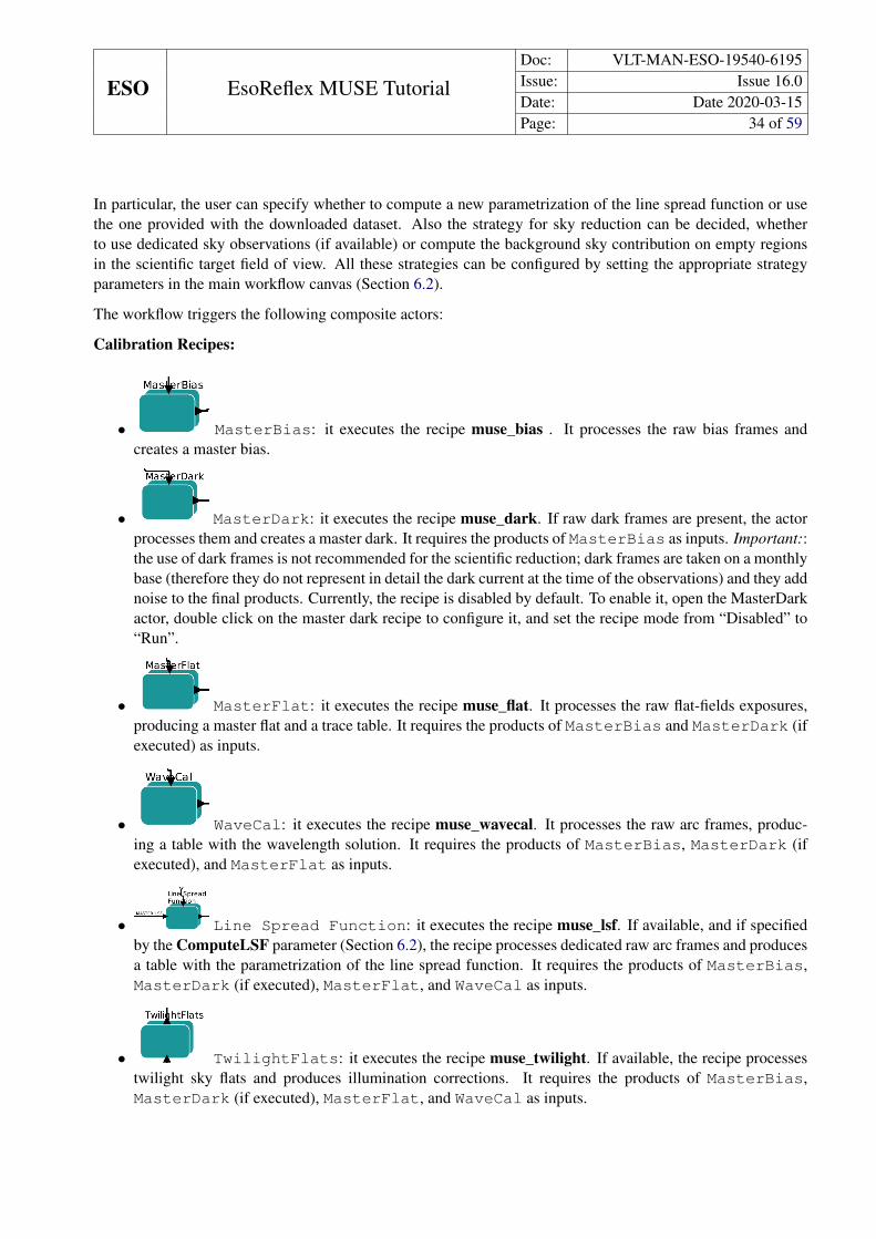
The workflow triggers the following composite actors:

Calibration Recipes:

• MasterBias: it executes the recipe muse_bias . It processes the raw bias frames andcreates a master bias.

• MasterDark: it executes the recipe muse_dark. If raw dark frames are present, the actorprocesses them and creates a master dark. It requires the products of MasterBias as inputs. Important::the use of dark frames is not recommended for the scientific reduction; dark frames are taken on a monthlybase (therefore they do not represent in detail the dark current at the time of the observations) and they addnoise to the final products. Currently, the recipe is disabled by default. To enable it, open the MasterDarkactor, double click on the master dark recipe to configure it, and set the recipe mode from “Disabled” to“Run”.

• MasterFlat: it executes the recipe muse_flat. It processes the raw flat-fields exposures,producing a master flat and a trace table. It requires the products of MasterBias and MasterDark (ifexecuted) as inputs.

• WaveCal: it executes the recipe muse_wavecal. It processes the raw arc frames, produc-ing a table with the wavelength solution. It requires the products of MasterBias, MasterDark (ifexecuted), and MasterFlat as inputs.

• Line Spread Function: it executes the recipe muse_lsf. If available, and if specifiedby the ComputeLSF parameter (Section 6.2), the recipe processes dedicated raw arc frames and producesa table with the parametrization of the line spread function. It requires the products of MasterBias,MasterDark (if executed), MasterFlat, and WaveCal as inputs.

• TwilightFlats: it executes the recipe muse_twilight. If available, the recipe processestwilight sky flats and produces illumination corrections. It requires the products of MasterBias,MasterDark (if executed), MasterFlat, and WaveCal as inputs.


Science Recipes:

• Standard Star: it executes the recipes muse_scibasic and muse_standard. It processesthe frames of the standard star and returns a response curve and a telluric correction. If standard starsobservations are not present in the dataset, it uses the response curve from the static calibration. It requiresthe products of the calibration recipes as input. It is possible to use user-supplied version of the responsecurve and telluric correction rather than those produced by the Standard Star actor (see Section 9.4).

• Sky: it executes the recipes muse_scibasic and muse_create_sky. If dedicated sky obser-vations are present in the dataset, it creates a list of sky emission lines and a sky continuum to be used inthe sky subtraction of the science observations. It requires the products of the calibration recipes and ofStandard Star as input. The recipe has an automatic procedure to determine the sky regions in theframe. It is hower possible to provide an optimized sky mask for this purpose (see Section 9.2).

• Science: it executes the recipe muse_scibasic and muse_scipost. It processes the raw sci-ence frames producing fully reduced datacubes (DATACUBE_FINAL), pixel table (PIXTABLE_REDUCED),and reconstructed images (IMAGE_FOV). The strategy for sky subtraction depends on the user set up ofthe SkyMethod strategic parameter (Section 6.2). It requires the the products of the calibration recipes, ofStandard Star, Astrometry (if executed), and Sky (according to the parameter set-up) as input.

• Combine Exposures: if the selected dataset contains multiple exposures to be alignedand combined together, the actor executes the recipes muse_exp_align and muse_exp_combine. It re-quires the products of the Science actor. It is an interactive actor, in the sense that the user can inspectthe prducts of the muse_exp_align recipe and decide wether to continue with the reduction or repeat thisstep with other parameters (see Section 8.3) .

For more information about the inputs and outputs of individual recipes and their configuration parameters,please consult the MUSE pipeline manual.

7.3.4 Workflow products

All the products of the individual recipes are saved into the temporary products directory (TMP_PRODUCTS_DIRthat can be set up in the main workflow canvas). The most important final products will be also copied into theEND_PRODUCTS_DIR final product directory; the exact category of final products that is copied there dependson the nature of the dataset.

If the processed dataset contains multiple exposures, the following final products obtained from the combinationof the individual exposures are saved in the final product directory:


• DATACUBE_FINAL: Output datacube. Its a 3 extensions fits file. The first extension contains the pri-mary header. The second extension contains the fully reduced datacube, obtained by combining thereconstructed cubes of the IFUs in each exposure that belong to the same object. The datacube is a three-dimensional array (x, y, λ), where the first two dimensions represent the spatial coordinates on the sky(RA and DEC, respectively). The third dimension is wavelength (in units of Å). Therefore for a given(x, y), the datacube shows the spectrum obtained at those RA and DEC coordinates on the sky. Units ofthe second extension are 10−20 ergs cm−2 Å−1 s−1. The third extension contains the error cube associatedto the second extension. Units of the third extension are (10−20ergs cm−2 Å−1 s−1)2.

• IMAGE_FOV: Field-of-view images corresponding to the –filter parameter (default: -filter=white).It is obtained by integrating the datacube along the wavelength direction using the filter transmission curvespecified by the –filter recipe parameter.

The products of the individual exposures are saved in the temporary directory TMP_ PRODUCTS_DIR.

If the dataset contains only single exposures, the following final products are saved in the END_PRODUCTS_DIRfinal product directory:

• DATACUBE_FINAL: Output datacube, as described above.

• IMAGE_FOV: Field-of-view images, as described above.

• PIXTABLE_REDUCED: Fully reduced pixel tables for each exposure. They contain the information ofcoordinates on the sky, flux, wavelength, data quality, error for each individual pixel in the detectors. Thedatacubes are obtained by resampling the reduced pixel tables onto a regular 3D grid.

The exact name of the final product depends on the header keywords of the input dataset, as specified in theconfiguration of the ProductRenamer.

At the end of the reduction of each dataset, a message will pop-up indicating the location of the final products.

7.3.5 The ProductExplorer

The ProductExplorer is an interactive component in the esoreflexworkflow whose main purpose is to list thefinal products with the associated reduction tree for each dataset and for each reduction attempt (see Fig. 3.4).

Configuring the ProductExplorer

You can configure the ProductExplorer GUI to appear after or before the data reduction. In the latter case youcan inspect products as reduction goes on.

1. To display the ProductExplorer GUI at the end of the datareduction:

• Click on the global parameter “ProductExplorerMode” before starting the data reduction. A configurationwindow will appear allowing you to set the execution mode of the Product Explorer. Valid options are:

– "Triggered" (default). This option opens the ProductExplorer GUI when all the selected datasetshave been reduced.


– "Enabled". This option opens the ProductExplorer GUI at the end of the reduction of each individualdataset.

– “Disable”. This option does not display the ProductExplorer GUI.

• Press the button to start the workflow.

2. To display the ProductExplorer GUI “before” starting the data reduction:

• double click on the composite Actor "Inspect previously reduced data". A configuration window willappear. Set to "Yes" the field "Inspect previously reduced data (Yes/No)". Modify the field "Continuereduction after having inspected the previously reduced data? (Continue/Stop/Ask)". "Continue" willcontinue the workflow and trigger the DataOrganizer. "Stop" will stop the workflow; "Ask" will promptanother window deferring the decision whether continuing or not the reduction after having closed theProduct Explorer.

• Press the button to start the workflow. Now the ProductExplorer GUI will appear before starting thedata organization and reduction.

Exploring the data reduction products

The left window of the ProductExplorer GUI shows the executions for all the datasets (see Fig. 3.4). Once youclick on a dataset, you get the list of reduction attemps. Green and red flags identify successfull or unsucessfullreductions. Each reduction is linked to the “Description” tag assigned in the “Select Dataset” window.

1. To identify the desired reduction run via the “Description” tag, proceed as follows:

• Click on the symbol at the left of the dataset name. The full list of reduction attempts for that dataset willbe listed. The column Exec indicates if the reduction was succesful (green flag: "OK") or not (red flag:"Failed").

• Click on the entries in the field "Description" to visualize the description you have entered associated tothat dataset on the Select Dataset window when reducing the data.

• Identify the desired reduction run. All the products are listed in the central window, and they are organizedfollowing the data reduction cascade.

You can narrow down the range of datasets to search by configuring the field "Show" at the top-left side of theProductExplorer (options are: "All", "Successful", "Unsuccessful"), and specifying the time range (Last, all,From-to).

2. To inspect the desired file, proceed as follows:

• Navigate through the data reduction cascade in the ProductExplorer by clicking on the files.


• Select the file to be inspected and click with the mouse right-hand button. The available options are:

– Options available always:

∗ Copy full path. It copies the full name of the file onto the clipboard. Shift+Ctr+v to past it intoa terminal.

∗ Inspect Generic. It opens the file with the fits viewer selected in the main workflow canvas.∗ Inspect with. It opens the file with an executable that can be specified (you have to provide the

full path to the executable).

– Options available for files in the TMP_PRODUCTS_DIR directory only:

∗ command line. Copy of the environment configuration and recipe call used to generate that file.∗ Xterm. It opens an Xterm at the directory containing the file.

– Options available for products associated to interactive windows only:

∗ Display pipeline results. It opens the interactive windows associated to the recipe call thatgenerated the file. Note that this is for visualization purposes only; the recipe parameters cannotbe changed and the recipe cannot be re-run from this window.


8 Combination of multiple exposures

The muse.xml workflow processes individual exposures independently and, depending of the content of thedataset, it aligns combines the exposures that belong to the same object and the same instrument configurationto generates a final combined datacube. The alignment and combination of individual exposures onto a finaldatacube is performed on datasets with the suffix combined_cubes in their names.

The alignment of individual exposures is done by the recipe muse_exp_align, and it uses bright sources asreference in the reconstructed IMAGE_FOV. The procedure computes offsets in RA and DEC for each individualexposure, no rotation or magnification are computed.

The combination of the individual exposure accounts for the offsets computed during the alignment, and itis performed by the recipe muse_exp_combine. Both the alignment and combination recipes are within thecomposite actor CombineExposures.

The alignment and combination of exposures can be done in three ways:

• via the muse.xml workflow. This is the recommended way; see Section 8.1 for further details of theexecuted steps.

• via a dedicated MUSE EsoReflex workflow, named muse_exp_combine.xml. It processes onlypre-reduced PIXTABLE_REDUCED and IMAGE_FOV, without the need of any raw or master calibrationfile. See Section 8.2 for this option.

• The automatic offsets computation and exposure combination can be run separately outside the workflowvia the esorex command line. The MUSE recipes that perform these two tasks are muse_exp_alignand muse_exp_combine, respectively. If needed, the combination of exposures can be done using offsetscomputed by other tools than the muse_exp_align recipe.

This solution is advisable only when the automatic alignment procedure proposed above fails, or does notcompute offsets that are accurate enough. This can happen, for example, if there are not enough brightsources in the field of view (or in the overlapping regions between adjacent pointings) or if the sourcesare too smooth and featureless to be used as reference.

Please consult the MUSE pipeline manual http://www.eso.org/sci/software/pipelines/ for this option.

8.1 Automatic combination within the muse.xml workflow

The MUSE workflow first processes individual scientific exposures separately, and then it creates one set ofproducts for each one of them (DATACUBE_FINAL, IMAGE_FOV, and PIXTABLE_REDUCED).

For the datasets with name ending in combined_cubes, the workflow groups together all the individualexposures and combines them into an unique final datacube.

The combination procedure includes the following steps, which are executed automatically by the workflow:

1. Execution of the muse_exp_align recipe for image alignment. This recipe performs the following tasks:

• Identify sources in each IMAGE_FOV frame.


• Compute the offsets of each frame with respect to a reference position by comparing the commonsources of each overlapping exposures. If an exposure has no overlap, its offset is set automaticallyto zero (i.e., the coordinates in the header will be used for alignment).

• Produces a fits table with the list of the offsets in RA and DEC for each of the exposures to combine(OFFSET_TABLE).

This step is supported by an interactive Python window that helps the user to judge the quality of thealignment before investing time in combining the exposures (see Section 8.3).

2. Combination of the PIXTABLE_REDUCED into an unique datacube using the muse_exp_combine recipeand the offsets defined in the OFFSET_TABLE. A reconstructed image (IMAGE_FOV) will also be pro-duced.

3. Copy the final results into the directory: END_PRODUCTS_DIR/ <timestamp> , where<timestamp> is the time stamp of the latest EsoReflex execution.

4. If set by the general parameter ProductExplorerEnabled, the product explorer will show up, show-ing the product association tree and allowing the inspection of each file in the data reduction chain.

To disable the alignment procedure (but still leaving the combination active), open the CombineExposure actor(right mouse button and select Open Actor), locate the muse_exp_align_1 recipe executer and configure it (rightmouse button and select Configure Actor). Set the recipe mode from “Run” to “Disable”.

8.2 Automatic combination within the muse_exp_combine.xml workflow

There might be the case where the user has only the PIXTABLE_REDUCED and IMAGE_FOV to combine, andno raw or master calibration frames. To this purpose, the muse_exp_combine.xml workflow can be used.

To use this workflow:

• Select the MUSE workflow by clicking on File -> Open.... and then selecting the filemuse-2.8.2/muse_exp_combine.xml in the file browser. A new window containing the work-flow will appear (see Figure 8.1).

• Edit the RAW_DIR and specify the directory containing the frames to be combined (PIXTABLE_REDUCEDand IMAGE_FOV). Files are searched recursively. Unique file names must be given to each file, regardlessof their absolute paths.

• Edit the CALIB_DATA_DIR to specify the location of static calibration directory (if necessary).

• Edit the bookkeeping, logs, temporary products, and final products directory as needed.

• Select the appropriate wavelength range of the final datacube by editing the LamMin and LamMaxparameters (see Section 6.2).

• Press to start the workflow.


The workflow will automatically perform the following steps:

1. Exposures are grouped belonging to the same object (defined by the header keyword HIERARCH ESOOBS TARG NAME) and the same instrument setup (defined by the header keyword HIERARCH ESOINS MODE). A Dataset chooser will pop-up, showing the datasets to be aligned and combined together.If one desires to combine all the exposures in the input data directory regardless of the object name, thiscan be done by editing the OCA rules in this way (before starting the workflow).

• Open the muse_wkf.oca file with an editor. To see its location it is sufficient to double click on theData Organizer actor (inside the CombineExposures composite actor) and look at the “OCA file”field.

• Change the command (approx at line 498 of the OCA file):

select execute(muse_exp_combine) from inputFileswhere REFLEX.CATG == "OBJECT" or REFLEX.CATG =="PIXTABLE_REDUCED" group by OBS.TARG.NAME,

INS.MODE as (TPL_A, combined_cubes);

with the command:

select execute(muse_exp_combine) from inputFileswhere REFLEX.CATG == "OBJECT" or REFLEX.CATG =="PIXTABLE_REDUCED" group by INS.MODE as

(TPL_A, combined_cubes);

Note that the grouping by instrument mode is still active.

• Change the section (approx at line 1527 of the OCA file):

action muse_exp_combine{minRet = 2; maxRet = 2000;select file as PIXTABLE_REDUCED from calibFiles whereREFLEX.CATG == "PIXTABLE_REDUCED"and inputFile.INS.MODE==INS.MODEand inputFile.OBS.TARG.NAME==OBS.TARG.NAME;

minRet = 2; maxRet = 2000;select file as IMAGE_FOV from calibFiles whereREFLEX.CATG == "IMAGE_FOV"and inputFile.INS.MODE==INS.MODEand inputFile.OBS.TARG.NAME==OBS.TARG.NAME;

With the section:


action muse_exp_combine{minRet = 2; maxRet = 2000;select file as PIXTABLE_REDUCED from calibFiles whereREFLEX.CATG == "PIXTABLE_REDUCED"and inputFile.INS.MODE==INS.MODE;

minRet = 2; maxRet = 2000;select file as IMAGE_FOV from calibFiles whereREFLEX.CATG == "IMAGE_FOV"and inputFile.INS.MODE==INS.MODE;

Note that the grouping by instrument mode is still active.

• Save the OCA rule file. It is recommended to use a different name for the new OCA rule file.

• Specify the new name of the OCA rule file inside the Data Organizer and press “Commit”.

• Press to start the workflow.

2. Execution of the muse_exp_align recipe for image alignment, as detailed in Section 8.1. This step issupported by an interactive Python window that helps the user to judge the quality of the alignmentbefore investing time in combining the exposures (see Section 8.3).

3. Combination of the PIXTABLE_REDUCED into an unique datacube using the muse_exp_combine recipeand the offsets defined in the OFFSET_TABLE. A reconstructed image (IMAGE_FOV) will also be pro-duced.

4. Final results are copied into the directory: END_PRODUCTS_DIR/ <timestamp> , where<timestamp> is the time stamp of the latest EsoReflex execution.

5. If set by the general parameter ProductExplorerEnabled, the product explorer will show up, show-ing the product association tree and allowing the inspection of each file in the data reduction chain.

To disable the alignment procedure (but still leaving the combination active), open the CombineExposure actor(right mouse button and select Open Actor), locate the muse_exp_align_1 recipe executer and configure it (rightmouse button and select Configure Actor). Set the recipe mode from “Run” to “Disable”.

8.3 Interactive alignment of multiple exposures

The muse.xml and muse_exp_combine.xml workflows have an interactive window that guides the usertrough the exposure alignment process, allowing to improve it before investing time on the combination.

The interactive window, which is associated to the pipeline recipe muse_exp_align, is shown in Figure 8.2.

The left part of the window shows the location of the detected sources on the input reconstructed images (i.e.,IMAGE_FOV). The user can select which image to display by clicking on the left-hand list. The user can also


Figure 8.1: The MUSE Reflex muse_exp_combine.xml workflow.


superimpose all the detections in a single image by selecting the second to last option. The quality of thealignment itself can be judged by the last option, that compares the position of the detected sources, correctedfor offset.

The right part of the interactive windows shows the recipe parameters that can be modified to improve thesource detection (second tab) and the alignment (first tab). Section 9.1 of this tutorial present a description ofthe algorithm, the main parameters, and some useful tricks to improve the alignment. For a full description ofthe recipe parameters we refer the user pipeline manual.


Figure 8.2: Interactive window associated to the exposure alignment.


9 Tips and tricks

9.1 Optimization of the automatic alignment

A full description of the MUSE recipe muse_exp_align and its parameters is provided in the MUSE pipelinemanual. Here we provide a brief description and some tips. Recipe parameters can be edited by configuring theRecipeExecuter associated to the muse_exp_align recipe, which can be found by opening the CombineExpo-sures composite actor.

9.1.1 The algorithm in a nutshell

The algorithm detects sources in the exposures, and iteratively finds the best coordinate offsets to apply to eachexposure in order to match the detections.

The source detection in each frame is done by finding objects above an intensity threshold -threshold)above the background; if negative or zero the threshold is taken as sigma above median background MedianAbsolute Deviation (MAD); if positive, the threshold is taken as absolute background level. The computationof the background MAD is regulated by other 2 parameters: -bkgignore (fraction of the image to be ignore)and -bkgfractionfraction of the image (without the ignored part) to be considered as background.

If the number of sources is larger than the maximum allowed (-srcmax) the threshold is increased by theamount specified by the parameter -step. If the number of sources is smaller than the minimum requested(-srcmin), the threshold is decreased by the amount specified by the parameter -step. This is repeated tillthe number of sources is within the allowed range or until the maximum number of iterations (-iterations)is reached.

The match is done on the basis of closest neighbors, the maximum allowed distance in arcsec at each iterationis regulated by the parameter -rsearch. The number of search iterations is determined by the number ofelements in -rsearch. These iterations are not to be confused by the source detection iterations.

First, the algorithm construct a 2D histogram of matches in a RA/DEC grid defined by the first element of-rsearch (amplitude of the grid in each direction) and -nbins (elements of the grid, in each direction).Typically, -step is the double of the first element in -rsearch. The peak of the histogram determines thethe zeroth order offsets. Then, the identified sources are are matched on the basis of the closest neighbors. Theoffsets are computed so that the distance between matched sources is minimized. The minimization is done forall images simultaneously, so that the exposures are simultaneously aligned with respect to each other, and notwith respect a single reference frame. Second, the iterative process starts, at each iteration the next distance in-rsearch is used.

9.1.2 Tips

Here we provide some tips that can help the user to optimize the alignment of the exposures to be combined, inthe case the default recipe set-up fails.

• Too many (or too few) sources were detected in one image. If the case, an error message pops up andthe user has the option to stop the workflow or to continue using header information for alignment. This


situation could be avoided by increasing/decreasing the threshold (recipe parameter -threshold), orthe threshold step (recipe parameter -step), or the number of iterations (-iterations). Alternatively,one can modify the permitted minimum and maximum number of detected sources (recipe parameters,-srcmin and -srcmax, respectively). In the case the field of view is populated by extended sources(e.g. group of galaxies) it might be helpful to increase the FWHM of the convolution kernel for detectionsources (recipe parameter -fwhm).

• The maximum number of allowed stars is detected, but the alignment is not correct. This can happenin crowded fields, and the alignment algorithm does not find the correct matching between the sourcesdetected in different frames. There are two tricks to overcome this issue. First, one could either decreasethe number of maximum sources allowed in the detection. However, this solution is not advisable formosaicing, because the number of reference sources in the overlapping regions could be too small. Sec-ond, if the offsets are known to be small 7, the user can decrease value of the first search radius and setthe corresponding recipe parameter (-rsearch) to, for example, 10.,4.,2.,0.8. The first entry (10 inthis example) forces the matching algorithm to find offsets of at most 10 arcseconds. If the first entry of-rsearch is modified, it might be required to change the -nbins parameter; a value twice the first-rsearch value is usually a good choice (-nbins=20 in the example above).

• Crowded field, dithered exposures. If the field is very crowded, but the exposures are targeting the samefield, it might be advisable to decrease the maximum number of maximum sources (recipe parameter-srcmax) to avoid problems in the matching algorithm. Alternatively, if there are brigth sources in thefield (e.g., if targeting globular clusters), it is advisable to increase the -threshold) and the -step)parameters.

• Crowded field, mosaicing exposures. Although a large number of sources are found, it might be necessaryto increase the minimum or maximum number of sources (recipe parameters -srcmin and -srcmax,respectively) to ensure enough stars in the overlapping region between the exposures. If the large numberof sources can create confusion, decrease the first entry of the -rsearch recipe parameter.

• Sparse field, the minumum number of sources is detected, but the alignment is not correct. This can besolved by increasing the number number of sources to detect (with the risk to introduce too many spuriousdetections), or by decreasing the first entry of the -rsearch recipe parameter.

9.2 Optimization of the empty sky regions for sky background evaluation

The pipelines recipes muse_create_sky and muse_scipost (which are executed within the composite actorsSky and Science, respectively) produce a file with category SKY_MASK. This file is a mask that specifies thespaxels in the field of view that were used to compute the sky by the recipes. However, these recipes can accepta SKY_MASK as input as well. In this case, the recipe will use the input mask and will not calculate one fromscratch.

If the user wants to use his/her own masks in a dataset, (s)he can include them within the raw data directory. TheData Organizer in Reflex associates for each file (target or sky exposure) the mask that has its same MJD-OBS,if present.

7The user can estimate of the offsets by looking at the combined image obtained without the alignment. To skip the alignment,open the CombineExposure actor, locate the RecipeExecuter muse_exp_align_1, click with the right mouse button on it and set therecipe mode to skip in the RecipeExecuter configuration window, and press commit. Remember to set the recipe mode to run after it.


If you use custom sky massk, please remember to set the SkyFr_1 and SkyFr_2 parameters accordingly to theneeds in the workflow main canvas.

The user can prepare the masks with any tool, as long as their structures are compatible with the muse pipeline.The most convenient way of doing it is to edit the masks previously created by the workflow, which are stored inthe temporary directory of the corresponding recipe: muse_create_sky_1/latest/products_dir/ contains the maskscreated by muse_create_sky in its latest execution, whereas muse_scipost_1/latest/products_dir/ contains themasks created by muse_scipost in its latest execution.

9.3 Optimization of the sky removal via post-processing: the muse_zap workflow

Typically, the sky removal leave residuals of the order of ∼5% of the sky signal in the reduced datacubes.These residual can be higher in the case the sky has been evaluated on dedicated exposures, because of the timedifference between the sky and target observations.

The current MUSE workflow release, contains an additional workflow, named muse_zap, that is designed torun the ZAP code by Soto et al. (2016, MNRAS, 458, 3210) to better remove the sky residuals on the finaldatacubes (either from single exposures or combined).

The workflow is visible via the command:

esoreflex -l

A dedicated tutorial on how to use the workflow is available at http://www.eso.org/sci/software/pipelines/

Note. The cleaning of residual sky lines via the ZAP algorithm might require the characterization of sky resid-uals on dedicated sky exposures, if available for a dataset. By default the MUSE workflow does not produce adatacube with sky residuals. To enable it, please set the configuration parameter Create Datacube withsky residuals to true. This will create the sky-subtracted pixeltables, datacubes, and reconstructed im-ages of each individual sky exposures. These files are saved in the end product directory (as specified byEND_PRODUCTS_DIR in the main reflex canvas), under the current time stamp, inside a directory that havethe same name of the dataset they refer to, with the additional suffix -SkyResidualCubes.

If your strategy foresees the combination of several sky residual cubes, you can run the muse_exp_combine.xmlworkflow to combine the desired sky residual pixeltables.

9.4 Using user-supplied response curves and telluric correction

Following the same principle of Section 9.2 it is possible to use a response curve STD_RESPONSE and a telluriccorrection STD_TELLURIC different from those produced by the workflow, as long as the structure of thesefiles is compatible with the one produced by the pipeline. The most convenient way of doing it is to edit thefiles previously created by the workflow, which are stored in the temporary directory of the muse_standardrecipe. For example, muse_create_sky_1/latest/products_dir/ contains the products of the latest execution ofmuse_standard.

In order to use the edited files, they need to be copied into the raw data directory. The workflow will asso-ciate the STD_RESPONSE and STD_TELLURIC which are closer in time to the observations as well as the


raw observations of the standard stars (if available). By default, the workflow processes the raw standard starobservations (if available).

To use the user-provided response curve and telluric correction, set Response = 1 and Telluric=2 in the mainreflex canvas.

To use the user-provided response curve and the telluric correction extracted from raw standard star observations,set Response = 1 and Telluric=1 in the main reflex canvas.

To use the response curve from the raw standard star observations and the user-provided telluric correction, setResponse = 0 and Telluric=2 in the main reflex canvas.

To disable the telluric correction, independently of the used response curve, set Telluric = 0. Please note that inregions where the contribution of the object is low, the telluric absorption features can be mis-interpreted as skyfeatures, and partially removed by the sky subtraction algorithm. The correction on telluric absorption featuresdirectly in the muse datacubes is recommended only for high signal to noise regions. To apply the correctionderived from high S/N regions to the entire datacube it is recommended to convert the telluric correction intothe same format as STD_TELLURIC, feed the workflow with this file, and re-run it with Telluric=2.

9.5 Masking bad pixels during combination of exposures

All the recipes in the MUSE pipeline that process raw data accept as input a table with the list of bad pixels.This is a FITS table, typically with 24 extensions (one per IFU). It is used in the low-level recipes working onraw data 8. Each extension lists known bad pixels of one IFU providing:

Column name Type Descriptionxpos int X position of a bad pixel (on untrimmed raw data) [pix].ypos int Y position of a bad pixel (on untrimmed raw data) [pix].status int 32bit bad pixel mask as defined by Euro3D.value float Extra value, e.g. depth for traps [count].

The EXTNAME keyword of each extension that contain data should be CHANXX, where XX = 01, 02, ..., 24 isthe ID of the IFU.

Each low-level recipe can accept multiple bad pixel tables, that are merged together. The user can specify itsown badpixel table, following the same format of the table included in the pipeline release, and put it in thedirectory with raw data. The workflow will use this user-provided table in all the low-level recipes together withthe already existing table.

There could be cases in which an additional badpixel table is desired only when processing the science data; inthis way the flagged pixels are ignored when combining the individual science exposures.

For example, one might want to mask a specific section of some IFUs and slices that are known to contain a"damaged" portion of the target spectrum, but does not want to mask these regions for other purposes (e.g.,wavelength calibration).

The user defined table has the same format of "regular" bad pixel table provided with the pipeline, but it mustcontain a dedicated keyword in the primary header USERTBL = "SCIENCE_BP_TABLE", the value of the

8muse_bias, muse_dark, muse_flat, muse_wavecal, muse_lsf, muse_twilight, and muse_scibasic.


"status" column should be 8192 (i.e, the code for damaged pixel in the Euro3D standard). It should contain onlythe extensions for which the masking is needed.

The MUSE workflow will attach any badpixel table with USERTBL = "SCIENCE_BP_TABLE" to the datasetand use it only in the Science actor, together with the one already provided by the pipeline.

If there is the need to have a different table for each science exposure, then one has to:

• change the MJD-OBS keyword of the badpixel table (the one with USERTBL = "SCIENCE_BP_TABLE")so that it matches the one of the science exposure it is has to be applied to. One can generate as manybadpixels tables as needed.

• modify the following instruction in the OCA rules file9:

select file as BADPIX_TABLE_SCIENCE from calibFiles wherePRO.CATG == "SCIENCE_BP_TABLE"and inputFile.INSTRUME==INSTRUME;

into:

select file as BADPIX_TABLE_SCIENCE from calibFiles wherePRO.CATG == "SCIENCE_BP_TABLE"and inputFile.MJD-OBS==MJD-OBSand inputFile.INSTRUME==INSTRUME;

In this way, a science frame will be processed with its dedicated badpixel table.

9.6 Execution of the workflow on computers with limited Memory

As discussed in Section 2.5 it is possible to analyze a short wavelength range and reduce a dataset on a computerwith limited ram (e.g. 8 Gb of memory).

This can be done by changing the LamMin, LamMax parameters, as illustrated in Section 6.2. However,the recipe muse_standard is not affected by these parameters, and any change of the -lambdamin and-lambdamax parameters in the corresponding RecipeExecuter actor will cause the recipe to fail in allo-cating the needed memory and the workflow to crash.

To avoid that, one can exclude the raw frames of the standard star from the dataset (inspect the dataset via theSelect Dataset window and deselect the muse_standard group of files). In this way the the response functionprovided in the static calibration directory (or a user-provided response curve, see Section 9.4) is used and themuse_standard recipe is not executed.

It might also be needed to deselect the twilight flats from your dataset, and set the parameters RecomputeWCSand ComputeLSF to false in the main workflow canvas.

9The location of the OCA rule file can be found by double clicking in the DataOrganizer in the main workflow canvas


9.7 Verification tools

The current MUSE pipeline distribution includes some verification and data-handling tools that are useful toverify the quality of the calibrations and inspect pixel tables.

These tools are not executed within the current workflow version, but they are available via command line.Depending on the configuration of your bash file, each verification tool <tool_name> can be launched eitherby typing its name on the terminal, or by typing the full path, i.e., <install_dir>/bin/<tool_name>.

The visual tools use gnuplot10 for plotting11. All tools mentioned here give a usage hint when called withoutparameters.

For more information on these tools, we refer the reader to the MUSE pipeline manual.

9.7.1 Verification of the tracing solution

When one has doubts about the validity of the tracing solution computed by the muse_flat recipe, one canspecify the --samples parameter so that the extra output product TRACE_SAMPLES is written (one file perIFU).

This file contains all tracing samples computed by the recipe, i.e. left and right edge as well as the slice centerat many vertical positions. These can be plotted using the tool muse_trace_plot_samples. If just usingthis file, only the central two slices are plotted:

muse_trace_plot_samples TRACE_SAMPLES-06.fits

If one also passes the number of the slices to show, one can e.g. plot all slices:

muse_trace_plot_samples -s1 1 -s2 48 TRACE_SAMPLES-06.fits

Tip: when the default gnuplot setup is used (with the x11, wxt, or qt "terminals"), one can use the right mousebutton on the plot window to zoom the display to a rectangular region.

When also passing the tracing table on the command line, the tool plots the polynomial solutions for both edgesand the center over the crosses that mark the sampling points:

muse_trace_plot_samples -s1 1 -s2 48 TRACE_SAMPLES-06.fits \TRACE_TABLE-06.fits

Here, one has to be careful to select files that belong to the same IFU! Then one can visually verify that thepolynomial solution matches the individual traced points.

Finally, one can also use the master flat-field product as background of the plot, so that one can actually checkthat the tracing points were correctly computed:

10Available from http://www.gnuplot.info/.11The plots can hence be customized in the same way as other gnuplot-based scripts. One can use e.g. using the file

$HOME/.gnuplot to set up the preferred terminal type or cause gnuplot to write to a file instead of displaying a window.

http://www.gnuplot.info/


Figure 9.1: The graphical window showing the output of the muse_trace_plot_samples tool, thenplotting slices 12 to 20 in IFU 6, using the trace samples table, the trace table, and the master flat-field image(see text for details).

muse_trace_plot_samples -s1 12 -s2 20 TRACE_SAMPLES-06.fits \TRACE_TABLE-06.fits MASTER_FLAT-06.fits

Plotting this may take a while, so it’s advisable to only use a subset of the slices. The result of this command isshown in Figure 9.1.

The widths of the slices on the CCD should be around 77 pixels, but their actual widths may slowly varybetween top and bottom of the CCD, and between the slices near the edges and in the center of the CCD. Thetool muse_trace_plot_widths was written to help to assess that there are no sudden jumps in the tracing.When called with a tracing samples table, the samples of all slices are shown, as displayed in Figure 9.2. Acolor gradient (from green on the left of the CCD to red on the right) plus different symbols are used to makethe slices distinguishable. It is apparent that the slices on the edges of the CCD are the widest (above 78 pix)while those near the center of the CCD are narrow (below 76 pixels).


Figure 9.2: The graphical window showing the output of the muse_trace_plot_widths tool, plottingslices 1 to 48 of IFU 6, using the trace samples table (see text for details).

9.7.2 Verification of the wavelength solution

The tool muse_wave_plot_residuals can be used to verify the two-dimensional wavelength solution ofeach slice or of all slices of one IFU. To use it one needs to run the muse_wavecal recipe with the --residualsoption, so that the extra product WAVECAL_RESIDUALS is created. Then one can run e.g.

muse_wave_plot_residuals WAVECAL_RESIDUALS-10.fits

and get a 2D map in CCD coordinates of the residuals of all the computed arc line centers with respect to thefinal solution. This is displayed in Figure 9.3. There, one can see regions on the CCD that are not covered byarc lines as white patches, and the points with the strongest blue and red colors give the strongest deviationsfrom the final solution. One can use the same command to change the vertical axis of the plot from CCD pixelsto wavelength, using the -l parameter:

muse_wave_plot_residuals -l WAVECAL_RESIDUALS-10.fits

In case one wants to look at only one slice, one can use the -s parameter with a slice number; color cuts areadjustable using the -c parameter with two numbers, and one can study a different iteration (by default, thefinal iteration of the fit in each slice is selected), using -i and a positive integer.

For a more in detail inspection of the solution of a single slice, one can use the muse_wave_plot_columntool. This needs both the wavelength calibration table and the table with the residuals (make sure to use the


Figure 9.3: The graphical window showing the output of the muse_wave_plot_residuals tool, plottingall slices of IFU 10, using the wavelength calibration residuals table (see text for details).

tables of the same recipe run and IFU!). It can be used on the data of a single slice (parameter -s) or on a singleCCD column (-c). It is most useful when displaying the vertical axis as residuals, using -r. Figure 9.4 showsthe output of the command

muse_wave_plot_column -s 12 -r WAVECAL_TABLE-10.fits \WAVECAL_RESIDUALS-10.fits

This is an example of a good calibration with low residuals (the final RMS for the solution in this slice was0.030 Å). The tool has automatically selected all columns belonging to this slice and colored them accord-ing to their horizontal position on the CCD (green is left, red is right), and used different symbols. As onecan see, the fainter arc lines (like the Ne I line at 5400.6 Å) have typically a much larger spread of residu-als than the bright lines (e.g. Ne I at 6678.3 Å). With the default parameters of muse_wavecal (i.e. option--fitweighting=cerrscatter) the weak lines are hence weighted much less in the fit of the wave-length solution than the bright lines.

9.8 Step by step product inspection

The current MUSE workflow has only an interactive component that allows to inspect the alignment of expo-sures, and not other reduction steps. However, Reflex allows to “pause” the workflow at any time in orderinspect some other intermediate products; for example, to inspect or edit the products of the Standard Star andthe Sky composite actors, follow these steps:

• Open the Standard Star (or the Sky) actor, by right-clicking with the mouse and selecting “Open Actor”.A subworkflow will appear.


Figure 9.4: The graphical window showing the output of the muse_wave_plot_column tool, plotting slice12 of IFU 10, using the wavelength calibration residuals and wavelength calibration tables (see text for details).

• Locate and configure the DataFilter Actor in the subworkflow window, by double clicking with the mouseon it.

• Set the mode of the DataFilter actor from “Skip” to “Select”, and press the “Commit” button.

• Execute the workflow.

When the workflow encounters the DataFilter, it prompts a window with all the files that are traveling along thatpath. It is possible to inspect each single file, and, by dragging the mouse on the file name, to get the full pathof the file.

The user can modify the SKY_MASK (produced either within the Sky or Science actor) or the STD_RESPONSEand/or STD_TELLURIC (produced by the Standard star actor). In order to be able to use the edited files, theuser needs to stop the workflow, put these edited files into the raw data directory, and restart the workflow.Consult Sections 9.2 and 9.4 for further details.

It is also possible to insert a DataFilter anywere in workflow, and inspect the files that are broadcasted to it.Please, consult the Reflex Development manual for how to drag and connect different actors in the workflow:http://ftp://ftp.eso.org/pub/dfs/reflex/reflex_dev_guide-1.0.pdf .

http://ftp://ftp.eso.org/pub/dfs/reflex/reflex_dev_guide-1.0.pdf


10 Frequently Asked Questions

• The error window fills the whole screen - how can I get to the Continue / Stop buttons?

Press the Alt key together with your left mouse button to move the window upwards and to the left. Atthe bottom the Continue / Stop buttons will be visible. This bug is known but could not yet be fixed.

• I tried to Open (or Configure) an Actor while the workflow is running and now it does not reactany more. What should I do?This is a limitation of the underlying Kepler engine. The only way out is to kill the workflow externally.If you want to change anything while a workflow is running you first need to pause it.

• After a successful reduction of a data set, I changed this data set in some way (e.g. modified orremoved some files, or changed the rules of the Data Organizer). When I restart Reflex, the DataSet Chooser correctly displays my new data set, but marks it as “reduced ok”, even though it wasnever reduced before. What does this mean?The labels in the column “Reduced” of the Data Set Chooser mark each dataset with “OK”, “Failed” or“-”. These labels indicate whether a data set has previously successfully been reduced at least once, allprevious reductions failed, or a reduction has never been tried respectively. Data sets are identified bytheir name, which is derived from the first science file within the data set. As long as the data set name ispreserved (i.e. the first science file in a data set has not changed), the Data Organizer will consider it tobe the same data set. The Data Organizer recognizes any previous reductions of data sets it considers tobe the same as the current one, and labels the current data set with “OK” if any of them was successful,even if the previously reduced data set differs from the current one.

Note that the Product Explorer will list all the previous reductions of a particular data set only at theend of the reduction. This list might include successful and/or unsuccessful reduction runs with differentparameters, or in your case with different input files. The important fact is that these are all reductionsof data sets with the same first raw science file. By browsing through all reductions of a particular rawscience file, the users can choose the one they want to use.

• Where are my intermediate pipeline products? Intermediate pipeline products are stored in the direc-tory <TMP_PRODUCTS_DIR> (defined on the workflow canvas, under Setup Directories) and organisedfurther in directories by pipeline recipe.

• Can I use different sets of bias frames to calibrate my flat frames and science data? Yes. In fact thisis what is currently implemented in the workflow(s). Each file in a DataSet has a purpose attached to it([1]). It is this purpose that is used by the workflow to send the correct set of bias frames to the recipesfor flat frame combination and science frame reduction, which may or may not be the same set of biasframes in each case.

• Can I run Reflex from the command line? Yes, use the command:

esoreflex -n <workflow_path>/<workflow>.xml

The -n option will set all the different options for Kepler and the workflows to avoid opening any GUIelements (including pipeline interactive windows).

It is possible to specify workflow variables (those that appear in the workflow canvas) in the commandline. For instance, the raw data directory can be set with this command:


esoreflex -n -RAW_DATA_DIR <raw_data_path> \<workflow_path>/<workflow>.xml

You can see all the command line options with the command esoreflex -h.

Note that this mode is not fully supported, and the user should be aware that the path to the workflow mustbe absolute and even if no GUI elements are shown, it still requires a connection to the window manager.

• How can I add new actors to an existing workflow? You can drag and drop the actors in the menuon the left of the Reflex canvas. Under Eso-reflex -> Workflow you may find all the actorsrelevant for pipeline workflows, with the exception of the recipe executer. This actor must be manu-ally instantiated using Tools -> Instantiate Component. Fill in the “Class name” field withorg.eso.RecipeExecuter and in the pop-up window choose the required recipe from the pull-down menu. To connect the ports of the actor, click on the source port, holding down the left mousebutton, and release the mouse button over the destination port. Please consult the Reflex User Manual([1]) for more information.

• How can I broadcast a result to different subsequent actors? If the output port is a multi-port (filledin white), then you may have several relations from the port. However, if the port is a single port (filled inblack), then you may use the black diamond from the toolbar. Make a relation from the output port to thediamond. Then make relations from the input ports to the diamond. Please note that you cannot click tostart a relation from the diamond itself. Please consult the Reflex User Manual ([1]) for more information.

• How can I manually run the recipes executed by Reflex? If a user wants to re-run a recipe on thecommand line he/she has to go to the appropriate reflex_book_keeping directory, which is generallyreflex_book_keeping/<workflow>/<recipe_name>_<number> There, subdirectories exist with the timestamp of the recipe execution (e.g. 2013-01-25T12:33:53.926/). If the user wants to re-execute the mostrecent processing he/she should go to the latest directory and then execute the script cmdline.sh.Alternatively, to use a customized esorex command the user can execute

ESOREX_CONFIG="INSTALL_DIR/etc/esorex.rc"PATH_TO/esorex --recipe-config=<recipe>.rc <recipe> data.sof

where INSTALL_DIR is the directory where Reflex and the pipelines were installed.

If a user wants to re-execute on the command line a recipe that used a specific raw frame, the wayto find the proper data.sof in the bookkeeping directory is via grep <raw_file> */data.sof.Afterwards the procedure is the same as before.

If a recipe is re-executed with the command explained above, the products will appear in the directoryfrom which the recipe is called, and not in the reflex_tmp_products or reflex_end_products directory, andthey will not be renamed. This does not happen if you use the cmdline.sh script.

• Can I reuse the bookkeeping directory created by previous versions of the pipeline?

In general no. In principle, it could be reused if no major changes were made to the pipeline. How-ever there are situations in which a previously created bookkeeping directory will cause problems due topipeline versions incompatibility. This is especially true if the parameters of the pipeline recipes havechanged. In that case, please remove the bookkeeping directory completely.


• How to insert negative values into a textbox?

Due to a bug in wxPython, the GUI might appear to freeze when attempting to enter a negative numberin a parameter’s value textbox. This can be worked around by navigating away to a different control inthe GUI with a mouse click, and then navigating back to the original textbox. Once focus is back on theoriginal textbox the contents should be selected and it should be possible to replace it with a valid value,by typing it in and pressing the enter key.

• I’ve updated my Reflex installation and when I run esoreflex the process aborts. How can I fix thisproblem?

As indicated in Section 2, in case of major or minor (affecting the first two digit numbers) Reflex upgrades,the user should erase the $HOME/KeplerData, $HOME/.kepler directories if present, to preventpossible aborts (i.e. a hard crash) of the esoreflex process.

• How can include my analysis scripts and algorithms into the workflow?

EsoReflex is capable of executing any user-provided script, if properly interfaced. The most convenientway to do it is through the Python actor. Please consult the tutorial on how to insert Python scripts into aworkflow available here: www.eso.org/sci/data-processing/Python_and_esoreflex.pdf

www.eso.org/sci/data-processing/Python_and_esoreflex.pdf

www.eso.org/sci/data-processing/Python_and_esoreflex.pdf


[1] Forchì V. Reflex User’s Manual. ESO/SCS/PPS, http://www.eso.org/sci/software/esoreflex/ , 3.9 edition,2018. VLT-MAN-ESO-19000-5037. 22, 56, 57

http://www.eso.org/sci/software/esoreflex/

EsoReflex MUSE Tutorial - FTP Directory Listing - Eso.org

Documents

Transcript of EsoReflex MUSE Tutorial - FTP Directory Listing - Eso.org