
5 advancement of helical gear design technology usaavlabs ...
Upload
khangminh22Category
view
1download
0
ANALYSIS OF HELICAL GEAR PERFORMANCE UNDER
ELASTOHYDRODYNAMIC LUBRICATION
by
Hazim U. A. Jamali
Thesis submitted in candidature for the degree of
Doctor of Philosophy at Cardiff University
Institute of Mechanics and Advance Materials
Cardiff School of Engineering
Cardiff University
March 2015

II
Declaration
The work has not previously been accepted in substance for any degree and is not being
concurrently submitted in candidature for any degree.
Signed ……………………....…… (Hazim Umran Alwan Jamali)
Date ……………………………
Statement 1
This thesis is the result of my own investigations, except where otherwise stated. Other
sources are acknowledged by the provision of explicit references.
Signed ……………………....…… (Hazim Umran Alwan Jamali)
Date ……………………………
Statement 2
I hereby give consent for my thesis, if accepted, to be available for photocopying and
for inter-library loan, and for the title and summary to be made available to outside
organisations.
Signed ……………………....…… (Hazim Umran Alwan Jamali)
Date ……………………………

III
Summary
In this thesis an elastohydrodynamic lubrication (EHL) solution method has been
developed for helical Gears. Helical gears mesh with each other and develop contact
areas under load that are approximately elliptical in shape. The contact ellipses have
aspect ratios which are large and lubricant entrainment takes place in the rolling /
sliding direction which is along the minor axis of the contact ellipse.
The contact between helical gear teeth is therefore considered as a point contact EHL
problem and the EHL analysis has been developed to include all aspects of the correct
gear geometry. This includes the variation in radius of relative curvature at the contact
over the meshing cycle, the introduction of tooth tip relief to prevent premature tooth
engagement under load, and axial profile relief to prevent edge contact at the face
boundaries of the teeth. The EHL solution is first obtained as a quasi-steady state
analysis at different positions in the meshing cycle and then developed into a transient
analysis for the whole meshing cycle. The software developed has been used to assess
the effects of geometrical modifications such as tip relief and axial crowning on the
EHL performance of a gear, and different forms of these profile modifications are
studied. The analysis shows that the transient squeeze film effect becomes significant
when the contact reaches the tip relief zone. Thinning of the film thickness occurs in
this region and is associated with high values of pressure which depend on the form of
tip relief considered.
A transient EHL analysis for helical gears having faceted tooth surfaces has also been
developed. Such surface features arise from the manufacturing process and can have a
significant effect on the predicted transient EHL behaviour. The EHL results have been
found to depend significantly on the facet spacing and thus on the manufacturing
process.
The important effect of surface roughness is also considered by developing a three
dimensional line contact model to include real surface roughness information by
considering a finite length of the nominal contact in the transverse direction of the tooth.
This model is based on the use of the fast Fourier transform method to provide the
repetition of the solution space along the nominal contact line between the helical teeth
with the inclusion of cyclic boundary conditions at the transverse boundaries of the
solution space. In helical gears the lay of tooth roughness (direction of finishing) is
generally inclined to the direction in which rolling (entrainment) and sliding take place,
and this is found to have a significant effect on both film thickness and pressure
distribution.

IV
Acknowledgment
First of all, I would like to praise and thank God for helping me to complete this thesis.
I am indebted to my supervisors, Prof. H.P. Evans and Prof. R.W. Snidle and Dr. K.J.
Sharif for their encouragement, thoughtful advice and support throughout my study. I
would particularly like to thank Prof. H.P. Evans for providing guidance and invaluable
experience to develop my skills as a researcher and also for dealing with me as a
colleague more than a student.
The work presented in this thesis would not have been possible without the financial
support of the Iraqi Ministry of Higher Education and Scientific Research and
University of Karbala.
I would also like to express my thanks to Dr. K.J. Sharif for providing the line contact
solver used for comparisons in this work and also for helping us to settle down in
Cardiff when we first came here.
Thanks are also due to all of my colleagues in the Tribology and Gearing group, in
particular: Dr. Anton Manoylov for our useful discussions about the FFT method, Dr.
Alastair Clarke for introducing me to the Profilometer and my friends Shaya Al
Shahrany (for almost daily discussions about our projects) and Ali Al Saffar.
I must thank my friends Amjad Al Hamood, Haider Galil, and Ahmed Al Moadhen. We
shared more than four years in Cardiff working on our PhD studies and together we
overcame the mutual difficulties that we encountered.
I would like to thank my family particularly: my mother, the memory of my
unforgettable father and my brother.
Finally, but by no means least, I would like to thank my dear wife for supporting me
and spending most of her time in looking after our son and daughter throughout the
duration of my studies.

V
Contents
Declaration ...................................................................................................................... II
Summary ........................................................................................................................ III
Acknowledgements ........................................................................................................ IV
Nomenclature.................................................................................................................. X
Chapter 1: Introduction and background
1.0 History of gears ........................................................................................................ 1
1.1 Gear use and advantages .......................................................................................... 2
1.1.1 Helical gears .................................................................................................... 3
1.2 Gear modes of failure ............................................................................................... 6
1.2.1 Scuffing ........................................................................................................... 7
1.2.2 Pitting .............................................................................................................. 8
1.3 Engineering surfaces ............................................................................................. 10
1.4 Tribology and elastohydrodynamic lubrication .................................................... 12
1.5 Development of the EHL analyses........................................................................ 13
1.6 Profile modification of gear teeth ......................................................................... 19
1.7 EHL analyses of gears........................................................................................... 23
1.8 3D line contact model ........................................................................................... 26
1.9 Software available as basis for research ……………………………………… 31
1.10 Research objectives .............................................................................................. 31
1.11 Thesis Organisation............................................................................................... 32
Chapter 2: Gear contact geometry
2.0 Introduction .......................................................................................................... 33
2.1 Path of contact in the transverse plane ................................................................. 37
VI
2.2 Zone of contact in helical gears ........................................................................... 39
2.2.1 Length of line of contact .............................................................................. 40
2.3 Contact geometry ................................................................................................. 43
2.4 Tip relief ............................................................................................................... 53
2.4.1 Undeformed geometry due to tip relief ....................................................... 55
2.5 Crowning of the gear teeth ................................................................................... 57
2.6 Total undeformed geometry ................................................................................. 57
Chapter 3: EHL point contact problem and solution methods
3.0 Introduction .......................................................................................................... 58
3.1 The hydrodynamic equation ................................................................................. 58
3.2 The Elastic deformation equation ........................................................................ 59
3.3 The pressure –viscosity equation ......................................................................... 60
3.4 The pressure-density equation.............................................................................. 61
3.5 Evaluation of the surface elastic deflection ......................................................... 61
3.6 The differential deflection method ....................................................................... 62
3.7 Discretization methods ......................................................................................... 64
3.7.1 Discretization of the hydrodynamic equation using FD method ................. 64
3.7.2 Discretization of the hydrodynamic equation using FEM method .............. 67
3.7.3 Elastic deformation equation ....................................................................... 69
3.8 Transient Analyses ............................................................................................... 71
3.8.1 Backward difference method ....................................................................... 72
3.9 Effect of Non-Newtonian oil behaviour ............................................................... 73
3.10 Solution techniques .............................................................................................. 78
3.11 EHL results using FEM and FD method .............................................................. 80

VII
Chapter 4: Transient EHL analysis: Introduction of axial crowning
4.0 Introduction .......................................................................................................... 83
4.1 Length of line of contact and the corresponding transmitted load ....................... 84
4.2 Radius of curvature and surfaces velocities ......................................................... 89
4.3 Profile and surface modifications......................................................................... 92
4.3.1 Form of crowning ........................................................................................ 93
4.4 EHL results .......................................................................................................... 95
4.5 Load convergence ................................................................................................ 99
4.6 Results for different forms of crowning ............................................................. 101
Chapter 5: Tip relief
5.0 Introduction ......................................................................................................... 113
5.1 Linear and parabolic profiles .............................................................................. 113
5.2 Features of the gap along y axis .......................................................................... 115
5.3 Results of parametric study ................................................................................. 120
5.4 Effect of k ............................................................................................................ 131
5.5 Effect of surface velocity .................................................................................... 136
5.6 Results for optimised power law ......................................................................... 138
5.7 Discussion of tooth bending ................................................................................ 146
Chapter 6: Transient EHL Analysis of Helical Gears Having Faceted Tooth
Surfaces
6.0 Introduction......................................................................................................... 147
6.1 Undeformed geometry ........................................................................................ 147
VIII
6.1.1 Smooth surface and the corresponding faceted profiles ............................ 157
6.2 EHL results .......................................................................................................... 160
6.2.1 Effect of mesh density .............................................................................. 160
6.2.2 EHL solution for the gear meshing cycle ................................................. 162
Chapter 7: 3D Line Contact Model
7.0 Introduction ......................................................................................................... 178
7.1 Convolution integrals and the FFT method ........................................................ 179
7.2 Numerical solution .............................................................................................. 181
7.3 Angle between contact line and grinding line ..................................................... 183
7.4 3D line contact verses line contact results for smooth surfaces........................... 189
7.5 FEM vs FD discretisation .................................................................................... 191
7.6 Selection of the roughness profile ........................................................................ 195
7.6.1 3D line contact versus line contact results for rough surfaces .................. 200
7.7 General results for the 3D Line contact model .................................................... 203
7.7.1 Effect of number of elements in the y direction ......................................... 204
7.7.2 Comparison between FEM and FD methods .............................................. 210
7.7.3 Effect of roughness orientation on the EHL results ................................... 212
7.8 Effect of surface velocity ..................................................................................... 214
7.9 Statistical analyses ............................................................................................... 216
7.10 Comparison between cyclic and no-flow boundary conditions ........................... 222
7.10.1 Case A ....................................................................................................... 223
7.10.2 Cases B and D ........................................................................................... 225

IX
Chapter 8: Conclusions and future work
8.1 Conclusions ........................................................................................................ 240
8.1.1 Transient solution of the helical gear meshing cycle including the effect of
tip relief and axial crown modifications (smooth surfaces) .............................. 243
8.1.2 Transient EHL Analysis of Helical Gears Having Faceted Tooth
Surfaces ............................................................................................................. 244
8.1.3 3D line contact model (rough surfaces) ................................................... 245
8.2 Suggestions for future work ............................................................................... 246
References ......................................................................................................... 249
Appendix
List of Publications Arising from this Study………………………………….258

X
Nomenclature
Symbol Description Units
a Hertz dimension in x direction m
b Hertz dimension y direction m
rc Clearance at the face edge m
tc Tip relief value at the tip radius m
d Surface deformation m
E Effective elastic modulus Nm-2
1E , 2E Elastic modulus, surface 1 and 2 Nm-2
F Face width m
f Weighting function used in the differential deflection
equation
m-1
g Weighting function used in the deflection equation m
h Film thickness m
oh Distance of common approach m
uh Undeformed geometry m
N, M Number of elements in the x and y direction
fn Number of facets fn
p Pressure Pa
xp , tbp , nbp Axial, transverse and normal pitch m
1R , 2R Radius of curvature, surface 1 and 2 m
startr Radius of relief starting point m
1br , 2br Radius of base circle, pinion and wheel m
1tipr 2tipr Tip radius, pinion and wheel m
mins Position of the first contact point m
maxs Position of the last contact point m
1U , 2U Velocity of surface 1 and 2 in the x direction m.s-1
us Sliding velocity v Mean velocity in the y direction m.s
-1
1V , 2V Velocity of surface 1 and 2 in the y direction m.s-1
x Co-ordinate in the entrainment direction y Co-ordinate transverse to the entrainment direction
cz Gap due to axial crowning m
tz Gap due to tip relief m
Pressure viscosity coefficient Pa-1
Parameter for tip relief
𝛽𝑏 Base helix angle Degree
Density pressure coefficient Pa-1
Absolute viscosity Pa.s

XI
0 Absolute viscosity at reference pressure Pa.s
ψ
Pressure angle deg.
Density pressure coefficient Pa-1
Density kg m
-3
0 Density at reference pressure kg m-3
x , y Flow factors, in the x and y directions m.s
s , r Flow factors, in the sliding and non-sliding direction m.s
Shear stress N.m-2
1υ , 2υ Poisson’s ratio for surface 1 and 2
Slide/roll ratio
1 , 2 Angular velocity for the pinion and the wheel s
-1
N.B. Other symbols are defined in the text when their use is local to the section
concerned.

Introduction and background
Chapter 1 1
Chapter 1
Introduction and background
History of gears 1.0
This thesis is concerned with the generation of elastohydrodynamic lubrication (EHL)
oil films between the teeth of gears. Gears are considered as one of the man’s earliest
mechanical devices. Early man used toothed wheels in addition to various other devices
such as the inclined plane and the lever to increase the force which could be applied to
an object. Dudley (1969) provided an interesting review of the history of gears and their
uses through the ages. Gears were described in the early writings as common devices in
everyday use rather than by viewing them as new inventions. The first known gearing
device from early times is the south pointing chariot, 2600 BC. The ancient Chinese
designed this chariot using a very complex differential gear train. In principle it was
used as a guide while traveling through the desert because it points south continuously.
In Iraq, it seems the Babylonians were using gear devices around 1000 BC in various
applications such as water lifting machines and also in temple devices. In the Roman
Empire (100BC-400AD) gears started to be used to provide continuous power, with
water power being used to drive flour mills through gears, for example. An historically
important mechanism was built in this era (82 BC) which has since become known as
the Antikythera mechanism. It was found in a sunken ship near the Greek island of
Antikythera. The Antikythera mechanism contains many gear trains and there were
indications of tooth breakage and repair.
The use of gears has been increasing throughout thousands of years and much
development has occurred in gear technology. The material used for gear has changed

Introduction and background
Chapter 1 2
from being wood to include various metals and even plastics. New gear types have been
invented such as spur, helical, bevel and worm gears compared with the simple toothed
wheel devices of ancient times. Recently, the machine tool industry has developed
highly sophisticated machines which have automated the manufacture and measurement
of the gear teeth. Despite all these developments through the thousands of years, we still
have gear troubles as did the Romans.
Gear use and advantages 1.1
The development of gear technology for making various types of gears gives the ability
to transmit motion and power between rotating shafts regardless of whether they rotate
about parallel axes, non-parallel axes, or intersecting axes. In comparison with other
power transmission systems, gear systems can be used with high reliability to transmit
high power with generally low space requirements. The gear system can also be
completely enclosed which prevents any exposure to the surroundings (Maitra, 1994).
These attributes and many others have made the gear wheel a vitally important element
in most types of machines in use today.
Nowadays gears are being used in toys, home appliances, automobiles, naval vessels,
industrial and other applications. In the aircraft field, gears are used to drive propellers,
pumps and many other accessories. Gears are essential in helicopters to drive the main
and tail rotors. Gears are manufactured in a relatively large size for some applications.
Mill gears, for example, are made up to 11 metres in diameter as shown in Figure 1.1
(Dudley, 1984).

Introduction and background
Chapter 1 3
Figure 1.1: Large size gear for a mill application (Dudley, 1984)
1.1.1 Helical gears
The gear wheel shown in Figure 1.1 is a helical gear and helical gears resulted from
development of spur gears to improve their performance. Spur gears transmit motion
and power between parallel shafts through teeth that run parallel to the gear axes across
the face width. The manufacturing cost of spur gears is comparatively low and, in
general, they are commonly used in relatively low power and low rotational speed
applications. The gear is described as helical when the teeth are not parallel to the axis
but are twisted at an angle with the gear axis. This angle is usually called the helix
angle and it gives the teeth a helix shape. In a pair of mating helical gears the helix

Introduction and background
Chapter 1 4
angle must have the same value. In addition, they must have opposite helix hand. A
typical helical gear pair is illustrated in Figure 1.2
Figure 1.2: A Pair of helical gears in contact (Litvin & Fuentes, 2004).
In a similar way to spur gears, helical gears are used in applications when the rotating
shafts are parallel. They are also adapted to the more general case where the shafts are
non-parallel or non-intersecting. In this case, they are called crossed helical gears
(Maitra, 1994). In helical gears, the tooth profile is usually chosen to be involute in the
section perpendicular to the axis of the gear. This section is described as the transverse
section.
Spur gears tend to produce noticeable noise in operation. The noise is related to the
intermittent nature of the tooth contact and consequently the transmission of the load. In
spur gears the tooth contact starts and ends suddenly over the whole tooth width. In

Introduction and background
Chapter 1 5
contrast, the contacting characteristics of a pair of helical gears are quite different from
that in spur gears. The motion is transmitted gradually and more smoothly between the
engaged helical teeth. The contact between a pair of helical gears starts at the tooth end,
and as the engagement develops, the contact progresses throughout the tooth face width
until it arrives at the other end of the tooth. This action is the essential cause of the
gradual, even action of the tooth and the more uniform distribution of the load. The line
of contact acts diagonally between the ends of the helical teeth. In addition, in a well-
designed helical gear there are always at least two pairs of teeth in contact. These
characteristics permit helical gears to have a significant increase in the load carrying
capacity as compared with the corresponding spur gears drive, or alternatively, the gears
may have longer life with the same spur gear load (Drago, 1988). The smooth and quiet
operation of helical gears make them preferred in applications that require high speed
drives.
The disadvantage of helical gears is that they produce an axial thrust in addition to the
radial and tangential spur gears load (Drago, 1988). To overcome this problem, either
appropriate thrust bearings are used, or the axial thrust can be neutralised by using
double helical gears (Houghton, 1961). In the latter case, the “hand” of the teeth on one
gear is opposite to the hand of the other gear teeth as shown in Figure 1.3. This
arrangement makes the resulting axial thrusts equal and opposite, so they have the effect
of cancelling each other and a thrust bearing is not needed (Dudley, 1984). Therefore,
with the regard of cost considerations of using double helical gear drives, they may be
used to realise the quiet running advantage of normal single helical gears without the
side thrust problem.

Introduction and background
Chapter 1 6
Figure 1.3: Double helical gear (B. K. Gears Pvt. Ltd)
Gear modes of failure: 1.2
Gears like many other machine elements are considered to have failed when they no
longer continue to carry out the purpose of their design with certain efficiency. This
definition of failure covers a wide range of causes such as fatigue, impact, wear, etc.
Fatigue is considered as one of the most frequent modes of failure in gear applications
(Alban, 1985) .
From a tribological point of view, in which the surfaces of mating teeth are supposed to
be separated by a very thin layer of lubricant, the major modes of tooth failure are likely
to be classified as pitting, scuffing, and also to some extent, mild wear. These forms of
failure are mainly related to the lubrication performance during the operation of the
gears. The breakdown in the lubricant film thickness, for whatever reason, may lead to a
catastrophic failure in some applications such as helicopters for example, and in such
Introduction and background
Chapter 1 7
cases failure must be avoided at all costs. These lubrication-related modes of failure are
briefly explained in the following sections.
1.2.1 Scuffing
Scuffing is essentially a wear mode of failure but the damage occurs very rapidly due to
metal to metal contact resulting from the breakdown of the film thickness or loos of
lubrication supply under severe conditions of relatively high sliding velocities and
applied load. The contact between the surface asperities under these conditions involves
a rapid increase in the surface temperatures associated with the failure of the lubricant to
separate the surfaces. As a result welding and subsequent tearing of the surfaces occurs
which completely changes the nature of the surface topography of the teeth. This
sequence of events is accompanied by noticeable noise and vibration and a rapid
increase in friction and can lead to a catastrophic failure involving tooth breakage.
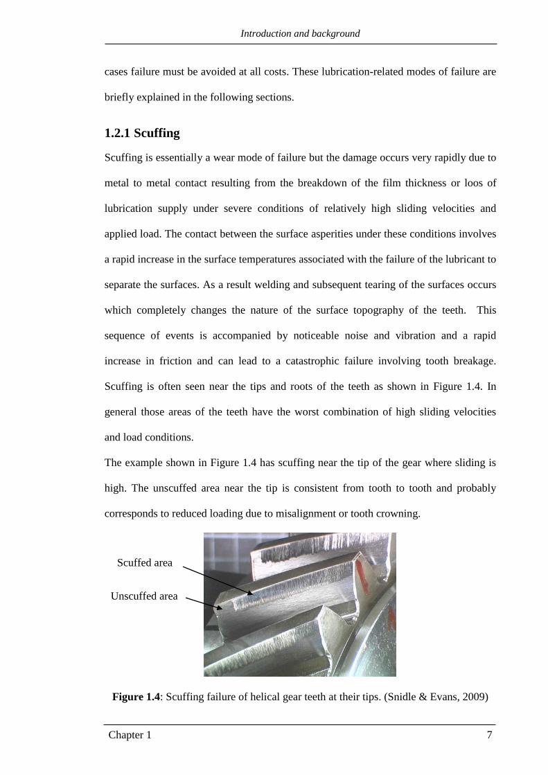
Scuffing is often seen near the tips and roots of the teeth as shown in Figure 1.4. In
general those areas of the teeth have the worst combination of high sliding velocities
and load conditions.
The example shown in Figure 1.4 has scuffing near the tip of the gear where sliding is
high. The unscuffed area near the tip is consistent from tooth to tooth and probably
corresponds to reduced loading due to misalignment or tooth crowning.
Figure 1.4: Scuffing failure of helical gear teeth at their tips. (Snidle & Evans, 2009)
Scuffed area
Unscuffed area

Introduction and background
Chapter 1 8
The occurrence of scuffing may be promoted by any factor leading to overloading under
high slide to roll ratio or the failure of the oil film separating the tooth surfaces. These
effects may be the result of various causes, such as insufficient tip relief modification,
thermal effects and the consequences of pitting of the teeth. Tooth surfaces need to be
protected from this sort of failure and this can be achieved to a large extent by using
special additives to improve lubricant properties under severe conditions of high
pressure and temperature (EP additives). Another means of protection is by reducing the
roughness of the surface by pre running of the gears at slowly increased increments of
load and speed or by “superfinishing”.
1.2.2 Pitting
The appearance of pits (or micro-pits) in gear teeth is a well-known fatigue effect. The
cause of these pits is of great interest for researchers at the present time because of
damage occurring in wind turbine gearboxes. Pitting of tooth surfaces is related to the
high contact stresses at the contacts between the teeth. Stresses higher than the nominal
Hertzian values may be the result of factors such as geometrical changes in the tooth
profiles, surface roughness and the consequent dramatic variation in the stresses over
the contacting surfaces. These high local values of stress tend to initiate (or exacerbate
existing) cracks which may propagate causing a removal of the material at those high
stress areas. The initial, minor pitting may arrest when the gears operate for a
considerable period of time. This is attributed to the surface asperities reducing with
time which promotes the surface stresses to be become more uniform. Sometimes,
however, pitting continues to progress rather than halting due to a high load. This
progression leads to pits merging with each other which then results in comparatively

Introduction and background
Chapter 1 9
larger size pits. This form of serious pitting is termed as spalling. It is difficult to predict
whether the initial pitting will come to a halt or will continue to the serious progressive
stage. The progressive form of pitting is likely to be found on the tooth dedendum but it
may spread further to the pitch line area as shown in Figure 1.5.
As progressive pitting continues, it will likely lead to a gear failure. Pitting sometimes
can be seen by the naked eye. The pit size in other cases is in the micrometre range and
is called micro pitting.
It is worth mentioning that mild wear can continue to remove material at the
rolling/sliding asperity encounters even when gears operate under conditions that may
not be severe enough to introduce pitting or scuffing failure. This material removal can
be attributed to many sources such as fatigue, corrosion, adhesion and others. However,
with time mild wear can affect the gear performance due to the change caused to the
tooth profiles.
Figure 1.5: Pitting of helical gear teeth (Alban, 1985)
Pitted area
Pitch line
Isolated pit

Introduction and background
Chapter 1 10
Engineering surfaces 1.3
All real surfaces that are used in engineering applications such as gears are in fact rough
when they are examined on the microscopic scale. More expensive methods of surface
preparation can only reduce the surface roughness to some extent, but cannot produce
perfect smoothness. Roughness has significant consequences in many engineering
applications involving concentrated contacts. One of its essential effects on the contact
between two surfaces is on the actual dimensions of the real contact area which is
smaller than expected. When such contact occurs, it starts at the tips of the highest
asperities. As the load is increased the contact area will involve other asperities due to
the deformation of the existing contacts as explained schematically in Figure 1.6.
Figure 1.6: The contact of rough surfaces, (a) Under zero load and (b) Under load
Experimental results, and numerical simulations of contact, emphasize that the true
load carrying area is much smaller than the apparent contact area and consequently the
(a)
(b)

Introduction and background
Chapter 1 11
contact of rough surfaces will produce high contact pressures in comparison with the
calculated nominal values based on the assumption of smooth surfaces. The surface
topography is therefore very important in studying the actual contact behaviour under
load due to the effects of local asperity shape on the asperity nature of deformation.
The roughness effect can also have a significant impact on the lubricated contact
problem. Examples of this occur in bearings and in the contact between gears teeth.
Tribologists tend to evaluate the effectiveness of lubrication at contacts in terms of the
ratio between the minimum lubricant film thickness which is calculated from the
smooth surface assumption to the mean surface roughness. This ratio is known as the
lambda ratio, , which also gives an indication for fatigue life in some bearing
applications. Reducing the gear tooth roughness by means of a surface finishing
process such as lapping or polishing is found to be beneficial in increasing the
resistance against the previously mentioned fatigue and wear modes of failure. In view
of the importance of surface finish there is the need to measure, assess and control the
roughness characteristics of gear surfaces in relation to their performance and
durability. Gear surfaces in recent and most current applications are usually produced
using various methods of finishing such as grinding, honing, etc. There are some
directional characteristics associated with each finishing processes which probably
have significant effects on the contact behaviour of surfaces. The surface roughness is
generally classified into two main components described as waviness and roughness.
Waviness describes the longer-wavelength features of a measured roughness profile
which are usually removed by a high pass filter. These features, which typically have a
“wavelength” in excess of a millimetre on gear teeth, do not affect the behaviour of the
nominal Hertzian contact which would typically be less than a millimetre in gears. It is
therefore the height and spatial characteristics of the shorter wavelength features that

Introduction and background
Chapter 1 12
are of importance. In engineering practice various roughness parameters are calculated
from profile data stored digitally. Digitally stored roughness profiles from gear tooth
surfaces will be used in some of the lubricated contact simulations to be described in
the following chapters of the thesis.
Tribology and elastohydrodynamic lubrication 1.4
Tribology as a term first appeared in 1966 in a report introduced by the UK Department
of Education and Science (Jost, 1966). This report defined tribology as “The science
and technology of interacting surfaces in relative motion and the practices related
thereto”. This term originates from the Greek ward tribos, which means rubbing. The
facts and concepts behind this relatively new definition of tribology can be traced back
to the period of prehistory.
Dowson (1979) has comprehensively described the history and development of human
activities related to tribology. Early man started to generate fire in the Palaeolithic
period, around 200, 000 years ago. The idea of using friction between pieces of wood or
stones to create fire can be considered as very early evidence of man’s application of
frictional heating. Another example of an ancient application of tribology is the potter’s
wheel which appeared about 5000 years ago in the Neolithic period and which relied on
an early form of journal bearing.
In the study of the lubrication of loaded gear tooth contacts it is generally accepted that
the mechanism responsible for the generation of an effective oil film is that of
elastohydrodynamic lubrication (EHL). A large and growing body of literature has
been concerned with EHL since the middle of the last century, and the term has come to
Introduction and background
Chapter 1 13
be used to refer to a form of hydrodynamic lubrication in which the combined effects of
elastic deformation and the tremendous increase of lubricant viscosity at high pressures
combine to generate an effective film in rolling/sliding contacts such as those between
rollers or gear teeth. Contacts of this type are described as “non-conforming” or of “low
geometrical conformity” or “concentrated” and in the case of perfectly smooth surfaces
the contact pressures and contact dimensions can be accurately calculated using the
classic equations of Hertz under dry, elastic conditions. Typical examples of this type of
lubrication are found in engineering applications such as gears, cams, roller and ball
bearings. These machine elements operate under heavy load and can be classified as
non-conforming contacts. In this regime the lubricant film thickness is generally of the
order of a micron and the maximum contact pressures are typically about 1.0 GPa in
gears and possibly up to 3.0 GPa in rolling element bearings. Despite this very thin
layer of lubricant, it is probably sufficient to prevent metal to metal contact between the
interacting surfaces provided that the surface finish is carefully controlled.
Development of the EHL analyses 1.5
Several studies such as Nijenbanning et al. (1994), Chittenden et al. (1985) and
Hamrock & Dowson (1976) developed expressions to predict the minimum and central
film thickness for the lubricated point contact between smooth surfaces operating in the
EHL regime. And in today’s applications full understanding of the EHL contact
behaviour between the surfaces plays a vital role in their design.
The EHL problem is defined by two basic equations: the hydrodynamic equation and
the surface elastic deformation equation (as will be considered in Chapter 3). This pair
of equations presents a highly non-linear system and thus has led researchers to develop
ingenious numerical solution models during the last six decades to solve this difficult

Introduction and background
Chapter 1 14
problem. EHL problems are usually solved using either a line contact or point contact
approach depending on the shape of the contact area under load. Line contacts are
present in roller bearings and spur and helical gears, and point contacts occur in ball
bearings and certain types of crossed-axis gears.
The real contact in engineering applications is two dimensional in nature. However,
early numerical studies in the EHL field mainly focused on the line contact problem
where the contact may be considered one dimensional. Although this relative
simplification of the EHL problem is valid for some applications, its study was related
to the limitations of computational resources in the early days of digital computers. The
development in the speed of calculations in the modern computer gives the ability to use
a point contact (two-dimensional) approach. Different methods have been developed to
provide reliable solutions to the EHL problem such as the Forward method, Inverse
method, Newton-Raphson method, Multigrid method, Coupled method and the novel
differential deflection method. Holmes (2002) provided an interesting description as
well as clarifying the limitations of these methods.
The Forward method was used in several studies such as Ranger et al. (1975) and
Evans & Snidle (1981). The inverse method was introduced by Dowson & Higginson
(1959) in a line contact problem and was subsequently developed for point contacts by
Evans & Snidle (1982). Houpert & Hamrock (1986) used a Newton-Raphson method
for the line contact problem. Lubrecht et al. (1986) were the first to use a Multigrid
method in EHL problems. Despite the widespread use of the multi grid method it is not
desirable for mixed EHL problems when the surface roughness is of moderate or high
frequency (Zhu, 2007).

Introduction and background
Chapter 1 15
The idea behind the more recent coupled method in contrast with the previous
techniques is that it attacks the solution of the two basic equations (Reynolds and elastic
equations) simultaneously. Elcoate (1996) and Elcoate et al. (1998) developed this
method initially in a fully-coupled form to solve a line contact problem and showed it to
be robust and reliable in dealing with high load contacts.
The coupled method was significantly developed when Evans & Hughes (2000) for the
first time used an ingenious differential form for the formulation of the elastic equation.
Hughes et al. (2000) solved the line contact EHL problem using this method and
compared the result with the standard method for handling the deflection calculation.
Two cases were examined, first where the surfaces were both smooth, and, second, the
case in which a smooth surface was moving against a stationary rough surface. In both
cases the results were obtained with an enormous reduction in the time of computing,
when using the differential deflection method, compared to the fully-coupled approach.
Elcoate et al. (2001) successfully used this method to solve the transient EHL line
contact proplem for moving rough surfaces.
Holmes et al. (2003a) and (2003b) extended this novel method to solve transient EHL
point contact proplems where the effect of surface roughness was also taken into
account.
With the progressive developments in the EHL analyses of contacting surfaces, the
incorporation of surface roughness effects has been given considerable attention over
the last 40 years or so. Lee & Cheng (1973) reported one of the first studies to consider

Introduction and background
Chapter 1 16
the effect of a single asperity on the EHL characteristics where a one dimensional
Reynolds equation is used in the analysis.
The effects of roughness orientation was examined by Patir & Cheng (1978) where an
average flow approach was developed. The levels of film thickness generated were
found to be related to the roughness orientation. The film thickness was predicted to
decrease as the direction of entrainment was altered from transverse, through isotropic,
to longitudinal.
The directional effect of the surface roughness was investigated by Lubrecht et al.
(1988) when sinusoidal longitudinal and transverse roughness features were
incorporated in a circular EHL contact model. The results were compared with
corresponding Patir & Cheng (1978) results. With this form of roughness feature they
found that the effect is overestimated by the flow factor model.
Similar results was found by Kweh et al. (1989) who analysed an EHL elliptical contact
when the surface roughness was 2D transverse and three dimensional sinusoidal in
profile.
Kweh et al. (1992) considered surface roughness in an EHL analysis of elliptical contact
when a smooth surface moves relative to a stationary rough surface. The roughness was
also sinusoidal in profile and straight extruded in the direction perpendicular to the
rolling/sliding direction. Two scales of amplitude and period for this transverse
roughness wave were used. It was found that the amplitude of the larger scale roughness

Introduction and background
Chapter 1 17
suffers the bigger proportional reduction in comparison with the smaller one. It should
be noted that the lubricant in these early solutions was assumed to be Newtonian.
Overall, the important results of these studies and many others highlighted the need to
include real roughness in the EHL analysis. Poon & Sayles (1994) developed an
elastic-plastic model to simulate the contact between a smooth ball on a real rough
surface as well as smooth and sinusoidal surfaces. The effect of fluid film was not
considered in this analysis.
Ai & Cheng (1994) studied the transient effect in a line contact EHL analysis for the
contact between surfaces having measured (i.e. “real”) surface roughness. It was found
that the transient effect due to the surface roughness has noticeable influences on the
EHL results.
Hu & Zhu (2000) developed a model for mixed EHL analysis. Three-dimensional real
roughness was incorporated in this point contact analysis. The surface radii of relative
curvature were equal in both directions which produced under load a circular contact
area of less than 0.5 mm in radius. The limits for the EHL solution space were -1.9a ≤ x
≤ 1.1a and -1.5a ≤ y ≤ 1.5a where x and y represent the rolling/sliding and transverse
directions respectively and a was the corresponding Hertzian radius of the contact area.
A fine mesh of 257*257 nodes was used in this analysis in order to make the model
sensitive to the roughness features. This model was questioned by a number of workers
in the field because it discarded the pressure gradient terms in the Reynolds equation for
small film thicknesses below 0.05 μm (Evans, 2015).

Introduction and background
Chapter 1 18
Tao et al. (2003) used real measured surface roughness in the line contact EHL analyses
of gear teeth. Breakdown of film thickness due to the interaction of asperities was found
which means the contact was under the mixed lubrication regime. In this regime of
lubrication the applied load is not carried only by the lubricating film but also by the
solid (“metal to metal”) contact at the asperities.
Zhu & Wang (2013) used a mixed EHL model to study the effect of roughness
orientation on film thickness levels in a line, circular and elliptical contact problems.
Three forms of roughness were used which are longitudinal, transverse and isotropic.
The orientation effect was found in general to be significant when the range of ratio
was between 0.05 and 1.
As the previous studies showed the roughness orientation has an important influence on
the contact behaviour, the roughness lay direction and its relation to the scuffing failure
for the ball on disc contact was studied by Li (2013) using a scuffing model developed
by Li et al. (2013). It was found that the scuffing performance was substantially affected
by the roughness lay direction where scuffing resistance was found to be inversely
proportion to the difference between the angles of orientation of the lays on the two
surfaces.
Because of the energy saving brought about by the use of low viscosity oils in engines,
for example, there is a tendency for lubricated contacts to operate with thinner films.
This requires a better understanding of the behaviour of EHL contacts which operate in
the mixed lubrication regime. Recently Morales-Espejel (2013) traced in a review the
development of solving the micro EHL problems during the last four decades. He
found that despite the wide range of literature available in this field, the problems of

Introduction and background
Chapter 1 19
mixed lubrication need more engineering and physics understanding in order to solve
practical problems of thin film lubrication.
Profile modification of gear teeth 1.6
In addition to surface roughness, other surface features such as discontinuities in the
profile of an otherwise smooth surface can be the source of lubrication and contact
problems. In the manufacture of gear teeth, for example, modifications are usually made
to the involute profile near the tips of the teeth (tip relief) in order to avoid severe
contact during meshing under load. Walker (1940) determined the required tip relief
modification to overcome the problem of tooth deflection in spur gear drives working
under heavy load.
The resulting tooth profiles are not perfect involutes in the area of modification (Bonori
et al. 2008). Such variation in the tooth profile geometry has consequences for the
contact and EHL behaviour between the gear teeth.
Kugimiya (1966) studied the profile modification effect on helical gear dynamic
properties. The levels of vibration were reduced using a suitable modification.
Simon (1989) carried out an investigation on the optimal tip relief and axial crowning
modifications in spur and helical gears . For the tip relief, only a linear profile was used
while linear and parabolic functions were examined for the crowning modification. The
amount and length of modification (for both tip relief and crowning) were used as
parameters in this study to evalute the load and stress distributions. The fluid film effect

Introduction and background
Chapter 1 20
was not considered in this study. The results presented suggested that the stress
distribution is related to the parametrs of modification to a considerable extent.
Kahraman & Blankenship (1999) carried out an interesting experimental study to
investigate the effect of tip relief modification on the vibration characteristics of spur
gears. Linear tip relief modification only was considered in this study. The results
showed that this type of modification is not optimum for applications that require a
gearing system to operate under a wide range of torque and suggested that alternate
forms of modification may be helpful.
Wagaj & Kahraman (2002) considered the effect of profile modification forms on the
durability of helical gears by examining the contact and bending stresses. The effect of
an EHL fluid film was not considered in this study. The contact mechanics models used
in this study considered both 2D and 3D profile modifications. These two kinds of
modification are illustrated in Figure 1.7. This study showed that for helical gears the
2D modification (which is the most common type of gear tooth modification where tip
relief and lead crowning are applied) is not optimum due to the directional difference
between the contact lines and the profile modifications. This difference was overcome
by using the second proposed form (3D modification). The stresses were first calculated
for unmodified gear teeth then compared with the corresponding results using the two
modification methods. The calculated stresses were increased by a smaller amount when
using the 3D modification.

Introduction and background
Chapter 1 21
Figure 1.7: Modification of helical gear teeth, (a) 2D and (b) 3D.
(Wagaj & Kahraman 2002)
Despite the possibility of improving the durability of helical gears by using this 3D
modification method, it is still not common due to the cost of production considerations
(Kahraman et al. 2005). Kahraman et al. (2005) investigated the effect of profile
(a)
(b)

Introduction and background
Chapter 1 22
modifications on helical gear wear and a design formula that explains the relation
between the initial wear rate and the modification parameters was proposed.
Edge contact (i.e. at the transverse edge faces) between the tooth surfaces due to
misalignment represents one of the major concerns in the design of helical gears.
Designers of gear drives usually provide simple chamfers at the edges of the tooth, or
more sophisticated crowning over the whole face width to avoid severe, and possibly
damaging, contact. However, in practice edge contact still occurs in many cases. This is
mainly because an accurate chamfer magnitude is not predetermined analytically as
reported by Litvin et al. (2005) where the misalignment effect on the dry contact
between helical gears having parallel axes was studied.
Sankar & Nataraj (2010) discussed a modified profile in their study on avoiding
damage in helical gear teeth for the drives used in wind turbine generators. They used in
addition to the tip relief modification a composite profile which consisted of epi-cycloid
and involute parts. The resulting bending stresses in the gear teeth due to the power
transmission between the gear drives were compared between the case when the new
proposed profile was applied and the corresponding case where the classical involute
profile was used. The composite profile was found more effective (showed lower levels
of stress) in this specific application of helical gears as the wind turbine generators
operate under severe conditions including high levels of fluctuation in the wind forces.

Introduction and background
Chapter 1 23
EHL analyses of gears. 1.7
The recent implementation of EHL in gear contact modelling started with spur gears as
this type gives rise to a relatively simple contact (from the geometry point of view) and
therefore can be modelled using a line contact model. Akbarzadeh & Khonsari (2008)
presented steady state solutions for the EHL contact of spur gears. Thermal effects and
surface roughness were taken into consideration in this study. The contact between the
gears along the line of action was modelled as that between two cylinders having radii
of curvature equivalent to those of the involute tooth profile.
Li & Kahraman (2010) provided a transient EHL analysis for the prediction of power
losses in spur gears. The transient effect in the analyses of spur gear contacts was
studied before that by Larsson (1997) when EHL results ( pressure and film thickness)
using a non-Newtonian fluid model were calculated throughout the meshing cycle of the
gears. In this isothermal and smooth surfaces model solution it was found that the
transient effect is most noticeable at the load transition positions (“change points”). The
transient effect was also investigated when the surface velocities and radius of relative
curvature varied during the meshing cycle, but this was found not to be as significant as
the load effect at the load transitions.
The same transient effect on the EHL result at the change points was also found by
Wang et al. (2004) when the thermal effect was taken into consideration in the analysis
of the spur gear meshing cycle. The tooth surfaces were assumed to be smooth, and a
Newtonian fluid model was used in this analysis.

Introduction and background
Chapter 1 24
A more advanced study for the EHL analysis of spur gear meshing cycle was presented
by Li & Kahraman ( 2010) which focussed on transient effects in a non-Newtonian and
mixed EHL model. The effect of profile modification was also investigated where a
gentle tip relief and circular crown profile were considered. The comparison between
steady state and corresponding transient EHL solutions was carried out for smooth
surfaces. The surface roughness effect was studied in the transient case. The solution
domain was fixed during the transient analysis which was 2.5 amax ≤ x ≤ 1.5 amax where
amax is the maximum half-Hertzian contact width during the meshing cycle. The results
showed the significant difference between steady state and transient analyses of the gear
meshing cycle (predominately due to the load variation) which emphasises the necessity
of including the transient effect in the EHL analysis of gears. The consideration of
surface roughness in the transient analysis had a significant effect on the prediction of
the pressure distribution where pressure values of more than three times the
corresponding smooth results were found. This high level of pressure was associated
with breakdown of the film thickness at several locations.
More recently, analysis of EHL of the geometrically simpler spur gear type has also
been reported by other workers. Wang et al. (2012) developed a transient EHL model in
a study of the effects of impact loads during the meshing of spur gears. Dynamic
loading of spur gear contacts under the EHL regime was also considered in a paper by
Liu et al. (2013), which included a treatment of thermal effects.
Relatively little work is available in the literature about EHL analysis of helical gears
particularly a full transient analyses of the meshing cycle. Simon (1988) investigated
EHL analysis of helical gears using a point contact model with a consideration of
Introduction and background
Chapter 1 25
thermal effects. This model considered only steady state analyses at a single position in
the meshing cycle when the contact acts over the whole face width, and this did not give
a complete picture of the variation of pressure distribution and film thickness during the
whole meshing cycle.
Li et al. (2009) provided an advanced treatment by considering the helical gear to be
represented as a number of thin slices of spur gears, with each individual slice modelled
as a transient line contact EHL problem between two cylinders. The radius of each
cylinder corresponded to the involute radius of curvature.
Ebrahimi Serest & Akbarzadeh (2013) presented a model to predict the EHL
performance of helical gears taking into account both surface roughness and thermal
effects. In this model, the helical gear was also treated as a series of narrow width spur
gears.
Han et al. (2013) also used an equivalent EHL line contact approach for the contact of
helical gear teeth, which included a consideration of roughness effects based on the
simple model of load sharing by asperity contacts in mixed lubrication prepared by
Johnson et al. (1972).
In considering the EHL behaviour associated with the edge contacts that occur where
the nominal line of contact reaches the end faces of the gears or at the ends of relieved,
crowned contacts, it is important to include the influence of side leakage of the
lubricant because this will cause significant thinning of the lubricant film. Dealing with
contact between modified profile teeth in helical gears as a line contact problem instead
of point contact problem leads to the important side leakage effect being ignored.

Introduction and background
Chapter 1 26
3D line contact model 1.8
Surface roughness has great influence in the life of machine elements that involve
power transmission through lubricated contact. The concentrated contacts at the
asperities produce very high contact pressure which consequently increases the
possibility of surface failure.
Previous studies mentioned in the above sections included well developed EHL point
contact models which involved 3D rough surface analysis. Even though these models
represent significant progress, there are limitations related to the size of the contact in
both directions. From the surface roughness point of view such models may not be
efficient enough to deal with relatively large contact areas. Gears are a typical example
of such contacts where the contact length in one direction (along the face width) is
considerably longer than the length in the nominally transverse direction. Using the
point contact approach to model such contacts may limit the resolution and hence the
accuracy along the larger length of the contact area. In addition, the classical EHL line
contact approach may be far from accurate in modelling the 3D surface topography.
These issues emphasize the advantage of developing a “3D Line contact” EHL model
that has the ability to model a selected area of the contact region and include the real 3D
surface roughness features without sacrificing the accuracy of the analysis.
In general, consideration of surface roughness in the analyses of contact problems
requires fine computing grids in order to give realistic modelling for the surface
features, which makes classical contact mechanics methods impractical in such analyses
Polonsky & Keer (2000).

Introduction and background
Chapter 1 27
The calculation of surface elastic deformation is a fundamental issue in EHL analyses,
particularly when fine grids and large numbers of grid points are used. Stanley & Kato
(1997) used a numerical technique which involves the fast Fourier transform (FFT)
method to obtain the surface deformation and contact pressure resulting from contact
between an elastic half-space and a rigid plane. The FFT method which was first
introduced by Cooly & Tukey (1965) is commonly used to speed up the process of
convolution calculations as will be shown in chapter 7, and has been adopted in the
present thesis.
Wang et al. (2003) compared discrete convolution and the fast Fourier transform
method with other methods for the calculation of surface deformation. The method was
found to be very efficient (from computing time point of view), particularly when a
large number of grid points are used in the analyses of contact and EHL problems.
Chen et al. (2008) developed a 3D model to analyse the dry contact between flat
surfaces with periodic surface roughness features. The fast Fourier transform method
was used to calculate the discreet convolution that occurs in the numerical calculation of
the surface elastic deformation. The model was modified to be applicable to the
simulation line contact problems where the contact length is infinite in one direction and
has a finite length in the other direction. In the latter case a mixed padding method was
used in the FFT implementation which depends on duplicating the pressure distribution
in the periodic direction (infinite length direction) and zero padding the pressure
distribution in the other direction (finite and non-periodic length direction) as shown in
Figure 1.8. The notation in this figure for the repeated domain in the periodic direction

Introduction and background
Chapter 1 28
is duplicated padding while in the current work the notation is repeated domain or
repeated solution space.
Ren et al. (2009) developed a novel 3D model which has the ability to analyse mixed
lubrication for a finite length line contact problem with consideration of surface
roughness.
In this analysis, the solution domain in the direction perpendicular (transverse) to the
entrainment direction is cut to a finite length. The idea behind this model was based on
considering the roughness feature as well as the pressure and film thickness
distributions over this reduced space size as being repeated periodically in the transverse
direction.
Figure 1.8: Mixed method for the solution of contact problems (Chen et al. 2008)
Repeated domain

Introduction and background
Chapter 1 29
The elastic deformation of contacting surfaces was analysed using the same method by
Liu et al. (2000) and a following development by Chen et al. (2008) where a discrete
convolution and FFT were used based on the mixed padding method as mentioned
previously. An example of a contact that can be analysed using the approach defined in
this study is depicted in Figure 1.9. A simple roller and a flat plane together with the
coordinate system are shown in Figure 1.9 (a). Figure 1.9 (b) illustrates how the contact
length in one direction (y) is significantly larger than that in the other direction (x). The
corresponding 3D line contact model is shown in Figure 1.10. The model has significant
limitation as zero slope is assumed for the pressure with respect to the y direction at the
boundaries of the solution space in the repeated direction. This assumption can only be
correct if the roughness profile is extruded parallel to the y direction, or the solution
domain has a groove at each of the repeated boundaries.
The 3D line contact model presented by Ren et al. (2009) was further developed by
Zhu et al. (2009) to predict the pitting life of gears but retained the restriction of the no-
flow condition at the transverse boundaries which is generally not the case for real 3D
roughness conditions.

Introduction and background
Chapter 1 30
Figure 1.9: A contact can be analysed using the 3D line contact model.
(a) A roller on a flat plate and (b) Contact zone dimensions (Ren et al. 2009)
Figure 1.10: 3D line contact model for the contact shown in
Figure 1.9 (Ren et al. 2009)
Duplicated Padding
Zero Padding zones
Implicit Padding
Solution domain
Contact Zone
Contact Length
(Can be infinite)
Contact
Width
Both surfaces
can be rough
(a) (b)
x
y

Introduction and background
Chapter 1 31
Software available as basis for research 1.9
At the onset of this research the author had access to existing EHL analysis software
developed within the research group. This was in the form of a code to provide transient
solution to the EHL point contact problem with non-Newtonian lubricant behaviour as
an option choice. The code was developed in its simplest form by Holmes (2002),
Holmes et al (2003a, 2003b) and developed for several particular engineering problems
and lubricant formulations by Sharif et al (2001) and Sharif et al (2004).
In the current research new subroutines were developed and introduced to the EHL code
to define the helical gear geometry and kinematic conditions occurring over the meshing
cycle of the gear pair. This included the fundamental geometry as described in chapter
2, tooth crowning as described in chapter 4, various forms of tip relief as described in
chapter 5 and faceting as described in chapter 6. These developments allowed the whole
gear transient analyses reported in this thesis to be obtained.
For the consideration of surface roughness effects a new program was developed by
significant adaptation of the transient EHL solver. This involved significant
modifications to the fundamental algorithms carrying out the numerical analysis as
reported in chapter 7.
Research objectives 1.10
The aims of the work reported in this thesis are concerned with the prediction of EHL
film thickness and pressure at the tooth contacts of helical gears. These aims can be
classified into three main categories:
- Carry out a full point contact transient EHL analysis for the helical gear meshing
cycle and study the effects of including profile modifications on the results of
this analysis. The tooth profile modifications considered involve different forms
of tip relief and crowning in the axial direction.

Introduction and background
Chapter 1 32
- Study the effect of generating the tooth profile by a process that results in axial
faceting on the transient EHL behaviour of helical gears.
- Develop a 3D line contact model based on a cyclic boundary condition concept
in order to consider the rough surfaces EHL problem in gear contacts.
Thesis Organisation 1.11
This thesis consists of eight chapters, and the following is a brief description of the
remaining chapters.
Chapter 2 addresses the contact geometry of helical gears where the total un-deformed
gap between mating teeth is calculated, including the effect of profile modifications.
Chapter 3 discusses the EHL point contact problem and gives a brief description of the
solution techniques used for the problem, including the Finite Element and Finite
Difference methods.
Chapters 4 and 5 focus on the transient EHL solution for the meshing cycle of helical
gears taking into account tooth profile modifications with the assumption of smooth
surfaces. Chapter 4 deals with crowning modifications and Chapter 5 focuses on the
effects of tip relief modifications considered.
Chapter 6 investigates the effect of axial faceting (due to the manufacturing process) of
helical gear teeth on the transient EHL results, and compares the outcome with the
corresponding smooth surface results given in Chapter 5.
Chapter 7 describes the development of a 3D line contact model for rough surfaces
using cyclic boundary conditions.
Chapter 8 draws conclusions from the results obtained in the previous chapters, and also
makes some suggestions for future work.

Gear contact geometry
Chapter 2 33
Chapter 2
Gear contact geometry
2.0 Introduction
The contacting characteristics of a pair of helical gears are different from that in spur gears.
The motion is transmitted gradually and more smoothly between the mating gears. In a
spur gear drive the contact occurs along a straight line which is parallel to the gear axis.
The contact initiates suddenly over the full face width at the start of the tooth meshing cycle
and also ends abruptly at the end.
In contrast, the contact between a pair of helical gears starts at the first tooth face end as a
point. As the gears rotate, the contact extends from being point to a line of steadily
increasing length which moves over the tooth flank extending in length until it reaches the
second tooth face. The contact line length subsequently reduces and ends as a point at the
second tooth face end. The line of contact acts diagonally between the face ends of the
helical teeth. In addition, there are at least two pairs of teeth always in contact when using
helical gear drives.
The nature of tooth meshing in helical gears is illustrated in Figure 2.1. Figure 2.1 (a)
shows the contact conditions at an instant of the gear meshing cycle where two pairs of
teeth are in contact, 𝑧1𝑧1′ and 𝑧2𝑧2
′ . Figure 2.1 (b) illustrates the contact at a further
position in the meshing cycle where teeth pair 𝑧1𝑧1′ leaves the contact. Meanwhile the

Gear contact geometry
Chapter 2 34
contact line of teeth pair 𝑧2𝑧2′ moves away from the lower gear tooth tip. This figure shows
another pair of teeth coming into contact as shown in the figure on the right side.
Figure 2.2 depicts a comparison between helical and spur gear drives, which shows the
directional difference of the line of contact in the two drives as well as the inclination of the
line of contact between helical gear teeth relative to the gear axis as a result of the helix
angle .
Figure 2.1: Nature of tooth engagement in helical gear drive (Maitra 1994).
(a) (b)
Another pair comes
into contact

Gear contact geometry
Chapter 2 35
Figure 2.2: Comparison between spur and helical gear contact, transverse section (upper
figure), spur gear (central) and helical gear (lower) (Maitra 1994).
In order to perform EHL analysis of contacting surfaces such as gears, which is the purpose
of the current work, the contact geometry needs to be determined as a first step of such
analysis. However, analysis of this kind of contact involves challenges. The major
difficulty is related to the continuous changing of contact geometry and kinematic
throughout the gear meshing cycle. These are mainly consequences of the nature of the
involute gear tooth profile having a different radius of curvature at each profile point in
addition to the movement of the point under consideration along the tooth profile.
Therefore, before proceeding to determine the gear geometry, it is necessary to understand
the way in which gears contact.
Figure 2.3 shows a schematic drawing of a transverse section of a pair of gears in contact.
This drawing applies to both spur and helical gears. Any pair of meshing involute teeth

Gear contact geometry
Chapter 2 36
develops contact along the straight line AB which is tangent to the gear base circles. This
line is termed as the line of action and is inclined to the line perpendicular to the gear
centres line O1O2 at an angle ψ termed the pressure angle.
Figure 2.3: Involute gears in contact. Note that the root form in this figure is shown
schematically as a rectangular recess.
O1
A
B
ψ
ψ Line of action
O2
s G
H
J ψ
Gear contact geometry
Chapter 2 37
2.1 Path of contact in the transverse plane
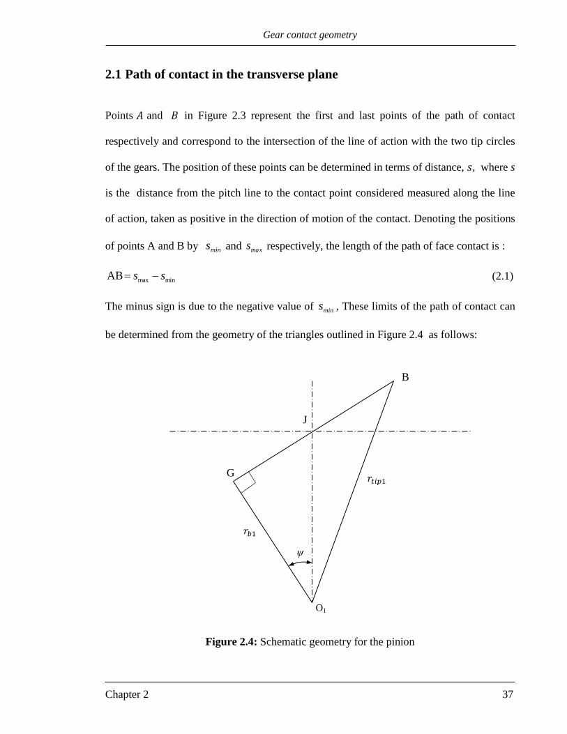
Points 𝐴 and 𝐵 in Figure 2.3 represent the first and last points of the path of contact
respectively and correspond to the intersection of the line of action with the two tip circles
of the gears. The position of these points can be determined in terms of distance, 𝑠, where s
is the distance from the pitch line to the contact point considered measured along the line
of action, taken as positive in the direction of motion of the contact. Denoting the positions
of points A and B by mins and maxs respectively, the length of the path of face contact is :
minmaxAB ss (2.1)
The minus sign is due to the negative value of mins , These limits of the path of contact can
be determined from the geometry of the triangles outlined in Figure 2.4 as follows:
Figure 2.4: Schematic geometry for the pinion
O1
G
B
J
ψ
𝑟𝑏1
𝑟𝑡𝑖𝑝1

Gear contact geometry
Chapter 2 38
Considering triangle O1GJ the distance GJ is given by:
GJ tan1br
The distance GB can be obtained from the triangle O1GB as:
GB 2
1
2
1 btip rr
Therefore, the position of the last point of contact, maxs is determined from
maxs GBGJ
tanrrrs 1b
2
1b
2
1tipmax (2.2)
Similarly the position of the first point of contact, mins is given by
2
2b
2
2tip2bmin rrtanrs (2.3)
where, subscript 1 is used to define the pinion (which is the lower gear), and subscript 2
refers to the wheel, br is the radius of base circle and tipr is the tip radius.
The velocity of the contact point as the contact progresses along the line of action between
mins and maxs is constant and is given by:
22b11bcontact rru
This equation can be used to determine the total time that is required to complete the
meshing cycle of a pair of teeth in contact. The time for contact to occur at a given axial
position is
contactminmaxcontact u/)ss(t
and the time for a pair of teeth to complete their meshing cycle in a pair of helical gears is
(see Figure 2.5)

Gear contact geometry
Chapter 2 39
contactbminmaxcontact u/)tanFss(t (2.4)
2.2 Zone of contact in helical gears
The contact between any pair of teeth occurs within the zone ABCD that is shown in Figure
2.5. This rectangular zone is tangential to the base cylinders of the gears and is called the
plane of contact. It is limited by the end faces at AB and DC, and the tip cylinders of the
mating gears at DA and CB (Tuplin 1962).
.
Figure 2.5: Zone of contact of a pair of helical gear teeth,
𝑃𝑥 : axial pitch, 𝑃𝑡𝑏: transverse pitch , O1O2: center distance
𝑟𝑏2
𝑟𝑏1
O1
O2
F
Path of contact
A,D
B,C
A
B
C
D Pnb
Ptb
Px
1
2
3
βb
C'
Base circle
ψ
𝜓
Base circle

Gear contact geometry
Chapter 2 40
The contact begins at point D which then extends to be a line inclined at the base helix
angle 𝛽𝑏 to the gear axis as shown by the typical contact lines 1, 2 and 3 in this figure. The
contact is limited by the boundaries of the zone of contact, i.e. one or both of the side edges
and the tip cylinder boundaries.
In the depicted tooth contacts, line 2 intersects CD at C at one end, and intersects AB at C
at the other end. Other, simultaneous, contacts occur on parallel straight lines at normal
spacing, 𝑃𝑛𝑏 . The number of these lines depends on the transverse contact ratio of the
gears.
2.2.1 Length of line of contact
As mentioned previously the contact between a pair of teeth in spur gears is a straight line.
The length of this line is equal to the face width of the tooth and this length remains
constant at all positions in the meshing cycle. This line is parallel to the axes of the gears.
On the other hand for a helical gear pair, due to the nature of the contact as illustrated in
Figure 2.5, the length of the line of contact generally depends on the face width (𝐹), base
helix angle (𝛽𝑏), and the position (𝑠𝑖) in the meshing cycle, where 𝑠𝑖 is defined as the s
coordinate at which the line of contact intersects boundary AB of the plane of contact as
seen in Figure 2.6.
In order to determine the length, 𝐿, of the line of contact in a general form for any pair of
helical gears and at any position in the meshing cycle, three different cases need to be
considered. The classification depends on the relation between the face width and the path
of contact (distance AB that was given by equation (2.1)). These cases are bF tan AB,
bF tan AB and when bF tan AB. Figures 2.6 (a), (b) and (c) show the variation of

Gear contact geometry
Chapter 2 41
the line of contact length with the position 𝑠𝑖 on the line of action for the three cases,
respectively. It can be shown from these figures that the required equations to calculate the
contact line length for each case are as follows:
Case 1: bF tan AB
b
imin
b
isin
ss
cos
FL
for minibmin sstanFs
max
b
i Lcos
FL
for bmaximin tanFsss
b
imaxi
sin
ssL
for maxibmax sstanFs
Case 2: bF tan AB
b
imin
b
isin
ss
cos
FL
for minibmin sstanFs
b
imaxi
sin
ssL
for xmaximin sss
Case 3: bF tan AB
b
imin
b
isin
ss
cos
FL
for bmaxibmin tanFsstanFs
max
b
minmaxi L
sin
ssL
for minibmax sstanFs
b
imaxi
sin
ssL
for xmaximin sss

Gear contact geometry
Chapter 2 42
(a) ∶ 𝐹 𝑡𝑎𝑛(𝛽𝑏) < path of contact
(b) ∶ 𝐹 𝑡𝑎𝑛(𝛽𝑏) = path of contact
(c) ∶ 𝐹 𝑡𝑎𝑛(𝛽𝑏) > path of contact
Figure 2.6: Variation of the length of line of contact with the position 𝑠𝑖.
A
B
C
D
: any line
𝑠𝑖 = 𝑠𝑚𝑎𝑥 − 𝐹 𝑡𝑎𝑛(𝛽𝑏)
𝑠𝑚𝑎𝑥
𝑠𝑚𝑖𝑛
𝑠𝑖
𝑠
𝛽𝑏 F
𝑠𝑖 = 𝑠𝑚𝑖𝑛 − 𝐹 𝑡𝑎𝑛(𝛽𝑏)
𝐿𝑚𝑎𝑥
𝑠𝑚𝑖𝑛 − 𝐹 𝑡𝑎𝑛(𝛽𝑏) 𝑠𝑚𝑖𝑛 𝑠𝑚𝑎𝑥
L
𝐿𝑚𝑎𝑥
𝑠𝑚𝑖𝑛 − 𝐹 𝑡𝑎𝑛(𝛽𝑏) 𝑠𝑚𝑎𝑥 − 𝐹 𝑡𝑎𝑛(𝛽𝑏)
𝑠𝑚𝑖𝑛 𝑠𝑚𝑎𝑥
L
C
𝑠𝑚𝑎𝑥
𝑠𝑖 = 𝑠𝑚𝑖𝑛 − 𝐹 𝑡𝑎𝑛(𝛽𝑏)
𝑠𝑚𝑖𝑛
𝑠𝑖
𝛽𝑏 F 𝑠
D
A
B
𝑠𝑚𝑎𝑥 − 𝐹 𝑡𝑎𝑛(𝛽𝑏)
𝑠𝑚𝑎𝑥
𝑠𝑚𝑖𝑛
𝑠𝑖
𝛽𝑏
𝑠𝑖 = 𝑠𝑚𝑖𝑛 − 𝐹 𝑡𝑎𝑛(𝛽𝑏)
A
B
C
D
F
𝑠
𝐿𝑚𝑎𝑥
𝑠𝑚𝑖𝑛 − 𝐹 𝑡𝑎𝑛(𝛽𝑏) 𝑠𝑚𝑖𝑛 𝑠𝑚𝑎𝑥 − 𝐹 𝑡𝑎𝑛(𝛽𝑏) 𝑠𝑚𝑎𝑥
L
is
is
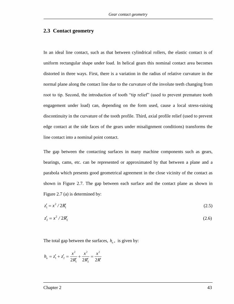
Gear contact geometry
Chapter 2 43
2.3 Contact geometry
In an ideal line contact, such as that between cylindrical rollers, the elastic contact is of
uniform rectangular shape under load. In helical gears this nominal contact area becomes
distorted in three ways. First, there is a variation in the radius of relative curvature in the
normal plane along the contact line due to the curvature of the involute teeth changing from
root to tip. Second, the introduction of tooth “tip relief” (used to prevent premature tooth
engagement under load) can, depending on the form used, cause a local stress-raising
discontinuity in the curvature of the tooth profile. Third, axial profile relief (used to prevent
edge contact at the side faces of the gears under misalignment conditions) transforms the
line contact into a nominal point contact.
The gap between the contacting surfaces in many machine components such as gears,
bearings, cams, etc. can be represented or approximated by that between a plane and a
parabola which presents good geometrical agreement in the close vicinity of the contact as
shown in Figure 2.7. The gap between each surface and the contact plane as shown in
Figure 2.7 (a) is determined by:
1
2
1 2R/xz (2.5)
2
2
2 2R/xz (2.6)
The total gap between the surfaces, uh , is given by:
R
x
R
x
R
xzzhu
222
2
2
2
1
2
21

Gear contact geometry
Chapter 2 44
where R is the equivalent radius of relative curvature for both surfaces as shown in Figure
2.7 (b) which is given by
21
111
RRR
In the spur gear case, the contact may be approximated by two rollers as shown in Figure
2.8. The radii of these rollers are equal to the local involute radii of curvature (i.e. the
tangential distance between the contact point and the base circle). Thus, the radii of
curvature at any point of contact can be determined by:
stanrR b 11 (2.7)
stanrR b 22
(2.8)
The total gap can then be evaluated by substituting these radii in equations (2.5) and (2.6)
respectively.

Gear contact geometry
Chapter 2 45
Figure 2.7: Geometry and coordinate system, (a) curvature of both surfaces,
(b) equivalent system
(a)
(b)
𝑥
Flat plate
Parabola
Roller
Parabolic
approximation
𝑥

Gear contact geometry
Chapter 2 46
Figure 2.8: Involute gear teeth showing equivalent rollers of
radius 1R and 2R at the contact P.
ψ
𝑟𝑏1
𝑟𝑏2
ω1
ω2
J
P
ψ
base circle
base circle
s

Gear contact geometry
Chapter 2 47
Unlike the spur gear geometry, in a helical gear pair each point on the line of contact has a
different radius of relative curvature.
By using the spur gear contact approximation the contact between a pair of helical gear
teeth can be also modelled with some modifications. Figure 2.9 shows a line of contact EE′
for a helical gear which moves in the plane of contact. Point O is fixed at the middle of the
face width. The common normal to the contacting helical gears teeth is Oz and the common
tangent plane at the line of contact is O𝑥𝑦.
Figure 2.9: Surface of action and contact line tangent plane, tr: tip relief zone
The required gap for the contact between the pair of spur gears is least in the transverse
direction O𝑧′. In helical gears the generation of a lubricant film between the contacting
teeth depends on the gap between them in the normal direction, Oz, and also depends on the
Common tangent plane
Plane of contact
x
y
z' βb
E'
E
y'
z
F
O
Pinion tip
tr
tr
Wheel tip
A
B
C
D

Gear contact geometry
Chapter 2 48
motion of the surfaces relative to the contact line. The relative motion between the tooth
surfaces and the contact line takes place in the Ox direction.
Figure 2.10 (a) shows tangent, normal and transverse planes at a specified point, P on the
line of contact. In order to determine the gap for the first surface at this point , suppose
point P1 zyx ,, is the point of intersection between curve 1 which has a radius of 1R and
curve 2 which has a radius 1R as illustrated in Figure 2.10 (b) , where :
1R : radius of curvature in the normal direction at point P.
1R : radius of curvature in the transverse direction at another point P1′ on the line of contact.

Gear contact geometry
Chapter 2 49
Figure 2.10: Contact geometry of helical gears teeth
b- The gap at point P1 determined by the
curvature 𝑅1′ at point P1
′ in the transverse plane
a- Tangent ,normal and transverse planes
at point P
Normal plane
𝑅2
Transverse plane Tangent plane
Line of contact
P
𝑅1
d- Both surfaces c- Relation between the transverse (𝑧 ′) and normal
(𝑧) gaps at point P1
P
𝑦P1′ − 𝑦P
B
P1
A
𝛽𝑏
P1′
𝑧1′
𝑧1
𝑧1𝑡𝑎𝑛𝛽𝑏
P1
P2′
𝑅2′
P2
P
P1′
𝑅1
𝑅1′
A
B
Curve 1
Curve 2
P
𝑦
𝑥
𝑧 P1
P1′
𝑅1 𝑅1′
A
B

Gear contact geometry
Chapter 2 50
The distances between the points shown in Figure 2.10 (b) are clarified in Figure 2.10 (c).
In this figure the gap in the transverse direction at point P1 is equal to the distance P1B and
can be obtained using equation (2.5) as
1P1
2
112
BP
yR
xz (2.9)
As mentioned previously the normal direction is inclined by an angle b to the transverse
direction. Therefore, the corresponding gap at this point in the normal direction is the
distance P1A, where:
bzz cosAP 111 (2.10)
Substituting equation (2.9) into equation (2.10) gives:
1P1
2
12
cos
yR
xz b which gives the relation between 𝑧1 and 𝑥.
It can be seen from Figure 2.10 (c) that:
bzyy tan1PP1
For each point on curve 1 there is a corresponding curve 2 from which the gap in the
transverse direction can be determined.
Therefore, the radius of curvature 1R depends on the 𝑥, 𝑦 and 𝑧 coordinates of the point on
curve 1. Generally, at any point on curve 1, the contact geometry is given by:
b11
b
2
1tanzyR2
cosxy,xz
(2.11)

Gear contact geometry
Chapter 2 51
For a given y,x position in order to evaluate 1z this equation needs to be applied
recursively with the radius of curvature obtained by modifying its argument
b11 tanzyR with successive 1z values until converged. The radius of curvature
1R is
obtained from the spur gear geometry in terms of the contact position s , which is known in
terms of y and 1z as discussed below. A similar equation can be obtained for the second
surface. Taking into consideration that 2Py is given by:
bzyy tan2PP2
the gap 2z on the other side of the contact is given by:
b22
b
2
2tanzyR2
cosxy,xz
(2.12)
The total undeformed gap hu in the normal direction is the combination of the two distances
1z and 2z (i.e.
21 zzhu ).
It is worth noting that for helical gears the distance s varies with the position y along the
line of contact as shown in Figure 2.11, where a single line of contact is illustrated.
Therefore, s can be given by:
b
b
i
Fyss
sin
cos2
(2.13)

Gear contact geometry
Chapter 2 52
Figure 2.11: Variation of 𝑠 with the position on the line of contact, 𝑦.
Thus, the radii of curvature at a given s position on the line of contact can be obtained by
subsuming equation (2.13) into equation (2.7) and (2.8).
(0,𝑦, 0) F
Path of contact
𝑠
𝑦
𝑧
Line of contact
(length= L)
𝑠𝑖
𝛽𝑏
𝑠 for point (0,𝑦, 0)
on the line of contact
𝑠𝑚𝑖𝑛
O

Gear contact geometry
Chapter 2 53
2.4 Tip relief
The implementation of tip relief leads to a decrease in the length of the path of contact as
shown in Figure 2.12 (a). Point B represents the last point of contact along the line of action
when no modification is made to the tooth profile, while point Q will be the last
engagement point if tip relief is applied. Therefore, the length of the path of contact is
reduced by an amount equal to the distance QB due to tip relief of the pinion teeth. This can
be determined from the triangles shown in Figure 2.12 (b) as follows:
GQ2
1
2
1 bstart rr
GB 2
1
2
1 btip rr
QB=GBGQ
2
1
2
1
2
1
2
1 bstartbtipp rrrrz (2.14)
where,
pz : equal the distance QB
startr : radius of relief starting point.
Similarly, as shown in Figure 2.12 (c) due to tip relief of the wheel teeth the path of
involute contact is also reduced bywz , where,
2
2b
2
2start
2
2b
2
2tipw rrrrz (2.15)

Gear contact geometry
Chapter 2 54
Figure 2.12: Tip relief of the gear teeth
G
(c)
(a) (b)
B
Q 𝑧𝑝
𝑧𝑤
F Path of contact
𝑠
Line of contact
(length= L)
𝑠𝑖
𝑟𝑏1
Q B
Base circle
Line of action
G
B
𝑟𝑏1
𝑟𝑠𝑡𝑎𝑟𝑡1 𝑟𝑡𝑖𝑝1
Q

Gear contact geometry
Chapter 2 55
2.4.1 Undeformed geometry due to tip relief
The undeformed gap due to the profile modification needs to be determined in order to
obtain the total gap between any pair of teeth in contact as a part of the EHL analysis.
Figure 2.13 shows point P on a pinion tooth for which the amount of relief needs to be
determined. The 𝑥-axis is tangent to the involute profile at the contact point, and point P is
in the negative x-direction. It can be shown by considering triangle OPT that:
211b
2
1b zstanrxry,xr (2.16)
where,
r : distance from the center of the pinion base circle to point p.
1z : gap between the involute profile and 𝑥-axis in the transverse direction.
The amount of relief, tz , is a function of the radius r according to the manufacturing
setting as will be shown in chapter 5.
Similarly, for the wheel tooth:
222b
2
2b zstanrxry,xr (2.17)
In contrast to the pinion the x-axis is negative towards the root of the wheel which gives a
different sign for x in equation (2.17). It is worth mentioning that these equations are
applicable at any transverse section on the contact line as s is y dependent as explained
previously.

Gear contact geometry
Chapter 2 56
Figure 2.13: Undeformed geometry due to tip relief of the pinion
Point of contact
Line of action
𝑟𝑏1
𝑧1𝑝′
𝑥+
𝜓
𝑟
𝑠
𝑥𝑝
J
P
T
O

Gear contact geometry
Chapter 2 57
2.5 Crowning of the gear teeth
Heavy end of tooth contacts at the side edges of the gears, which result from lack of
parallelism between the gear axes due to mounting errors or shaft deflections under load,
can be alleviated by axial crowning of the teeth. Axial crowning is expressed in terms of a
radius that provides a transverse clearance cr for each tooth at the side edges when contact
occurs at the centre of the gear under zero load. The gap due to this modification, y,xzc ,
will be considered in detail in chapter 4.
2.6 Total undeformed geometry
At a given 𝑥 and 𝑦 position, the distances ),(1 yxz , ),(2 yxz , ),( yxzt and ),( yxzc
can be
combined to give the total gap between any two teeth in contact measured normal to the
tangent plane as:
)y,x(z)y,x(z)y,x(z)y,x(z)y,x(h ctu 21 (2.18)
As the contact position changes throughout the meshing cycle from point D to point B in
Figure 2.5, the time varying total gap, )y,x(hu needs to be identified in advance before
solving the equations that describe the EHL problem for the gears.

EHL point contact problem and solution methods
Chapter 3 58
Chapter 3
EHL point contact problem and solution methods
3.0 Introduction
The EHL problem is described by two basic equations which are the elastic deformation
equation and the hydrodynamic equation. This chapter gives a brief description of these
equations for the point contact problem together with some related equations, and also
considers the discretization of these equations using both the finite element method
(FEM), and the finite difference method (FD). More details about the discretization
analysis can be found in Holmes (2002) where a full description for a point contact
software developed by Cardiff Tribology Group is also available. The basic transient
EHL point contact solver that described in this chapter was made available to the author
as a starting point for this research as described in section 1.9
3.1 The hydrodynamic equation
The hydrodynamic equation is the well-known Reynolds equation which has the
following form for the 2D problem:
0
h
thv
yhu
xy
p
yx
p
xyx (3.1)
where
221 UUu and 221 VVv .
For Newtonian oil behaviour the flow factors are
12
3hyx (3.1a)
Non-Newtonian behaviour is considered in detail in section 3.9.

EHL point contact problem and solution methods
Chapter 3 59
3.2 The Elastic deformation equation
The total gap between two contacting surfaces can be approximated by that between an
equivalent paraboloid and a plane as explained in section 2.3 (chapter 2). Figure 3.1
illustrates schematically a section at the centre of the contact between these surfaces
under load along the entrainment direction, x, from which the film thickness equation
can be written as
ou hyxdyxhyxh ),(),(),( (3.2)
where ),( yxhu is the undeformed gap between the two surfaces, ),( yxd is the surface
elastic deformation and oh is a constant that represents the distance of common
approach. The calculation of the undeformed gap between helical gears teeth was
shown in detail in Chapter 2. The surface elastic deformation is evaluated using the
equation for the deflection of a semi-infinite body subjected to a surface pressure
loading, p(x,y) as given by Timoshenko and Goodier (1951), for example.
dxdy
yyxx
yx,p
Eπ
2y,xd
A2
1
2
1
11
(3.3)
where 11 y,x represent the coordinates of the point where the deflection is calculated
and
2
2
2
1
2
1 112
EEE

EHL point contact problem and solution methods
Chapter 3 60
Figure 3.1: Section at the centre of the contact in the entrainment direction.
oh is a negative value
3.3 The pressure –viscosity equation
An empirical equation for the relation between the viscosity as given in equation (3.1)
(the Reynolds equation) and the pressure value was given by Roelands (1966) and is
adopted in the current work (isothermal analysis) in the form (Clarke et al. 2006)
1100 Z
plnexp (3.4)
where
R (undeformed geometry)
ho
d
h
hu
z
x
Deformed geometry
O

EHL point contact problem and solution methods
Chapter 3 61
61015.63 Pa.s,
1.5 GPa-1
Pa.s and
0
0
lnZ
3.4 The pressure-density equation
In addition to the viscosity, the density in equation (3.1) is also pressure dependent and
is assumed to be given by the Dowson and Higginson (1966) formula
p
pp
1
10 (3.5)
The values for the pressure coefficients and in the current work are
2662. GPa-1
6831. GPa-1
3.5 Evaluation of the surface elastic deflection
As can be seen in equation (3.2) the evaluation of surface deflection is required in order
to calculate the film thickness in the lubricated contact. This can be achieved by solving
equation (3.3) which is a convolution integration of pressure.
This integral can be evaluated numerically for any general pressure distribution such as
that which occurs in the contact between rough surfaces. As a result of numerical
discretization, this integral can be transformed to a summation of influence coefficients

EHL point contact problem and solution methods
Chapter 3 62
multiplied by the pressure value at all points of the solution domain, which can be
written (Evans & Hughes 2000) as
N
k
M
l
l,kjl,ikji p g 'E
)y,x(d1 1
2
(3.6)
The method of evaluating the influence coefficients is given by Kong (2001).
3.6 The differential deflection method
In this method the deflection equation (3.6) is expressed in a differential form as given
by Evans & Hughes (2000). Using this technique leads to localisation of the pressure
effect on the deflection calculation in comparison with the conventional method
described by equation (3.6). Evans & Hughes (2000) show detailed steps for the
implementation of this method where the differential form of the deflection is given by
2
2
2
22
y
d
x
dd
which may also be written in the following form
lallkall
lkjlikji pfE
yxd ,
,,
2 '
2),(
(3.7)
where jif , are the differential influence coefficients, and closed forms for these
coefficients are available in Evans & Hughes (2000). The advantage of using the
differential deflection method can be seen by comparing the g and f coefficients as
shown in Figure 3.2. This figure shows how the f coefficients decay rapidly in a short
distance from the point where the deflection value is required 0/ ax .

EHL point contact problem and solution methods
Chapter 3 63
Figure 3.2: Comparison between normalized f (dashed) and g (solid) coefficients.
This localised effect of the f coefficients has proved to be very useful in avoiding the
time consuming evaluation of equation (3.6) which is in the case of the conventional
calculation requires (NM)2 operations in a 2D problem. This advantage is taken into
consideration in evaluation of the Laplacian in the point contact software as the region
of calculation (solution space) is divided to two parts with respect to each point in the
solution space. These are described as the “close” and “far” contribution parts. The
contribution of the far points to the deflection of the point of interest (x/a = 0 in Figure
3.2) is calculated over relatively course mesh points and an interpolation method is used
to find the contribution values between these points for the other points of the far part.
The close part is a square area which involves the points where the influence
0.0
0.2
0.4
0.6
0.8
1.0
1.2
-1.0 -0.8 -0.6 -0.4 -0.2 0.0 0.2 0.4 0.6 0.8 1.0
g /
g0
0, f
/ f
00
x / a

EHL point contact problem and solution methods
Chapter 3 64
coefficients dominate the contribution to the Laplacian of deflection at the point of
interest.
3.7 Discretization methods
In this section a brief description to the solution of the steady state point contact EHL
problem using both FEM and FD methods is given.
3.7.1 Discretization of the hydrodynamic equation using FD method
The Poiseuille flow term in the Reynolds equation is discretised using the central
difference method while the wedge term is discretized using either a first order accurate
backward difference, a second order accurate backward difference, or a central
difference scheme.
The discretization is carried out using a rectangular control volume centred about each
node. The dimensions of this control volume are yx , . Figure 3.3 shows a single
control volume used to represent the Poiseuille term at node position i,j.
Using the illustration given in this figure the Poiseuille term, which involves the flow
due to the pressure gradients in the x and y direction, can then be given by
Δy
y
pσ
y
pσ
Δx
x
pσ
x
pσ
y
p
yx
p
x
d
d
c
c
b
b
a
a
yx
(3.8)
Where mean values for the flow factors are considered at the boundaries of the control
volume which can be given by
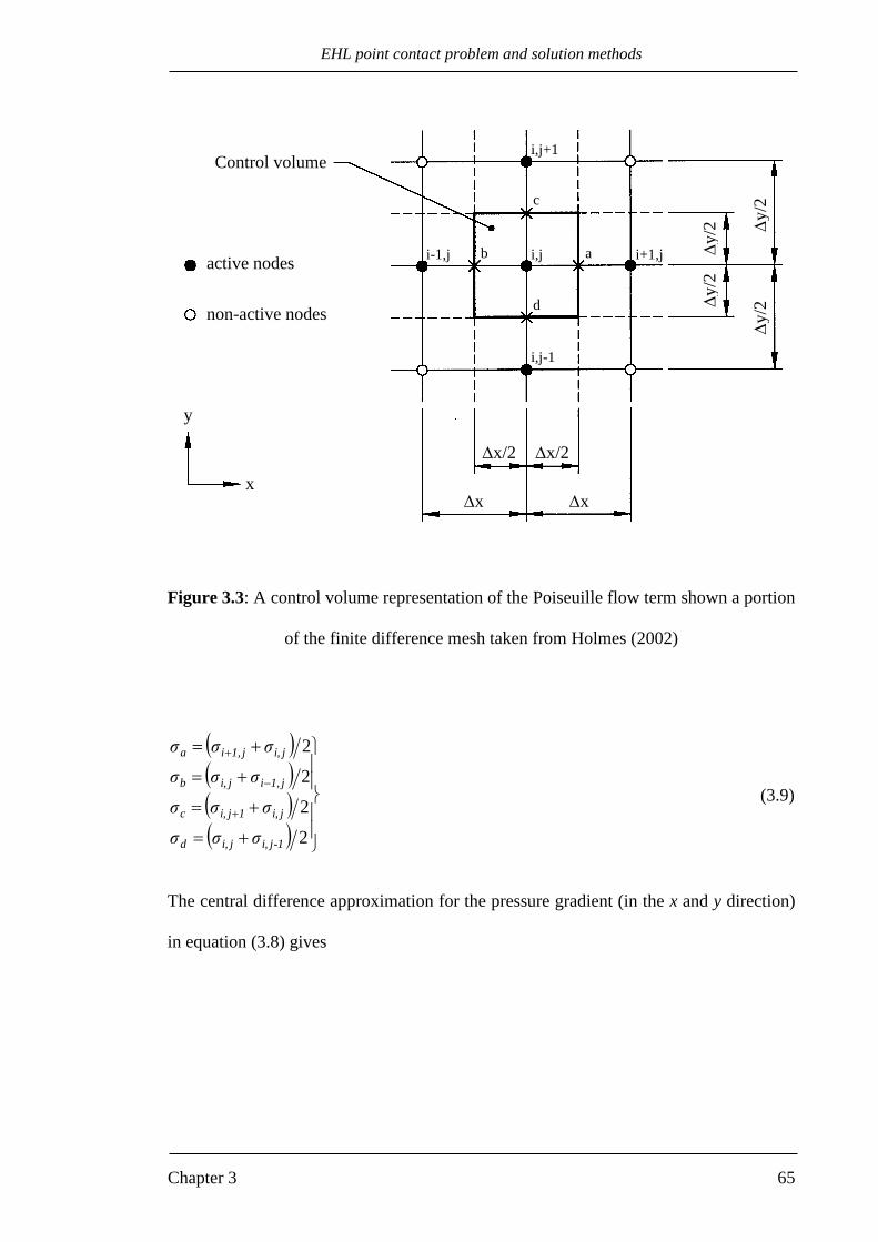
EHL point contact problem and solution methods
Chapter 3 65
Figure 3.3: A control volume representation of the Poiseuille flow term shown a portion
of the finite difference mesh taken from Holmes (2002)
2
2
2
2
1-ji,ji,d
ji,1ji,c
j1,iji,b
ji,j1,ia
σσσ
σσσ
σσσ
σσσ
(3.9)
The central difference approximation for the pressure gradient (in the x and y direction)
in equation (3.8) gives
Control volume
active nodes
non-active nodes
y
x x x
x/2 x/2
y/2
y/2
y/2
y/2
a b
c
d
i,j i+1,j i-1,j
i,j+1
i,j-1

EHL point contact problem and solution methods
Chapter 3 66
yppy
p
yppy
p
xppx
p
xppx
p
1-ji,ji,
d
ji,1ji,
c
j1,iji,b
ji,j1,ia
(3.10)
The wedge term in the Reynolds equation is
y
p
ph
y
hv-
x
p
ph
x
hu-
The central difference approximation of this term may be expressed as
y
hhv
y
pp
phv
x
hhu
x
pp
phu-
1-ji,1ji,1-ji,1ji,j1,ij1,ij1,ij1,i
2222
(3.11)
where the values of v,u ,ph , in this equation are taken at the node where the
hydrodynamic equation is applied. Substituting equations (3.10) and (3.11) in equation
(3.1) gives
022
22
y
hhv
y
pp
phv
Δy
ppσ
Δy
ppσ
x
hhu
x
pp
phu
Δx
ppσ
Δx
ppσ
1-ji,1ji,1-ji,1ji,
2
1-ji,ji,
d2
ji,1ji,
c
j1,ij1,ij1,ij1,i
2
j1,iji,
b2
ji,j1,i
a
which can be simplified after collecting the common factors to be in the following form

EHL point contact problem and solution methods
Chapter 3 67
022
2222
y
vh
y
vh
Δx
uh
Δx
uh
pΔy
hv
Δy
σp
pΔy
hv
Δy
σp
px2
hu
Δx
σp
px2
hu
Δx
σp
Δy
σ
Δy
σ
Δx
σ
Δx
σp
1-ji,1ji,
j1,-ij1,i2
d1ji,2
c1ji,
2
bj1,-i2
aj1,i2
d
2
c
2
b
2
aji,
The wedge term can also be discretised using any of the methods mentioned above
using the same general procedure for the central difference method.
3.7.2 Discretization of the hydrodynamic equation using FEM method
The discretization of the hydrodynamic equation by the FEM method involves the use
of the Galerkin method. In this approach, the same approximation is used for both the
weight functions and trial solution (Fish and Belytschko, 2012). Applying this method
to equation (3.1) gives
0dxdyy
p
ph
y
hNvdxdy
y
p
yN
dxdyx
p
ph
x
hNu dxdy
x
p
xN
iyi
ixi
(3.13)
where iN are standard shape functions.
The software considers a four nodes linear quadrilateral element, and the integrals given
by equation (3.13) are carried out over this element using two point Gauss integration.
Figure 3.4 shows the element adopted together with the Gauss points.
(3.12)

EHL point contact problem and solution methods
Chapter 3 68
Figure 3.4: The four nodes linear finite element
A detailed description of the discretisation method can be found in Holmes (2002).
Following integration by parts for the Poiseuille flow transforming and the weak
formulation (which is equivalent to the governing equation and the boundary
conditions), equation (3.13) becomes
04
1
4
1
4
1
4
1
4
1
4
1
dxdypy
N
p
~h~
hy
N~v~
Ndxdypy
N~
y
N
dxdypx
N
p
~h~
hx
N~u~
Ndxdypx
N~
x
N
j
j
j
j
j
j
i
j
j
j
yi
j
j
j
j
j
j
i
j
j
j
xi
(3.14)
where
kk
kk
k
kk
k
k
k
k
kk
k
kk y
k
kyk x
k
kx
pN
p
~ vNv
~ uNu
~
hNh~
N~ N~ N~
4
1
4
1
4
1
4
1
4
1
4
1
4
1
These average terms are evaluated over the element at the Gauss points.
Node number
Gauss points
4 3
1 2

EHL point contact problem and solution methods
Chapter 3 69
Performing the integration over an element results in a contribution from the film
thickness and pressure at each of its four nodes. Each node (except the boundary nodes)
has a contribution from four adjacent elements as shown in Figure 3.5. The coefficients
of pressure and film thickness at each node which involves all these contributions are
obtained by an assembling procedure.
Figure 3.5: The node i,j has contributions from the four adjacent elements (shaded)
3.7.3 Elastic deformation equation
The elastic equation can be written in the following form after substituting equation
(3.6) in equation (3.2)
o
lallkall
lkjliku hpgE
hh
,
,, '
2
(3.15)
The differential form of this equation is
l all,k all
l,kjl,iku p f'E
hh
222 (3.16)
where
i,j

EHL point contact problem and solution methods
Chapter 3 70
2
2
2
22
y
h
x
hh
The undeformed gap in this equation ( uh ) involves all surface modifications of the gear
teeth as explained in Chapter 2.
Discretising the derivative terms in this equation using the central difference method
gives
lallkall
lkjliku
jijijijijijipf
Eh
y
hhh
x
hhh
,
,,
2
2
,1,1,
2
,,1,1
'
222
(3.17)
The second term of the right hand side of equation (3.17) is split into two parts in the
solution process in addition to the point of interest (i,j). These are the ‘near’ part which
considers the contributions of the eight neighbouring nodes for the point of interest and
the remaining are denoted as ‘other’ contributions.
other
lkjlik
near
lkjlikji
lallkall
lkjlik pfE
pfE
pfE
pfE
,,,,,0,0
,
,, '
2
'
2
'
2
'
2
(3.18)
Equation (3.17) can be rearranged by using equation (3.18) and setting the pressure and
film thickness at point i,j on one side of the equation and moving all the other terms to
the other side.
other
lkjlik
near
lkjlik
u
jijijiji
jiji
p fE
p fE
hy
hh
x
hh
yxhf
Ep
,,,,
2
2
1,1,
2
,1,1
22,0,0,
'
2
'
2
112
'
2
(3.19)
letting:

EHL point contact problem and solution methods
Chapter 3 71
0,0,
'
2f
EC ji
,
22,
112
yxD ji
and
other
lkjlik
near
lkjliku
jijijiji
ji pfE
pfE
hy
hh
x
hhE ,,,,
2
2
1,1,
2
,1,1
, '
2
'
2
After these steps the elastic equation becomes
jijijijiji EhDpC ,,,,, (3.20)
where jiE , contains the near pressure contributions which are embedded in the
calculation and the other contribution which is evaluated for the current outer loop
results of pressure.
Also the Reynolds equation can be expressed in the following general form
ji
ji
nk
k
kk
ji
nk
k
kk RhBpAcc
,
,0,0
(3.21)
where:
kA are the Reynolds coefficients of pressure.
kB are the Reynolds coefficients of film thickness.
cn is the number of coefficients involved in the formulation.
j,iR is the right hand side, that has a zero value for steady state conditions
3.8 Transient Analyses
The software also has the ability to take the squeeze film term in the hydrodynamic
equation into consideration. Equation (3.21) can be written in the following form to
include the squeeze term
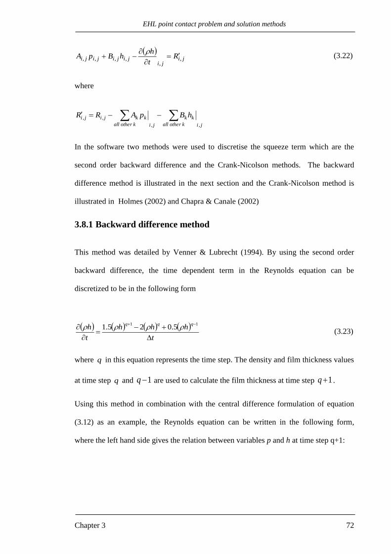
EHL point contact problem and solution methods
Chapter 3 72
ji
jijijijiji R
t
hhBpA ,
,,,,,
(3.22)
where
j,ik other all
kk
j,ik other all
kkj,ij,i hBpARR
In the software two methods were used to discretise the squeeze term which are the
second order backward difference and the Crank-Nicolson methods. The backward
difference method is illustrated in the next section and the Crank-Nicolson method is
illustrated in Holmes (2002) and Chapra & Canale (2002)
3.8.1 Backward difference method
This method was detailed by Venner & Lubrecht (1994). By using the second order
backward difference, the time dependent term in the Reynolds equation can be
discretized to be in the following form
t
hhh
t
hqqq
11
5.025.1 (3.23)
where q in this equation represents the time step. The density and film thickness values
at time step q and 1q are used to calculate the film thickness at time step 1q .
Using this method in combination with the central difference formulation of equation
(3.12) as an example, the Reynolds equation can be written in the following form,
where the left hand side gives the relation between variables p and h at time step q+1:

EHL point contact problem and solution methods
Chapter 3 73
j,i
ji,1-ji,1ji,
j1,-ij1,i2
d1ji,2
c1ji,
2
bj1,-i2
aj1,i2
d
2
c
2
b
2
aji,
Rt
h.h
t.h
y
vh
y
vh
Δx
uh
Δx
uh
pΔy
hv
Δy
σp
pΔy
hv
Δy
σp
px2
hu
Δx
σp
px2
hu
Δx
σp
Δy
σ
Δy
σ
Δx
σ
Δx
σp
1502
5122
2222
(3.24)
where
t
hhR
ji
1
,
5.02
It can be seen in equation (3.24) there is an additional 1
5.1
q
t
contribution added to
the central film thickness weighting due to the time dependent term, and the influence
of previous time steps appears in the non-zero right hand side, jiR , .
3.9 Effect of Non-Newtonian oil behaviour
The assumption of Newtonian oil behaviour overestimates the effective viscosity values
at high pressure levels which affects the EHL results. As sliding between the surfaces of
contacting teeth occurs due to the difference between their velocities, the lubricant
experiences extremely high rates of shear. The prediction of the lubricant behaviour in
such cases requires inclusion of a non-Newtonian rheological model, and in this study
the relation between the shear strain rate and the shear stress is taken to be the form
Fz
u
(3.25)
where F is a non-linear function.
EHL point contact problem and solution methods
Chapter 3 74
Several formulas have been proposed in the literature for the non-linear relation
between the shear strain rate and the shear stress. Johnson and Tevaarwerk (1977)
proposed the following relation based on the results of elastohydrodynamic friction
testing under controlled sample temperatures:
0
0
sinhF (3.26)
where 0 is the non-Newtonian parameter. This relationship is adopted in the current
study.
Equation (3.25) is used for a one dimensional problem and in two dimensional cases it
becomes (Sharif et al, 2001)
e
e
s Fz
u
(3.27)
e
e
r Fz
v
(3.28)
where s is the sliding direction, r is the perpendicular (non-sliding) direction and
22
rse
This generalisation is based on the assumption that the resultant shear stress is parallel
to the resultant strain rate and related to it according to equation (3.25). Note that suffix
s is used in this section to denote the sliding direction and should not be confused with
the more general use of s in the notation section.
The shear stress components can be related to the pressure gradient by considering the
equilibrium of a fluid element leading to the relations

EHL point contact problem and solution methods
Chapter 3 75
s
p
z
s
(3.29)
r
p
z
r
(3.30)
and since it is assumed that pressure does not vary in the z direction, these relations can
be integrated to give
zr
pz
zs
pz
rmr
sms
)(
)(
where
z : distance measured from the film thickness mid plane.
sm and rm are the mid-film shear stress components.
Integrating equations (3.27) and (3.28) across the thickness of the film, and applying
non-slip boundary conditions gives
2/
2/
0
h
h
e
e
ss zdFu
(3.31)
2/
2/
0
h
h
e
e
r zdF
(3.32)
The values of sm and rm are obtained by solving these equations numerically to
determine the shear stress values )(zs and )(zr which satisfy the kinematic
requirements. sm and rm are a function of ,p ,s
p
r
p
and h and vary throughout
the lubricant film.
(3.29a)
(3.30a)

EHL point contact problem and solution methods
Chapter 3 76
Sharif et al (2001) explain in detail how the non-Newtonian effect (involving the above
equations) can be incorporated in the formulation of the Reynolds equation when they
analysed the EHL behaviour of worm gears, which presents a general kinematic
problem.
Considering of the flow between the surfaces, the mass flow rate in each direction is
2/
2/
h
h
s zdzuQ
2/
2/
h
h
r zdzvQ
Integrating these equations by parts assuming does not vary across the film gives
2/
2/
h
h
s zdz
uz-huQ (3.33)
2
2
/h
/h
r zdz
vz-hvQ (3.34)
Substitution of equation (3.27) in (3.33) and (3.28) in (3.34) gives
2/
2/
h
h
e
e
ss zdFz-huQ
(3.35)
2/
2/
h
h
e
e
rr zdFz-hvQ
(3.36)
Morris (2000) showed that, when the formulation of flow equations is made in the
sliding and non-sliding directions, the second term in each of these equations (the
integral term) is proportional to the pressure gradient in that particular direction.
Therefore, equations (3.35) and (3.36) can be written in the forms

EHL point contact problem and solution methods
Chapter 3 77
s
p-huQ ss
(3.37)
r
p-huQ rr
(3.38)
Equating equation (3.35) with (3.37) and equation (3.36) with (3.38) gives
s
p
dzFz
h
h
ee
s
s
2/
2/
(3.39)
r
p
dzFz
h
h
ee
r
r
2/
2/
(3.40)
where s and r are given by equation (3.29a) and (3.30a) respectively.
These equations imply that the flow factors in the sliding and non-sliding directions are
different when the effect of non-linearity of the relation between shear stress and shear
strain rate is taken into consideration. This is not the case in the Newtonian situation
where the flow factors are equal in both directions as previously given by equation
(3.1a).
For the EHL of helical gears considered in this thesis, the surface velocities in the y
direction are zero. Therefore, sliding occurs in the x-direction throughout the film and
the flow factors in the x and y directions become:

EHL point contact problem and solution methods
Chapter 3 78
x
p
dzFz
h
h
e
e
x
x
2/
2/
(3.41)
y
p
dzFz
h
h
ee
y
y
2/
2/
(3.42)
where:
22yxe (3.43)
A routine for determining the flow factors given by equations (3.41) and (3.42) at each
mesh point as developed by Morris (2000) was incorporated in the software. As the
software is built in a general form to deal with both Newtonian and non-Newtonian oil
behaviour, the general form of the Reynolds equation given by equation (3.1) remains
as it is.
3.10 Solution techniques
Using the methods of formulation described in the previous sections, the Reynolds and
elastic equations can be written in the form:
jijijijiji
jijijijiji
EhDpC
RhBpA
,,,,,
,,,,, (3.44)
Both equations are clearly formulated in terms of pressure and film thickness at the
point i,j. These two equations need to be solved simultaneously (which is the idea
behind the coupled method). The software provides two methods to solve this pair of

EHL point contact problem and solution methods
Chapter 3 79
equations which are Gauss Seidel and alternate direction implicit (ADI) methods. The
ADI method solves the 2D problem as a series of 1D problems where each row is firstly
solved in one direction of the solution domain and then each column is solved. More
detail about this method can be found in Kreyszig (1999). However it has been found
that in the EHL problem the second stage of the ADI process (column solution) is
unnecessary and the solution is best obtained by repeated row solution (Holmes, 2002).
This is because transverse flow is not very influential in the transient problem and the
entrainment direction flow balance dominates the calculation.
In solving the pair of equations (3.44) simultaneously, the new values of j,ip and j,ih
can be calculated from
ji
new
jijijinew
ji
jijijiji
jijijijinew
ji
D
pCEh
CBDA
BEDRp
,
,,,
,
,,,,
,,,,
,
(3.45)
The results of these equations are used to update the pressure and film thickness until
convergence is obtained.
This procedure is used to solve for the points inside the solution space and boundary
conditions are applied at the boundaries of the solution space. The pressure values are
set to zero at the boundaries and the deflection in the elastic equation is calculated using
equation (3.6) based on the current pressure approximation to determine the value of the
film thickness on the boundary.
To calculate the film thickness at the boundary, the constant oh in equation (3.2) needs
to be determined. This can be achieved by using an empirical equation given by

EHL point contact problem and solution methods
Chapter 3 80
Chittenden et al. (1985) which gives the value of the central film thickness. At the
centre of the contact the value of the undeformed geometry is zero. Therefore equation
(3.2) becomes
occ hdh (3.46)
where cd is the surface deflection at the centre of the contact resulting from a Hertzian
pressure distribution. Therefore the constant oh can be calculated by rearranging
equation (3.46) to be
cco dhh (3.47)
This process gives the initial estimated value for oh to allow the steady state EHL
solution method to commence. The value of oh is continuously adjusted in the solution
algorithm to ensure that the converged result provides the specified load.
3.11 EHL results using FEM and FD method
Figure 3.6 shows a comparison between FEM and FD (central difference) methods for
the EHL analysis of a helical gear contact at a particular position in the meshing cycle.
Figure 3.6 (a) shows the film thickness (left) and pressure (right) results using the FEM
method and Figure 3.6 (b) shows the corresponding FD results. The required data that
were used to obtain these results are given in Chapter 4. No significant difference can be
seen in this figure between the results obtained using the two different methods. Further
sectional comparisons at the centre of the contact for the results shown in Figure 3.6 are
shown in Figure 3.7. Figure 3.7 (a) shows the section results in the entrainment
direction, x, and Figure 3.7 (b) shows the comparison in the y direction at x = 0. The
results of the two methods coincide very closely.

EHL point contact problem and solution methods
Chapter 3 81
It is worth mentioning that the solution to the EHL problem for the helical gears was
first approached using the FD method as it is easier to understand in comparison with
the FEM method. Then for the purpose of comparison the necessary understanding for
the FEM method was developed. This method was found to be more stable numerically
and therefore adopted as the default approach.
Figure 3.6: Comparison between FEM (upper) and FD (lower) EHL results at a position
in the meshing cycle of helical gear. Left: film thickness; right: pressure
h / µm p / GPa

EHL point contact problem and solution methods
Chapter 3 82
Figure 3.7: Comparison between FEM and FD EHL results at the centre
of the contact for the results shown in Figure 3.6 . (a) at y = 0 and (b) at x = 0
0.0
0.5
1.0
0.0
0.4
0.8
1.2
-0.5 0.0 0.5
h /
µm
p /
GP
a
x / mm
(a)
0.0
0.5
1.0
0.0
0.4
0.8
1.2
-25 -20 -15 -10 -5 0 5 10 15 20 25
h /
µm
p /
GP
a
y / mm
(b)

Transient EHL analysis: Introduction of axial crowning
Chapter 4 83
Chapter 4
Transient EHL analysis: Introduction of axial crowning
4.0 Introduction
The results shown in this chapter cover a full transient EHL analysis for a complete
meshing cycle of the helical gears considered. Software has been written in a general
form to solve the EHL contact problem for a pair of helical gears, whatever the contact
ratio. Two pairs of helical gears are considered as test cases which have significant
differences in their gear ratios and consequently different dimensions. The first pair
(design A), which has a 33:34 gear ratio, is from a test rig used for micropitting tests at
Newcastle University (Zhang & Shaw, 2011) for which transient mixed lubrication line
contact analyses were carried out by Evans et al. (2012) and Evans et al. (2013) to
examine near-surface fatigue effects in the context of micropitting. As the gear ratio of
set A is close to unity the resulting entrainment velocity at all positions in the meshing
cycle is almost constant. The second pair considered (design B) has a 33:99 gear ratio
which gives a greater variation of entrainment velocity during the meshing cycle. A
pinion torque and pinion rotational speed of 1.06 kNm and ω1= 235.62 rad/sec (2250
rpm) respectively, are assumed for both designs. The EHL analysis was isothermal and
the following lubricant parameters were assumed (Mobil Jet 2) (Mobil, 1979): ambient
pressure viscosity η0 = 0.00625 Pa.s; pressure-viscosity coefficient α = 13.3 GPa-1
; and
non-Newtonian shear thinning parameter τ0 = 10 MPa. Further details of the gears are
given in Table 4.1. The tip relief and tooth crowning values given in the table were the
default values used in this study and were applied for all cases except those for which
specified differences are given.

Transient EHL analysis: Introduction of axial crowning
Chapter 4 84
Table 4.1: Dimensions and parameters of gear pairs A and B
Design A Design B
Normal module / mm
4.5 4.5
Pinion tooth number 33 33
Wheel teeth number 34 99
Pressure angle / deg 20.0 20.0
Reference helix angle / deg 19.60 19.60
Pinion tip diameter / mm 166.61 166.61
Wheel tip diameter / mm 171.39 481.83
Centre distance / mm 160.00 315.22
Face width / mm 44.0 44.0
Tip relief value at the tip radius / µm 70 70
Tip relief radial distance / mm 2 2
Crown at the face edges / µm 8 8
4.1 Length of line of contact and the corresponding transmitted load.
In a spur gear drive, as the contact area during the meshing cycle is not significantly
changed, the most significant variation in the transmitted load comes from the sudden
change in the number of lines of contact at the change point positions in the meshing
cycle and the consequent effects on the tooth deflections. For helical gears, the
transmitted load will vary (in additional to other factors) due to the continuous

Transient EHL analysis: Introduction of axial crowning
Chapter 4 85
changing of the tooth contact area during the meshing cycle as the change of the number
of line of contacts is taking place very smoothly. This can be seen in Figure 4.1 which
shows the variation of length of a single line of contact, the transmitted load and the
total length of lines of contact throughout the meshing cycle in the absence of crowning
and tip relief. Figure 4.1 (a) shows these variations for design A, and those for design B
are shown in Figure 4.1 (b). The number of lines of contact (number of pairs of teeth in
contact at any instant) changes during the meshing cycle of a pair of helical gears. For
the gear ratio of design A and B the number of contact lines varies between two and
three throughout meshing cycle (the other two (or one) contact lines are not shown in
these figures). These figures show how a single line of contact in both designs starts at a
point and gradually changes to be a line of increasing, then constant and then decreasing
length, and finally ending as a point. It may be noticed in Figure 4.1 that there is no
significant change in the total length of the lines of contact and consequently the load
carried by a single line of contact is almost insensitive to the effect of change points.
On the other hand, the introduction of tip relief reduces the theoretical contact line
length which consequently decreases the total contact line length at any instant. Figures
4.2 (a) and (b) show the corresponding variations together with the transmitted load
when tip relief is taken into consideration. The decrease in the nominal contact line
length is clear in these figures where the total length is reduced by 41.18 % and 41.6 %
for design A and B respectively. However, the contact may extend into the tip relief
region depending on the form of tip relief in use.
In this study it was assumed that each contact line carried load in proportion to its
nominal length as a working approximation. The actual load distribution depends on the

Transient EHL analysis: Introduction of axial crowning
Chapter 4 86
tooth flexure and modelling this effect requires a complex 3D FEM with many teeth
included in the model and a fine mesh at the loaded flanks. However, dependence of
EHL film thickness on load is week (see equation 4.6) and if the flexure load variation
is known, it is possible to introduce a flexure misalignment of contact lines to account
for it in the EHL analysis. Such a task is not realistic for the current study which
assumes that the load is numerically uniformly distributed along the contact line as a
first approximation.
This means that the proportion of the total load carried by a contact is assumed to be
given by the instantaneous length of the contact line divided by the corresponding total
contact length for all tooth pairs in contact. For gear pairs A and B specified in Table
4.1 the total length of tooth contacts varied by 4.3% and 4.8% respectively at the
change points, so the load per unit length of a given contact varied only by this
relatively small amount. The maximum transmitted load is 14.4 kN which occurs when
the contact acts over the whole face width at 5.7is mm.

Transient EHL analysis: Introduction of axial crowning
Chapter 4 87
Figure 4.1: Variation of contact line length and contact line load for a
single contact line over its meshing cycle without tip relief. Also shown is the variation
in total length of the contact lines of the tooth pairs in contact .
(a) Design A; (b) Design B
0
2
4
6
8
10
12
14
16
18
20
0
10
20
30
40
50
60
70
80
90
-30 -20 -10 0 10
Load
/ k
N
Len
gth
/ m
m
si / mm
0
2
4
6
8
10
12
14
16
18
20
0
10
20
30
40
50
60
70
80
90
-30 -20 -10 0 10
Load
/ k
N
Len
gth
/ m
m
si / mm
(a)
(b)

Transient EHL analysis: Introduction of axial crowning
Chapter 4 88
Figure 4.2: Variation of contact line length and contact line load for a
single contact line over its meshing cycle with tip relief. Also shown is the variation in
total length of the contact lines of the tooth pairs in contact .
(a) Design A; (b) Design B
0
2
4
6
8
10
12
14
16
18
20
0
5
10
15
20
25
30
35
40
45
50
-30 -20 -10 0 10
Lo
ad /
kN
Len
gth
/ m
m
si / mm
0
2
4
6
8
10
12
14
16
18
20
0
5
10
15
20
25
30
35
40
45
50
-30 -20 -10 0 10
Load
/ k
N
Len
gth
/ m
m
si / mm
(a)
(b)

Transient EHL analysis: Introduction of axial crowning
Chapter 4 89
4.2 Radius of curvature and surfaces velocities
Figure 4.3 shows the variation of the radius of relative curvature, entrainment velocity,
and slide/roll ratio over the meshing cycles for the two designs. It can be seen that the
first contact for designs A and B occurs at s = 10.8 mm and s = 11.8 mm,
respectively, and in both designs the contact ends at s = 10.8 mm. In design B, the path
of contact is therefore 4.4% longer than that for design A. It can be seen from Figure 4.3
(a) that there is a significant difference in the radii of relative curvature over the
meshing cycle between the two pairs. The radius in design A (dashed line) is almost
symmetric as the two gears have slightly different dimensions. In design B the radius of
relative curvature increases as s increases.
For the kinematic behavior of the gears, the entrainment velocity takes place in the
rolling/sliding direction between the teeth, which is parallel to the minor axis of the
contact ellipse. Since the time varying radii of curvature are changed over the
instantaneous line of contact, the surface velocities are also varying and are given by:
111 ,, tysRtyu (4.1)
222 ,, tysRtyu (4.2)
The mean entrainment at the first position in the meshing cycle is 5.8 m/s for design B
which varies by 25% over the meshing cycle, whereas it is almost constant at 6.7 m/s
for design A as shown in Figure 4.3 (b). The figure also shows the slide-roll ratio
variation over the meshing cycle for the two designs.

Transient EHL analysis: Introduction of axial crowning
Chapter 4 90
Figure 4.3: Variation of contact characteristics during the meshing cycle. (a) Radius of
relative curvature; (b) entrainment velocity and slide /roll ratio,
𝒖A, 𝒖B, ζA,, ζB
Design B
Design A
10
14
18
22
26
-12 -8 -4 0 4 8 12
R /
mm
s / mm
-1
0
1
2
4
5
6
7
8
-12 -8 -4 0 4 8 12
ζ
s / mm
u̅
(a)
(b)

Transient EHL analysis: Introduction of axial crowning
Chapter 4 91
In the spur gear case, the radius of relative curvature, surface velocities, mean
entrainment velocity and slide/roll ratio are all constant over an individual contact
position specified by an s position in the meshing cycle. This is not the case in helical
gears contact as the contact lines are inclined to the gear axis at the base helix angle.
The contact line at a corresponding position in the meshing cycle acts over a range of s
and consequently all these values change over this range. The sliding velocity,
21 uuus for example is changing between negative, zero and positive values over
an individual contact area as shown in Figure 4.4. It is worth noting that this does not
reflect a change in direction of motion, rather it is a question of which of the two
surfaces is moving faster relative to the contact line. This figure shows the variation
along the major axis of the contact ellipse for a pinion input speed of 235.62 rad/s for
design A. This variation also takes place at other positions in the meshing cycle
wherever a contact line intersects the pitch line while in a spur gear, this sliding
velocity is either negative or zero or positive at any position in the meshing cycle.
Figure 4.4: Variation of sliding velocities over an individual contact line for design A
-4
-3
-2
-1
0
1
2
3
4
-25 -15 -5 5 15 25
us
/ m
/s
y / mm

Transient EHL analysis: Introduction of axial crowning
Chapter 4 92
4.3 Profile and surface modifications
Two forms of tooth geometry modifications are usually applied in practice. In order to
avoid bending deformation overlap of the loaded teeth (Park and Yoo, 2004) (also
called “pre-engagement”) and reduce the static transmission error under load
(Kahraman & Blankenship, 1999) (Tuplin, 1962) (Bonori et al., 2008) it is desirable to
modify the involute tooth form by removing some material from the tooth flanks near
their tips. In addition to increasing gear durability this modification also improves gear
dynamic response and reduces noise (Bahk and Parker, 2013). This modification is
termed “tip relief” which is important to avoid the damaging premature contact that
would otherwise begin on the top corner edge of the driven tooth due to tooth flexure
under load.
The second area of potential stress concentration and film thinning occurs at the side
edges of the teeth, which is exacerbated by any small degree of out-of-parallel
misalignment between the gears. In order to minimise this problem the teeth may be
“crowned” (Kahraman et al., 2005) (a modification in which the chordal thickness of
the teeth is diminished by a small amount from a maximum at the middle of the gear to
a minimum at the side edges). In principle crowning changes the contacts from “line” to
“point” form, but in practice the contact area becomes an elongated area approximately
elliptical in shape under load. By careful choice of the degree of crowning it is possible
to prevent heavy contact at the side edges of the teeth under all conditions of loading
and misalignment due to mounting errors or shaft deflections under load.
All four gears described in Table 4.1 have the same amount of profile relief at their tips
which is a maximum value of 70 m over a radial distance rtip rstart = 2 mm. In order
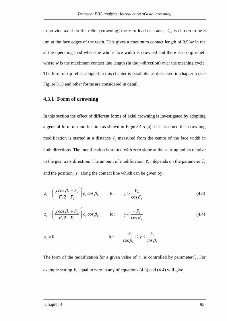
Transient EHL analysis: Introduction of axial crowning
Chapter 4 93
to provide axial profile relief (crowning) the zero load clearance, rc , is chosen to be 8
µm at the face edges of the teeth. This gives a maximum contact length of 0.93w in the
at the operating load when the whole face width is crowned and there is no tip relief,
where w is the maximum contact line length (in the y-direction) over the meshing cycle.
The form of tip relief adopted in this chapter is parabolic as discussed in chapter 5 (see
Figure 5.1) and other forms are considered in detail.
4.3.1 Form of crowning
In this section the effect of different forms of axial crowning is investigated by adopting
a general form of modification as shown in Figure 4.5 (a). It is assumed that crowning
modification is started at a distance oF measured from the centre of the face width in
both directions. The modification is started with zero slope at the starting points relative
to the gear axis direction. The amount of modification, cz , depends on the parameter oF
and the position, y , along the contact line which can be given by:
br
o
obc cosc
FF
Fcosyz
2
2
for
b
oFy
cos (4.3)
br
o
obc cosc
FF
Fcosyz
2
2
for
b
oFy
cos
(4.4)
0cz for b
o
b
o Fy
F
coscos
The form of the modification for a given value of rc is controlled by parameter oF . For
example setting oF equal to zero in any of equations (4.3) and (4.4) will give

Transient EHL analysis: Introduction of axial crowning
Chapter 4 94
brb
c coscF
cosy)y,xz
2
2
This equation represents a fully parabolic form as shown in Figure 4.5 (b). Figure 4.5
(c) shows the 3D total gap between the two teeth surfaces when FFo 25.0 and when
the contact acts over the whole face width for design B.
(a)
(b)
(c)
Figure 4.5: Form of crowning. (a) General form; (b) 0oF ; (c) FFo 25.0
F
𝑐𝑟
F
𝑐𝑟
Fo
y cos βb
Fo

Transient EHL analysis: Introduction of axial crowning
Chapter 4 95
4.4 EHL results
The solution space for the EHL analysis is the common tangent plane between the teeth
in the vicinity of the instantaneous contact line. This is discretised with a mesh spacing
Δx = a/40 in the rolling/sliding direction and Δy = w/857 in the contact line direction.
Here a is the contact semi-width in the x direction at the maximum load and w is the
maximum contact line length (in the y-direction) over the meshing cycle, as defined
previously.
The transient EHL analysis was carried out for a contact line from a nominal start
position where its length is 0.16w, to a nominal end position where its length falls below
0.16w. The transient EHL solution was obtained using range of time steps between 300
and 2300 time steps. For the meshing cycle it was found that the transient results are
almost identical when the number of time steps is greater than 400. The time step
adopted for the analyses divided the meshing cycle into 575 time steps for convenience
as the analysed meshing cycle length was 23 mm so that 25 time steps correspond to 1
mm distance. The initial condition was determined from a steady-state EHL analysis at
the geometric, kinematic and load conditions of the first time step.
The total gap between the tooth surfaces, which is the basis for the EHL model, is a
combination of relative curvature at the point considered plus the profile modification
effects.
As the curvature and the contact length change with the progression through the
meshing cycle, the undeformed-gap shape varies consequently. Figure 4.6 shows three
positions in the meshing cycle for which detailed comparisons for both designs will be
shown in chapter 4 and 5. These are at time steps 75, 300 and 500 and correspond to
positions where the contact (i) is mainly within the addendum of the wheel, (ii) occurs
over the whole face width, and (iii) is mainly within the addendum of the pinion.

Transient EHL analysis: Introduction of axial crowning
Chapter 4 96
Figure 4.6: Contact position at the three time steps considered,
(1): Timestep 75, (2): Timestep 300 and (3): Timestep 500, for the gears specified in
table 4.1. Pinion tip relief zone zp =4.3 mm, wheel tip relief zone zw = 4.4 mm
The undeformed gap between the two surfaces at these three positions with the
corresponding 3D EHL pressure distribution for design A and B are shown in Figure 4.7
and Figure 4.8 respectively. A full parabolic crown was used in both cases where oF in
equations (4.3) and (4.4) is equal to zero. As 0y at the centre of the face width in the
coordinate system adopted, the contact line for the first selected position is in the
positive y half of the plane of contact, the contact line for the second position is in both
halves of the plane of contact, and the last position is mainly in the negative y half of
the plane of contact.
Pressure spikes are produced at the first and third contact positions and are associated
with tip relief modification. The contact at position 2 for both designs is essentially
elliptic and covers the majority of the y axis range (most of the face width). The contact
at this position is effectively dominated by the crowning of the gear teeth in contact
rather than tip relief. This attributes to the position of tip relief with respect to the centre
of the contact.
zp
zw
Tip of pinion
Tip of wheel
z y
2
1
3
44 mm
21.5 mm
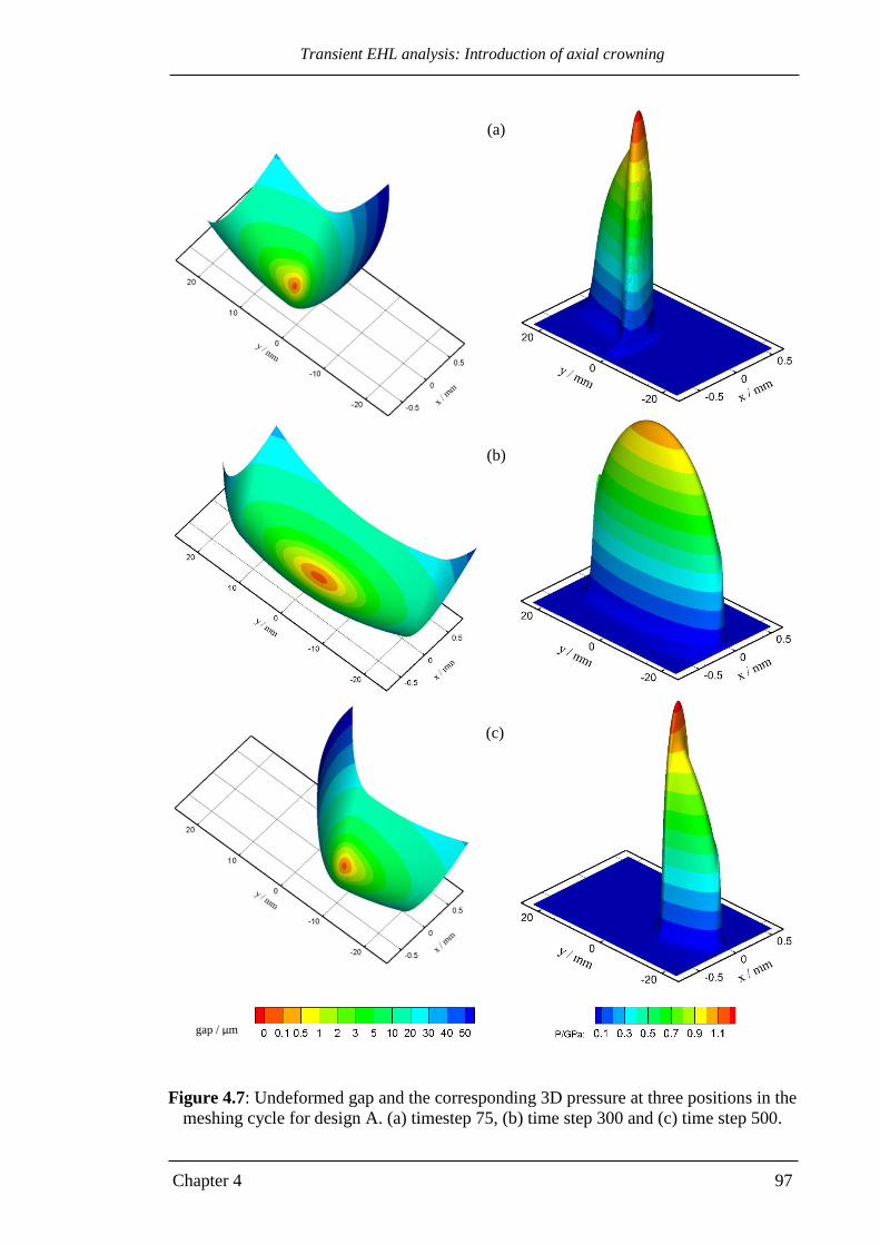
Transient EHL analysis: Introduction of axial crowning
Chapter 4 97
Figure 4.7: Undeformed gap and the corresponding 3D pressure at three positions in the
meshing cycle for design A. (a) timestep 75, (b) time step 300 and (c) time step 500.
(a)
(b)
(c)
gap / µm
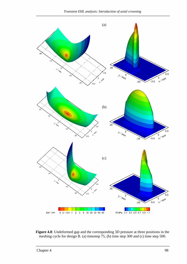
Transient EHL analysis: Introduction of axial crowning
Chapter 4 98
Figure 4.8: Undeformed gap and the corresponding 3D pressure at three positions in the
meshing cycle for design B. (a) timestep 75, (b) time step 300 and (c) time step 500.
(a)
(b)
(c)
gap / µm

Transient EHL analysis: Introduction of axial crowning
Chapter 4 99
4.5 Load convergence:
The load carried by an EHL contact can be calculated by integration of the generated
pressure over the solution domain. This is given by
Area
EHL dxdy pLoad (4.5)
Load convergence is maintained at each time step during the EHL solution of the gear
meshing cycle. This process ensures that the load result from the EHL solution is within
± 0.5 percent of the assumed input load for each time step. Variations of the load by this
amount has almost no consequent effect on the maximum pressure or minimum film
thickness values as given by the well-known equations for elliptical EHL contacts
(Hamrock and Dowson 1977)
68.0073.049.068.0
min e1WGU63.3H (4.6)
where W and Hmin in this equation represent the (non-dimensional) load applied on the
contacted surfaces and the minimum film thickness, respectively.
Obtaining the specified EHL load can be achieved by adjusting the separation between
the two surfaces. The pressure and consequently the load can be increased by reducing
the separation in the solution processes and vice versa until convergence is obtained.
Figures 4.9 (a) and 4.9 (b) show comparisons between the input load and the load
results from ensuring that equation (4.5) is satisfied throughout the meshing cycle of
design A and B respectively to the tolerance described above. The EHL load is
presented with a dashed line which can be seen to coincide with the input load almost
exactly for both designs. Full parabolic forms for both crowning and tip relief
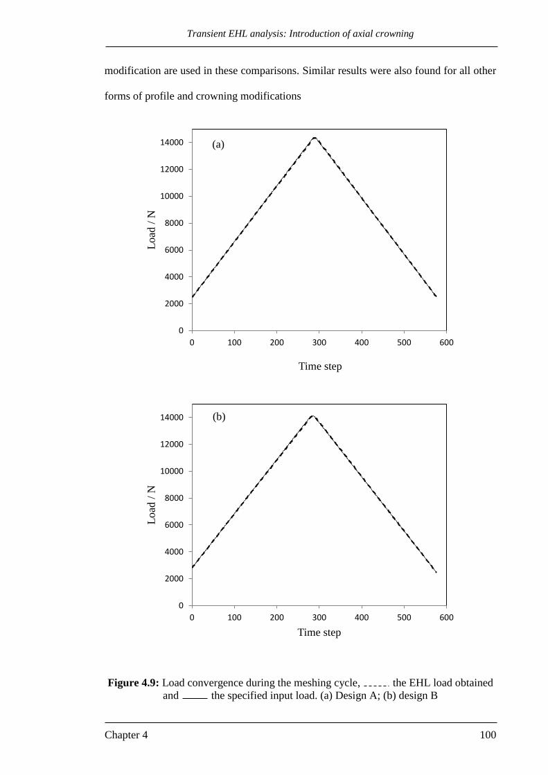
Transient EHL analysis: Introduction of axial crowning
Chapter 4 100
modification are used in these comparisons. Similar results were also found for all other
forms of profile and crowning modifications
Figure 4.9: Load convergence during the meshing cycle, the EHL load obtained
and the specified input load. (a) Design A; (b) design B
0
2000
4000
6000
8000
10000
12000
14000
0 100 200 300 400 500 600
Load
/ N
Time step
0
2000
4000
6000
8000
10000
12000
14000
0 100 200 300 400 500 600
Load
/ N
Time step
(a)
(b)

Transient EHL analysis: Introduction of axial crowning
Chapter 4 101
4.6 Results for different forms of crowning
Figure 4.10 shows the behaviour of the maximum pressure and minimum film thickness
during the meshing cycle for design A for five forms of crowning where oF 0 , 0.1F,
0.25F, 0.4F and 0.45F. With the parabolic form of tip relief that was used in this
comparison, the maximum pressure and the minimum film thickness behaviour obtained
varies significantly with the form of crowning. The case of full parabolic crowning
which corresponds to 0oF , gives the highest calculated EHL pressure of 1.25 GPa.
For the case of 0oF the maximum pressure occurs at one end or other of the contact
line where tip relief is achieve over approximately time step ranges 0 to 210 and 360 to
575. From time step 210 to 360 the maximum pressure occurs at the centre of the
contact and behaves differently. This features is typical of all the maximum pressure
results considered in this thesis that are presented in this way.
The magnitude of the maximum pressure experienced decreases as oF is increased. This
is essentially related to the increase of the contact area length along the y direction
which reduces the concentration of the load at a single point at the start of tip relief
modification. However, when FFo 45.0 , despite the noticeable reduction in the
maximum pressure trends at the first and last 200 time steps, pressure spikes appear at
the middle of the meshing cycle as shown in Figure 4.10 (a). This is associated with a
reduction in the film thickness levels which is 0.14 µm in comparison with 0.21 µm
when 0oF at time step 300 as shown in Figure 4.10 (b). The case of FFo 25.0
gives the best combination of maximum pressure and minimum film thickness trends
during the meshing cycle. With this form of crowning the maximum pressure varies

Transient EHL analysis: Introduction of axial crowning
Chapter 4 102
between 0.98 GPa and 1.17 GPa during the meshing cycle. The corresponding
minimum film thickness varies between 0.16 µm and 0.22 µm.
Figure 4.10: Variation of maximum pressure (upper) and minimum film thickness
during the meshing cycle for design A for five forms of crowning, green: 𝐹𝑜 = 0, blue:
𝐹𝑜 = 0.1𝐹, purple: 𝐹𝑜 = 0.25𝐹, red: 𝐹𝑜 = 0.4𝐹 and black: 𝐹𝑜 = 0.45𝐹, with parabolic
tip relief.
800
900
1000
1100
1200
1300
0 100 200 300 400 500 600
p /
GP
a
Time step
(a)
0.12
0.16
0.20
0.24
0 100 200 300 400 500 600
h /
μm
Time step
(b)

Transient EHL analysis: Introduction of axial crowning
Chapter 4 103
The effects of choosing different forms of crowning are more clearly apparent in Figure
4.11 which shows 3D isometric plots of the transient EHL analyses pressure distribution
at time step 300 for the five forms of crowning, together with the corresponding 2D film
thickness contours for the results shown in Figure 4.10. Figure 4.11 (a) shows a typical
point contact EHL result which corresponds to 0oF . With 0oF axial crowning
relieves the contact progressively along the contact line. As oF increases, for contact
lines that reach the tip relief zone before the crowning becomes active the contact is
limited by the tip relief imposed. This is clear in the cases where FFo 4.0 and
FFo 45.0 which are shown Figure 4.11 (d) and (e) respectively. In these cases the end
of contact line stress concentration effect appears on both sides of the contact but it is
more aggressive (has the effect of thinning the film thickness) on the left side of the
contours (positive y). This is because at this particular time step the start point of tip
relief on the tooth profile is closer to the starting position of crowning on the positive y
part of the contact area in comparison to the negative y (right side of the contact).
With the exception of the case of 0oF , two peak pressure areas can be seen in this
figure which are associated with the introduction of crowning modification on both
sides of the contact. Thinning of the film thickness occurs at the start of crowning
modification due to the side leakage which takes place in the y direction, which leads to
the occurrence of these pressure spikes. This can be clearly seen in Figure 4.12 which
shows transient pressure and film thickness distributions along the y direction at time
step 300 for the five forms of crowning for design A. A similar comparison at this
position in the meshing cycle was made for design B. In general, the same trend was
found as shown in Figure 4.13 with some differences in the compared values as design
B has different tooth curvature and surface velocities in comparison with design A.

Transient EHL analysis: Introduction of axial crowning
Chapter 4 104
Figure 4.11: Pressure distribution (left) and film thickness (right) at time step 300 for
five forms of crowning
(a) (a) Fo = 0
(b) Fo = 0.1F
(c) Fo = 0.25F
(d) Fo = 0.4F
(e) Fo = 0.45F

Transient EHL analysis: Introduction of axial crowning
Chapter 4 105
Figure 4.12: Pressure and film thickness distribution along y direction at x = 0 at time
step 300 for design A, 𝐹𝑜 = 0, 𝐹𝑜 = 0.1𝐹, 𝐹𝑜 = 0.25𝐹,
𝐹𝑜 = 0.4𝐹 and , 𝐹𝑜 = 0.45𝐹.
0.0
0.2
0.4
0.6
0.8
1.0
1.2
-25 -15 -5 5 15 25
p /
GP
a
y / mm
0.00
0.20
0.40
0.60
-25 -15 -5 5 15 25
h /
µm
y / mm

Transient EHL analysis: Introduction of axial crowning
Chapter 4 106
Figure 4.13: Pressure and film thickness distribution along y direction at x = 0 at time
step 300 for design B, 𝐹𝑜 = 0, 𝐹𝑜 = 0.1𝐹, 𝐹𝑜 = 0.25𝐹,
𝐹𝑜 = 0.4𝐹 and , 𝐹𝑜 = 0.45𝐹.
0.0
0.2
0.4
0.6
0.8
1.0
1.2
-25 -15 -5 5 15 25
p /
GP
a
y / mm
0.00
0.20
0.40
0.60
-25 -15 -5 5 15 25
h /
µm
y / mm

Transient EHL analysis: Introduction of axial crowning
Chapter 4 107
Figures 4.14, 4.15, 4.16, 4.17 and 4.18 show the 3D pressure distribution and the
corresponding film thickness contours for design A at three positions in the meshing
cycle for the cases 0oF , 0.1F, 0.25F, 0.4F, 0.45F respectively. These are the
positions shown in Figure 4.6 which are at time steps 75, 300 and 500 respectively. The
case of timestep 300 which was shown in Figure 4.11 is repeated in these figures for the
purpose of comparison. Figures 4.14 and 4.15 show single pressure spikes at time steps
75 and 500 which are related to the tip relief effect as the crowning effect when 0oF
and 0.1F is out of the contact region at this position in the meshing cycle. The other
figures (4.16, 4.17 and 4.18) show two pressure spikes at time steps 75 and 500. The
first pressure spike is associated with the introduction of crowning as stated previously,
while the second one results from tip relief modification. The film thickness contours
also show the reduction in the film thickness levels at the tip relief zone.
It is worth noting that although the contact and the pressure spikes elevate the pressure
noticeably, the maximum pressures at these locations are not significantly greater than
the central pressures seen for the case where 0oF .

Transient EHL analysis: Introduction of axial crowning
Chapter 4 108
Figure 4.14: 3D pressure distributions and film thickness contours for design A with
0oF at the three timesteps considered, timestep 75 (upper figures), timestep 300
(central), timestep 500 (lower).

Transient EHL analysis: Introduction of axial crowning
Chapter 4 109
Figure 4.15: 3D pressure distributions and film thickness contours for design A with
FFo 1.0 at the three timesteps considered, timestep 75 (upper figures), timestep 300
(central), timestep 500 (lower).

Transient EHL analysis: Introduction of axial crowning
Chapter 4 110
Figure 4.16: 3D pressure distributions and film thickness contours for design A with
FFo 25.0 at the three timesteps considered, timestep 75 (upper figures),
timestep 300 (central), timestep 500 (lower).

Transient EHL analysis: Introduction of axial crowning
Chapter 4 111
Figure 4.17: 3D pressure distributions and film thickness contours for design A with
FFo 4.0 at the three timesteps considered, timestep 75 (upper figures), timestep 300
(central), timestep 500 (lower).
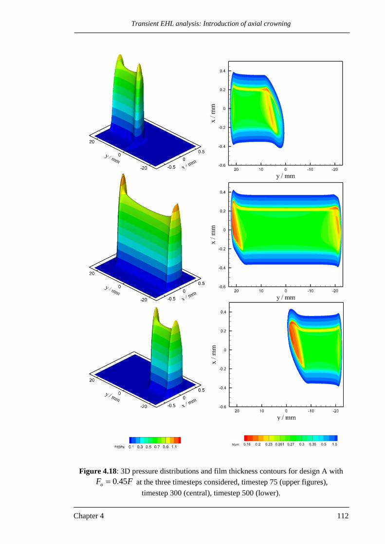
Transient EHL analysis: Introduction of axial crowning
Chapter 4 112
Figure 4.18: 3D pressure distributions and film thickness contours for design A with
FFo 45.0 at the three timesteps considered, timestep 75 (upper figures),
timestep 300 (central), timestep 500 (lower).
Tip relief
Chapter 5 113
Chapter 5
Tip relief
5.0 Introduction
In this chapter the effect of tip relief on the EHL performance of helical gears has been
investigated by adopting different forms for the relief geometry for the two gear pair
designs considered in chapter 4. The tip relief profiles are applied to the involute profile
over the radial range
rstart < r < rtip (5.1)
where r is the radius measured from the gear axis as given by equation (2.16).
The forms of tip relief used in this chapter can be categorized into two main cases which
are:
a- Combinations of linear and parabolic profiles.
b- Power law profile.
In this chapter the axial crowning is expressed in the full parabolic form where 00 F
in equations (4.3) and (4.4). The transverse clearance rc for each tooth at the side edges
is 8 μm when the contact occurs at the centre of the tooth under zero load.
5.1 Linear and parabolic profiles
The modification in this case consists of a combination of linear and parabolic profiles
which join at r = rce with equal slope as shown in Figure 5.1.

Tip relief
Chapter 5 114
(a) (b)
Figure 5.1: Illustration of tip relief geometry showing parabolic and linear sections
The amount of surface removal, tz , depends on parameters ce, ct, rstart, rtip and rce as
shown in Figure 5.1 (a). The parabolic modification starts with zero slope (relative to
the involute profile) at radius rstart and transition to the linear profile occurs at radius rce
where
)rr(krr starttipstartce (5.2)
The nature of the modification for a given value of ct is controlled by parameter k. A
simple linear tip relief profile corresponds to k = 0, and the fully parabolic form with
tooth slope continuity at r = rstart is given by k = 1 as shown in Figure 5.1 (b). For
intermediate values of k the transition between a parabolic profile and linear profile
occurs with no change of slope.
The gap due to tip relief can be determined by considering the equations for the straight
line and the parabolic curve as shown in Figure 5.1 (a). It can be easily shown that the
equation for the linear part is
ce
ct
rce rtip r
𝑧𝑡′
r𝑠𝑡𝑎𝑟𝑡
ct
rtip r
𝑧𝑡′
k=0
k=1
r𝑠𝑡𝑎𝑟𝑡
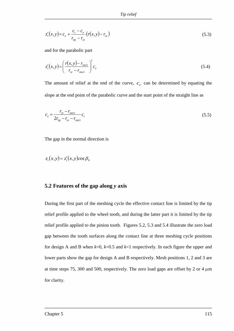
Tip relief
Chapter 5 115
ce
cetip
et
et ry,xrrr
cccy,xz
(5.3)
and for the parabolic part
e
startce
start
t crr
ry,xry,xz
2
(5.4)
The amount of relief at the end of the curve, ec can be determined by equating the
slope at the end point of the parabolic curve and the start point of the straight line as
t
startcetip
startcee c
rrr
rrc
2 (5.5)
The gap in the normal direction is
btt cosy,xzy,xz
5.2 Features of the gap along y axis
During the first part of the meshing cycle the effective contact line is limited by the tip
relief profile applied to the wheel tooth, and during the latter part it is limited by the tip
relief profile applied to the pinion tooth. Figures 5.2, 5.3 and 5.4 illustrate the zero load
gap between the tooth surfaces along the contact line at three meshing cycle positions
for design A and B when k=0, k=0.5 and k=1 respectively. In each figure the upper and
lower parts show the gap for design A and B respectively. Mesh positions 1, 2 and 3 are
at time steps 75, 300 and 500, respectively. The zero load gaps are offset by 2 or 4 m
for clarity.

Tip relief
Chapter 5 116
Figure 5.2 (a) shows the gap for design A when the tip relief profile is linear (k=0). For
position 2 in this figure, it is clear that the gap is given by the axial crown with the
pinion tip relief becoming apparent for y > 18.5 mm and for y < -21.5 mm . For
position 1 the contact is essentially limited by the wheel tip relief at y < 6.4 mm, and for
position 3 it is limited by the pinion tip relief for y > -6.3 mm. For positions 1 and 3 the
combination of the axial crown and the active tooth relief leads to contacts that are
curtailed at the onset of tip relief position where a significant stress concentration
emerges in the calculations. Generally, the same feature can be seen in the
corresponding gaps of design B which is shown in Figure 5.2 (b).
The severe change in the slope of the profile that is shown in Figure 5.2 for both designs
due to the linear modification is overcome by adding a transition parabolic curve over a
specified radial distance. The remaining part of modification is linear which meets with
the parabolic curve at equal slope. The case when the modification corresponds to k=0.5
in equation (5.2) is shown in Figure 5.3 for both designs. The modification is further
improved by using a full parabolic curve (k =1) as shown in Figure 5.4.

Tip relief
Chapter 5 117
Figure 5.2: Gap between gear surfaces (offset) along contact line at positions
1, 2 and 3 in the meshing cycle for linear tip relief modification, k =0 . Axial crown is
shown broken and symbol indicates starts of tip relief for each contact line.
(a) Design A; (b): Design B
0
4
8
12
16
20
-25-15-551525
Hei
gh
t /
µm
y / mm
0
4
8
12
16
20
-25-15-551525
Hei
ght
/ µ
m
y / mm
(b)
1
2
3
(a)
1
2
3

Tip relief
Chapter 5 118
Figure 5.3: Gap between gear surfaces (offset) along contact line at positions
1, 2 and 3 in the meshing cycle for mixed relief modification, k =0.5 . Axial crown is
shown broken and symbol indicates starts of tip relief for each contact line.
(a) Design A; (b): Design B
0
4
8
12
16
20
-25-15-551525
Hei
gh
t /
µm
y / mm
0
4
8
12
16
20
-25-15-551525
Hei
ght
/ µ
m
y / mm
(b)
1
2
3
1
2
3
(a)
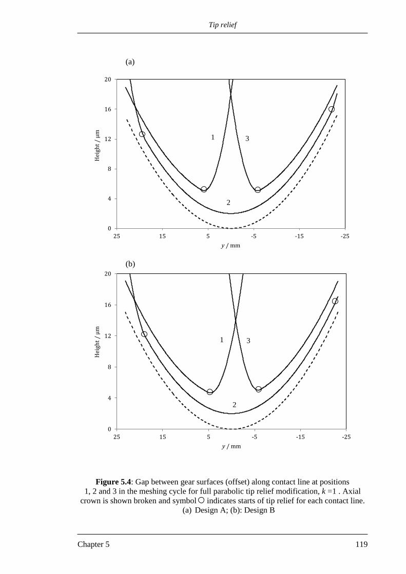
Tip relief
Chapter 5 119
Figure 5.4: Gap between gear surfaces (offset) along contact line at positions
1, 2 and 3 in the meshing cycle for full parabolic tip relief modification, k =1 . Axial
crown is shown broken and symbol indicates starts of tip relief for each contact line.
(a) Design A; (b): Design B
0
4
8
12
16
20
-25-15-551525
Hei
ght
/ µ
m
y / mm
0
4
8
12
16
20
-25-15-551525
Hei
ght
/ µ
m
y / mm
(a)
(b)
1
2
3
1
2
3
Tip relief
Chapter 5 120
5.3 Results of parametric study
All four gears in this chapter have the same amount of profile relief at their tips which is
70 m over a radial distance rtip rstart = 2 mm. This is the design specification for the
test gears of case A where a linear tip relief profile is utilised. The detailed results of the
transient EHL analyses presented correspond to the full parabolic tip relief profile i.e. k
= 1, and the effects of variation of k from unity to zero are also investigated. As far as
this kinematic analysis is concerned (where tooth bending is not taken into account) it
was found that the contact did not generate significant pressure beyond the radius where
tip relief is applied, and this was taken into account by using the effective contact line
length in the load specification.
Figure 5.5 compares the behaviour of the maximum pressure and the minimum film
thickness during the meshing cycle for the two designs for the case where k = 1. The
two designs generally give the same trend for both the maximum pressure and minimum
film thickness with some lack of symmetry in the maximum pressure of design B
towards the middle of the meshing cycle. This is related to the significant change in
radius of relative curvature over the meshing cycle as discussed in relation to Figure 4.3
(a).
Between time steps 204 and 370 for design A and between time steps 180 and 370 for
design B the contact line is effectively limited at both ends by the side faces of the gears
and at other times one end of the contact line is limited by the tip relief profile of either
the wheel or the pinion. With this form of tip relief the maximum calculated EHL
pressure varies between 1.02 GPa and 1.25 GPa for design A, and between 0.82 GPa
and 1.12 GPa for design B. This can be attributed to the differences in the radii of

Tip relief
Chapter 5 121
relative curvature between the two designs throughout the meshing cycles. The tooth
profile in design B has a larger radius of relative curvature at all contact positions which
gives a larger contact area, and as a result a smaller Hertzian pressure. The
corresponding minimum film thickness varies between 0.16 μm and 0.22 μm for design
A and between 0.16 μm and 0.25 μm for design B. The maximum pressure occurs
where the contact lines is terminated by tip relief over time step ranges 0 to 210 and 360
to 575 as explained in section 4.6 .The maximum pressure in both designs approaches
its highest value at time steps close to 100 and 500. These are the two contact lines that
intersect the tip relief boundary at the centre of the face width.
Figure 5.5: Variation of maximum contact pressure (solid lines) and minimum oil film
thickness (broken lines) during the meshing cycle for the case of full parabolic tip relief
modification, k = 1. Heavy lines: Design A; light lines: Design B.
Figure 5.6 shows the maximum pressure obtained during the meshing cycle when the tip
relief profile adopted is linear. The gears are operating at a nominal maximum Hertzian
pressure of about 1 GPa and it can be seen that during full contact width operation this
0.00
0.15
0.30
0.45
0
400
800
1200
0 100 200 300 400 500
h m
in /
µm
p m
ax /
MP
a
Time step

Tip relief
Chapter 5 122
is representative of the maximum pressure experienced. However, during the parts of
the meshing cycle where the tip relief profile limits the length of the contact, very high
pressures of up to 3.5 GPa are experienced and the fluid film is not able completely to
separate the surfaces.
The high pressure levels are due to the stress concentration caused by the tip relief
profile. This severe effect of the tip relief profile can be reduced by including a
parabolic transition between the involute profile and the linear tip relief so that the slope
of the tooth flank remains continuous, as will be shown later in this chapter.
Figure 5.6: Maximum pressure obtained in each time step for the case of linear tip relief
profile k = 0, design A (solid lines) and design B (broken lines).
Figures 5.7 and 5.8 illustrate comparisons between transient results and the
corresponding steady state results at time steps 75, 300 and 500 for both designs. These
positions were defined in section 4.4 and illustrated in Figure 4.6. Note that the scales of
the x and y axes are very different in these figures to allow the film thickness and
pressure contours to be compared. The real aspect ratio of the contact shown in Figure
5.7 (ii), for example, is 65:1. The results for case (2) in the two figures are very similar
0
500
1000
1500
2000
2500
3000
3500
4000
0 100 200 300 400 500 600
p m
ax /
MP
a
Time step

Tip relief
Chapter 5 123
for both the steady state and transient cases and correspond to that seen in high aspect
ratio transverse elliptical contacts. A characteristic horseshoe shaped restriction is seen
in the film thickness contours plot at the exit to the Hertzian zone and the pressure
distribution is essentially Hertzian. Transient effects are limited to the left hand limit of
the contact where the tip relief profile is active. For this case the results do not show a
visible stress concentration effect at the tip relief contact line limit (at y 20 mm)
because the load is relieved naturally by the axial crowning. For this case the centre of
contact for design A is at y = 0 while for design B it shifts away from y = 0. This is due
to the significant variation in the radius of relative curvature that occurs over the contact
area in design B.
The contact area dimensions at the positions shown in cases (1) and (3) of these figures
are noticeably different. In these cases the position of the minimum film thickness and
maximum pressure is controlled by the tip relief zone which appears at the right of the
figures in case (1), and on the left in case (3). The comparisons between transient and
equivalent steady state analyses show considerable similarity over much of the contact
but there are clear differences in film thickness behaviour in the areas where the contact
is limited by the tip relief zone. These are the result of transient changes due to
movement of the local geometry discontinuity as the tip relief zone moves along the
contact line, and the results show that this transient effect is detrimental leading to
thinner oil films in comparison with the equivalent steady state analyses. The
differences in pressure at these locations are less marked, however. The area of
similarity between the steady state and corresponding transient result at each of the
three positions for design A is marked by a red arrow as shown in Figure 5.7.
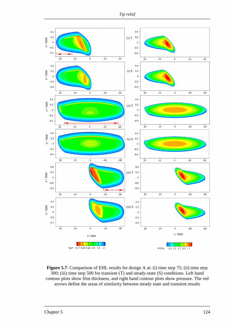
Tip relief
Chapter 5 124
Figure 5.7: Comparison of EHL results for design A at: (i) time step 75; (ii) time step
300; (iii) time step 500 for transient (T) and steady-state (S) conditions. Left hand
contour plots show film thickness, and right hand contour plots show pressure. The red
arrows define the areas of similarity between steady state and transient results
y/ mm y /mm
i T
(i) S
(ii) T
(ii) S
(iii) T
(iii) S
x /
mm
x
/ m
m
x /
mm
x
/ m
m
x /
mm
x
/ m
m

Tip relief
Chapter 5 125
Figure 5.8: Comparison of EHL results for design B at: (i) time step 75; (ii) time step
300; (iii) time step 500 for transient (T) and steady-state (S) conditions. Left hand
contour plots show film thickness, and right hand contour plots show pressure.
(iii) S
i T
(i) S
(ii) T
(ii) S
(iii) T
y / mm y / mm
x /
mm
x
/ m
m
x /
mm
x
/ m
m
x /
mm
x
/ m
m

Tip relief
Chapter 5 126
Figures 5.9, 5.10 and 5.11 show further detailed sectional comparisons between steady
state and transient results for design A at time steps 75, 300 and 500 respectively. The
sections shown are in the entrainment x-direction at a selection of y positions.
Comparison of the sections shows that for parts of the contact area that are not close to
the tip relief zone the results obtained using a steady state analysis are very similar to
those obtained from the transient analysis.
At time step 75 a substantial part of the contact line lies in the tip relief zone which
produces a significant difference in the behaviour of the film thickness in the transient
case. This is clear, for example, from the results at y = 2 and 5 mm in Figure 5.9.
Figure 5.9: Comparison of sections of film thickness and pressure in the 𝑥-direction at
timestep 75 for design A between transient (dashed) and steady state (solid) results.
(a) y = 2, (b) y = 5, and (c) y = 12 mm.
At time step 300 a significant proportion of the contact is outside the tip relief zone and
there is no significant difference between the two results (steady state and transient) as
can be seen from the sections at y = 19, 10, 0 and 16 mm in Figure 5.10. The
transient effect at the tip relief position is apparent at the sections with y =19 and 19.8
mm where the differences between transient and steady state film thickness can be
clearly seen.
p /
GP
a
h /
µm
x / mm x / mm x / mm
p
h

Tip relief
Chapter 5 127
Figure 5.10: Comparison of sections of film thickness and pressure in the 𝑥-direction at
time step 300 for design A between transient (dashed) and steady state (solid) results.
(a) y = -19, (b) y = -10, (c) y = 0, (d) y = 16, (e) y = 19, and (f) y = 19.8 mm.
The contact behaviour at time step 500 is similar to that found at time step 75 where a
substantial part of the contact line lies in the tip relief zone. The transient effect on the
film thickness behaviour is also clear at this time step. This is clear, for example, from
the results at y = 2 and 5 mm in Figure 5.11.
Figure 5.11: Comparison of sections of film thickness and pressure in the 𝑥-direction at
time step 500 for design A between transient (dashed) and steady state (solid) results.
(a) y = -2, (b) y = -5, and (c) y = -10 mm.
p
h
p /
GP
a
h /
µm
p /
GP
a
h /
µm
x / mm
x / mm x / mm
-0.5 -0.3 -0.1 0.1 0.3 -0.5 -0.3 -0.1 0.1 0.3 -0.5 -0.3 -0.1 0.1 0.3
p /
GP
a
x / mm
x / mm x / mm
h /
µm
p
h
p
h

Tip relief
Chapter 5 128
In all of the contacts there is a zone where the transient EHL result is essentially the
same as the steady state result for the geometry and kinematics at that position. This is
also found in the results of design B which are illustrated in Figures 5.12, 5.13 and 5.14
for the three mesh positions. These figures show sections of pressure and film thickness
in the rolling/sliding direction. The figures show the steady state 3D results as solid
lines and the transient results as broken lines. The equivalent 2D line contact result is
shown as a dash-dot curve in Figure 5.13 for the sections where the transient and 3D
steady state results are very similar at time step 300.
The sections shown in Figures 5.12 (a) and 5.12 (b) show considerable differences
between the transient and steady state analyses in the vicinity of the tip relief profile
modification. The pressure sections are almost identical but the film thickness shows
that the squeeze film terms in the Reynolds equation are active causing significant
differences in the lubricant films. For Figure 5.12 (c), which is typical of the rest of the
contact line, the transient and steady state results are very similar showing that the
squeeze film term is not influential away from the tip relief position.
Figure 5.12: Comparison of sections of film thickness and pressure in the 𝑥-direction at
time step 75 for design B between transient (dashed) and steady state (solid) results.
(a) y = 2, (b) y = 5, and (c) y = 12 mm.
p /
GP
a
x / mm x / mm x / mm
(a) (b) (c) h
/ μ
m
p
h

Tip relief
Chapter 5 129
Figure 5.13 shows sectional comparisons of film thickness and pressure in the x
direction for design B at time step 300. These sections present results for steady state
and transient point contact analyses, together with the equivalent steady state line
contact analysis. In order to carry out the equivalent steady state line contact analysis at
a specified y position along the line of contact, the radius of relative curvature in x
direction and the surface velocities were calculated at this y position, and the required
load was determined by integrating the steady state point contact pressure in the x-
direction at this y position. It is clear that despite the geometry and kinematic
differences between the gears in design B, the steady state point contact and the
equivalent steady state line contact analyses give good agreement with the transient
point contact results at this time step over much of the contact area. This
correspondence can be seen for the sections at y = 18, 10, 0 and 10 mm with
differences due to transient effects starting to appear at y = 17 mm. The comparison at y
= 18 mm (tip relief zone) is only made between steady state and transient point contact
results, as the undeformed geometry is changing rapidly in the y direction at this
position, and therefore cannot be represented by a one dimensional line contact
approximation.
The contact at this time step (300) acts over the whole face width, which produces a
relatively long contact ellipse with a small zone of tip relief at the left of the contact as
shown in Figure 5.8 (ii). The transient tip relief effect is more noticeable at the other
positions in the meshing cycle where tip relief is actively curtailing the effective length
of the contact line, whereas at time step 300, which is near the middle of the meshing
cycle, the tip relief becomes a modifying factor on the effect of the axial crown rather
than the cause of the contact line termination. The general behaviour of film thickness
(and the pressure) at this time step is similar to that in design A.

Tip relief
Chapter 5 130
Figure 5.13: Comparison of sections of film thickness and pressure in the 𝑥-direction at
time step 300 for design B between transient point contact (dashed), steady state point
contact results (solid). (a) y = 18, (b) y = 10, (c) y = 0, (d) y = 10, (e) y = 17, and (f) y
= 18 mm. The equivalent steady state line contact results are included in figures (a) to
(e) and are indistinguishable from the steady state point contact except for minor
differences in case (e).
Figure 5.14 shows results that are similar to those for Figure 5.8 in that steady state
behaviour is apparent in Figure 5.14 (c), which is representative of most of the contact
line, with significant transient effects in Figures 5.14 (a) and 5.14 (b) which are in the
vicinity of the tip relief profile modification. Again, the pressure sections are almost
identical, with significant film thickness differences due to squeeze effects.
Figure 5.14: Comparison of sections of film thickness and pressure in the 𝑥-direction at
time step 500 for design B between transient (dashed) and steady state (solid) results.
(a) y = -2, (b) y = -5, and (c) y = -10 mm.
p
/ G
Pa
h
/ µ
m
(a) (b) (c)
x / mm x / mm x / mm
p
h
p /
GP
a
h
/ µ
m
h /
µm
p
/ G
Pa
(a) (b) (c)
(d) (e) (f)
x / mm x / mm x / mm
p
h
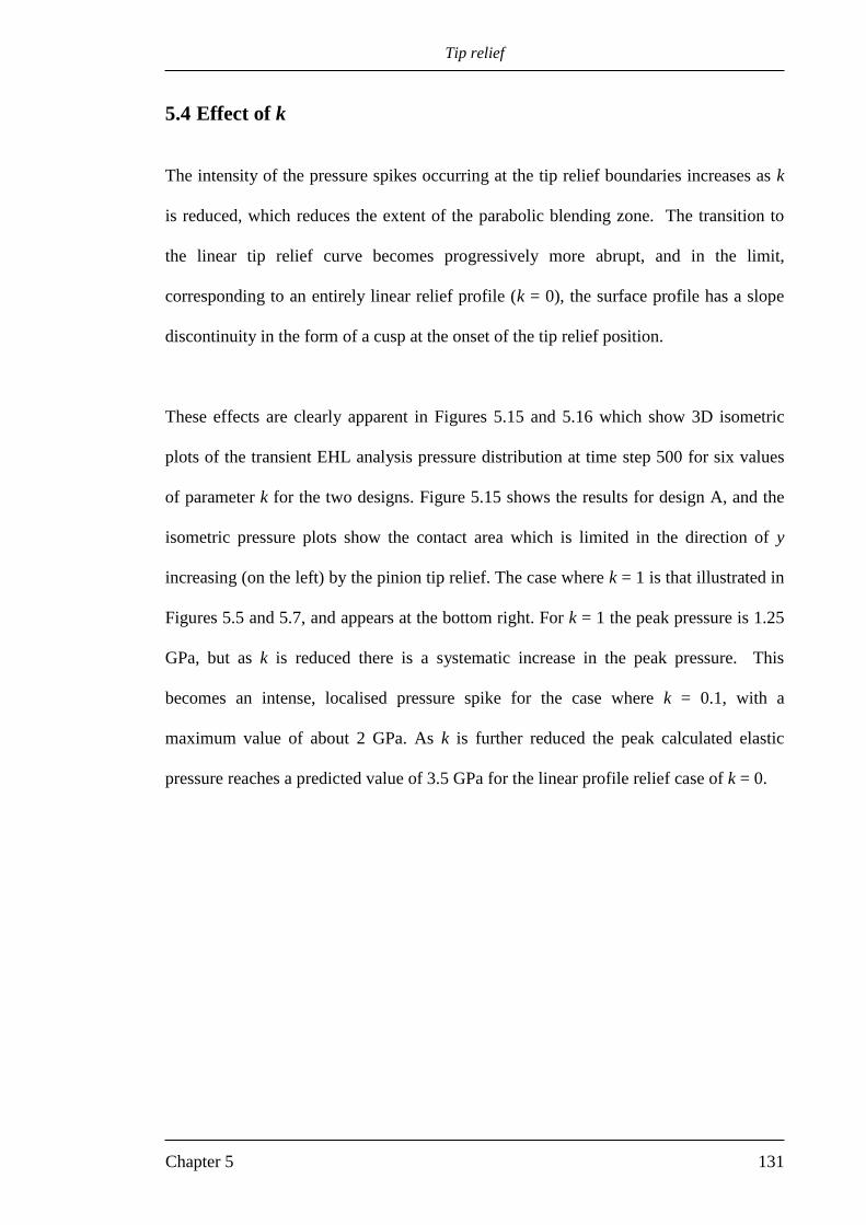
Tip relief
Chapter 5 131
5.4 Effect of k
The intensity of the pressure spikes occurring at the tip relief boundaries increases as k
is reduced, which reduces the extent of the parabolic blending zone. The transition to
the linear tip relief curve becomes progressively more abrupt, and in the limit,
corresponding to an entirely linear relief profile (k = 0), the surface profile has a slope
discontinuity in the form of a cusp at the onset of the tip relief position.
These effects are clearly apparent in Figures 5.15 and 5.16 which show 3D isometric
plots of the transient EHL analysis pressure distribution at time step 500 for six values
of parameter k for the two designs. Figure 5.15 shows the results for design A, and the
isometric pressure plots show the contact area which is limited in the direction of y
increasing (on the left) by the pinion tip relief. The case where k = 1 is that illustrated in
Figures 5.5 and 5.7, and appears at the bottom right. For k = 1 the peak pressure is 1.25
GPa, but as k is reduced there is a systematic increase in the peak pressure. This
becomes an intense, localised pressure spike for the case where k = 0.1, with a
maximum value of about 2 GPa. As k is further reduced the peak calculated elastic
pressure reaches a predicted value of 3.5 GPa for the linear profile relief case of k = 0.

Tip relief
Chapter 5 132
Figure 5.15: Contact pressure surfaces corresponding to six different patterns of
the tip relief profile for design A.
Figure 5.16 shows the corresponding results for the case of design B, and it is clear that
the pressure distributions and spikes for the two designs follow a very similar pattern.
k = 0 k = 0.03 k = 0.05
k = 0.1 k = 0.5 k = 1

Tip relief
Chapter 5 133
Figure 5.16: Contact pressure surfaces corresponding to six different patterns of
the tip relief profile for design B.
The apparent oscillatory form of the pressure spike for the case k = 0 in both Figures
5.15 and 5.16 is caused by variation in the discretised second derivative of the surface
geometry at the transition position between the crowned involute surface and the tip
relief zone on the computing mesh.
Figure 5.17 shows the projection of lines of equal tip relief on to the tangent plane. The
start of tip relief is the heavy line on the right of the plot which makes an angle of 8.5
to the y axis. The other lines have small systematic differences in their orientation.
k = 0 k = 0.03 k = 0.05
k = 0.1 k = 0.5 k = 1
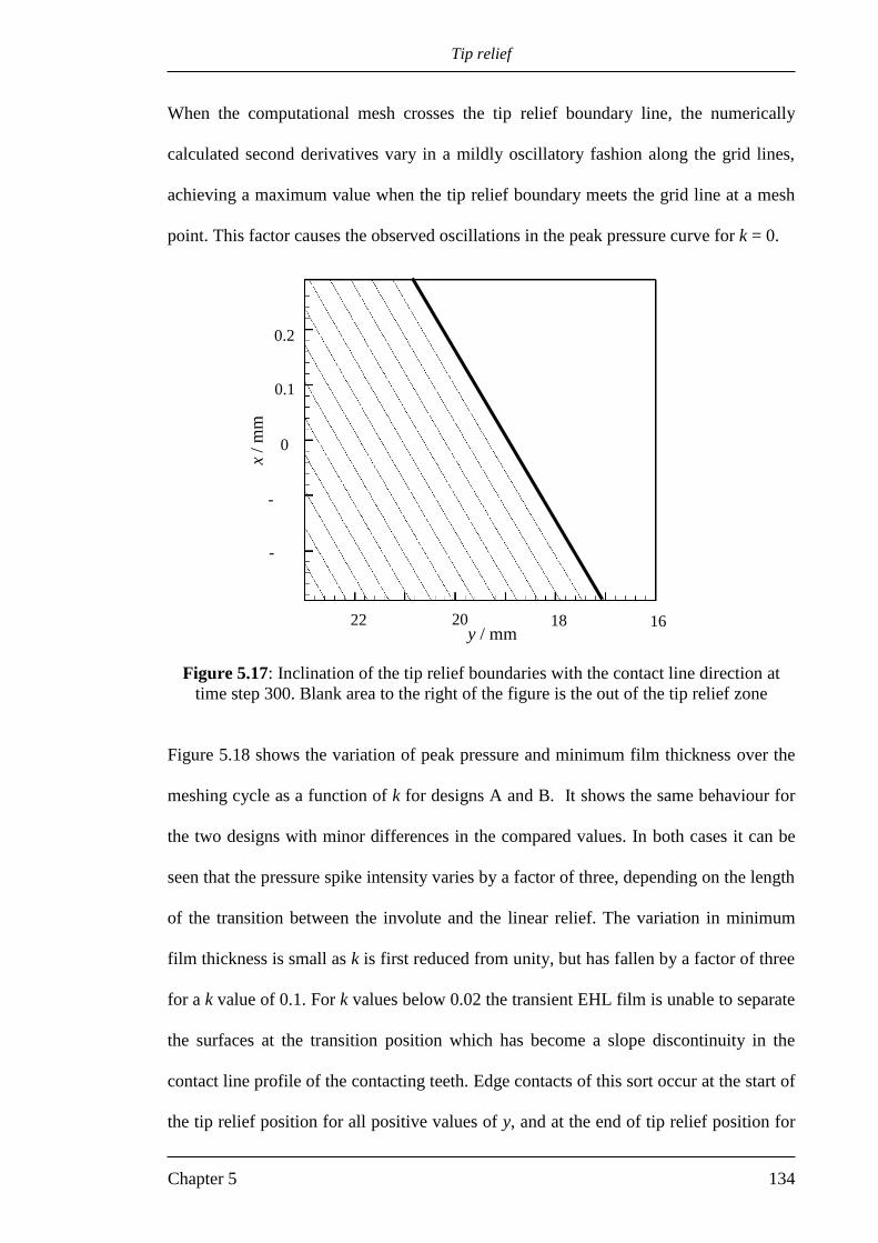
Tip relief
Chapter 5 134
When the computational mesh crosses the tip relief boundary line, the numerically
calculated second derivatives vary in a mildly oscillatory fashion along the grid lines,
achieving a maximum value when the tip relief boundary meets the grid line at a mesh
point. This factor causes the observed oscillations in the peak pressure curve for k = 0.
Figure 5.17: Inclination of the tip relief boundaries with the contact line direction at
time step 300. Blank area to the right of the figure is the out of the tip relief zone
Figure 5.18 shows the variation of peak pressure and minimum film thickness over the
meshing cycle as a function of k for designs A and B. It shows the same behaviour for
the two designs with minor differences in the compared values. In both cases it can be
seen that the pressure spike intensity varies by a factor of three, depending on the length
of the transition between the involute and the linear relief. The variation in minimum
film thickness is small as k is first reduced from unity, but has fallen by a factor of three
for a k value of 0.1. For k values below 0.02 the transient EHL film is unable to separate
the surfaces at the transition position which has become a slope discontinuity in the
contact line profile of the contacting teeth. Edge contacts of this sort occur at the start of
the tip relief position for all positive values of y, and at the end of tip relief position for
0.2
0.1
0
-
0.1
-
0.2
x /
mm
20 22 18 16 y / mm

Tip relief
Chapter 5 135
negative values of y. So it is clear that the values quoted for the gear (ratio of
smooth surface film thickness to composite surface roughness) will not represent the
real intensity of surface roughness effects at these locations. It is clear from a detailed
consideration of these results that the case of a linear tip relief (k = 0), which introduces
a definite discontinuity in the slope of the tooth profile in the form of a cusp, causes
severe conditions at the edge of the contact resulting in extreme pressures and a failure
of the lubricant film to separate the surfaces. The high level of similarity shown
between the results for designs A and B in Figures 5.15, 5.16 and 5.18 suggests strongly
that this behaviour is a consequence of the tooth relief profile and that the stress
concentration inherent in the abrupt profile modification is not mitigated by the
presence of an EHL lubricant film.
Figure 5.18. Variation of minimum lubricant film thickness and maximum
contact pressure with the tip relief parameter k for designs A and B,
hmin A, hmin B, pmax A and pmax B.
0.00
0.04
0.08
0.12
0.16
0.20
0
1
2
3
4
0 0.2 0.4 0.6 0.8 1
h m
in /
μm
p m
ax /
GP
a
k

Tip relief
Chapter 5 136
5.5 Effect of surface velocity
Figure 5.19 shows the effect of speed on the transient maximum pressure and minimum
film thickness over the meshing cycle for the case of design A with k = 1. Four different
entrainment speeds were used, u , u2 , u5 and u10 , where �̅� corresponds to the pinion
speed of 235.6 rad/s used for the results considered previously. The figure shows that
operating at higher speed increases minimum film thickness levels almost exactly as
, which coincides with the relation given in (Hamrock and Dowson 1977)
68.0073.049.068.0
min e1WGU63.3H
Scaling the film thickness curves by this factor makes them coincide almost exactly as
shown in Figure 5.20. However, the maximum pressure predicted is almost insensitive
to speed which again supports the view that the pressure spike associated with the tip
relief boundary is driven by elastic contact mechanics rather than elastohydrodynamic
considerations.
68.0u

Tip relief
Chapter 5 137
Figure 5.19: Variation of maximum pressure (solid) and minimum film thickness
(dashed) throughout the meshing cycle for four entrainment velocities. Minimum film
thickness curves shown in ascending order from u (lowest), u2 , u5 and u10 (highest),
respectively. Maximum pressure almost insensitive to the velocity variation.
Figure 5.20: Scaling of minimum film thickness for four entrainment
speeds ( u , u2 , u5 and u10 ) to a factor of 0.68
0.0
0.2
0.4
0.6
0.8
1.0
1.2
0.0
0.2
0.4
0.6
0.8
1.0
1.2
1.4
0 100 200 300 400 500 600
hm
in /
µm
pm
ax
/ G
Pa
timestep
0.10
0.15
0.20
0.25
0.30
0 100 200 300 400 500 600
hm
in /
µm
Time step

Tip relief
Chapter 5 138
5.6 Results for optimised power law
In this section further investigation on the form of tip relief is reported. The form of tip
relief considered in section 5.1 which describes linear, parabolic and a combination of
linear and parabolic forms is now modified to a more general power law form as
follows.
starttipstarttt rr/rrcz (5.6)
where r , startr , tipr and tc are as defined in section 5.1. The value of parameter is
varied between 1 and 4, where =1 corresponds to the linear profile, and all values of
greater than 1 have zero slope at startrr so the profile modification is tangential to the
involute at the start of tip relief .
Figure 5.21 illustrates the zero load gap between the tooth surfaces along the contact
line at three meshing cycle positions for design A and B when β = 3. The upper and
lower parts show the gap for design A and B respectively. Mesh positions 1, 2 and 3 are
at time steps 75, 300 and 500, respectively. The zero load gaps are offset by 2 or 4 m
for clarity.

Tip relief
Chapter 5 139
Figure 5.21 Gap between gear surfaces (offset) along contact line at positions
1, 2 and 3 in the meshing cycle for power law modification, β =3 . Axial crown is
shown broken and symbol indicates starts of tip relief for each contact line.
(a) Design A; (b): Design B
0
4
8
12
16
20
-25-15-551525
Hei
ght
/ µ
m
y / mm
0
4
8
12
16
20
-25-15-551525
Hei
gh
t /
µm
y / mm
(a)
(b)
1
2
3
1
2
3

Tip relief
Chapter 5 140
Figure 5.22 shows the variation of maximum pressure and minimum film thickness over
the meshing cycle for designs A and B for values of = 2, 3 and 4. The results for
design A shown in Figure 5.22 (a) show that the maximum pressures are reduced by a
factor of three or more when compared to the result for = 1 shown in Figure 5.6. The
value of can be seen to have a significant effect on the peak pressures and also on the
minimum film thickness experienced in the contact. The pressures are further reduced
for the higher values, but these are minor further changes. Similar behaviour is also
found in the corresponding results of design B as shown in Figure 5.22 (b).

Tip relief
Chapter 5 141
Figure 5.22: Maximum pressure (upper curves) and minimum film thickness (lower
curves) over the meshing cycle, β =2, β =3 and β =4. The corresponding
results for the linear case (β=1) is shown in Figure 5.6.
(a) design A, (b) design B
0.00
0.10
0.20
0.30
0
400
800
1200
0 100 200 300 400 500
(a)
0.00
0.15
0.30
0.45
0
400
800
1200
0 100 200 300 400 500
(b)
pm
ax /
MP
a p
max
/ M
Pa
hm
in /
µm
h
min
/ µ
m
Time step
Time step

Tip relief
Chapter 5 142
Figure 5.23 shows film thickness and pressure contours at time step 75 for the range of
powers specified for the analyses. These results are for design B. For the linear profile
= 1 the maximum pressure contour is 3.2 GPa and the minimum film thickness
contour is zero, indicating that the lubricant film is unable to separate the surfaces. This
extreme behaviour is not seen with the cases where = 2, 3 and 4 where the minimum
film thickness contours are around 0.185 m, and the maximum pressure contour values
are 1.1, 1.0 and 0.96 GPa, respectively. This figure illustrates how the linear
modification reduces the length of the contact area in the y direction in comparison with
the other cases when = 2, 3 and 4. The linear case ( = 1) produces a pressure of 0.1
GPa at 0y while the 0.1 GPa contour can be seen at 5y mm for the = 4 case.

Tip relief
Chapter 5 143
Figure 5.23: Film thickness contours / m (left) and pressure
contours / GPa (right) at time step 75 for the four values of .
β = 4
β = 3
β = 2
β = 1

Tip relief
Chapter 5 144
Further investigations on the effect of on the contact behaviour were also performed.
Figure 5.24 shows the contact line pressures for each time step assembled into a contour
plot for each of the tip relief profile forms considered for designs A and B. In both
designs for the = 1 case intense closed contours for 3, 2 and 1 GPa appear at the top
and bottom of the pressure map. The y axis is aligned with the contact line and the peak
pressure contour indicates that the highest pressures occur at the start of tip relief
positions, on the wheel at the bottom left of the contour plot, and on the pinion at the
top right. For the higher values of these contours become much less intense and the
peak contact line pressure levels approach those occurring at the peak load, full face
width contact lines.
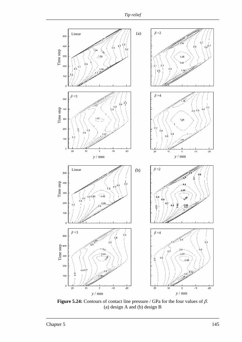
Tip relief
Chapter 5 145
Figure 5.24: Contours of contact line pressure / GPa for the four values of .
(a) design A and (b) design B
Tim
e st
ep
Tim
e st
ep
Tim
e st
ep
Tim
e st
ep
y / mm y / mm
y / mm y / mm
Linear β =2
β =3 β =4
Linear β =2
β =3 β =4
(a)
(b)

Tip relief
Chapter 5 146
5.7 Discussion
Linear tip relief is the common form of modification due to manufacturing
considerations. This form has been shown in this chapter to have very large stress
concentrations due to the significant slope discontinuity at the start of modification. The
suggested form of modification which consists of a parabolic blending curve in order to
maintain slope continuity at the start of modification showed significant improvement in
the EHL results. The lengths of the parabolic curve which correspond to k > 0.3 remove
the stress concentrations in the cases considered. Smaller values of k also improve the
result to some extent and the case of k = 0.1 for example reduces the maximum pressure
from 3.5 GPa to 2 GPa approximately (see Figure 5.18). Comparison between the
results of different power law modifications illustrates that the parabolic curve is the
ideal form and the other higher power law modifications do not lead to significant
improvement in the results. This results demonstrates that the continuous change of
slope is the important requirement.
In this study the effects of bending of the teeth under load are ignored, and it is assumed
that the share of the total tooth load carried by individual simultaneous contacts is
proportional to their length at any instant. However, it is clear that the effect of tooth
bending will lead to a different distribution of the load on the contacts. Furthermore,
the bending effect will cause contact lines to extend into the tip relief zone under heavy
loading conditions. These effects can potentially be included in the EHL analysis based
on the results of full 3D finite element analysis of helical gears in contact as discussed
in section 4.1, and this will be pursued in future work.

Transient EHL Analysis of Helical Gears Having Faceted Tooth Surfaces
Chapter 6 147
Chapter 6
Transient EHL Analysis of Helical Gears Having Faceted
Tooth Surfaces
6.0 Introduction
When the final finish of helical gears is achieved using the generation grinding process
the cutter passes axially over the tooth flank in a series of offset passes. This can result
in axial faceting where the tooth profile consists of a number of facets rather than being
a perfectly smooth curve. The number of facets will corresponds to the number of
passes used which will be part of the grinding specification. For the module considered
in this work between 20 and 40 facets are likely to be created. This chapter begins with
a derivation of closed form equations for the resulting gap between the faceted profiles
during the engagement between gear teeth and then investigates the effect of these axial
facets, as well as their numbers, on the transient EHL results for helical gears. Detailed
comparisons are also made with corresponding smooth surface results given in chapter 5
6.1 Undeformed geometry
The length of the active tooth profile in contact during a complete meshing cycle is
equal to the distance minmax ss along the line of action as explained in section 2.1. This
distance is divided into a number of complete facets, fn . Therefore, the arc length of
each facet is:
f
minmax
n
ssarc
(6.1)
The gap between the two teeth in contact needs to be determined as a part of the EHL

Transient EHL Analysis of Helical Gears Having Faceted Tooth Surfaces
Chapter 6 148
analysis of contacting surfaces. The procedure adopted in Chapter 2 (section 2.3) to
calculate the gap between two helical teeth in contact having involute profiles will be
modified in this chapter to calculate the undeformed geometry of faceted surfaces.
Figure 2-10 (c) (Chapter 2) shows how the gaps between gear teeth in the normal and
transverse directions are related to each other. The same way of determining 1z (and 1z )
as described in section 2.3 is used here to determine in which transverse section the
required normal gap is. Depending on this transverse section, the gap for the facetted
surface can be determined as will be shown later. The gap in the normal direction of the
faceted profile can then be easily determined by taking the effect of the helix into
account.
To illustrate this, Figure 6.1 shows a parabolic approximation of a transverse section of
an involute tooth profile together with the proposed faceted profile as an alternative to
the smooth surface. The x axis is the tangent to the profile at the contact point C (
0C x ) between the two mating teeth at a position ysC in the meshing cycle. Point P
represents a point on the tooth profile where 0x and point PF is the corresponding
point on the faceted profile at the same x position ( Px ) of point P. Points B1 and B2 are
the boundaries of the facet that contains point P.
Figure 6.1: Section in the x direction illustrates the gap between the tangent plane and
the facet profile. Only one facet step is shown in this figure.
x
P
C B2
B1
PF
xP

Transient EHL Analysis of Helical Gears Having Faceted Tooth Surfaces
Chapter 6 149
The total gap at point PF between the faceted profile and the x axis in the transverse
direction is the distance Fz which varies according to the x position of point P. This gap
is given by
dPF zzz (6.2)
where Pz is the distance between the parabolic curve and the x axis, and dz is the
deviation from the parabolic curve (both in the transverse direction).
The solution space for the EHL analysis is the tangent plane xy (see Chapter 2, Figure
2.9). The distance Pz (and its value in the normal direction) can be calculated at each
point in this solution space as explained in Chapter 2 (section 2.3). In the case of a
facetted profile the total gap at a given Px in this xy plane which includes the distances
Pz and dz can be determined using the method explained below.
The radial distances in the transverse direction between any point on the involute profile
(such as point P) and the gear axes can be determined using equations 2.16 and 2.17 in
chapter 2. These two equations were derived by considering Figure 2.13. The figure
and these equations are repeated here for clarity.
2
11
2
11 )()(),( zRxryxr b
(6.3-a)
2
22
2
22 )()(),( zRxryxr b
(6.3-b)
where 1 and 2 represent pinion and wheel respectively and 1R and 2R are the radii of
curvature of the surfaces at point C in the transverse direction which are given by
)(tan C11 ysrR b
)(tan C22 ysrR b

Transient EHL Analysis of Helical Gears Having Faceted Tooth Surfaces
Chapter 6 150
Figure 2.13: Undeformed geometry due to tip relief of the pinion,
repeated here for clarity and convenience
The gaps in the transverse direction are
1
2
1R2
xz
(6.4-a)
2
2
2R2
xz
(6.4-b)
Point of contact
Line of action
𝑟𝑏1
𝑧1𝑝′
𝑥+
𝜓
𝑟
𝑠
𝑥𝑝
J
P
T
O

Transient EHL Analysis of Helical Gears Having Faceted Tooth Surfaces
Chapter 6 151
In order to find the total gap at point P, it is required to identify the following
1- Its position on the tooth profile.
2- At what facet it lies.
3- The s values at the boundaries (B1 and B2 in Figure 6.1) of this facet.
The position of point P on the tooth profile can be determined in terms of s. For a given
x position, equation (6.3-a) gives the distance 1r . If the tooth in Figure 2.13 rotates
clockwise until point P lies on the line of action as shown in Figure 6.2, Ps can be
determined by considering the two triangles OET and OEP as
Figure 6.2: Determination of s position of point P
E
Line of action
𝑟𝑏1
𝜓
T
O
P
Transient EHL Analysis of Helical Gears Having Faceted Tooth Surfaces
Chapter 6 152
tan1
2
1
2
1P bb rrrs (6.5)
As the profile is divided into a number of facet steps as given by equation (6.1), the step
position of point P can be obtained from
)int( minPP
arc
ssk
(6.6)
where function int is the integer part of the argument.
Therefore, the s values of the boundaries of the facet defined by equation (6.6) can be
calculated from
arckss Pmin1B (6.7-a)
arcss 1B2B (6.7-b)
Using equation (6.7-a), the radius at B1, 1Br , with respect to the gear axis can also be
determined by rotating the tooth shown in Figure 2.13 until B1 lies on the line of action
which is given by:
2
1B1
2
11B )tan( srrr bb (6.8)
Similarly for the second boundary B2 with use of equation (6.6-b) gives
2
2B1
2
12B )tan( srrr bb
(6.9)
Equation (6.3-a) can be used to evaluate the x position of B1 and B2. Substituting
equations (6.4-a) in (6.3-a) gives

Transient EHL Analysis of Helical Gears Having Faceted Tooth Surfaces
Chapter 6 153
2
1
2
1B1
2
1B11B )2
()(R
xRxrr b
(6.10)
Equation (6.10) can be written, after some simplification, in the following form
00B11
4
1B4 axaxa (6.11)
where,
2
1
44
1
Ra
, 1b1 r2a ,
2
1
2
1
2
10 Bb rrRa and the radial distance 1Br is given by
equation (6.8).
A similar equation can be derived for point B2 using the previous procedure for point B1
which is
00B21
4
2B4 axaxa (6.12)
And the constants are defined by
2
1
44
1
Ra
, 1b1 r2a and
2
2B
2
1
2
10 rrRa b
Equations (6.11) and (6.12) are fourth order equations and solution of each equation
gives one physically realistic real root. These equations can be solved by making the
expression ixB as
1
4
B40B / axaax ii i 1 or 2.
and using this recursively to converge to the root of interest.
The gap at the boundaries B1 and B2 can be calculated using the solution of equations
(6.11) and (6.12) as

Transient EHL Analysis of Helical Gears Having Faceted Tooth Surfaces
Chapter 6 154
1
2
1B1B
R2
xz
1
2
2B2B
R2
xz
Figure 6.3 illustrates these distances at the parabolic approximation of the involute
profile. Using a linear interpolation between the heights at points PF, B1, and B2 the total
gap that includes the facet effect at Px can be determined by:
1B2B
1BP1B2B1BF )(
xx
xxzzzz
This equation gives the gap in the transverse direction. Therefore the gap in the normal
direction, Fz can be calculated by taking the effect of the helix angle into account as
bBzz cosFF
Figure 6.3: Relation between the gap at the point of interest, P, and the gaps at the facet
boundaries
P
C
B2
B1
x
PF

Transient EHL Analysis of Helical Gears Having Faceted Tooth Surfaces
Chapter 6 155
A similar procedure can be used to determine the gap between the tooth profile of the
wheel and the tangent plane which gives the same form of equations (6.11) and (6.12)
but with the following constants for the gap at B1
2
2
44
1
Ra
, 21 2 bra and
2
1B
2
2
2
20 wb rrRa
and the following for the gap at B2
2
2
44
1
Ra
, 21 2 bra and
2
2B
2
2
2
20 wb rrRa
where 1Bwr and 2Bwr are the radial distances from the centre of the wheel to point B1 and
B2 respectively.
This procedure is repeated for all points in the solution space (xy plane) and as a result
the 3D gap between the contacting teeth (with faceted profiles) at any position in the
meshing cycle is available for the transient EHL analysis. Examples of this 3D gap near
the middle of the meshing cycle between the pinion teeth and the tangent plane when
fn 20, 40 and 100fn are shown in Figure 6.4.

Transient EHL Analysis of Helical Gears Having Faceted Tooth Surfaces
Chapter 6 156
Figure 6.4 (continue)
(b)
20fn
60fn
(a)

Transient EHL Analysis of Helical Gears Having Faceted Tooth Surfaces
Chapter 6 157
Figure 6.4: ): Gap between pinion teeth and the tangent plane,
(a) 20fn , (b) 60fn and (c) 100fn
6.1.1 Smooth surface and the corresponding faceted profiles.
Figure 6.5 compares the faceted profile with the perfect smooth profile where
corresponding gaps for their profiles with respect to the tangent plane are shown. The
results shown in this figure are at a position in the meshing cycle where the contact
between the teeth acts over the whole face width. This position corresponds to time step
300 as defined by position 2 in Figure 4.6 (chapter 4). Three cases of fn = 40, 60 and
100 are shown in this figure where the section at the centre of the contact ( 0y ) is
shown for the profile of the pinion tooth in each figure. Figure 6.5 (a) shows the case
when fn = 40, and it is clear that in this case the faceted profile deviates considerably
100fn
(c)

Transient EHL Analysis of Helical Gears Having Faceted Tooth Surfaces
Chapter 6 158
from the smooth profile. The effective profile in the EHL analysis that lies within the
area of contact is in the range of axa as shown in this figure by the distance 2a.
There are severe changes of slope within these limits of the faceted profile which can be
expected to act as stress raisers, and may have the effect of thinning the lubricant film.
The divergence from the smooth profiles is reduced as the number of steps is increased.
This behaviour is clear in Figures 6.5 (b) and (c) where fn = 60 and 100 cases are
presented respectively. At the scale of drawing, the faceted profile in Figure 6.5 (c)
seems very close to the corresponding smooth one. However, the faceted profile still
diverges to some extent from the corresponding smooth profile.

Transient EHL Analysis of Helical Gears Having Faceted Tooth Surfaces
Chapter 6 159
Figure 6.5: Gap in the x direction between the tangent plane and the tooth profile at y =
0 when (a) 40fn , (b) 60fn and (c) 100fn ; smooth (dashed) and faceted
profiles (solid)
0
2
4
6
8
10
-1 -0.5 0 0.5 1
gap
/ m
m
x / mm
(a)
0
2
4
6
8
10
-1 -0.5 0 0.5 1
gap
/ m
m
x / mm
(b)
0
2
4
6
8
10
-1 -0.5 0 0.5 1
gap
/ m
m
x / mm
(c)
2a

Transient EHL Analysis of Helical Gears Having Faceted Tooth Surfaces
Chapter 6 160
6.2 EHL results
Results are shown for two faceted profiles (pinion and wheel profiles) with the same fn
which are compared with those for perfect smooth profiles. This investigation was
undertaken to find the minimum required fn number that will produce film thickness
and pressure distributions that are close to the corresponding results for smooth
surfaces. In general six cases are examined where the tooth profiles are generated using
fn = 20, 30, 40, 60, 80 and 100.
Similar procedures for the EHL analyses of the helical gear meshing cycle that was
discussed in chapters 4 and 5 were adopted in obtaining the results presented in this
chapter. The only difference is related to the undeformed geometry. The transient gap
between the smooth surfaces of the contacting teeth is replaced by the gap between the
faceted profiles as calculated in section 6.1.
6.2.1 Effect of mesh density
In this section the effect of mesh resolution on the EHL results of helical gears having
faceted tooth surfaces is investigated. Two cases are examined where the tooth profile
has 20fn and 100fn . Each case is analysed using three different mesh densities
which are (a/20, b/200), (a/40, b/400) and (a/80, b/800). These resolutions give a
corresponding total number of nodes in the solution space of (92*427), (182*857) and
(362*1717), respectively. The results of this investigation are shown in Figure 6.6
where Figures 6.6 (a) and 6.6 (b) correspond to cases 20fn and 100fn ,
respectively. In all cases changing the mesh density (twice doubling in both directions)
does not significantly affect the general behaviour of the results (particularly the
pressure distribution). The case 100fn shows very little effect of mesh density.

Transient EHL Analysis of Helical Gears Having Faceted Tooth Surfaces
Chapter 6 161
Figure 6.6: Effect of mesh density on the EHL results at the centre of contact (y = 0) at
time step 300; ……. (92*427), (182*857) and (362*1717).
(a) 20fn and (b) 100fn
0
0.2
0.4
0.6
0.8
1
0.0
0.5
1.0
1.5
2.0
2.5
3.0
-0.6 -0.4 -0.2 0 0.2 0.4 0.6
h /
μm
p /
GP
a
x / mm
(a)
0
0.2
0.4
0.6
0.8
1
0.0
0.5
1.0
1.5
-0.6 -0.4 -0.2 0 0.2 0.4 0.6
h /
μm
p /
GP
a
x / mm
(b)

Transient EHL Analysis of Helical Gears Having Faceted Tooth Surfaces
Chapter 6 162
6.2.2 EHL solution for the gear meshing cycle
Figure 6.7 compares the transient EHL results for the gear meshing cycle for the smooth
and faceted profiles. The results for the faceted profiles (pinion and wheel profiles) are
for fn = 20, 30, 40, 60, 80 and 100. Figure 6.7 (a) shows the variation of maximum
pressure throughout the meshing cycle and Figure 6.7 (b) shows the corresponding
minimum film thickness. The maximum pressure in the smooth surfaces case varies
between 1.02 and 1.25 GPa. Meanwhile, the film thickness varies between 0.16 and
0.22 μm. In the corresponding faceted profiles, the case of fn = 20 produces the highest
range of maximum pressure during the meshing cycle. In this case the maximum
pressure varies between 2.44 and 3.16 GPa. These results are expected as the faceted
profile has sharp discontinuities in the profile slope with fn = 20. Also in this case metal
to metal contact is predicted in significant parts of the meshing cycle. The maximum
pressure in the case of fn = 30 decreases to a value of 2.27 GPa. Although this
represents a reduction of about 28% with respect to the case of fn = 20, the level of the
minimum film thickness is relatively low, and a breakdown of the film thickness occurs
at some positions in the meshing cycle. In the case of fn = 40 the maximum pressure
varies between 1.6 and 1.9 GPa and the EHL mechanism succeeds in totally separating
the two surfaces during the whole meshing cycle. The range of minimum film thickness
variation is between 0.11 and 0.16 μm. Both these ranges of variation for the case of fn
= 40 represent a good improvement in the EHL response to the faceted profiles. The
improvement is continued as the value of fn is increased as shown for the cases
fn =
60, 80 and 100. In the last case (fn =100) the maximum pressure varies between 1.18
and 1.42 GPa. The upper limit differs from the smooth surfaces results by only 13.6% .

Transient EHL Analysis of Helical Gears Having Faceted Tooth Surfaces
Chapter 6 163
The corresponding film thickness varies between 0.14 and 0.2 μm where the lower limit
is 12.5% less than the corresponding smooth surface results.
Figure 6.7: Variation of (a) maximum contact pressure and (b) minimum oil film
thickness during the meshing cycle; green: smooth profile, orange: 100fn , purple:
80fn , blue: 60fn , black: 40fn , aqua: 30fn and red: 20fn
0
500
1000
1500
2000
2500
3000
3500
0 100 200 300 400 500 600
p /
MP
a
Time step
(a)
0.00
0.05
0.10
0.15
0.20
0 100 200 300 400 500 600
h /
µm
Time step
(b)

Transient EHL Analysis of Helical Gears Having Faceted Tooth Surfaces
Chapter 6 164
Detailed results for the contact between faceted surfaces (both pinion and wheel have
faceted profile) are presented in Figures 6.8 to 6.18. Three positions in the meshing
cycle are selected which are at time steps 75, 300 and 500. As explained in the previous
chapters these positions are examples where the contact is mainly within the pinion
dedendum at time step 75, over the whole face width at time step 300 and within the
addendum of the pinion at time step 500. In these figures the faceted profiles are
generated using fn = 20, 40, 60, 80 and 100. The y-axis represents the contact line
direction and the x-axis is the rolling/sliding direction.
Figure 6.8 shows the pressure distribution for the six cases at time step 75. It can be
seen in this figure how the pressure distribution tends towards the smooth surface
results as fn is increased from 20 to 100. Figure 6.9 shows the film thickness contours
corresponding to the cases shown in Figure 6.8. The effect of the facets is very clear in
these figures particularly at the lower fn number where a sequence of parallel, low film
thickness areas is apparent. The case of fn = 20 is the most extreme case in terms of
both pressure distribution and film thickness, which reflects the nature of the profile
which contains severe changes of slope
Comparisons of pressure and film thickness sections in the entrainment direction are
shown in Figure 6.10 at position y =12 mm. The case of fn = 20 is clearly significantly
different to the smooth surface result, and the differences decline with increasing facet
number. Case fn = 100 is the closest to the smooth surface result, nevertheless the
pressure is clearly disturbed by the faceting. For this test case 40 or more facets results
in small perturbations rather than significant ones.

Transient EHL Analysis of Helical Gears Having Faceted Tooth Surfaces
Chapter 6 165
Figure 6.8: Contact pressure surfaces corresponding to six different patterns of
tooth profile at time step 75
𝑛𝑓 = 20 𝑛𝑓 = 40
𝑛𝑓 = 60 𝑛𝑓 = 80
𝑛𝑓 = 100 smooth
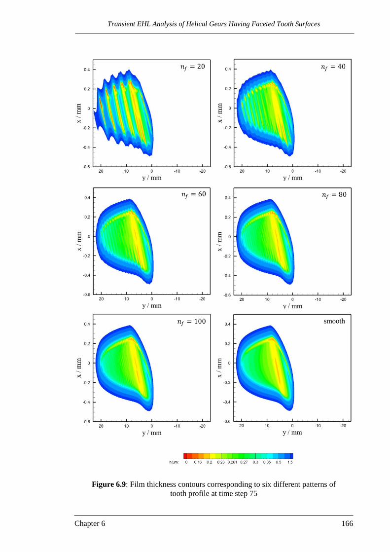
Transient EHL Analysis of Helical Gears Having Faceted Tooth Surfaces
Chapter 6 166
Figure 6.9: Film thickness contours corresponding to six different patterns of
tooth profile at time step 75
𝑛𝑓 = 20 𝑛𝑓 = 40
𝑛𝑓 = 60 𝑛𝑓 = 80
𝑛𝑓 = 100 smooth

Transient EHL Analysis of Helical Gears Having Faceted Tooth Surfaces
Chapter 6 167
Figure 6.10: Sections at time step 75 of (a) pressure and (b) film thickness at position
y = 12 mm; smooth profiles, fn = 100,
fn = 80,
fn = 60, …….fn = 40 and
fn = 20
0.0
0.4
0.8
1.2
1.6
2.0
-0.5 -0.25 0 0.25 0.5
p /
GP
a
x / mm
(a)
0.1
0.2
0.3
0.4
0.5
-0.5 -0.25 0 0.25 0.5
h /
µm
x / mm
(b)

Transient EHL Analysis of Helical Gears Having Faceted Tooth Surfaces
Chapter 6 168
Detailed results at time step 300 are given in Figures 6.11 to 6.15. Figure 6.11 illustrates
the effects of increasing the number of facets on the 3D pressure distributions. As fn is
increased from 20 to 100 the pressure distribution becomes close to typical results of an
elliptical contact which is the case for the smooth surface results. The cases of fn = 80
and 100 are essentially very similar. The corresponding film thickness contours at this
time step (300) are shown in Figure 6.12. The case of fn = 20 shows a behaviour typical
of an individual contact at the facet boundaries. This can also be seen in the previous
figure where the 3D pressure distribution for fn = 20 is not continuous and is separated
into 13 pressure spikes as the profiles are generated using a relatively course steps
distribution. The thinning of film thickness at the steps boundaries decreases with the
increase of fn and the film contours for the cases
fn = 60, 80 and 100 are in general
similar to the smooth surfaces results. The effect of tip relief can be seen in the left sides
of these contours, and this was discussed in detail in chapter 5.
Further comparisons for the result at this time step at three y (line of contact) positions
are also made using faceted and smooth profiles. These are at 19y , 0 and 19y
mm which are shown in Figures 6.13, 6.14 and 6.15 respectively. In each figure the
pressure distributions are shown in the upper part and the film thickness comparison is
shown in the lower part. The results presented in these figures show similar behaviour
to the results at time step 75 where the case of fn = 20 gives the biggest pressure spikes
and the lowest film thickness levels. The results for other cases also become closer to
the smooth case results as fn is increased.

Transient EHL Analysis of Helical Gears Having Faceted Tooth Surfaces
Chapter 6 169
Figure 6.11: Contact pressure surfaces corresponding to six different patterns of
tooth profile at time step 300
𝑛𝑓 = 20 𝑛𝑓 = 40
𝑛𝑓 = 60 𝑛𝑓 = 80
𝑛𝑓 = 100 smooth

Transient EHL Analysis of Helical Gears Having Faceted Tooth Surfaces
Chapter 6 170
Figure 6.12: Film thickness contours corresponding to six different patterns of
tooth profile at time step 300.
𝑛𝑓 = 20 𝑛𝑓 = 40
𝑛𝑓 = 60 𝑛𝑓 = 80
𝑛𝑓 = 100 smooth
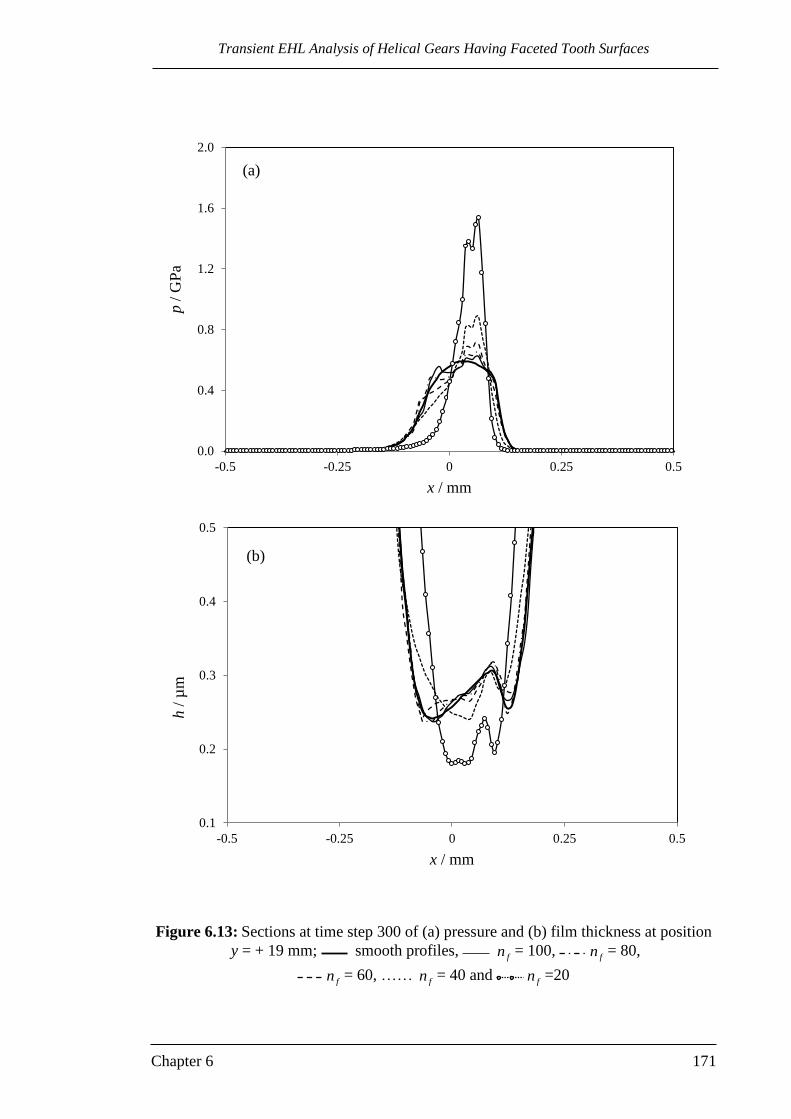
Transient EHL Analysis of Helical Gears Having Faceted Tooth Surfaces
Chapter 6 171
Figure 6.13: Sections at time step 300 of (a) pressure and (b) film thickness at position
y = + 19 mm; smooth profiles, fn = 100,
fn = 80,
fn = 60, …… fn = 40 and
fn =20
0.0
0.4
0.8
1.2
1.6
2.0
-0.5 -0.25 0 0.25 0.5
p /
GP
a
x / mm
(a)
0.1
0.2
0.3
0.4
0.5
-0.5 -0.25 0 0.25 0.5
h /
µm
x / mm
(b)

Transient EHL Analysis of Helical Gears Having Faceted Tooth Surfaces
Chapter 6 172
Figure 6.14: Sections at time step 300 of (a) pressure and (b) film thickness at position
y = 0; smooth profiles, fn = 100,
fn = 80,
fn = 60, ……
fn = 40 and fn = 20
0.0
0.5
1.0
1.5
2.0
2.5
3.0
-0.5 0 0.5
p /
GP
a
x / mm
(a)
0.0
0.1
0.2
0.3
0.4
0.5
-0.5 0 0.5
h /
µm
x / mm
(b)

Transient EHL Analysis of Helical Gears Having Faceted Tooth Surfaces
Chapter 6 173
Figure 6.15: Sections at time step 300 of (a) pressure and (b) film thickness at position
y = - 19 mm; smooth profiles, fn = 100,
fn = 80,
fn = 60, ……
fn = 40 and fn = 20
0.0
0.2
0.4
0.6
0.8
1.0
1.2
1.4
-0.5 -0.25 0 0.25 0.5
p /
GP
a
x / mm
(a)
0.1
0.2
0.3
0.4
0.5
-0.5 -0.25 0 0.25 0.5
h /
µm
x / mm
(b)

Transient EHL Analysis of Helical Gears Having Faceted Tooth Surfaces
Chapter 6 174
Similar comparisons are also made for the results at time step 500. The 3D pressure
distribution, film thickness contours and section comparisons at 10y mm are shown
in Figures 6.16, 6.17, and 6.18 respectively. Similar behaviour to the results obtained at
time step 75 and 300 are also found at this time step. The case fn = 20 is the most
extreme case for both pressure distribution and film thickness and the results for all the
other cases tend towards the smooth results as fn is increased.
In comparing the results it is clear that faceting modifies the pressure and film thickness
response in all of the cases considered. For the finest faceted surface, fn =100, the
modification can be regarded as a mild perturbation of the smooth surface results. As
the number of facets is reduced the modifications increased systematically. For the tooth
module considered it is clear that the fn = 20 case causes considerable disturbance and
results in extremely thin lubricant films, or metal to metal contact, on the lines
corresponds to facet boundaries.
The theoretical analyses indicate that when a facetted surface is being produced the
lubrication mechanism may be compromised unless the number of facets is large
enough or some further smoothing operations are introduced to the manufacturing
process.

Transient EHL Analysis of Helical Gears Having Faceted Tooth Surfaces
Chapter 6 175
Figure 6.16: Contact pressure surfaces corresponding to six different patterns of
tooth profile at time step 500
𝑛𝑓 = 20 𝑛𝑓 = 40
𝑛𝑓 = 60 𝑛𝑓 = 80
𝑛𝑓 = 100 smooth

Transient EHL Analysis of Helical Gears Having Faceted Tooth Surfaces
Chapter 6 176
Figure 6.17: Film thickness contours corresponding to six different patterns of
tooth profile at time step 500
𝑛𝑓 = 20 𝑛𝑓 = 40
𝑛𝑓 = 60 𝑛𝑓 = 80
𝑛𝑓 = 100 smooth

Transient EHL Analysis of Helical Gears Having Faceted Tooth Surfaces
Chapter 6 177
Figure 6.18: Sections at time step 500 of (a) pressure and (b) film thickness at position
y = - 10 mm; smooth profiles, fn = 100,
fn = 80,
fn = 60, ……
fn = 40 and fn = 20
0.0
0.5
1.0
1.5
2.0
2.5
-0.5 -0.25 0 0.25 0.5
p /
GP
a
x / mm
(a)
0.1
0.2
0.3
0.4
0.5
-0.5 -0.25 0 0.25 0.5
h /
µm
x / mm
(b)

3D Line Contact Model
Chapter 7 178
Chapter 7
3D Line Contact Model
7.0 Introduction
The 3D line contact model presented in this chapter is used to investigate the EHL
characteristics of the contact between helical gear teeth, and takes the effect of surface
roughness into consideration. A special roughness orientation may be found in the
helical gears contact and a close form equation is derived to describe its features, as will
be shown later. The model is based on the use of the fast Fourier transform (FFT)
method to calculate the surface deflection and its differential form where these terms are
represented by convolution integrals. This enables a model with limited length along the
contact line to be developed in such a way that it allows surface roughness to be
incorporated. Figure 7.1 shows an example of a helical gear tooth contact that can be
modelled by the method described in this chapter. Figure 7.1 (a) shows a single helical
gear tooth together with a typical contact line, and Figure 7.1 (b) illustrates
schematically the tangent plane to the tooth surface at the contact line where the length
of the contact zone is much bigger than the contact width.
Figure 7.1: Contact of helical gears; (a) contact line on a helical gear tooth and (b)
contact zone where its length is much bigger than the width
Tangent plane
Contact zone
(a) (b)

3D Line Contact Model
Chapter 7 179
7.1 Convolution integrals and the FFT method
This section explains that the equations which give the elastic surface deflection and its
differential form involve convolution integrals and also clarifies how the FFT method
can be used to evaluate them in a 3D line contact model of limited transverse extent.
In solving the EHL problem, the total gap between two smooth surfaces is defined by
equation (3.2)
ou hyxdyxhyxh ,,, (3.2)
This equation can be modified to take the effect of surface roughness into consideration
as
ou hyxyxyxdyxhyxh ,,,,, 21
where yx,1 and yx,2 are the surface roughness for the two surfaces.
The determination of the elastic deflection in this equation at any point in the solution
domain was given by equation (3.3) which is repeated here for clarity
dxdy
yyxx
yx,p
Eπ
2y,xd
A2
1
2
1
11
(3.3)
This equation represents a convolution integral. In a continuous system, convolution
integrals such as that given by equation (3.3) can be obtained using the convolution
theorem where the Fourier transform of a convolution of two functions e.g. g and p
is the product of their Fourier transforms.
pgpg *
Taking the inverse transform for this equation gives the required convolution integral:
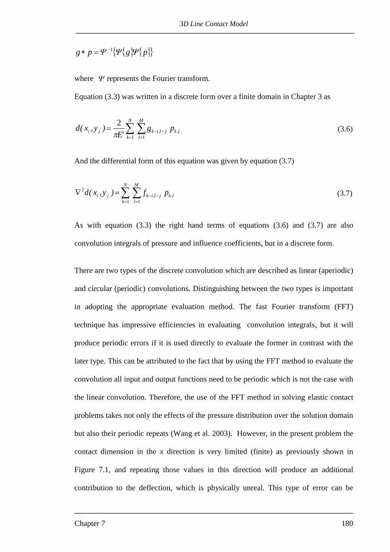
3D Line Contact Model
Chapter 7 180
pgpg 1
where represents the Fourier transform.
Equation (3.3) was written in a discrete form over a finite domain in Chapter 3 as
N
k
M
l
l,kjl,ikji p g 'E
)y,x(d1 1
2
(3.6)
And the differential form of this equation was given by equation (3.7)
N
k
M
l
l,kjl,ikji p f )y,x(d1 1
2 (3.7)
As with equation (3.3) the right hand terms of equations (3.6) and (3.7) are also
convolution integrals of pressure and influence coefficients, but in a discrete form.
There are two types of the discrete convolution which are described as linear (aperiodic)
and circular (periodic) convolutions. Distinguishing between the two types is important
in adopting the appropriate evaluation method. The fast Fourier transform (FFT)
technique has impressive efficiencies in evaluating convolution integrals, but it will
produce periodic errors if it is used directly to evaluate the former in contrast with the
later type. This can be attributed to the fact that by using the FFT method to evaluate the
convolution all input and output functions need to be periodic which is not the case with
the linear convolution. Therefore, the use of the FFT method in solving elastic contact
problems takes not only the effects of the pressure distribution over the solution domain
but also their periodic repeats (Wang et al. 2003). However, in the present problem the
contact dimension in the x direction is very limited (finite) as previously shown in
Figure 7.1, and repeating those values in this direction will produce an additional
contribution to the deflection, which is physically unreal. This type of error can be

3D Line Contact Model
Chapter 7 181
eliminated by using the “zero padding” strategy. In this approach the length of the input
function is extended with zeroes in the x and y directions so that the periodic effect
becomes negligible due to the localized effect of the influence coefficients g and f in
particular. However, in the 3D line contact model the input functions are assumed to be
repeated periodically in the y direction. Therefore, a mixed strategy of zero padding in x
direction and periodic repetition in the y direction for the input functions is adopted in
this model as illustrated in Figure 7.2.
Figure 7.2: Padding strategy for the 3D line contact problem
7.2 Numerical solution
The solution domain for the EHL analysis is defined numerically by:
1M,01N,0
Solution
space
Repeated
solution
space
Zero
padding
space
Zero
padding
space
x
y

3D Line Contact Model
Chapter 7 182
In order to implement the FFT method to calculate the convolution integrals given by
equations (3.6) and (3.7), the influence coefficients function in both equations needs to
be rewritten in a wrap-around order. This requires a grid size of twice the solution
domain size in each direction. A similar grid is also required for the pressure
distribution where the same pattern of pressure is repeated in one or both directions as
required. As a result the FFT method is performed in a domain defined by a grid size of
2N *2M.
In the discrete system for a finite length sequence, the discrete Fourier transform for the
pressure data in equation (3.6) can be that given by Nussbaumer (1982), for example:
),()/2exp()/2exp( 21
1
02
1
0
12,
1
kkpNikMjkpM
k
N
k
ji
where 1 and the two dimensional grid is defined by
10 Ni and 10 Mj
The discrete Fourier transform for the influence coefficient functions g and f can also be
evaluated using the previous equation. Therefore, equation (3.6) can be calculated from:
gpyxd ji 1),(
Similarly equation (3.7) can be evaluated as
fpyxd ji 12 ),(
The procedure (program) for the evaluation of discreet convolution integrals using the
FFT method is available widely in the literature and the one given by Press et. al.
(1992) is adopted in the current work.

3D Line Contact Model
Chapter 7 183
7.3 Angle between contact line and grinding line
The technique described in this section will be used to examine the effects of roughness
orientation on the EHL performance of helical gears. This orientation in question is
related to the inclination of grinding marks with respect to the line of contact between
the gear teeth in the tangent plane as shown in Figure 7.3. Figure 7.3 (a) shows a 3D
schematic drawing of a single helical gear tooth (pinion tooth) in contact. The
corresponding gear wheel tooth is not shown for the purpose of clarity. Contact of the
teeth occurs on the line AC at this specific position in the meshing cycle. Point A is the
limit of the contact line on the tooth face which moves along the line of action as the
contact progresses between the gear teeth. In spur gears, grinding of the gear teeth
usually takes place in the direction of the gear axis which is perpendicular to the tooth
face. In this case the grinding marks will be in the same direction as the contact line
(both are parallel to the gear axis). In helical gears the helix angle will affect the angle
between the contact line and the grinding marks. This can be seen clearly in Figure 7.3
(a) by comparing the direction of lines AC and AD where line AD represents the
grinding mark direction. Any point on this line is at a constant radius, Ar from the gear
axis.
A length AB from the contact line is selected to find the angle θ between the contact
line and the projection of the grinding mark line on the tangent plane which is the
solution space of the EHL analysis. This projection is represented by line AT where the
tangent plane contains the triangle ABT. This angle is given by
)AB/BT(tan 1 (7.1)
For any given AB distance along the line of contact, equation (7.1) can be used to
evaluate the angle θ by calculating the distance BT.

3D Line Contact Model
Chapter 7 184
Figure 7.3: Schematic drawing of helical gear tooth contact; (a) 3D drawing for a
pinion tooth, (b) parabolic approximation for the contact and (c) s positon of point B
with respect to point A
(a)
Q
B
T
A
B
s
(b) (c)
A
Q
B
T
ψ
Line of action
C
D
O
E
J
O′

3D Line Contact Model
Chapter 7 185
Figure 7.3 (b) shows a parabolic approximation of the involute profile at point B in the
transverse section. Thus, using this figure the distance QT is given by:
B
2
2
)BT(QT
R (7.2)
where BR is the tooth radius of curvature at point B which can be determined in terms of
the position, Bs of point B relative to the pitch point in the transverse direction:
B1B tan srR b (7.3)
Figure 7.3 (c) shows the contact line AC on the plane of contact. Using this figure, Bs
can be determined in terms of the position of point A which is known for all positions in
the meshing cycle:
bAB in AB sss (7.4)
Since points A and Q lie on line AD, their distances from the gear axis OO′ are:
QA rr (7.5)
From the triangle OEA in Figure 7.3 (a):
2
A1
2
1A )tan( srrr bb
The term in the bracket is the tooth radius of curvature at point A, AR . Therefore this
equation can be reduced to
2
A
2
1A Rrr b (7.6)
Using the schematic drawing of the transverse section at point B that is shown in Figure
7.3 (b), Qr can be given by:
2
B
2
1Q )QT()BT( Rrr b
Substituting equation (7.2) into this equation yields:
3D Line Contact Model
Chapter 7 186
2
B
2
B
2
1Q )2
)BT(()BT(
RRrr b (7.7)
Substitution of equations (7.6) and (7.7) in equation (7.5), yields
2
B
2
B
2
1
2
A
2
1 )2
)BT(()BT(
RRrRr bb
This equation can be written, after some simplification, in the following form
0BT24
)BT( 2
A
2
B12
B
4
RRrR
b (7.8)
Equation (7.8) has four roots and two of them are complex. However, solving this
equation at any position along the contact line will only produce one realistic real root.
Substituting the solution of equation (7.8) (BT) in equation (7.1) gives the angle
between the line of contact and the grinding mark direction at point B for the pinion
teeth. Since the tooth radius of curvature increases with y along the contact line (for the
pinion), the calculated angle with respect to point A also changes and depends on the
distance AB. This means that the projection of the grinding line on the tangent plane is
not a straight line.
A similar equation can be derived for the contacting wheel tooth using the same
procedure taking into account the fact that its radius of curvature decreases with
increasing y and equation (7.7) needs to be reformulated to the following form:
2
WB
2
WB
2
2WQ )2
)BT(()BT(
RRrr b
where WQr is the radial distance from the wheel axis to point Q in the transverse
direction and WBR is the wheel tooth radius of curvature at point B. Therefore, the
required equation for the wheel tooth is

3D Line Contact Model
Chapter 7 187
0BT24
)BT( 2
WA
2
WB22
WB
4
RRrR
b
Changing distance AB along the contact line means choosing a different s value to
calculate the radii of curvature for the two surfaces which correspond to the position of
point B. Therefore, the variation of the required angle described in equation (7.1) for
both surfaces is actually s dependent. Figure 7.4 shows this variation for both surfaces
throughout the meshing cycle (variation with s) for a distance AB = 1 mm, i.e. close to
the gear face at A. It can be seen that angle P varies between 4.6
o and 9.5
o and
W
varies between 9.5o and 4.6
o and both angles are equal at the pitch point
08.7PW . P increases and
W decreases with increasing s and the opposite
variation of these angles is related to the nature of radii of curvature variation with s for
the two teeth. For the pinion tooth, the first and last contact points in the meshing cycle
(which is defined by s) represent the lowest and highest radius of curvature,
respectively. For the wheel tooth they represent the highest and lowest radii of
curvature, respectively.
The inclination of the contact line with respect to the grinding direction in the tangent
plane calculated in this way can also be verified by drawing the gap between the two
teeth in contact with a 2 μm height feature added to this gap at a constant distance Ar
from the gear axis across the whole face width for both gears to represent grinding lines
as shown in Figure 7.5. The y axis represents the contact line direction. It is clear from
this figure that these lines are inclined at different angles with y direction and
consequently cross each other.
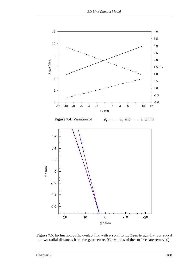
3D Line Contact Model
Chapter 7 188
Figure 7.4: Variation of P ,
W and ζ with s
Figure 7.5: Inclination of the contact line with respect to the 2 μm height features added
at two radial distances from the gear centre. (Curvatures of the surfaces are removed)
-1.0
-0.5
0.0
0.5
1.0
1.5
2.0
2.5
3.0
3.5
4.0
0
2
4
6
8
10
12
-12 -10 -8 -6 -4 -2 0 2 4 6 8 10 12
ζ
Angle
/ d
eg.
s / mm
y / mm
x /
mm

3D Line Contact Model
Chapter 7 189
7.4 3D line contact verses line contact results for smooth surfaces.
A comparison between the EHL results for the 3D model and the corresponding line
contact analysis is carried out to validate this model for smooth surfaces. For this
purpose the solution domain is defined by a selected length in the y direction, Ly = 2
mm, and a distance of 4 a ( )5.15.2 axa in the x direction. The number of elements
used in the entrainment direction, x, is 800 elements which is then padded with zeros (p
= 0) to be 1024 (the nearest power of 2 number). These additional 224 points
correspond physically to a distance of 1.12 a. The number of elements in the y direction
is 128. The input data for the 3D EHL solution is explained in Table 7.1. The geometry
and kinematic characteristics described in this table are also used for the line contact
analyses and an input load of 360 kN/m is adopted which is equal to the load/length
used in the 3D analyses.
The 3D pressure distribution and film thickness for smooth surfaces is shown in Figure
7.6. This figure shows how the pressure and film thickness surfaces are prismatic and
perfectly extruded in the y direction. Sections at a y position (pressure and film
thickness results) are compared with the corresponding line contact results as shown in
Figure 7.7. It can be seen in this figure that both pressure and film thickness curves
coincide almost exactly with the corresponding line contact results.
R/mm 14.0
Load/N 720
u / m/s 6.71
ζ 0.36
Table 7.1: Input data for the 3D model

3D Line Contact Model
Chapter 7 190
Figure 7.6: 3D smooth surface line contact results, (a) Pressure distribution and (b)
Film thickness
(a)
(b)

3D Line Contact Model
Chapter 7 191
Figure 7.7: Comparison between 3D line contact results and corresponding
line contact results for smooth surfaces.
7.5 FEM vs FD discretisation
The 3D EHL analysis is performed using both the finite element method (FEM) and
finite difference (FD) methods for the purpose of comparison and model development.
Figure 7.8 shows the discretisation of the solution domain using both methods. Only
one column of elements /nodes is shown in the solution domain for each method which
is discretised to four elements (or rows of nodes) for the purpose of clarity. The solution
domain is repeated in both transverse directions according to the FFT method and only
one repetition is shown in the figure. For the FD method the solution is straightforward.
In the central difference case for example, the evaluation of the second derivative of
0.1
0.2
0.2
0.3
0.3
0.4
0.4
0.5
0.5
0.0
0.2
0.4
0.6
0.8
1.0
-2.0 -1.5 -1.0 -0.5 0.0 0.5 1.0 1.5 2.0
h /
μm
p /
GP
a
x / a

3D Line Contact Model
Chapter 7 192
pressure, 22 yp , can be done directly at all nodes except the nodes on the first and last
rows where this requires the nodal values at the four neighbouring nodes of
(a)
(b)
Figure 7.8: Discretization of the solution domain. (a) FEM vs FD (only one column of
element/node is shown for each method) and (b) The four neighbour nodes of the
general point (i,M).
i,M i+1,M
i,M+1
i-1,M
i,M-1
Ly
Ly
Repeated
j =4
j =3
j =2
j =1
j =4
j =3
j =2
j =1
dy = Ly / 4
dy/2
FD FE

3D Line Contact Model
Chapter 7 193
the node under consideration. This can be achieved by exploiting the nature of repetition
of the FFT method where the same solution domain is repeated in both directions as
stated above. In the last row (j = M) for example the four neighbouring nodes of the
general point (i,M) are (i+1,M), (i-1, M), (i, M+1) and (i,M -1) as shown in Figure 7.8
(b) where i indicates the x position of the node and M represents the numbers of node
rows in the y direction of the solution domain. The only node outside the solution
domain is node (i, M+1) and the nodal value at this node is in fact the value at node (i,1)
in the first row of the solution domain which can be used to evaluate the required
derivative. Therefore, the second derivative at node (i,M) is now calculable for all i
values.
A similar procedure can be used for the nodes that lie on the first row by using the nodal
values from the Mth row. Adopting this cycling method, the nodal values at the
boundaries of the solution domain ensures continuity of flow at these boundaries. In the
x direction, boundary conditions are applied at the nodes of the first and last columns of
the solution domain.
For the FEM method a four node rectangular element is used with element integrations
achieved with four Gauss points. The discretisation of this problem using FEM is more
complicated in comparison with the FD method. The difficulty is related to the way of
dealing with boundaries of the solution domain in the y direction. Each node in the grid
has a contribution from four adjacent elements (except the boundary nodes at i =1 and i
= N). Therefore it is required to add contributions for the first and last rows of nodes in
the y direction which come from the elements in the repeated domains. This can be done
by adding one row of elements to the solution domain at each side of the boundaries of

3D Line Contact Model
Chapter 7 194
repetition in the y direction. The nodal values for these elements that are outside the
solution domain are obtained from the cyclically equivalent nodes that are inside the
solution domain. Care is necessary in adding two rows of elements as another
contribution will be added not only to the nodes at the boundaries but to the rest of the
nodes on the boundary elements and these contributions should be ignored. However,
in the assembly procedure adding one row of elements at one of the repetition
boundares is sufficient as it will add the contributions for both of the rows of nodes on
the boundaries. Figure 7.9 illustrates this method where Figure 7.9 (a) shows the
column of elements previously shown in Figure 7.8 (a) which consists of 4 elements
only for the purpose of clarity. Regarding this column, the actual rows of elements
inside the solution space considered in the EHL calculations are three (M-1) which is
shown in Figure 7.9 (b). Each node on the rows j=2 and j=3 have contributions from
two elements in this column which is the real case, while the nodes on rows j=1 and j=4
can get contributions from one element in this column. Therefore, it is necessary to add
the required missing contributions to the nodes at the rows j=1 and j=4. This can be
achieved by adding one row of elements at the upper boundary of the solution space as
shown in Figure 7.9 (c). This means there will be an additional row of nodes at j = 5 (j =
M+1), which physically represent the nodes at j=1 as the same nodal values of the
solution space are repeated in both directions as explained previously. Now, the new
number of elements considered in the EHL analysis is four (M). Adding this row of
elements will not only ensure adding the required contributions to the nodes at j=4 but
also to the nodes at row j=5 (which is equal to j=1).

3D Line Contact Model
Chapter 7 195
Figure 7.9: Dealing with boundaries in the FEM method. (a) Single column of
elements in the solution space, (b) The actual number of elements for this column in the
solution space and (c) Adding one row of elements (dashed line) at the upper boundary
of the solution space
7.6 Selection of the roughness profile
The roughness orientation is taken to be the same as the grinding lines direction with
respect to the line of contact as previously shown in Figure 7.4. Figure 7.10 (not to
scale) illustrates schematically this orientation in the tangent plane, xy, at a position in
the meshing cycle. The roughness lines for one tooth surface are shown in this figure for
clarity. With the use of the FFT method only a small rectangular area is required to
reflect the roughness features on the whole xy plane. A sample of this area which is
shown by broken lines can be selected for this purpose. The rectangle dimensions are Lx
and Ly in the x and y direction respectively. The required angle of roughness orientation
can be obtained by changing the proportion of this rectangle as shown in Figure 7.11
which illustrates the way in which the roughness profile is extruded. Figure 7.11 (a)
shows a schematic drawing of a roughness profile. The profile length is Lx and
roughness data are illustrated by filled circles at seven positions separated by an equal
dy/2
dy = Ly / 4
j =4
j =3
j =5 ≡ j =1
j =2
j =1
Ly
(a) (b) (c)

3D Line Contact Model
Chapter 7 196
step, Δ. Figure 7.11 (b) shows how the roughness profile on a single rectangle is
extruded and connected to the corresponding profile on the adjacent repeated rectangles.
Roughness at the first position (the relatively big circle) in one rectangle is always
extruded at an angle θ to the y direction and connected to the same position number on
the relevant repeated rectangle and so on for the other positions. Therefore, the angle of
extrusion is given by:
yx LL /)(tan 1
The length of the EHL solution domain in the y direction is Ly while its length in the x
direction is not necessarily equal to Lx. Choosing different profile length values, Lx for
the two surfaces will produce different extrusion angles. The procedure described above
ensures the conservation of lubricant mass as it maintains the equality between the
lubricant flows across the boundaries between the repeated domains in both directions.
It is worth mentioning that the extruded lines are assumed as perfectly straight lines
over the selected rectangular area defined by Lx and Ly as the deviation from a straight
line is trivial if Ly is relatively small.
Figure 7.10: Schematic illustration for the roughness orientation in the tangent plane.
Broken lines rectangle can be used to reflect the features of the whole plane.
Lx
Ly

3D Line Contact Model
Chapter 7 197
Figure 7.11: Roughness extrusion over the selected domain. (a) A selected profile of
length Lx in the x direction and (b) Relation between the roughness features over the
solution space and the repeated spaces.
Figure 7.12 shows two surface profiles which represent portions of a real measured
profile taken from a tooth surface. The profile in Figure 7.12 (a) has a length of Lx = 149
μm while the one in Figure 7.12 (b) has a length of Lx = 100 μm. These profiles are
repeated to provide long roughness profiles for the extruded analyses for any required
length. For example, Figure 7.12(c) shows the profile Lx = 149 μm repeated over a
distance of 5a. Using the method of extrusion described for these profiles over a
distance of 1 mm in the y direction (Ly = 1 mm) will produce angles of extrusion of 8.5o
and 5.7o for the long and short profiles, respectively. These angle values correspond to a
position in the meshing cycle of s = 5.75 in Figure 7.4.
θ Ly
Lx
Δ
dy
dy/2
Lx
Δ (b)
(a)

3D Line Contact Model
Chapter 7 198
Figure 7.12: Real surface profile. (a) Lx = 149 μm , (b) Lx = 100 μm and (c) repeating of
Lx = 149 μm profile over a 5a distance.
-1.0
-0.5
0.0
0.5
0 20 40 60 80 100 120 140
hig
ht
/ μ
m
distance / μm
(a)
-1.0
-0.5
0.0
0.5
0 20 40 60 80 100 120 140
hig
ht
/ μ
m
distance /μm
(b)
-1.0
-0.5
0.0
0.5
Hig
ht
/ μ
m
Length ≈ 5 a
(c)

3D Line Contact Model
Chapter 7 199
2D contours for the roughness features are shown in Figure 7.13. Figure 7.13 (a) shows
the case for 8.5o angle of extrusion and Figure 7.13 (b) shows a perfectly straight
extrusion for the same profile (parallel to the y direction). The two profile portions
shown in Figure 7.12, which can be extruded in y direction using any of the forms
shown in Figure 7.13, are used in this chapter to investigate the effect of roughness
orientation (relative to the entraining direction) on the EHL performance of helical
gears.
Figure 7.13: Forms of roughness features. (a) 5.8P and (b) 0P .
x
y
(a)
(b)
≈ 150 μm
a

3D Line Contact Model
Chapter 7 200
7.6.1 3D line contact versus line contact results for rough surfaces.
The 3D results were previously validated against the corresponding line contact result
for a smooth surface in section 7.4 which showed excellent agreement. In this section a
similar comparison is also made using rough surfaces. The profile shown in Figure 7.14
was taken from disk testing carried out by Patching et al. (1995) is used for this
comparison and has Ra value of 0.31 µm.
Figure 7.14: Real roughness profile of length 4 mm approximately.
In the 3D case this profile is applied to both surfaces and extruded parallel to the y axis
over a distance of 1 mm (Load = 360 N). The two surfaces thus have the same
roughness profile but they move at different speeds so that the surface asperities on the
two surfaces move relative to each other. Figure 7.15 shows transient results for the 3D
case at a particular time step. It can be seen in this figure that the calculated pressure
distribution and film thickness are both perfectly extruded in the y direction. Figure 7.16
shows a section comparison at this time step with the corresponding transient line
-5
-4
-3
-2
-1
0
1
2
0 1 2 3 4
hig
ht
/ µ
m
Length / mm

3D Line Contact Model
Chapter 7 201
contact results. It can be seen that both the pressure distribution (Figure 7.16 (a)) and
film thickness (Figure 7.16 (b)) coincide almost exactly for the two methods.
Figure 7.15: Transient results for the 3D line contact model at a particular time step.
(a) Pressure and (b) Film thickness
(a)
(b)

3D Line Contact Model
Chapter 7 202
Figure 7.16: Section comparison between line contact (solid) and the 3D model results
(dashed) shown in Figure 7.15. (a) Pressure and (b) Film thickness.
0.0
1.0
2.0
3.0
4.0
5.0
-0.4 -0.3 -0.2 -0.1 0 0.1 0.2 0.3 0.4
p /
GP
a
x / mm
(a)
0
1
2
3
4
-0.4 -0.3 -0.2 -0.1 0 0.1 0.2 0.3 0.4
h /
μm
x / mm
(b)

3D Line Contact Model
Chapter 7 203
7.7 General results for the 3D Line contact model
The transient 3D line contact EHL analysis is carried out using the surface profiles
shown previously in Figure 7.12. The extrusion width and length of profile are chosen
such that both 3D surfaces repeat exactly over distance Ly. This means that the problem
repeats exactly in the y direction and that there will be flow continuity at the transverse
boundaries of the modelled section. Film thickness and pressure distribution results for
a particular time step are shown in Figure 7.17. Due to the difference in the roughness
orientation in the two surfaces (8.5o and 5.7
o), their extruded roughness lines intersect
with each other. These intersections initially concentrate the transmitted load on limited
areas which produce high pressure spikes at those locations as shown in Figure 7.17 (a).
This is not the case when the roughness profile is extruded in the direction parallel to y
direction. In this situation the intersection between any two asperities acts over the
whole Ly distance which increases the area that supports the transmitted load. Figure
7.17 (b) shows the film thickness variation in the solution domain where metal to metal
contact (h = 0) is predicted at some points.
Figure 7.17: EHL results at a time step using the 3D line contact mode, pressure
distribution (left) and film thickness (right).

3D Line Contact Model
Chapter 7 204
7.7.1 Effect of number of elements in the y direction
In this section the effect of mesh density, M, in the y direction is examined. A length of
1 mm in the y direction is discretised to 32, 64, 128 and 256 elements. These numbers
coincide with the power of two condition required for the FFT method. The number of
nodes in the x direction is fixed to a 200⁄ in all cases as this number gives an element
length that corresponds approximately to the spacing at which the roughness data are
measured.
The solution starts from the steady state solution for smooth surfaces. The roughness
profiles are then fed into the contact zone from the inlet boundary with the moving
surfaces. The roughness is attenuated linearly by scaling with a factor that increases
linearly from zero to unity over the leading Hertzian dimension of the roughness profile.
The analysis becomes “fully rough” at the time when the attenuated parts of the profiles
have travelled through the contact zone and reached the exit area where the lubricant
film becomes cavitated. The transient analyses is carried out for 4488 time steps which
represent the time for the slower surface to move through the calculation zone by a
distance of 4a from the time at which the analysis becomes fully rough.
This transient problem is computationally demanding. The four different transverse
resolution models had grids involving 800 x 32, 800 x 64, 800 x 128 and 800 x 256
nodes / mesh points. The calculations were carried out on an Intel Core i7-2600 CPU @
3.40 GHz machine using the LINUX operating system with the code written in Fortran
90. The run times for these transient analyses were 1.5, 4, 9 and 21 hours respectively.

3D Line Contact Model
Chapter 7 205
Figure 7.18 shows the variation of maximum pressure over this distance when the two
roughness profiles are extruded at angles 8.5o and 5.7
o. The maximum pressure value is
constant at 0.95 GPa in the first 1250 time steps in all cases, which means in effect that
M = 32 is sufficiently fine to carry out a 3D smooth EHL analysis. During these time
steps the active profiles in the EHL analysis (−a ≤ x ≤ a) are still smooth. With the
progress of roughness through the EHL solution domain, the effect of mesh density
becomes more noticeable and the analysis becomes fully rough at time step 2888. It is
clear that the M value has an effect on the maximum EHL pressure results when the two
surfaces start to be fully rough. For example at time step 2500, the maximum pressure
value changes from 3 GPa to 4 GPa when M changes from 32 to 256 elements,
respectively. Disregarding the noise in the pressure values in the case of M = 128, it has
the same trend as the case M = 256. The variation of the corresponding minimum film
thickness values is not shown in this figure as metal to metal contact is always predicted
under the operating conditions adopted in this analysis.
Figure 7.18: Variation of maximum pressure during transient analysis with M.
The two roughness profiles are extruded at angles 8.5o and 5.7
o.
Green: M = 32, blue: M = 64, red: M = 128 and black: M =256
0
500
1000
1500
2000
2500
3000
3500
4000
4500
5000
0 1000 2000 3000 4000 5000
p m
ax
/ M
Pa
Time step

3D Line Contact Model
Chapter 7 206
Further section comparisons are shown in Figures 7.19, 7.20 and 7.21. Figure 7.19
shows pressure distribution and film thickness at time step 4000. The comparison is
made at the centre of the contact (x = 0) along the y direction. It can be seen that both
film thickness and pressure distribution when M = 128 give good agreement with the
case of M = 256. Figure 7.20 shows similar section comparison at x = 0.075 mm at time
step 4480. This is the position of the maximum pressure value when M = 128 at this
time step. Similarly, there is no significant difference between cases M = 128 and M =
256. The last comparison is carried out in the x direction at time step 4480 which is
shown in Figure 7.21. Two cases are compared when M = 128 and 256 at the first row
of nodes in the y direction. It can be seen that the results of the two cases coincide
almost exactly. A similar analysis was also made for the case when the roughness
profiles are extruded parallel to the y direction and is shown in Figure 7.22. Three cases
were examined where M = 32, 64 and 128 elements. It can be seen that changing the M
value has no effect on the maximum pressure behaviour. These comparisons lead to the
conclusion that 128 elements in the y direction is sufficient to resolve the problem. The
resolution in the x direction is 1.1886 μm, and for M = 128 the resolution in the y
direction is about 8 μm.
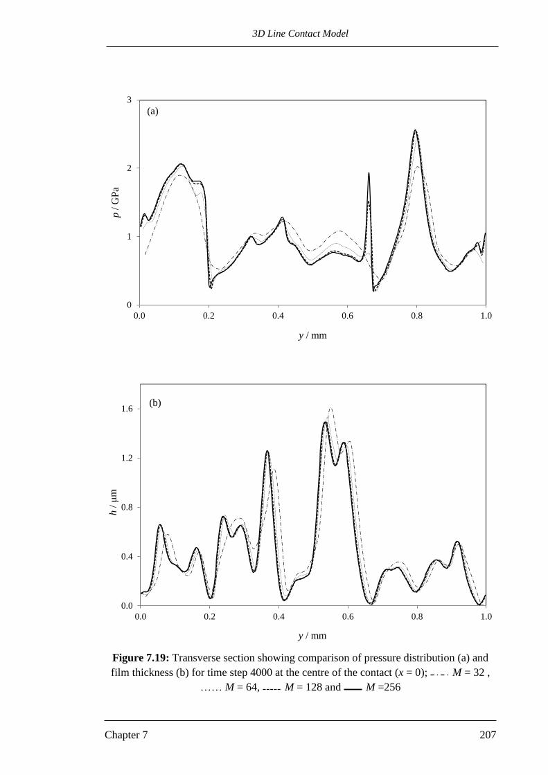
3D Line Contact Model
Chapter 7 207
Figure 7.19: Transverse section showing comparison of pressure distribution (a) and
film thickness (b) for time step 4000 at the centre of the contact (x = 0); M = 32 ,
…… M = 64, M = 128 and M =256
0
1
2
3
0.0 0.2 0.4 0.6 0.8 1.0
p /
GP
a
y / mm
(a)
0.0
0.4
0.8
1.2
1.6
0.0 0.2 0.4 0.6 0.8 1.0
h /
μm
y / mm
(b)

3D Line Contact Model
Chapter 7 208
Figure 7.20: Transverse section showing comparison of pressure distribution (a) and
film thickness (b) for time step 4480 at x = 0.075 mm; M = 32 ,
…… M = 64, M = 128 and M =256
0
1
2
3
4
0.0 0.2 0.4 0.6 0.8 1.0
p /
GP
a
y / mm
(a)
0.0
0.4
0.8
1.2
1.6
0.0 0.2 0.4 0.6 0.8 1.0
h /
μm
y / mm
(b)

3D Line Contact Model
Chapter 7 209
Figure 7.21: Entrainment direction section showing comparison of pressure distribution
(a) and film thickness (b). Results for time step 4480 at the first row of nodes (j = 1).
M =128 and M =256
0
1
2
3
-0.4 -0.3 -0.2 -0.1 0 0.1 0.2 0.3 0.4
p /
GP
a
x / mm
(a)
0.0
0.5
1.0
1.5
2.0
2.5
-0.4 -0.3 -0.2 -0.1 0 0.1 0.2 0.3 0.4
h /
μm
x / mm
(b)

3D Line Contact Model
Chapter 7 210
Figure 7.22: Variation of maximum pressure during transient analysis when the two
roughness profiles are extruded parallel to the y-direction.
. M = 32, M = 64, M = 128
7.7.2 Comparison between FEM and FD methods.
Figure 7.23 compares the EHL results using the finite element and finite difference
methods (central difference). The comparison is carried out at time step 4000 and results
at the first row of nodes (j = 1) are shown. The roughness profiles are extruded at angles
of 8.5o and 5.7
o for the fast and slow surfaces, respectively. In general the two methods
give the same behaviour for the calculated pressure distribution and the FEM gives less
aggressive pressure spikes as shown in Figure 7.23 (a). Film thickness variation is
illustrated in Figure 7.23 (b) and shows good agreement between the two methods.
0
500
1000
1500
2000
2500
3000
3500
4000
4500
0 1000 2000 3000 4000 5000
p m
ax /
MP
a
Time step

3D Line Contact Model
Chapter 7 211
Figure 7.23: Comparison between FEM (solid) and FD (dashed) method at time step
4000. Results are shown at the first row of nodes. The roughness profiles are extruded at
angles of 8.5o and 5.7
o . (a) Pressure and (b) Film thickness
0.0
1.0
2.0
3.0
-0.4 -0.3 -0.2 -0.1 0 0.1 0.2 0.3 0.4
p /
GP
a
x / mm
(a)
0.0
0.5
1.0
1.5
2.0
2.5
-0.4 -0.3 -0.2 -0.1 0 0.1 0.2 0.3 0.4
h /
μm
x / mm
(b)

3D Line Contact Model
Chapter 7 212
7.7.3 Effect of roughness orientation on the EHL results
Figure 7.24 compares the transient EHL analysis results for two cases. The roughness
profiles in the first case are extruded at angles of 8.5o and 5.7
o with the y direction while
the same roughness profiles are extruded parallel to the y axis in the second case. The
profiles used in these analyses are those shown in Figure 7.12. Figure 7.24 (a) shows
that the way in which the roughness profile is extruded significantly affects the
maximum pressure value at each time step. The case of “crossing” extrusion produces
much higher pressure values, and at some time steps the maximum pressure value for
this case reaches twice the value predicted in the straight extrusion case. A similar
important difference can also be seen in the comparison of film thickness variation
during the transient analyses that are shown in Figure 7.24 (b). For the crossing
extrusion case metal to metal contact is predicted in each time step following time step
1772. On the other hand, for the straight extrusion case a thin layer of lubricant is
generated at a significant number of time steps.

3D Line Contact Model
Chapter 7 213
Figure 7.24: Transient EHL comparison between straight (solid) and with angle
(dashed) extrusion of the roughness. (a) Pressure and (b) Film thickness
0
500
1000
1500
2000
2500
3000
3500
4000
4500
0 1000 2000 3000 4000 5000
p m
ax /
MP
a
Time step
(a)
0
0.02
0.04
0.06
0.08
0.1
0 1000 2000 3000 4000 5000
h m
in /
μm
Time step
(b)

3D Line Contact Model
Chapter 7 214
7.8 Effect of surface velocity
The effect of surface velocities on the EHL results is investigated in this section. The
profiles shown in Figure 7.12 are used in this analysis which were extruded parallel and
at an angle with the y direction as previously shown in Figure 7.13. The mean
entrainment velocity for the results shown in section 7.7 (where the surface profiles
were also those shown in Figure 7.12) was u = 6.71 m/s. These results are compared
with the corresponding EHL results for the cases when the mean entrainment velocities
are 2 u and 5u . The comparison is shown in Figures 7.25 and 7.26. Figure 7.25 shows
the maximum pressure variation throughout the transient analysis for the three
entrainment velocities for both straight and crossed extrusion of the surface roughness.
This figure shows the results after time step 1000 as the surface before this time step
(and even after short period of time after this time step) are still smooth as the roughness
profiles are attenuated as they enter the contact zone. The crossed extrusion of the
roughness always produces higher values of maximum pressure in the three cases
compared with the straight extrusion cases. In the crossed extrusion situation, the case
when the entrainment velocity is 5 u shows the lowest pressure levels, which are less
than 1.5 GPa in comparison with about 2.5 GPa and 4.2 GPa for the 2 u and u cases,
respectively. The corresponding minimum film thickness variations are shown in
Figure 7.26. Straight extrusion of the roughness gives higher minimum film thickness in
all compared cases. In the cases when the entrainment velocity is u and 2u , metal to
metal contact is predicted during the transient analysis, while in the 5 u case, the
minimum film thickness is always greater than approximately 0.2 µm.

3D Line Contact Model
Chapter 7 215
Figure 7.25: Variation of maximum pressure throughout a transient analysis for three
entrainment velocities. Crossed extrusion result shown in black curves in ascending
order from 5u (lowest), 2 u to u (highest), respectively. The straight extrusion results
are: Blue: 5 u , Green: 2 u and Red: u
Figure 7.26: Variation of minimum film thickness throughout transient analysis for
three entrainment velocities. Crossed extrusion result shown in black curves in
ascending order from u (lowest), 2 u to 5u (highest), respectively. The straight
extrusion results are: Blue: 5u , Green: 2 u and Red: u
0
500
1000
1500
2000
2500
3000
3500
4000
4500
1000 2000 3000 4000
pm
ax /
MP
a
Time step
0
0.1
0.2
0.3
0.4
0.5
0.6
1000 2000 3000 4000
hm
in /
µm
Time step

3D Line Contact Model
Chapter 7 216
7.9 Statistical analyses
In this section a statistical analysis is carried out based on EHL results for the straight
and crossed extrusion of the roughness profiles. Three different cases of the 3D surface
roughness are used in this comparison under same entrainment velocity, slide/roll ratio
and input load ( u = 6.71 m/s , ζ = 0.3632 and load =360 N). The profiles in the first
case (case A) are those previously shown in Figure 7.12, and the profiles for the second
case (case B) and third case (case C) are shown in Figures 7.27 and 7.28, respectively.
For the crossed extrusion, profiles for the fast and slow surfaces in cases A and B are
extruded at 8.5o and 5.7
o respectively while those in case C are extruded at 6.5
o and
7.5o. The profile used for cases A and B are taken from different parts of the full profile
shown in Figure 7.14. Comparisons of the results for cases A and B is therefore shows
differences due to the roughness features for the same extrusion angles. The profile used
for case C are taken from the same part of the full profile, with differing lengths, and
can be seen to have shared roughness features. Theses comparisons of the results for
cases A and C shows differences that are principally due to differences in the extrusion
angles and thus in the s value. The slide roll ratio used for case C corresponded to the
same s value.
The statistical results presented in this section are calculated at mesh points in the
corresponding Hertzian zone over the last 1600 time steps of the analysis where both
surfaces are fully rough. Figure 7.29 shows comparisons between the cumulative
distribution function of film thickness between straight and crossed extrusion for cases
A, B and C. It can be seen that the results of the crossed extrusion are, in all cases,
relatively skewed to the left. This means that the crossed extrusion of roughness tends to
generate lower film thickness levels, as well as the higher levels of contact seen in
previous sections.

3D Line Contact Model
Chapter 7 217
Figure 7.27: Real surface profile of case B. (a) Lx = 149 μm and (b) Lx = 100 μm
Figure 7.28: Real surface profile of case C. (a) Lx = 114 μm and (b) Lx =131 μm
-1.2
-0.8
-0.4
0.0
0.4
0.8
Hig
ht
/ μ
m
(a)
-1.2
-0.8
-0.4
0.0
0.4
0.8
0 20 40 60 80 100 120 140
Hig
ht
/ μ
m
Distance / μm
(b)
-1.2
-0.8
-0.4
0.0
0.4
0.8
Hig
ht
/ μ
m
(a)
-1.2
-0.8
-0.4
0.0
0.4
0.8
0 20 40 60 80 100 120 140
Hig
ht
/ μ
m
(b)
Distance / µm

3D Line Contact Model
Chapter 7 218
A more detailed film thickness comparison between the two types of extrusion is shown
in Figure 7.30 for the three cases. The figure shows frequency distributions (histograms)
for the film thickness values that are below 25 nm. It can be seen in Figure 7.30 (a),
which shows the results of case A, that metal to metal contact occurs at 128 nodes for
the crossing extrusion which represents three times the corresponding result for the
straight extrusion. The corresponding results for case B are 318 to 109 contact points
(3:1 approximately) which is shown in Figure 7.30 (b). The corresponding results of
case C show less difference between the number of contact points between the two
methods of extrusion (284/217≈ 1.3:1) as shown in Figure 7.30 (c). This means the
angle of extrusion as well as the difference between the angles of extrusion of the two
surfaces has an effect on the contact behaviour where Δθ = 2.8o
in case A and B while
Δθ = 1.0o in case C.
The comparison between the cumulative pressure distribution functions of the two
methods of extrusion for the three cases is shown in Figure 7.31. This figure shows that
in all cases the crossing extrusion tends to generate higher extreme pressure values.

3D Line Contact Model
Chapter 7 219
Figure 7.29: Comparison between cumulative film thickness distribution functions
(F(h)) of straight (solid) and crossed (dashed) extrusion. (a) case A, (b) case B and (c)
case C. Left and right figures show the same data but to different scales.
0.0
0.2
0.4
0.6
0.8
1.0
0 1 2 3
F(h
)
h / µm
0.00
0.02
0.04
0.06
0.08
0.10
0.00 0.05 0.10
F(h
)
h / µm
0.0
0.2
0.4
0.6
0.8
1.0
0 1 2 3
F(h
)
h / μm
0.00
0.02
0.04
0.06
0.08
0.10
0.00 0.05 0.10
F(h
)
h / μm
0.0
0.2
0.4
0.6
0.8
1.0
1.2
0 1 2 3
F(h
)
h / μm
0.00
0.02
0.04
0.06
0.08
0.10
0.00 0.05 0.10
F(h
)
h / μm
(a)
(b)
(c)

3D Line Contact Model
Chapter 7 220
Figure 7.30: Statistical analyses for the transient EHL results. Frequency of film
thickness values at 0-25 nm range for straight (light) and crossed (dark) extrusion. (a)
case A, (b) case B and (c) case C
0
20
40
60
80
100
120
140
160
0.0 2.5 7.5 12.5 17.5 22.5
Fre
qu
ency
h / nm
(a)
0
50
100
150
200
250
300
350
0.0 2.5 7.5 12.5 17.5 22.5
Fre
quen
cy
h / nm
(b)
0
50
100
150
200
250
300
0.00 2.50 7.50 12.50 17.50 22.50
Fre
quen
cy
h / nm
(c)

3D Line Contact Model
Chapter 7 221
Figure 7.31: Comparison between cumulative pressure distribution function (F(p)) of
straight (solid) and crossed (dashed) extrusion. (a) case A, (b) case B and (c) case C .
Left and right figures show the same data but to different scales.
0
0.2
0.4
0.6
0.8
1
0 1 2 3 4
1-F
(p)
p / GPa
0.00
0.02
0.04
0.06
0.08
0.10
2.0 2.5 3.0 3.5 4.0 4.5
1-F
(p)
p / GPa
0.0
0.2
0.4
0.6
0.8
1.0
0 1 2 3 4
1-F
(p)
p / GPa
0.00
0.02
0.04
0.06
0.08
0.10
2.0 2.5 3.0 3.5 4.0 4.5
1-F
(p)
p / GPa
0.0
0.2
0.4
0.6
0.8
1.0
1.2
0 1 2 3 4
1-F
(p)
p / GPa
0.00
0.02
0.04
0.06
0.08
0.10
2.0 2.5 3.0 3.5 4.0 4.5
1-F
(p)
p / GPa
(a)
(b)
(c)

3D Line Contact Model
Chapter 7 222
7.10 Comparison between cyclic and no-flow boundary conditions
The 3D line contact model presented in the current chapter deals with the boundary
between the solution space and its repeats in the transverse direction (y) on the basis of
cyclic boundary conditions. This approach represents the actual physical meaning of
the repeated solution space as explained in section 7.6. Ren et al. (2009) also used a 3D
line contact model to solve the mixed EHL problem but without using the concept of
cycling the boundary conditions. Instead, their model assumes that no flow crosses the
boundaries of the solution space in the y direction ( 0 yp ). In this section the
terminology used to denote these two methods are ‘cyclic’ and ‘no-flow’, respectively.
In this section detailed comparisons between these two methods of handling the
boundary conditions are made. Three cases of roughness profile (crossed extrusion) are
used in the comparisons. These are case A and case B as illustrated in section 7.9, and
another further case (case D) which has the same profiles of case A but with an
entrainment velocity equal to five times the entrainment velocity used in case A. The
comparisons for each case are made at time steps 3600, 4000 and 4400. The 400 time
step increment between these selected time steps corresponds to the fast surface moving
a distance of 2a (a complete Hertzian contact width).
Figure 7.32 shows an example for a comparison between the EHL results using cyclic
and no-flow methods for case A at time step 4000. Figure 7.32 (a) shows the pressure
contours while Figure 7.32 (b) shows the film thickness contours. This figure does not
show significant differences between the compared contours, but sections at the
boundaries (y ≈ 0 and y ≈ 1 mm) and at the centre of the contact (x = 0 and y = 0.5
mm) at this time step and at time step 3600 and 4400 give a clear view of the
differences between the two methods.

3D Line Contact Model
Chapter 7 223
Figure 7.32: Comparison between the EHL results using cyclic (left) and no-flow
(right) methods for case A at time step 4000. (a): pressure and (b): film thickness
7.10.1 Case A
Figure 7.33 shows section comparison of pressure and film thickness between the cyclic
and no-flow methods at x = 0 at the three selected time steps (3600, 4000 and 4400). It
can be seen that in all three time steps there are differences between the compared
values near the boundaries y = 0 and y = 1. These differences can be seen over a
(a)
(b)
3D Line Contact Model
Chapter 7 224
distance of approximately 10% of Ly from each side while the two methods give
approximately similar results over the remaining 80% distance (i.e. far from the two
edges). This can be seen clearly in the sectional comparison at y = 0.5 mm which is
shown in Figure 7.34 at the three time steps. The results of the two methods coincide
with each other in this comparison.
An example of the difference between the results of the two methods at the boundary
y ≈ 1 mm of case A at time step 4000 is shown in Figure 7.35. Figure 7.35 (a) compares
the pressure distributions and Figures 7.35 (b) and (c) show film thickness comparison
at different scales for clarity. The difference between the two methods at the boundaries
(y ≈ 0 and y ≈1) is further investigated at the three time steps as shown in Figure 7.36.
In this figure the differences ∆𝑝 = 𝑝cyclic − 𝑝no−flow and ∆ℎ = ℎcyclic − ℎno−flow are
shown at these boundaries for the three time steps. This figure shows how the difference
in the pressure can exceed 1.0 GPa at some positions. This difference represents about
25% of the maximum pressure value calculated in the transient analyses of case A. Also
the film thickness differences reach a relatively high value of about 0.14 µm at some
positions.
These comparisons illustrate the effect of allowing transverse flow at the boundary in
that where significant differences occur they are opposite in sign at the y ≈ 0 and y ≈ 1
boundaries. This indicates that when cross-boundary flow is correctly incorporated in
the analysis, significant transverse pressure gradients develop at the boundary. These
are associated with transverse flows that clearly influence the results. This can be
deduced from the anticorrelation between the pressure and film thickness differences in
each trace. As far as elastic deflection is concerned an increase in pressure generally
results in an increase in film thickness, but in these comparisons the opposite occurs.

3D Line Contact Model
Chapter 7 225
This indicates that significant cross boundary flow is occurring driven by the transverse
pressure gradient.
7.10.2 Cases B and D
The corresponding comparisons for the results of case B are shown in Figures 7.37,
7.38, 7.39 and 7.40, and for case D are shown in Figures 7.41, 7.42, 7.43 and 7.44. In
general similar behaviours to those found in the results of case A are found in these two
cases. The differences between the two methods are also found at and near the
boundary, and the two methods give almost the same results at positions well away
from the boundaries. It is worth mentioning that, for the results of case D shown in
Figure 7.44, although the difference between the pressure distribution at the boundaries
does not exceed 0.2 GPa, this value represents more than 10% of the transient maximum
pressure value calculated in this case which was previously shown in Figure 7.25 (case
5u in this figure).

3D Line Contact Model
Chapter 7 226
Figure 7.33: Section comparison of pressure (black) and film thickness (red) of case A
between the cyclic (solid) and no-flow (dashed) methods at x = 0, (a) time step 3600, (b)
time step 4000 and(c) time step 4400.
0.0
0.4
0.8
1.2
1.6
0
1
2
3
h /
µm
p /
GP
a
(a)
0
0.4
0.8
1.2
1.6
0
1
2
3
h /
µm
p /
GP
a
(b)
0
1
2
0
1
2
3
0 0.2 0.4 0.6 0.8 1
h /
µm
p /
GP
a
y / mm
(c)

3D Line Contact Model
Chapter 7 227
Figure 7.34: Section comparison of pressure (black) and film thickness (red) of case A
between the cyclic (solid) and no-flow (dashed) methods at y = 0.5 mm, (a) time step
3600, (b) time step 4000 and (c) time step 4400.
-2
-1
0
1
2
3
0
1
2
3
h /
µm
p /
GP
a
(a)
-2
-1
0
1
2
3
0
1
2
3
h /
µm
p /
GP
a
(b)
-2
-1
0
1
2
3
0
1
2
3
-0.4 -0.2 0 0.2 0.4
h /
µm
p /
GP
a
x / mm
(c)

3D Line Contact Model
Chapter 7 228
Figure 7.35: Section comparison between the results of the cyclic (solid) and no-flow
(dashed) methods at the boundary y ≈ 1 mm of case A at time step 4000, (a) pressure,
(b) and (c) film thickness at different scale.
0
1
2
3
4
p /
GP
a
(a)
0.0
0.5
1.0
1.5
2.0
h /
μm
(b)
0.00
0.05
0.10
0.15
-0.4 -0.2 0 0.2 0.4
h /
μm
(c)

3D Line Contact Model
Chapter 7 229
Figure 7.36: Difference between results of the cyclic and no flow methods for case A at
the boundaries y ≈ 0 (left) and y ≈1 (right), ∆𝑝 = 𝑝cyclic − 𝑝no flow (solid) and
∆ℎ = ℎcyclic − ℎno flow (dashed), (a) time step 3600, (b) time step 4000 and (c) time
step 4400.
-1.5
-1.0
-0.5
0.0
0.5
1.0
1.5
Δp /
GP
a
-0.15
-0.10
-0.05
0.00
0.05
0.10
0.15
Δh /
µm
-1.5
-1.0
-0.5
0.0
0.5
1.0
1.5
Δp /
GP
a
-0.15
-0.10
-0.05
0.00
0.05
0.10
0.15
Δh /
µm
-1.5
-1.0
-0.5
0.0
0.5
1.0
1.5
-0.4 -0.2 0 0.2 0.4
Δp /
GP
a
x / mm
-0.15
-0.10
-0.05
0.00
0.05
0.10
0.15
-0.4 -0.2 0 0.2 0.4
Δh /
µm
x / mm
(a)
(b)
(c)
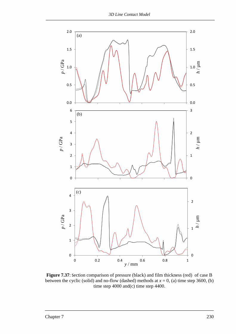
3D Line Contact Model
Chapter 7 230
Figure 7.37: Section comparison of pressure (black) and film thickness (red) of case B
between the cyclic (solid) and no-flow (dashed) methods at x = 0, (a) time step 3600, (b)
time step 4000 and(c) time step 4400.
0.0
0.5
1.0
1.5
2.0
0.0
0.5
1.0
1.5
2.0
h /
µm
p /
GP
a
(a)
0
1
2
3
0
1
2
3
4
5
6
h /
µm
p /
GP
a
(b)
0
1
2
0
1
2
3
4
0 0.2 0.4 0.6 0.8 1
h /
µm
p /
GP
a
y / mm
(c)

3D Line Contact Model
Chapter 7 231
Figure 7.38: Section comparison of pressure (black) and film thickness (red) of case B
between the cyclic (solid) and no-flow (dashed) methods at y = 0.5 mm, (a) time step
3600, (b) time step 4000 and (c) time step 4400.
-2
-1
0
1
2
3
0
1
2
3
h /
µm
p /
GP
a
(a)
-2
-1
0
1
2
3
0
1
2
3
4
h /
µm
p /
GP
a
(b)
-2
-1
0
1
2
3
0
1
2
3
-0.4 -0.2 0 0.2 0.4
h /
µm
p /
GP
a
x / mm
(c)

3D Line Contact Model
Chapter 7 232
Figure 7.39: Section comparison between the results of the cyclic (solid) and no-flow
(dashed) methods at the boundary y ≈ 1 mm of case B at time step 4000, (a) pressure,
(b) and (c) film thickness at different scale.
0
1
2
3
4
p /
GP
a
(a)
0
1
2
3
h /
μm
(b)
0.0
0.2
0.4
-0.4 -0.2 0 0.2 0.4
h /
μm
x / mm
(c)

3D Line Contact Model
Chapter 7 233
Figure 7.40: Difference between results of the cyclic and no-flow methods for case B at
the boundaries y ≈ 0 (left) and y ≈1 (right), ∆𝑝 = 𝑝cyclic − 𝑝no flow (solid) and ∆ℎ =
ℎcyclic − ℎno flow (dashed), (a) time step 3600, (b) time step 4000 and (c) time step 4400
-1.6
-0.8
0.0
0.8
1.6
Δp
/ G
Pa
-0.2
-0.1
0.0
0.1
0.2
Δh /
µm
-1.6
-0.8
0.0
0.8
1.6
Δp /
GP
a
-0.2
-0.1
0.0
0.1
0.2
Δh /
µm
-1.6
-0.8
0.0
0.8
1.6
-0.4 -0.2 0 0.2 0.4
Δp
/ G
Pa
x / mm
-0.20
-0.10
0.00
0.10
0.20
-0.4 -0.2 0 0.2 0.4
Δh
/µ
m
x / mm
(a)
(b)
(c)

3D Line Contact Model
Chapter 7 234
Figure 7.41: Section comparison of pressure (black) and film thickness (red) of case D
between the cyclic (solid) and no-flow (dashed) methods at x = 0, (a) time step 3600, (b)
time step 4000 and (c) time step 4400.
0.0
0.5
1.0
1.5
2.0
0.0
0.5
1.0
1.5
h /
µm
p /
GP
a
(a)
0.0
0.5
1.0
1.5
2.0
0.0
0.5
1.0
1.5
h /
µm
p /
GP
a
(b)
0
1
2
3
0.0
0.5
1.0
1.5
0 0.2 0.4 0.6 0.8 1
h /
µm
p /
GP
a
y / mm
(c)

3D Line Contact Model
Chapter 7 235
Figure 7.42: Section comparison of pressure (black) and film thickness (red) of case D
between the cyclic (solid) and no-flow (dashed) methods at y = 0.5 mm, (a) time step
3600, (b) time step 4000 and (c) time step 4400.
0
1
2
3
0.0
0.5
1.0
1.5
h /
µm
p /
GP
a
(a)
0
1
2
3
0.0
0.5
1.0
1.5
h /
µm
p /
GP
a
(b)
0
1
2
3
0.0
0.5
1.0
1.5
-0.4 -0.2 0 0.2 0.4
h /
µm
p /
GP
a
x / mm
(c)

3D Line Contact Model
Chapter 7 236
Figure 7.43: Section comparison between the results of the cyclic (solid) and no-flow
(dashed) methods at the boundary y ≈ 1 mm of case D at time step 4000, (a) pressure,
(b) and (c) film thickness at different scale.
0.0
0.5
1.0
1.5
p /
GP
a
(a)
0
1
2
3
h /
μm
(b)
0.2
0.4
0.6
0.8
-0.4 -0.2 0 0.2 0.4
h /
μm
x / mm
(c)
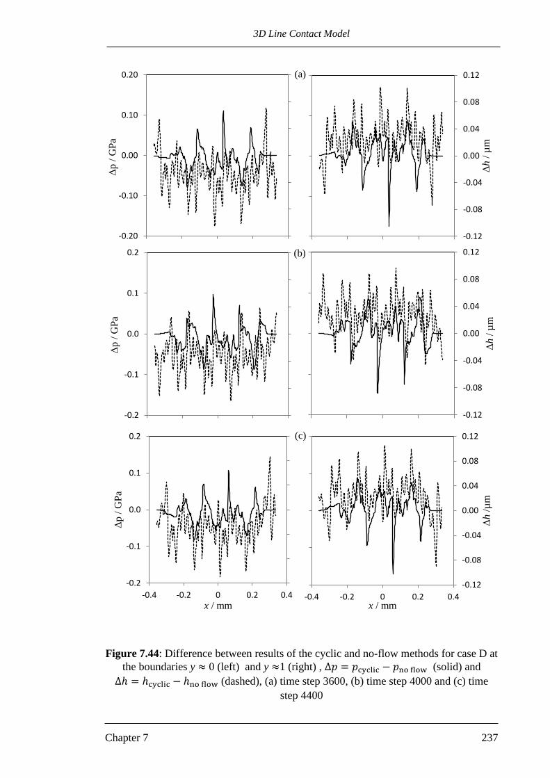
3D Line Contact Model
Chapter 7 237
Figure 7.44: Difference between results of the cyclic and no-flow methods for case D at
the boundaries y ≈ 0 (left) and y ≈1 (right) , ∆𝑝 = 𝑝cyclic − 𝑝no flow (solid) and
∆ℎ = ℎcyclic − ℎno flow (dashed), (a) time step 3600, (b) time step 4000 and (c) time
step 4400
-0.20
-0.10
0.00
0.10
0.20
-0.12
-0.08
-0.04
0.00
0.04
0.08
0.12
Δh
/ µ
m
-0.2
-0.1
0.0
0.1
0.2
Δp /
GP
a
-0.12
-0.08
-0.04
0.00
0.04
0.08
0.12
Δh /
µm
-0.2
-0.1
0.0
0.1
0.2
-0.4 -0.2 0 0.2 0.4
Δp /
GP
a
x / mm
-0.12
-0.08
-0.04
0.00
0.04
0.08
0.12
-0.4 -0.2 0 0.2 0.4
Δh /
µm
x / mm
(a)
(b)
(c)
Δp
/ G
Pa

3D Line Contact Model
Chapter 7 238
The above comparisons give an indication of the difference between the results of
adopting cyclic and no-flow boundary conditions at the boundaries and at the centre of
the contact. A comparison between the results of the two concepts at other positions in
the solution space also needs to be investigated.
The maximum differences between the two methods in both film thickness and pressure
distribution is found in case B at time step 3600 as previously shown in Figure 7.40 (a).
Therefore the results at this time step are further investigated by making more sectional
comparisons between the two methods. Figure 7.45 shows the difference between the
results of the two methods at thirteen y positions. The first and last comparisons (y ≈ 0
and y ≈ 1 mm) in this figure are those previously shown in Figure 7.40 (a) which are
repeated here to give a complete picture of the comparisons over the whole solution
space. It is clear that as the distance from the boundaries is increased, both ∆𝑝 and ∆ℎ
decay significantly. For example, between y ≈ 0.2 mm and y ≈ 0.8 mm results of the
two methods are very similar, and at y ≈ 0.5 mm (centre of the solution space) the
differences are almost zero.

3D Line Contact Model
Chapter 7 239
Figure 7.45: Difference between results of the cyclic and no-flow methods for case B at
time step 3600 at 13 y positions, ∆𝑝 = 𝑝cyclic − 𝑝no flow(solid) and ∆ℎ = ℎcyclic −
ℎno flow(dashed)
x / mm
y ≈ 1 mm
y ≈ 0.95 mm y ≈ 0.9 mm y ≈ 0.85 mm
y ≈ 0.8 mm y ≈ 0.7 mm y ≈ 0.5 mm
y ≈ 0.3 mm y ≈ 0.2 mm y ≈ 0.15 mm
y ≈ 0.1 mm y ≈ 0.05 mm y ≈ 0

Conclusions and future work
Chapter 8 240
Chapter 8
Conclusions and future work
8.1 Conclusions
The thesis has been concerned with the EHL analysis of helical gears where both
smooth and rough surface profiles are considered, and the effect of profile modifications
(such as tip relief and axial crowning ) is also investigated
A full transient point contact numerical analysis procedure for predicting the pressure
and film thickness over the full the meshing cycle of helical gear teeth is developed and
presented in this thesis. Various aspects of the numerical analyses are described in detail
in the thesis and the differential deflection technique is used in the formulation of the
fundamental EHL problem. The point contact solver was available as a starting point for
the work and this was developed to be able to solve the helical gear contact problem.
A range of subroutines were developed to specify all aspects of the kinematics and the
3D shape of the tooth flanks as contact proceeded through the meshing cycle. The EHL
action takes place in the common tangent plane at the contact of the tooth flanks. The
geometry specification in this plane requires the calculation of the contact
characteristics due to the variation in the radius of relative curvature in the plane normal
to the contact line, which changes continually as the contact moves from root to tip.
This fundamental geometry of the involute gears is modified due to profile modification
effects in the transverse and axial directions (tip relief and axial crowning).

Conclusions and future work
Chapter 8 241
Results of EHL analysis were obtained for two examples of helical gear contacts. The
4.5 mm module pinion was the same for both gear pairs with 33 teeth and a 44 mm face
width. The meshing gears gave gear ratios of 1.03 and 3.0, and were chosen to allow the
effect of gear ratio to be assessed as the higher ratio gives a greater variation of
entrainment velocity during the meshing cycle.
Tip relief modification is used to prevent premature tooth engagement under load due to
flexure of the loaded teeth. This can cause a local stress-raising discontinuity in the
curvature of the tooth profile according to the form of tip relief profile adopted. In
addition, axial profile relief is used to prevent edge contact at the side faces of the gears
under misalignment conditions due to mounting errors or shaft deflections. Both of
these microgeometry modifications were included in the analysis and their effects were
considered by variation of the form adopted.
The basic form of tip relief adopted was parabolic so that the slope of the gear profile
was maintained at the transition to the tip relief zone. Using the basic tip relief, a series
of different axial form modifications was introduced with the same edge clearance at the
face edges. Full transient analyses for these cases allowed the effect of the axial form
modifications to be assessed and compared.
A simple axial crown radius was used for evaluations of a number of different tip relief
profiles with each providing the same amount of relief at the tip of the gear. Two forms
of tip relief profile were adopted for the tests. The first was a combination of a parabolic
transition curve to a linear relief profile, with slope continuity throughout. These

Conclusions and future work
Chapter 8 242
profiles varied according to the length of the parabolic section and the subsequent slope
of the linear section. The case of a linear profile was used as an asymptotic limit for the
combined profile. The other profile form adopted was a power law for which a number
of powers were adopted including power 2 to give the parabolic profile. The effect of
the tip relief profile adopted was found to be significant in terms of the peak stresses
and the lubricant film thickness at the location of the transition to tip relief.
A further geometrical modification of the involute form was examined in the form of
axial faceting that results from the generation grinding process. This was found to lead
to significant changes in the EHL results, particularly so for the case of the smallest
number of facets considered (20) which corresponds to facets that are approximately 1
mm long for the gear considered.
Incorporating surface roughness in the EHL analysis of helical gears is a very
significant numerical challenge. This is due to the relatively large size of the contact
area which requires very high resolution to make the model sensitive to the surface
roughness. The transient analyses of the helical tooth contacts led to the conclusion that
most of the contact line behaved as if it was a quasi-steady state line contact. This
observation was developed to provide a means of investigating 3D roughness effects in
the gear contact. A 3D line contact model was developed to solve the EHL problem
over a representative length of the contact line with cyclic transverse boundary
conditions. The elastic deflection analysis was carried out using a Fast Fourier
Transform approach to exploit the periodicity properties in such a way as to obtain an
effective 3D line contact analysis. The advantage of developing such an EHL model is

Conclusions and future work
Chapter 8 243
to have the ability to model a selected area of the contact region and include the real 3D
surface roughness features without sacrificing the accuracy of the analysis.
The conclusions from the work can be categorised into three main parts:
8.1.1 Transient solution of the helical gear meshing cycle including the
effect of tip relief and axial crown modifications (smooth
surfaces):
Comparison of transient and quasi-steady EHL analyses shows the important
influence of time-varying behaviour in helical gears, particularly in its effect on
the detailed distribution of film thickness at the tooth contacts brought about by
tip geometry modifications. This work clearly demonstrates the necessity for
inclusion of the transient terms in the hydrodynamic equation when analysing
gear tooth contacts. Over most of the contact between the meshing teeth an
effective EHL film is predicted, but significant thinning of the film occurs where
the contact reaches the tip relief zone, where transient squeeze film effects
become significant.
Severe thinning of the film where the lubricated line of contact would otherwise
reach the side faces of the gears is substantially alleviated by the introduction of
appropriate crowning. This is most effective in preventing edge contact for
contact lines that cross the centre plane of the teeth but has a diminished effect at
the beginning and end of contact. (It is suggested that this is not the case for spur
gears where crowning can be expected to prevent side edge contact throughout
the meshing cycle).

Conclusions and future work
Chapter 8 244
It is shown that the detailed geometry of the tip relief feature can have a
profound effect on the local contact pressure distribution. For the gear pairs
considered, application of a simple “linear” tip relief introduces a more than
three-fold increase in the nominal contact pressure at the profile modification
start-point compared to that for a gradually blended parabolic relief geometry.
This aggressive stress concentration is accompanied by poor local film forming
capability.
Comparison between the results of different power law modifications illustrates
that the parabolic curve is the ideal form of those considered and the other
higher power law modifications do not lead to significant improvement in the
results. This demonstrates that the continuous change of slope is the important
requirement.
8.1.2 Transient EHL Analysis of Helical Gears Having Faceted Tooth
Surfaces
Closed form equations were derived for the resulting gap between faceted
profiles during the engagement between gear teeth.
The presence of axial facets on the tooth surfaces, which can be the result of the
intermittent nature of the finishing process, have been found to have a
significant effect on the predicted transient EHL behaviour of helical gears.
Small numbers of facets such as 20fn , lead to high stress concentrations
producing maximum pressures of more than three times the corresponding
smooth surface values. This is associated with a breakdown in the film thickness
throughout the meshing cycle. The predictions are considerably improved by

Conclusions and future work
Chapter 8 245
increasing the number of facets, and the case 100fn , for example, shows very
similar results to those found in the smooth surface case.
8.1.3 3D line contact model (rough surfaces)
A 3D line contact EHL model has been developed to predict the effect of surface
roughness on the EHL analysis over a finite length in the transverse direction of
the tooth. This model is based on the use of the FFT method to reflect the
repetition of the solution space along the nominal contact line between the
helical teeth, and is applied to repeating roughness profiles so that transverse
flow at the model boundaries is correctly calculated.
Unlike the case of spur gears, in helical gears the lay of tooth roughness is
generally inclined to the direction in which rolling (entrainment) and sliding take
place. In order to include this feature in the EHL model a closed form equation
has been derived, for the case where the roughness is inclined at an angle with
respect to the nominal contact line. The concept of cyclic boundary conditions at
the boundary of the solution space has been used for the first time in order to
correctly model the behaviour of a short, representative section of the total
contact line.
Cases in which the roughness lay on the two surfaces is either aligned or
“crossed” have been modelled. In general, the crossed extrusion of the
roughness profile produces about three times as many predicted metal to metal
contact points in comparison with aligned extrusion, with a tendency to produce
much higher local pressure values.
A comparison between the concepts of a cyclic boundary condition as presented
in this thesis with the no-flow boundary approach adopted by other workers,

Conclusions and future work
Chapter 8 246
shows that significant transverse pressure gradients develop at the boundary
which are wrongly neglected by imposing the no-flow condition. These pressure
gradients are associated with transverse flows that significantly influence the
results.
8.2 Suggestions for future work
The transient EHL solution of helical gears based on the point contact approach with the
consideration of profile modifications effects is a complex problem. As stated above
this thesis introduces a numerical analysis of all these aspects in addition to developing
the 3D line contact model in order to consider the surface roughness and due to time
constraints there are still other important aspects not considered in this work. Therefore,
it is recommended that further research be undertaken in the following areas:
Inclusion of the thermal effect in the EHL solution of the helical gear meshing
cycle.
The thermal effects can be considered in the EHL analyses by solving the
energy equation for the lubricant film and for the gear flanks. Knowing the
temperature distribution is important due to the lubricant viscosity dependency
on the temperature and the consequence effects on the film thickness. This will
also have to be developed for the case where the lubricant film breaks down and
direct contact occurs between the gears over limited areas.
Considering of the plastic deformation of the roughness asperities in the EHL
analyses.
The interaction between the surfaces asperities during the gear meshing cycle
produces high level of pressure which may lead to a plastic deformation. The

Conclusions and future work
Chapter 8 247
work in this thesis only considers the elastic deformation of the surface which
represents an approximation to the real contact problem. In reality plastic
deflection occurs as new, more extreme, operating conditions are encountered
and the gear pair operates elastically after some shakedown as plastic
deformation occurs.
Development of a contact model for helical gears to calculate the real load
sharing between simultaneous pairs of teeth in contact due to elastic deformation
(predominantly bending) of the teeth under load. This will require a detailed
FEM analysis of the tooth contacts to establish the way in which the load is
distributed in along the contact lines. It may then be possible to use this
information in the EHL analysis to provide solutions which have the same
contact line load distribution characteristics. A way of attempting this would be
to introduce a misalignment of the contact lines of the tooth surfaces in the EHL
analysis and to adjust it so that the resulting contact line load distribution
corresponds to the FEM result.
Development of the current 3D line contact model to consider the effect of
roughness orientation on the predicted fatigue life of the helical gears.
It has been shown in this thesis how the transient pressure distribution resulting
from the EHL analysis of rough surfaces deviates significantly from the
corresponding smooth surface results. As the surface asperities in the two
surfaces interact with each other, a kind of cycling pressure variation over the
contact area occurs. Such loading condition may produce micropitting at the
roughness asperities particularly for low ratio where the pressure deviations

Conclusions and future work
Chapter 8 248
are particularly large. This form of surface failure is considered as a fatigue
failure. Researchers tend to solve the EHL problem related to this form of
fatigue failure in gears based on a line contact EHL approach. This may
introduce significant approximations to the solution of the contact problem from
a fatigue failure consideration. Therefore, extending the 3D line contact model
developed in this thesis to incorporate fatigue analyses may have an impact on
predicting the life of gears.

References
249
References
Ai, X. and Cheng, H. 1994. A transient EHL analysis for line contacts with measured
surface roughness using multigrid technique. Journal of tribology 116, pp. 549–556.
Akbarzadeh, S. and Khonsari, M.M. 2008. Thermoelastohydrodynamic Analysis of
Spur Gears with Consideration of Surface Roughness. Tribology Letters 32, pp. 129–
141.
Alban, L. 1985. Systematic Analysis of Gear Failures. American Society for Metals
B. K. Gears Pvt. Ltd. Available at: http://www.bkgears.com/gears.html#demo2
(Accessed: 2 December 2014).
Bahk, C. and Parker, R.G. 2013. Analytical investigation of tooth profile modification
effects on planetary gear dynamics. Mechanism and Machine Theory 70, pp. 298–319.
Bonori, G., Barbieri, M. and Pellicano, F. 2008. Optimum profile modifications of spur
gears by means of genetic algorithms. Journal of Sound and Vibration 313, pp. 603–
616
Chapra, S.C. and Canale, R. P. 2006. Numerical methods for engineers. 5th ed.
McGraw-Hill.
Chen, W. Liu, S. and Wang, Q. 2008. Fast Fourier Transform Based Numerical
Methods for Elasto-Plastic Contacts of Nominally Flat Surfaces. Journal of Applied
Mechanics 75, pp. 011022(1–11).
Chittenden, R., Dowson, D., Dunn, J. F. and Taylor, C. M. 1985. A theoretical analysis
of the isothermal elastohydrodynamic lubrication of concentrated contacts. II. General
Case, with lubricant entrainment along either principal axis of the Hertzian contact
ellipse or at some intermediate angle. Proc. R. Soc. London, pp. 271-294.
Chittenden, R., Dowson, D., Dunn, J. F. and Taylor, C. M. 1985. A Theoretical
Analysis of the Isothermal Elastohydrodynamic Lubrication of Concentrated Contacts.
I. Direction of Lubricant Entrainment Coincident with the Major Axis of the Hertzian
Contact Ellipse. Proc. R. Soc. London, pp. 245–269.

References
250
Clarke, A. Sharif, K., Evans, H.P., Snidle, R.W. 2006. Heat partition in rolling/sliding
elastohydrodynamic contacts. Journal of Tribology 128, pp. 67-78.
Cooly, J. and Tukey, J. 1965. An algorithm for the machine calculation of complex
Fourier series. Mathmatics Computation 19, pp. 297–301.
Dowson, D. and Higginson, G.R. 1959. A Numerical Solution to the Elasto-
Hydrodynamic Problem. Journal of Mechanical Engineering Science 1, pp. 6–15.
Dowson, D. and Higginson, G.R. 1966. Elastohydrodynamic Lubrication. Pergamon,
Oxford.
Dowson, D. 1979. History of tribology. Longman Ltd
Drago, R.J. 1988. Fundamentals of gear design. Butterworths.
Dudley, D.W. 1969. The evolution of the gear art. American Gear Manufacturers
Association.
Dudley, D.W. 1984. Handbook of practical gear design. McGraw-Hill
Ebrahimi, A. and Akbarzadeh, S. 2013. Mixed-elastohydrodynamic analysis of helical
gears using load-sharing concept. Proceedings of the Institution of Mechanical
Engineers, Part J: Journal of Engineering Tribology 228, pp. 320–331.
Elcoate, C. D. 1996. Coupled solution methods for the elasto- hydrodynamic problem.
PhD thesis, University of Wales, Cardiff.
Elcoate, C.D. , Evans, H.P. and Hughes, T.G. 1998. On the coupling of the
elastohydrodynamic problem. Proceedings of the Institution of Mechanical Engineers,
Part C: Journal of Mechanical Engineering Science 212, pp. 307–318.
Elcoate, C.D. Evans, H.P., Hughes, T.G. and Snidle, R.W. 2001. Transient
elastohydrodynamic analysis of rough surfaces using a novel coupled differential
deflection method. Proceedings of the Institution of Mechanical Engineers, Part J:
Journal of Engineering Tribology 215, pp. 319–337.
Evans, H.P. 2015, Private Communication.

References
251
Evans, H.P. and Snidle, R.W. 1981. The isothermal elastohydrodynamic lubrication of
spheres. Journal of Lubrication Technology 103, pp. 547-557.
Evans, H. P. and Snidle, R.W. 1982. The elastohydrodynamic lubrication of point
contacts at heavy loads. Proc. R. Soc. London, A 382, pp. 183-199.
Evans, H.P. and Hughes, T.G. 2000. Evaluation of deflection in semi-infinite bodies by
a differential method. Proceedings of the Institution of Mechanical Engineers, Part C:
Journal of Mechanical Engineering Science 214, pp. 563–584.
Evans, H.P., Snidle, R.W., Sharif , K.J. and Bryant, M. J. 2012. Predictive modelling of
fatigue failure in concentrated lubricated contacts. Faraday Discussions 156, pp. 105-
121.
Evans, H.P. Snidle, R.W., Sharif, K., Shaw, B. and Zhang, J. 2013. Analysis of micro-
EHL and prediction of surface fatigue damage in micropitting tests on helical gears.
Journal of Tribology 135, p. 011501(1-9).
Fish, J. and Belytschko, T. 2012. A First Cource in Finite Elements. John Wiley & Sons
Ltd.
Hamrock, B.J. and Dowson, D. 1976. Isothermal Elastohydrodynamic Lubrication of
Point Contacts. Part II—Ellipticity Parameter Results. Journal of Lubrication
Technology, pp. 375–381.
Hamrock, B.J. and Dowson, D. 1977. Isothermal elastohydrodynamic lubrication of
point contacts. Part III—Fully flooded results. Journal of Lubrication Technology, pp.
264–275.
Han, L. Zhang, D. and Wang, F. 2013. Predicting Film Parameter and Friction
Coefficient for Helical Gears Considering Surface Roughness and Load Variation.
Tribology Transactions 56, pp. 49–57.
Holmes, M. 2002. Transient analysis of the point contact elastohydrodynamic
lubrication problem using coupled solution methods. PhD thesis, Cardiff University,
UK.

References
252
Holmes, M., Evans, H.P., Hughes, T.G., and Snidle, R.W. 2003a. Transient
elastohydrodynamic point contact analysis using a new coupled differential deflection
method, Part 1: Theory and validation. Proceedings of the Institution of Mechanical
Engineers, Part J: Journal of Engineering Tribology 217, pp. 289–304.
Holmes, M., Evans, H.P., Hughes, T.G., and Snidle, R.W. 2003b. Transient
elastohydrodynamic point contact analysis using a new coupled differential deflection
method Part 2: results. Proceedings of the Institution of Mechanical Engineers, Part J:
Journal of Engineering Tribology 217, pp. 305–321.
Houghton, P.S. 1961. Gears: Spur, Helical, Bevel and Worms. The Technical Press
LTD, London .
Houpert, L. and Hamrock, B. 1986. Fast approach for calculating film thicknesses and
pressures in elastohydrodynamically lubricated contacts at high loads. Journal of
Tribology 108, pp. 411–419.
Hu, Y. and Zhu, D. 2000. A full numerical solution to the mixed lubrication in point
contacts. Journal of Tribology 122, pp. 1–9.
Hughes, T.G. Elcoate, C.D., and Evans, H.P. 2000. Coupled solution of the
elastohydrodynamic line contact problem using a differential deflection method.
Proceedings of the Institution of Mechanical Engineers, Part C: Journal of Mechanical
Engineering Science 214, pp. 585–598.
Johnson, K. Greenwood, J. and Poon, S. 1972. A simple theory of asperity contact in
elastohydro-dynamic lubrication. Wear 19, pp. 91–108.
Johnson, K.L. and Tevaarwerk, J.L. 1977. Shear Behaviour of Elastohydrodynamic Oil
Films. Proc. R. Soc. London, A.356, pp. 215–236
Jost, P.H. 1966. Lubrication (Tribology) Education and Research. A Report on the
Present Position and Industry Needs. London.

References
253
Kahraman, A. and Blankenship, G. 1999. Effect of involute tip relief on dynamic
response of spur gear pairs. Journal of Mechanical Design 121, pp. 313-315.
Kahraman, A., Bajpai, P., and Anderson, N. 2005. Influence of Tooth Profile Deviations
on Helical Gear Wear. Journal of Mechanical Design 127, pp. 656-663.
Kong, S. 2001. Contact, kinematics and film formation in worm gears. PhD thesis,
University of Wales, UK.
Kreyszig, E. 1999. Advanced engineering mathematics. 8th edition. John Wiley & Son,
Inc.
Kugimiya, H. 1966. Profile Modification of Helical Gear Teeth. The Japan Society of
Mechanical Engineers 9, pp. 829–841.
Kweh, C.C., Evans, H.P., and Snidle, R.W. 1989. Micro-elastohydrodynamic
lubrication of an elliptical contact with transverse and three-dimensional sinusoidal
roughness. Journal of Tribology 111, pp. 577–584.
Kweh, C.C., Patching, M.J., Evans, H.P. and Snidle, R.W. 1992. Simulation of
elastohydrodynamic contacts between rough surfaces. Journal of Tribology 114, pp.
412–419.
Larsson, R. 1997. Transient non-Newtonian elastohydrodynamic lubrication analysis of
an involute spur gear. Wear 207, pp. 67–73.
Lee, K., and Cheng, H.S. 1973. Effect of surface asperity on elastohydrodynamic
lubrication. NASA CR-2195.
Li, S., Vaidyanathan, A., Harianto, J. and Kahraman, A. 2009. Influence of Design
Parameters on Mechanical Power Losses of Helical Gear Pairs. Journal of Advanced
Mechanical Design, Systems, and Manufacturing 3, pp. 146–158.
Li, S. and Kahraman, a. 2010. A Transient Mixed Elastohydrodynamic Lubrication
Model for Spur Gear Pairs. Journal of Tribology 132, pp. 011501(1-9).

References
254
Li, S. and Kahraman, A. 2010. Prediction of Spur Gear Mechanical Power Losses Using
a Transient Elastohydrodynamic Lubrication Model. Tribology Transactions 53, pp.
554–563.
Li, S. 2013. Influence of Surface Roughness Lay Directionality on Scuffing Failure of
Lubricated Point Contacts. Journal of Tribology 135, pp. 041502(1-9).
Li, S., Kahraman, A., Anderson, N. and Wedeven, L. 2013. A model to predict scuffing
failures of a ball-on-disk contact. Journal of Tribology International 60, pp. 233–245.
Litvin, F. and Fuentes, A. 2004. Gear Geometry and Applied Theory. Cambridge
University Press.
Litvin, F., Gonzalez, I., Fuentes, A., Hayasaka, K. and Yukishima, K. 2005. Topology
of modified surfaces of involute helical gears with line contact developed for
improvement of bearing contact, reduction of transmission errors, and stress analysis.
Journal of Mathematical and Computer Modelling 42, pp. 1063–1078.
Liu, H., Mao, K., Zhu, C., Chen, S., Xu, X. and Liu, M. 2013. Spur Gear Lubrication
Analysis with Dynamic Loads. Tribology Transactions 56, pp. 41–48.
Liu, S. Wang, Q. And Liu, G. 2000. A versatile method of discrete convolution and FFT
(DC-FFT) for contact analyses. Wear 243, pp. 101–111.
Lubrecht, A. Napel, W. and Bosma, R. 1986. Multigrid, an alternative method for
calculating film thickness and pressure profiles in elastohydrodynamically lubricated
line contacts. Journal of Tribology 108. pp. 551-556
Lubrecht, A., Ten, W. And Bosma, R. 1988. The influence of longitudinal and
transverse roughness on the elastohydrodynamic lubrication of circular contacts.
Journal of Tribology 110, pp. 421–426.
Maitra, G.M. 1994. Handbook of Gear Design. Tata McGraw-Hill Education.
Mobil Oil Corporation, 1979, “Mobil EHL Guide Book”, Products Department, 150
East 42nd Street, New York.

References
255
Morales-Espejel, G.E. 2013. Surface roughness effects in elastohydrodynamic
lubrication: A review with contributions. Proceedings of the Institution of Mechanical
Engineers, Part J: Journal of Engineering Tribology 0, pp. 1-26
Morris, S.J. 2000.Traction in elliptical point contacts, PhD thesis, University of Wales,
UK.
Nijenbanning, G., Venner, C. and Moes, H. 1994. Film thickness in
elastohydrodynamically lubricated elliptic contacts. Wear 176, pp. 217-229
Nussbaumer, H.J. 1982. Fast Fourier transform and convolution algorithms. 2nd ed.
Springer-Verlag.
Park, S. and Yoo, W. 2004. Deformation overlap in the design of spur and helical gear
pair. Finite Elements in Analysis and Design 40, pp. 1361–1378.
Patir, N. and Cheng, H. 1978. An average flow model for determining effects of three-
dimensional roughness on partial hydrodynamic lubrication. Journal of lubrication
Technology 100, pp. 12–17.
Patching, M.J., Kweh, C.C., Evans, H.P., & Snidle, R.W., 1995, “Conditions for
scuffing failure of ground and superfinished steel disks at high sliding speeds using a
gas turbine engine oil”, Trans. ASME Journal of Tribology, v.117, pp. 482-489.
Polonsky, I. and Keer, L. 2000. Fast Methods for Solving Rough Contact Problems: A
Comparative Study. Journal of Tribology 122, pp. 36–41.
Poon, C. and Sayles, R. 1994. Numerical Contact Model of a Smooth Ball on an
Anisotropic Rough Surface. Journal of Tribology 116, pp. 194-201
Press, W., Teukolsky, S., Vetterling, W., and Flannery, B. 1992. Numerical recipes in
FORTRAN, The art of scientific computing. Cambridge University Press.
Ranger, A., Ettles, C. and Cameron, A. 1975. The Solution of the Point Contact Elasto-
Hydrodynamic Problem. Proc. R. Soc. London, A.346, pp. 227–244
Ren, N., Dong, Z., Chen, W., Liu, Y. And Wang, Q. 2009. A Three-Dimensional
Deterministic Model for Rough Surface Line-Contact EHL Problems. Journal of
Tribology 131, pp. 011501(1–9).

References
256
Roelands, C. 1966. Correlational aspects of the viscosity-temperature-pressure
relationships of lubricating oils. PhD thesis, Technical University Delft, The
Netherlands
Sankar, S. and Nataraj, M. 2010. Prevention of helical gear tooth damage in wind
turbine generator: A case study. Proceedings of the Institution of Mechanical Engineers,
Part A: Journal of Power and Energy 224, pp. 1117–1125.
Sharif, K.J. Kong, S., Evans, H.P. and Snidle, R.W. 2001. Contact and
elastohydrodynamic analysis of worm gears Part 1: theoretical formulation.
Proceedings of the Institution of Mechanical Engineers, Part C: Journal of Mechanical
Engineering Science 215, pp. 817–830
Sharif, K.J. Evans, H. P., Snidle, R. W. and Newall, J. P. 2004. Modeling of Film
Thickness and Traction in a Variable Ratio Traction Drive Rig. Journal of Tribology
126, 92-104
Simon, V. 1988. Thermo-EHD analysis of lubrication of helical gears. Journal of
Mechanisms, Transmissions, and Automation in Design 110, pp.330-336
Simon, V. 1989. Optimal tooth modifications for spur and helical gears. Journal of
Mechanisms, Transmissions, and Automation in Design 111, pp. 611–615.
Snidle, R.W. and Evans, H.P. 2009. Some aspects of gear tribology. Proceedings of the
Institution of Mechanical Engineers, Part C: Journal of Mechanical Engineering
Science 223, pp. 103–141.
Stanley, H. and Kato, T. 1997. An FFT-based method for rough surface contact. Journal
of tribology 119, pp. 481–485.
Tao, J., Hughes, T.G., Evans, H.P., Snidle, R.W., Hopkinson, N.A., Talks, M., and
Starbuck, J.M. 2003. Elastohydrodynamic Lubrication Analysis of Gear Tooth Surfaces
From Micropitting Tests. Journal of Tribology 125, pp. 267-274.
Timoshenko, S.P. and Goodier, J.N. 1951. Theory of elasticity. 2nd ed. McGraw-Hill.

References
257
Tuplin, W.A. 1962. Involute gear geometry. Chatto and Windus, London.
Venner, C. and Lubrecht, A. 1994. Numerical simulation of a transverse ridge in a
circular EHL contact under rolling/sliding. Journal of Tribology 116. pp. 751-761
Wagaj, P. and Kahraman, A. 2002. Influence of Tooth Profile Modification on Helical
Gear Durability. Journal of Mechanical Design 124, pp. 501-510.
Walker, H. 1940. Gear tooth deflection and profile modification. The Engineer 166. pp.
102-104.
Wang, W, Wang, H., Liu, Y., Hu, Y., and Zhu, D. 2003. A comparative study of the
methods for calculation of surface elastic deformation. Proceedings of the Institution of
Mechanical Engineers, Part J: Journal of Engineering Tribology 217, pp. 145–153.
Wang, Y. Li, H., Tong, J., Yang, P. 2004. Transient thermoelastohydrodynamic
lubrication analysis of an involute spur gear. Tribology International 37, pp. 773–782.
Wang, Y.Q. He, Z. and Su, W. 2012. Effect of Impact Load on Transient
Elastohydrodynamic Lubrication of Involute Spur Gears. Tribology Transactions 55,
pp. 155–162.
Zhang, J. and Shaw, B.A. 2011. The Effect of Superfinishing on the Contact Fatigue of
Case Carburised Gears. Journal of Applied Mechanics and Materials 86, pp. 348–351.
Zhu, D. 2007. On some aspects of numerical solutions of thin-film and mixed
elastohydrodynamic lubrication. Proceedings of the Institution of Mechanical
Engineers, Part J: Journal of Engineering Tribology 221, pp. 561–579.
Zhu, D., Ren, N. and Wang, Q. 2009. Pitting Life Prediction Based on a 3D Line
Contact Mixed EHL Analysis and Subsurface von Mises Stress Calculation. Journal of
Tribology 131(4), pp. 041501(1–8).
Zhu, D. and Wang, Q. 2013. Effect of Roughness Orientation on the
Elastohydrodynamic Lubrication Film Thickness. Journal of Tribology 135, p.
031501(1-9).

List of Publications Arising from this Study
Appendix 258
Appendix
List of Publications Arising from this Study
1- Jamali, H.U., Sharif, K., Evans, H.P. and Snidle, R.W. 2014. The transient
effects of profile modification on elastohydrodynamic oil films in helical
gears. Tribology Transactions 58 (1), pp. 119-130.
2- Jamali, H.U., Sharif, K., Evans, H.P. and Snidle, R.W. 2014. Transient EHL
analysis of helical gears. Presented at: International Gear Conference 2014,
Lyon Villeurbanne, France, 26-28 August 2014. International Gear Conference
2014 - Conference Proceedings. Cambridge: Woodhead Publishing, pp. 721-
730.
3- Clarke, A., Jamali, H.U., Weeks, I., Sharif, K., Evans, H.P. and Snidle,
R.W. 2014. The influence of macro and micro geometry on the generation of
adverse contact conditions associated with micropitting in gear tooth
contacts. Presented at: Gears 2014 technical awareness seminar, Newcastle,
England, 20 November 2014.
4- Jamali, H.U., Sharif, K., Evans, H.P. and Snidle, R.W. 2013. Analysis of
elastohydrodynamic lubrication of helical gear tooth contacts including the
effects of crowning and the form of tip relief. Presented at: International
Conference on Gears 2013, Dusseldorf, Germany, 7-9 October 2013.
5- Snidle, R.W., Sharif, K., Evans, H.P. and Jamali, H.U. 2013. Transient
elastohydrodynamic analysis of helical gear tooth contacts. Presented at: 68th
STLE Annual Meeting & Exhibition, Detroit Marriott at the Renaissance Center
Detroit, MI, USA, 5-9 May 2013.
Copyright © 2022 FDOKUMEN