ANALYSIS OF FLOW IN SOLAR CHIMNEY
312
ANALYSIS OF FLOW IN SOLAR CHIMNEY FOR AN OPTIMAL DESIGN PURPOSE Atit Koonsrisuk A Thesis Submitted in Partial Fulfillment of the Requirements for the Degree of Doctor of Philosophy in Mechanical Engineering Suranaree University of Technology Academic Year 2009
-
Upload
khangminh22 -
Category
Documents
-
view
0 -
download
0
Transcript of ANALYSIS OF FLOW IN SOLAR CHIMNEY

ANALYSIS OF FLOW IN SOLAR CHIMNEY
FOR AN OPTIMAL DESIGN PURPOSE
Atit Koonsrisuk
A Thesis Submitted in Partial Fulfillment of the Requirements for the
Degree of Doctor of Philosophy in Mechanical Engineering
Suranaree University of Technology
Academic Year 2009

การวิเคราะหการไหลในระบบปลองลมแดดเพื่อหาแนวทางออกแบบ
ใหไดประสิทธิภาพสูงสุด
นายอาทิตย คูณศรีสุข
วิทยานิพนธนีเ้ปนสวนหนึง่ของการศึกษาตามหลักสูตรปริญญาวิศวกรรมศาสตรดษุฎีบัณฑิต
สาขาวิชาวิศวกรรมเครื่องกล
มหาวิทยาลัยเทคโนโลยีสุรนารี
ปการศึกษา 2552


อาทิตย คูณศรีสุข : การวิเคราะหการไหลในระบบปลองลมแดดเพื่อหาแนวทางออกแบบใหไดประสิทธิภาพสูงสุด (ANALYSIS OF FLOW IN SOLAR CHIMNEY FOR AN OPTIMAL DESIGN PURPOSE) อาจารยที่ปรึกษา : รองศาสตราจารย ดร.ทวิช จิตรสมบูรณ, 278 หนา รายงานวิจัยนี้ศึกษาการไหลในระบบปลองลมแดด ซ่ึงเปนอุปกรณที่ใชแสงแดดสรางการ
ไหลของลมขึ้นภายในระบบ จากนั้นใชกังหันเทอรไบนเปลี่ยนรูปพลังงานของกระแสลมไปเปนกระแสไฟฟา จุดประสงคหลักของงานวิจัยนี้เพื่อหาทางเพิ่มประสิทธิภาพใหระบบ โดยศึกษาลักษณะการทํางานที่เหมาะสมสําหรับปลองลมแดดเพื่อหาแนวทางการออกแบบใหไดประสิทธิภาพสูงสุด
ในชวงตนของการศึกษานี้ ไดใชการวิเคราะหมิติ (dimensional analysis) เพื่อหาตัวแปรไรมิติ (dimensionless variables) ที่สําคัญสําหรับการไหลในระบบปลองลมแดด เพื่อชวยในการออกแบบการทดลอง ที่สามารถใชขอมูลที่ทดสอบจากแบบจําลองระบบปลองลมแดดขนาดเล็ก ในการทํานายผลที่จะเกิดขึ้นในโรงงานตนแบบปลองลมแดดได จากการศึกษาพบวา เมื่อแบบจําลองขนาดเล็ก (model) มีความเสมือนทางดานรูปทรง (geometric similarity) กับโรงงานตนแบบ (prototype) ระบบทั้งสองจะมีความเสมือนทางดานพลศาสตร (dynamic similarity) ก็ตอเมื่อ คาความเขมแสงแดด (insolation) ของระบบทั้งสองตองไมเทากัน ซ่ึงเปนสภาวะที่ทําไดยากในทางปฏิบัติ อยางไรก็ตาม ในการศึกษาที่บังคับใหคาความเขมแสงแดดของระบบทั้งสองตองเทากันพบวา ระบบทั้งสองสามารถมีความเสมือนทางดานพลศาสตรได หากระบบทั้งสองมีความเสมือนทางดานรูปทรงเพียงบางสวน (partial geometric similarity) กลาวคือ รัศมีหลังคารับแดด (solar collector) ของแบบจําลองตองสั้นกวาที่ควรจะเปนสําหรับแบบจําลองที่มีความเสมือนทางดานรูปทรงกับโรงงานตนแบบ ในการตรวจสอบความถูกตองของผล ที่ไดจากการวิเคราะหมิตินี้ ผูวิจัยไดใชการคํานวณเชิงตัวเลข (numerical method) เพื่อหาคาคุณสมบัติการไหล (flow properties) ในระบบ แลวนําผลที่ไดมาคํานวณหาคาตัวแปรไรมิติ ซ่ึงผลการคํานวณยืนยันความนาเชื่อถือท่ีพบในการศึกษานี้ และจากรูปแบบความสัมพันธระหวางตัวแปรไรมิติที่คนพบในครั้งนี้ ไดนําไปสูการยุบรวมตัวแปรที่สําคัญของระบบทั้งหมดไดเปนตัวแปรไรมิติเพียงหนึ่งตัวแปร ซ่ึงจากผลการคํานวณเชิงตัวเลขและผลการทดลองจากโรงงานตนแบบที่ไดเคยมีการสรางไวจริงที่ประเทศสเปนพบวา คาตัวแปรไรมิติตัวใหมที่พบนี้มีคาประมาณ 1 สําหรับแบบจําลองทุกขนาดที่มีการตรวจสอบ

II
จากนั้นไดนําผลที่ตัวแปรไรมิติมีคาเทากับ 1 นี้ ไปสรางเปนแบบจําลองคณิตศาสตร(mathematical model) เพื่อใชประเมินศักยภาพของระบบปลองลมแดด และใชเปรียบเทียบกับผลการคํานวณของแบบจําลองคณิตศาสตรที่นักวิจัยทานอื่นไดพัฒนาไวอีกจํานวน 5 แบบจําลอง โดยในการคํานวณนี้ไดศึกษาผลกระทบเมื่อขนาดของโรงงาน ไดแก รัศมีกับความสูงของหลังคารับแดด และรัศมีกับความสูงของปลองลมเปลี่ยนไป รวมทั้งผลกระทบเมื่อความเขมแสงแดดเปลี่ยนไปดวย เมื่อเปรียบเทียบผลการคํานวณทั้งหมดกับผลการคํานวณเชิงตัวเลขจากโปรแกรมสําเร็จรูป พบวาแตละแบบจําลองมีขอดี-ขอเสียตางกันไป ซ่ึงในการศึกษานี้ไดใหคําแนะนําในการเลือกใชแบบจําลองที่เหมาะสมไวดวย
เมื่อไดศึกษาผลกระทบของการเปลี่ยนแปลงขนาดหนาตัดการไหลโดยใชแบบจําลองคณิตศาสตรรวมกับการคํานวณเชิงตัวเลขพบวา เมื่ออัตราสวนระหวางพื้นที่หนาตัดของหลังคารับแดดที่ทางเขาตอดวยที่ทางออกมีคานอยกวา 1 จะสามารถเพิ่มศักยภาพใหระบบได และเมื่ออัตราสวนระหวางพื้นที่หนาตัดของปลองลมที่ทางออกตอดวยที่ทางเขามีคามากกวา 1 ศักยภาพของระบบก็เพิ่มขึ้นเชนกัน และสําหรับระบบที่ใชหลังคารับแดดที่มีอัตราสวนระหวางพื้นที่หนาตัดที่ทางเขาตอดวยที่ทางออกมีคานอยกวา 1 รวมกับปลองลมที่มีอัตราสวนระหวางพื้นที่หนาตัดที่ทางออกตอดวยที่ทางเขามีคามากกวา 16 พบวาคาศักยภาพของระบบเพิ่มขึ้นหลายรอยเทาจากระบบปกติที่ใชกัน
ในการศึกษาที่กลาวมาแลวนั้น เนื่องจากเปนการประเมินศักยภาพของระบบจึงยงัไมไดรวมกังหันเทอรไบนไวในการศึกษา และเมื่อไดมีการพัฒนาแบบจําลองคณิตศาสตรที่รวมกังหันเทอรไบนไวดวย พบวา คาอัตราสวนระหวางความดันที่กังหันเทอรไบนดูดซับไวไดตอดวยความดันรวมที่เกิดขึ้นในระบบมีคาเทากับ 2/3 สําหรับระบบที่กําหนดใหความดันรวมดังกลาวนี้มีคาคงที่ไมขึ้นกับความดันที่กังหันเทอรไบนดูดซับไวได แตสําหรับระบบที่ใหความดันรวมแปรผันไดตามความดันที่กังหันเทอรไบนดูดซับพบวา คาอัตราสวนของความดันดังกลาวนั้นมีคาเปลี่ยนแปลงขึ้นกับขนาดโรงงานและความเขมแสงแดด
เพื่อจะประเมินผลการศึกษาเชิงทฤษฎีและเชิงตัวเลข ไดมีการสรางแบบจําลองขนาดเล็กของระบบปลองลมแดดที่ไมมีกังหันเทอรไบนขึ้นจํานวน 4 ชุดที่มหาวิทยาลัยเทคโนโลยีสุรนารี อ.เมือง จ.นครราชสีมา พบวาผลการทดลองมีคาตางไปจากคาที่ทํานายไว แตมีแนวโนมของขอมูลเหมือนที่ทํานายไว ซ่ึงคาดวาเปนผลเนื่องจากความเขมแสงแดดที่ไมคงที่ขณะทําการทดลองและเนื่องจากระบบมีหลังคาที่เล็กไปเมื่อเทียบกับขนาดของปลองลม นอกจากนี้ คาตัวแปรไรมิติที่คํานวณจากชุดทดลองที่ออกแบบใหมีความเสมือนกันทางพลศาสตร ก็มีความตางกันซึ่งคาดวาเปนผลเนื่องจากความผันแปรของสภาพอากาศขณะวัดผล


ATIT KOONSRISUK : ANALYSIS OF FLOW IN SOLAR CHIMNEY FOR
AN OPTIMAL DESIGN PURPOSE. THESIS ADVISOR : ASSOC. PROF.
TAWIT CHITSOMBOON, Ph.D., 278 PP.
SOLAR CHIMNEY/SOLAR TOWER/DIMENSIONAL ANALYSIS/GEOMETRIC
EFFECTS/THEORETICAL MODEL/SOLAR ENERGY/CONSTRUCTAL
DESIGN/NATURAL CONVECTION.
The thesis studies flow in a solar chimney, a device for generating electricity
from solar energy by means of a turbine extracting the flow energy from the hot air
rising through a tall chimney with the ultimate goal of a better design to obtain a
higher efficiency. Operating characteristics that are significant to the flow in solar
chimney are sought and studied to aid in the optimization of solar chimney design.
Dimensional analysis is applied to determine the dimensionless variables to
guide the experimental study of flow in a small-scale solar chimney model. The study
shows that if the model is required to be geometrically similar to the prototype, then
the dynamic similarity condition requires the solar heat fluxes of the two cases to be
different, an inconvenient requirement in an experimental setup. Further study shows
that, to achieve the same-heat-flux condition, the roof radius between the prototype
and its scaled models must be dissimilar, while all other remaining dimensions of the
models remain similar to those of the prototype. The functional relationship obtained
suggests that it would be possible to group all the relevant variables into a single
dimensionless product. Three physical configurations of the plant were numerically
tested for similarity: fully geometrically similar, partially geometrically similar, and
dissimilar types. The values of the proposed single dimensionless variable for all these

V
cases are found to be nominally equal to unity. The value for the physical plant
actually built and tested previously is also evaluated and found to be about the same as
that of the numerical simulations, suggesting the validity of the proposition.
Moreover, the study compares the predictions of performances of solar
chimney power plants by using five theoretical models that have been proposed in the
literature. The parameters used in the study are various plant geometrical parameters
and the solar heat flux. Numerical results from the carefully calibrated CFD
simulations are used for comparison with the theoretical predictions. The power output
and the efficiency of the solar chimney plants are used as functions of the studied
parameters to compare relative merits of the five theoretical models. Models that
performed better are finally recommended.
Guided by a theoretical prediction, CFD is used to investigate the changes in
flow properties caused by the variation of flow area. It appears that the sloping
collector affects the flow properties through the plant. The divergent-top chimney
leads to significant augmentations in kinetic energy at the tower base. It is shown that
the proper combination of the sloping roof and the divergent-top chimney can produce
power as much as hundreds times that of the conventional solar chimney power plant.
An analytical turbine model is developed in order to evaluate the performance
of the solar chimney power plant. The relationships between the ratio of the turbine
pressure drop to the pressure potential (available system pressure difference), the mass
flow rate, the temperature rise across the collector and the power output are presented.
The model shows that, for the system with a constant pressure potential, the optimum
ratio of the turbine pressure drop to the pressure potential is 2/3. For the system with


ACKNOWLEDGEMENTS
The process of bringing this thesis to its final state has not been smooth; it has
run a gauntlet of various discouraging and disappointing circumstances. However,
through the support and understanding of many this thesis is now complete. It is my
great pleasure to thank many people who have contributed to this thesis.
I would like to thank Dr.Tawit Chitsomboon for the role he has played as my
thesis advisor. Despite a very busy schedule, he always found the time to listen and to
offer constructive advice. His suggestions have always been excellent and he has been
a pleasure to work with.
With gratitude, I acknowledge the advice and expertise of the brilliant teachers
who helped me learn thermal physics, Dr.Vorapot Khompis. I also would like to thank
Dr.Kontorn Chamniprasart for the support and encouragement he has given me. In
addition, I am also thankful for the support and useful advice from Dr.Eckart Schulz.
It has been a pleasure to know Dr.Arjuna Peter Chaiyasena and his wife,
Mantana, whose confidence in my ability has always exceeded my own. To them, I
express my warm appreciation and sincere thanks.
I am greatly indebted to Prof. Adrian Bejan, Duke University, and Prof. Sylvie
Lorente, Université de Toulouse, for their generous support in so many ways. I would
like to thank them for their kind encouragements. I would also like to thank Duke
University for their support of my research activities as a Visiting Research Scholar in
the Constructal Design Group at Duke University.
I thank the faculty and staff of Suranaree University of Technology, for
providing support in a multitude of forms, and especially for creating an environment

VIII
in which research work was valued and encouraged. I take this opportunity to extend
my very sincere thanks to Mr.Prasittichai Dumnoentitikij, Mr.Satip Churirutporn and
Mr.Satta Posawang, the staff of the Center for Scientific and Technological
Equipment of Suranaree University of Technology, for their ungrudging moral and
technical support in this work.
I owe special thanks to my friends and their families for their invaluable
help and encouragement. Their influence and stimulation are impossible to
quantify or detail in full. Six people, however, may be fondly acknowledged:
Mr.Chatchai Chanprasert, Mr.Chawean Chaiyapoom, Mr.Choowong Chareonsawat,
Mr.Khajornwit Uttawat, Mr.Methee Sophon, and Mr.Somporn Srichoo. It was and is
a pleasure to know all of them.
This research has been supported financially by the Royal Golden Jubilee
(RGJ) Ph.D. Program of the Thailand Research Fund (TRF). The support is gratefully
acknowledged.
Finally, I shall be failing in my obligation if I do not express a special
acknowledgement to my mother, Mrs.Neeracha Koonsrisuk. She endured missing me
for a long time while the thesis was being studied, but provided me steadfast support
and understanding. Her encouragement and patience have been unlimited.
Let me end the list here and note that, despite all the help and advice I
received, I remain responsible for errors and infelicities of this thesis.
Atit Koonsrisuk

TABLE OF CONTENTS
Page
ABSTRACT (THAI) ...................................................................................................... I
ABSTRACT (ENGLISH) ........................................................................................... IV
ACKNOWLEDGEMENT..........................................................................................VII
TABLE OF CONTENTS ............................................................................................ IX
LIST OF TABLES .....................................................................................................XV
LIST OF FIGURES................................................................................................. XVII
LIST OF SYMBOLS AND ABBREVIATIONS.................................................. XXVI
CHAPTER
I INTRODUCTION ............................................................................ 1
1.1 Rationale of the Study .................................................................. 1
1.2 Research Objectives ..................................................................... 7
1.3 Thesis Contents ............................................................................ 7
1.4 Expectation................................................................................. 10
1.5 Reference.................................................................................... 10
II LITERATURE REVIEW .............................................................. 11
Reference.......................................................................................... 14

X
TABLE OF CONTENTS (continued)
Page
III DYNAMIC SIMILARITY IN SOLAR
CHIMNEY MODELING............................................................... 17
3.1 Abstract ...................................................................................... 17
3.2 Introduction ................................................................................ 17
3.3 Dimensional Analysis................................................................. 21
3.4 CFD Modeling............................................................................ 29
3.5 Results and Discussion............................................................... 33
3.6 Conclusion.................................................................................. 41
3.7 Reference.................................................................................... 43
IV PARTIAL GEOMETRIC SIMILARITY FOR SOLAR
CHIMNEY POWER PLANT MODELING ................................ 45
4.1 Abstract ...................................................................................... 45
4.2 Introduction ................................................................................ 46
4.3 Dimensional Analysis................................................................. 50
4.4 Computational Work .................................................................. 55
4.5 Results and Discussion............................................................... 58
4.6 Engineering Interpretation of the Dimensionless variables ....... 63
4.7 Conclusion.................................................................................. 64
4.8 Reference.................................................................................... 65
XI
TABLE OF CONTENTS (continued)
Page
V A SINGLE DIMENSIONLESS VARIABLE FOR SOLAR
CHIMNEY POWER PLANT MODELING ................................ 68
5.1 Abstract ...................................................................................... 68
5.2 Introduction ................................................................................ 69
5.3 Dimensional Analysis................................................................. 72
5.4 Computational Work .................................................................. 74
5.5 Results and Discussion............................................................... 78
5.6 Conclusion.................................................................................. 88
5.7 Reference.................................................................................... 89
VI ACCURACY OF THEORETICAL MODELS IN THE
PREDICTION OF SOLAR CHIMNEY POWER PLANT
PERFORMANCE .......................................................................... 91
6.1 Abstract ...................................................................................... 91
6.2 Introduction ................................................................................ 91
6.3 Theoretical Models..................................................................... 93
6.4 Computational Work .................................................................. 98
6.5 Results and Discussion............................................................. 100
6.6 Conclusion................................................................................ 111
6.7 Reference.................................................................................. 112

XII
TABLE OF CONTENTS (continued)
Page
VII EFFECT OF FLOW AREA CHANGE ON THE
POTENTIAL OF SOLAR CHIMNEY POWER
PLANT .......................................................................................... 114
7.1 Abstract .................................................................................... 114
7.2 Introduction .............................................................................. 114
7.3 Derivation of the Theoretical Models....................................... 117
7.4 Computational Work ................................................................ 121
7.5 Results and Discussion............................................................. 126
7.6 Conclusion................................................................................ 130
7.7 Reference.................................................................................. 138
VIII THEORETICAL TURBINE POWER YIELD IN SOLAR
CHIMNEY POWER PLANT...................................................... 140
8.1 Abstract .................................................................................... 140
8.2 Introduction .............................................................................. 141
8.3 Optimal Pressure Ratio............................................................. 143
8.4 Analytical Model ...................................................................... 146
8.5 Analytical Solution Procedure.................................................. 149
8.6 Results and Discussion............................................................. 150
8.7 Conclusion................................................................................ 163
8.8 Reference.................................................................................. 170

XIII
TABLE OF CONTENTS (continued)
Page
IX EXPERIMENTAL PERFORMANCE OF A
DEMONSTRATION SOLAR CHIMNEY MODEL ................ 173
9.1 Abstract .................................................................................... 173
9.2 Introduction .............................................................................. 174
9.3 The physical Models ................................................................ 175
9.4 Experimental Methodology...................................................... 175
9.5 Computational Works............................................................... 176
9.6 Results and Discussion............................................................. 177
9.7 Conclusion................................................................................ 224
9.8 Problems and Challenges in the Research................................ 225
9.9 Reference.................................................................................. 226
X CONSTRUCTAL SOLAR CHIMNEY CONFIGURATION
AND MULTI-SIZE DISTRIBUTION ON LAND .................... 227
10.1 Abstract .................................................................................. 227
10.2 Introduction ............................................................................ 228
10.3 Geometry ............................................................................... 231
10.4 Pumping Effect....................................................................... 231
10.5 More Air Flow Rate .............................................................. 234
10.6 More Power ............................................................................ 236
10.7 Volume Constraint ................................................................ 238

XIV
TABLE OF CONTENTS (continued)
Page
10.8 Model Validation.................................................................... 239
10.9 Additional Losses .................................................................. 244
10.10 Few large, or many small? ................................................... 246
10.11 Conclusion............................................................................ 261
10.12 Reference.............................................................................. 262
XI CONCLUSION AND RECOMMENDATION.......................... 264
APPENDICES
APPENDIX A A SET UP OF THE ANSYS-CFX 10.0 SOLVER........... 268
APPENDIX B LIST OF PUBLICATIONS .............................................. 275
BIOGRAPHY............................................................................................................ 278

LIST OF TABLES
Table Page
1.1 Advantages and disadvantages of the solar chimney technology........................8
1.2 Categories of the approaches used in each chapter............................................. 9
3.1 Powers of primitive variables in terms of fundamental dimensions................. 25
3.2 Solar heat absorption per unit volume (S.H.A.V.) requirements
for dynamic similarity....................................................................................... 42
4.1 Specification of prototype and models ............................................................. 56
5.1 Specification of prototype and models ............................................................. 76
5.2 Dimensionless variable for prototype and models............................................ 81
6.1 List of unknowns in theoretical models. ......................................................... 101
6.2 Boundary conditions (based on the settings for ANSYS CFX)...................... 101
7.1 List of models illustrated in Fig. 7.2. .............................................................. 124
7.2 Power at the chimney base scaled by the power of the reference case,
the square of and the efficiency at chimney entrance, 43AR
rAqVm ′′×= 235.0100 &η .................................................................................. 137
8.1 Geometrical dimensions of the pilot plant in Manzanares, Spain .................. 154
8.2 Comparison between measured data from Manzanares pilot plant
and theoretical results; data on 2nd September 1982....................................... 154
8.3 Data of Manzanares pilot plant for 1st September 1989. ................................ 155

XVI
LIST OF TABLES (Continued)
Table Page
8.4 Comparison between measured data from Manzanares pilot plant
and theoretical results. (data on 1st September 1989) ..................................... 155
9.1 Specification of the Experimental Sets ........................................................... 179
9.2 Details of measuring locations ....................................................................... 188
9.3 Descriptions of the test cases ......................................................................... 195
9.4 Power of the test cases scaled by the power of its reference case .................. 211
9.5 Comparative data for dimensional analysis .................................................... 222
10.1 The global power output of the multi-size arrangements (a) – (e)
shown in Fig. 10.6........................................................................................... 258

LIST OF FIGURES
Figure Page
1.1 .Schematic layout of solar chimney power plant. ................................................ 3
3.1 .Schematic layout of solar chimney power plant. .............................................. 20
3.2 Unstructured mesh used for the 5 degree axis-symmetric
computational domain....................................................................................... 31
3.3 vs. number of grid elements........................................................................ 32 1Π
3.4 Typical velocity field around the junction of the roof
and the chimney ................................................................................................ 36
3.5 Numerical prediction of velocity profiles for insolation
= 800 W/m2. ...................................................................................................... 37
3.6 Numerical prediction of temperature profiles for insolation
= 800 W/m2. ...................................................................................................... 38
3.7 Numerical prediction of pressure profiles for insolation
= 800 W/m2 . ..................................................................................................... 39
3.8 characteristics. ..................................................................................... 40 21 -ΠΠ
4.1 Schematic layout of solar chimney power plant. .............................................. 47
4.2 Computational domain: (a) 5 degree axis-symmetric section;
(b) numerical grid. ............................................................................................ 57
4.3 Numerical prediction of updraft velocity at tower top
as a function of insolation. ................................................................................ 60

XVIII
LIST OF FIGURES (Continued)
Figure Page
4.4 Numerical prediction of flow power as a function of insolation. ..................... 61
4.5 characteristics..................................................................................... 62 21 Π−Π
5.1 Schematic layout of solar chimney power plant. .............................................. 70
5.2 Computational domain:
(a) 5 degree axis-symmetric section;
(b) computational grid....................................................................................... 77
5.3 Numerical prediction of updraft velocity at tower top as a
function of insolation ........................................................................................ 79
5.4 Numerical prediction of temperature at roof exit as a function
of insolation ...................................................................................................... 80
5.5 Numerical prediction of temperature profiles for insolation
= 1,000 W/m2 .................................................................................................... 85
6.1 Schematic layout of solar tower plant............................................................... 94
6.2 Computational domain:
(a) 5 degree axis-symmetric section;
(b) numerical grid ........................................................................................... 102
6.3 Effect of roof radius on plant performance for insolation
= 800 W/m2 ..................................................................................................... 106

XIX
LIST OF FIGURES (Continued)
Figure Page
6.4 Effect of roof height on plant performance for insolation
= 800 W/m2 ..................................................................................................... 107
6.5 Effect of tower radius on plant performance for insolation
= 800 W/m2 ..................................................................................................... 108
6.6 Effect of tower height on plant performance for insolation
= 800 W/m2 ..................................................................................................... 109
6.7 Effect of insolation on plant performance ...................................................... 110
7.1 The main features of a solar chimney ............................................................. 116
7.2 Schematic layout of (a) reference plant;
(b) a sloping collector with a constant-area chimney;
(c) a constant-height collector with a convergent-top chimney;
(d) a constant-height collector with a divergent-top chimney;
(e) a sloping collector with a convergent-top chimney;
(f) a sloping collector with a divergent-top chimney...................................... 123
7.3 Computational domain:
(a) 5 degree axis-symmetric section;
(b) Side view of the domain............................................................................ 125
7.4 Effect of area variation on the pressure profiles ............................................. 131
7.5 Effect of area variation on the mass flow rate
(scaled by the mass flow rate of the reference case)....................................... 132

XX
LIST OF FIGURES (Continued)
Figure Page
7.6 Effect of area variation on the collector temperature rise
(scaled by the temperature rise of the reference case) .................................... 133
7.7 Effect of 12AR on the flow power
(scaled by the flow power of prototype at position 3) .................................... 134
7.8 Effect of on the flow power 43AR
(scaled by the flow power of prototype at position 3) .................................... 135
7.9 Combined effect of 12AR and on the flow power 43AR
(scaled by the flow power of prototype at position 3) .................................... 136
8.1 Schematic layout of solar chimney power plant ............................................. 142
8.2 Momentary measurements on 2nd September 1982 from
Manzanares prototype plant:
a) global radiation I and ............................................................................ 152 1T
b) thermal efficiency of the collector.............................................................. 152
c) and ................................................................................................ 153 12TΔ cV
d) pressure differences .................................................................................... 153
8.3 Influence of the mass flow rate on the power output for solar
irradiation = 600 W/m2. ( 2=rh m and 4=cr m for all plants) ........................157
8.4 Influence of the pressure ratio [cf. Eq. (8.2)] on the power
output for solar irradiation = 600 W/m2.
( m and m for all plants) ............................................................. 158 2=rh 4=cr

XXI
LIST OF FIGURES (Continued)
Figure Page
8.5 Influence of the mass flow rate on the collector
temperature rise for solar irradiation = 600 W/m2.
( m and m for all plants) ............................................................. 159 2=rh 4=cr
8.6 Influence of the mass flow rate on the power output
along lines of constant solar irradiation.
( m, m, 2=rh 200=rr 400=ch m and 4=cr m for all cases) ...................... 160
8.7 Influence of the pressure ratio on the power output
along lines of constant solar irradiation.
( m, m, 2=rh 200=rr 400=ch m and 4=cr m for all cases) ...................... 161
8.8 Influence of the mass flow rate on the total pressure
potential along lines of constant solar irradiation.
( m and m for all plants) ............................................................. 164 2=rh 4=cr
8.9 Influence of the mass flow rate on the turbine pressure
drop along lines of constant solar irradiation.
( m and m for all plants) ............................................................. 165 2=rh 4=cr
8.10 Influence of the mass flow rate on the useful heat gain extracted
from the collector along lines of constant solar irradiation
( m and m for all plants) ............................................................. 166 2=rh 4=cr

XXII
LIST OF FIGURES (Continued)
Figure Page
8.11 Influence of the mass flow rate on the collector efficiency
[cf. Eq. (8.26)] along lines of constant solar irradiation.
( m and m for all plants) ............................................................. 167 2=rh 4=cr
8.12 Influence of the mass flow rate on the dimensionless 13pΔ
[cf. Eq. (8.29)] along lines of constant solar irradiation.
( m and m for all plants) ............................................................. 168 2=rh 4=cr
8.13 Influence of the mass flow rate on the plant total pressure loss
along lines of constant solar irradiation.
( m and m for all plants) ............................................................. 169 2=rh 4=cr
9.1 Schematic layout of solar chimney power plant ............................................. 178
9.2 Layout of Experimental Set 1 ......................................................................... 180
9.3 Layout of Experimental Set 2 ......................................................................... 182
9.4 Layout of Experimental Set 3 ......................................................................... 184
9.5 Layout of Experimental Set 4 ......................................................................... 186
9.6 Layout of measuring locations........................................................................ 189
9.7 Descriptions of flow parameters for the calculations
of average properties....................................................................................... 190

XXIII
LIST OF FIGURES (Continued)
Figure Page
9.8 Computational domain of Experimental Sets 1, 2 and 4:
(a) 5 degree axis-symmetric section;
(b) computational grid of Experimental Set 1;
(c) computational grid of Experimental Set 2;
(d) computational grid of Experimental Set 4................................................. 191
9.9 Computational domain of Experimental Set 3:
(a) layout; (b) computational grid ................................................................... 192
9.10 Boundary settings of computation domain ..................................................... 193
9.11 Airflow properties of experimental Case 1:
(a) velocity distribution; (b) temperature distribution .................................... 196
9.12 Illustration of the shadow of the chimney casting on the roof........................ 200
9.13 Airflow properties of experimental Case 2:
(a) velocity distribution; (b) temperature distribution .................................... 201
9.14 Airflow properties of experimental Case 3:
(a) velocity distribution; (b) temperature distribution. ................................... 204
9.15 Airflow properties of experimental Case 4:
(a) velocity distribution; (b) temperature distribution .................................... 205
9.16 Airflow properties of experimental Case 5:
(a) velocity distribution; (b) temperature distribution .................................... 206
9.17 Airflow properties of experimental Case 6:
(a) velocity distribution; (b) temperature distribution .................................... 207

XXIV
LIST OF FIGURES (Continued)
Figure Page
9.18 Illustration of the flow direction under the sloping roof................................. 210
9.19 Airflow properties of experimental Case 7:
(a) velocity distribution; (b) temperature distribution. ................................... 214
9.20 Illustration of the roof access system of Experiment Set 3............................. 215
9.21 (a) velocity vectors of flow under the roof of Experiment Set 3;
(b) magnification of the recirculation zone..................................................... 217
9.22 Airflow properties of experimental Case 8:
(a) velocity distribution; (b) temperature distribution. ................................... 219
9.23 Airflow properties of experimental Case 9:
(a) velocity distribution; (b) temperature distribution. ................................... 220
9.24 Airflow properties of experimental Case 10:
(a) velocity distribution; (b) temperature distribution. ................................... 221
10.1 The main features of a solar chimney. ............................................................ 229
10.2 Comparison between theoretical model and numerical model. ...................... 242
10.3 The power predictions from theoretical model. .............................................. 243
10.4 Pressure losses scaled by the pressure acceleration in a collector
as a function of svelteness............................................................................... 248
10.5 Designs of the projection pattern for multi-scale solar chimneys
on the square land. .......................................................................................... 254

XXV
LIST OF FIGURES (Continued)
Figure Page
10.6 Redesign of the patterns in Fig. 10.5, in which all designs
share the same territory ( X ) and the same largest element ( ). 0D
(Note: Fig. 10.6a is exactly the same as Fig. 10.5a) ....................................... 256
10.7 Compactness [cf. Eq. (10.56)] and dimensionless power
[cf. Eq. (10.45)] of the power plants in Fig. 10.6. .......................................... 259

LIST OF SYMBOLS AND ABBREVIATIONS
a constant
A flow area, m2
A horizontal area, m2
cA cross-sectional area, m2
rA roof area, m2
12AR ratio of the collector inlet area to the collector outlet area
43AR ratio of the chimney outlet area to the chimney inlet area
b constant
b number of basic dimensions involved
C compactness
constants 4,3,2,1C
pc specific heat at constant pressure, J/(kg.K)
iD disc diameters, m
f friction factor
g gravitational acceleration, m/s2
Gr Grashof number
h height, m
chimney height, m ch
rh roof height above the ground, m

XXVII
LIST OF SYMBOLS AND ABBREVIATIONS (Continued)
totalh total enthalpy, m2/s2
I solar irradiation, W/m2
inletK collector inlet loss coefficient
l constant
M Mach number
m& mass flow rate, kg/s
n constant
n total number of quantities involved
p pressure, Pa
q heat transfer rate per unit mass, W/kg
q ′′ insolation, W/m2
q ′′′ solar heat source per unit volume, W/m3
R ideal gas constant, 11KkgJ −−
r radius, m
iR disc radii, m
Re Reynolds number
Ri Richardson number
cr chimney radius, m
rr roof radius, m
S source term in ANSYS CFX
S territory, m2

XXVIII
LIST OF SYMBOLS AND ABBREVIATIONS (Continued)
s number of dimensionless variables
ES source term in energy equation, W/m3
MS source term in momentum equations, N/m3
φS source term
Sv svelteness
T absolute temperature, K
0T atmospheric temperature, K
t time, s
U collector loss coefficient, W/m2.K
u velocity vector
V flow velocity, m/s
Vol volume, m3
W& flow power, W
X side of square territory, m2
x general coordinate
x pressure ratio, Eq. (8.2)
z cartesian coordinate in vertical direction
∀ chimney volume, m3

XXIX
LIST OF SYMBOLS AND ABBREVIATIONS (Continued)
Greek symbols
α collector absorption coefficient
β volumetric coefficient of thermal expansion, 1/K
pΔ pressure drop, Pa
accpΔ acceleration pressure drop, Pa
inletpΔ collector inlet pressure drop, Pa
junctionpΔ pressure drop at the collector-to-chimney transition section, Pa
TΔ temperature difference in roof portion, K
ρΔ density difference
junctionε loss coefficient at the collector-to-chimney transition section
Φ auxiliary function, Eq. (10.17)
φ flow variable
φΓ diffusion coefficient, Ns/m2
γ specific heat ratio
∞γ lapse rate of temperature (K/m)
η efficiency
colη collector efficiency
λ Lagrange multiplier
λ thermal conductivity, W/mK
v specific volume

XXX
LIST OF SYMBOLS AND ABBREVIATIONS (Continued)
Π dimensionless parameter
ρ density, kg/m3
0ρ air density at , kg/m0T 3
quantity proportional to the total power generation rate ∑
τ fluid shear stress
Ψ auxiliary function, Eq. (10.22)
Subscripts
1 position at roof inlet
2 position at roof outlet
3 position at chimney inlet
4 position at chimney outlet
c chimney
const constant
dyn dynamic pressure component
ext extraction by the turbine
i component i
j component j
loss difference between the total pressure potential and the turbine pressure
drop
m model

XXXI
LIST OF SYMBOLS AND ABBREVIATIONS (Continued)
max maximum
turbno without turbine
o overall
opt optimum
p constant pressure process or potential or prototype
r roof
ref reference state
t turbine
tot total pressure component
turb turbine
w wall
turbwith with turbine
x horizontal passage
y vertical passage
∞ free stream

CHAPTER I
INTRODUCTION
1.1 RATIONALE OF THE STUDY
Current electricity production from fossil fuels like natural gas, oil or coal is
damaging to the environment and stresses the limitation that it relies upon non-
renewable energy sources. Many developing countries cannot afford these
conventional energy sources, and in some of these locations nuclear power is
considered an unacceptable risk. It has been shown that a lack of energy may be
connected to poverty and power to population explosions. The need for an
environmentally friendly and cost effective electricity generating scheme is thus
clearly indicated and will become more pronounced in the future.
A possible solution to this ever-increasing problem is solar energy. It is an
abundant, renewable source of energy that only needs to be harnessed to be of use.
Solar power plants in use in the world are equipped to transform solar radiation into
electrical energy via any one of a number of cycles or natural phenomena. Few,
however, have the ability to store sufficient energy during the day so that a supply can
be maintained during the night as well; when the solar radiation is negligible. The
necessary capacity of this storage is usually too high to be viable.
The solar chimney power plant concept proposed by Schlaich (1995) in the
late 1970’s is possibly a good solution to the problems involved with conventional
power generators. The operation of a solar chimney power plant is based on a simple
principle: when air is heated by the greenhouse effect under the large glass solar

2
collector, this less dense hot air rises up a chimney at the centre of the collector. At
the base of the chimney is the turbine driving a generator (Figure 1.1). The only
operational solar chimney power plant built was an experimental plant in Manzanares,
Spain (Haaf et al., 1983); however, it proved that the concept works.
There are a number of different methods of generating power from solar
radiation. It is useful to investigate these briefly and compare them to the solar
chimney. The comparison given here is largely based on the work by Trieb et al.
(1997) supplemented with additional knowledge gained by studying the solar chimney
plant. The main solar technologies that are being investigated on a large scale are
listed along with their primary characteristics below.
Parabolic Trough Solar Electric Generating System (SEGS): The solar
receiver consists of rows of reflective parabolic troughs. Along the focal line of these
troughs are black absorber tubes that contain either a synthetic oil or water. In the case
of oil it is used to heat water in a separate heat exchanger. In the case of water, steam
is created directly and used to drive a turbine to create electrical power. The system
can be built in a modular fashion with a power range of 30-150 MW.
Central Receiver Power Plants: In this type of plant, a large field of two axis
tracked mirrors (heliostats) concentrates direct beam radiation onto a central receiver,
mounted on the top of a tower. A number of absorber concepts have been tested:
direct steam generating tubular receivers, open volumetric air receiver, molten salt
tubular or film receiver and others. Usually a normal steam cycle is connected to the
system for the electricity generation. Heat storage can be included in the system to
reduce the effect of solar fluctuations. The molten salt concept is especially well
suited to this.

3
Figure 1.1 Schematic layout of solar chimney power plant.

4
Solar Chimney Power Plant: This concept uses both the diffuse and direct
incoming solar radiation. Heat storage in the ground is inherent to the solar collector
and it could be vastly improved through the use of water bags. The small temperature
gradients found in the solar chimney make heat storage effective as heat losses to the
environment are low.
Dish-Stirling Systems: This type of plant makes use of direct beam radiation
that is focused using a paraboloidal dish reflector that is tracked in two axes. The heat
absorber is usually a tube- or heat-pipe-absorber that is placed at the focal point of the
dish reflector. The Stirling engine is an externally heated reciprocating piston engine
with working fluids of either hydrogen or helium.
Solar Pond Power Plants: The naturally occurring phenomenon of a salt
gradient in ponds allows hot water to rest on the bottom. High temperature water is
able to dissolve more salt. The density of the liquid increases with the salt
concentration, resulting in a higher density and temperature stable layer at the bottom
of the ponds. A black absorbing surface is placed on the pond bottom and
temperatures here can reach 900C without convection losses. A fluid with a boiling
point of less than 1000C is used to generate power in a separate cycle. Significant
energy storage is possible in salt gradient ponds.
Photovoltaic Power Plant: This is probably one of the most commonly
known methods of solar electricity generation. These semiconductor devices have the
ability to convert sunlight into direct current electricity. They can be coupled in series
and parallel to generate high voltages and powers. Energy storage is only possible
using batteries.

5
Summary: The following table is taken from Trieb et al. (1997) with some
changes. It summarizes the advantages and disadvantages of the solar chimney power
plant generation scheme. For more details, please consult Trieb et al. (1997), where
will be found the advantages and disadvantages of the various solar power generation
schemes allowing for easier comparison. The following table summarizes their views
on the solar chimney.
Since the Manzanares plant, there has been no construction of any other
operational plants. A full-scale solar chimney is a capital-intensive undertaking, hence
before building one, a good understanding of plant operation is required. The analyses
that have been performed have tended to simulate the plant operation at a particular
operating point. The turbine of the solar chimney is an important component of the
plant as it extracts the energy from the air and transmits it to the generator. It has
significant influence on the plant as the turbine pressure drop and plant mass flow rate
are coupled. The turbine must operate efficiently and be correctly matched to the
system to ensure proper plant operation. To design the turbine effectively its operating
region must be defined. Designing a turbine for an incorrect operating point may
result in unpredictable plant operation. Phenomena such as stalling may occur
resulting in a sudden decrease in the turbine pressure-drop. The raw data showing
pressure drop, volume flow rate and power output allowed rudimentary turbine
efficiencies to be calculated for the Manzanares plant (Haaf, 1984). The turbine
efficiency based on these readings was found to be lower than predicted. This is
thought to be due to the turbine operating away from its design region. The need
exists to demonstrate that a suitable turbine can be built that can operate at a high
efficiency in the required design range for a full-scale plant.

6
Several commercial plants have been proposed in research literatures. All of
them consist of the thousands-meters-in-diameter collector and thousands-meters-high
chimney. In the 1990s, a project in which a solar chimney power plant with the
capacity of 100 MW was proposed for construction in Rajasthan, India, and was about
to be implemented. Its collector had a radius of 1,800 m and a chimney height and
diameter of 950 m and 115 m, respectively (Rohmann, 2000). However, the project
was cancelled owing to the potential danger of nuclear competition between India and
Pakistan. The Australian government planned to build a 200 MW commercial plant
with a chimney 1,000 m high. Recently, the plant was downsized to 50 MW and a 480
m-high chimney, in order to make it economically viable and eligible for government
funding (EnviroMission, 2006). The construction and safety of a massive structure
poses significant engineering challenges. Consequently, the work described in this
thesis is stimulated by the quest for better designs of a plant with the roof radius and
chimney height of order of 100 m.
Large-scale production of electricity from solar power is the goal of a solar
chimney power plant. Experimental study of a full scale solar chimney prototype is
very expensive and time consuming since a “small” power plant is of the order of 100
m in height. Small-scale model testing is obviously desirable but a similarity scaling
law must first be established. The dimensional analysis methodology focuses on
combining the effects of various primitive variables into fewer dimensionless
variables, thereby scaling the primitive variables to exhibit similar effects on the
different physical models. Aside from the scaling law, dimensional analysis also helps
reduce the number of independent variables resulting in lesser experimental trials.

7
1.2 RESEARCH OBJECTIVES
The overall objective of the proposed thesis is to study the flow within the
solar chimney and its operating characteristics that are significant in optimizing the
solar chimney design.
1.3 THESIS CONTENTS
This thesis diversified approaches to find ways to improve the efficiency of a
solar chimney. The approaches can be divided into categories of theoretical,
experimental and numerical methodologies. The categories of approaches used in
each chapter are listed in Table 1.2. Chapter I describes the objectives, the problems
and rational, and the methodology of the research. Chapter II presents the results of
literature review. Dimensional analysis was used in Chapters III – V to determine the
scaling law for the flow in solar chimney systems and the results obtained were
verified by using the Computational Fluid Dynamics technique (CFD). The finding of
Chapter V leads to the development of the mathematical in Chapter VI. Inspection of
the mathematical model suggests the flow area ratio that can increase the plant
performance. To support the idea, the mathematical analysis was carried out in
Chapter VII and then proved by CFD. The mathematical model of the system with a
turbine was developed in Chapter VIII to evaluate the plant performance. Chapter IX
shows the experimental performance of four small-scale physical models. It aimed to
prove the findings of Chapters II and VII. Finally, the method of constructal design
was used to search for a better design of the flow system in Chapter X. Chapter XI
concludes the research results and provides recommendations for the future research

8
Table 1.1 Advantages and disadvantages of the solar chimney technology.
Advantages Disadvantages
• The glass collector uses diffuse and
beam radiation.
• The soil under the collector acts as
heat storage, avoiding sharp
fluctuations and allowing power
supply after sunset.
• Easily available and low cost
materials for construction.
• Simple fully automatic operation.
• No water requirements.
• Potential for large amount of energy
storage in collector to extend
operating hours.
• Low thermodynamic efficiency.
• Hybridization not possible.
• Large, completely flat areas
required for the collector.
• Large material requirements for the
chimney and for the collector.
• Very high chimney is necessary for
high power output (e.g. 750m for a
30MW plant).
• High cosine losses for low solar
angles.

9
Table 1.2 Categories of the approaches used in each chapter.
Chapter Approach used Category
III Dimensional analysis
CFD
Theoretical
Numerical
IV Dimensional analysis
CFD
Theoretical
Numerical
V Dimensional analysis
CFD
Theoretical
Numerical
VI Mathematical model Theoretical
VII Mathematical analysis
CFD
Theoretical
Numerical
VIII Mathematical model Theoretical
IX Experimental setup Experimental
X Constructal design
Mathematical model
Theoretical
Theoretical

10
studies. The thesis was written as the series of research articles. Consequently, some
parts of the content might seem repetitive between chapters.
1.4 EXPECTATIONS:
- To obtain the important dimensionless parameters for the flow in solar
chimneys
- To obtain the efficient mathematical model of flow in solar chimney.
- To obtain the flow area configuration that can augment the plant
performance.
1.5 REFERENCE
EnviroMission's Solar. Tower Of Power, <http://seekingalpha.com/article/14935-
enviromission-s-solar-tower-of-power>, 2006.
Haaf, W., Friedrich, K., Mayr, G., Schlaich, J., 1983. Solar chimneys: part I: principle
and construction of the pilot plant in Manzanares. International Journal of
Solar Energy, Vol. 2, pp 3-20.
Haaf, W., 1984. Solar chimneys: part II: preliminary test results from the Manzanares
plant. International Journal of Solar Energy, Vol. 2, pp 141-161.
Rohmann, M., 2000. Solar Chimney Power Plant, Bochum University of Applied
Sciences.
Schlaich, J., 1995. The Solar Chimney. Edition Axel Menges: Stuttgart, Germany.
Trieb, F., Langniss, O., Klaiss, H., 1997. Solar electricity generation: -a comparative
view of technologies, costs and environmental impact. Solar Energy, Vol. 59,
pp. 89-99.

CHAPTER II
REVIEW OF THE LITERATURE
A solar chimney power plant is a rather new technology proposed to be a
device that generates electricity in large scale by transforming solar energy into
mechanical energy. The idea of the solar chimney was proposed initially by two
German engineers, Jörg Schlaich and Rudolf Bergermann in 1976 (Hoffmann and
Harkin, 2001). In 1979 they developed the first prototype with a designed peak output
of 50 kW in Manzanares, about 100 miles south of Madrid, Spain. It consisted of a
chimney with a radius of 5 m and a height of 195 m and collector with a radius of 120
m and a variable height of between 2 m at the inlet to 6 m at the junction with the
tower. This pilot plant ran from the year 1982 to 1989. Tests conducted have shown
that the concept is technically viable and operated reliably (Haaf et al., 1983; Haaf,
1984). The energy balance, design criteria and cost analysis were discussed in Haaf et
al. (1983). It indicates that the power production cost for the plant is 0.25 DM/KWh
(0.098 USD/kWh based on the exchange rate in 1983). A second paper (Haaf, 1984)
dealt with the preliminary test results from the plant. Inspection of the available
experimental data shows that the plant efficiency is only about 0.1%. Since then,
power plant using solar chimney technology has not been built yet, but the operating
and design characteristics of such plant have been extensively reported by several
researchers.
Mullett (1987) presents an analysis for evaluating the overall plant efficiency.
It was inferred that solar chimney power plants have low efficiency, making large

12
scale plants the only economically feasible option. This deduction is confirmed by
Schlaich (1995). Studied by Yan et al. (1991) and Padki and Sherif (1989a, 1989b,
1999) conducted some of the earliest work on the thermo-fluid analysis of a solar
tower plant. The articles just mentioned assumed the flow through the system as
incompressible. On the other hand, Von BackstrÖm and Gannon (2000) presented a
one-dimensional compressible flow approach for the calculation of the flow variables
as dependence on chimney height, wall friction, additional losses, internal drag and
area change. Afterward they also carried out an investigation of the performance of a
solar chimney turbine (Gannon and Von BackstrÖm, 2003). Lodhi (1999) and
Bernardes et al. (2003) developed a comprehensive mathematical model
independently. They both neglected the theoretical analysis of pressure in the system
but gave a comparatively simple driving force expression. Chitsomboon (2001)
proposed an analytical model with a built-in mechanism through which flows in
various parts of a solar chimney can naturally interact. Moreover, thermo-mechanical
coupling was naturally represented without having to assume an arbitrary temperature
rise in the system. Schlaich and Weinrebe (2005) developed theory, practical
experience, and economy of solar tower plant to give a guide for the design of 200
MW commercial plant systems. Bilgen and Rheault (2005) designed a solar chimney
system at high latitudes and its performance has been evaluated. Suitable mountain
hills act as the sloped collector and chimney which seems a good way to weaken the
difficulty to build a high chimney. Onyango and Ochieng (2006) considered the
applicability of a solar tower plant to rural villages and have indicated that the
minimum dimension of a practical solar tower plant would serve approximately fifty
households in a typical rural setting. Pretorius and KrÖger (2006) evaluated a

13
convective heat transfer equation, more accurate turbine inlet loss coefficient and
various types of soil on the performance of a large scale solar tower plant. The
resultant optimal plant collector height is not as predicted by KrÖger and Buys (2001)
or Pretorius et al. (2004). Tingzhen et al. (2006) proposed a mathematical model in
which the effects of various parameters, such as the tower height and radius, collector
radius and solar radiation, on the relative static pressure, driving force, power output
and efficiency can be investigated.
The research mentioned above consisted of analytical and numerical
approaches. Some have compared their results with the experimental data obtained
from the prototype in Manzanares. Furthermore, there are many other studies carried
out with small-sized physical models constructed onsite. Krisst (1983) built a solar
tower setup of 10 W in Connecticut, U.S.A., with its collector of 6 m diameter and 10
m height. Kulunk (1985) demonstrated a plant with 9 m2 collector and 2 m high tower
of 3.5 cm radius with power output of 0.14 W in Izmit, Turkey. Pasumarthi and Sherif
(1998a) developed an approximate mathematical model for a solar tower plant and
followed with a subsequent article (Pasumarthi and Sherif, 1998b) validating the
model against experimental results from small-scale plant models in the University of
Florida. In particular, the influence of various geometrical configurations on the
performance and efficiency is investigated. Zhou et al. (2007a) built a pilot
experimental setup in China with 10 m roof diameter and 8 m tower height and 0.3 m
diameter, with a rated power of 50 W. Later Zhou et al. (2007b) changed the
structural and operation parameters of tower during simulation and obtained a primary
optimization. Ferreira et al. (2007) assessed the feasibility of a solar chimney for food
drying. A pilot model with a roof diameter of 25 m and a tower of 12.3 m high and

14
1 m diameter was built in Brazil. The yearly average mass flow was found to be 1.40 ±
0.08 kg/s and a yearly average rise in temperature of 13 ± 1 °C compared to the
ambient temperature.
REFERENCES
Bernardes, M. A., Dos, S., Voβ, A., Weinrebe, G., 2003. Thermal and technical
analyses of solar chimneys. Solar Energy, Vol. 75 (6), pp. 511–524.
Bilgen, E., Rheault, J., 2005. Solar chimney power plants for high latitudes. Solar
Energy, Vol. 79, pp. 449-458.
Chitsomboon, T., 2001. A validated analytical model for flow in solar chimney.
International Journal of Renewable Energy Engineering, Vol. 3(2), pp.
339-346.
Ferreira, A. G., Maia, C. B., Cortez, M. F. B., Valle, R. M., 2007. Technical feasibility
assessment of a solar chimney for food drying. Solar Energy, doi:
10.1016/j.solener.2007.08.002
Gannon, A. J., Von Backström, T. W., 2003. Solar chimney turbine performance.
ASME Journal of Solar Energy Engineering, Vol. 125(1). pp. 101-106.
Haaf, W., Friedrich, K., Mayr, G., Schlaich, J., 1983. Solar chimneys: part I: principle
and construction of the pilot plant in Manzanares. International Journal of
Solar Energy, Vol. 2, pp 3-20.
Haaf, W., 1984. Solar chimneys: part II: preliminary test results from the Manzanares
plant. International Journal of Solar Energy, Vol. 2, pp 141-161.
Hoffmann, P., Harkin, T., 2001. Tomorrow’s energy: hydrogen, fuel cells, and the
prospects for a cleaner planet. MIT Press, Massachusetts.

15
Krisst, R. J. K., 1983. Energy transfer system. Alternative Sources of Energy, Vol.
63, pp. 8–11.
Kröger, D. G., Buys, J. D., 2001. Performance evaluation of a solar chimney power
plant. ISES 2001 Solar World Congress, Adelaide, Australia.
Kulunk, H., 1985. A prototype solar convection chimney operated under Izmit
conditions. In: Proceedings of the 7th Miami International Conference on
Alternative Energy Sources, Veiroglu TN (ed.), Vol. 162.
Lodhi, M. A. K., 1999. Application of helio-aero-gravity concept in producing energy
and suppressing pollution. Energy Conversion and Management, Vol. 40,
pp. 407-421.
Mullett, L. B., 1987. The solar chimney - overall efficiency, design and performance.
International Journal of Ambient Energy, Vol. 8(1), pp. 35-40.
Onyango, F. N., Ochieng, R. M., 2006. The potential of solar chimney for application
in rural areas of developing countries. Fuel, Vol. 85, pp. 2561-2566
Padki, M. M., Sherif, S. A., 1989a. Solar chimney for medium-to-large scale power
generation. In: Proceedings of the Manila International Symposium on the
Development and Management of Energy Resources, Manila, Philippines,
Vol. 1, pp. 423-437.
Padki, M. M., Sherif, S. A., 1989b. Solar chimney for power generation in rural areas.
Seminar on Energy Conservation and Generation Through Renewable
Resources, Ranchi, India, pp. 91-96.
Padki, M. M., Sherif, S. A., 1999. On a simple analytical model for solar chimneys.
International Journal of Energy Research, Vol. 23, no. 4, pp 345-349.

16
Pasumarthi N., Sherif S. A., 1998a. Experimental and theoretical performance of a
demonstration solar chimney model Part I: mathematical model development.
International Journal of Energy Research, Vol. 22, pp.277–288.
Pasumarthi N., Sherif S. A., 1998b. Experimental and theoretical performance of a
demonstration solar chimney model Part II: experimental and theoretical results
and economic analysis. International Journal of Energy Research, Vol. 22,
pp. 443–461.
Pretorius, J. P., Kröger, D. G. 2006. Critical evaluation of solar chimney power plant
performance. Solar Energy, Vol. 80, pp. 535-544.
Pretorius, J. P., Kröger, D. G., Buys, J. D., Von Backström, T. W., 2004. Solar tower
power plant performance characteristics. In: Proceedings of the ISES
EuroSun2004 International Sonnenforum 1, Freiburg, Germany, pp. 870–
879.
Schlaich J. 1995. The Solar Chimney. Edition Axel Menges: Stuttgart, Germany.
Schlaich J., Weinrebe, G., 2005. Design of commercial solar updraft tower systems
utilization of solar induced convective flows for power generation. Journal of
Solar Energy Engineering, Vol. 127, pp.117–124.

CHAPTER III
DYNAMIC SIMILARITY IN SOLAR
CHIMNEY MODELING
3.1 ABSTRACT
Dimensionless variables are proposed to guide the experimental study of flow
in a small-scale solar chimney: a solar power plant for generating electricity. Water
and air are the two working fluids chosen for the modeling study. Computational fluid
dynamics (CFD) methodology is employed to obtain results that are used to prove the
similarity of the proposed dimensionless variables. The study shows that air is more
suitable than water to be the working fluid in a small-scale solar chimney model.
Analyses of the results from CFD show that the models are dynamically similar to the
prototype as suggested by the proposed dimensionless variables.
3.2 INTRODUCTION
Solar chimney is a rather new solar technology proposed to be a device that
generates electricity in large scale by transforming solar energy into mechanical
energy. In other words, it can be classified as an artificial wind generator. The
schematic of a typical solar chimney power plant is sketched in Fig. 3.1. Solar
radiation strikes the transparent roof surface, heating the air underneath as a result of
the greenhouse effect. Due to buoyancy effect, the heated air flows up the chimney and
induces a continuous flow from the perimeter towards the middle of the roof where the

18
chimney is located. Shaft energy can be extracted from thermal and kinetic energy of
the flowing air to turn an electrical generator (Schlaich, 1995).
Numerous analytical investigations to predict the flow in solar chimney had
been proposed (Gannon and Von Backström, 2000; Haaf et al., 1983; Padki and
Sherif, 1988; Padki and Sherif, 1989a; Padki and Sherif, 1989b; Padki and Sherif,
1992; Schlaich, 1995; Von Backström and Gannon, 2000; Yan, et al., 1991). There are
common features of all these investigations in that they developed mathematical
models from the fundamental equations in fluid mechanics. In doing this the
temperature rise due to solar heat gain had been assumed to be a reasonable value
using engineering intuition. Flows in the roof and the chimney were studied
individually without a mechanism to let them interact. Chitsomboon (2001a) proposed
an analytical model with a built-in mechanism through which flows in various parts of
a solar chimney can naturally interact. Moreover, thermo- mechanical coupling was
naturally represented without having to assume an arbitrary temperature rise in the
system. The results predicted were compared quite accurately with numerical solutions
from CFD.
Experimental study of a full scale solar chimney prototype is very expensive
and time consuming since a “small” power plant is of the order of 100 m in height.
Small-scale model testing is obviously desirable but a similarity scaling law must first
be established. The dimensional analysis methodology focuses on combining the
effects of various primitive variables into fewer dimensionless variables, thereby
scaling the primitive variables to exhibit similar effects on the different physical
models. Aside from the scaling law, dimensional analysis also helps reduce the
number of independent variables resulting in lesser experimental trials.
19
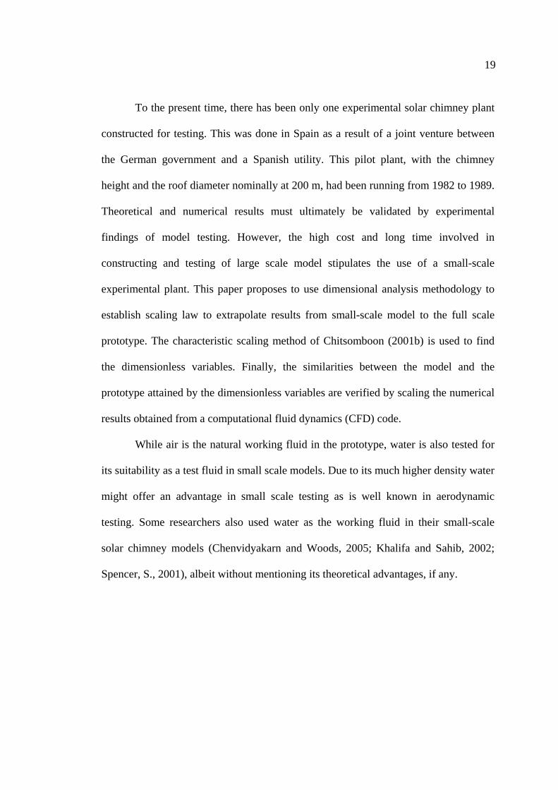
To the present time, there has been only one experimental solar chimney plant
constructed for testing. This was done in Spain as a result of a joint venture between
the German government and a Spanish utility. This pilot plant, with the chimney
height and the roof diameter nominally at 200 m, had been running from 1982 to 1989.
Theoretical and numerical results must ultimately be validated by experimental
findings of model testing. However, the high cost and long time involved in
constructing and testing of large scale model stipulates the use of a small-scale
experimental plant. This paper proposes to use dimensional analysis methodology to
establish scaling law to extrapolate results from small-scale model to the full scale
prototype. The characteristic scaling method of Chitsomboon (2001b) is used to find
the dimensionless variables. Finally, the similarities between the model and the
prototype attained by the dimensionless variables are verified by scaling the numerical
results obtained from a computational fluid dynamics (CFD) code.
While air is the natural working fluid in the prototype, water is also tested for
its suitability as a test fluid in small scale models. Due to its much higher density water
might offer an advantage in small scale testing as is well known in aerodynamic
testing. Some researchers also used water as the working fluid in their small-scale
solar chimney models (Chenvidyakarn and Woods, 2005; Khalifa and Sahib, 2002;
Spencer, S., 2001), albeit without mentioning its theoretical advantages, if any.

20
Figure 3.1 Schematic layout of solar chimney power plant.

21
3.3 DIMENSIONAL ANALYSIS
In Chitsomboon (2001a), by synthesizing the conservation equations of mass
and energy together with ideal gas relations, the mathematical model for the
frictionless, one-dimensional flow in a solar chimney was proposed as,
∫∫ ∫∫′′
=⎥⎥⎦
⎤
⎢⎢⎣
⎡+
′′+−
2
13
12
1
2
13
1
211
2
12
11
13
2111
21
22221
rp
r
p
dATc
qghAdA
RTghA
AdA
TcVqA
AdAAVm ρ
γρρρ& (3.1)
The results obtained from the above model were compared with numerical
results from the self-developed CFD computer code (Chitsomboon, 2001a). This CFD
code solved the full two-dimensional, compressible Navier-Stokes equations using an
implicit finite volume methodology. The test cases investigated represent the solar
chimney system with a roof radius of 100 m, roof height of 2 m and chimney radius of
4 m. Two parameters were used in the test: 1) the chimney height, and 2) the
insolation. Good agreements between analytical and numerical results in terms of
kinetic power predictions, both quantitatively and qualitatively, were observed.
Therefore various parameters appeared in Eq. (3.1) perhaps could be used to guide the
development of the present dimensional analysis. In particular by realizing that the
heat flux term always appears together with , the term pcpc
q ′′ is therefore proposed
as a single fundamental variable in the analysis (physically this term should represent
the temperature rise). The variable, however, is modified to be pc
q ′′′ (volumetric heat
source) so that it is compatible with the way the CFD code handles the heat flux.
can be obtained from simply by dividing by the roof height. Obviously this is q ′′′ q ′′

22
correct only in the ideal situation wherein the incident energy is totally and uniformly
absorbed by the air under the roof that is the assumption presumed in this study. The
uniformity assumption should be quite realistic because the dominant mode of heat
transfer is that of radiation through a thin gas while the totality assumption tends to
overestimate the heat absorption; this is not a serious issue since at this level we are
just trying to establish mathematical similarity among various parameters involved in
the problem. In practice, an empirical factor (less than 1) should be found to help
adjust the heat absorption to be close to the true value and this should depend on the
type of roof material and the ground conditions as well.
The primitive variables involved are proposed to be . It
should be noted that a solar chimney system without a turbine is considered here. In
addition, viscous effect is ignored at this level. Past numerical testing (Koonsrisuk and
Chitsomboon, 2004) have confirmed that viscous effect is negligible in solar chimney
flow. By the guidance of Eq. (3.1), the principal dependent variable is proposed to be
ghcqVA cp ,,,,,,, ''' βρ
22Vm& or ( )
22VAVρ instead of just V since it gives a good engineering meaning of
the total kinetic energy in the chimney. The procedural steps to find the dimensionless
variables are now listed as follows:
Step 1 Propose the variables affecting the power as:
),,,,(2
2
cp
n hcqgfVAV βρρ′′′
= (3.2)

23
All other variables on the right hand side, except forβ , are those that would be
intuitively expected (given that pc
q ′′′ stands for temperature rise). β comes in to
represent the effect of buoyancy which is the main driving force for this problem.
Step 2 Use mass (M), length (L), time (t), and temperature (Θ ) as the
fundamental dimensions.
Step 3 The fundamental dimensions of the listed variables can be expressed in
multiple powers of M, L, t, as shown in Table 3.1. Θ
Step 4 Choose β,,pc
qg ′′′ , and as the scaling (repeating) variables. While
the choice of scaling variables is quite arbitrary, in so far as they are not mutually
dependent and can form a complete dimensional bases for all other dimensions, but a
judicious selection can help in engineering interpretation (which will be elucidated
later). The methodology proposed in Chitsomboon (2001b) is used to form
dimensionless groups. In this method ‘pure’ dimensions are extracted from
‘compound’ dimensions embedded in the fundamental variables by combining them
together which could be analogized to chemical reaction processes in extracting pure
substance.
ch
chL = (3.3)
β=Θ
1 (3.4)
gt c=
h (3.5)

24
( )gc
hqMp
c 2β′′′=
7
(3.6)
Most of the time (including this one) the pure dimension can be extracted
simply by observation, without having to solve algebraic equations. In rare cases,
solving algebraic equations might be necessary but then they need to be solved only
once and for all.
Step 5 The dimension of 2
2VAVρ is . The relations for from
Eqs. (3.6), (3.3) and (1.5), respectively, can now be easily inserted without having to
solve a system of algebraic equations as conventionally practiced in the Buckingham’s
pi theorem. The scaling variable so obtained is
321 −tLM tLM ,,
( ) ( )3
2
1
27 −
⎟⎟⎠
⎞⎜⎜⎝
⎛⎟⎟
⎠
⎞
⎜⎜
⎝
⎛ ′′′g
hhgc
hq cc
p
cβ .
After some rearranging, the final dimensionless group is,
4
2
12
cp
hc
gq
VAV
β
ρ
′′′=Π (3.7)
Repeating the same procedure for ρ ,

25
Table 3.1 Powers of primitive variables in terms of fundamental dimensions.
M L T Θ
2
2VAVρ 1 2 -3 0
ρ 1 -3 0 0
g 0 1 -2 0
pcq ′′′
1 -3 -1 1
β 0 0 0 -1
ch 0 1 0 0

26
[ ] [ ] ( ) [ ] gh
cq
hgc
hqLM c
pcp
cβρ
β
ρρ′′′
=
⎥⎥
⎦
⎤
⎢⎢
⎣
⎡ ′′′==Π
−
−
3
1
27312 (3.8)
Step 6 Finally, the functional relationship is, , or )( 21 ∏=∏ nf
)(24
2
gh
cq
fh
cgq
VAV
c
p
n
cp
βρ
β
ρ
′′′=′′′ (3.9)
Hence the original eight primitive variables ( ) in Eq.
(3.2), have been combined and the number is reduced to only two dimensionless
variables. Note that the Buckingham’s pi theorem dictates that the number of
dimensionless variables is four. The reduction of another two dimensionless variables
is made possible by combining primitive variables together by using engineering
intuition and the guidance from the above mathematical model (Eq. (3.1). This should
help make the ensuing experiments much simpler. The use of traditional
Buckingham’s pi theorem procedure also leads to the same dimensionless variables;
the advantage of using the present methodology is that the algebraic work is reduced.
The validity and completeness of the derived dimensionless variables, however,
remain to be proven. To this end, a commercial CFD code “CFX” is employed to
obtain numerical solutions of three different-size solar chimneys. The primitive-
valued results are used to calculate the values of
ghcqVA cp ,,,,,,, ''' βρ
1Π and 2Π in order to verify the
validity of the proposed dimensionless variables.

27
Engineering Interpretation
As alluded to earlier, physical meaning of a dimensionless group helps in
engineering interpretation, which deepens the understanding of the problem. The
scaling variable of , 1Π 4c
phc
gq ⎟⎠⎞
⎜⎝⎛ ′′′ β , could be interpreted as the energy that the
buoyant force produces in floating from the base to the top of the chimney. To clarify
this, first note that pc
q ′′′ is proportional to TmΔ~ , where m~ is mass flow rate through
the 1 m3 volume being received the solar heat absorption per unit volume, . When
this term is multiplied to
q ′′′
β ( ⎟⎠⎞⎜
⎝⎛
∂∂= Tρ
ρ1 ), the term is proportional to tΔ
Δρ ,
where is time scale of the problem (time for flowing past 1 mtΔ 3 volume). Further
multiplication by , resulting into, cccc hghghgh ∀== 34 thg c ΔΔ )( ∀ρ . The term in the
parenthesis is the buoyant force in the chimney; this force acts through the distance
in time , which is the energy the air expenses in floating from the base to the top as
mention earlier. So, could be interpreted as total kinetic energy of the system
measured in the scaling unit that is proportional to the buoyant energy of the heated
air.
ch
tΔ
1Π
As for the scaling variable for 2Π ( gh
cq c
p⎟⎠⎞
⎜⎝⎛ ′′′ β ) this could be interpreted
as the buoyant force. Note from above discussion that pc
q β′′′ could be interpreted as
tΔΔρ , and that g
hc is time scale which should be of the same order as tΔ .
Therefore the entire term is proportional to ρΔ . 2Π now becomes ρρΔ , the invert of

28
which could be interpreted as the buoyant force scaled by the weight of the fluid of the
same volume.
The entire relation of can be summarized as trying to find the
relation of kinetic energy (the intuitive output) as a function of the principal driving
force of the system (the intuitive input).
)( 21 ∏=∏ nf
Similarity Requirements
For two flows to be completely similar it is necessary that their geometries and
dynamics be similar. Geometric similarity is quite trivial in most cases and is already a
basic requirement in this study, hence only dynamic similarity is a concern left to be
studied. It is necessary to duplicate all but one of the significant dimensionless groups
to achieve complete dynamic similarity between geometrically similar flows (Fox and
McDonald, 1994). Thus, if the proposed dimensionless variables are valid, duplicating
between models and prototype ensured dynamically similar flows. The stipulation
required by in Eq. (3.8) is
2Π
2Π
p
c
pm
c
p gh
cq
gh
cq
⎥⎥⎥⎥⎥
⎦
⎤
⎢⎢⎢⎢⎢
⎣
⎡
′′′=
⎥⎥⎥⎥⎥
⎦
⎤
⎢⎢⎢⎢⎢
⎣
⎡
′′′ βρ
βρ (3.10)
where subscript m stands for model and p stands for prototype. After some
manipulations, there is obtained,
mc
pc
m
p
pp
mp
p
mpm h
hcc
qq,
,
ββ
ρρ′′′=′′′ (3.11)

29
It had been hoped that water would offer a good alternative as a test working
fluid, as in aerodynamic testing. By using Eq. (3.11), the solar heat absorption per unit
volume required for three geometrically similar models are presented in Table 3.2, for
air and water as the test working fluids. It is seen from the table that the solar heat
absorption per unit volume required for water are very high, making it unpractical, if
not impossible, in experimental set up. In numerical modeling, of course, high solar
heat absorption per unit volume can be easily implemented; but the difficulty may
arise in terms of thermodynamic states and properties of water at very high
temperatures. As a result of the anticipated difficulties and inconveniences, water was
dropped from consideration as a test working fluid.
3.4 CFD Modeling
As real experiments in this type of flow are very expensive and time
consuming, at this early stage it should be sufficient to perform ‘numerical
experiments’ to verify the validity of the proposed similarity because CFD has over
time proven to be quite a reliable tool in fluid dynamic research and application
especially when only global phenomena is being sought after. CFX was chosen since it
has been widely accepted in the research and application communities and partly
because of its versatility with grid generation and boundary conditions. For this
purpose, CFX solves the conservation equations for mass, momenta, and energy using
a finite volume method. Adaptive unstructured tetrahedral meshes are used in the
present study. The plants studied are modeled as axis-symmetry where the centerline
of the chimney is the axis of symmetry. To simulate axis-symmetry, a 5 degree section
of the plant is cut out from the entire periphery as shown in Fig. 3.2. To make certain

30
that similarity (or the lack thereof) was not affected by grid-topology irregularity, grid
similarity for all the test cases was enforced. Grid similarity means that when the
small-scale model is scaled up to be the same size as the prototype, its grid is exactly
the same as that of the prototype. Moreover, grid convergence was also ensured by
varying the numbers of grid until no change in output parameter was noticed. Fig. 3.3,
as an example of grid convergence examination, illustrates the plot of vs. number
of grid elements.
1Π
The solar heat absorption per unit volume of the air is modeled as a uniform
heat source within the air that is flowing underneath the roof. This should not incur
significant errors since the dominant mode of heat transfer is that of solar radiation
through a thin gas. For buoyancy calculations, a source term is added to the
momentum equations as follows:
gS refbuoyancy )( ρρ −= (3.12)
where the density difference refρρ − is evaluated directly from equation of state, not
approximately by the Boussinesq’s model.
High flow gradients occur in the vicinity of the roof-chimney juncture. In order
to accurately capture flow features, several grid points have to be located at this
region. A typical mesh system for the computational domain is shown in Fig. 3.2.
Proper boundary conditions are needed for a successful computational work. At
the roof inlet, the total pressure and temperature are specified; whereas at the chimney

31
Figure 3.2 Unstructured mesh used for the 5 degree axis-symmetric computational
domain.

32
Figure 3.3 1Π vs. number of grid elements

33
exit the ‘outlet’ condition with zero static pressure is prescribed. Additionally, the
‘symmetry’ boundary conditions are applied at the two sides of the sector. The
adiabatic free-slip conditions are prescribed to the remaining boundaries. As specified
above that frictionless flow be modeled, then the free-slip conditions are applied to all
walls. All test cases were computed until residuals of all equations had reached their
respective minimum. Moreover, global conservation of mass had been rechecked to
further ascertain the convergence of the test cases.
3.5 RESULTS AND DISCUSSION
A typical velocity field in the vicinity of the roof-chimney juncture is shown in
Fig. 3.4 wherein a flaring of the turn angle is used to mitigate separation caused by the
90 degree flow deflection. All plots to be subsequently presented are displayed along
the scaled flow path, which is the non-dimensioned streamwise location of the flow,
equaling zero at inlet and one at outlet (chimney top). Incidentally, 0.5 is the location
at which the roof-chimney juncture is located. The results using air as the working
fluid are illustrated in Figs. 3.5 - 3.7. The numerical solutions by MOYA, a self-
developed CFD code (Chitsomboon, 2001a), are also presented in the figures for
comparison purpose. Quasi one dimensional model is used in MOYA, whereas axis-
symmetry model is used in this study. The different coordinate systems used in
MOYA and CFX is believed to be the reason behind the discrepancies in the
computational results of the two CFD codes shown in Figs. 3.5 - 3.7.
Figure 3.5 shows the average velocity along the flow path; it can be seen that
the velocities of the flow under the roof increase along the flow path, resulting from

34
the flow area reduction but constant mass flow rate, and remains unchanging along the
chimney.
In Fig. 3.6, the temperature rises toward the chimney because the air
accumulates thermal energy along the flow path in the roof section. The air
temperature drops slightly while rising in the chimney. This drop is in accord with the
pressure drop through isentropic relation. A numeral check shows that this temperature
reduction did indeed undergo an isentropic change.
In Fig. 3.7, the pressure distributions are seen to be nominally constant under
the roof before falling linearly in the chimney portion, to meet the hydrostatic pressure
distribution at the chimney top. Note that the ordinate is the gauge pressure scaled
such that pressures at the top of chimney are always zero.
Figures 3.5 - 3.7 showed the differences of the primitive flow variables
between the prototype with and the different-size models, which are
geometrically similar and -similar to the prototype.
2W/m800=′′q
2Π 2Π for all cases are already set
to be equaled before hand because it was used to compute the similar solar heat
absorptions per unit volume required for the test cases. If similarity existed as
proposed, scaled data of the various cases in Figs. 3.5 - 3.7 must collapse. To this end,
Figures 3.8 presents the distributions of the dimensionless variable, 1Π ,
computed from the involved primitive variables. The figure displays the values of 1Π
when are at 164.1, 246.1, 492.2, and 984.4, which correspond to the condition
when the insolation of prototype are at 1200, 800, 400, and 200 W/m
2Π
2, respectively. It
is clearly seen that the once scattered data now collapse, suggesting similarity. Despite

35
there are slight variation from prototype’s values of model’s values, the 1Π
characteristics follow the same pattern over a wide range of 2Π .
The deviation of (about 15%) at high value of 1Π 2Π might be the result of
viscous effects. Note that though the inviscid equations are being solved, but there
exists the so-called ‘numerical viscosity’ in the numerical scheme. As is well known in
CFD, numerical viscosity is an inescapable quantity associated with numerical
discretization of the differential convective terms. Note also that could be
interpreted as
2Π
ρρΔ , then for the same physical model, high value of means low
value of numerical Grashof number (=
2Π
3
2n
g xρρ
ν
Δ), where nν is the numerical
viscosity whose size being proportional to xΔ which in turns is proportional to x .
Since the grids are also similar so for the different physical models being studied the
ratio of the Grashof numbers should be scaled by x . At the same , the ratios of the
Grashof number values for model II, model I and the prototype are then 1, 5 and 125.
It is possible that the low values of the numerical Grashof numbers, in conjunction
with their vast different in magnitudes, are contributable to the 15% departures of the
similarity curves of the cases being studied.
2Π
Table 3.2 suggests that when the plant size reduces, the plant needs higher solar
heat per unit volume. Actually, as the plant size decreases, the roof height also
decreases; this makes the volume under the roof decrease accordingly. When the solar
radiation per unit volume for each plant is converted to solar radiation per unit roof

36
Figure 3.4 Typical velocity field around the junction of the roof and the chimney.

37
Figure 3.5 Numerical prediction of velocity profiles for insolation = 800 W/m2.

38
Figure 3.6 Numerical prediction of temperature profiles for insolation = 800 W/m2.

39
Figure 3.7 Numerical prediction of pressure profiles for insolation = 800 W/m2.

40
Figure 3.8 21 -ΠΠ characteristics.

41
area, it shows that, for similar condition, as the plant size decreases, theplant needs
lower solar radiation per unit area. This should pose a serious obstacle for conducting a
“similar” experiment using a small model because means for reducing insolation is
needed, such as by using glass of various shades of colors. Better similarity variables
that do not require different insolations are obviously desirable.
3.6 CONCLUSION
CFD study in three geometrically similar cases indicated that the proposed
dimensionless variables are appropriate for obtaining similarity for flows in prototype
and small-scale models of a solar chimney. By using engineering intuition and
guidance from a mathematical model, the number of dimensionless variables
developed is less than that dictated by the Buckingham’s pi theorem; this helps reduce
the complexity of experimental work. The study shows that water is not suitable as a
test working fluid because the solar heat absorption per unit volume required for
similarity is too high. Using air for a small-scale model, though quite natural, requires
lower insolations than that of the prototype for dynamic similarity; this requires roof
material treatments such as tinting or using artificial insolation.

42
Table 3.2 Solar heat absorption per unit volume (S.H.A.V.) requirements
for dynamic similarity
Case Working
fluid
Chimney
height
(m)
Roof
height
(m)
Chimney
radius
(m)
Roof
radius
(m)
S.H.A.V.
(W/m3)
Prototype Air 100 2 4 100 400
Model 1 Air 20 0.4 0.8 20 894.43
Model 2 Air 5 0.1 0.2 5 1,788.85
Model 3 Water 20 0.4 0.8 20 30,053,033
Model 4 Water 5 0.1 0.2 5 60,106,066
Note: The specification of prototypical plant is the same as the plant studied in
Chitsomboon (2001a).

43
3.7 REFERENCES
Chenvidyakarn, T., Woods, A., 2005. Multiple steady states in stack ventilation.
Building and Environment, 40(2005), pp. 399-410.
Chitsomboon, T., 2001a. A validated analytical model for flow in solar chimney.
International Journal of Renewable Energy Engineering, 3(2), pp. 339-346.
Chitsomboon, T., 2001b. Construction and interpretation of dimensionless variables in
a new way. In: Proceedings of the 15th National Mechanical Engineering
Conference, Vol. 1, pp. TF39-TF45.
Fox, R. W., McDonald, A. T., 1994. Introduction to fluid mechanics, 4th edition,
John Wiley & Sons, United States of America.
Gannon, A.J., Von Backström, T.W., 2000. Solar chimney cycle analysis with system
loss and solar collector performance. ASME Journal of Solar Energy
Engineering, Vol. 122, no. 3, pp. 133-137.
Haaf, W., Friedrich, K., Mayr, G., Schlaich, J., 1983. Solar chimneys: part I: principle
and construction of the pilot plant in Manzanares. International Journal of
Solar Energy, Vol. 2, no. 1, pp. 3-20.
Khalifa, A.J.N., Sahib, W.K., 2002. Turbulent buoyancy driven convection in partially
divided enclosures. Energy Conversion and Management, 43(2002), pp.
2115-2121.
Koonsrisuk, A., Chitsomboon, T., 2004. Frictional effect on the flow in a solar
chimney. In: Proceedings of the 4th National Symposium on Graduate
Research, Chiang Mai, Thailand.

44
Padki, M.M., Sherif, S.A., 1988. Fluid dynamics of solar chimney. In: Proceedings of
the ASME Winter Annual Meeting, Chicago, Illinois, FED-Vol.70, pp. 43-
46.
Padki, M.M., Sherif, S.A., 1989a. Solar chimney for medium-to-large scale power
generation. In: Proceedings of the Manila International Symposium on the
Development and Management of Energy Resources, Manila, Philippines,
1, pp. 423-437.
Padki, M.M., Sherif, S.A., 1989b. Solar chimney for power generation in rural areas.
Seminar on Energy Conservation and Generation Through Renewable
Resources, Ranchi, India, pp. 91-96.
Padki, M.M., Sherif, S.A., 1992. A mathematical model for solar chimneys. In:
Proceedings of the 1992 International Renewable Energy Conference,
Amman, Vol. 1, pp. 289-294.
Schlaich, J., 1995 . The Solar Chimney: Electricity from the Sun, Axel Menges,
Stuttgart.
Spencer, S., 2001. An experimental investigation of a solar chimney natural
ventilation system, Master Thesis, Concordia University, Montreal, Quebec,
Canada.
Von Backström, T.W., Gannon, A.J., 2000. Compressible flow through solar power
plant chimneys. ASME Journal of Solar Energy Engineering, Vol. 122, no.
3, pp. 138-145.
Yan, M.Q., Sherif, S.A., Kridli, G.T., Lee, S.S., Padki, M.M., 1991. Thermo-fluid
analysis of solar chimneys. Ind. Applic. Fluid Mech. ASME FED-2, pp. 125-
130.

CHAPTER IV
PARTIAL GEOMETRIC SIMILARITY FOR SOLAR
CHIMNEY POWER PLANT MODELING
4.1 ABSTRACT
A solar chimney power plant derives its mechanical power from the kinetic
power of the hot air which rises through a tall chimney, the air being heated by solar
energy through a transparent roof surrounding the chimney. In our previous studies,
the achievement of complete dynamic similarity between a prototype and its models
imposed the use of different solar heat fluxes between them. It is difficult to conduct
an experiment by using dissimilar heat fluxes with different physical models.
Therefore, this study aimed to maintain dynamic similarity for a prototype and its
models while using the same solar heat flux. The study showed that, to achieve the
same-heat-flux condition, the roof radius between the prototype and its scaled models
must be dissimilar, while all other remaining dimensions of the models are still similar
to those of the prototype. In other words, the models are ‘partially’ geometrically
similar to the prototype. The functional relationship that provides the condition for this
partial similarity is proposed and its validity is proved by scaling the primitive
numerical solutions of the flow. Engineering interpretations of the similarity variables
are also presented.

46
4.2 INTRODUCTION
Solar chimney (sometimes called solar tower) was proposed as an alternate
means to harness energy from the sun (Schlaich, 1995). The schematic of a typical
solar chimney power plant is sketched in Fig. 4.1. A hot air is obtained under the
transparent roof surface as a result of the greenhouse effect. Due to buoyancy, the
heated air flows up the hollow tower (chimney) inducing a continuous flow from the
perimeter towards the middle of the roof where the tower is located. Shaft energy can
be extracted from the thermal and kinetic energy of the flowing air to turn an electrical
generator.
An experimental solar chimney power plant, with tower height and roof
diameter nominally at 200 m, design peak electrical output at 50 kW, was constructed
in Manzanares desert (Spain) as a joint effort between the German government and a
Spanish utility company. The experiment indicated that the solar chimney concept was
technically viable and the plant had been operating productively from 1982 to 1989
before its collapse due to a storm. The design criteria and cost analysis of this plant
were discussed in Haaf et al. (1983) and the preliminary test results from the plant
were reported in Haaf (1984). An inspection of the available experimental data
showed, however, that the overall plant efficiency was only about 0.1%. Since then, no
solar chimney power plant has been built again, though a number of theoretical and
numerical studies have been carried out by some researchers. It is apparent that much
more research is needed before solar chimney power plant can become a serious
competitor to other forms of renewable energy technology.

47
Figure 4.1 Schematic layout of solar chimney power plant.

48
Padki and Sherif (1989a, 1989b, 1999) and Yan et al. (1991) conducted some
of the earliest works on thermo-fluid aspects of solar chimney power plants by using
various quasi-one-dimensional approaches. Pasumarthi and Sherif (1998a) presented a
more detailed mathematical model which was validated with the experimental results
of their own (Pasumarthi and Sherif, 1998b) and of the Manzanares plant. Von
BackstrÖm and Gannon (2000) used a one-dimensional compressible flow approach to
conduct their study which included important effects such as wall friction, internal
drag and area change. Subsequently, they also investigated the performance of a solar
chimney turbine (Gannon and Von BackstrÖm, 2003). Chitsomboon (2001) proposed
an analytical model with thermo-mechanical mechanisms that allow flows in various
parts of a solar chimney to interact. Bernardes et al. (2003) developed analytical and
numerical models and compared the predicted results with the experimental results
from the pilot plant at Manzanares. Guidelines for the design of a 200 MW
commercial plant, based on engineering theories, economics and experience, were
developed by Schlaich and Weinrebe (2005). Onyango and Ochieng (2006) considered
the suitability of solar chimney power plants for small rural villages. Pretorius and
KrÖger (2006) solved a convective heat transfer equation, evaluated a more accurate
turbine inlet loss coefficient and the effects of various types of soil on the performance
of a large scale solar chimney power plant. Their resultant optimal plant collector
height was not the same as that predicted by KrÖger and Buys (2001) or Pretorius et al.
(2004). In the work of Tingzhen et al. (2006), a mathematical model was proposed
that could predict the effects of various parameters, such as the tower height and its
radius, the collector radius and the solar radiation, on the relative static pressure, the
driving force, the power output and the efficiency of a solar chimney.
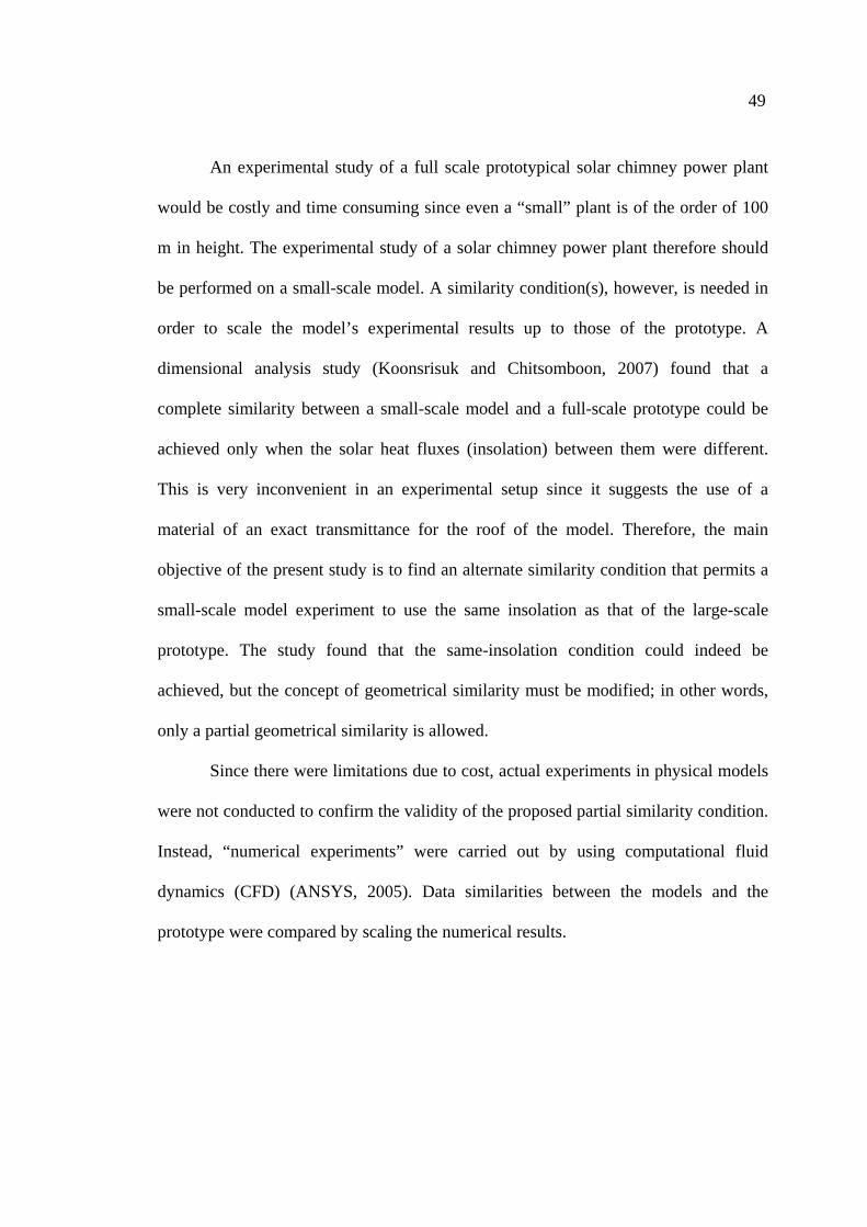
49
An experimental study of a full scale prototypical solar chimney power plant
would be costly and time consuming since even a “small” plant is of the order of 100
m in height. The experimental study of a solar chimney power plant therefore should
be performed on a small-scale model. A similarity condition(s), however, is needed in
order to scale the model’s experimental results up to those of the prototype. A
dimensional analysis study (Koonsrisuk and Chitsomboon, 2007) found that a
complete similarity between a small-scale model and a full-scale prototype could be
achieved only when the solar heat fluxes (insolation) between them were different.
This is very inconvenient in an experimental setup since it suggests the use of a
material of an exact transmittance for the roof of the model. Therefore, the main
objective of the present study is to find an alternate similarity condition that permits a
small-scale model experiment to use the same insolation as that of the large-scale
prototype. The study found that the same-insolation condition could indeed be
achieved, but the concept of geometrical similarity must be modified; in other words,
only a partial geometrical similarity is allowed.
Since there were limitations due to cost, actual experiments in physical models
were not conducted to confirm the validity of the proposed partial similarity condition.
Instead, “numerical experiments” were carried out by using computational fluid
dynamics (CFD) (ANSYS, 2005). Data similarities between the models and the
prototype were compared by scaling the numerical results.

50
4.3 DIMENSIONAL ANALYSIS
According to the work of Chitsomboon (2001), the mathematical model of the
flow in a solar chimney power plant was proposed as
∫∫ ∫∫′′
=⎥⎥⎦
⎤
⎢⎢⎣
⎡+
′′+−
3
13
13
1
3
13
1
211
3
12
11
13
2111
21
22221
rp
ccr
p
dATc
qghAdA
RTghA
AdA
TcVqA
AdAAVm ρ
γρρρ& . (4.1)
This mathematical model was obtained by a synthesis of the conservation
equations of mass, momentum and energy, together with the ideal gas relation. The
forms of the terms appearing in this equation could be used as a guide for selecting
primitive variables in the dimensional analysis. Accordingly, the dependence of the
kinetic power, ( ) 22VAVρ , on the independent variables is proposed as
),,,,(2
2
cp
rn hcAqgfVAV βρρ′′
= . (4.2)
Note that the viscosity is not included as a variable in Eq. (4.2) since we wish
to focus on the inviscid effect first. Including viscosity would further cloud the
similarity issue, especially when the numerical approach is used to verify the similarity
condition since CFD has its own problems of turbulence modeling. Besides our
previous work (Koonsrisuk and Chitsomboon, 2004) found that friction loss in a
typical solar chimney was negligible. Temperature rise (intuitively a very important
variable) does not appear explicitly but is hidden in pr cAq ′′ via the energy
conservation principle ( TcmAq pr Δ&=′′ ). The thermal expansion coefficient,β

51
(pT ⎟⎠⎞⎜
⎝⎛
∂∂−= ρ
ρ1 ), is a most important variable because it represents the buoyant
driving force for the system as a result of the temperature rise.
Koonsrisuk and Chitsomboon (2007) used pcq ′′′ instead of pr cAq ′′ as a
variable ( rhqq ′′=′′′ ); they proposed the dimensionless relation as,
)(24
2
gh
cq
fh
cgq
VAV
c
p
n
cp
βρ
β
ρ
′′′=′′′ . (4.3)
The validity of Eq. (4.3) was proved by scaling and comparing the numerical
results of various models. To ensure the dynamic similarity required by Eq. (4.3), the
roof height ratio was related to the insolation ratio by
21
⎟⎟⎠
⎞⎜⎜⎝
⎛=
′′′′
p,r
m,r
p
m
hh
qq (4.4)
with subscripts p and m denoting “prototype” and “model”, respectively. The condition
in Eq. (4.4) imposes a lesser insolation level for a small-scale model than that of a
prototype.
Later on, it was determined by the author that the undesirable condition of our
previous study might be due to the use of )hq(q r′′=′′′ instead of . Therefore, this
study proposes the use of . Eq. (4.1) shows, however, that this term always appears
in combination as
q ′′
q ′′
pr cAq ′′ . Hence this quantity, rather than just q , is proposed in this
study.
′′

52
The procedural steps in finding the similarity variables are listed as follows:
Step 1 Propose the primitive-variable functional relationship:
),,,,,,(2
2
rccp
rn hrhcAqgfVAV βρρ′′
= . (4.5)
Note the additional geometric variables from that of Eq. (4.2), an attempt to be more
inclusive than our previous study. The size of the plant is characterized by the tower
height ( ), tower radius ( ), roof height ( ) and roof radius ( ) (hidden in ) ch cr rh rr rA
Step 2 Use mass (M), length (L), time (t), and temperature (Θ) as the
fundamental dimensions. The dimensional matrix of the various variables becomes
2
2VAVρ
ρ
g p
r
cAq ′′
β
ch
cr
rh
M 1 1 0 1 0 0 0 0
L 2 -3 1 0 0 1 1 1
t -3 0 -2 -1 0 0 0 0
Θ 0 0 0 1 -1 0 0 0
Step 3 Choose βρ ,, g , and as the scaling variables (or repeating variables).
The fundamental dimensions can now be extracted from the scaling variables as:
ch
chL = (4.6)
3hM ρ= c (4.7)

53
gt c=
h (4.8)
β=Θ
1 . (4.9)
(Note: The methodology used here is presented in Chitsomboon (2003). It
yields the same result as the familiar Buckingham’s pi theorem but with much less
algebraic complexity).
Step 4 Scale the remaining variables according to the powers of their
fundamental dimensions (see the matrix above):
( ) ( ) ( ) ( ) 2327
2
03213
2
121
12
gh
Vm
ghhh
VAV
ccccρβρ
ρ &==Π − (4.10)
( ) ( ) ( ) ( ) 21251101321 gh
c
ghhh
c
c
p
ccc
p
ρ
AqAq rr β
βρ
′′
==Π −
′′
(4.11)
3ch
Π = cr (4.12)
4ch
Π = rh . (4.13)
Finally, the functional relationship is found to be , or ),,( 4321 ΠΠΠ=Π nf

54
⎟⎟⎠
⎞⎜⎜⎝
⎛ ′′=
c
r
c
c
cp
rn
c hh,
hr,
ghcAqf
gh
Vm21252327
2
21
ρβ
ρ
&. (4.14)
Similarity Requirements
Consider Eq. (4.14), for a geometrically similar model cc hr and cr hh are
taken care of by the requirements that they are of the same value for both the models
and the prototype. The remaining similarity requirement is,
pcp
r
mcp
r
ghcAq
ghcAq
⎥⎥⎦
⎤
⎢⎢⎣
⎡ ′′=
⎥⎥⎦
⎤
⎢⎢⎣
⎡ ′′21252125 ρ
βρ
β . (4.15)
If the same working fluid and the ‘fully’ geometrical similar condition were
assumed, Eq. (4.15) would, again, reduce to Eq. (4.4); this repeats the ‘dissimilar’
solar-heat-flux condition as established in the previous study. Alternatively, we now
force the insolations of the two cases to be the same. Thus from Eq. (4.15) the required
condition for dynamic similarity now is
45
⎟⎟⎠
⎞⎜⎜⎝
⎛=
p,c
m,c
p,r
m,r
hh
rr
(4.16)
Equation (4.16) implies that the ratio p,cp,r hr is not equal to m,cm,r hr as
required by the usual geometric similarity condition. It is apparent that two types of
dimension distortion are possible in order to achieve the partial similarity condition,
namely, distortion of and distortion of . The distortion of , however, is not
acceptable since it is a fundamental scaling variable. Its distortion would nullify the
rr ch ch

55
constancy assumptions made earlier of the scaled geometrical values: cc hr and
cr hh . Therefore, only the distortion of is acceptable. Recall that, in order to
achieve a dynamic similarity, the scaled driving forces between the two flows must be
identical. Because the principal driving force for this system is the solar heat gain
( ), therefore adjustment of the heat gain could be controlled by altering the
magnitude of .
rr
2rrq π′′=
rr
As a result, Eq. (4.16) indicates that the roof radius scales with the tower height
to the power of 45 while all the remaining length dimensions scale with the power of
1. As such, the model’s roof radius is distorted from a truly physically similar model.
In other words, the scaled model must be partially geometrically similar to the
prototype.
The dimensions of the prototype, four fully geometrically similar models and
four partially geometrically similar models (using Eq. (4.16)) that were used to
simulate the numerical test cases are presented in Table 4.1. The three test cases that
were set up and the insolations for each plant are also listed in Table 4.1.
4.4 COMPUTATIONAL WORK
For the numerical simulations, the CFD code (ANSYS, 2005) solves the
conservation equations for mass, momentum, and energy using the finite volume
method. To simulate the axis-symmetry condition in the 3-dimensional setting, a pie
shape domain was created by cutting a 5 degree wedge out of the whole power plant
geometry. The side faces of the domain were taken as symmetric boundary conditions
as shown in Fig. 4.2a. Adaptive unstructured tetrahedral meshes were used to

56
Table 4.1 Specification of prototype and models
Insolation (W/m2)
Plant
Chimney height,
hc
(m)
Roof height,
hr
(m)
Chimney radius,
rc
(m)
Roof radius,
rr
(m) Case 1 Case 2 Case 3
Prototype (reference)
100 2 4 100 200 600 1,000
Model 1-f (fully similar)
5 0.1 0.2 5 44.72 134.16 223.61
Model 2-f (fully similar)
20 0.4 0.8 20 89.44 268.33 447.21
Model 3-f (fully similar)
40 0.8 1.6 40 126.49 379.47 632.46
Model 4-f (fully similar)
80 1.6 3.2 80 178.89 536.66 894.43
Model 1-p (partially similar)
5 0.1 0.2 2.36 200 600 1,000
Model 2-p (partially similar)
20 0.4 0.8 13.37 200 600 1,000
Model 3-p (partially similar)
40 0.8 1.6 31.81 200 600 1,000
Model 4-p (partially similar)
80 1.6 3.2 75.66 200 600 1,000
Note: The specification of prototype, model 1-f, and model 2-f are the same as the
plants studied in Koonsrisuk and Chitsomboon (2007).

57
(a)
(b)
Figure 4.2 Computational domain: (a) 5 degree axis-symmetric section;
(b) numerical grid.

58
discretize the domain and the grid convergence issue was already investigated
previously (Koonsrisuk and Chitsomboon, 2007). Thus those grid configurations are
adopted in this work. A typical grid for the computational domain is shown in Fig.
4.2b.
Proper boundary conditions are needed for a successful computational work. At
the roof perimeter (inlet), the flow direction was set as normal to the periphery and the
total pressure and the static temperature were specified. Zero static pressure (gauge)
was prescribed at the chimney exit. Symmetry conditions were applied at the two side
wallsof the pie-shape domain while adiabatic free-slip conditions were prescribed to
the remaining boundaries (since the flow is assumed to be inviscid). All the test cases
were computed until the residuals of all the governing equations reached their required
convergence precisions. It should be mentioned that the numerical procedure used in
this study had already been carefully calibrated and validated in our previous studies to
achieve a satisfactory level of confidence.
4.5 RESULTS AND DISCUSSION
Computations were conducted for the test cases listed in Table 4.1. Their
results are illustrated in Figs. 4.3 - 4.5. In these figures, the solid symbols were used to
identify the data points for the fully geometrically similar models (model 1f – 4f)
whereas the hollow symbols were used for the partially geometrically similar models
(model 1p– 4p).
Figure 4.3 shows the computed updraft velocities at the tower top of all the test
cases, as a function of insolations. All distributions display the expected increasing
trends as the insolation increases. The rates of increase of the velocities appear to be

59
slightly lower as the insolation increases. It should be noted again that the insolations
for the fully similar models were less than that of the prototype (according to Eq. (4.4))
while the partially similar models used the same insolation as the prototype. The
kinetic powers (output) at the chimney tops are presented in Fig. 4.4 as functions of
insolations (input).
Huge discrepancies in the distributions for all the different-size models and the
prototype are observed. These discrepancies are intuitively expected for physical
models of widely different sizes since the data are presented in primitive (dimensional)
forms.
When the data in Fig. 4.4 were scaled according to the proposed scaling law in
this study, the results are as shown in Fig. 4.5. It can be clearly seen that the once
widely scattered lines of dimensional data all collapse (almost) into a single line in this
non-dimensional plot. This confirms the validity of the partial similarity law being
proposed in this study. It also confirms the different-insolations similarity law that was
proposed in our previous study. The slight non-overlapping of the data lines might be
attributable to various numerical errors (such as discretization error and numerical
diffusion), as well as the neglected viscous effect. These should be resolved in further
studies.
Further inspection of Fig. 4.5 reveals that all curves have a slope of unity and
pass through the origin. This suggests a linear fit as
21252327
2
21
ghcAq
gh
Vm
cp
r
c ρβ
ρ′′
=&

60
or, after simplifying
Figure 4.3 Numerical prediction of updraft velocity at tower top as a function of
insolation.

61
Figure 4.4 Numerical prediction of flow power as a function of insolation.

62
Figure 4.5 21 Π−Π characteristics.

63
cp
r ghcAqVm β′′
=2
21& . (4.17)
Recall that, Eq. (4.1) can be rearranged as
cp
r
r
c
r
c
p
ghcAq
DD
hD
TcVq
AA
RTgh
Vm β
ργ
′′
⎪⎭
⎪⎬⎫
⎪⎩
⎪⎨⎧ ′′
+⎥⎥⎦
⎤
⎢⎢⎣
⎡−⎟⎟
⎠
⎞⎜⎜⎝
⎛+
=
ln11
121
131
2
1
3
1
23& . (4.18)
When the term multiplying pcr cghAq β′′ on the right-hand side of the equation
is computed from the primitive variables involved, it was found that the average values
of each case are about unity. Consequently, the equation practically reduces to
cp
r ghcAqVm β′′
=232
1& . (4.19)
This is the same as Eq. (4.17), reassuring that the results obtained here are in
accord with the theoretical predictions (and vice versa).
4.6 ENGINEERING INTERPRETATION OF THE
DIMENSIONLESS VARIABLES
Engineering interpretation often results in a deeper understanding of the
physical phenomenon represented by the mathematics. The scaling variables for 1Π ,
2327 ghcρ , could be interpreted as the flow work. To clarify this, first note that cgh
could be interpreted as the velocity scale of the problem. Accordingly,
( )( )( ) VF~VAp~ghhghgh cccc ⋅⋅⋅= Δρρ 22327 = Flow work in chimney.

64
So, could be interpreted as the kinetic power of the system measured in the
scaling unit that is proportional to the quantity of the flow work.
1Π
The first law of thermodynamics stipulates that TmcAq pr Δββ &≈′′ .
Accordingly, the scaling variable for 2Π (Eq. 4.11) could be interpreted as
mAV~ghhgh ccc &== ρρρ 22125 .
now becomes 2Π TΔβ which is proportional to ρρΔ and thus could be
interpreted as the buoyant force ( ρΔ ) scaled by the weight of the fluid of the same
volume.
Therefore, the entire relation of could be interpreted simply and
rationally as the effect of the principal characteristic driving force (input) on the
characteristic kinetic energy (output).
)( 21 Π=Π nf
4.7 CONCLUSION
The study showed that a complete dynamic similarity for scaled models and a
full scale solar chimney prototype, while maintaining the same insolation, is
achievable provided that the model’s roof radius is distorted from its fully similar
configuration according to a prescribed rule that was proposed in the study. This
‘partially similar’ proposition was proven to be valid which was evident by the
collapse of the scaled numerical results of the widely disparage test cases. The
seemingly complicated similarity variables were interpreted simply as the
characteristic output power (scaled kinetic energy) and the characteristic input power
(scaled buoyant force).
4.8 REFERENCES

65
ANSYS, Inc. ANSYS CFX, Release 10.0: reference guide. ANSYS, 2005.
Bernardes, M. A., Dos, S., Voß, A., Weinrebe, G., 2003. Thermal and technical
analyses of solar chimneys. Solar Energy, Vol. 75(6), pp. 511-524.
Chitsomboon, T., 2001. A validated analytical model for flow in solar chimney.
International Journal of Renewable Energy Engineering, Vol. 3(2), pp.
339-346.
Chitsomboon, T., 2003. Fluid Mechanics. McGraw-Hill/Top, Thailand.
Gannon, A. J., Von Backström, T. W., 2003. Solar chimney turbine performance.
Journal of Solar Energy Engineering, Vol. 125(1). pp. 101-106.
Haaf, W., Friedrich, K., Mayr, G., Schlaich, J., 1983. Solar chimneys: part I: principle
and construction of the pilot plant in Manzanares. International Journal of
Solar Energy, Vol. 2, pp 3-20.
Haaf, W., 1984. Solar chimneys: part II: preliminary test results from the Manzanares
plant. International Journal of Solar Energy, Vol. 2, pp 141-161.
Koonsrisuk, A., Chitsomboon, T., 2004. Frictional effect on the flow in a solar
chimney. In: Proceedings of the 4th National Symposium on Graduate
Research, Chiang Mai, Thailand.
Koonsrisuk, A., Chitsomboon, T., 2007. Dynamic similarity in solar chimney
modeling. Solar Energy, Vol. 81, pp. 1439-1446.
Kröger, D. G., Buys, J. D., 2001. Performance evaluation of a solar chimney power
plant. ISES 2001 Solar World Congress, Adelaide, Australia.
Onyango, F. N., Ochieng, R. M., 2006. The potential of solar chimney for application
in rural areas of developing countries. Fuel, Vol. 85, pp. 2561-2566.

66
Padki, M. M., Sherif, S. A., 1989a. Solar chimney for medium-to-large scale power
generation. In: Proceedings of the Manila International Symposium on the
Development and Management of Energy Resources, Manila, Philippines,
Vol. 1, pp. 423-437.
Padki, M. M., Sherif, S. A., 1989b. Solar chimney for power generation in rural areas.
Seminar on Energy Conservation and Generation Through Renewable
Resources, Ranchi, India, pp. 91-96.
Padki, M. M., Sherif, S. A., 1999. On a simple analytical model for solar chimneys.
International Journal of Energy Research, Vol. 23, no. 4, pp 345-349.
Pasumarthi, N., Sherif, S. A., 1998a. Experimental and theoretical performance of a
demonstration solar chimney model – part I: mathematical model development,
International Journal of Energy Research, Vol. 22, no. 3, pp 277-288.
Pasumarthi, N., Sherif, S. A., 1998b. Experimental and theoretical performance of a
demonstration solar chimney model – part II: experimental and theoretical
results and economic analysis, International Journal of Energy Research,
Vol. 22, no. 5, pp 443-461.
Pretorius, J. P., Kröger, D. G., 2006. Critical evaluation of solar chimney power plant
performance. Solar Energy, Vol. 80, pp. 535-544.
Pretorius, J. P., Kröger, D. G., Buys, J. D., Von Backström, T. W., 2004. Solar tower
power plant performance characteristics. In: Proceedings of the ISES
EuroSun2004 International Sonnenforum 1, Freiburg, Germany, pp. 870–
879.
Schlaich, J., 1995. The Solar Chimney. Edition Axel Menges: Stuttgart, Germany.

67
Schlaich, J., Weinrebe, G., 2005. Design of commercial solar updraft tower systems
utilization of solar induced convective flows for power generation. Journal of
Solar Energy Engineering, Vol. 127, pp.117–124.
Tingzhen, M., Wei, L., Guoliang, X., 2006. Analytical and numerical investigation of
the solar chimney power plant systems. International Journal of Energy
Research, Vol. 30, pp. 861-873.
Von Backström, T. W., Gannon, A. J., 2000. Compressible flow through solar power
plant chimneys. ASME Journal of Solar Energy Engineering, Vol. 122(3),
pp. 138-145.
Yan, M. Q., Sherif, S. A., Kridli, G. T., Lee, S. S., Padki, M. M., 1991. Thermo-fluid
analysis of solar chimneys. Ind. Applic. Fluid Mech. ASME FED-2, pp. 125-
130.
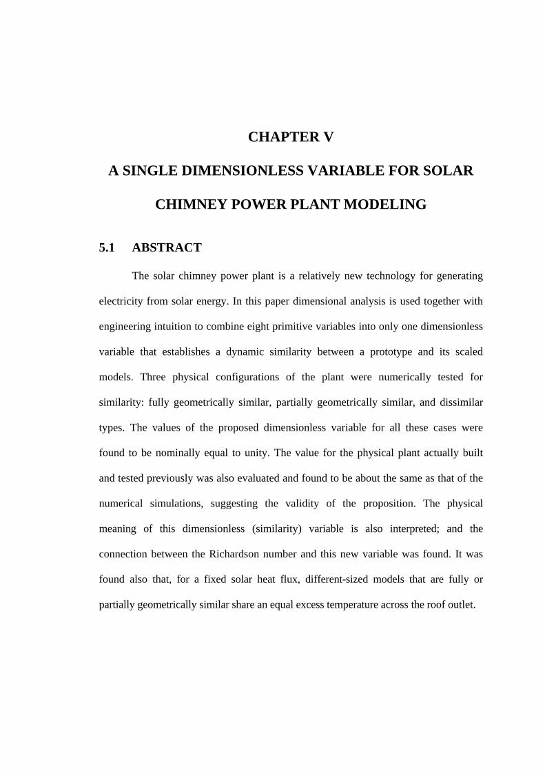
CHAPTER V
A SINGLE DIMENSIONLESS VARIABLE FOR SOLAR
CHIMNEY POWER PLANT MODELING
5.1 ABSTRACT
The solar chimney power plant is a relatively new technology for generating
electricity from solar energy. In this paper dimensional analysis is used together with
engineering intuition to combine eight primitive variables into only one dimensionless
variable that establishes a dynamic similarity between a prototype and its scaled
models. Three physical configurations of the plant were numerically tested for
similarity: fully geometrically similar, partially geometrically similar, and dissimilar
types. The values of the proposed dimensionless variable for all these cases were
found to be nominally equal to unity. The value for the physical plant actually built
and tested previously was also evaluated and found to be about the same as that of the
numerical simulations, suggesting the validity of the proposition. The physical
meaning of this dimensionless (similarity) variable is also interpreted; and the
connection between the Richardson number and this new variable was found. It was
found also that, for a fixed solar heat flux, different-sized models that are fully or
partially geometrically similar share an equal excess temperature across the roof outlet.

69
5.2 INTRODUCTION
Large-scale production of electricity from solar power is the goal of a solar
chimney power plant. The basic idea of the solar chimney power plant, as shown in
Fig. 5.1, is to combine the greenhouse effect, in which air and soil are heated
underneath the transparent roof (collector) by solar radiation, with the chimney effect.
The combined effects create a strong upward air draft due to a density differential
which drives a turbine, to which an electrical generator is connected.
The idea of the solar chimney power plant was proposed initially by two
German engineers, Jörg Schlaich and Rudolf Bergermann in 1976 (Hoffmann and
Harkin, 2001). In 1979 they developed the first prototype with a designed peak output
of 50 kW in Manzanares, about 100 miles south of Madrid, Spain. It consisted of a
chimney with a radius of 5 m and a height of 195 m and collector with a radius of 120
m and a variable height of between 2 m at the inlet to 6 m at the junction with the
tower. This pilot plant ran from the year 1982 to 1989. Tests conducted have shown
that the prototype plant operated reliably and the concept is technically viable (Haaf et
al., 1983; Haaf, 1984). The energy balance, design criteria and cost analysis were
discussed in Haaf et al. (1983). An analysis showed that the power production cost for
the plant was 25 DM/kWh (0.098 USD/kWh based on the exchange rate in 1983.)
Since then, no solar chimney power plant has been built but numerous theoretical and
numerical studies have been carried out by many researchers.
Several commercial plants have been proposed in research literatures. Solar
chimneys with thousands-meters-in-diameter collector and thousands-meters-high
chimney were presented in Schlaich (1995) as power plants with an electrical power

70
Figure 5.1 Schematic layout of solar chimney power plant.

71
capacity of hundreds MW. A case study in the Northwestern regions of China (Dai et
al., 2003) concluded that the solar chimney power plant in which the height and
diameter of the chimney are 200 m and 10 m, respectively, and the collector’s radius
is 500 m is able to produce 110-190 kW electric power. Another group of researchers
(Bilgen and Rheault, 2005) proposed to construct a solar chimney on a sloped surface
or on suitable hills in a high latitude area. It was found analytically that a nominal
power of 5 MW would be produced by a system with a collector area of 950,000 m2
and an equivalent chimney height (= hill + chimney) of 547 m. A system with a
1500m high chimney was simulated by several authors (Gannon and Von BackstrÖm,
2000; Von BackstrÖm, 2003; Pretorius and KrÖger, 2006a). Some researchers
(Pretorius and KrÖger, 2006b; Bernardes et al., 2008) carried out their analysis with a
plant that has a chimney of 1,000 m high, 210 m in diameter and a collector of radius
5,000 m. It is obvious that these plants required a large amount of investment in
construction and operation. Consequently, a small-scale physical model should be
built, tested and altered experimentally until the unit function properly and
economically. The satisfactory use of the model requires a clear understanding of the
principles involved in the relationship between model and prototype.
Koonsrisuk and Chitsomboon (2009) developed a scaling law that enabled a
reliable prediction to be made from observations on a small-scale model. This law
describes the qualitative relationship between two dimensionless variables of the
system [cf. Eq. (5.2)]. When graphed, it appeared that these variables have a linear
relationship with a slope of unity. In other words, they have the same magnitude for
fixed solar radiation. This insight suggested that the ratio between them is a constant,
and that it would be possible to reduce two governing dimensionless variables into a
72
single dimensionless product. The present study utilizes dimensional analysis to
establish that single dimensionless variable. Additionally, the validation is performed
using data from numerical simulations and measurements from the Manzanares
prototype.
5.3 DIMENSIONAL ANALYSIS
It was earlier suggested that the significant variables governing the flow in a
solar chimney were (Koonsrisuk and Chitsomboon, 2007). In a
subsequent work (Koonsrisuk and Chitsomboon, 2009), certain primitive variables
were grouped together and presented as
ghcqVA cp ,,,,,,, ''' βρ
)h,,cAq,g,(fVAV cp
rn βρρ′′
=2
2
(5.1)
and the dimensionless relationship was found to be , or )(f n ΠΠ = 21
⎟⎟⎟
⎠⎜⎜⎜
⎝
′′=
21
25
23
27
2
ghc
Aqfgh
Vm
cp
rn
c ρ
β
ρ
& ⎞⎛21
(5.2)
According to the Buckingham Pi theorem,
bns −= (5.3)
In this case, one dimensionless variable is desired and four basic dimensions
[mass (M), length (L), time (t), and temperature (Θ)] are involved, or and 1=s 4=b .
Hence only five quantities are required.

73
Equation (5.1) has six quantities involved, which are
βρρ ,cAq,g,,AV pr′′23 and . So we start with this set of quantities, and then
select two from among six of them to merge into one new term.
ch
The chimney effect, which depends on and , is one of the driving
mechanisms in the solar chimney system. Therefore,
g ch
chg ⋅ is chosen to be a new
variable in this work. As a result, the pertinent variables are reduced to
),,,(2
2
cp
rn ghcAqfVAV βρρ′′
= (5.4)
The matrix of dimensions for this case is
2
2VAVρ ρ
p
r
cAq ′′
β
cgh
M 1 1 1 0 0
L 2 -3 0 0 2
t -3 0 -1 0 -2
Θ 0 0 1 -1 0
Using Pi theorem, the result becomes
cp
rconst
ghcAq
VAVβ
ρΠ ′′= 2
2
. (5.5)
When only one non-dimensional group exists, it cannot be a function of any
other variable. Therefore it must equal a constant. Thus,

74
constant2
2
=′′=c
p
rconst
ghcAq
VAV
β
ρΠ . (5.6)
Now the original eight primitive variables ( ghcqVA cp ,,,,,,, βρ ′′ ) have been
combined and the number of variables is reduced to only one. This should help make
the ensuing experiments much simpler and more economical. The validity of the
derived dimensionless variable, however, remains to be proven. To this end,
Computational Fluid Dynamics (CFD) was employed to obtain numerical solutions of
several solar chimneys of different sizes. The numerical results of those plants were
scaled to obtain , and compared to verify the validity of the proposed
dimensionless variable.
constΠ
5.4 COMPUTATIONAL WORK
To validate the reliability of the proposed dimensionless variable, three classes
of scaled models are set up as listed in Table 5.1. Geometrically similar models, being
scale reproductions of the prototype, form the first category to which belong models 1
and 2 in this paper. The second category, distorted or partially similar models, to
which belong models 3 and 4, is adopted from Koonsrisuk and Chitsomboon (2009),
where the solar chimney model's roof radius does not ‘fully’ satisfy the geometric
similarity condition, but is calculated from the relation ( ) p,rp,cm,cm,r rhhr 45= . The
advantage of this ‘partial similarity’ is that it produces dynamic similarity without
having to resort to different insolations for a prototype and scale models. The last

75
category, that of dissimilar models which do not bear any similarity (fully or partial) to
the prototype, consists of models 5 and 6 in this paper.
The governing equations for mass, momentum, and energy for each plant are
solved using the commercial CFD code (ANSYS, 2005). The iteration continues until
the RMS error of all equations converges to a specified value. A typical run takes four
to six hours on a desktop computer. The computation is performed using the
assumption of steady laminar inviscid flow with a uniform heat source added to the
collector portion. To correctly handle the body force due to buoyancy effect, source
terms for momentum and energy equations are added and defined in the following
manner:
( )gS refM ρρ −= (5.7)
rE hqS ′′= . (5.8)
The code is implemented in 3D through the axis-symmetry approximation. As
illustrated in Fig. 5.2a, only a 5-degree pie-shape of the whole domain is modeled with
the side faces treated as symmetric boundaries.
In our previous work (Koonsrisuk and Chitsomboon, 2007) suitable grid and
time step size were carefully chosen after performing grid and time step independence
tests of the numerical results, thus those configurations are adopted in this work. An
example of grid-independence mesh system is presented in Fig. 5.2b.

76
Table 5.1 Specification of prototype and models
Case Tower
height
(m)
Roof
height
(m)
Tower
radius
(m)
Roof
radius
(m)
Geometric similarity
characteristics
Prototype 100 2 4 100 reference
Model 1 20 0.4 0.8 20 similar
Model 2 5 0.1 0.2 5 similar
Model 3 20 0.4 0.8 13.37 partially similar
Model 4 5 0.1 0.2 2.36 partially similar
Model 5 50 1 2 25 dissimilar
Model 6 200 1 2 50 dissimilar
Model 7 194.6 1.85 5.08 122 dissimilar
Note: The specification of prototype, model 1, and model 2 are the same as the
plants studied in Koonsrisuk and Chitsomboon (2007); models 3 and 4 are
the distorted models of models 1 and 2, respectively; models 5 and 6 are
the non-geometrically similar models of prototype; model 7 is the
Manzanares plant.

77
(a)
(b)
Figure 5.2 Computational domain: (a) 5 degree axis-symmetric section;
(b) computational grid.
78
The same boundary condition settings in the previous work are also employed
here. The total pressure and temperature were imposed at the collector entrance and
the flow direction was set as normal to the roof perimeter. At the chimney top, the
‘outlet’ boundary condition with zero static gauge-pressure was prescribed. Symmetry
boundary conditions were applied at the side faces of the sector (Fig. 5.2a) and
adiabatic free-slip conditions were imposed at the remaining exposed surfaces.
5.5 RESULTS AND DISCUSSION
The numerical flow properties of the prototype and model 1-6 are computed for
representative values of insolation. Fig. 5.3 depicts the comparisons of velocity at the
chimney top of each plant. The distributions of the graphs appear to be in accord with
their physical sizes and the requirements of the governing conservation principles.
The temperature distributions at the collector exit are displayed in Fig. 5.4
wherein it can be seen that the exit temperature of the prototype and all fully and
partially similar models, despite their wide differences in geometry, are closely
identical. This rather intriguing phenomenon will be elaborated further, after the main
results are presented.
Table 5.2 presents the values of constΠ that were computed from the involved
variables of each plant. It is evident that the numerical values of the proposed constΠ
for all the cases are about the same, of the order of 1.0, even though the operating
conditions were widely different. It is interesting to note that the dissimilarity of

79
Figure 5.3 Numerical prediction of updraft velocity at tower top as a function of
insolation.

80
Figure 5.4 Numerical prediction of temperature at roof exit as a function of
insolation.

81
Table 5.2 Dimensionless variable for prototype and models.
Case q ′′
(W/m2)
constΠ Percent Difference
Prototype 1,000 1.03 - 600 1.05 1.97 200 1.13 9.55
Model 1 1,000 1.00 3.71 600 1.00 3.28 200 1.01 1.71
Model 2 1,000 0.99 4.37 600 0.99 4.23 200 0.99 3.87
Model 3 1,000 0.99 4.07 600 0.99 3.61 200 1.01 2.00
Model 4 1,000 0.98 5.42 600 0.98 5.19 200 0.98 4.68
Model 5 1,000 1.02 0.71 600 1.04 1.34 200 1.13 9.15
Model 6 1,000 1.11 7.80 600 1.16 12.97 200 1.38 25.17
Model 7 1,017 0.95 8.33
Note: The percentage difference for each cases are based on the case of prototype
with q =1,000 W/m′′ 2.

82
model 5 does not strongly affect the condition of constΠ but model 6 departs quite
significantly from the condition. This could be due to the fact that model 5 is only
slightly dissimilar from the partially similar condition while model 6 departs
significantly from both the similar and partially similar conditions.
To test the similarity issue further, constΠ for the prototype that was actually
built and tested in the Manzanares desert in southern Spain is also computed.
Experimental data taken from Weinrebe and Schiel (2001), compensated with the 0.32
collector efficiency, the 32 ratio of pt pp (Haaf et al., 1983) and the 0.15 pressure
loss co-efficient (Weinrebe and Schiel, 2001), were used in the computation. This is
shown in Table 5.2 as the data in model 7, in which it is shown that the value of constΠ
is only about 8% off the bench mark value of 1.0. Here we noticed that the similarity
between plants is acceptable.
The unified values of this variable under wide (even partially dissimilar)
conditions have prompted us to investigate further. It is noted that without an
extracting turbine the whole buoyant energy resulting from the insolation is converted
into kinetic energy. The overall efficiency of the system can be defined in conjunction
with Eq. (5.6) as
cp
constr
o ghcAq
VAV βΠρ
η ×=′′
= 2
2
. (5.9)
It has been well established that T1=β for an ideal gas, then could be
arranged as
constΠ

83
⎟⎟⎠
⎞⎜⎜⎝
⎛÷=
1Tcgh
p
coconst ηΠ . (5.10)
Considering that the overall efficiency was proposed by Gannon and Von
BackstrÖm (2000) and Schlaich and Weinrebe (2005) as 1Tcgh pc , then it was not a
surprise that the value of should be nominally equal to 1.0 since it is obviously
an efficiency divided by “itself”. In other words, the similarity variable (Pi group)
proposed in this study could be interpreted from another perspective which is related to
the overall efficiency formulated by other researchers.
constΠ
Physical meaning of a Pi group aids in engineering interpretation to deepen the
understanding of a problem. The scaling variable of constΠ , ( ) cpr ghcAq β′′ , could be
interpreted as the rate of energy that the air expends in floating from the base to the top
of tower. To clarify this, first note that according to the first law of thermodynamics
pr cAq ′′ is equal to (when kinetic energy is neglected), where TmΔ& AVm ρ=& . When
this term is multiplied by β ( ⎟⎠⎞⎜
⎝⎛Δ
Δ≈⎟⎠⎞⎜
⎝⎛
∂∂
TTρ
ρρ
ρ11= ), it is then approximately
proportional to AVρΔ . Further multiplication by results in cgh V)g( ρΔ∀ . The term
in the parenthesis is the buoyant force in chimney; thus, the whole term is the flow
power due to buoyancy of the hot air in tower. So, constΠ could be interpreted, from
yet another perspective, as total kinetic energy of the system measured in the scaling
unit that is proportional to the buoyant energy of the heated air.
The peculiar nature of the proposed similarity variable will now be further
elaborated. Note that the Richardson number, which is sometimes interpreted as a

84
measure of the relative importance of free and forced convections (Cebeci and
Bradshaw, 1988), is defined as
( ) 22
23
2 Vgh
VhThg
ReGrRi cc
ρρΔ
υυΔβ
=== (5.11)
With similar order of magnitude representations as used in the previous
paragraph, it can be shown that Riconst ⋅
=2
1Π .
It is ironic that this study, which began as an inviscid study, should end up with
a Pi group that could be interpreted in a viscous context that is related to the
Richardson number. To elaborate this irregularity, we can rewrite the Richardson
number as
3AVgVRi ρρΔ ∀= (5.12)
The above relation can be interpreted, in the same fashion as the proposed
similarly variable, as the ratio of buoyant energy to the kinetic energy, precluding the
viscous effect altogether. From this view point, the Richardson number seems to
exhibit a dual character.

85
Figure 5.5 Numerical prediction of temperature profiles for insolation = 1,000 W/m2.

86
Let us return to the side issue of temperature similarity between the prototype
and its fully and partially similar models mentioned earlier. To further investigate this
similarity, the temperature distribution along the normalized flow path for the
prototype and models 1-4, using an insolation of 1000 W/m2, are shown in Fig. 5.5. It
is seen that the temperatures along the towers are the same but are slightly different
along the roofs. The reason for this similarity might be explained by considering the
governing equation in non-dimensional form.
The theoretical model of Chitsomboon (2001) will be used as the basis for the
investigation because it was fairly simple but contained important interactions of the
flows between roof and chimney portions. The model proposed the governing equation
for a solar chimney system as
∫∫∫∫′′
=⎥⎥⎦
⎤
⎢⎢⎣
⎡+
′′+−
3
13
3
13
21
1
3
121
111
3
13
21
21
222121
rp
ccr
p
dATcqgh
AdAA
RTgh
AdAA
TcVq
AdAAVm
γρ& . (5.13)
The variables will now be scaled in the following manner:
refrefref Vhmm 2
*
ρ&
& = ; refV
VV 1*1 = ;
refρρρ 1*
1 = ; 2
**
refhAA = ;
21refh
A = 1* A ; 2ref
r hA =* rA
refc h
h = ch* ; T
TTΔ
= 11* ;
TT*TΔ
= 33
Rewriting Eq. (5.13) in terms of these dimensionless variables yields

87
∫
∫
∫
∫
⎟⎟⎠
⎞⎜⎜⎝
⎛
Δ
′′=
⎥⎥⎥⎥⎥⎥⎥⎥⎥
⎦
⎤
⎢⎢⎢⎢⎢⎢⎢⎢⎢
⎣
⎡
⎟⎟⎠
⎞⎜⎜⎝
⎛Δ
+
⎟⎟⎠
⎞⎜⎜⎝
⎛
Δ′′
+
−
3
1
**
3
*
3
3
13*
*
*1
2*1
*
3
12*
*
*1
2*1
*
*1
3
13*
*2*
1
2*1
*
2
2
21
21
rc
prefref
ref
cref
r
prefref
dATh
TcVqgh
AdA
TAh
TRgh
AdA
TVA
TcVq
AdAA
Vmρ
γ
ρρ&
(5.14)
The three terms in parentheses, namely, TcVq prefref ΔρΠ ′′=′1 , TRghref ΔγΠ =′2
and TcVqgh prefrefref ΔρΠ 33 ′′=′ , are dimensionless. Consequently, the solutions for these
plants will be identical when expressed in dimensionless forms if the three variables
, and 1Π ′ 2Π ′ 3Π ′ for all the plants take on the same values. Moreover, since any
combination of these variables is also a system variable, a new variable can be
formed by letting
1Π ′′
322
233
323
11 TcRq
qghTcV
TRgh
TcVq
prefref
prefrefref
prefref ΔργΔρ
ΔγΔρΠΠΠΠ
′′=⎟
⎟⎠
⎞⎜⎜⎝
⎛
′′⋅⎟⎟⎠
⎞⎜⎜⎝
⎛⋅⎟
⎟⎠
⎞⎜⎜⎝
⎛ ′′=′÷′×′=′′ . (5.15)
For complete similarity of a multivariate problem, 1Π ′′ must be identical
between a prototype and its model, thus
mprefppref TcRq
TcRq
⎥⎥⎦
⎤
⎢⎢⎣
⎡ ′′=
⎥⎥⎦
⎤
⎢⎢⎣
⎡ ′′322
2
322
2
ΔργΔργ. (5.16)
For the same working fluid with the same insolation, this yields,
mp TT ΔΔ = . (5.17)

88
Surprisingly, this is also applicable for the partially geometrically similar plants
too; but evidently this does not apply to the dissimilar cases as indicated in Figs 5.4
and 5.5.
Finally, it could be expected that this temperature similarity would occur only
in the ideal situations as assumed in this study were met where the heat gain is totally
and uniformly absorbed by the air under the roof, and the system is perfectly adiabatic
and frictionless. In practice, the scale effect might contribute to a dissimilarity of solar
heat absorption between plants, and friction losses will further complicate the
similarity issue.
5.6 CONCLUSION
This study proposed a single dimensionless similarity variable for the solar
chimney power plant that has proved to be valid for both the fully similar case and the
partially similar case. This should enable the experimental study of a solar chimney
power plant to be simpler and more economical. This variable was interpreted as the
total kinetic energy scaled by the buoyant energy of the rising hot air. The proposed
variable was examined from various perspectives and was found to be related to the
overall efficiency proposed by other researchers and also to the Richardson number.
The equality of temperature rises across roof portions for the prototype and its fully
and partially similar models (a dimension quantity) was observed and explained in the
context of similarity.

89
5.7 REFERENCES
ANSYS, Inc. ANSYS CFX, Release 10.0: reference guide. ANSYS, 2005.
Bilgen, E., Rheault, J., 2005. Solar chimney power plants for high latitudes. Solar
Energy, Vol.79, pp. 449-458.
Bernardes, M. A. S., Von Backström, T. W., Kröger, D. G., 2008. Analysis of some
available heat transfer coefficients applicable to solar chimney power plant
collectors. Solar Energy, doi: 10.1016/j.solener.2008.07.019.
Cebeci, T., Bradshaw, P., 1988. Physical and computational aspects of convective
heat transfer. Springer-Verlag, New York.
Chitsomboon, T., 2001. A validated analytical model for flow in solar chimney.
International Journal of Renewable Energy Engineering, Vol. 3(2), pp.
339-346.
Dai, Y. J., Huang, H. B., Wang, R. Z., 2003. Case study of solar chimney power plants
in northwestern regions of China. Renewable Energy, Vol. 28, pp. 1295-1304.
Gannon, A. J., Von Backström, T. W., 2000. Solar chimney cycle analysis with system
loss and solar collector performance. Journal of Solar Energy Engineering,
Vol. 122. pp. 133-137.
Haaf, W., Friedrich, K., Mayr, G., Schlaich, J., 1983. Solar chimneys: part I: principle
and construction of the pilot plant in Manzanares. International Journal of
Solar Energy, Vol. 2, pp 3-20.
Haaf, W., 1984. Solar chimneys: part II: preliminary test results from the Manzanares
plant. International Journal of Solar Energy, Vol. 2, pp 141-161.
Hoffmann, P., Harkin, T., 2001. Tomorrow’s energy: hydrogen, fuel cells, and the
prospects for a cleaner planet. MIT Press, Massachusetts.

90
Koonsrisuk, A., Chitsomboon, T., 2007. Dynamic similarity in solar chimney
modeling. Solar Energy, Vol. 81, pp. 1439-1446.
Koonsrisuk, A., Chitsomboon, T., 2009. Partial geometric similarity for solar chimney
power plant modeling. Solar Energy, Vol. 83, pp. 1611-1618.
Pretorius, J. P., Kröger, D. G., 2006a. Critical evaluation of solar chimney power plant
performance. Solar Energy, Vol. 80, pp. 535-544.
Pretorius, J. P., Kröger, D. G., 2006b. Solar chimney power plant performance.
Journal of Solar Energy Engineering, Vol. 128, pp. 302-311.
Schlaich, J., 1995. The Solar Chimney. Edition Axel Menges: Stuttgart, Germany.
Schlaich, J., Weinrebe, G., 2005. Design of commercial solar updraft tower systems
utilization of solar induced convective flows for power generation. Journal of
Solar Energy Engineering, Vol. 127, pp. 117–124.
Von Backström, T. W., 2003. Calculation of pressure and density in solar power plant
chimneys. Journal of Solar Energy Engineering, Vol. 125, pp. 127-129.
Weinrebe, G., Schiel, W., 2001. Up-draught solar tower and down-draught energy
tower – A comparison. In: Proceedings of the ISES solar world congress
2001, Adelaide, Australia.

CHAPTER VI
ACCURACY OF THEORETICAL MODELS IN THE
PREDICTION OF SOLAR CHIMNEY PERFORMANCE
6.1 ABSTRACT
A solar chimney is a solar power plant which generates mechanical energy
(usually in terms of turbine shaft work) from a rising hot air that is heated by solar
energy. The present paper compares the predictions of performances of solar chimney
plants by using five simple theoretical models that have been proposed in the
literature. The parameters used in the study were various plant geometrical parameters
and the insolation. Computational Fluid Dynamics (CFD) simulation was also
conducted and its results compared with the theoretical predictions. The power output
and the efficiency of the solar chimney plants as functions of the studied parameters
were used to compare relative merits of the five theoretical models. Models that
performed better than the rest are finally recommended.
6.2 INTRODUCTION
A typical solar chimney power plant consists of a solar collector, a chimney
and a turbine. The solar collector is a round, transparent roof, elevated above the
ground and open at its periphery. The chimney is located at the center of the collector
and the turbine is installed at its base (see Fig. 6.1). The air under the roof is heated up
by solar radiation with the help of the greenhouse effect causing it to flow up the

92
chimney due to the difference of air density within the chimney and its surroundings.
The flowing air is used to drive the turbine to generate electricity. Schlaich (1995) was
credited as being the first to propose solar chimney as a means to harness energy from
the sun.
Even though the technology involved in constructing a solar chimney plant is
quite simple, considerable insights concerning many aspects are required before the
plant can be designed for an optimal performance. Two of these aspects are the effects
of geometry and insolation level on the plant performance. These issues have been
examined by several researchers. The study of Haaf et al. (1983) showed that an
increase of the collector radius increased output power but reduced plant efficiency.
On the other hand, efficiency increased with the tower height, and mass flow rate
increased with the tower radius while the flow velocity remained constant. Pasumarthi
and Sherif (1998a, 1998b) reported that increase of tower height resulted in higher
velocity and mass flow rate; and when the insolation was fixed, an increase in the mass
flow rate was accompanied by a lower air temperature at the collector outlet.
Chitsomboon (2000) found that efficiency of the plant was invariant with respect to the
insolation level, the size of the roof and the tower diameter. He also found that the
functional relationships between the power and the efficiency with the tower height
were linear. Dai et al. (2003) demonstrated that the power output increased
nonlinearly with the size of the plant, rapidly when the size was small and at a slower
rate when the size was larger. Gannon and Backström (2000) and Schlaich et al.
(2005) proposed that the overall efficiency was influenced only by the tower height.
More recently, Tingzhen et al. (2006) reported that efficiency should also be affected
by solar radiation and collector radius.

93
The common unfortunate features of all the findings are that the plant
efficiency is very low. However, the efficiency increases with the plant size.
Consequently, only large-scale plants, which require large amount of investment, were
proposed in literatures. To design an economically practical system, geometric
optimization is needed. It is advantageous to have a simple, but accurate, theoretical
model as a tool to optimize the system mathematically. The objective of this study was
to evaluate five simple theoretical models that had been proposed in the literature for
their relative merits in comparison with the results of an accurate CFD procedure.
6.3 THEORETICAL MODELS
Only the ‘simple’ theoretical models found in the literature by the authors were
selected to be evaluated for their relative merits. The theoretical models evaluated in
this study (in chronological order) are: Chitsomboon (2001), Schlaich et al. (2005),
Tingzhen et al. (2006), Zhou et al. (2009) and Koonsrisuk and Chitsomboon (2009).
The CFD code (see reference 1) was also used to obtain numerical solutions. The
numerical procedure used in this work had been carefully validated in a previous study
(Koonsrisuk and Chitsomboon, 2007). The five theoretical models investigated in this
study will be briefly presented in chronological order.
Model 1 Chitsomboon (2001) proposed his model as:

94
Figure 6.1 Schematic layout of solar tower plant.

95
∫∫ ∫∫′′
=⎥⎥⎦
⎤
⎢⎢⎣
⎡+
′′+−
3
13
13
1
3
13
1
211
3
12
11
13
2111
21
22221
rp
ccr
p
dATc
qghAdA
RTghA
AdA
TcVqA
AdAAVm ρ
γρρρ& . (6.1)
The model was the result of a synthesis of the conservation equations of mass,
momentum and energy, together with the ideal gas relation. After some manipulations,
the flow power of the plant becomes
⎪⎭
⎪⎬⎫
⎪⎩
⎪⎨⎧ ′′
+⎥⎥⎦
⎤
⎢⎢⎣
⎡−⎟⎟
⎠
⎞⎜⎜⎝
⎛+
′′
=
r
c
r
c
prr
cc
p
rc
rr
hr
TcVq
hrr
RTgh
TcAqgh
Vm
ln12
121
2
2
131
22
1
323
ργ
& . (6.2)
Therefore, the efficiency is represented as
⎪⎭
⎪⎬⎫
⎪⎩
⎪⎨⎧ ′′
+⎥⎥⎦
⎤
⎢⎢⎣
⎡−⎟⎟
⎠
⎞⎜⎜⎝
⎛+
=′′
=
r
c
r
c
prr
cc
p
c
r
rrln
hr
TcVq
hrr
RTgh
Tcgh
Aq
Vm
2
2
131
22
1
32
3
12
1
21
ργ
η&
. (6.3)
Model 2 Schlaich et al. (2005), by balancing the kinetic and potential energies
of the flow, proposed that the speed reached by the free convection current can be
expressed as
21
13 2 ⎟⎟
⎠
⎞⎜⎜⎝
⎛=
TTghV c
Δ . (6.4)
Accordingly, the available flow power can be written as

96
23
13
23 2
21
21
⎟⎟⎠
⎞⎜⎜⎝
⎛ Δρ=
TTghAVm cc& .(6.5)
The heat gain through the collector is , thus the efficiency can be
written as
rAqQ ′′=&
1Tcgh
p
c=η . (6.6)
Note that this efficiency is a function of only. ch
Model 3 Tingzhen et al. (2006) modeled the static pressure difference between
the outside and the inside of a chimney and coupled it to the continuity and the energy
equations for the solar collector. The corresponding power output and efficiency of
this model are
qrhTcgW rc
p
′′= 2
13
1 πρρ& (6.7)
13 Tcpρ1 ghcρη = . (6.8)
Model 4 Zhou et al. (2009) determined the pressure difference between the
chimney base and the ambient by an empirical relation. When combined with the
energy equation for the flows in the collector and chimney, the model becomes
⎟⎟⎠
⎞⎜⎜⎝
⎛+−
′′⋅= ∞ cc
pp
rcc hh
cg
mcqrghAV.W γπ
21
2003530
2
3 && (6.9)

97
⎟⎟⎠
⎜⎜⎝
+−′′
= ∞ ccpp
r
r
cc hhcmcqr
γπ
η222
3
&
⎞⎛ ′′⋅ gqrghAV. π 1003530 2
. (6.10)
When the dry adiabatic lapse rate ( )pcg=∞γ is employed in the analysis, it
yields
3
2
003530ρπ
p
rc
cqrgh.W′′
=& (6.11)
3
003530ρ
ηpc
.= cgh . (6.12)
Model 5 Koonsrisuk and Chitsomboon (2009) proposed a dimensionless
variable for a solar chimney power plant as
12
2
=′′c
p
r ghcAq
VAV
β
ρ. (6.13)
As a result, the flow power can be written as
cp
r ghcAqVm β′′
=232
1& . (6.14)
and the system efficiency is defined by
p
c
cghβη = . (6.15)

98
Recall that T1=β for a perfect gas. Using this relation, Eqs. (6.6) and (6.15)
are identical. However, in this study β was taken from a table for the properties of air;
therefore the predictions of Eqs. (6.6) and (6.15) might be slightly different.
It can be seen that, although the five theoretical models presented above have
some common features, there are also disagreements among them. All models (except
the last one) were developed from the fundamental equations in fluid mechanics and
the distinct assumptions made in each of them are the reason for their disagreements
Normally, simple theoretical models like these five models cannot represent
faithfully the results of all the related and interacting parameters over a wide range. On
the other hand, Computational Fluid Dynamics (CFD) procedures solve all the
interacting governing equations in a coupled manner, albeit in a finite frame work.
With a careful use of CFD, its results could be used to validate those of the theoretical
models, at least qualitatively. Therefore this study will employ CFD to obtain
numerical solutions to the problem and compare its results with those of the theoretical
models.
To compute the power production and efficiency of a solar chimney, each
model needs unknowns and these unknowns are listed in Table 6.1. The values of
these unknowns could be judiciously assumed. In this study, however, they were
obtained directly from the CFD results. Note that model 5 needs no unknown and this
is its advantage over the other models; though its accuracy has yet to be proven.
6.4 COMPUTATIONAL WORKS
A commercial CFD code (ANSYS, 2005) was used in this study. Steady
inviscid, laminar assumptions were employed in order to be consistent with the

99
conditions used in the theoretical models. The set of conservation equations used by
CFD are:
Mass conservation: ( ) 0=∂∂
ii
ux
ρ . (6.16)
Momentum conservation: ( ) Mj
jij
Sx
uux
+∂
p∂−=
∂∂ ρ . (6.17)
Energy conservation: ( ) EMiii
totalii
SSuxx
hux
++⎟⎟⎠
⎜⎜⎝ ∂∂
=∂
λρ T ⎞⎛ ∂∂∂ . (6.18)
Source terms are added to the momentum and energy equation as follows,
( )gS refM ρρ −= (6.19)
rE hqS ′′= . (6.20)
where ( )refρρ − is evaluated directly from the equation of state for a perfect gas, and
not from the Boussinesq approximation.
This approach involves discretizing the spatial domain into finite control
volumes using a mesh system. The code uses a non-staggered grid layout such that the
control volumes are identical for all transport equations. Finite element shape
functions are used to evaluate spatial derivatives for all the diffusion terms and the
pressure gradient term within mesh elements. The convection terms in conservation
equations are represented by the high resolution upwind differencing scheme (ANSYS,

100
2005). With this scheme, the derivatives are approximated locally between the first-
order and second-order upwind schemes, depending upon local discontinuities.
The geometry of the solar chimney is selected to be a circular collector (roof)
with a vertical cylindrical chimney at its center. A turbine is not included in the solar
chimney model in order to be compatible with the theoretical model configurations.
Due to symmetry only a 5-degree wedge of the whole geometry was simulated, with
the two side faces defined as symmetry planes as shown in Fig. 6.2a.
Adaptive unstructured tetrahedral mesh system was used in the present study.
The grid convergence issue was already investigated in the previous study (Koonsrisuk
and Chitsomboon, 2007), hence those grid configurations were adopted in this work. A
typical mesh system for the computational domain is illustrated in Fig. 6.2b.
The boundary conditions used in the numerical scheme are summarized in
Table 6.2. Note that the condition at the inlet was of ‘opening’ type rather than the
usual ‘inlet’ type. This was determined from our past experience that the inlet type
often caused a non-convergent solution due to flow reversal at the inlet. Finally,
convergences of the numerical results were assured by requiring that the RMS
residuals of all the conservation equations reached their respective minima.
6.5 RESULTS AND DISCUSSION
The parameters investigated in this study were: roof height, roof radius, tower
height, tower radius and insolation. The prototypical plant has the following

101
Table 6.1 List of unknowns in theoretical models.
Reference article Equations Unknowns
Chitsomboon (2001) (6.2) and (6.3) 3V and 3T
Schlaich et al. (2005) (6.5) and (6.6) 3ρ and TΔ
Tingzhen et al. (2006) (6.7) and (6.8) 3ρ
Zhou et al. (2009) (6.11) and (6.12) 3ρ
Koonsrisuk and Chitsomboon (2009) (6.14) and (6.15) none
Table 6.2 Boundary conditions (based on the settings for ANSYS CFX, release 10.0)
Place Position in Figure 2a Type Boundary details
Collector entrance A Opening Total pressure = 0,
T = 308K
Ground surface B Wall adiabatic free-slip
Roof surface C Wall adiabatic free-slip
Chimney surface D Wall adiabatic free-slip
Sector sides E Symmetry -
Chimney outlet F Outlet Static pressure = 0

102
(a)
(b)
Figure 6.2 Computational domain: (a) 5 degree axis-symmetric section;
(b) numerical grid.

103
dimensions: roof radius, 100 m; roof height above ground, 2 m; tower radius, 4 m; and
tower height, 100 m. Figs. 6.3 - 6.6 show the effects of the plant geometric parameters
on the output power and efficiency while holding insolation constant at 800 W/m2.
In Figure 6.3, the values of were varied from 25 to 200 m. It is apparent that
the flow power increases with while the opposite is generally true for the efficiency.
The CFD results agree generally well with all the theoretical predictions.
rr
rr
For the sake of briefness, acronyms will be used to refer to the five theoretical
models as follows: Ch = Chitsomboon (2001), Se = Schlaich et al. (2005), Te =
Tingzhen et al. (2006), Ze = Zhou et al. (2009), KC = Koonsrisuk and Chitsomboon
(2009). When compared to CFD, Te and Ze models show reverse trends in the
efficiency prediction. Ch model appreciably underestimates power and efficiency but
it is the only model that shows qualitative consistency with the CFD prediction in that
it predicted the reduction of efficiency as the radius increased. The underestimations of
the power and efficiency are consistent with its intended built-in feature (so called
conservative modeling.) The powers and efficiencies predicted by Se and KC models
are very close together and seem to be invariant with respect to . These two models
show good quantitative comparisons with CFD especially at roof radius larger than
about 150 m. Considering that practical collector of a solar chimney would be much
larger than 150 m., this suggests the validity of these two models for a practical case.
rr
Figure 6.4 shows the effects of roof height ( ) which was varied from 1 to 4
m. All models, as well as of CFD, predict flat results for both power and efficiency.
This suggests that might be assumed fixed in an optimization study. Se and KC are
the two models which compare most favorably with CFD.
rh
rh

104
The effects of chimney radius ( ) variation are displayed in Fig. 6.5, where
was varied from 2 to 8 m. It is clearly seen that the power and efficiency predicted by
CFD increase with . Ch model again quantitatively underestimates the CFD values
but again it is the only model that shows qualitative agreement with the CFD trend. Te
and Ze models again show trend reversal when compared to CFD. Se and KC models
predict flat responses for both power and efficiency. The results of these two models
compare well with those of CFD at low radius value but are worsen as the radius
increases further. Note that only Ch model took the momentum equation inside the
chimney into consideration. It is thus not a surprise that this is the only model that
gives a plausible response to the chimney area variation.
cr cr
cr
The finding of CFD that the power increases with is interesting and deserves
a further investigation. If the trend predicted here were true it would be another means
to increase solar chimney efficiency. In our on-going study using a more versatile
theoretical model we also predicted a power increase when the chimney was gradually
expanded. This power increase is believed to be the same effect as was found in this
study whereby the chimney area is abruptly increased at its base.
cr
The effects of the chimney height, , will now be considered. The values of
were varied from 25 to 400 m. Not surprisingly, an increase of results in
increases of power and efficiency as shown in Fig. 6.6. It is evident that CFD predicts
the flow power and efficiency as weak nonlinear functions of but all the theoretical
models predict linear responses and underestimate the CFD results. The differences
between the theoretical and CFD predictions may be caused by the fact that the simple
ch
ch ch
ch
105
1-dimensional models used here cannot represent accurately the highly accelerating
radial flow occurring inside the collector, especially when . m100hc >
Figure 6.7 shows the effect of the insolation, q ′′ . It is evident that the powers
increase with q ′′ while the efficiencies are relatively constant. All of the output powers
compare reasonably with one another and seem to be linearly dependent on q ′′ . The
efficiencies predicted by Se and KC models are constant whereas those of Te and Ze
models exhibit increasing trends. Ch model is the only one that predicts a decreasing
trend which is in qualitative agreement with the CFD prediction but it underestimates
the flow power and efficiency by about 15%.
The discrepancies between the predictions of CFD and theoretical models in
Figs. 6.3 - 6.7 might be related to the fact that all theoretical models are based on the
1-dimensional flow assumption; on the contrary, CFD simulations solved the system
of 3-dimensional equations. Referring to Eqs. (6.3), (6.8) and (6.12), ( )3Ch 1 Tf~η ,
while ( ) ( )33ZeTe 1 Tf~f~& ρηη and this might be the reason why Te and Ze models
always predict results in opposite trends to those of Ch model (which is always in the
same trends as those of CFD).
The results shown in Figs. 6.3 - 6.7 indicate a general trend that the power
productions are strong functions of , and rr ch q ′′ but the efficiencies depend
significantly on only. Se and KC models predict almost identical results in all cases
except for the effect of case, which deserves a further investigation.
ch
cr

106
Figure 6.3 Effect of roof radius on plant performance for insolation = 800 W/m2.
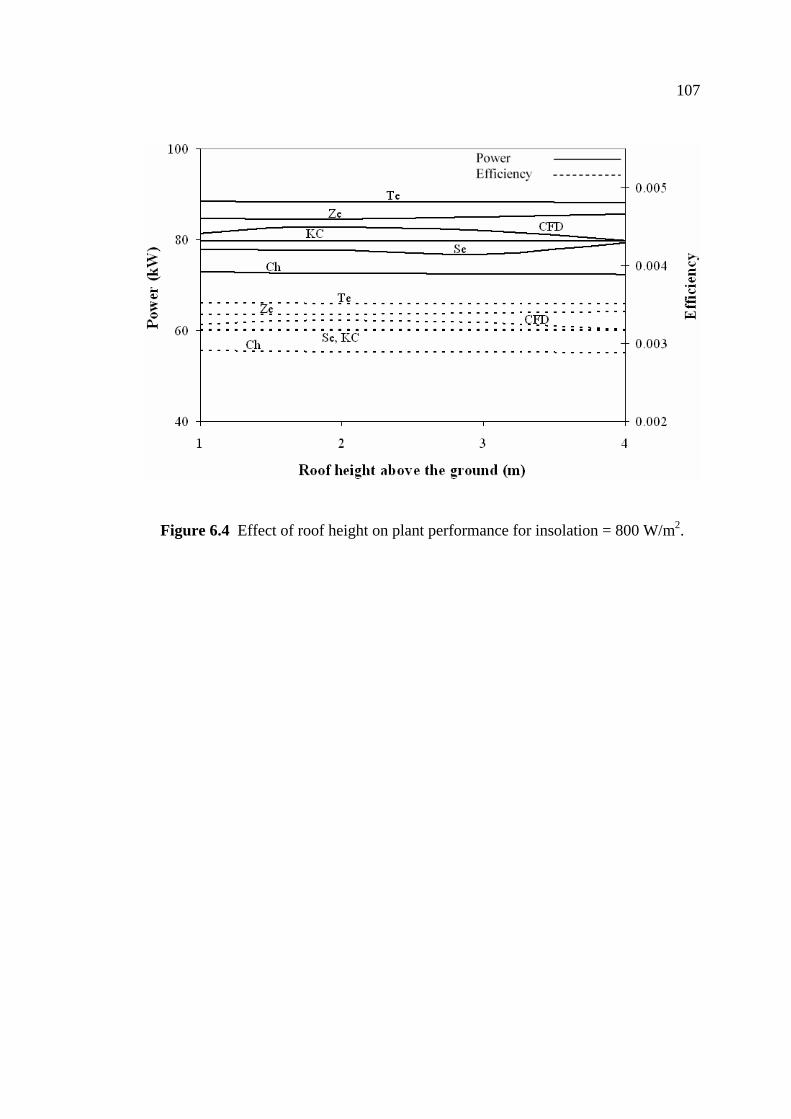
107
Figure 6.4 Effect of roof height on plant performance for insolation = 800 W/m2.

108
Figure 6.5 Effect of tower radius on plant performance for insolation = 800 W/m2.

109
Figure 6.6 Effect of tower height on plant performance for insolation = 800 W/m2.

110
Figure 6.7 Effect of insolation on plant performance.

111
6.6 CONCLUSION
The influences of roof height, roof radius, tower height, tower radius, and
insolation on solar chimney power plant performances have been studied by using five
simple theoretical models from the literature and a carefully calibrated CFD procedure.
Important observations are concluded as follows:
1) Model of Chitsomboon (2001) underestimates plant performances by about
15% in all cases that were investigated due probably to its built-in
conservative error estimation procedure; but it is the only model that
predicts qualitatively trends when compared to CFD results.
2) Model of Schlaich et al. (2005) is easy to use and gives reasonable results.
However, its use requires a judicious guess of a temperature difference in
the plant.
3) Model of Tingzhen et al. (2006) is easy to use but requires a judicious
guess of the density in the tower. The model tends to over-predict plant
performances.
4) Model of Zhou et al. (2009) has features that are quite similar to the model
of Tingzhen et al. The model tends to over-predict plant performances but
to a lesser degree than Tingzhen et al. model.
5) Model of Koonsrisuk and Chitsomboon (2009) is easy to use and gives
reasonable solutions comparable to the model of Schlaich et al.; it has an
advantage over the latter in that it does not require any guessed parameter
as an input.

112
According to this study, the models of Schlaich et al. and Koonsrisuk and
Chitsomboon are recommended because they compared more favorably with the CFD
results than the other models for all the test cases that were investigated.
6.7 REFERENCES
ANSYS, Inc. ANSYS CFX, Release 10.0: reference guide. ANSYS, 2005.
Chitsomboon, T., 2000. Potential and efficiency of solar chimney in the production of
electrical energy. Research and Development Journal of the Engineering,
Institute of Thailand, Vol.11(3), pp. 38-44.
Chitsomboon, T., 2001. A validated analytical model for flow in solar chimney.
International Journal of Renewable Energy Engineering, Vol. 3(2), pp.
339-346.
Dai, Y. J., Huang, H. B., Wang, R. Z., 2003. Case study of solar chimney power plants
in northwestern regions of China. Renewable Energy, Vol.28, pp. 1295-1304.
Gannon, A. J., Von Backström, T. W., 2000. Solar chimney cycle analysis with system
loss and solar collector performance. Journal of Solar Energy Engineering,
Vol. 122. pp. 133-137.
Haaf, W., Friedrich, K., Mayr, G., Schlaich, J., 1983. Solar chimneys: part I: principle
and construction of the pilot plant in Manzanares. International Journal of
Solar Energy, Vol. 2, pp. 3-20.
Koonsrisuk, A., Chitsomboon, T., 2007. Dynamic similarity in solar chimney
modeling. Solar Energy. Vol. 81(2007), pp. 1439-1446.
Koonsrisuk, A., Chitsomboon, T., 2009. A single dimensionless variable for solar
tower plant modeling. Solar Energy. doi:10.1016/j.solener.2009.07.015.

113
Pasumarthi, N., Sherif, S. A., 1998a. Experimental and theoretical performance of a
demonstration solar chimney model – part I: mathematical model development,
International Journal of Energy Research, Vol. 22, no. 3, pp. 277-288.
Pasumarthi, N., Sherif, S. A., 1998b. Experimental and theoretical performance of a
demonstration solar chimney model – part II: experimental and theoretical
results and economic analysis, International Journal of Energy Research,
Vol. 22, no. 5, pp. 443-461.
Schlaich, J., 1995. The Solar Chimney. Edition Axel Menges: Stuttgart, Germany.
Schlaich, J., Bergermann, R., Schiel, W., Weinrebe, G., 2005. Design of commercial
solar updraft tower systems utilization of solar induced convective flows for
power generation. Journal of Solar Energy Engineering, Vol. 127, pp. 117–
124.
Tingzhen, M., Wei, L., Guoliang, X., 2006. Analytical and numerical investigation of
the solar chimney power plant systems. International Journal of Energy
Research, Vol. 30, pp. 861-873.
Zhou, X., Yang, J., Xiao, B., Hou, G., Xing, F., 2009. Analysis of chimney height for
solar chimney power plant. Applied Thermal Engineering, Vol. 29, pp. 178-
185.

CHAPTER VII
EFFECT OF FLOW AREA CHANGE ON THE
POTENTIAL OF SOLAR CHIMNEY POWER PLANT
7.1 ABSTRACT
The solar chimney power plant is a solar power plant for electricity generation
by means of air flow induced through a tall chimney. Guided by a theoretical
prediction, this paper uses CFD technology to investigate the changes in flow
properties caused by the variation of flow area. It was found that the sloping collector
affects the flow properties through the plant. The divergent-top chimney leads to
augmentations in kinetic energy at the tower base significantly. The proper
combination between the sloping roof and the divergent-top chimney can produce the
power as much as hundreds times that of the conventional solar chimney power plant.
7.2 INTRODUCTION
The solar chimney power plant is a power plant proposed to generate electricity
in large scale by transforming solar energy into mechanical energy. The schematic of a
typical solar chimney power plant is sketched in Fig. 7.1. It consists of a transparent
circular roof or solar collector with a chimney at its center and a turbine, which is
generally installed at the chimney’s base. Solar radiation penetrates the roof and heats
the air underneath as a result of the greenhouse effect. Due to buoyancy effect, the
heated air flows up the tower and induces a continuous flow from the perimeter

115
towards the tower. Mechanical energy can be extracted from the energy of the flowing
air to turn an electrical generator.
Research works on solar tower started around 1970s, after the construction of a
50 kW prototype in Manzanares, Spain. This pilot plant operated from the year 1982 to
1989 and was connected to the local electric network between 1986 and 1989 (Haaf et
al., 1983; Haaf, 1984). Tests conducted have shown that the prototype plant operated
reliably and the concept is technically viable.
The effects of various geometrical parameters on the plant performance were
examined by several researchers. Padki and Sherif (1999) reported that the power and
efficiency could be increased by tapering the top end of the tower. Chitsomboon
(1999) developed a mathematical model and it showed that, as the tower top is made
convergent, the power and efficiency does not increase but stays relatively constant.
Von Backström and Gannon (2000) employed a one-dimensional compressible flow
model for the calculation of the thermodynamic variables as functions of several
parameters, including the chimney area change. The study showed that, for a given
chimney height, an increase in area ratio leads to augmentations in static pressure in
the chimney. Based on a mathematical model, Schlaich (1995) reported that optimal
dimensions for a solar chimney do not exist. However, if construction costs are taken
into account, thermoeconomically optimal plant configurations may be established for
individual sites. It was shown numerically in Pretorius and Kröger (2007) that plant
power production is a function of the collector roof shape and inlet height. Maia et al.
(2008) carried out a simulation study and found that the height and diameter of the
chimney are the most important geometric dimensions for solar chimney design. Zhou
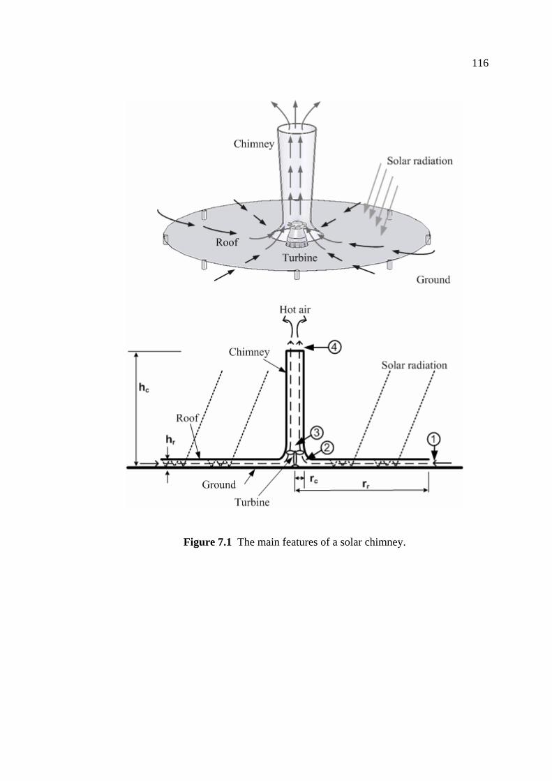
116
Figure 7.1 The main features of a solar chimney.

117
et al. (2009) reported the maximum chimney height in order to avoid negative
buoyancy, and the optimal chimney height for maximum power output. They found
that the maximum height and the optimal height increase with collector radius. A
common feature in these findings is that the plant efficiency is very low, and that it
increases with the plant size.
The work described in this paper is stimulated by the quest for a better design,
and focused on increasing the plant performance by controlling the flow area of the
system. It is guided by the theoretical investigation along with the CFD-based design
analysis. Based on the results of the computational simulation, the influence of the
flow area parameters of the solar chimney on the behavior of the airflow was assessed.
The area parameters analyzed were the areas at the collector entrance and chimney
exit, while the areas at the collector exit and the chimney entrance were kept constant.
7.3 DERIVATION OF THEORETICAL MODEL
In this simple analysis the power generated by a solar chimney power plant as
shown in Fig. 7.1 can be expressed as
( ) ( 2332 2
ppmpmW turbturb
−+
−≈Δ=ρρρ&&& ) . (7.1)
Equation (7.1) shows that W becomes larger when is amplified and is
attenuated. To determine the geometry layout that can fulfill this, the governing
equations for the movement of air within the collector and chimney are considered
separately.
&3p 2p

118
Collector. The one-dimensional steady compressible flow in a variable-area
passage is considered here. It is assumed that the solar heat gain is totally absorbed by
the air under the roof. In the absence of friction and heat loss, the conservation
equations in differential form are as follows
Continuity: 0=++A
dAVdVd
ρρ (7.2)
Momentum: VdV−=ρdp
dqVdVdTc
(7.3)
Energy: p =+ (7.4)
State equation: 0=−−Tp ρdTddp ρ . (7.5)
Let mdAqdq r &′′= and the height of the roof is given by where is
the constant and
rahr ⋅= a
r is the roof radius. Combining all equations, we have
⎟⎟⎠
⎞⎜⎜⎝
⎛ ′′−= 233
2
2 aTrcmdrq
AdAmdp
p&
&
πρ. (7.6)
Next we assume that q ′′ , , pc ρ and T are approximately constant. Integrate
from the entrance to the outlet of the collector, Eq. (7.6) becomes,
⎟⎟⎠
⎞⎜⎜⎝
⎛−
′′+⎟⎟⎠
⎞⎜⎜⎝
⎛−−= 2
12
21122
1221
2
1211
411
2 rrTcamq
AAmpp
pρπρ&&
. (7.7)

119
Chimney. The air movement inside a chimney is assumed a frictionless
adiabatic process. The system of equations for a one-dimensional steady compressible
flow in a variable-area chimney is as follows
Continuity: 0=++A
dAVdVd
ρρ (7.8)
Momentum: VdVgdz −=+ρdp
0
(7.9)
Energy: + + =gdzVdVdTcp (7.10)
State equation: 0=−−Tp ρdTddp ρ . (7.11)
Combining Eqs. (7.8) – (7.11) gives
32
AdAmgdzdpρ
ρ &+−= . (7.12)
Integrating between chimney’s inlet and outlet yields
⎟⎟⎠
⎞⎜⎜⎝
⎛−++= 2
3243
2
34311
2 AAmghpp c ρ
ρ&
. (7.13)
For a variable area collector and chimney,
21 AnA = (7.14)

120
34 AlA = . (7.15)
where and l are any constants. n
Substituting Eqs. (7.7), (7.13), (7.14) and (7.15) into Eq. (7.1):
( ) ⎥⎥⎦
⎤
⎢⎢⎣
⎡⎟⎟⎠
⎞⎜⎜⎝
⎛−
′′−⎟⎟
⎠
⎞⎜⎜⎝
⎛ −+
−+
−= 21
2211
222
233
2
32
114
1122 rrTca
mqnAn
lAlmmW
pρπρρρ&&&& (7.16)
It should be noted that when the heat loss and friction are not included in the
analysis, the power is not a function of the shape of collector or chimney. An order of
magnitude analysis reveals that, on the right-hand side of Eq. (7.16), the first term is
much greater than the second term. Thus Eq. (7.16) becomes
⎟⎟⎠
⎞⎜⎜⎝
⎛ −+
−−≅ 2
223
22
3 11nAn
lAlmW
ρ&& (7.17)
When and are changed, and l n m& 2ρ will be changed correspondingly.
However, Eq. (7.17) suggests that W may be increased when and . In other
words,
& 1>l 1<n
21 AA < . (7.18)
43 AA < . (7.19)
This finding makes recommendations regarding the arrangement of plant’s area
ratio. To evaluate it, numerical calculations of several solar chimneys with different

121
collector and chimney’s shapes were carried out to illustrate the varying behavior of
the plant performances.
7.4 Computational work
The plant layouts studied in this work are schematically depicted in Fig. 7.2.
They are: (a) a constant-height collector with a constant-area chimney, (b) a sloping
collector with a constant-area chimney, (c) a constant-height collector with a
convergent-top chimney, (d) a constant-height collector with a divergent-top chimney,
(e) a sloping collector with a convergent-top chimney, and (f) a sloping collector with
a divergent-top chimney. Their details are listed in Table 7.1. To investigate the effect
of flow area variation, we define the dimensionless measures
2112 AAAR = (7.20)
3443 AAAR = . (7.21)
To date, the performance of solar chimney has been widely investigated for the
limiting case of configuration (a). The collector is customarily of a circular shape,
while its height is relatively constant with some inclination angle, and the chimney is
modeled as a constant-diameter tube. Thus a reference plant’s geometry is simplified
to that of a horizontal disc above the ground with a constant-diameter chimney in the
center of the disc. Configuration (a) is the reference plant in this study. Its collector has
a diameter of 200 m and a height of 2 m, and it has a 100 m high chimney with a
diameter of 8 m. So and 2512AR a = 143AR a = .

122
The commercial CFD code “CFX” (ANSYS, 2005) has been proven to be a
reliable tool to simulate the flow in solar chimney (Koonsrisuk and Chitsomboon,
2007). Consequently, the numerical model had been built using CFX in this work. In
CFX, equations for the conservation of mass, momentum and energy equations are
solved using a control volume technique. The steady transport equations can be written
in general form as follows:
( ) φφ φφρ Su =∇Γ−⋅∇ (7.22)
The buoyancy term in the momentum equation and the solar heat gain in the
energy equation are given as
( )gS refM ρρ −= (7.23)
rE hqS ′′= . (7.24)
where refρ is the reference operating density specified at the inlet fluid condition of
308 K and 1 atm absolute pressure. The equations were discretized by a non-staggered
grid scheme. A high resolution upwind differencing scheme (ANSYS, 2005) was
applied for the convective terms of equations. The convergence criterion was that the
normalized residuals for mass, momentum and energy were required to be below than
10-7.
A solar chimney is a cylindrical structure, so an axis-symmetric representation
is assumed. As a result, a 5-degree pie shape of the plant was simulated as shown in
Fig. 7.2a. An unstructured, non-uniform mesh was constructed. In order to ensure the

123
(a)
(b)
(c)
(d)
(e)
(f)
Figure 7.2 Schematic layout of (a) reference plant; (b) a sloping collector with a
constant-area chimney; (c) a constant-height collector with a convergent
top chimney; (d) a constant-height collector with a divergent-top chimney;
(e) a sloping collector with a convergent-top chimney; (f) a sloping
collector with a divergent-top chimney.

124
Table 7.1 List of models illustrated in Fig. 7.2.
Configuration Objective Remark
(a)
A constant-height collector with
a constant-area chimney
Reference plant A simple geometry
version of the
conventional solar
chimney power plant
(b)
A sloping collector with a
constant-area chimney
Investigate the system when
21 AA < and 34 AA = .
cf. expression (18).
(c)
A constant-height collector with
a convergent-top chimney
Investigate the effect of
on the system with
a constant-height collector.
43 AA >
Adopt the idea from
Padki and Sherif
(1999).
(d)
A constant-height collector with
a divergent-top chimney
Investigate the effect of
43 AA < on the system with
a constant-height collector.
cf. expression (19).
(e)
A sloping collector with a
convergent-top chimney
Investigate the combined
effect of 21 AA <
and . 43 AA >
-
(f)
A sloping collector with a
divergent-top chimney
Investigate the combined
effect of 21 AA <
and 43 AA < .
-
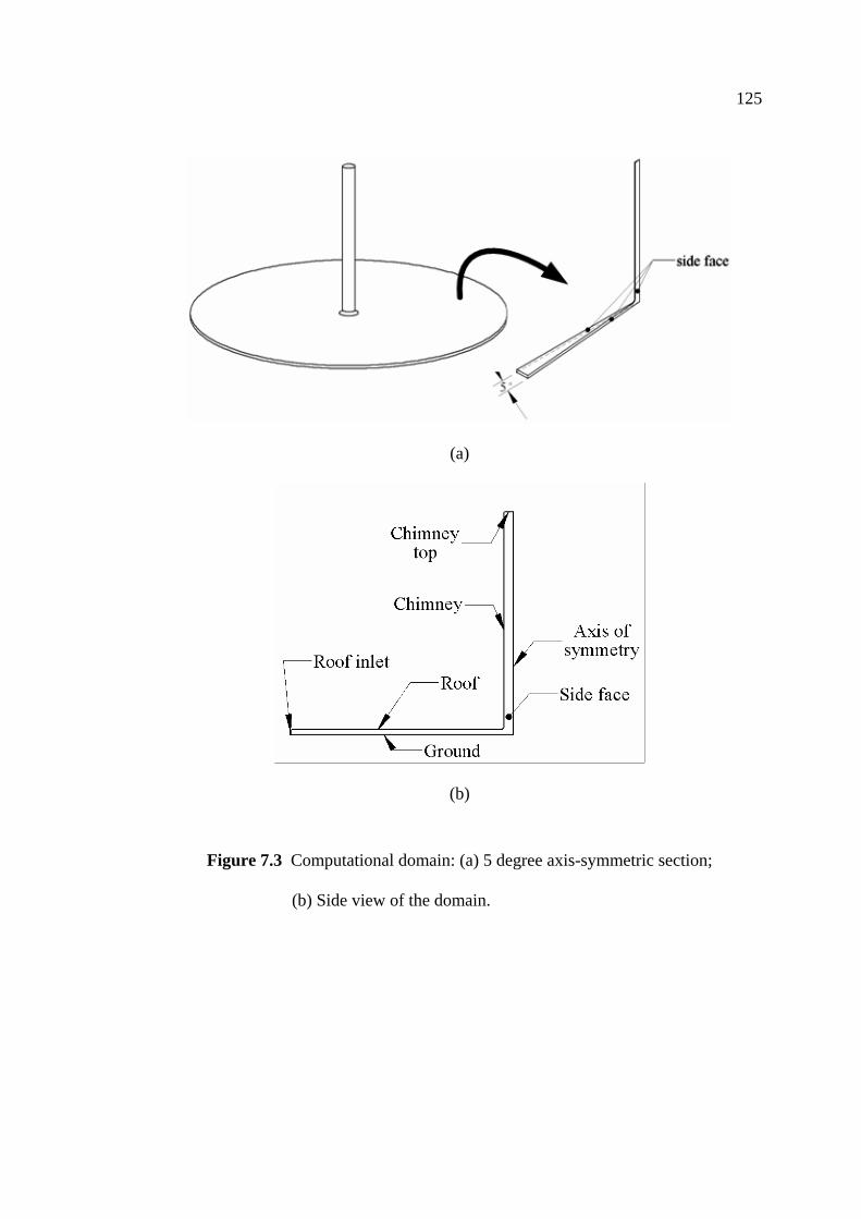
125
(a)
(b)
Figure 7.3 Computational domain: (a) 5 degree axis-symmetric section;
(b) Side view of the domain.

126
accuracy of the numerical results, a grid dependence study was realized. Furthermore,
the adaptive grid refinement algorithm locally refined the mesh only where needed
based on regionally velocity variation. It should be mentioned that the numerical
procedure used in this study had already been carefully calibrated and validated in
Koonsrisuk and Chitsomboon (2007) to achieve a satisfactory level of confidence.
The boundary conditions used are shown in Fig. 7.3b. At the center of the plant, axis-
symmetric conditions were utilized. At the walls, free-slip and adiabatic boundary
conditions were used. These conditions were applied at the roof, transition section,
chimney wall and ground surface. The total pressure and temperature are prescribed at
the roof inlet and the flow direction was set as normal to the roof perimeter. At the
chimney top, the ‘outlet’ boundary condition with zero static gauge-pressure is
imposed.
7.5 RESULTS AND DISCUSSION
Figure 7.4 shows the gauge pressure distributions inside the plants. It should be
noted that the gauge pressures were scaled so that they are equal zero at the chimney
top. It can be observed that ( )32 pp − of configuration (b) increases a little when
compare with configuration (a). One can notice that ( ) ( )ab pppp 2121 −<− while
. For configuration (c), and in such a way
that
( ) ( ab pppp 4343 −≅− )
)
a,c, pp 33 > a,c, pp 22 >
( ) ( ac pppp 3232 −≅− . On the other hand, a,d, pp 33 < and and we
found that ( ) . It was found that the numerical computation of
configuration (e) had convergence difficulties, causing a failed simulation. To mitigate
the problem, instead of testing the case of
a,d, pp 22 <
( ad pppp 3232 −>− )
21 AA < together with , we traded 43 AA >

127
off configuration (e) to the case of 21 AA = together with . In that case we
found that and in the manner that
43 AA >
a,e, pp 33 > a,e, pp 22 > ( ) ( )ae pppp 3232 −≅− . For
configuration (f) it appears that ( ) ( )af pppp 3232 −>− . It is important to notice that
the pressure change inside the system does not show a strong sensitivity to the change
of 12AR (configuration (b)), as it does to the change of (configuration (d)).
When we combine the effect of changing
43AR
12AR and together (configuration
(f)), however, the reduction of
43AR
12AR can yield a vacuum pressure inside the system as
shown in Fig. 7.4.
The favorable flow behavior when 21 AA < can be explained by the fact that
the flow velocity and pressure do not change measurably under the roof for this area
ratio layout. The flow area is increasing along the divergent-top chimney, this affects
the flow velocity and can reduce the flow acceleration, resulting in the decrease of the
pressure gradient across the chimney. The order of magnitude reveals that the pressure
drop due to the flow acceleration along the chimney is large when compared with
other pressure drops. Therefore using the appropriate can increase ( )43AR 32 pp −
significantly.
The effect of the flow area variation on the mass flow rate is presented in Fig.
7.5. The mass flow ratio depicted in Fig. 7.5 is defined as the mass flow rate of the test
cases divided by the mass flow rate of the reference case, in which and
. The results show that the varying
2512 =AR
143 =AR 12AR does not affect the mass flow rate
for the system with a constant-area chimney. On the other hand, an increase in
produces an increase in the mass flow rate. The augmentation of mass flow rate is
43AR

128
observed in cases of varying and , except the case of 43AR 75.012 >AR 25.012 =AR
and in which the flow recirculation occurred around the chimney exit. 843=AR
Figure 7.6 shows the temperature rise across the roof. It is presented in
dimensionless form and defined as the ratio of the temperature rise of the test cases to
the temperature of the reference case. The values of temperature rise are consistent
with the differences in mass flow rates presented in Fig. 7.5, since, in accordance with
the conservation of energy principle, a higher mass flow rate should give a lower
temperature rise for an equal amount of energy input.
Figures 7.7 and 8 present the sensitivity of the flow power (= 22Vm& ) with
respect to the changes of 12AR and , respectively. The ordinates of the figures
are the normalized power, which is the power of the test cases scaled by the power at
position 3 of the reference case, while the abscissas are the positions depicted in Fig.
7.1. The chimney diameter of the cases tested in Fig. 7.7 is constant. It is obvious that
the power at position 1 is a function of
43AR
12AR and a sloping roof leads to the power
reduction inside the chimney. Although decreasing 12AR can increase the power at
position 1 notably, but this power rise is still lower than the power inside the chimney.
Further inspection reveals that the collector efficiency (= rp AqTcm ′′Δ& ) of the system
with a sloping collector and a constant-area chimney is a weak function of 12AR , and
its overall efficiency (= rAqVm ′′235.0 & ) is relatively constant.
It is apparent in Fig. 7.8, in which the roof height is constant, that the power at
position 3 is a strong function of . It should be noted that the case of
offers higher power than that of
43AR
1643 =AR 3243=AR due to the flow recirculation
occurring near the chimney exit when 3243=AR .

129
Table 7.2 presents the normalized power at the chimney base (position 3); the
square of of each case is also shown. It is observed that the power increases in
proportion to
43AR
( )243AR when AR ranges between 0.25 to 8 and at a lower rate
thereafter. This quadratic trend is suggested by Eq. (7.17). It would seem that there is
an upper bound on that can boost up the power. Too high would
eventually lead to boundary layer separation. Friction that comes with high velocity
would also reduce the benefit. Further inspection of Table 7.2 shows that the efficiency
also increases as increases. Efficiency in this case is defined as power at tower
base divided by the total solar heat gain. This definition is unfair to the convergent-top
case because its potential is at the top, not at the base. However, numerical results
reveal that the power at the top of the convergent tower remains the same as the
constant area case. So, its potential remains unchanged in relation to the constant area
case.
43AR 43AR
43AR
The combined effect of 12AR and was shown in Fig 7.9. Because the
flow velocity of the cases of
43AR
25.012 =AR is very high, so the flow recirculation is
presented when . This is the reason that the power of the cases of
is less than those of
143 >AR
25.012 =AR 5.012 =AR . As observed in the plots of pressure and
mass flow rate that the ‘proper’ combination between 12AR and offers the
largest power. It was found that the ‘proper’ combination depends on the whole size of
the plant.
43AR
In any case, it is evident that high leads to augmentation in power at the
tower base. This suggests the potential of harnessing more turbine power from the high
system.
43AR
43AR

130
7.6 CONCLUSION
A solar chimney system with varying flow area was studied and its
performance was evaluated. Theoretical analysis suggests that the solar chimney with
sloping collector and divergent-top chimney would perform better than that of a
conventional system. CFD calculations show that a divergent tower helps increase the
static pressure, mass flow rate and power over that of the constant area tower. For the
convergent tower, the power remains the same as the constant area case. The sloping
collector helps increase the static pressure across the roof and the power at the roof
entrance. The system with the sloping collector and divergent-top chimney of tower
area ratio of 16 can produce power as much as 400 times that of the reference case.

131
Figure 7.4 Effect of area variation on the pressure profiles.

132
Figure 7.5 Effect of area variation on the mass flow rate (scaled by the mass flow rate
of the reference case).

133
Figure 7.6 Effect of area variation on the collector temperature rise (scaled by the
temperature rise of the reference case).

134
Figure 7.7 Effect of 12AR on the flow power (scaled by the flow power of prototype
at position 3).

135
Figure 7.8 Effect of on the flow power (scaled by the flow power of prototype 43AR
at position 3).

136
Figure 7.9 Combined effect of 12AR and on the flow power (scaled by the 43AR
flow power of prototype at position 3).

137
Table 7.2 Power at the chimney base scaled by the power of the reference case, the
square of and the efficiency at chimney entrance, 43AR
rAqVm ′′×= 235.0100 &η .
43AR ( )243AR Power η (%) Note
1 1 1 0.36 Reference case
0.25 0.06 0.06 0.02
0.5 0.25 0.25 0.09
0.75 0.56 0.54 0.19
2 4 4.27 1.54
4 16 18.49 6.66
8 64 69.07 24.89
16 256 179.16 64.55
Note: All test cases use the constant-diameter chimney.

138
7.7 REFERENCES
ANSYS, Inc. ANSYS CFX, Release 10.0: reference guide. ANSYS, 2005.
Chitsomboon, T., 1999. The effect of chimney-top convergence on efficiency of a
solar chimney. In: Proceeding of the 13th National Mechanical Engineering
Conference, Thailand.
Von Backström, T. W. and Gannon, A. J., 2000. Compressible flow through solar
power plant chimneys. ASME Journal of Solar Energy Engineering, Vol.
122(3), pp. 138-145.
Haaf, W., Friedrich, K., Mayr, G., Schlaich, J., 1983. Solar chimneys: part I: principle
and construction of the pilot plant in Manzanares. International Journal of
Solar Energy, Vol. 2, pp. 3-20.
Haaf, W., 1984. Solar chimneys: part II: preliminary test results from the Manzanares
plant. International Journal of Solar Energy, Vol. 2, pp. 141-161.
Koonsrisuk, A., Chitsomboon, T., 2007. Dynamic similarity in solar chimney
modeling. Solar Energy, Vol. 81(12), pp. 1439-1446.
Maia, C. B., Ferreira, A. G., Valle, R. M., Cortez, M. F. B., 2008. Theoretical
evaluation of the influence of geometric parameters and materials on the
behavior of the airflow in a solar chimney. Computers & Fluids, doi:
10.1016/j.compfluid.2008.06.005
Padki, M. M., Sherif, S. A., 1999. On a simple analytical model for solar chimneys,
International Journal of Energy Research, Vol. 23, pp. 289-294.
Pretorius, J. P., Kröger, D. G., 2007. Sensitivity analysis of the operating and technical
specifications of a solar chimney power plant. ASME Journal of Solar
Energy Engineering, Vol. 129, pp. 171-178.

139
Schlaich, J., 1995. The Solar Chimney. Edition Axel Menges: Stuttgart, Germany.
Zhou, X., Yang, J., Xiao, B., Hou, G., Xing, F., 2009. Analysis of chimney height for
solar chimney power plant. Applied Thermal Engineering, Vol. 29, pp. 178-
185.

CHAPTER VIII
THEORETICAL TURBINE POWER YIELD IN
SOLAR CHIMNEY POWER PLANTS
8.1 ABSTRACT
The solar chimney power plant is a promising system to generate electrical
power from free solar energy. The analysis was carried out to improve the description
of the operation mode and efficiency. The solar collector, chimney and turbine are
modeled together theoretically, and iteration techniques were then carried out to solve
the mathematical model developed. This model was developed to estimate power
output of solar chimneys as well as to examine the effect of solar heat flux and
structural dimensions on the power output. Results from the mathematical model were
validated by measurements from the physical plant actually built and the model was
further used to predict the performance characteristics of large-scale commercial solar
chimneys. The results show that the plant size, the factor of pressure drop at the
turbine and the solar heat flux are the important parameters for the performance
enhancement.
8.2 INTRODUCTION
The solar chimney power plant is a solar electricity production facility
employing solar radiation to increase the internal energy of air flowing through the
system. The schematic of a typical solar chimney is sketched in Fig. 8.1. In this plant,
air is heated as a result of the greenhouse effect under a translucent roof (collector). As

141
the roof is open at its periphery, buoyancy drives a continuous flow from the roof
perimeter into the chimney which is located at the middle of the roof. An electricity-
generating turbine is set in the path of the air current to convert the kinetic energy of
the flowing air into electricity.
Solar chimney power plants can convert only a small portion of the solar
energy collected into electricity, but their cheap, robust construction and low
maintenance costs make up for this disadvantage (Schlaich, 1995). To make this
technology economically viable, the optimum configurations of each component are
needed. Efficient conversion of fluid power to shaft power depends primarily on the
operation of turbine. During the day, mass flow through the system is varying due
mainly to variation of solar radiation. Accordingly, the turbine blade pitch should be
adjusted during operation to regulate power output. Seemingly, there should be a
relevant optimum turbine setting for maximum power output.
To evaluate the available plant power output, researchers defined the ratio of
the pressure drop across the turbine to the total available system pressure difference.
This ratio is symbolized as totturb pp herein. Most investigators have assumed that
the optimum totturb pp is 2/3 (Haaf et al., 1983; Mullett, 1987; Schlaich, 1995; Lodhi,
1999; Von Backström and Gannon, 2000; Dai et al., 2003; Zhou et al., 2007).

142
Figure 8.1 Schematic layout of solar chimney power plant

143
Though computations of the values taken from a table of data given by Schlaich
(1995) showed that totturb pp used is 0.82. Hedderwick (2001) illustrated that the ratio
is between 0.66-0.7 during the day. Furthermore, Schlaich et al. (2005) presented,
without reference, that the optimum ratio is 0.8. Meanwhile, Bernardes et al. (2003)
reported an optimum value of 0.97. Although the turbine under consideration is
encased by the tower, some authors use the ratio as 16/27 (Pasumarthi and Sherif,
1998; Pastohr et al., 2004; Onyango and Ochieng, 2006), which is the Betz limit
obtained for an actuator disc in a free stream situation.
Here a detailed theoretical model is developed to evaluate the performance of
solar chimney power system. The present paper also presents the operating range of
the turbine. It tries to determine how to maximize the fluid power by adjusting the
pressure drop across the turbine and the flow through it.
8.3 OPTIMAL PRESSURE RATIO
According to the operation principle mentioned above, the air inside the system
is less dense than the atmospheric air outside. A driving pressure generated can
be subdivided into a static pressure difference, drops at the turbine, and the dynamic
component, describes the kinetic energy of the airflow, neglecting friction losses:
totpΔ
dynturbtot ppp Δ+Δ=Δ . (8.1)
Let’s define the ratio totturb pp as x , it yields
totturb pxp Δ=Δ . (8.2)

144
Using the standard definition for dynamic pressure:
2
21
turbwithcdyn Vp ρ=Δ . (8.3)
Without turbine, a maximum flow speed is achieved and the whole driving
potential is used to accelerate the flow thus,
2
21
turbnoctot Vp ρ=Δ . (8.4)
Substituting Eqs. (8.2), (8.3) and (8.4) into Eq. (8.1), this yields
( )xVV turbnoturbwith −= 1 . (8.5)
The theoretical power extracted by the turbine can be determined from the
energy equation and the Gibb’s relation from classical thermodynamic which can be
written as
turbturb
ext pmvdpmW Δ≈= ∫ ρ&
&& . (8.6)
Substituting Eqs. (8.2) and (8.5) into Eq. (8.6) yields
totturbnocext pxVxAW Δ⋅⋅⋅−⋅= 1& . (8.7)

145
The optimal x for maximum power extraction can be obtained by assuming
that and are not the function of turbnoV totpΔ x and solving 0=∂∂ xWext& . The result
for the optimal pressure ratio is
32
=optx . (8.8)
Consequently, the maximum power is obtained when the turbine pressure drop
is 2/3 of the no-flow pressure drop. It corresponds to the value that most researchers
have utilized. From the assumptions made, the result is true for all systems with a
constant pressure potential.
Equation (8.7) shows that the plant power output can be increased by adjusting
the turbine pressure drop. Later in the analysis, it will be shown that the mass flow rate
and turbine pressure drop are coupled.
In addition, with the stations numbering as given in Fig. 8.1, the temperature
rise can be estimated from the energy equation across the roof portion,
( ) ( ) rp AqVVmTTcm ′′=−+− 21
2212 2
1&& (8.9)
where, for simplicity, frictional effect is ignored because the velocity in this region is
quite low. Because the flow is in the very low Mach number regime, the kinetic energy
contribution can be safely neglected, therefore,
rp AqTcm ′′=Δ& . (8.10)

146
When the inlet solar radiation is assumed constant, Eq. (8.10) shows that the
mass flow rate is inversely proportional to the temperature rise. Accordingly, the
pressure potential is dependent on the flow. As a result, the assumption that and
are not the function of
turbnoV
totpΔ x would make the predicted power inexact.
8.4 ANALYTICAL MODEL
In this analysis, the turbine is treated as the Rankine-Froude actuator disc
(Eggleston and Stoddard, 1987). The assumptions on which this actuator disc is based
are as follows:
1. Steady, homogeneous wind.
2. Uniform flow velocity at disc.
3. Static pressure decreases discontinuously across the disc.
4. No rotation of flow produced by disc.
Accordingly, Eq. (8.6) becomes,
( ) ( 3232 2
ppmWext −+
=ρρ&& ) . (8.11)
By synthesizing equations for continuity, momentum and energy of the flow
under the roof, Chitsomboon (2001) proposed that
( )∫ ⎟⎟⎠
⎞⎜⎜⎝
⎛ ′′−
−=−
2
12
2
12 1 TcmdAq
AdA
MVpp
p
r
&
ρ . (8.12)
Assuming that , and are constant while q ′′ pc m& ρ and T can be
approximated to be 1ρ and without significantly affecting the numerical values of 1T

147
the terms. The Mach number is presumed to be very low and thus is neglected; the
equation is then simplified to be,
⎟⎟⎠
⎞⎜⎜⎝
⎛−−
′′+= 2
1221
2
11212
112
ln2 AA
mrr
Tchqmpp
c
r
pr ρρπ&&
(8.13)
where , 1p 1ρ and are approximated as , 1T ∞p ∞ρ and , respectively. Eq. (8.13)
shows that is the combination of the inlet pressure, , with the pressure increase
due to heat addition,
∞T
2p 1p
c
r
pr rr
Tchqm ln
2 112ρπ
′′&, and the pressure decrease due to flow area
reduction, ⎟⎟⎠
⎞⎜⎜⎝
⎛− 2
1221
2 112 AAmρ&
towards the roof center. Order of magnitude analysis
reveals that ⎟⎟⎠
⎞⎜⎜⎝
⎛− 2
1221
2 112 AAmρ&
is significantly greater than c
r
pr rr
Tchqm ln
2 112ρπ
′′&.
Refer to Eq. (8.10), rearranging yields
p
r
cmAqTT&
′′+= 12 (8.14)
where
TUIq Δ⋅−⋅=′′ α (8.15)
(Duffie and Beckman, 1991).
Accordingly,
UAcm
ITrp +⋅
⋅=Δ&
α . (8.16)
148
If the turbine work extraction process is assumed to be an isentropic process,
then
γγ 1
2
323
−
⎟⎟⎠
⎞⎜⎜⎝
⎛=
ppTT . (8.17)
Furthermore, the momentum equation for flow through a constant area vertical
tower of height, is ch
( ) ⎟⎟⎠
⎞⎜⎜⎝
⎛−⎟⎟
⎠
⎞⎜⎜⎝
⎛+⋅⋅++=
34
2
434311
21
ρρρρ
cc A
mhgpp&
. (8.18)
The hydrostatic equilibrium requires that
gdzdp ρ−= . (8.19)
According to Calvert (1990), when the atmospheric air parcel is regarded as
unsaturated medium and expand slowly to a lower atmospheric pressure without
exchange of heat, the dry adiabatic temperature lapse rate equation can be written as
zcgTT
p
−= ∞ . (8.20)
Let us assume that the air behaves as a perfect gas. Eq. (8.20) can be
substituted into Eq. (8.19) to give as 4p

149
Rc
cp
p
hTcgpp ⎟
⎟⎠
⎞⎜⎜⎝
⎛−=
∞∞ 14 . (8.21)
Consider that a dry adiabatic lapse rate can be applicable to the flow in a tower.
In accordance with Eq. (8.19),
cp
hcgTT −= 34 . (8.22)
For a thermally perfect air,
4
44
3
33
2
22 ,,
RTp
RTp
RTp
=== ρρρ . (8.23)
Consider the pressure potential as the available pressure difference between the
tower base and the surroundings. Consequently, in this analysis,
. (8.24) 31 ppptot −=Δ
8.5 ANALYTICAL SOLUTION PROCEDURE
According to the formulation above, if mass flow rate is known or assumed
then the power output can be attained. The steps of calculating the plant power output
are:
1. Choose the mass flow rate,
2. Calculate using Eq. (8.16), 2T
3. Calculate using Eq. (8.15), q ′′

150
4. Calculate using Eq. (8.13), 2p
5. Calculate 2ρ using Eq. (8.23),
6. Calculate using Eq. (8.21), 4p
7. Estimate , then calculate , 3p 3T 3ρ , , 4T 4ρ using Eq. (8.17), Eq. (8.23), Eq.
(8.22) and Eq. (8.23), respectively. Calculate using Eq.(8.18), then
compare the new to the former . Perform the iteration process until
the difference between corresponding new and old is less than the
acceptable value.
3p
3p 3p
3p
8. Calculate using Eq. (8.11), extW&
9. Calculate using Eq. (8.24). totpΔ
8.6 RESULTS AND DISCUSSION
Validity of the method for the Manzanares prototype
To validate the analytical models, the theoretical data were compared with the
experimental results of the prototype from Manzanares, Spain. The plant dimensions
are given in Table 8.1.
Firstly, according to Haaf (1984) the measured data for September 2nd, 1982
are displayed in Fig. 8.2. The comparisons between theoretical and experimental are
presented in Table 8.2. Based on the data provided by the reference article, q ′′ for
these data set, instead of using Eq. (8.15), are computed from
Iq coll ⋅=′′ η . (8.25)

151
where collη is the collector efficiency computed from the experiment data. It is
obvious that all prediction values are underestimated. This is consistent with the
intended built-in feature of as stated in Chitsomboon (2001) (so called conservative
modeling). It should also note that the differences between the experimental data and
prediction of
2p
totpΔ are very large. Though Haaf (1984) claimed that the total pressure
differences, presented in Fig. 8.2(d), were from the roof entrance to the tower top,
these differences are close to the theoretical 13pΔ which are the total pressure
differences proposed in this present work.
Furthermore, the measured data from Manzanares prototype plant for
September 1st, 1989 are taken from Weinrebe (2001). The data adopted is presented in
Table 8.3. The comparisons are shown in Table 8.4. The results show good agreement
between analytical models and experimental results. These should warrant the
reliability of the proposed models.

152
Time (h)
Am
bien
t tem
pera
ture
, Ta
(ºC)
Glo
bal r
adia
tion,
G (W
/m2 )
G
Ta
20 min interval measurements on 2nd of Sept., 82
(a)
measured on 2nd of September 1982
early model with idealized input data
Collector efficiency
(%)
daily mean
model measured
Time [h]
34% 31.3%
(b)

153
Time [h]
V
ΔT
ΔT (º
C)
Vel
ocity
, V (m
/s)
(c)
measurement at 20-min intervals on 2 Sept 82 20 min interval measurements on 2nd Sept 82
ambient pressure (zero level) Pa ≈ 939 m bar
total pressure difference
Chimney pipe friction
friction at inlet section
turbine pressure drop
Time [h]
Pres
sure
diff
eren
ces Δ
p (m
bar)
(d)
Figure 8.2 Momentary measurements on 2nd September 1982 from Manzanares
prototype plant: a) global radiation I and ; b) thermal efficiency of the 1T
collector; c) and ; d) pressure differences 12TΔ cV
(adapted from Haaf (1984)).

154
Table 8.1 Geometrical dimensions of the pilot plant in Manzanares, Spain.
Mean roof radius, rr 122 m
Average roof height, rh 1.85 m
Tower height, ch 194.6 m
Tower radius, cr 5.08 m
Table 8.2 Comparison between measured data from Manzanares pilot plant and
theoretical results; data on 2nd September 1982 taken from Haaf (1984).
4V (m/s) turbpΔ (mbar) 14pΔ (mbar) 13pΔ
(mbar)
Time I
(W/m2)
collη
(%)
1T
(°C)
12TΔ
(°C)
measured theory measured theory measured theory theory
10.00 744.4 24.3 21.1 14.8 7 6.72 0.8 0.62 1.24 21.1 1.0
12.00 850 27.1 23.4 17.8 9 7.25 0.8 0.74 1.44 20.9 1.18
14.00 755.6 25.7 26.1 17.4 7 6.29 0.84 0.81 1.7 20.7 1.14
16.00 455.6 23.6 27.9 11.3 7.7 5.28 0.6 0.51 1.2 20.6 0.74

155
Table 8.3 Data of Manzanares pilot plant for 1st September 1989 taken from
Weinrebe (2001).
Global solar radiation (W/m2), I 1,017
Ambient temperature (°C), 1T 18.5
Ambient pressure (Pa), 1p 92,930
Collector absorption coefficient, α 0.65
Collector loss coefficient (W/m2.K), U 15
Turbine efficiency 0.85
Generator and gearbox efficiency 0.9
Upwind velocity (m/s), 4V 8.1
Table 8.4 Comparison between measured data from Manzanares pilot plant and
theoretical results. (data on 1st September 1989)
Parameter Measured Theory
2T (°C) 38 41.5
extW& (kW) 48.4 48.3
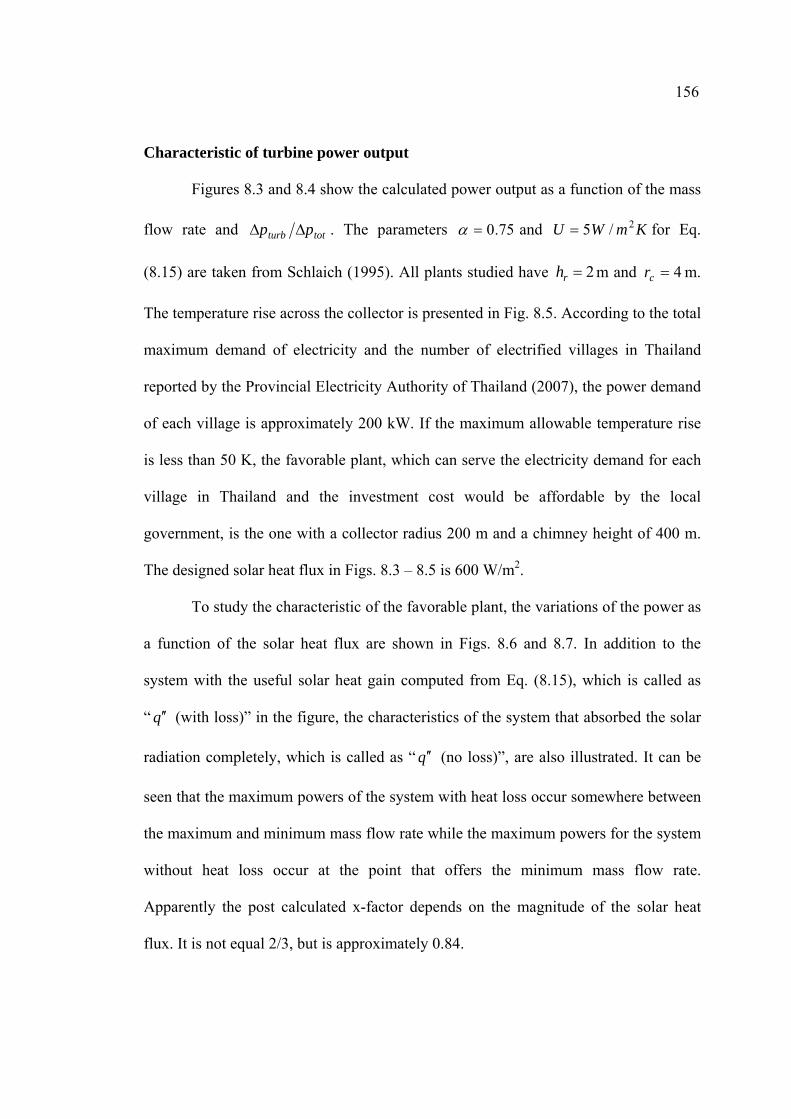
156
Characteristic of turbine power output
Figures 8.3 and 8.4 show the calculated power output as a function of the mass
flow rate and totturb pp ΔΔ . The parameters 75.0=α and for Eq.
(8.15) are taken from Schlaich (1995). All plants studied have m and
KmWU 2/5=
2=rh 4=cr m.
The temperature rise across the collector is presented in Fig. 8.5. According to the total
maximum demand of electricity and the number of electrified villages in Thailand
reported by the Provincial Electricity Authority of Thailand (2007), the power demand
of each village is approximately 200 kW. If the maximum allowable temperature rise
is less than 50 K, the favorable plant, which can serve the electricity demand for each
village in Thailand and the investment cost would be affordable by the local
government, is the one with a collector radius 200 m and a chimney height of 400 m.
The designed solar heat flux in Figs. 8.3 – 8.5 is 600 W/m2.
To study the characteristic of the favorable plant, the variations of the power as
a function of the solar heat flux are shown in Figs. 8.6 and 8.7. In addition to the
system with the useful solar heat gain computed from Eq. (8.15), which is called as
“ (with loss)” in the figure, the characteristics of the system that absorbed the solar
radiation completely, which is called as “
q ′′
q ′′ (no loss)”, are also illustrated. It can be
seen that the maximum powers of the system with heat loss occur somewhere between
the maximum and minimum mass flow rate while the maximum powers for the system
without heat loss occur at the point that offers the minimum mass flow rate.
Apparently the post calculated x-factor depends on the magnitude of the solar heat
flux. It is not equal 2/3, but is approximately 0.84.
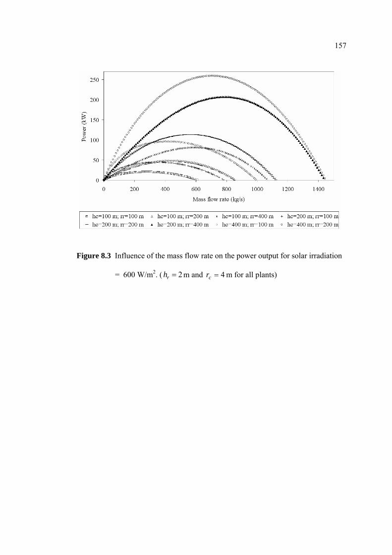
157
Figure 8.3 Influence of the mass flow rate on the power output for solar irradiation
= 600 W/m2. ( 2=rh m and 4=cr m for all plants)

158
Figure 8.4 Influence of the pressure ratio [cf. Eq. (8.2)] on the power output for solar
irradiation = 600 W/m2. ( 2=rh m and 4=cr m for all plants)

159
Figure 8.5 Influence of the mass flow rate on the collector temperature rise for solar
irradiation = 600 W/m2. ( 2=rh m and 4=cr m for all plants)
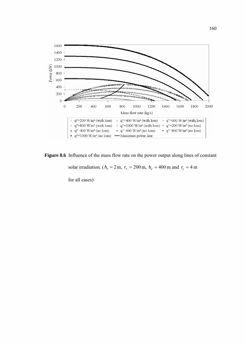
160
Figure 8.6 Influence of the mass flow rate on the power output along lines of constant
solar irradiation. ( 2=rh m, 200=rr m, 400=ch m and m 4=cr
for all cases)

161
Figure 8.7 Influence of the pressure ratio on the power output along lines of constant
solar irradiation. ( 2=rh m, 200=rr m, 400=ch m and m 4=cr
for all cases)

162
To investigate further the effect of plant size on the flow characteristics, Fig.
8.8 – 8.10 show the relationships between 13pΔ , 23pΔ , q ′′ and of different-size
plants, including the favorable plant. It is clear that their relations depend on the plant
sizes. Fig. 8.11 shows the collector efficiency that is defined as
m&
rpcol AqTcm ′′Δ= 12&η . (8.26)
It is apparent that the collector efficiency is not a function of the solar heat
gain. It depends on the plant size and there is no representative value. We observe that
for all the collectors, the efficiency decreases with increasing the plant size. This can
be explained by the fact that, when the plant size increases, the flow velocity increases
and the time to extract the useful energy from the collector decreases.
Although the flow properties between plants are widely scattered as displayed
in Fig. 8.8 – 8.11, it is important to notice from Fig. 8.12 that the values of
pcr
c
cghAqVApβ′′
Δ 213 are approximately equal to one for all plants. Koonsrisuk and
Chitsomboon (2009) proposed that
1222 =
′′ pcr cghAqVm
β&
. (8.27)
Assume that the whole pressure difference is used to accelerate the air and is
thus converted completely into kinetic energy:
222213 VmVAp c &=Δ . (8.28)

163
Consequently,
1213 =′′Δ
pcr
c
cghAqVApβ
, (8.29)
confirmed by Fig. 8.12.
Figure 8.13 presents losspΔ , which is the pressure difference between and
. Surprisingly all data collapse into one single line and it is found that
13pΔ
23pΔ
213 0002.0 mp &=Δ (8.30)
regardless of the plant size or the solar heat flux. As a result, we can use Eqs. (8.29)
and (30) together with the collector efficiency from Fig. 8.11 to approximate the
turbine power of the plant of a specific size.
8.7 CONCLUSION
Theoretical simulations were conducted in order to evaluate the performance of
the solar chimney power plant. The relationships between the x-factor and the mass
flow rate, the temperature rise across the collector and the power output are presented.
It was found that, for a system with constant pressure potential (available system
pressure difference), the optimum ratio of the turbine pressure drop to the pressure
potential is 2/3. For the system with the pressure potential not constant, it is clear that
this optimum ratio is a function of the plant size and solar heat flux. This study may be
helpful in preliminary plant design.

164
Figure 8.8 Influence of the mass flow rate on the total pressure potential along lines
of constant solar irradiation. ( 2=rh m and 4=cr m for all plants)

165
Figure 8.9 Influence of the mass flow rate on the turbine pressure drop along lines of
constant solar irradiation. ( 2=rh m and 4=cr m for all plants)
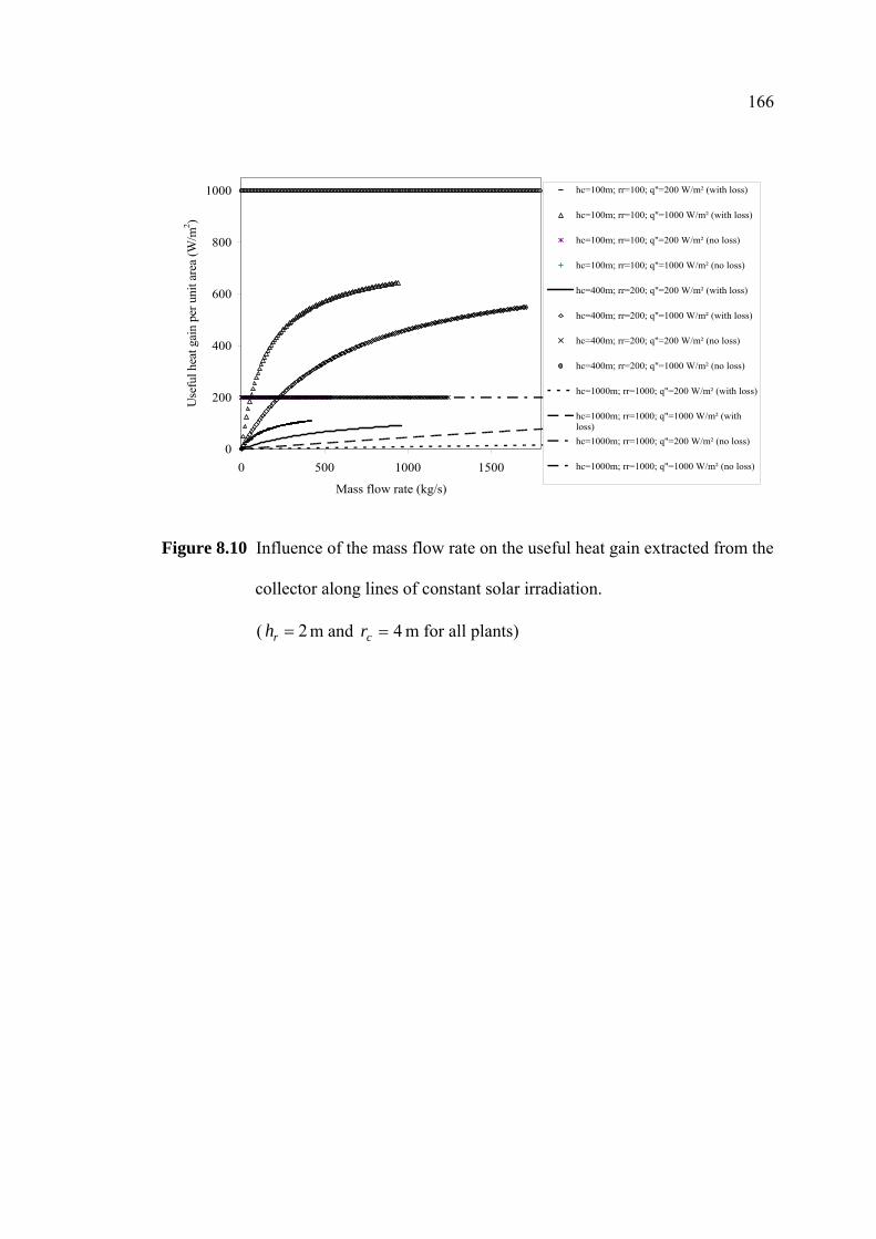
166
0
200
400
600
800
1000
0 500 1000 1500
Mass flow rate (kg/s)
Use
ful h
eat g
ain
per u
nit a
rea
(W/m
2 )hc=100m; rr=100; q"=200 W/m² (with loss)
hc=100m; rr=100; q"=1000 W/m² (with loss)
hc=100m; rr=100; q"=200 W/m² (no loss)
hc=100m; rr=100; q"=1000 W/m² (no loss)
hc=400m; rr=200; q"=200 W/m² (with loss)
hc=400m; rr=200; q"=1000 W/m² (with loss)
hc=400m; rr=200; q"=200 W/m² (no loss)
hc=400m; rr=200; q"=1000 W/m² (no loss)
hc=1000m; rr=1000; q"=200 W/m² (with loss)
hc=1000m; rr=1000; q"=1000 W/m² (withloss)hc=1000m; rr=1000; q"=200 W/m² (no loss)
hc=1000m; rr=1000; q"=1000 W/m² (no loss)
Figure 8.10 Influence of the mass flow rate on the useful heat gain extracted from the
collector along lines of constant solar irradiation.
( 2= m and rh 4=cr m for all plants)
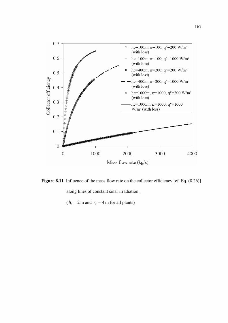
167
Figure 8.11 Influence of the mass flow rate on the collector efficiency [cf. Eq. (8.26)]
along lines of constant solar irradiation.
( 2= m and rh 4=cr m for all plants)

168
Figure 8.12 Influence of the mass flow rate on the dimensionless 13pΔ
[cf. Eq. (8.29)] along lines of constant solar irradiation.
( 2= m and rh 4=cr m for all plants)

169
Figure 8.13 Influence of the mass flow rate on the plant total pressure loss along lines
of constant solar irradiation. ( 2=rh m and 4=cr m for all plants)
170
8.8 REFERENCES
Bernardes, M. A., Dos, S., Voß, A., Weinrebe, G., 2003. Thermal and technical
analyses of solar chimneys. Solar Energy, Vol. 75(6), pp. 511-524.
Calvert, J. G. 1990. Glossary of atmospheric chemistry terms (Recommendations
1990). Pure and applied chemistry, Vol. 62(11), pp. 2167-2219.
Chitsomboon, T. 2001. A validated analytical model for flow in solar chimney.
International Journal of Renewable Energy Engineering, Vol. 3(2), pp.
339-346.
Dai, Y. J., Huang, H. B., Wang, R. Z. 2003. Case study of solar chimney power plants
in northwestern regions of China. Renewable Energy, Vol.28, pp. 1295-1304.
Duffie, J., Beckman, W. A. 1991. Solar Engineering of Thermal Processes. 2nd ed.
John Wiley & Sons, Inc., USA.
Eggleston, D. M., Stoddard, F. S. 1987. Wind Turbine Engineering Design. Van
Nostrand Reinhold Company, Inc., USA.
Haaf, W., Friedrich, K., Mayr, G., Schlaich, J. 1983. Solar chimneys: part I: principle
and construction of the pilot plant in Manzanares. International Journal of
Solar Energy, Vol. 2, pp. 3-20.
Haaf, W., 1984. Solar chimneys: part II: preliminary test results from the Manzanares
plant. International Journal of Solar Energy, Vol. 2, pp. 141-161.
Hedderwick, R. A., 2001. Performance evaluation of a solar chimney power plant.
M.Sc. Eng.-thesis, University of Stellenbosch, Stellenbosch, South Africa.
Koonsrisuk, A., Chitsomboon, T., 2009. A single dimensionless variable for solar
tower plant modeling. Solar Energy. doi:10.1016/j.solener.2009.07.015.

171
Lodhi, M. A. K. 1999. Application of helio-aero-gravity concept in producing energy
and suppressing pollution. Energy Conversion & Management, Vol. 40, pp.
407-421.
Mullett, L. B., 1987. The solar chimney - overall efficiency, design and performance.
Int. J. Ambient Energ., Vol. 8(1), pp. 35–40.
Onyango, F. N., Ochieng, R. M., 2006. The potential of solar chimney for application
in rural areas of developing countries. Fuel, Vol. 85, pp. 2561-2566.
Pastohr, H., Kornadt, O., Gürlebeck, K. 2004. Numerical and analytical calculations of
the temperature and flow field in the upwind power plant. International
Journal of Energy Research, Vol. 28, pp. 495-510.
Pasumarthi, N., Sherif, S.A. 1998. Experimental and theoretical performance of a
demonstration solar chimney model – part I: mathematical model
developement. International Journal of Energy Research, Vol. 22, pp. 277-
288.
Provincial Electricity Authority of Thailand. 2007. Annual report. [On-line].
Available: http://www.pea.co.th/annualreport/2007/PEA.swf
Schlaich, J. 1995. The Solar Chimney. Edition Axel Menges: Stuttgart, Germany.
Schlaich, J., Bergermann, R., Schiel, W., Weinrebe, G. 2005. Design of commercial
solar updraft tower systems utilization of solar induced convective flows for
power generation. Journal of Solar Energy Engineering, Vol. 127, pp. 117–
124.
Von Backström, T. W., Gannon, A. J., 2000. The solar chimney air standard
thermodynamic cycle. SAIMechE R&D Journal, Vol. 16 (1), pp. 16–24.

172
Weinrebe, G., Schiel, W., 2001. Up-draught solar tower and down-draught energy
tower - a comparison. In: Proceedings of the ISES Solar World Congress
2001, Adelaide, Australia.
Zhou, X., Yang, J., Xiao, B., Hou, G., 2007. Simulation of a pilot solar chimney
thermal power generating equipment. Renewable Energy, Vol.32, pp. 1637-
1644.

CHAPTER IX
EXPERIMENTAL PERFORMANCE OF A
DEMONSTRATION SOLAR CHIMNEY MODEL
9.1 ABSTRACT
Four small-scale physical models of the solar chimney were constructed at
Suranaree University of Technology, Nakhon Ratchasima Province, Thailand. The
height of the roof inlet was adjustable in some plants, so that the ratio of flow areas
between roof inlet and roof outlet could be varied. In addition, there were plants with
constant-cross-sectional-area towers and a plant with a divergent tower. Also there
was one plant with a novel roof shape designed by the researcher. To verify the
reliability of the dimensionless variables predicted by previous studies, one plant, a
half size of the others, was constructed. Through field measurements, results indicate
that the flow power increases with the decrease in the ratio of flow areas between roof
inlet and roof outlet. The divergent chimney also results in significant increase in flow
power compared to that of the constant area chimney. It was observed that the system
with the proposed novel roof shape provides approximately the same performance as
the conventional shaped system, while the ratio of flow areas between roof inlet and
roof outlet for the novel system could be practically reduced. Correspondingly the
increase in performance to some specific value which is much lower than the typical
system could be achieved. The experimental results are different from the predicted
values, but show the same trends. This may be caused by the fluctuating solar heat

174
flux and the effect of the large chimney diameter when compared with the roof size.
Moreover, the difference of dimensionless variables between the large and the small
plant is noticeable, contrary to the theoretical and numerical predictions. Reasons
could be the varying atmospheric conditions when the tests were run.
9.2 INTRODUCTION
A solar chimney is a combination of three established technologies, namely,
the translucent circular roof (or solar collector), the chimney and the turbine. The
chimney, a long tubular structure, is placed in the center of the roof, while the turbine
is generally mounted at the chimney base. This unique combination accomplishes the
task of converting solar energy into electrical energy. This solar-to-electric conversion
involves two intermediate stages. In the first stage, conversion of solar energy into
thermal energy is accomplished in the collector by means of the greenhouse effect. In
the second stage, the chimney converts the generated thermal energy into kinetic and
ultimately into electric energy by using a combination of a turbine and generator. Fig.
9.1 provides an overall view of a typical solar chimney system.
Previous theoretical and numerical research (Koonsrisuk and Chitsomboon,
2004; Koonsrisuk and Chitsomboon, 2006; Koonsrisuk and Chitsomboon, 2007;
Koonsrisuk and Chitsomboon, 2009) led to the establishment of four small-scale
experimental plants on a site at Suranaree University of Technology (Nakhon
Ratchasima, Thailand). The experimental system was designed and constructed and
was used to study the temperature and velocity profiles within the solar chimney. A
numerical model for each plant was also developed and compared the simulated
results with experimental observations.

175
9.3 THE PHYSICAL MODELS
Four physical models were built specifically for this study:
1. Experimental Set 1 has the roof with adjustable inlet height and constant-
diameter chimney.
2. Experimental Set 2 has the roof with adjustable inlet height and divergent-
top chimney.
3. Experimental Set 3 has the collector with a novel roof shape designed by the
researcher and a constant-diameter chimney.
4. Experimental Set 4 is the half-size model of Experimental Set 1.
More details of the experimental sets are listed in Table 9.1.
9.4 EXPERIMENTAL METHODOLOGY
The characterization of airflow under the roof and inside the chimney involved
the determination of meteorological and flow conditions. The thermal anemometer
with separate velocity and temperature probe (Testo model 425) were used to measure
ambient temperature, airflow temperatures and velocity. Incident solar radiation was
measured with CM3 pyranometer of Kipp and Zonen B.V. Uncertainties of ± 5°C, ±
0.05 m/s and ± 25 W/m2 were specified for the anemometer and pyranometer,
respectively.
Table 9.2 shows the details of measuring locations along the collector and the
chimney. The measurement at each location was made at different heights in the
collector and different radii in the chimney as depicted in Fig. 9.7a and 9.7b,
respectively. As a result, the variation of velocity and temperature over the cross-

176
section can be ignored, they being assumed to be constant and equal to the mean value
(V and T ), defined as
∑
∑
=
== n
ii
n
iii
A
AVV
1
1 and (9.1)
∑
∑
=
== n
ii
n
iiii
VA
TVAT
1
1
ρ
ρ (9.2)
respectively.
9.5 COMPUTATIONAL WORKS
The governing equations for mass, momentum, and energy for each plant are
solved using the commercial CFD code (ANSYS, 2005). Experimental Sets 1, 2 and 4
are simplified to that of a horizontal disc above the ground with a vertical cylinder in
the center of the disc as shown in Fig. 9.8a. The code is implemented in 3D through
the axis-symmetry approximation. As illustrated in Fig. 9.8a, only a 5-degree pie-
shape of the whole domain is modeled with the side faces treated as symmetric
boundaries. In our previous work (Koonsrisuk and Chitsomboon, 2007), suitable grid
and time step size were carefully chosen after performing grid and time step
independence tests of the numerical results, thus those configurations are adopted in
this work. The examples of grid-independence mesh system are presented in Fig. 9.8b-

177
d. Figure 9.9a displays the shape of Experimental Set 3. Again, to simulate the axis-
symmetry condition, a 1/4 of the whole plant is modeled as depicted in Fig. 9.9b.
The boundary conditions used are shown in Fig. 9.10. At the center of the
plant, axis-symmetric conditions were utilized. At the walls, free-slip and adiabatic
boundary conditions were used. These conditions were applied at the roof, transition
section, chimney wall and ground surface. The total pressure and temperature are
prescribed at the roof inlet and the flow direction was set as normal to the roof
perimeter. At the chimney top, the ‘outlet’ boundary condition with zero static gauge-
pressure is imposed.
9.6 RESULTS AND DISCUSSION
Ten test cases as listed in Table 9.3 were set up and tested for their performance. It
was found that experimental results obtained from each experimental set up varied
little on different days. The experimental results presented were thus selected from an
actual data set, not from an average of the days measured. The values from each
experimental set are displayed in the form of two graphs: velocity versus flow path
and temperature versus flow path. The flow path is the distance that the air current
moves in the experimental set up, with zero value at the outer edge of the roof, and
then assuming the value of the distance the air travels beneath the roof into the
chimney. The final position of the distance displayed is at the chimney top. Each
graph shows the actual measurement results at four points along the roof and two
points along the chimney. The displayed numerical results are the average values
across the flow area at the considered position.

178
Figure 9.1 Schematic layout of solar chimney power plant.

179
Table 9.1 Specification of the Experimental Sets.
Model Chimney
height
(m)
Roof
description
Roof inlet
height
above the
ground
Geometric
sizes
Appearance Note
1 8 Octagonal
shape; fully
opened at the
edges.
selectable at
0.06, 0.08,
0.13, 0.25
and 0.5 m.
See Fig.
9.2a
See Fig.
9.2b
Reference
plant;
constant-
diameter
chimney
2 8 Octagonal
shape; fully
opened at the
edges.
selectable at
0.06, 0.08,
0.13, 0.25
and 0.5 m.
See Fig.
9.3a
See Fig.
9.3b
The same
size as model
1; divergent-
top chimney
3 8 Squared
shape;
partially
opened at the
edges.
Fixed at
0.5 m.
See Fig.
9.4a
See Fig.
9.4b
The same
roof area for
solar
collection as
model 1;
constant-
diameter
chimney
4 4 Octagonal
shape; fully
opened at the
edges.
selectable at
0.04, 0.05,
0.07, 0.15
and 0.25 m.
See Fig.
9.5a
See Fig.
9.5b
Half size of
model 1

180
(a)
Figure 9.2 Layout of Experimental Set 1.
181
(b)
Figure 9.2 Layout of Experimental Set 1 (continued).

182
(a)
Figure 9.3 Layout of Experimental Set 2.
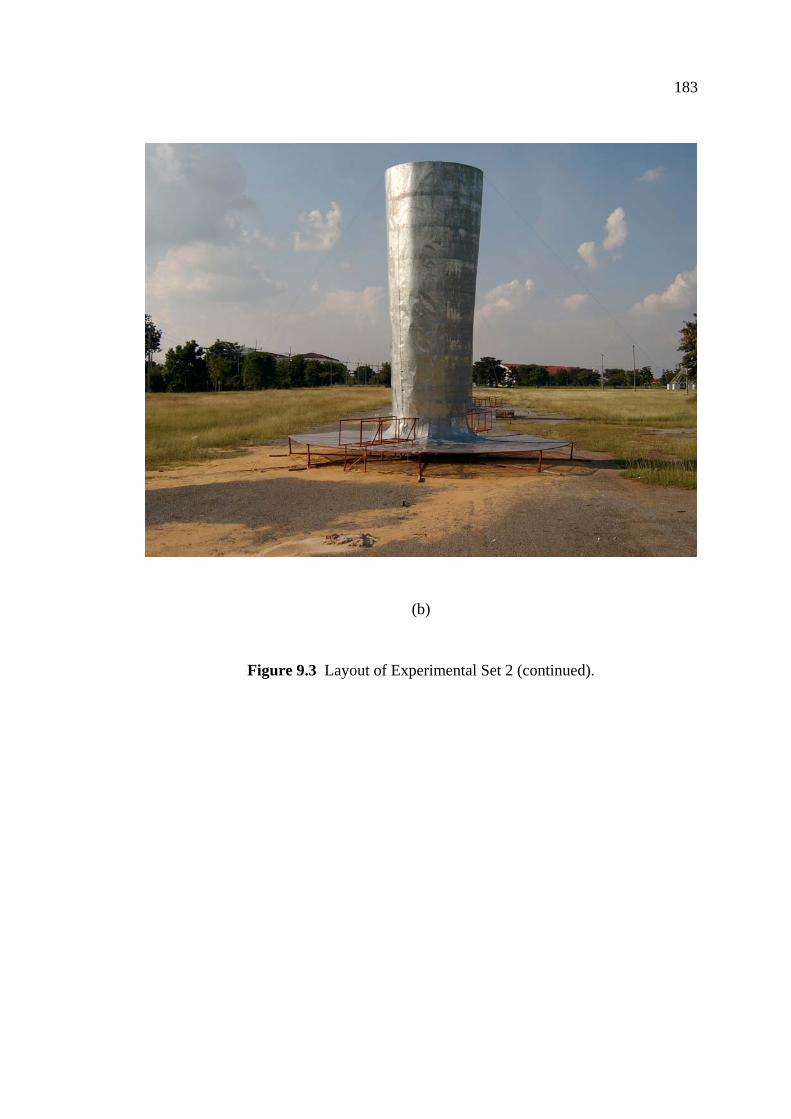
183
(b)
Figure 9.3 Layout of Experimental Set 2 (continued).

184
(a)
Figure 9.4 Layout of Experimental Set 3.

185
(b)
Figure 9.4 Layout of Experimental Set 3 (continued).

186
(a)
Figure 9.5 Layout of Experimental Set 4.

187
(b)
Figure 9.5 Layout of Experimental Set 4 (continued).

188
Table 9.2 Details of measuring locations.
Collector Chimney
Model
Number
of
measuring
locations
Measuring
positions
measured
from the roof
perimeter
Number
of
measuring
locations
Measuring
positions
measured above
the ground
Note
1 4 At 0.1, 0.6,
1.1 and 1.6 m
2 At 1.5 and 2 m
2 4 At 0.1, 0.6,
1.1 and 1.6 m
2 At 1.5 and 2 m
3 5 At 0.6, 1.1,
1.6, 2.1 and
2.5 m
2 At 1.5 and 2 m
4 4 At 0.042,
0.252, 0.462
and 0.672 m
2 At 1.0 and 1.25 m
See Fig. 9.6

189
(a)
(b)
(c)
Figure 9.6 Layout of measuring locations.

190
(a)
(b)
Figure 9.7 Descriptions of flow parameters for the calculations of average properties.

191
(a)
(b) (c)
(d)
Figure 9.8 Computational domain of Experimental Sets 1, 2 and 4: (a) 5 degree axis-
symmetric section; (b) computational grid of Experimental Set 1;
(c) computational grid of Experimental Set 2;
(d) computational grid of Experimental Set 4.

192
(a)
(b)
Figure 9.9 Computational domain of Experimental Set 3: (a) layout;
(b) computational grid.

193
Figure 9.10 Boundary settings of computation domain.

194
The plots of the airflow temperatures and velocities of each case will present
onward. The abscissas of all plots are the flow path, which is the streamwise location
of the flow, equaling zero at inlet and ending at outlet (chimney top).
Case 1: Experimental Set 1 when the height of entry roof is 0.5 m.
As Experimental Set 1 has the constant-diameter chimney and the roof height
setting allows the roof of Experimental Set 1 to have uniform height all over, the
results of this experimental set thus serves as reference values for the other
experimental sets. It is noted that 12AR for this set is approximately 4.0. The results
of the experiments are shown in Fig. 9.11.
Numerical results indicate that velocity increases along flow path under the
roof and remains constant in the chimney. It can be seen that the actual experimental
values are very close and follow the numerical predictions. The temperature graph
has the same characteristics.
However, it can be seen that the measured properties are very close to the
values from numerical computations that correspond to lower sunlight intensities that
actually measured. Some measured properties are different from those obtained from
numerical computation when compared to values at other positions. For example, the
measured results at the third position under the roof and both positions in the chimney
are significantly different and can be explained as following:
1. The numerical computation assumed that the sunlight, once entered, would
not reflect. Along the flow line, it was assumed no heat loss from the walls. However
in the actual experiment, some of the sunlight through the roof would be reflected.
Some heat would be lost to the ground, as well as along the walls of the experimental

195
Table 9.3 Descriptions of the test cases.
Case Model Roof inlet
r1(m)
h1(m)
h2(m) AR12 Chimney
area hc
(m) r2
(m) r3
(m) AR43 Note
1 1 Fully
opened 4 0.5 0.5 4 constant 8 1 1 1
A constant-height collector with a constant-area chimney (reference)
2 1 Fully
opened 4 0.13 0.5 1.01 constant 8 1 1 1
Investigate the effect of AR12 = 1 on the system with a constant-area chimney
3 1 Fully
opened 4 0.06 0.5 0.47 constant 8 1 1 1
Investigate the effect of AR12 = 0.5 on the system with a constant-area chimney
4 2 Fully
opened 4 0.5 0.5 4 increasing
with hc 8 1 1.41 1.99
Investigate the effect of AR43 = 2 on the system with a constant-height collector
5 2 Fully
opened 4 0.13 0.5 1.01 increasing
with hc 8 1 1.41 1.99
Investigate the effect of AR12 = 1 and AR43 = 2
6 2 Fully
opened 4 0.06 0.5 0.47 increasing
with hc 8 1 1.41 1.99
Investigate the effect of AR12 = 0.5 and AR43 = 2
7 3 Partially opened 8.1 0.5 0.5 1 constant 8 1 1 1
Novel roof shape
8 4 Fully
opened 1.68 0.25 0.25 3.36 constant 4 0.5 0.5 1
Inspect the dynamic similarity between cases 1 and 8
9 4 Fully
opened 1.68 0.07 0.25 0.94 constant 4 0.5 0.5 1
Inspect the dynamic similarity between cases 2 and 9
10 4 Fully
opened 1.68 0.04 0.25 0.54 constant 4 0.5 0.5 1
Inspect the dynamic similarity between cases 3 and 10

196
(a)
(b)
Figure 9.11 Airflow properties of experimental Case 1: (a) velocity distribution;
(b) temperature distribution.

197
set. Thus the experimental values would correspond to numerical results assuming
lower intensity of sunlight. In this case the values agreed most when sun heat flux of
200 W/m2 was used.
2. The numerical computations did not take into account the wind outside the
experimental set. The actual airflow speed inside the system was not too high
compared to external wind speeds, even if the experiment had to wait for the wind
outside to quiet and measurements were conducted numerous times to be averaged.
However sometimes measurement in the presence of external wind speeds was
unavoidable, such as after measurement of two positions, wind would occur. Waiting
for the wind to subside to measure the third position may result in significant change
of sunlight intensity due to clouds. These factors may have contributed to a deviation
of experimental values from the numerical values expected.
3. Limitations of budget prohibited building an experimental set with a large
roof compared to the diameter of the chimney. Actual construction found that the
shadow of the chimney covered about an eighth of the roof as depicted in Fig. 9.12.
Numerical computation employed the presupposition that the air under the
collector receives heat energy from the sun in a uniform manner, and that the pressure
difference between the top of the chimney and the base of the chimney enables the air
to flow from the outermost edge of the roof to the base of the chimney from all
directions and subsequently rise past the top of the chimney. However in the
experiment, since part of the roof did not receive sunlight along its radius, the
direction of flow of some of the air current may have deviated from that dictated by
hypotheses. This may be a cause that actual measurements in the chimney are
different from the numerical values. Perhaps if there were more apertures for

198
measurement along the chimney circumference at each chimney height’s measuring
location to yield more measurements, the average value of such measurements may be
more accurate.
Case 2: Experimental Set 1 when the height of entry roof is 0.13 m.
At such a roof height was found that 12AR has value of approximately 1.01.
This case is a validation of previous theoretical work (Koonsrisuk and Chitsomboon,
2004), stating that if 12AR decreases, the potential of the system will increase. This
potential is measured from the flow at the roof entry, 3
21 AVρ , where ρ is air density,
A is the flow cross sectional area and V is the flow velocity. Thus the increased
potential of the Case 2 compared to Case 1 can be seen from the velocity at the roof
entry point. If the velocity at the roof entry point increases from Case 1, it would
imply that the system’s potential has increased. Experimental results are displayed in
Fig. 9.13a.
From numerical results, velocity at the roof entry point is high compared to the
reference case (Experimental set 1 with 0.5 m height of the access roof). After that,
the velocity decreases to a certain value and then increases until it remains constant in
the chimney. The velocity decreasing and increasing in this manner is due to the
change of the area under the roof: It is slightly larger than the chimney area at the
roof entry point and then increases to a certain value and then decreases until it is the
same as the size of the chimney entry point. Conservation of mass makes speed
inversely proportional to flow cross sectional area. The cross sectional area varies in
this manner because of construction. However the roof entry area being slightly larger
than the chimney area is really due to the attempt to equalize the areas of the roof

199
entry and chimney inlet. However, due to the irrationality of 3.14159…. that is
involved in the area of the circular chimney, and the roof entry is rectangular, it was
not possible to exactly equalize the areas. The resulting design would have the roof
entry point to be slightly larger in area than the chimney area, as seen from the fact
that the speed at the roof entry point was slightly less than the speed in the chimney,
agreeing with the predictions of the previous theoretical study.
The graph indicates that actual measured speeds tend to be close to numerical
results, but less in value. This has been explained in Case 1. Computed and
experimental temperatures have the same trend as Case 1 (Fig. 9.13b).
Case 3: Experimental Set 1 when the height of entry roof is 0.06 m.
When the access height is 0.06 meters, it was found that 12AR has value of
0.47. Case 3 is used to validate results following from Case 2, to see if 12AR is
further decreased would result in further increase of potential. The results are
displayed in the Fig. 9.14.
Numerical results indicate that the flow velocity in this Case 3 has a similar
profile to Case 2, except that the velocity at the roof entrance is about twice as much
of the speed in the chimney, a consequence of the design to have the roof entry area to
be half of the cross sectional area of the chimney. Experimentally measured velocities
tend to be as those predicted by numerical computation, but the velocity at the roof
entry area is approximately equal to the speed in the chimney, probably due to the
very low roof access point, with the position at the edge of the roof. The air flowing
in may be turning from a higher position, while the equipment to measure speeds
could only measure speeds in only one direction and thus could not measure rotating

200
Figure 9.12 Illustration of the shadow of the chimney casting on the roof.

201
(a)
(b)
Figure 9.13 Airflow properties of experimental Case 2: (a) velocity distribution;
(b) temperature distribution.

202
air speed correctly. Numerically predicted and experimental temperatures exhibit the
same tendencies as in Case 1.
Case 4: Experimental Set 2 when the height of entry roof is 0.5 m.
As already stated in Case 1, the 0.5 meter height at access point is the height
that allows the roof to be of uniform height all over. The second experiment set has
the chimney diverging, with equal to 1.99. Case 4 is to observe results when
the chimney diverges. Previous theoretical studies (Koonsrisuk and Chitsomboon,
2006) found the divergent chimney to have better potential than the straight chimney.
This potential is measured from the flow power in the chimney,
43AR
3
21 AVρ . Hence the
increased potential in Case 4 compared to that of Case 1 can be seen from increased
velocity in the chimney: if the velocity in the chimney increases, this means that the
potential of the system has increased. Experimental results are displayed in Fig. 9.15.
Numerical results indicate an increase of air velocity at the flow path under the
roof as in Case 1. Velocity at the base of the chimney in Case 4 is about 1.4 times of
that of Case 1. The velocity then decreases until, at the chimney top, it is about the
same as in Case 1. These profiles were as previous theoretical studies predicted.
The graph indicates that the measured velocities tend to be as the numerically
computed velocities, but less in magnitude, a phenomenon already explained in Case1.
The numerically predicted and experimental temperatures have the same trends as in
Case 1.

203
Case 5: Experimental Set 2 when the height of entry roof is 0.13 m.
This case is to test whether decreasing the ratio of areas of flow between roof
inlet and roof outlet points as well as incorporating the divergent chimney would
increase the potential of the system. Experimental results are displayed in Fig. 9.16.
Numerical results indicate that the velocity graph is similar to joining the
velocity under the roof of Case 2 with the velocity graph in the chimney in Case 4. It
should be noted that the velocity at the roof entry point of Case 5 is slightly higher that
that of Case 2, and that the speed in entry point of the chimney in Case 5 is slightly
higher that that of Case 4 as well. This may be the result of slightly higher velocities
in one part encouraging higher speeds in other parts. When the part under the roof
drives the part in the chimney and the part in the chimney drives the part under the
roof as well, the velocities become higher.
The graphs indicate that experimentally measured velocities have similar
profiles to numerically predicted velocities, but are of less magnitude, a phenomenon
explained in Case 1. Numerically predicted and experimentally measured
temperatures exhibit the same tendencies as in Case 1.
Case 6: Experimental Set 2 when the height of entry roof is 0.06 m.
Case 6 is used to follow up Case 5: if 12AR is further decreased, would the
potential increase? The experimental results are displayed in the Fig. 9.17.
Numerical computations indicate that speeds in Case 6 are similar to that in
Case 5: the speed graph is like joining the graph of the speed under the roof of Case 3
with the graph of the speed within the chimney of Case 4. The speed at the roof entry

204
(a)
(b)
Figure 9.14 Airflow properties of experimental Case 3: (a) velocity distribution;
(b) temperature distribution.

205
(a)
(b)
Figure 9.15 Airflow properties of experimental Case 4: (a) velocity distribution;
(b) temperature distribution.

206
(a)
(b)
Figure 9.16 Airflow properties of experimental Case 5: (a) velocity distribution;
(b) temperature distribution.

207
(a)
(b)
Figure 9.17 Airflow properties of experimental Case 6: (a) velocity distribution;
(b) temperature distribution.

208
point of Case 6 is higher that that of Case 3, and the speed at the chimney access point
in Case 6 is higher than that of Case 4, just as in Case 5, which may result from the
mutual driving of speeds as explained in Case 5.
The graph indicates that actual measured velocities tend to be similar to those
predicted by numerical computations, but lesser in magnitude. This phenomenon was
explained in Case 1. The temperatures obtained from computation and experimental
measurement exhibit the same trend as in Case 1.
Pairing Case 1 with Case 4, Case 2 with Case 5, and Case 3 with Case 6, it was
found that the velocities at the roof entry points of each pair were very close: Pair 1
had a value of 0.2 m/s, Pair 2 had a value of 0.25 m/s, and Pair 3 had a value of about
0.3 – 0.4 m/s. Pair 1’s value agreed very closely with numerical computations, while
Pairs 2 and 3’s values were lower than numerically computed values. Possible causes
are:
1. Pair 1 consists of uniformly constant height of roof. The air flow under the
roof should be parallel to the roof at all times. Thus the velocity measured under the
roof would agree very closely with numerical predictions. Discrepancies at some
points under the roof and in the chimney may have arisen from causes analyzed in No.
2 and 3 of Case 1.
2. Pairs 2 and 3 have smaller roof entry points and the roof makes an angle to
the land, which may cause some parts of the air current to turn from outside and the
direction of the air current from the roof’s edge to the chimney is divergent according
to the Law of Conservation of Mass. Since the speed measurement equipment for the
experiment was effective in only one direction, and that direction was parallel to the

209
ground (as in Fig. 9.18), the measured velocity may have been less that the actual
velocity.
As the measured velocity was less than the actual velocity, it is natural to ask if
this measured velocity could be used for analysis. If we consider velocity to be a
vector, which can be decomposed into three components perpendicular to each other,
use of cylindrical coordinates requires us to have an axial direction along the
chimney’s axis; the second would be the radial direction of the chimney and the third
would be the circumferential direction of the chimney. When considering the
experimental flow conditions, it was found that the principle direction of flow under
the roof was towards the chimney parallel to the ground, implying the negligibility of
the circumferential component. The axial component’s magnitude on the other hand
would vary according to the degree of turning. However, the velocity in the
chimney’s axial direction would surely be less than the radial component, the principal
direction. Thus it can be said that even though the measured velocity is less than the
actual velocity, the trend of their magnitudes should correspond with actual
conditions.
Cases 1–6’s numerical results can be summarized as in Table 9.4. Table 9.4
indicates that decreasing 12AR increases wind energy potential. Increasing can
increase wind energy potential as well. In the experimental set that decreased
43AR
12AR
as well as increased , higher potential at the roof access point was obtained than
just decreasing
43AR
12AR alone by an equal amount. Potential at the chimney base was
also higher than the system that increased alone by an equal amount. However,
even when decreasing
43AR
12AR helped increase potential, but continual decrease found
that the height of the entry roof corresponding to the highest potential that could be

210
Figure 9.18 Illustration of the flow direction under the sloping roof.
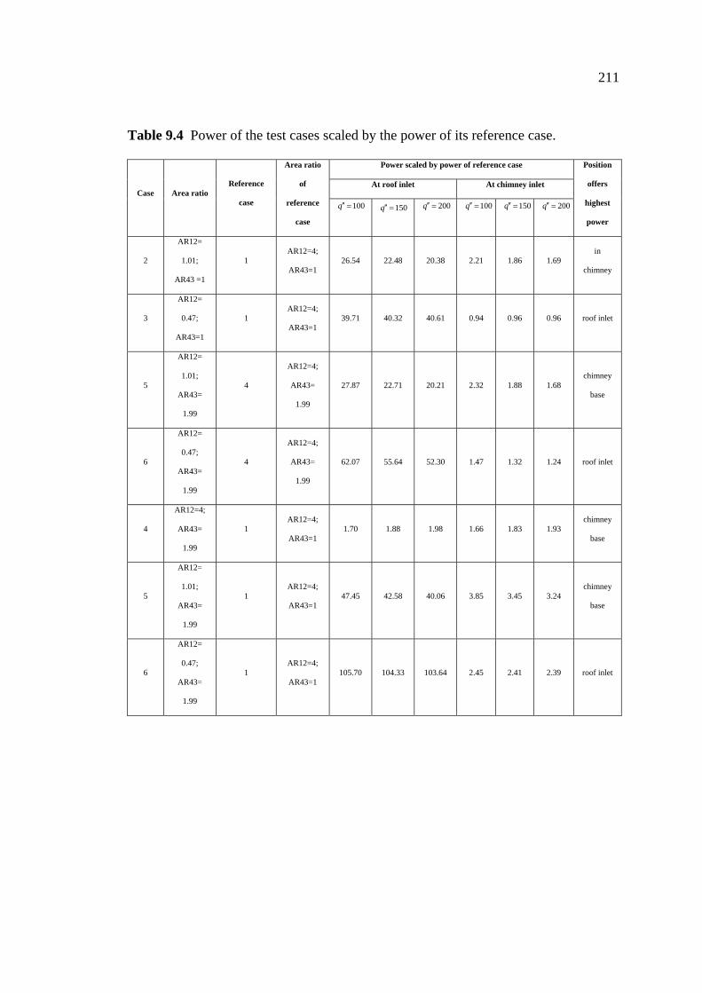
211
Table 9.4 Power of the test cases scaled by the power of its reference case.
Power scaled by power of reference case
At roof inlet At chimney inlet Case Area ratio
Reference
case
Area ratio
of
reference
case
100=′′q
150=′′q
200=′′q 200=′′q
100=′′q
150=′′q
Position
offers
highest
power
2
AR12=
1.01;
AR43 =1
1 AR12=4;
AR43=1 26.54 22.48 20.38 2.21 1.86 1.69
in
chimney
3
AR12=
0.47;
AR43=1
1 AR12=4;
AR43=1 39.71 40.32 40.61 0.94 0.96 0.96 roof inlet
5
AR12=
1.01;
AR43=
1.99
4
AR12=4;
AR43=
1.99
27.87 22.71 20.21 2.32 1.88 1.68 chimney
base
6
AR12=
0.47;
AR43=
1.99
4
AR12=4;
AR43=
1.99
62.07 55.64 52.30 1.47 1.32 1.24 roof inlet
4
AR12=4;
AR43=
1.99
1 AR12=4;
AR43=1 1.70 1.88 1.98 1.66 1.83 1.93
chimney
base
5
AR12=
1.01;
AR43=
1.99
1 AR12=4;
AR43=1 47.45 42.58 40.06 3.85 3.45 3.24
chimney
base
6
AR12=
0.47;
AR43=
1.99
1 AR12=4;
AR43=1 105.70 104.33 103.64 2.45 2.41 2.39 roof inlet

212
obtained was too low to install turbines for production of electric energy at that point.
It was thus proposed the roof as in Experimental Set 3, with partial apertures for air to
enter the collector, and not opened all around as in the regular models. Even if 12AR
were decreased, such apertures would be of sufficient size for turbine installation.
This case tests the possibility of changing the roof configuration from the
standard model, the roof open all around, as used in Experiment Sets 1, 2 and 4, to be
a partially accessible roof (details of apertures is depicted in Fig. 9.4). Cases 2 and 3
indicate that the smaller the roof access, the more the potential of the roof entry
system. The limitation of this type of roof is that the smaller the entry points, the
lower the entry roof, making actual construction and utilization very difficult. The
roof of Experiment Set 3 controls the width and length of the apertures to be uniform,
so that even if the accessibility sizes are decreased, the apertures are of sufficient size
as to not be an obstacle to construction and actual use. Moreover, as the potential at
Case 7: Experiment set 3
This case tests the possibility of changing the roof configuration from the
standard model, the roof open all around, as used in Experiment Sets 1, 2 and 4, to be
a partially accessible roof (details of apertures is depicted in Figure 4). Cases 2 and 3
indicate that the smaller the roof access, the more the potential of the roof entry
system. The limitation of this type of roof is that the smaller the entry points, the
lower the entry roof, making actual construction and utilization very difficult. The
roof of Experiment Set 3 controls the width and length of the apertures to be uniform,
so that even if the accessibility sizes are decreased, the apertures are of sufficient size
as to not be an obstacle to construction and actual use. Moreover, as the potential at
the roof entry points increases as the size of the apertures of the roof seem to be of

213
sufficient size, the idea arose to install the turbines at the apertures, which would be
convenient to install and maintain, especially if this system is many hundred meters in
size, the subject of future studies.
Design of Experiment Set 3 involved computation so that its sunlight receiving
area would be near in size to that of Sets 1 and 2. (Note that the design, from an upper
point of view, shows a different shape of the roof from Sets 1 and 2). It was
determined that the total area of the apertures of Set 3 be close to the area of the cross
section of the chimney (why the areas would not exactly match is in the discussion of
Case 2): that is, the ratio of the area of the roof entry apertures to the area of the cross
section of the chimney be approximately equal to 1. Theoretical studies indicate that
the potential of this case at the roof access points and in the chimney would be close in
size to that of Case 2. The experimental results are displayed in Fig. 9.19.
Numerical computations indicate that velocities at the roof entry points are
very close to those of Case 2. After that, the velocities would increase to a certain
value and then decrease to a constant value in the chimney. The velocity in the
chimney is very close in value to that of Case 1, so that it can be said that theoretical
predictions concerning potentials at the roof entry points and chimney entry points are
quite accurate. However, it can be seen that the maximum velocity occurs at about
half of the flow route in the chimney. The cause of such behavior should be the shape
of the roof, readily explained as follows.
Fig. 9.20 displays a view of Experimental Set 3, viewed from above. The circle
is the chimney and the octagon is the boundary of the roof, with four apertures as in
the figure, and the remaining being closed walls. The cross sectional area of the roof

214
(a)
(b)
Figure 9.19 Airflow properties of experimental Case 7: (a) velocity distribution;
(b) temperature distribution.

215
Figure 9.20 Illustration of the roof access system of Experiment Set 3.

216
access apertures was designed to equal to the cross sectional area as showed by dotted
lines, and the sum of the areas of the apertures of all four sides was designed to equal
to the chimney cross sectional area. All this was to control the velocities that occurred.
The broken diagonal lines indicate symmetry lines within the system, since numerical
computations indicated that flow within Experimental Set 3, the air current divides
into four parts via the four apertures of the roof according to the broken lines. The air
currents then flow to combine in the chimney according to the Fig. 9.21a, which
shows a part of the velocity vectors of flow under the roof. This part will join with
other parts of the roof at the “symmetrical plane” in the picture. The other three parts
have the same types of velocity vectors as in this figure. The figure shows that there is
a turbulent area, indicated by broken line circles. Fig. 9.21b is a magnification of the
recirculation zones.
Recirculation causes the flow cross sectional area to be less than it should be,
so that velocities in this area are higher than the velocities at the roof entry points,
even after designing them to have equal cross sectional areas. Thus improvement of
shape is required for the position of highest velocity to be at the roof entry point or at
the chimney entry point.
The graph indicates that actual measured speeds tend to be similar to those
predicted by numerical computations, but lesser in magnitude. This phenomenon was
explained in Case 1. The temperatures obtained from computation and experimental
measurement exhibit the same trend as in Case 1.

217
(a)
(b)
Figure 9.21 (a) velocity vectors of flow under the roof of Experiment Set 3;
(b) magnification of the recirculation zone.

218
Case 8: Experimental Set 4 when the height of entry roof is 0.25 m.
Experiment Set 4 was designed to test previous theoretical studies (Koonsrisuk
and Chitsomboon, 2009) which predicted that two solar chimneys of different size
under identical atmospheric conditions, receiving the same solar energy, may be
constructed to achieve dynamic similarity through partial geometric similarity, under
the following equations:
⎟⎟⎟
⎠
⎞
⎜⎜⎜
⎝
⎛′′
=21
25
23
27
2
21
ghc
Aqfgh
Vm
cp
rn
c ρ
β
ρ
&, (9.3)
designating 23272
21 ghVm cρ& to be 1∏ and 2125 ghcAq cpr ρβ′′ to be ∏ . 2
The theory from the aforementioned work was used in designing Experiment
Set 4: let every part be half the size of Experiment Set 1, except for the roof, which
would be 0.42 of Experimental Set 1 (Koonsrisuk and Chitsomboon, 2009). If one
performs Experiment Sets 1 and 4 under identical atmospheric conditions and solar
heat fluxes, it would be found that 2∏ of both Experiment Sets were equal, and if both
Experiment Sets achieve dynamic similarity, it would be found that of both would
be the same as well. Experimental results are as depicted in Fig. 9.22.
1∏
The graph indicates that actual measured velocities tend to be similar to those
predicted by numerical computations, but lesser in magnitude. This phenomenon was
explained in Case 1. The temperatures obtained from computation and experimental
measurement exhibit the same trend as in Case 1.

219
(a)
(b)
Figure 9.22 Airflow properties of experimental Case 8: (a) velocity distribution;
(b) temperature distribution.
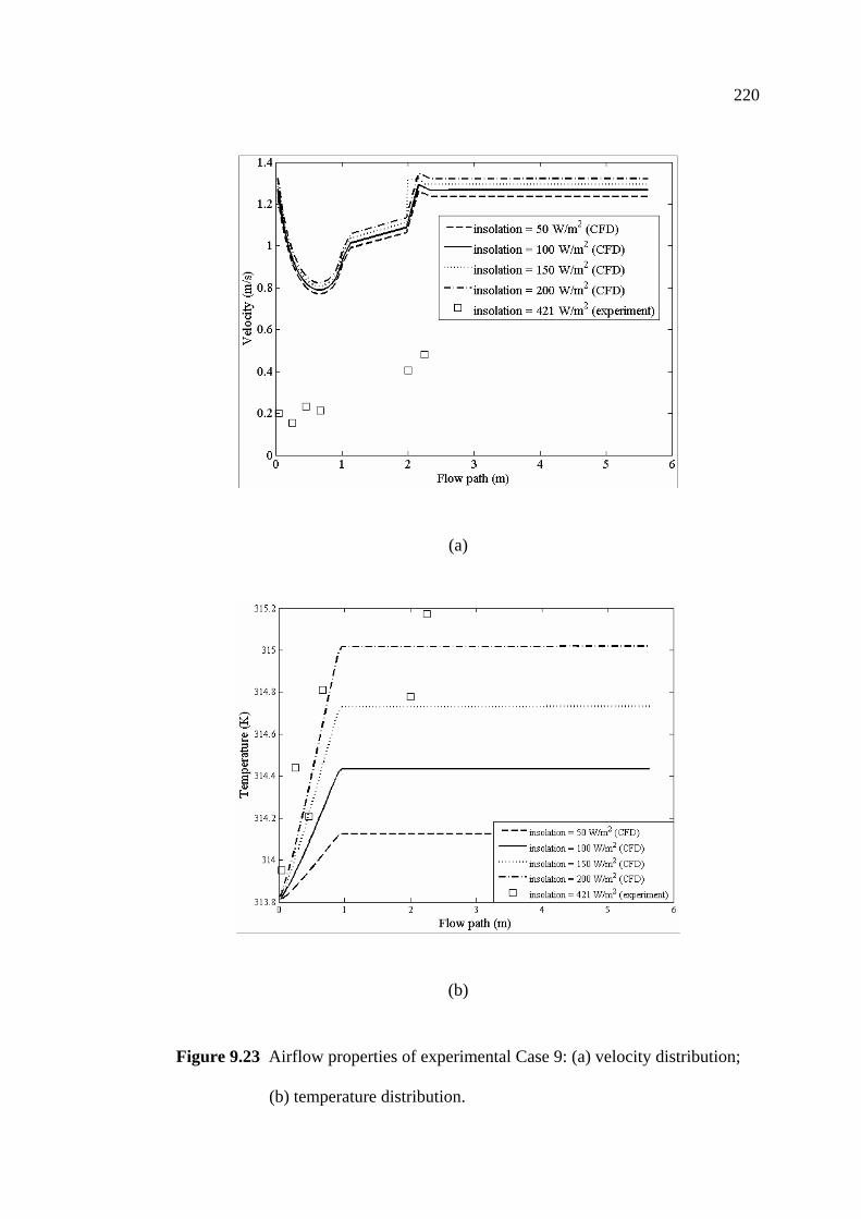
220
(a)
(b)
Figure 9.23 Airflow properties of experimental Case 9: (a) velocity distribution;
(b) temperature distribution.

221
(a)
(b)
Figure 9.24 Airflow properties of experimental Case 10: (a) velocity distribution;
(b) temperature distribution.

222
Table 9.5 Comparative data for dimensional analysis.
Pair Case
Roof inlet
temperature
(K)
Solar heat flux
(W/m2) 2∏ 1∏
1 1 307.7 458 1.06E-05 1.06E-05
8 311.3 487 9.82E-05 1.29E-05
2 2 309.6 347 8.06E-06 1.49E-05
9 313.8 421 8.49E-05 6.59E-06
3 3 307.6 343 7.96E-06 3.67E-06
10 315.1 342 6.89E-05 2.39E-06
Note: Entry point temperature points and solar heat fluxes are actual
measurements, while the values of 1∏ and 2∏ are from calculation
at Position 1 in the chimney.

223
Case 9: Experimental Set 4 when the height of entry roof was 0.07 m.
Case 9 can be used to check out the effect of 12AR , by comparing the results
with Case 8 to see if the results are as in the comparison of Case 2 with Case 1. Thus
Case 9 can be used to compare dynamic similarity with Case 2. Experimental results
are displayed in Fig. 9.23.
The graph indicates that actual measured velocities tend to be similar to those
predicted by numerical computations, but lesser in magnitude. This phenomenon was
explained in Case 1. The temperatures obtained from computation and experimental
measurement exhibit the same trend as in Case 1.
Case 10: Experiment Set 4 when the height of the entry roof is 0.04 meters.
Case 10 can be used to inspect the effect of 12AR , by comparing the results
with Case 8 to see if the results are as in the comparison of Case 3 with Case 1. Thus
Case 10 can be used to compare dynamic similarity with Case 2. Experimental results
are displayed in Fig. 9.24.
The graph indicates that actual measured speeds tend to be similar to those
predicted by numerical computations, but lesser in magnitude. This phenomenon was
explained in Case 1. The temperatures obtained from computation and experimental
measurement exhibit the same trend as in Case 1.
Entry point temperature values, average of solar heat fluxes, values of and
, obtained from Cases 1, 2, 3, 8, 9 and 10 are displayed in Table 9.5. The table
indicates that only the in the first pair are close in value, and differ a little in the
third pair. The in the second pair however differ by 3 times, which should be
consequence of different atmospheric conditions and sunlight intensities, indicated by
1∏
2∏
1∏
1∏

224
the differing values of each pair. If numerical results are used by inputting actual
atmospheric condition and solar heat flux values, the values of and of each
pair would differ as well, but if the same values for atmospheric conditions and solar
heat fluxes are used for each pair, it was found that the computed values of and
of each pair are equal. The calculations were tested by experimenting at identical
atmospheric conditions and solar heat fluxes, a very difficult feat, considering that two
experimental sets had to be performed simultaneously. However there was only one
set of measuring equipment and the time to collect data for a particular experimental
set was required to be quite long, hence the inability to collect data from Set 1 and
then Set 4 immediately after.
2∏
1∏ 2∏
1∏
2∏
Experiment Set 4 yielded the profile of the velocity graph as discussed in the
section following Case 6: the measured velocity were not too far away from the
computed values of Case 8, which was the case of the roof parallel to the ground.
With Cases 9 and 10, with the roof forming an oblique angle to the ground, the
measured velocities tended to be similar to the computed velocities, but different in
magnitude.
9.7 CONCLUSION
1. Decreasing of the 12AR yielded higher potential of wind energy at the entry
point of the roof.
2. Increasing yielded higher potential of wind energy at the entry point
to the chimney.
43AR

225
3. It was found that decreasing 12AR in conjunction with increasing
allowed higher potential at the roof access point to be obtained rather than just
individually decreasing
43AR
12AR or increasing by an equal amount. 43AR
4. The energy potential in the chimney of Experimental Set 3 was close to that
of Cases 1 and 2, while its energy potential at the roof entrance was larger. This leads
to the idea of installing the turbines at the apertures, which would be convenient to
install and maintain.
5. The experimental results differ comparatively but have the same trends as to
the predicted values. This may follow from the fluctuating solar heat flux and the
effect of the large chimney diameter when compared with the roof size.
6. The difference of dimensionless variables between the large and the small
plant is noticeable, contrary to the theoretical and numerical predictions. Reasons
could be the varying atmospheric conditions when the tests were run.
9.8 PROBLEMS AND CHALLENGES IN THE RESEARCH
1. When studying the theory, it was found that there were a variety of
directives in designs which needed to be tested experimentally, requiring an
amendment to the budget request from the Thailand Research Fund (TRF). Once
approved by the TRF, it was then the rainy season, causing further delays in the
construction. Construction was completed at the end of the rainy season and
beginning of winter, so the weather was unpredictable and rendered further obstacles
in collecting data to compare to mathematical models. The mathematical models
assumed constancy of the intensity of sunlight and no influence from outside wind
currents, while the actual experimental atmospheric conditions varied with heavy

226
clouds leading to variable sunlight intensity and occasional winds in each day,
rendering experimentation very difficult.
2. Due to the small size of the chimneys, in the design phase, it was found that
the air flow velocity was larger than the actual atmospheric conditions. Actual
experiments found that the flow velocity that occurred inside the chimney was just
slightly higher than the external wind velocities, so that during experimentation, it was
found that external winds had a noticeable effect on the wind currents inside the
system. This problem persisted even in the summer, and would readily be rectifiable if
a sufficiently large chimney could be built that would house internal air flow with
many times the speed of that of the external winds.
9.9 REFERENCE
ANSYS, Inc. ANSYS CFX, Release 10.0: reference guide. ANSYS, 2005.
Koonsrisuk, A, Chitsomboon, T., 2004. The effect of roof height to the flow in solar
chimney. In: Proceedings of the RGJ-Ph.D. Congress V. Chon Buri,
Thailand.
Koonsrisuk, A., Chitsomboon, T., 2006. Effect of Tower Area Change on the Potential
of Solar Tower. In: Proceedings of the 2nd Joint International
Conference on Sustainable Energy and Environment, Bangkok,
Thailand.
Koonsrisuk, A., Chitsomboon, T., 2007. Dynamic similarity in solar chimney
modeling. Solar Energy, Vol. 81(12), pp. 1439-1446.
Koonsrisuk, A., Chitsomboon, T., 2009. Partial geometric similarity for solar chimney
power plant modeling. Solar Energy, Vol. 83, pp. 1611-1618.

CHAPTER X
CONSTRUCTAL SOLAR CHIMNEY CONFIGURATION
AND MULTI-SIZE DISTRIBUTION ON LAND
10.1 ABSTRACT
In this study the constructal-theory search for the geometry of a solar chimney
is reported. The objective is to increase the power production over the area occupied
by the plant. The optimal height/radius, maximum mass flow rate and maximum
power under the constraints of a fixed area and volume are determined. The power
generated per unit of land area is proportional to the length scale of the power plant. A
more detailed mathematical model shows that the simple model proposed here may be
useful in the initial estimation of plant performance. Pressure losses in terms of the
dimensionless length scale of the system are illustrated graphically. Results indicate
that the pressure drop at the collector inlet and at the transition section between the
collector and chimney are negligible and the friction loss in the collector might be
neglected when the svelteness [cf. Eq.10.39] is greater than 6.5. Because of the flow
resistances associated with distributing the power over a territory, the size of the
territory must be finite and optimally allocated to each power plant. Several patterns of
the multi-scale plants on a square area are explored. The finding has strong intuitive
appeal; the global performance of different patterns could be equated with lower
compactness [cf. Eq. 10.56] for the design with larger plants, which are able to
economize on extracting power from an available land area.

228
10.2 INTRODUCTION
The solar chimney is a power plant that uses (1) solar radiation to raise the
temperature of the air, and (2) buoyancy to accelerate the air flowing through the
system. The main features of the solar chimney are sketched in Fig. 10.1. Air is heated
as a result of the greenhouse effect under a transparent roof (the collector). Because the
roof is open around its periphery, the buoyancy of the fall air column draws a
continuous flow from the roof perimeter into the chimney. A turbine is set in the path
of the air current to convert the kinetic energy of the flowing air into electricity.
In 1981, a solar chimney prototype of 50 kW, with the chimney height and roof
diameter nominally at 200 m, was built in Manzanares, Spain. The plant operated from
1982 to 1989, and was connected to the local power network between 1986 and 1989
(Schlaich, 1995). This project demonstrated the viability and reliability of the solar
chimney concept. Since then, numerous investigations to predict the flow in solar
chimneys have been conducted. Generally, it was found that the electricity yielded by
a solar chimney is in proportion with the intensity of global solar radiation, collector
area and chimney height. Based on a mathematical model, Schlaich (1995) reported
that optimal dimensions for a solar chimney do not exist. However, if construction
costs are taken into account, thermoeconomically optimal plant configurations may be
established for individual sites. It was shown numerically in Pretorius and Kröger
(2006) that plant power production is a function of the collector roof shape and inlet
height. Maia et al. (2008) carried out a simulation study and found that the height and
diameter of the chimney are the most important geometric dimensions for solar
chimney design. Zhou et al. (2009) reported the maximum chimney height in order to

229
Figure 10.1 The main features of a solar chimney.

230
avoid negative buoyancy, and the optimal chimney height for maximum power output.
They found that the maximum height and the optimal height increase with collector
radius. A common feature in these findings is that the plant efficiency is very low, and
that it increases with the plant size.
Consequently only large-scale plants, in which the chimney heights are 1,000
m or more, were proposed in the literature. In the 1990s, a project in which a solar
chimney power plant with the capacity of 100 MW was proposed for construction in
Rajasthan, India, and was about to be implemented. Its collector had a radius of 1,800
m and a chimney height and diameter of 950 m and 115 m, respectively (Rohmann,
2000). However, the project was cancelled owing to the potential danger of nuclear
competition between India and Pakistan. The Australian government planned to build
a 200 MW commercial plant with a chimney 1,000 m high. Recently, the plant was
downsized to 50 MW and a 480 m-high chimney, in order to make it economically
viable and eligible for government funding (EnviroMission, 2006). The construction
and safety of a massive structure poses significant engineering challenges.
The work described in this paper is stimulated by the quest for better designs,
and focuses on the generation of shape and structure by maximizing global
performance of the flow system. It is based on the method of constructal design
(Bejan and Lorente, 2008). This work shows that the configuration of the solar
chimney can be determined, along with the scaling rules for being able to scale-up and
scale-down the design.

231
10.3 GEOMETRY
The system geometry is simplified to that of a horizontal disc above the ground
with a vertical cylinder in the center of the disc. The solar chimney configuration has
the four dimensions shown in Fig. 10.1: , , and . We assume that the flow is
fully developed and turbulent in all the flow passages, and that the friction factors in
the vertical tube ( ) and the horizontal channel ( ) are approximately constant. The
air flow rate ( ) enters at atmospheric temperature ( ) and is heated with uniform
heat flux ( q ) as it flows to the base of the chimney, where its temperature reaches
cr ch rr rh
yf xf
m& 0T
′′
TT Δ+0 .
10.4 PUMPING EFFECT
The air stream is driven by the buoyancy effect due to the vertical column of
hot air (height , temperature ch TT Δ+0 ), which communicates with the ambient air of
the same height and lower temperature ( ). The net pressure difference that drives
the air stream in the tower is (Bejan, 2004)
0T
Tghghghp ccTTcT ΔρβρρΔ Δ =−= +00 (10.1)
where ρ is the average air density, and β is the coefficient of volumetric thermal
expansion.
The pumping effect pΔ is opposed by friction forces in the vertical tube ( ypΔ )
and in the horizontal channel ( xpΔ ) and the acceleration due to flow area reduction
( accpΔ ).

232
For the vertical tube, we write (Bejan, 1993)
2
212
yc
cyy V
rhfp ρΔ = (10.2)
where ( )2cy rmV ρπ&= . The pressure loss along the horizontal channel is determined
from a balance of flow resistance
22 rwxflow rpA πτΔ = (10.3)
where rrflow hrA π2= , wτ is the wall shear stress, and represents the roof and
ground surface in the horizontal channel for shear stress computation. The wall shear
stress in terms of friction factor is defined as (Bejan, 1993)
22 rrπ
2
21
xxw Vf ρτ = (10.4)
Consequently, the pressure loss in the horizontal passage is
2
21
xr
rxx V
hrfp ρΔ = (10.5)
where is the average air velocity at the entrance, xV ( )rrx hrmV πρ2&= . The horizontal
flow experiences acceleration and heating in a channel with variable cross-sectional
area (Chitsomboon, 2001) cA
( ) ⎟⎟⎠
⎞⎜⎜⎝
⎛ ′′−
−=
TcmdAq
AdA
MVdp
p
r
c
c
&2
2
1ρ (10.6)

233
Next we assume that in the horizontal flow q ′′ , , pc ρ and T are
approximately constant. The Mach number, M , is negligible, and Eq. (10.6) reduces to
c
r
pracc r
rTch
qmAA
mp ln2
112 00
221
220
2
ρπρΔ
′′−⎟⎟
⎠
⎞⎜⎜⎝
⎛−=
&& (10.7)
where 1 and 2 denote the channel entrance and channel exit, respectively. This
equation shows that the pressure increases due to heat addition (the second term) while
it decreases due to flow area reduction towards the roof center (the first term). An
order of magnitude analysis reveals that the first term is much greater than the second
term. In addition, because , Eq. (10.7) becomes 22
21 AA >>
420
2
2 cacc r
mpπρ
Δ&
≅ (10.8)
The losses balance the driving pressure difference, accxy pppp ΔΔΔΔ ++= , or
2
2
22
2 22
22 ⎟⎟⎠
⎞⎜⎜⎝
⎛+⎟⎟
⎠
⎞⎜⎜⎝
⎛+⎟⎟
⎠
⎞⎜⎜⎝
⎛=
crrr
rx
cc
cyc r
mhr
mhrf
rm
rhfTgh
ρπρ
πρρ
ρπρΔρβ
&&& (10.9)
Equation (10.9) relates the flow rate ( ) to the excess temperature reached at
the base of the cylinder (
m&
TΔ ). The second equation needed for determining and m&
TΔ is the first law of thermodynamics for the horizontal channel as a control volume:
Tcmrq Pr Δπ &=′′ 2 (10.10)
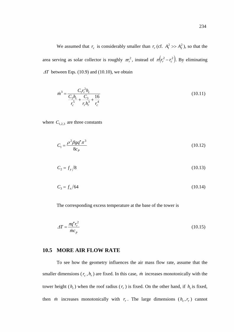
234
We assumed that is considerably smaller than (cf. ), so that the
area serving as solar collector is roughly , instead of
cr rr22
21 AA >>
2rrπ ( )22
cr rr −π . By eliminating
TΔ between Eqs. (10.9) and (10.10), we obtain
433
52
213
16
crrc
c
cr
rhrC
rhC
hrCm++
=& (10.11)
where are three constants 3,2,1C
PcqgC
8
32
1πβρ ′′
= (10.12)
8fC =2 y (10.13)
64fC =3 x (10.14)
The corresponding excess temperature at the base of the tower is
p
r
cmrqT
&
2′′=πΔ (10.15)
10.5 MORE AIR FLOW RATE
To see how the geometry influences the air mass flow rate, assume that the
smaller dimensions ( , ) are fixed. In this case, increases monotonically with the
tower height ( ) when the roof radius ( ) is fixed. On the other hand, if is fixed,
then increases monotonically with . The large dimensions ( , ) cannot
cr rh m&
ch rr ch
m& rr ch rr
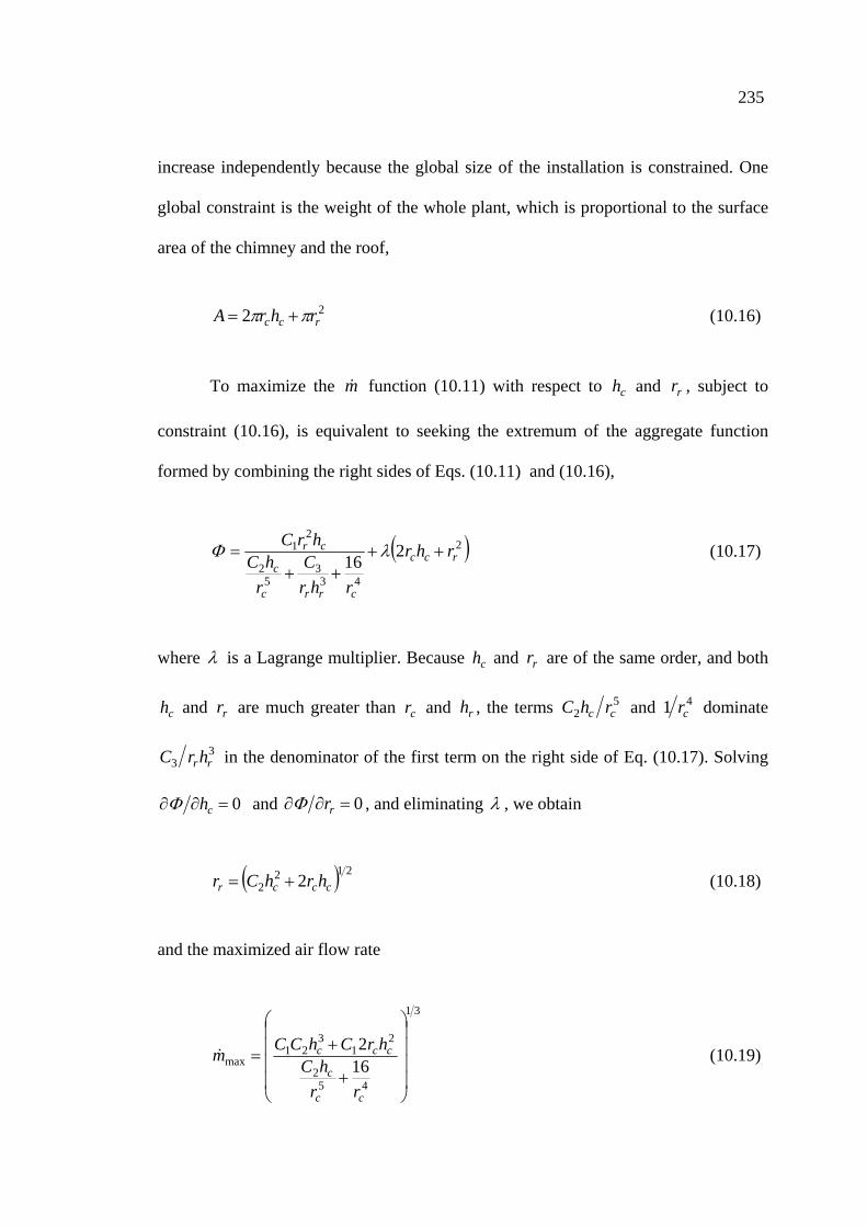
235
increase independently because the global size of the installation is constrained. One
global constraint is the weight of the whole plant, which is proportional to the surface
area of the chimney and the roof,
22 rcc rhrA ππ += (10.16)
To maximize the function (10.11) with respect to and , subject to
constraint (10.16), is equivalent to seeking the extremum of the aggregate function
formed by combining the right sides of Eqs. (10.11) and (10.16),
m& ch rr
( 2
433
52
21 216 rcc
crrc
c
cr rhr
rhrC
rhC
hrC++
++= λΦ ) (10.17)
where λ is a Lagrange multiplier. Because and are of the same order, and both
and are much greater than and , the terms
ch rr
ch rr cr rh 52 cc rhC and 41 cr dominate
33 rrhrC in the denominator of the first term on the right side of Eq. (10.17). Solving
0=∂∂ chΦ and 0=∂∂ rrΦ , and eliminating λ , we obtain
( ) 2122 2 cccr hrhCr += (10.18)
and the maximized air flow rate
31
452
21
321
max 162
⎟⎟⎟⎟
⎠
⎞
⎜⎜⎜⎜
⎝
⎛
+
+=
cc
c
ccc
rrhC
hrChCCm& (10.19)

236
Note that is neglected in Eq. (10.19) because of the order of magnitude
reasoning. As a result, Eq. (10.19) shows only the effect of , which until now was
assumed fixed.
rh
cr
10.6 MORE POWER
The generation of power calls for a design that maximizes and m& pΔ as a
product, i.e. not alone. The thermodynamic ideal level of the power produced by a
turbine inserted in a duct with the air stream m driven by the pressure difference
m&
& pΔ
is
24~~ rcrhCpmW ρΔ&& (10.20)
where
pcqgC πβ ′′
=4 (10.21)
To determine the optimal and for which W is maximized, we construct
the linear combination of Eqs. (10.20) and (10.16),
ch rr &
( )224 2 rccrc rhrrhC ++= λΨ (10.22)
Again, after eliminating λ we obtain ( )crc rrh 22= , or
( )cr
c
rA
rh
22 21π
= (10.23)

237
The maximized power level that corresponds to the optimal configuration is
crACW 2
2
4max 8π=& (10.24)
This result shows that the power level increases rapidly as the available size
increases. If 21A represents the length scale of the entire flow system, then it is
reasonable to anticipate that will vary more or less in proportion with cr21A . This
leads to the conclusion that scales with maxW& 23A .
In addition, because scales with 2rr A [cf. Eq. (10.16)], it follows that the
maximum power generated per land area ( )2max rrW π& varies in proportion with the
length scale of the installation, 21A . The important conclusion is that the maximum
use of land surface requires the use of larger solar chimney power plants. The
existence of “economies of scale” raises the question of how to extract most solar
power from an available land area. We consider this fundamental question in Section
10.9.
10.7 VOLUME CONSTRAINT
An alternative to the wall area (or weight) constraint (10.16) is the total volume
constraint,
rrcc hrhrVol 22 ππ += (10.25)
The results of maximizing W of Eq. (10.20) subject to the volume constraint
are
&

238
22c
r
r
c
rh
rh
= (10.26)
rr h
rπ2
=Vol2
( )
(10.27)
224
max 4 crrhW
π=&
2VolC (10.28)
Once again, the power output increases with the total size squared. If and
scale with the linear scale of the entire installation,
rh cr
( ) 31Vol , then scales with
, not . In this case, the power produced per unit of land area
maxW&
Vol ( )2Vol ( )2max rrW π&
increases with ( ) ( ) 3132 VolVolVol = , which represents the length scale of the power
plant. In conclusion, the economies-of-scale trend is the same as at the end of the
preceding section.
10.8 MODEL VALIDATION
The work presented in Sections 10.5 and 10.6 was based on scale analysis. In
order to validate its conclusions [Eqs. (10.24) and (10.28)]. , we also developed a
detailed mathematical model for the flow in a solar chimney. The pressure changed
due to acceleration in the collector is computed using Eq. (10.7). The temperature is
estimated from the energy equation across the roof portion
p
r
cmAqTT&
′′+= 12 (10.29)

239
The pressure changed along the chimney can be calculated from the
momentum equation for flow through a constant area vertical tube,
( ) ⎟⎟⎠
⎞⎜⎜⎝
⎛−⎟⎟
⎠
⎞⎜⎜⎝
⎛+++=
34
2
434311
21
ρρρρ
cc A
mghpp&
(10.30)
The hydrostatic equilibrium requires that
gdzdp ρ−= (10.31)
According to Calvert (1990), when the atmospheric air parcel is regarded as
unsaturated medium and expands slowly to a lower atmospheric pressure without
exchange of heat, the rate of temperature change with altitude is written as
zcgTTp
−= 1 (10.32)
Because air behaves as an ideal gas, Eqs. (10.31) and (10.32) yields
Rc
cp
p
hTc
gpp ⎟⎟⎠
⎞⎜⎜⎝
⎛−=
114 1 (10.33)
Consider that a dry adiabatic lapse rate can be applicable to the flow in a tower.
In accordance with Eq. (10.32),
cp
hcgTT −= 34 (10.34)

240
and
4
44
3
33
2
22 ,,
RTp
RTp
RTp
=== ρρρ (10.35)
The turbine is not modeled in this analysis: the flow properties at point 2 are
the same as those at point 3. The pressure potential is the available pressure difference
between the tower base and the surroundings, therefore the available turbine power is
( 212 2
ppmW −=ρ&& ) (10.36)
The application of the computational fluid dynamics code (ANSYS, 2005) has
been carefully investigated and validated in Koonsrisuk and Chitsomboon (2007).
Consequently, to verify the present model, we first compared its results with those of
CFD simulations. Fig. 10.2 shows that the results of the model agree very well with
those of CFD computations.
To validate Eqs. (10.24) and (10.28), we based the calculations on the
Manzanares prototype. The collector had a diameter of 244 m and a height of 1.85 m,
and it had a 194.6 m high chimney with a diameter of 10.16 m. Koonsrisuk and
Chitsomboon (2009) tested several published mathematical models and found that
changing does not affect noticeably the power or efficiency of the system. Here we
investigated two scenarios when and varied while and were kept constant
and when and varied while and were kept constant. The constraints were
fixed area or fixed volume.
rh
ch rr cr rh
ch cr rr rh

241
Figure 10.3 shows that when we vary and the theoretical maximal power
is in agreement with the prediction of Eqs. (10.24) and (10.28) for both cases of fixed
surface and fixed volume. Because
ch rr
( )rrc hrh 212 = when the surface is fixed [cf. Eq.
(10.23)], and 22crrc rhrh = when the volume is fixed [cf. Eq. (10.26)], we find that
the optimal of the fixed surface case is higher than the for fixed volume ( ,
and are the same), resulting in more power when the surface is fixed.
ch ch rr rh
cr
Note from Fig. 10.3 that the case with fixed and volume offers the highest
maximal power. However, we cannot use Eq. (10.20) to determine the optimal
chimney geometry ( and relation). The highest maximal power occurs
somewhere between the predictions made with Eqs. (10.24) and (10.28). In
conclusion, we can use Eq. (10.24) to determine the optimal
rr
ch cr
2rc rh , and the optimal
relation between and should be the subject of continuing research. ch cr

242
Figure 10.2 Comparison between theoretical model and numerical model
(In the figure H and R represent and , respectively). ch rr

243
Figure 10.3 The power predictions from theoretical model (In the figure H, D and R
represent , and , respectively). ch cr2 rr

244
10.9 ADDITIONAL LOSSES
In the scale analysis of Section 3, only the pressure losses due to friction in the
collector and chimney and due to acceleration in the collector were taken into
consideration. In a real plant there are other losses, such as the collector inlet pressure
drop ( inletpΔ ), the local loss at the transition section between the collector outlet and
the chimney inlet ( junctionpΔ ) and the drag pressure drop due to obstructions such as
supports or internal braces inside the collector and chimney. To justify the validity of
the analysis of Section 3, we evaluated and compared the magnitude of these
additional losses.
The effect of drag is not considered in the present study because we focus on
the system with the simplest geometry first, i.e. collector and chimney without
obstructions. Therefore we include inletpΔ , accpΔ [cf. Eq. (10.7)], xpΔ [cf. Eq. (10.5)],
junctionpΔ and ypΔ [cf. Eq. (10.2)] into the model presented in Section 10.7. In Kröger
and Buys (2001), the collector inlet pressure drop is defined as
22 211
211 VVKp inletinlet ρρΔ += (10.37)
where is the collector inlet loss coefficient and Hedderwick (2001)
recommended . The pressure drop at the collector-to-chimney transition
section is
inletK
1=inletK
2222Vp junctionjunction ρεΔ = (10.38)

245
where junctionε is the loss coefficient at the junction. This coefficient depends on the
inlet guide vane (IGV) stagger angle and the ratio of cr rh . Kirstein and von
Backström (2006) developed a semi-empirical formula to predict this coefficient. If the
IGV stagger angle and cr rh are 22.5° and 0.356, the loss coefficient is 0.056.
To evaluate the wall friction loss coefficient, we adopted from Von Backström
et al. (2003) the chimney wall friction loss coefficient = 0.00846. In addition,
according to the numerical simulations the Reynolds number based on collector’s
diameter was of order , therefore we use the relation
yf
610 51Re046.0 −=xf (Bejan,
1993) for collector wall friction.
To investigate the effect of power plant geometry on the significance of
junction and other local losses, we used the concept of svelteness , which is the
global geometric property defined as (Lorente and Bejan, 2005)
Sv
( ) 3122ccrr
cr
hrhr
hrSvππ +
+= (10.39)
The svelteness is the ratio between the external length scale and the internal
length scale of the system. The external length scale is the distance from the roof
entrance to the chimney top. The internal length scale is 31Vol , where Vol is the
internal flow space of the entire system.
The numerical part of the analysis was conducted for the Manzanares plant
with varying and . From the results plotted in Fig. 10.4 we see that ch rr inletpΔ and
junctionpΔ are negligible when compared with accpΔ . This means that the neglect of
local losses in Section 10.3 is justified.

246
Furthermore, xpΔ can be neglected when is fixed and is varied. On the
other hand, when is varied and is fixed,
rr ch
rr ch accx pp ΔΔ increases sharply when
approaches approximately 6. It is evident from Eq. (10.39) that decreases as
increases. Therefore, when > 6.5 the losses due to
Sv
Sv rr
Sv inletpΔ , junctionpΔ and xpΔ can
be neglected, and the analysis is much simpler. The threshold > 6.5 is in good
agreement with the > 10 threshold derived in Ref. [1] for the design domain where
local pressure losses are negligible.
Sv
Sv
10.10 FEW LARGE, OR MANY SMALL?
Larger power plants produce more power per unit of territory, and this can be
exploited for benefit on a large fixed territory that is to be covered completely with
power plants. To begin with, the power produced per unit area ( )2rrW π& is
synonymous with the energy conversion efficiency of the power plant,
2rrq
Wπ
η′′
=&
(10.40)
because the solar heat input per unit area ( )q ′′ is a constant parameter of the region.
The conclusion that η increases with the size of the installation ( )3121 or,, VolAR
agrees qualitatively with observations of scaling in power plants and refrigeration
plants across the board (Kim et al., 2009). The larger installations are more efficient.
This scaling has two important implications in energy design for global
sustainability. The reason is that the surface on which power can be produced is fixed
( ), because territory comes at a premium. S

247
The first implication is that the drive toward more power pushes the design
toward progressively larger sizes, ultimately toward one power plant assigned to an
area of order . Progress in this direction is not always possible. From the point of
view of producing useful power per unit area, one counterproductive aspect of a larger
area served by a single power plant is that the access of all the flows (in, out) that serve
the power plant (and the inhabitants who depend on it) is impeded when the area
increases. Every stream that flows has a flow rate that increases with , and must
overcome a resistance that increases with the distance that the stream travels, namely
S
S
21S .
For example, if the stream is the power generated by the solar plant, then the
stream is proportional to Sη (or 23S ), and the useful power destroyed in order to
distribute the stream on increases as S 22123 SSS =⋅ . This means that the net power
that reaches the population living on has two components, one positive and the
other negative
S
223 bSaSWnet −=& (10.41)
where ( ) are two constants fixed by the technology of the time. When the two
components are in balance, the net power is maximum. This happens when the surface
allocated to the single (large) power plant has an optimal size,
ba,
2
0 ~ ⎟⎠⎞
⎜⎝⎛
baS (10.42)

248
Figure 10.4 Pressure losses scaled by the pressure acceleration in a collector as a
function of svelteness.

249
In this case scales as a max,netW& 230S , and the efficiency scales as .21
0S One
power plant on a larger surface would be more efficient and more productive, but it
will be less efficient in its ability to distribute the power to its users on the area.
The second implication is this: because the largest size of a single power plant
is fixed by the technology tradeoff shown in Eq. (10.41), how should a larger territory
( )02 SX >> be covered with power plants of fixed size? Should 2X be covered by a
few large power plants, or by many small power plants? And, in what pattern, i.e. in
what arrangement on the map?
To illustrate this second aspect of global design, consider the square territory
designs shown in Fig. 10.5, where one disc area plays the role of in the preceding
discussion. Each disc of diameter is the land area allocated to the power plant of
size . The size scales with , and . The power generated on the
square territory by all the power plants is proportional to the sum:
0S
iD
2iRπ iD iR ii RD >>
...322
311
300 +++=∑ DnDnDn (10.43)
where ... are the numbers of discs of sizes ... that are inscribed
in the area
,,, 210 nnn ,,, 210 DDD
XX × . The diameters are cubed because of the earlier discussion,
where the power generated by one plant increases as
iD
230S , i.e. as the length scale
cubed. Because the territory 2X is fixed, we may use X as length scale to
nondimensionalize all the ’s, iD
XDD ii =~ (10.44)

250
such that Eq. (10.43) becomes
...~~~ 322
311
3003 +++=
∑ DnDnDnX
(10.45)
There is an infinite number of ways in which to fill the square with discs of
many sizes, such that the largest has a diameter of order 0D X [or of order 210S , cf.
Eq. (10.42)]. In the design of Fig. 10.5a, the disc numbers and diameters are:
( ) ( ) 108.025.125.1~4414.012~1
1~1
212122
2111
00
=−−===−==
==
−DnDnDn
(10.46)
The global performance of this design is
( ) ( ) ( ) ( )( ) 076.1...25.125.1412111321213213
3 ≅+−−⋅+−⋅+⋅=∑ −
Xa (10.47)
Consider next a design where the largest power plants are more numerous, e.g.
Fig. 10.5b. The downside of such a design is that when increases decreases.
The design of Fig. 10.5b has the following numbers and sizes of power discs:
0n 0D
077.0223
23~8
293.021~2707.02~2
21
23
22
2111
2100
=−⋅
−==
=−=====
−
−
Dn
DnDn
(10.48)
The global power generation rate in Fig. 10.5b is

251
( ) ( ) 761.0...223
238212223
21
233213213 ≅+⎟⎟
⎠
⎞⎜⎜⎝
⎛
−⋅−
⋅+−⋅+⋅=∑ −−
Xb (10.49)
The power decreases by 29 percent in going from design (a) to design (b).
Another possible design is shown in Fig. 10.5c, where the plant sizes, numbers
and global performance are as follows:
( ) 054.0232
23~16
207.022~45.02~4
21
23
22
12111
100
=−−
==
=−=====
−−
−
Dn
DnDn
(10.50)
( ) ( ) 538.0...26231622424 23
3121313 ≅+⎟⎟
⎠⎜⎜⎝ −
−⋅+−⋅+⋅=
∑ −−−
Xc
323 ⎞⎛ (10.51)
This power level is half of that of design (a). Note further that pattern (c) is the
same as pattern (a), and that the length scale of the discs on (c) are half of the length
scale on (a). In conclusion, if all the area elements shrink by a factor of 41 (because
all the ’s are reduced by iD 21 ), then the aggregate power output of the XX ×
territory decreases by 21 .
The patterns in Figs. 10.5a – c are diagonally symmetric. In order to increase
the scale, the pattern must be asymmetric, as in Figs. 10.5d, e. For the design of
Fig. 10.5d we obtain
0D
( )109.0~2
307.021222~2414.12~21
22
21212111
2100
===+⋅−+==
===
DnDnDn
(10.52)

252
475.13 ≅∑X
d (10.53)
Here the power output is greater than in design (a). One reason is that the
largest scale of design (d) (namely ) is 1.41 times larger than the scale in
design (a). If we recalculate Eq. (10.53) by reducing all the ’s by the factor
and adding more discs under an equivalence relation to cover the whole
land area (as shown in Fig. 10.6d), the value of
dD ,0 0D
iD
( ) 71.041.1 1 =−
3Xd∑ becomes approximately
1.049. This is comparable with the performance of design (a).
The corresponding geometry and performance of the design of Fig. 10.5e are
( )( )
103.0~~22
~2~2
172.0~28
~2~2
343.021
22~1
2~41
221
223
233
211
21
21
22
21
23
11
00
=+⋅+
==
=+⋅
−==
=+−
==
==
DDDDn
DDDn
Dn
Dn
(10.54)
061.23 ≅∑X
e (10.55)
This large value is due to the fact that the largest element ( ) is larger than
in all the preceding designs. If is reduced to the size of , as illustrated in Fig.
10.6e, then the value of
eD ,0
eD ,0 aD ,0
3Xe∑ drops from 2.06 to 1.03.
This calculation was performed for designs (b) and (c) as well, so that we may
evaluate the five designs on the same basis: the same territory ( X ) and the same

253
largest element ( ). The new version of these designs is shown in Fig. 10.6, where
Fig. 10.6a is identical to Fig. 10.5a, and Figs. 10.6b - e derive from Figs. 10.5b - e,
respectively. The comparison is presented in Table 10.1. The highest performance is
offered by design (b), in which is the largest when compared with other designs.
0D
0n
In conclusion, the power generated depends primarily on the land area
occupied by the largest plant. To investigate this effect more closely, we define the
dimensionless measure

254
Figure 10.5 Designs of the projection pattern for multi-scale solar chimneys on the
square land.
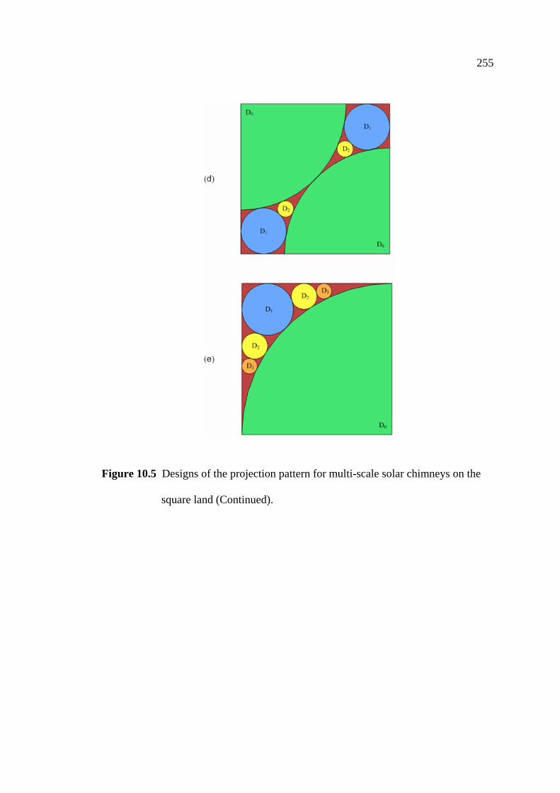
255
Figure 10.5 Designs of the projection pattern for multi-scale solar chimneys on the
square land (Continued).

256
Figure 10.6 Redesign of the patterns in Fig. 10.5, in which all designs share the same
territory ( X ) and the same largest element ( ) 0D
(Fig. 10.6a is exactly the same as Fig. 10.5a).

257
Figure 10.6 Redesign of the patterns in Fig. 10.5, in which all designs share the same
territory ( X ) and the same largest element ( ) 0D
(Note: Fig. 10.6a is exactly the same as Fig. 10.5a) (Continued).

258
Table 10.1 The global power output of the multi-size arrangements (a) – (e) shown in
Fig. 10.6 when the largest length scale ( ) is the same in all the 0D
arrangements.
Design 3Χ∑
a 1.076
b 1.199
c 1.076
d 1.049
e 1.025

259
Figure 10.7 Compactness [cf. Eq. (10.56)] and dimensionless power [cf. Eq. (10.45)]
of the power plants in Fig. 10.6.
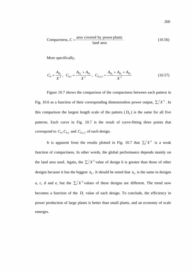
260
Compactness, Carealand
plantspowerbycoveredarea= (10.56)
More specifically,
22,1,021,020210100 ,,
XAAA
CX
AAC
XA
C DDDDDD ++=
+== (10.57)
Figure 10.7 shows the comparison of the compactness between each pattern in
Fig. 10.6 as a function of their corresponding dimensionless power output, 3X∑ . In
this comparison the largest length scale of the pattern ( ) is the same for all five
patterns. Each curve in Fig. 10.7 is the result of curve-fitting three points that
correspond to and of each design.
0D
1,00 ,CC 2,1,0C
It is apparent from the results plotted in Fig. 10.7 that 3X∑ is a weak
function of compactness. In other words, the global performance depends mainly on
the land area used. Again, the 3X∑ value of design b is greater than those of other
designs because it has the biggest . It should be noted that is the same in designs
a, c, d and e, but the
0n 0n
3X∑ values of these designs are different. The trend now
becomes a function of the value of each design. To conclude, the efficiency in
power production of large plants is better than small plants, and an economy of scale
emerges.
1D

261
10.11 CONCLUSION
In this paper we presented the optimal solar chimney power plant
configurations, based on the method of constructal design. The maximum mass flow
rate and maximum flow power in terms of geometry are proposed. It was found that
the maximum flow power is the function of plant length scale. Results indicate that the
larger plants produce more power per unit of territory. Comparisons between the
maximum power proposed and the prediction of the detailed mathematical model are
also presented. The inclusion of pressure losses into the analysis indicated that the
collector inlet pressure drop and the pressure drop over the junction between the
collector and chimney are negligible. It was shown that when the svelteness [cf. Eq.
(10.39)] is greater than 6.5 the friction loss in the collector can be neglected as well.
Though one plant which occupies the whole area might generate the maximum power,
but the study shows that it will be less efficient in power distribution. The proposed
model demonstrates mathematically that the maximum power production can be
obtained by allocating the optimal land area to the plant. This paper also presents some
arrangement patterns for the multi-scale plants on the square area. It reveals that, to
generate the electricity efficiently, the land area allocated for the largest plant is the
most important factor. While the other plants, which are smaller than the largest plant,
have only a small contributions to the whole power generated. Hence, there is
economy, in the sense of efficiency for power production, to be gained on a larger
scale.

262
10.12 REFERENCES
ANSYS, Inc. ANSYS CFX, Release 10.0: reference guide. ANSYS, 2005.
Bejan, A., 1993. Heat Transfer, Wiley, New York.
Bejan, A., 2004. Convection Heat Transfer, 3rd ed., Wiley, Hoboken, NJ.
Bejan, A., Lorente, S., 2008. Design with Constructal Theory, Wiley, Hoboken, NJ.
Calvert, J. G., 1990. Glossary of atmospheric chemistry terms (Recommendations
1990). Pure and applied chemistry, Vol. 62(11), pp. 2167-2219.
Chitsomboon, T,. 2001. A validated analytical model for flow in solar chimney.
International Journal of Renewable Energy Engineering, Vol. 3, pp. 339-
346.
EnviroMission's Solar. Tower Of Power, 2006. [On-line]. Available:
http://seekingalpha.com/article/14935-enviromission-s-solar-tower-of-power
Hedderwick, R. A., 2001. Performance evaluation of a solar chimney power plant.
M.Sc. Eng.-thesis, University of Stellenbosch, Stellenbosch, South Africa.
Kim, Y. S., Lorente, S., Bejan, A., 2009. Distribution of size in steam turbine power
plants, International Journal of Energy Research. doi:10.1002/er.1528
Kirstein, C. F., Von Backström, T. W., 2006. Flow through a solar chimney power
plant collector-to-chimney transition section, ASME Journal of Solar Energy
Engineering, Vol. 128, pp.312–317.
Koonsrisuk, A., Chitsomboon, T., 2007. Dynamic similarity in solar chimney
modeling. Solar Energy, Vol. 81, pp.1439-1446.
Koonsrisuk, A., Chitsomboon, T., 2009. Accuracy of theoretical models in the
prediction of solar chimney power plant performance. Solar Energy.
doi:10.1016/j.solener.2009.05.012.

263
Kröger, D. G., Buys, J. D., 2001. Performance evaluation of a solar chimney power
plant. ISES 2001 Solar World Congress, Adelaide, Australia.
Lorente, S., Bejan, A., 2005. Svelteness, freedom to morph, and constructal multi-
scale flow structures. International Journal of Thermal Science, Vol. 44, pp.
1123-1130.
Maia, C. B., Ferreira, A. G., Valle, R. M., Cortez, M. F. B., 2008. Theoretical
evaluation of the influence of geometric parameters and materials on the
behavior of the airflow in a solar chimney. Computers & Fluids. doi:
10.1016/j.compfluid.2008.06.005
Pretorius, J. P., Kröger, D. G., 2006. Solar chimney power plant performance. Journal
of Solar Energy Engineering, Vol. 128, pp.302-311.
Rohmann, M., 2000. Solar Chimney Power Plant. Bochum University of Applied
Sciences.
Schlaich, J., 1995. The Solar Chimney. Edition Axel Menges: Stuttgart, Germany.
Von Backström, T. W., Bernhardt, A., Gannon, A. J., 2003. Pressure drop in solar
power plant chimneys, ASME Journal of Solar Energy Engineering, Vol.
125 , pp.165–169.
Zhou, X., Yang, J., Xiao, B., Hou, G., Xing, F., 2009. Analysis of chimney height for
solar chimney power plant. Applied Thermal Engineering, Vol. 29, pp. 178-
185.

CHAPTER XI
CONCLUSION AND RECOMMENDATION
This work investigates the behavior of the flow in solar chimney with the
ultimate goal of a better design to obtain a higher efficiency. Dimensional analysis is
applied to determine the dimensionless parameters that characterize the flow. CFD
study in geometrically similar cases indicated that the proposed dimensionless
variables are appropriate for obtaining similarity for flows in prototype and small-
scale models of a solar chimney. The study shows that water is not suitable as a test
working fluid because the solar heat absorption per unit volume required for similarity
is too high. Using air for a small-scale model, though quite natural, requires lower
insolations than that of the prototype for dynamic similarity; this requires roof
material treatments such as tinting or using artificial insolation, which is difficult in
practice.
Further study shows that a complete dynamic similarity for scaled models and
a full scale solar chimney prototype, while maintaining the same insolation, is
achievable if the model’s roof radius is distorted from its fully similar configuration
according to a prescribed rule that was proposed in the study. This ‘partially similar’
proposition is proved to be valid which is evident by the collapse of the scaled
numerical results of the widely disparage test cases. The seemingly complicated
similarity variables were interpreted simply as the characteristic output power (scaled
kinetic energy) and the characteristic input power (scaled buoyant force).

265
A single dimensionless similarity variable for the solar chimney power plant is
proposed and proved to be valid for both the fully similar case and the partially
similar case. This should enable the experimental study of a solar chimney power
plant to be simpler and more economical. This variable was interpreted as the total
kinetic energy scaled by the buoyant energy of the rising hot air. The proposed
variable was examined from various perspectives and was found to be related to the
overall efficiency proposed by other researchers and also to the Richardson number.
The equality of temperature rises across roof portions for the prototype and its fully
and partially similar models was observed and explained in the context of similarity.
In addition, the influences of roof height, roof radius, tower height, tower
radius, and insolation on solar chimney power plant performances have been studied
by using five theoretical models from the literature and a carefully calibrated CFD
procedure. Important observations are concluded. According to this study, the models
of Schlaich et al. (2005) and Koonsrisuk and Chitsomboon (2009) are recommended
because they compared more favorably with the CFD results than the other models for
all the test cases that were investigated.
Furthermore, a solar chimney system with varying flow area is studied and its
performance is evaluated. Theoretical analysis suggests that the solar chimney with
sloping collector and divergent-top chimney would perform better than that of a
conventional system. CFD calculations show that a divergent tower helps increase the
static pressure, mass flow rate and power over that of the constant area tower. For the
convergent tower, the power remains the same as the constant area case. The sloping
collector helps increase the static pressure across the roof and the power at the roof

266
entrance. The system with the sloping collector and divergent-top chimney of tower
area ratio of 16 can produce power as much as 400 times that of the reference case.
A detailed mathematical model of the solar chimney power plant is developed in
order to evaluate the turbine work extraction. It appears that, for the system with a
constant pressure potential (available system pressure difference), the optimum ratio
of the turbine pressure drop to the pressure potential is 2/3. For the system with the
pressure potential is not constant, it is obvious that this optimum ratio is a function of
the plant size and solar heat flux. This study may be helpful in the preliminary plant
design.
Through field measurements on four small-scale models built at Suranaree
University of Technology, results indicate that the flow power increases with the
decrease in the ratio between roof inlet area and tower inlet area. The divergent
chimney also results in significant increase in flow power compared to that of the
constant area chimney. It was observed that the system with the proposed novel roof
shape designed by the researcher provides approximately the same performance as the
conventional shaped system, while the ratio of roof inlet area and tower inlet area for
the proposed system could be practically reduced. Correspondingly the increase in
performance, to some specific value which is much higher than the typical system
could be achieved. The experimental results differ comparatively but have the same
trends as to the predicted values. This may follow from the fluctuating solar heat flux
and the effect of the large chimney diameter when compared with the roof size.
Moreover, the difference of dimensionless variables between the large and the small
plant is noticeable, contrary to the theoretical and numerical predictions. Reasons
could be the varying atmospheric conditions when the tests were run.

267
The optimal solar chimney power plant configurations are based on the
guiding of constructal design, the maximum mass flow rate and maximum flow power
in terms of geometry are proposed. It was found that the maximum flow power is a
function of plant length scale. Results indicate that the larger plants produce more
power per unit of territory. Comparisons between the maximum power proposed and
the prediction of the detailed mathematical model are also presented. The inclusion of
pressure losses into the analysis indicated that the collector inlet pressure drop and the
pressure drop over the junction between the collector and chimney are negligible. It
was shown that when the svelteness is greater than 6.5, the friction loss in the
collector can be neglected as well. Though one plant occupying the whole area might
generate the maximum power, the study shows that it will be less efficient in power
distribution. The proposed model demonstrates mathematically that the maximum
power production can be obtained by allocating the optimal land area to the plant.
This paper also presents some arrangement patterns for the multi-scale plants on the
square area. It reveals that, to generate the electricity efficiently, the land area
allocated for the largest plant is the most important factor. While the other plants,
which are smaller than the largest plant, have only a small contributions to the whole
power generated. Hence, there is economy, in the sense of efficiency for power
production, to be gained on a larger scale.

APPENDIX A
A SET UP OF THE ANSYS-CFX 10.0 SOLVER
APPENDIX B

269
+--------------------------------------------------------------------+ CFX Command Language for Run +--------------------------------------------------------------------+ LIBRARY: MATERIAL: Air Ideal Gas Material Description = Air Ideal Gas (constant Cp) Material Group = Air Data, Calorically Perfect Ideal Gases Option = Pure Substance Thermodynamic State = Gas PROPERTIES: Option = General Material ABSORPTION COEFFICIENT: Absorption Coefficient = 0.01 [m^-1] Option = Value END DYNAMIC VISCOSITY: Dynamic Viscosity = 1.831E-05 [kg m^-1 s^-1] Option = Value END EQUATION OF STATE: Molar Mass = 28.96 [kg kmol^-1] Option = Ideal Gas END REFRACTIVE INDEX: Option = Value Refractive Index = 1.0 [m m^-1] END SCATTERING COEFFICIENT: Option = Value Scattering Coefficient = 0.0 [m^-1] END SPECIFIC HEAT CAPACITY: Option = Value Reference Pressure = 1 [atm] Reference Specific Enthalpy = 0. [J/kg] Reference Specific Entropy = 0. [J/kg/K] Reference Temperature = 25 [C] Specific Heat Capacity = 1.0044E+03 [J kg^-1 K^-1] Specific Heat Type = Constant Pressure END THERMAL CONDUCTIVITY: Option = Value Thermal Conductivity = 2.61E-2 [W m^-1 K^-1] END

270
END END END EXECUTION CONTROL: PARALLEL HOST LIBRARY: HOST DEFINITION: cad201 Remote Host Name = CAD2-01 Host Architecture String = intel_p4.sse2_winnt5.1 Installation Root = C:\Program Files\ANSYS Inc\CFX\CFX-%v END END PARTITIONER STEP CONTROL: Multidomain Option = Independent Partitioning Runtime Priority = Standard MEMORY CONTROL: Memory Allocation Factor = 1.0 END PARTITIONING TYPE: MeTiS Type = k-way Option = MeTiS Partition Size Rule = Automatic END END RUN DEFINITION: Definition File = \ C:/CFX/work/freeWakeT/converdiver_2hr1_4rc4_MC5deg_0p55_0p0381_0p23_r10\ _RefLo0c0c100_3adap2_inIN_1e7_outAverPs_TotalEnergy_q2p800.def Interpolate Initial Values = Off Run Mode = Full END SOLVER STEP CONTROL: Runtime Priority = Standard EXECUTABLE SELECTION: Double Precision = On END MEMORY CONTROL: Memory Allocation Factor = 1.0 END PARALLEL ENVIRONMENT: Number of Processes = 1 Start Method = Serial END END END FLOW: DOMAIN: Domain 1 Coord Frame = Coord 0 Domain Type = Fluid

271
Fluids List = Air Ideal Gas Location = B30,B37,B42 BOUNDARY: in Boundary Type = INLET Location = in BOUNDARY CONDITIONS: FLOW DIRECTION: Option = Normal to Boundary Condition END FLOW REGIME: Option = Subsonic END HEAT TRANSFER: Option = Static Temperature Static Temperature = 308 [K] END MASS AND MOMENTUM: Option = Total Pressure Relative Pressure = 0 [Pa] END END END BOUNDARY: out Boundary Type = OUTLET Location = out BOUNDARY CONDITIONS: FLOW REGIME: Option = Subsonic END MASS AND MOMENTUM: Option = Average Static Pressure Relative Pressure = 0 [Pa] END PRESSURE AVERAGING: Option = Average Over Whole Outlet END END END BOUNDARY: wall Boundary Type = WALL Location = wall BOUNDARY CONDITIONS: HEAT TRANSFER: Option = Adiabatic END WALL INFLUENCE ON FLOW: Option = Free Slip END

272
END END BOUNDARY: ground Boundary Type = WALL Location = ground BOUNDARY CONDITIONS: HEAT TRANSFER: Option = Adiabatic END WALL INFLUENCE ON FLOW: Option = Free Slip END END END BOUNDARY: symXp Boundary Type = SYMMETRY Location = symXp END BOUNDARY: symXm Boundary Type = SYMMETRY Location = symXm END DOMAIN MODELS: BUOYANCY MODEL: Buoyancy Reference Density = 1.146 [kg m^-3] Gravity X Component = 0 [m s^-2] Gravity Y Component = -9.807 [m s^-2] Gravity Z Component = 0 [m s^-2] Option = Buoyant BUOYANCY REFERENCE LOCATION: Cartesian Coordinates = 0 [m], 0 [m], 100 [m] Option = Cartesian Coordinates END END DOMAIN MOTION: Option = Stationary END REFERENCE PRESSURE: Reference Pressure = 1 [atm] END END FLUID MODELS: COMBUSTION MODEL: Option = None END HEAT TRANSFER MODEL: Option = Total Energy END

273
THERMAL RADIATION MODEL: Option = None END TURBULENCE MODEL: Option = Laminar END END SUBDOMAIN: insolation Coord Frame = Coord 0 Location = B42 SOURCES: EQUATION SOURCE: energy Option = Source Source = 400 [W m^-3] END END END END INITIALISATION: Option = Automatic INITIAL CONDITIONS: Velocity Type = Cartesian CARTESIAN VELOCITY COMPONENTS: Option = Automatic with Value U = 0 [m s^-1] V = 0 [m s^-1] W = 0 [m s^-1] END STATIC PRESSURE: Option = Automatic END TEMPERATURE: Option = Automatic with Value Temperature = 308 [K] END END END OUTPUT CONTROL: RESULTS: File Compression Level = Default Option = Standard END END SIMULATION TYPE: Option = Steady State END SOLUTION UNITS: Angle Units = [rad]

274
Length Units = [m] Mass Units = [kg] Solid Angle Units = [sr] Temperature Units = [K] Time Units = [s] END SOLVER CONTROL: ADVECTION SCHEME: Option = High Resolution END CONVERGENCE CONTROL: Length Scale Option = Conservative Maximum Number of Iterations = 80000 Timescale Control = Auto Timescale END CONVERGENCE CRITERIA: Residual Target = 1.0e-07 Residual Type = RMS END DYNAMIC MODEL CONTROL: Global Dynamic Model Control = On END PRESSURE LEVEL INFORMATION: Cartesian Coordinates = 0 [m], 0 [m], 100 [m] Option = Cartesian Coordinates END END END COMMAND FILE: Version = 10.0 Results Version = 10.0 END

APPENDIX B
LIST OF PUBLICATIONS

276
Articles in Refereed Journals (5)
Koonsrisuk, A., Lorente, S. and Bejan, A. (2009). Constructal solar chimney
configuration. International Journal of Heat and Mass Transfer. (accepted)
Koonsrisuk, A. and Chitsomboon, T. (2009). A single dimensionless variable for
solar chimney power plant modeling. Solar Energy.
doi:10.1016/j.solener.2009.07.015.
Koonsrisuk, A. and Chitsomboon, T. (2009). Accuracy of theoretical models in the
prediction of solar chimney performance. Solar Energy.
doi:10.1016/j.solener.2009.05.012.
Koonsrisuk, A. and Chitsomboon, T. (2009). Partial geometric similarity for solar
chimney power plant modeling. Solar Energy, Volume 83, pp. 1611 - 1618.
Koonsrisuk, A. and Chitsomboon, T. (2007). Dynamic similarity in solar chimney
modeling. Solar Energy, Volume 81, pp. 1439 - 1446.
Articles in Conference Proceedings (10)
Koonsrisuk, A. and Chitsomboon, T. (2007). The Effect of Plant Geometry on the
Potential of a Solar Tower, In Proceedings of the 11st Annual National
Symposium on Computational Science and Engineering, Phuket,
Thailand.
Koonsrisuk, A. and Chitsomboon, T. (2006). Effect of Tower Area Change on the
Potential of Solar Tower. In Proceedings of the 2nd Joint International
Conference on Sustainable Energy and Environment, Bangkok,
Thailand.

277
Koonsrisuk, A. and Chitsomboon, T. (2006). Partial Similarity in Solar Tower
Modeling. In Proceedings of the 20th Conference on Mechanical
Engineering Network of Thailand, Nakhon Ratchasima, Thailand.
Koonsrisuk, A. and Chitsomboon, T. (2005). Actuator Disc Approximation for the
Flow through Turbine in a Solar Tower. In Proceedings of the 1st
Conference on Energy Network of Thailand. Chon Buri, Thailand.
Koonsrisuk, A. and Chitsomboon, T. (2004). Similarity Analysis in Scale Modeling
of a solar chimney. In Proceedings of the 18th National Mechanical
Engineering Conference. Khon Khaen, Thailand.
Koonsrisuk, A. and Chitsomboon, T. (2004). Frictional effect on the flow in a solar
chimney. In Proceedings of the 4th National Symposium on Graduate
Research. Chiang Mai, Thailand.
Koonsrisuk, A. and Chitsomboon, T. (2004). The study of dynamic similarity in
physical modeling of a solar chimney. In Proceedings of the RGJ Seminar
Series 29: Engineering Applications. Chiang Mai, Thailand.
Koonsrisuk, A. and Chitsomboon, T. (2004). Dynamic similarity in model testing of
the flow in solar chimney. In Proceedings of the 15th International
Symposium on Transport Phenomena. Bangkok, Thailand.
Koonsrisuk, A. and Chitsomboon, T. (2004). The effect of roof height to the flow in
solar chimney. In Proceedings of the RGJ-Ph.D. Congress V. Chon Buri,
Thailand.
Koonsrisuk, A. and Chitsomboon, T. (2003). Dimensional analysis for the flow
through a solar chimney. In Proceedings of the 17th National Mechanical
Engineering Conference. Prachin Buri, Thailand, pp. EM56 - EM61.

BIOGRAPHY
Atit Koonsrisuk was born in Ubon Ratchathani Province on August 11, 1974, the son
of Kaehua Saekoo and Neeracha Koonsrisuk. He attended high school at Sisaket Wittayalai in
Sisaket Province and graduated in 1992. Atit received his Bachelor of Engineering degree in
Mechanical Engineering from Suranaree University of Technology in 1997. In 1999, he
enrolled in the Master’s degree program in the School of Mechanical Engineering at Suranaree
university of Technology. Later, he was awarded a scholarship for a Doctoral Degree, so he
enrolled in the Ph.D. Program of the same School in 2002.
During his graduate work, Atit worked as a teaching assistant in the School of
Mechanical Engineering. He was awarded a Royal Golden Jubilee (RGJ) Ph.D. Program
Scholarship from the Thailand Research Fund (TRF) in 2002. He was also a recipient of the
Basic Research Grant (BGJ) from the Thailand Research Fund (TRF) in 2004. In October
2008, he was a Visiting Scholar in the Constructal Design Group at Duke University, USA,
with Prof. Adrian Bejan and Prof. Sylvie Lorente. His research focuses on optimizing the
design of a solar chimney power plant.