analysis and evaluation of segmental concrete tunnel linings

ANALYSIS AND EVALUATION OF SEGMENTAL CONCRETE TUNNEL LININGS - SEISMIC AND

DURABILITY CONSIDERATIONS

(Spine title: Analysis And Evaluation of Segmental Concrete Tunnel Linings)

(Thesis format: Integrated-Article)

By

Hairy EINaggar

Graduate Program in Engineering Science

Department of Civil and Environmental Engineering

A thesis submitted in partial fulfillment

of the requirements for the degree of

Doctor of Philosophy

Faculty of Graduate Studies

The University of Western Ontario

London, Ontario, Canada

September 2007

© Hany H. Elnaggar 2007

1*1 Library and Archives Canada

Published Heritage Branch

395 Wellington Street Ottawa ON K1A0N4 Canada

Bibliotheque et Archives Canada

Direction du Patrimoine de I'edition

395, rue Wellington Ottawa ON K1A0N4 Canada

Your file Votre reference ISBN: 978-0-494-39262-1 Our file Notre reference ISBN: 978-0-494-39262-1

NOTICE: The author has granted a nonexclusive license allowing Library and Archives Canada to reproduce, publish, archive, preserve, conserve, communicate to the public by telecommunication or on the Internet, loan, distribute and sell theses worldwide, for commercial or noncommercial purposes, in microform, paper, electronic and/or any other formats.

AVIS: L'auteur a accorde une licence non exclusive permettant a la Bibliotheque et Archives Canada de reproduire, publier, archiver, sauvegarder, conserver, transmettre au public par telecommunication ou par Plntemet, prefer, distribuer et vendre des theses partout dans le monde, a des fins commerciales ou autres, sur support microforme, papier, electronique et/ou autres formats.

The author retains copyright ownership and moral rights in this thesis. Neither the thesis nor substantial extracts from it may be printed or otherwise reproduced without the author's permission.

L'auteur conserve la propriete du droit d'auteur et des droits moraux qui protege cette these. Ni la these ni des extraits substantiels de celle-ci ne doivent etre imprimes ou autrement reproduits sans son autorisation.

In compliance with the Canadian Privacy Act some supporting forms may have been removed from this thesis.

Conformement a la loi canadienne sur la protection de la vie privee, quelques formulaires secondaires ont ete enleves de cette these.

While these forms may be included in the document page count, their removal does not represent any loss of content from the thesis.

Canada

Bien que ces formulaires aient inclus dans la pagination, il n'y aura aucun contenu manquant.

THE UNIVERSITY OF WESTERN ONTARIO FACULTY OF GRADUATE STUDIES

CERTIFICATE OF EXAMINATION

Supervisor

Dr. Sean Hinchberger

Supervisory Committee

Dr. K.Y. Lo

Examiners

Prof. Maged Ali Youssef

Timothy Newson

Dr. Kristy Tiampo

Tarek Abdoun

The thesis by

Hany Hamed EINaggar

entitled:

Analysis and Evaluation of Segmental Concrete Tunnel Linings Seismic and Durability Considerations

is accepted in partial fulfillment of the requirements for the degree of

Doctor of Philosophy

Date Chair of the Thesis Examination Board

ii

ABSTRACT

Tunnels have been constructed by many civilizations, and over time, exciting new

advancements in tunnelling techniques and methods have emerged. One such notable

advancement is the tunnel boring machine (TBM), which facilitated the evolution of

rapid excavation by shield driven tunnelling method. Precast segmental concrete tunnel

linings are widely used in conjunction with the shield driven tunnelling method, and these

linings have been implemented on numerous tunnelling projects during the second half of

the 20th century. In some cases, long-term exposure of reinforced concrete linings to

sulphates or chlorides in groundwater can lead to concrete deterioration and consequent

reduction in the lining load carrying capacity. Engineers may thus be required to evaluate

the distribution of moment and thrust in degraded liners to assess their factor of safety.

Closed-form solutions can represent an attractive tool for such applications, especially if

liner degradation is wide spread in a tunnel system of variable depth.

This thesis presents a series of analytical solutions for analyzing tunnel linings in elastic

ground. First, two closed-form solutions for composite tunnel linings are developed. The

first solution considers the lining as an inner thin-walled shell and an outer thick-walled

cylinder embedded in elastic ground and it accounts for the effect of ground convergence

prior to installation of the lining (the gap). The second solution extends the first solution

to account for the rotational stiffness of the tunnel's joints for analysis of segmental

concrete linings. Both solutions are shown to be useful analytical tools for assessing the

moments and thrusts in degraded segmental concrete tunnel linings by applying them to

study various tunnel problems.

in

In addition, both composite solutions are adapted to permit calculation of in-plane

stresses in tunnel lining induced by earthquakes. The composite lining solutions are then

used to study the effect of local soil nonlinearity caused by an excavation damaged zone

(EDZ) around bored tunnels (using the equivalent linear approach) during earthquakes.

Finally, this thesis concludes by presenting the results of detailed numerical analysis

involving the static and seismic response of tunnels with intact and degraded concrete

liners. The analysis use both nonlinear methods and linear elastic closed form solutions to

gain insight into the stresses in intact and degraded tunnel linings for both static and

seismic loadings. In addition, the finite element results help to define limits for analysis

of degraded linings using closed form linear elastic solutions.

Keywords: closed form solution, segmental tunnel lining, joint stiffness, in-plane shear,

EDZ, finite element analysis, concrete degradation.

IV

COPYRIGHT AND CO-AUTHORSHIP

Several parts of this thesis were submitted for publication to peer-reviewed technical

journals. Also, some other parts are published in national and international conferences.

The candidate conducted all the development and analysis and wrote the initial versions

of all papers listed below. His thesis advisor revised the documents and contributed to the

development of the final version of these papers:

1. El Naggar, H. and Hinchberger, S. (2007) "An Analytical Solution for Jointed

Tunnel Linings in a Homogeneous Infinite Isotropic Elastic medium", Canadian

Geotechnical Journal, Canada. (Accepted)

2. El Naggar, H., Hinchberger, S. and Lo, K. Y. (2006) "A Closed-Form Solution

for Tunnel Linings in a Homogenous Infinite Isotropic Elastic Medium",

Canadian Geotechnical Journal, Canada. (In Press)

3. El Naggar, H., Hinchberger, S. and El Naggar, M.H. (2007) "Approximate

Evaluation of Nonlinearity Effects on Seismically Induced In-Plane Stresses in

Tunnel Lining", 4th International Conference on Earthquake Geotechnical

Engineering, June 25-27, 2007, Greece.

4. Hinchberger, S.D. and El Naggar, H. (2005) "On the Use of Simplified Methods

to Estimate Moments and Thrust in Segmental Concrete Tunnel Linings", K.Y.

Lo Symposium, July 7-9 2005, The University of Western Ontario, London,

Canada, pp.319-329.

v

Dedicated to the memory of my parents

vi

ACKNOWLEDGMENTS

I want to express my sincere gratitude and appreciation to Dr. Sean Hinchberger for his

support throughout the duration of my study. His guidance, efforts and encouragements

will forever be remembered and appreciated.

My thanks are also extended to my co-supervisor Dr. K. Y. Lo for his parentally warm

feelings, support and encouragements.

I also want to thank the members of my advisory committee, Dr. Maged Youssef and Dr.

Tim Newson. My thanks are also extended to all of the administrative staff in the

Department of Civil and Environmental Engineering, and the Geotechnical Research

Center, at the University of Western Ontario. In addition, I want to acknowledge the

financial support of the Ministry of Colleges and Universities through the Ontario

Graduate Scholarship, OGS, which made this research possible.

Special thanks are extended to my brother Dr. Hesham El Naggar for his mentoring,

guidance, advices and encouragements.

Last but not least, I am grateful to all my family members, especially my wife and best

friend Norhan and my children Abdelmoneim, Hana and Ahmed for their love, patience,

encouragement, support and understanding, without which, this effort would have been

much difficult.

vu

TABLE OF CONTENTS

Certificate of Examination ii

ABSTRACT iii

COPYREIGHTANDCO-AUTHOURSfflP v

DEDICATION vi

ACKNOWLEDGMENTS vii

TABLE OF CONTENTS viii

LIST OF TABLES xvi

LIST OF FIGURES xvii

LIST OF APPENDICES xxii

LIST OF SYMBOLS xxiii

Chapterl Introduction 1

1.1 Statement of the Problem 1

1.2 Thesis Objectives and Original Contributions 3

1.3 Scope and Organization of the Thesis 4

References 6

Chapter 2 Evaluation of Simplified Methods for

Estimating Moments and Thrust in Segmental Concrete

Tunnel Linings 7

viii

2.1 Introduction 7

2.2 Methods for Predicting Lining Loads 8

2.2.1 Solutions for the Static In-situ Stresses 9

2.3 Analysis of a Typical Subway Tunnel 12

2.3.1 Problem Definition 12

2.3.1.1 Generalized Geologic Setting 12

2.3.1.2 Geotechnical Conditions 13

2.3.1.3 Tunnel Lining 15

2.3.2 Analytical Methods. 16

2.3.2.1 Closed-Form Solutions 16

2.3.2.1.1 Multi-liner Solution Ogawa (1986) 16

2.3.2.1.2 Simplified Analysis (Einstein and Schwartz, 1979) 17

2.3.2.2 The Finite Element Model 18

2.3.3 Liner-Ground Interaction 19

2.3.3.1 The Concept of Soil Structure Interaction 19

2.3.4 Comparison of Closed-form and Finite Element Solutions 21

2.3.4.1 The Influence of Gap Closure on Moments and Thrusts 24

2.3.4.2 Effect of the Joints on the Lining Stiffness 26

2.4 Summary And Conclusions 29

References 32

IX

Chapter 3 A Closed-Form Solution for Composite Tunnel

Linings in a Homogeneous Infinite Isotropic Elastic

Medium 34

3.1 Introduction 34

3.2 Problem Definition 36

3.3 Stresses and displacements in the Ground due to Full Stress Relief 39

(i) Hydrostatic Component, Po 39

(ii) Deviatoric Component, Qo 40

(iii) Combined Solution 41

3.4 Stresses and Displacements in the Ground due to Liner Reactions 42

(i) Hydrostatic Component 44


3.5 Equations for Stresses and Displacements of the Outer Liner 45

(ii) Hydrostatic Component 45

(ii) Deviatoric Component 46

(iii) Combined Solution - Hydrostatic and Deviatoric 48

3.6 Equations for Reactions due to the Inner Liner 49

3.6.1 Governing Equations 49



78

3.7 Interaction between the Ground and Composite Liner System 52

x


(ii) Deviatoric Component - No Slip 55

(iii) Deviatoric Component - Full Slip at r=R2 and r=R3 59

(iv) Deviatoric Component - Full Slip at R2, No Slip at RJ 60

(v) Deviatoric Component-No Slip at R2, Full Slip at R3 61

3.8 Moment and Thrust 63


(ii) Deviatoric Component-No Slip 63

(iii) Deviatoric Component - Full Slip 64

(iv) Deviatoric Component - Full Slip at R2, No Slip at R3 64

(v) Deviatoric Component-No Slip at R2, Full Slip at R3 65

3.9 Typical Results 66

3.9.1 The Effect of Ground Convergence prior to Liner Installation 66

3.9.2 The Effect of Composite Lining Behaviour 70

3.10 Conclusions 75

References 76

Chapter 4 An Analytical Solution for Jointed Tunnel

Linings in a Homogeneous Infinite Isotropic Elastic

medium 77

4.1 Introduction 77

4.2 Problem Definition 80

xi

4.3 Stresses and displacements in the Ground due to Full Stress Relief 81

(i) Hydrostatic Component, Po 82


4.4 Stresses and Displacements in the Ground due to Liner Reactions 83



(iii) Combined Solution 84

4.5 Equations for Stresses and Displacements of the Outer Liner 87

(i)Hydrostatic Component 87


(iii) Combined Solution - Hydrostatic and Deviatoric 90

4.6 Equations for Reactions due to the Inner Jointed Liner 91

4.6.1 Governing Equations 91



4.7 Interaction between the Ground and Composite Liner System 97


(ii) Deviatoric Component - No Slip 99

(iii) Deviatoric Component - Full Slip 103

4.8 Evaluation of the solution 104

4.8.1 Finite Element Analysis 106

4.8.1.1 Liner with 4-Segments 107

4.8.2 Modification for Low Joint Stiffnesses 109

xii

4.8.3 Comparison of Revised Solution with FE Analysis 110

4.8.3.1 4-Segments 110

4.8.3.2 6-Segments 113

4.8.3.3 8-Segments 114

4.9 Example 120

4.10 Summary and Conclusions 122

References 124

Chapter 5 Approximate Evaluation of Nonlinear Effects

on Seismically Induced In-Plane Shear Stresses in Continuous

and Segmental Tunnel Linings 126

5.1 Introduction 126

5.2 The Double Liner Solution 127

5.2.1 Problem Geometry 127

5.2.2 Internal Reactions - (Equilibrium) 130

5.2.3 Governing Equations for the Inner Lining 131

5.2.4 Hydrostatic Component 133

5.2.5 Deviatoric Component 134

5.2.5.1 Case of No Slip at r = R2and r = R3 135

5.2.6 The In-Plane Shear Wave Component 137

5.3 Seismic Performance of Tunnels 139

5.3.1 Case of a Continuous Tunnel lining 140

xiii

5.3.1.1 Effect of the Weakened Zone 140

5.3.1.2 Effect of the Angle of Incidence 146

5.3.1.3 Discussion of Results of the Continuous Tunnel lining Case 148

5.3.2 Case of Jointed Segmental Tunnel lining 149

5.3.2.1 Effect of the Rotational Stiffness of the Joints on Seismically

Induced In-plane Stresses 150

5.3.2.2 Discussion of Results of the Jointed Tunnel lining Case 151

5.4 SUMMARY AND CONCLUSIONS 152

References 156

Chapter 6 Comparison of Finite Element and Closed

Form Solutions for Problems Involving Seismicity and Liner

Degradation 159

6.1 Introduction 159

6.2 Methodology 161

6.2.1 Problem Geometry 161

6.2.2 Material Models 163

6.2.2.1 The Soil 163

6.2.2.2 The Concrete Tunnel Lining 163

6.3 The Finite Element Analysis 170

6.3.1 Finite Element Mesh Details 170

6.3.2 Finite Element Solution Sequence 172

xiv

6.3.3 Simulation of Concrete Spalling at the Intrados 175

6.3.4 Finite Element Solution Sequence 176

6.3.5 Pseudo Static Analysis of In-Plane Seismic Stresses 177

6.4 Results and Discussion 180

6.4.1 Results of Static Loading 180

6.4.1.1 The Intact Liner 180

6.4.1.2 The Degraded Liner 182

6.4.2 Evaluation of Combined Static and Seismic Loading 188

6.4.2.1 The Intact Liner 189

6.4.2.2 Influence of Soil and Concrete Plasticity 190

6.4.2.3 The Degraded Liner during a Seismic Event 193

6.4.2.4 Influence of Soil and Concrete Plasticity 195


References 199

Chapter 7 Summary, Conclusions and Recommendations

for Future Research 201


7.1.1 Closed form solutions 202

7.1.2 Seismic considerations 203

7.1.3 Numerical Evaluations 204

7.2 Recommendations for future research 205

VITA 217

XV

LIST OF TABLES

Table 2.1: Summary of geotechnical properties 14

Table 2.2: Material parameters used with the closed-form solutions 22

Table 3.1: Comparison of closed-form solutions for circular tunnels in elastic ground....36

Table 3.2: Material parameters used in the study 71

Table 4.1: Liner configurations considered in the analyses 105

Table 4.2: Soil properties considered in the analysis 120

Table 5.1: Material parameters used in the analysis 140

Table 6.1: Soil and lining's properties considered in the analysis 162

Table 6.2: Joints material properties 172

Table 6.3: Elastic properties used in the closed form solution 176

xvi

LIST OF FIGURES

Figure 2.1: An opening in an infinite plate subjected to: (a) uniaxial stress field,

(b) biaxial stress field 10

Figure 2.2: Generalized Subsurface Conditions 13

Figure 2.3: Geotechnical Conditions Considered 14

Figure 2.4: Idealized tunnel Liner Geometry 16

Figure 2.5: Schematic drawing for the multi-liner solution 18

Figure 2.6: Simplified Liner-Ground Interaction 21

Figure 2.7: Calculated distribution of moments - N o Gap Closure & No Joints 23

Figure 2.8: Calculated distribution of Thrust - N o Gap Closure & No Joints 23

Figure 2.9: The influence of gap closure on the calculated moment- No Slip & No Joints.

25

Figure 2.10: The effect of gap closure on the calculated thrust No Slip & No Joints 25

Figure 2.11: Crown Displacement and maximum moment (After Lingenfelser, 1985)... 27

Figure 2.12: The influence of joints on moments 29

Figure 2.13: The impact of ground deformation and joints on the reserve liner capacity.

31

Figure 3.1: Common double lining systems 35

Figure 3.2: Problem geometry - composite lining 38

Figure 3.3: Hydrostatic and deviatoric components of the solution 38

Figure 3.4: Reactive stresses - hydrostatic component 43

Figure 3.5: Reactive stresses - deviatoric component 43

Figure 3.6: Radial displacement at the crown of the inner lining 68

xvii

Figure 3.7: Radial displacement at the springline of the inner lining 68

Figure 3.8: Thrust at the springline of the inner lining 69

Figure 3.9: Moment at the springline of the inner lining 69

Figure 3.10: Radial displacement at the crown and the springline of the inner lining 71

Figure 3.11: Thrust at the crown and the springline of the inner lining 72

Figure 3.12: Moment at the crown and the springline of the inner lining 72

Figure 3.13: Moment distribution in the inner lining for 50mm thick grout 74

Figure 3.14: Thrust distribution in the inner lining for 50mm thick grout 74

Figure 4.1: Problem geometry - composite lining 79


Figure 4.3: Reactive stresses, a) hydrostatic component, b) deviatoric component 86

Figure 4.4: Contribution of the joints to the horizontal displacement at the springline.

96

Figure 4.5: Liner configurations considered in the analyses 106

Figure 4.6: Normalized displacements, moments and thrusts for the 4 joint

configurations (before correction) 108


configurations (low values of A ) I l l


configurations (higher values of A ) 112


configurations (low values of A) 115


xviii

configurations (higher values of A) 116

Figure 4.11: Comparison between the results of the FE and the closed form solution

for the 6 joint configuration 117


configurations (low values of A) 118


configurations (higher values of A) 119

Figure 4.14: Moment distribution in the inner lining 121

Figure 4.15: Thrust distribution in the inner lining 122

Figure 5.1: Problem geometry - Jointed double liners system 128


Figure 5.3: Reactive stresses - a) Hydrostatic component, b) Deviatoric component... 131

Figure 5.4: a) Earthquake induced shear stresses, b) Equivalent principle stresses 138

Figure 5.5: The incidence angle 139

Figure 5.6: The effect of the nonlinearity of the weakened zone on the internal forces

of the liner (Static loads only). Moments at a) the crown, b) 8=45°; Thrust at c) the

crown, d) 9=45° 143

Figure 5.7: The effect of the nonlinearity of the weakened zone on the internal forces

of the liner (Earthquake loads only). Moments at a) the crown, b) 9=45°; Thrust at c) the

crown, d) 9=45° 144

Figure 5.8: The effect of the nonlinearity of the weakened zone on the total internal

forces of the liner (Static plus earthquake loads). Moments at a) the crown, b) 9=45°;

Thrust at c) the crown, d) 9=45° 145

xix

Figure 5.9: The effect of the angle of incidence on the internal forces of the liner 147

Figure 5.10: Moment distribution in the circumferential direction around the tunnel

(seismically induced loads only) 154

Figure 5.11: Thrust distribution in the circumferential direction around the tunnel

(seismically induced loads only) 154


forces of the jointed liner (Static plus earthquake loads) 155

Figure 6.1: Geometry of the considered problem 162

Figure 6.2: Compression and tension meridians for concrete (from Hinchberger

2007) 164

Figure 6.3: a) 3-D, b) biaxial shape of the envelop (from Hinchberger 2007) 165

Figure 6.4: (a) Concrete (elements in central part of liner without flexural steel),

(b) Reinforced concrete (elements at the extrados and intrados of the liner) 169

Figure 6.5: The finite element mesh 171

Figure 6.6: 2D simulation of the tunnelling process 174

Figure 6.7: The three considered degradation scenarios 176

Figure 6.8: Input motions and matched spectra for a) LSZ, b) MSZ, and c) HSZ 179

Figure 6.9: Distribution of normal stresses at the liner extrados 181

Figure 6.10: Distribution of normal stresses at the liner intrados 181

Figure 6.11: Stresses at the liner extrados degradation Scenario 1 183

Figure 6.12: Stresses at the liner intrados degradation Scenario 1 183

Figure 6.13: Rotation of major principle stresses at the transition zone 184


xx




Figure 6.18: Results of the ground response analysis 188

Figure 6.19: Stresses at the liner extrados in low, moderate and high seismicity zones

compared to that of the static case 189

Figure 6.20: Stresses at the liner intrados in low, moderate and high seismicity zones

compared to that of the static case 190

Figure 6.21: Comparison of the stresses in the liner for low seismicity 191

Figure 6.22: Comparison of the stresses in the liner for medium seismicity 191

Figure 6.23: Comparison of the stresses in the liner's extrados for high seismicity. ... 192

Figure 6.24: Location of plastic zones for MSZ and HSZ 192

Figure 6.25: Stresses at the liner extrados in low, moderate and high seismic zones

(compared with the static case) 194

Figure 6.26: Stresses at the liner intrados in low, moderate and high seismic zones

(compared with the static case) 194

Figure 6.27: Stresses at the liner extrados degradation Scenario 3 and MSZ 196

Figure 6.28: Stresses at the liner intrados degradation Scenario 3 and MSZ 196

xxi

List of Appendices

Appendix A 207

Appendix B 212

Appendix C 215

xxn

LIST OF SYMBOLS

9 Angle which is measured counter clockwise from the springline

crv The initial vertical stress in the ground

a h The initial horizontal stress in the ground

K'0 the coefficient of lateral earth pressure at rest

P0 The hydrostatic component

Q0 The deviatoric component

Eg Elastic modulus of the ground

vg Poisson's ratio of the ground

E2 Elastic modulus of the outer liner

v2 Poisson's ratio of the outer liner

Ej Elastic modulus of the inner liner

V! Poisson's ratio of the inner liner

Aj Cross-sectional area of the inner liner

I j Moment of inertia moment of inertia of the inner liner

Rj Intrados of the inner liner

R 2 Extrados of the inner liner

R3 Extrados of the outer liner

Rc l Radius of centerline of the inner liner

6 j Location of the ith j oint

xxiii

ke Rotational stiffness of the joints

a R Radial stress

cie Tangential stress

t R e Shear stress

AcR Radial stress change

Aae Tangential stress change

AxRe Shear stress change

sR Radial strain

s e Tangential strain

ug Radial ground displacement

vg Tangential ground displacement

ug reaction Radial ground displacement due to the reaction force

vg reaction Tangential ground displacement due to the reaction force

uL1 Radial displacement of the inner liner

vL1 Tangential displacement of the inner liner

uL 2 Radial displacement of the outer liner

vL 2 Tangential displacement of the outer liner

uLlEI Radial displacement due to the stiffness of continuous lining

VL 1 E I Tangential displacement due to the stiffness of continuous lining

P i Rotation at j oint the i* j oint

xxiv

Cs Constant to account for contribution of the joint to the radial displacement

Radial reaction between the inner and outer liners due to the hydrostatic

component

Radial reaction between the outer liner and the ground due to the

hydrostatic component

The maximum radial reaction between the inner and outer liners due to the

deviatoric component

The maximum radial reaction between the outer liner and the ground due

to the deviatoric component

The maximum tangential reaction between the inner and outer liners due to

the deviatoric component

The maximum tangential reaction between the outer liner and the ground

due to the deviatoric component

h Square of the ratio between the intrados and extrados of the outer liner

a j to (Oj

Constants of the outer liner a2toco2

Dc Compressibility constant of the inner liner

Df Flexibility constant of the inner liner

Cx to C12 Constants to abbreviate the mathematics

Elements of the solution matrix for the deviatoric component for the no

a}! to a44 slip conditions

CTN1

CTN2

CTN1

CTN2

LT1

TT2

XXV

bntob 33

11 ^33

Elements of the solution matrix for the deviatoric component for the full

slip at R2 and no slip at R3 condition

Elements of the solution matrix for the deviatoric component for the no

slip at R2 and full slip at R3 condition

r The ratio between a ^ and aN2

A The ratio between xj] and T-p2

M Moment

T Thrust

<P Angle which is measured clockwise from the crown

u

Superscript refers to the hydrostatic component

SuperscriptD refers to the deviatoric component

XXVI

1

Chapter 1

Introduction

1.1 Statement of the Problem

Since the dawn of civilization, tunnels have been used for many purposes. Ancient

Egyptians built underground warehouses, underground worshipping rooms, tombs and

aqueduct systems and they built tunnels to access these underground facilities (El Salam,

2002). In ancient Persia, it was recognized that most rivers in Persian lands were

seasonal and not able to meet the water needs of urban settlements. To overcome this

problem, ancient Persians built a water distribution system known as "Qanat". The Qanat

ran mainly from the top of mountains at higher elevations, and then split into a

distributing system of smaller underground canals (small diameter tunnels) called "Kariz"

when reaching the city. The oldest known Qanat is 45 kilometres long in the city of

Gonabad, Iran, and about 2700 years old. This Qanat still supplies drinking and

agricultural water to nearly 40,000 people (Wikipedia, 2007). All of these ancient tunnels

where built using the cut-and-cover method of construction in which a trench is

excavated and a support system installed or erected then roofed over or buried.

Over thousands of years tunnelling methods have been advanced especially in the last

century. One of the most important milestones in the field of tunnelling was the

introduction of Tunnel-Boring Machines (TBM) which automate the entire tunnelling

process. There are a variety of TBMs that can operate in a variety of conditions varying

2

from soft soils to hard rock. Jointed precast segmental concrete tunnel linings are now

commonly used in conjunction with the shield driven tunnelling method. Jointed

segmental linings have several advantages: They permit single pass installation

eliminating the need for a secondary tunnel support system; one ring (typically 1 m wide)

can be erected in less than an hour allowing for immediate ground support and these

linings can be expanded into place to minimize surface settlement and ensure optimum

interaction between the lining and ground.

Generally, design and construction of tunnels involves several technical challenges,

predicting the internal forces and stresses in tunnel linings is one of the main challenges.

Many tunnels are built using the shield driven tunnelling method in conjunction with

jointed pre-cast segmental concrete tunnel linings. Existing closed-from solutions do not

explicitly account for the effect of joint flexibility on the loads developed in a tunnel

lining. It is common practice to use these solutions by applying an empirically based

reduction factor, n, to the flexural rigidity (r]EI) of the lining (e.g. Peck et al. 1972 and

Muir Wood 1975) or by neglecting the effect of joints. Thus, there is a need for

developing analytical procedures or techniques to better analyse segmental concrete

tunnel linings by closed form solutions. In addition, seismic effects on buried structures

represent a major design consideration in seismic regions. Thus, extending closed form

solutions to account for seismic loading would be desirable.

3

1.2 Thesis Objectives and Original Contributions

The research presented in this thesis focuses on extending and developing closed form

analytical tools that can be used in either the design of new tunnels or the assessment of

older ones. First, an overview of existing analytical tools is conducted to highlight their

advantages and shortcomings and to highlight the need for the research detailed in this

thesis. Following this, a series of analytical solutions are developed and compared with

finite element solutions. Example applications are also presented to illustrate typical

applications of the new solutions. The main original contributions of this thesis are

considered to be:

> A closed-form solution for composite tunnel linings in a homogeneous infinite

isotropic elastic medium. This solution approximately accounts for partial closure

of the gap (Lee et al. 1992) prior to lining installation. And it is formulated such

that it can be extended in the future to analyze pressure tunnels.

> A closed-form solution for an inner jointed segmental lining and an outer thick-

walled cylinder embedded in a homogeneous infinite elastic medium. This

solution explicitly accounts for the effect of joint flexibility on the loads

developed in a tunnel lining.

> The closed form solutions developed were modified to analyze problems

involving in-plane shear stresses in tunnel lining induced by earthquakes. The

4

composite lining solutions are used to approximately account for the effect of

local soil nonlinearity caused by earthquakes around bored tunnels using the

equivalent linear approach.

> A detailed finite element analysis was conducted using an advanced concrete

model (in compression and in tension) to study the accuracy of the developed

closed form solutions, and to investigate the effect of some limited concrete loss

(spalling) on the factor of safety of tunnel linings for both static and seismic load

cases.

1.3 Scope and Organization of the Thesis

This thesis comprises: (1) a detailed overview of the available analytical tools for

analysis and design of tunnel linings; (2) derivation of two closed form solutions for

continuous and segmental composite tunnel linings; (3) extension of the developed closed

form solutions to account for in-plane shear stresses induced by earthquakes using the

pseudo-static approach, and (4) to investigate the behaviour of degraded tunnel linings.

The layout and organization of the thesis is summarized in the following section:

Chapter 2 explores the issue of estimating the distribution of moment and thrust in

precast segmental concrete tunnel linings. In this chapter, a general overview of available

closed form solutions for predicting the internal forces in tunnel linings is presented. In

addition, two closed-form solutions are evaluated using a Toronto case history. One

solution has been modified by the authors to account for the effect of partial closure of

the gap on ground-liner interaction. The closed-form solutions are compared with finite

5

element calculations to investigate their limitations. The evaluation illustrates the

considerations involved in assessing the distribution of moment and thrust in segmental

concrete tunnel linings.

Chapter 3 presents the derivation of a closed-form solution for composite tunnel

linings in a homogeneous infinite isotropic elastic medium. The tunnel lining is treated

as an inner continuous thin-walled shell and an outer thick-walled cylinder embedded in

linear elastic soil or rock. Solutions for moment and thrust have been derived for cases

involving slip and no slip at the lining-ground interface and lining-lining interface. A

case involving a composite tunnel lining is studied to illustrate the usefulness of the

solution.

Chapter 4 presents a closed-form solution for an inner jointed segmental lining and an

outer thick-walled cylinder embedded in a homogeneous infinite elastic medium.

Solutions for moment and thrust have been derived for cases involving slip and no slip at

the lining-ground interface and lining-lining interface. In addition, the closed-form

solution is verified by comparing it with finite element results where it is shown to agree

well with this more sophisticated method of analysis.

In Chapter 5, the closed form solution presented in Chapter 4 is extended to account

for the in-plane shear stresses induced by earthquakes using a pseudo-static approach.

The effect of an excavation damaged zone (EDZ) that forms around the tunnel due to the

excavation process itself or due to the high shear strains induced by earthquakes is also

investigated.

Chapter 6 presents the results of a comprehensive finite element analysis (FEA)

conducted to investigate the behaviour of degraded segmental tunnel linings. In the FEA,

6

an advanced nonlinear concrete model is used. A smeared concrete model which accounts

for both concrete and flexural reinforcement was used to model the structural response of

reinforced segmental concrete tunnels, to investigate the accuracy of closed form

solutions developed in Chapters 3 & 4 and to investigate the impact of limited concrete

spalling on the liner's stresses.

Finally, Chapter 7 summarizes the findings and conclusions deduced from the whole

thesis and proposes areas for future research.

References

El Salam, M. E. A. 2002. Construction of underground works and tunnels in ancient

Egypt, Tunnelling and Underground Space Technology, 17: 295-304.

Lee, K.M., Rowe, R.K. and Lo, K.Y. 1992. Subsidence owing to tunnelling: I

Estimating the gap parameter. Canadian Geotechnical Journal, 29 (6): 929- 940.

Muir Wood, A. M. 1975. The circular tunnel in elastic ground, Geotechnique, 25(1):

115-127.

Peck R.B., Hendron, A. J., and Mohraz, B. 1972. State of the art of soft ground tunnelling.

1st Rapid Excavation and Tunnel Conference, Illinois. 1: 259-286.

Wikipedia, 2007. Tunnels, the international encyclopaedia, website visited May 2007

7

Chapter 2

Evaluation of Simplified Methods for Estimating Moments and

Thrust in Segmental Concrete Tunnel Linings

2.1 Introduction

Since Peck's (1969) state-of-the-art report on soft ground tunnelling, the concept of soil-

structure interaction has been widely adopted in tunnel lining design. In the early 1970's,

several North American cities (e.g. Toronto, Washington DC, and Mexico City)

expanded their subway systems using for the first time precast segmental concrete tunnel

linings. Predicting the internal forces in tunnel linings is one of the major issues to be

addressed in the design of new tunnels or the assessment and evaluation of older tunnels.

These internal forces can be due to the static in-situ loads or due to seismic induced

stresses especially in regions with high seismicity.

Several closed form solutions were developed to predict the internal forces in tunnel

linings; each of these solutions can be applied to very specific conditions and geometry.

Some of these solutions are devoted to the static analysis of liners and liner loads, and

another group focuses on the effect of seismic induced stresses on tunnel linings.

Generally, closed form solutions posses several attractive features including their relative

simplicity, and ability to account for soil-liner or rock-liner interaction.

8

This chapter presents a general overview of the available methods for predicting the

internal forces in tunnel linings. In addition, this chapter examines the use of simplified

methods of analysis to estimate moments and thrusts in segmental concrete tunnel

linings. A non-linear finite element (FE) model and two closed-form elastic solutions

(Ogawa 1986, and Einstein and Schwartz 1979) are used to study a typical precast

segmental tunnel lining constructed in Toronto. Both closed-form solutions have been

implemented in a computer program that can be used to study ground-liner interaction.

The FE method and closed-form solutions are used to study factors affecting moments

and thrusts in tunnel linings. It is shown that, for cases where the anticipated ground

response is predominantly elastic, closed-form solutions should be adequate for assessing

the impact of concrete degradation on lining stresses.

2.2 Methods for Predicting Lining Loads

The main purpose of a tunnel lining is to support the vertical and horizontal stresses in

the ground. The lining system is usually designed to resist all loads developed during

construction activities and short term ground loads. Also it should be able to resist any

additional loading resulting from future change in the in-situ stresses in the long term. In

general, if the gravitational stress gradient from crown to invert and the soil-structure-

interaction are ignored, the radial pressure, P, and the lining moments and thrusts, M and

T, respectively, can be expressed as follows;

p . l ] P = iyH[(l + K0)-(l-K0)cos29]

9

_rHfl^)Elcos2e 6

[2.3] T = PR

where y is the unit weight of the soil or rock, H is the depth to the springline of the

tunnel, K0 is the coefficient of earth pressure at rest, 0 is the angle measured counter

clockwise from the springline of the tunnel, and R is the radius of the tunnel.

However, the tunnel lining usually will not carry the full load of the overburden due to

arching within the soil or rock, which occurs as a result of the redistribution of the in-situ

stresses around the opening. Thus, theoretically the lining should support only those

stresses not arched to the adjacent ground.

Several analytical solutions for displacements, moments and thrusts in tunnel linings have

been developed using Equation 2.1 for the distribution of the far field pressures.

Invariably, these solutions involve the use of a suitable stress function that can represent

the distorted stress field after excavation of the tunnel (such as Airy's stress functions).

2.2.1 Solutions for the Static In-situ Stresses

Kirsch (1898) solved for the stresses and deformations of a circular unlined opening in an

infinite isotropic elastic medium subjected to a uniaxial stress field, as shown in Figure

2.1a. Then, Mindlin (1939) expanded the solution to include the more general biaxial

stress field such as that given by Equation 2.1 and depicted in Figure 2.1b. This solution

is well known and was presented by many authors (e.g. Jaeger and Cook 1976). Several

10

researchers (e.g. Morgan 1961 and Muir Wood 1975) utilized this elastic solution to

develop solutions for the case of lined tunnels.

(a)

Koo"

H H U t t l \

t t t t t t t f t t (b)

Figure 2.1: An opening in an infinite plate subjected to: (a) uniaxial stress field, (b)

biaxial stress field.

Morgan (1961) developed a solution for lined tunnels embedded within an elastic

homogenous isotropic medium subject to an initial anisotropic stress field. In the

solution, the ground was assumed to obey Hooke's law and the stress distribution was

assumed to follow the Airy's stress function (Timoshenko and Goodier, 1934). The lining

was modelled as a structural ring. This solution contains an oversimplified assumption

that the sum of the radial and tangential stresses in the ground medium is constant which

implies that plane strain entailed plane stress conditions. This assumption leads to

overestimation of predicted loads. Furthermore, this solution only considers the case

when there is no shear transmission between the ground and the liner (full-slip case).

11

Muir Wood (1975) corrected the basic error in Morgan's solution and extended the

solution using Airy's stress function and plane strain conditions to account for the effect

of the shear stresses at the interface between ground and the liner due to the deviatoric

component of the initial stresses. However, Muir Wood (1975) assumed that the normal

and shear components of the initial deviatoric stresses were equally shared between the

ground and the liner.

Burns and Richard (1964) and Hoeg (1968) derived closed form solutions for the

interaction of an elastic medium with a buried cylinder. These solutions were developed

to study the behaviour of culverts; However, Peck et al. (1972) extended these solutions

to calculate the internal forces and deformations of deeply embedded tunnel linings. Peck

et al. (1972) assumed that the condition of full slip was more suitable for the behaviour of

tunnels in soft grounds due to the existence of high shear stresses at the interface between

the liner and the ground.

In 1979, Einstein and Schwartz (1979) developed a simplified closed form solution for

the analysis of a circular tunnel in an initially anisotropic stress field. The solution was

developed for plane strain conditions utilizing Hooke's law, Mitchell's generalized stress

function (Timoshenko and Goodier, 1934) and the elastic continuum approach. This

solution will be explored in detail later in this chapter.

As an alternative approach, Yuen (1979) presented an analytical closed form solution for

the interaction between a circular tunnel and an infinite elastic continuum. The lining

was modelled as a thick-walled cylinder and the ground was assumed to be elastic

follows Hooke's law and the stress distribution was assumed to obey Airy's stress

function.

12

Ogawa (1986) extended Yuen's solution to composite tunnel linings. In this solution, the

outer and inner linings were modelled as thick-walled cylinders assuming plane strain

conditions. The Ogawa (1986) solution will also be investigated in details later in this

chapter.

2.3 ANALYSIS OF A TYPICAL SUBWAY TUNNEL

2.3.1 Problem Definition

2.3.1.1 Generalized Geologic Setting

Figure 2.2 shows a longitudinal profile and generalized subsurface conditions below

Yonge St in Toronto, Ontario, Canada. The profile considered extends from York Mills

Rd to Sheppard Avenue. The subsurface conditions comprise a thin layer of surfacial fill

overlying a complex sequence of glacial till and interglacial deposits. The fill thickness

varies from about 2m to locally more than 10m. Underlying the fill, there is a very dense

brown to grey glacial till. This deposit comprises predominantly silt with some sand and

gravel with Standard Penetration Test (SPT) N-values typically exceeding lOOblows/ft.

An extensive interglacial deposit of sandy silt is situated below the glacial till. This

deposit is also very dense with SPT N-values in excess of lOOblows/ft at the section

considered (see Section 1 in Figure 2.2). Although boreholes did not extend to bedrock,

for the purpose of this study it is assumed that the bedrock is situated at about el. 104-m.

Figure 2.2 also summarizes the generalized groundwater conditions. For the section

considered (Section 1 in Figure 2.2), a deep groundwater table is situated below el. 133m.

This groundwater table slopes from north to south towards the Don River Valley. To the

13

north (near Sheppard Ave.), the soil sequence and consequent groundwater conditions

become more complex. These conditions have not been considered in the present study.

180 TO SHEPPARD AVE-»-

110

.APPROX. 5.QCK

1_00

SOUTH NORTH

Figure 2.2: Generalized subsurface conditions.

2.3.1.2 Geotechnical Conditions

Figure 2.3 shows the idealized ground conditions considered for subsequent analysis.

The subsurface conditions consist of three main layers: (i) surficial fill extending to a

depth of 4m, (ii) a deposit of very dense silt till between 4m and 14m, (iii) sandy silt

extending from 14m to 48m below ground surface. As shown in Figures 2.2 and 2.3, the

groundwater table is situated below the subway tunnel. Consequently, for the following

analysis, the soil above the subway tunnel was assumed to be saturated but subject to a

14

nominal head of less than lm. Thus, total stresses and effective stresses are

approximately equal. Table 2.1 summarizes the geotechnical properties assumed in the

analysis of ground-liner interaction. Properties for the sandy silt layer were derived from

triaxial extension tests conducted by Lo and Ramsay (1990) on soil samples retrieved on

the northeast side of the intersection of York Mills Rd. and Yonge St.

VERY DENSE SANDY SILT

EXTENT OF INVESTIGATIONS (MESH BOUNDARY)

4 ID

10

20

| 30

Q-LU

Q 40

50

60

ELASTIC MODULUS (MPa)

25 50 75 100 125

50 L

70

100

Figure 2.3: Geotechnical conditions considered.

Table 2.1: Summary of geotechnical properties

Soil Layer

Fill

Silt till

Sandy silt

Depth

(m)

0-4

4-14

14-48

Elastic modulus, E

(MPa)

50

70

100

•'f

(°)

32

36

40

c'f

(kPa)

0

0

0.2

Poisson's

Ratio, v

0.3

0.4

0.4

f Input parameters for elastic perfectly plastic F.E. analysis.

15

2.3.1.3 Tunnel Lining

The geometry of the subway lining is shown in Figure 2.4. The tunnel lining comprises 8

precast concrete segments and a key segment situated at the crown: each segment is

600mm wide. Tangential joints between the segments are not staggered and are situated

at roughly 45-degree intervals. The segments are bolted together in the tangential

direction to form rings and the rings are bolted together in the longitudinal direction

forming the tunnel lining. The nominal liner thickness is 150mm except at bolt pockets

where the liner thickness is locally reduced. In this evaluation, the full-liner cross section

is considered (see Figure 2.4) although in principle the approach and analysis considered

also applies to the bolt-pocket sections. The inside and outside diameter (O.D.) of the

tunnel lining is 4.88m and 5.18m, respectively.

Based on construction records, the section of tunnel considered was driven by shield

excavation. The shield comprised 25mm thick steel with an inside diameter (I.D.) of

5.26m. Consequently, the clearance between the O.D. of the tunnel lining and the

minimum excavated diameter was at least 38 mm (see Figure 2.4).

16

EXCAVATED DIAMETER 38mm (MIN. CLEARANCE)

SEGMENT (TYP.)

SECTION A

GAP TYPICALLY FILLED WITH GROUT

150mm - - 600mm -

SECTION A - ORIGINAL LINING (FULL THICKNESS) p 38mm

YW'Sf'"""""'"*)/^^^ DELAMINATED

150mm J u - 600mm -

SECTION A - DEGRADED LINING SECTION

Figure 2.4: Idealized tunnel liner geometry.

2.3.2 ANALYTICAL METHODS

2.3.2.1 Closed-Form Solutions

Several closed-form solutions have been proposed for the analysis of circular tunnels in

an infinite elastic medium (e.g. Rankine et al. 1978, Muir Wood 1975, and Einstein and

Schwartzl979). In this chapter, two analytical solutions have been considered: solutions

by Ogawa (1986) and Einstein and Schwartz (1979). Figure 2.5 shows the initial stress

field and field variables considered in both solutions.

2.3.2.1.1 Multi-liner Solution Ogawa (1986)

The interaction of a two-liner system in an infinite elastic medium was studied by Ogawa

(1986). Ogawa (1986) solved the plane strain stresses and displacements in a composite

tunnel liner embedded in an infinite elastic medium using Airy's stress function and the

elastic continuum approach. With the Ogawa solution, it is possible to study the

17

influence of a grout zone on the moments and thrusts in segmental concrete tunnel

linings. Such analyses may be of use to engineers to assess the reserve capacity of tunnel

linings. With this solution, however, it is not easy to account for the effect of liner joints

on the behaviour of segmental tunnel linings. In the present study, the Ogawa (1986)

solution has been modified by the authors to account for the effect of the gap parameter

(see Lee et al., 1992) on ground-liner interaction. Although the solution has been

formulated for either slip or no slip conditions at each interface, only the no slip case has

been considered below. This solution is referred to as the multi-liner solution for the

remainder of the chapter.

2.3.2.1.2 Simplified Analysis (Einstein and Schwartz, 1979)

Einstein and Schwartz (1979) developed a simplified closed-form solution for the

analysis of a circular tunnel in a homogenous infinite elastic medium. The solution was

derived for plain-strain conditions using Hooke's Law, Mitchell's generalized stress

function (see Timonshenko and Goodier, 1934) and the elastic continuum approach. In

contrast with the Ogawa (1986) solution, Einstein and Schwartz (1979) treat the liner as a

structural shell permitting engineers to easily account for the effect of joints on the

bending stiffness of the liner. In its present form, however, the solution cannot be used

to assess the reserve capacity of a tunnel lining for the case where a significant grouted

zone is present at the liner extrados. For the remainder of this chapter, the Einstein and

Schwartz (1979) solution is referred to as the Simplified Solution, and as noted above,

only the case of no slip at the liner-ground interface has been considered.

18

Figure 2.5: Schematic drawing for the multi-liner solution.

2.3.2.2 The Finite Element Model

Lastly, a finite element model was used to assess the limitations of using elastic theory to

analyse tunnel liner response for the soil conditions considered in Figure 2.3. Taking into

account symmetry, the finite element mesh comprised 3497 eight nodded quadrilateral

elements and 64 beam elements. The soil deposit was modelled to a distance of 25m

beyond the tunnel centreline (5D) where a smooth rigid boundary was assumed. A rough

rigid boundary was adopted at a distance of 25m (or 5D) below the tunnel obvert. The

tunnel excavation was simulated by incrementally reducing the initial ground stresses to

zero and by applying beam elements to the ground-liner interface. In some cases, the

beam elements were activated after allowing some initial closure of the gap. Closures of

19

2mm and 4mm have been considered. In all cases, slip was neglected at the ground-liner

interface consistent with the closed-form solutions considered. An elastic perfectly

plastic constitutive law was used for the soil based on the Mohr-Coulomb failure criteria

(see Table 2.1) and an associated flow-rule.

2.3.3 LINER-GROUND INTERACTION

2.3.3.1 The Concept of Soil Structure Interaction

Estimating the distribution of moments and thrusts in a tunnel liner involves

consideration of soil-structure interaction. For flexible support systems, the tunnel lining

will deform and change shape under the influence of the in-situ ground stresses. The

reactions on the soil mass due to the tunnel lining will in turn influence the in-situ

stresses and deformations of the ground (see Figure 2.5). Accordingly, as a minimum,

the deformation response of the tunnel liner and ground must be taken into account to

assess the degree of interaction.

For the soil conditions summarized in Figure 2.3, a Finite Element (FE) analysis was

undertaken to estimate the ground response caused by excavation of the tunnel and

release of the in-situ stress field. The calculated ground characteristic curve (Peck 1969)

is plotted in Figure 2.6. Referring to Figure 2.6, it can be seen that the ground response is

predominantly elastic during the initial stage of the analysis. This is a direct consequence

of the constitutive assumptions (elastic perfectly plastic). Significant nonlinearity begins

to develop only after about 60% reduction of the initial stresses. Plastic collapse of the

excavation occurs at about 80-85% stress relief. The analysis shows that the plane strain

excavation will be unstable without support.

20

By developing a characteristic curve for the tunnel liner, it is possible to estimate the

loads acting on an ideally flexible support system (e.g. no bending moments develop).

This analysis is illustrated in Figure 2.6 for two cases: (i) where the liner (see Figure 2.4)

is installed at the onset of the excavation and (ii) for the case where liner installation

occurs after some initial ground deformation is permitted (closure of the gap). Thus,

using characteristic curves for the liner and ground, it is possible to obtain an engineering

estimate of the thrust developed in an ideally flexible lining. For linings with some

stiffness, the maximum moment developed in a lining can be estimated using Equation

2.4:

[2.4] Mmax= H V°oy

where R is the radius of the tunnel lining, E is Young's Modulus, I , is the moment of

inertia of the lining and AD/D represents the liner squat (or diametric strain) caused by

the mobilized ground pressures. Thus, soil structure interaction can be accounted for

approximately with knowledge of the ground characteristic curve, the liner characteristic

curve and with some estimate of the diametric compression or squat anticipated. Such an

approach requires considerable judgement.

o Q.

S:

o.ooo 0.002 0.004 0.006 0.008 0.010

8D/D

Figure 2.6: Simplified liner-ground interaction

21

2.3.4 Comparison of Closed-form and Finite Element Solutions

Closed-form solutions can potentially eliminate some of the judgement involved in the

analysis of ground-liner interaction. Accordingly, the Multi-Liner Solution and

Simplified Solution are compared with the results of Finite Element analysis to evaluate

their use for estimating moments and thrusts in tunnel linings. Table 2.2 provides a

summary of material properties used for the analysis. The problem considered is that

shown in Figures 2.2, 2.3, 2.4 and for now the liner is assumed to be continuous (i.e.

joints neglected). In all cases, no slip was assumed at the liner-ground interface and the

liner was applied at the start of excavation before closure of the gap could occur. For the

Multi-Liner Solution, the thickness of the outer liner was set to a small value so that it did

not impact the calculated moments and thrusts. For both closed-form solutions, the in-

22

situ ground stresses were calculated at the tunnel springline. In contrast, the initial

stresses in the F.E. analysis were assumed to vary with depth.

Table 2.2: Material parameters used with the closed-form solutions.

Data item Value

Soil elastic modulus, Es (MPa) 90

Soil Poisson's ratio, v 0.4

Coefficient of earth pressure at rest, K'0 0.7

Initial vertical stress, ov (kN/m2) 344

Initial horizontal stress, ah (kN/m2) 241

Lining elastic modulus, Ei (GPa) 30

Lining Poisson's ratio, v 0.2

Figures 2.7 and 2.8 compare calculated moments and thrusts for both closed-form

solutions and finite element calculations. Overall, there is good agreement between the

closed-form solutions and the FE results. The maximum difference is less than 5%. The

main difference between closed-form and FE solutions is the location of the maximum

thrust and moment. For the FE solution, the maximum moment and thrust occur about 10

degrees below springline. This is attributed to the initial stress field, which varies with

depth in the FE calculations. In general, however, the comparison is favourable and both

closed-form solutions appear to provide results similar to those obtained using FE

analysis. It should be noted that the closed form solutions are for deep tunnels (infinite

elastic medium) and in spite of this there is a good agreement with the finite element

analysis which takes into account the finite depth (H/D = 2.5).

23

E £ z c 0) E o

1*0

© (Degrees)

Figure 2.7: Calculated distribution of moments -No Gap Closure & No Joints.

900

800

700

3 ...r 600

in S 500

400

300 h

200

Simplified Solution

•+•

jlti Liner Solution

20 40 60 80 100 120 140 160 180

© (Degrees)

Figure 2.8: Calculated distribution of Thrust - No Gap Closure & No Joints.

24

2.3.4.1 The Influence of Gap Closure on Moments and Thrusts

As noted in Figure 2.6, some closure of the gap between the O.D. of the tunnel liner and

the excavated soil can reduce the loads carried by the lining. From a practical point of

view, some deformation of the ground during construction is likely, and accordingly, the

Ogawa (1986) solution was modified to account for this effect. Estimation of the amount

of gap closure for use in analysis requires careful examination of as-built records of

settlement during construction, which is beyond the scope of this chapter.

Figures 2.9 and 2.10 compare the calculated distribution of moment and thrust for 2mm

and 4mm closure of the gap. Again, these figures show there is good agreement between

the calculated moments and thrust for both closed-form and finite element solutions. The

difference is generally less than 10%. Although the location of the maximum moment is

not the same, the comparison in Figures 2.9 and 2.10 gives some confidence in the Multi-

Liner solution and its ability to account for some initial stress relief due to ground

deformation (or gap closure). Thus, for cases where the gap closure does not cause

significant soil plasticity, the Multi-Liner solution appears to be a useful analytical tool

for engineering evaluation notwithstanding that the joints have been neglected. Referring

to Figure 2.6, the ground response is entirely elastic for gap closure less than about 7 to 8

mm.

25

® (Degrees)

Figure 2.9: The influence of gap closure on the calculated moment- No Slip & No Joints.

0 20 40 60 80 100 120 140 160 180

© (Degrees)

Figure 2.10: The effect of gap closure on the calculated thrust No Slip & No Joints.

26

2.3.4.2 Effect of the Joints on the Lining Stiffness

Following World War II, the shield driven tunnelling method was widely used for the

construction of tunnels in medium to soft ground. Jointed segmental concrete tunnel

linings are the preferred lining type to be used in conjunction with this construction

method. The lining system in segmental tunnels is not a continuous ring structure due to

the presence of the joints. As such, the behaviour of segmental linings is not the same as

continuous ring systems and the effect of the joints should be considered in analysis of

the lining.

Muir Wood (1975) suggested an empirical relation for the effective moment of inertia of

linings to account for the presence of the joints. This relation is given as follows:

[2.5] Ie = Ij + - I ( I e < I , n > 4 )

where Ieand I are the effective and initial moment of inertia, respectively, Ij is the

effective moment of inertia at the joint and n is the number of joints. The main

shortcoming of the Muir Wood (1975) relation is that it does not take into account the

rotational stiffness of the joints itself. As a result, it was found to overestimate the

flexibility of linings with joints, which in turns underestimates the moments in the case of

moderate to relatively stiff joints.

Paul et al. (1983) conducted an analytical and experimental study to investigate the effect

of the joints. In this study, the results of a continuous 44 in-diameter tunnel lining were

compared to that of a segmental tunnel lining having the same diameter and six convex-

27

concave joints. The results showed that there is a reduction of the stiffness and resultant

moments of the jointed lining compared to the continuous lining. The reduction was in

the range of 70-75%.

Lingenfelser (1985) studied numerically the effect of the joints on the stiffness of

segmental tunnel linings using elastic finite element analysis. The linings were modelled

using beam elements, while the joints were modelled using rotational springs. The results

of this study show that the crown deflection, 8C, increases and the maximum bending

moment decreases as the number of joints increase as shown in Figure 2.11.

200

150

? g 100

0 4 5 6 7 8 9 10

Number of segments per ring

Figure 2.11: Crown Displacement and maximum moment (After Lingenfelser, 1985).

ou

60

40 E £ o

20

28

To conclude, the effects of liner joints and joint stiffness have been investigated below by

this author using Finite Element methods and both simplified and multi-liner closed-form

solutions. The results are summarized in Figure 2.12 for the case of 8 liner joints (see

Figure 2.4) with a joint stiffness of 6000kNm/m/rad. Closure of the gap has been

neglected in the analysis. The moment of inertia of the liner was varied in the Simplified

Solution (Einstein and Schwartz 1979) until good agreement was obtained in terms of

moment and thrust, with the finite element results.

Referring to Figure 2.12, it is evident that joints in the tunnel liner cause a reduction in

the magnitude of the bending moments in the lining. Although it is not shown, joints

were found to have a negligible impact on the liner thrust. Closed-form solutions can

approximately account for the reduction in bending moment due to joints. As shown in

Figure 2.12, reasonable agreement between the FE solution and the closed-form solution

can be obtained for a jointed liner, provided the liner moment of inertia is divided by 2

(for the closed-form solution). For comparison, Muir Wood (1975) suggests reducing the

moment of inertial by lA for linings with 8 joints. This approach appears to be slightly

unconservative for the present case. In general, the above analyses and and discussions

highlight the need for a closed solution that can account for the stiffness of liner joints

without the need for approximations such as that in Equation 2.5.

29

E £

c E o 2

© (Degrees)

Figure 2.12: The influence of joints on moments.

2.4 SUMMARY AND CONCLUSIONS

In this chapter, the moment and thrust in a concrete tunnel lining has been theoretically

investigated using two closed-form solutions. Both closed-form solutions were verified

using a two-dimensional finite element model. It is concluded that the analytical solutions

investigated give reasonable estimates of the moment and thrust developed in a tunnel

lining provided the soil response is predominately elastic and neglecting the effect of

liner joints. Such simplified methods of analysis could be useful in assessing the effects

of liner degradation on the structural capacity of tunnel linings for the conditions

examined.

30

The analytical tools evaluated in this chapter were also used to assess the effect of factors

such as joints (see Fig. 2.12), and initial ground deformation (gap closure), see Figure

2.9, on ground-liner interaction. The results of these investigations are summarized in

Figure 2.13, which shows the moment-thrust capacity of both intact and degraded tunnel

linings. For Figure 2.13, the segmental concrete lining capacity was determined using the

structural concrete analysis software RESPONSE 2000 in accordance with the CSA

A23.3. Both intact and degraded cross-sections (see sections A-A in Fig. 2.4) have been

considered.

From Figure 2.13, it is evident that two factors have a major impact on the capacity of

both intact and degraded tunnel linings. First, initial ground deformation or gap closure

can reduce the moments and thrusts carried by a tunnel lining (compare Point 2 and lin

Fig. 2.13). Ideally, analytical methods should be capable of accounting for some closure

of the gap since ignoring this effect could be overly conservative. In this chapter, the

Ogawa solution (1986) has been modified to account for some initial ground deformation.

Secondly, joints also have a significant impact on the capacity of a tunnel lining (compare

Point 3 and 1 in Figure 2.13). Although joints do not affect the thrust developed in a

tunnel liner, they have a significant impact on the maximum moments developed

(reducing them). The effect of joints can be accounted for using finite element methods,

or alternatively, moments can be estimated using closed-form solutions with a reduced

moment of inertia for the lining. The Simplified Solution (Einstein and Schwartz 1979)

studied in this chapter is best suited for this type of analysis, however there may be

considerable error in assessing the effects of joints using simplified equations such as

Equation 2.5. Thus, it is concluded that an analytical solution that incorporates the best

31

features of the Ogawa (1986) and Einstein and Schwartz (1979) solutions and that can

explicitly account for the rotational stiffness of joints would be useful.

Moment (kNni/ring)

i LEGEND: • CASE 1 - NO GAP, NO JOINTS : CASE 2 - 2mm GAP CLOSURE,

NO JOINTS. : CASE 3 - NO GAP, WITH JOINTS

500

TNTACT LINER (FAILURE;)

DEGRADED I000 • • • LINER (CRACKING)

-2500-

Thrust (kN/ring)

Figure 2.13: The impact of ground deformation and joints on the reserve liner capacity.

32

References

Einstien, H. H. and Schwartz, C. W. (1979). Simplified Analysis For Tunnel Support,

Journal of the Geotechnical Engineering Division, ASCE, Vol.105, No. GT4, pp. 499-

518.

Kirsch, 1898, Die Theorie der Elastizitat und die Bediirfnisse der Festigkeitslehre.

Zeitshrift des Vereines deutscher Ingenieure, 42: 797-807.

Lee, K.M., Rowe, R.K. and Lo, K.Y., 1992. Subsidence owing to tunnelling:

I - Estimating the gap parameter. Canadian Geotechnical Journal, Vol. 29, No. 6,

pp. 929-940.

Lingenfelser, H.H. 1985. Reinforced concrete segments as one-pass lining for shield-

driven tunnels. Proceedings of International Symposium, Tunneling in soft and Water-

Bearing Grounds, Lyon, 251-253.

Lo K.Y. and Ramsay J. A. (1990). The effects of construction on existing subway tunnels,

Canadian Tunnelling, September, pp. 85-106.

Mindlin. 1939. Stress distribution around a tunnel. American Society of Civil Engineers,

New York.

Muir Wood, A. M. (1975). The Circular Tunnel in Elastic Ground, Geotechnique,

London, England, Vol.25, No. 1, pp. 115-127.

Ogawa, T. (1986). Elasto-Plastic, Thermo-Mechanical and Three-Dimensional Problems

in Tunneling, Ph.D. Thesis, The University of Western Ontario, London, Ontario,

Canada.

Paul, S.L., Hendron, A.J., Cording, E.J., Sgouros, G.E., and Saha, P.K. 1983. Design

recommendations for concrete tunnel linings: Results of model tests and analysis

33

parameter studies. Report # UMTA-MA-06-0100-83-1, Department of Civil

Engineering, University of Illinois at Urbana-Champaign.

Peck, R. B. (1969). Deep Excavations and Tunneling in Soft Ground, Proceeding,

Seventh International Conference on Soil Mechanics and Foundation Engineering,

Mexico City, Mexico, State-of-the-Art Vol. 1, pp. 225-290.

Ranken, R. E., Ghaboussi, J. and Hendron, A. J. (1978). Analysis of Ground-Liner

Interaction For Tunnels, Report No. UMTA-IL-06-0043-78-3, Department of Civil

Engineering, University of Illinois at Urbana-Champaign, 441 p.

Timoshenko, S. P. and Goodier, J. N. (1934). Theory of Elasticity, 3rd Edition,

McGraw-Hill Book Co., Inc., New York.

34

Chapter 3

A Closed-Form Solution for Composite Tunnel Linings in a

Homogeneous Infinite Isotropic Elastic medium

3.1 Introduction

Many closed-form solutions have been developed to estimate the distribution of

moment and thrust in tunnel supports (e.g. Morgan 1961, Muir Wood 1975, Rankine et

al. 1978, Einstein and Schwartz 1979, and Yuen 1979). However, none of these solutions

account for composite linings such as those shown in Figure 3.1 nor do they account for

the initial stress relief that can occur due to ground convergence prior to installation of

the liner (e.g. Lee et al 1992). Only Lo and Yuen (1981) have accounted implicitly for

ground convergence prior to installation of the liner; however, their solution was for a

single tunnel lining embedded in a visco-elastic medium. Ogawa (1986) has studied

composite tunnel linings comprising inner and outer thick-walled cylinders embedded in

an infinite elastic medium. However, this solution (Ogawa 1986) is not easily applied to

segmental concrete tunnel linings and it also does not account for stress relief prior to

liner installation. Table 3.1 summarizes the existing closed-form solutions.

This chapter presents a new closed-form solution for composite tunnel liners

embedded in an infinite elastic medium (see Fig 3.2). In the solution, the lining system

is idealized as an inner thin-walled shell and an outer thick-walled cylinder. The ground

is treated as an infinite elastic medium governed by Hooke's law and the principle of

superposition is used to approximately account for the impact of some initial ground

35

convergence during construction on moments and thrusts mobilized in the liner system.

The solution applies to tunnels in intact rock or strong soils above the groundwater table

that remain predominantly elastic during tunnel construction. Its advantages are: (i) that it

is easier to apply to cases involving segmental concrete tunnel linings, and (ii) that it can

be used to approximately account for partial closure of the gap (Lee et al. 1992) prior to

lining installation. The solution, which is considered to be a new and useful tool for the

tunnel engineers, is used to study the impact of a thick grouted annulus on moments and

thrusts in a segmental concrete tunnel lining.

a) Segmental lining with grout b) Typical pressure tunnel

Figure 3.1: Common double lining systems.

36

Table 3.1: Comparison of closed-form solutions for circular tunnels in elastic ground.

Solution

Morgan 1961

Muir Wood 1975

Einstein and Schwartz 1979

Yuen 1979

Ogawa 1986

Stress Function

Airy

Airy

Mitchell

Airy

Airy

Liner Idealization

Thin-walled tube

Thin-walled tube

Thin-walled shell

Thick-walled cylinder

Inner and Outer thick-walled cylinders

Joints

Easy: by Reducing

* liner

Easy: by Reducing

* liner

Easy: by Reducing

* liner

Possible: by reducing the liner thickness and adjusting E Possible: by reducing the liner thickness and adjusting E

Gap Closure

No provision

No provision

No provision

No provision

No provision

3.2 Problem Definition

Figure 3.2 shows the problem geometry. Solutions for moment, thrust, stress and

displacement are derived in terms of the angle 0, which is measured counter clockwise

from the longitudinal (or spring line) axis of the tunnel. In this chapter, the circular

tunnel is assumed to be embedded in a homogenous infinite elastic medium subject to an

initial anisotropic stress field. The initial vertical and horizontal stresses in the ground

are av anda^, respectively, where ah =K 0 c v and K0 is the coefficient of lateral earth

pressure at rest. For the solution, the initial stress field (see Fig 3.3) is separated into a

hydrostatic component, P0, and deviatoric component, Q0:

[3.1a] P 0 = ( a v + a h ) / 2 and

[3.1b] Q 0 =(a h - c r v ) /2

37

Since tunnels are long linear structures, plane strain conditions have been assumed.

The mechanical properties of the ground are assumed to obey Hooke's law with elastic

modulus Eg and Poisson's ratio vg . The outer lining is treated as a thick-walled cylinder

with elastic modulusE2, Poisson's ratio v2 and inner (intrados) and outer (extrados)

radii R2andR3 , respectively. The inner lining is treated as a thin-walled shell with

elastic modulus E l 5 Poisson's ratio v l5 cross-sectional area A!, and moment of inertia Ij.

The intrados and extrados of the inner lining are defined byRjandR2 , respectively.

Excavation of the tunnel is assumed to cause a reduction of the boundary stresses around

the circumference of the opening at r=R3 until the new boundary stresses reach

equilibrium with the liner reactions. The following sections present the derivation of

moments and thrust in a composite tunnel lining for the case of no slip

atr = R2 and r=R 3 . Solutions for slip and no slip atr = R2 and r = R3 , respectively, and

full slip at both r = R2 and r=R3 are also included.

av

• I I 1 I I I 1 I I 1 I M .

©h

Elastic ground (Eg? V|)

R6

Outer lining (Ej. V;)

Inner lining

TTTTTTTTTTTTT Ov

Figure 3.2: Problem geometry - composite lining.

<5h

U - _ ,

f I f ? f ''

ah - av

f ! t t t t

V©

t f f t 1 t

i I 1 I I I a) Hydrostatic b) Deviatoric

Figure 3.3: Hydrostatic and deviatoric components of the solution.

39

3.3 Stresses and displacements in the Ground due to Full Stress Relief

There are several solutions for the distribution of stresses and displacements in an

infinite elastic medium due to full stress relief (see Table 3.1). These solutions typically

employ some form of stress function in conjunction with Hooke's law and the

equilibrium equations. For example Timoshenko and Goodier (1934) and Einstein and

Schwartz (1979) used Mitchell's stress function in their solution; whereas, Morgan

(1961), Muir Wood (1975), Yuen (1979) and Ogawa (1986) employed Airy's stress

function. In this chapter, solutions based on Airy's stress function are utilized.

(i) Hydrostatic Component, P0

For the hydrostatic component, P0, the Airy's stress function is:

[3.2] 0 H = A r 2 + C l n r

where r is the radial distance from the longitudinal tunnel axis and A and C are

coefficients that are determined from suitable boundary conditions. Considering

equilibrium equations, the change in radial, tangential and shear stress in the ground is

given by:

H_id<D_OA c ' r 2 [3.3a] Aa£=- — = 2A + -

r or ~L

[3.3b] A a eH = ^ = 2 A - 4

or r

and

[3.3c] A ^ e = - | -or r dr J

In accordance with Yuen (1979), the radial deformation in the ground due to the

excavation and consequent full stress relief is:

40

[3.4] u" = H P0(l + vg)R3

2

E„r

and, the resultant stress field in the ground is:

[3.5a] a" = a r o+Aa r =P0 ' R ^ 2

v r J

[3.5b] a" =a e o+Aa e =P0 «{¥, and

[3.5c] x" =0

(ii) Deviatoric Component, Q0

Considering now the full stress relief of the deviatoric component, Q0, the Airy's

stress function is given by:

[3.6] O D = A r 2 + B r 4 + 4 + D cos 20

and again utilizing the equilibrium equations the change in radial and tangential stresses

is given by:

r- - , A D i a o D ^ i 3 2 o D

[3.7a] ACTR = — — + -T T-g r dr r

2 592

2A + 6 ^ + 4 ^ -r r

cos 29

[3.7b] A < 2 / K D

8r7 2A + 12Br2+6- cos29

and

[3.7c] Ax£6g = d_ dr

A i a o D ^ r dr

2A + 6Br 2 -6-^--2^- sin20

41

where the coefficients, A, B, C, and D are determined from the boundary conditions;

AcrR =-Q 0 cos29 and AxRe =Q0sin20 at r = R3and Aar ^Ax^ = 0 at r = oo.

Again, in accordance with Yuen (1979), the change in radial, tangential and shear

stress are:

[3.8a] AogL=Q0 3 l r J

4

- 4 I r J

2~

cos 20

[3.8b] Aa2' =-3Q0 ' l O 4

v r j cos 29

and

[3.8c] AxjL=Q 0 3 I r J

4

- 2 I r J

2"

sin 20

and the radial and tangential displacements in the ground due to the excavation are:

[3.9a] u ! M s r d r = Qo(l + vg) K.-I ivq

4 ( l - v g ) ^ - cos 29

u„ [3.9b] v j , = { [ s e - ^ ^ ] r d 0 = -QoO + vg)

2 ( l - v g ) ^ - + ^ sin 20

(Hi) Combined Solution

The overall response of the ground to full stress relief at r = R3 can be obtained by

superposition of the hydrostatic and deviatoric solutions presented above. For example,

equations 3.4 and 3.9a can be combined to obtain the radial displacement,ug, in the

ground viz.:

42

[3.10a] u . = P0( l + vg)R2

3 Q 0 ( l + vg)

V • + • 4(l-vR)-?—f

g-r rJ

cos 20,

Similarly, the tangential displacement, v a , is:

[3.10b] v . = Q 0 ( l + vg)

Ec 8 r r3

sin 26,

and the radial, tangential and shear stresses are:

[3.11a] CTRg=P0 R,

v r j + Qo

' R , ^ 4

V r )

' l O

V r ; cos2G

[3.11b] G 9 = P 0 ^

-3QC ' R ^

cos 20 and V * J

[3.11c] xR 9 g=Q 0 [•K 4

- 2 { r J

2"

sin 20

3.4 Stresses and Displacements in the Ground due to Liner Reactions

For the hydrostatic component, the liner reaction at r = R3 in the radial direction is

denoted by a^2 ( s e e Fig 3.4). While, for the deviatoric component, the liner reaction at

r = R3 comprises both normal and tangential components denoted by a ^ cos 20

andxT2 sin20, respectively (see Fig 3.5).

a) Inner lining b) Outer lining

Figure 3.4: Reactive stresses - hydrostatic component.

a) Inner lining b) Outer lining

Figure 3.5: Reactive stresses - deviatoric component.

44

(i) Hy drostatic Component

The stresses and displacements at the interface between the ground and the outer

lining due to the reactive force, a^2 a r e (Yuen 1979):

[3.12a] <JR" (r = R3) = a" L J R 8 reaction v 3J Nl

[3.12b] a e" (r = R,)=-aN 2 L J e 8 reaction V 3J N 2

„ CTN2(1 + V £ ) R 3

[3.12c] u? , (r = R3) = — — ^—^ S reaction Jy p


For the boundary conditions, crR = a°2cos20 and xRe = -xT2sin20 at r = R3 and

xRe = GR = 0 at r = oo, the stresses and displacements in the ground medium due to the

reactive forces, a ° 2 and XT2 are (Yuen 1979):

[ 3 - 1 3 ] ° R g reaction = [ 2 ( a N 2 + ^ T 2 ) ( ^ 1 ) 2 - ( ^ ^ 2 + 2 X T 2 ) ( ^ 1 ) 4 ] COS 20

t3-1 4^e^ r e a c t i o n = [2xT 2 +aS 2 ] (^) 4cos20

[ 1 1 5 ] x^greacti0„ =KaN2 +x T 2 ) ( ^ ) 2 - ( e g , + 2xT 2)(^) 4] sin29

( 1 4 ^ K ° N 2 + 2 X T 2 ) ( — ) 4 -6 ( l -v g ) (a° 2 + x T 2 ) (^ 3E„ r r

f3-16^ ugreactio„ = i ^ i L K G N 2 + 2 x T 2 X - ^ ) 4 - 6 ( l - v g X a ° 2 + T T 2 X - i ) 2 ] cos20

t 3 J 7 3 V g reaction = ^ F ^ t ( ° N 2 + 2 X T 2 ) ( ^ - ) 4 + 3(1 - 2 v g ) ( a £ 2 + X T 2 ) ( ^ ) 2 ] Sin 20

i t i g r r

Accordingly, the radial and tangential displacements at the interface of the ground and

the outer lining (r = R3) due to the reactive forces, ag2 andxT2 are:

45

t3-1NugD

reaction(r = R3)=- ( 1 +3

VE

g ) R 3^5-6 vg)gN2+(4-6vg)xT 2]cos29

t 3 - 1 8 b ] < r e a c t i o n ( r = R 3 > = ^ ^ [ ( 4 " 6 v g ) a ° 2 + (5 - 6 v g ) x T 2 ] sin 29

As noted above, Figures 3.4 and 3.5 show the reactions at the extrados and intrados of

the outer liner.

3.5 Equations for Stresses and Displacements of the Outer Liner

For the hydrostatic component (see Fig. 3.4), the liner reactions at r = R3 and r = R2

are in the radial direction and denoted by a"2 and a"] , respectively. For the deviatoric

component (see Fig. 3.5), the liner reactions at r = R3 comprise both normal and

tangential components denoted by C?N2COS20 andxT2sin29, respectively. In addition,

there are normal and tangential reactions between the inner liner (Liner 1) and the outer

liner (Liner 2) at r = R2 denoted by a ^ cos 29 andxT1 sin 29, respectively. Both Yuen

(1979) and Ogawa (1986) have developed solutions for the stresses and displacements in

a thick walled cylinder subject to these external loads which are presented in Appendix

A. The equations utilized in this chapter are summarized below.

(ii) Hydrostatic Component

In a similar manner to that used for the ground, the resultant radial, tangential and

shear stresses in the outer lining for the boundary conditions, CTR =a"2 at r = R3 and

aR = ( JNI atr = R2,are:

46

[3.19a] G R L 2 = C T N 1

/

f*2] I r ;

2 ^

- h

1-h

V J

+ crN2

1-

l

< r J l - h

[3.19b] o£ , = - o g eL2 ~ UNI

V

1-

2 >

+ h

h

J

+ CTN2

1 + l r J l - h

2^j

J

and

[3.19c] T £ L 2 = 0

where h = (R2 / R3) . The radial displacement of the outer lining, u"2, is:

[3.20]<2={seH

2dr (l + v2)r

E2( l -h) R R

(l-2v2)h oS,+ J - f + ( l-2v2) K ! N2

For r = R2 and r = R3, the radial displacements at the intrados and the extrados are:

[3.21] u£(r = R3)= ( ** V 2 ) * 3 [{-2(l-v2)h}ag1+{(h + l-2v2)}cTg2]

[3.22] ur2(r = R 2 ) = - ^ - ^ [ { - l - ( l - 2 v 2 ) h } a g 1 + { 2 ( l - v 2 ) } a g 2 ] E2( l-h)

(ii) Deviatoric Component

For the deviatoric component the radial and tangential displacements of the outer

lining are:

[3 .23]u° 2 =fs r dr= 2 ( 1 ^ V 2 ) r [ -A-2v 2 Br 2 +^- + 2( l-v 2)4]cos29 to r r

47

and

[3-24] v P 2 = f [ s e - ^ ^ ] r d 8 = 2 ( 1 ^ V 2 ) r [ A + (3-2v2)Br2+-^-(l-2v2)^-]sin29 r E2 r4 r

Accordingly, the stresses and displacements at the interface between the ground and

the outer lining (at r = R3) due to the reactive force, a^ , a ° 2 , tT1 and xT2 are:

[3.25a] a£L2 (r = R3) = -[2A + 6-^- + 4-^-] cos 29 = c£2 cos 20 R_3 R.3

[3.25b]a^L2(r = R3) = [2A + 12BR2+6-^-] cos20 R 3

[3.25c] T°eL2 = [2A + 6BR3 - 6 — - 2 — ] sin 20 = -T T 2 sin20 R3 R3

[3.26] ug2(r = R3)= ( ^ 2 ) R 3 [a2ag2 +p2tT2 +x2crg1 +52xT1]cos20 3E2(l-h)3

and

[3.27] vg2 (r = R3)= J",^ , 3 [\|/2ag2 +Y2TT 2 + r\2a^ +(02xT1]sin28 3E2(l-h)3

Similarly, at the intrados of the outer lining (r = R2), the stresses and displacements

are:

[3.28a] a£L2(r = R2) = -[2A + 6 - 2 ^ + 4 - ^ r ] cos29 = og1 cos20 h R3 hR3

[3.28b] a£L2(r = R2) = [2A + 12BhRJ+6-^- ] cos 20 h R3

[3.28c] T°9L2 (r = R2) = [2A + 6BhR2 - 6 - ^ - 2 - ^ ] sin 20 = -rT1 sin0 h R3 hR3

48

[3.29] u°2(r = R2) =^^&_[al^2 + p\xT2 + X l oS 1 + 51xT1]cos29 3E 2 ( l - h )

and

[3.30] v?2(r = R2) = +*2\ * [VxOm + YI?T2 + ^ M +co1xT1]sin2e 3 E 2 ( l - h )

f//0 Combined Solution - Hydrostatic and Deviatoric

Now, the fxxll solution for stresses and displacements in the outer liner (thick-walled

cylinder) can be obtained by superposition of the hydrostatic and deviatoric solutions.

Since the stresses and displacements at the intrados of the outer liner (r = R2) are

required to derive equations for the inner lining (Liner 1), the full solution at r = R2 is as

follows:

[3.31a] oRL2(r = R2) = oS1 + ag1cos29

n m i „ A--P ^ -gNl(1 + n) + 2 o : N 2 [3.31b] a 9 u ( r = R2) = —

[3.31c] TR6L2(r = R2) = -xT1sin29

+ 2A + 1 2 B h R ? + - ^ T h2R?

cos 29

[3.3 Id]

and

uL2(r = R 2 )= (l+„2)*2 [ { - l - ( l -2v 2 )h}a^ 1 + {2( l -v 2 ) }a^ E 2 ( l - h ) N2

+ (l + v2)R2 D

3E 2 ( l -h ) 3 [<*1°N2 + I V T 2 +Xl°Nl +51TT1]C0S26

[3.31e]vL2(r = R2) = (l + v2)R2 „

3E 2 ( l -h ) 3 [Vi<*N2 + Yi*T2 + rhCTm + ©1xT1]sin29

49

Thus far, existing equations governing stresses and displacements in the ground and

outer liner have been presented. The following sections present the governing equations

for the inner thin-walled shell and a new solution that accounts for ground-liner

interaction in the case of a composite liner in elastic ground and accounting for some

ground convergence prior to installation of the lining.

3.6 Equations for Reactions due to the Inner Liner

3.6.1 Governing Equations

From Fltigge (1966), the stresses and displacement of a thin shell are related by

Equations 3.32 and 3.33:

r u n d2v du R2

[3.32] — - +— = x-a de2 de DC *

and

r a « ! d v Df (d*u od*u 1 R 2

[3.33] — + U + i-r- T+2 - + U = <7r

de DcR2^e4 de2 J DC

where Dc=E1A1/(l-v1 ) , Df =EJ1 /(l-v1 ), and Al5 I1? Ej and vx are the cross-

sectional area, moment of inertia, elastic modulus and Poisson's ratio of the inner lining.

Similar to solutions for the ground and outer liner, equations for the inner lining can be

broken up into hydrostatic and deviatoric components.

(i) Hydrostatic Component

Since u and v do not vary with 0 for the hydrostatic case, the following equation

can be derived from equation 3.33 for the radial displacement of the inner lining:

50

DciRci + D f l

where G^I is the normal reaction at r = R2 (see Fig. 3.4), and Rcl is the radius of the

centroid of the inner lining.


For the deviatoric component, u and v vary with9 and two cases must be considered:

full slip and no slip atr = R2. Assuming the radial, u^ , and tangential, vf ,

displacements of the inner lining are equal to the radial and tangential displacements of

the outer lining at r = R2(no slip) , u, v and partial derivatives <52v/392, and du/dQ

can be derived from equations 3.29 and 3.30 and substituted into equation 3.32 with the

boundary condition xRe =TT1 sin 29 to obtain:

HC8x|/, -2C8a1]aJ2 +[-4C8n1 -2C8x1]a°1 +[-4CgYl - 2 C 8 P , ] T T 2

[3.35] R2, + [-4C8co1-2C881--^]xT 1=0

whereC8 =(l + v2)R2/(3E2(l-h)3). Similarly,u,v,5v/59, a2u/592and d4u/594 can

be obtained from equations 3.29 and 3.30 and substituted into equation 3.33 with the

boundary condition aR = a ^ cos 29 to obtain:

[3.36]

9D 9D R2

[2CgVl + C g a i + — - I L - C g a , ^ +PC.T,! +C8Xl +_- IL-C 8 x 1 " ^ K i +

[2C8Yl +C8p, + - ^ C 8 p , ] T T 2 +[20,0, +C.5, + - ^ C 8 5 , ] T T 1 = 0 ^ C l ^ c l D C l K c l

For conditions of no slip at r = R2, equation 3.32 reduces to:

51

[3.37a] —r- + — = 0 J d92 dG

and

dv [3.37b] u = - —

d0

Thus, equation 3.33 becomes:

[3.38] -=-£-(A*

D,R

d\ i „dzu + 2 — - + u

de4 de2 c

D _ „ D

Do

Again, assuming uL1=uL2at r = R2 (continuity condition), partial derivatives

52u/d02andd4u/d94 can be derived from equation 3.30 and substituted into equation

3.38 to obtain.

[3.39] [ ^ • C . a , ^ + & C 8 X l - R i l a g , =0 K c l K c l

So far equations have been developed relating the stresses and displacements in the

ground, the outer liner and the inner liner. For the hydrostatic component of the solution,

the radial reaction at r = R2 is governed by equation 3.34. For the deviatoric component

of the solution, equations 3.35 and 3.36 relate the reactions at r = R2 to the elastic

properties of the inner and outer linings and the ground for the case of no-slip. Equation

3.39 governs the case of full-slip. In the following sections, the principle of superposition

will be used to develop the full solution for a thick-walled cylinder and thin-walled shell

in an infinite elastic medium.

52

3.7 Interaction between the Ground and Composite Liner System

Equations governing the interaction between the ground, the outer liner and the inner

liner can be derived by considering compatible displacements at each of the interfaces at

r = R3andr = R2 . However, during construction of a shield driven tunnel, there is

normally a gap between the extrados of the liner and the excavated diameter of the

tunnel. Deformation of the ground into the gap prior to installation of the lining can lead

to stress relief, which is ignored in current closed-form solutions. From Equation 3.10a,

the tunnel convergence, ADF / D 0 , at springline corresponding to full stress relief is:

2 P 0 ( l + v„)R 3 2 Q 0 ( l + v £ ) ( 3 - 4 v „ ) R 3

[3.40] AD F /D 0 = — — iL-L + -2±± Ml §L_L D F D F

Below, Equation 3.41 is used to define the case where the springline convergence is less

than that for full stress relief:

2QP 0 ( l + v e ) R 3 2 Q Q 0 ( l + v g ) ( 3 - 4 v £ ) R 3

[3.41] ADp/D 0 = — ¥—± + — ^ ¥-+• D F D F

where the parameter Q donates the fraction of the full stress relief solution caused by

partial convergence of the tunnel before installation of the lining. The radial displacement

into the gap is then:

H _ D _ QP0( l + v g ) R 3 L Q Q 0 ( l + Vg)(3-4v g )R 3 [3.42a] ug a p =ug

iap +ug

Jap = u v ^ J + ^ ^ ^—^cos26

and the corresponding tangential displacement is:

Q Q 0 ( l + v e ) ( l - 2 v e ) R 3 [3.42b] vg a p = ^ 1 ^ ^ - s i n 2 0

53

Provided that ADp /D0is less than the physical gap, equations 3.42a and 3.42b can

be used to approximately account for some stress relief caused by ground convergence

prior to installation of the liner as shown below. In the following section, full solutions

are developed for a composite tunnel liner in an infinite elastic medium. The full

solutions presented below are separated into hydrostatic and deviatoric components. As a

result, the radial stress atr = R3 takes the following general form:

[3.43a] aR(r = R3) = GN2+aN2Cos2e

and the tangential reactions at r = R3 are:

[3.43b] tRe(r = R3) = xT2 sin 20

Similarly at r = R2

[3.44a] aR(r = R2) = a ^ + a ^ c o s 2 0

and

[3.44b] xRe(r = R2) = xT1 sin20


At the interface between the ground and the outer lining, the displacement of the outer

lining, u{;2, plus the radial displacement into the gap, UgL, must equal the displacement

of the ground caused by full stress relief, u ? , plus the displacement of the ground due to

the reactive force, CT"2 . Thus, Equation 3.45 below defines the compatibility constrain

atr = R3.

[3.45] u^2(r = R3) + u^ap =ugH(r = R3) + u^reaction(r = R3)

Substituting from Equations 3.4, 3.12c, 3.21 and 3.42a into equation 3.45 gives:

54

*££%• [{- 2(l-v2)h}<C +{(h+l-2v2)}aS2] b2(l-n) [ 1 4 6 ]

+ _QP0(l + v g )R 3 P0( l + v g )R 3 a g 2 ( l + v g )R 3

Eg

which can be simplified to

[3.47] ( l - Q ) P 0 - o £ 2 =C,[C 2 ag 1 +C 3 cg 2 ]

where Ci, C2 and C3 are,

E g ( l + v2) [3.48a] C1 =

[3.48b] C2 = -

E 2 ( l + vg)

2 ( l - v 2 ) h

(1 -h )

[3.48c] C3 = h + ( 1 " 2 V 2 )

3 (1-h)

At the interface between the outer lining and the inner lining, the compatibility

condition is:

[3.49]uJi(r = R2) = uS( r = R2)

which implies that the radial displacement of the inner lining is equal to the radial

displacement of the outer lining atr = R3 . Substituting equations 3.22 and 3.34 into

equation 3.49 and rearranging gives:

[3.50] C4aN1 =C 5 ag! +C 6og 2

where C4, C5 and C6 are,

R4

[3.51a] C 4 = ^ DciRc

2i+Dfl

55

[3.51b] C5 = i l ± ^ l ( - l - ( l - 2 v 2 ) h ) R 2 E 2 ( l -h)

[3.51c] C6 = 2 ( 1 + V 2 ) ( 1 - V 2 ) R 2 6 E 2 ( l - h ) 2

The reactions a^j and a"2at r = R2andr = R3, respectively, can be obtained by

solving Equations 3.47 and 3.50 to obtain:

[3.52] „ » , - Q=Bh N1 C!(C2+C3C7) + C7

[3.53] aN2=-C1(C2+C3C7) + C7

where,

[3.54]C7 = ( C 4 ~ C 5 )

The above solution applies to conditions of slip and no slip at either of the interfaces at

r = R2or r = R3.

(ii) Deviatoric Component - No Slip

Equation 3.45 can also be applied to the radial displacements resulting from the

deviatoric component of the initial stress field. Thus, at r = R3the compatibility

condition is:

[3.55] u°2(r = R3) + ugD

ap =u°(r = R3) + ugD

reaction(r = R3)

where UL20" = R3)is the radial displacement of the outer liner at r = R3, uPapis the

radial displacement of the ground into the gap prior to installation of the liner,

ug(r = R3)is the ground displacement caused by full stress relief and

56

u t- (r = R-3)is the ground displacement due to the liner reaction. Substituting

equations 3.26, 3.42a, 3.9a and 3.18a into equation 3.55 gives:

3 ( l - Q ) Q o ( 3 - 4 v g ) = [ C 1 0 + C 9 a 2 ] a ^ 2 + [ C 9 x 2 K 1 + [ C u + C 9 p 2 ] x T 2

+ [C 9 8 2 ]T T 1

where,

d + v2)Eg [3.57a] C9=-

(l + v g ) E 2 ( l - h ) J

[3.57b]C1 0=5-6vg

[3.57c] C u = 4 - 6 v g

Similarly, the following compatibility equation can be derived for the tangential

displacements: [3.58] vg2(r = R 3 ) + vgp = vJ>(r = R3) + v° reacd0I1(r = R3)

Substituting equations 3.27, 3.42b, 3.9b and 3.18b into equation 3.58 gives:

[3.59]

3( l -Q)Q 0 (3-4v g ) = [(Cu -C9 i | /2]o52 -[C9Th]°Si +[C10 ~C9y2]TT2 -[C9co2]xT1

where C9, CJQand C n are given in equations 3.57a to c, inclusive.

There are now four equations relating (JNIS0 'N2'TTI andxT2to Q0for the deviatoric

component of the solution. Combining equations 3.35 and 3.36 for the inner lining and

3.56 and 3.59 for the outer lining gives the following system of equations:

57

[3.60]

CTN2

CTN1

xT2

, T T 1 .

•X

a l l a12 a13 l14

a 2 1 a 2 2 a 2 3 a 24

a 3 1 a 32 a 33 a 34

a 4 1 a 4 2 a 4 3 a 44

0

0

3( l -Q)Q 0 (3 -4v g )

3 ( l -Q)Q 0 (3 -4v g )

where,

a l l = - 4 C 8 V l - 2 C 8 a l

a 1 2 = - 4 C 8 T l l - 2 C 8 X l

a i3=-4C 8 y 1 -2C 8 p 1

R; a 1 4 = - 4 C 8 a ) 1 - 2 C 8 5 1 - - ^

D ci

a2i =2C8\}/I+C8a1 + 9DT

DClRci C8a (

a2 2=2C8 t i1+C8x1 + 9D* c 8 X l -

R ^ DciRci D Cl

9D a 2 3 = 2 C 8 Y 1 + C 8 p i + - ^ 2 - C 8 p 1

a24 = 2Cgfflj + C 8 8 l +

&31 = » io + ^g^2

a32 = ^9X2

a33 = ^ 1 1 +C9P2

a34 = C9O2

a41 = C n -C 9V|/ 2

9DT

D r ,R -CgSj

Ci l v cl

58

a42 - ""^9112

a43 =ClO - ^9Y2

a44 - -C9(D2

(Note :C 8 =( l + v 2 ) R 2 / ( 3 E 2 ( l - h ) 3 ) )

Explicit solutions for ONI,CTN2»TTI andTT2 are:

3 ( l - Q ) Q 0 ( 3 - 4 v g ) ( - ^ - + a14) [3.61] a ° 2 = A _

(a31 + a 3 2 r ) ( - p - + a14) - ( a n + a 1 2 r ) ( - ^ + a3 4) A A

[ 3 . 6 2 ] a ° 1 = r a ° 2

3 ( l - Q ) Q 0 ( 3 - 4 v g ) ( a 1 1 + a 1 2 r ) [3.63] xT2 = -

(a31 +a 3 2 r ) (a 1 3 + a 1 4 A ) - ( a u +a 1 2 r ) (a 3 3 +a 3 4 A)

[3.64] tT 1 =AxT 2

where,

[3.65a]

(a31 -a 4 1 ) (a 1 4 a 2 3 - a 2 4a 1 3 ) + (a33 -a 4 3 ) (a 1 1a 24 - a 2 1 a 1 4 ) + (a34 -a 4 4 ) ( a 2 1 a 1 3 - a n a 2 3 )

r = — (a32 _ a 42Xai4a 2 3 ~a24a13) + (a33 "a43Xa12a24 _ a22 a14) + ( a34 _a44Xa22a13 _ a12 a23)

[3.65b]

A = **31 ~ a 4 l ) ( a 2 2 3 1 3 ~a12a23) + (a32 ~a42Xalla23 ~a21a13>+ (a33 ~a43Xa21a12 ~ a l l a22) (a31 -a4 1)(a2 2ai4 - a 1 2 a 2 4 ) + (a32 - a4 2 ) ( a n a 2 4 - a 2 1 a 1 4 ) +(a34 -a 4 4 ) (a 2 1a 1 2 - a 1 1 a 2 2 )

59

(Hi) Deviatoric Component - Full Slip at r=/?2 and r=R3

For the case of full slip atr = R2 andr = R3 , the boundary conditions are:

° R =^N2COS20 and TRQ =0 atr = R3, aR = 0^008 29 and TRQ =0 atr = R 2 , and

a R =TRG = 0 atr = oo. Thus, from equation 3.18a the radial displacement in the ground

at r = R3 is:

[66] u°eaction(r = R3) = - ° + y R ' [ (5-6v g)c° 2]cos29 3bg

Also from equation 3.26, the radial displacement of the outer lining atr = R3 is

[3.67] u?2(r = R3) = <* + * 2 )* 33 [a2crg2 +x2ag1]cos29

3 E 2 ( l - h ) J

Considering compatibility of the radial displacement at r = R3(see Equation 3.55) the

following equation can be developed by combining Equations 3.67, 3.42a, 3.9a and 3.66:

(l + v2)R3 r D D l „ 0 « Q 0 ( l + v ) (3 -4v g )R 3

[3.68] 3 E 2 ( l - h ) 3

Q 0 ( l + v g ) (3 -4v g )R 3 _ (l + vg)R3 I i _ I cos29 - %—^- [(5 - 6v )a£2 ] cos 29 Eg 3Ee

which can be rearranged to give:

[3 .69]3( l -Q)Q o (3-4v g ) = [ C 1 0 + C 9 a 2 K 2 + [ C 9 X 2 ] a ^

Thus, for full slip atr = R2 andr = R3 , there are now two equations relating a^and

aN2 t o Q0f° r t n e deviatoric component. Hence, by solving Equations 3.39 and 3.69, the

reactions a^i and a ° 2 at r = R2 andr = R3 are:

[3 .70]cr° 1=C 1 23(l-Q)Q o (3-4v g ) 9Dfi R c l

CRa,

60

[3.71]a£2=C123(l-Q)Q0(3-4vg) 9D

R r-CgXi-Rci

where,

[3.72] C12=-,9D, .9D, ( C . o + C ^ X - f - C s X . - R ^ - C C ^ X - f - C g a , )

R„i R kcl cl

(iv) Deviatoric Component- Full Slip at R2, No Slip at R3

For the case of full slip at r = R2 and no slip at r = R3 the boundary conditions are:

aR=a°2cos29 and TRQ =Tx2sin29 atr = R3, aR=a^iCos20 and TRQ =0

atr = R2and aR =xr0 = 0 atr = oo. Using a similar approach to that followed for the

previous two cases, the following system of equations can be developed:

[3.73]

_ D <*N2

' GN1

TT2 » J

>X

b n b12 b13

^21 b 2 2 b 2 3

^31 "32 b 3 3 _

= *

3( l -Q)Q 0 (3-4v g )

3( l -Q)Q 0 (3-4v g )

0

where,

"11 - Q o +C9a2

"12 =(--9X2

"13 = ^ 1 1 +C9P2

"21 = ^ n ""C 9 \ | ; 2

"22 = "CgTh

D23 = M0 ~^'9Y2

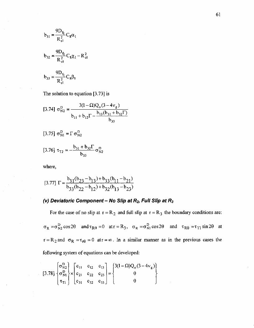
61

b31 =

b32 =

b33 =

2 C 8 a l K c l

9Dfl

K c l

9Df,

K c l

_ R c l

The solution to equation [3.73] is

[3.74] f 7 D -a N 2 -h..

3(1-

+ h..

Q)Q 0 (3-4v g )

b1 3(b3 1+b3 : J) J 3 3

[3.75] a ^ T a ^ 'N2

[3.76] xT2 = -

where,

b31 +b32r D 'N2

>33

[ 3 7 7 ] r _b 3 1 ^ b 2 3 " b 1 3 ) + b 3 3 ( b l l " b 2 p

b33 (b22~b12 ) + b32 (b13~b23 )

(v) Deviatoric Component- No Slip at R2, Full Slip at R3

For the case of no slip at r = R2 and full slip at r = R3 the boundary conditions are:

aR =<j°2cos20 andtRQ =0 atr = R.3, aR=a°jCos20 and TRQ =TTisin20 at

r = R2and a R = t r e = 0 atr = oo. In a similar manner as in the previous cases the

following system of equations can be developed:

[3.78]

CTN2

' °N1

xT1

•X

C l l C12 C13

C21 C22 C23

c31 c32 c33_ = .

3( l -Q)Q 0 (3 -4v g )

0

0

where,

c n -C-10 +C 9 a 2

ci2 =£9X2

c13 - C 9 5 2

9DF. c21 =2Cg\|/j +C 8a, +——L-C8aj

9Df, R2, c22 = 2C8Tll + CgXl +——4-C8X! - - ^ L

9Df

C2 3 = 2 C 8 ° > 1 + C 8 5 1 + - p 2 C 8 5 l

c31 =-40811/!-2C8a!

c32 = - 4C 8 r | 1 -2C8Xi

C33 = —4C8c0j - 2C88j • R c l

Dei

Explicit solutions for the unknowns c r ^ a ^

nvQictD 3( l -Q)Q 0 (3 -4v g ) [3.79] oN 2 =

_ , _ T- C13(C31 + C 3 2 H c l l " l " c 12 i

C33

[3.80]a^=ra° 2

[ 3 . 8 1 ] T T 1 = - ^ ± ^ C T ° 2 C33

where,

[3 .82]T- C 2 3 C 3 1 °2 lC33

C22C33 ~ C 23 C 32

63

3.8 Moment and Thrust

From Fliigge (1966) the moments and thrusts for a thin-walled shell in polar

coordinates are:

D, ( A2.A [3.83a] M = f

R2 u + -dzu d0 2

[3.83b] T = M u + * 0 + M R I, dej R


From equations 3.83a and 3.83b, moments and thrusts in the inner lining (lining 1)

due to the hydrostatic component of the solution are

D f R c l 2

[3.84a] M H = l— a", D R / + D o c1 cl f,

H D ^ i R c l 3 „ M H

[3.84b] T H = L - ag, + f -D

C lR c l +Df1

R d

Equations 3.84a and 3.84b apply to both cases of slip and no slip at r = R2.

(ii) Deviatoric Component- No Slip

Using equations 3.83a and 3.83b, moments and thrusts in the inner lining due to the

deviatoric component are:

and

f [3.85a] M D =-—L[-3Cg (ot1<rg2 +(5^^ +x1a°1 +51TT 1)]COS29

64

[3.85b]

D

R

u

T D = [ - ^ - C 8 [(aj + 2 V I ) C T S 2 +(Pj +2Yl)xT2 +( X l +2Ti1)a°1 +(8j + 2 ^ ) ^ , ] cl

M D

+ —]cos29

R c l

(Hi) Deviatoric Component- Full Slip

For conditions of no slip atr = R2 , from Equation 3.37, u equals -dv /d0 and

hence, Equation 3.83b degrades to:

M [3.86] T= —

R giving,

D [3.87a] MD = - - f [- 3C8 (a^2 + %A) ]cos 29

R c i

MD

[3.87b] T D = — c o s 2 9

R c l

By similar process, moment and thrust for other cases are given by equations 3.88 and

3.89.

(iv) Deviatoric Component- Full Slip at R2, No Slip at R3

[3.88a] MD = - - f [-3C8 (a ,a° 2 + X l a£ , + P ,T T 2 ) ]COS29 R c l

MD

[3.88b] TD = — c o s 2 9 R„ ^cl

65

(v) Deviatoric Component- No Slip at R2, Full Slip at R3

[3.89a] MD = - - f [-3C8 (a,a°2 +Xlog, +51xT1)]cos2e R

D„

cl

[3.89b]

TD = [ - ^ C 8 1 (a, + 2V l)a82 +(Xi +2TI,)O81 +(6, +2CD,)TT1 R„

M1

R -]cos 20

cl

Thus, full solutions for displacement, moment and thrust in the inner thin walled shell

have been derived and presented above. In the following sections, use of the solution is

demonstrated for a composite lining in an infinite elastic medium.

66

3.9 Typical Results

This section presents the results of analysis using the composite lining solution. To

illustrate some of the characteristics of the solution, normalized displacements, thrusts

and moments are presented versus the flexibility ratio (Einstein and Schwartz 1979). In

this chapter, the flexibility ratio is defined in accordance with Einstein and Schwartz

(1979) viz.:

[3.90a] F= g cl r^-E^d-oJ)

and the normalized displacements, uc, thrust, Tc, and moment, Mc, are

unE_ [3.90b]uc=

s

[3.90c] Tc = °v R c l

and

M

CTvRcl(l + U g )

T

[3.90d] Mc = C ^ v R c i

3.9.1 The Effect of Ground Convergence prior to Liner installation

Figures 3.6 through 3.9 show the effect of Q on displacements, moment and thrust in

the inner lining. For this group of figures, the thickness of the outer liner was assumed

to be 0.001m. Consequently, the outer lining has no effect on the inner lining behaviour

and for Q = 0 the composite lining solution is essentially equivalent to the Einstein and

Schwartz (1979) solution. In accordance with Equations 3.40 and 3.41, the parameter Q

represents the fraction of the full stress relief solution (Equations 3.10a and 3.10b) that is

67

permitted to occur prior to installation of the lining. As shown on each of the figures,

solutions have been developed for K'o=0.7 and thickness ratios, ti/Rci of 0.05 and 0.1 for

the inner lining.

It can be seen from Figure 3.6 that the radial displacement at the crown of the inner

lining increases as the flexibility ratio increases. ForQ = 0, the composite lining solution

reduces to a single lining solution that agrees with Einstein and Schwartz (1979).

Furthermore, the radial displacement of the inner lining at the crown decreases as the

degree of ground convergence prior to the liner installation increases (e.g. as Q

increases). Similar trends in behaviour can also be observed in Figure 3.7 for the

springline. At springline, however, the radial displacement of the inner lining is

generally inward for low flexibility ratios. For thickness ratios, ti/Rci, of 0.05 and 0.1,

the radial displacement reverses direction becoming inward when the flexibility ratio

exceeds 2500 and 550, respectively. As the flexibility ratio becomes very large, the

radial displacements approach those obtained using Equation 3.10a (no lining).

Figures 3.8 and 3.9 show the normalized thrust and moment in the inner lining at

springline. Again, increasing the flexibility ratio results in a decrease in both moment

and thrust. Similarly, increasing the parameter Q also reduces moment and thrust in the

inner lining. It is interesting to note that the moments are much more sensitive to the

flexibility ratio than are the liner thrust.

68

0.80 i

0,70 -

0.60 -

0.50-

0.40-

0.30-

0.20 -

0.10-

0.00 -

Ko=QJ t /R -j = .0.05

—-—-—r 1 _ •-;— ( , — j

0 500 1000 1500 2000 2500 0 '"I I '—~t ' T

500 1000 1500 2000 2500

Figure 3.6: Radial displacement at the crown of the inner lining.

-0.20

-0.15 -I

-0.10

-0.05

0.00

0,05 H

J 0-10

0.15 H

0.20

0.25 -

0,30 -

0.40 -

K'o^O.7 i t1m c 1so.o5l

K'o=0.7 VRc1 = 0.1

— — f i = 0,0 - 0 = 0,1 - . _ . . Q = 0.2 Q = 0.4

0 500 1000 1500 2000 2500 0 500 1 1500 2000 2500

Figure 3.7: Radial displacement at the springline of the inner lining.

69

0.80 i

0.60 -

0.40-

0.23 -

0.00 -

K'o = 0.7 " ^ ^ ~ ^ ~ ^ ^ ^ t,'Rc1 = 0.05

•*,,.,

' ' * * " • • • * • - . , . . .

~ I' — T " ,-T r

K'o = 0.7 V'RC1 = 0.1

- 0 = 0 . 0 -• 0 = 0 . 2 --

•-Q = 0.1 - •0= 0.4

~i 1 i' •"••""• i""

0 500 1000 1500 2000 2500 0 p

500 1000 1500 2000 2500

Figure 3.8: Thrust at the springline of the inner lining

-1.0E-02, • i

4.0E-03

~8.GE~03 4 1

-4.0E-03 4

-2.0E-03 A

0.0E+00

K'o = 0.7 VR c 1 = 0.05

. 0 = 0.0 0=0.1

.Qs0.2 .......Q=0.4 Kfe=-0.7 | ti/Rci = 0.1 j

-i ; < t i i i i,

0 500 1000 1500 2000 2500 0 500 1000 1500 2000 2500

Figure 3.9: Moment at the springline of the inner lining.

70

3.9.2 The Effect of Composite Lining Behaviour

Now, consider a composite tunnel lining comprising an inner segmental concrete

tunnel lining surrounded by a thick annulus of grout and situated 13.5m below the ground

surface (depth to the springline axis of the tunnel). This condition is rare, however, such a

case has recently been encountered in Toronto that has been confirmed by coring through

the lining. Table 3.2 summarizes the soil properties assumed in the analysis. Figure 3.2

shows the liner geometry.

For the present analysis, it is assumed that the tunnel shown in Fig. 3.2 is situated

above the groundwater table and embedded in a soil of sufficient strength to preclude

significant plasticity in the soil mass. The inner lining is assumed to comprise a 150mm

thick precast segmental concrete lining (8 segments) with radial joints situated at the

springline and crown and at 45 degree intervals from the springline. The inside and

outside diameter of the segmental lining are 4.88m and 5.18m, respectively, and the liner

is assumed to possess constant thickness. To illustrate composite lining behaviour, it is

also assumed that the inner lining is surrounded by a grouted annulus. Solutions for

displacement, moment and thrust of the inner lining are obtained for outer lining

thicknesses, t2, ranging from 0 up to 300mm. The properties of the annulus grout are

summarized in Table 3.2. Figures 3.10, 3.11 and 3.12 show the effect of t2 on the radial

displacement, moment and thrust in the inner lining neglecting the effect of the joints on

the bending stiffness ( E ^ ) . In this case, t2 may be viewed as the average thickness of

grout since normally the grout thickness will vary around a tunnel lining. In addition, the

grout would normally be neglected in design, however, it may be useful to consider the

grout when evaluating the capacity of old or aging tunnels.

Table 3.2: Material Parameters used in the study

71

Parameter Value

Soil elastic modulus, Eg (MPa) 90

Soil Poisson's ratio, vg 0.4

Coefficient of earth pressure at rest, K'0 0.7

Initial vertical stress, ov (kN/m )

Initial horizontal stress, ah (kN/m )

Elastic modulus of concrete, Ei (GPa)

Poisson's ratio of concrete, vi

Elastic modulus of grout, E2 (GPa)

Poisson's ratio of grout, \i

344

241

30

0.2

20

0.2

-0.003

-0.002 +"•--"—- "•

-0.001

0 £5

i 0.001

0,002

0.003

0.004 A

0

Sprtngline

NoSlip Full-Slip

Crown

50 100 150 200 250 300

Thickness of outer lining fgrout), mm

350

Figure 3.10: Radial displacement at the crown and the springline of the inner lining.

50 100 150 200 250 300 350

Thickness of outer lining (grout), mm

Figure 3.11: Thrust at the crown and the springline of the inner lining.

Springline

No-Slip Full-Slip

50 100 150 200 250 300

Thickness of outer lining (grout), mm

350

Figure 3.12: Moment at the crown and the springline of the inner lining.

73

From Figure 3.10, it can be seen that the radial displacement at the crown (inner

lining) decreases as the thickness of the outer lining increases. The impact of the outer

lining is generally small however it becomes more predominant as the thickness exceeds

about 200mm. Figures 3.11 and 3.12 show the main features of the composite behaviour.

From Figure 3.11, the thickness of the outer lining (in this case a grouted annulus, t2) has

a pronounced effect on the magnitude of thrust in the inner lining at both the crown and

springline. In contrast, the moments in the inner lining (see Fig. 3.12) are relatively

insensitive to t2 for the geometries considered here. From Figure 3.12, it can be seen that

the outer lining begins to impact the inner lining bending moments only when t2 reaches

about 175mm at which point the bending stiffness of the outer and inner linings are

similar.

Lastly, Figures 3.13 and 3.14 show the distribution of moment and thrust in the

inner lining accounting for the effect of joints. In this case, the impact of joints can be

accounted for by reducing the moment of inertia of the inner lining in accordance with

Muir Wood (1975) or Lee and Ge (2001). In Figures 3.13 and 3.14, the moment of

inertia of the inner lining has been factored by 0.5 to account for jointing. As expected,

the main influence of liner joints is to reduce the moments in the lining. This is evident

from Figures 3.13 and 3.14 which show a negligible impact on thrust in the inner lining

but a 48% reduction of moment at springline.

74

NoSlip Full-Slip

Figure 3.13: Moment distribution in the inner lining for 50mm thick grout.

7 5 0 i — — - """"" ' • " - """""" """• —••• """"- - - -

700-

650

H 6°°

550

500

450 4

400

Neglecting Joint With Joints (l=i;-2)

1... * * « M » • « . * * « • » • * » ! 1 8 ! S » t »•>**** . , _ . _ . , . . . . . . . . . s i a , .

Neglecting Joints

With Joints (1=1:. 2) ( fU No-Slip Full-Slip

20 40 60 80 100 120 140 160 180

Figure 3.14: Thrust distribution in the inner lining for 50mm thick grout.

75

3.10 Conclusions

In this chapter, a closed-form solution has been presented for displacements,

moments and thrusts in a composite tunnel lining. In the solution, the ground is treated as

an infinite elastic medium subject to an initial anisotropic stress field. The tunnel lining

is idealized as an outer thick-walled cylinder and an inner thin-walled shell. In general,

the solution is suitable for the analysis of double lining systems installed in either intact

rock or strong soils above the groundwater table and that remain predominantly elastic

during construction of the tunnel.

The general behaviour of the solution was demonstrated for various cases

involving both single and double linings. From the analysis, it is shown that the solution

can be used to calculate displacements, moments, and thrusts in double linings. The

solution can also be used to approximately account for such factors as jointing of the

inner lining and some stress relief due to ground convergence prior to installation of the

lining. In addition, a solution can be obtained for a single lining by assuming that the

thickness of the outer lining is very small (e.g. 0.01m). For this condition, the solution is

essentially identical to the Einstein and Schwartz (1979) solution. The main difference is

the stress functions used to analyze the ground response. Based on the analyses and

discussions presented in this chapter, it is concluded that the composite lining solution is

versatile, it covers a great number of different lining geometries and conditions and thus

it should be a useful tool for design considerations in tunnelling.

76

References

Einstien, H. H. and Schwartz, C. W., 1979. Simplified analysis for tunnel support,

Journal of the Geotechnical Engineering Division, ASCE, 105, (GT4): 499-518.

Flugge, W. 1966 Stresses in shells, Springier-Verlag, Inc., New York, N.Y.

Lee, K.M., Rowe, R.K. and Lo, K.Y. 1992. Subsidence owing to tunnelling: I

Estimating the gap parameter. Canadian Geotechnical Journal, 29 (6): 929- 940.

Lee, K.M. and Ge, X.W. 2001. The equivalence of a jointed shield-driven tunnel lining to

a continuous ring structure. Canadian Geotechnical Journal, 38 (3): 461- 483.

Lo, K.Y. and Yuen, C. M. 1981. Design of tunnel lining in rock for long term time

effects. Canadian Geotechnical Journal, 18 (1): 24-39.

Morgan, H. D. 1961. A contribution to the analysis of stress in a circular tunnel,

Geotechnique, 11(1): 37-46.


115-127.

Ogawa, T. 1986. Elasto-plastic, thermo-mechanical and three-dimensional problems in

tunneling, Ph.D. Thesis, Department of Civil and Environmental Engineering, The

University of Western Ontario, London, Ontario, Canada.

Ranken, R. E., Ghaboussi, J. and Hendron, A. J. 1978. Analysis of ground-liner

interaction for tunnels, Report No. UMTA-IL-06-0043-78-3, Department of Civil


Yuen, C. M. 1979. Rock-Structure time interaction, Ph.D. Thesis, Department of Civil

and Environmental Engineering, The University of Western Ontario, London, Ontario,

Canada.

77

Chapter 4

An Analytical Solution for Jointed Tunnel Linings in a

Homogeneous Infinite Isotropic Elastic medium

4.1 Introduction

Many tunnels are built using the shield driven tunnelling method in conjunction with

jointed pre-cast segmental concrete tunnel linings. Segmental concrete tunnel linings

consist of precast reinforced concrete segments that are bolted together in the

circumferential direction forming a ring, and the rings are bolted together in the

longitudinal direction forming the tunnel lining. The design of such a lining system must

fulfill basic requirements for structural stability, durability and cost. To achieve these

design requirements, it is important to be able to estimate the forces that the lining will

experience during its service life.

Several closed-from solutions have been developed to estimate the distribution of

moment and thrust in contiguous concrete linings (Morgan 1961, Muir Wood 1975,

Rankin et al. 1978, Einstein et al. 1979, Yuen 1979, Ogawa 1986, and El Naggar et al.

2007). Closed-form solutions are useful during preliminary design of a tunnel lining

since they permit evaluation of several loading cases without the need for more

sophisticated and time-consuming methods of analysis such as those based on finite

element or finite difference methods. This can help to reach an optimum liner design.

78

Currently, existing closed-from solutions do not explicitly account for the effect of joint

flexibility on the loads developed in a tunnel lining. It is common practice to use these

solutions by applying an empirically based reduction factor, r\, to the flexural rigidity

(rjEI) of the lining (e.g. Peck et al. 1972 and Muir Wood 1975) or by neglecting the

effect of joints. Recently, attempts have been made to analytically derive reduction

factors for the flexural rigidity (EI) of segmental tunnel linings (e.g. Lui and Hou 1991,

and Lee et al. 2001). There have also been attempts to derive a closed-form solution for

jointed linings embedded in soil or rock (e.g. Lee and Ge 2001, and Bloom 2002).

Although this recent work has been a useful step forward, the solution by Lee and Ge

(2001) is limited to very soft soils and it does not explicitly consider soil structure

interaction; Bloom's (2002) solution idealizes the soil as radial springs and it has been

derived only for the case of full slip between the liner and soil. Thus, there is a need for a

closed-form solution that can be used to calculate the moments and thrusts in precast

segmental concrete tunnel linings accounting for interaction of the lining with a soil or

rock continuum.

This chapter presents a closed-form solution for an inner jointed segmental lining and

an outer thick-walled cylinder embedded in a homogeneous infinite elastic medium (see

Fig 4.1). The closed-form solution is verified by comparing it with finite element results

where it is shown to agree well with this more sophisticated method of analysis. Since

the tunnel liner is treated as a composite inner jointed thin-walled shell and an outer

thick-walled cylinder, the solution is quite flexible and it can be applied to investigate a

79

wide range of tunnel lining problems and load cases. As such, the solution outlined in

this chapter should be of interest to geotechnical and tunnel engineers.

ov

<*b

M I I I I I 1 I I 1 M Elastic ground

(Eg* Vg)

ter lining (E2 J v2)

0f=? Staler lining

(Ei, vi)

TTTTTTTTTTTn 0V

Oh

Figure 4.1: Problem geometry - composite lining.

80

4.2 Problem Definition

The problem considered involves a circular composite tunnel embedded in a

homogenous infinite elastic medium subject to an initial anisotropic stress field (see Fig.

4.1). The initial vertical and horizontal stresses in the ground are taken as a v anda^,

respectively, where ah =K0 CTV and K0 is the coefficient of lateral earth pressure at rest.

For the solution, the initial stress field is separated into a hydrostatic component,

P0 = ( a v + a h ) / 2 , and deviatoric component, Q 0 = ( a h - a v ) / 2 , and the final solution

is obtained using the principle of superposition. Figure 4.2 illustrates the two

components. Solutions for moment, thrust, stress and displacement are derived in terms

of the angle 9 , assuming plane strain conditions. The mechanical properties of the

ground are assumed to obey Hooke's law with elastic modulus Eg and Poisson's

ratio vg . The outer lining is treated as a thick-walled cylinder with elastic modulus E2 ,

Poisson's ratiov2. The inner and the outer radii of the outer liner areR2andR3,

respectively. The inner lining is a jointed thin-walled shell with elastic modulus E l 5

Poisson's ratio Vj, cross-sectional areaAl5 moment of inertia It and joint rotational

stiffnesske. The inner and the outer radii of the inner lining are denoted byRjandR2,

respectively. The locations of the liner's joints are 0i=1 to9 i = n . The following sections

present the derivation of moments and thrust in a composite tunnel lining for the case of

no slip atr = R2 and r=R 3 . Solutions for slip and no slip atr = R2 and r=R 3 ,

respectively, and full slip at both r = R2 and r=R3 are also included.

81

Po

P = ®v + gfa

? ? ? ? ? I

t i t 111

Q0 = _ g h ~ g v

t I t ft 1

W i l l i

a) Hydrostatic b)Deviatotie


4.3 Stresses and displacements in the Ground due to Full Stress Relief

The distribution of stresses and displacements in an infinite elastic medium due to full

stress relief has been solved previously by many researchers (Timoshenko and Goodier

1934, Morgan 1961, Muir Wood 1975, Jaeger and Cook 1976 and Yuen 1979). In each of

these solutions, Airy's stress function was employed. A solution based on Airy's stress

function is used in this chapter.

82

(i) Hydrostatic Component, P0

For the hydrostatic component, it can be shown (see Yuen 1979) that the resultant

stress field in the ground after excavation of the tunnel opening (i.e. removing the

boundary stresses at r=R 3 ) is:

[4.1a] a g . = o r o + A o r =P0 1. R,

V * J

[4.1b] a " = a e o + A a e =P0 0 +

and

[4.1c] x£ e g=0

The resultant radial deformation of the ground due to the full stress relief is given by:

[4.2] u" = H P 0( l + vg)R3

2

E„r


For the deviatoric component, the change in stress due to full stress relief is:

[4.3a] Aa° =Q 0 ^ 3 - 4 ^ cos 29

[4.3b] AaeD

g=-3Q0 ' R ^

cos 20 v * y

and

[4.3c] Ax° =Q 0 R,

- 2 (RA

v l J

sin 20

and the resultant radial and tangential displacements are:

83

D ,_ , Q0(l + vg) [4.4a] u"=Je r dr = -

E g

4(l-vg)^-—f B r r cos 20

[4.4b] v J=J[e e —£.] id9 U g D , „ ^ Q o ( 1 + V g )

Eg

~„ *. R^ R^ 2(l-vg)-?- + - f 6 r Ti

sin 29

4.4 Stresses and Displacements in the Ground due to Liner Reactions

Excavation for a tunnel causes a reduction in the boundary stresses around the

circumference of the opening at r=R3 until the new boundary stresses reach equilibrium

with the liner reactions. For the hydrostatic component, the liner reaction at r = R3 is in

the radial direction and denoted bya"2 . For the deviatoric component, the liner reactions

at r = R3 in the radial and tangential directions are denoted by a ° 2 cos 20 andxT2 sin 20,

respectively (see Fig 4.3).

(i) Hydrostatic Component In accordance with Yuen (1979) the stresses and displacements at r = R3 due to the

reactive force, a"2> are:

„ CTN2(1 + V „ ) R 3

[4.5c] u? . (r = R3) = — — s—-L J g reaction v •>' p

n g


Considering the deviatoric component of the initial stress field, the stresses and

displacements in the ground medium due to liner reactions aR = (7 2 cos 20 and

84

TR9 = -xT2 sin 26 at r = R3 and the far field boundary conditions T R 6 = C T R = 0 atr = oo

are:

t 4 - 6 ^ aRgreactio„ = [ 2 ( a N 2 + ^ T 2 ) ( ^ ) 2 - K 2 + 2 T T 2 ) ( ^ ) 4 ] COS 20

[4-6b^< reaction = PxT2 + ag2] ( ^ ) 4 cos 26

[4-6c] x*°g reaction = K°N2 + xi2 )("^)2 - (<& + 2xT2 ) ( ^ ) 4 ] sin 26

t 4 - 6 d ] U g r e a c t i o n = ^ : ^ K G N 2 + 2 T T 2 X — ) ' " 6(1 ~ V g ) ( < + T T 2 ) ( ^ ) 2 ] COS 26

iC,s r r

t 4 - 6 ^ Vg reaction = ^ F ^ [ ( G N 2 + 2*12*—? + 3 0 " 2 v g ) ( a ° 2 + T T 2 ) ( ^ ) 2 ] sin 26

3 i i g r r

Accordingly, the radial and tangential displacements at the interface of the ground and

the outer lining (r = R3) due to the reactive forces,CT°2 andxT2are:

t 4 - 7 a l Ug reaction^ = R 3 ) = - G + ^ ^ [(5 - 6 v g ) a ° 2 + (4 - 6 v g ) x T 2 ] COS 26

t 4 J b ] vg°reaction^ = R3> = - ^ ^ - [ ( 4 - 6 v g ) a ° 2 + (5-6vg)-cT2]sin26

(Hi) Combined Solution The overall state of stress in the ground due to excavation of the tunnel opening and

development of liner reactions can be obtained by superposition of the hydrostatic and

deviatoric solutions presented above. Thus, the radial displacement, u„, and the tangential

displacement, v , in the ground are given by:

85

[4.8a]

(P 0 -a£ 2 ) ( l + v g )R 2

ug = - *- +

Qo(l + vg) 4(1 - v . )

R3 R3 (l + vg)r 3E„

cos 20

(a£2 + 2xT 2)(^-)4 - 6(1 - vg)(cr£2 + x T 2 ) ( ^ ) 2

j . 6 j .

[4.8b]

f

v g = Q 0 ( i + vg)

2 ( l - v g ) ^ + % (l + v.)r

3E„

( a ° 2 + 2 x T 2 ) ( ^ ) 4 + r

3 ( l - 2 v g ) ( a ° 2 + x T 2 ) ( ^ ) 2

r j 7

sin 20

Similarly, the radial, tangential and shear stresses are:

[4.9a]

°Rg=Po ' R ^ 2

V r ) +

R, R \ 1 _ 4 i ^

V r ; U ;

2 ( < + x T 2 ) ( ^ ) 2

r

( a » 2 + 2 x T 2 ) ( ^ ) 4

r

cos 20

[4.9b] a e g = P 0 (1 + (R^

v i J 3QC

' R . ^ ,R \

3 \ 4

J V v ^ y + ( 2 x „ + c g 2 ) ( - i )

r cos20 and

y

[4.9c]

T R 6 g - Qo 3 l r J

4

- 2 I r J

2"

- ( a° 2 + x T 2 ) ( ^ ) 2 - (aND

2 + 2 x T 2 ) ( ^ ) 4

r r sin 20

86

Thus, Equations 4.1 through 4.9 define the stresses and displacements in the ground

caused by excavation and subsequent mobilization of the liner reactions atr = R3 . The

following section summarizes solutions for the stresses and displacements in the outer

liner.

*)

Figure 4.3: Reactive stresses, a) hydrostatic component, b) deviatoric component

87

4.5 Equations for Stresses and Displacements of the Outer Liner

Yuen (1979) and Ogawa (1986), utilizing Airy's stress function, developed solutions

for the distribution of stresses and displacements of a thick-walled cylinder subject to

radial and tangential stresses at the intrados and the extrados. For the hydrostatic

component, the liner reactions at r = R3 and r = R2 are in the radial direction only and

denoted by ag2 andag t, respectively. For the deviatoric component, the liner reactions at

r = R3 comprise both radial and tangential components denoted by aR = G°2COS20

andxRe =TT2sin20, respectively. At r = R2 the liner reactions are aR=a°iCos20

andtRe = xT1 sin 20 (see Figure 4.3).

(i)Hydrostatic Component In accordance with Ogawa (1986), the radial, tangential and shear stresses in the outer

liner due to the boundary conditions, aR =cjg2 at r = R3 andcrR =a" t at r = R2, are:

[4.10a] a j ^ a g ,

f

V

l r J 1-

2 >

- h

h

J

+ CTN2

1-

V

I r J 1-h

2\

J

[ 4 . 1 0 b ] o ^ - e g , "*0V

1-h

f

+ a N2

R ^ 1+ ^

I r J 1-h

and

[4.10c] T £ L 2 = 0

where h = (R 2 /R 3 y

88

and the radial displacement at r = R2 andr = R3, respectively, are:

[4.11a] u»2(r = R 2 ) = i i ± ^ - [ { - l - ( l - 2 v 2 ) h } a ^ 1 + { 2 ( l - v 2 ) } a ^ 2 ]

[4.11b] u?2(r = R3) = (l+"!2)^ [{-2(l-v2)h}o^+{(h + l-2v2)}ag2]


For the deviatoric component, the radial, tangential and shear stresses at r = R3, as

well as the radial and tangential displacements of the outer lining due to the reactive

forces, CT°2 andxT2 are (Ogawa 1986):

[4.12a] a£L2(r = R3) = a°2cos2e

[4.12b]

aeD

u (r = R3) = — ^ - [ ( - h 3 - 5h2 + 5h + l)a°2 + 2(-h3 - h 2 + 3h - l)tT2 + 4(h3 - h ) < (1-h)

+ 4(h2-h)tT1]cos20

[4.12c] XR6 = -xT 2 sin2G

[4.12d]u?2(r = R3) = i ^ ^ [ a 2 a ° 2 + p 2 x T 2 + x 2 a ° , + 8 2 x T 1 ] c o s 2 9 3E2( l-h) J

and

[4.12e] v£2 (r = R3)= + ^ z ) 3 [\|/2ag2 +y2xT2 + n2a£1 +co2TT1]sin20

3E2(l-h)

where,

a 2 = ( 5 - 6 v 2 ) h 3 +(9-6 v2)h2 +(15-18 v2)h + (3-2v 2 )

89

p 2 = ( 4 - 6 v 2 ) h 3 + ( 1 2 - 6 v 2 ) h 2 - 6 v 2 h + 2v2

X 2 =-4( l -v 2 )h(3h 2 +2h + 3)

8 2 = - 4 ( l - v 2 ) h ( h + 3)

y 2 =-(5-6v 2 )h 3 - (9-6v 2 )h 2 +(9-6v 2 )h- (3-2v 2 )

T l 2=4(l-v2)h2(3h + l)

co2=8(l-v2)h2

Similarly, the stresses and displacements at the intrados of the outer lining (r = R2)

due to the reactive forces, a°i and xT1 are:

[4.13a] C T D L 2 ( r = R2) = -[2A + 6 - ^ T + 4 - ^ r 3 cos20 = og, cos20 h R3 hK3

G ° L 2 ( r = R 2 ) = ( I T h 7 [ 4 ( h 2 ~ 1 ) C T ° 2 +4 (h' "h)TT2 +(_h3 "5h2 + 5h + 1)a™ + 2(h 3-3h 2+h + l)xT1]cos20

[4.13c] T°6L2 (r = R2) =[2A + 6BhR2 - 6 - ^ T - 2 - ^ 2 - ] s i n 2 0 = -xT1 sin0 h R3 hR3

[4.13d]u?2(r = R 2 ) = i i ^ ^ [ a 1 a ° 2 + p i T T 2 + X l a ° 1 + 5 1 T T 1 ] c o s 2 0 3E2(l-h)3

and

[4.13e] v£2(r = R2) = f * , *3 [ y ^ + Yi*T2 +T1ICTNI +co1xT1]sin20 3E2(l-h)

90

where,

P1=Ti2/h

5 C l=-(3-2v2)h3-(15-18v2)h2-(9-6v2)h-(5-6v2)

8!=-2v2h3 +6v 2 h 2 - (12-6v 2 )h-(4-6v 2 )

Vi =S 2 /h

y, =-co2/h

Tli = - 5 !

co1=(3-2v2)h3-(9-6v2)h2+(9-6v2)h + (5-6v2)

(Hi) Combined Solution - Hydrostatic and Deviatoric

The principle of superposition can be applied to obtain solutions for the radial,

tangential and shear stresses in the outer liner in addition to the radial and tangential

displacements. In accordance with Ogawa (1986), it can be shown that the stresses and

displacements at the intrados of the outer liner (r = R2) are:

[4.14a] aRL2(r = R2) = C +a°lCos20

~ (r T> ^ -g N 1 ( l + h) + 2a N 2 1 F / l ^ 2 1 W D , A(U2 ^_ CT0T (r = R 2 ) = + H 4 ( n - l ) ° N 2 + 4 C n - n / c T 2

[4.14b] °L2 1-h (1-h)3

+ (-h3 - 5h2 + 5h +1)^ ! + 2(h3 - 3h2 + h + 1)TT1 ] cos 20

[4.14c] TR6L2(r = R2) =-xT1sin26

uL2(r = R 2 ) = - ^ - ^ 2 - [ { - l - ( l - 2 v 2 ) h } a » 1 + { 2 ( l - v 2 ) } a ^ 2 ] E2( l-h)

[4.14d] + , / / ? u , 2

3 [ a l g N2+Pl^T2 +Xl^Nl +SlXT1]COS20 3E2( l-h) J

91

and

[4.14e] vL2 (r = R2) = ^ +*2 2 [ ^a j ^ +J1TT2 + Ti1og1 +©1xT1]sin20 3E2(l-h)

Thus far, existing solutions governing the stresses and displacements in the ground

and outer liner have been presented. The following section presents the governing

equations for the inner thin-walled shell and a new solution that accounts for: (i) ground-

liner interaction for the case of a composite liner in an elastic soil or rock continuum and

(ii) the rotational stiffness of longitudinal joints in the liner.

4.6 Equations for Reactions due to the Inner Jointed Liner

4.6.1 Governing Equations From Fliigge (1966), the stresses and displacement of a continuous thin-walled shell

are governed by Equations 4.15 and 4.16:

d2v du__R_2

d02 d0~ D, [4-15] ^ + = - ^ x r e

and

dv Df [4.16] —+ u +

'd 4 u „d2u

d0 D„R + 2 — - + u

de4 de2 Do

where DC=E1A1 / ( l - Vj2), Df =EJj/(1-Vj2), and A1? I l5 Ej and Vj are the cross-


In addition, the equations relating the moment and thrust in the thin shell to the

displacements u and v are:

92

[4.17a] M = -Df ( d V

1 ' u + R2 2 J

[4.l7b]T = M u + ^ R de

M + —

R

Similar to solutions for the ground and outer liner, equations for the inner lining can

be broken into hydrostatic and deviatoric components. In addition, the effect of liner

joints can be superimposed on the deviatoric component as shown below.


For the hydrostatic case, the liner at r = R2is subject toaR = CT"1? only (see Fig. 4.3).

The radial displacement of the inner lining is:

R 4

M i o i „ H _ ^ c l _ H |4.1»J u u = — — - - — — < * N I

DrfRci +Dfi where Rcl is the radial distance to the centroid of the inner lining. From shell theory, the

corresponding moment and thrust are given by:

D f R c l 2

[4.19a] M H = X— ogi D R / + D , c, cl f,

3

[4.19b] TH = L- o»1 + £ -D

C lR c l + \ R d


Solving Equations 4.15 and 4.16 for the boundary conditions a r = GNICOS20 and

Tre = - T T I sin20 atr = R 2 , the following equations can be obtained for the radial and

tangential displacements fields for the deviatoric component:

93

_ R-cl / ^ D , XT1 [4.20a] u L l m = ^ - ( a ^ 1 + - ^ - ) c o s 2 e

[4.20b] vLlFT =- (Al_ c r D + ( A l _ + £cL )T ) s i n 2 0 LlEI v18Df N1 v36Df 4 D / rV

and the moment and thrust are:

R 2 T

[4.20c] MD =-i^£L(og1 + -^-)cos29

[4.20d] TD = - ^ - ( a ° ! -2TT 1)COS29

To account for the effect of a jointed inner liner, an approach similar to that of Blom

(2002) was followed. In accordance with Blom (2002), it is assumed that the bending

stiffness and normal stiffness of each segment is infinite and that the longitudinal joints

have a rotational stiffness equal toke. The deformation of the shell due to the

longitudinal joints can be determined by estimating the rotation of each joint, viz:

M(e,) [4.21] P i

ke

In Equation 4.21, p4 is the rotation at joint i, ke is the joint rotational stiffness and

M(0j) is the bending moment in the liner at joint i. The effect of the liner joints can be

approximately accounted for using Equation 4.21 and assuming rigid body rotations of

the segments as described below.

Consider a tunnel liner comprising six segments with six joints as shown in Figure

4.4. If point A at springline of the lining is assumed to be fully restrained (e.g. u = 0 and

P = 0) then the radial displacement at point B on the springline can be calculated from

94

the rotations at joints 1, 2 and 3. From geometric considerations, it can be shown that for

rigid body rotations the radial displacement at B resulting from a rotation at the 1th joint,

Pi, is equal to the rotation times the perpendicular distance of the joint from the

springline axis. Thus, if utis the radial displacement at B due topi5 then,

ui=1 = pi=1 Rc sin(0i=1), ui=2 = pj=2 RC sin(9i=2 ) andui=3 = pi=3 RC sin(9i=3) as shown

in Figures 4.4(b), 4.4(c) and 4.4(d), respectively. Superimposing these effects and

dividing by 2 since the liner is not fixed at A in the overall solution gives:

[4.22] u = |(P i=1Rcsin9 i=1 +pi=2 Rcsin6i=2 +pi=3 Rcsin0i=3)

and in a generalized form for a liner with n joints the radial displacement is:

R 6i<* [4.23]u = - ^ I P i s i n ( 9 i )

2 0<6;

The rotation of each joint can be estimated from shell theory using Equation 4.20c as

follows:

[4 .24]p i =-^i - (a° 1 + ^- )cos29 i

and Equation 4.24 can be inserted into 4.23 to obtain:

R 3 6i<7t ™ T

[4.25] u =--f- £ (CTg, +IlL)cos(29i) s in^) 6 k e o<Oi 2

Now, assuming that the inner liner will deform into an elliptical shape that is

compatible with the ground (e.g. see Eq. 4.7a) and of the form:

[4.26] u£ ( J o i n t s ) = U m a x COS20

and the following equation can be derived for the radial displacements of the inner lining

by combining Equations 4.25 and 4.26:

95

[4.27]uC ( Jo in t s )=C s(a°1+^)cos20

where,

R 3 , ei<7t

C^-r^-Ecosae j ) since,) OK e 0<9j

Equation 4.27 approximately accounts for the effect of the liner joints on the radial

displacements and when combined with Equation 4.20a gives:

[4.28] uL1 = ^ M C + ^ ) c o s 2 9 + C s ( C + ^ ) c o s 2 9

which defines the radial displacement of a jointed inner liner accounting for both

displacements of the segments and joint rotations caused by the external stresses

ar = a° , cos 29 and x^ = -xT1 sin29.

As shown later in this chapter, the use of equation 4.20c to evaluate the moment at

each joint and the resultant joint rotations leads to overestimation of the rotations and

underestimation of the bending moments for low joint stiffness, ke. This impact will be

explored further by finite element analysis and a modification will be introduced to

improve the solution for low values of ke. In addition, the term Cs is valid for joint

configurations that are symmetric about the vertical, horizontal and 45° axes (e.g. for

cases where Cs derived at the springline axis is equal to Cs derived at the crown to invert

axis). For configurations that violate this condition, the accuracy of calculated moments

decreases for low joint stiffness as discussed later.

96

(a)

Cb) (c) (d)

Figure 4.4: Contribution of the joints to the horizontal displacement at the springline.

97

4.7 Interaction between the Ground and Composite Liner System

Equations governing interaction between the ground, the outer liner and the inner

liner can be derived by considering compatible displacements at each of the interfaces at

r = R3 andr = R2. In the following section, full solutions are developed for a segmental

liner and thick-walled cylinder embedded in an infinite elastic medium. Consistent with

previous sections of this chapter, the full solutions presented below are separated into

hydrostatic and deviatoric components. As a result, the radial and the tangential reactions

take the following general forms:

[4.29a] aR(r = R3) = aN2 + cr°2cos29 and xRe(r = R3) = TT2sin29, atr = R3

and

[4.29b] aR(r = R2) = a"i +^m cos29 and xRe(r = R2) = -xT1 sin29, atr = R2

(I) Hydrostatic Component At the interface between the ground and the outer lining, the displacement of the outer

TT TT

lining, UL2, equals the displacement of the ground caused by full stress relief, Ug , plus

the displacement of the ground due to the reactive force, <s"2. Thus, Equation 4.30

defines the compatibility constraint atr = R3:

[4.30] u?2(r = R3) = uj?(r = R3) + ugH

reaction(r = R3)

Substituting Equations 4.2, 4.5c and 4.1 lb into Equation 4.30 gives:

98

[4.31]

E 2 ( l - h )

which can be simplified to

[4.32] P0-oS2=C1[C2aS1+C3oS2]

where Ci, C2 and C3 are,

Eg

C,= E g ( l + v2)

E 2 ( l + vg)

r _ 2 ( l - v 2 ) h v-2 - ~ "

(1 -h )

_ h + ( l - 2 v 2 ) 3 d - h )

At the interface between the outer lining and the inner lining, the compatibility

condition is:

[4.33] U& (r = R2 ) = lift (r = R2)

which requires that the radial displacement of the inner lining is equal to the radial

displacement of the outer lining atr = R2 . Substituting Equations 4.11a and 4.18 into

Equation 4.33 and rearranging gives:

[ 4 . 3 4 ] C 4 < = C 5 a £ , + C 6 a £ 2

where C4, C5 and C6 are,

C, = K c l

4 DciRci+Dfi

(1 + v , ) C5 = - i — l l L ( _ i _ ( i _ 2 v 2 ) h ) R 2 5 E 2 ( l - h )

99

_2( l + v 2)( l -v 2) 6 E2(l-h) 2

Now, solving Equations 4.32 and 4.34, the reactions CT"J and cj^2at r = R2 and

r = R3, respectively, can be obtained.

[4.35] < = P° C1(C2+C3C7) + C7

L4.36J aN 2=-C1(C2+C3C7) + C7

where,

(c4-c5) c7 = c6

The above solution applies to conditions of slip and no slip at either of the interfaces

at r = R2or r = R3, and it is based on the assumption that the joints do not significantly

affect the axial stiffness of the lining.

(ii) Deviatoric Component - No Slip For the deviatoric component, u and v vary with 9 and two cases are considered: full

slip and no slip atr = R2. Similar to the hydrostatic case, Equation 4.30 also governs the

compatibility conditions of the radial displacements resulting from the deviatoric

component at r = R3. Thus, for the deviatoric component Equation 4.30 takes the

following form:

[4.37] u?2(r = R3) = ugD(r = R3) + u°eaction(r = R3)

where the radial displacement of the outer liner at r = R3,UL2(r = Rs)> equals the

ground displacement caused by full stress relief, Ug(r = R3) , plus the ground

100

displacement due to the liner reaction, ug r e a c t jo n( r = R3) • Substituting equations 4.4a,

4.7a and 4.12d into equation 4.37 gives:

[4.38] 3 Qo(3 -4v g ) = [C10 + C 9 a 2 ] a ° 2 + [ C 9 x 2 ] < +[C n +C9P2]xT2

+ [C982]xT1

where,

(l + v2)Eg

9 " ( l + v g ) E 2 ( l - h ) 3

C 1 0 =5-6v g

C n = 4 - 6 v g

Also, in the tangential direction at the interface between the ground and the outer

liner, the tangential displacement of the outer liner,VL2(r = R 3 ) , equals the ground

displacement caused by full stress relief, v°(r = R 3 ) , plus the ground displacement due

to the liner reaction, v°reaction(r = R3) . Thus, the equation governing compatibility of v at

r = R3 for the case of no slip is:

[4.39]v?2(r = R3) = v°(r = R3) + vgD

reaction(r = R3)

Substituting Equations 4.4b, 4.7b and 4.12e into Equation 4.39 gives:

[4.40]3Qo(3-4vg) = [(Cu -C 9 i | / 2 ]a° 2 - [ C 9 T I 2 ] < +[C10 -C9y2]xT 2 -[C9co2]xT1

To satisfy the compatibility conditions for the case of no slip, the radial, u{^, and

tangential, v°i, displacements of the inner lining should equal to the radial and tangential

displacements of the outer lining at r = R2 , subject to the boundary stresses

CTR = cr°1cos20 and T R 6 = - T T 1 sin 20.

101

At r = R2 the compatibility condition is:

[4.41] u°(r = R2) = u°2(r = R2)

and substituting Equations 4.13d and 4.28 into 4.41 gives:

[4.42] [C ja^ fe +[C8Xl - JLsL-Clog, +[C8pi]xT2 + [0,8, ' ^ — y f r i =0

Similarly, for the tangential displacements, the compatibility condition is:

[4.43] v°(r = R2) = v?2(r = R2)

which after substituting Equations 4.13e and 4.20b into 4.43 yields:

[4.44] [C8Vl ]a°2 + [C.T1, + T ^ - l a g i + [C8y, ]xT2 + [C,©, + - ^ - + ^f-]xT 1 = 0

where C8 = (1 + v2)R2 /(3E2 (1 - h)3). For conditions of full slip at r = R2, Equation 4.44

vanishes since v ^ r = R2) * v°2(r = R2) and Equation 4.42 reduces to:

[4.45] [C8 a i]a°2 +[CgXl - ^ f — C s ] a ° ! =0

y L , f i

Thus far equations have been developed relating the stresses and displacements in the

ground, the outer liner and the inner liner. For the case of no slip at r = R2 and r = R3, there are four equations (Equations 4.38, 4.40, 4.42 and 4.44) and four unknowns for the

deviatoric component of the solution. Explicit solutions for the unknowns, a°i ,

(TJSJ2 , T-pi and Tj 2 , are:

3Q 0 (3 -4v g ) (^ + a14) [4-46] a ° 2 = - A _

(a31 + a3 2r)(-^ + a14) - (an + a12r)(-^- + a34) A A

102

[4.47]aS1=ra£2

3Q0(3-4v,)(an+a1 2r) [4.48] t T 2 = -

(a31 +a32r)(a13 + a 1 4 A ) - ( a n +a12r)(a33 +a34A)

[4.49] TT1 = AtT2

where T and A are:

[4.50]

(a 3 1 - a 4 1 ) ( a 1 4 a 2 3 - a 2 4 a 1 3 ) + (a33 - a 4 3 ) ( a n a 2 4 - a 2 i a 1 4 ) + ( a 3 4 - a 4 4 ) ( a 2 1 a 1 3 - a n a 2 3 )

r = — (a32 _ a 4 2 X a 1 4 a 2 3 ~ a 2 4 a 1 3 > + ^a33 ~ a 43X a 12 a 24 ~ a 2 2 a 1 4 ) + ( a 3 4 _ a 4 4 X a 2 2 a 1 3 ~ a 12 a 23)

[4.51]

A - ^a31 ~ a 41^ a 22 a 13 ~ a12 a23) + (a32 ~ a 42X a l l a 23 ~ a 2 1 a 1 3 ) + (a33 ~a43Xa21a12 ~ a l l a 2 2 )

(a3 1 - a 4 1 ) ( a 2 2 a 1 4 - a 1 2 a 2 4 ) + (a3 2 - a 4 2 ) ( a l i a 2 4 - a 2 1 a 1 4 ) + (a 3 4 - a 4 4 ) ( a 2 1 a 1 2 - a l i a 2 2 )

and,

an = CgOCj

a12 = C g X l " R c l

9Dfl -c.

a13 - C g p j

a14 - C g S j Rcl Cs

18Df, 2 'fi

a21 = CgX|/i

R? 18Dfl

a22 -CgTIj + l O T^

a23 = C g Y i

103

R4 R2

a24 = CSGO, + — — + — — 8 ' 36Dfl 4Dcl

a3i = ^10 + C9oc2

a32 = ^9X2

a33 = C n +C9p2

a34 = C902

a4i = C n -C9 i | /2

a42 = ~C 9 r ] 2

a43 =Cio ~C9y2

a44 = -C9©2

(Note:C8=(l + v 2 )R 2 / (3E 2 ( l -h ) 3 ) )

(Hi) Deviatoric Component - Full Slip

For the case of full slip at r = R2andr = R3, there are two governing equations in

terms ofagj andag2 satisfying the boundary conditions: crR = 0 ^ cos20 and TRQ =0

atr = R3, <TR =<JNI cos20 and TRQ =0 atr = R2, and CJR =*RB =0 atr = 00. The first

equation evolves from Equation 4.38 as xT1 and xT2 vanishes to give:

[4.52] 3 Q0(3 - 4 v g ) = [C10 + C9a2]a£2 + [ C ^ J o g ,

the second equation comes from the compatibility condition of the radial displacement at

the interface between the two linings and is given by Equation 4.45 above. Thus the

explicit solutions for the unknowns, ag, and ag2 are:

104

[4.53]og1=C123Q0(3-4vg)[-C8o1]

[4.54]a°2=C123Q0(3-4vg)

where,

[4.55] C12= l

R4

8X1 9Dfl s

(C10 + C9a2)(C8Xl " ^ " ~ C s ) -(C9x2)(C8a,) y u f i

For solutions for the cases of slip and no slip atr = R2 and r=R3 , respectively, see

appendix B.

4.8 Evaluation of the solution

Below, the closed-form solution is evaluated by comparing displacements, moments

and thrusts derived using the solution to those obtained from finite element analysis.

Tunnels with a flexibility ratio, F, of 50 derived in accordance with Einstein et al. (1979)

were investigated; representing tunnel linings of medium flexibility. Joint stiffness

ratios, X, of 0.1, 0.4, 0.8, 1.0, and 1.5 were also studied. Table 4.1 summarizes the cases

considered in the evaluation and the following is a brief description of the methodology

used in the finite element calculations. The flexibility ratio, F, and joint stiffness ratio, X,

are:

EgR^(l-u?) [4.56] F= g cl ±-

13,1,(1-^)

and

105

[4.57] X = ^ EI

The results of displacements, moments and thrust are presented in a normalized form

where:

[4.58a] Uc = UuE g

a vR c l( l + u )

[4.58b] Tc = °VRcl

and

[4.58c] Mc = M

C ^ v R c i

Table 4.1: Liner configurations considered in the analyses

Description

K Flexibility, F

t i /Roi

Considered values of A,

Joint locations, (p°, 1st group

Joint locations, cp°, 2nd group

for

for

4-joints configurations

0.7

50

0.1 0.1,0.4,0.8,1.0

1.5,00

(Continuous)

0°, 90°, 180° and 270°

45°, 135°, 225° and 315°

6-joints configurations

0.7

50

0.1 0.1,0.4,0.8,1.0

1.5,00

(Continuous)

0°,60o,120o,180°, 240° and 300°

0o,30°,90o,150°, 210° and 270°

8- joints configurations

0.7

50

0.1

0.1,0.4,0.8,1.0

1.5, oo (Continuous) 0°, 45°,

90°,135°,180°, 225°, 270° and 315° 22.5°, 67.5°, 112.5°,

157.5°, 202.5°, 247.5°, 292.5° and

337.5°

106

4.8.1 Finite Element Analysis

Finite element (FE) analyses were performed using the commercial program PLAXIS

V8. For the FE calculations, plane strain conditions were assumed. Tunnel liners with 4,

6 and 8 joints of various configurations were modeled using forty-eight 5-noded

structural shell elements with axial stiffness EA and flexural stiffness EI. The joints

were modeled using spring elements with rigid axial stiffness and a rotational stiffness

denoted by, ke. Figure 4.5 shows the liner configurations that were analyzed.

Hf*~X

.-0 * *

4 - Segments

t 6 - Segments

^p^w*,—>*^»

8 - Segments

Figure 4.5: Liner configurations considered in the analyses.

The soil was modeled using 2236 fifteen-nodded cubic strain triangular elements

assuming linear elastic isotropic material behaviour governed by Hooke's law. Since the

approach was to model the exact geometric and boundary conditions of the closed-form

solution, each finite element mesh was extended to a distance of 50 meters from the

tunnel axis in both the horizontal and vertical directions. The initial anisotropic stress

107

field, av andch, was applied to the far-field boundaries in accordance with Figure 4.1

and the tunnel excavation was simulated by removing elements within the excavated

diameter of the tunnel and simultaneously activating the elements representing the lining.

No-slip was assumed at the liner-soil interface. In the following section, FE solutions are

compared with the closed-form solution for a single liner only. This was done by

assuming the thickness of the outer liner is 0.01 m with values of E and v identical to that

of soil.

4.8.1.1 Liner with 4-Segments

Figures 4.6 shows compare the displacements, moments and thrust; from the closed-

form solution and the FE analysis for four joint configurations and low values of ke (e.g.

X < 0.8). It be seen from Figure 4.6 that the pattern of the displacements match well

except at the crown and the springline locations where the FE and closed-form results

vary by 20% for 1 = 0.1, 15% for A. = 0.4, and less than 8% for 1 = 0.8. For the

moments, the results of the closed-form solution for the maximum moments are lower

than that predicted by the FE analyses for X = 0.1 and 0.4 by 34% and 15% respectively;

whereas, for X = 0.8 the results are within 4%. In general, the solution and FE results are

within 5% fori > 1.0.

108

140 160 180

-5H

40

-15 H

-20

F=50

VRdsQ.1

/140 180 110

1 -

0.8-

0.6-

0.4-

0.2-

0-

^0r

F=50 t-|/Rci=

1 —

*

0.1

*^5*,

LX=o.1 =0.4 =0.8

/ t x

"i r 1 — i

_ f £ A — JS

— r 1

i -

0.8-

0.6 -

0.4 -

0.2-

0 -

^A=0.1 \ • ^ p ^ =0.4 " * * * * * i

=0.8

""" i i T — r- i r i i

0 20 40 60 80 100 120 140 180 180 0 20 40 80 80 100 120 140 180 180

Figure 4.6: Normalized displacements, moments and thrusts for the 4 joint configurations

(before correction).

109

4.8.2 Modification for Low Joint Stiffnesses

As shown in Figure 4.6 and discussed above, using continuous shell theory (Equation

4.20c) in conjunction with Equation 4.21 to evaluate joint rotations leads to

underestimation of the moments in the liner for joint stiffness ratios, X, less than 0.8.

Although joint stiffness ratios, X, less than 0.8 are relatively uncommon, it is desirable

to introduce a modification to the solution to improve its accuracy. This was done by

adopting an iterative scheme as described in the following paragraph.

First, a correction factor can be introduced into Equation 4.27 giving:

[4-59] u°Joints) =mCs(°m +^f) cos 29

where,

fj,j = Mjj /Mc Mcis the maximum moment in the continuous lining based on

continuous shell theory and Mj, is the maximum moment in the jointed lining deduced

from the closed form solution assuming the correction factor is initially 1. Typically, the

value of \x{ is less than one after the first iteration and subsequent iterations can be done

using the closed-form solution with Equation 4.59 and successively revising the

correction factor n{ until it converges (e.g. [x{ = |aM). Thus, the initial solution which is

derived using continuous shell theory can be iteratively corrected using the moments

deduced from the jointed shell theory. Such an approach is analogous to moment

distribution methods commonly used in the analysis of frame structures.

110

4.8.3 Comparison of Revised Solution with FE Analysis

4.8.3.1 4-Segments

Figures 4.7 and 4.8 compare displacements, moments and thrust obtained from the

jointed solution and from FE analysis for liners with four joints and low and high values

of X, respectively. For convenience, the results are presented in terms of the angle

cp measured from the vertical direction around the tunnel (cp = 0 + 90°).

It can be seen from Figures 4.7 and 4.8 that the patterns of displacement, moment and

thrust predicted by the closed-form solution are similar to that predicted by the FE

analysis. For the configuration with joints located at 0°, 90°, 180° and 270°, the

maximum difference in displacement is 17% at the crown for the case of the lowest value

of X(0.1). For higher values of X, the maximum difference is less than 8% for X = land

3% for the continuous case. It can be seen from Figures 4.7 and 4.8 for this joints

configuration that the maximum absolute moment obtained using the closed-form

solution is higher than that predicted by the FE analysis by about 18% for low values of X

and by less than 8% for higher values of X (e.g. X = 1.5). Thus, for X = 0.1 the error is

reduced from 34% to 18% and the predicted moments now exceeds the FE results which

is more desirable. In terms of thrust, the FE results and closed-form solution are in very

good agreement. In the worse case for X = 0.1, the difference is only 6%. For the 4 joint

configuration with joints at 45°, 135°, 225° and 315°, there is no effect for the rotational

stiffness of the joints and the results are identical to that of the continuous lining. This is

due to the fact that the joints in this configuration are located at points of inflections (zero

moments), thus the joints have no effect on the results.

I l l

140 160 110

F=50 VRc1= 0.1

"i "i r

0 20 40 80 80 100 120 140 180 180 0 20 40 SO 80 100 120 140 160 180


(low values of X).

112

140 160 110

n 1— fUQ 180 110

1 -

0.8-

0.8-

0.4-

0.2-

0-

F=50

'-""i

*s

i 0.1

—A=1.0 ^ ^ =1.5

continuous

• " " IN ' 2Vi \ J FEA "'"i i——r* ~r~—f—— i i 1 i ) i i r

0 20 40 80 80 100 120 140 180 180 0 20 40 80 80 100 120 140 180 180


(higher values of X).

113

4.8.3.2 6-Segments

For the six joint configuration O'oints at 0°, 60°, 120°, 180°, 240° and 300°), the

overall patterns of displacement, moment and thrust obtained using the jointed solution is

similar to that predicted by the FEA as shown in Figures 4.9 and 4.10. The calculated

displacements match very well as shown in these figures. For moments, the maximum

absolute moment for the jointed liner solution is lower than that predicted by the FEA by

26% for A, = 0.1. The agreement improves for X = 0.4 where the difference is less than

10%, and 5% forX, = 0.8. For higher values of X, the difference is even less. Again,

thrusts are in a very good agreement (less than 5% difference for the worst case; X = 0.1).

Similar patterns of behaviour can be observed for the six joint configuration with joints

located at 0°, 30°, 90°, 150°, 210° and 270°.

As discussed above, the predictions of the jointed liner solution of moments for very

low values of X for the six joint configurations is lower than that of the FE by up to 26%

even after iterations. This under prediction is due to the variation between the

contribution of the joints to the radial displacements at the springline axis versus the

crown to invert axis. The value of the constant Cs calculated for the springline axis is

almost one and half that calculated for the vertical direction. This limitation was further

explored for tunnels with different flexibility ratios to find the magnitude of variation in

results. Figure 4.11 show a comparison between the results of the jointed liner solution

and the FE calculations. The solid line curves represent the case of evenly distributed six

joint configurations with the first joint at the crown; whereas, the dotted lines represent

the case of evenly distributed six joint configurations with first joint at 30°. As it can be

seen from Figure 4.11, the results of the jointed liner solution are within 15% for X > 0.4.

114

For A. < 0.4, the potential error in the solution should be accounted for in cases where the

constant Cs is not symmetric.

4.8.3.3 8-Segments

It can be seen from Figures 4.12 and 4.13 that the eight joint configurations with

joints located at 0°, 45°, 90°, 135°, 180°, 225°, 270° and 315° gives results that are

identical to that obtained from the four joints configuration with joints locations 0°, 90°,

180° and 270°, as expected since the joints at the points of inflection have no effect.

Whereas for the eight joint configuration with joints at 22.5°, 67.5°, 112.5°, 157.5°,

202.5°, 247.5°, 292.5° and 337.5°, all of the joints interacted and contributed to the

displacements, moments and thrust as shown in Figures 4.12 and 4.13. For this case, the

displacement patterns obtained using the jointed liner solution match very well with that

predicted by the FE analysis. Similarly, the moments and thrusts are also in satisfactory

agreement.

115

0.4

0,2 1 F=50 ( feS

_ F E A — JS

-i 1 r

0.4 H

0.2

T r 140 160 100

160 110

0 20 40 80 80 100 120 140 160 180 0 20 40 60 80 100 120 140 160 180


(low values of A,).

WRd- 0-1 _ FEA

0 20 40 60 80 100 120 140 180 180

Figure 4.10: Normalized displacements,

configurations (higher values of A,).

116

Q .] , , , , , , , , 1

0 20 40 80 80 100 120 140 180 180

moments and thrusts for the 6 joint

117

25 50 75

F

100 125 150

Figure 4.11: Comparison between the results of the FE and the closed form solution for

the 6 joint configuration.

118

1 -

0.8-

0.8-

0.4 -

02-

0 -

*** 5535T "

^0^ A=0,1 =0.4 =0.8

F* 50 ^~-«-^

tt/Rct=0.1

.

*%*

__FEA

~r~—i ' \

0.4 H

0.2 A

— t i i [ 1 1 1 1 —

0 20 40 80 80 100 120 140 180 180 0 20 40 80 80 100 120 140 160 180


configurations (low values of X).

119

VRC,= 0.1 _ FEA

0 20 40 80 80 100 120 140 180 180

Figure 4.13: Normalized displacements,

Q .J , , 1 1 1 I 1 I i

0 20 40 80 80 100 120 140 180 180

moments and thrusts for the 8 joint

configurations (higher values of A,).

120

4.9 Example

The composite lining solution can be applied to analyze many linings types (e.g.

pressure tunnels, outer rib and lagging with inner concrete lining, etc); however, to

illustrate one practical application of the jointed solution presented above, a typical

subway tunnel design is considered below. The tunnel lining considered comprises 8

precast concrete segments with first joint situated at 22.5° from the crown. Each segment

is 1000mm wide. The segments are bolted together in the tangential direction to form

rings and the rings are bolted together in the longitudinal direction to form the tunnel

lining. The nominal liner thickness is 250 mm, the inside diameter is 5.50 m and the

outside diameter (O.D.) is 6.00 m. Table 4.2 summarizes the soil parameters, joints

rotational stiffness and the elastic properties of the tunnel that were used in the analysis.

In this example the effect of an excavation damaged zone (EDZ; Tsang et al., 2004)

adjacent to the tunnel is accounted for using the outer thick-walled cylinder to simulate a

degraded annular zone. The thickness of the weakened zone is assumed to be 10% of the

excavated diameter and its shear modulus is 40% of that of the intact soil. The

groundwater table is far below the tunnel elevation.

Table 4.2: Soil properties considered in the analysis

Parameter Soil elastic modulus, Eg (MPa) Soil Poisson's ratio, vg

Coeff. of earth pressure at

Joints rotational stiffness, ke

Value 105 0.36 0.7 25

Parameter Elastic modulus of concrete, Poisson's ratio of concrete, vx

Initial vertical stress, av (kN/m2) Initial horizontal stress,

Value 30 0.2 270 189

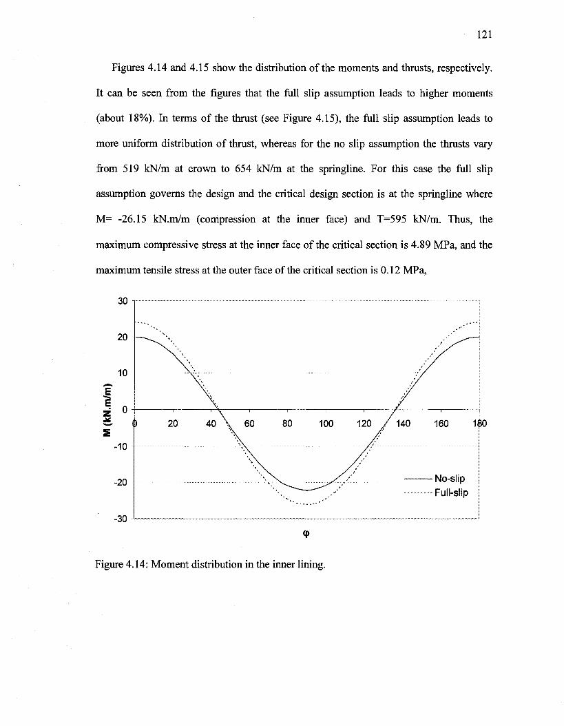
121

Figures 4.14 and 4.15 show the distribution of the moments and thrusts, respectively.

It can be seen from the figures that the full slip assumption leads to higher moments

(about 18%). In terms of the thrust (see Figure 4.15), the full slip assumption leads to

more uniform distribution of thrust, whereas for the no slip assumption the thrusts vary

from 519 IcN/m at crown to 654 kN/m at the springline. For this case the full slip

assumption governs the design and the critical design section is at the springline where

M= -26.15 kN.m/m (compression at the inner face) and T=595 kN/m. Thus, the

maximum compressive stress at the inner face of the critical section is 4.89 MPa, and the

maximum tensile stress at the outer face of the critical section is 0.12 MPa,

Figure 4.14: Moment distribution in the inner lining.

122

800

700

600

500

400

300

200

100

No-slip Full-slip

0 20 40 60 80 100 120 140 160 180

Figure 4.15: Thrust distribution in the inner lining.

4.10 Summary and Conclusions

In this chapter, a closed-form solution for displacements, moments and thrusts in a

jointed composite tunnel lining has been presented. The jointed tunnel is assumed to be

embedded in an infinite elastic medium subject to an initial anisotropic stress field. A

composite tunnel lining system is modelled as an outer thick-walled cylinder and an inner

jointed thin-walled shell. This solution is suitable for the analysis of circular tunnels

installed above the groundwater table in strong soils that remain primarily elastic during

construction of the tunnel.

123

An extensive parametric study was conducted to explore the proposed solution. The

results of the parametric study showed that the solution is able to predict the

displacements, moments and thrusts with reasonable accuracy. The applicability of the

solution is limited if the following two conditions exist: a large variation of Cs for the

springline and crown to invert axes; and values of A, less than 0.4. For such cases,

although uncommon, the potential error should be accounted for.

Based on the analysis and discussion presented in this chapter, it is concluded that the

jointed composite lining solution presented above is versatile, and thus it should be a

useful tool for engineers in this field or work.

124

References

Bloom, C.B.M. 2002. Design philosophy of segmented linings for tunnels in soft

soils. Ph.D. Thesis, Delft University of Technology, Netherland.

El Naggar, H., Hinchberger, S. and Lo, K. Y. 2006. A closed-form solution for tunnel

linings in a homogenous infinite isotropic elastic medium. Canadian Geotechnical

Journal, Canada. (Accepted for publication)

Einstien, H. H. and Schwartz, C. W., 1979. Simplified analysis for tunnel support,

Journal of the Geotechnical Engineering Division, ASCE, 105, (GT4): 499-518.

Fliigge, W. 1966 Stresses in shells, Springier-Verlag, Inc., New York, N.Y.

Jaeger, J.C. and Cook, N.G.W. 1976. Fundamentals of rock mechanics. Second

edition, Chapman and Hall, London.

Lee, K.M., Hou, X.Y., Ge, X.W., and Tang, Y. 2001. An analytical solution for a

jointed shield-driven tunnel lining. International Journal of Analytical and Numerical

Methods in Geomechanics, 25(4): 365-390.

Liu, J.H., and Hou, X.Y. 1991. Shield-driven tunnels. China Railway Press, Beijing,

China, 152-303.

Morgan, H. D. 1961. A contribution to the analysis of stress in a circular tunnel,

Geotechnique, 11(1): 37-46.


115-127.

Ogawa, T. 1986. Elasto-plastic, thermo-mechanical and three-dimensional problems

in tunneling, Ph.D. Thesis, Department of Civil and Environmental Engineering, The

University of Western Ontario, London, Ontario, Canada.

125

Peck R.B., Hendron, A.J., and Mohraz, B. 1972. State of the art of soft ground

tunnelling. 1st Rapid Excavation and Tunnel Conference, Illinois. 1: 259-286.

Timoshenko, S.P. and Goodier, J.N. 1934. Theory of elasticity. McGraw-Hill, New

York, N.Y.

Ranken, R. E., Ghaboussi, J. and Hendron, A. J. 1978. Analysis of ground-liner

interaction for tunnels, Report No. UMTA-IL-06-0043-78-3, Department of Civil


Yuen, C. M. 1979. Rock-Structure time interaction, Ph.D. Thesis, Department of

Civil and Environmental Engineering, The University of Western Ontario, London,

Ontario, Canada.

126

Chapter 5

Approximate Evaluation of Nonlinear Effects on Seismically

Induced In-Plane Shear Stresses in Continuous and Segmental

Tunnel Linings

5.1 Introduction

Population density in urban centres often requires construction of new underground

infrastructures to address social and economical needs. The design and construction of

tunnels poses several technical challenges, of which predicting the internal forces in

tunnel linings for different loading cases is a major one.

Seismic effects on buried structures represent a major design consideration in active

seismic regions. Hindy and Novak (1979; 1980) studied the axial deformation of

pipelines caused by seismic waves propagating in the longitudinal direction of the

pipeline. Atkinson et al. (1982) studied in-plane bending moments induced by spatial

incoherence of seismic waves. Merrit et al. (1985) and Wang (1993) studied various

aspects of the global seismic response of tunnels using the solution presented by Peck et

al. (1972), which assumes a hydrostatic stress field around the tunnel (Ko=1.0). Penzien

and Wu (1998) and Penzien (2000) evaluated the effect of in-plane shear stresses on

tunnel linings induced by earthquakes assuming that the free-field ground motion is

127

perpendicular to the tunnel's longitudinal axis. All these studies considered tunnel with

continuous linings constructed in a homogeneous medium. However, a weakened or

degraded zone can form around bored tunnels due to the construction process or due to

seismically induced shear waves. In addition, jointed tunnel linings are quite common.

In this chapter, a closed-form solution for continuous and jointed composite tunnel

linings in a homogeneous infinite isotropic elastic medium is presented and utilized to

solve for in-plane shear stresses induced by earthquakes. Solutions for moment and thrust

have been developed for cases of slip and no slip at the lining-ground interface. In

addition, the effect of nonlinearity of a weakened or degraded zone around the tunnel is

investigated using the equivalent linear approach.

5.2 The Double Liner Solution

5.2.1 Problem Geometry

El Naggar and Hinchberger (2007) developed an analytical solution for the internal

forces in composite circular tunnel linings embedded in a homogenous infinite elastic

medium and subjected to an initial anisotropic stress field; Figure 5.1 shows the problem

geometry. The initial vertical and horizontal stresses in the ground are denoted by CTV

andcrh, respectively, where oh =K0CTV, and K0is the coefficient of lateral earth

pressure. For the solution, the initial stress field (see Fig 5.2) is separated into a

hydrostatic component, P 0 = ( a v + a h ) / 2 and a deviatoric component,

128

Qo = (ch - av) / . The moment and thrust are determined in terms of the angle, 9

measured counter clockwise with respect to the spring line axis of the tunnel.

ov

J I 1 I I

ofo

Elastic ground (Eg. Vg)

iter lining (Ei, v>)

0i=7 Inner lining

(Ei.vi)

TTTTTTTTTTTTl

®h

Gv

Figure 5.1: Problem geometry - Jointed double liners system.

129

f f f f f i'

P0

t f t f f t

t t t t_ t t

Qo

n u n t) Hydrostatic b) Deviatoric


The closed-form solution (El Naggar and Hinchberger 2007) assumes that the lining

comprises an inner jointed thin-walled shell with elastic modulus Ej, Poisson's ratio Vj,

cross-sectional area A!, moment of inertia I}, and joints with rotational stiffness, Ke.

The intrados and extrados of the inner lining are defined by RL and R2, respectively. The

inner lining is surrounded by a thick annulus of soil (or a secondary liner as in the

original solution) that is modeled as a thick-walled cylinder with elastic modulus E2,

Poisson's ratio v2 and inner and outer radii R2andR3, respectively. The thin-walled

shell and thick-walled cylinder are embedded in elastic ground (e.g. strong soil or intact

rock) with elastic modulus Eg and Poisson's ratio vg. Plane strain conditions are

assumed.

130

5.2.2 Internal Reactions - (Equilibrium)

It is generally accepted that tunnel construction relieves the in situ stresses in the

ground, hence reducing the boundary stresses around the circumference of the tunnel

at r=R3 until new boundary stresses are reached that are in equilibrium with the liner

reactions. This condition is imposed herein to derive the solutions for moments and

thrust in the composite tunnel lining for the cases of: no slip atr = R2 and r=R3; slip

atr = R2 and no slip at r = R3; and full slip at bothr = R2 and r=R3 . For the hydrostatic

component (see Fig. 5.3a), the outer and inner liner reactions at r = R3 and r = R2 are in

the radial direction and denoted by cr^2 anda^, respectively. For the deviatoric

component (see Fig. 5.3b), the liner reactions in the radial and tangential directions at

r = R3are denoted by a°2cos20 andxT2sin20, and at r = R2by a ^ cos 20

andTT1sin20.

131

a)

b)

Figure 5.3: Reactive stresses - a) Hydrostatic component, b) Deviatoric component.

5.2.3 Governing Equations for the Inner Lining

The stresses and displacement of a continuous thin-walled shell are governed by the

following two differential equations (Flugge, 1966):

r . „ d2v du R2

[5.1] —=- +— = xrfl L J d92 d9 Dr

re

132

and

dv Df [5.2] —+ u + d9 DCR

'd 4u 0d2u ^ - + 2 r- + U

d04 d62

R2

where D ^ E ^ / ( l - v ^ ) , Df =E1I1/(1-v,2), and A1? I l3 Ej and V! are the cross-


Using the above differential equations, relations governing the hydrostatic and deviatoric

components of the inner lining were obtained. For the hydrostatic component, the loading

condition is axisymmetric as shown in Figure 5.3a, thus the joints will have no effect on

the hydrostatic case. However, the rotational stiffness of the joints will affect the

deviatoric component, hence is considered in the governing equations of the inner lining

subject to the deviatoric loading component as summarized below.

Assuming that the bending and normal stiffnesses of each segment are infinite and

that the longitudinal joints have a rotational stiffness equal to ke, the deformation of the

shell due to the longitudinal joints can be determined by estimating the rotation of each

joint, viz:

[5.3] 0 , = ^

where, p;is the rotation at joint i, ke is the joint rotational stiffness and M(0j) is the

bending moment in the liner at joint i. The effect of the liner joints can be approximately

accounted for using Equation 5.3 and assuming rigid body rotations of the segments. The

equations governing the radial and tangential displacements of the inner lining and

accounting for both displacements of the segments and joint rotations caused by the

133

external stresses a r =a°iCOs26 and Tre = - tT 1s in20 are given by (El Naggar and

Hinchberger 2007):

[5.4] uL1 = ^ J - ( o g , + - ) cos2e + CI(cg1 + ^ - ) cos29

[5.5] vL1 = - ( - ^ £ 1 _ 0 D + ( J k _ + J^L)T ) Sin 26 L1 18Df

N1 36Df 4DC 1V

where,

R 3 , Qi<* CS=--±Z 008(29;)sin(Gi)

OK e 0<8j

5.2.4 Hydrostatic Component

Enforcing compatibility of the radial displacement of the outer lining and ground

medium at r = R3 , and equating the radial displacements of the inner and outer linings at

r = R2 , the reactions a"2 a n d a ^ at r = R3andr = R2are given by (El Naggar and

Hinchberger 2007):

[5.6] eg, = P° v^i \V /2 ^ 3 ^ 7 / ^ 7

[5.7]ag2=- ^ C1(C2+C3C7) + C7

where the coefficients Cj through C7 inclusive are:

134

_E g ( l + v2) _ 2( l -v 2 )h _h + ( l-2v2) Rj,

E2(l + v B ) ' (1-h) J (1-h) * D 0 l R i + D

c J 1 ± ^ L ( _ 1 _ ( 1 _ 2 V 2 ) h ) R 2 ; C 6 = 2(l + v2)( l-v2) R 2 a n d C 7 = (C4-C5) 5 E2(l-h)V V 2 ^ 2» 6 E 2 ( l -h ) 2 7 C6

andh = (R2 /R3)2 , Dcl =EiA1/(l-v12)and Df^EjVCl-Vj2).

The moment and thrust in the inner lining are then given by:

[5.8] M H = - D f l R / eg, D c l R c l + D f l

D ,R -3 A/TH

[5.9] T H = " c l*c i „« g . D c l R c l + D f l R d

5.2.5 Deviatoric Component

The liner reactions in the radial and tangential directions at r = R3are a°2cos20

andxT2sin20, and CT°1COS20 andxT1sin20 at r = R2. Similar to the hydrostatic

component case, the continuity condition in the radial direction is satisfied by requiring

that the displacement of the outer lining atr = R3 is equal to the ground displacement due

to full stress relief minus displacement caused by the reactive force, a^2 cos 20. In

addition, the reactions of the outer and inner liners at r = R2 must be in equilibrium and

135

the displacements are equal. The continuity in the tangential direction, on the other hand,

is dependent on the assumed slippage conditions (i.e. no slip or full slip). For example,

the conditions for no slippage at both interfaces (at r = R2andr = R3) are: equal

tangential displacement of the outer liner and the ground atr = R3, and equal tangential

displacement for both liners at their interface (r = R2). For the case of full slip at both

interfaces, the tangential displacements of the outer and inner liners are independent and

not equal. The explicit solutions for the radial and tangential reactive forces are presented

in the following section for the case of no slip at both interfaces. For other cases refer to

El Naggar and Hinchberger (2007).

5.2.5.1 Case of No Slip at r = R2 and r = R3

For the case of no slip at both r = R2andr = R3, the boundary conditions are:

aR = ag2 cos29 and xRe = xT2 sin29 atr = R3, aR = agi cos29 and xRe = xT1 sin29 at

r = R2 and aR =tRe =0 atr = co. Thus, the explicit solutions for the reactive forces are

given by (El Naggar and Hinchberger, 2007):

3Q 0 (3-4v g ) (^ + a14) [5.10] og2= A

(a31 + a32r)(^p- + a14) - (a, { + a12r)(^f- + a34) A A

[5.11] org, = r o g 2

« „ , 3Q0(3-4vg)(a11+a12r) [5.12J xT2 = — (a31 +a32r)(a13 +a14A)-(an +a12r)(a33 +a34A)

136

[5.13] TT1 = AxT2

where,

[5.14]

p _ (a31 ~ a 4lX a 14 a 23 ~ a 24 a 13) + (a33 ~ a 4 3 X a l l a 2 4 ~a21a14> + (a34 ~ a44X a21 a13 ~ a l l a 23>

(a32 _ a 4 2 X a i 4 a 2 3 _ a 2 4 a 1 3 ) + (a33 ~ a 43X a l2 a 24 ~ a 22 a 14) + (a34 _ a 44X a 22 a 13 _ a 1 2 a 2 3 )

[5.15]

A = (a3 1 - a 4 1 ) ( a 2 2 a 1 3 - a 1 2 a23 ) + (a32 - a 4 2 ) ( a 1 1 a 2 3 - a 2 1 a 1 3 ) + (a 3 3 - a 4 3) (a 2 1 a 1 2 - a u a 2 2 )

(a3 1 - a 4 1 ) (a 2 2 a 1 4 - a 1 2 a 2 4 ) + (a3 2 - a 4 2 ) (a 1 1 a 2 4 - a 2 i a 1 4 ) + (a 3 4 - a 4 4 ) (a 2 1 a 1 2 - a 1 1 a 2 2 )

and the coefficients an to a44 and c^ to ©j are summarized in the Appendix C.

Thus, the moments and thrusts in the inner lining due to the deviatoric component are:

[ 5 . 1 6 ] M D = - ^ ( a £ 1 + ^ ) c o s 2 e

[ 5 , 7 ] T - - ^ « - 2 x T 1 ) c o s 2 e

(Note:C8=(l + v2)R2/(3E2(l-h)3))

To use this solution for continuous tunnel linings (no joints) the constant Cs should be

taken as zero.

137

5.2.6 The In-Plane Shear Wave Component

Distortion of the cross-section (ovaling) of a tunnel's liner during an earthquake can

severely compromise its integrity (Wang, 1993 and Hashash et al., 2001). Ovaling or

racking deformation in a tunnel is developed due to the in-plane shear stresses caused by

the vertically propagating horizontal shear waves induced by an earthquake. Generally,

there are two basic approaches in present seismic design practices. In the first approach, a

full dynamic non-linear soil-structure interaction analysis is performed using, for

example, the finite element method. In this approach, the time history of the motion is

applied as a boundary condition and the finite element formulation solves for the shear

wave propagation (ground response) and consequent lining-soil interaction. In the second

approach, the pseudo-static approach, the earthquake loading is simulated by applying a

static far-field shear stress or shear strain at the model boundaries to represent the seismic

effects. Such an approach is approximate and can be applied only if the shear wave length

is significantly larger than the tunnel diameter.

Current seismic design approaches for circular tunnels suggest the use of the pseudo-

static approach (e.g. Hendron and Fernandez, 1983; Merritt et al., 1985; Penzien and Wu,

1998; and Penzien, 2000). In this approach, the in-plane shear stress is assumed to be

linear over the tunnel's diameter. Using the vertically propagating shear wave model, the

average free-field shear strain of the soil in the transverse plane, yc, can be obtained from

ground response analysis. Thus, the corresponding state of stress is of the pure shear type

shown in Figure 5.4a, which is equivalent to the state of stress considered by Penzien,

138

1998, shown in Figure 5.4b. The magnitude of the far-field shear stress, xff, is then equal

to:

[5.18]Tff=yeG

where yc is the shear strain, and G is the shear modulus of the soil.

Lff

1

i t , f f

Figure 5.4: a) Earthquake induced shear stresses, b) Equivalent principle stresses

As shown in Figure 5.4b, the earthquake loading component imposes far field stress

conditions similar to that of the deviatoric component of the composite liner solution.

Consequently, the moment and thrust due to the earthquake component can be derived

from the solution for the deviatoric component by substituting into Equations 5.10

through 5.15, inclusive, the value of % for Q0, and rotating the coordinate system by

replacing 0 with ( 0 + 3TT/4-A,), where X is the angle, relative to the horizontal, at

139

which the earthquake waves will travel in the vertical plane as shown in Figure 5.5. For

far-field earthquakes as shown in Figures 5.4a and 5.4b, X is normally taken to be n/2

or 90° (e.g. Wang 1993; Penzien and Wu 1998 and Penzien 2000).

\ Propagation plane

Wave propagation ^ direction *V^

•}

Figure 5.5: The incidence angle

Finally, to obtain the overall stresses in the tunnel liner, the seismic induced stresses

are superimposed on the initial stresses (i.e. after construction).

5.3 Seismic Performance of Tunnels

In this section, the seismic performance of typical subway tunnels (continuous and

segmented) is investigated using the approach summarized above. The effect of

nonlinearity of soil adjacent to the tunnel is accounted for using the outer thick-walled

cylinder in order to simulate a weakened or degraded annular zone. It is assumed that the

140

tunnel passes through a homogeneous soil medium and that the groundwater table is far

below the tunnel axis.

5.3.1 Case of a Continuous Tunnel lining

The tunnel lining considered in this case is a continuous cast-in-place concrete liner.

The nominal liner thickness is 150mm, the inside diameter is 4.88m and the outside

diameter (O.D.) is 5.18m. Table 5.1 summarizes the average soil parameters and the

geometric properties of the tunnel that were used in the analysis. Using this example, the

effect of degraded modulus within the weakened zone and the angle of incident of the

earthquake induced shear wave were investigated. The results are presented in the

following sections.

Table 5.1: Material Parameters used in the analysis

Parameter Soil elastic modulus, Eg (MPa)

Soil Poisson's ratio, vg

Coeff. of earth pressure at rest, K0

Earthquake induced shear strain, yc

Value 90 0.4

0.7

0.0028

Parameter

Elastic modulus of concrete, El (GPa)

Poisson's ratio of concrete, Vj

Initial vertical stress, o\ (kN/m2)

Initial horizontal stress, c h (kN/m2)

Value 30 0.2 344

241

5.3.1.1 Effect of the Weakened Zone

The Atomic Energy of Canada Limited (AECL) constructed a 3.5-m-diameter circular

tunnel at a depth of 42 m below the ground surface using a non-explosive rock breaking

method (Maxwell et al., 1998), as part of an investigation into a deep nuclear fuel waste

repository. A subsequent investigation of the in-situ shear wave velocity around the

141

tunnel revealed reduced shear wave velocities near the tunnel within the excavation

damage zone (EDZ). In the intact rock (out of the EDZ), however, the shear wave

velocity remain unchanged. In addition, Sato et al. (2000) performed an in-situ

excavation disturbance experiment at the Tono mine in Japan. The main objectives of this

excavation disturbance experiment were to estimate the rock properties and the extent or

width of the EDZ. Based on the results of their experimental program, it was concluded

that the extent of the EDZ was in the range of 0.3 m and the shear wave velocity in the

EDZ was 65-70% of that of the intact rock. Recently, Cai and Kaiser (2005) studied the

extent of the EDZ numerically and compared their results with the experimental

observations of Maxwell et al. (1998). The results of the numerical study showed that the

extent of the EDZ can be in the range of 0.3 to 0.4 m.

Based on the above research, it is reasonable to assume an annular zone adjacent to

the tunnel that has been disturbed due to the construction process (i.e. EDZ) or due to

earthquake-induced shear strains. Thus, an extensive parametric study was conducted to

investigate the effect of this disturbed zone on the internal forces of the tunnel liner. The

weakened zone was modeled as an outer thick-walled cylinder with a shear modulus ratio

to that of the surrounding ground, G2/Gg, ranging from 0.1 to 1. The thickness of the

weakened zone, tw, as a ratio of the tunnel radius, Rci, was assumed to range from tw/Rd=

0.05 to 0.2.

Figures 5.6 to 5.8 summarize the results of the analysis which include: the initial liner

loads (static loads); seismically induced loads; and the overall total loads, for a

142

continuous or unjointed liner. Figures 5.6 and 5.7 show that the moments due to the

initial loads are maximum at the crown and negligible at the 0 = 45° +/- location. On the

other hand, the earthquake component induces zero moments at the crown with

maximum moment values at the 9 = 45°+/- locations as expected. Moreover, the

earthquake component has no contribution to the thrust at the crown as shown in Figure

5.7.

Figures 5.8a and 5.8b show the total moments at crown and at 9 = 45°+/- from the

crown. It can be seen that as G2/Gg decreases (i.e. increased nonlinearity or disturbance)

the moments increase. Figures 6a and b also show that the moments increase with an

increase in the size of the disturbed zone. This trend is expected because as the shear

modulus of the disturbed zone decreases, the liner becomes more rigid relative to the

disturbed zone, thus, attracting more load.

The total thrust at the crown and at 9 = 45° is shown in Figures 5.8c and 5.8d. It is

noted from these figures that the effect of nonlinearity is only significant for G2/Gg below

0.4, at which point the thrust starts to decrease rapidly. The effect of the size of the

disturbed zone on thrust is opposite to that observed for moments. The thrust decreases

with an increase in the size of the disturbed zone whereas the moments increased for such

conditions. Generally, it can be concluded that as G2/Gg decreases (higher nonlinearity)

the moments increase and the thrust decreases potentially causing tensile stresses to

develop in the lining as discussed later on.

143

0 0.2 0.4 0.6 0.8 G2/Gg

C) 700

650

1*600 z ^ 5 5 0

500

A*\(\

_ _ _ ™ ™ ™ , , . _ ™ ™ „ _ , _ _ _ » „ _ ™ , , ™ _ ,

tJRci= 0.05

0 . 1 / ' / i

l 0.2/

/

* r O U i r i

0 0.2 0.4 0.6 Gjj/Gg

1' '

0.8 1

b) 12.0

m/m

)

z

s

10.0

8.0

6.0

4.0

2.0

0.0

Negligible Moments due to Static Loads

0.2 0.4 0.6 0.8 G2/Gg

d)750

700

1*650 E Z600

h?550

500

450 0.2 0.4 0.6 0.8

G2/Gg

Figure 5.6: The effect of the nonlinearity of the weakened zone on the internal forces of

the liner (Static loads only). Moments at a) the crown, b) 9=45°; Thrust at c) the crown,

d) 0=45°.

144

a) 12.0

11.5

? "g 11.0 z J*

^10 .5 S

10.0

9.5

C) 700

650

E-600

Z

i-?550

500

450

No Moments at Crown due to Earthquake Loads

0.2 0.4 0.6 0.8 G2/Gg

No Thrust at Crown due to Earthquake Loads

b) 22.0

21.0

? £20.0

z "519.0

S

18.0

17.0

d) -150

-125

"§-100 E

I - 7 5

K -50

-25

0

\JRtf= 0.05

0.2 0.4 0.6 0.8 G2/Gg

0.2 0.4 0.6 0.8 G2/Gg

0.2 0.4 0.6 0.8 G2/Gg

Figure 5.7: The effect of the nonlinearity of the weakened zone on the internal forces of

the liner (Earthquake loads only). Moments at a) the crown, b) 9=45°; Thrust at c) the

crown, d) 0=45°.

145

a) 12.0

11.5

? "g 11.0 z

~10.5

s

10.0

9.5

C) 700

650

f 600 z

i3>550

500

450

\ > 0.2

\ \

:, \ . \ \0.1 \

X 1 X *

^v *

URc1= O fc

s N » *•-- *

"*>s^^ * ••

*N

N

^^ ^

b) 21.0

0.2 0.4 0.6 0.8 1 G2/Gg

tJRc-p 0.05

/ s

0.1/ / ' • / •

I 0.2/

/

0 0.2 0.4 0.6 0.8 G2/Gg

20.0 E E z

1 ? 19.0

18.0

17.0

\ \

\ x

V

\

VRct

0.2 \

\ \

\ , 0.1 \

= 0.05

» s

N N

*,... " • < •

0 0.2 0.4 0.6 0.8 1 G2/Gg

d)650

600

I I | E i z

Ifl

550

500

450

tJRc^ 0.05

/ 10.2

0.2 0.4 0.6 0.8 1 G2/Gg


forces of the liner (Static plus earthquake loads). Moments at a) the crown, b) 9=45°;

Thrust at c) the crown, d) 9=45°.

146

5.3.1.2 Effect of the Angle of Incidence

The incident angle,A,, is defined as the angle with the horizontal at which seismic

induced shear waves travel in the vertical plane (plane perpendicular to the tunnel's

longitudinal axis) as shown in Figure 5.5. Wang (1993), Penzien and Wu (1998) and

Penzien (2000) suggested that this angle is 90°, i.e., vertically propagating seismic waves.

The consideration of vertically propagating shear waves constitutes a simplification of

the actual phenomenon, especially in the case of near-field events involving complex

wave fields. For example, in the case of the 2003 Bam earthquake, Iran, the focal region

of the earthquake was at a horizontal distance of about 3 km and at a depth of about 8-

10km. By applying Snell's law and utilizing the shear wave velocities of each soil strata

in the region, it can be shown that a significant portion of the seismic waves arrived at

some angle with the vertical direction, i.e., the incident angle of the earthquake waves

was not 90° (see Rayhani and El Naggar, 2004).

The incident angle, X, will affect the moments and thrusts resulting from seismically

induced in-plane shear stresses whereas X does not affect the initial stresses in the lining

prior to an earthquake. Thus, to investigate the impact of X, Figures 5.9a through d show

only the internal forces in the tunnel lining due to seismically induces shear stresses for

incident angles, X, other than 90° (i.e. racking is not in the horizontal direction, see Fig.

5.5).

147

a) 24

20 |

£"16

E Z12

o

S 8

4

0

1 — G/Gmax=

*'/ / /

7

0.1

0.5 1

\

\

— r —

15 30 45 60 75 90

Figure 5.9: The effect of the angle of incidence on the internal forces of the liner.

Moments at a) the crown, b) 0=45°; Thrust at c) the crown, d) 8=45°.

Figures 5.9a through d show that the bending moment and tensile thrust at the crown

increase as the angle of incident increases until it reaches a maximum at X, = 45°; after

which it decreases again to zero at X = 90° (due to the rotation of the principle stresses as

X varies). Accordingly, the highest tensile stress at intrados of the crown occurs when

shear waves impact the tunnel atX = 45°. The moment at 6 = 45° location changes from

positive (tension at the inner face) for X < 45° to negative (compression at the inner face)

148

at incident angles greater than 45°. The maximum moment at the 45° location occurs at

incident angles 0° and 90°. Figures 5.7c and d show that the variation of the thrust with

the angle of incidence follows a similar trend to that observed for the moments.

5.3.1.3 Discussion of Results of the Continuous Tunnel lining Case

The moments and thrust at the crown in the liner due to the in situ stresses (e.g., the

post construction stresses) without considering the EDZ or disturbed annulus are 9.8

kNm/m and 640 kN/m, respectively. The moment and thrust at 9 = 45° are zero and 711

kN/m. Thus, for an un-jointed liner, the critical design section is the crown with Mc=9.8

kN.m/m and Tc=640 kN/m and the maximum stress at the inner face of the critical

section is 1.65 MPa (compression).

Referring to Figure 5.8, if seismic effects are superimposed onto the initial conditions

with a degraded zone around the tunnel, then the moments at the crown may increase by

up to 20% and the thrust may decrease by up to 23% (see results for G2/Gg=0.1 and

tw/Rci=0.2) and the resultant stress at the inner face of the critical section decreases to

about zero (e.g. tensile stresses will start to develop).

Taking into account the earthquake component (with A, = 90°), the critical design

section becomes the 45° location with a moment of 20.8 kN.m/m and a thrust of Tc=430

kN/m, which represents an increase of the design moment of approximately 110% and a

decrease in thrust in the range of 33%. Accordingly, for this case a tensile stress of 2.68

149

MPa develops at the inner face of the critical section, which is close to the tensile

strength of concrete.

The angle of incidence, X, plays an important role in the selection of the critical

section for continuous un-jointed linings. For example, if X = 0° or 90° the critical

section will be at the 45° location, whereas, if A, = 45° the critical section will be at the

crown as can be seen from Figure 5.9. Thus for X = 45°, the critical design section will be

at the crown where Mc=30.3 kN.m/m and Tc=615 kN/m. Consequently, for X = 45° the

maximum tensile stress at the inner face of the critical section is 3.98 MPa, which is close

to the tensile strength of concrete and may result in significant structural cracks in un-

reinforced concrete linings or in linings without adequate reinforcement.

5.3.2 Case of Jointed Segmental Tunnel lining

The tunnel lining considered in this case comprises 8 precast concrete segments and a

key segment situated at the crown: each segment is 600mm wide. The segments are

bolted together in the tangential direction to form rings and the rings are bolted together

in the longitudinal direction to form the tunnel lining. The nominal liner thickness is

150mm, the inside diameter is 4.88m and the outside diameter (O.D.) is 5.18m. Table 5.1

summarizes the average soil parameters and the geometric properties of the tunnel that

were used in the analysis. This example uses the same soil and geometric properties as

the first example for comparison. In the next section the effect of joints (i.e. joint's

rotational stiffness) on the bending rigidity of the lining has been investigated.

150

5.3.2.1 Effect of the Rotational Stiffness of the Joints on Seismically Induced In-

plane Stresses

Joint stiffness ratios,^, of 0.25, 0.50 and 1.50 were investigated, where L, is given by:

[5.19] ^ = ^ -• EI

The weakened zone was modeled using the outer thick-walled cylinder of the double

liner solution, with ratios of its shear modulus to that of the ground, G2/Gg, ranging from

0.1 to 1. The extent of the weakened zone was assumed to be either tw/Rci= 0.1 or 0.2.

In order to separate the effect of rotational stiffness of the joints on the seismically

induced in-plane moments and thrusts in the segmental liner, Figures 5.10 and 5.11 show

the distribution of the moments and thrusts, respectively, in the circumferential direction

only due to the seismically induced shear stresses. Also, the soil adjacent to the tunnel

was assumed to be undisturbed (i.e. the EDZ was ignored).

It is noted from Figure 5.10 that as the joint stiffness ratio, C,, decreases (i.e. the

rotational stiffness of the joints decreases) the moments decrease. The presence of the

joints resulted in a substantial reduction in the moments in comparison with the un-

jointed case. This behaviour is expected because as the rotational stiffness of the joints

decreases the liner becomes more flexible relative to the soil medium, thus attracting less

load.

Referring to Figure 5.11, the effect of rotational stiffness of the joints on the thrusts

was not as significant as in the moment's case. Nonetheless, the effect was in the range of

151

10% for the extreme case (comparing the thrusts in the un-jointed liner, C, - oo, to that of

the very flexible one, C, = 0.25).

Figures 5.12a to 5.12d inclusive summarize the results of the investigation of effect of

extent and degree of non-linearity of the EDZ on the jointed segmental tunnel. The

figures present the initial internal forces in the lining before the earthquake and the

earthquake-induced internal forces.

Figures 5.12a and 5.12b show the moments at crown and at 45° locations, whereas,

Figures 5.12c and 5.12d show the thrusts at the same locations, respectively. It can be

seen from Figures 5.12a and 5.12b that the moments increase as the amount of

nonlinearity or disturbance increases (G2/Gg decreases). In addition, as the size of the

disturbed zone increases the moments increase, same behaviour as in the case of

continuous tunnel lining. Thrusts also followed the same trend as that of the continuous

lining case as illustrated in Figures 5.12c and 5.12d.

5.3.2.2 Discussion of Results of the Jointed Tunnel lining Case

For the case of jointed liner with joint stiffness ratio £, = 0.5, if the seismically

induced loads and the effect of the EDZ are ignored, the critical design section is the

crown with Mc=5.4 kN.m/m and Tc=600 kN/m.

Referring to Figure 5.12, if the seismic effects are considered (earthquake component

superimposed to the post construction static loads) with a degraded zone around the

tunnel extending 0.2 Rd, the critical design section becomes the 45° location with a

moment of 12.5 kN.m/m and a thrust of Tc=510 kN/m.

152

As shown from the results of the analysis, the presence of joints suppressed the

developed moments in the tunnel lining by up to 50 %. However, the effect of the joints

on the developed thrust was not as significant (10 % or less). Thus, the effect of the joints

on the internal forces should be considered to achieve an economical design.

5.4 SUMMARY AND CONCLUSIONS

A closed-form solution for moments and thrusts in a jointed composite tunnel lining is

utilized to account for the in-plane shear stresses induced by vertically propagating

earthquake waves. In the solution, the ground is treated as an infinite elastic medium

subject to an initial anisotropic stress field. The tunnel lining is idealized as an inner

jointed thin-walled shell surrounded by an annulus of weakened or degraded soil (an

outer thick-walled cylinder).

The developed solution can be useful for preliminary design purposes since it permits

economic and efficient evaluation of design options without the need for complicated or

more sophisticated methods of analysis. This solution is suitable for the analysis of

circular tunnels installed in either intact rock or strong soils above the groundwater table

and that remain predominantly elastic during construction of the tunnel.

The effect of soil nonlinearity caused by the excavation damage zone, EDZ, and/or

earthquakes around bored tunnels was investigated using the equivalent linear approach.

In order to account for the soil nonlinearity approximately, a weakened annular zone of

soil was considered around the tunnel. The results of the analysis showed that as the

nonlinearity and/or the size (extent) of the weakened zone increases, the moments

153

increase and the thrust decreases, which can cause, under some circumstances, tensile

stresses to be induced in the liner.

The effect of incidence angle, X, on moments and thrust of the liner was investigated.

It was found that the highest tensile stresses at the crown at the inner face occur when

earthquake waves hit the tunnel at 45° with the horizontal axis. At this incidence angle,

the moment at the crown of un-jointed liners may increase by up to 200%.

The effect of the rotational stiffness of joints on the seismically induced moments and

thrusts in a typical segmental tunnel lining has been investigated. The analysis showed

that the presence of the may result in up to 50 % reduction in the developed moments.

Thus, in order to achieve economical design the effect of the joints should be considered.

The analysis and discussion presented in this study clearly demonstrate that the

effects of nonlinearity of the weakened or degraded zone and the in-plane shear stress

induced by earthquakes are significant and should be considered in the design process.

154

20

15

10

X X. X' X

No EDZ $=0.25 No EDZ $=0.50 No EDZ $=1.50

•180

Figure 5.10: Moment distribution in the circumferential direction around the tunnel

(seismically induced loads only)

250

160 180

No EDZ $=0.25 No EDZ $=0.50 No EDZ $=1.50

—*-~~ No EDZ $=«>

Figure 5.11: Thrust distribution in the circumferential direction around the tunnel

(seismically induced loads only)

155

Gj/Gg

T r 0.2 0.4 0.6 0.8

G2/Gg

£

Z

18

16

14

12

10

8

6

4

2

0

|=0.25 $=0.50 5=1.50

0 0.2 0,4 0.8 0.8

G2/Gg

570

G2/Gg


forces of the jointed liner (Static plus earthquake loads). Moments at a) the crown, b)

0=45°; Thrust at c) the crown, d) 0=45°.

156

References

Atkinson, G. M., Davenport, A. G. and Novak, M. 1982. Seismic risk to pipelines with

application to Northern Canada. Canadian Journal of Civil Engineering. 9: 248-264.

Cai, M. and Kaiser, P.K. 2005. Assesment of excavation damaged zone using a

micromechanical model. Journal of Tunneling and Underground Space Technology.

20:301-310

El Naggar, H., and Hinchberger, S. 2007. An analytical solution for jointed tunnel linings

in a homogeneous infinite isotropic elastic medium. Geotechnical Research Report

No. GEOT-01-07, The University of Western Ontario.

Fliigge, W. 1966. Stresses in shells. Springier-Verlag, Inc., New York, N.Y.

Hashash, Y. M. A., Hook, J. J., Schmidt, B. and Yao, J. I. 2001. Seismic design and

analysis of underground structures. Journal of Tunneling and Underground Space

Technology. 16: 247-293.

Hendron, A.J. and Fernandez, G. 1983. Dynamic and static design considerations for

underground chambers. In: Howard, T.R. (Ed.), Seismic Design of Embankments and

Caverns. ASCE, 157-197.

Hindy, A. and Novak, M. 1979. Earthquake response of underground pipes. Journal of

Earthquake Engineering and Structural Dynamics. 7: 451-476.

Hindy, A. and Novak, M. 1980. Earthquake response of buried insulated pipes. Journal of

the Engineering Mechanics Division, ASCE, 106(EM6): 1135-1149.

Jaeger, J. C. and Cook, N. G. W. 1976. Fundamentals of rock mechanics. Second Edition,

Chapman and Hall, London.

157

Merritt, J. L., Monsees, J. E. and Hendron, A. J. 1985. Seismic design of underground

structures. Proc. RETC, Vol. 1.

Morgan, H. D. 1961. A contribution to the analysis of stress in a circular tunnel.

Geotechnique, London, England, 11(1): 37-46.

Maxwell, S.C., Young, R.P. and Read, R.S. 1998. A micro-velocity tool to asses the

excavation damaged zone. International Journal of Rock and Mining Science.

35(2):235-247.

Muir Wood, A. M. 1975. The circular tunnel in elastic ground. Geotechnique, London,

England, 25(1): 115-127.

Peck, R. B., Hendron A J. and Mohraz, B. 1972. State of the art of soft-ground tunneling.

Proc. RETC, Vol. 1.

Penzien J. and Wu C. L. 1998. Stresses in linings of bored tunnels. Journal of Earthquake

Engineering and Structural Dynamics, 27: 283-300.

Penzien J. 2000. Seismically induced racking of tunnel linings. Journal of Earthquake


Rayhani, M.T., and El Naggar, M.H. 2004. Geotechnical aspects of the Bam earthquake.

POLO Earthquake Engineering Workshop, Queen's University, Canada.

Sato, T., Kikuchi, T. and Sugihara, K. 2000. In-situ experiments on an excavation

disturbed zone induced by mechanical excavation in Neogene sedimentary rock at

Tono mine, central Japan. Engineering Geology. 56: 97-108

Timoshenko, S. and Goodier, G. N. 1934. Theory of elasticity. McGraw-Hill, New York.

158

Tsang, C. F., Bernier, F. and Davies, C. 2004. Geohydromechanical processes in the

excavation damaged zone in crystalline rock, rock salt, and indurated and plastic clays.

International Journal of Rock Mechanics and Mining Sciences, 42: 109-125.

Wang, J. N. 1993. Seismic Design of tunnels. Monograph 7, Parsons Brinkerhoff Quade

& Douglas.

Yuen, C. M. 1979. Rock-Structure time interaction. Ph.D. Thesis, The University of

Western Ontario, London, Ontario, Canada.

159

Chapter 6

Comparison of Finite Element and Closed Form Solutions

for Problems Involving Seismicity and Liner Degradation

6.1 Introduction

The integrity of buried reinforced concrete structures depends in part on the durability

of the concrete in service. In some cases, concrete tunnel liners may experience

degradation when subjected to intermittent wetting and drying in the presence of

chloride-contaminated groundwater. An example is that of the Toronto subway system;

in particular, sections comprising precast segmental concrete lining rings installed in the

early 1970's. Some of these linings are now exhibiting signs of concrete degradation due

to chloride exposure and concrete spalling (Gaily 2005).

In addition to potential changes in liner integrity, in some cases design loads may also

change. For example, seismic provisions in the design codes of several countries have

been upgraded to reflect observed increase in seismic hazard. The new National Building

Code of Canada (NBCC 2005) postulates increased seismic hazard in Canada (Adams et

al. 1999). Existing structures that were designed and constructed prior to these new

design guidelines may be more susceptible to earthquake damage than originally

envisioned. If there is combined concrete degradation and increased seismic risk then the

structure may need to be upgraded.

160

In recent earthquakes, many tunnels and underground structures have experienced

damage which has varied from minor to serious. In the 1995 Kobe earthquake, ten tunnels

experienced serious damage that required extensive remediation and more than 30 tunnels

experienced minor damage (Asakura and Sato, 1996). Many underground structures also

experienced significant damage during the 1999 Taiwan Chi-Chi earthquake and the 1999

Kocaeli Turkey earthquake (Hashash et al., 2001). It is hypothesized that tunnels with

degraded concrete liners would sustain greater damage during a strong earthquake event.

Thus, there is a need to evaluate the impact of concrete degradation on stresses in

degraded precast segmental concrete linings subject to both long-term static and short-

term seismic loadings.

The main objectives of this chapter are: i) to investigate the effect of local concrete

degradation on the stress distribution in degraded tunnel linings; ii) to examine the

accuracy of a closed form solution (see Chapters 4 and 5) for static and pseudo-static

analysis of jointed tunnel linings in elastic ground and iii) to study the effect of seismic

events with different intensities on intact and degraded tunnel linings. To achieve these

objectives, a typical tunnel case is considered for three different seismic events

representing tunnels subject to relatively low, moderate and severe intensity earthquakes.

The same soil profile and geometry are considered for each of the three cases to facilitate

comparison of the seismic performance of the tunnel lining.

161

6.2 Methodology

The finite element program AFENA (Carter and Balaam, 2005) was used to perform

pseudo static seismic response analyses of tunnels with intact and degraded concrete

liners. The seismic loading was estimated by performing a local site response analysis

with bedrock input motions representing three levels of seismicity: low, moderate and

high. The seismic shear strain deduced from the site response analysis at the elevation of

the tunnel spring line was used to develop a displacement field applied as a boundary

condition in the finite element analysis. Full details of the numerical modeling are

provided in this section.

6.2.1 Problem Geometry

Figure 6.1 shows geometry of the problem. A typical circular segmental concrete

tunnel was analyzed, with a springline level at a depth of 29 m below the ground surface.

The tunnel lining is composed of eight 1 m wide reinforced concrete segments per ring

with a thickness of 150 mm. The joints are situated at 45° intervals with the first joint

situated at the crown. During installation, it assumed that the segments are kept in a

circular form and hence construction tolerances are neglected. In the analysis, 20 % stress

relief was assumed by permitting some closure of the soil prior to placement of the lining.

It has been assumed that, after installation of the lining, grout is injected to fill voids

between the lining and the ground medium, and thus, there is no slip at the liner-ground

interface. The overburden over the tunnel crown is roughly 5.5 times the tunnel diameter

(z/d « 5.5). The tunnel is embedded in stiff soil; the selected parameters for the soil and

the lining are summarized in Table 6.1.

G.L.

29 m

5.18m(O.D.)

150 mm

Figure 6.1: Geometry of the considered problem.

Table 6.1: Soil and lining's properties considered in the analysis

Parameter Value

Soil elastic modulus, Es (MPa) Soil Poisson's ratio, vs

effective shear strength, c' Effective friction angle, cp' Coefficient of earth pressure at rest, K Soil Unit weight, y (kN/m3) Initial elastic modulus of concrete (GPa) Poisson's ratio of concrete, vc

Joints rotational stiffness, ke (kN.m/rad) Compressive strength of concrete, f'c (MPa) Ratio of flexural steel, p

90 0.4 0.2 40 0.7 22 37 0.2

4500 35

0.01

163

6.2.2 Material Models

6.2.2.1 The Soil

Models based on linear elasticity and the Mohr-Coulomb failure criterion, are widely

used to simulate the non-linear behaviour of soil during excavation and construction of a

tunnel (e.g. Bernat et al. 1998, and Galli et al. 2004). Consequently, the soil continuum

was modelled using the Mohr-Coulomb elastoplastic model in AFENA.

The input parameters for elastoplastic analysis based on the Mohr-Coulomb failure

criterion are: modulus of elasticity, ESOii, Poisson's ratio, v, effective cohesion, c', and

effective friction angle, (()'. In addition, volumetric response at yield and failure is

governed by the dilatancy angle, \|/, using a flow rule of the form proposed by Davis

(1968). As noted above, Table 1 summarizes the material properties adopted for soil in

this study.

6.2.2.2 The Concrete Tunnel Lining

An advanced concrete model, implemented in AFENA by Hinchberger (2007a) was

used in this study. The model is a nonlinear elastic, strain-softening plastic model with

failure governed by a 3-dimensional failure criterion. The following is a summary of the

model.

The failure envelop adopted for concrete is a 6-parameter function:

[6.1] F = J 2 - 0.09358 rife)^2 'n) I^"

I i=I i"3T a

Ta=0.1fc

fr*\ \™

Po+Pl II PsSr

164

°r T3/2

where Ii, J2 are the stress invariants, fcis the compressive strength of concrete, n = 1.8,

p0= 0.80436, pj =0.0327, ps =1.955, and m =-0.345 (see Hinchberger, 2007b).

Figure 6.2 shows compression and tension strengths from Equation 1 (compared with test

data). Figure 6.3a shows the failure envelop in 3-D; Figure 6.3b shows the biaxial

strength envelop which represents the intersection of Equation 1 with the a3 = 0 plane.

This failure envelop is reasonably accurate for confining stresses up to 10 MPa and the

biaxial envelop, which governs in this problem, is very good.

Figure 6.2: Compression and tension meridians for concrete (from Hinchberger 2007).

165

a)

<Vfcy

b)

Figure 6.3: a) 3-D, b) biaxial shape of the envelop (from Hinchberger 2007).

166

Prior to failure, non-linear elastic response is assumed in compression; the tangent

modulus is given by:

[6.2] ET = E0Kh

A x

1- 1*^2

0.09358f (2-n) I* (f)y

[6.3]Kh=l + Psfy

where E0 is the initial elastic modulus, Kh is a factor that accounts for enhancements in

strength and ductility due to hoop reinforcement or stirrups (Scott et al., 1982), ps is the

ratio of the volume of hoop reinforcement to the volume of concrete core measured to

outside of the hoop reinforcement, fy is the yield strength of the hoop reinforcement,

RF = 0.995, and X - 0.2. For RF = 0.995, and X = 0.2, the stress strain response in

uniaxial compression is nearly identical (within 2-3 %) to that commonly assumed for

concrete (e.g. Scott et al., 1982):

[6.4]fc=Khf; 2 M Keo)

(z \ 2"

In Equation 6.4, fc is the compressive strength of concrete, s0 is the strain at the maximum

stress, and fc is the compressive stress at a given strain sc. If X = 1, Equation 6.2 is

essentially a hyperbolic elastic model (Duncan and Chang 1970) but modified for use

with Equation 6.1 rather than the traditional Mohr-Coulomb failure criterion. In tension,

167

the concrete response is assumed to be linear elastic (ft = Ece) until it reaches the

cracking stress, fcr.

The post-failure response of the model has been developed using conventional

approaches for concrete adopted for continuum analysis. After reaching its peak strength,

strain-softening is governed by:

[6.5]n(0=l-Z^p

where £p is the generalized plastic shear strain,

[6.6] ? =^ [ (en -£22)2 + (^2 -s3

p3)

2 +(s3p3 -sf,)2 +2sp

22 +28p

32 +2s^2

and

0.5 [6.7] Z =

3 + 0 - 2 9 t + 0.75psJ^-0.002Kh 145fc -100 " S \ S

In Equation 6.7, h' is the width of the concrete core measured to outside of the transverse

reinforcement and Sh is the centre-to-centre spacing of the transverse reinforcement: all

other parameters have been previously defined. Equations 6.5 and 6.7 were adopted from

Scott et al. (1982), which is commonly used for concrete analysis. Associated plastic flow

has been assumed in this study.

In tension, post failure strain-softening is governed by two equations. First, in the

presence of longitudinal rebar but without flexural steel, the tension stiffening model has

been adopted from Vecchio (1982) viz:

[6.8] rife)- 1— 1 + V500;p

168

where £p is again the generalized plastic shear strain. In the presence of flexural

reinforcement, a smeared reinforcement model has been used and the strain-softening

parameter is thus:

[6.9] ri(0= ^ = + PsEsssP

1 + V500£p

where 8J? is the normal plastic concrete strain parallel to the flexural steel, ps is the ratio

of flexural steel area to the gross area of the element. Refer to Table 6.1 for the material

parameters assumed for the concrete tunnel lining and Figure 6.4 shows the bimodal

stress-strain response of the concrete model used in this study. Such behaviour is typical

of concrete (see Scott et al. 1982, and Youssef and Moftah 2007). In tension, the effect of

the flexural steel has been smeared (Vecchio, 1982) and the flexural steel has been

neglected in compression. In general, the model is considered to reasonably predict

concrete behaviour up to failure and for some post-failure straining in both compression

and tension. Figure 6.4 illustrates where each of the tension models was implemented in

the analysis.

169

f (MPa) Extrados

50

40

30

20

10

f (MPa)

No Flexural Reinforcement

-0.004 -0.

(a)

0.002 0.004 0.006 -0.004 -0.002 1)

-10

(b)

0.002 0.004 0.006 e

Figure 6.4: (a) Reinforced concrete (elements at the extrados and intrados of the liner)

(b) Concrete (elements in central part of liner without flexural steel).

170

6.3 The Finite Element Analysis

6.3.1 Finite Element Mesh Details

Figure 6.5 shows the finite element (F.E.) mesh used to study the problem described

above and in Figure 6.1. The mesh comprised 6132 6-noded linear strain triangular

elements. Three separate materials were considered: (1) the soil, (2) reinforced concrete

lining, and (3) linear elastic joints as discussed below. The mesh density is very fine near

the tunnel lining and graded to become coarser with distance from the tunnel.

The tunnel lining was assumed to be circular with an I.D. (inner diameter) of 4.88 m

and O.D. (outer diameter) of 5.18 m and embedded at a depth of 29 m measured from the

ground surface to the springline. The liner thickness is 150 mm. The soil continuum was

modelled to a depth of 63 m and width of 50m. The lateral boundaries were thus situated

5 times the tunnel diameter from the tunnel axis. Smooth rigid boundary conditions were

adopted at the bottom and lateral mesh boundaries.

171

JZW7WWWWW5S

a) Entire mesh with inner soil b) Local details near the liner

c) Excavated mesh

Figure 6.5: The finite element mesh

172

Liner joints were modelled using thin zones of linear elastic elements, see Figure 6.4b.

In total, 8 joints were considered and the elastic properties where selected based on the

following equation (from bending theory):

k t [6.10J Eequivalent = ——

where ke is the rotational stiffness, t is the thickness of the joint zone (Fig. 6.5b) and I is

the moment of inertia of the liner section (I=bd3/12). Table 6.2 summarizes the joint

properties which were selected to give ke = 4500 kN.m/rad and a joint to liner stiffness

ratio (r| = ke /EI) of 0.45. The joints are situated at 45° intervals starting at the crown.

There are no interface elements between the liner and soil. Consequently, it has been

assumed that there is no slip between the liner and soil deposit.

Table 6.2: Joints material properties

Parameter Value

Joints rotational stiffness, ke (kN.m/rad) 4500 thickness of the joint zone, t (m) 0.02

Equivalent elastic modulus, Eequiva,ent (MPa) 320

6.3.2 Finite Element Solution Sequence

Figure 6.6 summarizes the solution sequence. First, the initial geostatic stresses were

established assuming increasing stress with depth (av =yZ) and K0 =0.7. The unit

weight of the liner was assumed to be equal to that of the soil (K0 also) for the purpose of

173

setting up the initial stress state in the soil. The ground water table is assumed to be very

deep (e.g. well below the tunnel).

Next, the soil elements (inside the tunnel lining) and tunnel lining elements were

removed incrementally using 100 steps. This was done to simulate construction. In this

approach, the elements stiffness are removed instantly and the body forces due to their

unit weight are removed incrementally to simulate gradual stress relief in the soil at the

tunnel extrados.

Typically there is some stress relief during tunnelling induced in the soil because of

closure of the gap or clearance between the O.D. of the liner and the excavated diameter.

To account for some partial stress relief, the tunnel lining elements were re-activated in

the F.E. analysis after the 20th increment (see above) after which from increment 20 to

100 there was soil-liner interaction. The resultant solutions therefore correspond to 20 %

stress relief before installation of the lining.

Lastly, after establishing the post-construction stresses in the tunnel lining,

displacements were incrementally applied to the lateral mesh boundaries using 400

increments to induce pure shear in the soil and consequent in-plane stresses in the lining

due to the seismic induced in-plane shear. This part of the analysis was done to assess

seismic effects caused by propagation of shear waves in the soil deposit and for

comparison with the closed form solution in Chapter 5. This pseudo-static FE analysis of

seismic effects is described in more detail below. The finite element model was verified

by comparing AFENA results to those obtained using PLAXIS for the static analysis

only. This comparison showed that there was agreement between both programs for cases

where there was no plasticity in the liner (cases involving plasticity were not studied).

174

Geostatic (Gravity) Ch=K 0 (Jv

a) Initial stresses

Continue ^ \ reducing P0 J) to zero _J?

c) Reinstatement of liner elements

b) Remove liner & inner soil (20 increments)

d) Prescribed displacements

Figure 6.6: 2D simulation of the tunnelling process.

6.3.3 Simulation of Concrete Spalling at the Intrados

To conclude the F.E. analysis, three different degradation scenarios were considered

for the concrete at the intrados. Two of these scenarios simulated local concrete

degradation at the intrados of the liner, whereas, the third scenario simulated the extreme

case of complete intrados degradation. Such degradation may occur due to infiltration of

175

chloride-contaminated water into the tunnel through one or more of the joints. The three

scenarios (see Figure 6.7) considered in this study are:

Scenario 1: comprising local concrete spalling at the crown zone. The elements of

the inner layer of the liner between 0 = ±45° from the crown were removed

gradually in 100 steps to simulate concrete spalling to a depth of 50 mm (depth to

the bottom of the flexural steel).

Scenario 2: comprised concrete spalling near the 9 = ±45° locations. The elements of

the inner layer of the liner between 0 = 22.5° to 67.5° and between 0 =-22.5° to

-67.5° (from the crown) were removed gradually in 100 steps to simulate local

concrete spalling.

Scenario 3: comprised extensive spalling where all elements of the inner layer (50

mm depth) of the liner were removed gradually in 100 steps after establishing the post

construction stresses. This scenario was used to study the extreme case of complete

intrados degradation.

176

Scenario 1 Scenario 2 Scenario 3

Figure 6.7: The three considered degradation scenarios.

6.3.4 Closed-form Solutions

For select analyses, the finite element results were compared with the closed form

solution described in Chapters 4 and 5. For comparison purposes, identical elastic

properties were considered in both F.E. calculations and the closed form solutions (see

Table 6.3 for the elastic properties).

Table 6.3: Elastic properties used in the closed form solution

Parameter Value

Soil elastic modulus, Es (MPa) 90~ Soil Poisson's ratio, vs 0.4 Initial elastic modulus of concrete (GPa) 37 Poisson's ratio of concrete, vc 0.2

Joints rotational stiffness, ke (kN.m/rad) 4500

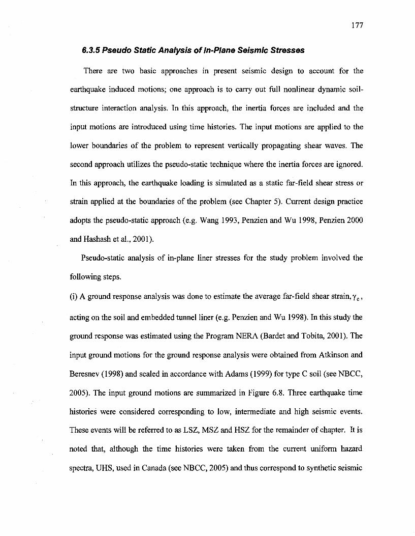
177

6.3.5 Pseudo Static Analysis of In-Plane Seismic Stresses

There are two basic approaches in present seismic design to account for the

earthquake induced motions; one approach is to carry out full nonlinear dynamic soil-

structure interaction analysis. In this approach, the inertia forces are included and the

input motions are introduced using time histories. The input motions are applied to the

lower boundaries of the problem to represent vertically propagating shear waves. The

second approach utilizes the pseudo-static technique where the inertia forces are ignored.

In this approach, the earthquake loading is simulated as a static far-field shear stress or

strain applied at the boundaries of the problem (see Chapter 5). Current design practice

adopts the pseudo-static approach (e.g. Wang 1993, Penzien and Wu 1998, Penzien 2000

and Hashash et al., 2001).

Pseudo-static analysis of in-plane liner stresses for the study problem involved the

following steps,

(i) A ground response analysis was done to estimate the average far-field shear strain, yc ,

acting on the soil and embedded tunnel liner (e.g. Penzien and Wu 1998). In this study the

ground response was estimated using the Program NERA (Bardet and Tobita, 2001). The

input ground motions for the ground response analysis were obtained from Atkinson and

Beresnev (1998) and scaled in accordance with Adams (1999) for type C soil (see NBCC,

2005). The input ground motions are summarized in Figure 6.8. Three earthquake time

histories were considered corresponding to low, intermediate and high seismic events.

These events will be referred to as LSZ, MSZ and HSZ for the remainder of chapter. It is

noted that, although the time histories were taken from the current uniform hazard

spectra, UHS, used in Canada (see NBCC, 2005) and thus correspond to synthetic seismic

178

events for major Canadian cities, it is anticipated that the results are applicable to

elsewhere in the world.

(ii) Next, the average shear strain in the ground (soil), estimated in step (i) above, was

used to calculate far field shear stress for use in closed form solutions viz.

[6.11]Tff=ycG

where yc is the shear strain, and G is the shear modulus of the soil.

(iii) Psuedo-static solutions for seismic induced in-plane stresses were obtained using

AFENA by incrementally applying prescribed boundary displacements as shown in

Figure 6.6d to achieve pure shear in the soil layer (with embedded tunnel) of a magnitude

estimated in step (i) above.

(iv) The free field stresses arising from yc were used with the closed form solution in

Chapter 5 to estimate the in-plane stresses caused by each of the seismic events

considered.

The following is a detailed description of the analysis results.

c)

3 c o

3 •_ 0)

"33 <

10 15 Time (s)

20 25

0.50

3 0.40

.2 0.30 (0

I 0.20 o

< 0.10

0.00

0.8

3 0.6

SS 0.4

I

1.4

^ 1.2

r 1

•M6.0R50

UHS Adams (1999)

1 2

Period (s)

M7.0R70

UHS Adams (1999)

1 2 Period (s)

• M 6.5 R30

UHS Adams (1999)

1 2 Period (s)

Figure 6.8: Input motions and matched spectra for a) LSZ, b) MSZ, and c) HSZ.

180

6.4 Results and Discussion

This section summarizes the results of analyses for the static and seismic loadings,

respectively, and for scenarios involving an intact tunnel lining, various degraded liners

(due to concrete spalling). First, the static loading results are presented followed by the

seismic results (pseudo-static results).

6.4.1 Results of Static Loading

6.4.1.1 The Intact Liner

Figure 6.9 and 6.10 compare the stresses at the liner extrados and intrados,

respectively, after construction. From these figures, it can be seen that there is good

agreement between the stresses calculated by F.E. analysis and closed form solution,

which is due to the absence of plasticity in the F.E. calculations. Thus, the closed form

solution is adequate for the static case and hence it will be used for comparison with F.E.

analyses involving liner degradation and plasticity so as to explore its range of

application.

AFENA Closed form sol.

0 20 40 60 80 100 120 140 160 180 e°

Figure 6.9: Distribution of normal stresses at the liner extrados.

Figure 6.10: Distribution of normal stresses at the liner intrados.

182

6.4.1.2 The Degraded Liner

• Scenario 1 - Local Spalling Near the Crown

Figures 6.11 and 6.12 show the stress distribution at the extrados and the intrados of

the liner for degradation Scenario 1 and static loading. In addition, results obtained using

the closed form solution for two extreme cases, intact liner and liner with the entire

intrados degraded (Scenario 3 - Fig. 6.7), are also presented in these figures. From both

Figures 6.11 and 6.12, it can be seen that the closed form solution provides approximate

upper and lower bounds for the stresses corresponding to degradation Scenario 1. In the

degraded zone, the stress level of the closed form solution (assuming the entire intrados is

degraded) matches with that of Scenario 1 for the F.E. analysis. At a short distance from

the degraded zone, results of the closed form solution for the intact liner match that of

Scenario 1 in the undegraded zone. The fluctuation in stress at the transition from intact

to degraded zones (e.g. see about 0=40°) is due to the rotation of principle stresses at

theses locations. Figure 6.13 shows the principle stresses near this transition. For Scenario

1, the maximum calculated stress is 12 MPa (compression) and there are no tensile

stresses.

15

12

(0

°- 9 CO (0

£ e (0

F.E. Results (Scenario 1)

7-Closed form sol. (Full degradation)

((

Closed form sol. (Intact)

i F.E. Results (Intact)

Scenario 1

0 20 40 60 80 100 120 140 160 180

e°

Figure 6.11: Stresses at the liner extrados degradation Scenario 1.

Closed form sol. *4Fulldegradation)..

r^_ F.E. Results (Scenario 1)

Closed form sol.' (Intact)

20 40 60 80 100 120 140 160 180

e°

Figure 6.12: Stresses at the liner intrados degradation Scenario 1.

184

Figure 6.13: Rotation of major principle stresses at the transition zone.

• Scenario 2 - Local Spalling at the Tunnel Shoulders

Figures 6.14 and 6.15 show the stress distribution at the extrados and intrados of the

liner due to static loading and corresponding to degradation Scenario 2. Again as in the

previous figures, the closed form solution is able predicting the upper and lower bounds

of the stresses for this degradation scenario. Similar to that observed for Scenario 1, there

is sudden variation in stress at the location of transitions from intact to degraded linings

(thickness change). For this scenario, as one moves further from the degraded zone

(nearly one segment away) the stresses remain unchanged from that of the intact liner

after construction. For Scenario 2, the maximum stress is 17.9 MPa (compression) and

there are no tensile stresses.

15

12

(B CL

s (0 (0

£ (0

F.E. Results (Scenario 2)

Closed form sol. (Full degradation)


Scenario 2

20 40 60 80 100 120 140 160 180


20

20 40 60 80 100 120 140 160 180


186

• Scenario 3 - Complete Degradation of the Intrados

This scenario represents the extreme case of intrados degradation, where the

entire inner layer of the lining is degraded. Figures 6.16 and 6.17 show the stress

distribution at the extrados and the intrados of the liner under static loading

conditions. For this case; the maximum stress is 14.3 MPa (compression) and there

are no tensile stresses in the lining. It can be observed from the results that the value

of maximum stress for this degradation scenario is lower than the other two

degradation scenarios; even though the extent of degradation is greater. This occurs

because there are no stress concentrations near transitions in the thickness of intact

lining. Again the closed form solution shows excellent ability to predict the stresses

within the lining (compared to the F.E. calculation).

15

F.E. Results {Scenario. .3)..


F.E. Results (Intact)

Scenario 3

20 40 60 80 100 120 140 160 180


20 / /

16

// i u

W

\ \

I-//

F.E. Results tScervarfo 3) ^_>


F.E. Results (Intact)

Closed form sol.' (Intact)

20 40 60 80 e°

100 120 140 160 180


188

6.4.2 Evaluation of Combined Static and Seismic Loading

In this section the results of static plus seismic load cases are presented for the

scenarios considered in section 6.4.1. Three levels of seismic intensity, varying from low

to high were considered, which as noted above, are referred to as LSZ, MSZ and HSZ.

Following the procedure presented in section 6.3.5, the following distribution of peak

shear strain with depth was obtained for the three levels of seismic intensity (see Figure

6.18): 0.12 %, 0.33% and 1.25%, for LSZ, MSZ and HSZ, respectively. These calculated

shear strain values (using NERA) were used in the pseudo-static analyses presented in the

following sections.

LSZ MSZ HSZ 0

10

20

E30

&40

50

60

70

- 5e-

...J

Rock

0

10

20

E.30

g-40 Q

50

60

70

- e

" " " • • !

Rock

0.00 0.10 0.20

Peak shear strain (%)

0.00 0.20 0.40 0.60


0.00 2.00 4.00


Figure 6.18: Results of the ground response analysis.

189

6.4.2.1 The Intact Liner

Figures 6.19 and 6.20 show the stress distribution at the extrados and the intrados of

the intact liner for the three seismic events considered. In addition, the static loading is

also presented to highlight the incremental impact of each seismic event. For the extrados,

the stress level from the crown to the springline decreases as the seismicity increases until

in the worst case (HSZ) the tensile capacity of the concrete is reached. On the other hand,

from the springline to the invert, the stresses increase as the seismicity increases. For the

intrados a reversed trend are observed. The seismicity causes increased bending in the

jointed lining increasing the bending stresses at the extrados and intrados. Although the

lining considered would be satisfactory for low and medium intensity earthquakes, it

would develop tensile cracking locally if exposed to high seismicity.

Figure 6.19: Stresses at the liner extrados in low, moderate and high seismicity zones

compared to that of the static case.

190

Figure 6.20: Stresses at the liner intrados in low, moderate and high seismicity zones

compared to that of the static case.

6.4.2.2 Influence of Soil and Concrete Plasticity

Figure 6.21 compares stresses calculated by F.E. and closed form solution at the

extrados and intrados of the liner, respectively, for the LSZ. Figures 6.22 and 6.23 show

similar information for the MSZ and HSZ events. It can be seen from Figures 6.21 to 6.23

that there is good agreement between the closed form solution and F.E. results for low

seismicity. However, for medium and high seismic cases, there is divergence in the order

of 19 % for the MSZ and 28 % for the HSZ. This difference is attributed to plasticity that

occurred in both the soil and the liner, which is not accounted for in the elastic closed

form solution. However, the closed form solution is able to highlight the potential for

cracking as it shows the tensile stresses locally exceeds the tensile capacity of the

191

concrete (see Figure 6.23). Figure 6.24 shows the location of plastic zones for MSZ and

HSZ; there were no plastic zones for the LSZ case.

Closed form solution LSZ

20 40 60 80 100 120 140 160 180

e°

Figure 6.21: Comparison of the stresses in the liner for low seismicity.

15

20 40 60 80 100 120 140 160 180

Figure 6.22: Comparison of the stresses in the liner for medium seismicity.

Q.

I

Figure 6.23: Comparison of the stresses in the liner's extrados for high seismicity.

a) Plastic zones - MSZ b) Plastic zones - HSZ

Figure 6.24: Location of plastic zones for MSZ and HSZ.

193

6.4.2.3 The Degraded Liner during a Seismic Event

For degradation Scenario 1, similar trends to those observed in the intact liner case

were also observed for the liner with a degraded crown. At the transitions from intact to

degraded cross-sections, the stresses were found to fluctuate similar to that observed in

the static case. Figures 6.25 and 6.26 present the stresses at the liner extrados and

intrados, respectively. It is interesting to note that there is an absence of tensile cracking

of the extrados between 50° and 80° compared with the intact case (see Fig. 6.23) for the

HSZ case. This is due to the reduced flexural rigidity of the lining over the degraded

zone, which in turn reduces the mobilized moments. The extent of tensile cracking at the

intrados is identical to the intact case since the cracked zone is well away from the

degraded zone and isolated by joints. As discussed below, for degradation Scenarios 2

and 3, similar trends to those observed for the intact liner case and the degraded crown

case (Scenario 1) were also observed.

194

80 100 120 140 160 |-»- Absence of tensile cracking

180

e°

Figure 6.25: Stresses at the liner extrados in low, moderate and high seismic zones

(compared with the static case).

100 M20__J4Q~~«~~J£0_wy 180

-*\ Tensile cracking p—

Figure 6.26: Stresses at the liner intrados in low, moderate and high seismic zones

(compared with the static case).

195

6.4.2.4 Influence of Soil and Concrete Plasticity

For degradation Scenarios 2 and 3, similar trends to those observed for the intact liner

case were also observed (e.g. in terms of the influence of soil and concrete plasticity).

Consequently, only the results for Scenario 2 in MSZ are presented. Figures 6.27 and

6.28 compare stresses calculated by F.E. and closed form solution at the extrados and

intrados of the liner, respectively, for the MSZ seismic event. It can be seen from the

figures that the closed form solution is not able to predict the upper and lower bounds of

the stresses in the degraded liner as observed earlier in the static cases. There is a 35%

difference between the F.E. calculations and the closed form upper and lower bound

solutions at the location of degradation and transitions from intact to degraded liner.

This difference is attributed to plasticity that occurred in both the soil and the liner, which

is not accounted for in the elastic closed form solution. Figures 6.27 and 6.28 suggest

that the closed-form solution does to provide good estimates of stresses in the liner for

cases were the liner condition has degraded due to spawling of the concrete intrados. For

such cases, a finite element analysis appears to be required.

20

16

(0 9: 12

! •

i -/1

Scenario 2 F.E. Results



0 20 40 60 80 100 120 140 160 180

Figure 6.27: Stresses at the liner extrados degradation Scenario 3 and MSZ.

20 40 60 80 100 120 140 160 180

Figure 6.28: Stresses at the liner intrados degradation Scenario 3 and MSZ.

197


The finite element program AFENA (Carter and Balaam, 2005) was used to perform

static and pseudo static seismic response analyses of tunnels with intact and degraded

concrete liners. An advanced concrete model was used to model the material behaviour of

a segmental concrete tunnel lining under both compression and tension loading. The

effect of local concrete degradation on the stresses developed in degraded tunnel linings

was investigated in addition to the effect of three earthquake events with different

intensities on the stresses in intact and degraded tunnel linings. Lastly, the accuracy of

the results obtained from the closed form solutions developed in Chapters 3, 4 and 5 were

evaluated by comparing them to results obtained from a non-linear elastoplastic finite

element analysis.

The following conclusions can be made from the results and discussions presented

above:

1) There is good agreement between F.E. calculations and the closed form solution

for the static case of intact linings.

2) The closed form solutions for the intact and fully degraded linings bracket the

F.E. results for degraded linings (static loading). In the intact zones, the F.E.

results are comparable to those calculated by closed form solution for the intact

case; whereas in the degraded zones the F.E. results were comparable to thos

calculated by closed form solution for a fully degraded liner. These results are

of interest and should be investigated further to explore for any limitations.

3) Seismicity can induce significant stresses in tunnel linings. For the intact case,

tensile cracking is possible in high seismic zones.

198

4) There is good agreement between F.E. calculations and closed form solutions

for low seismicity, but progressively increasing error (19 % and 28 %) was

observed for medium and high seismic events due to soil and liner plasticity.

However, the closed form solution is able to identify zones of potential

cracking though.

5) Liner degradation has a detrimental effect on stresses in the lining for the static

loading case. However, during a seismic event, the reduced liner stiffness in

the degraded zone leads to lower moments and consequent stresses near the

zones of degradation. Thus, degradation does not appear to have a detrimental

effect in this case due to soil-structure interaction, which is contrary to that

hypothesized in the introduction.

6) Lastly, it is concluded that a detailed F.E. analysis should be done to adequately

assess the distribution of stresses in degraded concrete tunnel linings for

medium and high seismic events.

199

References

Adams, J., Weichert, D., and Halchuk, S. 1999. Lowering the probability level - Fourth

generation seismic hazard results for Canada at the 2% in 50 year probability level.

Proceedings of 8th Canadian Conference on Earthquake Engineering, Vancouver, 6

pages

Atkinson, G.M. and Beresnev, LA. 1998. Compatible ground-motion time histories for

new national seismic hazard maps. Canadian Journal of Civil, 25: 305-318.

Asakura, T., Sato, Y., 1996. Damage to mountain tunnels in hazard area. Soils and

Foundations, Japanese Geotechnical Society, Special Issue, pp. 301-310.

Bernat, S. and Cambou, B. 1998. Soil-structure Interaction in shield tunnelling in soft

soil. Computers and Geotechnics. 22(3/4): 221-242

Carter, J.P. and Balaam, N.P. 2005. AFENA v7.4. Finite Element Software - Users

Manual. Sydney, Australia.

Davis, E.H. 1968. Theories of plasticity and the failure of soil masses. Soil Mechanics

Selected Topics, Butterworths, Sydney.

Duncan, J.M. and Chang, C.Y. 1970. Nonlinear analysis of stress and strain in soils. J. of

Soil Mech. and Foundation Division, ASCE, 96(SM5): 1629-1653.

Galli, G., Grimaldi, A. and Leonardi, A. 2004. Three-dimensional modelling of tunnel

excavation and lining. Computers and Geotechnics. 31: 171-183

Hashash, Y. M. A., Hook, J. J., Schmidt, B. and Yao, J. I. 2001. Seismic design and

analysis of underground structures. Journal of Tunneling and Underground Space

Technology. 16: 247-293.

200

Hinchberger, S.D. 2007a. A finite element implementation for concrete subject to

general 3-dimensional stresses. Geotechnical Research Centre Report No. GEOT-07-

9, The University of Western Ontario.

Hinchberger, S. D. 2007b. On the application of a hierarchical yield function to concrete.

Geotechnical Research Report No. GEOT-07-10, The University of Western Ontario.

NBCC 2005. The National building code of Canada. National Research Council, Canada.

Penzien J. and Wu C. L. 1998. Stresses in linings of bored tunnels. Journal of Earthquake


Penzien J. 2000. Seismically induced racking of tunnel linings. Journal of Earthquake


Scott B.D., Park R.,and Priestley M.J.N. 1982. Stress-strain behaviour of concrete

confined by overlapping hoops at low and high strain-rates. ACI Journal, 79(1): 13-27

Vecchio, F. 1982. The response of reinforced concrete to in-plane shear and normal

stresses. Ph.D. Thesis, Department of Civil Engineering, University of Toronto,

Canada.

Wang, J. N. 1993. Seismic Design of tunnels. Monograph 7, Parsons Brinkerhoff Quade

& Douglas.

Youssef, M. and Moftah, M. 2007. General stress-strain relationship for concrete at

elevated temperatures. Journal of Engineering Structures. (In press).

201

CHAPTER 7

Summary, Conclusions and Recommendations for Future

Research

A successful tunnel design must fulfill basic requirements for soil-structural stability,

durability and cost effectiveness with reasonable accuracy. To achieve this, engineers

must estimate the distribution of internal forces and stresses in tunnel linings. Closed

form solutions are useful during preliminary design of a tunnel lining since they permit

quick and efficient evaluation of several loading cases. This can help identify an

optimum liner design that can then be verified using more sophisticated approaches based

on finite element or finite difference techniques.

This thesis presented analytical and numerical tools and procedures in order to better

analyse continuous and segmental concrete tunnel linings, and to assess performance of

older degraded tunnel linings using closed form solutions. These tools have been applied

to both static and seismic loading condition.


The work presented in this thesis essentially falls into three main parts. The first part

deals with the development of closed form solutions for internal forces and stress of

continuous and segmental tunnel linings (Chapters 3 and 4). The second part covers

different seismic considerations for tunnels (Chapter 5). The third and last part includes a

202

comprehensive investigation of the accuracy of the analytical tools developed in parts one

and two and their application to assess the stresses in older degraded tunnel linings; for

both static and seismic conditions. These parts are summarized below.

7.1.1 Closed form solutions

Two closed form solutions were developed and presented in Chapters 3 and 4. These

solutions are suitable for the analysis of circular tunnels installed in either intact rock or

strong soils above the groundwater table and that remain predominantly elastic during

construction of the tunnel.

The first solution is for continuous composite tunnel linings in a homogeneous

infinite isotropic elastic medium. The tunnel lining system is treated as an inner

continuous thin-walled shell and an outer thick-walled cylinder embedded in linear elastic

soil or rock. The main advantages of this solution are that it considers the composite

action of double liner systems; and it can be used to approximately account for partial

closure of the gap prior to lining installation. Solutions for moment and thrust have been

derived for cases involving slip and no slip at the lining-ground interface and lining-

lining interface. The general behaviour of the solution was demonstrated for various cases

involving both single and double lining systems.

The second closed form solution solves for displacement, moment and thrust in

jointed tunnel linings. In this solution, the lining system is modelled as an inner jointed

segmental lining and an outer thick-walled cylinder. The composite tunnel lining was

assumed to be embedded in an infinite elastic medium subject to an initial anisotropic

203

stress field. The solution was verified by comparing it with finite element results where it

was shown to agree well with this more sophisticated method of analysis. An extensive

parametric study was conducted to explore the proposed solution. The results of the

parametric study showed that the solution is able to predict the displacements, moments

and thrusts with reasonable accuracy. The applicability of the solution is limited if the

following two conditions exist: a large variation of Cs (factor accounting for the joints

effect) for the springline and crown to invert axes; and values of X (joint to liner stiffness

ratio) less than 0.4. For such cases, although uncommon, the potential error should be

accounted for (refer to Chapter 4 for more details).

7.1.2 Seismic considerations

The closed-form solution for the case of jointed composite tunnel lining was utilized

to account for the in-plane stresses induced by vertically propagating earthquake waves.

Cases of continuous and jointed tunnel linings were investigated. The effect of soil

nonlinearity due an excavation damage zone, EDZ, was investigated using an equivalent

linear approach. In order to approximately account for the soil nonlinearity, a weakened

annular zone of soil was considered around the tunnel. The results of the analysis

showed that as the size (extent) of the weakened zone increases, the moments increase

and the thrust decreases, which can cause, under some circumstances, tensile stresses to

be induced in the liner. Also, the effect of the incidence angle, X, of an earthquake on

moments and thrust of the liner was investigated. It was found that the highest tensile

stresses at the crown at the inner face occur when earthquake waves hit the tunnel at 45°

with the horizontal axis. At this incidence angle, the moment at the crown of un-jointed

204

liners may increase by up to 200%. For the jointed tunnel lining case, the analysis

showed that the presence of the joints may result in up to 50 % reduction in the developed

moments. Thus, in order achieve an economical design, the effect of the joints should be

considered.

7.1.3 Numerical Evaluations

In Chapter 6, the finite element program AFENA (Carter and Balaam, 2005) was used

to perform static and pseudo static seismic response analyses of tunnels with intact and

degraded concrete liners. The seismic loading was evaluated by performing a local site

response analysis with bedrock input motion representing three levels of seismicity: low,

moderate and strong. The seismic shear strain at the elevation of the tunnel spring line

was used to develop a displacement field that was then applied as a boundary condition.

An advanced concrete model was used to model the material behaviour of a typical

segmental concrete tunnel lining under both compression and tension loading.

The effect of local concrete degradation on the stresses in degraded tunnel linings was

investigated. It was found that the effect of local degradation is only local in nature (i.e.

only in the region of degradation). Also, the effect of seismic loads of different intensities

on intact and degraded tunnel linings was studied. It was found that the seismicity

strength is a key factor that governs the overall stress level in the liner and its effect can

cause significant damage to the liner.

The accuracy of the results obtained from the developed closed form solutions and

analytical tools (presented in Chapters 3, 4 and 5) was evaluated by comparing them to

the results of a detailed finite element model. The comparison showed that the closed

205

form solutions are capable of predicting post-construction stresses within 10% from that

obtained from the more sophisticated finite element model under static loading case.

When considering the seismic loads, in addition to the static loads, for low to medium

intensity seismic zones, the closed form solutions showed results that again fall in the

range of 10% to 15 % from that of the finite element results. However, for the strong

seismicity zone, the extensive plasticity that occurred in the soil and the liner is beyond

the limits of the closed form solution, nonetheless the results are within 28 % of those

predicted using the finite element model.

The analyses and discussions presented in this thesis clearly demonstrated that the

composite lining solution is versatile and is reasonably accurate. They can cover a variety

of different lining geometries and conditions and thus it should be a useful tool for design

considerations in tunnelling.

7.2 Recommendations for future research

The following outlines some aspects that should be considered in future research:

1) An analytical procedure is needed to evaluate the rotational stiffness of liner

joints. This procedure should account for the geometry and configuration of the

joint. Also, it should take into account the effect of post stressing of the bolts

and gasket materials.

206

2) Several researches have investigated the excavation damaged zone. However,

the size and extent of nonlinearity needs to be determined more rigorously. For

example, through extensive experimental and numerical work, formulas that

can relate the method of excavation and ground conditions to the size of EDZ

can be developed.

3) Investigate the use of closed form solutions to interpret field observations. For

example, a procedure is needed such that through joints rotations the extent of

degradation in the liner can be assessed.

4) Solution for staggered joints (e.g. staggered in the longitudinal direction).

5) Investigate other mechanisms of liner degradation (e.g. sulphate attack, fire

exposure).

6) More detailed assessment of spalling degradation to confirm the conclusions in

Chapter 6 for a wide range of conditions.

207

Appendix A: Equations for Stresses and Displacements of the Outer Liner

This section summarizes the solutions developed by Yuen (1979) and Ogawa (1986)

for the stresses and displacements in a thick walled cylinder subject to both normal and

tangential external loads.

(i) Hydrostatic Co mponent

In a similar manner to that used for the ground, the radial, tangential and shear stresses

in the outer lining can be solved for using Airy's stress function and, equations 2 and 3a,

3b and 3c, respectively. For the boundary conditions, aR =a"2 at r = R3 and

aR =CT J at r = R2, the Airy's coefficients A and C in Equation 2 are:

[A.la] A = g N 2 - g N l h

2(1-h)

[A.lb]C = R 2 ( g N 2 - g N l )

(1-h)

where h = (R.2 / R3) . The resultant stresses in the outer lining are:

[A.2a] ol7=o% RL 2 _ U N 1

f I r J

2 ^

- h

1-h

v J

+ CTN2

1-

L

I r J 1-h

2\

J

[A.2b] ceH

T,=-og 6L2 ~ " N l

r

V

f R 2 l I r J

1-

2 ^

+ h

h

J

+ aN2

1 + fR0 l r J l - h

2^|

and

208

[A.2c] x^L2=0

From generalized Hooke's law, it can be shown that the radial displacement of the

outer lining, UL2, is:

[A.3] u«2=JseH

2dr = i l ± ^ E2(l-h)

.M-a-2v2)hlog, +| M + ( i _2v 2 ) l a5 2

For r = R2 and r = R3, the radial displacements at the intrados and the extrados are:

[A.4] u?2(r = R3)= ( l + ^ 3 [{-2(l-v2)h}ag1+{(h + l-2v2)}ag2]

[A.5] uiJ2(r = R2) = - ^ ^ - [ { - l - a - 2 v 2 ) h } o g 1 + { 2 a - v 2 ) } o g 2 ' E2( l -h)


For the deviatoric component, Q0, the Airy's stress function is given by equation 6

and the radial, tangential and shear stresses are governed by the equilibrium equations 7a

to c, respectively. Referring to Fig. 5, the boundary conditions for the outer lining are:

[A.6a] aR = a ° 2 cos 29 at r = R3

[A.6b] xRe = -T T 2 sin 20 at r = R3

[A.6c] aR = a^i cos 20 at r = R2

and

[A.6d] xRe = -xT1 sin 20 at r = R2

where ag, and crg2 are the maximum radial stresses acting on the outer lining at the

intrados and the extrados, respectively, and TT1 and xT2 are the maximum tangential

209

shear stresses acting at the intrados and the extrados, respectively. Again, Figure 5 shows

the assumed stress conditions at the two interfaces.

For the above boundary conditions, the constants A, B, C and D of the Airy's stress

function are:

[A.7a] A = l—^r[- (2h2 + h +1) cr£2 - 2h2 TT2 + (h3 + h2 + 2h) a j j + 2h xT1 ] 2(1-h)

[A.7b] B= ^3T^ 2[(3h + l ) a g 2 + ( 3 h - l ) x T 2 - ( h 2 + 3 h ) a " 1 + ( h 2 - 3 h ) T T 1 ] 6 ( l -h ) J R 3

[A.7c] C = h R\3 [-(h + 3)ag2 -2hT T 2 +(3h + l)og1 +2xT1] 6(1-h)

hR2

[A.7d] D = J [ ( h 2 + h + 2 ) a ° 2 + ( h 2 + h ) T T 2 - ( 2 h 2 + h + l ) a g 1 - ( h + l)tT 1] 2.(1 li)

Using generalized Hooke's law, the radial and tangential displacements of the outer

lining are:

[A.8] u P 2 = f s r d r = 2 ( 1 ^ V 2 ) r [ - A - 2 v 2 B r 2 + 4 + 2( l -v 2 )^ - ]cos2e E2 r r

and

[A.9] v g 2 = J [ e e - ^ ] r d e = 2 ( 1 ^ V 2 ) r [ A + ( 3 - 2 v 2 ) B r 2

+ - ^ - ( l - 2 v 2 ) % s i n 2 e r E2 r r

Accordingly, the stresses and displacements at the interface between the ground and

the outer lining (atr = R3) due to the reactive force, CT^I,C7°2,TT1 and iT 2 are:

[A. 10a] a£ L 2 ( r = R3) = -[2A + 6-^- + 4-^-] cos29 = a£ 2 cos26 R3 R3

[A. 10b] a°L2(r = R3) = [2A + 1 2 B R 3 + 6 - % cos 20 R 3

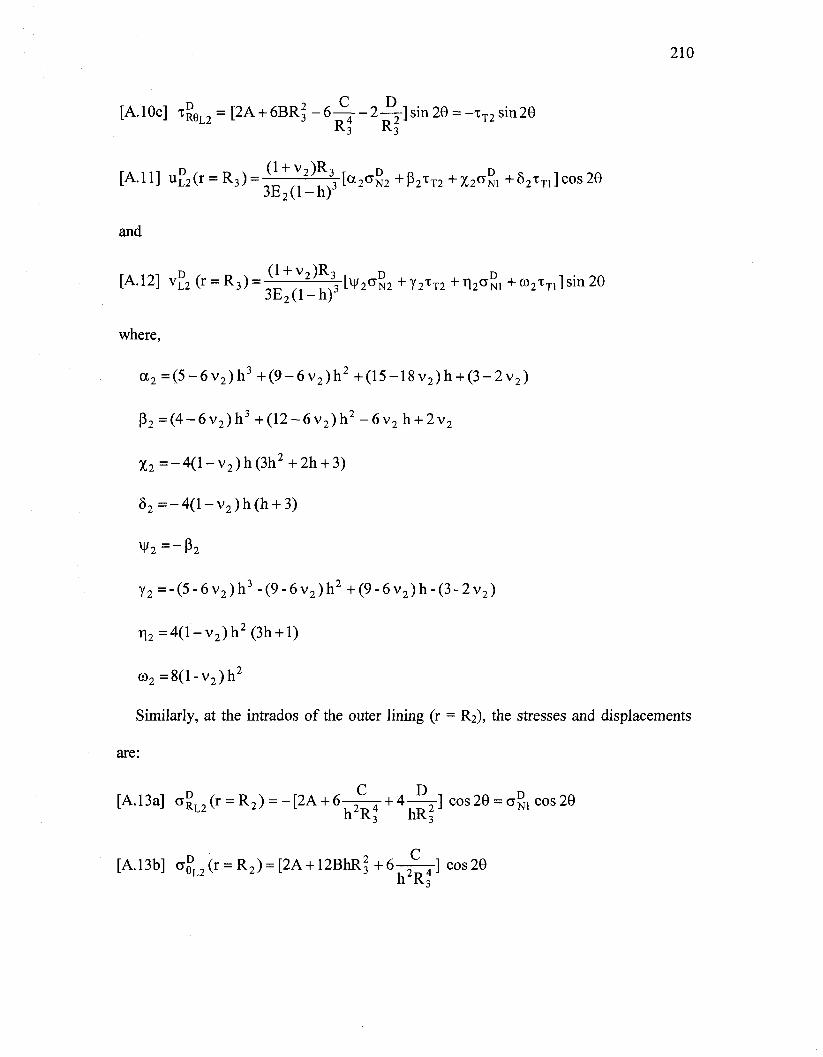
210

[A. 10c] TJBL2 = [2A + 6 B R ^ - 6 - ^ — 2 ^ - ] s i n 2 e = -TT2sin29 R3 R3

[A.11] ^2(r = R3) = -^^^[a2cs^2+^2xT2+l2a^+b2xTi]cos2Q 3 E 2 ( l - h ) 3

and

[A.12] v°2 (r = R 3 )= * , 3 [^2gN2 +Y2^T2 +T12^NI + CO2TT1] sin 20 3 E 2 ( l - h )

where,

a 2 = ( 5 - 6 v 2 ) h 3 + ( 9 - 6 v 2 ) h 2 + ( 1 5 - 1 8 v 2 ) h + ( 3 - 2 v 2 )

p 2 = ( 4 - 6 v 2 ) h 3 + ( 1 2 - 6 v 2 ) h 2 - 6 v 2 h + 2v2

X 2 = - 4 ( l - v 2 ) h ( 3 h 2 + 2 h + 3)

8 2 = - 4 ( l - v 2 ) h ( h + 3)

¥2=-P 2

y 2 = - ( 5 - 6 v 2 ) h 3 - ( 9 - 6 v 2 ) h 2 + ( 9 - 6 v 2 ) h - ( 3 - 2 v 2 )

n 2 = 4 ( l - v 2 ) h 2 ( 3 h + l)

co 2=8(l-v 2)h 2

Similarly, at the intrados of the outer lining (r = R2), the stresses and displacements

are:

[A. 13a] a^L2(r = R2) = -[2A + 6 - ^ T + 4-^2-] cos 29 = a ^ cos 20 n R3 hR3

[A.13b] o^ (1 = R2) = [2A + 12BhR.l +6-£-T] cos 20 h R3

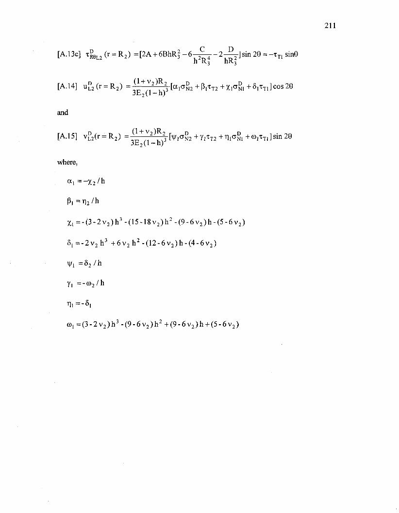
[A.13c] T£ e u ( r = R2) = [2A + 6 B h R 2 - 6 ^ - 2 - ^ ] s i n 2 e = -xT1 sinG h K3 11K3

[A.14] u°2(r = R2) = ^ ^ ^ - [ 0 , 0 8 2 H - ^ T ^ + X I O B I + S , ^ , ] c o s 2 0 3 b 2 ( l - n )

and

[A.15] v£2(r = R2) =^-^^-J[M/ 1 a^ 2 +Y 1 T T 2 +ri 1 aB 1 +© 1 T T 1 ]s in2e 3 b 2 ( l - n )

where,

a ! = - x 2 / h

P i = r | 2 / h

X l = - ( 3 - 2 v 2 ) h 3 - ( 1 5 - 1 8 v 2 ) h 2 - ( 9 - 6 v 2 ) h - ( 5 - 6 v 2 )

dl=-2v2hi + 6 v 2 h 2 - ( 1 2 - 6 v 2 ) h - ( 4 - 6 v 2 )

Vi = 8 2 / h

Yi = - r a 2/ h

Til = - 8 1

©! = ( 3 - 2 v 2 ) h 3 - ( 9 - 6 v 2 ) h 2 + ( 9 - 6 v 2 ) h + (5-6v 2 )

212

Appendix B

(i) Deviatoric Component - Full Slip at R2, No Slip at R3

For the case of full slip at r = R2 and no slip at r = R3 the boundary conditions are:

aR =a^2cos20 and xRe =xT2sin26 atr = R3, CTR =a^,cos20 and TRQ =0 at r = R2

and aR =xa = 0 atr = 00 . Thus, the following system of equations can be developed to

calculate a ° 2 , a ^ and xT2:

n 3Q 0 (3-4v. ) na 11 —D _ x ° v s / |B.1J CTN2 =

u , u r b1 3(b3 1+b3 2r) D l l + D12 i T

b33

[B.2] CTNI = r <JN2

TO "31 -r - ^31 + b 3 2 ^ ^D [BJJ xT2 = aN2

b33

where,

[B.4] r =b 3 1 ( b 2 3 ~ b 1 3 ) + b 3 3 ^ b l l " b 2 1 )

b 3 3 ( b 2 2 _ b 1 2 ) + b 3 2 ( b 1 3 " b 2 3 )

and

"11 =^-io +C 9 a 2

b12=C9X2

b13=Cu+C9p2

b2i = C n -C9i)/2

b22 = """C^

b23 = ^ io ~C9Y2

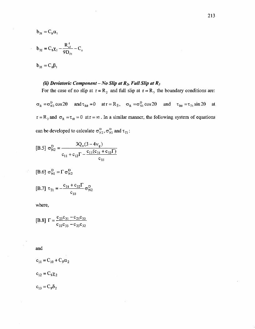
213

R*

"3\ — ^ 8 * ^ 1

b33 = C 8 P l

(ii) Deviatoric Component - No Slip at R2, Full Slip at R3

For the case of no slip at r = R2 and full slip at r = R3 the boundary conditions are:

aR=CT°2cos29 andxRe =0 atr = R3, aR =0^,00829 and xRe=xT1sin29 at

r = R2 and aR =xr6 = 0 atr = 00 . In a similar manner, the following system of equations

can be developed to calculate CT°2 , cy i and xT1:

3Q0(3-4vg) [B.5] og2 =

- , „ r C 1 3 ( C 3 1 + C 3 2 n

C33

[B.6]a°1 = : raS2

[ B . 7 ] x T 1 = - ^ ± ^ a £ 2 "33

where,

TB 81 r = C 2 3 ° 3 1 C21C33 C22C33 — C23C32

and

C12 = C 9 % 2

13 — 9 2

214

C21 — *^8ai

R c2 2-Cg X l * C

C23 — ^8°1 Rl, C„

18Dfl 2

c31=C8\|/,

R °3 2 _ C 8 T 1 l + 18Df

Ri R c 3 3 = C 8 ° ) i + T 7 ^ - + cl

36D„ 4Dcl

Appendix C

Coefficients of the closed form solution.

a i = - X 2/ h

P1=T l 2 /h

X l=-(3-2v 2)h 3-(15-18v 2)h 2-(9-6v 2)h-(5-6v 2)

5 1=-2v 2h 3 +6v 2 h 2 - (12-6v 2 )h-(4-6v 2 )

\|/j = 8 2 / h

Yi = - c o 2 / h

T I , = - 5 ,

coj =(3-2v2)h3 -(9-6v2)h2 +(9-6v2)h + (5-6v2)

a 2 =(5-6v 2 )h 3 +(9-6v 2 )h 2 +(15-18v 2 )h + (3-2v 2 )

p 2 = ( 4 - 6 v 2 ) h 3 + ( 1 2 - 6 v 2 ) h 2 - 6 v 2 h + 2v2

X 2 =-4( l -v 2 )h(3h 2 +2h + 3)

5 2 = - 4 ( l - v 2 ) h ( h + 3)

y2=-P2

y 2 =-(5-6v 2 )h 3 - (9-6v 2 )h 2 +(9-6v 2 )h-(3-2v 2 )

n 2 =4( l -v 2 )h 2 (3h + l)

co2=8(l-v2)h2

216

an _ C80Cj

R a12 _ CgXl - ~ C

9D fi

a13 -C8(3j

R i Cc a i4 - C g S j - — — — 18Dfl 2

a2 1 -CgVi/j

R a 2 2 _ C 8 T 1 l + T8D:

a23 -CgYi

R4 R2

a24 = Co©, + — — + —— 24 8 l 36Dfl 4Dcl

a3i =C-io + C9oc2

a32 = C9X2

a33 = ^ - l l + ^ 9 P 2

a34 ~ C962

a41 = C n " "^9^2

a42 = "Cg'Hi

a43 = ^ 1 0 " ^ 9 7 2

&44 = L-9CO2

217

VITA

Name: Hany Hamed EINaggar

Education and Degrees:

Ph.D., the University of Western Ontario, London, Ontario, Canada. Thesis Title: The analysis and evaluation of jointed segmental concrete tunnel linings - seismic and durability considerations. (2004- 2007)

M.E.Sc., the University of Western Ontario, London, Ontario, Canada. Thesis Title: An innovative cellular pre-cast concrete pipe. (2002-2004)

Post Graduate Diploma, American University in Cairo, Egypt. (2000-2001)

B.E.Sc., Alexandria University. Egypt Thesis Title: Effect ofretardant dose on the performance of the concrete mix. (1990-1996)

General Certificate of Education, London University, U.K. (1989-1990)

Honours and Awards:

1. Ontario Graduate Scholarship (OGS): The University of Western Ontario, May 2007 to May 2008

2. Graduate Thesis Research Award: Faculty of Engineering, The University of Western Ontario, May 2007.

3. The Outstanding Teaching Assistant Award for the Academic Year 2005-2006: Department of Civil and Environmental Engineering, The University of Western Ontario.

4. L. G. Soderman Award for Excellence in Studies in Geotechnique: The University of Western Ontario, June 2006.

5. Ontario Graduate Scholarship (OGS): The University of Western Ontario, May 2006 to May 2007.

6. R.M. Quigley Award: The University of Western Ontario, September 2005.

7. Western Engineering Scholarship (WES): The University of Western Ontario, May 2005 to May 2008.

8. Special University Scholarship (SUS): The University of Western Ontario, May 2004 to May 2005.

9. Milos Novak Memorial Award: The University of Western Ontario, May 2004.

218

Engineering Research and Teaching:

Sep. 2002 - Present

Nov. 2001-Aug.2002

Publications

Journal Publications: 1. El Naggar, H. and Hinchberger, S. (2007) "An Analytical Solution for Jointed Tunnel Linings in a

Homogeneous Infinite Isotropic Elastic medium", Canadian Geotechnical Journal, Canada. (Accepted)

2. El Naggar, H., Hinchberger, S. and Lo, K. Y. (2006) "A Closed-Form Solution for Tunnel Linings in a Homogenous Infinite Isotropic Elastic Medium", Canadian Geotechnical Journal, Canada.(In Press)

3. El Naggar, H., Allouche, E. and El Naggar, M.H. (2006) "Development of New Class of Pre-cast Concrete Pipes: Numerical Evaluation", Canadian Journal of Civil Engineers, Canada. (In press)

4. El Naggar, H., Allouche, E. and El Naggar, M.H. (2006) "Development of New Class of Pre-cast Concrete Pipes: Experimental Evaluation", Canadian Journal of Civil Engineers, Canada. (In press)

Conference Publications: 1. El Naggar, H., Hinchberger, S. and El Naggar, M.H. (2007) "Approximate Evaluation of

Nonlinearity Effects on Seismically Induced In-Plane Stresses in Tunnel Lining", 4th International Conference on Earthquake Geotechnical Engineering, June 25-27, 2007, Greece.

2. El Naggar, H. and El Naggar, M.H. (2007) "Simplified Approach to Group Effect in Pile Dynamics" 4th International Conference on Earthquake Geotechnical Engineering, June 25-27, 2007, Greece.

3. Hinchberger, S.D. and El Naggar, H. (2005) "On the Use of Simplified Methods to Estimate Moments and Thrust in Segmental Concrete Tunnel Linings", K.Y. Lo Symposium, July 7-9 2005, The University of Western Ontario, London, Canada, pp.319-329.

Research Reports: 1. EI Naggar, H., Hinchberger, S. and Lo, K. Y. (2006) "A Closed-Form Solution for Tunnel Linings in

a Homogenous Infinite Isotropic Elastic Medium", Geotechnical Research Report No. GEOT-05-06, The University of Western Ontario.

2. El Naggar, H. and Allouche, E. (2004) "Innovative Cellular Pre-cast Concrete Pipe: Numerical & Experimental Evaluation", The science of success conference, Materials and Manufacturing Ontario (MMO), Toronto, Canada.

3. El Naggar, H. and Allouche, E. (2003) "Development of an innovative cellular concrete pipe", Materials and Manufacturing Ontario (MMO) funded researchers exhibiting at Partnerships 2003.

4. El Naggar, H. and Allouche, E. (2003) "Parametric study to determine the optimal shape and Size of the longitudinal cavities", Ontario Concrete Pipe Association (OCPA), 2003.

Research Assistant& Teaching Assistant The University of Western Ontario Faculty of Engineering

Research Assistant Geotechnical Research Centre The University of Western Ontario

analysis and evaluation of segmental concrete tunnel linings

Documents

Transcript of analysis and evaluation of segmental concrete tunnel linings