An Investigation of Agricultural Produce Cooling Tunnel ...

University of Windsor University of Windsor

Scholarship at UWindsor Scholarship at UWindsor

Electronic Theses and Dissertations Theses, Dissertations, and Major Papers

1-29-2016

An Investigation of Agricultural Produce Cooling Tunnel An Investigation of Agricultural Produce Cooling Tunnel

Performance Performance

Jean-Paul Edward Martins University of Windsor

Follow this and additional works at: https://scholar.uwindsor.ca/etd

Recommended Citation Recommended Citation Martins, Jean-Paul Edward, "An Investigation of Agricultural Produce Cooling Tunnel Performance" (2016). Electronic Theses and Dissertations. 5650. https://scholar.uwindsor.ca/etd/5650

This online database contains the full-text of PhD dissertations and Masters’ theses of University of Windsor students from 1954 forward. These documents are made available for personal study and research purposes only, in accordance with the Canadian Copyright Act and the Creative Commons license—CC BY-NC-ND (Attribution, Non-Commercial, No Derivative Works). Under this license, works must always be attributed to the copyright holder (original author), cannot be used for any commercial purposes, and may not be altered. Any other use would require the permission of the copyright holder. Students may inquire about withdrawing their dissertation and/or thesis from this database. For additional inquiries, please contact the repository administrator via email ([email protected]) or by telephone at 519-253-3000ext. 3208.

https://scholar.uwindsor.ca/

https://scholar.uwindsor.ca/etd

https://scholar.uwindsor.ca/theses-dissertations-major-papers

https://scholar.uwindsor.ca/etd?utm_source=scholar.uwindsor.ca%2Fetd%2F5650&utm_medium=PDF&utm_campaign=PDFCoverPages

https://scholar.uwindsor.ca/etd/5650?utm_source=scholar.uwindsor.ca%2Fetd%2F5650&utm_medium=PDF&utm_campaign=PDFCoverPages

mailto:[email protected]

An Investigation of Agricultural Produce Cooling Tunnel Performance

by

Jean-Paul E. Martins

A Thesis

Submitted to the Faculty of Graduate Studies

through the Department of Mechanical, Automotive & Materials Engineering

in Partial Fulfillment of the Requirements for

the Degree of Master of Applied Science

at the University of Windsor

Windsor, Ontario, Canada

2016

© 2016 Jean-Paul Martins

An Investigation of Agricultural Produce Cooling Tunnel Performance

by

Jean-Paul E. Martins

APPROVED BY:

______________________________________________

Dr. T. Bolisetti

Department of Civil and Environmental Engineering

______________________________________________

Dr. B. Zhou

Department of Mechanical, Automotive & Materials Engineering

______________________________________________

Dr. G. W. Rankin, Advisor

Department of Mechanical, Automotive & Materials Engineering

January 21st 2016

iii

Declaration of Originality

I hereby certify that I am the sole author of this thesis and that no part of this thesis has

been published or submitted for publication.

I certify that, to the best of my knowledge, my thesis does not infringe upon anyone’s

copyright nor violate any proprietary rights and that any ideas, techniques, quotations, or

any other material from the work of other people included in my thesis, published or

otherwise, are fully acknowledged in accordance with the standard referencing practices.

Furthermore, to the extent that I have included copyrighted material that surpasses the

bounds of fair dealing within the meaning of the Canada Copyright Act, I certify that I

have obtained a written permission from the copyright owner(s) to include such

material(s) in my thesis and have included copies of such copyright clearances in

Appendix A.

I declare that this is a true copy of my thesis, including any final revisions, as approved

by my thesis committee and the Graduate Studies office, and that this thesis has not been

submitted for a higher degree to any other University or Institution.

iv

Abstract

The goal of this research is to numerically and experimentally investigate the

performance of a forced air agricultural produce cooling tunnel. A porous medium

approach is used to represent the produce within the containers in the numerical model.

The pressure loss coefficients associated with the porous media are determined

experimentally, while the heat transfer coefficients are obtained using empirical

relationships from the literature. Full scale experimental studies, within a production

setting, indicate a high variation in initial product temperatures and varying cold room

temperatures over time. The numerical model is modified based on these findings and

compared with experimental results. The numerical model shows good agreement with

experimental values of pressures and the discrepancies are reduced if leaks are estimated.

The numerical and experimental transient temperature variations are shown to be in

significant disagreement, which indicates that alternative methods of determining the heat

transfer coefficient are required to accurately determine the performance.

v

Dedication

I dedicate this work to my wife Jenna, and to my son Maxim. Thank you for your

undying love and support.

vi

Acknowledgments

I would like to thank my advisor Dr. Gary Rankin, without whom this thesis would not

have been possible. I would also like to thank Heri Diego Alecrim de Lima, who helped

tremendously with the data acquisition and experiments. Thank you to the hard working

members of the University of Windsor CFD lab group of CEI room 1123. Finally, thank

you to the Department of Mechanical, Automotive & Materials Engineering faculty,

students, and support staff.

A portion of this work was supported through a Natural Sciences and Engineering

Research Council of Canada (NSERC) Engage Grant in partnership with Clifford

Produce. I would also like to thank NSERC for their financial support and Clifford for

their in-kind contributions and use of their facility.

vii

Table of Contents Declaration of Originality .............................................................................................. iii

Abstract .......................................................................................................................... iv

Dedication ........................................................................................................................v

Acknowledgments .......................................................................................................... vi

List of Figures ................................................................................................................ xi

List of Tables ..................................................................................................................xv

List of Appendices ....................................................................................................... xvi

Nomenclature ............................................................................................................. xviii

1. Introduction ..................................................................................................................1

2. Literature Review .........................................................................................................3

2.1 Postharvest Cooling ................................................................................................3

2.2 Forced Air Cooling .................................................................................................3

2.3 1/2 and 7/8 Cooling Times .....................................................................................4

2.4 Modeling Approaches .............................................................................................5

2.4.1 Zoned Approach ...............................................................................................5

2.4.2 Fully Distributed Approach..............................................................................6

2.4.3 Porous Media Approach ...................................................................................7

2.5 Historical Background of the Porous Media Model ...............................................8

2.6 Porous Media in Detail ...........................................................................................9

2.6.1 Microscopic vs Macroscopic..........................................................................10

2.6.2 Porosity ..........................................................................................................10

2.6.3 Darcy Velocity ...............................................................................................11

2.6.4 Continuity .......................................................................................................11

2.6.5 Darcy’s Law ...................................................................................................12

2.6.6 Forchheimer’s Equation .................................................................................13

2.6.7 Brinkman’s Equation .....................................................................................14

2.6.8 Energy Equation .............................................................................................14

viii

2.6.9 Local Thermal Non-Equilibrium ...................................................................14

2.6.10 Heat transfer coefficient ...............................................................................15

2.6.11 Concept of a Porous Jump ...........................................................................16

2.7 Problem Statement and Research Objectives .......................................................16

2.8 Layout of the Remainder of the Thesis .................................................................18

3. Numerical Methodology ............................................................................................19

3.1 Flow Assumptions and Geometry ........................................................................19

3.2 Boundary and Initial Conditions ...........................................................................20

3.3 Solution Grid ........................................................................................................21

3.4 Governing Equations ............................................................................................22

3.4.1 Porosity ..........................................................................................................23

3.4.2 Continuity .......................................................................................................23

3.4.3 Momentum .....................................................................................................23

3.4.4 Energy and Heat Transfer ..............................................................................24

3.5 Numerical Solution ...............................................................................................26

4. Numerical Results of the Initial Model ......................................................................27

4.1 Non-dimensional Analysis....................................................................................27

4.2 Dimensionless Vacuum Pressure and Velocity Magnitude Distribution .............27

4.3 7/8 Cooling Time Distribution ..............................................................................30

4.4 Tunnel Minimum and Maximum 7/8 Cooling Times...........................................31

4.5 Product Temperature Distribution at End of Cooling...........................................32

4.6 Summary and Discussion of Initial Model Simulation Results ............................33

5. Experimental Study ....................................................................................................34

5.1 Experimental Facility ............................................................................................34

5.2 Product Configuration ..........................................................................................35

5.3 Experimental Equipment ......................................................................................36

5.4 Data Acquisition ...................................................................................................37

5.5 Instrumentation Procedure ....................................................................................37

5.6 Experimental Procedure ........................................................................................38

5.7 Experimental Results ............................................................................................38

ix

5.7.1 Initial Core Temperatures ..............................................................................38

5.7.2 Average Dimensionless Vacuum Pressures ...................................................40

5.7.3 Time Dependent Dimensionless Core Temperatures .....................................41

5.7.4 Time Dependent Room Temperature .............................................................42

5.8 Summary of Experimental Study..........................................................................43

6. Modified Numerical Model ........................................................................................44

6.1 Modified Mesh ......................................................................................................44

6.2 Modified Boundary Conditions ............................................................................45

6.3 Modified Initial Conditions ..................................................................................45

6.4 Modified Cool Room and Zone Conditions .........................................................46

7. Modified Numerical Model and Experimental Result Comparison ...........................48

7.1 Percent Difference ................................................................................................48

7.2 Dimensionless Pressure Comparisons ..................................................................48

7.3 Numerical Velocity Magnitude ............................................................................49

7.4 Numerical Heat Transfer Coefficients ..................................................................50

7.5 Time Dependent Temperature Comparisons ........................................................50

7.6 Half Cooling Time Comparison ...........................................................................52

7.7 Summary of the Modified Numerical Model Study .............................................53

8. Numerical Model with Leaks and Comparisons ........................................................55

8.1 Mesh and Boundary Conditions with Leaks .........................................................55

8.2 Dimensionless Experimental Vacuum Pressure Comparison with Numerical

Model Including Leaks ...............................................................................................55


8.4 Numerical Heat Transfer Coefficient ...................................................................57

8.5 Time Dependent Dimensionless Temperature Comparison .................................57

8.6 Half Cooling Time Comparison ...........................................................................59

8.7 Summary and Discussion of the Numerical Model Including Leaks Study .........60

9. Investigation of Alternate Cooling Tunnel Configuration .........................................61

9.1 Alternate Configuration Mesh ..............................................................................61

9.2 Boundary Conditions ............................................................................................62

x

9.3 Initial Conditions ..................................................................................................62

9.4 Cool Room Conditions .........................................................................................62

9.5 Dimensionless Vacuum Pressure Comparison .....................................................63


9.7 Numerical Heat Transfer Coefficient ...................................................................64

9.8 Time Dependent Dimensionless Temperature Comparison .................................65

9.9 Alternate Configuration Summary .......................................................................67

10. Comparison of Numerical Models and Discussion ..................................................69

10.1 Comparison of Numerical Models ......................................................................69

10.2 Discussion ...........................................................................................................70

11. Conclusions and Recommendations for Future Work .............................................71

11.1 Conclusions.........................................................................................................71

11.2 Recommendations for Future Work ...................................................................71

Bibliography ...................................................................................................................73

Appendices .....................................................................................................................75

Vita Auctoris ................................................................................................................131

xi

List of Figures

Figure 1: Forced Air Cooling Tunnel [5] ............................................................................ 4

Figure 2: Cooling Curve ..................................................................................................... 5

Figure 3: Darcy’s Experiment ............................................................................................. 9

Figure 4: Porous Media [18] ............................................................................................. 10

Figure 5: Horizontal Flow in a Porous Medium ............................................................... 12

Figure 6: Tunnel Configuration [23]................................................................................. 17

Figure 7: Container Opening Alignment .......................................................................... 20

Figure 8: Resultant 2-D Flow Field .................................................................................. 21

Figure 9: Initial Boundary Conditions .............................................................................. 21

Figure 10: Mesh Generated with GAMBIT ...................................................................... 22

Figure 11: Nusselt Number Correlations with Particle Reynolds Number....................... 26

Figure 12: Contours of Dimensionless Vacuum Pressure from the Initial Solution ......... 28

Figure 13: Contours of Dimensionless Vacuum Pressure in the Tunnel Region from

Initial Solution ...................................................................................................... 29

Figure 14: Velocity Magnitude Contours from the Initial Solution ................................. 29

Figure 15: Seven Eights Cooling Time Distribution ........................................................ 31

Figure 16: Limits of Product Temperatures ...................................................................... 32

Figure 17: Dimensionless Temperature Contours in Produce When All Produce is at

Least 7/8 Cool ....................................................................................................... 33

Figure 18: Experimental Facility ...................................................................................... 35

Figure 19: Medium Cucumber Box Indexing Arrangement ............................................. 36

Figure 20: Initial Temperature Distribution in Middle Layer ........................................... 39

Figure 21: Initial Temperature Distribution in Bottom and Top Layers .......................... 40

Figure 22: Experimental Dimensionless Vacuum Pressures in the Middle Layer of Boxes

on the Right Side of the Tunnel ............................................................................ 41

Figure 23: Experimental Dimensionless Temperatures .................................................... 42

Figure 24: Experimental Room Temperature ................................................................... 43

Figure 25: Modified Numerical Mesh .............................................................................. 44

Figure 26: Modified Boundary Conditions ....................................................................... 45

Figure 27: Transient Room Temperature .......................................................................... 47

xii

Figure 28: Dimensionless Vacuum Pressure Comparison ................................................ 49

Figure 29: Numerical Velocity Magnitude of Modified Model ....................................... 50

Figure 30: Numerical Heat Transfer Coefficient of Modified Model .............................. 50

Figure 31: Transient Dimensionless Produce Temperature from Modified Model: Part 1

............................................................................................................................... 51

Figure 32: Transient Dimensionless Produce Temperature of Modified Model: Part 2 ... 52

Figure 33: Comparison of Half Cooling Times of Modified Model ................................ 53

Figure 34: Boundary Conditions with Leaks .................................................................... 55

Figure 35: Dimensionless Vacuum Pressure Comparisons with Leaks............................ 56

Figure 36: Numerical Velocity Magnitude of Model with Leaks..................................... 57

Figure 37: Numerical Heat Transfer Coefficient in Models with Leaks .......................... 57

Figure 38: Transient Dimensionless Temperature for Model with Leaks: Part 1 ............. 58

Figure 39: Transient Dimensionless Temperature for Model with Leaks: Part 2 ............. 59

Figure 40: Half Cooling Time Comparisons of Model with Leaks .................................. 60

Figure 41: Alternate Configuration Mesh ......................................................................... 61

Figure 42: Alternate Configuration Boundary Conditions ............................................... 62

Figure 43: Transient Room Temperature for the Alternate Configuration ....................... 63

Figure 44: Dimensionless Vacuum Pressure Comparison for the Alternate Configuration

............................................................................................................................... 64

Figure 45: Numerical Velocity Magnitude for the Alternate Configuration .................... 64

Figure 46: Numerical Heat Transfer Coefficient for the Alternate Configuration ........... 65

Figure 47: Transient Dimensionless Produce Temperature for the Alternate

Configuration: Part 1............................................................................................. 65



Figure 49: Transient Dimensionless Product Temperature for the Alternate


Figure B1: Photo of Test Section ...................................................................................... 78

Figure B2: Test Section Schematic ................................................................................... 79

Figure B3: Matlab Code for Preliminary Experiments ..................................................... 83

Figure B4: Pressure Drop vs Superficial Velocity ............................................................ 84

xiii

Figure B5: Assembly Drawing of Test Section ................................................................ 85

Figure B6: Front Panel ...................................................................................................... 86

Figure B7: 2X4 Runner ..................................................................................................... 86

Figure B8: Front Top Panel .............................................................................................. 87

Figure B9: Mid Top Panel ................................................................................................ 87

Figure B10: Rear Top Panel ............................................................................................. 88

Figure B11: Side Panel ..................................................................................................... 88

Figure B12: Rear Panel ..................................................................................................... 89

Figure B13: Orifice Plate .................................................................................................. 89

Figure B14: Sharp Edge Orifice ....................................................................................... 90

Figure B15: 2X2 Pillar ...................................................................................................... 90

Figure B16: Baffle ............................................................................................................ 91

Figure B17: 3/8 Threaded Rod ......................................................................................... 91

Figure B18: Box Plate ....................................................................................................... 92

Figure B19: Bottom Panel ................................................................................................ 92

Figure D1: 7/8 Cooling Time Flowchart .......................................................................... 96

Figure D2: C Code Used for Initial Model UDF .............................................................. 97

Figure E1: Airflow through a Single Lane of Containers ................................................. 98

Figure E2 Fan and System Curves .................................................................................... 99

Figure E3: Cooling Tunnel Design ................................................................................. 101

Figure E4: Fan Wall ........................................................................................................ 102

Figure E5: Back Wall...................................................................................................... 102

Figure E6: Top Angle ..................................................................................................... 103

Figure E7: Pillow Block.................................................................................................. 103

Figure E8: Roller Shaft ................................................................................................... 104

Figure E9: Vertical Angle ............................................................................................... 104

Figure E10: Left Support ................................................................................................ 105

Figure E11: Side Angle ................................................................................................... 105

Figure E12: Bottom Angle .............................................................................................. 106

Figure E13: Vertical Fan Angle ...................................................................................... 106

Figure E14: Horizontal Fan Angle .................................................................................. 107

xiv

Figure E15: Right Support .............................................................................................. 107

Figure E16: Centre Board ............................................................................................... 108

Figure E17: Connecting Board ....................................................................................... 108

Figure E18: Side Board ................................................................................................... 109

Figure E19: Throttle Door .............................................................................................. 109

Figure E20: Side Spacer.................................................................................................. 110

Figure E21: Side Seal...................................................................................................... 110

Figure E22: Bottom Spacer ............................................................................................. 111

Figure E23: Bottom Seal ................................................................................................. 111

Figure F1: Labview Front Panel ..................................................................................... 112

Figure F2: Labview Block Diagram ............................................................................... 113

Figure F3: Labview Sub VI ............................................................................................ 114

Figure H1: Initialize Flowchart ....................................................................................... 119

Figure H2: C Code for Temperature Initialization UDF ................................................ 121

Figure I1: Room Temperature Flowchart ....................................................................... 122

Figure I2: C Code for Transient Room Temperature UDF............................................. 123

Figure J1: Heat Transfer Coefficient Flowchart ............................................................. 124

Figure J2: C Code for Heat Transfer Coefficient UDF................................................... 126

Figure K1: Cooling Time Flowchart............................................................................... 128

Figure K2: C Code for Cooling Time UDF .................................................................... 130

xv

List of Tables

Table 1: Percent Difference in Pressures Summary ......................................................... 69

Table 2: Percent Difference in Temperature Summary .................................................... 70

xvi

List of Appendices

Appendix A Permissions ................................................................................................75

A.1 Permissions for Use of Figure 1 and Figure 2 .....................................................75

A.2 Permission for Use of Figure 4 ............................................................................76

Appendix B Preliminary Experiments ...........................................................................78

B.1 Description of the Test Section and Functionality ...............................................78

B.2 Preliminary Experiments Procedure ....................................................................79

B.3 Data Reduction .....................................................................................................80

B.4 Matlab Code .........................................................................................................81

B.5 Detailed Drawings of Test Section ......................................................................84

Appendix C Calculation of the Heat Transfer Coefficients ...........................................93

C.1 Required Values ...................................................................................................93

C.2 Calculation of the Heat Transfer Coefficient in the Short Direction ...................93

C.3 Calculation of the Heat Transfer Coefficient in the Long Direction ...................94

Appendix D User Defined Function for Initial Model ...................................................95

D.1 User Defined Functions Explained ......................................................................95

D.2 7/8 Cooling Time UDF for the Initial Numerical Model.....................................95

Appendix E Fan Selection and Tunnel Design ..............................................................98

E.1 Fan Selection ........................................................................................................98

E.2 Cooling Tunnel Design ......................................................................................100

Appendix F Labview Data Acquisition Programs .......................................................112

Appendix G Uncertainty Analysis ...............................................................................115

G.1 Design Stage Uncertainty ..................................................................................115

G.2 Uncertainty of Functions Composed of Independent Variables ........................115

G.3 Uncertainty in Pressure ......................................................................................115

G.4 Uncertainty in Dimensionless Vacuum Pressure ...............................................116

G.5 Uncertainty in Temperature ...............................................................................116

G.6 Uncertainty in Dimensionless Temperature ......................................................116

Appendix H UDF used to Initialize Product Temperatures .........................................118

xvii

Appendix I UDF to Model Transient Room Temperature ...........................................122

Appendix J UDF to Calculate Heat Transfer Coefficients ...........................................124

Appendix K UDF Used To Calculate Cooling Times..................................................127

xviii

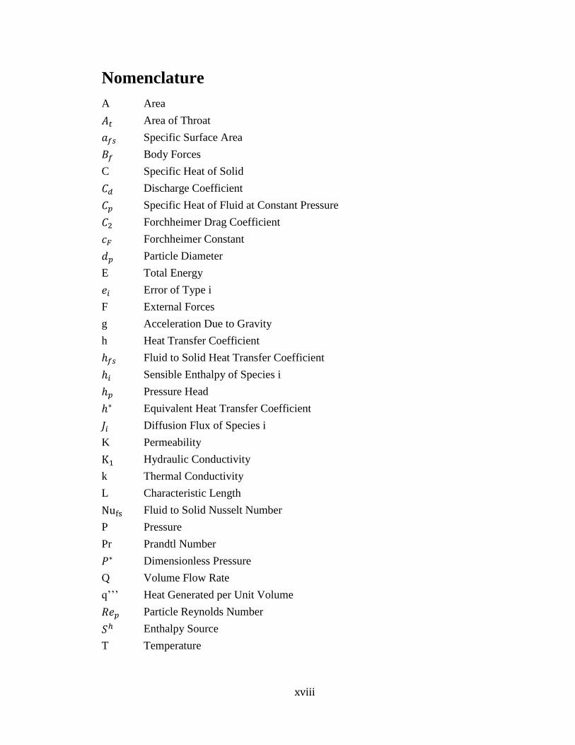
Nomenclature

A Area

Area of Throat

Specific Surface Area

Body Forces

C Specific Heat of Solid

Discharge Coefficient

Specific Heat of Fluid at Constant Pressure

Forchheimer Drag Coefficient

Forchheimer Constant

Particle Diameter

E Total Energy

Error of Type i

F External Forces

g Acceleration Due to Gravity

h Heat Transfer Coefficient

Fluid to Solid Heat Transfer Coefficient

Sensible Enthalpy of Species i

Pressure Head

Equivalent Heat Transfer Coefficient

Diffusion Flux of Species i

K Permeability

Hydraulic Conductivity

k Thermal Conductivity

L Characteristic Length

Fluid to Solid Nusselt Number

P Pressure

Pr Prandtl Number

Dimensionless Pressure

Q Volume Flow Rate

q’’’ Heat Generated per Unit Volume

Particle Reynolds Number

Enthalpy Source

T Temperature

xix

Initial Temperature

Lowest Room Temperature

T(t) Instantaneous Temperature

t Time

Instrument Error Uncertainty

Design Stage Uncertainty

Zero Order Uncertainty

Uncertainty in Function R

V Intrinsic Average Velocity

Velocity at the Throat

v Superficial Velocity

z Vertical Elevation

Geometric Heat Transfer Parameter

Ratio of Diameters

Viscosity

Equivalent Viscosity

Density

Dimensionless Temperature

Shear Stress

Porosity

Partial Derivative Operator

Del Operator

Laplace Operator

Volume

1

1. Introduction

Leamington is a municipality within Essex County, Ontario, which boasts the largest

concentration of greenhouses in North America. A number of agricultural product

handling facilities exist in the surrounding area to support the greenhouse community.

The agricultural commodities pass through various postharvest processes at the handling

facility, which can include, cooling, cleaning, sorting, and packaging. The overall care

taken in the postharvest processing stages greatly affects the resulting quality of the

produce. It is widely accepted that cooling of the agricultural product to the proper level

is paramount in maintaining produce of high quality. The importance is so great that

retail stores supplied by the product handling facilities refuse to accept produce

shipments not cooled to a sufficient level.

Clifford Produce, a local produce handling facility, has been cooling produce by placing

it in cool rooms and relying on natural convection, which requires a number of days to

achieve. The result of the long cooling time is their inability to supply certain orders, and

hence loss of revenue. This generated their interest in a rapid cooling alternative to their

current method of room cooling. Many methods of postharvest cooling are available to

the product handlers, but forced air cooling is the most popular. Clifford’s main concern

was to be able to reduce the cooling times of their produce and to be able to estimate the

expected cooling times and operating conditions of a force air cooling system for the

range of products they handle as well as investigate the relative merits of various pallet-

stacking configurations.

Mathematical models are of great use when trying to predict and understand the forced

air cooling process. Many authors have investigated the modeling of forced air cooling of

agricultural products using different approaches. In general, three modeling methods are

available, with varying computational cost for each; however, each approach is product

and configuration specific. The literature offers some guidance regarding modeling a

forced air cooling process specific to Clifford’s needs.

This thesis involves the development of a simplified numerical model using

commercially available software. The complex geometry and flow conditions inside the

2

produce containers are approximated using a porous media approach. The method is

semi-empirical as the loss coefficients associated to the specific product containers and

produce within are determined experimentally. The numerical model is then compared

with full-scale experiments and any discrepancies investigated.

3

2. Literature Review

2.1 Postharvest Cooling

Postharvest cooling was introduced to the US Department of Agriculture by Powell in

1904, as mentioned by Brosnan [1]. Postharvest cooling is also widely known as pre-

cooling. It is defined as the rapid removal of field heat from an agricultural product after

harvest [1].The purpose of this process is to reduce the respiration rate of the living

agricultural commodity. The rate of decay is proportional to the respiratory metabolism

of the product, thus; reduced respiratory rates yield longer shelf life [2]. Generally, it is

accepted that postharvest cooling is paramount in achieving long shelf life [1]. Other

positive consequences are: less water loss (wilting), reduced amounts of molds and

bacteria, and lower production of ethylene [3]. Some common methods of pre-cooling are

room cooling, forced air cooling, vacuum cooling, package icing, hydro cooling and

finally cryogenic cooling. These methods exist in many similar but different

configurations tailored to the product handler’s specific needs. The selection of the pre-

cooling method depends on the nature of the product, packaging requirements, product

flow, and economic constraints [1].

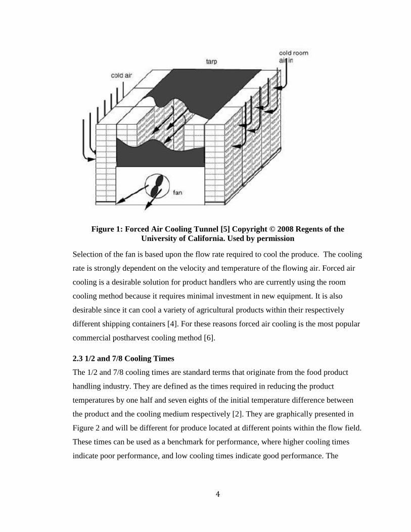
2.2 Forced Air Cooling

The forced air cooling method is a modification of the room cooling method in which the

boxes filled with produce are placed in a cold room, and allowed to cool under natural

convection conditions in relatively stagnant air. In forced air cooling, high capacity fans

pull cool air from the room directly over the product. As can be seen in Figure 1, cold air

is drawn into openings of the packaging containers and over the produce driven by the

negative (vacuum) pressure generated by an axial fan. Forced air cooling generally cools

the produce 4 to 10 times faster than room cooling [1]. Pulling the air through the

produce is recommended rather than blowing it, since the air is less susceptible to bypass

and yields more homogenous temperatures throughout [4].

4

Figure 1: Forced Air Cooling Tunnel [5] Copyright © 2008 Regents of the

University of California. Used by permission

Selection of the fan is based upon the flow rate required to cool the produce. The cooling

rate is strongly dependent on the velocity and temperature of the flowing air. Forced air

cooling is a desirable solution for product handlers who are currently using the room

cooling method because it requires minimal investment in new equipment. It is also

desirable since it can cool a variety of agricultural products within their respectively

different shipping containers [4]. For these reasons forced air cooling is the most popular

commercial postharvest cooling method [6].

2.3 1/2 and 7/8 Cooling Times

The 1/2 and 7/8 cooling times are standard terms that originate from the food product

handling industry. They are defined as the times required in reducing the product

temperatures by one half and seven eights of the initial temperature difference between

the product and the cooling medium respectively [2]. They are graphically presented in

Figure 2 and will be different for produce located at different points within the flow field.

These times can be used as a benchmark for performance, where higher cooling times

indicate poor performance, and low cooling times indicate good performance. The

5

cooling rate is dependent on the difference in the air and produce temperatures and hence

is highest when cooling begins and lowest near the end of the cooling process.

Figure 2: Cooling Curve

2.4 Modeling Approaches

It is convenient to separate the different approaches to modeling velocity and heat

transfer in forced air produce cooling into three categories: zoned, fully distributed, and

porous medium.

2.4.1 Zoned Approach

In the case of zoned modeling, the flow domain is separated into a number of regions or

zones. The desired flow variables in each zone are described using ordinary differential

equations since the air within each zone is assumed to be perfectly mixed and hence have

uniform conditions. Transport of the fluid through each zone is modeled using a plug

flow approach or by some other approximation. In the plug flow approach, the zones are

arranged in such a way that the flow moves through the zones successively as it would

physically. In the case of zoned models, only the average fluid concentrations and

6

temperatures in each zone are determined. Momentum equations are in general not

solved, but rather data for the fluid velocity is obtained experimentally [7]. Zoned models

are the least computationally expensive models, but since the airflow is based on

empirical data, it is difficult to apply these models to different package designs and

product arrangements.

Amos [8] used this type of approach, in 1995, to model the cooling of apples. Within his

research, the airflow in each zone is modeled based on the total mass flow and

proportioning coefficients based on measured velocities within product containers. It is

concluded that, further measurements were required to accurately predict the cooling of

alternative packaging systems. He states the major weakness of his modeling approach is

the description of the airflow between zones.

In 2002, Tanner et al [9] attempted to increase the generality of the zoned approach. The

authors were successful in developing a more general model by including sub-models for

heat and mass transfer. The sub-models are modified at any time without affecting each

other, which gives good flexibility. Although the generality of the zoned model approach

increased, the main drawbacks remained, namely the requirement of extensive good

quality input data for the operating conditions such as data for the external environment

and airflow between zones.

2.4.2 Fully Distributed Approach

The fully distributed models apply computational fluid dynamic (CFD) methods to solve

two-dimensional (2D) or three-dimensional (3D) equations of momentum transfer

(Navier-Stokes), mass conservation (continuity), and energy transfer (First Law of

Thermodynamics). With this method researchers are able to solve for air velocity,

temperature and humidity ratio, as well as product temperature [7]. To achieve

reasonably correct results, accurate models for effects such as turbulence and convective

heat transfer at the differential level are required as well as a large amount of computing

capacity. When modeling transport within the produce package, a complex grid system is

necessary to model the complicated geometry within the produce package.

In 2008, Ferrua and Singh [10] investigated the forced air cooling of strawberries within

their clamshell packaging with the fully distributed approach. From their computational

results, they concluded that approximately 75% of the airflow bypasses the clamshells

7

entirely. They also observed that approximately 46% percent of the air that did enter the

clamshells bypassed the strawberries entirely. This behavior is observed to increase the

heterogeneity of the temperatures of the cooled strawberries. Ferrua and Singh [11] also

conducted experiments with a simplified geometry to validate their numerical model.

They observed good agreement between their experimental and numerical results

concluding the observed differences could be explained by considering the limits of the

experimental uncertainty. The fully distributed approach can therefore be assumed to be

the most accurate approach, but also the most computationally expensive.

2.4.3 Porous Media Approach

Porous media models use a macroscopic volume-averaged approach to approximate the

complex flow phenomena throughout the produce containers. The complicated

discontinuous configuration of air space and produce within the container is modeled as a

continuous distribution of air and produce that have uniform properties. The macroscopic

continuity, momentum, and energy equations for the air and produce are solved to

determine the volume-average fluid velocity and temperature, as well as produce

temperature variation within each container. Some information is lost in the volume-

averaging process, therefore; some empirical models are needed for closure of the

equations. The empirical relationships are necessary for quantities such as the porosity,

permeability, Forchheimer constant, thermal and mass dispersion, and interfacial heat

transfer coefficient [7]. The porous media approach removes the need to generate

complex meshes to describe the complicated geometry associated with produce in its

container. Instead, a more simple structured mesh can be used. In general, the porous

media approach is more computationally expensive than the zoned approach but less

expensive than the fully distributed approach.

The use of the porous media model to simulate forced air cooling of agricultural produce

was first introduced by Talbot [12] in 1988. The author used commercial finite element

software to model the pressure drop and velocity within a container containing oranges.

Experiments were also conducted by Talbot to validate the numerical model. Although

Talbot observed significant disagreement between numerical and experimental

temperatures, he concludes that the porous media model coupled with the appropriate

8

heat transfer model is a valuable tool that can be used on practically any configuration

concerning forced air cooling of agricultural products.

Another attempt at modeling forced air cooling of agricultural produced was made by Xu

and Burfoot [13] in 1998. The authors conducted a 3-D numerical analysis on the forced

air cooling of potatoes. They compared their numerical results with the experimental

results of Misener and Shove[14] from 1967. Good agreement between their numerical

and the experimental results was found with differences of up to 1.4°C. The numerical

model also included moisture transfer and was able to simulate the total produce weight

loss by drying to within 4.5% of the experimental results.

In 2006, Verboven et al.[15] conducted a review on advances in modeling the transport

phenomena in refrigerated food bulks, packages, and stacks. The authors summarized the

strengths and weaknesses of recent approaches taken by various researchers. Within their

summary, the authors state that few researchers have addressed the package itself

(containing the produce) as a source of resistance to the airflow. Their summary

concluded that great care is required in order to successfully implement a porous media

model to simulate forced air cooling of agricultural produce. Transport phenomena are

complicated for many reasons including variations in size and shape of the products,

venting of packages, and the presence of turbulence. They also mentioned the popularity

of direct numerical simulations (fully distributed approach) as they offer valuable

fundamental understanding of the underlying process, but at a significant computational

cost.

2.5 Historical Background of the Porous Media Model

Henry Darcy published a report in 1856 regarding the construction of a municipal water

system in Dijon, France [16]. Within the report is a relationship for the flow rate of water

through sand filters similar in form, but symbolically different than Equation 1.

( )

(1)

In this equation, Q is the volume flow rate and, A is the cross-sectional area of the sand

filter. K1 is the hydraulic conductivity of the sand and, L is the distance between the two

pressure taps used to measure the pressure difference. The symbol represents the

pressure head while z is the vertical elevation. The most notable parameter in Equation 1

9

is the hydraulic conductivity K1, which requires experimental determination. Darcy

conducted careful experiments using a vertical steel column filled with sand as

schematically shown in Figure 3. The column was instrumented with mercury

manometers to measure the pressure head. The volume flow rate was determined by

measuring the total volume that was collected in the basin and dividing it by the total

experiment time.

Figure 3: Darcy’s Experiment

Darcy used this data and equation to determine the hydraulic conductivity of the sand

filter and validate his newly discovered equation which forms the basis of the porous

media model [17].

2.6 Porous Media in Detail

In general, a porous medium consists of a solid matrix with voids that are interconnected.

In most, but not all cases, the solid matrix is rigid. The network of voids or pores allows

for the transport of one or more fluids. Some examples of naturally occurring porous

media include sand, limestone, and the human lung [18].

10

2.6.1 Microscopic vs Macroscopic

The microscopic approach to analyzing flow through a porous media is to consider every

void and obstruction in the flow domain. Modeling with the microscopic approach

involves solving the equations of motion for the flow variables within the voids. The

voids in this approach are generally irregular, and if the flow domain is large and

considers many voids, the solution becomes computationally expensive [18].

Alternatively, the macroscopic approach involves determining a representative

elementary volume (REV) seen in Figure 4. The entire flow domain then takes on the

properties of the REV and the porous media equations solved to obtain the flow

variables. Experimentally measured flow variables are averages of the values over areas

that cross many pores much like the REV. These flow variables are considered to be

continuous with respect to space and time [18]. The macroscopic approach involves the

loss of some information on the pore scale, but has the advantage of being less

computationally expensive than the microscopic approach.

Figure 4: Porous Media [18]

2.6.2 Porosity

The porosity, , is defined as the ratio of void volume in the REV to total volume of the

REV as described in Equation 2.

(2)

11

It follows that is the ratio of solid matrix to total volume of the REV. In the case

that the porous medium is isotropic, the porosity can be calculated as the ratio of void

area divided by the total area.

2.6.3 Darcy Velocity

A continuum flow model is created with a Cartesian reference frame based on the

macroscopic REV approach. It is assumed that the volume elements are sufficiently large

compared to void volumes to yield reliable volume averages. Simply put, the porosity is

independent of the choice of the location of the REV within the flow domain [18]. When

averages of the variables are taken with respect to the medium (both solid and fluid),

those variables are denoted with a subscript m. Similarly, if the average of the variable is

taken with respect to the fluid only, those variables will be denoted with the subscript f.

In the case of a single phase fully immersed porous medium, the void volume can be

denoted as . Equation 1 divided by the total cross-sectional area of the porous material

results in a velocity. In Darcy’s experiments the area is defined as the cross-sectional area

of the column. This means that the resultant velocity represents the volume average

velocity with respect to the medium. In general, the velocity can be a vector of three

components. The velocity has been given different names by many authors including,

seepage velocity, filtration velocity, superficial velocity, Darcy velocity, and volumetric

flux density. The terms Darcy and superficial velocity are employed in this thesis. It is

important to note that the Darcy velocity does not represent the velocity of the fluid

within the voids of the porous medium. The intrinsic average velocity of the fluid,

more accurately represents the true velocity of the fluid flowing within the pores. The

Darcy velocity and the intrinsic average fluid velocity are related using the Dupuit-

Forchheimer relationship given by Equation 3 [18].

(3)

2.6.4 Continuity

With the continuum in mind, the usual arguments are applied to derive differential

equations to express the conservation laws. One such equation is the conservation of fluid

mass or continuity equation represented by Equation 4.

( ) (4)

12

The density of the fluid is denoted by . Equation 4 is derived using an elementary unit

volume of the medium and equating the rate of increase of the fluid mass within that

volume

, to the net mass flux into the volume ( ). It is important to note that

the porosity is assumed to not be a function dependent on time.

2.6.5 Darcy’s Law

In the current literature, Darcy’s Law for one-dimensional flow through a differential

element is typically represented as seen in Equation 5 [18].

(5)

Equation 5 is very similar to Equation 1 if Darcy’s column is to be considered to be lying

on its side, depicted in Figure 5. In such a case, the z terms cancel because there is not a

change in elevation and the velocity is in the x direction.

Figure 5: Horizontal Flow in a Porous Medium

In the current version of the equation ⁄ represents the pressure gradient in the x

direction. If the pressure gradient is constant, it is equal to ,

and is L. Since is equal to

⁄ the permeability is equal to µK1/ρg. The more

recent form of Darcy’s Law is independent of the properties of the fluid and hence,

depends only on the nature of the medium. When considering Darcy’s law in three

dimensions, Equation 6 takes the form seen in Equation 6 [18].

(6)

L

Q

hp2

hp1

x

z

A

13

Equation 6 represents the case where the permeability is anisotropic in which case is a

diagonal tensor. Alternatively, in the case where the porous medium is isotropic Equation

6 simplifies to Equation 7.

(7)

The term on the right hand side of Equation 7 is known as the Darcy term. Many authors

have conducted experiments and have verified Darcy’s law.

2.6.6 Forchheimer’s Equation

In Darcy’s Equation 7, the pressure gradient is linearly related to the Darcy velocity. This

relationship is valid only if the superficial velocity is sufficiently small. The velocity is

considered to be sufficiently small if the particle Reynolds number is of the order of unity

or less. The particle Reynolds number is defined much like the general Reynolds number,

where the length scale is the diameter of the particle seen in Equation 8.

(8)

As the particle Reynolds number increases past unity and up to 10, there is a smooth

transition from linear pressure drop to quadratic pressure drop. It is important to note that

this transition is not a laminar to turbulent transition, since the Reynolds numbers are still

quite small. It is believed that the transition is due to the form drag from the solid

obstacles being comparable, in magnitude, with the surface drag due to friction [18]. At

higher particle Reynolds numbers it is advisable to use a modification of Darcy’s

equation seen in Equation 9 known as Forchheimer’s equation.

| | (9)

In Equation 9, is a dimensionless form drag constant also known as the Forchhiemer

constant. Following the previously stated convention, represents the density of the

fluid. The second term on the right side of Equation 9 is referred to as the Forchhiemer

term. Equation 9 correlates well with experimental data.

14

2.6.7 Brinkman’s Equation

Another modification of Darcy’s equation is known as Brinkman’s equation seen in

Equation 10.

(10)

The second term on the right hand side of Equation 10 is known as the Brinkman term

and is analogous to the Laplacian term seen in the Navier-Stokes equation. The symbol

represents the effective viscosity. Brinkman equates to , but this should not be the

case in general. In general, the relationship of depends on the geometry of the

medium and can be greater or less than unity. It is believed that Brinkman’s equation

should be restricted to cases where the porosity is greater than 0.6[18]. There has been

limited research in the validation of Brinkman’s equation. For many practical purposes,

the inclusion of the Brinkman term is not needed. The Laplacian term is however

required if one aims to model the no-slip boundary condition.

2.6.8 Energy Equation

In order to model changes in temperature the equation for energy or first law of

thermodynamics must be included in the solution. The equation must be written

separately, for each of the solid matrix and fluid phase(s). Within this work, it will be

assumed that the porous medium is isotropic and radiation, viscous dissipation, and

pressure work are negligible.

2.6.9 Local Thermal Non-Equilibrium

If it is required to model the heat transfer between the solid and fluid, then they must not

be in thermal equilibrium. In such cases, the energy balance for the solid and fluid can be

described by Equations 11 and 12 respectively.

( )

(11)

( )

(12)

In the above equations, the subscripts s and f describe the solid matrix and fluid phase

respectively. The specific heat of the solid is represented by the symbol C, similarly,

15

represents the specific heat of the fluid at constant pressure. As usual k represents the

thermal conductivity, and finally q’’’ is the heat generated per unit volume. It is

important to recognize the term in Equation 12, which describes the

convective heat transfer of the fluid. On the right side of both equations is the term h,

which is the heat transfer coefficient. The above equations are also commonly known as

the two-equation energy model for porous media. When considering the use the two-

equation model the correct determination of h becomes paramount.

2.6.10 Heat transfer coefficient

The heat transfer coefficient in Equations 11 and 12 can be determined by an empirical

relationship, starting with Equation 13.

(13)

In the above equation represents the specific surface area defined by Equation 14,

which is dependent on the geometric nature of the porous medium.

(14)

According to Dixon and Cresswell the correct determination of is based on a lumped

parameter model defined by Stuke as given in Equation 15 [19].

(15)

In this equation is a dimensionless constant, the value of which depends on the shape of

the particle. The value of equates to 10, 8, and 6 for spheres, cylinders, and slabs

respectively [19]. Finally, in the above equation denotes the fluid to solid heat transfer

coefficient, which is related to the fluid to solid Nusselt number by the relationship given

by Equation 16.

(16)

There have been many attempts at determining an empirical relationship for .

Handley and Heggs had developed the relationship seen in Equation 17 [20].

(17)

16

This equation correlates well with experimental data at particle Reynolds numbers above

100. An alternative to the above equation has been suggested by Wakao and Kaguei, seen

in Equation 18[21].

(18)

Both above equations have the shortcoming of offering limited confidence at lower

Reynolds numbers. Kothari has developed a relationship seen in Equation 19 that

depends only on the Reynolds number [22].

(19)

The above relationship is applicable in the lower Reynolds number range from

approximately 1 to 100. It is therefore, recommended to use relationships offered by

Handley and Heggs or Wakao and Kagei at higher Reynolds numbers flows and

Kothari’s equation at lower Reynolds number flows.

2.6.11 Concept of a Porous Jump

A Porous jump is a one-dimensional simplification to the porous media model,

where the same equations are solved but the pressure drop occurs suddenly across

a boundary. In such a case, the length of the porous medium is specified to

determine the total pressure drop. Porous jumps are used whenever possible due

to their simplicity; however, cannot be used to model pressure gradients or heat

transfer within the porous medium.

2.7 Problem Statement and Research Objectives

In this thesis, a specific cooling tunnel configuration is modeled using porous media

theory combined with computational fluid dynamics. An instrumented experimental

tunnel is then constructed and tested to evaluate the numerical model. The configuration

of the cooling tunnel investigated is shown in Figure 6. It consists of four pallets of

agricultural product, two walls, one industrial vane axial fan, and a tarp. The entire

configuration resides in a cool room kept at a temperature of 10 .The pallets are

separated into two groups of two pallets each with a gap equivalent to the width of one

17

pallet between them, forming a tunnel between the pallets. The fan causes a low pressure

within the tunnel, pulling air through the boxes and over the produce. The solid walls and

tarp restrict the airflow from entering in certain directions in order to pull cool air from

the room through the openings in the sides of the product boxes into the tunnel, and

finally out through the fan. The size of the produce boxes and stack layer configuration

depend on the type of produce considered. This potentially introduces complex flow

networks within each stacked layer of product. In the case of the large cucumbers

considered initially, each box was 0.299m by 0.413m by 0.108m in size and contained 12

large cucumbers.

Figure 6: Tunnel Configuration [23]

The specific objectives of this study are to

1. develop a simple two dimensional numerical model for the approximation of the

transient temperature variation of agricultural produce in a forced air cooling

tunnel.

2. construct a cooling tunnel test facility and conduct full scale experiments to

determine the validity of the assumptions made and the accuracy of the numerical

model.

18

3. identify and investigate improvements to the numerical model

4. modify the constructed cooling tunnel test facility to investigate an alternate

configuration.

2.8 Layout of the Remainder of the Thesis

Firstly, the details of the numerical model and its solution are described in Chapter 3.

Results of the initial numerical solutions are presented and discussed in Chapter 4. This

followed by a description of the experimental apparatus and procedures in Chapter 5

along with experimental results. Chapter 6 contains a description of a modified numerical

model which includes adjustments made which are required to allow a fair comparison of

the numerical and experimental results. The comparison of the two sets of data is

presented in Chapter 7 and an investigation of the effects of air leakage given in Chapter

8. An alternate tunnel configuration is presented in Chapter 9. Also included is a

comparison of the numerical and experimental results for that configuration along with a

discussion on the relative performance of each configuration. Chapter 10 includes a

discussion of the accuracy of all the numerical models. Conclusions and

recommendations for future work are made in Chapter 11.

19

3. Numerical Methodology

The numerical models are constructed and solved using commercially available

computational fluid dynamic software; namely ANSYS Fluent 14. Details of flow

assumptions, geometry, boundary and initial conditions, solution grid, and governing

equations are presented in the following sections. All results have been computed using

an Intel(R) Core™ i7 CPU [email protected] processor, equipped with 12 GB RAM, and a

64-bit operating system.

3.1 Flow Assumptions and Geometry

The first assumption made is that of incompressible flow. This notion is reasonable for

the relatively low velocity magnitudes expected. Secondly, there is no flow between the

layers of stacked produce. It is also assumed that there is little to no difference between

the flow patterns in each respective layer of boxes. Although there is an obvious

geometrical difference between the flow field in the horizontal plane of the top and

bottom layers of boxes due to the location of the fan, it is anticipated (and later verified)

that the pressure distribution is approximately uniform at the inlets and outlets of each

stack of product. The benefit of such an assumption is the ability to use the simplified

two-dimensional formulation, which greatly reduces computational cost. Lastly, it is

assumed that there is a negligible difference in the flow patterns within the two respective

groups of product stacks on either side of the tunnel space. This allows the use of a

vertical symmetry plane through the center of the tunnel that essentially splits the tunnel

and computational domain in half.

Preliminary experiments, the details of which can be found in Appendix B, indicate that

the bulk of the flow resistance is due to the produce containers openings (vent-holes).

The internal produce provides a smaller contribution to the flow resistances. It is also

important to note that these resistances are dependent on the direction of flow (front to

back or side to side) through the container, meaning the losses are anisotropic. Based on

these findings, the product container vent-hole openings and contained produce are

modeled using porous jumps, and anisotropic porous media respectively. The container

opening shapes, number and location are different at the ends compared to the sides. In

many cases when the boxes are arranged in layers to fit onto the pallet, the openings will

20

not coincide, essentially creating a wall. An example of when the container openings do

not coincide can be seen in Figure 7. In the figure, blocked holes are represented with

red areas, and unblocked holes as green areas. Each different type of agricultural product

offered by the industrial partner is packaged in different containers, therefore; offering

different layer arrangements.

Figure 7: Container Opening Alignment

3.2 Boundary and Initial Conditions

Based on the flow assumptions, a 2-D flow field can be generated representing the pink

area seen in Figure 8. The 2-D geometry and boundary conditions, for one layer of large

cucumbers, can be visualized with the aid of Figure 9. In the figure, red lines and grey

filled areas respectively represent the porous jumps and porous media. The porous media

is assumed to be at a uniform initial temperature of 28 . Walls are shown with black

lines, with the simple boundary condition assumption of adiabatic walls with the no slip

condition imposed. The blue line represents the pressure inlet assumed to be at standard

atmospheric pressure with a constant temperature of 10 . The zones not occupied by the

produce contain air depicted as white filled areas. A velocity outlet is used to simulate the

effect of the vane axial fan, which is illustrated as a green line. The magnitude of the

velocity at the outlet is based on the total desired flow rate of air through all the boxes

21

filled with produce. Lastly, the yellow line indicates the plane of symmetry between the

two groups of pallets.

Figure 8: Resultant 2-D Flow Field

Figure 9: Initial Boundary Conditions

3.3 Solution Grid

A quadrilateral block structured format is implemented to mesh the flow domain as this

gives accurate solutions near walls, and it requires less computational effort compared to

other mesh types of the same spatial resolution. A dual cell mesh is employed within the

Legend:

Pressure Inlet

Porous Jumps

Walls

Velocity Outlet

Symmetry Plane

Air

Porous Medium

22

porous media zones in order to take advantage of the non-equilibrium thermal model. A

coincident mesh must be created for both the solid matrix and fluid, on which the

corresponding energy equation will be solved (recall Equations 18 and 19). This feature

has been made available in ANSYS Fluent 14.0, released in December 2011.The material

properties of the solid matrix and fluid must be specified within the model. The

properties of the agricultural product were assumed to be those of water, since the

produce considered is composed primarily of water [24]. Initially the solid matrix is

assumed to be at a uniform temperature of 28 . Figure 10 shows the numerical grid,

generated using GAMBIT, and used in numerical calculations.

Figure 10: Mesh Generated with GAMBIT

3.4 Governing Equations

In order to simulate the transient temperature pattern within the porous medium, some

parameters associated with the mathematical model need to be specified. A discussion of

these parameters and the governing equations that are required to achieve an accurate

simulation of the physical behavior of the produce cooling tunnel is given in this section.

23

3.4.1 Porosity

The numerical solution requires that the porosity of the medium be specified. In the

specific case considered, the void volume is determined by subtracting the volume

occupied by the produce from the total volume of the box. The volume occupied by the

produce is manually determined based on the total weight of the product in each

container and the specific weight of the produce. Knowing the void volume and total

volume of the box the porosity can easily be specified with the use of Equation 2. In this

specific case, the porosity is calculated to be 0.522.

3.4.2 Continuity

Within the ANSYS Fluent user guide, the continuity equation for a single-phase flow

through porous media, with isotropic porosity, is defined using Equation 20.

( ) (20)

In the above equation, V represents the intrinsic average velocity, or the physical

velocity. When the porosity is assumed constant with time and the Dupuit-Forchhiemer

relationship (Equation 3) is employed, Equation 20 becomes equal to Equation 4.

3.4.3 Momentum

The standard linear momentum equation takes the form found below.

( ) ( ) (21)

In the above equation, on the left hand side, the accumulation and convection terms

( ) and ( ) can be found respectively. The right hand side of the equation

consists of, , the stress tensor, , the gravitational body force, and , any other

external body forces. The term is used to include other model dependent source terms,

including terms associated to the porous media model. When the model dependent source

terms for porous media are included in Equation 21, it takes the form seen in Equation

22.

( ) ( )

*

| | + (22)

24

In this equation includes all body forces, including gravitational, and the last two

terms within the square brackets represent the viscous and inertial drag forces caused by

the pore walls. The porosity appears in Equations 20 and 22 to account for the fact that

the fluid only occupies the volume of the pores while the model assumes that it fills the

entire volume. The permeability, , and the Forchhiemer drag coefficient, , require

empirical determination. The details of the experiment conducted to determine the porous

medium empirical constants is presented in Appendix B. When the fluid flow is steady,

the porous medium geometrically fixed, body forces are negligible and no macroscopic

velocity gradients, Equation 22 reduces to a form consistent with Equation 9 [25]. In

order for Equation 22 to reduce exactly to that of Equation 9 from Equation 22 would

have to be equal to √ ⁄ from Equation 9.

The specified coefficients depend on the flow direction being in the long or short

direction of the product container. For the case of the porous medium in the long

direction (ie: flow through the short ends), the viscous resistance (K) and the inertial

resistance ( ) are and respectively. In the short direction (ie:

flow through the long ends) of the product container the viscous resistance (K) and

inertial resistance ( ) of the porous medium are and

respectively. Although the viscous resistance is negative, which is unrealistic,

the inertial resistance dominates, therefore; the combined behavior is that of a momentum

sink. The porous jump coefficients are specified in the same manner. The porous jump

coefficients (K and ) for the long and short directions are and

and and respectively. In both cases the length of

the porous jump is specified as , which is the measured thickness of the cardboard

container. Details of how the porous medium and porous jump coefficients are obtained

can be found in Appendix B.

3.4.4 Energy and Heat Transfer

In order to simulate convective heat transfer from the solid agricultural product to air

passing around it, the use of the non-equilibrium thermal model is required. The two-

equation non-equilibrium energy equation takes the form found in Equations 23 and 24,

for the solid and fluid phases respectively.

25

[ ] [ ]

( ) (23)

( ) [ ( )]

[ ∑ ] ( ) (24)

In the above equations denotes the total energy, and represents the enthalpy source

term, with the usual subscripts for the solid or fluid phase. In Equation 24, represents

the diffusion flux, and represents the sensible enthalpy, of species . The density of the

solid, , and the density of the fluid, , are specified as 998.2 ⁄ and

1.225 ⁄ respectively. If one chooses to neglect enthalpy transport due to species

diffusion, and any thermal energy created by viscous shear flow, Equations 23 and 24

become similar to Equations 11 and 12. When the incompressible flow assumption is

applied, pressure work and kinetic energy within the total energy term become negligible,

Equations 23 and 24 become equal to Equations 11 and 12 respectively.

The time variation of temperature within the porous medium, the appropriate empirical

heat transfer model for each Reynolds number range needs careful attention for accurate

simulation. The available relationships between the Nusselt number and the particle

Reynolds number for Wakao and Kagei [21], Handley and Heggs [20] and Kothari [22]

are graphically presented in Figure 11. In this figure, the intersection points of Kothari’s

correlation with the other two are calculated and plotted on the curve. The Reynolds

Numbers at the points of intersection are found to be 80.5and 147.1 for the relationships

offered by Handley and Heggs, and Wakao and Kagei respectively. Within this work, the

relationships used are those of Kothari and Handley and Heggs for low and high

Reynolds numbers respectively. The relationship given by Wakao and Kagei gives

elevated Nusselt Number compared to that from Handley and Heggs from Figure 11.

Therefore, the relationship given by Handley and Heggs is used, and the relationship

given by Wakao and Kagei is not, since in general, the numerical models will be shown

later to over predict the heat transfer.

26

Figure 11: Nusselt Number Correlations with Particle Reynolds Number

3.5 Numerical Solution

The governing equations are solved sequentially using the pressure based segregated

solver for each cell. The “SIMPLE” method is used for pressure velocity coupling.

Pressure discretization is achieved using the standard method available in Fluent and the

standard model is used to model the turbulence. The default order of the

discretization schemes are chosen as follows. Second order upwind schemes are used for

momentum and energy while first order upwind schemes are used for turbulent kinetic

energy and dissipation rate. Lastly, first order time advancement is used, with a time step

size of 1 second (s), since time step sizes of one-half that amount gave essentially the

same result and the overall computational time was of an acceptable value. It is believed

that the default discretization orders offer a balance of numerical diffusion and

dispersion. In general, first order methods offer lower computational cost at the expense

of lower accuracy; however, solutions generated using all second order methods gave no

noticeable difference in the results.

27

4. Numerical Results of the Initial Model

The initial numerical model is solved and the results are presented as follows. Firstly, the

velocity and dimensionless vacuum pressure distributions throughout the flow field are

considered followed by the 7/8 cooling time distribution. The time dependent

dimensionless temperature is then investigated at locations that have the shortest and

longest 7/8 cooling time. Finally, the temperature distribution throughout the entire flow

field corresponding to that at the instant in time when the last point in the entire amount

of agricultural product has reached the 7/8 cooling temperature is presented.

4.1 Non-dimensional Analysis

In the post processing of numerical and experimental results, normalization of some flow

variables is implemented. The normalization technique used is a max-min type

normalization within the range of 0 to 1 [26]. The standard equation for this type of

technique is given in Equation 25.

(25)

The static pressure and temperature are normalized using this technique. The static

pressure is normalized in order to make more appropriate comparisons of the numerical

and experimental models. In the case of the temperature of the produce the seven eights

and half-cooling temperatures correspond to dimensionless temperatures of 0.125 and .5.

This makes it easy to identify the seven eights and half cooling time on a plot of

dimensionless temperature versus time. Normalization of other variables such as the

velocity and heat transfer coefficient do not provide the same benefits and therefore, are

not conducted.

4.2 Dimensionless Vacuum Pressure and Velocity Magnitude Distribution

Although the initialized values of pressure and velocity throughout the flow field are

taken to be 0 Pa (gauge) and 0 m/s respectively, their values at the end of the first time

step are already those of the steady state. This is due to the widely differing time scales of

the flow and thermal characteristics because of the incompressible nature of the flow.

These values remain constant throughout the remainder of the cooling period.

28

The computed dimensionless vacuum pressure, , variation within the flow field is

shown in Figure 12. In this equation the minimum pressure is standard atmospheric

pressure (0 Pa gauge), and the maximum pressure is the maximum vacuum pressure

(tunnel pressure gauge). The influence of the porous jumps can be seen to be dominant

since the pressures within each box are relatively uniform. The variation of the pressures

in the boxes with their long dimension vertical (henceforth referred to as "vertically

oriented") compared to those with their long dimension horizontal (henceforth referred

to as horizontally orientated) is due to the difference in the porous jump coefficients, and

the influence of the air space in the center of each pallet.

(26)

Figure 12: Contours of Dimensionless Vacuum Pressure from the Initial Solution

The small pressure variation in the tunnel region is not apparent in Figure 12 due to its

relatively low variation in magnitude compared to that seen across the boxes of produce.

The pressure variation within the tunnel portion of the flow field is clearer in Figure 13.

From these results, it can be seen that the variation of the pressure acting on the boxes is

relatively low (less than 5% difference). The minimum pressure of -138 gauge occurs at

the region of separation where the fluid is flowing around a sharp edge into the fan.

𝑃

29

Figure 13: Contours of Dimensionless Vacuum Pressure in the Tunnel Region from

Initial Solution

Results for the contours of the velocity magnitude are presented in Figure 14. It is

important to note that these contours represent the magnitude of the superficial velocity

within the region of the produce boxes. These velocities are consistent with the static

pressure variation. The area weighted average velocity of the horizontally and vertically

oriented boxes are used to calculate the heat transfer coefficient used in the transient

simulation. A sample of these calculations can be found in Appendix C.

Figure 14: Velocity Magnitude Contours from the Initial Solution

𝑃

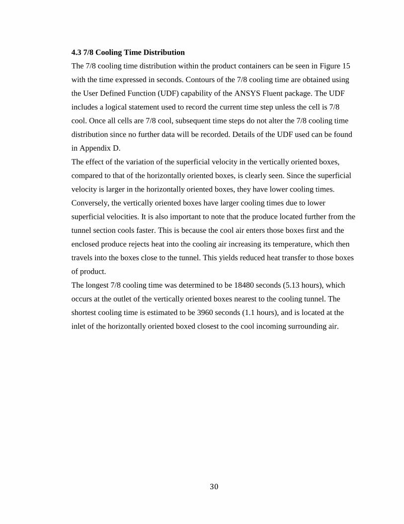
30

4.3 7/8 Cooling Time Distribution

The 7/8 cooling time distribution within the product containers can be seen in Figure 15

with the time expressed in seconds. Contours of the 7/8 cooling time are obtained using

the User Defined Function (UDF) capability of the ANSYS Fluent package. The UDF

includes a logical statement used to record the current time step unless the cell is 7/8

cool. Once all cells are 7/8 cool, subsequent time steps do not alter the 7/8 cooling time

distribution since no further data will be recorded. Details of the UDF used can be found

in Appendix D.

The effect of the variation of the superficial velocity in the vertically oriented boxes,

compared to that of the horizontally oriented boxes, is clearly seen. Since the superficial

velocity is larger in the horizontally oriented boxes, they have lower cooling times.

Conversely, the vertically oriented boxes have larger cooling times due to lower

superficial velocities. It is also important to note that the produce located further from the

tunnel section cools faster. This is because the cool air enters those boxes first and the

enclosed produce rejects heat into the cooling air increasing its temperature, which then

travels into the boxes close to the tunnel. This yields reduced heat transfer to those boxes

of product.

The longest 7/8 cooling time was determined to be 18480 seconds (5.13 hours), which

occurs at the outlet of the vertically oriented boxes nearest to the cooling tunnel. The

shortest cooling time is estimated to be 3960 seconds (1.1 hours), and is located at the

inlet of the horizontally oriented boxed closest to the cool incoming surrounding air.

31

Figure 15: Seven Eights Cooling Time Distribution

4.4 Tunnel Minimum and Maximum 7/8 Cooling Times

The dimensionless produce temperature versus time corresponding to the region of

minimum and maximum 7/8 cooling time can be seen in Figure 16. The dimensionless

temperature is defined in Equation 27.

(27)

The dimensionless temperature is calculated knowing the instantaneous

temperature , initial temperature , and final temperature . In this simple case, the

final temperature is the same as the constant room temperature.

[s]

32

Figure 16: Limits of Product Temperatures

The shortest time case is important since it indicates the largest rate of heat rejection from

the produce. Excessively high rates could potentially result in damage to the agricultural

product. The longest cooling time is important as well, since it indicates how long the

cooling tunnel is required to run. All other points in the flow field fall between the curves

for shortest and longest cooling times.

4.5 Product Temperature Distribution at End of Cooling

Contours of the dimensionless temperature within the produce at the largest 7/8 cooling

time are shown in Figure 17. The variation of the dimensionless temperature in Figure 17

is from fully cool to seven eights cool, with corresponding values of 0 and 0.125

respectively. This figure is helpful to see which areas are fully cooled to the surrounding

room temperature once all the produce is at least 7/8 cool. From the figure, it can be seen

that the horizontally oriented boxes are almost all fully cooled by the time all the produce

is 7/8 cool.

33

Figure 17: Dimensionless Temperature Contours in Produce When All Produce is at

Least 7/8 Cool

4.6 Summary and Discussion of Initial Model Simulation Results

The initial 2D numerical model, with symmetric flow, no flow between layers, uniform

initial temperature, and constant room temperature using the porous medium approach

has successfully been implemented using typical values for the initial and boundary

conditions. The simulations are valuable in identifying zones of fast and slow cooling and

in characterizing the homogeneity of the process. In spite of the simplifying assumptions

and approximations, the model yields reasonable results compared to cooling times seen

in industry [4].The numerical results are verified to be consistent with the porous medium

and jump coefficients supplied to the computational software.

34

5. Experimental Study

In order to validate the numerical model, full-scale experiments are performed. The

experiments are conducted at the industry partner’s facility during production hours

within a cool storage room. The experiments allow for an evaluation of the numerical

model to determine areas requiring improvements.

5.1 Experimental Facility

The experimental facility consists of four pallets each having 13 layers of boxes

containing field heated agricultural product as previously depicted in Figure 6. The air is

restricted to enter only the outer face of the pallets by using two self-standing portable

walls in the front and back, and a tarp on top. Foam seals are used between pallets and

boxes in order to reduce air bypass (short-circuiting). In order to pull the air through the

pallets, a 24-inch diameter, direct drive, 8-blade cast aluminum propeller, Twin City

WPD-24-E8-24 vane axial fan is mounted to the front wall. The back wall is equipped

with a bypass door in order to have control over the negative (vacuum) pressure of the

tunnel. Details on the fan selection and drawings of the prototype cooling tunnel can be

found in Appendix E.

The test produce used in the experiments consisted of medium size cucumbers because

they were the only agricultural product with sufficient quantity and field heat available

during the time allocated for testing. A picture of the experimental setup is presented in

Figure 18. The visible pallets in the figure are referred to as the right pallets, while the

other pallets (on the far side) are referred to as left pallets. The pallets on each side are

numbered with pallet 1 being closest to the fan side of the cooling tunnel, and pallet 2

being further from the fan side.

35

Figure 18: Experimental Facility

The experiments are performed in a large cooling room located within the production

facility of the industrial partner. The cooling room is 21.5m long, 11m wide and 5m tall.

The room is kept at the desired holding temperature with four refrigeration units, also

seen in Figure 18.

5.2 Product Configuration

It is important to note that the arrangement for medium cucumbers is not the same as the

arrangement for large cucumbers seen in the initial numerical investigation. The size of

the medium cucumber box is 0.283m by 0.384m by 0.108m and contains approximately

12 medium cucumbers. The 13 layers of boxes in each pallet are configured in the same

pattern, each of which contained 10 boxes of medium cucumbers. Figure 19 depicts the

box configuration for each layer used in the medium cucumber case.

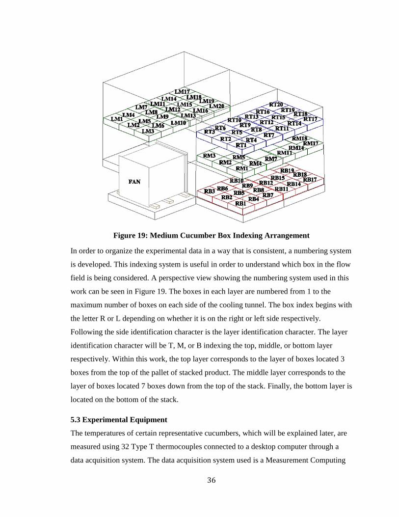
36

Figure 19: Medium Cucumber Box Indexing Arrangement

In order to organize the experimental data in a way that is consistent, a numbering system

is developed. This indexing system is useful in order to understand which box in the flow

field is being considered. A perspective view showing the numbering system used in this

work can be seen in Figure 19. The boxes in each layer are numbered from 1 to the

maximum number of boxes on each side of the cooling tunnel. The box index begins with

the letter R or L depending on whether it is on the right or left side respectively.

Following the side identification character is the layer identification character. The layer

identification character will be T, M, or B indexing the top, middle, or bottom layer

respectively. Within this work, the top layer corresponds to the layer of boxes located 3

boxes from the top of the pallet of stacked product. The middle layer corresponds to the

layer of boxes located 7 boxes down from the top of the stack. Finally, the bottom layer is

located on the bottom of the stack.

5.3 Experimental Equipment

The temperatures of certain representative cucumbers, which will be explained later, are

measured using 32 Type T thermocouples connected to a desktop computer through a

data acquisition system. The data acquisition system used is a Measurement Computing

37

24-bit, isolated, high channel count multifunction DAQ module (USB-2416), coupled

with an analog input expansion module (USB-EXP32). The room relative humidity is

also monitored using a Honeywell HIH-4021-003 humidity sensor. The humidity sensor

is also connected to a separate identical multifunction DAQ. Pressures are measured

using a handheld electronic manometer (Omega Model HHP-103), and recorded

manually.

5.4 Data Acquisition

The multifunction DAQ is situated in the cold room and connected to computer via USB.

National Instruments data acquisition software (LabVIEW) is used to record all data. The

analog input data from the DAQ is converted into the desired units and saved on a 5

second interval. LabVIEW is also used in order to be able to monitor the temperatures in

real-time. Details of the virtual instruments used in this work is contained in Appendix F.

5.5 Instrumentation Procedure

Instrumentation of boxes during the production process (original loading of the boxes and

pallets) is not possible, as it would slow down production. Pallets of medium cucumbers,

stacked in the appropriate arrangement ready for shipment, are then arranged in the

cooling room in the desired cooling tunnel configuration. Partial disassembly of the

stacks is required in order to instrument the boxes. Each of the pallets requiring

instrumentation is disassembled to the bottom layer to be instrumented with the required

thermocouples and Tygon® tubing as needed. For temperature measurement, the

thermocouples are either placed under the plastic protective layer on the cucumber for

surface temperature measurement, or inserted into the middle of the cucumber by

puncturing the cucumber with the thermocouple, for core temperature measurement.

Locations RM12, RM15, and RM20 (see Figure 19) are instrumented with both core and

surface mounted thermocouples. The room is also instrumented with a thermocouple.

Tygon® tubing ends are situated in the boxes in regions of low air velocity so that an

accurate pressure measurement can be taken. Pressures are recorded in the boxes located

in the right middle layer (RM) locations mostly, but are also placed in locations LM20,

RT2, and RB20 in order to evaluate assumptions made in the numerical model. The

38

pallets are then rebuilt to original configuration from the bottom up with included

instrumentation as required.

5.6 Experimental Procedure

Once the boxes are instrumented, the tarp is pulled over the top of the pallets, and the

foam installed to achieve a good seal. The axial fan is then started which produces a

vacuum pressure in the tunnel. The desired vacuum tunnel pressure is achieved by

adjusting the bypass door on the back wall of the tunnel. The value is then recorded and

the data acquisition system started in order to collect the data. Pressure readings are

manually recorded for the boxes instrumented with Tygon® tubes. These pressure

readings are taken at approximately 60 minute intervals to ensure that the flow conditions

remain constant.

It is important to mention that, in some cases, the overall testing time was restricted

because that testing was performed during the industrial partner’s normal production

hours. It is also important to note that during the testing period forklifts and personnel

were sometimes actively present in the cooling room, which may have a minor effect on

the results.

5.7 Experimental Results

In the following section, results from the full-scale experiment are presented. First, the

initial core temperatures are considered. Recorded pressures are presented in their

dimensionless form. Finally, results for the time dependent dimensionless core

temperatures and room temperature are shown.

5.7.1 Initial Core Temperatures

The initial core temperatures of the produce for the middle layer are given in Figure 20.

The boxes are colored such that the warmer boxes are red (25 ) and the colder boxes are

blue (14 ). It is evident that there is a significant variation in the initial product

temperature. The maximum temperature difference between boxes is found to be 9 . It

can also be seen that there is a large initial temperature variation within containers 11-20,

whereas; in containers 1-10 the temperature variation is much smaller. There is also a

noticeable difference in the initial temperatures of products of similarly located boxes on

opposing sides of the tunnel; for example RM2 and LM2. This reflects the variation that

39

can occur in a production environment as opposed to more controller laboratory setting. It

is clear that the assumption made of uniform initial temperature that is made in the initial

numerical model is not valid.

Figure 20: Initial Temperature Distribution in Middle Layer

The variation in initial core temperatures of the top and bottom layers can be seen in

Figure 21. Again, there is a smaller variation in containers 1-10 than in containers 11-20

when considering boxes of similar locations.

40

Figure 21: Initial Temperature Distribution in Bottom and Top Layers

Because of the variation of initial core temperatures throughout the pallets, only the

temperatures measurements taken in boxes RM1 to RM10 will be considered for

comparison with the numerical transient temperature results. The larger temperature

variation throughout the other produce should not influence the temperatures in the layer

considered, since the openings in the boxes that are in contact between the two pallets are

not aligned, similar to what is seen in Figure 7. There should therefore, be no airflow

from containers 1-10 to 11-20 or vice versa.

5.7.2 Average Dimensionless Vacuum Pressures

The average dimensionless vacuum pressure values for each box in the middle layer of

the right pallet are depicted in Figure 22. In this case the minimum pressure is the

atmospheric pressure of 0 Pa gauge and the maximum vacuum pressure is defined as the

tunnel pressure of -113 Pa gauge. The pressures are observed to be lower in boxes closer

to the tunnel side and, as expected, tend to increase toward the cold room side. To

RT3

RT2

23.29

RT1

RT6

RT5

RT4

RT10

RT8

RT7

22.74

RT9

RT13

RT12

RT11

RT16

RT15

RT14

RT20

14.73

RT19

RT18

RT17

RB3

RB2

24.56

RB1

RM6

RM5

RM4

RB10

RB8

RB7

24.21

RB9

RB13

RB12

RB11

RB16

RB15

RB14

RB20

18.65

RB19

RB18

RB17

41

investigate the variation in pressure in the different layers and on the different sides, the

dimensionless pressures are calculated for boxes LM20, RT2, and RB20. They are found

to be 0.91, 0.87, and 0.95 respectively. When comparing these dimensionless vacuum

pressures with those located in similar locations in the middle right plane depicted in

Figure 22, it is observed that the differences are less than 7%. For this reason, it can be

concluded that the assumptions of symmetry and no variations between layers are

reasonably valid.

Figure 22: Experimental Dimensionless Vacuum Pressures in the Middle Layer of

Boxes on the Right Side of the Tunnel

5.7.3 Time Dependent Dimensionless Core Temperatures

The time dependent dimensionless core temperatures of the cucumbers in boxes RM1 to

RM10 are presented in Figure 23. It should be noted that boxes RM5 and RM9 not

instrumented. These cooling curve trends are quite similar to those predicted in the initial

numerical study as shown in Figure 2. The dimensionless temperature corresponding to

7/8 and 1/2 cool are 0.125 and 0.5 respectively. From the figure of the experimental

values of dimensionless temperatures, it becomes clear that not all boxes in the

experiment have reached the 7/8 cooling temperature criteria. This is because the tunnel

did not run for a sufficiently long time due to the limitation of the operating hours of

RM3

RM2

0.94

RM1

RM6

RM5

RM4

RM10

RM8

RM7

RM9

RM13

0.93

RM12

0.81

RM11

0.59

RM16

0.92

RM15

RM14

0.59

RM20

0.91

RM19

RM18

0.77

RM17

0.48

42

industrial partner’s facility. As a result, only comparisons of the half-cooling times of the

numerical and experimental results are made.

Figure 23: Experimental Dimensionless Temperatures

5.7.4 Time Dependent Room Temperature

The room temperature as monitored during the experiment can be seen in Figure 24. The

room temperature rises initially and then, after some time, comes back down. The room

temperature increased because the refrigeration units could not adequately reject the heat

provided to the room by the cooling tunnel. As the agricultural product cools, the cooling

tunnel provides less heat to the room and the refrigeration unit is capable of sustaining a

constant room temperature. It is believed that the two large sudden spikes in temperature

evident in Figure 24, are a result of an accidental handling of the thermocouple and do

not reflect actual changes in the room temperature. These results indicate that the

assumption of constant room temperature is not valid. In cases such as this, the term

43

used to determine the dimensionless temperature in Equation 27 is taken to be the

lowest measured temperature of the room

Figure 24: Experimental Room Temperature

5.8 Summary of Experimental Study

From the experimental results, it is observed that the initial core temperatures of the

produce in separate containers are non-uniform, contrary to the assumption made in the

numerical model. The results for the dimensionless vacuum pressure are found to support

the assumption of no flow between layers and symmetric flow about the centerline of the

cooling tunnel. The pressure difference between similarly located containers was a

maximum of 7%. The uncertainty in the dimensionless vacuum pressures, measured

during the experiment, are determined to range from ±6.9% to ±8.8% for measured

pressures of -0.218 inches of water (-54 Pa), and -0.455 inches of water (-113 Pa)

respectively. Details of the uncertainty calculations can be found in Appendix G. The

transient dimensionless temperatures of the products are observed to behave similarly to

what is expected from reports of industrial applications [4]. The assumption of constant

room temperature is also determined to be invalid, as the room temperature changes

significantly with time. In order to make a fair comparison of the numerical and

44

experimental results, modification of the numerical model is required to take into account

the incorrect initial assumptions made in that model.

6. Modified Numerical Model

From the results of the full scale cooling tunnel experiments, the numerical model

requires modification to the, mesh, boundary conditions, initial conditions, and zone

conditions. Most of these modifications are accomplished by enhancing the functionality

of the compiled UDFs.

6.1 Modified Mesh

The numerical grid requires modification since the pallets in the original numerical model

contained large cucumbers, while in the full-scale experiments they contained medium

cucumbers. Since each agricultural product has specific container dimensions, the layout

of a single layer differs from one agricultural product to another. The porous medium and

porous jump coefficients also required adjustment. The Modified numerical grid is

generated using GAMBIT meshing software and can be seen in Figure 25.

Figure 25: Modified Numerical Mesh

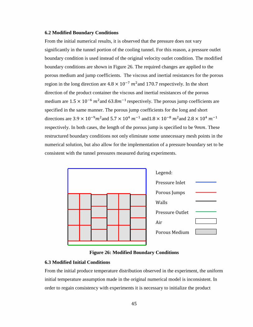
45

6.2 Modified Boundary Conditions

From the initial numerical results, it is observed that the pressure does not vary

significantly in the tunnel portion of the cooling tunnel. For this reason, a pressure outlet

boundary condition is used instead of the original velocity outlet condition. The modified

boundary conditions are shown in Figure 26. The required changes are applied to the

porous medium and jump coefficients. The viscous and inertial resistances for the porous

region in the long direction are and respectively. In the short

direction of the product container the viscous and inertial resistances of the porous

medium are and respectively. The porous jump coefficients are

specified in the same manner. The porous jump coefficients for the long and short

directions are and and and

respectively. In both cases, the length of the porous jump is specified to be . These

restructured boundary conditions not only eliminate some unnecessary mesh points in the

numerical solution, but also allow for the implementation of a pressure boundary set to be

consistent with the tunnel pressures measured during experiments.

Figure 26: Modified Boundary Conditions

6.3 Modified Initial Conditions

From the initial produce temperature distribution observed in the experiment, the uniform

initial temperature assumption made in the original numerical model is inconsistent. In

order to regain consistency with experiments it is necessary to initialize the product

Legend:

Pressure Inlet

Porous Jumps

Walls

Pressure Outlet

Air

Porous Medium

46

temperatures in each box to the temperatures observed in the experiment. In the boxes

where the temperatures are not measured, the average temperature of the box above and

below the box in question is used. This strategy is implemented with a UDF, the details

of which can be found in Appendix H.

6.4 Modified Cool Room and Zone Conditions

In the original numerical model, the temperature of the room is assumed constant. From

the results of the experiment, it is observed that the temperature in the room does not

remain constant. In order to make a direct comparison between the numerical model and

the experiments, it is necessary to model the transient room temperature. An expression

for the time dependent room temperature is obtained using a Fourier series

approximation, and is implemented with a UDF for the cold room zone. This allows the

cold room zone temperature to match that of the experimental data. The details of the

UDF used to achieve this is described in Appendix I.

More advanced UDFs have been generated to determine the heat transfer coefficient,

seven eights cooling times and half-cooling times in the solid porous zones (produce).

Details of the UDFs to determine the heat transfer coefficient and cooling times are given

in Appendix J and Appendix K respectively.

Although not a result of the numerical solution, the room temperature versus time from

the experimental and numerical investigation can be seen plotted in Figure 27. It is clear

that the UDF with Fourier series approximation accurately simulates the room

temperature conditions found during the experiment. The figure serves as a check to

ensure that the UDF properly defines the cold room zone temperature, which is critical to

the proper comparison with the numerical and experimental results.

47

Figure 27: Transient Room Temperature

48

7. Modified Numerical Model and Experimental Result

Comparison

To evaluate the validity of the numerical model, comparison with the experimental

results is necessary. In the following sections, the numerical results (from the modified

model) for pressure, time dependent temperature, and half-cooling time for each box are

compared to the full scale experimental results.

7.1 Percent Difference

The percent difference is used to determine the relative agreement between the

numerical and experimental results. Within this work, the percent difference is defined as

the difference between the experimental and numerical values divided by the maximum

possible difference as indicated in Equation 28.

(28)

As an example, consider the calculation of the percent difference of the non-dimensional

temperature found in Equation 29.

(29)

In the case of temperature, the maximum possible difference is the initial difference

between the produce and the room. Similarly, in the case of dimensionless vacuum

pressure, the maximum possible difference is the difference between the room pressure

and the tunnel pressure.

7.2 Dimensionless Pressure Comparisons

In order to compare the pressures, the area weighted average value of the numerical

dimensionless vacuum pressure of the product in the containers is compared to the

measured average dimensionless vacuum pressure for the corresponding experimental

container. A comparison of the dimensionless vacuum pressures is presented in Figure

28. It is seen that the numerical and experimental results are not in good agreement. The

maximum and minimum percent difference between the two data sets are 41% and 6%

respectively. It can also be seen that the boxes situated closer to the tunnel section are in

49

better agreement than boxes closer to the cold room side. The maximum and minimum

percent differences occur at locations RM2 and RM20 respectively.

Figure 28: Dimensionless Vacuum Pressure Comparison

7.3 Numerical Velocity Magnitude

Although the velocity magnitude of the air is not measured during the experiment, the

numerical results for the velocity magnitude are helpful in understanding the behavior of

the model and will be referred to when explaining the results of the transient produce

temperature variations in Section 7.5. The velocity magnitude from the numerical model

is shown in Figure 29. It can clearly be seen that the superficial velocity magnitudes in

the horizontally oriented boxes are predicted to be larger than those predicted for the

vertically oriented boxes.

Numerical

Experimental

RM1

RM2

0.94

RM3

RM4

RM5

RM6

RM7

RM9

RM10

RM8

RM11

0.59

RM12

0.81

RM13

0.93

RM14

0.59

RM15

RM16

0.92

RM17

0.48

RM19

RM20

0.91

RM18

0.77

RM1

0.25

RM2

0.53

RM3

0.81

RM4

0.25

RM5

0.53

RM6

0.81

RM7

0.21

RM9

0.64

RM10

0.85

RM8

0.42

RM11

0.25

RM12

0.53

RM13

0.81

RM14

0.25

RM15

0.53

RM16

0.81

RM17

0.21

RM19

0.64

RM20

0.85

RM18

0.42

50

Figure 29: Numerical Velocity Magnitude of Modified Model

7.4 Numerical Heat Transfer Coefficients

The variation of heat transfer coefficient throughout the boxes is also useful in explaining

the results of the model and will be referred to in Section 7.5. Contours of the predicted

heat transfer coefficients, expressed in the units of ⁄ , can be seen in Figure 30.

From the figure, it becomes clear why the horizontally oriented boxes cool the fastest.

Conversely, the vertically oriented boxes cool slower due to their reduced heat transfer

coefficient compared to the horizontal containers.

Figure 30: Numerical Heat Transfer Coefficient of Modified Model

7.5 Time Dependent Temperature Comparisons

The time dependent dimensionless temperature of the product in containers RM1 to

RM10 (skipping RM5 and RM9 since they were not obtained experimentally) from the

RM1

RM2

RM3

RM4

RM5

RM6

RM7

RM9

RM10

RM8

RM11

RM12

RM13

RM14

RM15

RM16

RM17

RM19

RM20

RM18

RM1

RM2

RM3

RM4

RM5

RM6

RM7

RM9

RM10

RM8

RM11

RM12

RM13

RM14

RM15

RM16

RM17

RM19

RM20

RM18

𝑊 𝑚 𝐾⁄

51

experiment and numerical simulation are plotted in Figures 30 and 31. The plots are

separated into two groups to reduce the congestion of the trend lines to allow clear

comparisons. Each box is indicated using a specific color for comparison; however, data

representing the experimental values are shown with symbols and the numerical data

without symbols. The data corresponding to the slower cooling boxes RM6, RM3, RM2,

and RM1 are presented in Figure 31 while the data corresponding to the faster cooling

boxes RM10, RM8, RM7, and RM4 are shown in Figure 32.

Figure 31: Transient Dimensionless Produce Temperature from Modified Model:

Part 1

In Figure 31, it can be seen, for both the experimental and numerical results that the

produce in container R1 cools the fastest of the four containers shown. This is due to the

produce box in location RM1 being the first box to receive fresh cool air from the cold

room. As the air flows in from the cold room, it cools the produce, and in turn gains heat.

This leads to reduced potential for heat transfer as the warmed air must flow through

subsequent containers into the tunnel section. Containers RM3 and RM6 show very

similar experimental and numerical results due to their similar location with respect to the

cold room.

52

Results similar to those seen in Figure 31 are observed in Figure 32. Once again, the

fastest cooling produce container, RM7, is located closest to the cold room side.

Although container RM4 is also situated next to the cold room, it is observed, both

experimentally and numerically, to cool slower, than container RM7. This is due to the

orientation of the containers and the resultant flow rate across the containers associated

with those losses, consistent with Figures 28 and 29.

Figure 32: Transient Dimensionless Produce Temperature of Modified Model: Part

2

The maximum difference of the experimental and numerical time dependent

dimensionless temperature is 18% that occurs at the RM8 location. The minimum

difference is found at the RM3 location with a difference of 3%.

7.6 Half Cooling Time Comparison

The experimental and numerical results for the average half-cooling time (in hours) for

each container can be seen in Figure 33. The maximum and minimum percent difference

between the numerical and experimental results are 43% and 2% respectively. The

maximum percent difference occurs in container RM8, while the minimum percent

difference occurs in container RM6.

53

Figure 33: Comparison of Half Cooling Times of Modified Model

7.7 Summary of the Modified Numerical Model Study

Direct comparisons are made with experimental results and the modified numerical

model for the case of medium cucumbers. The modified model includes non-uniform

initial temperature and the variation in the room temperature. Despite the disagreement

for pressure, the numerical transient temperature trends and values are in reasonable

agreement with the experiment. This is based on the maximum percent difference of 41%

with an experimental uncertainty ranging from ±6.9% to ±8.8% for measured pressures

of -0.218 inches of water (-54.36 Pa), and -0.455 inches of water (-113.25 Pa)

respectively. It is believed that zones of fluid by-pass (leaks) in the experiment that were

not taken into account in the modified numerical model are the main source of the

discrepancy. The predicted industry standard metric of half-cooling times are also

compared and most containers show reasonable agreement. The maximum percent

difference is determined to be 18%. This is considered as acceptable considering all the

simplifying assumptions. The minimum uncertainty in the dimensionless temperature is

±4.7% occurring at location RM7. The maximum uncertainty in the dimensionless

temperature is ±6.7 %, also at RM7. Additional modifications to the numerical model are

Numerical

RM1

0.78

RM2

1.72

RM3

2.35

RM4

0.97

RM5

RM6

2.29

RM7

0.69

RM9

RM10

1.73

RM8

0.93

RM11

RM12

RM13

RM14

RM15

RM16

RM17

RM19

RM20

RM18

RM1

1.16

RM2

1.62

RM3

2.39

RM4

1.13

RM5

RM6

2.73

RM7

.93

RM9

RM10

2.32

RM8

1.54

RM11

RM12

RM13

RM14

RM15

RM16

RM17

RM19

RM20

RM18

Experimental

54

made to investigate whether leaks which cause by-pass of some of the cooling air around

the produce boxes is a source of the discrepancy.

55

8. Numerical Model with Leaks and Comparisons

The effects of leaks in the numerical model are investigated using the same room zone

conditions and initial values used in the previous chapter. The main difference is with the

mesh and boundary conditions.

8.1 Mesh and Boundary Conditions with Leaks

In order to include areas where the cool air could by-pass the produce, zones of open air

spaces are included in the mesh. They are added on each of the sides of the pallets of

agricultural produce. The size of the by-pass zone is selected to be 1.5 inches (3.81cm).

This yields gaps between the pallets and the walls of 1.5 inches (3.81cm) and a gap

between the pallets of 3 inches (7.62cm). With the addition of the leak areas, porous

jumps are included to the interacting container edges previously assumed to be blocked.

The boundary conditions of the numerical model including provision for the leaks is

shown in Figure 34.

Figure 34: Boundary Conditions with Leaks

8.2 Dimensionless Experimental Vacuum Pressure Comparison with Numerical

Model Including Leaks

Comparison of the dimensionless pressure seen in the numerical model those in the

experiments is shown in Figure 35. The pressure variation in the model containing leaks

is in significantly better agreement with the experiment compared to the previous model

Legend:

Pressure Inlet

Porous Jumps

Walls

Pressure Outlet

Air

Porous Medium

56

without leaks. The maximum and minimum percent difference is determined to be 18%

and 5% respectively.

Figure 35: Dimensionless Vacuum Pressure Comparisons with Leaks


Contours or the velocity magnitude obtained from the model accounting for leaks are

presented in Figure 36. It is observed that the velocity magnitude is largest at the outer

edges of the product containers, which are in direct contact with either the cold room or

leak area. The velocity magnitude is also observed to be lowest in the containers, which

have no edges in direct contact with the leak area or cold room.

Numerical

Experimental

RM1

0.54

RM2

0.76

RM3

0.93

RM4

0.51

RM5

0.76

RM6

0.93

RM7

0.35

RM9

0.73

RM10

0.90

RM8

0.56

RM11

0.44

RM12

0.65

RM13

0.87

RM14

0.42

RM15

0.65

RM16

0.87

RM17

0.45

RM19

0.84

RM20

0.96

RM18

0.69

RM1

RM2

0.94

RM3

RM4

RM5

RM6

RM7

RM9

RM10

RM8

RM11

0.59

RM12

0.81

RM13

0.93

RM14

0.59

RM15

RM16

0.92

RM17

0.48

RM19

RM20

0.91

RM18

0.77

57

Figure 36: Numerical Velocity Magnitude of Model with Leaks

8.4 Numerical Heat Transfer Coefficient

Contours of the heat transfer coefficient in units of ⁄ are presented in Figure 37. It

can be seen that the maximum heat transfer coefficient is larger in the model containing

leaks compared to those seen in the model without leaks. Similarly, the minimum heat

transfer is lower as well. This is due to the non-uniform velocity field compared to those

seen in the model with leaks.

Figure 37: Numerical Heat Transfer Coefficient in Models with Leaks

8.5 Time Dependent Dimensionless Temperature Comparison

The time dependent dimensionless temperature comparison of the results of the

numerical model with leaks to the experimental results is presented in Figure 38 and 39

in the same way as presented in the previous chapter. From both figures, it is clear that

RM1

RM2

RM3

RM4

RM5

RM6

RM7

RM9

RM10

RM8

RM1

1

RM1

2

RM1

3

RM1

4

RM15

RM16

RM17

RM19

RM20

RM18

RM1

RM2

RM3

RM4

RM5

RM6

RM7

RM9

RM10

RM8

RM11

RM12

RM13

RM14

RM15

RM16

RM17

RM19

RM20

RM18

𝑊𝑚 𝐾⁄

m/s

58

the numerical model with leaks predicts faster cooling compared to the experiment. The

maximum and minimum difference is computed to be 21% and 5% respectively. The

maximum difference occurs in container RM8 and the minimum occurs in container

RM6. The percent difference has increased, in general, compared to the model with no

leaks.

Figure 38: Transient Dimensionless Temperature for Model with Leaks: Part 1

59

Figure 39: Transient Dimensionless Temperature for Model with Leaks: Part 2

8.6 Half Cooling Time Comparison

Comparisons of the half-cooling times predicted using the numerical model containing

leaks and experiment can be seen in Figure 40. It is clear that the numerical model

containing leaks is not in very good agreement with the half cooling times seen in the

experiment. The maximum and minimum percent difference is determined to be 69% and

6% respectively, occurring in containers RM1 and RM6 respectively.

60

Figure 40: Half Cooling Time Comparisons of Model with Leaks

8.7 Summary and Discussion of the Numerical Model Including Leaks Study

An effort is made to investigate the modified numerical model with leaks to determine if

they are responsible for the discrepancy between the numerical and experimental

pressures. This is achieved by allowing fluid to by-pass some boxes into gaps that are

introduced between containers and the walls across additional porous jumps. The

maximum percent difference for the dimensionless vacuum pressure is reduced to 17%.

Not only is the maximum percent difference reduced by 23%, but the whole flow field

can be visualized to be in much better agreement. It is important to note however that the

size of the by-pass areas can only be estimated. The size of the by-pass area and relative

size of the gap area between the pallets compared to those between the pallets and the

walls have an impact on the numerical results. The agreement of the transient non-

dimensional temperatures is observed to worsen with the inclusion of leaks. The

maximum percent difference is seen to grow to 21%. This seems to imply that the heat

transfer coefficients might not be appropriate. The experimental uncertainties for the

dimensionless vacuum pressures and temperatures are the same as those indicated in

section 7.7.

RM1 0.56

RM2 1.42

RM3

2.07

RM4 0.69

RM5

RM6 2.57

RM7 0.48

RM9

RM10 1.57

RM8 0.84

RM11

RM12

RM13

RM14

RM15

RM16

RM17

RM19

RM20

RM18

RM1 1.16

RM2 1.62

RM3

2.39

RM4 1.13

RM5

RM6 2.73

RM7 .93

RM9

RM10 2.32

RM8 1.54

RM11

RM12

RM13

RM14

RM15

RM16

RM17

RM19

RM20

RM18

Numerical

Experimental

61

9. Investigation of Alternate Cooling Tunnel

Configuration

From the results seen in previous chapter it is apparent that leaks are a significant factor

affecting the accuracy of the simulation of forced air cooling in produce cooling tunnels.

An alternate configuration is therefore, chosen for investigation that would potentially be

less susceptible to leaks. The alternate configuration only considers one pallet on each

side of the cooling tunnel due to the limited amount of product available during the day

of experimental testing. All other conditions are kept the same in order to conduct a

proper comparison. This configuration is also similar to a configuration made available

commercially by Global Cooling Inc. [27].

9.1 Alternate Configuration Mesh

The alternate cooling tunnel configuration requires a different mesh than those used in

previous chapters for two reasons. The first reason is the change in geometry already

mentioned. The second reason is that the air is allowed to enter three sides of the pallet

instead of just one seen in previous chapters. The mesh for the alternate configuration is

displayed in Figure 41.

Figure 41: Alternate Configuration Mesh

62

9.2 Boundary Conditions

The conditions on the boundaries must be changed in order to allow air to flow into three

sides of the pallets instead of just one. This is accomplished by removing the wall on the

left and right hand sides and replacing them with porous jumps. The boundary conditions

can be visualized with the help of Figure 42.

Figure 42: Alternate Configuration Boundary Conditions

9.3 Initial Conditions

The initial conditions for the alternate configuration are the same as those used in the

modified numerical model. The initial temperatures of the produce are initialized to the

same values as those seen in the experiment. It is important to note however that in this

experiment the initial product temperatures are different from those seen in previous

chapters. The initial product temperature range is from 20 to 17 .

9.4 Cool Room Conditions

The cool room conditions are also approximated in the same manner as in the modified

numerical model, however; the transient temperature of the room is significantly

different. The transient experimental room temperature data can be seen to be in good

agreement with the numerical approximation plotted in Figure 43. The behavior of the

room temperature is cyclical due to the activation and deactivation of the cooling system

based on some upper limit of temperature near 12.5

Legend:

Pressure Inlet

Porous Jumps

Walls

Pressure Outlet

Air

Porous Medium

63

Figure 43: Transient Room Temperature for the Alternate Configuration

9.5 Dimensionless Vacuum Pressure Comparison

Comparison of the numerical and experimental results for the dimensionless vacuum

pressure, for a tunnel pressure of -138 Pascals (Pa), can be seen in Figure 44. It is clear

that the numerical and experimental results are in good agreement. The alternate

configuration offers the best agreement between the non-dimensional vacuum pressures

when comparing the numerical and experimental results. The maximum and minimum

percent differences are found to be -6% and -1% respectively.

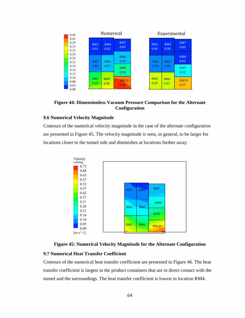
64

Figure 44: Dimensionless Vacuum Pressure Comparison for the Alternate

Configuration


Contours of the numerical velocity magnitude in the case of the alternate configuration

are presented in Figure 45. The velocity magnitude is seen, in general, to be larger for

locations closer to the tunnel side and diminishes at locations further away.

Figure 45: Numerical Velocity Magnitude for the Alternate Configuration

9.7 Numerical Heat Transfer Coefficient

Contours of the numerical heat transfer coefficient are presented in Figure 46. The heat

transfer coefficient is largest in the product containers that are in direct contact with the

tunnel and the surroundings. The heat transfer coefficient is lowest in location RM4.

RM1

0.01

RM2

0.05

RM3

0.23

RM4

0.02

RM5

0.07

RM6

0.30

RM7

0.03

RM9

0.18

RM10

0.42

RM8

0.08

RM1

0.00

RM2

0.04

RM3

0.29

RM4

0.00

RM5

0.06

RM6

0.31

RM7

0.00

RM9

0.12

RM10

0.37

RM8

0.03

Numerical Experimental

RM9

RM1

RM2

RM3

RM4

RM5

RM6

RM7

RM10

RM8

65

Figure 46: Numerical Heat Transfer Coefficient for the Alternate Configuration

9.8 Time Dependent Dimensionless Temperature Comparison

The numerical and experimental time dependent dimensionless temperatures are plotted

in Figure 47 and 48 in the same way as in previous chapters. These figures show that the

numerical model predicts faster cooling compared to the experiment. The fluctuating

transient room temperature is also seen to have a more significant effect on the behavior

of the cooling curve as indicated by their wavy behaviour.


Configuration: Part 1

RM9

RM1

RM2

RM3

RM4

RM5

RM6

RM7

RM10

RM8

66



In Figure 48, the experimental results for locations RM7 and RM8 are suspected to be

faulty. This is due to the sudden large decrease in dimensionless temperature that occurs

at particular times during the cooling process. The slope of the sudden decrease is larger

than that of the fastest cooling cucumber, which raises doubt on the validity of the

measurement. It is clear that some transient event drastically affected the thermocouple

readings in those two containers. For this reason, locations RM7 and RM8 have been

replaced with data from locations RM5 and RM9 respectively and are plotted in Figure

49. Comparisons are made with Figure 47 and 49, as they are believed to represent more

trustworthy data compared to Figure 48. The maximum percent difference is determined

to be 25% and occurs in container RM4. The minimum percent difference occurs at

location RM10 and is 14%.

67

Figure 49: Transient Dimensionless Product Temperature for the Alternate


9.9 Alternate Configuration Summary

An alternate configuration is investigated where the air is allowed to enter through three

sides of the pallets, as described in section 9.2 to 9.5. This type of configuration is

believed to have to have less potential for by-pass (leak) errors. This is confirmed with

the best overall agreement of dimensionless vacuum pressures. The maximum percent

difference between the numerical and experimental dimensionless vacuum pressure is

found to be -6%. Experimental uncertainty in the measured pressures are found to be in

the range ±5.1% to ±7.3% for measured pressures of 0 inches of water (0 Pa), and -

0.552inches of water (-138Pa) respectively. The agreement between the transient

dimensionless temperatures however, is found to be the worst. The maximum percent

difference between the dimensionless temperatures is calculated to be 25%. The

minimum experimental uncertainty in the dimensionless temperature is ±5.6%, occurring

at location RM5. The maximum experimental uncertainty in the dimensionless

temperature is determined to be ±8.5%, in container RM10. When analyzing the

comparisons time dependent dimensionless temperatures for the alternate configuration

some consistency in the trends can be seen. Although the numerical model is observed to

68

over predict the cooling rate, the order of which containers cool (fastest to slowest) are in

very good agreement. The alternate configuration also demonstrates the significant effect

of the transient room temperature, numerically and experimentally.

69

10. Comparison of Numerical Models and Discussion

10.1 Comparison of Numerical Models

A summary of the maximum percent difference in the case of pressure variation in each

tunnel configuration is found in Table 1. The experimental and numerical results for

pressure are in the best agreement compared to other geometrical configurations in

previous chapters. It is believed that this is due to the alternate orientation being less

susceptible to by-pass since there are less blockages.

Model

Experimental

Dimensionless

Vacuum

Pressure

Numerical

Dimensionless

Vacuum

Pressure

Tunnel

Pressure (Pa)

%

Difference

Modified 0.94 0.53 -113 41%

Leaks Included 0.94 0.76 -113 18%

Alternate

Configuration 0.12 0.18 -138 -6%

Table 1: Percent Difference in Pressures Summary

When comparing the numerical and experimental dimensionless produce temperature, the

percent difference is seen to increase, compared to the previous configurations. The

maximum percent difference for temperature is summarized in Table 2. Comparisons of

the half-cooling times are not considered as not all the products reached half cool within

the experiment due to time constraints.

Model

Experimental

Dimensionless

Temperature

Numerical

Dimensionless

Temperature

Minimum

Room

Temperature

(°C)

%

Difference

Modified 0.52 0.44 12 18%

Leaks Included 0.62 0.41 12 21%

Alternate

Configuration 0.64 0.40 9 24%

70

Table 2: Percent Difference in Temperature Summary

10.2 Discussion

It is believed that the alternate configuration yields the most accurate comparison to

experiment within this work. The reason for this is due to its superior agreement for the

dimensionless vacuum pressures. It is important to recall that the numerical results for

pressure rely on previously obtained empirical results. For this reason, the pressures

obtained in the experiment should be in relatively good agreement. Since the superficial

velocity and volume flow rates are directly related to the pressure, it is safe to assume

that these flow variables are the most accurately predicted compared to previous models.

When comparing the experimental and numerical temperatures, the agreement is the

worst compared to other configurations in spite of the best agreement with pressures.

The empirical models used for modeling forced convective heat transfer; however, have

not been obtained experimentally within this work. In fact, the produce is not uniformly

distributed within its container, unlike the conditions used to obtain the relationships for

the heat transfer coefficients found in the literature. It is expected that a percentage of the

air entering the product containers is bypassing the produce altogether, consistent with

observations made by Ferrua and Singh [10]. This type of behavior would yield reduced

heat transfer coefficients, as not all the cooling air encounters the produce.

71

11. Conclusions and Recommendations for Future

Work

11.1 Conclusions

The following conclusions are made from this work:

A simple computational model using the porous medium approximation is

successfully developed to simulate forced air cooling in an agricultural produce

cooling tunnel.

Based on the results of the full-scale experiments, the assumptions of no flow

between layers, and symmetric flow about the centre of the cooling tunnel, are

shown to be appropriate; however, the assumptions of uniform initial temperature

and constant room temperature are not.

Modifications to the original numerical model to account for different initial

produce temperatures as well as varying room temperature yielded reasonable

results for the variation of produce temperature with time but not the product

container pressures.

Further modification of the model to approximate the leakage of air around rather

than through the produce containers resulted in a much improved prediction of the

produce container pressures but yielded produce temperature variations with time

that are less accurate, hence flow leakage should be considered in studies of

produce cooling tunnels

Similar modeling of an alternative cooling tunnel configuration in which leakage

is not a factor resulted in similar findings.

The model used to estimate the heat transfer from the produce to the air is thought

to be the likely cause of the discrepancies in temperature and hence improved

methods must be developed.

11.2 Recommendations for Future Work

Treating the produce as a continuous porous medium does not accurately describe the

heat transfer that occurs. It is expected that better agreement with the experimental results

would be achieved with a 3-D model of the flow through one layer of stacked product,

72

which allows for the effect of the locations of the openings in the containers to be taken

into account. The same empirically determined porous jump boundary conditions can be

used to numerically model the container openings. The produce would still be treated as a

porous medium to reduce computational time, however, the porous medium would

occupy only regions of the container where produce is found, and not be fully distributed

throughout each container. In this way some non-homogeneous flow would be observed,

which would more accurately represent the physical behavior of the air within the

containers. With the additional dimension, out of plane temperature gradients within the

porous medium (produce) could also be captured.

Because the temperature of the room can have a significant effect on the cooling of the

produce, some consideration should be made to estimate the response of the room to the

rapid heat rejection by the produce. This will require more information on the

characteristics of the room and cooling system.

73

Bibliography

[1] Brosnan, T., and Sun, D.-W., 2001, “Pre-cooling techniques and applications for

horticultural products — a review,” International Journal of Refrigeration, 24(2),

pp. 154–170.

[2] Gross, K.C., C.Y. Wang, and M. Saltveit, 2002, The Commercial Storage of Fruits,

Vegetables, and Florist and Nursery Stocks.

[3] Boyette, M. D., 1989, Introduction to Proper Postharvest Cooling and Handling

Methods, The North Carolina Agricultural Extension Service, Raleigh, North

Carolina Agricultural and Technical State University at Greensboro,.

[4] Fraser, H., 2014, “OMAFRA Factsheet 14-039: Forced-Air Cooling Systems for

Fresh Ontario Fruits and Vegetables.”

[5] Thompson, J. F., Mitchell, F. G., and Rumsay, T. R., 2008, Commercial Cooling of

Fruits, Vegetables, and Flowers, University of California, Agriculture and Natural

Resources.

[6] Pathare, P., Opara, U., Vigneault, C., Delele, M., and Al-Said, F.-J., 2012, “Design

of Packaging Vents for Cooling Fresh Horticultural Produce,” Food and

Bioprocess Technology, 5(6), pp. 2031–2045.

[7] Zou, Q., 2002, “A CFD modelling system for air flow and heat transfer in

ventilated packing systems during forced-air cooling of fresh produce,” Doctor of

Philosophy, Massey University.

[8] Amos, N. D., 1995, “Mathematical Modelling of Heat Transfer and Water Vapour

Transport in Apple Coolstores,” Doctor of Philosophy, Massey University.

[9] Tanner, J. D., 1998, “Mathematical Modelling for Design of Horticultural

Packaging.,” Massey University.

[10] Ferrua, M. J., and Singh, R. P., 2009, “Modeling the forced-air cooling process of

fresh strawberry packages, Part I: Numerical model,” International Journal of

Refrigeration, 32(2), pp. 335–348.

[11] Ferrua, M. J., and Singh, R. P., 2009, “Modeling the forced-air cooling process of

fresh strawberry packages, Part II: Experimental validation of the flow model,”

Int.J.Refrig., 32(2), pp. 349–358.

[12] Talbot, M. T., 1988, “An Approach to Better Design of Pressure-Cooled Produce

Containers,” Proceedings of the Florida State Horticultural Society, 101, pp. 165–175.

[13] Xu, Y., and Burfoot, D., 1999, “Simulating the bulk storage of foodstuffs,”

Journal of Food Engineering, 39(1), pp. 23–29.

[14] G. C. Misener and Gene C. Shove, 1976, “Simulated Cooling of Potatoes,”

Transactions of the American Society of Agricultural Engineers, 19(5), pp. 954–957&961.

[15] Verboven, P., Flick, D., Nicolaï, B. M., and Alvarez, G., 2006, “Modelling

transport phenomena in refrigerated food bulks, packages and stacks: basics and

advances,” International Journal of Refrigeration, 29(6), pp. 985 – 997.

74

[16] Brown, G. O., 2002, “Henry Darcy and the making of a law,” Water Resources

Research, 38(7), pp. 11–1–11–12.

[17] Gauch, H. G., 2003, Scientific Method in Practice, Cambridge University Press.

[18] Nield, D. A., and Bejan, A., 2012, Convection in Porous Media, Springer.

[19] Dixon, A. G., and Cresswell, D. L., 1979, “Theoretical prediction of effective heat

transfer parameters in packed beds,” AIChE Journal, 25(4), pp. 663–676.

[20] Handley, D., and Heggs, P., 1968, “Momentum and heat transfer mechanisms in

regular shaped packings,” Transactions of the Institution of Chemical Engineers

and the Chemical Engineer, 46(9), p. T251.

[21] Wakao, N., and Kagei, S., 1982, Heat and Mass Transfer in Packed Beds, Gordon

and Breach Science Publishers.

[22] Basu, P., 2006, Combustion and Gasification in Fluidized Beds, CRC Press.

[23] Martins, J. P., and Rankin, G. W., 2015, “An Investigation of Produce Cooling

Tunnel Performance.,” 11th International Conference on Heat Transfer, Fluid

Mechanics and Thermodynamics, Skukuza, Kruger National Park, South Africa, pp.

737–742.

[24] “Water Content and Water Activity: Two Factors That Affect Food Safety”

[Online]. Available: http://www.gov.mb.ca/agriculture/food-safety/at-the-food-

processor/water-content-water-activity.html. [Accessed: 22-May-2014].

[25] DeGroot, C. T., 2012, “Numerical Modelling of Transport in Complex Porous

Media: Metal Foams to the Human Lung,” University of Western Ontario.

[26] Priddy, K. L., and Keller, P. E., 2005, Artificial Neural Networks: An Introduction,

Society of Photo Optical.

[27] “Portable precooler and recooler, best precooler, pressure cooler, and forced air

precooler” [Online]. Available: http://www.pre-coolers.net/jet-precoolers.php.

[Accessed: 15-Jun-2014].

[28] White, F. M., 2011, Fluid Mechanics, McGraw Hill.

[29] Fraser, H. W., 1998, Tunnel Forced-Air Coolers for Fresh Fruits and Vegetables,

Ontario Ministry of Agriculture, Food and Rural Affairs, Ontario.

[30] Figliola, R. S., and Beasley, D. E., 2008, Theory and Design for Mechanical

Measurements, 3RD ed, Wiley India Pvt. Limited.

[31] Kline, S. J., and McClintock, F., 1953, “Describing uncertainties in single-sample

experiments,” Mechanical engineering, 75(1), pp. 3–8.

75

Appendix A Permissions

A.1 Permissions for Use of Figure 1 and Figure 2

Dear Jean-Paul - By way of this e-mail, permission is granted to Jean-Paul Martins to use Figure 7, appearing on page 8 and Figure 10 appearing on page 10 in Commercial Cooling of Fruits, Vegetables and Flowers, (ANR Publication 21567, ISBN 978-1-60107-619-9, J. Thompson) in your masters thesis as described in your e-mail inserted below. Please indicate that the material is “Copyright © 2008 Regents of the University of California. Used by permission.” Because of the age of this publication, we do not have an original file of the requested artwork; you may feel free to use a scan of the figures in your thesis. Thank you for your interest in our publications, and furthering the work of Cooperative Extension. Best regards, Cynthia Cynthia Kintigh Marketing Director University of California Division of Agriculture and Natural Resources Communication Services and IT 2801 2nd Street, Room 126 Davis, CA 95618 V: 530-750-1217 ucanr.edu anrcatalog.ucanr.edu

tel:530-750-1217

http://ucanr.edu/

http://anrcatalog.ucdavis.edu/

76

A.2 Permission for Use of Figure 4

78

Appendix B Preliminary Experiments

Preliminary experiments are necessary to obtain the porous medium and porous jump

coefficients for the produce and produce container respectively. The test section

constructed to obtain the required empirical coefficients and its functionality are

described in section B.1. The experimental procedure, in point form, is covered in section

B.2. The steps taken to reduce the data are given in section B.3. The Matlab code used

along with an example of the curves fitted is included in section B.4. Finally, detailed

drawings for the designed and constructed test section can be found in section B.5

B.1 Description of the Test Section and Functionality

A photo of the designed and constructed test section can be seen in Figure B1. In the

figure, the test section is shown with the lid removed to display the enclosed produce.

Figure B1: Photo of Test Section

The experiments are conducted with the produce inside the product container and with

the container empty in order to separate the effect of the product from that of the box. A

vacuum is connected to the valve, which pulls air into the test section sown in the

schematic Figure B2. The pressure drop is recorded across the full and empty boxes at

pressure taps, on each side of the produce container, with an OMEGA HHP-103

handheld manometer. The flow rates are varied with the use of a valve set at different

positions. The flow rates are obtained with the use of a Meriam Instruments E200I

79

handheld manometer along with the relationship of the pressure drop vs flow rate across a

sharp edged orifice.

Figure B2: Test Section Schematic

B.2 Preliminary Experiments Procedure

In order to obtain the coefficient for multiple produce types and across both directions of

the boxes the following experimental procedure is used:

1. Place produce container filled with produce into test section

2. Seal potential leak areas with tape

3. Place lid on test section and seal

4. Set valve to almost closed

5. Turn on vacuum on low setting

6. Record pressure drop across the container and orifice

7. Adjust valve to half closed


9. Adjust valve to fully open


11. Set valve to almost closed

12. Switch vacuum to high setting

13. Repeat steps 6 to 10

14. Complete a second trial by repeating steps 4 to 13

15. Turn the vacuum off

16. Open the lid and remove the produce from the container

17. Place lid on test section and seal

Valve

E200I

Flow

Out Flow In

HHP-103

Sharp

Edged

Orifice

Produce

Container

80

18. Repeat steps 4 to 14

19. Turn the vacuum off

This procedure is conducted for 7 different produce types in both (perpendicular)

directions of the produce container with the container full and then empty. A total of 28

data sets are obtained.

B.3 Data Reduction

The resulting data set from one container in a single direction (full or empty) contains 12

measurements for both pressure drops across the entire produce container and sharp

edged orifice. First, the pressure readings are converted from inches of water to Pa. The

pressure drops are then divided by the length of the container in the flow direction; this

will yield units of Pa/m. The pressure drops across the sharp edged orifice is converted

into volume flow rates using Equation B1 obtained from Fluid mechanics 7th

edition by

Frank M. White [28].

[

⁄

]

(B1)

In the above equation Q is the volume flow rate in units of . It is assumed that the

dimensionless discharge coefficient is 0.6 and that the ratio of diameters is sufficiently

large for to be essentially zero. The density of air, , isassumed to be 1.225

while represents the cross-sectional area of the sharp edged orifice of diameter 1.25

inches (0.03175 m). The volume flow rate is then used to determine the superficial

velocity by dividing the flow rate by the cross-sectional area of the container. Finally, the

data for the pressure drop across the container per unit length is plotted against the

superficial velocity, and a least squares fit with y intercept of zero is obtained to

determine A and B in Equation B2. The coefficients obtained in the previous step can

then be related to the required porous medium coefficients K and using Equation B2.

| | (B2)

To separate the pressure losses associated with the vent holes in the product container

from that of the flow passing through the porous medium, experiments are conducted

81

with the product containers full of produce and with empty containers. In this way when

the pressure for the empty produce container is subtracted from that of the product

container full of product, the pressure loss associated to the produce is all that remains.

The assumption is also made that the pressure drop for the air entering or exiting the

empty container is equal to half of that of the pressure drop across the entire empty

container.

B.4 Matlab Code

The post processing of the experimental data obtained in the initial experiments is

conducted using Matlab. The original data and some parameters are scanned into Matlab

from the original Excel files using the built in “xlsread” function. The data is then

processed accordingly in order to get the coefficients in the correct desired units. A

sample code for the data reduction of medium cucumbers can be found below in Figure

B3, along with the curve for the pressure drop vs superficial velocity in Figure .

%medium cucumber

clear

clc

%data collection and plotting

%Global variables

rho=1.225; %air density in (kg/m^3)

mu=1.7894*(10^-5); %air viscosity in (kg/m*s)

tb=.35*25.4/1000; %measured thickness of the cardboard box in (m)

H2OtoPa=249.174; %coverts inches of water to pascals

Cd=0.6; %dimesionless discharge coeficcient

dt=1.25*25.4/1000; %diameter of the orifice in (m)

At=(pi*dt^2)/4; %area of the orifice in (m^2)

%Dimensions of the box

ll=xlsread('medium cucumber nov 5th long.xlsx','Test1','N2'); %length of the box in (m)

ls=xlsread('medium cucumber nov 5th short.xlsx','Test1','N2'); %width of the box in (m)

hbox=4.25*25.4/1000; %height of the box in (m)

%Long Direction Full

dpfulll=xlsread('medium cucumber nov 5th long.xlsx','Test1','D2:D13'); %reads pressure

drop across the box in inches of water

dpfulll=dpfulll*H2OtoPa; %converts inches of water to Pa

plfulll=dpfulll./ll;

dpofulll=xlsread('medium cucumber nov 5th long.xlsx','Test1','E2:E13'); %reads pressure

drop across the orifice in inches of water

dpofulll=dpofulll*H2OtoPa;

Qfulll=Cd*At*sqrt(2*dpofulll./rho);

82

Ufulll=Qfulll./(ls*hbox);

%fitting the data

plfl=polyfitzero(Ufulll,plfulll,2);

plflcurve=polyval(plfl,linspace(0,max(Ufulll)));

Cfl=2*plfl(1)/rho;

Kfl=mu/plfl(2);

dpfl=polyfitzero(Qfulll,dpfulll,2);

%Long Direction Empty

dpempl=xlsread('medium cucumber nov 5th long.xlsx','Test1','D17:D28'); %reads pressure


dpempl=dpempl*H2OtoPa; %converts inches of water to Pa

plempl=dpempl./ll;

dpoempl=xlsread('medium cucumber nov 5th long.xlsx','Test1','E17:E28'); %reads pressure


dpoempl=dpoempl*H2OtoPa;

Qempl=Cd*At*sqrt(2*dpoempl./rho);

Uempl=Qempl./(ls*hbox);

%fitting the data

plel=polyfitzero(Uempl,plempl,2);

plelcurve=polyval(plel,linspace(0,max(Uempl)));

Cel=2*plel(1)/rho;

Kel=mu/plel(2);

dpel=polyfitzero(Qempl,dpempl,2);

%Short Direction Full

dpfulls=xlsread('medium cucumber nov 5th short.xlsx','Test1','D2:D13'); %reads pressure


dpfulls=dpfulls*H2OtoPa; %converts inches of water to Pa

plfulls=dpfulls./ls;

dpofulls=xlsread('medium cucumber nov 5th short.xlsx','Test1','E2:E13'); %reads pressure


dpofulls=dpofulls*H2OtoPa;

Qfulls=Cd*At*sqrt(2*dpofulls./rho);

Ufulls=Qfulls./(ll*hbox);

%fitting the data

plfs=polyfitzero(Ufulls,plfulls,2);

plfscurve=polyval(plfs,linspace(0,max(Ufulls)));

Cfs=2*plfs(1)/rho;

Kfs=mu/plfs(2);

dpfs=polyfitzero(Qfulls,dpfulls,2);

%Short Direction Empty

dpemps=xlsread('medium cucumber nov 5th short.xlsx','Test1','D17:D28'); %reads pressure


dpemps=dpemps*H2OtoPa; %converts inches of water to Pa

plemps=dpemps./ls;

dpoemps=xlsread('medium cucumber nov 5th short.xlsx','Test1','E17:E28'); %reads pressure


dpoemps=dpoemps*H2OtoPa;

Qemps=Cd*At*sqrt(2*dpoemps./rho);

Uemps=Qemps./(ll*hbox);

%fitting the data

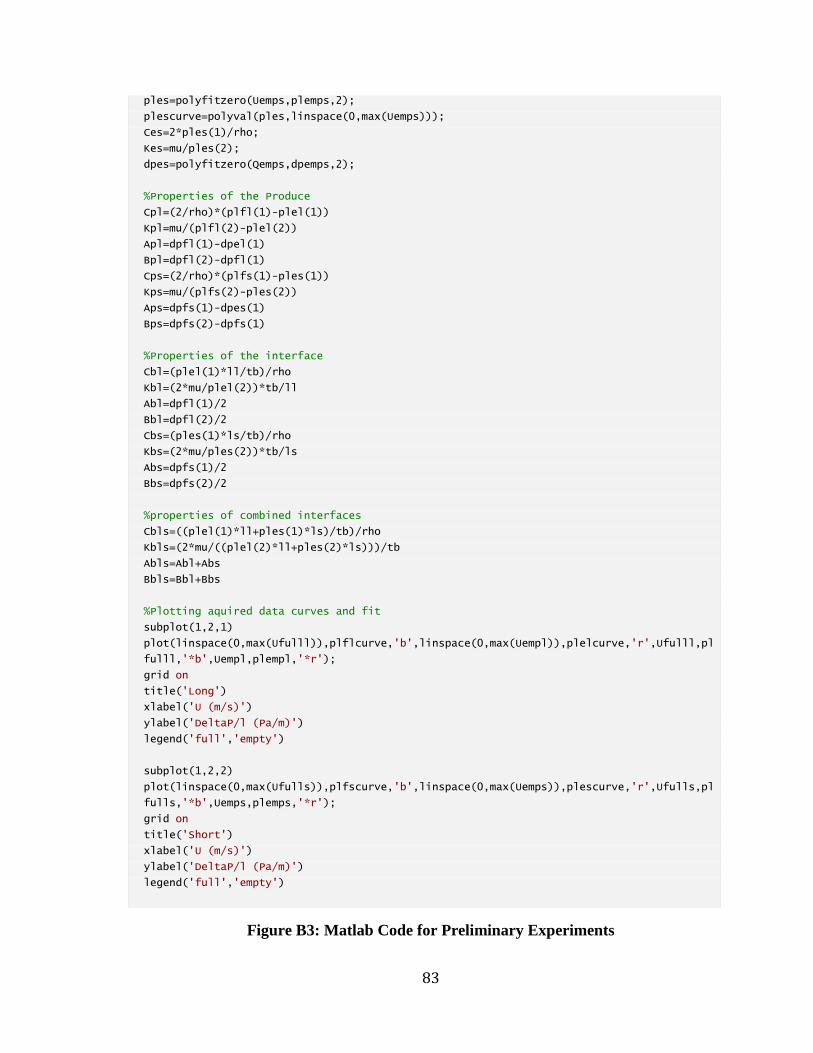
83

ples=polyfitzero(Uemps,plemps,2);

plescurve=polyval(ples,linspace(0,max(Uemps)));

Ces=2*ples(1)/rho;

Kes=mu/ples(2);

dpes=polyfitzero(Qemps,dpemps,2);

%Properties of the Produce

Cpl=(2/rho)*(plfl(1)-plel(1))

Kpl=mu/(plfl(2)-plel(2))

Apl=dpfl(1)-dpel(1)

Bpl=dpfl(2)-dpfl(1)

Cps=(2/rho)*(plfs(1)-ples(1))

Kps=mu/(plfs(2)-ples(2))

Aps=dpfs(1)-dpes(1)

Bps=dpfs(2)-dpfs(1)

%Properties of the interface

Cbl=(plel(1)*ll/tb)/rho

Kbl=(2*mu/plel(2))*tb/ll

Abl=dpfl(1)/2

Bbl=dpfl(2)/2

Cbs=(ples(1)*ls/tb)/rho

Kbs=(2*mu/ples(2))*tb/ls

Abs=dpfs(1)/2

Bbs=dpfs(2)/2

%properties of combined interfaces

Cbls=((plel(1)*ll+ples(1)*ls)/tb)/rho

Kbls=(2*mu/((plel(2)*ll+ples(2)*ls)))/tb

Abls=Abl+Abs

Bbls=Bbl+Bbs

%Plotting aquired data curves and fit

subplot(1,2,1)

plot(linspace(0,max(Ufulll)),plflcurve,'b',linspace(0,max(Uempl)),plelcurve,'r',Ufulll,pl

fulll,'*b',Uempl,plempl,'*r');

grid on

title('Long')

xlabel('U (m/s)')

ylabel('DeltaP/l (Pa/m)')

legend('full','empty')

subplot(1,2,2)

plot(linspace(0,max(Ufulls)),plfscurve,'b',linspace(0,max(Uemps)),plescurve,'r',Ufulls,pl

fulls,'*b',Uemps,plemps,'*r');

grid on

title('Short')

xlabel('U (m/s)')

ylabel('DeltaP/l (Pa/m)')

legend('full','empty')

Figure B3: Matlab Code for Preliminary Experiments

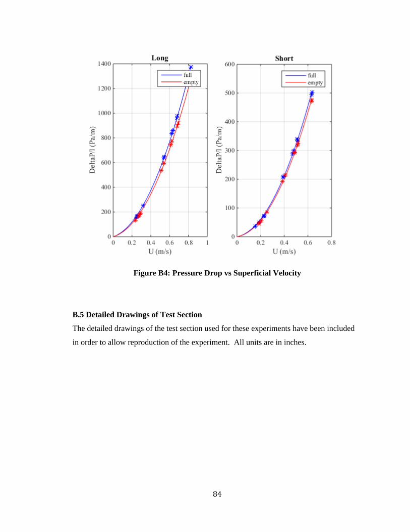
84

Figure B4: Pressure Drop vs Superficial Velocity

B.5 Detailed Drawings of Test Section

The detailed drawings of the test section used for these experiments have been included

in order to allow reproduction of the experiment. All units are in inches.

85

Figure B5: Assembly Drawing of Test Section

86

Figure B6: Front Panel Figure B7: 2X4 Runner

87

Figure B8: Front Top Panel Figure B9: Mid Top Panel

88

Figure B10: Rear Top Panel Figure B11: Side Panel

89

Figure B12: Rear Panel Figure B13: Orifice Plate

90

Figure B14: Sharp Edge Orifice Figure B15: 2X2 Pillar

91

Figure B16: Baffle Figure B17: 3/8 Threaded Rod

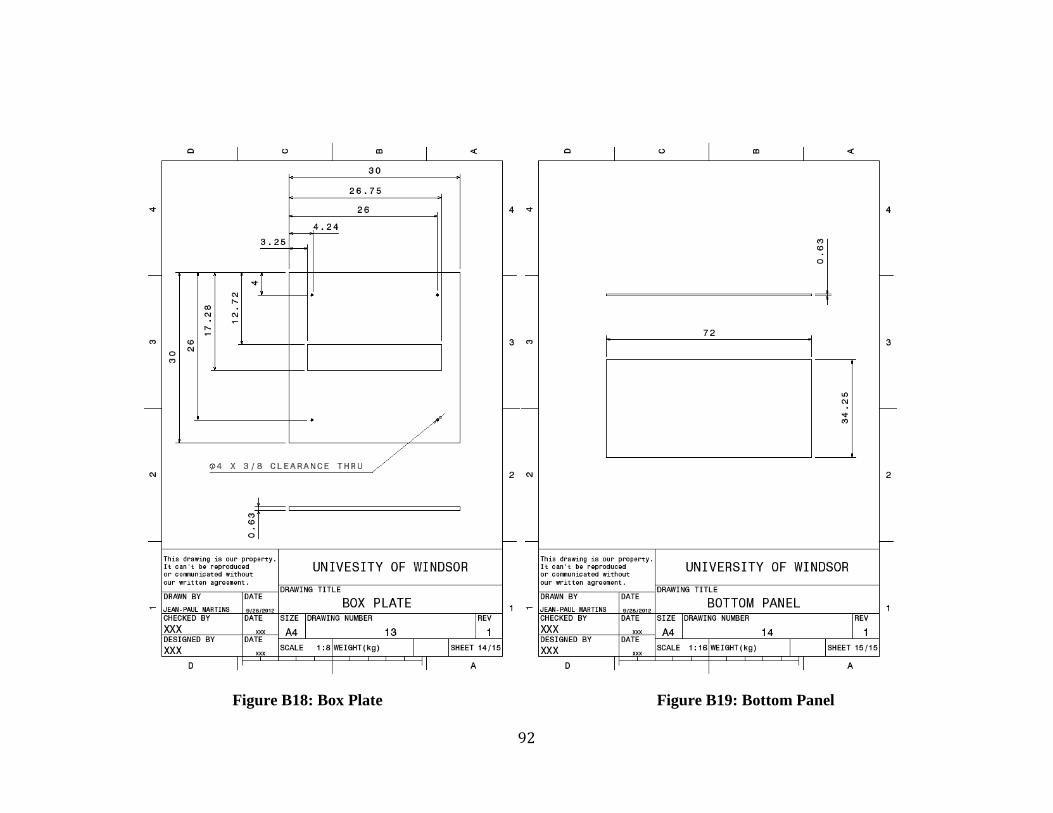
92

Figure B18: Box Plate Figure B19: Bottom Panel

93

Appendix C Calculation of the Heat Transfer

Coefficients

Empirical equations obtained from the literature are used to determine the heat transfer

coefficient. Within this appendix, sample calculations are given for the determination of

the heat transfer coefficients along with the required values. Procedures for calculating

the heat transfer coefficient with example values are then presented for the cases of flow

across the short and long direction of the produce containers.

C.1 Required Values

In order to complete the following sample calculations, certain material properties,

geometrical characteristic lengths, and flow variables are required. The material

properties are the thermal conductivity of the fluid and solid (air and cucumber)

represented by and respectively as well as the specific heat at constant pressure,

viscosity, and density of the working fluid represented by , , and respectively.

The geometrical parameters associated with the produce porous media model include the

porosity given by the symbol , the particle diameter denoted by and the shape factor

for the flow aligned with the short and long directions across the produce containers

given by , and , respectively. The flow variable that needs to be

specified is the area weighted average fluid velocity denoted by . The particular

values used for these quantities are as follows:

.

C.2 Calculation of the Heat Transfer Coefficient in the Short Direction

First, it is required to calculate the particle Reynolds Number, with the air flowing across

the short direction of the container, defined by Equation 8 from section2.6.6.

94

=

Next, the Prandtl Number must be calculated.

Once the Reynolds and Prandtl Numbers have been calculated, they can be used to

determine the fluid solid Nusselt Number ( ) from Equation 17 in section 2.6.10.

Recall the relationship used is the one presented by Handley and Heggs, since .

From the fluid solid Nusselt Number the fluid to solid heat transfer coefficient ( ) can

be determined using Equation 16 in section 2.6.10.

Finally, the heat transfer coefficient can be calculated using Equation 15 from section

2.6.10.

(

)

Thus the heat transfer coefficient ( ) for the flow aligned with the short length of the

containers, is

in the short direction.

C.3 Calculation of the Heat Transfer Coefficient in the Long Direction

The calculation procedure is the same as that for the short direction, except the area

weighted average velocity ( ) and shape factor ( ) are different.

95

Appendix D User Defined Function for Initial Model

Within this appendix the User Defined Functions (UDFs) are explained, and then 7/8

cooling time UDF for use in the initial numerical model is described.

D.1 User Defined Functions Explained

ANSYS Fluent allows UDFs to be used to enhance the standard features of the solver. A

UDF is written in the C computer language. Some additional macros are made available

within the UDF language to simplify the functionality of the written C codes. The macros

allow the code to be executed at the end of each iteration or time step, and upon exit or

loading of the case. UDFs are advantageous when customized boundary conditions,

property definitions, surface and volume reaction rates, and transport equations are

required. The UDF can also be useful in the initialization of the model. They can be used

to adjust computed values on a per iteration basis. Lastly, UDFs can be used to enhance

post processing of the numerical models.

D.2 7/8 Cooling Time UDF for the Initial Numerical Model

In the initial User Defined Function the “DEFINE_PROPERTY” macro is used. This

macro is applied to an entire material within the numerical model. In this specific case, it

is applied to the density of the solid. Each time the density of the solid is used within the

numerical solution, the UDF is executed. A flow chart describing the functioning of the

UDF can be seen in Figure D1.

96

Figure D1: 7/8 Cooling Time Flowchart

The UDF begins by determining the flow time. The temperature of each cell is then

determined. If the temperature of the cell is greater than the seven eights cooling

temperature, the time in seconds is stored for that cell. If temperature is below the seven

eights cooling temperature the time is not stored for that cell. The UDF terminates by

97

returning the density of the solid, which is constant. The C code used can be found in

Figure D2 below.

#include "udf.h"

DEFINE_PROPERTY(rho,cell,thread)

{

real t = CURRENT_TIME;

real rho=998.2;

real sect;

real temp = C_T(cell,thread);

if (temp >= 285.25)

{

sect = CURRENT_TIME;

C_UDMI(cell,thread,0)=sect;

}

return rho;

}

Figure D2: C Code Used for Initial Model UDF

98

Appendix E Fan Selection and Tunnel Design

The method used to select the cooling tunnel fan and other details of the tunnel

construction are given in this appendix for completeness.

E.1 Fan Selection

In order to select a fan to ensure proper operation and sufficient cooling of the produce,

rough estimates of the system requirements are made. In the case of forced air cooling of

cucumbers, it is recommended that the airflow should be 1.5-0.5 cubic feet per minute

(CFM) for every 1 pound (lb.) of agricultural product or 0.39-1.16 cubic meters per hour

for every kilogram (kg) of product[29]. It is assumed that the small cucumber orientation

of containers, seen in Figure E1, offer the largest resistance to flow, since that

configuration has the largest number of porous jumps in series with the largest flow

resistance. Hence, it is taken as the worst-case scenario for the system requirements. The

use of the small cucumber arrangement is also beneficial due to its simple layout

compared to other products. Since it has previously been seen that the produce offers

negligible pressure drop compared to the container openings, the losses associated with

the product are overlooked and the losses due to the containers only considered. It is also

assumed that there is no flow between lanes of containers as there should not be any

pressure gradients in that direction.

Figure E1: Airflow through a Single Lane of Containers

First, it is required to estimate the total volume flow rate. This is done by knowing

approximately the weight of cucumbers in each product container. Each product

container is assumed to contain approximately 10 lbs. of cucumbers since there are 12

containers in each layer, 13 layers in each pallet, and 4 pallets of produce, the total

Cold Air In

from

Room

Warm Air

Out Into

Fan

Lane of Containers

99

volume flow rate required is 6420 CFM (3.03 ⁄ ). The midpoint of the suggested

range of cooling flow rates per pound (1 CFM/lb) is used in the calculation. The

superficial velocity can be determined by dividing the volume flow rate going through

one lane of containers by the cross-sectional area of the container (0.108 m x 0.2826 m)

which gives 0.464 m/s. The pressure drop equation through a single lane of product

containers is the sum of the pressure losses associated to the four container openings seen

in Figure E1. Since all the pressure drops are identical and they are in series, the resulting

equation for the total pressure drop is similar to a single container opening only with four

times the length. In this specific case, the viscous and inertial resistances are

and respectively. The resulting pressure drop is 422.26Pa.

This means the selection of the fan must be such that it can supply 6420 CFM

(3.03 ⁄ ) of air at a pressure of 422.26 Pa (1.695 inches of water). A Twin City Fan

and Blower Company fan with part number WPD-24-E8-24 is selected. The pump curve

along with the system curve is presented in Figure E2.

Figure E2 Fan and System Curves

From the figure, it is clear that the fan will not be able to achieve 6420 CFM (3.03 ⁄ )

at 1.695 inches of water (422.26 Pa), but rather it will be able to achieve around 5500

CFM (2.6 ⁄ ) at close to 1.5 inches of water (373.68 Pa). If we substitute this value

100

into equation E1, we find the flow rate per pound of product is approximately 0.88

CFM/lb. (0.68 ⁄ ). , which is well above the suggested minimum airflow of 0.5

CFM/lb. Since this configuration is our worst-case scenario, all other products should

obtain higher flow rates at lower pressures.

E.2 Cooling Tunnel Design

Knowing the dimensions of the selected axial flow fan, the cooling tunnel is designed.

The assembly drawing, and detail drawings can be found on the following pages.

101

Figure E3: Cooling Tunnel Design

102

Figure E4: Fan Wall

Figure E5: Back Wall

103

Figure E6: Top Angle

Figure E7: Pillow Block

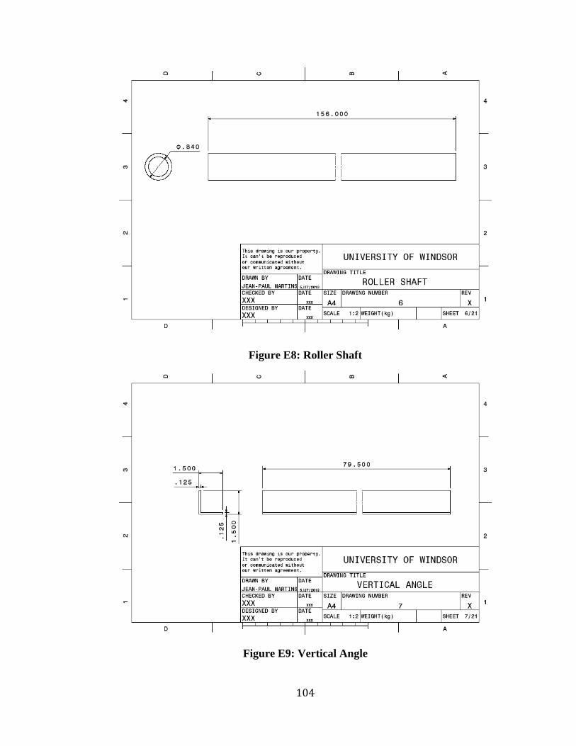
104

Figure E8: Roller Shaft

Figure E9: Vertical Angle

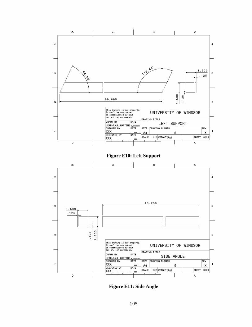
105

Figure E10: Left Support

Figure E11: Side Angle

106

Figure E12: Bottom Angle

Figure E13: Vertical Fan Angle

107

Figure E14: Horizontal Fan Angle

Figure E15: Right Support

108

Figure E16: Centre Board

Figure E17: Connecting Board

109

Figure E18: Side Board

Figure E19: Throttle Door

110

Figure E20: Side Spacer

Figure E21: Side Seal

111

Figure E22: Bottom Spacer

Figure E23: Bottom Seal

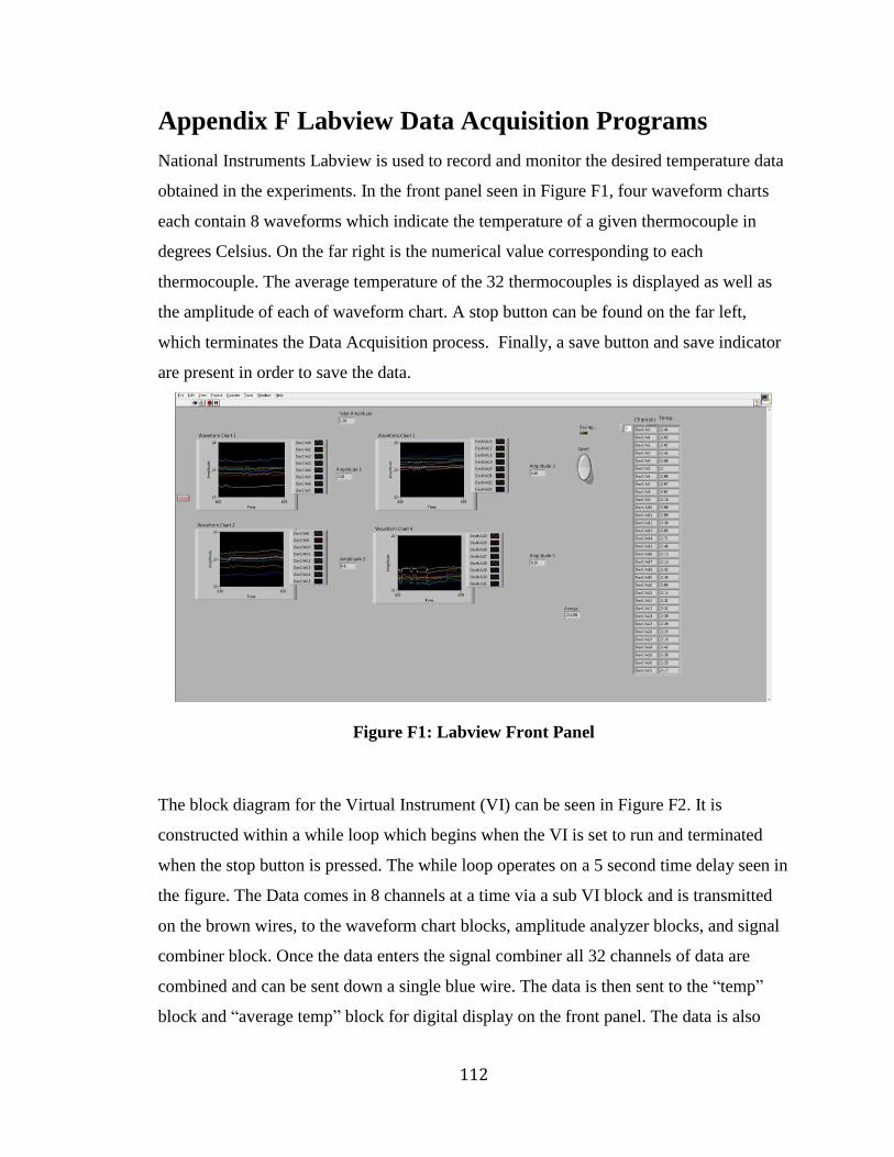
112

Appendix F Labview Data Acquisition Programs

National Instruments Labview is used to record and monitor the desired temperature data

obtained in the experiments. In the front panel seen in Figure F1, four waveform charts

each contain 8 waveforms which indicate the temperature of a given thermocouple in

degrees Celsius. On the far right is the numerical value corresponding to each

thermocouple. The average temperature of the 32 thermocouples is displayed as well as

the amplitude of each of waveform chart. A stop button can be found on the far left,

which terminates the Data Acquisition process. Finally, a save button and save indicator

are present in order to save the data.

Figure F1: Labview Front Panel

The block diagram for the Virtual Instrument (VI) can be seen in Figure F2. It is

constructed within a while loop which begins when the VI is set to run and terminated

when the stop button is pressed. The while loop operates on a 5 second time delay seen in

the figure. The Data comes in 8 channels at a time via a sub VI block and is transmitted

on the brown wires, to the waveform chart blocks, amplitude analyzer blocks, and signal

combiner block. Once the data enters the signal combiner all 32 channels of data are

combined and can be sent down a single blue wire. The data is then sent to the “temp”

block and “average temp” block for digital display on the front panel. The data is also

113

sent to the write to measurement file block that saves all the data into an Excel sheet.

Finally, the pink string blocks are present in order to keep track of the data coming from

each channel.

Figure F2: Labview Block Diagram

The sub VI block diagram is shown in Figure F3, and is required to read the data from the

multifunction DAQ . The purple IO block indicates which channels to be scanned for

analog data. The data then passes into a Read block and is output on the brown wire to a

waveform graph and converted into an array data type. Finally, it passes to a write block

and is checked for errors.

114

Figure F3: Labview Sub VI

115

Appendix G Uncertainty Analysis

Within this section, equations used to determine the uncertainty of measurements are

presented. The methodology for determining the uncertainty of the dimensionless

pressure and temperature measurements are also given.

G.1 Design Stage Uncertainty

In general the uncertainty in the measurement given by the device is called the design

stage uncertainty and given by equation G1[30].

√

(G1)

In Equation G1, corresponds to the zero order uncertainty given by Equation G2, and

corresponds to instrument errors defined by Equation G3.

(G2)

√∑

(G3)

In equation G3, represents the errors listed by the manufacturer with the index i given

since there may be more than one.

G.2 Uncertainty of Functions Composed of Independent Variables

In the case where the uncertainty of a function composed of multiple independent

variables is required (i.e. ), the equation proposed by Kline and

McClintock is used shown in Equation G4 [31].

√(

)

(

)

(

)

(G4)

In Equation G4 denotes the uncertainty of each independent variable.

G.3 Uncertainty in Pressure

The design stage uncertainty of the measurements taken with the HHP-103 handheld

manometer is determined to be ±0.0201 inches of water (±5 Pa). The zero order error is

determined from the device resolution of 0.001 inches of water. The manufacturer’s

specification of 0.2 % of high scale range of 10.04 inches of water for is used for the

instrument error. It is assumed that the error due to the spatial variation of the pressure

inside the containers, and the unknown exact orientation of the pressure tap is equal to the

116

design stage uncertainty. The total uncertainty in the pressure is determined to be

±0.0284 inches of water (±7Pa).

G.4 Uncertainty in Dimensionless Vacuum Pressure

To determine the uncertainty in the dimensionless vacuum pressure we must recall

Equation 26 restated as Equation G5.

(G5)

During the experimental investigation, pressures are measure using the HHP-103

handheld manometer. This specific manometer takes differential pressure measurements;

thus, one port on the handheld manometer is always open to the pressure in the room,

which corresponds to . The dimensionless vacuum pressure is therefore composed of

two measurements. The numerator of equation G1 corresponds to any pressure measured

within the flow field, and similarly the denominator represents the maximum pressure

measured within the flow field. In the specific application of tunnel forced air cooling of

produce, the maximum pressure always occurs in the tunnel.

Equation J4 is used with equation J5 to calculate the uncertainty in the dimensionless

vacuum pressure. The minimum uncertainty in the dimensionless pressure is determined

to be ±0.051with the lowest measured pressure of 0 inches of water (0 Pa). Similarly, the

maximum uncertainty is determined to be ±0.088 from the maximum measured pressure

of -0.455 inches of water (-113.25 Pa).

G.5 Uncertainty in Temperature

The design stage uncertainty of the measurements taken with the USB-2416 is estimated

to be ±0.487 . The zero order error is determined based on the device resolution of

0.001 . The instrument error is determined based on the manufacturer’s specification of

±0.487 . No other assumptions are made to increase the level of uncertainty of the

temperature measurements; therefore, the total uncertainty in temperature is the same as

the design stage uncertainty of ±0.487 .

G.6 Uncertainty in Dimensionless Temperature

Equation G4 is used along with Equation 27 from the main text, stated below as

Equation G6. From Equation G6 it can be seen that the resulting uncertainty of the

117

dimensionless vacuum pressure is a function of three variables: the initial temperature

( ), the minimum room temperature ( ), and the instantaneous temperature ( ).

(G6)

The minimum uncertainty in the dimensionless temperature is determined to be ±0.047,

occurring in the original configuration in location RM7. The maximum uncertainty in the

dimensionless temperature is determined to be ±0.085, occurring at location RM10 in the

experiment for the alternate configuration.

118

Appendix H UDF used to Initialize Product

Temperatures

An Initialize UDF is written in order to initialize the product temperatures to those seen

in the experiment. This is accomplished with the use of the DEFINE_INIT macro

available in the ANSYS Fluent UDF library. The DEFINE_INIT macro ensured that the

code is executed when the fluent case is initialized. The Initialize routine begins by

patching the initial temperature of the room and saving it to a .txt file. It then loops

through the product containers and patches the temperature in the container to be

identical to that seen in the experiment. While looping through the product containers the

program also calculates the seven eights and half-cooling temperatures of each container

for future use. The initial temperature of each container is also saved in a .txt file within

the loop. Once the program has looped through all the product containers, the program

terminates. A flow chart describing the behavior of the UDF code can be seen in Figure

H1. Finally, the C code used can be found in Figure H2.

119

Figure H1: Initialize Flowchart

120

/* UDF which initialized the Temperature of the boxes to

match those of the data*/

#include "udf.h"

double

Temp[20]={296.5059,296.0633,296.3793,296.7549,296.7930,296.

8311,295.7876,297.5839,297.1672,296.7505,295.7495,296.4921,

291.4679,295.8683,292.1760,288.3836,294.2593,291.7912,289.3

230,291.0190};

double Tse[20];

double Thalf[20];

double Tf=284.9792;

double time;

double RoomT;

char str[sizeof "p10.txt"];

int roomid=3.;

FILE *temperature;

/* C function that returns the Volume average temperature

of zone id*/

double roomtemp(int id)

{

Thread *t;

Domain *d;

cell_t c;

double Volume=0;

double Tr=0;

d=Get_Domain(1);

t=Lookup_Thread(d,id);

/*determining the volume average temperature*/

begin_c_loop(c,t)

{

Tr+=C_T(c,t)*C_VOLUME(c,t);

Volume+=C_VOLUME(c,t);

}

end_c_loop(c,t)

Tr=Tr/Volume;

return Tr;

}

DEFINE_INIT(ITemp,d)

{

Thread *t;

121

cell_t c;

int i;

int j=0;

time=0;

RoomT=0;

/*this portion saves the room temperature*/

RoomT=roomtemp(roomid);

temperature = fopen("troom.txt","a+");

fprintf(temperature,"%f %f\n",time,RoomT);

fclose(temperature);

/*this portion loops throught the produce*/

for (i=23;i>3;i--)

{

sprintf(str,"p%02d.txt",j+1);

temperature = fopen(str,"a+");

fprintf(temperature,"%f %f\n",time,Temp[j]);


Tse[j]=(Temp[j]-Tf)*0.125 + Tf;

Thalf[j]=(Temp[j]-Tf)*0.5 + Tf;

t= Lookup_Thread(d,i);

begin_c_loop(c,t)

C_UDMI(c,t,5)=Tse[j];

C_UDMI(c,t,6)=Thalf[j];

C_T(c,t)=Temp[j];

end_c_loop(c,t)

j=j+1;

}

}

Figure H2: C Code for Temperature Initialization UDF

122

Appendix I UDF to Model Transient Room

Temperature

The room temperature is not constant in the experiments and in some cases show a

cyclical behavior. For this reason a Fourier series approximation is used to model the

transient behavior of the room temperature. The DEFINE_PROFILE UDF macro is used

to attach the code to the cold room zone of the numerical model. The UDF for the room

temperature begins by inputting the Fourier series coefficients. The code then scans the

flow time, inputs the flow time into the Fourier serious to determine the temperature at

that specific time, and finally returns it to Fluent for use as the instantaneous room

temperature. A flow chart describing the behavior of the UDF can be seen in Figure I1.

The source code for the room temperature UDF can be found in Figure I2.

Figure I1: Room Temperature Flowchart

123

/* Time dependat temperature based on a fourier series that

utilizes C_PROFILE*/

#include "udf.h"

#define PI 3.14159265359

double a[26]={572.9165,0.1944,-0.2567,0.2969,-

0.1868,0.0872,-0.0529,0.0402,-0.0507,0.0576,-0.0163,-

0.0191,0.0227,-0.0294,0.0052,-0.0112,0.0019,0.0106,-

0.0072,0.0269,-0.0408,0.0140,-0.0175,-0.0052,-

0.0007,0.0110};

double b[25]={-0.9714,0.3849,-0.1615,-

0.0183,0.0185,0.0041,-0.0116,-0.0027,0.0321,-

0.0494,0.0368,-0.0254,-0.0180,0.0305,-0.0020,0.0232,-

0.0173,0.0265,-0.0272,-0.0045,0.0063,-0.0076,0.0195,-

0.0029,0.0030};

double time;

DEFINE_PROFILE(Troom,t,nv)

{

cell_t c;

double sum_cos=0;

double sum_sin=0;

int i=1;

real Temp;

time=CURRENT_TIME;

for(i=1;i<26;i++)

{

sum_cos=sum_cos+a[i]*cos(i*PI*(2.*time/13330.-1.));

sum_sin=sum_sin+b[i-1]*sin(i*PI*(2.*time/13330.-1.));

}

begin_c_loop(c,t)

Temp=a[0]/2+sum_cos+sum_sin;

C_PROFILE(c,t,nv) = Temp;

end_c_loop(c,t)

} Figure I2: C Code for Transient Room Temperature UDF

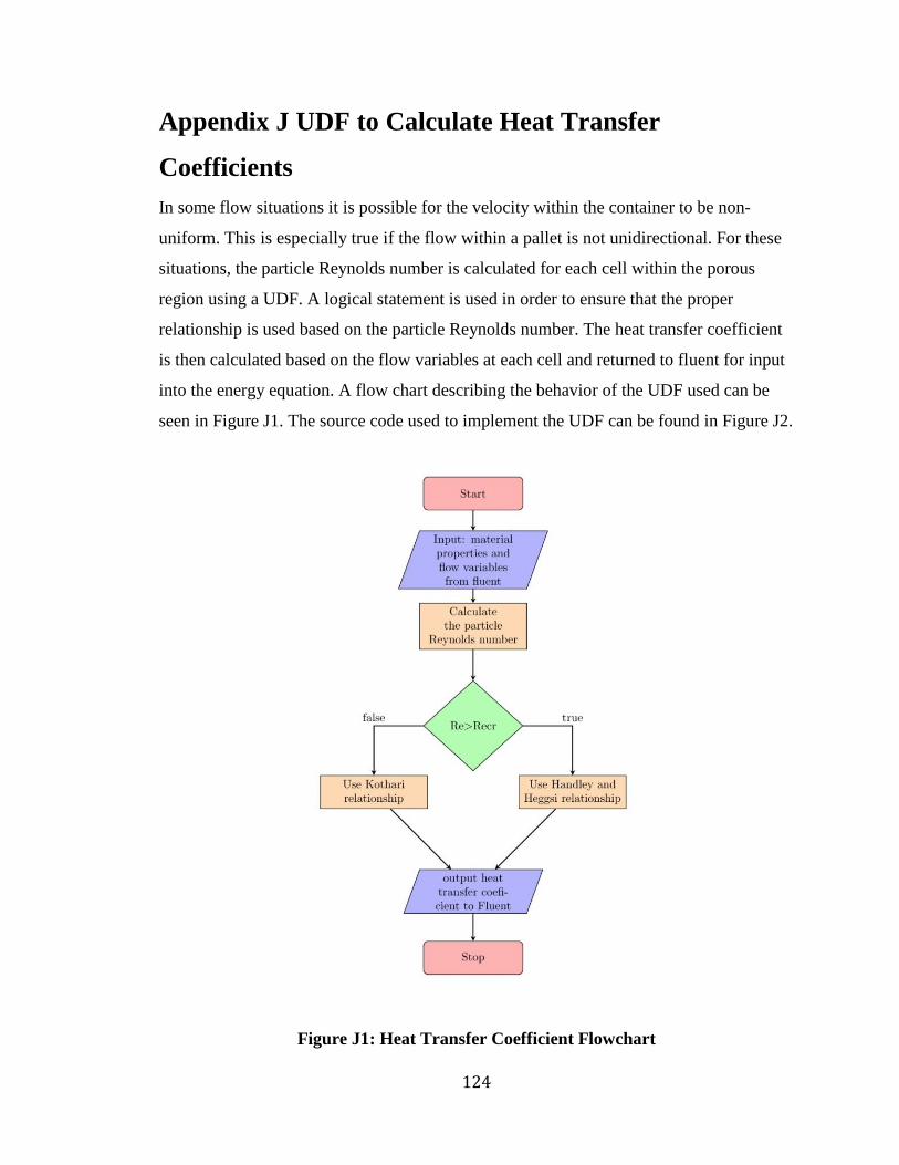
124

Appendix J UDF to Calculate Heat Transfer

Coefficients

In some flow situations it is possible for the velocity within the container to be non-

uniform. This is especially true if the flow within a pallet is not unidirectional. For these

situations, the particle Reynolds number is calculated for each cell within the porous

region using a UDF. A logical statement is used in order to ensure that the proper

relationship is used based on the particle Reynolds number. The heat transfer coefficient

is then calculated based on the flow variables at each cell and returned to fluent for input

into the energy equation. A flow chart describing the behavior of the UDF used can be

seen in Figure J1. The source code used to implement the UDF can be found in Figure J2.

Figure J1: Heat Transfer Coefficient Flowchart

125

/* Heat Transfer Coeficient Profile UDF in a Porous Zone

that utilizes C_PROFILE*/

#include "udf.h"

DEFINE_PROFILE(hlongDC,t,nv)

{

cell_t c;

double Nufsy;

double Nufsx;

double hfsy;

double hfsx;

double h;

double a=0.3333333333; /*power of Pr*/

double b=0.6666666667; /*power of Re*/

double Bi;

real lc = 0.0211;

begin_c_loop(c,t)

real T = C_T(c,t); /* Temperature */

real rho = C_R(c,t); /* Density */

real Cp = C_CP(c,t); /* Specific Heat*/

real mu = C_MU_L(c,t); /* Laminar Viscosity */

real ka = C_K_L(c,t); /*Thermal Conductivity of air*/

real E = 0.5737; /* Porosity (calculated)*/

real vy = C_V(c,t); /* Y-Component of velocity*/

real vx = C_U(c,t); /* X-Component of velocity*/

real kw = 0.6; /* Thermal Conductivity of Water

(estimated)*/

real dp = 0.037; /*diameter of produce 2* is for slab*/

real By = 6; /* Beta is 10,8,6 for spheres, cylinders, and

slabs*/

real Bx = 8; /* Beta is 10,8,6 for spheres, cylinders, and

slabs respectively*/

real Pr= Cp*mu/ka; /* Calculates the Prandtl Number*/

real Rey= fabs(vy*dp*rho/mu); /* Calculates the Reynolds

Number in Y */

real Rex= fabs(vx*dp*rho/mu); /* Calculates the Reynolds

Number in X */

real Recr=80.4994; /*this is the critical reynolds number

to switch nusselt coreelations*/

C_UDMI(c,t,1)=Rey; /*Displaying contours of reynolds number

in Y*/

C_UDMI(c,t,2)=Rex; /*Displaying contours of reynolds number

in X*/

if (Rey>Recr)

{

Nufsy= (0.255/E)*(pow(Pr,a))*(pow(Rey,b));

} /*calculates the films solid Nusselt Number in Y*/

else

126

{

Nufsy=0.033*(pow(Rey,1.3));

}

if (Rex>Recr)

{

Nufsx= (0.255/E)*(pow(Pr,a))*(pow(Rex,b));

} /*calculates the films solid Nusselt Number in X*/

else

{

Nufsx=0.033*(pow(Rex,1.3));

}

hfsy=Nufsy*ka/dp; /* calculates the film solid heat

transfer coeficient in Y */

hfsx=Nufsx*ka/dp; /* calculates the film solid heat

transfer coeficient in X */

h=1/((1/hfsy)+((dp/By)/kw))+1/((1/hfsx)+((dp/Bx)/kw));

C_UDMI(c,t,0)=h; /* checking the h value */

C_PROFILE(c,t,nv) = h;

Bi=h*lc/kw;

C_UDMI(c,t,7)=Bi; /* checking the Bi Number */

end_c_loop(c,t)

} Figure J2: C Code for Heat Transfer Coefficient UDF

127

Appendix K UDF Used To Calculate Cooling Times

The seven eights and half-cooling times are obtained through use of the

DEFINE_EXECUTE_AT_END macro within a UDF. The macro ensures that the

specific code executes once at the end of each time step. The code begins by computing

the average temperature of the room and stores it to file. The code then loops through

each container of product checking if the temperature of each cell is greater than the

seven eights and half cooling temperature. If the temperature is greater than seven eights

and half cooling temperature, the current time is returned to Fluent. Once temperature is

no longer greater than the seven eights or half-cooling temperature, the time will no

longer be returned. The program also takes this time to save the average temperature of

the produce in each container to file. Once the program has looped through all the

product containers, the program terminates until the end of the next time step. A

flowchart of describing the behavior of the UDF can be seen in figure K1. Finally, the

source code for the UDF can be found in Figure K2.

128

Figure K1: Cooling Time Flowchart

129

/* UDF wich calculates and returns the Seven eights and

half cooling times*/

#include "udf.h"

extern double Tse[20];

extern double Thalf[20];

double time;

extern char str[sizeof "p10.txt"];

extern int roomid;

FILE *temperature;

/* C function that returns the Volume average temperature

of zone id*/

double boxtemp(int id)

{

Thread *t;

Domain *d;

cell_t c;

double Volume=0;

double Tr=0;

d=Get_Domain(1);

t=Lookup_Thread(d,id);

/*determining the volume average temperature*/

begin_c_loop(c,t)

{

Tr+=C_T(c,t)*C_VOLUME(c,t);

Volume+=C_VOLUME(c,t);

}

end_c_loop(c,t)

Tr=Tr/Volume;

return Tr;

}

DEFINE_EXECUTE_AT_END(CoolingTimes)

{

Domain *d;

Thread *t;

cell_t c;

double BoxT=0;

int x=0;

int i;

time=CURRENT_TIME;

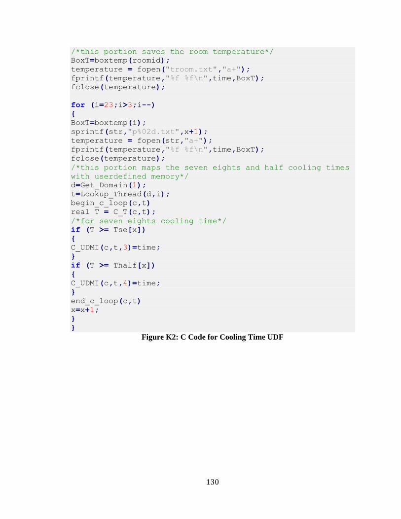
130

/*this portion saves the room temperature*/

BoxT=boxtemp(roomid);

temperature = fopen("troom.txt","a+");

fprintf(temperature,"%f %f\n",time,BoxT);


for (i=23;i>3;i--)

{

BoxT=boxtemp(i);

sprintf(str,"p%02d.txt",x+1);

temperature = fopen(str,"a+");

fprintf(temperature,"%f %f\n",time,BoxT);


/*this portion maps the seven eights and half cooling times

with userdefined memory*/

d=Get_Domain(1);

t=Lookup_Thread(d,i);

begin_c_loop(c,t)

real T = C_T(c,t);

/*for seven eights cooling time*/

if (T >= Tse[x])

{

C_UDMI(c,t,3)=time;

}

if (T >= Thalf[x])

{

C_UDMI(c,t,4)=time;

}

end_c_loop(c,t)

x=x+1;

}

} Figure K2: C Code for Cooling Time UDF

131

Vita Auctoris

Name: Jean-Paul E. Martins

Place of Birth: Windsor, Ontario

Year of Birth: 1985

Education: St. Clair College, Windsor ON

2004-2007 Technical Diploma

University of Windsor, Windsor ON

2007-2012 BASc

University of Windsor, Windsor ON

2012-2016 MASc

An Investigation of Agricultural Produce Cooling Tunnel ...

Documents

Transcript of An Investigation of Agricultural Produce Cooling Tunnel ...