Analisis Matricial 1de 3
220
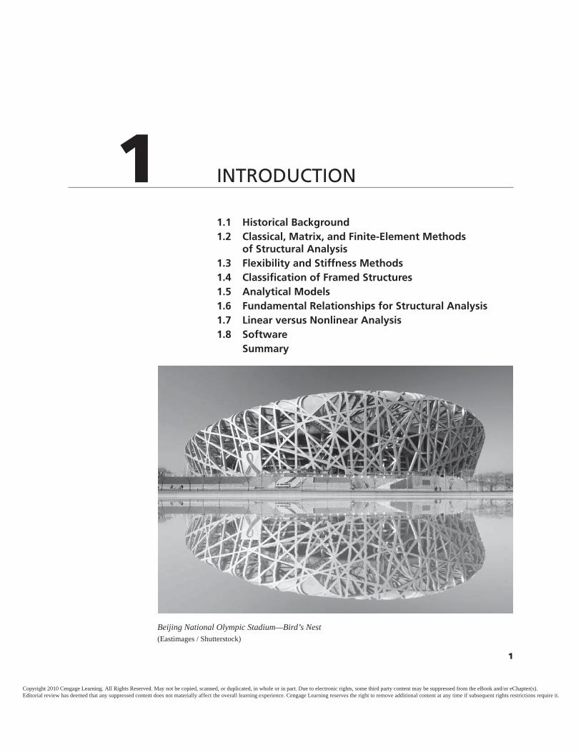
1 1.1 Historical Background 1.2 Classical, Matrix, and Finite-Element Methods of Structural Analysis 1.3 Flexibility and Stiffness Methods 1.4 Classification of Framed Structures 1.5 Analytical Models 1.6 Fundamental Relationships for Structural Analysis 1.7 Linear versus Nonlinear Analysis 1.8 Software Summary 1 INTRODUCTION Beijing National Olympic Stadium—Bird’s Nest (Eastimages / Shutterstock) Copyright 2010 Cengage Learning. All Rights Reserved. May not be copied, scanned, or duplicated, in whole or in part. Due to electronic rights, some third party content may be suppressed from the eBook and/or eChapter(s). Editorial review has deemed that any suppressed content does not materially affect the overall learning experience. Cengage Learning reserves the right to remove additional content at any time if subsequent rights restrictions require it.
-
Upload
independent -
Category
Documents
-
view
2 -
download
0
Transcript of Analisis Matricial 1de 3
11.1 Historical Background1.2 Classical, Matrix, and Finite-Element Methods
of Structural Analysis1.3 Flexibility and Stiffness Methods1.4 Classification of Framed Structures1.5 Analytical Models1.6 Fundamental Relationships for Structural Analysis1.7 Linear versus Nonlinear Analysis1.8 Software
Summary
1
INTRODUCTION
Beijing National Olympic Stadium—Bird’s Nest(Eastimages / Shutterstock)
Copyright 2010 Cengage Learning. All Rights Reserved. May not be copied, scanned, or duplicated, in whole or in part. Due to electronic rights, some third party content may be suppressed from the eBook and/or eChapter(s).Editorial review has deemed that any suppressed content does not materially affect the overall learning experience. Cengage Learning reserves the right to remove additional content at any time if subsequent rights restrictions require it.
Structural analysis, which is an integral part of any structural engineering project,is the process of predicting the performance of a given structure under a pre-scribed loading condition. The performance characteristics usually of interest instructural design are: (a) stresses or stress resultants (i.e., axial forces, shears, andbending moments); (b) deflections; and (c) support reactions. Thus, the analysisof a structure typically involves the determination of these quantities as caused bythe given loads and/or other external effects (such as support displacements andtemperature changes). This text is devoted to the analysis of framed structures—that is, structures composed of long straight members. Many commonly usedstructures such as beams, and plane and space trusses and rigid frames, are clas-sified as framed structures (also referred to as skeletal structures).
In most design offices today, the analysis of framed structures is routinelyperformed on computers, using software based on the matrix methods of struc-tural analysis. It is therefore essential that structural engineers understand thebasic principles of matrix analysis, so that they can develop their own com-puter programs and/or properly use commercially available software—and ap-preciate the physical significance of the analytical results. The objective of thistext is to present the theory and computer implementation of matrix methodsfor the analysis of framed structures in static equilibrium.
This chapter provides a general introduction to the subject of matrix computer analysis of structures. We start with a brief historical background inSection 1.1, followed by a discussion of how matrix methods differ from classi-cal and finite-element methods of structural analysis (Section 1.2). Flexibilityand stiffness methods of matrix analysis are described in Section 1.3; the sixtypes of framed structures considered in this text (namely, plane trusses, beams,plane frames, space trusses, grids, and space frames) are discussed in Section 1.4;and the development of simplified models of structures for the purpose of analy-sis is considered in Section 1.5. The basic concepts of structural analysis neces-sary for formulating the matrix methods, as presented in this text, are reviewedin Section 1.6; and the roles and limitations of linear and nonlinear types ofstructural analysis are discussed in Section 1.7. Finally, we conclude the chap-ter with a brief note on the computer software that is provided on the publisher’swebsite for this book (Section 1.8). (www.cengage.com/engineering)
1.1 HISTORICAL BACKGROUNDThe theoretical foundation for matrix methods of structural analysis was laidby James C. Maxwell, who introduced the method of consistent deformationsin 1864; and George A. Maney, who developed the slope-deflection method in1915. These classical methods are considered to be the precursors of the ma-trix flexibility and stiffness methods, respectively. In the precomputer era, themain disadvantage of these earlier methods was that they required direct solu-tion of simultaneous algebraic equations—a formidable task by hand calcula-tions in cases of more than a few unknowns.
The invention of computers in the late 1940s revolutionized structuralanalysis. As computers could solve large systems of simultaneous equations,the analysis methods yielding solutions in that form were no longer at a
2 Chapter 1 Introduction
Copyright 2010 Cengage Learning. All Rights Reserved. May not be copied, scanned, or duplicated, in whole or in part. Due to electronic rights, some third party content may be suppressed from the eBook and/or eChapter(s).Editorial review has deemed that any suppressed content does not materially affect the overall learning experience. Cengage Learning reserves the right to remove additional content at any time if subsequent rights restrictions require it.
disadvantage, but in fact were preferred, because simultaneous equations couldbe expressed in matrix form and conveniently programmed for solution oncomputers.
S. Levy is generally considered to have been the first to introduce theflexibility method in 1947, by generalizing the classical method of consistentdeformations. Among the subsequent researchers who extended the flexibilitymethod and expressed it in matrix form in the early 1950s were H. Falken-heimer, B. Langefors, and P. H. Denke. The matrix stiffness method was devel-oped by R. K. Livesley in 1954. In the same year, J. H. Argyris and S. Kelseypresented a formulation of matrix methods based on energy principles. In 1956,M. T. Turner, R. W. Clough, H. C. Martin, and L. J. Topp derived stiffness ma-trices for the members of trusses and frames using the finite-element approach,and introduced the now popular direct stiffness method for generating the struc-ture stiffness matrix. In the same year, Livesley presented a nonlinear formula-tion of the stiffness method for stability analysis of frames.
Since the mid-1950s, the development of matrix methods has continued ata tremendous pace, with research efforts in recent years directed mainly towardformulating procedures for the dynamic and nonlinear analysis of structures,and developing efficient computational techniques for analyzing largestructures. Recent advances in these areas can be attributed to S. S. Archer,C. Birnstiel, R. H. Gallagher, J. Padlog, J. S. Przemieniecki, C. K. Wang, andE. L. Wilson, among others.
1.2 CLASSICAL, MATRIX, AND FINITE-ELEMENTMETHODS OF STRUCTURAL ANALYSIS
Classical versus Matrix MethodsAs we develop matrix methods in subsequent chapters of this book, readerswho are familiar with classical methods of structural analysis will realizethat both matrix and classical methods are based on the same fundamentalprinciples—but that the fundamental relationships of equilibrium, compatibil-ity, and member stiffness are now expressed in the form of matrix equations, sothat the numerical computations can be efficiently performed on a computer.
Most classical methods were developed to analyze particular types of struc-tures, and since they were intended for hand calculations, they often involve cer-tain assumptions (that are unnecessary in matrix methods) to reduce the amountof computational effort required for analysis. The application of these methodsusually requires an understanding on the part of the analyst of the structural be-havior. Consider, for example, the moment-distribution method. This classicalmethod can be used to analyze only beams and plane frames undergoing bend-ing deformations. Deformations due to axial forces in the frames are ignoredto reduce the number of independent joint translations. While this assumptionsignificantly reduces the computational effort, it complicates the analysis by re-quiring the analyst to draw a deflected shape of the frame corresponding to eachdegree of freedom of sidesway (independent joint translation), to estimate the rel-ative magnitudes of member fixed-end moments: a difficult task even in the case
Section 1.2 Classical, Matrix, and Finite-Element Methods of Structural Analysis 3
Copyright 2010 Cengage Learning. All Rights Reserved. May not be copied, scanned, or duplicated, in whole or in part. Due to electronic rights, some third party content may be suppressed from the eBook and/or eChapter(s).Editorial review has deemed that any suppressed content does not materially affect the overall learning experience. Cengage Learning reserves the right to remove additional content at any time if subsequent rights restrictions require it.
of a few degrees of freedom of sidesway if the frame has inclined members.Because of their specialized and intricate nature, classical methods are generallynot considered suitable for computer programming.
In contrast to classical methods, matrix methods were specifically devel-oped for computer implementation; they are systematic (so that they can beconveniently programmed), and general (in the sense that the same overall for-mat of the analytical procedure can be applied to the various types of framedstructures). It will become clear as we study matrix methods that, because ofthe latter characteristic, a computer program developed to analyze one type ofstructure (e.g., plane trusses) can be modified with relative ease to analyzeanother type of structure (e.g., space trusses or frames).
As the analysis of large and highly redundant structures by classicalmethods can be quite time consuming, matrix methods are commonly used.However, classical methods are still preferred by many engineers for analyz-ing smaller structures, because they provide a better insight into the behaviorof structures. Classical methods may also be used for preliminary designs,for checking the results of computerized analyses, and for deriving the mem-ber force–displacement relations needed in the matrix analysis. Furthermore,a study of classical methods is considered to be essential for developing anunderstanding of structural behavior.
Matrix versus Finite Element MethodsMatrix methods can be used to analyze framed structures only. Finite-elementanalysis, which originated as an extension of matrix analysis to surface struc-tures (e.g., plates and shells), has now developed to the extent that it can be applied to structures and solids of practically any shape or form. From a theo-retical viewpoint, the basic difference between the two is that, in matrix methods,the member force–displacement relationships are based on the exact solutionsof the underlying differential equations, whereas in finite-element methods,such relations are generally derived by work-energy principles from assumeddisplacement or stress functions.
Because of the approximate nature of its force–displacement relations,finite-element analysis generally yields approximate results. However, as willbe shown in Chapters 3 and 5, in the case of linear analysis of framed structurescomposed of prismatic (uniform) members, both matrix and finite-elementapproaches yield identical results.
1.3 FLEXIBILITY AND STIFFNESS METHODSTwo different methods can be used for the matrix analysis of structures: the flex-ibility method, and the stiffness method. The flexibility method, which is alsoreferred to as the force or compatibility method, is essentially a generalizationin matrix form of the classical method of consistent deformations. In this ap-proach, the primary unknowns are the redundant forces, which are calculatedfirst by solving the structure’s compatibility equations. Once the redundantforces are known, the displacements can be evaluated by applying the equationsof equilibrium and the appropriate member force–displacement relations.
4 Chapter 1 Introduction
Copyright 2010 Cengage Learning. All Rights Reserved. May not be copied, scanned, or duplicated, in whole or in part. Due to electronic rights, some third party content may be suppressed from the eBook and/or eChapter(s).Editorial review has deemed that any suppressed content does not materially affect the overall learning experience. Cengage Learning reserves the right to remove additional content at any time if subsequent rights restrictions require it.
The stiffness method, which originated from the classical slope-deflectionmethod, is also called the displacement or equilibrium method. In this ap-proach, the primary unknowns are the joint displacements, which are deter-mined first by solving the structure’s equations of equilibrium. With the jointdisplacements known, the unknown forces are obtained through compatibilityconsiderations and the member force–displacement relations.
Although either method can be used to analyze framed structures, the flexi-bility method is generally convenient for analyzing small structures with a few re-dundants. This method may also be used to establish member force-displacementrelations needed to develop the stiffness method. The stiffness method is moresystematic and can be implemented more easily on computers; therefore, it is pre-ferred for the analysis of large and highly redundant structures. Most of the com-mercially available software for structural analysis is based on the stiffnessmethod. In this text, we focus our attention mainly on the stiffness method, withemphasis on a particular version known as the direct stiffness method, which iscurrently used in professional practice. The fundamental concepts of the flexibil-ity method are presented in Appendix B.
1.4 CLASSIFICATION OF FRAMED STRUCTURESFramed structures are composed of straight members whose lengths are signif-icantly larger than their cross-sectional dimensions. Common framed struc-tures can be classified into six basic categories based on the arrangement oftheir members, and the types of primary stresses that may develop in theirmembers under major design loads.
Plane TrussesA truss is defined as an assemblage of straight members connected at their endsby flexible connections, and subjected to loads and reactions only at the joints(connections). The members of such an ideal truss develop only axial forceswhen the truss is loaded. In real trusses, such as those commonly used for sup-porting roofs and bridges, the members are connected by bolted or welded con-nections that are not perfectly flexible, and the dead weights of the membersare distributed along their lengths. Because of these and other deviations fromidealized conditions, truss members are subjected to some bending and shear.However, in most trusses, these secondary bending moments and shears aresmall in comparison to the primary axial forces, and are usually not consideredin their designs. If large bending moments and shears are anticipated, then thetruss should be treated as a rigid frame (discussed subsequently) for analysisand design.
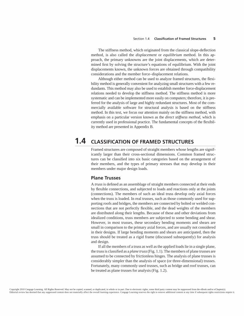
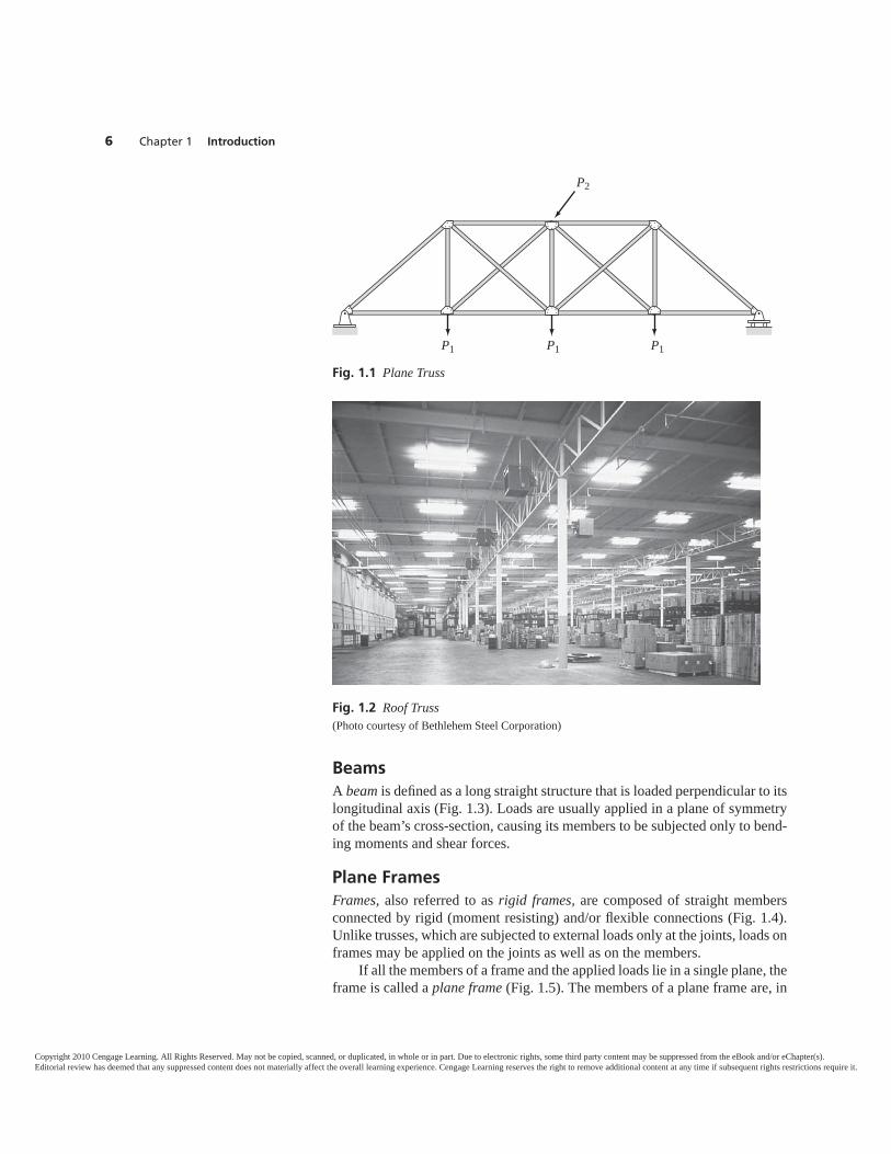
If all the members of a truss as well as the applied loads lie in a single plane,the truss is classified as a plane truss (Fig. 1.1). The members of plane trusses areassumed to be connected by frictionless hinges. The analysis of plane trusses isconsiderably simpler than the analysis of space (or three-dimensional) trusses.Fortunately, many commonly used trusses, such as bridge and roof trusses, canbe treated as plane trusses for analysis (Fig. 1.2).
Section 1.4 Classification of Framed Structures 5
Copyright 2010 Cengage Learning. All Rights Reserved. May not be copied, scanned, or duplicated, in whole or in part. Due to electronic rights, some third party content may be suppressed from the eBook and/or eChapter(s).Editorial review has deemed that any suppressed content does not materially affect the overall learning experience. Cengage Learning reserves the right to remove additional content at any time if subsequent rights restrictions require it.
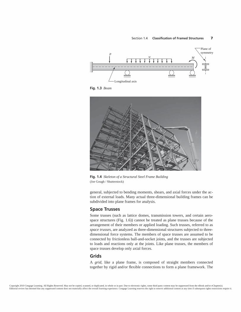
BeamsA beam is defined as a long straight structure that is loaded perpendicular to itslongitudinal axis (Fig. 1.3). Loads are usually applied in a plane of symmetryof the beam’s cross-section, causing its members to be subjected only to bend-ing moments and shear forces.
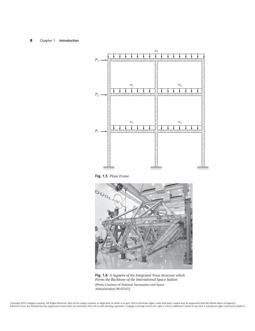
Plane FramesFrames, also referred to as rigid frames, are composed of straight membersconnected by rigid (moment resisting) and/or flexible connections (Fig. 1.4).Unlike trusses, which are subjected to external loads only at the joints, loads onframes may be applied on the joints as well as on the members.
If all the members of a frame and the applied loads lie in a single plane, theframe is called a plane frame (Fig. 1.5). The members of a plane frame are, in
6 Chapter 1 Introduction
Fig. 1.2 Roof Truss(Photo courtesy of Bethlehem Steel Corporation)
Fig. 1.1 Plane Truss
P1 P1 P1
P2
Copyright 2010 Cengage Learning. All Rights Reserved. May not be copied, scanned, or duplicated, in whole or in part. Due to electronic rights, some third party content may be suppressed from the eBook and/or eChapter(s).Editorial review has deemed that any suppressed content does not materially affect the overall learning experience. Cengage Learning reserves the right to remove additional content at any time if subsequent rights restrictions require it.
general, subjected to bending moments, shears, and axial forces under the ac-tion of external loads. Many actual three-dimensional building frames can besubdivided into plane frames for analysis.
Space TrussesSome trusses (such as lattice domes, transmission towers, and certain aero-space structures (Fig. 1.6)) cannot be treated as plane trusses because of thearrangement of their members or applied loading. Such trusses, referred to asspace trusses, are analyzed as three-dimensional structures subjected to three-dimensional force systems. The members of space trusses are assumed to beconnected by frictionless ball-and-socket joints, and the trusses are subjectedto loads and reactions only at the joints. Like plane trusses, the members ofspace trusses develop only axial forces.
GridsA grid, like a plane frame, is composed of straight members connectedtogether by rigid and/or flexible connections to form a plane framework. The
Section 1.4 Classification of Framed Structures 7
Fig. 1.4 Skeleton of a Structural Steel Frame Building(Joe Gough / Shutterstock)
Fig. 1.3 Beam
PM
Longitudinal axis
Plane of symmetry
w
Copyright 2010 Cengage Learning. All Rights Reserved. May not be copied, scanned, or duplicated, in whole or in part. Due to electronic rights, some third party content may be suppressed from the eBook and/or eChapter(s).Editorial review has deemed that any suppressed content does not materially affect the overall learning experience. Cengage Learning reserves the right to remove additional content at any time if subsequent rights restrictions require it.
8 Chapter 1 Introduction
Fig. 1.5 Plane Frame
w3
w2
w1 w1
w2
P3
P2
P1
Fig. 1.6 A Segment of the Integrated Truss Structure whichForms the Backbone of the International Space Station(Photo Courtesy of National Aeronautics and Space Administration 98-05165)
Copyright 2010 Cengage Learning. All Rights Reserved. May not be copied, scanned, or duplicated, in whole or in part. Due to electronic rights, some third party content may be suppressed from the eBook and/or eChapter(s).Editorial review has deemed that any suppressed content does not materially affect the overall learning experience. Cengage Learning reserves the right to remove additional content at any time if subsequent rights restrictions require it.
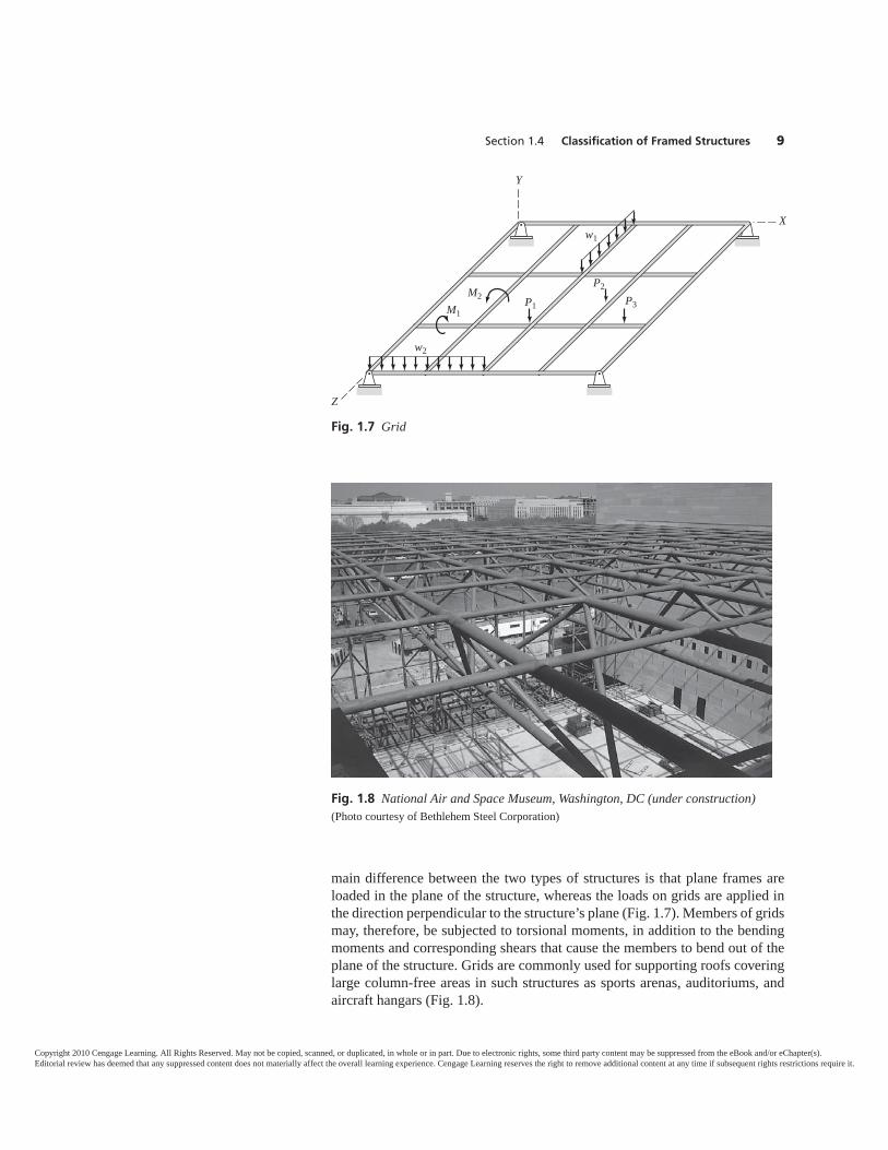
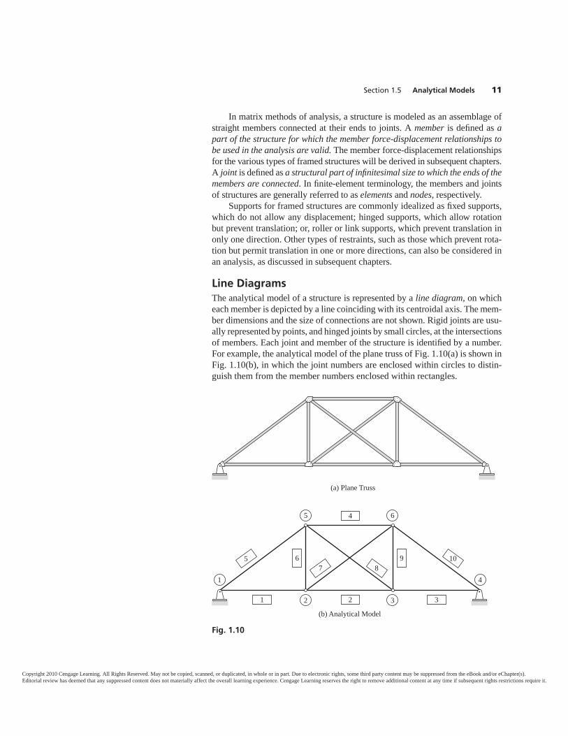
main difference between the two types of structures is that plane frames areloaded in the plane of the structure, whereas the loads on grids are applied inthe direction perpendicular to the structure’s plane (Fig. 1.7). Members of gridsmay, therefore, be subjected to torsional moments, in addition to the bendingmoments and corresponding shears that cause the members to bend out of theplane of the structure. Grids are commonly used for supporting roofs coveringlarge column-free areas in such structures as sports arenas, auditoriums, andaircraft hangars (Fig. 1.8).
Section 1.4 Classification of Framed Structures 9
Fig. 1.7 Grid
w2
w1
M1P1
P2
P3M2
Z
X
Y
Fig. 1.8 National Air and Space Museum, Washington, DC (under construction)(Photo courtesy of Bethlehem Steel Corporation)
Copyright 2010 Cengage Learning. All Rights Reserved. May not be copied, scanned, or duplicated, in whole or in part. Due to electronic rights, some third party content may be suppressed from the eBook and/or eChapter(s).Editorial review has deemed that any suppressed content does not materially affect the overall learning experience. Cengage Learning reserves the right to remove additional content at any time if subsequent rights restrictions require it.

Space FramesSpace frames constitute the most general category of framed structures.Members of space frames may be arranged in any arbitrary directions, andconnected by rigid and/or flexible connections. Loads in any directions may beapplied on members as well as on joints. The members of a space frame may,in general, be subjected to bending moments about both principal axes, shearsin both principal directions, torsional moments, and axial forces (Fig. 1.9).
1.5 ANALYTICAL MODELSThe first (and perhaps most important) step in the analysis of a structure is todevelop its analytical model. An analytical model is an idealized representationof a real structure for the purpose of analysis. Its objective is to simplify theanalysis of a complicated structure by discarding much of the detail (aboutconnections, members, etc.) that is likely to have little effect on the structure’sbehavioral characteristics of interest, while representing, as accurately aspractically possible, the desired characteristics. It is important to note that thestructural response predicted from an analysis is valid only to the extent thatthe analytical model represents the actual structure. For framed structures, theestablishment of analytical models generally involves consideration of issuessuch as whether the actual three-dimensional structure can be subdivided intoplane structures for analysis, and whether to idealize the actual bolted orwelded connections as hinged, rigid, or semirigid joints. Thus, the develop-ment of accurate analytical models requires not only a thorough understandingof structural behavior and methods of analysis, but also experience and knowl-edge of design and construction practices.
10 Chapter 1 Introduction
Fig. 1.9 Space Frame(© MNTravel / Alamy)
Copyright 2010 Cengage Learning. All Rights Reserved. May not be copied, scanned, or duplicated, in whole or in part. Due to electronic rights, some third party content may be suppressed from the eBook and/or eChapter(s).Editorial review has deemed that any suppressed content does not materially affect the overall learning experience. Cengage Learning reserves the right to remove additional content at any time if subsequent rights restrictions require it.
In matrix methods of analysis, a structure is modeled as an assemblage ofstraight members connected at their ends to joints. A member is defined as apart of the structure for which the member force-displacement relationships tobe used in the analysis are valid. The member force-displacement relationshipsfor the various types of framed structures will be derived in subsequent chapters.A joint is defined as a structural part of infinitesimal size to which the ends of themembers are connected. In finite-element terminology, the members and jointsof structures are generally referred to as elements and nodes, respectively.
Supports for framed structures are commonly idealized as fixed supports,which do not allow any displacement; hinged supports, which allow rotationbut prevent translation; or, roller or link supports, which prevent translation inonly one direction. Other types of restraints, such as those which prevent rota-tion but permit translation in one or more directions, can also be considered inan analysis, as discussed in subsequent chapters.
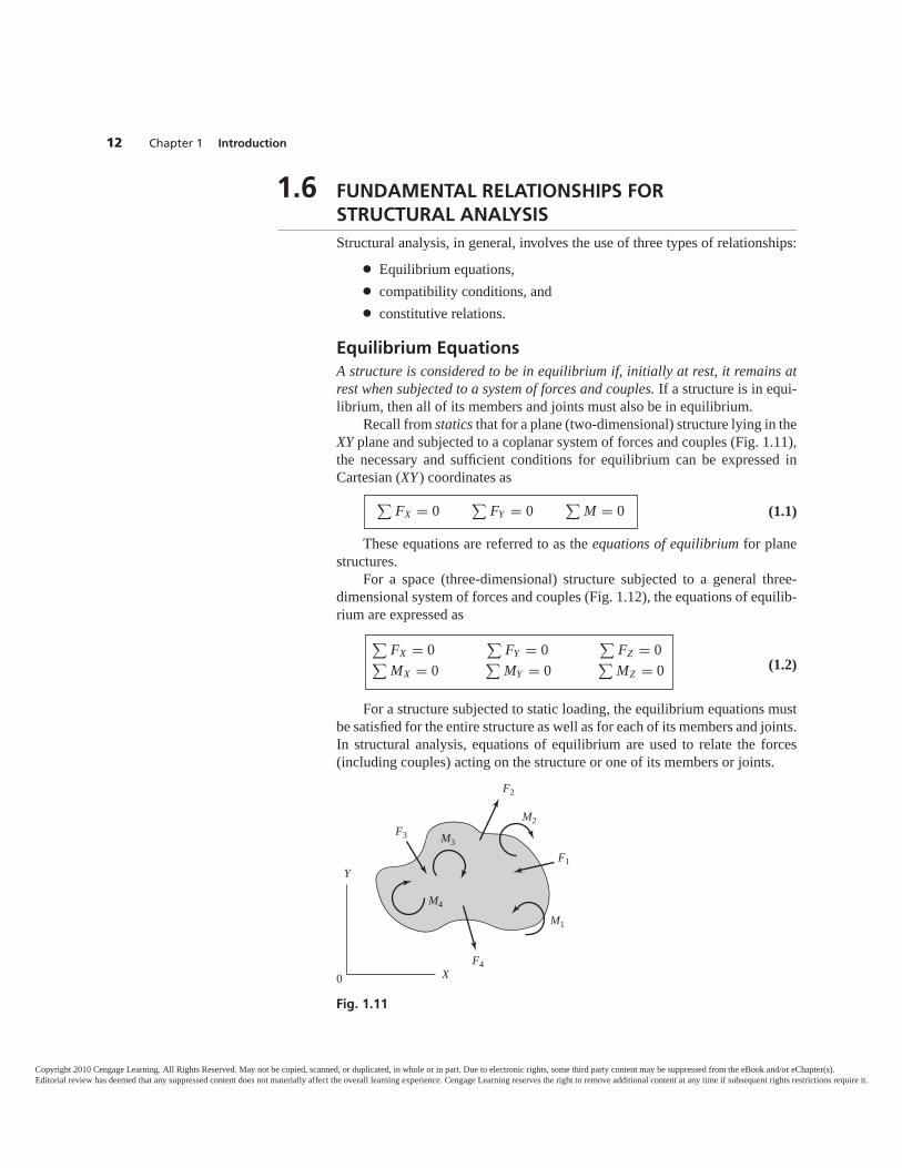
Line DiagramsThe analytical model of a structure is represented by a line diagram, on whicheach member is depicted by a line coinciding with its centroidal axis. The mem-ber dimensions and the size of connections are not shown. Rigid joints are usu-ally represented by points, and hinged joints by small circles, at the intersectionsof members. Each joint and member of the structure is identified by a number.For example, the analytical model of the plane truss of Fig. 1.10(a) is shown inFig. 1.10(b), in which the joint numbers are enclosed within circles to distin-guish them from the member numbers enclosed within rectangles.
Section 1.5 Analytical Models 11
Fig. 1.10
(a) Plane Truss
32
5
1 4
6
1 32
7 8105
(b) Analytical Model
4
6 9
Copyright 2010 Cengage Learning. All Rights Reserved. May not be copied, scanned, or duplicated, in whole or in part. Due to electronic rights, some third party content may be suppressed from the eBook and/or eChapter(s).Editorial review has deemed that any suppressed content does not materially affect the overall learning experience. Cengage Learning reserves the right to remove additional content at any time if subsequent rights restrictions require it.
12 Chapter 1 Introduction
1.6 FUNDAMENTAL RELATIONSHIPS FOR STRUCTURAL ANALYSISStructural analysis, in general, involves the use of three types of relationships:
● Equilibrium equations,
● compatibility conditions, and
● constitutive relations.
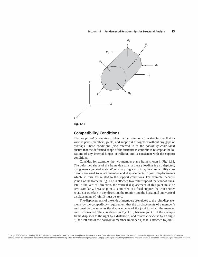
Equilibrium EquationsA structure is considered to be in equilibrium if, initially at rest, it remains atrest when subjected to a system of forces and couples. If a structure is in equi-librium, then all of its members and joints must also be in equilibrium.
Recall from statics that for a plane (two-dimensional) structure lying in theXY plane and subjected to a coplanar system of forces and couples (Fig. 1.11),the necessary and sufficient conditions for equilibrium can be expressed inCartesian (XY) coordinates as
(1.1)
These equations are referred to as the equations of equilibrium for planestructures.
For a space (three-dimensional) structure subjected to a general three-dimensional system of forces and couples (Fig. 1.12), the equations of equilib-rium are expressed as
∑FX = 0
∑FY = 0
∑FZ = 0∑
MX = 0∑
MY = 0∑
MZ = 0 (1.2)
For a structure subjected to static loading, the equilibrium equations mustbe satisfied for the entire structure as well as for each of its members and joints.In structural analysis, equations of equilibrium are used to relate the forces(including couples) acting on the structure or one of its members or joints.
∑FX = 0
∑FY = 0
∑M = 0
Fig. 1.11
F4
M1
F1
M2
F2
M3F3
Y
X0
M4
Copyright 2010 Cengage Learning. All Rights Reserved. May not be copied, scanned, or duplicated, in whole or in part. Due to electronic rights, some third party content may be suppressed from the eBook and/or eChapter(s).Editorial review has deemed that any suppressed content does not materially affect the overall learning experience. Cengage Learning reserves the right to remove additional content at any time if subsequent rights restrictions require it.
Compatibility ConditionsThe compatibility conditions relate the deformations of a structure so that itsvarious parts (members, joints, and supports) fit together without any gaps oroverlaps. These conditions (also referred to as the continuity conditions)ensure that the deformed shape of the structure is continuous (except at the lo-cations of any internal hinges or rollers), and is consistent with the supportconditions.
Consider, for example, the two-member plane frame shown in Fig. 1.13.The deformed shape of the frame due to an arbitrary loading is also depicted,using an exaggerated scale. When analyzing a structure, the compatibility con-ditions are used to relate member end displacements to joint displacementswhich, in turn, are related to the support conditions. For example, becausejoint 1 of the frame in Fig. 1.13 is attached to a roller support that cannot trans-late in the vertical direction, the vertical displacement of this joint must bezero. Similarly, because joint 3 is attached to a fixed support that can neitherrotate nor translate in any direction, the rotation and the horizontal and verticaldisplacements of joint 3 must be zero.
The displacements of the ends of members are related to the joint displace-ments by the compatibility requirement that the displacements of a member’send must be the same as the displacements of the joint to which the memberend is connected. Thus, as shown in Fig. 1.13, because joint 1 of the exampleframe displaces to the right by a distance d1 and rotates clockwise by an angleθ1, the left end of the horizontal member (member 1) that is attached to joint 1
Section 1.6 Fundamental Relationships for Structural Analysis 13
Fig. 1.12
Y
X
Z
0
M4
M2
M1
M3
F1
F5
F4
F3
F2
Copyright 2010 Cengage Learning. All Rights Reserved. May not be copied, scanned, or duplicated, in whole or in part. Due to electronic rights, some third party content may be suppressed from the eBook and/or eChapter(s).Editorial review has deemed that any suppressed content does not materially affect the overall learning experience. Cengage Learning reserves the right to remove additional content at any time if subsequent rights restrictions require it.
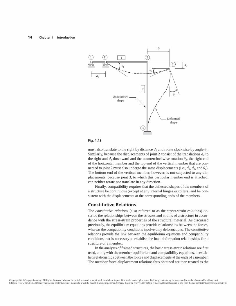
must also translate to the right by distance d1 and rotate clockwise by angle θ1.Similarly, because the displacements of joint 2 consist of the translations d2 tothe right and d3 downward and the counterclockwise rotation θ2, the right endof the horizontal member and the top end of the vertical member that are con-nected to joint 2 must also undergo the same displacements (i.e., d2, d3, and θ2).The bottom end of the vertical member, however, is not subjected to any dis-placements, because joint 3, to which this particular member end is attached,can neither rotate nor translate in any direction.
Finally, compatibility requires that the deflected shapes of the members ofa structure be continuous (except at any internal hinges or rollers) and be con-sistent with the displacements at the corresponding ends of the members.
Constitutive RelationsThe constitutive relations (also referred to as the stress-strain relations) de-scribe the relationships between the stresses and strains of a structure in accor-dance with the stress-strain properties of the structural material. As discussedpreviously, the equilibrium equations provide relationships between the forces,whereas the compatibility conditions involve only deformations. The constitutiverelations provide the link between the equilibrium equations and compatibilityconditions that is necessary to establish the load-deformation relationships for astructure or a member.
In the analysis of framed structures, the basic stress-strain relations are firstused, along with the member equilibrium and compatibility equations, to estab-lish relationships between the forces and displacements at the ends of a member.The member force-displacement relations thus obtained are then treated as the
14 Chapter 1 Introduction
Fig. 1.13
Undeformedshape
Deformedshape
d1
d2
d3θ1
θ2
θ2
1′ 2
3
2′
1 1
2
Copyright 2010 Cengage Learning. All Rights Reserved. May not be copied, scanned, or duplicated, in whole or in part. Due to electronic rights, some third party content may be suppressed from the eBook and/or eChapter(s).Editorial review has deemed that any suppressed content does not materially affect the overall learning experience. Cengage Learning reserves the right to remove additional content at any time if subsequent rights restrictions require it.
constitutive relations for the entire structure, and are used to link the structure’sequilibrium and compatibility equations, thereby yielding the load-deformationrelationships for the entire structure. These load-deformation relations can then besolved to determine the deformations of the structure due to a given loading.
In the case of statically determinate structures, the equilibrium equationscan be solved independently of the compatibility and constitutive relations toobtain the reactions and member forces. The deformations of the structure, ifdesired, can then be determined by employing the compatibility and constitu-tive relations. In the analysis of statically indeterminate structures, however,the equilibrium equations alone are not sufficient for determining the reactionsand member forces. Therefore, it becomes necessary to satisfy simultaneouslythe three types of fundamental relationships (i.e., equilibrium, compatibility,and constitutive relations) to determine the structural response.
Matrix methods of structural analysis are usually formulated by direct ap-plication of the three fundamental relationships as described in general termsin the preceding paragraphs. (Details of the formulations are presented in sub-sequent chapters.) However, matrix methods can also be formulated by usingwork-energy principles that satisfy the three fundamental relationships indi-rectly. Work-energy principles are generally preferred in the formulation offinite-element methods, because they can be more conveniently applied toderive the approximate force-displacement relations for the elements ofsurface structures and solids.
The matrix methods presented in this text are formulated by the direct ap-plication of the equilibrium, compatibility, and constitutive relationships. How-ever, to introduce readers to the finite-element method, and to familiarize themwith the application of the work-energy principles, we also derive the memberforce-displacement relations for plane structures by a finite-element approachthat involves a work-energy principle known as the principle of virtual work. Inthe following paragraphs, we review two statements of this principle pertainingto rigid bodies and deformable bodies, for future reference.
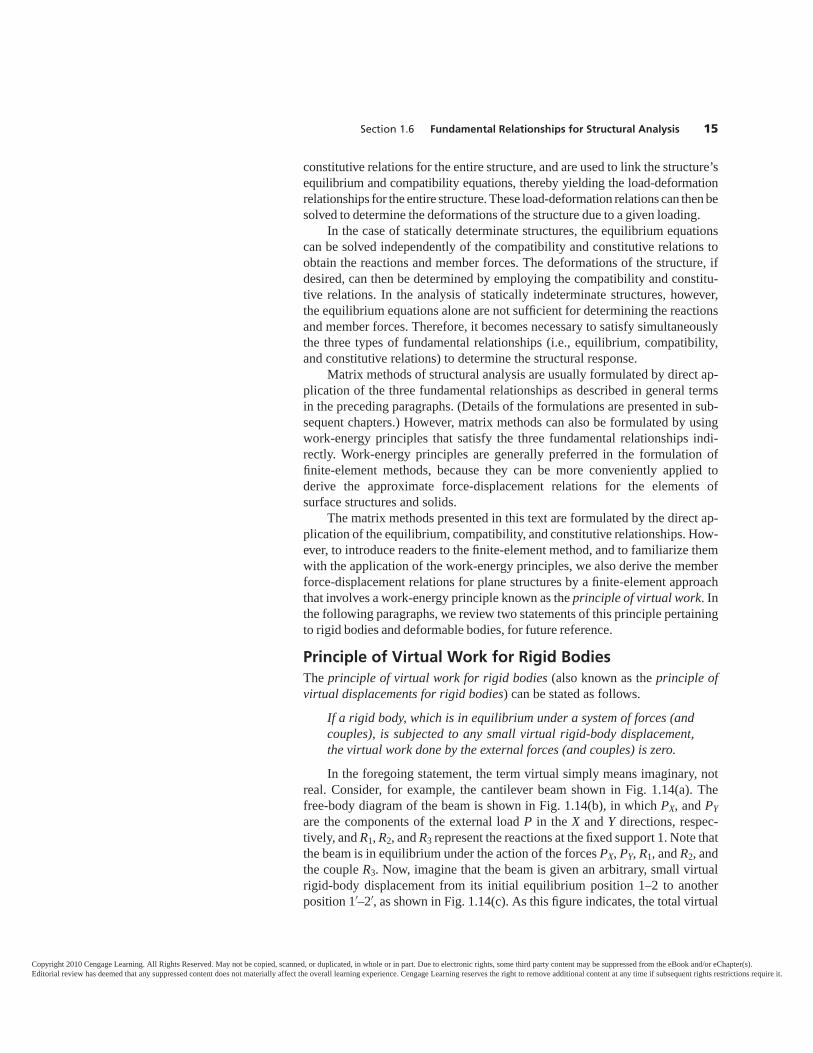
Principle of Virtual Work for Rigid BodiesThe principle of virtual work for rigid bodies (also known as the principle ofvirtual displacements for rigid bodies) can be stated as follows.
If a rigid body, which is in equilibrium under a system of forces (andcouples), is subjected to any small virtual rigid-body displacement,the virtual work done by the external forces (and couples) is zero.In the foregoing statement, the term virtual simply means imaginary, not
real. Consider, for example, the cantilever beam shown in Fig. 1.14(a). Thefree-body diagram of the beam is shown in Fig. 1.14(b), in which PX, and PYare the components of the external load P in the X and Y directions, respec-tively, and R1, R2, and R3 represent the reactions at the fixed support 1. Note thatthe beam is in equilibrium under the action of the forces PX, PY, R1, and R2, andthe couple R3. Now, imagine that the beam is given an arbitrary, small virtualrigid-body displacement from its initial equilibrium position 1–2 to anotherposition 1′–2′, as shown in Fig. 1.14(c). As this figure indicates, the total virtual
Section 1.6 Fundamental Relationships for Structural Analysis 15
Copyright 2010 Cengage Learning. All Rights Reserved. May not be copied, scanned, or duplicated, in whole or in part. Due to electronic rights, some third party content may be suppressed from the eBook and/or eChapter(s).Editorial review has deemed that any suppressed content does not materially affect the overall learning experience. Cengage Learning reserves the right to remove additional content at any time if subsequent rights restrictions require it.
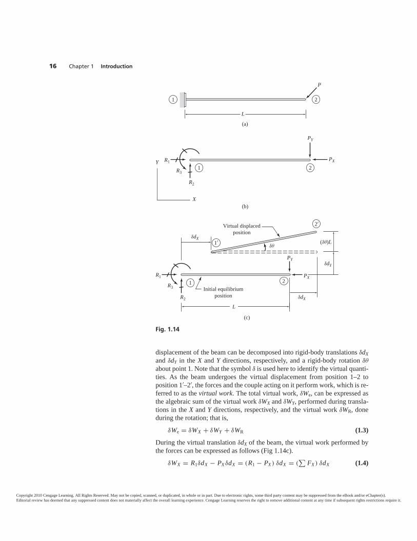
displacement of the beam can be decomposed into rigid-body translations δdXand δdY in the X and Y directions, respectively, and a rigid-body rotation δθ
about point 1. Note that the symbol δ is used here to identify the virtual quanti-ties. As the beam undergoes the virtual displacement from position 1–2 toposition 1′–2′, the forces and the couple acting on it perform work, which is re-ferred to as the virtual work. The total virtual work, δWe, can be expressed asthe algebraic sum of the virtual work δWX and δWY, performed during transla-tions in the X and Y directions, respectively, and the virtual work δWR, doneduring the rotation; that is,
δWe = δWX + δWY + δWR (1.3)
During the virtual translation δdX of the beam, the virtual work performed bythe forces can be expressed as follows (Fig 1.14c).
δWX = R1δdX − PXδdX = (R1 − PX ) δdX = (∑
FX ) δdX (1.4)
16 Chapter 1 Introduction
1 2
L
P
(a)
1 2
PY
R2
R3
R1 PXY
X(b)
1
1′
2′
2
PY
R2
R3
R1 PX
δdX
δdX
δdY
δθ(δθ)L
L
Initial equilibriumposition
Virtual displacedposition
(c)
Fig. 1.14
Copyright 2010 Cengage Learning. All Rights Reserved. May not be copied, scanned, or duplicated, in whole or in part. Due to electronic rights, some third party content may be suppressed from the eBook and/or eChapter(s).Editorial review has deemed that any suppressed content does not materially affect the overall learning experience. Cengage Learning reserves the right to remove additional content at any time if subsequent rights restrictions require it.
Similarly, the virtual work done during the virtual translation δdY is given by
δWY = R2δdY − PY δdY = (R2 − PY ) δdY = (∑
FY ) δdY (1.5)
and the virtual work done by the forces and the couple during the small virtualrotation δθ can be expressed as follows (Fig. 1.14c).
δWR = R3δθ − PY (Lδθ) = (R3 − PY L) δθ = (∑
M©1 ) δθ (1.6)
The expression for the total virtual work can now be obtained by substi-tuting Eqs. (1.4–1.6) into Eq. (1.3). Thus,
δWe = (∑
FX ) δdX + (∑
FY ) δdY + (∑
M©1 ) δθ (1.7)
However, because the beam is in equilibrium, ∑
FX = 0,∑
FY = 0, and∑M©1 = 0; therefore, Eq. (1.7) becomes
(1.8)
which is the mathematical statement of the principle of virtual work for rigidbodies.
Principle of Virtual Work for Deformable BodiesThe principle of virtual work for deformable bodies (also called the principleof virtual displacements for deformable bodies) can be stated as follows.
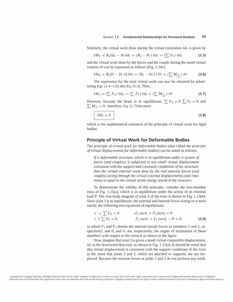
If a deformable structure, which is in equilibrium under a system offorces (and couples), is subjected to any small virtual displacementconsistent with the support and continuity conditions of the structure,then the virtual external work done by the real external forces (andcouples) acting through the virtual external displacements (and rota-tions) is equal to the virtual strain energy stored in the structure.To demonstrate the validity of this principle, consider the two-member
truss of Fig. 1.15(a), which is in equilibrium under the action of an externalload P. The free-body diagram of joint 3 of the truss is shown in Fig. 1.15(b).Since joint 3 is in equilibrium, the external and internal forces acting on it mustsatisfy the following two equations of equilibrium:
+ → ∑FX = 0 −F1 sin θ1 + F2 sin θ2 = 0
+ ↑ ∑FY = 0 F1 cos θ1 + F2 cos θ2 − P = 0 (1.9)
in which F1 and F2 denote the internal (axial) forces in members 1 and 2, re-spectively; and θ1 and θ2 are, respectively, the angles of inclination of thesemembers with respect to the vertical as shown in the figure.
Now, imagine that joint 3 is given a small virtual compatible displacement,δd, in the downward direction, as shown in Fig. 1.15(a). It should be noted thatthis virtual displacement is consistent with the support conditions of the trussin the sense that joints 1 and 2, which are attached to supports, are not dis-placed. Because the reaction forces at joints 1 and 2 do not perform any work,
δWe = 0
Section 1.6 Fundamental Relationships for Structural Analysis 17
Copyright 2010 Cengage Learning. All Rights Reserved. May not be copied, scanned, or duplicated, in whole or in part. Due to electronic rights, some third party content may be suppressed from the eBook and/or eChapter(s).Editorial review has deemed that any suppressed content does not materially affect the overall learning experience. Cengage Learning reserves the right to remove additional content at any time if subsequent rights restrictions require it.

the total virtual work for the truss, δW, is equal to the algebraic sum of the vir-tual work of the forces acting at joint 3. Thus, from Fig. 1.15(b),
δW = Pδd − F1(δd cos θ1) − F2(δd cos θ2)
which can be rewritten asδW = (P − F1 cos θ1 − F2 cos θ2) δd (1.10)
As indicated by Eq. (1.9), the term in parentheses on the right-hand side ofEq. (1.10) is zero. Therefore, the total virtual work, δW, is zero. By substitutingδW = 0 into Eq. (1.10) and rearranging terms, we write
P(δd) = F1(δd cos θ1) + F2(δd cos θ2) (1.11)
in which the quantity on the left-hand side represents the virtual external work,δWe, performed by the real external force P acting through the virtual externaldisplacement δd. Furthermore, because the terms (δd )cos θ1 and (δd )cos θ2 areequal to the virtual internal displacements (elongations) of members 1 and 2,respectively, we can conclude that the right-hand side of Eq. (1.11) represents
18 Chapter 1 Introduction
Fig. 1.15
3
3
Y
X
Real jointforces
F2F1 θ1 θ2
(a)
(b)
21
3
3'
θ1 θ2
Virtual jointdisplacements
θ1θ2
δd
δd
(δd)cos θ1(δd)co
s θ 2
P
Initial equilibriumposition
Virtual displacedposition
P
1 2
Copyright 2010 Cengage Learning. All Rights Reserved. May not be copied, scanned, or duplicated, in whole or in part. Due to electronic rights, some third party content may be suppressed from the eBook and/or eChapter(s).Editorial review has deemed that any suppressed content does not materially affect the overall learning experience. Cengage Learning reserves the right to remove additional content at any time if subsequent rights restrictions require it.
the virtual internal work, δWi, done by the real internal forces acting throughthe corresponding virtual internal displacements; that is,
δWe = δWi (1.12)
Realizing that the internal work is also referred to as the strain energy, U, wecan express Eq. (1.12) as
(1.13)
in which δU denotes the virtual strain energy. Note that Eq. (1.13) is the math-ematical statement of the principle of virtual work for deformable bodies.
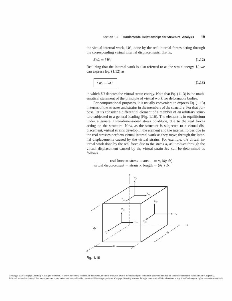
For computational purposes, it is usually convenient to express Eq. (1.13)in terms of the stresses and strains in the members of the structure. For that pur-pose, let us consider a differential element of a member of an arbitrary struc-ture subjected to a general loading (Fig. 1.16). The element is in equilibriumunder a general three-dimensional stress condition, due to the real forcesacting on the structure. Now, as the structure is subjected to a virtual dis-placement, virtual strains develop in the element and the internal forces due tothe real stresses perform virtual internal work as they move through the inter-nal displacements caused by the virtual strains. For example, the virtual in-ternal work done by the real force due to the stress σx as it moves through thevirtual displacement caused by the virtual strain δεx can be determined asfollows.
real force = stress × area = σx (dy dz)virtual displacement = strain × length = (δεx) dx
δWe = δU
Section 1.6 Fundamental Relationships for Structural Analysis 19
Fig. 1.16
x
z
y
dydz
dx
σy
�x
σz
τyz
τyz
τzxτzx
τxy
τxy
Copyright 2010 Cengage Learning. All Rights Reserved. May not be copied, scanned, or duplicated, in whole or in part. Due to electronic rights, some third party content may be suppressed from the eBook and/or eChapter(s).Editorial review has deemed that any suppressed content does not materially affect the overall learning experience. Cengage Learning reserves the right to remove additional content at any time if subsequent rights restrictions require it.
Therefore,virtual internal work = real force × virtual displacement
= (σx dy dz) (δεx dx)= (δεx σx) dV
in which dV = dx dy dz is the volume of the differential element. Thus, the vir-tual internal work due to all six stress components is given by
virtual internal work in element dV= (δεxσx + δεyσy + δεzσz + δγxyτxy + δγyzτyz + δγzxτzx) dV (1.14)
In Eq. (1.14), δεx , δεy, δεz, δγxy, δγyz, and δγzx denote, respectively, the vir-tual strains corresponding to the real stresses σx , σy, σz, τxy, τyz, and τzx ,shown in Fig. 1.16.
The total virtual internal work, or the virtual strain energy stored in the en-tire structure, can be obtained by integrating Eq. (1.14) over the volume V ofthe structure. Thus,
δU =∫
V
(δεxσx + δεyσy + δεzσz + δγxyτxy + δγyzτyz + δγzxτzx
)dV
(1.15)
Finally, by substituting Eq. (1.15) into Eq. (1.13), we obtain the statement ofthe principle of virtual work for deformable bodies in terms of the stresses andstrains of the structure.
(1.16)
1.7 LINEAR VERSUS NONLINEAR ANALYSISIn this text, we focus our attention mainly on linear analysis of structures.Linear analysis of structures is based on the following two fundamentalassumptions:
1. The structures are composed of linearly elastic material; that is, thestress-strain relationship for the structural material follows Hooke’s law.
2. The deformations of the structures are so small that the squares andhigher powers of member slopes, (chord) rotations, and axial strains arenegligible in comparison with unity, and the equations of equilibriumcan be based on the undeformed geometry of the structure.
The reason for making these assumptions is to obtain linear relationshipsbetween applied loads and the resulting structural deformations. An impor-tant advantage of linear force-deformation relations is that the principle of
δWe =∫
V
(δεxσx + δεyσy + δεzσz + δγxyτxy + δγyzτyz + δγzxτzx
)dV
20 Chapter 1 Introduction
Copyright 2010 Cengage Learning. All Rights Reserved. May not be copied, scanned, or duplicated, in whole or in part. Due to electronic rights, some third party content may be suppressed from the eBook and/or eChapter(s).Editorial review has deemed that any suppressed content does not materially affect the overall learning experience. Cengage Learning reserves the right to remove additional content at any time if subsequent rights restrictions require it.
superposition can be used in the analysis. This principle states essentially thatthe combined effect of several loads acting simultaneously on a structureequals the algebraic sum of the effects of each load acting individually on thestructure.
Engineering structures are usually designed so that under service loads theyundergo small deformations, with stresses within the initial linear portions ofthe stress-strain curves of their materials. Thus, linear analysis generally provesadequate for predicting the performance of most common types of structuresunder service loading conditions. However, at higher load levels, the accuracyof linear analysis generally deteriorates as the deformations of the structureincrease and/or its material is strained beyond the yield point. Because of itsinherent limitations, linear analysis cannot be used to predict the ultimate loadcapacities and instability characteristics (e.g., buckling loads) of structures.
With the recent introduction of design specifications based on the ultimatestrengths of structures, the use of nonlinear analysis in structural design is in-creasing. In a nonlinear analysis, the restrictions of linear analysis are removedby formulating the equations of equilibrium on the deformed geometry of thestructure that is not known in advance, and/or taking into account the effects ofinelasticity of the structural material. The load-deformation relationships thusobtained for the structure are nonlinear, and are usually solved using iterativetechniques. An introduction to this still-evolving field of nonlinear structuralanalysis is presented in Chapter 10.
1.8 SOFTWARESoftware for the analysis of framed structures using the matrix stiffnessmethod is provided on the publisher’s website for this book, www.cengage.com/engineering. The software can be used by readers to verify the correctness ofvarious subroutines and programs that they will develop during the course ofstudy of this text, as well as to check the answers to the problems given at theend of each chapter. A description of the software, and information on how toinstall and use it, is presented in Appendix A.
SUMMARY
In this chapter, we discussed the topics summarized in the following list.1. Structural analysis is the prediction of the performance of a given
structure under prescribed loads and/or other external effects.2. Both matrix and classical methods of structural analysis are based on the
same fundamental principles. However, classical methods were developed toanalyze particular types of structures, whereas matrix methods are more generaland systematic so that they can be conveniently programmed on computers.
3. Two different methods can be used for matrix analysis of structures;namely, the flexibility and stiffness methods. The stiffness method is more sys-tematic and can be implemented more easily on computers, and is thereforecurrently preferred in professional practice.
Summary 21
Copyright 2010 Cengage Learning. All Rights Reserved. May not be copied, scanned, or duplicated, in whole or in part. Due to electronic rights, some third party content may be suppressed from the eBook and/or eChapter(s).Editorial review has deemed that any suppressed content does not materially affect the overall learning experience. Cengage Learning reserves the right to remove additional content at any time if subsequent rights restrictions require it.
4. Framed structures are composed of straight members whose lengthsare significantly larger than their cross-sectional dimensions. Framed struc-tures can be classified into six basic categories: plane trusses, beams, planeframes, space trusses, grids, and space frames.
5. An analytical model is a simplified (idealized) representation of a realstructure for the purpose of analysis. Framed structures are modeled as assem-blages of straight members connected at their ends to joints, and these analyti-cal models are represented by line diagrams.
6. The analysis of structures involves three fundamental relationships:equilibrium equations, compatibility conditions, and constitutive relations.
7. The principle of virtual work for deformable bodies states that if adeformable structure, which is in equilibrium, is subjected to a small compati-ble virtual displacement, then the virtual external work is equal to the virtualstrain energy stored in the structure.
8. Linear structural analysis is based on two fundamental assumptions:the stress-strain relationship for the structural material is linearly elastic, andthe structure’s deformations are so small that the equilibrium equations can bebased on the undeformed geometry of the structure.
22 Chapter 1 Introduction
Copyright 2010 Cengage Learning. All Rights Reserved. May not be copied, scanned, or duplicated, in whole or in part. Due to electronic rights, some third party content may be suppressed from the eBook and/or eChapter(s).Editorial review has deemed that any suppressed content does not materially affect the overall learning experience. Cengage Learning reserves the right to remove additional content at any time if subsequent rights restrictions require it.
22.1 Definition of a Matrix2.2 Types of Matrices2.3 Matrix Operations2.4 Gauss–Jordan Elimination Method
SummaryProblems
23
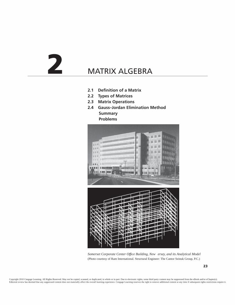
MATRIX ALGEBRA
Somerset Corporate Center Office Building, New ersey, and its Analytical Model(Photo courtesy of Ram International. Structural Engineer: The Cantor Seinuk Group, P.C.)
Copyright 2010 Cengage Learning. All Rights Reserved. May not be copied, scanned, or duplicated, in whole or in part. Due to electronic rights, some third party content may be suppressed from the eBook and/or eChapter(s).Editorial review has deemed that any suppressed content does not materially affect the overall learning experience. Cengage Learning reserves the right to remove additional content at any time if subsequent rights restrictions require it.
In matrix methods of structural analysis, the fundamental relationships ofequilibrium, compatibility, and member force–displacement relations areexpressed in the form of matrix equations, and the analytical procedures areformulated by applying various matrix operations. Therefore, familiaritywith the basic concepts of matrix algebra is a prerequisite to understandingmatrix structural analysis. The objective of this chapter is to concisely pre-sent the basic concepts of matrix algebra necessary for formulating themethods of structural analysis covered in the text. A general procedure forsolving simultaneous linear equations, the Gauss ordan method, is alsodiscussed.
We begin with the basic definition of a matrix in Section 2.1, followed bybrief descriptions of the various types of matrices in Section 2.2. The matrixoperations of equality, addition and subtraction, multiplication, transposition,differentiation and integration, inversion, and partitioning are defined in Sec-tion 2.3; we conclude the chapter with a discussion of the Gauss–Jordan elim-ination method for solving simultaneous equations (Section 2.4).
2.1 DEFINITION OF A MATRIXA matrix is defined as a rectangular array of quantities arranged in rowsand columns. A matrix with m rows and n columns can be expressed asfollows.
A = A =
⎡⎢⎢⎢⎢⎣
A11 A12 A13 · · · · · · A1nA21 A22 A23 · · · · · · A2nA31 A32 A33 · · · · · · A3n· · · · · · · · · · · · Ai j · · ·Am1 Am2 Am3 · · · · · · Amn
⎤⎥⎥⎥⎥⎦ i th row
(2.1)
jth column m × n
As shown in Eq. (2.1), matrices are denoted either by boldface letters (A) orby italic letters enclosed within brackets ( A ). The quantities forming amatrix are referred to as its elements. The elements of a matrix are usuallynumbers, but they can be symbols, equations, or even other matrices (calledsubmatrices). Each element of a matrix is represented by a double-subscriptedletter, with the first subscript identifying the row and the second subscriptidentifying the column in which the element is located. Thus, in Eq. (2.1),A23 represents the element located in the second row and third column ofmatrix A. In general, Aij refers to an element located in the ith row and jthcolumn of matrix A.
The size of a matrix is measured by the number of its rows and columnsand is referred to as the order of the matrix. Thus, matrix A in Eq. (2.1), whichhas m rows and n columns, is considered to be of order m × n (m by n). As an
24 Chapter 2 Matrix Algebra
Copyright 2010 Cengage Learning. All Rights Reserved. May not be copied, scanned, or duplicated, in whole or in part. Due to electronic rights, some third party content may be suppressed from the eBook and/or eChapter(s).Editorial review has deemed that any suppressed content does not materially affect the overall learning experience. Cengage Learning reserves the right to remove additional content at any time if subsequent rights restrictions require it.
example, consider a matrix D given by
D =
⎡⎢⎢⎣
3 5 378 −6 0
12 23 27 −9 −1
⎤⎥⎥⎦
The order of this matrix is 4 × 3, and its elements are symbolically denotedby Dij with i = 1 to 4 and j = 1 to 3; for example, D13 = 37, D31 = 12,D42 = −9, etc.
2.2 TYPES OF MATRICESWe describe some of the common types of matrices in the following paragraphs.
Column Matrix (Vector)If all the elements of a matrix are arranged in a single column (i.e., n = 1), it iscalled a column matrix. Column matrices are usually referred to as vectors, andare sometimes denoted by italic letters enclosed within braces. An example ofa column matrix or vector is given by
B = {B} =
⎡⎢⎢⎢⎢⎣
359
123
26
⎤⎥⎥⎥⎥⎦
Row MatrixA matrix with all of its elements arranged in a single row (i.e., m = 1) is re-ferred to as a row matrix. For example,
C = 9 35 −12 7 22
Square MatrixIf a matrix has the same number of rows and columns (i.e., m = n), it is calleda square matrix. An example of a 4 × 4 square matrix is given by
A =
⎡⎢⎢⎢⎢⎢⎣
6 12 0 2015 −9 −37 3
−24 13 8 140 0 11 −5
⎤⎥⎥⎥⎥⎥⎦ (2.2)
main diagonal
Section 2.2 Types of Matrices 25
Copyright 2010 Cengage Learning. All Rights Reserved. May not be copied, scanned, or duplicated, in whole or in part. Due to electronic rights, some third party content may be suppressed from the eBook and/or eChapter(s).Editorial review has deemed that any suppressed content does not materially affect the overall learning experience. Cengage Learning reserves the right to remove additional content at any time if subsequent rights restrictions require it.
26 Chapter 2 Matrix Algebra
As shown in Eq. (2.2), the main diagonal of a square matrix extends from theupper left corner to the lower right corner, and it contains elements with match-ing subscripts—that is, A11, A22, A33, . . . , Ann. The elements forming the maindiagonal are referred to as the diagonal elements the remaining elements of asquare matrix are called the off-diagonal elements.
Symmetric MatrixWhen the elements of a square matrix are symmetric about its main diagonal(i.e., Aij = Aji), it is termed a symmetric matrix. For example,
A =
⎡⎢⎢⎣
6 15 −24 4015 −9 13 0
−24 13 8 1140 0 11 −5
⎤⎥⎥⎦
Lower Triangular MatrixIf all the elements of a square matrix above its main diagonal are zero, (i.e.,Aij = 0 for j > i), it is referred to as a lower triangular matrix. An example ofa 4 × 4 lower triangular matrix is given by
A =
⎡⎢⎢⎣
8 0 0 012 −9 0 033 17 6 0−2 5 15 3
⎤⎥⎥⎦
Upper Triangular MatrixWhen all the elements of a square matrix below its main diagonal are zero (i.e.,Aij = 0 for j < i), it is called an upper triangular matrix. An example of a 3 × 3upper triangular matrix is given by
A =⎡⎣ −7 6 17
0 12 110 0 20
⎤⎦
Diagonal MatrixA square matrix with all of its off-diagonal elements equal to zero (i.e., Aij = 0for i � j ), is called a diagonal matrix. For example,
A =
⎡⎢⎢⎣
6 0 0 00 −3 0 00 0 11 00 0 0 27
⎤⎥⎥⎦
Copyright 2010 Cengage Learning. All Rights Reserved. May not be copied, scanned, or duplicated, in whole or in part. Due to electronic rights, some third party content may be suppressed from the eBook and/or eChapter(s).Editorial review has deemed that any suppressed content does not materially affect the overall learning experience. Cengage Learning reserves the right to remove additional content at any time if subsequent rights restrictions require it.
Unit or Identity MatrixIf all the diagonal elements of a diagonal matrix are equal to 1 (i.e., Iij = 1 andIij = 0 for i �= j), it is referred to as a unit (or identity) matrix. Unit matrices arecommonly denoted by I or I . An example of a 3 × 3 unit matrix is given by
I =⎡⎣ 1 0 0
0 1 00 0 1
⎤⎦
Null MatrixIf all the elements of a matrix are zero (i.e., Oij = 0), it is termed a null matrix.Null matrices are usually denoted by O or O . An example of a 3 × 4 nullmatrix is given by
O =⎡⎣ 0 0 0 0
0 0 0 00 0 0 0
⎤⎦
2.3 MATRIX OPERATIONS
EqualityMatrices A and B are considered to be equal if they are of the same order and iftheir corresponding elements are identical (i.e., Aij = Bij). Consider, forexample, matrices
A =⎡⎣ 6 2
−7 83 −9
⎤⎦ and B =
⎡⎣ 6 2
−7 83 −9
⎤⎦
Since both A and B are of order 3 × 2, and since each element of A is equal tothe corresponding element of B, the matrices A and B are equal to each other;that is, A = B.
Addition and SubtractionMatrices can be added (or subtracted) only if they are of the same order. Theaddition (or subtraction) of two matrices A and B is carried out by adding(or subtracting) the corresponding elements of the two matrices. Thus, ifA + B = C, then Cij = Aij + Bij; and if A − B = D, then Dij = Aij − Bij . Thematrices C and D have the same order as matrices A and B.
Section 2.3 Matrix Operations 27
E X A M P L E 2.1 Calculate the matrices C = A + B and D = A − B if
A =⎡⎣ 6 0
−2 95 1
⎤⎦ and B =
⎡⎣ 2 3
7 5−12 −1
⎤⎦
Copyright 2010 Cengage Learning. All Rights Reserved. May not be copied, scanned, or duplicated, in whole or in part. Due to electronic rights, some third party content may be suppressed from the eBook and/or eChapter(s).Editorial review has deemed that any suppressed content does not materially affect the overall learning experience. Cengage Learning reserves the right to remove additional content at any time if subsequent rights restrictions require it.
S O L U T I O N
C = A + B =⎡⎣ (6 + 2) (0 + 3)
(−2 + 7) (9 + 5)
(5 − 12) (1 − 1)
⎤⎦ =
⎡⎣ 8 3
5 14−7 0
⎤⎦ Ans
D = A − B =⎡⎣ (6 − 2) (0 − 3)
(−2 − 7) (9 − 5)
(5 + 12) (1 + 1)
⎤⎦ =
⎡⎣ 4 −3
−9 417 2
⎤⎦ Ans
28 Chapter 2 Matrix Algebra
Multiplication by a ScalarThe product of a scalar c and a matrix A is obtained by multiplying eachelement of the matrix A by the scalar c. Thus, if cA = B, then Bij = cAij.
E X A M P L E 2.2 Calculate the matrix B = cA if c = −6 and
A =⎡⎣ 3 7 −2
0 8 112 −4 10
⎤⎦
S O L U T I O N
B = cA =⎡⎣ −6(3) −6(7) −6(−2)
−6(0) −6(8) −6(1)
−6(12) −6(−4) −6(10)
⎤⎦ =
⎡⎣−18 −42 12
0 −48 −6−72 24 −60
⎤⎦ Ans
Multiplication of MatricesTwo matrices can be multiplied only if the number of columns of the first ma-trix equals the number of rows of the second matrix. Such matrices are said tobe conformable for multiplication. Consider, for example, the matrices
A =⎡⎣ 1 8
4 −2−5 3
⎤⎦ and B =
[6 −7
−1 2
](2.3)
3 × 2 2 × 2
The product AB of these matrices is defined because the first matrix, A, of thesequence AB has two columns and the second matrix, B, has two rows. How-ever, if the sequence of the matrices is reversed, then the product BA does notexist, because now the first matrix, B, has two columns and the second matrix,A, has three rows. The product AB is referred to either as A postmultiplied byB, or as B premultiplied by A. Conversely, the product BA is referred to eitheras B postmultiplied by A, or as A premultiplied by B.
When two conformable matrices are multiplied, the product matrix thusobtained has the number of rows of the first matrix and the number of columns
Copyright 2010 Cengage Learning. All Rights Reserved. May not be copied, scanned, or duplicated, in whole or in part. Due to electronic rights, some third party content may be suppressed from the eBook and/or eChapter(s).Editorial review has deemed that any suppressed content does not materially affect the overall learning experience. Cengage Learning reserves the right to remove additional content at any time if subsequent rights restrictions require it.
Section 2.3 Matrix Operations 29
Any element Cij of the product matrix C can be determined by multiplyingeach element of the ith row of A by the corresponding element of the jthcolumn of B (see Eq. 2.4), and by algebraically summing the products; that is,
Ci j = Ai1 B1 j + Ai2 B2 j + · · · + Aim Bmj (2.5)
Eq. (2.5) can be expressed as
(2.6)
in which m represents the number of columns of A, or the number of rowsof B. Equation (2.6) can be used to determine all elements of the productmatrix C = AB.
Ci j =m∑
k=1Aik Bkj
⎡⎢⎢⎢⎢⎢⎢⎢⎢⎣
Ai1 Ai2 · · · · · · Aim
⎤⎥⎥⎥⎥⎥⎥⎥⎥⎦
⎡⎢⎢⎢⎢⎢⎢⎣
B1 j
B2 j......
Bmj
⎤⎥⎥⎥⎥⎥⎥⎦
=
⎡⎢⎢⎢⎢⎢⎢⎢⎢⎣
Ci j
⎤⎥⎥⎥⎥⎥⎥⎥⎥⎦
j th columnj th column
i th rowi th row
A(l × m)
B(m × n)
C(l × n)
=equal
of the second matrix. Thus, if a matrix A of order l × m is postmultiplied by amatrix B of order m × n, then the product matrix C = AB has the order l × n;that is,
(2.4)
E X A M P L E 2.3 Calculate the product C = AB of the matrices A and B given in Eq. (2.3).
S O L U T I O N
C = AB =⎡⎣ 1 8
4 −2−5 3
⎤⎦ [
6 −7−1 2
]=
⎡⎣ −2 9
26 −32−33 41
⎤⎦ Ans
(3 × 2) (2 × 2) (3 × 2)
The element C11 of the product matrix C is determined by multiplying each element ofthe first row of A by the corresponding element of the first column of B and summing
Copyright 2010 Cengage Learning. All Rights Reserved. May not be copied, scanned, or duplicated, in whole or in part. Due to electronic rights, some third party content may be suppressed from the eBook and/or eChapter(s).Editorial review has deemed that any suppressed content does not materially affect the overall learning experience. Cengage Learning reserves the right to remove additional content at any time if subsequent rights restrictions require it.
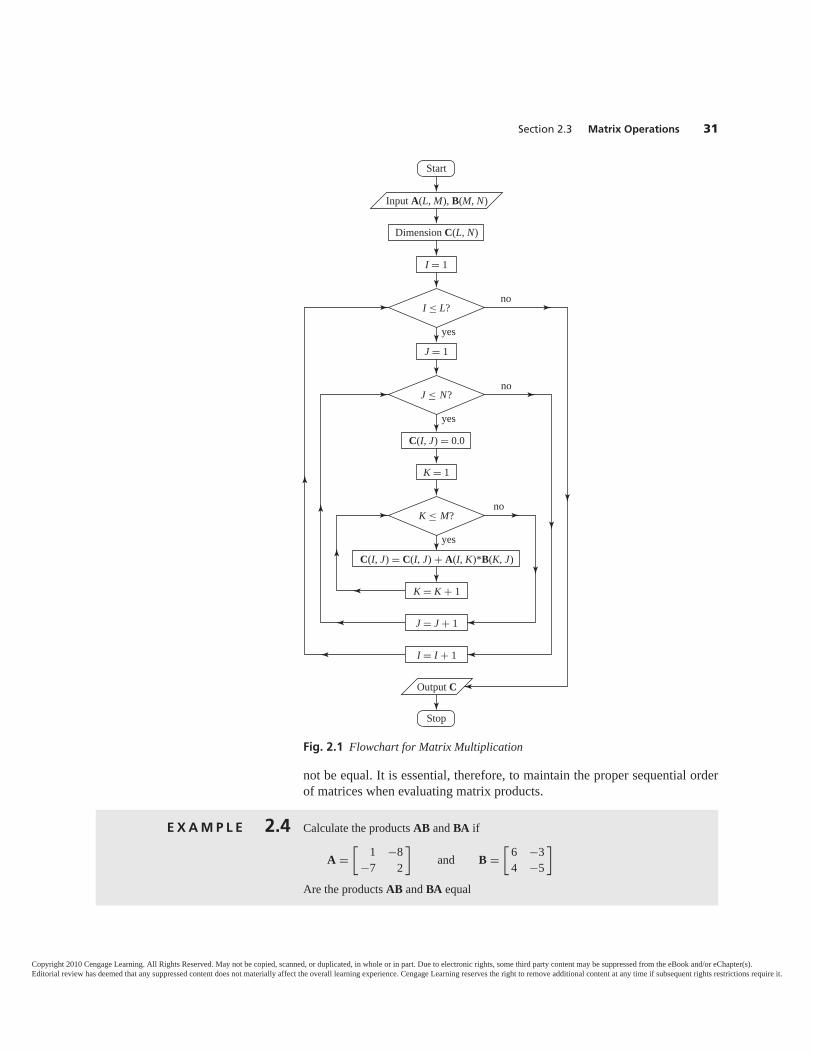
A flowchart for programming the matrix multiplication procedure on a com-puter is given in Fig. 2.1. Any programming language (such as FORTRAN,BASIC, or C, among others) can be used for this purpose. The reader is encour-aged to write this program in a general form (e.g., as a subroutine), so that it canbe included in the structural analysis computer programs to be developed in laterchapters.
An important application of matrix multiplication is to express simultane-ous equations in compact matrix form. Consider the following system of linearsimultaneous equations.
A11x1 + A12x2 + A13x3 + A14x4 = P1
A21x1 + A22x2 + A23x3 + A24x4 = P2
A31x1 + A32x2 + A33x3 + A34x4 = P3
A41x1 + A42x2 + A43x3 + A44x4 = P4
(2.7)
in which xs are the unknowns and As and Ps represent the coefficients and con-stants, respectively. By using the definition of multiplication of matrices, thissystem of equations can be expressed in matrix form as⎡
⎢⎢⎢⎣A11 A12 A13 A14A21 A22 A23 A24A31 A32 A33 A34A41 A42 A43 A44
⎤⎥⎥⎥⎦
⎡⎢⎢⎢⎣
x1x2x3x4
⎤⎥⎥⎥⎦ =
⎡⎢⎢⎢⎣
P1P2P3P4
⎤⎥⎥⎥⎦ (2.8)
or, symbolically, asAx = P (2.9)
Matrix multiplication is generally not commutative that is,
(2.10)
Even when the orders of two matrices A and B are such that both products ABand BA are defined and are of the same order, the two products, in general, will
AB �= BA
30 Chapter 2 Matrix Algebra
the resulting products; that is,C11 = 1(6) + 8(−1) = −2
Similarly, the element C12 is obtained by multiplying the elements of the first row ofA by the corresponding elements of the second column of B and adding the resultingproducts; that is,
C12 = 1(−7) + 8(2) = 9The remaining elements of C are computed in a similar manner:
C21 = 4(6) + (−2)(−1) = 26C22 = 4(−7) −2(2) = −32C31 = −5(6) + 3(−1) = −33C32 = −5(−7) + 3(2) = 41
Copyright 2010 Cengage Learning. All Rights Reserved. May not be copied, scanned, or duplicated, in whole or in part. Due to electronic rights, some third party content may be suppressed from the eBook and/or eChapter(s).Editorial review has deemed that any suppressed content does not materially affect the overall learning experience. Cengage Learning reserves the right to remove additional content at any time if subsequent rights restrictions require it.
not be equal. It is essential, therefore, to maintain the proper sequential orderof matrices when evaluating matrix products.
Section 2.3 Matrix Operations 31
Start
Stop
Input A(L, M), B(M, N)
Output C
Dimension C(L, N)
I = 1
J = 1
K = 1
C(I, J) = 0.0
K = K + 1
I = I + 1
J = J + 1
C(I, J) = C(I, J) + A(I, K)*B(K, J)
I ≤ L?
J ≤ N?
K ≤ M?
yes
yes
yes
no
no
no
Fig. 2.1 Flowchart for Matrix Multiplication
E X A M P L E 2.4 Calculate the products AB and BA if
A =[
1 −8−7 2
]and B =
[6 −34 −5
]
Are the products AB and BA equal
Copyright 2010 Cengage Learning. All Rights Reserved. May not be copied, scanned, or duplicated, in whole or in part. Due to electronic rights, some third party content may be suppressed from the eBook and/or eChapter(s).Editorial review has deemed that any suppressed content does not materially affect the overall learning experience. Cengage Learning reserves the right to remove additional content at any time if subsequent rights restrictions require it.
32 Chapter 2 Matrix Algebra
Matrix multiplication is associative and distributive, provided that the se-quential order in which the matrices are to be multiplied is maintained. Thus,
ABC = (AB)C = A(BC) (2.11)
andA(B + C) = AB + AC (2.12)
The product of any matrix A and a conformable null matrix O equals anull matrix; that is,
AO = O and OA = O (2.13)
For example,[2 −4
−6 8
] [0 00 0
]=
[0 00 0
]
The product of any matrix A and a conformable unit matrix I equals theoriginal matrix A; thus,
AI = A and IA = A (2.14)
For example,[2 −4
−6 8
] [1 00 1
]=
[2 −4
−6 8
]and [
1 00 1
] [2 −4
−6 8
]=
[2 −4
−6 8
]We can see from Eqs. (2.13) and (2.14) that the null and unit matrices servepurposes in matrix algebra that are similar to those of the numbers 0 and 1, re-spectively, in scalar algebra.
Transpose of a MatrixThe transpose of a matrix is obtained by interchanging its corresponding rowsand columns. The transposed matrix is commonly identified by placing asuperscript T on the symbol of the original matrix. Consider, for example, a3 × 2 matrix
B =⎡⎣ 2 −4
−5 81 3
⎤⎦
3 × 2
S O L U T I O N
AB =[
1 −8−7 2
] [6 −34 −5
]=
[ −26 37−34 11
]Ans
BA =[
6 −34 −5
] [1 −8
−7 2
]=
[27 −5439 −42
]Ans
Comparing products AB and BA, we can see that AB �= BA. Ans
Copyright 2010 Cengage Learning. All Rights Reserved. May not be copied, scanned, or duplicated, in whole or in part. Due to electronic rights, some third party content may be suppressed from the eBook and/or eChapter(s).Editorial review has deemed that any suppressed content does not materially affect the overall learning experience. Cengage Learning reserves the right to remove additional content at any time if subsequent rights restrictions require it.
Section 2.3 Matrix Operations 33
The transpose of B is given by
BT =[
2 −5 1−4 8 3
]2 × 3
Note that the first row of B becomes the first column of BT. Similarly, the sec-ond and third rows of B become, respectively, the second and third columns ofBT. The order of BT thus obtained is 2 × 3.
As another example, consider the matrix
C =⎡⎣ 2 −1 6
−1 7 −96 −9 5
⎤⎦
Because the elements of C are symmetric about its main diagonal (i.e.,Cij = Cji for i � j), interchanging the rows and columns of this matrixproduces a matrix CT that is identical to C itself; that is, CT = C. Thus, thetranspose of a symmetric matrix equals the original matrix.
Another useful property of matrix transposition is that the transpose of aproduct of matrices equals the product of the transposed matrices in reverseorder. Thus,
(2.15)
Similarly,(ABC)T = CTBTAT (2.16)
(AB)T = BTAT
E X A M P L E 2.5 Show that (AB)T = BTAT if
A =⎡⎣ 9 −5
2 1−3 4
⎤⎦ and B =
[6 −1 10
−2 7 5
]
S O L U T I O N
AB =⎡⎣ 9 −5
2 1−3 4
⎤⎦ [
6 −1 10−2 7 5
]=
⎡⎣ 64 −44 65
10 5 25−26 31 −10
⎤⎦
(AB)T =⎡⎣ 64 10 −26
−44 5 3165 25 −10
⎤⎦ (1)
BT AT =⎡⎣ 6 −2
−1 710 5
⎤⎦ [
9 2 −3−5 1 4
]=
⎡⎣ 64 10 −26
−44 5 3165 25 −10
⎤⎦ (2)
By comparing Eqs. (1) and (2), we can see that (AB)T = BT AT . Ans
Copyright 2010 Cengage Learning. All Rights Reserved. May not be copied, scanned, or duplicated, in whole or in part. Due to electronic rights, some third party content may be suppressed from the eBook and/or eChapter(s).Editorial review has deemed that any suppressed content does not materially affect the overall learning experience. Cengage Learning reserves the right to remove additional content at any time if subsequent rights restrictions require it.
Differentiation and IntegrationA matrix can be differentiated (or integrated) by differentiating (or integrating)each of its elements.
34 Chapter 2 Matrix Algebra
E X A M P L E 2.6 Determine the derivative dA/dx if
A =⎡⎣ x2 3 sin x −x4
3 sin x −x cos2 x−x4 cos2 x 7x3
⎤⎦
S O L U T I O N By differentiating the elements of A, we obtain
A11 = x2 d A11dx = 2x
A21 = A12 = 3 sin x d A21dx = d A12
dx = 3 cos x
A31 = A13 = −x4 d A31dx = d A13
dx = −4x3
A22 = −x d A22dx = −1
A32 = A23 = cos2 x d A32dx = d A23
dx = −2 cos x sin x
A33 = 7x3 d A33dx = 21x2
Thus, the derivative dA/dx is given by
dAdx =
⎡⎣ 2x 3 cos x −4x3
3 cos x −1 −2 cos x sin x−4x3 −2 cos x sin x 21x2
⎤⎦ Ans
E X A M P L E 2.7 Determine the partial derivative ∂B/∂y if
B =⎡⎣ 2y3 −yz −2xz
3xy2 yz −z2
2x2 −2xz 3xy2
⎤⎦
S O L U T I O N We determine the partial derivative, ∂Bij/∂y, of each element of B to obtain
∂B∂y =
⎡⎣ 6y2 −z 0
6xy z 00 0 6xy
⎤⎦ Ans
E X A M P L E 2.8 Calculate the integral ∫ L
0 AAT dx if
A =
⎡⎢⎢⎣
1 − xL
xL
⎤⎥⎥⎦
Copyright 2010 Cengage Learning. All Rights Reserved. May not be copied, scanned, or duplicated, in whole or in part. Due to electronic rights, some third party content may be suppressed from the eBook and/or eChapter(s).Editorial review has deemed that any suppressed content does not materially affect the overall learning experience. Cengage Learning reserves the right to remove additional content at any time if subsequent rights restrictions require it.
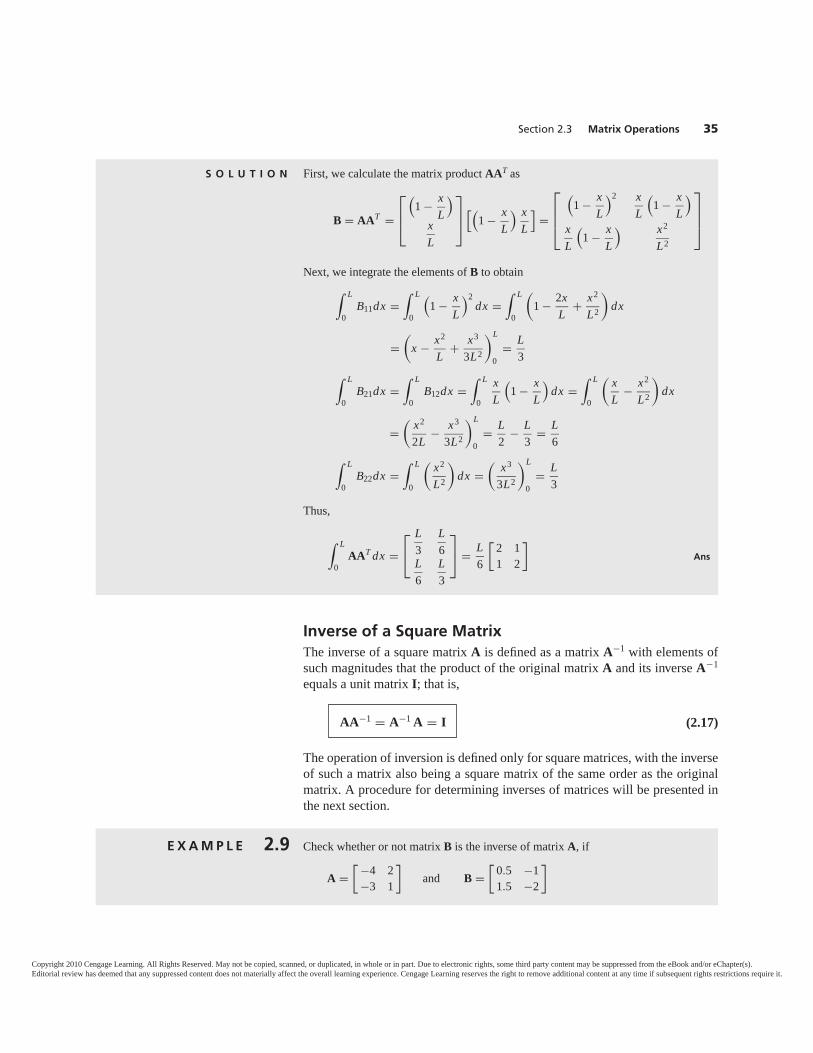
E X A M P L E 2.9 Check whether or not matrix B is the inverse of matrix A, if
A =[ −4 2
−3 1
]and B =
[0.5 −11.5 −2
]
Inverse of a Square MatrixThe inverse of a square matrix A is defined as a matrix A−1 with elements ofsuch magnitudes that the product of the original matrix A and its inverse A�1
equals a unit matrix I; that is,
(2.17)
The operation of inversion is defined only for square matrices, with the inverseof such a matrix also being a square matrix of the same order as the originalmatrix. A procedure for determining inverses of matrices will be presented inthe next section.
AA−1 = A−1 A = I
Section 2.3 Matrix Operations 35
S O L U T I O N First, we calculate the matrix product AAT as
B = AAT =
⎡⎢⎣
(1 − x
L
)xL
⎤⎥⎦ [(
1 − xL
) xL
]=
⎡⎢⎢⎣
(1 − x
L
)2 xL
(1 − x
L
)xL
(1 − x
L
) x2
L2
⎤⎥⎥⎦
Next, we integrate the elements of B to obtain∫ L
0B11dx =
∫ L
0
(1 − x
L
)2dx =
∫ L
0
(1 − 2x
L + x2
L2
)dx
=(
x − x2
L + x3
3L2
)L
0= L
3∫ L
0B21dx =
∫ L
0B12dx =
∫ L
0
xL
(1 − x
L
)dx =
∫ L
0
( xL − x2
L2
)dx
=( x2
2L − x3
3L2
)L
0= L
2 − L3 = L
6∫ L
0B22dx =
∫ L
0
( x2
L2
)dx =
( x3
3L2
)L
0= L
3
Thus,
∫ L
0AAT dx =
⎡⎣
L3
L6
L6
L3
⎤⎦ = L
6
[2 11 2
]Ans
Copyright 2010 Cengage Learning. All Rights Reserved. May not be copied, scanned, or duplicated, in whole or in part. Due to electronic rights, some third party content may be suppressed from the eBook and/or eChapter(s).Editorial review has deemed that any suppressed content does not materially affect the overall learning experience. Cengage Learning reserves the right to remove additional content at any time if subsequent rights restrictions require it.
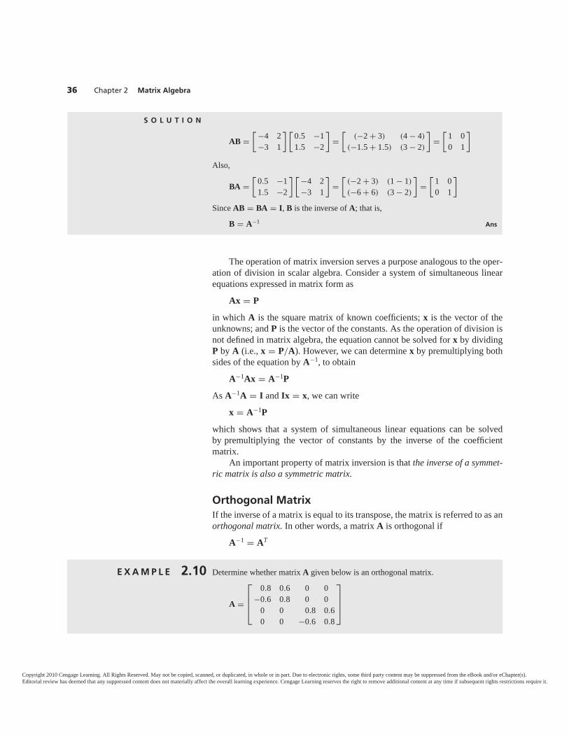
36 Chapter 2 Matrix Algebra
The operation of matrix inversion serves a purpose analogous to the oper-ation of division in scalar algebra. Consider a system of simultaneous linearequations expressed in matrix form as
Ax = P
in which A is the square matrix of known coefficients; x is the vector of theunknowns; and P is the vector of the constants. As the operation of division isnot defined in matrix algebra, the equation cannot be solved for x by dividingP by A (i.e., x = P/A). However, we can determine x by premultiplying bothsides of the equation by A−1, to obtain
A−1Ax = A−1P
As A−1A = I and Ix = x, we can writex = A−1P
which shows that a system of simultaneous linear equations can be solvedby premultiplying the vector of constants by the inverse of the coefficientmatrix.
An important property of matrix inversion is that the inverse of a symmet-ric matrix is also a symmetric matrix.
Orthogonal MatrixIf the inverse of a matrix is equal to its transpose, the matrix is referred to as anorthogonal matrix. In other words, a matrix A is orthogonal if
A−1 = AT
S O L U T I O N
AB =[ −4 2
−3 1
] [0.5 −11.5 −2
]=
[(−2 + 3) (4 − 4)
(−1.5 + 1.5) (3 − 2)
]=
[1 00 1
]
Also,
BA =[
0.5 −11.5 −2
] [−4 2−3 1
]=
[(−2 + 3) (1 − 1)
(−6 + 6) (3 − 2)
]=
[1 00 1
]
Since AB = BA = I, B is the inverse of A; that is,
B = A−1 Ans
E X A M P L E 2.10 Determine whether matrix A given below is an orthogonal matrix.
A =
⎡⎢⎢⎣
0.8 0.6 0 0−0.6 0.8 0 0
0 0 0.8 0.60 0 −0.6 0.8
⎤⎥⎥⎦
Copyright 2010 Cengage Learning. All Rights Reserved. May not be copied, scanned, or duplicated, in whole or in part. Due to electronic rights, some third party content may be suppressed from the eBook and/or eChapter(s).Editorial review has deemed that any suppressed content does not materially affect the overall learning experience. Cengage Learning reserves the right to remove additional content at any time if subsequent rights restrictions require it.
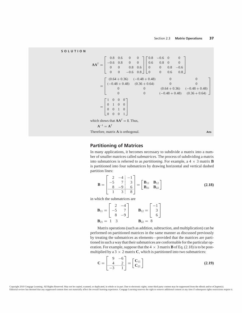
Partitioning of MatricesIn many applications, it becomes necessary to subdivide a matrix into a num-ber of smaller matrices called submatrices. The process of subdividing a matrixinto submatrices is referred to as partitioning. For example, a 4 × 3 matrix Bis partitioned into four submatrices by drawing horizontal and vertical dashedpartition lines:
B =
⎡⎢⎢⎣
2 −4 −1−5 7 3
8 −9 61 3 8
⎤⎥⎥⎦ =
[B11 B12B21 B22
]������
�������(2.18)
in which the submatrices are
B11 =⎡⎣ 2 −4
−5 78 −9
⎤⎦ B12 =
⎡⎣ −1
36
⎤⎦
B21 = 1 3 B22 = 8Matrix operations (such as addition, subtraction, and multiplication) can be
performed on partitioned matrices in the same manner as discussed previouslyby treating the submatrices as elements—provided that the matrices are parti-tioned in such a way that their submatrices are conformable for the particular op-eration. For example, suppose that the 4 × 3 matrix B of Eq. (2.18) is to be post-multiplied by a 3 × 2 matrix C, which is partitioned into two submatrices:
C =⎡⎣ 9 −6
4 2−3 1
⎤⎦ =
[C11C21
]�����
(2.19)
Section 2.3 Matrix Operations 37
S O L U T I O N
AAT =
⎡⎢⎢⎣
0.8 0.6 0 0−0.6 0.8 0 0
0 0 0.8 0.60 0 −0.6 0.8
⎤⎥⎥⎦
⎡⎢⎢⎣
0.8 −0.6 0 00.6 0.8 0 00 0 0.8 −0.60 0 0.6 0.8
⎤⎥⎥⎦
=
⎡⎢⎢⎣
(0.64 + 0.36) (−0.48 + 0.48) 0 0(−0.48 + 0.48) (0.36 + 0.64) 0 0
0 0 (0.64 + 0.36) (−0.48 + 0.48)
0 0 (−0.48 + 0.48) (0.36 + 0.64)
⎤⎥⎥⎦
=
⎡⎢⎢⎣
1 0 0 00 1 0 00 0 1 00 0 0 1
⎤⎥⎥⎦
which shows that AAT = I. Thus,A−1 = AT
Therefore, matrix A is orthogonal. Ans
Copyright 2010 Cengage Learning. All Rights Reserved. May not be copied, scanned, or duplicated, in whole or in part. Due to electronic rights, some third party content may be suppressed from the eBook and/or eChapter(s).Editorial review has deemed that any suppressed content does not materially affect the overall learning experience. Cengage Learning reserves the right to remove additional content at any time if subsequent rights restrictions require it.
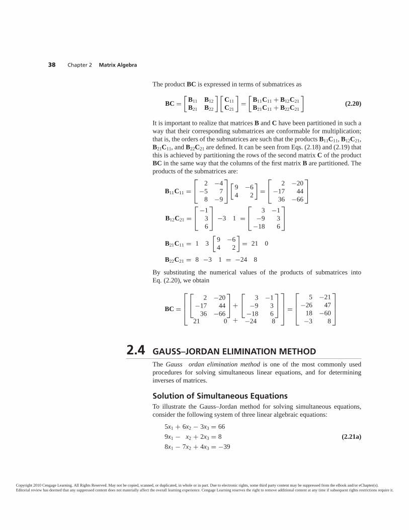
The product BC is expressed in terms of submatrices as
BC =[
B11 B12B21 B22
] [C11C21
]=
[B11C11 + B12C21B21C11 + B22C21
](2.20)
It is important to realize that matrices B and C have been partitioned in such away that their corresponding submatrices are conformable for multiplication;that is, the orders of the submatrices are such that the products B11C11, B12C21,B21C11, and B22C21 are defined. It can be seen from Eqs. (2.18) and (2.19) thatthis is achieved by partitioning the rows of the second matrix C of the productBC in the same way that the columns of the first matrix B are partitioned. Theproducts of the submatrices are:
B11C11 =⎡⎣ 2 −4
−5 78 −9
⎤⎦ [
9 −64 2
]=
⎡⎣ 2 −20
−17 4436 −66
⎤⎦
B12C21 =⎡⎣ −1
36
⎤⎦ −3 1 =
⎡⎣ 3 −1
−9 3−18 6
⎤⎦
B21C11 = 1 3[
9 −64 2
]= 21 0
B22C21 = 8 −3 1 = −24 8
By substituting the numerical values of the products of submatrices intoEq. (2.20), we obtain
BC =
⎡⎢⎢⎣
⎡⎣ 2 −20
−17 4436 −66
⎤⎦
21 0
⎡⎣ 3 −1
−9 3−18 6
⎤⎦
−24 8
⎤⎥⎥⎦ =
⎡⎢⎢⎣
5 −21−26 47
18 −60−3 8
⎤⎥⎥⎦
2.4 GAUSS–JORDAN ELIMINATION METHODThe Gauss ordan elimination method is one of the most commonly usedprocedures for solving simultaneous linear equations, and for determininginverses of matrices.
Solution of Simultaneous EquationsTo illustrate the Gauss–Jordan method for solving simultaneous equations,consider the following system of three linear algebraic equations:
5x1 + 6x2 − 3x3 = 669x1 − x2 + 2x3 = 8 (2.21a)
8x1 − 7x2 + 4x3 = −39
38 Chapter 2 Matrix Algebra
+
+
Copyright 2010 Cengage Learning. All Rights Reserved. May not be copied, scanned, or duplicated, in whole or in part. Due to electronic rights, some third party content may be suppressed from the eBook and/or eChapter(s).Editorial review has deemed that any suppressed content does not materially affect the overall learning experience. Cengage Learning reserves the right to remove additional content at any time if subsequent rights restrictions require it.
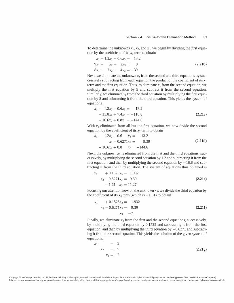
To determine the unknowns x1, x2, and x3, we begin by dividing the first equa-tion by the coefficient of its x1 term to obtain
x1 + 1.2x2 − 0.6x3 = 13.29x1 − x2 + 2x3 = 88x1 − 7x2 + 4x3 = −39
(2.21b)
Next, we eliminate the unknown x1 from the second and third equations by suc-cessively subtracting from each equation the product of the coefficient of its x1term and the first equation. Thus, to eliminate x1 from the second equation, wemultiply the first equation by 9 and subtract it from the second equation.Similarly, we eliminate x1 from the third equation by multiplying the first equa-tion by 8 and subtracting it from the third equation. This yields the system ofequations
x1 + 1.2x2 − 0.6x3 = 13.2− 11.8x2 + 7.4x3 = −110.8− 16.6x2 + 8.8x3 = −144.6
(2.21c)
With x1 eliminated from all but the first equation, we now divide the secondequation by the coefficient of its x2 term to obtain
x1 + 1.2x2 − 0.6 x3 = 13.2x2 − 0.6271x3 = 9.39
− 16.6x2 + 8.8 x3 = −144.6(2.21d)
Next, the unknown x2 is eliminated from the first and the third equations, suc-cessively, by multiplying the second equation by 1.2 and subtracting it from thefirst equation, and then by multiplying the second equation by −16.6 and sub-tracting it from the third equation. The system of equations thus obtained is
x1 + 0.1525x3 = 1.932x2 − 0.6271x3 = 9.39
− 1.61 x3 = 11.27(2.21e)
Focusing our attention now on the unknown x3, we divide the third equation bythe coefficient of its x3 term (which is −1.61) to obtain
x1 + 0.1525x3 = 1.932x2 − 0.6271x3 = 9.39
x3 = −7(2.21f)
Finally, we eliminate x3 from the first and the second equations, successively,by multiplying the third equation by 0.1525 and subtracting it from the firstequation, and then by multiplying the third equation by −0.6271 and subtract-ing it from the second equation. This yields the solution of the given system ofequations:
x1 = 3x2 = 5
x3 = −7(2.21g)
Section 2.4 Gauss–Jordan Elimination Method 39
Copyright 2010 Cengage Learning. All Rights Reserved. May not be copied, scanned, or duplicated, in whole or in part. Due to electronic rights, some third party content may be suppressed from the eBook and/or eChapter(s).Editorial review has deemed that any suppressed content does not materially affect the overall learning experience. Cengage Learning reserves the right to remove additional content at any time if subsequent rights restrictions require it.
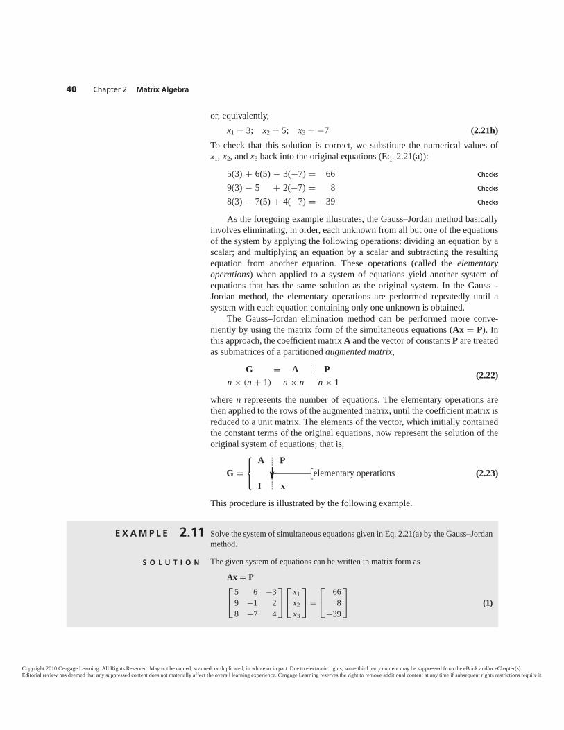
or, equivalently,x1 = 3; x2 = 5; x3 = −7 (2.21h)
To check that this solution is correct, we substitute the numerical values ofx1, x2, and x3 back into the original equations (Eq. 2.21(a)):
5(3) + 6(5) − 3(−7) = 66 Checks
9(3) − 5 + 2(−7) = 8 Checks
8(3) − 7(5) + 4(−7) = −39 Checks
As the foregoing example illustrates, the Gauss–Jordan method basicallyinvolves eliminating, in order, each unknown from all but one of the equationsof the system by applying the following operations: dividing an equation by ascalar; and multiplying an equation by a scalar and subtracting the resultingequation from another equation. These operations (called the elementaryoperations) when applied to a system of equations yield another system ofequations that has the same solution as the original system. In the Gauss–-Jordan method, the elementary operations are performed repeatedly until asystem with each equation containing only one unknown is obtained.
The Gauss–Jordan elimination method can be performed more conve-niently by using the matrix form of the simultaneous equations (Ax = P). Inthis approach, the coefficient matrix A and the vector of constants P are treatedas submatrices of a partitioned augmented matrix,
Gn × (n + 1)
= An × n
� Pn × 1
(2.22)
where n represents the number of equations. The elementary operations arethen applied to the rows of the augmented matrix, until the coefficient matrix isreduced to a unit matrix. The elements of the vector, which initially containedthe constant terms of the original equations, now represent the solution of theoriginal system of equations; that is,
G =⎧⎨⎩
A
I
�
�
P
x−−−−−−−[
elementary operations (2.23)
This procedure is illustrated by the following example.
40 Chapter 2 Matrix Algebra
E X A M P L E 2.11 Solve the system of simultaneous equations given in Eq. 2.21(a) by the Gauss–Jordanmethod.
S O L U T I O N The given system of equations can be written in matrix form as
Ax = P⎡⎣ 5 6 −3
9 −1 28 −7 4
⎤⎦
⎡⎣ x1
x2x3
⎤⎦ =
⎡⎣ 66
8−39
⎤⎦ (1)
Copyright 2010 Cengage Learning. All Rights Reserved. May not be copied, scanned, or duplicated, in whole or in part. Due to electronic rights, some third party content may be suppressed from the eBook and/or eChapter(s).Editorial review has deemed that any suppressed content does not materially affect the overall learning experience. Cengage Learning reserves the right to remove additional content at any time if subsequent rights restrictions require it.
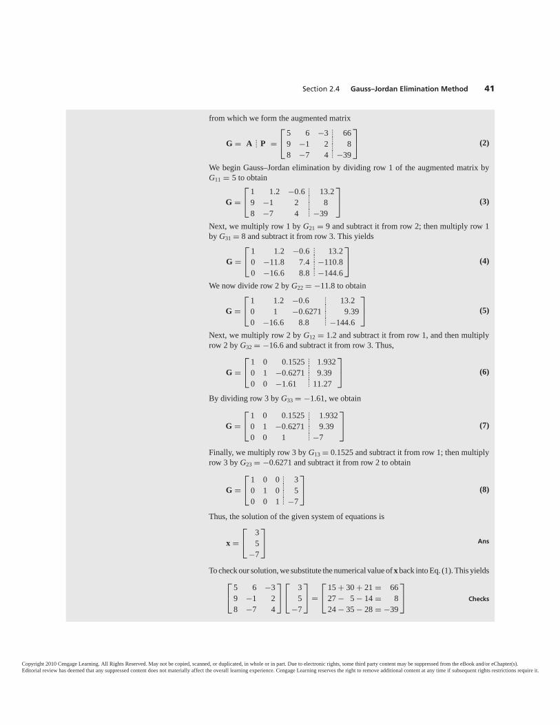
Section 2.4 Gauss–Jordan Elimination Method 41
from which we form the augmented matrix
G = A�P =⎡⎣ 5 6 −3 66
9 −1 2 88 −7 4 −39
⎤⎦�
���
(2)
We begin Gauss–Jordan elimination by dividing row 1 of the augmented matrix byG11 = 5 to obtain
G =⎡⎣ 1 1.2 −0.6 13.2
9 −1 2 88 −7 4 −39
⎤⎦�
���
(3)
Next, we multiply row 1 by G21 = 9 and subtract it from row 2; then multiply row 1by G31 = 8 and subtract it from row 3. This yields
G =⎡⎣ 1 1.2 −0.6 13.2
0 −11.8 7.4 −110.80 −16.6 8.8 −144.6
⎤⎦�
���
(4)
We now divide row 2 by G22 = −11.8 to obtain
G =⎡⎣ 1 1.2 −0.6 13.2
0 1 −0.6271 9.390 −16.6 8.8 −144.6
⎤⎦�
���
(5)
Next, we multiply row 2 by G12 = 1.2 and subtract it from row 1, and then multiplyrow 2 by G32 = −16.6 and subtract it from row 3. Thus,
G =⎡⎣ 1 0 0.1525 1.932
0 1 −0.6271 9.390 0 −1.61 11.27
⎤⎦�
���
(6)
By dividing row 3 by G33 = −1.61, we obtain
G =⎡⎣ 1 0 0.1525 1.932
0 1 −0.6271 9.390 0 1 −7
⎤⎦�
���
(7)
Finally, we multiply row 3 by G13 = 0.1525 and subtract it from row 1; then multiplyrow 3 by G23 = −0.6271 and subtract it from row 2 to obtain
G =⎡⎣ 1 0 0 3
0 1 0 50 0 1 −7
⎤⎦�
���
(8)
Thus, the solution of the given system of equations is
x =⎡⎣ 3
5−7
⎤⎦ Ans
To check our solution, we substitute the numerical value of x back into Eq. (1). This yields⎡⎣ 5 6 −3
9 −1 28 −7 4
⎤⎦
⎡⎣ 3
5−7
⎤⎦ =
⎡⎣ 15 + 30 + 21 = 66
27 − 5 − 14 = 824 − 35 − 28 = −39
⎤⎦ Checks
Copyright 2010 Cengage Learning. All Rights Reserved. May not be copied, scanned, or duplicated, in whole or in part. Due to electronic rights, some third party content may be suppressed from the eBook and/or eChapter(s).Editorial review has deemed that any suppressed content does not materially affect the overall learning experience. Cengage Learning reserves the right to remove additional content at any time if subsequent rights restrictions require it.
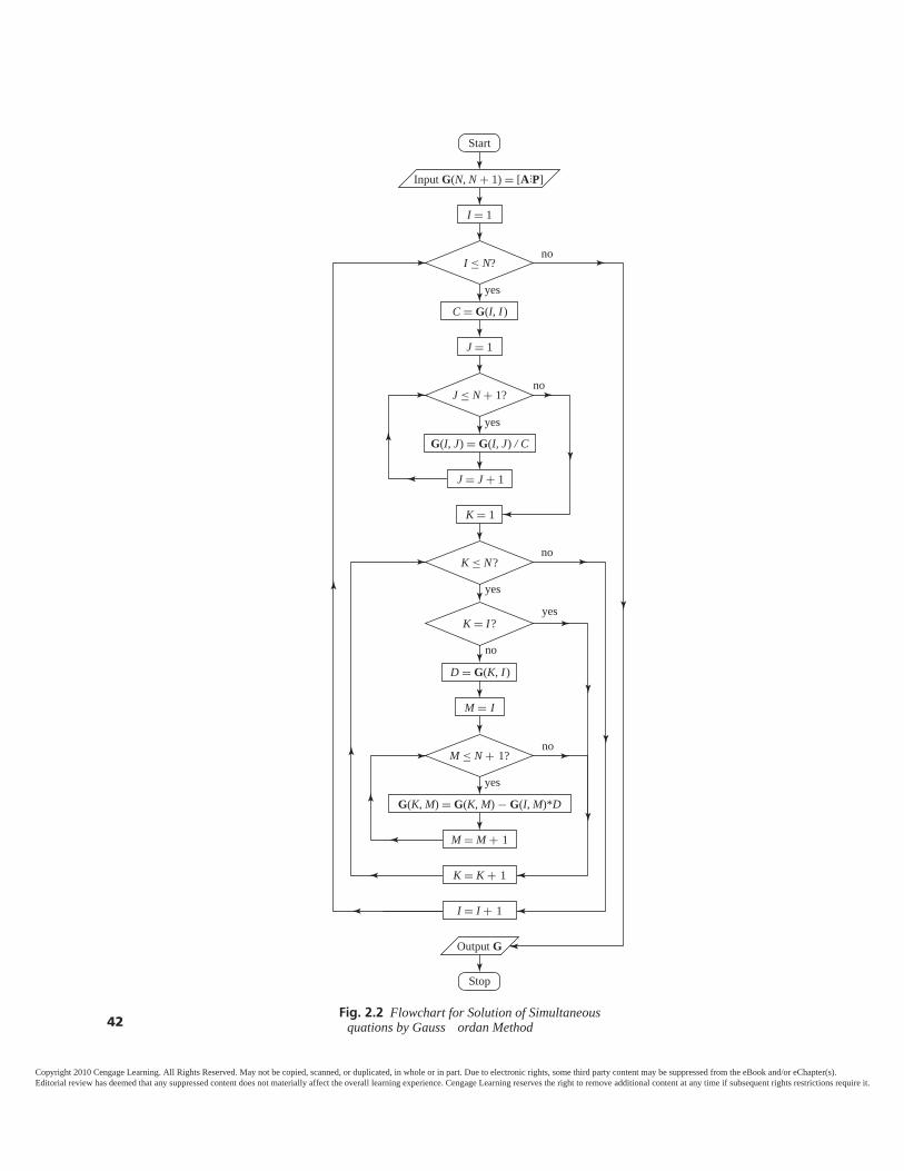
Stop
Input G(N, N + 1) = [A P]
Output G
I = 1
J = 1
C = G(I, I )
G(I, J) = G(I, J) / C
J = J + 1
K = 1
D = G(K, I )
M = I
M = M + 1
G(K, M) = G(K, M) − G(I, M)*D
I ≤ N?
J ≤ N + 1?
K ≤ N?
K = I?
M ≤ N + 1?
yes
yes
yes
yes
yes
no
no
no
no
no
Start
K = K + 1
I = I + 1
Fig. 2.2 Flowchart for Solution of Simultaneousquations by Gauss ordan Method42
Copyright 2010 Cengage Learning. All Rights Reserved. May not be copied, scanned, or duplicated, in whole or in part. Due to electronic rights, some third party content may be suppressed from the eBook and/or eChapter(s).Editorial review has deemed that any suppressed content does not materially affect the overall learning experience. Cengage Learning reserves the right to remove additional content at any time if subsequent rights restrictions require it.
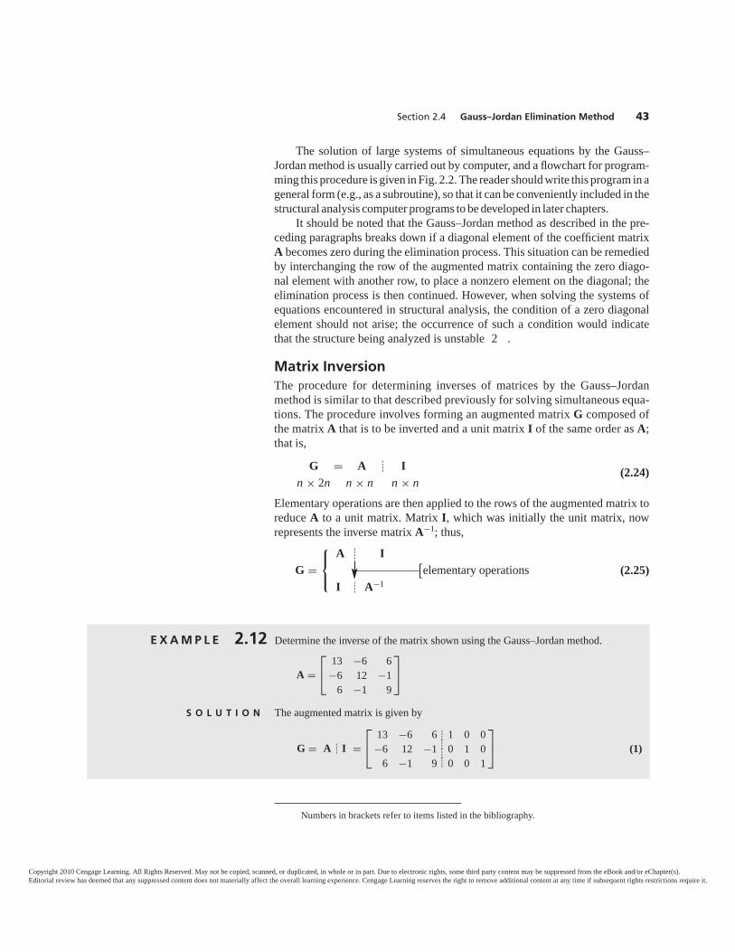
The solution of large systems of simultaneous equations by the Gauss–Jordan method is usually carried out by computer, and a flowchart for program-ming this procedure is given in Fig. 2.2. The reader should write this program in ageneral form (e.g., as a subroutine), so that it can be conveniently included in thestructural analysis computer programs to be developed in later chapters.
It should be noted that the Gauss–Jordan method as described in the pre-ceding paragraphs breaks down if a diagonal element of the coefficient matrixA becomes zero during the elimination process. This situation can be remediedby interchanging the row of the augmented matrix containing the zero diago-nal element with another row, to place a nonzero element on the diagonal; theelimination process is then continued. However, when solving the systems ofequations encountered in structural analysis, the condition of a zero diagonalelement should not arise; the occurrence of such a condition would indicatethat the structure being analyzed is unstable 2 .
Matrix InversionThe procedure for determining inverses of matrices by the Gauss–Jordanmethod is similar to that described previously for solving simultaneous equa-tions. The procedure involves forming an augmented matrix G composed ofthe matrix A that is to be inverted and a unit matrix I of the same order as A;that is,
Gn × 2n
= An × n
� In × n
(2.24)
Elementary operations are then applied to the rows of the augmented matrix toreduce A to a unit matrix. Matrix I, which was initially the unit matrix, nowrepresents the inverse matrix A−1; thus,
G =⎧⎨⎩
A
I
�
�
I
A−1−−−−−−−−−[
elementary operations (2.25)
Section 2.4 Gauss–Jordan Elimination Method 43
Numbers in brackets refer to items listed in the bibliography.
E X A M P L E 2.12 Determine the inverse of the matrix shown using the Gauss–Jordan method.
A =⎡⎣ 13 −6 6
−6 12 −16 −1 9
⎤⎦
S O L U T I O N The augmented matrix is given by
G = A�I =⎡⎣ 13 −6 6 1 0 0
−6 12 −1 0 1 06 −1 9 0 0 1
⎤⎦�
���
(1)
Copyright 2010 Cengage Learning. All Rights Reserved. May not be copied, scanned, or duplicated, in whole or in part. Due to electronic rights, some third party content may be suppressed from the eBook and/or eChapter(s).Editorial review has deemed that any suppressed content does not materially affect the overall learning experience. Cengage Learning reserves the right to remove additional content at any time if subsequent rights restrictions require it.
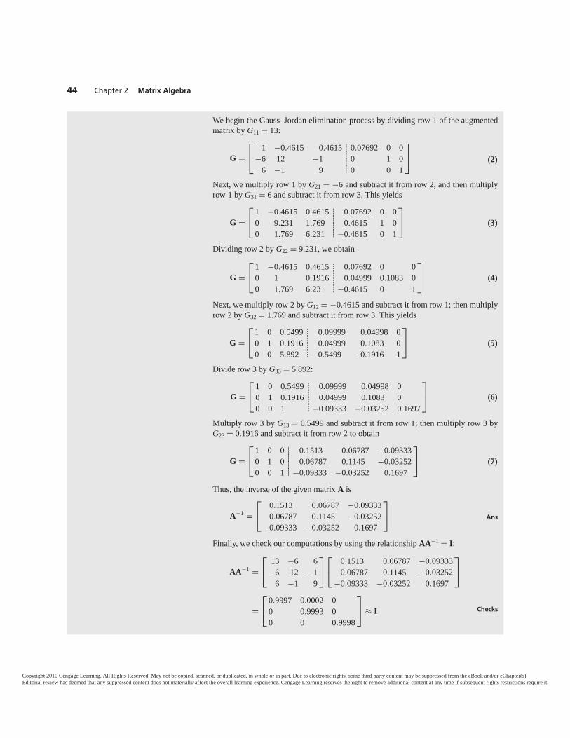
44 Chapter 2 Matrix Algebra
We begin the Gauss–Jordan elimination process by dividing row 1 of the augmentedmatrix by G11 = 13:
G =⎡⎣ 1 −0.4615 0.4615 0.07692 0 0
−6 12 −1 0 1 06 −1 9 0 0 1
⎤⎦�
���
(2)
Next, we multiply row 1 by G21 = −6 and subtract it from row 2, and then multiplyrow 1 by G31 = 6 and subtract it from row 3. This yields
G =⎡⎣ 1 −0.4615 0.4615 0.07692 0 0
0 9.231 1.769 0.4615 1 00 1.769 6.231 −0.4615 0 1
⎤⎦�
���
(3)
Dividing row 2 by G22 = 9.231, we obtain
G =⎡⎣ 1 −0.4615 0.4615 0.07692 0 0
0 1 0.1916 0.04999 0.1083 00 1.769 6.231 −0.4615 0 1
⎤⎦�
���
(4)
Next, we multiply row 2 by G12 = −0.4615 and subtract it from row 1; then multiplyrow 2 by G32 = 1.769 and subtract it from row 3. This yields
G =⎡⎣ 1 0 0.5499 0.09999 0.04998 0
0 1 0.1916 0.04999 0.1083 00 0 5.892 −0.5499 −0.1916 1
⎤⎦�
���
(5)
Divide row 3 by G33 = 5.892:
G =⎡⎣ 1 0 0.5499 0.09999 0.04998 0
0 1 0.1916 0.04999 0.1083 00 0 1 −0.09333 −0.03252 0.1697
⎤⎦�
���
(6)
Multiply row 3 by G13 = 0.5499 and subtract it from row 1; then multiply row 3 by G23 = 0.1916 and subtract it from row 2 to obtain
G =⎡⎣ 1 0 0 0.1513 0.06787 −0.09333
0 1 0 0.06787 0.1145 −0.032520 0 1 −0.09333 −0.03252 0.1697
⎤⎦�
���
(7)
Thus, the inverse of the given matrix A is
A−1 =⎡⎣ 0.1513 0.06787 −0.09333
0.06787 0.1145 −0.03252−0.09333 −0.03252 0.1697
⎤⎦ Ans
Finally, we check our computations by using the relationship AA−1 = I:
AA−1 =⎡⎣ 13 −6 6
−6 12 −16 −1 9
⎤⎦
⎡⎣ 0.1513 0.06787 −0.09333
0.06787 0.1145 −0.03252−0.09333 −0.03252 0.1697
⎤⎦
=⎡⎣ 0.9997 0.0002 0
0 0.9993 00 0 0.9998
⎤⎦ ≈ I Checks
Copyright 2010 Cengage Learning. All Rights Reserved. May not be copied, scanned, or duplicated, in whole or in part. Due to electronic rights, some third party content may be suppressed from the eBook and/or eChapter(s).Editorial review has deemed that any suppressed content does not materially affect the overall learning experience. Cengage Learning reserves the right to remove additional content at any time if subsequent rights restrictions require it.
SUMMARY
In this chapter, we discussed the basic concepts of matrix algebra that are nec-essary for formulating the matrix methods of structural analysis:
1. A matrix is defined as a rectangular array of quantities (elements)arranged in rows and columns. The size of a matrix is measured by itsnumber of rows and columns, and is referred to as its order.
2. Two matrices are considered to be equal if they are of the same order,and if their corresponding elements are identical.
3. Two matrices of the same order can be added (or subtracted) by adding(or subtracting) their corresponding elements.
4. The matrix multiplication AB = C is defined only if the number ofcolumns of the first matrix A equals the number of rows of the secondmatrix B. Any element Cij of the product matrix C can be evaluated byusing the relationship
Ci j =m∑
k=1Aik Bkj (2.6)
where m is the number of columns of A, or the number of rows of B.Matrix multiplication is generally not commutative; that is, AB �= BA.
5. The transpose of a matrix is obtained by interchanging its correspond-ing rows and columns. If C is a symmetric matrix, then CT = C.Another useful property of matrix transposition is that
(AB)T = BTAT (2.15)
6. A matrix can be differentiated (or integrated) by differentiating (or in-tegrating) each of its elements.
7. The inverse of a square matrix A is defined as a matrix A−1 whichsatisfies the relationship:
AA−1 = A−1A = I (2.17)
8. If the inverse of a matrix equals its transpose, the matrix is called anorthogonal matrix.
9. The Gauss–Jordan method of solving simultaneous equations essen-tially involves successively eliminating each unknown from all but oneof the equations of the system by performing the following operations:dividing an equation by a scalar; and multiplying an equation by ascalar and subtracting the resulting equation from another equation.These elementary operations are applied repeatedly until a system witheach equation containing only one unknown is obtained.
Summary 45
Copyright 2010 Cengage Learning. All Rights Reserved. May not be copied, scanned, or duplicated, in whole or in part. Due to electronic rights, some third party content may be suppressed from the eBook and/or eChapter(s).Editorial review has deemed that any suppressed content does not materially affect the overall learning experience. Cengage Learning reserves the right to remove additional content at any time if subsequent rights restrictions require it.
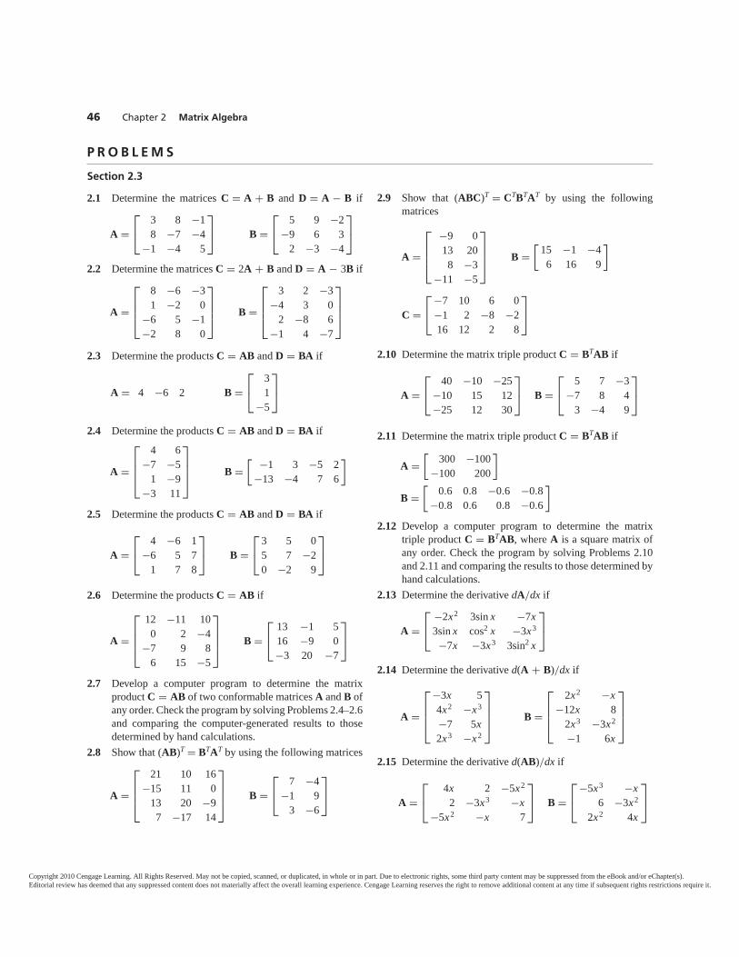
2.9 Show that (ABC)T = CTBTAT by using the followingmatrices
A =
⎡⎢⎢⎣
−9 013 208 −3
−11 −5
⎤⎥⎥⎦ B =
[15 −1 −46 16 9
]
C =⎡⎣ −7 10 6 0
−1 2 −8 −216 12 2 8
⎤⎦
2.10 Determine the matrix triple product C = BTAB if
A =⎡⎣ 40 −10 −25
−10 15 12−25 12 30
⎤⎦ B =
⎡⎣ 5 7 −3
−7 8 43 −4 9
⎤⎦
2.11 Determine the matrix triple product C = BTAB if
A =[
300 −100−100 200
]
B =[
0.6 0.8 −0.6 −0.8−0.8 0.6 0.8 −0.6
]
2.12 Develop a computer program to determine the matrixtriple product C = BTAB, where A is a square matrix ofany order. Check the program by solving Problems 2.10and 2.11 and comparing the results to those determined byhand calculations.
2.13 Determine the derivative dA/dx if
A =⎡⎣ −2x2 3sin x −7x
3sin x cos2 x −3x3
−7x −3x3 3sin2 x
⎤⎦
2.14 Determine the derivative d(A + B)/dx if
A =
⎡⎢⎢⎣
−3x 54x2 −x3
−7 5x2x3 −x2
⎤⎥⎥⎦ B =
⎡⎢⎢⎣
2x2 −x−12x 8
2x3 −3x2
−1 6x
⎤⎥⎥⎦
2.15 Determine the derivative d(AB)/dx if
A =⎡⎣ 4x 2 −5x2
2 −3x3 −x−5x2 −x 7
⎤⎦ B =
⎡⎣−5x3 −x
6 −3x2
2x2 4x
⎤⎦
Section 2.3
2.1 Determine the matrices C = A + B and D = A − B if
A =⎡⎣ 3 8 −1
8 −7 −4−1 −4 5
⎤⎦ B =
⎡⎣ 5 9 −2
−9 6 32 −3 −4
⎤⎦
2.2 Determine the matrices C = 2A + B and D = A − 3B if
A =
⎡⎢⎢⎣
8 −6 −31 −2 0
−6 5 −1−2 8 0
⎤⎥⎥⎦ B =
⎡⎢⎢⎣
3 2 −3−4 3 0
2 −8 6−1 4 −7
⎤⎥⎥⎦
2.3 Determine the products C = AB and D = BA if
A = 4 −6 2 B =⎡⎣ 3
1−5
⎤⎦
2.4 Determine the products C = AB and D = BA if
A =
⎡⎢⎢⎣
4 6−7 −5
1 −9−3 11
⎤⎥⎥⎦ B =
[ −1 3 −5 2−13 −4 7 6
]
2.5 Determine the products C = AB and D = BA if
A =⎡⎣ 4 −6 1
−6 5 71 7 8
⎤⎦ B =
⎡⎣ 3 5 0
5 7 −20 −2 9
⎤⎦
2.6 Determine the products C = AB if
A =
⎡⎢⎢⎣
12 −11 100 2 −4
−7 9 86 15 −5
⎤⎥⎥⎦ B =
⎡⎣ 13 −1 5
16 −9 0−3 20 −7
⎤⎦
2.7 Develop a computer program to determine the matrixproduct C = AB of two conformable matrices A and B ofany order. Check the program by solving Problems 2.4–2.6and comparing the computer-generated results to thosedetermined by hand calculations.
2.8 Show that (AB)T = BTAT by using the following matrices
A =
⎡⎢⎢⎣
21 10 16−15 11 0
13 20 −97 −17 14
⎤⎥⎥⎦ B =
⎡⎣ 7 −4
−1 93 −6
⎤⎦
46 Chapter 2 Matrix Algebra
P R O B L E M S
Copyright 2010 Cengage Learning. All Rights Reserved. May not be copied, scanned, or duplicated, in whole or in part. Due to electronic rights, some third party content may be suppressed from the eBook and/or eChapter(s).Editorial review has deemed that any suppressed content does not materially affect the overall learning experience. Cengage Learning reserves the right to remove additional content at any time if subsequent rights restrictions require it.
2.16 Determine the partial derivatives ∂A/∂x, ∂A/∂y, and∂A/∂z, if
A =⎡⎣ x2 −y2 2z2
−y2 3xy −yz2z2 −yz 4xz
⎤⎦
2.17 Calculate the integral ∫ L
0 A dx if
A =
⎡⎢⎢⎣
−5 −3x2
4x −x3
2x4 65x2 −x
⎤⎥⎥⎦
2.18 Calculate the integral ∫ L
0 A dx if
A =⎡⎣ 2x − sin x 2 cos2 x
− sin x 5 −4x3
2 cos2 x −4x3 (1 − x2)
⎤⎦
2.19 Calculate the integral ∫ L
0 AB dx if
A =[−x3 2x2 3
2x −x2 2x3
]B =
⎡⎣−2x x2
5 −2x3x3 −3
⎤⎦
2.20 Determine whether the matrices A and B given below areorthogonal matrices.
A =
⎡⎢⎢⎣
−0.28 −0.96 0 00.96 −0.28 0 00 0 −0.28 −0.960 0 0.96 −0.28
⎤⎥⎥⎦
B =
⎡⎢⎢⎣
−0.28 0.96 0 00.96 −0.28 0 00 0 −0.28 0.960 0 0.96 −0.28
⎤⎥⎥⎦
Section 2.4
2.21 through 2.25 Solve the following systems of simultane-ous equations by the Gauss–Jordan method.
2.21 2x1 − 3x2 + x3 = −18−9x1 + 5x2 + 3x3 = 18
4x1 + 7x2 − 8x3 = 53
2.22 20x1 − 9x2 + 15x3 = 354− 9x1 + 16x2 − 5x3 = −275
15x1 − 5x2 + 18x3 = 307
2.23 4x1 − 2x2 + 3x3 = 37.23x1 + 5x2 − x3 = −7.2
x1 − 4x2 + 2x3 = 30.3
2.24 6x1 + 15x2 − 24x3 + 40x4 = 190.915x1 + 9x2 − 13x3 = 69.8
−24x1 − 13x2 + 8x3 − 11x4 = −96.340x1 − 11x3 + 5x4 = 119.35
2.25 2x1 − 5x2 + 8x3 + 11x4 = 3910x1 + 7x2 + 4x3 − x4 = 127−3x1 + 9x2 + 5x3 − 6x4 = 58
x1 − 4x2 − 2x3 + 9x4 = −142.26 Develop a computer program to solve a system of simulta-
neous equations of any size by the Gauss–Jordan method.Check the program by solving Problems 2.21 through2.25 and comparing the computer-generated results tothose determined by hand calculations.
2.27 through 2.30 Determine the inverse of the matrices shownby the Gauss–Jordan method.
2.27 A =⎡⎣ 5 3 −4
3 8 −2−4 −2 7
⎤⎦
2.28 A =⎡⎣ 6 −4 1
−1 9 34 2 5
⎤⎦
2.29 A =
⎡⎢⎢⎣
7 −6 3 −2−6 4 −1 5
3 −1 8 9−2 5 9 2
⎤⎥⎥⎦
2.30 A =
⎡⎢⎢⎣
5 −7 −3 1110 −6 −13 2−1 12 8 −4−9 7 −5 6
⎤⎥⎥⎦
Problems 47
Copyright 2010 Cengage Learning. All Rights Reserved. May not be copied, scanned, or duplicated, in whole or in part. Due to electronic rights, some third party content may be suppressed from the eBook and/or eChapter(s).Editorial review has deemed that any suppressed content does not materially affect the overall learning experience. Cengage Learning reserves the right to remove additional content at any time if subsequent rights restrictions require it.
33.1 Global and Local Coordinate Systems3.2 Degrees of Freedom3.3 Member Stiffness Relations in the Local Coordinate
System3.4 Finite-Element Formulation Using Virtual Work3.5 Coordinate Transformations3.6 Member Stiffness Relations in the Global Coordinate
System3.7 Structure Stiffness Relations3.8 Procedure for Analysis
SummaryProblems
PLANE TRUSSES
Goethals Bridge, a Cantilever Truss Bridge between Staten Island, NY, and lizabeth, N .(Photo courtesy of Port Authority of New ork and New Jersey)
48
Copyright 2010 Cengage Learning. All Rights Reserved. May not be copied, scanned, or duplicated, in whole or in part. Due to electronic rights, some third party content may be suppressed from the eBook and/or eChapter(s).Editorial review has deemed that any suppressed content does not materially affect the overall learning experience. Cengage Learning reserves the right to remove additional content at any time if subsequent rights restrictions require it.
Section 3.1 Global and Local Coordinate Systems 49
A plane truss is defined as a two-dimensional framework of straight prismaticmembers connected at their ends by frictionless hinged joints, and subjected toloads and reactions that act only at the joints and lie in the plane of the struc-ture. The members of a plane truss are subjected to axial compressive or tensileforces only.
The objective of this chapter is to develop the analysis of plane trussesbased on the matrix stiffness method. This method of analysis is general, inthe sense that it can be applied to statically determinate, as well as indetermi-nate, plane trusses of any size and shape. We begin the chapter with the defini-tions of the global and local coordinate systems to be used in the analysis. Theconcept of degrees of freedom is introduced in Section 3.2; and the memberforce–displacement relations are established in the local coordinate system,using the equilibrium equations and the principles of mechanics of materials,in Section 3.3. The finite-element formulation of member stiffness relationsusing the principle of virtual work is presented in Section 3.4; and transfor-mation of member forces and displacements from a local to a global coor-dinate system, and vice versa, is considered in Section 3.5. Member stiffnessrelations in the global coordinate system are derived in Section 3.6; the for-mulation of the stiffness relations for the entire truss, by combining the memberstiffness relations, is discussed in Section 3.7; and a step-by-step procedurefor the analysis of plane trusses subjected to joint loads is developed inSection 3.8.
3.1 GLOBAL AND LOCAL COORDINATE SYSTEMSIn the matrix stiffness method, two types of coordinate systems are employedto specify the structural and loading data and to establish the necessaryforce–displacement relations. These are referred to as the global (or structural)and the local (or member) coordinate systems.
Global Coordinate SystemThe overall geometry and the load–deformation relationships for an entirestructure are described with reference to a Cartesian or rectangular global co-ordinate system.
When analyzing a plane (two-dimensional) structure, the origin of theglobal XY coordinate system can be located at any point in the plane of the struc-ture, with the X and Y axes oriented in any mutually perpendicular directions inthe structure’s plane. However, it is usually convenient to locate the origin at a
The global coordinate system used in this text is a right-handed XYZcoordinate system with the plane structure lying in the XY plane.
Copyright 2010 Cengage Learning. All Rights Reserved. May not be copied, scanned, or duplicated, in whole or in part. Due to electronic rights, some third party content may be suppressed from the eBook and/or eChapter(s).Editorial review has deemed that any suppressed content does not materially affect the overall learning experience. Cengage Learning reserves the right to remove additional content at any time if subsequent rights restrictions require it.
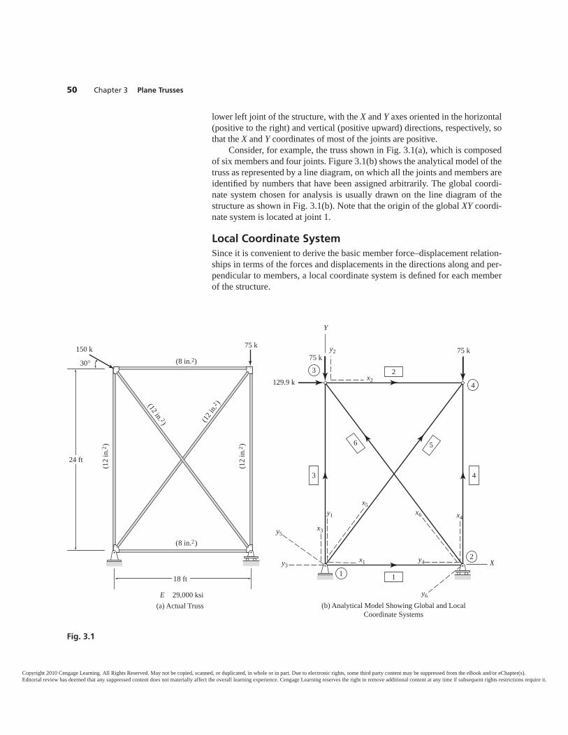
50 Chapter 3 Plane Trusses
lower left joint of the structure, with the X and Y axes oriented in the horizontal(positive to the right) and vertical (positive upward) directions, respectively, sothat the X and Y coordinates of most of the joints are positive.
Consider, for example, the truss shown in Fig. 3.1(a), which is composedof six members and four joints. Figure 3.1(b) shows the analytical model of thetruss as represented by a line diagram, on which all the joints and members areidentified by numbers that have been assigned arbitrarily. The global coordi-nate system chosen for analysis is usually drawn on the line diagram of thestructure as shown in Fig. 3.1(b). Note that the origin of the global XY coordi-nate system is located at joint 1.
Local Coordinate SystemSince it is convenient to derive the basic member force–displacement relation-ships in terms of the forces and displacements in the directions along and per-pendicular to members, a local coordinate system is defined for each memberof the structure.
(a) Actual Truss
18 ft
150 k
30°
75 k
(8 in.2)
(8 in.2)
(12
in.2 )
(12
in.2 )
(12 in. 2) (12 in
.2 )
E 29,000 ksi
24 ft
75 k75 k
129.9 k
x1
x2
x4
x3
x5x6
y6
y2
y5
y4y3
y1
Y
X2
1
4
3
(b) Analytical Model Showing Global and LocalCoordinate Systems
1
2
43
6 5
Fig. 3.1
Copyright 2010 Cengage Learning. All Rights Reserved. May not be copied, scanned, or duplicated, in whole or in part. Due to electronic rights, some third party content may be suppressed from the eBook and/or eChapter(s).Editorial review has deemed that any suppressed content does not materially affect the overall learning experience. Cengage Learning reserves the right to remove additional content at any time if subsequent rights restrictions require it.
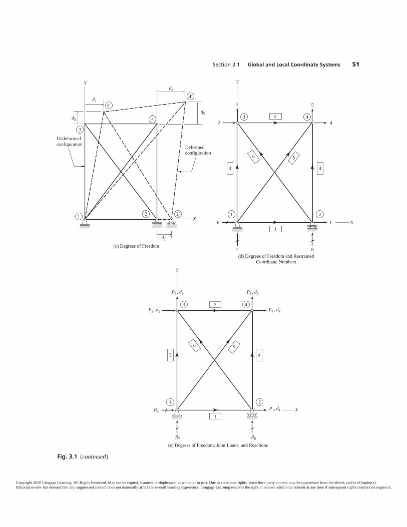
Section 3.1 Global and Local Coordinate Systems 51
Undeformedconfiguration Deformed
configuration
Y
X
d5
d4
d2
d3
d1
1 2′2
3
3′
4
4′
(c) Degrees of Freedom
21
43
R6
R7 R8
X
Y
P1, d1
P5, d5P3, d3
P2, d2 P4, d4
(e) Degrees of Freedom, Joint Loads, and Reactions
1
2
43
6 5
X
21
44
3
8
16
2
7
53
Y
(d) Degrees of Freedom and RestrainedCoordinate Numbers
1
2
43
6 5
Fig. 3.1 (continued)
Copyright 2010 Cengage Learning. All Rights Reserved. May not be copied, scanned, or duplicated, in whole or in part. Due to electronic rights, some third party content may be suppressed from the eBook and/or eChapter(s).Editorial review has deemed that any suppressed content does not materially affect the overall learning experience. Cengage Learning reserves the right to remove additional content at any time if subsequent rights restrictions require it.
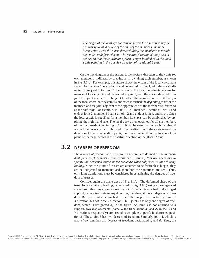
52 Chapter 3 Plane Trusses
On the line diagram of the structure, the positive direction of the x axis foreach member is indicated by drawing an arrow along each member, as shownin Fig. 3.1(b). For example, this figure shows the origin of the local coordinatesystem for member 1 located at its end connected to joint 1, with the x1 axis di-rected from joint 1 to joint 2; the origin of the local coordinate system formember 4 located at its end connected to joint 2, with the x4 axis directed fromjoint 2 to joint 4, etcetera. The joint to which the member end with the originof the local coordinate system is connected is termed the beginning joint for themember, and the joint adjacent to the opposite end of the member is referred toas the end joint. For example, in Fig. 3.1(b), member 1 begins at joint 1 andends at joint 2, member 4 begins at joint 2 and ends at joint 4, and so on. Oncethe local x axis is specified for a member, its y axis can be established by ap-plying the right-hand rule. The local y axes thus obtained for all six membersof the truss are depicted in Fig. 3.1(b). It can be seen that, for each member, ifwe curl the fingers of our right hand from the direction of the x axis toward thedirection of the corresponding y axis, then the extended thumb points out of theplane of the page, which is the positive direction of the global Z axis.
3.2 DEGREES OF FREEDOMThe degrees of freedom of a structure, in general, are defined as the indepen-dent joint displacements (translations and rotations) that are necessary tospecify the deformed shape of the structure when subjected to an arbitraryloading. Since the joints of trusses are assumed to be frictionless hinges, theyare not subjected to moments and, therefore, their rotations are zero. Thus,only joint translations must be considered in establishing the degrees of free-dom of trusses.
Consider again the plane truss of Fig. 3.1(a). The deformed shape of thetruss, for an arbitrary loading, is depicted in Fig. 3.1(c) using an exaggeratedscale. From this figure, we can see that joint 1, which is attached to the hingedsupport, cannot translate in any direction; therefore, it has no degrees of free-dom. Because joint 2 is attached to the roller support, it can translate in theX direction, but not in the Y direction. Thus, joint 2 has only one degree of free-dom, which is designated d1 in the figure. As joint 3 is not attached to asupport, two displacements (namely, the translations d2 and d3 in the X andY directions, respectively) are needed to completely specify its deformed posi-tion 3′. Thus, joint 3 has two degrees of freedom. Similarly, joint 4, which isalso a free joint, has two degrees of freedom, designated d4 and d5. Thus, the
The origin of the local xyz coordinate system for a member may bearbitrarily located at one of the ends of the member in its unde-formed state, with the x axis directed along the member’s centroidalaxis in the undeformed state. The positive direction of the y axis isdefined so that the coordinate system is right-handed, with the localz axis pointing in the positive direction of the global Z axis.
Copyright 2010 Cengage Learning. All Rights Reserved. May not be copied, scanned, or duplicated, in whole or in part. Due to electronic rights, some third party content may be suppressed from the eBook and/or eChapter(s).Editorial review has deemed that any suppressed content does not materially affect the overall learning experience. Cengage Learning reserves the right to remove additional content at any time if subsequent rights restrictions require it.
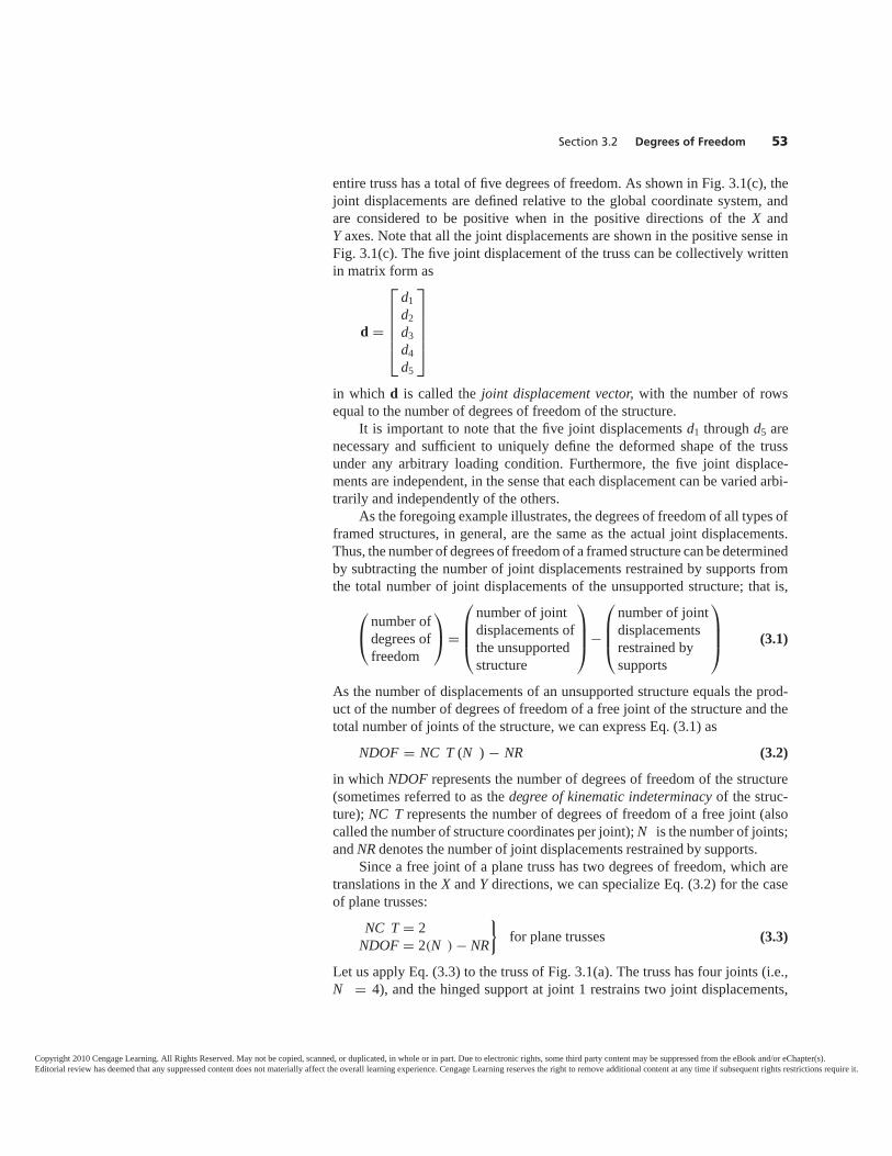
Section 3.2 Degrees of Freedom 53
entire truss has a total of five degrees of freedom. As shown in Fig. 3.1(c), thejoint displacements are defined relative to the global coordinate system, andare considered to be positive when in the positive directions of the X andY axes. Note that all the joint displacements are shown in the positive sense inFig. 3.1(c). The five joint displacement of the truss can be collectively writtenin matrix form as
d =
⎡⎢⎢⎢⎢⎣
d1d2d3d4d5
⎤⎥⎥⎥⎥⎦
in which d is called the joint displacement vector, with the number of rowsequal to the number of degrees of freedom of the structure.
It is important to note that the five joint displacements d1 through d5 arenecessary and sufficient to uniquely define the deformed shape of the trussunder any arbitrary loading condition. Furthermore, the five joint displace-ments are independent, in the sense that each displacement can be varied arbi-trarily and independently of the others.
As the foregoing example illustrates, the degrees of freedom of all types offramed structures, in general, are the same as the actual joint displacements.Thus, the number of degrees of freedom of a framed structure can be determinedby subtracting the number of joint displacements restrained by supports fromthe total number of joint displacements of the unsupported structure; that is,
⎛⎝ number of
degrees offreedom
⎞⎠ =
⎛⎜⎜⎝
number of jointdisplacements ofthe unsupportedstructure
⎞⎟⎟⎠−
⎛⎜⎜⎝
number of jointdisplacementsrestrained bysupports
⎞⎟⎟⎠ (3.1)
As the number of displacements of an unsupported structure equals the prod-uct of the number of degrees of freedom of a free joint of the structure and thetotal number of joints of the structure, we can express Eq. (3.1) as
NDOF = NC T (N ) − NR (3.2)
in which NDOF represents the number of degrees of freedom of the structure(sometimes referred to as the degree of kinematic indeterminacy of the struc-ture); NC T represents the number of degrees of freedom of a free joint (alsocalled the number of structure coordinates per joint); N is the number of joints;and NR denotes the number of joint displacements restrained by supports.
Since a free joint of a plane truss has two degrees of freedom, which aretranslations in the X and Y directions, we can specialize Eq. (3.2) for the caseof plane trusses:
NC T = 2NDOF = 2(N ) − NR
}for plane trusses (3.3)
Let us apply Eq. (3.3) to the truss of Fig. 3.1(a). The truss has four joints (i.e.,N = 4), and the hinged support at joint 1 restrains two joint displacements,
Copyright 2010 Cengage Learning. All Rights Reserved. May not be copied, scanned, or duplicated, in whole or in part. Due to electronic rights, some third party content may be suppressed from the eBook and/or eChapter(s).Editorial review has deemed that any suppressed content does not materially affect the overall learning experience. Cengage Learning reserves the right to remove additional content at any time if subsequent rights restrictions require it.
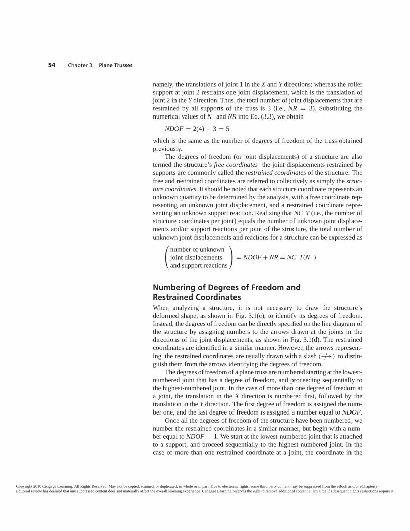
namely, the translations of joint 1 in the X and Y directions; whereas the rollersupport at joint 2 restrains one joint displacement, which is the translation ofjoint 2 in the Y direction. Thus, the total number of joint displacements that arerestrained by all supports of the truss is 3 (i.e., NR = 3). Substituting thenumerical values of N and NR into Eq. (3.3), we obtain
NDOF = 2(4) − 3 = 5which is the same as the number of degrees of freedom of the truss obtainedpreviously.
The degrees of freedom (or joint displacements) of a structure are alsotermed the structure’s free coordinates the joint displacements restrained bysupports are commonly called the restrained coordinates of the structure. Thefree and restrained coordinates are referred to collectively as simply the struc-ture coordinates. It should be noted that each structure coordinate represents anunknown quantity to be determined by the analysis, with a free coordinate rep-resenting an unknown joint displacement, and a restrained coordinate repre-senting an unknown support reaction. Realizing that NC T (i.e., the number ofstructure coordinates per joint) equals the number of unknown joint displace-ments and/or support reactions per joint of the structure, the total number ofunknown joint displacements and reactions for a structure can be expressed as⎛
⎝ number of unknownjoint displacementsand support reactions
⎞⎠ = NDOF + NR = NC T(N )
Numbering of Degrees of Freedom andRestrained CoordinatesWhen analyzing a structure, it is not necessary to draw the structure’sdeformed shape, as shown in Fig. 3.1(c), to identify its degrees of freedom.Instead, the degrees of freedom can be directly specified on the line diagram ofthe structure by assigning numbers to the arrows drawn at the joints in thedirections of the joint displacements, as shown in Fig. 3.1(d). The restrainedcoordinates are identified in a similar manner. However, the arrows represent-ing the restrained coordinates are usually drawn with a slash (−→/ ) to distin-guish them from the arrows identifying the degrees of freedom.
The degrees of freedom of a plane truss are numbered starting at the lowest-numbered joint that has a degree of freedom, and proceeding sequentially tothe highest-numbered joint. In the case of more than one degree of freedom ata joint, the translation in the X direction is numbered first, followed by thetranslation in the Y direction. The first degree of freedom is assigned the num-ber one, and the last degree of freedom is assigned a number equal to NDOF.
Once all the degrees of freedom of the structure have been numbered, wenumber the restrained coordinates in a similar manner, but begin with a num-ber equal to NDOF + 1. We start at the lowest-numbered joint that is attachedto a support, and proceed sequentially to the highest-numbered joint. In thecase of more than one restrained coordinate at a joint, the coordinate in the
54 Chapter 3 Plane Trusses
Copyright 2010 Cengage Learning. All Rights Reserved. May not be copied, scanned, or duplicated, in whole or in part. Due to electronic rights, some third party content may be suppressed from the eBook and/or eChapter(s).Editorial review has deemed that any suppressed content does not materially affect the overall learning experience. Cengage Learning reserves the right to remove additional content at any time if subsequent rights restrictions require it.
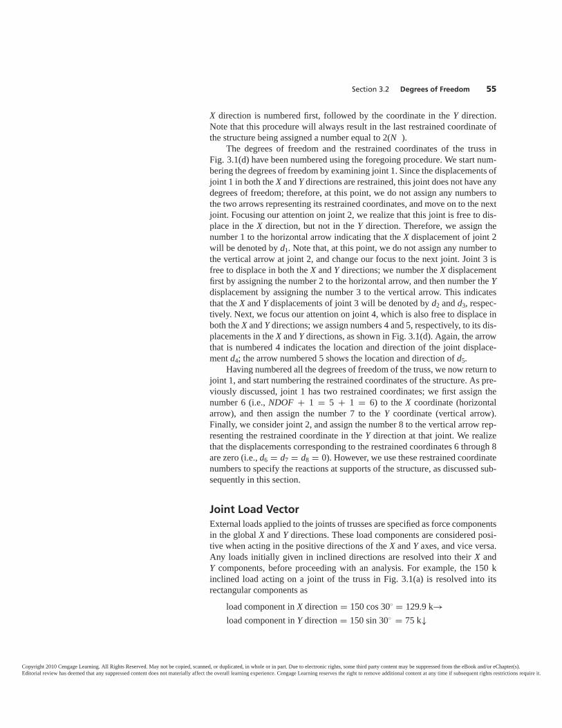
X direction is numbered first, followed by the coordinate in the Y direction.Note that this procedure will always result in the last restrained coordinate ofthe structure being assigned a number equal to 2(N ).
The degrees of freedom and the restrained coordinates of the truss inFig. 3.1(d) have been numbered using the foregoing procedure. We start num-bering the degrees of freedom by examining joint 1. Since the displacements ofjoint 1 in both the X and Y directions are restrained, this joint does not have anydegrees of freedom; therefore, at this point, we do not assign any numbers tothe two arrows representing its restrained coordinates, and move on to the nextjoint. Focusing our attention on joint 2, we realize that this joint is free to dis-place in the X direction, but not in the Y direction. Therefore, we assign thenumber 1 to the horizontal arrow indicating that the X displacement of joint 2will be denoted by d1. Note that, at this point, we do not assign any number tothe vertical arrow at joint 2, and change our focus to the next joint. Joint 3 isfree to displace in both the X and Y directions; we number the X displacementfirst by assigning the number 2 to the horizontal arrow, and then number the Ydisplacement by assigning the number 3 to the vertical arrow. This indicatesthat the X and Y displacements of joint 3 will be denoted by d2 and d3, respec-tively. Next, we focus our attention on joint 4, which is also free to displace inboth the X and Y directions; we assign numbers 4 and 5, respectively, to its dis-placements in the X and Y directions, as shown in Fig. 3.1(d). Again, the arrowthat is numbered 4 indicates the location and direction of the joint displace-ment d4; the arrow numbered 5 shows the location and direction of d5.
Having numbered all the degrees of freedom of the truss, we now return tojoint 1, and start numbering the restrained coordinates of the structure. As pre-viously discussed, joint 1 has two restrained coordinates; we first assign thenumber 6 (i.e., NDOF + 1 = 5 + 1 = 6) to the X coordinate (horizontalarrow), and then assign the number 7 to the Y coordinate (vertical arrow).Finally, we consider joint 2, and assign the number 8 to the vertical arrow rep-resenting the restrained coordinate in the Y direction at that joint. We realizethat the displacements corresponding to the restrained coordinates 6 through 8are zero (i.e., d6 = d7 = d8 = 0). However, we use these restrained coordinatenumbers to specify the reactions at supports of the structure, as discussed sub-sequently in this section.
Joint Load VectorExternal loads applied to the joints of trusses are specified as force componentsin the global X and Y directions. These load components are considered posi-tive when acting in the positive directions of the X and Y axes, and vice versa.Any loads initially given in inclined directions are resolved into their X andY components, before proceeding with an analysis. For example, the 150 kinclined load acting on a joint of the truss in Fig. 3.1(a) is resolved into itsrectangular components as
load component in X direction = 150 cos 30 = 129.9 k→load component in Y direction = 150 sin 30 = 75 k↓
Section 3.2 Degrees of Freedom 55
Copyright 2010 Cengage Learning. All Rights Reserved. May not be copied, scanned, or duplicated, in whole or in part. Due to electronic rights, some third party content may be suppressed from the eBook and/or eChapter(s).Editorial review has deemed that any suppressed content does not materially affect the overall learning experience. Cengage Learning reserves the right to remove additional content at any time if subsequent rights restrictions require it.
These components are applied at joint 3 of the line diagram of the truss shownin Fig. 3.1(b).
In general, a load can be applied to a structure at the location and in thedirection of each of its degrees of freedom. For example, a five-degree-of-freedom truss can be subjected to a maximum of five loads, P1 through P5, asshown in Fig. 3.1(e). As indicated there, the numbers assigned to the degreesof freedom are also used to identify the joint loads. In other words, a load cor-responding to a degree of freedom di is denoted by the symbol Pi. The five jointloads of the truss can be collectively written in matrix form as
P =
⎡⎢⎢⎢⎢⎣
P1P2P3P4P5
⎤⎥⎥⎥⎥⎦ =
⎡⎢⎢⎢⎢⎣
0129.9−75
0−75
⎤⎥⎥⎥⎥⎦ k
in which P is called the joint load vector of the truss. The numerical form of Pis obtained by comparing Figs. 3.1(b) and 3.1(e). This comparison shows that:P1 = 0; P2 = 129.9 k; P3 = −75 k; P4 = 0; and P5 = −75 k. The negativesigns assigned to the magnitudes of P3 and P5 indicate that these loads act inthe negative Y (i.e., downward) direction. The numerical values of P1 throughP5 are then stored in the appropriate rows of the joint load vector P, as shownin the foregoing equation. It should be noted that the number of rows of Pequals the number of degrees of freedom (NDOF ) of the structure.
Reaction VectorA support that prevents the translation of a joint of a structure in a particular di-rection exerts a reaction force on the joint in that direction. Thus, when a trussis subjected to external loads, a reaction force component can develop at thelocation and in the direction of each of its restrained coordinates. For example,a truss with three restrained coordinates can develop up to three reactions, asshown in Fig. 3.1(e). As indicated there, the numbers assigned to the restrainedcoordinates are used to identify the support reactions. In other words, a reac-tion corresponding to an ith restrained coordinate is denoted by the symbol Ri.The three support reactions of the truss can be collectively expressed in matrixform as
=⎡⎣ R6
R7R8
⎤⎦
in which is referred to as the reaction vector of the structure. Note that thenumber of rows of equals the number of restrained coordinates (NR) of thestructure.
The procedure presented in this section for numerically identifying thedegrees of freedom, joint loads, and reactions of a structure considerably sim-plifies the task of programming an analysis on a computer, as will becomeapparent in Chapter 4.
56 Chapter 3 Plane Trusses
Copyright 2010 Cengage Learning. All Rights Reserved. May not be copied, scanned, or duplicated, in whole or in part. Due to electronic rights, some third party content may be suppressed from the eBook and/or eChapter(s).Editorial review has deemed that any suppressed content does not materially affect the overall learning experience. Cengage Learning reserves the right to remove additional content at any time if subsequent rights restrictions require it.
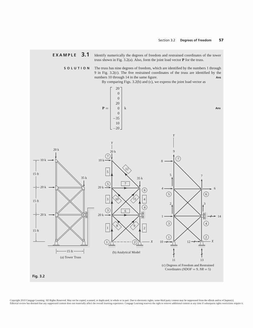
E X A M P L E 3.1 Identify numerically the degrees of freedom and restrained coordinates of the towertruss shown in Fig. 3.2(a). Also, form the joint load vector P for the truss.
S O L U T I O N The truss has nine degrees of freedom, which are identified by the numbers 1 through9 in Fig. 3.2(c). The five restrained coordinates of the truss are identified by thenumbers 10 through 14 in the same figure. Ans
By comparing Figs. 3.2(b) and (c), we express the joint load vector as
P =
⎡⎢⎢⎢⎢⎢⎢⎢⎢⎢⎢⎢⎢⎢⎣
2000
2000
−3510
−20
⎤⎥⎥⎥⎥⎥⎥⎥⎥⎥⎥⎥⎥⎥⎦
k Ans
Section 3.2 Degrees of Freedom 57
Fig. 3.2
10 k
20 k
35 k
15 ft
20 k
20 k
15 ft
15 ft
15 ft
(a) Tower Truss
1
3
5
7
6
4
12
10 k
20 k
35 k
20 k
20 k
X
Y
2
(b) Analytical Model
7
6
5
3
1
410 11
982
9
7
5 6
3
1
4
2
32
75
8
4 6
1
10
14
11 13
Y
X12
(c) Degrees of Freedom and RestrainedCoordinates (NDOF = 9, NR = 5)
Copyright 2010 Cengage Learning. All Rights Reserved. May not be copied, scanned, or duplicated, in whole or in part. Due to electronic rights, some third party content may be suppressed from the eBook and/or eChapter(s).Editorial review has deemed that any suppressed content does not materially affect the overall learning experience. Cengage Learning reserves the right to remove additional content at any time if subsequent rights restrictions require it.
3.3 MEMBER STIFFNESS RELATIONS IN THELOCAL COORDINATE SYSTEMIn the stiffness method of analysis, the joint displacements, d, of a structuredue to an external loading, P, are determined by solving a system of simulta-neous equations, expressed in the form
P = d (3.4)
in which is called the structure stiffness matrix. It will be shown subse-quently that the stiffness matrix for the entire structure, , is formed by assem-bling the stiffness matrices for its individual members. The stiffness matrix fora member expresses the forces at the ends of the member as functions of thedisplacements of those ends. In this section, we derive the stiffness matrix forthe members of plane trusses in the local coordinate system.
To establish the member stiffness relations, let us focus our attention on anarbitrary member m of the plane truss shown in Fig. 3.3(a). When the truss issubjected to external loads, m deforms and internal forces are induced at itsends. The initial and displaced positions of m are shown in Fig. 3.3(b), whereL, , and A denote, respectively, the length, oung’s modulus of elasticity,and the cross-sectional area of m. The member is prismatic in the sense that itsaxial rigidity, A, is constant. As Fig. 3.3(b) indicates, two displacements—translations in the x and y directions—are needed to completely specify the dis-placed position of each end of m. Thus, m has a total of four end displacementsor degrees of freedom. As shown in Fig. 3.3(b), the member end displacementsare denoted by u1 through u4, and the corresponding member end forces aredenoted by 1 through 4. Note that these end displacements and forces are de-fined relative to the local coordinate system of the member, and are consideredpositive when in the positive directions of the local x and y axes. As indicated in
58 Chapter 3 Plane Trusses
Fig. 3.3
y
Y
x
X
b
e
m
(a) Plane Truss
b′
e′
eb m
Initialposition
Displacedposition
y
x
u2
Q2
Q1
Q4
Q3
u1
u3 u4
L
EA = constant(b) Member Forces and Displacements
in Local Coordinate System
�
Copyright 2010 Cengage Learning. All Rights Reserved. May not be copied, scanned, or duplicated, in whole or in part. Due to electronic rights, some third party content may be suppressed from the eBook and/or eChapter(s).Editorial review has deemed that any suppressed content does not materially affect the overall learning experience. Cengage Learning reserves the right to remove additional content at any time if subsequent rights restrictions require it.
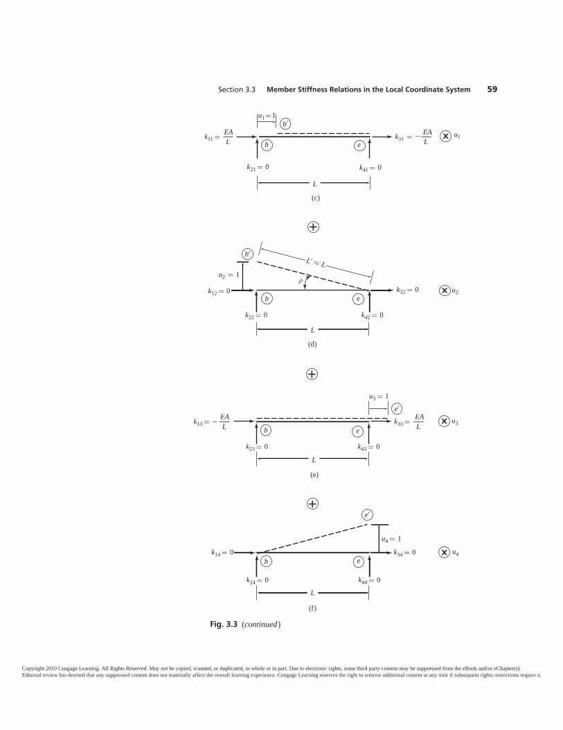
Section 3.3 Member Stiffness Relations in the Local Coordinate System 59
b′
eb
k41 � 0k21 � 0
k11 �
u1�1
u1
L
Lk31 � − EA
L
(c)
×EA
b′
eb
k42 � 0k22 � 0
k12 � 0 k32 � 0u2 � 1
L
L ′ ≈ Lρ
+
u2×
(d)
e′
eb
k43 � 0k23 � 0
u3 � 1
u3
L
k33 � EAL
k13 � − EAL
+
(e)
×
e′
eb
k44 � 0k24 � 0
k14 � 0 k34 � 0
L
u4
u4 � 1×
+
(f)
Fig. 3.3 (continued)
Copyright 2010 Cengage Learning. All Rights Reserved. May not be copied, scanned, or duplicated, in whole or in part. Due to electronic rights, some third party content may be suppressed from the eBook and/or eChapter(s).Editorial review has deemed that any suppressed content does not materially affect the overall learning experience. Cengage Learning reserves the right to remove additional content at any time if subsequent rights restrictions require it.
Fig. 3.3(b), the numbering scheme used to identify the member end displace-ments and forces is as follows:
It should be remembered that our objective here is to determine the rela-tionships between member end forces and end displacements. Such relation-ships can be conveniently established by subjecting the member, separately, toeach of the four end displacements as shown in Figs. 3.3(c) through (f); and byexpressing the total member end forces as the algebraic sums of the end forcesrequired to cause the individual end displacements. Thus, from Figs. 3.3(b)through (f), we can see that
1 = k11u1 + k12u2 + k13u3 + k14u4 (3.5a)
2 = k21u1 + k22u2 + k23u3 + k24u4 (3.5b)
3 = k31u1 + k32u2 + k33u3 + k34u4 (3.5c)
4 = k41u1 + k42u2 + k43u3 + k44u4 (3.5d)
in which kij represents the force at the location and in the direction of i re-quired, along with other end forces, to cause a unit value of displacement uj,while all other end displacements are zero. These forces per unit displacementare called stiffness coefficients. It should be noted that a double-subscript nota-tion is used for stiffness coefficients, with the first subscript identifying theforce and the second subscript identifying the displacement.
By using the definition of matrix multiplication, Eqs. (3.5) can be ex-pressed in matrix form as⎡
⎢⎢⎣1234
⎤⎥⎥⎦ =
⎡⎢⎢⎣
k11 k12 k13 k14k21 k22 k23 k24k31 k32 k33 k34k41 k42 k43 k44
⎤⎥⎥⎦
⎡⎢⎢⎣
u1u2u3u4
⎤⎥⎥⎦ (3.6)
or, symbolically, as
(3.7)
in which and u are the member end force and member end displacement vec-tors, respectively, in the local coordinate system; and is called the memberstiffness matrix in the local coordinate system.
= u
Member end displacements and forces are numbered by beginningat the end of the member designated b , where the origin of thelocal coordinate system is located, with the translation and force inthe x direction numbered first, followed by the translation and forcein the y direction. The displacements and forces at the opposite endof the member, designated e, are then numbered in the samesequential order.
60 Chapter 3 Plane Trusses
Copyright 2010 Cengage Learning. All Rights Reserved. May not be copied, scanned, or duplicated, in whole or in part. Due to electronic rights, some third party content may be suppressed from the eBook and/or eChapter(s).Editorial review has deemed that any suppressed content does not materially affect the overall learning experience. Cengage Learning reserves the right to remove additional content at any time if subsequent rights restrictions require it.
The stiffness coefficients kij can be evaluated by subjecting the member,separately, to unit values of each of the four end displacements. The memberend forces required to cause the individual unit displacements are then deter-mined by applying the equations of equilibrium, and by using the principles ofmechanics of materials. The member end forces thus obtained represent thestiffness coefficients for the member.
Let us determine the stiffness coefficients corresponding to a unit value ofthe displacement u1 at end b of m, as shown in Fig. 3.3(c). Note that all other dis-placements of m are zero (i.e., u2 = u3 = u4 = 0). Since m is in equilibrium, theend forces k11, k21, k31, and k41 acting on it must satisfy the three equilibriumequations:
∑Fx = 0,
∑Fy = 0, and
∑M = 0.Applying the equations of
equilibrium, we write+ → ∑
Fx = 0 k11 + k31 = 0k31 = −k11 (3.8)
+ ↑ ∑Fy = 0 k21 + k41 = 0 (3.9)
+ ∑Me = 0 −k21(L) = 0
Since L is not zero, k21 must be zero; that isk21 = 0 (3.10)
By substituting Eq. (3.10) into Eq. (3.9), we obtaink41 = 0 (3.11)
Equations (3.8), (3.10), and (3.11) indicate that m is in equilibrium under theaction of two axial forces, of equal magnitude but with opposite senses, appliedat its ends. Furthermore, since the displacement u1 = 1 results in the shorten-ing of the member’s length, the two axial forces causing this displacementmust be compressive; that is, k11 must act in the positive direction of the localx axis, and k31 (with a magnitude equal to k11) must act in the negative direc-tion of the x axis.
To relate the axial force k11 to the unit axial deformation (u1 = 1) of m, weuse the principles of the mechanics of materials. Recall that in a prismaticmember subjected to axial tension or compression, the normal stress σ isgiven by
σ = axial forcecross-sectional area = k11
A (3.12)
and the normal strain, ε, is expressed as
ε = change in lengthoriginal length = 1
L (3.13)
For linearly elastic materials, the stress–strain relationship is given by Hooke’slaw as
σ = ε (3.14)
Substitution of Eqs. (3.12) and (3.13) into Eq. (3.14) yieldsk11A =
( 1L
)
a
Section 3.3 Member Stiffness Relations in the Local Coordinate System 61
Copyright 2010 Cengage Learning. All Rights Reserved. May not be copied, scanned, or duplicated, in whole or in part. Due to electronic rights, some third party content may be suppressed from the eBook and/or eChapter(s).Editorial review has deemed that any suppressed content does not materially affect the overall learning experience. Cengage Learning reserves the right to remove additional content at any time if subsequent rights restrictions require it.
from which we obtain the expression for the stiffness coefficient k11,
k11 = AL (3.15)
The expression for k31 can now be obtained from Eq. (3.8) as
k31 = −k11 = − AL
(3.16)
in which the negative sign indicates that this force acts in the negative x direc-tion. Figure 3.3(c) shows the expressions for the four stiffness coefficientsrequired to cause the end displacement u1 = 1 of m.
By using a similar approach, it can be shown that the stiffness coefficientsrequired to cause the axial displacement u3 = 1 at end e of m are as follows(Fig. 3.3e).
k13 = − AL k23 = 0 k33 = A
L k43 = 0 (3.17)
The deformed shape of m due to a unit value of displacement u2, while allother displacements are zero, is shown in Fig. 3.3(d). Applying the equilibriumequations, we write
+ → ∑Fx = 0 k12 + k32 = 0
k32 = −k12 (3.18)
+ ↑ ∑Fy = 0 k22 + k42 = 0 (3.19)
+ ∑Me = 0 −k22(L) = 0
from which we obtain
k22 = 0 (3.20)
Substitution of Eq. (3.20) into Eq. (3.19) yields
k42 = 0 (3.21)
Thus, the forces k22 and k42, which act perpendicular to the longitudinal axis ofm, are both zero.
As for the axial forces k12 and k32, Eq. (3.18) indicates that they must be ofequal magnitude but with opposite senses. From Fig. 3.3(d), we can see that thedeformed length of the member, L′, can be expressed in terms of its unde-formed length L as
L ′ = Lcos ρ
(3.22)
in which the angle ρ denotes the rotation of the member due to the end dis-placement u2 = 1. Since the displacements are assumed to be small, cos ρ ≈ 1and Eq. (3.22) reduces to
L ′ ≈ L (3.23)
a
62 Chapter 3 Plane Trusses
Copyright 2010 Cengage Learning. All Rights Reserved. May not be copied, scanned, or duplicated, in whole or in part. Due to electronic rights, some third party content may be suppressed from the eBook and/or eChapter(s).Editorial review has deemed that any suppressed content does not materially affect the overall learning experience. Cengage Learning reserves the right to remove additional content at any time if subsequent rights restrictions require it.
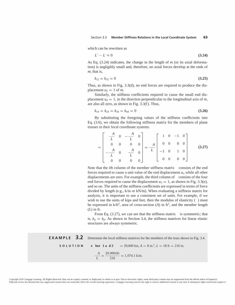
which can be rewritten asL ′ − L ≈ 0 (3.24)
As Eq. (3.24) indicates, the change in the length of m (or its axial deforma-tion) is negligibly small and, therefore, no axial forces develop at the ends ofm; that is,
k12 = k32 = 0 (3.25)
Thus, as shown in Fig. 3.3(d), no end forces are required to produce the dis-placement u2 = 1 of m.
Similarly, the stiffness coefficients required to cause the small end dis-placement u4 = 1, in the direction perpendicular to the longitudinal axis of m,are also all zero, as shown in Fig. 3.3(f). Thus,
k14 = k24 = k34 = k44 = 0 (3.26)
By substituting the foregoing values of the stiffness coefficients intoEq. (3.6), we obtain the following stiffness matrix for the members of planetrusses in their local coordinate systems.
=
⎡⎢⎢⎢⎢⎢⎢⎢⎣
AL 0 − A
L 0
0 0 0 0
− AL 0 A
L 0
0 0 0 0
⎤⎥⎥⎥⎥⎥⎥⎥⎦
= AL
⎡⎢⎢⎢⎢⎢⎢⎣
1 0 −1 0
0 0 0 0
−1 0 1 0
0 0 0 0
⎤⎥⎥⎥⎥⎥⎥⎦
(3.27)
Note that the ith column of the member stiffness matrix consists of the endforces required to cause a unit value of the end displacement ui, while all otherdisplacements are zero. For example, the third column of consists of the fourend forces required to cause the displacement u3 = 1, as shown in Fig. 3.3(e),and so on. The units of the stiffness coefficients are expressed in terms of forcedivided by length (e.g., k/in or kN/m). When evaluating a stiffness matrix foranalysis, it is important to use a consistent set of units. For example, if wewish to use the units of kips and feet, then the modulus of elasticity ( ) mustbe expressed in k/ft2, area of cross-section (A) in ft2, and the member length(L) in ft.
From Eq. (3.27), we can see that the stiffness matrix is symmetric; thatis, kij = kji. As shown in Section 3.4, the stiffness matrices for linear elasticstructures are always symmetric.
Section 3.3 Member Stiffness Relations in the Local Coordinate System 63
E X A M P L E 3.2 Determine the local stiffness matrices for the members of the truss shown in Fig. 3.4.
S O L U T I O N e ber 1 a d 2 = 29,000 ksi, A = 8 in.2, L = 18 ft = 216 in.
AL = 29,000(8)
216 = 1,074.1 k/in.
Copyright 2010 Cengage Learning. All Rights Reserved. May not be copied, scanned, or duplicated, in whole or in part. Due to electronic rights, some third party content may be suppressed from the eBook and/or eChapter(s).Editorial review has deemed that any suppressed content does not materially affect the overall learning experience. Cengage Learning reserves the right to remove additional content at any time if subsequent rights restrictions require it.
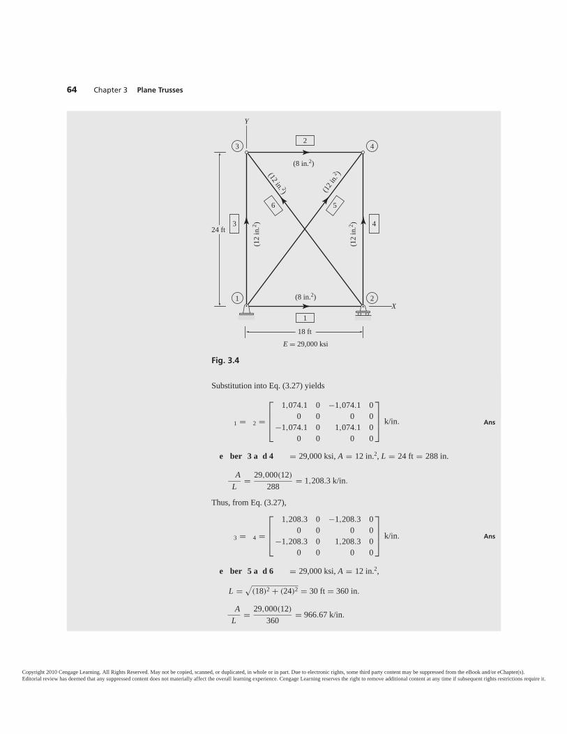
Substitution into Eq. (3.27) yields
1 = 2 =
⎡⎢⎢⎣
1,074.1 0 −1,074.1 00 0 0 0
−1,074.1 0 1,074.1 00 0 0 0
⎤⎥⎥⎦ k/in. Ans
e ber 3 a d 4 = 29,000 ksi, A = 12 in.2, L = 24 ft = 288 in.
AL = 29,000(12)
288 = 1,208.3 k/in.
Thus, from Eq. (3.27),
3 = 4 =
⎡⎢⎢⎣
1,208.3 0 −1,208.3 00 0 0 0
−1,208.3 0 1,208.3 00 0 0 0
⎤⎥⎥⎦ k/in. Ans
e ber 5 a d 6 = 29,000 ksi, A = 12 in.2,
L =√
(18)2 + (24)2 = 30 ft = 360 in.
AL = 29,000(12)
360 = 966.67 k/in.
64 Chapter 3 Plane Trusses
Fig. 3.4
21
43
X
Y
E = 29,000 ksi
(8 in.2)(12 in. 2) (1
2 in.
2 )
(8 in.2)
(12
in.2 )
(12
in.2 )
18 ft
24 ft
2
1
43
6 5
Copyright 2010 Cengage Learning. All Rights Reserved. May not be copied, scanned, or duplicated, in whole or in part. Due to electronic rights, some third party content may be suppressed from the eBook and/or eChapter(s).Editorial review has deemed that any suppressed content does not materially affect the overall learning experience. Cengage Learning reserves the right to remove additional content at any time if subsequent rights restrictions require it.
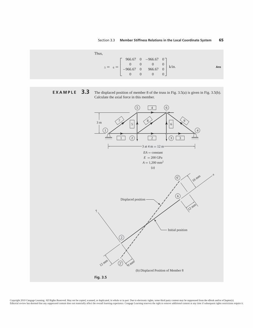
Thus,
5 = 6 =
⎡⎢⎢⎣
966.67 0 −966.67 00 0 0 0
−966.67 0 966.67 00 0 0 0
⎤⎥⎥⎦ k/in. Ans
E X A M P L E 3.3 The displaced position of member 8 of the truss in Fig. 3.5(a) is given in Fig. 3.5(b).Calculate the axial force in this member.
Section 3.3 Member Stiffness Relations in the Local Coordinate System 65
Fig. 3.5
41
5 6
2 3
3 m
3 at 4 m � 12 m
EA � constantE � 200 GPa
A � 1,200 mm2
(a)
4
65
21
7 8 9
3
Initial position
Displaced position
2
2′
6
6′
y
x
16 mm
12 mm
12 mm9 mm
(b) Displaced Position of Member 8
Copyright 2010 Cengage Learning. All Rights Reserved. May not be copied, scanned, or duplicated, in whole or in part. Due to electronic rights, some third party content may be suppressed from the eBook and/or eChapter(s).Editorial review has deemed that any suppressed content does not materially affect the overall learning experience. Cengage Learning reserves the right to remove additional content at any time if subsequent rights restrictions require it.
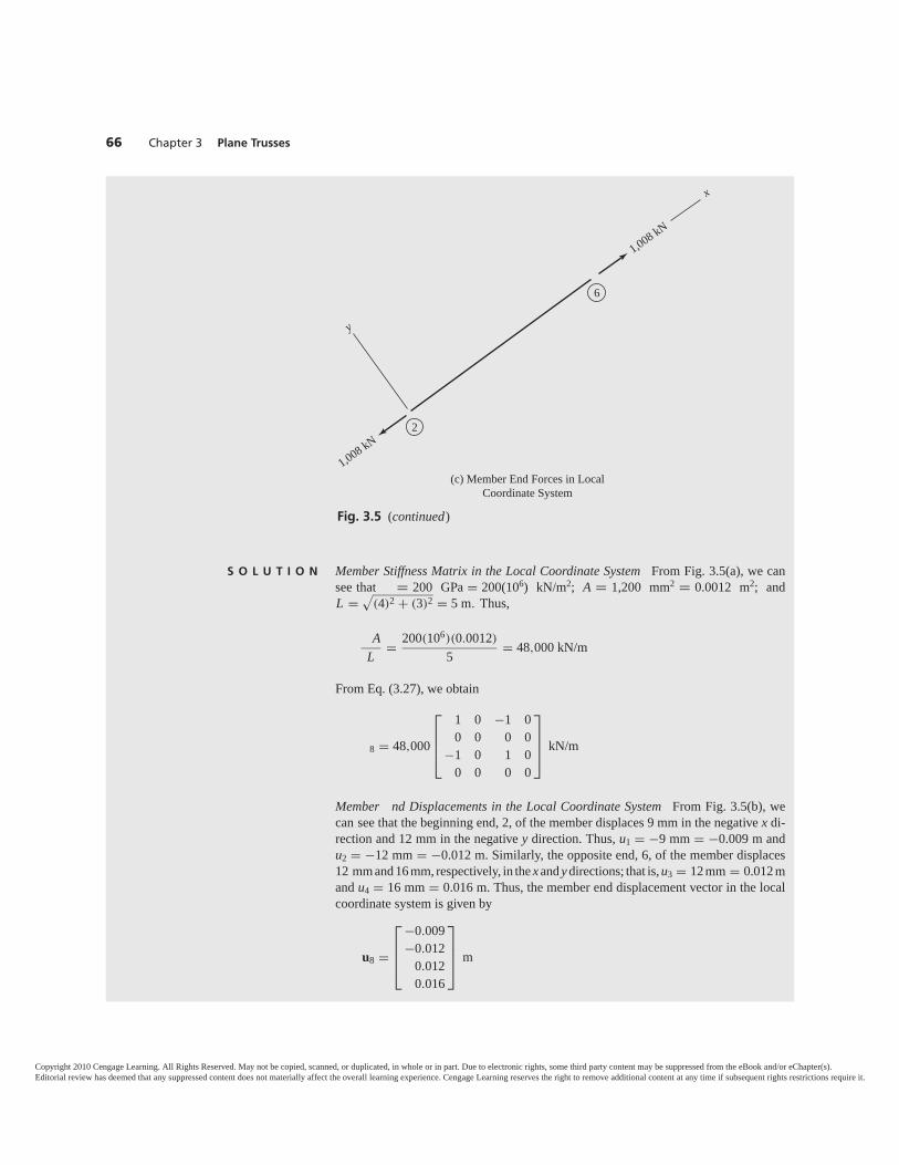
S O L U T I O N Member Stiffness Matrix in the Local Coordinate System From Fig. 3.5(a), we cansee that = 200 GPa = 200(106) kN/m2; A = 1,200 mm2 = 0.0012 m2; andL =
√(4)2 + (3)2 = 5 m. Thus,
AL = 200(106)(0.0012)
5 = 48,000 kN/m
From Eq. (3.27), we obtain
8 = 48,000
⎡⎢⎢⎣
1 0 −1 00 0 0 0
−1 0 1 00 0 0 0
⎤⎥⎥⎦ kN/m
Member nd Displacements in the Local Coordinate System From Fig. 3.5(b), wecan see that the beginning end, 2, of the member displaces 9 mm in the negative x di-rection and 12 mm in the negative y direction. Thus, u1 = −9 mm = −0.009 m andu2 = −12 mm = −0.012 m. Similarly, the opposite end, 6, of the member displaces12 mm and 16 mm, respectively, in the x and y directions; that is, u3 = 12 mm = 0.012 mand u4 = 16 mm = 0.016 m. Thus, the member end displacement vector in the localcoordinate system is given by
u8 =
⎡⎢⎢⎣
−0.009−0.012
0.0120.016
⎤⎥⎥⎦ m
66 Chapter 3 Plane Trusses
6
2
y
x
1,008 kN
1,008 kN
(c) Member End Forces in LocalCoordinate System
Fig. 3.5 (continued)
Copyright 2010 Cengage Learning. All Rights Reserved. May not be copied, scanned, or duplicated, in whole or in part. Due to electronic rights, some third party content may be suppressed from the eBook and/or eChapter(s).Editorial review has deemed that any suppressed content does not materially affect the overall learning experience. Cengage Learning reserves the right to remove additional content at any time if subsequent rights restrictions require it.
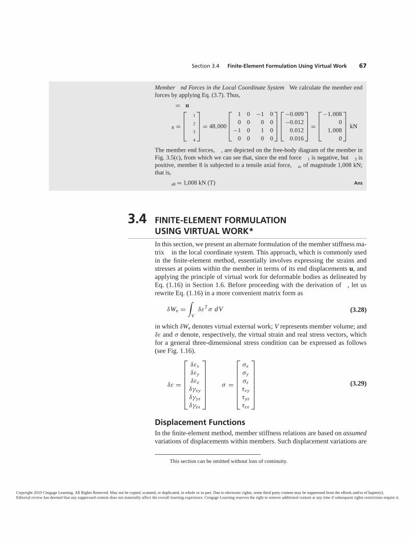
3.4 FINITE-ELEMENT FORMULATION USING VIRTUAL WORK*In this section, we present an alternate formulation of the member stiffness ma-trix in the local coordinate system. This approach, which is commonly usedin the finite-element method, essentially involves expressing the strains andstresses at points within the member in terms of its end displacements u, andapplying the principle of virtual work for deformable bodies as delineated byEq. (1.16) in Section 1.6. Before proceeding with the derivation of , let usrewrite Eq. (1.16) in a more convenient matrix form as
δWe =∫
VδεT σ dV (3.28)
in which δWe denotes virtual external work; V represents member volume; andδε and σ denote, respectively, the virtual strain and real stress vectors, whichfor a general three-dimensional stress condition can be expressed as follows(see Fig. 1.16).
δε =
⎡⎢⎢⎢⎢⎢⎢⎣
δεxδεyδεzδγxyδγyzδγzx
⎤⎥⎥⎥⎥⎥⎥⎦
σ =
⎡⎢⎢⎢⎢⎢⎢⎣
σxσyσzτxyτyzτzx
⎤⎥⎥⎥⎥⎥⎥⎦
(3.29)
Displacement FunctionsIn the finite-element method, member stiffness relations are based on assumedvariations of displacements within members. Such displacement variations are
Section 3.4 Finite-Element Formulation Using Virtual Work 67
This section can be omitted without loss of continuity.
Member nd Forces in the Local Coordinate System We calculate the member endforces by applying Eq. (3.7). Thus,
= u
8 =
⎡⎢⎢⎣
1
2
3
4
⎤⎥⎥⎦ = 48,000
⎡⎢⎢⎣
1 0 −1 00 0 0 0
−1 0 1 00 0 0 0
⎤⎥⎥⎦
⎡⎢⎢⎣
−0.009−0.012
0.0120.016
⎤⎥⎥⎦ =
⎡⎢⎢⎣
−1,0080
1,0080
⎤⎥⎥⎦ kN
The member end forces, , are depicted on the free-body diagram of the member inFig. 3.5(c), from which we can see that, since the end force 1 is negative, but 3 ispositive, member 8 is subjected to a tensile axial force, a, of magnitude 1,008 kN;that is,
a8 = 1,008 kN (T) Ans
Copyright 2010 Cengage Learning. All Rights Reserved. May not be copied, scanned, or duplicated, in whole or in part. Due to electronic rights, some third party content may be suppressed from the eBook and/or eChapter(s).Editorial review has deemed that any suppressed content does not materially affect the overall learning experience. Cengage Learning reserves the right to remove additional content at any time if subsequent rights restrictions require it.
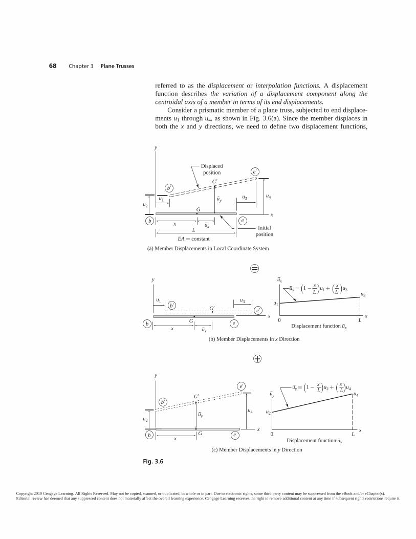
referred to as the displacement or interpolation functions. A displacementfunction describes the variation of a displacement component along thecentroidal axis of a member in terms of its end displacements.
Consider a prismatic member of a plane truss, subjected to end displace-ments u1 through u4, as shown in Fig. 3.6(a). Since the member displaces inboth the x and y directions, we need to define two displacement functions,
68 Chapter 3 Plane Trusses
Fig. 3.6
(a) Member Displacements in Local Coordinate System
b′
e′
ebInitial
position
Displacedposition
y
x
x
u2
u1u3 u4
LEA = constant
G′
G
uy
ux
b′e′
eb
y
x x
x
u1 u1u3
u3
G′
Gux
ux
�
L0Displacement function ux
(b) Member Displacements in x Direction
ux =(1 − x )
u1 + ( x )
u3LL
x
u2
u4uy
+
uy =(1 − x )
u2 + ( x )
u4L L
L
b′
e′
eb
y
x
x
u2
u4
G′
G
uy
0Displacement function uy
(c) Member Displacements in y Direction
Copyright 2010 Cengage Learning. All Rights Reserved. May not be copied, scanned, or duplicated, in whole or in part. Due to electronic rights, some third party content may be suppressed from the eBook and/or eChapter(s).Editorial review has deemed that any suppressed content does not materially affect the overall learning experience. Cengage Learning reserves the right to remove additional content at any time if subsequent rights restrictions require it.
ux and u y, for the displacements in the x and y directions, respectively. InFig. 3.6(a), the displacement functions ux and u y are depicted as the displace-ments of an arbitrary point G located on the member’s centroidal axis at a dis-tance x from end b (left end).
The total displacement of the member (due to u1 through u4) can be de-composed into the displacements in the x and y directions, as shown inFigs. 3.6(b) and (c), respectively. Note that Fig. 3.6(b) shows the member sub-jected to the two end displacements, u1 and u3, in the x direction (with u2 =u4 = 0); Fig. 3.6(c) depicts the displacement of the member due to the two enddisplacements, u2 and u4, in the y direction (with u1 = u3 = 0).
The displacement functions assumed in the finite-element method areusually in the form of complete polynomials,
u(x) =n∑
i=0ai xi with ai �= 0 (3.30)
in which n is the degree of the polynomial. The polynomial used for a particulardisplacement function should be of such a degree that all of its coefficients canbe evaluated by applying the available boundary conditions; that is,
n = nbc − 1 (3.31)
with nbc = number of boundary conditions.Thus, the displacement function ux for the truss member (Fig. 3.6b) is as-
sumed in the form of a linear polynomial asux = a0 + a1x (3.32)
in which a0 and a1 are the constants that can be determined by applying the fol-lowing two boundary conditions:
at x = 0 ux = u1
at x = L ux = u3
By applying the first boundary condition—that is, by setting x = 0 and ux = u1in Eq. (3.32)—we obtain
a0 = u1 (3.33)
Next, by using the second boundary condition—that is, by setting x = L andux = u3—we obtain
u3 = u1 + a1Lfrom which follows
a1 = u3 − u1L (3.34)
By substituting Eqs. (3.33) and (3.34) into Eq. (3.32), we obtain the expressionfor ux ,
ux = u1 +(u3 − u1
L
)x
Section 3.4 Finite-Element Formulation Using Virtual Work 69
Copyright 2010 Cengage Learning. All Rights Reserved. May not be copied, scanned, or duplicated, in whole or in part. Due to electronic rights, some third party content may be suppressed from the eBook and/or eChapter(s).Editorial review has deemed that any suppressed content does not materially affect the overall learning experience. Cengage Learning reserves the right to remove additional content at any time if subsequent rights restrictions require it.
or
(3.35)
The displacement function u y, for the member displacement in the y dire-ction (Fig. 3.6(c)), can be determined in a similar manner; that is, using a linearpolynomial and evaluating its coefficients by applying the boundary conditions.The result is
(3.36)
The plots of the displacement functions ux and u y are shown in Figs. 3.6(b)and (c), respectively.
It is important to realize that the displacement functions as given byEqs. (3.35) and (3.36) have been assumed, as is usually done in the finite-element method. There is no guarantee that an assumed displacement functiondefines the actual displacements of the member, except at its ends. In general,the displacement functions used in the finite-element method only approximatethe actual displacements within members (or elements), because they representapproximate solutions of the underlying differential equations. For this reason,the finite-element method is generally considered to be an approximate methodof analysis. However, for the prismatic members of framed structures, the dis-placement functions in the form of complete polynomials do happen to de-scribe exactly the actual member displacements and, therefore, such functionsyield exact member stiffness matrices for prismatic members.
From Fig. 3.6(c), we observe that the graph of the displacement functionu y exactly matches the displaced shape of the member’s centroidal axis due tothe end displacements u2 and u4. As this displaced shape defines the actual dis-placements in the y direction of all points along the member’s length, we canconclude that the function u y, as given by Eq. (3.36), is exact.
To demonstrate that Eq. (3.35) describes the actual displacements in the x direction of all points along the truss member’s centroidal axis, consider againthe member subjected to end displacements, u1 and u3, in the x direction asshown in Fig. 3.7(a). Since the member is subjected to forces only at its ends,the axial force, a, is constant throughout the member’s length. Thus, the axialstress, σ, at point G of the member is
σ = aA
(3.37)
in which A represents the cross-sectional area of the member at point G. Notethat the axial stress is distributed uniformly over the cross-sectional area A. Bysubstituting the linear stress–strain relationship ε = σ/ into Eq. (3.37), we
u y =(
1 − xL
)u2 +
( xL
)u4
ux =(
1 − xL
)u1 +
( xL
)u3
70 Chapter 3 Plane Trusses
Copyright 2010 Cengage Learning. All Rights Reserved. May not be copied, scanned, or duplicated, in whole or in part. Due to electronic rights, some third party content may be suppressed from the eBook and/or eChapter(s).Editorial review has deemed that any suppressed content does not materially affect the overall learning experience. Cengage Learning reserves the right to remove additional content at any time if subsequent rights restrictions require it.
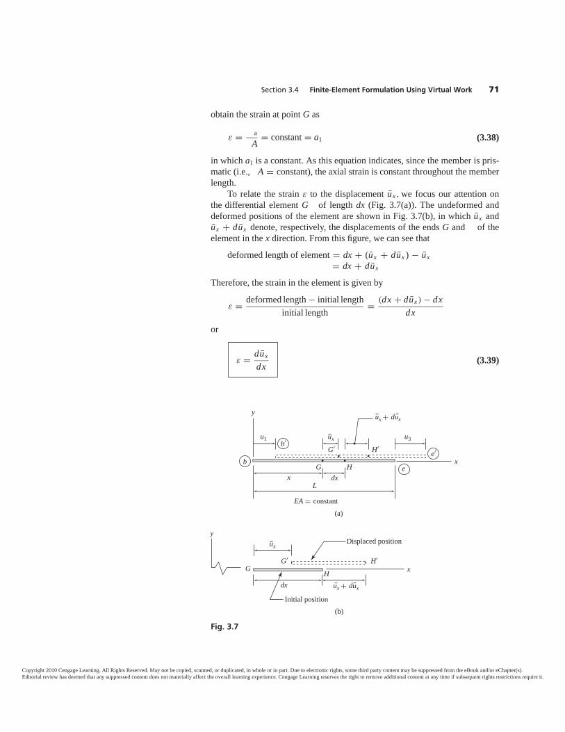
obtain the strain at point G as
ε = aA = constant = a1 (3.38)
in which a1 is a constant. As this equation indicates, since the member is pris-matic (i.e., A = constant), the axial strain is constant throughout the memberlength.
To relate the strain ε to the displacement ux , we focus our attention onthe differential element G of length dx (Fig. 3.7(a)). The undeformed anddeformed positions of the element are shown in Fig. 3.7(b), in which ux andux + dux denote, respectively, the displacements of the ends G and of theelement in the x direction. From this figure, we can see that
deformed length of element = dx + (ux + dux ) − ux= dx + dux
Therefore, the strain in the element is given by
ε = deformed length − initial lengthinitial length = (dx + dux ) − dx
dxor
(3.39)ε = duxdx
Section 3.4 Finite-Element Formulation Using Virtual Work 71
b′
e′
eb
y
x
x
u1 u3
G′ H′
G
L
H
ux
dx
EA � constant
ux + dux
(a)
Fig. 3.7
x
y
G′ H′
HG
ux
dx ux + dux
Displaced position
Initial position(b)
Copyright 2010 Cengage Learning. All Rights Reserved. May not be copied, scanned, or duplicated, in whole or in part. Due to electronic rights, some third party content may be suppressed from the eBook and/or eChapter(s).Editorial review has deemed that any suppressed content does not materially affect the overall learning experience. Cengage Learning reserves the right to remove additional content at any time if subsequent rights restrictions require it.
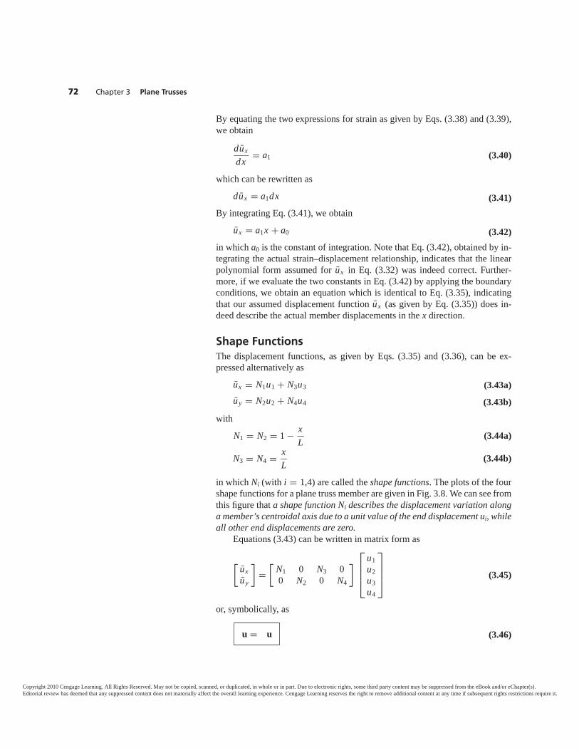
By equating the two expressions for strain as given by Eqs. (3.38) and (3.39),we obtain
duxdx = a1 (3.40)
which can be rewritten asdux = a1dx (3.41)
By integrating Eq. (3.41), we obtainux = a1x + a0 (3.42)
in which a0 is the constant of integration. Note that Eq. (3.42), obtained by in-tegrating the actual strain–displacement relationship, indicates that the linearpolynomial form assumed for ux in Eq. (3.32) was indeed correct. Further-more, if we evaluate the two constants in Eq. (3.42) by applying the boundaryconditions, we obtain an equation which is identical to Eq. (3.35), indicatingthat our assumed displacement function ux (as given by Eq. (3.35)) does in-deed describe the actual member displacements in the x direction.
Shape FunctionsThe displacement functions, as given by Eqs. (3.35) and (3.36), can be ex-pressed alternatively as
ux = N1u1 + N3u3 (3.43a)
u y = N2u2 + N4u4 (3.43b)
withN1 = N2 = 1 − x
L (3.44a)
N3 = N4 = xL (3.44b)
in which Ni (with i = 1,4) are called the shape functions. The plots of the fourshape functions for a plane truss member are given in Fig. 3.8. We can see fromthis figure that a shape function Ni describes the displacement variation alonga member’s centroidal axis due to a unit value of the end displacement ui, whileall other end displacements are zero.
Equations (3.43) can be written in matrix form as
[uxu y
]=
[N1 0 N3 00 N2 0 N4
] ⎡⎢⎢⎣
u1u2u3u4
⎤⎥⎥⎦ (3.45)
or, symbolically, as
(3.46)u = u
72 Chapter 3 Plane Trusses
Copyright 2010 Cengage Learning. All Rights Reserved. May not be copied, scanned, or duplicated, in whole or in part. Due to electronic rights, some third party content may be suppressed from the eBook and/or eChapter(s).Editorial review has deemed that any suppressed content does not materially affect the overall learning experience. Cengage Learning reserves the right to remove additional content at any time if subsequent rights restrictions require it.
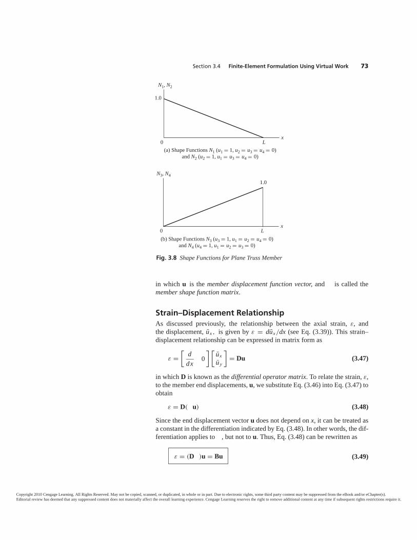
in which u is the member displacement function vector, and is called themember shape function matrix.
Strain–Displacement RelationshipAs discussed previously, the relationship between the axial strain, ε, andthe displacement, ux , is given by ε = dux/dx (see Eq. (3.39)). This strain–displacement relationship can be expressed in matrix form as
ε =[
ddx 0
] [uxu y
]= Du (3.47)
in which D is known as the differential operator matrix. To relate the strain, ε,to the member end displacements, u, we substitute Eq. (3.46) into Eq. (3.47) toobtain
ε = D( u) (3.48)
Since the end displacement vector u does not depend on x, it can be treated asa constant in the differentiation indicated by Eq. (3.48). In other words, the dif-ferentiation applies to , but not to u. Thus, Eq. (3.48) can be rewritten as
(3.49)ε = (D )u = Bu
Section 3.4 Finite-Element Formulation Using Virtual Work 73
N1, N2
0x
L
1.0
(a) Shape Functions N1 (u1 = 1, u2 = u3 = u4 = 0)and N2 (u2 = 1, u1 = u3 = u4 = 0)
Fig. 3.8 Shape Functions for Plane Truss Member
N3, N4
0x
L
1.0
(b) Shape Functions N3 (u3 = 1, u1 = u2 = u4 = 0)and N4 (u4 = 1, u1 = u2 = u3 = 0)
Copyright 2010 Cengage Learning. All Rights Reserved. May not be copied, scanned, or duplicated, in whole or in part. Due to electronic rights, some third party content may be suppressed from the eBook and/or eChapter(s).Editorial review has deemed that any suppressed content does not materially affect the overall learning experience. Cengage Learning reserves the right to remove additional content at any time if subsequent rights restrictions require it.
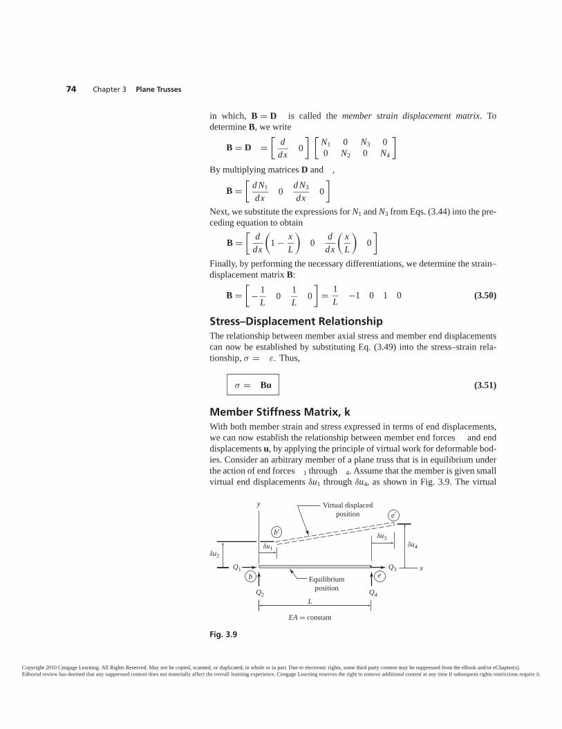
in which, B = D is called the member strain displacement matrix. Todetermine B, we write
B = D =[
ddx 0
] [N1 0 N3 00 N2 0 N4
]
By multiplying matrices D and ,
B =[
d N1dx 0 d N3
dx 0]
Next, we substitute the expressions for N1 and N3 from Eqs. (3.44) into the pre-ceding equation to obtain
B =[ d
dx
(1 − x
L
)0 d
dx
( xL
)0
]Finally, by performing the necessary differentiations, we determine the strain–displacement matrix B:
B =[
− 1L 0 1
L 0]
= 1L −1 0 1 0 (3.50)
Stress–Displacement RelationshipThe relationship between member axial stress and member end displacementscan now be established by substituting Eq. (3.49) into the stress–strain rela-tionship, σ = ε. Thus,
(3.51)
Member Stiffness Matrix, kWith both member strain and stress expressed in terms of end displacements,we can now establish the relationship between member end forces and enddisplacements u, by applying the principle of virtual work for deformable bod-ies. Consider an arbitrary member of a plane truss that is in equilibrium underthe action of end forces 1 through 4. Assume that the member is given smallvirtual end displacements δu1 through δu4, as shown in Fig. 3.9. The virtual
σ = Bu
74 Chapter 3 Plane Trusses
Fig. 3.9
b′
e′
eb Equilibriumposition
Virtual displacedposition
y
x
Q2 Q4
Q1 Q3
δu1δu4
δu3
δu2
L
EA = constant
Copyright 2010 Cengage Learning. All Rights Reserved. May not be copied, scanned, or duplicated, in whole or in part. Due to electronic rights, some third party content may be suppressed from the eBook and/or eChapter(s).Editorial review has deemed that any suppressed content does not materially affect the overall learning experience. Cengage Learning reserves the right to remove additional content at any time if subsequent rights restrictions require it.
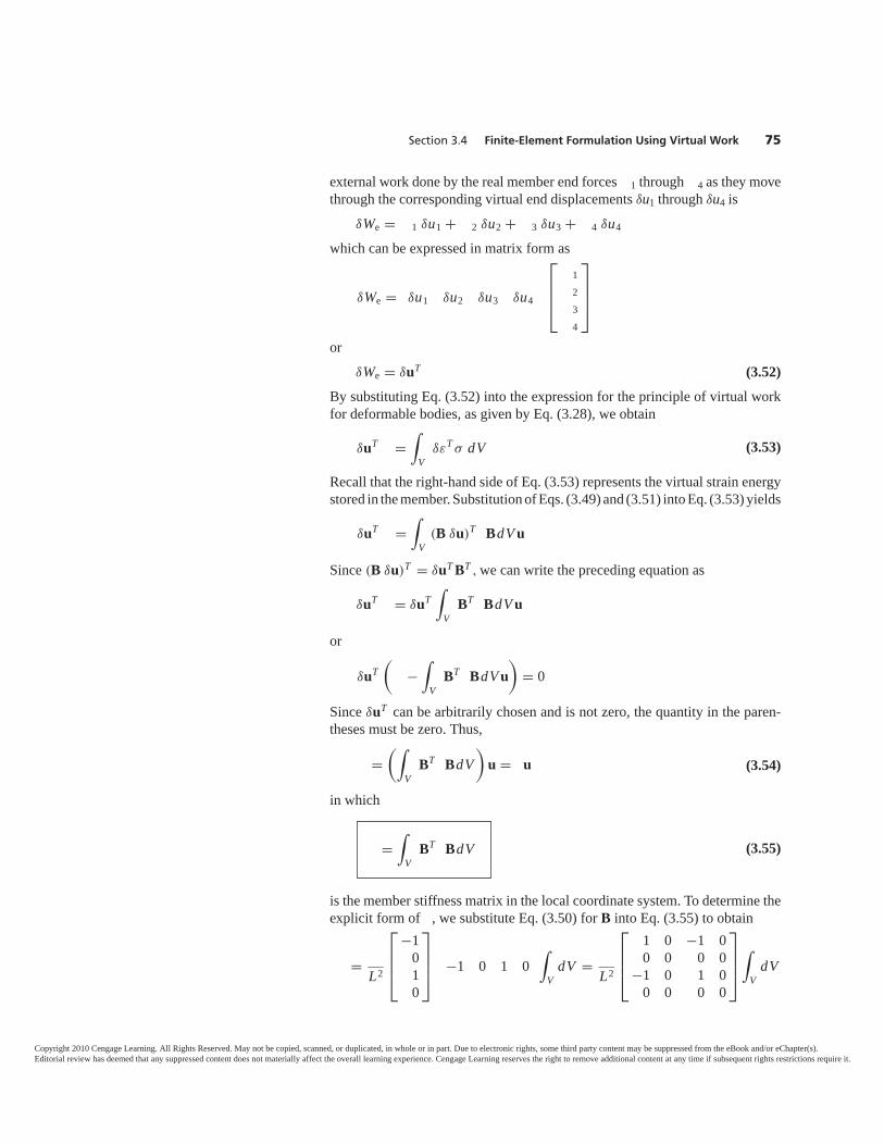
external work done by the real member end forces 1 through 4 as they movethrough the corresponding virtual end displacements δu1 through δu4 is
δWe = 1 δu1 + 2 δu2 + 3 δu3 + 4 δu4
which can be expressed in matrix form as
δWe = δu1 δu2 δu3 δu4
⎡⎢⎢⎣
1234
⎤⎥⎥⎦
orδWe = δuT (3.52)
By substituting Eq. (3.52) into the expression for the principle of virtual workfor deformable bodies, as given by Eq. (3.28), we obtain
δuT =∫
VδεT σ dV (3.53)
Recall that the right-hand side of Eq. (3.53) represents the virtual strain energystored in the member. Substitution of Eqs. (3.49) and (3.51) into Eq. (3.53) yields
δuT =∫
V(B δu)T BdV u
Since (B δu)T = δuT BT , we can write the preceding equation as
δuT = δuT∫
VBT BdV u
or
δuT(
−∫
VBT BdV u
)= 0
Since δuT can be arbitrarily chosen and is not zero, the quantity in the paren-theses must be zero. Thus,
=(∫
VBT BdV
)u = u (3.54)
in which
(3.55)
is the member stiffness matrix in the local coordinate system. To determine theexplicit form of , we substitute Eq. (3.50) for B into Eq. (3.55) to obtain
= L2
⎡⎢⎢⎣
−1010
⎤⎥⎥⎦ −1 0 1 0
∫V
dV = L2
⎡⎢⎢⎣
1 0 −1 00 0 0 0
−1 0 1 00 0 0 0
⎤⎥⎥⎦
∫V
dV
=∫
VBT BdV
Section 3.4 Finite-Element Formulation Using Virtual Work 75
Copyright 2010 Cengage Learning. All Rights Reserved. May not be copied, scanned, or duplicated, in whole or in part. Due to electronic rights, some third party content may be suppressed from the eBook and/or eChapter(s).Editorial review has deemed that any suppressed content does not materially affect the overall learning experience. Cengage Learning reserves the right to remove additional content at any time if subsequent rights restrictions require it.
Since∫
V dV = V = AL , the member stiffness matrix, , becomes
= AL
⎡⎢⎣
1 0 −1 00 0 0 0
−1 0 1 00 0 0 0
⎤⎥⎦
Note that the preceding expression for is identical to that derived in Sec-tion 3.3 (Eq. (3.27)) using the direct equilibrium approach.
Symmetry of the Member Stiffness MatrixThe expression for the stiffness matrix as given by Eq. (3.55) is general, inthe sense that the stiffness matrices for members of other types of framed struc-tures, as well as for elements of surface structures and solids, can also be ex-pressed in the integral form of this equation. We can deduce from Eq. (3.55)that for linear elastic structures, the member stiffness matrices are symmetric.
Transposing both sides of Eq. (3.55), we write
T =∫
V(BT B)TdV
Now, recall from Section 2.3 that the transpose of a product of matrices equalsthe product of the transposed matrices in reverse order; that is, (ABC)T =CTBTAT. Thus, the preceding equation becomes
T =∫
VBT T (BT )T dV
For linear elastic structures, is either a scalar (in the case of framed struc-tures), or a symmetric matrix (for surface structures and solids). Therefore,
T = . Furthermore, by realizing that (BT)T = B, we can express the preced-ing equation as
T =∫
VBT BdV (3.56)
Finally, a comparison of Eqs. (3.55) and (3.56) yields
(3.57)
which shows that is a symmetric matrix.
3.5 COORDINATE TRANSFORMATIONSWhen members of a structure are oriented in different directions, it becomesnecessary to transform the stiffness relations for each member from its localcoordinate system to a single global coordinate system selected for the entirestructure. The member stiffness relations as expressed in the global coordinatesystem are then combined to establish the stiffness relations for the wholestructure. In this section, we consider the transformation of member end forcesand end displacements from local to global coordinate systems, and vice versa,
T =
76 Chapter 3 Plane Trusses
Copyright 2010 Cengage Learning. All Rights Reserved. May not be copied, scanned, or duplicated, in whole or in part. Due to electronic rights, some third party content may be suppressed from the eBook and/or eChapter(s).Editorial review has deemed that any suppressed content does not materially affect the overall learning experience. Cengage Learning reserves the right to remove additional content at any time if subsequent rights restrictions require it.
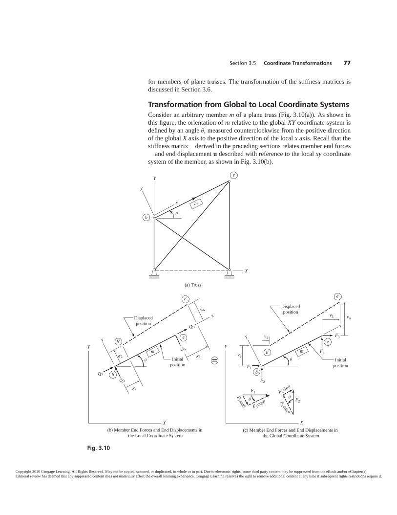
for members of plane trusses. The transformation of the stiffness matrices isdiscussed in Section 3.6.
Transformation from Global to Local Coordinate SystemsConsider an arbitrary member m of a plane truss (Fig. 3.10(a)). As shown inthis figure, the orientation of m relative to the global XY coordinate system isdefined by an angle θ, measured counterclockwise from the positive directionof the global X axis to the positive direction of the local x axis. Recall that thestiffness matrix derived in the preceding sections relates member end forces
and end displacement u described with reference to the local xy coordinatesystem of the member, as shown in Fig. 3.10(b).
Section 3.5 Coordinate Transformations 77
Fig. 3.10
Y
y
x
X
b
e
θ
(a) Truss
m
Yy
X
x
b
b′
e′
e
Displacedposition
Initialposition
u 2
u 1
u 3
u 4
Q 1
Q 2
Q 3
Q 4
(b) Member End Forces and End Displacements in the Local Coordinate System
θ
m
�
y
x
θ
b
b′
e′
e
Displacedposition
Initialposition
v3
v1
v2
v4
F2
F1
F4
F3
θ F2
F 2sinθ
F2 cosθ
θ
F1 sinθ F 1cosθ
F1
(c) Member End Forces and End Displacements in the Global Coordinate System
Y
X
m
Copyright 2010 Cengage Learning. All Rights Reserved. May not be copied, scanned, or duplicated, in whole or in part. Due to electronic rights, some third party content may be suppressed from the eBook and/or eChapter(s).Editorial review has deemed that any suppressed content does not materially affect the overall learning experience. Cengage Learning reserves the right to remove additional content at any time if subsequent rights restrictions require it.
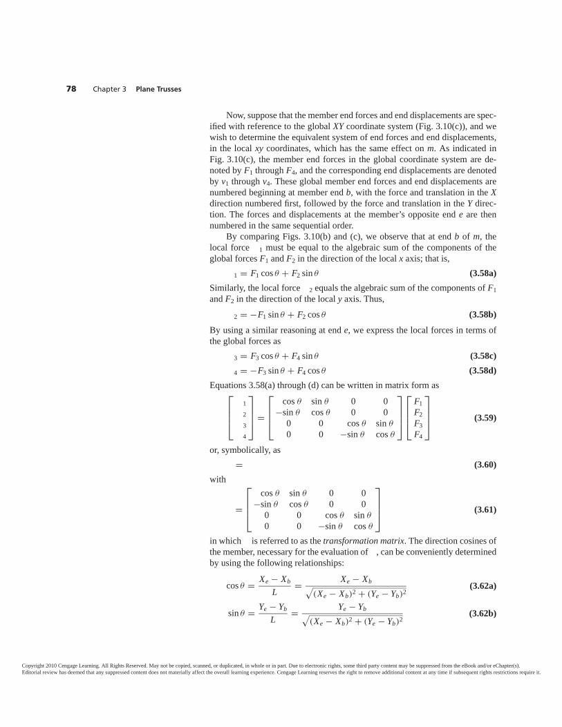
Now, suppose that the member end forces and end displacements are spec-ified with reference to the global XY coordinate system (Fig. 3.10(c)), and wewish to determine the equivalent system of end forces and end displacements,in the local xy coordinates, which has the same effect on m. As indicated inFig. 3.10(c), the member end forces in the global coordinate system are de-noted by F1 through F4, and the corresponding end displacements are denotedby v1 through v4. These global member end forces and end displacements arenumbered beginning at member end b, with the force and translation in the Xdirection numbered first, followed by the force and translation in the Y direc-tion. The forces and displacements at the member’s opposite end e are thennumbered in the same sequential order.
By comparing Figs. 3.10(b) and (c), we observe that at end b of m, thelocal force 1 must be equal to the algebraic sum of the components of theglobal forces F1 and F2 in the direction of the local x axis; that is,
1 = F1 cos θ + F2 sin θ (3.58a)
Similarly, the local force 2 equals the algebraic sum of the components of F1and F2 in the direction of the local y axis. Thus,
2 = −F1 sin θ + F2 cos θ (3.58b)
By using a similar reasoning at end e, we express the local forces in terms ofthe global forces as
3 = F3 cos θ + F4 sin θ (3.58c)
4 = −F3 sin θ + F4 cos θ (3.58d)
Equations 3.58(a) through (d) can be written in matrix form as⎡⎢⎢⎣
1234
⎤⎥⎥⎦ =
⎡⎢⎢⎣
cos θ sin θ 0 0−sin θ cos θ 0 0
0 0 cos θ sin θ
0 0 −sin θ cos θ
⎤⎥⎥⎦
⎡⎢⎢⎣
F1F2F3F4
⎤⎥⎥⎦ (3.59)
or, symbolically, as= (3.60)
with
=
⎡⎢⎢⎣
cos θ sin θ 0 0−sin θ cos θ 0 0
0 0 cos θ sin θ
0 0 −sin θ cos θ
⎤⎥⎥⎦ (3.61)
in which is referred to as the transformation matrix. The direction cosines ofthe member, necessary for the evaluation of , can be conveniently determinedby using the following relationships:
cos θ = Xe − XbL = Xe − Xb√
(Xe − Xb)2 + (Ye − Yb)2(3.62a)
sin θ = Ye − YbL = Ye − Yb√
(Xe − Xb)2 + (Ye − Yb)2(3.62b)
78 Chapter 3 Plane Trusses
Copyright 2010 Cengage Learning. All Rights Reserved. May not be copied, scanned, or duplicated, in whole or in part. Due to electronic rights, some third party content may be suppressed from the eBook and/or eChapter(s).Editorial review has deemed that any suppressed content does not materially affect the overall learning experience. Cengage Learning reserves the right to remove additional content at any time if subsequent rights restrictions require it.
in which Xb and Yb denote the global coordinates of the beginning joint b forthe member, and Xe and Ye represent the global coordinates of the end joint e.
The member end displacements, like end forces, are vectors, which are de-fined in the same directions as the corresponding forces. Therefore, the trans-formation matrix (Eq. (3.61)), developed for transforming end forces, canalso be used to transform member end displacements from the global to localcoordinate system; that is,
(3.63)
Transformation from Local to Global Coordinate SystemsNext, let us consider the transformation of member end forces and enddisplacements from local to global coordinate systems. A comparison ofFigs. 3.10(b) and (c) indicates that at end b of m, the global force F1 must beequal to the algebraic sum of the components of the local forces 1 and 2 inthe direction of the global X axis; that is,
F1 = 1 cos θ − 2 sin θ (3.64a)
In a similar manner, the global force F2 equals the algebraic sum of the com-ponents of 1 and 2 in the direction of the global Y axis. Thus,
F2 = 1 sin θ + 2 cos θ (3.64b)
By using a similar reasoning at end e, we express the global forces in terms ofthe local forces as
F3 = 3 cos θ − 4 sin θ (3.64c)
F4 = 3 sin θ + 4 cos θ (3.64d)
We can write Eqs. 3.64(a) through (d) in matrix form as⎡⎢⎢⎣
F1F2F3F4
⎤⎥⎥⎦ =
⎡⎢⎢⎣
cos θ −sin θ 0 0sin θ cos θ 0 0
0 0 cos θ −sin θ
0 0 sin θ cos θ
⎤⎥⎥⎦
⎡⎢⎢⎣
1234
⎤⎥⎥⎦ (3.65)
By comparing Eqs. (3.59) and (3.65), we observe that the transformation ma-trix in Eq. (3.65), which transforms the forces from the local to the global co-ordinate system, is the transpose of the transformation matrix in Eq. (3.59),which transforms the forces from the global to the local coordinate system.Therefore, Eq. (3.65) can be expressed as
(3.66)
Furthermore, a comparison of Eqs. (3.60) and (3.66) indicates that the inverseof the transformation matrix must be equal to its transpose; that is,
−1 = T (3.67)
which indicates that the transformation matrix is orthogonal.
= T
u =
Section 3.5 Coordinate Transformations 79
Copyright 2010 Cengage Learning. All Rights Reserved. May not be copied, scanned, or duplicated, in whole or in part. Due to electronic rights, some third party content may be suppressed from the eBook and/or eChapter(s).Editorial review has deemed that any suppressed content does not materially affect the overall learning experience. Cengage Learning reserves the right to remove additional content at any time if subsequent rights restrictions require it.
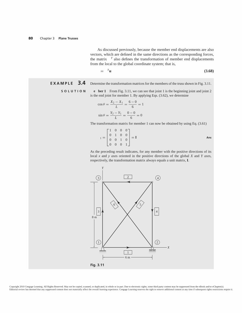
E X A M P L E 3.4 Determine the transformation matrices for the members of the truss shown in Fig. 3.11.
S O L U T I O N e ber 1 From Fig. 3.11, we can see that joint 1 is the beginning joint and joint 2is the end joint for member 1. By applying Eqs. (3.62), we determine
cos θ = X2 − X1L = 6 − 0
6 = 1
sin θ = Y2 − Y1L = 0 − 0
6 = 0
The transformation matrix for member 1 can now be obtained by using Eq. (3.61)
1 =
⎡⎢⎢⎣
1 0 0 00 1 0 00 0 1 00 0 0 1
⎤⎥⎥⎦ = I Ans
As the preceding result indicates, for any member with the positive directions of itslocal x and y axes oriented in the positive directions of the global X and Y axes,respectively, the transformation matrix always equals a unit matrix, I.
As discussed previously, because the member end displacements are alsovectors, which are defined in the same directions as the corresponding forces,the matrix T also defines the transformation of member end displacementsfrom the local to the global coordinate system; that is,
= Tu (3.68)
80 Chapter 3 Plane Trusses
Fig. 3.11
21
43
X
Y
8 m
6 m
2
3
6 5
4
1
Copyright 2010 Cengage Learning. All Rights Reserved. May not be copied, scanned, or duplicated, in whole or in part. Due to electronic rights, some third party content may be suppressed from the eBook and/or eChapter(s).Editorial review has deemed that any suppressed content does not materially affect the overall learning experience. Cengage Learning reserves the right to remove additional content at any time if subsequent rights restrictions require it.
Section 3.5 Coordinate Transformations 81
e ber 2
cos θ = X3 − X4L = 0 − 6
6 = −1
sin θ = Y3 − Y4L = 8 − 8
6 = 0
Thus, from Eq. (3.61)
2 =
⎡⎢⎢⎣
−1 0 0 00 −1 0 00 0 −1 00 0 0 −1
⎤⎥⎥⎦ Ans
e ber 3
cos θ = X3 − X1L = 0 − 0
8 = 0
sin θ = Y3 − Y1L = 8 − 0
8 = 1
Thus,
3 =
⎡⎢⎢⎣
0 1 0 0−1 0 0 0
0 0 0 10 0 −1 0
⎤⎥⎥⎦ Ans
e ber 4
cos θ = X2 − X4L = 6 − 6
8 = 0
sin θ = Y2 − Y4L = 0 − 8
8 = −1
Thus,
4 =
⎡⎢⎢⎣
0 −1 0 01 0 0 00 0 0 −10 0 1 0
⎤⎥⎥⎦ Ans
e ber 5
L =√
(X4 − X1)2 + (Y4 − Y1)2 =√
(6 − 0)2 + (8 − 0)2 = 10 m
cos θ = X4 − X1L = 6 − 0
10 = 0.6
sin θ = Y4 − Y1L = 8 − 0
10 = 0.8
5 =
⎡⎢⎢⎣
0.6 0.8 0 0−0.8 0.6 0 0
0 0 0.6 0.80 0 −0.8 0.6
⎤⎥⎥⎦ Ans
Copyright 2010 Cengage Learning. All Rights Reserved. May not be copied, scanned, or duplicated, in whole or in part. Due to electronic rights, some third party content may be suppressed from the eBook and/or eChapter(s).Editorial review has deemed that any suppressed content does not materially affect the overall learning experience. Cengage Learning reserves the right to remove additional content at any time if subsequent rights restrictions require it.
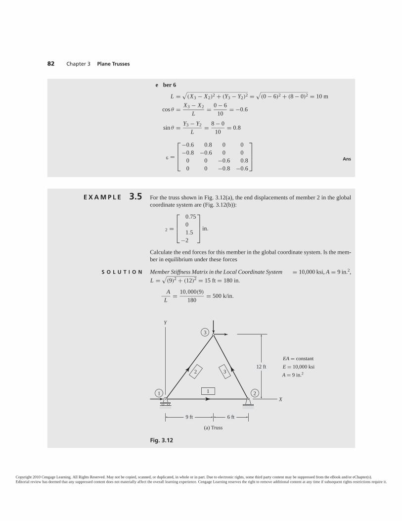
E X A M P L E 3.5 For the truss shown in Fig. 3.12(a), the end displacements of member 2 in the globalcoordinate system are (Fig. 3.12(b)):
2 =
⎡⎢⎢⎣
0.7501.5
−2
⎤⎥⎥⎦ in.
Calculate the end forces for this member in the global coordinate system. Is the mem-ber in equilibrium under these forces
S O L U T I O N Member Stiffness Matrix in the Local Coordinate System = 10,000 ksi, A = 9 in.2,L =
√(9)2 + (12)2 = 15 ft = 180 in.
AL = 10,000(9)
180 = 500 k/in.
e ber 6
L =√
(X3 − X2)2 + (Y3 − Y2)2 =√
(0 − 6)2 + (8 − 0)2 = 10 m
cos θ = X3 − X2L = 0 − 6
10 = −0.6
sin θ = Y3 − Y2L = 8 − 0
10 = 0.8
6 =
⎡⎢⎢⎣
−0.6 0.8 0 0−0.8 −0.6 0 0
0 0 −0.6 0.80 0 −0.8 −0.6
⎤⎥⎥⎦ Ans
82 Chapter 3 Plane Trusses
Fig. 3.12
21
3
X
Y
9 ft 6 ft
12 ftEA � constantE � 10,000 ksiA � 9 in.2
(a) Truss
1
2 3
Copyright 2010 Cengage Learning. All Rights Reserved. May not be copied, scanned, or duplicated, in whole or in part. Due to electronic rights, some third party content may be suppressed from the eBook and/or eChapter(s).Editorial review has deemed that any suppressed content does not materially affect the overall learning experience. Cengage Learning reserves the right to remove additional content at any time if subsequent rights restrictions require it.
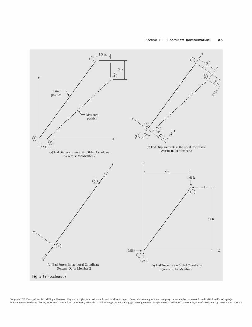
Section 3.5 Coordinate Transformations 83
Fig. 3.12 (continued)
3′
3
11′
Displacedposition
Initialposition
Y
X
0.75 in.
2 in.
1.5 in.
(b) End Displacements in the Global CoordinateSystem, v, for Member 2
3′
3
11′
y
x
0.6 in
.
2.4 in
.0.7
in.
0.45 i
n.
(c) End Displacements in the Local CoordinateSystem, u, for Member 2
3
1
y
x
575 k
575 k
(d) End Forces in the Local Coordinate System, Q, for Member 2
9 ft
12 ft
460 k
460 k
345 k
345 k
3
1
Y
X
(e) End Forces in the Global CoordinateSystem, F, for Member 2
Copyright 2010 Cengage Learning. All Rights Reserved. May not be copied, scanned, or duplicated, in whole or in part. Due to electronic rights, some third party content may be suppressed from the eBook and/or eChapter(s).Editorial review has deemed that any suppressed content does not materially affect the overall learning experience. Cengage Learning reserves the right to remove additional content at any time if subsequent rights restrictions require it.
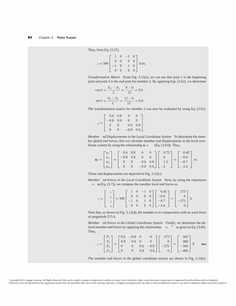
Thus, from Eq. (3.27),
2 = 500
⎡⎢⎢⎣
1 0 −1 00 0 0 0
−1 0 1 00 0 0 0
⎤⎥⎥⎦ k/in.
Transformation Matrix From Fig. 3.12(a), we can see that joint 1 is the beginningjoint and joint 3 is the end joint for member 2. By applying Eqs. (3.62), we determine
cos θ = X3 − X1L = 9 − 0
15 = 0.6
sin θ = Y3 − Y1L = 12 − 0
15 = 0.8
The transformation matrix for member 2 can now be evaluated by using Eq. (3.61):
2 =
⎡⎢⎢⎣
0.6 0.8 0 0−0.8 0.6 0 0
0 0 0.6 0.80 0 −0.8 0.6
⎤⎥⎥⎦
Member nd Displacements in the Local Coordinate System To determine the mem-ber global end forces, first we calculate member end displacements in the local coor-dinate system by using the relationship u = (Eq. (3.63)). Thus,
u2 =
⎡⎢⎢⎣
u1u2u3u4
⎤⎥⎥⎦ =
⎡⎢⎢⎣
0.6 0.8 0 0−0.8 0.6 0 0
0 0 0.6 0.80 0 −0.8 0.6
⎤⎥⎥⎦
⎡⎢⎢⎣
0.7501.5
−2
⎤⎥⎥⎦ =
⎡⎢⎢⎣
0.45−0.6−0.7−2.4
⎤⎥⎥⎦ in.
These end displacements are depicted in Fig. 3.12(c).Member nd Forces in the Local Coordinate System Next, by using the expression
= u (Eq. (3.7)), we compute the member local end forces as
2 =
⎡⎢⎢⎣
1
2
3
4
⎤⎥⎥⎦ = 500
⎡⎢⎢⎣
1 0 −1 00 0 0 0
−1 0 1 00 0 0 0
⎤⎥⎥⎦
⎡⎢⎢⎣
0.45−0.6−0.7−2.4
⎤⎥⎥⎦ =
⎡⎢⎢⎣
5750
−5750
⎤⎥⎥⎦ k
Note that, as shown in Fig. 3.12(d), the member is in compression with an axial forceof magnitude 575 k.Member nd Forces in the Global Coordinate System Finally, we determine the de-sired member end forces by applying the relationship = T as given in Eq. (3.66).Thus,
2 =
⎡⎢⎢⎣
F1F2F3F4
⎤⎥⎥⎦ =
⎡⎢⎢⎣
0.6 −0.8 0 00.8 0.6 0 00 0 0.6 −0.80 0 0.8 0.6
⎤⎥⎥⎦
⎡⎢⎢⎣
5750
−5750
⎤⎥⎥⎦ =
⎡⎢⎢⎣
345460
−345−460
⎤⎥⎥⎦ k Ans
The member end forces in the global coordinate system are shown in Fig. 3.12(e).
84 Chapter 3 Plane Trusses
Copyright 2010 Cengage Learning. All Rights Reserved. May not be copied, scanned, or duplicated, in whole or in part. Due to electronic rights, some third party content may be suppressed from the eBook and/or eChapter(s).Editorial review has deemed that any suppressed content does not materially affect the overall learning experience. Cengage Learning reserves the right to remove additional content at any time if subsequent rights restrictions require it.
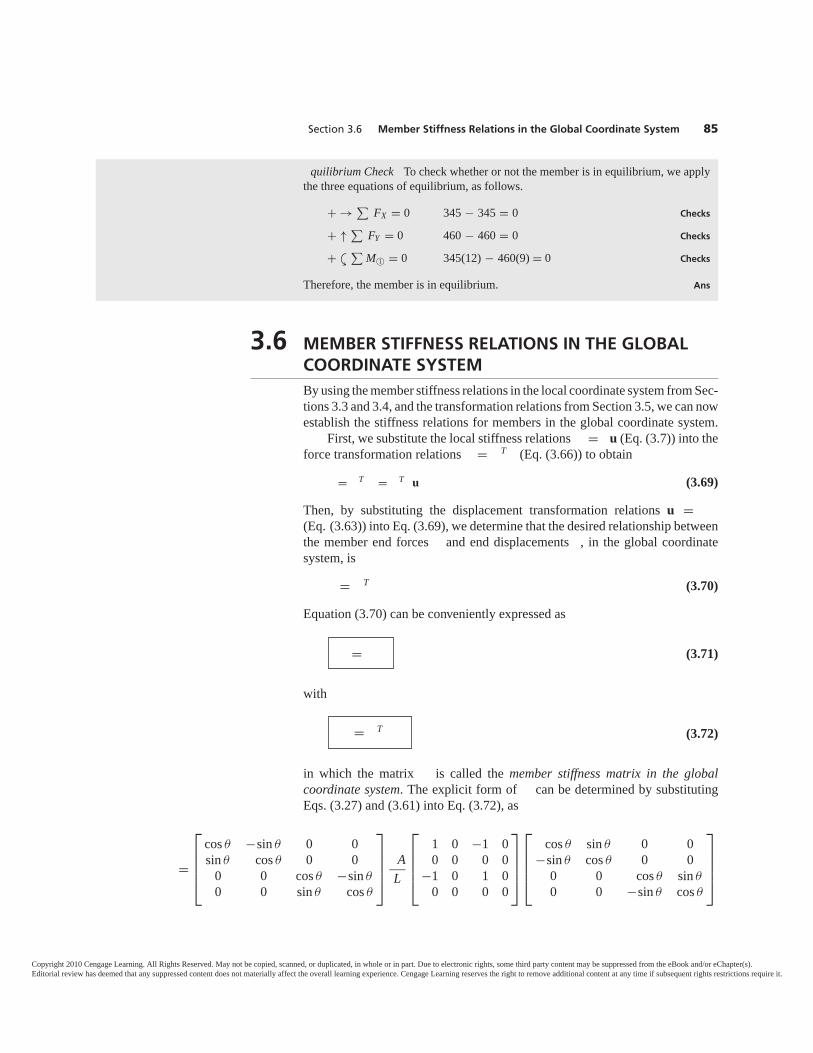
3.6 MEMBER STIFFNESS RELATIONS IN THE GLOBALCOORDINATE SYSTEMBy using the member stiffness relations in the local coordinate system from Sec-tions 3.3 and 3.4, and the transformation relations from Section 3.5, we can nowestablish the stiffness relations for members in the global coordinate system.
First, we substitute the local stiffness relations = u (Eq. (3.7)) into theforce transformation relations = T (Eq. (3.66)) to obtain
= T = T u (3.69)
Then, by substituting the displacement transformation relations u = (Eq. (3.63)) into Eq. (3.69), we determine that the desired relationship betweenthe member end forces and end displacements , in the global coordinatesystem, is
= T (3.70)
Equation (3.70) can be conveniently expressed as
(3.71)
with
(3.72)
in which the matrix is called the member stiffness matrix in the globalcoordinate system. The explicit form of can be determined by substitutingEqs. (3.27) and (3.61) into Eq. (3.72), as
=
⎡⎢⎢⎢⎣
cos θ −sin θ 0 0sin θ cos θ 0 0
0 0 cos θ −sin θ
0 0 sin θ cos θ
⎤⎥⎥⎥⎦ A
L
⎡⎢⎢⎢⎣
1 0 −1 00 0 0 0
−1 0 1 00 0 0 0
⎤⎥⎥⎥⎦
⎡⎢⎢⎢⎣
cos θ sin θ 0 0−sin θ cos θ 0 0
0 0 cos θ sin θ
0 0 −sin θ cos θ
⎤⎥⎥⎥⎦
= T
=
Section 3.6 Member Stiffness Relations in the Global Coordinate System 85
quilibrium Check To check whether or not the member is in equilibrium, we applythe three equations of equilibrium, as follows.
+ → ∑FX = 0 345 − 345 = 0 Checks
+ ↑ ∑FY = 0 460 − 460 = 0 Checks
+ ∑M©1 = 0 345(12) − 460(9) = 0 Checks
Therefore, the member is in equilibrium. Ans
Y
Copyright 2010 Cengage Learning. All Rights Reserved. May not be copied, scanned, or duplicated, in whole or in part. Due to electronic rights, some third party content may be suppressed from the eBook and/or eChapter(s).Editorial review has deemed that any suppressed content does not materially affect the overall learning experience. Cengage Learning reserves the right to remove additional content at any time if subsequent rights restrictions require it.
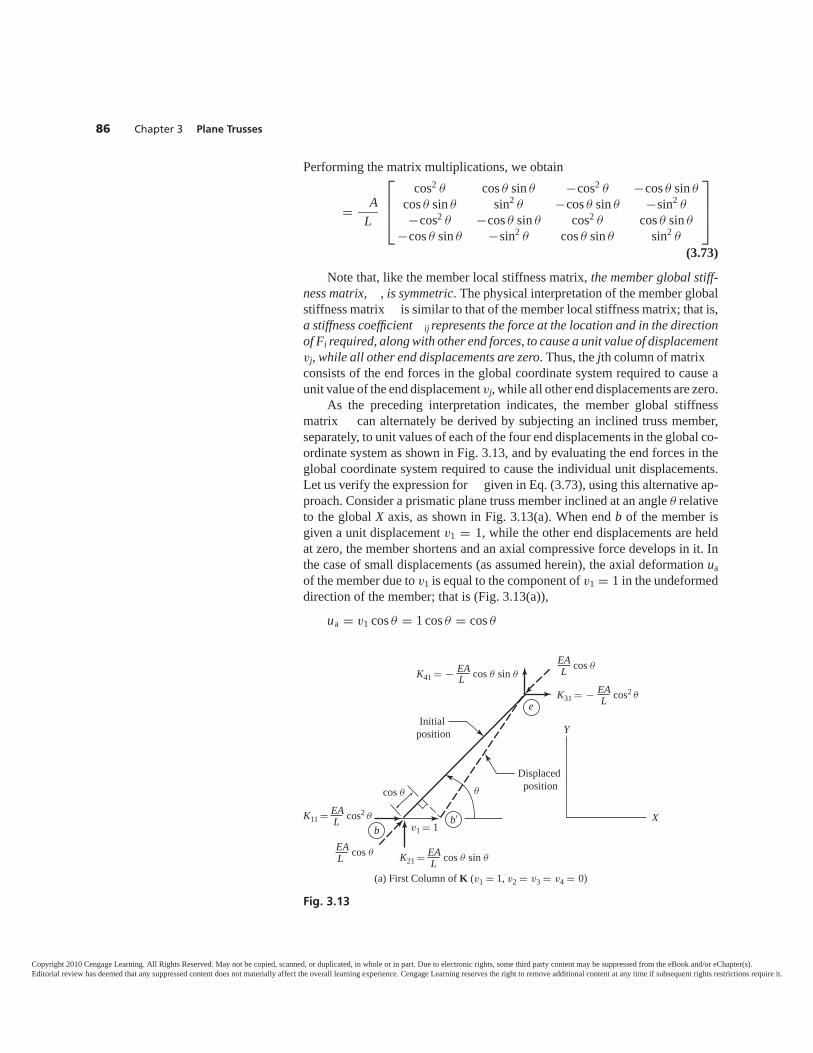
Performing the matrix multiplications, we obtain
= AL
⎡⎢⎢⎣
cos2 θ cos θ sin θ −cos2 θ −cos θ sin θ
cos θ sin θ sin2 θ −cos θ sin θ −sin2 θ
−cos2 θ −cos θ sin θ cos2 θ cos θ sin θ
−cos θ sin θ −sin2 θ cos θ sin θ sin2 θ
⎤⎥⎥⎦
(3.73)
Note that, like the member local stiffness matrix, the member global stiff-ness matrix, , is symmetric. The physical interpretation of the member globalstiffness matrix is similar to that of the member local stiffness matrix; that is,a stiffness coefficient ij represents the force at the location and in the directionof Fi required, along with other end forces, to cause a unit value of displacementvj, while all other end displacements are zero. Thus, the jth column of matrixconsists of the end forces in the global coordinate system required to cause aunit value of the end displacement vj, while all other end displacements are zero.
As the preceding interpretation indicates, the member global stiffnessmatrix can alternately be derived by subjecting an inclined truss member,separately, to unit values of each of the four end displacements in the global co-ordinate system as shown in Fig. 3.13, and by evaluating the end forces in theglobal coordinate system required to cause the individual unit displacements.Let us verify the expression for given in Eq. (3.73), using this alternative ap-proach. Consider a prismatic plane truss member inclined at an angle θ relativeto the global X axis, as shown in Fig. 3.13(a). When end b of the member isgiven a unit displacement v1 = 1, while the other end displacements are heldat zero, the member shortens and an axial compressive force develops in it. Inthe case of small displacements (as assumed herein), the axial deformation uaof the member due to v1 is equal to the component of v1 = 1 in the undeformeddirection of the member; that is (Fig. 3.13(a)),
ua = v1 cos θ = 1 cos θ = cos θ
86 Chapter 3 Plane Trusses
e
b′b
Y
X
Displacedposition
Initialposition
EA cos θK41 � − EA cos θ sin θ
cos θ
LL
L
L L
L
K21 � EA cos θ sin θ
v1 � 1
K31 � − EA cos2 θ
K11 � EA cos2 θ
EA cos θ
θ
(a) First Column of K (v1 = 1, v2 = v3 = v4 = 0)
Fig. 3.13
Copyright 2010 Cengage Learning. All Rights Reserved. May not be copied, scanned, or duplicated, in whole or in part. Due to electronic rights, some third party content may be suppressed from the eBook and/or eChapter(s).Editorial review has deemed that any suppressed content does not materially affect the overall learning experience. Cengage Learning reserves the right to remove additional content at any time if subsequent rights restrictions require it.
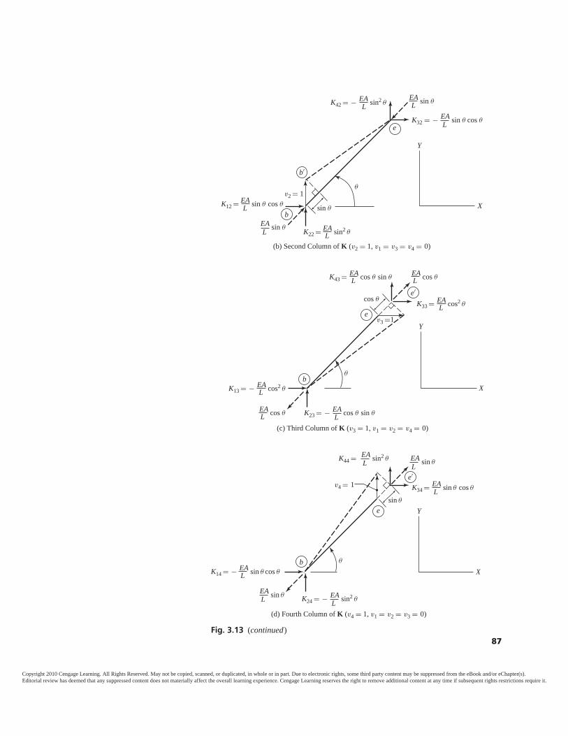
(b) Second Column of K (v2 = 1, v1 = v3 = v4 = 0)
e
b′
b
Y
X
EA sin θ
sin θK12 � EA sin θ cos θ
v2 � 1
K42 � − EA sin2 θL L
LL
L
K22 � EA sin2 θ
EA sin θ
θ
K32 = − EA sin θ cos θL
b
e
e′
Y
X
cos θK33 � EA cos2 θ
v3 �1
K23 � − EA cos θ sin θ
K13 � − EA cos2 θ
K43 � EA cos θ sin θEA cos θ
EA cos θ
θ
L
L L
L
LL
(c) Third Column of K (v3 = 1, v1 = v2 = v4 = 0)
e
e′
b
Y
X
sin θ
K34 � EA sin θ cos θv4 � 1
K44 � EA sin2 θ
K24 � − EA sin2 θ
K14 � − EA sin θ cos θ
EA sin θ
EA sin θ
L L
L
LL
L
(d) Fourth Column of K (v4 = 1, v1 = v2 = v3 = 0)
θ
Fig. 3.13 (continued)87
Copyright 2010 Cengage Learning. All Rights Reserved. May not be copied, scanned, or duplicated, in whole or in part. Due to electronic rights, some third party content may be suppressed from the eBook and/or eChapter(s).Editorial review has deemed that any suppressed content does not materially affect the overall learning experience. Cengage Learning reserves the right to remove additional content at any time if subsequent rights restrictions require it.
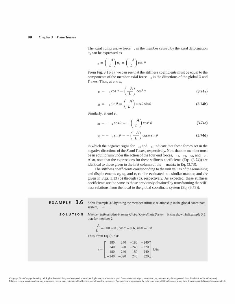
The axial compressive force a in the member caused by the axial deformationua can be expressed as
a =( A
L
)ua =
( AL
)cos θ
From Fig. 3.13(a), we can see that the stiffness coefficients must be equal to thecomponents of the member axial force a in the directions of the global X andY axes. Thus, at end b,
11 = a cos θ =( A
L
)cos2 θ (3.74a)
21 = a sin θ =( A
L
)cos θ sin θ (3.74b)
Similarly, at end e,
31 = − a cos θ = −( A
L
)cos2 θ (3.74c)
41 = − a sin θ = −( A
L
)cos θ sin θ (3.74d)
in which the negative signs for 31 and 41 indicate that these forces act in thenegative directions of the X and Y axes, respectively. Note that the member mustbe in equilibrium under the action of the four end forces, 11, 21, 31, and 41.Also, note that the expressions for these stiffness coefficients (Eqs. (3.74)) areidentical to those given in the first column of the matrix in Eq. (3.73).
The stiffness coefficients corresponding to the unit values of the remainingend displacements v2, v3, and v4 can be evaluated in a similar manner, and aregiven in Figs. 3.13 (b) through (d), respectively. As expected, these stiffnesscoefficients are the same as those previously obtained by transforming the stiff-ness relations from the local to the global coordinate system (Eq. (3.73)).
88 Chapter 3 Plane Trusses
E X A M P L E 3.6 Solve Example 3.5 by using the member stiffness relationship in the global coordinatesystem, = .
S O L U T I O N Member Stiffness Matrix in the Global Coordinate System It was shown in Example 3.5that for member 2,
AL = 500 k/in., cos θ = 0.6, sin θ = 0.8
Thus, from Eq. (3.73):
2 =
⎡⎢⎢⎣
180 240 −180 −240240 320 −240 −320
−180 −240 180 240−240 −320 240 320
⎤⎥⎥⎦ k/in.
Copyright 2010 Cengage Learning. All Rights Reserved. May not be copied, scanned, or duplicated, in whole or in part. Due to electronic rights, some third party content may be suppressed from the eBook and/or eChapter(s).Editorial review has deemed that any suppressed content does not materially affect the overall learning experience. Cengage Learning reserves the right to remove additional content at any time if subsequent rights restrictions require it.
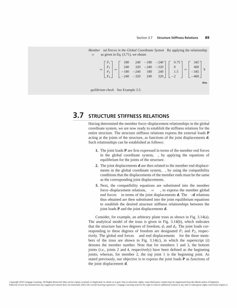
3.7 STRUCTURE STIFFNESS RELATIONSHaving determined the member force–displacement relationships in the globalcoordinate system, we are now ready to establish the stiffness relations for theentire structure. The structure stiffness relations express the external loads Pacting at the joints of the structure, as functions of the joint displacements d.Such relationships can be established as follows:
1. The joint loads P are first expressed in terms of the member end forcesin the global coordinate system, , by applying the equations ofequilibrium for the joints of the structure.
2. The joint displacements d are then related to the member end displace-ments in the global coordinate system, , by using the compatibilityconditions that the displacements of the member ends must be the sameas the corresponding joint displacements.
3. Next, the compatibility equations are substituted into the memberforce–displacement relations, = , to express the member globalend forces in terms of the joint displacements d. The –d relationsthus obtained are then substituted into the joint equilibrium equationsto establish the desired structure stiffness relationships between thejoint loads P and the joint displacements d.
Consider, for example, an arbitrary plane truss as shown in Fig. 3.14(a).The analytical model of the truss is given in Fig. 3.14(b), which indicatesthat the structure has two degrees of freedom, d1 and d2. The joint loads cor-responding to these degrees of freedom are designated P1 and P2, respec-tively. The global end forces and end displacements for the three mem-bers of the truss are shown in Fig. 3.14(c), in which the superscript (i)denotes the member number. Note that for members 1 and 3, the bottomjoints (i.e., joints 2 and 4, respectively) have been defined as the beginningjoints; whereas, for member 2, the top joint 1 is the beginning joint. Asstated previously, our objective is to express the joint loads P as functions ofthe joint displacement d.
Section 3.7 Structure Stiffness Relations 89
Member nd Forces in the Global Coordinate System By applying the relationship= as given in Eq. (3.71), we obtain
=
⎡⎢⎢⎣
F1F2F3F4
⎤⎥⎥⎦ =
⎡⎢⎢⎣
180 240 −180 −240240 320 −240 −320
−180 −240 180 240−240 −320 240 320
⎤⎥⎥⎦
⎡⎢⎢⎣
0.7501.5
−2
⎤⎥⎥⎦ =
⎡⎢⎢⎣
345460
−345−460
⎤⎥⎥⎦ k
Ans
quilibrium check See Example 3.5.
Copyright 2010 Cengage Learning. All Rights Reserved. May not be copied, scanned, or duplicated, in whole or in part. Due to electronic rights, some third party content may be suppressed from the eBook and/or eChapter(s).Editorial review has deemed that any suppressed content does not materially affect the overall learning experience. Cengage Learning reserves the right to remove additional content at any time if subsequent rights restrictions require it.
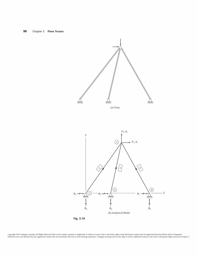
90 Chapter 3 Plane Trusses
Fig. 3.14
(a) Truss
1
32
4X
Y
R4
R5R3 R7
R6
P2, d2
P1, d1
R8
(b) Analytical Model
1 2 3
Copyright 2010 Cengage Learning. All Rights Reserved. May not be copied, scanned, or duplicated, in whole or in part. Due to electronic rights, some third party content may be suppressed from the eBook and/or eChapter(s).Editorial review has deemed that any suppressed content does not materially affect the overall learning experience. Cengage Learning reserves the right to remove additional content at any time if subsequent rights restrictions require it.
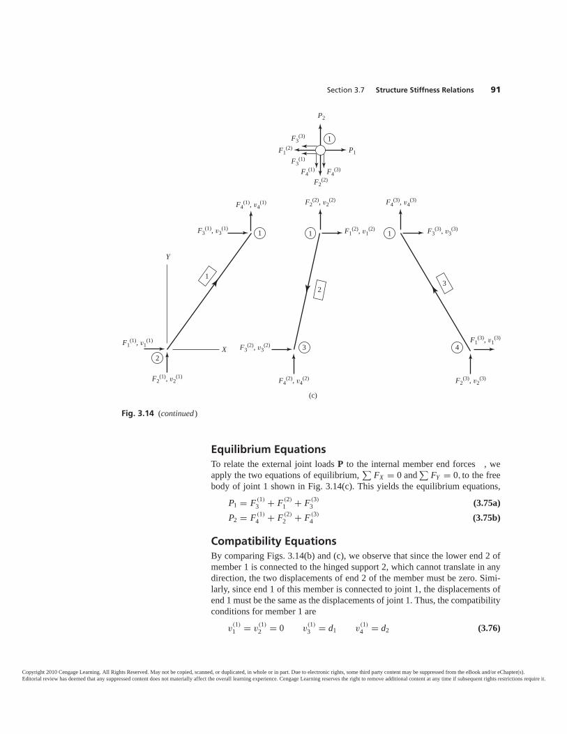
Equilibrium EquationsTo relate the external joint loads P to the internal member end forces , weapply the two equations of equilibrium,
∑FX = 0 and
∑FY = 0, to the free
body of joint 1 shown in Fig. 3.14(c). This yields the equilibrium equations,P1 = F (1)
3 + F (2)1 + F (3)
3 (3.75a)
P2 = F (1)4 + F (2)
2 + F (3)4 (3.75b)
Compatibility EquationsBy comparing Figs. 3.14(b) and (c), we observe that since the lower end 2 ofmember 1 is connected to the hinged support 2, which cannot translate in anydirection, the two displacements of end 2 of the member must be zero. Simi-larly, since end 1 of this member is connected to joint 1, the displacements ofend 1 must be the same as the displacements of joint 1. Thus, the compatibilityconditions for member 1 are
v(1)1 = v
(1)2 = 0 v
(1)3 = d1 v
(1)4 = d2 (3.76)
Section 3.7 Structure Stiffness Relations 91
23
1
4
11
Y
X
F3(1), v3
(1)
F4(1), v4
(1)
F1(1), v1
(1)
F2(1), v2
(1)
F2(2), v2
(2)
F1(2), v1
(2)
F1(3), v1
(3)
F2(3), v2
(3)
F3(3), v3
(3)
F4(3), v4
(3)
F3(2), v3
(2)
F4(2), v4
(2)
(c)
1
23
1
F4(1) F4
(3)
F3(3)
F3(1)
P1
P2
F2(2)
F1(2)
Fig. 3.14 (continued)
Copyright 2010 Cengage Learning. All Rights Reserved. May not be copied, scanned, or duplicated, in whole or in part. Due to electronic rights, some third party content may be suppressed from the eBook and/or eChapter(s).Editorial review has deemed that any suppressed content does not materially affect the overall learning experience. Cengage Learning reserves the right to remove additional content at any time if subsequent rights restrictions require it.
In a similar manner, the compatibility conditions for members 2 and 3, respec-tively, are found to be
v(2)1 = d1 v
(2)2 = d2 v
(2)3 = v
(2)4 = 0 (3.77)
v(3)1 = v
(3)2 = 0 v
(3)3 = d1 v
(3)4 = d2 (3.78)
Member Stiffness RelationsOf the two types of relationships established thus far, the equilibrium equations(Eqs. (3.75)) express joint loads in terms of member end forces, whereas thecompatibility equations (Eqs. (3.76) through (3.78)) relate joint displacementsto member end displacements. Now, we will link the two types of relationshipsby employing the member stiffness relationship in the global coordinate sys-tem derived in the preceding section.
We can write the member global stiffness relation = (Eq. (3.71)) inexpanded form for member 1 as
⎡⎢⎢⎢⎢⎢⎢⎣
F (1)1
F (1)2
F (1)3
F (1)4
⎤⎥⎥⎥⎥⎥⎥⎦
=
⎡⎢⎢⎢⎢⎢⎢⎣
(1)11
(1)12
(1)13
(1)14
(1)21
(1)22
(1)23
(1)24
(1)31
(1)32
(1)33
(1)34
(1)41
(1)42
(1)43
(1)44
⎤⎥⎥⎥⎥⎥⎥⎦
⎡⎢⎢⎢⎢⎢⎢⎣
v(1)1
v(1)2
v(1)3
v(1)4
⎤⎥⎥⎥⎥⎥⎥⎦
(3.79)
from which we obtain the expressions for forces at end 1 of the member:
F (1)3 = (1)
31 v(1)1 + (1)
32 v(1)2 + (1)
33 v(1)3 + (1)
34 v(1)4 (3.80a)
F (1)4 = (1)
41 v(1)1 + (1)
42 v(1)2 + (1)
43 v(1)3 + (1)
44 v(1)4 (3.80b)
In a similar manner, we write the stiffness relations for member 2 as⎡⎢⎢⎢⎢⎢⎢⎣
F (2)1
F (2)2
F (2)3
F (2)4
⎤⎥⎥⎥⎥⎥⎥⎦
=
⎡⎢⎢⎢⎢⎢⎢⎣
(2)11
(2)12
(2)13
(2)14
(2)21
(2)22
(2)23
(2)24
(2)31
(2)32
(2)33
(2)34
(2)41
(2)42
(2)43
(2)44
⎤⎥⎥⎥⎥⎥⎥⎦
⎡⎢⎢⎢⎢⎢⎢⎣
v(2)1
v(2)2
v(2)3
v(2)4
⎤⎥⎥⎥⎥⎥⎥⎦
(3.81)
from which we obtain the forces at end 1 of the member:
F (2)1 = (2)
11 v(2)1 + (2)
12 v(2)2 + (2)
13 v(2)3 + (2)
14 v(2)4 (3.82a)
F (2)2 = (2)
21 v(2)1 + (2)
22 v(2)2 + (2)
23 v(2)3 + (2)
24 v(2)4 (3.82b)
92 Chapter 3 Plane Trusses
Copyright 2010 Cengage Learning. All Rights Reserved. May not be copied, scanned, or duplicated, in whole or in part. Due to electronic rights, some third party content may be suppressed from the eBook and/or eChapter(s).Editorial review has deemed that any suppressed content does not materially affect the overall learning experience. Cengage Learning reserves the right to remove additional content at any time if subsequent rights restrictions require it.
Similarly, for member 3, the stiffness relations are written as⎡⎢⎢⎢⎢⎢⎢⎣
F (3)1
F (3)2
F (3)3
F (3)4
⎤⎥⎥⎥⎥⎥⎥⎦
=
⎡⎢⎢⎢⎢⎢⎢⎣
(3)11
(3)12
(3)13
(3)14
(3)21
(3)22
(3)23
(3)24
(3)31
(3)32
(3)33
(3)34
(3)41
(3)42
(3)43
(3)44
⎤⎥⎥⎥⎥⎥⎥⎦
⎡⎢⎢⎢⎢⎢⎢⎣
v(3)1
v(3)2
v(3)3
v(3)4
⎤⎥⎥⎥⎥⎥⎥⎦
(3.83)
and the forces at end 1 of the member are given by
F (3)3 = (3)
31 v(3)1 + (3)
32 v(3)2 + (3)
33 v(3)3 + (3)
34 v(3)4 (3.84a)
F (3)4 = (3)
41 v(3)1 + (3)
42 v(3)2 + (3)
43 v(3)3 + (3)
44 v(3)4 (3.84b)
Note that Eqs. (3.80), (3.82), and (3.84) express the six member end forces thatappear in the joint equilibrium equations (Eqs. (3.75)), in terms of member enddisplacements.
To relate the joint displacements d to the member end forces , wesubstitute the compatibility equations into the foregoing member force–displacement relations. Thus, by substituting the compatibility equations formember 1 (Eqs. (3.76)) into its force–displacement relations as given byEqs. (3.80), we express the member end forces (1) in terms of the joint dis-placements d as
F (1)3 = (1)
33 d1 + (1)34 d2 (3.85a)
F (1)4 = (1)
43 d1 + (1)44 d2 (3.85b)
In a similar manner, for member 2, by substituting Eqs. (3.77) into Eqs. (3.82),we obtain
F (2)1 = (2)
11 d1 + (2)12 d2 (3.86a)
F (2)2 = (2)
21 d1 + (2)22 d2 (3.86b)
Similarly, for member 3, substitution of Eqs. (3.78) into Eqs. (3.84) yields
F (3)3 = (3)
33 d1 + (3)34 d2 (3.87a)
F (3)4 = (3)
43 d1 + (3)44 d2 (3.87b)
Structure Stiffness RelationsFinally, by substituting Eqs. (3.85) through (3.87) into the joint equilibriumequations (Eqs. (3.75)), we establish the desired relationships between the jointloads P and the joint displacements d of the truss:
P1 = ((1)33 + (2)
11 + (3)33
)d1 + (
(1)34 + (2)
12 + (3)34
)d2 (3.88a)
P2 = ((1)43 + (2)
21 + (3)43
)d1 + (
(1)44 + (2)
22 + (3)44
)d2 (3.88b)
Section 3.7 Structure Stiffness Relations 93
Copyright 2010 Cengage Learning. All Rights Reserved. May not be copied, scanned, or duplicated, in whole or in part. Due to electronic rights, some third party content may be suppressed from the eBook and/or eChapter(s).Editorial review has deemed that any suppressed content does not materially affect the overall learning experience. Cengage Learning reserves the right to remove additional content at any time if subsequent rights restrictions require it.
Equations (3.88) can be conveniently expressed in condensed matrix form as
(3.89)
in which
=[
(1)33 + (2)
11 + (3)33
(1)34 + (2)
12 + (3)34
(1)43 + (2)
21 + (3)43
(1)44 + (2)
22 + (3)44
](3.90)
The matrix , which is a square matrix with the number of rows and columnsequal to the degrees of freedom (NDOF ), is called the structure stiffnessmatrix. The preceding method of determining the structure stiffness relation-ships by combining the member stiffness relations is commonly referred to asthe direct stiffness method 48 .
Like member stiffness matrices, structure stiffness matrices of linearelastic structures are always symmetric. Note that in Eq. (3.90) the two off-diagonal elements of are equal to each other, because (1)
34 = (1)43 ,
(2)12 = (2)
21 , and (3)34 = (3)
43 ; thereby making a symmetric matrix.
Physical Interpretation of Structure Stiffness MatrixThe structure stiffness matrix can be interpreted in a manner analogous to themember stiffness matrix. A structure stiffness coefficient Sij represents the forceat the location and in the direction of Pi required, along with other joint forces,to cause a unit value of the displacement dj, while all other joint displacementsare zero. Thus, the jth column of the structure stiffness matrix consists of thejoint loads required, at the locations and in the directions of all the degrees offreedom of the structure, to cause a unit value of the displacement dj while allother displacements are zero. This interpretation of the structure stiffness ma-trix indicates that such a matrix can, alternatively, be determined by subjectingthe structure, separately, to unit values of each of its joint displacements, andby evaluating the joint loads required to cause the individual displacements.
To illustrate this approach, consider again the three-member truss ofFig. 3.14. To determine its structure stiffness matrix , we subject the truss tothe joint displacements d1 = 1 (with d2 = 0), and d2 = 1 (with d1 = 0), asshown in Figs. 3.15(a) and (b), respectively. As depicted in Fig. 3.15(a), thestiffness coefficients S11 and S21 (elements of the first column of ) representthe horizontal and vertical forces at joint 1 required to cause a unit displace-ment of the joint in the horizontal direction (d1 = 1), while holding it in placevertically (d2 = 0). The unit horizontal displacement of joint 1 induces unitdisplacements, in the same direction, at the top ends of the three members con-nected to the joint. The member stiffness coefficients (or end forces) necessaryto cause these unit end displacements of the individual members are shown inFig. 3.15(a). Note that these stiffness coefficients are labeled in accordancewith the notation for member end forces adopted in Section 3.5. (Also, recall
P = d
94 Chapter 3 Plane Trusses
Copyright 2010 Cengage Learning. All Rights Reserved. May not be copied, scanned, or duplicated, in whole or in part. Due to electronic rights, some third party content may be suppressed from the eBook and/or eChapter(s).Editorial review has deemed that any suppressed content does not materially affect the overall learning experience. Cengage Learning reserves the right to remove additional content at any time if subsequent rights restrictions require it.
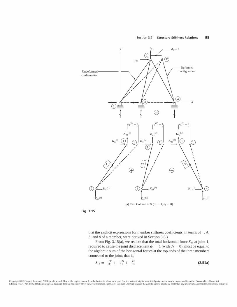
that the explicit expressions for member stiffness coefficients, in terms of , A,L, and θ of a member, were derived in Section 3.6.)
From Fig. 3.15(a), we realize that the total horizontal force S11 at joint 1,required to cause the joint displacement d1 = 1 (with d2 = 0), must be equal tothe algebraic sum of the horizontal forces at the top ends of the three membersconnected to the joint; that is,
S11 = (1)33 + (2)
11 + (3)33 (3.91a)
Section 3.7 Structure Stiffness Relations 95
1
1 1′
2 3 4
1
11′ 1′
1′
32
4X
Y S21
S11
DeformedconfigurationUndeformed
configuration
d1 � 1
v3(1) � 1
K33(1)
K13(1) K31
(2) K13(3)
K23(1) K41
(2) K23(3)
K43(1) K21
(2) K43(3)
K11(2) K33
(3)
v1(2) � 1 v3
(3) � 1
+ +
�
(a) First Column of S (d1 = 1, d2 = 0)
1 2 3
Fig. 3.15
Copyright 2010 Cengage Learning. All Rights Reserved. May not be copied, scanned, or duplicated, in whole or in part. Due to electronic rights, some third party content may be suppressed from the eBook and/or eChapter(s).Editorial review has deemed that any suppressed content does not materially affect the overall learning experience. Cengage Learning reserves the right to remove additional content at any time if subsequent rights restrictions require it.
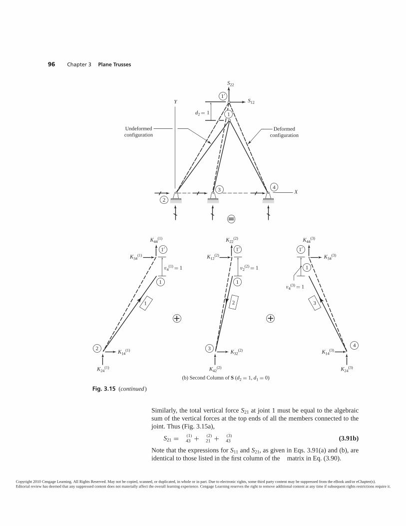
Similarly, the total vertical force S21 at joint 1 must be equal to the algebraicsum of the vertical forces at the top ends of all the members connected to thejoint. Thus (Fig. 3.15a),
S21 = (1)43 + (2)
21 + (3)43 (3.91b)
Note that the expressions for S11 and S21, as given in Eqs. 3.91(a) and (b), areidentical to those listed in the first column of the matrix in Eq. (3.90).
96 Chapter 3 Plane Trusses
1
1′
2 3 4
1
1
1′ 1′
1′
3
2
4X
Y
S22
S12
Deformedconfiguration
Undeformedconfiguration
v4(1) � 1
K34(1)
K14(1) K32
(2) K14(3)
K24(1) K42
(2) K24(3)
K44(1) K44
(3)
K12(2) K34
(3)
K22(2)
v2(2) � 1
v4(3) � 1
+
�
+
1d2 � 1
(b) Second Column of S (d2 = 1, d1 = 0)
1 2 3
Fig. 3.15 (continued)
Copyright 2010 Cengage Learning. All Rights Reserved. May not be copied, scanned, or duplicated, in whole or in part. Due to electronic rights, some third party content may be suppressed from the eBook and/or eChapter(s).Editorial review has deemed that any suppressed content does not materially affect the overall learning experience. Cengage Learning reserves the right to remove additional content at any time if subsequent rights restrictions require it.
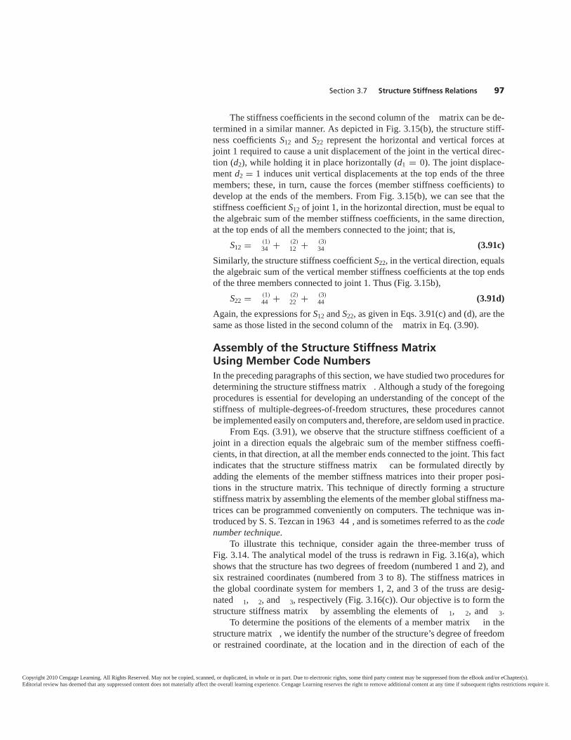
The stiffness coefficients in the second column of the matrix can be de-termined in a similar manner. As depicted in Fig. 3.15(b), the structure stiff-ness coefficients S12 and S22 represent the horizontal and vertical forces atjoint 1 required to cause a unit displacement of the joint in the vertical direc-tion (d2), while holding it in place horizontally (d1 = 0). The joint displace-ment d2 = 1 induces unit vertical displacements at the top ends of the threemembers; these, in turn, cause the forces (member stiffness coefficients) todevelop at the ends of the members. From Fig. 3.15(b), we can see that thestiffness coefficient S12 of joint 1, in the horizontal direction, must be equal tothe algebraic sum of the member stiffness coefficients, in the same direction,at the top ends of all the members connected to the joint; that is,
S12 = (1)34 + (2)
12 + (3)34 (3.91c)
Similarly, the structure stiffness coefficient S22, in the vertical direction, equalsthe algebraic sum of the vertical member stiffness coefficients at the top endsof the three members connected to joint 1. Thus (Fig. 3.15b),
S22 = (1)44 + (2)
22 + (3)44 (3.91d)
Again, the expressions for S12 and S22, as given in Eqs. 3.91(c) and (d), are thesame as those listed in the second column of the matrix in Eq. (3.90).
Assembly of the Structure Stiffness Matrix Using Member Code NumbersIn the preceding paragraphs of this section, we have studied two procedures fordetermining the structure stiffness matrix . Although a study of the foregoingprocedures is essential for developing an understanding of the concept of thestiffness of multiple-degrees-of-freedom structures, these procedures cannotbe implemented easily on computers and, therefore, are seldom used in practice.
From Eqs. (3.91), we observe that the structure stiffness coefficient of ajoint in a direction equals the algebraic sum of the member stiffness coeffi-cients, in that direction, at all the member ends connected to the joint. This factindicates that the structure stiffness matrix can be formulated directly byadding the elements of the member stiffness matrices into their proper posi-tions in the structure matrix. This technique of directly forming a structurestiffness matrix by assembling the elements of the member global stiffness ma-trices can be programmed conveniently on computers. The technique was in-troduced by S. S. Tezcan in 1963 44 , and is sometimes referred to as the codenumber technique.
To illustrate this technique, consider again the three-member truss ofFig. 3.14. The analytical model of the truss is redrawn in Fig. 3.16(a), whichshows that the structure has two degrees of freedom (numbered 1 and 2), andsix restrained coordinates (numbered from 3 to 8). The stiffness matrices inthe global coordinate system for members 1, 2, and 3 of the truss are desig-nated 1, 2, and 3, respectively (Fig. 3.16(c)). Our objective is to form thestructure stiffness matrix by assembling the elements of 1, 2, and 3.
To determine the positions of the elements of a member matrix in thestructure matrix , we identify the number of the structure’s degree of freedomor restrained coordinate, at the location and in the direction of each of the
Section 3.7 Structure Stiffness Relations 97
Copyright 2010 Cengage Learning. All Rights Reserved. May not be copied, scanned, or duplicated, in whole or in part. Due to electronic rights, some third party content may be suppressed from the eBook and/or eChapter(s).Editorial review has deemed that any suppressed content does not materially affect the overall learning experience. Cengage Learning reserves the right to remove additional content at any time if subsequent rights restrictions require it.

98 Chapter 3 Plane Trusses
1
32 4X
Y
R4
R5R3 R7
R6
P2, d2
P1, d1
R8
Two degrees of freedom (1 and 2);six restrained coordinates (3 through 8)
(a) Analytical Model
1 2 3
2
3
1
4
11
Y
X
F3(1), v3
(1)
F4(1), v4
(1)
F1(1), v1
(1)
F2(1), v2
(1)
F2(2), v2
(2)
F1(2), v1
(2)
F1(3), v1
(3)
F2(3), v2
(3)
F3(3), v3
(3)
F4(3), v4
(3)
F3(2), v3
(2)
F4(2), v4
(2)
(b) Member End Forces and End Displacements in the Global Coordinate System
1 2 3
Fig. 3.16
Copyright 2010 Cengage Learning. All Rights Reserved. May not be copied, scanned, or duplicated, in whole or in part. Due to electronic rights, some third party content may be suppressed from the eBook and/or eChapter(s).Editorial review has deemed that any suppressed content does not materially affect the overall learning experience. Cengage Learning reserves the right to remove additional content at any time if subsequent rights restrictions require it.
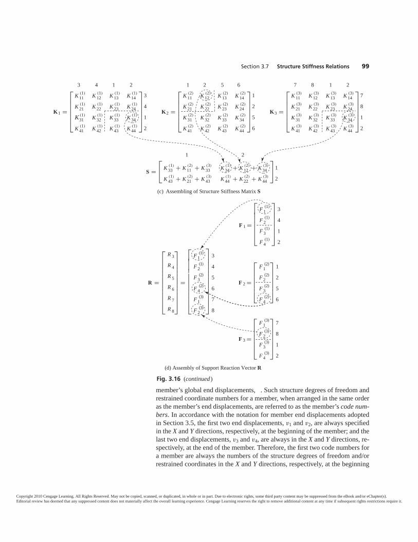
member’s global end displacements, . Such structure degrees of freedom andrestrained coordinate numbers for a member, when arranged in the same orderas the member’s end displacements, are referred to as the member’s code num-bers. In accordance with the notation for member end displacements adoptedin Section 3.5, the first two end displacements, v1 and v2, are always specifiedin the X and Y directions, respectively, at the beginning of the member; and thelast two end displacements, v3 and v4, are always in the X and Y directions, re-spectively, at the end of the member. Therefore, the first two code numbers fora member are always the numbers of the structure degrees of freedom and/orrestrained coordinates in the X and Y directions, respectively, at the beginning
Section 3.7 Structure Stiffness Relations 99
3 4 1 2 1 2 5 6 7 8 1 2
K1 =
⎡⎢⎢⎢⎢⎢⎣
K (1)11 K (1)
12 K (1)13 K (1)
14
K (1)21 K (1)
22 K (1)23 K (1)
24
K (1)31 K (1)
32 K (1)33 K (1)
34
K (1)41 K (1)
42 K (1)43 K (1)
44
⎤⎥⎥⎥⎥⎥⎦
3
4
1
2
K2 =
⎡⎢⎢⎢⎢⎢⎣
K (2)11 K (2)
12 K (2)13 K (2)
14
K (2)21 K (2)
22 K (2)23 K (2)
24
K (2)31 K (2)
32 K (2)33 K (2)
34
K (2)41 K (2)
42 K (2)43 K (2)
44
⎤⎥⎥⎥⎥⎥⎦
1
2
5
6
K3 =
⎡⎢⎢⎢⎢⎢⎣
K (3)11 K (3)
12 K (3)13 K (3)
14
K (3)21 K (3)
22 K (3)23 K (3)
24
K (3)31 K (3)
32 K (3)33 K (3)
34
K (3)41 K (3)
42 K (3)43 K (3)
44
⎤⎥⎥⎥⎥⎥⎦
7
8
1
2
1 2
S =⎡⎣ K (1)
33 + K (2)
11 + K (3)
33 K (1)
34 + K (2)
12 + K (3)
34
K (1)
43 + K (2)
21 + K (3)
43 K (1)
44 + K (2)
22 + K (3)
44
⎤⎦1
2
(c) Assembling of Structure Stiffness Matrix S
F 1 =
⎡⎢⎢⎢⎢⎢⎢⎣
F (1)1
F (1)2
F (1)3
F (1)4
⎤⎥⎥⎥⎥⎥⎥⎦
3
4
1
2
R =
⎡⎢⎢⎢⎢⎢⎢⎢⎢⎢⎢⎢⎣
R 3
R 4
R 5
R 6
R 7
R 8
⎤⎥⎥⎥⎥⎥⎥⎥⎥⎥⎥⎥⎦
=
⎡⎢⎢⎢⎢⎢⎢⎢⎢⎢⎢⎢⎢⎣
F (1)1
F (1)2
F (
(
2)3
F 2)4
F (3)1
F (3)2
⎤⎥⎥⎥⎥⎥⎥⎥⎥⎥⎥⎥⎥⎦
3
4
5
6
7
8
F 2 =
⎡⎢⎢⎢⎢⎢⎣
F (2)1
F (2)2
F (2)3
F (2)4
⎤⎥⎥⎥⎥⎥⎦
1
2
5
6
F 3 =
⎡⎢⎢⎢⎢⎢⎣
F (3)1
F (3)2
F (3)3
F (3)4
⎤⎥⎥⎥⎥⎥⎦
7
8
1
2
(d) Assembly of Support Reaction Vector R
Fig. 3.16 (continued)
Copyright 2010 Cengage Learning. All Rights Reserved. May not be copied, scanned, or duplicated, in whole or in part. Due to electronic rights, some third party content may be suppressed from the eBook and/or eChapter(s).Editorial review has deemed that any suppressed content does not materially affect the overall learning experience. Cengage Learning reserves the right to remove additional content at any time if subsequent rights restrictions require it.

joint for the member; and the third and fourth member code numbers are al-ways the numbers of the structure degrees of freedom and/or restrained coor-dinates in the X and Y directions, respectively, at the end joint for the member.
From Fig. 3.16(a), we can see that for member 1 of the truss, the beginningand the end joints are 2 and 1, respectively. At the beginning joint 2, the re-strained coordinate numbers are 3 and 4 in the X and Y directions, respectively;whereas, at the end joint 1, the structure degree of freedom numbers, in the Xand Y directions, are 1 and 2, respectively. Thus, the code numbers for member 1are 3, 4, 1, 2. Similarly, since the beginning and end joints for member 2 are1 and 3, respectively, the code numbers for this member are 1, 2, 5, 6. In a sim-ilar manner, the code numbers for member 3 are found to be 7, 8, 1, 2. The codenumbers for the three members of the truss can be verified by comparing themember global end displacements shown in Fig. 3.16(b) with the structuredegrees of freedom and restrained coordinates given in Fig. 3.16(a).
The code numbers for a member define the compatibility equations for themember. For example, the code numbers 3, 4, 1, 2 imply the following com-patibility equations for member 1:
v(1)1 = d3 v
(1)2 = d4 v
(1)3 = d1 v
(1)4 = d2
Since the displacements corresponding to the restrained coordinates 3 and 4are zero (i.e., d3 = d4 = 0), the compatibility equations for member 1 become
v(1)1 = v
(1)2 = 0 v
(1)3 = d1 v
(1)4 = d2
which are identical to those given in Eqs. (3.76).The member code numbers can also be used to formulate the joint equi-
librium equations for a structure (such as those given in Eqs. (3.75)). The equi-librium equation corresponding to an ith degree of freedom (or restrainedcoordinate) can be obtained by equating the joint load Pi (or the reaction Ri) tothe algebraic sum of the member end forces, with the code number i, of all themembers of the structure. For example, to obtain the equilibrium equations forthe truss of Fig. 3.16(a), we write the code numbers for its three members bythe side of their respective end force vectors, as
1 =
⎡⎢⎢⎢⎢⎣
F (1)1
F (1)2
F (1)3
F (1)4
⎤⎥⎥⎥⎥⎦
3412
2 =
⎡⎢⎢⎢⎢⎣
F (2)1
F (2)2
F (2)3
F (2)4
⎤⎥⎥⎥⎥⎦
1256
3 =
⎡⎢⎢⎢⎢⎣
F (3)1
F (3)2
F (3)3
F (3)4
⎤⎥⎥⎥⎥⎦
7812
(3.92)
From Eq. (3.92), we can see that the member end forces with the code number 1 are: F (1)
3 of member 1, F (2)1 of member 2, and F (3)
3 of member 3. Thus, the equi-librium equation corresponding to degree of freedom 1 is given by
P1 = F (1)3 + F (2)
1 + F (3)3
which is identical to Eq. 3.75(a). Similarly, the equilibrium equation corre-sponding to degree of freedom 2 can be obtained by equating P2 to the sum ofthe end forces, with code number 2, of the three members. Thus, from Eq. (3.92)
P2 = F (1)4 + F (2)
2 + F (3)4
which is the same as Eq. (3.75(b)).
100 Chapter 3 Plane Trusses
Copyright 2010 Cengage Learning. All Rights Reserved. May not be copied, scanned, or duplicated, in whole or in part. Due to electronic rights, some third party content may be suppressed from the eBook and/or eChapter(s).Editorial review has deemed that any suppressed content does not materially affect the overall learning experience. Cengage Learning reserves the right to remove additional content at any time if subsequent rights restrictions require it.

To establish the structure stiffness matrix , we write the code numbers ofeach member on the right side and at the top of its stiffness matrix , as shownin Fig. 3.16(c). These code numbers now define the positions of the elementsof the member stiffness matrices in the structure stiffness matrix . In otherwords, the code numbers on the right side of a matrix represent the row num-bers of the matrix, and the code numbers at the top represent the columnnumbers of . Furthermore, since the number of rows and columns of equalthe number of degrees of freedom (NDOF ) of the structure, only those ele-ments of a matrix with both row and column code numbers less than or equalto NDOF belong in . For example, since the truss of Fig. 3.16(a) has two de-grees of freedom, only the bottom-right quarters of the member matrices 1and 3, and the top-left quarter of 2, belong in (see Fig. 3.16(c)).
The structure stiffness matrix is established by algebraically adding thepertinent elements of the matrices of all the members, in their proper posi-tions, in the matrix. For example, to assemble for the truss of Fig. 3.16(a),we start by storing the pertinent elements of 1 in (see Fig. 3.16(c)). Thus,the element (1)
33 is stored in row 1 and column 1 of , the element (1)43 is
stored in row 2 and column 1 of , the element (1)34 is stored in row 1 and col-
umn 2 of (see Fig. 3.16(c)), and the element (1)44 is stored in row 2 and
column 2 of . Note that only those elements of 1 whose row and columncode numbers are either 1 or 2 are stored in . The same procedure is then re-peated for members 2 and 3. When two or more member stiffness coefficientsare stored in the same position in , then the coefficients must be algebraicallyadded. The completed structure stiffness matrix for the truss is shown in Fig. 3.16(c). Note that this matrix is identical to the one determined previouslyby substituting the member compatibility equations and stiffness relations intothe joint equilibrium equations (Eq. (3.90)).
Once has been determined, the structure stiffness relations, P = d(Eq. (3.89)), which now represent a system of simultaneous linear algebraicequations, can be solved for the unknown joint displacements d. With dknown, the end displacements for each member can be obtained by applyingthe compatibility equations defined by its code numbers; then the correspond-ing end displacements u and end forces and can be computed by using themember’s transformation and stiffness relations. Finally, the support reactions
can be determined from the member end forces , by considering the equi-librium of the support joints in the directions of the restrained coordinates, asdiscussed in the following paragraphs.
Assembly of the Support Reaction VectorUsing Member Code NumbersThe support reactions of a structure can be expressed in terms of the mem-ber global end forces , using the equilibrium requirement that the reaction ina direction at a joint must be equal to the algebraic sum of all the forces, in thatdirection, at all the member ends connected to the joint. Because the code num-bers of a member specify the locations and directions of its global end forceswith respect to the structure’s degrees of freedom and/or restrained coordi-nates, the reaction corresponding to a restrained coordinate can be evaluated by
Section 3.7 Structure Stiffness Relations 101
Copyright 2010 Cengage Learning. All Rights Reserved. May not be copied, scanned, or duplicated, in whole or in part. Due to electronic rights, some third party content may be suppressed from the eBook and/or eChapter(s).Editorial review has deemed that any suppressed content does not materially affect the overall learning experience. Cengage Learning reserves the right to remove additional content at any time if subsequent rights restrictions require it.
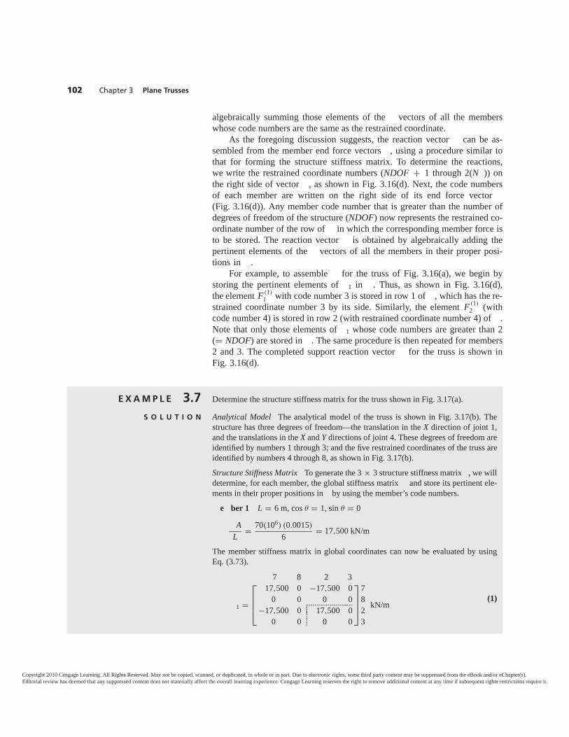
algebraically summing those elements of the vectors of all the memberswhose code numbers are the same as the restrained coordinate.
As the foregoing discussion suggests, the reaction vector can be as-sembled from the member end force vectors , using a procedure similar tothat for forming the structure stiffness matrix. To determine the reactions,we write the restrained coordinate numbers (NDOF + 1 through 2(N )) onthe right side of vector , as shown in Fig. 3.16(d). Next, the code numbersof each member are written on the right side of its end force vector (Fig. 3.16(d)). Any member code number that is greater than the number ofdegrees of freedom of the structure (NDOF) now represents the restrained co-ordinate number of the row of in which the corresponding member force isto be stored. The reaction vector is obtained by algebraically adding thepertinent elements of the vectors of all the members in their proper posi-tions in .
For example, to assemble for the truss of Fig. 3.16(a), we begin bystoring the pertinent elements of 1 in . Thus, as shown in Fig. 3.16(d),the element F (1)
1 with code number 3 is stored in row 1 of , which has the re-strained coordinate number 3 by its side. Similarly, the element F (1)
2 (withcode number 4) is stored in row 2 (with restrained coordinate number 4) of .Note that only those elements of 1 whose code numbers are greater than 2(= NDOF) are stored in . The same procedure is then repeated for members2 and 3. The completed support reaction vector for the truss is shown inFig. 3.16(d).
102 Chapter 3 Plane Trusses
E X A M P L E 3.7 Determine the structure stiffness matrix for the truss shown in Fig. 3.17(a).
S O L U T I O N Analytical Model The analytical model of the truss is shown in Fig. 3.17(b). Thestructure has three degrees of freedom—the translation in the X direction of joint 1,and the translations in the X and Y directions of joint 4. These degrees of freedom areidentified by numbers 1 through 3; and the five restrained coordinates of the truss areidentified by numbers 4 through 8, as shown in Fig. 3.17(b).Structure Stiffness Matrix To generate the 3 × 3 structure stiffness matrix , we willdetermine, for each member, the global stiffness matrix and store its pertinent ele-ments in their proper positions in by using the member’s code numbers.
e ber 1 L = 6 m, cos θ = 1, sin θ = 0A
L = 70(106) (0.0015)
6 = 17,500 kN/m
The member stiffness matrix in global coordinates can now be evaluated by usingEq. (3.73).
7 8 2 3
1 =
⎡⎢⎢⎣
17,500 0 −17,500 00 0 0 0
−17,500 0 17,500 00 0 0 0
⎤⎥⎥⎦
7823
kN/m����
������(1)
Copyright 2010 Cengage Learning. All Rights Reserved. May not be copied, scanned, or duplicated, in whole or in part. Due to electronic rights, some third party content may be suppressed from the eBook and/or eChapter(s).Editorial review has deemed that any suppressed content does not materially affect the overall learning experience. Cengage Learning reserves the right to remove additional content at any time if subsequent rights restrictions require it.
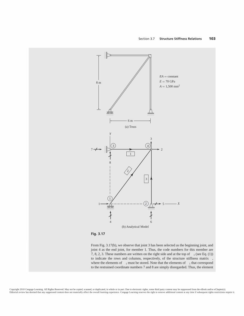
Section 3.7 Structure Stiffness Relations 103
Fig. 3.17
6 m
8 m
EA � constantE � 70 GPaA � 1,500 mm2
(a) Truss
1
43
21
7
8
2
5
6
3
4
X
Y
(b) Analytical Model
1
3
2
From Fig. 3.17(b), we observe that joint 3 has been selected as the beginning joint, andjoint 4 as the end joint, for member 1. Thus, the code numbers for this member are7, 8, 2, 3. These numbers are written on the right side and at the top of 1 (see Eq. (1))to indicate the rows and columns, respectively, of the structure stiffness matrix ,where the elements of 1 must be stored. Note that the elements of 1 that correspondto the restrained coordinate numbers 7 and 8 are simply disregarded. Thus, the element
Copyright 2010 Cengage Learning. All Rights Reserved. May not be copied, scanned, or duplicated, in whole or in part. Due to electronic rights, some third party content may be suppressed from the eBook and/or eChapter(s).Editorial review has deemed that any suppressed content does not materially affect the overall learning experience. Cengage Learning reserves the right to remove additional content at any time if subsequent rights restrictions require it.
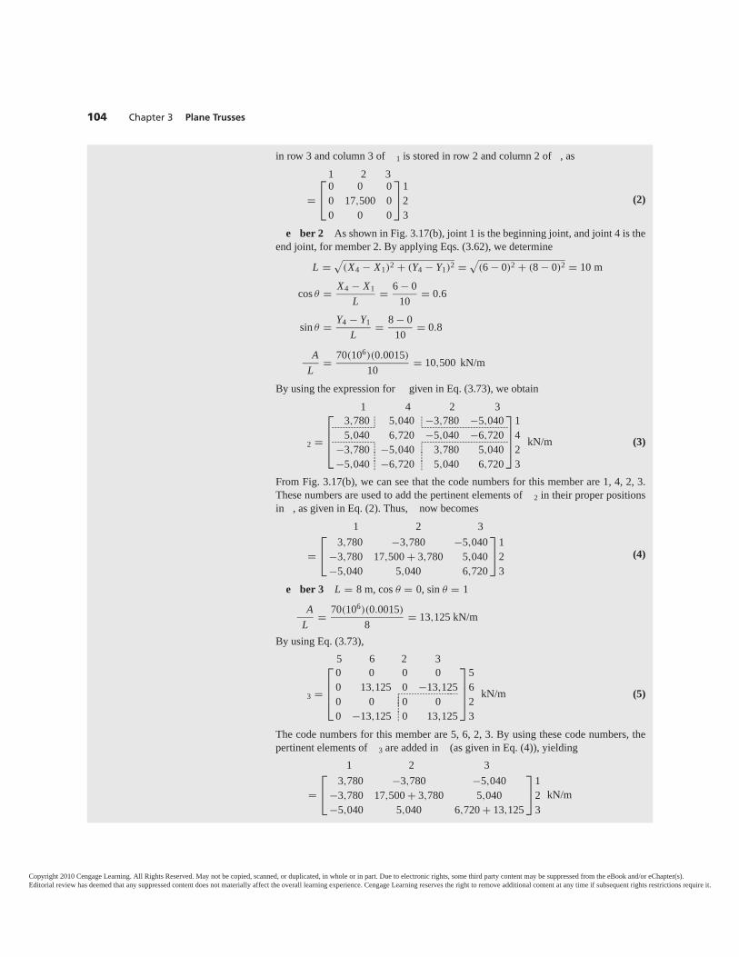
104 Chapter 3 Plane Trusses
in row 3 and column 3 of 1 is stored in row 2 and column 2 of , as1 2 3
=⎡⎣ 0 0 0
0 17,500 00 0 0
⎤⎦1
23
(2)
e ber 2 As shown in Fig. 3.17(b), joint 1 is the beginning joint, and joint 4 is theend joint, for member 2. By applying Eqs. (3.62), we determine
L =√
(X4 − X1)2 + (Y4 − Y1)2 =√
(6 − 0)2 + (8 − 0)2 = 10 m
cos θ = X4 − X1L = 6 − 0
10 = 0.6
sin θ = Y4 − Y1L = 8 − 0
10 = 0.8
AL = 70(106)(0.0015)
10 = 10,500 kN/m
By using the expression for given in Eq. (3.73), we obtain1 4 2 3
2 =
⎡⎢⎢⎣
3,780 5,040 −3,780 −5,0405,040 6,720 −5,040 −6,720
−3,780 −5,040 3,780 5,040−5,040 −6,720 5,040 6,720
⎤⎥⎥⎦
1423
kN/m���� ��������
���� ��������
� �
� �� �� �
(3)
From Fig. 3.17(b), we can see that the code numbers for this member are 1, 4, 2, 3.These numbers are used to add the pertinent elements of 2 in their proper positionsin , as given in Eq. (2). Thus, now becomes
1 2 3
=⎡⎣ 3,780 −3,780 −5,040
−3,780 17,500 + 3,780 5,040−5,040 5,040 6,720
⎤⎦1
23
(4)
e ber 3 L = 8 m, cos θ = 0, sin θ = 1A
L = 70(106)(0.0015)
8 = 13,125 kN/m
By using Eq. (3.73),5 6 2 3
3 =
⎡⎢⎢⎣
0 0 0 00 13,125 0 −13,1250 0 0 00 −13,125 0 13,125
⎤⎥⎥⎦
5623
kN/m����
������ (5)
The code numbers for this member are 5, 6, 2, 3. By using these code numbers, thepertinent elements of 3 are added in (as given in Eq. (4)), yielding
1 2 3
=⎡⎣ 3,780 −3,780 −5,040
−3,780 17,500 + 3,780 5,040−5,040 5,040 6,720 + 13,125
⎤⎦1
23
kN/m
Copyright 2010 Cengage Learning. All Rights Reserved. May not be copied, scanned, or duplicated, in whole or in part. Due to electronic rights, some third party content may be suppressed from the eBook and/or eChapter(s).Editorial review has deemed that any suppressed content does not materially affect the overall learning experience. Cengage Learning reserves the right to remove additional content at any time if subsequent rights restrictions require it.
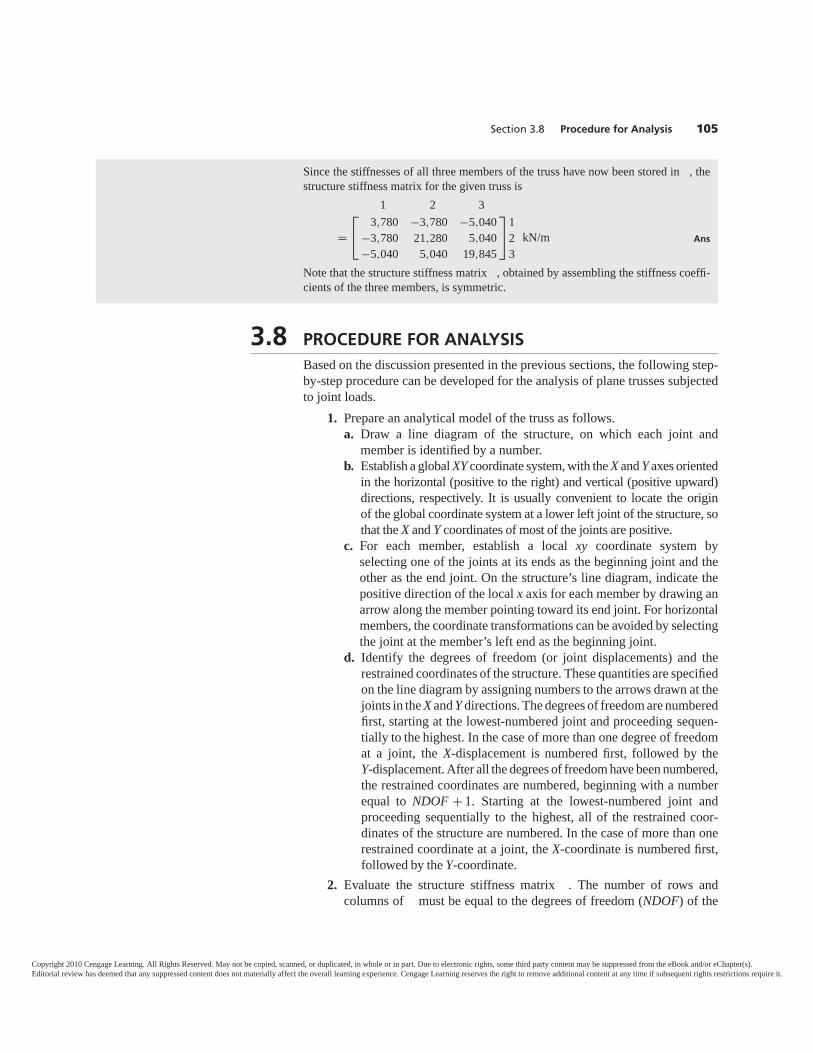
3.8 PROCEDURE FOR ANALYSISBased on the discussion presented in the previous sections, the following step-by-step procedure can be developed for the analysis of plane trusses subjectedto joint loads.
1. Prepare an analytical model of the truss as follows.a. Draw a line diagram of the structure, on which each joint and
member is identified by a number.b. Establish a global XY coordinate system, with the X and Y axes oriented
in the horizontal (positive to the right) and vertical (positive upward)directions, respectively. It is usually convenient to locate the originof the global coordinate system at a lower left joint of the structure, sothat the X and Y coordinates of most of the joints are positive.
c. For each member, establish a local xy coordinate system byselecting one of the joints at its ends as the beginning joint and theother as the end joint. On the structure’s line diagram, indicate thepositive direction of the local x axis for each member by drawing anarrow along the member pointing toward its end joint. For horizontalmembers, the coordinate transformations can be avoided by selectingthe joint at the member’s left end as the beginning joint.
d. Identify the degrees of freedom (or joint displacements) and therestrained coordinates of the structure. These quantities are specifiedon the line diagram by assigning numbers to the arrows drawn at thejoints in the X and Y directions. The degrees of freedom are numberedfirst, starting at the lowest-numbered joint and proceeding sequen-tially to the highest. In the case of more than one degree of freedomat a joint, the X-displacement is numbered first, followed by theY-displacement. After all the degrees of freedom have been numbered,the restrained coordinates are numbered, beginning with a numberequal to NDOF + 1. Starting at the lowest-numbered joint andproceeding sequentially to the highest, all of the restrained coor-dinates of the structure are numbered. In the case of more than onerestrained coordinate at a joint, the X-coordinate is numbered first,followed by the Y-coordinate.
2. Evaluate the structure stiffness matrix . The number of rows andcolumns of must be equal to the degrees of freedom (NDOF) of the
Section 3.8 Procedure for Analysis 105
Since the stiffnesses of all three members of the truss have now been stored in , thestructure stiffness matrix for the given truss is
1 2 3
=⎡⎣ 3,780 −3,780 −5,040
−3,780 21,280 5,040−5,040 5,040 19,845
⎤⎦1
23
kN/m Ans
Note that the structure stiffness matrix , obtained by assembling the stiffness coeffi-cients of the three members, is symmetric.
Copyright 2010 Cengage Learning. All Rights Reserved. May not be copied, scanned, or duplicated, in whole or in part. Due to electronic rights, some third party content may be suppressed from the eBook and/or eChapter(s).Editorial review has deemed that any suppressed content does not materially affect the overall learning experience. Cengage Learning reserves the right to remove additional content at any time if subsequent rights restrictions require it.

structure. For each member of the truss, perform the followingoperations.a. Calculate its length and direction cosines. (The expressions for cos θ
and sin θ are given in Eqs. (3.62).)b. Compute the member stiffness matrix in the global coordinate
system, , using Eq. (3.73).c. Identify its code numbers, and store the pertinent elements of
in their proper positions in , using the procedure described inSection 3.7.
The complete structure stiffness matrix, obtained by assembling thestiffness coefficients of all the members of the truss, must be asymmetric matrix.
3. Form the NDOF × 1 joint load vector P.4. Determine the joint displacements d. Substitute P and into the struc-
ture stiffness relations, P = d (Eq. (3.89)), and solve the resulting sys-tem of simultaneous equations for the unknown joint displacements d.To check that the solution of simultaneous equations has been carriedout correctly, substitute the numerical values of d back into the structurestiffness relations, P = d. If the solution is correct, then the stiffnessrelations should be satisfied. Note that joint displacements are consid-ered positive when in the positive directions of the global X and Y axes;similarly, the displacements are negative in the negative directions.
5. Compute member end displacements and end forces, and support reac-tions. For each member of the truss, do the following.a. Obtain member end displacements in the global coordinate system, ,
from the joint displacements, d, using the member’s code numbers.b. Calculate the member’s transformation matrix by using Eq.
(3.61), and determine member end displacements in the localcoordinate system, u, using the transformation relationship u =(Eq. (3.63)). For horizontal members with local x axis positive to theright (i.e., in the same direction as the global X axis), member enddisplacements in the global and local coordinate systems are thesame; that is, u = . Member axial deformation, ua, if desired, canbe obtained from the relationship ua = u1 − u3, in which u1 and u3are the first and third elements, respectively, of vector u. A positivevalue of ua indicates shortening (or contraction) of the member inthe axial direction, and a negative value indicates elongation.
c. Determine the member stiffness matrix in the local coordinate sys-tem, , using Eq. (3.27); then calculate member end forces in thelocal coordinate system by using the stiffness relationship = u(Eq. (3.7)). The member axial force, a, equals the first element, 1,of the vector (i.e., a = 1); a positive value of a indicates thatthe axial force is compressive, and a negative value indicates that theaxial force is tensile.
d. Compute member end forces in the global coordinate system, , byusing the transformation relationship = T (Eq. (3.66)). For hori-zontal members with the local x axis positive to the right, the member
106 Chapter 3 Plane Trusses
Copyright 2010 Cengage Learning. All Rights Reserved. May not be copied, scanned, or duplicated, in whole or in part. Due to electronic rights, some third party content may be suppressed from the eBook and/or eChapter(s).Editorial review has deemed that any suppressed content does not materially affect the overall learning experience. Cengage Learning reserves the right to remove additional content at any time if subsequent rights restrictions require it.
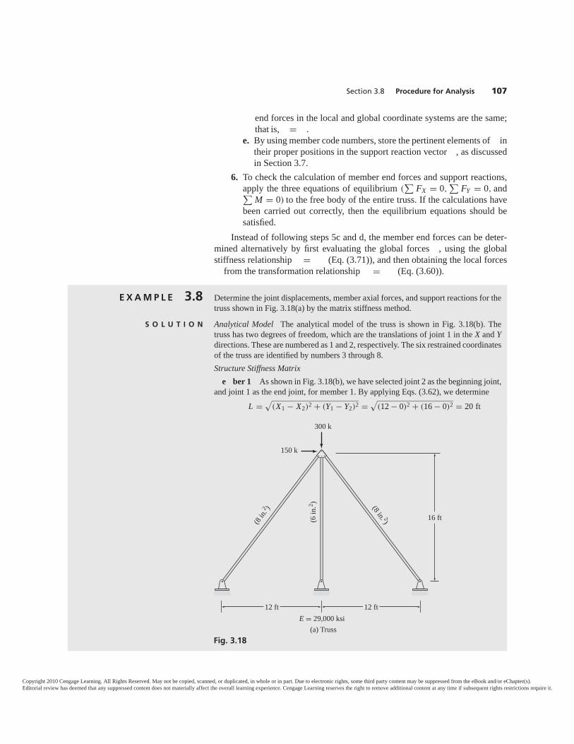
end forces in the local and global coordinate systems are the same;that is, = .
e. By using member code numbers, store the pertinent elements of intheir proper positions in the support reaction vector , as discussedin Section 3.7.
6. To check the calculation of member end forces and support reactions,apply the three equations of equilibrium (
∑FX = 0,
∑FY = 0, and∑
M = 0) to the free body of the entire truss. If the calculations havebeen carried out correctly, then the equilibrium equations should besatisfied.
Instead of following steps 5c and d, the member end forces can be deter-mined alternatively by first evaluating the global forces , using the globalstiffness relationship = (Eq. (3.71)), and then obtaining the local forces
from the transformation relationship = (Eq. (3.60)).
Section 3.8 Procedure for Analysis 107
Fig. 3.18
E X A M P L E 3.8 Determine the joint displacements, member axial forces, and support reactions for thetruss shown in Fig. 3.18(a) by the matrix stiffness method.
S O L U T I O N Analytical Model The analytical model of the truss is shown in Fig. 3.18(b). Thetruss has two degrees of freedom, which are the translations of joint 1 in the X and Ydirections. These are numbered as 1 and 2, respectively. The six restrained coordinatesof the truss are identified by numbers 3 through 8.Structure Stiffness Matrix
e ber 1 As shown in Fig. 3.18(b), we have selected joint 2 as the beginning joint,and joint 1 as the end joint, for member 1. By applying Eqs. (3.62), we determine
L =√
(X1 − X2)2 + (Y1 − Y2)2 =√
(12 − 0)2 + (16 − 0)2 = 20 ft
12 ft 12 ft
16 ft
(8 in. 2)(8 in
.2 )
(6 in
.2 )
300 k
150 k
(a) TrussE = 29,000 ksi
Copyright 2010 Cengage Learning. All Rights Reserved. May not be copied, scanned, or duplicated, in whole or in part. Due to electronic rights, some third party content may be suppressed from the eBook and/or eChapter(s).Editorial review has deemed that any suppressed content does not materially affect the overall learning experience. Cengage Learning reserves the right to remove additional content at any time if subsequent rights restrictions require it.
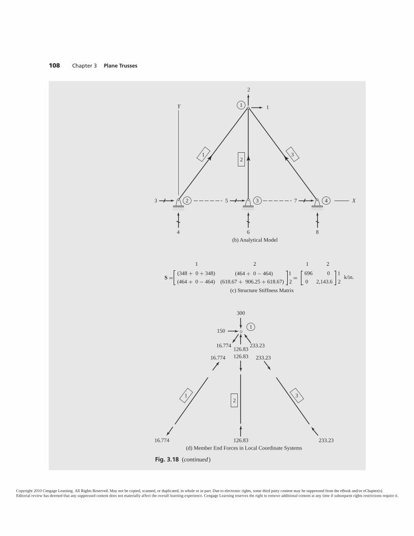
108 Chapter 3 Plane Trusses
Y
X
2
53 7
864
11
2 3 4
(b) Analytical Model
21 3
(c) Structure Stiffness Matrix
(348 + 0 + 348)S =
(464 + 0 − 464) (618.67 + 906.25 + 618.67) 2 =
0 2,143.6 2 (464 + 0 − 464) 696 0 11
1 2 21
k/in.
150
300
233.2316.774
233.23
233.23
16.774
16.774
126.83126.83
126.83
1
(d) Member End Forces in Local Coordinate Systems
21 3
Fig. 3.18 (continued)
Copyright 2010 Cengage Learning. All Rights Reserved. May not be copied, scanned, or duplicated, in whole or in part. Due to electronic rights, some third party content may be suppressed from the eBook and/or eChapter(s).Editorial review has deemed that any suppressed content does not materially affect the overall learning experience. Cengage Learning reserves the right to remove additional content at any time if subsequent rights restrictions require it.
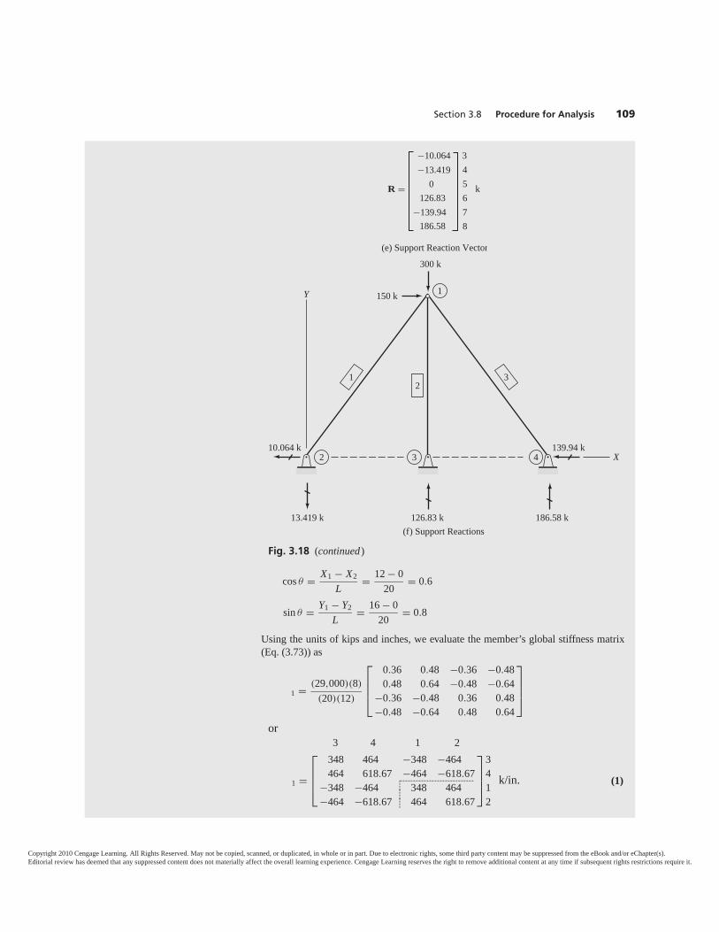
cos θ = X1 − X2L = 12 − 0
20 = 0.6
sin θ = Y1 − Y2L = 16 − 0
20 = 0.8
Using the units of kips and inches, we evaluate the member’s global stiffness matrix(Eq. (3.73)) as
1 = (29,000)(8)
(20)(12)
⎡⎢⎢⎣
0.36 0.48 −0.36 −0.480.48 0.64 −0.48 −0.64
−0.36 −0.48 0.36 0.48−0.48 −0.64 0.48 0.64
⎤⎥⎥⎦
or3 4 1 2
1 =
⎡⎢⎢⎣
348 464 −348 −464464 618.67 −464 −618.67
−348 −464 348 464−464 −618.67 464 618.67
⎤⎥⎥⎦
3412
���
������� k/in. (1)
Section 3.8 Procedure for Analysis 109
(e) Support Reaction Vector
186.58−139.94
126.830
−13.419−10.064 3
45678
kR �
Y
X
300 k
150 k
10.064 k 139.94 k
13.419 k 126.83 k 186.58 k
1
2 3 4
(f) Support Reactions
21 3
Fig. 3.18 (continued)
Copyright 2010 Cengage Learning. All Rights Reserved. May not be copied, scanned, or duplicated, in whole or in part. Due to electronic rights, some third party content may be suppressed from the eBook and/or eChapter(s).Editorial review has deemed that any suppressed content does not materially affect the overall learning experience. Cengage Learning reserves the right to remove additional content at any time if subsequent rights restrictions require it.
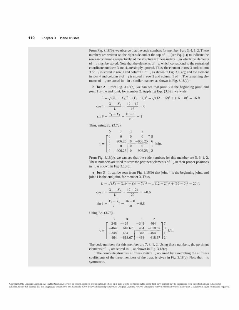
110 Chapter 3 Plane Trusses
From Fig. 3.18(b), we observe that the code numbers for member 1 are 3, 4, 1, 2. Thesenumbers are written on the right side and at the top of 1 (see Eq. (1)) to indicate therows and columns, respectively, of the structure stiffness matrix , in which the elementsof 1 must be stored. Note that the elements of 1, which correspond to the restrainedcoordinate numbers 3 and 4, are simply ignored. Thus, the element in row 3 and column3 of 1 is stored in row 1 and column 1 of , as shown in Fig. 3.18(c); and the elementin row 4 and column 3 of 1 is stored in row 2 and column 1 of . The remaining ele-ments of 1 are stored in in a similar manner, as shown in Fig. 3.18(c).
e ber 2 From Fig. 3.18(b), we can see that joint 3 is the beginning joint, andjoint 1 is the end joint, for member 2. Applying Eqs. (3.62), we write
L =√
(X1 − X3)2 + (Y1 − Y3)2 =√
(12 − 12)2 + (16 − 0)2 = 16 ft
cos θ = X1 − X3L = 12 − 12
16 = 0
sin θ = Y1 − Y3L = 16 − 0
16 = 1
Thus, using Eq. (3.73),5 6 1 2
2 =
⎡⎢⎢⎣
0 0 0 00 906.25 0 −906.250 0 0 00 −906.25 0 906.25
⎤⎥⎥⎦
5612
���
������ k/in.
From Fig. 3.18(b), we can see that the code numbers for this member are 5, 6, 1, 2.These numbers are used to store the pertinent elements of 2 in their proper positionsin , as shown in Fig. 3.18(c).
e ber 3 It can be seen from Fig. 3.18(b) that joint 4 is the beginning joint, andjoint 1 is the end joint, for member 3. Thus,
L =√
(X1 − X4)2 + (Y1 − Y4)2 =√
(12 − 24)2 + (16 − 0)2 = 20 ft
cos θ = X1 − X4L = 12 − 24
20 = −0.6
sin θ = Y1 − Y4L = 16 − 0
20 = 0.8
Using Eq. (3.73),7 8 1 2
3 =
⎡⎢⎢⎣
348 −464 −348 464−464 618.67 464 −618.67−348 464 348 −464
464 −618.67 −464 618.67
⎤⎥⎥⎦
7812
���
�������� k/in.
The code numbers for this member are 7, 8, 1, 2. Using these numbers, the pertinentelements of 3 are stored in , as shown in Fig. 3.18(c).
The complete structure stiffness matrix , obtained by assembling the stiffnesscoefficients of the three members of the truss, is given in Fig. 3.18(c). Note that issymmetric.
Copyright 2010 Cengage Learning. All Rights Reserved. May not be copied, scanned, or duplicated, in whole or in part. Due to electronic rights, some third party content may be suppressed from the eBook and/or eChapter(s).Editorial review has deemed that any suppressed content does not materially affect the overall learning experience. Cengage Learning reserves the right to remove additional content at any time if subsequent rights restrictions require it.
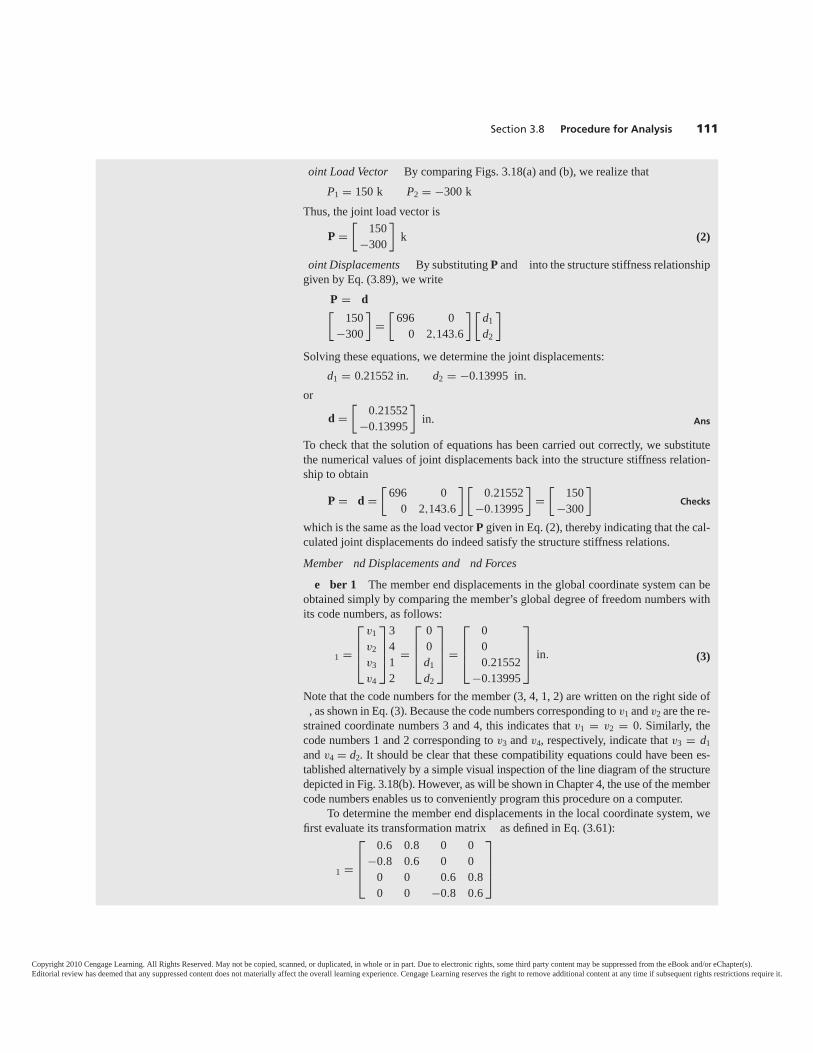
Section 3.8 Procedure for Analysis 111
oint Load Vector By comparing Figs. 3.18(a) and (b), we realize thatP1 = 150 k P2 = −300 k
Thus, the joint load vector is
P =[
150−300
]k (2)
oint Displacements By substituting P and into the structure stiffness relationshipgiven by Eq. (3.89), we write
P = d[150
−300
]=
[696 0
0 2,143.6
] [d1d2
]
Solving these equations, we determine the joint displacements:d1 = 0.21552 in. d2 = −0.13995 in.
or
d =[
0.21552−0.13995
]in. Ans
To check that the solution of equations has been carried out correctly, we substitutethe numerical values of joint displacements back into the structure stiffness relation-ship to obtain
P = d =[
696 00 2,143.6
] [0.21552
−0.13995
]=
[150
−300
]Checks
which is the same as the load vector P given in Eq. (2), thereby indicating that the cal-culated joint displacements do indeed satisfy the structure stiffness relations.Member nd Displacements and nd Forces
e ber 1 The member end displacements in the global coordinate system can beobtained simply by comparing the member’s global degree of freedom numbers withits code numbers, as follows:
1 =
⎡⎢⎢⎣
v1v2v3v4
⎤⎥⎥⎦
3412
=
⎡⎢⎢⎣
00d1d2
⎤⎥⎥⎦ =
⎡⎢⎢⎣
000.21552
−0.13995
⎤⎥⎥⎦ in. (3)
Note that the code numbers for the member (3, 4, 1, 2) are written on the right side of, as shown in Eq. (3). Because the code numbers corresponding to v1 and v2 are the re-
strained coordinate numbers 3 and 4, this indicates that v1 = v2 = 0. Similarly, thecode numbers 1 and 2 corresponding to v3 and v4, respectively, indicate that v3 = d1and v4 = d2. It should be clear that these compatibility equations could have been es-tablished alternatively by a simple visual inspection of the line diagram of the structuredepicted in Fig. 3.18(b). However, as will be shown in Chapter 4, the use of the membercode numbers enables us to conveniently program this procedure on a computer.
To determine the member end displacements in the local coordinate system, wefirst evaluate its transformation matrix as defined in Eq. (3.61):
1 =
⎡⎢⎢⎣
0.6 0.8 0 0−0.8 0.6 0 0
0 0 0.6 0.80 0 −0.8 0.6
⎤⎥⎥⎦
Copyright 2010 Cengage Learning. All Rights Reserved. May not be copied, scanned, or duplicated, in whole or in part. Due to electronic rights, some third party content may be suppressed from the eBook and/or eChapter(s).Editorial review has deemed that any suppressed content does not materially affect the overall learning experience. Cengage Learning reserves the right to remove additional content at any time if subsequent rights restrictions require it.
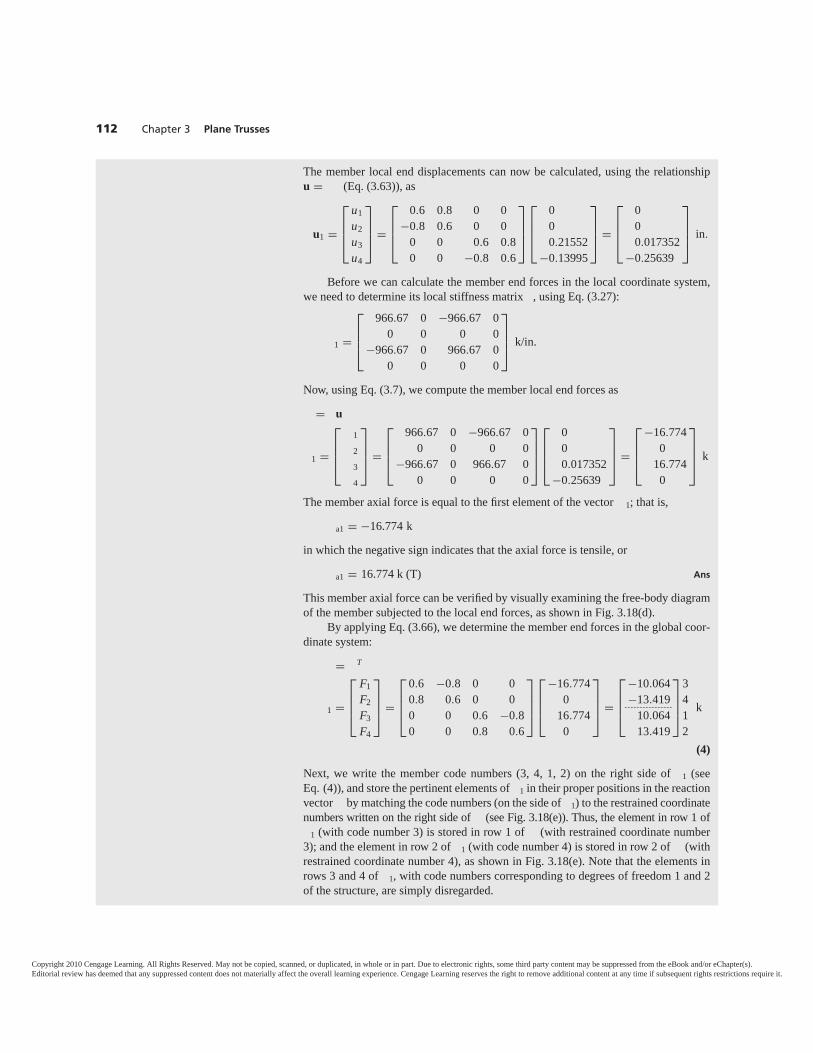
112 Chapter 3 Plane Trusses
The member local end displacements can now be calculated, using the relationshipu = (Eq. (3.63)), as
u1 =
⎡⎢⎢⎣
u1u2u3u4
⎤⎥⎥⎦ =
⎡⎢⎢⎣
0.6 0.8 0 0−0.8 0.6 0 0
0 0 0.6 0.80 0 −0.8 0.6
⎤⎥⎥⎦
⎡⎢⎢⎣
000.21552
−0.13995
⎤⎥⎥⎦ =
⎡⎢⎢⎣
000.017352
−0.25639
⎤⎥⎥⎦ in.
Before we can calculate the member end forces in the local coordinate system,we need to determine its local stiffness matrix , using Eq. (3.27):
1 =
⎡⎢⎢⎣
966.67 0 −966.67 00 0 0 0
−966.67 0 966.67 00 0 0 0
⎤⎥⎥⎦ k/in.
Now, using Eq. (3.7), we compute the member local end forces as
= u
1 =
⎡⎢⎢⎣
1
2
3
4
⎤⎥⎥⎦ =
⎡⎢⎢⎣
966.67 0 −966.67 00 0 0 0
−966.67 0 966.67 00 0 0 0
⎤⎥⎥⎦
⎡⎢⎢⎣
000.017352
−0.25639
⎤⎥⎥⎦ =
⎡⎢⎢⎣
−16.7740
16.7740
⎤⎥⎥⎦ k
The member axial force is equal to the first element of the vector 1; that is,
a1 = −16.774 k
in which the negative sign indicates that the axial force is tensile, or
a1 = 16.774 k (T) Ans
This member axial force can be verified by visually examining the free-body diagramof the member subjected to the local end forces, as shown in Fig. 3.18(d).
By applying Eq. (3.66), we determine the member end forces in the global coor-dinate system:
= T
1 =
⎡⎢⎢⎣
F1F2F3F4
⎤⎥⎥⎦ =
⎡⎢⎢⎣
0.6 −0.8 0 00.8 0.6 0 00 0 0.6 −0.80 0 0.8 0.6
⎤⎥⎥⎦
⎡⎢⎢⎣
−16.7740
16.7740
⎤⎥⎥⎦ =
⎡⎢⎢⎣
−10.064−13.419
10.06413.419
⎤⎥⎥⎦
3412
k����
(4)
Next, we write the member code numbers (3, 4, 1, 2) on the right side of 1 (seeEq. (4)), and store the pertinent elements of 1 in their proper positions in the reactionvector by matching the code numbers (on the side of 1) to the restrained coordinatenumbers written on the right side of (see Fig. 3.18(e)). Thus, the element in row 1 of
1 (with code number 3) is stored in row 1 of (with restrained coordinate number3); and the element in row 2 of 1 (with code number 4) is stored in row 2 of (withrestrained coordinate number 4), as shown in Fig. 3.18(e). Note that the elements inrows 3 and 4 of 1, with code numbers corresponding to degrees of freedom 1 and 2of the structure, are simply disregarded.
Copyright 2010 Cengage Learning. All Rights Reserved. May not be copied, scanned, or duplicated, in whole or in part. Due to electronic rights, some third party content may be suppressed from the eBook and/or eChapter(s).Editorial review has deemed that any suppressed content does not materially affect the overall learning experience. Cengage Learning reserves the right to remove additional content at any time if subsequent rights restrictions require it.
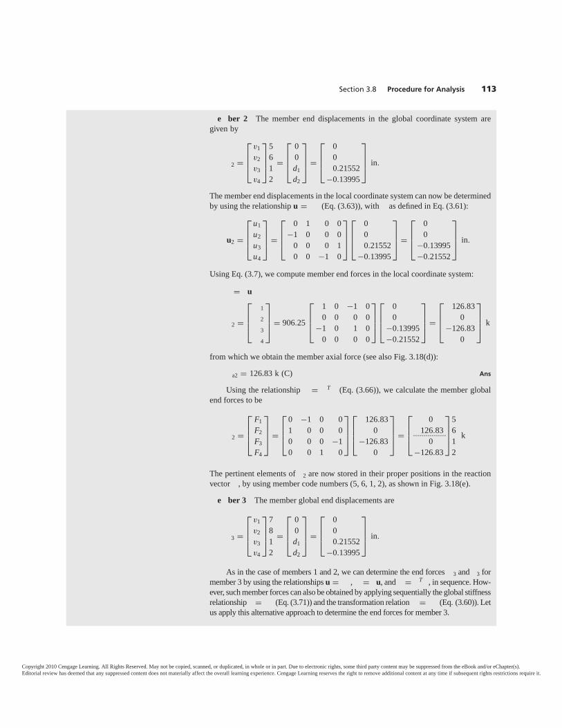
Section 3.8 Procedure for Analysis 113
e ber 2 The member end displacements in the global coordinate system aregiven by
2 =
⎡⎢⎢⎣
v1v2v3v4
⎤⎥⎥⎦
5612
=
⎡⎢⎢⎣
00d1d2
⎤⎥⎥⎦ =
⎡⎢⎢⎣
000.21552
−0.13995
⎤⎥⎥⎦ in.
The member end displacements in the local coordinate system can now be determinedby using the relationship u = (Eq. (3.63)), with as defined in Eq. (3.61):
u2 =
⎡⎢⎢⎣
u1u2u3u4
⎤⎥⎥⎦ =
⎡⎢⎢⎣
0 1 0 0−1 0 0 0
0 0 0 10 0 −1 0
⎤⎥⎥⎦
⎡⎢⎢⎣
000.21552
−0.13995
⎤⎥⎥⎦ =
⎡⎢⎢⎣
00
−0.13995−0.21552
⎤⎥⎥⎦ in.
Using Eq. (3.7), we compute member end forces in the local coordinate system:
= u
2 =
⎡⎢⎢⎣
1
2
3
4
⎤⎥⎥⎦ = 906.25
⎡⎢⎢⎣
1 0 −1 00 0 0 0
−1 0 1 00 0 0 0
⎤⎥⎥⎦
⎡⎢⎢⎣
00
−0.13995−0.21552
⎤⎥⎥⎦ =
⎡⎢⎢⎣
126.830
−126.830
⎤⎥⎥⎦ k
from which we obtain the member axial force (see also Fig. 3.18(d)):
a2 = 126.83 k (C) Ans
Using the relationship = T (Eq. (3.66)), we calculate the member globalend forces to be
2 =
⎡⎢⎢⎣
F1F2F3F4
⎤⎥⎥⎦ =
⎡⎢⎢⎣
0 −1 0 01 0 0 00 0 0 −10 0 1 0
⎤⎥⎥⎦
⎡⎢⎢⎣
126.830
−126.830
⎤⎥⎥⎦ =
⎡⎢⎢⎣
0126.83
0−126.83
⎤⎥⎥⎦
5612
k����
The pertinent elements of 2 are now stored in their proper positions in the reactionvector , by using member code numbers (5, 6, 1, 2), as shown in Fig. 3.18(e).
e ber 3 The member global end displacements are
3 =
⎡⎢⎢⎣
v1v2v3v4
⎤⎥⎥⎦
7812
=
⎡⎢⎢⎣
00d1d2
⎤⎥⎥⎦ =
⎡⎢⎢⎣
000.21552
−0.13995
⎤⎥⎥⎦ in.
As in the case of members 1 and 2, we can determine the end forces 3 and 3 formember 3 by using the relationships u = , = u, and = T , in sequence. How-ever, such member forces can also be obtained by applying sequentially the global stiffnessrelationship = (Eq. (3.71)) and the transformation relation = (Eq. (3.60)). Letus apply this alternative approach to determine the end forces for member 3.
Copyright 2010 Cengage Learning. All Rights Reserved. May not be copied, scanned, or duplicated, in whole or in part. Due to electronic rights, some third party content may be suppressed from the eBook and/or eChapter(s).Editorial review has deemed that any suppressed content does not materially affect the overall learning experience. Cengage Learning reserves the right to remove additional content at any time if subsequent rights restrictions require it.
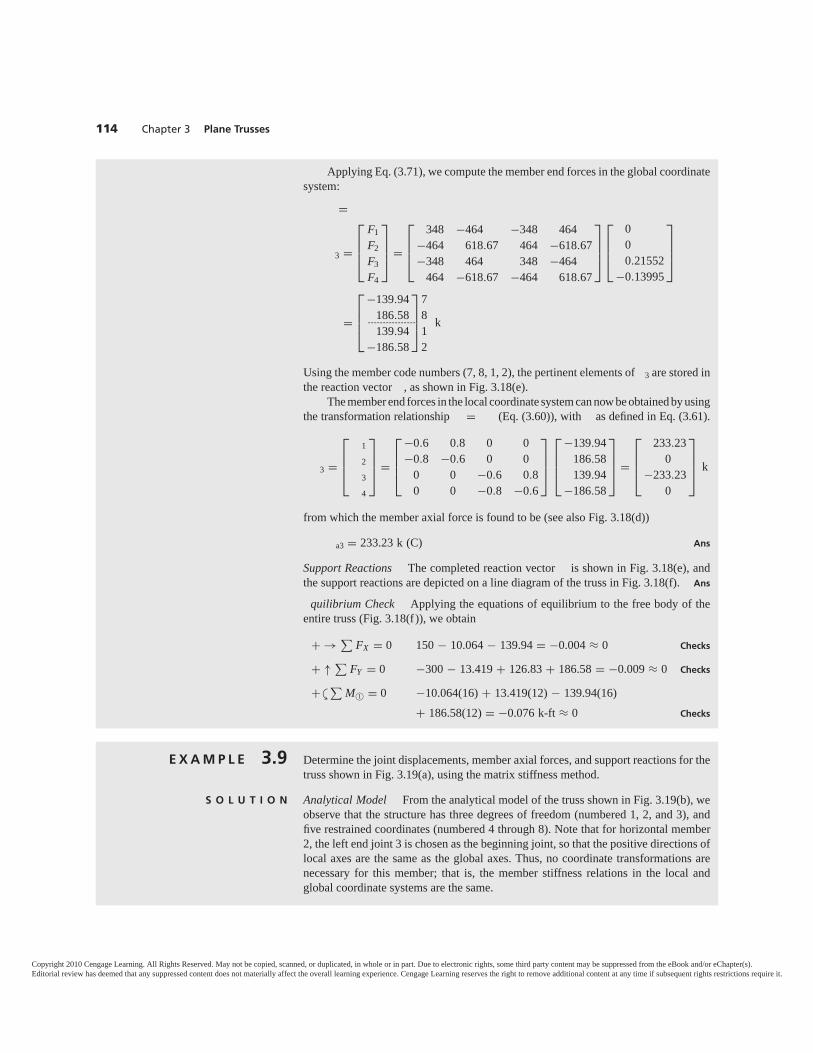
114 Chapter 3 Plane Trusses
Applying Eq. (3.71), we compute the member end forces in the global coordinatesystem:
=
3 =
⎡⎢⎢⎣
F1F2F3F4
⎤⎥⎥⎦ =
⎡⎢⎢⎣
348 −464 −348 464−464 618.67 464 −618.67−348 464 348 −464
464 −618.67 −464 618.67
⎤⎥⎥⎦
⎡⎢⎢⎣
000.21552
−0.13995
⎤⎥⎥⎦
=
⎡⎢⎢⎣
−139.94186.58139.94
−186.58
⎤⎥⎥⎦
7812
k����
Using the member code numbers (7, 8, 1, 2), the pertinent elements of 3 are stored inthe reaction vector , as shown in Fig. 3.18(e).
The member end forces in the local coordinate system can now be obtained by usingthe transformation relationship = (Eq. (3.60)), with as defined in Eq. (3.61).
3 =
⎡⎢⎢⎣
1
2
3
4
⎤⎥⎥⎦ =
⎡⎢⎢⎣
−0.6 0.8 0 0−0.8 −0.6 0 0
0 0 −0.6 0.80 0 −0.8 −0.6
⎤⎥⎥⎦
⎡⎢⎢⎣
−139.94186.58139.94
−186.58
⎤⎥⎥⎦ =
⎡⎢⎢⎣
233.230
−233.230
⎤⎥⎥⎦ k
from which the member axial force is found to be (see also Fig. 3.18(d))
a3 = 233.23 k (C) Ans
Support Reactions The completed reaction vector is shown in Fig. 3.18(e), andthe support reactions are depicted on a line diagram of the truss in Fig. 3.18(f). Ans
quilibrium Check Applying the equations of equilibrium to the free body of theentire truss (Fig. 3.18(f)), we obtain
+ → ∑FX = 0 150 − 10.064 − 139.94 = −0.004 ≈ 0 Checks
+ ↑ ∑FY = 0 −300 − 13.419 + 126.83 + 186.58 = −0.009 ≈ 0 Checks
+ ∑M©1 = 0 −10.064(16) + 13.419(12) − 139.94(16)
+ 186.58(12) = −0.076 k-ft ≈ 0 Checks
a
E X A M P L E 3.9 Determine the joint displacements, member axial forces, and support reactions for thetruss shown in Fig. 3.19(a), using the matrix stiffness method.
S O L U T I O N Analytical Model From the analytical model of the truss shown in Fig. 3.19(b), weobserve that the structure has three degrees of freedom (numbered 1, 2, and 3), andfive restrained coordinates (numbered 4 through 8). Note that for horizontal member2, the left end joint 3 is chosen as the beginning joint, so that the positive directions oflocal axes are the same as the global axes. Thus, no coordinate transformations arenecessary for this member; that is, the member stiffness relations in the local andglobal coordinate systems are the same.
Copyright 2010 Cengage Learning. All Rights Reserved. May not be copied, scanned, or duplicated, in whole or in part. Due to electronic rights, some third party content may be suppressed from the eBook and/or eChapter(s).Editorial review has deemed that any suppressed content does not materially affect the overall learning experience. Cengage Learning reserves the right to remove additional content at any time if subsequent rights restrictions require it.
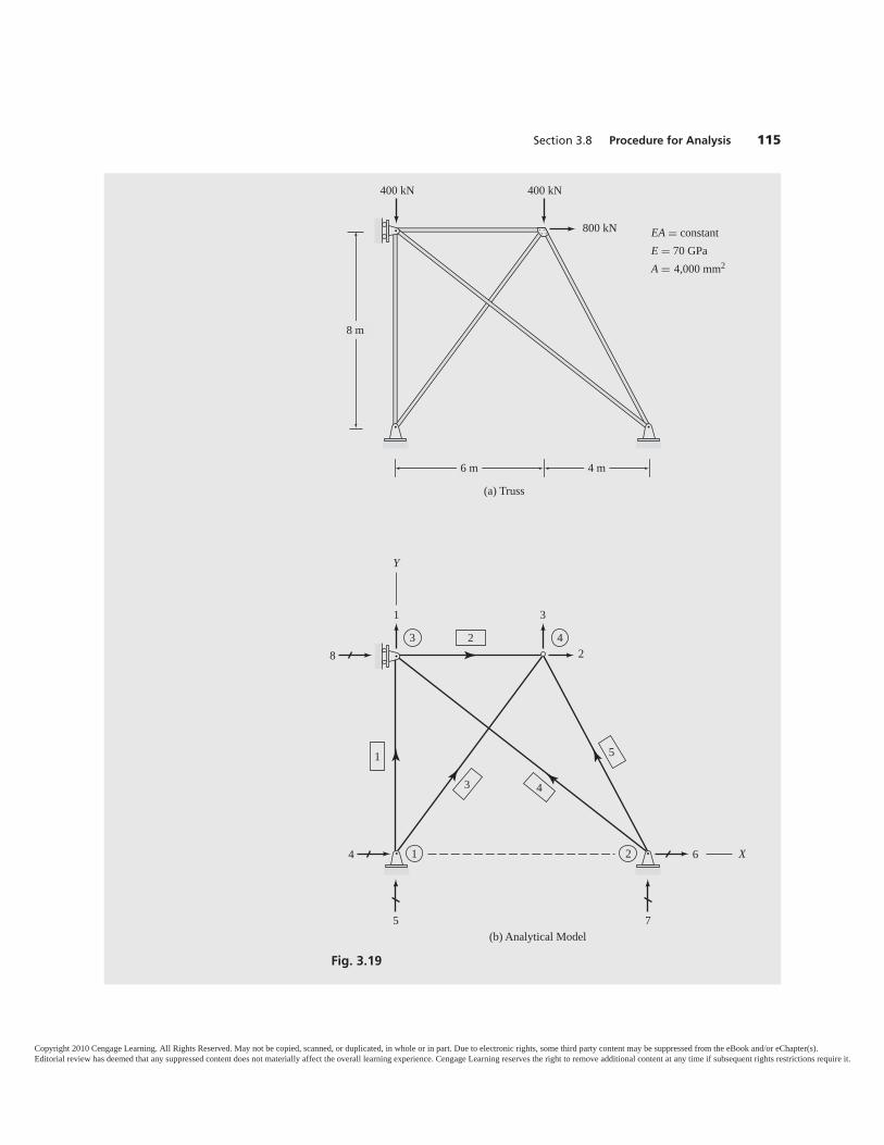
Section 3.8 Procedure for Analysis 115
6 m 4 m
8 m
EA � constantE � 70 GPaA � 4,000 mm2
400 kN 400 kN
800 kN
(a) Truss
1 3
2
64
75
8
Y
X
43
1 2
(b) Analytical Model
2
1
3 4
5
Fig. 3.19
Copyright 2010 Cengage Learning. All Rights Reserved. May not be copied, scanned, or duplicated, in whole or in part. Due to electronic rights, some third party content may be suppressed from the eBook and/or eChapter(s).Editorial review has deemed that any suppressed content does not materially affect the overall learning experience. Cengage Learning reserves the right to remove additional content at any time if subsequent rights restrictions require it.
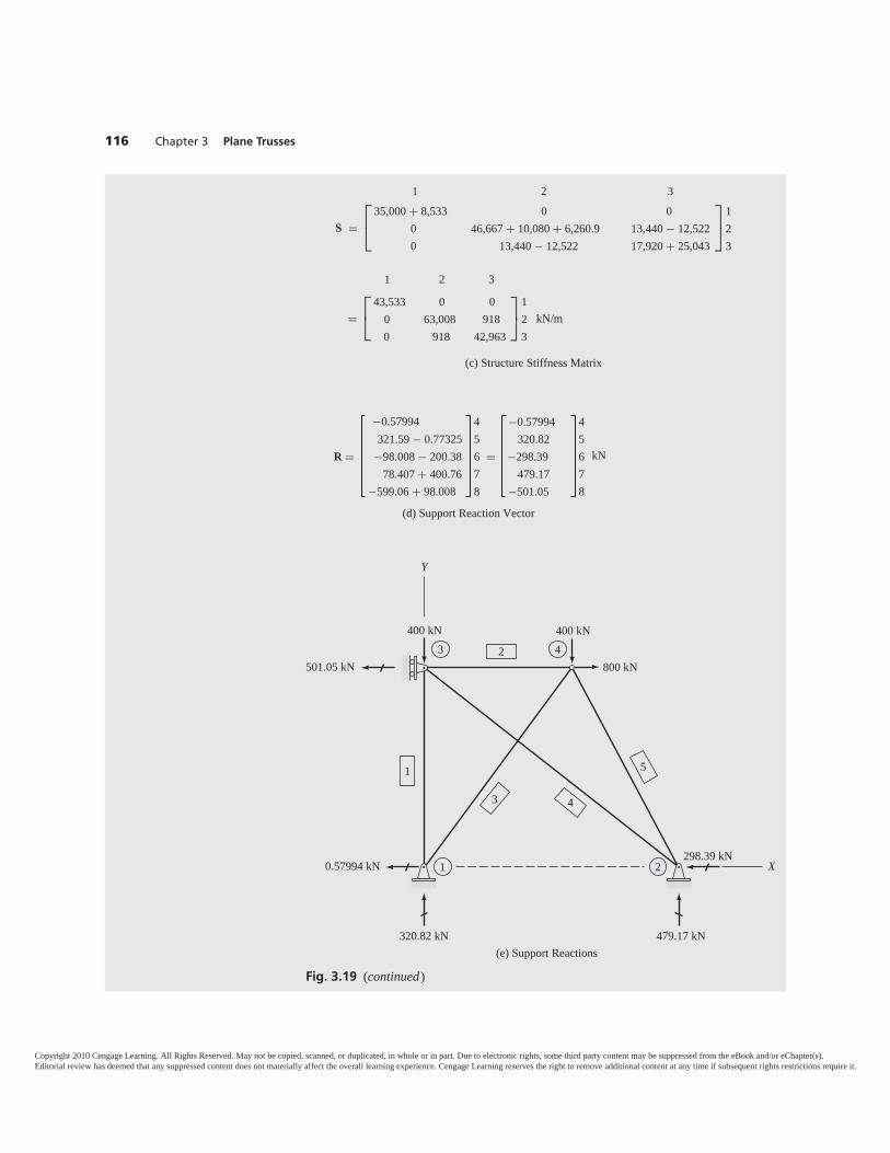
116 Chapter 3 Plane Trusses
Fig. 3.19 (continued)
S =
⎡⎣ 35,000 + 8,533 0 0
0 46,667 + 10,080 + 6,260.9 13,440 − 12,5220 13,440 − 12,522 17,920 + 25,043
⎤⎦1
23
=⎡⎣ 43,533 0 0
0 63,008 9180 918 42,963
⎤⎦1
23
kN/m
(c) Structure Stiffness Matrix
1
1 2 3
2 3
(d) Support Reaction Vector
−0.57994321.59 − 0.77325−98.008 − 200.38 = −298.39
78.407 + 400.76−599.06 + 98.008
R =
45678
−0.57994
479.17
320.82
−501.05
kN
45678
400 kN 400 kN
800 kN501.05 kN
320.82 kN
0.57994 kN298.39 kN
479.17 kN
Y
X
43
1 2
(e) Support Reactions
2
1
3 4
5
Copyright 2010 Cengage Learning. All Rights Reserved. May not be copied, scanned, or duplicated, in whole or in part. Due to electronic rights, some third party content may be suppressed from the eBook and/or eChapter(s).Editorial review has deemed that any suppressed content does not materially affect the overall learning experience. Cengage Learning reserves the right to remove additional content at any time if subsequent rights restrictions require it.
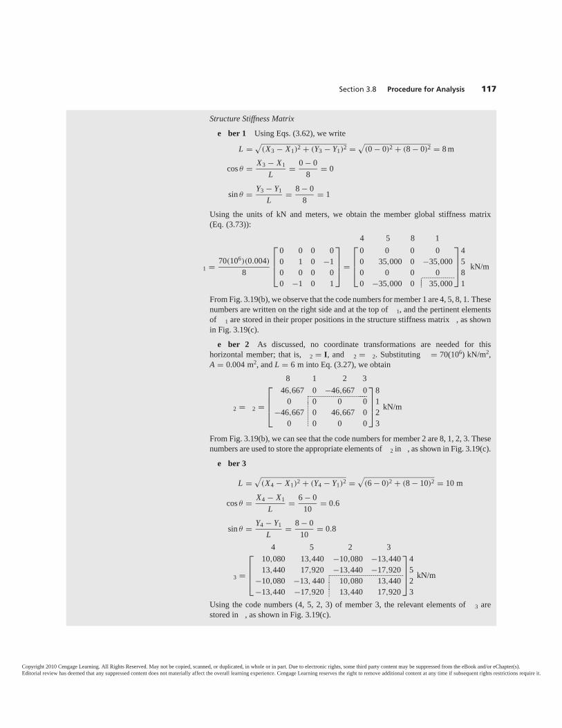
Section 3.8 Procedure for Analysis 117
Structure Stiffness Matrixe ber 1 Using Eqs. (3.62), we write
L =√
(X3 − X1)2 + (Y3 − Y1)2 =√
(0 − 0)2 + (8 − 0)2 = 8 m
cos θ = X3 − X1L = 0 − 0
8 = 0
sin θ = Y3 − Y1L = 8 − 0
8 = 1
Using the units of kN and meters, we obtain the member global stiffness matrix(Eq. (3.73)):
4 5 8 1
1 = 70(106)(0.004)
8
⎡⎢⎢⎣
0 0 0 00 1 0 −10 0 0 00 −1 0 1
⎤⎥⎥⎦ =
⎡⎢⎢⎣
0 0 0 00 35,000 0 −35,0000 0 0 00 −35,000 0 35,000
⎤⎥⎥⎦
4581
kN/m
������
From Fig. 3.19(b), we observe that the code numbers for member 1 are 4, 5, 8, 1. Thesenumbers are written on the right side and at the top of 1, and the pertinent elementsof 1 are stored in their proper positions in the structure stiffness matrix , as shownin Fig. 3.19(c).
e ber 2 As discussed, no coordinate transformations are needed for thishorizontal member; that is, 2 = I, and 2 = 2. Substituting = 70(106) kN/m2,A = 0.004 m2, and L = 6 m into Eq. (3.27), we obtain
8 1 2 3
2 = 2 =
⎡⎢⎢⎣
46,667 0 −46,667 00 0 0 0
−46,667 0 46,667 00 0 0 0
⎤⎥⎥⎦
8123
kN/m����
��������
From Fig. 3.19(b), we can see that the code numbers for member 2 are 8, 1, 2, 3. Thesenumbers are used to store the appropriate elements of 2 in , as shown in Fig. 3.19(c).
e ber 3
L =√
(X4 − X1)2 + (Y4 − Y1)2 =√
(6 − 0)2 + (8 − 10)2 = 10 m
cos θ = X4 − X1L = 6 − 0
10 = 0.6
sin θ = Y4 − Y1L = 8 − 0
10 = 0.8
4 5 2 3
3 =
⎡⎢⎢⎣
10,080 13,440 −10,080 −13,44013,440 17,920 −13,440 −17,920
−10,080 −13, 440 10,080 13,440−13,440 −17,920 13,440 17,920
⎤⎥⎥⎦
4523
kN/m���
���������
Using the code numbers (4, 5, 2, 3) of member 3, the relevant elements of 3 arestored in , as shown in Fig. 3.19(c).
Copyright 2010 Cengage Learning. All Rights Reserved. May not be copied, scanned, or duplicated, in whole or in part. Due to electronic rights, some third party content may be suppressed from the eBook and/or eChapter(s).Editorial review has deemed that any suppressed content does not materially affect the overall learning experience. Cengage Learning reserves the right to remove additional content at any time if subsequent rights restrictions require it.
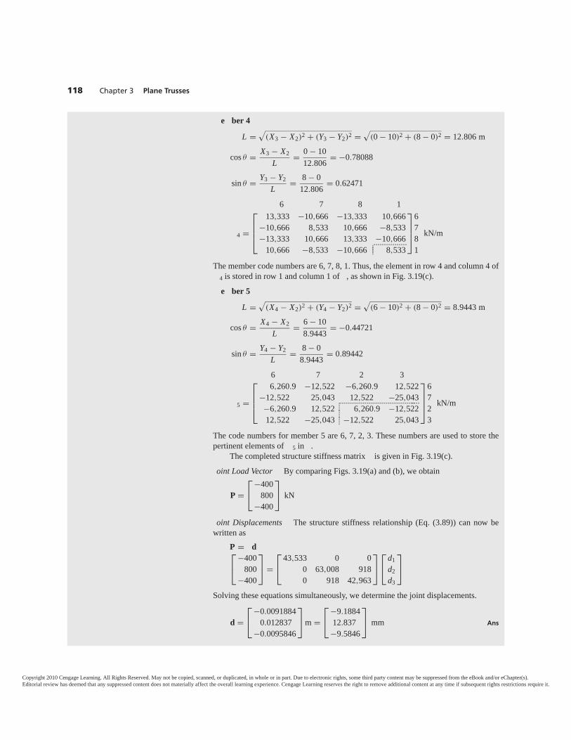
118 Chapter 3 Plane Trusses
e ber 4
L =√
(X3 − X2)2 + (Y3 − Y2)2 =√
(0 − 10)2 + (8 − 0)2 = 12.806 m
cos θ = X3 − X2L = 0 − 10
12.806 = −0.78088
sin θ = Y3 − Y2L = 8 − 0
12.806 = 0.62471
6 7 8 1
4 =
⎡⎢⎢⎣
13,333 −10,666 −13,333 10,666−10,666 8,533 10,666 −8,533−13,333 10,666 13,333 −10,666
10,666 −8,533 −10,666 8,533
⎤⎥⎥⎦
6781
kN/m
������
The member code numbers are 6, 7, 8, 1. Thus, the element in row 4 and column 4 of4 is stored in row 1 and column 1 of , as shown in Fig. 3.19(c).e ber 5
L =√
(X4 − X2)2 + (Y4 − Y2)2 =√
(6 − 10)2 + (8 − 0)2 = 8.9443 m
cos θ = X4 − X2L = 6 − 10
8.9443 = −0.44721
sin θ = Y4 − Y2L = 8 − 0
8.9443 = 0.89442
6 7 2 3
5 =
⎡⎢⎢⎣
6,260.9 −12,522 −6,260.9 12,522−12,522 25,043 12,522 −25,043−6,260.9 12,522 6,260.9 −12,52212,522 −25,043 −12,522 25,043
⎤⎥⎥⎦
6723
kN/m���
����������
The code numbers for member 5 are 6, 7, 2, 3. These numbers are used to store thepertinent elements of 5 in .
The completed structure stiffness matrix is given in Fig. 3.19(c).oint Load Vector By comparing Figs. 3.19(a) and (b), we obtain
P =⎡⎣ −400
800−400
⎤⎦ kN
oint Displacements The structure stiffness relationship (Eq. (3.89)) can now bewritten as
P = d⎡⎣ −400
800−400
⎤⎦ =
⎡⎣ 43,533 0 0
0 63,008 9180 918 42,963
⎤⎦
⎡⎣ d1
d2d3
⎤⎦
Solving these equations simultaneously, we determine the joint displacements.
d =⎡⎣ −0.0091884
0.012837−0.0095846
⎤⎦ m =
⎡⎣ −9.1884
12.837−9.5846
⎤⎦ mm Ans
Copyright 2010 Cengage Learning. All Rights Reserved. May not be copied, scanned, or duplicated, in whole or in part. Due to electronic rights, some third party content may be suppressed from the eBook and/or eChapter(s).Editorial review has deemed that any suppressed content does not materially affect the overall learning experience. Cengage Learning reserves the right to remove additional content at any time if subsequent rights restrictions require it.
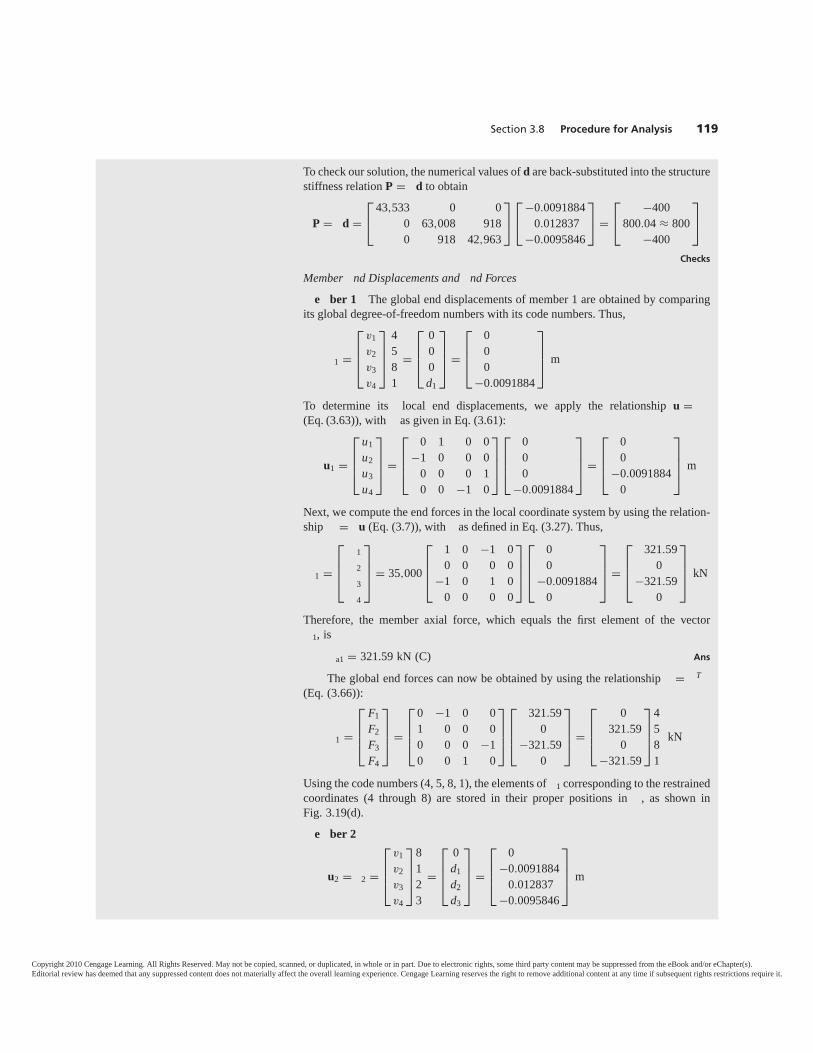
Section 3.8 Procedure for Analysis 119
To check our solution, the numerical values of d are back-substituted into the structurestiffness relation P = d to obtain
P = d =⎡⎣ 43,533 0 0
0 63,008 9180 918 42,963
⎤⎦
⎡⎣ −0.0091884
0.012837−0.0095846
⎤⎦ =
⎡⎣ −400
800.04 ≈ 800−400
⎤⎦
Checks
Member nd Displacements and nd Forcese ber 1 The global end displacements of member 1 are obtained by comparing
its global degree-of-freedom numbers with its code numbers. Thus,
1 =
⎡⎢⎢⎣
v1v2v3v4
⎤⎥⎥⎦
4581
=
⎡⎢⎢⎣
000d1
⎤⎥⎥⎦ =
⎡⎢⎢⎣
000
−0.0091884
⎤⎥⎥⎦ m
To determine its local end displacements, we apply the relationship u =(Eq. (3.63)), with as given in Eq. (3.61):
u1 =
⎡⎢⎢⎣
u1u2u3u4
⎤⎥⎥⎦ =
⎡⎢⎢⎣
0 1 0 0−1 0 0 0
0 0 0 10 0 −1 0
⎤⎥⎥⎦
⎡⎢⎢⎣
000
−0.0091884
⎤⎥⎥⎦ =
⎡⎢⎢⎣
00
−0.00918840
⎤⎥⎥⎦ m
Next, we compute the end forces in the local coordinate system by using the relation-ship = u (Eq. (3.7)), with as defined in Eq. (3.27). Thus,
1 =
⎡⎢⎢⎣
1
2
3
4
⎤⎥⎥⎦ = 35,000
⎡⎢⎢⎣
1 0 −1 00 0 0 0
−1 0 1 00 0 0 0
⎤⎥⎥⎦
⎡⎢⎢⎣
00
−0.00918840
⎤⎥⎥⎦ =
⎡⎢⎢⎣
321.590
−321.590
⎤⎥⎥⎦ kN
Therefore, the member axial force, which equals the first element of the vector1, is
a1 = 321.59 kN (C) Ans
The global end forces can now be obtained by using the relationship = T
(Eq. (3.66)):
1 =
⎡⎢⎢⎣
F1F2F3F4
⎤⎥⎥⎦ =
⎡⎢⎢⎣
0 −1 0 01 0 0 00 0 0 −10 0 1 0
⎤⎥⎥⎦
⎡⎢⎢⎣
321.590
−321.590
⎤⎥⎥⎦ =
⎡⎢⎢⎣
0321.59
0−321.59
⎤⎥⎥⎦
4581
kN
Using the code numbers (4, 5, 8, 1), the elements of 1 corresponding to the restrainedcoordinates (4 through 8) are stored in their proper positions in , as shown inFig. 3.19(d).
e ber 2
u2 = 2 =
⎡⎢⎢⎣
v1v2v3v4
⎤⎥⎥⎦
8123
=
⎡⎢⎢⎣
0d1d2d3
⎤⎥⎥⎦ =
⎡⎢⎢⎣
0−0.0091884
0.012837−0.0095846
⎤⎥⎥⎦ m
Copyright 2010 Cengage Learning. All Rights Reserved. May not be copied, scanned, or duplicated, in whole or in part. Due to electronic rights, some third party content may be suppressed from the eBook and/or eChapter(s).Editorial review has deemed that any suppressed content does not materially affect the overall learning experience. Cengage Learning reserves the right to remove additional content at any time if subsequent rights restrictions require it.
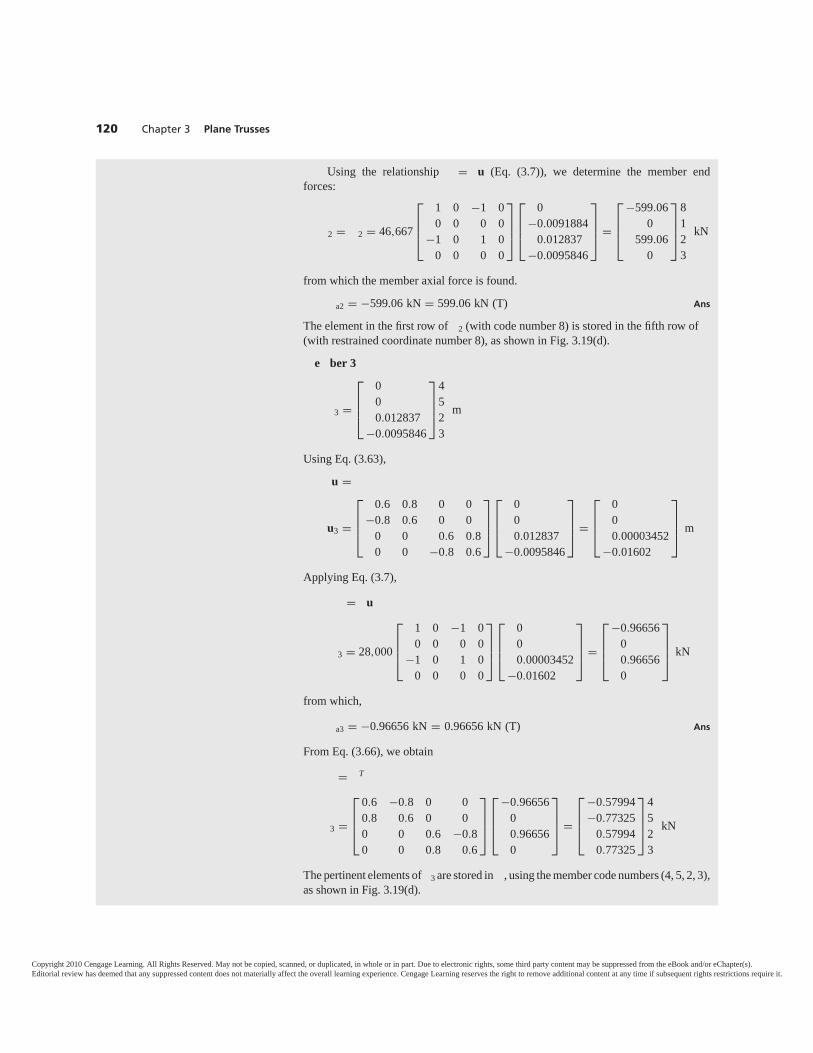
120 Chapter 3 Plane Trusses
Using the relationship � u (Eq. (3.7)), we determine the member endforces:
2 = 2 = 46,667
⎡⎢⎢⎣
1 0 −1 00 0 0 0
−1 0 1 00 0 0 0
⎤⎥⎥⎦
⎡⎢⎢⎣
0−0.0091884
0.012837−0.0095846
⎤⎥⎥⎦ =
⎡⎢⎢⎣
−599.060
599.060
⎤⎥⎥⎦
8123
kN
from which the member axial force is found.
a2 = −599.06 kN = 599.06 kN (T) Ans
The element in the first row of 2 (with code number 8) is stored in the fifth row of (with restrained coordinate number 8), as shown in Fig. 3.19(d).
e ber 3
3 =
⎡⎢⎢⎣
000.012837
−0.0095846
⎤⎥⎥⎦
4523
m
Using Eq. (3.63),
u =
u3 =
⎡⎢⎢⎣
0.6 0.8 0 0−0.8 0.6 0 0
0 0 0.6 0.80 0 −0.8 0.6
⎤⎥⎥⎦
⎡⎢⎢⎣
000.012837
−0.0095846
⎤⎥⎥⎦ =
⎡⎢⎢⎣
000.00003452
−0.01602
⎤⎥⎥⎦ m
Applying Eq. (3.7),
= u
3 = 28,000
⎡⎢⎢⎣
1 0 −1 00 0 0 0
−1 0 1 00 0 0 0
⎤⎥⎥⎦
⎡⎢⎢⎣
000.00003452
−0.01602
⎤⎥⎥⎦ =
⎡⎢⎢⎣
−0.9665600.966560
⎤⎥⎥⎦ kN
from which,
a3 = −0.96656 kN = 0.96656 kN (T) Ans
From Eq. (3.66), we obtain
= T
3 =
⎡⎢⎢⎣
0.6 −0.8 0 00.8 0.6 0 00 0 0.6 −0.80 0 0.8 0.6
⎤⎥⎥⎦
⎡⎢⎢⎣
−0.9665600.966560
⎤⎥⎥⎦ =
⎡⎢⎢⎣
−0.57994−0.77325
0.579940.77325
⎤⎥⎥⎦
4523
kN
The pertinent elements of 3 are stored in , using the member code numbers (4, 5, 2, 3),as shown in Fig. 3.19(d).
Copyright 2010 Cengage Learning. All Rights Reserved. May not be copied, scanned, or duplicated, in whole or in part. Due to electronic rights, some third party content may be suppressed from the eBook and/or eChapter(s).Editorial review has deemed that any suppressed content does not materially affect the overall learning experience. Cengage Learning reserves the right to remove additional content at any time if subsequent rights restrictions require it.
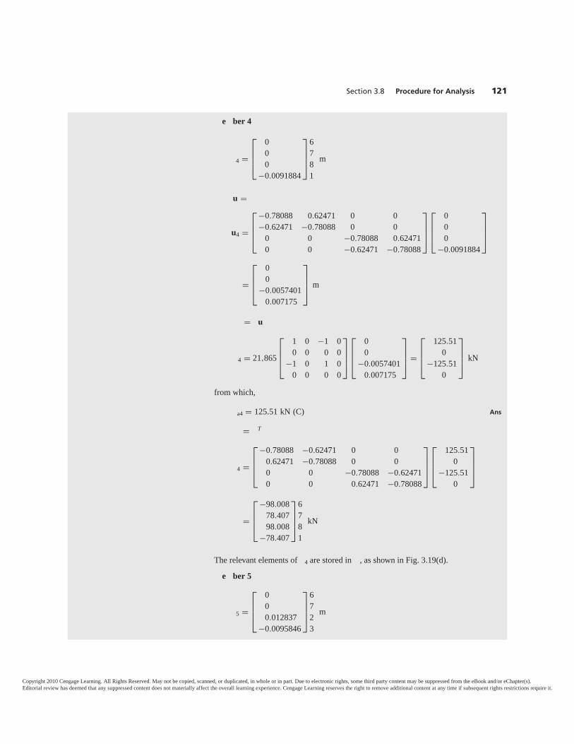
Section 3.8 Procedure for Analysis 121
e ber 4
4 =
⎡⎢⎢⎣
000
−0.0091884
⎤⎥⎥⎦
6781
m
u �
u4 =
⎡⎢⎢⎣
−0.78088 0.62471 0 0−0.62471 −0.78088 0 0
0 0 −0.78088 0.624710 0 −0.62471 −0.78088
⎤⎥⎥⎦
⎡⎢⎢⎣
000
−0.0091884
⎤⎥⎥⎦
=
⎡⎢⎢⎣
00
−0.00574010.007175
⎤⎥⎥⎦ m
= u
4 = 21,865
⎡⎢⎢⎣
1 0 −1 00 0 0 0
−1 0 1 00 0 0 0
⎤⎥⎥⎦
⎡⎢⎢⎣
00
−0.00574010.007175
⎤⎥⎥⎦ =
⎡⎢⎢⎣
125.510
−125.510
⎤⎥⎥⎦ kN
from which,
a4 = 125.51 kN (C) Ans
= T
4 =
⎡⎢⎢⎣
−0.78088 −0.62471 0 00.62471 −0.78088 0 00 0 −0.78088 −0.624710 0 0.62471 −0.78088
⎤⎥⎥⎦
⎡⎢⎢⎣
125.510
−125.510
⎤⎥⎥⎦
=
⎡⎢⎢⎣
−98.00878.40798.008
−78.407
⎤⎥⎥⎦
6781
kN
The relevant elements of 4 are stored in , as shown in Fig. 3.19(d).
e ber 5
5 =
⎡⎢⎢⎣
000.012837
−0.0095846
⎤⎥⎥⎦
6723
m
Copyright 2010 Cengage Learning. All Rights Reserved. May not be copied, scanned, or duplicated, in whole or in part. Due to electronic rights, some third party content may be suppressed from the eBook and/or eChapter(s).Editorial review has deemed that any suppressed content does not materially affect the overall learning experience. Cengage Learning reserves the right to remove additional content at any time if subsequent rights restrictions require it.
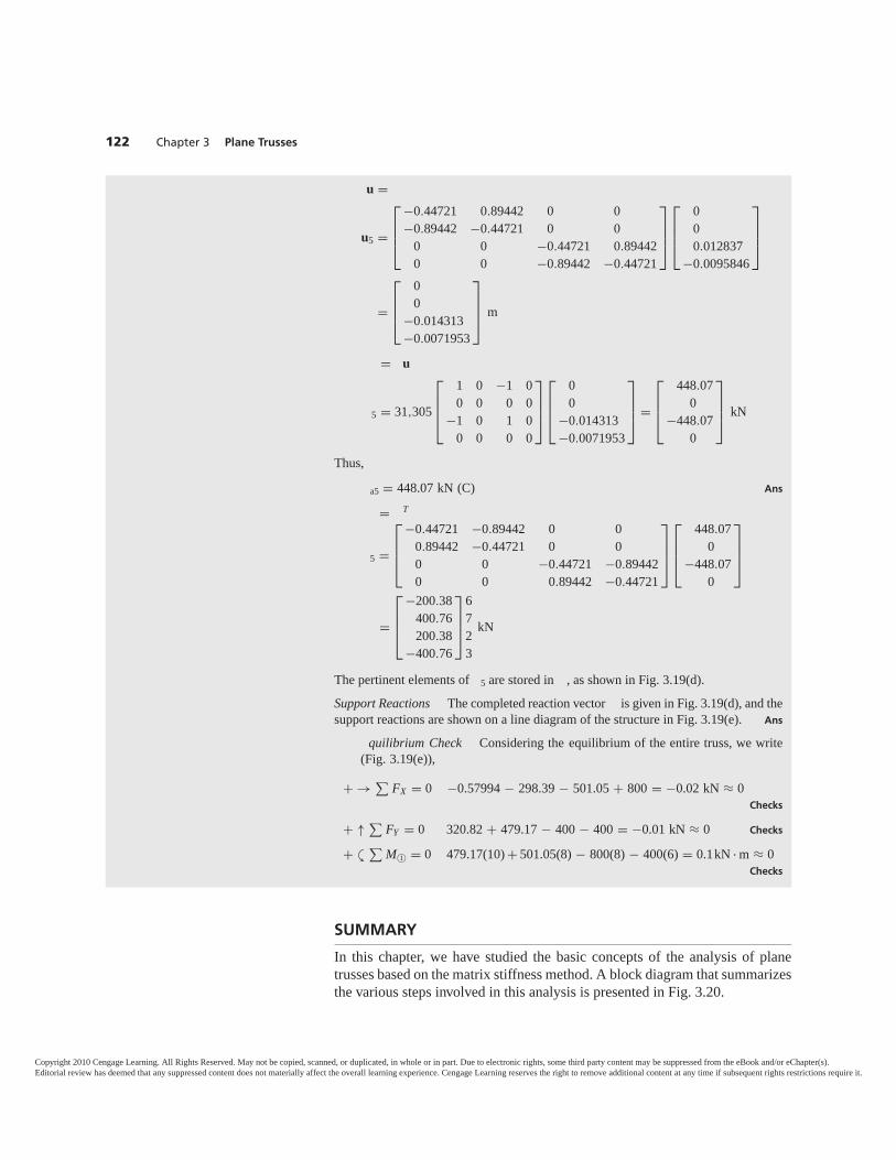
122 Chapter 3 Plane Trusses
u =
u5 =
⎡⎢⎢⎣
−0.44721 0.89442 0 0−0.89442 −0.44721 0 0
0 0 −0.44721 0.894420 0 −0.89442 −0.44721
⎤⎥⎥⎦
⎡⎢⎢⎣
000.012837
−0.0095846
⎤⎥⎥⎦
=
⎡⎢⎢⎣
00
−0.014313−0.0071953
⎤⎥⎥⎦ m
= u
5 = 31,305
⎡⎢⎢⎣
1 0 −1 00 0 0 0
−1 0 1 00 0 0 0
⎤⎥⎥⎦
⎡⎢⎢⎣
00
−0.014313−0.0071953
⎤⎥⎥⎦ =
⎡⎢⎢⎣
448.070
−448.070
⎤⎥⎥⎦ kN
Thus,
a5 = 448.07 kN (C) Ans
= T
5 =
⎡⎢⎢⎣
−0.44721 −0.89442 0 00.89442 −0.44721 0 00 0 −0.44721 −0.894420 0 0.89442 −0.44721
⎤⎥⎥⎦
⎡⎢⎢⎣
448.070
−448.070
⎤⎥⎥⎦
=
⎡⎢⎢⎣
−200.38400.76200.38
−400.76
⎤⎥⎥⎦
6723
kN
The pertinent elements of 5 are stored in , as shown in Fig. 3.19(d).Support Reactions The completed reaction vector is given in Fig. 3.19(d), and thesupport reactions are shown on a line diagram of the structure in Fig. 3.19(e). Ans
quilibrium Check Considering the equilibrium of the entire truss, we write(Fig. 3.19(e)),
+ → ∑FX = 0 −0.57994 − 298.39 − 501.05 + 800 = −0.02 kN ≈ 0
Checks
+ ↑ ∑FY = 0 320.82 + 479.17 − 400 − 400 = −0.01 kN ≈ 0 Checks
+ ∑M©1 = 0 479.17(10) + 501.05(8) − 800(8) − 400(6) = 0.1kN . m ≈ 0
Checks
a
SUMMARY
In this chapter, we have studied the basic concepts of the analysis of planetrusses based on the matrix stiffness method. A block diagram that summarizesthe various steps involved in this analysis is presented in Fig. 3.20.
Copyright 2010 Cengage Learning. All Rights Reserved. May not be copied, scanned, or duplicated, in whole or in part. Due to electronic rights, some third party content may be suppressed from the eBook and/or eChapter(s).Editorial review has deemed that any suppressed content does not materially affect the overall learning experience. Cengage Learning reserves the right to remove additional content at any time if subsequent rights restrictions require it.
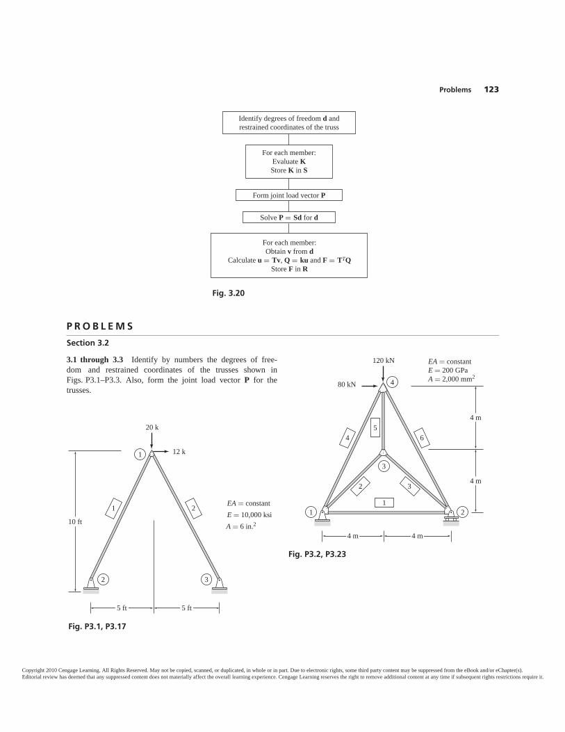
P R O B L E M S
Problems 123
Fig. 3.20
Identify degrees of freedom d andrestrained coordinates of the truss
For each member:Evaluate KStore K in S
Form joint load vector P
Solve P = Sd for d
For each member:Obtain v from d
Calculate u = Tv, Q = ku and F = TTQStore F in R
20 k
12 k1
2 3
5 ft 5 ft
10 ft
EA � constantE � 10,000 ksiA � 6 in.2
1 2
Fig. P3.1, P3.17
120 kN
80 kN 4
3
1 2
4 m 4 m
4 m
4 m
EA � constantE � 200 GPaA � 2,000 mm2
4 6
1
5
2 3
Fig. P3.2, P3.23
Section 3.2
3.1 through 3.3 Identify by numbers the degrees of free-dom and restrained coordinates of the trusses shown inFigs. P3.1–P3.3. Also, form the joint load vector P for thetrusses.
Copyright 2010 Cengage Learning. All Rights Reserved. May not be copied, scanned, or duplicated, in whole or in part. Due to electronic rights, some third party content may be suppressed from the eBook and/or eChapter(s).Editorial review has deemed that any suppressed content does not materially affect the overall learning experience. Cengage Learning reserves the right to remove additional content at any time if subsequent rights restrictions require it.
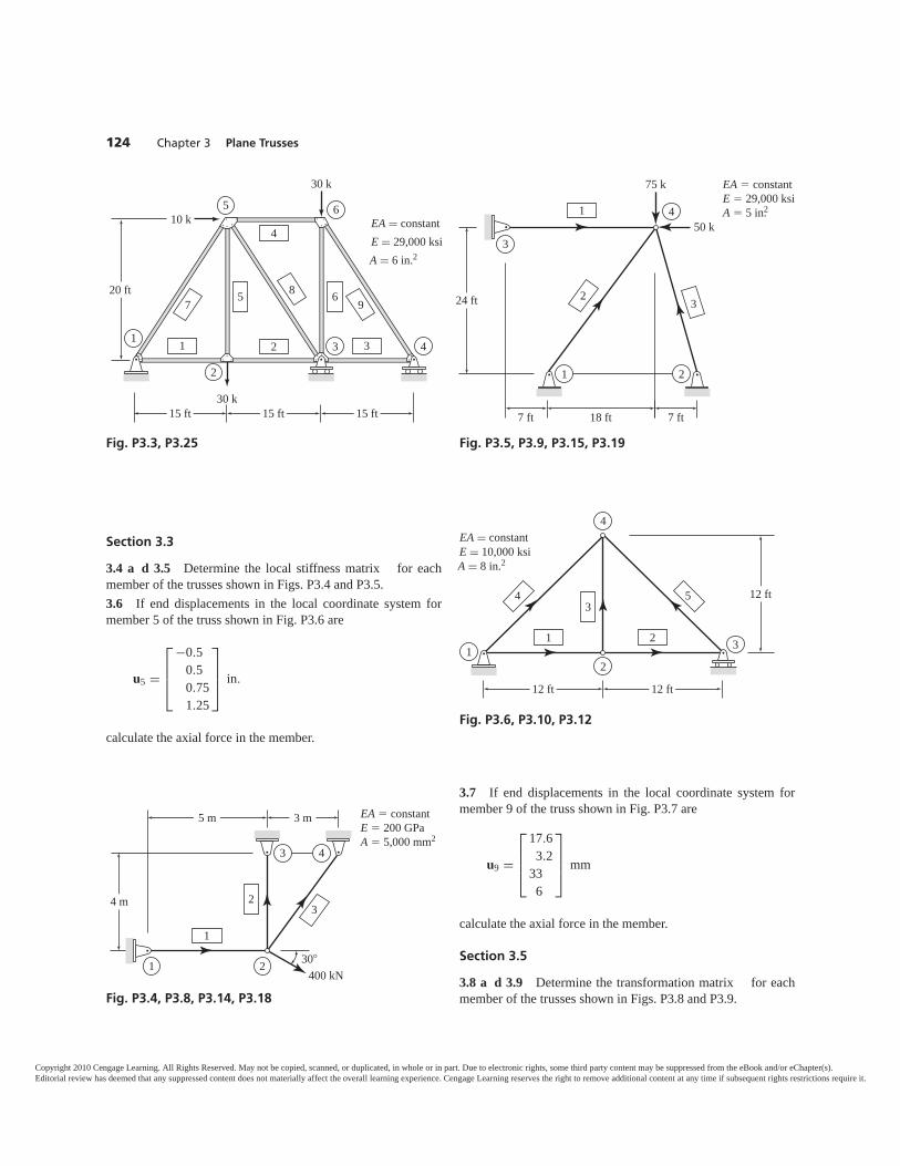
3.7 If end displacements in the local coordinate system formember 9 of the truss shown in Fig. P3.7 are
u9 =
⎡⎢⎢⎣
17.63.2
336
⎤⎥⎥⎦ mm
calculate the axial force in the member.
Section 3.5
3.8 a d 3.9 Determine the transformation matrix for eachmember of the trusses shown in Figs. P3.8 and P3.9.
124 Chapter 3 Plane Trusses
3
4
21
7 ft7 ft 18 ft
1
23
EA � constantE � 29,000 ksiA � 5 in.2
24 ft
75 k
50 k
Fig. P3.5, P3.9, P3.15, P3.19
21 3
4
12 ft
12 ft
12 ft
EA � constantE � 10,000 ksiA � 8 in.2
21
34 5
Fig. P3.6, P3.10, P3.12
5
2
6
3 41
3
30 k
30 k
10 k
15 ft
20 ft
15 ft 15 ft
EA � constantE � 29,000 ksiA � 6 in.2
1 2
5 6
4
7 98
Fig. P3.3, P3.25
1 2
3
5 m 3 m
4 m
1
3
4
2
400 kN30�
EA � constantE � 200 GPaA � 5,000 mm2
Fig. P3.4, P3.8, P3.14, P3.18
Section 3.3
3.4 a d 3.5 Determine the local stiffness matrix for eachmember of the trusses shown in Figs. P3.4 and P3.5.3.6 If end displacements in the local coordinate system formember 5 of the truss shown in Fig. P3.6 are
u5 =
⎡⎢⎢⎣
−0.50.50.751.25
⎤⎥⎥⎦ in.
calculate the axial force in the member.
Copyright 2010 Cengage Learning. All Rights Reserved. May not be copied, scanned, or duplicated, in whole or in part. Due to electronic rights, some third party content may be suppressed from the eBook and/or eChapter(s).Editorial review has deemed that any suppressed content does not materially affect the overall learning experience. Cengage Learning reserves the right to remove additional content at any time if subsequent rights restrictions require it.
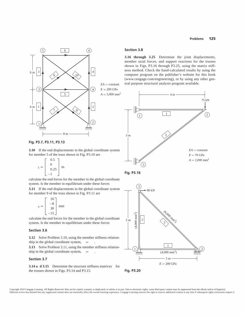
Section 3.8
3.16 through 3.25 Determine the joint displacements,member axial forces, and support reactions for the trussesshown in Figs. P3.16 through P3.25, using the matrix stiff-ness method. Check the hand-calculated results by using thecomputer program on the publisher’s website for this book(www.cengage.com/engineering), or by using any other gen-eral purpose structural analysis program available.
Problems 125
1
5
6
EA � constantE � 200 GPaA � 5,000 mm2
4
2
3
5 6
6 m
6 m
8 m
3
1
4109
872
Fig. P3.7, P3.11, P3.13
21
3
3 m
75 kN
4 m
EA � constantE � 70 GPaA � 2,000 mm2
1
2
Fig. P3.16
80 kN
21
3
5 m
5 mE � 200 GPa
(4,000 mm2)
(4,0
00 m
m2 ) (6,000 mm 2)
1
23
Fig. P3.20
3.10 If the end displacements in the global coordinate systemfor member 5 of the truss shown in Fig. P3.10 are
5 =
⎡⎢⎢⎣
0.500.25
−1
⎤⎥⎥⎦ in.
calculate the end forces for the member in the global coordinatesystem. Is the member in equilibrium under these forces3.11 If the end displacements in the global coordinate systemfor member 9 of the truss shown in Fig. P3.11 are
9 =
⎡⎢⎢⎣
16−830
−15
⎤⎥⎥⎦ mm
calculate the end forces for the member in the global coordinatesystem. Is the member in equilibrium under these forces
Section 3.6
3.12 Solve Problem 3.10, using the member stiffness relation-ship in the global coordinate system, = .3.13 Solve Problem 3.11, using the member stiffness relation-ship in the global coordinate system, = .
Section 3.7
3.14 a d 3.15 Determine the structure stiffness matrices forthe trusses shown in Figs. P3.14 and P3.15.
Copyright 2010 Cengage Learning. All Rights Reserved. May not be copied, scanned, or duplicated, in whole or in part. Due to electronic rights, some third party content may be suppressed from the eBook and/or eChapter(s).Editorial review has deemed that any suppressed content does not materially affect the overall learning experience. Cengage Learning reserves the right to remove additional content at any time if subsequent rights restrictions require it.
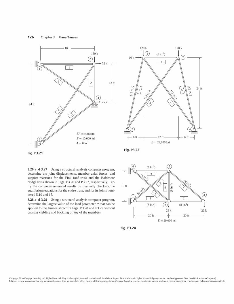
126 Chapter 3 Plane Trusses
1
E = 29,000 ksi
4 5
2
3
20 ft20 ft
(8 in.2)
(6 in. 2) (8 in. 2)
(6 in
.2 )
(6 in.2 )
(8 in.2) (8 in.2)
25 k 25 k
16 ft
15
7
46
2
3
Fig. P3.24
1
E � 29,000 ksi
4
2
3
24 ft
6 ft 6 ft12 ft
(8 in.2)
(12
in.2 ) (12 in. 2)
(12 i
n.2 ) (12 in. 2)
120 k
60 k
120 k
1
2 5
43
Fig. P3.22
2
1
3
4
12 ft
24 ft
16 ft
75 k
150 k
75 k
EA � constantE � 10,000 ksiA � 6 in.2
1
23
45
Fig. P3.21
3.26 a d 3.27 Using a structural analysis computer program,determine the joint displacements, member axial forces, andsupport reactions for the Fink roof truss and the Baltimorebridge truss shown in Figs. P3.26 and P3.27, respectively. er-ify the computer-generated results by manually checking theequilibrium equations for the entire truss, and for its joints num-bered 5,10 and 15.3.28 a d 3.29 Using a structural analysis computer program,determine the largest value of the load parameter P that can beapplied to the trusses shown in Figs. P3.28 and P3.29 withoutcausing yielding and buckling of any of the members.
Copyright 2010 Cengage Learning. All Rights Reserved. May not be copied, scanned, or duplicated, in whole or in part. Due to electronic rights, some third party content may be suppressed from the eBook and/or eChapter(s).Editorial review has deemed that any suppressed content does not materially affect the overall learning experience. Cengage Learning reserves the right to remove additional content at any time if subsequent rights restrictions require it.
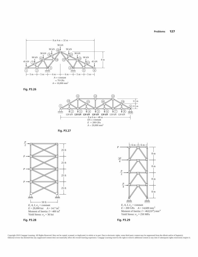
Problems 127
1 23
14 15745 kN
89
1011
1213
654
5 m5 m6 m6 m5 m5 mA � constant� 70 GPa
A � 10,000 mm2
90 kN90 kN
90 kN90 kN
90 kN90 kN
90 kN45 kN
8 m
8 at 4 m � 32 m
Fig. P3.26
1
10
2
9
EA � constantE � 200 GPaA � 20,000 mm2
14
131211
15 16
120 kN 120 kN120 kN 120 kN120 kN 120 kN120 kN8 at 6 m = 48 m
120 kN120 kN 120 kN 120 kN3 4 5 6 7 8
3.5 m
3.5 m
Fig. P3.27
25 ft
25 ft
25 ft
25 ft
50 ftE, A, I, σy = constantE = 29,000 ksi A = 14.7 in.2Moment of Inertia: I = 400 in.4Yield Stress: σ y = 36 ksi
P—2
P
P
P
Fig. P3.28
8 m
8 m
8 m
8 m
6 m6 mP
3P—4
P—2
P—4
E, A, I, σ y = constantE = 200 GPa A = 14,600 mm2
Moment of Inertia: I = 462(106) mm4
Yield Stress: σ y = 250 MPa
Fig. P3.29
Copyright 2010 Cengage Learning. All Rights Reserved. May not be copied, scanned, or duplicated, in whole or in part. Due to electronic rights, some third party content may be suppressed from the eBook and/or eChapter(s).Editorial review has deemed that any suppressed content does not materially affect the overall learning experience. Cengage Learning reserves the right to remove additional content at any time if subsequent rights restrictions require it.
128
4 4.1 Data Input4.2 Assignment of Structure Coordinate Numbers4.3 Generation of the Structure Stiffness Matrix4.4 Formation of the Joint Load Vector4.5 Solution for Joint Displacements4.6 Calculation of Member Forces and Support Reactions
SummaryProblems
COMPUTER PROGRAM FORANALYSIS OF PLANE TRUSSES
Truss Bridge(Capricornis Photographic Inc. / Shutterstock)
Copyright 2010 Cengage Learning. All Rights Reserved. May not be copied, scanned, or duplicated, in whole or in part. Due to electronic rights, some third party content may be suppressed from the eBook and/or eChapter(s).Editorial review has deemed that any suppressed content does not materially affect the overall learning experience. Cengage Learning reserves the right to remove additional content at any time if subsequent rights restrictions require it.
Section 4.1 Data Input 129
In the previous chapter, we studied the basic principles of the analysis of planetrusses by the matrix stiffness method. In this chapter, we consider the com-puter implementation of the foregoing method of analysis. Our objective is todevelop a general computer program that can be used to analyze any staticallydeterminate or indeterminate plane truss, of any arbitrary configuration, sub-jected to any system of joint loads.
From a programming viewpoint, it is generally convenient to divide astructural analysis program into two parts or modules: (a) input module, and(b) analysis module (Fig. 4.1). The input module reads, and stores into thecomputer’s memory, the structural and loading data necessary for the analysis;the analysis module uses the input data to perform the analysis, and communi-cates the results back to the user via an output device, such as a printer or amonitor. The development of a relatively simple input module is presented inSection 4.1; in the following five sections (4.2 through 4.6), we considerprogramming of the five analysis steps discussed in Chapter 3 (Fig. 3.20). Thetopics covered in these sections are as follows: assignment of the degree-of-freedom and restrained coordinate numbers for plane trusses (Section 4.2);generation of the structure stiffness matrix by assembling the elements of themember stiffness matrices (Section 4.3); formation of the joint load vector(Section 4.4); solution of the structure stiffness equations to obtain joint dis-placements (Section 4.5); and, finally, evaluation of the member axial forcesand support reactions (Section 4.6).
The entire programming process is described by means of detailed flow-charts, so that readers can write this computer program in any programminglanguage. It is important to realize that the programming process presented inthis chapter represents only one of many ways in which the matrix stiffnessmethod of analysis can be implemented on computers. Readers are stronglyencouraged to conceive, and attempt, alternative strategies that can make thecomputer implementation (and/or application of the method) more efficient.One such strategy, which takes advantage of the banded form of the structurestiffness matrix, will be discussed in Chapter 9.
4.1 DATA INPUTIn this section, we focus our attention on the input module of our computerprogram. As stated previously, the input module of a structural analysis pro-gram reads the structural and loading data necessary for analysis from a fileor another type of input device, and stores it in the computer’s memory so thatit can be processed conveniently by the program for structural analysis.
Structural Analysis Program
Input Module Analysis Module
Fig. 4.1
Copyright 2010 Cengage Learning. All Rights Reserved. May not be copied, scanned, or duplicated, in whole or in part. Due to electronic rights, some third party content may be suppressed from the eBook and/or eChapter(s).Editorial review has deemed that any suppressed content does not materially affect the overall learning experience. Cengage Learning reserves the right to remove additional content at any time if subsequent rights restrictions require it.
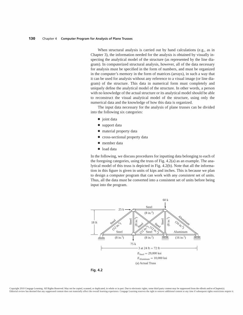
130 Chapter 4 Computer Program for Analysis of Plane Trusses
When structural analysis is carried out by hand calculations (e.g., as inChapter 3), the information needed for the analysis is obtained by visually in-specting the analytical model of the structure (as represented by the line dia-gram). In computerized structural analysis, however, all of the data necessaryfor analysis must be specified in the form of numbers, and must be organizedin the computer’s memory in the form of matrices (arrays), in such a way thatit can be used for analysis without any reference to a visual image (or line dia-gram) of the structure. This data in numerical form must completely anduniquely define the analytical model of the structure. In other words, a personwith no knowledge of the actual structure or its analytical model should be ableto reconstruct the visual analytical model of the structure, using only thenumerical data and the knowledge of how this data is organized.
The input data necessary for the analysis of plane trusses can be dividedinto the following six categories:
● joint data● support data● material property data● cross-sectional property data● member data● load data
In the following, we discuss procedures for inputting data belonging to each ofthe foregoing categories, using the truss of Fig. 4.2(a) as an example. The ana-lytical model of this truss is depicted in Fig. 4.2(b). Note that all the informa-tion in this figure is given in units of kips and inches. This is because we planto design a computer program that can work with any consistent set of units.Thus, all the data must be converted into a consistent set of units before beinginput into the program.
18 ft
3 at 24 ft � 72 ftESteel � 29,000 ksiEAluminum � 10,000 ksi
(8 in.2)(8 in.2) (16 in.2)
(16 in. 2)
Aluminum
(8 in.2)
(8 in
.2 )
75 k
25 k
60 k
Steel
SteelSteel Aluminum
Stee
l
(12 in.2 )Stee
l
(12 in.2 )Stee
l(12 in. 2)
Steel (8 in
.2 )
Stee
l
(a) Actual Truss
Fig. 4.2
Copyright 2010 Cengage Learning. All Rights Reserved. May not be copied, scanned, or duplicated, in whole or in part. Due to electronic rights, some third party content may be suppressed from the eBook and/or eChapter(s).Editorial review has deemed that any suppressed content does not materially affect the overall learning experience. Cengage Learning reserves the right to remove additional content at any time if subsequent rights restrictions require it.
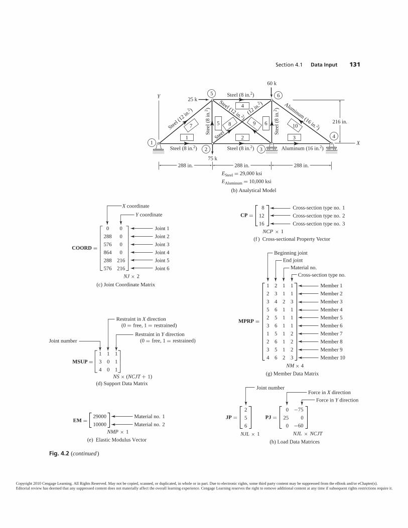
Section 4.1 Data Input 131
216 in.
288 in.288 in. 288 in.ESteel = 29,000 ksiEAluminum = 10,000 ksi
Steel (8 in.2)Steel (8 in.2)
Steel (8 in.2)
Stee
l (8
in.2 )
Stee
l (8
in.2 )
Aluminum (16 in.2)
Aluminum (16 in. 2)
75 k
25 k
60 k
Steel (1
2 in.2 )
Steel
(12 in.2 )Steel (12 in. 2)
Y
X
65
12 3
4
(b) Analytical Model
321
4
65 9 1087
Fig. 4.2 (continued )
X coordinateY coordinate
COORD =
⎡⎢⎢⎢⎢⎢⎢⎢⎢⎣
0 0288 0576 0864 0288 216576 216
⎤⎥⎥⎥⎥⎥⎥⎥⎥⎦
Joint 1Joint 2Joint 3Joint 4Joint 5Joint 6
NJ × 2(c) Joint Coordinate Matrix
Joint number⎡⎢⎣
1 1 13 0 14 0 1
⎤⎥⎦MSUP =
Restraint in Y direction (0 = free, 1 = restrained)
Restraint in X direction (0 = free, 1 = restrained)
NS × (NCJT + 1)(d) Support Data Matrix
EM = 2900010000
Material no. 1Material no. 2
NMP × 1(e) Elastic Modulus Vector
NCP × 1
CP =8
1216
Cross-section type no. 1Cross-section type no. 2Cross-section type no. 3
(f ) Cross-sectional Property Vector
NM × 4
Beginning jointEnd joint
Material no.Cross-section type no.
MPRP =
1 2 1 12 3 1 13 4 2 35 6 1 12 5 1 13 6 1 11 5 1 22 6 1 23 5 1 24 6 2 3
Member 1Member 2Member 3Member 4Member 5Member 6Member 7Member 8Member 9Member 10
(g) Member Data Matrix
Joint numberForce in X direction
Force in Y direction
JP =256
PJ =0
25 00
NJL × 1 NJL × NCJT(h) Load Data Matrices
−75
−60
Copyright 2010 Cengage Learning. All Rights Reserved. May not be copied, scanned, or duplicated, in whole or in part. Due to electronic rights, some third party content may be suppressed from the eBook and/or eChapter(s).Editorial review has deemed that any suppressed content does not materially affect the overall learning experience. Cengage Learning reserves the right to remove additional content at any time if subsequent rights restrictions require it.
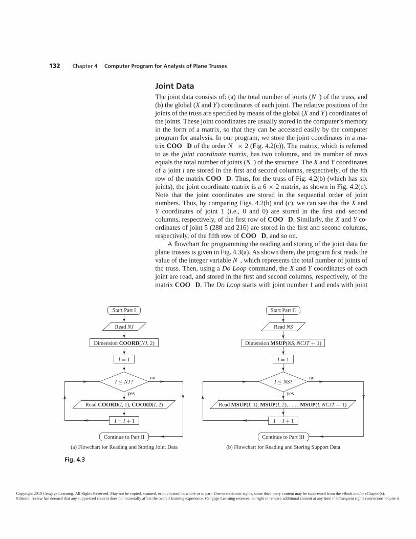
132 Chapter 4 Computer Program for Analysis of Plane Trusses
Joint DataThe joint data consists of: (a) the total number of joints (N ) of the truss, and(b) the global (X and Y ) coordinates of each joint. The relative positions of thejoints of the truss are specified by means of the global (X and Y ) coordinates ofthe joints. These joint coordinates are usually stored in the computer’s memoryin the form of a matrix, so that they can be accessed easily by the computerprogram for analysis. In our program, we store the joint coordinates in a ma-trix COO D of the order N × 2 (Fig. 4.2(c)). The matrix, which is referredto as the joint coordinate matrix, has two columns, and its number of rowsequals the total number of joints (N ) of the structure. The X and Y coordinatesof a joint i are stored in the first and second columns, respectively, of the ithrow of the matrix COO D. Thus, for the truss of Fig. 4.2(b) (which has sixjoints), the joint coordinate matrix is a 6 × 2 matrix, as shown in Fig. 4.2(c).Note that the joint coordinates are stored in the sequential order of jointnumbers. Thus, by comparing Figs. 4.2(b) and (c), we can see that the X andY coordinates of joint 1 (i.e., 0 and 0) are stored in the first and secondcolumns, respectively, of the first row of COO D. Similarly, the X and Y co-ordinates of joint 5 (288 and 216) are stored in the first and second columns,respectively, of the fifth row of COO D, and so on.
A flowchart for programming the reading and storing of the joint data forplane trusses is given in Fig. 4.3(a). As shown there, the program first reads thevalue of the integer variable N , which represents the total number of joints ofthe truss. Then, using a Do Loop command, the X and Y coordinates of eachjoint are read, and stored in the first and second columns, respectively, of thematrix COO D. The Do Loop starts with joint number 1 and ends with joint
Read NJ
I = 1
Dimension COORD(NJ, 2)
yes
noI ≤ NJ?
Read COORD(I, 1), COORD(I, 2)
I = I + 1
(a) Flowchart for Reading and Storing Joint Data
Start Part I
Continue to Part II
Read NS
I = 1
Dimension MSUP(NS, NCJT + 1)
yes
noI ≤ NS?
Read MSUP(I, 1), MSUP(I, 2), . . . , MSUP(I, NCJT + 1)
I = I + 1
(b) Flowchart for Reading and Storing Support Data
Start Part II
Continue to Part III
Fig. 4.3
Copyright 2010 Cengage Learning. All Rights Reserved. May not be copied, scanned, or duplicated, in whole or in part. Due to electronic rights, some third party content may be suppressed from the eBook and/or eChapter(s).Editorial review has deemed that any suppressed content does not materially affect the overall learning experience. Cengage Learning reserves the right to remove additional content at any time if subsequent rights restrictions require it.
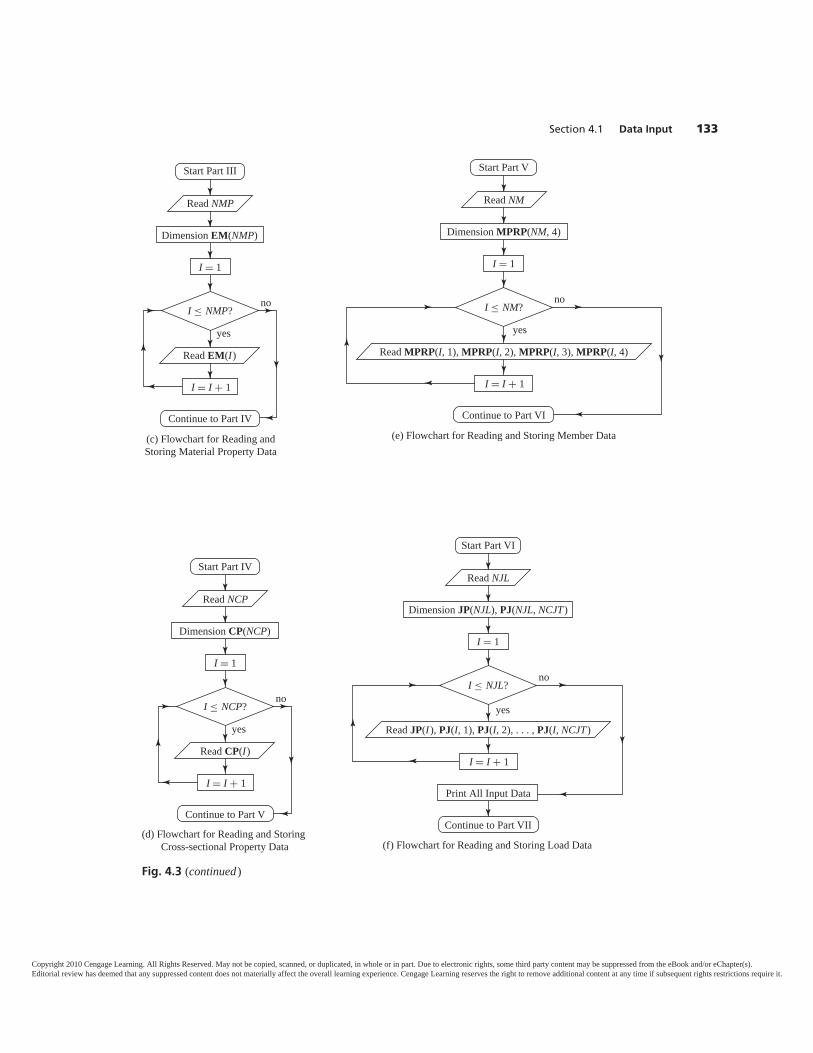
Section 4.1 Data Input 133
Read NMP
I = 1
Dimension EM(NMP)
yes
noI ≤ NMP?
Read EM(I)
I = I + 1
(c) Flowchart for Reading andStoring Material Property Data
Start Part III
Continue to Part IV
Read NCP
I = 1
Dimension CP(NCP)
yes
noI ≤ NCP?
Read CP(I)
I = I + 1
(d) Flowchart for Reading and Storing Cross-sectional Property Data
Start Part IV
Continue to Part V
Read NM
I = 1
Dimension MPRP(NM, 4)
yes
noI ≤ NM?
Read MPRP(I, 1), MPRP(I, 2), MPRP(I, 3), MPRP(I, 4)
I = I + 1
(e) Flowchart for Reading and Storing Member Data
Start Part V
Continue to Part VI
Fig. 4.3 (continued)
Read NJL
I = 1
yes
noI ≤ NJL?
Read JP(I ), PJ(I, 1), PJ(I, 2), . . . , PJ(I, NCJT)
I = I + 1
Print All Input Data
Dimension JP(NJL), PJ(NJL, NCJT)
(f) Flowchart for Reading and Storing Load Data
Start Part VI
Continue to Part VII
Copyright 2010 Cengage Learning. All Rights Reserved. May not be copied, scanned, or duplicated, in whole or in part. Due to electronic rights, some third party content may be suppressed from the eBook and/or eChapter(s).Editorial review has deemed that any suppressed content does not materially affect the overall learning experience. Cengage Learning reserves the right to remove additional content at any time if subsequent rights restrictions require it.
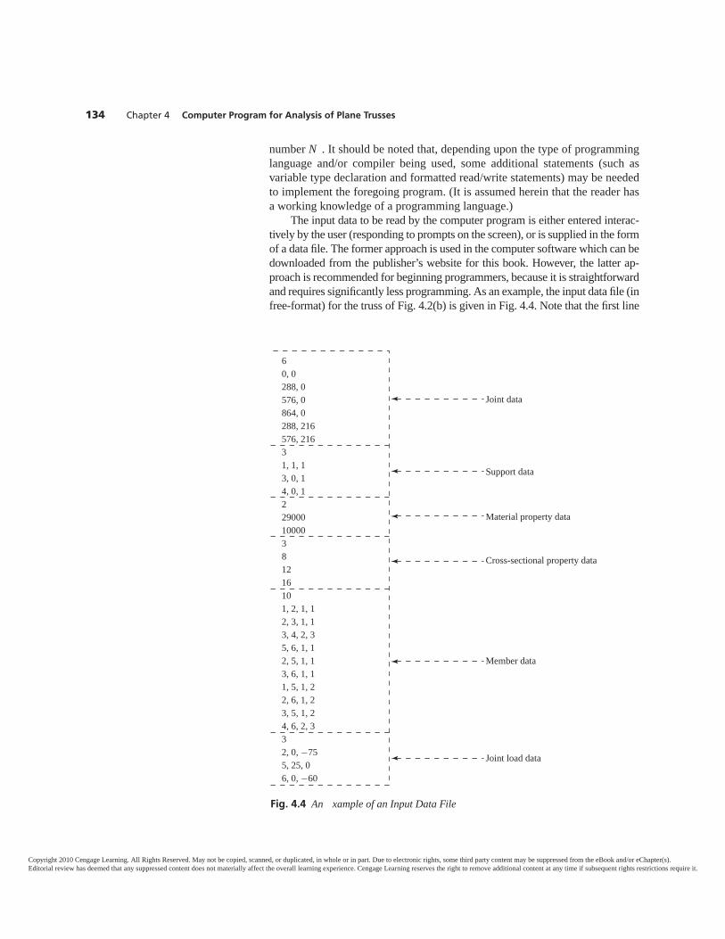
134 Chapter 4 Computer Program for Analysis of Plane Trusses
number N . It should be noted that, depending upon the type of programminglanguage and/or compiler being used, some additional statements (such asvariable type declaration and formatted read/write statements) may be neededto implement the foregoing program. (It is assumed herein that the reader hasa working knowledge of a programming language.)
The input data to be read by the computer program is either entered interac-tively by the user (responding to prompts on the screen), or is supplied in the formof a data file. The former approach is used in the computer software which can bedownloaded from the publisher’s website for this book. However, the latter ap-proach is recommended for beginning programmers, because it is straightforwardand requires significantly less programming. As an example, the input data file (infree-format) for the truss of Fig. 4.2(b) is given in Fig. 4.4. Note that the first line
60, 0288, 0576, 0864, 0288, 216576, 21631, 1, 13, 0, 14, 0, 122900010000381216101, 2, 1, 12, 3, 1, 13, 4, 2, 35, 6, 1, 12, 5, 1, 13, 6, 1, 11, 5, 1, 22, 6, 1, 23, 5, 1, 24, 6, 2, 332, 0, −755, 25, 06, 0, −60
Joint data
Support data
Material property data
Cross-sectional property data
Member data
Joint load data
Fig. 4.4 An xample of an Input Data File
Copyright 2010 Cengage Learning. All Rights Reserved. May not be copied, scanned, or duplicated, in whole or in part. Due to electronic rights, some third party content may be suppressed from the eBook and/or eChapter(s).Editorial review has deemed that any suppressed content does not materially affect the overall learning experience. Cengage Learning reserves the right to remove additional content at any time if subsequent rights restrictions require it.
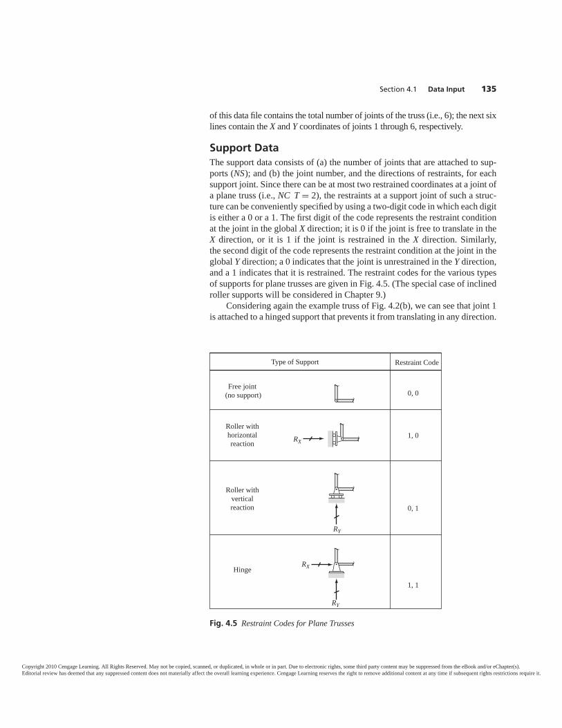
Section 4.1 Data Input 135
of this data file contains the total number of joints of the truss (i.e., 6); the next sixlines contain the X and Y coordinates of joints 1 through 6, respectively.
Support DataThe support data consists of (a) the number of joints that are attached to sup-ports (NS); and (b) the joint number, and the directions of restraints, for eachsupport joint. Since there can be at most two restrained coordinates at a joint ofa plane truss (i.e., NC T = 2), the restraints at a support joint of such a struc-ture can be conveniently specified by using a two-digit code in which each digitis either a 0 or a 1. The first digit of the code represents the restraint conditionat the joint in the global X direction; it is 0 if the joint is free to translate in theX direction, or it is 1 if the joint is restrained in the X direction. Similarly,the second digit of the code represents the restraint condition at the joint in theglobal Y direction; a 0 indicates that the joint is unrestrained in the Y direction,and a 1 indicates that it is restrained. The restraint codes for the various typesof supports for plane trusses are given in Fig. 4.5. (The special case of inclinedroller supports will be considered in Chapter 9.)
Considering again the example truss of Fig. 4.2(b), we can see that joint 1is attached to a hinged support that prevents it from translating in any direction.
Type of Support Restraint Code
Free joint (no support)
Roller withhorizontalreaction
Roller withverticalreaction
Hinge
0, 0
1, 0
0, 1
1, 1
RY
RX
RX
RY
Fig. 4.5 Restraint Codes for Plane Trusses
Copyright 2010 Cengage Learning. All Rights Reserved. May not be copied, scanned, or duplicated, in whole or in part. Due to electronic rights, some third party content may be suppressed from the eBook and/or eChapter(s).Editorial review has deemed that any suppressed content does not materially affect the overall learning experience. Cengage Learning reserves the right to remove additional content at any time if subsequent rights restrictions require it.
136 Chapter 4 Computer Program for Analysis of Plane Trusses
Thus, the restraint code for joint 1 is 1,1 indicating that this joint is restrainedfrom translating in both the X and Y directions. Similarly, the restraint codes forjoints 3 and 4, which are attached to roller supports, are 0,1 because thesejoints are free to translate in the horizontal (X) direction, but are restrained bythe rollers from translating in the vertical (Y) direction. The restraint codes ofthe remaining joints of the truss, which are free to translate in any direction,can be considered to be 0,0. However, it is not necessary to input codes for freejoints, because the computer program considers every joint to be free, unless itis identified as a support joint.
The support data can be stored in the computer’s memory in the form ofan integer matrix P of order NS × (NC T + 1) (Fig. 4.2(d)). For planetrusses, because NC T = 2, the support data matrix P consists of threecolumns, with the number of rows equal to the number of support joints (NS).In each row of P, the support joint number is stored in the first column,and the first and second digits of the corresponding restraint code are stored inthe second and third columns, respectively. Thus, for the truss of Fig. 4.2(b),which has three support joints, the support data matrix is a 3 × 3 matrix, asshown in Fig. 4.2(d). Note that in the first row of P the support jointnumber 1 is stored in the first column, and the first and second digits of the re-straint code for this joint (i.e., 1 and 1) are stored in the second and thirdcolumns, respectively. Similarly, the second row of P consists of thesupport joint number 3 in the first column, and the two digits of the corre-sponding restraint code (i.e., 0 and 1) in the second and third columns, re-spectively, and so on.
A flowchart for programming the reading and storing of the support data isgiven in Fig. 4.3(b), in which, as noted previously, the integer variable NC Tdenotes the number of structure coordinates per joint. Like this flowchart, manyparts of the computer program presented in this chapter are given in a generalform in terms of the variable NC T, so that they can be conveniently incorpo-rated into computer programs for analyzing other types of framed structures(e.g., beams and plane frames), which are considered in subsequent chapters.For example, as discussed in this section, by setting NC T = 2, the flowchartof Fig. 4.3(b) can be used to input support data for plane trusses; whereas, asdiscussed subsequently in Chapter 6, the same flowchart can be used to inputsupport data for plane frames, provided NC T is set equal to three.
An example of how the support data for a plane truss may appear in aninput data file is given in Fig. 4.4.
Material Property DataThe material property data involves (a) the number of materials used inthe structure (NMP), and (b) the modulus of elasticity ( ) of each material. Theelastic moduli are stored by the program in an elastic modulus vector . Thenumber of rows of equals the number of materials (NMP), with the elasticmodulus of material i stored in the ith row of the vector (Fig. 4.2(e)).
Consider, for example, the truss of Fig. 4.2(b). The truss is composed oftwo materials; namely, steel and aluminum. We arbitrarily select the steel( = 29,000 ksi) to be material number 1, and the aluminum ( = 10,000 ksi)
Copyright 2010 Cengage Learning. All Rights Reserved. May not be copied, scanned, or duplicated, in whole or in part. Due to electronic rights, some third party content may be suppressed from the eBook and/or eChapter(s).Editorial review has deemed that any suppressed content does not materially affect the overall learning experience. Cengage Learning reserves the right to remove additional content at any time if subsequent rights restrictions require it.

Section 4.1 Data Input 137
to be material number 2. Thus, the elastic modulus vector, , of the trussconsists of two rows, as shown in Fig. 4.2(e); the elastic modulus of materialnumber 1 (i.e., 29,000) is stored in the first row of , and the elastic modu-lus of material number 2 (i.e., 10,000) is stored in the second row.
Figure 4.3(c) shows a flowchart for programming the reading and storingof the material property data; Fig. 4.4 illustrates how this type of data may ap-pear in an input data file.
Cross-Sectional Property DataThe cross-sectional property data consists of (a) the number of different cross-section types used for the truss members (NCP); and (b) the cross-sectionalarea (A) for each cross-section type. The cross-sectional areas are stored by theprogram in a cross-sectional property vector CP. The number of rows of CPequals the number of cross-section types (NCP), with the area of cross-sectioni stored in the ith row of the vector (Fig. 4.2(f)).
For example, three types of member cross-sections are used for the trussof Fig. 4.2(b). We arbitrarily assign the numbers 1, 2, and 3 to the cross-sections with areas of 8, 12, and 16 in.2, respectively. Thus, the cross-sectionalproperty vector, CP, consists of three rows; areas of cross-section types 1, 2,and 3 are stored in rows 1, 2, and 3, respectively, as shown in Fig. 4.2(f).
A flowchart for reading and storing the cross-sectional property data intocomputer memory is given in Fig. 4.3(d); Fig. 4.4 shows an example of aninput data file containing this type of data.
Member DataThe member data consists of (a) the total number of members (NM) of thetruss; and (b) for each member, the beginning joint number, the end joint num-ber, the material number, and the cross-section type number.
The member data can be stored in computer memory in the form of aninteger member data matrix, P P, of order NM × 4 (Fig. 4.2(g)). The in-formation corresponding to a member i is stored in the ith row of P P; itsbeginning and end joint numbers are stored in the first and second columns, re-spectively, and the material and cross-section numbers are stored in the thirdand fourth columns, respectively.
For example, since the truss of Fig. 4.2(b) has 10 members, its memberdata matrix is a 10 × 4 matrix, as shown in Fig. 4.2(g). From Fig. 4.2(b), wecan see that the beginning and end joints for member 1 are 1 and 2, respec-tively; the material and cross-section numbers for this member are 1 and 1,respectively. Thus, the numbers 1, 2, 1, and 1 are stored in columns 1through 4, respectively, of the first row of P P, as shown in Fig. 4.2(g).Similarly, we see from Fig. 4.2(b) that the beginning joint, end joint, mater-ial, and cross-section numbers for member 3 are 3, 4, 2, and 3, respectively,and they are stored, respectively, in columns 1 through 4 of row 3 of P P,and so on.
Figure 4.3(e) shows a flowchart for programming the reading and storingof the member data. An example of how member data may appear in an inputdata file is given in Fig. 4.4.
Copyright 2010 Cengage Learning. All Rights Reserved. May not be copied, scanned, or duplicated, in whole or in part. Due to electronic rights, some third party content may be suppressed from the eBook and/or eChapter(s).Editorial review has deemed that any suppressed content does not materially affect the overall learning experience. Cengage Learning reserves the right to remove additional content at any time if subsequent rights restrictions require it.
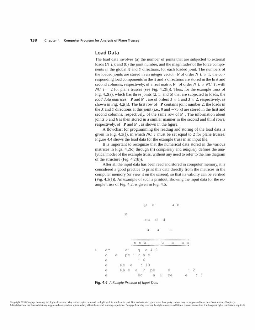
138 Chapter 4 Computer Program for Analysis of Plane Trusses
Load DataThe load data involves (a) the number of joints that are subjected to externalloads (N L); and (b) the joint number, and the magnitudes of the force compo-nents in the global X and Y directions, for each loaded joint. The numbers ofthe loaded joints are stored in an integer vector P of order N L × 1; the cor-responding load components in the X and Y directions are stored in the first andsecond columns, respectively, of a real matrix P of order N L × NC T, withNC T = 2 for plane trusses (see Fig. 4.2(h)). Thus, for the example truss ofFig. 4.2(a), which has three joints (2, 5, and 6) that are subjected to loads, theload data matrices, P and P , are of orders 3 × 1 and 3 × 2, respectively, asshown in Fig. 4.2(h). The first row of P contains joint number 2; the loads inthe X and Y directions at this joint (i.e., 0 and −75 k) are stored in the first andsecond columns, respectively, of the same row of P . The information aboutjoints 5 and 6 is then stored in a similar manner in the second and third rows,respectively, of P and P , as shown in the figure.
A flowchart for programming the reading and storing of the load data isgiven in Fig. 4.3(f), in which NC T must be set equal to 2 for plane trusses.Figure 4.4 shows the load data for the example truss in an input file.
It is important to recognize that the numerical data stored in the variousmatrices in Figs. 4.2(c) through (h) completely and uniquely defines the ana-lytical model of the example truss, without any need to refer to the line diagramof the structure (Fig. 4.2(b)).
After all the input data has been read and stored in computer memory, it isconsidered a good practice to print this data directly from the matrices in thecomputer memory (or view it on the screen), so that its validity can be verified(Fig. 4.3(f)). An example of such a printout, showing the input data for the ex-ample truss of Fig. 4.2, is given in Fig. 4.6.
p e a e
M ec d d
a a a
e e a c a a aP ec e: g e 4-2
c e pe : P a e e : 6e Me e : 10e Ma e a P pe e : 2e - ec a P pe e : 3
Fig. 4.6 A Sample Printout of Input Data
Copyright 2010 Cengage Learning. All Rights Reserved. May not be copied, scanned, or duplicated, in whole or in part. Due to electronic rights, some third party content may be suppressed from the eBook and/or eChapter(s).Editorial review has deemed that any suppressed content does not materially affect the overall learning experience. Cengage Learning reserves the right to remove additional content at any time if subsequent rights restrictions require it.
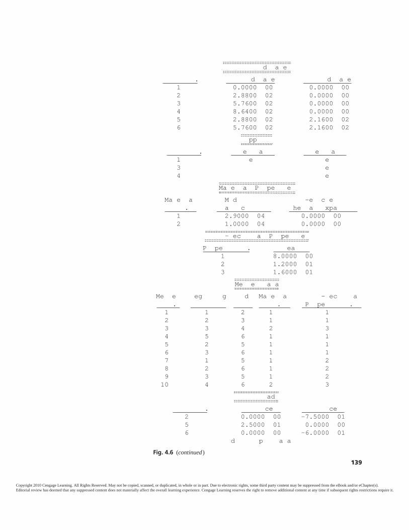
d a e . d a e d a e
1 0.0000 00 0.0000 002 2.8800 02 0.0000 003 5.7600 02 0.0000 004 8.6400 02 0.0000 005 2.8800 02 2.1600 026 5.7600 02 2.1600 02
pp . e a e a
1 e e3 e4 e
Ma e a P pe eMa e a M d -e c e
. a c he a xpa1 2.9000 04 0.0000 002 1.0000 04 0.0000 00
- ec a P pe eP pe . ea
1 8.0000 002 1.2000 013 1.6000 01
Me e a aMe e eg g d Ma e a - ec a
. . P pe .1 1 2 1 12 2 3 1 13 3 4 2 34 5 6 1 15 2 5 1 16 3 6 1 17 1 5 1 28 2 6 1 29 3 5 1 210 4 6 2 3
ad . ce ce
2 0.0000 00 -7.5000 015 2.5000 01 0.0000 006 0.0000 00 -6.0000 01
d p a a Fig. 4.6 (continued)
139
Copyright 2010 Cengage Learning. All Rights Reserved. May not be copied, scanned, or duplicated, in whole or in part. Due to electronic rights, some third party content may be suppressed from the eBook and/or eChapter(s).Editorial review has deemed that any suppressed content does not materially affect the overall learning experience. Cengage Learning reserves the right to remove additional content at any time if subsequent rights restrictions require it.
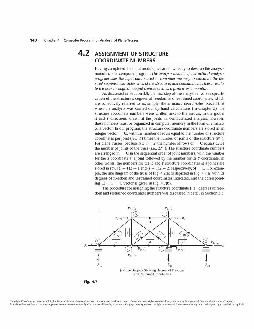
140 Chapter 4 Computer Program for Analysis of Plane Trusses
4.2 ASSIGNMENT OF STRUCTURECOORDINATE NUMBERSHaving completed the input module, we are now ready to develop the analysismodule of our computer program. The analysis module of a structural analysisprogram uses the input data stored in computer memory to calculate the de-sired response characteristics of the structure, and communicates these resultsto the user through an output device, such as a printer or a monitor.
As discussed in Section 3.8, the first step of the analysis involves specifi-cation of the structure’s degrees of freedom and restrained coordinates, whichare collectively referred to as, simply, the structure coordinates. Recall thatwhen the analysis was carried out by hand calculations (in Chapter 3), thestructure coordinate numbers were written next to the arrows, in the globalX and Y directions, drawn at the joints. In computerized analysis, however,these numbers must be organized in computer memory in the form of a matrixor a vector. In our program, the structure coordinate numbers are stored in aninteger vector C, with the number of rows equal to the number of structurecoordinates per joint (NC T ) times the number of joints of the structure (N ).For plane trusses, because NC T = 2, the number of rows of C equals twicethe number of joints of the truss (i.e., 2N ). The structure coordinate numbersare arranged in C in the sequential order of joint numbers, with the numberfor the X coordinate at a joint followed by the number for its Y coordinate. Inother words, the numbers for the X and Y structure coordinates at a joint i arestored in rows (i − 1)2 + 1 and (i − 1)2 + 2, respectively, of C. For exam-ple, the line diagram of the truss of Fig. 4.2(a) is depicted in Fig. 4.7(a) with itsdegrees of freedom and restrained coordinates indicated, and the correspond-ing 12 × 1 C vector is given in Fig. 4.7(b).
The procedure for assigning the structure coordinate (i.e., degrees of free-dom and restrained coordinate) numbers was discussed in detail in Section 3.2.
P2, d2
P5, d5
P1, d1
P4, d4
P3, d3
P6, d6
R9
R10
P8, d8
P7, d7
Y
X
65
1
2 3
4
R11 R12
(a) Line Diagram Showing Degrees of Freedom and Restrained Coordinates
321
4
659 1087
Fig. 4.7
Copyright 2010 Cengage Learning. All Rights Reserved. May not be copied, scanned, or duplicated, in whole or in part. Due to electronic rights, some third party content may be suppressed from the eBook and/or eChapter(s).Editorial review has deemed that any suppressed content does not materially affect the overall learning experience. Cengage Learning reserves the right to remove additional content at any time if subsequent rights restrictions require it.
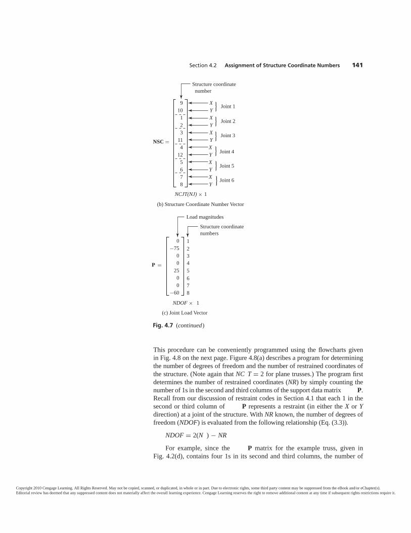
Section 4.2 Assignment of Structure Coordinate Numbers 141
This procedure can be conveniently programmed using the flowcharts givenin Fig. 4.8 on the next page. Figure 4.8(a) describes a program for determiningthe number of degrees of freedom and the number of restrained coordinates ofthe structure. (Note again that NC T = 2 for plane trusses.) The program firstdetermines the number of restrained coordinates (NR) by simply counting thenumber of 1s in the second and third columns of the support data matrix P.Recall from our discussion of restraint codes in Section 4.1 that each 1 in thesecond or third column of P represents a restraint (in either the X or Ydirection) at a joint of the structure. With NR known, the number of degrees offreedom (NDOF) is evaluated from the following relationship (Eq. (3.3)).
NDOF = 2(N ) − NR
For example, since the P matrix for the example truss, given inFig. 4.2(d), contains four 1s in its second and third columns, the number of
910123
114
125678
NSC �
XYXYXYXYXYXY
Joint 1
Joint 2
Joint 3
Joint 4
Joint 5
Joint 6
Structure coordinate number
NCJT(NJ) × 1
(b) Structure Coordinate Number Vector
{{{{{{
0−75
00
2500
−60
P �
12345678
Load magnitudes
NDOF × 1
Structure coordinatenumbers
(c) Joint Load Vector
Fig. 4.7 (continued)
Copyright 2010 Cengage Learning. All Rights Reserved. May not be copied, scanned, or duplicated, in whole or in part. Due to electronic rights, some third party content may be suppressed from the eBook and/or eChapter(s).Editorial review has deemed that any suppressed content does not materially affect the overall learning experience. Cengage Learning reserves the right to remove additional content at any time if subsequent rights restrictions require it.
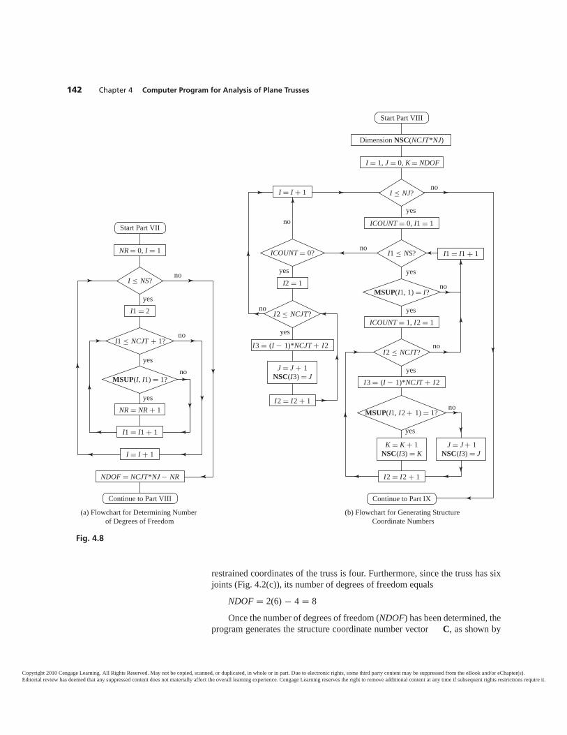
142 Chapter 4 Computer Program for Analysis of Plane Trusses
restrained coordinates of the truss is four. Furthermore, since the truss has sixjoints (Fig. 4.2(c)), its number of degrees of freedom equals
NDOF = 2(6) − 4 = 8Once the number of degrees of freedom (NDOF) has been determined, the
program generates the structure coordinate number vector C, as shown by
NR = 0, I = 1
yes
yes
yes
no
no
no
I ≤ NS?
I1 ≤ NCJT + 1?
MSUP(I, I1) = 1?
I1 = I1 + 1
I = I + 1
I1 = 2
NR = NR + 1
NDOF = NCJT*NJ − NR
(a) Flowchart for Determining Number of Degrees of Freedom
Start Part VII
Continue to Part VIII
I = 1, J = 0, K = NDOF
ICOUNT = 0, I1 = 1
ICOUNT = 1, I2 = 1
K = K + 1NSC(I3) = K
J = J + 1NSC(I3) = J
J = J + 1NSC(I3) = J
I3 = (I − 1)*NCJT + I2
I3 = (I − 1)*NCJT + I2
Dimension NSC(NCJT*NJ)
yes
yes
yes
yes
yes
yes
yes
no
no
no
no
no
no
no
I ≤ NJ?
I2 ≤ NCJT?
I2 ≤ NCJT?
I1 ≤ NS?ICOUNT = 0?
MSUP(I1, I2 + 1) = 1?
I2 = I2 + 1
I2 = I2 + 1
I = I + 1
I2 = 1
I1 = I1 + 1
MSUP(I1, 1) = I?
(b) Flowchart for Generating Structure Coordinate Numbers
Start Part VIII
Continue to Part IX
Fig. 4.8
Copyright 2010 Cengage Learning. All Rights Reserved. May not be copied, scanned, or duplicated, in whole or in part. Due to electronic rights, some third party content may be suppressed from the eBook and/or eChapter(s).Editorial review has deemed that any suppressed content does not materially affect the overall learning experience. Cengage Learning reserves the right to remove additional content at any time if subsequent rights restrictions require it.
Section 4.3 Generation of the Structure Stiffness Matrix 143
the flowchart in Fig. 4.8(b). Again, NC T should be set equal to 2 for planetrusses. As this flowchart indicates, the program uses two integer counters,
and , to keep track of the degrees-of-freedom and restrained coordinatenumbers, respectively. The initial value of is set equal to 0, whereas the ini-tial value of is set equal to NDOF.
The structure coordinates are numbered, one joint at a time, starting atjoint 1 and proceeding sequentially to the joint number N . First, the number ofthe joint under consideration, I, is compared with the numbers in the firstcolumn of the support matrix P to determine whether or not I is a supportjoint. If a match is found between I and one of the numbers in the first columnof P, then the counter ICOUNT is set equal to 1; otherwise, the value ofICOUNT remains 0 as initially assigned.
If joint I is not a support joint (i.e., ICOUNT = 0), then the number for itsdegree of freedom in the X direction is obtained by increasing the degrees-of-freedom counter by 1 (i.e., = + 1), and this value of is stored in rownumber (I − 1)2 + 1 of the C vector. Next, the value of is again increasedby 1 (i.e., = + 1) to obtain the number for the degree of freedom of joint Iin the Y direction, and the new value of is stored in row (I − 1)2 + 2 of the
C vector.If joint I is found to be a support joint (i.e., ICOUNT = 1), then the second
column of the corresponding row of P is checked to determine whetherjoint I is restrained in the X direction. If the joint is restrained in the X direction,then the number for its X-restrained coordinate is obtained by increasing the re-strained coordinate counter by 1 (i.e., = + 1), and this value of isstored in row (I − 1)2 + 1 of the C vector. However, if the joint is not re-strained in the X direction, then the degrees-of-freedom counter is increasedby 1, and its value (instead of that of ) is stored in row (I − 1)2 + 1 of the
C vector. Next, the restraint condition in the Y direction at joint I is deter-mined by checking the third column of the corresponding row of P. If thejoint is found to be restrained, then the counter is increased by 1; otherwise,the counter is increased by the same amount. The new value of either oris then stored in row (I − 1)2 + 2 of the C vector.
The computer program repeats the foregoing procedure for each joint ofthe structure to complete the structure coordinate number vector, C. Asshown in Fig. 4.8(b), this part of the program (for generating structure coordi-nate numbers) can be conveniently coded using Do Loop or For Next types ofprogramming statements.
4.3 GENERATION OF THE STRUCTURESTIFFNESS MATRIXThe structure coordinate number vector C, defined in the preceding section,can be used to conveniently determine the member code numbers needed to es-tablish the structure stiffness matrix , without any reference to the visual
Copyright 2010 Cengage Learning. All Rights Reserved. May not be copied, scanned, or duplicated, in whole or in part. Due to electronic rights, some third party content may be suppressed from the eBook and/or eChapter(s).Editorial review has deemed that any suppressed content does not materially affect the overall learning experience. Cengage Learning reserves the right to remove additional content at any time if subsequent rights restrictions require it.
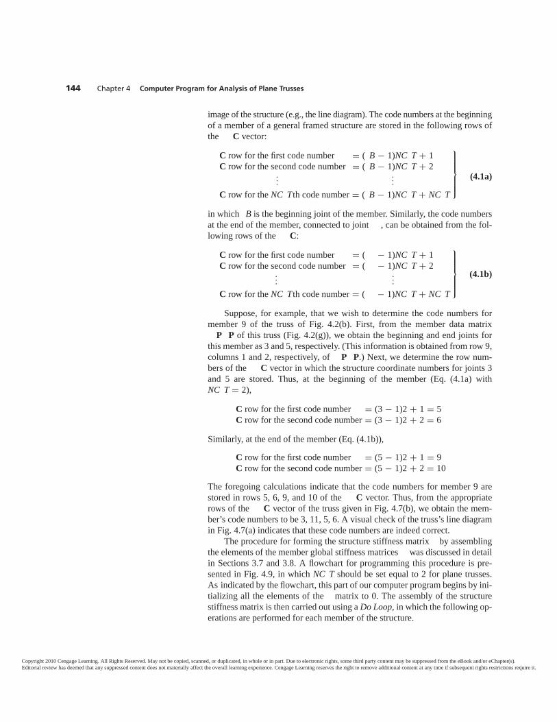
144 Chapter 4 Computer Program for Analysis of Plane Trusses
image of the structure (e.g., the line diagram). The code numbers at the beginningof a member of a general framed structure are stored in the following rows ofthe C vector:
C row for the first code number = ( B − 1)NC T + 1C row for the second code number = ( B − 1)NC T + 2
......
(4.1a)
C row for the NC Tth code number = ( B − 1)NC T + NC T
in which B is the beginning joint of the member. Similarly, the code numbersat the end of the member, connected to joint , can be obtained from the fol-lowing rows of the C:
C row for the first code number = ( − 1)NC T + 1C row for the second code number = ( − 1)NC T + 2
......
(4.1b)
C row for the NC Tth code number = ( − 1)NC T + NC T
Suppose, for example, that we wish to determine the code numbers formember 9 of the truss of Fig. 4.2(b). First, from the member data matrix
P P of this truss (Fig. 4.2(g)), we obtain the beginning and end joints forthis member as 3 and 5, respectively. (This information is obtained from row 9,columns 1 and 2, respectively, of P P.) Next, we determine the row num-bers of the C vector in which the structure coordinate numbers for joints 3and 5 are stored. Thus, at the beginning of the member (Eq. (4.1a) withNC T = 2),
C row for the first code number = (3 − 1)2 + 1 = 5C row for the second code number = (3 − 1)2 + 2 = 6
Similarly, at the end of the member (Eq. (4.1b)),
C row for the first code number = (5 − 1)2 + 1 = 9C row for the second code number = (5 − 1)2 + 2 = 10
The foregoing calculations indicate that the code numbers for member 9 arestored in rows 5, 6, 9, and 10 of the C vector. Thus, from the appropriaterows of the C vector of the truss given in Fig. 4.7(b), we obtain the mem-ber’s code numbers to be 3, 11, 5, 6. A visual check of the truss’s line diagramin Fig. 4.7(a) indicates that these code numbers are indeed correct.
The procedure for forming the structure stiffness matrix by assemblingthe elements of the member global stiffness matrices was discussed in detailin Sections 3.7 and 3.8. A flowchart for programming this procedure is pre-sented in Fig. 4.9, in which NC T should be set equal to 2 for plane trusses.As indicated by the flowchart, this part of our computer program begins by ini-tializing all the elements of the matrix to 0. The assembly of the structurestiffness matrix is then carried out using a Do Loop, in which the following op-erations are performed for each member of the structure.
⎫⎪⎪⎪⎪⎪⎬⎪⎪⎪⎪⎪⎭
⎫⎪⎪⎪⎪⎪⎬⎪⎪⎪⎪⎪⎭
Copyright 2010 Cengage Learning. All Rights Reserved. May not be copied, scanned, or duplicated, in whole or in part. Due to electronic rights, some third party content may be suppressed from the eBook and/or eChapter(s).Editorial review has deemed that any suppressed content does not materially affect the overall learning experience. Cengage Learning reserves the right to remove additional content at any time if subsequent rights restrictions require it.
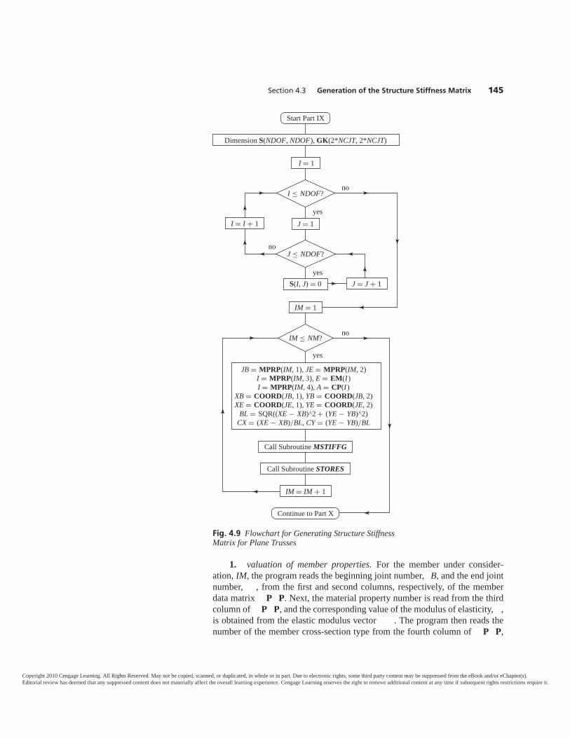
Section 4.3 Generation of the Structure Stiffness Matrix 145
I = 1
J = 1
IM = 1
Call Subroutine MSTIFFG
Call Subroutine STORES
Dimension S(NDOF, NDOF), GK(2*NCJT, 2*NCJT)
yes
yes
yes
no
no
I ≤ NDOF?
IM ≤ NM?
J ≤ NDOF?
IM = IM + 1
I = I + 1
J = J + 1S(I, J) = 0
JB = MPRP(IM, 1), JE = MPRP(IM, 2)I = MPRP(IM, 3), E = EM(I )I = MPRP(IM, 4), A = CP(I )
XB = COORD(JB, 1), YB = COORD(JB, 2)XE = COORD(JE, 1), YE = COORD(JE, 2)
BL = SQR((XE − XB)^2 + (YE − YB)^2)CX = (XE − XB)/BL, CY = (YE − YB)/BL
no
Start Part IX
Continue to Part X
Fig. 4.9 Flowchart for Generating Structure StiffnessMatrix for Plane Trusses
1. valuation of member properties. For the member under consider-ation, IM, the program reads the beginning joint number, B, and the end jointnumber, , from the first and second columns, respectively, of the memberdata matrix P P. Next, the material property number is read from the thirdcolumn of P P, and the corresponding value of the modulus of elasticity, ,is obtained from the elastic modulus vector . The program then reads thenumber of the member cross-section type from the fourth column of P P,
Copyright 2010 Cengage Learning. All Rights Reserved. May not be copied, scanned, or duplicated, in whole or in part. Due to electronic rights, some third party content may be suppressed from the eBook and/or eChapter(s).Editorial review has deemed that any suppressed content does not materially affect the overall learning experience. Cengage Learning reserves the right to remove additional content at any time if subsequent rights restrictions require it.
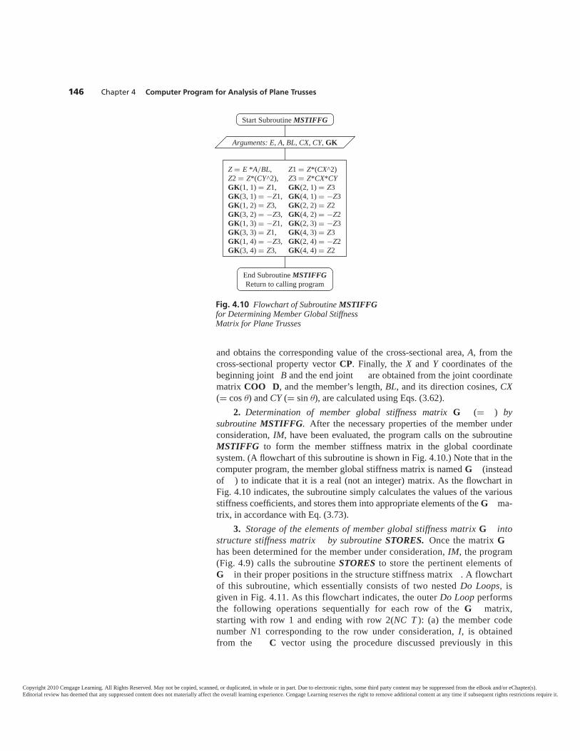
146 Chapter 4 Computer Program for Analysis of Plane Trusses
Arguments: E, A, BL, CX, CY, GK
Z1 = Z*(CX^2)Z3 = Z*CX*CYGK(2, 1) = Z3GK(4, 1) = −Z3GK(2, 2) = Z2GK(4, 2) = −Z2GK(2, 3) = −Z3GK(4, 3) = Z3GK(2, 4) = −Z2GK(4, 4) = Z2
Start Subroutine MSTIFFG
End Subroutine MSTIFFGReturn to calling program
Z = E *A/BL,Z2 = Z*(CY^2),GK(1, 1) = Z1,GK(3, 1) = −Z1,GK(1, 2) = Z3,GK(3, 2) = −Z3,GK(1, 3) = −Z1,GK(3, 3) = Z1,GK(1, 4) = −Z3,GK(3, 4) = Z3,
Fig. 4.10 Flowchart of Subroutine MSTIFFGfor Determining Member Global StiffnessMatrix for Plane Trusses
and obtains the corresponding value of the cross-sectional area, A, from thecross-sectional property vector CP. Finally, the X and Y coordinates of thebeginning joint B and the end joint are obtained from the joint coordinatematrix COO D, and the member’s length, BL, and its direction cosines, CX(= cos θ) and CY (= sin θ), are calculated using Eqs. (3.62).
2. Determination of member global stiffness matrix G (= ) bysubroutine MSTIFFG. After the necessary properties of the member underconsideration, IM, have been evaluated, the program calls on the subroutineMSTIFFG to form the member stiffness matrix in the global coordinatesystem. (A flowchart of this subroutine is shown in Fig. 4.10.) Note that in thecomputer program, the member global stiffness matrix is named G (insteadof ) to indicate that it is a real (not an integer) matrix. As the flowchart inFig. 4.10 indicates, the subroutine simply calculates the values of the variousstiffness coefficients, and stores them into appropriate elements of the G ma-trix, in accordance with Eq. (3.73).
3. Storage of the elements of member global stiffness matrix G intostructure stiffness matrix by subroutine STORES. Once the matrix Ghas been determined for the member under consideration, IM, the program(Fig. 4.9) calls the subroutine STORES to store the pertinent elements ofG in their proper positions in the structure stiffness matrix . A flowchartof this subroutine, which essentially consists of two nested Do Loops, isgiven in Fig. 4.11. As this flowchart indicates, the outer Do Loop performsthe following operations sequentially for each row of the G matrix,starting with row 1 and ending with row 2(NC T ): (a) the member codenumber N1 corresponding to the row under consideration, I, is obtainedfrom the C vector using the procedure discussed previously in this
Copyright 2010 Cengage Learning. All Rights Reserved. May not be copied, scanned, or duplicated, in whole or in part. Due to electronic rights, some third party content may be suppressed from the eBook and/or eChapter(s).Editorial review has deemed that any suppressed content does not materially affect the overall learning experience. Cengage Learning reserves the right to remove additional content at any time if subsequent rights restrictions require it.
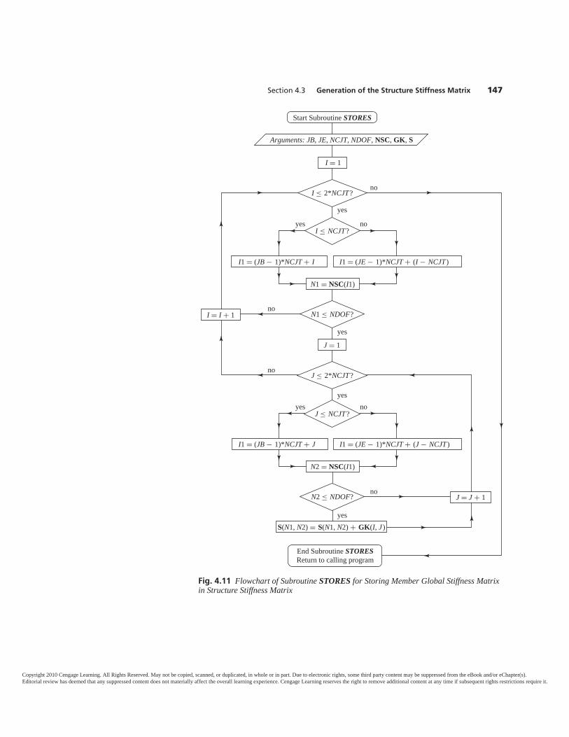
Section 4.3 Generation of the Structure Stiffness Matrix 147
I = 1
I1 = (JE − 1)*NCJT + (I − NCJT)I1 = (JB − 1)*NCJT + I
I1 = (JE − 1)*NCJT + (J − NCJT)I1 = (JB − 1)*NCJT + J
N1 = NSC(I1)
N2 = NSC(I1)
yes
yes
yesyes
yes
yes
no
no
no
no
no
no
I ≤ 2*NCJT?
J ≤ 2*NCJT?
I ≤ NCJT?
J ≤ NCJT?
N1 ≤ NDOF?
N2 ≤ NDOF? J = J + 1
I = I + 1
J = 1
Arguments: JB, JE, NCJT, NDOF, NSC, GK, S
S(N1, N2) = S(N1, N2) + GK(I, J )
Start Subroutine STORES
End Subroutine STORESReturn to calling program
Fig. 4.11 Flowchart of Subroutine STORES for Storing Member Global Stiffness Matrixin Structure Stiffness Matrix
Copyright 2010 Cengage Learning. All Rights Reserved. May not be copied, scanned, or duplicated, in whole or in part. Due to electronic rights, some third party content may be suppressed from the eBook and/or eChapter(s).Editorial review has deemed that any suppressed content does not materially affect the overall learning experience. Cengage Learning reserves the right to remove additional content at any time if subsequent rights restrictions require it.

148 Chapter 4 Computer Program for Analysis of Plane Trusses
section; (b) if N1 is less than or equal to NDOF, then the inner Do Loop isactivated; otherwise, the inner loop is skipped; and (c) the row number I isincreased by 1, and steps (a) through (c) are repeated. The inner loop, activatedfrom the outer loop, performs the following operations sequentially for eachcolumn of the G matrix, starting with column 1 and ending with column2(NC T ): (a) the member code number N2 corresponding to the column underconsideration, , is obtained from the C vector; (b) if N2 is less than or equalto NDOF, then the value of the element in the Ith row and th column of G isadded to the value of the element in the N1th row and N2th column of ;otherwise, no action is taken; and (c) the column number is increased by 1,and steps (a) through (c) are repeated. The inner loop ends when its steps (a)and (b) have been applied to all the columns of G ; the program control is thenreturned to step (c) of the outer loop. The subroutine STORES ends when steps(a) and (b) of the outer loop have been applied to all the rows of the G matrix,thereby storing all the pertinent elements of the global stiffness matrix of themember under consideration, IM, in their proper positions in the structurestiffness matrix .
Refocusing our attention on Fig. 4.9, we can see that formation of thestructure stiffness matrix is complete when the three operations, describedin the foregoing paragraphs, have been performed for each member of thestructure.
4.4 FORMATION OF THE JOINT LOAD VECTORIn this section, we consider the programming of the next analysis step, whichinvolves formation of the joint load vector P. A flowchart for programming thisprocess is shown in Fig. 4.12. Again, when analyzing plane trusses, the valueof NC T should be set equal to 2 in the program. It is seen from the figure thatthis part of our computer program begins by initializing each element of P to 0.The program then generates the load vector P by performing the followingoperations for each row of the load data vector P, starting with row 1 andproceeding sequentially to row N L:
1. For the row under consideration, I, the number of the loaded joint I1 isread from the P vector.
2. The number of the X structure coordinate, N, at joint I1 is obtainedfrom row I2 = (I1 − 1)2 + 1 of the C vector. If N ≤ NDOF, then the valueof the element in the Ith row and the first column of the load data matrix P(i.e., the X load component) is added to the Nth row of the load vector P; oth-erwise, no action is taken.
3. The C row number I2 is increased by 1 (i.e., I2 = I2 + 1), and thestructure coordinate number, N, of the Y coordinate is read from the C. IfN ≤ NDOF, then the value of the element in the Ith row and the second columnof P (i.e., the Y load component) is added to the Nth row of P; otherwise, noaction is taken.
Copyright 2010 Cengage Learning. All Rights Reserved. May not be copied, scanned, or duplicated, in whole or in part. Due to electronic rights, some third party content may be suppressed from the eBook and/or eChapter(s).Editorial review has deemed that any suppressed content does not materially affect the overall learning experience. Cengage Learning reserves the right to remove additional content at any time if subsequent rights restrictions require it.
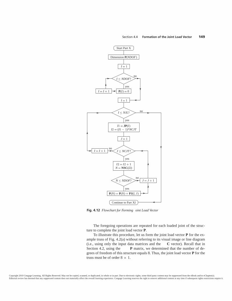
Section 4.4 Formation of the Joint Load Vector 149
The foregoing operations are repeated for each loaded joint of the struc-ture to complete the joint load vector P.
To illustrate this procedure, let us form the joint load vector P for the ex-ample truss of Fig. 4.2(a) without referring to its visual image or line diagram(i.e., using only the input data matrices and the C vector). Recall that inSection 4.2, using the P matrix, we determined that the number of de-grees of freedom of this structure equals 8. Thus, the joint load vector P for thetruss must be of order 8 × 1.
Fig. 4.12 Flowchart for Forming oint Load Vector
I = 1
I = 1
J = 1
P(I ) = 0
I1 = JP(I )I2 = (I1 − 1)*NCJT
I2 = I2 + 1N = NSC(I2)
Dimension P(NDOF )
yes
yes
yes
yes
no
no
no
no
I ≤ NDOF?
I ≤ NJL?
J ≤ NCJT?
P(N) = P(N) + PJ(I, J )
I = I + 1
J = J + 1N ≤ NDOF?
I = I + 1
Start Part X
Continue to Part XI
Copyright 2010 Cengage Learning. All Rights Reserved. May not be copied, scanned, or duplicated, in whole or in part. Due to electronic rights, some third party content may be suppressed from the eBook and/or eChapter(s).Editorial review has deemed that any suppressed content does not materially affect the overall learning experience. Cengage Learning reserves the right to remove additional content at any time if subsequent rights restrictions require it.
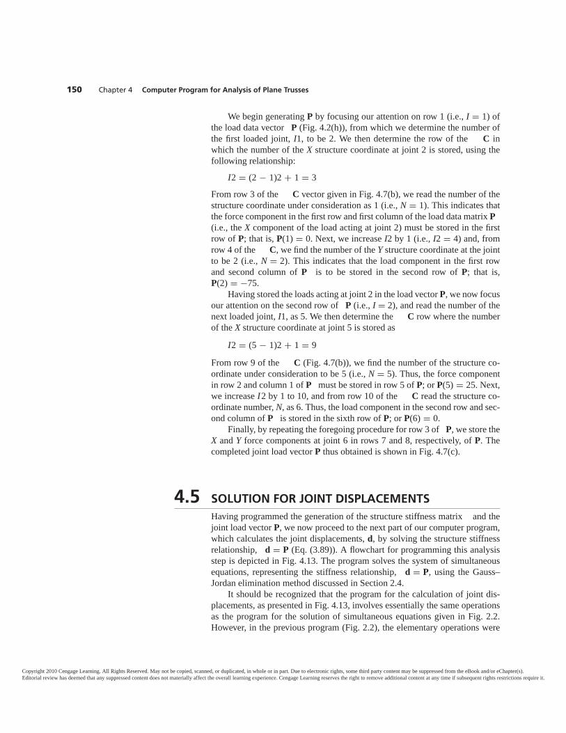
150 Chapter 4 Computer Program for Analysis of Plane Trusses
We begin generating P by focusing our attention on row 1 (i.e., I = 1) ofthe load data vector P (Fig. 4.2(h)), from which we determine the number ofthe first loaded joint, I1, to be 2. We then determine the row of the C inwhich the number of the X structure coordinate at joint 2 is stored, using thefollowing relationship:
I2 = (2 − 1)2 + 1 = 3From row 3 of the C vector given in Fig. 4.7(b), we read the number of thestructure coordinate under consideration as 1 (i.e., N = 1). This indicates thatthe force component in the first row and first column of the load data matrix P(i.e., the X component of the load acting at joint 2) must be stored in the firstrow of P; that is, P(1) = 0. Next, we increase I2 by 1 (i.e., I2 = 4) and, fromrow 4 of the C, we find the number of the Y structure coordinate at the jointto be 2 (i.e., N = 2). This indicates that the load component in the first rowand second column of P is to be stored in the second row of P; that is,P(2) = −75.
Having stored the loads acting at joint 2 in the load vector P, we now focusour attention on the second row of P (i.e., I = 2), and read the number of thenext loaded joint, I1, as 5. We then determine the C row where the numberof the X structure coordinate at joint 5 is stored as
I2 = (5 − 1)2 + 1 = 9
From row 9 of the C (Fig. 4.7(b)), we find the number of the structure co-ordinate under consideration to be 5 (i.e., N = 5). Thus, the force componentin row 2 and column 1 of P must be stored in row 5 of P; or P(5) = 25. Next,we increase I2 by 1 to 10, and from row 10 of the C read the structure co-ordinate number, N, as 6. Thus, the load component in the second row and sec-ond column of P is stored in the sixth row of P; or P(6) = 0.
Finally, by repeating the foregoing procedure for row 3 of P, we store theX and Y force components at joint 6 in rows 7 and 8, respectively, of P. Thecompleted joint load vector P thus obtained is shown in Fig. 4.7(c).
4.5 SOLUTION FOR JOINT DISPLACEMENTSHaving programmed the generation of the structure stiffness matrix and thejoint load vector P, we now proceed to the next part of our computer program,which calculates the joint displacements, d, by solving the structure stiffnessrelationship, d = P (Eq. (3.89)). A flowchart for programming this analysisstep is depicted in Fig. 4.13. The program solves the system of simultaneousequations, representing the stiffness relationship, d = P, using the Gauss–Jordan elimination method discussed in Section 2.4.
It should be recognized that the program for the calculation of joint dis-placements, as presented in Fig. 4.13, involves essentially the same operationsas the program for the solution of simultaneous equations given in Fig. 2.2.However, in the previous program (Fig. 2.2), the elementary operations were
Copyright 2010 Cengage Learning. All Rights Reserved. May not be copied, scanned, or duplicated, in whole or in part. Due to electronic rights, some third party content may be suppressed from the eBook and/or eChapter(s).Editorial review has deemed that any suppressed content does not materially affect the overall learning experience. Cengage Learning reserves the right to remove additional content at any time if subsequent rights restrictions require it.
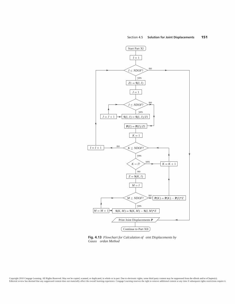
Section 4.5 Solution for Joint Displacements 151
Fig. 4.13 Flowchart for Calculation of oint Displacements byGauss ordan Method
I = 1
J = 1
K = 1
M = I
Z1 = S(I, I )
S(I, J ) = S(I, J )/Z1
P(I ) = P(I )/Z1
Z = S(K, I )
yes
yes
yes
yes
yes
no
no
no
no
no
I ≤ NDOF?
J ≤ NDOF?
M ≤ NDOF?
K = I?
P(K ) = P(K ) − P(I )*Z
S(K, M ) = S(K, M ) − S(I, M )*Z
K = K + 1
J = J + 1
M = M + 1
Print Joint Displacements P
K ≤ NDOF?I = I + 1
Start Part XI
Continue to Part XII
Copyright 2010 Cengage Learning. All Rights Reserved. May not be copied, scanned, or duplicated, in whole or in part. Due to electronic rights, some third party content may be suppressed from the eBook and/or eChapter(s).Editorial review has deemed that any suppressed content does not materially affect the overall learning experience. Cengage Learning reserves the right to remove additional content at any time if subsequent rights restrictions require it.
152 Chapter 4 Computer Program for Analysis of Plane Trusses
applied to an augmented matrix; in the present program (Fig. 4.13), to savespace in computer memory, no augmented matrix is formed, and the elemen-tary operations are applied directly to the structure stiffness matrix and thejoint load vector P. Thus, at the end of the Gauss–Jordan elimination process,the matrix is reduced to a unit matrix, and the P vector contains values of thejoint displacements. In the rest of our computer program, therefore, P (insteadof d) is considered to be the joint displacement vector. The joint displacementsthus obtained can be communicated to the user through a printout or on thescreen.
4.6 CALCULATION OF MEMBER FORCESAND SUPPORT REACTIONSIn this section, we consider programming of the final analysis step, which in-volves calculation of the member forces and support reactions. A flowchart forprogramming this analysis step is presented in Fig. 4.14, with NC T = 2 forplane trusses. As shown there, this part of our computer program begins by ini-tializing each element of the reaction vector, , to 0. The member forces andsupport reactions are then determined by performing the following operationsfor each member of the structure, via a Do Loop.
1. valuation of member properties. For the member under consid-eration, IM, the program reads the beginning joint number B, the end jointnumber , the modulus of elasticity , the cross-sectional area A, and the Xand Y coordinates of the beginning and end joints. It then calculates themember length, BL, and direction cosines, CX (= cos θ) and CY (= sin θ),using Eqs. (3.62).
2. valuation of member global end displacements (= ) by subrou-tine MDISPG. After the properties of the member under consideration,IM, have been calculated, the computer program calls subroutine MDISPG,to obtain the member end displacements in the global coordinate system. Aflowchart of this subroutine is given in Fig. 4.15. As this flowchart indicates,after initializing V to 0, the subroutine reads, in order, for each of the mem-ber end displacements, VI, the number of the corresponding structure coordi-nate, N, at joint B or , from the NSC vector. If the structure coordinatenumber N, corresponding to an end displacement VI, is found to be less thanor equal to NDOF, then the value of the element in the Nth row of the joint-displacement vector P (= d) is stored in the Ith row of the memberdisplacement vector V.
3. Determination of member transformation matrix T by subroutineMTRANS. After the global end-displacement vector V for the member underconsideration, IM, has been evaluated, the main program (Fig. 4.14) calls onthe subroutine MTRANS to form the member transformation matrix T. A flow-chart of this subroutine is shown in Fig. 4.16. As this figure indicates, the sub-routine first initializes T to 0, and then simply stores the values of the direction
Copyright 2010 Cengage Learning. All Rights Reserved. May not be copied, scanned, or duplicated, in whole or in part. Due to electronic rights, some third party content may be suppressed from the eBook and/or eChapter(s).Editorial review has deemed that any suppressed content does not materially affect the overall learning experience. Cengage Learning reserves the right to remove additional content at any time if subsequent rights restrictions require it.
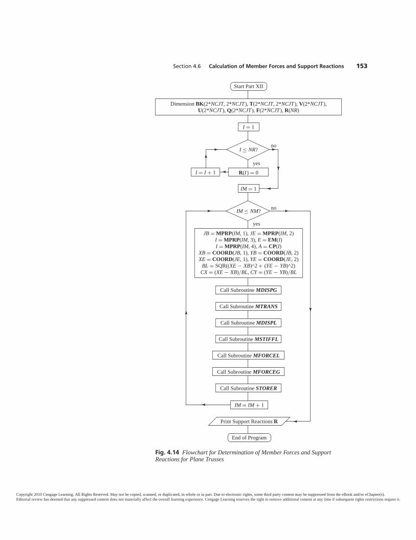
Section 4.6 Calculation of Member Forces and Support Reactions 153
Fig. 4.14 Flowchart for Determination of Member Forces and SupportReactions for Plane Trusses
Dimension BK(2*NCJT, 2*NCJT), T(2*NCJT, 2*NCJT), V(2*NCJT),U(2*NCJT), Q(2*NCJT), F(2*NCJT), R(NR)
I = 1
IM = 1
R(I ) = 0
JB = MPRP(IM, 1), JE = MPRP(IM, 2)I = MPRP(IM, 3), E = EM(I)I = MPRP(IM, 4), A = CP(I)
XB = COORD(JB, 1), YB = COORD(JB, 2)XE = COORD(JE, 1), YE = COORD(JE, 2)
BL = SQR((XE − XB)^2 + (YE − YB)^2)CX = (XE − XB)/BL, CY = (YE − YB)/BL
yes
yes
no
no
I ≤ NR?
Call Subroutine MDISPG
Call Subroutine MTRANS
Call Subroutine MDISPL
Call Subroutine MSTIFFL
Call Subroutine MFORCEL
Call Subroutine MFORCEG
Call Subroutine STORER
I = I + 1
IM = IM + 1
Print Support Reactions R
IM ≤ NM?
Start Part XII
End of Program
Copyright 2010 Cengage Learning. All Rights Reserved. May not be copied, scanned, or duplicated, in whole or in part. Due to electronic rights, some third party content may be suppressed from the eBook and/or eChapter(s).Editorial review has deemed that any suppressed content does not materially affect the overall learning experience. Cengage Learning reserves the right to remove additional content at any time if subsequent rights restrictions require it.
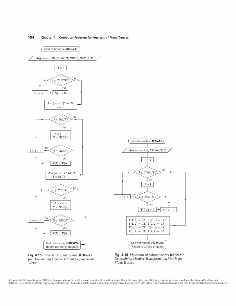
154 Chapter 4 Computer Program for Analysis of Plane Trusses
I = 1
yes
yes
yes
yes
yes
no
no
no
no
I ≤ 2*NCJT?
I ≤ 2*NCJT?
I ≤ NCJT?
N ≤ NDOF?
I = I + 1
I = I + 1
I = I + 1
Arguments: JB, JE, NCJT, NDOF, NSC, P, V
V(I) = 0
V(I ) = P(N)
V(I ) = P(N)
J = (JB − 1)* NCJTI = 1
J = J + 1N = NSC(J)
N ≤ NDOF?
J = J + 1N = NSC(J)
J = (JE − 1) * NCJTI = NCJT + 1
no
Start Subroutine MDISPG
End Subroutine MDISPGReturn to calling program
Fig. 4.15 Flowchart of Subroutine MDISPGfor Determining Member Global DisplacementVector
Fig. 4.16 Flowchart of Subroutine MTRANS forDetermining Member Transformation Matrix forPlane Trusses
I = 1
J = 1yes
yes
no
no
I ≤ 2*NCJT?
J ≤ 2*NCJT?I = I + 1
J = J + 1
Arguments: CX, CY, NCJT, T
T(I, J ) = 0
T(1, 1) = CX, T(2, 1) = −CYT(1, 2) = CY, T(2, 2) = CXT(3, 3) = CX, T(4, 3) = −CYT(3, 4) = CY, T(4, 4) = CX
Start Subroutine MTRANS
End Subroutine MTRANSReturn to calling program
Copyright 2010 Cengage Learning. All Rights Reserved. May not be copied, scanned, or duplicated, in whole or in part. Due to electronic rights, some third party content may be suppressed from the eBook and/or eChapter(s).Editorial review has deemed that any suppressed content does not materially affect the overall learning experience. Cengage Learning reserves the right to remove additional content at any time if subsequent rights restrictions require it.

Section 4.6 Calculation of Member Forces and Support Reactions 155
cosines CX and CY, with appropriate plus or minus signs, into various elementsof in accordance with Eq. (3.61).
4. Calculation of member local end displacements (= u) by subroutineMDISPL. Next, as shown in Fig. 4.14, the program calls subroutine MDISPLto obtain the local end displacements of the member under consideration, IM.From the flowchart given in Fig. 4.17, we can see that after initializing to 0,this subroutine calculates the member local end-displacement vector by apply-ing the relationship = (Eq. (3.63)). The procedure for multiplying ma-trices was discussed in Section 2.3, and subroutine MDISPL (Fig. 4.17) usesessentially the same operations as the program for matrix multiplication givenin Fig. 2.1.
5. Determination of member local stiffness matrix B (= ) by sub-routine MSTIFFL. After the local end displacements of the member under
Start Subroutine MDISPL
I = 1
I = 1
J = 1
J = J + 1
I = I + 1
U(I ) = 0
U(I ) = U(I ) + T(I, J) * V(J)
I = I + 1
I ≤ 2*NCJT?
I ≤ 2*NCJT?
J ≤ 2*NCJT?
Arguments: NCJT, V, T, U
no
no
no
yes
yes
yes
End Subroutine MDISPLReturn to calling program
Fig. 4.17 Flowchart of Subroutine MDISPL for DeterminingMember Local Displacement Vector
Copyright 2010 Cengage Learning. All Rights Reserved. May not be copied, scanned, or duplicated, in whole or in part. Due to electronic rights, some third party content may be suppressed from the eBook and/or eChapter(s).Editorial review has deemed that any suppressed content does not materially affect the overall learning experience. Cengage Learning reserves the right to remove additional content at any time if subsequent rights restrictions require it.
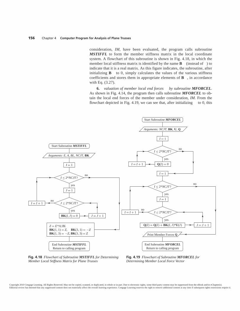
156 Chapter 4 Computer Program for Analysis of Plane Trusses
consideration, IM, have been evaluated, the program calls subroutine MSTIFFL to form the member stiffness matrix in the local coordinatesystem. A flowchart of this subroutine is shown in Fig. 4.18, in which themember local stiffness matrix is identified by the name B (instead of ) toindicate that it is a real matrix. As this figure indicates, the subroutine, afterinitializing B to 0, simply calculates the values of the various stiffnesscoefficients and stores them in appropriate elements of B , in accordancewith Eq. (3.27).
6. valuation of member local end forces by subroutine MFORCEL.As shown in Fig. 4.14, the program then calls subroutine MFORCEL to ob-tain the local end forces of the member under consideration, IM. From theflowchart depicted in Fig. 4.19, we can see that, after initializing to 0, this
I ≤ 2*NCJT?
J ≤ 2*NCJT?
Start Subroutine MSTIFFL
Arguments: E, A, BL, NCJT, BK
I = 1
J = 1
I = I + 1
J = J + 1BK(I, J ) = 0
Z = E*A/BLBK(1, 1) = Z, BK(3, 1) = −ZBK(1, 3) = −Z, BK(3, 3) = Z
no
no
yes
yes
End Subroutine MSTIFFLReturn to calling program
Fig. 4.18 Flowchart of Subroutine MSTIFFL for DeterminingMember Local Stiffness Matrix for Plane Trusses
I ≤ 2*NCJT?
I ≤ 2*NCJT?
Start Subroutine MFORCEL
Arguments: NCJT, BK, U, Q
I = 1
I = 1
J = 1
I = I + 1
J ≤ 2*NCJT?I = I + 1
J = J + 1
Q(I ) = 0
Q(I ) = Q(I ) + BK(I, J )*U(J )
no
no
yes
Print Member Forces Q
yes
yes
no
End Subroutine MFORCELReturn to calling program
Fig. 4.19 Flowchart of Subroutine MFORCEL forDetermining Member Local Force Vector
Copyright 2010 Cengage Learning. All Rights Reserved. May not be copied, scanned, or duplicated, in whole or in part. Due to electronic rights, some third party content may be suppressed from the eBook and/or eChapter(s).Editorial review has deemed that any suppressed content does not materially affect the overall learning experience. Cengage Learning reserves the right to remove additional content at any time if subsequent rights restrictions require it.

Section 4.6 Calculation of Member Forces and Support Reactions 157
subroutine calculates the member local end forces using the relationship= B (Eq. (3.7)). The vector thus obtained is then printed or displayed
on the screen.7. Calculation of member global end forces by subroutine MFORCEG.
After the local end forces of the member under consideration, IM, have beenevaluated, the computer program calls subroutine MFORCEG to calculatethe member end forces in the global coordinate system. A flowchart of thissubroutine is given in Fig. 4.20. From the figure, we can see that after initializ-ing to 0, the subroutine calculates the global end forces by applying the rela-tionship = T (Eq. (3.66)); these forces are then communicated to the userthrough a printer or on the screen.
I ≤ 2 NC T
I ≤ 2 NC T
≤ 2 NC T
Start Subroutine MFORCEG
Arguments NC T, , ,
I = 1
I = 1
= 1
(I ) = 0
(I ) = (I ) + ( , I ) ( )
Print Member Forces
I = I + 1
I = I + 1
= + 1
no
no
no
yes
yes
yes
End Subroutine MFORCEGReturn to calling program
Fig. 4.20 Flowchart of Subroutine MFORCEG for DeterminingMember Global Force Vector
Copyright 2010 Cengage Learning. All Rights Reserved. May not be copied, scanned, or duplicated, in whole or in part. Due to electronic rights, some third party content may be suppressed from the eBook and/or eChapter(s).Editorial review has deemed that any suppressed content does not materially affect the overall learning experience. Cengage Learning reserves the right to remove additional content at any time if subsequent rights restrictions require it.
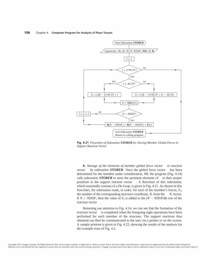
158 Chapter 4 Computer Program for Analysis of Plane Trusses
Start Subroutine STORER
I = 1
I = I + 1
N = NSC(I1)
R(N − NDOF ) = R(N − NDOF ) + F(I )
I1 = (JB − 1)*NCJT + I I1 = (JE − 1)*NCJT + (I − NCJT)
I ≤ 2*NCJT?
I ≤ NCJT?
N > NDOF?
Arguments: JB, JE, NCJT, NDOF, NSC, F, R
no
no
no
yes
yes
yes
End Subroutine STORERReturn to calling program
Fig. 4.21 Flowchart of Subroutine STORER for Storing Member Global Forces inSupport Reaction Vector
8. Storage of the elements of member global force vector in reactionvector by subroutine STORER. Once the global force vector has beendetermined for the member under consideration, IM, the program (Fig. 4.14)calls subroutine STORER to store the pertinent elements of in their properpositions in the support reaction vector . A flowchart of this subroutine,which essentially consists of a Do Loop, is given in Fig. 4.21. As shown in thisflowchart, the subroutine reads, in order, for each of the member’s forces, FI,the number of the corresponding structure coordinate, N, from the C vector.If N > NDOF, then the value of FI is added to the (N − NDOF)th row of thereaction vector .
Returning our attention to Fig. 4.14, we can see that the formation of thereaction vector is completed when the foregoing eight operations have beenperformed for each member of the structure. The support reactions thusobtained can then be communicated to the user via a printer or on the screen.A sample printout is given in Fig. 4.22, showing the results of the analysis forthe example truss of Fig. 4.2.
Copyright 2010 Cengage Learning. All Rights Reserved. May not be copied, scanned, or duplicated, in whole or in part. Due to electronic rights, some third party content may be suppressed from the eBook and/or eChapter(s).Editorial review has deemed that any suppressed content does not materially affect the overall learning experience. Cengage Learning reserves the right to remove additional content at any time if subsequent rights restrictions require it.
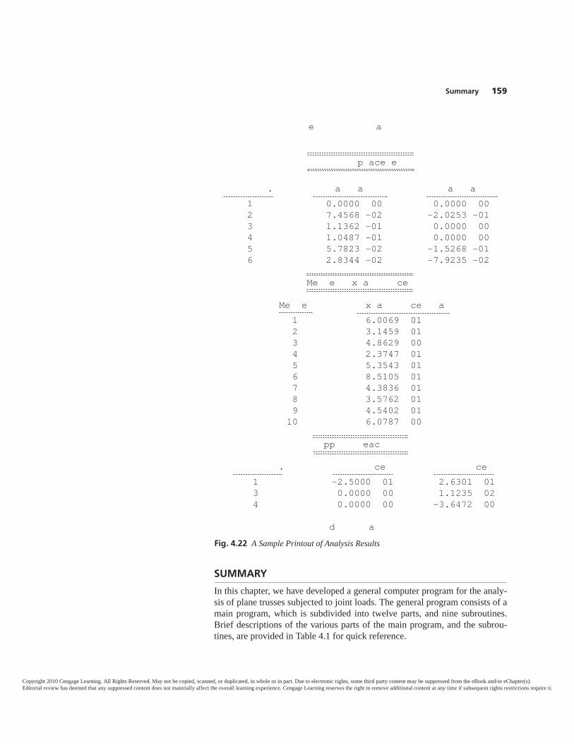
e a
p ace e
. a a a a1 0.0000 00 0.0000 002 7.4568 -02 -2.0253 -013 1.1362 -01 0.0000 004 1.0487 -01 0.0000 005 5.7823 -02 -1.5268 -016 2.8344 -02 -7.9235 -02
Me e x a ce
Me e x a ce a1 6.0069 01 2 3.1459 01 3 4.8629 00 4 2.3747 01 5 5.3543 01 6 8.5105 01 7 4.3836 01 8 3.5762 01 9 4.5402 01 10 6.0787 00
pp eac
. ce ce1 -2.5000 01 2.6301 013 0.0000 00 1.1235 024 0.0000 00 -3.6472 00
d a
Summary 159
SUMMARY
In this chapter, we have developed a general computer program for the analy-sis of plane trusses subjected to joint loads. The general program consists of amain program, which is subdivided into twelve parts, and nine subroutines.Brief descriptions of the various parts of the main program, and the subrou-tines, are provided in Table 4.1 for quick reference.
Fig. 4.22 A Sample Printout of Analysis Results
Copyright 2010 Cengage Learning. All Rights Reserved. May not be copied, scanned, or duplicated, in whole or in part. Due to electronic rights, some third party content may be suppressed from the eBook and/or eChapter(s).Editorial review has deemed that any suppressed content does not materially affect the overall learning experience. Cengage Learning reserves the right to remove additional content at any time if subsequent rights restrictions require it.
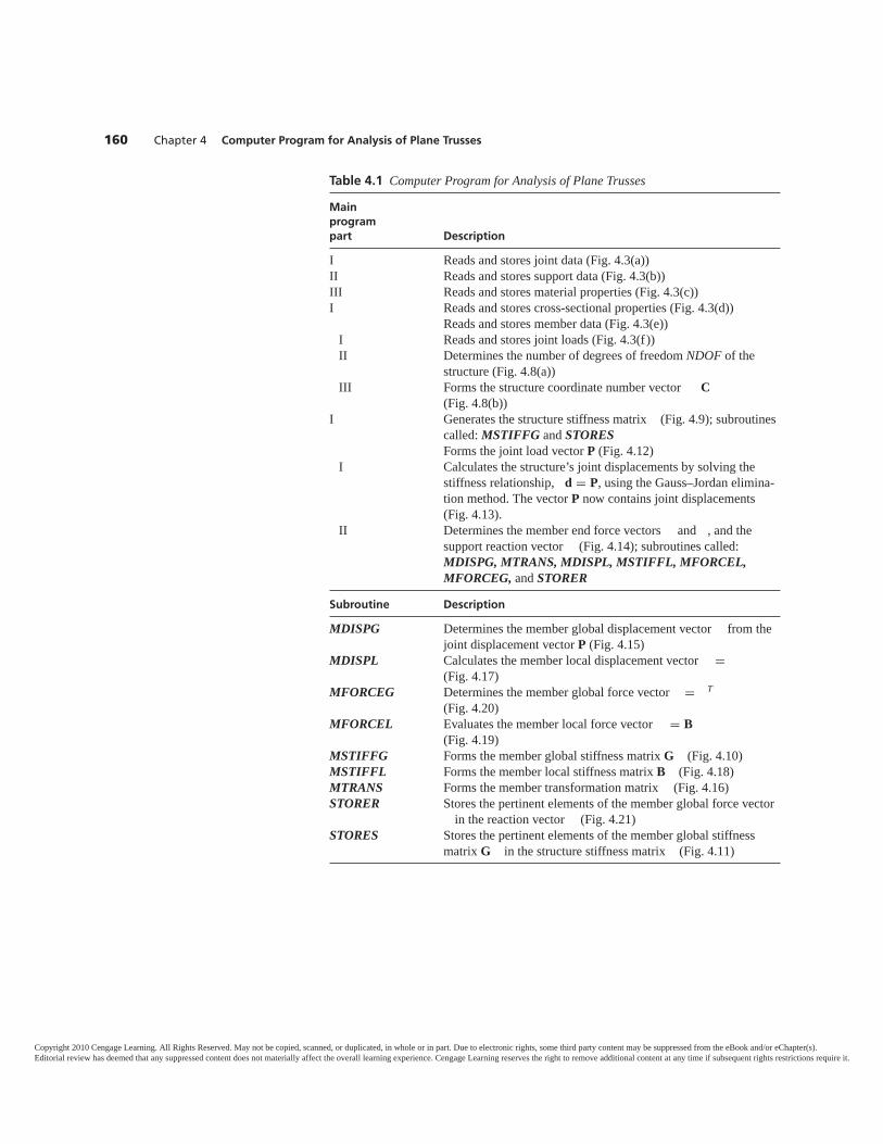
160 Chapter 4 Computer Program for Analysis of Plane Trusses
Table 4.1 Computer Program for Analysis of Plane Trusses
Mainprogram part Description
I Reads and stores joint data (Fig. 4.3(a))II Reads and stores support data (Fig. 4.3(b))III Reads and stores material properties (Fig. 4.3(c))I Reads and stores cross-sectional properties (Fig. 4.3(d))
Reads and stores member data (Fig. 4.3(e))I Reads and stores joint loads (Fig. 4.3(f))II Determines the number of degrees of freedom NDOF of the
structure (Fig. 4.8(a))III Forms the structure coordinate number vector C
(Fig. 4.8(b))I Generates the structure stiffness matrix (Fig. 4.9); subroutines
called: MSTIFFG and STORESForms the joint load vector P (Fig. 4.12)
I Calculates the structure’s joint displacements by solving thestiffness relationship, d = P, using the Gauss–Jordan elimina-tion method. The vector P now contains joint displacements(Fig. 4.13).
II Determines the member end force vectors and , and thesupport reaction vector (Fig. 4.14); subroutines called:MDISPG, MTRANS, MDISPL, MSTIFFL, MFORCEL,MFORCEG, and STORER
Subroutine Description
MDISPG Determines the member global displacement vector from thejoint displacement vector P (Fig. 4.15)
MDISPL Calculates the member local displacement vector =(Fig. 4.17)
MFORCEG Determines the member global force vector = T
(Fig. 4.20)MFORCEL Evaluates the member local force vector = B
(Fig. 4.19)MSTIFFG Forms the member global stiffness matrix G (Fig. 4.10)MSTIFFL Forms the member local stiffness matrix B (Fig. 4.18)MTRANS Forms the member transformation matrix (Fig. 4.16)STORER Stores the pertinent elements of the member global force vector
in the reaction vector (Fig. 4.21)STORES Stores the pertinent elements of the member global stiffness
matrix G in the structure stiffness matrix (Fig. 4.11)
Copyright 2010 Cengage Learning. All Rights Reserved. May not be copied, scanned, or duplicated, in whole or in part. Due to electronic rights, some third party content may be suppressed from the eBook and/or eChapter(s).Editorial review has deemed that any suppressed content does not materially affect the overall learning experience. Cengage Learning reserves the right to remove additional content at any time if subsequent rights restrictions require it.

Problems 161
P R O B L E M S
Section 4.3
4.3 Extend the program of Problem 4.2 to generate, and print,the structure stiffness matrix . Use the program to generate thestructure stiffness matrices for the trusses of Problems 3.16through 3.25, and compare the computer-generated matricesto those obtained by hand calculations.
Section 4.4
4.4 Extend the program developed in Problem 4.3 to form,and print, the joint load vector P. Apply the program tothe trusses of Problems 3.16 through 3.25, and compare thecomputer-generated P vectors to those obtained by handcalculations.
Section 4.5
4.5 Extend the program of Problem 4.4 so that it can: (a) cal-culate the structure’s joint displacements by solving the stiff-ness relationship, d = P, using the Gauss–Jordan eliminationmethod; and (b) print the joint displacements. Using theprogram, determine the joint displacements for the trusses ofProblems 3.16 through 3.25, and compare the computer-generated results to those obtained by hand calculations.
Section 4.6
4.6 Extend the program developed in Problem 4.5 so that itcan determine and print: (a) the local end forces, , for eachmember of the truss; and (b) the support reaction vector . Usethe program to analyze the trusses of Problems 3.16 through3.25, and compare the computer-generated results to thoseobtained by hand calculations.
The objective of the following problems is to develop, incre-mentally, a computer program for the analysis of plane trusses;while testing each program increment for correctness, as it isbeing developed. The reader is strongly encouraged to manuallysolve as many of the problems (3.16 through 3.25) as possible,so that these hand-calculation results can be used to check thecorrectness of the various parts of the computer program.
Section 4.1
4.1 Develop an input module of a computer program forthe analysis of plane trusses, which can perform the followingoperations:
a. read from a data file, or computer screen, all the necessaryinput data;
b. store the input data in computer memory in the form ofscalars, vectors, and/or matrices, as appropriate; and
c. print the input data from computer memory.
Check the program for correctness by inputting data for thetrusses of Problems 3.16 through 3.25, and by carefully exam-ining the printouts of the input data to ensure that all data havebeen correctly read and stored.
Section 4.2
4.2 Extend the program developed in Problem 4.1, so that itcan perform the following additional operations:
a. determining the number of degrees of freedom (NDOF) ofthe structure;
b. forming the structure coordinate number vector C; andc. printing out the NDOF and C.
To check the program for correctness, use it to determine theNDOF and C for the trusses of Problems 3.16 through 3.25,and compare the computer-generated results to those obtainedby hand calculations.
Copyright 2010 Cengage Learning. All Rights Reserved. May not be copied, scanned, or duplicated, in whole or in part. Due to electronic rights, some third party content may be suppressed from the eBook and/or eChapter(s).Editorial review has deemed that any suppressed content does not materially affect the overall learning experience. Cengage Learning reserves the right to remove additional content at any time if subsequent rights restrictions require it.
55.1 Analytical Model5.2 Member Stiffness Relations5.3 Finite-Element Formulation Using Virtual Work5.4 Member Fixed-End Forces Due to Loads5.5 Structure Stiffness Relations5.6 Structure Fixed-Joint Forces and Equivalent Joint Loads5.7 Procedure for Analysis5.8 Computer Program
SummaryProblems
BEAMS
A Continuous Beam Bridge(Photo courtesy of Bethlehem Steel Corporation)
162
Copyright 2010 Cengage Learning. All Rights Reserved. May not be copied, scanned, or duplicated, in whole or in part. Due to electronic rights, some third party content may be suppressed from the eBook and/or eChapter(s).Editorial review has deemed that any suppressed content does not materially affect the overall learning experience. Cengage Learning reserves the right to remove additional content at any time if subsequent rights restrictions require it.

Section 5.1 Analytical Model 163
The term “beam” is used herein to refer to a long straight structure, which issupported and loaded in such a way that all the external forces and couples(including reactions) acting on it lie in a plane of symmetry of its cross-section,with all the forces perpendicular to its centroidal axis. Under the action of ex-ternal loads, beams are subjected only to bending moments and shear forces(but no axial forces).
In this chapter, we study the basic concepts of the analysis of beams bythe matrix stiffness method, and develop a computer program for the analysisof beams based on the matrix stiffness formulation. As we proceed throughthe chapter, the reader will notice that, although the member stiffness relationsfor beams differ from those for plane trusses, the overall format of the methodof analysis remains essentially the same—and many of the analysis steps de-veloped in Chapter 3 for the case of plane trusses can be directly applied tobeams. Therefore, the computer program developed in Chapter 4 for theanalysis of plane trusses can be modified with relative ease for the analysis ofbeams.
We begin by discussing the preparation of analytical models of beams inSection 5.1, where the global and local coordinate systems and the degrees offreedom of beams are defined. Next, we derive the member stiffness relationsin the local coordinate system in Section 5.2; and present the finite-elementformulation of the member stiffness matrix, via the principle of virtual work, inSection 5.3. The derivation of the member fixed-end forces, due to externalloads applied to members, is considered in Section 5.4; and the formation ofthe stiffness relations for the entire beam, by combining the member stiffnessrelations, is discussed in Section 5.5. The procedure for forming the structurefixed-joint force vectors, and the concept of equivalent joint loads, are intro-duced in Section 5.6; and a step-by-step procedure for the analysis of beams ispresented in Section 5.7. Finally, a computer program for the analysis of beamsis developed in Section 5.8.
5.1 ANALYTICAL MODELFor analysis by the matrix stiffness method, the continuous beam is modeled asa series of straight prismatic members connected at their ends to joints, so thatthe unknown external reactions act only at the joints. Consider, for example,the two-span continuous beam shown in Fig. 5.1(a). Although the structure ac-tually consists of a single continuous beam between the two fixed supports atthe ends, for the purpose of analysis it is considered to be composed of threemembers (1, 2, and 3), rigidly connected at four joints (1 through 4), as shownin Fig. 5.1(b). Note that joint 2 has been introduced in the analytical model sothat the vertical reaction at the roller support acts on a joint (instead of on amember), and joint 3 is used to subdivide the right span of the beam into twomembers, each with constant flexural rigidity ( I ) along its length. This divi-sion of the beam into members and joints is necessary because the formulationof the stiffness method requires that the unknown external reactions act only atthe joints (i.e., all the member loads be known in advance of analysis), and the
Copyright 2010 Cengage Learning. All Rights Reserved. May not be copied, scanned, or duplicated, in whole or in part. Due to electronic rights, some third party content may be suppressed from the eBook and/or eChapter(s).Editorial review has deemed that any suppressed content does not materially affect the overall learning experience. Cengage Learning reserves the right to remove additional content at any time if subsequent rights restrictions require it.
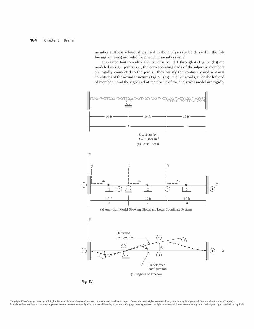
164 Chapter 5 Beams
Fig. 5.1
10 ft 10 ft 10 ft
I 2I
E = 4,000 ksiI = 13,824 in.4
(a) Actual Beam
2 31
41 2 3
10 ftI
10 ftI
(b) Analytical Model Showing Global and Local Coordinate Systems
10 ft2I
y1
x1 x2 x3X
y2 y3
Y
2
3
3′
1 4d1
d1d2
d3
X
Y
Deformedconfiguration
Undeformedconfiguration
(c) Degrees of Freedom
member stiffness relationships used in the analysis (to be derived in the fol-lowing sections) are valid for prismatic members only.
It is important to realize that because joints 1 through 4 (Fig. 5.1(b)) aremodeled as rigid joints (i.e., the corresponding ends of the adjacent membersare rigidly connected to the joints), they satisfy the continuity and restraintconditions of the actual structure (Fig. 5.1(a)). In other words, since the left endof member 1 and the right end of member 3 of the analytical model are rigidly
Copyright 2010 Cengage Learning. All Rights Reserved. May not be copied, scanned, or duplicated, in whole or in part. Due to electronic rights, some third party content may be suppressed from the eBook and/or eChapter(s).Editorial review has deemed that any suppressed content does not materially affect the overall learning experience. Cengage Learning reserves the right to remove additional content at any time if subsequent rights restrictions require it.
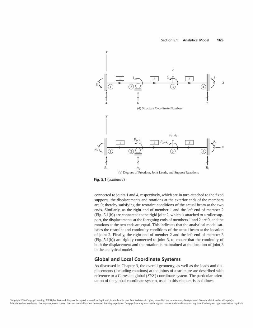
Section 5.1 Analytical Model 165
connected to joints 1 and 4, respectively, which are in turn attached to the fixedsupports, the displacements and rotations at the exterior ends of the membersare 0; thereby satisfying the restraint conditions of the actual beam at the twoends. Similarly, as the right end of member 1 and the left end of member 2(Fig. 5.1(b)) are connected to the rigid joint 2, which is attached to a roller sup-port, the displacements at the foregoing ends of members 1 and 2 are 0, and therotations at the two ends are equal. This indicates that the analytical model sat-isfies the restraint and continuity conditions of the actual beam at the locationof joint 2. Finally, the right end of member 2 and the left end of member 3(Fig. 5.1(b)) are rigidly connected to joint 3, to ensure that the continuity ofboth the displacement and the rotation is maintained at the location of joint 3in the analytical model.
Global and Local Coordinate SystemsAs discussed in Chapter 3, the overall geometry, as well as the loads and dis-placements (including rotations) at the joints of a structure are described withreference to a Cartesian global (XYZ ) coordinate system. The particular orien-tation of the global coordinate system, used in this chapter, is as follows.
1
4 6(d) Structure Coordinate Numbers
5
7
3 8
32
2
1 4X
Y
2 31
R5
R8P1, d1 P3, d3
P2, d2
R4 R6(e) Degrees of Freedom, Joint Loads, and Support Reactions
R7
321 4X
Y
2 31
Fig. 5.1 (continued)
Copyright 2010 Cengage Learning. All Rights Reserved. May not be copied, scanned, or duplicated, in whole or in part. Due to electronic rights, some third party content may be suppressed from the eBook and/or eChapter(s).Editorial review has deemed that any suppressed content does not materially affect the overall learning experience. Cengage Learning reserves the right to remove additional content at any time if subsequent rights restrictions require it.
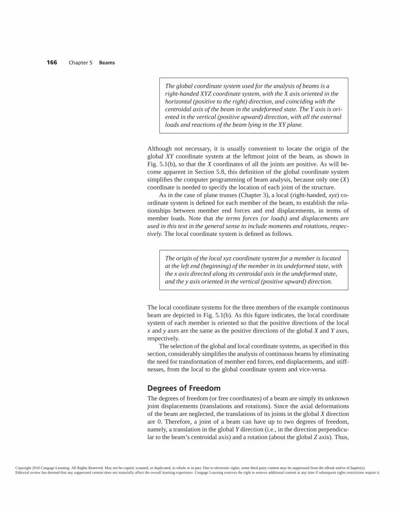
Although not necessary, it is usually convenient to locate the origin of theglobal XY coordinate system at the leftmost joint of the beam, as shown inFig. 5.1(b), so that the X coordinates of all the joints are positive. As will be-come apparent in Section 5.8, this definition of the global coordinate systemsimplifies the computer programming of beam analysis, because only one (X)coordinate is needed to specify the location of each joint of the structure.
As in the case of plane trusses (Chapter 3), a local (right-handed, xyz) co-ordinate system is defined for each member of the beam, to establish the rela-tionships between member end forces and end displacements, in terms ofmember loads. Note that the terms forces (or loads) and displacements areused in this text in the general sense to include moments and rotations, respec-tively. The local coordinate system is defined as follows.
The local coordinate systems for the three members of the example continuousbeam are depicted in Fig. 5.1(b). As this figure indicates, the local coordinatesystem of each member is oriented so that the positive directions of the localx and y axes are the same as the positive directions of the global X and Y axes,respectively.
The selection of the global and local coordinate systems, as specified in thissection, considerably simplifies the analysis of continuous beams by eliminatingthe need for transformation of member end forces, end displacements, and stiff-nesses, from the local to the global coordinate system and vice-versa.
Degrees of FreedomThe degrees of freedom (or free coordinates) of a beam are simply its unknownjoint displacements (translations and rotations). Since the axial deformationsof the beam are neglected, the translations of its joints in the global X directionare 0. Therefore, a joint of a beam can have up to two degrees of freedom,namely, a translation in the global Y direction (i.e., in the direction perpendicu-lar to the beam’s centroidal axis) and a rotation (about the global Z axis). Thus,
The origin of the local xyz coordinate system for a member is locatedat the left end (beginning) of the member in its undeformed state, withthe x axis directed along its centroidal axis in the undeformed state,and the y axis oriented in the vertical (positive upward) direction.
The global coordinate system used for the analysis of beams is aright-handed XYZ coordinate system, with the X axis oriented in thehorizontal (positive to the right) direction, and coinciding with thecentroidal axis of the beam in the undeformed state. The Y axis is ori-ented in the vertical (positive upward) direction, with all the externalloads and reactions of the beam lying in the XY plane.
166 Chapter 5 Beams
Copyright 2010 Cengage Learning. All Rights Reserved. May not be copied, scanned, or duplicated, in whole or in part. Due to electronic rights, some third party content may be suppressed from the eBook and/or eChapter(s).Editorial review has deemed that any suppressed content does not materially affect the overall learning experience. Cengage Learning reserves the right to remove additional content at any time if subsequent rights restrictions require it.
Section 5.1 Analytical Model 167
the number of structure coordinates (i.e., free and/or restrained coordinates) ata joint of a beam equals 2, or NC T = 2.
Let us consider the analytical model of the continuous beam as given inFig. 5.1(b). The deformed shape of the beam, due to an arbitrary loading, is de-picted in Fig. 5.1(c) using an exaggerated scale. From this figure, we can seethat joint 1, which is attached to the fixed support, can neither translate norrotate; therefore, it does not have any degrees of freedom. Since joint 2 ofthe beam is attached to the roller support, it can rotate, but not translate. Thus,joint 2 has only one degree of freedom, which is designated d1 in the figure. Asjoint 3 is not attached to a support, two displacements—the translation d2 in theY direction, and the rotation d3 about the Z axis—are needed to completelyspecify its deformed position 3′. Thus, joint 3 has two degrees of freedom.Finally, joint 4, which is attached to the fixed support, can neither translate norrotate; therefore, it does not have any degrees of freedom. Thus, the entirebeam has a total of three degrees of freedom.
As indicated in Fig. 5.1(c), joint translations are considered positive whenvertically upward, and joint rotations are considered positive when counter-clockwise. All the joint displacements in Fig. 5.1(c) are shown in the positivesense. The NDOF × 1 joint displacement vector d for the beam is written as
d =⎡⎣ d1
d2d3
⎤⎦
Since the number of structure coordinates per joint equals 2 (i.e.,NC T = 2), the number of degrees of freedom, NDOF, of a beam can beobtained from Eq. (3.2) as
(5.1)
in which, as in the case of plane trusses, N represents the number of joints ofthe beam, and NR denotes the number of joint displacements restrained by sup-ports (or the number of restrained coordinates). Let us apply Eq. (5.1) to theanalytical model of the beam in Fig. 5.1(b). The beam has four joints (i.e.,N = 4); two joints, 1 and 4, are attached to the fixed supports that together re-strain four joint displacements (namely, the translations in the Y direction andthe rotations of joints 1 and 4). Furthermore, the roller support at joint 2 re-strains one joint displacement, which is the translation of joint 2 in the Y direc-tion. Thus, the total number of joint displacements that are restrained by allsupports of the beam is 5 (i.e., NR = 5). Substitution of the numerical valuesof N and NR into Eq. (5.1) yields
NDOF = 2(4) − 5 = 3
which is the same as the number of degrees of freedom of the beam obtainedpreviously. As in the case of plane trusses, the free and restrained coordinatesof a beam are collectively referred to simply as the structure coordinates.
NC T = 2NDOF = 2(N ) − NR
}for beams
Copyright 2010 Cengage Learning. All Rights Reserved. May not be copied, scanned, or duplicated, in whole or in part. Due to electronic rights, some third party content may be suppressed from the eBook and/or eChapter(s).Editorial review has deemed that any suppressed content does not materially affect the overall learning experience. Cengage Learning reserves the right to remove additional content at any time if subsequent rights restrictions require it.
When analyzing a beam, it is not necessary to draw its deformed shape, asshown in Fig. 5.1(c), to identify the degrees of freedom. Instead, all the struc-ture coordinates (i.e., degrees of freedom and restrained coordinates) are usu-ally directly specified on the beam’s line diagram by assigning numbers to thearrows drawn at the joints in the directions of the joint displacements, as shownin Fig. 5.1(d). In this figure, a slash (/) has been added to the arrows corre-sponding to the restrained coordinates to distinguish them from those repre-senting the degrees of freedom.
The procedure for assigning numbers to the structure coordinates ofbeams is similar to that for the case of plane trusses, discussed in detail inSection 3.2. The degrees of freedom are numbered first, starting at the lowest-numbered joint, that has a degree of freedom, and proceeding sequentially tothe highest-numbered joint. If a joint has two degrees of freedom, then thetranslation in the Y direction is numbered first, followed by the rotation. Thefirst degree of freedom is assigned the number 1, and the last degree of freedomis assigned a number equal to NDOF.
After all the degrees of freedom of the beam have been numbered, its re-strained coordinates are numbered beginning with a number equal toNDOF + 1. Starting at the lowest-numbered joint that is attached to a sup-port, and proceeding sequentially to the highest-numbered joint, all of therestrained coordinates of the beam are numbered. If a joint has two restrainedcoordinates, then the coordinate in the Y direction (corresponding to thereaction force) is numbered first, followed by the rotation coordinate (corre-sponding to the reaction couple). The number assigned to the last restrainedcoordinate of the beam is always 2(N ). The structure coordinate numbers forthe example beam, obtained by applying the foregoing procedure, are given inFig. 5.1(d).
Joint Load and Reaction VectorsUnlike plane trusses, which are subjected only to joint loads, the external loadson beams may be applied at the joints as well as on the members. The externalloads (i.e., forces and couples or moments) applied at the joints of a structureare referred to as the joint loads, whereas the external loads acting between theends of the members of the structure are termed the member loads. In this sec-tion, we focus our attention only on the joint loads, with the member loads con-sidered in subsequent sections. As discussed in Section 3.2, an external jointload can, in general, be applied to the beam at the location and in the directionof each of its degrees of freedom. For example, the beam of Fig. 5.1(b), withthree degrees of freedom, can be subjected to a maximum of three joint loads,P1 through P3, as shown in Fig. 5.1(e). As indicated there, a load correspond-ing to a degree of freedom di is denoted symbolically by Pi. The 3 × 1 jointload vector P for the beam is written in the form
P =⎡⎣ P1
P2P3
⎤⎦
NDOF × 1
168 Chapter 5 Beams
Copyright 2010 Cengage Learning. All Rights Reserved. May not be copied, scanned, or duplicated, in whole or in part. Due to electronic rights, some third party content may be suppressed from the eBook and/or eChapter(s).Editorial review has deemed that any suppressed content does not materially affect the overall learning experience. Cengage Learning reserves the right to remove additional content at any time if subsequent rights restrictions require it.
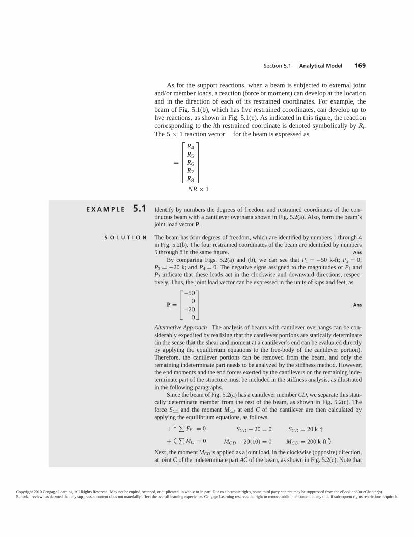
Section 5.1 Analytical Model 169
As for the support reactions, when a beam is subjected to external jointand/or member loads, a reaction (force or moment) can develop at the locationand in the direction of each of its restrained coordinates. For example, thebeam of Fig. 5.1(b), which has five restrained coordinates, can develop up tofive reactions, as shown in Fig. 5.1(e). As indicated in this figure, the reactioncorresponding to the ith restrained coordinate is denoted symbolically by Ri.The 5 × 1 reaction vector for the beam is expressed as
=
⎡⎢⎢⎢⎢⎣
R4R5R6R7R8
⎤⎥⎥⎥⎥⎦
NR × 1
E X A M P L E 5.1 Identify by numbers the degrees of freedom and restrained coordinates of the con-tinuous beam with a cantilever overhang shown in Fig. 5.2(a). Also, form the beam’sjoint load vector P.
S O L U T I O N The beam has four degrees of freedom, which are identified by numbers 1 through 4in Fig. 5.2(b). The four restrained coordinates of the beam are identified by numbers5 through 8 in the same figure. Ans
By comparing Figs. 5.2(a) and (b), we can see that P1 = −50 k-ft; P2 = 0;P3 = −20 k; and P4 = 0. The negative signs assigned to the magnitudes of P1 andP3 indicate that these loads act in the clockwise and downward directions, respec-tively. Thus, the joint load vector can be expressed in the units of kips and feet, as
P =
⎡⎢⎢⎣
−500
−200
⎤⎥⎥⎦ Ans
Alternative Approach The analysis of beams with cantilever overhangs can be con-siderably expedited by realizing that the cantilever portions are statically determinate(in the sense that the shear and moment at a cantilever’s end can be evaluated directlyby applying the equilibrium equations to the free-body of the cantilever portion).Therefore, the cantilever portions can be removed from the beam, and only theremaining indeterminate part needs to be analyzed by the stiffness method. However,the end moments and the end forces exerted by the cantilevers on the remaining inde-terminate part of the structure must be included in the stiffness analysis, as illustratedin the following paragraphs.
Since the beam of Fig. 5.2(a) has a cantilever member CD, we separate this stati-cally determinate member from the rest of the beam, as shown in Fig. 5.2(c). Theforce SCD and the moment MCD at end C of the cantilever are then calculated byapplying the equilibrium equations, as follows.
+ ↑ ∑FY = 0 SC D − 20 = 0 SC D = 20 k ↑
+ ∑MC = 0 MC D − 20(10) = 0 MC D = 200 k-ft
Next, the moment MCD is applied as a joint load, in the clockwise (opposite) direction,at joint C of the indeterminate part AC of the beam, as shown in Fig. 5.2(c). Note that
aY
Copyright 2010 Cengage Learning. All Rights Reserved. May not be copied, scanned, or duplicated, in whole or in part. Due to electronic rights, some third party content may be suppressed from the eBook and/or eChapter(s).Editorial review has deemed that any suppressed content does not materially affect the overall learning experience. Cengage Learning reserves the right to remove additional content at any time if subsequent rights restrictions require it.
Fig. 5.2
15 ft 15 ft 10 ft
I = constant= 29,000 ksi
I = 500 in.4
(a) Continuous Beam
A B C D
50 k-ft 20 k
6
5 7(b) Analytical Model (NDOF = 4, NR = 4)
1 2 4
3
321 4
8
X
Y
21 3
15 ft 15 ft 10 ft
A B C C D
50 k-ft 200 k-ft MCD = 200 k-ft
SCD = 20 k
20 k
Statically indeterminate partto be analyzed by stiffness method(c) Statically Determinate and Indeterminate Parts of the Beam
Statically determinate part
4
3 5(d) Analytical Model of Statically Indeterminate Part (NDOF = 2, NR = 4)
6
1 2
321X
Y
21
170
Copyright 2010 Cengage Learning. All Rights Reserved. May not be copied, scanned, or duplicated, in whole or in part. Due to electronic rights, some third party content may be suppressed from the eBook and/or eChapter(s).Editorial review has deemed that any suppressed content does not materially affect the overall learning experience. Cengage Learning reserves the right to remove additional content at any time if subsequent rights restrictions require it.
Section 5.2 Member Stiffness Relations 171
the end force SCD (= 20 k) need not be considered in the analysis of the indeterminatepart because its only effect is to increase the reaction at support C by 20 k.
The analytical model of the indeterminate part of the beam is drawn in Fig. 5.2(d).Note that the number of degrees of freedom has now been reduced to only two, identi-fied by numbers 1 and 2 in the figure. The number of restrained coordinates remains atfour, and these coordinates are identified by numbers 3 through 6 in Fig. 5.2(d). Bycomparing the indeterminate part of the beam in Fig. 5.2(c) to its analytical model inFig. 5.2(d), we obtain the joint load vector as
P =[ −50
−200
]k-ft Ans
Once the analytical model of Fig. 5.2(d) has been analyzed by the stiffness method,the reaction force R6 must be adjusted (i.e., increased by 20 k) to account for the endforce SCD being exerted by the cantilever CD on support C.
5.2 MEMBER STIFFNESS RELATIONSWhen a beam is subjected to external loads, internal moments and shears gen-erally develop at the ends of its individual members. The equations expressingthe forces (including moments) at the end of a member as functions of the dis-placements (including rotations) of its ends, in terms of the external loads ap-plied to the member, are referred to as the member stiffness relations. Suchmember stiffness relations are necessary for establishing the stiffness relationsfor the entire beam, as discussed in Section 5.5. In this section, we derive thestiffness relations for the members of beams.
To develop the member stiffness relations, we focus our attention on anarbitrary prismatic member m of the continuous beam shown in Fig. 5.3(a).When the beam is subjected to external loads, member m deforms and internalshear forces and moments are induced at its ends. The initial and displaced po-sitions of m are depicted in Fig. 5.3(b), in which L, , and I denote the length,Young’s modulus of elasticity, and moment of inertia, respectively, of the mem-ber. It can be seen from this figure that two displacements—translation in they direction and rotation about the z axis—are necessary to completely specify
X
Y
(a) Beam
y
x
b em
Fig. 5.3
Copyright 2010 Cengage Learning. All Rights Reserved. May not be copied, scanned, or duplicated, in whole or in part. Due to electronic rights, some third party content may be suppressed from the eBook and/or eChapter(s).Editorial review has deemed that any suppressed content does not materially affect the overall learning experience. Cengage Learning reserves the right to remove additional content at any time if subsequent rights restrictions require it.
172 Chapter 5 Beams
x
y
b
b′
e
e′
L
Displacedposition
u1
u2u3
u4
Q4
Q3Q1
Q2
uy
x
EI = constant(b) Member Forces and Displacements in the Local Coordinate System
m
Initialposition
Fig. 5.3 (continued)
xb
b′
e
u1 = 1u1
x
y
L
(c)
=
×k21 = 6EI
L2
k41 = 6EIL2
k11 = 12EIL3 k31 = −12EI
L3
N1 = 1 − 3( x )2 + 2( x )3L L
xe
u2 = 1u2
x
y
L
(d)
+
×k22 = 4EI
L
k42 = 2EIL
k12 = 6EIL2 k32 = − 6EI
L2
N2 = x(1 − x )2L
b
Copyright 2010 Cengage Learning. All Rights Reserved. May not be copied, scanned, or duplicated, in whole or in part. Due to electronic rights, some third party content may be suppressed from the eBook and/or eChapter(s).Editorial review has deemed that any suppressed content does not materially affect the overall learning experience. Cengage Learning reserves the right to remove additional content at any time if subsequent rights restrictions require it.
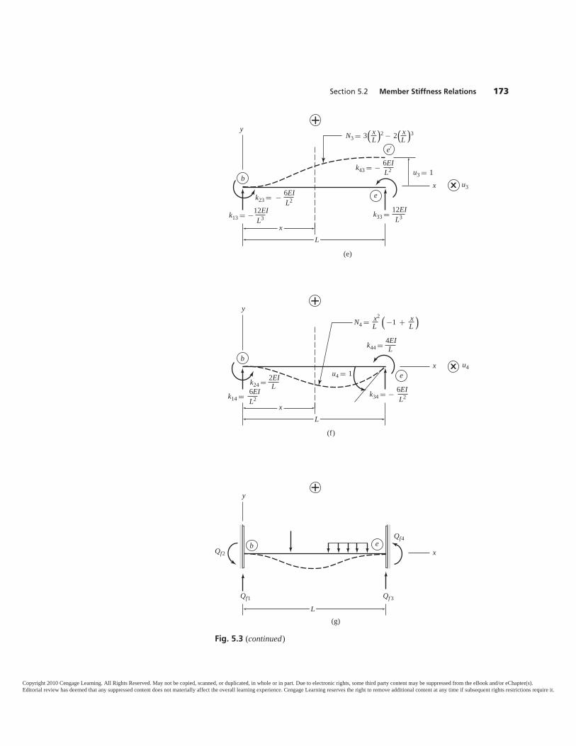
Section 5.2 Member Stiffness Relations 173
x
e′
u3 = 1u3
x
y
L
(e)
+
×
k33 = 12EIL3k13 = −12EI
L3
k23 = − 6EIL2
k43 = − 6EIL2
N3 = 3( x )2 − 2( x )3L L
b
e
xeu4 = 1
u4
x
y
L
(f)
+
×
k14 = 6EIL2
k24 = 2EIL
k44 = 4EIL
k34 = − 6EIL2
N4 = x2 ( −1 + x )L L
b
xe
y
L(g)
+
bQf2
Qf4
Qf1 Qf 3
Fig. 5.3 (continued)
Copyright 2010 Cengage Learning. All Rights Reserved. May not be copied, scanned, or duplicated, in whole or in part. Due to electronic rights, some third party content may be suppressed from the eBook and/or eChapter(s).Editorial review has deemed that any suppressed content does not materially affect the overall learning experience. Cengage Learning reserves the right to remove additional content at any time if subsequent rights restrictions require it.
the displaced position of each end of the member. Thus, the member has a totalof four end displacements or degrees of freedom. As Fig. 5.3(b) indicates, themember end displacements (including rotations) are denoted by u1 through u4,and the corresponding end forces (including moments) are denoted by 1through 4. Note that the member end translations and forces are consideredpositive when vertically upward (i.e., in the positive direction of the local y axis),and the end rotations and moments are considered positive when counterclock-wise. The numbering scheme used for identifying the member end displace-ments and forces is similar to that used previously for plane trusses in Chapter 3.As indicated in Fig. 5.3(b), the member end displacements and forces are num-bered by beginning at the left end b of the member, which is the origin of the localcoordinate system, with the vertical translation and force numbered first, fol-lowed by the rotation and moment. The displacements and forces at the oppositeend e of the member are then numbered in the same sequential order.
The relationships between member end forces and end displacements canbe conveniently established by subjecting the member, separately, to each ofthe four end displacements and external loads, as shown in Figs. 5.3(c) through(g); and by expressing the total member end forces as the algebraic sums of theend forces required to cause the individual end displacements and the forcescaused by the external loads acting on the member with no end displacements.Thus, from Figs. 5.3(b) through (g), we can see that
1 = k11u1 + k12u2 + k13u3 + k14u4 + f 1 (5.2a)
2 = k21u1 + k22u2 + k23u3 + k24u4 + f 2 (5.2b)
3 = k31u1 + k32u2 + k33u3 + k34u4 + f 3 (5.2c)
4 = k41u1 + k42u2 + k43u3 + k44u4 + f 4 (5.2d)
in which, as defined in Chapter 3, a stiffness coefficient kij represents the forceat the location and in the direction of i required, along with other end forces,to cause a unit value of displacement uj, while all other end displacements are0, and the member is not subjected to any external loading between its ends.The last terms, f i (with i = 1 to 4), on the right sides of Eqs. (5.2), representthe forces that would develop at the member ends, due to external loads, ifboth ends of the member were fixed against translations and rotations (seeFig. 5.3(g)). These forces are commonly referred to as the member fixed-endforces due to external loads. Equations (5.2) can be written in matrix form as⎡
⎢⎢⎣1
2
3
4
⎤⎥⎥⎦ =
⎡⎢⎢⎣
k11 k12 k13 k14k21 k22 k23 k24k31 k32 k33 k34k41 k42 k43 k44
⎤⎥⎥⎦
⎡⎢⎢⎣
u1u2u3u4
⎤⎥⎥⎦ +
⎡⎢⎢⎣
f 1
f 2
f 3
f 4
⎤⎥⎥⎦ (5.3)
or, symbolically, as
(5.4)= u + f
174 Chapter 5 Beams
Copyright 2010 Cengage Learning. All Rights Reserved. May not be copied, scanned, or duplicated, in whole or in part. Due to electronic rights, some third party content may be suppressed from the eBook and/or eChapter(s).Editorial review has deemed that any suppressed content does not materially affect the overall learning experience. Cengage Learning reserves the right to remove additional content at any time if subsequent rights restrictions require it.
Section 5.2 Member Stiffness Relations 175
in which and u represent the member end force and member end displace-ment vectors, respectively, in the local coordinate system; is the memberstiffness matrix in the local coordinate system; and f is called the memberfixed-end force vector in the local coordinate system.
In the rest of this and the following section, we focus our attention on thederivation of the member stiffness matrix . The fixed-end force vector f isconsidered in detail in Section 5.4.
Derivation of Member Stiffness Matrix kVarious classical methods of structural analysis, such as the method of consis-tent deformations and the slope-deflection equations, can be used to determinethe expressions for the stiffness coefficients kij in terms of member length andits flexural rigidity, I. In the following, however, we derive such stiffness ex-pressions by directly integrating the differential equation for beam deflection.This direct integration approach is not only relatively simple and straightfor-ward, but it also yields member shape functions as a part of the solution. Theshape functions are often used to establish the member mass matrices for thedynamic analysis of beams [34]; they also provide insight into the finite-element formulation of beam analysis (considered in the next section).
It may be recalled from a previous course on mechanics of materials thatthe differential equation for small-deflection bending of a beam, composed oflinearly elastic homogenous material and loaded in a plane of symmetry of itscross-section, can be expressed as
(5.5)
in which u y represents the deflection of the beam’s centroidal axis (which co-incides with the neutral axis) in the y direction, at a distance x from the originof the xy coordinate system as shown in Fig. 5.3(b); and M denotes the bend-ing moment at the beam section at the same location, x. It is important to real-ize that the bending moment M is considered positive in accordance with thebeam sign convention, which can be stated as follows (see Fig. 5.4).
To obtain the expressions for the coefficients ki1 (i = 1 through 4) in thefirst column of the member stiffness matrix (Eq. (5.3)), we subject the
The bending moment at a section of a beam is considered positive whenthe external force or couple tends to bend the beam concave upward(in the positive y direction), causing compression in the fibers above(in the positive y direction), and tension in the fibers below (in thenegative y direction), the neutral axis of the beam at the section.
d2u ydx2 = M
I
Copyright 2010 Cengage Learning. All Rights Reserved. May not be copied, scanned, or duplicated, in whole or in part. Due to electronic rights, some third party content may be suppressed from the eBook and/or eChapter(s).Editorial review has deemed that any suppressed content does not materially affect the overall learning experience. Cengage Learning reserves the right to remove additional content at any time if subsequent rights restrictions require it.
member to a unit value of the end displacement u1 at end b, as shown inFig. 5.3(c). Note that all other end displacements of the member are 0 (i.e.,u2 = u3 = u4 = 0), and the member is in equilibrium under the action of twoend moments k21 and k41, and two end shears k11 and k31. To determine theequation for bending moment for the member, we pass a section at a distancex from end b, as shown in Fig. 5.3(c). Considering the free body to the left ofthis section, we obtain the bending moment M at the section as
M = −k21 + k11x (5.6)
Note that the bending moment due to the couple k21 is negative, in accordancewith the beam sign convention, because of its tendency to bend the memberconcave downward, causing tension in the fibers above and compression in thefibers below the neutral axis. The bending moment k11x due to the end shear k11is positive, however, in accordance with the beam sign convention.
Substitution of Eq. (5.6) into Eq. (5.5) yields
d2u ydx2 = 1
I (−k21 + k11x) (5.7)
in which the flexural rigidity I of the member is constant because the memberis assumed to be prismatic. The equation for the slope θ of the member can bedetermined by integrating Eq. (5.7) as
θ = duydx = 1
I
(−k21x + k11
x2
2
)+ C1 (5.8)
in which C1 denotes a constant of integration. By integrating Eq. (5.8), weobtain the equation for deflection as
u y = 1I
(−k21
x2
2+ k11
x3
6
)+ C1x + C2 (5.9)
in which C2 is another constant of integration. The four unknowns in Eqs. (5.8)and (5.9)—that is, two constants of integration C1 and C2, and two stiffness
176 Chapter 5 Beams
x
x
y
M M
Positive bending moment
Fig. 5.4 Beam Sign Convention
Copyright 2010 Cengage Learning. All Rights Reserved. May not be copied, scanned, or duplicated, in whole or in part. Due to electronic rights, some third party content may be suppressed from the eBook and/or eChapter(s).Editorial review has deemed that any suppressed content does not materially affect the overall learning experience. Cengage Learning reserves the right to remove additional content at any time if subsequent rights restrictions require it.
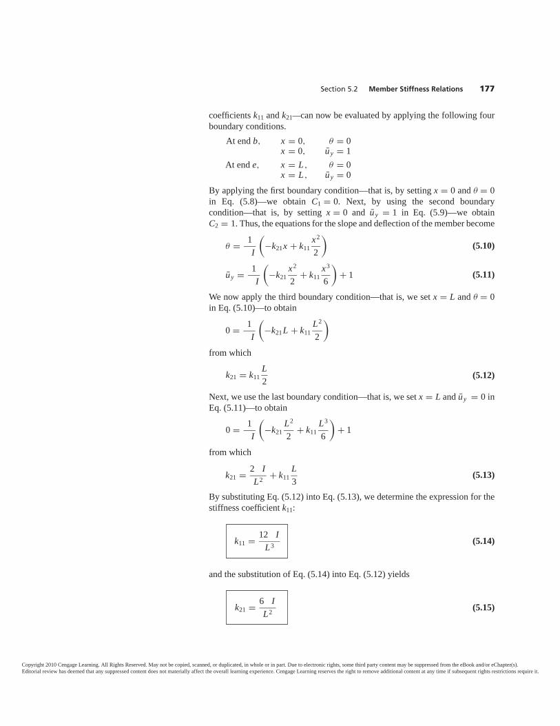
Section 5.2 Member Stiffness Relations 177
coefficients k11 and k21—can now be evaluated by applying the following fourboundary conditions.
At end b, x = 0, θ = 0x = 0, u y = 1
At end e, x = L , θ = 0x = L , u y = 0
By applying the first boundary condition—that is, by setting x = 0 and θ = 0in Eq. (5.8)—we obtain C1 = 0. Next, by using the second boundarycondition—that is, by setting x = 0 and u y = 1 in Eq. (5.9)—we obtainC2 = 1. Thus, the equations for the slope and deflection of the member become
θ = 1I
(−k21x + k11
x2
2
)(5.10)
u y = 1I
(−k21
x2
2+ k11
x3
6
)+ 1 (5.11)
We now apply the third boundary condition—that is, we set x = L and θ = 0in Eq. (5.10)—to obtain
0 = 1I
(−k21L + k11
L2
2
)
from which
k21 = k11L2
(5.12)
Next, we use the last boundary condition—that is, we set x = L and u y = 0 inEq. (5.11)—to obtain
0 = 1I
(−k21
L2
2+ k11
L3
6
)+ 1
from which
k21 = 2 IL2 + k11
L3
(5.13)
By substituting Eq. (5.12) into Eq. (5.13), we determine the expression for thestiffness coefficient k11:
(5.14)
and the substitution of Eq. (5.14) into Eq. (5.12) yields
(5.15)k21 = 6 IL2
k11 = 12 IL3
Copyright 2010 Cengage Learning. All Rights Reserved. May not be copied, scanned, or duplicated, in whole or in part. Due to electronic rights, some third party content may be suppressed from the eBook and/or eChapter(s).Editorial review has deemed that any suppressed content does not materially affect the overall learning experience. Cengage Learning reserves the right to remove additional content at any time if subsequent rights restrictions require it.
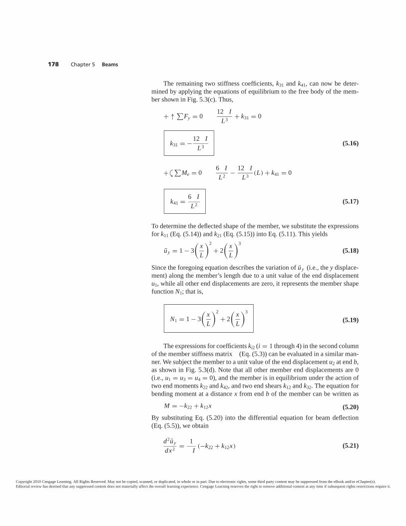
The remaining two stiffness coefficients, k31 and k41, can now be deter-mined by applying the equations of equilibrium to the free body of the mem-ber shown in Fig. 5.3(c). Thus,
+ ↑ ∑Fy = 0
12 IL3 + k31 = 0
(5.16)
+ ∑Me = 0
6 IL2 − 12 I
L3 (L) + k41 = 0
(5.17)
To determine the deflected shape of the member, we substitute the expressionsfor k11 (Eq. (5.14)) and k21 (Eq. (5.15)) into Eq. (5.11). This yields
u y = 1 − 3( x
L
)2
+ 2( x
L
)3
(5.18)
Since the foregoing equation describes the variation of u y (i.e., the y displace-ment) along the member’s length due to a unit value of the end displacementu1, while all other end displacements are zero, it represents the member shapefunction N1; that is,
(5.19)
The expressions for coefficients ki2 (i = 1 through 4) in the second columnof the member stiffness matrix (Eq. (5.3)) can be evaluated in a similar man-ner. We subject the member to a unit value of the end displacement u2 at end b,as shown in Fig. 5.3(d). Note that all other member end displacements are 0(i.e., u1 = u3 = u4 = 0), and the member is in equilibrium under the action oftwo end moments k22 and k42, and two end shears k12 and k32. The equation forbending moment at a distance x from end b of the member can be written as
M = −k22 + k12x (5.20)
By substituting Eq. (5.20) into the differential equation for beam deflection(Eq. (5.5)), we obtain
d2u ydx2 = 1
I (−k22 + k12x) (5.21)
N1 = 1 − 3( x
L
)2
+ 2( x
L
)3
k41 = 6 IL2
Y
k31 = −12 IL3
178 Chapter 5 Beams
Copyright 2010 Cengage Learning. All Rights Reserved. May not be copied, scanned, or duplicated, in whole or in part. Due to electronic rights, some third party content may be suppressed from the eBook and/or eChapter(s).Editorial review has deemed that any suppressed content does not materially affect the overall learning experience. Cengage Learning reserves the right to remove additional content at any time if subsequent rights restrictions require it.
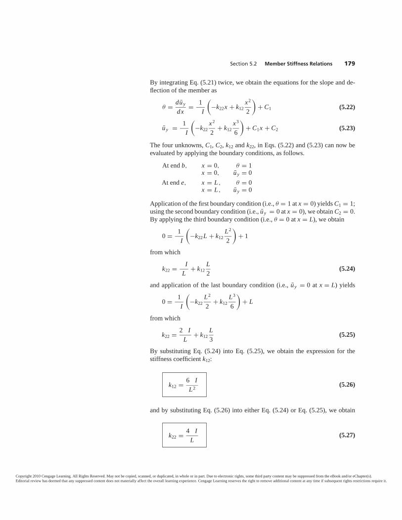
Section 5.2 Member Stiffness Relations 179
By integrating Eq. (5.21) twice, we obtain the equations for the slope and de-flection of the member as
θ = duydx = 1
I
(−k22x + k12
x2
2
)+ C1 (5.22)
u y = 1I
(−k22
x2
2+ k12
x3
6
)+ C1x + C2 (5.23)
The four unknowns, C1, C2, k12 and k22, in Eqs. (5.22) and (5.23) can now beevaluated by applying the boundary conditions, as follows.
At end b, x = 0, θ = 1x = 0, u y = 0
At end e, x = L , θ = 0x = L , u y = 0
Application of the first boundary condition (i.e., θ = 1 at x = 0) yields C1 = 1;using the second boundary condition (i.e., u y = 0 at x = 0), we obtain C2 = 0.By applying the third boundary condition (i.e., θ = 0 at x = L), we obtain
0 = 1I
(−k22L + k12
L2
2
)+ 1
from which
k22 = IL + k12
L2
(5.24)
and application of the last boundary condition (i.e., u y = 0 at x = L) yields
0 = 1I
(−k22
L2
2+ k12
L3
6
)+ L
from which
k22 = 2 IL + k12
L3
(5.25)
By substituting Eq. (5.24) into Eq. (5.25), we obtain the expression for thestiffness coefficient k12:
(5.26)
and by substituting Eq. (5.26) into either Eq. (5.24) or Eq. (5.25), we obtain
(5.27)k22 = 4 IL
k12 = 6 IL2
Copyright 2010 Cengage Learning. All Rights Reserved. May not be copied, scanned, or duplicated, in whole or in part. Due to electronic rights, some third party content may be suppressed from the eBook and/or eChapter(s).Editorial review has deemed that any suppressed content does not materially affect the overall learning experience. Cengage Learning reserves the right to remove additional content at any time if subsequent rights restrictions require it.
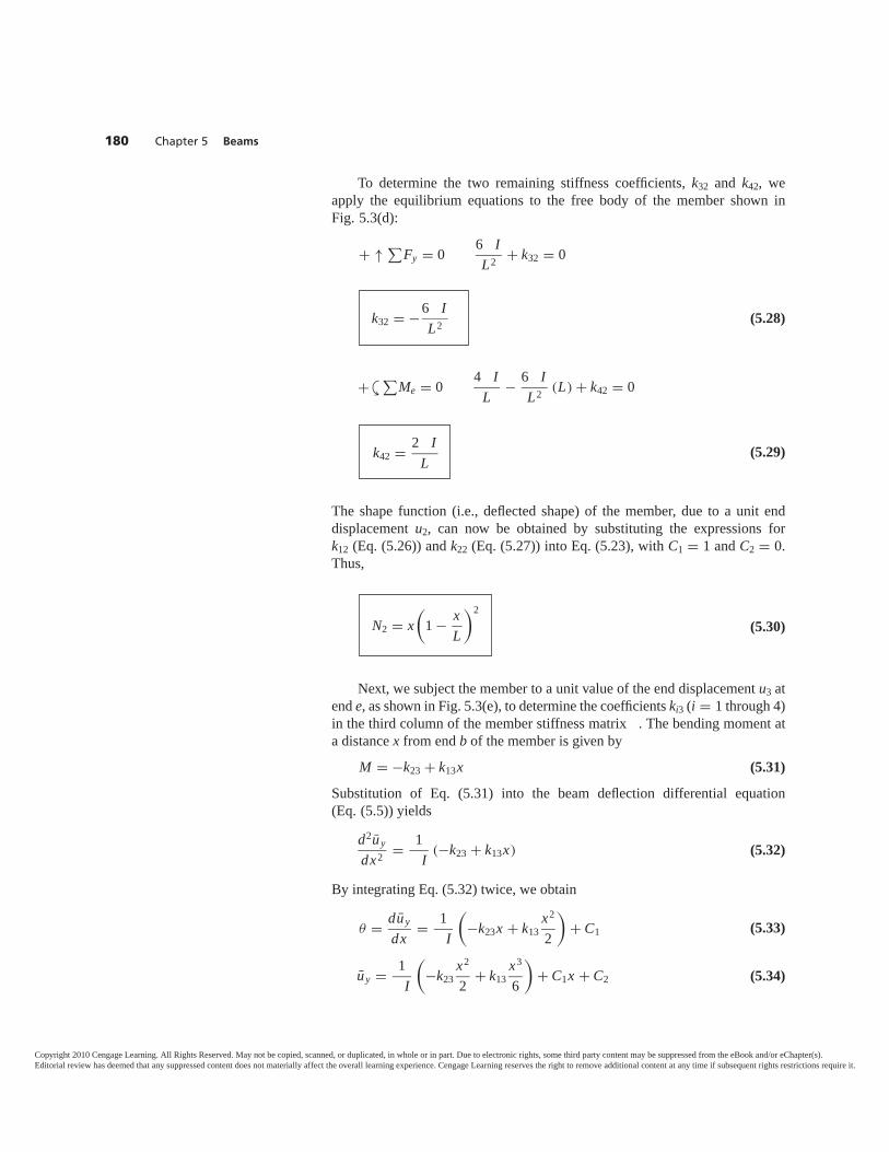
To determine the two remaining stiffness coefficients, k32 and k42, weapply the equilibrium equations to the free body of the member shown inFig. 5.3(d):
+ ↑ ∑Fy = 0
6 IL2 + k32 = 0
(5.28)
+ ∑Me = 0
4 IL − 6 I
L2 (L) + k42 = 0
(5.29)
The shape function (i.e., deflected shape) of the member, due to a unit enddisplacement u2, can now be obtained by substituting the expressions fork12 (Eq. (5.26)) and k22 (Eq. (5.27)) into Eq. (5.23), with C1 = 1 and C2 = 0.Thus,
(5.30)
Next, we subject the member to a unit value of the end displacement u3 atend e, as shown in Fig. 5.3(e), to determine the coefficients ki3 (i = 1 through 4)in the third column of the member stiffness matrix . The bending moment ata distance x from end b of the member is given by
M = −k23 + k13x (5.31)
Substitution of Eq. (5.31) into the beam deflection differential equation(Eq. (5.5)) yields
d2u ydx2 = 1
I (−k23 + k13x) (5.32)
By integrating Eq. (5.32) twice, we obtain
θ = duydx = 1
I
(−k23x + k13
x2
2
)+ C1 (5.33)
u y = 1I
(−k23
x2
2+ k13
x3
6
)+ C1x + C2 (5.34)
N2 = x(
1 − xL
)2
k42 = 2 IL
Y
k32 = −6 IL2
180 Chapter 5 Beams
Copyright 2010 Cengage Learning. All Rights Reserved. May not be copied, scanned, or duplicated, in whole or in part. Due to electronic rights, some third party content may be suppressed from the eBook and/or eChapter(s).Editorial review has deemed that any suppressed content does not materially affect the overall learning experience. Cengage Learning reserves the right to remove additional content at any time if subsequent rights restrictions require it.
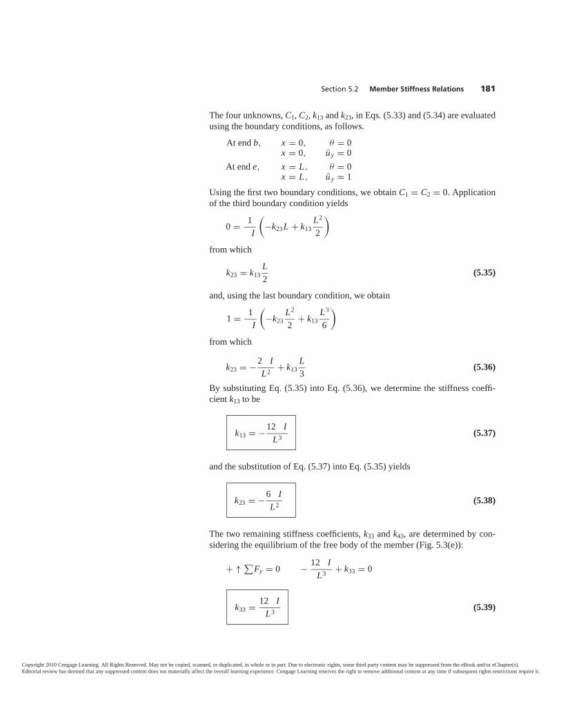
Section 5.2 Member Stiffness Relations 181
The four unknowns, C1, C2, k13 and k23, in Eqs. (5.33) and (5.34) are evaluatedusing the boundary conditions, as follows.
At end b, x = 0, θ = 0x = 0, u y = 0
At end e, x = L , θ = 0x = L , u y = 1
Using the first two boundary conditions, we obtain C1 = C2 = 0. Applicationof the third boundary condition yields
0 = 1I
(−k23L + k13
L2
2
)
from which
k23 = k13L2
(5.35)
and, using the last boundary condition, we obtain
1 = 1I
(−k23
L2
2+ k13
L3
6
)
from which
k23 = −2 IL2 + k13
L3
(5.36)
By substituting Eq. (5.35) into Eq. (5.36), we determine the stiffness coeffi-cient k13 to be
(5.37)
and the substitution of Eq. (5.37) into Eq. (5.35) yields
(5.38)
The two remaining stiffness coefficients, k33 and k43, are determined by con-sidering the equilibrium of the free body of the member (Fig. 5.3(e)):
+ ↑ ∑Fy = 0 − 12 I
L3 + k33 = 0
(5.39)k33 = 12 IL3
k23 = −6 IL2
k13 = −12 IL3
Copyright 2010 Cengage Learning. All Rights Reserved. May not be copied, scanned, or duplicated, in whole or in part. Due to electronic rights, some third party content may be suppressed from the eBook and/or eChapter(s).Editorial review has deemed that any suppressed content does not materially affect the overall learning experience. Cengage Learning reserves the right to remove additional content at any time if subsequent rights restrictions require it.
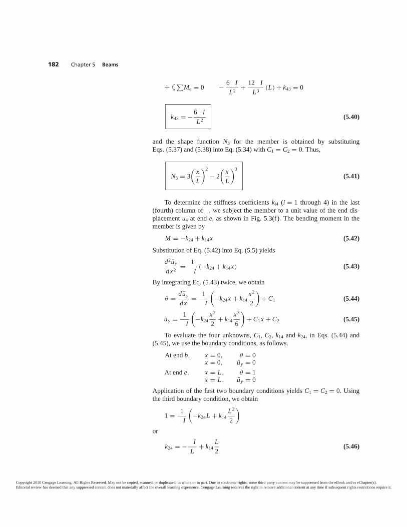
+ ∑Me = 0 − 6 I
L2 + 12 IL3 (L) + k43 = 0
(5.40)
and the shape function N3 for the member is obtained by substitutingEqs. (5.37) and (5.38) into Eq. (5.34) with C1 = C2 = 0. Thus,
(5.41)
To determine the stiffness coefficients ki4 (i = 1 through 4) in the last(fourth) column of , we subject the member to a unit value of the end dis-placement u4 at end e, as shown in Fig. 5.3(f). The bending moment in themember is given by
M = −k24 + k14x (5.42)
Substitution of Eq. (5.42) into Eq. (5.5) yields
d2u ydx2 = 1
I (−k24 + k14x) (5.43)
By integrating Eq. (5.43) twice, we obtain
θ = duydx = 1
I
(−k24x + k14
x2
2
)+ C1 (5.44)
u y = 1I
(−k24
x2
2+ k14
x3
6
)+ C1x + C2 (5.45)
To evaluate the four unknowns, C1, C2, k14 and k24, in Eqs. (5.44) and(5.45), we use the boundary conditions, as follows.
At end b, x = 0, θ = 0x = 0, u y = 0
At end e, x = L , θ = 1x = L , u y = 0
Application of the first two boundary conditions yields C1 = C2 = 0. Usingthe third boundary condition, we obtain
1 = 1I
(−k24L + k14
L2
2
)or
k24 = − IL + k14
L2
(5.46)
N3 = 3( x
L
)2
− 2( x
L
)3
k43 = −6 IL2
Y
182 Chapter 5 Beams
Copyright 2010 Cengage Learning. All Rights Reserved. May not be copied, scanned, or duplicated, in whole or in part. Due to electronic rights, some third party content may be suppressed from the eBook and/or eChapter(s).Editorial review has deemed that any suppressed content does not materially affect the overall learning experience. Cengage Learning reserves the right to remove additional content at any time if subsequent rights restrictions require it.
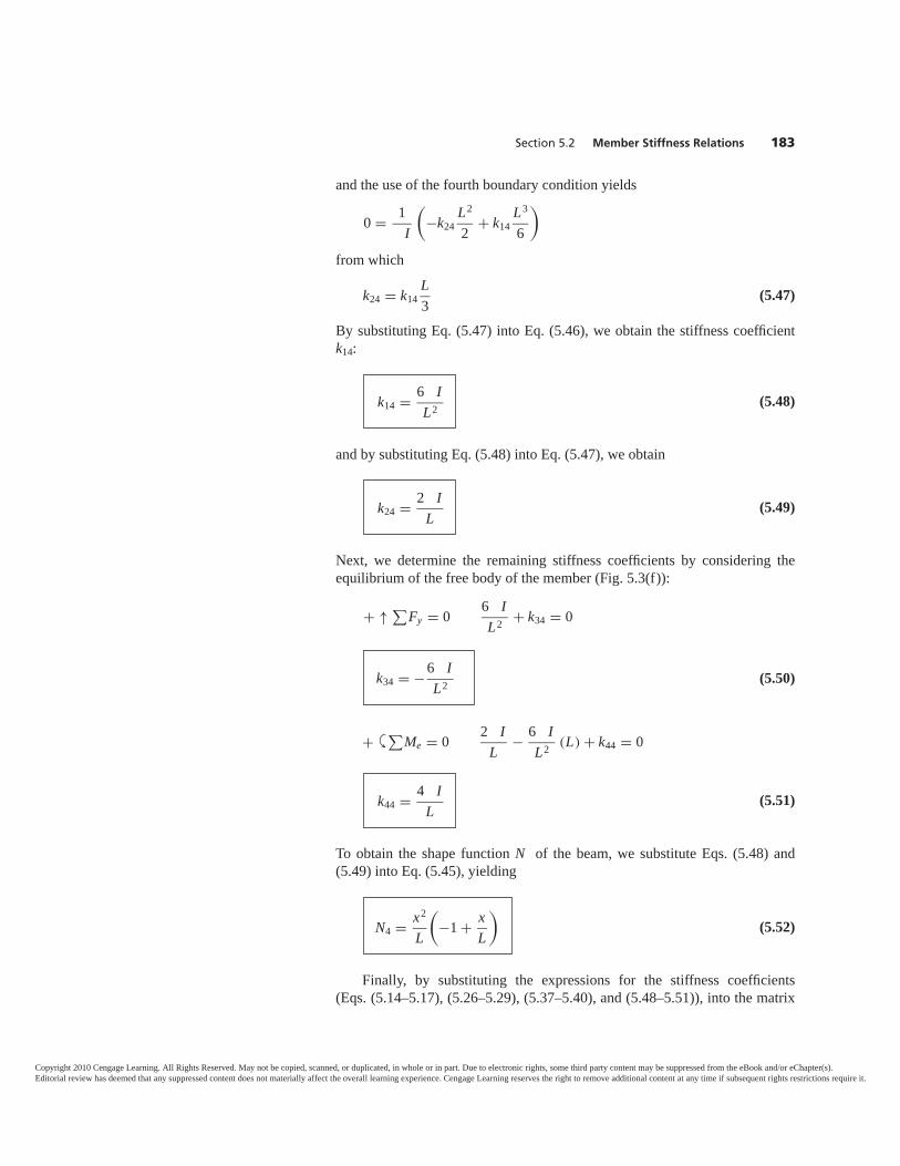
Section 5.2 Member Stiffness Relations 183
and the use of the fourth boundary condition yields
0 = 1I
(−k24
L2
2+ k14
L3
6
)
from which
k24 = k14L3
(5.47)
By substituting Eq. (5.47) into Eq. (5.46), we obtain the stiffness coefficientk14:
(5.48)
and by substituting Eq. (5.48) into Eq. (5.47), we obtain
(5.49)
Next, we determine the remaining stiffness coefficients by considering theequilibrium of the free body of the member (Fig. 5.3(f)):
+ ↑ ∑Fy = 0
6 IL2 + k34 = 0
(5.50)
+ ∑Me = 0
2 IL − 6 I
L2 (L) + k44 = 0
(5.51)
To obtain the shape function N of the beam, we substitute Eqs. (5.48) and(5.49) into Eq. (5.45), yielding
(5.52)
Finally, by substituting the expressions for the stiffness coefficients(Eqs. (5.14–5.17), (5.26–5.29), (5.37–5.40), and (5.48–5.51)), into the matrix
N4 = x2
L
(−1 + x
L
)
k44 = 4 IL
Y
k34 = −6 IL2
k24 = 2 IL
k14 = 6 IL2
Copyright 2010 Cengage Learning. All Rights Reserved. May not be copied, scanned, or duplicated, in whole or in part. Due to electronic rights, some third party content may be suppressed from the eBook and/or eChapter(s).Editorial review has deemed that any suppressed content does not materially affect the overall learning experience. Cengage Learning reserves the right to remove additional content at any time if subsequent rights restrictions require it.
E X A M P L E 5.2 Determine the stiffness matrices for the members of the beam shown in Fig. 5.5.
S O L U T I O N e ber 1 = 29,000 ksi, I = 875 in.4, L = 15 ft = 180 in.
IL3 = 29,000 (875)
(180)3 = 4.351 k/in.
Substitution in Eq. (5.53) yields
1 =
⎡⎢⎢⎣
52.212 4,699.1 −52.212 4,699.14,699.1 563,889 −4,699.1 281,944
−52.212 −4,699.1 52.212 −4,699.14,699.1 281,944 −4,699.1 563,889
⎤⎥⎥⎦ Ans
e ber 2 = 29,000 ksi, I = 1,750 in.4, L = 20 ft = 240 in.
IL3 = 29,000 (1,750)
(240)3 = 3.6712 k/in.
Thus, from Eq. (5.53)
2 =
⎡⎢⎢⎣
44.054 5,286.5 −44.054 5,286.55,286.5 845,833 −5,286.5 422,917
−44.054 −5,286.5 44.054 −5,286.55,286.5 422,917 −5,286.5 845,833
⎤⎥⎥⎦ Ans
form of given in Eq. (5.3), we obtain the following local stiffness matrix forthe members of beams.
= IL3
⎡⎢⎢⎣
12 6L −12 6L6L 4L2 −6L 2L2
−12 −6L 12 −6L6L 2L2 −6L 4L2
⎤⎥⎥⎦ (5.53)
Note that the stiffness matrix is symmetric; that is, kij = kji.
184 Chapter 5 Beams
X
Y
1 32
= 29,000 ksiI = 875 in.4
15 ftI
20 ft2I
21
Fig. 5.5
Copyright 2010 Cengage Learning. All Rights Reserved. May not be copied, scanned, or duplicated, in whole or in part. Due to electronic rights, some third party content may be suppressed from the eBook and/or eChapter(s).Editorial review has deemed that any suppressed content does not materially affect the overall learning experience. Cengage Learning reserves the right to remove additional content at any time if subsequent rights restrictions require it.
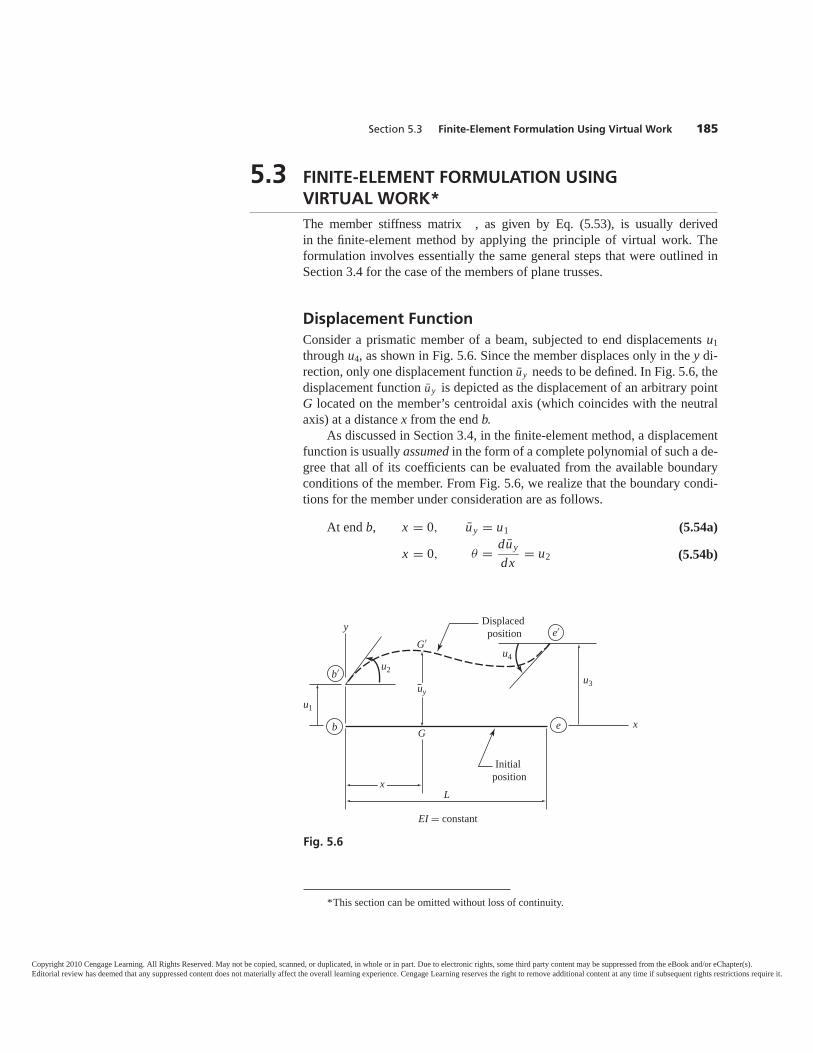
Section 5.3 Finite-Element Formulation Using Virtual Work 185
5.3 FINITE-ELEMENT FORMULATION USINGVIRTUAL WORK*The member stiffness matrix , as given by Eq. (5.53), is usually derivedin the finite-element method by applying the principle of virtual work. Theformulation involves essentially the same general steps that were outlined inSection 3.4 for the case of the members of plane trusses.
Displacement FunctionConsider a prismatic member of a beam, subjected to end displacements u1through u4, as shown in Fig. 5.6. Since the member displaces only in the y di-rection, only one displacement function u y needs to be defined. In Fig. 5.6, thedisplacement function u y is depicted as the displacement of an arbitrary pointG located on the member’s centroidal axis (which coincides with the neutralaxis) at a distance x from the end b.
As discussed in Section 3.4, in the finite-element method, a displacementfunction is usually assumed in the form of a complete polynomial of such a de-gree that all of its coefficients can be evaluated from the available boundaryconditions of the member. From Fig. 5.6, we realize that the boundary condi-tions for the member under consideration are as follows.
At end b, x = 0, u y = u1 (5.54a)
x = 0, θ = duydx = u2 (5.54b)
*This section can be omitted without loss of continuity.
x
y
b
b′
e
e′
L
Displacedposition
u1
u2u3
u4
Initialposition
uy
x
EI = constant
G
G′
Fig. 5.6
Copyright 2010 Cengage Learning. All Rights Reserved. May not be copied, scanned, or duplicated, in whole or in part. Due to electronic rights, some third party content may be suppressed from the eBook and/or eChapter(s).Editorial review has deemed that any suppressed content does not materially affect the overall learning experience. Cengage Learning reserves the right to remove additional content at any time if subsequent rights restrictions require it.
At end e, x = L , u y = u3 (5.54c)
x = L , θ = duydx = u4 (5.54d)
Since there are four boundary conditions, we can use a cubic polynomial (withfour coefficients) for the displacement function u y, as
u y = a0 + a1x + a2x2 + a3x3 (5.55)
in which a0 through a3 are the constants to be determined by applying the fourboundary conditions specified in Eqs. (5.54). By differentiating Eq. (5.55) withrespect to x, we obtain the equation for the slope of the member as
θ = duydx = a1 + 2a2x + 3a3x2 (5.56)
Now, we apply the first boundary condition (Eq. (5.54a)) by setting x = 0 andu y = u1 in Eq. (5.55). This yields
a0 = u1 (5.57)
Similarly, using the second boundary condition—that is, by setting x = 0 andθ = u2 in Eq. (5.56)—we obtain
a1 = u2 (5.58)
Next, we apply the third boundary condition, setting x = L and u y = u3 inEq. (5.55). This yields
u3 = a0 + a1L + a2L2 + a3L3 (5.59)
By substituting a0 = u1 (Eq. (5.57)) and a1 = u2 (Eq. (5.58)) into Eq. (5.59),we obtain
a3 = 1L3
(−u1 − u2L + u3 − a2L2) (5.60)
To apply the fourth boundary condition (Eq. (5.54d)), we set x = L and θ = u4in Eq. (5.56). This yields
u4 = a1 + 2a2L + 3a3L2 (5.61)
By substituting Eqs. (5.57), (5.58), and (5.60) into Eq. (5.61), and solving theresulting equation for a2, we obtain
a2 = 1L2 (−3u1 − 2u2L + 3u3 − u4L) (5.62)
and the backsubstitution of Eq. (5.62) into Eq. (5.60) yields
a3 = 1L3 (2u1 + u2L − 2u3 + u4L) (5.63)
Finally, by substituting Eqs. (5.57), (5.58), (5.62), and (5.63) into Eq. (5.55), we obtain the following expression for the displacement functionu y, in terms of the end displacements u1 through u4.
186 Chapter 5 Beams
Copyright 2010 Cengage Learning. All Rights Reserved. May not be copied, scanned, or duplicated, in whole or in part. Due to electronic rights, some third party content may be suppressed from the eBook and/or eChapter(s).Editorial review has deemed that any suppressed content does not materially affect the overall learning experience. Cengage Learning reserves the right to remove additional content at any time if subsequent rights restrictions require it.
Section 5.3 Finite-Element Formulation Using Virtual Work 187
(5.64)
Shape FunctionsThe displacement function u y, as given by Eq. (5.64), can alternatively bewritten as
u y = N1u1 + N2u2 + N3u3 + N4u4 (5.65)
with
N1 = 1 − 3( x
L
)2
+ 2( x
L
)3
(5.66a)
N2 = x(
1 − xL
)2
(5.66b)
N3 = 3( x
L
)2
− 2( x
L
)3
(5.66c)
N4 = x2
L
(−1 + x
L
)(5.66d)
in which Ni (i = 1 through 4) are the member shape functions. A comparisonof Eqs. (5.66a) through (5.66d) with Eqs. (5.19), (5.30), (5.41), and (5.52), re-spectively, indicates that the shape functions determined herein by assuming acubic displacement function are identical to those obtained in Section 5.2 byexactly solving the differential equation for bending of beams. This is becausea cubic polynomial represents the actual (or exact) solution of the governingdifferential equation (Eq. (5.5)), provided that the member is prismatic and it isnot subjected to any external loading.
Equation (5.65) can be written in matrix form as
u y = [ N1 N2 N3 N4 ]
⎡⎢⎢⎣
u1u2u3u4
⎤⎥⎥⎦ (5.67)
or, symbolically, as
(5.68)
in which is the member shape-function matrix.
u y = u
u y =[
1 − 3( x
L
)2
+ 2( x
L
)3]
u1 +[
x(
1 − xL
)2]
u2
+[
3( x
L
)2
− 2( x
L
)3]
u3 +[ x2
L
(−1 + x
L
)]u4
Copyright 2010 Cengage Learning. All Rights Reserved. May not be copied, scanned, or duplicated, in whole or in part. Due to electronic rights, some third party content may be suppressed from the eBook and/or eChapter(s).Editorial review has deemed that any suppressed content does not materially affect the overall learning experience. Cengage Learning reserves the right to remove additional content at any time if subsequent rights restrictions require it.
Strain–Displacement RelationshipWe recall from mechanics of materials that the normal (longitudinal) strain ε ina fiber of a member, located at a distance y above the neutral axis, can beexpressed in terms of the displacement u y of the member’s neutral axis, by therelationship
ε = −y d2u ydx2 (5.69)
in which the minus sign indicates that the tensile strain is considered positive.By substituting Eq. (5.68) into Eq. (5.69), we write
ε = −y d2
dx2 ( u) (5.70)
Since the end-displacement vector u is not a function of x, it can be treatedas a constant for the purpose of differentiation. Thus, Eq. (5.70) can be ex-pressed as
(5.71)
To determine the member strain-displacement matrix B, we write
B = −y d2
dx2 = −y[
d2N1
dx2d2N2
dx2d2N3
dx2d2N4
dx2
](5.72)
By differentiating twice the equations for the shape functions as given byEqs. (5.66), and substituting the resulting expressions into Eq. (5.72), weobtain
B = − yL2
[6(
−1 + 2xL
)2L
(−2 + 3
xL
)6(
1 − 2xL
)2L
(−1 + 3
xL
)](5.73)
Stress–Displacement RelationshipTo establish the relationship between the member normal stress and the enddisplacements, we substitute Eq. (5.71) into the stress–strain relation σ = ε.This yields
(5.74)
Member Stiffness Matrix, kWith both the member strain and stress expressed in terms of end displace-ments, we can now establish the member stiffness matrix by applying theprinciple of virtual work for deformable bodies. Consider an arbitrary member
σ = Bu
ε =(
−y d2
dx2
)u = Bu
188 Chapter 5 Beams
Copyright 2010 Cengage Learning. All Rights Reserved. May not be copied, scanned, or duplicated, in whole or in part. Due to electronic rights, some third party content may be suppressed from the eBook and/or eChapter(s).Editorial review has deemed that any suppressed content does not materially affect the overall learning experience. Cengage Learning reserves the right to remove additional content at any time if subsequent rights restrictions require it.
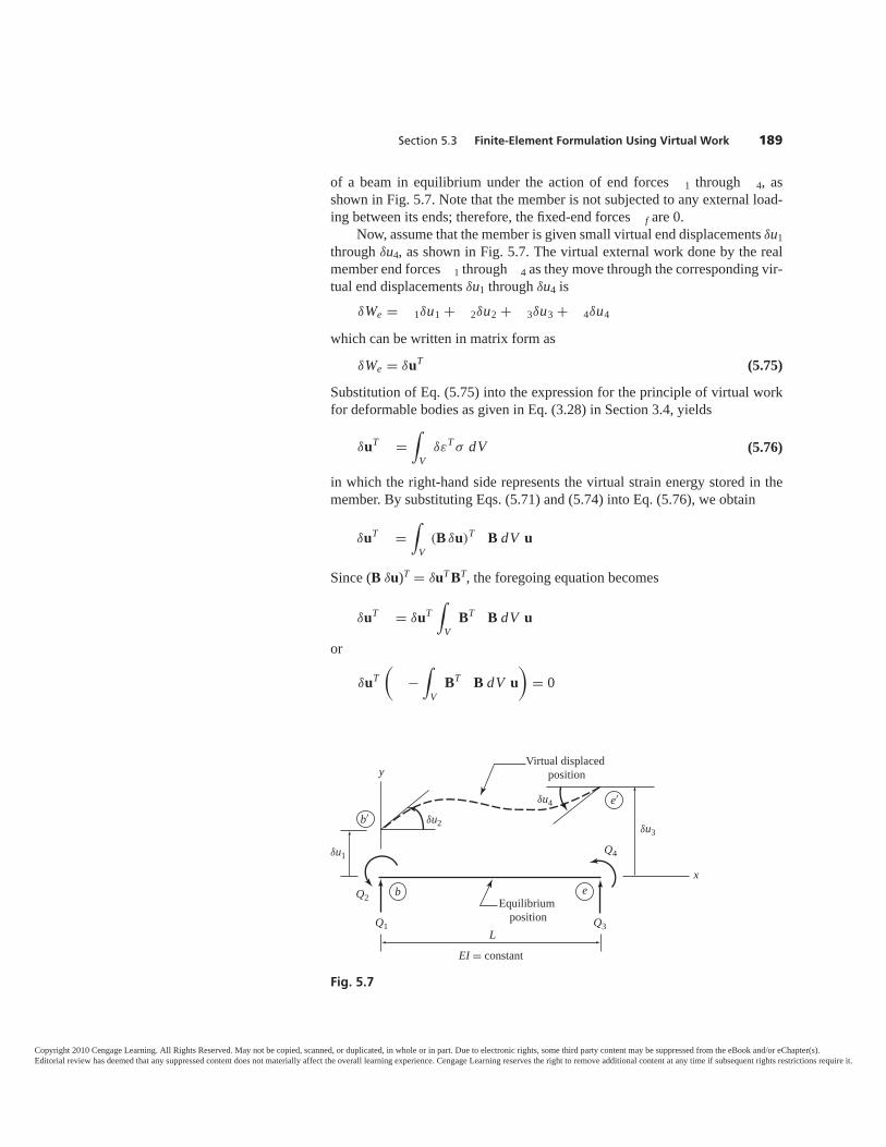
Section 5.3 Finite-Element Formulation Using Virtual Work 189
of a beam in equilibrium under the action of end forces 1 through 4, asshown in Fig. 5.7. Note that the member is not subjected to any external load-ing between its ends; therefore, the fixed-end forces f are 0.
Now, assume that the member is given small virtual end displacements δu1through δu4, as shown in Fig. 5.7. The virtual external work done by the realmember end forces 1 through 4 as they move through the corresponding vir-tual end displacements δu1 through δu4 is
δWe = 1δu1 + 2δu2 + 3δu3 + 4δu4
which can be written in matrix form as
δWe = δuT (5.75)
Substitution of Eq. (5.75) into the expression for the principle of virtual workfor deformable bodies as given in Eq. (3.28) in Section 3.4, yields
δuT =∫
VδεT σ dV (5.76)
in which the right-hand side represents the virtual strain energy stored in themember. By substituting Eqs. (5.71) and (5.74) into Eq. (5.76), we obtain
δuT =∫
V(B δu)T B dV u
Since (B δu)T = δuT BT, the foregoing equation becomes
δuT = δuT∫
VBT B dV u
or
δuT(
−∫
VBT B dV u
)= 0
x
y
b
b′
e
e′
L
Virtual displaced position
δu1
δu2δu3
δu4
Q4
Q3Q1
Q2 Equilibriumposition
EI = constant
Fig. 5.7
Copyright 2010 Cengage Learning. All Rights Reserved. May not be copied, scanned, or duplicated, in whole or in part. Due to electronic rights, some third party content may be suppressed from the eBook and/or eChapter(s).Editorial review has deemed that any suppressed content does not materially affect the overall learning experience. Cengage Learning reserves the right to remove additional content at any time if subsequent rights restrictions require it.
As δuT may be arbitrarily chosen and is not 0, the quantity in the parenthesesmust be 0; thus,
=(∫
VBT B dV
)u = u (5.77)
with
(5.78)
Note that the foregoing general form of for beam members is the same as thatobtained in Section 3.4 for the members of plane trusses (Eq. (3.55)). Toexplicitly determine the member stiffness matrix , we substitute Eq. (5.73) forB into Eq. (5.78). This yields
= L4
∫V
y2
⎡⎢⎢⎢⎢⎢⎢⎢⎢⎢⎢⎢⎢⎢⎢⎢⎢⎢⎢⎣
6
(−1 + 2
xL
)
2L(
−2 + 3xL
)
6
(1 − 2
xL
)
2L(
−1 + 3xL
)
⎤⎥⎥⎥⎥⎥⎥⎥⎥⎥⎥⎥⎥⎥⎥⎥⎥⎥⎥⎦
[6
(−1 + 2
xL
)2L
(−2 + 3
xL
)6
(1 − 2
xL
)2L
(−1 + 3
xL
)]dV (5.79)
By substituting dV = (dA) dx into Eq. (5.79), and realizing that ∫
A y2 dA = I,we obtain
= IL4
∫ L
0
×
⎡⎢⎢⎢⎢⎢⎢⎢⎢⎢⎢⎢⎣
36(−1 + 2
xL
)212L
(−2 + 3
xL
) (−1 + 2
xL
)−36
(−1 + 2
xL
)212L
(−1 + 3
xL
) (−1 + 2
xL
)
12L(−2 + 3
xL
) (−1 + 2
xL
)4L2
(−2 + 3
xL
)212L
(−2 + 3
xL
) (1 − 2
xL
)4L2
(−2 + 3
xL
) (−1 + 3
xL
)
−36(−1 + 2
xL
)212L
(−2 + 3
xL
) (1 − 2
xL
)36
(−1 + 2
xL
)212L
(−1 + 3
xL
) (1 − 2
xL
)
12L(−1 + 3
xL
) (−1 + 2
xL
)4L2
(−2 + 3
xL
) (−1 + 3
xL
)12L
(−1 + 3
xL
) (1 − 2
xL
)4L2
(−1 + 3
xL
)2
⎤⎥⎥⎥⎥⎥⎥⎥⎥⎥⎥⎥⎦
dx
(5.80)
=∫
VBT B dV
190 Chapter 5 Beams
Copyright 2010 Cengage Learning. All Rights Reserved. May not be copied, scanned, or duplicated, in whole or in part. Due to electronic rights, some third party content may be suppressed from the eBook and/or eChapter(s).Editorial review has deemed that any suppressed content does not materially affect the overall learning experience. Cengage Learning reserves the right to remove additional content at any time if subsequent rights restrictions require it.
Section 5.4 Member Fixed-End Forces Due to Loads 191
which, upon integration, becomes
= IL3
⎡⎢⎢⎣
12 6L −12 6L6L 4L2 −6L 2L2
−12 −6L 12 −6L6L 2L2 −6L 4L2
⎤⎥⎥⎦
Note that the foregoing expression for is identical to that derived in Section 5.2(Eq. (5.53)) by directly integrating the differential equation for beam deflectionand applying the equilibrium equations.
5.4 MEMBER FIXED-END FORCES DUE TO LOADSIt was shown in Section 5.2 that the stiffness relationships for a member of abeam can be written in matrix form (see Eq. (5.4)) as
= u + f
As the foregoing relationship indicates, the total forces that can develop atthe ends of a member can be expressed as the sum of the forces u due to theend displacements u, and the fixed-end forces f that would develop at themember ends due to external loads if both member ends were fixed againsttranslations and rotations.
In this section, we consider the derivation of the expressions for fixed-endforces due to external loads applied to the members of beams. To illustrate theprocedure, consider a fixed member subjected to a concentrated load W, asshown in Fig. 5.8(a). As indicated in this figure, the fixed-end moments at themember ends b and e are denoted by FMb and FMe, respectively, whereas FSband FSe denote the fixed-end shears at member ends b and e, respectively. Ourobjective is to determine expressions for the fixed-end moments and shears interms of the magnitude and location of the load W; we will use the direct in-tegration approach, along with the equations of equilibrium, for this purpose.
As the concentrated load W acts at point A of the member (Fig. 5.8(a)), thebending moment M cannot be expressed as a single continuous function of xover the entire length of the member. Therefore, we divide the member intotwo segments, bA and Ae; and we determine the following equations for bend-ing moment in segments bA and Ae, respectively:
0 ≤ x ≤ l1 M = −F Mb + F Sbx (5.81)
l1 ≤ x ≤ L M = −F Mb + F Sbx − W (x − l1) (5.82)
By substituting Eqs. (5.81) and (5.82) into the differential equation for beamdeflection (Eq. (5.5)), we obtain, respectively,
0 ≤ x ≤ l1d2u ydx2 = 1
I (−F Mb + F Sbx) (5.83)
l1 ≤ x ≤ L d2u ydx2 = 1
I [−F Mb + F Sbx − W (x − l1)] (5.84)
Copyright 2010 Cengage Learning. All Rights Reserved. May not be copied, scanned, or duplicated, in whole or in part. Due to electronic rights, some third party content may be suppressed from the eBook and/or eChapter(s).Editorial review has deemed that any suppressed content does not materially affect the overall learning experience. Cengage Learning reserves the right to remove additional content at any time if subsequent rights restrictions require it.

By integrating Eq. (5.83) twice, we obtain the equations for the slope and de-flection in segment bA of the member:
0 ≤ x ≤ l1 θ = duydx = 1
I
(−FMbx + FSb
x2
2
)+ C1 (5.85)
0 ≤ x ≤ l1 u y = 1I
(−FMb
x2
2+ FSb
x3
6
)+ C1x + C2 (5.86)
Similarly, by integrating Eq. (5.84) twice, we obtain the equations for the slopeand deflection in the segment Ae:
l1 ≤ x ≤ L θ = 1I
[−FMbx + FSb
x2
2− Wx
2(x − 2l1)
]+ C3 (5.87)
l1 ≤ x ≤ L uy = 1I
[−FMb
x2
2+ FSb
x3
6− Wx2
6(x − 3l1)
]+ C3x + C4 (5.88)
192 Chapter 5 Beams
x
y
b eFMe
FMb
FSb FSe
L
(a) Fixed Member
A
W
l1 l2
b e
L
(b) Fixed-End Forces
W
l1 l2
−Wl12l2L2
Wl1l22
L2
Wl22 (3l1 + l2)L3
Wl12 (l1 + 3l2)L3
Fig. 5.8
Copyright 2010 Cengage Learning. All Rights Reserved. May not be copied, scanned, or duplicated, in whole or in part. Due to electronic rights, some third party content may be suppressed from the eBook and/or eChapter(s).Editorial review has deemed that any suppressed content does not materially affect the overall learning experience. Cengage Learning reserves the right to remove additional content at any time if subsequent rights restrictions require it.
Section 5.4 Member Fixed-End Forces Due to Loads 193
Equations (5.85) through (5.88) indicate that the equations for the slopeand deflection of the member contain a total of six unknowns; that is, four con-stants of integration, C1 through C4, and two fixed-end forces, FMb and FSb.These six unknowns can be evaluated by applying four boundary conditions(i.e., the slopes and deflections at the two fixed ends, b and e, must be 0), andtwo continuity conditions requiring that the slope and the deflection of themember’s elastic curve be continuous at point A. By applying the two bound-ary conditions for the fixed end b (i.e., at x = 0, θ = u y = 0) to Eqs. (5.85) and(5.86), we obtain
C1 = C2 = 0 (5.89)
Next, to evaluate the constant C3, we use the condition that the slope must becontinuous at point A. This condition requires that the two slope equations(Eqs. (5.85) and (5.87)) yield the same slope θA at x = l1. By setting x = l1 inEqs. (5.85) and (5.87), and equating the resulting expressions, we obtain
1I
(−FMbl1 + FSb
l212
)= 1
I
(−FMbl1 + FSb
l212
+ Wl21
2
)+ C3
By solving for C3, we determine that
C3 = − Wl21
2 I (5.90)
In a similar manner, we evaluate the constant C4 by applying the condition ofcontinuity of deflection at point A. By setting x = l1 in the two deflection equa-tions (Eqs. (5.86) and (5.88)), and equating the resulting expressions, we obtain
1I
(−FMb
l212
+ FSbl316
)
= 1I
(−FMb
l212
+ FSbl316
+ Wl31
3
)− Wl3
12 I + C4
from which
C4 = Wl31
6 I (5.91)
With the four constants of integration known, we can now evaluate the tworemaining unknowns, FSb and FMb, by applying the boundary conditions thatthe slope and deflection at the fixed end e must be 0 (i.e., at x = L, θ = u y = 0).By setting x = L in Eqs. (5.87) and (5.88), with θ = 0 in Eq. (5.87) and u y = 0in Eq. (5.88), we obtain
1I
[−FMb L + FSb
L2
2− WL
2(L − 2l1)
]− Wl2
12 I = 0 (5.92)
1I
[−FMb
L2
2+ FSb
L3
6− WL2
6(L − 3l1)
]− Wl2
1 L2 I + Wl3
16 I = 0
(5.93)
Copyright 2010 Cengage Learning. All Rights Reserved. May not be copied, scanned, or duplicated, in whole or in part. Due to electronic rights, some third party content may be suppressed from the eBook and/or eChapter(s).Editorial review has deemed that any suppressed content does not materially affect the overall learning experience. Cengage Learning reserves the right to remove additional content at any time if subsequent rights restrictions require it.
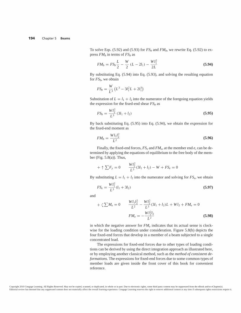
To solve Eqs. (5.92) and (5.93) for FSb and FMb, we rewrite Eq. (5.92) to ex-press FMb in terms of FSb as
FMb = FSbL2
− W2
(L − 2l1) − Wl21
2L (5.94)
By substituting Eq. (5.94) into Eq. (5.93), and solving the resulting equationfor FSb, we obtain
FSb = WL3
(L3 − 3l2
1 L + 2l31)
Substitution of L = l1 + l2 into the numerator of the foregoing equation yieldsthe expression for the fixed-end shear FSb as
FSb = Wl22
L3 (3l1 + l2) (5.95)
By back substituting Eq. (5.95) into Eq. (5.94), we obtain the expression forthe fixed-end moment as
FMb = Wl1l22
L2(5.96)
Finally, the fixed-end forces, FSe and FMe, at the member end e, can be de-termined by applying the equations of equilibrium to the free body of the mem-ber (Fig. 5.8(a)). Thus,
+ ↑ ∑Fy = 0
Wl22
L3 (3l1 + l2) − W + FSe = 0
By substituting L = l1 + l2 into the numerator and solving for FSe, we obtain
FSe = Wl21
L3 (l1 + 3l2) (5.97)
and
+ ∑Me = 0
Wl1l22
L2 − Wl22
L3 (3l1 + l2)L + Wl2 + FMe = 0
FMe = −Wl21l2
L2 (5.98)
in which the negative answer for FMe indicates that its actual sense is clock-wise for the loading condition under consideration. Figure 5.8(b) depicts thefour fixed-end forces that develop in a member of a beam subjected to a singleconcentrated load.
The expressions for fixed-end forces due to other types of loading condi-tions can be derived by using the direct integration approach as illustrated here,or by employing another classical method, such as the method of consistent de-formations. The expressions for fixed-end forces due to some common types ofmember loads are given inside the front cover of this book for convenientreference.
Y
194 Chapter 5 Beams
Copyright 2010 Cengage Learning. All Rights Reserved. May not be copied, scanned, or duplicated, in whole or in part. Due to electronic rights, some third party content may be suppressed from the eBook and/or eChapter(s).Editorial review has deemed that any suppressed content does not materially affect the overall learning experience. Cengage Learning reserves the right to remove additional content at any time if subsequent rights restrictions require it.
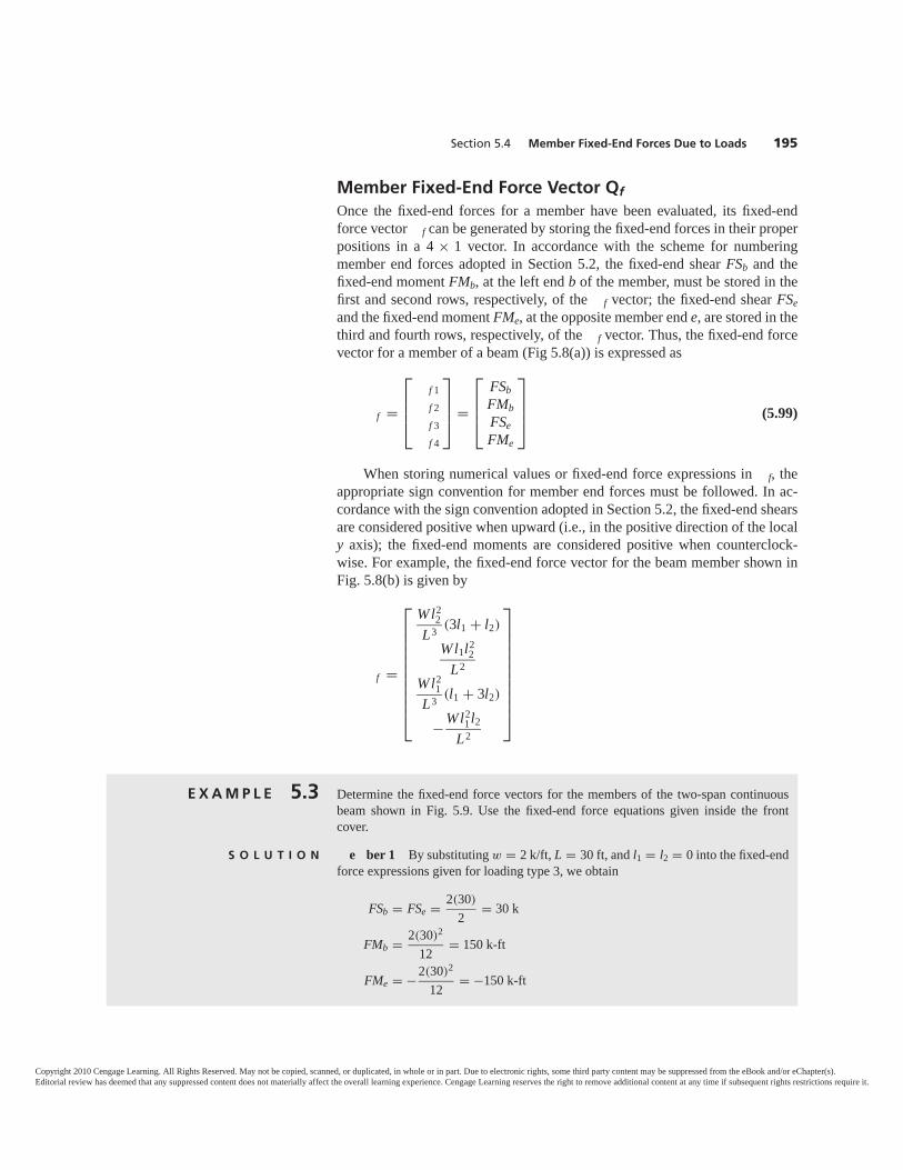
Section 5.4 Member Fixed-End Forces Due to Loads 195
Member Fixed-End Force Vector Qf
Once the fixed-end forces for a member have been evaluated, its fixed-endforce vector f can be generated by storing the fixed-end forces in their properpositions in a 4 × 1 vector. In accordance with the scheme for numberingmember end forces adopted in Section 5.2, the fixed-end shear FSb and thefixed-end moment FMb, at the left end b of the member, must be stored in thefirst and second rows, respectively, of the f vector; the fixed-end shear FSeand the fixed-end moment FMe, at the opposite member end e, are stored in thethird and fourth rows, respectively, of the f vector. Thus, the fixed-end forcevector for a member of a beam (Fig 5.8(a)) is expressed as
f =
⎡⎢⎢⎣
f 1
f 2
f 3
f 4
⎤⎥⎥⎦ =
⎡⎢⎢⎣
FSbFMbFSeFMe
⎤⎥⎥⎦ (5.99)
When storing numerical values or fixed-end force expressions in f, theappropriate sign convention for member end forces must be followed. In ac-cordance with the sign convention adopted in Section 5.2, the fixed-end shearsare considered positive when upward (i.e., in the positive direction of the localy axis); the fixed-end moments are considered positive when counterclock-wise. For example, the fixed-end force vector for the beam member shown inFig. 5.8(b) is given by
f =
⎡⎢⎢⎢⎢⎢⎢⎢⎢⎢⎣
Wl22
L3 (3l1 + l2)
Wl1l22
L2
Wl21
L3 (l1 + 3l2)
−Wl21l2
L2
⎤⎥⎥⎥⎥⎥⎥⎥⎥⎥⎦
E X A M P L E 5.3 Determine the fixed-end force vectors for the members of the two-span continuousbeam shown in Fig. 5.9. Use the fixed-end force equations given inside the frontcover.
S O L U T I O N e ber 1 By substituting w = 2 k/ft, L = 30 ft, and l1 = l2 = 0 into the fixed-endforce expressions given for loading type 3, we obtain
FSb = FSe = 2(30)
2= 30 k
FMb = 2(30)2
12= 150 k-ft
FMe = −2(30)2
12= −150 k-ft
Copyright 2010 Cengage Learning. All Rights Reserved. May not be copied, scanned, or duplicated, in whole or in part. Due to electronic rights, some third party content may be suppressed from the eBook and/or eChapter(s).Editorial review has deemed that any suppressed content does not materially affect the overall learning experience. Cengage Learning reserves the right to remove additional content at any time if subsequent rights restrictions require it.
196 Chapter 5 Beams
30 ft 10 ft 20 ft
2 k/ft
18 k
EI = constant(a) Two-Span Continuous Beam
X
Y
1 32
30 ft
(b) Analytical Model
30 ft
21
Fig. 5.9
By substituting these values of fixed-end forces into Eq. (5.99), we obtain the fixed-end force vector for member 1:
f 1 =
⎡⎢⎢⎣
3015030
−150
⎤⎥⎥⎦ Ans
e ber 2 From Fig. 5.9(a), we can see that this member is subjected to two differ-ent loadings—a concentrated load W = 18 k with l1 = 10 ft, l2 = 20 ft, and L = 30 ft(load type 1), and a uniformly distributed load w = 2 k/ft with l1 = l2 = 0 and L = 30 ft(load type 3). The fixed-end forces for such a member, due to the combined effect ofseveral loads, can be conveniently determined by superimposing (algebraicallyadding) the fixed-end forces due to each of the loads acting individually on the mem-ber. By using superposition, we determine the fixed-end forces for member 2 to be
FSb = 18(20)2
(30)3 [3(10) + (20)] + 2 (30)
2= 43.333 k
FMb = 18 (10) (20)2
(30)2 + 2 (30)2
12= 230 k-ft
FSe = 18(10)2
(30)3 [10 + 3(20)] + 2 (30)
2= 34.667 k
FMe = −18 (10)2 (20)
(30)2 − 2 (30)2
12= −190 k-ft
Copyright 2010 Cengage Learning. All Rights Reserved. May not be copied, scanned, or duplicated, in whole or in part. Due to electronic rights, some third party content may be suppressed from the eBook and/or eChapter(s).Editorial review has deemed that any suppressed content does not materially affect the overall learning experience. Cengage Learning reserves the right to remove additional content at any time if subsequent rights restrictions require it.
Section 5.5 Structure Stiffness Relations 197
Thus, the fixed-end force vector for member 2 is
f 2 =
⎡⎢⎢⎣
43.333230
34.667−190
⎤⎥⎥⎦ Ans
5.5 STRUCTURE STIFFNESS RELATIONSThe procedure for establishing the structure stiffness relations for beams is es-sentially the same as that for plane trusses discussed in Section 3.7. The proce-dure, called the direct stiffness method, involves: (a) expressing the joint loadsP in terms of the member end forces by applying the joint equilibrium equa-tions; (b) relating the joint displacements d to the member end displacementsu by using the compatibility conditions that the member end displacements androtations must be the same as the corresponding joint displacements and rota-tions; and (c) linking the joint displacements d to the joint loads P by means ofthe member force-displacement relations = u + f.
Consider, for example, an arbitrary beam subjected to joint and memberloads, as depicted in Fig. 5.10(a). The structure has three degrees of freedom,d1 through d3, as shown in Fig. 5.10(b). Our objective is to establish the struc-ture stiffness relationships, which express the external loads as functions of thejoint displacements d. The member end forces and end displacements u forthe three members of the beam are given in Fig. 5.10(c), in which the super-script (i) denotes the member number.
By applying the equations of equilibrium ∑
FY = 0 and ∑
M = 0 to thefree body of joint 2, and the equilibrium equation
∑M = 0 to the free body of
joint 3, we obtain the following relationships between the external joint loadsP and the internal member end forces .
P1 = (1)3 + (2)
1 (5.100a)
P2 = (1)4 + (2)
2 (5.100b)
P3 = (2)4 + (3)
2 (5.100c)
Next, we determine compatibility conditions for the three members ofthe beam. Since the left end 1 of member 1 is connected to fixed support 1(Fig. 5.10(b)), which can neither translate nor rotate, the displacements u1
(1)
and u(1)2 of end 1 of the member (Fig. 5.10(c)) must be 0. Similarly, since end 2
of this member is connected to joint 2, the displacements u(1)3 and u(1)
4 of end2 must be the same as the displacements d1 and d2, respectively, of joint 2.Thus, the compatibility equations for member 1 are:
u(1)1 = u(1)
2 = 0 u(1)3 = d1 u(1)
4 = d2 (5.101)
Copyright 2010 Cengage Learning. All Rights Reserved. May not be copied, scanned, or duplicated, in whole or in part. Due to electronic rights, some third party content may be suppressed from the eBook and/or eChapter(s).Editorial review has deemed that any suppressed content does not materially affect the overall learning experience. Cengage Learning reserves the right to remove additional content at any time if subsequent rights restrictions require it.
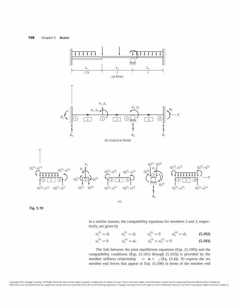
In a similar manner, the compatibility equations for members 2 and 3, respec-tively, are given by
u(2)1 = d1 u(2)
2 = d2 u(2)3 = 0 u(2)
4 = d3 (5.102)
u(3)1 = 0 u(3)
2 = d3 u(3)3 = u(3)
4 = 0 (5.103)
The link between the joint equilibrium equations (Eqs. (5.100)) and thecompatibility conditions (Eqs. (5.101) through (5.103)) is provided by themember stiffness relationship = u + f (Eq. (5.4)). To express the sixmember end forces that appear in Eqs. (5.100) in terms of the member end
198 Chapter 5 Beams
L2
IL3
IL1
1.5I(a) Beam
R5
R8
P1, d1P3, d3
P2, d2
R4 R7
321 4X
Y
R6
(b) Analytical Model
21 3
Q2(2)
Q3(1) Q1
(2)
P1P2
Q4(1) 2
Q2(3)
Q3(2) Q1
(3)
R6
Q4(2)
P3
3
Y
Q4(1), u4
(1)
Q1(1), u1
(1) Q3(1), u3
(1)
Q2(1), u2
(1)
1 2
Q1(2), u1
(2) Q3(2), u3
(2)
Q4(2), u4
(2)Q2(2), u2
(2)
2 32X
Q1(3), u1
(3)
Q2(3), u2
(3) Q4(3), u4
(3)
Q3(3), u3
(3)
3 43
(c)
21
Fig. 5.10
Copyright 2010 Cengage Learning. All Rights Reserved. May not be copied, scanned, or duplicated, in whole or in part. Due to electronic rights, some third party content may be suppressed from the eBook and/or eChapter(s).Editorial review has deemed that any suppressed content does not materially affect the overall learning experience. Cengage Learning reserves the right to remove additional content at any time if subsequent rights restrictions require it.
Section 5.5 Structure Stiffness Relations 199
displacements, we will use the expanded form of the member stiffness rela-tionship given in Eqs. (5.2). Thus, the end forces (1)
3 and (1)4 , of member 1,
can be expressed in terms of the member end displacements as(1)3 = k(1)
31 u(1)1 + k(1)
32 u(1)2 + k(1)
33 u(1)3 + k(1)
34 u(1)4 + (1)
f 3 (5.104a)
(1)4 = k(1)
41 u(1)1 + k(1)
42 u(1)2 + k(1)
43 u(1)3 + k(1)
44 u(1)4 + (1)
f 4 (5.104b)
Similarly, the end forces (2)1 ,
(2)2 , and (2)
4 , of member 2, are written as(2)1 = k(2)
11 u(2)1 + k(2)
12 u(2)2 + k(2)
13 u(2)3 + k(2)
14 u(2)4 + (2)
f 1 (5.105a)
(2)2 = k(2)
21 u(2)1 + k(2)
22 u(2)2 + k(2)
23 u(2)3 + k(2)
24 u(2)4 + (2)
f 2 (5.105b)
(2)4 = k(2)
41 u(2)1 + k(2)
42 u(2)2 + k(2)
43 u(2)3 + k(2)
44 u(2)4 + (2)
f 4 (5.105c)
and the end force (3)2 ,of member 3, is expressed as
(3)2 = k(3)
21 u(3)1 + k(3)
22 u(3)2 + k(3)
23 u(3)3 + k(3)
24 u(3)4 + (3)
f 2 (5.106)
Next, we relate the joint displacements d to the member end forces bysubstituting the compatibility equations, Eqs. (5.101), (5.102), and (5.103),into the member force-displacement relations given by Eqs. (5.104), (5.105),and (5.106), respectively. Thus,
(1)3 = k(1)
33 d1 + k(1)34 d2 + (1)
f 3 (5.107a)
(1)4 = k(1)
43 d1 + k(1)44 d2 + (1)
f 4 (5.107b)
(2)1 = k(2)
11 d1 + k(2)12 d2 + k(2)
14 d3 + (2)f 1 (5.107c)
(2)2 = k(2)
21 d1 + k(2)22 d2 + k(2)
24 d3 + (2)f 2 (5.107d)
(2)4 = k(2)
41 d1 + k(2)42 d2 + k(2)
44 d3 + (2)f 4 (5.107e)
(3)2 = k(3)
22 d3 + (3)f 2 (5.107f)
Finally, by substituting Eqs. (5.107) into the joint equilibrium equations(Eqs. (5.100)), we establish the desired structure stiffness relationships as
P1 =(
k(1)33 + k(2)
11
)d1 +
(k(1)
34 + k(2)12
)d2 + k(2)
14 d3 +(
(1)f 3 + (2)
f 1
)(5.108a)
P2 =(
k(1)43 + k(2)
21
)d1 +
(k(1)
44 + k(2)22
)d2 + k(2)
24 d3 +(
(1)f 4 + (2)
f 2
)(5.108b)
P3 = k(2)41 d1 + k(2)
42 d2 +(
k(2)44 + k(3)
22
)d3 +
((2)f 4 + (3)
f 2
)(5.108c)
Equations (5.108) can be conveniently expressed in matrix form as
P = d + P f
or
(5.109)P − P f = d
Copyright 2010 Cengage Learning. All Rights Reserved. May not be copied, scanned, or duplicated, in whole or in part. Due to electronic rights, some third party content may be suppressed from the eBook and/or eChapter(s).Editorial review has deemed that any suppressed content does not materially affect the overall learning experience. Cengage Learning reserves the right to remove additional content at any time if subsequent rights restrictions require it.
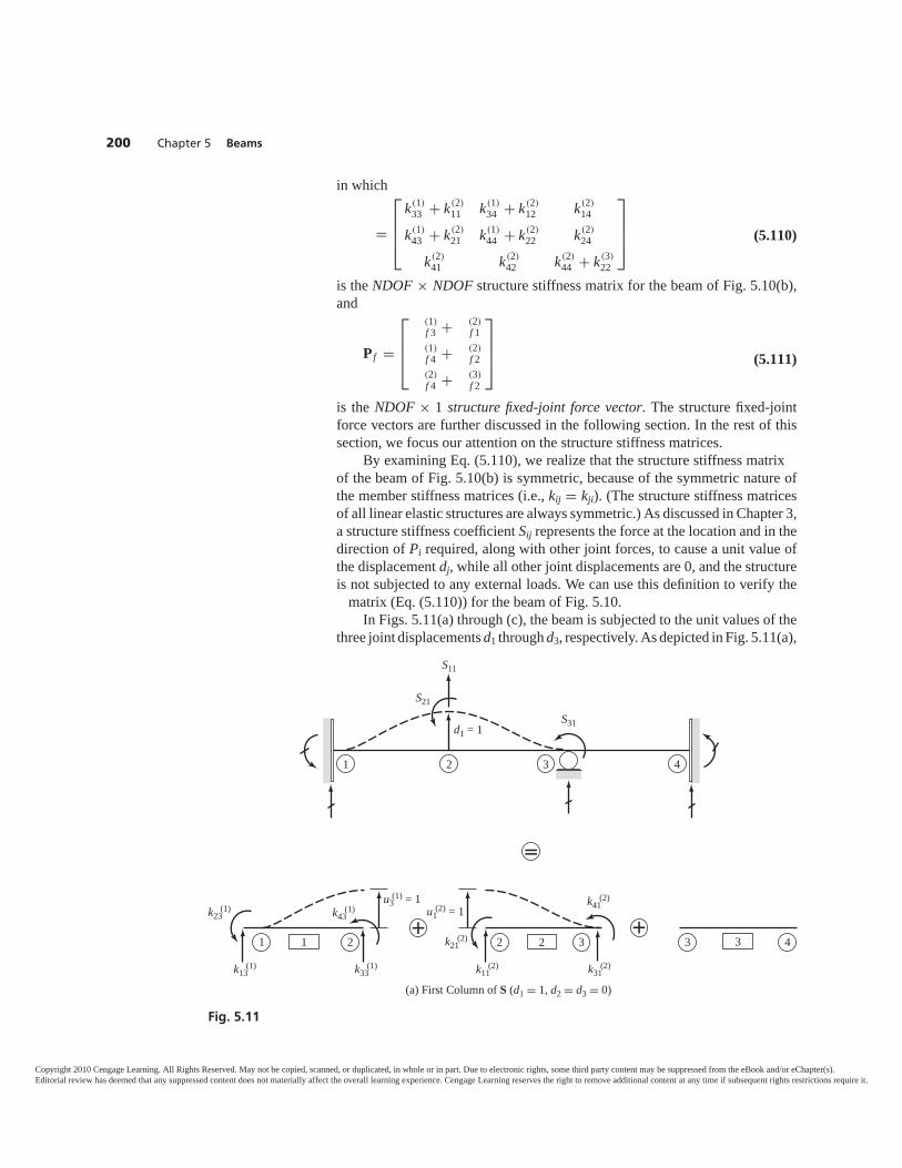
in which
=
⎡⎢⎢⎣
k(1)33 + k(2)
11 k(1)34 + k(2)
12 k(2)14
k(1)43 + k(2)
21 k(1)44 + k(2)
22 k(2)24
k(2)41 k(2)
42 k(2)44 + k(3)
22
⎤⎥⎥⎦ (5.110)
is the NDOF × NDOF structure stiffness matrix for the beam of Fig. 5.10(b),and
P f =
⎡⎢⎢⎣
(1)f 3 + (2)
f 1(1)f 4 + (2)
f 2(2)f 4 + (3)
f 2
⎤⎥⎥⎦ (5.111)
is the NDOF × 1 structure fixed-joint force vector. The structure fixed-jointforce vectors are further discussed in the following section. In the rest of thissection, we focus our attention on the structure stiffness matrices.
By examining Eq. (5.110), we realize that the structure stiffness matrix of the beam of Fig. 5.10(b) is symmetric, because of the symmetric nature ofthe member stiffness matrices (i.e., kij = kji). (The structure stiffness matricesof all linear elastic structures are always symmetric.) As discussed in Chapter 3,a structure stiffness coefficient Sij represents the force at the location and in thedirection of Pi required, along with other joint forces, to cause a unit value ofthe displacement dj, while all other joint displacements are 0, and the structureis not subjected to any external loads. We can use this definition to verify the
matrix (Eq. (5.110)) for the beam of Fig. 5.10.In Figs. 5.11(a) through (c), the beam is subjected to the unit values of the
three joint displacements d1 through d3, respectively. As depicted in Fig. 5.11(a),
200 Chapter 5 Beams
2 31 4
S11
S21
S31d1 = 1
u3(1) = 1
k23(1)
k13(1) k33
(1) k11(2)
k21(2)
k31(2)
k41(2)
k43(1) u1
(2) = 1
2 2 31+ +
3 4
(a) First Column of S (d1 = 1, d2 = d3 = 0)
�
2 31
Fig. 5.11
Copyright 2010 Cengage Learning. All Rights Reserved. May not be copied, scanned, or duplicated, in whole or in part. Due to electronic rights, some third party content may be suppressed from the eBook and/or eChapter(s).Editorial review has deemed that any suppressed content does not materially affect the overall learning experience. Cengage Learning reserves the right to remove additional content at any time if subsequent rights restrictions require it.
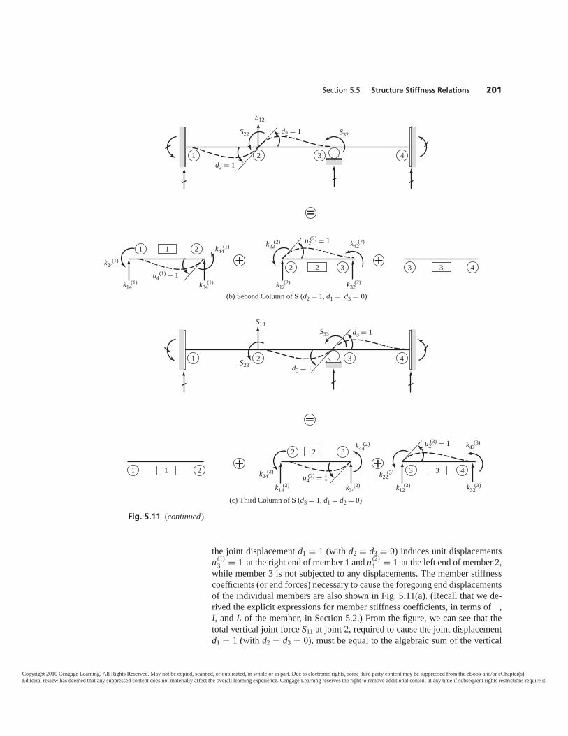
Section 5.5 Structure Stiffness Relations 201
the joint displacement d1 = 1 (with d2 = d3 = 0) induces unit displacementsu(1)
3 = 1 at the right end of member 1 and u(2)1 = 1 at the left end of member 2,
while member 3 is not subjected to any displacements. The member stiffnesscoefficients (or end forces) necessary to cause the foregoing end displacementsof the individual members are also shown in Fig. 5.11(a). (Recall that we de-rived the explicit expressions for member stiffness coefficients, in terms of ,I, and L of the member, in Section 5.2.) From the figure, we can see that thetotal vertical joint force S11 at joint 2, required to cause the joint displacementd1 = 1 (with d2 = d3 = 0), must be equal to the algebraic sum of the vertical
2 31 4
S12
S22 S32
d2 = 1
d2 = 1
k24(1)
k44(1) k22
(2)
k14(1) k34
(1) k12(2) k32
(2)
k42(2)
2
2 3
1+ +
1
3 43u4
(1) = 1
u2(2) = 1
(b) Second Column of S (d2 = 1, d1 = d3 = 0)
�
2
Fig. 5.11 (continued)
2 31 4
S13
S23
S33
d3 = 1
d3 = 1
+k22
(3)
k12(3) k32
(3)
k42(3)
3 43
u2(3) = 1
+1 21 k24
(2)
k44(2)
k14(2) k34
(2)
32 2
u4(2) = 1
(c) Third Column of S (d3 = 1, d1 = d2 = 0)
�
Copyright 2010 Cengage Learning. All Rights Reserved. May not be copied, scanned, or duplicated, in whole or in part. Due to electronic rights, some third party content may be suppressed from the eBook and/or eChapter(s).Editorial review has deemed that any suppressed content does not materially affect the overall learning experience. Cengage Learning reserves the right to remove additional content at any time if subsequent rights restrictions require it.
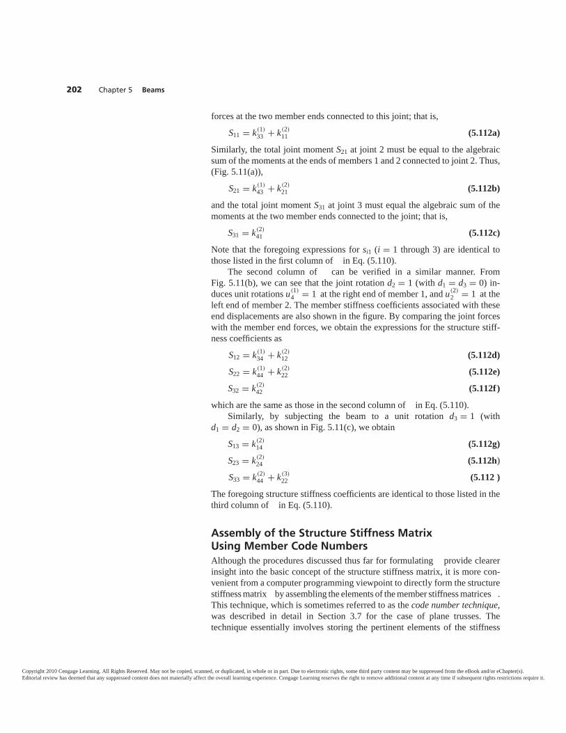
forces at the two member ends connected to this joint; that is,
S11 = k(1)33 + k(2)
11 (5.112a)
Similarly, the total joint moment S21 at joint 2 must be equal to the algebraicsum of the moments at the ends of members 1 and 2 connected to joint 2. Thus,(Fig. 5.11(a)),
S21 = k(1)43 + k(2)
21 (5.112b)
and the total joint moment S31 at joint 3 must equal the algebraic sum of themoments at the two member ends connected to the joint; that is,
S31 = k(2)41 (5.112c)
Note that the foregoing expressions for si1 (i = 1 through 3) are identical tothose listed in the first column of in Eq. (5.110).
The second column of can be verified in a similar manner. FromFig. 5.11(b), we can see that the joint rotation d2 = 1 (with d1 = d3 = 0) in-duces unit rotations u(1)
4 = 1 at the right end of member 1, and u(2)2 = 1 at the
left end of member 2. The member stiffness coefficients associated with theseend displacements are also shown in the figure. By comparing the joint forceswith the member end forces, we obtain the expressions for the structure stiff-ness coefficients as
S12 = k(1)34 + k(2)
12 (5.112d)
S22 = k(1)44 + k(2)
22 (5.112e)
S32 = k(2)42 (5.112f)
which are the same as those in the second column of in Eq. (5.110).Similarly, by subjecting the beam to a unit rotation d3 = 1 (with
d1 = d2 = 0), as shown in Fig. 5.11(c), we obtain
S13 = k(2)14 (5.112g)
S23 = k(2)24 (5.112h)
S33 = k(2)44 + k(3)
22 (5.112 )
The foregoing structure stiffness coefficients are identical to those listed in thethird column of in Eq. (5.110).
Assembly of the Structure Stiffness MatrixUsing Member Code NumbersAlthough the procedures discussed thus far for formulating provide clearerinsight into the basic concept of the structure stiffness matrix, it is more con-venient from a computer programming viewpoint to directly form the structurestiffness matrix by assembling the elements of the member stiffness matrices .This technique, which is sometimes referred to as the code number technique,was described in detail in Section 3.7 for the case of plane trusses. Thetechnique essentially involves storing the pertinent elements of the stiffness
202 Chapter 5 Beams
Copyright 2010 Cengage Learning. All Rights Reserved. May not be copied, scanned, or duplicated, in whole or in part. Due to electronic rights, some third party content may be suppressed from the eBook and/or eChapter(s).Editorial review has deemed that any suppressed content does not materially affect the overall learning experience. Cengage Learning reserves the right to remove additional content at any time if subsequent rights restrictions require it.
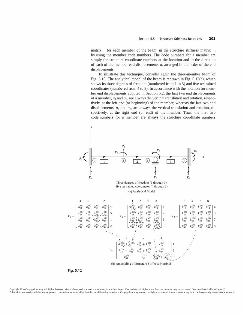
Section 5.5 Structure Stiffness Relations 203
matrix for each member of the beam, in the structure stiffness matrix ,by using the member code numbers. The code numbers for a member aresimply the structure coordinate numbers at the location and in the directionof each of the member end displacements u, arranged in the order of the enddisplacements.
To illustrate this technique, consider again the three-member beam ofFig. 5.10. The analytical model of the beam is redrawn in Fig. 5.12(a), whichshows its three degrees of freedom (numbered from 1 to 3) and five restrainedcoordinates (numbered from 4 to 8). In accordance with the notation for mem-ber end displacements adopted in Section 5.2, the first two end displacementsof a member, u1 and u2, are always the vertical translation and rotation, respec-tively, at the left end (or beginning) of the member, whereas the last two enddisplacements, u3 and u4, are always the vertical translation and rotation, re-spectively, at the right end (or end) of the member. Thus, the first twocode numbers for a member are always the structure coordinate numbers
R5
R8
P1P3P2
R4 R7
321 4X
Y
2 31
R6
Three degrees of freedom (1 through 3);five restrained coordinates (4 through 8)
(a) Analytical Model
4 5 1 2 1 2 6 3 6 3 7 8
k1 =
⎡⎢⎢⎢⎢⎢⎢⎣
k (1)11 k (1)
12 k (1)13 k (1)
14
k (1)21 k (1)
22 k (1)23 k (1)
24
k (1)31 k (1)
32 k (1)33 k (1)
34
k (1)41 k (1)
42 k (1)43 k (1)
44
⎤⎥⎥⎥⎥⎥⎥⎦
4
5
1
2
k2 =
⎡⎢⎢⎢⎢⎢⎢⎣
k (2)11 k (2)
12 k (2)13 k (2)
14
k (2)21 k (2)
22 k (2)23 k (2)
24
k (2)31 k (2)
32 k (2)33 k (2)
34
k (2)41 k (2)
42 k (2)43 k (2)
44
⎤⎥⎥⎥⎥⎥⎥⎦
1
2
6
3
k3 =
⎡⎢⎢⎢⎢⎢⎢⎣
k (3)11 k (3)
12 k (3)13 k (3)
14
k (3)21 k (3)
22 k (3)23 k (3)
24
k (3)31 k (3)
32 k (3)33 k (3)
34
k (3)41 k (3)
42 k (3)43 k (3)
44
⎤⎥⎥⎥⎥⎥⎥⎦
6
3
7
8
1 2 3
S =
⎡⎢⎢⎢⎣
k (1)33 + k (2)
11 k (2)14
k (1)43 + k (2/
21 k (1)44 + k (2)
22
k (1)34 + k (2)
12
k (2)24
k (2)41 k (2)
42 k (2)44 + k (3)
22
⎤⎥⎥⎥⎦
1
2
3
(b) Assembling of Structure Stiffness Matrix S
Fig. 5.12
Copyright 2010 Cengage Learning. All Rights Reserved. May not be copied, scanned, or duplicated, in whole or in part. Due to electronic rights, some third party content may be suppressed from the eBook and/or eChapter(s).Editorial review has deemed that any suppressed content does not materially affect the overall learning experience. Cengage Learning reserves the right to remove additional content at any time if subsequent rights restrictions require it.

corresponding to the vertical translation and rotation, respectively, of the be-ginning joint; and the third and fourth member code numbers are always thestructure coordinate numbers corresponding to the vertical translation and ro-tation, respectively, of the end joint.
From Fig. 5.12(a) we can see that, for member 1 of the beam, the begin-ning joint is 1 with restrained coordinates 4 and 5, and the end joint is 2 withdegrees of freedom 1 and 2. Thus, the code numbers for member 1 are 4, 5, 1, 2.Similarly, the code numbers for member 2, for which the beginning and endjoints are 2 and 3, respectively, are 1, 2, 6, 3. In a similar manner, the codenumbers for member 3 are found to be 6, 3, 7, 8.
To establish the structure stiffness matrix , we write the code numbers ofeach member on the right side and at the top of its stiffness matrix i (i = 1, 2,or 3), as shown in Fig. 5.12(b). These code numbers now define the positions ofthe elements of the member stiffness matrices in the structure stiffness matrix
. In other words, the code numbers on the right side of a matrix represent therow numbers of ; and the code numbers at the top represent the column num-bers of . Furthermore, since the number of rows and columns of equal thenumber of degrees of freedom (NDOF ) of the beam, only those elements of a
matrix for which both the row and the column code numbers are less than orequal to NDOF belong in the structure stiffness matrix . The structure stiffnessmatrix is obtained by algebraically adding the pertinent elements of the ma-trices of all the members in their proper positions in the matrix.
To assemble the matrix for the beam of Fig. 5.12(a), we start by storingthe pertinent elements of the stiffness matrix of member 1, 1, in the matrix(see Fig. 5.12(b)). Thus, the element k(1)
33 is stored in row 1 and column 1 of ,the element k(1)
43 is stored in row 2 and column 1 of , the element k(1)34 is stored
in row 1 and column 2 of , and the element k(1)44 is stored in row 2 and column
2 of . It should be noted that since the beam has three degrees of freedom,only those elements of 1 whose row and column code numbers both are lessthan or equal to 3 are stored in . The same procedure is then used to store thepertinent elements of 2 and 3, of members 2 and 3, respectively, in the ma-trix. Note that when two or more member stiffness coefficients are stored in thesame element of , then the coefficients must be algebraically added. The com-pleted structure stiffness matrix for the beam is shown in Fig. 5.12(b), and isidentical to the one derived previously (Eq. (5.110)) by substituting the mem-ber compatibility and stiffness relations into the joint equilibrium equations.
204 Chapter 5 Beams
E X A M P L E 5.4 Determine the structure stiffness matrix for the three-span continuous beam shownin Fig. 5.13(a).
S O L U T I O N Analytical Model The analytical model of the structure is shown in Fig. 5.13(b). Thebeam has two degrees of freedom—the rotations of joints 2 and 3—which areidentified by the structure coordinate numbers 1 and 2 in the figure.
Structure Stiffness Matrix To generate the 2 × 2 structure stiffness matrix , we willdetermine, for each member, the stiffness matrix and store its pertinent elements intheir proper positions in by using the member code numbers.
Copyright 2010 Cengage Learning. All Rights Reserved. May not be copied, scanned, or duplicated, in whole or in part. Due to electronic rights, some third party content may be suppressed from the eBook and/or eChapter(s).Editorial review has deemed that any suppressed content does not materially affect the overall learning experience. Cengage Learning reserves the right to remove additional content at any time if subsequent rights restrictions require it.
Section 5.5 Structure Stiffness Relations 205
e ber 1 By substituting L = 16 m into Eq. (5.53), we obtain
3 4 5 1
1 = I
⎡⎢⎢⎣
0.0029297 0.023438 −0.0029297 0.0234380.023438 0.25 −0.023438 0.125
−0.0029297 −0.023438 0.0029297 −0.0234380.023438 0.125 −0.023438 0.25
⎤⎥⎥⎦
3451
(1)
From Fig. 5.13(b), we observe that the code numbers for this member are 3, 4, 5, 1.These numbers are written on the right side and at the top of 1 in Eq. (1), to indicatethe rows and columns, respectively, of the structure stiffness matrix , where the ele-ments of 1 are to be stored. Thus, the element in row 4 and column 4 of 1 is storedin row 1 and column 1 of , as
1 2
= I[
0.25 00 0
]12
(2)
Note that the elements of 1 corresponding to the restrained coordinate numbers 3, 4,and 5 are disregarded.
e ber 2 L = 12 m. By using Eq. (5.53),
5 1 6 2
2 = I
⎡⎢⎢⎣
0.0069444 0.041667 −0.0069444 0.0416670.041667 0.33333 −0.041667 0.16667
−0.0069444 −0.041667 0.0069444 −0.0416670.041667 0.16667 −0.041667 0.33333
⎤⎥⎥⎦
5162
(3)
16 m 8 m6 m6 m
15 kN/m100 kN
I = constant(a) Three-Span Continuous Beam
4
1 28
321 4
2 31
53 76
X
Y
(b) Analytical Model
Fig. 5.13
Copyright 2010 Cengage Learning. All Rights Reserved. May not be copied, scanned, or duplicated, in whole or in part. Due to electronic rights, some third party content may be suppressed from the eBook and/or eChapter(s).Editorial review has deemed that any suppressed content does not materially affect the overall learning experience. Cengage Learning reserves the right to remove additional content at any time if subsequent rights restrictions require it.
From Fig. 5.13(b), we can see that the code numbers for this member are 5, 1, 6, 2.These numbers are used to add the pertinent elements of 2 in their proper positionsin the structure stiffness matrix given in Eq. (2), which now becomes
1 2
= I[
0.25 + 0.33333 0.166670.16667 0.33333
]12
(4)
e ber 3 L = 8 m. Thus,
6 2 7 8
3 = I
⎡⎢⎢⎣
0.023438 0.09375 −0.023438 0.093750.09375 0.5 −0.09375 0.25
−0.023438 −0.09375 0.023438 −0.093750.09375 0.25 −0.09375 0.5
⎤⎥⎥⎦
6278
(5)
The code numbers for this member are 6, 2, 7, 8. Thus, the element in row 2 andcolumn 2 of 3 is added in row 2 and column 2 of in Eq. (4), as
1 2
= I[
0.25 + 0.33333 0.166670.16667 0.33333 + 0.5
]12
Since the stiffnesses of all three members of the beam have now been stored in , thestructure stiffness matrix for the given beam is
1 2
= I[
0.58333 0.166670.16667 0.83333
]12
Ans
Note that the structure stiffness matrix is symmetric.
5.6 STRUCTURE FIXED-JOINT FORCES ANDEQUIVALENT JOINT LOADSAs discussed in the preceding section, the force–displacement relationships foran entire structure can be expressed in matrix form (see Eq. (5.109)) as
P − P f = d
in which Pf represents the structure fixed-joint force vector. It was also shownin the preceding section that by using the basic equations of equilibrium, com-patibility, and member stiffness, the structure fixed-joint forces Pf can be ex-pressed in terms of the member fixed-end forces f (see Eq. (5.111)). In thissection, we consider the physical interpretation of the structure fixed-jointforces; and discuss the formation of the Pf vector, by assembling the elementsof the member f vectors, using the member code numbers.
The concept of the structure fixed-joint forces Pf is analogous to that of themember fixed-end forces f. The structure fixed-joint forces represent the re-action forces (and or moments) that would develop at the locations and in thedirections of the structure’s degrees of freedom, due to the external member
206 Chapter 5 Beams
Copyright 2010 Cengage Learning. All Rights Reserved. May not be copied, scanned, or duplicated, in whole or in part. Due to electronic rights, some third party content may be suppressed from the eBook and/or eChapter(s).Editorial review has deemed that any suppressed content does not materially affect the overall learning experience. Cengage Learning reserves the right to remove additional content at any time if subsequent rights restrictions require it.
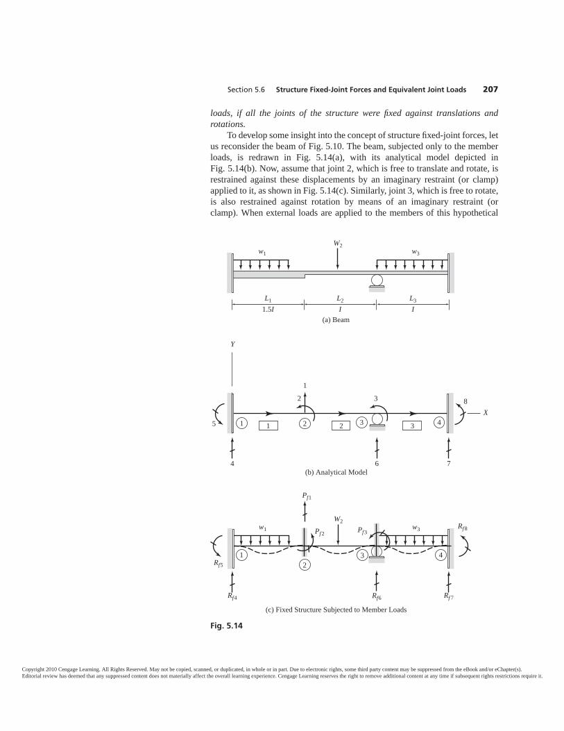
Section 5.6 Structure Fixed-Joint Forces and Equivalent Joint Loads 207
loads, if all the joints of the structure were fixed against translations androtations.
To develop some insight into the concept of structure fixed-joint forces, letus reconsider the beam of Fig. 5.10. The beam, subjected only to the memberloads, is redrawn in Fig. 5.14(a), with its analytical model depicted inFig. 5.14(b). Now, assume that joint 2, which is free to translate and rotate, isrestrained against these displacements by an imaginary restraint (or clamp)applied to it, as shown in Fig. 5.14(c). Similarly, joint 3, which is free to rotate,is also restrained against rotation by means of an imaginary restraint (orclamp). When external loads are applied to the members of this hypothetical
L2
IL3
IL1
1.5I
W2w1 w3
(a) Beam
5
2 3 8
321 4
1
4 76
X
Y
(b) Analytical Model
2 31
W2
Pf1
Pf2 Pf3
Rf4 Rf 7Rf6
Rf5
Rf8w1 w3
12
3 4
(c) Fixed Structure Subjected to Member Loads
Fig. 5.14
Copyright 2010 Cengage Learning. All Rights Reserved. May not be copied, scanned, or duplicated, in whole or in part. Due to electronic rights, some third party content may be suppressed from the eBook and/or eChapter(s).Editorial review has deemed that any suppressed content does not materially affect the overall learning experience. Cengage Learning reserves the right to remove additional content at any time if subsequent rights restrictions require it.
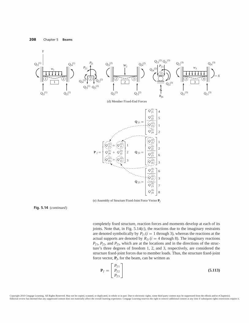
completely fixed structure, reaction forces and moments develop at each of itsjoints. Note that, in Fig. 5.14(c), the reactions due to the imaginary restraintsare denoted symbolically by Pf i (i = 1 through 3), whereas the reactions at theactual supports are denoted by Rf i (i = 4 through 8). The imaginary reactionsPf1, Pf2, and Pf3, which are at the locations and in the directions of the struc-ture’s three degrees of freedom 1, 2, and 3, respectively, are considered thestructure fixed-joint forces due to member loads. Thus, the structure fixed-jointforce vector, Pf, for the beam, can be written as
P f =⎡⎣ Pf 1
Pf 2Pf 3
⎤⎦ (5.113)
208 Chapter 5 Beams
Qf2(1)
Qf1(1) Qf 3
(1)
Qf4(1)
Qf 2(2)
Qf3(1) Qf1
(2)
Pf1Pf 2
Qf4(1) 2
Qf2(3)
Qf 3(2) Qf1
(3)
Rf6
Qf4(2)
Pf 3
3
Y
1 21
Qf 2(2)
Qf1(2) Qf 3
(2)
Qf4(2)
2 32
X
(d) Member Fixed-End Forces
w1
W2Qf2
(3)
Qf1(3) Qf 3
(3)
Qf4(3)
3 43
w3
Q f1 =
⎡⎢⎢⎢⎢⎢⎢⎢⎣
Q (1)f1
Q (1)f2
Q (1)f3
Q (1)f4
⎤⎥⎥⎥⎥⎥⎥⎥⎦
4
5
1
2
P f =
⎡⎢⎢⎢⎣
Q (1)f3 + Q (2)
f1
Q (1)f4 + Q (2)
f2
Q (2)f4 + Q (3)
f2
⎤⎥⎥⎥⎦
1
2
3
Q f2 =
⎡⎢⎢⎢⎢⎢⎢⎢⎣
Q (2)f1
Q (2)f2
Q (2)f3
Q (2)f4
⎤⎥⎥⎥⎥⎥⎥⎥⎦
1
2
6
3
Q f3 =
⎡⎢⎢⎢⎢⎢⎢⎢⎢⎣
Q (3)f1
Q (3)f2
Q (3)f3
Q (3)f4
⎤⎥⎥⎥⎥⎥⎥⎥⎥⎦
6
3
7
8
⎥⎥⎥⎥⎢⎢⎢ ⎢⎢⎢
(e) Assembly of Structure Fixed-Joint Force Vector Pf
Fig. 5.14 (continued)
Copyright 2010 Cengage Learning. All Rights Reserved. May not be copied, scanned, or duplicated, in whole or in part. Due to electronic rights, some third party content may be suppressed from the eBook and/or eChapter(s).Editorial review has deemed that any suppressed content does not materially affect the overall learning experience. Cengage Learning reserves the right to remove additional content at any time if subsequent rights restrictions require it.
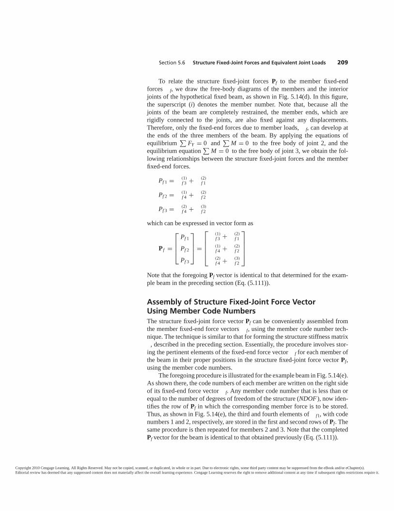
Section 5.6 Structure Fixed-Joint Forces and Equivalent Joint Loads 209
To relate the structure fixed-joint forces Pf to the member fixed-endforces f, we draw the free-body diagrams of the members and the interiorjoints of the hypothetical fixed beam, as shown in Fig. 5.14(d). In this figure,the superscript (i) denotes the member number. Note that, because all thejoints of the beam are completely restrained, the member ends, which arerigidly connected to the joints, are also fixed against any displacements.Therefore, only the fixed-end forces due to member loads, f, can develop atthe ends of the three members of the beam. By applying the equations ofequilibrium
∑FY = 0 and
∑M = 0 to the free body of joint 2, and the
equilibrium equation∑
M = 0 to the free body of joint 3, we obtain the fol-lowing relationships between the structure fixed-joint forces and the memberfixed-end forces.
Pf 1 = (1)f 3 + (2)
f 1
Pf 2 = (1)f 4 + (2)
f 2
Pf 3 = (2)f 4 + (3)
f 2
which can be expressed in vector form as
P f =
⎡⎢⎢⎣
Pf 1
Pf 2
Pf 3
⎤⎥⎥⎦ =
⎡⎢⎢⎢⎣
(1)f 3 + (2)
f 1(1)f 4 + (2)
f 2(2)f 4 + (3)
f 2
⎤⎥⎥⎥⎦
Note that the foregoing Pf vector is identical to that determined for the exam-ple beam in the preceding section (Eq. (5.111)).
Assembly of Structure Fixed-Joint Force VectorUsing Member Code NumbersThe structure fixed-joint force vector Pf can be conveniently assembled fromthe member fixed-end force vectors f, using the member code number tech-nique. The technique is similar to that for forming the structure stiffness matrix
, described in the preceding section. Essentially, the procedure involves stor-ing the pertinent elements of the fixed-end force vector f for each member ofthe beam in their proper positions in the structure fixed-joint force vector Pf,using the member code numbers.
The foregoing procedure is illustrated for the example beam in Fig. 5.14(e).As shown there, the code numbers of each member are written on the right sideof its fixed-end force vector f. Any member code number that is less than orequal to the number of degrees of freedom of the structure (NDOF ), now iden-tifies the row of Pf in which the corresponding member force is to be stored.Thus, as shown in Fig. 5.14(e), the third and fourth elements of f1, with codenumbers 1 and 2, respectively, are stored in the first and second rows of Pf. Thesame procedure is then repeated for members 2 and 3. Note that the completedPf vector for the beam is identical to that obtained previously (Eq. (5.111)).
Copyright 2010 Cengage Learning. All Rights Reserved. May not be copied, scanned, or duplicated, in whole or in part. Due to electronic rights, some third party content may be suppressed from the eBook and/or eChapter(s).Editorial review has deemed that any suppressed content does not materially affect the overall learning experience. Cengage Learning reserves the right to remove additional content at any time if subsequent rights restrictions require it.
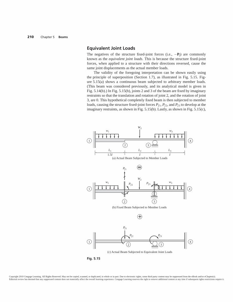
Equivalent Joint LoadsThe negatives of the structure fixed-joint forces (i.e., −Pf) are commonlyknown as the equivalent joint loads. This is because the structure fixed-jointforces, when applied to a structure with their directions reversed, cause thesame joint displacements as the actual member loads.
The validity of the foregoing interpretation can be shown easily usingthe principle of superposition (Section 1.7), as illustrated in Fig. 5.15. Fig-ure 5.15(a) shows a continuous beam subjected to arbitrary member loads.(This beam was considered previously, and its analytical model is given inFig. 5.14(b).) In Fig. 5.15(b), joints 2 and 3 of the beam are fixed by imaginaryrestraints so that the translation and rotation of joint 2, and the rotation of joint3, are 0. This hypothetical completely fixed beam is then subjected to memberloads, causing the structure fixed-joint forces Pf1, Pf 2, and Pf 3 to develop at theimaginary restraints, as shown in Fig. 5.15(b). Lastly, as shown in Fig. 5.15(c),
210 Chapter 5 Beams
L2
IL3
IL1
1.5I
W2w1 w3
1 42 3
(a) Actual Beam Subjected to Member Loads
=
W2
Pf1
Pf 2 Pf3w1 w3
1
2 3
4
(b) Fixed Beam Subjected to Member Loads
1 42 3
Pf1
Pf2 Pf 3
(c) Actual Beam Subjected to Equivalent Joint Loads
+
Fig. 5.15
Copyright 2010 Cengage Learning. All Rights Reserved. May not be copied, scanned, or duplicated, in whole or in part. Due to electronic rights, some third party content may be suppressed from the eBook and/or eChapter(s).Editorial review has deemed that any suppressed content does not materially affect the overall learning experience. Cengage Learning reserves the right to remove additional content at any time if subsequent rights restrictions require it.
Section 5.6 Structure Fixed-Joint Forces and Equivalent Joint Loads 211
the actual beam is subjected to external loads at its joints, which are equal inmagnitude to Pf1, Pf 2, and Pf 3, but are reversed in direction.
By comparing Figs. 5.15(a), (b), and (c), we realize that the actual loadingapplied to the beam in Fig. 5.15(a) equals the algebraic sum of the loadingsgiven in Figs. 5.15(b) and (c), because the reactive forces Pf1, Pf 2, and Pf 3 inFig. 5.15(b) cancel the corresponding applied loads in Fig. 5.15(c). Thus, ac-cording to the principle of superposition, any joint displacement of the actualbeam due to the member loads (Fig. 5.15(a)) must equal the algebraic sum ofthe corresponding joint displacement of the fixed beam due to the memberloads (Fig. 5.15(b)), and the corresponding joint displacement of the actualbeam subjected to no member loads, but to the fixed-joint forces with their di-rections reversed. However, the joint displacements of the fixed beam (Fig.5.15(b)) are 0. Therefore, the joint displacements of the beam due to the mem-ber loads (Fig. 5.15(a)) must be equal to the corresponding joint displacementsof the beam due to the negatives of the fixed-joint forces (Fig. 5.15(c)). In otherwords, the negatives of the structure fixed-joint forces do indeed cause thesame joint displacements of the beam as the actual member loads; and in thatsense, such forces can be considered to be the equivalent joint loads. It is im-portant to realize that this equivalency between the negative fixed-joint forcesand the member loads is valid only for joint displacements, and cannot be gen-eralized to member end forces and reactions, because such forces are generallynot 0 in fixed structures subjected to member loads.
Based on the foregoing discussion of equivalent joint loads, we can definethe equivalent joint load vector Pe for a structure as simply the negative of itsfixed-joint force vector Pf ; that is,
(5.114)
An alternative form of the structure stiffness relations, in terms of the equiv-alent joint loads, can now be obtained by substituting Eq. (5.114) intoEq. (5.109). This yields
(5.115)
Once , Pf (or Pe), and P have been evaluated, the structure stiffness rela-tions (Eq. (5.109) or Eq. (5.115)), which now represent a system of simultane-ous linear equations, can be solved for the unknown joint displacements d.With d known, the end displacements u for each member can be determined byapplying the compatibility equations defined by its code numbers; then the cor-responding end forces can be computed by applying the member stiffness re-lations. Finally, the support reactions are determined from the memberend forces , by considering the equilibrium of the support joints in the direc-tions of the restrained coordinates via member code numbers, as discussed inChapter 3 for the case of plane trusses.
P + Pe = d
Pe = −P f
Copyright 2010 Cengage Learning. All Rights Reserved. May not be copied, scanned, or duplicated, in whole or in part. Due to electronic rights, some third party content may be suppressed from the eBook and/or eChapter(s).Editorial review has deemed that any suppressed content does not materially affect the overall learning experience. Cengage Learning reserves the right to remove additional content at any time if subsequent rights restrictions require it.
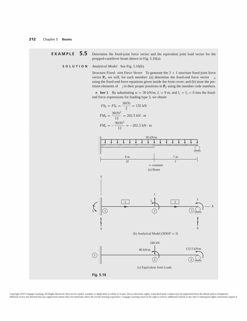
E X A M P L E 5.5 Determine the fixed-joint force vector and the equivalent joint load vector for thepropped-cantilever beam shown in Fig. 5.16(a).
S O L U T I O N Analytical Model See Fig. 5.16(b).
Structure Fixed- oint Force Vector To generate the 3 × 1 structure fixed-joint forcevector Pf, we will, for each member: (a) determine the fixed-end force vector f,using the fixed-end force equations given inside the front cover; and (b) store the per-tinent elements of f in their proper positions in Pf, using the member code numbers.
e ber 1 By substituting w = 30 kN/m, L = 9 m, and l1 = l2 = 0 into the fixed-end force expressions for loading type 3, we obtain
FSb = FSe = 30(9)
2= 135 kN
FMb = 30(9)2
12= 202.5 kN · m
FMe = −30(9)2
12= −202.5 kN · m
212 Chapter 5 Beams
9 m2I
7 mI
30 kN/m
= constant(a) Beam
5
2 3
321
21
1
4 6
X
Y
(b) Analytical Model (NDOF = 3)
80 kN•m 122.5 kN•m
321
240 kN
(c) Equivalent Joint Loads
Fig. 5.16
Copyright 2010 Cengage Learning. All Rights Reserved. May not be copied, scanned, or duplicated, in whole or in part. Due to electronic rights, some third party content may be suppressed from the eBook and/or eChapter(s).Editorial review has deemed that any suppressed content does not materially affect the overall learning experience. Cengage Learning reserves the right to remove additional content at any time if subsequent rights restrictions require it.
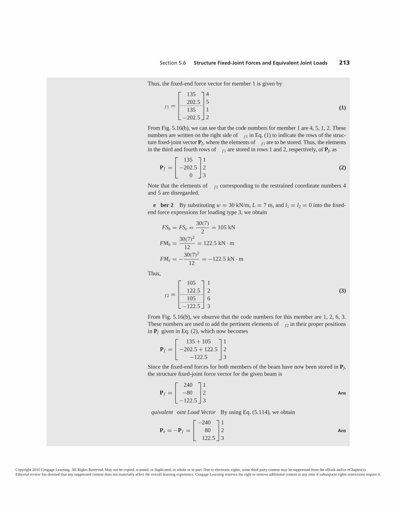
Section 5.6 Structure Fixed-Joint Forces and Equivalent Joint Loads 213
Thus, the fixed-end force vector for member 1 is given by
f 1 =
⎡⎢⎢⎣
135202.5135
−202.5
⎤⎥⎥⎦
4512
���� (1)
From Fig. 5.16(b), we can see that the code numbers for member 1 are 4, 5, 1, 2. Thesenumbers are written on the right side of f 1 in Eq. (1) to indicate the rows of the struc-ture fixed-joint vector Pf, where the elements of f 1 are to be stored. Thus, the elementsin the third and fourth rows of f 1 are stored in rows 1 and 2, respectively, of Pf, as
P f =⎡⎣ 135
−202.50
⎤⎦1
23
(2)
Note that the elements of f 1 corresponding to the restrained coordinate numbers 4and 5 are disregarded.
e ber 2 By substituting w = 30 kN/m, L = 7 m, and l1 = l2 = 0 into the fixed-end force expressions for loading type 3, we obtain
FSb = FSe = 30(7)
2= 105 kN
FMb = 30(7)2
12= 122.5 kN · m
FMe = −30(7)2
12= −122.5 kN · m
Thus,
f 2 =
⎡⎢⎢⎣
105122.5105
−122.5
⎤⎥⎥⎦
1263
����
����
(3)
From Fig. 5.16(b), we observe that the code numbers for this member are 1, 2, 6, 3.These numbers are used to add the pertinent elements of f 2 in their proper positionsin Pf given in Eq. (2), which now becomes
P f =⎡⎣ 135 + 105
−202.5 + 122.5−122.5
⎤⎦1
23
Since the fixed-end forces for both members of the beam have now been stored in Pf,the structure fixed-joint force vector for the given beam is
P f =⎡⎣ 240
−80−122.5
⎤⎦1
23
Ans
quivalent oint Load Vector By using Eq. (5.114), we obtain
Pe = −P f =⎡⎣ −240
80122.5
⎤⎦1
23
Ans
Copyright 2010 Cengage Learning. All Rights Reserved. May not be copied, scanned, or duplicated, in whole or in part. Due to electronic rights, some third party content may be suppressed from the eBook and/or eChapter(s).Editorial review has deemed that any suppressed content does not materially affect the overall learning experience. Cengage Learning reserves the right to remove additional content at any time if subsequent rights restrictions require it.
5.7 PROCEDURE FOR ANALYSISBased on the concepts presented in the previous sections, we can develop thefollowing step-by-step procedure for the analysis of beams by the matrix stiff-ness method. The reader should note that the overall format of this procedureis essentially the same as the procedure for analysis of plane trusses presentedin Chapter 3.
1. Prepare an analytical model of the beam, as follows.a. Draw a line diagram of the beam, and identify each joint and mem-
ber by a number. The origin of the global XY coordinate system isusually located at the farthest left joint, with the X and Y axes ori-ented in the horizontal (positive to the right) and vertical (positiveupward) directions, respectively. For each member, establish a localxy coordinate system, with the origin at the left end (beginning) ofthe member, and the x and y axes oriented in the horizontal (positiveto the right) and vertical (positive upward) directions, respectively.
b. Number the degrees of freedom and restrained coordinates of thebeam, as discussed in Section 5.1.
2. Evaluate the structure stiffness matrix and fixed-joint force vector Pf.The number of rows and columns of must be equal to the number ofdegrees of freedom (NDOF) of the beam; the number of rows of Pfmust equal NDOF. For each member of the structure, perform the fol-lowing operations.a. Compute the member stiffness matrix (Eq. (5.53)).b. If the member is subjected to external loads, then evaluate its fixed-
end force vector f, using the expressions for fixed-end forces giveninside the front cover.
c. Identify the member code numbers and store the pertinent elementsof and f in their proper positions in the structure stiffness matrix
, and the fixed-joint force vector Pf, respectively. The completestructure stiffness matrix , obtained by assembling the stiffnesscoefficients of all the members of the beam, must be symmetric.
3. If the beam is subjected to joint loads, then form the NDOF × 1 jointload vector P.
4. Determine the joint displacements d. Substitute P, Pf, and intothe structure stiffness relations, P − Pf = d (Eq. (5.109)), and solvethe resulting system of simultaneous equations for the unknownjoint displacements d. To check that the simultaneous equations havebeen solved correctly, substitute the numerical values of the joint dis-placements d back into the structure stiffness relations, P − Pf = d.
214 Chapter 5 Beams
These equivalent joint loads, when applied to the beam as shown in Fig. 5.16(c), causethe same joint displacements as the actual 30 kN/m uniformly distributed load givenin Fig. 5.16(a).
Copyright 2010 Cengage Learning. All Rights Reserved. May not be copied, scanned, or duplicated, in whole or in part. Due to electronic rights, some third party content may be suppressed from the eBook and/or eChapter(s).Editorial review has deemed that any suppressed content does not materially affect the overall learning experience. Cengage Learning reserves the right to remove additional content at any time if subsequent rights restrictions require it.
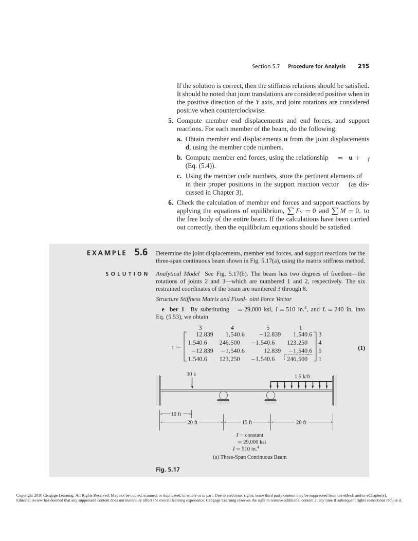
Section 5.7 Procedure for Analysis 215
E X A M P L E 5.6 Determine the joint displacements, member end forces, and support reactions for thethree-span continuous beam shown in Fig. 5.17(a), using the matrix stiffness method.
S O L U T I O N Analytical Model See Fig. 5.17(b). The beam has two degrees of freedom—therotations of joints 2 and 3—which are numbered 1 and 2, respectively. The sixrestrained coordinates of the beam are numbered 3 through 8.
Structure Stiffness Matrix and Fixed- oint Force Vectore ber 1 By substituting = 29,000 ksi, I = 510 in.4, and L = 240 in. into
Eq. (5.53), we obtain
3 4 5 1
1 =
⎡⎢⎢⎣
12.839 1,540.6 −12.839 1,540.61,540.6 246,500 −1,540.6 123,250−12.839 −1,540.6 12.839 −1,540.6
1,540.6 123,250 −1,540.6 246,500
⎤⎥⎥⎦
3451
������
(1)
If the solution is correct, then the stiffness relations should be satisfied.It should be noted that joint translations are considered positive when inthe positive direction of the Y axis, and joint rotations are consideredpositive when counterclockwise.
5. Compute member end displacements and end forces, and supportreactions. For each member of the beam, do the following.a. Obtain member end displacements u from the joint displacements
d, using the member code numbers.b. Compute member end forces, using the relationship = u + f
(Eq. (5.4)).c. Using the member code numbers, store the pertinent elements of
in their proper positions in the support reaction vector (as dis-cussed in Chapter 3).
6. Check the calculation of member end forces and support reactions byapplying the equations of equilibrium,
∑FY = 0 and
∑M = 0, to
the free body of the entire beam. If the calculations have been carriedout correctly, then the equilibrium equations should be satisfied.
I = constant= 29,000 ksi
I = 510 in.4
20 ft 15 ft 20 ft10 ft
30 k 1.5 k/ft
(a) Three-Span Continuous Beam
Fig. 5.17
Copyright 2010 Cengage Learning. All Rights Reserved. May not be copied, scanned, or duplicated, in whole or in part. Due to electronic rights, some third party content may be suppressed from the eBook and/or eChapter(s).Editorial review has deemed that any suppressed content does not materially affect the overall learning experience. Cengage Learning reserves the right to remove additional content at any time if subsequent rights restrictions require it.
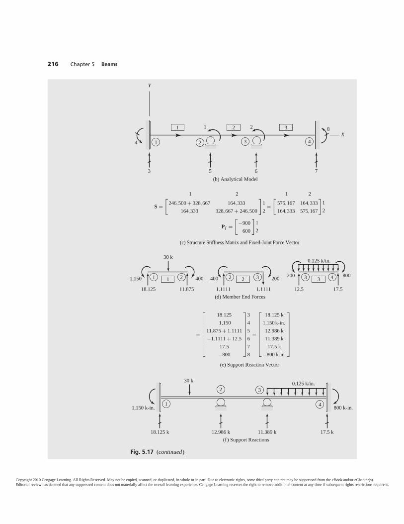
216 Chapter 5 Beams
4
2 8
321 4
2 31 1
3 765
X
Y
(b) Analytical Model
1 2 1 2
S =[
246,500 + 328,667 164,333164,333 328,667 + 246,500
]12
=[
575,167 164,333164,333 575,167
]12
Pf =[
−900600
]12
(c) Structure Stiffness Matrix and Fixed-Joint Force Vector
1 21
30 k
1,150 400
18.125 11.875
3 43
0.125 k/in.
200 800
12.5 17.5
2 32400 200
1.1111 1.1111(d) Member End Forces
30 k 0.125 k/in.
1,150 k-in. 800 k-in.
3
4
2
1
18.125 k 17.5 k11.389 k12.986 k(f) Support Reactions
=
⎡⎢⎢⎢⎢⎢⎢⎢⎢⎣
18.1251,150
11.875 + 1.1111−1.1111 + 12.5
17.5−800
⎤⎥⎥⎥⎥⎥⎥⎥⎥⎦
345678
=
⎡⎢⎢⎢⎢⎢⎢⎢⎢⎣
18.125 k1,150k-in.12.986 k11.389 k17.5 k
−800 k-in.
⎤⎥⎥⎥⎥⎥⎥⎥⎥⎦
(e) Support Reaction Vector
Fig. 5.17 (continued)
Copyright 2010 Cengage Learning. All Rights Reserved. May not be copied, scanned, or duplicated, in whole or in part. Due to electronic rights, some third party content may be suppressed from the eBook and/or eChapter(s).Editorial review has deemed that any suppressed content does not materially affect the overall learning experience. Cengage Learning reserves the right to remove additional content at any time if subsequent rights restrictions require it.
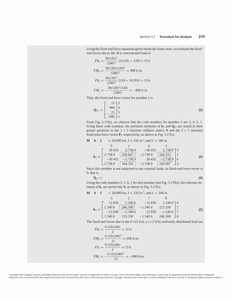
Section 5.7 Procedure for Analysis 217
Using the fixed-end force equations given inside the front cover, we evaluate the fixed-end forces due to the 30 k concentrated load as
FSb = 30(120)2
(240)3 [3(120) + 120] = 15 k
FMb = 30(120)(120)2
(240)2 = 900 k-in.
FSe = 30(120)2
(240)3 [120 + 3(120)] = 15 k
FMe = −30(120)2(120)
(240)2 = −900 k-in.
Thus, the fixed-end force vector for member 1 is
Q f 1 =
⎡⎢⎢⎣
1590015
−900
⎤⎥⎥⎦
3451
���
(2)
From Fig. 5.17(b), we observe that the code numbers for member 1 are 3, 4, 5, 1.Using these code numbers, the pertinent elements of k1 and Q f1 are stored in theirproper positions in the 2 × 2 structure stiffness matrix S and the 2 × 1 structurefixed-joint force vector Pf, respectively, as shown in Fig. 5.17(c).
M b 2 = 29,000 ksi, I = 510 in.4, and L = 180 in.5 1 6 2
k2 =
⎡⎢⎢⎣
30.432 2,738.9 −30.432 2,738.92,738.9 328,667 −2,738.9 164,333−30.432 −2,738.9 30.432 −2,738.9
2,738.9 164,333 −2,738.9 328,667
⎤⎥⎥⎦
5162
(3)
Since this member is not subjected to any external loads, its fixed-end force vector is0; that is,
Q f 2 = (4)Using the code numbers 5, 1, 6, 2 for this member (see Fig. 5.17(b)), the relevant ele-ments of k2 are stored into S, as shown in Fig. 5.17(c).
M b 3 = 29,000 ksi, I = 510 in.4, and L = 240 in.6 2 7 8
k3 =
⎡⎢⎢⎣
12.839 1,540.6 −12.839 1,540.61,540.6 246,500 −1,540.6 123,250−12.839 −1,540.6 12.839 −1,540.6
1,540.6 123,250 −1,540.6 246,500
⎤⎥⎥⎦
6278
(5)
The fixed-end forces due to the 0.125 k/in. (=1.5 k/ft) uniformly distributed load are
FSb = 0.125(240)
2= 15 k
FMb = 0.125(240)2
12= 600 k-in.
FSe = 0.125(240)
2= 15 k
FMe = −0.125(240)2
12= −600 k-in.
������ ������
����������������
������� �
������ ������
Copyright 2010 Cengage Learning. All Rights Reserved. May not be copied, scanned, or duplicated, in whole or in part. Due to electronic rights, some third party content may be suppressed from the eBook and/or eChapter(s).Editorial review has deemed that any suppressed content does not materially affect the overall learning experience. Cengage Learning reserves the right to remove additional content at any time if subsequent rights restrictions require it.
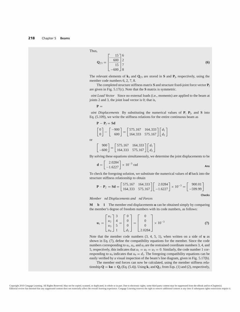
218 Chapter 5 Beams
Thus,
Q f 3 =
⎡⎢⎢⎣
1560015
−600
⎤⎥⎥⎦
6278
���
��� (6)
The relevant elements of k3 and Q f3 are stored in S and Pf, respectively, using themember code numbers 6, 2, 7, 8.
The completed structure stiffness matrix S and structure fixed-joint force vector Pfare given in Fig. 5.17(c). Note that the S matrix is symmetric.
oint Load Vector Since no external loads (i.e., moments) are applied to the beam atjoints 2 and 3, the joint load vector is 0; that is,
P =oint Displacements By substituting the numerical values of P, Pf, and S into
Eq. (5.109), we write the stiffness relations for the entire continuous beam as
P − Pf = Sd[00
]−
[ −900600
]=
[575,167 164,333164,333 575,167
] [d1d2
]or [
900−600
]=
[575,167 164,333164,333 575,167
] [d1d2
]
By solving these equations simultaneously, we determine the joint displacements to be
d =[
2.0284−1.6227
]× 10−3 rad Ans
To check the foregoing solution, we substitute the numerical values of d back into thestructure stiffness relationship to obtain
P − P f = Sd =[
575,167 164,333164,333 575,167
][2.0284
−1.6227
]× 10−3 =
[900.01
−599.99
]Checks
Member nd Displacements and nd ForcesM b 1 The member end displacements u can be obtained simply by comparingthe member’s degree of freedom numbers with its code numbers, as follows:
u1 =
⎡⎢⎢⎣
u1u2u3u4
⎤⎥⎥⎦
3451
=
⎡⎢⎢⎣
000d1
⎤⎥⎥⎦ =
⎡⎢⎢⎣
000
2.0284
⎤⎥⎥⎦ × 10−3 (7)
Note that the member code numbers (3, 4, 5, 1), when written on a side of u asshown in Eq. (7), define the compatibility equations for the member. Since the codenumbers corresponding to u1, u2, and u3 are the restrained coordinate numbers 3, 4, and5, respectively, this indicates that u1 = u2 = u3 = 0. Similarly, the code number 1 cor-responding to u4 indicates that u4 = d1. The foregoing compatibility equations can beeasily verified by a visual inspection of the beam’s line diagram, given in Fig. 5.17(b).
The member end forces can now be calculated, using the member stiffness rela-tionship Q = ku + Q f (Eq. (5.4)). Using k1 and Q f1 from Eqs. (1) and (2), respectively,
Copyright 2010 Cengage Learning. All Rights Reserved. May not be copied, scanned, or duplicated, in whole or in part. Due to electronic rights, some third party content may be suppressed from the eBook and/or eChapter(s).Editorial review has deemed that any suppressed content does not materially affect the overall learning experience. Cengage Learning reserves the right to remove additional content at any time if subsequent rights restrictions require it.
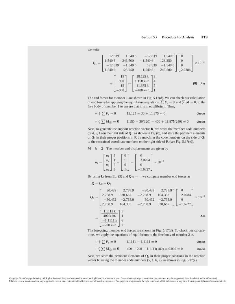
Section 5.7 Procedure for Analysis 219
we write
Q1 =
⎡⎢⎢⎣
12.839 1,540.6 −12.839 1,540.61,540.6 246,500 −1,540.6 123,250−12.839 −1,540.6 12.839 −1,540.6
1,540.6 123,250 −1,540.6 246,500
⎤⎥⎥⎦
⎡⎢⎢⎣
0002.0284
⎤⎥⎥⎦ × 10−3
+
⎡⎢⎢⎣
1590015
−900
⎤⎥⎥⎦ =
⎡⎢⎢⎣
18.125 k1,150 k-in.11.875 k
−400 k-in.
⎤⎥⎥⎦
3451
�����
(8) Ans
The end forces for member 1 are shown in Fig. 5.17(d). We can check our calculationof end forces by applying the equilibrium equations,
∑Fy = 0 and
∑M = 0, to the
free body of member 1 to ensure that it is in equilibrium. Thus,
+ ↑ ∑Fy = 0 18.125 − 30 + 11.875 = 0 Checks
+ ∑M©1 = 0 1,150 − 30(120) − 400 + 11.875(240) = 0 Checks
Next, to generate the support reaction vector R, we write the member code numbers(3, 4, 5, 1) on the right side of Q1, as shown in Eq. (8), and store the pertinent elementsof Q1 in their proper positions in R by matching the code numbers on the side of Q1to the restrained coordinate numbers on the right side of R (see Fig. 5.17(e)).
M b 2 The member end displacements are given by
u2 =
⎡⎢⎢⎣
u1u2u3u4
⎤⎥⎥⎦
5162
=
⎡⎢⎢⎣
0d10d2
⎤⎥⎥⎦ =
⎡⎢⎢⎣
02.02840
−1.6227
⎤⎥⎥⎦ × 10−3
By using k2 from Eq. (3) and Q f 2 = , we compute member end forces as
Q = ku + Q f
Q2 =
⎡⎢⎢⎣
30.432 2,738.9 −30.432 2,738.92,738.9 328,667 −2,738.9 164,333−30.432 −2,738.9 30.432 −2,738.9
2,738.9 164,333 −2,738.9 328,667
⎤⎥⎥⎦
⎡⎢⎢⎣
02.02840
−1.6227
⎤⎥⎥⎦ × 10−3
=
⎡⎢⎢⎣
1.1111 k400 k-in.
−1.1111 k−200 k-in.
⎤⎥⎥⎦
5162
�����
�����
�����
Ans
The foregoing member end forces are shown in Fig. 5.17(d). To check our calcula-tions, we apply the equations of equilibrium to the free body of member 2 as
+ ↑ ∑Fy = 0 1.1111 − 1.1111 = 0 Checks
+ ∑M©2 = 0 400 − 200 − 1.1111(180) = 0.002 ≈ 0 Checks
Next, we store the pertinent elements of Q2 in their proper positions in the reactionvector R, using the member code numbers (5, 1, 6, 2), as shown in Fig. 5.17(e).
Y
Y
Copyright 2010 Cengage Learning. All Rights Reserved. May not be copied, scanned, or duplicated, in whole or in part. Due to electronic rights, some third party content may be suppressed from the eBook and/or eChapter(s).Editorial review has deemed that any suppressed content does not materially affect the overall learning experience. Cengage Learning reserves the right to remove additional content at any time if subsequent rights restrictions require it.
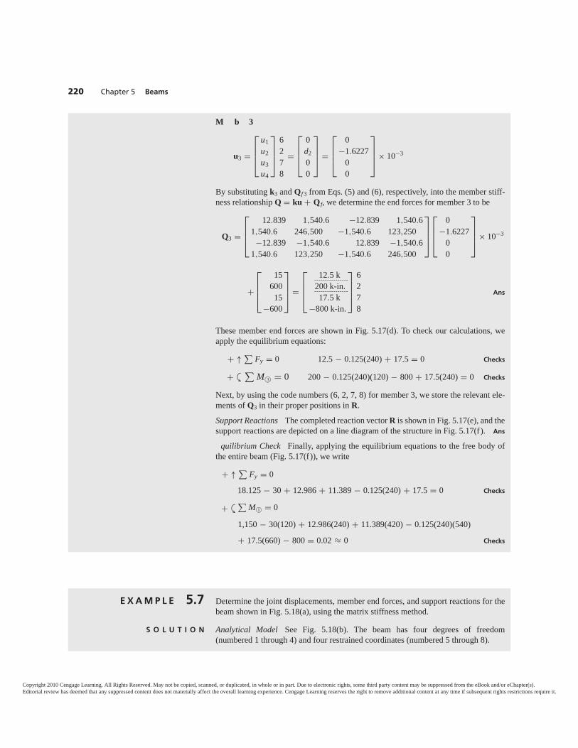
220 Chapter 5 Beams
M b 3
u3 =
⎡⎢⎢⎣
u1u2u3u4
⎤⎥⎥⎦
6278
=
⎡⎢⎢⎣
0d200
⎤⎥⎥⎦ =
⎡⎢⎢⎣
0−1.6227
00
⎤⎥⎥⎦ × 10−3
By substituting k3 and Qf 3 from Eqs. (5) and (6), respectively, into the member stiff-ness relationship Q = ku + Q f, we determine the end forces for member 3 to be
Q3 =
⎡⎢⎢⎣
12.839 1,540.6 −12.839 1,540.61,540.6 246,500 −1,540.6 123,250−12.839 −1,540.6 12.839 −1,540.6
1,540.6 123,250 −1,540.6 246,500
⎤⎥⎥⎦
⎡⎢⎢⎣
0−1.6227
00
⎤⎥⎥⎦ × 10−3
+
⎡⎢⎢⎣
1560015
−600
⎤⎥⎥⎦ =
⎡⎢⎢⎣
12.5 k200 k-in.17.5 k
−800 k-in.
⎤⎥⎥⎦
6278
����
���� Ans
These member end forces are shown in Fig. 5.17(d). To check our calculations, weapply the equilibrium equations:
+ ↑ ∑Fy = 0 12.5 − 0.125(240) + 17.5 = 0 Checks
+ ∑M©3 = 0 200 − 0.125(240)(120) − 800 + 17.5(240) = 0 Checks
Next, by using the code numbers (6, 2, 7, 8) for member 3, we store the relevant ele-ments of Q3 in their proper positions in R.
Support Reactions The completed reaction vector R is shown in Fig. 5.17(e), and thesupport reactions are depicted on a line diagram of the structure in Fig. 5.17(f). Ans
quilibrium Check Finally, applying the equilibrium equations to the free body ofthe entire beam (Fig. 5.17(f)), we write
+ ↑ ∑Fy = 0
18.125 − 30 + 12.986 + 11.389 − 0.125(240) + 17.5 = 0 Checks
+ ∑M©1 = 0
1,150 − 30(120) + 12.986(240) + 11.389(420) − 0.125(240)(540)
+ 17.5(660) − 800 = 0.02 ≈ 0 Checks
Y
Y
E X A M P L E 5.7 Determine the joint displacements, member end forces, and support reactions for thebeam shown in Fig. 5.18(a), using the matrix stiffness method.
S O L U T I O N Analytical Model See Fig. 5.18(b). The beam has four degrees of freedom(numbered 1 through 4) and four restrained coordinates (numbered 5 through 8).
Copyright 2010 Cengage Learning. All Rights Reserved. May not be copied, scanned, or duplicated, in whole or in part. Due to electronic rights, some third party content may be suppressed from the eBook and/or eChapter(s).Editorial review has deemed that any suppressed content does not materially affect the overall learning experience. Cengage Learning reserves the right to remove additional content at any time if subsequent rights restrictions require it.