An overview of a highly versatile forward and stableinverse algorithm for airborne, ground-based andborehole electromagnetic and electric data

Esben Auken1,8 Anders Vest Christiansen1 Casper Kirkegaard1 Gianluca Fiandaca1 Cyril Schamper2

AhmadAliBehroozmand1,7AndrewBinley3EmilNielsen4FlemmingEffersø5NielsBøieChristensen1

Kurt Sørensen1,5 Nikolaj Foged1 Giulio Vignoli1,6

1Department of Earth Sciences, Aarhus University, C.F. Møllers Allé 4, DK-8000 Aarhus C, Denmark.2Sorbonne Universités, UPMC Univ Paris 06, 4 Place Jussieu, 75005 Paris, France.3Lancaster University, Bailrigg, Lancaster LA1 4YW, UK.4Danish Technical University, Anker Engelunds Vej 1, Bygning 101A 2800 Kgs. Lyngby, Denmark.5SkyTEM Surveys, Dyssen 2, DK-8200 Aarhus N, Denmark.6Geological Survey of Denmark and Greenland (GEUS), Lyseng Allé 1, 8270 Højbjer, Denmark.7School of Earth Sciences, Stanford University, 397 Panama Mall, Mitchell Building, Suite 101, Stanford,CA 94305-2210, USA.

8Corresponding author. Email: esben.auken@geo.au.dk

Abstract. Wepresent an overviewof amature, robust and general algorithmproviding a single framework for the inversionof most electromagnetic and electrical data types and instrument geometries. The implementation mainly uses a 1D earthformulation for electromagnetics and magnetic resonance sounding (MRS) responses, while the geoelectric responses areboth 1D and 2D and the sheet’s response models a 3D conductive sheet in a conductive host with an overburden of varyingthickness and resistivity. In all cases, the focus is placedondelivering full system forwardmodelling across all supported typesof data. Our implementation is modular, meaning that the bulk of the algorithm is independent of data type, making it easyto add support for new types. Having implemented forward response routines and file I/O for a given data type providesaccess to a robust and general inversion engine. This engine includes support for mixed data types, arbitrarymodel parameterconstraints, integration of prior information and calculation of both model parameter sensitivity analysis and depth ofinvestigation.We present a review of our implementation andmethodology and show four different examples illustrating theversatility of the algorithm. The first example is a laterally constrained joint inversion (LCI) of surface time domain inducedpolarisation (TDIP) data and borehole TDIP data. The second example shows a spatially constrained inversion (SCI) ofairborne transient electromagnetic (AEM) data. The third example is an inversion and sensitivity analysis ofMRSdata,wherethe electrical structure is constrained with AEM data. The fourth example is an inversion of AEM data, where the model isdescribed by a 3D sheet in a layered conductive host.

Key words: airborne electromagnetic, frequency domain electromagnetic, geoelectric, inversion, magnetic resonancesounding, transient electromagnetic.

Received 28 November 2013, accepted 26 May 2014, published online 29 July 2014

Introduction

A wide range of near-surface electric and electromagneticgeophysical measurement techniques are routinely employedfor vastly different purposes within a variety of disciplines inmodern science and engineering. Combining advanced forwardmodelling with sophisticated inversion schemes allows forobtaining accurate information on electric resistivity propertiesof geological layers, however, such algorithms are typicallylimited to the modelling of a single or a few types of data.Examples of this include:

* 1D inversion of frequency domain ground conductivity meterdata (Santos, 2004),

* airborne frequency domain data in 1D (Sengpiel and Siemon,2000),

* versatile inversion of frequency domain EM data in 1D(Oldenburg and Jones, 2011b),

* 1D holistic inversion of airborne frequency (Brodie andSambridge, 2006a) and time domain EM data (Brodie andSambridge, 2006b),

* 1D inversion of frequency and time domain data (Christensenand Auken, 1992),

* 1D approximate inversion of time domain data (Tartaras et al.,2000; Christensen, 2002; Macnae et al., 1991),

* 1D inversion ofmultiple types of time domain data (Oldenburgand Jones, 2011c),

* 3D inversion of airborne time and frequency domain data(Newman and Alumbaugh, 1997; Cox et al., 2010, Oldenburget al., 2013),

* 2D inversion of resistivity (electrical resistivity tomography,ERT)and inducedpolarisation (IP)data (LokeandBarker, 1996;Lokeet al., 2006;OldenburgandLi, 1994,Fiandaca et al., 2013),

* 3D inversion of ERT data (Günther et al., 2006; Rücker et al.,2006),

CSIRO PUBLISHING

Exploration Geophysicshttp://dx.doi.org/10.1071/EG13097

Journal compilation � ASEG 2014 www.publish.csiro.au/journals/eg

* 3D inversion of ERT data with IP (Yoshioka and Zhdanov,2005; Loke, 2011; Oldenburg and Jones, 2011a),

* 3D inversion of magnetotellurics data (Gribenko et al.,2010),

* inversion ofmagnetic resonance soundings (MRSs) recoveringwater content (Mohnke and Yaramanci, 2002; Mueller-Petkeand Yaramanci, 2010; Hertrich et al., 2005)

Implementing just the base of such inversion algorithms can be atremendous task in itself and often resourceswill limit the stage ofdevelopment that canbe reached. For this paperwepresent amoreunusual research algorithm, AarhusInv, in the sense that itsupports a broad spectrum of data types. AarhusInv has furtherbeen allowed to reach a point of production maturity, while at thesame time being very actively developed for various researchprojects. Reaching this stage has to a large degree been madepossible by support from the ongoing Danish national mappingof groundwater resources (Thomsen et al., 2004; Møller et al.,2009). This project was initiated in the late 1990s and hasprovided stable funding and extensive production use of thealgorithm, including inversion of ERT data, PACES (Sørensenet al., 2005), ground-based TEM and airborne SkyTEM data(Sørensen and Auken, 2004). Furthermore, there have beenmany contributions on various parts of the algorithm, hencethe long list of co-authors on this paper.

The main distinction to other algorithms reported in theliterature is how different high accuracy forward models,spanning multiple data types, are brought together in acommon inversion framework. This framework is not onlyoptimised for production but also flexible for research, bysupporting arbitrary spatial constraints and full integration ofa priori information on any model parameter.

AarhusInv is freely available for university researchinstitutions. Over time, it has been used for the inversion of anextensive amount of vastly different datasets, collected over allcontinents of the world. Some of the most prominent includean 18 000 line km Versatile Time-domain ElectroMagnetic(VTEM) survey conducted over the Okavango delta,Botswana (Podgorski et al., 2013); a 34 000 line km SkyTEMsurvey in the Broken Hill area of Australia in 2009; a 14 000line km survey in India in 2013; and a 1000 line km TEMPESTsurvey on Eyre peninsula of South Australia (Auken et al.,2009a). For the Danish groundwater mapping project it hasbeen used for inversion of ~40 000 ground-based TEMsoundings, 25 000 line km of SkyTEM and several thousandERT profiles. We estimate that the algorithm has invertedmore than 400 000 line km of airborne data since 2005,including data from the Resolve system (Fugro Inc.), DigHEM(Fugro Inc.), SkyTEM (Sørensen and Auken, 2004), VTEM(Witherly et al., 2004), AeroTEM (Balch et al., 2003) andTEMPEST (Lane et al., 2000).

In this paper, we provide a review of the numericalimplementation and demonstrate its flexibility and capabilitiesthrough examples. A core component is a constrained modelframework which has proven successful for many differentgeologies, ranging from mapping of paleo channels insedimentary environments to mapping of perched aquifers in aweathered volcanic geology (Jørgensen and Sandersen, 2006;d’Ozouville et al., 2008; Danielsen et al., 2003; Reid et al., 2007;Siemon et al., 2002). We begin by describing the design of thealgorithm alongwith a list of supported data types and instrumentgeometries. This is followed by a review of the forward andinverse modelling schemes. Finally four field data examplesillustrate the algorithms versatility to operate on data collectedon the ground, in the ground and in the air.

Methodology

Modular algorithm layout

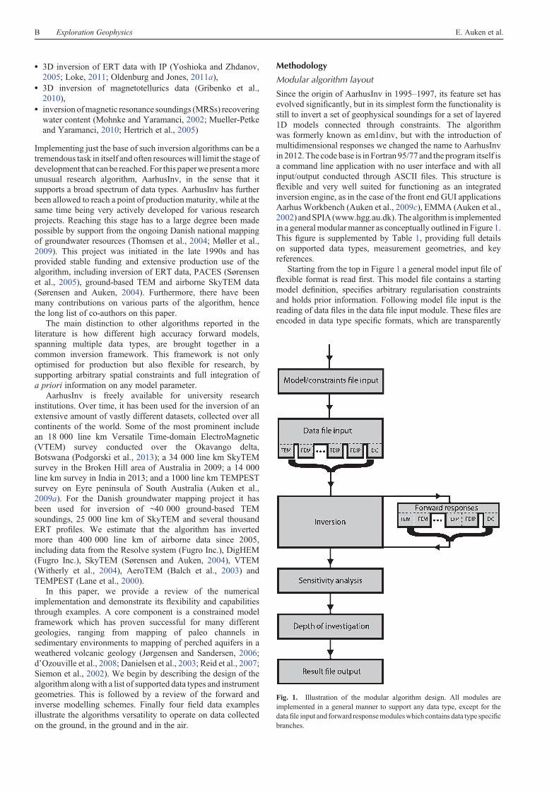
Since the origin of AarhusInv in 1995–1997, its feature set hasevolved significantly, but in its simplest form the functionality isstill to invert a set of geophysical soundings for a set of layered1D models connected through constraints. The algorithmwas formerly known as em1dinv, but with the introduction ofmultidimensional responses we changed the name to AarhusInvin 2012.The code base is inFortran 95/77 and the program itself isa command line application with no user interface and with allinput/output conducted through ASCII files. This structure isflexible and very well suited for functioning as an integratedinversion engine, as in the case of the front end GUI applicationsAarhus Workbench (Auken et al., 2009c), EMMA (Auken et al.,2002) andSPIA(www.hgg.au.dk).Thealgorithm is implementedin a generalmodularmanner as conceptually outlined in Figure 1.This figure is supplemented by Table 1, providing full detailson supported data types, measurement geometries, and keyreferences.

Starting from the top in Figure 1 a general model input file offlexible format is read first. This model file contains a startingmodel definition, specifies arbitrary regularisation constraintsand holds prior information. Following model file input is thereading of data files in the data file input module. These files areencoded in data type specific formats, which are transparently

Fig. 1. Illustration of the modular algorithm design. All modules areimplemented in a general manner to support any data type, except for thedatafile input and forward responsemoduleswhich contains data type specificbranches.

B Exploration Geophysics E. Auken et al.

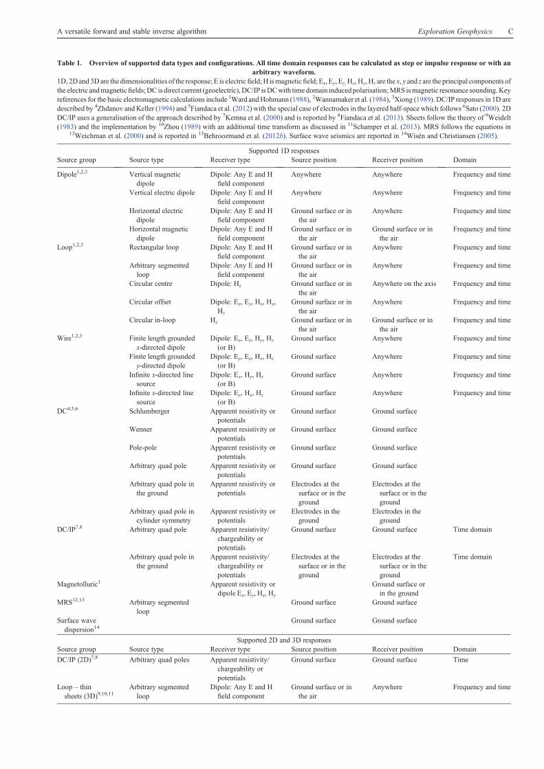
Table 1. Overview of supported data types and configurations. All time domain responses can be calculated as step or impulse response or with anarbitrary waveform.

1D, 2Dand 3Dare the dimensionalities of the response; E is electricfield;H ismagneticfield; Ex, Ey, Ez, Hx, Hy, Hz are the x, y and z are the principal components ofthe electric andmagneticfields;DC is direct current (geoelectric), DC/IP isDCwith time domain inducedpolarisation;MRS ismagnetic resonance sounding.Keyreferences for the basic electromagnetic calculations include 1Ward andHohmann (1988), 2Wannamaker et al. (1984), 3Xiong (1989). DC/IP responses in 1D aredescribed by 4Zhdanov and Keller (1994) and 5Fiandaca et al. (2012) with the special case of electrodes in the layered half-space which follows 6Sato (2000). 2DDC/IP uses a generalisation of the approach described by 7Kemna et al. (2000) and is reported by 8Fiandaca et al. (2013). Sheets follow the theory of 9Weidelt(1983) and the implementation by 10Zhou (1989) with an additional time transform as discussed in 11Schamper et al. (2013). MRS follows the equations in

12Weichman et al. (2000) and is reported in 13Behroozmand et al. (2012b). Surface wave seismics are reported in 14Wisén and Christiansen (2005).

Supported 1D responsesSource group Source type Receiver type Source position Receiver position Domain

Dipole1,2,3 Vertical magneticdipole

Dipole: Any E and Hfield component

Anywhere Anywhere Frequency and time

Vertical electric dipole Dipole: Any E and Hfield component

Anywhere Anywhere Frequency and time

Horizontal electricdipole

Dipole: Any E and Hfield component

Ground surface or inthe air

Anywhere Frequency and time

Horizontal magneticdipole

Dipole: Any E and Hfield component

Ground surface or inthe air

Ground surface or inthe air

Frequency and time

Loop1,2,3 Rectangular loop Dipole: Any E and Hfield component

Ground surface or inthe air

Anywhere Frequency and time

Arbitrary segmentedloop

Dipole: Any E and Hfield component

Ground surface or inthe air

Anywhere Frequency and time

Circular centre Dipole: Hz Ground surface or inthe air

Anywhere on the axis Frequency and time

Circular offset Dipole: Ex, Ey, Hx, Hy,Hz

Ground surface or inthe air

Anywhere Frequency and time

Circular in-loop Hz Ground surface or inthe air

Ground surface or inthe air

Frequency and time

Wire1,2,3 Finite length groundedx-directed dipole

Dipole: Ex, Ez, Hy, Hz

(or B)Ground surface Anywhere Frequency and time

Finite length groundedy-directed dipole

Dipole: Ey, Ez, Hx, Hz

(or B)Ground surface Anywhere Frequency and time

Infinite x-directed linesource

Dipole: Ex, Hy, Hz

(or B)Ground surface Anywhere Frequency and time

Infinite x-directed linesource

Dipole: Ey, Hx, Hz

(or B)Ground surface Anywhere Frequency and time

DC4,5,6 Schlumberger Apparent resistivity orpotentials

Ground surface Ground surface

Wenner Apparent resistivity orpotentials

Ground surface Ground surface

Pole-pole Apparent resistivity orpotentials

Ground surface Ground surface

Arbitrary quad pole Apparent resistivity orpotentials

Ground surface Ground surface

Arbitrary quad pole inthe ground

Apparent resistivity orpotentials

Electrodes at thesurface or in theground

Electrodes at thesurface or in theground

Arbitrary quad pole incylinder symmetry

Apparent resistivity orpotentials

Electrodes in theground

Electrodes in theground

DC/IP7,8 Arbitrary quad pole Apparent resistivity/chargeability orpotentials

Ground surface Ground surface Time domain

Arbitrary quad pole inthe ground

Apparent resistivity/chargeability orpotentials

Electrodes at thesurface or in theground

Electrodes at thesurface or in theground

Time domain

Magnetolluric1 Apparent resistivity ordipole Ex, Ey, Hx, Hy

Ground surface orin the ground

MRS12,13 Arbitrary segmentedloop

Ground surface Ground surface

Surface wavedispersion14

Ground surface Ground surface

Supported 2D and 3D responsesSource group Source type Receiver type Source position Receiver position Domain

DC/IP (2D)7,8 Arbitrary quad poles Apparent resistivity/chargeability orpotentials

Ground surface Ground surface Time

Loop – thinsheets (3D)9,10,11

Arbitrary segmentedloop

Dipole: Any E and Hfield component

Ground surface or inthe air

Anywhere Frequency and time

A versatile forward and stable inverse algorithm Exploration Geophysics C

handled by the modules internal branching to the relevant submodules. Note that mixing of any number of different data typesis supported, allowing for unrestricted joint inversions. Havingfilled the internal data structures from input files these structuresare passed on to the general inversion module which starts theiterative inversion process. During the iterative course ofminimising the residual the inversion module calls the forwardresponse module (see Appendix A) for the calculation of forwardresponse updates and derivatives. The forward response modulealso handles data type specific branching transparently, simplyperforming the requested calculations and returning the result tothe inversion module. Internally, the forward response modulemakes data type dependent calls to a library of common routines.Having iteratively solved the inverse problem (see next paragraphand Appendix B) the result is sent to the general model analysismodule, which calculates a model parameter sensitivity analysis.Finally the depth of investigation (DOI) is calculated based on theactual model output from the inversion process and a recalculatedsensitivity (Jacobian) matrix (Christiansen and Auken, 2012).Following the DOI calculation a result file is finally written in ageneral file format.

Forward modelling

From a forward modelling point of view AarhusInv provides awide range of options for simulating a given measurementsystem. This is particularly important for TEM data, asneglecting the influence of system parameters such asgeometry, waveform or filters can lead to serious modellingerror as described for TEM by Christiansen et al. (2011) andFiandaca et al. (2012) for DC/IP. The extent to which thealgorithm allows for full system forward modelling isrelatively unique and makes it possible to compare modelresults from different data types as directly as possible. Keyreferences for the forward modelling are given in the caption ofTable 1. It is outside the scope of this paper to describe all thesedifferent solutions and therefore we have in Appendix A chosento give descriptive details on the 1D EM solutions which arealso the most used parts of AarhusInv.

The forward modelling is an implemented parallel usingOpenMP and scales close to linearly running on 1–64 processors.All vectors and matrices are furthermore implemented sparselymaking the memory consumption relatively low even for verylarge inverse problems. It is out of the scope of this paper todescribe the details of this implementation and we thereforerefer to Kirkegaard and Auken (2014) for all details.

Inverse modelling

The mathematical formalism of the inverse modelling schemefollows the established practice by Menke (1989). Detailsare provided by Auken et al. (2005) and Appendix B givesin-depth details to the implementation of the inversion.Here, we focus on presenting the flexibility and capabilitiesof the algorithm. Essentially, we use a Gauss-Newton style

minimisation scheme with a Marquardt modification(Marquardt, 1963) to find the set of model parameters thatminimise the L2 misfit with respect to observed data,regularising and prior information. All datasets are invertedsimultaneously, minimising a common object function.Consequently, the output models are balanced between theconstraints, the physics and the data. Model parameters thathave little influence on the data will be controlled by theconstraints, and vice versa. The use of, for example, lateral orspatial constraints on a collection of models allows forinformation to propagate across a survey area.

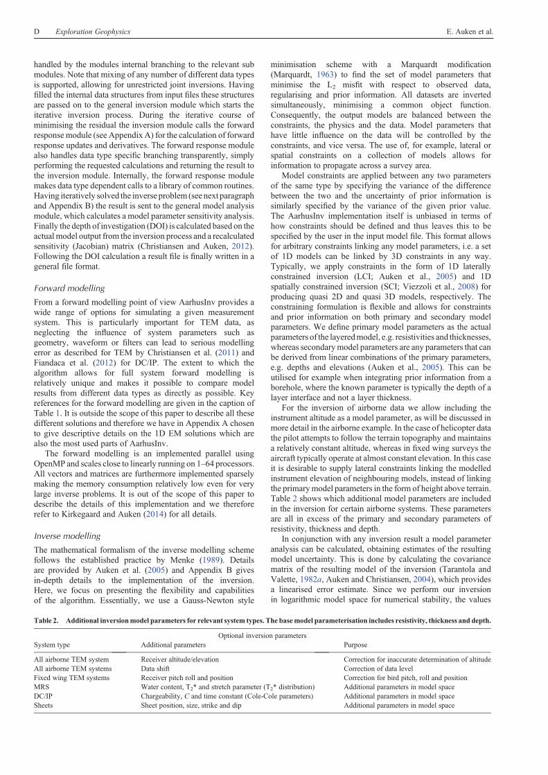
Model constraints are applied between any two parametersof the same type by specifying the variance of the differencebetween the two and the uncertainty of prior information issimilarly specified by the variance of the given prior value.The AarhusInv implementation itself is unbiased in terms ofhow constraints should be defined and thus leaves this to bespecified by the user in the input model file. This format allowsfor arbitrary constraints linking any model parameters, i.e. a setof 1D models can be linked by 3D constraints in any way.Typically, we apply constraints in the form of 1D laterallyconstrained inversion (LCI; Auken et al., 2005) and 1Dspatially constrained inversion (SCI; Viezzoli et al., 2008) forproducing quasi 2D and quasi 3D models, respectively. Theconstraining formulation is flexible and allows for constraintsand prior information on both primary and secondary modelparameters. We define primary model parameters as the actualparameters of the layeredmodel, e.g. resistivities and thicknesses,whereas secondarymodel parameters are any parameters that canbe derived from linear combinations of the primary parameters,e.g. depths and elevations (Auken et al., 2005). This can beutilised for example when integrating prior information from aborehole, where the known parameter is typically the depth of alayer interface and not a layer thickness.

For the inversion of airborne data we allow including theinstrument altitude as a model parameter, as will be discussed inmore detail in the airborne example. In the case of helicopter datathe pilot attempts to follow the terrain topography and maintainsa relatively constant altitude, whereas in fixed wing surveys theaircraft typically operate at almost constant elevation. In this caseit is desirable to supply lateral constraints linking the modelledinstrument elevation of neighbouring models, instead of linkingthe primarymodel parameters in the form of height above terrain.Table 2 shows which additional model parameters are includedin the inversion for certain airborne systems. These parametersare all in excess of the primary and secondary parameters ofresistivity, thickness and depth.

In conjunction with any inversion result a model parameteranalysis can be calculated, obtaining estimates of the resultingmodel uncertainty. This is done by calculating the covariancematrix of the resulting model of the inversion (Tarantola andValette, 1982a, Auken and Christiansen, 2004), which providesa linearised error estimate. Since we perform our inversionin logarithmic model space for numerical stability, the values

Table 2. Additional inversionmodel parameters for relevant system types. The basemodel parameterisation includes resistivity, thickness and depth.

Optional inversion parametersSystem type Additional parameters Purpose

All airborne TEM system Receiver altitude/elevation Correction for inaccurate determination of altitudeAll airborne TEM systems Data shift Correction of data levelFixed wing TEM systems Receiver pitch roll and position Correction for bird pitch, roll and positionMRS Water content, T2* and stretch parameter (T2* distribution) Additional parameters in model spaceDC/IP Chargeability, C and time constant (Cole-Cole parameters) Additional parameters in model spaceSheets Sheet position, size, strike and dip Additional parameters in model space

D Exploration Geophysics E. Auken et al.

obtained from such a sensitivity analysis can conveniently beregarded relative measures of uncertainty. Absolute errorestimates from logarithmic space are translated into a standarddeviation factor in linear space, such that 1.0 is equal to perfectresolution and 1.1 corresponds to a standard deviation of ~10%.We find that when such linearised error estimates become muchlarger than unity they are best viewed as guidelines, however.The use of error estimates will be illustrated in the followingexamples.

We finalise the inverse modelling procedure by calculatingthe DOI for the resulting output models, an operation whichrelies on a reweighting of the Jacobian matrix. The computationsemploy a global and absolute sensitivity threshold value, whichhas been tuned for operating in logarithmic model/dataspace (Christiansen and Auken, 2012). For a given model, theDOI calculations consider only the parts of the Jacobian relatedto observed data, implying that the effect of lateral, spatial orvertical model parameter constraints and a priori informationis not included. With this type of DOI estimate it is possibleto judge when the information in a model is driven by data orheavily dependent on the starting model or specifics of theregularisation.

Limitations due to dimensionality of the forward responseand inversion

The functionalities described so far illustrate the generalcapabilities of the algorithm at its current stage of development,but obviously its inherent limitations should also be considered.

First of all the algorithm base began as a 1D implementationand the whole suite of EMmethods are still limited to 1D forwardmodelling with the exception of 3D sheets. For DC and IP theforward algorithms are present in both 1D and 2D versions anda 3D implementation is close to being complete. Solving thephysical problem in1Dcanbe a limitation for applications such asmineral exploration, whereas studies of sedimentary settings fitswell within a 1D modelling envelope (e.g. Auken et al., 2008;Viezzoli et al., 2010).

Second,while being implemented asgenerally as possible, ourregularisation and inversion schemes are fundamentally basedon a static formulation. This means that it is not possible toexperiment with e.g. Tikhonov-style variable regularisationparameters. However, the least-squares (L2-norm) solution canbe changed to use the L1-norm or the sharp boundary formalismby Zhdanov et al. (2000) and Vignoli et al. (2013).

Examples

In the following we show four examples demonstrating thecapabilities and versatility of the AarhusInv algorithm. In theexamples we show inversions of data collected on the ground, inthe ground and in the air. We also illustrate the use of spatial,lateral and vertical constraints. The examples are chosen toillustrate widely varying scales of interest, ranging from smallscale engineering typeofproblems to large regional scale surveys.We further illustrate the use of prior information and provide asynthetic example of joint inversion of mixed type data. Finallywe provide a synthetic example inverting an airborne dataset witha 3D sheet model.

On and in the ground: DC and time domain inducedpolarisation

For our first example we present a novel application of joint 1DLCI inversion of surface time domain induced polarisation(TDIP) data and borehole TDIP data. The TDIP method is anatural and efficient extension of standard DC multi electrode

profiling by simply adding the measurement of the timedependence of discharge after an injection current is turnedoff. Modelling the complete time decay of each data pointin the Cole–Cole formulation (Pelton et al., 1978) allows forextracting additional independent model parameters, oftenmaking it possible to discriminate earth structures with anotherwise identical signature. Apart from resistivity, each layerof an IP model includes the parameters t, C and M0. Here m0 isthe magnitude of the chargeability when the injection current isturned off at t= 0, t is the decay time constant andC is a constantcontrolling the frequency dependence of the response. The TDIPimplementation is described in full detail byFiandaca et al. (2012)and includesmodelling of the full injection currentwaveform andlow pass filters, which can be a cause of serious modelling errorwhen neglected. Compared to the methodology presented byFiandaca et al. (2012) we add in this example borehole TDIP datafor a joint inversion of two data types sharing a common modelspace, in order to demonstrate the versatility of the algorithm.

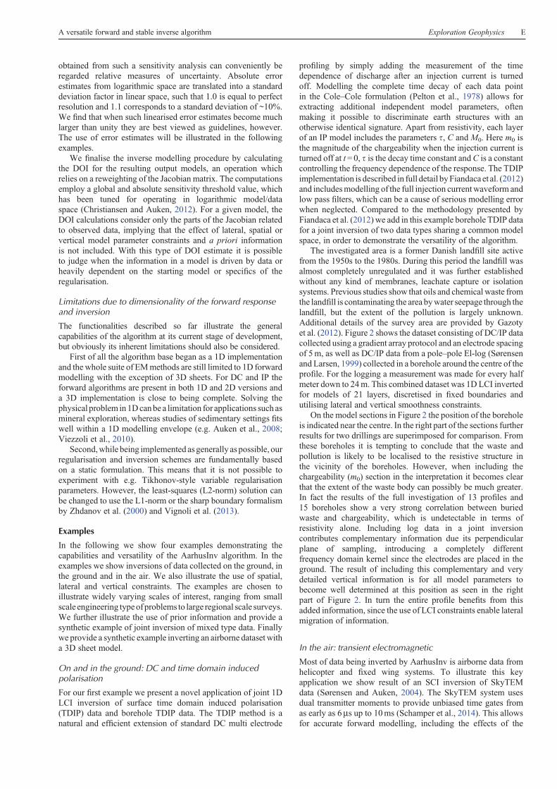
The investigated area is a former Danish landfill site activefrom the 1950s to the 1980s. During this period the landfill wasalmost completely unregulated and it was further establishedwithout any kind of membranes, leachate capture or isolationsystems. Previous studies show that oils and chemical waste fromthe landfill is contaminating the area bywater seepage through thelandfill, but the extent of the pollution is largely unknown.Additional details of the survey area are provided by Gazotyet al. (2012). Figure 2 shows the dataset consisting of DC/IP datacollected using a gradient array protocol and an electrode spacingof 5m, as well as DC/IP data from a pole–pole El-log (Sørensenand Larsen, 1999) collected in a borehole around the centre of theprofile. For the logging a measurement was made for every halfmeter down to 24m. This combined dataset was 1D LCI invertedfor models of 21 layers, discretised in fixed boundaries andutilising lateral and vertical smoothness constraints.

On the model sections in Figure 2 the position of the boreholeis indicated near the centre. In the right part of the sections furtherresults for two drillings are superimposed for comparison. Fromthese boreholes it is tempting to conclude that the waste andpollution is likely to be localised to the resistive structure inthe vicinity of the boreholes. However, when including thechargeability (m0) section in the interpretation it becomes clearthat the extent of the waste body can possibly be much greater.In fact the results of the full investigation of 13 profiles and15 boreholes show a very strong correlation between buriedwaste and chargeability, which is undetectable in terms ofresistivity alone. Including log data in a joint inversioncontributes complementary information due its perpendicularplane of sampling, introducing a completely differentfrequency domain kernel since the electrodes are placed in theground. The result of including this complementary and verydetailed vertical information is for all model parameters tobecome well determined at this position as seen in the rightpart of Figure 2. In turn the entire profile benefits from thisadded information, since the use of LCI constraints enable lateralmigration of information.

In the air: transient electromagnetic

Most of data being inverted by AarhusInv is airborne data fromhelicopter and fixed wing systems. To illustrate this keyapplication we show result of an SCI inversion of SkyTEMdata (Sørensen and Auken, 2004). The SkyTEM system usesdual transmitter moments to provide unbiased time gates fromas early as 6ms up to 10ms (Schamper et al., 2014). This allowsfor accurate forward modelling, including the effects of the

A versatile forward and stable inverse algorithm Exploration Geophysics E

waveforms of the dual transmitter moments, low pass filters,front gate and finite width gates. For the inversion we usemeasurements of the vertical component of the secondary fieldonly and include instrument altitude as a model parameter. In themore general case of fixed wing type geometry the algorithmallows for inversion of all field components, including receiverpitch and roll asmodel parameters (Auken et al., 2009b).Wehavealso implemented inversion for receiver coil response modelparameter, allowing for the use of data from time gates asearly as 6ms (Schamper et al., 2014)

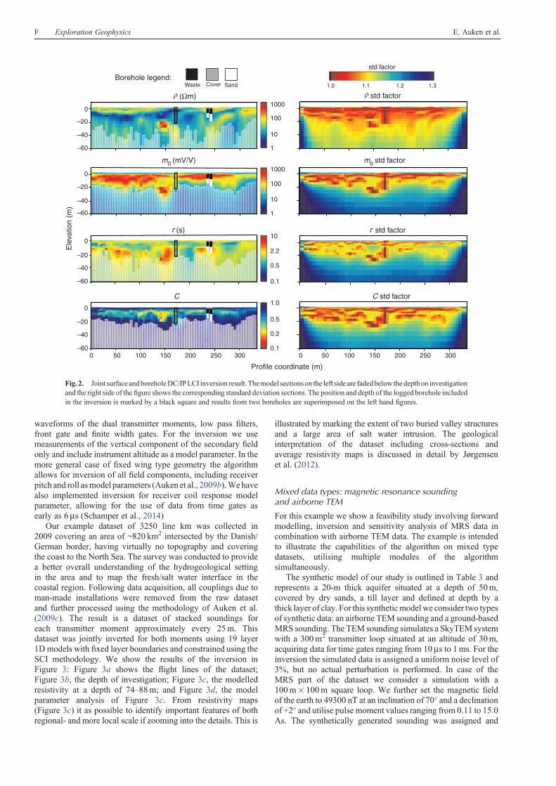
Our example dataset of 3250 line km was collected in2009 covering an area of ~820 km2 intersected by the Danish/German border, having virtually no topography and coveringthe coast to the North Sea. The survey was conducted to providea better overall understanding of the hydrogeological settingin the area and to map the fresh/salt water interface in thecoastal region. Following data acquisition, all couplings due toman-made installations were removed from the raw datasetand further processed using the methodology of Auken et al.(2009c). The result is a dataset of stacked soundings foreach transmitter moment approximately every 25m. Thisdataset was jointly inverted for both moments using 19 layer1Dmodels with fixed layer boundaries and constrained using theSCI methodology. We show the results of the inversion inFigure 3: Figure 3a shows the flight lines of the dataset;Figure 3b, the depth of investigation; Figure 3c, the modelledresistivity at a depth of 74–88m; and Figure 3d, the modelparameter analysis of Figure 3c. From resistivity maps(Figure 3c) it as possible to identify important features of bothregional- and more local scale if zooming into the details. This is

illustrated by marking the extent of two buried valley structuresand a large area of salt water intrusion. The geologicalinterpretation of the dataset including cross-sections andaverage resistivity maps is discussed in detail by Jørgensenet al. (2012).

Mixed data types: magnetic resonance soundingand airborne TEM

For this example we show a feasibility study involving forwardmodelling, inversion and sensitivity analysis of MRS data incombination with airborne TEM data. The example is intendedto illustrate the capabilities of the algorithm on mixed typedatasets, utilising multiple modules of the algorithmsimultaneously.

The synthetic model of our study is outlined in Table 3 andrepresents a 20-m thick aquifer situated at a depth of 50m,covered by dry sands, a till layer and defined at depth by athick layer of clay. For this syntheticmodelwe consider two typesof synthetic data: an airborne TEM sounding and a ground-basedMRS sounding. The TEM sounding simulates a SkyTEM systemwith a 300m2 transmitter loop situated at an altitude of 30m,acquiring data for time gates ranging from 10ms to 1ms. For theinversion the simulated data is assigned a uniform noise level of3%, but no actual perturbation is performed. In case of theMRS part of the dataset we consider a simulation with a100m� 100m square loop. We further set the magnetic fieldof the earth to 49300 nT at an inclination of 70� and a declinationof +2� and utilise pulse moment values ranging from 0.11 to 15.0As. The synthetically generated sounding was assigned and

01000

100

10

1

1000

10

2.2

0.5

0.1

1.0

0.5

0.2

0.1

100

10

1

–20

–40

–60

0

–20

–40

–60

0

–20

–40

–60

0

–20

–40

–600 50 100 150 200 250 300 0 50 100 150 200 250 300

Profile coordinate (m)

Ele

vatio

n (m

)Borehole legend:

Waste Cover

m0 (mV/V) m0 std factor

Sand 1.0 1.1

std factor

std factorρ (Ωm)ρ

(s)τ τ std factor

C std factorC

1.2 1.3

Fig. 2. Joint surface andboreholeDC/IPLCI inversion result. Themodel sections on the left side are fadedbelow the depthon investigationand the right side of the figure shows the corresponding standard deviation sections. The position and depth of the logged borehole includedin the inversion is marked by a black square and results from two boreholes are superimposed on the left hand figures.

F Exploration Geophysics E. Auken et al.

perturbed for a base noise level of 20 nV, with an additionaluniform noise contribution of 3%.

Traditionally MRS data has been inverted in what can bereferred to as step-wise inversion schemes (e.g. Günther et al.,

2011; Mueller-Petke and Yaramanci, 2010; Behroozmand et al.,2012b). This type of inversion starts by inverting a TEM or DCsounding for a resistivity model, which is then assumed to be thetrue model in a subsequent inversion for MRS model parameters(water content ratio W and relaxation time T2*). In other wordsthe MRS kernel function, which is a function of the resistivitymodel, is assumed fixed. Behroozmand et al. (2012a) proposes ajoint inversion methodology where the resistivity modelparameters are free in the inversion, implying that the MRSkernel has to be updated for each iteration of the inversionrequiring a fast numerical implementation of the MRS kernel.In the following we compare the resolution capabilities of thesetwo methods.

In Figure 4, the model results of a traditional step-wiseinversion of the simulated data is shown. The figure featuresdashed blue lines for indicating 68% confidence intervals, as

(a) (b)

(c) (d )

Fig. 3. SkyTEM SCI inversion results. (a) Flight lines of the dataset, (b) depth of investigation, (c) modelled resistivity at a depth of 74–88m and (d) modelparameter analysis of (c).

Table 3. The synthetic model used for mixed modelling of MRS andairborne TEM data.

Layer Lithology Resistivity(Wm)

Thickness(m)

Watercontent(m3/m3)

T2*(s)

C

1 Till, some water 40 30 0.1 0.1 12 Dry sand 300 20 0.02 0.2 13 Saturated sand 80 20 0.4 0.2 14 Clay 5 0.4 0.02 1

A versatile forward and stable inverse algorithm Exploration Geophysics G

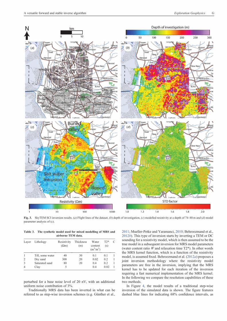
obtained from a sensitivity analysis. It is clear that the upper- andlower-most boundaries of the resistivity model are very wellresolved, whereas the layering in between these boundaries iscompletely undetermined. If a noise perturbation had beenapplied to the TEM data, the obtained model result wouldhave been very far from the true model for the two highlyresistive layers. Turning to the MRS model we see that thewater content of the synthetic model is well resolved for thetop two layers, but underestimated for the lower lying waterbearing sand layer with the true value out of range of the model’s68%confidence intervals. Thismismatch is caused by the slightly

wrong layer thicknesses fixed in the resistivity model, which inturn forces the modelled water content to compensate for theMRS kernel function being slightly off. For the bottom layer theinverted water content is found to be even further from the truemodel, but in this case the deviation can to a larger degree beattributed to a high degree of uncertainty as it is closer to the depthof investigation. In general, T2*values are found to be reasonablywell resolved for all layers.

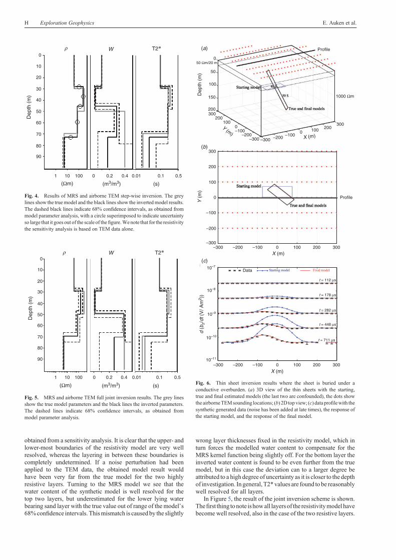
In Figure 5, the result of the joint inversion scheme is shown.Thefirst thing tonote is howall layers of the resistivitymodel havebecome well resolved, also in the case of the two resistive layers.

0W T2*ρ

10

20

30

40

50

60

Dep

th (

m)

70

80

90

1 10 100 0 0.2 0.4 0.01 0.1 0.5

(Ωm) (m3/m3) (s)

Fig. 4. Results of MRS and airborne TEM step-wise inversion. The greylines show the true model and the black lines show the invertedmodel results.The dashed black lines indicate 68% confidence intervals, as obtained frommodel parameter analysis, with a circle superimposed to indicate uncertaintyso large that it goes out of the scale of thefigure.Wenote that for the resistivitythe sensitivity analysis is based on TEM data alone.

(a)

(b)

(c)

50

050 Ωm/20 m

100

150

200

200100

–100–200

–300 –300 –200 –1000 100 200

300

1000 Ωm

Profile

Profile

0

300

300

200

100

0

–100

–200

–300

10–7

10–8

10–9

10–10

10–11

–300 –200

Data

–100 0 100 200

t = 112 μs

t = 178 μs

t = 282 μs

t = 448 μs

t = 711 μs

300

–300 –200 –100 0 100 200

X (m)

X (m)

Y (

m)

d (b

z/dt

(V

/ Am

2 ))

Dep

th (

m)

X (m)

Y (m)

300

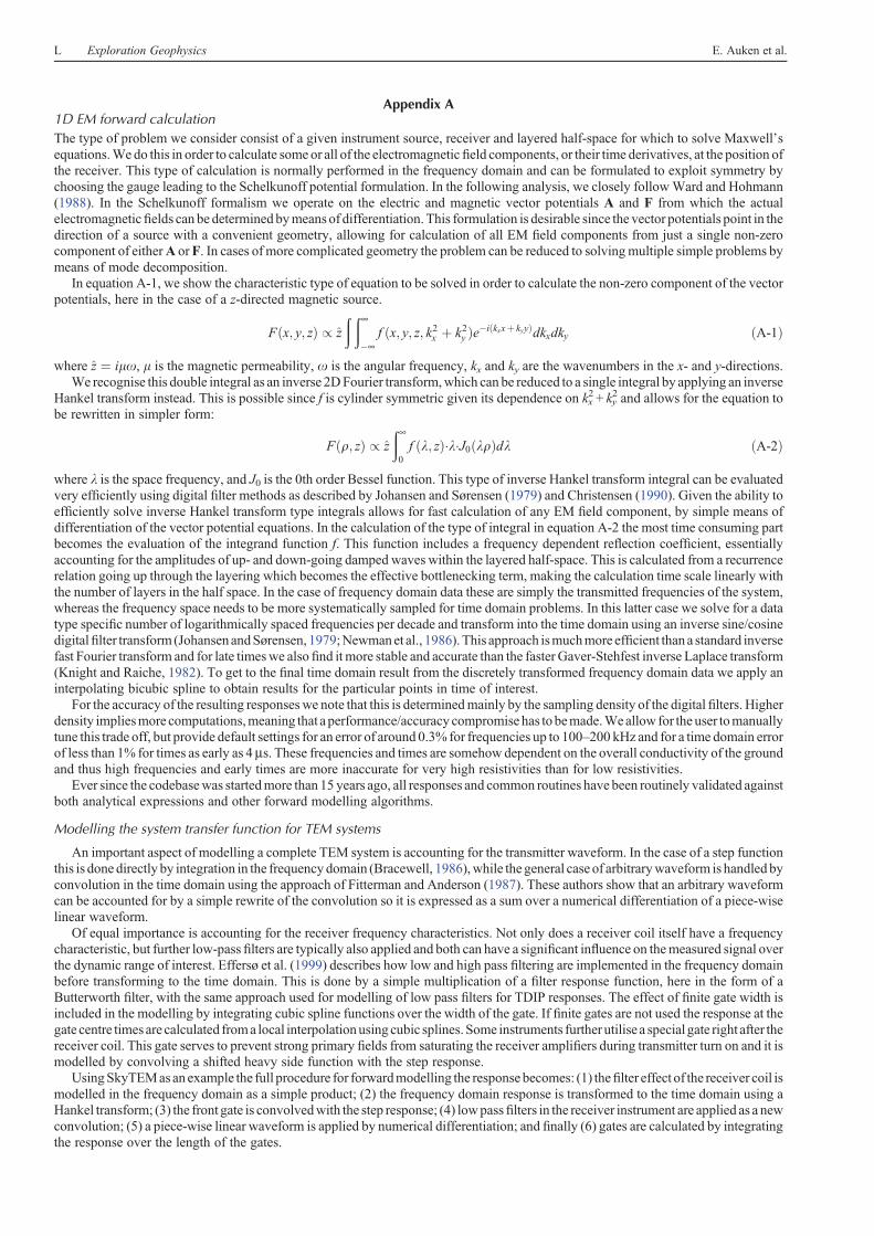
Fig. 6. Thin sheet inversion results where the sheet is buried under aconductive overburden. (a) 3D view of the thin sheets with the starting,true and final estimated models (the last two are confounded), the dots showthe airborneTEMsounding locations; (b) 2D topview; (c) data profilewith thesynthetic generated data (noise has been added at late times), the response ofthe starting model, and the response of the final model.

W T2*ρ0

10

20

30

40

50

60

70

Dep

th (

m)

80

90

1 10 100 0 0.2 0.4 0.01 0.1 0.5

(Ωm) (m3/m3) (s)

Fig. 5. MRS and airborne TEM full joint inversion results. The grey linesshow the true model parameters and the black lines the inverted parameters.The dashed lines indicate 68% confidence intervals, as obtained frommodel parameter analysis.

H Exploration Geophysics E. Auken et al.

Determination of layer thicknesses has improved in particular,due to the combined, complementary information providedby the SkyTEM and MRS signals. In the case of MRS modelparameters this point can be seen from the water content modelbeing very accurately reproduced for the top three layers, whilethe improvement for the deepest lying layer is less pronounced asit is closer to the depth of investigation. For the T2* model theimpact of the coupled scheme is very little.

Airborne TEM and sheets inversion

In the AarhusInv code, the forward modelling of thin sheets isbased on the algorithm developed by Zhou (1989) with themathematical formulation from Weidelt (1983). This algorithmcalculates the response from several arbitrarily located thin sheetsin a conductive layered host. The sheets have both inductive andchannelling current modes. If several sheets are used they will beinductively coupled. To speed up the computation the algorithmuses OpenMP to take advantage of multi-processor computerarchitecture, and an efficient solver has been added to compute thescattered fields for inversion of airborne datasets where manysource-receiver locations need to be computed. Furthermore, thealgorithmhas been extended to include both dipole andfinite loopsources, and it calculates responses both in the time and frequencydomain as stated in Tables 1 and 2.

Wewill illustrate the use of this part ofAarhusInv on synthetictransient AEM data as shown in Figure 6. The model has a 20mconductive overburden of 50 Wm, covering a resistive halfspaceof 1000 Wm. The sheet is in the resistive host and has aconductance of 50 S, a top depth of 30m, a maximum depthof 175m, and both its dip and strike angles are 45� (Figure 6a).The simulated AEM dataset has a line spacing of 100m witha sounding spacing of 20m along the lines (Figure 6b) andz-component data only. The flight altitude is 30m andrecorded times span from ~10ms to a few ms depending onthe noise. Random noise at a slope of t–1/2 and a noise level of1 nV/m2 at 1ms was added to the data (Schamper et al., 2014).Figure 6c illustrates the fit obtained after inversion with some ofthe recorded times along the central profile. The starting modelparameters are indicated in the figure. The parameters in theinversion are sheet conductance, dip, strike, layered modelparameters and flight altitude. In the present case, the sheet iswell determined with the TEM method and the final estimatedmodel iswell recoveredandalmost identical to the truemodel as isalso indicated by the parameter determination (not shown here).

Conclusions

Wehave presented an overview of a proven, versatile andflexibleproduction inversion algorithm, capable of invertingmost electricand electromagnetic data types and supporting most instrumentsnormally used within the field of near surface geophysics. Thealgorithm is freely available for academic use and providesthe user with freedom to specify arbitrary 3D regularisationconstraints, include any amount of prior information and invertfor mixed type datasets. Our implementation focuses onconsistently accurate system forward modelling independent ofdata type and instrument, which not only ensures accuracy,but can also be regarded a prerequisite for joint inversion ofdata collected using instruments of different transfer function.The implementation is modular, meaning that the bulk ofthe algorithm is independent of data type, making it very easyto add support for new types of data. Calculation of both modelparameter sensitivity analysis and depth of investigation is a keyfeature and it is handled automatically regardless of configurationand data types.

The versatility of the algorithm is illustrated by four differentexamples. First, we showed the joint inversion of a resistivity/time-domain IP datasetwith electrodes both located in the groundand on the surface. This example provides an illustration of howincluding Cole–Cole parameters in the model greatly improvesthe delineation of a former landfill. Second, we have shownresults of a large scale airborne TEM survey where the combinedinformation from maps of average resistivity, depth-of-investigation and model parameter analysis improves theunderstanding of the underlying geology. Third, we haveshown a synthetic example where we jointly invert AirborneTEMdatawith ground-basedMRSdata. These twomodel-spacesareonly vaguely related, butwe showhow themutual informationsignificantly improves the resolution of both the resistivity- andthe water content model. In the fourth example we showed asynthetic example inverting Airborne TEMdata with a 3D sheetsmodel.

Acknowledgements

Over the years the development of the code has been supported by severaldifferent research projects. Themost prominent has been theHOBECenter ofExcellence (Villum Kahn Rasmussen Foundation) and the four projectsRiskPoint, NICA, CO2GS and HyGEM, all larger research projects fundedby the Danish Counsel for Strategic Research. Also the Nature Agency underthe Danish Ministry of the Environment has greatly supported our work asan integrated part of the national groundwater mapping program. Lastly, wehave to thank numerous students who had to suffer long nights with newimplementations not always working as expected in the first beta releases.

References

Auken, E., and Christiansen, A. V., 2004, Layered and laterally constrained2D inversion of resistivity data: Geophysics, 69, 752–761. doi:10.1190/1.1759461

Auken, E., Nebel, L., Sørensen, K. I., Breiner, M., Pellerin, L., andChristensen, N. B., 2002, EMMA – a geophysical training andeducation tool for electromagnetic modeling and analysis: Journal ofEnvironmental & Engineering Geophysics, 7, 57–68. doi:10.4133/JEEG7.2.57

Auken, E., Christiansen, A. V., Jacobsen, B. H., Foged, N., and Sørensen,K. I., 2005, Piecewise 1D laterally constrained inversion of resistivitydata: Geophysical Prospecting, 53, 497–506. doi:10.1111/j.1365-2478.2005.00486.x

Auken, E., Christiansen, A. V., Jacobsen, L., and Sørensen, K. I., 2008,A resolution study of buried valleys using laterally constrained inversionof TEM data: Journal of Applied Geophysics, 65, 10–20. doi:10.1016/j.jappgeo.2008.03.003

Auken, E., Christiansen, A. V., Viezzoli, A., Fitzpatrick, A., Cahill, K.,Munday, T., and Berens, V., 2009a, Investigation on the groundwaterresources of the South Eyre Peninsula, South Australia, determined fromlaterally constrained inversion of TEMPEST data: ASEG ExtendedAbstracts 2009, 1–5.

Auken, E., Christiansen, A. V., Viezzoli, A., Fitzpatrick, A., andMunday, T.,2009b, Laterally constrained inversion of TEMPEST data fromEyre Peninsula area, South Australia: 15th European Meeting ofEnvironmental and Engineering Geophysics, 2009.

Auken, E., Christiansen,A.V.,Westergaard, J. A., Kirkegaard, C., Foged,N.,and Viezzoli, A., 2009c, An integrated processing scheme for high-resolution airborne electromagnetic surveys, the SkyTEM system:Exploration Geophysics, 40, 184–192. doi:10.1071/EG08128

Balch, S. J., Boyko,W. P., and Paterson, N. R., 2003, TheAeroTEMairborneelectromagnetic system: The Leading Edge, 22, 562–566. doi:10.1190/1.1587679

Behroozmand,A.A.,Auken,E.,Fiandaca,G., andChristiansen,A.V., 2012a,Improvement in MRS parameter estimation by joint and laterallyconstrained inversion of MRS and TEM data: Geophysics, 74,WB191–WB200.

Behroozmand, A. A., Auken, E., Fiandaca, G., Christiansen, A. V., andChristensen,N.B., 2012b, Efficient full decay inversion ofMRSdatawith

A versatile forward and stable inverse algorithm Exploration Geophysics I

a stretched-exponential approximation of the T2* distribution:Geophysical Journal International, 190, 900–912. doi:10.1111/j.1365-246X.2012.05558.x

Bracewell, R. N., 1986, The Fourier transform and its applications(2nd edition): McGraw-Hill, Inc.

Brodie, R., and Sambridge, M., 2006a, A holistic approach to inversion offrequency-domain airborne EM data: Geophysics, 71, G301–G312.doi:10.1190/1.2356112

Brodie, R., and Sambridge, M., 2006b, A holistic approach to inversion oftime-domain airborne EM: ASEG Extended Abstracts 2006, 1–4.

Christensen, N. B., 1990, Optimized fast Hankel transform filters:Geophysical Prospecting, 38, 545–568. doi:10.1111/j.1365-2478.1990.tb01861.x

Christensen, N. B., 2002, A generic 1-D imaging method for transientelectromagnetic data: Geophysics, 67, 438–447. doi:10.1190/1.1468603

Christensen, N. B., and Auken, E., 1992, Simultaneous electromagneticlayered model analysis: Proceedings of the Interdisciplinary InversionWorkshop 1, Geoskrifter, 49–56.

Christiansen, A. V., and Auken, E., 2012, A global measure for depth ofinvestigation: Geophysics, 77, WB171–WB177.

Christiansen, A. V., Auken, E., and Viezzoli, A., 2011, Quantification ofmodelingerrors in airborneTEMcausedby inaccurate systemdescription:Geophysics, 76, F43–F52. doi:10.1190/1.3511354

Cox,L.H.,Wilson,G.A., andZhdanov,M.S., 2010, 3D inversionof airborneelectromagnetic data using a moving footprint: Exploration Geophysics,41, 250–259. doi:10.1071/EG10003

d’Ozouville, N., Auken, E., Sørensen, K. I., Violette, S., Marsily, G. D.,Deffontaines, B., and Merlen, G., 2008, Extensive perched aquifer andstructural implications revealed by 3D resistivity mapping in a Galapagosvolcano: Earth and Planetary Science Letters, 269, 518–522.doi:10.1016/j.epsl.2008.03.011

Danielsen, J. E., Auken, E., Jørgensen, F., Søndergaard, V. H., and Sørensen,K. I., 2003, The application of the transient electromagnetic method inhydrogeophysical surveys: Journal of Applied Geophysics, 53, 181–198.doi:10.1016/j.jappgeo.2003.08.004

Effersø, F., Auken, E., and Sørensen, K. I., 1999, Inversion of band-limitedTEM responses: Geophysical Prospecting, 47, 551–564. doi:10.1046/j.1365-2478.1999.00135.x

Fiandaca, G., Auken, E., Gazoty, A., and Christiansen, A. V., 2012, Time-domain induced polarization: full-decay forward modeling and 1Dlaterally constrained inversion of Cole-Cole parameters: Geophysics,77, E213–E225. doi:10.1190/geo2011-0217.1

Fiandaca, G., Ramm, J., Binley, A., Gazoty, A., Christiansen, A. V., andAuken, E., 2013, Resolving spectral information from time domaininduced polarization data through 2-D inversion: Geophysical JournalInternational, 192, 631–646. doi:10.1093/gji/ggs060

Fitterman, D. V., and Anderson, W. L., 1987, Effect of transmitter turn-offtime on transient soundings: Geoexploration, 24, 131–146. doi:10.1016/0016-7142(87)90087-1

Gazoty, A., Fiandaca, G., Pedersen, J., Auken, E., and Christiansen, A.V.,2012, Mapping of landfills using time-domain spectral inducedpolarization data: the Eskelund case study: Near Surface Geophysics,10, 563–574.

Gribenko, A., Wan, L., and Zhdanov, M. S., 2010, Three-dimensionalinversion of magnetotelluric data for complex resistivity: Proceedingsof the CEMI Annual Meeting, 269–294.

Günther, T., Rücker, C., and Spitzer, K., 2006, Three-dimensional modellingand inversion of dc resistivity data incorporating topography –

II. Inversion: Geophysical Journal International, 166, 506–517.doi:10.1111/j.1365-246X.2006.03011.x

Günther, T., Liebau, J., Akca, I., and Mueller-Petke, M., 2011, Block jointinversion (BJI) of MRS and DC resistivity soundings for aquifer imagingat the North Sea island, Borkum: Near Surface 2011 – The 17th EuropeanMeeting of Environmental and Engineering Geophysics, 2011.

Hertrich, M., Braun, M., and Yaramanci, U., 2005, Magnetic resonancesoundings with separated transmitter and receiver loops: Near SurfaceGeophysics, 3, 141–154.

Johansen, H. K., and Sørensen, K. I., 1979, Fast Hankel transforms:Geophysical Prospecting, 27, 876–901. doi:10.1111/j.1365-2478.1979.tb01005.x

Jørgensen, F., andSandersen,P.B.E., 2006,Buried andopen tunnel valleys inDenmark – erosion beneath multiple ice sheets: Quaternary ScienceReviews, 25, 1339–1363. doi:10.1016/j.quascirev.2005.11.006

Jørgensen, F., Scheer, W., Thomsen, S., Sonnenborg, T. O., Hinsby, K.,Wiederhold, H., Schamper, C., Roth, B., Kirsch, R., andAuken, E., 2012,Transboundary geophysical mapping of geological elements and salinitydistribution critical for the assessment of future sea water intrusion inresponse to sea level rise: Hydrology and Earth System Sciences, 16,1845–1862. doi:10.5194/hess-16-1845-2012

Kemna,A., Binley,A.,Ramirez,A., andDaily,W., 2000,Complex resistivitytomography for environmental applications: Chemical EngineeringJournal, 77, 11–18. doi:10.1016/S1385-8947(99)00135-7

Kirkegaard,C., andAuken,E., 2014,Aparallel, scalable andmemoryefficientinversion code for very large scale airborne EM surveys: GeophysicalProspecting, in press.

Knight, J. H., and Raiche, A. P., 1982, Transient electromagnetic calculationsusing the Gaver-Stehfest inverse Laplace transformmethod:Geophysics,47, 47–50. doi:10.1190/1.1441280

Lane,R.,Green,A.G.,Golding,C.,Owers,M.,Pik,P., Plunkett,C.,Sattel,D.,and Thorn, B., 2000, An example of 3D conductivity mapping using theTEMPEST airborne electromagnetic system: Exploration Geophysics,31, 162–172. doi:10.1071/EG00162

Loke, M. H., 2011, RES3DINV: Geotomo software. Available at www.geoelectrical.com

Loke, M. H., and Barker, R. D., 1996, Rapid least squares inversion ofapparent resistivity pseudosections by a quasi-Newton method:Geophysical Prospecting, 44, 131–152. doi:10.1111/j.1365-2478.1996.tb00142.x

Loke, M. H., Chambers, J. E., and Ogilvy, R. D., 2006, Inversion of 2Dspectral induced polarization imaging data:Geophysical Prospecting, 54,287–301. doi:10.1111/j.1365-2478.2006.00537.x

Macnae, J. C., Smith, R., Polzer, B. D., Lamontagne, Y., and Klinkert, P. S.,1991, Conductivity-depth imaging of airborne electromagnetic step-response data: Geophysics, 56, 102–114. doi:10.1190/1.1442945

Marquardt, D., 1963, An algorithm for least squares estimation of nonlinearparameters: SIAM Journal of the Society for Industrial and AppliedMathematics, 11, 431–441. doi:10.1137/0111030

Menke, W., 1989, Geophysical data analysis discrete inverse theory:Academic Press.

Mohnke, O., and Yaramanci, U., 2002, Smooth and block inversion ofsurface NMR amplitudes and decay times using simulated annealing:Journal of Applied Geophysics, 50, 163–177. doi:10.1016/S0926-9851(02)00137-4

Møller, I., Verner, H., Søndergaard, V. H., Flemming, J., Auken, E., andChristiansen, A. V., 2009, Integrated management and utilization ofhydrogeophysical data on a national scale: Near Surface Geophysics,7, 647–659.

Mueller-Petke, M., and Yaramanci, U., 2010, QT inversion – comprehensiveuse of the complete surface NMR data set: Geophysics, 75,WA199–WA209. doi:10.1190/1.3471523

Newman, G. A., and Alumbaugh, D. L., 1997, Three-dimensional massivelyparallel electromagnetic inversion – I. Theory: Geophysical JournalInternational, 128, 345–354. doi:10.1111/j.1365-246X.1997.tb01559.x

Newman, G. A., Hohmann, G. W., and Anderson, W. L., 1986, Transientelectromagnetic response of a three-dimensional body in a layered earth:Geophysics, 51, 1608–1627. doi:10.1190/1.1442212

Oldenburg, D. W., and Jones, F. H. M., 2011a, DCIP3D (Inversion forApplied Geophysics): University of British Columbia GeophysicalInversion Facility. Available at www.eos.ubc.ca/ubcgif/iag/

Oldenburg, D. W., and Jones, F. H. M., 2011b, EM1DFM (Inversion forApplied Geophysics): University of British Columbia GeophysicalInversion Facility. Available at www.eos.ubc.ca/ubcgif/iag/

Oldenburg, D. W., and Jones, F. H. M., 2011c, EM1DTM (Inversion forApplied Geophysics): University of British Columbia GeophysicalInversion Facility. Available at www.eos.ubc.ca/ubcgif/iag/

Oldenburg, D. W., and Li, Y., 1994, Inversion of induced polarization data:Geophysics, 59, 1327–1341. doi:10.1190/1.1443692

Oldenburg, D. W., Haber, E., and Shekhtman, R., 2013, Three dimensionalinversion of multisource time domain electromagnetic data: Geophysics,78, E47–E57. doi:10.1190/geo2012-0131.1

J Exploration Geophysics E. Auken et al.

Pelton, W. H., Ward, S. H., Hallof, P. G., Sill, W. R., and Nelson, P. H.,1978, Mineral discrimination and removal of inductive couplingwith multifrequency induced-polarization: Geophysics, 43, 588–609.doi:10.1190/1.1440839

Podgorski, J.E.,Auken,E.,Schamper,C.,Christiansen,A.V.,Kalscheuer,T.,and Green, A. G., 2013, Processing and inversion of commercialhelicopter time-domain electromagnetic data for environmentalassessments and geologic and hydrologic mapping: Geophysics, 78,E149–E159. doi:10.1190/geo2012-0452.1

Reid, J. E., Munday, T., and Fitzpatrick, A., 2007, High-resolutionairborne electromagnetic surveying for dryland salinity management:the Toolibin Lake SkyTEM case study, W.A.: ASEG ExtendedAbstracts 2007, 1–5.

Rücker, C., Günther, T., and Spitzer, K., 2006, Three-dimensional modellingand inversion of dc resistivity data incorporating topography – I.Modelling: Geophysical Journal International, 166, 495–505.doi:10.1111/j.1365-246X.2006.03010.x

Santos, F. A.M., 2004, 1-D laterally constrained inversion of EM34 profilingdata: Journal of Applied Geophysics, 56, 123–134. doi:10.1016/j.jappgeo.2004.04.005

Sato, H.K., 2000, Potentialfield from a dc current source arbitrarily located ina nonuniform layeredmedium:Geophysics, 65, 1726–1732. doi:10.1190/1.1444857

Schamper, C., Auken, E., and Kirkegaard, C., 2013, 3D sheets inversion withaccurate modeling of AEM systems: SAGA AEM, South Africa, 1–2.

Schamper, C., Auken, E., and Sørensen, K. I., 2014, Coil response inversionfor very early time modelling of helicopter-borne time-domainelectromagnetic data and mapping of near-surface geological layers:Geophysical Prospecting, 62, 658–674. doi:10.1111/1365-2478.12104

Sengpiel, K. P., and Siemon, B., 2000, Advanced inversion methods forairborne electromagnetic exploration: Geophysics, 65, 1983–1992.doi:10.1190/1.1444882

Siemon, B., Stuntebeck, C., Sengpiel, K. P., Röttger, B., Rehli, H., andEberle, D. G., 2002, Investigation of hazardous waste sites and theirenvironment using BGRhelicopter-borne geophysical system: Journal ofEnvironmental & Engineering Geophysics, 7, 169–181. doi:10.4133/JEEG7.4.169

Sørensen, K. I., and Auken, E., 2004, SkyTEM – a new high-resolutionhelicopter transient electromagnetic system:Exploration Geophysics, 35,191–199.

Sørensen, K. I., and Larsen, F., 1999, Ellog auger drilling: 3-in-one methodfor hydrogeological data collection: Ground Water Monitoring andRemediation, 19, 97–101. doi:10.1111/j.1745-6592.1999.tb00245.x

Sørensen, K. I., Auken, E., Christensen, N. B., and Pellerin, L., 2005, Anintegrated approach for hydrogeophysical investigations: newtechnologies and a case history, in D. K. Butler, ed., Near-surfacegeophysics, Part II: SEG, 585–603.

Tarantola, A., and Valette, B., 1982a, Generalized nonlinear inverseproblems solved using a least squares criterion: Reviews of Geophysicsand Space Physics, 20, 219–232. doi:10.1029/RG020i002p00219

Tarantola, A., and Valette, B., 1982b, Inverse problems = quest forinformation: Journal of Geophysics, 50, 159–170.

Tartaras, E., Zhdanov, M. S., Wada, K., Saito, A., and Hara, T., 2000, Fastimaging of TDEM data based on S-inversion: Journal of AppliedGeophysics, 43, 15–32. doi:10.1016/S0926-9851(99)00030-0

Thomsen,R., Søndergaard,V.H., andSørensen,K. I., 2004,Hydrogeologicalmapping as a basis for establishing site-specific groundwater protectionzones in Denmark: Hydrogeology Journal, 12, 550–562. doi:10.1007/s10040-004-0345-1

Viezzoli, A., Christiansen,A.V.,Auken, E., andSørensen,K. I., 2008,Quasi-3D modeling of airborne TEM data by spatially constrained inversion:Geophysics, 73, F105–F113. doi:10.1190/1.2895521

Viezzoli, A.,Munday, T., Auken, E., andChristiansen, A. V., 2010, Accuratequasi 3D versus practical full 3D inversion of AEM data – theBookpurnong case study: Preview, 149, 23–31.

Vignoli, G., Fiandaca,G., Christiansen, A.V., Kirkegaard, C., andAuken, E.,2013, Sharp Spatially Constrained Inversion (sSCI) with applications totransient electromagnetic data: Geophysical Prospecting, in press.

Wannamaker, P. E., Hohmann, G. W., and SanFilipo, W. A., 1984,Electromagnetic modeling of three-dimensional bodies in layeredearths using integral equations: Geophysics, 49, 60–74. doi:10.1190/1.1441562

Ward, S. H., and Hohmann, G. W., 1988, Electromagnetic theory forgeophysical applications, in M. N. Nabighian, ed., Electromagneticmethods in applied geophysics, Vol. 1: Society of ExplorationGeophysicists, 131–311.

Weichman, P. B., Lavely, E. M., and Ritzwoller, M. H., 2000, Theory ofsurface nuclear magnetic resonance with applications to geophysicalimaging problems: Physical Review E: Statistical Physics, Plasmas,Fluids, and Related Interdisciplinary Topics, 62, 1290–1312.doi:10.1103/PhysRevE.62.1290

Weidelt, P., 1983, The harmonic and transient electromagnetic response of athin dipping dike: Geophysics, 48, 934–952. doi:10.1190/1.1441520

Wisén, R., and Christiansen, A. V., 2005, Laterally and mutually constrainedinversion of surface wave seismic data and resistivity data: Journal ofEnvironmental & Engineering Geophysics, 10, 251–262. doi:10.2113/JEEG10.3.251

Witherly,K.E., Irvine,R. J., andMorrison,E., 2004,TheGeotechVTEMtimedomain helicopter EM system: ASEG Extended Abstracts 2004, 1–4.

Xiong, Z., 1989, Electromagnetic fields of electric dipoles embedded in astratified anisotropic earth: Geophysics, 54, 1643–1646. doi:10.1190/1.1442633

Yoshioka, K., and Zhdanov, M. S., 2005, Three-dimensional nonlinearregularized inversion of the induced polarization data based on theCole-Cole model: Physics of the Earth and Planetary Interiors, 150,29–43. doi:10.1016/j.pepi.2004.08.034

Zhdanov, M. S., and Keller, G. V., 1994, The geoelectrical methods ingeophysical exploration: Elsevier.

Zhdanov, M. S., Fang, S., and Hursán, G., 2000, Electromagnetic inversionusing quasi-linear approximation: Geophysics, 65, 1501–1513.doi:10.1190/1.1444839

Zhou, Q., 1989, Audio-frequency electromagnetic tomography for reservoirevaluation:Ph.D.dissertation,LawrenceBerkeleyLaboratory,Universityof California.

A versatile forward and stable inverse algorithm Exploration Geophysics K

Appendix A1D EM forward calculationThe type of problem we consider consist of a given instrument source, receiver and layered half-space for which to solve Maxwell’sequations.Wedo this in order to calculate some or all of the electromagneticfield components, or their time derivatives, at the position ofthe receiver. This type of calculation is normally performed in the frequency domain and can be formulated to exploit symmetry bychoosing the gauge leading to the Schelkunoff potential formulation. In the following analysis, we closely followWard and Hohmann(1988). In the Schelkunoff formalism we operate on the electric and magnetic vector potentials A and F from which the actualelectromagneticfields can be determinedbymeans of differentiation. This formulation is desirable since the vector potentials point in thedirection of a source with a convenient geometry, allowing for calculation of all EM field components from just a single non-zerocomponent of eitherA orF. In cases of more complicated geometry the problem can be reduced to solvingmultiple simple problems bymeans of mode decomposition.

In equation A-1, we show the characteristic type of equation to be solved in order to calculate the non-zero component of the vectorpotentials, here in the case of a z-directed magnetic source.

Fðx; y; zÞ / z

ð ð¥�¥

f ðx; y; z; k2x þ k2y Þe�iðkxxþ kyyÞdkxdky ðA-1Þ

where z ¼ imo, m is the magnetic permeability, o is the angular frequency, kx and ky are the wavenumbers in the x- and y-directions.We recognise this double integral as an inverse 2DFourier transform,which can be reduced to a single integral by applying an inverse

Hankel transform instead. This is possible since f is cylinder symmetric given its dependence on kx2 + ky

2 and allows for the equation tobe rewritten in simpler form:

Fðr; zÞ / z

ð¥0f ðl; zÞ�l�J0ðlrÞdl ðA-2Þ

where l is the space frequency, and J0 is the 0th order Bessel function. This type of inverse Hankel transform integral can be evaluatedvery efficiently using digital filter methods as described by Johansen and Sørensen (1979) and Christensen (1990). Given the ability toefficiently solve inverse Hankel transform type integrals allows for fast calculation of any EM field component, by simple means ofdifferentiation of the vector potential equations. In the calculation of the type of integral in equation A-2 the most time consuming partbecomes the evaluation of the integrand function f. This function includes a frequency dependent reflection coefficient, essentiallyaccounting for the amplitudes of up- and down-going damped waves within the layered half-space. This is calculated from a recurrencerelation going up through the layering which becomes the effective bottlenecking term, making the calculation time scale linearly withthe number of layers in the half space. In the case of frequency domain data these are simply the transmitted frequencies of the system,whereas the frequency space needs to be more systematically sampled for time domain problems. In this latter case we solve for a datatype specific number of logarithmically spaced frequencies per decade and transform into the time domain using an inverse sine/cosinedigitalfilter transform (Johansen andSørensen, 1979;Newmanet al., 1986). This approach ismuchmore efficient thana standard inversefast Fourier transform and for late timeswe alsofind it more stable and accurate than the faster Gaver-Stehfest inverse Laplace transform(Knight and Raiche, 1982). To get to the final time domain result from the discretely transformed frequency domain data we apply aninterpolating bicubic spline to obtain results for the particular points in time of interest.

For the accuracy of the resulting responseswe note that this is determinedmainly by the sampling density of the digital filters. Higherdensity impliesmore computations,meaning that a performance/accuracy compromise has tobemade.Weallow for the user tomanuallytune this trade off, but provide default settings for an error of around 0.3% for frequencies up to 100–200 kHz and for a time domain errorof less than 1% for times as early as 4ms. These frequencies and times are somehow dependent on the overall conductivity of the groundand thus high frequencies and early times are more inaccurate for very high resistivities than for low resistivities.

Ever since the codebasewas startedmore than 15 years ago, all responses and common routines have been routinely validated againstboth analytical expressions and other forward modelling algorithms.

Modelling the system transfer function for TEM systems

An important aspect of modelling a complete TEM system is accounting for the transmitter waveform. In the case of a step functionthis is done directly by integration in the frequency domain (Bracewell, 1986),while the general case of arbitrarywaveform is handled byconvolution in the time domain using the approach of Fitterman and Anderson (1987). These authors show that an arbitrary waveformcan be accounted for by a simple rewrite of the convolution so it is expressed as a sum over a numerical differentiation of a piece-wiselinear waveform.

Of equal importance is accounting for the receiver frequency characteristics. Not only does a receiver coil itself have a frequencycharacteristic, but further low-pass filters are typically also applied and both can have a significant influence on themeasured signal overthe dynamic range of interest. Effersø et al. (1999) describes how low and high pass filtering are implemented in the frequency domainbefore transforming to the time domain. This is done by a simple multiplication of a filter response function, here in the form of aButterworth filter, with the same approach used for modelling of low pass filters for TDIP responses. The effect of finite gate width isincluded in the modelling by integrating cubic spline functions over the width of the gate. If finite gates are not used the response at thegate centre times are calculated froma local interpolationusingcubic splines.Some instruments further utilise a special gate right after thereceiver coil. This gate serves to prevent strong primary fields from saturating the receiver amplifiers during transmitter turn on and it ismodelled by convolving a shifted heavy side function with the step response.

UsingSkyTEMasan example the full procedure for forwardmodelling the responsebecomes: (1) thefilter effect of the receiver coil ismodelled in the frequency domain as a simple product; (2) the frequency domain response is transformed to the time domain using aHankel transform; (3) the front gate is convolvedwith the step response; (4) lowpassfilters in the receiver instrument are applied as a newconvolution; (5) a piece-wise linear waveform is applied by numerical differentiation; and finally (6) gates are calculated by integratingthe response over the length of the gates.

L Exploration Geophysics E. Auken et al.

Appendix BLeast-squares inversionThe inversion is performed iteratively, by following the established practice of linearised approximation of the non-linear forwardmapping of the model to the data space, by the first term of the Taylor expansion (Menke, 1989; Auken et al., 2005). The n+1th updateof the model vector mn+1 is obtained by:

mnþ1 ¼ mn þ ½G0Tn C

0�1G0n þ lnI ��1�½G0T

n C0�1dd0n� ðB-1Þ

where the Jacobian Gn0 , the data vector update ddn0 and the covariance matrix C0 incorporate both the a priori and the roughness

constraints and are defined as:

G0n ¼

Gn

P

R

264

375 ðB-2Þ

dd0n ¼ddndmn

drn

264

375 ¼

dn � dobsmn �mprior

�Rmn

264

375 ðB-3Þ

C 0 ¼Cobs 0 0

0 Cprior 0

0 0 CR

264

375 ðB-4Þ

In equation B-2, Gn represents the Jacobian of the forward mapping. For 1D LCI/SCI solutions the matrix Gn is computed bydifferentiation of forward responsesF1D:Gn

i,j= (F1Di (m+Dmj) –F1D

i (m))/(Dmj), for datum i andmodel parameter j. On the contrary, inthe 2D DC/IP implementation the Jacobian is computed with the adjoint method approach (Fiandaca et al., 2013). P is the matrix withdimension Nm�Nm (Nm being the number of model parameters), necessary to impose the constraints on the a priori values. R is theroughness matrix, in which each row represents one roughness constraint (each row is zero everywhere except for the two elementscorresponding to constrained parameters, elements being equal to 1 and –1).

The constraints also appear as extra terms in the definition of the data vector update ddn0 (equation B-3), that is composed of thedistance ddn between the nth forward response dn and the observed data dobs, the distance dmn between the nth model vector mn

and the a priorimodel vectormprior (used also as starting model for the iterative procedure) and the roughness of the nth model vectordrn= –Rmn.

The covariancematrixC0 of equationB-4 is defined in termsof the covariance on the observeddataCobs, the covariance on theaprioriinformationCprior and the covariance on the roughness constraintsCR. All threematrices are considered diagonal; the elements ofCprior

and CR control the strength of the constraints, while the elements of Cobs reflect the noise content of the data.The matrices P, R, Cprior and CR, as well as the vectors dmn and drn are split in two parts in order to account for prior/roughness

constraints on both the primary parameters (e.g. resistivity and thickness) and on depths. In fact, the depths are not included directly inthe model space, and a special formulation of the matrices is needed to include the depth prior/roughness constraints in equation B-1(see Auken et al. (2005) for details)

In equation B-1, the parameter ln is the Marquardt damping parameter (Marquardt, 1963), iteratively updated to stabilise theinversionprocess throughanadaptive algorithm that damps the step size.This algorithmuses asdampingvalueln themaximumdiagonalvalue of the Gn

0T C0–1 Gn0 matrix, reduced by an iterative-dependent scaling factor fn:

ln ¼ max diagðG0Tn C

0�1G0nÞ�fn ðB-5Þ

The damping is used to stabilise the solution of the linear system of equation B-1, but a constraint on the ‘step size’ of the iteration,i.e. the size of the model update mn+1 – mn, is also imposed through fn (the step size is reduced by increasing fn). Whenincreasing the iteration number n, the scaling factor fn is decreased and the step size is increased ensuring a robust and efficientdamping scheme.

The object function minimised by equation B-1 is expressed by

Q ¼ ½dd0TC 0�1dd0�Nd þ Nm þ NR

� �12 ðB-6Þ

in which Nd, Nm, NR represent the number of data points, the number of model parameters and the number of constraints. The outputmodels are then balanced between the data (through the forward response, i.e. the physics), the a priori constraints and the roughnessconstraints.

Finally the covariance of the estimator errorCest (Tarantola andValette, 1982b) is used inAarhusInv to estimate the resolution of theinverted model by using its expression for linear mappings on the last iteration Nite:

Cest ¼ ðG0TNite

C0�1G0

NiteÞ�1 ðB-7Þ

A versatile forward and stable inverse algorithm Exploration Geophysics M

www.publish.csiro.au/journals/eg