An Introduction to Diffusion Maps

J. de la Porte†, B. M. Herbst†, W. Hereman?, S. J. van der Walt†

† Applied Mathematics Division, Department of Mathematical Sciences,University of Stellenbosch, South Africa

? Colorado School of Mines, United States of Americajolanidlp@googlemail.com, herbst@sun.ac.za,

hereman@mines.edu, stefan@sun.ac.za

Abstract

This paper describes a mathematical technique [1] fordealing with dimensionality reduction. Given data in ahigh-dimensional space, we show how to find parametersthat describe the lower-dimensional structures of which itis comprised. Unlike other popular methods such as Prin-ciple Component Analysis and Multi-dimensional Scal-ing, diffusion maps are non-linear and focus on discov-ering the underlying manifold (lower-dimensional con-strained “surface” upon which the data is embedded). Byintegrating local similarities at different scales, a globaldescription of the data-set is obtained. In comparisons, itis shown that the technique is robust to noise perturbationand is computationally inexpensive. Illustrative examplesand an open implementation are given.

1. Introduction: Dimensionality ReductionThe curse of dimensionality, a term which vividly re-minds us of the problems associated with the process-ing of high-dimensional data, is ever-present in today’sinformation-driven society. The dimensionality of a data-set, or the number of variables measured per sample, caneasily amount to thousands. Think, for example, of a100 by 100 pixel image, where each pixel can be seento represent a variable, leading to a dimensionality of10, 000. In such a high-dimensional feature space, datapoints typically occur sparsely, causes numerous prob-lems: some algorithms slow down or fail entirely, func-tion and density estimation become expensive or inaccu-rate, and global similarity measures break down [4].

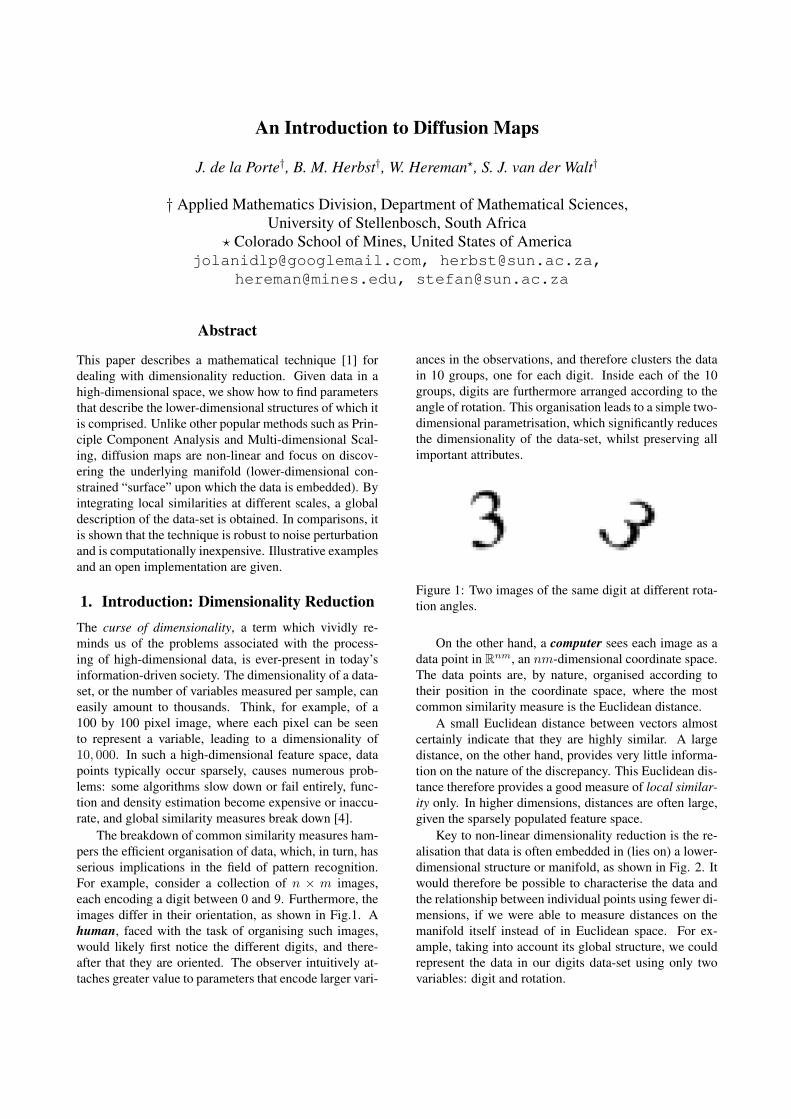
The breakdown of common similarity measures ham-pers the efficient organisation of data, which, in turn, hasserious implications in the field of pattern recognition.For example, consider a collection of n × m images,each encoding a digit between 0 and 9. Furthermore, theimages differ in their orientation, as shown in Fig.1. Ahuman, faced with the task of organising such images,would likely first notice the different digits, and there-after that they are oriented. The observer intuitively at-taches greater value to parameters that encode larger vari-

ances in the observations, and therefore clusters the datain 10 groups, one for each digit. Inside each of the 10groups, digits are furthermore arranged according to theangle of rotation. This organisation leads to a simple two-dimensional parametrisation, which significantly reducesthe dimensionality of the data-set, whilst preserving allimportant attributes.

Figure 1: Two images of the same digit at different rota-tion angles.

On the other hand, a computer sees each image as adata point in Rnm, an nm-dimensional coordinate space.The data points are, by nature, organised according totheir position in the coordinate space, where the mostcommon similarity measure is the Euclidean distance.

A small Euclidean distance between vectors almostcertainly indicate that they are highly similar. A largedistance, on the other hand, provides very little informa-tion on the nature of the discrepancy. This Euclidean dis-tance therefore provides a good measure of local similar-ity only. In higher dimensions, distances are often large,given the sparsely populated feature space.

Key to non-linear dimensionality reduction is the re-alisation that data is often embedded in (lies on) a lower-dimensional structure or manifold, as shown in Fig. 2. Itwould therefore be possible to characterise the data andthe relationship between individual points using fewer di-mensions, if we were able to measure distances on themanifold itself instead of in Euclidean space. For ex-ample, taking into account its global structure, we couldrepresent the data in our digits data-set using only twovariables: digit and rotation.

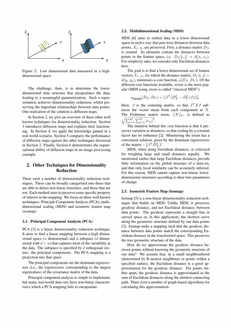
Figure 2: Low dimensional data measured in a high-dimensional space.

The challenge, then, is to determine the lower-dimensional data structure that encapsulates the data,leading to a meaningful parametrisation. Such a repre-sentation achieves dimensionality reduction, whilst pre-serving the important relationships between data points.One realisation of the solution is diffusion maps.

In Section 2, we give an overview of three other wellknown techniques for dimensionality reduction. Section3 introduces diffusion maps and explains their function-ing. In Section 4, we apply the knowledge gained in areal world scenario. Section 5 compares the performanceof diffusion maps against the other techniques discussedin Section 2. Finally, Section 6 demonstrates the organi-sational ability of diffusion maps in an image processingexample.

2. Other Techniques for DimensionalityReduction

There exist a number of dimensionality reduction tech-niques. These can be broadly categorised into those thatare able to detect non-linear structures, and those that arenot. Each method aims to preserve some specific propertyof interest in the mapping. We focus on three well knowntechniques: Principle Component Analysis (PCA), multi-dimensional scaling (MDS) and isometric feature map(isomap).

2.1. Principal Component Analysis (PCA)

PCA [3] is a linear dimensionality reduction technique.It aims to find a linear mapping between a high dimen-sional space (n dimensional) and a subspace (d dimen-sional with d < n) that captures most of the variability inthe data. The subspace is specified by d orthogonal vec-tors: the principal components. The PCA mapping is aprojection into that space.

The principal components are the dominant eigenvec-tors (i.e., the eigenvectors corresponding to the largesteigenvalues) of the covariance matrix of the data.

Principal component analysis is simple to implement,but many real-world data-sets have non-linear character-istics which a PCA mapping fails to encapsulate.

2.2. Multidimensional Scaling (MDS)

MDS [6] aims to embed data in a lower dimensionalspace in such a way that pair-wise distances between datapoints, X1..N , are preserved. First, a distance matrix DX

is created. Its elements contain the distances betweenpoints in the feature space, i.e. DX [i, j] = d(xi, xj).For simplicity sake, we consider only Euclidean distanceshere.

The goal is to find a lower-dimensional set of featurevectors, Y1..N , for which the distance matrix, DY [i, j] =d(yi, yj), minimises a cost function, ρ(DX , DY ). Of thedifferent cost functions available, strain is the most pop-ular (MDS using strain is called “classical MDS”):

ρstrain(DX , DY ) = ||JT (D2X −D2

Y )J)||2F .

Here, J is the centering matrix, so that JTXJ sub-tracts the vector mean from each component in X .The Frobenius matrix norm, ||X||F , is defined as√∑M

i=1

∑Nj=1 |xij |

2.The intuition behind this cost function is that it pre-

serves variation in distances, so that scaling by a constantfactor has no influence [2]. Minimising the strain has aconvenient solution, given by the dominant eigenvectorsof the matrix − 1

2JTD2

XJ .MDS, when using Euclidean distances, is criticised

for weighing large and small distances equally. Wementioned earlier that large Euclidean distances providelittle information on the global structure of a data-set,and that only local similarity can be accurately inferred.For this reason, MDS cannot capture non-linear, lower-dimensional structures according to their true parametersof change.

2.3. Isometric Feature Map (Isomap)

Isomap [5] is a non-linear dimensionality reduction tech-nique that builds on MDS. Unlike MDS, it preservesgeodesic distance, and not Euclidean distance, betweendata points. The geodesic represents a straight line incurved space or, in this application, the shortest curvealong the geometric structure defined by our data points[2]. Isomap seeks a mapping such that the geodesic dis-tance between data points match the corresponding Eu-clidean distance in the transformed space. This preservesthe true geometric structure of the data.

How do we approximate the geodesic distance be-tween points without knowing the geometric structure ofour data? We assume that, in a small neighbourhood(determined by K-nearest neighbours or points within aspecified radius), the Euclidean distance is a good ap-proximation for the geodesic distance. For points fur-ther apart, the geodesic distance is approximated as thesum of Euclidean distances along the shortest connectingpath. There exist a number of graph-based algorithms forcalculating this approximation.

Once the geodesic distance has been obtained, MDSis performed as explained above.

A weakness of the isomap algorithm is that the ap-proximation of the geodesic distance is not robust to noiseperturbation.

3. Diffusion maps

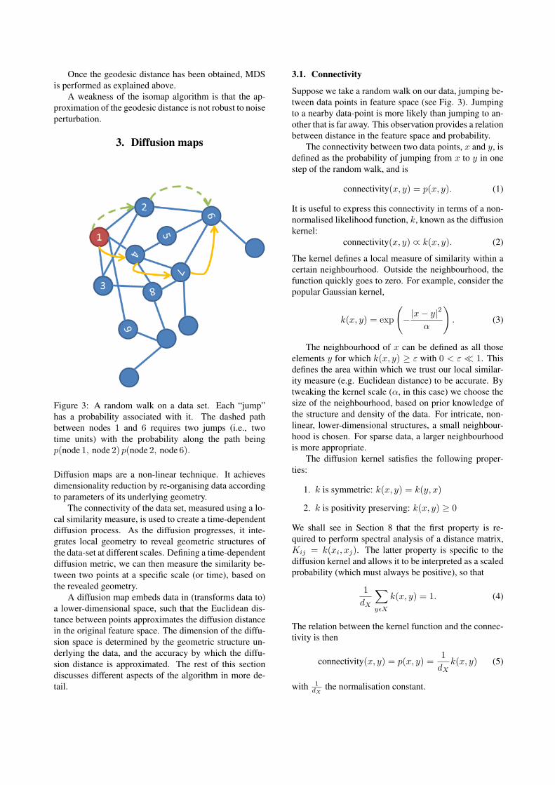
Figure 3: A random walk on a data set. Each “jump”has a probability associated with it. The dashed pathbetween nodes 1 and 6 requires two jumps (i.e., twotime units) with the probability along the path beingp(node 1, node 2) p(node 2, node 6).

Diffusion maps are a non-linear technique. It achievesdimensionality reduction by re-organising data accordingto parameters of its underlying geometry.

The connectivity of the data set, measured using a lo-cal similarity measure, is used to create a time-dependentdiffusion process. As the diffusion progresses, it inte-grates local geometry to reveal geometric structures ofthe data-set at different scales. Defining a time-dependentdiffusion metric, we can then measure the similarity be-tween two points at a specific scale (or time), based onthe revealed geometry.

A diffusion map embeds data in (transforms data to)a lower-dimensional space, such that the Euclidean dis-tance between points approximates the diffusion distancein the original feature space. The dimension of the diffu-sion space is determined by the geometric structure un-derlying the data, and the accuracy by which the diffu-sion distance is approximated. The rest of this sectiondiscusses different aspects of the algorithm in more de-tail.

3.1. Connectivity

Suppose we take a random walk on our data, jumping be-tween data points in feature space (see Fig. 3). Jumpingto a nearby data-point is more likely than jumping to an-other that is far away. This observation provides a relationbetween distance in the feature space and probability.

The connectivity between two data points, x and y, isdefined as the probability of jumping from x to y in onestep of the random walk, and is

connectivity(x, y) = p(x, y). (1)

It is useful to express this connectivity in terms of a non-normalised likelihood function, k, known as the diffusionkernel:

connectivity(x, y) ∝ k(x, y). (2)

The kernel defines a local measure of similarity within acertain neighbourhood. Outside the neighbourhood, thefunction quickly goes to zero. For example, consider thepopular Gaussian kernel,

k(x, y) = exp

(−|x− y|

2

α

). (3)

The neighbourhood of x can be defined as all thoseelements y for which k(x, y) ≥ ε with 0 < ε � 1. Thisdefines the area within which we trust our local similar-ity measure (e.g. Euclidean distance) to be accurate. Bytweaking the kernel scale (α, in this case) we choose thesize of the neighbourhood, based on prior knowledge ofthe structure and density of the data. For intricate, non-linear, lower-dimensional structures, a small neighbour-hood is chosen. For sparse data, a larger neighbourhoodis more appropriate.

The diffusion kernel satisfies the following proper-ties:

1. k is symmetric: k(x, y) = k(y, x)

2. k is positivity preserving: k(x, y) ≥ 0

We shall see in Section 8 that the first property is re-quired to perform spectral analysis of a distance matrix,Kij = k(xi, xj). The latter property is specific to thediffusion kernel and allows it to be interpreted as a scaledprobability (which must always be positive), so that

1dX

∑yεX

k(x, y) = 1. (4)

The relation between the kernel function and the connec-tivity is then

connectivity(x, y) = p(x, y) =1dX

k(x, y) (5)

with 1dX

the normalisation constant.

Define a row-normalised diffusion matrix, P , withentries Pij = p(Xi, Xj). Each entry provides the con-nectivity between two data points,Xi andXj , and encap-sulates what is known locally. By analogy of a randomwalk, this matrix provides the probabilities for a singlestep taken from i to j. By taking powers of the diffusionmatrix1, we can increase the number of steps taken. Forexample, take a 2× 2 diffusion matrix,

P =[p11 p12

p21 p22

].

Each element, Pi,j , is the probability of jumping betweendata points i and j. When P is squared, it becomes

P 2 =[p11p11 + p12p21 p12p22 + p11p12

p21p12 + p22p21 p22p22 + p21p12

].

Note that P11 = p11p11 + p12p21, which sums two prob-abilities: that of staying at point 1, and of moving frompoint 1 to point 2 and back. When making two jumps,these are all the paths from point i to point j. Similarly,P tij sum all paths of length t from point i to point j.

3.2. Diffusion Process

As we calculate the probabilities P t for increasing valuesof t, we observe the data-set at different scales. This is thediffusion process2, where we see the local connectivityintegrated to provide the global connectivity of a data-set.

With increased values of t (i.e. as the diffusion pro-cess “runs forward”), the probability of following a pathalong the underlying geometric structure of the data setincreases. This happens because, along the geometricstructure, points are dense and therefore highly connected(the connectivity is a function of the Euclidean distancebetween two points, as discussed in Section 2). Pathwaysform along short, high probability jumps. On the otherhand, paths that do not follow this structure include oneor more long, low probability jumps, which lowers thepath’s overall probability.

In Fig. 4, the red path becomes a viable alternativeto the green path as the number of steps increases. Sinceit consists of short jumps, it has a high probability. Thegreen path keeps the same, low probability, regardless ofthe value of t .

1The diffusion matrix can be interpreted as the transition matrix ofan ergodic Markov chain defined on the data [1]

2In theory, a random walk is a discrete-time stochastic process,while a diffusion process considered to be a continuous-time stochasticprocess. However, here we study discrete processes only, and considerrandom walks and diffusion processes equivalent.

Figure 4: Paths along the true geometric structure of thedata set have high probability.

3.3. Diffusion Distance

The previous section showed how a diffusion process re-veals the global geometric structure of a data set. Next,we define a diffusion metric based on this structure. Themetric measures the similarity of two points in the obser-vation space as the connectivity (probability of “jump-ing”) between them. It is related to the diffusion matrixP , and is given by

Dt(Xi, Xj)2 =∑uεX

|pt(Xi, u)− pt(Xj , u)|2 (6)

=∑

k

∣∣P tik − P tkj∣∣2 . (7)

The diffusion distance is small if there are many highprobability paths of length t between two points. Unlikeisomap’s approximation of the geodesic distance, the dif-fusion metric is robust to noise perturbation, as it sumsover all possible paths of length t between points.

As the diffusion process runs forward, revealing thegeometric structure of the data, the main contributors tothe diffusion distance are paths along that structure.

Consider the term pt(x, u) in the diffusion distance.This is the probability of jumping from x to u (for anyu in the data set) in t time units, and sums the probabil-ities of all possible paths of length t between x and u.As explained in the previous section, this term has largevalues for paths along the underlying geometric structureof the data. In order for the diffusion distance to remainsmall, the path probabilities between x, u and u, y mustbe roughly equal. This happens when x and y are bothwell connected via u.

The diffusion metric manages to capture the similar-ity of two points in terms of the true parameters of changein the underlying geometric structure of the specific dataset.

3.4. Diffusion Map

Low-dimensional data is often embedded in higher di-mensional spaces. The data lies on some geometric struc-ture or manifold, which may be non-linear (see Fig. 2).In the previous section, we found a metric, the diffusiondistance, that is capable of approximating distances alongthis structure. Calculating diffusion distances is computa-tionally expensive. It is therefore convenient to map data

points into a Euclidean space according to the diffusionmetric. The diffusion distance in data space simply be-comes the Euclidean distance in this new diffusion space.

A diffusion map, which maps coordinates betweendata and diffusion space, aims to re-organise data accord-ing to the diffusion metric. We exploit it for reducingdimensionality.

The diffusion map preserves a data set’s intrinsic ge-ometry, and since the mapping measures distances on alower-dimensional structure, we expect to find that fewercoordinates are needed to represent data points in the newspace. The question becomes which dimensions to ne-glect, in order to preserve diffusion distances (and there-fore geometry) optimally.

With this in mind, we examine the mapping

Yi :=

pt(Xi, X1)pt(Xi, X2)

...pt(Xi, XN )

= PTi∗. (8)

For this map, the Euclidean distance between twomapped points, Yi and Yj , is

‖Yi − Yj‖2E =∑uεX

|pt(Xi, u)− pt(Xj , u)|2

=∑

k

∣∣P tik − P tkj∣∣2 = Dt(Xi, Yj),2

which is the diffusion distance between data pointsXi and Xj . This provides the re-organisation we soughtaccording to diffusion distance. Note that no dimension-ality reduction has been achieved yet, and the dimensionof the mapped data is still the sample size, N .

Dimensionality reduction is done by neglecting cer-tain dimensions in the diffusion space. Which dimen-sions are of less importance? The proof in Section 8 pro-vides the key. Take the normalised diffusion matrix,

P = D−1K,

where D is the diagonal matrix consisting of the row-sums of K. The diffusion distances in (8) can be ex-pressed in terms of the eigenvectors and -values of P as

Y ′i =

λt1ψ1(i)λt2ψ2(i)

...λtnψn(i)

, (9)

where ψ1(i) indicates the i-th element of the first eigen-vector of P . Again, the Euclidean distance betweenmapped points Y ′i and Y ′j is the diffusion distance. Theset of orthogonal left eigenvectors of P form a basis forthe diffusion space, and the associated eigenvalues λl in-dicate the importance of each dimension. Dimension-ality reduction is achieved by retaining the m dimen-sions associated with the dominant eigenvectors, which

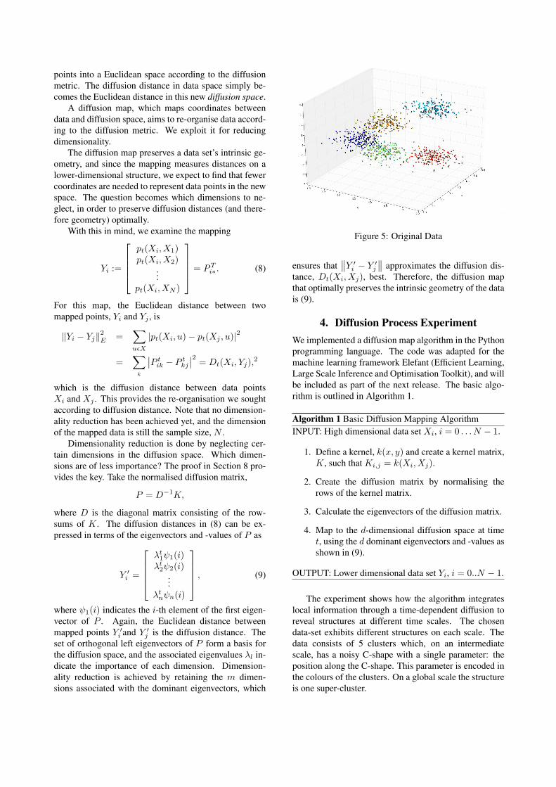
Figure 5: Original Data

ensures that∥∥Y ′i − Y ′j ∥∥ approximates the diffusion dis-

tance, Dt(Xi, Xj), best. Therefore, the diffusion mapthat optimally preserves the intrinsic geometry of the datais (9).

4. Diffusion Process ExperimentWe implemented a diffusion map algorithm in the Pythonprogramming language. The code was adapted for themachine learning framework Elefant (Efficient Learning,Large Scale Inference and Optimisation Toolkit), and willbe included as part of the next release. The basic algo-rithm is outlined in Algorithm 1.

Algorithm 1 Basic Diffusion Mapping AlgorithmINPUT: High dimensional data set Xi, i = 0 . . . N − 1.

1. Define a kernel, k(x, y) and create a kernel matrix,K, such that Ki,j = k(Xi, Xj).

2. Create the diffusion matrix by normalising therows of the kernel matrix.

3. Calculate the eigenvectors of the diffusion matrix.

4. Map to the d-dimensional diffusion space at timet, using the d dominant eigenvectors and -values asshown in (9).

OUTPUT: Lower dimensional data set Yi, i = 0..N − 1.

The experiment shows how the algorithm integrateslocal information through a time-dependent diffusion toreveal structures at different time scales. The chosendata-set exhibits different structures on each scale. Thedata consists of 5 clusters which, on an intermediatescale, has a noisy C-shape with a single parameter: theposition along the C-shape. This parameter is encoded inthe colours of the clusters. On a global scale the structureis one super-cluster.

As the diffusion time increases, we expect differentscales to be revealed. A one dimensional curve charac-terised by a single parameter should appear. This is theposition along the C-shape, the direction of maximumglobal variation in the data. The ordering of colours alongthe C-shape should be preserved.

4.1. Discussion

In these results, three different geometric structures arerevealed, as shown in figures (5) and (6):

At t = 1, the local geometry is visible as five clusters.The diffusion process is still restricted individual clusters,as the probability of jumping to another in one time-stepis small. Therefore, even with reduced dimensions, wecan clearly distinguish the five clusters in the diffusionspace.

At t = 3, clusters connect to form a single structure indiffusion space. Paths of length three bring them together.Being better connected, the diffusion distance betweenclusters decreases.

At this time scale, the one-dimensional parameter ofchange, the position along the C-shape, is recovered: inthe diffusion space the order of colours are preservedalong a straight line.

At t = 10, a third geometric structure is seen. Thefive clusters have merged to form a single super-cluster.At this time scale, all points in the observation space areequally well connected. The diffusion distances betweenpoints are very small. In the lower dimensional diffu-sion space it is approximated as zero, which projects thesuper-cluster to a single point.

This experiment shows how the algorithm uses theconnectivity of the data to reveal geometric structures atdifferent scales.

5. Comparison With Other Methods

We investigate the performance of those dimensionalityreduction algorithms discussed in Section 2, and comparethem to diffusion maps. We use a similar data set as inthe previous experiment, the only difference being an in-creased variance inside clusters. Which of the algorithmsdetect the position along the C-shape as a parameter ofchange, i.e. which of the methods best preserve the or-dering of the clusters in a one-dimensional feature space?Being linear techniques, we expect PCA and MDS to fail.In theory, isomap should detect the C-shape, although itis known that it struggles with noisy data.

5.1. Discussion

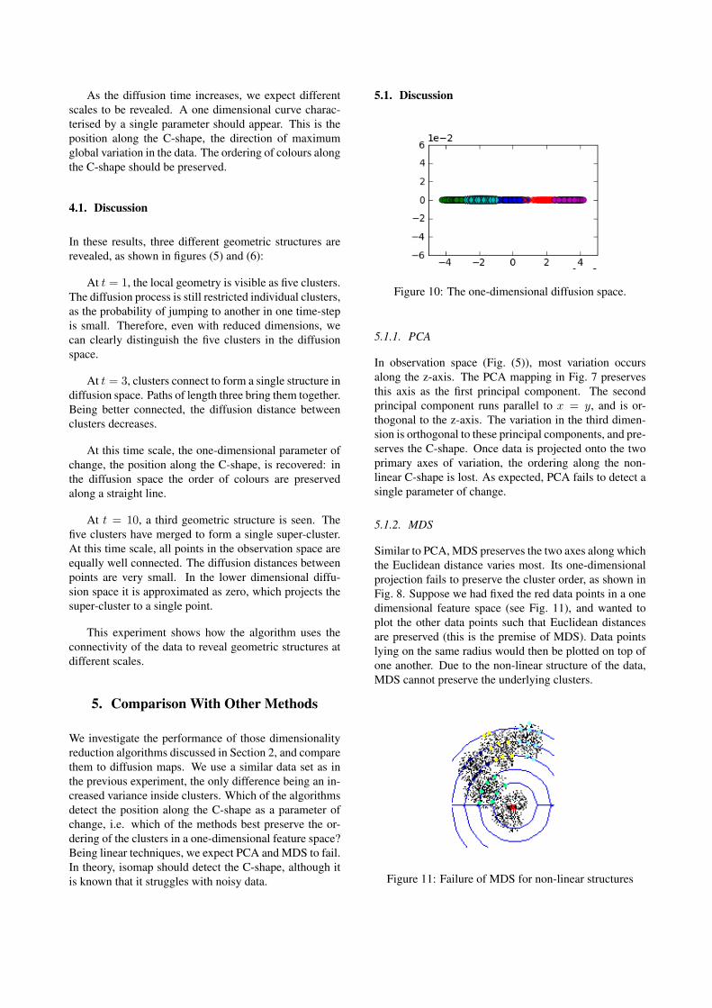
Figure 10: The one-dimensional diffusion space.

5.1.1. PCA

In observation space (Fig. (5)), most variation occursalong the z-axis. The PCA mapping in Fig. 7 preservesthis axis as the first principal component. The secondprincipal component runs parallel to x = y, and is or-thogonal to the z-axis. The variation in the third dimen-sion is orthogonal to these principal components, and pre-serves the C-shape. Once data is projected onto the twoprimary axes of variation, the ordering along the non-linear C-shape is lost. As expected, PCA fails to detect asingle parameter of change.

5.1.2. MDS

Similar to PCA, MDS preserves the two axes along whichthe Euclidean distance varies most. Its one-dimensionalprojection fails to preserve the cluster order, as shown inFig. 8. Suppose we had fixed the red data points in a onedimensional feature space (see Fig. 11), and wanted toplot the other data points such that Euclidean distancesare preserved (this is the premise of MDS). Data pointslying on the same radius would then be plotted on top ofone another. Due to the non-linear structure of the data,MDS cannot preserve the underlying clusters.

Figure 11: Failure of MDS for non-linear structures

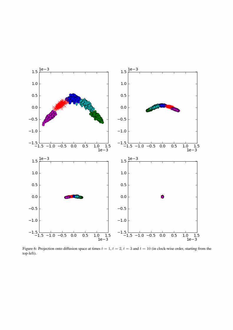
Figure 6: Projection onto diffusion space at times t = 1, t = 2, t = 3 and t = 10 (in clock-wise order, starting from thetop-left).

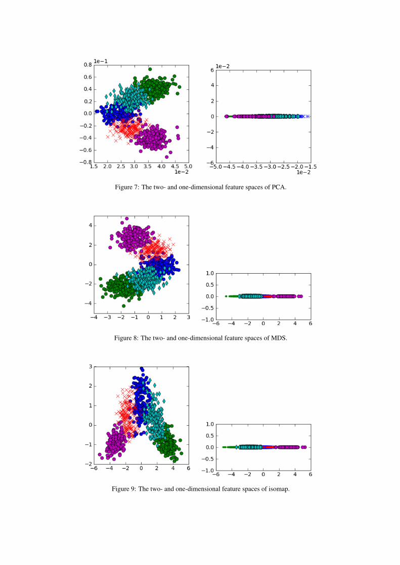
Figure 7: The two- and one-dimensional feature spaces of PCA.

Figure 8: The two- and one-dimensional feature spaces of MDS.

Figure 9: The two- and one-dimensional feature spaces of isomap.

5.1.3. Isomap

When determining geodesic distances, isomap searchesa certain neighbourhood. The choice of this neighbour-hood is critical: if too large, it allows for “short circuits”whereas, if it is too small, connectivity becomes verysparse. These “short circuits” can skew the geometry ofthe outcome entirely. For diffusion maps, a similar chal-lenge is faced when choosing kernel parameters.

Isomap is able to recover all the clusters in this ex-periment, given a very small neighbourhood. It even pre-serve the clusters in the correct order. Two of the clustersoverlap a great deal, due to the algorithm’s sensitivity tonoise.

5.1.4. Comparison with Diffusion Maps

Fig. 10 shows that a diffusion map is able to preserve theorder of clusters in one dimension. As mentioned before,choosing parameter(s) for the diffusion kernel remainsdifficult. Unlike isomap, however, the result is based ona summation over all data, which lessens sensitivity to-wards kernel parameters. Diffusion maps are the onlyone of these techniques that allows geometric analysis atdifferent scales.

6. Demonstration: Organisational Ability

A diffusion map organises data according to its under-lying parameters of change. In this experiment, we vi-sualise those parameters. Our data-set consists of ran-domly rotated versions of a 255 × 255 image template(see Fig. 12). Each rotated image represents a single,65025-dimensional data-point. The data is mapped to thediffusion space, and the dimensionality reduced to two.At each 2-dimensional coordinate, the original image isdisplayed.

Figure 12: Template: 255 x 255 pixels.

6.1. Discussion

Figure 13: Organisation of images in diffusion space.

In the diffusion space, the images are organised accord-ing to their angle of rotation (see Fig. 13). Images withsimilar rotations lie close to one another.

The dimensionality of the data-set has been reducedfrom 65025 to only two. As an example, imaging runninga K-means clustering algorithm in diffusion space. Thiswill not only be much faster than in data space, but wouldlikely achieve better results, not having to deal with amassive, sparse, high-dimensional data-set.

7. ConclusionWe investigated diffusion maps, a technique for non-linear dimensionality reduction. We showed how it inte-grates local connectivity to recover parameters of changeat different time scales. We compared it to three othertechniques, and found that the diffusion mapping is morerobust to noise perturbation, and is the only technique thatallows geometric analysis at differing scales. We further-more demonstrated the power of the algorithm by organ-ising images. Future work will revolve around applica-tions in clustering, noise-reduction and feature extraction.

8. ProofThis section discusses the mathematical foundation ofdiffusion maps. The diffusion distance, given in (7), isvery expensive to calculate but, as shown here, it can bewritten in terms of the eigenvectors and values of the dif-fusion matrix. These values can be calculated efficiently.

We set up a new diffusion space, where the coordi-nates are scaled components of the eigenvectors of thediffusion matrix. In the diffusion space, Euclidean dis-tances are equivalent to diffusion distances in data space.

Lemma 1: Suppose K is a symmetric, n × n kernelmatrix such that K[i, j] = k(i, j). A diagonal matrix, D,

normalises the rows of K to produce a diffusion matrix

P = D−1K. (10)

Then, the matrix P ′, defined as

P ′ = D1/2PD−1/2, (11)

1. is symmetric

2. has the same eigenvalues as P

3. the eigenvectors, x′k of P ′ are multiplied by D−1/2

and D12 to get the left (eTP = λeT ) and right

eigenvectors (P v = λv) of P respectively.

Proof: Substitute (10) into (11) to obtain

P ′ = D−1/2KD−1/2. (12)

As K is symmetric, P ′ will also be symmetric.We can make P the subject of the equation in (11),

P = D−1/2P ′D1/2. (13)

As P ′ is symmetric, there exists an orthonormal set ofeigenvectors of P ′ such that

P ′ = SΛST , (14)

where Λ is a diagonal matrix containing the eigenvaluesof P ′ and S is a matrix with the orthonormal eigenvectorsof P ′ as columns.

Substituting (14) into (13),

P = D−1/2SΛSTD1/2.

Since S is an orthogonal matrix

P = D−1/2SΛS−1D1/2

= (D−1/2S)Λ(D−1/2S)−1 (15)= QΛQ−1. (16)

Therefore, the eigenvalues of P ′ and P are the same. Fur-thermore, the right eigenvectors of P are the columns of

Q = D−1/2S, (17)

while the left eigenvectors are the rows of

Q−1 = STD12 . (18)

From (17) we see that the equation for the eigenvectorsof P can be given in terms of the eigenvectors x′k of P ′.The right eigenvectors of P are

vk = D−12 x′k (19)

and the left eigenvectors are

ek = D12 x′k. (20)

From (15) we then obtain the eigen decomposition,

P =∑k

λkvkeTk . (21)

When we examine this eigen decomposition further, wesee something interesting. Eq. 21 expresses each row ofthe diffusion matrix in terms of a new basis: ek, the lefteigenvectors of the diffusion matrix.

In this new coordinate system in Rn, a row i of P isrepresented by the point

Mi =

λ1v1[i]λ2v2[i]

...λnvn[i]

,where vn[i] is the i-th component of the n-th right eigen-vector. However, P is not symmetric, and so the coordi-nate system will not be orthonormal, i.e.

eTk ek 6= 1

or, equivalently,eTk I ek 6= 1

andeTl I ek 6= 0 for l 6= k.

This is a result of the scaling applied to the orthogonaleigenvectors of P ′ in (19) and (20). This scaling can becounter-acted by using a different metric Q, such that

eTkQek = 1

andeTl Q ek = 0 for l 6= k

where Q must be a positive definite, symmetric matrix.We choose

Q = D−1,

where D is the diagonal normalisation matrix. It satisfiesthe two requirements for a metric and leads to

eTkQ ek = eTk (D−12 )T (D−

12 ) ek

= x′Tk x′k= 1,

using (20). In the same way we can show that

eTl D−1ek = 0 for l 6= k.

Therefore the left eigenvectors of the diffusion matrixform an orthonormal coordinate system of Rn , given thatthe metric is D−1. We define Rn with metric D−1 as the

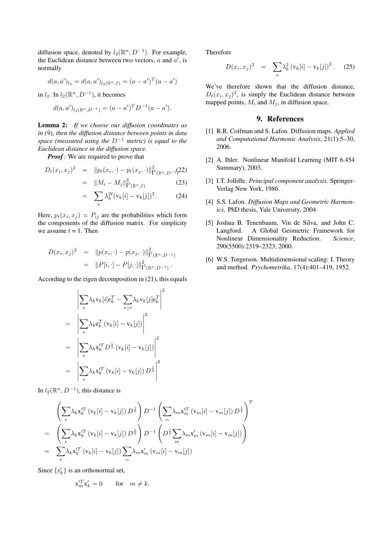
diffusion space, denoted by l2(Rn, D−1). For example,the Euclidean distance between two vectors, a and a′, isnormally

d(a, a′)l2 = d(a, a′)l2(Rn,I) = (a− a′)T (a− a′)

in l2. In l2(Rn, D−1), it becomes

d(a, a′)l2(Rn,D−1) = (a− a′)TD−1(a− a′).

Lemma 2: If we choose our diffusion coordinates asin (9), then the diffusion distance between points in dataspace (measured using the D−1 metric) is equal to theEuclidean distance in the diffusion space.

Proof : We are required to prove that

Dt(xi, xj)2 = ‖pt(xi, ·)− pt(xj , ·)‖2l2(Rn,D−1)(22)

= ‖Mi −Mj‖2l2(Rn,I)(23)

=∑

k

λ2tk (vk[i]− vk[j])2. (24)

Here, pt(xi, xj) = Pij are the probabilities which formthe components of the diffusion matrix. For simplicitywe assume t = 1. Then

D(xi, xj)2 = ‖p(xi, ·)− p(xj , ·)‖2l2(Rn,D−1)

= ‖P [i, ·]− P [j, ·]‖2l2(Rn,D−1).

According to the eigen decomposition in (21), this equals∣∣∣∣∣∑k

λkvk[i]eTk −∑k≥0

λkvk[j]eTk

∣∣∣∣∣2

=

∣∣∣∣∣∑k

λkeTk (vk[i]− vk[j])

∣∣∣∣∣2

=

∣∣∣∣∣∑k

λkx′Tk D12 (vk[i]− vk[j])

∣∣∣∣∣2

=

∣∣∣∣∣∑k

λkx′Tk (vk[i]− vk[j])D12

∣∣∣∣∣2

In l2(Rn, D−1), this distance is(∑k

λkx′Tk (vk[i]− vk[j])D12

)D−1

(∑m

λmx′Tm (vm[i]− vm[j])D12

)T

=

(∑k

λkx′Tk (vk[i]− vk[j])D12

)D−1

(D

12

∑m

λmx′m (vm[i]− vm[j])

)=

∑k

λkx′Tk (vk[i]− vk[j])∑

m

λmx′m (vm[i]− vm[j])

Since {x′k} is an orthonormal set,

x′Tm x′k = 0 for m 6= k.

Therefore

D(xi, xj)2 =∑

k

λ2k (vk[i]− vk[j])2 . (25)

We’ve therefore shown that the diffusion distance,Dt(xi, xj)2, is simply the Euclidean distance betweenmapped points, Mi and Mj , in diffusion space.

9. References[1] R.R. Coifman and S. Lafon. Diffusion maps. Applied

and Computational Harmonic Analysis, 21(1):5–30,2006.

[2] A. Ihler. Nonlinear Manifold Learning (MIT 6.454Summary), 2003.

[3] I.T. Jolliffe. Principal component analysis. Springer-Verlag New York, 1986.

[4] S.S. Lafon. Diffusion Maps and Geometric Harmon-ics. PhD thesis, Yale University, 2004.

[5] Joshua B. Tenenbaum, Vin de Silva, and John C.Langford. A Global Geometric Framework forNonlinear Dimensionality Reduction. Science,290(5500):2319–2323, 2000.

[6] W.S. Torgerson. Multidimensional scaling: I. Theoryand method. Psychometrika, 17(4):401–419, 1952.