Diffusion maps for changing dataI

Ronald R. Coifman, Matthew J. Hirn∗

Yale UniversityDepartment of Mathematics

P.O. Box 208283New Haven, Connecticut 06520-8283

USA

Abstract

Graph Laplacians and related nonlinear mappings into low dimensional spaces have been shownto be powerful tools for organizing high dimensional data. Here we consider a data set X inwhich the graph associated with it changes depending on some set of parameters. We analyzethis type of data in terms of the diffusion distance and the corresponding diffusion map. As thedata changes over the parameter space, the low dimensional embedding changes as well. We givea way to go between these embeddings, and furthermore, map them all into a common space,allowing one to track the evolution of X in its intrinsic geometry. A global diffusion distanceis also defined, which gives a measure of the global behavior of the data over the parameterspace. Approximation theorems in terms of randomly sampled data are presented, as are potentialapplications.

Keywords: diffusion distance; graph Laplacian; manifold learning; dynamic graphs;dimensionality reduction; kernel method; spectral graph theory

1. Introduction

In this paper we consider a changing graph depending on certain parameters, such as time,over a fixed set of data points. Given a set of parameters of interest, our goal is to organize thedata in such a way that we can perform meaningful comparisons between data points derivedfrom different parameters. In some scenarios, a direct comparison may be possible; on the otherhand, the methods we develop are more general and can handle situations in which the changes tothe data prevent direct comparisons across the parameter space. For example, one may considersituations in which the mechanism or sensor measuring the data changes, perhaps changing theobserved dimension of the data. In order to make meaningful comparisons between differentrealizations of the data, we look for invariants in the data as it changes. We model the data set asa normalized, weighted graph, and measure the similarity between two points based on how the

IApplied and Computational Harmonic Analysis, volume 36, issue 1, pages 79-107, January 2014. arXiv:1209.0245.∗Corresponding authorEmail addresses: coifman@math.yale.edu (Ronald R. Coifman), matthew.hirn@ens.fr (Matthew J. Hirn)URL: www.di.ens.f/∼hirn/ (Matthew J. Hirn)

Preprint submitted to Applied and Computational Harmonic Analysis January 21, 2014

local subgraph around each point changes over the parameter space. The framework we developwill allow for the comparison of any two points derived from any two parameters within thegraph, thus allowing one to organize not only along the data points but the parameter space aswell.

An example of this type of data comes from hyperspectral image analysis. A hyperspectralimage is in fact a set of images of the same scene that are taken at different wavelengths. Puttogether, these images form a data cube in which the length and width of the cube correspondto spatial dimensions, and the height of the cube corresponds to the different wavelengths. Thuseach pixel is in fact a vector corresponding to the spectral signature of the materials containedin that pixel. Consider the situation in which we are given two hyperspectral images of thesame scene, and we wish to highlight the anomalous (e.g., man made) changes between the two.Assume though, that for each data set, different cameras were used which measured differentwavelengths, perhaps also at different times of day under different weather conditions. In sucha scenario a direct comparison of the spectral signatures between different days becomes muchmore difficult. Current work in the field often times goes under the heading change detection, asthe goal is to often find small changes in a large scene; see [1] for more details.

Other possible areas for applications come from the modeling of social networks as graphs.The relationships between people change over time and determining how groups of people inter-act and evolve is a new and interesting problem that has usefulness in marketing and other areas.Financial markets are yet another area that lends itself to analysis conducted over time, as arecertain evolutionary biological questions and even medical problems in which patient tests areupdated over the course of their lives.

The tools developed in this paper are inspired by high dimensional data analysis, in whichone assumes that the data has a hidden, low dimensional structure (for example, the data lieson a low dimensional manifold). The goal is to construct a mapping that parameterizes this lowdimensional structure, revealing the intrinsic geometry of the data. We are interested in highdimensional data the evolves over some set of paramaters, for example time. We are particularlyinterested in the case in which one does not have a given metric by which to compare the dataacross time, but can only compare data points from the same time instance. The hyperspectraldata situation described above is one such example of this scenario; due to the differing sensormeasurements at different times, a direct comparison of images is impossible.

Let I denote our parameter space, and let Xα, with α ∈ I, be the data in question. Theelements of our data set are fixed, but the graph changes depending on the parameter α. In otherwords, there is a known bijection between Xα and Xβ for α, β ∈ I, but the corresponding graphweights of X have changed between the two parameters. For a fixed α, the diffusion maps frame-work developed in [2] gives a multiscale way of organizing Xα. If Xα has a low dimensionalstructure, then the diffusion map will take Xα into a low dimensional Euclidean space that char-acterizes its geometry. More specifically, the diffusion mapping maps Xα into a particular `2

space in which the usual `2 distance corresponds to the diffusion distance on Xα; in the case ofa low dimensional data set, the `2 space can be “truncated” to Rd, with the standard Euclideandistance. However, for different parameters α and β, the diffusion map may take Xα and Xβ

into different `2 spaces, thus meaning that one cannot take the standard `2 distance between theelements of these two spaces. Our contribution here is to generalize the diffusion maps frame-work so that it works independently of the parameter α. In particular, we derive formulas forthe distance between points in different embeddings that are in terms of the individual diffusionmaps of each space. It is even possible to define a mapping from one embedding to the other,so that after applying this mapping the standard `2 distance can once again be used to compute

2

diffusion distances. In particular, this additional mapping gives a common parameterization ofthe data across all of I that characterizes the evolving intrinsic geometry of the data. Once thisgeneralized framework has been established, we are able to define a global distance between allof Xα and Xβ based on the behavior of the diffusions within each data set. This distance in turnallows one to model the global behavior of Xα as it changes over I.

Earlier results that use diffusion maps to compare two data sets can be found in [3]. Fur-thermore, there is recent work contained in [4] that also involves combining diffusion geometryprinciples via tree structures with evolving graphs. In [5], the author considers the case of anevolving Riemannian manifold on which a diffusion process is spreading as the manifold evolves.In our work, we separate out the two processes, effectively using the diffusion process to orga-nize the evolution of the data. Also tangentially related to this work are the results containedin [6] on shape analysis, in which shapes are compared via their heat kernels. More generally,this paper fits into the larger class of research that utilizes nonlinear mappings into low dimen-sional spaces in order to organize potentially high dimensional data; examples include locallylinear embedding (LLE) [7], ISOMAP [8], Hessian LLE [9], Laplacian eigenmaps [10], and theaforementioned diffusion maps [2].

An outline of this paper goes as follows: in the next section, we take care of some notationand review the diffusion mapping first presented in [2]. In Section 3 we generalize the diffusiondistance for a data set that changes over some parameter space, and show that it can be computedin terms the spectral embeddings of the corresponding diffusion operators. We also show howto map each of the embeddings into one common embedding in which the `2 distance is equalto the diffusion distance. The global diffusion distance between graphs is defined in Section 4;it is also seen to be able to be computed in terms of the eigenvalues and eigenfunctions of therelevant diffusion operators. In Section 5 we set up and state two random sampling theorems, onefor the diffusion distance and one for the global diffusion distance. The proofs of these theoremsare given in Appendix B. Section 6 contains some applications, and we conclude with someremarks and possible future directions in Section 7.

2. Notation and preliminaries

In this section we introduce some basic notation and review certain preliminary results thatwill motivate our work.

2.1. NotationLet R denote the real numbers and let N , 1, 2, 3, . . . be the natural numbers. Often we

will use constants that depend on certain variables or parameters. We let C(·), C1(·), C2(·), etc,denote these constants; note that they can change from line to line.

We recall some basic notation from operator theory. LetH be a real, separable Hilbert spacewith scalar product 〈·, ·〉 and norm ‖ · ‖. Let A : H → H be a bounded, linear operator, and letA∗ be its adjoint. The operator norm of A is defined as:

‖A‖ , sup‖ f ‖=1‖A f ‖.

A bounded operator A is Hilbert-Schmidt if∑i≥1

‖Ae(i)‖2 < ∞

3

for some (and hence any) Hilbert basis e(i)i≥1. The space of Hilbert-Schmidt operators is also aHilbert space with scalar product

〈A, B〉HS ,∑i≥1

〈Ae(i), Be(i)〉.

We denote the corresponding norm as ‖ · ‖HS . Note that if an operator is Hilbert-Schmidt, then itis compact. A Hilbert-Schmidt operator is trace class if∑

i≥1

〈√

A∗Ae(i), e(i)〉 < ∞

for some (and hence any) Hilbert basis e(i)i≥1. For any trace class operator A, we have

Tr(A) ,∑i≥1

〈Ae(i), e(i)〉 < ∞,

where Tr(A) is called the trace of A. The space of trace class operators is a Banach space endowedwith the norm

‖A‖TC , Tr(√

A∗A).

Note that the different operator norms are related as follows:

‖A‖ ≤ ‖A‖HS ≤ ‖A‖TC .

For more information on trace class operators, Hilbert Schmidt operators and related topics, werefer the reader to [11].

2.2. Diffusion maps

In this section we consider just a single data set that does not change and review the notion ofdiffusion maps on this data set. We assume that we are given a measure space (X, µ), consistingof data points X that are distributed according to µ. We also have a positive, symmetric kernelk : X × X → R that encodes how similar two data points are. From X and k, one can construct aweighted graph Γ , (X, k), in which the vertices of Γ are the data points x ∈ X, and the weightof the edge xy is given by k(x, y).

The diffusion maps framework developed in [2] gives a multiscale organization of the dataset X. Additionally, if X ⊂ Rd is high dimensional, yet lies on a low dimensional manifold, thediffusion map gives an embedding into Euclidean space that parameterizes the data in terms ofits intrinsic low dimensional geometry. The idea is that the kernel k should only measure localsimilarities within X at small scales, so as to be able to “follow” the low dimensional structure.The diffusion map then pieces together the local similarities via a random walk on Γ.

Define the density, m : X → R, as

m(x) ,∫X

k(x, y) dµ(y), for all x ∈ X. (1)

We assume that the density m satisfies

m(x) > 0, for µ a.e. x ∈ X, (2)4

andm ∈ L1(X, µ). (3)

Given (2), the weight function

p(x, y) ,k(x, y)m(x)

is well defined for µ ⊗ µ almost every (x, y) ∈ X × X. Although p is no longer symmetric, it doessatisfy the following useful property:∫

X

p(x, y) dµ(y) = 1, for µ a.e. x ∈ X.

Therefore we can view p as the transition kernel of a Markov chain on X. Equivalently, ifp ∈ L2(X × X, µ ⊗ µ), the integral operator P : L2(X, µ)→ L2(X, µ), defined as

(P f )(x) ,∫X

p(x, y) f (y) dµ(y), for all f ∈ L2(X, µ),

is a diffusion operator. In particular, the value p(x, y) represents the probability of transition inone time step from the vertex x to the vertex y, which is proportional to the edge weight k(x, y).For t ∈ N, let p(t)(x, y) represent the probability of transition in t time steps from the node x tothe node y; note that p(t) is the kernel of the operator Pt. As shown in [2], running the Markovchain forward, or equivalently taking powers of P, reveals relevant geometric structures of X atdifferent scales. In particular, small powers of P will segment the data set into several smallerclusters. As t is increased and the Markov chain diffuses across the graph Γ, the clusters evolveand merge together until in the limit as t → ∞ the data set is grouped into one cluster (assumingthe graph is connected).

The phenomenon described above can be encapsulated by the diffusion distance at time tbetween two vertices x and y in the graph Γ. In order to define the diffusion distance, we firstnote that the Markov chain constructed above has the stationary distribution π : X → R, where

π(x) =m(x)∫

X m(y) dµ(y).

Combining (2) and (3) we see that π(x) is well defined for µ a.e. x ∈ X. The diffusion distancebetween x, y ∈ X is then defined as:

D(t)(x, y)2 ,∥∥∥p(t)(x, ·) − p(t)(y, ·)

∥∥∥2L2(X,dµ/π)

=

∫X

(p(t)(x, u) − p(t)(y, u)

)2 dµ(u)π(u)

.

A simplified formula for the diffusion distance can be found by considering the spectral decom-position of P. Define the kernel a : X × X → R as

a(x, y) ,√

m(x)√m(y)

p(x, y) =k(x, y)

√m(x)

√m(y)

, for µ ⊗ µ a.e. (x, y) ∈ X × X.

5

If a ∈ L2(X × X, µ ⊗ µ), then P has a discrete set of eigenfunctions υ(i)i≥1 with correspondingeigenvalues λ(i)i≥1. It can then be shown that

D(t)(x, y)2 =∑i≥1

(λ(i)

)2t (υ(i)(x) − υ(i)(y)

)2. (4)

Inspired by (4), [2] defines the diffusion map Υ(t) : X → `2 at diffusion time t to be:

Υ(t)(x) ,((λ(i)

)tυ(i)(x)

)i≥1.

Therefore, the diffusion distance at time t between x, y ∈ X is equal to the `2 norm of the differ-ence between Υ(t)(x) and Υ(t)(y):

D(t)(x, y) =∥∥∥Υ(t)(x) − Υ(t)(y)

∥∥∥`2 .

One can also define a second diffusion distance in terms of the symmetric kernel a as opposedto the asymmetric kernel p. In particular, define the operator A : L2(X, µ)→ L2(X, µ) as

(A f )(x) ,∫X

a(x, y) f (y) dµ(y), for all f ∈ L2(X, µ).

Like the diffusion operator P, the operator A and its powers, At, reveal the relevant geometricstructures of the data set X. Letting a(t) : X ×X → R denote the kernel of the operator At, we candefine another diffusion distance D(t) : X × X → R as follows:

D(t)(x, y)2 ,∥∥∥a(t)(x, ·) − a(t)(y, ·)

∥∥∥2L2(X,µ)

=

∫X

(a(t)(x, u) − a(t)(y, u)

)2dµ(u).

As before, we consider the spectral decomposition of A. Let λ(i)i≥1 and ψ(i)i≥1 denote theeigenvalues and eigenfunctions of A (indeed, the nonzero eigenvalues of P and A are the same),and define the diffusion map Ψ(t) : X → `2 (corresponding to A) as

Ψ(t)(x) =

((λ(i)

)tψ(i)(x)

)i≥1.

Then, under the same assumptions as before, we have

D(t)(x, y)2 =∥∥∥Ψ(t)(x) − Ψ(t)(y)

∥∥∥2`2 =

∑i≥1

(λ(i)

)t (ψ(i)(x) − ψ(i)(y)

)2. (5)

We make a few remarks concerning the differences between the two formulations. First, wenote that the original diffusion distance D(t) is defined as an L2 distance under the weighted mea-sure dµ/π. The second diffusion distance, D(t), due to the symmetric normalization built into thekernel a, is defined only in terms of the underlying measure µ. Furthermore, the eigenfunctionsof A are orthogonal, unlike the eigenfunctions of P. Finally, as we have already noted, the eigen-values of P and A are in fact the same, and furthermore they are contained in (−1, 1]. If the graphΓ is connected, then the eigenfunction of P with eigenvalue one is simply the function that maps

6

every element of X to one. The corresponding eigenfunction of A though is the square root of thedensity, i.e.,

√m(x). Thus, while both versions of the diffusion distance merge smaller clusters

into large clusters as t grows, D(t) will merge every data point into the same cluster in the limitas t → ∞, while D(t) will reflect the behavior of the density m in the limit as t → ∞.

Finally, recalling the discussion at the beginning of this section and regardless of the par-ticular operator used (P or A), if X has a low dimensional structure to it, then the number ofsignificant eigenvalues will be small. In this case, from (5) it is clear that one can in fact map Xinto a low dimensional Euclidean space via the dominant eigenfunctions while nearly preservingthe diffusion distance.

3. Generalizing the diffusion distance for changing data

In this section we generalize the diffusion maps framework for data sets with input parame-ters.

3.1. The data modelWe now turn our attention to the original problem introduced at the beginning of this paper.

In its most general form, we are given a parameter space I and a data set Xα that depends onα ∈ I. The data points of Xα are given by xα. The parameter space I can be continuous, discrete,or completely arbitrary. Recall from the introduction that we are working under the assumptionthat there is an a priori known bijective correspondence between Xα and Xβ for any α, β ∈ I (inAppendix A we discuss relaxing this assumption).

We consider the following model throughout the remainder of this paper. We are given asingle measure space (X, µ) that we think of as changing over I. The changes in X are encodedby a family of metrics dα : X × X → R, so that for each α ∈ I we have a metric measurespace Xα = (X, µ, dα). The measure µ here represents some underlying distribution of the pointsin X that does not change over I. There is no a priori assumption of a universal metric d :(X × I) × (X × I) → R that can be used to discern the distance between points taken from Xα

and Xβ for arbitrary α, β ∈ I, α , β.

Remark 3.1. If such a universal metric does exist, then one could still use the techniques devel-oped in this paper, by defining the metrics dα in terms of the restriction of the universal metric dto the parameter α. Alternatively, the original diffusion maps machinery could be used by defin-ing a kernel k : (X × I) × (X × I) → R in terms of the universal metric d. Further discussionalong these lines is given in Section 3.5.

3.2. Defining the diffusion distance on a family of graphsOur goal is to reveal the relevant geometric structures of X across the entire parameter space

I, and to furthermore have a way of comparing structures from one parameter to other structuresderived from a second parameter. To do so, we shall generalize the diffusion distance so thatwe can compare diffusions derived from different parameters. For each instance of the dataXα = (X, µ, dα), we derive a kernel kα : X × X → R. The first step is to once again consider eachpairing X and kα as a weighted graph, which we denote as Γα , (X, kα).

Updating our notation for this dynamic setting, for each parameter α ∈ I we have the densitymα : X → R defined as

mα(x) ,∫X

kα(x, y) dµ(y), for all α ∈ I, x ∈ X.

7

For reasons that shall become clear later, we slightly strengthen the assumptions on mα as com-pared to those in equations (2) and (3). In particular, we assume that

mα(x) > 0, for all α ∈ I, x ∈ X,

andmα ∈ L1(X, µ), for all α ∈ I.

We then define two classes of kernels aα : X × X → R and pα : X × X → R in the same manneras earlier:

aα(x, y) ,kα(x, y)

√mα(x)

√mα(y)

, for all α ∈ I, (x, y) ∈ X × X, (6)

andpα(x, y) ,

kα(x, y)mα(x)

, for all α ∈ I, (x, y) ∈ X × X.

Assume that aα, pα ∈ L2(X × X, µ ⊗ µ). Their corresponding integral operators are given byAα : L2(X, µ)→ L2(X, µ) and Pα : L2(X, µ)→ L2(X, µ), where

(Aα f )(x) ,∫X

aα(x, y) f (y) dµ(y), for all α ∈ I, f ∈ L2(X, µ), (7)

and(Pα f )(x) ,

∫X

pα(x, y) f (y) dµ(y), for all α ∈ I, f ∈ L2(X, µ).

Finally, we let a(t)α and p(t)

α denote the kernels of the integral operators Atα and Pt

α, respectively.Returning to the task at hand, in order to compare Γα with Γβ, it is possible to use the operators

Aα and Aβ or Pα and Pβ. We choose to perform our analysis using the symmetric operators, asit shall simplify certain things. For now, consider the function aα(x, ·) for a fixed x ∈ X. Wethink of this function in the following way. Consider the graph Γα, and imagine dropping a unitof mass on the node x and allowing it to spread, or diffuse, throughout Γα. After one unit oftime, the amount of mass that has spread from x to some other node y is proportional to aα(x, y).Similarly, if we want to let the mass spread throughout the graph for a longer period of time, wecan, and the amount of mass that has spread from x to y after t units of time is then proportionalto a(t)

α (x, y). The diffusion distance at time t, which is the L2 norm of a(t)α (x, ·) − a(t)

α (y, ·), is thencomparing the behavior of the diffusion centered at x with the behavior of the diffusion centeredat y. We wish to extend this idea for different parameters α and β. In other words, we wish tohave a meaningful distance between x at parameter α and y at parameter β that is based on thesame principle of measuring how their respective diffusions behave.

Our solution is to generalize the diffusion distance in the following way. For each diffusiontime t ∈ N, we define a dynamic diffusion distance D(t) : (X × I) × (X × I)→ R as follows. Letxα , (x, α) ∈ X × I, and set

D(t)(xα, yβ)2 ,∥∥∥∥a(t)

α (x, ·) − a(t)β (y, ·)

∥∥∥∥2

L2(X,µ)

=

∫X

(a(t)α (x, u) − a(t)

β (y, u))2

dµ(u).

8

This notion of distance can be thought of as comparing how the neighborhood of xα differs fromthe neighborhood of yβ. In particular, if we are comparing the same data point but at differentparameters, for example xα and xβ, the diffusion distance between them will be small if theirneighborhoods do not change much from α to β. On the other hand, if say a large change occursat x at parameter β, then the neighborhood of xβ should differ from the neighborhood of xα andso they will have a large diffusion distance between them.

Some more intuition about the quantity D(t)(xα, yβ) can be derived from the triangle inequal-ity. In particular, one application of it gives

D(t)(xα, yβ) ≤ D(t)(xα, xβ) + D(t)(xβ, yβ).

Thus we see that D(t)(xα, yβ) is bounded from above by the change in x from α to β (i.e. thequantity D(t)(xα, xβ)) plus the diffusion distance between x and y in the graph Γβ (i.e. the quantityD(t)(xβ, yβ)).

Remark 3.2. As noted earlier, we have chosen to generalize the diffusion distance in terms ofthe symmetric kernels aα as opposed to the asymmetric kernels pα. The primary reason forthis choice is that when using the kernel pα to compute the diffusion distance between x andy, we must use the weighted measure dµ/πα, where πα denotes the stationary distribution ofthe Markov chain on Γα. Thus, when computing the diffusion distance between xα and yβ, onemust incorporate this weighted measure as well. Since the stationary distribution will invariablychange from α to β, the most natural generalization in this case would be:

D(t)(xα, yβ)2 ,∫X

p(t)α (x, u)√πα(u)

−p(t)β (y, u)√πβ(u)

2

dµ(u).

Alternatively, in [12], we describe how to construct a bi-stochastic kernel b : X × X → Rfrom a more general affinity function. The kernel is bi-stochastic under a particular weightedmeasure Ω2µ, where Ω : X → R is derived from the affinity function. In this case, one can defineyet another alternate diffusion distance as:

D(t)(xα, yβ)2 ,∫X

(b(t)α (x, u) Ωα(u) − b(t)

β (y, u) Ωβ(u))2

dµ(u).

In either case, the results that follow can be translated for these particular diffusion distancesby following the same arguments and making minor modifications where necessary.

3.3. Diffusion maps for G = Γαα∈I

Analogous to the diffusion distance for a single graph Γ = (X, k), we can write the diffusiondistance for G , Γαα∈I in terms the spectral decompositions of Aαα∈I. We first collect thefollowing mild, but necessary, assumptions, some of which have already been stated.

Assumption 1. We assume the following properties:

1. (X, µ) is a σ-finite measure space and L2(X, µ) is separable.2. The kernel kα is positive definite and symmetric for all α ∈ I.3. For each α ∈ I, mα ∈ L1(X, µ) and mα > 0.

9

4. For any α ∈ I, the operator Aα is trace class.

A few remarks concerning the assumed properties. First, the reader may have noticed thatwe replaced the assumption that kα be positive with the stronger assumption that it is positivedefinite. This combined with the third property that mα(x) > 0 for all x ∈ X, implies that aα isalso positive definite. Thus the operators Aα are positive and self adjoint.

If one wished to revert back to the weaker assumption that kα merely be positive, then thefollowing adjustment could be made. Clearly the symmetrically normalized kernel aα will stillbe positive, but the operator Aα may not be. However, one could replace Aα, for each α ∈ I, withthe graph Laplacian Lα : L2(X, µ)→ L2(X, µ), which is defined as

Lα ,12

(I − Aα),

where I : L2(X, µ) → L2(X, µ) is the identity operator. The graph Laplacian Lα is a positiveoperator with eigenvalues contained in [0, 1]. The analysis that follows would still apply withonly minor adjustments.

The fourth item that Aα be trace class plays a key role in the results of this section, anditself implies that these operators are Hilbert-Schmidt and so also compact. Thus, as a furtherconsequence, aα ∈ L2(X × X, µ ⊗ µ) for each α ∈ I. Ideally, one would replace the fourth itemwith a condition on the kernel kα that implies that Aα is trace class. Unfortunately, unlike the caseof Hilbert Schmidt operators, there is not a simple theorem of this nature. Further informationon trace class integral operators, as well as various results, can be found in [11, 13, 14].

We note that assumptions three and four are both satisfied if for each α ∈ I the kernel kα iscontinuous, bounded from above and below, and if the measure of X is finite. That is, if for eachα,

0 < C1(α) ≤ kα(x, y) ≤ C2(α) < ∞, for all (x, y) ∈ X × X,

andµ(X) < ∞,

then we can derive assumptions three and four.As an immediate consequence of the properties contained in Assumption 1, we see from the

Spectral Theorem that for each α the operator Aα has a countable collection of positive eigen-values and orthonormal eigenfunctions that form a basis for L2(X, µ). Let λ(i)

α i≥1 and ψ(i)α i≥1 be

the eigenvalues and a set of orthonormal eigenfunctions of Aα, respectively, so that

(Aαψ(i)α )(x) = λ(i)

α ψ(i)α (x), for µ a.e. x ∈ X,

and〈ψ(i)

α , ψ( j)α 〉L2(X,µ) = δ(i − j), for all i, j ≥ 1.

Furthermore, as noted in [2], the eigenvalues of Pα are bounded in absolute value by one, withat least one eigenvalue equaling one. Since the eigenvalues of Aα and Pα are the same, we alsohave

1 = λ(1)α ≥ λ

(2)α ≥ λ

(3)α ≥ . . . ,

where λ(i)α → 0 as i→ ∞.

As with the original diffusion distance defined on a single data set, our generalized notionof the diffusion distance for dynamic data sets has a simplified form in terms of the spectraldecompositions of the relevant operators.

10

Theorem 3.3. Let (X, µ) be a measure space and kαα∈I a family of kernels defined on X. If(X, µ) and kαα∈I satisfy the properties of Assumption 1, then the diffusion distance at time tbetween xα and yβ can be written as:

D(t)(xα, yβ)2 =∑i≥1

(λ(i)α

)2tψ(i)α (x)2 +

∑j≥1

(λ

( j)β

)2tψ

( j)β (y)2

− 2∑i, j≥1

(λ(i)α

)t (λ

( j)β

)tψ(i)α (x)ψ( j)

β (y) 〈ψ(i)α , ψ

( j)β 〉L2(X,µ), (8)

where for each pair (α, β) ∈ I×I, equation (8) converges in L2(X×X, µ⊗µ). If, additionally, kαis continuous for each α ∈ I, X ⊆ Rd is closed, and µ is a strictly positive Borel measure, then(8) holds for all (x, y) ∈ X × X.

Notice that equation (8) is in fact an extension of the formula given for the diffusion distanceon a single data set. Indeed, if one were to take xα and yβ = yα, the formula given in (8) wouldsimplify to (5) with the underlying kernel taken to be kα. Thus, it is natural to define the diffusionmap Ψ

(t)α : X → `2 for the parameter α and diffusion time t as

Ψ(t)α (x) ,

((λ(i)α

)tψ(i)α (x)

)i≥1. (9)

For v ∈ `2, let v[i] denote the ith element of the sequence u. Using (9), one can write equation (8)as

D(t)(xα, yβ)2 =∥∥∥Ψ(t)

α (x)∥∥∥2`2 +

∥∥∥Ψ(t)β (y)

∥∥∥2`2 − 2

∑i, j≥1

Ψ(t)α (x)[i] Ψ

(t)β (y)[ j] 〈ψ(i)

α , ψ( j)β 〉L2(X,µ). (10)

In particular, one has in general that

D(t)(xα, yβ) ,∥∥∥∥Ψ(t)

α (x) − Ψ(t)β (y)

∥∥∥∥`2.

Intuitively, the thing to take away from this discussion is that for each parameter α ∈ I, thediffusion map Ψ

(t)α maps X into an `2 space that itself also depends on α. The `2 embedding

corresponding to α is not the same as the `2 embedding corresponding to β ∈ I, but equation(10) gives a way of computing distances between the different `2 embeddings.

Also, once again paralleling the original diffusion distance, we see that if the eigenvaluesof Aα and Aβ decay sufficiently fast, then the diffusion distance can be well approximated by asmall, finite number of eigenvalues and eigenfunctions of these two operators. In particular, weneed only map Γα and Γβ into finite dimensional Euclidean spaces.

Proof of Theorem 3.3. We first use the fact that for each α ∈ I, Aα is a positive, self-adjoint,trace class operator. Thus Aα is Hilbert-Schmidt, and so we know that for each α ∈ I (see, forexample, Theorem 2.11 from [11]),

a(t)α (x, y) =

∑i≥1

(λ(i)α

)tψ(i)α (x)ψ(i)

α (y), with convergence in L2(X × X, µ ⊗ µ). (11)

If the additional assumptions hold that kα is continuous, X is a closed subset of Rd, and µ is astrictly positive Borel measure, then by Mercer’s Theorem (see [15, 16]) equation (11) will hold

11

for all (x, y) ∈ X × X. In this case the proof can be easily amended to get the stronger result; weomit the details.

Expand the formula for D(t)(xα, yβ) as follows:

D(t)(xα, yβ)2 =

∫X

(a(t)α (x, u)2 − 2a(t)

α (x, u) a(t)β (y, u) + a(t)

β (y, u)2)

dµ(u). (12)

We shall evaluate each of the three terms in (12) separately. For the cross term we have,∫X

a(t)α (x, u) a(t)

β (y, u) dµ(u) =

∫X

∑i, j≥1

(λ(i)α

)t (λ

( j)β

)tψ(i)α (x)ψ( j)

β (y)ψ(i)α (u)ψ( j)

β (u)

dµ(u), (13)

with convergence in L2(X × X, µ ⊗ µ). At this point we would like to switch the integral and thesummation in line (13); this can be done by applying Fubini’s Theorem, which requires one toshow the following:∑

i, j≥1

∫X

∣∣∣∣(λ(i)α

)t (λ

( j)β

)tψ(i)α (x)ψ( j)

β (y)ψ(i)α (u)ψ( j)

β (u)∣∣∣∣ dµ(u) < ∞. (14)

One can prove (14) for µ ⊗ µ almost every (x, y) ∈ X × X through the use of Holder’s Theoremand the fact that we assumed that Aα is a trace class operator for each α ∈ I; we leave the detailsto the reader. Thus for µ ⊗ µ almost every (x, y) ∈ X × X we can switch the integral and thesummation in line (13), which gives:∫

X

a(t)α (x, u) a(t)

β (y, u) dµ(u) =∑i, j≥1

(λ(i)α

)t (λ

( j)β

)tψ(i)α (x)ψ( j)

β (y) 〈ψ(i)α , ψ

( j)β 〉L2(X,µ), (15)

again with convergence in L2(X × X, µ ⊗ µ). A similar calculation shows that, for each α ∈ I,∫X

a(t)α (x, u)2 dµ(u) =

∑i≥1

(λ(i)α

)2tψ(i)α (x)2, with convergence in L2(X, µ). (16)

Combining equations (15) and (16) we arrive at the desired formula for D(t)(xα, yβ).

Remark 3.4. One interesting aspect of the diffusion distance is its asymptotic behavior as t → ∞,and in particular that behavior when each graph Γα ∈ G is a connected graph. In this case, eachoperator Aα has precisely one eigenvalue equal to one, and the corresponding eigenfunction isthe square root of the density (normalized), i.e.,

1 = λ(1)α > λ(2)

α ≥ λ(3)α ≥ . . . , and ψ(1)

α =√

mα

/ ∥∥∥√mα

∥∥∥L2(X,µ) .

To compute limt→∞ D(t)(xα, yβ), we utilize equation (8) from Theorem 3.3 and pull the limitas t → ∞ inside the summations. We justify the interchange of the limit and the sum by utilizingthe Dominated Convergence Theorem. In particular, treat each sum as an integral over N with thecounting measure. Let us focus on the double summation in (8); the other two single summationsfollow from similar arguments. For the double summation, we have a sequence of functions

ft(i, j) ,(λ(i)α

)t (λ

( j)β

)tψ(i)α (x)ψ( j)

β (y) 〈ψ(i)α , ψ

( j)β 〉L2(X,µ).

12

We dominate the sequence ftt≥1 with the function g(i, j) as follows:

| ft(i, j)| ≤ g(i, j) ,∣∣∣∣λ(i)α λ

( j)β ψ

(i)α (x)ψ( j)

β (y)∣∣∣∣ .

We claim that g is integrable over N × N with the counting measure. To see this, first note:

∑i, j≥1

g(i, j) =

∑i≥1

∣∣∣λ(i)α ψ

(i)α (x)

∣∣∣∑

j≥1

∣∣∣∣λ( j)β ψ

( j)β (y)

∣∣∣∣ .Now define the function hα : X → R as:

hα(x) ,∑i≥1

∣∣∣λ(i)α ψ

(i)α (x)

∣∣∣ .Using Tonelli’s Theorem, Holder’s Theorem, and the fact that Aα is trace class, one can showthat hα ∈ L2(X, µ). Thus, hα(x) < ∞ for µ almost every x ∈ X. In particular, for µ ⊗ µ almostevery (x, y) ∈ X × X, the function g(i, j) is integrable. To conclude, the Dominated ConvergenceTheorem holds, and for µ ⊗ µ almost every (x, y) ∈ X × X, we can interchange the summationsand the limit as t → ∞.

From here, it is quite simple to show:

limt→∞

D(t)(xα, yβ)2 =(ψ(1)α (x) − ψ(1)

β (y))2

+ ψ(1)α (x)ψ(2)

β (y)∥∥∥∥ψ(1)

α − ψ(1)β

∥∥∥∥2

L2(X,µ). (17)

Recalling that the first eigenfunctions are simply the normalized densities, we see that the asymp-totic diffusion distance can be computed without diagonalizing any of the diffusion operators.Furthermore, it is not just the pointwise difference between the densities, but rather the asymp-totic diffusion distance is the pointwise difference plus a term that takes into account the globaldifference between the two densities. It can be used as a fast way of determing significant changesfrom α to β; see Section 6.1 for an example.

3.4. Mapping one diffusion embedding into anotherAs mentioned in the previous subsection, the diffusion map Ψ

(t)α takes X into an `2 space

that itself depends on α. While (10) gives a way of computing distances between two diffusionembeddings, it is also possible to map the embedding Ψ

(t)β (X) into the `2 space of Ψ

(t)α (X). Fur-

thermore, the operator that does so is quite simple. The eigenfunctions ψ(i)α i≥1 are essentially a

basis for the embedding of X with parameter α, while the eigenfunctions ψ(i)β i≥1 are essentially

a basis for the embedding of X with parameter β. The operator that maps one space into the otheris similar to the change of basis operator. Define Oβ→α : `2 → `2 as

Oβ→αv ,

∑j≥1

v[ j] 〈ψ(i)α , ψ

( j)β 〉L2(X,µ)

i≥1

, for all v ∈ `2.

By the Spectral Theorem, we know that the eigenfunctions of Aα can be taken to form anorthonormal basis for L2(X, µ). Thus, the operator Oα→β preserves inner products. Indeed, definethe operator S α : L2(X, µ)→ `2 as

S α f ,(〈ψ(i)

α , f 〉L2(X,µ)

)i≥1, for all f ∈ L2(X, µ).

13

The adjoint of S α, S ∗α : `2 → L2(X, µ), is then given by

S ∗αv =∑i≥1

v[i]ψ(i)α , for all v ∈ `2.

Since ψ(i)α i≥1 is an orthonormal basis for L2(X, µ), S ∗αS α = IL2(X,µ). Therefore, for any v,w ∈ `2,

〈Oβ→αv,Oβ→αw〉`2 =∑j,k≥1

v[ j] w[k]

∑i≥1

〈ψ(i)α , ψ

( j)β 〉L2(X,µ)〈ψ

(i)α , ψ

(k)β 〉L2(X,µ)

=

∑j,k≥1

v[ j] w[k] 〈S αψ( j)β , S αψ

(k)β 〉`2

=∑j,k≥1

v[ j] w[k] δ( j − k)

= 〈v,w〉`2 (18)

As asserted, the operator Oβ→α preserves inner products. In particular, it preserves norms, so wehave∥∥∥Ψ(t)

α (x) − Oβ→αΨ(t)β (y)

∥∥∥2`2 =

∥∥∥Ψ(t)α (x)

∥∥∥2`2 +

∥∥∥Oβ→αΨ(t)β (y)

∥∥∥2`2 − 2〈Ψ(t)

α (x),Oβ→αΨ(t)β (y)〉`2

=∥∥∥Ψ(t)

α (x)∥∥∥2`2 +

∥∥∥Ψ(t)β (y)

∥∥∥2`2 − 2

∑i, j≥1

Ψ(t)α (x)[i] Ψ

(t)β (y)[ j] 〈ψ(i)

α , ψ( j)β 〉L2(X,µ)

= D(t)(xα, xβ).

Thus the operator Oβ→α maps the diffusion embedding Ψ(t)β (X) into the same `2 space as the

diffusion embedding Ψ(t)α (X), and furthermore preserves the diffusion distance between the two

spaces; it is easy to see that it also preserves the diffusion distance within Γβ. In particular, itis possible to view both embeddings in the same `2 space, where the `2 distance is equal to thediffusion distance both within each graph Γα and Γβ and between the two graphs.

Suppose now that we have three or more parameters in I that are of interest. Can we map alldiffusion embeddings of these parameters into the same `2 space, while preserving the diffusiondistances? The answer turns out to be “yes,” and in fact we can use the same mapping as before.Let γ ∈ I be the base parameter to which all other parameters are mapped, and let α, β ∈ Ibe two other arbitrary parameters. We know that we can map the embedding Ψ

(t)α (X) into the `2

space of Ψ(t)γ (X), and that we can also map the embedding Ψ

(t)β (X) into the `2 space of Ψ

(t)γ (X),

and that these mappings will preserve diffusion distances both within Γγ, Γα, and Γβ, and alsobetween Γγ and Γα as well as between Γγ and Γβ. We just need to show that they preserve thediffusion distance between points of Γα and points of Γβ. Using essentially the same calculationas the one used to derive (18), one can obtain the following for any v,w ∈ `2:

〈Oα→γv,Oβ→γw〉`2 =∑i, j≥1

v[i] w[ j] 〈ψ(i)α , ψ

( j)β 〉L2(X,µ).

But then we have:∥∥∥Oα→γΨ(t)α (x) − Oβ→γΨ

(t)β (y)

∥∥∥2`2 =

∥∥∥Oα→γΨ(t)α (x)

∥∥∥2`2 +

∥∥∥Oβ→γΨ(t)β (y)

∥∥∥2`2 − 2〈Oα→γΨ

(t)α (x),Oβ→γΨ

(t)β (y)〉`2 ,

=∥∥∥Ψ(t)

α (x)∥∥∥2`2 +

∥∥∥Ψ(t)β (y)

∥∥∥2`2 − 2

∑i, j≥1

Ψ(t)α (x)[i] Ψ

(t)β (y)[ j] 〈ψ(i)

α , ψ( j)β 〉L2(X,µ)

= D(t)(xα, yβ).14

Thus, after mapping the α and β embeddings appropriately into the γ embedding, the `2 distanceis equal to all possible diffusion distances. It is therefore possible to map each of the embeddingsΨ

(t)α (X)α∈I into the same `2 space. In particular, one can track the evolution of the intrinsic

geometry of X as it changes over I. We summarize this discussion in the following theorem.

Theorem 3.5. Let (X, µ) be a measure space and kαα∈I a family of kernels defined on X. Fixa parameter γ ∈ I. If (X, µ) and kαα∈I satisfy the properties of Assumption 1, then for all(α, β) ∈ I × I,

D(t)(xα, yβ) =∥∥∥∥Oα→γΨ

(t)α (x) − Oβ→γΨ

(t)β (y)

∥∥∥∥`2, with convergence in L2(X × X, µ ⊗ µ).

Remark 3.6. The choice of the fixed parameter γ ∈ I is important in the sense that the evolutionof the intrinsic geometry of X will be viewed through the lens of the important features (i.e., thedominant eigenfunctions) of X at parameter γ. In particular, when approximating the diffusiondistance by a small number of dominant eigenfunctions, one must be careful to select enougheigenfunctions at the γ parameter to sufficiently characterize the geometry of the data across allof I.

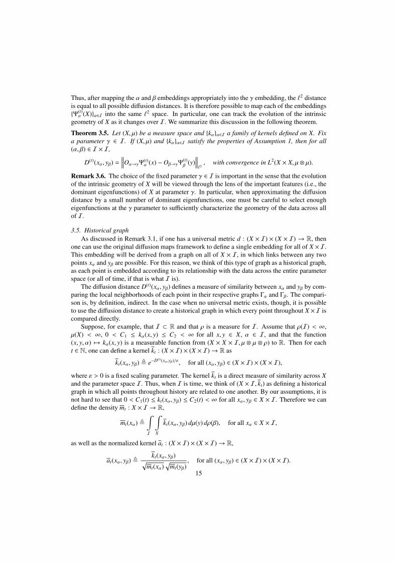
3.5. Historical graphAs discussed in Remark 3.1, if one has a universal metric d : (X × I) × (X × I) → R, then

one can use the original diffusion maps framework to define a single embedding for all of X ×I.This embedding will be derived from a graph on all of X × I, in which links between any twopoints xα and yβ are possible. For this reason, we think of this type of graph as a historical graph,as each point is embedded according to its relationship with the data across the entire parameterspace (or all of time, if that is what I is).

The diffusion distance D(t)(xα, yβ) defines a measure of similarity between xα and yβ by com-paring the local neighborhoods of each point in their respective graphs Γα and Γβ. The compari-son is, by definition, indirect. In the case when no universal metric exists, though, it is possibleto use the diffusion distance to create a historical graph in which every point throughout X ×I iscompared directly.

Suppose, for example, that I ⊂ R and that ρ is a measure for I. Assume that ρ(I) < ∞,µ(X) < ∞, 0 < C1 ≤ kα(x, y) ≤ C2 < ∞ for all x, y ∈ X, α ∈ I, and that the function(x, y, α) 7→ kα(x, y) is a measurable function from (X × X × I, µ ⊗ µ ⊗ ρ) to R. Then for eacht ∈ N, one can define a kernel kt : (X × I) × (X × I)→ R as

kt(xα, yβ) , e−D(t)(xα,yβ)/ε, for all (xα, yβ) ∈ (X × I) × (X × I),

where ε > 0 is a fixed scaling parameter. The kernel kt is a direct measure of similarity across Xand the parameter space I. Thus, when I is time, we think of (X × I, kt) as defining a historicalgraph in which all points throughout history are related to one another. By our assumptions, it isnot hard to see that 0 < C1(t) ≤ kt(xα, yβ) ≤ C2(t) < ∞ for all xα, yβ ∈ X × I. Therefore we candefine the density mt : X × I → R,

mt(xα) ,∫I

∫X

kt(xα, yβ) dµ(y) dρ(β), for all xα ∈ X × I,

as well as the normalized kernel at : (X × I) × (X × I)→ R,

at(xα, yβ) ,kt(xα, yβ)√

mt(xα)√

mt(yβ), for all (xα, yβ) ∈ (X × I) × (X × I).

15

Once again using the given assumptions, one can conclude that at ∈ L2(X×I×X×I, µ⊗ρ⊗µ⊗ρ).Thus it defines a Hilbert-Schmidt integral operator At : L2(X × I, µ ⊗ ρ)→ L2(X × I, µ ⊗ ρ),

(At f )(xα) ,∫I

∫X

at(xα, yβ) f (yβ) dµ(y) dρ(β), for all f ∈ L2(X × I, µ ⊗ ρ).

Let ψ(i)t i≥1 and λ

(i)t i≥1 denote the eigenfunctions and eigenvalues of At, respectively. The cor-

responding diffusion map Ψ(s)t : (X × I)→ `2 is given by:

Ψ(s)t (xα) ,

((λ

(i)t

)sψ

(i)t (xα)

)i≥1, for all xα ∈ X × I.

In the case when I is time, this diffusion map embeds the entire history of X across all of Iinto a single low dimensional space. Unlike the common embedding defined by Theorem 3.5,each point xα is embedded in relation to the entire history of X, not just its relationship to otherpoints yα from the same time. As such, for each x ∈ X, one can view the trajectory of x throughtime as it relates to all of history, i.e., one can view:

Tx : I → `2

Tx(α) , Ψ(s)t (xα).

In turn, the trajectories Txx∈X can be used to define a measure of similarity between the datapoints in X that takes into account the history of each point.

Remark 3.7. It is also possible to define kt in terms of the inner products of the symmetricdiffusion kernels, i.e.,

kt(xα, yβ) ,∫X

a(t)α (x, u) a(t)

β (y, u) dµ(u).

Remark 3.8. The diffusion distance and corresponding analysis contained in Section 3 can beextended to the more general case in which one has a sequence of data sets Xαα∈I for whichthere does not exist a bijective correspondence between each pair. If there is a sufficiently largeset S such that S ⊂ Xα for each α ∈ I, then one can compute a diffusion distance from anyxα ∈ Xα to any yβ ∈ Xβ through the common set S . See Appendix A for more details.

4. Global diffusion distance

Now that we have developed a diffusion distance between pairs of data points from (X ×I)×(X ×I), it is possible to define a global diffusion distance between Γα and Γβ. The aim here is todefine a diffusion distance that gives a global measure of the change in X from α to β. In turn,when applied over the whole parameter space, one can organize the global behavior of the dataas it changes over I. For each diffusion time t ∈ N, letD(t) : G×G → R be this global diffusiondistance, where

D(t)(Γα,Γβ)2 ,∥∥∥At

α − Atβ

∥∥∥2

HS

=∥∥∥∥a(t)

α − a(t)β

∥∥∥∥2

L2(X×X,µ⊗µ)

=

∫∫X×X

(a(t)α (x, y) − a(t)

β (x, y))2

dµ(x) dµ(y).

16

In fact, since µ is a σ-finite measure, the global diffusion distance can be written in terms ofthe pointwise diffusion distance by applying Tonelli’s Theorem:

D(t)(Γα,Γβ)2 =

∫X

D(t)(xα, xβ)2 dµ(x).

Thus the global diffusion distance measures the similarity between Γα and Γβ by comparing thebehavior of each of the corresponding diffusions on each of the graphs. Therefore, the globaldiffusion distance will be small if Γα and Γβ have similar geometry, and large if their geometry issignificantly different.

As with the pointwise diffusion distance D(t), the global diffusion distance can be written ina simplified form in terms of the spectral decompositions of the operators Aα and Aβ.

Theorem 4.1. Let (X, µ) be a measure space and kαα∈I a family of kernels defined on X. If(X, µ) and kαα∈I satisfy the properties of Assumption 1, then the global diffusion distance attime t between Γα and Γβ can be written as:

D(t)(Γα,Γβ)2 =∑i, j≥1

((λ(i)α

)t−

(λ

( j)β

)t)2〈ψ(i)

α , ψ( j)β 〉

2L2(X,µ). (19)

Equation (19) gives a new way to interpret the global diffusion graph distance. The orthonor-mal basis ψ(i)

α i≥1 is a set of diffusion coordinates for Γα, while the orthonormal basis ψ( j)β j≥1

is a set of diffusion coordinates for Γβ. Interpreting the summands of (19) in this context, wesee that the global diffusion distance measures the similarity of Γα and Γβ by taking a weightedrotation of one coordinate system into the other.

Proof of Theorem 4.1. Since

D(t)(Γα,Γβ)2 =

∫X

Dt(xα, xβ)2 dµ(x),

we can build upon Theorem 3.3. In particular, we have

D(t)(Γα,Γβ)2 =

∫X

∑i≥1

(λ(i)α

)2tψ(i)α (x)2 +

∑j≥1

(λ

( j)β

)2tψ

( j)β (x)2

−2∑i, j≥1

(λ(i)α

)t (λ

( j)β

)tψ(i)α (x)ψ( j)

β (x) 〈ψ(i)α , ψ

( j)β 〉L2(X,µ)

dµ(x).

As in the proof of Theorem 3.3 we have three terms that we shall evaluate separately. Focusingon the cross terms as before, we would like to switch the integral and the summation; this timewe need to show ∑

i, j≥1

∫X

∣∣∣∣(λ(i)α

)t (λ

( j)β

)tψ(i)α (x)ψ( j)

β (x) 〈ψ(i)α , ψ

( j)β 〉L2(X,µ)

∣∣∣∣ dµ(x) < ∞. (20)

One can show (20) by using Holder’s Theorem, the Cauchy-Schwarz inquality, and the assump-tion that Aα is a trace class operator for each α ∈ I. Therefore we can switch the integral and the

17

summation, which gives:∫X

∑i, j≥1

(λ(i)α

)t (λ

( j)β

)tψ(i)α (x)ψ( j)

β (x) 〈ψ(i)α , ψ

( j)β 〉L2(X,µ) dµ(x) =

∑i, j≥1

(λ(i)α

)t (λ

( j)β

)t〈ψ(i)

α , ψ( j)β 〉

2L2(X,µ). (21)

A similar calculation also shows that for each α ∈ I,∫X

∑i≥1

(λ(i)α

)2tψ(i)α (x)2 dµ(x) =

∑i≥1

(λ(i)α

)2t. (22)

Putting (21) and (22) together, we arrive at:

D(t)(Γα,Γβ)2 =∑i≥1

(λ(i)α

)2t+

∑j≥1

(λ

( j)β

)2t− 2

∑i, j≥1

(λ(i)α

)t (λ

( j)β

)t〈ψ(i)

α , ψ( j)β 〉

2L2(X,µ). (23)

Furthermore, recall that we have taken ψ(i)α i≥1 and ψ( j)

β j≥1 to be orthonormal bases for L2(X, µ).In particular, ∑

i≥1

〈ψ(i)α , ψ

( j0)β 〉

2 =∑j≥1

〈ψ(i0)α , ψ

( j)β 〉

2 = 1, for all i0, j0 ≥ 1.

Therefore we can simplify (23) to

D(t)(Γα,Γβ)2 =∑i, j≥1

((λ(i)α

)t−

(λ

( j)β

)t)2〈ψ(i)

α , ψ( j)β 〉

2L2(X,µ).

Remark 4.2. As with the pointwise diffusion distance, the asymptotic behavior of the globaldiffusion distance when G is a family of connected graphs is both interesting and easy to char-acterize. Under the same connectivity assumptions as Remark 3.4, one can use (23) to showthat

limt→∞D(t)(Γα,Γβ)2 = 2

(1 −

⟨ψ(1)α , ψ

(1)β

⟩2

L2(X,µ)

).

5. Random sampling theorems

In applications, the given data is finite and often times sampled from some continuous dataset X. In this section we examine the behavior of the pointwise and global diffusion distanceswhen applied to a randomly sampled, finite collection of samples taken from X.

5.1. Updated assumptions

In order to frame this discussion in the appropriate setting, we update our assumptions onthe measure space (X, µ) and the kernels kαα∈I. The results from this section will rely heavilyupon the work contained in [17, 18], and so we follow their lead. First, for any l ∈ N, let Cl

b(X)denote the set of continuous bounded functions on X such that all derivatives of order l exist andare themselves continuous, bounded functions.

Assumption 2. We assume the following properties:

18

1. The measure µ is a probability measure, so that µ(X) = 1.2. X is a bounded open subset of Rd that satisfies the cone condition (see page 93 of [19]).3. For each α ∈ I, the kernel kα is symmetric, positive definite, and bounded from above and

below, so that0 < C1(α) ≤ kα(x, y) ≤ C2(α) < ∞.

4. For each α ∈ I, kα ∈ Cd+1b (X × X).

Note that every property from Assumption 1 is either contained in or can be derived from theproperties in Assumption 2. Therefore the results of the previous sections still apply under thesenew assumptions.

The first assumption that µ be a probability measure is needed since we will be randomlysampling points from X. The probability measure from which we sample is µ. The secondand fourth assumptions are necessary to apply certain Sobolev embedding theorems which areintegral to constructing a reproducing kernel Hilbert space that contains the family of kernelsaαα∈I and their empirical equivalents. More details can be found in Appendix B.

5.2. Sampling and finite graphsConsider the space X and suppose that Xn , x(1), . . . , x(n) ⊂ X are sampled i.i.d. according

to µ. We are going to discretize the framework we have developed to accommodate the samplesXn. Let Γα,n , (Xn, kα|Xn ) be the finite graph with vertices Xn and weighted edges given by kα|Xn .We now define the finite, matrix equivalents to the continuous operators from Section 3.2. Tostart, first define for each α ∈ I the n × n matrices Kα as:

Kα[i, j] ,1n

kα(x(i), x( j)), for all i, j = 1, . . . , n.

We also define the corresponding diagonal degree matrices Dα as:

Dα[i, i] ,1n

n∑j=1

kα(x(i), x( j)) =

n∑j=1

Kα[i, j], for all i = 1, . . . , n.

Finally, the discrete analog of the operator Aα is given by the matrix Aα, which is defined as

Aα , D−12

α KαD− 1

2α , for all α ∈ I.

We can now define the pointwise and global diffusion distances for the finite graphs Gn ,Γα,nα∈I in terms of the matrices Aαα∈I. Set x(i)

α , (x(i), α) ∈ Xn × I, and let D(t)n : (Xn × I) ×

(Xn × I)→ R denote the empirical version of the pointwise diffusion distance. We define it as:

D(t)n (x(i)

α , x( j)β )2 , n2

∥∥∥Atα[i, ·] − At

β[ j, ·]∥∥∥2

Rn

= n2n∑

k=1

(Atα[i, k] − At

β[ j, k])2.

LetD(t)n : Gn × Gn → R denote the empirical global diffusion distance, where

D(t)n (Γα,n,Γβ,n)2 ,

∥∥∥Atα − At

β

∥∥∥HS

=

n∑i, j=1

(Atα[i, j] − At

β[i, j])2.

We then have the following two theorems relating D(t)n to D(t) andD(t)

n toD(t), respectively.19

Theorem 5.1. Suppose that (X, µ) and kαα∈I satisfy the conditions of Assumption 2. Let n ∈ Nand sample Xn = x(1), . . . , x(n) ⊂ X i.i.d. according to µ; also let t ∈ N, τ > 0, and α, β ∈ I.Then, with probability 1 − 2e−τ,∣∣∣∣D(t)(x(i)

α , x( j)β ) − D(t)

n (x(i)α , x

( j)β )

∣∣∣∣ ≤ C(α, β, d, t)√τ√

n, for all i, j = 1, . . . , n.

Theorem 5.2. Suppose that (X, µ) and kαα∈I satisfy the conditions of Assumption 2. Let n ∈ Nand sample Xn = x(1), . . . , x(n) ⊂ X i.i.d. according to µ; also let t ∈ N, τ > 0, and α, β ∈ I.Then, with probability 1 − 2e−τ,

∣∣∣D(t)(Γα,Γβ) −D(t)n (Γα,n,Γβ,n)

∣∣∣ ≤ C(α, β, d, t)√τ√

n.

6. Applications

6.1. Change detection in hyperspectral imagery data

In this section we consider the problem of change detection in hyperspectral imagery (HSI)data. Additionally, we use this particular experiment to illustrate two important properties of thediffusion distance. First, the representation of the data does not matter, even if it is changingacross the parameter space. Secondly, the diffusion distance is robust to noise.

The main ideas are the following. A hyperspectral image can be thought of as a data cube C,with dimensions L × W × D. The cube C corresponds to an image whose pixel dimensions areL×W. A hyperspectral camera measures the reflectance of this image at D different wavelengths,giving one D images, which, put together, give one the cube C. Thus we think of a hyperspectralimage as a regular image, but each pixel now has a spectral signature in RD.

The change detection problem is the following. Suppose you have one scene for which youhave several hyperspectral images taken at different times. These images can be taken underdifferent weather conditions, lighting conditions, during different seasons of the year, and evenwith different cameras. The goal is to determine what has changed from one image to the next.

To test the diffusion distance in this setting, we used some of the data collected in [1]. Usinga hyperspectral camera that captured 124 different wavelengths, the authors of [1] collected hy-perspectral images of a particular scene during August, September, October, and November (oneimage for each month). In October, they also recorded a fifth image in which they added twosmall tarp bundles so as to introduce small changes into the scene as a means for testing changedetection algorithms. For our purposes, we selected a particular 100×100×124 sub-cube acrossall five images that contains one of the aforementioned introduced changes. Color images of thefour months plus the additional fifth image containing the tarp are given in Figure 1. In all fiveimages one can see in the foreground grass and in the background a tree line, with a metal panelresting on the grass. In the additional fifth image, there is also a small tarp sitting on the grass.The images were obviously taken during different times of the year, ranging from Summer toFall, and it is also evident that the lighting is different from image to image. One can see thesechanges in how the spectral signature of a particular pixel changes from month to month; seeFigure 2(a) for an example of a grass pixel.

We set the parameter space as I = aug, sep, oct, nov, chg, where chg denotes the Octoberdata set with the tarp in it. We also set I(4) , aug, sep, oct, nov ⊂ I. For each α ∈ I, we letXα denote the corresponding 100 × 100 × 124 hyperspectral image. The data points x ∈ Xα are

20

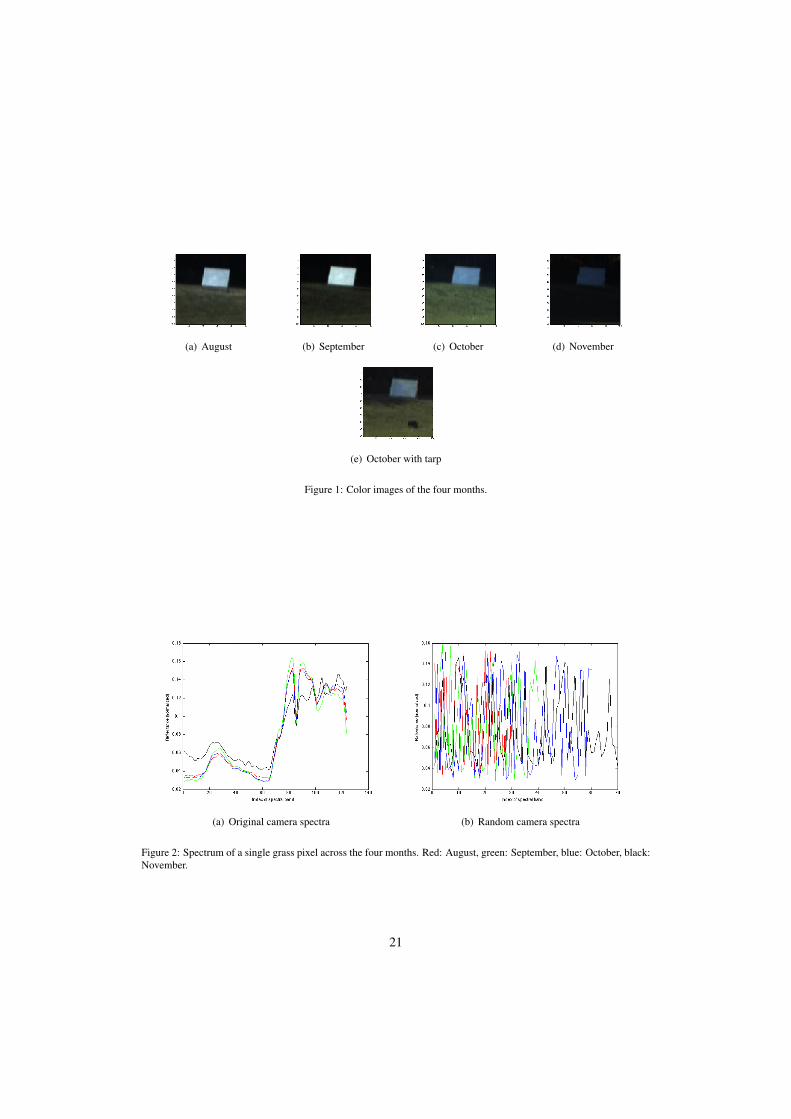
(a) August (b) September (c) October (d) November

(e) October with tarp

Figure 1: Color images of the four months.

(a) Original camera spectra (b) Random camera spectra

Figure 2: Spectrum of a single grass pixel across the four months. Red: August, green: September, blue: October, black:November.

21

(a) August (original) (b) September (original) (c) October (original) (d) November (original)

(e) August (random) (f) September (random) (g) October (random) (h) November (random)

(i) August (noisy random) (j) September (noisy ran-dom)

(k) October (noisy random) (l) November (noisy ran-dom)

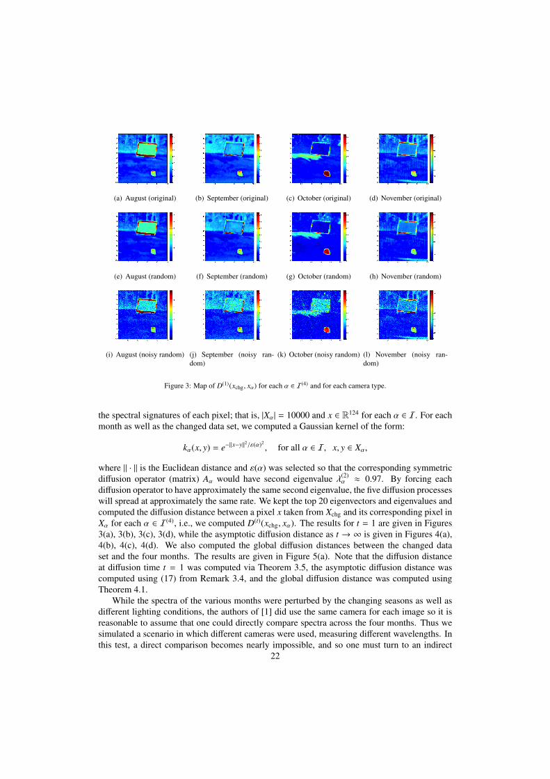
Figure 3: Map of D(1)(xchg, xα) for each α ∈ I(4) and for each camera type.

the spectral signatures of each pixel; that is, |Xα| = 10000 and x ∈ R124 for each α ∈ I. For eachmonth as well as the changed data set, we computed a Gaussian kernel of the form:

kα(x, y) = e−‖x−y‖2/ε(α)2, for all α ∈ I, x, y ∈ Xα,

where ‖ · ‖ is the Euclidean distance and ε(α) was selected so that the corresponding symmetricdiffusion operator (matrix) Aα would have second eigenvalue λ(2)

α ≈ 0.97. By forcing eachdiffusion operator to have approximately the same second eigenvalue, the five diffusion processeswill spread at approximately the same rate. We kept the top 20 eigenvectors and eigenvalues andcomputed the diffusion distance between a pixel x taken from Xchg and its corresponding pixel inXα for each α ∈ I(4), i.e., we computed D(t)(xchg, xα). The results for t = 1 are given in Figures3(a), 3(b), 3(c), 3(d), while the asymptotic diffusion distance as t → ∞ is given in Figures 4(a),4(b), 4(c), 4(d). We also computed the global diffusion distances between the changed dataset and the four months. The results are given in Figure 5(a). Note that the diffusion distanceat diffusion time t = 1 was computed via Theorem 3.5, the asymptotic diffusion distance wascomputed using (17) from Remark 3.4, and the global diffusion distance was computed usingTheorem 4.1.

While the spectra of the various months were perturbed by the changing seasons as well asdifferent lighting conditions, the authors of [1] did use the same camera for each image so it isreasonable to assume that one could directly compare spectra across the four months. Thus wesimulated a scenario in which different cameras were used, measuring different wavelengths. Inthis test, a direct comparison becomes nearly impossible, and so one must turn to an indirect

22

(a) August (original) (b) September (original) (c) October (original) (d) November (original)

(e) August (random) (f) September (random) (g) October (random) (h) November (random)

(i) August (noisy random) (j) September (noisy ran-dom)

(k) October (noisy random) (l) November (noisy ran-dom)

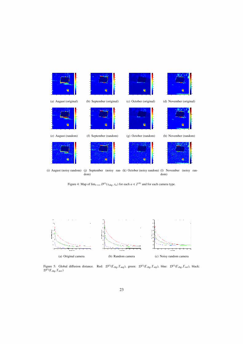
Figure 4: Map of limt→∞ D(t)(xchg, xα) for each α ∈ I(4) and for each camera type.

(a) Original camera (b) Random camera (c) Noisy random camera

Figure 5: Global diffusion distance. Red: D(t)(Γchg,Γaug), green: D(t)(Γchg,Γsep), blue: D(t)(Γchg,Γoct), black:D(t)(Γchg,Γnov)

23

comparison such as the diffusion distance.To carry out the experiment, we did the following. For each of the five images, we randomly

selected Dα bands to use out of the original 124 bands; we also randomly reordered each set ofDα bands. The values of Dα are the following: Daug = 30, Dsep = 40, Doct = 60, Dnov = 70,and Dchg = 50. Thus for this experiment, Xα, for each α ∈ I, contains data points in RDα . Tosee an example of these new spectra, we refer the reader to Figure 2(b). Using the measurementsfrom this “random camera,” we then proceeded to carry out the experiment exactly as before,computing the diffusion distance for t = 1 (Figures 3(e), 3(f), 3(g), 3(h)), the asymptotic diffusiondistance (Figures 4(e), 4(f), 4(g), 4(h)), and the global diffusion distance (Figure 5(b)).

For a third and final experiment, we took the spectra from the random camera in the previousexperiment and added Gaussian noise sampled from the normal distribution with mean zero andstandard deviation 0.01. This gave us an average signal to noise ratio (SNR) of 19.2 dB (note, wecompute SNR = 10 log10(mean(x2)/mean(η2)), where x is the signal and η is the noise). Oncemore we carried out the experiment, the same as before, computing the diffusion distance fort = 1 (Figures 3(i), 3(j), 3(k), 3(l)), the asymptotic diffusion distance (Figures 4(i), 4(j), 4(k),4(l)), and the global diffusion distance (Figure 5(c)).

Examining Figures 3, 4, and 5, we see that the results are similar across all three cameras (theoriginal camera, the random camera, and the noisy random camera). This result points to the twoproperties mentioned at the beginning of this section: that the common embedding defined byTheorem 3.5 is sensor independent and robust against noise. Thus the method is consistent undera variety of different conditions.

In terms of the change detection task, the diffusion distance is also accurate. For the diffusiontime t = 1, we see from the maps in Figure 3 that the tarp is recognized as a change. However,other changes due to the lighting or the change in seasons also appear. For example, even inOctober, the small change in the shadow is visible, while in August, September, and Novemberthe change in lighting causes the panel to be highlighted. Also, in some months even the treeshave a weak, but noticeable difference in the their diffusion distances. When we allow t →∞ though, the smaller clusters merge together and the changes due to lighting and seasonaldifferences are filtered out. As one can see from Figure 4, all that is left is the change due to theadded tarp (note that the change around the border of the panel is due to it being slightly shiftedfrom month to month). Thus we see that the diffusion distance and corresponding diffusion mapgives a natural representation of the data that can be used to filter types of changes at differentscales. In practice, after these mappings and distances have been computed, the images can behanded off to an analyst who should be able to pick out the changes with ease; alternatively, aclassification algorithm can be used on the backend (for example, one that looks for diffusiondistances across images that are larger than a certain prescribed scale).

For the global diffusion distances in Figure 5, we see several intuitions borne out in thisparticular application. First, the closer the month in real time to October (the month in which thechanged data set was recorded), the smaller the global diffusion distance. Secondly, we see thatas the diffusion time t gets larger, the smaller the global diffusion distance.

6.2. Parameterized difference equations

In this section we consider discrete time dynamical systems (difference equations) that de-pend on input parameters. The idea is to use the diffusion geometric principles outlined in thispaper to understand how the geometry of the system changes as one changes the parameters ofthe system.

24

To illustrate the idea we use the following example of the Standard Map, first brought to ourattention by Igor Mezic and Roy Lederman (personal correspondence). The Standard Map is anarea preserving chaotic map from the torus T2 , 2π(S 1 × S 1) onto itself. Let (p, θ) ∈ T2 denotean arbitrary coordinate of the torus. For any initial condition (p0, θ0) ∈ T2, the Standard Map isdefined by the following two equations:

p`+1 , p` + α sin(θ`) mod 2π,

θ`+1 , θ` + p`+1 mod 2π,

where α ∈ I = [0,∞) is a parameter, ` ∈ N ∪ 0, and (p`, θ`) ∈ T2 for all ` ≥ 0. The sequenceof points γ(p0, θ0) , (p`, θ`)`≥0 constitutes the orbit derived from the initial condition (p0, θ0).When α = 0, the Standard Map consists solely of periodic and quasiperiodic orbits. For α > 0,the map is is increasingly nonlinear as α grows, which in turn increases the number of initialconditions that lead to chaotic dynamics.

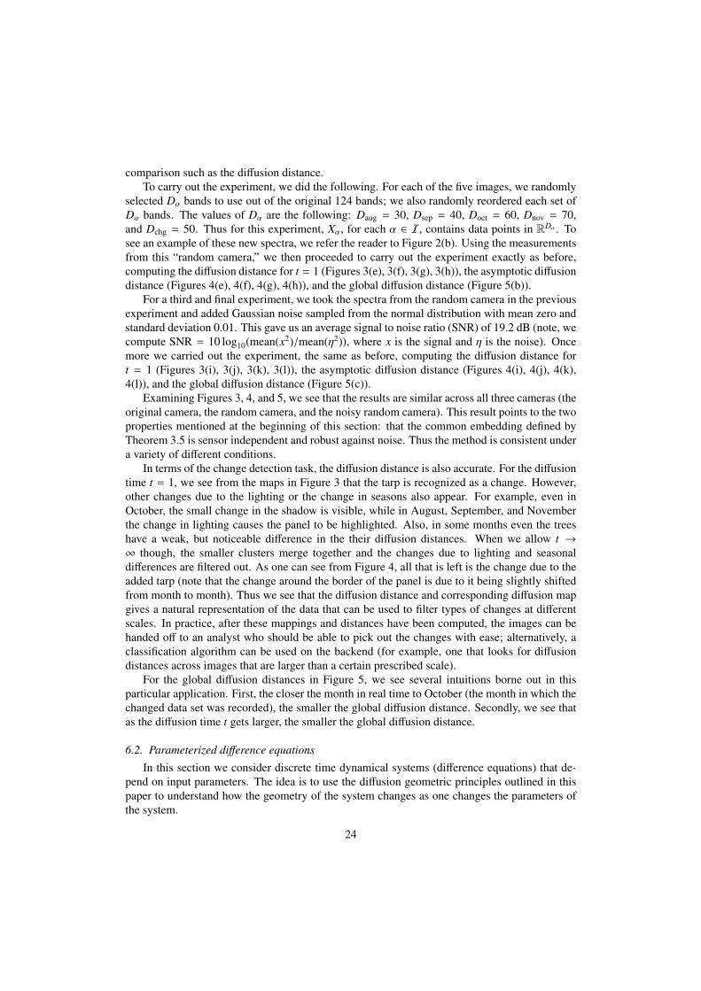
We take the data set Xα to be the set of orbits of the Standard Map for the parameter α.Using the ideas developed in [20, 21], it is possible to define a kernel kα that acts on this dataset. One can in turn use this kernel to define a diffusion map on the orbits. For the purposes ofthis experiment, we discretize the orbits by selecting a grid of initial conditions on T2 and let thesystem run forward a prescribed number of time steps. An example for small α is given in Figure6. Notice how the diffusion map embedding into R3 organizes the Standard Map according tothe geometry of the orbits.

For each α ∈ [0,∞), we have a similar embedding. Using the ideas contained in Section 3(in particular Theorem 3.5), it is possible to map each embedding, for all α ∈ I, into a single lowdimensional Euclidean space. Doing so allows one to observe how the geometry of the systemchanges as the parameter α is increased; see Figure 7 for more details. In the forthcoming paper[22], we give a full treatment of these ideas.

6.3. Global embeddingsIn this section we seek to illustrate how the global diffusion distance can be used to recover

the parameters governing the global geometrical behavior of Xα as α ranges over I. As anexample, we shall take a torus that is being deformed according to two parameters:

1. The location of the deformation, which in this case is a pinch (imagine squeezing the torusat a certain spot).

2. The strength of the deformation, i.e., how hard we pinch the torus.

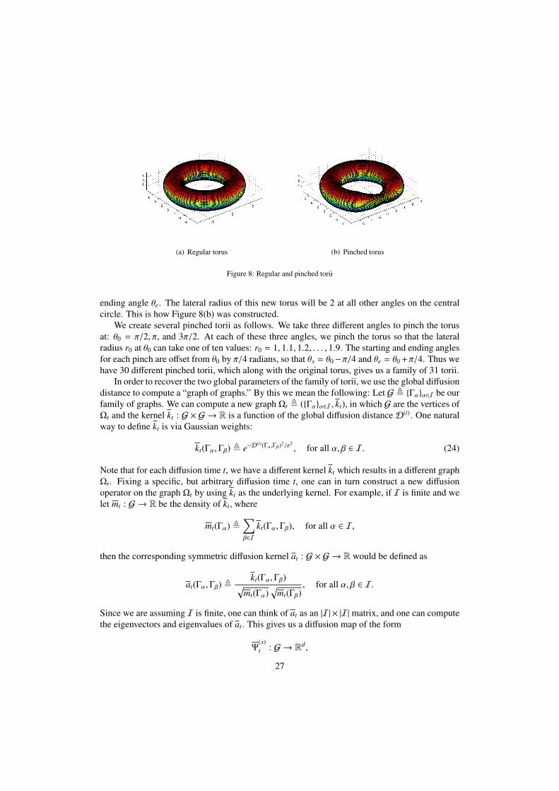
Let I = 0, 1, . . . , 30. X0 shall be the standard torus with no pinch; for 1 ≤ α ≤ 30, Xα willhave a pinch at a prescribed location on the torus with a prescribed strength. For an image of thestandard torus as well as a pinched torus, see Figure 8.

More specifically, we take X0 to be a torus with a central radius of six and a lateral radius oftwo, i.e., X , (6S 1) × (2S 1). We assume that the central circle 6S 1 and the lateral circle 2S 1

are oriented, so that each point on the torus has a specific coordinate location (note that whileX0 ⊂ R3, the points of the torus have a two dimensional coordinate system consisting of twoangles, one for the central circle and one for the lateral circle).

From X0 we build a family of “pinched” torii as follows. We pick an angle on the centralcircle 6S 1, say θ0, and we pinch the torus at θ0 so that its lateral radius at this angle is now r0,where r0 < 2. So that we do not rip the torus, from a starting angle θs, the lateral radius willdecrease linearly from 2 at θs to r0 at θ0, and then increase linearly from r0 at θ0 back to 2 at some

25

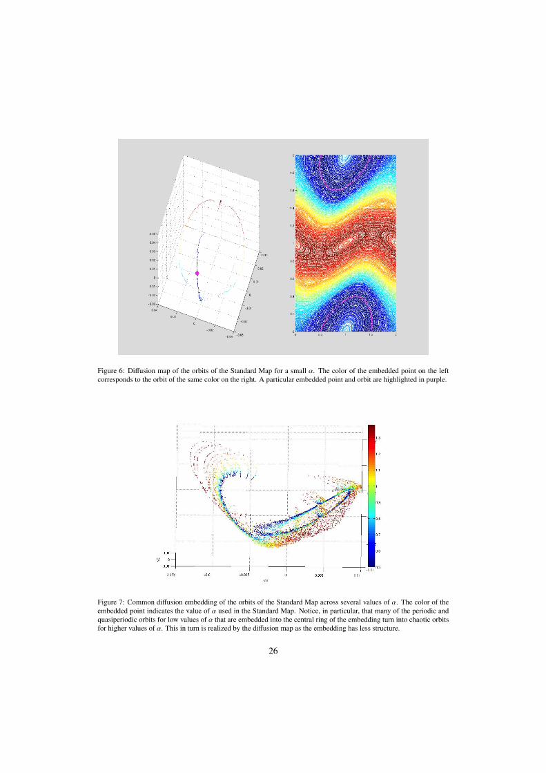
Figure 6: Diffusion map of the orbits of the Standard Map for a small α. The color of the embedded point on the leftcorresponds to the orbit of the same color on the right. A particular embedded point and orbit are highlighted in purple.

Figure 7: Common diffusion embedding of the orbits of the Standard Map across several values of α. The color of theembedded point indicates the value of α used in the Standard Map. Notice, in particular, that many of the periodic andquasiperiodic orbits for low values of α that are embedded into the central ring of the embedding turn into chaotic orbitsfor higher values of α. This in turn is realized by the diffusion map as the embedding has less structure.

26

(a) Regular torus (b) Pinched torus

Figure 8: Regular and pinched torii

ending angle θe. The lateral radius of this new torus will be 2 at all other angles on the centralcircle. This is how Figure 8(b) was constructed.

We create several pinched torii as follows. We take three different angles to pinch the torusat: θ0 = π/2, π, and 3π/2. At each of these three angles, we pinch the torus so that the lateralradius r0 at θ0 can take one of ten values: r0 = 1, 1.1, 1.2, . . . , 1.9. The starting and ending anglesfor each pinch are offset from θ0 by π/4 radians, so that θs = θ0−π/4 and θe = θ0 +π/4. Thus wehave 30 different pinched torii, which along with the original torus, gives us a family of 31 torii.

In order to recover the two global parameters of the family of torii, we use the global diffusiondistance to compute a “graph of graphs.” By this we mean the following: Let G , Γαα∈I be ourfamily of graphs. We can compute a new graph Ωt , (Γαα∈I, kt), in which G are the vertices ofΩt and the kernel kt : G × G → R is a function of the global diffusion distanceD(t). One naturalway to define kt is via Gaussian weights:

kt(Γα,Γβ) , e−D(t)(Γα,Γβ)2/ε2

, for all α, β ∈ I. (24)

Note that for each diffusion time t, we have a different kernel kt which results in a different graphΩt. Fixing a specific, but arbitrary diffusion time t, one can in turn construct a new diffusionoperator on the graph Ωt by using kt as the underlying kernel. For example, if I is finite and welet mt : G → R be the density of kt, where

mt(Γα) ,∑β∈I

kt(Γα,Γβ), for all α ∈ I,

then the corresponding symmetric diffusion kernel at : G × G → R would be defined as

at(Γα,Γβ) ,kt(Γα,Γβ)√

mt(Γα)√

mt(Γβ), for all α, β ∈ I.

Since we are assuming I is finite, one can think of at as an |I| × |I| matrix, and one can computethe eigenvectors and eigenvalues of at. This gives us a diffusion map of the form

Ψ(s)t : G → Rd,

27

where s is the diffusion time for the graph of graphs. This diffusion embedding can then be usedto cluster the family of graphs G, treating each graph Γα ∈ G as a single data point.

Our goal is to build a graph of graphs in which each vertex is one of the 31 torii. To do sowe approximate the global diffusion distance between each pair of torii by taking 7744 randomsamples from X0 (using the uniform distribution), and then using the same corresponding samplesfor each pinched torus. For each torus we used a Gaussian kernel of the form

kα(x, y) = e−‖x−y‖2/ε(α)2, for all α ∈ I,

where ε(α) was selected so that the corresponding symmetric diffusion operator (matrix) Aα

would have second eigenvalue λ(2)α = 0.5. The pairwise global diffusion distance was further

approximated by taking the top ten eigenvalues and eigenvectors of each of the 31 diffusionoperators, and was then computed for diffusion time t = 2 using Theorem 4.1. Two remarks:first, the diffusion time t = 2 = 1/(1 − λ(2)

α ) corresponds to the approximate time it would takefor the diffusion process to spread through each of the graphs; secondly, by Theorem 5.2, thisapproximate global diffusion distance is, with high probability, nearly equal to the true globaldiffusion distance between each of the torii.

After computing the pairwise global diffusion distances, we constructed the kernel kt, fort = 2, defined in equation (24). We took ε in this kernel to be the median of all pairwise globaldiffusion distances between the 31 torii. We then computed the symmetric diffusion operatorfor this graph of graphs, which turned out to have second eigenvalue λ(2) ≈ 0.48. We took thetop three eigenvalues and eigenvectors of the diffusion operator, and used them to compute thediffusion map into R3 at diffusion time s ≈ 1/(1 − 0.48) = 1.92.

A plot of this diffusion map is given in Figure 9. The central, dark blue, circle correspondsto the regular torus in both images. In Figure 9(a), the other three colors correspond to the angleat which the torus was pinched. In Figure 9(b), the colors correspond to the strength of the pinch(dark blue - no pinch, dark red - strongest pinch). As one can see, the diffusion embeddingorganizes the torii by both the location of the pinch (i.e. what arc the embedded torus lies on),and the strength of the pinch (i.e. how far from the regular torus each pinched torus lies), givinga global view of how the data set changes over the parameter space.

7. Conclusion

In this paper we have generalized the diffusion distance to work on a changing graph. Thisnew distance, along with the corresponding diffusion maps, allow one to understand how theintrinsic geometry of the data set changes over the parameter space. We have also defined aglobal diffusion distance between graphs, and used this to construct meta graphs in which eachvertex of the meta graph corresponds to a graph. Formulas for each of these diffusion distancesin terms of the spectral decompositions of the relevant diffusion operators have been proven,giving a simple and efficient way to approximate these diffusion distances. Finally, it was shownthat a random, finite sample of data points from a continuous, changing data set X is, with highprobability, enough to approximate the diffusion distance and the global diffusion distance tohigh accuracy.

Future work could include generalizing these notions of diffusion distance further so thatthey can apply to sequences of graphs in which there is no bijective correspondence betweenthe graphs (beyond the simple generalization of Appendix A). Also, it would be interestingto investigate how this work fits in with the recent research on vectorized diffusion operatorscontained in [23, 24].

28

(a) Colored by location of pinch. Each color correspondsto one of the angles at which the pinch occurs.

(b) Colored by strength of pinch. Dark blue indicates nopinch, followed by light blue, green, yellow, orange, andfinally dark red which indicates the strongest pinch.

Figure 9: Diffusion embedding of the 31 torii. Each data point corresponds to a torus. The embedding organizes the toriiaccording to the two parameters governing the global geometrical behavior of the data over the parameter space.

8. Acknowledgements

This research was supported by Air Force Office of Scientific Research STTR FA9550-10-C-0134 and by Army Research Office MURI W911NF-09-1-0383. We would also like to thankthe anonymous reviewers for their extremely helpful comments and suggestions, which greatlyimproved this paper.

Appendix A. Non-bijective correspondence

In this appendix we consider the case in which our changing data set does not have a singlebijective correspondence across the parameter set I. We make a few small changes to the no-tation. Continue to let I denote the parameter space, but let (X, µ) denote a “global” measurespace. Our changing data is given by Xαα∈I with data points xα ∈ Xα, and satisfies

Xα ⊆ X, for all α ∈ I.

We assume that each data set Xα is a measurable set under µ. Suppose, additionally, that thereexists a sufficiently large set S ⊂ X such that

S ⊂ Xα, for all α ∈ I.

We maintain the remaining notations and assumptions from Section 3, and simply update themto apply for each Xα. In particular, for each α ∈ I, we have the symmetric diffusion kernelaα : Xα × Xα → R, with corresponding trace class operator Aα : L2(Xα, µ) → L2(Xα, µ). Theset of functions ψ(i)

α i≥1 ⊂ L2(Xα, µ) still denote a set of orthonormal eigenfunctions for Aα, withcorresponding eigenvalues λ(i)

α i≥1. The diffusion map is still given by Ψ(t)α : Xα → `2, with

Ψ(t)α (xα) =

((λ(i)α

)tψ(i)α (xα)

)i≥1

.

Under this more general setup, for any α, β ∈ I, the sets Xα\Xβ and Xβ\Xα may be nonempty.Thus it is not possible to compare the diffusions on Γα and Γβ as they spread through each graph.

29

On the other hand, since we have a common set S ⊂ Xα ∩ Xβ, we can compare the diffusioncentered at xα ∈ Xα with the diffusion centered at yβ ∈ Xβ as they spread through the subgraphsof Γα and Γβ with common vertices S . Formally, we define this diffusion distance as:

D(t)(xα, yβ; S )2 ,∫S

(a(t)α (xα, s) − a(t)

β (yβ, s))2

dµ(s), for all α, β ∈ I, (xα, yβ) ∈ Xα × Xβ.

A result similar to Theorem 3.5 can be had for this subgraph diffusion distance. Since theeigenfunctions for Aα will not be orthonormal when restricted to L2(S , µ), one must use an ad-ditional orthonormal basis e(i)i≥1 for L2(S , µ) when rotating the diffusion maps across I into acommon embedding. In particular, we define a new family of rotation maps Oα,S : `2 → `2 as:

Oα,S v ,

∑j≥1

v[ j] 〈e(i), ψ( j)α 〉L2(S ,µ)

i≥1

.

Using these rotation maps, along with the same ideas from Section 3, one can show:

D(t)(xα, yβ; S ) =∥∥∥∥Oα,S Ψ(t)

α (xα) − Oβ,S Ψ(t)β (yβ)

∥∥∥∥`2, with convergence in L2(Xα × Xβ, µ ⊗ µ).

Remark Appendix A.1. Analogously to Remark 3.6, one should be careful when choosing thebasis e(i)i≥1 for L2(S , µ). Ideally it will depend on the desired application, and can thus prioritizecertain features in the data.

Appendix B. Proof of random sampling theorems

In this appendix we prove the random sampling Theorems 5.1 and 5.2 from Section 5.Throughout the appendix we shall assume that (X, µ) and kαα∈I satisfy Assumption 2.

The proof shall rely upon a result from [17] as well as several results on the asymmetric graphLaplacian I − P that are contained in [18]. All of these results are easily translated for our familyof operators Aαα∈I, and we shall simply restate the needed results from [18] in these terms.

Appendix B.1. Reproducing kernel Hilbert spaces

Critical to our analysis will the be existence of a single reproducing kernel Hilbert space(RKHS) that contains the set of kernels aαα∈I, their empirical approximations, and relatedfunctions. In [18] such a RKHS is constructed. Here we recall the definition of a RKHS as wellthe aforementioned construction.

A set H is a RKHS [25] if it is a Hilbert space of functions f : X → R such that for eachx ∈ X, there exists a constant C(x) so that

f (x) ≤ C(x) ‖ f ‖H .

The name RKHS comes from the fact that one can show that there is a unique symmetric, positivedefinite kernel h : X × X → R associated withH such that for each f ∈ H ,

f (x) = 〈 f , h(x, ·)〉H , for all x ∈ X.

30

We utilize a specific RKHS first presented in [18]; the construction is rewritten here forcompleteness. Let l be a positive integer, and define the Sobolev spaceH l as

H l , f ∈ L2(X, dx) : Dγ f ∈ L2(X, dx) for all |γ| = l,

where Dγ f is the weak derivative of f with respect to the multi-index γ , (γ1, . . . , γd) ∈ Nd,|γ| , γ1 + · · · + γd, and dx denotes the Lebesgue measure. The space H l is a separable Hilbertspace with scalar product

〈 f , g〉H l , 〈 f , g〉L2(X,dx) +∑|γ|=l

〈Dγ f ,Dγg〉L2(X,dx).

Also note that the space Clb(X) is a Banach space with respect to the norm

‖ f ‖Clb(X) , sup

x∈X| f (x)| +

∑|γ|=l

supx∈X|Dγ f (x)|.

As explained in [18], since X is bounded, we have Clb(X) ⊂ H l and ‖ f ‖H l ≤ C(l)‖ f ‖Cl

b(X). ViaCorollary 21 of section 4.6 from [19], if m ∈ N and l − m > d/2, then we also have:

H l ⊂ Cmb (X) and ‖ f ‖Cm

b (X) ≤ C(l,m) ‖ f ‖H l . (B.1)

Following [18], if one takes s , bd/2c+ 1, then using (B.1) with l = s and m = 0 we see thatH s

is a RKHS with a continuous, real valued, bounded kernel hs.

Appendix B.2. Additional operatorsIn this section we define several operators that will bridge the gap between the matrix Aα

and the operator Aα. All of these definitions are based on those from [18] for the asymmetricaldiffusion operators (i.e. P). To start, define the empirical density maps mα,n : X → R in terms ofthe samples Xn = x(1), . . . , x(n) as

mα,n(x) ,1n

n∑i=1

kα(x, x(i)), for all α ∈ I, x ∈ X.

Note that mα,n(x(i)) = Dα[i, i]. We also define the empirical kernels aα,n : X × X → R as

aα,n(x, y) ,kα(x, y)√

mα,n(x)√

mα,n(y), for all α ∈ I, x, y ∈ X.

We then have the following lemma from [18], adapted for symmetric diffusion operators.

Lemma Appendix B.1 (Lemma 16 from [18]). Assume that (X, µ) and kαα∈I satisfy the con-ditions of Assumption 2. Then, for all α ∈ I and for all x ∈ X,

kα(x, ·),mα,mα,n,1

mα,

1mα,n

∈ Cd+1b (X) ⊂ Hd+1 ⊂ H s,

‖kα(x, ·)‖Cd+1b (X) , ‖mα‖Cd+1

b (X) ,∥∥∥mα,n

∥∥∥Cd+1

b (X) ,

∥∥∥∥∥ 1mα

∥∥∥∥∥Cd+1

b (X),

∥∥∥∥∥∥ 1mα,n

∥∥∥∥∥∥Cd+1

b (X)≤ C(α, d),

aα(x, ·), aα,n(x, ·) ∈ Cd+1b (X) ⊂ Hd+1 ⊂ H s,

‖aα(x, ·)‖H s ,∥∥∥aα,n(x, ·)

∥∥∥H s ≤ C(α, d).

31

Lemma Appendix B.1 allows one to define the operators Aα,H s : H s → H s and Aα,n : H s →

H s,

(Aα,H s f )(x) ,∫X

aα(x, y) 〈 f , hs(y, ·)〉H s dµ(y), for all α ∈ I, f ∈ H s,

(Aα,n f )(x) ,1n

n∑i=1

aα,n(x, x(i)) 〈 f , hs(x(i), ·)〉H s , for all α ∈ I, f ∈ H s.

We also define similar operators TH s : H s → H s and Tn : H s → H s, but in terms of thereproducing kernel hs.

(TH s f )(x) ,∫X

hs(x, y) 〈 f , hs(y, ·)〉H s dµ(y), for all f ∈ H s,

(Tn f )(x) ,1n

n∑i=1

hs(x, x(i)) 〈 f , hs(x(i), ·)〉H s , for all f ∈ H s.

The above operators, as well as Aα and Aα, can be decomposed in terms of the appropriaterestriction and extension operators. We begin with the two restriction operators, RH s : H s →

L2(X, µ) and Rn : H s → Rn.

(RH s f )(x) , 〈 f , hs(x, ·)〉H s , for µ a.e. x ∈ X, for all f ∈ H s,

Rn f , ( f (x(1)), . . . , f (x(n))), for all f ∈ H s.

For each α ∈ I we also have two extension operators, Eα,H s : L2(X, µ) → H s and Eα,n : Rn →

H s, where

(Eα,H s f )(x) ,∫X

aα(x, y) f (y) dµ(y), for all x ∈ X, f ∈ L2(X, µ),

(Eα,nv)(x) ,1n

n∑i=1

v[i] aα,n(x, x(i)), for all x ∈ X, v ∈ Rn.

Using these operators, one can easily show the following identities:

Aα = RH s Eα,H s and Aα,H s = Eα,H s RH s ,

Aα = RnEα,n and Aα,n = Eα,nRn, (B.2)TH s = R∗

H s RH s and Tn = R∗nRn.

Appendix B.3. Similarity between empirical and continuous operators

Here we collect remaining results that we shall need that involve the similarity between theempirical and continuous versions of the previously defined operators and functions. All of theseresults can be found in [17, 18].

Theorem Appendix B.2 ([17], also Theorem 7 from [18]). Suppose that (X, µ) and kαα∈Isatisfy the conditions of Assumption 2. Let n ∈ N and sample Xn = x(1), . . . , x(n) ⊂ X i.i.d.

32

according to µ; also let τ > 0. Then the operators TH s and Tn are Hilbert-Schmidt, and withprobability 1 − 2e−τ,

‖TH s − Tn‖HS ≤ C(d)√τ√

n.

Theorem Appendix B.3 (Theorem 15 from [18]). Suppose that (X, µ) and kαα∈I satisfy theconditions of Assumption 2. Let n ∈ N and sample Xn = x(1), . . . , x(n) ⊂ X i.i.d. according toµ; also let τ > 0 and α ∈ I. Then the operators Aα,H s and Aα,n are Hilbert-Schmidt, and withprobability 1 − 2e−τ, ∥∥∥Aα,H s − Aα,n

∥∥∥HS ≤ C(α, d)

√τ√

n.

Lemma Appendix B.4 (Lemma 18 from [18]). Suppose that (X, µ) and kαα∈I satisfy theconditions of Assumption 2. Let n ∈ N and sample Xn = x(1), . . . , x(n) ⊂ X i.i.d. according to µ;also let τ > 0 and α ∈ I. Then, with probability 1 − 2e−τ,

∥∥∥mα − mα,n

∥∥∥Hd+1 ≤ C(α, d)

√τ√

n.

Appendix B.4. Proof of Theorem 5.1

In this section we prove Theorem 5.1, which we restate here.

Theorem Appendix B.5 (Theorem 5.1). Suppose that (X, µ) and kαα∈I satisfy the conditionsof Assumption 2. Let n ∈ N and sample Xn = x(1), . . . , x(n) ⊂ X i.i.d. according to µ; also lett ∈ N, τ > 0, and α, β ∈ I. Then, with probability 1 − 2e−τ,∣∣∣∣D(t)(x(i)

α , x( j)β ) − D(t)

n (x(i)α , x

( j)β )

∣∣∣∣ ≤ C(α, β, d, t)√τ√

n, for all i, j = 1, . . . , n.

Proof of Theorem 5.1. First an additional piece of notation. Recall the d-dimensional index γ =

(γ1, . . . , γd). Let ∂γxaα denote the γth partial derivative of aα with respect to the variable x.We begin with the empirical diffusion distance. Recall that D(t)

n (x(i)α , x

( j)β )2 = n2‖At

α[i, ·] −Atβ[ j, ·]‖2Rn . For each i = 1, . . . , n, define the vector e(i) ∈ Rn as

e(i)[ j] ,

1, if j = i,0, if j , i, for all j = 1, . . . , n.

We then have

D(t)n (x(i)

α , y( j)β )2 = n2

∥∥∥Atαe(i) − At

βe( j)

∥∥∥2

Rn

= n2〈Atαe(i),At

αe(i)〉Rn + n2〈Atβe

( j),Atβe

( j)〉Rn − 2n2〈Atαe(i),At

βe( j)〉Rn . (B.3)

A similar expression can be had for the continuous diffusion distance. By Assumption 2,kα ∈ Cd+1

b (X × X) and kα ≥ C1(α). These imply that aα ∈ Cd+1b (X × X). We can then apply

Mercer’s Theorem to get that

a(t)α (x, y) =

∑`≥1

(λ(`)α

)tψ(`)α (x)ψ(`)

α (y), for all (x, y) ∈ X × X, (B.4)

33

with absolute convergence and uniform convergence on compact subsets of X. In fact, since Aα

is also trace class, we can get uniform convergence on all of X. Indeed,

Tr(Aα) =∑`≥1

λ(`)α < ∞.

Therefore, for all ε > 0 and for each α ∈ I, there exists N(ε, α) ∈ N such that∑`>N(ε,α)

(λ(`)α

)t< ε.

Furthermore, since aα is bounded, ψ(`)α ≤ C2(α) for all ` ≥ 1. Therefore,∑

`>N(ε,α)

(λ(`)α

)tψ(`)α (x)ψ(`)

α (y) ≤ C2(α)∑

`>N(ε,α)

(λ(`)α

)t< C2(α) ε, for all (x, y) ∈ X × X. (B.5)

Now define a family of functions ϕ(N,i)α ∈ L2(X, µ) for all N ∈ N and i ∈ 1, . . . , n,

ϕ(N,i)α (x) ,

N∑`=1

ψ(`)α (x(i))ψ(`)

α (x).

We claim that ∣∣∣a(t)α (x(i), x) − At

αϕ(N(ε,α),i)α (x)

∣∣∣ < C2(α) ε, for all x ∈ X. (B.6)

Indeed,

Atαϕ

(N,i)α (x) =

∫X

a(t)α (x, y)ϕ(N,i)

α (y) dµ(y),

=

∫X

∑m≥1

(λ(m)α

)tψ(m)α (x)ψ(m)

α (y)

N∑`=1

ψ(`)α (x(i))ψ(`)

α (y)

dµ(y),

=∑m≥1

N∑`=1

(λ(m)α

)tψ(m)α (x)ψ(`)

α (x(i))∫X

ψ(m)α (y)ψ(`)

α (y) dµ(y),

=

N∑`=1

(λ(`)α

)tψ(`)α (x(i))ψ(`)

α (x). (B.7)

Therefore, using (B.4), (B.7), and (B.5), we obtain

∣∣∣a(t)α (x(i), x) − At

αϕ(N(ε,α),i)α (x)

∣∣∣ =

∣∣∣∣∣∣∣∣∑

`>N(ε,α)

(λ(`)α

)tψ(`)α (x(i))ψ(`)

α (x)

∣∣∣∣∣∣∣∣ < C2(α) ε,

and so (B.6) holds.Using (B.6), it not hard to see that∣∣∣∣∣D(t)(x(i)

α , y( j)β ) −

∥∥∥∥Atαϕ

(N(ε,α),i)α − At

βϕ(Nε,β),i)β

∥∥∥∥L2(X,µ)

∣∣∣∣∣ ≤ C3(α, β) ε.

34

Thus it is enough to consider ‖Atαϕ

(N(ε,α),i)α − At

βϕ(N(ε,β), j)β ‖L2(X,µ). Expanding the square of this

quantity one has∥∥∥∥Atαϕ

(N(ε,α),i)α − At

βϕ(N(ε,β), j)β

∥∥∥∥2

L2(X,µ)= 〈At

αϕ(N(ε,α),i)α , At

αϕ(N(ε,α),i)α 〉L2(X,µ)

+ 〈Atβϕ

(N(ε,β), j)β , At

βϕ(N(ε,β), j)β 〉L2(X,µ) − 2〈At

αϕ(N(ε,α),i)α , At

βϕ(N(ε,β), j)β 〉L2(X,µ).

(B.8)

The three inner products in (B.3) correspond to the three inner products in (B.8). We aim toshow that each pair is nearly identical. We will do so explicitly for the pair n2〈At

αe(i),Atβe

( j)〉Rn

and 〈Atαϕ

(N(ε,α),i)α , At

βϕ(N(ε,β), j)β 〉L2(X,µ); the other two pairs are simply special cases of this one. We

begin with the discrete inner product, for which we have the following with probability 1− 2e−τ:

n2〈Atαe(i),At

βe( j)〉Rn = n2〈(RnEα,n)te(i), (RnEβ,n)te( j)〉Rn (B.9)

= n2〈(Eα,nRn)t−1Eα,ne(i),R∗nRn(Eβ,nRn)t−1Eβ,ne( j)〉H s

= 〈At−1α,n aα,n(x(i), ·),TnAt−1

β,n aβ,n(x( j), ·)〉H s (B.10)

≤ 〈At−1α,H s aα,n(x(i), ·),TH s At−1

β,H s aβ,n(x( j), ·)〉H s + C(α, β, d, t)√τ√

n, (B.11)

where (B.9) follows from (B.2), (B.10) follows from (B.2) and the definitions of Eα,n and e(i), and(B.11) follows from Lemma Appendix B.1, Theorem Appendix B.2, Theorem Appendix B.3,and the Cauchy-Schwarz inequality. Since the argument is symmetric, we have, with probability1 − 2e−τ,∣∣∣∣n2〈At

αe(i),Atβe

( j)〉Rn − 〈At−1α,H s aα,n(x(i), ·),TH s At−1

β,H s aβ,n(x( j), ·)〉H s

∣∣∣∣ ≤ C(α, β, d, t)√τ√

n. (B.12)

Now return to the continuous inner product. With probability 1 − 2e−τ, we have:

〈Atαϕ

(N(ε,α),i)α , At

βϕ(N(ε,β), j)β 〉L2(X,µ) = 〈(RH s Eα,H s )tϕ(N(ε,α),i)

α , (RH s Eβ,H s )tϕ(N(ε,β), j)β 〉L2(X,µ) (B.13)

= 〈(Eα,H s RH s )t−1Eα,H sϕ(N(ε,α),i)α ,R∗

H s RH s (Eβ,H s RH s )t−1Eβ,H sϕ(N(ε,β), j)β 〉H s

= 〈At−1α,H s Eα,H sϕ(N(ε,α),i)

α ,TH s At−1β,H s Eβ,H sϕ

(N(ε,β), j)β 〉HS , (B.14)

where (B.13) and (B.14) both follow from (B.2).Examining (B.12) and (B.14), it is clear that to complete the proof we must bound the quan-

tity ‖aα,n(x(i), ·) − Eα,H sϕ(N(ε,α),i)α ‖H s . We break it into two parts:∥∥∥aα,n(x(i), ·) − Eα,H sϕ(N(ε,α),i)

α

∥∥∥H s ≤

∥∥∥aα,n(x(i), ·) − aα(x(i), ·)∥∥∥H s +

∥∥∥aα(x(i), ·) − Eα,H sϕ(N(ε,α),i)α

∥∥∥H s .

(B.15)For the first part, some simple manipulations give:

aα,n(x(i), x) − aα(x(i), x) = f (i)α,n(x) + g(i)

α,n(x),

where

f (i)α,n(x) =

kα(x(i), x) (√

mα(x) −√

mα,n(x))√mα,n(x(i))

√mα,n(x)

√mα(x)

35

and

g(i)α,n(x) =

kα(x(i), x) (√

mα,n(x(i)) −√

mα(x(i)))√mα,n(x(i))

√mα(x(i))

√mα(x)

.

For the first of these two functions, using Lemma Appendix B.1 and Lemma Appendix B.4 it iseasy to see that ‖ f (i)

α,n‖H s ≤ C(α, d)√τ√

n with probability 1 − 2e−τ. For g(i)α,n, note that∣∣∣mα,n(x(i)) − mα(x(i))

∣∣∣ ≤ supx∈X

∣∣∣mα,n(x) − mα(x)∣∣∣

=∥∥∥mα,n − mα

∥∥∥C0

b(X)

≤ C(d)∥∥∥mα,n − mα

∥∥∥Hd+1

≤ C(α, d)√τ√

n, (B.16)

where in (B.16) we once again used Lemma Appendix B.4. Thus ‖g(i)α,n‖H s ≤ C(α, d)

√τ√

n withprobability 1 − 2e−τ, and so we have bounded the first term on the right hand side of (B.15). Forthe second term on the right hand side of (B.15), recall the definition of ‖ · ‖H s . If we can bound‖∂

γxaα(x(i), ·) − ∂γxEα,H sϕ(N(ε,α),i)

α ‖L2(X,dx), where γ = 0 (i.e., no derivative) or |γ| = s, then we willhave bounded this term as well. Note that aα ∈ Cd+1

b (X × X) implies that ψ(`)α ∈ C s

b(X) for all` ≥ 1. Furthermore, the derivative ∂γxaα(x(i), ·) can be computed term by term from (B.4). Thus,using nearly the same argument we used to show (B.6), one can show that∣∣∣∂γxaα(x(i), x) − ∂γxEα,H sϕ(N(ε,α),i)

α (x)∣∣∣ < C4(α) ε, for all x ∈ X, |γ| ≤ s. (B.17)

Using (B.17), we have:∥∥∥∂γxaα(x(i), ·) − ∂γxEα,H sϕ(N(ε,α),i)α

∥∥∥L2(X,dx) ≤

√|X|C4(α) ε,

where |X| denotes the Lebesgue measure of X. Since X was assumed to be bounded, we have|X| ≤ C. Returning to (B.15), we have now shown that:

∥∥∥aα,n(x(i), ·) − Eα,H sϕ(N(ε,α),i)α

∥∥∥H s ≤ C(α, d)

√τ√

n+ Cε.

Taking ε =√τ√

n completes the proof.

Appendix B.5. Proof of Theorem 5.2

Finally, we prove Theorem 5.2.

Theorem Appendix B.6 (Theorem 5.2). Suppose that (X, µ) and kαα∈I satisfy the conditionsof Assumption 2. Let n ∈ N and sample Xn = x(1), . . . , x(n) ⊂ X i.i.d. according to µ; also lett ∈ N, τ > 0, and α, β ∈ I. Then, with probability 1 − 2e−τ,

∣∣∣D(t)(Γα,Γβ) −D(t)n (Γα,n,Γβ,n)

∣∣∣ ≤ C(α, β, d, t)√τ√

n.

36

Proof. Recall that D(t)(Γα,Γβ) = ‖Atα − At

β‖HS . From Proposition 13 in [18], we know thatλ ∈ (0, 1] is an eigenvalue of Aα if and only if it is an eigenvalue of Aα,H s . Using the sameideas, one can show that λ′ , 0 is an eigenvalue of At

α − Atβ if and only if it is an eigenvalue of

Atα,H s − At

β,H s . Therefore, ∥∥∥Atα − At

β

∥∥∥HS

=∥∥∥∥At

α,H s − Atβ,H s

∥∥∥∥HS.

Similarly, one can show that ∥∥∥Atα − At

β

∥∥∥HS

=∥∥∥At

α,n − Atβ,n

∥∥∥HS.

Thus, using the above and Theorem Appendix B.3 we have, with probability 1 − 2e−τ,

D(t)(Γα,Γβ) = ‖Atα,H s − At

β,H s‖HS

≤ ‖Atα,n − At

β,n‖HS + ‖Atα,H s − At

α,n‖HS + ‖Atβ,H s − At

β,n‖HS

≤ D(t)n (Γα,n,Γβ,n) + C(α, β, d, t)

√τ√

n.

Since the argument is symmetric, we get the desired inequality.

References

[1] M. T. Eismann, J. Meola, R. C. Hardie, Hyperspectral change detection in the presence of diurnal and seasonalvariations, IEEE Transactions on Geoscience and Remote Sensing 46 (2008) 237–249.

[2] R. R. Coifman, S. Lafon, Diffusion maps, Applied and Computational Harmonic Analysis 21 (2006) 5–30.[3] U. Vaidya, G. Hagen, S. Lafon, A. Banaszuk, I. Mezic, R. R. Coifman, Comparison of systems using diffusion

maps, in: Proceedings of the 44th IEEE Conference on Decision and Control, and the European Control Conference2005, Seville, Spain, pp. 7931–7936.

[4] J. D. Lee, M. Maggioni, Multiscale analysis of time series of graphs, in: Proceedings of The 9th InternationalConference on Sampling Theory and Applications, Singapore.

[5] H. Abdallah, Processus de Diffusion sur un Flot de Varietes Riemanniennes, Ph.D. thesis, L’Universite de Grenoble,2010.

[6] F. Memoli, A spectral notion of Gromov-Wasserstein distance and related methods, Applied and ComputationalHarmonic Analysis 30 (2011) 363–401.

[7] S. T. Roweis, L. K. Saul, Nonlinear dimensionality reduction by locally linear embedding, Science 290 (2000)2323–2326.

[8] J. B. Tenenbaum, V. de Silva, J. C. Langford, A global geometric framework for nonlinear dimensionality reduction,Science 290 (2000) 2319–2323.

[9] D. L. Donoho, C. Grimes, Hessian eigenmaps: new locally lienar embedding techniques for high-dimensional data,Proceedings of the National Academy of Sciences of the United States of America 100 (2003) 5591–5596.

[10] M. Belkin, P. Niyogi, Laplacian eigenmaps for dimensionality reduction and data representation, Neural Compu-tation 15 (2003) 1373–1396.

[11] B. Simon, Trace Ideals and Their Applications, volume 120 of Mathematical Surveys and Monographs, AmericanMathematical Society, 2nd edition, 2005.

[12] R. R. Coifman, M. Hirn, Bi-stochastic kernels via asymmetric affinity functions, To appear in Applied andComputational Harmonic Analysis (2013). Also available at arXiv:1209.0237.

[13] C. Brislawn, Kernels of trace class operators, Proceedings of the American Mathematical Society 104 (1988)1181–1190.

[14] C. Brislawn, Traceable integral kernels on countably generated measure spaces, Pacific Journal of Mathematics150 (1991) 229–240.

[15] J. Mercer, Functions of positive and negative type and their connection with the theory of integral equations,Philosophical Transactions of the Royal Society of London, Series A 209 (1909) 415–446.

37

[16] H. Q. Minh, P. Niyogi, Y. Yao, Mercer’s theorem, feature maps, and smoothing, in: Conference on LearningTheory, Lecture Notes in Computer Science, Springer, Pittsburgh, Pennsylvania, USA, 2006, pp. 154–168.

[17] E. D. Vito, L. Rosasco, A. Caponnetto, U. D. Giovannini, F. Odone, Learning from examples as an inverse problem,Journal of Machine Learning Research 6 (2005) 883–904.

[18] L. Rosasco, M. Belkin, E. D. Vito, On learning with integral operators, Journal of Machine Learning Research 11(2010) 905–934.

[19] V. I. Burenkov, Sobolev Spaces on Domains, Teubner-Texte zur Mathematik, B.G. Teubner, Stuttgart-Leipzig,1998.

[20] Z. Levnajic, I. Mezic, Ergodic theory and visualization I: Mesochronic plots for visualization of ergodic partitionand invariant sets, Chaos 20 (2010) 033114.

[21] Z. Levnajic, I. Mezic, Ergodic theory and visualization II: Visualization of resonances and periodic sets, 2008.ArXiv:0808.2182v1.

[22] R. R. Coifman, M. Hirn, R. Lederman, Diffusion embeddings of parameterized difference equations, 2012. Inpreparation.

[23] A. Singer, H. tieng Wu, Vector diffusion maps and the connection Laplacian, Communications on Pure and AppliedMathematics 65 (2012) 1067–1144.

[24] G. Wolf, A. Averbuch, Linear-projection diffusion on smooth Euclidean submanifolds, Applied and ComputationalHarmonic Analysis (2012). In press.

[25] N. Aronszajn, Theory of reproducing kernels, Transacations of the American Mathematical Society 68 (1950)337–404.

38