1

AN INTER-COMPARISON EXERCISE ON THE CAPABILITIES OF

CFD MODELS TO PREDICT THE SHORT AND LONG TERM

DISTRIBUTION AND MIXING OF HYDROGEN IN A GARAGE

A.G. Venetsanos1, E. Papanikolaou

1, M. Delichatsios

1,10, J. Garcia

2, O.R. Hansen

3, M. Heitsch

4,

A. Huser5, W. Jahn

6, T. Jordan

7, J-M. Lacome

8, H.S. Ledin

9, D. Makarov

10, P. Middha

3, E.

Studer11

, A.V. Tchouvelev12

, A. Teodorczyk13

, F. Verbecke10

, M.M. van der Voort14

1 Environmental Research Laboratory, National Centre for Scientific Research Demokritos (NCSRD),

Aghia Paraskevi, Attiki, 15310, Greece, venets@ipta.demokritos.gr 2 Escuela Técnica Superior de Ingenieros Industriales, Universidad Politécnica de Madrid (UPM), José

Gutiérrez Abascal, 2, E-28006 Madrid, Spain 3 GEXCON AS, (GXC) Fantoftvegen 38 Box 6015 Postterminalen N-5892 BERGEN Norway

4 Gesellschaft für Anlagen-und Reaktorsicherheit (GRS)mbH, Research Management Division

Schwertnergasse 1, 50667 Köln 5 Det Norske Veritas (DNV) AS Energy Solutions, Oslo, Norway 6 Forschungszentrum Juelich, (FZJ) 52425 Juelich, Germany

7 IKET, Forschungszentrum Karlsruhe, (FZK) Postfach 3640, 76021 Karlsruhe, Germany

8 Explosion-Dispersion Unit, Institut National de l’Environnement industriel et des RISques (INERIS),

Parc Technologique Alata, BP2, F-60550 Verneuil-en-Halatte, France 9 Health and Safety Laboratory, (HSL) Harpur Hill, Buxton, Derbyshire, SK17 9JN, UK

10 FireSERT Institute, University of Ulster, (UU) Newtownabbey, BT37 0QB, Northern Ireland, UK 11 Heat Transfer and Fluid Mechanics Laboratory, Commissariat à l’Energie Atomique, (CEA) F-

91191 Gif-sur-Yvette Cedex, France 12 A.V.Tchouvelev & Associates Inc. (AVT) 6591 Spinnaker Circle, Mississauga, ON L5W 1R2, CA

13 Warsaw University of Technology, (WUT) Poland

14 TNO Defence, Security and Safety Process Safety and Dangerous Goods P.O. Box 45 2280 AA

Rijswijk, The Netherlands

Abstract

The paper presents the results of the CFD inter-comparison exercise SBEP-V3, performed within the

activity InsHyde, internal project of the HYSAFE network of excellence, in the framework of

evaluating the capability of various CFD tools and modeling approaches in predicting the physical

phenomena associated to the short and long term mixing and distribution of hydrogen releases in

confined spaces. The experiment simulated was INERIS-TEST-6C, performed within the InsHyde

project by INERIS, consisting of a 1 g/s vertical hydrogen release for 240 s from an orifice of 20 mm

diameter into a rectangular room (garage) of dimensions 3.78x7.2x2.88 m in width, length and height

respectively. Two small openings at the front and bottom side of the room assured constant pressure

conditions. During the test hydrogen concentration time histories were measured at 12 positions in the

room, for a period up to 5160 s after the end of release, covering both the release and the subsequent

diffusion phases. The benchmark was organized in two phases. The first phase consisted of blind

simulations performed prior to the execution of the tests. The second phase consisted of post-

calculations performed after the tests were concluded and the experimental results made available. The

participation in the benchmark was high: 12 different organizations (2 non-HYSAFE partners) 10

different CFD codes and 8 different turbulence models. Large variation in predicted results was found

in the first phase of the benchmark, between the various modeling approaches. This was attributed

mainly to differences in turbulence models and numerical accuracy options (time/space resolution and

discretization schemes). During the second phase of the benchmark the variation between predicted

results was reduced.

1 INTRODUCTION

Understanding of the conditions under which small to medium hydrogen releases (up to 1g s-1) in

confined spaces become dangerous is a key objective of the InsHyde internal project of the HYSAFE

Network of Excellence program funded by EC. Within this framework a blind benchmark exercise

2

was organized in order to further evaluate the various CFD codes and modeling approaches available

in HYSAFE, in predicting hydrogen distribution in a garage both during the release phase (short term)

and during the diffusion phase, i.e. after stop of the release period (long term). In parallel an

experimental investigation of the hydrogen distribution field within the garage was organized and

performed by INERIS.

Previous HYSAFE experience on CFD benchmarking for hydrogen releases in a hermetically sealed

cylinder was presented in [1]. Previous experimental/theoretical work on hydrogen or helium releases

in confined spaces has been reviewed by [2]. Further experimental work regarding H2 releases from

BMW cars equipped with LH2 storage has been reported in [3].

2 EXPERIMENTAL DESCRIPTION

The INERIS “garage” is roughly rectangular in shape with average dimensions 7.2 x 3.78 x 2.88 m in

length, width and height respectively, see Figure 1, resulting in effective volume of 78.38 m3. The

height of the facility is not constant. The garage ceiling is flat while the distance to ground ranges

from 2.85 to 2.92 m, see [4] for a more detailed description. It is located in rock, so that three of the

four walls, the roof and ceiling, will remain at the same temperature throughout the duration of the

experiment. The fourth sidewall (the front side) is made up of a curtain or plastic sheeting, which will

be hermetically sealed. The walls have a surface roughness of five to 10 mm. Two small vents, each

with 0.05 m diameter, are located on the wall with plastic sheeting. The centers of the two vents are

located 0.075 m above the floor and a distance of 0.075 m on either side of the centre plane.

Gaseous hydrogen is de-pressurized external to the garage, then transported in 3 mm diameter pipe

into the stabilization chamber located within the garage. The chamber is 0.265 m in height and has an

internal diameter of 0.12 m. The chamber contains a 30-40 mm thick layer of dispersion bed particles,

with diameters in the range 10 to 15 mm, in order to homogenize the flow. The dispersion bed is

located halfway up the chamber and the hydrogen pipe releases the gas into the chamber at a point

below the dispersion bed. The gas is released into the garage through a circular orifice of 20 mm

diameter located on the top surface of the chamber. The hydrogen flow rate is 1 g s-1 and the release

duration 240 s.

Sensor X (cm) Y (cm) Z (cm)1 0 0 283

4 40 0 283

6 140 0 283

7 1.84 0 283

8 140 0 268

9 140 0 238

10 140 0 188

11 140 0 138

12 140 0 88

13 0 0 268

14 0 0 238

16 0 0 138

Figure 1 Experimental facility with openings at the front side, the source and the concentration

sensors.

3 BENCHMARK DESCRIPTION

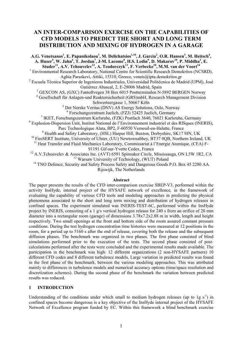
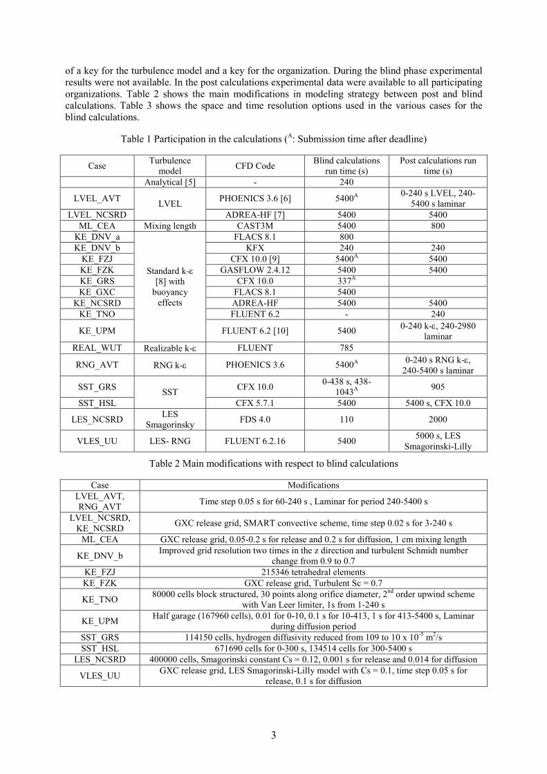
Table 1 shows that the participation in the blind and post benchmark exercise was large: 12

organizations, two of which were non-HYSAFE partners (AVT and GRS), with 10 different CFD

codes applying 8 different turbulence models. Code name for each case is defined using a combination

3

of a key for the turbulence model and a key for the organization. During the blind phase experimental

results were not available. In the post calculations experimental data were available to all participating

organizations. Table 2 shows the main modifications in modeling strategy between post and blind

calculations. Table 3 shows the space and time resolution options used in the various cases for the

blind calculations.

Table 1 Participation in the calculations (A: Submission time after deadline)

Case Turbulence

model CFD Code

Blind calculations

run time (s)

Post calculations run

time (s)

Analytical [5] - 240

LVEL_AVT PHOENICS 3.6 [6] 5400A

0-240 s LVEL, 240-

5400 s laminar

LVEL_NCSRD

LVEL

ADREA-HF [7] 5400 5400

ML_CEA Mixing length CAST3M 5400 800

KE_DNV_a FLACS 8.1 800

KE_DNV_b KFX 240 240

KE_FZJ CFX 10.0 [9] 5400A 5400

KE_FZK GASFLOW 2.4.12 5400 5400

KE_GRS CFX 10.0 337A

KE_GXC FLACS 8.1 5400

KE_NCSRD ADREA-HF 5400 5400

KE_TNO FLUENT 6.2 - 240

KE_UPM

Standard k-ε [8] with

buoyancy

effects

FLUENT 6.2 [10] 5400 0-240 k-ε, 240-2980

laminar

REAL_WUT Realizable k-ε FLUENT 785

RNG_AVT RNG k-ε PHOENICS 3.6 5400A

0-240 s RNG k-ε, 240-5400 s laminar

SST_GRS CFX 10.0 0-438 s, 438-

1043A

905

SST_HSL

SST

CFX 5.7.1 5400 5400 s, CFX 10.0

LES_NCSRD LES

Smagorinsky FDS 4.0 110 2000

VLES_UU LES- RNG FLUENT 6.2.16 5400 5000 s, LES

Smagorinski-Lilly

Table 2 Main modifications with respect to blind calculations

Case Modifications

LVEL_AVT,

RNG_AVT Time step 0.05 s for 60-240 s , Laminar for period 240-5400 s

LVEL_NCSRD,

KE_NCSRD GXC release grid, SMART convective scheme, time step 0.02 s for 3-240 s

ML_CEA GXC release grid, 0.05-0.2 s for release and 0.2 s for diffusion, 1 cm mixing length

KE_DNV_b Improved grid resolution two times in the z direction and turbulent Schmidt number

change from 0.9 to 0.7

KE_FZJ 215346 tetrahedral elements

KE_FZK GXC release grid, Turbulent Sc = 0.7

KE_TNO 80000 cells block structured, 30 points along orifice diameter, 2

nd order upwind scheme

with Van Leer limiter, 1s from 1-240 s

KE_UPM Half garage (167960 cells), 0.01 for 0-10, 0.1 s for 10-413, 1 s for 413-5400 s, Laminar

during diffusion period

SST_GRS 114150 cells, hydrogen diffusivity reduced from 109 to 10 x 10-5 m

2/s

SST_HSL 671690 cells for 0-300 s, 134514 cells for 300-5400 s

LES_NCSRD 400000 cells, Smagorinski constant Cs = 0.12, 0.001 s for release and 0.014 for diffusion

VLES_UU GXC release grid, LES Smagorinski-Lilly model with Cs = 0.1, time step 0.05 s for

release, 0.1 s for diffusion

4

Table 3 Space and time resolution options (blind calculations)

Case Domain / Grid / Convective scheme Time step , Time scheme

LVEL_AVT and

RNG_AVT Half garage, 38×52×35 cells, 8 cells of 0.0044 m each for half the orifice, Hybrid scheme

0.005 s for 0-1 s; 0.01 s for 2-5 s; 0.025 s for 6-

10 s; 0.05 s for 11-60 s; 0.1 s for 61-240 s; 0.8 s

for 241-400 s; 2 s for 401-1000 s; 4 s for 1001-

5400 s, First order fully implicit

LVEL_NCSRD

and KE_NCSRD

Half garage, extended 1m beyond door, 27x91x37 cells, 1cm horizontal, 2cm vertical, FOU (first

order upwind) scheme

0.01-0.05 s for 3-240 s and 1 s for 260-5400 s,

Fully implicit 2nd order

ML_CEA 2 nodes in the orifice radius, 2nd order in space

0.05 s from 240-360 s and then a gradual

increase up to 1 s, Semi-implicit first order

KE_DNV_a Full garage, 37506 Structured, One grid cell in the jet outlet

KE_DNV_b Full garage, 97104 cells Structured, One grid cell in the jet outlet, Upwind scheme, (90 % 2

nd

order, 10 % 1rst order) 0.1 s for 240-1180 s, Implicit

KE_FZJ Half garage, 69654 cells (tetrahedral), H2 source is a semi circle composed of 14 cell faces and

side lengths between ~ 3 and ~ 10 mm., High resolution scheme

0.0001-0.05 s for 0-1 s, 0.05 s for 1-240 s,

0.05-0.5 s for 240-560 s, 0.5 s for 560-1290, 1 s

for the rest, Second order

KE_FZK Full garage, 31 x 59 x 45 cells, 1.861 cm x 1.772 cm x 3.5 cm, FOU scheme 0.0005 s for release, 0.001-0.02 s for diffusion,

First order explicit

KE_GRS and

SST_GRS

Full garage, 147500 structured, 7500 unstructured cells, High Resolution (2nd order), 48 cells in

the orifice 112 cells across chamber 0.08-2 s, 2

nd order

KE_GXC

Full garage, 0.9m beyond door, 29 x 46 x 33 cells during 0-500 s, One grid cell in the jet outlet,

5 cm from the floor to the top of the release chamber with smooth transition to 10 cm further

from the orifice, 9 x 18 x 29 cells during 500-5400 s, Kappa schemes with weighting between

2nd order upwind and 2

nd order central difference. Delimiters are used for some equations

0.00567 s for 240-5400 s, first order

KE_UPM 335920 structured hexahedral mesh, 1.7 mm close to source, Second order upwind 0.01 for 0-10, 0.1 s for 10-240, 1 s for 240-

1000 s, 10 s for 240-5400 s, First order implicit

REAL_WUT Grid size near inlet mean value =70 mm 0.0001 s for 240-5400 s, 2nd order implicit

SST_HSL

205821 (six layers of prismatic cells in the near-wall region and tetrahedral cells elsewhere),

mesh size is between 0.0024 m and 0.003 m in the region near the orifice, FOU for k, ε, ω

(frequency) For other variables 20% FOU and 80% CDS (central differences)

0.5 s for 240-5400 s, 2nd order

LES_NCSRD 550000 cells structured 0.001 s for release

VLES_UU 160928 (unstructured tetrahedral), 0.015 m in vicinity of the hydrogen inflow, ~ about 0.03 m

close to vents, ~ 0.15-0.20 m in the rest of the domain, Power law scheme

0.0025 s for release, up to 1 s for diffusion,

implicit

5

4 RESULTS AND DISCUSSION

In order to perform a qualitative and quantitative evaluation of the overall SBEP (Standard Benchmark

Exercise Problem) results mean hydrogen concentrations were calculated by averaging the individual

time series for each sensor and each CFD case or experiment. Release and diffusion phases have been

treated separately. An averaging period from 30 to 240 s was used for the release phase and from 300

to 5400 s for the diffusion phase.

Calculated mean experimental molar concentrations Co (%) are presented in Table 4. Ratios between

predicted (Cp) and observed mean hydrogen concentrations, as function of sensor number with

different symbols for each CFD case are shown in Figure 2 and Figure 3 for the blind and post

calculations of the release phase and in Figure 6 and Figure 7 for the blind and post calculations of the

diffusion phase respectively. For the cases where post calculations were not performed, blind phase

results were used in the post-phase figures.

Quantitative evaluation of the SBEP results was performed using statistical performance measures.

Mean relative bias (MRB) and mean relative square error (MRSE) were used in this work, to quantify

bias and spread, because they are considered more balanced with respect to high and low

concentration values than other measures, see [11]. Table 4 presents the calculated MRB and MRSE

values for each sensor. In the definition of MRB and MRSE given below over-bars denote averaging

over all CFD cases for a given sensor. Optimum values of MRB and MRSE are zero, denoting zero

bias and spread respectively. A positive MRB shows that the model overestimates the experimental

data.

+

−≡

op

op

CC

CCMRB 2 ,

2

4

+

−≡

op

op

CC

CCMRSE

Table 4 Mean experimental concentrations (molar %), Mean Relative Bias (MRB) and Mean Relative

Square Error (MRSE) over all CFD runs for each sensor

Release phase Diffusion phase

Blind Post Blind Post Sensor Co

(%) MRB MRSE MRB MRSE

Co

(%) MRB MRSE MRB MRSE

1 7.34 0.12 0.08 0.11 0.05 7.37 -0.33 0.14 -0.15 0.04

4 5.97 0.00 0.01 0.03 0.01 7.36 -0.33 0.14 -0.15 0.04

6 5.30 -0.06 0.02 0.00 0.02 7.39 -0.33 0.14 -0.15 0.04

7 4.69 0.05 0.02 0.11 0.03 7.21 -0.30 0.13 -0.13 0.03

8 4.70 -0.06 0.03 -0.01 0.02 7.19 -0.31 0.13 -0.13 0.03

9 3.78 0.00 0.02 0.08 0.02 6.84 -0.29 0.12 -0.11 0.03

10 3.07 -0.12 0.06 -0.06 0.02 5.57 -0.19 0.06 -0.04 0.01

11 0.66 0.55 0.73 0.44 0.38 2.87 0.24 0.07 0.18 0.07

12 0.06 0.93 2.04 0.36 1.69 0.89 0.76 0.79 0.17 0.62

13 6.52 0.27 0.14 0.25 0.10 7.29 -0.32 0.14 -0.14 0.04

14 8.04 0.16 0.12 0.15 0.07 6.84 -0.29 0.12 -0.11 0.03

16 16.50 0.06 0.16 0.13 0.09 2.75 0.28 0.10 0.20 0.10

4.1 Release phase

Before comparing the CFD predictions with the present experimental data, it is important to compare

the data with other experiments or available correlations. It is well known [12] that the jet flow can be

divided into three regions according to the relative importance of buoyancy: the non-buoyant jet

region (NBJ for 5.0≤MoLz ), the buoyant jet region (BJ for 55.0 ≤≤ MoLz ) and the buoyant

6

plume region (BP for 5≤MoLz ), where z here denotes the vertical distance from the source and MoL

is the Morton length scale (≈ 0.23 m in the present experiment). In the definitions below ω is the ratio

between ambient (air) and density at source (hydrogen), which is approximately 14.4 and F is the

densimetric Froude number (≈ 513).

dFLMo41

21 −

= ω , 0ρ

ρω a= ,

( )gdU

Fa 0

2

00

ρρρ−

=

Table 5 presents hydrogen molar concentrations for sensors 13-16 calculated using the correlation for

axi-symmetric buoyant plumes suggested by [13]. For sensor 16, which lies marginally inside the

buoyant jet region use was also made of the correlation reported in [14] valid for this region. The

applied correlations are given below in terms of mass fraction (f) similarity. Also shown in Table 5 are

molar concentrations calculated under the Boussinesqu approximation (f<<1). The relationship

between molar concentration and mass fraction given below under this approximation becomes:

fCBous ω≈ .

( )ω

ω1

35.9 3

13

5

Fd

zfBP

−

= , ω

ω1

4.4 16

7

8

14

5

Fd

zfBJ

−

= , ( )11 −+

=ωωf

fC

Table 5 Concentration and jet region for sensors 13-16 from similarity compared with experiment

Sensor MoLz Region BousC (vol. %) C (vol. %) Co (%)

16 4.79 BJ 20.11

(22.21 for BP)

16.94

(18.40 for BP) 16.50

15 6.94 BP 12.00 10.80 -

14 9.09 BP 7.67 7.16 8.04

13 10.39 BP 6.15 5.82 6.52

Table 5 shows that the present mean axial experimental concentration in the plume region are higher

compared to the Chen and Rodi (1980) correlations. Larger mean concentrations and narrower plumes

were also reported in the measurements by Dai et al. [15]. These authors suggested a coefficient value

of 10.73 instead of the value of 9.35 suggested by Chen and Rodi and the much lower value of 7.75

suggested by George at al. [16]. For sensor 16 on the other hand the experimental concentration is

lower compared to the buoyant jet correlation of Paranjpe (2004) as well as that of Ogino et al. [17],

who reported a coefficient value of 4.8 instead of 4.4 for Paranjpe.

The CFD predictions are examined next. A general observation for the blind calculations is that

predicted mean concentrations were generally in the range of factor of 2 (from 1/2 to 2 times) with

respect to experiment. Such spread was expected given the blind character of the exercise as well as

previous experience [1]. Figure 2 and Table 4 show that the maximum spread is observed for sensors

11 and 12, located far from the jet axis and closest to ground. From the remaining sensors those lying

along the jet axis (1, 13, 14, 16) present the highest spread, with a maximum observed for sensor 16.

The high spread for sensor 16 was unexpected, since this sensor is located the closest to the source.

For the post calculations of the release phase Figure 3 shows that the spread has been reduced but not

significantly. Table 4 shows that MRSE values were improved by 44% for sensor 16, 17% for sensor

12 and 48 % for sensor 11.

The observed variation between various predictions can in general be attributed to differences in the

physical models applied, to differences in the numerical options or to differences in both. Below the

various predictions are examined in groups of same turbulence model. This way one can trace any

spread between predictions to numerical options. Discussion will be focused on sensor 16 for which

7

predicted concentration time series compared to experiment are presented in Figure 4 for the blind and

Figure 5 for the post calculations.

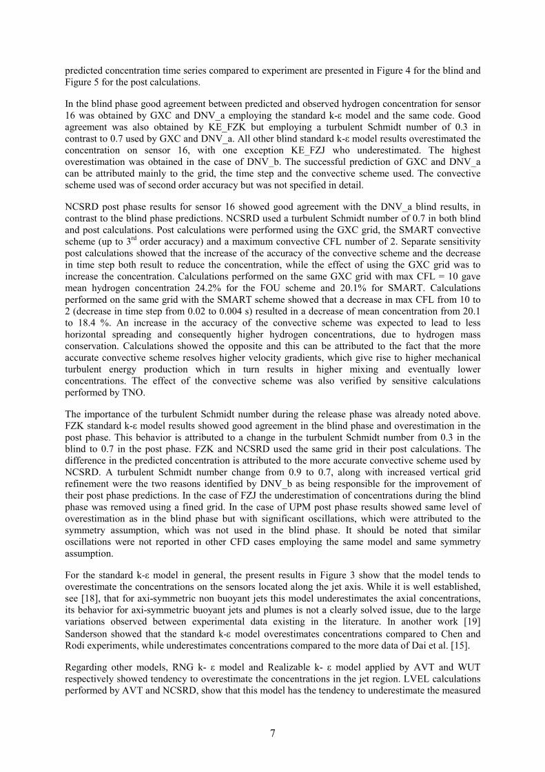
In the blind phase good agreement between predicted and observed hydrogen concentration for sensor

16 was obtained by GXC and DNV_a employing the standard k-ε model and the same code. Good

agreement was also obtained by KE_FZK but employing a turbulent Schmidt number of 0.3 in

contrast to 0.7 used by GXC and DNV_a. All other blind standard k-ε model results overestimated the

concentration on sensor 16, with one exception KE_FZJ who underestimated. The highest

overestimation was obtained in the case of DNV_b. The successful prediction of GXC and DNV_a

can be attributed mainly to the grid, the time step and the convective scheme used. The convective

scheme used was of second order accuracy but was not specified in detail.

NCSRD post phase results for sensor 16 showed good agreement with the DNV_a blind results, in

contrast to the blind phase predictions. NCSRD used a turbulent Schmidt number of 0.7 in both blind

and post calculations. Post calculations were performed using the GXC grid, the SMART convective

scheme (up to 3rd order accuracy) and a maximum convective CFL number of 2. Separate sensitivity

post calculations showed that the increase of the accuracy of the convective scheme and the decrease

in time step both result to reduce the concentration, while the effect of using the GXC grid was to

increase the concentration. Calculations performed on the same GXC grid with max CFL = 10 gave

mean hydrogen concentration 24.2% for the FOU scheme and 20.1% for SMART. Calculations

performed on the same grid with the SMART scheme showed that a decrease in max CFL from 10 to

2 (decrease in time step from 0.02 to 0.004 s) resulted in a decrease of mean concentration from 20.1

to 18.4 %. An increase in the accuracy of the convective scheme was expected to lead to less

horizontal spreading and consequently higher hydrogen concentrations, due to hydrogen mass

conservation. Calculations showed the opposite and this can be attributed to the fact that the more

accurate convective scheme resolves higher velocity gradients, which give rise to higher mechanical

turbulent energy production which in turn results in higher mixing and eventually lower

concentrations. The effect of the convective scheme was also verified by sensitive calculations

performed by TNO.

The importance of the turbulent Schmidt number during the release phase was already noted above.

FZK standard k-ε model results showed good agreement in the blind phase and overestimation in the

post phase. This behavior is attributed to a change in the turbulent Schmidt number from 0.3 in the

blind to 0.7 in the post phase. FZK and NCSRD used the same grid in their post calculations. The

difference in the predicted concentration is attributed to the more accurate convective scheme used by

NCSRD. A turbulent Schmidt number change from 0.9 to 0.7, along with increased vertical grid

refinement were the two reasons identified by DNV_b as being responsible for the improvement of

their post phase predictions. In the case of FZJ the underestimation of concentrations during the blind

phase was removed using a fined grid. In the case of UPM post phase results showed same level of

overestimation as in the blind phase but with significant oscillations, which were attributed to the

symmetry assumption, which was not used in the blind phase. It should be noted that similar

oscillations were not reported in other CFD cases employing the same model and same symmetry

assumption.

For the standard k-ε model in general, the present results in Figure 3 show that the model tends to

overestimate the concentrations on the sensors located along the jet axis. While it is well established,

see [18], that for axi-symmetric non buoyant jets this model underestimates the axial concentrations,

its behavior for axi-symmetric buoyant jets and plumes is not a clearly solved issue, due to the large

variations observed between experimental data existing in the literature. In another work [19]

Sanderson showed that the standard k-ε model overestimates concentrations compared to Chen and Rodi experiments, while underestimates concentrations compared to the more data of Dai et al. [15].

Regarding other models, RNG k- ε model and Realizable k- ε model applied by AVT and WUT

respectively showed tendency to overestimate the concentrations in the jet region. LVEL calculations

performed by AVT and NCSRD, show that this model has the tendency to underestimate the measured

8

concentrations. Generalized mixing length model calculations performed by CEA underestimated

concentration on sensor 16 in the blind phase, but showed significant improvement in the post phase,

possibly due to the new grid. LES Smagorinski calculations performed by NCSRD show that the

default Smagorinski constant Cs = 0.2 used in the blind phase results in significant overestimation of

concentrations, while a value of 0.12 gives concentration in close agreement to the experiment. SST

model calculations performed by HSL and GRS show that this model has the tendency to produce

hydrogen concentrations in the jet region lower than the standard k-ε model and in better agreement with the present experiment.

Finally the effect of modeling the release at the interior of the release chamber was taken into account

in the cases KE_GXC, KE_GRS, SST_HSL and SST_GRS. In the remaining cases the release was

assumed from the top of the chamber with a flat velocity profile. Sensitivity tests by GRS with SST

model showed that the first approach, which is more realistic, leads to slightly higher hydrogen

concentrations along the jet axis.

4.2 Diffusion phase

Before comparing the computational results to the experimental it is important to consider

experimental and computational hydrogen mass balance during the diffusion phase. The experimental

total hydrogen mass variation with time was approximately calculated by INERIS using the measured

hydrogen concentrations time series and assuming seven horizontally homogeneous layers between

the ceiling the sensors and the floor, with heights 5, 15, 30, 50, 50, 50 and 88 cm respectively. It was

shown that there was a limited uncontrolled linear mass loss of the order of 0.01 g/s, with the total

hydrogen mass dropping from 263 g at 322 s to 210 g at 5400 s. On the other hand, in the blind and

post diffusion phase calculations the total hydrogen mass was practically constant, approximately

equal to 240 g in most cases, corresponding to 1g/s for 240 s. The deviation of the experimental total

hydrogen mass from the preset value of 240 g was considered acceptable for further comparison with

the present CFD results.

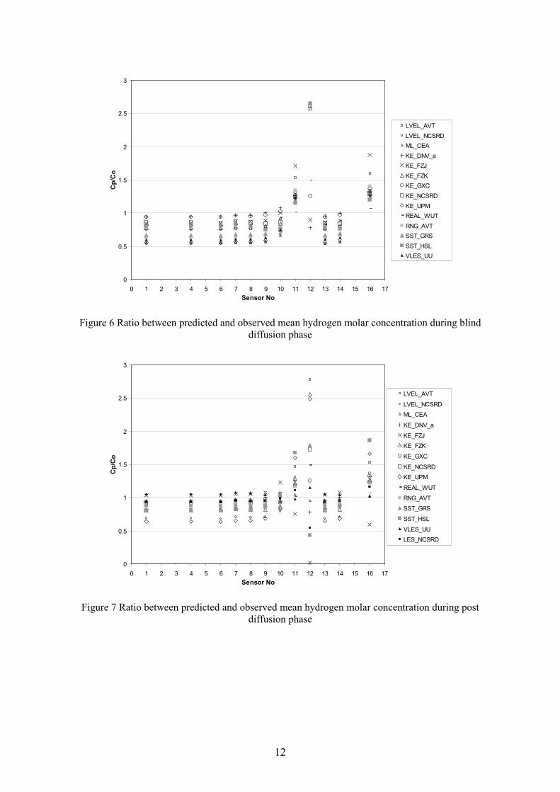
The predicted mean concentrations are shown in Figure 6 for the blind phase. It can be observed that

mean concentrations are in the range of factor of 2 with respect to experiment. It can be observed that

the models generally tend to under predict the concentrations at the sensors located closer to the

ceiling and over predict the concentrations at the sensors closest to the ground (sensors 11, 16 and 12).

This behavior suggests the explanation that the models generally tend to over predict turbulent mixing

during the diffusion phase. The highest spread in predicted mean concentrations is observed for

sensors 11, 16 and 12, with a maximum for sensor 12, being the closest to the ground. The predicted

mean concentrations for the post phase are shown in Figure 7. The two abovementioned figures along

with Table 4, summarizing the statistical results, show that both bias (MRB) and spread (MRSE) have

been reduced in the post phase. Detailed comparison between predicted and experimental

concentration time series for sensor 12 are shown in Figure 8 and Figure 9 for the blind and post

phase respectively.

Reasons identified as being mainly responsible for the improvement of the predictions in the post

phase were the time step restriction, the reduction of vertical grid spacing and the increase in the order

of the convective scheme. The molecular diffusivity of hydrogen in air used in the various CFD cases

was between 6.1 and 7.7 (x10-5 m

2/s), with the exception of GEXCON who used a value of 20.0

(default in FLACS) and GRS with a value of 109.0 (due to a typing error). In the post phase the

SST_GRS results were improved (less mixing) and GRS attributed this to the molecular diffusivity

reduced by one order of magnitude. Laminar flow was forced during the post diffusion phase, by

explicitly turning the turbulence model off, in three of the cases: LVEL_AVT, RNG_AVT and

KE_UPM. Results for flammable volume (see below) were improved compared to the corresponding

blind calculations for two of these cases: RNG_AVT and KE_UPM. Given that in the other CFD cases

excessive diffusion was avoided without the option of “manually” turning the turbulence model off

suggests that this option cannot be regarded as a general rule.

9

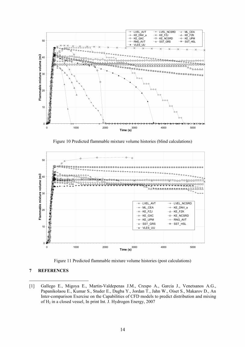
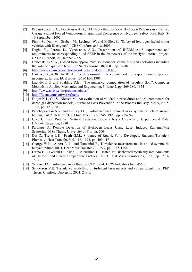
For risk assessment it is important to know the flammable mixture volume and flammable hydrogen

mass distribution in space and time. The predicted flammable mixture volume as function of time for

each CFD case is shown in Figure 10 and Figure 11 for the blind and post phases respectively. Blind

predictions show two types of physical behavior, either approximately constant stratification or fast

transition to homogeneous hydrogen distribution in the room. It is noted that the second behavior is

associated with the total flammable mixture volume becoming zero, since the corresponding mean

hydrogen concentration would be 3.53% (2.76 m3 released hydrogen homogeneously distributed in a

78.38 m3 room). The corresponding experimental behavior can be drawn from Table 4. Mean

experimental concentrations reported in Table 4 for the diffusion phase show that a layer of hydrogen

exists close to the ceiling, which is horizontally quasi homogeneous and vertically stratified with the

limit of the flammable cloud between sensors 10 and 11. This gives an estimated experimental

flammable volume between 27.2 and 40.8 m3. Therefore it can be concluded that predicted flammable

volumes below and above these limits should rather be considered as not corresponding to

experimental behavior.

5 CONCLUSIONS

A blind and post CFD benchmark exercise was organized within HYSAFE in order to evaluate various

modeling approaches in predicting the physical phenomena associated to the short and long term

mixing and distribution of hydrogen releases in confined spaces. The experiment simulated was

INERIS-TEST-6C. The performed analysis led to the following conclusions:

The effect of the turbulence model is clearly important. In the jet region during the release phase the

standard k-ε model when applied without previous knowledge of the experimental data (blind

prediction) generally tended to overestimate the concentrations. This was shown to be rectified either

using a low turbulent Schmidt number (0.3) in combination with a first order upwind scheme or using

the usual value of 0.7 for turbulent Schmidt combined with a smaller time step and higher order

convective scheme. From the two approaches the second is recommended. RNG k- ε and Realizable k-

ε models showed tendency to overestimate the concentrations. LVEL model generally tended to

underestimate concentrations. The SST model was found to produce hydrogen concentrations in the jet

region lower than the standard k-ε model and in better agreement with the present experiment. The LES Smagorinski model was found in good agreement with measured concentrations when the

Smagorinski constant was set equal to 0.12.

In the diffusion phase blind predictions showed two types of physical behavior, either approximately

constant stratification or fast transition to homogeneous hydrogen (non-flammable) distribution in the

room. Experiments showed that a layer of hydrogen exists close to the ceiling, which is horizontally

quasi homogeneous and vertically stratified. Improvement of the predictions and reduction of spread

between models was achieved in the post phase mainly by applying time step restrictions, reduction of

vertical grid spacing and increase of the order of the convective scheme. The option of “manually”

turning the turbulence model off although improved predictions in some cases cannot be suggested as

a general recommendation. Comparison between predicted and observed concentrations shows that the

models generally tend to overestimate turbulent mixing.

Finally the whole exercise helped the HYSAFE consortium as well as the external collaborating

organizations in obtaining consensus regarding issues associated with prediction of hydrogen releases

in confined spaces. Further CFD benchmark exercises are planned within HYSAFE in the near future.

6 ACKNOWLEDGEMENTS

The authors would like to thank the European Commission for funding of this work in the framework

of the HYSAFE FP6 Network of Excellence (contract no. SES6-CT-2004-502630). TNO contribution

was in cooperation between TNO and the University of Technology Delft (Dr. M.J.B.M. Pourquie).

10

0

0.5

1

1.5

2

2.5

3

0 1 2 3 4 5 6 7 8 9 10 11 12 13 14 15 16 17

Sensor No

Cp/Co

LVEL_AVT

LVEL_NCSRD

ML_CEA

KE_DNV_a

KE_DNV_b

KE_FZJ

KE_FZK

KE_GRS

KE_GXC

KE_NCSRD

KE_UPM

REAL_WUT

RNG_AVT

SST_GRS

SST_HSL

VLES_UU

LES_NCSRD

Figure 2 Ratio between predicted and observed mean hydrogen molar concentration during blind

release phase

0

0.5

1

1.5

2

2.5

3

0 1 2 3 4 5 6 7 8 9 10 11 12 13 14 15 16 17

Sensor No

Cp/Co

LVEL_AVT

LVEL_NCSRD

ML_CEA

KE_DNV_a

KE_DNV_b

KE_FZJ

KE_FZK

KE_GRS

KE_GXC

KE_NCSRD

KE_TNO

KE_UPM

REAL_WUT

RNG_AVT

SST_GRS

SST_HSL

VLES_UU

LES_NCSRD

Figure 3 Ratio between predicted and observed mean hydrogen molar concentration during post

release phase

11

Sensor 16

0

5

10

15

20

25

30

35

40

0 100 200 300 400 500Time (s)

H2 concentration (by vol. %)

LVEL_AVT LVEL_NCSRD

ML_CEA KE_DNV_a

KE_DNV_b KE_FZJ

KE_FZK KE_GXC

KE_GRS KE_NCSRD

KE_UPM REAL_WUT

RNG_AVT SST_GRS

SST_HSL VLES_UU

LES_NCSRD EXP_INERIS

Figure 4 Predicted hydrogen concentration (vol. %) histories for sensor 16 (blind calculations)

Sensor 16

0

5

10

15

20

25

30

35

40

0 100 200 300 400 500Time (s)

H2 concentration (by vol. %)

LVEL_AVT LVEL_NCSRD

ML_CEA KE_DNV_a

KE_DNV_b KE_FZJ

KE_FZK KE_GRS

KE_GXC KE_NCSRD

KE_TNO KE_UPM

REAL_WUT RNG_AVT

SST_GRS SST_HSL

VLES_UU LES_NCSRD

EXP_INERIS

Figure 5 Predicted hydrogen concentration (vol. %) histories for sensor 16 (post calculations)

12

0

0.5

1

1.5

2

2.5

3

0 1 2 3 4 5 6 7 8 9 10 11 12 13 14 15 16 17

Sensor No

Cp/Co

LVEL_AVT

LVEL_NCSRD

ML_CEA

KE_DNV_a

KE_FZJ

KE_FZK

KE_GXC

KE_NCSRD

KE_UPM

REAL_WUT

RNG_AVT

SST_GRS

SST_HSL

VLES_UU

Figure 6 Ratio between predicted and observed mean hydrogen molar concentration during blind

diffusion phase

0

0.5

1

1.5

2

2.5

3

0 1 2 3 4 5 6 7 8 9 10 11 12 13 14 15 16 17

Sensor No

Cp/Co

LVEL_AVT

LVEL_NCSRD

ML_CEA

KE_DNV_a

KE_FZJ

KE_FZK

KE_GXC

KE_NCSRD

KE_UPM

REAL_WUT

RNG_AVT

SST_GRS

SST_HSL

VLES_UU

LES_NCSRD

Figure 7 Ratio between predicted and observed mean hydrogen molar concentration during post

diffusion phase

13

Sensor 12

0

1

2

3

4

5

6

0 1000 2000 3000 4000 5000Time (s)

H2 concentration (by vol. %)

LVEL_AVT LVEL_NCSRD

ML_CEA KE_DNV_a

KE_FZJ KE_FZK

KE_GXC KE_NCSRD

KE_UPM REAL_WUT

RNG_AVT SST_GRS

SST_HSL VLES_UU

EXP_INERIS

Figure 8 Predicted hydrogen concentration (vol. %) histories for sensor 12 (blind calculations)

Sensor 12

0

1

2

3

4

5

6

0 1000 2000 3000 4000 5000Time (s)

H2 concentration (by vol. %)

LVEL_AVT LVEL_NCSRD

ML_CEA KE_DNV_a

KE_FZJ KE_FZK

KE_GXC KE_NCSRD

KE_UPM REAL_WUT

RNG_AVT SST_GRS

SST_HSL VLES_UU

LES_NCSRD EXP_INERIS

Figure 9 Predicted hydrogen concentration (vol. %) histories for sensor 12 (post calculations)

14

0

10

20

30

40

50

0 1000 2000 3000 4000 5000Time (s)

Flammable mixture volume (m3)

LVEL_AVT LVEL_NCSRD ML_CEA

KE_DNV_a KE_FZJ KE_FZK

KE_GXC KE_NCSRD KE_UPM

RNG_AVT SST_GRS SST_HSL

VLES_UU

Figure 10 Predicted flammable mixture volume histories (blind calculations)

0

10

20

30

40

50

0 1000 2000 3000 4000 5000Time (s)

Flammable mixture volume (m3)

LVEL_AVT LVEL_NCSRD

ML_CEA KE_DNV_a

KE_FZJ KE_FZK

KE_GXC KE_NCSRD

KE_UPM RNG_AVT

SST_GRS SST_HSL

VLES_UU

Figure 11 Predicted flammable mixture volume histories (post calculations)

7 REFERENCES

[1] Gallego E., Migoya E., Martin-Valdepenas J.M., Crespo A., Garcia J., Venetsanos A.G.,

Papanikolaou E., Kumar S., Studer E., Dagba Y., Jordan T., Jahn W., Oíset S., Makarov D., An

Inter-comparison Exercise on the Capabilities of CFD models to predict distribution and mixing

of H2 in a closed vessel, In print Int. J. Hydrogen Energy, 2007

15

[2] Papanikolaou E.A., Venetsanos A.G., CFD Modelling for Slow Hydrogen Releases in a Private

Garage without Forced Ventilation, International Conference on Hydrogen Safety, Pisa, Italy, 8-

10 September, 2005

[3] Fürst, S., Dub, M., Gruber, M., Lechner, W. and Müller, C, "Safety of hydrogen-fueled motor

vehicles with IC engines", ICHS Conference Pisa 2005

[4] Dagba Y., Perette L., Venetsanos A.G., Description of INERIS-test-6 experiment and

requirements for corresponding blind SBEP in the framework of the InsHyde internal project,

HYSAFE report, 24 October 2005

[5] Delichatsios M.A., Closed form approximate solutions for smoke filling in enclosures including

the volume expansion term, Fire Safety Journal 38, 2003, pp. 97-101.

[6] http://www.cham.co.uk/phoenics/d_polis/d_docs/tr000.htm

[7] Bartzis J.G., ADREA-HF: A three dimensional finite volume code for vapour cloud dispersion

in complex terrain, EUR report 13580 EN, 1991.

[8] Launder B.E. and Spalding D.B., “The numerical computation of turbulent flow”, Computer

Methods in Applied Mechanics and Engineering, 3, Issue 2, pp. 269-289, 1974

[9] http://www.ansys.com/products/cfx.asp

[10] http://fluent.com/software/fluent/

[11] Duijm N.J., Ott S., Nielsen M., An evaluation of validation procedures and test parameters for

dense gas dispersion models, Journal of Loss Prevention in the Process Industry, Vol 9, No 5,

1996, pp. 323-338.

[12] Panchapakesan N.R. and Lumley J.L., Turbulence measurement in axisymmetric jets of air and

helium, part 2. Helium Jet, J. Fluid Mech., Vol. 246, 1993, pp. 225-247.

[13] Chen C.J. and Rodi W., Vertical Turbulent Buoyant Jets - A review of Experimental Data,

HMT-4. Pergamon, 1980

[14] Paranjpe S., Remote Detection of Hydrogen Leaks Using Laser Induced Rayleigh/Mie

Scattering, MSc Thesis, University of Florida, 2004

[15] Dai Z., Tseng L-K., Faeth G.M., Structure of Round, Fully Developed, Buoyant Turbulent

Plumes, J. Heat Transfer, Vol. 116, 1994, pp. 409-417

[16] George W.K., Alpert R. L. and Tamanini F., Turbulence measurements in an axi-symmetric

buoyant plume, Int. J. Heat Mass Transfer 20, 1977, pp. 1145-1154

[17] Ogino F., Takeuchi H., Kudo I., Mizushina T., Heated Jet Discharged Vertically into Ambients

of Uniform and Linear Temperature Profiles, Int. J. Heat Mass Transfer 23, 1980, pp. 1581-

1588

[18] Wilcox D.C. Turbulence modelling for CFD, 1994, DCW Industries Inc., 456 p.

[19] Sanderson V.E. Turbulence modelling of turbulent buoyant jets and compartment fires, PhD

Thesis, Cranfield University 2001, 248 p.