An h-adaptive method in the generalized finite differences

J.J. Benito a,*, F. Ure~nna a, L. Gavete b, R. Alvarez c

a Escuela T�eecnica Superior de Ingenieros Industriales, U.N.E.D., Apdo. Correos 60149, Madrid 28080, Spainb Escuela T�eecnica Superior de Ingenieros de Minas, U.P.M., C/Rios Rosas 21, Madrid 280003, Spain

c Escuela T�eecnica Superior de Ingenieros Industriales, U.P.M., C/Jos�ee Gutierrez Abascal 2, Madrid 28006, Spain

Received 25 May 2001; received in revised form 2 October 2002

Abstract

This paper describes an h-adaptive method in generalized finite difference (GFD) to solve second-order partialdifferential equations. These equations representing the behaviour of many physical processes. The explicit difference

formulae obtained make it possible to propose an a posteriori error indicator which serves as starting point for an h-adaptive method to improve the solution by selectively adding nodes to the domain.

This paper also analyses the influence of key parameters, as the number of nodes to add in each step or the minimum

distance between nodes, through the analysis of the obtained solutions for different types of differential equations.

� 2002 Elsevier Science B.V. All rights reserved.

Keywords: Adaptive methods; Generalized finite differences; Meshless methods; Posteriori error indicator

1. Introduction

The rapid development of computer technology has allowed the use of finite difference methods to solve

partial differential equations in irregular meshes. In 1953 MacNeal [16] and in 1960 Forsythe and Wasow [7]proposed the division of irregular grids into regular subdomains. Later on, Frey [8] considered irregular

subdomains with restricted topology.

In 1972 Jensen [10] published the basis of a finite difference method which made use of irregular grids

with six point stars. Using Taylor�s series expansion he obtained finite difference formulae which ap-proached derivatives up to the second-order. The main disadvantage of this method was the frequent

singularity or ill-conditioning of the star. In order to overcome this handicap, Perrone and Kao [22]

suggested adding nodes in the star, while Szmelter and Kurowski [23] proposed the triangulation of the

domain, replacing the stars by the nodes situated in the vertices of triangles, all of which with a commoncentral point. Tribillo [24], Cendrowicz and Tribillo [5] and Kaczkowski and Tribillo [11] all followed

*Corresponding author. Tel.: +34-91-3986457; fax: +34-91-3986046.

E-mail address: jbenito@ind.uned.es (J.J. Benito).

0045-7825/03/$ - see front matter � 2002 Elsevier Science B.V. All rights reserved.

PII: S0045-7825 (02 )00594-7

Comput. Methods Appl. Mech. Engrg. 192 (2003) 735–759

www.elsevier.com/locate/cma

similar approaches. Out of these papers, representing early stage of the method, the most elaboratedversion was given by Wyatt et al. [25].

The idea of using an eight node star and weight functions to obtain finite difference formulae for ir-

regular meshes, was first put forward by Liska and Orkisz [13,14], using moving least squares (MLS) in-

terpolation, and the most advanced version of the generalized finite difference method (GFDM) was given

by Orkisz [19–21], including: mesh generation, local approximation, generation of finite difference (FD)

formulae and FD equations resulting from local (collocation) or global (Galerkin, variational,. . .) for-mulations. GFDM is included in the so-called meshless methods (MM) [1,2,6,14,15,17,18]. A meshless

methods overview is given in [3,21]. In Lancaster and Salkauskas [12] is described the moving least squaresapproximation that it is used in MM.

The subject of error approximation for GFDMmethod and a consequent adaptive analysis, in which the

approximation is successively refined to reach predetermined standards of accuracy, is central to the ef-

fective use of computer codes for practical engineering analysis. Orkisz [19] presented an adaptive multigrid

GFDM. A solution convergence rate

bki ¼

kuki � uk�1i kkuki k

6 c3 8i ¼ 1; . . . ; no: of common nodes ð1Þ

is examined at those nodes Pi, i ¼ 1; 2; . . . which keep the same location in the subsequent meshes . . . ;k � 2; k � 1; k; . . .; c3 is an imposed threshold value resulting from the required solution precision. Using aserror indicators the residuals of the solution and bk

i , a series of more and more dense meshes can be

generated to establish an adaptive solution process. Also Orkisz [21] presented an error estimator for the

GFDM.

In this paper we present an h-adaptive procedure for the generalized finite difference (GFD) based in asimple error indicator that it is used to solve different partial differential equations of second-order which

represent the behaviour of many physical processes.

The paper is organised as follows. Section 2 describes a posteriori error indicator using GFDM. Section

3 analyses several ways of reducing error. The h-adaptive method proposed in this paper is given in Section4. Section 5 illustrates the performance of the presented adaptive method in different partial differential

equations with known analytical solutions, including the selection of the key parameters involved. Finally,

in Section 6 some conclusions are given.

2. A posteriori error indicator in the generalized finite differences

Let us consider a problem governed by

L2½U � ¼ f in X ð2aÞ

with boundary conditions

L1½U � ¼ g on C; ð2bÞwhere X R2 with boundary C; L2 and L1 are linear partial differential second- and first-order operatorsrespectively; and f and g two known functions.On defining the central node with a set of nodes surrounding the same, the star then refers to a group of

established nodes in relation to a central node. In general each node in the domain is assigned an associated

star. If U0 is the value of the function at the central node of the star and Ui the function values at the rest of

nodes, with i ¼ 1; . . . ;N , then, according to the Taylor series expansion it is known that

736 J.J. Benito et al. / Comput. Methods Appl. Mech. Engrg. 192 (2003) 735–759

Ui ¼ U0 þ hioU0ox

þ kioU0oy

þ 12

h2io2U0ox2

�þ k2i

o2U0oy2

þ 2hikio2U0oxoy

�þ � � � ; ð3Þ

where (x0, y0) are the coordinates of the central node, (xi, yi) the coordinates of the ith node in the star andhi ¼ xi � x0, ki ¼ yi � y0.If the unwritten terms in the equation above are ignored, an approximation of second-order for the Ui

function is obtained, which is indicated as ui, and when ignoring the terms over the fourth-order in the sameEq. (3), an approximation of third-order for Ui is obtained. It is then possible to define the functions B5ðuÞand B9ðuÞ as in [4,21]

B5ðuÞ ¼XNi¼1

u0

��� ui þ hi

ou0ox

þ kiou0oy

þ h2i2

o2u0ox2

þ k2i2

o2u0oy2

þ hikio2u0oxoy

�wðhi; kiÞ

�2; ð4Þ

B9ðuÞ ¼XNi¼1

u0

��� ui þ hi

ou0ox

þ kiou0oy

þ h2i2

o2u0ox2

þ k2i2

o2u0oy2

þ hikio2u0oxoy

þ h3i6

o3u0ox3

þ h2i ki2

o3u0ox2 oy

þ hik2i2

o3u0oxoy2

þ k3i6

o3u0oy3

�wðhi; kiÞ

�2; ð5Þ

where B5ðuÞ and B9ðuÞ are two norms corresponding to the second- and third-order approximations, re-spectively, and wðhi; kiÞ a weighting function.If the norms B5ðuÞ and B9ðuÞ are minimised with respect to the partials derivatives, included in formulae

(4) and (5), respectively, the following linear equations systems are obtained

APDuP ¼ bP; ð6Þwhere the AP are matrices of 5� 5, when P ¼ 5, and 9� 9, when P ¼ 9, and the vectors DuP are given by

Du5 ¼ou0ox

;ou0oy

;o2u0ox2

;o2u0oy2

;o2u0oxoy

� �T; ð7Þ

Du9 ¼ou0ox

;ou0oy

;o2u0ox2

;o2u0oy2

;o2u0oxoy

;o3u0ox3

;o3u0ox2 oy

;o3u0oxoy2

;o3u0oy3

� �T; ð8Þ

where bP is the vector of independent terms, including the values u0, ui (i ¼ 1;N ) to be solved by usingGFDM as described in [4,21].From the previously obtained matrix equation (6) and, by virtue of the fact that the matrices of coef-

ficients AP are symmetrical, it is then possible to use the Cholesky method to solve the same. The aim is to

obtain the decomposition in upper and lower triangular matrices LLT. The coefficients of the matrix L are

denoted for Lði; jÞ.On solving the systems (6), the following explicit difference formulae are obtained

DuPðkÞ ¼1

Lðk; kÞ

� u0

XNi¼1

Mðk; iÞci þXNj¼1

ujXPi¼1

Mðk; iÞdji

!!; ðk ¼ 1; . . . ; P Þ; ð9Þ

in which, P ¼ 5 if only second-order Taylor series expansion terms are included and P ¼ 9 if third-orderterms are also included and where

Mði; jÞ ¼ ð�1Þ1�dij 1

Lði; iÞXi�1k¼j

Lði; kÞMðk; jÞ for j < i ði and j ¼ 1; . . . ; P Þ;

J.J. Benito et al. / Comput. Methods Appl. Mech. Engrg. 192 (2003) 735–759 737

Mði; jÞ ¼ 1

Lði; iÞ for j ¼ i ði and j ¼ 1; . . . ; PÞ;

Mði; jÞ ¼ 0 for j > i ði and j ¼ 1; . . . ; P Þ;with dij the Kronecker delta function, and

ci ¼XNj¼1

dji;

dj1 ¼ hjW 2; dj2 ¼ kjW 2; dj3 ¼h2j2W 2; dj4 ¼

k2j2W 2; dj5 ¼ hjkjW 2; dj6 ¼

h3i6W 2;

dj7 ¼k3i6W 2; dj8 ¼

h2i ki2

W 2; dj9 ¼hik2i2

W 2

where

W 2 ¼ ðwðhi; kiÞÞ2: ð10ÞOn including the explicit expressions for the values of the partial derivatives (9) in Eq. (2a) the star

equation is obtained as

k0u0 þ kiui ¼ f ðx0; y0Þ: ð11ÞThen

u0 ¼XNi¼1

miui þ mf f ð12Þ

with

XNi¼1

mi ¼ 1: ð13Þ

It is possible to go on with the idea of taking more terms of the Taylor�s series expansion to obtain theapproximate value of the function in any node of the star. The solution of a second-order partial differential

equation, by the GDFM, may then be approximated by

ui ¼ u0 þ hiou0ox

þ kiou0oy

þ 12

h2io2u0ox2

�þ 2hiki

o2u0oxoy

þ k2io2u0oy2

�

þ 16

o3u0ox3

h3i

�þ o3u0

oy3k3i þ 3

o3u0ox2 oy

h2i ki þ 3o3u0oxoy2

hik2i

�

þ 1

24

o4u0ox4

h4i

�þ 4 o4u0

ox3 oyh3i ki þ 6

o4u0ox2 oy2

h2i k2i þ 4

o4u0oxoy3

hik3i þo4u0oy4

k4i

�: ð14Þ

The difference between (14) and the second-order approximation, is

½ui�order 4 � ½ui�order 2 ¼1

6

o3u0ox3

h3i

�þ o3u0

oy3k3i þ 3

o3u0ox2 oy

h2i ki þ 3o3u0oxoy2

hik2i

�

þ 1

24

o4u0ox4

h4i

�þ 4 o4u0

ox3 oyh3i ki þ 6

o4u0ox2 oy2

h2i k2i þ 4

o4u0oxoy3

hik3i þo4u0oy4

k4i

�: ð15Þ

738 J.J. Benito et al. / Comput. Methods Appl. Mech. Engrg. 192 (2003) 735–759

The expression (15) is valid for i ¼ 1; . . . ;N , where N is the number of nodes of the star. On the otherhand, the star equation (12) indicates that the value of the function at the central node of the star, is the

weighting average of the function values at the rest of nodes, plus the corresponding to the independent

term of the differential equation (2a). The error at the central node of the star may then be approximated

(indicated) by adding the absolute values as shown in (16) for the terms involving the third- and fourth-

order partial derivatives

Indðu0Þ ¼XNi¼1

mi1

6

o3u0ox3

h3i

�� þ o3u0oy3

k3i þ 3o3u0ox2 oy

h2i ki þ 3o3u0oxoy2

hik2i

�

þ 1

24

o4u0ox4

h4i

�þ 4 o4u0

ox3 oyh3i ki þ 6

o4u0ox2 oy2

h2i k2i þ 4

o4u0oxoy3

hik3i þo4u0oy4

k4i

��þ mf f ; ð16Þ

where the third- and fourth-order partial derivatives are obtained by the explicit formula GFD (9) and

using

osu0oxq oyr

¼ oq

oxqoru0oyr

� �¼ or

oyroqu0oxq

� �; ð17Þ

where s ¼ qþ r, s ¼ 3; 4 and q; r ¼ 0; 1; 2.These formulae (16) and (17) can be easily calculated and they will be denominated in this paper as

‘‘error indicator’’. It is interesting to note that this error indicator is different of the previously developed

Orkisz error estimator [21] (see Appendix A).

3. Several means to reduce the error in the solution when solving second-order partial differential equations by

GFDM

On solving second-order partial differential equations by GFDM two types of errors are introduced in

the solution: (a) the error due to use of GFDM, and (b) the error due to truncation of terms higher than the

second-order in the generalized finite differences formulae.

The error is evaluated using the following global error formula:

Error ¼

ffiffiffiffiffiffiffiffiffiffiffiffiffiffiffiffiffiffiffiffiffiffiffiffiffiffiffiffiffiffiffiffiPN

i¼1ðsolðiÞ�exacðiÞÞ2

N

rjexacmaxj

� 100; ð18Þ

where solðiÞ is the GFDM solution in the node ‘‘i’’, exacðiÞ is the exact value of the solution in the node ‘‘i’’,exacmax is the maximum value of the exact values in the cloud of nodes considered and N is the total numberof nodes of the domain considered.

Three different approaches are tested in order to reduce these errors:

First approach. We can decrease (b)-error by increasing the number of terms of Taylor series expansionused to obtain the generalized finite differences formulae. In Table 1 the global error calculated according

Table 1

Second-order Third-order

Error (%) 1st case 4:31� 10�4 3:82� 10�4Error (%) 2nd case 2:20� 10�3 1:94� 10�3Error (%) 3rd case 1:84� 10�1 1:81� 10�1

J.J. Benito et al. / Comput. Methods Appl. Mech. Engrg. 192 (2003) 735–759 739

with formula (18) is given when solving Laplace equation in three different cases, by using GFD formulae

including second- or third-order of the Taylor series. Let us then consider three different cases, solving the

Laplace equation with Dirichlet boundary conditions, and using in all cases the weighting function,

expð�5ðx2 þ y2ÞÞ.First case. Laplace equation solution in a square domain of unit side, the cloud of points used was ir-

regular (102 nodes) and is shown as cloud 1 in Fig. 1. The exact solution for this case is Uðx; yÞ ¼ x2 � y2.Second case. Laplace equation solution in a square domain of unit side, the cloud of the points utilised

was irregular (289 nodes) and is indicated as cloud 2 in Fig. 1. The exact solution for this case is

Uðx; yÞ ¼ ex sin y.Third case. Laplace equation solution in the domain D ¼ fðx; yÞ 2 R2, 0:01 < x < 1, 0 < y < 1g. The

cloud of points utilised was irregular (80 nodes) and is indicated as cloud 3 in Fig. 1. The exact solution for

this case is Uðx; yÞ ¼ 10Logðx2 þ y2Þ.As can be appreciated in Fig. 1, three examples of clouds of different density have been chosen, always

sparse, and for different function solution regularities.

The global errors obtained in the three cases considered are given in Table 1.

It is interesting in Table 1 to compare for each case the two values corresponding to the second- and

third-order. When using more terms of Taylor series expansion to obtain the generalized finite differences

formulae of third-order, the error may be seen to be somewhat reduced as compared using until the second-

order, but in the three cases this reduction does not justify the additional amount of the calculations re-

quired.

Second approach. We can decrease (a)-error by acting over the star using different ways:

(1) Increasing the number of nodes in each of the stars in the domain. It has been shown in [4] that the

error decreases in this case, although for a number of nodes higher than eight (without the central

one), this reduction does not justify the increase in calculations.

(2) Different procedures can be followed in order to select the nodes of the stars. For example, according to

[4], and when using the quadrant criterion to select the nodes of the star, we obtain a smaller error than

with the distance criterium.

(3) Furthermore, in accordance with [4], it is also possible to decrease the error by choosing a suitableweighting function in each case.

Third approach. We can decrease (a)-error by increasing the number of nodes in the mesh. It has been

shown in [4] that the error decreases when the number of nodes is increased in a regular mesh. However, in

the case of an irregular mesh, the addition of nodes must be selective, since the distribution is not less

Fig. 1. Three examples of clouds of different density.

740 J.J. Benito et al. / Comput. Methods Appl. Mech. Engrg. 192 (2003) 735–759

important than number of nodes, and it is necessary to use an h-adaptive method as the algorithm describedin the following paragraph.

It is interesting to note that not only number, but location of nodes influences FD operator quality and

that is recommended to use good quality clouds of nodes. At the same time it is necessary to take into

account that by increasing the number of nodes of a mesh may decrease the solution error (h-adaptiveapproach), but it does not change precision of FD operators.

4. The h-adaptive method

By using the a posteriori error indicator as proposed in (16), it is possible to find an algorithm to de-

crease the error in the domain by selectively increasing the number of nodes. This algorithm is an ap-

proximated procedure, because the largest errors cannot be located in the nodes of the domain.

It is not difficult to obtain the mean value of the error indicator in the nodes of the domain and to use it

(or a multiple) as an error limit in order to mark the nodes in which the error indicator is higher than the

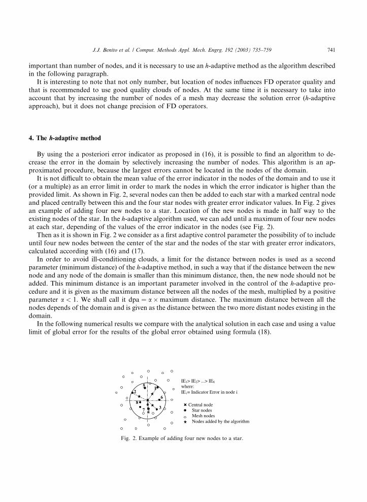
provided limit. As shown in Fig. 2, several nodes can then be added to each star with a marked central node

and placed centrally between this and the four star nodes with greater error indicator values. In Fig. 2 givesan example of adding four new nodes to a star. Location of the new nodes is made in half way to the

existing nodes of the star. In the h-adaptive algorithm used, we can add until a maximum of four new nodesat each star, depending of the values of the error indicator in the nodes (see Fig. 2).

Then as it is shown in Fig. 2 we consider as a first adaptive control parameter the possibility of to include

until four new nodes between the center of the star and the nodes of the star with greater error indicators,

calculated according with (16) and (17).

In order to avoid ill-conditioning clouds, a limit for the distance between nodes is used as a second

parameter (minimum distance) of the h-adaptive method, in such a way that if the distance between the newnode and any node of the domain is smaller than this minimum distance, then, the new node should not be

added. This minimum distance is an important parameter involved in the control of the h-adaptive pro-cedure and it is given as the maximum distance between all the nodes of the mesh, multiplied by a positive

parameter a < 1. We shall call it dpa ¼ a �maximum distance. The maximum distance between all the

nodes depends of the domain and is given as the distance between the two more distant nodes existing in the

domain.

In the following numerical results we compare with the analytical solution in each case and using a value

limit of global error for the results of the global error obtained using formula (18).

Fig. 2. Example of adding four new nodes to a star.

J.J. Benito et al. / Comput. Methods Appl. Mech. Engrg. 192 (2003) 735–759 741

5. Numerical results

This includes a selection of analysed cases in order to illustrate the influence of the parameters defined in

the previous point (error limit and minimum distance).

In these examples, as a matter of academic concern, in most of the cases we used clouds generated

uncertainly to avoid taking into consideration the exact solution to the problem. This way of generating the

clouds has not permitted consider the known criterion of uniformity, density and smooth transition in

the changes. All of this makes sometimes poor clouds. However, these poor clouds permit us to appreciatethe influence of the indicated parameters and the necessity of using the general criterions.

5.1. Influence of the error limit

In this section the previous h-adaptive method is used to solve three second-order partial differentialequations (elliptic, hyperbolic and parabolic), with the objective of checking the influence of the selected

error limit.

The following three examples show that it is preferable to apply the h-adaptive method several times andto fix progressively smaller error limits, rather than impose very small error limits at the outset. The nodes

added in each step serve as a reference for the following step, in order to obtain more balanced meshes at

the end of the process.

5.1.1. Elliptic type

Application of the adaptive method to solve Laplace equation, with the exact solution Uðx; yÞ ¼10Logðx2 þ y2Þ, using the weighting function

1

ðdistÞ3; ð19Þ

where ‘‘dist’’ is the distance between the central node and the considered node in the star and where thedomain is defined by

fðx; yÞ 2 R2; �0:5 < x < 0:5; �0:5 < y < 0:5g: ð20ÞFig. 3 shows the successive clouds of points obtained when the adaptive method is applied using the

cloud 4 as starting cloud of adaptive refinement process and taking 0.025 dmax as minimum distance (dmax

is the maximum distance between two nodes of the mesh). The clouds of points 5 and 6 are obtained for

0.05 and 0.025 values of the error limit (values to be obtained when formula (18) is applied) and are the two

last steps of a series of progressively refined clouds with error limits of 0.5, 0.25, 0.1, 0.075, 0.06, that have

been employed to go from cloud 4 until cloud 5, following the h-adaptive procedure.

Fig. 3. The successive clouds of points when the h-adaptive method is applied.

742 J.J. Benito et al. / Comput. Methods Appl. Mech. Engrg. 192 (2003) 735–759

Fig. 4 shows the reduction in the global error calculated according formula (18), when the h-adaptivemethod is applied.

5.1.2. Hyperbolic type

Application of the adaptive method to solve the equation

o2uox2

� o2uoy2

¼ 0; ð21Þ

where the exact solution is

Uðx; yÞ ¼ sinðxÞ sinðyÞ ð22Þand when using the weighting function cubic spline

1� 6ðdist=0:3Þ2 þ 8ðdist=0:3Þ3 � 3ðdist=0:3Þ4 if dist 6 0:3; 10�5 if dist > 0:3: ð23ÞThe domain is

fðx; yÞ 2 R2=0 < x < 1; 0 < y < 1g: ð24ÞFig. 5 shows the clouds generated by application of the h-adaptive method starting by the irregular cloud

7 of 81 nodes. With error limit 0.01 and dpa equals 0.05 dmax, the algorithm add nine new nodes and then

the cloud 8 (90 nodes) is obtained. If we impose now an error limit of 0.005 and the minimum distance

(0.025 dmax) is used, then the cloud 9 (94 nodes) is generated.

In the clouds in Fig. 5, the nodes may be seen to be distributed in a more uniform manner than in the

previous case, this obviously depending of the analytical solution of each case. Fig. 6 shows how the so-

lution error decreases by the application of the h-adaptive method.

Fig. 4. Global error reduction when the h-adaptive method is applied to solve Laplace equation.

Fig. 5. The successive clouds of points when the h-adaptive method is applied.

J.J. Benito et al. / Comput. Methods Appl. Mech. Engrg. 192 (2003) 735–759 743

As it is shown in Fig. 6 even with a few nodes added in each cloud of nodes obtained using the h-adaptivealgorithm, we can decrease the solution error. All it depending obviously of the regularity of the solution.

Due to the fact that the error approximation is punctual, a moving least squares method (Shepard�smethod, that corresponds to the case when the approximation is taken as a constant), has been used in Figs.

7–9, Figs. 12–15, and Figs. 17–20 to obtain an approximated picture of the error.

Figs. 7–9 show the evolution of the absolute error (value multiplied by 103), for each interior node when

using the clouds 7, 8 and 9 respectively and Shepard�s method.

5.1.3. Parabolic type

Application of the adaptive method to solve the equation

o2uox2

� 2 o2uoxoy

þ o2uoy2

� ouox

þ 2 ouoy

¼ 0; ð25Þ

where the exact solution is

Uðx; yÞ ¼ exy: ð26ÞUsing the weighting function

expð�10ðdistÞ2Þ ð27Þin the domain

fðx; yÞ 2 R2=0 < y < x; x2 þ y2 < 1g: ð28Þ

Fig. 6. Global error reduction when the h-adaptive method is applied to solve the hyperbolic differential equation (21).

Fig. 7. (Abs. error) (cloud 7).

744 J.J. Benito et al. / Comput. Methods Appl. Mech. Engrg. 192 (2003) 735–759

As in previous cases, the h-adaptive algorithm is applied in order to improve the equation solution (25),starting from the irregular cloud 10 (75 nodes).

The irregular cloud of 80 nodes, indicated as cloud 11 in Fig. 10, is obtained by applying the adaptive

method to cloud 10 with a dpa equals to 0.025 dmax and an error limit of 0.001. When repeating the same

procedure, the irregular cloud of 88 nodes, indicated as cloud 12 in Fig. 10, is obtained applying the

adaptive method to cloud 11 with dpa equals to 0.025 dmax and an error limit of 0.0001.

Fig. 11 shows how the solution global error (18) decreases by the application of the adaptive method

adding a few number of new nodes in each cloud. As can be seen in Fig. 10, the application of the method

concentrates the new nodes at the sharper corners, which is where the generalized differences formulae givesbigger errors. In this case, the corners also coincide with the high gradients area of the exact solution (26).

This is the reason why the error decreases quickly in Fig. 11.

Figs. 12–14 show the evolution in absolute error of the solution (value multiplied by 104) for each in-

terior node by using the clouds 10, 11 and 12 respectively and Shepard�s method to represent the errorsurfaces.

Fig. 8. (Abs. error) (cloud 8).

Fig. 9. (Abs. error) (cloud 9).

J.J. Benito et al. / Comput. Methods Appl. Mech. Engrg. 192 (2003) 735–759 745

In all cases considered the h-adaptive method may be seen to provide an error reducing procedure.However, it is necessary to take into account that the error limit value for each step of the adaptive method,

is conditioned by the fact that it is larger than the average of the estimated error of nodes. Moreover, itis recommended that the number of inner nodes that overcome this error limit should not be greater than

20% of the inner number of nodes, as it is better to apply the adaptive method several times and to fix

Fig. 10. Irregular clouds.

Fig. 11. Global errors.

Fig. 12. (Abs. error) (cloud 10).

746 J.J. Benito et al. / Comput. Methods Appl. Mech. Engrg. 192 (2003) 735–759

progressively smaller error limits, than to impose a very small error limit at the outset. Then more balancedclouds of nodes are obtained at the end of the adaptive process.

The computer program automatically provides the indicator error value for each node, the number of

nodes with an error over the error limit and the number of new nodes to be added, in such a way that is

possible to adjust the error limit, before starting the new stage, in order to suit the sed conditions.

5.2. Verification of the error indicator

Using partial differential equation (25) in the domain (28) and cloud 12 (88 nodes) of Fig. 10 as abenchmark case, the quality of the error indicator is shown when is compared with the true error obtained.

Fig. 15 show the evolution in error indicator of the solution (value multiplied by 104) for each interior

node by using the cloud 12 and Shepard�s method. By comparing Figs. 14 (abs error) and 15 (error indi-cator), is possible to appreciate the similarity of both surfaces given in Figs. 14 and 15.

Fig. 13. (Abs. error) (cloud 11).

Fig. 14. (Abs. error) (cloud 12).

J.J. Benito et al. / Comput. Methods Appl. Mech. Engrg. 192 (2003) 735–759 747

The graphs of the surfaces of the indicated error for the rest of the clouds of this paper are included in

Appendix B to be compared with the surfaces of the corresponding error.

5.3. Influence of the minimum distance

In this section, the adaptive method is used to solve a second-order partial differential equation with the

objective of checking the minimum distance influence (dpa) in the clouds refinements obtained with the h-adaptive algorithm. Different possibilities of adding nodes procedure are explored in this example de-

pending of the control parameters used.

The partial differential equation to be solved is

o2uox2

þ 2 o2uoy2

þ ouox

¼ 0 ð29Þ

and the exact solution is

Uðx; yÞ ¼ ex sin y ð30Þusing the weighting function (19)

1

ðdistÞ3ð31Þ

and where the domain is

fðx; yÞ 2 R2; 0 < x < 1; 0 < y < 1g:As in the previous cases, the adaptive method is applied in order to improve the equation solution (29),

beginning from the irregular cloud 13 (81 nodes) in Fig. 16. The irregular cloud of 133 nodes, indicated as

cloud 14 in Fig. 16, is then obtained by applying the h-adaptive method to cloud 13 with dpa equal 0.0001dmax and an error limit of 0.003. A further possibility is to obtain the irregular cloud of 132 nodes, in-

dicated as cloud 15 in Fig. 16, by applying the adaptive method to cloud 13 with dpa equals 0.001 dmax and

an error limit of 0.003.

Another possibility is to obtain the irregular cloud 16 (87 nodes) in Fig. 16, by the application of the

adaptive method to cloud 13 with dpa equal 0.05 dmax and an error limit of 0.003. In this case, if the error

Fig. 15. (Error indicator) (cloud 12).

748 J.J. Benito et al. / Comput. Methods Appl. Mech. Engrg. 192 (2003) 735–759

limit is decreased to 0.001 in a second step, no nodes are added. Then if the error limit is decreased again,the irregular cloud 17 (92 nodes), in Fig. 16, is obtained using as error limit 0.0005 in the second step.

Clouds 13–17 show how ‘‘bald patches’’ may appear in certain areas. For example in order to eliminate a

blank area, five nodes are added by hand in cloud 17. The irregular cloud 18 (105 nodes), in Fig. 16, is then

obtained after applying the algorithm to the modified cloud 17 (92þ 5 nodes) with dpa equal 0.05 dmaxand an error limit of 0.00023.

Table 2 shows the solution global error results obtained for the four quadrants criterium (three nodes by

quadrant), using the sequence of irregular clouds progressively refined included in Fig. 16. The table shows

how the solution error for clouds 14 and 15, increases with respect to the solution error for cloud 13 as aresult of the very small minimum distances (dpa) obtained which gives rise to ill-conditioned. However, it

is also possible to appreciate an important drop in the value of the solution errors in clouds 16–18 be-

cause the nodes density is more uniformly distributed and, in this case, it ameliorates the accuracy of the

solution.

Fig. 16. Different possibilities of adaptivity of clouds of points.

Table 2

Global errors for different possibilities of adaptivity of clouds of points

Nodes 81 87 92 105 132 133

Cloud 13 16 17 18 15 14

0.0001 dmax 1:894� 10�2 �����������������������������������������������! 1.46

0.001 dmax 1:894� 10�2 �������������������������������������! 1.46 –

0.05 dmax 1:894� 10�2 1:60� 10�2 1:46� 10�2 8:09� 10�3 – –

J.J. Benito et al. / Comput. Methods Appl. Mech. Engrg. 192 (2003) 735–759 749

It is advisable (in this case and many others obtained producing similar results) that a minimum distance(dpa) be recommended to limit any increase in nodes to less than 15% of the total number of nodes (inner

and boundary nodes) of the previous cloud for each step of the algorithm.

The computer program automatically gives the number of nodes that would be necessary to add in the

next step for the selected minimum distance (dpa), in such a way that is possible to adjust this parameter in

order to comply with this condition.

Figs. 17–20 show the evolution in absolute error of the solution (value multiplied by 104) for each in-

terior node by using the clouds 13 and 16–18, respectively and using Shepard�s method, to represent theerror surfaces.

5.4. Comparison with other numerical results

The numerical results obtained by application of the generalized finite difference method, including the

h-adaptive algorithm are compared with the results given in Ref. [9] after solving the Laplace equation, andare shown in Table 3. The exact solution is

Fig. 17. (Abs. error) (cloud 13).

Fig. 18. (Abs. error) (cloud 16).

750 J.J. Benito et al. / Comput. Methods Appl. Mech. Engrg. 192 (2003) 735–759

uðx; yÞ ¼ �x3 � y3 þ 3x2y þ 3xy2: ð32ÞThe domain is

fðx; yÞ 2 R2; 06 x; y6 1gand the weight function is the quartic spline function

Table 3

Global errors

Algorithm h-Adaptive method GFDM Ref. [9]

Nodes 124 (irregular) 81 (regular) 81 (regular)

Error sol.% 2:012� 10�2 2:615� 10�4 2:476� 10�1

Fig. 19. (Abs. error) (cloud 17).

Fig. 20. (Abs. error) (cloud 18).

J.J. Benito et al. / Comput. Methods Appl. Mech. Engrg. 192 (2003) 735–759 751

wðdÞ ¼ 1� 6 d0:292

� �2þ 8 d

0:292

� �3� 3 d

0:292

� �4for

d0:292

6 1;

wðdÞ ¼ 0 ford

0:292> 1:

ð33Þ

In this case, the error formula used is (18) but with N being the number of inner nodes in spite of the

total number of nodes in the domain. We compare the results obtained for regular cloud 19 (81 nodes) and

for irregular refined cloud 20 (124 nodes) obtained with the h-adaptive algorithm (Fig. 21).

In Table 3, it may be seen that the solution global error, when using the GFDM for cloud 19 (regular

with 81 nodes) is smaller than the solution error indicated in paper [9]. Table 3 also shows how it is possible

to improve the solution for the same example using the h-adaptive method. In this case, the result in Table 3corresponds to cloud 20 (irregular with 124 nodes) in Fig. 10, which is obtained after the application ofthree steps (107, 115, 124 nodes) of the h-adaptive algorithm to an initial (103 nodes) cloud.

6. Conclusions

This paper proposes a simple error indicator and an h-adaptive algorithm when using the GFDM. The h-adaptive algorithm consists of selectively adding nodes around the areas where the greater errors are lo-

cated. The algorithm efficiency has been checked, analysing the reduction in the solution error value as wellas the situation of the added nodes for different partial differential equation, defined in several domains,

with various boundary conditions.

The results obtained for different cases, show that the drop in solution error value when applying GFD

(6) with P ¼ 9 instead of P ¼ 5, does not justify the increase in the computer time required.The application of the h-adaptive method to several cases, show that better results are obtained when the

error limit is progressively reduced in every step in order to reach the fixed error limit. The two main control

parameters of the h-adaptive method are the error limit of each step and the minimum distance between

nodes. Both parameters having several limitations in terms of effective use.The error limit value for each step of the h-adaptive method, must be larger than the average of the

estimated error of the nodes. Furthermore, the number of inner nodes that exceed this error limit should be

not greater than 20% of the inner number of nodes.

The minimum distance (dpa) also has some limitations as the number of newly added nodes can not be

greater than 15% the total number of nodes (inner and boundary nodes) of the previous cloud in each

adaptive step of the algorithm.

Fig. 21. Clouds of points.

752 J.J. Benito et al. / Comput. Methods Appl. Mech. Engrg. 192 (2003) 735–759

The computer program developed automatically gives the estimated error value for each node, thenumber of nodes with an error over the error limit and the number of nodes to be added in each successive

step. It is then possible to adjust the error limit and the minimum distance (dpa) before starting new

adaptive steps in order to comply with the previously established conditions.

The accuracy in the numerical results of examples included in this article would permit thinking of a

bigger efficiency of the method if, from the beginning, the clouds are made considering the known criterions

of density, uniformity and smooth transitions.

The comparison of the results obtained using the h-adaptive algorithm with those obtained using othernumerical methods, shows the efficiency of the proposed algorithm.

Appendix A. Example of beam deflection analysis with irregular distribution of nodes (Fig. 22)

Star of nodes 0, 1 and 2

w0 ¼ w1 � 2hw01 þ 2h2w00

1 �8h3w000

1

6þ 16h

4wIV124

� � � � � � � � � � ;

w2 ¼ w1 þ 2hw01 þ 2h2w00

1 þ8h3w000

1

6þ 16h

4wIV124

þ � � � � � � � � �

Then adding both Taylor approximations and operating

w0 � 2w1 þ w24h2

¼ w001 þ

h2wIV13

þ � � � � � � � � �

Star of nodes 1, 2 and 3

w1 ¼ w2 � 2hw02 þ 2h2w00

2 �8h3w000

2

6þ 16h

4wIV224

� � � � � � � � � � ;

w3 ¼ w2 þ hw02 þ

h2

2w002 þ

h3w0002

6þ h4wIV2

24þ � � � � � � � � �

Then taking both Taylor approximations and operating

13w1 � w2 þ 2

3w3

h2¼ w00

2 �h3w0002 þ h2

4wIV2 þ � � � � � � � � �

Star of nodes 2, 3 and 4

w2 ¼ w3 � hw03 þ

h2

2w003 �

h3w0003

6þ h4wIV3

24� � � � � � � � � � ;

w4 ¼ w3 þ hw03 þ

h2

2w003 þ

h3w0003

6þ h4wIV3

24þ � � � � � � � � �

Fig. 22. Beam with irregular distribution of nodes, Lw ¼ w00 ¼ f ðxÞ, f ðxÞ ¼ 1=2 ðx2 � 1Þ, wIV ¼ f 00 ¼ 1.

J.J. Benito et al. / Comput. Methods Appl. Mech. Engrg. 192 (2003) 735–759 753

Then adding both Taylor approximations and operating

w2 � 2w3 þ w4h2

¼ w003 þ

h2wIV312

þ � � � � � � � � �

Second-order solution

�2wð2Þ1 þ wð2Þ

2 ¼ �1681

1

3wð2Þ1 � wð2Þ

2 þ 23wð2Þ3 ¼ �4

81

and then solving the system equations,

wð2Þ2 � 2wð2Þ

3 ¼ �5162

wð2Þ1 ¼ 93

486; wð2Þ

2 ¼ 45

243; wð2Þ

3 ¼ 210

1944

being the exact values

w1 ¼ 88=486; w2 ¼ 44=243; w3 ¼ 205=1944:Calculation of the error indicator according with the formula (16)

The formula (16) for one dimension is

IndðwiÞ ¼ mi�1h3i�16

w000i

� þ h4i�124

wIVi

�þ miþ1h3iþ16

w000i

� þ h4iþ124

wIVi

�;Indðw1Þ ¼

1

2

�827

� �1

6

� ��13

� � þ 12

16

1944

� �þ 1

2

8

27

� �1

6

� ��13

� � þ 12

16

1944

� � ¼ � 4

243;

ð34Þ

Indðw2Þ ¼1

3

�827

� �1

6

� �1

3

� � þ 13

16

1944

� �þ 2

3

1

27

� �1

6

� �1

3

� � þ 23

1

1944

� � ¼ � 26

5832; ð35Þ

Indðw3Þ ¼1

2

�127

� �1

6

� �2

3

� � þ 12

1

1944

� �þ 1

2

1

27

� �1

6

� �2

3

� � þ 12

1

1944

� � ¼ � 8

1944: ð36Þ

Calculation of the error estimator according with Orkisz [21]

Equation of the star of nodes 0, 1 and 2

LðDw1Þ ¼ ð1=4Þh�2ðDw0 � 2Dw1 þ Dw2Þ ¼ ð1=3Þh2wIV1 ;

Dw0 � 2Dw1 þ Dw2 ¼ ð4=3Þh4wIV1 :ð�Þ

Equation of the star of nodes 1, 2 and 3

LðDw2Þ ¼ h�2ðð1=3ÞDw1 � Dw2 þ ð2=3ÞDw3Þ ¼ ð�1=3Þhw0002 þ ð1=4Þh2wIV2 ;

ð1=3ÞDw1 � Dw2 þ ð2=3ÞDw3 ¼ ð�1=3Þh3w0002 þ ð1=4Þh4wIV2 ;

ð��Þ

Equation of the star of nodes 2, 3 and 4

LðDw1Þ ¼ h�2ðDw2 � 2Dw3 þ Dw4Þ ¼ ð1=12Þh2wIV1 ;

Dw2 � 2Dw3 þ Dw4 ¼ ð1=12Þh4wIV3 ;ð� � �Þ

754 J.J. Benito et al. / Comput. Methods Appl. Mech. Engrg. 192 (2003) 735–759

Fig. 23. (Error indicator) (cloud 7).

Fig. 24. (Error indicator) (cloud 8).

Fig. 25. (Error indicator) (cloud 9).

J.J. Benito et al. / Comput. Methods Appl. Mech. Engrg. 192 (2003) 735–759 755

Fig. 26. (Error indicator) (cloud 10).

Fig. 27. (Error indicator) (cloud 11).

Fig. 28. (Error indicator) (cloud 13).

756 J.J. Benito et al. / Comput. Methods Appl. Mech. Engrg. 192 (2003) 735–759

Fig. 29. (Error indicator) (cloud 16).

Fig. 30. (Error indicator) (cloud 17).

Fig. 31. (Error indicator) (cloud 18).

J.J. Benito et al. / Comput. Methods Appl. Mech. Engrg. 192 (2003) 735–759 757

By solving other time the finite differences equations (�), (��), (���), the error estimators are calculated ateach point

�2Dw1 þ Dw2 ¼4

3

� �1

81

� �;

1

3Dw1 � Dw2 þ

2

3Dw3 ¼

�181

� �1

3

� �þ 1

81

� �1

4

� �;

Dw2 � 2Dw3 ¼1

81

� �1

12

� �;

Dw1 ¼�5486

; Dw2 ¼�1243

; Dw3 ¼�51944

:

Fourth-order solution

Error indicator Orkisz ½21�

wð4Þ1 ¼ 93

486� 8

486; wð4Þ

1 ¼ 93

486� 5

486;

wð4Þ2 ¼ 1080

5832� 26

5832; wð4Þ

2 ¼ 10805832

� 24

5832;

wð4Þ3 ¼ 210

1944� 8

1944; wð4Þ

3 ¼ 210

1944� 5

1944;

As it is shown in this example Orkisz approach is a real estimator of the solution. approach proposed in the

paper can be considered an error indicator. Orkisz approach is exact but to obtain it, it is necessary to solve

other time the FD equations.

Appendix B

Graphics of the surfaces of indicated error for the clouds of points 7, 8, 9, 10, 11, 13, 16, 17 and 18 are

given in the following figures: (Figs. 23–31).

References

[1] I. Babuska, J.M. Melenk, The partion of unity method, Internat. J. Numer. Methods Engrg. 40 (1997) 727–758.

[2] T. Belytschko, Y.Y. Lu, L. Gu, Element free-Galerkin method, Internat. J. Numer. Methods Engrg. 37 (1994) 229–256.

[3] J.J. Benito, M�eetodos sin malla, trabajo de investigaci�oon presentado para el concurso de una plaza de Catedr�aatico de Universidad,

Madrid, Spain, 1998 (in Spanish).

[4] J.J. Benito, F. Ure~nna, L. Gavete, Influence of several factors in the generalized finite difference method, Appl. Math. Modelling 25(2001) 1039–1053.

[5] J. Cendrowicz, R. Tribillo, Variational approach to the static analysis of plates of an arbitrary shape (in Polish), Arch. Inz.

Ladowej 3 (24) (1978).

[6] A. Duarte, J.T. Oden, H–P cloud––an h–p meshless method, Numer. Methods Partial Differential Equations 12 (1996) 673–705.[7] G.E. Forsythe, W.R. Wasow, Finite-Difference Methods for Partial Differential Equations, Wiley, New York, 1960.

[8] W.H. Frey, Flexible finite-difference stencils from isoparametric finite elements, Internat. J. Numer. Methods Engrg. 12 (1978)

229–235.

[9] L. Gavete, J.J. Benito, S. Falc�oon, A. Ruiz, Implementation of essential boundary conditions in a meshless method, Commun.Numer. Methods Engrg. 16 (2000) 409–421.

758 J.J. Benito et al. / Comput. Methods Appl. Mech. Engrg. 192 (2003) 735–759

[10] P.S. Jensen, Finite difference technique for variable grids, Comput. Struct. 2 (1972) 17–29.

[11] Z. Kaczkowski, R. Tribillo, A generalization of the finite difference method (in Polish), Arch. Inz. Ladowej 2 (21) (1975) 287–

293.

[12] J. Lancaster, K. Salkauskas, Surfaces generated by moving squares methods, Math. Comput. 155 (37) (1981) 141–158.

[13] T. Liszka, An interpolation method for an irregular net of nodes, Internat. J. Numer. Methods Engrg. 20 (1984) 1599–1612.

[14] T. Liszka, J. Orkisz, The finite difference method at arbitrary irregular grids and its application in applied mechanics, in:

Computers and Structures, vol. II, Pergamon Press, Oxford, 1980, pp. 83–95.

[15] W.K. Liu, S. Jun, S. Li, J. Adee, T. Belytschko, Reproducing kernel particle methods for structural dynamics, Internat. J. Numer.

Methods Engrg. 38 (1995) 1655–1679.

[16] R.H. MacNeal, An asymmetrical finite difference network, Appl. Math. 11 (1953) 295–310.

[17] B. Nayroles, G. Touzot, P. Villon, Generalizing the finite element method: diffuse approximation and diffuse elements, Comput.

Mech. 10 (1992) 307–318.

[18] E. O~nnate, S. Idelshon, D.C. Zienkiewicz, R.L. Taylor, A finite point method in computational mechanics. Applications to

conductive transport and fluid flow, Internat. J. Numer. Methods Engrg. 39 (1996) 3839–3866.

[19] J. Orkisz, Meshless finite difference method II. Adaptive approach, in: Idelshon, O~nnate, Duorkin (Eds.), Computational

Mechanics, IACM, CINME, 1998.

[20] J. Orkisz, Meshless finite difference method I. Basic approach, in: Idelshon, O~nnate, Duorkin (Eds.), Computational Mechanics,

IACM, CINME, 1998.

[21] J. Orkisz, Finite difference method (Part III), in: M. Kleiber (Ed.), Handbook of Computational Solid Mechanics, Springer-

Verlag, Berlin, 1998, pp. 336–432.

[22] N. Perrone, R. Kao, A general finite difference method for arbitrary meshes, Computers Struct. 5 (1975) 45–58.

[23] J. Szmelter, Z. Kurowski, A complete program for solving systems of linear partial differential equations in plain domains, (in

Polish), in: Proceedings of Third Conference On Computational Methods In Structural Mechanics, Opole, Poland, 1977, pp. 237–

247.

[24] R. Tribillo, Application of algebraic structures to a generalized finite difference method, (in Polish) in: Politechnika Bialestocka,

Zeszyt Naukowy nr9, Bialystok, 1976.

[25] M.J. Wyatt, G. Davies, C. Snell, A new difference based finite element method, Instn. Engrs. 59 (2) (1975) 395–409.

J.J. Benito et al. / Comput. Methods Appl. Mech. Engrg. 192 (2003) 735–759 759