A MATLAB implementation of upwind finite differences and ...

Journal of Computational and Applied Mathematics 183 (2005) 245–258

www.elsevier.com/locate/cam

A MATLAB implementation of upwind finite differences andadaptive grids in the method of lines

A. Vande Wouwera,∗, P. Saucezb, W.E. Schiesserc, S. Thompsond

aFaculté Polytechnique de Mons, Service d’Automatique, Boulevard Dolez 31, Mons 7000, BelgiumbFaculté Polytechnique de Mons, Service de Mathématique et Recherche Opérationnelle, Belgium

cMathematics and Engineering, Lehigh University, Bethlehem, USAdDepartment of Mathematics and Statistics, Radford University, USA

Received 20 May 2004; received in revised form 6 September 2004

Abstract

In this paper, we report on the development of a MATLAB library for the solution of partial differential equationsystems following the method of lines. In particular, we focus attention on upwind finite difference schemes andgrid adaptivity, i.e., grid movement or grid refinement. Several algorithms are presented and their performance isdemonstrated with illustrative examples including a fixed-bed reactor with periodic flow reversal, a model of flamepropagation, and the Korteweg–de Vries equation.© 2005 Elsevier B.V. All rights reserved.

MSC:65M20; 65M06; 65M50

Keywords:Partial differential equations; Grid refinement; Moving grid; Catalytic combustion; Flame propagation;Korteweg–de Vries equation

1. Introduction

Computational modeling is now routinely applied in various disciplines of science and engineering.As the systems under consideration are often characterized by several independent variables, e.g., spaceand time, they are described by sets of, generally nonlinear, partial differential equations (PDEs). One

∗ Corresponding author. Tel.: +32 6537 4141; fax: +32 6537 4136.E-mail address:[email protected](A. Vande Wouwer).

0377-0427/$ - see front matter © 2005 Elsevier B.V. All rights reserved.doi:10.1016/j.cam.2004.12.030

brought to you by COREView metadata, citation and similar papers at core.ac.uk

provided by Elsevier - Publisher Connector

https://core.ac.uk/display/81981657?utm_source=pdf&utm_medium=banner&utm_campaign=pdf-decoration-v1

http://www.elsevier.com/locate/cam

mailto:[email protected]

246 A. VandeWouwer et al. / Journal of Computational and Applied Mathematics 183 (2005) 245–258

of the most popular approaches to the numerical solution of PDE models is the method of lines (MOL),which proceeds in two separate steps:

• approximation of the spatial derivatives using finite difference, finite element or finite volume tech-niques;

• time integration of the resulting semi-discrete (discrete in space, but continuous in time) equationsusing an appropriate solver.

The success of the MOL stems from its simplicity of implementation and the availability of high-qualitytime integrators for solving a wide range of problems, including ordinary differential equations (ODEs),and mixed systems of algebraic and ordinary differential equations (AEs and ODEs forming a system ofdifferential-algebraic equations (DAEs)).

Several general-purpose FORTRAN libraries, e.g., NAG[1,8] or DSS/2[12], can be used to developcodes following the MOL approach. Recently, several MATLAB-based libraries have also been proposedfor the solution of ODE/DAE systems[13] and for the solution of PDE systems using spectral methods[18,14]. MATLAB is now widely available in industry and academia and provides a very convenient basisfor the development of MOL tools, allowing compact vector/matrix operations, and requiring minimumprogramming expertise.

In a recent paper[16], the authors report on the development of a collection of MATLAB routines(called MATMOL) implementing various finite difference schemes (FDs) and flux limiters, as well as adiscussion of some preliminary results concerning the implementation of a grid refinement strategy. Thepresent paper elaborates on these preliminary results and focuses attention on the following techniquesapplied to PDE problems with solutions displaying moving fronts (e.g., moving fronts of temperatureand concentration, water waves):

• upwind finite difference schemes for the solution of convection–diffusion–reaction problems, withapplication to a catalytic fixed-bed reactor operated with periodic flow reversal;

• a dynamic grid adaptation strategy based on the equidistribution principle and ideas borrowed from[17,2], with application to a flame propagation problem and Korteweg–de Vries equation;

• a more elaborate version of our static grid refinement strategy, with application to the same two standardproblems.

This paper is organized as follows. The next section briefly introduces the MOL strategy and the develop-ment of MATLAB routines for spatial discretization. Section 3 presents upwind finite difference schemesand their application to a catalytic combustion problem[4]. In Section 4, the MATLAB implementationof a moving grid algorithm, similar in spirit to the FORTRAN code MOVGRD[17,2], is discussed. Thealgorithm is then applied to two standard PDE problems, i.e., Dwyer and Sanders’ flame propagationproblem[3], and the classical Korteweg–de Vries equation[7]. Section 5 presents the MATLAB imple-mentation of a static grid refinement algorithm, based on the FORTRAN code AGEREG[10], and itsapplication to the two standard PDE problems considered in the previous section. Finally, Section 6 drawssome conclusions.

2. A MATLAB-based method of lines library

Consider the PDE problem

xt = f (z, t, x, xz, xzz, xzzz, . . .), z ∈ �, t�0, (1)

A. VandeWouwer et al. / Journal of Computational and Applied Mathematics 183 (2005) 245–258 247

0 = b(z, t, x, xz, . . .), z ∈ �, t >0, (2)

x(t = 0, z) = x0(z), z ∈ � ∪ �, (3)

wherex ∈ Rnpde is the vector of dependent variables (e.g., temperature, concentration),z is the vector ofspatial independent variables (in general, three orthogonal spatial coordinates), andt is an initial valueindependent variable (typically time). A subscript notation is used for the several partial derivatives, i.e.,xt = �x/�t , xz = �x/�z. Eqs. (1)–(3) represent a system of PDEs defined in a spatial domain�, theirassociated boundary conditions (BCs) defined on the boundary surface� of �, and initial conditions (ICs)defined on the complete spatial domain.

Following the MOL, finite differences (or other techniques such as spectral methods, but in the contin-uation of this article we will restrict ourselves to FDs) can be used to approximate the spatial derivativesappearing in PDEs (1) and BCs (2) and the corresponding linear transformation can be convenientlyimplemented using the concept of a differentiation matrixD, i.e.,

xz = D1x, (4)

xzz = D2x, (5)

... . (6)

Substitution of (4)–(6) into (1)–(2) yields a semi-discrete ODE or DAE system

xt = f (z, t, x, xz, xzz, xzzz, . . .), z ∈ �, t�0, (7)

0 = b(z, t, x, xz, . . .), z ∈ �, t >0, (8)

x(t = 0, z) = x0(z), z ∈ � ∪ �, (9)

wherex is the approximate solution. This ODE/DAE system can be integrated in time using one of thesolvers available in the MATLAB ODE Suite[13], e.g., ode15s (which is suitable for stiff ODEs andindex 1 DAEs).

3. Upwinding in the method of lines

For convective PDE problems, upwind FDs[9], e.g.,

xz(zi) = (−x(zi−3) + 6x(zi−2) − 18x(zi−1) + 10x(zi) + 3x(zi+1))/(12�z) (10)

for a flow from left to right or

xz(zi) = (−3x(zi−1) − 10x(zi) + 18x(zi+1) − 6x(zi+2) + x(zi+3))/(12�z) (11)

for a flow from right to left, work very effectively and avoid spurious oscillations as generated by centeredFDs. Upwind schemes with various orders of accuracy have been implemented in MATLAB, either onuniform grids or on nonuniform grids (to this end, the algorithm WEIGHTS of Fornberg[5] can be veryconveniently used to compute the finite difference weights).

For illustration purposes, the five-point (fourth-order accurate) biased upwind (10) and (11) on uniformgrids are now applied to a catalytic combustion problem described in[4].


0 0.1 0.2 0.3 0.4 0.5 0.6 0.7 0.8 0.9 1-2

0

2

4

6

8

10

12

14x 10

-5

z

c(z,

t)Concentration profiles inside the reactor

Fig. 1. Evolution of the concentration profiles in the catalytic fixed-bed reactor att = 0,100, . . . ,9500.

Mass and energy balances yield the following PDEs:

ct = Dczz − vcz − kce(−E/RT ),¯�cpTt = �Tzz − �gcpg�Tz + �kce(−E/RT )(−�HR), 0<z<L, t >0, (12)

wherec (kmol/m3) is the concentration of reactive species,T (K) the temperature,D = 5× 10−3 m2/sthe diffusivity constant,v = 1 m/s the gas velocity,k = 29 732 s−1 the rate constant,E/R = 8000 K theactivation temperature,�cp=400 kJ/(m3 K) the heat capacity of the fixed bed,�=2.06×10−3 kW/(mK)

the effective axial heat conductivity,�gcpg = 0.5 kJ/(m3 K) the heat capacity of the gas,� = 0.8 the bedvoid fraction,(−�HR) = 206 000 kJ/kmol the heat of reaction,L = 1 m the reactor length.

For weakly exothermic reactions, operation of the fixed-bed catalytic reactor with periodic flow rever-sals is of particular interest. This way, the front and end parts of the catalyst bed act as regenerative heatexchangers for feed and effluent, allowing the reactions to be operated autothermally at high temperatures.

After a start-up phase (heretstart = 1500 s), where the gas enters at high temperature (cin = 1.21 ×10−4 kmol/m3 atTin =873 K), the feed temperature is decreased (Tin =293 K) and periodic flow reversalallows the reactor to be operated autothermally.


0 0.1 0.2 0.3 0.4 0.5 0.6 0.7 0.8 0.9 1200

300

400

500

600

700

800

900

1000

1100

1200

z

T(z

,t)Temperature profiles inside the reactor

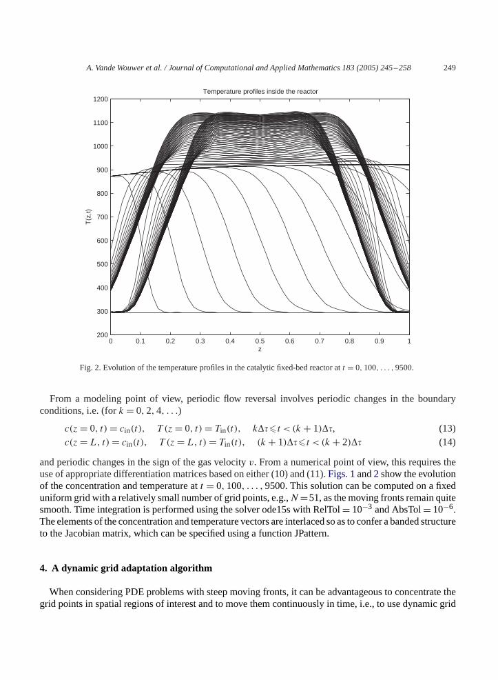
Fig. 2. Evolution of the temperature profiles in the catalytic fixed-bed reactor att = 0,100, . . . ,9500.

From a modeling point of view, periodic flow reversal involves periodic changes in the boundaryconditions, i.e. (fork = 0,2,4, . . .)

c(z = 0, t) = cin(t), T (z = 0, t) = Tin(t), k�� t < (k + 1)��, (13)c(z = L, t) = cin(t), T (z = L, t) = Tin(t), (k + 1)�� t < (k + 2)�� (14)

and periodic changes in the sign of the gas velocityv. From a numerical point of view, this requires theuse of appropriate differentiation matrices based on either (10) and (11).Figs. 1and2 show the evolutionof the concentration and temperature att = 0,100, . . . ,9500. This solution can be computed on a fixeduniform grid with a relatively small number of grid points, e.g.,N =51, as the moving fronts remain quitesmooth. Time integration is performed using the solver ode15s with RelTol= 10−3 and AbsTol= 10−6.The elements of the concentration and temperature vectors are interlaced so as to confer a banded structureto the Jacobian matrix, which can be specified using a function JPattern.

4. A dynamic grid adaptation algorithm

When considering PDE problems with steep moving fronts, it can be advantageous to concentrate thegrid points in spatial regions of interest and to move them continuously in time, i.e., to use dynamic grid


adaptation, so that their locations follow the moving fronts and remain near optimal. Not only the numberof grid points can be significantly reduced, as fewer grid points are used in regions of low solution activity,but also larger time steps can usually be taken as the moving fronts are less likely to cross grid points(generating large changes in time derivatives at these grid points).

In this section, we consider the development of dynamic grid adaptation algorithm based on ideasborrowed from[17]. This algorithm is based on the Lagrangian formulation of the PDE problem (1).Consider the continuous time trajectories of the grid points

z1<z2(t)< · · ·<zi(t)< · · ·<zN . (15)

Along z(t) = zi(t) the total temporal derivative ofx is given by

x = xt + zxz = f (x) + zxz. (16)

The ODEs defining the grid point movement, i.e.,z = g(t), can be derived based on some physical apriori knowledge, such as a flow-related quantity, or so as to equally distribute a monitor functionm(x)

such as the arc-length of the solution (several other monitor functions can be considered, e.g., based onthe solution curvature), i.e.,

m(x) =√(� + ‖uz‖2

2), (17)

Mi−1�zi−1 = Mi�zi = c, 2�i�N − 1, (18)

where�zi = zi+1 − zi is the local grid spacing,Mi is a discrete approximant of the monitor functionm(x) in the grid interval[zi, zi+1], andc is a constant. In order to avoid excessive spatial distortion andtemporal oscillation of the grid, two regularization procedures are used in[17]. To this end, the spatialequidistribution equation (18) is expressed in terms of the grid densityni = 1/�zi

ni−1

Mi−1= ni

Mi

, 2�i�N − 1. (19)

First, spatial smoothing is accomplished by replacing the grid densityni in (19) by

n0 = n0 − �(� + 1)(n1 − n0),ni = ni − �(� + 1)(ni+1 − 2ni + ni−1), 2�i�N − 1,nN = nN − �(� + 1)(nN−1 − nN), (20)

where� is a positive parameter. The introduction of the ‘anti-diffused’ densityni ensures that the grid islocally bounded, i.e., that adjacent grid spacings do not differ too much from one another (the completedevelopments can be found in[17])

�

� + 1�ni−1

ni�

� + 1

�. (21)

Second, temporal smoothing is accomplished by replacing the system ofAE (19) by a system of differentialequations

ni−1 + � ˙ni−1

Mi−1= ni + � ˙ni

Mi

, 2�i�N − 1, (22)

where the positive parameter� acts as a time constant preventing abrupt changes in the grid movement.


Experience shows that spatial smoothing is more important than temporal smoothing.In contrast with the original Fortran software implementation MOVGRD[2], in which a nonlinear

Galerkin discretization of the Lagrangian description of the PDEs (16) is applied, our MATLAB imple-mentation is based on simple finite difference schemes on nonuniform grids (as introduced in the previoussection). This choice has the advantage of simplicity and flexibility. Indeed, finite difference schemes canaccommodate any spatial differential operators, whereas the nonlinear Galerkin discretization used inMOVGRD is dedicated to convection–diffusion problems. However, finite difference schemes can beless efficient on some of these problems.

The semi-discrete equations resulting from (16) are then combined with Eq. (22) to yield a system ofODEs in the form of

x − A(x, z)z = f (x, z),�B(x, z)z = g(x, z) (23)

or

M() = q(), (24)

where is a vector of dependent variables in which the elements ofx andzare interlaced (following theprogression of the spatial grid), so thatM takes a block-pentadiagonal matrix structure (the dimension ofthe blocks isnpde+1×npde+1). The ODE system (24) is solved using the BDF/NDF solver ode15s[13].The sparsity pattern of the mass matrix and of the Jacobian matrix is defined using functions MvPatternand JPattern.

To illustrate the performance of this code, we consider first a model of flame propagation[3] consistingof two coupled equations for mass density and temperature

�t = �zz − NDA�,Tt = Tzz + NDA�, 0<z<1, t >0, (25)

whereNDA = 3.52× 106 e−4/T .The initial conditions are given by

�(z,0) = 1, T (z,0) = 0.2, 0�z�1, (26)

and the boundary conditions are

�z(0, t) = 0, Tz(0, t) = 0,�z(1, t) = 0, T (1, t) = f (t), t�0, (27)

with

f (t) ={

0.2 + t/2 × 10−4, t�2 × 10−4,

1.2, t�2 × 10−4.(28)

The heat source located atz = 1 generates a flame front that propagates from right to left at an almostconstant speed.

From a numerical point of view, the main challenge in this problem is to accurately capture the ignitionphase and to subsequently reproduce the correct propagation speed of the flame front. To this end, arelatively large number of points, e.g.,N = 501, is needed when using finite differences on fixed uniform


0 0.1 0.2 0.3 0.4 0.5 0.6 0.7 0.8 0.9 1-0.2

0

0.2

0.4

0.6

0.8

1

1.2

1.4

ρ(z,

t) a

nd T

(z,t)

z0 0.1 0.2 0.3 0.4 0.5 0.6 0.7 0.8 0.9 1

-0.2

0

0.2

0.4

0.6

0.8

1

1.2

1.4

ρ(z,

t) a

nd T

(z,t)

z

Flame propagation Flame propagation

Fig. 3. Fixed uniform grid solution of the flame propagation problem att = 0.001, . . . ,0.006. The right plot corresponds toN = 81 grid points, whereas the left plot corresponds toN = 501 gridpoints. The propagation speed is largely underestimatedin the former case.

0 0.1 0.2 0.3 0.4 0.5 0.6 0.7 0.8 0.9 1

0

0.2

0.4

0.6

0.8

1

1.2

ρ(z,

t) a

nd T

(z,t)

Flame propagation

0 0.1 0.2 0.3 0.4 0.5 0.6 0.7 0.8 0.9 10

2

4

6

z

t

x10 -3

Fig. 4. Moving grid solution of the flame propagation problem:N = 29,� = 0.5, � = 1, � = 10−6.


30 20 10 0 10 20 30 40 50 60 700

0.05

0.1

0.15

0.2

0.25

u(z,

t)Korteweg-de Vries equation

30 20 10 0 10 20 30 40 50 60 700

50

100

z

t

Fig. 5. Moving grid solution of the Korteweg–de Vries equation: initialisation with grid refinement,N = 113,� = 0.0, � = 2,� = 10−4 (solid line: analytic solution).

grids.Fig. 3 illustrates two extreme cases corresponding toN = 81 and 501, respectively. In the formercase, the propagation speed is largely underestimated.The problem is solved on the time interval(0,0.006)and time integration is performed using ode15s with AbsTol= 10−3 and RelTol= 10−3. A moving grid,which concentrates the nodes where they are needed, could therefore be advantageous in this case. Thefollowing tuning parameter values are selected:N = 29, � = 0.5, � = 1, � = 10−6. Time integration isperformed using ode15s with AbsTol= 10−3 and RelTol= 10−3. Very satisfactory numerical resultsare obtained, which are represented inFig. 4. The computational expense is about the same as the onerequired to compute a fixed grid solution withN=81 (seeFig. 3—about 15 s with anAMDAthlon2400+),and represents about1

30 of that required withN = 501.As a second test example, we consider the classical Korteweg–de Vries equation, which was originally

introduced by Korteweg and deVries in 1895[7] to describe the behavior of small amplitude shallow-waterwaves in one space dimension,

ut = −6uuz − uzzz − ∞�z�∞, t�0, (29)

= − 3(u2)z − uzzz, (30)

u(z,0) = u0(z), (31)


which combines the effect of nonlinearity and dispersion. In the following, the propagation of a singlesoliton

u(z, t) = 0.5s sech2 [0.5√s(z − st)] (32)

is investigated numerically.u(z, t) of (32) is the analytical solution to (30)–(31) and serves as a standardby which the accuracy of the numerical solution can be assessed. Particular attention must be paid to theselection of finite difference schemes for the approximation of the spatial derivatives. Here, the secondform (30) of the equation is used. The first-order derivative term is computed using a five-point biasedupwind scheme, and the third-order derivative term is computed using stagewise differentiation, i.e.,uzzz=D1(D1(D1u)), with a three-point centered differentiation matrixD1.Fig. 5shows the propagation ofa single soliton on the time interval[0,50].Time integration is performed using ode15s with AbsTol=10−3

and RelTol= 10−3. The following tuning parameter values are selected:� = 0.0, � = 2, � = 10−4. Todetermine an appropriate number of grid points and to initially concentrate them in the soliton, a call tothe grid refinement algorithm presented in the next section (withc=0.005 andK = (�+1)/�) is made att =0. As a result,N =113 grid points are used, which very effectively follow the soliton in its movement.The computational expense is reasonable, e.g., about 115 s with an AMDAthlon2400+.

5. A static grid refinement algorithm

An alternative procedure to adapt the grid point locations is static grid refinement. Basically, thisapproach proceeds in four steps:

(1) approximation of the spatial derivatives on a fixed nonuniform grid;(2) time integration of the resulting semi-discrete ODEs;(3) adaptation/refinement of the spatial grid;(4) interpolation of the solution to produce new initial conditions.

The movement of the grid points is therefore no longer continuous in time, but time integration is haltedperiodically to update the grid. This approach has several advantages:• it is simple to implement;• PDE solution and grid adaptation/refinement are uncoupled and can be programmed in separate MAT-

LAB functions (programming therefore requires less expertise from the end user);• there areN ODEs to solve (for the PDE solution) instead of 2N ODEs (for the PDE solution and the

grid movement in the previous approach);• grid refinement allows spatial accuracy to be controlled as grid points are added or deleted depending

on the evolution of spatial activity of the solution (for instance the birth of new moving fronts canbe easily accommodated, whereas a dynamic moving grid with a fixed number of grid points can beunable to resolve unforeseen spatial activity with enough accuracy).

But has also several drawbacks:

• as the grid movement is no longer continuous in time, grid points are suboptimally located, i.e., theycan for instance lag behind the front if the grid is not updated sufficiently frequently;


0 0.1 0.2 0.3 0.4 0.5 0.6 0.7 0.8 0.9 10

0.5

1

1.5ρ(

z,t)

and

T(z

,t)Flame propagation

0 0.1 0.2 0.3 0.4 0.5 0.6 0.7 0.8 0.9 10

2

4

6

z

t

x10 -3

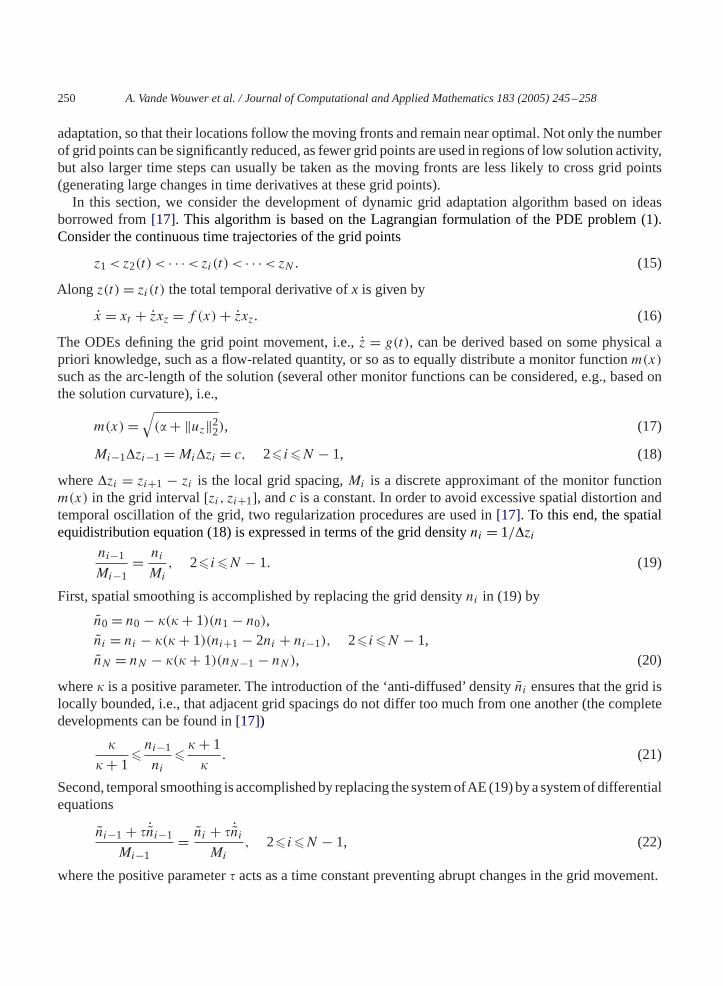
Fig. 6. Adaptive grid refinement solution of the flame propagation problem:N = 33,� = 0.05,c = 0.2,K = 1.4.

• periodic solver restarts involve some computational overhead (and usually one-step solvers, such asimplicit Runge–Kutta or Rosenbrock algorithms, which do not require the past solution history, willperform better than BDF solvers);

• interpolation to produce new initial conditions is an additional source of errors.

Despite these drawbacks, the authors have successfully applied an adaptive grid refinement algorithm,called AGEREG[15], to a variety of problems (see also[11] in this journal issue for numerical ex-periments with the original Fortran code and a generalized fifth-order KdV equation), and a MATLABimplementation is considered in the following.

Again, the grid movement is based on the equidistribution of a specified monitor function (18). To limitgrid distortion, a spatial regularization procedure due to Kautsky and Nichols[6] is used, which ensuresthat the grid is locally bounded with respect to a constraintK�1 (see also (21), whereK = (� + 1)/�),

1

K�

�zi�zi−1

�K, 2�i�N − 1. (33)

To ensure this property, the monitor function is modified, keeping its maximal values, but increasingits minimum values, in a procedure called “padding”. The resulting padded monitor function is thenequidistributed yielding a grid whose ratios of consecutive grid steps are bounded as required. In practice,the padding is chosen (there is, in principle, an infinity of possibilities to achieve padding) so that the


30 20 10 0 10 20 30 40 50 60 700

0.05

0.1

0.15

0.2

0.25

u(z,

t)Korteweg-de Vries equation

30 20 10 0 10 20 30 40 50 60 700

20

40

t

z

Fig. 7. Adaptive grid refinement solution of the Korteweg–de Vries equation:N = 154,� = 0.0, c = 0.2,K = 1.4.

equidistributing grid has adjacent steps with constant ratios equal to the maximum allowed. MATLABimplementation involves the following issues:

• the Rosenbrock solver ode23s is usually the preferred algorithm as it does not require the past solutionhistory;

• the solver is periodically halted, after a fixed number of time steps, using anEventsfunction, whichmonitors the evolution of the number of steps;

• the solution is interpolated using cubic splines as implemented inSplinein order to generate initialconditions on the new grid.

To evaluate the performance of this code, we consider the same two test examples, e.g., the flame propa-gation problem (25), and the classical Korteweg–de Vries (29)–(30).

Fig. 6 shows the solution of the flame propagation problem (25), using a curvature-based monitorfunction

m(u) = √(� + ‖uxx‖∞ (34)

and the tuning parameters� = 0.05, c = 0.2, K = 1.4, AbsTol= 10−3, and RelTol= 10−3. In thisfigure, the solution is plotted everynsteps= 10, when ode23s is halted to refine the grid, in order toshow how the adaptive grid solution proceeds. The average number of grid points isN = 33, and the


computational expense is similar to the one required with the moving grid algorithm (i.e., about 15 s withan AMDAthlon2400+). The grid refinement algorithm is particularly robust with respect to parametertuning, and numerical solutions can be computed according to the desired level of resolution.Fig. 7showsthe propagation of a single soliton. Here, an arc-length monitor function (17) is used, and the followingtuning parameters are selected� = 0.0, c = 0.2, K = 1.4, AbsTol= 10−4, and RelTol= 10−3. Thesolution is plotted everynsteps=1, i.e., ode23s is halted every time step to refine the grid. The algorithm isextremely effective, generating a solution in only 2.5 s with an AMDAthlon2400+! The average numberof grid points isN = 154.

6. Conclusions

In this paper, we report on the development of a MATLAB library for the method of lines solution ofpartial differential equation problems. Particularly, we focus attention on PDE problems with steep movingfronts, and the use of upwind finite differences and grid adaptation/refinement. Grid adaptivity appears tobe a very useful tool, allowing the computational load to be significantly reduced, and small-scale featuresof the solution to be captured with better accuracy (than fixed grid with a comparable number of points).In addition, grid refinement allows spatial accuracy to be controlled, and problems with time-varyingspatial activity (birth or decay of fronts) to be accommodated. A MATLAB implementation of AGEREG[15] is presented, which performs very well on nonlinear wave propagation problems. The toolbox isavailable on request from the authors ([email protected] or [email protected]) and alsofrom the web atwww.autom.fpms.ac.be

References

[1] M. Berzins, Developments in NAG library software for parabolic equations, in: J.C. Mason (Ed.), Scientific SoftwareSystems, Chapman & Hall, London, 1989.

[2] J.G. Blom, P.A. Zegeling, Algorithm 731: a moving-grid interface for systems of one-dimensional time-dependent partialdifferential equations, ACM Trans. Math. Software 20 (1994) 194–214.

[3] H.A. Dwyer, B.R. Sanders, Numerical modeling of unsteady flame propagation, Sandia National Laboratory LivermoreReport SAND77-8275, 1978.

[4] G. Eigenberger, C. Nieken, Catalytic combustion with periodic flow reversal, Chem. Eng. Sci. 43 (1988) 2109–2115.[5] B. Fornberg, Calculation of weights in finite difference formulas, SIAM Rev. 40 (1998) 685–691.[6] J. Kautsky, N.K. Nichols, Equidistributing meshes with constraints, SIAM J. Sci. Stat. Comput. 1 (1980) 499–511.[7] D.J. Korteweg, G. de Vries, On the change of form of long waves advancing in a rectangular canal and on a new type of

long stationary waves, Philos. Mag. 39 (1895) 422–443.[8] S.V. Pennington, M. Berzins, New NAG library software for first-order systems of time-dependent PDEs, ACM Trans.

Math. Software 20 (1994) 63.[9] P. Saucez, W.E. Schiesser, A. Vande Wouwer, Upwinding in the method of lines, Math. Comput. Simulat. 56 (2001)

171–185.[10] P. Saucez, A. Vande Wouwer, W.E. Schiesser, Some observations on a static spatial remeshing method based on

equidistribution principles, J. Comput. Phys. 128 (1996) 274–288.[11] P. Saucez, A. Vande Wouwer, P. Zegeling, Adaptive mesh computations for the extended fifth-order Korteweg–de Vries

equation, J. Comput. Appl. Math., this issue, doi:10.1016/j.cam.2004.12.028.[12] W.E. Schiesser, The Numerical Method of Lines: Integration of Partial Differential Equations, Academic Press, San Diego,

1991.[13] L.F. Shampine, I. Gladwell, S. Thompson, Solving ODEs with MATLAB, Cambridge University Press, Cambridge, 2003.

http://www.autom.fpms.ac.be

http://10.1016/j.cam.2004.12.028


[14] L.N. Trefethen, Spectral Methods in MATLAB, SIAM, Philadelphia, 2000.[15] A. Vande Wouwer, Ph. Saucez, W.E. Schiesser (Eds.), Adaptive Method of Lines, Chapman & Hall/CRC, Boca Raton,

2001.[16] A. Vande Wouwer, Ph. Saucez, W.E. Schiesser, Simulation of distributed parameter systems using a MATLAB-based

method of lines toolbox—chemical engineering applications, Ind. Eng. Chem. Res. 43 (2004) 3469–3477.[17] J.G. Verwer, J.G. Blom, R.M. Furzeland, P.A. Zegeling, A moving-grid method for one-dimensional PDEs based on the

method of lines, in: J.E. Flaherty, P.J. Paslow, M.S. Shephard, J.D.Vasilakis (Eds.),Adaptive Methods for Partial DifferentialEquations, SIAM, Philadelphia, 1989, pp. 160–175.

[18] J.A.C. Weideman, S.C. Reddy, A MATLAB differentiation matrix suite, ACM Trans. Math. Software 26 (2000) 465–519.

A MATLAB implementation of upwind finite differences and ...

Documents

Transcript of A MATLAB implementation of upwind finite differences and ...