An Efficient Routing Algorithm to preserve k-Coverage in Wireless Sensor Networks

J SupercomputDOI 10.1007/s11227-013-1054-0

An efficient routing algorithm to preserve k-coveragein wireless sensor networks

Ali Ahmadi · Mohammad Shojafar ·Seyede Fatemeh Hajeforosh · Mehdi Dehghan ·Mukesh Singhal

© Springer Science+Business Media New York 2013

Abstract One of the major challenges in the area of wireless sensor networks issimultaneously reducing energy consumption and increasing network lifetime. Effi-cient routing algorithms have received considerable attention in previous studies forachieving the required efficiency, but these methods do not pay close attention to cov-erage, which is one of the most important Quality of Service parameters in wirelesssensor networks. Suitable route selection for transferring information received fromthe environment to the sink plays crucial role in the network lifetime. The proposedmethod tries to select an efficient route for transferring the information. This paperreviews efficient routing algorithms for preserving k-coverage in a sensor networkand then proposes an effective technique for preserving k-coverage and the reliability

A. AhmadiElectrical and Computer Department, Islamic Azad University,Qazvin Branch, Qazvin, Iran

M. Shojafar (B)Department of Information Engineering, Electronic and Telecommunication (DIET),“Sapienza” University of Rome, via Eudossiana 18, 00184 Rome, Italye-mail: [email protected]; [email protected]

S. F. HajeforoshElectrical Engineering Department, Mazandaran University of Scienceand Technology, Babol, Iran

M. DehghanComputer Engineering Department, Amirkabir University of Technology ,Tehran, Irane-mail: [email protected]

M. SinghalComputer Science and Engineering, University of California,Merced, USAe-mail: [email protected]

123

A. Ahmadi et al.

of data with logical fault tolerance. It is assumed that the network nodes are awareof their residual energy and that of their neighbors. Sensors are first categorized intotwo groups, coverage and communicative nodes, and some are then re-categorizedas clustering and dynamic nodes. Simulation results show that the proposed methodprovides greater efficiency energy consumption.

Keywords Wireless sensor network · Localization · Energy-efficient routing ·Energy saving · k-coverage · Euclidean distance

1 Introduction

There has been a recent progression in micro-electro-mechanical systems of smartsensors, wireless communications platforms, and digital electronics followed by aplausible construction of tiny sensor nodes, which have low energy consumption andare cost-effective sensor nodes that are capable of connecting as wireless networks[1,2]. These nodes contain the main elements of wireless sensor networks (WSNs),and are capable of sensing and measuring environmental factors in the vicinity, such astemperature, pressure, voice, and different types of noise pollution, for data processingand transmission [3–5].

Crucial issues for WSNs include coverage and routing. Several routing methodshave been proposed in [6–8]. All of these methods concentrate only on routing regard-less of their coverage. Coverage concerns how the nodes can be enabled to cover anarea effectively. One of the main goals is to achieve maximal coverage for an areawith the least amount of energy consumed by the sensors [9]. Coverage is one ofthe Quality of Service parameters in networks used for surveillance [9]. One of theprimary major operations performed by each sensor node is to review and processthe node’s vicinity to discover incident events that are available in the environment,including the information required for use in application programs [10]. Techniquesused to represent coverage retention in sensor networks are based on the quantityand order of coverage (the number of nodes providing coverage for an area), com-bined with energy consumption [11]. Interestingly, these techniques play a crucial rolebecause increasing the order of coverage and supporting an order increment to k-orderis crucial in WSNs for attaining reliable information about their environment [12,13].It is necessary to provide sensor node coverage for some applications, such as targettracking. Thus, improved coverage and support of k-coverage, which means that eachpoint of an object region has coverage from at least k sensor nodes, is a prerequisitefor applied WSNs [13–17].

If all of the network targets are diagnosed with coverage sensors, but all of thegathered information do not send to the sink (is the node that has unlimited energy)(i.e., the nodes do not connect with multi-hop to the sink) connective hole will exist.It means, Target coverage in network environment is the most important tasks of thesensor nodes for receiving the information of the target status. But, target coverage isnot enough and the links between the sink and sensors should be established for trans-mitting information that keep the network efficiency in the network lifetime. [18–21].This is the primary challenge that should be studied in protocol designs for networks,

123

An efficient routing algorithm

since management of energy consumption aims for optimal utilization of a battery,while the relevant data should be made available from the receiving environment tothe data processing performed in an optimized wireless sensor network with minimumtime consumed [11,22]. Routing algorithms are among the main elements for design-ing sensor networks, and retention of network coverage is one of the critical issues inthe routing protocols [23–26].

In this paper, we present a method for transferring sensor information in whichk-order region coverage is maintained: the method reduces communication expensesand results in a longer network lifetime and greater reliability. The rest of this paperis organized as follows. Section 2 reviews related work. Section 3 presents a systemmodel. Section 4 presents our proposed method, and Sect. 5 presents our simulationresults. Finally, Sect. 6 discusses our conclusions and future research directions.

2 Related work

This section reviews the methods that are related to coverage in a WSN. One of themost important issues in the area of sensor networks understands the conditions ofarea coverage (AC) by sensor nodes. Whenever the Euclidean distance between arelevant target and the localization of a sensor node is less than the coverage radius,it is under the coverage of the sensor node [13,16,17,27]. Different segmentationsare used for sensor networks, each one subdividing the area according to the specificprotocol. Segmentations can be categorized into three groups according to their targetcoverage; these are AC, point coverage (PC), and barrier coverage (BC) [28]. The mainobjective of sensor networks with respect to area coverage is to provide completecoverage and supervision in an environment, while the aim of point coverage is toprovide dispersed coverage over a specific distance in the area and barrier coverageaims at eliminating noncoverage in an area. While iterative routing protocols aim toreduce energy consumption as a cost-effective strategy, the issue of coverage is moreimportant in the following protocols [29,30].

Hybrid Energy-Efficient Distributed Clustering (HEED) [31,32] is a protocol thatperiodically selects cluster heads according to a combination of the node’s residualenergy and a secondary parameter, through constant time iterations. It uses the primaryparameter, i.e., residual energy, to select an initial set of cluster heads. Unlike previousprotocols that require knowledge of the network density or homogeneity of nodedispersion in the field, HEED does not make any assumptions about the network suchas density and size. Every node runs HEED individually. At the end of the process,each node either becomes a cluster head or a child of a cluster head.

Coverage-Preserving Cluster Head Selection Algorithm (CPCHSA): CPCHSA [33]is used for sustainable coverage in sensor networks based on the design of the LowEnergy Adaptive Clustering Hierarchy (LEACH) [34] algorithm. The technique inCPCHSA changes the function of the LEACH cluster head to coordinate energy con-sumption along with improving coverage. Thus, the technique uses nodes that are avail-able in less congested areas for cluster heads due to the high rate of cluster head energyconsumption that arises from the aggregation of data and the transfer of data to the sink.

The coverage area in the CPCHSA method is based on the estimation of neighboringnodes according to the received signal potential, and the precise coverage neighbors

123

A. Ahmadi et al.

are not determined. Consequently, the results are merely an estimated range, whichis reliable in distribution and high congestion modes. The algorithm functions withrandom numbers, and it is possible to encounter cluster heads with no further physicaldistribution in the network.

Energy-Aware Routing Protocol (EAP): The EAP protocol represents clusters forthe routing algorithm; thus the protocol features cost-effective energy consumption forinter-network or in-network communication to create a balance of energy consumptionin the entire resulting network. EAP provides an algorithm for resolving networkchallenges that uses the coverage available in clusters under the power control of aradio transmitter, so that nodes apply more potential for remote (far) distances, butless for close distances. A cluster head is initially appointed in each period, and EAP’srepresentation algorithm is used for randomly chosen maintenance without a guarantyof network coverage. Whenever sufficient density is found in a distribution of nodes,there is a trend of a convenient balance of coverage [35]. It means, if the nodes densityis high in the network, sensing nodes or coverage nodes have been selected withsuitable distribution in the network and it is not related to the specific area of thenetwork. Also, in the proposed method, the communicative and coverage nodes areconsidered fixed, and we try to change the cluster head in time interval to decreaseenergy consumption and increase network lifetime. Moreover, we use single-hope fortransmitting information to the cluster heads.

Priority-Based Energy-Aware and Coverage Preserving (PBEACP): The PBEACP[36,37] algorithm is a technique for wireless sensor network routing that is basedon a modification of the LEACH method; thus selection of cluster heads is crucialfor improving/controlling energy consumption and reinforcing network coverage byconvenient energy distribution in the line of a geographical distribution of nodes.Nodes with more neighbors are selected as candidates for cluster head in the PBEACPmethod, by a calculation of node density in the placement of nodes.

The PBEACP protocol uses the CPCHSA [33] method to distinguish neighboringnodes and the potential of received signals, but it is useless for the precise placement ofcoverage neighbors and does not provide the required precision for network coveragelike CPCHSA does. But, in the proposed method, the direction and angle of the nodesrelated to each other are determined.

3 System model

In this paper, it is assumed that all sensors are fixed and all nodes are aware of theirproper placement, targets, and sink. For example, we want to transmit the information(by the help of the heating sensor nodes that we were distributed and sent them by air-plane in the military zone) of some gates (that are targets) of the underground militarystations that are on the ground, and group of sensors near targets report the heatinginformation of their environments based on their diagnosis radius. Sink nodes are freeof any energy constraints and have a fixed placement, and all sensors are aware ofthis situation. Each sensor has a sensing range radius and two communication rangesthat are greater than or equal to the sensing radius, nodes’ communicative radiusesare greater than their sensing radiuses, with double the range covered, and all nodes

123


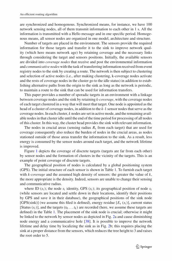
are synchronized and homogenous. Synchronized means, for instance, we have 100network sensing nodes, all of them transmit information to each other in 1 s. All theinformation is transmitted with a Hello message and in one specific period. Homoge-nous means, all sensor nodes are organized in one model, architecture and structure.

Number of targets are placed in the environment. The sensors provide the requiredinformation for those targets and transfer it to the sink to improve network qual-ity (which here means network age) by retaining coverage and the necessary linksthrough considering the target and sensors positions. Initially, the available sensorsare divided into coverage nodes that receive and post the environmental informationand communicative nodes with the task of transferring information received from eventregistry nodes to the sink by creating a route. The network is then subject to clusteringand selection of active nodes (i.e., after making clustering, k-coverage nodes activateand the rests of coverage nodes in the cluster go to the idle status) in addition to estab-lishing alternative paths from the origin to the sink as long as the network is periodic,to maintain a route to the sink that can be used for information transfers.

This paper provides a number of sporadic targets in an environment with a linkagebetween coverage nodes and the sink by retaining k-coverage, with the coverage nodesof each target clustered in a way that will meet that target. One node is appointed as thehead of a cluster of coverage nodes, in addition to the k-1 sensor nodes that serve as thecoverage nodes. In each cluster, k nodes are set in active mode, and the remaining avail-able nodes in that cluster idle until the end of the time period for processing of all nodesof this cluster. In this way, the cluster head provides the sink with relevant information.

The nodes in crucial areas (sensing radius Rs from each target) that are used forcoverage consequently also reduce the burden of nodes in the crucial areas, as nodesstationed outside of those areas transfer the information to the sink. As a result, lessenergy is consumed by the sensor nodes around each target, and the network lifetimeis improved.

Figure 1 depicts the coverage of discrete targets (targets are far from each other)by sensor nodes and the formation of clusters in the vicinity of the targets. This is anexample of point coverage of discrete targets.

The geographical position of nodes is calculated by a global positioning system(GPS). The initial structure of each sensor is shown in Table 1. To furnish each targetwith k-coverage and the assumed high density of sensors: the greater the value of k,the more appropriate is the density. Indeed, sensors are unable to change their sensingand communicative radius.

where ID (si ); the node si identity, GPS (si ); its geographical position of node si

(while sensors are located and settle down in their locations, identify their positionsby GPS and save it in their database), the geographical positions of the sink node[GPS(sink)] (we assume this filed is defined), energy residue [Er (si )], current status[Status (si )], and the targets (t0 . . . tk) are recorded (here, we assume these targets aredefined) in the Table 1. The placement of the sink node is crucial; otherwise it mightbe linked to the network by sensor nodes as depicted in Fig. 2a and cause diminishingnode energy and a communicative hole [38]. It is possible to improve the networklifetime and delay time by localizing the sink as in Fig. 2b; this requires placing thesink at a proper distance from the sensors, which reduces the tree height to 3 and raisesthe root order to 5.

123

A. Ahmadi et al.

Fig. 1 An example of point coverage for discrete targets

Table 1 Initial sensorinformation

ID (si )

GPS (si )

GPS (sink)

GPS (t0 )

…

GPS (tk )

Status (si )

Er(si )

Fig. 2 a Location of sink at an improper distance from sensors. b Location of sink at a convenient distancefrom sensors

Let the range of sensor node si be the circular area with Coverage radius Rsi (i.e.,this range illustrates the effective range or coverage range of communication withother nodes as shown in Fig. 3, here Rs = Rsi, for each i). The sensor nodes’ binarycoverage model, cov(t j , si ), is defined by Eq. (1):

cov(t j , si ) ={

1 if d(t j , si ) ≤ Rs

0 otherwise., (1)

123


Fig. 3 Coverage radius Rsi and Communicative radius Rci for node i

Fig. 4 Example of coverageneighbors set

where d(t j , si ) is the Euclidean distance between sensor node si and target t j . In thebinary detection model (i.e., when detecting the targets), an explicit target is definedin the node coverage area. Each node si establishes a communication range with thethreshold distance defined as the communicative radius Rci. Communication shall beestablished as single-hop or one-hop whenever the Euclidean distance between twonodes si and s j is less than or equal to the communicative radius. Figure 3 depicts thecoverage provided by sensor si ’s communicative radius besides coverage radius Rsi.

Sensing/coverage neighbors Set of Target t j : In Principle, according to the proposedmodel, each sensor node will identify all targets in its coverage area. Hence, thecoverage neighbor set of target ti includes all of the sensor nodes that cover/sensethe target t j in their coverage area, as defined by Eq. (2). In other words, all sensingnodes whose Euclidean distances to target t j are less than Rsi. For example, in Fig. 4,sensing neighbors set of target t j includes {1, 2, 3} considering the target is denotedas the black star.

Ns(t j ) = {si∣∣ d(t j , si ) < Rs} , (2)

Communicative neighbors set: The communicative neighbors of sensor si are theset of sensor nodes inbound of node si for the exchange of information, as defined byEq. (3). In other words, the communicative neighbors of sensor si are all the sensorswhose Euclidean distance from the sensing node si is less than communicative radius

123

A. Ahmadi et al.

Fig. 5 Example ofcommunicative neighbors set

(Rci or Rc for all i). A node si is able to interact with its communicative neighbors andtransfer/receive information. For example, in Fig. 5, the communicative neighbors setof node 1 is the set {3, 4, 6} [i.e., the internal circle of the node 1 intersected by theinternal circle of these nodes: check the blue shaded areas and its intersection by theinternal circle of node 1 (communicative radius) of node 3, 4, and 6].

Ns(si ) = {s j∣∣ d(si , s j ) < Rc} , (3)

4 Proposed method

In this section, we explain our proposed method in detail. Informally speaking, we usethe sink’s geographical position as the coordinate origin for the Cartesian coordinatevectors (always, we have one sink and its position considered as a origin of ourCartesian coordinate vector). Thus, the target and sensor positions shall be definedby the geographical location of sensors and targets relative to the sink’s geographicalposition. The algorithm consists of three phases:

• Phase I: Collection and processing of primary information.• Phase II: Creation of coverage clusters for targets and selection of cluster heads.• Phase III: Selection of active transmitting nodes for information transfer to the sink.

4.1 Phase I: collection and processing of primary information

In this phase, the primary required information to be used for the following phasesis gathered that consists of sensing status, the initialized energy for each sensor nodeand the position of each sensor. We assume that as a default, all sensor nodes are inan idle communicative position, so that the initial value of the Status field is 0. Eachsensor node’s Status field (si ) shall be set in one of the positions specified in Table 2:

123


Table 2 Sensor Positions/statusStatus (si ) Descriptions

0 Idle communicative

1 Idle coverage

2 Active communicative

3 Active coverage

4 Cluster heads

Table 3 Target Table for node i(si )

ID (si )

Dsink(tk )

d(si , tk )

GPS (tk )

Table 4 Hello messageID (si )

GPS (si )

Er (si )

Status (si )

ID (tk )

Each sensor updates its target table by updating the initial sensor information table(Table 1) by processing its target table as follows: if it covers a target, then it transformsfrom communicative to coverage position and set its status field to 1, otherwise it retainsthe status value 0. The nodes’ with state 1, try to fill their Table 3 by the informationthey gain from the Table 1. Specifically, Dsink(tk) is the Euclidean distance betweensink from the tk that is calculated and added to the Table 3 of the node i, also, d(si , tk)is Euclidean distance between node i or si from the tk that is calculated and added.Last two fields come directly from Table 1. In the records of Table 1, the nodes whoseEuclidean distances from the tk are less than or equal to Rc are inserted into the Table 3(e.g., if each node in its coverage radius has tk , it is added into the Table 3 as si and allother parameters are calculated for this record). The coverage target table is depicted inTable 3. This table includes the coverage target’s distance to the sink denoted as Dsink(tk), the distance of the sensor to the target denoted as d(si , tk), the target’s position[GPS (tk)], and the target’s identity or ID (si ).

Each sensor node then transmits its identity [ID (si )], coordinates [GPS (si )], resid-ual energy [Er (si )], current status [Status (si )], and its coverage target identity [ID(tk)] to single-hop neighbors with a hello message. Whenever a sensor fails to covera target, the ID (tk) will be null. The hello message format is depicted in Table 4.

On the top of the hello message a sensor node updates its neighbors table. Theformat of sensor si ’s neighbors table, with s j , j = 1 . . . m (the number of node si ’sneighbors), is depicted in Table 5.

where sensor s j ’s neighbors table consists of s j ’s identity [ID (s j )], s j ’s coordinates[GPS (s j )], s j ’s residue energy [Er(s j )], s j ’s sensor status [Status (s j )], the identity of

123

A. Ahmadi et al.

Table 5 Sensor si neighborstable (node s j is a neighbor)

ID (s j )

GPS (s j )

Er (s j )

Status (s j )

ID (tk )

d (s j , si )

Dsink(s j )

the target covered by s j [ID (tk)], the distance to sensor si [d (s j , si,)], and the distanceto s j ’s sink [Dsink(s j )]. At the end of this phase, each node is aware of its neighbors’details to apply the required information in the following phases.

In a nutshell, each sensor node contains three tables: initial sensor information Table(Table 1), Target Table (Table 3) and Neighbors Table (Table 5). Table 3 is establishedbased on the position/status of the current node and the targets positions.

Algorithm 1 presents pseudocode for Phase I.

Algorithm 1. Pseudocode for Phase I (First_node_setup (si))

Input: si list Output: First_node_setup (si) 1 : Begin2 . Repeat // continue until the targets are available the target table (Table 3) 3 . Compute destination si ,tk with d(si,tk)= sqrt((xi-xt)

2+(yi-yt) 2);

4 . If (d(si,tk) < sensing range) then si.status=1; 5 : si broadcasts hello message to its 1-hop(single-hop) neighbors , id, GPS, Er, Status, ID(tk); 6 : If (Hello message from neighbors sensor is received*) 7 : Begin8 : Update neighboring set (si); 9 : Compute destination between si & sj as d(si, sj)= sqrt((xi- xj)

2+( yi -yj) 2);

10 : Compute destination between sink & sj as Dsink(sj)= sqrt((xsink- xj) 2+(ysink- yj)

2); 11 : End If12 : Until (tk is available) 13 : Return14 :End

* Here, we calculate the time needs for each target, which is defined as time takento find the positions (Table 1) + time for updating the targets table (Table 3) + timetaken to send Hello message to the sensor nodes neighbors (one-hop) (Table 4)

4.2 Phase II: creation of coverage clusters for targets and selection of cluster heads

In this phase, a cluster is initially created for each target. Members of the clusterare nodes located within the maximum distance Rc from the target whose coverageincludes the target. Then the cluster head is nominated as follows.

In the first step, each node creates a coverage neighbors record from its coveragetarget. It is best to assign a cluster head for each target to provide a specific mechanismfor transferring the collected information to the sink, i.e., node 1 processes its neighborstable and adds the neighbors that have similar object coverage nodes to node 1 to node1’s coverage neighbors table (or Table 6). The coverage neighbor table format fortarget tk for node si is shown in Table 6.

123


Table 6 Coverage neighborstable format for target tk fornode si (i.e., here, s j is one ofsi ’s neighbors that has the sametk )

ID (s j )

GPS (s j )

Er(s j )

Status (s j )

ID (tk )

d (si , s j )

Dsink(s j )

d (s j , tk )

CHeff(tk )

θ(tk , s j )

where θ(tk, s j ) is the angle of the sensor node to the target node, CHeff(tk) is thefitness function of the cluster head (CHeff is the acronym of Cluster Head Efficient),and d(s j , tk) is the distance of the sensor node from the target node. The sensors that arein the coverage table for each target node make a cluster with the name of that target.

Now, we explain the mechanism that helps us to select the cluster head for eachtarget node. Then, we will be able to transmit the information that is gathered by thecovering sensors to the sink node.

In the second step, a fitness function is used to identify the cluster head, based onEq. (4). The values α0 and α1 define the impact strength coefficients (probabilities)of each of the parameters for the cluster head fitness function (each of them is in therange[0,1], where 0 means that the parameter has no effect on the cluster head fitnessfunction and 1 means the parameter has full effect on the cluster head function); thesevalues are assumed to be 0.7 and 0.3, respectively (we consider the residual energyof each node to be more important than the distance of that node to the target node).The node with the highest value is defined as the cluster head. If the assigned nodehas no alternative, a timed loop will indicate that no message has been received fromits neighbors and either it will change its position to cluster head (change its value to4) or it will provide a convenient message to its coverage neighbors concerning therelevant target; otherwise it waits to receive messages from its coverage neighbors andupdates the information in the coverage table. Here, Emax is the total energy that isconsidered for each node. Note that, if we have multiple nodes with the same CHeff,our algorithm will select the node that has the smallest Dsink(si ).

CHeff(tk) = α0Er(si )

Emax+ α1

Dsink(tk)

Dsink(si ). (4)

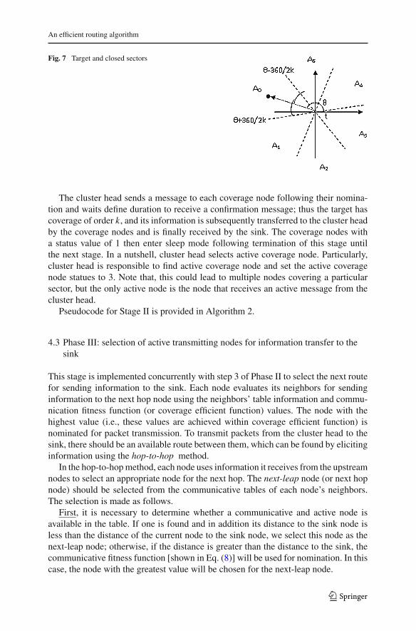
In the third step, it is necessary to know the angle of each node with respect to thecoverage target to find the proper locations of other k-1 nodes. Cluster head selectsactive coverage node by Eq. (5). Equation (5) is the usual formula for calculating theangle of each coverage target:

θ(tk, s j ) =⎧⎨⎩

π + tan−1(

ysi−ytkxsi−xtk

)(xsi − xtk ) < 0

tan−1(

ysi−ytkxsi−xtk

)(xsi − xtk ) > 0

, (5)

123

A. Ahmadi et al.

Fig. 6 Location of each sensor in the neighbor of each target

Figure 6 shows the location of each sensor in the neighbor of each target node.In principle, assume that the cluster head is in the bisector of sector A0, it is in sector

[((θ − 2π)/2k)mod2π, ((θ + 2π)/2k)mod2π]. Consider that the circumference ofthe target that is segmented into k-1 sectors is used to calculate the bisection of eachsector. Interestingly, we select each node in each bisector as an active coverage nodeand change its status field to 3. The bisector of sectors A j , Bs(A j ), j = 1, 2 . . . , ∗is calculated as in Eq. (6):

Bs(A j ) =(

θ +(

j ∗ 2π

k

))mod 2π j = 1, 2, . . . , k − 1, (6)

We use the coverage fitness function to appoint the coverage node for each sector,where the node with the highest value is assigned to be the sector coverage node. In thecoverage fitness function or coverage efficient function denoted as covEff and expressedin Eq. (7), values β0, β1, and β2 are the impact strength coefficients (probabilities)applied to the parameters in the cluster head fitness function; the relevant values are0.6, 0.2, and 0.2, in that order. Figure 7 depicts a target and closed sectors.

covEff(si ) = β0Er(si )

Emax+ β1

1∣∣Bs(sec j ) − θ(tk, si )∣∣ + ε

+ β2d(si , tk)

Rsi, (7)

where Emax is the total energy that is considered for node si . Obviously, Bs(sec j )isdefined in (6), Rsi is coverage radius for node si , θ(tk, s j ) is angle of the sensor nodeto the target node, d(s j , tk) is the distance of the sensor node from the target node, ε

the fault tolerance parameter and Er (si ) is si ’s residual energy.

123


Fig. 7 Target and closed sectors

The cluster head sends a message to each coverage node following their nomina-tion and waits define duration to receive a confirmation message; thus the target hascoverage of order k, and its information is subsequently transferred to the cluster headby the coverage nodes and is finally received by the sink. The coverage nodes witha status value of 1 then enter sleep mode following termination of this stage untilthe next stage. In a nutshell, cluster head selects active coverage node. Particularly,cluster head is responsible to find active coverage node and set the active coveragenode statues to 3. Note that, this could lead to multiple nodes covering a particularsector, but the only active node is the node that receives an active message from thecluster head.

Pseudocode for Stage II is provided in Algorithm 2.

4.3 Phase III: selection of active transmitting nodes for information transfer to thesink

This stage is implemented concurrently with step 3 of Phase II to select the next routefor sending information to the sink. Each node evaluates its neighbors for sendinginformation to the next hop node using the neighbors’ table information and commu-nication fitness function (or coverage efficient function) values. The node with thehighest value (i.e., these values are achieved within coverage efficient function) isnominated for packet transmission. To transmit packets from the cluster head to thesink, there should be an available route between them, which can be found by elicitinginformation using the hop-to-hop method.

In the hop-to-hop method, each node uses information it receives from the upstreamnodes to select an appropriate node for the next hop. The next-leap node (or next hopnode) should be selected from the communicative tables of each node’s neighbors.The selection is made as follows.

First, it is necessary to determine whether a communicative and active node isavailable in the table. If one is found and in addition its distance to the sink node isless than the distance of the current node to the sink node, we select this node as thenext-leap node; otherwise, if the distance is greater than the distance to the sink, thecommunicative fitness function [shown in Eq. (8)] will be used for nomination. In thiscase, the node with the greatest value will be chosen for the next-leap node.

123

A. Ahmadi et al.

Algorithm 2: Pseudocode for Phase II (Sensing_node_setup (si,tu)) Input: si and tu

Output: Sensing_node_setup (si,tu) 1 : begin 2 : Add information node si into coverage neighboring set (si,tu); 3 : from table neighboring set (si) While(ID(sj)) 4 : If ( tu==tk ) then 5 : begin6: Update coverage neighboring set (si,tu); 7 : Compute destination si ,tk with d(sj,tk)= sqrt((xj-xt)

2+(yj-yt)2);

8 : Compute cluster_head efficient sj with CHeff= [α0×Er(sj)/Emax]+[α1×Dsink(tk)/Dsink(sj)] 9 : for i=1 to d-1

10: Compute angle sj to target with

11 :end if12 : Find max from field CHeff in table neighboring set (si); 13: If CHeff is not unique then14: Find Minimum (Dsink(sz)) [z={list of nodes that have same CHeff}] 15: CHeff=CHeff(sn); //n is the node belongs to z and has Maximum CHeff 16 : If ( ID(CHeff _max)==ID(si)) then 17 : begin 18 : status(si)=4; 19 : si broadcasts its ID, Status to its 1-hop(single-hop) neighbors; 20 : =θ(tk,si); 21 : CHeff=si; 22 : end if

23 :else if (receive message from neighbors) then24 : Update coverage neighboring set (si, tu)&&Update neighboring set (si); 25 :for ( m=1 ; m<k ;m++) 26 : begin

27 : Bs(secm)= +(m* 2 /k) mod 2 ; 28 : covEff (max)=0;

29 : While(θ>Bs(secm)- 2 /2k) mod 2 && θ<Bs(secm)+ 2 /2k) mod 2 ) 30 : Begin31 : Compute coverage efficient sector m with

32 : if ( covEff(si)> covEff (smax)) then //find node with maximum energy; i.e. smax is the maximum energy of all nodes

33 : covEff (smax)=covEff (si); 34 : ID(smax)=ID(si); 35 : End while36 : CHeff broadcasts ID(smax), Status=3 to its 1-hop neighbors; 37 :end for38 : Return39 : End

This procedure is repeated until the sink is reached. So that there always a routeexists for transmission from the cluster head to the sink [39].

The reason for using the distance from the sink in the fitness function for coverageis to prevent deviation in the main route for packets to the sink. In addition, it is usedfor finding the fewest leaps in establishing a route to the sink.

Second, after selecting the next-leap (next hop node), that node is notified by aspecial message that it has been selected. Then the node changes its status to 2 andannounces to its single-hop neighbors that it is an active communication node. Finally,this node selects the next node based on this same method, and this continues until thesink node is reached.

Next, after finishing an each iteration of the loop, as the next iteration commences,the nodes that had been activated in the previous iteration change their status to

123


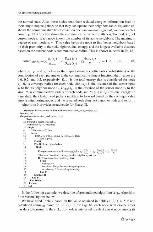
the normal state. Also, these nodes send their residual energies information back totheir single-hop neighbors so that they can update their neighbors table. Equation (8)shows the communicative fitness function or communicative efficient function denotescommEff . This function shows the communicative value for j th neighbor node (s j ) ofcurrent node si . Each node knows the number of its active neighbors. The maximumdegree of each node is m. This value helps the node to find better neighbors basedon their proximity to the sink, high residual energy, and the longest available distancebased on the current node’s communicative radius. This is shown in detail in Eq. (8).

commEff(s j )=γ0Er(s j )

Emax+γ1

Dsink(si )

Dsink(s j )+γ2

d(si , s j )

Rcj = 1, 2, . . . , m, (8)

where γ0, γ1 and γ2 define as the impact strength coefficients (probabilities) or thecontribution of each parameter to the communicative fitness function; their values are0.6, 0.2, and 0.2, respectively. Emax is the total energy that is considered for nodes j . Rs is coverage radius for each node, d(si , s j ) is the distance of the sensor nodesi to the its neighbor node s j , Dsink(s j ) is the distance of the sensor node s j to thesink, Rc is communicative radius of each node and Er (s j ) is s j ’s residual energy. Ina nutshell, the cluster head picks a next hop to forward based on the commEff valueamong neighboring nodes, and the selected node then picks another node and so forth.

Algorithm 3 provides pseudocode for Phase III.

Algorithm 3: Pseudocode for Phase III (communicative_node_setup (si,tu)) Input: si and tu

Output: communicative _node_setup (si,tu) Begin

2 : from table neighboring set (si) While (GPS(sj)!=GPS(sink))

3 : Begin4: If (Status (sj)==2) then5 : Begin6 : If (Dsink(sj)<=Dsink(si) && Er(sj)>Emax/2) then7 : next-hop=sj; 8 : End If 9 : Else If (Status (sj)==0) then10: Begin

11: Compute commEff sj with γ γ γ

12: Find max from field commEff in table neighboring set (si); 13 : If ( ID(commEff (smax))==ID(sj)) then 14 : Begin15 : Status(sj)=2; 16 : broadcasts ID(sj), Status to 1-hop neighbors; 17: next-hop=sj; // for next-leap in routing 18: End If 19: End Else If 20: End If 21: End While 22: Return 23: End

In the following example, we describe aforementioned algorithm (e.g., Algorithm3) in various figures below.

We have filled Table 7 based on the value obtained in Tables 1, 2, 3, 4, 5, 6 andcalculated commEff based on Eq. (8). In the Fig. 8a, each node with orange colorhas data to transmit to the sink; this node is interested to select a next node among its

123

A. Ahmadi et al.

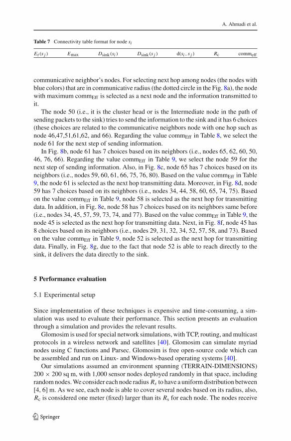
Table 7 Connectivity table format for node si

Er(s j ) Emax Dsink(si ) Dsink(s j ) d(si , s j ) Rc commeff

communicative neighbor’s nodes. For selecting next hop among nodes (the nodes withblue colors) that are in communicative radius (the dotted circle in the Fig. 8a), the nodewith maximum commEff is selected as a next node and the information transmitted toit.

The node 50 (i.e., it is the cluster head or is the Intermediate node in the path ofsending packets to the sink) tries to send the information to the sink and it has 6 choices(these choices are related to the communicative neighbors node with one hop such asnode 46,47,51,61,62, and 66). Regarding the value commEff in Table 8, we select thenode 61 for the next step of sending information.

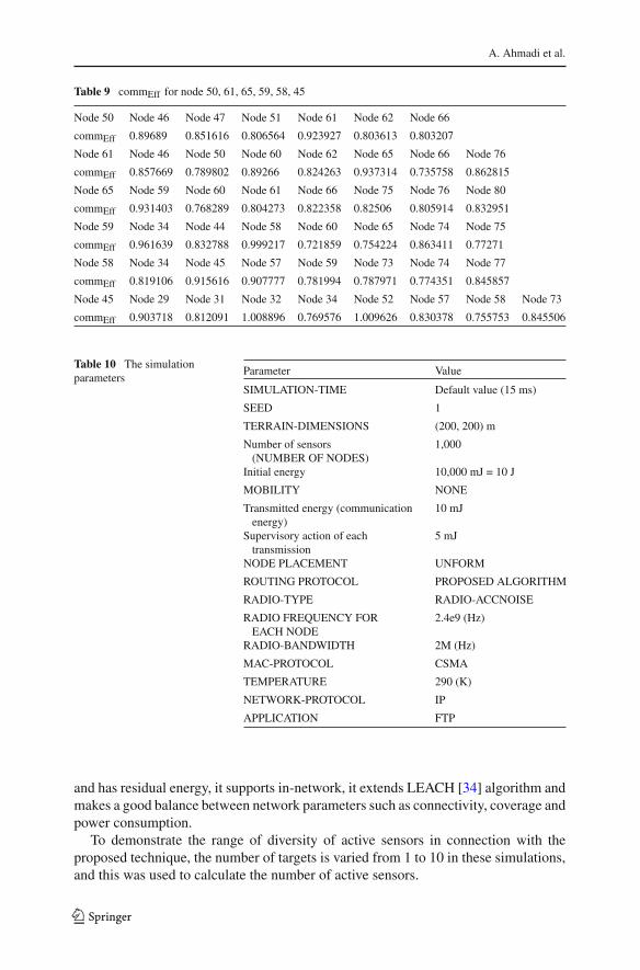
In Fig. 8b, node 61 has 7 choices based on its neighbors (i.e., nodes 65, 62, 60, 50,46, 76, 66). Regarding the value commEff in Table 9, we select the node 59 for thenext step of sending information. Also, in Fig. 8c, node 65 has 7 choices based on itsneighbors (i.e., nodes 59, 60, 61, 66, 75, 76, 80). Based on the value commEff in Table9, the node 61 is selected as the next hop transmitting data. Moreover, in Fig. 8d, node59 has 7 choices based on its neighbors (i.e., nodes 34, 44, 58, 60, 65, 74, 75). Basedon the value commEff in Table 9, node 58 is selected as the next hop for transmittingdata. In addition, in Fig. 8e, node 58 has 7 choices based on its neighbors same before(i.e., nodes 34, 45, 57, 59, 73, 74, and 77). Based on the value commEff in Table 9, thenode 45 is selected as the next hop for transmitting data. Next, in Fig. 8f, node 45 has8 choices based on its neighbors (i.e., nodes 29, 31, 32, 34, 52, 57, 58, and 73). Basedon the value commEff in Table 9, node 52 is selected as the next hop for transmittingdata. Finally, in Fig. 8g, due to the fact that node 52 is able to reach directly to thesink, it delivers the data directly to the sink.

5 Performance evaluation

5.1 Experimental setup

Since implementation of these techniques is expensive and time-consuming, a sim-ulation was used to evaluate their performance. This section presents an evaluationthrough a simulation and provides the relevant results.

Glomosim is used for special network simulations, with TCP, routing, and multicastprotocols in a wireless network and satellites [40]. Glomosim can simulate myriadnodes using C functions and Parsec. Glomosim is free open-source code which canbe assembled and run on Linux- and Windows-based operating systems [40].

Our simulations assumed an environment spanning (TERRAIN-DIMENSIONS)200 × 200 sq m, with 1,000 sensor nodes deployed randomly in that space, includingrandom nodes. We consider each node radius Rs to have a uniform distribution between[4, 6] m. As we see, each node is able to cover several nodes based on its radius, also,Rc is considered one meter (fixed) larger than its Rs for each node. The nodes receive

123


Fig. 8 An example of selection of active transmitting nodes for information transfer to the sink

123

A. Ahmadi et al.

Fig. 8 continued

123


Fig. 8 continued

Table 8 Table 7 values for the Fig. 8a

Node 46 Node 47 Node 51 Node 61 Node 62 Node 66

Er(s j ) 4.5 4.6 4.4 4.7 4.5 4.3

Emax 5 5 5 5 5 5

Dsink(50) 11.303 11.303 11.303 11.303 11.303 11.303

Dsink(s j ) 9.757 11.521 12.913 9.975 11.841 10.146

d(50,s j ) 1.252 1.034 1.035 1.333 0.727 0.644

Rc 2 2 2 2 2 2

commEff 0.89689 0.851616 0.806564 0.923927 0.803613 0.803207

object information and transfer it through cluster heads and communicative nodes toa sink location situated at the center of the environment. The simulation parametersare listed in Table 10.

Specifically, the objects are varied in their circumstances; the initial energy of thesensors is 10,000 mJ while the transmitted energy is 10 mJ across the greatest distance;and there is 5 mJ for each supervisory action.

5.2 Experimental results

The proposed algorithm is compared with the EAP technique with respect to objects,links, and energy consumption. The coverage and relevant results are presented. Com-pared with the two classic protocols for sensor networks, HEED [32] and LEACH [34],the performance of EAP [31,35] is more optimized due to its network coverage andinformation transfer. Each test was carried out in different conditions and with differentsettings. The graphs that are displayed depict the average of the several test results. Inconclusion, we use EAP because it pays close attention to clustering, energy-efficiencyand energy consumption of nodes in whole networks, and each node uses broadcasting

123

A. Ahmadi et al.

Table 9 commEff for node 50, 61, 65, 59, 58, 45

Node 50 Node 46 Node 47 Node 51 Node 61 Node 62 Node 66

commEff 0.89689 0.851616 0.806564 0.923927 0.803613 0.803207

Node 61 Node 46 Node 50 Node 60 Node 62 Node 65 Node 66 Node 76

commEff 0.857669 0.789802 0.89266 0.824263 0.937314 0.735758 0.862815


commEff 0.931403 0.768289 0.804273 0.822358 0.82506 0.805914 0.832951


commEff 0.961639 0.832788 0.999217 0.721859 0.754224 0.863411 0.77271


commEff 0.819106 0.915616 0.907777 0.781994 0.787971 0.774351 0.845857

Node 45 Node 29 Node 31 Node 32 Node 34 Node 52 Node 57 Node 58 Node 73

commEff 0.903718 0.812091 1.008896 0.769576 1.009626 0.830378 0.755753 0.845506

Table 10 The simulationparameters

Parameter Value

SIMULATION-TIME Default value (15 ms)

SEED 1

TERRAIN-DIMENSIONS (200, 200) m

Number of sensors(NUMBER OF NODES)

1,000

Initial energy 10,000 mJ = 10 J

MOBILITY NONE

Transmitted energy (communicationenergy)

10 mJ

Supervisory action of eachtransmission

5 mJ

NODE PLACEMENT UNFORM

ROUTING PROTOCOL PROPOSED ALGORITHM

RADIO-TYPE RADIO-ACCNOISE

RADIO FREQUENCY FOREACH NODE

2.4e9 (Hz)

RADIO-BANDWIDTH 2M (Hz)

MAC-PROTOCOL CSMA

TEMPERATURE 290 (K)

NETWORK-PROTOCOL IP

APPLICATION FTP

and has residual energy, it supports in-network, it extends LEACH [34] algorithm andmakes a good balance between network parameters such as connectivity, coverage andpower consumption.

To demonstrate the range of diversity of active sensors in connection with theproposed technique, the number of targets is varied from 1 to 10 in these simulations,and this was used to calculate the number of active sensors.

123


Fig. 9 Number of active nodes proportional to the number of targets

Fig. 10 Percentage of delivered packets that are received in the network (lifetime in ms)

For comparing the proposed technique with the EAP technique, the range of cover-age was assumed to be in status (position number) number 4 (i.e., according to Table 2),since the range of coverage affects the simulation results. Figure 9 shows the numberof active nodes as a function of the targets’ number. The number of active nodes inthe proposed technique is higher than in the EAP technique, and the communicativeradius of sensors remains at the highest value. This decreases the proposed technique’srate of energy consumption in the network, because we are able to use the k-coverageagain to transmit information to the sink with the help of other nodes that are in thecoverage area.

The percentage of delivered packets is shown in Fig. 10.Delivered ratio means the ratio of the (received) delivered packets in sink into

produced and transmitted packets over times. The proposed method has better perfor-mance by increasing the time than does EAP, because the packets are transferred to

123

A. Ahmadi et al.

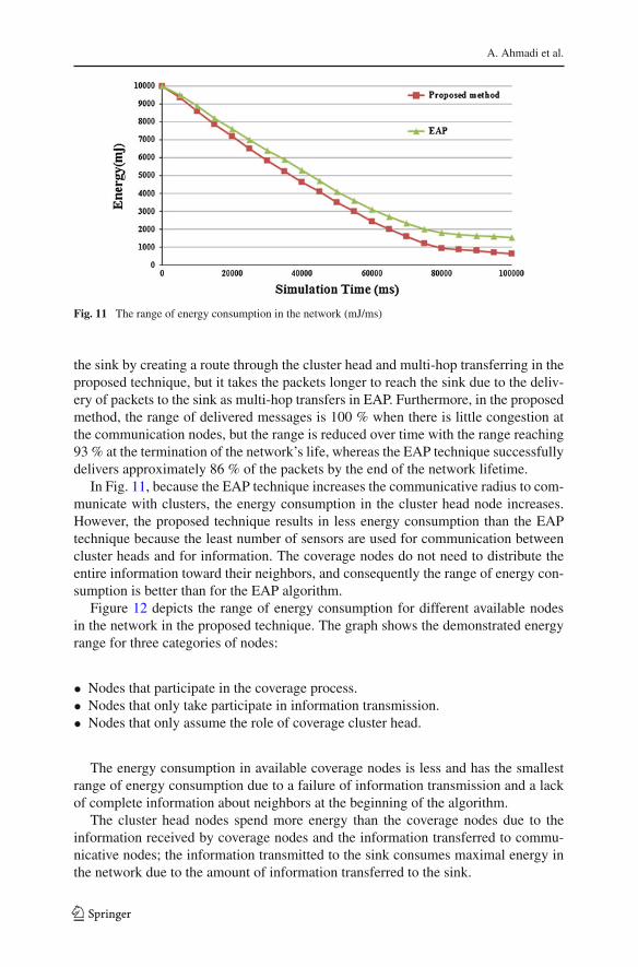
Fig. 11 The range of energy consumption in the network (mJ/ms)

the sink by creating a route through the cluster head and multi-hop transferring in theproposed technique, but it takes the packets longer to reach the sink due to the deliv-ery of packets to the sink as multi-hop transfers in EAP. Furthermore, in the proposedmethod, the range of delivered messages is 100 % when there is little congestion atthe communication nodes, but the range is reduced over time with the range reaching93 % at the termination of the network’s life, whereas the EAP technique successfullydelivers approximately 86 % of the packets by the end of the network lifetime.

In Fig. 11, because the EAP technique increases the communicative radius to com-municate with clusters, the energy consumption in the cluster head node increases.However, the proposed technique results in less energy consumption than the EAPtechnique because the least number of sensors are used for communication betweencluster heads and for information. The coverage nodes do not need to distribute theentire information toward their neighbors, and consequently the range of energy con-sumption is better than for the EAP algorithm.

Figure 12 depicts the range of energy consumption for different available nodesin the network in the proposed technique. The graph shows the demonstrated energyrange for three categories of nodes:

• Nodes that participate in the coverage process.• Nodes that only take participate in information transmission.• Nodes that only assume the role of coverage cluster head.

The energy consumption in available coverage nodes is less and has the smallestrange of energy consumption due to a failure of information transmission and a lackof complete information about neighbors at the beginning of the algorithm.

The cluster head nodes spend more energy than the coverage nodes due to theinformation received by coverage nodes and the information transferred to commu-nicative nodes; the information transmitted to the sink consumes maximal energy inthe network due to the amount of information transferred to the sink.

123


Fig. 12 Residual energy for different categories of nodes in the proposed technique (J/ms)

6 Conclusion and future research

Regional coverage is one of the main characteristics in a wireless sensor network,with the main aim being to achieve the maximum coverage in the area with the leastenergy consumption by the sensors. The initial and main operation of each sensornode is to review its vicinity to provide the required information for operating pur-poses. The routing protocol for coverage should provide low energy consumption toincrease the network lifetime and the warranty of network connection. High coverageis advantageous for promoting error tolerance and the validity of received informa-tion. Our simulation results and comparison of the routing algorithms’ retention ofcoverage prove that the proposed algorithm preserves the network with its low energyconsumption.

The paper reviews the relevant characteristics of sensor nodes, the functions andapplications represented, as well as the types of sensor and their structures and theconstraints they encounter. The constraints of these networks are energy limitations,network lifetime, and network coverage. Therefore, relevant strategies are provided tocontrol the network coverage. The proposed technique is a rapid reduction of nodesaround the sink. Only a few nodes are used around the sink in spite of a high nodedensity assumed in the environment. These nodes assume the burden of relayinginformation to the sink resulting in a reduction of energy consumption in the nodes.One way to address this challenge is the enervation of the sink in the environment.

It is plausible to increase the range of coverage by k nodes to upgrade the toleranceagainst faults in the future, but that strategy is insufficient because the connection ofthe sink with an object or part of the network is vulnerable to de-linkage in the caseof a discrepancy along the route or a discrepancy of the supervisory node. Therefore,it is desirable to provide a convenient strategy for upgrading the network’s resistanceto network discrepancy. Specifically, we mention that, if a hole exists, we try to find

123

A. Ahmadi et al.

another path around hole to bypass the hole and it might be a longer path. In the worstcase, if our network breaks into two completely isolated sub-networks, no algorithmcan find a path.

References

1. Akyildiz I, Su W, Sankarasubramaniam Y, Cayirci E (2008) A survey on sensor networks. ComputNetw 52(12):2292–2330

2. Pottie GJ, Kaiser WJ (2000) Wireless sensor networks. Commun ACM 43(5):51–583. Labrador MA, Wightman PM (2009) Topology control in wireless sensor networks. In Springer, Berlin

ISBN: 978-1-40209589-94. Shojafar M, Pooranian Z, Shojafar M, Abraham A (2013) LLLA: New Efficient Channel Assignment

Method in Wireless Mesh Networks. Springer International Publishing, Innovations in Bio-inspiredComputing and Applications 237:143–152

5. Akyildiz IF, Melodia T, Chowdhurry KR (2007) A survey on wireless multimedia sensor networks.Comput Netw 51(4):921–960

6. Sayyad A, Ahmadi A, Shojafar M, Meybodi MR (2010) Improvement multiplicity of routs in directeddiffusion by learning automata new approach in directed diffusion. In: International conference oncomputer technology and, development, pp 195–200

7. Sayyad A, Shojafar M, Delkhah Z, Ahamadi A (2011) Region directed diffusion in sensor networkusing learning automata: RDDLA. J Adv Comput Res 1(3):71–83

8. Sayyad A, Shojafar M, Delkhah Z, Meybodi MR (2010) Improving directed diffusion in sensor networkusing learning automata: ddla new approach in directed diffusion. In: 2nd International conference oncomputer technology and development (ICCTD 2010), pp 189–194

9. Ghosh A, Das SK (2008) Coverage and connectivity issues in wireless sensor networks: a survey.Pervasive Mobile Comput 4(1):303–334

10. Younis M, Akkaya K (2008) Strategies and techniques for node placement in wireless sensor networks:a survey. Elsevier Ad Hoc Netw 6:621–655

11. Stojmenovic I, Lin X (2001) Loop-free hybrid single-path/flooding routing algorithms with guaranteeddelivery for wireless networks. IEEE Trans Parallel Distrib Syst 12(10):1045–9219

12. Yang S, Dai F, Cardei M, Wu J (2006) On connected multiple point coverage in wireless Sensornetworks. J Wirel Inf Netw

13. Huang Y, Tseng Y (2003) The coverage problem in a wireless sensor networks. In: Proceedings of the2th ACM international conference on information proceedings in sensor networks and applications,pp 115–121

14. Benyuan L, Dousse O, Nain P, Towsley D (2013) Dynamic coverage of mobile sensor networks. IEEETrans Parallel Distrib Syst 24(2):301–311

15. Li S, Kao HC (2010) Distributed K-coverage self-location estimation scheme based on Voronoi dia-gram. Commun IET 4(2):167–177

16. So AM, Ye Y (2005) On solving coverage problems in a wireless sensor network using Voronoidiagrams. In: Proceedings of workshop on internet and network economics, vol 3828, pp 584–593

17. Okabe T, Boots B, Sugihara K, Chiu SN (2000) Spatial tessellations: concepts and applications ofVoronoi diagrams. 2nd edn. Wiley, New York

18. Powers RA (1995) Batteries for low power electronics. Proc IEEE 83(4):687–69319. Shen CC, Srisathapornphat C, Jaikaeo C (2001) Sensor information networking architecture and appli-

cations. IEEE Pers Commun 8(4):52–5920. Howard A, Mataric M, Sukhatme G (2002) Mobile sensor network deployment using potential fields: a

distributed, scalable solution to the area coverage problem. In: Distributed autonomous robotic systems,vol 5. Springer, Berlin, pp 299–308

21. Hefeeda M, Bagheri M (2007) Randomized K-Coverage algorithms for dense sensor networks. In:Proceedings of 26th IEEE international conference on communications pp 2376–2380

22. Nath S, Gibbons PB (2007) Communicating via fireflies: geographic routing on duty-cycled sensors.In: Proceedings of the 6th international conference on information proceedings in sensor, networks,pp 440–449

123


23. Anastasi G, Conti M, Francesco MD, Passarella A (2009) Energy conservation in wireless sensornetworks: a survey. Ad Hoc Netw 7(3):537–568

24. Wang L, Xiao Y (2006) A survey of energy-efficient scheduling mechanism in sensor networks. MobileNetw Appl 11(5):723–740

25. Chakrabarty K, Iyengar S, Qi H, Cho E (2002) Grid coverage for surveillance and target location indistributed sensor networks. IEEE Trans Comput 51(12):1448–1453

26. Jin Yu, Jian P, Zhousi W, LinYa P (2009) A survey on position-based routing algorithms in wirelesssensor networks. Algorithms 2(1):158–182

27. Xing G, Wang W, Zhang Y, Lu C, Pless R, Gill C (2005) Integrated coverage and connectivity config-uration in wireless sensor networks. ACM Trans Sensor Netw (TOSN) 1(1)

28. Ilyas M, Mahgoub I (2005) Handbook of sensor networks: compact wireless and wired sensing systems.CRC Press, Boca Raton ISBN: 0-8493-1968-4

29. Cordeschi N, Shojafar M, Baccarelli E (2013) Energy-saving selfconfiguring networked data centers.Comput Netw 57(17): 3479–3491.

30. Zhang H, Hou J (2005) Maintaining sensing coverage and connectivity in large sensor networks. AdHoc Sensor Wirel Netw 1(12):89–123

31. Younis O, Fahmy S (2004) HEED: a hybrid, energy-efficient, distributed clustering approach for adhoc sensor networks. IEEE Trans Mobile Comput 3(4):366–379

32. Luchmun R, Pyanee M, Khedo KK (2012) Hierarchical hybrid energy efficient distributed clusteringalgorithm. Int J Comput Distrib Syst 2(1)

33. Tsai Y (2007) Coverage-preserving routing protocols for randomly distributed wireless sensor net-works. IEEE Trans Wirel Commun 6(4):1240–1245

34. Heinzelman WR, Chandrakasan A, Balakrishnan H (2000) Energy efficient communication protocolsfor wireless micro sensor networks. In: Proceedings of Hawaii international conference on systemsciences

35. Liu A, Jin X, Cui G, Chen Z (2013) Deployment guidelines for achieving maximum lifetime andavoiding energy holes in sensor network. Inf Sci 230:197–226

36. Dong Y, Quan Q, Zhang J (2008) Priority-based energy aware and coverage preserving routing forwireless sensor network. In: Proceedings of vehicular technology conference, pp 138–142

37. Jin Y, Jo J, Wang L, Ki Y (2008) ECCRA: an energy-efficient coverage and connectivity preservingrouting algorithm under border effects in wireless sensor networks. Comput Commun 31(10):2398–2407

38. Ahmed N, Kanhere SS, Jha S (2005) The holes problem in wireless sensor networks: a survey. ACMSIGMOBILE Mobile Comput Commun Rev 9(2):4–18

39. Omranpour H, Ebadzadeh MM, Barzegar S, Shojafar M (2008) Distributed coloring of the graphedges. In: Proceedings of 7th IEEE international conference on cybernetic intelligent systems 2008(CIS2008), UK, pp 1–5

40. Zeng X, Bagrodia R, Gerla M (1998) GloMoSim: a library for parallel simulation of large-scale wirelessnetworks. In: Proceedings of parallel and dstributed simulation, (PADS 98), vol 161, p 154

123

An Efficient Routing Algorithm to preserve k-Coverage in Wireless Sensor Networks

Documents

Transcript of An Efficient Routing Algorithm to preserve k-Coverage in Wireless Sensor Networks