An Efficient Approach for Seismic Fragility Assessment with Application to Old Reinforced Concrete...

Journal of Earthquake Engineering, 14:231–251, 2010

Copyright � A.S. Elnashai & N.N. Ambraseys

ISSN: 1363-2469 print / 1559-808X online

DOI: 10.1080/13632460903086028

An Efficient Approach for Seismic FragilityAssessment with Application

to Old Reinforced Concrete Bridges

GIANMARCO DE FELICE and RENATO GIANNINI

Department of Structures, University Roma Tre, Rome, Italy

A procedure for seismic fragility assessment, suitable for application to non ductile RC structures ispresented, which is based on the estimate of a response surface that gives the probability of failureof the structure as a function of the random variables that affect the response. The seismic fragilityor risk is then evaluated through numerical integration. The method considers different sources ofuncertainty: (i) in the seismic input, through the use of different accelerograms for the dynamicanalysis; (ii) in the structural response, through the use of a refined nonlinear finite element model;and (iii) in the ultimate state capacity, taking into account the different modes of failure which mayoccur, for which a random mechanical capacity model is available. Aiming at reducing the numberof simulation analyses, the uncertainties on the seismic input and on the mechanical parametersgoverning the response are treated according to the response surface methodology, while the limit-state randomness is treated explicitly during the simulations.

Using the proposed procedure, the seismic safety of two reinforced concrete bridges fromItalian highway network, with simply supported deck and either single stem or frame piers, isevaluated. The results are expressed in terms of fragility curves as function of spectral acceleration.The obtained results highlight the influence of material randomness on reliability and the relativeimportance of seismic input with respect to mechanical and epistemic uncertainty.

Keywords Seismic Fragility; Simulation; Bridges; Assessment; Reinforced Concrete; ResponseSurface Method

1. Introduction

Various approaches at different levels of complexity have been proposed in the recent

past for the assessment of seismic risk of structures [Pinto et al., 2004]. As regards the

structural behaviour, although fairly reliable models are available in the nonlinear field,

they tend not to be included in the framework of probabilistic analysis, because of the

long computation times involved. As regards the model of action, the use of samples of a

stochastic process underwent severe criticism, since it was considered incapable of

reproducing the whole complex reality and variability of seismic motion [Naeim and

Lew, 1995; Bommer and Acevedo, 2004]. The only approach capable of utilizing models,

of both structure and action, which are adequately accurate and realistic, is simulation;

however, the Monte Carlo method, also in the more efficient versions recently proposed

(i.e., Au and Beck, 2001, 2003), proves to be exceedingly onerous from the computa-

tional point of view, especially in the case of complex structures analyzed with refined

models, whose randomness depends on many variables.

Received 24 June 2008; accepted 15 May 2009.

Address correspondence to Gianmarco de Felice, Department of Structures, University Roma Tre, via

Corrado Segre, 6 - 00146 Rome, Italy; E-mail: [email protected]

231

Dow

nloa

ded

by [

Uni

vers

ita d

egli

Stud

i Rom

a T

re]

at 0

2:33

09

Apr

il 20

15

Since rigor and accuracy are not compatible with a practically acceptable amount of

computation, the present thrust of the research is towards methods that are admittedly of

less than general nature and contain approximate assumptions, but are capable of provid-

ing satisfactory results when used in their proper context (i.e., Pinto, 2001).

An efficient method was developed in Shome et al. [1998] to calibrate the partial

safety coefficients used in the FEMA-350 guidelines, which is based on a simple

analytical formulation for the probability of failure, whose parameters are obtained on

the basis of a limited number of analyses with different earthquakes, scaled to the

intensity of the expected value of the site response spectrum, corresponding to the

fundamental period of the structure. The IDA (Incremental Dynamic Analysis) method

[Vamvatsikos and Cornell, 2001] requires several analyses for each earthquake sample

and for each intensity level. In any case, the efficiency of these methods is achieved by

neglecting the randomness of the structure’s mechanical parameters (as, for instance,

strength and stiffness of the structural elements) and their influence on the possible failure

mechanisms that may occur. This is not completely satisfactory, especially in the case of

existing reinforced concrete structures, which is the focus of the present study, since not

infrequently the degree of uncertainty on the mechanical model becomes comparable

with that related to the hazard [Ibarra and Krawinkler 2005; Liel et al., 2009]. The

variability of the basic constituent materials, concrete and steel, with respect to their

nominal, or to the in situ measured values, is of course one of the factors, but rarely the

most significant one, if compared with the uncertainties due to imperfect knowledge of

the amount and layout of reinforcement. The influence of even minor differences in the

amount of reinforcement, curtailing of the rebars, detailing of certain regions, etc., can be

paramount in determining a good or bad performance of the structure, and their con-

sideration is therefore essential for a meaningful estimate of the probability of failure. All

of the mentioned aspects are carefully controlled by present seismic codes, so that

properly designed new structures should in principle only fail according to clearly defined

mechanisms, with a negligible probability of occurrence of the undesired ones. A simple

and global failure condition for these structures, such as the maximum inter-story drift,

may be adequate. Conversely, old structures often neglect these rules and may fail

according to different failure mechanisms that have to be considered in the assessment.

To take into account multiple failure modes, that may interest one or more structural

elements, is a rather difficult task; also, because the structural models are not able to

properly reproduce all the different mechanism that may develop. Besides, the assump-

tion that failure coincide with the lost of convergence of the numerical solver, is not

satisfactory since it strongly depends on the efficiency of the integration algorithm. For

these structures, in the absence of other well-recognized criteria, it seems careful and

reasonable to assume that the global failure coincides with that of the first load-bearing

element. Even with this assumption, the check of the collapse remains uncertain to a large

extent, since the capacity formula, such as the ultimate chord rotation of a plastic hinge

[Panagiotakos and Fardis, 2001] or the shear strength of a column [Priestley et al., 1994],

are affected by a large scatter, which is of the same order of magnitude as the scatter in

the demand due to record-to-record variability. Aiming at taking into account multiple

failure modes and structural randomness, the statistic technique of the response surface

has been used recently [Franchin et al., 2003; Schotanus et al. 2004; Liel et al., 2009] for

seismic assessment. The method consists in determining, through a limited number of

targeted experiments, a simple relation of polynomial type between the random variables

and a structural response parameter measuring the performance of the structure. Such

measurement, if expressed in terms of ground motion intensity (e.g., peak ground accel-

eration or spectral acceleration at the fundamental period of the structure), may be

232 G. de Felice and R. Giannini

Dow

nloa

ded

by [

Uni

vers

ita d

egli

Stud

i Rom

a T

re]

at 0

2:33

09

Apr

il 20

15

directly compared with the seismic hazard. The limit of the Response Surface Method

(RSM) lies in the fact that it loses efficiency if the number of random factors considered

is not sufficiently small (4–6). In fact, the number of simulations necessary in order to

construct the response surface grows exponentially with the number n of variables, so that

if n is large, the number of experiments necessary becomes comparable with that required

by the Monte Carlo method.

Another procedure, defined as Effective Fragility Analysis (EFA) was recently

proposed [de Felice et al., 2002; Pinto et al., 2004], in order to achieve a significant

reduction in the number of variables on which the structural response depends. In the

versions presented earlier, the method did not have recourse to the response surface

technique; the dependence of the probability of failure on the variables considered was

expressed by means of a Taylor series expansion truncated after the second order.

In the present work, the EFA is integrated with the RSM in order to permit a better

estimate of probabilities and to further reduce the number of simulations necessary, while

taking seismic variability into account. The method is able to incorporate any significant

sources of uncertainty, related to both the action and the structure; it makes use of a full

nonlinear dynamic analysis under samples (recorded accelerograms) of the excitation

process, and calculates the probability of exceeding any specified limit-state, conditioned

to each sample. By repeating the analyses according to a prescribed experimental plan,

when varying the mechanical properties of the structure, the response surface is finally

obtained, which gives the dependence of the probability of failure of the bridge as a

function of structural random variables. The seismic risk is then estimated by means of

convolution with the probability density function of the hazard at the site and of the

structural random variables, using as a model of structural behaviour the simple poly-

nomial relation obtained earlier. A similar approach was proposed in Schotanus et al.

[2004], where the RSM was used to estimate the relation between the seismic intensity

leading to collapse and the random variables, and the fragility obtained through FORM

analyses. In the present case, however, the randomness in the capacity model is included

in the formulation and a lower number of analyses are required, since the intensity

measure is included among the fixed effect variables. The result is expressed directly

in terms of probability of collapse and then the fragility results simply by convolution of

the response surface.

Hereafter, EFA will be briefly presented (Sec. 2), then after a rapid illustration of the

RSM (Sec. 3), we will clarify how the two methods are joined together (Sec. 4).

Eventually, the approach is applied to two existing bridges of the Italian highway network

(Sec. 5).

2. Effective Fragility Analysis

Accurate seismic reliability methods for nonlinear structures require performing a number

of dynamic analyses, and this usually takes the largest part of total computing effort

required. Reducing the number of the structural analyses is therefore a goal common to

all methods. With this objective in mind, in the present approach the vector of random

structural variables is partitioned into two sub-vectors. The first one, X, is of relatively

small dimensions and contains the variables (named external) which have a significant

influence on the response, as for example, the stiffness, masses, yield strength, etc., and in

general all variables a change of whose values would reasonably require performing a

new analysis. The second sub-vector, Y, of much larger dimensions, is composed instead

of variables of local nature (named internal), which are suitable for detecting a state of

failure of the structure, but whose own state is not such as to affect significantly the

Efficient Approach for Seismic Fragility Assessment 233

Dow

nloa

ded

by [

Uni

vers

ita d

egli

Stud

i Rom

a T

re]

at 0

2:33

09

Apr

il 20

15

global dynamic response of the structure. Strictly speaking, all the geometrical and

mechanical variables influence both the strength and the dynamic response of the

structure; for instance, the shear or bending failure of a single element may affect the

global structural response. The separation between ‘‘internal’’ and ‘‘external’’ variables is

accordingly largely conventional and depends to a large extent on the structural model

adopted for evaluating the seismic demand. In fact, those parameters that do not appear in

the model clearly cannot influence the seismic demand, even if this may not be com-

pletely realistic. Moreover, if the failure condition adopted is of fragile type, it is not

necessary to analyze the effect of this collapse on the subsequent response of the

structure, since, in any case, the conventional limit state has been exceeded. Experience

shows that the separation between internal and external variables, carried out according to

the model adopted and on the base of engineering judgement, often leads to acceptable

approximations.

The mechanical properties of the materials, concrete and steel, certainly alter, not

only the resistance, but also the dynamic response. However, if we separate randomness

of the mechanical properties into two parts, one, average for the whole structure, and the

other which expresses its local fluctuations, we may venture the hypothesis that the latter,

while affecting the resistance, has only a limited influence on the response.

The expedient of separating the random variables makes it possible to greatly reduce

the number of analyses implied by the simulation process; in fact, after fixing the external

variables and the action, the structural response proves to be deterministic and thus

calculation of the probability of failure (conditioned by the values of the external

variables) may be carried out relatively rapidly.

2.1. Unconditioned Probability Computation

Upon assignment of a value to the vector X, the structural response to the j-th sample

accelerogram becomes deterministic and can be evaluated. In the general case, failure

may occur according to different mechanisms in different elements of the structure, as,

for instance, when the strength is reached in a brittle element, or the displacement

capacity is attained for a ductile element. The failure of a structural element does not

strictly imply the overall collapse, especially for capacity-designed new structures; but in

the case of existing structures, as stated previously, once the load-bearing elements and

their possible failure mechanisms are singled out, we may assume that failure of any of

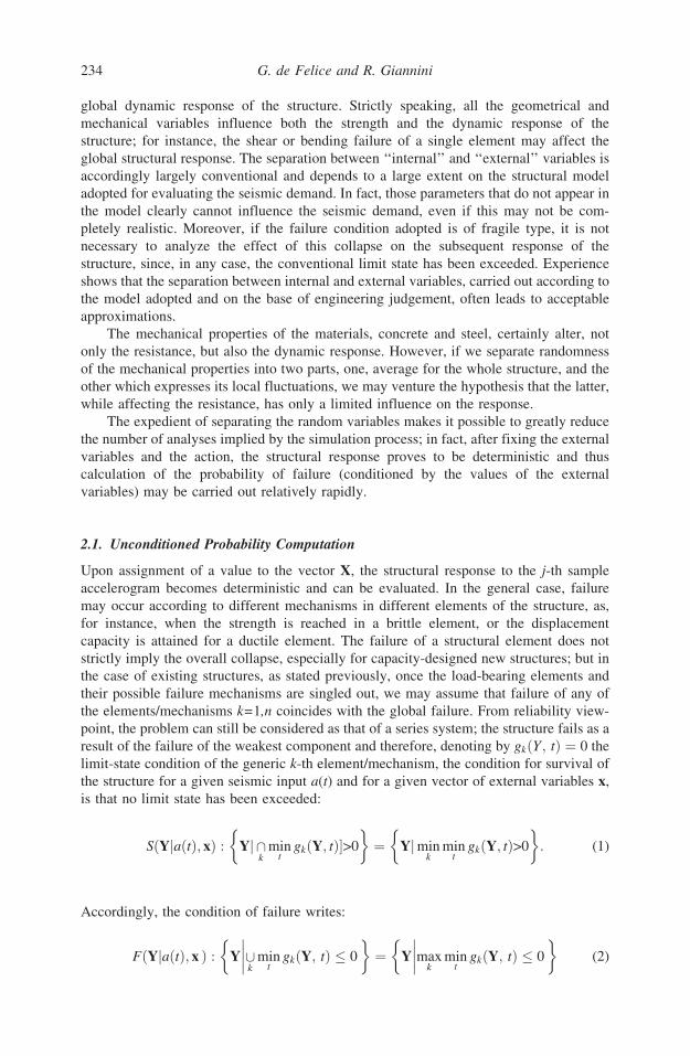
the elements/mechanisms k=1,n coincides with the global failure. From reliability view-

point, the problem can still be considered as that of a series system; the structure fails as a

result of the failure of the weakest component and therefore, denoting by gk Y ; tð Þ ¼ 0 the

limit-state condition of the generic k-th element/mechanism, the condition for survival of

the structure for a given seismic input a(t) and for a given vector of external variables x,

is that no limit state has been exceeded:

S YjaðtÞ; xð Þ : Yj \k

mint

gkðY; tÞ�>0

� �¼ Yjmin

kmin

tgkðY; tÞ>0

� �: (1)

Accordingly, the condition of failure writes:

F Y aðtÞj ; xð Þ : Y [k

mint

gk Y; tð Þ � 0

��

¼ Y maxk

mint

gk Y; tð Þ � 0

��

(2)


Dow

nloa

ded

by [

Uni

vers

ita d

egli

Stud

i Rom

a T

re]

at 0

2:33

09

Apr

il 20

15

and the probability of failure, given by PF ¼ Pr F aðtÞ; X ¼ xjf g , may be calculated from

(2), contemporaneously for all the element/mechanisms, using an efficient Monte Carlo

method. Application of the Monte Carlo method is straightforward since the computation

of the limit state functions gkðY; tÞ does not require a new structural analysis; each

simulation merely requires the computation of functions gk, which often have a fairly

simple form. However if, as often happens, many of the mechanisms are not well

correlated, convergence of the procedure could be considerably slowed down; in these

cases, the efficiency of the method can be improved having recourse to the subset

simulation as proposed by Au and Beck [2001].

The computation of the probability of failure becomes more rapid when the limit

state equations can be expressed in the form:

gk Y; tð Þ ¼ ck Yð Þ � dk tð Þ; k ¼ 1; n; (3)

where ck Yð Þ represents the capacity of the structure, not dependent on time t, while dk tð Þexpresses the demand that, for given input a(t) and external variables x, is obtained from

the results of the dynamic analysis as a deterministic function of time t. In such a case, the

failure condition of the generic k-th element/mechanism becomes:

Fk : mint

ck Yð Þ � dkðtÞ � 0f g ¼ ck Yð Þ �maxt2T

dk tð Þf g � 0 ¼ ck Yð Þ � dk max � 0 (4)

and the probability of failure PFk ¼ Pr ck Yð Þ � dk max � 0ja tð Þ;X ¼ xf g may be com-

puted using the usual methods of time-invariant reliability, for example by means of

the First Order Reliability Method (FORM).

The probability of the union PF ¼ Pr [k

Fk

� �may be obtained in an approximate way

using, for example, the Ditlevsen bounds [Ditlevsen, 1979], which require evalua-

tion of the probabilities of the intersections two by two Fi \ Fj

� �, or improved

bounds based on higher-order intersections [Zang, 1993; Song and Der Kiureghian,

2003]; the latter may be used also for evaluating the reliability of more general

systems consisting of elements in series and in parallel. Alternatively, the probability

of failure may be estimated by means of the approximate evaluation of the multi-

variate normal distribution [Tang and Melchers, 1987; Pandey, 1998; Yuan and

Pandey, 2006].

The probability of failure computed in the abovementioned way is conditioned to the

value x of external r.v. X and to the particular accelerogram a(t) used in the analysis. It is

therefore necessary to make this probability no longer conditional on the external random

variables. This is achieved, in the present article, by using the Response Surface Method,

i.e., approximating the probability of failure PF(x) by means of a second order poly-

nomial function defined in an appropriate sub-region of the X-space. If n is the dimension

of the X-space, the number of coefficients needed for a full second-order polynomial is:

(1+n+n2). This number represents the required minimum number of experiments, each

one providing a value of PF, necessary for estimating the coefficients of the polynomial

function. In order to improve the smoothness of the surface and its fit to the experimental

results, however, a larger number of experiments has to be employed, which also allows

computation of the dispersion due to the lack of fit of the model, as will be detailed

below.


Dow

nloa

ded

by [

Uni

vers

ita d

egli

Stud

i Rom

a T

re]

at 0

2:33

09

Apr

il 20

15

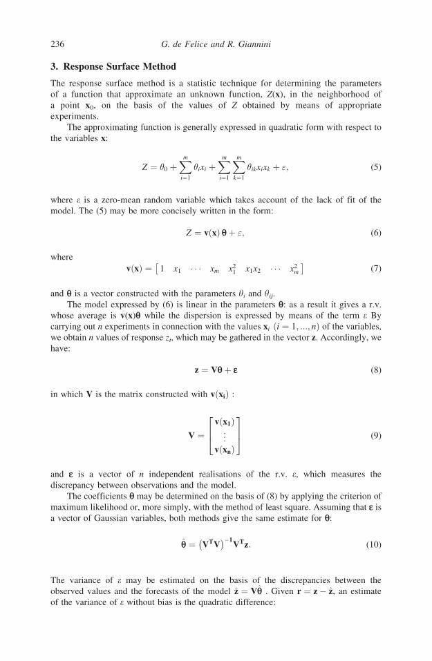
3. Response Surface Method

The response surface method is a statistic technique for determining the parameters

of a function that approximate an unknown function, Z(x), in the neighborhood of

a point x0, on the basis of the values of Z obtained by means of appropriate

experiments.

The approximating function is generally expressed in quadratic form with respect to

the variables x:

Z ¼ �0 þXm

i¼1

�ixi þXm

i¼1

Xm

k¼1

�ikxixk þ "; (5)

where e is a zero-mean random variable which takes account of the lack of fit of the

model. The (5) may be more concisely written in the form:

Z ¼ v xð Þ qþ "; (6)

where

v xð Þ ¼ 1 x1 � � � xm x21 x1x2 � � � x2

m

(7)

and q is a vector constructed with the parameters yi and yij.

The model expressed by (6) is linear in the parameters q: as a result it gives a r.v.

whose average is v(x)q while the dispersion is expressed by means of the term e By

carrying out n experiments in connection with the values xi ði ¼ 1; :::; nÞ of the variables,

we obtain n values of response zi, which may be gathered in the vector z. Accordingly, we

have:

z ¼ Vqþ e (8)

in which V is the matrix constructed with v xið Þ :

V ¼v x1ð Þ

..

.

v xnð Þ

264

375 (9)

and e is a vector of n independent realisations of the r.v. e, which measures the

discrepancy between observations and the model.

The coefficients q may be determined on the basis of (8) by applying the criterion of

maximum likelihood or, more simply, with the method of least square. Assuming that e is

a vector of Gaussian variables, both methods give the same estimate for q:

q ¼ VTV� ��1

VTz: (10)

The variance of e may be estimated on the basis of the discrepancies between the

observed values and the forecasts of the model z ¼ Vq . Given r ¼ z� z, an estimate

of the variance of e without bias is the quadratic difference:


Dow

nloa

ded

by [

Uni

vers

ita d

egli

Stud

i Rom

a T

re]

at 0

2:33

09

Apr

il 20

15

s2" ¼

rTr

n� m; (11)

where n indicates the number of experiments and m the number of parameters gathered in

the vector q. Equation (11) shows that, in order to reduce the dispersion of error, it is

necessary to carry out a considerably larger number of experiments than that of the

parameters.

The variance of Z depends, not only on the variance of e and of the matrix V, but also

on point x where the estimate is made. The design of experiments that makes the variance

of Z dependent exclusively on the distance from the central point, is defined as rotatable.

The conditions for rotatability may be found in the specialized texts [Box and Draper,

1987].

The minimum number of experiments necessary for determining q is equal to the

number of the parameters but, as has been seen, this number must be increased if the

estimate of q is to be sufficiently reliable; accordingly, a compromise must be found

between the two contrasting requirements of accuracy and economy. The choice of a

rational design for the experiments is thus an essential point in the procedure.

A complete factorial design consists of fixing two levels for each of the variables m

and then carrying out 2m experiments corresponding to all of their possible combinations.

This design does not explore the effects of the variations of a single variable at a time and

accordingly does not permit an accurate estimate of pure quadratic terms of (6).

Therefore, it is customary to combine the factorial design with a ‘‘star’’ design, forming

what is called a central composite design (Fig. 1). Denoting by x�i and xþi the two levels

for each variable in the factorial design, the central point has coordinates x0i ¼ x�i þxþi

2and

thus, utilizing the coordinate transformation xi ¼ x0i þ�i�i, in which �i ¼ xþi�x�i2

, a

standardized space is obtained in which the points of the factorial experiments are the

apices of a hypercube centred on the origin and located in the points of coordinates

�i ¼ �1. The star part of the experiment is represented by points of coordinates

�i ¼ ��; i ¼ 1; . . . ; m; �j ¼ 0; 8j 6¼ i� �

. The value of a is established by the conditions

of rotatability of the design: in the absence of repetitions � ¼ 2m=4.

(a) Factorial design

( ) ( )1,1,1,, 321±±±=ξξξ

(b) Star design

( ) ( )( )( )α

α

αξξξ

±

±

±=

,0,0

0,,0

0,0,,,321

(c) Central point

( ) ( )0,0,0,, 321=ξξξ

FIGURE 1 Diagram of a central composite design of experiments.


Dow

nloa

ded

by [

Uni

vers

ita d

egli

Stud

i Rom

a T

re]

at 0

2:33

09

Apr

il 20

15

When the experiment consists of a simulation with a mathematical model, if the

variables in x completely define the model, the response is clearly deterministic and

accordingly, repetition of the experiment is useless. When on the contrary the

experiment is carried out in the field, the result always depends on a large number

of parameters, many of which cannot be controlled, so that, if the experiment is

repeated for the same values of x, in general different results are obtained. This fact

may also be considered in the case of numerical simulations, by introducing other

parameters, not included in vector x, which vary randomly between one simulation

and another.

In order to take a random effect into account, an additive random term d should

be added into Eq. (6). One possible way of estimating this term consists of repeating

the entire project of experiments for the different samples of the random factor.

However, this procedure is unattractive because of the large number of experiments

required. A more performing method consists of subdividing (the factorial part of) the

experimental design into as many blocks as samples of the random factor are

considered. The division of the experiments into blocks implies a certain loss of

information; it could be shown that, assuming random effects to be of additive type,

block design will mask the interactions between some of the variables governing the

fixed effects. The order of effects that are masked depends on the dimensions of the

blocks and on the way in which the experiments are divided into the blocks. The

division of experiments into blocks must ensure that only interactions of the higher

order are masked, as illustrated in the specialized literature [Box and Draper, 1987].

In any case, the blocks cannot be too small; therefore, if the number of blocks

necessary for estimating random effects is large compared to the number of factorial

experiments, it would be advisable to repeat twice or more the whole programme of

experiments, using different random factors in the various repetitions. If z is the

vector of the results of experiments, V is the matrix of the polynomial terms already

seen in (9) and q is the vector of the unknown parameters, the model with random

effects could be formulated as follows:

z ¼ V qþ Bd þ e (12)

in which B is a matrix n · b which applies the b random effects contained in d with the n

experiments, according to the diagram of division into blocks. Thus, if experiment i is

included in block k, this gives Bik = 1, otherwise Bik = 0. Matrix B introduces a correlation

between the terms of vector z that does not allow determination of the coefficients qindependently from the variances of d and of e. The procedure for estimating q, ��, and

�", based on the criterion of maximum likelihood, becomes more complex, requiring an

iterative method, since the problem is non-linear. More details may be found in Searle

et al. [1992].

In conclusion, for the given vector of r.v. X, once the dependence of the response

parameter Z on X has been approximately established on the basis of the response

surface, it should be possible to express Z in the form:

Z ¼ v xð Þ qþ � þ " (13)

which clearly shows that Z is a r.v. depending not only on x, but also on d and e which

represent the random factor introduced by the random effects and by the lack-of-fit of the

model, respectively.


Dow

nloa

ded

by [

Uni

vers

ita d

egli

Stud

i Rom

a T

re]

at 0

2:33

09

Apr

il 20

15

4. Combination of EFA and RSM

As we have seen in Sec. 2, the probability of failure PF conditional on given values of the

external variables X can be computed for a particular accelerogram according to the EFA

method. In order to obtain the unconditional probability of failure, a functional relation-

ship between PF and X should be established using the RSM.

As a first step utilizing the RSM in this context, we should ensure that no values of

PF less than zero or greater than one are attained. This will be done by applying to PF a

one-to-one transformation which projects the interval [0.1] over the whole real axis. The

inverse of the standard normal distribution ��1 is used, so that PF is transformed into the

reliability index b:

� ¼ ��1 PFð Þ : (14)

The subsequent considerations are accordingly applied to b instead of PF directly.

The result of each simulation depends not only on the values assigned to the external

variables, but also on the ground motion used in the analysis. In order to account for such

a dependence, an intensity measure of the earthquake, such as a peak ground acceleration

or an elastic spectral value, should be defined and included among the random variables

responsible for the fixed effect. However, this does not cover completely the effect of

ground motion variability on randomness of the response, since different time histories of

ground motion with the same earthquake intensity may produce different outputs giving

rise to different values of PF. As suggested in Franchin et al. [2003], the effect of time

history, by parity of ground motion intensity, may play the role of the random effect in

the RSM described in the previous paragraph. As illustrated heretofore, account may be

taken of this effect without increasing the number of experiments, that is, of dynamic

analyses of the structure. The design of numerical simulations to be carried out is divided

into as many blocks as the number of earthquake samples used.

4.1. Earthquake Samples and Seismic Intensity Measure

The applicability of the RSM to EFA is conditioned by the fact that the random effect

introduced by the choice of a ground motion time history should not be too great, so as

not to cover the fixed effects due to the parameters controlled in the simulation. The

dispersion introduced by the variation of time-history from sample to sample, at parity of

intensity, depends to a large extent on the chosen intensity measure. This problem is not

very important if artificially generated accelerograms as samples of a random process are

employed, since the response scatter is quite low; however, the present trend favors the

use of recorded accelerograms, rightly considered to reflect more realistically the natural

variability of ground motion for given values of the macroseismic parameters like

magnitude and distance.

Several ground motion intensity measures, aiming at minimizing the scatter of the

nonlinear response without introducing bias in the result, were proposed in the recent past

[Kurama and Farrow, 2003; Baker and Cornell, 2005; Luco and Cornell, 2007]; but,

besides its efficiency in reducing the variability in structural response, the chosen

intensity, should also ensure hazard computability. Nowadays, the hazard is normally

provided either in terms of peak ground acceleration, velocity or displacement, or in

terms of the ordinates of the elastic response spectrum. At present, a widely popular

scaling factor is the value of the spectral acceleration at or around the first natural period


Dow

nloa

ded

by [

Uni

vers

ita d

egli

Stud

i Rom

a T

re]

at 0

2:33

09

Apr

il 20

15

of the structure [Shome et al., 1998]. For elastic structures dominated by the first mode,

the criterion provides almost no dispersion; but when the structure becomes non-linear,

the fundamental period increases, and efficacy is less guaranteed, especially for structures

with a small period (0.2 � 0.4 s). In this range, the spectra vary very rapidly with period,

and even a slight change in the mechanical properties (either as an effect of nonlinear

behavior, or as a result of the variation in mechanical properties) may produce a high

scatter in the response.

In order to divide the experiments into blocks, in particular as regards its factorial

part consisting of 2m analyses, the number of random effects must be a power of 2. It

would seem reasonable that the number of natural accelerograms samples to be consid-

ered, should be either 8 or 16.

The design of experiments depends to a large extent on the number of variables

contained in the vector x [Schotanus et al., 2004]. If this is high, the total number of

experiments required is high, and accordingly also a division into 8 or 16 blocks may be

accepted; if not, it would be advisable to divide the experiment into a smaller number of

blocks and to repeat it integrally, combining this with a further series of accelerograms.

For example, if the terms in x are 6, the factorial part consists of 26 = 64 experiments,

which can be subdivided into 8 blocks, each of which consists of 8 experiments. The star

part of the design could combine 6 of the 8 samples, one for each variable, while at the

central point of the design, the analyses for all the samples could be repeated. In this way,

it would be necessary to carry out 26 þ 2� 6þ 8 ¼ 84 analyses for the whole experi-

mental plan. In the case of 4 variables only, the number of factorial experiments is 24 =

16, which clearly cannot be divided into 8 blocks without confusing the fixed effects. It is

advisable in that case to repeat the whole experimental plan, dividing each one into 4

blocks, so that the total number of analyses becomes 2� 24 þ 2� 4þ 4ð Þ ¼ 56, which is

not very different from that of the preceding case.

4.2. Computation of Unconditional Probability

Once the relation between b and x has been established in explicit form, the probability of

failure PF is obtained by inverting (14):

PF X; �; "ð Þ ¼ � � vðXÞ qþ � þ "ð Þ½ � ; (15)

where d and e are Gaussian r.v. with zero-mean and known standard deviations sd and se.Vector X collects the variables controlling the fixed effects. In order to compute uncon-

ditional probability, it is therefore necessary to carry out a multidimensional convolution

between the function (15) and the probability density functions of the variables to be

saturated (d, e and the components of X). If the variables in X include seismic intensity,

we are faced with two possible alternatives. Either the probability of failure is not

saturated with respect to seismic intensity, giving rise to the fragility curve of the

structure or, a convolution with the hazard curve at the site is performed, giving rise to

the seismic risk.

Denoting by X_

the vector, sub-set of X, of the m variables to be saturated, the

probability of failure, conditional on the remaining, X^

is:

PF X^ �

¼Z

Rm

Z 1�1

Z 1�1

PF x^; x_; �; "

�fX_ x

_ �

f� �ð Þ f" "ð Þ dx_

d� d": (16)


Dow

nloa

ded

by [

Uni

vers

ita d

egli

Stud

i Rom

a T

re]

at 0

2:33

09

Apr

il 20

15

If x^

is reduced to the parameter of seismic intensity alone, (16) gives the fragility curve of

the structure. Apart from the purpose of obtaining the seismic fragility, this approach is

also useful for understanding the behavior of the structure, in particular the dependence of

its probability of failure on the random mechanical properties; therefore, it is also

possible to determine those parameters that have a larger influence on the probability

of collapse, and hence to concentrate on these latter both for their probabilistic modeling

and for the acquisition of data.

The integral (16) should be computed numerically: given the nature of the integrated

functions, one appropriate method could be the Monte Carlo method itself.

The fact that, at the end of this complex procedure, we have reverted to the MC

method may appear circular, but we should bear in mind that now the integrand function

in (16) has a simple explicit form and its evaluation requires only few operations at a

limited computational cost.

5. Application to Highway R.C. Bridges

In this section, the method described in the previous paragraph is applied to the evalua-

tion of the seismic fragility of two reinforced concrete bridges, which are part of the

Italian highway network. The selected bridges have simply supported deck with either

single stem (Fig. 3) or frame piers (Fig. 5). Since the deck is merely supported, for the

purposes of seismic analysis, the bridge is modeled as if it consisted of independent piers,

each of which is connected at the top with a mass proportional to the weight transmitted

by the deck and to a fraction of its own weight.

In the first bridge examined (Vallone del Duca), the single stem piers are modelled as

simple columns fixed at the base; in the second (Olmeta), the piers are modeled as a

frame with five pillars connected at the top by the cap beam. Fiber beam elements have

been used, in which the concrete is modelled according to the Popovic-Mander stress-

strain curve and the steel follows the Menegotto-Pinto law.

The seismic response of the bridges has been considered affected by four external

random variables, three of which are structural properties: the total mass, M, the steel

yielding strength, fy, the concrete strength, fc; and the fourth is related to the seismic

input, representing the spectral acceleration Sa of the 5% elastic response spectrum,

centred at the first natural period of the structure. It is assumed that collapse may occur

according to two alternative mechanisms: as a result of exceeding maximum rotation

ductility or shear strength capacity in one of the pillars forming the pier (which is a single

one in the former case). The capacity threshold for both mechanisms is defined using

well-known empirical formulae as described in Sec. 5.2. The internal random variables

controlling the capacity are: the plastic hinge length, the yielding and ultimate bending

curvatures of the critical sections, and the modeling errors of the capacity formula.

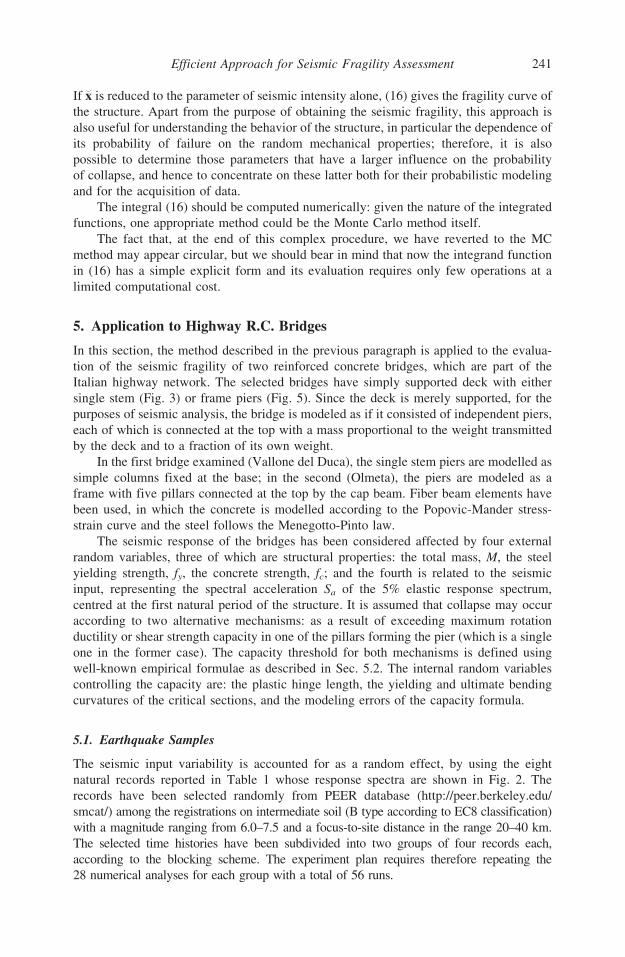
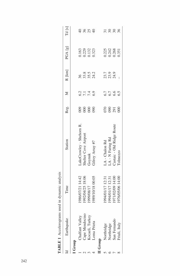
5.1. Earthquake Samples

The seismic input variability is accounted for as a random effect, by using the eight

natural records reported in Table 1 whose response spectra are shown in Fig. 2. The

records have been selected randomly from PEER database (http://peer.berkeley.edu/

smcat/) among the registrations on intermediate soil (B type according to EC8 classification)

with a magnitude ranging from 6.0–7.5 and a focus-to-site distance in the range 20–40 km.

The selected time histories have been subdivided into two groups of four records each,

according to the blocking scheme. The experiment plan requires therefore repeating the

28 numerical analyses for each group with a total of 56 runs.


Dow

nloa

ded

by [

Uni

vers

ita d

egli

Stud

i Rom

a T

re]

at 0

2:33

09

Apr

il 20

15

TA

BL

E1

Acc

eler

og

ram

su

sed

ind

yn

amic

anal

ysi

s

IdE

arth

qu

ake

Tim

eS

tati

on

Reg

.M

R[k

m]

PG

A[g

]T

d[s

]

IG

rou

p

1C

hal

fan

tV

alle

y1

98

6/0

7/2

11

4:4

2L

akeC

row

ley

-S

heh

orn

R.

00

96

.23

60

.16

34

0

2C

ape

Men

do

cin

o1

99

2/0

4/2

51

8:0

6S

hel

ter

Co

ve

Air

po

rt0

00

7.1

33

.80

.22

93

6

3K

oca

eli,

Tu

rkey

19

99

/08

/17

Go

yn

uk

00

07

.43

5.5

0.1

32

25

4L

om

aP

riet

a1

98

9/1

0/1

80

0:0

5G

ilro

yA

rray

#7

09

06

.92

4.2

0.3

23

40

IIG

rou

p

5N

ort

hri

dg

e1

99

4/0

1/1

71

2:3

1L

A-

Ch

alo

nR

d0

70

6.7

23

.70

.22

53

1

6N

ort

hri

dg

e1

99

4/0

1/1

71

2:3

1L

A-

NF

arin

gR

d0

90

6.7

23

.90

.24

23

0

7S

anF

ern

and

o1

97

1/0

2/0

91

4:0

0C

asta

ic-

Old

Rid

ge

Ro

ute

29

16

.62

4.9

0.2

68

30

8F

riu

li,

Ital

y1

97

6/0

5/0

61

4:0

0T

olm

ezzo

00

06

.5–

0.3

51

36

242

Dow

nloa

ded

by [

Uni

vers

ita d

egli

Stud

i Rom

a T

re]

at 0

2:33

09

Apr

il 20

15

5.2. Limit States and Capacity Formulas

The capacity formulas for failure mechanisms of RC structures are generally built upon a

relatively simple mechanical model, to which elements of empirical origin are added.

These formulas are presumed to be unbiased (i.e., to provide a correct estimate of the

mean value), but they are accompanied by a significant scatter due to modelling error. For

the purpose of the present approach, the capacity of the k-th mechanism/element is

expressed in the form:

Ck ¼ CkðY; tÞ"k; (17)

where CkðY;tÞrepresents the average capacity, which is a function of internal variables

gathered in vector Y and time t, and ek is the modeling error, assumed as a log-normal

random variable with unitary mean and coefficient of variation (c.o.v.) to be selected on

the basis of the model accuracy. In this case, even if correlation exists between the basic

variables governing two different mechanisms or the same mechanism in two different

elements, the overall correlation between the capacities Ck and Cj of the two mechanisms/

elements k and j is considerably reduced by the presence of the independent r.v. "k and "j.

Flexural rotational capacity of piers is defined as:

C� ¼ �yLs

3þ �u � �y

� �Lp; (18)

where �u; �y are, respectively, ultimate and yielding curvature of the critical section, Ls,

is the distance from the point of counter-flexure, Lp ¼ Lp 1� Lp=ð2LsÞ� �

, and Lp is the

length of the plastic hinge. In our case, the plastic hinge length has been estimated as

Lp ¼ 0:08Ls þ 0:22fyd, where the second term accounts for the strain penetration effects

due to anchored longitudinal rebar (d is their diameter, fy their yielding strength in MPa).

The choice to express the limit state in terms of chord rotation rather than in terms of

section curvature is due to the aim to obtain a more stable result, not affected by possible

localization of plastic deformations induced by the integration algorithm used by the

computational model. Alternative expressions may be introduced, if deemed more appro-

priate, with the general procedure remaining unaffected. The comparison between the

FIGURE 2 Response Spectra of the eight accelerograms used in the simulations.


Dow

nloa

ded

by [

Uni

vers

ita d

egli

Stud

i Rom

a T

re]

at 0

2:33

09

Apr

il 20

15

flexural capacity model and the results of experimental tests available in the literature,

show a significant scatter that suggest selecting a modelling error ey with a c.o.v. of 50%

[Panagiotakos and Fardis, 2001].

For what concerns the shear collapse, predictive equations for shear strength capacity

of concrete columns have been proposed in Priestley et al. [1994] and Kowalsky and

Priestley [2000]. The demand is represented by the shear carried by the pier and accord-

ingly the capacity is given the form:

CVðtÞ ¼ VCðtÞ þ VS þ VNðtÞf g"V ; (19)

where the average term is the sum of three main contributions:

VC ¼ 0:8AgkðtÞffiffiffiffifc

p; VS ¼ Asw

sfyD cotð30Þ; VN ¼ NðtÞ tan�ðtÞ (20)

representing, respectively, the contribution of concrete, shear reinforcement, and normal

force. In Eq. (20), the meaning of variables is the following: Ag is the shear effective area

of concrete, fc is the concrete strength, kðtÞ ¼ k ðtÞð Þ is a coefficient accounting for the

decrease of concrete contribution with increasing ductility demand m, Asw is the trans-

versal reinforcement area, s the stirrup distance, fy is the steel yielding strength, D is the

net length of concrete in tension measured in the direction of shear stress, N(t) is the axial

load, and a(t) is the angle between the compression strut and the axis of the element. The

ductility demand ðtÞ ¼ �ðtÞ=�y can be computed as a function of the chord rotation y(t)

the shear length of the pier Ls and the above defined plastic hinge length Lp :

ðtÞ ¼ �ðtÞLpþ 1� Ls

3Lp: (21)

According to a limited number of experimental/theoretical comparisons carried out by the

shear model developers, a c.o.v. equal to 0.3 is assumed for the model error eV, which is

slightly higher than the value indicated in Priestly et al. [1994] to account for the

imperfect knowledge of shear region details.

As regards the components of the sub-vector Y, i.e., of the variables that define the

attainment of a limit-state, apart from the model errors, ey and eV, the ultimate and

yielding curvatures of critical sections �u; �y have been treated as internal random

variables in order to take into account the uncertainties on the estimate of their value;

the plastic hinge length, Lp, which has to be considered as a conventional rather than a

physical quantity, is treated as an internal random variable as well. In all the above cases

randomness has been treated assuming the parameter as a best estimate value times a log-

normal fluctuation with a given c.o.v. as reported in Table 2.

TABLE 2 Internal random variables and log-normal parameters

No Random varaiable c.o.v.

1 ey Model error for flexural capacity 0.5

2 eV Model error for shear capacity 0.3

3 ewy Yielding curvature 0.1

4 ewu Ultimate curvature 0.1

5 eLp Plastic hinge length 0.3


Dow

nloa

ded

by [

Uni

vers

ita d

egli

Stud

i Rom

a T

re]

at 0

2:33

09

Apr

il 20

15

5.3. The Vallone Del Duca Viaduct

The viaduct is along the highway A16 Napoli-Canosa, in Southern Italy, between

Benevento and Avellino. The bridge has been recently retrofitted restraining the deck

gaps and introducing seismic isolators at pier caps, but has been studied in the ‘‘as-built’’

conditions.

The bridge has 6 spans, each 32 mt long with a structural scheme of a simple

supported beam. The deck is composed by three pre-stressed beams 1.92 mt high,

connected by 5 traversal links and a slab 20 cm thick and 9.54 mt wide (Fig. 3). The

r.c. piers have a single stem with a rectangular solid section 1.40 · 2.70 mt and a total

longitudinal reinforcement of 40 rebars 28 and stirrups 10/28 cm. Each pier is founded

on plinths on 4 piles with diameter 1.50 mt.

Mechanical properties of materials have been obtained from the original design

documentation and from experimental tests carried out when the retrofitted was planned:

concrete strength, on the basis of core samplings at pier base, has been evaluated on

average about �fc ¼ 45MPa and c.o.v. equal to 0.20. The reinforcing steel is classified

Aq50, a mild steel type following old Italian regulation, for which we can assume an

average yielding strength �fy ¼ 370MPa, and an ultimate average strength �fu ¼ 545MPa

with a c:o:v: ¼ 0:08.

Two piers have been taken into account, namely pier n 3, the most slender, having

16 mt height, with a fundamental period T3 = 0.98 s, and pier n 5, the squatter, with 5.5

mt height, with T5 = 0.18 s (see Fig. 3). For each pier, the procedure previously described

has been applied, consisting in 56 nonlinear analyses according to the central composite

design plan with two repetitions. Each simulation provides an estimate of the reliability

index of the pier. The coefficients of the response surface are then evaluated through the

maximum likelihood method, together with the variances of the lack of fit of the model

and the random effect.

FIGURE 3 Vallone Del Duca viaduct (A16 highway, between Benevento and

Avellino).


Dow

nloa

ded

by [

Uni

vers

ita d

egli

Stud

i Rom

a T

re]

at 0

2:33

09

Apr

il 20

15

The following values are obtained: �" ¼ 0:167 and �� ¼ 0:237 for pier 3, �" ¼ 0:210

and �� ¼ 0:028 for pier 5. The random effect is relevant for pier n3, while being almost

negligible for pier n5; such a difference is due to the fact that pier n5 reaches the

collapse in shear before the attainment of yielding of steel, and therefore, by parity of

spectral acceleration, the different seismic inputs provide almost the same estimate of the

probability of failure, since the structure behaves elastically and is driven by the first

vibration mode.

In Fig. 4, the influence of the external random variables X_

¼ fc; fy;M� �T

, on the

probability of failure of each pier is depicted in the standardized space �_

i ¼X_

i�X_

i

�X_

i

, for

spectral acceleration equal to 0.4 and 0.9 g for piers 3, and 5 respectively, corresponding

to a mean return period at the site of 975 years; a probability of failure of the order of

magnitude 10�3 is obtained for average values of the mass and the material strengths. The

figure shows a quite small influence of the external variables on the probability of failure,

except for the concrete strength in pier n5, in which failure is reached essentially in

shear, with a strong correlation of fc to failure probability; on the contrary, in the more

slender pier, failure is reached essentially in flexure and therefore the concrete strength

has a smaller influence on the reliability estimate.

The fragility curves of the two piers are obtained through convolution between the

response surface and the external random variables gathered in vector X_

, and the two

random variables d and e, according to (16), as shown in Fig. 5. The figure also displays

the effect of seismic record variability and concrete strength dispersion on seismic

fragility: the plots show the fragility curve evaluated at the average value and at ± one

standard deviation of r.v. d and fc. A completely different result is obtained for the two

piers: for the taller (pier n2) the concrete strength does not affect the fragility estimate,

which is mainly affected by the random effect, whilst for the squatter pier (n5) the

–2 –1 0 1 2

ξ0.003

0.0035

0.004

0.0045

0.005

Pf concrete strengthsteel strengthtotal mass

–2 –1 0 1 2

ξ0

0.004

0.008

0.012

0.016Pf concrete strength

steel strengthtotal mass

FIGURE 4 Vallone del Duca viaduct pier n.3 with 16 mt height (left) and pier n5 with

5.5 mt height (right): dependence of the probability of failure on external random

variables fc, fy, M in standardized space, evaluated for spectral acceleration equal to

0.4 and 0.9 g, respectively, both corresponding to a mean return period at the site of 975

years.


Dow

nloa

ded

by [

Uni

vers

ita d

egli

Stud

i Rom

a T

re]

at 0

2:33

09

Apr

il 20

15

concrete strength plays a crucial role in the fragility estimate, higher than the dispersion

induced by seismic input.

5.4. The Olmeta Viaduct

The Olmeta viaduct (Fig. 6) is along A1 highway between Bologna and Florence, in

central Italy. It was built during the early 1960s, without seismic provisions. It is

composed of two separate ways, with 12 spans for a total length of 254 mt; the deck

has five pre-stressed beams with a span 21.16 mt long and a slab 9.60 mt wide excluding

sidewalks about 70 cm wide; the piers (Fig. 7) have a framed structure with five columns

with a section 100 · 60 cm each and a spacing of 2.40 mt among them, linked together by

a cap beam with a section 100 · 110 cm. The pier height varies to a maximum of 12 mt;

the deck is simply supported by piers. Pier reinforcement consists of 12 rebars 16

longitudinally and 10 stirrups every 16 cm transversally. In 1974, the viaduct was

retrofitted: the slab was rebuilt and the pier columns jacketed by a 10 cm thick concrete

layer reinforced longitudinally by 6 rebars 20 and transversally by 10 stirrups every

0 0.5 1 1.5 2

Sa (g)0.0E+000

5.0E-002

1.0E-001

1.5E-001Pf

Pier n.3Pier n.5

0 0.5 1 1.5 2

Sa (g)0.0E+000

5.0E-002

1.0E-001

1.5E-001Pf − st.dev(fc)

− st.dev(δ) average+ st.dev(δ)+ st.dev( fc)Pier n.3

Pier n.5

FIGURE 5 Seismic fragility of Vallone del Duca viaduct piers n3 and n5: fragility

curves (left) and effect of seismic record variability and concrete strength randomness on

seismic fragility (right): the plots show the fragility curve of piers valuated at the average

value and at ± one standard deviation of r.v. d and fc.

FIGURE 6 Olmeta viaduct (A1 highway, between Florence and Bologna): plan and

front view.


Dow

nloa

ded

by [

Uni

vers

ita d

egli

Stud

i Rom

a T

re]

at 0

2:33

09

Apr

il 20

15

20 cm. Aiming at evaluating the effects of the reinforcement, the reliability analysis has

been carried out in both the original ‘‘as-built’’ status and the present retrofitted state; the

results are presented for pier n2 (Fig. 7), having columns of 8.98 mt high and transversal

natural period T = 1.14 s in the as built status and period T = 0.76 s in the present

retrofitted state.

For this viaduct, in the absence of design values or in-site measures, the material

properties have been estimated according to the values provided in Verderame et al.

[2001], where the data of about 600 structures commissioned by public administrations in

Italy in the year 1960 have been analyzed. For concrete strength, an average value of 28.2

MPa is estimated with a c.o.v. = 0.34, while for reinforcing steel, an average yielding

strength �fy ¼ 325MPa, and an ultimate average strength �fu ¼ 467MPa can been assumed,

corresponding to Aq42 steel class; yield and ultimate strength have been considered as

correlated log-normal R.V. with a c:o:v: ¼ 0:07. For the mass, an average value of 350

tons is assumed according to the design documentation, with a c:o:v: ¼ 0:07.

The effective fragility analysis is then applied, according to the experimental plan

previously described, comprising 56 nonlinear analyses that have been performed in the

range of spectral acceleration between 0.055 and 0.24 g, corresponding to a mean return

period at the site between 95 and 2,475 years. The coefficients of the response surface

and the standard deviations of both error term and random effect have been estimated by

means of the maximum likelihood method. The following values have been obtained:

�" ¼ 0:358, �� ¼ 0:391 and �" ¼ 0:263, �� ¼ 0:501, for pier n2 before and after

strengthening, respectively. The results display a high dispersion induced by both random

effect and lack of fit of the response surface.

As shown in Figs. 8 and 9a, a significant enhancement in reliability is provided with

rehabilitation, since the probability of failure decreases by three orders of magnitude. As

in the previous section, the influence of the external random variables fc; fy;M, on the

probability of failure is depicted in a standardized space (Fig. 8): the concrete strength fc,

which has a much higher dispersion, plays the most relevant role in both cases, before and

after strengthening.

FIGURE 7 Olmeta viaduct: pier geometry and reinforcement details.


Dow

nloa

ded

by [

Uni

vers

ita d

egli

Stud

i Rom

a T

re]

at 0

2:33

09

Apr

il 20

15

The comparison between the effects of the dispersion induced by seismic input and

structural randomness is shown in Fig. 9b, where the fragility curve of the pier before

strengthening is evaluated at the average value and at ± one standard deviation of r.v. d and

fc; in the present case, the scatter induced by sample-to-sample earthquake record variability, has

a comparable effect on seismic fragility to that induced by the randomness of concrete strength.

6. Conclusions

A procedure for evaluating the seismic fragility, suitable for application to non ductile RC

structures is presented, which makes it possible to obtain an accurate estimate, using

-2 -1 0 1 2

ξ0

0.01

0.02

0.03Pf

concrete strengthsteel strengthtotal mass

-2 -1 0 1 2

ξ0.0E+000

5.0E-005

1.0E-004

1.5E-004

2.0E-004Pf concrete strength

steel strengthtotal mass

FIGURE 8 Olmeta viaduct pier n.2 before (left) and after (right) rehabilitation: depen-

dence of the probability of failure on external random variables fc, fy, M in standardized

space, evaluated for Sa = 0.115 g.

0 0.05 0.1 0.15 0.2 0.25

Sa (g)0.00

0.04

0.08

0.12

0.16

0.20

Pf unreinforcedreinforced

0 0.05 0.1 0.15 0.2 0.25

Sa (g)0.0E+000

4.0E-002

8.0E-002

1.2E-001

1.6E-001Pf -st.dev(fc)

- st.dev.(delta) average+ st.dev.(delta)+ st.dev.(fc)

FIGURE 9 Seismic fragility of Olmeta viaduct pier n2: (a) comparison of fragility

before and after rehabilitation; (b) effect of seismic record variability and concrete

strength randomness on seismic fragility: the plots show the fragility curve evaluated at

the average value and at ± one standard deviation of r.v. d and fc.


Dow

nloa

ded

by [

Uni

vers

ita d

egli

Stud

i Rom

a T

re]

at 0

2:33

09

Apr

il 20

15

refined models for the structural analysis and natural accelerograms, at low computational

cost. This method consists of an enhanced version of the Effective Fragility Analysis

(EFA) integrated with the Response Surface Method (RSM). Random variables for both

structural model and seismic action are taken into account: the random variables referring

to the structure are divided into two groups, one of which contains all of those variables

(internal) that, while influencing the resistance, have little effect on the dynamic

response; whereas the other collects the remaining structural variables (external) that

strongly affect the dynamic response. Once the external variables have been fixed, and a

ground motion at the base of the structure selected, the conditioned probability of failure

(PF) is computed using standard reliability methods (FORM). The response surface

method is then used to establish a function approximating the dependence of PF on

external variables and on seismic intensity. The accelerogram sample-to-sample varia-

bility is accounted for by introducing a random effect within the RSM, without increasing

the number of analyses. The fragility curve of the structure is finally obtained by

convolution with the probability density functions of external random variables.

The procedure is applied to assess the seismic fragility of two existing RC bridges of

the Italian highway network with simply supported deck and either single stem or frame

piers. The procedure is capable of considering several modes of failure; in the examples

considered, flexural ductility and shear capacity have been taken into account. The results

highlight the features of the method, its capability of representing the dependence of the

fragility on material randomness as well as the relative importance of seismic input with

respect to mechanical and epistemic uncertainty.

References

Au, S.-K. and Beck, J. L. [2001] ‘‘Estimation of small probabilities in high dimensions by subset

simulation,’’ Probabilistic Engineering Mechanics 16(4), 263–277.

Au, S.-K. and Beck, J. L. [2003] ‘‘Important sampling in high dimensions,’’ Structural Safety 25(2),

139–163.

Baker, J. W. and Cornell, C. A. [2005] ‘‘A vector-valued ground motion intensity measure

consisting of spectral acceleration and epsilon,’’ Earthquake Engineering and Structural

Dynamics 34(10), 1193–1217.

Bommer, J. and Acevedo, A. [2004] ‘‘The use of real earthquake accellerograms as input to

dynamic analysis,’’ Journal of Earthquake Engineering 8(1), 43–91.

Box, G. E. P. and Draper, N. R. [1987] Empirical Model-Building and Response Surfaces, John

Wiley & Sons, New York.

de Felice, G., Giannini, R., and Pinto P. E. [2002] ‘‘Probabilistic seismic assessment of existing R/C

buildings: static pushover versus dynamic analysis,’’ Proc. 12th European Conference on

Earthquake Engineering, Elsevier, London.

Ditlevsen, O. [1979] ‘‘Narrow reliability bounds for structural systems,’’ Journal of Structural

Mechanics 7(4), 453–472.

Franchin, P., Lupoi, A., and Pinto, P. E. [2003] ‘‘Seismic fragility of reinforced concrete structures

using a response surface approach,’’ Journal of Earthquake Engineering 7(NS1), 45–77.

Kowalsky, M. J. and Priestley, M. J. N. [2000] ‘‘Improved analytical model for shear strength

of circular reinforced concrete columns in seismic regions,’’ ACI Structural Journal 97(3),

388–396.

Kurama, Y. C. and Farrow, K. T. [2003] ‘‘Ground motion scaling methods for different site

conditions and structure characteristics,’’ Earthquake Engineering and Structural Dynamics

32(15), 2425–2450.

Ibarra, L. F. and Krawinkler, H. [2005] ‘‘Global collapse of frame structures under seismic

excitations,’’ PEER Report 2005/06.


Dow

nloa

ded

by [

Uni

vers

ita d

egli

Stud

i Rom

a T

re]

at 0

2:33

09

Apr

il 20

15

Liel, A. B., Haselton, C. B., Deierlein G. G., and Baker, J. W. [2009] ‘‘Incorporating modeling

uncertainties in the assessment of seismic collapse risk of buildings,’’ Structural Safety 31, 197–211

Luco, N. and Cornell, C. A. [2007] ‘‘Structure-specific scalar intensity measures for near-source

and ordinary earthquake ground motions,’’ Earthquake Spectra 23(2), 357–392.

Naeim, F. and Lew, M. [1995] ‘‘On the use of design spectra compatible time histories,’’

Earthquake Spectra 11(1), 111–127.

Panagiotakos, T. B. and Fardis, M. N. [2001] ‘‘Deformation of reinforced concrete members at

yielding and ultimate,’’ ACI Structural Journal 98(2), 135–148.

Pandey, M. D. [1998] ‘‘An effective approximation to evaluate multinormal integrals,’’ Structural

Safety 20(1), 51–67.

Pinto, P. E. [2001] ‘‘Reliability methods in earthquake engineering,’’ Progress in Structural

Engineering and Materials 3(1), 76–85.

Pinto, P. E., Giannini, R., and Franchin, P. [2004] Seismic Reliability Analysis of Structures, IUSS

Press, Pavia, Italy.

Priestley, M. J. N., Seible, F., and Calvi, G. M. [1996] Seismic Design and Retrofit of Bridges. John

Wiley & Sons, New York.

Priestley, M. J. N., Verma, R., Xiao, Y. [1994] ‘‘Seismic shear strength of reinforced concrete

columns,’’ Journal of Structural Engineering, ASCE 120(4), 2310–2329.

Schotanus, M. I. J., Franchin, P., Lupoi, A., and Pinto P. E. [2004] ‘‘Seismic fragility analysis of 3D

structures,’’ Structural Safety 26(4), 421–441.

Searle, S. R., Casella, G., and McCulloch, C. E. [1992] Variance Components. Prentice-Hall,

Englewood Cliffs, NJ.

Shome, N., Cornell, C., Bazzurro, P., and Carballo, J. [1998] ‘‘Earthquakes, records, and nonlinear

responses,’’ Earthquake Spectra 14(3), 469–500.

Song, J. and Der Kiureghian, A. [2003] ‘‘Bounds on system reliability by linear programming,’’

Journal of Engineering Mechanics, ASCE,129(6), 627–636.

Tang, L. K. and Melchers, R. E. [1987] ‘‘Dominant mechanisms in stochastic plastic frames,’’

Reliability Engineering 18(2), 101–115.

Vamvatsikos, D. and Cornell, C. A. [2001] ‘‘Incremental dynamic analysis,’’ Earthquake

Engineering and Structural Dynamics 31(3), 491–514.

Verderame, G. M. and Manfredi, G. [2001] ‘‘Le proprieta meccaniche dei calcestruzzi impiegati

nelle strutture in cemento armato realizzate negli anni ’60,’’ Atti del X Congr. Naz. L’ingegneria

Sismica in Italia, Anidis, Potenza (in Italian).

Yuan X.-X. and Pandey, M. D. [2006] ‘‘Analysis of approximations for multinormal integration in

system reliability computation,’’ Structural Safety 28(4), 361–377.

Zang, Y. C. [1993] ‘‘High-order reliability bounds for series systems and application to structural

systems,’’ Computers & Structures 46(2), 381–386.


Dow

nloa

ded

by [

Uni

vers

ita d

egli

Stud

i Rom

a T

re]

at 0

2:33

09

Apr

il 20

15

An Efficient Approach for Seismic Fragility Assessment with Application to Old Reinforced Concrete...

Documents

Transcript of An Efficient Approach for Seismic Fragility Assessment with Application to Old Reinforced Concrete...