Allowing Traffic Over Mainshock-Damaged Bridges

This article was downloaded by: [Universita Studi la Sapienza]On: 31 October 2012, At: 11:00Publisher: Taylor & FrancisInforma Ltd Registered in England and Wales Registered Number: 1072954 Registeredoffice: Mortimer House, 37-41 Mortimer Street, London W1T 3JH, UK

Journal of Earthquake EngineeringPublication details, including instructions for authors andsubscription information:http://www.tandfonline.com/loi/ueqe20

Allowing Traffic Over Mainshock-Damaged BridgesPaolo Franchin a & Paolo E. Pinto aa Department of Structural & Geotechnical Engineering, Universityof Rome La Sapienza, Rome, ItalyVersion of record first published: 27 May 2009.

To cite this article: Paolo Franchin & Paolo E. Pinto (2009): Allowing Traffic Over Mainshock-DamagedBridges, Journal of Earthquake Engineering, 13:5, 585-599

To link to this article: http://dx.doi.org/10.1080/13632460802421326

PLEASE SCROLL DOWN FOR ARTICLE

Full terms and conditions of use: http://www.tandfonline.com/page/terms-and-conditions

This article may be used for research, teaching, and private study purposes. Anysubstantial or systematic reproduction, redistribution, reselling, loan, sub-licensing,systematic supply, or distribution in any form to anyone is expressly forbidden.

The publisher does not give any warranty express or implied or make any representationthat the contents will be complete or accurate or up to date. The accuracy of anyinstructions, formulae, and drug doses should be independently verified with primarysources. The publisher shall not be liable for any loss, actions, claims, proceedings,demand, or costs or damages whatsoever or howsoever caused arising directly orindirectly in connection with or arising out of the use of this material.

http://www.tandfonline.com/loi/ueqe20

http://dx.doi.org/10.1080/13632460802421326

http://www.tandfonline.com/page/terms-and-conditions

Journal of Earthquake Engineering, 13:585–599, 2009

Copyright � A.S. Elnashai & N.N. Ambraseys

ISSN: 1363-2469 print / 1559-808X online

DOI: 10.1080/13632460802421326

Allowing Traffic Over Mainshock-Damaged Bridges

PAOLO FRANCHIN and PAOLO E. PINTO

Department of Structural & Geotechnical Engineering, University of Rome La

Sapienza, Rome, Italy

A criterion is proposed for deciding whether, after a damaging mainshock, a bridge can still beopen for either emergency or ordinary traffic. The criterion is based on the comparison between thecollapse risk of the mainshock-damaged structure and the pre-mainshock risk of the intactstructure. The approach requires fragilities for multiple damage states for the intact structure,and transition probabilities from these states to collapse for the damaged structure. The aftershockrisk decreases with time, hence a decision for reopening might have to wait until the risk level goesdown to an acceptable value. A realistic application demonstrates the approach.

Keywords Aftershock; Progressive Damage; Transition Fragility; Time-Varying Collapse Risk

1. Introduction

In the aftermath of earthquakes striking urbanized areas, whose continued activity

depends on the availability of a multitude of bridges and viaducts, it is of great conse-

quence to be able to distinguish between structures which, though still standing, are

actually mechanically failed and those which, though bearing the signs of various types

and levels of damage, are still capable of carrying safely a traffic load. At present, the

task of distinguishing is left to the judgment of the officials in charge, and there is little

doubt that this would be beneficially complemented with information coming from some

form of prior analytical and/or experimental investigation. Ideally, this would involve

establishing, for all bridge typologies existing in a given area, a correlation between

observable damage patterns and residual traffic capacity.

There are, however, two challenging difficulties to overcome in order to implement the

above lines of thought. The first one is simply the inadequacy of the available numerical

models in accounting for the various mechanisms taking place in (old) reinforced concrete

structures subjected to large amplitude cyclic deformations, leading to progressive degrada-

tion of the mechanical efficiency of the elements. In most cases, the models are unable to

provide reliable answers as how far a given structure is from physical collapse after having

suffered damages from a strong earthquake. Secondly, given that the decision regarding

closure cannot be realistically based on other than a relatively rapid visual damage

observation, one has to account for the large uncertainty involved in relating the observed

damage patterns with actual loss of capacity. To overcome this problem one might think of

placing at each bridge site an instrument to record the actual motion and, hence, of taking

the decision of whether closing or not the bridge based on both the visual information and

prior analysis. The two aspects of difficulty described above compound with each other and

this is a sufficient justification for the scarcity of the literature on this topic.

Received 20 February 2008; accepted 23 June 2008.

Address correspondence to Paolo Franchin, Department of Structural & Geotechnical Engineering,

University of Rome La Sapienza, Via Gramsci 53, Rome, I-00197, Italy; E-mail: [email protected]

585

Dow

nloa

ded

by [

Uni

vers

ita S

tudi

la S

apie

nza]

at 1

1:00

31

Oct

ober

201

2

In one recent study [Mackie and Stojadinovic, 2006], a functional relationship (with

an error term) is proposed linking loss of vertical bearing capacity of a bridge with

reduction in traffic volume. Analytical determination of loss of vertical capacity as

function of the intensity of the mainshock, however, proved to be affected by significant

uncertainty, in all of the different approaches that were attempted. The results are given in

terms of fragility curves for different percentages of traffic reduction and show quite large

differences according to the approach employed.

The present study acknowledges the de facto inability to determine analytically the

loss of vertical capacity due to prior lateral shaking and renounces the idea of providing

probabilities for partial traffic limitation. As will be explained later, the bridges after a

mainshock will be either closed, open only for emergency traffic, or fully operational, and

the criterion for such a decision is the survival probability of the mainshock-damaged

bridge under the sequence of the aftershocks as determined from an aftershock probabil-

istic seismic hazard analysis (APSHA). Similar criteria have been adopted in [Bazzurro

et al., 2004; Luco et al., 2004].

2. Description of the Method

The approach comprises two phases. In the first one, a number of states of increasing

damage, ending with collapse, is defined. The seismic intensity leading to each damage

state is probabilistically characterized in terms of a fragility curve1 P DSijSað Þ, and the

risk of collapse is evaluated by combining the corresponding fragility with the seismic

hazard from a regular PSHA. The second phase consists of determining the aftershock

intensity leading to collapse from each of the lower damage states, probabilistically

characterized in terms of aftershock or transition fragility curves P DSnjDSi; Sað Þ. The

aftershock collapse risk is then evaluated. This risk, as it is well known, is time-

dependent and a suitable criterion must be used in order to convert it to an equivalent

constant annual risk. Opening to traffic is then decided based on a comparison between

the two risks.

2.1. Fragility Analysis for the Intact Structure

Following Jalayer et al. [2007], the state of the bridge with reference to a given state of

damage DS is expressed in terms of the global scalar variable (damage measure) defined as:

YDS ¼ maxt

maxj¼1;...;Nm

mink2Ij

Dk tð ÞCDS

k tð Þ ; (2:1)

where Dk tð Þ is the demand (response) in the k-th component, CDSk tð Þ is the corresponding

capacity for damage state DS, Ij is the set of components’ indices whose joint failure

causes failure according to mode j, and Nm is the number of considered failure modes2.

The above variable expresses the global state of a structure according to the cut-set

formulation, whereby a (structural) system is described as a series of parallel sub-systems

of its components. Variable Y is called critical demand to capacity ratio, since it is the

1In this work, the employed intensity measure is the spectral acceleration close to thefundamental period of the structure, denoted by Sa.

2Several components correspond in general to the same structural member, e.g., drift and shearforce. The simplest failure modes consist of a single component, e.g., shear failure of a singlecolumn, but more general failure modes can involve the combined failure of several components.

586 P. Franchin and P. E. Pinto

Dow

nloa

ded

by [

Uni

vers

ita S

tudi

la S

apie

nza]

at 1

1:00

31

Oct

ober

201

2

ratio between demand and capacity for the component that leads the system closer to

damage state DS, at the attainment of which Y equals unity.

The risk that the structure attains a given state of damage can be evaluated by first

conditioning on the ground motion intensity measure. The probability that YDS exceeds

unity as a function of Sa (the fragility function) is found here by assuming that:

P YDS > 1��Sa

� �¼;P SYDS¼1

a < Sa

� �; (2:2)

where SYDS¼1a (or simply SDS

a ) is the (random) intensity that induces the damage state DS.

In the application, three damage states are considered, called light damage

(DS1 ¼ LD), (DS2 ¼ SD), and collapse (DS3 ¼ CO). Correspondingly, three critical

demand to capacity ratios YLD, YSD, and YCO are defined. In the following, for simplicity

of notation, the corresponding fragility functions are denoted by Fi Sað Þ.The fragility curves are estimated based on the results of inelastic response

analyses with a limited number of records. Each record is scaled in order to collect a

sample of SDSa values, from which the parameters of an assumed distribution are

estimated. Here, the well-established assumption of lognormality is adopted, and the

estimated parameters are the median �i and log-standard deviation �i. Hence, the

fragility curve is expressed as:

Fi Sað Þ ¼ � ln Sa � ln �ið Þ=�i½ �: (2:3)

Uncertainty in member capacity models (the models used to evaluate member deform-

ability or strength, usually semi-empirical in nature, and denoted above by CDSk tð Þ) and

other mechanical parameters can be accounted for by associating to each record a sample

from their distribution [Schotanus and Franchin, 2004; Pinto et al., 2004].

2.2. Mainshock Risk

The mean annual rate of structural collapse, or risk, due to mainshocks (lm3 ) is given by

the well-known expression:

lm3 ¼

Xi

�mi

Z 10

F3 xð Þf mSa;i xð Þdx; (2:4)

where the subscript i denotes the seismogenetic area/fault, summation is carried out over

all areas contributing to the hazard at the site, f mSa;i xð Þ and �m

i are, respectively, the

probability density function of Sa given an event in area i, and the corresponding mean

annual rate of events of all magnitudes of interest, i.e., included in the interval Ml;Mu½ �,that appears in the truncated Gutemberg-Richter law:

lm;i Mð Þ ¼ �mi 1�

1� exp �� M �Ml;i

� �� 1� exp �� Mu;i �Ml;i

� �� " #

¼ �mi G Mð Þ; (2:5)

where G Mð Þ ¼ 1� F Mð Þ is the complementary cumulative distribution function

(CCDF) of M, given an event (a truncated exponential distribution between upper and

lower magnitudes Mu;i and Ml;i).

Allowing Traffic Over Mainshock-Damaged Bridges 587

Dow

nloa

ded

by [

Uni

vers

ita S

tudi

la S

apie

nza]

at 1

1:00

31

Oct

ober

201

2

In the simple case of a single seismogenetic area or fault contributing to the hazard at

the site, Eq. (2.4) reduces to:

lm3 ¼ �m

Z 10

F3 xð Þf mSa xð Þdx: (2:6)

In the following, reference is made to this simpler case.

2.3. Aftershock Hazard Analysis

Conceptually, APSHA follows lines which are similar to those of conventional, main-

shock PSHA. The necessary information is the same, specifically, a model for spatial-

temporal distribution of events, and a distribution for event magnitude [Yeo, 2005]. For

what concerns their spatial distribution, aftershocks generally occur in an area close to the

mainshock epicenter, a fact that restricts the number of seismogenetic areas to be

considered in the analysis. As shown by Utsu, the magnitude distribution of aftershocks,

given an aftershock event, is practically coincident with the corresponding mainshock

distribution. The main difference resides in the mean rate of events, which, according to

the ‘‘modified Omori law’’ [Utsu, 1995] is inversely proportional to the elapsed time

t from the mainshock occurrence and depends on its magnitude Mm. Building on this,

Reasenberg and Jones [1989] proposed the following expression for the instantaneous

daily rate of events with magnitude M or larger:

la t;Mm;Mð Þ ¼ 10aþb Mm�Mð Þ

t þ cð Þp ; (2:7)

where a, b, c, and p are regional parameters. The expression above, developed for

California, has been found to apply for other seismic regions as well. In the application

to follow the parameters used in Eq. (2.7) have been taken from Lolli and Gasperini

[2003], who fitted them to aftershock sequences for various regions of Italy.

Equation (2.7) can be rewritten in the following form:

la t;Mm;Mð Þ ¼exp ln 10aþb Mm�Mð Þ� �

t þ cð Þp ¼exp ln 10aþbMm� �

t þ cð Þp � exp �b ln 10 �Mð Þ

¼ �a t;Mmð Þe��M ¼ �a t;Mmð Þ � G Mð Þ;(2:8)

where � ¼ b ln 10 and G Mð Þ ¼ 1� F Mð Þ is the exponential CCDF of M. Equation (2.8)

has the same form as the non truncated Gutemberg-Richter recurrence law for the

mainshock events, but for the elapsed-time and mainshock-magnitude dependence of

the rate of aftershock events �a.

In the application the ‘‘truncated’’ version of Eq. (2.8) is employed, obtained by

replacing G Mð Þ from (2.8) with that from (2.5) and considering the mean rate of all

aftershock events with magnitude between Ml and Mu ¼ Mm:

�a t;Ml;Mmð Þ ¼ la t;Mm;Mlð Þ � la t;Mm;Mmð Þ

¼ 10aþb Mm�Mlð Þ � 10aþb Mm�Mmð Þ

t þ cð Þp ¼ 10aþb Mm�Mlð Þ � 10a

t þ cð Þp(2:9)


Dow

nloa

ded

by [

Uni

vers

ita S

tudi

la S

apie

nza]

at 1

1:00

31

Oct

ober

201

2

la t;Mm;Ml;Mð Þ ¼ �a t;Ml;Mmð Þ � G Mð Þ (2:10)

2.4. Fragility Analysis for the Mainshock-Damaged Structure

Following the mainshock fragility analysis, one knows for record j, j=1,..,nr the mainshock

intensity inducing damage state i, i=1,. . .,n, denoted by Sia;j. The objective is to obtain the

distribution of the aftershock intensity leading from damage state i < n to the collapse

damage state n, denoted by Si;na . This is achieved by collecting sample values of Si;n

a by

subjecting the structure to mainshock-aftershock sequences. The first record in the sequence

(mainshock) is always scaled to Sia;j, the second is scaled until YCO ¼ 1. Under the

assumption that the aftershock spectral acceleration capacity is also lognormal, its median

�i;n and log-standard deviation �i;n are evaluated based on the collected Si;na values. The

resulting spectral acceleration capacity distribution, denoted by Fi;n Sað Þ, is denominated

transition fragility from state i to state n, and has the same functional form of Eq. (2.3).

Regarding the choice of the aftershock records, in this work the same set of records

used to represent the mainshocks has been used for the aftershocks (with random

permutation for the purpose of building mainshock-aftershock sequences).

2.5. Aftershock Risk

Under the assumption that aftershocks are generated within the same seismogenetic area/

fault of the mainshock, the daily rate of transitions from the i-th damage state to collapse

at t days from a mainshock of magnitude Mm is given by:

lai;3 tð Þ ¼ �a t;Mm;Mlð Þ

Z 10

Fi;3 xð Þf aSa xð Þdx ¼ �a t;Mm;Mlð Þ � Pi;n; (2:11)

where Pi;n is the probability of reaching collapse from the i-th damage state, given the

occurrence of an aftershock.

The risk in Eq. (2.11) cannot be directly compared with the time-independent risk in

Eq. (2.4) or (2.5). In this article, this risk is transformed into an equivalent annual risk

through the following relation:

~lai;3 t;Mm;Mlð Þ ¼ T1y

T � t

Z T

t

lai;3 �ð Þd�

¼ T1y

T � t

Z T

t

�a �;Mm;Mlð Þd��

� Pi;n ¼ ~�a t;Mm;Mlð Þ � Pi;n

(2:12)

where T1y ¼ 356 is the length of one year in units of days, t is the elapsed time from the

mainshock event, and T is the estimated duration of the aftershock sequence (see, for

example, Lolli and Gasperini, 2003).

2.6. Opening/Closure Decision

For given values of the estimated duration T and mainshock magnitude Mm the equivalent

annual aftershock risk given by Eq. (2.11) is a decreasing of the elapsed time t. In the first

days after the mainshock, ~lai;3 may or may not, depending on the Mm value and also the

state of damage caused by the mainshock (as reflected in the value of Pi;n), be larger than

the constant mainshock risk lm3 given by Eq. (2.4).


Dow

nloa

ded

by [

Uni

vers

ita S

tudi

la S

apie

nza]

at 1

1:00

31

Oct

ober

201

2

A decision criterion on the opening to traffic can be formulated based on the

pre-mainshock risk of all the bridges on the transportation network in the affected area.

Since the network is likely to be several decades old, the average pre-mainshock risk

value over the bridge population will likely be larger than that accepted for new designs,

indicating the need (existing even before the mainshock struck) for a general seismic

upgrade of the network to meet more stringent requirements. These bridges, however,

were open to traffic before the mainshock, it is therefore logical to use their average pre-

mainshock risk as a term of reference for the decision, since this risk level was implicitly

accepted by the community. Obviously, this criterion should be adapted to account for

weaker bridges, i.e., those characterized by a higher than average pre-mainshock risk. In

conclusion, the proposed criterion can be summarized as:

~lai;3 � g �max lm

3 ; ��3

� �; (2:12)

where �l3 is the average pre-mainshock collapse risk and the factor g differentiates the

tolerable risk level for ordinary traffic (g ¼ 1) from that for emergency operators

(e.g., � ¼ 3� 5).

If for t =1, the inequality in Eq. (2.12) is satisfied, the bridge can be open immedi-

ately to traffic. If the opposite is true, the bridge cannot be open, until the risk eventually

goes down to an acceptable value.

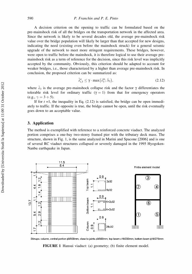
3. Application

The method is exemplified with reference to a reinforced concrete viaduct. The analyzed

portion comprises a one-bay two-storey framed pier with the tributary deck mass. The

structure, shown in Fig. 1, is the same analyzed in Marini and Spacone [2006] and is one

of several RC viaduct structures collapsed or severely damaged in the 1995 Hyogoken-

Nanbu earthquake in Japan.

FIGURE 1 Hansui viaduct: (a) geometry; (b) finite element model.


Dow

nloa

ded

by [

Uni

vers

ita S

tudi

la S

apie

nza]

at 1

1:00

31

Oct

ober

201

2

3.1. Structural Modeling

A plane model is set up in the OPENSEES finite element analysis program [McKenna et al.,

2007]. Flexibility-based elements with five Gauss-Lobatto integration points are

employed. P-delta is included. At each integration point a section aggregator is used to

construct a section coupling axial/flexural response (M-N), modeled by a fiber-

discretized section, with shear response (V), modeled by a uniaxial hysteretic law. Note

that, although the M-N and the V models in the section aggregator are uncoupled

resulting in a section tangent stiffness of the form:

ks ¼@N=@"0 @N=@� 0

@M=@"0 @M=@� 0

0 0 @V=@�

24

35; (3:1)

the moments and shears are still coupled trough the element equilibrium. In Eq. (3.1),

"0; �; � are the generalized section deformations: axial strain, curvature, and shear

distortion angle.

Kent-Park concrete and Menegotto-Pinto steel models have been used for the fiber

section (with values of material parameters equal to fc ¼ 27 MPa, "c0 ¼ 0:0025,

fcu ¼ 0:6 fc, "cu ¼ 0:0050, fy ¼ 440 MPa).

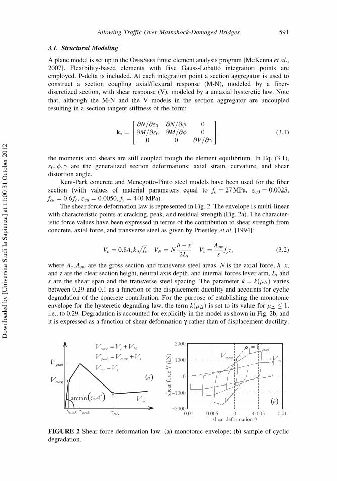
The shear force-deformation law is represented in Fig. 2. The envelope is multi-linear

with characteristic points at cracking, peak, and residual strength (Fig. 2a). The character-

istic force values have been expressed in terms of the contribution to shear strength from

concrete, axial force, and transverse steel as given by Priestley et al. [1994]:

Vc ¼ 0:8Ackffiffiffiffifc

pVN ¼ N

h� x

2Ls

Vs ¼Asw

sfyz; (3:2)

where Ac;Asw are the gross section and transverse steel areas, N is the axial force, h, x,

and z are the clear section height, neutral axis depth, and internal forces lever arm, Ls and

s are the shear span and the transverse steel spacing. The parameter k ¼ k �ð Þ varies

between 0.29 and 0.1 as a function of the displacement ductility and accounts for cyclic

degradation of the concrete contribution. For the purpose of establishing the monotonic

envelope for the hysteretic degrading law, the term k �ð Þ is set to its value for � � 1,

i.e., to 0.29. Degradation is accounted for explicitly in the model as shown in Fig. 2b, and

it is expressed as a function of shear deformation g rather than of displacement ductility.

FIGURE 2 Shear force-deformation law: (a) monotonic envelope; (b) sample of cyclic

degradation.


Dow

nloa

ded

by [

Uni

vers

ita S

tudi

la S

apie

nza]

at 1

1:00

31

Oct

ober

201

2

Hysteretic behavior and degradation start right after Vcrack has been exceeded, as it is

typical for older non-ductile members (see also Pincheira et al., 1999).

As it regards the characteristic strains, the cracking strain is simply calculated using

elastic shear stiffness gcrack ¼ Vcrack=GA�. The elastic stiffness has been reduced by a

factor of ten to account for diagonal cracking in order to compute strain at peak strength.

Finally, the strain at residual strength has been somewhat arbitrarily assigned a value of

ten times the strain at peak strength (some indications on the strains at peak and residual

strength can be found in a very recent article by Sezen, 2008). In the OPENSEES program,

the V � � law has been modeled with two Hysteretic laws (one degrading with ductility

damage parameter 0.03 and one non degrading) in Parallel.

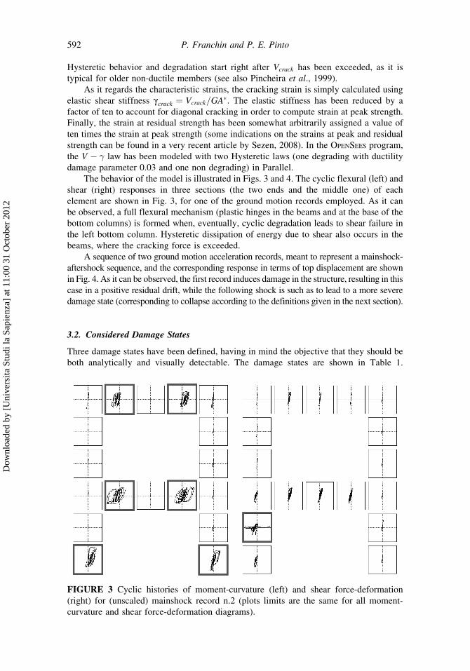
The behavior of the model is illustrated in Figs. 3 and 4. The cyclic flexural (left) and

shear (right) responses in three sections (the two ends and the middle one) of each

element are shown in Fig. 3, for one of the ground motion records employed. As it can

be observed, a full flexural mechanism (plastic hinges in the beams and at the base of the

bottom columns) is formed when, eventually, cyclic degradation leads to shear failure in

the left bottom column. Hysteretic dissipation of energy due to shear also occurs in the

beams, where the cracking force is exceeded.

A sequence of two ground motion acceleration records, meant to represent a mainshock-

aftershock sequence, and the corresponding response in terms of top displacement are shown

in Fig. 4. As it can be observed, the first record induces damage in the structure, resulting in this

case in a positive residual drift, while the following shock is such as to lead to a more severe

damage state (corresponding to collapse according to the definitions given in the next section).

3.2. Considered Damage States

Three damage states have been defined, having in mind the objective that they should be

both analytically and visually detectable. The damage states are shown in Table 1.

FIGURE 3 Cyclic histories of moment-curvature (left) and shear force-deformation

(right) for (unscaled) mainshock record n.2 (plots limits are the same for all moment-

curvature and shear force-deformation diagrams).


Dow

nloa

ded

by [

Uni

vers

ita S

tudi

la S

apie

nza]

at 1

1:00

31

Oct

ober

201

2

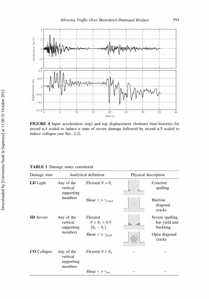
FIGURE 4 Input acceleration (top) and top displacement (bottom) time-histories for

record n.4 scaled to induce a state of severe damage followed by record n.5 scaled to

induce collapse (see Sec. 3.2).

TABLE 1 Damage states considered

Damage state Analytical definition Physical description

LD Light Any of the

vertical

supporting

members

Flexural > y Concrete

spalling

Shear � > �crack Hairline

diagonal

cracks

SD Severe Any of the

vertical

supporting

members

Flexural

> y þ 0:5u � y

� �Severe spalling,

bar yield and

buckling

Shear � > �peak Open diagonal

cracks

CO Collapse Any of the

vertical

supporting

members

Flexural > u – –

Shear � > �res – –


Dow

nloa

ded

by [

Uni

vers

ita S

tudi

la S

apie

nza]

at 1

1:00

31

Oct

ober

201

2

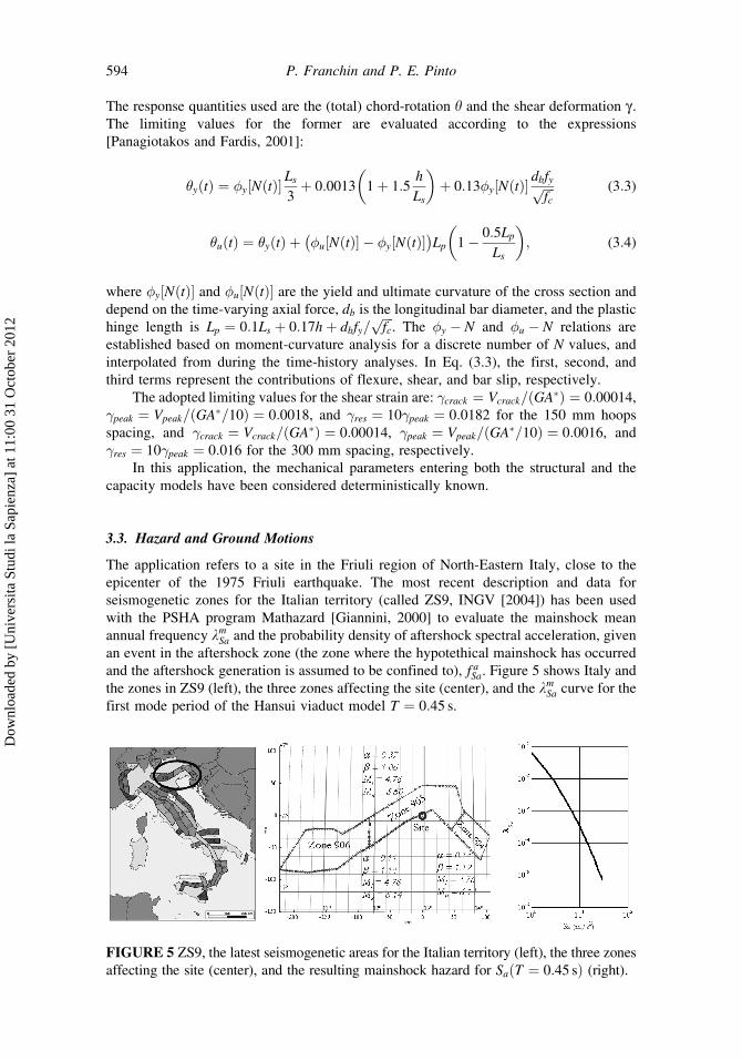
The response quantities used are the (total) chord-rotation y and the shear deformation g .

The limiting values for the former are evaluated according to the expressions

[Panagiotakos and Fardis, 2001]:

y tð Þ ¼ �y N tð Þ½ � Ls

3þ 0:0013 1þ 1:5

h

Ls

�þ 0:13�y N tð Þ½ � dbfyffiffiffiffi

fc

p (3:3)

u tð Þ ¼ y tð Þ þ �u N tð Þ½ � � �y N tð Þ½ ��

Lp 1� 0:5Lp

Ls

�; (3:4)

where �y N tð Þ½ � and �u N tð Þ½ � are the yield and ultimate curvature of the cross section and

depend on the time-varying axial force, db is the longitudinal bar diameter, and the plastic

hinge length is Lp ¼ 0:1Ls þ 0:17hþ dbfy=ffiffiffiffifc

p. The �y � N and �u � N relations are

established based on moment-curvature analysis for a discrete number of N values, and

interpolated from during the time-history analyses. In Eq. (3.3), the first, second, and

third terms represent the contributions of flexure, shear, and bar slip, respectively.

The adopted limiting values for the shear strain are: �crack ¼ Vcrack= GA�ð Þ ¼ 0:00014,

�peak ¼ Vpeak= GA�=10ð Þ ¼ 0:0018, and �res ¼ 10�peak ¼ 0:0182 for the 150 mm hoops

spacing, and �crack ¼ Vcrack= GA�ð Þ ¼ 0:00014, �peak ¼ Vpeak= GA�=10ð Þ ¼ 0:0016, and

�res ¼ 10�peak ¼ 0:016 for the 300 mm spacing, respectively.

In this application, the mechanical parameters entering both the structural and the

capacity models have been considered deterministically known.

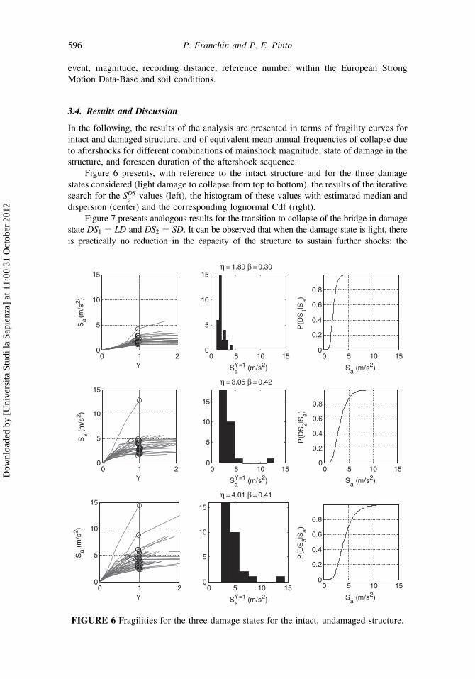
3.3. Hazard and Ground Motions

The application refers to a site in the Friuli region of North-Eastern Italy, close to the

epicenter of the 1975 Friuli earthquake. The most recent description and data for

seismogenetic zones for the Italian territory (called ZS9, INGV [2004]) has been used

with the PSHA program Mathazard [Giannini, 2000] to evaluate the mainshock mean

annual frequency lmSa and the probability density of aftershock spectral acceleration, given

an event in the aftershock zone (the zone where the hypotethical mainshock has occurred

and the aftershock generation is assumed to be confined to), f aSa. Figure 5 shows Italy and

the zones in ZS9 (left), the three zones affecting the site (center), and the lmSa curve for the

first mode period of the Hansui viaduct model T ¼ 0:45 s.

FIGURE 5 ZS9, the latest seismogenetic areas for the Italian territory (left), the three zones

affecting the site (center), and the resulting mainshock hazard for Sa T ¼ 0:45 sð Þ (right).


Dow

nloa

ded

by [

Uni

vers

ita S

tudi

la S

apie

nza]

at 1

1:00

31

Oct

ober

201

2

For the rate of aftershock events �a t;Mm;Mlð Þ, the parameters for this area of North-

Eastern Italy are taken from the mentioned study by Lolli and Gasperini [2003]: a = �2,

b ¼ 1, log10 c ¼ �1:65, and p ¼ 0:9.

For the purpose of fragilities calculation, 30 ground motion records have been

selected in 3 groups of 10 motions each, in order to match on average the uniform-

hazard spectrum at the site for the average return periods of 100, 500, and 1,000 years,

respectively. The same records, after a random permutation, have been used as aftershock

records. Table 2 reports details on the employed ground motion records, and in particular,

TABLE 2 Ground motion records employed

ID Earthquake M r(km) Record Soil

Records matching on average the 100 years average return period

1 Izmit 7.8 77 1251 soft soil

2 Montenegro (aftershock) 6.3 9 230 stiff soil

3 Vrancea 5.8 77 6773 ?

4 Umbria-Marche 5.5 3 591 stiff soil

5 Alkion 6.7 10 333 soft soil

6 Umbria-Marche 5.9 4 594 rock

7 Friuli (aftershock) 6 9 147 stiff soil

8 Alkion 6.7 8 334 soft soil

9 Umbria-Marche 5.9 3 592 stiff soil

10 Friuli (aftershock) 6 9 146 stiff soil


1 Duzce 7.3 0 1703 soft soil

2 Montenegro 7 9 197 stiff soil

3 Duzce 7.3 18 1560 soft soil

4 Gazli 7 4 74 soil

5 Montenegro 7 12 199 stiff soil



8 Izmit (aftershock) 5.8 5 6386 ?

9 Tabas 7.4 3 187 stiff soil




2 Manjil 7.5 92 480 soft soil

3 Montenegro 7 9 198 rock


5 Dinar 6 0 879 soft soil

6 Campano Lucano 6.9 13 291 stiff soil

7 Kalamata 5.8 0 414 stiff soil

8 Erzincan 6.9 1 535 stiff soil

9 Kalamata 5.8 0 413 stiff soil

10 Vrancea 6.9 51 6757 ?


Dow

nloa

ded

by [

Uni

vers

ita S

tudi

la S

apie

nza]

at 1

1:00

31

Oct

ober

201

2

event, magnitude, recording distance, reference number within the European Strong

Motion Data-Base and soil conditions.

3.4. Results and Discussion

In the following, the results of the analysis are presented in terms of fragility curves for

intact and damaged structure, and of equivalent mean annual frequencies of collapse due

to aftershocks for different combinations of mainshock magnitude, state of damage in the

structure, and foreseen duration of the aftershock sequence.

Figure 6 presents, with reference to the intact structure and for the three damage

states considered (light damage to collapse from top to bottom), the results of the iterative

search for the SDSa values (left), the histogram of these values with estimated median and

dispersion (center) and the corresponding lognormal Cdf (right).

Figure 7 presents analogous results for the transition to collapse of the bridge in damage

state DS1 ¼ LD and DS2 ¼ SD. It can be observed that when the damage state is light, there

is practically no reduction in the capacity of the structure to sustain further shocks: the

0 1 20

5

10

15

Y

Sa (

m/s

2 )

0 1 20

5

10

15

Y

Sa (

m/s

2 )

0 1 20

5

10

15

Y

Sa

(m/s

2 )

0 5 10 150

5

10

15

SaY=1 (m/s2)

η = 1.89 β = 0.30

0 5 10 150

0.2

0.4

0.6

0.8

Sa (m/s2)

P(D

S1|S

a)

0 5 10 150

5

10

15

SaY=1 (m/s2)

η = 3.05 β = 0.42

0 5 10 150

0.2

0.4

0.6

0.8

Sa (m/s2)

P(D

S2|S

a)

0 5 10 150

5

10

15

SaY=1 (m/s2)

η = 4.01 β = 0.41

0 5 10 150

0.2

0.4

0.6

0.8

Sa (m/s2)

P(D

S3|S

a)

FIGURE 6 Fragilities for the three damage states for the intact, undamaged structure.


Dow

nloa

ded

by [

Uni

vers

ita S

tudi

la S

apie

nza]

at 1

1:00

31

Oct

ober

201

2

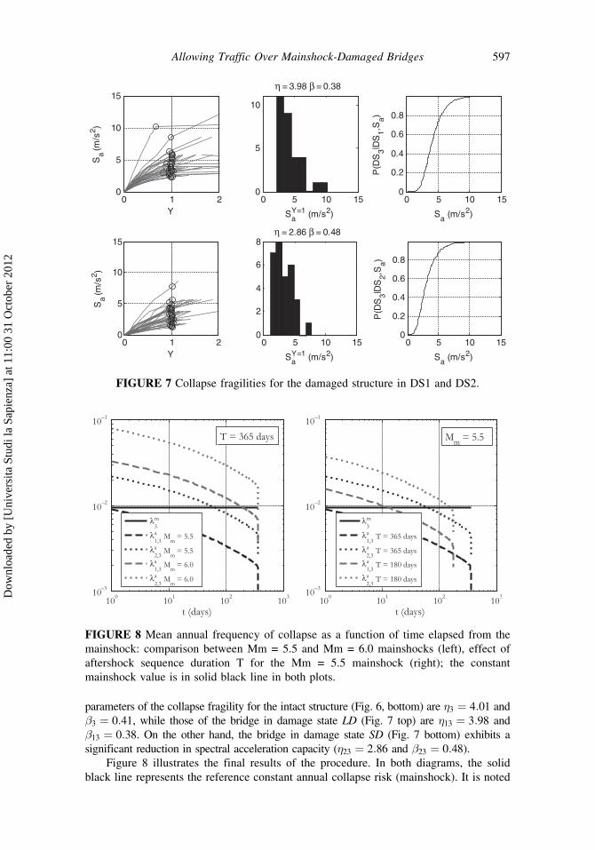
parameters of the collapse fragility for the intact structure (Fig. 6, bottom) are �3 ¼ 4:01 and

�3 ¼ 0:41, while those of the bridge in damage state LD (Fig. 7 top) are �13 ¼ 3:98 and

�13 ¼ 0:38. On the other hand, the bridge in damage state SD (Fig. 7 bottom) exhibits a

significant reduction in spectral acceleration capacity (�23 ¼ 2:86 and �23 ¼ 0:48).

Figure 8 illustrates the final results of the procedure. In both diagrams, the solid

black line represents the reference constant annual collapse risk (mainshock). It is noted

0 1 20

5

10

15

Y

Sa (

m/s

2 )

0 1 20

5

10

15

Y

Sa (

m/s

2 )

0 5 10 150

5

10

SaY=1 (m/s2)

η = 3.98 β = 0.38

0 5 10 150

0.2

0.4

0.6

0.8

Sa (m/s2)

P(D

S3|D

S1,S

a)

0 5 10 150

2

4

6

8

SaY=1 (m/s2)

η = 2.86 β = 0.48

0 5 10 150

0.2

0.4

0.6

0.8

Sa (m/s2)

P(D

S3|D

S2,S

a)FIGURE 7 Collapse fragilities for the damaged structure in DS1 and DS2.

FIGURE 8 Mean annual frequency of collapse as a function of time elapsed from the

mainshock: comparison between Mm = 5.5 and Mm = 6.0 mainshocks (left), effect of

aftershock sequence duration T for the Mm = 5.5 mainshock (right); the constant

mainshock value is in solid black line in both plots.


Dow

nloa

ded

by [

Uni

vers

ita S

tudi

la S

apie

nza]

at 1

1:00

31

Oct

ober

201

2

that the value is indeed quite large, much higher than any acceptable upper bound risk

(see Sec. 2.6), corresponding to an average return period of collapse close to 100 years.

Such a value would not be accepted for an existing structure, i.e., this bridge should be

seismically upgraded in all cases before the occurrence of a mainshock. It is recalled that

this example structure dramatically collapsed in the 1995 Hyogoken-Nanbu event.

Ignoring this, in the following the attention is focused on comparing the equivalent

annual collapse risk due to aftershocks with this reference mainshock risk.

In Fig. 8, left, the aftershock sequence duration T is set to one year, which is regarded

as a likely upper bound for this duration. Black and red curves refer to an hypothetical

mainshock of magnitude Mm ¼ 5:5 and Mm ¼ 6:0, while dashed curve and dotted curve

refer to bridge in LD and SD damage states, respectively. It is observed that if the bridge

is only lightly damaged after the Mm ¼ 5:5 main event, it can be immediately open to

traffic, since the decreasing aftershock risk starts at t = 1 below the reference mainshock

risk. In all other cases, opening of the bridge to all traffic has to be postponed to some

extent. The worst situation is for the bridge in SD after the Mm ¼ 6:0 event, where the

aftershock risk is still double than the reference risk one year after the mainshock. The

curve then drops to zero, consistently with the assumption of finite duration T of the

aftershock sequence, which of course does not mean that the seismic risk vanishes. On the

contrary, the bridge remains exposed to future mainshock in a state of reduced capacity.

Figure 8, right, which refers to the Mm ¼ 5:5 mainshock, examines the influence of the

estimated duration of the aftershock sequence T on the mean annual frequency of collapse.

As it can be seen this parameter is quite influential in determining the opening time. This

time increases with decreasing value of T, due to the fact that, in order to determine the

equivalent annual rate of aftershocks (��a t;Mm;Mlð Þ in Eq. (2.11)), the instantaneous rate

�a t;Mm;Mlð Þ, which is larger for small t (see Eq. (2.9)), is averaged over a shorter period

of time. For example, for the bridge in damage state LD, changing T from one year to six

months changes the decision from immediate opening to a ten day delay. For the bridge in

damage state SD, the corresponding shift is from 50 days to more than 150 days.

4. Conclusions

The ability to estimate the residual traffic-load carrying capacity of bridges damaged by a

mainshock in view of the emergency-management needs not to be emphasized. This

capacity is related to a combination of residual stiffness and strength with respect to both

vertical and horizontal actions, which has so far eluded attempts to capture it analytically

with acceptable confidence.

An alternative approach has been taken in this article, that renounces the idea of

providing probabilities for partial traffic limitation: the bridges after a mainshock will be

either closed, open only for emergency traffic, or fully operational, and the criterion for

such a decision is the survival probability of the mainshock-damaged bridge under the

sequence of the aftershocks as determined from an aftershock probabilistic seismic

hazard analysis. The approach requires fragilities for multiple damage states for the intact

structure, and transition probabilities from these states to collapse for the damaged

structure. The aftershock risk decreases with time, hence a decision for reopening

might have to wait until the risk level goes down to an acceptable value. A realistic

example has demonstrated the feasibility of the approach.

The application of the approach requires pre-analysis of the bridges on a network,

real-time estimation of the mainshock parameters (e.g., by means of a regional

early-warning system) and availability of dependable correlations between visual and

numerical damage assessment. This latter aspect would obviously benefit from the


Dow

nloa

ded

by [

Uni

vers

ita S

tudi

la S

apie

nza]

at 1

1:00

31

Oct

ober

201

2

generalized adoption of monitoring systems which would provide quantitative data on

the actual response of the bridge.

Acknowledgments

This work was supported by the LESSLOSS Project – Subproject 9, funded by the

European Commission – under Award Number GOCE-CT-2003-505488. This support

is gratefully acknowledged.

References

Bazzurro, P., Cornell, C. A., Menun, C., and Motahari, M. [2004] ‘‘Guidelines for seismic assessment

of damaged buildings,’’ Proc. of 13th World Conference on Earthquake Engineering, Vancouver,

BC. (paper 1708)

Giannini, R. [2000] ‘‘Mathazard: a program for seismic hazard analysis,’’ University of Roma Tre,

Rome, Italy (in Italian).

INGV [2004] ‘‘Redazione della mappa di pericolosita sismica prevista dall’Ordinanza PCM 3274

del 20 marzo 2003. Rapporto conclusivo per il Dipartimento di Protezione Civile, INGV,

Milano-Roma,’’ INGV, Milan-Rome, Italy (in Italian).

Jalayer, F., Franchin, P., and Pinto, P. E. [2007] ‘‘A scalar damage measure for seismic reliability

analysis of RC frames,’’ Earthquake Engineering & Structural Dynamics 36(13), 2044–2059,

Special Issue on ‘‘Seismic reliability analysis of structures,’’ Guest Editor C.A. Cornell.

Lolli, B. and Gasperini, P. [2003] ‘‘Aftershock hazard in Italy Part I: estimation of time-magnitude

distribution model parameters and computation of probabilities of occurrence,’’ Journal of

Seismology 7, 235–257.

Luco, N., Bazzurro, P., and Cornell, C. A. [2004] ‘‘Dynamic versus static computation of the

residual capacity of a mainshock damaged building to withstand an aftershock,’’ Proc. of 13th

World Conference on Earthquake Engineering, Vancouver, BC. (paper 2405)

Mackie, K. R., and Stojadinovic, B. [2006] ‘‘Post-earthquake functionality of highway overpass

bridges,’’ Earthquake Engineering & Structural Dynamics 35, 77–93.

Marini, A. and Spacone, E. [2006] ‘‘Analysis of reinforced concrete elements including shear

effects,’’ ACI Structural Journal 103(5), 645–655.

McKenna, F., Fenves, G. L., and Scott, M. H. [2007] ‘‘OpenSees: open system for earthquake

engineering simulation,’’ http://opensees.berkeley.edu, Pacific Earthquake Engineering

Research Center, University of California, Berkeley, CA

Panagiotakos, T. B. and Fardis, M. N. [2001] ‘‘Deformations of reinforced concrete members at

yielding and ultimate,’’ ACI Structural Journal 98(2), 135–148.

Pincheira, J. A., Dotiwala, F. S., and D’Souza, J. T. [1999] ‘‘Seismic Analysis of Older Reinforced

Concrete Columns,’’ Earthquake Spectra 15(2), Earthquake Eng. Research Inst., Oakland, CA.

Pinto, P. E., Giannini, R., and Franchin, P. [2004] Methods for Seismic Reliability Analysis of

Structures. IUSS Press, Pavia, Italy.

Priestley, M. J. N., Verma, R., and Xiao, Y. [1994] ‘‘Seismic shear strength of reinforced concrete

buildings,’’ ASCE Journal of Structural Engineering 120(8), 2310–2329.

Reasenberg, P. A. and Jones, L. M. [1989] ‘‘Earthquake hazard after a mainshock in California,’’

Science 243, 1173–1176.

Schotanus, M. I J. and Franchin, P. [2004] ‘‘Seismic reliability analysis using response surface: a

simplified approach,’’ Proc. of 2nd ASRANet Colloquium, Barcelona, Spain.

Sezen H. [2008]. ‘‘Shear deformation model for reinforced concrete columns,’’ Structural

Engineering and Mechanics 28(1), TechnoPress, Yusong Daejeon, Korea.

Utsu, T. [1995] ‘‘The centenary of the Omori formula for a decay law of aftershock activity,’’

Journal of the Physics of the Earth 43, 1–33.

Yeo, G. L. [2005] ‘‘Stochastic characterization and decision-bases under time-dependent aftershock

risk in performance-based earthquake engineering,’’ Ph.D. dissertation, Stanford University, CA.


Dow

nloa

ded

by [

Uni

vers

ita S

tudi

la S

apie

nza]

at 1

1:00

31

Oct

ober

201

2

Allowing Traffic Over Mainshock-Damaged Bridges

Documents

Transcript of Allowing Traffic Over Mainshock-Damaged Bridges