An analytical approach to estimating aberrations in curved multilayer optics for hard x-rays: 1....

An analytical approach to estimating aberrations in curved multilayer optics for hard x-rays:

1. Derivation of caustic shapes

J-P. Guigay1*, Ch. Morawe1, V. Mocella2, and C. Ferrero1*

1ESRF, BP 220, 6, rue Jules Horowitz, F-38043 Grenoble cedex, France 2CNR-IMM -Sezione di Napoli, via P. Castellino 111, I-80131 Napoli, Italy

*[email protected], *[email protected]

Abstract: An analytical approach has been developed to derive aberration effects in parabolic and elliptic multilayer optics with weak interaction between photons and matter. The method is based on geometrical ray tracing including refraction effects up to the first order of the refractive index decrement δ. In the parabolic case, the derivation leads to simple parametric equations for the caustic shape. In the elliptic case, the analytical results more involved, but can be well approximated by the parabolic solution. Both geometries are compared with regard to the fundamental impact on their focusing properties.

©2008 Optical Society of America

OCIS codes: (340.6720) X-ray optics, Synchrotron Radiation; (340.7470) X-ray optics, X-ray Mirrors; (080.2720) Geometrical optics, mathematical methods; (080.4228) Geometrical optics, Non-spherical Mirror Surfaces; (080.1010) Geometrical optics, Aberrations (global).

References and links

1. W. Chao, B. D. Harteneck, J. A. Liddle, E. H. Anderson, and D. T. Attwood, “Soft X-ray microscopy at a spatial resolution better than 15 nm,” Nature 435, 1210-1213 (2005).

2. C. G. Schroer, O. Kurapova, J. Patommel, P. Boye, J. Feldkamp, B. Lengeler, M. Burghammer, C. Riekel, L. Vincze, A. van der Hart, and M. Küchler, “Hard X-ray nanoprobe based on refractive X-ray lenses,” Appl. Phys. Lett. 87, 124103 (2005).

3. A. Jarre, C. Fuhse, C. Ollinger, J. Seeger, R. Tucoulou, and T. Salditt, “Two-dimensional hard X-ray beam compression by combined focusing and waveguide optics,” Phys. Rev. Lett. 94, 074801 (2005).

4. D. H. Bilderback, S. A. Hoffman, and D. J. Thiel, “Nanometer spatial resolution achieved in hard X-ray imaging and Laue diffraction experiments,” Science 263, 201-203 (1994).

5. H. Mimura, S. Matsuyama, H. Yumoto, H. Hara, K. Yamamura, Y. Sano, M. Shibahara, K. Endo, Y. Mori, Y. Nishino, K. Tamasaku, M. Yabashi, T. Ishikawa, and K. Yamauchi, “Hard X-ray diffraction-limited nanofocusing with Kirkpatrick-Baez mirrors,” J. J. Appl. Phys. 44, L539 – L542 (2005).

6. W. Liu, G. E. Ice, J. Z. Tischler, A. Khounsary, C. Liu, L. Assoufid, and A.T. Macrander, “Short focal length Kirkpatrick-Baez mirrors for a hard X-ray nanoprobe,” Rev. Sci. Instr. 76, 113701 (2005).

7. Ch. Morawe, O. Hignette, P. Cloetens, W. Ludwig, Ch. Borel, P. Bernard, and A. Rommeveaux, “Graded multilayers for focusing hard X rays below 50 nm,” Proc. SPIE 6317, 63170F (2006).

8. F. Pfeiffer, C. David, J. F. van der Veen, and C. Bergemann, “Nanometer focusing properties of Fresnel zone plates described by dynamical diffraction theory,” Phys. Rev. B 73, 245331 (2006).

9. C. G. Schroer and B. Lengeler, “Focusing hard X rays to nanometer dimensions by adiabatically focusing lenses,” Phys. Rev. Lett. 94, 054802 (2005).

10. K. Yamauchi, K. Yamamura, H. Mimura, Y. Sano, A. Saito, A. Souvorov, M. Yabashi, K. Tamasaku, T. Ishikawa, Y. Mori, “Nearly diffraction-limited line focusing of hard X-ray beam with an elliptically figured mirror,” J. Synchrotron Rad. 9, 313 - 316 (2002).

11. C. M. Kewish, L. Assoufid, A. T. Macrander, and J. Qian, “Wave-optical simulation of hard X-ray nanofocusing by precisely figured elliptical mirrors,” Appl. Opt. 46, 2010 - 2021 (2007).

12. C. G. Schroer, “Focusing hard X rays to nanometer dimensions using Fresnel zone plates,” Phys. Rev. B 74, 033405 (2006).

13. H. Yan, J. Maser, A.T. Macrander, Q. Shen, S. Vogt, G.B. Stephenson, H.C. Kang, “Takagi-Taupin description of X-ray dynamical diffraction from diffractive optics with large numerical aperture,” Phys. Rev. B 76, 115438 (2007).

#96574 - $15.00 USD Received 23 May 2008; revised 9 Jul 2008; accepted 13 Jul 2008; published 28 Jul 2008

(C) 2008 OSA 4 August 2008 / Vol. 16, No. 16 / OPTICS EXPRESS 12050

14. H. Mimura, S. Matsuyama, H. Yumoto, S. Handa, T. Kimura, Y. Sano, K. Tamasaku, Y. Nishino, M. Yabashi, T. Ishikawa, K. Yamauchi, “Reflective optics for sub-10nm hard X-ray focusing,” Proc. SPIE 6705, 67050L (2007).

15. A. Authier, Dynamical Theory of X-ray Diffraction, IUCr monographs, (Oxford, University Press. 2001)

1. Introduction

Recent years have seen a rapid evolution in hard x-ray optics, particularly boosted by the use of extremely brilliant 3rd generation synchrotron radiation sources. X-ray beams were focused down to spots below 50 nm using various optical elements such as Fresnel Zone Plates (FZPs) [1], Compound Refractive Lenses (CRLs) [2], Wave Guides (WGs) [3], capillary optics [4], curved Total Reflection Mirrors (TRMs) [5], transmission Multilayer Laue Lenses (MLLs) [6], and Reflective Multilayers (RMLs) [7]. The question arose, whether the ultimate spatial resolution of x-ray optical elements is limited by physical properties other than the wavelength and the numerical aperture. Several theoretical studies, mainly numerical wave optical calculations, were published treating the cases of FZPs [8], CRLs [9], TRMs [10,11], and MLLs [12,13]. Advanced numerical ray tracing calculations have been applied to RMLs [14]. This paper describes the case of RMLs using a geometrical and purely analytical approach.

2. Basic assumptions and geometry

The model is based on the following assumptions and geometrical boundary conditions. Only one-dimensional focusing will be considered. This corresponds to the frequently used Kirkpatrick-Baez (KB) focusing geometry, where two successively mounted and one-dimensionally curved mirrors are utilized. Two cases will be discussed: the parabola (Fig. 1) and the ellipse (Fig. 2). For the calculations either a parallel incident beam (parabola) or an ideal point source (ellipse) are assumed. The parabolic approximation appears justified since 3rd generation synchrotron radiation sources are small and far away from the focusing optics. For optical layouts with finite source distances, the elliptic geometry would be more appropriate. In many cases, however, when the RML is illuminated under grazing incidence, a very eccentric ellipse can be sufficiently well approximated by a parabola. Instead of treating the full ML structure and its multiple internal reflections, the whole stack is represented by only two interfaces filled with a medium of a real average optical index n = 1 – δ. The starting point for the following calculations is the selection of a reflecting interface at a certain depth in the ML stack. This depth should be varied about the extinction length known from the dynamical theory of x-ray diffraction for a perfect crystal [15]. The aim is to follow the traces of rays reflected from this interface and localize their envelope (caustic) near the ideal focus, the latter being formed by rays reflected from the entrance surface. In the following, all analytical expressions are linearized with respect to δ. The validity of the present approach is thus limited by the requirement that δ << 1, which is fulfilled in the case of hard x-rays (δ ~10-6).

The caustic described in the present work results from a simplified model of the diffraction process inside the RML; it is therefore an “artificial” caustic which must not be confused with the “real” caustic (the envelope of the rays associated to the actual outgoing wavefront). This model can be handled analytically with the purpose to get a crude estimation of the aberrations due to refraction effects at the RML interfaces.

3. Derivation of the parametric equations for the caustic curve

3.1. Parabolic case

We consider two parabolas (P) and (P’) having the same focus F (0,0) and vertices in (p/2,0) and (p/2+s,0) (Fig. 1). Their equations in polar coordinates, with origin in F, are



2 and

1 cos 1 cos 1 cos 1 cos

p p s p kpρ ρϕ ϕ ϕ ϕ

′+= = = =+ + + +

, with p

kp

′= (1)

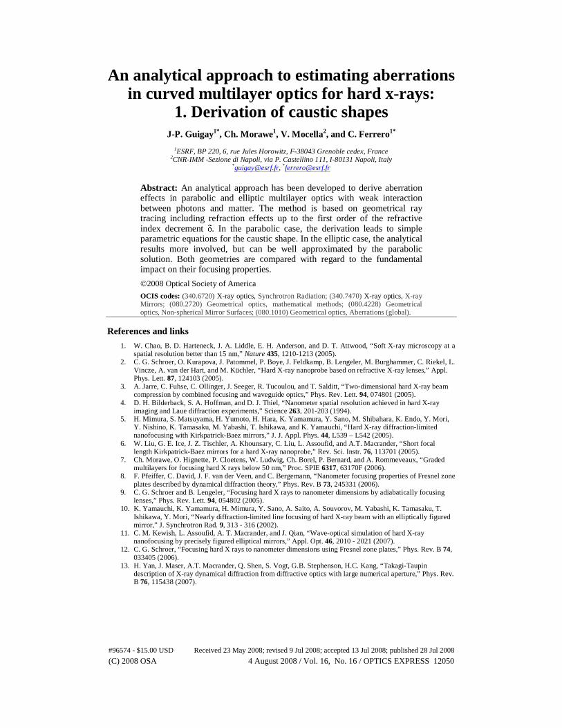
Fig. 1. Focusing geometry of a parabolic RML. The red solid line shows a ray reflected from the entrance RML surface reaching the ideal focus F. The blue solid line indicates a ray that is first refracted when crossing (P) in point C, then reflected at point N on (P’), and again refracted when crossing (P) in point D. The green solid line illustrates the resulting envelope of all rays reflected from (P’). The polar angle φ is defined by the virtual ray reflected in point N without refraction in the RML medium (broken line). The dimensions are not in scale.

Consider an incident ray parallel to the x-axis, crossing (P) in point C, reflected on (P’) at point N and crossing (P) again in point D. This ray can be defined by the polar angle ϕ of the point N. Let ANBF be the corresponding trajectory in the ideal case without refraction, with reflection taking place at the same point N, A and B being the corresponding entrance and exit points. The angular deviations due to refraction are equal to / tanδ θ , where δ = 1− n is the refractive index decrement and θ is the grazing incidence angle. The coordinates of the point D and the slope m(t) of the emergent ray have to be calculated analytically in terms of

tan( / 2)t ϕ= ,

the terms of order > 1 in δ being neglected. The angular deviations in C and in D are

tan( / 2) tan( / 2) and C C A Dkt tε δ ϕ δ ϕ δ ε δ= ≈ = =

The polar angle at the point D is , where ( 1)D C

BNht h k k

BFϕ ϕ ε ϕ δ≅ − = − = − .

One can derive the position of point D and the slope of outgoing ray:



2 2 2cos( ) [1 (1 )] / 2

1 cosD

DD

x t p p t ht tϕ

ϕ= = − + +

+

2sin( ) [1 (1 ) / 2]

1 cosD

DD

y t p pt h tϕ

ϕ= = − +

+ (2)

22

2 2

2 1( ) tan( ) ( ) ( 1)

1 1C D

t tm t k t

t tϕ ε ε δ+= + − = + −

− −

The emerging ray is defined by

( ) ( ) ( ) ( )D DY m t X y t m t x t− = − (3)

The caustic curve is obtained by solving the system of equations formed by (3) and:

'( ) ( ) 'D Dm t X y mx− = −

It is useful to write:

0 1 0 1 0 1( ) ( ) ( ) , y ( ) ( ) ( ) , ( ) ( ) ( )D D Dx t x t x t t y t y t m t m t m t= + = + = + , where the term

with index 1 is proportional to the small factor ( 1)kδ − . Eliminating the terms of 2nd order in this small factor, the parametric equations of the caustic curve are found to be

1 0 0 1 1 0 1 1 0 0 1( ) ( ) / , ( ) ( )X t m x m x y m Y t X t y m x m x′ ′= + − = + − − (4)

After calculating the different derivatives and suitably regrouping terms one obtains the parametric equations

( ) ( )( )( ) ( )

2 4

3

1 1 6 3

1 8

X t s s p t t

Y t s s p t

δ

δ

= + + −

= + (5)

For δ = 0 or s = 0 this caustic reduces just to the focus F(0,0).

Equation (5) can be discussed following two approximations:

a) Grazing incidence

Using the approximations θ << 1, φ → π, and t >> 1, one obtains

( ) ( )( ) ( )

4

3

3 1

8 1

x t s s p t

y t s s p t

δ

δ

≈ − +

= + (6)

For s/p << 1 this further simplifies to



( )( )

4

3

3

8

x t st

y t st

δ

δ

≈ −

= (7)

By eliminating t, Eq. (7) can be combined into the functional form

( ) ( )1 4 3 43 4

8

3y x s xδ≈ ∓ (8)

where the negative sign applies to positive polar angles φ and vice versa.

b) Normal incidence

Applying the approximations θ → π/2, φ → 0, and t → 1 one obtains

( ) ( )( )( ) ( )

2

3

1 1 6

8 1

x t s s p t

y t s s p t

δ

δ

≈ + +

= + (9)

For s/p << 1 this simplifies to

( ) ( )( )

2

3

1 6

8

x t s t

y t st

δ

δ

≈ +

= (10)

Equation (10) can be combined in a functional form into

( ) ( ) 1 2 3 23 2

8

6y x s xδ −≈ ±� � (11)

with x x sδ= −� , the positive sign holding for positive polar angles φ.

3.2. Elliptic case

We consider two confocal ellipses with foci in S and F and with different eccentricities e and e’. Their equations in polar coordinates, with origin in S or in F, and axis along SF are

or 1 cos 1 cosS F

p p

e eρ ρ

α ϕ= =

− + , where

2 2

2SF / 2 , (1 )a c

c ea p e aa

−= = = = − (12)



Fig. 2. Focusing geometry of an elliptic RML using a notation similar to that used in Fig. 1.

Let’s consider a ray SCND refracted in C, reflected in N and refracted in D and let the associated ray be SANBF in the ideal case without refraction. The polar angles at the point N, with origin in S or in F will be denoted as and α ϕ , respectively. The angular deviations in C and D follow as

sintan( / 2)

1 cosC A ee

αε δ ω δα

= =−

, sin

tan( / 2)1 cosD B e

e

ϕε δ ω δϕ

= =+

(13)

The N-angles in the triangles SNC and FND are equal and both approximated as

2

(1 cos ) 1 cossin

(1 cos ) (1 cos )C C

SA p e e e

SN p e k e

α δ αη ε ε αα α

′ ′− −= = =′ − −

(14)

The F-angle of the triangle NDF is

(1 cos ) 1 ( )cos

[ 1](1 cos ) 1 cos

BN p e k ke e

BF p e e

ϕ ϕβ η η ηϕ ϕ

′ ′+ − + −= = − =′ ′+ +

(15)

Similarly to Eq. (2) one obtains the system

2

cos( ) cos sin

1 cos( ) 1 cos (1 cos )D

p p px

e e e

ϕ β ϕ ϕβϕ β ϕ ϕ−= = +

+ − + +

2

sin( ) sin ( cos )

1 cos( ) 1 cos (1 cos )D

p p p ey

e e e

ϕ β ϕ ϕβϕ β ϕ ϕ− += = −

+ − + + (16)

2tan( ) tan ( )(1 tan )D F Dm ϕ η ε ϕ η ε ϕ= + − = + − +



Using the relation (1 ) tan( / 2) (1 ) tan( / 2)e eα ϕ′ ′+ = − , it is possible to express β and η as rational functions of tan( / 2)t ϕ= . Consequently, , and D Dx y m can also be

expressed as rational functions of t. The parametric equations of the caustic curve can hence be obtained by the same approach as in the parabolic case. However, their derivation does not lead to so simple expressions as Eq. (5).

Since focusing geometries for hard x-rays usually imply very eccentric ellipses, it appears adequate to derive an approximate solution where both and e e′ are very close to 1 and where α is a very small angle.

The expressions for xD , yD, and m given above for the ellipse can then be shown to converge towards the corresponding Eq. (5) for the parabola.

Considering and 02 2

p pg g kg

c c

′′= = = → , simple analytical expressions at the

first order in g and g’ can be written. The eccentricity, which satisfies 22 1ge e= − , reduces

to 21 2e g g= − + ; , where tan( / 2)tg tα ϕ′= = . We thus obtain the following approximations:

2 2 2 2 11 cos 1 (1 )(1 ) (1 )

2 2 2

g g t te g g gα ′ ′ −′ ′ ′ ′− = − − + − = +

2 2 2 2 2 11 cos 1 (1 )(1 ) (1 )

2 2 2

g g t k te g g gα ′ −− = − − + − = +

2

2 22

1 cos 1[1 ( 1)]

(1 cos ) 2

e k tkg g k t

e g

αα

′− −= + − −−

(17)

(1 ) (1 ) 1ke e k g kg k′− = − − − = − ; 21 cos 1

11 cos 2

tg

e

ϕϕ

+ −′= +′+

22 2 1

[1 (1 )]2

tk t g t k kη δ −= + − + ; 2( 1) [1 (1 )(1 ) / 2]D e k t g t kη ε δ− = − + + +

2 2(1 ) , where ( 1)ht gk t h k kβ δ= − = −

System (16) can thereby be written as

2 2 22 2 2 2

2 2 22 2

22 2

2 2

1 1 1[1 ] [1 (1 )]

2 2 21 1 1 3

[1 ] [1 ] [1 ]2 2 2

2 1( ) ( 1){1 (1 )[1 (1 )]}

1 1 2

D

D

t t tx p g pht g t k t

t t ty pt g pht gk t g

t t gm t k k t k

t tδ

− − += + + + − −

− + −= + − − +

+= + − − + + +− −

(18)



Neglecting terms containing the factor δ(k-1)g , which is very small since these three factors are small, Eq. (18) simplify to

2 2 22

2 2

22

2 2

1 1 1[1 ] ( 1)

2 2 21 1

[1 ] ( 1)2 2

2 1( ) ( 1)

1 1

D

D

t t tx p g p k k t

t ty pt g p k k t

t tm t k

t t

δ

δ

δ

− − += + + −

− += + − −

+= + −− −

(19)

Using Eq. (4) with increments:

2 2

21 1 0 1 1

1 1( ) , , 0

2 2t t

x pg y pgt m x m− −Δ = Δ = = Δ Δ = , one obtains the same

parametric formulas (5) as in the parabolic case.

4. Discussion

4.1 Comparison between parabolic and elliptic RMLs

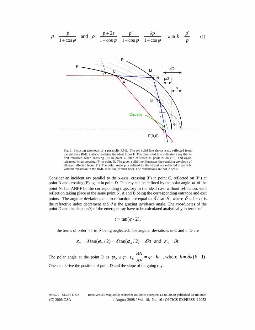
To understand the basic differences of the caustic curves deriving from parabolic and elliptic RMLs, two computations basing on Eqs. (2) or (5) and (16) were performed using focusing parameters typical of a 3rd generation synchrotron beamline. Figure 3 describes the behaviour of both the location (x,y) (positive branch only) of the caustic (red) and, implicitly, of the corresponding incidence angle θ on the RML (blue). Solid lines correspond to an ellipse, open circles to a parabola. The insert zooms in on the zone very close to the ideal geometrical focus. The arrows indicate the evolution of the caustic when starting at normal incidence. For large angles of incidence (θ > 10°) the caustic remains sub-nanometric. For grazing angles of incidence (θ < 1°), however, the caustic evolves quickly to several hundred nanometers in the y direction and up to tens of micrometers along the optical axis. In the present case of a very eccentric ellipse (e ≈ 1 – 4·10-8) the difference between the ellipse and parabola cases remains very small and becomes appreciable only at angles θ < 0.2°. It appears therefore that the analytical Eq. (5) are suitable to describe the fundamental properties of the caustic with sufficient precision as long as the angles of incidence remain above this limit. It should be pointed out that the linear treatment of the refraction as explained in section 3 fails when the critical angle of total reflection is approached. Below this angle there is no beam penetration beyond the external surface and the model does not apply any more.



0

100

200

300

400

0

0.5

1

1.5

2

-1 105 -8 104 -6 104 -4 104 -2 104 0

y [n

m] Θ

[deg]

x [nm]

0

1 10-5

2 10-5

3 10-5

4 10-5

20

30

40

50

60

70

80

90

-1 10-5 -5 10-6 0 5 10-6

E = 24550 eVP = 150 mQ = 0.077 mδ = 2.7e-6

p = 5775 nms = 0.253 nm

Fig. 3. Positive branch of the caustic curve y(x) (red) and corresponding grazing incidence angle θ(x) (blue) for a given set of parameters. The insert is a zoom into the zone around the ideal focus and the corresponding angles of incidence. Arrows indicate the evolution of the curves starting at normal incidence. The curves clearly indicate the “left turn” of the caustic when starting from normal incidence.

0

10

20

30

40

50

60

-5000 -4000 -3000 -2000 -1000 0

y [n

m]

x [nm]

y = y(x(s))

y = y(x(Θ))

Θ = 0.2...0.5 deg

P = 150 mQ = 0.077 mδ = 2.7e-6

s = 0.05...0.25 nm

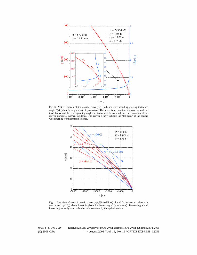
Fig. 4. Overview of a set of caustic curves. y(x(θ)) (red lines) plotted for increasing values of s (red arrow). y(x(s)) (blue lines) is given for increasing θ (blue arrow). Decreasing s and increasing θ clearly reduce the aberrations caused by the optical system.



4.2 Angular variation and beam penetration

The simplicity of Eq. (5) allows a preliminary interpretation of the caustic shape. In a curved RML both the angular variation, described by t, and the beam penetration, characterized by s, contribute to the formation of the caustic around the ideal focus.

The influence of both angular variations and beam penetration is illustrated in Fig. 4. Red curves show angular effects for fixed penetration depths. Blue lines show penetration effects for fixed incidence angles . Based on this type of diagram, the caustic area of a given RML can be estimated by calculating the corresponding parameter pairs (t,s) along the optical element. In the numerical results of Figs. 3 and 4, absorption is not explicitly taken into account. Allowing for it would however change only the value of the penetration depth (and consequently the parameter s) chosen for the calculations. This will be discussed in detail in the second part of this investigation.

5. Summary and outlook

A purely analytical ray tracing approach was developed to describe aberration effects in curved RML optics. It allows an estimate of shape and dimensions of a caustic around the ideal focus as a function of incidence angle, beam penetration, and the average refractive index of the RML materials. In the case of hard x-ray focusing geometries implying very eccentric ellipses, both parabolic and elliptic approaches lead to nearly identical results. However, the model breaks down when approaching the critical angle of total external reflection.

It should be emphasized that real RML coatings are designed in a way as to meet locally the conditions for constructive interference between neighbouring RML periods. This implies that only the entrance optical surface is elliptic while all inner interfaces slightly deviate from the ideal elliptical shape. The caustic derived above has thereby to be considered as an approximation that likely overestimates the actual dimensions of the aberrations. Nevertheless, the simplicity of the analytic solution provides a tool to understand fundamental properties of the focusing characteristics. The forthcoming part (part 2) of this work will cover a refined interpretation of the results and a comparison with available experimental data.



An analytical approach to estimating aberrations in curved multilayer optics for hard x-rays: 1....

Documents

Transcript of An analytical approach to estimating aberrations in curved multilayer optics for hard x-rays: 1....