Study and Control of Caustic Soda Production by Solvay ...

Study and Control of Caustic Soda Production by Solvay Process

Alsunni Osman Hassan Alsunni

B.Sc. (Honours) in Chemical Engineering Technology

University of Gezira, (2014)

A Dissertation

Submitted to the University of Gezira in Partial Fulfillment of the

Requirement for the Award of the Degree of Master of Science

in

Chemical Engineering

Department of Chemical Engineering and Chemical Technology

Faculty of Engineering and Technology

May 2016



Supervision Committee:

Name Position Signature

Prof. Gurashi Abdullah Gasmelseed Main Supervisor …..……...

Dr. Fath Alrahman Abbas Alsheikh Co- supervisor …………..

Date: 4/5/2016



Examination Committee:

Name Position Signature

Prof. Gurashi Abdalla Gasmelseed Chair Person ……………

Prof. Ibrahim Hassan Mohamed Alamin External Examiner ………………….

Dr. Magdi Ali Osman Internal Examiner ……..….….

Date of Examination: 23/4/2016

4

اآلية

قال تعالي

وح من أمر ربي وما أوتيتم من العلم إلا قليلا )85( ( وح قل الر ) ويسألونك عن الر

سورة اإلسراء، اآليــة )85(

5

DEDICATION

To my family, for their unconditional love and support throughout the

courses of this work.

Also, this thesis is dedicated to my supervisors who have been a great

source of motivation and inspiration and to my friends.

6

ACKNOWLEDMENTS

Above all, I render my thanks to the merciful “Allah” how offered me

health and patience to accomplish this study. This research work would

have never been successfully undertaken without the unreserved

support of my main adviser Prof.Gurashi Abdella Gasmelseed. I would

like to express my deepest gratitude to Ust. Reham Abd Elmonem

Ahmed Mohamed for her rigorous interest and for sharing me her

profound knowledge and experience. Her continued discussion and

critical comments helped me a lot to improve and refine the final draft

of the thesis.

Sincere thanks are extended to my family for their help and cooperation

in various stages of this work.

Last but not least, thanks go to everyone, who contributed to this work.

7



Abstract

Control systems are used to maintain process conditions at their

desired values by manipulating certain process variables to adjust the

variables of interest. The Solvay process including Continuous Stirred

Tank Reactor (CSTR) and Multi-Effect Evaporators. A Continuous

Stirred Tank Reactor surrounded by a jacket with specific dimensions is

used for the endothermic reaction for the production of liquid caustic

soda from the reaction of calcium hydroxide and sodium carbonate.

MultiــEffect Evaporators are used to increase the concentration of

sodium hydroxide output. The aims of this study are to investigate the

production of liquid caustic soda by Solvay process, automatic control

of the Continuous Stirred Tank Reactor and MultiــEffect Evaporators

and analyze the stability of the Continuous Stirred Tank Reactor and

Multi Effect Evaporators using different methods. A single input/single

output (SISO) system was used to control the level of the solution inside

the reactor, composition of caustic soda and the temperature in the

third evaporator. A cascade control system was used to control the

reactor temperature. The characteristic equation, the open loop

transfer function (OLTF) and the overall transfer function were

obtained for stability analysis and tuning. The methods used for tuning

and stability analysis were Routh–Hurwitz, direct substitution, Root-

Locus and Bode plot to determine the ultimate gain (Ku) and the

ultimate period (Pu). The response of the system was plotted by

inserting the adjustable obtained parameters. MATLAB documentation

(m file) was used to determine the system stability analysis and tuning.

The results of this study were for four loops, for level of the solution

inside the reactor control loop1 the average ultimate gain Ku is 18.18

8

and the average ultimate period is Pu 1.825sec, for the reactor

temperature control loop2 the average ultimate gain Ku is 7.2 and the

average ultimate period Pu is 3.6sec, for temperature in the third

evaporator at multi-effect evaporators control loop3 the average

ultimate gain Ku is 369.77 and the average ultimate period Pu is

0.238sec and for composition control loop4 the average ultimate gain

Ku is 16.88 and the average ultimate period Pu is 0.755sec. These

methods are proved to be identical in the results and each of them is

qualified to be used for tuning and stability analysis without loss of

accuracy. It is recommended that the Cascade control system should be

use to control the temperature of the Continuous Stirred Tank Reactor.

9

دراسة و التحكم في انتاج الصودا الكاوية بواسطة عمليات سولفي

السني عثمان حسن السني

ملخص الدراسة

تستخدم أنظمة التحكم للمحافظة علي ظروف العملية عند القيم المطلوبة من خلل معالجة

.عمليات سولفي تتضمن المفاعل ذو متغيرات العملية لضبط هذه المتغيرات عند القيم المطلوبة

الخلط المستمر و المبخرات متعددة التاثير. المفاعل ذو الخلط المستمر و المحاط بغلف ذو ابعاد

الناتجة من تفاعل محددة استخدم للتفاعل الماص للحرارة إلنتاج مادة الصودا الكاوية السائلة

هيدروكسيد الكالسيوم و كربونات الصوديوم. المبخرات متعددة التاثير استخدمت لزيادة تركيز

محلول هيدروكسيد الصوديوم الناتج . تهدف هذه الدراسة الي بحث و دراسة انتاج مادة الصودا

الكاوية السائلة عن طريق عمليات سولفي و التحكم اللي في المفاعل ذو الخلط المستمر و

المبخرات متعددة التاثير و تحليل الستقرارية للمفاعل ذو الخلط المستمر و المبخرات متعددة

التاثير. استخدم النظام ذو الدخال و الخراج الحاد و ذلك للتحكم في مستو المحلول داخل

المفاعل و تركيب نواتج المبخرات متعددة التاثير و الحرارة في المبخر الثالث . استخدم نظام

درجة الحرارة للمفاعل . تم وضع استراتيجية التتالي ذو الدخال و الخراج الحاد للتحكم في

للتحكم. وتم ايجاد التوابع الناقلة كما ح ددت المعادلت المميزة و التوابع الناقلة الكلية ومعدلت

الدورات المفتوحة حيث استخدمت في الضبط و تحديد الستقراريه و المحاكاة للنظام . استخدمت

اربعة طرق لضبط وتحليل الستقرارية هي روث-هورويتز و التعويض المباشر و جذور لوكس

باستخدام النظام استجابة رسم تم والفترة الحرجة. وقد و مخطط بود لتحديد المكسب الحرج

ماتلب لتحديد استقرارالنظام وضبطه. و كانت للتعديل. ايضا استخدم برنامج المتغيرات القابلة

النتائج لهذه الدراسة لربعة دوائر للتحكم، الدائرة الولي للتحكم في مستو المحلول داخل

ثانية ، الدائره 1.825 ومتوسط الفترة الحرجة 18.18المفاعل و وجد ان متوسط المكسب الحرج

ومتوسط الفتره 7.2الثانية للتحكم في درجة الحرارة للمفاعل و وجد ان متوسط المكسب الحرج

الحرجة 3.6ثانية ، الدائرة الثالثة للتحكم في درجة حرارة المبخر الثالث في المبخرات متعددة

ثانية و 0.238التاثير و وجد ان متوسط المكسب الحرج 369.77 ومتوسط الفترة الحرجة

ومتوسط 16.88الدائرة الرابعة للتحكم في تركيب النواتج و وجد ان متوسط المكسب الحرج

ثانية . اثبتت هذه الطرق تطابق كبير في النتائج وكل منها يستخدم لضبط 0.755الفترة الحرجة

لذلك أوصت الدراسة بأن يتم استخدام نظام التتالي وتحليل استقرارية النظام دون فقدان الدقة.

ذوالدخال و الخراج الحاد للتحكم في درجة الحرارة للمفاعل ذو الخلط المستمر .

10

Table of Contents

Dedication ……………………………………………………….…..ii

Acknowledgments ………………….……………………………….….iii

Abstract ……………………………..………………..………..………..iv

Abstract (Arabic) …………………………..………………...………..v

Table of contents ………………………………………………………vi

List of Figures ……………………………………...……………..….xiii

List of Tables ……………...………….……….…………………..…....xiv

List of Abbreviations ………………….………….…………………….xvi

Chapter one: Introduction

1.1 Caustic Soda ………………… …………………..…………………..1

1.2 Manufacture of Caustic Soda..........................................................…..2

1.3 Uses of Caustic Soda ……… …………………….………….……….2

1.4 Control System …………………..……………..…………………....3

1.5 Type of Controllers......................................................................... 4

1.5.1 Proportional Control……………………………………… …….…4

1.5.2 Proportional Integral (PI)

Control…………………………………….……….………………….…. 5

1.5.3 Proportional Plus Integral Plus Derivative (PID) Control …......5

1.6 Control Classification……….…………………................................5

1.6.1 Manual Control ……………………….……………….................5

1.6.2 Automatic

Control……………..…………………………………………………. .5

1.6.3 Open-Loop Control: …………………………… ………………….6

1.6.4 Closed-Loop Control……………….………..….… ………….6

1.7 Statement of The Research

Problem…………………………………………………............................ .6

1.8 Layout of The Thesis………………………………………..……..... 6

1.9 Research Objectives:-:…………… ……………………..….... ..7

11

Chapter Tow: Literature Review

2.1 Ernest Solvay:………………… ………………………………. ..8

2.2 Manufacturing of Caustic Soda :……………………… ……… .8

2.2.1 Production Caustic Soda from Soda Ash………………….……..8

2.2.2 Production Caustic Soda by Electrolysis :……… ……………. …9

2.2.3 Energetic of the Electrolytic Process : …………………..…10

2.2.4 Types of Cells :……………………………… ……………………11

2.3 Manufacture of Soda Ash by Solvay Process…………………….. .11

2.3.1 Preparation of Brin :……………………………… …….11

2.3.2 Ammunition of Brine:……………… ……………….. …….. ...11

2.3.3 Carbonation of Brine:………………… …….. …… ………….....11

2.3.4 Calcinations: ………………………………….………………… 12

2.4 Uses of Soda Ash : …………………………………… ……………..12

2.5 Manufacture of Caustic Soda by Solvay Process………………….13

2.5.1 Causticization :………………………………… …………….. .14

2.5.2 The Reaction………………………………………………13

2.5.3 Evaporation: ………………………. …………………….…14

2.5.4 Concentration : …………………………………………………... 14

2.6 Background of Control System…………………………. ................15

2.7 Feedback Control System:……………………………..…………...16

2.8 Feed-Forward Control System:-………… ……………………..17

Chapter Three: Materials and Methods

3.1 Introduction ………………………………………………...18

3.2 Optimum Design and Design

Strategy…………………..………………………………..…………….18

3.3 Evaporators Control …………………………….………………..18

3.4 Continuous Stirred Tank Reactor

12

System:…………..………………………..……………………… 20

3.4.1 Some Important Aspects of CSTR:-……… ……...…… ………..20

3.5 Cascade Control: ……...…………..………………………………... 21

3.5.1General Cascade Control Schematic…………………………… 22

2.6 Process: …………….…………………………………………… 23

2.6.1 Measuring Instruments or Sensor:…………… … …………… 23

2.6.2 Transmission Lines:…..…….. ……… …………………23

2.6.3 Final Control Element:..…….…………….…………… ……23

2.6.4 Controller: ……………………………………….….……… …. 23

3.7 System Stability and Tuning…. …………………………...………. .23

3.7.1. Stability………………………………………………………….…24

3.7.2 The Algebraic Methods:…………………………… …………..25

3.7.2.1 The Routh Stability Criterion:…………………………… ….25

3.7.2.2 Direct Substitution Analysi…………………….……………26

3.7.2.3 Root Locus Analysis……………………………………26

3.7.2.4 Bode Plots…………………………………….………………..28

3.8 Tuning Controllers………………………………………………….29

3.8.1 Ziegler – Nichols Tuning Technique:……………… … … ……30

3.9 Time Response………………………………………………31

3.10 Sensors and Measuring Devices……………………………..31

3.11 MATLAB Software:……………………… ………………..32

Chapter four: Results and discussion

4.1 Control Strategy:- ……………….………………….. …33

4.1.1 Dissolving Process :……………………………... ………

33 4.1.2 Causticization r Precipitation Reaction :………… …… 33

4.1.3 Separation Process: ……..…………………………….……...34

4.1.4 Evaporation Process:……………………… ………………. 34

4.1.5 Control of Causticizer :……………………………… ………...35

4.1.6 Continuous Stirred Tank Reactor System Tuning and

13

Stability………………:……………… …….35

4.1.7 Level Control Loop Transfer

Function:………………………………………………………….. ..35

4.1.8 Over All Transfer Function of Loop

(1):…………………………………………………………….. 35

4.1.9 Application of Routh-Hurwitz

Array:……………………………………………………….. ……36

4.1.10 Using Direct Substitution

Method:……………………………………………………………….37

4.1.11 Apply the Root – Locus Using

MATLAB:…………………………………..……………………38

4.1.12 System Stability Using Bode

Method:……………………………………………………………39

4.1.13 Determination of Adjustable

Parameters:………………………………………………………...40

4.1.14 Response of the System for P

Controller:……………………………………………………41

4.1.15 Response of the System for PI Controller:-

……………………………………………………43

4.1.15 Response of the System for PID Controller:-

…………………………………………………43

4.2 Temperature Control Loop Transfer

Function:………………………………………………………...45


2:…………………………………………………………..46

4.2.2 Block Diagram for Loop

2:…………………………………………………………………………46

4.3 Inner Loop

:………………………………………………………………………………

14

…………..47

4.3.1 Apply The Root – Locus Diagram Using

MATLAB:……………………………………………...47

4.4 Outer Loop :………………………………… ……………………….48

4.4.1 Block Diagram for Outer Loop :………………… ………………49

4.4.2 Apply the Root – Locus and Bode Diagram Using

MATLAB:…………………………………….49


Method:……………………………………………………………..50


Array:………………………………………………………………..51


Method:………………………….………………………………………53


Parameters:……………….……………………………………….…53

4.4.8 Response of The System for P Controller :………………… …54

4.5 Multi-Effect Evaporators System Tuning and

Stability:………………………………………………56


3:……………………………………………………..……….56

4.5.2 Temperature Control Loop Transfer

Function:……………………………………………………..57


Array:……………………………………………………………….57


Method:………………………………………………………….……..58

4.5.5 Apply The Root – Locus Diagram Using

MATLAB:……………………….……………………..59


15

Method:……………………………………………………………..60


Parameters:………………………………………………………….61

4.5.8 Response of the System for P Controller :-………… …………62

4.5.9 Response of the System for PI Controller:-……… …………64

4.5.10 Response of the System for PID Controller :-… ……65

4.1.11 Response of the System for P, PI and PID Controller:- ……66

4.6 Over all Transfer Function of Loop

4:……….…………………………………………………….66

4.6.1 Composition Control Loop Transfer

Function…………………………………………………..66


Array:…………………………………………………...……...67


Method:…………………………………………………………..……68

4.6.3 Apply The Root – Locus and Bode Diagram Using

MATLAB:…………….…………….…..68

4.6.4System Stability Using Bode

Method:………………………………..………………………..….69


Parameters:………………………………………………………..70

4.6.7 Response of the System for P Controller:-

…………………………………………………….….71


……………………………………………………….72

4.6.7 Response of the System for PID Controller:-

…………………………………………………….74

4.6.10 Response of the System for P, PI and PID Controller:-

…………………………………………75

16

4.7

Discussion……………………………………………………………………

…………………………………..….76

Chapter Five: Conclusion and Recommendations

5.1. Conclusion ………………………………………………………77

5. 2. Recommendations………………………………….………...…….77

5.3 References …………………………………..………...78

17

List of Tables

Table (3.1) Routh Array

………………………………………..……………………………….…25

Table (3.2): Ziegler-Nichols Z –N adjustable controller parameters for

additives loop for Routh _Hurwitz

……………………………………..…………………………….….....30

Table (3.3) list typical measuring devices encountered in various

applications of process control……......31

Table (4.1) Z –N tuning parameter using average ultimate gains and

period (Ku , Pu ) for loop (1)

…………………………………………………………………………...41

Table (4.2): simulation parameter of loop 1 for P

Controller:……………………………….……..……..42


Controller:……………………………….……..……..43


Controller:……………………………….……..……..44

Table (4.3) Z – N adjustable controller parameters for loop (2) using

array Ku(av) and Pu(av)

………………………………………………….………………...…54

Table (4.2): simulation parameter of loop

2…………………………………………………..…………….55


array Ku(av) and Pu(av)

………………………………………………………..…..……………62

Table (4.2): simulation parameter of loop 3 for P Controller

………………………………….…………..63

Table (4.2): simulation parameter of loop 3 for PI Controller

…………………………………….……..64

18

Table (4.2): simulation parameter of loop 3 for PID Controller

……………………………….…………..65


array Ku(av) and Pu(av)… ……….71

Table (4.2): simulation parameter of loop 4 for P Controller

……………………………………………...72

Table (4.2): simulation parameter of loop 4 for PI Controller

……..……………………………………...73

Table (4.2): simulation parameter of loop 4 for PID Controller

…………………………………………...74

List of Figures

Figure (1.1): Description of a control

system………………………………….……………………………..3

Figure (2.1) Flow diagram of production of caustic soda by solvay

process……………………….………..14

Figure (2.2) Standard block diagram of the feedback control

system………………..……………………….17

Figure (3.1): General block diagram of cascade systems

………………………….…………………………22

Figure 3: Physical diagram of cascade control

systems……………………………………………................22

Figure(3.1) Root

Locus……………………………..………...…………..……………28

Figure (3.2) Bode

plot……………………………………………………………………...29

Figure (4.1) Dissolving of sodium Carbonate (soda ash)

……………………………………………….…33

Figure (4.2) Causticization Or Precipitation Reaction.

………………………………………….…..33

19

Figure (4.3) Separation of Caustic Soda from Calcium

Carbonate……………………………………..…….34

Figure (4.4) Multi_Effect Evaporators..… … ………………………34

Figure (4.5) Physical diagram for Temperature and level control loop

………………... …..………………...35

Figure (4.6) general block diagram of the conventional CSTR feedback

control……………………………35

Figure (4.7) conventional loop one feedback

control……………………………………..………………….36

Figure (4.8) Root Locus of loop

(1)………………………………………………………………………...39

Figure (4.9) Bode plot of loop

(1)……………………………………………………………………………..

40

Figure (4.10) Step response of loop (1) for P

Controller…………………….…………………………………42

Figure (4.10) Step response of loop (1) for PI

Controller………………………..………………………………43

Figure (4.10) Step response of loop (1) for PID

Controller……………………..………………………………44

Figure (4.13) Step Response Of loop 3 for P, PI and PID

Controller…………………………………...……45

Figure (4.11): General block diagram of cascade

systems……………………………………………………45

Figure (4.12) conventional inner loop of cascade

systems….…………………….………………………….46

Figure (4.13) Root Locus of Inner

loop..……………………….………………………………………………..4

8

20

Figure(4.14): General reduced block diagram of the cascade

system………………………………………..48

Figure (4.15) Conventional outer loop of the cascade

system……..………………………………………..49

Fig (4.16) Root Locus of Outer loop

………………..………………………………………………………..50

Figure (4.17) Bode diagram for outer loop

…….……………….……………………………………………51

Figure (4.18) Step Response of loop

2……………………………………………………………………….55

Figure (4.19) Physical diagram for Temperature and composition

control loop…………………………56

Figure (4.20) conventional loop three feedback

control………………………………………….………...57

Figure (4.21):Root-locus method for loop

3…………………….……………………………………60

Figure (4.22) Bode diagram for loop

3……………………………………………………………………...61

Figure (4.23) Step Response Of loop 3 for P

Controller.………………………………………………….63

Figure (4.23) Step Response Of loop 3 for PI

Controller.………………………………………………….64

Figure (4.23) Step Response Of loop 3 for PID

Controller.……………………………………………….65

Figure (4.28) Step Response Of loop 3 for P, PI and PID

Controller………….…………………………..66

Figure (4.24) conventional loop four feedback control

……………………………………………………66

Figure (4.25) Root-locus method for loop

21

4………………………………………………………………69

Figure (4.26) Bode diagram for loop

4……………………………………………………………………..70

Figure (4.27) Step Response of loop 4 for P

Controller……………………………………….……..……72

Figure (4.27) Step Response of loop 4 for PI

Controller……………………………………………..……73

Figure (4.27) Step Response of loop 4 for PID

Controller…………………………………….……..……74

Figure (4.35) Step Response Of loop 4 for P, PI and PID Controller.

…………………………..…..……75

22

List of Abbreviations

APV Adjusted Present Value

BPE Boiling point elevation

CSTR Continuous Stirred Tank Reactor

Kc Proportional controller gain

Ku Ultimate gain

Pu Ultimate period

τI The integration time

τd The deviation time

Gc The controller transfer function

Gp Process transfer function

Gv The valve transfer function

Gm Measurement transfer function

Qs Process output

C(s) Laplace transform of controlled output c(t)

PI Proportional integral

PID Proportional integral derivative

Z-N Zigler –Nichols

Av Average

Summing point symbol, used to denote algebraic

summation

23

Chapter One

Introduction

1.1 Caustic Soda:

Caustic soda is the usual commercial name for sodium hydroxide NaOH and its solution.

Any body knows the essential and vital role, which the industry of NaOH play. It gains the

importance especially if we put the historical review in our consideration in United States

and Italy. Caustic soda and chlorine are one of the most important heavy chemical

industries. These chemicals rank close to sulfuric acid and ammonia magnitude of dollar

value of use. The applications are so diverse that hardly a consumer product is sold that is

not dependent at some stage in its manufacture on chlorine and alkali's [1].

Sodium hydroxide derives from sodium carbonate, formerly named “caustic soda”. In

Ancient Egypt, sodium carbonate was already mixed with lime to synthetize an alkali: the

hydroxide ion OH- in solution with the sodium ion Na+. Through the ages, several processes

were developed to synthetize it, such as the Solvay process in 1861. Today, sodium

hydroxide is mostly produced by the electrolysis of a solution of sodium chloride [1].

The most common process for the manufacture of caustic soda is the electrolysis of

sodium chloride brine. The electrolytic processes produce a caustic soda solution that has to

be concentrated by evaporation. This evaporation process is difficult since caustic soda

solutions have a high boiling point elevation (BPE).

At 50% concentration the BPE is about 80°F (45°C). This limits the number of effects

usually to three, with the evaporator operated in reverse flow so that the highest

concentration in on the first effect. This effect will typically operate at over 260°F

(125°C).

An additional problem is that at high temperature, caustic soda solutions corrode

stainless steel. The first and second effect calandrias are usually fabricated in nickel,

which is resistant to corrosion. The third effect can be Avesta 254SLX, which is far less

expensive than nickel. The vapor side of the evaporator can be 304 stainless steel and

sometimes carbon steel. Tubular falling film evaporators have been the standard for this

application. In recent years, The Adjusted Present Value (APV) has employed a plate

evaporator for caustic soda. The plate employs nickel welded pairs and proprietary

gaskets. The APV design for caustic soda has proven to be the best solution to minimize

nickel pickup, which is important to the bleach manufacturing industry [1].

24

1.2 Manufacture of Caustic Soda:-

Caustic soda manufactured or produce by two methods:

1. Produce caustic soda from soda ash and lime.

2. Produce caustic soda by electrolysis of sodium chloride brine and electrolysis of

molten sodium chloride [2].

1.3 Uses of Caustic Soda:-

Almost all caustic soda is major chemical raw material finding extensive use in many

segments of industry such as:

1. In textile processing caustic soda is used for mercerization of cotton, when caustic

soda is applied to cotton and then washed out while the cloth is under tension the

crystalline orientation of the fiber is changed, this results in fabric having improved

luster.

2. In petroleum refining caustic soda is used to removed sulfur compounds such as H2S

and mercaptans.

3. In food processing caustic soda is used to peel fruits and vegetables, to process olives

and to refine vegetable oils.

4. In alumina production caustic soda is used to dissolve bauxite as first step in the

production of aluminum.

5. In glass production sodium hydroxide can be used to replace part of the soda ash as

source of Na2O the foregoing examples are not intended to be complete and do not

cover very large uses of NaOH in the production of specific chemicals.

6. The traditional uses in the fields of soap , manufacture of pulp, production of

detergents, rayon, dyes, drugs, doods, rubber textiles, chemicals, bleaching, petroleum

and explosives.

7. We use the caustic soda in pulp and paper production [1].

25

1.4 Control System:-

The technological explosion of the twentieth century, which was accelerated by the

advent of computers and control systems, has resulted in tremendous advances in the

field of science.

Control systems are an interdisciplinary field covering many areas of engineering and

sciences. They exist in many systems of engineering, sciences and human body.

Control means to regulate, direct, command, or govern. A system is a collection, set, or

arrangement of elements (sub systems) [3].

A Control system is an interconnection of components forming a system configuration

that will provide a desired system response. Hence, a control system is an arrangement of

physical components connected or related in such a manner as to command, regulate,

direct or govern itself or another system [4].

In order to identify, delineate, or define a control system, we introduce two terms: input

and output. Here, the input is the stimulus, excitation, or command applied to a control

system, and the output is the actual response resulting from a control system. The output

may or may not be equal to the specified response implied by the input.

Inputs could be physical variables or abstract ones such as reference, set point or desired

values for the output of the control system. Control system can have more than one input

or output. The input and output represent the desired response and the actual response

respectively. A control system provides an output or response for a given input or

stimulus, as shown in fig (1.1).

If the output and input are known, it is possible to identify or define the nature of the

system’s components. In general there are three basic types of control systems:

1. Man-made control systems.

2. Natural including biological-control systems.

3. Control systems whose components are both man-made and natural.

The design of control systems is the selection and arrangement of control system

component to perform prescribed task and the analysis of control systems is investigation

26

of the properties and performance of existing control systems [4].

Control systems engineering consists of analysis and design of control systems

configurations. Control systems are dynamic, in that they respond to an input by first

undergoing a transient response before attaining a steady-state response which

corresponds to the input.

There are three main objectives of control systems analysis and design. They are:

1. Producing the response to a transient disturbance which is acceptable.

2. Minimizing the steady-state errors.

3. Achieving stability.

Control systems must be designed to be stable. Their natural response should decay to

a zero values as time approaches infinity, or oscillate. The design and analysis of

dynamic control systems are based on an accurate mathematical models of complex

physical systems. These mathematical models, which follow from the physical laws of

the process, are generally highly coupled nonlinear differential equations. Definition of

stability an unconstrained linear system is said to be stable if the output response is

bounded for all bounded input, otherwise it is said to be unstable. By a bounded input,

we mean an input variable that stay within upper and lower limit for all values of time.

Automatic control systems enable a process to be operated in safe and profitable

method. Control systems are focusing on safety that is including the safety of people,

the environment and equipment [4].

1.5 Type of Controllers:-

Process control is the measurement of a process variable, the comparison of that

variables with its respective set point, and the manipulation of the process in a way that

will hold the variable at its set point when the set point changes or when a disturbance

changes the process. One way to improve the step response of a control system is to add

a controller to the feedback control system, the closed loop systems can be controlled by

Proportional control, Proportional Integral (PI) control and Proportional plus Integral

plus Derivative (PID) control [8].

1.5.1 Proportional Control:-

The proportional action is responds quickly to changes in error deviation; however the

proportion controller does not guarantee a zero steady state control error. The

proportional controller is consider to be simple controller which is the best and can be

27

used when non zero steady state error is acceptable or if the controlled system contain

pure integrator. Generally, it used in pressure control or level control [8].

1.5.2 Proportional Integral (PI) Control:-

The reset (or integral) contribution from more mathematical point of view, at any time

the rate of change of the output is the gain time the reset rate times the error is acceptable

or if the controlled system contains pure integrator . Generally, it used in pressure control

or level control [8].

1.5.3 Proportional Plus Integral Plus Derivative (PID) Control:-

The PID control algorithm is made of three basic responses, proportional (or gain),

integral (or reset), and derivative. Derivative is the third and final element of PID

control. Derivative responds to the rate of change of the process (or error). Derivative is

the normally applied to the process only. Analog PID controllers are common in many

applications. They can be easily constructed using analog devices such as operational

amplifiers, capacitors and resistors. They are reliable in mechanical feedback systems

and able to satisfy many control problems [8].

1.6 Control Classification:-

Control is first classified as being either manual or automatic. This division generally

refers to the amount of human effort needed to achieve a common function [8].

1.6.1 Manual Control:-

Manual control is voluntarily initiated within the system with very little human

effort. The terms open-loop and forward-feed are frequently used to describe manual

control systems. Valve adjustments and switching functions are examples of manual

control operations. In general, this type of control is achieved by some degree of physical

effort on the part of a human operator [8].

1.6.2 Automatic Control:-

Automatic control by comparison, applies to those things that are achieved, during

normal operation, without human intervention. This type of control is used where

continuous attention to system operation would be demanded for a long period without

interruptions. Automatic control does not, however, necessarily duplicate the type of

control achieved by a human operator. Equipment that employs automatic control is

28

limited to only those things that can be forecast by the input data. Terms such as closed-

loop control and feedback are commonly used to describe automatic control functions

[16].

1.6.3 Open-Loop Control:-

Open-loop control is relatively easy to achieve because it does not employ any

automatic equipment to compare the actual output with the desired output. In

manufacturing, open-loop operations are achieved by adjustment of the system to some

predetermined setting by a human operator. The system then responds to this setting

without any modification. Any changes made in operation are based entirely on some

outside human judgment to correct the desired output [8].

1.6.4 Closed-Loop Control:-

Closed-loop refers to a type of system that is self-regulating. In this type of system, the

actual output is measured and compared with a predetermined output setting. A feedback

signal generated by the output sensing component is used to regulate the control element

so that the output conforms to the desired value. The term feedback refers to the

direction in which the measured output signal is returned to the control element. In a

sense, the output of this type of system serves as the input signal source for the feedback

control element. Closed-loop control is so named because of the return path created by

the feedback loop from the output to the input [8].

1.7 Statement of the Research Problem:-

Generally, the essential problem of the control system in the chemical plants is the

control mechanism that will make the proper changes on the process to cancel the

negative impact that effect on the desired operation of chemical plant. However, the good

performance of the plant is relevant to control mechanism which was used. The aiming is

tuning the control loops of CSTR and multi effect evaporators and checking the stability

using different methods, in order to develop an appropriate control strategy for the CSTR

and multi effect evaporators.

1.8 Layout of the Thesis:-

The thesis starts with an abstract that summarizes the methodology and results of the

thesis. The thesis is divided to five chapters. Chapter one is an introduction where the

general features, research incentives, problem statement and objectives are covered.

29

Chapter two covers the literature Review. Chapter three materials and methods describe

the materials that have been used in this work and the overall methodology followed for

process control. Chapter four includes the results of the study represented in illustrative

graphs and tables. Chapters five summarize the most important results, conclusion and

recommendations. All the reference cites in the thesis are presented in the reference list.

1.10 Research Objectives:-

The objectives of this work are:

1. To investigate and study Production of liquid caustic soda by Solvay process.

2. To suggest automatic control of the Continuous Stirred Tank Reactor and

MultiــEffect Evaporators.

3. To analyze the stability of the Continuous Stirred Tank Reactor and Multi Effect

Evaporators using different methods.

30

Chapter Two

Literature review

2.1 Ernest Solvay:-

In 1861, Ernest Solvay, a man with passionate interest in science, research and

innovation, developed revolution ray ammonia soda process for production sodium

carbonate. Ernest Solvay was born in 1838, the son of quarry master from rebeca_rognon

in belgium from a very young age he exhibited passion for physics, chemistry and natural

history , and at the age at 23 he and his brother Alfred developed a new process for the

industrial production of sodium carbonate. They founded the company Solvay and Cie on

December 24, 1863 and hirted with bankruptcy on several occasion due to the nearly 10

years it took them to perfect the process. But in the end of they succeeded, thanks both to

their perseverance and to active support of their friends and family. From 1870, to 1880,

solvay promoted the global expansion of the company .Factories were set up in Belgium,

France, England, Germany, Russia and United States. Ernest Solvay oversaw the

organization and development of the industrial empine with remarkable insight, for

example, he was one the first to employ the industrial use of electrolysis [2].

2.2 Manufacturing of Caustic Soda:-

Caustic soda manufactured or produced by two methods:

1. Produce caustic soda from soda ash and lime by solvay process.

2. Produce caustic soda by electrolysis of sodium chloride brine and electrolysis of

molten sodium chloride [2].

2.2.1 Production Caustic Soda From Soda Ash:-

Caustic soda was originally made by batch wise cauterization of soda (ash) with lime.

Na2CO3 + Ca(OH)2 2NaOH + CaCO3

Depending up on the fact that calcium carbonate is almost insoluble in caustic solution.

31

The electrolytic production of caustic soda known in the eighteenth century, but it was

not until 1890 that caustic was actually produced in this way for industrial consumption.

Until shortly before World War 1, the amount of caustic soda sold as aco-product of

chlorine from the electrolytic process was almost negligible compared with that made

from soda ash lime causticization.

In 1940, however, electrolytic caustic began to exceed lime soda caustic and by 1962

the latter had almost disappeared [2].

2.2.2 Production of Caustic Soda by Electrolysis:-

The most common process for the manufacture of caustic soda is the electrolysis of

sodium chloride brine. The electrolytic processes produce a caustic soda solution that

has to be concentrated by evaporation. This evaporation process is difficult since caustic

soda solutions have a high boiling point elevation (BPE).

At 50% concentration the BPE is about 80°F (45°C). This limits the number of

effects usually to three, with the evaporator operated in reverse flow so that the highest

concentration in on the first effect. This effect will typically operate at over 260°F

(125°C) [1].

An additional problem is that at high temperature, caustic soda solutions corrode

stainless steel. The first and second effect calandrias are usually fabricated in nickel,

which is resistant to corrosion. The third effect can be Avesta 254SLX, which is far less

expensive than nickel. The vapor side of the evaporator can be 304 stainless steel and

sometimes carbon steel. Tubular falling film evaporators have been the standard for this

application. In recent years, APV has employed a plate evaporator for caustic soda. The

plate employs nickel welded pairs and proprietary gaskets. The APV design for caustic

soda has proven to be the best solution to minimize nickel pickup, which is important to

the bleach manufacturing industry [1].

32

Almost all Caustic soda manufactured today is produced by the electrolysis of NaCl

brines since chlorine is produced as a co_product the technology of caustic soda is

intimately bound with that for Cl2. Chlorine and caustic are produced almost entirely by

the electrolysis of equeous solutions of alkali metal chlorides , or from fused chlorides .

brine electrolysis produces chlorine at the anode and hydrogen along with alkali

hydroxide at the cathode.

If chlorine and the alkali hydroxide are to be the final product, cell design must keep

them from mixing [1].

2.2.3 Energetic of the Electrolytic process:-

Chlorine and sodium hydroxide are prepared by the following serious of reaction:

Anode:

2cl- Cl2 +2 e- E˳ = 1.36v (at 25 °C)

Cathode :

2H2O + 2 e- H2 + 2 OH- E˳ = 0.84 v (at 25 °C)

The over all reaction is:

2Na- + 2Cl- +2H2O 2Na- +2OH- + Cl2 +H2

∆G = 421.7 K J (at 25 °C).

The free energy of the of reaction is positive and is provide in the from of electricity.

The minimum voltage required for reaction to take place at working temperature of 95

°C is determined as 2.23v. However, this does not take in to consideration the anodic and

cathodic over voltages nor the voltage required to over come the internal resistance of

cell [1].

33

2.2.4 Types of Cells:-

There are three main types of cell:

1. Diaphragm cells.

2. Membrane cells.

3. Mercury cells.

Only a few years ago, it seemed that than mercury cell would soon dominate the field

because of the high quality of its product and the reduced evaporation required, but

unexpected difficulties arose.

In 1979, 50 percent of world production was by mercury cell and 49 percent by

diaphragm cells. In United States 74.3 percent of the plants used diaphragm and 20.3

percent mercury cell.

In Japan where mercury cells must be totally replaced by 1984, membrane cells [1].

2.3 Manufacture of Soda Ash by Solvay Process:-

2.3.1 Preparation of Brine:-

Saturated salt brine is purified in a serious of absorber with ammonia and carbon dioxide

from waste process gases.

Calcium, Magnesium, and other heavy metals, ions precipitate as a mud, which is

removed is series of setting tanks [2].

2.3.2 Ammunition of Brine:-

Purified brine is pumped to an internally cooled absorbing tower to pick up Ammonia

fed into the bottom of the absorber [2].

2.3.3 Carbonation of Brine:-

Ammoniated brine leaving the absorber at 20 to 25 °C is pumped to two carbonating

towers in series in which it first meet lean carbon dioxides gases from the kiln and than

rich carbon dioxides from the bicarbonate calciner.

34

Sodium bicarbonate is formed in the towers and the slurry leaving the bottom of the

second tower consists of sodium bicarbonate crystals and solution of ammonium

bicarbonate, ammonium chloride, unreacted Sodium chloride, soluble sodium bicarbonate

and carbon dioxides.

Lean carbon dioxides leaving the top of the carbonating towers and ammonia gases

leaving the top of the absorber are led to the brine purification system for recovery [2].

2.3.4 Calcinations:-

The bicarbonate slurry is filtered under vacuum. The filtrate is sent to free ammonia

still, carbon dioxide and ammonia gases go back to the bottom of carbonating tower. The

filtered solid is conveyed to a calciner and heated to 175 °C in a sealed rotary calciner.

The product is light ash.

In free ammonia still ammonium salts are decomposed by heating with milk and lime

to recovered ammonia and returned to the absorber [2].

2.4 Uses of Soda Ash:-

1. Soda ash is used in many industrial processes, and its production is sometimes used as

an indicator of economic health. The principal current uses include:

2. Glass making: More than half the worldwide production of soda ash is used to make

glass. Bottle and window glass (Soda-lime glass) is made by melting a mixture of

sodium carbonate, calcium carbonate and silica sand (silicon dioxide (SiO2)).

3. Water treatment: Sodium carbonate is used to soften water (precipitates out Mg2+ and

Ca2+ carbonates). This is used both industrially and domestically (in some washing

powders).

4. Making soaps and detergents: Often sodium carbonate is used as a cheaper alternative

to lye (sodium hydroxide (NaOH)).

5. Paper making: Sodium carbonate is used to make sodium bisulphite (NaHSO3) for the

"sulfite" method of separating lignin from cellulose [2].

6. As a common alkali in many chemical factories because it is cheaper than NaOH and

far safer to handle.

7. Making sodium bicarbonate: NaHCO3 is used in baking soda and in fire

extinguishers. Although NaHCO3 is itself an intermediate product of the Solvay

https://en.wikipedia.org/wiki/Soda-lime_glass

https://en.wikipedia.org/wiki/Silicon_dioxide

https://en.wikipedia.org/wiki/Sodium_hydroxide

https://en.wikipedia.org/wiki/Sodium_bisulphite

https://en.wikipedia.org/wiki/Lignin

https://en.wikipedia.org/wiki/Sodium_hydroxide

https://en.wikipedia.org/wiki/Sodium_bicarbonate

35

process, the heating needed to remove the ammonia that contaminates it decomposes

some NaHCO3, making it more economic to react finished Na2CO3 with CO2.

8. Removing sulphur dioxide (SO2) from flue gases in power stations. This is becoming

more common, especially where stations have to meet stringent emission controls [25].

2.5 Manufacture of Caustic Soda by Solvay Process:-

2.5.1 Causticization:-

In the lime soda process , a solution of sodium carbonate (soda ash ) is treated with

calcium hydroxide (slaked lime) to produce precipitate of calcium carbonate and an

aqueous solution of sodium hydroxide .In the latter , a 20 percent solution of sodium

carbonate is charged in to a causticizer with a slight excess of slaked or milk of lime.

After agitating for about 1 hr, the solution is settled in thickeners [1].

2.5.2 The Reaction:-

CaCO3 CaO + CO2

C + O2 CO2

CaO + H2O Ca(OH)2

NH3 + H2O NH4OH

NH4OH + CO2 NH4CO3

NH4CO3 + NaCl NaHCO3 + NH4Cl

2 NaHCO3 + Heat Na2CO3 + CO2 + H2O

2NH4Cl + Ca(OH)2 2NH3 + CaCl2 + H2O

Na2CO3 + Ca(OH)2 2NaOH + CaCO3 [1 , 23].

https://en.wikipedia.org/wiki/Sulphur_dioxide

36

2.5.3 Evaporation:-

The over flow solution from the first or weak__liquor thickener is run to the evaporator

of the concentration or is used as finished product . The clear liquor from the first

thickener contains about 11% sodium hydroxide and 1.7% sodium carbonate . This weak

solution is concentrated in multiple effect evaporators to produce 50 percent sodium

hydroxide. As the concentration sodium hydroxide increases , the sodium carbonate

becomes less soluble and finally precipitated . After setlling in an other thickener, the

clear solution is stored. The 50% sodium hydroxide solution is either sold from storage

or concentrated further.[1 ,23]

2.5.4 Concentration:-

In some recent plants solid caustic soda is produced 50 percent liquor

continuously in a tripl effect evaporator or concentrator [20]. Manufacturing of

caustic soda by solvay process shown in Fig (2.1).

Figure (2.1) Flow diagram of production of caustic soda by Solvay process.

37

2.6 Background of Control System:-

The technological explosion of the twentieth century, which was accelerated by the

advent of computers and control systems, has resulted in tremendous advances in the

field of science. Thus, automatic control systems and computers permeate life in all

advanced societies today. These systems and computers have acted and are acting as

catalysts in promoting progress and development, propelling society into the twenty-first

century [4].

Technological developments have made possible high-speed bullet trains; exotic

vehicles capable of exploration of other planets and outer space; the establishment of the

Alpha space station; safe, comfortable, and efficient automobiles; sophisticated civilian

and military [manual and uninhabited] aircraft; efficient robotic assembly lines; and

efficient environmentally friendly pollution controls for factories. The successful

operation of all of these systems depends on the proper functioning of the large number

of control systems used in such ventures. The action of steering an automobile to

maintain a prescribed direction of movement satisfies the definition of a feedback control

system [24].

The prescribed direction is the reference input. The driver’s eyes perform the function

of comparing the actual direction of movement with the prescribed direction, the desired

output. The eyes transmit a signal to the brain, which interprets this signal and transmits

a signal to the arms to turn the steering wheel, adjusting the actual direction of

movement to bring it in line with the desired direction. Thus, steering an automobile

constitutes a feedback control system. One of the earliest open-loop control systems was

Hero’s device for opening the doors of a temple. The command input to the system was

lighting a fire upon the altar. The expanding hot air under the fire drove the water from

the container into the bucket. As the bucket became heavier, it descended and turned the

door spindles by means of ropes, causing the counterweight to rise. The door could be

closed by dousing the fire. As the air in the container cooled and the pressure was

thereby reduced, the water from the bucket siphoned back into the storage container [4].

Thus, the bucket became lighter and the counterweight, being heavier, moved down,

thereby closing the door. This occurs as long as the bucket is higher than the container.

The device was probably actuated when the ruler and his entourage started to ascend the

temple steps. The system for opening the door was not visible or known to the masses.

Thus, it created an air of mystery and demonstrated the power of the Olympian gods.

38

James Watt’s fly ball governor for controlling speed, developed in 1788, can be

considered the first widely used automatic feedback control system.

Maxwell, in 1868, made an analytic study of the stability of the fly ball governor. This

was followed by a more detailed solution of the stability of a third-order fly ball

governor in1876 by the Russian engineer Wischnegradsky. Minorsky made one of the

earlier deliberate applications of nonlinear elements in closed-loop systems in his study

of automatic ship steering about 1922 [22].

Significant date in the history of automatic feedback control systems is 1934, when

Hazen’s paper ‘Theory of Servomechanisms’ was published in the Journal of the

Franklin Institute, marking the beginning of the very intense interest in this new field. It

was in this paper that the word servomechanism originated, from the words servant (or

slave) and mechanism. Black’s important paper on feedback amplifiers appeared in the

same year. After the Second World War, control theory was studied intensively and

applications have proliferated.

Many books and thousands of articles and technical papers have been written, and the

application of control systems in the industrial and military fields has been extensive.

This rapid growth of feedback control systems was accelerated by the equally rapid

development and widespread use of computers [22].

2.7 Feedback Control Systems:-

Feedback is the property of a closed loop system, which allows the output to be

compared with the input to the system such that the appropriate control action may be

formed as some function of the input and output [5].

For more accurate and more adaptive control, a link or feedback must be provided

from output to the input of an open-loop control system. So, the controlled signal should

be fed back and compared with the reference input, and an actuating signal proportional

to the difference of input and output must be sent through the system to correct the error.

In general, feedback is said to exist in a system when a closed sequence of cause and

effect relations exists between system variables. The reference input N reset the desired

idle-speed. The engine idle speed N should agree with the reference value N rand any

difference such as the load-torque T is sensed by the speed-transducer and the error

detector. The controller will operate on the difference and provide a signal to adjust the

throttle angle to correct the error [5].

The basic hardware components of the feedback control loop are the following bellow:

39

D

Yd

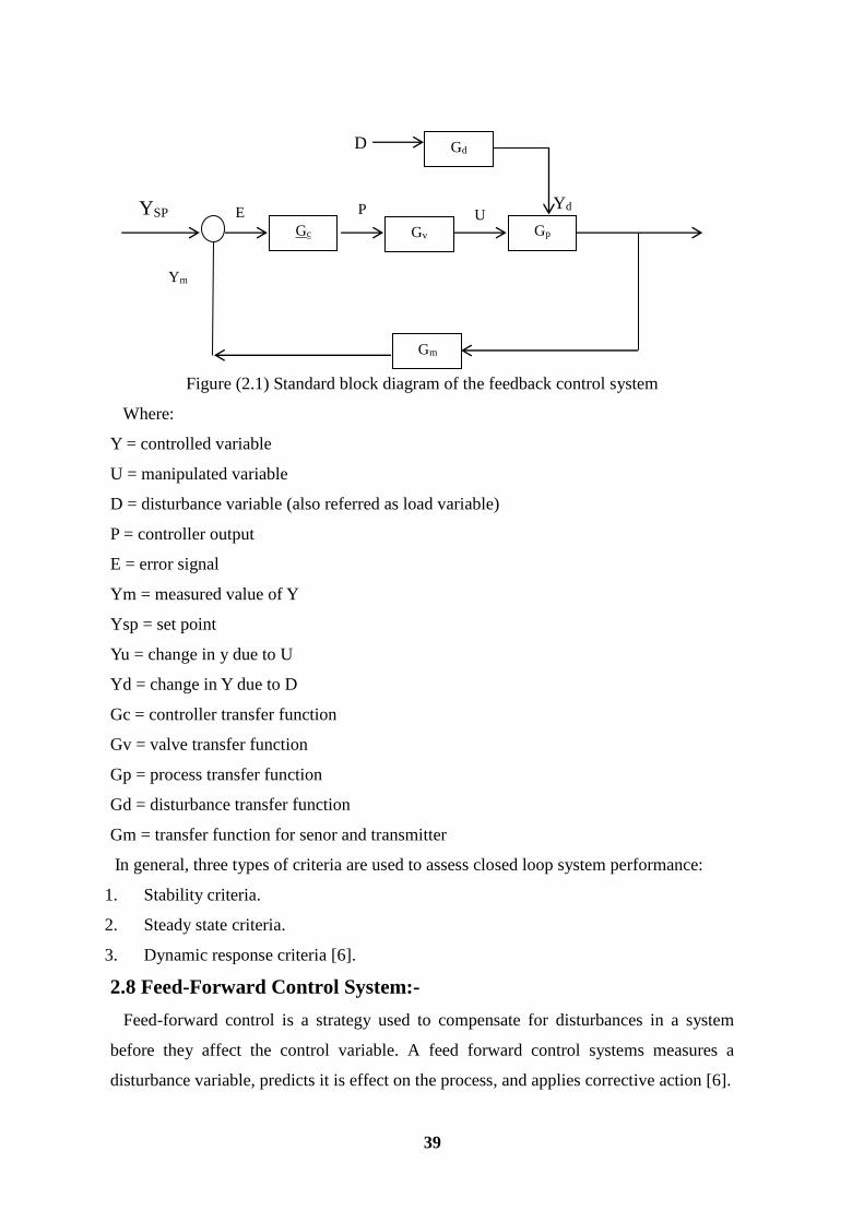
Figure (2.1) Standard block diagram of the feedback control system

Where:

Y = controlled variable

U = manipulated variable

D = disturbance variable (also referred as load variable)

P = controller output

E = error signal

Ym = measured value of Y

Ysp = set point

Yu = change in y due to U

Yd = change in Y due to D

Gc = controller transfer function

Gv = valve transfer function

Gp = process transfer function

Gd = disturbance transfer function

Gm = transfer function for senor and transmitter

In general, three types of criteria are used to assess closed loop system performance:

1. Stability criteria.

2. Steady state criteria.

3. Dynamic response criteria [6].

2.8 Feed-Forward Control System:-

Feed-forward control is a strategy used to compensate for disturbances in a system

before they affect the control variable. A feed forward control systems measures a

disturbance variable, predicts it is effect on the process, and applies corrective action [6].

Gm

Gd

Gp Gv Gc

YSP

Ym

E P U

40

Chapter Three

Materials and Methods

3.1 Introduction:-

This chapter contains brief information about the methods for determining optimum

conditions to manufacturing of caustic soda by Solvay process (graphically and

analytically) and types of materials used in this research such as: sensors or transmitters,

controllers and brief history about MATLAB software. Also the stability tests, tuning

controllers and overall system response.

3.2 Optimum Design and Design Strategy:-

An optimum design is based on the best or most favorable conditions. These optimum

conditions can ultimately be reduced to a consideration of costs or profits. Thus, an

optimum economic design could be based on conditions giving the least cost per unit of

time or the maximum profit per unit of production. When one design variable is changed,

it is often found that some costs increase and others decrease. Under these conditions, the

total cost may go through a minimum at one value of the particular design variable, and

this value would be considered as an optimum [19].

Although cost considerations and economic balances are the basis of most optimum

designs, there are times when factors other than cost can determine the most favorable

conditions. For example, in the operation of a catalytic reactor, an optimum operation

temperature may exist for each reactor size because of equilibrium and reaction-rate

limitations. This particular temperature could be based on the maximum percentage

conversion or on the maximum amount of final product per unit of time. Ultimately cost

variables need to be considered, and the development of an optimum operation design is

usually merely one step in the determination of an optimum economic design [10].

3.3 Evaporators Control:-

The control of most chemical industrial evaporators systems is quite simple. With

hygienic evaporators the control is somewhat more complicated due to the need to start

up, operate, shut down and then clean at quite frequent intervals. As a result

sophisticated control is more likely to be needed on hygienic systems [21].

41

On almost all evaporation systems there are only two basic objectives:

• To concentrate a liquid to a pre-defined solids content.

• To process a pre-defined feed rate of raw material.

Product concentration has been measured using refractive index, density and viscosity

techniques.

Over the last ten years, the use of mass flow meters for density measurement has

become the standard. This type of meter provides an accurate measurement (usually out

to the 4th decimal place) of both flow and density. The density measurement, which is

easily converted to solids content, can then be used to control either product removal rate

from the evaporator, steam flow, or feed flow.

There are two techniques used to control evaporators, and the choice is based on the

design of the evaporator. In applications where liquid recirculation is required to

maintain sufficient wetting in the final stage of the evaporator, the product concentration

control is simple and accurate. The procedure is to set the steam flow rate at the design

value, remove product based on density in the recirculation loop, and adjust the feed

flow to maintain liquid levels in the evaporator. When a higher throughput is required,

then the steam rate is increased. This technique provides excellent control of the product

concentration with conventional analog controllers For heat sensitive products, it is best

to avoid recirculation whenever possible. In the case of once-through-flow in the final

stage, there is no recirculation loop in which to install the transmitter and to delay

discharge of product when not on specification. In this case, the method is to set the feed

flow rate to the desired value and then change the energy input to produce the product

concentration required. The energy input may be the steam rate or the power into the

MVR. This technique does not control product quality particularly accurately, since

response is slow. However it is satisfactory for most purposes and the user can always

apply more sophisticated PLC control when necessary [21].

Almost all evaporators will have to be cleaned at some time. Some chemical

evaporators may run for months between cleaning cycle. Also with non-hygienic duties,

the only requirement is to clean the heat transfer surface sufficiently to restore design

performance. In the case of hygienic evaporators, the concern is not only plant operation,

but also contamination from bacteria. Typically, a hygienic evaporator will be cleaned

42

every day. Dairy evaporators, which are designed and constructed to 3A standards, are

subject to one of the highest cleaning standards. The inspector will expect that the

equipment be cleaned completely with no residue left on any surfaces. The potential

labor costs to start up, shut down and go through a complex cleaning cycle, on a daily

basis, are very high. A fully automatic system is therefore required to perform all these

operations. These functions are ideally performed by a PLC [21].

3.4 Control of Continuous Stirred Tank Reactor System:-

The most unit operation in a chemical process is generally a chemical reactor. A type

of the reactor used very commonly in industrial process is stirred tank operated

continuously .it is referred to the continuous- stirred tank reactor (CSTR) back mix

reactor. The (CSTR) is normally run at steady state and usually operated so as to be quite

well mix. As the result of the latter quality, the (CSTR) is generally modeled as having

no spatial variation in concentration temperature, or reaction rate throughout the vessel.

Since the temperature and concentration are identical ever where within the reaction

vessel, they are the same at the exit point as they are elsewhere in the tank .thus; the

temperature and concentration in the exit stream are modeled as being the same as these

inside the reactor. In the CSTR one or more fluid regent are introduced into a tank

reactor equipped with an impeller the impeller stirs the regent to ensure proper mixing.

Simply dividing the volume of the tank by the average volumetric flow rate through the

tank gives the residence time, or the average amount of time discrete quality of the

regent spends inside the tank. Using chemical kinetics, the reaction expected present

completion can be calculated [7].

3.4.1 Some Important Aspects of CSTR:-

1. At steady state the flow rates in most equal the mass flow rate out, otherwise the

tank will over flow or go empty (transient state).

2. While the reactants are in transient state the module equation must be derived from

differential mass and energy balance.

3. The reactions proceed at the reaction rate associate with the final (output

concentration).

4. The behavior of CSTR is often approximated or module by that of a continuous

ideally (CISTR). All calculations performed with CISTR assume perfect mixing [7].

The system under consideration is an ideal CSTR (second order-no delay time) with

an endothermic reaction for the production of liquid caustic soda from the reaction of

43

calcium hydroxide and sodium carbonate. The dynamic of this process is highly non-

mainly due to the heat generation process. Many reactors are inherently unstable, so

an effective and well- designed control system is necessary in order to assure stable

operation. The instability appears when reversible endothermic reaction is carried out

in a CSTR. These reactions tend to produce a large increment in temperature, forcing

the rupture of safety and reducing the life time of the reactor [9].

3.5 Cascade Control:-

In a cascade control configuration we have one manipulated variable and more

than one measurement [12].

Single input, single output (SISO) systems involves a single loop control that uses

only one measured signal (input). This signal is then compared to a set point of the

control variable (output) before being sent to an actuator (i.e. pump or valve) that

adjusts accordingly to meet the set point. Cascade controls, in contrast, make use of

multiple control loops that involve multiple signals for one manipulated variable.

Utilizing cascade controls can allow a system to be more responsive to disturbances

[23].

The simplest cascade control scheme involves two control loops that use two

measurement signals to control one primary variable. In such a control system, the

output of the primary controller determines the set point for the secondary controller.

The output of the secondary controller is used to adjust the control variable.

Generally, the secondary controller changes quickly while the primary controller

changes slowly. Once cascade control is implemented, disturbances from rapid

changes of the secondary controller will not affect the primary controller.

To illustrate how cascade control works and why it is used, a typical control system

will be analyzed. This control system is one that is used to adjust the amount of steam

used to heat up a fluid stream in a heat exchanger. Then an alternative cascade control

system for the same process will be developed and compared to the typical single loop

control [23].

44

Fig(3,1)General block diagram of cascade systems

3.5.1General Cascade Control Schematic:-

The reactor below needs to be cooled during continuous-feed operation of an

exothermic reaction. The reactor has been equipped with a cooling water jacket with the

water flow rate being controlled by cold water valve. This valve is controlled by two

separate temperature controllers. An “inner-loop” or “slave” (highlighted in orange)

temperature transmitter communicates to the slave controller the measurement of the

temperature of the jacket. The “outer-loop” or “master” (green) temperature controller

uses a master temperature transmitter to measure the temperature of the product within

the reactor. The output from the slave controller is fed into the master controller and used

to adjust the cold water valve accordingly [24].

Fig(3,2) Physical diagram of cascade control systems

https://controls.engin.umich.edu/wiki/index.php/File:Cascade.jpg

https://controls.engin.umich.edu/wiki/index.php/File:Cascade.jpg

https://controls.engin.umich.edu/wiki/index.php/File:CascadeReactorEx.jpg

45

The cascade control loop used to control the reactor temperature can be generalized with the

schematic below. We will use this main diagram to go through the formal derivation of the

equations describing the behavior of the system when there are changes in the loads U1 and

U2 but with no change in the set point, R1(t). The general equations derived below can be

used to model any type of process (first, second, third order differential equations, ect.) and

use any type of control mechanism (proportional-only, PI, PD, or PID control). See wiki

pages titled “first-order differential equations” and “P, I, D, PI, PD, PID Control” for more

details [6].

2.6 Process:-

The material equipment along with the physical or chemical operations which take

place (multiــeffect evaportors, reactors…etc.) [13].

2.6.1 Measuring Instruments or Sensor:-

For example, thermocouples (for temperature), bellow or diaphragms (pressure or

liquid level) [16].

2.6.2 Transmission Lines:-

Used to carry the measurements signal from the sensors to the controller and control

signals from controllers to the final element. These lines can be either pneumatic or

electrical [23].

2.6.3 Final Control Element:-

This is the device that receives the control signal from the controller and implements it

by physically adjusting the value of the manipulated variables. Usually, a control valve

or a variable-speed metering pump [23].

2.6.4 Controller:-

Between the measuring device and final control element comes the controller; it is

considered as the brain of the control loop. The controller performs the decision

operation in the control system. its function is to receive the measured output signal

ym(t) and after comparing it with the set point ysp to produce the actuating signal p(t) in

such a way as to return the output to the desired value ysp .therefore, the input to the

controller is the error E(t) = ysp- ym(t) ,while its output is p(t) [6].

3.7 System Stability and Tuning:-

Mathematical models of a system have been obtained in transfer function form, and

46

then these models can be analyzed to predict how the system will respond in the both the

time and frequency domains [23].

3.7.1 Stability:-

Systems have several properties such as controllability, observability, stability, and

inevitability these characteristics; stability plays the most important role.

Dynamically a stable system is the one for which the output is bounded for all bounded

inputs. A system exhibiting an unbounded response to a bounded input is unstable.

Bounded output is a function of time that always remains between an upper and lower

limit [11].

The most basic practical control problem is the design of a closed-loop system such

that its output follows its input as closely as possible, unstable systems cannot

guarantee such behavior and therefore are not useful in practice.. As soon as stability is

guaranteed, then one seeks to satisfy other design requirements, such as speed of

response, settling time, bandwidth, and steady-state error. The concept of stability has

been studied in depth, and various criteria for testing the stability of a system have

been proposed. Among the most celebrated stability criteria are those of Routh,

Hurwitz, Nyquist and Bode [23].

System stable if the output remains bounded for all bounded inputs. Practically, this

means that the system will not blow up while in operation.

The system can be considering its response to a finite input signal. This means the

analysis of the system dynamics in the actual time-domain. Several methods have been

developed to deduce the system Stability from its characteristic equation. They are

“short-cut” methods for providing information without finding out the actual response of

the system. All these methods are based on the criterion that a sufficient condition for

stability of a control loop is to have a characteristic equation with only negative real

roots and /or complex roots with negative real parts. The methods or technique for

assessment of the stability of a system include the following:

1. Direct substitution method.

2. Routh-Hurwith test.

3. Root-Locus method.

4. Bode method.

47

3.7.2 The Algebraic Methods:-

The algebraic stability criteria are based on the characteristic equation of the system to

be analyzed. They contain algebraic conditions as inequalities between coefficients,

which are only valid if all roots of the polynomial lie in the left- half S-plane [22].

3.7.2.1 The Routh Stability Criterion:-

The Routh stability criterion provides a convenient method of determining control

systems stability. It’s also determines the number of characteristic roots within the left

half, and the number of roots on the S-plane, and the number characteristic roots in the

stable left half, and the number of roots on the imaginary axis. it does not locate the

roots.

The method may also be used to establish limiting values for a variable factor beyond

which the system would become unstable.

Assume the characteristic equation of interest is an N th-order polynomial.

[22].

Table (3.1) Routh Array:

Coefficients Row

1

2

3

4

5

6

48

The Routh array is formed as given below:

Routh array =

Where the a1, b1,… are calculated from the equations

Then the first column of the array of equation is examined. The number of sign changes

of this column is equal to the number of roots of the polynomial that are in the (RHP).

Frist column =

Thus for the system to be stable there can be no sign changes in the first column of the

Routh array [22]

3.7.2.2 Direct Substitution Analysis:-

The closed-loop poles may lie on the imaginary axis at the moment a system becomes

unstable. We can substitute s = iω in the closed-loop characteristic equation to find the

proportional gain that corresponds to this stability limit (which may be called marginal

unstable). The value of this specific proportional gain is called the critical or ultimate

gain. The corresponding frequency is called the crossover or ultimate frequency[31].The

ultimate gain and ultimate period that can be used in Z-N continuous cycling relations

,and the result on ultimate gain is consistent with Routh array analysis and limited to

relatively simple systems. [22]

3.7.2.3 Root Locus Analysis:-

The idea of a root locus plot is simple if we have a computer. We pick one design

parameter, say, the proportional gain, and write a small program to calculate the roots of

the characteristic polynomial for each chosen value of s in 0, 1, 2, 3,...., 100,..., etc. The

49

results (the values of the roots) can be tabulated or better yet, plotted on the complex

plane. Even though the idea of plotting a root locus sounds so simple, it is one of the

most powerful techniques in controller design and analysis when there is no time delay.

Root locus is a graphical representation of the roots of the closed-loop characteristic

polynomial (i.e., the closed-loop poles) as a chosen parameter is varied. Only the roots

are plotted [15].

The values of the parameter are not shown explicitly. The analysis most commonly

uses the proportional gain as the parameter. The value of the proportional gain is varied

from 0 to infinity, or in practice, just "large enough."

Consider the characteristic equation:

........................................................................ (3.1)

Equation can be written as

………………………………………………………………..… (3.2)

Where num is the numerator of the polynomial and den is the denominator polynomial,

and K is the gain (K > 0). The vector K contains all the gain values for which the closed

loop poles are to be computed.

The root locus is plotted by using the MATLAB command

rlocus (num, den)…………………………………………………...…………..……..(3.3)

The gain vector K is supplied by the user.

The matrix r and gain vector K are obtained by the following MATLAB commands:

[r, k] = rlocus (num, den)

[r, k] = rlocus (num, den, k)

[r, k] = rlocus (A, B, C, D)

[r, k] = rlocus (A, B, C, D, K)

[r, k] = rlocus (sys)

The following MATLAB commands are used for plotting the root loci with mark ‘0’ or

‘x’:

r = rlocus (num, den)…………………………………………………………...........(3.4)

Plot (r, ‘0’) or plot (r, ‘x’).

50

Figure(3.1) Root Locus

A root locus plot is a figure that shows how the roots of the closed loop characteristic

equation vary as the gain of the feedback controller changes from zero to infinity. The

abscissa is the real part of the closed loop root; the ordinate is the imaginary part. Since

we are plotting closed loop roots, the time constants and damping coefficients that we

pick off these root locus plots are all closed loop time constants and closed loop damping

coefficients [15].

Root locus is the plots, in complex plane, of the roots of the OLTF.

They are very useful to determine the stability of closed loop system as the gain

changes.

The value of the frequency which take from the Root locus plot used to calculate the

limit gain and ultimate period.

One absolute method of determining whether complex or reel roots lie in the right

hand plane is by use of routh’s criterion the method entails systematically generating a

column of numbers that are then analyzed for sign variations. The first step is to

arrange the denominator of the transfer function into descending powers of s. All terms

including those that are zero should be included.[11]

3.7.2.4 Bode Plots:-

Bode plots require two curves to be plotted instead of one. This increase in the number

of plots is well worth the trouble because complex transfer functions can be handled

much more easily using Bode plots. The two curves show how magnitude ratio and

phase angle (argument) vary with frequency.

51

Bode diagrams are rectangular plots. Bode diagram are also known as logarithmic plot

and consist of two graphs: the first one is a plot of the logarithmic of the magnitude of a

sinusoidal transfer function; the second one is a plot of the phase angle. Both these

graphs are plotted against the frequency on a logarithmic scale. The MATLAB command

“bode” obtains the magnitudes and phase angles of the frequency response of continuous

time, linear, time invariant systems.

The MATLAB Bode commands commonly used are:

Bode (num, den)

Bode (num, den, w)

Bode (A, B, C, D)

Figure (3.2) Bode plot

The value of the frequency which take from the Bode plot used to calculate the limit

gain and ultimate period [11].

3.8 Tuning Controllers:-

Tuning means setting the adjustable parameters (proportional band/gain, integral

gain/reset, derivative gain/rate) of a controller to give best performance. For the PID

controller [23].

52

3.8.1 Ziegler – Nichols Tuning Technique:-

The Ziegler-Nichols (ZN) controller settings (.I. G. Ziegler and N. B. Nichols, Trans.

ASME 64: 759, 1942) are pseudo-standards in the control field. They are easy to find

and to use and give reasonable performance on some loops. The ZN method consists of

first finding the ultimate gain Kc the value of gain at which the loop is at the limit of

stability with a proportional-only feedback controller. The period of the resulting

oscillation is called the ultimate period, Pu (minutes per cycle). The ZN settings are then

calculated from Ku and Pu by the formulas [23].

Given in Table for the three types of controllers. Notice that a lower gain is used when

integration is included in the controller (PI) and that the addition of derivative permits a

higher gain and faster reset.

The Z-N method is based on frequency response analysis. Unlike the process reaction

curve method which uses data from the open- loop response of system. The Z-N tuning

technique is a closed –loop procedure [18].

Bring the system to the desired operation level (design conditions).

Using P- control only ,and with the feedback- loop closed , introduce a sinusoidal set pt.

changing with low amplitude and varying frequency until the system oscillates

continuously , the frequency of continuous oscillation is the crossover frequency ,ωco. let

M = amplitude ratio of the system's response at the crossover frequency.

Ultimate gain = ku = 1/M

Ultimate period

Table (3.1): Ziegler-Nichols adjustable controller parameters for additives loop for Routh

_Hurwitz,[23]

Type of controller Kc

P 0.5Ku - -

PI 0.45Ku

-

PID 0.6Ku

53

3.9 Time Response:-

The time response represents how the state of dynamic system changes in time when

subjected to particular input. Since the models has been derived consist of differential

equations, some integration must be performed in order to determine the time response

of the system. Fortunately, MATLAB provides many useful resources for calculating

time responses for many types of inputs.

MATLAB provides tools for automatically choosing optimal PID gains.

The tuning algorithm directly using “pidtune” or through using “pidtool”[23].

3.10 Sensors and Measuring Devices:-

The successful operation of any feedback control system depends in a very critical

manner. There are different commercial measuring devices which differ either in the

basic measuring principle or their construction characteristics [8].

Table(3.3) list typical measuring devices encountered in various applications of

process control [8]:

Measuring process variable Measuring device Comments

Temperature Thermocouple Resistance

thermometer Radiation pyrometer

Oscillating quartz crystal

Most comment for relatively

low temperature

Used for high temperature

Pressure Manometers Bourdon – tube

elements Diaphragm elements

Strain pages

Piezoresistivity elements

Piezoelectric elements

With floats or displaces

Used to convert pressure to

electrical signal

Flow Orifice plate Venture flow

Nozzle flow Turbine flow meters

Ultrasound

Hot-wire anemometry

Measuring pressure drop

across flow constriction.

For high precision

54

Liquid level Float-actuated devices Displacer

devices

Liquid head pressure devices

Conductivity measurement

Sonicresponse

Couple with various types of

indicators and signal

converters

Good for system with two

phases

Composition Infrared analyzers

Ultraviolet analyzers

Visible –radiation analyzers

Turbidimetry analyzers

Para magnetism analyzers

Nephelomerty analyzers

Potentiometer Conductimetry

Osillometric

pH meters polar graphic analyzers

coulometer

spectrometers(xray,electon,ion

,Mossabauser,raman)

Differential thermal analyzers

Long times required for

analysis.

Convenient for one or two

chemicals.

Not very Convenient for

process control Expensive for

low-cost control loops

3.11 MATLAB Software:-

The name MATLAB is an acronym for matrix laboratory. MATLAB software has

become popular in engineering fields as result it has been considered as the world

standard for performing simulation and analyzing linear and nonlinear dynamic systems.

MATLAB was developed primarily by Cleve Moler in1970’s. It combines nicely

calculations and graphic plotting. MATLAB also integrates programming, visualization

and computation in an easy to use environment. MATLAB is a high level technical

computing environment suitable for solving scientific and engineering problems.

MATLAB features a family of applications-specific solutions called toolboxes.

Toolboxes are comprehensive collection of MATLAB functions (M-file) that extend the

MATLAB environment to solve particular classes of problems. Areas in which toolboxes

are available including signal processing, control systems, neural networks, fuzzy logic

wavelets, simulation and many others. The control system toolboxes are a collection of

algorithms, written mostly as M-file, that implement common control system design,

analysis and modeling techniques [12].

55

Chapter Four

Results and Discussion

4.1 Control Strategy:-

One control strategy was developed as shown in Figure (4.5) and Figure (4.19).

1. A single input/single output (SISO) system was used to control the level of the

solution inside the reactor.

2. A cascade control system was used to control the reactor temperature.

3. A single input/single output (SISO) system was used to control composition of

caustic soda and the temperature in the third evaporator.

4. A single input/single output (SISO) system was used to control of the

temperature in the third evaporator.

4.1.1 Dissolving Process:

Figure (4.1) Dissolving of Sodium Carbonate (Soda Ash)

4.1.2 Causticization or Precipitation Reaction(CSTR):-

Calcium Hydroxide Sodium Carbonate Solution

Caustic Soda Solution +

Calcium Carbonate

Cold Water in Hot Water Out

Weak liquor

Sodium Carbonate (Soda Ash)

Sodium Carbonate Solution

Dissolving Tank

Fig(4.2) Causticization or Precipitation Reaction

56

4.1.3 Separation Process:-

Figure (4.3) Separation of Caustic Soda from Calcium Carbonate

4.1.4 Evaporation Process:-

Figure (4.4) Multi-Effect Evaporators.

Caustic Soda

Solution 10.5%

Caustic Soda Solution

+ Calcium Carbonate

Calcium Carbonate

1

2

3

Vapor

Caustic Soda 10.5%

Caustic Soda 50%

Steam

57

4.1.5 Control of Causticizer :-

Reactor CSTR

Fig (4.5) Physical diagram for Temperature and level control loop

Stability:Tank Reactor System Tuning and Continuous Stirred 4.1.6

4.1.7 Level Control Loop Transfer Function:-

Figure (4.6) General block diagram of the conventional CSTR feedback control

4.1.8 Over all Transfer Function of Loop (1):-

…………………………………………(4.1)………………….………………C =KC G

GM(S)

_

Ysp + Y(S)

GC GV GP

SP

SP

SP

Caustic soda & calcium

carbonate

Calcium Hydroxide Sodium carbonate solution

Cold water in

Loop2

TT Loop1

1

Backg

round

of

contro

l

syste

m

TC

TT

TC

LC

LT

Hot water out

58

………………………………….(4.2)…………………..= 1/(0.2S+1) …………… VG

……………………………………..(4.3)……...………+1) …………S+2= .4/(.5SP G

……………………….(4.4)…………………………….= 1 ……………………… MG

Figure (4.7) Conventional loop one feedback control

4.1.9 Application of Routh-Hurwitz array:-

…………..(4.5)……………………..…………………………OLTF=

The characteristic equation:-

1+ OLTF=0

………………………………………..(4.6)...……………………… 1+

…………………………………..(4.7)…………….= 0. CKS+1)+0.4+2S+1)(0.5S(0.2

The chr.eq:

……………………………..(4.8).…………………= 0 C+1.2S+1+ 0.4K 2+ 0.7S3 0.1S

Using Routh array:

Number of rows=4

KC 1/(0.2S+1)

_

+ Ysp Y(S) 0.4/(0.5S2+S+

1)

1

59

0.1 1.2 3S

C0.7 1+0.4K 2 S

2b1 b 1S

2c

1c 0S

0.1 1.23 S

C.7 1+0.4K 2 S

.04Kc)/.7 0-(.74 1 S

1+0.4Kc 00 S

..(4.9).………………………………………………………)/0.7 = 0 ……C0.04K-(.74

………………..(4.10)……..………………………………………= 0.74 …… C0.04K

= 18.5 …………………………………………………………………..(4.11) CKu=K

This system is stable.

4.1.10 Using Direct Substitution Method:-

Obtain the frequency:

The Characteristic equation:-

= 0 C1.2S+1+ 0.4K+ 2+ 0.7S3 0.1S

1):-= 2S= iω , (iSet

……………..(4.12)…...……= 0 …………… C+ 1.2 iω + 1 + 0.4K 20.7 ω – 30.1 iω -

60

Taking imaginary part of this loop=0

…………………..(4.13)= 0 …………………………………………+1.2 iω 30.1 iω -

= 1.2 20.1 iω

ω = 3.46 red/s

Taking the real part of loop =0

…………………………..(4.14)= 0 ………………………………... C0.4K+1+ 2ω0.7-

= 0 C+1 +0.4K 20.7(3.46)-

= Ku= 18.45 CK

co=2π/ωuP

=2π / 3.46 = 1.81 sec uP

4.1.11 Apply the Root – Locus Using MATLAB:-

Plot Root – Locus:-

……………..(4.15)……………………………….……...OLTF =

MATLAB former:-

>>num=[0.4];

>> den=conv([0.2 1],[0.5 1 1]);

>> rlocus(num,den)

61

-20 -15 -10 -5 0 5-15

-10

-5

0

5

10

15

System: sys

Gain: 17.8

Pole: -0.0186 + 3.42i

Damping: 0.00546

Overshoot (%): 98.3

Frequency (rad/sec): 3.42

Root Locus

Real Axis

Imagin

ary

Axis

Fig (4.8) Root Locus of loop (1)

= 17.8 uK

ω = 3.42 red/sec

=2π/3.42 = 1.84secu P

4.1.12 System Stability Using Bode Method:-

).uand ultimate gain (K )u(P Determination of ultimate period

………………………………………………..(4.16)………… OLTF=

MATLAB former:-

>>num=[0.4];

>> den=conv([0.2 1],[0.5 1 1]);

>> sys=tf(num,den);

>> bode(sys),grid

62

Bode Diagram

Frequency (rad/sec)

10-2

10-1

100

101

102

103

-270

-180

-90

0

System: sys


Phase (deg): -179

Phase (

deg)

-200

-150

-100

-50

0

System: sys


Magnitude (dB): -25.1

Magnitu

de (

dB

)

Figure (4.9) Bode diagram for loop(1)

ω = 3.41red/sec

magnitude(dB)= -25.1

20logAR=dB

20logAR=-25.1

AR = 0.055

= 1/AR uK

= 1/0.055 =17.99 uK

sec=2π/3.41= 1.84 uP

4.1.13 Determination of adjustable parameters:-

sec=1.825) / 3u,3 + P u,2+ P u,1) = ( Pu,avThe average (P

) / 4 = 18.18u4K +u,3+ K u,2+ K u,1) = ( Ku,avThe average (K

63

Table (4.1) Z-N tuning parameters of loop 1

cK Type of controller

_ _ 9.09 P

_ 1.52 8.18 PI

0.228 0.9125 10.9 PID


………………………………………………..(4.17)) ………………L /(1 + π F= π SY

…………………………..(4.18) ………………………………… = Fπ

…………………………..(4.19)….…. = 1 + L1 + π

……………………………..(4.20) …………………………= SY

= 9.09C ting KPut

……………………………..(4.21) ……..……………..………= SY

MATLAB former:-

>>num=[3.636];

>> den=[0.1 0.7 1.2 4.636];

>> step(num,den),grid

64

0 2 4 6 8 10 12 140

0.2

0.4

0.6

0.8

1

1.2

1.4

System: sys

Time (sec): 3.7

Amplitude: 0.981

System: sys

Time (sec): 1.31

Amplitude: 1.24

System: sys

Time (sec): 0.791

Amplitude: 0.781

System: sys

Time (sec): 12.5

Amplitude: 0.785

Step Response

Time (sec)

Am

plit

ude

Figure (4.10) Step Response of loop 1 for P Controller.

Table (4.2) Simulation Parameter of Loop 1 for P Controller:-

Time(sec) Items

0.798 Rise time

1.31 Beak time

12.5 Response time

1.24 Over shoot

=0.79 = Decay Ratio

65


>>num=[4.97 3.272];

>> den=[0.152 1.064 1.824 6.49 3.272];


0 5 10 15 20 25 30 350

0.2

0.4

0.6

0.8

1

1.2

1.4

1.6

System: sys

Time (sec): 0.889

Amplitude: 1.01

System: sys

Time (sec): 1.38

Amplitude: 1.57

System: sys

Time (sec): 4.03

Amplitude: 1.39

System: sys

Time (sec): 24.8

Amplitude: 1

Step Response

Time (sec)

Am

plitu

de

Figure (4.11) Step Response of Loop 1 for PI Controller.

Table (4.3) Simulation Parameter of Loop 1 for PI Controller:-:

Time(sec) Items

0.889 Rise time

1.38 Beak time

24.8 Response time

1.39 Over shoot

4.1.16 Response of the System for PID Controller :-

>>num=([.907 3.9785 4.36]);

>> den=[.01925 .6385 2.002 4.891 4.16];


66

0 1 2 3 4 5 60

0.2

0.4

0.6

0.8

1

1.2

1.4System: sys

Time (sec): 1.2

Amplitude: 1.25

System: sys

Time (sec): 0.73

Amplitude: 1.05

System: sys

Time (sec): 3.86

Amplitude: 1.06

System: sys

Time (sec): 4.29

Amplitude: 1.06

Step Response

Time (sec)

Am

plit

ude

Figure (4.12) Step Response of Loop 1 for PID Controller.

Table (4.4) Simulation Parameter of Loop 1 for PID Controller:-:

Time(sec) Items

0.73 Rise time

1.2 Beak time

4.29 Response time

1.25 Over shoot

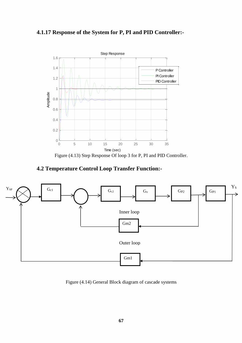
67


0 5 10 15 20 25 30 350

0.2

0.4

0.6

0.8

1

1.2

1.4

1.6

Step Response

Time (sec)

Am

plit

ude

P Controller

PI Controller

PID Controller


-unction:4.2 Temperature Control Loop Transfer F

Figure (4.14) General Block diagram of cascade systems

Inner loop

Outer loop

YSP YS

Gc1 Gc2

Gv GP1 GP2

Gm2

Gm1

68

4.2.1 Over all transfer function of loop (2):-

)……………..(4.22.…………….…………..………..………………………C2=KC2 G

……………..(4.23)…….…(0.05S+1) ………………..…………………..……= 1/ VG

…………………..(4.24)………………1/(0.5S+1)(s+1) ……………..………… =P2 G

…………………………..…..(4.25)……………………) …………= 0.2/(0.2S+1 M2G

……….…..(4.26).………………………..……………………………………1C=KC1G

……………………………...(4.27)+1) ……………..……………………= 1.5/(2sP1 G

.1S+1) ……………..……………..………………………..………..(4.28)= 0.1/(0 M1G

4.2.2 Block Diagram for loop 2

,

Figure (4.15) Conventional Inner Loop of Cascade Systems

Inner loop

Outer loop

Kc1 Kc2 1/(.05s+1) 1/(.5S+1)(S+1) 1.5/(2S+1)

.2/(.2s+1)

.1/(.1s+1)

YSP

YS

69

4.3 Inner loop :

4.3.1 Apply the Root – Locus diagram using MATLAB:-

29)………….(4...............…………… OLTF =

MATLAB Former:

>>num=[.2 1];

>> a=conv([.05 1],[.5 1]);

>> b=conv([1 1],[.2 1]);

>> den=conv(a,b);

>> sys=tf(num,den)

Transfer function:

1+ 1.75 S+ 2885 S+ 0. 3S+ 0.14 4S0.005

>> rlocus(sys)

70

Root Locus

Real Axis

Imagin

ary

Axis

-70 -60 -50 -40 -30 -20 -10 0 10 20 30-50

-40

-30

-20

-10

0

10

20

30

40

50

System: sys

Gain: 35.1

Pole: 0.0316 + 7.91i

Damping: -0.00399

Overshoot (%): 101


Fig (4.16) Root Locus of Inner loop

4.4 Outer Loop:-

Figure(4.17): General reduced block diagram of the cascade system

Gm1

Gc1

Gp1 YSP

YS

71

4.4.1 Block Diagram for Outer Loop:-

Figure (4.18) Conventional outer loop of the cascade system

4.4.2 Apply the Root – Locus and Bode Diagram Using MATLAB:-

Plot Root – Locus :-

…..(4.31)....…………...OLTF =

MATLAB former:

>>num=[1.35];

>> den=[0.001 0.0385 0.476 2.3485 5.12 7.63 2.8];

>> rlocus(num,den)

YSP YS

Kc1

1.5/(2s+1)

.1/(.1s+1)

72

Root Locus

Real Axis

Imagin

ary

Axis

-80 -60 -40 -20 0 20 40 60-80

-60

-40

-20

0

20

40

60

80

System: sys

Gain: 7.56

Pole: 0.0526 + 1.88i

Damping: -0.0279

Overshoot (%): 109


Fig (4.19) Root Locus of Outer loop

=7.56uK

ω =1.88

= 3.34uP

4.4.3 System Stability Using Bode method:-

).uKd ultimate gain () anu(P Determination of ultimate period

………..………..(4.32)…OLTF=

MATLAB former:-

>>num=[1.35];

>> den=[0.001 0.0385 0.476 2.3485 5.12 7.63 2.8];

>> bode(num,den),grid

73

Bode Diagram

Frequency (rad/sec)

10-2

10-1

100

101

102

103

-540

-360

-180

0

System: sys


Phase (deg): -180

Phase (

deg)

-300

-250

-200

-150

-100

-50

0

System: sys



Magnitu

de (

dB

)

Figure (4.20) Bode Diagram for Outer Loop

20 log AR = dB

20 log AR = -16.7

AR = 0.14

= 7.14

ω =1.86 red/sec

=3.37 secuP

4.4.4 Application of Routh-Hurwitz Array:-

……..………..(4.33) OLTF=

74


1+ OLTF=0

..(4.34)…..= 0…. OLTF=1+


..(4.35)=0 ... C1+7.63S+2.8 1.35K 25.12S +38 S+2.3454 +0.476 S 5+ 0.0385 S 60.001S

Using Routh array:

Number of rows=7

2.8+1.35Kc1 0.001 0.476 5.12 6S

0 7.63 0.0385 2.3458 5 S

0 4.921 2.8+1.35 Kc1 0.415 4S

0 0 0.125 Kc1 –7.63 1.889 S

0 0 3.24+0.027 Kc1 2.8+0.1.35 Kc1 2 S

0 0 0 X 1S

0 0 0 2.8+0.1.35 Kc1 0S

X=(3.24+0.0275 Kc1)(7.63–0.125 Kc1) – (1.889*(2.8+1.35 Kc1)) / (3.24+0.0275

Kc1)…… ………………………………………………………………….……..(4.36)

(3.24+0.0275 Kc1)(7.63–0.125 Kc1) – (1.889*(2.8+1.35 Kc1)) / (3.24+0.0275 Kc1)

=0 ………..……………………………………………………………..………..(4.37)

24.75 – 0.40 Kc1 + 0.20 Kc1 – 0.0034 Kc12 –5.289 – 2.55Kc1 =0 ….………….(4.38)

19.47 – 2.74595 Kc1 – 0.0034375 Kc12 =0 …………………..…..……………..(4.39)

roots([-0.0034375 -2.74595 19.47])

ans =7.0286

75

= 7.0286 C=KuK


4.4.5 Using direct substitution method:-



.(4.40)= 0…. C1+7.63S+2.8 1.35K 25.12S +3+2.3458 S4 +0.476 S 5+ 0.0385 S 60.001S

1):-= 2Set S= iω , (i

+7.63 2 5.12 ω – 32.3485 iω – 4 +.476 ω 5 .0385 iω – 6.001 ω –

iω+(2.8+1.35Kc1)=0……………………………………………………………..(4.41)


……….………..(4.42)……………..…………+7.63 iω = 0 32.3485 iω –5 0.0385 iω -

MATLAB From:

>> roots([-0.0385 0 -2.348 0 7.65])

ans = 1.7608

ω = 1.7608 red/s


.………..(4.43)+(2.8+1.35Kc1) = 0…………………2 5.12 ω – 4 +.476 ω 6.001 ω –

= 6.8 uK

co=2π/ωuP

=2π / 1.7608 = 3.5 sec uP

4.4.6 Determination of adjustable parameters:-

) / 3=3.6u,3 + P u,2+ P u,1) = ( Pu,avThe average (P

) / 4 = 7.2u4+ Ku,3+ K u,2+ K u,1) = ( Ku,avThe average (K

76


Kc Type of controller

_ _ 3.6 P

_ 3 3.24 PI

0.45 1.8 4.32 PID


)L /(1 + π F= π SY

……………………………………………....(4.44)= Fπ

= 1 +Lπ1 +

….………..(4.45).................………=

).(4.46………………… = SY

= 3.6C Putting K

…..………..(4.47) = SY

MATLAB former:-

>> num=[0.486 4.86];

>> den=[0.001 0.0385 0.476 2.3485 5.12 7.63 7.66];


77

0 2 4 6 8 10 12 14 160

0.1

0.2

0.3

0.4

0.5

0.6

0.7

0.8

0.9

System: sys

Time (sec): 2.5

Amplitude: 0.88

System: sys

Time (sec): 1.71

Amplitude: 0.633

System: sys

Time (sec): 6.06

Amplitude: 0.71 System: sys

Time (sec): 12.6

Amplitude: 0.634

Step Response

Time (sec)

Am

plit

ude

Figure (4.21) Step Response Of loop 2

Table (4.6) Simulation Parameter of Loop 2 for P Controller:-

Time(sec) Items

1.71 Rise time

2.5 Beak time

12.6 Response time

0.88 Over shoot

= 0.80 Decay Ratio =

78

4.5 Multi- Effect Evaporators System Tuning and Stability:-

Fig (4.22) Physical diagram for Temperature and composition control loop

4.5.1Over all transfer function of loop (3):-

…………(4.48)……………………………………………...…………………C =KC G

(4.49)………………………………………= 1/(0.05S+1)………………………… VG

……………………………………………………………(4.50).= 1.5/(2S+1) ……P G

…………………………………………………(4.51)= 0.2/(0.03S+1) ………….. MG

LOOP 3

Steam

Vapor

S.P

Loop4

Caustic

soda50%

Caustic

soda 10.5%

S.P

1

2

3

CT TT

CC CT

79

4.5.2 Temperature control loop transfer function:-

) conventional loop three feedback controlFigure (4.23

4.5.3 Application of Routh-Hurwitz Array:-

……………(4.52)………………………..………= OLTF


1+ OLTF=0

………(4.53)……………………………….………=0

1+

(0.05s+1)(2s+1)(0.03s+1)+Kc=0………………………………………………(4.54)

The chr.eq:

……………………………………(4.55)= 0… C+2.08S+1+ 0.3K 2+ 0.1615S 30.003S

Using Routh array

Number of rows=4

_

+ Ysp Y(S)

KC 1/(0.05S+1) 1.5/(2S+1)

0.2/(0.03S+1)

80

0.003 2.08 3S

C0.1615 1+0.3K 2 S

2b1 b 1S

2c 1c

0S

0.003 2.08 3 S

C0.1615 1+0.3K2 S

0 )/0.1615C0.0009K-(.331 S

0 C1+0.3K 0 S

…………………………(4.56)/0.1615 = 0 ……………………………)C0.0009K-(.33

= 0.33 C0.0009K

….……………………………………(4.57)= 369.9……………………… CKu=K





……………………(4.58)= 0………………… C+2.08S+1+ 0.3K 2+ 0.1615S 30.003S

1):-= 2Set S= iω , (i

……………(4.59)= 0……………… C+ 2.08 iω + 1 + 0.3K 20.1615 ω – 30.003 iω -


81

60)……………………………………………(4.+2.08 iω = 0………… 30.003 iω -

= 2.08 20.003 iω

ω = 26.33red/s


…………………………(4.61)= 0…………………………… C+1+0.3K 20.1615w-

= 0C+1+ 0.3K 20.1615(26.33)-

= Ku = 369.87 CK

co=2π/ωuP

=2π / 26.33 = 0.238sec uP


..............................................................(4.62) OLTF =

MATLAB Former:-

>>num=[0.3];

>> a=conv([2 1],[.05 1]);

>> den=conv(a,[0.03 1]);

>> rlocus(num,den)

82

Root Locus

Real Axis

Imag

inar

y A

xis

-120 -100 -80 -60 -40 -20 0 20 40-100

-80

-60

-40

-20

0

20

40

60

80

100

System: sys

Gain: 369

Pole: 0.012 + 26.3i

Damping: -0.000457

Overshoot (%): 100


Fig(4.24):Root-locus method for loop 3

Ku = 369

ω = 26.3 red/sec

=2π/26.3 = 0.238 secu P

4.5.6 System Stability Using Bode Method:-

).uK) and ultimate gain (uDetermination of ultimate period(P

)……(4.63……………………………………OLTF=

MATLAB former:-

>>num=[0.3];

>> b=conv([2 1],[0.05 1]);

>> den=conv(b,[.03 1]);

>> sys=tf(num,den);

>> bode(sys),grid

83

Bode Diagram

Frequency (rad/sec)

-150

-100

-50

0System: sys



Magnitu

de (

dB

)

10-2

10-1

100

101

102

103

-270

-180

-90

0

System: sys


Phase (deg): -180

Phase (

deg)

Figure (4.25) Bode diagram for loop 3

ω = 26.3 red/sec

magnitude (dB)= -51.4

20logAR=dB

20logAR=-51.4

AR = 0.0027

Ku = 1/AR

= 1/0.0027 =370.3 uK

=2π/26.3= 0.238 uP

4.5.7 Determination of Adjustable Parameters:-

Z-N stability of the tuning system , Routh ,Root – locus , direct substutation and

Bode methods :

84

) / 3 =0.238u,3+ P u,2+ P u,1) = ( Pu,avThe average (P

) / 4 = 369.77u,4K u,3++ K u,2+ K u,1) = ( Ku,avThe average (K


Kc Type of controller

_ _ 184.885 P

_ 0.198 166.39 PI

0.0298 0.119 221.8 PID

4.5.8 Response of the System for P Controller :-

)L /(1 + π F= π SY

…………………………………………………………(4.64) = Fπ

= 1 +L1 + π

4.65)(………………………………………………….=

…………………………………(4.66)………=S Y

= 184.885C Putting K

……………………(4.67)………………………= SY

……(4.68) ………………………………………… Ys=

MATLAB former:-

>>num=[8.31 277.3];

>> den=[0.003 0.1615 2.08 56.5];

85


0 0.2 0.4 0.6 0.8 1 1.2 1.4 1.6 1.80

1

2

3

4

5

6

7

8

9

System: sys

Time (sec): 1.69

Amplitude: 4.91

System: sys

Time (sec): 0.474

Amplitude: 6.1

System: sys

Time (sec): 0.0797

Amplitude: 4.9

System: sys

Time (sec): 0.157

Amplitude: 8.11

Step Response

Time (sec)

Am

plit

ude

Figure (4.26) Step Response Of loop 3 for P Controller.

Table (4.8): simulation parameter of loop 3 for P Controller:-

Time(sec) Items

0.0797 Rise time

0.157 Beak time

1.69 Response time

8.11 Over shoot

=0.75 = Decay Ratio =

86

4.5.9 Response of the System for PI Controller :-

>>num=conv([47.418 249.585],[.3 1]);

>> den=[.000594 .0319 0.4059 10.84 49.917];


0 1 2 3 4 5 6-20

-15

-10

-5

0

5

10

15

20

25

30

System: sys

Time (sec): 0.122

Amplitude: 28.4

System: sys

Time (sec): 0.441

Amplitude: 22

System: sys

Time (sec): 0.0235

Amplitude: 4.93

System: sys

Time (sec): 5.29

Amplitude: 5.03

Step Response

Time (sec)

Am

plit

ude

Figure (4.26) Step Response Of loop 3 for PI Controller.

Table (4.9): simulation parameter of loop 3 for PI Controller:-

Time(sec) Items

0.0235 Rise time

0.122 Beak time

5.29 Response time

28.4 Over shoot

=0.75 = Decay Ratio =

87


>>num=conv([1.1798 39.59 332.7],[.3 1]);

>> den=[.000357 .0192 0.483 8.037 66.54];


0 0.2 0.4 0.6 0.8 1 1.2-10

-5

0

5

10

15

20

25

30

System: sys

Time (sec): 0.00578

Amplitude: 4.97

System: sys

Time (sec): 0.063

Amplitude: 29.8

System: sys

Time (sec): 0.383

Amplitude: 9.19System: sys

Time (sec): 0.906

Amplitude: 4.8

Step Response

Time (sec)

Am

plit

ude

Figure (4.27) Step Response Of loop 3 for PIDController

Table (4.10): simulation parameter of loop 3

Time(sec) Items

0.00578 Rise time

0.063 Beak time

0.906 Response time

29.8 Over shoot

88


0 1 2 3 4 5 6-20

-15

-10

-5

0

5

10

15

20

25

30

Step Response

Time (sec)

Am

plitu

de

P controller

PI controller

PID controller

Figure (4.28) Step Response Of loop 3 for P, PI and PID Controller

4.6 Over all transfer function of loop (4):-

…(4.69)………………………………………………………………………C =KC G

)…………………….(4.70……………….= 1/(0.2S+1) ………………………… VG

………………..(4.71)………………..= 1/(0.8S+1) ………………………………P G

…………………….(4.72)………………..= 1/(0.1S+1) ………………………… MG

4.6.1 Composition control loop transfer function:-

feedback control onventional loop 4) CFigure (4.30

Ysp Y(S)

KC 1/(0.2S+1) 1/(0.8S+1)

1/(0.1S+1)

_

+

89

4.6.2 Application of Routh-Hurwitz array:-

……………………………………………(4.73).OLTF=


1+ OLTF=0

……………………(4.74)= 0………………………. 1+

………………………(4.75)= 0…………………….. CS+1)(0.1S+1) + K(0.2S+1)(0.8

The chr.eq:

…………………………(4.76)0……………… =) C+ 11 S + (10+10K2+ 2.6 S 30.16 S

Using Routh array:

Number of rows=4

11 0.16 3 S

C10+10K 2.6 2 S

0 1.6Kc)/2.6 -(27 1 S

0 C 10+10K 0S

)/2.6 = 0C1.6K-(27

= 27 C1.6K

= 16.875 C= 16.875 Ku=K CK


90




…………………(4.77)………)= 0……………… C + 11 S + (10+10K2+ 2.6 S 30.16 S

1):-= 2Set S= iω , (i

………………(4.78)) = 0…………………C+ 11 iω + (10 + 10K 22.6 ω - 30.16 iω -


…………………………………….………………………(4.1)+11 iω = 0 30.16 iω -

= 11 20.16 ω

ω = 8.29 red/s


……………………………(4.79)) = 0………………………… C+ (10 + 10K 22.6 ω -

) = 0 C+(10 + 10K 22.6(8.29)-

= 16.875 CK

co=2π/ωuP

=2π / 8.29 = 0.757 sec uP


………………….…………………(4.80) OLTF=

MATLAB former:-

>> num=[1];

>> a=conv([0.2 1],[0.8 1]);

>> den=conv(a,[0.1 1]);

91

>> rlocus(num,den)

Root Locus

Real Axis

Imag

inar

y A

xis

-30 -25 -20 -15 -10 -5 0 5 10-20

-15

-10

-5

0

5

10

15

20System: sys

Gain: 16.9

Pole: 0.0132 + 8.29i

Damping: -0.00159

Overshoot (%): 100


Fig(4.31):Root-locus method for loop 4

Ku = 16.9

ω = 8.29 red/sec

=2π/8.26 = 0.76secu P

4.6.5 System stability using Bode method:-

).uK) and ultimate gain (u(P ultimate period Determination of

………………………………………(4.81)……OLTF=

MATLAB former:-

>> num=[1];

>> a=conv([0.2 1],[0.8 1]);

>> den=conv(a,[0.1 1]);

>> bode(num,den),grid

92

Bode Diagram

Frequency (rad/sec)

-150

-100

-50

0

System: sys



Magnitu

de (

dB

)

10-2

10-1

100

101

102

103

-270

-180

-90

0

System: sys


Phase (deg): -180

Phase (

deg)

Figure (4.32) Bode diagram for loop 4

ω = 8.28red/sec

magnitude (dB)= -24.6

20logAR=dB

20logAR=-24.6

AR = 0.0588

Ku = 1/AR

= 1/0.0588= 16.9 uK

=2π/8.28 = 0.75 uP

4.6.6 Determination of Adjustable Parameters:-

Z-N stability of the tuning system , Routh ,Root – locus and Bode methods : -

sec) / 3 =0.755u,3 + P u,2+ P u,1) = ( Pu,avThe average (P

93

) / 4 = 16.88u,4+ Ku,3+ K u,2+ K u,1) = ( Ku,avThe average (K


cK Type of controller

_ _ 8.44 P

_ 0.629 7.596 PI

0.094 0.377 10.128 PID


)L /(1 + π F= π SY

.………………………………………………(4.82)…………………= Fπ

………………………………………(4.83)= 1 + L1 + π

…………………(4.84)

= 8.44C Putting K

……………………………(4.85)

MATLAB former:-

>> num=[0.844 8.44];

>> den=[0.16 2.6 94.4];


94

0 0.1 0.2 0.3 0.4 0.5 0.6 0.7 0.80

0.05

0.1

0.15

0.2

0.25

System: sys

Time (sec): 0.0189

Amplitude: 0.0897

System: sys

Time (sec): 0.0773

Amplitude: 0.203

System: sys

Time (sec): 0.342


Time (sec): 0.562

Amplitude: 0.0891

Step Response

Time (sec)

Am

plit

ude

Figure (4.33) Step Response Of loop 4 for P Controller.

Table (4.12) Simulation Parameter of Loop 4:-

Time(sec) Items

0.0189 Rise time

0.0773 Beak time

0.562 Response time

0.203 Over shoot

0.50 = Decay Ratio =

4.6.8 Response of the System for PI Controller :-

>>num=conv([4.78 7.596],[.1 1]);

>> den=[.010064 .16354 0.6919 5.409 7.596];


95

0 2 4 6 8 10 12 140

0.2

0.4

0.6

0.8

1

1.2

1.4

1.6

1.8

2

System: sys

Time (sec): 0.514

Amplitude: 1.87

System: sys

Time (sec): 0.257

Amplitude: 1

System: sys

Time (sec): 1.63

Amplitude: 1.55

System: sys

Time (sec): 11.6

Amplitude: 1

Step Response

Time (sec)

Am

plit

ude

Figure (4.33) Step Response Of loop 4 for PI Controller.


Time(sec) Items

0.257 Rise time

0.514 Beak time

11.6 Response time

1.87 Over shoot

96


>>num=conv([0.359 3.818 10.128],[.1 1]);

>> den=[.006032 .09802 0.7737 4.195 10.128];


0 0.5 1 1.5 2 2.5 3 3.50

0.2

0.4

0.6

0.8

1

1.2

1.4

1.6

1.8

System: sys

Time (sec): 0.353

Amplitude: 1.62

System: sys

Time (sec): 0.154

Amplitude: 1

System: sys

Time (sec): 1.34


Time (sec): 2.59

Amplitude: 1

Step Response

Time (sec)

Am

plit

ude

Figure (4.34) Step Response Of loop 4 for PID Controller.


Time(sec) Items

0.154 Rise time

0.353 Beak time

0.259 Response time

1.62 Over shoot

97


0 2 4 6 8 10 12 140

0.2

0.4

0.6

0.8

1

1.2

1.4

1.6

1.8

2

Step Response

Time (sec)

Am

plitu

de

P controller

PI Controller

PID Controller


98

4.7 Discussion:-

The control of the Continuous Stirred Tank Reactor and Multi Effect Evaporators system

used four methods Routh Hurwitz method , direct substitution , Root Locus and Bode

method.

These methods are proved to be identical in the results and each of them is qualified to

be used for tuning and stability analysis without loss of accuracy.

After using the three types of controller (P, PI, and PID) to control each of the reactor

level, the third evaporator temperature and the composition of the product; we found

that the (PID) controller has the fastest response after comparing between them.

The reaction in the process is very sensitive to temperature. Thus, the reaction must

be executed at certain temperature to avoid byproducts and to insure high conversion

rate, according to this a cascade controller has been used to insure very accurate

control.

99

Chapter Five

Conclusion and Recommendations

5.1 Conclusion:-

1. It was concluded that the selecting of an effective tuning method depend on the

highest gain and the best performance of the methods, in this research it was

found that a Root Locus tuning method was more effective for temperature

control loop, level control loop and composition control loop which give the

highest gain in each control loops.

2. four loops were used to control the system temperature, level and composition.

3. A control system was designed , tuned and checked for stability.

5.2 Recommendations:-

Base on the study the we recommend the following:-

1. The Cascade control system should be used to control the temperature of the

Continuous Stirred Tank Reactor.

2. The equipment under investigation should always be designed to understand

the equipment behavior. This will help in development of an appropriate

control system.

3. The process control system should be applied practically in any continuous

chemical process systems.

4. To apply control system to produce solid caustic soda (in the form of powder)

by using any method of producing it.

5. The process control system should be applied practically in any continuous

chemical process systems.

6. The process control system should be applied for the production of caustic soda

in the form of crystals so that it could be easy to transport from one place to an

other.

100

References:-5.3

1. History of Natural Sciences and Technology, Vol. IV, Art. 1. ISSN 1136-

2049. Archived by WebCite from this original URL on 2008-03-01.

2. HOU (T-P.), Manufacture of Soda, Rheinhold Publishing Corp., New York, 1969.

3. Norman S. Nise, “Control system engineering”, sixth edition, Asia edition,

John Wiley & sons, 2011.

4. Katsuhiko O., “Modern Control Engineering”, Prentice Hall, Fifth edition,

New Gersy, 2010.

5. Edger, T. F., “Process Dynamics control”, John Wiley & sons, Inc, New York,

2011.

6. Ronald S., “Advanced control engineering”, Butterwoth-Heinemann, Oxford,

2001.

7. Erol I., ‘Kinetics of esterification of ethyl alcohol by acetic acid on a catalytic

resin’, journal of engineering science, Vol. 8, No. 1, Istanbul, 2002.

8. Gasmelseed, G.A. “Advanced control for graduate students”, G-town,

Khartoum, 2012.

9. Chau, C., “Chemical Process Control”, Reed educational and professional

publishing Ltd., San Diego, 2001.

10. Luyben W., “Process modeling, simulation and control for chemical

engineering”, McGraw Hill Publishing company, Singapore, 1999.

11. Abu-Gouokh, M.E., “Controlling Techniques and System Stability”,

University of Khartoum Press, Khartoum, 2003.

12. Prof. Gurashi A. Gasmelseed, “A Textbook of Engineering Process Control”,2014.

13. Tewari A., “Modern Control design with MATLAB and SIMULINK”, John

Wiley & sons, Inc, India, 2002.

14. Thoma M., “Selected topics in Dynamics and Control of Chemical and

Biological Process”, Springer Science media, Germany, 2007.

15. Stephanopoulos, G., “Chemical process control, an introduction to theory and

practice”, Prentice Hall of India Private limited, New Delhi, 2005.

16. Carlos A., “Principles and practice of Automatic Process Control”, John Wiley

& sons, Inc, Asia edition, 2006.

http://www.ucm.es/info/antilia/revista/vol4-en/ant4-1-en.htm

101

17. Luyben W. and Luyben M., “Essentials of process control”, McGraw Hill,

Singapore,1997.

18. Donald R. and Steven E., “Process system analysis and control”, McGraw

Hill, 2009.

19. Gasmelseed, G.A. “Advanced control for graduate students”, G-town,

Khartoum, 2012.

20. Jefferys G. V., “Chemical Engineering Data Book”, Wiley, London, 1926.

21. Sinnot R. K., “Chemical Engineering Design”, 4th edition, Elsevier

Butterwoth-Heinemann, Oxford, 2005.

22. Billet, R. (2012). “Evaporation”. In: Ullmann’s Encyclopedia of Industrial Chemistry.

Vol. 13. Wiley-VCH.

23. George Stephanopoulos, 2004, Chemical Process Control, Massachusetts

Institute of Technology.

24. Marlin, Thomas E. Process Control. 2nd ed. Boston, MA: McGraw-Hill,

2000.ISBN: 0070393621.

25. BRAUNE (G.), SCHNEIDER (H.), Kali-Chemie AG. Natrium carbonat und

Natriumhydrogencarbonat. Ullmanns Enzyclopädie der technischen

Chemie, Verlag Chemie, Weinheim, Band 17, pp159-165, 1979.

Study and Control of Caustic Soda Production by Solvay ...

Documents

Transcript of Study and Control of Caustic Soda Production by Solvay ...