http://journal.uir.ac.id/index.php/JGEET

E-ISSN : 2541-5794 P-ISSN : 2503-216X

Journal of Geoscience, Engineering, Environment, and Technology Vol 04 No 01 2019

Irawan, S., et al./ JGEET Vol 04 No 01/2019 1

RESEARCH ARTICLE

An Analysis of the Accuracy of Time Domain 3D Image Geology Model Resulted from PSTM and Depth Domain 3D Image

Geology Model Resulted from PSDM in Oil and Gas Exploration

Sudra Irawan 1, *, Yeni Rokhayati2 , Satriya Bayu Aji1 1 Geomatics Engineering Study Program, Politeknik Negeri Batam, Ahmad Yani Street Batam Center, Indonesia.

2 Multimedia and Network Engineering Study Program, Politeknik Negeri Batam, Ahmad Yani Street Batam Center, Indonesia.

* Corresponding author : sudra@polibatam.ac.id Tel.: +62857-4341-9535

Received: Sept 14, 2018; Accepted: February 28, 2019. DOI: 10.25299/jgeet.2019.4.1.2121

Abstract

This study aims to obtain a geological model which is close to the truth and compare accuracy between the time domain 3D image of the PSTM results with the depth domain 3D image of PSDM results. There are 3 parameters to determine the accuracy of an interval velocity model in the production of a geology model: depth gathering that is already flat, semblance that has concurred with zero residual move-out axes, and depth image which conforms to the marker (well seismic tie). The analytical method employed is Horizon Based Tomography, which is a method to correct the seismic wave travel time error along the analyzed horizon. Reducing errors in the travel time of the seismic wave will decrease depth errors. This improvement is expected to provide correct information about subsurface geological conditions. The results showed that the depth domain image generated by the PSDM process represents the actual geological model better than time domain image produced by the PSTM process, evidenced by the sharpening of the reflector continuity, reduction of pull-up effect, and high resolution. Keywords: Geology Model, Time Domain 3D Image, PSTM, PSDM, Horizon-Based Tomography

1. Introduction

3D seismic data processing is a method that is being widely used in the world of seismic exploration. 3-D seismic data processing consists of 3-D dip-moveout correction, 3-D refraction and residual statics corrections, and 3-D migration (Yilmaz, 2001). More complicated acquisition and longer, more expensive processing cause 3D seismic has only been used recently. 3D seismic method can provide a better subsurface picture compared to 2D seismic because it can provide complete information about the subsurface structure of the earth so that the surface image obtained is not just a 2D structure but a description of the entire volume of the acquisition area. Kirchhoff migration is the most popular method of 3D dimensional prestack depth migration because of its flexibility and efficiency (Hill, 2001).

Pre Stack Depth Migration (PSDM) is a migration technique before stacking, with very complex medium velocity variations such as thrust belt, zone around carbonate (reef), salt dome, etc. The difference in time migration and depth migration is not a time domain or depth domain problem but depends on the velocity model used. Time migration has smooth velocity variations, while depth migration has a complex velocity (Evita et al., 2014). Pre Stack Time Migration

(PSTM) only accommodates vertical velocity variations. A prestack reverse time‐migration image is not properly scaled with increasing depth. The main reason for the image being unscaled is the geometric spreading of the wavefield arising during the back‐propagation of the measured data and the generation of the forward-modeled wavefields (Shin et al., 2001). In PSDM using explicit extrapolators, the attenuation and dispersion of the seismic wave have been neglected so far (Mittet, 1995).

Lateral velocity variations present complex geological models with variations in velocity not only in the vertical direction but also in the lateral direction (Irawan and Khoirunnisa, 2017). However, PSDM requires an accurate interval velocity model. Without an accurate velocity model, the final result obtained will not be better than time migration. This velocity model requires several stages starting from the creation of the Root Mean Square (RMS) velocity model, the creation of an interval velocity model to the improvement of the interval velocity model using specific methods. Strong refraction of waves in the migration velocity model introduces kinematic artifacts-coherent events not corresponding to actual reflectors-into the image volumes produced by prestack depth migration applied to individual data bins (Stolk, et al., 2004).

2 Irawan, S., et al./ JGEET Vol 04 No 01/2019

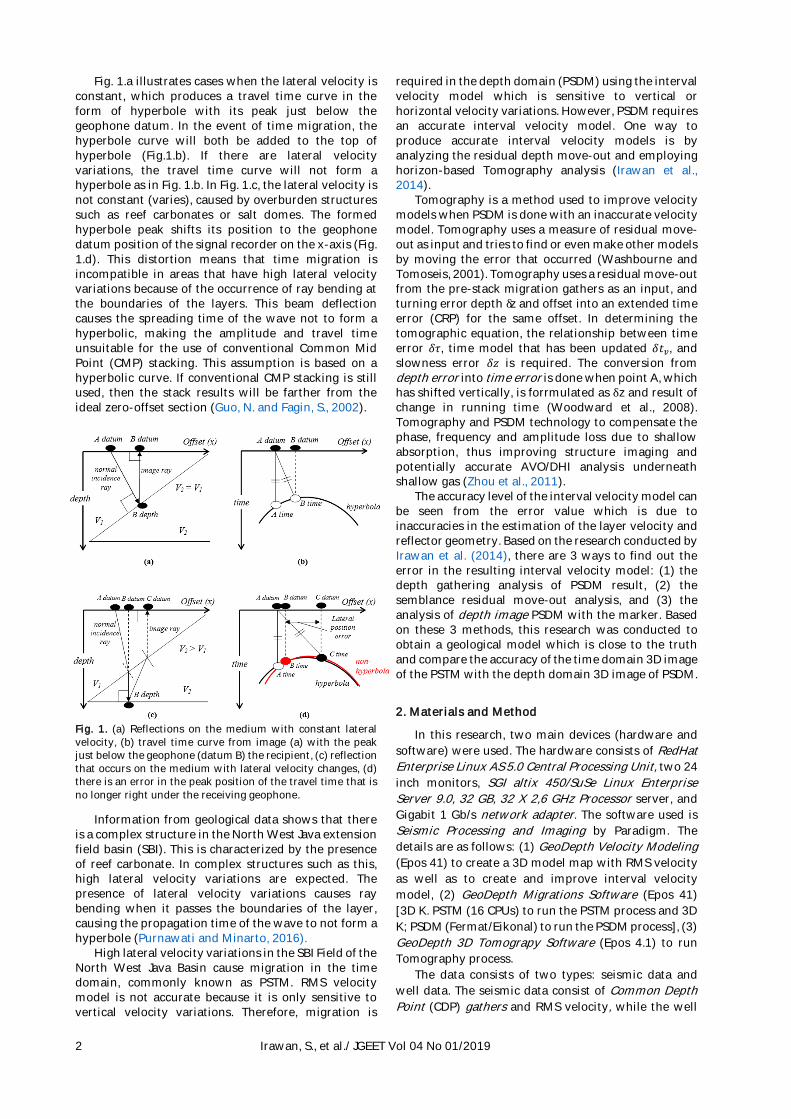
Fig. 1.a illustrates cases when the lateral velocity is constant, which produces a travel time curve in the form of hyperbole with its peak just below the geophone datum. In the event of time migration, the hyperbole curve will both be added to the top of hyperbole (Fig.1.b). If there are lateral velocity variations, the travel time curve will not form a hyperbole as in Fig. 1.b. In Fig. 1.c, the lateral velocity is not constant (varies), caused by overburden structures such as reef carbonates or salt domes. The formed hyperbole peak shifts its position to the geophone datum position of the signal recorder on the x-axis (Fig. 1.d). This distortion means that time migration is incompatible in areas that have high lateral velocity variations because of the occurrence of ray bending at the boundaries of the layers. This beam deflection causes the spreading time of the wave not to form a hyperbolic, making the amplitude and travel time unsuitable for the use of conventional Common Mid Point (CMP) stacking. This assumption is based on a hyperbolic curve. If conventional CMP stacking is still used, then the stack results will be farther from the ideal zero-offset section (Guo, N. and Fagin, S., 2002).

Fig. 1. (a) Reflections on the medium with constant lateral velocity, (b) travel time curve from image (a) with the peak just below the geophone (datum B) the recipient, (c) reflection that occurs on the medium with lateral velocity changes, (d) there is an error in the peak position of the travel time that is no longer right under the receiving geophone.

Information from geological data shows that there is a complex structure in the North West Java extension field basin (SBI). This is characterized by the presence of reef carbonate. In complex structures such as this, high lateral velocity variations are expected. The presence of lateral velocity variations causes ray bending when it passes the boundaries of the layer, causing the propagation time of the wave to not form a hyperbole (Purnawati and Minarto, 2016).

High lateral velocity variations in the SBI Field of the North West Java Basin cause migration in the time domain, commonly known as PSTM. RMS velocity model is not accurate because it is only sensitive to vertical velocity variations. Therefore, migration is

required in the depth domain (PSDM) using the interval velocity model which is sensitive to vertical or horizontal velocity variations. However, PSDM requires an accurate interval velocity model. One way to produce accurate interval velocity models is by analyzing the residual depth move-out and employing horizon-based Tomography analysis (Irawan et al., 2014).

Tomography is a method used to improve velocity models when PSDM is done with an inaccurate velocity model. Tomography uses a measure of residual move-out as input and tries to find or even make other models by moving the error that occurred (Washbourne and Tomoseis, 2001). Tomography uses a residual move-out from the pre-stack migration gathers as an input, and turning error depth δz and offset into an extended time error (CRP) for the same offset. In determining the tomographic equation, the relationship between time error 𝛿𝜏, time model that has been updated 𝛿𝑡𝑣, and slowness error 𝛿𝑧 is required. The conversion from depth error into time error is done when point A, which has shifted vertically, is forrmulated as δz and result of change in running time (Woodward et al., 2008). Tomography and PSDM technology to compensate the phase, frequency and amplitude loss due to shallow absorption, thus improving structure imaging and potentially accurate AVO/DHI analysis underneath shallow gas (Zhou et al., 2011).

The accuracy level of the interval velocity model can be seen from the error value which is due to inaccuracies in the estimation of the layer velocity and reflector geometry. Based on the research conducted by Irawan et al. (2014), there are 3 ways to find out the error in the resulting interval velocity model: (1) the depth gathering analysis of PSDM result, (2) the semblance residual move-out analysis, and (3) the analysis of depth image PSDM with the marker. Based on these 3 methods, this research was conducted to obtain a geological model which is close to the truth and compare the accuracy of the time domain 3D image of the PSTM with the depth domain 3D image of PSDM.

2. Materials and Method

In this research, two main devices (hardware and

software) were used. The hardware consists of RedHat

Enterprise Linux AS 5.0 Central Processing Unit, two 24

inch monitors, SGI altix 450/SuSe Linux Enterprise

Server 9.0, 32 GB, 32 X 2,6 GHz Processor server, and

Gigabit 1 Gb/s network adapter. The software used is

Seismic Processing and Imaging by Paradigm. The

details are as follows: (1) GeoDepth Velocity Modeling

(Epos 41) to create a 3D model map with RMS velocity

as well as to create and improve interval velocity

model, (2) GeoDepth Migrations Software (Epos 41)

[3D K. PSTM (16 CPUs) to run the PSTM process and 3D

K; PSDM (Fermat/Eikonal) to run the PSDM process], (3)

GeoDepth 3D Tomograpy Software (Epos 4.1) to run

Tomography process.

The data consists of two types: seismic data and

well data. The seismic data consist of Common Depth

Point (CDP) gathers and RMS velocity, while the well

Irawan, S., et al./ JGEET Vol 04 No 01/2019 3

data comprise sonic log, density log, resistivity log,

Gamma Ray (GR) log, and neutron log. The log data is

used to calculate the estimated hydrocarbon reserves.

Data processing in this research consists of 3 main

activities: (1) creating a 3D RMS velocity model map,

(2) creating and correcting interval velocity models, (3)

creating a 3D PSTM and PSDM sectional drawing

model.

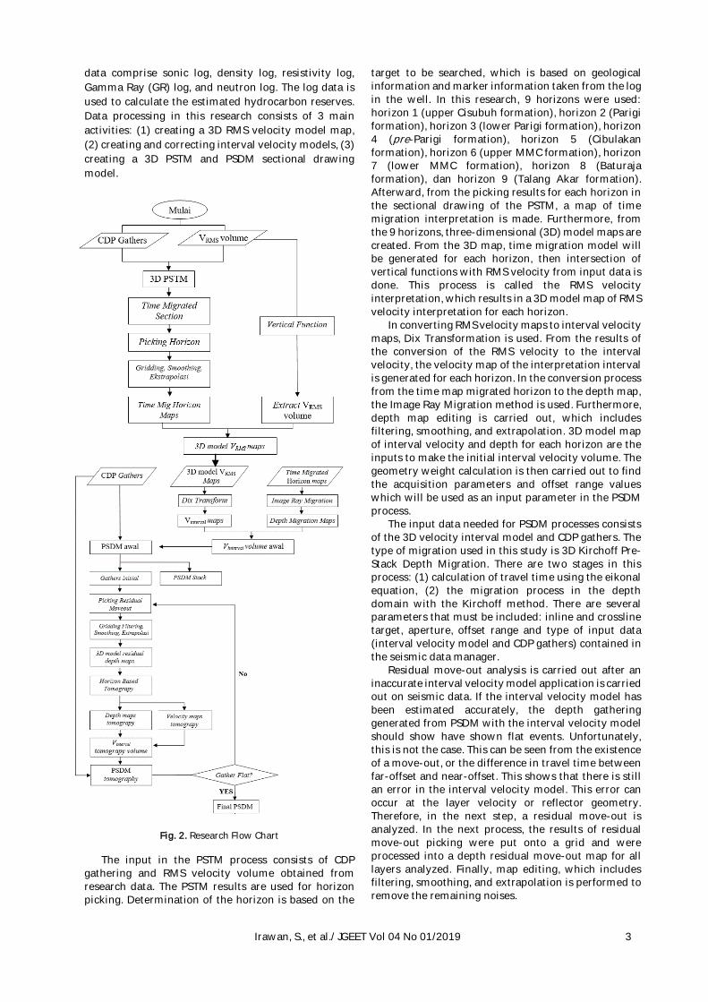
Fig. 2. Research Flow Chart

The input in the PSTM process consists of CDP gathering and RMS velocity volume obtained from research data. The PSTM results are used for horizon picking. Determination of the horizon is based on the

target to be searched, which is based on geological information and marker information taken from the log in the well. In this research, 9 horizons were used: horizon 1 (upper Cisubuh formation), horizon 2 (Parigi formation), horizon 3 (lower Parigi formation), horizon 4 (pre-Parigi formation), horizon 5 (Cibulakan formation), horizon 6 (upper MMC formation), horizon 7 (lower MMC formation), horizon 8 (Baturaja formation), dan horizon 9 (Talang Akar formation). Afterward, from the picking results for each horizon in the sectional drawing of the PSTM, a map of time migration interpretation is made. Furthermore, from the 9 horizons, three-dimensional (3D) model maps are created. From the 3D map, time migration model will be generated for each horizon, then intersection of vertical functions with RMS velocity from input data is done. This process is called the RMS velocity interpretation, which results in a 3D model map of RMS velocity interpretation for each horizon.

In converting RMS velocity maps to interval velocity maps, Dix Transformation is used. From the results of the conversion of the RMS velocity to the interval velocity, the velocity map of the interpretation interval is generated for each horizon. In the conversion process from the time map migrated horizon to the depth map, the Image Ray Migration method is used. Furthermore, depth map editing is carried out, which includes filtering, smoothing, and extrapolation. 3D model map of interval velocity and depth for each horizon are the inputs to make the initial interval velocity volume. The geometry weight calculation is then carried out to find the acquisition parameters and offset range values which will be used as an input parameter in the PSDM process.

The input data needed for PSDM processes consists of the 3D velocity interval model and CDP gathers. The type of migration used in this study is 3D Kirchoff Pre-Stack Depth Migration. There are two stages in this process: (1) calculation of travel time using the eikonal equation, (2) the migration process in the depth domain with the Kirchoff method. There are several parameters that must be included: inline and crossline target, aperture, offset range and type of input data (interval velocity model and CDP gathers) contained in the seismic data manager.

Residual move-out analysis is carried out after an inaccurate interval velocity model application is carried out on seismic data. If the interval velocity model has been estimated accurately, the depth gathering generated from PSDM with the interval velocity model should show have shown flat events. Unfortunately, this is not the case. This can be seen from the existence of a move-out, or the difference in travel time between far-offset and near-offset. This shows that there is still an error in the interval velocity model. This error can occur at the layer velocity or reflector geometry. Therefore, in the next step, a residual move-out is analyzed. In the next process, the results of residual move-out picking were put onto a grid and were processed into a depth residual move-out map for all layers analyzed. Finally, map editing, which includes filtering, smoothing, and extrapolation is performed to remove the remaining noises.

4 Irawan, S., et al./ JGEET Vol 04 No 01/2019

A depth map of the residual move-out 3D model resulted from the analysis of the residual move-out is used as the input for the Tomography process with the Horizon-Based Tomography method. This method calculates the travel time error used to correct (or update) the interval velocity model and depth map. One parameter that must be determined is ray-tracing step, which shows the origin of the location of the ray (ray-tracing starts or is traced from this point).

There are 3 analyses carried out: (1) Analysis of interval velocity models, which involves comparing interval velocity models before and after residual move-out correction using horizon based Tomography method. The analysis is prioritized for target areas where well data (sonic log and well marker) has been taken. In addition, identification of errors in interval velocity models is carried out at each stage, (2) analysis of sectional drawing of the obtained PSTM and final PSDM, especially the clarity and continuity of the reflector throughout the seismic section in the target area, which will then be compared, (3) analysis of the sectional drawing of PSDM of the target before and after Tomography by looking at the reflector on each seismic section.

3. Result and Discussion

3.1 Interval Velocity Model Analysis

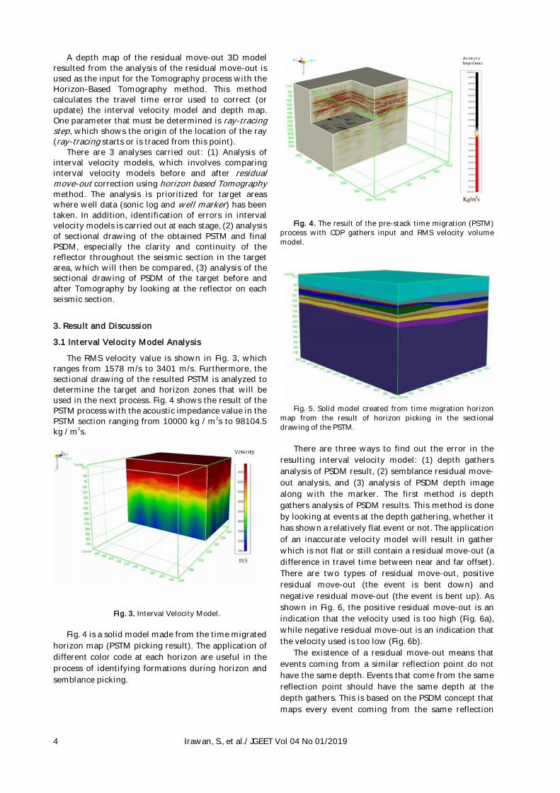
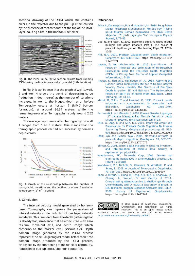
The RMS velocity value is shown in Fig. 3, which ranges from 1578 m/s to 3401 m/s. Furthermore, the sectional drawing of the resulted PSTM is analyzed to determine the target and horizon zones that will be used in the next process. Fig. 4 shows the result of the PSTM process with the acoustic impedance value in the PSTM section ranging from 10000 kg / m

2s to 98104.5

kg / m2s.

Fig. 3. Interval Velocity Model.

Fig. 4 is a solid model made from the time migrated

horizon map (PSTM picking result). The application of

different color code at each horizon are useful in the

process of identifying formations during horizon and

semblance picking.

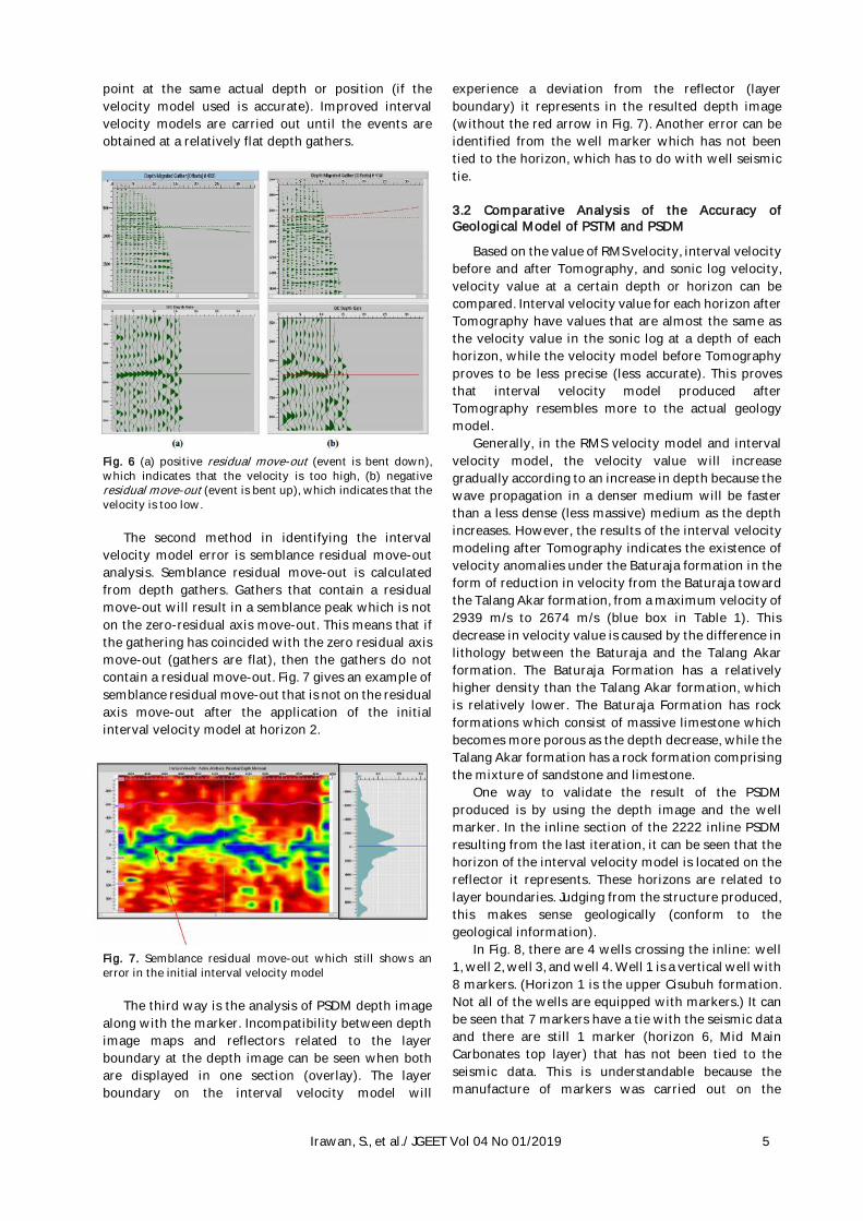
Fig. 4. The result of the pre-stack time migration (PSTM) process with CDP gathers input and RMS velocity volume model.

Fig. 5. Solid model created from time migration horizon

map from the result of horizon picking in the sectional drawing of the PSTM.

There are three ways to find out the error in the

resulting interval velocity model: (1) depth gathers

analysis of PSDM result, (2) semblance residual move-

out analysis, and (3) analysis of PSDM depth image

along with the marker. The first method is depth

gathers analysis of PSDM results. This method is done

by looking at events at the depth gathering, whether it

has shown a relatively flat event or not. The application

of an inaccurate velocity model will result in gather

which is not flat or still contain a residual move-out (a

difference in travel time between near and far offset).

There are two types of residual move-out, positive

residual move-out (the event is bent down) and

negative residual move-out (the event is bent up). As

shown in Fig. 6, the positive residual move-out is an

indication that the velocity used is too high (Fig. 6a),

while negative residual move-out is an indication that

the velocity used is too low (Fig. 6b).

The existence of a residual move-out means that

events coming from a similar reflection point do not

have the same depth. Events that come from the same

reflection point should have the same depth at the

depth gathers. This is based on the PSDM concept that

maps every event coming from the same reflection

Irawan, S., et al./ JGEET Vol 04 No 01/2019 5

point at the same actual depth or position (if the

velocity model used is accurate). Improved interval

velocity models are carried out until the events are

obtained at a relatively flat depth gathers.

Fig. 6 (a) positive residual move-out (event is bent down), which indicates that the velocity is too high, (b) negative residual move-out (event is bent up), which indicates that the velocity is too low.

The second method in identifying the interval

velocity model error is semblance residual move-out

analysis. Semblance residual move-out is calculated

from depth gathers. Gathers that contain a residual

move-out will result in a semblance peak which is not

on the zero-residual axis move-out. This means that if

the gathering has coincided with the zero residual axis

move-out (gathers are flat), then the gathers do not

contain a residual move-out. Fig. 7 gives an example of

semblance residual move-out that is not on the residual

axis move-out after the application of the initial

interval velocity model at horizon 2.

Fig. 7. Semblance residual move-out which still shows an error in the initial interval velocity model

The third way is the analysis of PSDM depth image

along with the marker. Incompatibility between depth

image maps and reflectors related to the layer

boundary at the depth image can be seen when both

are displayed in one section (overlay). The layer

boundary on the interval velocity model will

experience a deviation from the reflector (layer

boundary) it represents in the resulted depth image

(without the red arrow in Fig. 7). Another error can be

identified from the well marker which has not been

tied to the horizon, which has to do with well seismic

tie.

3.2 Comparative Analysis of the Accuracy of Geological Model of PSTM and PSDM

Based on the value of RMS velocity, interval velocity

before and after Tomography, and sonic log velocity,

velocity value at a certain depth or horizon can be

compared. Interval velocity value for each horizon after

Tomography have values that are almost the same as

the velocity value in the sonic log at a depth of each

horizon, while the velocity model before Tomography

proves to be less precise (less accurate). This proves

that interval velocity model produced after

Tomography resembles more to the actual geology

model.

Generally, in the RMS velocity model and interval

velocity model, the velocity value will increase

gradually according to an increase in depth because the

wave propagation in a denser medium will be faster

than a less dense (less massive) medium as the depth

increases. However, the results of the interval velocity

modeling after Tomography indicates the existence of

velocity anomalies under the Baturaja formation in the

form of reduction in velocity from the Baturaja toward

the Talang Akar formation, from a maximum velocity of

2939 m/s to 2674 m/s (blue box in Table 1). This

decrease in velocity value is caused by the difference in

lithology between the Baturaja and the Talang Akar

formation. The Baturaja Formation has a relatively

higher density than the Talang Akar formation, which

is relatively lower. The Baturaja Formation has rock

formations which consist of massive limestone which

becomes more porous as the depth decrease, while the

Talang Akar formation has a rock formation comprising

the mixture of sandstone and limestone.

One way to validate the result of the PSDM

produced is by using the depth image and the well

marker. In the inline section of the 2222 inline PSDM

resulting from the last iteration, it can be seen that the

horizon of the interval velocity model is located on the

reflector it represents. These horizons are related to

layer boundaries. Judging from the structure produced,

this makes sense geologically (conform to the

geological information).

In Fig. 8, there are 4 wells crossing the inline: well

1, well 2, well 3, and well 4. Well 1 is a vertical well with

8 markers. (Horizon 1 is the upper Cisubuh formation.

Not all of the wells are equipped with markers.) It can

be seen that 7 markers have a tie with the seismic data

and there are still 1 marker (horizon 6, Mid Main

Carbonates top layer) that has not been tied to the

seismic data. This is understandable because the

manufacture of markers was carried out on the

6 Irawan, S., et al./ JGEET Vol 04 No 01/2019

sectional drawing of the PSTM which still contains

errors in the reflector due to the pull up effect caused

by the presence of reef carbonate at the top of the MMC

layer, causing a lift in the horizon 6 reflector.

Fig. 8. The 2222 inline PSDM section results from running PSDM using the final interval velocity model (fifth iteration)

In Fig. 9, it can be seen that the graph of well 1, well,

2 and well 4 shows the trend of decreasing curve

(reduction in depth error) as the number of iterations

increases. In well 1, the biggest depth error before

Tomography occurs at horizon 7 (MMC bottom

formation), at around 96.54 meters, while the

remaining error after Tomography is only around 2.52

meters.

The average depth error after Tomography on well

1 ranged from 1 to 3 meters. This means that the

tomographic process carried out successfully corrects

depth errors.

Fig. 9. Graph of the relationship between the number of tomographic iterations and the depth error of well 1 and after Tomography (1st-5th iteration)

4. Conclusion

The interval velocity model generated by horizon-

based Tomography can improve the parameters of

interval velocity model, which includes layer velocity

and depth. This is evident from the depth gathering that

is already flat, semblance that has concurred with zero

residual move-out axis, and depth image which

conforms to the marker (well seismic tie). Depth

domain image generated by the PSDM process

represents the actual geological model better than time

domain image produced by the PSTM process,

evidenced by the sharpening of the reflector continuity,

reduction of pull-up effect, and high resolution.

References

Evita, A., Danusaputro, H. and Mualimin, M., 2014. Pengolahan Model Kecepatan Menggunakan Metode Ray Tracing untuk Migrasi Domain Kedalaman (Pre Stack Depth

Youngster Physics Journal, 3, 77-82.

Guo, N. and Fagin, S., 2002. Becoming effective speed-model builders and depth imagers, Part 1 The basics of prestack depth migration. The Leading Edge, 21, 1205-1209.

Hill, N.R., 2001. Prestack Gaussian-beam depth migration. Geophysics , 66, 1240 -1250. https : //doi.org/10.1190/ 1.1487071

Irawan, S. and Khoirunnisa, H., 2017. Identification of Reservoir Thickness and Estimation of Hydrocarbon Reservation used the Pre-Stack Depth Migration (PSDM) in Cikung Area. Journal of Applied Geospatial Information, 1, 5-10.

Irawan, S., Sismanto, Sukmatiawan, A., 2014. Applying the Horizon Based Tomography Method to Update Interval Velocity Model, Identify The Structure of Pre-Stack Depth Migration 3D and Estimate The Hydrocarbon Reserve In SBI Field of North West Java Basin. Jurnal Teknologi, 69, 53-58.

Mittet, R., Sollie, R. and Hokstad, K., 1995. Prestack depth migration with compensation for absorption and dispersion. Geophysics, 60, 1485-1494. https://doi.org/10.1190/1.1443882

Purnawati, L. and Minarto, E., 2016. Koreksi Struktur Lapangan

Migration (PSDM). Jurnal Sains dan Seni ITS, 5. Shin, C., Jang, S. and Min, D.J., 2001. Improved Amplitude

Preservation for Prestack Depth Migration By Inverse Scattering Theory. Geophysical prospecting, 49, 592-606. https://doi.org/10.1046/j.1365-2478.2001.00279.x

Stolk, C.C. and Symes, W.W., 2004. Kinematic artifacts in prestack depth migration. Geophysics, 69, 562-575. https://doi.org/10.1190/1.1707076

Yilmaz, Ö., 2001. Seismic data analysis: Processing, inversion, and interpretation of seismic data. Society of exploration geophysicists.

Washbourne, J.K., Tomoseis Corp, 2001. System for eliminating headwaves in a tomographic process. U.S. Patent 6,269,310.

Woodward, M.J., Nichols, D., Zdraveva, O., Whitfield, P. and Johns, T., 2008. A decade of Tomography. Geophysics, 73, VE5-VE11. https://doi.org/10.1190/1.2969907

Zhou, J., Birdus, S., Hung, B., Teng, K.H., Xie, Y., Chagalov, D., Cheang, A., Wellen, D. and Garrity, J., 2011. Compensating attenuation due to shallow gas through Q tomography and Q-PSDM, a case study in Brazil. In SEG Technical Program Expanded Abstracts 2011, 3332-3336. Society of Exploration Geophysicists. https://doi.org/10.1190/1.3627889

© 2019 Journal of Geoscience, Engineering, Environment and Technology. All rights reserved. This is an open access article

distributed under the terms of the CC BY-SA License

(http://creativecommons.org/licenses/by-sa/4.0/).