Leica Rugby 880 & 870 Ultimate grade reliability and accuracy
Upload
khangminh22Category
view
1download
0

Accuracy andReliability in
Scientific Computing

SOFTWARE • ENVIRONMENTS • TOOLSThe series includes handbooks and software guides as well as monographs
on practical implementation of computational methods, environments, and tools.The focus is on making recent developments available in a practical format
to researchers and other users of these methods and tools.
Editor-in-ChiefJack J. Dongarra
University of Tennessee and Oak Ridge National Laboratory
Editorial BoardJames W. Demmel, University of California, BerkeleyDennis Gannon, indiana UniversityEric Grosse, AT&T Bell LaboratoriesKen Kennedy, Rice UniversityJorge J. More, Argonne National Laboratory
Software, Environments, and ToolsBo Einarsson, editor, Accuracy and Reliabilty in Scientific Computing
Michael W. Berry and Murray Browne, Understanding Search Engines: Mathematical Modeling and TextRetrieval, Second Edition
Craig C. Douglas, Gundolf Haase, and Ulrich Langer, A Tutorial on Elliptic PDE Solvers and Their ParallelizationLouis Komzsik, The Lanczos Method: Evolution and ApplicationBard Ermentrout, Simulating, Analyzing, and Animating Dynamical Systems: A Guide to XPPAUT for Researchers
and Students
V. A. Barker, L. S. Blackford, J. Dongarra, J. Du Croz, S. Hammarling, M. Marinova, J. Wasniewski, andP. Yalamov, LAPACK95 Users' Guide
Stefan Goedecker and Adolfy Hoisie, Performance Optimization of Numerically Intensive Codes
Zhaojun Bai, James Demmel, Jack Dongarra, Axel Ruhe, and Henk van der Vorst,Templates for the Solution of Algebraic Eigenvalue Problems: A Practical Guide
Lloyd N. Trefethen, Spectral Methods in MATLAB
E. Anderson, Z. Bai, C. Bischof, S. Blackford, J. Demmel, J. Dongarra, J. Du Croz,A. Greenbaum, S. Hammarling, A. McKenney, and D. Sorensen, LAPACK Users' Guide, Third Edition
Michael W. Berry and Murray Browne, Understanding Search Engines: Mathematical Modeling and Text Retrieval
Jack J. Dongarra, lain S. Duff, Danny C. Sorensen, and Henk A. van der Vorst, Numerical Linear Algebra forHigh-Performance Computers
R. B. Lehoucq, D. C. Sorensen, and C. Yang, ARRACK Users' Guide: Solution of Large-Scale EigenvalueProblems with Implicitly Restarted Arnoldi Methods
Randolph E. Bank, PLTMG: A Software Package for Solving Elliptic Partial Differential Equations, Users' Guide 8.0
L. S. Blackford, J. Choi, A. Cleary, E. D'Azevedo, J. Demmel, I. Dhillon, J. Dongarra, S. Hammarling,G. Henry, A. Petitet, K. Stanley, D. Walker, and R. C. Whaley, ScaLAPACK Users' Guide
Greg Astfalk, editor, Applications on Advanced Architecture Computers
Francoise Chaitin-Chatelin and Valerie Fraysse, Lectures on Finite Precision Computations
Roger W. Hockney, The Science of Computer Benchmarking
Richard Barrett, Michael Berry, Tony F. Chan, James Demmel, June Donato, Jack Dongarra, Victor Eijkhout, RoldanPozo, Charles Romine, and Henk van der Vorst, Templates for the Solution of Linear Systems: BuildingBlocks for Iterative Methods
E. Anderson, Z. Bai, C. Bischof, J. Demmel, J. Dongarra, J. Du Croz, A. Greenbaum, S. Hammarling,A. McKenney, S. Ostrouchov, and D. Sorensen, LAPACK Users' Guide, Second Edition
jack J. Dongarra, lain S. Duff, Danny C. Sorensen, and Henk van der Vorst, Solving Linear Systems on Vectorand Shared Memory Computers
J. J. Dongarra, J. R. Bunch, C. B. Moler, and G. W. Stewart, Linpack Users' Guide

Accuracy andReliability in
Scientific Computing
Edited byBo EinarssonLinkoping UniversityLinkoping, Sweden
siam.Society for Industrial and Applied Mathematics
Philadelphia

Copyright © 2005 by the Society for Industrial and Applied Mathematics.
1 0 9 8 7 6 5 4 3 2 1
All rights reserved. Printed in the United States of America. No part of this book may bereproduced, stored, or transmitted in any manner without the written permission of thepublisher. For information, write to the Society for Industrial and Applied Mathematics,3600 University City Science Center, Philadelphia, PA 19104-2688.
MATLAB® is a registered trademark of The MathWorks, Inc. For MATLAB® productinformation, please contact The MathWorks, Inc., 3 Apple Hill Drive, Natick, MA 01 760-2098 USA, 508-647-7000, Fax: 508-647-7101, [email protected], www.mathworks.com/
Trademarked names may be used in this book without the inclusion of a trademark symbol.These names are used in an editorial context only; no infringement of trademark is intended.
Library of Congress Cataloging-in-Publication Data
Accuracy and reliability in scientific computing / edited by Bo Einarsson.p. cm. — (Software, environments, tools)
Includes bibliographical references and index.ISBN 0-89871-584-9 (pbk.)
1. Science—Data processing. 2. Reliability (Engineering)—Mathematics. 3. Computerprograms—Correctness—Scientific applications. 4. Software productivity—Scientificapplications. I. Einarsson, Bo, 1939- II. Series.
Q183.9.A28 2005502'.85-dc22
2005047019
is a registered trademark.

Contents
List of Contributors
List of Figures
List of Tables
Preface
I PITFALLS IN NUMERICAL COMPUTATION
1 What Can Go Wrong in Scientific Computing?Bo Einarsson
1.1 Introduction1.2 Basic Problems in Numerical Computation
1.2.1 Rounding1.2.2 Cancellation1.2.3 Recursion1.2.4 Integer overflow
1.3 Floating-point Arithmetic1.3.1 Initial work on an arithmetic standard1.3.2 IEEE floating-point representation1.3.3 Future standards
1.4 What Really Went Wrong in Applied Scientific Computing! . . .1.4.1 Floating-point precision1.4.2 Illegal conversion between data types1.4.3 Illegal data1.4.4 Inaccurate finite element analysis1.4.5 Incomplete analysis . ....
1.5 Conclusion
2 Assessment of Accuracy and ReliabilityRonald F. Boisvert, Ronald Cools, Bo Einarsson
2. 1 Models of Scientific Computing2.2 Verification and Validation
xiii
XV
xix
xxi
1
3
334456667999
1111111212
13
1315
V

vi Contents
3
2.3 Errors in Software 172.42.52.6
Precision, Accuracy, and ReliabilityNumerical Pitfalls Leading to Anomalous Program BehaviorMethods of Verification and Validation2.6.1 Code verification2.6.2 Sources of test problems for numerical software2.6.3 Solution verification2.6.4 Validation
20222324262831
Approximating Integrals, Estimating Errors, and Giving the Wrong Solutionfor a Deceptively Easy Problem 33
Ronald Cools
4
3.13.23.33.43.53.63.73.83.9
IntroductionThe Given ProblemThe First Correct AnswerView Behind the CurtainA More Convenient SolutionEstimating Errors: Phase 1Estimating Errors: Phase 2The More Convenient Solution RevisitedEpilogue
An Introduction to the Quality of Computed Solutions
333434363638404041
43Sven Hammarling
5
4.14.24.34.4
4.54.64.74.84.9
IntroductionFloating-point Numbers and IEEE ArithmeticWhy Worry About Computed Solutions?Condition, Stability, and Error Analysis4.4.1 Condition4.4.2 Stability4.4.3 Error analysisFloating-point Error AnalysisPosing the Mathematical ProblemError Bounds and SoftwareOther ApproachesSummary
Qualitative Computing
434446505056606470717475
77Franqoise Chaitin-Chatelin, Elisabeth Traviesas-Cassan
5.15.2
IntroductionNumbers as Building Blocks for Computation5.2.1 Thinking the unthinkable5.2.2 Breaking the rule5.2.3 Hypercomputation inductively defined by multiplication .5.2.4 The Newcomb— Borel paradox5.2.5 Effective calculability
77777878787980

Contents vii
5.3 Exact Versus Inexact Computing5.3.1 What is calculation?5.3.2 Exact and inexact computing :5.3.3 Computer arithmetic5.3.4 Singularities in exact and inexact computing5.3.5 Homotopic deviation5.3.6 The map : z p(Fz)5.3.7 Graphical illustration
5.4 Numerical Software5.4.1 Local error analysis in finite precision computations .5.4.2 Homotopic deviation versus normwise perturbation .5.4.3 Application to Krylov-type methods
5.5 The Levy Law of Large Numbers for Computation5.6 Summary
II DIAGNOSTIC TOOLS
6 PRECISE and the Quality of Reliable Numerical SoftwareFrancoise Chaitin-Chatelin, Elisabeth Traviesas-Cassan
6.1 Introduction6.2 Reliability of Algorithms6.3 Backward Error Analysis
6.3.1 Consequence of limited accuracy of data6.3.2 Quality of reliable software
6.4 Finite Precision Computations at a Glance6.5 What Is PRECISE?
6.5.1 Perturbation values6.5.2 Perturbation types6.5.3 Data metrics6.5.4 Data to be perturbed6.5.5 Choosing a perturbation model
6.6 Implementation Issues6.7 Industrial Use of PRECISE6.8 PRECISE in Academic Research6.9 Conclusion
7 Tools for the Verification of Approximate Solutions to DifferentialEquations
Wayne H. Enright7.1 Introduction
7.1.1 Motivation and overview7.2 Characteristics of a PSE7.3 Verification Tools for Use with an ODE Solver7.4 Two Examples of Use of These Tools7.5 Discussion and Future Extensions
8181828283838687888889909192
93
95
95969698989999
101102103103103105107108108
109
109109110
1ll112119

viii Contents
III TECHNOLOGY FOR IMPROVING ACCURACY AND RELIABILITY
8 General Methods for Implementing Reliable and Correct SoftwareBo Einarsson
8.1 AdaBrian Wichmann, Kenneth W. Dritz
8.1.1 Introduction and language features8.1.2 The libraries8.1.3 The Numerics Annex8.1.4 Other issues8.1.5 Conclusions
8.2 CCraig C. Douglas, Hans Fetter Langtangen
8.2.1 Introduction8.2.2 Language features8.2.3 Standardized preprocessor, error handling, and debuggin8.2.4 Numerical oddities and math libraries8.2.5 Calling Fortran libraries8.2.6 Array layouts8.2.7 Dynamic data and pointers8.2.8 Data structures8.2.9 Performance issues
8.3 C++Craig C. Douglas, Hans Petter Langtangen
8.3.1 Introduction8.3.2 Basic language features8.3.3 Special features8.3.4 Error handling and debugging8.3.5 Math libraries8.3.6 Array layouts8.3.7 Dynamic data8.3.8 User-defined data structures8.3.9 Programming styles8.3.10 Performance issues
8.4 FortranVan Snyder
8.4.1 Introduction8.4.2 History of Fortran8.4.3 Major features of Fortran 958.4.4 Features of Fortran 20038.4.5 Beyond Fortran 20038.4.6 Conclusion
8.5 JavaRonald F. Boisvert, Roldan Pozo
8.5.1 Introduction8.5.2 Language features
123
125
. 127
127. 128no13?135136
136136
ig 138139140140141
. 141142142
14?143145146
. 147147147147148148149
149. 149
149151153153153
153154

Contents ix
9
10
8.5.3 Portability in the Java environment8.5.4 Performance challenges8.5.5 Performance results8.5.6 Other difficulties encountered in scientific programming
in Java8.5.7 Summary
8.6 PythonCraig C. Douglas, Hans Petter Langtangen
8.6.1 Introduction8.6.2 Basic language features8.6.3 Special features8.6.4 Error handling and debugging8.6.5 Math libraries8.6.6 Array layouts8.6.7 Dynamic data8.6.8 User defined data structures8.6.9 Programming styles8.6.10 Performance issues
The Use and Implementation of Interval Data TypesG. William Walster
9.1 Introduction9.2 Intervals and Interval Arithmetic
9.2.1 Intervals9.2.2 Interval arithmetic
9.3 Interval Arithmetic Utility9.3.1 Fallible measures9.3.2 Enter interval arithmetic
9.4 The Path to Intrinsic Compiler Support9.4.1 Interval-specific operators and intrinsic functions9.4.2 Quality of implementation opportunities
9.5 Fortran Code Example 9.6 Fortran Standard Implications
9.6.1 The interval-specific alternative 9.6.2 The enriched module alternative
9.7 Conclusions
Computer-assisted Proofs and Self-validating MethodsSiegfried M. Rump
10.1 Introduction10.2 Proofs and Computers10.3 Arithmetical Issues10.4 Computer Algebra Versus Self- validating Methods10.5 Interval Arithmetic 10.6 Directed Roundings 10.7 A Common Misconception About Interval Arithmetic
155156158
160162162
162163166167167168169169170170
173
173173174174175175176177179184191193193194194
195
195195200?03?04?06?09

x Contents
10.8 Self- validating Methods and INTLAB10.9 Implementation of Interval Arithmetic10.10 Performance and Accuracy10.11 Uncertain Parameters10.12 Conclusion
11 Hardware-assisted AlgorithmsCraig C. Douglas, Hans Petter Langtangen
11.1 Introduction11.2 A Teaser11.3 Processor and Memory Subsystem Organization11.4 Cache Conflicts and Trashing11.5 Prefetching11.6 Pipelining and Loop Unrolling11.7 Padding and Data Reorganization11.8 Loop Fusion11.9 Bitwise Compatibility11.10 Useful Tools
12 Issues in Accurate and Reliable Use of Parallel Computing inNumerical Programs
William D. Gropp12.1 Introduction12.2 Special Features of Parallel Computers
12.2.1 The major programming models12.2.2 Overview
12.3 Impact on the Choice of Algorithm12.3.1 Consequences of latency12.3.2 Consequences of blocking
12.4 Implementation Issues12.4.1 Races12.4.2 Out-of-order execution12.4.3 Message buffering12.4.4 Nonblocking and asynchronous operations . . . .12.4.5 Hardware errors12.4.6 Heterogeneous parallel systems
12.5 Conclusions and Recommendations
13 Software-reliability Engineering of Numerical SystemsMladen A. Vouk
13.1 Introduction13.2 About SRE13.3 Basic Terms13.4 Metrics and Models
13.4.1 Reliability13.4.2 Availability
2 1 52202 2 82 3 0239
241
2412 4 22 4 3245245246247248249250
253
2 5 32532542542552552572 5 82 5 82592602612 6 22 6 2262
265
2652 6 62 6 72 6 92 6 9274

Contents xi
13.5
13.6
13.7
13.8
Bibliography
Index
General Practice13.5.113.5.213.5.313.5.4
Verification and validationOperational profileTestingSoftware process control
Numerical Software13.6.113.6.213.6.3
13.6.4
Acceptance testingExternal consistency checkingAutomatic verification of numerical precision (error prop-agation control)Redundancy-based techniques
Basic Fault-tolerance Techniques13.7.113.7.213.7.313.7.4Summary
Check-pointing and exception handlingRecovery through redundancyAdvanced techniquesReliability and performance
277277279280284284285286
287289294294295297298298
301
335

This page intentionally left blank

List of Contributors
Ronald F. BoisvertMathematical and Computational Sci-ences Division, National Institute of Stan-dards and Technology (NIST), Mail Stop8910, Gaithersburg, MD 20899, USA,email: [email protected]
Francoise Chaitin-ChatelinUniversite Toulouse 1 and CERFACS(Centre Europeen de Recherche et de For-mation Avancee en Calcul Scientifique),42 av. G. Coriolis, FR-31057 ToulouseCedex, France,e-mail: [email protected]
Ronald CoolsDepartment of Computer Science,Katholieke Universiteit Leuven, Celestij-nenlaan 200A, B-3001 Heverlee, Belgium,email: [email protected]
Craig C. DouglasCenter for Computational Sciences, Uni-versity of Kentucky, Lexington, Kentucky40506-0045, USA,email: douglas@ccs. uky. edu
Kenneth W. DritzArgonne National Laboratory, 9700 SouthCass Avenue, Argonne, Illinois 60439,USA,email: dritz@anl. gov
Bo EinarssonNational Supercomputer Centre and theMathematics Department, Linkopings uni-versitet, SE-581 83 Linkoping, Sweden,email: boein@nsc .liu.se
Wayne H. EnrightDepartment of Computer Science, Univer-sity of Toronto, Toronto, Canada M553G4,email: enright@cs . utoronto. ca
William D. GroppArgonne National Laboratory, 9700 SouthCass Avenue, Argonne, Illinois 60439,USA,email: gropp@mcs . anl. gov
Sven HammarlingThe Numerical Algorithms Group Ltd,Wilkinson House, Jordan Hill Road,Oxford OX2 8DR, England,email: sven@nag. co. uk
Hans Petter LangtangenInstitutt for informatikk, Universitetet iOslo, Box 1072 Blindern, NO-0316 Oslo,and Simula Research Laboratory, NO-1325 Lysaker, Norway,email: [email protected]
Roldan PozoMathematical and Computational Scien-ces Division, National Institute of Stan-dards and Technology (NIST), Mail Stop8910, Gaithersburg, MD 20899, USA,email: boisvert@nist. gov
xiii

XIV List of Contributors
Siegfried M. RumpInstitut fiir Informatik III, Technische Uni-versitat Hamburg-Harburg, Schwarzen-bergstrasse 95, DE-21071 Hamburg,Germany,email: rump@tu-harburg. de
Van SnyderJet Propulsion Laboratory, 4800 OakGrove Drive, Mail Stop 183-701,Pasadena, CA 91109, USA,email: van. snyder@ jpl. nasa. gov
Elisabeth Traviesas-CassanCERFACS, Toulouse, France. Presentlyat TRANSICIEL Technologies, FR-31025Toulouse Cedex, France,e-mail: ecassan@mail. transiciel,com
Mladen A. VoukDepartment of Computer Science, Box8206, North Carolina State University,Raleigh, NC 27695, USA,email: vouk@csc. ncsu. edu
G. William WalsterSun Microsystems Laboratories, 16 Net-work Circle, MS UMPK16-160, MenloPark, CA 94025, USA,email: [email protected]
Brian WichmannRetired,email: [email protected]

List of Figures
2.12.2
3.13.23.33.43.5
4.14.24.34.44.54.64.74.8
5.15.2
5.3
7.17.27.37.47.57.67.77.87.97.107.11
A model of computational modelingA model of computational validation
f .(x) for several values ofError as a function of N for = 0.5, 0.75, 1, 1.2, 1.3, and 1.5i[ f ], q4[ f ] Q6[ f ], Q8 [ f ]Reliability of the primitive error estimatorNaive automatic integration with requested error = 0.05
Floating-point number exampleHypotenuse of a right angled triangleCubic equation exampleIntegral exampleLinear equations exampleStable ODE exampleUnstable ODE exampleJames Hardy Wilkinson (1919-1986)
The map for the matrix One in three dimensionsMap : z p(E(A — zI)--1), A = B — E, with B = Venice and E isrank 1Map y : z A = B-E, with B = Venice
Approximate solution for predator-prey problem . .Approximate solution for Lorenz problemETOL(x) with low toleranceETOL(x) with medium toleranceETOL(x) with high toleranceCheck 1, Check 2, and Check 4 results for low toleranceCheck 1, Check 2, and Check 4 results for medium toleranceCheck 1, Check 2, and Check 4 results for high toleranceCheck 3 results for low toleranceCheck 3 results for medium toleranceCheck 3 results for high tolerance
1416
3537393941
4548515757595962
88
9091
113114116117117118118119119170120
XV

xvi List of Figures
8.1
8.2
10.110.210.310.410.5
10.610.710.8
10.9
10.1010.1110.12
10.1310.1410.1510.1610.1710.1810.1910.2010.2110.2210.2310.24
10.25
10.26
10.27
10.2810.29
Java Scimark performance on a 333 MHz Sun Ultra 10 system usingsuccessive releases of the JVMPerformance of Scimark component benchmarks in C and Java on a 500MHz Pentium III system
IBM prime letterheadUniversity of Illinois postmarkPocket calculators with 8 decimal digits, no exponentPoint matrix times interval vectorINTLAB program to check (I — RA x < x and therefore the nonsingu-larity of AINTLAB program for checking nonsingularity of an interval matrix . . .Naive interval Gaussian elimination: Growth ofrad(Uii)Plot of the function in equation (10.8) with 20 meshpoints in x- andy-directionsPlot of the function in equation (10.8) with 50 meshpoints in x- andy-directionsINTLAB program for the inclusion of the determinant of a matrix . . . .Comparison of a naive interval algorithm and a self- validating method . .INTLAB program of the function in equation (10.9) with special treat-ment ofINTLAB results of verifynlss for Broyden's function (10.9)INTLAB example of quadratic convergenceDot productDot product with unrolled loopijk-loop for matrix multiplicationTop-down approach for point matrix times interval matrixImproved code for point matrix times interval matrixINTLAB program to convert inf-sup to mid-rad representationINTLAB program for point matrix times interval matrixINTLAB program for interval matrix times interval matrixInclusion as computed by verifylss for the example in Table 10.12 .Inner and outer inclusions and true solution set for the linear system withtolerances in Table 10.12Monte Carlo approach to estimate the solution set of a parameterizedlinear systemResult of Monte Carlo approach as in the program in Figure 10.12 for100 x 100 random linear system with tolerances, projection of 1st and2nd component of solutionInner and outer inclusions of symmetric solution set for the example inTable 10.12Nonzero elements of the matrix from Harwell/Boeing BCSSTK15 . . . .Approximation of eigenvalues of the matrix in Table 10.14 computed byMATLAB
159
160
196196199206
207208210
212
212214215
218219220221221222223224226226227233
234
234
235
236237
238

List of Figures xvii
11.111.2
12.1
13.113.213.3
13.413.513.6
13.7
13.813.9
Refinement patternsAn unstructured grid
Two orderings for summing 4 values. Shown in (a) is the ordering typi-cally used by parallel algorithms. Shown in (b) is the natural "do loop"ordering
Empirical and modeled failure intensityObserved and modeled cumulative failuresEmpirical and modeled intensity profile obtained during an early testingphaseEmpirical and modeled failures obtained during an early testing phase . .Field recovery and failure rates for a telecommunications product . . . .Unavailability fit using LPET and constant repair rate with data up to"cut-off point" onlyFraction of shipped defects for two ideal testing strategies based on sam-pling with and without replacement, and a nonideal testing under scheduleand resource constraintsIllustration of failure space for three functionally equivalent programs . .Illustration of comparison events
242250
257
272273
273274275
276
282291294

This page intentionally left blank

List of Tables
2.1
3.13.23.3
4.14.24.3
5.1
6.16.2
7.17.27.37.4
9.19.2
10.1
10.210.310.410.510.6
10.7
10.810.9
Sources of test problems for mathematical software
Some numerical resultsWhere the maximum appears to beLocation of maximum by combination of routines
IEEE 754 arithmetic formatsForward recurrence for yn
Asymptotic error bounds for Ax = x
Properties of R(t, z) as a function of t and z
Unit roundoff u for IEEE 754 standard floating-point arithmeticGeneral scheme for generating data for a backward error analysis
Check 1 resultsCheck 2 resultsCheck 3 resultsCheck 4 results
Set-theoretic interval operatorsInterval-specific intrinsic functions
Exponential growth of radii of forward substitution in equation (10.7) innaive interval arithmeticRelative performance without and with unrolled loopsRelative performance for different methods for matrix multiplication. . .Performance of LAPACK routines using Intel MKLPerformance of ATLAS routinesPerformance of algorithms in Figures 10.18 and 10.19 for point matrixtimes interval matrix.Relative performance of MATLAB matrix multiplication with interpre-tation overheadPerformance of interval matrix times interval matrixMeasured computing time for linear system solver.
28
363742
455773
85
102106
114115115116
183184
210221222223223
225
225227229
xix

xx List of Tables
10.10
10.11
10.1210.1310.14
11.1
13.113.213.313.413.513.6
MATLAB solution of a linear system derived from (10.12) for n = 70and T = 40INTLAB example of verifynlss for Broyden's function (10.9) withuncertain parameters
230
731INTLAB example of verifylss for a linear system with uncertain data.232Computing time without and with verificationMatrix with ill-conditioned eigenvalues
Speedups using a cache aware multigrid algorithm on adaptively refinedstructured grids
Hypothetical telephone switchUser breakdown of the profileMode decompositionIllustration of parameter valuesPairwise test casesExample of standard deviation computation
736237
242
279779780783283788

Preface
Much of the software available today is poorly written, inadequate in its facilities,and altogether a number of years behind the most advanced state of the art.—Professor Maurice V. Wilkes, September 1973.
Scientific software is central to our computerized society. It is used to design airplanesand bridges, to operate manufacturing lines, to control power plants and refineries, to analyzefinancial derivatives, to map genomes, and to provide the understanding necessary for thediagnosis and treatment of cancer. Because of the high stakes involved, it is essential that thesoftware be accurate and reliable. Unfortunately, developing accurate and reliable scientificsoftware is notoriously difficult, and Maurice Wilkes' assessment of 1973 still rings truetoday. Not only is scientific software beset with all the well-known problems affectingsoftware development in general, it must cope with the special challenges of numericalcomputation. Approximations occur at all levels. Continuous functions are replaced bydiscretized versions. Infinite processes are replaced by finite ones. Real numbers arereplaced by finite precision numbers. As a result, errors are built into the mathematicalfabric of scientific software which cannot be avoided. At best they can be judiciouslymanaged. The nature of these errors, and how they are propagated, must be understoodif the resulting software is to be accurate and reliable. The objective of this book is toinvestigate the nature of some of these difficulties, and to provide some insight into how toovercome them.
The book is divided into three parts.
1. Pitfalls in Numerical Computation.We first illustrate some of the difficulties in producing robust and reliable scientificsoftware. Well-known cases of failure by scientific software are reviewed, and the"what" and "why" of numerical computations are considered.
2. Diagnostic Tools.We next describe tools that can be used to assess the accuracy and reliability of existingscientific applications. Such tools do not necessarily improve results, but they can beused to increase one's confidence in their validity.
3. Technology for Improving Accuracy and Reliability.We describe a variety of techniques that can be employed to improve the accuracy andreliability of newly developed scientific applications. In particular, we consider theeffect of the choice of programming language, underlying hardware, and the parallel
xxi

xx ii Preface
computing environment. We provide a description of interval data types and theirapplication to validated computations.
This book has been produced by the International Federation for Information Pro-cessing (IFIP) Working Group 2.5. An arm of the IFIP Technical Committee 2 on SoftwarePractice and Experience, WG 2.5 seeks to improve the quality of numerical computation bypromoting the development and availability of sound numerical software. WG 2.5 has beenfortunate to be able to assemble a set of contributions from authors with a wealth of expe-rience in the development and assessment of numerical software. The following WG 2.5members participated in this project: Ronald Boisvert, Francoise Chaitin-Chatelin, RonaldCools, Craig Douglas, Bo Einarsson, Wayne Enright, Patrick Gaffney, Ian Gladwell, WilliamGropp, Jim Pool, Siegfried Rump, Brian Smith, Van Snyder, Michael Thune, Mladen Vouk,and Wolfgang Walter. Additional contributions were made by Kenneth W. Dritz, Sven Ham-marling, Hans Petter Langtangen, Roldan Pozo, Elisabeth Traviesas-Cassan, Bill Walster,and Brian Wichmann. The volume was edited by Bo Einarsson.
Several of the contributions have been presented at other venues in somewhat dif-ferent forms. Chapter 1 was presented at the Workshop on Scientific Computing and theComputational Sciences, May 28-29, 2001, in Amsterdam, The Netherlands. Chapter 5was presented at the IFIP Working Group 2.5 Meeting, May 26-27, 2001, in Amsterdam,The Netherlands. Four of the chapters—6,7,10, and 13—are based on lectures presented atthe SIAM Minisymposium on Accuracy and Reliability in Scientific Computing held July9, 2001, in San Diego, California. Chapter 10 was also presented at the Annual Conferenceof Japan SIAM at Kyushu-University, Fukuoka, October 7-9, 2001.
The book has an accompanying web http: / /www. nsc . 1 iu. se /wg2 5 /book/with updates, codes, links, color versions of some of the illustrations, and additionalmaterial.
A problem with references to links on the internet is that, as Diomidis Spinellis hasshown in [422], the half-life of a referenced URL is approximately four years from itspublication date. The accompanying website will contain updated links.
A number of trademarked products are identified in this book. Java, Java HotSpot,and SUN are trademarks of Sun Microsystems, Inc. Pentium and Itanium are trademarksof Intel. PowerPC is a trademark of IBM. Microsoft Windows is a trademark of Microsoft.Apple is a trademark of Apple Computer, Inc. NAG is a trademark of The NumericalAlgorithms Group, Ltd. MATLAB is a trademark of The MathWorks, Inc.
While we expect that developing accurate and reliable scientific software will remaina challenging enterprise for some time to come, we believe that techniques and tools arenow beginning to emerge to improve the process. If this volume aids in the recognition ofthe problems and helps point developers in the direction of solutions, then this volume willhave been a success.
Linkoping and Gaithersburg, September 15, 2004.
Bo Einarsson, Project Leader
Ronald F. Boisvert, Chair, IFIP Working Group 2.5

Preface xxiii
Acknowledgment
As editor I wish to thank the contributors and the additional project members for sup-porting the project through submitting and refereeing the chapters. I am also very gratefulto the anonymous reviewers who did a marvelous job, gave constructive criticism and muchappreciated comments and suggestions. The final book did benefit quite a lot from theirwork!
I also thank the National Supercomputer Centre and the Mathematics Department ofLinkopings universitet for supporting the project.
Working with SIAM on the publication of this book was a pleasure. Special thanks goto Simon Dickey, Elizabeth Greenspan, Ann Manning Allen, and Linda Thiel, for all theirassistance.
Bo Einarsson

This page intentionally left blank

Part I
PITFALLS IN NUMERICALCOMPUTATION
1

This page intentionally left blank

Chapter 1
What Can Go Wrong inScientific Computing?
Bo Einarsson
1.1 IntroductionNumerical software is central to our computerized society. It is used, for example, to designairplanes and bridges, to operate manufacturing lines, to control power plants and refineries,to analyze financial derivatives, to determine genomes, and to provide the understandingnecessary for the treatment for cancer. Because of the high stakes involved, it is essentialthat the software be accurate, reliable, and robust.
A report [385] written for the National Institute of Standards and Technology (NIST)states that software bugs cost the U.S. economy about $ 60 billion each year, and that morethan a third of that cost, or $ 22 billion, could be eliminated by improved testing. Notethat these figures apply to software in general, not only to scientific software. An article[18] stresses that computer system failures are usually rooted in human error rather thantechnology. The article gives a few examples: delivery problems at a computer company,radio system outage for air traffic control, delayed financial aid. Many companies are nowworking on reducing the complexity of testing but are still requiring it to be robust.
The objective of this book is to investigate some of the difficulties related to scientificcomputing, such as accuracy requirements and rounding, and to provide insight into how toobtain accurate and reliable results.
This chapter serves as an introduction and consists of three sections. In Section 1.2we discuss some basic problems in numerical computation, like rounding, cancellation, andrecursion. In Section 1.3 we discuss implementation of real arithmetic on computers, andin Section 1.4 we discuss some cases where unreliable computations have caused loss oflife or property.
1.2 Basic Problems in Numerical ComputationSome illustrative examples are given in this section, but further examples and discussioncan be found in Chapter 4.
3

4 Chapter 1. What Can Go Wrong in Scientific Computing?
Two problems in numerical computation are that often the input values are not knownexactly, and that some of the calculations cannot be performed exactly. The errors obtainedcan cooperate in later calculations, causing an error growth, which may be quite large.
Rounding is the cause of an error, while cancellation increases its effect and recursionmay cause a build-up of the final error.
1.2.1 Rounding
The calculations are usually performed with a certain fixed number of significant digits,so after each operation the result usually has to be rounded, introducing a rounding errorwhose modulus in the optimal case is less than or equal to half a unit in the last digit. At thenext computation this rounding error has to be taken into account, as well as a new roundingerror. The propagation of the rounding error is therefore quite complex.
Example 1.1 (Rounding) Consider the following MATLAB code for advancing from a tob with the step h = (b — a ) / n .
function s tep(a ,b ,n)% step from a to b with n stepsh=(b-a)/n;x=a;disp(x)while x < b,x = x + h;disp(x)
end
We get one step too many with a = l,b = 2, and n = 3, but the correct number ofsteps with b = 1.1. In the first case because of the rounding downward of h = 1/3 afterthree steps we are almost but not quite at b, and therefore the loop continues. In the secondcase also b is an inexact number on a binary computer, and the inexact values of x and bhappen to compare as wanted. It is advisable to let such a loop work with an integer variableinstead of a real variable. If real variables are used it is advisable to replace while x < bwith while x < b-h/2.
The example was run in IEEE 754 double precision, discussed in section 1.3.2. Inanother precision a different result may be obtained!
1.2.2 Cancellation
Cancellation occurs from the subtraction of two almost equal quantities. Assume x1 =1.243 ± 0.0005 and x2 = 1.234 ± 0.0005. We then obtain x 1 - x 2 = 0.009 ± 0.001, a resultwhere several significant leading digits have been lost, resulting in a large relative error!
Example 1.2 (Quadratic equation) The roots of the equation ax2 + bx + c = 0 are given

1.2. Basic Problems in Numerical Computation 5
by the following mathematically, but not numerically, equivalent expressions:
Using IEEE 754 single precision and a = 1.0 • 10-5, b = 1.0 • 103, and c = 1.0 • 103
we get = -3.0518, x = -1.0000 .10 , = -1.0000, and x = -3.2768 • 107. Wethus get two very different sets of roots for the equation! The reason is that since b2 is muchlarger than 4 the square root will get a value very close to , and when the subtractionof two almost equal values is performed the error in the square root evaluation will domi-nate. In double precision the value of the square root of 106 - 0.04 is 999.9999799999998,which is very close to b = 1000. The two correct roots in this case are one from each set,
and x, for which there is addition of quantities of the same sign, and no cancellationoccurs. •
Example 1.3 (Exponential function) The exponential function ex can be evaluated usingthe MacLaurin series expansion. This works reasonably well for x > 0 but not for x < —3where the expansion terms an will alternate in sign and the modulus of the terms will increaseuntil n . Even for moderate values of x the cancellation can be so severe that a negativevalue of the function is obtained!
Using double (or multiple) precision is not the cure for cancellation, but switching toanother algorithm may help. In order to avoid cancellation in Example 1.2 we let the signof b decide which formula to use, and in Example 1.3 we use the relation e-x = 1/ex .
1.2.3 Recursion
A common method in scientific computing is to calculate a new entity based on the previousone, and continuing in that way, either in an iterative process (hopefully converging) or in arecursive process calculating new values all the time. In both cases the errors can accumulateand finally destroy the computation.
Example 1.4 (Differential equation) Let us look at the solution of a first order differentialequation y' = f ( x , y). A well-known numerical method is the Euler method yn+\ =yn + h • f(xn, yn). Two alternatives with smaller truncation errors are the midpoint methodyn+1 = yn-1 + 2h • f(xn, yn), which has the obvious disadvantage that it requires twostarting points, and the trapezoidal method yn+1 = yn + • [f(xn, yn) + f ( x n + 1 , yn+1)],which has the obvious disadvantage that it is implicit.
Theoretical analysis shows that the Euler method is stable1 for small h, and the mid-point method is always unstable, while the trapezoidal method is always stable. Numericalexperiments on the test problem y' = —2y with the exact solution y(x) = e-2x confirmthat the midpoint method gives a solution which oscillates wildly.2
1Stability can be defined such that if the analytic solution tends to zero as the independent variable tends toinfinity, then also the numeric solution should tend to zero.
2Compare with Figures 4.6 and 4.7 in Chapter 4.

6 Chapter 1. What Can Go Wrong in Scientific Computing?
1.2.4 Integer overflow
There is also a problem with integer arithmetic: integer overflow is usually not signaled.This can cause numerical problems, for example, in the calculation of the factorial function"n!". Writing the code in a natural way using repeated multiplication on a computer with32 bit integer arithmetic, the factorials up to 12! are all correctly evaluated, but 13! getsthe wrong value and 17! becomes negative. The range of floating-point values is usuallylarger than the range of integers, but the best solution is usually not to evaluate the factorialfunction. When evaluating the Taylor formula you instead successively multiply with
for each n to get the next term, thus avoiding computing the large quantity n!. Thefactorial function overflows at n = 35 in IEEE single precision and at n = 171 in IEEEdouble precision.
Multiple integer overflow vulnerabilities in a Microsoft Windows library (before apatch was applied) could have allowed an unauthenticated, remote attacker to execute arbi-trary code with system privileges [460].
1.3 Floating-point ArithmeticDuring the 1960's almost every computer manufacturer had its own hardware and its ownrepresentation of floating-point numbers. Floating-point numbers are used for variableswith a wide range of values, so that the value is represented by its sign, its mantissa,represented by a fixed number of leading digits, and one signed integer for the exponent,as in the representation of the mass of the earth 5.972 • 1024 kg or the mass of an electron9.10938188 • 10-31 kg.
An introduction to floating-point arithmetic is given in Section 4.2.The old and different floating-point representations had some flaws; on one popular
computer there existed values a > 0 such that a > 2 • a. This mathematical impossibilitywas obtained from the fact that a nonnormalized number (a number with an exponent thatis too small to be represented) was automatically normalized to zero at multiplication.3
Such an effect can give rise to a problem in a program which tries to avoid divisionby zero by checking that a 0, but still I/a may cause the condition "division by zero."
1.3.1 Initial work on an arithmetic standard
During the 1970's Professor William Kahan of the University of California at Berkeleybecame interested in defining a floating-point arithmetic standard; see [248]. He managedto assemble a group of scientists, including both academics and industrial representatives(Apple, DEC, Intel, HP, Motorola), under the auspices of the IEEE.4 The group becameknown as project 754. Its purpose was to produce the best possible definition of floating-point arithmetic. It is now possible to say that they succeeded; all manufacturers now followthe representation of IEEE 754. Some old systems with other representations are however
3 Consider a decimal system with two digits for the exponent, and three digits for the mantissa, normalized sothat the mantissa is not less than 1 but less than 10. Then the smallest positive normalized number is 1.00 • 10_99
but the smallest positive nonnormalized number is 0.01 • 10--99.4Institute for Electrical and Electronic Engineers, USA.

1.3. Floating-point Arithmetic 7
still available from Cray, Digital (now HP), and IBM, but all new systems also from thesemanufacturers follow IEEE 754.
The resulting standard was rather similar to the DEC floating-point arithmetic on theVAX system.5
1.3.2 IEEE floating-point representation
The IEEE 754 [226] contains single, extended single, double, and extended double precision.It became an IEEE standard [215] in 1985 and an IEC6 standard in 1989. There is an excellentdiscussion in the book [355].
In the following subsections the format for the different precisions are given, but thestandard includes much more than these formats. It requires correctly rounded operations(add, subtract, multiply, divide, remainder, and square root) as well as correctly roundedformat conversion. There are four rounding modes (round down, round up, round towardzero, and round to nearest), with round to nearest as the default. There are also five exceptiontypes (invalid operation, division by zero, overflow, underflow, and inexact) which must besignaled by setting a status flag.
1.3.2.1 IEEE single precision
Single precision is based on the 32 bit word, using 1 bit for the sign s, 8 bits for the biasedexponent e, and the remaining 23 bits for the fractional part / of the mantissa. The fact thata normalized number in binary representation must have the integer part of the mantissaequal to 1 is used, and this bit therefore does not have to be stored, which actually increasesthe accuracy.
There are five cases:
1. e = 255 and f 0 give an x which is not a number (NaN).2. e = 255 and /= 0 give infinity with its sign,
x = (-1)s.3. 1 e 254, the normal case,
x = (-1)s• (1.f)-2e-127.Note that the smallest possible exponent gives numbers of the formx = (-1)s• (1.f)-2-126.
4. e = 0 and f 0, gradual underflow, subnormal numbers,x = (-l)s.(0.f)-2-126.
5. e = 0 and f= 0, zero with its sign,x = (-1)s. 0.
The largest number that can be represented is (2 - 2-23) • 2127 3.4028 • 1038,the smallest positive normalized number is 1 • 2-126 1.1755 • 10-38, and the smallest
5After 22 successful years, starting 1978 with the VAX 11/780, the VAX platform was phased out. HP willcontinue to support VAX customers.
6 The International Electrotechnical Commission handles information about electric, electronic, and electrotech-nical international standards and compliance and conformity assessment for electronics.

8 Chapter 1. What Can Go Wrong in Scientific Computing?
positive nonnormalized number is 2-23 .2-126 = 2-149 1.4013.10--45. The unit roundoffu = 2-24 5.9605 • 10-8 corresponds to about seven decimal digits.
The concept of gradual underflow has been rather difficult for the user communityto accept, but it is very useful in that there is no unnecessary loss of information. Withoutgradual underflow, a positive number less than the smallest permitted one must either berounded up to the smallest permitted one or replaced with zero, in both cases causing a largerelative error.
The NaN can be used to represent (zero/zero), (infinity - infinity), and other quantitiesthat do not have a known value. Note that the computation does not have to stop for overflow,since the infinity NaN can be used until a calculation with it does not give a well-determinedvalue. The sign of zero is useful only in certain cases.
1.3.2.2 IEEE extended single precision
The purpose of extended precision is to make it possible to evaluate subexpressions to fullsingle precision. The details are implementation dependent, but the number of bits in thefractional part / has to be at least 31, and the exponent, which may be biased, has tohave at least the range —1022 exponent 1023. IEEE double precision satisfies theserequirements!
1.3.2.3 IEEE double precision
Double precision is based on two 32 bit words (or one 64 bit word), using 1 bit for the signs, 11 bits for the biased exponent e, and the remaining 52 bits for the fractional part / ofthe mantissa. It is very similar to single precision, with an implicit bit for the integer partof the mantissa, a biased exponent, and five cases:
1. e = 2047 and f 0 give an x which is not a number (NaN).2. e = 2047 and /= 0 give infinity with its sign,
x = (-1)S. .
3. 1 e 2046, the normal case,x = (-1)s . (1.f). 2e-1023.Note that the smallest possible exponent gives numbers of the formx = (-1)s. (1.f). 2-1022.
4. e = 0 and f 0, gradual underflow, subnormal numbers,x = (-1)s - ( 0 . f ) .2-1022.
5. e = 0 and /= 0, zero with its sign,x = (-1)s .0.
The largest number that can be represented is (2 - 2_52) • 21023 1.7977 • 10308,the smallest positive normalized number is 1 • 2--1022 2.2251 • 10--308, and the smallestpositive nonnormalized number is 2_52 • 2_1022 = 2_1074 . 4.9407 • 10_324. The unitroundoff u= 2_53 1.1102 • 10_16 corresponds to about 16 decimal digits.

1.4. What Really Went Wrong in Applied Scientific Computing! 9
The fact that the exponent is wider for double precision is a useful innovation notavailable, for example, on the IBM System 360.7 On the DEC VAX/VMS two differentdouble precisions D and G were available: D with the same exponent range as in singleprecision, and G with a wider exponent range. The choice between the two double preci-sions was done via a compiler switch at compile time. In addition there was a quadrupleprecision H.
1.3.2.4 IEEE extended double precision
The purpose of extended double precision is to make it possible to evaluate subexpressionsto full double precision. The details are implementation dependent, but the number ofbits in the fractional part / has to be at least 63, and the number of bits in the exponent parthas to be at least 15.
1.3.3 Future standards
There is also an IEEE Standard-for Radix-Independent Floating-Point Arithmetic, ANSI/IEEE 854 [217]. This is however of less interest here.
Currently double precision is not always sufficient, so quadruple precision is availablefrom many manufacturers. There is no official standard available; most manufacturersgeneralize the IEEE 754, but some (including SGI) have another convention. SGI quadrupleprecision is very different from the usual quadruple precision, which has a very large range;with SGI the range is about the same in double and quadruple precision. The reason isthat here the quadruple variables are represented as the sum or difference of two doubles,normalized so that the smaller double is 0.5 units in the last position of the larger. Caremust therefore be taken when using quadruple precision.
Packages for multiple precision also exist.
1.4 What Really Went Wrong in Applied ScientificComputing!
We include only examples where numerical problems have occurred, not the more commonpure programming errors (bugs). More examples are given in the paper [424] and in theThomas Ruckle web site Collection of Software Bugs [212]. Quite a different view is takenin [4], in which how to get the mathematics and numerics correct is discussed.
1.4.1 Floating-point precision
Floating-point precision has to be sufficiently accurate to handle the task. In this section wegive some examples where this has not been the case.
7 IBM System 360 was announced in April 1964 and was a very successful spectrum of compatible computersthat continues in an evolutionary form to this day.
Following System 360 was System 370, announced in June, 1970. The line after System 370 continued underdifferent names: 303X (announced in March, 1977), 308X, 3090, 9021, 9121, and the /Series. These machinesall share a common heritage. The floating-point arithmetic is hexadecimal.

10 Chapter 1. What Can Go Wrong in Scientific Computing?
1.4.1.1 Patriot missile
A well-known example is the Patriot missile8 failure [158, 419] with a Scud missile9 onFebruary 25, 1991, at Dhahran, Saudi Arabia. The Patriot missile was designed, in orderto avoid detection, to operate for only a few hours at one location. The velocity of theincoming missile is a floating-point number but the time from the internal clock is an integer,represented by the time in tenths of a second. Before that time is used, the integer numberis multiplied with a numerical approximation of 0.1 to 24 bits, causing an error 9.5 • 10_8
in the conversion factor. The inaccuracy in the position of the target is proportional to theproduct of the target velocity and the length of time the system has been running. Thisis a somewhat oversimplified discussion; a more detailed one is given in [419]. With thesystem up and running for 100 hours and a velocity of the Scud missile of 1676 meters persecond, an error of 573 meters is obtained, which is more than sufficient to cause failure ofthe Patriot and success for the Scud. The Scud missile killed 28 soldiers.
Modified software, which compensated for the inaccurate time calculation, arrivedthe following day. The potential problem had been identified by the Israelis and reported tothe Patriot Project Office on February 11, 1991.
1.4.1.2 The Vancouver Stock Exchange
The Vancouver Stock Exchange (see the references in [154]) in 1982 experienced a problemwith its index. The index (with three decimals) was updated (and truncated) after eachtransaction. After 22 months it had fallen from the initial value 1000.000 to 524.881, butthe correctly evaluated index was 1098.811.
Assuming 2000 transactions a day a simple statistical analysis gives directly that theindex will lose one unit per day, since the mean truncation error is 0.0005 per transaction.Assuming 22 working days a month the index would be 516 instead of the actual (but stillfalse) 524.881.
1.4.1.3 Schleswig-Holstein local elections
In the Schleswig-Holstein local elections in 1992, one party got 5.0 % in the printed results(which was correctly rounded to one decimal), but the correct value rounded to two decimalswas 4.97 %, and the party did therefore not pass the 5 % threshold for getting into the localparliament, which in turn caused a switch of majority [481]. Similar rules apply not onlyin German elections. A special rounding algorithm is required at the threshold, truncatingall values between 4.9 and 5.0 in Germany, or all values between 3.9 and 4.0 in Sweden!
8The Patriot is a long-range, all-altitude, all-weather air defense system to counter tactical ballistic missiles,cruise missiles, and advanced aircraft.
Patriot missile systems were deployed by U.S. forces during the First Gulf War. The systems were stationed inKuwait and destroyed a number of hostile surface-to-surface missiles.
9The Scud was first deployed by the Soviets in the mid-1960s. The missile was originally designed to carrya 100 kiloton nuclear warhead or a 2000 pound conventional warhead, with ranges from 100 to 180 miles. Itsprincipal threat was its warhead's potential to hold chemical or biological agents.
The Iraqis modified Scuds for greater range, largely by reducing warhead weight, enlarging their fuel tanks, andburning all of the fuel during the early phase of flight. It has been estimated that 86 Scuds were launched duringthe First Gulf War.

1.4. What Really Went Wrong in Applied Scientific Computing! 11
1.4.1.4 Criminal usages of roundoff
Criminal usages of roundoff have been reported [30], involving many tiny withdrawalsfrom bank accounts. The common practice of rounding to whole units of the currency (forexample, to dollars, removing the cents) implies that the cross sums do not exactly agree,which diminishes the chance/risk of detecting the fraud.
1.4.1.5 Euro-conversion
A problem is connected with the European currency Euro, which replaced 12 nationalcurrencies from January 1, 2002. Partly due to the strictly defined conversion rules, theroundoff can have a significant impact [162]. A problem is that the conversion factors fromold local currencies have six significant decimal digits, thus permitting a varying relativeerror, and for small amounts the final result is also to be rounded according to local customsto at most two decimals.
1.4.2 Illegal conversion between data types
On June 4, 1996, an unmanned Ariane 5 rocket launched by the European Space Agencyexploded forty seconds after its lift-off from Kourou, French Guiana. The Report by theInquiry Board [292, 413] found that the failure was caused by the conversion of a 64 bitfloating-point number to a 16 bit signed integer. The floating-point number was too largeto be represented by a 16 bit signed integer (larger than 32767). In fact, this part of thesoftware was required in Ariane 4 but not in Ariane 5!
A somewhat similar problem is illegal mixing of different units of measurement (SI,Imperial, and U.S.). An example is the Mars Climate Orbiter which was lost on entering orbitaround Mars on September 23,1999. The "root cause" of the loss was that a subcontractorfailed to obey the specification that SI units should be used and instead used Imperial unitsin their segment of the ground-based software; see [225]. See also pages 35-38 in thebook [440].
1.4.3 Illegal data
A crew member of the USS Yorktown mistakenly entered a zero for a data value in September1997, which resulted in a division by zero. The error cascaded and eventually shut downthe ship's propulsion system. The ship was dead in the water for 2 hours and 45 minutes;see [420, 202].
1.4.4 Inaccurate finite element analysis
On August 23, 1991, the Sleipner A offshore platform collapsed in Gandsfjorden nearStavanger, Norway. The conclusion of the investigation [417] was that the loss was causedby a failure in a cell wall, resulting in a serious crack and a leakage that the pumps couldnot handle. The wall failed as a result of a combination of a serious usage error in thefinite element analysis (using the popular NASTRAN code) and insufficient anchorage ofthe reinforcement in a critical zone.

12 Chapter 1. What Can Go Wrong in Scientific Computing?
The shear stress was underestimated by 47 %, leading to insufficient strength in thedesign. A more careful finite element analysis after the accident predicted that failure wouldoccur at 62 meters depth; it did occur at 65 meters.
1.4.5 Incomplete analysis
The Millennium Bridge [17, 24, 345] over the Thames in London was closed on June 12,directly after its public opening on June 10, 2000, since it wobbled more than expected. Thesimulations performed during the design process handled the vertical force (which was allthat was required by the British Standards Institution) of a pedestrian at around 2 Hz, butnot the horizontal force at about 1 Hz. What happened was that the slight wobbling (withintolerances) due to the wind caused the pedestrians to walk in step (synchronous walking)which made the bridge wobble even more.
On the first day almost 100000 persons walked the bridge. This wobbling problemwas actually noted already in 1975 on the Auckland Harbour Road Bridge in New Zealand,when a demonstration walked that bridge, but that incident was never widely published. Thewobbling started suddenly when a certain number of persons were walking the MillenniumBridge; in a test 166 persons were required for the problem to appear. The bridge wasreopened in 2002, after 37 viscous dampers and 54 tuned mass dampers were installed andall the modifications were carefully tested. The modifications were completely successful.
1.5 ConclusionThe aim of this book is to diminish the risk of future occurrences of incidents like thosedescribed in the previous section. The techniques and tools to achieve this goal are nowemerging; some of them are presented in parts II and III.

Chapter 2
Assessment of Accuracyand Reliability
Ronald F. Boisvert, Ronald Cools, andBo Einarsson
One of the principal goals of scientific computing is to provide predictions of thebehavior of systems to aid in decision making. Good decisions require good predictions.But how are we to be assured that our predictions are good? Accuracy and reliability aretwo qualities of good scientific software. Assessing these qualities is one way to provideconfidence in the results of simulations. In this chapter we provide some background onthe meaning of these terms.10
2.1 Models of Scientific ComputingScientific software is particularly difficult to analyze. One of the main reasons for this isthat it is inevitably infused with uncertainty from a wide variety of sources. Much of thisuncertainty is the result of approximations. These approximations are made in the contextof each of the physical world, the mathematical world, and the computer world.
To make these ideas more concrete, let's consider a scientific software system de-signed to allow virtual experiments to be conducted on some physical system. Here, thescientist hopes to develop a computer program which can be used as a proxy for some realworld system to facilitate understanding. The reason for conducting virtual experimentsis that developing and running a computer program can be much more cost effective thandeveloping and running a fully instrumented physical experiment (consider a series of crashtests for a car, for example). In other cases performing the physical experiment can bepractically impossible—for example, a physical experiment to understand the formation ofgalaxies! The process of abstracting the physical system to the level of a computer programis illustrated in Figure 2.1. This process occurs in a sequence of steps.
• From real world to mathematical modelA length scale is selected which will allow the determination of the desired resultsusing a reasonable amount of resources, for example, atomic scale (nanometers) or
10Portions of this chapter were contributed by NIST, and are not subject to copyright in the USA.
13

14 Chapter 2. Assessment of Accuracy and Reliability
Figure 2.1. A model of computational modeling.
macro scale (kilometers). Next, the physical quantities relevant to the study, suchas temperature and pressure, are selected (and all other effects implicitly discarded).Then, the physical principles underlying the real world system, such as conserva-tion of energy and mass, lead to mathematical relations, typically partial differentialequations (PDEs), that express the mathematical model. Additional mathematical ap-proximations may be introduced to further simplify the model. Approximations caninclude discarded effects and inadequately modeled effects (e.g., discarded terms inequations, linearization).
• From mathematical model to computational modelThe equations expressing the mathematical model are typically set in some infinitedimensional space. In order to admit a numerical solution, the problem is transformedto a finite dimensional space by some discretization process. Finite differences andfinite elements are examples of discretization methods for PDE models. In such com-putational models one must select an order of approximation for derivatives. One alsointroduces a computational grid of some type. It is desirable that the discrete modelconverges to the continuous model as either the mesh width approaches zero or theorder of approximation approaches infinity. In this way, accuracy can be controlledusing these parameters of the numerical method. A specification for how to solve thediscrete equations must also be provided. If an iterative method is used (which is cer-tainly the case for nonlinear problems), then the solution is obtained only in the limit,

2.2. Verification and Validation 15
and hence a criterion for stopping the iteration must be specified. Approximationscan include discretization of domain, truncation of series, linearization, and stoppingbefore convergence.
• From computational model to computer implementationThe computational model and its solution procedure are implemented on a particu-lar computer system. The algorithm may be modified to make use of parallel pro-cessing capabilities or to take advantage of the particular memory hierarchy of thedevice. Many arithmetic operations are performed using floating-point arithmetic.Approximations can include floating-point arithmetic and approximation of standardmathematical or special functions (typically via calls to library routines).
2.2 Verification and ValidationIf one is to use the results of a computer simulation, then one must have confidence that theanswers produced are correct. However, absolute correctness may be an elusive quantityin computer simulation. As we have seen, there will always be uncertainty—uncertainty inthe mathematical model, in the computational model, in the computer implementation, andin the input data. A more realistic goal is to carefully characterize this uncertainty. This isthe main goal of verification and validation.
• Code verificationThis is the process of determining the extent to which the computer implementationcorresponds to the computational model. If the latter is expressed as a specification,then code verification is the process of determining whether an implementation cor-responds to its lowest level algorithmic specification. In particular, we ask whetherthe specified algorithm has been correctly implemented, not whether it is an effectivealgorithm.
• Solution verificationThis is the process of determining the extent to which the computer implementationcorresponds to the mathematical model. Assuming that the code has been verified(i.e., that the algorithm has been correctly implemented), solution verification askswhether the underlying numerical methods correctly produce solutions to the abstractmathematical problem.
• ValidationThis is the process of determining the extent to which the computer implementationcorresponds to the real world. If solution verification has already been demonstrated,then the validation asks whether the mathematical model is effective in simulatingthose aspects of the real world system under study.
Of course, neither the mathematical nor the computational model can be expected tobe valid in all regions of their own parameter spaces. The validation process must confirmthese regions of validity.
Figure 2.2 illustrates how verification and validation are used to quantify the relation-ship between the various models in the computational science and engineering process. In a

16 Chapter 2. Assessment of Accuracy and Reliability
Figure 2.2. A model of computational validation.
rough sense, validation is the aim of the application scientist (e.g., the physicist or chemist)who will be using the software to perform virtual experiments. Solution verification is theaim of the numerical analyst. Finally, code verification is the aim of the programmer.
There is now a large literature on the subject of verification and validation. Never-theless, the words themselves remain somewhat ambiguous, with different authors oftenassigning slightly different meanings. For software in general, the IEEE adopted the fol-lowing definitions in 1984 (they were subsequently adopted by various other organizationsand communities, such as the ISO11).
• Verification: The process of evaluating the products of a software development phaseto provide assurance that they meet the requirements defined for them by the previousphase.
• Validation: The process of testing a computer program and evaluating the results toensure compliance with specific requirements.
These definitions are general in that "requirements" can be given different meaning fordifferent application domains. For computational simulation, the U.S. Defense Modeling
11 International Standards Organization.

2.3. Errors in Software 17
and Simulation Office (DMSO) proposed the following definitions (1994), which weresubsequently adopted in the context of computational fluid dynamics by the AmericanInstitute of Aeronautics and Astronautics [7].
• Verification: The process of determining that a model implementation accuratelyrepresents the developer's conceptual description of the model and the solution to themodel.
• Validation: The process of determining the degree to which a model is an accuraterepresentation of the real world from the perspective of the intended users of themodel.
The DMSO definitions can be regarded as special cases of the IEEE ones, givenappropriate interpretations of the word "requirements" in the general definitions. In theDMSO proposal, the verification is with respect to the requirements that the implementationshould correctly realize the mathematical model. The DMSO validation is with respect tothe requirement that the results generated by the model should be sufficiently in agreementwith the real world phenomena of interest, so that they can be used for the intended purpose.
The definitions used in the present book, given in the beginning of this chapter, differfrom those of DMSO in that they make a distinction between the computational model andthe mathematical model. In our opinion, this distinction is so central in scientific computingthat it deserves to be made explicit in the verification and validation processes. The modelactually implemented in the computer program is the computational one. Consequently,according to the IEEE definition, validation is about testing that the computational modelfulfills certain requirements, ultimately those of the DMSO definition of validation. Thefull validation can then be divided into two levels. The first level of validation (solutionverification) will be to demonstrate that the computational model is a sufficiently accuraterepresentation of the mathematical one. The second level of validation is to determine thatthe mathematical model is sufficiently effective in reproducing properties of the real world.
The book [383] and the more recent paper [349] present extensive reviews of theliterature in computational validation, arguing for the separation of the concepts of errorand uncertainty in computational simulations. A special issue of Computing in Science andEngineering (see [452]) has been devoted to this topic.
2.3 Errors in SoftwareWhen we ask whether a program is "correct" we want to know whether it faithfully follows itslowest-level specifications. Code verification is the process by which we establish correct-ness in this sense. In order to understand the verification process, it is useful to be mindfulof the most typical types of errors encountered in scientific software. Scientific software isprone to many of the same problems as software in other areas of application. In this sectionwe consider these. Problems unique to scientific software are considered in Section 2.5.
Chapter 5 of the book [440] introduces a broad classification of bugs organized by theoriginal source of the error, i.e., how the error gets into the program, that the authors Tellesand Hsieh call "Classes of Bugs." We summarize them in the following list.

18 Chapter 2. Assessment of Accuracy and Reliability
• Requirement bugs.The specification itself could be inadequate. For example, it could be too vague,missing a critical requirement, or have two requirements in conflict.
• Implementation bugs.These are the bugs in the logic of the code itself. They include problems like not fol-lowing the specification, not correctly handling all input cases, missing functionality,problems with the graphic user interface, improper memory management, and codingerrors.
• Process bugs.These are bugs in the runtime environment of the executable program, such as im-proper versions of dynamic linked libraries or broken databases.
• Build bugs.These are bugs in the procedure used to build the executable program. For example,a product may be built for a slightly wrong environment.
• Deployment bugs.These are problems with the automatic updating of installed software.
• Future planning bugs.These are bugs like the year 2000 problem, where the lifetime of the product wasunderestimated, or the technical development went faster than expected (e.g., the 640KiB12 limit of MS-DOS).
• Documentation bugs.The software documentation, which should be considered as an important part ofthe software itself, might be vague, incomplete, or inaccurate. For example, whenproviding information on a library routine's procedure call it is important to providenot only the meaning of each variable but also its exact type, as well as any possibleside effects from the call.
The book [440] also provides a list of common bugs in the implementation of soft-ware. We summarize them in the following list.
• Memory or resource leaks.A memory leak occurs when memory is allocated but not deallocated when it is nolonger required. It can cause the memory associated with long-running programsto grow in size to the point that they overwhelm existing memory. Memory leakscan occur in any programming language and are sometimes caused by programmingerrors.
• Logic errors.A logic error occurs when a program is syntactically correct but does not performaccording to the specification.
• Coding errors.Coding errors occur when an incorrect list of arguments to a procedure is used, ora part of the intended code is simply missing. Others are more subtle. A classicalexample of the latter is the Fortran statement DO 25 I = 1.10 which in Fortran 77
12"Ki" is the IEC standard for the factor 210 = 1024, corresponding to "k" for the factor 1000, and "B" standsfor "byte." See, for example, http: //physics .nist.gov/cuu/Units/binary.html.

2.3. Errors in Software 19
(and earlier, and also in the obsolescent Fortran 90/95 fixed form) assigns the variableDO25I the value 1.10 instead of creating the intended DO loop, which requires theperiod to be replaced with a comma.
• Memory overruns.Computing an index incorrectly can lead to the access of memory locations outside thebounds of an array, with unpredictable results. Such errors are less likely in modernhigh-level programming languages but may still occur.
• Loop errors.Common cases are unintended infinite loops, off-by-one loops (i.e., loops executedonce too often or not enough), and loops with improper exits.
• Conditional errors.It is quite easy to make a mistake in the logic of an if-then-else-endif construct. Arelated problem arises in some languages, such as Pascal, that do not require an explicitendif.
• Pointer errors.Pointers may be uninitialized, deleted (but still used), or invalid (pointing to somethingthat has been removed).
• Allocation errors.Allocation and deallocation of objects must be done according to proper conventions.For example, if you wish to change the size of an allocated array in Fortran, you mustfirst check if it is allocated, then deallocate it (and lose its content), and finally allocateit to its correct size. Attempting to reallocate an existing array will lead to an errorcondition detected by the runtime system.
• Multithreaded errors.Programs made up of multiple independent and simultaneously executing threads aresubject to many subtle and difficult to reproduce errors sometimes known as raceconditions. These occur when two threads try to access or modify the same memoryaddress simultaneously, but correct operation requires a particular order of access.
• Timing errors.A timing error occurs when two events are designed and implemented to occur ata certain rate or within a certain margin. They are most common in connectionwith interrupt service routines and are restricted to environments where the clock isimportant. One symptom is input or output hanging and not resuming.
• Distributed application errors.Such an error is defined as an error in the interface between two applications in adistributed system.
• Storage errors.These errors occur when a storage device gets a soft or hard error and is unable toproceed.
• Integration errors.These occur when two fully tested and validated individual subsystems are combinedbut do not cooperate as intended when combined.
• Conversion errors.Data in use by the application might be given in the wrong format (integer, floating

20 Chapter 2. Assessment of Accuracy and Reliability
point, ...) or in the wrong units (m, cm, feet, inches, ...). An unanticipated resultfrom a type conversion can also be classified as a conversion error. A problem of thisnature occurs in many compiled programming languages by the assignment of 1 / 2to a variable of floating-point type. The rules of integer arithmetic usually state thatwhen two integers are divided there is an integer result. Thus, if the variable A isof a floating-point type, then the statement A = 1/2 will result in an integer zero,converted to a floating-point zero assigned to the variable A, since 1 and 2 are integerconstants, and integer division is rounded to zero.
• Hard-coded lengths or sizes.If sizes of objects like arrays are defined to be of a fixed size, then care must betaken that no problem instance will be permitted a larger size. It is best to avoid suchhard-coded sizes, either by using allocatable arrays that yield a correctly sized arrayat runtime, or by parameterizing object sizes so that they are easily and consistentlymodified.
• Version bugs.In this case the functionality of a program unit or a data storage format is changedbetween two versions, without backward compatibility. In some cases individualversion changes may be compatible, but not over several generations of changes.
• Inappropriate reuse bugs.Program reuse is normally encouraged, both to reduce effort and to capitalize uponthe expertize of subdomain specialists. However, old routines that have been care-fully tested and validated under certain constraints may cause serious problems ifthose constraints are not satisfied in a new environment. It is important that highstandards of documentation and parameter checking be set for reuse libraries to avoidincompatibilities of this type.
• Boolean bugs.The authors of [440] note on page 159 that "Boolean algebra has virtually nothingto do with the equivalent English words. When we say 'and', we really mean theBoolean 'or' and vice versa." This leads to misunderstandings among both users andprogrammers. Similarly, the meaning of "true" and "false" in the code may be unclear.
Looking carefully at the examples of the Patriot missile, section 1.4.1.1, and theAriane 5 rocket, section 1.4.2, we observe that in addition to the obvious conversion errorsand storage errors, inappropriate reuse bugs were also involved. In each case the failingsoftware was taken from earlier and less advanced hardware equipment, where the softwarehad worked well for many years. They were both well tested, but not in the new environment.
2.4 Precision, Accuracy, and ReliabilityMany of the bugs listed in the previous section lead to anomalous behavior that is easy torecognize, i.e., the results are clearly wrong. For example, it is easy to see if the output ofa program to sort data is really sorted. In scientific computing things are rarely so clear.Consider a program to compute the roots of a polynomial, Checking the output here seemseasy; one can evaluate the function at the computed points. However, the result will seldombe exactly zero. How close to zero does this residual have to be to consider the answer

2.4. Precision, Accuracy, and Reliability 21
correct? Indeed, for ill-conditioned polynomials the relative sizes of residuals provide avery unreliable measure of accuracy. In other cases, such as the evaluation of a definiteintegral, there is no such "easy" method.
Verification and validation in scientific computing, then, is not a simple process thatgives yes or no as an answer. There are many gradations. The concepts of accuracy andreliability are used to characterize such gradations in the verification and validation ofscientific software. In everyday language the words accuracy, reliability, and the relatedconcept of precision are somewhat ambiguous. When used as quality measures they shouldnot be ambiguous. We use the following definitions.
• Precision refers to the number of digits used for arithmetic, input, and output.• Accuracy refers to the absolute or relative error of an approximate quantity.• Reliability measures how "often" (as a percentage) the software fails, in the sense
that the true error is larger than what is requested.
Accuracy is a measure of the quality of the result. Since achieving a prescribed accu-racy is rarely easy in numerical computations, the importance of this component of qualityis often underweighted.
We note that determining accuracy requires the comparison to something external (the"exact" answer). Thus, stating the accuracy requires that one specifies what one is compar-ing against. The "exact" answer may be different for each of the computational model, themathematical model, and the real world. In this book most of our attention will be on solu-tion verification; hence we will be mostly concerned with comparison to the mathematicalmodel.
To determine accuracy one needs a means of measuring (or estimating) error. Absoluteerror and relative error are two important such measures. Absolute error is the magnitudeof the difference between a computed quantity x and its true value x*, i.e.,
Relative error is the ratio of absolute error to the magnitude of the true value, i.e.,
Relative error provides a method of characterizing the percentage error; when the relativeerror is less than one, the negative of the Iog10 of the relative error gives the number ofsignificant decimal digits in the computer solution. Relative error is not so useful a measureas x* approaches 0; one often switches to absolute error in this case. When the computedsolution is a multicomponent quantity, such as a vector, then one replaces the absolute valuesby an appropriate norm.
The terms precision and accuracy are frequently used inconsistently. Furthermore,the misconception that high precision implies high accuracy is almost universal.
Dahlquist and Bjorck [108] use the term precision for the accuracy with which thebasic arithmetic operations +, —, x, and / are performed by the underlying hardware. Forfloating-point operations this is given by the unit roundoff u.13 But even on that there is nogeneral agreement. One should be specific about the rounding mode used.
13 The unit roundoff u can roughly be considered as the largest positive floating-point number u, such that1 + u = 1 in computer arithmetic. Because repeated rounding may occur this is not very useful as a strictdefinition. The formal definition of u is given by (4.1).

22 Chapter 2. Assessment of Accuracy and Reliability
The difference between (traditional) rounding and truncation played an amusing rolein the 100 digit challenge posed in [447, 446]. Trefethen did not specify whether digitsshould be rounded or truncated when he asked for "correct digits." First he announced 18winners, but he corrected this a few days later to 20. In the interview included in [44] heexplains that two teams persuaded him that he had misjudged one of their answers by 1digit. This was a matter of rounding instead of truncating.
Reliability in scientific software is considered in detail in Chapter 13. Robustnessis a concept related to reliability that indicates how "gracefully" the software fails (this isnonquantitative) and also its sensitivity to small changes in the problem (this is related tocondition numbers). A robust program knows when it might have failed and reports thatfact.
2.5 Numerical Pitfalls Leading to Anomalous ProgramBehavior
In this section we illustrate some common pitfalls unique to scientific computing that canlead to the erosion of accuracy and reliability in scientific software. These "numerical bugs"arise from the complex structure of the mathematics underlying the problems being solvedand the sometimes fragile nature of the numerical algorithms and floating-point arithmeticnecessary to solve them. Such bugs are often subtle and difficult to diagnose. Some of theseare described more completely in Chapter 4.
• Improper treatment of constants with infinite decimal expansions.The coding of constants with infinite decimal expansions, like , 2, or even 1/9,can have profound effects on the accuracy of a scientific computation. One will neverachieve 10 decimal digits of accuracy in a computation in which is encoded as3.14159 or 1/9 is encoded as 0.1111. To obtain high accuracy and portability suchconstants should, whenever possible, be declared as constants (and thus computed atcompile time) or be computed at runtime. In some languages, e.g.,MATLAB, isstored to double precision accuracy and is available by a function call.For the constants above we can in Fortran 95 use the working precision wp, with atleast 10 significant decimal digits:
integer, parameter : : wp = selected_real_kind(10)real(kind=wp), parameter :: one = 1.0_wp, two = 2.0_wp, &
& four = 4.0_wp, ninth = 1.0_wp/9.0_wpreal(kind=wp) :: pi, sqrt2pi - four*atan(one)sqrt2 = sqrt(two)
• Testing on floating-point equality.In scientific computations approximations and roundoff lead to quantities that arerarely exact. So, testing whether a particular variable that is the result of a computationis 0.0 or 1.0 is rarely correct. Instead, one must determine what interval around 0.0 or1.0 is sufficient to satisfy the criteria at hand and then test for inclusion in that interval.See, e.g., Example 1.1.

2.6. Methods of Verification and Validation 23
• Inconsistent precision.The IEEE standard for floating-point arithmetic defined in [226] requires the avail-ability of at least two different arithmetic precisions. If you wish to obtain a correctresult in the highest precision available, then it is usually imperative that all floating-point variables and constants are in (at least) that precision. If variables and constantsof different precisions (i.e., different floating-point types) are mixed in an arithmeticexpression, this can result in a loss of accuracy in the result, dropping it to that of thelowest precision involved.
• Faulty stopping criteria.See, e.g., Example 1.1.
• Not obviously wrong code.A code can be wrong but it can still work more or less correctly. That is, the codemay produce results that are acceptable, though they are somewhat less accuratethan expected, or are generated more slowly than expected. This can happen whensmall errors in the coding of arithmetic expressions are made. For example, if onemakes a small mistake in coding a Jacobian in Newton's method for solving nonlinearsystems, the program may still converge to the correct solution, but, if it does, itwill do so more slowly than the quadratic convergence that one expects of Newton'smethod.
• Not recognizing ill-conditioned problems.Problems are ill-conditioned when their solutions are highly sensitive to perturba-tions in the input data. In other words, small changes in the problem to be solved(such as truncating an input quantity to machine precision) lead to a computationalproblem whose exact solution is far away from the solution to the original problem.Ill-conditioning is an intrinsic property of the problem which is independent of themethod used to solve it. Robust software will recognize ill-conditioned problems andwill alert the user. See Sections 4.3 and 4.4 for illuminating examples.
• Unstable algorithms and regions of instability.A method is unstable when rounding errors are magnified without bound in the solu-tion process. Some methods are stable only for certain ranges of its input data. Robustsoftware will either use stable methods or notify the user when the input is outsidethe region of guaranteed stability. See section 4.4.2 for examples.
2.6 Methods of Verification and ValidationIn this section we summarize some of the techniques that are used in the verification andvalidation of scientific software. Many of these are well known in the field of softwareengineering; see [6] and [440], for example. Others are specialized to the unique needs ofscientific software; see [383] for a more complete presentation. We emphasize that noneof these techniques are foolproof. It is rare that correctness of scientific software can berigorously demonstrated. Instead, the verification and validation processes provide a seriesof techniques, each of which serves to increase our confidence that the software is behavingin the desired manner.

24 Chapter 2. Assessment of Accuracy and Reliability
2.6.1 Code verification
In code verification we seek to determine how faithfully the software is producing thesolution to the computational model, i.e., to its lowest level of specification. In effect, weare asking whether the code correctly implements the specified numerical procedure. Ofcourse, the numerical method may be ineffective in solving the target mathematical problem;that is not the concern at this stage.
Sophisticated software engineering techniques have been developed in recent years toimprove and automate the verification process. Such techniques, known as formal methods,rely on mathematically rigorous specifications for the expected behavior of software. Givensuch a specification, one can (a) prove theorems about the projected program's behavior,(b) automatically generate much of the code itself, and/or (c) automatically generate testsfor the resulting software system. See [93], for example. Unfortunately, such specificationsare quite difficult to write, especially for large systems. In addition, such specifications donot cope well with the uncertainties of floating-point arithmetic. Thus, they have rarelybeen employed in this context. A notable exception is the formal verification of low-levelfloating-point arithmetic functions. See, for example, [197, 198]. Gunnels et al. [184]employed formal specifications to automatically generate linear algebra kernels. In ourdiscussion we will concentrate on more traditional code verification techniques. The twogeneral approaches that we will consider are code analysis and testing.
2.6.1.1 Code analysis
Analysis of computer code is an important method of exposing bugs. Software engineershave devised a wealth of techniques and tools for analyzing code.
One effective means of detecting errors is to have the code read and understoodby someone else. Many software development organizations use formal code reviews touncover misunderstandings in specifications or errors in logic. These are most effectivelydone at the component level, i.e., for portions of code that are easier to assimilate by personsother than the developer.
Static code analysis is another important tool. This refers to automated techniques fordetermining properties of a program by inspection of the code itself. Static analyzers studythe flow of control in the code to look for anomalies, such as "dead code" (code that cannotbe executed) or infinite loops. They can also study the flow of data, locating variables thatare never used, variables used before they are set, variables defined multiple times beforetheir first use, or type mismatches. Each of these are symptoms of more serious logic errors.Tools for static code analysis are now widely available; indeed, many compilers have optionsthat provide such analysis.
Dynamic code analysis refers to techniques that subject a code to fine scrutiny as itis executed. Tools that perform such analysis must first transform the code itself, insertingadditional code to track the behavior of control flow or variables. The resulting "instru-mented" code is then executed, causing data to be collected as it executes. Analysis of thedata can be done either interactively or as a postprocessing phase. Dynamic code analy-sis can be used to track the number of times that program units are invoked and the timespent in each. Changes in individual variables can be traced. Assertions about the state ofthe software at any particular point can be inserted and checked at runtime. Interactive

2.6. Methods of Verification and Validation 25
code debuggers, as well as code profiling tools, are now widely available to perform thesetasks.
2.6.1.2 Software testing
Exercising a code actually performing the task for which it was designed, i.e., testing, is anindispensable component of software verification. Verification testing requires a detailedspecification of the expected behavior of the software to all of its potential inputs. Tests arethen designed to determine whether this expected behavior is achieved.
Designing test sets can be quite difficult. The tests must span all of the functionalityof the code. To the extent possible, they should also exercise all paths through the code.Special attention should be paid to provide inputs that are boundary cases or that triggererror conditions.
Exhaustive testing is rarely practical, however. Statistical design of experiments [45,317] provides a collection of guiding principles and techniques that comprise a frameworkfor maximizing the amount of useful information resident in a resulting data set, whileattending to the practical constraints of minimizing the number of experimental runs. Suchtechniques have begun to be applied to software testing. Of particular relevance to codeverification are orthogonal fractional factorian designs, as well as the covering designs;see [109].
Because of the challenges in developing good test sets, a variety of techniques hasbeen developed to evaluate the test sets themselves. For example, dynamic analysis tools canbe used to assess the extent of code coverage provided by tests. Mutation testing is anothervaluable technique. Here, faults are randomly inserted into the code under test. Then thetest suite is run, and the ability of the suite to detect the errors is thereby assessed.
Well-designed software is typically composed of a large number of components (e.g.,procedures) whose inputs and outputs are limited and easier to characterize than the completesoftware system. Similarly, one can simplify the software testing process by first testing thebehavior of each of the components in turn. This is called component testing or unit testing.Of course, the interfaces between components are some of the most error-prone parts ofsoftware systems. Hence, component testing must be followed by extensive integrationtesting, which verifies that the combined functionality of the components is correct.
Once a software system attains a certain level of stability, changes to the code areinevitably made in order to add new functionality or to fix bugs. Such changes run therisk of introducing new bugs into code that was previously working correctly. Thus, it isimportant to maintain a battery of tests which extensively exercise all aspects of the system.When changes are applied to the code, then these tests are rerun to provide confidence thatall other aspects of the code have not been adversely affected. This is termed regressiontesting. In large active software projects it is common to run regression tests on the currentversion of the code each night.
Elements of the computing environment itself, such as the operating system, compiler,number of processors, and floating-point hardware, also have an effect on the behavior ofsoftware. In some cases faulty system software can lead to erroneous behavior. In othercases errors in the software itself may not be exposed until the environment changes. Thus,it is important to perform exhaustive tests on software in each environment in which it willexecute. Regression tests are useful for such testing.

26 Chapter 2. Assessment of Accuracy and Reliability
Another useful technique is to enlist a team other than the developers to provide aseparate evaluation of the software. The testing team obtains the requirements for the code,inspects it, analyzes it, and develops tests and runs them. Such a team often brings a newperspective which can uncover problems overlooked by the developers. One form of thisapproach is to enlist prospective users of the software to perform early testing; the alphaand beta releases now common in open source software development are examples of this.
The mathematical software community has established a similar type of evaluationprocess for reusable components. Since 1975 the ACM Transactions on MathematicalSoftware has used a formal refereeing process to evaluate software which is then publishedas part of the Collected Algorithms of the ACM [62]. The journal also publishes independentcertifications of previously published algorithms.
2.6.2 Sources of test problems for numerical software
Both the code verification and the solution verification steps require the use of test data, or testproblems, with which to exercise the software or its components. Such tests are particularinstances of the abstract mathematical problem to be solved. Methods for obtaining suchdata sets are somewhat problem dependent. Nevertheless there are a few general techniques.
2.6.2.1 Analytical solutions
A test problem is most useful if one knows its solution, since it is only then that we canassess the error in the computation with absolute certainty. In many cases there are problemswhose analytical solutions are well known that can be used for testing. If the software isto compute something straightforward like definite integrals, then one can test the softwareby integrating elementary functions. One can also find challenging functions in a tableof integrals. In more complex mathematical models, such as those describing fluid flow,analytical solutions may be more difficult to find, although there are often special cases(possibly simple or degenerate) whose solutions are known that can be used. It is sometimesdifficult to find such problems that will exercise all aspects of a code, however.
In many cases it is possible to artificially construct any number of problems withknown solutions. Consider the case of software for solving Poisson's equation,
on the unit square (0, 1) x (0, 1) subject to Dirichlet boundary conditions (that is, u(x, y)is specified on the boundary). To construct a test problem, first pick any (smooth) functionu to use as the solution, for example,
Then, put the solution into (2.3), differentiating as necessary to produce a right-hand-sidefunction /, i.e.,
Similarly, one can obtain boundary conditions directly from (2.4).

2.6. Methods of Verification and Validation 27
So, we now have the complete specification for a Poisson problem, i.e.,
subject to
The solution to this problem is given by (2.4).Such a procedure can be used to generate test problems for most operator equations,
e.g., differential equations, integral equations, and systems of algebraic equations. Themethod is sometimes known as the method of manufactured solutions.
One can argue that the problems generated by this technique are not representativeof real problems found in practice. However, if one is simply searching for bugs in thecode, i.e., doing verification testing, then this procedure can be used, with care, to generatea wealth of problems that exercise all aspects of a code. For example, in our example ofPoisson's equation, the artificiality comes from an unnatural forcing function /. However,the main part of the computation that one is testing is the assembly of a sparse matrix andthe solution of the resulting linear system. The structure of this matrix depends only on theform of the differential operator and the boundary conditions, not on the forcing function.
Particularly helpful test problems for verification testing are those for which the un-derlying numerical method is exact. For example, Simpson's rule for numerical integrationis exact when integrating cubic polynomials. Since the only numerical errors for such aproblem are roundoff errors, then (provided the underlying method is stable) one shouldobtain a result whose error is of the same size as the machine precision. Using such prob-lems it is easy to determine whether the underlying coding of the method is incorrect. Manynumerical methods for operator equations are exact on spaces of polynomials; in thesecases the method of manufactured solutions can be used to generate problems for which thesolution should be exact to machine precision.
2.6.2.2 Test set repositories
A number of collections of test problems suitable for code verification and solution ver-ification testing have been developed. These are often put together by communities ofresearchers interested in numerical methods for particular problem classes. Although themain interest here is the development of a set of standard problems or benchmarks to supportthe comparison of competing methods, such problems are also useful in verification andvalidation. Such test problem sets often contain problems whose exact solution is known.However, problems whose analytical solution is not known are sometimes also used. Inthe latter case test comparisons are typically made with best effort computations from theliterature.
Some examples of test data set collections used in the numerical analysis communityare provided in Table 2.1. More are available on the accompanying website http: //www.nsc. liu. se/wg25/book/.

28 Chapter 2. Assessment of Accuracy and Reliability
Table 2.1. Sources of test problems for mathematical software.
Statisticshttp: //www.itl .nist.gov/div898/strd/Sparse Linear Algebra [42]http: //math.nist .gov/MatrixMarket/Sparse Linear Algebrahttp: //www. cise.uf1 . edu/ research/ sparse /mat rices/Initial Value ODEshttp: //pitagora.dm.uniba. it/~testset/Initial Value ODEshttp : / /www . ma . ic . ac . uk/ j cash/IVP_sof tware/readme . phpStiff ODEs [186]http: / /www. unige.ch/~hairer/ test set /test set .htmlBoundary Value ODEshttp: //www. ma. ic . ac. uk/ j cash/ BVP_software/readme. phpElliptic PDEs [377]Multivariate Definite Integralshttp : / /www . math . wsu . edu/ faculty /genz / software /software . htmlOptimizationhttp : / /plato . la . asu . edu/bench . htmlOptimization [142]http : / /titan . prince ton . edu/Test Problems/Optimizationhttp : / /www-fp .mcs . anl . gov/otc/Guide/TestProblems/
2.6.3 Solution verification
In solution verification we try to determine the extent to which the program can be usedto solve the abstract mathematical problem that has been posed. Since it is unrealistic toexpect an exact solution to be obtained in scientific software, we must be more preciseabout what we mean here. Most numerical methods have some discretization parameter,such as a characteristic mesh size, h, or the number of terms in a critical approximatingseries or the number of iterations, n, such that the computed solution approaches the exactsolution as h- 0 or n- . A numerical method with this property is termed convergent.If a numerical method is convergent, then given a target accuracy, it will be possible toselect method parameters (i.e., h or n) such that the code will deliver a solution to theproblem with the desired accuracy. (Note that different values of h and n may be needed fordifferent problem instances.) Of course, in practice computing resources such as CPU time,memory, or arithmetic precision may not be available to achieve arbitrarily high accuracy.The solution verification process, then, establishes what levels of numerical convergencecan be expected in practice.

2.6. Methods of Verification and Validation 29
2.6.3.1 Convergence testing
Testing numerical convergence is an important part of solution verification. To make ourdiscussion concrete, consider the case of a numerical method with a discretization mesh sizeh. (Examples include methods for computing integrals or solving differential equations.)Convergence testing solves a test problem multiple times with different values of h to verifythat some measure e of the norm of the error in the computed solution is approaching zeroas h decreases.
Not only can convergence testing be used to demonstrate the validity of the code, itcan also be used to uncover errors in the code. Suppose that theory tells us that the norm ofthe error e behaves as
for some c independent of h. Such a method is said to have order of convergence p. Typicallysuch error behavior is based upon an asymptotic analysis, i.e., the behavior is valid only forsufficiently small h. During the validation process, one can experimentally determine anobserved order of convergence P and determine whether the observed value approaches thetheoretical value as h gets small, i.e., whether P p as h 0. In particular, given distinctmesh sizes hi < hi_1 leading to computed errors ei < 1,_i, respectively, the observedconvergence rate can be computed from
If one computes this value for a sequence of decreasing hi, one should see Pi - p; ifnot, then there may be a problem with the code. One instance is with the classical Runge-Kutta method for solving an ODE, which wrongly coded may give P = 1 instead of thetheoretical p = 4. However, this result may also occur because the user's coding of thefunction defining the ODE has been done in such a way as to make the definition less smooththan is required for the software to function at the higher order. Order of convergence p — 1is often what results. But this error must also be addressed.
It is also possible to estimate the convergence rate in cases where the solution isunknown. If you do not know the exact solution, you may perform three computationsusing the step lengths h, qh, q2h and get the results y(h), y(qh), y(q2h). Now comparewith the unknown solution yo- Using the formula error = y(h) — yo = chp several times,you form
The value on the far left is a known computed quantity, and the parameter p (or rather p)on the far right is now the only unknown and is easy to determine. You can therefore test ifyour program behaves as theory predicts.
A related testing technique is available when one is solving time-dependent systemsof differential equations, such as fluid flow problems. Here one can often find problems withknown unique steady-state solutions. One can use such problems to check for convergence

30 Chapter 2. Assessment of Accuracy and Reliability
to steady state as t gets large. Of course, this does not tell us that correct transient behaviorwas computed.
It may also be the case that the numerical method in use by the code does not alwaysconverge. The method may be stable only for certain combinations of the problem or methodparameters. Similarly, approximations used in the method may only be valid for certaininputs. Solution verification testing must also determine regions of convergence for thesoftware. To help determine good tests for determining these, the analyst should be familiarwith the theoretical properties of the numerical method in use. Note that good softwareshould be sensitive to these parameters and report failure on its own rather than simplydeliver an incorrect result.
Chapter 6 of this volume describes a general-purpose tool, PRECISE, which can behelpful in performing numerical experiments to determine the quality of convergence ofnumerical software components. There are many other types of diagnostics that can becomputed to help in the code verification and solution verification process. Often these relyon particular properties of the given problem domain. Examples of such indicators for thecase of initial-value problems for ODEs are provided in Chapter 7.
2.6.3.2 Dynamic analysis methods
In many cases it is possible to develop procedures for estimating errors in computations. Forexample, the problem may be solved using two different computational meshes, the seconda refinement of the first. The difference between the two solutions may then be taken as anestimate of the error for the solution on the coarser mesh. Other procedures use the knownform of the theoretical error to develop estimation procedures. Providing an estimate ofthe error is a very useful feature in mathematical software components, although the errorestimate itself must be the subject of verification testing.
Such a posteriori error estimates can be used to improve the functionality of the soft-ware itself, of course. For example, error estimates can be used to make a code self-adaptive.Given a target error tolerance from the user, the software can solve the problem on a se-quence of grids until the error estimate is small enough. In other cases one can use local errorestimates to automatically determine where in the computational domain the grid should berefined, or where it can be made coarser. If estimates are good, then the software can makeoptimal use of resources to solve a given problem. Such adaptive methods have becomequite common in computing integrals and in solving differential equations. Adaptive soft-ware of this type poses particular difficulties for verification and validation since theadaptivity may hide problems with the implementation of the numerical methods thatunderlie it.
Another type of dynamic error monitoring is the use of interval arithmetic. Here onereplaces floating-point numbers with intervals. The width of the interval indicates the un-certainty in the value. All arithmetic operations can be performed using intervals. By usingintervals one can automatically track the uncertainty in input quantities through a computa-tion, providing an uncertainty in the result. A variety of tools for computing with intervalsis now available. Details on the use of intervals are provided in Chapter 9. When usedcarefully, intervals can provide the basis for computer-assisted proofs and self-validatingnumerical methods; see Chapter 10. Such methods can take reliability of numerical softwareto new levels.

2.6. Methods of Verification and Validation 31
2.6.4 Validation
Validation is the process of determining the extent to which the computer implementationcorresponds to the real world system being modeled. This is the most important concern forthe scientist who wishes to predict the behavior of a physical system. (For software designedonly to solve a class of abstract mathematical problems, validation does not apply.)
In some cases, computational models are useful only for qualitative understanding.In other cases, specific levels of quantitative understanding are desired. For the developerof a multipurpose modeling system, the goal of validation testing is to determine the regionswithin parameter space in which the model produces acceptable accuracy for its intendedpurpose. For someone using a modeling system for a particular application, the goal of val-idation is to characterize the uncertainty of the results. Methods for validation are typicallyhighly problem dependent.
For simulation software, the most meaningful validation procedures involve the com-parison with data from real physical systems. However, collecting such real world data isoften challenging and sometimes impossible. If the model is computing something simple,like the density of a fluid system, then there may be a wealth of existing benchmark data uponwhich to draw. But if the simulation output is more complex, such as the flow field aroundan aircraft wing, then it can be difficult to obtain suitable benchmark data for comparison.Experimental conditions in previously published data may not have been specified in enoughdetail to be able to specify the mathematical model parameters accurately. In other cases,the exact experimental conditions may be difficult to model. Conversely, experimentalistsmay not be able to match the somewhat idealized conditions that may be assumed in themathematical model. Some problem domains are just impossible to realize experimentally;consider long-term climate change!
Even when detailed comparisons of results with real systems are impractical, thereare often well-known quantities that can be used as indicators of success, such as the timeuntil a particular event occurs. In most problems a variety of consistency checks is alsopossible. For example, one can check whether energy or mass is properly conserved, butthese measures can also be deceptive if the conservation law is built into the underlyingnumerical model; i.e., the solution may be nowhere near as accurate as the quantity beingconserved. Indeed, it is possible for a solution to be totally incorrect yet a physical quantityto be conserved to high accuracy.
Another technique that can be used in these cases is comparison with other computa-tional models and simulations. Such comparisons are most meaningful when the underlyingmathematical model and the numerical solution methods are completely different. A recentdevelopment in the area of finite element software is encouraging in this regard. Preprocess-ing tools are now available that take as input a description of a problem and computationalgrid and are capable of producing the input for several different finite element solutionpackages for the given problem. This greatly eases the ability of users to compare results ofmultiple packages.
Finally, a sound statistical basis can be critical to the success of the validation pro-cess. For example, statistical design of experiments [45, 317] is very useful in maximizingthe amount of useful information while minimizing the number of experiments. Histori-cally, experiment design has played an important role in the physical sciences and will nodoubt play an increasingly important role in validation for the computational sciences. Such

32 Chapter 2. Assessment of Accuracy and Reliability
techniques are especially important when (a) models have large numbers of input param-eters that must be studied, (b) computational experiments require long runs on high-endcomputers, and/or (c) physical experiments are difficult or expensive to perform.
Statistical techniques originally developed for physical metrology may also have a rolehere. In such studies, the analysis of measurement errors from all sources (both randomand systematic) and their combination into a formal "error budget" are performed in orderto develop rigorous estimates of the uncertainties in a measurement [156, 116].
Bayesian inference techniques have also been successfully exploited to develop pro-cedures for quantifying uncertainties in complex computer simulations. Here one developsprobability models for distributions of errors from various sources, such as errors in mod-els, input parameters, and numerical solutions to governing equations. By sampling fromthe relevant probability distributions a series of computer experiments is specified and per-formed. The Bayesian framework provides systematic methods for updating knowledge ofthe system based on data from such experiments. See [115] for a description of how thishas been applied to problems as wide ranging as flow in porus media and shock waveinteractions.

Chapter 3
Approximating Integrals,Estimating Errors, andGiving the Wrong Solutionfor a DeceptivelyEasy Problem
Ronald Cools
3.1 IntroductionThis is a story about asking the right questions. In the meantime several other problems willbe implicitly addressed, and we show that some things are not as obvious as some peopleexpect.
Once upon a time a researcher involved in a large scientific computing project, whichas usual used a combination of several basic numerical techniques, ran into a numericalproblem. He decided to consult a numerical computation expert only after isolating theproblem. The expert gave a perfectly good answer for the problem, to the best of hisknowledge. The practitioner tried it and discovered that it did not work. In isolating theproblem, the practitioner wanted to make it easier for the numerical analyst. He actuallymade it too easy, leaving out critical information, without knowing that it was critical. Inthe end he decided to derive his own method and that worked very well. (At least that'swhat he still believes.) He concluded that he would not consult an "expert" in an area ofnumerical analysis again soon. This will no doubt sound familiar to some readers. It's evenvisible if you look at some journals.
A lot can go wrong in a situation as described above. Below we will illustrate someissues using an example that many will find easy to understand but nevertheless containssurprises. The isolated numerical problem is the approximation of an integral. As back-ground information for you we say that an optimization problem is hidden behind it. Youwill see the story both from the practitioner's and the numerical analyst's point of view.
A set of MATLAB [305] m-files comes with this chapter. You can pick it up in thecompressed file available in [100].
You should try it before looking at the figures to better understand what goes on.
33

34 Chapter 3. Approximating Integrals and Giving the Wrong Solution
3.2 The Given ProblemOn a nice sunny morning a practitioner enters the office of a numerical analyst with thefollowing problem.
"Consider the function
which depends on a parameter E [1,2]. I want to compute
for several values of A., not yet available, but all in the range [1, 2]." (Ignore that thisparticular integral can be computed analytically.)
This is part of a bigger problem. The practitioner's original problem is that he wantsto know where the function
reaches its maximum in the interval [1,2]. He has a nice routine for optimization available,based on the golden ratio, so he only worries about the integral. He needs something hecan easily plug into his optimization routine. This is a deceptively easy problem that canactually be a very difficult problem, partially because of software interfaces. The actualexample is not very difficult but is used as an illustration of potential problems.
3.3 The First Correct AnswerLet us investigate, as the numerical analyst does, what (x) looks like for x E [1, 2], forseveral values of . Is it a smooth function or not?
Figure 3.1 shows (*) for . = 1 + 0.25, s = 0,. . . , 5. (It can be obtained usingthe MATLAB m-file engl .m.)
The numerical analyst looks at the integrand, as you just did, and concludes thatbecause .(x) is a smooth function on the given interval and for the specified values of theparameter ., no sophisticated method to approximate the integral is required. A classicalGauss-Legendre quadrature formula is a conventional choice. We denote the result ofapplying a properly scaled version of the Gauss-Legendre rule with N points to a function
by QN[ ]. Any numerical analyst will easily find a routine that applies Gauss-Legendrequadrature to a finite interval.
Such a routine might have a calling interface, such as the MATLAB routinegauleg.m:
Usage: int = gauleg (f, a, b, key,...)Function gauleg calculates the integral of f in the interval
[a, b] .

3.3. The First Correct Answer 35
Figure 3.1. (x}for several values of ..
Input:f: name of the function that must be integrated;a, b: boundaries of the integration interval;key: integer that determines which Gauss-Legendre formula
must be used.The formula using key points, of degree 2*key - 1 is
used;...: extra parameters for the integrand function.
Output:int: approximation for the integral.
With the integrand in the m-file f. m,
function value = f(x,lambda)value = O.I./((x-lambda)."2+0.01),
we compute the integral for fixed , for a sequence of quadrature rules of increasingaccuracy,
lambda = 1.2for key = 5:5:40
gauleg('f',1,2,key,lambda)end
obtaining the second column of Table 3.1.

36 Chapter 3. Approximating Integrals and Giving the Wrong Solution
Table 3.1. Some numerical results.
key = N510152025303540
= 1.22.917125279889712.521106309761222.556552785721822.553323142658502.553613963552642.553587918510532.553590239146632.55359003333128
= 1.32.477668421452732.715141514855602.685734198101442.678601311919952.677938270525692.677935229925282.677943675973642.67794497275429
3.4 View Behind the CurtainThe exact value of this integral is
This is available in the m-file exact. m. The script eng2 . m combines what we have doneso far to plot graphs of the absolute error in the approximations for TV -point Gauss-Legendreformulas with N = 1, 2 , . . . , 40. Try . = 1.2 and 1.3 first, and then try 0.3 by accident!
Figure 3.2 shows the error as a function of the number of points for several valuesof . Discover that for X < 1 or A > 2 the problem is much easier than for 1 2.Anyway, it appears that relatively few points are needed to obtain significant accuracy.
What this practitioner really wants to know is for what value of A does
reach its maximum. Observe that the additional term destroys the symmetry of the function.The answer to the above question is A = 1.503379725865 ...
3.5 A More Convenient SolutionWhen the practitioner watched the numerical analyst produce the numbers in Table 3.1 heconcluded that approximation errors can be estimated by comparing two approximations.If N2 > N1, one expects that QN2 is more accurate than QN1,. So, it's simply a matter oftaking the number of points high enough.
The practitioner went back to his office, plugged in the routine the numerical analystgave to him with a reasonable large number N of points, and discovered to his surprise thathis original optimization problem appeared to have more than one (local) maximum. Someresults of a search for various values of N in several subintervals [a, b] are listed in Table3.2. (These can be obtained using the MATLAB m-file eng3 . m.) So he returned to the

3.5. A More Convenient Solution 37
Figure 3.2. Error as a function of N for = 0.5, 0.75, 1,1.2, 1.3, and 1.5.
Table 3.2. Where the maximum appears to be.
N a b argmax
1010101010151520202020
1.01.01.01.01.01.51.01.01.01.01.0
1.31.41.51.62.02.02.01.51.61.72.0
1.28701.40001.42611.42611.57401.50001.50021.47041.47041.53131.5313
numerical analyst and asked him how one can know the accuracy of the approximation andhow to choose the required number of quadrature points.
For lack of anything better, in many situations one uses the difference between twoapproximations | QN1 [ ] — QN2 [ ] as an estimate of the error of the least accurate approxi-mation, and one expects (assumes) that this is QN1, the one using the lowest number of points.
Based on what we have seen before, one can easily offer the following algorithm.Let Eabs be the (absolute) error desired. That is, we want to select the smallest k such that

38 Chapter 3. Approximating Integrals and Giving the Wrong Solution
Here we choose to start with the four-point rule and we skip theodd ones, but that can be changed.
t := 4; i := 2Compute Qt[f] and Qt+i[f]while
t :=t + iCompute Qt+i[f]
end whileResult := &+/[/] with estimated error
The practitioner went back to his office, plugged this piece of code in his program, anddiscovered that things didn't work very well any more. With some frustration he watchedthe sun go below the horizon, he looked at his watch, and he decided to go home. It wasFriday the 13th anyway.
3.6 Estimating Errors: Phase 1We will now see how unreliable the error estimate of the previous section can be. Let uslook at the problem as if the real problem is the approximation of . Before proceeding,think a while about how as a function of looks like. (That's the easy question.)What does (QN[ ]look like? (That's more difficult!)
The MATLAB m-file eng4 . m shows you the exact value of /[ ] as a function ofand the approximation for your favorite value of N. In Figure 3.3 , Q(Q6 [ ]and Q8[ ]are shown.
It's not a surprise that is a very nice function of It's symmetric in the giveninterval and it doesn't have a large variation.
For many the fact that oscillates around the exact value is a surprise. Itshouldn't be. This is a typical phenomenon, similar to that experienced in polynomial ap-proximations of functions. The frequency of the oscillation increases with N. Thus, depen-ding on the value of N we end up with an approximation of the original function that looksdifferent.
This should change our view on using [ ] — 2[ as an estimate for theerror of with N1 < N2. Because and are oscillating with differentfrequencies, they will be identical for several values of At these values of our estimateof the error will be zero. The actual error is not zero at these points. This discussioncan be developed to demonstrate that an error estimator based on comparing two suchapproximations is sometimes unreliable.
With the MATLAB m-file eng5 .m you can experiment. You may enter N1 and N2
The script generates a figure showing , , and \Because — I is considered an error estimate for the least precise
approximation, i.e., QN1, we say that this estimator is unreliable if the estimated error islarger than the true error:

3.6. Estimating Errors: Phase 1 39
Figure 3.3. I[F ], (Q4[ ], Q6[ ], Q8[ ].
Figure 3.4. Reliability of the primitive error estimator.

40 Chapter 3. Approximating Integrals and Giving the Wrong Solution
Whenever this inequality holds, a red dot will appear on the -axis. Otherwise a green dotappears.
Take, e.g., N1 = 4 and N2 = 8. What reliability do you expect? The result is shownin Figure 3.4 in black and white (green became dashed, red became dotted, and magentabecame solid; green dots appear as thick dots); you obtain a reliability of (only) 55 %.
Please experiment a bit and experience how difficult it is to find a pair of formulasthat gives a higher reliability.
It should be clear now that in general, using two approximations in this way to derivean error estimate is not a safe idea.
3.7 Estimating Errors: Phase 2Although the difference between two approximations tells us something about the error ofthe least precise approximation, in practice one always presents this error estimate togetherwith the result of the (expected) most accurate rule, i.e., the one that required the most work.Indeed, we spent time to obtain this more accurate result, so why suppress it?
Note that we actually don't know which of the two approximations is the more preciseone!
So we return with error estimate | - Some might say thatthis returns a pessimistic error estimate. In view of what we have seen before, in practice,however, returning almost always increases the reliability of this error estimator.
The MATLAB m-file eng6 .m is a minor variant of eng5 . m implementing what isdescribed above. What do you expect to obtain if you take, e.g., N1 = 4 and N2 = 8? Itturns out that the reliability is increased to 96 %. This is still not very high. You can increasethe reliability by increasing the difference between N1and N2.
3.8 The More Convenient Solution RevisitedThe problem with sending the practitioner away with a routine to evaluate the integral with aGauss-Legendre rule, as above, is that he must select the number of points N. It's easy, andthus tempting, to make his life easier by offering him a naive automatic integration routinewhich selects the right value of N to obtain a desired accuracy.
The algorithm given in Section 3.5 returns a result with an estimated error lower thanwhat the user requires. What does the graph of the true error look like as a function of A?How reliable will the result be?
The algorithm comparing the method of Section 3.5 with the true error is available inthe MATLAB m-file eng7 . m. Try it with, e.g., a requested accuracy of 0.1, 0.05, or 0.01.The result for 0.05 is given in Figure 3.5.
The result is unreliable if the true error is larger than the requested accuracy. (Wecould also say that it is unreliable if the real error is larger than the estimated error. That issomething different, and stronger!) The unreliability is rather large.
The graph is very irregular. That's because it consists of parts of the graphs of QNpasted together.

3.9. Epilogue 41
Figure 3.5. Naive automatic integration with requested error = 0.05.
3.9 Epilogue
Sending the practitioner home with the Gauss-Legendre rule did not make him happy. Thenice function was replaced by something oscillating with many local maxima.
It is not a surprise that he was not amused with the naive adaptive routine. It re-placed his nice function by something irregular, something that is not appreciated by mostoptimization software. It is possible to deal with such problems if one is prepared.
So, never give the obvious answer to the short question asked. The first thing to do ifsomeone asks to approximate an integral is ask him why he wants to do that. It is impossibleto predict how many questions you will ask before the problem will be solved.
We admit that the example integral was easy and that the problems we showed diminishif more accurate (whatever that means) quadrature rules are used. The problem that a niceconvex function is replaced by an oscillating function (if a simple rule is used) or a functionwith discontinuities (if a more sophisticated algorithm with conditions is used) remains,and that may cause problems elsewhere. The problem was enlarged by considering onlyGauss-Legendre rules with an even number of points. Then happens to have a localminimum at the maximum of , which is nearby the desired maximum of g . That isa consequence of both the symmetry of and the symmetry of the Gauss-Legendre rule.
One should always be careful if the output of one numerical problem is the inputfor another numerical problem. As a rule of thumb for the type of problem discussedin this chapter, we suggest that the inaccuracy of the inner problem (the oscillations andirregularities of the quadrature problem) should be below the noise level of the outer problem.

42 Chapter 3. Approximating Integrals and Giving the Wrong Solution
If the relative error of the inner problem is E, one can hope that the relative error of the outerproblem is . This is an oversimplification of course. There is no easy general solutionfor this type of problem.
In Table 3.3 we give the value of obtained by the standard MATLAB optimizationroutine f minbnd in combination with the "convenient" quadrature algorithm of Section 3.5(with k = 4 and i = 1) and the MATLAB function quad. These numbers can be obtainedusing the MATLAB m-file eng8 .m. They illustrate the rule of thumb given above.
Table 3.3. Location of maximum by combination of routines.
Requestedquadrature Location
accuracy naive algorithmLocationMATLAB quad
10-210-310-410-510-610-710-8exact
1.5 41247995327881.5 08412466190441.50 4023812365371.5034 52277489811.5033 74594478381.50338 3341662081.50338 4389898091.503379725865
1.5 45777597792441.50 2421265474811.503 338504497211.5033 59861013661.503384141752751.50338 2482455401.5033 69273992961.503379725865
Finally, we remark that currently we know how to estimate errors in numerical inte-gration rules in a very reliable way. Nevertheless primitive error estimating procedures arestill widely used. Even the "new" MATLAB function quadl is far behind the current stateof the art in this respect, but that's a different story.
AcknowledgmentThe problem that was used here to illustrate several things is borrowed from a very nicepaper by Lyness [296]. The presentation of this chapter benefited a lot from discussionswith him.

Chapter 4
An Introduction to theQuality of ComputedSolutions
Sven Hammarling
4.1 IntroductionThis chapter is concerned with the quality of the computed numerical solutions of mathe-matical problems. For example, suppose we wish to solve the system of linear equationsAx = b using a numerical software package. The package will return a computed solution,say, X, and we wish to judge whether or not x is a reasonable solution to the equations.Sadly, all too often software packages return poor, or even incorrect, numerical results andgive the user no means by which to judge the quality of the numerical results. In 1971,Leslie Fox commented [148, p. 296]
"I have little doubt that about 80 per cent of all the results printed from thecomputer are in error to a much greater extent than the user would believe,..."
More than thirty years later that paper is still very relevant and worth reading. Another veryreadable article is Forsythe [144].
The quality of computed solutions is concerned with assessing how good a com-puted solution is in some appropriate measure. Quality software should implement reliablealgorithms and should, if possible, provide measures of solution quality.
In this chapter we give an introduction to ideas that are important in understanding andmeasuring the quality of computed solutions. In particular we review the ideas of condition,stability, and error analysis and their realization in numerical software. We take as theprincipal example LAPACK [12], a package for the solution of dense and banded linearalgebra problems, but also draw on examples from the NAG Library [332] and elsewhere.The aim is not to show how to perform an error analysis, but to indicate why an understandingof the ideas is important in judging the quality of numerical solutions and to encouragethe use of software that returns indicators of the quality of the results. We give simpleexamples to illustrate some of the ideas that are important when designing reliable numericalsoftware.
43

44 Chapter 4. An Introduction to the Quality of Computed Solutions
Computing machines use floating-point arithmetic for their computation, and so westart with an introduction to floating-point numbers. Floating-point numbers and IEEEarithmetic are also discussed in Chapter 1.
4.2 Floating-point Numbers and IEEE ArithmeticFloating-point numbers are a subset of the real numbers that can be conveniently representedin the finite word length of a computer without unduly restricting the range of numbersrepresented. For example, the ANSI/IEEE standard for binary floating-point arithmetic[215] uses 64 bits to represent double precision numbers in the approximate range 10 308.
A. floating-point number, x, can be represented in terms of four integers as
where b is the base or radix, t is the precision, e is the exponent with an exponent range of[emin> emax ]and m is the mantissa or significand, satisfying 0 m b' — 1. If x 0 andm bt-1, then x is said to be normalized. An alternative, equivalent representation of x is
where each digit satisfies 0 di b — 1. If d1 0, then we say that x is normalized. Ifd1 =0 and x 0, then x is said to be denormalized. Denormalized numbers between 0 andthe smallest normalized number are called subnormal. Note that denormalized numbers donot have the full t digits of precision.14
The following example, which is not intended to be realistic, illustrates the model.
Example 4.1 (Floating-point numbers)
All the normalized numbers have d\ = 1 and either d2 = 0 or d2 = 1; that is, m is oneof the two binary integers m = 10 (= 2) or m = 11 (= 3). Denormalized numbers havem = 01 (= 1). Thus the smallest positive normalized number is 2 • 2emin-t = and thelargest is 3 • 2emax-t = 3. The value 1 • 2emin-t = is the only positive subnormal numberin this system. The complete set of nonnegative normalized numbers is
The set of nonnegative floating-point numbers is illustrated in Figure 4.1, where thesubnormal number is indicated by a dashed line.
Note that floating-point numbers are not equally spaced absolutely, but the relativespacing between numbers is approximately equal. The value
14Note that for convenience of exposition here, we use a slightly different representation than that of Chapter 1.

4.2. Floating-point Numbers and IEEE Arithmetic 45
Figure 4.1. Floating-point number example.
is called the unit roundoff, or the relative machine precision, and is the furthest distance rel-ative to unity between a real number and the nearest floating-point number. In Example 4.1,u = = 0.25 and we can see, for example, that the furthest real number from 1.0 is 1.25and the furthest real number from 2.0 is 2.5. The quantity u is fundamental to floating-pointerror analysis.
The value Em = 2u is called machine epsilon or machine precision .The ANSI/IEEE standard mentioned above (usually referred to as IEEE 754 arith-
metic), which of course has b = 2 and uses an implicit bit, specifies the following:
• floating-point number formats,
• results of the basic floating-point operations,
• rounding modes,
• signed zero, infinity (±00), and not-a-number (NaN),
• floating-point exceptions and their handling, and
• conversion between formats.
Thankfully, currently almost all machines use IEEE arithmetic. There is also a genericANSI/IEEE, base independent, standard [217]. The formats supported by the IEEE 754binary standard are indicated in Table 4.1.
Table 4.1. IEEE 754 arithmetic formats.
Format
singledoubleextended
Precision
24 bits53 bits
64 bits
Exponent
8 bits11 bits
15 bits
Approx range
10±38
10±308
10±4932
Approx precision
10-8
10-16
10-20
While the IEEE 754 standard has been an enormous help in standardizing floating-point computation, it should be noted that moving a computation between machines thatimplement IEEE arithmetic does not guarantee that the computed results will be the same.

46 Chapter 4. An Introduction to the Quality of Computed Solutions
Variations can occur due to such things as compiler optimization, use of extended precisionregisters, and fused multiply-add.
Further discussion of floating-point numbers and IEEE arithmetic can be found inHigham [205] and Overton [355].
The value u can be obtained from the LAPACK function SLAMCH for single pre-cision arithmetic or DLAMCH for double precision arithmetic and is also returned by theNAG Fortran Library routine X02AJF.15 It should be noted that on machines that trun-cate rather than round, EM is returned in place of u, but such machines are now rare. TheMATLAB built-in variable eps returns eM [305], as does the Fortran 95 numeric enquiryfunction epsiIon [315].
4.3 Why Worry About Computed Solutions?Chapter 1 gives a number of examples from real applications where numerical problemshave occurred. In this section we consider some simple examples of numerical computationthat need care in order to obtain reasonable solutions. For clarity of exposition, most ofthe examples in this and the following sections are illustrated with decimal floating-point(significant figure) arithmetic.
The first example illustrates the problem of damaging subtraction, usually referred toas cancellation.
Example 4.2 (Cancellation) Using four figure decimal arithmetic, suppose we wish tocompute s = 1.000 + 1.000 • 104 — 1.000 • 104. If we compute in the standard way fromleft to right we obtain
instead of the correct result of 1.0. Although the cancellation (subtraction) was performedexactly, it lost all the information for the solution.
As Example 4.2 illustrates, the cause of the poor result often happens before the can-cellation, and the cancellation is just the final nail in the coffin. In Example 4.2, the damagewas done in computing s = 1.000+1.000-104, where we lost important information (1.000).It should be said that the subtraction of nearly equal numbers is not always damaging.
Most problems have alternative formulations which are theoretically equivalent, butmay computationally yield quite different results. The following example illustrates this inthe case of computing sample variances.
Example 4.3 (Sample variance [205, Section 1.9]) The sample variance of a set of nvalues JCi, J C 2 , . . . , xn is defined as
15In some ports it actually returns u + b1-2t. See the X02 Chapter introduction [333].

4.3. Why Worry About Computed Solutions? 47
where x is the sample mean of the n values
An alternative, theoretically equivalent, formula to compute the sample variance whichrequires only one pass through the data is given by
If XT - (10000 10001 10002), then using 8 figure arithmetic (4.2) gives s2 = 1.0, thecorrect answer, but (4.3) gives s2 = 0.0, with a relative error of 1.0.
Equation (4.3) can clearly suffer from cancellation, as illustrated in the example. Onthe other hand, (4.2) always gives good results unless n is very large [205, Problem 1.10].See also Chan, Golub, and LeVeque [85] for further discussion of the problem of computingsample variances.
Sadly, it is not unknown for software packages and calculators to implement thealgorithm of (4.3). For example in Excel 2002 from Microsoft Office XP (and in previousversions of Excel also), the function STDEV computes the standard deviation, s, of the data
as s = 0. Considering the pervasive use of Excel and the importance of standard deviationand its use in applications, it is disappointing to realize that (4.3) is used by these versionsof Excel.16 See Cox, Dainton, and Harris [104] for further information, as well as Kniisel[266], McCullough and Wilson [310], and McCullough and Wilson [311]. The spreadsheetfrom OpenOffice.org version 1.0.2 produces the same result but gives no information onthe method used in its help system; on the other hand, the Gnumeric spreadsheet (version1.0.12) gives the correct result, although again the function description does not describethe method used.
A result that is larger than the largest representable floating-point number is said tooverflow. For example, in double precision IEEE arithmetic for which the approximaterange is 10±308, if x = 10200, then x2 would overflow. Similarly, x~2 is said to underflowbecause it is smaller than the smallest nonzero representable floating-point number.
As with the unit roundoff or machine epsilon discussed in Section 4.2, the overflowand underflow thresholds can be obtained from the LAPACK function S/DLAMCH; fromthe NAG Fortran Library routines X02ALF and X02AKF, respectively; the MATLAB built-in variables realmax and realmin; and from the Fortran 95 numeric enquiry functionshuge and tiny.
Care needs to be taken to avoid unnecessary overflow and damaging underflow. Thefollowing example illustrates this care in the case of computing the hypotenuse of the rightangled triangle shown in Figure 4.2.
16The algorithm seems to have been replaced in Excel from Office 2003, which now gives the correct answer.

48 Chapter 4. An Introduction to the Quality of Computed Solutions
Figure 4.2. Hypotenuse of a right angled triangle.
Example 4.4 (Hypotenuse) In Figure 4.2, if x or y is very large there is a danger of over-flow, even if z is representable. Assuming that x and y are nonnegative, a safe method ofcomputing z is
a = max(x, y), b = min(x, y),
This also avoids z being computed as zero if x2 and y2 both underflow. We note that [426,p. 139 and p. 144] actually recommends computing z as
because this is slightly more accurate on a hexadecimal machine.
We can see that (4.3) of Example 4.3 also has the potential for overflow and underflowand, as well as implementing this formula rather than a more stable version, Excel doesnot take the necessary care to avoid underflow and overflow. For example, for the values(1.0E200, 1.0E200), STDEV in Excel 2003 from Microsoft Office 2003 returns the myste-rious symbol #NUM ! , which signifies a numeric exception, in this case overflow, due to thefact that (10.0200)2 overflows in IEEE double precision arithmetic. The correct standard de-viation is of course 0. Similarly, for the values (0, 1 .OE-200, 2.0E-200), STDEV returns thevalue 0 rather than the correct value of 1. OE-200. OpenOffice.org version 1.0.2 also returnszero for this data and overflows on the previous data. Mimicking Excel is not necessarily agood thing!
The computation of the modulus of a complex number x = xr + ixi requires almostthe same computation as that in Example 4.4.
Example 4.5 (Modulus of a complex number)
Again this also avoids \x\ being computed as zero if and both underflow.

4.3. Why Worry About Computed Solutions? 49
Another example where care is needed in complex arithmetic is complex division
Again, some scaling is required to avoid overflow and underflow. See, for example, Smith[421] and Stewart [425], Algol 60 procedures for the complex operations of modulus,division, and square root are given in Martin and Wilkinson [304] and the NAG LibraryChapter, A02, for complex arithmetic has routines based upon those Algol procedures; see,for example, NAG [333]. Occasionally, some aspect of complex floating-point arithmeticis incorrectly implemented; see, for example, [36, Section 7].
Another example, similar to the previous examples, requiring care to avoid overflowand damaging underflow is that of real plane rotations where we need to compute c = cos 9and s = sin 0 such that
or alternatively
Another convenient way to express the two choices is as
If G is the plane rotation matrix
then, with the choices of (4.4),
When used in this way for the introduction of zeros the rotation is generally termed a Givensplane rotation [164, 170]. Givens himself certainly took care in the computation of c ands. To see an extreme case of the detailed consideration necessary to implement a seeminglysimple algorithm, but to be efficient, to preserve as much accuracy as possible throughoutthe range of floating-point numbers, and to avoid overflow and damaging underflow, seeBindel et al. [33], where the computation of the Givens plane rotation is fully discussed.
Sometimes computed solutions are in some sense reasonable but may not be what theuser was expecting. In the next example, the computed solution is close to the exact solutionbut does not meet a constraint that the user might have expected the solution to meet.
Example 4.6 (Sample mean [206]) Using three-figure floating-point decimal arithmetic,
and we see that the computed value is outside the range of the data, although it is notinaccurate.

50 Chapter 4. An Introduction to the Quality of Computed Solutions
Whether or not such a result matters depends upon the application, but it is an issuethat needs to be considered when implementing numerical algorithms. For instance, if
then we probably expect the property 1 to be preserved computationally, so that avalue > 1 is never returned. For a monotonic function we may expect monotonicity tobe preserved computationally.
In the next section we look at ideas that help our understanding of what constitutes aquality solution.
4.4 Condition, Stability, and Error Analysis
4.4.1 ConditionFirst we look at the condition of a problem. The condition of a problem is concerned with thesensitivity of the problem to perturbations in the data. A problem is ill-conditioned if smallchanges in the data cause relatively large changes in the solution. Otherwise a problem iswell-conditioned. Note that condition is concerned with the sensitivity of the problem andis independent of the method we use to solve the problem. We now give some examples toillustrate somewhat ill-conditioned problems.
Example 4.7 (Cubic equation) Consider the cubic equation
whose exact roots are x1 = 1, X2 = x3 = 10. If we perturb the coefficient of x3 to give
the roots become x\ 1.000, *2 11.17, *3 9.041, so that the changes in the two roots*2 and x3 are significantly greater than the change in the coefficient. On the other hand, theroots of the perturbed cubic equation
are x1 1.000, x2, x3 9.896 ± 1.044/, and this time the double root has become acomplex conjugate pair with a significant imaginary part.
We can see that the roots *2 and *3 are ill-conditioned. Note that we cannot deduceanything about the condition of x1 just from this data. The three cubic polynomials areplotted in Figure 4.3.
Example 4.8 (Eigenvalue problem) The matrix

4.4. Condition, Stability, and Error Analysis 51
Figure 4.3. Cubic equation example.
has eigenvalues AI = = = = 10, whereas the slightly perturbed matrix
has eigenvalues = 11,
Example 4.9 (Integral)
When a = b = 1, / = 0, but when a = l,b = 1.01, 7 -220. The function/(x) = aex — be -x when a = b = 1 is plotted in Figure 4.4. Notice that the vertical scalehas a scale factor I04, so that a small change in function can make a large change in the areaunder the curve. I
Example 4.10 (Linear equations) The equations Ax = b given by
have the solution x1 = X2 = 1, but the equations
have the solution x\ = 100, x2 = —99. The two straight lines represented by (4.5) are

52 Chapter 4. An Introduction to the Quality of Computed Solutions
Figure 4.4. Integral example.
Figure 4.5. Linear equations example.
plotted in Figure 4.5, but due to the granularity of the graph we cannot tell the two linesapart.
To be able to decide whether or not a problem is ill-conditioned it is clearly desirable tohave some measure of the condition of a problem. We show two simple cases where we canobtain such a measure and quote the result for a third example. For the first case we derivethe condition number for the evaluation of a function of one variable [205, Section 1.6].

4.4. Condition, Stability, and Error Analysis 53
Let y = f ( x ) with / twice differentiable and f ( x ) 0. Also let y" = f(x +Then, using the mean value theorem,
giving
The quantity
is called the condition number of / since
Thus if K(X) is large the problem is ill-conditioned; that is, small perturbations in x caninduce large perturbations in the solution y.
Example 4.11 Let y = f ( x ) = cos x. Then we see that
and, as we might expect, cos x is most sensitive close to asymptotes of tan x, such as x closeto /2.17 If we take x = 1.57 and E = -0.01 then we find that
which is a very good estimate of (y — y)/y \ =12.55739....
For the second example we consider the condition number of a system of linearequations Ax = b. If we let x be the solution of the perturbed equations
then
giving
The quantity
is called the condition number of A with respect to the solution of the equations Ax = b,or the condition number of A with respect to matrix inversion. Since 7 = A A - 1 , for anynorm such that | = 1, we have that 1 k(A), with equality possible for the 1, 2, andnorms. If A is singular then k(A) = .
17The given condition number is not valid at x = /2, since cos /2 = 0.

54 Chapter 4. An Introduction to the Quality of Computed Solutions
Example 4.12 (Condition of matrix) For the matrix of Example 4.10 we have that
and
so that
Thus we can see that if A is only accurate to about four figures, we cannot guarantee anyaccuracy in the solution.
The term condition was first introduced by Turing in the context of systems of linearequations [458]. Note that for an orthogonal or unitary matrix Q, K 2 (Q) = 1.
As a third illustration we quote results for the sensitivity of the root of a polynomial.Consider
and let a be a single root of f ( x ) so that f(A) = 0, but f(A) 0. Let p(x) be the perturbedpolynomial
with root a = a + , so that p(a) = 0. Then [485, Section 7 of Chapter 2] shows that
Wilkinson also shows that if a is a double root then
Example 4.13 (Condition of cubic) For the root a = x\ = 1 of the cubic equation ofExample 4.7, with g(x) = x3 and e = —0.01, we have
so that
and hence this root is very well-conditioned with respect to perturbations in the coefficientof x3. On the other hand, for the root a = 10, we have

4.4. Condition, Stability, and Error Analysis 55
so that
and this time the perturbation of € produces a rather larger perturbation in the root. Becausee is not particularly small the estimate of 8 is not particularly accurate, but we do get a goodwarning of the ill-conditioning.
The book [205, Section 25.4] gives a result for the sensitivity of a root of a generalnonlinear equation.
Problems can be ill-conditioned simply because they are poorly scaled, often as theresult of a poor choice of measurement units. Some algorithms, or implementations ofalgorithms, are insensitive to scaling or attempt automatic scaling, but in other cases a goodchoice of scaling can be important to the success of an algorithm. It is also all too easy toturn a badly scaled problem into a genuinely ill-conditioned problem.
Example 4.14 (Badly scaled matrix) If we let A be the matrix
then K2(A) 1.67 • 1018 and so A is ill-conditioned. However, we can row scale A as
for which K2(B) = 3, so that B is well-conditioned. On the other hand, if we perform aplane rotation on A with c = 0.8, s = 0.6, we get
Since G is orthogonal, k2(C) = K 2 (A) 1.67 • I018, and so C is of course as ill-conditionedas A, but now scaling cannot recover the situation. To see that C is genuinely ill-conditioned,we note that
which is singular. In double precision IEEE arithmetic, this would be the floating-pointrepresentation of C.
Many of the LAPACK routines perform scaling or have options to equilibrate thematrix in the case of linear equations [12, Sections 2.4.1 and 4.4.1], [205, Sections 7.3 and9.8] or to balance in the case of eigenvalue problems [12, Sections 4.8.1.2 and 4.11.1.2].

56 Chapter 4. An Introduction to the Quality of Computed Solutions
4.4.2 Stability
The stability of a method for solving a problem is concerned with the sensitivity of themethod to (rounding) errors in the solution process. A method that guarantees as accurate asolution as the data warrants is said to be stable; otherwise the method is unstable. Stabilityis concerned with the sensitivity of the method of solution.
An example of an unstable method is that of (4.3) for computing sample variance. Wenow give two more simple illustrative examples.
Example 4.15 (Quadratic equation) Consider the quadratic equation
Four significant figure arithmetic when using the standard formula
givesx
If we use the relationship x1x2 = c/a to compute x2 from x\ we instead find that
The correct solution is x1 = 62.55, X2 = 0.0125. We can see that in using the standardformula to compute the smaller root we have suffered from cancellation, sinceis close to (—b).
Even a simple problem such as computing the roots of a quadratic equation needsgreat care. A very nice discussion is to be found in Forsythe [143].
Example 4.16 (Recurrence relation) Consider the computation of yn defined by
where n is a nonnegative integer. We note that, since in the interval [0, 1], (1/e)ex is boundedby unity, it is easy to show that
Integrating (4.7) by parts gives
and we have a seemingly attractive method for computing yn for a given value of n. Theresult of using this forward recurrence relation, with IEEE double precision arithmetic, tocompute the values of yi up to y21 is shown in Table 4.2. Bearing in mind the bounds of(4.8), we see that later values are diverging seriously from the correct solution.

4.4. Condition, Stability, and Error Analysis 57
Table 4.2. Forward recurrence for yn.
yo0.6321
y8
0.1009yi6
0.0555
yi0.3679
y9
0.0916
y170.0572
y20.2642
yio0.0839
3>i8-0.0295
y3
0.2073y11
0.0774Y19
1.5596
Y4
0.1709y12
0.0718y20
-30.1924
y5
0.1455Y13
0.0669y21
635.0403
Y6
0.1268y14
0.0627
y7
0.1124Y15
0.0590
A simple analysis shows the reason for the instability. Since yo cannot be representedexactly, we cannot avoid starting with a slightly perturbed value, yo. So let
Then, even if the remaining computations are performed exactly we see that
and a straightforward inductive proof shows that
When n = 21,n!?«5.1091-1019. We see clearly that this forward recurrence is an unstablemethod of computing yn, since the error grows rapidly as we move forward.
The next example illustrates a stable method of computing yn.
Example 4.17 (Stable recurrence) Rearranging (4.9) we obtain the backward recurrence
Suppose that we have an approximation, yn+m, to yn+m and we let
Then, similarly to the result of Example 4.16, we find that
and this time the initial error decays rapidly, rather than grows rapidly as in Example 4.16.If we take an initial guess of ^21 = 0, we see from (4.8) that
Using this backward recurrence relation, with IEEE double precision arithmetic, gives thevalue

58 Chapter 4. An Introduction to the Quality of Computed Solutions
which is correct to all the figures shown. We see that this backward recurrence isstable.
It should also be said that the integral of (4.7) can be evaluated stably without diffi-culty using a good numerical integration (quadrature) formula, since the function f(x) =(1/e)xne x is nonnegative and monotonic throughout the interval [0, 1].
In the solution of ordinary and partial differential equations (ODEs and PDEs) oneform of instability can arise by replacing a differential equation by a difference equation.We first illustrate the problem by the solution of a simple nonlinear equation.
Example 4.18 (Parasitic solution) The equation
has a solution close to x = 0.01. By expanding ex as a power series we have that
and hence an approximate solution of (4.10) is a root of the quadratic equation
which has the two roots x1 0.0100005, *2 199.99. The second root clearly has nothingto do with the original equation and is called a parasitic solution.
In the above example we are unlikely to be fooled by the parasitic solution, since itso clearly does not come close to satisfying (4.10). But in the solution of ODEs or PDEssuch bifurcations, due to truncation error, may not be so obvious.
Example 4.19 (Instability for ODEs) For the initial value problem
the midpoint rule, or leap-frog method, for solving the differential equation is given by
where h = xt — xi_1 for all i and fr — /(xr,, yr). This method has a truncation error of0(h3) [224, Section 1.3, Chapter 8].18 This method requires two starting values, so onestarting value must be estimated by some other method. Consider the case where
so that the solution of (4.11) is y = eax. Figures 4.6 and 4.7 show the solution obtainedby using (4.12) when h = 0.1 for the cases a = 2.5 and a = —2.5, respectively. In eachcase the value of y1 is taken as the correct four figure value, yi = 1.284 when a = 2.5 andy1 = 0.7788 when a = —2.5. We see that in the first case the numerical solution does a
18 Here it is called the centered method. It is an example of a Nystrom method.

4.4. Condition, Stability, and Error Analysis 59
Figure 4.6. Stable ODE example.
Figure 4.7. Unstable ODE example.
good job in following the exact solution, but in the second case oscillation sets in and thenumerical solution diverges from the exact solution. •
The reason for the behavior in the above example is that (4.12) has the solution
where A and B are constants that depend on the intial conditions. With the initial conditionsy0 = 1, xo= 0 and y1 = eah, x1 = h we find that A = 1 + O(h3), B = O(h3). We can see

60 Chapter 4. An Introduction to the Quality of Computed Solutions
that the first term in (4.13) approximates the exact solution, but the second term is a parasiticsolution. When a > 0 the exact solution increases and the parasitic solution decays, andso is harmless, but when a < 0 the exact solution decays and parasitic solution grows asillustrated in Figure 4.7. An entertaining discussion, in the context of the Milne-Simpsonmethod, of the above phenomenon is given in [3, Chapter 5], a book full of good adviceand insight. A more recent book by Acton in the same vein is [4].
4.4.3 Error analysis
Error analysis is concerned with analyzing the cumulative effects of errors. Usually theseerrors will be rounding or truncation errors. For example, if the polynomial
is evaluated at some point x = a using Horner's scheme (nested multiplication) as
we might ask under what conditions, it any, on the coemcients P0, p 1 , . . . , pn and a, thesolution will, in some sense, be reasonable? To answer the question we need to perform anerror analysis.
Error analysis is concerned with establishing whether or not an algorithm is stable forthe problem at hand. A forward error analysis is concerned with how close the computedsolution is to the exact solution. A backward error analysis is concerned with how well thecomputed solution satisfies the problem to be solved. On first acquaintance, that a backwarderror analysis, as opposed to a forward error analysis, should be of interest often comes as asurprise. The next example illustrates the distinction between backward and forward errors.
Example 4.20 (Linear equations) Let
Then the exact solution of the equations Ax = b is given by
Also let ;X be an approximate solution to the equations and define the residual vector r as
Of course, for the exact solution r = 0 and we might hope that for a solution close to x,rshould be small. Consider the approximate solution
and so 'x looks to be a rather poor solution. But for this solution we have that

4.4. Condition, Stability, and Error Analysis 61
and we have almost solved the original problem. On the other hand, the approximate solution
gives
and, although x is close to A:, it does not solve a problem close to the original problem. I
Once we have computed the solution to a system of linear equations Ax = b we carof course, readily compute the residual of (4.14). If we can find a matrix E such that
then
and we thus have a measure of the perturbation in A required to make x an exact solutionA particular E that satisfies (4.15) is given by
From this equation we have that
and from (4.15) we have that
and hence
Thus, this particular E minimizes . Since XTX = , it also minimizes E in theFrobenius norm. This gives us an a posteriori bound on the backward error.
Example 4.21 (Perturbation in linear equations) Consider the equations Ax = b of Ex-ample 4.20 and the "computed" solution
Then

62 Chapter 4. An Introduction to the Quality of Computed Solutions
and
Note that and so the computed solution corresponds to a smallrelative perturbation in A.
From (4.6) we have that
and so, if we know k(A), then an estimate of the backward error allows us to estimate theforward error.
As a general rule, we can say that approximately
Although the idea of backward error analysis had been introduced by others, it wasJames Hardy Wilkinson who really developed the theory and application and gave us ourunderstanding of error analysis and stability, particularly in the context of numerical linearalgebra. See the classic books Wilkinson [485] and Wilkinson [486]. A typical picture ofWilkinson, cheerfully expounding his ideas, is shown in Figure 4.8. A wonderful modernbook that continues the Wilkinson tradition is Higham [205]. The solid foundation for the
Figure 4.8. James Hardy Wilkinson (1919-1986).

4.4. Condition, Stability, and Error Analysis 63
numerical linear algebra of today relies heavily on the pioneering work of Wilkinson; seealso Wilkinson and Reinsch [490].19
Wilkinson recognized that error analysis could be tedious and often required greatcare but was nevertheless essential to our understanding of the stability of algorithms.
"The clear identification of the factors determining the stability of an al-gorithm soon led to the development of better algorithms. The proper under-standing of inverse iteration for eigenvectors and the development of the QRalgorithm by Francis are the crowning achievements of this line of research."
"For me, then, the primary purpose of the rounding error analysis wasinsight" [489, p. 197].
As a second example to illustrate forward and backward errors, we consider thequadratic equation of Example 4.15.
Example 4.22 (Errors in quadratic equation) For the quadratic equation of Example4.15we saw that the standard formula gave the roots x1 = 62.53, x2 = 0.03125. Since the cor-rect solution is xi = 62.55, x2 = 0.0125 the second root has a large forward error. If weform the quadratic q(x) = l.6(x — x\)(x — x2), rounding the answer to four significantfigures, we get
and the constant term differs significantly from the original value of 1.251, so that there isalso a large backward error. The standard method is neither forward nor backward stable.On the other hand, for the computed roots x1 = 62.53, x2= 0.01251 we get
so this time we have both forward and backward stability.
An example of a computation that is forward stable but not backward stable is that ofcomputing the coefficients of the polynomial
In this case, since the x1, are all of the same sign, no cancellation occurs in computing thecoefficients of p(x) and the computed coefficients will be close to the exact coefficients,and thus we have small forward errors. On the other hand, as Example 4.7 illustrates, theroots of polynomials can be sensitive to perturbations in the coefficients, and so the roots ofthe computed polynomial could differ significantly from x1, x2,..., xn.
Example 4.23 (Ill-conditioned polynomial) The polynomial whose roots are Xj = i,i =1.2 20, is
19Givens's 1954 technical report quoted earlier [164], which was never published in full and must be one of themost often quoted technical reports in numerical analysis, as well as the introduction of Givens plane rotations,describes the use of Sturm sequences for computing eigenvalues of tridiagonal matrices and contains probably thefirst explicit backward error analysis. Wilkinson, who so successfully developed and expounded the theory andanalysis of rounding errors, regarded the a priori error analysis of Givens as "one of the landmarks in the historyof the subject" [486, additional notes to Chapter 5].

64 Chapter 4. An Introduction to the Quality of Computed Solutions
Suppose that the coefficient of jc19 is computed as —(210+2 -23); then we find that x16, x17
16.73 ± 2.813i. Thus a small error in computing a coefficient produced a polynomial withsignificantly different roots from those of the exact polynomial. This polynomial is discussedin [485, Chapter 2, Section 9] and [487]. See also [488, Section 2].
4.5 Floating-point Error AnalysisFloating-point error analysis is concerned with the analysis of errors in the presence offloating-point arithmetic. It is concerned with relative errors. We give just a brief introduc-tion to floating-point error analysis in order to illustrate the ideas.
Let x be a real number; then we use the notation fl(x) to represent the floating-pointvalue of jc. The fundamental assumption is that
where u is the unit roundoff of (4.1). Of course,
A useful alternative is
Example 4.24 (Floating-point numbers) Consider four figure decimal arithmetic with
If x = = 2.645751..., then fl(x) = 2.646 and
If x = 1.000499..., then fl(x) = 1.000 and
If x = 1000.499..., then fl(x) = 1000 and again
Bearing in mind (4.16), if x and y are floating point numbers, then the standard modelof floating-point arithmetic, introduced by Wilkinson [483], is given by

4.5. Floatine-ooint Error Analvsis 65
It is assumed, of course, that x y produces a value that is in the range of representablefloating-point numbers. Comparable to (4.17), a useful alternative is
When we consider a sequence of floating-point operations we frequently obtain products oferror terms of the form
so that
If we ignore second order terms then we have the reasonable assumption that20
We now give three illustrative examples. In all three examples the xi, are assumed to befloating-point numbers, that is, they are values that are already represented in the computer.This is, of course, a natural assumption to make when we are analyzing the errors in acomputation.
Example 4.25 (Product of values) Let x = XoX1 ... xn and x = fl(x). Thus we have nproducts to form, each one introducing an error bounded by u. Hence from (4.18) we get
and from (4.19) we see that
where
We can see from (4.21) that this computation is forward stable, because the result is closeto the exact result, and from (4.20) the computation is also backward stable, because theresult is exact for a slightly perturbed problem; that is, the result is exact for the dataX0, X 1 ( l + E1), X2(l + €2), . . . , Xn(l + 6M).
Example 4.26 (Sum of values) Let s = x1 + x2 +...+ xn and s = fl(s). By considering
sr = ft(sr-i + xr), s1 = xi,
it is straightforward to show that
Here we see that summation is backward stable but is not necessarily forward stable. Ex-ample 4.2 gives a case where summation is not forward stable.
20Those who are uncomfortable with the approximation may prefer to replace the bound e ru with one ofthe form , where r = (ru)/(l — ru) and ru < 1 is assumed. See Higharm [205, Lemma 3.1].

66 Chapter 4. An Introduction to the Quality of Computed Solutions
Note that if the xt all have the same sign, then summation is forward stable becausethen
so that
Example 4.27 (Difference of two squares) Consider the computation
We can, of course, also express z as
If we compute z from (4.22) we find that
and so this is backward stable, but not forward stable. On the other hand, if we compute zfrom (4.23) we find that
and so this is both backward and forward stable. As an example, if we take
and use four significant figure arithmetic we find that
Clearly 'z has suffered from cancellation, but 'z has not.
We now quote some results, without proof, of solving higher level linear algebraproblems to illustrate the sort of results that are possible. Principally we consider thesolution of the n linear equations
by Gaussian elimination and we assume that the reader is familiar with Gaussian elimination.The kth step of Gaussian elimination can be expressed as
where Pk and Qk are permutation matrices, one or both of which may be the unit matrix,chosen to implement whatever pivoting strategy is used and Mk is the multiplier matrix

4.5. Floating-point Error Analysis 67
chosen to eliminate the elements below the diagonal of the kth column of Ak-1. This resultsin the factorization
where P and Q are permutation matrices, L is a unit lower triangular matrix, and U is uppertriangular. To simplify analysis it is usual to assume that, with hindsight, A has alreadybeen permuted so that we can work with A PTAQT. In this case (4.25) becomes
and Mk and Ak-1 have the form
ntk is chosen to eliminate ak-1, so that
Ak-1 is updated as
and
Since
we have that
It can be shown that the computed factors L and U satisfy
where various bounds on F are possible; for example, for the 1, , or F norms
g is called the growth factor. Similarly it can be shown that the computed solution of (4.24),x, satisfies

68 Chapter 4. An Introduction to the Quality of Computed Solutions
where a typical bound is
We can see that this bound is satisfactory unless g is large, so it is important to choose P orQ, or both, in order to control the size of g. This is essentially the classic result of Wilkinson[484] and [485, Section 25], where the norm is used and the use of partial pivoting isassumed; see also [205, Theorem 9.5].
The next example gives a simple demonstration of the need for pivoting.
Example 4.28 (The need for pivoting) Consider the matrix
and the use of four significant figure arithmetic. Since this is just a two by two matrixwe have that =L and M\ A= U. Denoting the computed matrix X by X, we find that
which gives
and
Thus while is small relative to , it corresponds to a large relative perturbation in|. On the other hand, if we permute the two rows of A to give
we have that
and
This time is small relative to both and ||A||.
If we put m = max | then we can show that

4.5. Floating-point Error Analysis 69
Partial pivoting ensures that
Only very special examples get anywhere near this bound, one example due to Wilkinsonbeing matrices of the form
Despite such examples, in practice partial pivoting is the method of choice, but carefulsoftware should at least include an option to monitor the growth factor.
There are classes of matrices for which pivoting is not needed to control the growth ofg [205, Table 9.1]. Perhaps the most important case is that of symmetric positive definitematrices for which it is known a priori that growth cannot occur, and so Gaussian eliminationis stable when applied to a system of equations for which the matrix of coefficients issymmetric positive definite.21
The choice of pivots is affected by scaling and equilibration, and a poor choice of scal-ing can lead to a poor choice of pivots. A full discussion on pivoting strategies, equilibration,and scaling, as well as sage advice, can be found in Higham [205].
For methods that use orthogonal transformations we can usually obtain similar errorbounds, but without the growth factor since orthogonal transformations preserve the 2 normand F norm. For example, if we use Householder transformations to perform a QR factor-ization of A for the solution of the least squares problem minx , where A is an mby n, m n matrix of rank n [169], the computed solution x satisfies
where / and E satisfy bounds of the form
and c1 and c2 are small integer constants [284, p. 90].Similarly, for the solution of the eigenvalue problem Ax = , where A is an n by n
matrix, using Housholder transformations to reduce A to upper Hessenberg form, followedby the QR algorithm to further reduce the Hessenberg form to upper triangular Schur form,the computed solution satisfies
where
and p(n) is a modestly growing function of n [486, 12].21The variant of Gaussian elimination that is usually used in this case is Cholesky's method.

70 Chapter 4. An Introduction to the Quality of Computed Solutions
We note that the bounds discussed so far are called normwise bounds, but in manycases they can be replaced by componentwise bounds which bound the absolute values ofthe individual elements, and so are rather more satisfactory. For instance, if A is a sparsematrix, we would probably prefer not to have to perturb the elements that are structurallyzero. As a simple example, consider the triangular equations
and let jc be the solution computed by forward or backward substitution, depending onwhether T is lower or upper triangular, respectively. Then it can readily be shown that xsatisfies
which is a strong componentwise result showing backward stability [205, Theorem 8.5].Associated with componentwise error bounds are componentwise condition numbers.
Once again see [205] for further details and references.
4.6 Posing the Mathematical ProblemIn this short section we merely wish to raise awareness of the need to model a problemcorrectly, without offering any profound solution.
It can be all too easy to transform a well-conditioned problem into an ill-conditionedproblem. For instance, in Example 4.16 we transformed the well-conditioned quadratureproblem of finding
into the ill-conditioned problem of finding yn from the forward recurrence relation
As another example, we noted in section 4.4.3 that polynomials can be very ill-conditioned. It follows that the eigenvalues of a matrix A should most certainly not becomputed via the characteristic equation of A. For example, if A is a symmetric matrix witheigenvalues = i, i = 1, 2 , . . . , 20, then the characteristic equation of A, det(A — A), isvery ill-conditioned (see Example 4.23). On the other hand, the eigenvalues of a symmetricmatrix are always well-conditioned [486, Section 31, Chapter 2].
The above two examples illustrate the dangers in transforming the mathematical prob-lem. Sometimes it can be poor modeling of the physical problem that gives rise to anill-conditioned mathematical problem, and so we need to think carefully about the wholemodeling process.
We cannot blame software for giving us poor solutions if we provide the wrongproblem. We can, of course, hope that the software might provide a measure for the conditionof the problem, or some measure of the accuracy of the solution to give us warning of apoorly posed problem.
At the end of section 4.4.1 we also mentioned the desirability of careful choice ofmeasurement units, in order to help avoid the effects of poor scaling.

4.7. Error Bounds and Software 71
4.7 Error Bounds and SoftwareIn this section we give examples of reliable software that return information about the qualityof the solution. First we look at the freely available software package LAPACK [12], andthen at an example of a commercial software library, the NAG Library [332]. The authorof this chapter has to declare an interest in both of these software products; he is one ofthe authors of LAPACK and is a software developer employed by NAG Ltd. Naturally, theexamples are chosen because of familiarity with the products and belief in them as qualityproducts, but I have nevertheless tried not to introduce bias.
LAPACK stands for Linear Algebra PACKage and is a numerical software packagefor the solution of dense and banded linear algebra problems aimed at PCs, workstations,and high-performance shared memory machines. One of the aims of LAPACK was tomake the software efficient on modern machines, while retaining portability, and to thisend it makes extensive use of the Basic Linear Algebra Subprograms (BLAS), using block-partitioned algorithms based upon the Level 3 BLAS wherever possible. The BLAS specifythe interface for a set of subprograms for common scalar and vector (Level 1), matrix-vector(Level 2), and matrix-matrix operations (Level 3). Their motivation and specification aregiven in Lawson et al. [285], Dongarra et al. [124], and Dongarra et al. [122], respectively.Information on block-partitioned algorithms and performance of LAPACK can be found in[12, Chapter 3]. See also [170, particularly Section 1.3], and [426, Chapter 2], which alsohas some nice discussion on computation.
LAPACK has routines for the solution of systems of linear equations, linear leastsquares problems, eigenvalue and singular value problems, including generalized problems,as well as for the underlying computational components such as matrix factorizations. Inaddition, a lot of effort was expended in providing condition and error estimates. Quotingfrom the first paragraph of Chapter 4 ("Accuracy and Stability") of the LAPACK Users'Guide,
"In addition to providing faster routines than previously available, LAPACKprovides more comprehensive and better error bounds. Our goal is to provideerror bounds for most quantities computed by LAPACK."
In many cases the routines return the bounds directly; in other cases the Users' Guide givesdetails of error bounds and provides code fragments to compute those bounds.
As an example, routine DGESVX22 solves a system of linear equations AX = B,where B is a matrix of one or more right-hand sides, using Gaussian elimination withpartial pivoting. Part of the interface is
SUBROUTINE DGESVX( ..., RCOND, FERR, BERR, WORK, ..., INFO)
where the displayed arguments return the following information:
RCOND - estimate of reciprocal of condition number, 1 /K (A),FERRO') - estimated forward error for Xj,BERR(j) - componentwise relative backward error for Xj (smallest relative change
in any element of A and Bj that makes Xj an exact solution),
22In the LAPACK naming scheme, D stands for double precision, GE for general matrix, SV for solver, and Xfor expert driver.

72 Chapter 4. An Introduction to the Quality of Computed Solutions
WORK(l) - reciprocal of pivot growth factor, 1 / g ,INFO - returns a positive value if the computed triangular factor U is singular
or nearly singular.
Thus DGESVX is returning all the information necessary to judge the quality of the com-puted solution.
The routine returns an estimate of 1 / k ( A ) rather than k(A) to avoid overflow when Ais singular, or very ill-conditioned. The argument INFO is the LAPACK warning or errorflag and is present in all the LAPACK user callable routines. It returns zero on successfulexit, a negative value if an input argument is incorrectly supplied, for example, n < 0, anda positive value in the case of failure, or near failure as above. In the above example, INFOreturns the value i if ii = 0, in which case no solution is provided since U is exactlysingular, but returns the value n + 1 if l/k(A) < u, in which case A is singular to workingprecision. In the latter case a solution is returned, and so INFO = n + 1 acts as a warningthat the solution may have no correct digits. The routine also has the option to equilibratethe matrix A. See the documentation of the routine for further information, either in theUsers' Guide or in the source code available from netlib.23
As a second example from LAPACK, routine DGEEVX solves the eigenproblemAx = x for the eigenvalues and eigenvectors, i, xi, i = 1, 2 , . . . , n, of the n by n matrixA. Optionally, the matrix can be balanced and the left eigenvectors of A can also becomputed. Part of the interface is
SUBROUTINE DGEEVX( ..., ABNRM, RCONDE, RCONDV, ... )
where the displayed arguments return the following information:
ABNRM - norm of the balanced matrix,RCONDE(j) - reciprocal of the condition number for the ith eigenvalue, si,RCONDV(i) - reciprocal of the condition number for the i th eigenvector, sepi.
Following a call to DGEEVX, approximate error bounds for the computed eigenvalues andeigenvectors, say, EERRBD(i) and VERRBD(i), such that
where ( i , vi ) is the angle between the computed and true eigenvector, may be returned bythe following code fragment, taken from the Users' Guide:
EPSMCH = DLAMCH('E')DO 10 I = 1, N
EERRBD(I) = EPSMCH*ABNRM/RCONDE(I)VERRBD(I) = EPSMCH*ABNRM/RCONDV(I)
10 CONTINUE
These bounds are based upon Table 4.3, extracted from Table 4.5 of the LAPACK Users'Guide, which gives approximate asymptotic error bounds for the nonsymmetric eigenprob-lem. These bounds assume that the eigenvalues are simple eigenvalues. In addition if the
23http://www.netlib.org/lapack/index.html

4.7. Error Bounds and Software 73
problem is ill-conditioned, these bounds may only hold for extremely small ||E||2 and sothe Users' Guide also provides a table of global error bounds which are not so restrictiveon ||E||2- The tables in the Users' Guide include bounds for clusters of eigenvalues andfor invariant subspaces, and these bounds can be estimated using DGEESX in place ofDGEEVX. For further details see The LAPACK Users' Guide [12, Chapter 4] and forfurther information see [170, Chapter 7] and Stewart and Sun [427].
Table 4.3. Asymptotic error bounds for Ax = x.
LAPACK is freely available via netlib,24 is included in the NAG Fortran 77 Library,and is the basis of the dense linear algebra in the NAG Fortran 90 and C Libraries. Tunedversions of a number of LAPACK routines are included in the NAG Fortran SMP Library.The matrix computations of MATLAB have been based upon LAPACK since Version 6[305, 204].
We now take an example from the NAG Fortran Library. Routine D01AJF is a generalpurpose integrator using an adaptive procedure, based on the QUADPACK routine QAGS[361], which performs the integration
where [a, b] is a finite interval. Part of the interface to D01AJF is
SUBROUTINE D01AJF( ..., EPSABS, EPSREL, RESULT, ABSERR, ... )
where the displayed arguments return the following information:
EPSABS - the absolute accuracy required,EPSREL - the relative accuracy required,RESULT - the computed approximation to I,ABSERR - an estimate of the absolute error.
In normal circumstances ABSERR satisfies
See the NAG Library documentation [333] and Piessens et al. [361] for further details.QUADPACK is freely available from netlib.25 A Fortran 90 version of QAGS is availablefrom an updated quadrature package, CUBPACK, which is available from netlib. Typicallythe error estimate for a quadrature routine is obtained at the expense of additional compu-tation with a finer interval, or mesh, or the use of a higher order quadrature formula. Seealso Chapter 3 of this book for expert information on numerical quadrature.
244http://www.netlib.org/lapack/index.html5http://www.netlib.org/quadpack/
Simple eigenvalue
Eigenvector

74 Chapter 4. An Introduction to the Quality of Computed Solutions
As a second example from the NAG Library we consider the solution of an ODE.Routine D02PCF integrates
where y is the n element solution vector and t is the independent variable, using a Runge-Kutta method. Following the use of D02PCF, routine D02PZF may be used to computeglobal error estimates. Part of the interface to D02PZF is
SUBROUTINE D02PZF( RMSERR, ERRMAX, TERRMX, ... )
where the displayed arguments return the following information:
RMSERR(i) - approximate root mean square error for yi,ERRMAX - maximum approximate true error,TERRMX - first point at which maximum approximate true error occurred.
The assessment of the error is determined at the expense of computing a more accuratesolution using a higher order method than that used for the original solution.
The NAG D02P routines are based upon the RKSUITE software by Brankin et al.[49], which is also available from netlib.26 See also Shampine and Gladwell [406] andBrankin, Gladwell, and Shampine [50]. A Fortran 90 version of RKSUITE is also avail-able27; see Brankin and Gladwell [48]. See also Chapter 7 of this book for information onthe verification of approximate solutions of ODE solvers.
Many routines in the NAG Library attempt to return information about accuracy.The documentation of the routines includes a section labeled "Accuracy" which, whenappropriate, gives further advice or information. For instance, the optimization routinesgenerally quote the optimality conditions that need to be met for the routine to be successful.These routines are cautious, and sometimes return a warning, or error, when it is likely thatan optimum point has been found, but not all the optimality conditions have been met. NAGand the authors of the routines feel that this is the best approach for reliability—even if userswould sometimes prefer that we were more optimistic!
4.8 Other ApproachesWhat does one do if the software does not provide suitable estimates for the accuracy ofthe solution, or the sensitivity of the problem? One approach is to run the problem withperturbed data and compare solutions. Of course, the difficulty with this approach is toknow how best to choose perturbations. If a small perturbation does significantly changethe solution, then we can be sure that the problem is sensitive, but of course we cannot relyon the converse. If we can trust that the software implements a stable method, then anysensitivity in the solution is due to the problem, but otherwise we cannot be sure whether itis the method or problem that is sensitive.
To help estimate such sensitivity there exists software that uses stochastic methods togive statistical estimates of backward error, or of sensitivity. One such example, PRECISE,
26http://www.netlib.org/ode/rksuite/27http://www.netlib.org/ode/rksuite/ orhttp://www.netlib.org/toms/771

4.9. Summary 75
is described in Chapter 6 of this book and provides a module for statistical backward erroranalysis as well as a module for sensitivity analysis. Another example is CADNA28; see,for example, Vignes [467].
Another approach to obtaining bounds on the solution is the use of interval arithmetic,in conjunction with interval analysis. Some problems can be successfully solved usinginterval arithmetic throughout, but for some problems the bounds obtained would be far toopessimistic; however, interval arithmetic can often be applied as an a posteriori tool to obtainrealistic bounds. Interval analysis and arithmetic are discussed in Chapters 9 and 10 of thisbook. We note that there is a nice interval arithmetic toolbox for MATLAB, INTLAB, thatis freely available; this is also described in Chapter 10. It should be noted that in general,the aim of interval arithmetic is to return forward error bounds on the solution.
Example 4.29 (Cancellation and interval arithmetic) As a very simple example considerthe computation of s in Example 4.2 using four figure interval arithmetic. Bearing in mindthat interval arithmetic works with intervals that are guaranteed to contain the exact solution,we find that
so while the result is somewhat pessimistic, it does give due warning of thecancellation.
Finally we comment that one should not be afraid to exert pressure on softwaredevelopers to provide features that allow one to estimate the sensitivity of the problemand the accuracy of the solution.
4.9 SummaryWe have tried to illustrate the niceties of numerical computation and the detail that needs tobe considered when turning a numerical algorithm into reliable, robust numerical software.We have also tried to describe and illustrate the ideas that need to be understood to judge thequality of a numerical solution, especially condition, stability, and error analysis, includingthe distinction between backward and forward errors.
We emphasize that one should most certainly be concerned about the quality of com-puted solutions and use trustworthy quality software. We cannot just blithely assume thatresults returned by software packages are correct.
This is not always easy since scientists wish to concentrate on their science, andshould not really need to be able to analyze an algorithm to understand whether or not it is astable method for solving their problem. Hence we emphasize the desirability of softwareproviding proper measures of the quality of the solution.
28At the time of writing, a free academic version is available from http: / /www-anp. lip6. f r/cadna/Accueil.php.

76 Chapter 4. An Introduction to the Quality of Computed Solutions
We conclude with a quotation:
"You have been solving these damn problems better than I can pose them."Sir Edward Bullard, Director NPL, in a remark to Wilkinson in the mid-
1950s. See [488, p. 11].
Software developers should strive to provide solutions that are at least as good as the datadeserves.

Chapter 5
Qualitative Computing
Framboise Chaitin-Chatelin andElisabeth Traviesas-Cassan
5.1 IntroductionComputing is a human activity which is much more ancient than any historical record cantell, as testified by stone or bone tallies found in many prehistorical sites. It is one of thefirst skills to be taught to small children. However, everyone senses that there is more tocomputing than the multiplication table.
Why do we compute? What does it mean to compute? To what end? Our technologicalsociety wants to compute more and more efficiently. The question of "how to compute"overshadows that of "why compute" in high-technology circles.
And indeed the meaning of the act of computing seems to vanish, while we aregradually surrounded by a digital reality, which tends to shield us from the natural reality.It is vital therefore, more than ever, that we analyze computation through the two questionsof why, as well as how. This can lead the way toward a better understanding of intensivecomputer simulations in particular and of the dynamics of evolution in general.
These two questions about computation have many different facets which are allinterrelated. We refer to them under the global umbrella term of Qualitative Computing.
5.2 Numbers as Building Blocks for ComputationNatural integers such as 1, 2, 3, . . . are recorded to have emerged in Sumer in the 3rd Mil-lennium BC, where scribes were skilled in basis 60. They used a positional representationand had a special mark for missing digits. However, neither them, nor the Greeks, whowere the great computer scientists of the times, had the concept of zero, which is today soevident to us. Why?
77

78 Chapter 5. Qualitative Computing
5.2.1 Thinking the unthinkable
Zero is not merely a number like any other. It is, before all, a formidable philosophicalconcept. It takes great courage to pose as an evident truth: "There exists the non existence,and it is called Zero." Aristotle took the risk, then shied away from the logical impossi-bility. Finally, the leap was taken gradually by various Indian mathematical thinkers, fromBrahmagupta (600 A. D.), who conceived of zero, to Bhaskara (1100 A. D.), who showedhow to compute with it.
When unleashed and tamed by computation, zero allowed the art of computing, ini-tially developed in India, the Middle East, and Central Asia, to blossom in the Western world.However, algebra, the new Arabic art of computing, was at first met with strong oppositionfrom the abacists, who did not need zero to compute. The new written arithmetic, done withpen and paper, eventually won because it was without rival to balance the checkbooks of theEuropean merchants, while keeping track of all transactions. Once accepted, zero openedthe door to the solution of equations, not only linear, but of degree 2, 3, and 4, until a newchallenge was met.
5.2.2 Breaking the rule
If the practical notions of debit and credit helped spread the acceptance of negative numbers,it was not the case with the new concept created by Cardano to represent one of thetwo solutions of the equation x2 + 1 =0. Even with the computing rules enunciatedby Bombelli, the strange was met by extremely strong opposition, as testified bythe adjective impossible, or imaginary, which was invariably used to describe it. And theresistance was justified: is not a natural, or real, number, because its square is — 1.It is not positive as it should be to qualify; breaks the rule that for any real numberx 0, its square x2 is positive. And it took another 300 years before complex numbersbecame fully accepted. This acceptance was brought about in two steps: first Euler inventedthe symbol i, and then several scientists used the plane to give it a geometric interpretation.Because a complex number a + ib is in effect two dimensional, it has two real components aand b on two different axes perpendicular to each other. The first, the real axis, represents thereal numbers with positive square. And the second, the imaginary axis, represents "alien"numbers, the imaginary numbers with negative square. Therefore a complex number is anew kind of number; it is a mix of the two types of numbers, the real and the imaginary types,which are required for the complete solution of equations encountered in classical algebra.
The example of the introduction of 0 and shows clearly the long maturationprocess required, after their creation, for the use of new concepts which eventually turn outto be essential for our scientific representation of the world. But the story of numbers doesnot stop with the realization of the complex numbers, if one wants to go beyond classicalalgebra.
5.2.3 Hypercomputation inductively defined by multiplication
To make a long story short, the complex numbers open the door to more new numbers, thehypercomplex numbers, which are vectors of dimension 2k, k > 1, on which a multiplica-tion can be defined, in conjunction to the usual vector addition. They form hypercomplex

5.2. Numbers as Building Blocks for Computation 79
algebras in which the multiplication is defined inductively for k > 1, from that at the pre-vious level, of dimension 2 k - l , by the Dickson doubling process. Two families of suchalgebras are important for applications:
i) the family of real algebras Ak, starting from A0 = R, the field of real numbers, and
ii) the family of binary algebras Bk, starting from B0 = {0, 1}, the binary algebraZ2 = Z/2Z of computation mod 2.
The two families have, in a sense, complementary properties; see [71]. The realalgebras express Euclidean geometry; their multiplication is not commutative for k > 2and not associative for k > 3. Difficult and spectacular results in algebraic and differentialtopology, as well as in Lie groups, rely on the first four algebras A0 to A3, which are the fourdivision algebras: the reals R, the complex numbers A\ = C, the quaternions A 2 = H, andthe octonions A3 = G. See, for example, [22]. Various models of the universe in theoreticalPhysics also use these algebras, as well as the hexadecanions A4.
The binary algebras, on the other hand, do not yield a scalar product; their multipli-cation is associative and commutative for all k > 0. B0 is the usual binary algebra (mod 2),and B\ easily explains the not logical gate realized by quantum interference [81]. Withan appropriate labeling of the sequences of 0 and 1 of dimension 1, 2, 4, the algebras B0,B1, and B2 are closely related to computation mod 2, 4, and 8, respectively.
What makes hypercomplex numbers so essential in Mathematics and Physics? Theyallow us to multiply certain vectors that are finite sequences of length 2k, k > 1, consistingof ordinary real numbers. Although hypercomplex multiplication becomes noncommuta-tive (k > 2), nonassociative (k > 3), and nonisometric (k > 4), it retains enough structureto allow hypercomplex exponentiation whose unexpected properties explain important phe-nomena in life's evolution [71] which generalize, in higher dimensions, the classical Eulerformula e = — 1.
Processing in a similar fashion binary sequences of length 2k reveals tantalizing con-nections between Arithmetic, Geometry, and certain fundamental equations, such as thewave equation and the heat equation [72].
Speaking at a more concrete level, multiplication is at the heart of any serious com-putation, as we are taught by the Newcomb-Borel paradox, to be described now.
5.2.4 The Newcomb-Borel paradox
In 1881, the astronomer Simon Newcomb reported the experimental fact that the significantdigits of a number chosen at random from physical data or computation were not uniformlydistributed. He stated that, instead, the logarithm of their mantissa is uniformly distributed.In 1909, the mathematician Emile Borel proved that, if one chooses at random a real numberbetween 0 and 1, its decimal digits are almost surely equally distributed.
These two truths, one experimental and the second mathematical, seem at odds [89].Can they be reconciled? Yes, if we realize that Borel and Newcomb do not see the samenumbers. Borel considers the static fixed point representation for x e R+
where [x] is the integer part of x, and {x} is the fractional part of x, 0 < {x} < 1.

80 Chapter 5. Qualitative Computing
Newcomb, on the contrary, looks at the dynamic floating-point representation in basefor x e R+
which is multiplicative. It is the representation actually used to compute in base B.The law of Newcomb follows immediately from a theorem by Levy [288] about
the sum mod 1 of identically distributed and independent random variables: {logBx} isuniformly distributed on [0,1]. The law of Newcomb is ubiquitous in intensive computing.It has found its way to Wall Street and the Internal Revenue Service (to detect frauds).
In any result of a serious computational process involving multiplication or division,the first decimal digit has a 6 times greater chance to be 1 than 9. The Newcomb-Borelparadox is a welcome reminder of the fact that any actual computation creates meaning: theNewcomb law allows us to discriminate between the leading digits, which bear meaning,and the trailing digits, which are uniformly distributed [89].
The Newcomb view (based on x, and the floating-point representation) is very dif-ferent from Borel's (based on +). The paradox suggests the natural hierarchy betweenoperations on numbers which follow from computation in a given basis (x is dominant over+) and creates meaning in the chosen basis.
5.2.5 Effective calculability
It was already clear to the Pythagorean school that numbers have a dual personality: they canbe perceived as discrete, as the integers 1, 2, 3 , . . . , or continuous, as on the number line.This dual character shows up in the axiomatic presentation of the construction of numbersbased on addition, in the notion of limit of a Cauchy sequence. One creates the integers byrepeatedly adding 1 to the preceding number, starting from 1 (or 0). Then solving ax = byields the set of rationals Q. The real numbers (resp., complex numbers) are the closure ofthe rational (resp., algebraic) numbers.
Continuity is therefore a limit property, which might be viewed by some, like Borel,as ineffective. Borel repeatedly questioned the usefulness of real numbers for effective cal-culation: he thought that the mind could not process consciously more than a denumerableinfinity of steps (as in mathematical induction). And, indeed, the finitist program of Hilbertwanted to exclude from mathematical proof any recourse to a limit process which was notcountable. The 1-dimensional version of this program has been shattered by Godel, Turing,and, most of all, by Chaitin, in a way which allows randomness to invade formal Mathe-matics, the domain of ultimate rigor [66]. This algorithmic view of randomness (expressedas program size) is used in Theoretical Computer Science to expose the limit of Turingcomputability with numbers which are 1-dimensional.
Does it mean that any finitist program is doomed to failure, as many have argued inthe aftermath of Godel's incompleteness result for Arithmetic? To better understand theissues at stake, let us look at another finitist program, the Greeks' program, which was moreflexible than Turing's in a subtle but essential way. They allowed all operations that could berealized with ruler and compass. This means, broadly speaking and in modern vocabulary,that they allowed quadratic numbers (i.e., numbers that are solutions of equations of degree2 with integer coefficients). When they could not produce an exact rational solution, theyworked with rational approximations of irrational numbers. They clearly realized that the

5.3. Exact Versus Inexact Computing 81
world could not be captured with rational numbers only. The profoundity of their program,the Greek miracle, was that they had a working compromise, by means of Geometry in2 and 3 dimensions and of successive approximations, between what they conceived ofcomputing and what they could actually compute. Time only adds to the shining perfectionof Archimedes' method to approximate the transcendental number .
It becomes clear that the main difference between Turing and the Greeks is in termsof the dimension of the numbers they allow in their computing game. In both cases, theprocedure is algorithmic. But Turing numbers are 1-dimensional; they are discrete points onthe number line. Whereas the Greeks' numbers are 2-dimensional; their variety of quadraticnumbers cannot be represented on a line, but in a plane. And we know that certain problemsapparently stated on 1-dimensional numbers can be solved only by a call to 2-dimensionalnumbers. The most famous example is the d'Alembert-Gauss theorem of Algebra: anypolynomial of odd degree with real coefficients has at least one real solution. It cannot beproved without an appeal to continuity, elegantly resolved by going complex. This is thefirst instance of the "topological thorn" planted in the "flesh" of algebra. The phenomenonis intimately connected with the notion of connectivity, which is sensitive to the topologicaldimension.
Remarkably, at the time that the Austrian logician Godel discovered the incomplete-ness of Arithmetic (1931), the Polish logician Tarski had already shown the completenessof elementary 2-dimensional Geometry (1930) [438]. In other words, incompleteness canexist with 1-dimensional numbers but not with 2-dimensional numbers! It is worth com-menting that the negative result of Godel attracted much more attention than the positiveresult of Tarski. The greater generality of Godel's result overshadowed the constructivepower of Tarski's own result. This is still true today, despite the fact that Tarski's result isat the foundation of Computer Algebra, one of the success stories of Computer Science!
In summary, the problem for computation is not in the limit (potential versus actualinfinity). It is in the number of dimensions of the building blocks used for computation.And as Dickson showed, once you allow two dimensions instead of one, you might as wellallow any number 2k for dimension: you construct inductively all hypercomplex numbers!
It is interesting to remark that Turing's dimensional limitation was bypassed, at least intheory, in the 1980's by the emergence of Quantum Computing, a theory of computabil-ity based on 2-dimensional numbers to represent the probability amplitudes of QuantumMechanics. Quantum Computing can be seen as the computer age version of the Greeks'program [81]. It remains to be seen if this intensively researched topic can be turned into apractical tool.
5.3 Exact Versus Inexact Computing
5.3.1 What is calculation?
Calculation is a transformation of information from the implicit to the explicit. For example,to solve an equation f ( x ) = g, where / and g are known, is to find the solution x. Theimplicit solution x becomes explicit in the form x = f - 1 ( g ) . This operation can seldombe performed exactly. As an example, only polynomial equations in one variable of degreeless than 5 are explicitly solvable with radicals. So one very quickly faces the need forapproximation techniques, which is the domain of mathematical analysis.

82 Chapter 5. Qualitative Computing
But suppose we know how to compute x = f - l ( g ) exactly; a new and equallyimportant question arises. Is the exact solution always pertinent to understanding the visibleworld around us, a world of phenomena perceived with limited accuracy?
The fool says yes (exact is always better than approximate), but the wise realizes thatin certain phenomena of very unstable evolution, the exact solution of the model can be sounstable that it is not realized in the physical world, because its window of stability is belowthe threshold necessary for us to see it.
5.3.2 Exact and inexact computing
It is very important to keep in mind that the challenge of calculation is expressed by the twoquestions "how" and "why," as we maintained in the introduction.
The answer to the question of "how" appears easy: it suffices in principle to use analgorithm, a mechanical procedure, which after a finite number of steps delivers a solution.However, it cannot be that simple in practice: everyone has experienced the frustrationcreated by a bad algorithm!
One of the difficulties of "how to design a good algorithm" is that the designer shouldhave a clear view of the type of understanding that is expected from running the algorithm.He should know "Why compute?" There are two very different types of world for whichinsight can be sought:
i) a type of world where accuracy is unlimited, as exemplified by Mathematics, or
ii) a type of world where accuracy of the available data is intrinsically limited, as in thephenomenological world of Natural Sciences (Physics, Biology, etc.).
To refer conveniently to the act of computing in one of these two types of world, weshall speak of exact versus inexact computing.
5.3.3 Computer arithmetic
Implicitly, theoretical mathematical analysis applies to a world of type i) where abstractnotions such as convergence to 0, exact arithmetic, and equality have a meaning. This iswhy certain numerical methods that are proved convergent in mathematics fail miserablyon a computer: they ignore the issue of algorithmic reliability required by the limitedprecision of computer arithmetic. The basic principles to address such a question, with astrong emphasis on "why," are given in [75], where the key notion of an optimally reliablealgorithm is developed.
In a nutshell, an algorithm which is optimally reliable shields the user from the possiblynegative consequences of the limited precision of computer arithmetic.
Expert numerical software developers make the necessarily finite precisionof computer arithmetic become transparent with respect to the effect
of the limited accuracy available for the data.

5.3. Exact Versus Inexact Computing 83
More on reliable algorithms and the toolbox PRECISE to test the quality of reliablesoftware on a computer can be found in Chapter 6, on pages 95-108.
If an optimally reliable algorithm is used, then computer arithmetic is never to beblamed for unexpected behavior. On the contrary, it is an asset in the sense that it can reveala computational difficulty, but it cannot create it.
The bad reputation of computer arithmetic is largely undeserved. It may not be thebest of all possible arithmetics for exact computing (like for Mathematics), but it is, foressential reasons, without rival for inexact computing (that is for experimental sciences). Itallows computer simulations to capture aspects of the phenomenological reality that exactcomputation would miss, especially in the area of chaotic evolution.
Despite its powerful practical implications for science and technology, this fact is farfrom appreciated, even by software developers. So strong is the appeal of exact computing,even in a world of limits.
5.3.4 Singularities in exact and inexact computing
Singularity and regularity are mathematical notions that give technical content to the ideaof abrupt change: a property that was present disappears suddenly in certain conditions, ora new property emerges. Singularities are, in some sense, exceptional with respect to thebackground, which is regular.
In many areas of classical mathematics, singularities can be ignored because they arenot generic [395]; they form a set whose interior is empty. Does this extend to inexactcomputing?
Not at all. Let us look at the simple example of a matrix A. The singular points ofthe resolvent map z -> (A — z I ) - 1 are the eigenvalues of A. They form the spectrum of A,a nongeneric finite set of points in C of measure zero.
Now let us assume that we cannot distinguish between the given matrix A and anymatrix of the form A + A A, for A such that || AA ||< a, where or denotes the level ofuncertainty of the data. Therefore any z in C that is an eigenvalue of A + A A, but not of A,will nevertheless be interpreted as an eigenvalue of A. The spectrum of A, denoted (A),in exact computing becomes, in inexact computing, the pseudospectrum of A (relative tothe level a), that is,
which is a closed set of positive Lebesgue measure in C, and generic [75].The classical theory of singularities does not apply in inexact computing, because
pseudosingularities form a generic set. As a consequence, singularities cannot be ignored.Their influence can be enormous. Chapter 11 in [75] provides illuminating examples of thisphenomenon. See also the website "Gateway to Pseudospectra" in [135].
5.3.5 Homotopic deviation
Considering a nearby matrix A' = A + AA to analyze the properties of A is one of thefavorite devices in the numerical analyst's toolbox. And it can go a long way toward a usefuldescription of the local neighborhood of A, for || A A || small enough [75, 87, 88,90]. This

84 Chapter5. Qualitative Computing
amounts to explaining a computation on A by the local topology in the variety of matricesaround A.
If one is to take the consequences of limited accuracy seriously, however, one shouldnot rule out the possibility of nonlocal effects in which A A is not small in a metric sense. Inother words, how can we weaken the constraint of perturbation theory, which is expressedby "|| A A || small enough"?
One possibility is by means of homotopic deviation. In addition to A, let there begiven a deviation matrix E. We introduce a complex parameter t to define the homotopicfamily of matrices A(t) = A + tE, such that A(0) = A. The family realizes a homotopicdeviation of A, associated with E.
A linear problem, such as solving a set of n linear equations in n unknowns, is regularwhenever the matrix of the system is regular, that is, invertible. Associated with a matrixA, there are two dual classes of problems: the regular (resp., singular) problems, which areassociated with the matrix A — zI for z e C, whenever it is invertible (resp., singular). Wedenote by p(A) the spectral radius of A, that is, p(A) = max(| |, . e (A)).
Solving linear systems with the matrix A — zl of full rank is the regular problemassociated with A, while the eigenproblem for A is the associated singular problem. Weaddress the general question: is it possible to relate the singular/regular problems posed onA(t) = A + tE to the ones posed on A with no assumption on El The answer turns out tobe remarkably simple. This is possible by analyzing the factorization,
where z € C is not an eigenvalue of A, that is, z € C\cr(A). Let u Z denote an eigenvalueof FZ = —E(A — z I ) - 1 for z (A). The point z (A) is an eigenvalue of A + tE ifand only if there exists an eigenvalue u Z 0 of Fz such that tuz = 1.
Any z in C that is not an eigenvalue of A can be interpreted as an eigenvalue of atleast one matrix A + tE, as long as0 < p ( F z ) < . This is not possible if p(Fz) = 0,because all u Z = 0, and t is not defined. In parallel to this interpretation, any z such that0 < p(Fz) < can be interpreted as a regular point: A + tE — zl is invertible for any tsuch that t 1/ uz.
The two interpretations (z an eigenvalue of A + tE, versus A + t E — zl invertible)hold in parallel for any z in C\ (A) such that p(Fz) > 0.
Definition 5.1. A point z e C\ (A) such that p(E(A — z I ) - 1 ) = 0 is a critical pointassociated with (A, E). We denote by K(A, E) the set of critical points for (A, E), andwrite S(A, E) = (A) U K(A, E).
This definition follows from the fact that such a z is a singular point for the mapz ->• p(Fz) (see [65] and paragraph 5.3.6 below). Do critical points exist, that is, canK(A, E) be nonempty? We know that
Do there exist points z at finite distance such that p(Fz) = 0? If E is rank 1, such thatE2 0, the answer is yes in general. There exist at most n — 1 points in C such that F2 = 0;hencep(F2) = 0[83,68]. What is the meaning of such critical points from the point of view

5.3. Exact Versus Inexact Computing 85
of computation when rank E = 1, E2 0? If e K(A, E), then cannot be interpretedas an eigenvalue of A + tE. There is only one possible interpretation: A + tE — is aregular (invertible) matrix for which we know a. finite representation, valid for any t (recallthat F is nilpotent: F2 = 0):
and
The analyticity domain (with respect to t) in C of R(t,z), which is {t t p(Fz) < 1}for z in C\cr(A) but not in K(A, E), becomes all of C when z is a critical point. Theconvergence in t is not conditional on z; z and t are independent. This is a nonlocal effectthat depends on the algebraic structure of E (rank E = 1) and not on a metric condition on||£"11. Moreover, the eigenvalues of A(f) which remain at finite distance when 11 \ -»converge to the critical points in K(A, E), which are not in a (A) (see [68]).
The above discussion can be summarized by looking at the properties of the resolventmatrix R(t, z) = (A + t E — z I ) - 1 as a function of the two complex parameters t and z.Three properties are of interest: existence or nonexistence (singularity), and, if existence,analyticity in t for a given z.
The choice of one property induces a specific relationship between z and t, which islisted in Table 5.1. In this table, u,z denotes any eigenvalue of Fz = — E(A — zI ) - 1 that isnot 0, and pz = p (F z ) .
Table 5.1. Properties ofR(t, z) as a function oft and z.
Singularity
nonexistence
Existence
Analyticity
Yes
No
Yes
No
Yes
No

86 Chapter 5. Qualitative Computing
Table 5.1 shows clearly that the nature of the coupling between t and z changeswith our point of view. The change can be smooth or abrupt, and this has computationalconsequences. The "why" rules the "how."
5.3.6 The map p : z p(Fz)
The map p : z p(Fz) will provide a useful graphical tool to analyze homotopic deviation.The role of y conies from the fundamental property that it is a subharmonic function of z.A subharmonic function is the analogue, for a function of two real variables, of a convexfunction in one real variable. The level curves z p ( F z ) = constant are closed curves thatenclose eigenvalues of A (maximal value p = +00) or local minima of p with values > 0.There are two values for which the map <p has special properties, namely, the value andthe value 0.
a) The value p = oo: there exist n points in C, the n eigenvalues of A such that(A — z/) -1 does not exist, and therefore p(E(A — zI) - 1) = +00 for any matrix E.The spectrum of A is the set of singular points of z (A — zI) - 1 . It also belongsto the set of singular points of p, because p is not defined at any eigenvalue of A, foran arbitrary E. At such points in C, the value of rank(A — zI) jumps from n to avalue < n — 1.
b) The value p = 0: we know that p -> 0 as | z | -»• oo. The critical points at finitedistance that satisfy p = 0 also belong to the set of singular points of <p. At suchpoints, there is a qualitative change in the behavior of the Neumann series. It jumpsfrom an asymptotic representation (an infinite number of nonzero terms) to a finiteone (for example, two nonzero terms when rank E'= 1).
This shows that globally the properties of A + t E can be affected not only by theeigenvalues of A, but also by the critical points of (A, E) when they exist. The singularpoints of p (where p takes the value 0 or +00) consist of both the eigenvalues of A and thecritical points of (A, E).
In exact computing, these singular points have zero measure and their influence isalmost surely nonexistent. However this cannot be true any longer in inexact computing.And the phenomenon is clearly visible if one considers the computed map p : z -> p(E(A —zI) - 1) . This amounts to taking machine precision as the relative level of uncertainty ofthe data. The maps p and p do not describe the same reality. The map p expresses theview of homotopic deviation in exact arithmetic, whereas the computed map p expressesthe view in finite precision . The two views differ in the region of (A) in a way that iswell understood, thanks to the notion of pseudospectrum. They also differ in the region ofK(A, E) in a way that has been uncovered only recently [83].
In both cases, the effect of inexact computing is to replace the set of singularitiesof measure 0 by a set of positive measure. In the case of (A), this is usually viewed asnegative because this decreases the domain where A + tE — z I i s invertible. But, in thecase of K(A, E) nonempty, this has definitely a positive flavor: on a region of positivemeasure around the critical set K(A, E), the convergence is better than predicted becausethe computational process is essentially finite rather than asymptotic. The role of finiteprecision on the singular points of p is twofold:

5.3. Exact Versus Inexact Computing 87
i) In the pseudospectrum region around a (A), it makes the eigenvalues of A appearcloser than they are in exact arithmetic (this is a local effect, 11 small).
ii) In the pseudocritical region around K(A, E), it makes the eigenvalues of A appearfarther apart than they are (this is a nonlocal effect, large). Or said differently, itmakes the solution of linear systems on a computer easier than predicted by mathe-matics: the computation is essentially a finite process.
For a general E, the set K(A, E) can be empty. But we know that if E is of rank1, E2 0, then K(A, E) consists of at most n — 1 points in C. And the question askedat the beginning of paragraph 5.3.5 has been answered in the following way by homotopicdeviation: the introduction of the parameter t has allowed us to replace the metric condition"|| E || small enough" by the algebraic structure condition " of rank 1." Meanwhile,this has complemented the set of n eigenvalues a (A) by the set of at most n — 1 criticalpoints K (A, E). In the neighborhood of these points finite precision creates computationalopportunities by providing better convergence than predicted: the computational processis finite rather than asymptotic.
Our exposition of homotopic deviation theory has focused so far on the very partic-ular case where E is of rank 1 and nondefective (E2 0), due to its extreme simplicity.The complete theory of homotopic deviation studies the general dynamics of the couplingt ->• A(t) = A + tE, where t e C, and E is a deviation matrix of rank < n. A comprehen-sive treatment is given in [68, 70, 73] depending on whether 0 is an eigenvalue of E or not.When 0 e (E), one has to distinguish whether 0 is semisimple or defective. In the lattercase, the sophisticated perturbation theory of Lidskii plays an essential role [324].
A quadratic eigenproblem in computational acoustics is treated in [84]. It consists ofthe wave equation with a partially impeding boundary condition. The homotopy parameteris the complex admittance, that is, the inverse of the impedance.
5.3.7 Graphical illustration
We illustrate the map (p (or rather ( p - l ) on the following example. We call One(n) the matrixA of order n that is the companion matrix associated with the polynomial
The eigenvalues of A are the roots of pn(z) = 0, that is, the n roots of zn+1 = 1 that aredistinct from 1.
We choose the deviation matrix E such that A + E is the companion matrix associatedwith zn. That is, we set E = eeT
n, with e = ( l , . . . , l ) r , and en is the nth canonical vectorin Cn. The eigenvalues of A(t) = A +tE are the roots of pn(z, t) — zn + tpn-1(z).
E is of rank 1. The critical points of (A, E} are the roots of pn-1(z) = 0. Thereforethe n eigenvalues and the n — 1 critical points are the roots of 1 of order n + 1 and n,respectively, each different from 1. They are intertwined on the unit circle |z| = 1.
For n = 8, Figure 5.1 displays the map p-l : z 1 \ / p ( E ( A — z I ) - 1 ) (in logarithmicscale) in three dimensions. The bold curve is the unit circle |z| = p = 1.

88 Chapter 5. Qualitative Computing
Figure 5.1. The map p-l : z -> 1 / p ( E ( A - zI)-1 for the matrix One (n = 8) inthree dimensions. The alternating peaks and sinks are clearly visible.
Figure 5.1 indicates that a small variation in z near the unit circle induces a drasticchange in p(Fz), from extremely small to extremely large values. This global knowledgeallows a better control of the quality of the algorithmic resolution as t varies, by knowing inadvance that, of the n eigenvalues X(t) of A(t), n — 1 converge, as 11 \ —> oo, to the rootsof pn-i (z) = 0, and that one escapes to oo.
5.4 Numerical SoftwareAs we already pointed out in the previous section, the design and use of good numericalsoftware intended to provide insight on a particular question of experimental sciences isbest analyzed with the conceptual tools of inexact computing. Most important amongstthem is the method called backward error analysis, which emerged in the 1950's and1960's, mainly under the influence of Wilkinson. The basic idea has the ideal beauty ofsimplicity: just consider any computed solution (any output of computer simulations) asthe exact solution of a nearby problem. The curious reader should also look at Chapter 6,pages 95-108, which presents a complementary viewpoint on backward error analysis: itgives guidelines on how to realize such an analysis in practice.
5.4.1 Local error analysis in finite precision computations
One of the most important features of backward error analysis is that it allows us to factorout in the error bound the contribution of the algorithm (the backward error) from the

5.4. Numerical Software 89
contribution of the problem (the condition number). In this subsection we consider onlyperturbations due to roundoff, which is the situation originally considered in [164] and[483].
Let us suppose that the problem to be solved is Ax = b. A computed solution x isinterpreted as the solution of a nearby problem of the same form, that is,
In general, A A and are not unique and are not known. However, in this simple case,there are formulae to compute min(|| AA||, || b||), which is the backward error associatedwith x. Subtleties of the perturbations A , b are discussed at length in [75]; see alsoChapter 6.
Therefore a local error analysis can be carried out by means of the first order bound
forward error < condition number x backward error
whenever the problem to be solved is regular, where the backward error results from roundoffonly.
This approach can be easily related to the homotopic deviation presented in the previ-ous section. If we choose to allow perturbation only in A, and not in b, then equation (5.1)becomes (A + A); = b, where A is a perturbation matrix that is unknown; we haveaccess only to the metric quantity min || A A || which represents the normwise backward errorresulting from roundoff. Because there is a condition on || AA||, we call A A a perturbationof A. And, as said previously, we reserve the term deviation for E without metric constraint.
Therefore, finite precision computations can be analyzed in the framework of ho-motopic deviation where the deviation matrix is unknown, with an arbitrary or prescribedstructure (preserving sparsity, for example).
The same remark extends readily to computation with uncertain data, leading to thenotion of uncertain computing. The relationship between inexact and uncertain computingis analyzed in [70].
5.4.2 Homotopic deviation versus normwise perturbation
It is interesting to compare the homotopic deviation theory of Section 5.3 to the moretraditional approach of normwise perturbation theory [75]. In particular, the normwisepoint of view leads to the notion of the normwise pseudospectrum of a matrix A of levela [75, Chapter 11] which is defined for any a, > 0 as
The map y : z —> \\ (A — zl} -1 defined on C\ (A) is also subharmonic. However,the properties of a norm exclude the possibility of critical points.
Let us compare the maps (p and y in the following example.
Example 5.2 We call Venice the companion matrix B associated with the polynomial

90 Chapter 5. Qualitative Computing
Figure 5.2. Map p : z -> p(E(A - zI)-1), A = B - E, with B = Venice and Eis rank 1.
and we consider the rank 1 perturbation E = ee with e — (1, . . . , l)r and e8 =(0, . . . ,0 , I)T.
We set A = B — E: it is the companion matrix associated with the polynomialq(z) = p(z) + r(z), with r(z) = X] The 7 zeros of r(z) = 0 on me unit circle arethe critical points of (A, E). Figures 5.2 and 5.3 display, respectively, the maps p : z •p(E(A - zI)-1) and y : z -+ \\(A - z l ) - 1 \\-
The critical zone for p is clearly visible in Figure 5.2: there is a very sharp sink whichresolves in 7 points on the unit circle | z | = 1, p = 0. Interestingly, the map y in Figure5.3 displays also a local minimum in the same region of the complex plane. From thedefinition of a norm, it follows that the exact value of this minimum is necessarily positive.Its computed value is, indeed, larger than 1. A detailed analysis of Venice can be found in[83].
5.4.3 Application to Krylov-type methods
It was realized during the 1990's that Krylov-type methods exhibit a remarkable robustnessunder large perturbations. As a result, inner-outer iterations, where the outer iteration is ofKrylov type, can accept inexact inner iterations with almost no degradation of the globalconvergence [80].
A convincing explanation of this wonderful robustness can be given by means ofhomotopic deviation theory applied to the incomplete Arnoldi algorithm, where the deviation

5.5. The Levy Law of Large Numbers for Computation 91
Figure 5.3. Map y : z | (A - zI) -l , A = B - E, with B = Venice.
matrix E is rank 1 and defective (E2 = 0). A simplified version of Lidskii's theory applieswhich gives a purely algebraic justification based on the structure of E [69, 73].
5.5 The Levy Law of Large Numbers for ComputationThe law of large numbers, which assesses the activity of measurements (in data collectionand its interpretation), is given by the Laplace-Gauss normal distribution: the average(arithmetic mean) of a large number of random variables has a normal distribution.
Because this law is so ubiquitous in experimental sciences, it has been assumed thatit also rules computation. And indeed, this can be the case in very specific situations suchas fixed point computation, but not in general, when floating point is the rule.
We already indicated that the Newcomb-Borel paradox means that the Levy uniformdistribution is at work in floating-point computation (in a given base) and induces thedominant role of multiplication over addition. The Levy law is concerned with the limitdistribution of the sum mod 1 of N independent random variables with a common law asN -> oo [288]: the limit distribution is uniform.
In floating-point computation, it applies to the logarithms of the mantissa. Anotherimportant domain of application of the Levy law is clearly the multiplication of complexnumbers in the trigonometric form of Euler: the arguments add mod 2n; therefore theyare uniformly distributed in [0, 2n[. This fact accounts for some of the differences, inMathematics, between analysis in real or complex variables. It has important consequencesin Fourier analysis.
92 Chapter 5. Qualitative Computing
Another way to reflect upon these phenomena is to realize that there are major differ-ences, from the point of view of computation, between working with numbers of dimension1 (which are scalars) or with numbers of higher dimension (dim > 1).
We mentioned this fact when discussing the two finitist programs of Hilbert and ofthe Greeks.
At that point, the topological notion of connectivity arose. Later, when presentinghomotopic deviation, we encountered the algebraic notion of a nilpotent matrix (all theeigenvalues are zero but the matrix itself is nonzero), which enables a genetically non-polynomial computation to become polynomial at critical points.
These are two prominent aspects (topology and algebra) under which the dimensionalquality of numbers manifests itself most naturally in computation.
5.6 SummaryWe have analyzed two basic principles which underlie scientific computing. The first prin-ciple is the dominant role of multiplication/division in any nonlinear floating-point com-putation in a given base. This entails a nonuniform distribution for the leading digit: it ismore likely to be 1 in a typical result. As a consequence, the law of large numbers whichapplies in general to scientific computing is the Levy law. The domain of validity of thenormal law of large numbers is reduced to particular calculations, such as linear fixed pointcomputation.
However, there exists a natural way to define inductively the multiplication of anytwo vectors of size 2k, k > 0, leading to algebras of hypercomplex numbers. Hypercom-plex exponentiation uncovers new properties beyond Euler's formula (1 + e = 0), withapplication for life's evolution by synthesis.
The second principle is the role of backward analysis to understand the consequencesof uncertainty in the data and/or roundoff, which are always present in experimental sci-ences. The traditional normwise approach for backward analysis has been complementedby Homotopic Deviation theory, which studies the coupling A + tE when the couplingparameter t ranges over C. This allows us to capture nonlocal effects (| t \ large, t |—> oo)which are out of reach by a classical normwise approach. This results in a purely alge-braic justification of successful heuristics for Krylov-type methods (such as restart, inexactmatrix-vector product, and preconditioning).
All technical reports from the CERFACS Parallel Algorithms Project are availableonline from http: //www.cerfacs . fr/algor/reports/.

Part II
DIAGNOSTIC TOOLS
93

This page intentionally left blank

Chapter 6
PRECISE and the Quality ofReliable NumericalSoftware
Francoise Chaitin-Chatelin andElisabeth Traviesas-Cassan
6.1 IntroductionIt is well known that a computation becomes unstable (and in particular computer resultsdiffer significantly from exact ones) in the neighborhood of a singularity. And a singularityis not generic: the perturbations generated by finite-precision arithmetic are such that onealmost always solves a regular problem. However, the properties of computations are ruledby the underlying singularity, and the distance to the mathematical singularity, as viewedby the computer, is an essential parameter in interpreting the computation.
We present an overview of the toolbox PRECISE (PRecision Estimation and ControlIn Scientific and Engineering computing) designed to assess the quality of numerical soft-ware in industrial environments, as well as for research purposes. PRECISE is a set of toolsto perform numerical experiments exploring the robustness of computational schemes. De-signed for developers and users of numerical software, it provides a means for studyingthe reliability and stability properties of both numerical algorithms and mathematical prob-lems. Using PRECISE, one can determine the quality of computed solutions with respectto a choice of algorithm, finite-precision arithmetic, data imprecision, or any other uncer-tainties. When used with a backward stable algorithm, one may investigate instabilitiesin the physical or mathematical problem itself, particularly near singularities. Conversely,when used with well-understood mathematical problems, one can study the reliability of anumerical algorithm and its implementation.
An important aspect of PRECISE is that it is based on the analysis of computed re-sults, that is, those that are actually obtained by a computer implementation of a numericalalgorithm applied to a specific problem. As such, a PRECISE analysis is complementaryto the standard a priori error bounds usually obtained for numerical algorithms. Moreover,since a priori error bounds are generally overestimates of worse-case error and often as-sume error-free implementations, the results obtained by PRECISE may be viewed as more
95

96 Chapter 6. PRECISE and the Quality of Reliable Numerical Software
pertinent to the problem at hand. For those who have ever obtained a numerical result andthen wondered "Is it correct?" PRECISE is designed to address the inherent subtleties ofthis question.
Like any tool PRECISE requires both knowledge and experience for its effective use.For this purpose, Section 6.3 is included to provide background material on the ideas behindPRECISE. It gives an elementary introduction to the concepts necessary for experiments innumerical stability and reliability; references to the ample literature in this field are providedto allow further investigations into specific areas. For researchers already familiar with thistype of numerical analysis, this section should serve as a reminder and reference during theuse of the PRECISE modules.
6.2 Reliability of Algorithms
We first introduce the very important notion of "machine precision," which is equal to^ = 1+ — 1, where 1+ is the successor of 1 in the computer's arithmetic.
In the rigorous theory of computability in finite precision presented in [75, Chapter 1],it is essential to prove that there exists a limit (equal to the exact solution) to the computationin finite precision as the parameter tends to 0. This corresponds to a mantissa of increasinglength for the computer representation of numbers. In practice, this is, of course, impossible:such a goal can be achieved by mathematical analysis only. The classical way to realizethis is to analyze the first-order propagation of a particular type of error in an algorithm,namely, the roundoff errors resulting from the finite-precision arithmetic of the computer.This leads to the notion of numerical stability with respect to roundoff, or, in short, numericalstability, as it came to be called after Wilkinson, Bauer, Dahlquist, and Bjorck, to name afew authorities.
However, this historical terminology is very unfortunate for two important reasons:
1. It conflicts with the earlier mathematical notion of numerical stability (in exact arith-metic) for a numerical method to approximate integral or differential equations.
2. No notion of "stability" (in the mathematical sense) is involved. Instead, this is anotion of consistency of order 1 in the parameter .
This explains why we have abandoned such misleading terms to replace them by thenotion of arithmetical reliability; see [75, pp. 20-23].
In what follows, we assume that the algorithms under study have been proven reliablewith respect to machine precision. They are assumed to be arithmetically reliable.
6.3 Backward Error Analysis
Backward error analysis was introduced by Givens in the late 1950's and developed byWilkinson in the 1960's to analyze the quality of algorithmic computations in a world oflimited accuracy. It is the tool of choice to address the question of the quantification ofthe arithmetic quality of an algorithm, in order to assess the choice of this algorithm tosolve a problem on a given computer. It is therefore an important method for devisingrecommender systems [372, 371, 82]. Below, all quantities overlined by a tilde representcomputed versions of their exact counterparts.

6.3. Backward Error Analysis 97
The essence of backward error analysis is to set the exact and the finite precisioncomputations in a common framework by means of the following trick, that we call theWilkinson principle:
Consider the computed solution x as the exact solutionof a nearby problem.
This almost trivial idea turns out to be much more powerful than it looks:
i) It allows us to hide the details of the computer arithmetic: the errors made during thecourse of the computation are interpreted in terms of equivalent perturbations in thegiven problem, and the computed quantities are exact for the perturbed problem.
ii) One advantage is that rounding errors are placed on the same footing as errors in theoriginal data, and the effect of uncertainty in the data must usually be considered inany case.
iii) It enables us to draw on powerful tools, such as derivatives and perturbation theory.
iv) It allows us to factor out in the error bound the contribution of the algorithm from thecontribution of the problem.
v) Finally, it allows us great flexibility in the sensitivity analysis by providing a largechoice of perturbations to the data of the problem.
Such an error analysis is referred to as backward error analysis because the errors arereflected back into the original problem. One essential ingredient is the backward errorthat we now define in a sketchy presentation. All the necessary details can be found in [75],in particular, in Chapter 5 on "Arithmetic Quality of Reliable Algorithms."
Let x = G(y) = g(z) be the computed solution for the problem (P) F(x) = y bymeans of the finite algorithm G, that is, x = G(y) = g(z). The backward error measuresthe minimal distance of (P) to the set of perturbed problems that are solved exactly by x.Such a notion requires us to specify the admissible perturbations of (P), that is, the class(T) of admissible perturbations Az of the data z (a subset of F, y which defines (P)) in aspace Z and the norm || . ||z on Z.
Definition 6.1. The backward error at x associated with (T) is defined by
assuming that the set
The backward error at x gives the minimal size of the perturbation Az of the data zwhen Az varies in the set £. If the class (T) of perturbations of Az is a good model for theperturbations actually generated by the computer arithmetic, then B(x) gives the minimalsize of perturbation of the data that is equivalent to computation in finite precision.
is nonempty.

98 _ Chapter 6. PRECISE and the Quality of Reliable Numerical Software
6.3.1 Consequence of limited accuracy of data
Although the notion of backward error is mainly used by software developers and scientiststo assess the quality of computer simulations, it has a broader scope. It should not be seen asjust a method restricted to the analysis of the effects of roundoff due to the limited precisionof the computer arithmetic. In fact, it is a way to analyze the impact of limited accuracy ofthe data on a solution whether or not it is computed in exact arithmetic. Indeed it is clearin Definition 6. 1 that x does not need to be the computed solution. It can be any potentialsolution of a nearby problem that is indistinguishable from the original problem because ofthe limited accuracy of the data.
Therefore, backward error analysis is an essential tool to assess the solution of anyproblem in experimental sciences where no data are exact (Physics, Biology, etc.). It isonly in Mathematics, where accuracy is unlimited, that alternate routes can be taken, suchas computer algebra.
6.3.2 Quality of reliable software
The arithmetic quality of a reliable algorithm/numerical method is related to the size of thebackward error, which should be as small as possible compared to the level of accuracyof the data. The best one can do by running an algorithm on a computer is to introduceno more uncertainty than the unavoidable one that results from introducing the data in thecomputer. The level of this unavoidable uncertainty is that of machine precision *I>. Indeedthe reliability of an algorithm is equivalent to the fact that the backward error B(x) is oforder 1 in at regular points. But, the algorithm is of poor quality when the smallestconstant C such that B( x) < C is too large.
Definition 6.2. The quality index of a reliable algorithm at x is defined by
By definition, J( x) > 1. The best quality corresponds to / = 1, and poor quality to Jsignificantly larger than 1.
Definition 6.3. A reliable algorithm is said to be optimal when J 1.
In the numerical software literature, the property of an algorithm that we have justdefined as optimal reliability is referred to as backward stability, after [483]. Here wehave changed the conventional terminology once more in order to avoid another conflict withthe classical concept of stability in Mathematics and Physics. The term "optimal reliability"clearly conveys the notion that the quality of the computed solution is as good as can beachieved by the finite-precision arithmetic.
When the data are known with a relative accuracy of the order of 77 (i.e., || AA|| ~||A||, for instance), then the backward error should be compared to ; this is important
when r] is significantly larger than machine precision. Such a situation is frequent in mostapplications outside mathematics: for instance, uncertainty in physical measurements leadsto inaccurate data. The accuracy of the computed solution may decrease accordingly: itcannot be smaller than n.

6.4. Finite Precision Computations at a Glance 99
How should we stop iterative algorithms which, in exact mathematics, yield the so-lution after an infinite number of steps? In this case again, backward error is the answer: itprovides a reliable stopping criterion that no forward error can match [16, 23, 75, 309].
In numerical software, the essence of backward analysis is to set the exact and com-puted problems in a common framework of perturbation theory in order to derive, for regularproblems, an estimate of the error in the computed solution, that is, the forward error, viathe first order bound
where the condition number quantifies the stability of the problem (/*). How accurate thiserror estimate is depends on the ability of the model for the perturbations (data, metrics,structure), chosen to derive the condition number and the backward error, to representaccurately the perturbations actually created by the implemented algorithm when run on agiven computer [75].
6.4 Finite Precision Computations at a GlanceThe following three criteria are crucial for assessing the validity of numerical software.They are listed below in the strict order in which they have to be considered.
A. Computability in finite precision
numerical stability with respect to roundoff arithmetical reliability=> computability in finite precision
B. Quality of reliable software
backward error ~ C(data) x machine precisionbackward stability o optimal reliability C(data) 1
C. Robustness under perturbations
behavior of the constant C(data) under perturbations on the data
The reader is referred to [75] for a comprehensive presentation of these three criteria.Criterion A requires a rigorous mathematical analysis [205], whereas the two criteria Band C are on the borderline between theory and practice, as is evidenced by the sign incriterion B. The last two criteria are the "raison d'etre" for the toolbox PRECISE that weproceed to describe.
6.5 What Is PRECISE?PRECISE is a set of tools provided to help the user set up computer experiments to explorethe impact of finite precision, as well as other types of prescribed perturbations of the data,on the quality of convergence of numerical methods. Because stability is at the heart of thephenomena under study—mathematical as well as numerical stabilities—PRECISE allowsone to experiment with stability by a straightforward randomization of selected data and

100 Chapter 6. PRECISE and the Quality of Reliable Numerical Software
then lets the computer produce a sample of perturbed solutions and associated residuals ora sample of perturbed spectra.
The idea of using random perturbations on a selection of data, or parameters, to obtaininformation on the stability of dynamical processes is very natural and very old. It has beenused extensively in Physics and technology. But it has not gained popularity in numericalanalysis, nor in numerical software. However, the idea has often been recommended by thebest specialists, as illustrated by the following quotation taken from [108]:
"In larger computational problems, the relations between input data and output data are socomplicated that it is difficult to directly apply the general formulas for the propagation of error. Oneshould then investigate the sensitivity of the output data for errors in the input data by means of anexperimental perturbational calculation: one performs the calculations many times with perturbedinput data and studies the relation between the changes (perturbations) in the input data and the changesin the output data."
This quotation serves as an excellent introduction to PRECISE, which provides anexperimental environment for the engineer or the software developer to test the robustness ofa numerical method or of an algorithm with respect to finite precision and data uncertainty.It allows us to perform a complete statistical backward error analysis on a numerical methodor an algorithm to solve a general nonlinear problem of the form F(x) = y (notably matrixor polynomial equations) at regular points or in the neighborhood of algebraic singularities.It provides an estimate of the distance to the nearest singularity viewed by the computer, aswell as of the order of this singularity. It can also help us to perform a sensitivity analysisby means of graphical displays of samples of perturbed solutions.
PRECISE offers the following facilities [75, 309]:
• Module 1: a module for statistical backward error analysis providing a statisticalestimation for:
- condition numbers at regular and singular points, for the algorithm/method andthe problem,
- backward errors,
- reliability and quality indexes,
- distances to singularity, or dangerous borders,
- order of Holder-singularities.
• Module 2: a module for sensitivity analysis providing graphical displays of:
- perturbed spectra,
- spectral portraits and pseudospectra for matrices, and matrix pencils,
- sensitivity portraits and sets of pseudozeros for polynomials,
- divergence portraits for iterations depending on a parameter.

6.5. What Is PRECISE? 101
The backward error is closely linked to the type of perturbations allowed in the data ofthe problem to be solved. Most discussions of backward error are written in terms ofperturbations of the size of the machine precision , since these must always be consideredwith any numerical algorithm. Similarly, the backward stability (i.e., optimal reliability) ofan algorithm is often expressed strictly in terms of machine precision.
However, it is important to keep in mind for the use of PRECISE that if an algorithmis indeed backward stable, it will be stable for a range of perturbation sizes and not onlyfor those close to the machine precision. Thus, one may examine numerical stability (i.e.,reliability) by intentionally introducing, in a controlled way, perturbations to a problem andobserving the resulting outcomes. One may observe how different types of perturbationsaffect the results and can lead to the discovery of sensitive or unreliable features in thesolution. In cases where the perturbations reveal no instabilities, then the analysis providesthe user with further evidence of the fact that the computed solution can be consideredaccurate, stable, or reliable, i.e., a "good" solution.
Interestingly, different types of perturbations can produce markedly different behaviorfor the same algorithm applied to the same problem. It is not only a question of the sizeof the perturbations; the manner in which they are applied to the problem under study canaffect the outcomes. The term perturbation model is used to describe the set of perturbationsthat are chosen to produce the computed results. It is important to keep in mind that thequantitative measures of reliability and sensitivity are defined only with respect to a specificperturbation model. In other words, the values for backward error and condition numbersdiffer according to each perturbation model. There is an infinite variety of perturbationmodels that can be applied to any problem.
Behind the use of all the PRECISE software is the use of structured perturbationsto the numerical data. The notion behind a perturbation model is to mimic the effects offinite-precision arithmetic or data uncertainty to the point of producing observable, quan-tifiable behavior. It is most interesting to observe the behavior over a range of meaningfulperturbation sizes and observe if the behavior remains consistent over the entire range. Ifinstabilities are found, then this reveals much about the numerical problem; if not, thisprovides strong evidence of numerical reliability.
The basic items that compose a perturbation model are the range of perturbation sizes,the type of metric for the data, the choice of data items to be perturbed, and the type ofperturbations to be performed. Each of these items is explained below.
6.5.1 Perturbation values
In general, a wide range of perturbation values should be used, spanning at least a feworders of magnitude. For data obtained from experimental measurements or truncatedapproximations, the perturbation range should include the order of the data uncertainty; weneed to know if there is a qualitative change in the results for perturbations of this size.
For the same reason, perturbations of the same order of magnitude as the unit roundoffu=|4> are also frequently used. For computers implementing IEEE 754 [215] floating-point arithmetic, the values for the unit roundoff u are shown in Table 6.1. An examplerange of perturbation values, therefore, might be ten values taken uniformly from the range[2-54, 2-10.]. The magnitude of the perturbation values is closely related to the type ofperturbations applied to the data, which are discussed below.

102 Chapter 6. PRECISE and the Quality of Reliable Numerical Software
Table 6.1. Unit roundoff u for IEEE 754 standard floating-point arithmetic.
Single precision
Double precision
u = 2-24 5.96 x 10- 8
u = 2-53 1.11 x 1.11 X10-16
6.5.2 Perturbation types
For numerical linear algebra algorithms, the two most common types of perturbation mod-els involve either normwise or componentwise perturbations. As the name implies, in anormwise model the data components of (P) are perturbed by values || F \\ and || y ||, whichcorrespond to the magnitude of the data with respect to the chosen metric.
In a componentwise model the data components are perturbed according to eachcomponent's individual value, | F \ and | y |, which correspond to the modulus of the valuesof the data. As an example, consider the case of studying a linear system Ax = b withperturbations of size t. A normwise perturbation model would produce a set of perturbedsystems of the form (A + A)x = (b + b), where the perturbation matrices satisfy
while in a componentwise perturbation model, the inequalities defining the perturbationsare given by
where the modulus inequalities are understood to be satisfied for each component. Thecomponentwise model is seen to preserve the structure of the data; in particular, for sparsematrices the sparsity pattern is maintained by the componentwise perturbations, but not fornormwise perturbations.
These distinctions were originally developed because of the type of theoretical analysisperformed for certain algorithms. Inspection of the above inequalities shows that a normwiseanalysis is based on more of a global treatment of the problem than a componentwiseanalysis. As such, analytical error bounds obtained through a normwise analysis may bemore pessimistic in some cases than those obtained from a componentwise analysis; this isthe case, for example, in the solution of linear systems by Gaussian elimination.
For the purposes of PRECISE, however, these distinctions are not so critical. Onepowerful aspect of PRECISE is that any type of perturbation model can be used to search formeaningful results; there is no restriction in this regard. It is useful, therefore, to generalizethe inequalities defining the perturbation types. The normwise perturbations must satisfy

6.5. What Is PRECISE? 103
for some quantities a > 0 and B > 0, which can be adjusted according to the perturbationmodel. For instance, values of a || A \\ and B = 0 indicate the same normwise perturbationon the matrix A as before, but no perturbations on the right-hand-side b. Another examplemight be a = 1 and B = 1, specifying perturbations that are fixed in size for both A andb. Any combination of values for a and B gives a valid perturbation model for a study byPRECISE, except of course the combination a = 0 and B = 0.
Similarly, the componentwise perturbations are generalized by the inequalities
where E is any matrix of the same order as A and f is a vector of the same size as b, with bothE and / having nonnegative components. For problems involving sparse matrices, both Eand / are usually specified to have the same structural properties as A and b, respectively.
6.5.3 Data metrics
This choice pertains to the choice of norm used to measure distances in the data space. Forinstance, in linear algebra contexts commonly used norms are the 2 norm, the 1 norm, the oonorm, or in some cases, the Frobenius norm. In Module 1, a metric is required to determinethe estimators for the backward error. This choice is problem dependent and depends alsoon the goals of the user. For normwise perturbation models, this choice obviously affectsthe magnitude of the perturbations to the components. To perform an error analysis, asuitable choice is often the oo norm, which gives a good upper bound on error quantitiesand, in addition, is inexpensive to compute, particularly when the data are distributed in amultiprocessor environment.
6.5.4 Data to be perturbed
One has the flexibility to perturb all or just a subset of the data components in the problem.For example, when studying a linear system Ax = b, one can perturb only the matrix A,only the right-hand-side b, or both A and b. One might also choose to perturb only a fewelements of A, for instance, those that correspond to certain critical unknown variables.One usually starts with a simple approach, such as perturbing all the data elements, and thentrying other combinations for comparison.
6.5.5 Choosing a perturbation model
While there are infinite possibilities for choosing a perturbation model, there are some clearguidelines to follow to make the choice quite straightforward When performing a stabilityanalysis, most often, a series of perturbation models will be used to gain deeper insightinto the numerical behavior of the problem and its solution. Therefore, one may start withalmost any model and then refine the choice according to the phenomena that are observed.The choices are alway problem dependent, but the following general principles can be usedto guide the analysis.
Initially, one usually starts with a wide range of perturbation sizes that includes themachine precision or any level of data uncertainty. For example, if the numerical procedure

104 Chapter 6. PRECISE and the Quality of Reliable Numerical Software
calls for a parameter to define the error tolerance of the approximate solution, then the per-turbation range should include this value. A special case of this situation is the specificationof the stopping criterion for iterative solvers; for example, if the iterations are stopped usinga criterion of I 0 - k , then the perturbation interval should bracket this value. While the rangeof perturbation values can initially be quite large, the actual number of perturbation sizestaken from the range does not have to be large. Five to ten perturbation sizes taken fromthe range should suffice for initial tests. As values for the stability indicatorsare observed, one may increase the number of perturbations taken form the range, and alsoadjust the values of Kmin and kmax accordingly. Note that the user is free to specify any valuefor , but a value of = 2 allows a fine sampling of the interval range.
The choices of perturbation types, data metrics, and the data to be perturbed are allproblem dependent. If the numerical algorithm under study is known to exhibit certainbehavior for a particular type of perturbation, then this most certainly should be used in astability analysis. On the other hand, if no theoretical behavior is predicted, then the useris free to make these choices based on other criteria. Notably, the manner in which thenumerical procedure is implemented can be used to guide the choice for an initial perturba-tion model. In other words, the model that is most conveniently implemented may be usedfirst. See also Section 6.6 for a discussion on implementation issues concerning perturbationmodels.
Finally, after an initial perturbation model has been selected and the results interpreted,the choice of subsequent perturbation models will depend on the observed results. Thereare in general three categories of behavior that might be observed. If the results show noevidence of numerical instability, then this provides corroborative evidence of the reliabilityof the numerical procedure. In this case, one might apply more rigorous tests to the problemin the hope that the same positive results can be obtained. The more tests that are appliedwith positive outcomes, the stronger the validation of the numerical procedure. For thissituation, the user is free to change the perturbation model in any number of ways, forinstance, by changing the perturbation sizes, the perturbation type, or the data metric. Theprocess can continue in this way until the user is confident of the results.
The second category of results involves the situation when instabilities are observed.Thus, the subsequent perturbation models should be designed to investigate this condition.If instabilities are observed, further insight can be gained by using the same perturbationsizes and changing the type of perturbation or by limiting the data that are being perturbed.In such cases, it is not uncommon for different perturbation models to produce remark-ably different behavior in the numerical problem; the results are not contradictory, butprovide a more complete characterization of the numerical properties of the problem understudy.
It can happen that the indicators may be inconclusive for some perturbation values.This can either be the result of an ill-chosen perturbation model or an actual problem in thenumerical procedure. In this case, the range of perturbation values should be changed todetermine if the indicators reveal different results. Different perturbation types or data met-rics may also be used. If a number of perturbation models are attempted without conclusiveresults, then most likely some anomaly in the numerical procedure is present. For example,a numerical procedure that returns a constant error value for a certain range of perturbationvalues would exhibit this behavior. Thus, in such cases, the numerical procedure requires amore thorough inspection to determine the cause.

6.6. Implementation Issues 105
6.6 Implementation IssuesA backward error analysis requires a small amount of programming effort.
• The first task is to implement the perturbation model, including the iteration to producesamples of perturbed solutions for each perturbation size.
• A second task involves processing the samples to calculate the statistical indicators.This processing may be done simultaneously while the data are generated, or thesamples may be written to a file and the indicators calculated in a separate phase.
• A final task is to visualize the stability indicators once they have been calculated. Thistask depends on the type of graphical software available.
These issues are examined in what follows. For examples of completed implemen-tations of backward error analysis routines using popular software libraries, see [75, 309].A general discussion of perturbation models was given in Section 6.5. Here, some practi-cal concerns when implementing a perturbation model are discussed. One should also beaware of these issues when deciding what perturbation model(s) to apply for a study withPRECISE; the choice of perturbation model may depend on how it is to be implemented.
The main idea is to use perturbation sizes t taken from a range of valuesFor each perturbation size, a number of samples of perturbed solutions will be produced. Astarting point is to decide how to specify the perturbation values. Since in general a widerange of values is required that spans several orders of magnitude, a simple method is tospecify the lower and upper exponents of the range. That is, using some base value such as
= 2, for instance, one need only specify the range by providing k min andKmax
. Any base value can be used. However, the particular choices of = 10 or =2 areusually the most convenient; the former value allows perturbations of corresponding decimaldigits in the data components, while the latter value corresponds to bitwise perturbations ofthe data. To store the perturbation values in an array, a counter k can be incremented fromkmin to kmax to produce a uniform sample of perturbation values t. In a distributed parallelenvironment, each processor can perform this operation without communication, as long askmin and kmax are constants known to all processors. Note that the particular order in whichthe perturbation sizes are used to produce indicators is usually not important; they can beincreasing or decreasing in size during the indicator calculations as long as the correct orderis presented during their visualization.
A number of samples will be generated for each perturbation size t. The number ofsamples does not need to be large; usually between 5 and 15 samples give very satisfactoryresults [75]. The number of samples should remain constant for all the different perturbationvalues taken from the perturbation range.
A random number generator is also required. All the routines in PRECISE use theroutine named RANDOM, which can be modified according to system requirements (seeSection 3.3 in [309]). If perturbations are to be produced on distributed data in a parallelenvironment, care should be taken to ensure the sequences of pseudorandom numbers oneach processor are independent; this can be achieved by using different seeds on eachprocessor.
Another issue concerns perturbations of real or complex data. When randomly per-turbing a real data value x by a perturbation of size t, the result is either x + t or x — t,

106 Chapter 6. PRECISE and the Quality of Reliable Numerical Software
each having equal probability. However, when randomly perturbing a complex data value,care should be taken since random number generators usually produce only real random(or, more precisely, pseudorandom) numbers. To perturb a complex data value z by a per-turbation size t, let r represent a random number between 0 and 1; then a valid perturbationis given by z + w, where w = te .
In some cases, the perturbations may need to be adjusted to suit a particular data metric.For example, when performing a normwise analysis on matrices, care should be taken toensure that the inequalities defining normwise perturbations are satisfied as equalities. Thetype of norm used may require additional scaling of the perturbation values. In particular,using the 11 . 11 matrix norm, the perturbation of each component should be scaled accordingto the number of nonzero row elements. This is particularly important for large, sparsematrices, where one usually chooses to perturb only the nonzero elements since algorithmsfor these problems are designed specifically to manipulate only these elements.
A diagram of the general procedure for producing the sample data is given in Table 6.2.First, the numerical problem under study is solved without introducing user-defined pertur-bations. Following this, an iteration is required, where a number of samples of perturbedproblems are solved for each perturbation size. For each perturbed solution x obtained,both x and the value obtained by the reverse mapping F(x) are required for the analysis.Note that in general F(x) differs from F(x), and only the former quantity is needed. Forexample, if the problem under study is a linear system Ax = b and the perturbed problemAx = b is solved, then the quantities used for the analysis are x and Ax.
Table 6.2. General scheme for generating data for a backward error analysis. Thedata are indicated by arrows (=>). Note that after each perturbed solution x is obtained,the unperturbed mapping F (not F) is used to generate the image F(x).
for each perturbation size t:for each sample:
For most applications, it should be quite straightforward to place the numerical solverin an iterative procedure as shown in Table 6.2. In general, the iteration requires a separatecopy of all the input data for the problem to be saved so that it will be available for eachsubsequent perturbed problem. If this is not feasible due to memory constraints, then theinitial data for the problem may be reloaded from disk files for each perturbation. While thiscan be time-consuming, the issue of efficiency is not the primary concern during a backwarderror analysis. If the numerical solver has been designed to work in a parallel environment,we should ensure that the processors are synchronized throughout the iteration.
6.7. Industrial Use of PRECISE 107
The example software discussed in [309] can be used to generate perturbations formost types of problems. In those examples, routines to produce perturbations on vectors canbe used for matrices as well. Modifications to these routines to produce more complicatedperturbation models can be easily performed. In addition, other perturbation techniquesare possible for special cases. For instance, since iterative algorithms for large, sparsematrices usually access the matrix data only through matrix-vector multiplications, it maybe worthwhile to perturb only the vector resulting from the matrix-vector product. Asexplained above, any approach to producing perturbations can produce valid results in thecontext of PRECISE.
6.7 Industrial Use of PRECISEPRECISE has been used intensively, since 1988, in several industrial environments (IBM-France, Thomson-CSF, and CERFACS) to test various laws of computation that emergefrom invariant patterns of behavior for computations in finite precision (see [75]). It hasalso been used, more classically, to assess the numerical quality of computations in industrialproblems such as
- the flutter phenomenon for Aerospatiale [47, 166],
- an aeroelasticity problem for ONERA (Division Helicopteres) [29, 46],
- electromagnetic guided waves for Thomson-CSF [46],
- the reliability of an orbitography software for CNES [78, 76, 151, 174, 175],
- fluid dynamics and electromagnetism at CERFACS [150, 153,445],
- ambiguity resolution in GPS (the Jason project) for CNES [74],
- astrophysics for Observatoire Midi-Pyrenees and Politechnico Milano.
The PRECISE code was a vital part of the HPCN (High Performance Computingand Networking) European project PINEAPL (1996-1998) to produce a general purposelibrary of parallel numerical software suitable for a wide range of computationally intensiveindustrial applications and to port several application codes that use this library to parallelcomputers. The industrial consortium led by NAG included British Aerospace, CERFACS,LCR Thomson-CSF, CPS (Napoli, Italy), the Danish Hydraulic Institute (Denmark), IBMSEMEA, the University of Manchester (UK), Math-Tech, and Piaggio (Italy).
The toolbox PRECISE for MATLAB given in the Annex of [75] was translated intoFortran to allow large and realistic problems to be handled and was used to test each itemof numerical software produced during the project. The Fortran toolbox is now avail-able as freeware from CERFACS at http://www.cerfacs.fr/algor/Softs/PRECISE/precise.html [309].
Between July 2000 and May 2002 a total of 86 MATLAB and Fortran PRECISE codeshave been downloaded from this web site by users from Argentina, China, England, France,Greece, Ireland, Morocco, Russia, Spain, and the U.S.A.

108 Chapter 6. PRECISE and the Quality of Reliable Numerical Software
6.8 PRECISE in Academic ResearchIn parallel to its use in various industrial environments, PRECISE has been used to testmany conjectures about computer simulations in the neighborhood of singularities. Suchconjectures range from the influence of nonnormality on iterative processes [77,79] and oneigenvalues [29,67,47,166] to the assessment of computation near algebraic singularities.The computation of a Jordan form has been a point of special focus [222, 79].
We conclude by stating that PRECISE has proved an extremely versatile tool to testalgorithmic behavior on the computer as illustrated by the following example. The spectralnorm 2 for a very large matrix A can be computed using the Lanczos algorithm onA* A, with inversion. Such an algorithm requires the solution of linear systems of the kindA*Ax = b.
Extensive experimentations with PRECISE led to the discovery of the theoreticalformulae for the the condition number and the backward error for such linear systemswhere only A is perturbed. This study is of importance in designing a reliable code forcomputing the spectral portrait of a matrix [152, 309]. So PRECISE helped design itself.For more, the interested reader is referred to the Qualitative Computing Group web pagesat http: / /www. cerfacs . fr/algor/Qualitative/Qualitative.html.
6.9 ConclusionThe toolbox PRECISE (PRecision Estimation and Control In Scientific and Engineeringcomputing) is not intended to be yet another software tool for automatic control of roundofferror propagation. It is as much a matter of personal taste as of performance that shouldguide the user's choice among the available methods and software for automatic control ofaccuracy.
We view PRECISE as an aid in investigating difficult cases, such as computations inthe neighborhood of a singularity, or computations in the presence of high nonnormality, togain better insight on the underlying mathematical instability.
In particular, PRECISE helps greatly in the many cases where there do not yet existany closed form formulae for the backward error or the condition number. The betterunderstanding of the problem provided by PRECISE allows in turn a better use of currentsoftware for error control. We foresee tools such as PRECISE to be more in demand as ourtechnological society relies more exclusively on numerical simulation, in areas where thehuman safety is central, such as civil engineering or biotechnologies.

Chapter 7
Tools for the Verification ofApproximate Solutions toDifferential Equations
Wayne H. Enright
7.1 IntroductionScientific computation is often carried out in general purpose problem-solving environments(PSEs), such as MATLAB or MAPLE, or in application-specific PSEs, such as those as-sociated with large-scale, high-performance simulations. When practitioners work in theseenvironments it is essential that they have access to state-of-the-art numerical software andtools to visualize approximate solutions produced by such software. It is equally essential(although not yet standard practice) to have available tools that can be used to verify (orvalidate) that the approximate solution is consistent with the true solution of the underlyingmathematical model. In this chapter we will identify a suite of tools that has been devel-oped to address this need for the case where the underlying model is a system of ordinarydifferential equations (ODEs).
The resulting suite of tools can be used to improve the practitioner's confidence in theresults and are suitable for use with any numerical method. In developing and implementingthese tools we have assumed that the approximate solution is provided as a piecewisepolynomial on an arbitrary mesh. The tools perform such tasks as measuring the size ofthe associated defect, estimating the global error, estimating the condition number, andchecking that a different method generates a consistent approximate solution.
7.1.1 Motivation and overview
In the last decade there has been a significant change in the way scientific computing isundertaken. Software developers must become aware of this change if their software isever going to be widely used and have an impact. Applications often require data compres-sion, interactive data viewing (or data mining), and remote visualization, and involve thedistributed collaboration of experts.
109

110 Chapter 7. Tools for the Verification of Approximate Solutions
A PSE is often how students are first exposed to scientific computing. It is also theenvironment where scientists and engineers formulate and investigate approximate solu-tions to their problems. We focus on this environment, but the tools we develop and theobservations we make are also applicable in any environment where large-scale simulationsare investigated.
In the next section we identify various aspects of a PSE that affect how numericalsoftware can be implemented and used effectively. We then justify and develop four "ver-ification tools" for use with standard ODE solvers. In the fourth section we present theapplication of these tools to two typical simulations and show how the tools we have devel-oped can give insight into and understanding of the quality of an approximate solution. Weconclude with a discussion of current and future extensions of this work.
7.2 Characteristics of a PSEAlthough the basic problem we consider is to approximate the continuous solution y(x)of an ODE on a specified interval of interest [a, b], most numerical methods partition theinterval [a, b] into a discrete set of mesh points a = X0 < x1 < • • • = b and provideapproximate solution values, yi, y(xi), only for these mesh points. In a PSE the focusis on visualizing and investigating various aspects of approximate solutions. Visualizationgenerally involves graphical representation of a "subset" of the results. It can involve theuse of color, texture, lighting, animation, and sound. Although stringent accuracy is rarelynecessary, some off-mesh accuracy is frequently required. It is essential that the toolsand packages that are provided in a PSE be easy to understand and use. The interface anddocumentation must be simple and structured in a hierarchical fashion. (Information shouldbe hidden unless necessary to define the problem.) In this environment ease of use is asimportant as efficiency.
A consequence of these observations is that software that is used in PSEs should satisfysome extra design requirements. For example, robustness is as important as reliability. Inparticular, it is acceptable for the software to fail, as long as it does so gracefully and early. Itis also important to adopt a standard interpretation of error control, and a standard programinterface (calling sequence) for methods that perform the same or similar tasks. Similarly,options and additional parameters (if required) should be specified in the same way forall methods. This includes mesh-constraints, initial guess of the solution, specificationof partial derivatives, and accuracy specification. It is also important to adopt a standardrepresentation of an approximate solution. (For example, in the case of solving systemsof ODEs one can choose to represent an approximate solution by a vector of piecewisepolynomials.)
An effective PSE must provide tools to do the following:
1. Formulate a mathematical model of the problem.
2. Approximate the solution of the mathematical problem.
3. Visualize an approximate solution.
4. Verify that an approximate solution is consistent with the mathematical model andthe requested accuracy.

7.3. Verification Tools for Use with an ODE Solver 1 1 1
5. Verify that the mathematical model is well-posed. (That is, quantify the underlyinginherent conditioning.)
Of these requirements, the first three are satisfied in virtually all PSEs for most classesof problems, while the latter two requirements are often not satisfied. The verification toolsthat do address these latter requirements are generally designed to be used for particularproblem classes but they are a very important part of computer simulations. In the nextsection we will develop and justify a collection of such tools for use when solving ODEproblems in a PSE. We will use the MATLAB PSE [305] and in particular the numericalmethod, ode45, to illustrate the details and trade-offs one faces when introducing and usingthese tools. For a good introduction to MATLAB and its use in scientific computation see[204], and for details and guidance in formulating and visualizing mathematical models inMATLAB involving systems of ODEs see [407].
7.3 Verification Tools for Use with an ODE SolverIf the underlying numerical method provides a continuous approximation to the solution(over the domain of interest) then generic tools for the verification of an approximate solutionand the estimation of the mathematical conditioning can be developed. Examples of suchtools that would be useful and which we have implemented include those based on assessingthe magnitude of the defect (or residual) of the approximate solution; estimating the globalerror by solving the same problem with a more stringent accuracy request or with a differentmethod; and estimating the global error by determining the exact error associated with theapproximate solution of a "nearby problem" using the same method.
The key assumption we make of the methods that generate the approximate solutionsis that, when applied to the initial value problem (IVP)
with a specified accuracy TOL, the numerical method M generates a piecewise polynomialZTOL(X), defined for x e [a, b] and satisfying
This assumption is satisfied by most state-of-the-art ODE software and certainly bythe built-in numerical methods of MATLAB [408]. Note that KM can depend on the methodand the problem and can be interpreted as the "numerical condition number" associated withmethod M.
The restrictions we imposed on the tools we produced include the following:
1. They must be easy to use. If possible the calling sequence should be the same as thatused to generate the approximate solution, with no more information required.
2. The "cost" associated with applying the tool should not be much greater than thatinvolved in generating the approximate solution (or visualizing it).
3. The calling sequence should be the same for any method to which it is applied. Thetool may require some knowledge of the method, but this information is transparentto the user. Some of the tools can be independent of the method.

112 Chapter 7. Tools for the Verification of Approximate Solutions
The four verification tools we have implemented for ODEs in MATLAB are as follows:
Check 1: A consistency check based on solving the problem with a more stringent valueforTOL and returning the difference between the two approximations as a piecewisepolynomial. That is, we compute
where TO LI < TOL. The "cost" of computing this quantity will depend on theorder of the method and the value of T O L1 but will generally be no more than doublethe cost of generating ZTOL(X).
Check 2: A consistency check based on solving the problem with an alternative method,M. The piecewise polynomial returned by this routine is
where HTOL(X} is the approximate solution associated with M. (Note that this checkis most credible if the method M is very different from M. For example, in ourimplementation of this tool we use a variable-order Adams method when assessing aRunge-Kutta method from MATLAB.)
Check 3: A check that computes the defect,
Note that although DTOL(X} is not a piecewise polynomial, it is a function that canbe evaluated at any point in [a, b].
Check 4: A consistency check based on the idea of [502], where we determine a piecewisepolynomial,
where WTOL(X) is the approximate solution produced by method M (applied to theperturbed IVP, z' = f ( x , Z)+DTOL(X)) on the same mesh that was used to determineZTOL(X).
For each of the vector- valued functions returned by Check 1, Check 2, and Check4, we can interpret its max value for x e [a, b] to be a measure of the maximum globalerror. Therefore, a crude indicator of the numerical condition number is the ratio of thismax value to TOL. Similarly, for Check 3, the maximum magnitude of the components ofDTOL (x}/TOL can be considered an indication of the contribution of the numerical methodto the overall numerical conditioning of the problem (it does not reflect the underlyingmathematical conditioning of the problem).
7.4 Two Examples of Use of These ToolsA predator-prey relationship can be modeled by the well-known IVP

7.4. Two Examples of Use of These Tools 113
with
where yi(jc) represents the "prey" population at time x and y(x) represents the "predator"population at time x. The solution can then be visualized as a standard x/y solution plot orby a "phase portrait" plot.
Figure 7.1. Approximate solution produced by ode45 for predator-prey problem.
A second example is the well-known Lorenz problem, which arises in the study ofdynamical systems and is known to have solutions that are potentially poorly conditioned.We will consider the IVP
with
Using ode45 to investigate solutions of these problems allows us to illustrate the abilityof our tools to detect potential conditioning difficulties. Figures 7.1-7.2 show visualiza-tions of numerical solutions to these problems determined by ode45, and Tables 7.1-7.4and Figures 7.3-7.11 report the results of applying our verification tools to a selection ofnumerical solutions computed by ode45.
In the tables, whenever a maximum value is reported it has been determined numer-ically by sampling over 500 equally spaced points in the interval of integration. In these

114 Chapter 7. Tools for the Verification of Approximate Solutions
Figure 7.2. Approximate solution produced by ode45for Lorenz problem.
Table 7.1. Check 1 results for ode45.
RTOL10-3
10-5
10-7
max\\E(x)\\R
.16-10-1
.26 -10-1
.31 • 10-4
.38 • 10-4
.23 • I0-6
.22 • 10-6
CoNum15.826.2
3.13.8
2.32.2
NST198
232
582
NST2232
582
1461
TOL10-6
10-8
10-10
max\\E(x)\\R
.35 • 102
.21 • 103
.31 • 101
.85 • 102
.23 • 102
.64 • 10°
.23 • 10°.63 • 10-1
.13-10-1
CoNum.35 • 108
.21 • 109
.31 • 107
.85 • 1010
.23 • 1010
.64 • 108
.23 • 1010
.63 • 109
.13-109
NST11086
2754
6914
NST22754
6914
17358
(a) Predator-Prey Problem (b) Lorenz Problem
tables we report the number of steps required by ode45 to generate the numerical solution,NST1, and the number of extra steps, NST2, required by the respective tool. (This lattercount quantifies the cost of applying the tool relative to that of generating the approximatesolution.) For Check 1, Check 2, and Check 4, results also include the indicator of thenumerical condition number, CoNum. Similarly, for Check 3 we include the indicator ofthe contribution of the method to the numerical conditioning, NCon.
The method ode45 allows one to specify a mixed relative and absolute error toleranceby setting ATOL and RTOL, respectively. For the predator-prey problem, as Figure 7.1shows, the components of the solution remain bounded and positive and a pure relative error

7.4. Two Examples of Use of These Tools 115
Table 7.2. Check 2 results for ode45.
RTOL10-3
10-5
10-7
max\\E(x)\\R
.20 • 10-1
.28 • 10-1
.11 • 10-3
.12-10-3
.91 • 10-6
.12-10-5
CoNum19.528.5
10.612.1
9.112.0
NST198
232
582
NST2271
515
772
TOL10-6
10-8
10-10
max\\E(x)\\R
.64 • 102
.25 • 104
.13-101
.42 • 103
.17-102
.13 • 101
.18 • 10°.52 • 10-1
.11-10-1
CoNum.64 • 108
.25 -1010
.13-107
.42 • 1011
.17-1010
.13-109
.18-1010
.52 • 109
.11-109
NST11086
2754
6914
NST21530
2291
3141
(a) Predator-Prey Problem (b) Lorenz Problem
Table 7.3. Check 3 results for ode45.
RTOL10-3
10-5
10-7
max\\D(x)\\R
.13 • 101
.44 • 101
.18 • 10°.42 • 10-1
.24 • 10-3
.42 • 10-3
NCon17.416.6
18.815.0
69.860.0
max\\D2(x)\\R
.12-101
.14-101
.19-10-1
.38 • 10-2
.16 • 10-4
.44 • 10-4
NCon215.517.3
6.56.8
2.42.4
NST198
232
582
TOL10-6
10-8
10-10
max\\D(x)\\R
.63 • 10-3
.75 • 10-3
.82 • 10-3
.19-10-4
.77 • 10-4
.37 • 10-4
.65 • 10-7
.67 • 10-6
.11 • 10-4
NCon9.8
18.013.0
16.026.039.0
40.059.087.0
max\\m(x)\\R.20 • 10-3
.70 • 10-4
.12-10-3
.15 • 10-5
.11 • 10-6
.24 • 10-5
.13-10-7
.99 • 10-8
.87 • 10-7
NCon21.61.61.0
1.11.7.82
1.11.4.84
NST11086
2754
6914
(a) Predator-Prey Problem (b) Lorenz Problem
control is appropriate. We have chosen to use a range of RTOL = TOL values that wouldbe typical in a PSE (10~3,10~5, and 10~7). In cases where we report a norm of a vector(as one of the statistics) we tabulate for each component of the vector the magnitude ofthat component relative to the magnitude of the corresponding solution component. Thatis, we report a measure of the componentwise relative error. For the Lorenz problem, asFigure 7.2 shows, YI(JC) and y2(x) oscillate around zero while y^(x) remains positive. Amixed relative/absolute error control is appropriate in this case and we have used RTOL =ATOL = TOL with a range of values (10~6, 1(T8, and 10"10).
In visualizing the results of the verification tools (that is, the respective piecewisepolynomials or function) for the Lorenz problem (where exponential growth in the globalerror as a function of the length of the integration interval is to be expected) we found thatstandard plots were not particularly helpful. We found it more meaningful to present plots

116 Chapter 7. Tools for the Verification of Approximate Solutions
Table 7.4. Check 4 results for ode45.
RTOL10-3
10-5
10-7
max\\EST(x)\\R
.34 • 1C-1
.18-10-1
.25 • IO-4
.26 • IO-4
.24 • IO-6
.22 - IO-6
CoNum33.718.2
2.52.6
2.42.2
NST198
232
582
TOLio-6
10-8
10-io
max\\EST(x)\\R
.27 • IO3
.24 • IO2
.35 • IO1
.51 • IO1
.41 • IO2
.28 • IO1
.17-10°.62 • IO-1
.14-1Q-1
CoNum.27 • IO9
.24 • IO8
.35 • IO7
.51 • IO9
.41 • IO10
.28 • IO9
.17-1010
.62 • IO9
.14-109
NST11086
2754
6914
(a) Predator-Prey Problem (b) Lorenz Problem
Figure 7.3. ETOL(X) forode45.
of the logarithm of the magnitude of the respective global error estimate for each componentof the approximate solution, and this is what is presented in Figures 7.3-7.11.
From these results one observes a consistent estimate of the condition number foreach of the relevant tools (Check 1, Check 2, and Check 4) at each tolerance. This conditionnumber estimate can be seen to be exponential in the length of the interval of integration.That is, if the interval were [0, T], then the condition number estimate for each componentroughly satisfies
This observation can be used to help decide when a higher order method should be used

7.4. Two Examples of Use of These Tools 117
Figure 7.4. ETOL (x)for ode45.
Figure 7.5. ETOL (•*) for ode45.
(because of the need for stringent values of TOL) and when higher precision (such asquadruple precision) would be necessary in a computation.
Table 7.3 and Figures 7.9-7.11 reveal that the size of the defect and the associatedpotential contribution to the overall mathematical conditioning are both greater than wouldbe expected, especially at the more stringent values of TOL. The reason for this is thatthe piecewise polynomial returned by ode45 has a corresponding defect that is only O(h4)rather than the O(h5) accuracy associated with the underlying method. It is well knownthat a piecewise polynomial with an O(h5) defect is available for any fifth order numericalmethod (see, for example, [137]). We have derived such a generic interpolant at a cost of

118 Chapter 7. Tools for the Verification of Approximate Solutions
Figure 7.6. Check 1, Check 2, and Check 4 results for ode45.
Figure 7.7. Check 1, Check 2, and Check 4 results for ode45.
two extra derivative evaluations per step, and the resulting piecewise polynomial, ZTOL(X),has an associated defect, D2(x). Table 7.3 reports the maximum magnitude of this defectand the corresponding indicator of the numerical contribution to the overall mathematicalconditioning, NCon2.
The numerical experience reported here for ode45 on these two problems is typicalof our experience with other problems. The tests show, as one would expect from thedefinitions, that Check 2 gives a less accurate estimate of the magnitude of the global errorthan that provided by the more expensive verification tools, Check 1 and Check 3. On theother hand, all the tools give a consistent confirmation when the results are reliable. In

7.5. Discussion and Future Extensions 119
(a) y2(x) of Predator-Prey Problem, TOL = 1CT7 (b) y3 (x ) of Lorenz Problem, TOL = 1CT10
Figure 7.8. Check 1, Check 2, and Check 4 results for ode45.
Figure 7.9. Check 3 results for ode45.
particular, they allow one to have confidence in the quality of solution, and they all indicatethat the predator-prey problem is well-conditioned over the specified range of TOL valuesand that the Lorenz problem is poorly conditioned (but that accurate approximate solutionsare possible as long as appropriate values of TOL are specified).
7.5 Discussion and Future ExtensionsWe implemented these verification tools as standard MATLAB functions and demonstratedthat they can be used in an effective way to quantify the quality of an approximate solution.

120 Chapter 7. Tools for the Verification of Approximate Solutions
Figure 7.10. Check 3 results for ode45.
Figure 7.11. Check 3 results for ode45.
These tools could have options that would be specified in a straightforward way that isidentical to (or at least consistent with) the way options are set when using the ODE methodsof MATLAB. Possible options include the number of sample points used to "visualize" ordisplay the function associated with each verification tool (we have used a default value of500); the reference alternative method to use in Check 2 (we have used the method odel 13as the default); and the stringent value to use for TO Ll in Check2 (we have used TOLf 100as the default value). Such options could be changed from their respective default values inthe same way that the default options are now changed for the different ODE methods ofMATLAB.

7.5. Discussion and Future Extensions 121
We are currently developing tools similar to those introduced here for use on otherproblem classes in the MATLAB PSE. In particular, we are experimenting with prelimi-nary versions of similar tools for use with boundary value problems and differential delayproblems. We are also considering the design of such a tool for classes of two-dimensionaland three-dimensional partial differential equations (PDEs). For PDEs the costs involved ingenerating and visualizing the approximate solution are much greater than that for ODEs,and the complexity and cost of each verification tool will also be greater.

This page intentionally left blank

Part III
TECHNOLOGY FORIMPROVING ACCURACY AND
RELIABILITY
123

This page intentionally left blank

Chapter 8
General Methods forImplementing Reliable andCorrect Software
Bo Einarsson
The simplest and quickest way for a knowledgeable user to get accurate and reliableresults is to use a standard package built in to a problem-solving environment (PSE), suchas Maple, Mathematica, or MATLAB.29 Such environments have good data visualizationfacilities, which enables the problem area to be explored in depth.
In some cases, the PSE route may not be appropriate, for instance, because the resultingcode needs to be integrated into another system, there is a need to produce a specializedsolution, very high performance is required, or there is a need for the code to be in a specificlanguage.
If you wish to program yourself it is advisable to use a programming language withsome built-in security, like Ada 95, Fortran 95, or Java. Such languages protect the program-mer against many mistakes and therefore enable a reliable solution to be developed quickly.In contrast, C provides very little protection, although its mathematical library now containsa few new functions, for example, loglp (x) =log (1+x) and expml (x) =exp (x) -1,with the purpose of avoiding common cases of cancellation. FORTRAN 77 cannot be recom-mended since it lacks the convenience of the current Fortran standard.
An article which stresses the importance of type-safe languages is [492]; althoughthat article is slanted toward security, much of its content also applies to accuracy andreliability.
While spreadsheets are often very convenient for producing a quick solution to somesimple problems, they cannot be recommended due to the inherent difficulties in maintainingsuch code. Also, specific systems like Excel lack a detailed semantic description necessaryto ensure that software will always produce the desired result.
For good accuracy and reliability it is also advisable to use high-quality software likeBLAS and LAPACK, routines from TOMS or net lib, or one of the commercial librariesIMSLorNAG.
The control of the accuracy of a computation is a difficult area which can be the key
29There are also open-source systems which could be useful in some contexts.
125

126 Chapter 8. General Methods for Implementing Reliable and Correct Software
to an effective solution for some problems. The accuracy may be improved by simply usinghigher precision, provided that the environment supports such higher precision. The use of amultiple-precision package is also a possibility. Similarly, further improvement is obtainedwith almost exact arithmetic [272] (inner products delivering the exact result before the finalrounding) or interval arithmetic [273], but interval methods are mainly used as diagnostictools. See also the book [242].
In order to obtain accurate and reliable scientific computing it is certainly not onlyimportant to observe all the numerical properties that may be important, but even morethat all the rules of programming in general are observed. There exists an internationaljournal devoted to reliable mathematical computations based on finite representations andguaranteed accuracy, Reliable Computing, from Kluwer Academic Publishers, ISSN 1385-3139. Two relatively old but still most readable reports on software reliability and qualityare [39] and [110]. Data flow analysis, which can be applied to improve software reliability,is described in, for example, [145].
The importance of teaching testing has been stressed recently in an article by TerryShepard, Margaret Lamb, and Dianne Kelley in [410].
A most interesting book on errors in scientific software is the one by Les Hatton, SaferC: Developing Software for High-integrity and Safety-critical Systems [200]. Chapter 6 ofthat book contains a comparison with other languages; Section 6.3 on comparing C withC++ is most interesting. He concludes, "the author's experience in implementing safety-related systems in C++, although limited, suggests that very considerable restrictions arecurrently necessary to promote a safe style."
Debugging is given full treatment in the book The Science of DEBUGGING [440].The book [336] Managing Software Quality discusses cost and budget limitations, scheduledue dates, and other systems engineering constraints which influence the degree to whichsoftware development and maintenance can achieve maximum quality.
Present-day compilers do much more than compile the program. They check that theformal rules of the language are followed, signal usage of language extensions (if allowedat all), and indicate variables that may not have been assigned a value and variables whosevalues have never been used. In addition, runtime checks may be performed; for example,the Fortran standard does not require a processor dynamically to check the validity of indices,but most compilers have that feature as an option. The article [14] on comparing Fortrancompilers discusses diagnostic capabilities of compilers and how they can be used to detectdifferent possible errors.
It is important to study the compiler warnings and any additional information, perhapsavailable as options, very carefully. Data-Flow Analysis is a valuable tool; both staticand dynamic versions exist. Debuggers can also be used for the analysis of a workingprogram.
We now discuss the properties of some important programming languages: Ada, C,C++, Fortran, Java, and Python.
Further information will be available on the accompanying website ht tp: / /www.nsc.liu.se/wg25/book/.

8.1. Ada 127
8.1 AdaBrian Wichmann and Kenneth W. Dritz
8.1.1 Introduction and language features
This introduction to Ada emphasizes the numerical features of the language and appliesmost strongly to numerically intensive applications.'
The Ada language [228], based on Pascal, has a "readable" syntax that uses reservedwords. Identifiers, like reserved words, are case insensitive. By convention, reservedwords are written in lower case, but numerous styles for capitalization within identifiers areexhibited by individual authors. Ada programs are free-format, but a particular formattingis used consistently in the standard and in textbooks.
A distinguishing feature of Ada is the package, which provides a mechanism for col-lecting related entities, such as types, variables, and the operations on them. Packages, likesubprograms, have a specification and a body. These two parts can be compiled separately,allowing substantial implementation detail to be hidden within the body. Interface errors cantherefore be detected at compile time, which is often not the case in other languages. Detailsof a type declared in a package can also be hidden by making the type private. Packagesand private types play a major role in the creation of abstractions and in information hiding,thus helping to ensure reliable and robust applications.
Subprogram parameters can have a default value, which can be used to increase thegenerality of a subprogram without burdening the user with excessive detail. This featuresupports reusability, which enhances the reliability of a program by reducing the number ofits parts that have to be designed, written, and tested, thereby lowering the chance for error.
A subprogram or a package can be made generic and given generic parameters, intro-ducing a further level of parameterization and providing another means to achieve reusabil-ity. Such parameterization can include types, as well as values needed to characterize typeswithin an application. A generic unit must be explicitly instantiated to obtain an ordinary(nongeneric) package or subprogram for use within a program. Generic instantiation bindsactual types, values, names, and so forth to the generic parameters. This powerful featureis not just text substitution, nor should it be confused with the compilation of the genericunit; it is an action that occurs logically at runtime.
The Ada standard [228] defines the semantics of the running program in great detail.This includes the behavior of a program when a precondition needed for the successfulexecution of a statement or evaluation of an expression is not satisfied. For instance, if anarray index is not within the bounds of an array, then an exception is raised. Without usinglow-level features of the language, it is not possible for an Ada program to "run wild."
An Ada program can have more than one thread of control via tasking. This facilityis not considered in detail here. Tasking is a major area of research in programming, bothnumerical and nonnumerical. Suffice it to say that the techniques being developed to ex-ploit parallel computation on multiprocessors, which usually involve extralingual means toexpress, partition, and otherwise harness the concurrent parts of an application, can be prac-ticed in Ada without going outside the language itself. They are therefore highly portable,given Ada implementations on suitable multiprocessors. Programs using Ada's taskingfeatures also run, without change, on uniprocessors, though without speedup (of course).

128 Chapter 8. General Methods for Implementing Reliable and Correct Software
Speaking of portability, Ada programs are typically highly portable since the languageis widely implemented with standardized semantics. Ada encourages the view that the pro-gram should be able to run in any appropriate environment. There are natural limitations tothis; for instance, if a program uses the library package for accessing command-line param-eters, then, since considerable freedoms are permitted to implementations of that package, itis clear that the program will almost surely not be portable to an environment that primarilysupports embedded applications. In many cases, suitable use of attributes allows programsto adapt to their execution environment. In general, attributes are expressions that queryparticular characteristics of a type, a variable, or other object, or the environment, thoughsome have another purpose. Such self-adaptation to the environment represents an essentialkind of portability. As an example, the most appropriate action might depend on whetheror not an exception is raised on floating-point overflow:
if Float'Machine_0verflows then
else
end if;
Note that this example appears to evaluate an attribute dynamically during execution,exhibiting a programming style quite different from the usual textual preprocessing practicedin C to adapt programs to their environment. The potential inefficiency of the runtimeevaluation is not an issue in Ada, however; compilers are free to evaluate expressions atcompile time if their runtime values can be reliably predicted, and they are also free toremove "dead code" that can never be reached. Ada compilers uniformly do a good job ofsuch compile-time optimization.
The Ada language includes object-oriented features; they were added in the 1995revision of the Ada standard, making Ada the first object-oriented language to be definedby an ISO standard. These features are not used in the standard mathematical libraries,nor typically in the numerically intensive parts of applications (though they may be usedto decompose and structure parts of any application, including numerically intensive appli-cations), and hence, for simplicity, we ignore them here, except to say that, like Java, Adaexcludes multiple inheritance.
The language contains several Annexes. Two are part of the core language and musttherefore be supported by all implementations; six are Specialized Needs Annexes, whichimplementations may or may not support. Serious numerical programming requires the useof the Numerics Annex, one of the Specialized Needs Annexes, and the use of the strict modedefined in that Annex (to ensure tight bounds on the accuracy of floating-point operations,for example). Fortunately, the compilers of most, if not all, Ada vendors implement theNumerics Annex. Here we assume the use of this Annex and the strict mode. (In thestrict mode, an implementation cannot perform a floating-point division by instead usingmultiplication by the reciprocal; if it did, it would not satisfy the accuracy requirements.)
8.1.2 The libraries
The libraries in Ada are defined by specifications in the core language. The actual im-plementation can be written in Ada and often is. The use of generics and default

8.1. Ada 129
parameters allows for substantial generality, which is fully exploited in, say, the input-outputlibrary.
The standard library is hierarchical with the root package, Standard, visible im-plicitly. The entire hierarchy is as follows, with library units that must be provided by everyimplementation of Ada marked by an asterisk:
Standard (*)Ada (*)
Asynchronous_Task_ControlCalendar (*)Characters (*)
Handling (*)Latin_l (*)
C ommand_L i ne (*)DecimalDirect_IO (*)Dynamic_PrioritiesExceptions (*)Finalization (*)Interrupts
NamesIO_Exceptions (*)Numerics (*)
Complex_Elementary_FunctionsComplex_TypesDiscrete_Random (*)Elementary_Functions (*)Float_Random (*)
Generic_Complex_Elementary_FunctionsGeneric_Complex_TypesGeneric_Elementary_Functions (*)
Real_TimeSequential_IO (*)Storage_IO (*)Streams {*)
Stream_IO (*)Strings (*)
Bounded (*)Fixed (*)Maps (*)
Constants (*)Unbounded (*)Wide_Bounded (*)Wide_Fixed (*)Wide_Maps (*)
Wide_Constants (*)Wide_Unbounded (*)
Synchronous_Task_ControlTags {*)Task Attributes

130 Chapter 8. General Methods for Implementing Reliable and Correct Software
Task_Identification
Text_IO (*)
Complex_IO
Editing
Text_Streams (*)
Unchecked_Conversion (*)
Unchecked_Deallocation (*)
Wide_Text_IO (*)
Complex_IOEditing
Text_Streams (*)
Interfaces (*)
C (*)Pointers (*)
Strings (*)
COBOL (*)
Fortran (*)
System (*)
Address_To_Access_Conversion (*)
Machine_Code (*)
RFCStorage_Elements (*)
Storage_Pools (*)
The purpose of this list is to illustrate the functionality available (either on a requiredor an optional basis) in the predefined library. Optional functionality is defined in oneSpecialized Needs Annex or another. Ada implementations are not required to support anyparticular Special Needs Annex, but if they do, then they must provide all the functionalitydefined by that annex. As indicated, some of the children of Ada. Numerics (one of theSpecialized Needs Annexes) are required for all implementations; the remaining childrenof Ada. Numer ics are required only for those implementations supporting the NumericsAnnex (see section 8.1.3). Not shown are several children of Ada.Numerics that arenongeneric equivalents to the predefined floating-point types other than Float; they havethe namesLong_Elementary_Functions, Short_Complex_Types, Long_Complex_Types, Long_Long_Complex_Elementary_Functions, etc.
8.1.3 The Numerics Annex
The Numerics Annex is required for serious numerical computation, and it should be sup-ported in those environments where such computation is likely to be performed. This ensuresgood accuracy of the operations and functions provided.
The package Ada .Numerics merely defines two constants, but it has generic andnongeneric child packages for the elementary functions, etc., as listed in the previous section.Its specification is as follows:
package Ada.Numerics ispragma Pure(Numerics);Argument_Error : exception;

8.1. Ada 131
Pi : constant :=3.14159_26535_89793_23846_26433_83279_50288_41971_69399_37511;
e : constant :=2.71828_18284_59045_23536_02874_71352_66249_77572_47093_69996;
end Ada.Numerics;
The pragma informs the compiler that there is no change in state when the package iselaborated,30 thus permitting some optimizations. The declaration of the exception allowsthe user to provide a single exception handler for erroneous calls of the functions providedby instantiations of the generic child packages (such as the square root of a negative value);that is, all such instantiations share this one exception instead of defining independentexceptions. Note that the declarations of the two constants are effectively named literalsand can therefore be used in any real expression (both single and double precision, or evenfixed point, say).
Now consider the following excerpt from the elementary functions package in itsgeneric form:
generictype Float_Type is digits <>;
package Ada.Numerics.Generic_Elementary_Functions is
pragma Pure(Generic_Elementary_Functions);function Sqrt (X: Float_Type'Base) return Float_Type'Base;function Log (X: Float_Type'Base) return Float_Type'Base;function Log (X, Base : Float_Type'Base) return Float_Type'Base;function Exp (X: Float_Type'Base) return Float_Type'Base;function "**" (Left, Right : Float_Type'Base) return Float_Type'Base;function Sin (X: Float_Type'Base) return Float_Type'Base;function Sin (X, Cycle : Float_Type'Base) return Float_Type'Base;
The use of Float_Type' Base is to ensure that any instantiation with a subtype(having a constraint, say, just positive values) does not then force range checking on theimplementation of each of the functions; it also ensures that the same constraint, even whencorrect for the arguments, does not apply to the result, which could be mathematically in-correct. Note that there are two Log functions—an example of overloading in Ada. Thisallows for the generality of an arbitrary base while providing a convenient default for naturallogarithms. (Note that an alternate specification would have sufficed: a single Log function,with arbitrary base, and with a default value for the Base parameter. With either specifi-cation, the user obtains natural logarithms by writing, e.g., Log ( X ) . However, numericalanalysts know that the best implementations of the natural logarithm function require a spe-cially tailored argument reduction step, necessitating a separate function implementation.)Similar considerations apply to the Sin function.
The exponentiation operation can be invoked using the conventional infix notation,which is distinct from the predefined exponentiation operation whose right argument is aninteger. Hence there should be no confusion between X* * 3, which is equivalent to X*X*X,and X**3 .0, which invokes the operation defined in the above package and yields anapproximation to the value of exp(3.0 * log(X)), with error bounds specified if the strict
30Elaboration is the action performed at runtime when a declaration, or the specification or body of a programunit, is encountered.

132 Chapter 8. General Methods for Implementing Reliable and Correct Software
mode applies. Of course, the right operand of the exponentiation operation will typicallynot have an integral value.
Further packages are available for the complex type and for vectors and matrices[230]. For machines having special fast machine instructions for vectors, one would expectthe implementation of these packages to exploit the machine's capabilities.
8.1.4 Other issues
The consideration here of a number of key issues allows the characteristics of Ada to becontrasted with those of other languages.
Understanding a program. Ada was specifically designed for writing large systems.Managing such systems is always a challenge, especially if reliability is a majorconcern. The Ada package concept helps, but when it comes to the millions of linestypical of some defense systems, other technical measures are also needed.
However software is written, maintenance and enhancement require a detailed un-derstanding that is often difficult to obtain. The compiler, in some sense, has thenecessary understanding in order to produce the machine code. There is a secondarystandard for Ada that provides a means for the information collected during compi-lation to be preserved as a data structure. The Ada Semantic Interface Specification(ASIS) [227] provides a means for an analysis of a program in ways that are barelypossible otherwise. No other language seems to have this capability.
High- and low-level code. Ada is a broad-spectrum language. One can use Ada in a con-ventional procedural style or in a higher-level object-oriented or functional style. Incontrast, one can perform much machine-level processing by using explicit low-levelfeatures of the language. For instance, if a device produces input in which severalvalues are packed into a word, then this can be handled directly in Ada using a featureto specify the layout of a record.
Some care is needed to ensure high portability in numeric codes. For instance, thetype Long_Float will not exist on an implementation that has only one floatingtype, since this will be Float.
It is informative to compare Java with Ada on these issues. Naturally, Java excludessuch low-level features needed to lay out a record in order to have a very high level ofportability. In Ada, one has this option—very high-level portability is possible. Codewritten in a portable Ada style can even be compiled into J-code!31
General storage management. Like most modern languages, Ada (implicitly) uses stackstorage. In addition, the runtime system must support dynamic storage for objectswhose size can vary, as well as storage for multiple tasks, which can come and go inan arbitrary order.
If storage is allocated for objects of a variable size, then that storage will be recoveredonce the scope of the corresponding type declaration is exited. Given an application
3'The Java High-Order Language defined by Sun is intended to compile to an executable bytecode, sometimescalled J-code.

8.1. Ada 133
that requires a general (nonstack) storage scheme for some type (say, sparse matrices)but in which exit from the scope of the type is not possible, then one can write one'sown storage scheme—the snag being that this uses low-level features of the language,potentially compromising portability. Alternatively, it may be sufficient (especiallywith modern paging systems) not to recover storage, in which case portability is easyto achieve. (In C terms, malloc is safe, but free is not, since a dangling pointercould result.)
In principle, the Ada language allows compilers to recover storage automatically.However, compilers do not do this, since it conflicts with hard real-time performanceconstraints, which are important for many applications. Also, since Ada has explicit(but safe) pointers, recovery is technically more demanding than with Java.
High-integrity software. In the revision of the language in 1995, it was recognized that Adawas being used for many critical applications, like railway signaling. Providing thenecessary high assurance is not easy. On the other hand, if Ada coding is restricted tothose features that can be easily analyzed, then aspects like strong typing can facilitatetechniques like formal proof of program correctness. Reasoning along these linesled to the Ada Safety and Security Annex and the development of a guide to theuse of Ada in high-integrity systems [232]. Ada is the only language to have suchinternationally accepted guidance. Of course, such high-integrity systems invariablyinclude numerical computations.
Full support for IEEE 754. This standard, usually referred to as the IEEE floating-pointstandard [215, 226], provides extensive functionality in a complete implementation.The Ada language itself does not require support for IEEE 754 (unlike Java). Instead,Ada systems using IEEE 754 are able to exploit most features of that standard.
For instance, if 'Machine_0verflows is False, then operations that wouldotherwise raise Const rain t_Err or can produce an infinite value as required byIEEE 754. On the other hand, Ada does not provide literals for infinite values orNaNs. (This is not a serious impediment, since, if needed, they can be generateddynamically, once, during "program initialization.")
In Ada, numeric expressions can come in three flavors: those that must be evaluated atcompile time (such as those involving only numeric literals); those that may be evalu-ated at compile time as a consequence of some optimization; and those that cannot beevaluated at compile time and therefore must be evaluated at runtime. If one's aim isto obtain the same result, bit for bit, on all systems, then the very small differences inthe evaluation of these expressions can cause problems. Although the evaluation mustbe at least as accurate as that of the floating-point type, implementations are allowedto evaluate with more accuracy, hence giving rise to differences in the rounding errorsbetween implementations. Unlike Java, Ada does not therefore support portability tothe level of rounding errors.
Ada is designed so that substantial optimization is possible. This usually involvesdiscrete expressions, but to exclude real expressions would be unnatural. In conse-quence, the multiply-and-add instructions on some machines can be exploited by anAda compiler, unlike the situation of the strictly conforming Java system.

134 Chapter 8. General Methods for Implementing Reliable and Correct Software
For those Ada implementations for which ' Signed_Zeros is True (likely to bethose systems supporting IEEE 754), various requirements are made to facilitate theuse of that feature:
• The sign is preserved in a literal (or static expression).
• The standard gives implementation advice on complex addition and several othercomplex operations and functions.
• The standard requires that the appropriate sign of zero be delivered for the cyclicstandard functions.
• If a value underflows to zero, it has the proper sign.
• When a number composed from a fraction and exponent using the ' Composefunction yields a result of zero, the zero has the sign of the fraction. (Such a resultmay be produced by an underflow, or by a zero fraction.) Similar considerationsapply to related functions.
• The standard provides a Copy_Sign function, which can be used, among otherpurposes, to transfer the sign of a zero value to some other (typically nonzero)value, or to impose a particular sign on a zero value.
• The sign of zero is preserved on input.
For full details of the above, see [223, 228].
One can see from the above that a significant attempt has been made to accommodateIEEE 754. However, Ada does not support the following:
• Control over rounding.
• Signaling NaNs.
• Use of the exact mode.
Alternative arithmetics. Ada provides an infix notation for functions; for an example ofits use, see the exponentiation function "**" on page 131. By overloading the pre-defined infix operations with new function definitions, it is possible for the user towrite packages that provide interval arithmetic or arbitrary length arithmetic withoutresorting to nested function calls. Even so, such packages are tedious to write, since,for user convenience, many operations and type conversions need to be provided. Forinstance, the operations on the type Complex, as defined in the Numerics Annex,include 60 functions. However, the result of using the infix notation makes the callsvery readable.
Efficiency. In some cases, the efficiency of numerical codes is vital. It may be possibleto gain speed by the use of the relaxed mode—the alternative to the strict mode. Inthe relaxed mode, the implementation is free to generate any available fast machineinstructions that do not meet the accuracy requirements of the strict mode; for example,it is permitted to use multiplication by the reciprocal instead of floating-point division.Similarly, speed can be gained by suppressing the checks necessary to raise exceptions(as required by default in Ada) when such checks are not provided "for free" by the

8.1. Ada 135
hardware and must therefore be implemented in software (at some cost in runtime).Clearly, careful examination of the application (to determine what approximationsare acceptable) and perhaps defensive programming (for example, screening of datain initialization steps to support assertions that exceptions cannot logically occursubsequently in computationally more expensive inner loops) should be undertakenbefore using these options. Getting "the wrong result fast" is not the Ada way!
As an example of an optimization issue, the vector and matrix packages have func-tions that can return a value of variable size. Depending on the compiler, using suchfunctions may have a significant overhead compared with the equivalent using pro-cedures.
Efficiency can also sometimes be increased by judicious use of compile-time options.Alternatively, it may be that efficient and effective code already exists, typically in For-tran. In this case, the optimal Ada solution may be to use Interfaces. Fortranto call the Fortran routine from the Ada program, in conjunction with
pragma Convention(Fortran,...)
as a means of informing the Ada compiler to store matrices passed to the Fortranroutine in Fortran's column-major order; without the pragma, such matrices willbe copied from the row-major form in which Ada normally stores matrices into acolumn-major temporarily before being passed, and copied back after the return.
Any comparison of Ada with a language or system that does not support runtimechecks unfairly brands Ada as inefficient. When the Ada language feature of discreteranges is used properly, simple optimizations implemented by most Ada compilerswill remove most, if not all, subscript-range checking. On the other hand, Ada codeobtained by literally converting a program from another language typically does notuse discrete ranges, thus making it much more difficult for the compiler to producecode competitive with that obtained by translating to C instead. Given well-writtenAda code, there are many cases in which the best Ada compilers will produce machinecode superior to that generated by C.
Fixed point. This introduction to Ada has concentrated on the use of conventional floating-point arithmetic, since most numerical computation is undertaken with floating point,supported by special hardware. However, many embedded microprocessors do nothave floating-point hardware, and emulating floating point would be inefficient. Con-sequently, Ada has very powerful fixed-point facilities in which the scaling and ac-curacy are part of the type system. The scaling can be chosen to reflect the units ofthe input data from (say) a sensor. The scaling is not limited to powers of two andeven includes a facility to handle decimal values consistent with commercial financialpractice. The authors know of no other major mainstream language, except for Cobol,that offers this capability.
8.1.5 Conclusions
There is no universal solution to the problem of numerical programming. However, Adaprovides almost all that could be expected of a conventional, compiled programming

136 Chapter 8. General Methods for Implementing Reliable and Correct Software
language. Java provides stricter portability than Ada, while having much in common, butfor an Ada view of Java, see [160].
8.2 CCraig C. Douglas and Hans Fetter Langtangen
8.2.1 Introduction
C [231] is a language that originated at Bell Labs in the 1970's as the language to programthe UNIX operating system in [257]. Since UNIX in the 1970's came with source code, thelanguage was learned and used by many students who took computer science courses.
The early C compilers are now referred to as either Kernighan and Ritchie or K&R Ccompilers, but tended to be slightly different due to individual interpretations, additions, ormissing features. Many C compilers today still support K&R C through a compiler switch.
C was standardized in 1989 as ANSI C [13]. A very nice history of C up through thestandardization was published in [380] and is reproduced on the Web by permission of theACM.
C is very popular. In fact, Borland reported that it sold more than 4 million licensedcopies of version 5 of its C/C++ compiler (this includes paid-for updates). Due to a subse-quent takeover of Borland, this figure was actually confirmed.
Many students have learned basic C programming with respect to numerical codingusing Numerical Recipes in C [367]. The book is now available in its entirety on the Web.The programs in the book are not known for high performance, nor robustness, but providein one place a very large collection of solution routines that give a beginner a good start atsolving numerical problems.
C has also led to a number of variations and new languages that are widely used today,including C++, Java, and to a degree C#.
8.2.2 Language features
C delivers a number of nice features:
• Multitasking, Multithreading, and Shared Memory SegmentsUsing the fork system call,32 multiple tasks can be created—either separate tasksor light weight ones. Communication between tasks can be done easily using sharedmemory. Writing an overlapped I/O and computation package is easily accomplishedusing this technique.
• Type CheckingA programmer has to type cast an object in order to use it as something it is not declaredto be (leading to all sorts of neat programming, but data type crimes). Robustnessand reliability are not supported with C's type checking.
• Scope of VariablesVariables can be either local to a routine or global to all. Any variable declared in a
2Available in Unix and also on Windows with Posix compliant libraries.

8.2. C 137
routine is local and only accessible in that routine. Any variable declared outside of aroutine is global. Great care must be given to global variable names in order to avoidconflicts at link time.
• Dynamic Memory ManagementC (using malloc and free) provides a completely user controlled set of librarycalls for dynamic object creation and destruction. Many programs do not check tosee if malloc succeeds. Many bugs are caused by calling free more than once formemory allocated by malloc or using an invalid memory address. Memory leaksare common by not calling free once objects are no longer needed. See section8.2.7 for more details.
• Standardized PreprocessorMacros, spaghetti coding, parameter-based compilation of code segments, etc. are allportably and reliably supported. The C preprocessor has been used in clever ways toextend many languages, including text processing systems (e.g., LATEX).
Standardized LibrariesLibraries are accessed in C through the # inc lude preprocessor directive and headerfiles in the /usr / include directory hierarchy and at runtime through (dynamicallylinked) already compiled libraries. Declarations of subprograms and global constantsare thus provided in files that are processed as if they are part of the source code. Liter-ally hundreds of standard header files are in the standard /usr / include directoryand subdirectories, not all of which are part of standard C, however.
Math LibrariesC supports a mathematical library similar to what FORTRAN 77 supports. Functionslike sin(jc) or exp(;t) produce double results for the sine and e* functions. Thearguments are double valued since call by value is used (see section 8.2.4 for moredetails on numerical oddities).
Variable Length Argument Lists to FunctionsFunctions can optionally be written to accept a variable number of arguments. Areliable mechanism is provided so that only the provided arguments are used.
I/OAn alternative to Fortran's format statements that is powerful, easy to use, and self-implementable in C is part of the stdio library. Formatted output uses the libraryfunction print f and formatted input uses scanf . There are variations for standardinput and output, error output, file access, and using memory variables as the sourceor target of I/O. Both print f and scanf support variable length argument lists.
Access to System CallsThe system libraries in UNIX became a de facto standard for C programmers on allother operating systems that C has been ported to. This led to the POSIX standardfor which many operating systems now are accredited.

138 Chapter 8. General Methods for Implementing Reliable and Correct Software
• User Defined Data Structures and TypesThis is one of C's most powerful features that is trivially learned and is used ex-tensively. Object-oriented features can be achieved somewhat using typedef andmacros to emulate simple C++ classes (cf. sections 8.2.8 and 8.3.9).
• Array Edge Methodology to Access Array Parts and ElementsC allows several ways of accessing all or part of arrays. The methodology turnedout to be a significant contribution to compiler optimization for many languages. Seesection 8.2.6 for more details.
• Address/Pointer ArithmeticThis allows almost assembler-like coding in a higher-level language. Whether or notit is readable is another story. No effort is made to check if a pointer is pointing to alegitimate memory location, however.
• AssertionsThis is a macro package to discover logic versus implementation errors at runtime.See section 8.2.3 for more details.
C does not provide the following features:
• Array Bounds CheckingThere are clever (mostly commercial) packages that add this to C. When checking isadded to C, robustness improves at the standard expense that is seen in languages likeJava and Ada.
• Classes and InheritanceClasses can be simulated using data structures and very careful programming. Afterall, early versions of C++ (the CFRONT program) produced C code for compilation.Inheritance is much harder to do in C in a readable form, but it can be done. However,classes and inheritance is beyond the programming abilities of all but a tiny numberof C programmers.
• Operator OverloadingWhat you see is what it really is. C is not like C++ or APL, which are, in a sense,write-only languages that are difficult to tell easily what standard operators really aredoing on a random line of code. For example, in a user defined C++ matrix class, theoperator + can be defined to add two matrices or it can be defined to be the pseudo-inverse multiplied by the object on the right. Both make sense mathematically, but areader must know which was defined to really understand a line of code that reads,"M + N" In C, the -I- operator means addition.
8.2.3 Standardized preprocessor, error handling, and debugging
C was one of the first languages to allow both user defined data types and a well-defined,integrated preprocessor. The preprocessor originally was a separate program, however, andhas been routinely used by other applications and languages.
Some vendors have erroneously left out a separate preprocessor from their proprietaryC compiler. This leads to a wave of user complaints and normally leads to the addition of

8.2. C 139
a separate preprocessor. It is quite common to find the GNU C preprocessor on systemswhere the rest of the compiler is not installed.
The preprocessor has been so popular that on the UNIX and UNIX-like systems, thefile extension .F is associated with passing the file first through the C preprocessor, then theFortran compiler, whereas the file extension .f is associated only with the Fortran compiler(note the file extension case sensitivity).
The output of a preprocessor rarely resembles the source code input. Extra linesand spacing are common. This makes using source code debuggers difficult. Speciallyformatted directives keep track of the original source lines so that debuggers can be givenenough information to provide a user with the correct source code line(s) at runtime.
Standard directives are provided for defining (#def ine), undefining (#undef),including other files (# include), and if-then and if-then-else (# i f, # then, #el se,and #elif), There are variations of the if, such as if defined (#ifdef) and also ifundefined (# i f unde f). Arguments can be concatenated with other symbols and argumentsin standard C using the ## operator.
Related to the preprocessor is a sophisticated assertion package which is used with(#include <assert. h>). By setting assertions, program correctness (see [177]) canbe guaranteed in a simple, routine by routine manner. Global program correctness is beyondthe scope of this package, however. All manners of logic versus implementation errors canbe quickly discovered at runtime using this package.
8.2.4 Numerical oddities and math libraries
C still suffers to a degree in that what precision you get on one machine may not be exactly thesame on the next. This is rapidly going away as an issue due the almost uniform acceptanceof IEEE 754 arithmetic. However, there is a potential in the future that it can come back tohaunt programmers.
Floating-point numbers are represented as
• double: typically assumed to be 64 bits,
• float: typically assumed to be 32 bits.
Note that there is no built-in complex data type in C.33
Programmers used to get an unpleasant experience on Cray supercomputers sinceboth float and double had twice as many bits as above. Since 128 bits were supportedthrough software emulation, a Cray could be converted into (slowed down to) a VAX justby using double instead of float. Eventually a compiler switch was added to do whatwas finally tolerated by programmers (both as 64 bits).
Any floating-point calculation by default results in a double, whether or not itis wanted or appropriate to the calculation. This feature leads to unexpected roundoffproperties when single precision arithmetic is expected.
All floating numbers put on the stack to pass as call-by-value arguments are convertedto double. Hence, even though a variable can be declared as float in the callingprogram, the resulting variable in the subprogram header must be declared double. Onlyusing call-by-reference results in a float in the subprogram.
Type complex has been added in [231] but is not widely implemented.

140 Chapter 8. General Methods for Implementing Reliable and Correct Software
In essence, C assumes that double precision is what all calculations are wanted in andprovides it independent of the programmer's wishes. This feature irritates some theoreticalnumerical analysts but does not seem to bother computational scientists.
C has catered well to the group of numerically intensive programmers who wantresults and assume that the reliability and accuracy are just good enough and do not wantto know the details.
8.2.5 Calling Fortran libraries
Libraries like Lapack, the BLAS, ATLAS, and most other known libraries are accessibleeasily from C. If the library is written in Fortran, there can be a naming problem due to howcompilers handle program name translation. The four most common translations (or namemangling as the C++ community added to compiler terminology) of Fortran names are asfollows:
• Add one underscore after the name, which is in lower case.
• Add two underscores after the name, which is in lower case.
• Convert the name to all upper case, no underscores.
• Convert the name to all lower case, no underscores.
By far the most common Fortran naming convention on UNIX or UNIX-like systems is thefirst translation rule.
Some compilers have a mechanism to define that a called program is in a particularlanguage and the resulting translated name and calling sequence are correctly generated.This feature is not standard in C and is definitely not portable.
Due to no standard name translation in compilers (which the standards committeesfor all languages should define precisely), calling other language programs from C is bestdone using macros and conditional compilation (see section 8.2.3).
An interesting bug in the early Intel Math Library for Linux was that the library waswritten in C and its Fortran interface assumed that the underscores should go before thename, not after. Hence, Fortran could not call the Pentium nor Itanium tuned BLAS orLapack whereas C and C++ could.
8.2.6 Array layouts
The order of indices in C is the reverse of Fortran. While Fortran always allocates an arrayas one large memory block and standard C requires it, there have been C compilers withcompiler options that allow for a different memory layout that enhances cache memoryreuse (see the last paragraph of this section).
Consider an example of a two-dimensional array in C:
double A[4][5];
The array A has 4 rows and 5 columns, corresponding to the Fortran array A(5,4).C is 0 based, not 1 based. So A[0][0] is the same as the Fortran A(l,l). C programmers
cannot access A[4] [5] since it is out of bounds. The correct construction for accessing the

8.2. C 141
last element is A [3] [4]. The difference between 0 and 1 based languages is irritating toprogrammers who use both systems routinely and has led to numerous bugs that have to befound and fixed. It is a primary reason why C programmers do not use Fortran, no matterhow many new features similar to C are introduced in new versions of Fortran.
C uses edge arrays to access array data. This technique is now a standard compileroptimization trick used even in some Fortran compilers. A[2][3] points to the element inA in row 2, column 3 (assuming C's 0 based notation). A[2] points to the first element inrow 2 and is a perfectly valid C construct to use while programming. *A[2] is equivalentto A[2][0] and is also a valid C construct.
A few C compilers have options to allow array memory to be laid out in a cachememory aware manner. Hence, A is not one block of memory in our example, but each rowis allocated separately with memory padding in order to avoid cache thrashing problems.This requires a significant change in how machine language code is generated by a Ccompiler.
8.2.7 Dynamic data and pointers
C has supported dynamic memory, pointers, and pointer arithmetic from its first origins.These features are essential in writing an operating system. They were quickly cited as anexample of the superiority of C over early versions of Fortran and any version of either Pascalor Modula. Clearly pointers are useful since both Cray and Digital Equipment Corporation(DEC) added both pointers and dynamic memory allocation to their Fortran compilers. Afault of the GNU FORTRAN 77 compiler is that it never allowed an easy mechanism to adddynamic memory allocation to it (as most vendors provided in slightly incompatible forms).
No built-in methods exist to provide safety from pointer errors, pointer over- or under-runs, reuse of freed memory, or freeing memory multiple times. The number of bugs relatedto these deficiencies in C is an uncountable number.
There is no garbage collector. Finding memory leaks requires auxiliary software thatis not part of C's standard libraries. A small collection of companies have made fortunesproviding memory safe (or tracing) software that can actually be implemented by a goodprogrammer in a few hours.
8.2.8 Data structures
C allows quite general user defined data types and structures. A structure is a block of dataencapsulating one or many different datums. There are no serious restrictions on the datumsas long as each is already a defined data type or a pointer to a data type. Once a structure isdefined, using the typedef key word, a data type is defined that can be conveniently usedin declarations later.
Many types of data represent a set of objects (e.g., fruit could be a set of apples,oranges, and kiwis). Using the enum key word, a set can be defined with named data (e.g.,the fruits). The named data are given small integer values by the compiler which are usedin generating code without the developer having to worry about the actual values.
Combining the struct, typedef, and enum definition methods with the macropreprocessor, a surprising amount of object-based programming (see section 8.3.9) can bedone in C easily. While operator overloading, inheritance, and conveniently hiding local

142 Chapter 8. General Methods for Implementing Reliable and Correct Software
data and functions either cannot be done or is very difficult to do robustly, many C programscan be written in a style similar to C++ codes for enhanced maintenance and reliability.
8.2.9 Performance issues
Many years ago, C was noted as a language that produced machine language code signifi-cantly slower than an equivalent numerically intensive code written in Fortran. This is nolonger really true for several reasons:
• Most vendors' compilers now use the same back end no matter what language's frontend is used by a programmer. Optimizations now work equally well for multiplelanguages. Vendors are unwilling to spend money on multiple, uniquely programmedcompilers, nor should they for efficiency reasons.
• Fortran has added a number of features over the years that are similar to features in Cand C++. What caused C and C++ programs to not optimize well now cause Fortranprograms to not optimize well.
• C has matured as a language and programmers have learned many of the same tricksthat only Fortran programmers once seemed to use.
8.3 C++Craig C. Douglas and Hans Fetter Langtangen
8.3.1 Introduction
C++ [429] was created by Bjarne Stroustrup at Bell Labs at the beginning of the 1980'sso that he would never again have to add linked list functionality to a new data structurewhile programming in C. In hindsight, it is surprising how one irritating, missing feature ina language like C can lead to an entire new language.
C++ extended C with object-oriented programming support, with much of the inspi-ration coming from the Simula67 programming language. During the 1990's the languagewas extended significantly and standardized by an ANSI committee [233]. Despite thestandardization efforts, C++ compilers still differ in their support of the standard, and onlya subset of the standard can be used if portability is an important issue.
C++ quickly attracted a lot of attention. In particular, lots of C programmers con-verted to C++. In the early 1990's, C++ was a very widespread and popular language, butmainly for nonnumerical applications. Through the last decade the language has attractedsignificant interest also for numerical applications, as the initial inferior performance com-pared to FORTRAN 77 has decreased, because of advances in compiler technology and betterknowledge of how to use C++ constructs carefully in scientific computing contexts.
There are literally hundreds (thousands?) of books teaching different groups how toprogram in C++. Two of note to the computational science community are [253,499]. Theformer is a first course in numerical analysis but assumes that all problems will be solvedon a parallel computer using MPI. The latter is a more traditional book for engineers andscientists. The software developed in both books is readily available.

8.3. C++ 143
8.3.2 Basic language features
C is a subset of C++ so (almost) all features of C are available in C++. However, certainC constructs are not recommended or are replaced by alternative C++ constructs. Macros,assertions, and pr intf-formatting are three examples. However, this is subject to debateand personal taste.
• Type CheckingC++ applies the same type checking as C; i.e., all variables must be declared with aspecific type, and this type cannot change during execution. Types include both thebuilt-in fundamental types (int, char*, etc.) as well as user defined types in termsof classes. The use of void* (no type) is highly discouraged in C++.
• Scope of VariablesVariables declared in a function are local to that function and are deleted upon return.Global variables can be defined, but it is considered better in C++ to use static variablesin a class (i.e., a global variable in a class namespace) instead. Variables defined insidea block, e.g., in a for-loop, are local to that block and deleted when the leaving theblock. Nested declarations of utility variables (e.g., a counter i) leads to very hardto find errors in assignment statements (unless the compiler issues warnings aboutshadowed variables).
C++ supports namespaces. The name and extent of namespaces are defined by theprogrammer. There is support for working with a default namespace and therebyavoiding the namespace prefix.
• Standard PreprocessorC++ compilers call up a C preprocessor in the same way as a C compiler does (cur-rently the preprocessor is sometimes not a stand-alone cpp program, but a part of theC++ compiler). The preprocessor is mainly used for conditional compiling and in-cluding header files. C++ has constructs (especially inline functions and constantvariables) to reduce the need for macros.
• Standardized LibrariesThe standard C library can be called from C++, but many parts of the standard Clibrary have been improved and extended for C++. Two important examples are stringoperations and input/output functionality. C++ comes with the Standard TemplateLibrary, known as STL, which offers many common data structures and associatedalgorithms. The types of data structures in STL include vector, list, and hash (map).
• Built-in Numerical TypesC++ has (of course) the same types as C: double, float, and int. In addition,there is a complex type where the real and imaginary parts can be of any othernumerical type.
• User Defined Data Structures and TypesNew types are created by writing classes. A special feature of C++ is the potentialspeed of the code even if classes are utilized to a large degree. Using the inlinekey word causes small functions to be compiled without the function call, assuming

144 Chapter 8. General Methods for Implementing Reliable and Correct Software
that the C++ compiler follows the request (which is considered advisory only). Seesection 8.3.10.
• Array StructuresThe basic array structures in C++ are the same as in C. However, STL offers ageneral vector type (vector) and a special vector type for numerical computing(val array). Unfortunately, there are no standard class implementations for higher-dimensional arrays, although there are many third-party array libraries, both commer-cial and free (some examples are [43, 117, 112, 350, 414, 444, 463]).
• Array Bounds CheckingThere is no built-in array bounds checking in plain C/C++ arrays, but array classesin C++ libraries sometimes have a compilation mode (macro definition) that turns onarray bounds checking.
• Address/Pointer ArithmeticC++ contains C's pointer functionality. In addition, C++ offers references, whichare implemented in terms of pointers, but without arithmetics and assignment (i.e.,a reference cannot change). C++ programmers tend to prefer references instead ofpointers, especially in function and class interfaces.
• Dynamic Memory ManagementC++ employs basically the same tools as C for dynamic memory management, butthe operators new and delete are used instead of C's malloc and free. Whenan object is declared as a standard variable, e.g., MyClass x in a function, x isdestroyed when it goes out of scope at the end of the function. If x is created bynew, as in MyClass x = *new MyC 1 ass (), the programmer is responsible fordeallocating the object. Memory management is as error-prone as in C and representsperhaps the biggest obstacle for creating reliable code.
• Constant Data StructuresC++ has a keyword const for indicating that a variable should be constant. Ifthe variable holds a user defined object, const means that only const memberfunctions of the object can be called. The const member functions do not alter thestate of the object. In this way it is possible to build large libraries with a consistentuse of constant data structures; the compiler will check that any variable (or functionargument) declared as const is not altered. Compared to C and Fortran, one canuse const to protect arrays from being changed.
• I/O and FormattingC++ may use the I/O facilities of C, but it is more common to apply the improved C++-specific I/O tools, represented by the iostream hierarchy of classes. The authorsof this section think formatting with iostream is tedious and lengthy compared tothe printf family of functions and recommend the stdio C++ class instead.
• Access to System CallsC++ applies C's system function to run other applications or operating system com-mands.

8.3. C++ 145
• Multitasking, Multithreading, and Shared Memory SegmentsThe support for process management tasks consists of the corresponding C tools, butoften a class-based interface, which is more convenient to use, can be found. Forexample, see [61].
• Error HandlingC++ has support for exceptions, and this is now the standard way of handling errors.However, exceptions were added in the 1990's and it took some time before all majorcompilers supported exceptions in a portable way, so there are many C++ librariesaround that handle errors in a more manual way (C assert calls, library-specificclass hierarchies, or functions for error treatment).
• Classes and InheritanceBoth single and multiple inheritance are allowed in C++ classes.
• Operator OverloadingAll operators in the C++ language can be defined by the user. Overloaded operators incombination with templates make it difficult to realize what an operation like a+=bactually means, since the exact type of neither a nor b is known and therefore theassociated operator+= function is unknown. Sometimes uncommon operatorsare overloaded to achieve what the programmer thinks is a nice syntax, e.g., "A toindicate the transpose of a matrix A. Confusion due to overloaded operators representspotential decreased reliability and sometimes gives C++ a bad reputation as a write-only language like APL.
• Compilation and LinkingC++ programs are compiled and linked similarly to C and Fortran code. It is thereforeeasy to call up C and Fortran functions. However, such functions must be prototypedin a special environment to notify the C++ compiler about their existence and theirsignatures.
8.3.3 Special features
• Compatibility with CGiven the large amount of reliable C code that has been developed over the last threedecades, a great strength of C++ is its ability to easily integrate with C. This also meansthat C++ can be used for procedural-oriented programming, i.e., just as a better andsafer C, without employing the potential overhead of classes.
• TemplatesContrary to other strongly typed languages, such as Fortran, C, and Java, C++ canparameterize a type in terms of templates. A single function can in this way work formany different types of arguments. A class can parameterize, via templates, the typeof internal data structures and the type of member function arguments. Templatesprovide some of the flexibility found in dynamically typed languages, like Python andPerl (a variable cannot change its type, however). Until recently, templates have beenimplemented differently by different compiler vendors, a fact that has contributed toportability problems with template-based code. Many portable C++ libraries therefore

146 Chapter 8. General Methods for Implementing Reliable and Correct Software
use other methods (macros, automatic code generation) to offer code that works withmany types.
Templates also represent a kind of programmer-controlled compiler. This has led totemplate metaprogramming, or expression templates, which enable C++ libraries toperform optimizations that otherwise are in the hands of a compiler [463]. The tech-nique has been used to create very flexible software, yet with a very high performancefor numerical computing [464]. However, expression templates are challenging toimplement and debug, and might therefore provide a source of decreased softwarereliability.
• Inline FunctionsThe great advantage of C++ over C is classes, where data structures can be accessedthrough convenient functions. Especially for numerical computations, function callsimply unacceptable overhead. To solve this problem, C++ has a keyword inl ine tomark inline functions, i.e., functions whose bodies should be copied into the callingcode. This should eliminate the overhead of function calls and still keep the flexibilityand convenience of class interfaces. Unfortunately, the inline keyword is only asuggestion to the compiler, and it is up to the compiler to decide whether to makethe function inline or not. Nested inline function calls have (at least until recently)been hard for most compilers to unroll. The result is often that the code is fullof functions specified as inline, but the compiled code still has calls to some ofthese inline functions. This is crucial for array classes with overloaded subscriptingoperators calling up other inline functions.
• Public/Nonpublic AccessC++ has three keywords for controlling access to data and functions in classes:public (access for all), protected (access for subclasses), and private (noexternal access). In theory, this allows for a compiler to guarantee that the code out-side a class does not alter data structures in the class. In practice, such reliability isnot achieved automatically: the programmer must use these keywords (along withconst) in a careful way to implement the desired degree of reliability.
Extension of software libraries or coupling to other libraries occasionally requiresaccess to certain nonpublic parts of an interface, a fact that sometimes leads to uglyworkarounds or declaring nonpublic parts as public. Possible access of nonpublicparts in exceptional cases, by a careful programmer, would then be advantageous.
8.3.4 Error handling and debugging
The C++ programmer must apply the same tools as the C programmer for debugging code.The only difference is that the C++ programmer has exceptions at his disposal. This doesnot directly enhance debugging, in comparison with assert and plain tests, but librariesare easier to use for application codes if errors are handled as exceptions. We refer to the"C" section for further information about debugging support and techniques.

8.3. C++ 147
8.3.5 Math libraries
The standard math library in C (math. h) is also used from C++. In addition, C++ hasa complex type with associated numerical functions. No additional standard libraries aidmathematical computations.
However, there is now a wide range of numerical libraries written in C++. TheWeb site [347] represents one overview with many links to numerical C++ software. Atpresent, there are many contributions, but there is little tendency to standardizing interfaces(in special disciplines, like linear systems solution, attempts to standardize interfaces havebeen made [448]).
8.3.6 Array layouts
The plain C++ arrays have the same layout as in C, and we refer to the "C" section fordetails. Array classes in C++ are normally implemented in terms of plain C/C++ arrays, atleast when we speak of dense arrays.
8.3.7 Dynamic data
Dynamic memory management basically follows the ideas and tools of C. However, withC++ classes programmers tend to build more complicated dynamic data structures than whatis encouraged by the C language. Tracking the life-time of objects and deleting them atthe right time and place is challenging. Memory leaks, dangling pointers, and unexpectedsegmentation faults are therefore common in C++ code.
Fortunately, C++ classes make it possible to build memory management tools withhigh reliability. Most large libraries have, for example, a "smart pointer" class. Usually,such a class contains a pointer, plus some extra data for keeping track of objects beingpointed to. Smart pointers mostly use reference counting to check whether an object is nolonger in use. In that case, the smart pointer deletes the object. This solves to a large degreemost of the memory management problems in C and C++ and provides the same memorymanagement reliability as experienced in Java and Python. With overloaded operators,smart pointers may look and (seemingly) behave like ordinary pointers.
8.3.8 User defined data structures
User defined data structures are created in terms of classes. C++ classes are more flexiblethan Java classes (e.g., C++ has overload operators), but less dynamic than those in Python(e.g., C++ needs a fixed interface at compile time).
Since C++ is strongly typed, a particular class can only work with a set of predefinedclasses, and this is checked by the compiler. Given two objects, their interaction is onlypossible if the programmer has explicitly notified the compiler about their potential inter-action. This is often taken as a basic ingredient of reliable software. Unfortunately, objectsare often cast to other types, thus reducing the compiler's ability to check that types reallymatch according to the declarations.

148 Chapter 8. General Methods for Implementing Reliable and Correct Software
8.3.9 Programming styles
C++ is a flexible programming language with full support for traditional procedural pro-gramming, object-oriented programming, and generic programming (template program-ming). Most C++ programs utilize user defined data structures (i.e., classes) to a highdegree. There are typically three programming styles associated with classes:
• object-based programming: mostly stand-alone classes,
• object-oriented programming: classes collected in hierarchies, mainly accessedthrough virtual function calls,
• generic programming: separation of algorithms and data, with data typesparameterized by templates.
Object-based programming is the supported style in Fortran 90. Java programming issolely object-oriented, while scripting languages like Python are mostly used in a genericprogramming style.
8.3.10 Performance issues
C++ was constructed to have the flexibility of object-oriented languages, yet with the speedof C. This is in theory fulfilled, but the practical realization of the performance potentialmight be hard for nonexperts. Unfortunately, C++ equips the programmer with manyeasy to use (even encouraged, no less) tools for reducing the performance. To obtainimplementations with good performance the programmer needs to know the language welland have considerable experience.
When it comes to numerical code, C++ has traditionally been somewhat slower thanFORTRAN 77 code. After Fortran 90 started to gain widespread use, experience showedthat both Fortran 90 and C++ were normally slower than either FORTRAN 77 or C. Such apotential performance loss is typical when a language gets too many new features with toomuch flexibility.
The efficiency of C++ has improved over the years, partly due to better understand-ing of how to use the language [234] and partly due to better compilers. There is muchexperience and evidence that C++ codes can compete with FORTRAN 77 code with respectto speed [15] and in some cases the flexibility of C++ makes it possible to beat FORTRAN 77[464, 463]. Today, most compiler vendors apply the optimization techniques to a commonobject code, implying that C++ and FORTRAN 77 should be equally fast if exactly the sameprogramming technique is used. Usually this means that the programming technique mustbe FORTRAN 77-style array processing, i.e., for loops over plain C++ array structures. Appli-cation of sophisticated data structures with many small objects may decrease performancesignificantly. Nevertheless, more flexible but less efficient data structures may lead to fasterproblem solving, so there is always a trade-off between computer and human efficiency.
The potentially high performance of C++ together with the support for classes andtemplates constitutes a powerful tool for a wide range of application areas, including nu-merical computing. Given sufficient experience, knowledge of the many technical detailsof the language, and careful programming, C++ may lead to more reliable and flexible codethan what is obtained with C and Fortran, yet with (almost) the same performance.

8.4. Fortran 149
C++'s reliability and safety in programming is still debatable. Hatton [200] documentssafety issues with respect to programming in C instead. On the other hand, in [189] a safeC++ toolbox for reliable computing is developed and documented.
8.4 FortranVan Snyder
8.4.1 Introduction
Fortran was developed at IBM in the mid-1950's, by John Backus and his colleagues, forthe purpose of scientific and technical computing. The name was an acronym for FORmulaTRANslation. One of their criteria for success was that programs written in Fortran wouldnot be much slower or larger than programs written in "machine language."
Fortran became successful, and remains successful, because it met Backus's originalcriteria, and because using Fortran reduces labor costs and increases reliability.
8.4.2 History of Fortran
The original Fortran was twice revised by IBM, being called FORTRAN II and FORTRANIV. It was then standardized by the American Standards Association (ASA) in 1966 as X3.9,and again by the American National Standards Institute (ANSI), the successor to ASA, in1978. This revision was known as FORTRAN 77. A major revision, commonly known asFortran 90, was published in 1991 by the Organization for International Standardization(ISO). Fortran 90 provided substantially better support for modern software engineeringpractices than had FORTRAN 77. A minor revision, commonly known as Fortran 95 [229],was published in 1997. Two minor additions to the 1997 standard have been published, inthe form of Type 2 Technical Reports [376] and [97]. A draft of a substantial revision of the1997 standard was completed in August 2003; publication by ISO was in November 2004.This revision will be commonly known as Fortran 2003.
Almost all compilers now support Fortran 95, so we will emphasize this versionhere. Although Fortran 95 is a substantially more powerful language than FORTRAN 77(some might even say unrecognizably different), the goals of efficient usage of computingresources, and compatibility with FORTRAN 77, have been maintained and satisfied.
8.4.3 Major features of Fortran 95
The distinguishing characteristic of Fortran is that it provides important features specificallyintended for numeric computation, designed in such a way as to allow processors to produceprograms that are portable and maintainable and that use computing resources efficiently.
• Fortran 90 introduced the concept of a parameterized type, and a number called akind type parameter that indicates which range, precision, or representation is to beused for an object of the type. Inquiry functions can be used to get the kind typeparameter corresponding to characteristics of the object, such as range or precision.If one is careful to use a named constant, perhaps with a value gotten by reference

150 Chapter 8. General Methods for Implementing Reliable and Correct Software
to an inquiry function, instead of a literal constant for the kind parameter, one canchange a program unit from one precision to another with one local change instead ofchanging the declaration of every variable, as would be required in FORTRAN 77, C,or C++. FORTRAN 77 provided for a length parameter for objects of character type,which specifies the number of characters in a scalar character object, or each elementof an array character object.
• At least two precisions of floating-point numbers, called real numbers, are distin-guished by their kind type parameters.
• The processor offers built-in complex numbers and complex arithmetic, for real num-bers of every kind.
• Arrays of up to seven dimensions. Dimensions of arrays can have fixed bounds orbounds that are determined as the program executes. The variable-size feature makesit possible to write general-purpose linear algebra software. Procedure arguments thatare arrays include dimension bounds information, which allows for runtime boundschecking, and bounds determination without using additional arguments.
Automatic arrays are arrays that have dimension extents determined when the programexecutes, but that are not procedure dummy arguments. These are especially usefulfor intermediate results. In FORTRAN 77 it was common practice for a procedure thatneeded space for intermediate results to be given the space by the calling procedure.In Fortran 90, this is no longer necessary.
• Expressions that operate on whole arrays or array sections. This allows for clearexpression of many array operations without the use of loops.
• Numerous built-in procedures—115 altogether in Fortran 95—including square root,exponential, logarithm, trigonometric, and inverse trigonometric functions, for bothreal and complex numbers, inquiry about the arithmetic, operations on arrays, etc.A technical report [376] has amended Fortran 95 to include access to features of theIEEE floating-point standard.
Fortran also incorporates features to support good software engineering practices,which reduces the long-term ownership cost of software.
• The most important feature added in Fortran 90 to support modern software engineer-ing practices is the module. Modules are a powerful tool to collect related procedures,type definitions, variables, and named constants. These entities can be shared withother program units (or not), according to PUBLIC and PRIVATE declarations in themodule.
• Although FORTRAN 77 provided only the block-IF and DO control structures, Fortran95 provides a complete complement of modern control structures, which usuallyallows one to eliminate use of GO TO statements.
• In FORTRAN 77, it was the programmer's responsibility to ensure that a procedure wasreferenced with actual arguments that had the same type as their corresponding dummy

8.4. Fortran 151
arguments. Deliberate abuse was always considered a poor practice, but FORTRAN 77provided no built-in mechanisms to detect accidents. An important addition in Fortran90 was the explicit procedure interface. If a procedure has an explicit interface, aFortran 95 processor is required to check that actual arguments and correspondingdummy arguments have identical type, kind, and number of dimensions.
• Generic interfaces allow procedures that operate on data that have different type orkind to be collected together and given a common name or operator symbol, or usedto define assignment. This allows a program to be written in a more abstract form. Ifcarefully done, this makes it easier to understand a program.
• Structured data objects are useful to organize data in any but the simplest programs.The type of a structured data object is called a derived type.
• Two mechanisms for storage allocation, deallocation, and dynamic data structures.The POINTER is type safe but is otherwise quite general. Pointers include informationabout array bounds and strides. Arithmetic operations on pointers per se are notpermitted, and the addresses of objects cannot be determined. This prevents numerouserrors that could otherwise arise from the use of pointers. Declared objects thatare the targets of pointers must be explicitly specified to have the target attribute.This allows optimizers to make more advantageous assumptions concerning registerusage; even so, using pointers still sabotages several optimizations. ALLOCATABLEvariables have semantics that restrict their generality but allow more possibilities foroptimization and reduce risks of memory leaks.
• Optional procedure arguments and procedure arguments identified by name instead ofposition provide for easy usage of "library" software and allow extension of existingsoftware without affecting existing usage.
8.4.4 Features of Fortran 2003
Fortran 2003 is a major revision. The two technical reports [376] and [97] that amendedFortran 95 are included in Fortran 2003. Numerous features that are not directly importantto numerical software are not mentioned here.
• 45 new built-in procedures, including those for access to features of the IEEE floating-point standard.
• Substantial new capabilities for derived types:
- In the same way that Fortran 95 provides for a kind parameter for every intrinsictype, and a length parameter for character type, derived types in Fortran 2003can have kind and length parameters. In the same way as for intrinsic types,kind type parameters must be constants and can be used for generic procedureresolution, while length parameters need not be fixed but cannot be used forgeneric resolution.
- Procedures can be bound to types, so that the procedure is always accessiblefrom every scoping unit that contains an object of the type. A type-bound

152 Chapter 8. General Methods for Implementing Reliable and Correct Software
procedure is referenced using the same syntax as for a data component, or byway of a type-bound operator or assignment. If the object is polymorphic (twoparagraphs below), the invoked procedure is the one associated with its dynamictype.
- The most commonly used variety of derived types is extensible. The extensiontype is a new derived type that has all of the components and type-bound pro-cedures of the extensible type, and any desired additional ones. Type-boundprocedures of the extensible type can be overridden in the extension type.
- Polymorphic data objects can have, during execution, any type that is an exten-sion of their declared type. The dynamic type of a pointer or allocatable objectis determined when it is allocated. The dynamic type of a pointer object isdetermined by its target. The dynamic type of a dummy argument is determinedby its associated actual argument.
These new features provide a powerful object-oriented programming facility.
• Extensive facilities to interoperate with the C programming language.
• Specification and initialization expressions can now access essentially all of the in-trinsic functions.
• Finalization is a process that can be applied to objects of derived type, to make surethey cease to exist correctly. This is especially useful in releasing memory for pointercomponents.
• Procedure pointers—especially ones that are components of derived types—are usefulto specify user-provided code to a "library" procedure.
• The array constructor syntax includes provision to specify the data type of the ele-ments.
• A PROTECTED attribute allows access to a variable in a module, while prohibitingchanges to it except from within procedures in the same module.
• User defined derived-type input/output procedures allow for input and output accord-ing to the user's needs. This also allows for input and output of derived-type objectsthat have pointer components. There are numerous other input/output enhancements.
In Fortran 2003 it is possible to implement abstractions for arithmetics not providedby the standard, such as extended precision, polynomials, intervals, and Taylor series, whilemaintaining reasonable efficiency and not "leaking memory."
A complete summary of additions to Fortran in 2003 can be found at f tp: / / f tp.nag.co.uk/sc22wg5/Nl551-Nl600/Nl579.pdf or f tp : / / f tp .nag .co .uk/sc22wg5/Nl551-N!600/N1579.ps.gz.
The complete Final Committee Draft of Fortran 2003 can be found at ht tp: / / www.nag.co.uk/sc22wg5/.
The new Standard was published on November 18, 2004, as ISO/IEC 1539-1:2004.

8.5. Java 153
8.4.5 Beyond Fortran 2003
Technical report ISO/IEC TR 19767:2005, which was published on March 1,2005, providesa new program unit, a submodule. This provides for substructuring a module, and allowsto divide a procedure into separately compiled interface and body, in the same way as canbe done in Modula-2 and Ada. This breaks "compilation cascades," which cause irritat-ing delays during development, but more importantly can cause substantial recertificationexpense in large programs.
8.4.6 Conclusion
Throughout the history of Fortran, new features have been introduced to improve its abilityto express solutions to scientific and technical problems, while maintaining compatibilitywith previous standards. Care has been taken in its development to continue to allowproducing programs that use computing resources efficiently. As new methods of programexpression and software engineering are developed, tried in other languages, and found toreduce labor costs for development and maintenance, the best features of those methodsare incorporated into Fortran, so long as doing so does not compromise users' investmentsin existing software, or the ability of processors to produce programs that use computingresources efficiently.
8.5 Java
Ronald F. Boisvert and Roldan Pozo34
8.5.1 Introduction
The Java programming language and environment have become extremely popular sincetheir introduction in the mid-1990's. Indeed, some claim that the number of Java pro-grammers will soon exceed those who use C/C++. Java was not designed for numericalcomputing, and few scientific applications exist in pure Java as of this writing. Nevertheless,Java has a number of features that make it quite desirable if one's goal is the developmentof highly reliable software. Among these are the portability provided by the Java VirtualMachine (JVM) and language features that promote safety. In addition, Java provides anobject-oriented development framework, a network-aware environment, and access to a richbase of system utilities that make the development of complete applications quite convenient.Such features make it an attractive alternative to Fortran, C, or C++ for the development ofscientific applications.
Our goal here is to provide some guidance to non-Java programmers as to whetherJava might be appropriate for scientific applications. We will discuss some of Java's fea-tures which promote safety, reliability, and portability, and then briefly address the biggest
34This section is a contribution of NIST, and is thus not subject to copyright in the USA.A number of trademarked products are identified in this section. The identification of commercial products
in this paper is done for informational purposes only. Such identification does not represent recommendation orendorsement by NIST.

154 Chapter 8. General Methods for Implementing Reliable and Correct Software
concern of most scientific users: performance. We conclude with a short discussion of somedeficiencies of Java in the context of scientific computing.
8.5.2 Language features
While Java's first applications were related to the development of embedded systems, thelanguage itself is a general-purpose programming language [172]. Its syntax is very similarto C/C++. It is object-oriented like C++, although it is a much simpler language. Forexample, in Java everything except a small set of primitive types is an object; conventionalconstructs like C structs have been eliminated.
It is widely believed that the simplicity of the Java language leads to an ease inconstructing software which, itself, leads to software with fewer errors. Unfortunately, therehas yet to be a definitive study which establishes this. We are aware of only one publishedwork on this topic [360]. While it was a very limited experiment,35 the conclusion was thatprogramming in C++ resulted in three times as many bugs as in a comparable Java program.
The features that Java eliminates from C/C++ that have been accused of leading toprogrammer error and unintended behavior at runtime include the following.
• Address/Pointer ArithmeticWhile there are pointer variables in Java one cannot perform arithmetic operations onthem. One cannot determine the address of objects or primitive variables in Java. Asa result, many types of vulnerabilities associated with undisciplined or malicious useof pointers and addresses are avoided.
• malloc/freeIn Java there is no explicit deallocation of memory. One creates an object with aNew statement and the runtime system decides when the associated memory can bedeallocated (i.e., when nothing is pointing to it). The Java runtime system uses agarbage collector to manage memory on behalf of the user. This eliminates the verycommon problem of memory leaks in C/C++ programs.
• goto StatementsIt has long been known that goto statements are not necessary in programming lan-guages, and most people agree that their undisciplined use leads to inscrutable code.Nevertheless, most languages still include goto statements, and their use persists.Java does not have a goto statement.
• Multiple InheritanceThe concept of inheritance is fundamental to object-oriented languages. This remainsthe case in Java. C++ allows classes to be descendants of two or more different parentclasses. This multiple inheritance leads to very complex code dependencies that canresult in unintended behavior. In Java, a class can have only one parent, greatlysimplifying class hierarchies.
Java adds to the mix a number of features, only partially supported in Fortran/C/C++,that promote safety and reliability of software. Among these are the following.
35 A single experienced programmer implemented two systems of comparable size, each requiring three monthsof work, using a formal process to record information about work time, software defects, and bugs.

8.5. Java 155
• Type CheckingArguments passed to procedures in FORTRAN 77 and Kernighan and Ritchie C are notchecked to determine whether they match the types expected by the procedure. Whilethis is used as a "feature" by some programmers, argument mismatches are the cause ofmuch unintended behavior in numerical software. Java, like Fortran 90 and StandardC/C++, is a strongly typed language. The Java runtime system is required to checkvariables passed as arguments to verify that they are of the correct type. This catchesmany programmer errors during software development, leading to more reliable code.
• Runtime Array Bounds ChecksAnother common programmer error is indexing an array outside its boundaries. TheJava specification requires that all index variables be verified for legality before theyare used. This protects both the programmer and the system which is running thesoftware.
• Applet Security ModelJava introduces the notion of an applet, a special type of Java application that can bedownloaded over the network to execute in the local environment. Of course, down-loading executables poses significant security risks. Because of this, Java appletsexecute in a special restricted environment (a "sandbox"). Many system calls areprohibited, including those providing access to local files. These restrictions, alongwith the additional safety that comes from features such as array bounds checking,work to ensure that applets can be safely executed.
• Exception HandlingJava, like C++, supplies a uniform method of handling all exceptional conditions,such as out-of-bounds array references or attempting to access an object through anull pointer. Programmers can write code to "catch" exceptions and handle themas they see fit. Programmers can also extend system defined exceptions with thoseof their own. When error handling is a natural part of the language, programmersneed not invent ad hoc error handling facilities. Such ad hoc facilities may conflictwhen multiple external packages are utilized in a given application. The use of Javaexception handling avoids this.
8.5.3 Portability in the Java environment
Portability is itself an aspect of reliability. One hopes to get similar behavior from anapplication regardless of the hardware on which it executes. The sensitivity of numericalcomputations to the details of floating-point arithmetic make cross-platform reliability avery difficult issue to deal with in scientific applications.
Java's high level of portability is a result of the Java Virtual Machine (JVM) [291].The JVM is a simple stack-oriented machine with a well-defined instruction set. Floating-point operations are based on the IEEE 754 standard [355]. In order to run a Java programone needs an emulator for the JVM; this is provided as a part of each Java implementation.Java programs are compiled into a sequence of instructions, called bytecodes, for the JVM.The compiled Java class files are then device-independent object files which can execute inany Java environment.

156 Chapter 8. General Methods for Implementing Reliable and Correct Software
One of the goals of Java is to support programs that behave exactly the same regard-less of what hardware/software environment in which they execute. The JVM is the keycontributor to this. Another is the strict semantics of the Java language itself. More thanother languages, Java regulates how compilers map language constructs to object code (byte-codes in this case). In many cases it is possible to get exact cross-platform reproducibilityof results with Java to an extent impossible with other languages.
Another feature of Java which enhances portability of applications is the wealth of stan-dard class libraries for various types of utility operations, or for particular types of appli-cations. Portability of applications in other languages is impeded because many of thesefacilities are not universally available, or are provided in a different way on different plat-forms. In Java, libraries for developing graphical user interfaces (GUIs) are standardized,for example, allowing one to develop GUIs that are portable between Unix, Windows, andApple platforms. Libraries for two-dimensional and three-dimensional graphics are avail-able. Classes for manipulating network sockets are standardized. Threads are included asan integral part of the language to support concurrent programming.
The portability provided by the JVM and standardized class libraries admits the possi-bility of dynamic network distribution of software components. Such a distribution systemwould greatly simplify the maintenance of scientific applications.
8.5.4 Performance challenges
Java programs have a reputation of being highly inefficient. Indeed, many of the featuresthat promote reliability, safety, and portability add overhead to Java's runtime processing.Early experience with Java certainly verified this impression for many. Java systems aresteadily improving in their performance, however, and today there are Java systems thatrival (and sometimes exceed) the performance of Fortran or C code. This is an issue whichis critical in the selection of a scientific computing language. In this section we will touchon some of the main issues regarding the performance of Java.
One of the main characteristics of Java performance has been its high variability[41, 60]. This is partly due to the fact that Java is a relatively young programming languageand many routes to its optimizations have barely begun to be explored. Nevertheless, it iscertain that the Java environment is much more complex that that of traditional programminglanguages like Fortran or C [254]. For example, in Java one must cope with two levels ofcompilation. First, a Java compiler converts source code to Java bytecodes. Then, perhapsusing a different Java system on a computer of different manufacture, the bytecodes are"executed" by a JVM simulator. Each step employs separate layers of abstraction andhence provides further opportunities for inefficiencies to creep in.
The earliest JVMs simply interpreted bytecodes, leading to horribly inefficient execu-tion. Today almost all JVMs employ some kind of just-in-time (JIT) compilation strategy;i.e., the bytecodes are compiled into native machine code as a runtime preprocessing step.Various strategies have been proposed for reducing the effect of the preprocessing phase forJIT compilers, the most notable being Sun's HotSpot JVM. HotSpot begins by interpretingbytecodes, while generating an execution profile. When it discovers portions of the codethat are heavily executed, it compiles just those parts into machine code. Using this strategy,compilation overhead is expended only where it is likely to pay off. At the other end of thespectrum are Java native compilers, which translate Java directly into machine code. While

8.5. Java 157
such compilers have demonstrated fairly high levels of performance, they sacrifice the porta-bility provided by Java bytecodes, one of the main reasons for using Java in the first place.
The issues that make obtaining high performance in Java a challenge for compilerwriters include the following.
• Array Bounds CheckingJava mandates that all references to array elements outside of declared bounds generatea runtime exception. Array bounds checks can lead to very inefficient code, thoughthe reported effects vary widely [322, 378]. A variety of optimizations exists toallow compilers to minimize the overhead of bound checking, and these are findingtheir way into Java environments. Such checks can, for example, be overlapped withother computation on modern processors with multiple functional units. Checks canbe removed completely if the fact that no exceptions will occur can be deduced atcompile time. Unfortunately, such theorem-prover approaches are sometimes tootime-consuming for a dynamic compilation environment. Even if such deductionsare impossible at compile time, code versioning can remove many checks. Here, codefor a given loop both with and without checks is generated. At runtime a logic test isperformed to determine whether an exception will occur. If no exception will occur,the code without checks is executed.
• Strict Exception SemanticsJava requires that exceptions are thrown precisely, i.e., at the point corresponding tothe Java source code at which they occur. This requirement places severe restrictionson the compile-time optimization of Java code. For example, it prevents rearrangingthe order of execution of statements across points where exceptions might occur. Thismakes optimizing of array bounds checks a challenge.
• Floating-point SemanticsFloating-point numbers in Java (float and double variables) adhere to the IEEE754 standard for single and double precision numbers. Each floating-point operationin Java must, in general, produce numbers in this format. This presents a problem onsome architectures (such as Intel's X86, the basis of the Pentium) which has registersbased on the optional IEEE 754 single extended and double extended formats. Theextended formats provide additional bits in both the fractional part and the exponent.Naive adherence to the requirements of Java on such machines led to the practice ofstoring the result of each floating-point operation to memory to properly round it downand to cause an exception if the exponent was out of range. As you might expect,such practices lead to very severe performance penalties for compute-intensive codes(as much as 10-fold in some cases).
With the release of Java 1.2, a slight loosening of this requirement suggested by [244]of [243] was introduced which removed this performance penalty. Technically, inJava's default floating-point mode, anonymous variables, i.e., temporaries introducedby the compiler, may have extended exponents. Since Pentium processors have acontrol bit which automatically rounds the fractional part of results to single anddouble precision, only the extended exponent length is at issue. Allowing temporaryvariables to have larger exponent ranges permits them to stay in registers, removing a

158 Chapter 8. General Methods for Implementing Reliable and Correct Software
significant part of the performance penalty. At the same time, this loosens the implicitrequirement that all executions of Java bytecode produce the exact same result on allJVMs, though not by much.36 Java programmers who need universal reproducibilitymay use the s t r i c t f p modifier on classes and methods to obtain the Java's originalstrict floating-point semantics.
• Elementary FunctionsA related issue is the definition of elementary functions, such as sin and exp. Theoriginal strict definition of these functions was operational; i.e., it required imple-mentations to reproduce the results f dlibm, the freely available C libm softwaredeveloped by Sun. This had several problems. First, while f dlibm was widelyacknowledged as good software, it did not produce the correctly rounded version ofthe exact result. Thus, it required results be forever inaccurate, even in the face of im-proved algorithms. Second, it was largely ignored. This definition was subsequentlyreplaced by one suggested by the Java Numerics Working Group, which allowed anyresult within one unit in the last place (ulp) of the correctly rounded result (0.5 ulp isoptimal). Although this again relaxed Java's requirement for exact reproducibility, itadmitted highly efficient machine-specific implementations of the elementary func-tions. A new standard Java class library StrictMath, which does produce the sameresults on all platforms, is now available for users who require exact reproducibility.
• Floating Multiply-add InstructionsAnother roadblock to high levels of floating-point performance in Java is the implicitprohibition of the use of floating multiply-add instructions (FMAs). FMAs computeax + y as a single instruction (i.e., with a single round). Java's semantics requiretwo rounds, which is less accurate but reproducible on all architectures. This canlead to as much as a 50 % performance penalty in the inner loops of linear algebracomputations on processors, such as the PowerPC and the Itanium, on which FMAsare available. This issue has yet to be resolved for Java.
8.5.5 Performance results
In spite of the challenges facing Java system designers, the performance of Java systems forscientific applications, as tracked in a variety of benchmarks and studies, has been steadilyincreasing [60, 399, 378]. One benchmark useful for tracking Java peak performance is[399]. Scimark includes five kernel benchmarks: fast Fourier transform (FFT), dense LUmatrix factorization, Jacobi SOR matrix iteration, sparse matrix multiply, and Monte Carloquadrature. The benchmark comes in two versions, one whose problems fit into most caches,and one whose problems do not. A version of each component is also provided in C. Thein-cache benchmark is distributed from the Scimark Web page as a Java applet; clicking onthe URL will download the benchmark, run the applet, and allow one to upload the resultsback to an NIST database. Results are reported in megaflops; both individual componentsand an average of the five components are reported. The results are continuously updatedon the Scimark Web page; as of this writing some 1500 results have been submitted. Therange of reported results is impressive: from 0.03 Mflops (on a Winbook running Netscape
36Operations which overflow on one processor might complete successfully on another.

8.5. Java 159
in 1999) to 404 Mflops (on a 2.8 GHz Pentium IV running Linux 2.5.52 and an IBM 1.4.0JVM in 2003).
One thing immediately evident from Scimark results is the steady improvement ofperformance over time due to better Java compilation systems and JVMs. Figure 8.1 illus-trates this by showing increasing performance of the Scimark benchmark over time on a333 MHz Sun Ultra 10 system using successive releases of a particular Java system.
Figure 8.1. Java Scimark performance on a 333 MHz Sun Ultra 10 system usingsuccessive releases of the JVM.
Much variability of Java performance across platforms has also been reported, how-ever. JVMs for PC-based systems have been seen to outperform their counterparts runningon traditional Unix workstations and servers [41]. This may seem counterintuitive; however,it may simply reflect the fact that developers of Java for PC-based systems have been moreaggressive in producing efficient Java implementations than then- counterparts on traditionalhigh-performance workstations. Since a variety of JVMs are available for most platforms,we also see variability in Java performance on a single processor.
Recently we compared the performance of Scimark on two separate C/C++ environ-ments and three separate Java environments on a 500 MHz Pentium III system runningMicrosoft Windows. The Java applications ran at 46, 55, and 58 Mflops, while the C ap-plications ran at 40 and 42 Mflops. (High levels of optimization were enabled for the Ccompilers.) Remarkably, the applications written in Java outperformed those written in Con this platform. Figure 8.2 shows the performance of the Scimark component benchmarkson this platform for the best Java and C environments from these tests.
While the relative performance of C and Java shown here is far from universal, itdoes illustrate that much more attention has been directed in recent years to optimizing Java

160 Chapter 8. General Methods for Implementing Reliable and Correct Software
Figure 8.2. Performance of Scimark component benchmarks in C and Java on a500 MHz Pentium III system.
performance on PC platforms than to optimizing C performance. In many real scientificapplications Java performance is typically 50 % of that of optimized Fortran or C [378].
8.5.6 Other difficulties encountered in scientific programming inJava
While the performance of Java is steadily improving, there are a number of additionaldifficulties that one encounters when attempting to use Java for large-scale scientific andengineering computations. Some of these are outlined below.
• Lack of Complex Data TypeThere is no complex data type in Java as there is in Fortran. Since Java is an object-oriented language, this should, in principle, present no problem. One simply definesa complex class and develops a set of methods which operate on objects in that classto implement the basic arithmetic operations. For Java, a straightforward approachlike this leads to performance disaster [494]. Complex numbers implemented in thisway are subject to substantial overhead, and paying this overhead for each arithmeticoperation leads to extremely inefficient code. Also, each operation creates a temporaryobject, and the accumulation of huge numbers of small objects can lead to repeatedcalls to the garbage collector. Finally, code based upon such a class would be veryunpleasant to write and to read. For example, a simple operation such as

8.5. Java 161
would be expressed as either
a.assign(Complex.sum(b,Complex.product(c,d) )
or
a.assign(b.plus(c.times(d)))
Efficient manipulation of complex numbers requires that the programmer managereal and complex parts separately, a burden that is both inconvenient and error-prone.
• Difficulty in Implementing Alternate ArithmeticsThe same difficulties as noted above for complex arithmetic exist in the implemen-tation of any alternate arithmetics in Java, such as interval or multiprecision arith-metic. The problem stems from the fact that no lightweight aggregation facilities,like C structs, are available. In addition, no facilities for operator overloadingare available to make arithmetic on alternate datatypes look natural. The absence oflightweight objects and operator overloading contribute significantly to the simplicityof the language, a feature that is central to Java's design philosophy, and hence it isunlikely that they will be added.
A much more feasible approach is the development of language preprocessors admit-ting specialized datatypes of interest to the scientific computing community. If suchpreprocessors would emit pure Java, then all the advantages of Java would be pre-served, while providing an environment much more conducive to the development ofscientific applications. The feasibility of such preprocessors for complex arithmetichas been demonstrated [185].
• Lack of True Multidimensional ArraysThe performance of scientific applications is often dependent upon linear algebra op-erations, such as the matrix multiplication, or the solution to linear systems, which lieat the core of the computation. As a result, highly optimized linear algebra librarieshave been developed to provide the best performance possible for these fundamentaloperations. Effective management of the flow of data through the memory hierarchyis key to obtaining high performance on modern architectures. Doing this requiresa careful coordination of data and how it is laid out in memory and the order ofprocessing in a given algorithm. Fortran provides a complete specification of howmultidimensional arrays are linearized for storage, thus providing the algorithm de-signer with a good indication of how such arrays may be laid out in memory.
Java does not support multidimensional arrays. Instead, Java provides arrays of one-dimensional arrays, as in C. Rows of these simulated multidimensional arrays neednot be contiguous in memory. Indeed, there is no guarantee in Java that adjacentelements of a one-dimensional array are contiguous! These facts make developinghighly efficient and portable Java linear algebra kernels somewhat problematic. Allkernels in the Scimark benchmark use native Java arrays, with fairly satisfactory per-formance, however. Nevertheless, there has been considerable interest in developingJava language extensions or specialized class libraries for efficient manipulation ofmultidimensional arrays [323].

162 Chapter 8. General Methods for Implementing Reliable and Correct Software
• 32-bit AddressingIndexes to Java arrays are limited to 32-bit integers, implying that one-dimensionalarrays longer than 2,147,483,647 are not possible. While this is quite large, the size ofroutine numerical computations is also growing quite fast. While new 64-bit computerarchitectures support much larger address spaces, Java programs are unable to takeadvantage of them.
• Lack of a Legacy of Mathematical Software PackagesSince Java remains a relatively new language, it suffers from the lack of an existingbase of available mathematical software components to aid in the development of ap-plications. In addition, since the numerical analysis community remains wedded toFortran, and to some extent C and C++, new packages that demonstrate state-of-the-artmethods are not finding their way to Java. While it is possible to invoke componentsfrom other languages from the Java environment, this removes the advantages ofportability provided by pure Java. Some Java class libraries for fundamental mathe-matical operations have begun to emerge, but progress has been slow. A list of knownJava class libraries for numerical computing is maintained on the Java Numerics Webpage atNIST[244].
8.5.7 Summary
Java has a number of features which naturally lead to more reliable software. These, alongwith Java's universal availability, make it a strong candidate for general-purpose scientificand engineering applications. However, these advantages come at a cost. While Java's rawperformance can exceed that of optimized C in some cases, it still lags behind optimized Cand Fortran on many platforms. Also, since it was not designed with scientific applicationsin mind, and there is not yet a strong legacy of scientific codes in Java, programmers face anumber of inconveniences in practical code development. Nevertheless, Java may be a rea-sonable candidate, especially when portability and reproducibility are extremely important.
8.6 PythonCraig C. Douglas and Hans Fetter Langtangen
8.6.1 Introduction
Python [369] was originally created by Guido van Rossum in the late 1980's, when he wasworking at the CWI in Amsterdam. The language design borrows ideas from Modula, C,and ABC. It was created because the distributed operating system Amoeba that van Rossumwas helping to create needed a general-purpose scripting language [465].
Python soon attracted interest among computational scientists as a replacementfor Unix shell scripts to glue applications and automate numerical experiments. Inthe mid-1990's, a group of people wrote the Numerical Python extension (see [348]) thatoffered efficient array processing of the nature found in MATLAB. Scientific computingwith Python normally implies heavy use of the Numerical Python extension.

8.6. Python 163
Along with the growth of e-commerce and the need for dynamic Web sites at the endof the 1990's, a boost in the use of and interest in scripting languages arose. Among suchlanguages, Perl attracted by far the greatest attention. However, Python's popularity grewquickly since it delivered basically the same functionality as Perl but tended to be easierto maintain and use in large projects. The many built-in consistency checks in Python alsoprovided high reliability and thereby fast and safe development.
During the last 20 years, MATLAB has become the scripting language of choice in thescientific computing workplace. It is used for prototyping codes as well as general purposecomputing. MATLAB's market has shifted from primarily academia to many other fieldsthat generate quite significant revenue as well as intellectually interesting research areas forthe The Math Works to tackle.
Python and its extensions (particularly Numerical Python) are easily combined withtools allowing smooth integration with existing Fortran, C, and C++ libraries. Hence, Pythonmay well be the basis for interesting, freely available replacements for MATLAB in the nearfuture.
Like MATLAB, Python puts a premium on saving people time, not saving computerstime. However, its extensibility allows saving time for both under the right conditions.
8.6.2 Basic language features
The Python interpreter is implemented in C, a fact that made it natural and easy to supportmany of C's features. In addition, Python incorporates most of the operating system inter-action provided by Unix shells, as well as programming with user defined objects along thelines of C++ and Java.
• Type CheckingA variable in Python may contain any type so there is, seemingly, no type checking.However, at runtime the interpreter will often detect if the type of a variable is incom-patible with the current operation on it. Most of the type inconsistencies detected bycompilers in type-safe languages (such as C, C++, Fortran, and Java) are thereforefound by the interpreter at runtime in the case of dynamically typed languages likePython.
• Scope of VariablesVariables declared in a function are local to that function and are automatically deletedupon return. Variables in the main program are considered global; they can be lookedup in functions, but not modified, unless they are explicitly declared as global in thefunction. Class variables and functions must be prefixed by the name of the classobject. Similarly, variables and functions in a module are prefixed by the name ofthe module (there is a way to avoid this prefix, if desired). Classes and modules thusprovide convenient name spaces.
• Standard PreprocessorThere is no associated preprocessor. The need for a preprocessor is less than in Cand C++ since conditional compilation is not an issue; no files need to be includedand the code is interpreted so the efficiency gain of macros (inline functions) is less

164 Chapter 8. General Methods for Implementing Reliable and Correct Software
important. If the convenience of macros for writing compact and readable code iswanted, the m4 tool is an option.
• Standardized LibrariesPython has a huge standard library, much larger than what programmers are used to inC, C++, and Fortran. There are also a large number of modules and packages availableon the Internet [462]. It seems that the Python community, to a large extent, avoidsproducing multiple, competing modules for doing a certain task, thereby achieving akind of implicit standardization of third-party modules. Many of these modules findtheir way into the core Python distribution over time.
• Built-in Numerical TypesPython has a floating-point number type (float) corresponding to double in Cand an integer type corresponding to C's int. There is also a double precisioncomplex type and also arbitrary length integers. Single precision is not available inpure Python, but the Numerical Python extension offers arrays with different type ofprecision, including 16-bit integers and 32-bit floating-point numbers.
• User-Defined Data Structures and TypesPython offers the class concept to define new types and tailored data structures. Theclass concept is more flexible and dynamic than what is found in C++ and Java. Asimple combination of built-in list and hash types may yield tailored data structureswithout writing new classes.
• Array StructuresPlain Python has a list structure, which is internally implemented in terms of C vectors.The list structure can be nested and thus used for multidimensional arrays. However,the flexibility of lists makes such structures computationally inefficient. NumericalPython has a multidimensional array type, which should always be used for numericalcomputing. The base index of all Python array-like structures is zero. Actually it doesnot make much sense in simulating an arbitrary base index because negative indicesin Python have a special and rather useful meaning: a[-l] is the last element, a[-2] isthe second last element, and so on.
Python, like most scripting languages, has an efficient implementation of hash struc-tures, called dictionaries in Python terminology, which occasionally constitute a con-venient replacement for lists or arrays. The key in Python dictionaries is not limitedto a string. It can be almost any object as long as the object cannot be modified.
• Array Bounds CheckingIndices out of bounds are immediately detected in both plain Python lists and Numer-ical Python arrays.
• Address/Pointer ArithmeticPython has no pointer or reference type and cannot perform pointer arithmetics.
• Dynamic Memory ManagementData in Python can be created on the fly when needed. The garbage collection systemautomatically deallocates data structures that are no longer in use.

8.6. Python 165
• Constant Data StructuresThere is no keyword in Python to specify that a data structure cannot be modified.However, Python distinguishes clearly between mutable and immutable types. Mu-table types allow in-place modifications, while with an immutable type any changesresult in a new variable; i.e., the contents of the original variable are preserved. Lists,dictionaries, arrays, and user defined objects are mutable, while tuples ("constantlists"), strings, and numbers are immutable. The bottom line, in a scientific comput-ing setting, is that the most common data structures (arrays and user defined objects)allow in-place modifications, and there is no way to prevent this.
• I/O and FormattingAll the file types known from C are available in Python, i.e., sequential ASCII andbinary files for reading, writing, and appending. Direct file access as in C is alsooffered. A built-in xdr module allows writing and reading binary files in a platform-independent way using the XDR library.
Format control is achieved by a syntax borrowed from C's print f family of func-tions.
• Access to System CallsThe system call known from C is also available in Python. This is the preferred wayto launch other applications from Python programs. If input or output to/from suchapplications is desired, a pipe version of the system call can be used.
• Multitasking, Multithreading, and Shared Memory SegmentsMost of Unix and Windows process management is supported by Python, often in across-platform fashion. The multitasking of C is mirrored, while multithreading isbased on Unix threads (like pthreads) with a Java-inspired programming interface ontop.
• Error HandlingErrors occurring at runtime are reported in terms of exceptions (as in Java and C++).Exceptions that are not explicitly handled lead to termination of execution and a reportof the error.
• Classes and InheritancePython supports classes with both single and multiple inheritance. With the recentintroduction of Python 2.2, the resolution of method calls in cases of multiple inheri-tance has been revised in a manner that is not entirely backward compatible. Hence,older code may require modification to maintain correctness. As with any featurerevision that is not backward compatible, this can lead to reliability problems withold scripts (so-called dusty decks) that no one remembers writing.
• Operator OverloadingPython classes can define the call operator, the four arithmetic operators, the poweroperator, output operators, indexing and slicing operators, comparison operators,Boolean evaluation of an object, conversion (to float, int, complex) operators,and in-place arithmetic operators (+=, *=, etc.). Compared with C++, Python lacksonly the assignment operator (but it is partly present in terms of properties', see the

166 Chapter 8. General Methods for Implementing Reliable and Correct Software
"User Defined Data Structures" section). The combination of dynamically typed dataand overloaded operators makes it difficult to predict, by just looking at the code,what an expression like a*b really means.
• Compilation and LinkingPython programs are compiled to bytecode and then interpreted, much in the sameway as Java programs. However, the compilation to bytecode is not explicit; onejust runs the program. From a programmer's point of view, it appears that Pythonprograms are neither compiled nor linked. The benefit is a fast edit-and-run debuggingand development process.
8.6.3 Special features• Clean Syntax
A striking and attractive feature of Python is its clean syntax. There are no specialcharacters as in Perl, a semicolon does not need to end a statement (unless there aremultiple statements on a line), there are no curly braces, and indentation is required(I).
• Keyword ArgumentsBesides standard (positional) arguments, Python functions may take keyword argu-ments. Such arguments consist of a keyword (argument name) and a default value:
plot(data, xrange=[0,10], xlabel='t ')
The hypothetical function plot has one required (positional) argument data, whilethe rest are optional keyword arguments. In the sample call we specify two keywordarguments, and plot may have lots of other keyword arguments for fine-tuning a plot(title, tickmarks, linetype, etc.). Keyword arguments simplify usage and contributeto documenting the function interface.
• Generation of Code at RuntimePython, like many other scripting languages, enables generation of code at runtime.Any code segment can be represented as a string and executed. This makes it possibleto let parts of the code depend on input data.
• Cross-Platform OS InterfaceAnother special feature of scripting languages, Python included, is a rich set ofplatform-independent functions for performing operating system commands like re-moving files and directories, getting the size and age of files, listing files, recursivetraversal of directory trees, and launching other applications, just to mention a fewtypical tasks.
• PropertiesDirect access of class attributes may imply a function call, typically through "get/set"functions, as in C#.
• Extensions in C, C++, and FortranPython was initially designed to be extended with new functionality written in C. Thesupport for C programming actually implies convenient combination with C++ and

8.6. Python 167
Fortran as well. For scientific computing this means that Python can be extendedwith efficient computational modules implemented in C, C++, or Fortran. NumericalPython is an example of such a module and is already a standardized extension [348].
8.6.4 Error handling and debugging
Perhaps the most important feature for reliable programming in Python is the comprehensivesystem for error handling. Errors are issued as exceptions, and the Python libraries performextensive runtime checking and raise exceptions when inconsistencies are detected. Suchexceptions can be handled explicitly in the calling code, and appropriate remedies can beimplemented. If the calling code does not handle a raised exception, the program terminateswith a printout of the exception type and the call stack with references to source code lines.In practice this means that a Python program aborts with an instructive error message as soonas a detectable error has occurred. Such errors include wrong use of a variable (inconsistenttype, for instance), opening of nonexisting files, list indices out of bounds, and look up ofnonexisting hash keys.
Exceptions are organized in a class hierarchy. Any programmer can define his or herown exceptions, and raise and handle these when needed. In many occasions reuse of thewide range of built-in exceptions is sufficient.
Debugging and code development become fast and safe in Python due to the built-inconsistency checks and the fact that the program can be quickly edited and immediately runwithout any time-consuming compilation and linking process.
8.6.5 Math libraries
The standard math library of C and Fortran is mirrored in Python (i.e., the C functions definedin C's header file math. h are offered in the Python module math, to be precise). Thereis a counterpart of complex functions to be used with Python's complex type. Beyondthat, the Numerical Python extension offers a standard array manipulation and computinglibrary.
There is a software package [398] containing lots of useful functionality for scientificcomputing: automatic differentiation, integration, vector and tensor analysis, handling ofFortran and netCDF files, conversion of physical units, simple statistics, and some visual-ization tools.
A current initiative, [400], tries to offer an extended numerical library for Python,much like the NAG and IMSL Fortran libraries. Most of SciPy's numerical functionalityis based on Netlib packages written in FORTRAN 77. For example, SciPy offers interfacesto (the Atlas version of) BLAS, LAPACK, FFTPACK, ODEPACK (for numerical solu-tion of ordinary differential equations), MINPACK (for optimization), SuperLU (for sparseGaussian elimination), and others.
Making a Python interface to a Fortran package is quite easy with the aid of F2PY[138], This tool reads the Fortran files and automatically generates an interface (wrappercode) such that the Fortran functions can be called directly from Python programs. Fortranarrays are mapped to Numerical Python arrays and vice versa. Despite different layoutsof Fortran and Numerical Python arrays, F2PY handles the differences transparently (ata cost of array copying when strictly needed). A very nice feature of F2PY is that the

168 Chapter 8. General Methods for Implementing Reliable and Correct Software
Python interface is very Pythonic; i.e., arrays are transferred without explicit arguments fortheir sizes, work arrays (needed in many Fortran libraries) may be automatically allocatedand hidden in the wrapper code, and functions called from the Fortran libraries may beimplemented in Python. In other words, the calling Python program is not affected by thevery different programming style of Fortran.
SWIG [433] is a tool for automatically generating wrapper code for C and C++functions such that these can be called from Python. Unfortunately, SWIG has no explicitsupport for mapping Numerical Python arrays to C/C++ arrays. This means that interfacingscientific computing libraries written in C or C++, which make heavy use of arrays, is not aseasy as interfacing Fortran packages with F2PY. Numerical Python arrays also do not havemultiple pointers and are hence not compatible with multidimensional C/C++ arrays builtwith, e.g., double- and triple-edge pointers (see the "Array layouts" section for more details).
It should be mentioned that one can, of course, write wrapper code manually andthereby generate tailored interfaces to numerical libraries in C/C++ and Fortran.
There is a Web source [462] trying to collect all freely available third-party Pythonmodules. Here one can find many ready-made interfaces to classical Fortran and C packagesfor scientific computing and visualization. Hence, when programmers have used F2PYor SWIG to generate an interface to some numerical Fortran or C/C++ library, or whenthe library is written entirely in Python, the code is often available from the Vaults ofParnassus.
8.6.6 Array layouts
When discussing arrays in Python, we limit the attention to Numerical Python arrays, here-after called NumPy arrays. A NumPy array is, as seen from C, a struct with a char* pointerto a memory segment containing the data plus a set of variables holding the dimensions ofthe array. The array data are stored as in C and C++, i.e., row by row. There are no pointersto the beginning of each row, as in C and C++. This may cause some trouble when sendingNumPy arrays to Fortran or C/C++ functions.
Fortran arrays apply a column-by-column storage scheme. That is, a NumPy arraymust be transposed before being sent to a Fortran function. The NumPy array data are thenfully compatible with a Fortran array.
C functions requiring multidimensional arrays often apply multiple pointers (see sec-tion 8.2.6). For example, if a C function has a two-dimensional array as argument, theargument type is often a double pointer like double * *A. NumPy arrays do not containsuch a double pointer; only the pointer to the whole data segment in memory, &A [ 0 ] [ 0 ],is available. This fact makes communication with such C code cumbersome as the wrap-per code may need to allocate extra row pointers before calling the C function expecting adouble pointer.
C++ functions taking array arguments employ either plain C/C++ arrays (pointers) orarray objects defined in some library. In the latter case, some conversion between a NumPyarray and the library's array classes is needed. Unfortunately, different C++ libraries tendto use different array classes. The amount of work required to write the conversion dependson the differences in the layout of the NumPy array and the C++ array class.

8.6. Python 169
As soon as proper wrapper code is established between NumPy arrays and the actualarray type used in C or C++ code, the data transfer is normally efficient: a pointer to thearray data is transferred, plus occasionally some extra data (dimensions, row pointers, orsimilar data).
8.6.7 Dynamic data
The most convenient feature of Python, as seen from a Fortran, C, and C++ programmer'spoint of view, might well be the handling of dynamic data. There is no need to freememory as this is the responsibility of the built-in garbage collector. All communication ofdata is done via references (actually C pointers with reference counting in the underlyingimplementation). Hence, data are created when needed and passed around without anyconcern for inefficient copying or dangling pointers. In other words, the programmer canforget thinking about memory handling, a fact that makes programming very convenientand reliable.
The only concern with automatic memory management is the possible overhead,especially with respect to temporary arrays that are created without explicit control of theprogrammer. Simple tests with intensive large-scale computations in Numerical Pythonshow that the garbage collector is capable of removing large temporary arrays quickly andavoiding growth in memory usage. The user can also to some extent force deallocation inthe sense that variables can be deleted with the del keyword.
8.6.8 User defined data structures
A Python class can be used to implement a user defined data structure, as in C++ and Java.However, the convenient programming with nested, heterogeneous list and hash structures inPython greatly reduces the need to create a new class in order to store some compound data.
The classes in Python are more dynamic than those in C++ and Java. For example, onecan add or remove class data (variables and functions) at runtime. This allows for buildinguser defined data structures according to input data.
The contents of a class are visible to any programmer. That is, all variables and func-tions are public. Nonpublic entries are indicated by prefixing the names with an underscore,but this is just a programming convention and not a technical means for eliminating modi-fications from a user code. Names prefixed with two underscores are mangled in a specialway so direct access is protected, but the name-mangling scheme is known (and simple) sothere is actually no technical obstacle with respect to accessing any part of a class.
With Python 2.2 a new feature, called properties, was added. Properties allow variableassignment and look-up (using the = operator) to be associated with functions. Thinkof the statement a .m=2, where the integer 2 is stored in the variable m in an object a.Having declared m as a property, the assignment a .m=2 actually implies a function call,say, a. set_m ( 2 ) , which controls what actually happens in the assignment. Similarly, avariable look-up, say, b=a. m, may imply a function call b=a. get_m (). When defininga property, one can define a get function, a set function, and a delete function (for deletingthe underlying variable). Omitting the set function makes assignment impossible. In thisway, properties can be used to limit the access to certain data.

170 Chapter 8. General Methods for Implementing Reliable and Correct Software
The dynamic behavior of Python classes and the minor technical support for protectingthe class interfaces may be considered as features reducing the reliability of programming,because the user may accidentally modify the state of the data structures. Python's propertyconstruction improves the situation to some extent. One might say that the protection ofclass interfaces, as known from C++ and Java, is traded in favor of more programmingconvenience and dynamic behavior.
8.6.9 Programming styles
Python supports traditional procedural programming, object-oriented programming, andgeneric programming (also known as template programming in C++). The latter techniqueis supported by the fact that variables are not constrained to be of a specific type. Hence, afunction written with one class of argument types in mind may well be applied to other types(as a template function in C++). Python also offers elements from function programming(e.g., lambda functions, reduce and filter operations).
Some developers claim that the lack of strong typing in scripting languages reducessoftware reliability. The main reason is that a function may be applied to data, reliablestructures it was not intended for. Object-oriented programming ensures that only an objectof a type registered in a class hierarchy can be accepted in a function. In a nutshell, object-oriented programming limits the applications of functions, while lack of strong typingextends the possible use of functions. Very often, programmers need more flexibility thanwhat object-oriented programming offers and therefore cast objects to some base class.Sometimes such casting throws away the benefits of strong typing. For example, in Javathe need for flexibility may imply a cast to Obj ect, while in C, a similar cast to void* isoften performed for flexibility. In both cases, the type information (and checking) is lost.
8.6.10 Performance issues
Python has numerous features that contribute to a more reliable code development thanwhat is achieved in compiled languages like Fortran, C, C++, and Java. Since the reliabilityis closely related to extensive consistency checking at runtime, the cost is naturally speed.Computational scientists are traditionally very concerned about any trade of speed, almostregardless of the gain. Despite the fundamental importance of performance in numericalcomputing, we want to point out two facts that make Python relevant also in a scientificcomputing context: (i) Python may be fast enough, and (ii) slow code may be migrated toC, C++, or Fortran.
Regarding (i), much work of computational scientists does not require large amountsof CPU time on modern laptop or desktop computers. If the response time of a certainoperation in a Python code is just a few seconds, it may not be serious that the sameoperation executes in milliseconds in Fortran or C/C++.
Loops over large array structures constitute the main area where Python code is reallyslow. For example, filling all 00 x 1100 array with function values takes 200 times longerin pure Python, with two nested loops, than in Fortran 77, C, or (plain) C++. A mathematicalformula given as string can be evaluated like a function call at runtime (as in MATLAB).With the grid point values given in terms of a string formula, the Python code ran about 700times slower than Python.

8.6. Python 171
With Numerical Python and vectorized expressions (such as those needed for speedin MATLAB), the Python code runs only two times slower than Fortran 77, even whenthe expression for the grid point values is given as a string instead of a Python function(the string is evaluated once in a vector operation so the evaluation overhead is negligible).In contrast to MATLAB, Python functions for scalar arguments will often work withoutmodifications even for array arguments, a feature that simplifies vectorization.
If the two nested loops in the pure Python code are migrated to a Fortran, C, or C++function, and the grid point values are computed one by one by a callback to a Pythonfunction, the resulting program requires about 140 times the CPU time of the FORTRAN 77code. In other words, callbacks from Fortran to Python are very expensive (but also veryconvenient). Therefore, callbacks should be vectorized such that the Python function op-erates on the whole array at once. Migrating the loops from Python to Fortran, C, or C++code and computing the grid point values in a function in the compiled language (no Pythoncallback) can be done without any measureable overhead in this test case.
According to our experience, the differences between the speed of Python and thespeed of MATLAB are rather small in this test problem, provided that one compares similarprogramming styles (native loops, vectorization, or migration of loops to compiled code).

This page intentionally left blank

Chapter 9
The Use andImplementation of IntervalData Types
G. William Walster
9.1 IntroductionThe use and implementation of interval data types are examined. In particular, innovationsare described and justified that support intrinsic interval data types in Sun Microsystem'sSun™ ONE Studio Fortran 95 compiler and C++ class library.37 Implications for futureFortran and other language extensions are described.
The chapter elaborates topics that naturally arise when implementing intrinsic supportfor interval data types in Fortran and C++ compilers. The topics are noteworthy for a numberof reasons:
• Each is the result of designing complete, flexible, fast, and user-friendly compilersupport of interval data types.
• Some are new to computer language design.
• Some lead directly to new results in real and interval analysis.
• Some logically lead to computer language extensions.
For readers unfamiliar with interval arithmetic and analysis, a brief introduction isprovided.
9.2 Intervals and Interval ArithmeticIn "The dawning" Ramon Moore [321] describes the genesis of his idea to use computersto perform arithmetic on intervals that are both closed and bounded. The date was 1957.The place: Lockheed Missiles and Space Company Inc. in Sunnyvale, California. Interval
37 © 2004 Sun Microsystems, Inc. All rights reserved. Sun, Sun Microsystems, the Sun Logo, and Forte aretrademarks or registered trademarks of Sun Microsystems, Inc., in the United States and other countries.
173
174 Chapter 9. The Use and Implementation of Interval Data Types
Analysis [318] traces the idea of computing numerical bounds to Archimedes, but Moorewas the first to recognize both the power of interval analysis (as contrasted with real analysisof points) and the practical utility of implementing interval arithmetic on digital computers.A brief history of early interval research and computing can be found in [194].
The paper [501] deals with arithmetic on sets of values and thus is an early precursorof interval arithmetic. Several people independently had the idea of bounding roundingerrors by computing with intervals; see, e.g., [130, 432, 479, 480, 486]. However, intervalmathematics and analysis can be said to have begun with the appearance of R. E. Moore'sbook Interval Analysis in 1966. Moore's work transformed this simple idea into a viabletool for error analysis. In addition to treating rounding errors, Moore extended the use ofinterval analysis to bound the effect of errors from all sources, including approximationerrors and errors in data.
9.2.1 Intervals
The book [318] defines interval arithmetic for rational functions composed of finite se-quences of the four basic arithmetic operations on closed and bounded intervals of real num-bers. Moore and most others since then have defined interval arithmetic in terms of arithmeticon real numbers. Therefore, corresponding to the situation with real numbers, operations onintervals with extended (including infinite) endpoints and division by intervals containingzero were not defined. Originally, neither was raising an interval to an integer power. Sincethe original formulation, the integer and real power functions have been given interval exten-sions, but only for intervals contained within a function's natural domain of definition. Thesets of real values that interval operations are defined to contain are described as follows:
Let [a, b] denote a real, closed, bounded interval constant. That is, for example,
where R denotes the set of finite real numbers {jc | —oo < x < +00}.
9.2.2 Interval arithmetic
If • e {+, —, x, -7-} denotes one of the four basic arithmetic operations, then arithmeticoperations on a pair of intervals, [a, b] and [c, d], must produce a new interval, say, [e, f],such that
where d < 0 or 0 < c in the case of division, because division by zero is not defined forreal numbers. The right-hand side of (9.2) defines the sets of values that must be containedin interval arithmetic operations on finite real intervals. While computing narrow intervalsis desirable, the only requirement is containment. The right-hand side of (9.2) is the set ofvalues that the operation [0, b] • [c, d] must contain. The term containment set is used torefer to this set of values. The relation in (9.2) is referred to as the containment constraintof interval arithmetic.
Arithmetic operation monotonicity makes possible the following rules for computingendpoints of finite interval arithmetic operations from their endpoints:

9.3. Interval Arithmetic Utility 175
where, to exclude division by intervals containing zero, d < 0 or 0 < c. Directed roundingis used to guarantee containment when interval operations are implemented using IEEE 754floating-point arithmetic. See [477] and [215].
9.3 Interval Arithmetic UtilityWith the above brief introduction, the utility of computing with intervals is now described.First the logical consequences and implications of fallible data are described. Then theconnection to interval arithmetic is made.
9.3.1 Fallible measures
Except when counting objects, almost all measurements contain uncertainty. The mostaccurate (to about 10 decimal digits), frequently used, measured physical constants aredocumented by the National Institute of Standards and Technology in [346]. The implicationis that almost all measured continuous inputs to any computation should be intervals to boundthe consequences of input uncertainty.
The following example illustrates the fact that useful intervals need not have narrowwidth. Suppose one wants to calculate how long it will take to double a sum of moneyif invested at an annual interest rate (compounded monthly) in the interval [3, 6] %. Theminimum value in months is the interval [11 jr. 7 mo., 23 yr. 2 mo.].
Alternatively, to illustrate that the interval evaluation of an expression does not al-ways increase interval result width, evaluate the expression in (9.4) over the short interval[2.716, 2.7181:
The answer is [0.3678793, 0.3678795]. A simple convention (see [475, 397, 431] andsection 9.4.2.3) can be used to display numbers accurate to ±1 unit in the last digit(uld) printed. For example, denote the interval X = 2.717 (which represents the inter-val [2.716, 2.718]). Then the value of / (X) is 0.3678794 (which represents the interval[0.3678793, 0.3678795]), clearly showing decreased interval width in / (X) compared tothe width of X.
The familiar "x ± e" notation is convenient to represent fallible values; however,using this notation to compute is cumbersome. Using assumed statistical distributions torepresent input uncertainty is even more difficult, cumbersome, and risky unless intervalbounds are included in the development. Steady progress using intervals to solve thisproblem continues to be made; see [31]. If input uncertainty and finite precision arithmetic

176 Chapter 9. The Use and Implementation of Interval Data Types
errors are simultaneously considered, the complexity of nonlinear expression error analysisquickly becomes overwhelming. Rigorous error analysis of even modestly small algorithmsis so labor-intensive that in practice it is almost never performed. At the same time, there isan ever-increasing requirement to use computers for mission-critical computations in whicherrors must be bounded because their consequences can be catastrophic; see [245].
A single number written in scientific notation (such as 2.35 x 10⁻³) contains implicitaccuracy information in the number of digits of the fractional part—in this case the three dig-its 2.35. A frequently used convention is to let the last displayed digit be incorrect by at most± 1 unit. Unfortunately, no accuracy information exists in the floating-point representationused to store such numbers in computers. Using floating-point computer notation, when thenumber 2.35E-03 is entered, it is incorrectly stored as if it were much more accurate.
Unfortunately, two problems arise as a consequence:
• First, the actual input value uncertainty has no convenient way to be either representedor rigorously propagated through a floating-point computation.
• Second, most real numbers cannot even be represented as finite precision floating-point values.
Without intervals, validated arithmetic (that produces guaranteed bounds on correct results)has been almost unknown in numerical computing. To the exclusion of any concern foraccuracy, computer science focus has been only on speed as measured by floating-pointoperations per second (FLOPS). Evidence of this fact is not difficult to find. For example,the Fortran language standard contains not a single word about accuracy of floating-pointor even integer results. See the Fortran standards committee [235].
As critical decisions are increasingly based on unvalidated computing, the resultingrisk becomes essentially unbounded. Clearly, there are growing requirements to solve ever-increasingly difficult nonlinear problems; to do so with guaranteed accuracy; and finally, todo so the first time. See [346].
9.3.2 Enter interval arithmetic
These requirements are logically satisfied by interval arithmetic. An interval is simply arange of numbers bounded by the interval's endpoints. For example, the range from 950to 1050 is written as [950, 1050] and contains all the numbers between and including 950and 1050. Hence, in planning a trip, assume the following: number of traveled miles willbe bounded by the interval [950, 1050] miles; the number of miles traveled per gallon ofgasoline is bounded by the interval [20, 23] miles; and the price of gasoline per gallonis bounded by the interval $[1.15, 2.00]. Performing arithmetic on the given intervalsproduces the interval $ [47.50, 105.00] that must contain the set of all possible total costsof gasoline for the planned trip.
The width of any interval is a natural accuracy measure. Computing with intervalsmakes accuracy as visible as program execution time. A direct consequence of seeingnumerical accuracy is the motivation to develop interval procedures and algorithms thatquickly return ever narrower (more accurate) intervals.

9.4. The Rath to Intrinsic Compiler Support 177
The two common ways to improve numerical accuracy also reduce interval width:
• First, reduce the width of input values.
• Second, increase the number of interval data values used to compute interval boundson a given parameter.
Although the first is obvious, the second is more subtle because working with intervalsleads to new and unfamiliar ways to compute parameter bounds from fallible interval data.
For example, given n interval measurements Xi (i = 1,. . . , n) of the same truevalue, say, t, the best way to compute a narrow interval bound T on t is not to compute theaverage value (or arithmetic mean) of the interval observations. Rather, the intersection ofthe interval observations is used. The logic for this is simple: Given that each and everyobservation Xi must contain t, so must their- intersection; see [475]. If all the observationsdo not contain at least one common value, then their intersection is the empty interval.The beauty of this interval procedure is that the empty outcome is unambiguous proof thatsomething is wrong: The assumed error in the observations might be too small, or becauseof uncontrolled factors in the measurement procedure, there might really be no single valuet in the given observations. That is, the observation model (or theory) is wrong.
Another simplicity of this interval parameter estimation procedure is that it requiresonly interval observation error bounds. No assumption about statistical error distributionsmust be made. Nevertheless, if available in any of a variety of forms, statistical distribu-tions also can be used rigorously in interval algorithms, even when computing complicatednonlinear expressions. See [31] and, for example, [187].
Three properties of intervals and interval arithmetic precisely link the fallible obser-vations of real engineering and scientific observations to mathematics and floating-pointnumbers:
• Any contiguous set of real numbers (a continuum) is represented by a containinginterval.
• The fundamental theorem of interval analysis guarantees that interval evaluation of anyexpression produces an interval bound on the expression's range over the expression'sinterval arguments.
• Intervals provide a convenient and mechanical way to represent and compute errorbounds from fallible data.
With the use of directed rounding, the most important properties of infinite preci-sion intervals are preserved in finite precision floating-point interval arithmetic. Directedrounding is commonly available on all computers supporting the IEEE 754 floating-pointstandard; see [215]. The raison d'etre for directed rounding in the floating-point standardis to support rigorously computed interval bounds.
9.4 The Path to Intrinsic Compiler SupportWhen Moore published his first interval analysis book in 1966, no existing computing lan-guage supported operator overloading and user defined types. Most early interval programs

178 Chapter 9. The Use and Implementation of Interval Data Types
were implemented using subroutine calls to perform each interval arithmetic operation orfunction call. As a consequence, only members of the interval research community werewilling to spend the time and effort required to write experimental interval programs. Mostlythese codes were used to produce the numerical results for interval analysis and algorithmdemonstrations in journal articles and books.
In [500] Yohe describes the early efforts to provide compilers and precompilers supportto remove the drudgery of writing subroutine calls. Pre-compilers did not improve runtimeperformance, which could be up to 300 times slower than the same precision floating-pointarithmetic. Nevertheless, great strides were made by formalizing the mathematical founda-tions of finite interval analysis and elaborating possible syntax and semantics of languagesupport for interval data types in Algol 60, Pascal, Fortran, C, and C++. A list of intervalbibliographies is available on line; see [270].
The "dependence problem" of interval arithmetic (see below) caused unnecessarilywide results to be produced in early experiments with simple interval ports of linear algebraalgorithms. The dependence problem and these early pessimistic results convinced many toabandon interval arithmetic as impractical. Interval arithmetic is now becoming mainstreamcomputing technology because enough interval researchers remained undaunted by theseearly negative results.
Ada, C++, Fortran 90, and Fortran 95 provide a convenient way for users to implementsupport for user defined data types. The book Fortran 90/95 Explained [315] uses intervalexamples to illustrate how to implement user defined types and operator overloading.
In parallel, interval analysis developments were made, including the recognition thatintervals can be used to compute bounds on the entire set of solutions to nonlinear problems;see [242]. It is arguable that the interval version of Newton's algorithm (discovered byMoore [318]) for finding the roots of nonlinear functions, and the interval global optimizationalgorithm (discovered by Hansen [ 192], developed primarily in [ 193], and extended in [ 191 ])are two of the most important and uniquely interval algorithms. In addition, increasinglysophisticated interval algorithms continue to be developed, all with the goal of efficientlyproducing narrow interval bounds on the set of all possible outcomes. See [242] and [191].Important practical examples include:
• Martin Berz' cosy infinity system for integrating ordinary differential equations inparticle beam physics; see [32];
• Mark Stadtherr's award winning work minimizing the Gibbs free energy equation inComputational Chemistry; see [423].
Other successful interval applications are documented in [270]; other bibliographies are onthe Internet.
Interval algorithm developments and practical interval applications continue to bemade. Support for computing with intervals now exists in Mathematica [491], Maple [303],MATLAB [389], and MuPAD [183]. Support for interval graphics exists in GrafEq [457].In spite of the increasing availability of interval support, published commercial applicationshave been rare. However, interval algorithms and interval products are quietly being usedcommercially even though not much has been said publicly about this fact. The reason isthat intervals can be a competitive advantage within a given vertical market.

9.4. The Rath to Intrinsic Compiler Support 179
Until recently:
• Companies were reluctant to use fundamental computing technology that is not sup-ported by major hardware and software manufacturers.
• C++ class and Fortran 95 module implementations made the interval software devel-opment process so difficult that commercial software developers were not eager towrite interval-based products.
Then Sun Microsystems Inc. provided full intrinsic support for interval data types inFortran 95. With the release of Forte™ Developer 6 Fortran 95 (now Sun™ ONE StudioFortran 95 and hereafter in this chapter simply f 9 5), all of the normal software developmenttools are now available that are required to write and support commercial interval programs.Intrinsic compiler support for interval data types is not yet available in the C, C++, andJava™ languages, and there remain opportunities to further improve support for intervalsin f 95. However, this first step will make it increasingly difficult for skeptics to sit on thesidelines while early adopters use intervals to establish competitive advantages.
In the remainder of this paper, different aspects of compiler support for intervals inf 95 are described and justified. Section 9.4.1 contains an overview of the interval-specificfeatures in f 9 5 that developers both expect to see and frequently use. The goal is to provideinsight into why these features have been included. User documentation and supportingtechnical white papers are available on line; see [431].
9.4.1 Interval-specific operators and intrinsic functions
Given defined arithmetic operations on bounded intervals, it is straightforward to over-load the four basic arithmetic operators to implement interval versions of required standardFortran intrinsic functions. Interval-specific operators and intrinsic functions also must besupplied in a complete implementation of interval data types.
9.4.1.1 Operators
Excluding division by intervals containing zero, interval arithmetic operations on boundedintervals have been defined by Moore. Refinements have been made, for example, with theinteger power operation (X* *N in Fortran).
Integer powers. Evaluating the interval expression X x X does not always producea sharp bound on the range of x2. This is an example of an easily solved form of thedependence problem of interval arithmetic. The solution is to treat x2 as a function ofone variable, jc, rather than as a function of two variables, jc and y.
Multiplication can be thought of as a function of two variables:
To compute x2 using points, one can simply evaluate

180 Chapter 9. The Use and Implementation of Interval Data Types
For points and degenerate (zero width) intervals, expressions (9.6a) and (9.6b) are identical.However, interval arithmetic does not recognize when the same interval variable appearsmore than once, either in different interval arguments of a function or in operands of anarithmetic operation.
For example, if X = [-1, 2] and Y = [-1, 2], then X x Y = [-2,4]. However, therange of the function
over the interval X = [— 1, 2] is
Computing fx (X, X) in place of fx2 (X) with a nondegenerate interval argument is notwrong. The containment set (or cset for short) is contained in the interval result. However,answers will not always be as narrow as possible (or as sharp) when a nondegenerate intervalvariable appears more than once in an arithmetic expression. For example,
To compute sharp bounds on integers and real powers, dependence can be explicitlytaken into account by associating the Fortran * * operator with the functions
and
respectively. For an interval argument, X = [X_, X], the following expression defines therequired result for xn:
This example illustrates the important point that it is not always obvious how tocompute sharp bounds on the range of interval expressions. Quality compiler support forinterval data types automatically produces code to compute narrow bounds on the range ofarbitrary expressions over any interval arguments. A compiler should construct the requiredexecutable code without requiring programmers to contort their algorithm's source code.
Order relations. Ordering finite real numbers is unambiguous. Similarly, the setof Fortran operators, {. LT., . LE., . EQ., . NE. , . GE., . GT.} or equivalently {<,<=,==, /=, >=, >}, on REAL- and INTEGER-type variables is unambiguous. Likewise, adegenerate interval's order is unambiguous. However, because nondegenerate intervals arereal number continua, their order is inherently ambiguous. For example, the two inter-vals [1,3] and [2,4] contain points that are simultaneously less than, equal to, and greaterthan points in the other. To resolve this ambiguity, three useful classes of interval-specificorder relations are implemented in f 95. Each is defined using Fortran order relations on

9.4. The Path to Intrinsic Compiler Support 181
interval endpoints. Coding INTERVAL-type relational tests using interval-specific opera-tors increases readability and thereby reduces coding errors.
The three interval order relation classes are illustrated using the less-than relation:
1. [a, b] < [c, d] is true if b < c.
2. [a, b] < [c, d] is true if a < d.
3. [a, b] < [c, d] is true if a < c and b < d.
Associating an interpretation with each interval-specific relation class clarifies how to definethe remaining interval-specific relations.
Certainly true relations. In the first case above, every element of the interval [a, b]is less than every element of the interval [c, d]. Consequently, it is reasonable to say theinterval [a, b] is certainly less than the interval [c, d]. For each of the relations in the set{<, <, =, , >, >}, there is a certainly true interval equivalent. The intervals [a, b]and [c, d] are certainly equal if a = d and b = c, or equivalently, given a < b and c < d,ifa = b = c = d.
Possibly true relations. In the second case, there is at least one element of the inter-val [a, b] that is less than one element of the interval [c, d]. Consequently, it is reasonablein this case to say that the interval [a, b] is possibly less than the interval [c, d]. As with cer-tainly true relations, each of the relations in the set {<, <, =, , >, >} has a possiblytrue equivalent. The intervals [a, b] and [c, d] are possibly equal ifa<d and c < b.
Set relations. In the third case, relations apply to the elements of the operandintervals as sets, in which case the following two conditions must both be true:
1. For every element x € [a,b], there exists an element y e [c, d] for which x < y.
2. For every element y e [c, d], there exists an element x e [a, b] for which x < y.
As with certainly true and possibly true relations, each of the relations in the following set{<, <, =, , >, >} has an equivalent set definition. The intervals [a, b] and [c, d]are set-equal if a = c and b = d.
Convergence. When both interval relation operands are degenerate, the certainly,possibly, and set relations converge to the corresponding point operations. Interval relationaloperations on a pair of degenerate intervals are the same as the corresponding point relationaloperations on a pair of points. In this case the distinctions between certainly, possibly, andset operators vanish.
Naming order relations. Given the variety of possible interval order operations,how should they be named? An obvious convention that distinguishes among the three setsof operators is to introduce a three-letter mnemonic in which the first letter is an element ofthe set {C, P, S} to represent the certainly, possibly, or set case, and the last two lettersare the same as those in standard Fortran. Therefore, the certainly less-than relationaloperator is denoted . CLT..

182 Chapter 9. The Use and Implementation of Interval Data Types
The next question is which relations should be the default? Two intervals are normallytreated as equal if they are equal as sets. Therefore, the default . EQ. and .NE. (or ==and /=) operators in Fortran, when applied to INTERVAL data items, perform the . SEQ.and . SNE. operations. All other relational operations on INTERVAL data items explicitlyuse the three-letter specification to identify the type of operation. By making interval codeexplicit, both programmers and algorithm developers are encouraged in every situation tochoose the most appropriate relational operator.
Negating interval relational operations. When one or both interval operands isnot degenerate, negating an interval expression is not the same as negating the operation.For example,
.NOT. (X .CLT.Y) (9.12)
does not have the same truth value as
X. CGE . Y.
In fact, the expression in (9.12) has the same truth value as
X. PGE . Y.
In general, let op be used to denote an element of the set of Fortran relational operators{LT, LE, EQ, NE, GE, GT} and nop be used to denote the complement of the operator op.For example, if op is LT, nop is GE. Then the general rule is
X.Cop.Y = .NOT.(X.Pnop.Y) (9.13a)
andX.Pop.Y = .NOT. (X.Cnop.Y). (9.13b)
This De Morgan-like rule can be used to construct exhaustive sets of relational tests. Thisis important to preclude an empty interval from leading to an unanticipated branch. With-out the full complement of certainly and possibly relations, coding complicated relationalexpressions is more difficult to write and read, and more likely to lead to coding errors.
Implementation choices. By simply changing data type declaration statements,meaningful interval algorithms generally cannot be constructed from existing point algo-rithms. In particular, this is true if the algorithms contain relational tests. In addition tothe requirement to resolve relational test ambiguity, the logic of interval algorithms can bequite different from that of point algorithms. For example, an interval algorithm can provewhere solutions are impossible. At algorithm termination, the remaining set of intervals (orboxes in n-dimensional Cartesian space) bounds all possible solutions. There is no pointalgorithm counterpart to this interval algorithm logic.
Interval-specific operators. In addition to interval versions of standard Fortranoperators, useful interval-specific, set-theoretic operators are implemented in f 95. Eachrow in Table 9.1 contains the name of the operator, its mathematical notation, Fortran syntax,and result type. In this table, the Fortran variables X and Y have the INTERVAL type, whileR has type REAL.

9.4. The Path to Intrinsic Compiler Support 183
Table 9.1. Set-theoretic interval operators.
NameInterval hullIntersectionDisjointElementInteriorProper subsetProper supersetSubsetSuperset
Math, notation
XUY (1)xnY
X F =r eF
F < X and X < FX FX FX FX F
Fortran
X . I H . YX.IX.YX . D J . YR . IN . Y
X . INT . YX.PSB.YX.PSP.YX . SB . YX.SP.Y
Result typeINTERVALINTERVALLOGICALLOGICAL
LOGICALLOGICALLOGICALLOGICALLOGICAL
Note: (1) The symbol U is used by some interval authors to denotethe convex, or interval hull operator.
9.4.1.2 Intrinsic functions
As with operators, interval intrinsic functions can be grouped into interval versions of Fortranintrinsic functions and interval-specific forms. In the f 95 compiler, all Fortran intrinsicfunctions have an interval counterpart if they either return a REAL type result or acceptREAL type arguments. The type conversion intrinsic routine INTERVAL plays the samerole for interval data types as the REAL and COMPLEX type conversion routines do for theirrespective data types.
When kind type parameter value (KTPV38) conversion is performed from an intervalwith one KTPV to another, containment is guaranteed, as it is with all interval operationsand intrinsic functions. When the INTERVAL type conversion intrinsic function is used toconvert two higher KTPV REAL values into a lower KTPV INTERVAL, argument's KTPVsare first converted and then the interval result is formed. This sequence follows standardFortran type conversion practice.
Provided indeterminate forms do not arise, as in X* * Y with X and Y both equal to zero,it is a simple matter to code the logic required to identify which argument endpoints to usewhen computing interval result endpoints. Either Fortran intrinsic functions are monotonicor monotonic subdomains are precisely known.
Care is taken with periodic trigonometric functions to perform correct large-anglereductions. As an illustrative example, for a degenerate interval angle A with a value of1. OE50, the expression SIN (A) returns a valid interval result having a width of 1 or 2ulps.39
Interval-specific intrinsic functions. Interval-specific intrinsic functions are pro-vided to give access to interval endpoints and standard functions thereof. (See the firstsix entries in Table 9.2.) Because the empty interval is supported, an intrinsic function is
38Readers who are unfamiliar with the Fortran expression "kind type parameter value," KTPV can be read as"precision."
39An ulp is one unit in the last place of the mantissa of a floating-point number.

1 84 Chapter 9. The Use and Implementation of Interval Data Types
provided to test for an empty interval. An intrinsic function is also provided to computethe number of digits in a single-number-formatted interval. See the discussion of intervalinput/output in sections 9.4.1.3 and 9.4.2.3.
Table 9.2. Interval-specific intrinsic functions.
NameInfimumSupremumWidthMidpointMagnitudeMignitudeEmpty interval testNumber of digits
Definition
inf([al,b]) =asup([a, b]) = b
w([a, b]) = b — asee note (1)see note (2)see note (3)see note (4)see note (5)
Generic nameINFSUPWIDMIDMAGMIG
ISEMPTYNDIGITS
Result typeREALREALREALREALREALREAL
LOGICAL
INTEGER
Notes: (1) mid ([a, b]) = (a + b) /2. A valid finite real valueis returned for all real a and b e HUGE x [— 1, 1].
(2) mag ([a, b]) = max (|x|) given x e [a, b]= max(|a|, |b|).
(3) mig ([a, b]) = min (|x|) given x e [a, b]min(|a|, |b|), if0 [a,b]
1 0, otherwise.(4) ISEMPTY returns true if argument interval is empty.(5) NDIGITS returns the maximum number of digits
using the Y edit descriptor.
9.4.1.3 Input/output
The syntax in Fortran modules is not sufficiently rich to support reading and writing intervaldata with the same power and flexibility provided by standard Fortran edit descriptors.In f 95 all the edit descriptors that accept REAL data items also accept INTERVAL data.Square brackets are used to delimit intervals, so input and displayed values follow theaccepted [inf,sup] form.
This concludes a general description of intrinsic compiler support of bounded finiteinterval data types. In the next section, enhancement opportunities are described.
9.4.2 Quality of implementation opportunities
The above description contains no surprises, because it includes the features most usersexpect in a competent, intrinsic, interval-data-type compiler implementation. However, anumber of issues have been glossed over and a number of opportunities have not been seizedto use inherent interval properties to good advantage. These difficulties and opportunitiesare now described, together with the resulting quality of implementation features that havebeen introduced to support intervals in f 95.

9.4. The Path to Intrinsic Compiler Support 185
9.4.2.1 Difficulties
As long as intervals are viewed as sets of real numbers, and interval operations are definedin terms of real arithmetic operations, interval arithmetic is constrained by the limitations ofreal analysis. For example, when undefined events are encountered, compilers treat them asan IEEE exception by halting, issuing a message, transferring control to a specified address,and/or returning a special value such as an IEEE default NaN. The following difficulties witharithmetic on points have been successfully overcome using interval innovations introducedinf95.
Singularities and indeterminate forms. Division by zero is undefined. Therefore,division by an interval containing zero remains undefined. Similarly, indeterminate formssuch as xy when x = y = 0, and operations on infinite values including — , oo/oo,and 0 x , are undefined for points and therefore remain undefined for intervals.
Domain constraints. When a point argument is outside a function's domain ofdefinition, the result is undefined. Similarly, when an interval argument of an intrinsic oruser defined function is partially or completely outside the function's domain of definition,interval results remain undefined. Therefore, in a real-based interval systemand
The value of a literal constant. In Fortran, the internal value of a literal constant isan approximation to the value represented by the literal constant's character string. Becausethere is no accuracy requirement in the Fortran standard, the internal value associated witha given literal constant cannot be known without performing runtime tests. It is thereforedifficult to anticipate, for example, if the REAL literal constant 0 .1 is less than or greaterthan . As a consequence, it is difficult to know how to construct a one-ulp-width intervalthat contains a given real value, such as 0.1.
To ameliorate this difficulty, the concept of the external value of a literal constant isintroduced. The notation ev (s tr ing) is used to denote the external mathematical value of aliteral constant's character string. In any interval expression containing a literal constant, theconstant's external value must be available to construct an internal, machine-representableinterval that contains the constant's external value. The difficulty is that the concept of aliteral constant's external value does not yet exist in the Fortran standard.
9.4.2.2 Opportunities
In addition to the above difficulties addressed in f 95, a number of opportunities exist touse interval properties in ways that are impossible with points. In each case, the question iswhat syntax and semantics are required to achieve the desired results.
Closed interval systems. The fact that intervals are sets of values rather than singlepoints can be used to define events that are undefined in point systems. As a result, closedinterval systems with respect to arithmetic operations can be constructed in which there areno undefined outcomes. The practical consequence for interval compiler support is thatexceptional events are impossible.
are both undefined.

186 Chapter 9. The Use and Implementation of Interval Data Types
Literal constants. With the Fortran 95 standard, literal constants have a type and aKTPV, just like variables with the same type. As a consequence, when changing the KTPVof expressions, all the literal constants must be physically altered to reflect the changedKTPV. For example, in standard Fortran 95, the code fragment
REAL XX = 0.1
must be changed to
DOUBLE PRECISION XX = 0.1DO
or else the value of X will not be the DOUBLE PRECIS ION approximation of the number
10'
Mixed-mode expressions. Because the accuracy of interval results are self-evidentin the width of computed intervals, interval programmers are naturally compelled to selectalgorithms that produce narrow interval results. Sometimes a change in precision is needed.To facilitate making KTPV changes, it is necessary to evaluate mixed-mode expressionscontaining interval variables of more than one KTPV, as well as interval and nonintervalvariables and literal constants.
Input/output. Entering and reading interval data in the [ inf, sup ] format can betime consuming and error prone. A simple alternative facilitates convenient interval input/output.
In the next section, specific f 95 Fortran extensions are described that:
• surmount the difficulties outlined in section 9.4.2.1, and
• realize the opportunities outlined in section 9.4.2.2.
9.4.2.3 Interval-specific features in £95
Inherent interval features are used to provide flexible, powerful, and easy-to-use intervalcompiler support. The result is a set of interval-specific innovations in the form of languageextensions. No changes to noninterval data types are required. These innovations arebriefly summarized below and more completely documented in the f 95 and C++ intervaldocumentation and technical white papers; see [431].
Closed interval systems. There is one and only one requirement that any intervalsystem must satisfy: The containment constraint of interval arithmetic must be satisfied.Speed, narrow width, and ease of use are all quality of implementation features. The con-tainment constraint must never be violated. If it is, the ability to construct numerical proofsis lost.
As long as interval operations, functions, and expressions are defined in terms of finitereal variables, undefined outcomes can be avoided by precluding singularities and indeter-minate forms. This has been done using the IEEE exception mechanism described above.

9.4. The Rath to Intrinsic Compiler Support 187
Fortunately an exception-free alternative exists. To realize it, a broader set-based con-ception is needed for all possible values that an interval operation or expression evaluationmust contain. This set is the result's containment set or cset. The cset of any operation orexpression might or might not be an interval, but all the values in the cset must be enclosedin the result of any interval operation or expression evaluation.
The idea is to define csets of algebraically equivalent expressions so that they areidentical even when only one of the expressions has a normally defined value. To do this ina consistent way requires that expression csets can be sets not just points and that expressioncsets can contain infinite values.
Two expressions are algebraically equivalent if they have the same value for allexpression arguments in the intersection of their natural domains. The cset is the smallestset of values that always satisfies the containment constraint for all algebraically equivalentexpressions. For example, consider the expressions
and
The functions f and g are equal except when x = — 1 because / (x) and g (x) are undefined;or when x = 0 because only g (x) is undefined. Whenever the expressions f and g are bothdefined, they are identical and therefore algebraically equivalent.
For an expression, /, and the point, X0, the cset is symbolically represented using thenotation
The second argument in (9.15) is enclosed in braces because the cset is a mapping of setsto sets, in this case from the singleton set { X 0 } to the cset of f. Any expression's cset mustbe equal to the expression's value if it is defined.
The reason the expressions f and g in (9.14) are not everywhere identical is becauseargument values exist where / is defined and g is not. This is the reason their natural domainsare not the same. Because csets need not be singleton sets (whereas real functions mustbe single-valued), it is possible for cset equivalence to hold when algebraically equivalentexpressions do not have the same natural domain. Imposing cset equivalence for all argumentvalues is the condition needed to define csets of expressions at any point. As a consequence,two positive results are achieved:
1. Sets are defined that an interval expression must contain, even when the original pointexpression is undefined.
2. Real and extended-real-system domain limitations are eliminated.
For example, in the present case cset equivalence requires that if functions f and gare to be cset equivalent then
for all values of X0, including and

188 Chapter 9. The Use and Implementation of Interval Data Types
From this requirement, a conclusion can be made about the cset of the expressionh (x) = at the point X0 = 0. Because is undefined in the real number system, it isnatural to conclude that the cset of h at the point X0 = 0 is the empty set, 0. However,this leads to the conclusion that the cset of g in (9.14b) at the point X0 = 0 must alsobe empty. This contradicts the cset equivalence requirement that the csets of f and g areeverywhere identical. The contradiction occurs because / (0) is defined and equal to zero.Therefore cset (f, {0}) ={0}, but cset equivalence requires that cset (g, {0}) = cset(f, {0}).A consistent value for cset (h, {0}) is the set {— , +00} = {— } U {+ }. This result isalso consistent with the csets of f and g both being the set {— , + } if X0 = — 1.
The interval hull of an expression's cset is the narrowest interval result that can bereturned for the enclosure of an expression evaluated at a point. The cset of an expressionevaluated over an arbitrary set X0 is simply the union of all possible csets as argumentsrange over their values. That is,
Because intervals are sets, the cset of any expression over interval arguments is immediatelydefined by letting the set {X0} in (9.17) be an interval. Therefore, the containment constrainton the interval evaluation of an expression / when evaluated over an interval X is
where hull ( S 1 , . . . , Sn) is the convex hull (or the narrowest closed interval) containing allthe values in the set {S1 , . . . , Sn}.
Extending this line of reasoning, it can be proved that the cset of any expression atany point inside its natural domain is simply the value of the expression. Strictly outside anexpression's domain, the expression's cset is empty. On the boundary of the expression'snatural domain, its cset is the expression's closure. The closure of an expression at a pointis the union of all possible limiting sequences of the expression as its argument approachesthe argument value in question. For example, with Xj = limj Xj = 0, and with
h(x) = , then
Note that in this case the cset is the set of two disjoint values, — and +00. Using thetraditional notation h for the closure of the expression, h,
This is a particular example of the cset closure identity, which is proved in [478].A subtle point is that an expression's closure is not defined if the expression has an
empty domain. This case is described in Chapter 4 of [191].

9.4. The Rath to Intrinsic Compiler Support 189
The csets for the arithmetic indeterminate forms are
The cset closure identity extends to expressions of n variables, whether the expressionsare single-valued functions with different natural domains or multivalued relations. Thepractical consequence for the implementation of compiler support of interval data typesis that without exception, any interval expression's cset is a defined set of values that theinterval result of evaluating the expression must contain. It is this fact that permits closedinterval systems to be defined and implemented.
To simplify notation, the formally correct cset (f, {x0}) notation can be replaced byf ( X 0 ) , with the understanding that any symbolic expression or function represents theexpression's or the function's cset. Hereafter, this convention is followed.
Context-dependent literal constants. Literal interval constants are representedwith square brackets and a comma separating the infimum and supremum, for example,in [0.1, 0 .2 ]. To represent a degenerate interval containing a particular value, thenotation [0.1] is also accepted in f95. This eliminates the need to enter both the lowerand upper bounds when they are equal.
Because the external value of a literal constant is self-evident, internal interval con-stants can be constructed with an appropriate KTPV provided by context from the expressionin which the literal constant appears. For example, in the interval code fragment
INTERVAL (8) XX = [0.1_4]
KIND (X) = 8 and KIND (0 .1_4) = 4. If the literal constant [ 0 .1_4 ] is interpretedas a KTPV-4 INTERVAL containing the number 1/10, then the interval variable, X, willbe set to this value, which is not as narrow as the interval [ 0 .1_8 ]. Alternatively, if it isrecognized that the external value of the literal constant [ 0 .1_4 ] is exactly 1/10, then thenarrowest possible KTPV-8 interval containing this value can be constructed and assigned tothe interval variable, X. The context of the expression in which the literal constant appears isused to determine the KTPV of the interval to which the external value of the literal constantis converted.
A significant convenience associated with this mechanism is that the KTPV of X canbe changed and no expression in which X occurs needs to be touched. All the literal constantsin these expressions will be adjusted accordingly when expression context changes. Indeed,no KTPVs are necessary when specifying interval literal constants.
Only when there is no expression context, as in the code fragment
PRINT *, [0.1],
is the KTPV of the literal interval constant used.

190 Chapter 9. The Use and Implementation of Interval Data Types
Widest-need expression evaluation, f 95 has two expression processing modesdenoted by the command-line macros
-xia=strict, and-xia=widestneed, or simply-xia.
In -xia=strict mode, all the data items in any interval expression must be intervalswith the same KTPV. Any deviation is a compile-time error that is flagged. "Strict" is theonly available mode in the C++ class library.
Widest-need expression processing (see [101] and [476]) is used to guarantee thatmixed-mode expressions involving interval and noninterval (REAL and/or INTEGER) dataitems satisfy the containment constraint of interval arithmetic. Widest-need expression pro-cessing promotes data items to the required type and highest KTPV in the expression beforeexpression evaluation begins. In an interval context, the compiler scans each expression todetermine if it contains any interval data items. In assignment statements, the left-hand side(or object of the assignment) is included in the scan for interval types. If any interval dataitems are found, the expression to be evaluated is an interval expression and all data itemsin it are promoted to intervals with the maximum KTPV found anywhere in the assignmentstatement, including the object of the assignment. Only then does expression evaluationbegin. Widest-need expression processing permits interval and noninterval data items, in-cluding variables and literal constants, to be freely mixed in the same expression withoutviolating the containment constraint of interval arithmetic.
Single-number input/output. An inconvenient aspect of interval arithmetic is read-ing and interactively entering interval data. Scanning interval output to determine the ac-curacy of printed results is mind numbing and eye straining. Entering interval data is errorprone when the infimum and supremum differ only in the last few of many digits.
To avoid this difficulty, a single-number interval format (see [475] and [397]) issupported in f 95. In this format, the last decimal digit is used to construct an interval.Any single decimal number not contained in square brackets denotes an interval constructedby subtracting and adding one unit to the last decimal digit of the single number. Forexample,
Trailing zero digits are significant, for example, in
To denote a degenerate interval, square brackets around a single number are used as describedabove in the case of literal interval constants. Thus

9.5. Fortran Code Example 191
New, interval-specific format edit descriptors are introduced to support single-numberinput/output. Whenever a data item is input into a variable in an interval input list item,single-number processing is automatically available, regardless of the edit descriptor used.On output, the interval data display format can be controlled. The intrinsic functionNDIGITS is used during program execution to identify the maximum number of digitsneeded to display the maximum possible accuracy of a given interval data item using asingle-number edit descriptor.
9.5 Fortran Code ExampleThe following code example40 illustrates how the above syntax and semantics are usedto write a small program that implements the interval version of Newton's algorithm forcomputing roots of a given continuous nonlinear function of one variable. The intervalalgorithm is noteworthy because it has the same asymptotic quadratic convergence as thepoint version of Newton's method. In addition, the interval algorithm has none of theundesirable characteristics of the point method. In particular, the interval version convergesat least as quickly as bisection and is guaranteed never to cycle. Even more importantly, theinterval algorithm (within the limits of the floating-point precision employed) isolates andbounds all the roots of a continuous nonlinear function. The algorithm can be extended tosystems of nonlinear equations. See [193] and [191]. It can also be extended to gracefullyhandle discontinuous functions.
SUBROUTINE Newton(init_X, root_eps, f_eps)INTERVAL(8), INTENT(IN) :: init_XREAL(8), INTENT(IN) :: f_eps, root_epsREAL(8) mid_o f_XINTEGER, PARAMETER :: STACK_SIZE = 1000INTERVAL(8) domain_stack(STACK_SIZE)INTEGER stack_pointerINTERVAL(8) cur_X, new_X, I_mid_of_X, I_deriv, I_val_fstack_pointer = 1domain_stack(stack_pointer) = init_XMAIN_LOOP: DO WHILE (stack_pointer .NE. 0)cur_X = domain_stack(stack_pointer)stack_pointer = stack_pointer - 1DO
I_val_f - f_interval(cur_X)IF (.NOT. (0.0 .IN. I_val_f)) CYCLE MAIN_LOOPIF (wid(cur_X) < root_eps .AND. mag(I_val_f) < f_eps) THENCALL print_root(cur_X)CYCLE MAIN_LOOP
ENDIF ! (wid(cur_X) < root_eps )mid_of_X = mid(cur_X)I_deriv = f_deriv(cur_X)IF (0.0 .IN. I_deriv) THENIF (mid_of_X == inf(cur_X) .OR. mid_of_X == sup(cur_X)) &
& CYCLE MAIN_LOOPstack_pointer = stack_pointer + 1IF (stack_pointer > STACK_SIZE) THEN
40Thanks for this program to Alexander Kulibaba, Alexander Semenov, and Ilya Vazhev of the Interval CompilerTeam at UniPro in Novosibirsk, Siberia.

192 Chapter 9. The Use and Implementation of Interval Data Types
PRINT *, "More than ", STACK_SIZE, "intervals required."PRINT *, "Increase PARAMETER STACK_SIZE in SUBROUTINE Newton."RETURN
ENDIFdomain_stack(stack_pointer) = INTERVAL(mid_of_X, sup(cur_X))cur_X = INTERVAL(inf(cur_X), mid_of_X)CYCLE
ELSE ! f' is bounded away from 0 => a Newton stepI_mid_of_X = INTERVAL(mid_of_X)new_X = cur_X .IX. I_mid_of_X - f_interval(I_mid_of_X)/I_derivIF (IS EMPTY(new_X)) THENCYCLE MAINJLOOP
ELSEIF (cur_X == new_X) THENCALL print_root(cur_X)CYCLE MAIN_LOOP
ELSEcur_X = new_XCYCLE
ENDIFENDIF ! (0.0 .IN. I_deriv)
ENDDOENDDO MAIN_LOOPCONTAINSINTERVAL(8) FUNCTION f_interval(x) ! interval functionINTERVAL(8), INTENT(IN) :: xf_interval = exp(x) - x - 5.0END FUNCTION f_interval!
INTERVAL(8) FUNCTION f_deriv(x) ! interval first derivativeINTERVAL(8), INTENT(IN) :: x
f_deriv = exp(x) - 1.0END FUNCTION f_deriv!
END SUBROUTINE NewtonI
PROGRAM TEST_NEWTONINTERVAL(8) X_0REAL(8) f_eps, root_epsX_0 = [-100.0_8, 100.0_8]f_eps = 1.0E-5_8root_eps = 1.0E-5_8PRINT*, "Over the interval ", X_0, "use the interval "PRINT*, "Newton algorithm to find all roots of the nonlinear "PRINT*, "function f(X) = EXP(X) - X - 5.0."PRINT*, "Roots are printed using the [inf, sup] and single-number"PRINT*, "format in which root + [-1, +l]_uld contains the root."PRINT*CALL Newton(X_0, root_eps, f_eps)END PROGRAM TEST_NEWTON
SUBROUTINE print_root(X)INTERVAL(8), INTENT(IN) :: XWRITE(UNIT=6, FMT="(' root = ', VF40.15, ' or ', Y25.15)") X, XEND SUBROUTINE print_root

9.6. Fortran Standard Implications 193
Compiling this program with the command "f 95 -xia" and running it producesthe following output:
Over the interval [-100.0,100.0] use the intervalNewton algorithm to find all roots of the nonlinearfunction f(X) = EXP(X) - X - 5.0.Roots are printed using the [inf, sup] and single-numberformat in which root + [-1, +l]_uld contains the root.
rootroot
- [-4.
[ 1.
.993216486979403,
.936847403131665,-4.1..993216048078400].936847411893129]
oror
-4.1..993216.93684741
The code uses support for interval data types to implement the interval version ofNewton's algorithm for isolating and tightly bounding all the roots of the nonlinear functionof one variable
The code on pages 191-193 can be modified easily to find all the roots of a user-supplied function.
9.6 Fortran Standard ImplicationsThe interval-specific innovations that are implemented in f 95 and briefly described aboveare designed to provide complete, reliable, and easy-to-use intrinsic compiler support forinterval data types. To accomplish these goals, some deviations from the Fortran 95 andFortran 2003 standards are necessary. For interval data types to become part of standardFortran, these deviations must be addressed. There are two alternatives: If intervals areadded as an intrinsic data type to Fortran, then the required extensions (or their equivalent)must be added to guarantee that the containment constraint of interval arithmetic is not vio-lated. Alternatively, if interval support is only possible through Fortran modules, additionalmodule features will be required to support the interval features users expect.
9.6.1 The Interval-specific alternative
If intrinsic interval data types are introduced, language simplicity can be achieved by permit-ting only strict expression processing. This forces programmers to bear the responsibilityfor all data type and KTPV conversions. Ease-of-use features, such as single-number in-put/output can also be eliminated to keep the standard small.
Mixed-mode and KTPV expressions require widest-need expression processing, whichcan be argued is permitted by the standard under the "mathematically equivalent" clause inthe discussion of permitted Fortran expression processing optimizations. Intervals introducea second optimization goal besides speed: narrow interval width.
The next challenge to compiler developers is to introduce compile-time algorithmchanges that simultaneously increase runtime speed and reduce interval result width. Pro-vided the containment constraint of interval arithmetic is not violated, there must be nolanguage constraints imposed on permitted compiler optimizations to achieve runtime per-formance and narrow interval width. The need to perform symbolic expression-alteringoptimizations to achieve narrow interval width is a good reason why interval data typesupport is best made intrinsic.

194 Chapter 9. The Use and Implementation of Interval Data Types
9.6.2 The enriched module alternative
If interval modules (or class libraries) are to provide the features users require, a number ofadditions must be made to the existing Fortran module and C++ class infrastructures. Theseinclude
• edit-descriptor overloading and user defined, type-specific edit descriptors to permitsingle-number input/output;
• expression processing control as represented in widest-need expression processingand context-dependent literal constants;
• overloaded and user defined operator precedence;
• user defined variable attributes and associated functionality; and
• software development tool integration, as provided in debuggers and performanceanalysis tools.
These features and others under development are required to support commercialapplications that employ user defined types. The existing, or somewhat enhanced, modulefunctionality is sufficient to support many user defined types. However, core functionality—such as that provided by intervals—is best made intrinsic.
9.7 ConclusionsIntervals contain the features needed to cause a renaissance in scientific and technical high-performance computing. Consequently, Fortran is a natural language in which to write manyfoundation interval solvers and applications. With its enhanced object-oriented features,Fortran should be able to successfully compete with C++ in many numerical applicationsthat have drifted away from Fortran. For example, numerically intense nonlinear intervalsolvers should remain Fortran's purview.
Intervals have attained the stature and success needed to justify them being an intrinsicdata type in Fortran, because of the following:
• Rigorous error analysis is more often required when computers are used (as theyincreasingly are) to perform calculations for which correct answers are unknown.
• The processing power of computers makes it possible to solve nonlinear design andanalysis problems using interval nonlinear solvers. See [111], for example.
• Closed interval systems have fundamental consequences for both real and intervalanalysis.
Sun f 95 includes much of the necessary and sufficient syntax and semantics to sup-port commercial interval applications. More is under development at Sun MicrosystemsLaboratories.

Chapter 10
Computer-assisted Proofsand Self-validatingMethods
Siegfried M. Rump
10.1 IntroductionIn this chapter41 we discuss the possibility of computing validated answers to mathematicalproblems. Among such approaches are so-called computer-assisted proofs, exact com-putations, methods from computer algebra, and self-validating methods. We will discusscommon aspects and differences of these methods, as well as their potential reliability.We present in detail some concepts for self-validating methods, and their mathematicalbackground, as well as implementation details.
Self-validating methods will be introduced using INTLAB, a MATLAB toolboxentirely written in MATLAB. Due to the operator concept it is a convenient way to getacquainted with self-validating methods. Many examples in this chapter are given in exe-cutable INTLAB code. This toolbox is freely available from our homepage for noncom-mercial use. To date we have an estimated number of 3500 users in more than 40 countries.
We stress that this exposition will cover only a small part of the subject, some basicconcepts of self-validating methods. Nevertheless, we hope to give some impression of thisinteresting and promising area.
10.2 Proofs and ComputersSince the invention of digital computers the question has arisen (again) whether computerscan perform mathematical proofs. Put into that form the answer, in my opinion, is a simple"No!" since computers don't do anything without some person ordering them to do so. Soa more appropriate formulation may be whether proofs may be performed with the aid ofdigital computers.
41 Extended workout of the special lecture presented at the Annual Conference of Japan SIAM at KyushuUniversity, Fukuoka, October 7-9, 2001; an excerpt has been published in Bull. JSIAM, 2004.
195

196 Chapter 10. Computer-assisted Proofs and Self-validating Methods
Figure 10.1. IBM prime letterhead.
There are a number of famous examples where people claimed to have proven atheorem with the aid of digital computers. And people became proud of this so that it evenfound its way into letterheads and postmarks. For example, when you received a letter fromIBM Thomas J. Watson Research Center in Yorktown Heights in the 1970's, the letterheadappeared as pictured in Figure 10.1. At that time this was the largest known Mersenne [312]prime, with some 600 decimals. Primality was proven in 1971 [456] by the Lucas-Lehmertest, and this fact even found its way into the Guiness book of records. A new era in therun for the largest explicitly known prime began with the Great Internet Mersenne PrimeSearch (GIMPS). In this mutual international effort 26972593 — 1, a number with more thantwo million decimal digits, was found and earned the discoverer Nayn Hajratwala some50,000 U.S. dollars. The latest finding in 2004 is 224036583 - 1 with more than seven milliondigits.
Figure 10.2. University of Illinois postmark.
When receiving a letter from the University of Illinois at Urbana-Champaign in thelate 1970's or early 1980's, next to the postage stamp you would see what is pictured inFigure 10.2 (thanks to Bhama Srinivasan for providing the original picture), crediting thecelebrated effort of Kenneth Appel and Wolfgang Haken. They checked thousands of samplegraphs using some two thousand hours of computing time to attack the Four Color Theorem.At the time there was (and still is) quite some discussion about whether their efforts really"proved" the theorem. There are significant differences between the first and the secondexample.
The first example, proving primality of a Mersenne number, uses solely long integerarithmetic. There are numerous implementations of such packages for algebraic compu-tations. And, the Lucas-Lehmer test for n = 19937 takes less than a minute on today'slaptops. Moreover, the implementation is very clear and straightforward, and the arithmeticprograms have been tested innumerable times. So it seems not "likely" that there are errorsin such programs.

10.2. Proofs and Computers 197
In contrast, the attack of the Four Color Theorem consists of very many individualprograms, seeking coloring patterns for individual graphs. The programming is by no meansstraightforward, and comparatively few people have looked at the programs. Once I askedWolfgang Haken what would be his answer to the obvious question of whether the proof isvalid. He explained, "Well, put it this way. Every error in our programming found so far hasbeen repaired within 24 hours." We tend to agree with Paul Erdos, the late ever-travelingmathematician, who said [208], "I'm not an expert on the four color problem, but I assumethe proof is true. However, it's not beautiful. I'd prefer to see a proof that gives insightinto why four colors are sufficient." In fact, the proof by Appel and Haken seems ill suitedfor Proofs from THE BOOK [9]. There are newer approaches to proving the Four ColorTheorem; see, for example, [384].
Before going on we collect some more examples of possibilities of proofs by com-puters. Tarski [437] proved his famous theorem that the elementary theory of real closedfields is decidable. Later Collins [99] developed his Quantifier elimination method, whichdrastically reduces the necessary computational time to "prove" a corresponding theorem.With this quantifier elimination method, questions from geometry can be reduced to equiv-alent, quantifier-free formulae. The input formula is a theorem if and only if it reduces to"1" or "always true."
Another famous example is Risch's algorithm [379,173] for integration in finite terms.This algorithm "decides" whether some function consisting of basic arithmetic operations,roots, powers, and elementary standard functions can be integrated in finite terms, and if so,it calculates a closed formula for the integral. It is a decision algorithm, and the maximumcomputing time can be estimated in terms of the length of the input. The algorithm isavailable, for example, in the computer algebra system Maple. For the input
the integral can also be easily calculated by standard methods. But that
is a nontrivial result: It proves that no finite combination of arithmetic operations, powers,or elementary standard functions can be found such that the derivative is equal to ex . Infact, the algorithm does more by calculating that
involving the error function, which cannot be expressed in finite terms.Another recent example is the Kepler conjecture that the face-centered cubic packing
is the densest packing of equally sized balls. This almost 400-year-old conjecture was solvedby Hales in 1998 [188]. More examples can be found in [155].
So what is common and what are differences in the above examples? In other words,
What is a proof?
We do not want (and cannot) give a final answer to that question, but we want to offer somerelevant thoughts. The traditional mathematical proof can be followed line by line with

198 Chapter 10. Computer-assisted Proofs and Self-validating Methods
pencil and paper. And this is still the classical way mathematicians work. As mathematiciansare human beings, they might draw false conclusions, and there are famous examples ofthat. Often such "false" approaches, originally intended to prove some specific problem,lead to other interesting and new insights. A typical and well-known example is Kummer'sapproach to prove Fermat's Last Theorem. Although it did not prove the theorem, it led toa deep and different understanding of the matter.
There are also examples of "theorems" that were accepted for years but proved laterto be false. A nice example is the following.
NOT A THEOREM. Let a Cl function f : R2 -> R be given. For some given point X0,assume that for every y e R2 the projection fy: R -> R with fy( ) := f(X0 + y) has aminimum at X = 0. Then f has a minimum at X0.
This was presented in beginners' courses in calculus some 100 years ago by sayingthe "proof is obvious. With today's education we have seen too many counterexamples ofsimilar "theorems" and would ask for a solid proof. In this case, Peano (cf. [430]) gave thenice counterexample f ( x 1 , x2) = (x2
2 — x22px1)(x
22 — 2qx1) at the origin, where p > q > 0.
Moreover, a proof becomes a proof by human beings reading, understanding, andaccepting the proof. If a proof becomes lengthy and difficult, naturally the number ofmathematicians who really follow the ideas decreases. A famous example is the celebratedresult by Feit and Thompson, who proved in 1963 that all nonabelian finite simple groupsare of even order. They published this result in "Solvability of Groups of Odd Order," a250-page paper that appeared in the Pacific Journal of Mathematics, 13 (1963), pp. 775-1029. Despite the importance of the paper several journals declined to publish it becauseof its length.
Of course, we do not question the correctness of the result. The point is that acceptanceof a proof is also based on mutual trust: If trustworthy colleagues accept a proof, we alsotend to accept it—a very reasonable point of view.
So what does it mean to "follow and to accept" a proof? Consider the following story.At the meeting of the American Mathematical Society in October 1903 in New York City,Frank N. Cole gave a quite unusual "talk." The story goes that when his talk was announced,Cole went to the blackboard and wrote the following two integers
761838257287 * 193707721
and multiplied them out manually. He then wrote
267-l
on the board and worked it out manually. The results of the two computations were equal.Thunderous applause broke out. Cole sat down. He never spoke a word, and there wereno questions. The account of this event appeared in a letter in the February 1983 issue ofScientific American. When asked later how long it took to find this factorization of theMersenne number, Cole explained, "Three years, every Sunday."
Imagine if this happened today: how many of us would sit down and work out themultiplications by hand? I guess many would at least use a pocket calculator or use somecomputer algebra system—which can also be found on advanced pocket calculators today

10.2. Proofs and Computers 199
(such as mupad and derive). I also guess that many of us would have no difficulty acceptingthe use of such electronic equipment as part of the proof.
However, there are different levels of trust. I think it is fair to say that for the purposeof supporting a mathematical proof,
• the use of pocket calculators is widely accepted,
• the use of computer algebra systems is more or less accepted,
• but the use of floating-point arithmetic seems questionable to many mathematicians..
But is this fair? Common sense is sometimes biased by what we want to believe. Forexample, statistics tells us that the chance is higher one would be killed by a bee than bya shark. Similarly, pocket calculators look simple enough to be reliable because—whichis of course true in a certain sense—the probability of an error may be considered to beproportional to the complexity of the system. But does this mean that pocket calculators,on the market for decades, are error-free?
We know that this is not true. Severe errors due to the limited length of the internalaccumulator occur in many pocket calculators (see Figure 10.3): the standard 8-digit plus-minus-times-divide-square root pocket calculator with decimal point but without exponent,the one you may have found as an ad in your mail for some years, are still widely in use today.
Figure 10.3. Pocket calculators with 8 decimal digits, no exponent.

200 Chapter 10. Computer-assisted Proofs and Self-validating Methods
Calculate with any calculator of this kind
1000000-999999.99
Both numbers have 8 significant digits, so both can be stored in the calculator without anyerror. If the units are Dollars, the result is obviously 1 cent, whereas the calculator will givethe result as 10 cents—a typical effect of the too short internal 8-digit accumulator: Firstthe numbers are adjusted according to their decimal point such that digits of equal value canbe added.
1000000999999.9 9
0.1
This implies that the subtrahend 999 999.99 has to be shifted one to the right. However, theinternal accumulator is also only 8 decimal digits long, so that the final figure 9 vanishes.The result is a kind of catastrophic cancellation, but due to an inappropriate implementationof the arithmetic.
So if such simple machines can produce results with a relative error of 900 %, wemight ask whether personal computers or mainframes can produce any reliable result at all.Many would answer this question with a simple "no" meaning that "results obtained byfloating-point operations are per se not reliable." Not long ago numerical mathematics wasconsidered "dirty." And many people believe(d) that floating-point computations, where al-most every operation is afflicted with some error, may produce some useful approximations,but they are not suited for any kind of verification or guarantee.
The above example occurs not only in pocket calculators. For example, mainframessuch as the Univac 1108 in use until the 1980's calculated
16777216 - 16777215 = 2.
The reason is again the short accumulator of length 24 bits, the same as the working precision,and 16777216 = 224. A similar error occurred in the early 1960's in IBM S/360 mainframes,and we can thank Vel Kahan that the company changed the architecture to cure this. Evenuntil very recently similarly poor implementations could be found in Cray supercomputers.This is the reason why sometimes the statement
can be found in programs. It "simulates" one bit less precision so that an accumulator ofworking precision has one additional bit compared to this reduced precision.
10.3 Arithmetical IssuesTo discuss whether it is at all possible to produce correct or validated results on a digitalcomputer, consider the following example. Let a real matrix A be given, and for simplicityassume that all entries A,ija are floating-point numbers. In other words, the matrix is exactlyrepresentable in the computer. Can we "prove" that the matrix A is nonsingular?
A typical aspect of self-validating methods is the mutual benefit of theoretical analysisand practical implementation. A possible theoretical approach goes as follows. Let R be an

10.3. Arithmetical Issues 201
arbitrary real matrix, a preconditioner. If the spectral radius Q(I — RA) is less than 1, thenR and A are nonsingular because otherwise C := I — RA would have an eigenvalue 1. ByPerron-Frobenius theory we know that p(C) < p(|C|), where |C| denotes the nonnegativematrix consisting of entry wise absolute values |Cij|. Moreover, a well-known theorem byCollatz [98] says that
for an arbitrary entrywise positive vector jc implies p(\I — RA\) < 1, and therefore p(I —RA) < 1 and R and A are nonsingular. In other words, if we can prove (10.1) for anypositive vector x, for example, the vector consisting of all 1 's, then we have proved A to benonsingular. The result remains true without any further requirements on the matrix R. Agood choice is an approximate inverse of A.
Now we aim to verify (10.1) in floating-point arithmetic. To do that we need furtherinformation about properties of floating-point arithmetic or, as trivial as it sounds, we needto know
How is the floating-point arithmetic in use denned?
Until the 1980's not much information about this was available from computer manufac-turers. This was one reason for a mutual initiative to define the first standardization offloating-point arithmetic, the IEEE 754 binary standard in [215]. Among other things,this standard defines the maximum relative error of all floating-point operations to be lessthan or equal to the unit roundoff u. Moreover, the floating-point standard defines directedroundings, a rounding downward and a rounding upward.
Today the IEEE 754 standard of floating-point arithmetic is implemented in the largemajority of all computers in use in scientific computation, from PCs to workstations tomainframes. Switching the rounding mode is frequently done by setting the processor intoa specific rounding mode. For example, if the processor is switched to rounding downward,then every subsequent floating-point operation yields as the result the unique maximalfloating-point number less than or equal to the exact result. This is quite a remarkableproperty, and it is a mathematical property we can build upon.
Denote by fl(expression) the value of an expression with all operations executed asfloating-point operations. Moreover, let (expression) and fl (expression) denote that therounding mode has been switched to downward or upward, respectively (if the roundingsymbol is omitted, we assume rounding to nearest). Then, we already obtain the mathemat-ical statement
The (true, real) result of a floating-point operation is a (representable) floating-point numberif and only if the floating-point results obtained by rounding downward and rounding upwardare equal. This is also true for subtraction, multiplication, and division. It is also true forthe square root:
These results are also true in the presence of underflow; it is a mathematically reliablestatement. At this point one may argue that this, as a mathematical statement, is true onlyas long as

202 Chapter 10. Computer-assisted Proofs and Self-validating Methods
• the implementation of floating-point arithmetic actually follows the definition by theIEEE 754 standard,
• the compiler, the operating system, and in fact all of the hardware and softwareinvolved are working correctly,
• no external distortions, such as very short power failures, radiation, and other nastythings occur.
This is absolutely true. In this sense we can never trust the result of any machine, andmathematical proofs with the aid of computers are not possible at all (however, humanbrains may also fail). On the other hand, the arithmetic of digital computers is tested verythoroughly every day, and a failure, at least due to one of the first two reasons, seems unlikely.
But there is more than a "likeliness argument," and we want to further explore this.Years ago I was working on a rigorous implementation of elementary standard functions,and I had an intensive discussion about the accuracy and reliability of the standard functionsprovided by some library. In a nutshell, I was asked why it is necessary at all to work on"reliable" standard functions when no example is known where the existing library producesan error greater than one unit in the last place.
But there is a fundamental difference between the accuracy of the floating-point arith-metic and the accuracy of standard functions in a library. The latter are implemented byvery clever techniques such as continued fractions, table-based approaches, or Cordic al-gorithms. Everything is done to provide an accurate approximation of the result. But formost libraries there is no rigorous error estimate valid for all possible input arguments.And millions of nonfailing tests cannot prove that an algorithm never fails. In contrast,the implementation of floating-point algorithms according to the IEEE 754 standard is wellunderstood, and the analysis shows that conclusions like (10.1) are valid for all possibleinput arguments.
So the mathematical specification of the algorithms for floating-point arithmetic canbe correct and never-failing, but the implementation might not follow the specification. Weassume in the following that the implementation of floating-point arithmetic follows itsspecification and therefore the IEEE 754 standard, and that the software and hardware inuse are operating correctly. Then, we may ask again whether it is possible to validate resultswith the aid of digital computers.
For the above example, to validate (10.1) and therefore the nonsingularity of the matrixA this is simple. The only additional knowledge we need is that when x is a floating-pointnumber, |jc| is a floating-point number as well. Then, for given R, A, and jc, we calculate
By definition,
and therefore2,

10.4. Computer Algebra Versus Self-validating Methods 203
where the comparison is to be understood entrywise. This implies
where maximum, absolute value, and comparison are again to be understood component-wise. Combining this with (10.1) it follows that
Note that the inequalities need not to be true when replacing RA—I by I—RA. Also note thatthis approach needs two switches of the rounding mode and otherwise only floating-pointoperations; in particular, no branches are required. This means that matrix multiplicationscan be performed by BLAS routines [285, 124, 120, 122] and thus are very fast. So in acertain way the rounded operations create speed with rigor. In the following we want todiscuss this in more detail, particularly the domain of applicability and the distinction fromcomputer algebra methods.
10.4 Computer Algebra Versus Self-validating Methods
A major objective of computer algebra methods is to deliver not only correct answers butalso exact answers. For example, it is standard to calculate in algebraic number fields [173].Then, for instance, is not calculated by some numerical approximation withinhundreds of digits of accuracy but as an element of a suitable algebraic extension of the fieldof rational numbers. Thus the operation is exact. This allows for the development of so-called decision algorithms: Given an inquiry as a yes/no problem, a decision algorithm willdefinitely answer this question in a finite computing time, where the latter can be estimatedin terms of the length of the input data.
We already mentioned famous examples of decision algorithms, such as quantifierelimination and Risch's integration in finite terms. Another famous and well-known examplefor the power of computer algebra algorithms is Grobner bases. For a given system ofmultivariate polynomial equations it can be decided whether these are solvable, and thenumber of solutions can be calculated as well as inclusion intervals for the roots. A majorbreakthrough was the development of constructive and fast algorithms [58, 59].
Computer algebra methods generally always compute exactly. There are exceptionsin the sense that error bounds may be calculated, if this is sufficient. But in that case thereis usually a fall-back algorithm if error bounds are not of sufficient quality.
Exact computations may take quite some computing time. In contrast, self-validatingmethods calculate in floating-point arithmetic. This means they are fast, with the possibilityof failure in the sense that no answer can be given. As we will see, they can never fail bygiving a false answer.
This is the reason why self-validating methods are applicable only to well-posedproblems. For example, we can verify that a matrix is nonsingular, but in general it is notpossible to verify that it is singular. If the answer to a problem can change for arbitrarilysmall changes of the input data, then the problem is ill-posed and the slightest roundingerror may change the answer. But self-validating methods intentionally use floating-pointarithmetic, so such problems are beyond their scope.

204 Chapter 10. Computer-assisted Proofs and Self-validating Methods
Similarly, it is possible to calculate an inclusion of a multiple eigenvalue [390] or of amultiple root of a polynomial [393]. However, it is not possible to verify that the eigenvalueor root is indeed multiple, that is, that the multiplicity is greater than one. The computationof error bounds for a multiple root is well-posed, whereas the fact that the multiplicity isgreater than one is ill-posed: The fact may change for arbitrarily small perturbations of theinput data. So we may say that one reason for the speed of self-validating methods is theinaccuracy (the rounding) of floating-point operations.
One example of self-validating methods is that equation (10.1) implies nonsingularityof the matrices A and R. This is in fact a mainstream of self-validating methods, that is,
to verify the assumptions of mathematical theorems with the aid of digital computers.
This implies validity of the assertions, as in the simple example the nonsingularity of ma-trices. Obviously, the only requirement for the arithmetic in use to verify (10.1) is theavailability of true error bounds. Using directed roundings is one possibility, using exactarithmetic would be another, and there are more possibilities. Another possibility that iswidely used is interval arithmetic. Interval operations have the advantage of easy formu-lation and implementation. However, interval arithmetic does not have the best reputation.We will come to that in a moment.
10.5 Interval ArithmeticClosed intervals are one possibility for representing sets of numbers. They were alreadydescribed in a little recognized but nevertheless very comprehensive paper by Sunaga [432];see also [318]. For the moment we ignore rounding errors and representation on the computerbut define the set MR of real intervals as usual by
In the degenerate case a = a, the interval [a, a] represents one real number a = a = a andcan be identified with it. This defines the natural embedding of R into M using so-calledpoint intervals [a, a]. The interval operations between real intervals are just the power setoperations. One easily verifies for all A = [a, a], B = [b, b] e IR and o e {+, — , - , / }
where 0 B in case of division. It is also evident that
The quality of an interval may be measured by its diameter d(A) = d([a_, a]) =a — a. Onecomputes

10.5. Interval Arithmetic 205
but also d(A - B) = d([a -b,a-b]) = (a-b)-(a-b) = (a-a) + (b-b),andtherefore
So the diameter of the sum and of the difference of two intervals is equal to the sum of thediameters. This is a major reason for overestimation, as we will discuss in more detail later.
Similarly, bounds for multiplication and division can be determined by some casedistinctions depending on the operands being entirely positive, negative, or including zero,respectively. Interval vectors can be defined equivalently by
where the latter uses the partial ordering of vectors by componentwise comparison. Weproceed similarly for matrices and define operations among matrices, vectors, and scalarsby replacing every operation in the usual definition by the corresponding interval operation.For example, Y = AX for interval quantities X, Y e IRn and A € IRnxn is defined by
with for
where additions and multiplications are the corresponding (scalar) interval operations. Ob-viously,
This is one incarnation of the fundamental underlying principle of the inclusion isotonicityfor all interval operations:
Inclusion isotonicity: For all interval quantities A, B and all operations o € {+, — , - , / }such that a o b is well defined for a e A, b e B there holds
Inclusion isotonicity, the central property of interval arithmetic
We mention that the definition of interval operations is the best possible with respectto inclusion isotonicity: Moving any of the bounds "inward" will violate (10.4). However,there is nevertheless some overestimation. Consider
This defines a linear transformation of a rectangle resulting in a parallelogram. Theresulting interval vector is the best possible in the sense that both interval components [0, 5]and [3, 8] cannot be narrowed without violating inclusion isotonicity. It is easy to find (real)vectors out of X such that the bounds 0, 5, 3, and 8 of the resulting interval vector are met.

206 Chapter 10. Computer-assisted Proofs and Self-validating Methods
Figure 10.4. Point matrix times interval vector.
However, Figure 10.4 displays the true rectangle AX. Obviously no vector x 6 X canbe found such that Ax = (0, 3)Tfor x € X. This illustrates a common pitfall of intervalarithmetic: Given A e Rnxn, b e R", and X e IRn, and check b e AX to verify A - l b e X.This is an incorrect conclusion because
but not necessarily
These fundamentals of interval operations have been written down many times, and the inter-ested reader is referred to [319], [340], or [11] and the literature cited therein for more details.
We briefly mention that complex interval arithmetic can be defined as well. In thiscase, for function theoretical reasons, it seems more appropriate to use discs, i.e., a midpoint-radius arithmetic (but rectangular arithmetic is also used). Define for a e C, 0 < r e R,
Then interval operations satisfying inclusion isotonicity have been defined in [159], forexample,
Corresponding complex interval vector and matrix operations are defined similarly as in(10.3).
10.6 Directed RoundingsThe definitions thus far are for real bounds and exactly performed operations. For imple-mentation on digital computers, special care must be taken since the result of a floating-point

10.6. Directed Round ings 207
operation is, in general, not a floating-point number. These problems can be solved by us-ing directed rounding. First, recall that the set IF of intervals with floating-point bounds isdefined by
Note that the two floating-point bounds a and a represent the set of all real numbers betweenthem. In the degenerate case a = a this is one single floating-point number, and everyfloating-point number can be identified with this point interval. In other words, F c IF withthe natural embedding. When computing with intervals having floating-point endpoints thesame definitions as above can be used except that the lower bound is computed by roundingdownward, and the upper bound is computed by rounding upward. For example,
or
Other definitions follow the same lines. For example, definition (10.3) of Y = AX doesnot change, but interval additions and multiplications are now performed with floating-pointendpoints; i.e., the operations are executed with directed roundings. One may argue that thisrequires many switches of the rounding mode and may slow the computation significantly.This is indeed true, and we will discuss how to overcome this problem later.
Before continuing we mention that the interval arithmetical operations are imple-mented in a number of software packages. Most easy to use is INTLAB [389], a recentimplementation as a MATLAB interval toolbox. A nice introduction to INTLAB and atutorial can be found in [196]. INTLAB has a built-in new data type called intval, anddue to operator overloading every operation between an intval-quantity and somethingelse (for example, a real or complex number, or a real or complex interval) is recognizedas an interval operation and executed with directed rounding. For example, an INTLABimplementation, i.e., executable code, of the above algorithm to verify nonsingularity of amatrix may be as in the program in Figure 10.5.
R = inv(A);C = abss(eye(n)-R*intval(A));x = ones(n,1);setround(+l)nonsingular = all( C*x < x )
Figure 10.5. INTLAB program to check \I — RA\x < x and therefore the nonsin-gularity of A.
We want to stress that this is executable code in INTLAB. Given a square matrix A ofdimension n, first an approximate inverse R is computed using pure floating-point arithmetic.Then, the multiplication R*intval (A) is performed in interval arithmetic since the typecast intval (A) transforms the matrix A to an interval matrix. The result is of typeintval, so that the subtraction eye (n) -R*intval (A) is also an interval subtraction.For an interval matrix C e IFnxn, the function abss is defined by

208 Chapter 10. Computer-assisted Proofs and Self-validating Methods
where the maximum is to be understood entry wise. So abss (C) e Fnxn satisfies |C| <abss (C) for all C e C, and this is the entrywise smallest matrix with this property. Thisimplies
where C denotes the computed (floating-point) result. The vector x is defined to be a vectorof"ones, and setround (+1) switches the rounding mode to upward. So the product C*xof the nonnegative quantities C and x is an upper bound of the true value of the product.The assertion follows.
Note that the value nonsingular=l proves A to be nonsingular, whereas the valuenonsingular=0 means the algorithm failed to prove nonsingularity. Rather than givinga false answer the result is to be interpreted as "don't know." So this self-validating programmay fail to prove nonsingularity (for very ill-conditioned matrices), but it never gives a falseanswer. In contrast, a computer algebra algorithm could always decide nonsingularity orsingularity when computing in sufficiently long arithmetic or infinite precision.
At this point we note that almost every self-validating algorithm for point data canbe transformed into a corresponding one accepting interval data. In the above case let aninterval matrix A € EFnx" be given. It represents the set of all real matrices A within theinterval entries. The question is whether every matrix A within A is nonsingular. Considerthe algorithm in Figure 10.6.
R = inv(mid(A));C = abss(eye(n)-R*intval(A));x = ones(n,1);setround(+1)nonsingular = all( C*x < x )
Figure 10.6. INTLAB program for checking nonsingularity of an interval matrix.
The only difference between this and the program in Figure 10.5 is the first line. Heremid (A) denotes the mid-point matrix of A. We claim that the result nonsingular=lproves that every matrix A e A is nonsingular. The proof of this fact is very simple and verytypical for self-validating methods. Let A e A be a fixed but arbitrary (real) matrix. Then,by the fundamental principle (10.4) of inclusion isotonicity,
and the assertion follows. The point is to take any fixed but arbitrary data out of the inputdata and apply inclusion isotonicity. What is true for interval data is true for every pointdata out of the interval data.
For interval rather than floating-point input data intval in the second line of theprogram in Figure 10.6 could be omitted. In the stated way the program works correctly forinterval as well as for noninterval input matrices.
We note that the proof of nonsingularity of an interval matrix is nontrivial. In fact thisis an NP-hard problem; see [365]. We also note that the present implementation is nothingelse but to check ||7 — RA\\oo < 1, which, of course, implies nonsingularity of R and A. Ifthe vector x=ones (n, 1) fails to prove nonsingularity, one may iterate x. This is a poweriteration to approximate the Perron vector of C.

10.7. A Common Misconception About Interval Arithmetic 209
1 0.7 A Common Misconception About Interval ArithmeticThe arguments so far follow a simple but powerful pattern: If arithmetic operations arereplaced by their corresponding interval operations, then the true result must be an elementof the interval result. In our example we used this to prove \I — RA\x < x and thereforethe nonsingularity of the matrix A. This technique might be applied to any numerical al-gorithm, for example, to Gaussian elimination for a linear system Ax = b. After execution,the true result, the solution of the system of linear equations Ax = b must be an elementof the computed interval result, provided no pivot element contained zero, because otherwisethe algorithm would come to a premature end.
This technique is called naive interval arithmetic and represents the most commonmisuse of interval arithmetic. For a general application this approach will most certainly fail.Note that the assertion, namely, that the final interval result contains the exact solution ofthe linear system, thereby also proving nonsingularity of the matrix in use, is true. However,this approach will most certainly come to a premature end due to a pivot interval containingzero. The reason is interval dependency, and we will explain the effects with a simpleexample.
Consider a linear system with lower triangular matrix, where all elements on andbelow the diagonal are equal to 1, and a right-hand side with all elements being equal to 1except the first one, which is equal to 0.1. For n = 4 the linear system looks as follows:
The real number 0.1 is not exactly representable in binary floating point, so to treat theoriginal linear system it has to be replaced by some interval [B, B] containing 0.1, whereft and ft are adjacent binary floating-point numbers. This is an optimal inclusion, the bestone can do in finite precision. For simplicity of the following we change this interval tomidpoint-radius notation [B, B] = a ± u, where a is the midpoint of [ B , B ] and u is theradius. Now we perform a forward substitution using interval operations, and we will do thistheoretically without any further rounding, i.e., using real interval operations. Obviously,
The point is that the interval subtraction X2 — X2 does not cancel to zero but is an intervalwith midpoint zero and doubled diameter. As we saw in equation (10.2), this is always thecase.
So, from X2 on, the diameter of every X, doubles and the overestimation growsexponentially! Unfortunately, this is the typical behavior for this kind of naive intervalapproach. For the same reason it is most likely, even for small dimensions, that a pivotinterval will contain zero at an early stage of naive interval Gaussian elimination—unlessthe matrix has special properties such as being an M-matrix.

210 Chapter 10. Computer-assisted Proofs and Self-validating Methods
In Table 10.1 we show some statistics obtained for randomly generated matrices, whereall matrix elements are uniformly distributed within [—1, 1]. For matrix dimensions n =40... 70 we generate 100 samples each and monitor the average and maximum conditionnumber, the number of failures of naive interval Gaussian elimination, i.e., the number ofcases where a pivot element contains zero, and, for the nonfailing cases, the average andmaximum of the radius of Unn.
Table 10.1. Exponential growth of radii of forward substitution in equation (10.7)in naive interval arithmetic.
n
40506070
average
4.5280 •8.9590 •1.6132-1.1159'
cond(A)maximum
102
102
103
103
9.4.9.4.
.7333 •
.5984 .
.1094-
.3883 •
103
104
104
104
failed
01
98100
average
3,7.1.
.5633 •,1158-.5774 •
rad(Unn)maximum
10-4
10-1
10°
4.6208 •3.8725 •1.5603-
10-3
101
102
The failure is not a question of the condition number of the matrix but of the numberof operations. The failure is due to the fact that certain computations depend on previouscomputations. The previously computed results are already perturbed by some error, andthis amplifies in the next computation and so forth. This effect can also be read off the radiusof the diagonal elements Uii,-,-. Figure 10.7 shows typical behavior for a random matrix ofdimension n = 50 on a semilogarithmic scale.
Figure 10.7. Naive interval Gaussian elimination: Growth 0/rad(U ii ).

10.7. A Common Misconception About Interval Arithmetic 211
These observations also give the key to the design of self-validating methods. First,using already computed data may cause amplification of interval diameters; therefore, oneshould try to use original data as much as possible. Second, the only way to decrease theradius of result intervals is to multiply them by a small factor (or divide by a large one).Adding and subtracting intervals add the radii. Therefore, one should try to have smallfactors multiplying interval quantities where possible.
Before continuing, two things should be mentioned. First, the application of intervalmethods is not restricted to linear problems and/or basic arithmetical operations. Thereare libraries for the standard elementary functions available [51, 2671 for real and complexpoint and interval data. Also INTLAB provides rigorous interval standard functions forreal and complex input data [391]. For any elementary standard function / and for anyreal or complex interval X, the computed result f ( X ) is a superset of all f(x) for jc e X.For monotone functions such as the exponential or logarithm this requires only rigorousstandard functions for a point argument. For functions like sine some case distinctionsare necessary. For the sine and other periodic functions an accurate argument reduction isalso necessary [358] in order to maintain accuracy of the result for larger arguments. Allthis is implemented in INTLAB, which is fast and accurate even for very large arguments,following the methods presented in [391 ].
The second remark is that the naive interval approach may cause exponential over-estimation, as in naive interval Gaussian elimination, but it need not. Consider the fol-lowing example which describes exactly how it happened to us. In global optimizationthere are a number of well-known test functions, among them the following example byGriewank:
The minimum of this function in the domain
is sought. In order to obtain a first overview we plotted this function. Figure 10.8 fromMATLAB displays 20 meshpoints in each coordinate direction.
At first sight one may wonder why it should be difficult to find the minimum ofthis (apparently convex) function. Calculating the minimum of the function values at themeshpoints yields 1.7119. By nature this is in fact an upper bound for the minimum. Intervalevaluation is also very simple. The following
G = inline{'(x"2+y~2)/4000+cos(x)*cos(y)/sqrt{2}+!')
» X = infsup(-60,60); Y = X; G(X,Y)
is executable INTLAB code and yields
intval ans =[ 0.2928, 3.5072]

212 Chapter 10. Computer-assisted Proofs and Self-validating Methods
Figure 10.8. Plot of the function in equation (10.8) with 20 meshpoints in x- andy-directions.
Note that the left endpoint is a true lower bound of the true minimum of the function g withinthe domain under investigation. One may argue that some, though not much, overestimationtook place. However, evaluating the same function with 50 meshpoints in each directionproduces Figure 10.9.
Figure 10.9. Plot of the function in equation (10.8) with 50 meshpoints in x- andy-directions.

10.7. A Common Misconception About Interval Arithmetic 213
This reveals more of the true nature of this nasty function and justifies its use as atest function for global optimization. The minimum of the 502 function values is 0.3901,again an upper bound for the true minimum. Evaluation at 2000 meshpoints in each di-rection, that is, a total of 4 million meshpoints, yields the upper bound 0.2957 for thetrue minimum, not too far from the valid lower bound 0.2928 obtained by naive intervalevaluation.
Although sometimes affected by overestimation, naive interval evaluation provides avery powerful tool to estimate the range of a function over a domain. This estimation isvalid and rigorous and is obtained in a very simple way without any further knowledge ofthe behavior of the function, a quite remarkable property.
This is why during the first steps of the development of verification algorithms peoplewere a little overwhelmed by this powerful property. So sometimes interval methods wereadvocated to solve numerical problems per se in an easy and elegant way, with automaticverification of the correctness of the results. To be fair, we must say that up to that time,in the 1960's, computers and programming languages were in a fairly premature state.Compared to today's possibilities we readily have at hand, this is more like a horse pulledcarriage compared to a sportscar. In particular, powerful interactive numerical programmingenvironments like MATLAB were not widely available. So testing was not as easy as wehave become accustomed to today at the push of the fingertip.
No wonder it took some time until others could try to verify the claims. Additionally,this was hindered by the fact that interval operations were available to few. And finally,computers were still slow. It could take a couple of minutes to solve a 100 x 100 linearsystem (cf. the enlightening Table 9.2 in [205]), not to mention how much additional timesoftware simulation of interval operations would consume; and, of course, not everybodyhad access to the fastest computers.
But then people tried standard examples, such as naive interval Gaussian elimination,and had to assert that there is quite some overestimation. In fact, exponential overesti-mation is not only not rare but rather typical. No wonder interval advocates were mea-sured by their own claims, and this remains the reason for divided reputation of intervalanalysis.
Naive interval arithmetic can also be regarded as an automated forward error analysis:The worst case of every single operation is estimated. For Gaussian elimination this hasbeen shown in the famous paper [344]. The results were very pessimistic, as are those ofnaive interval arithmetic. This paper led for some time even to the conclusion that largerlinear systems could not be solved reliably on digital computers because of accumulatingrounding errors. Here, "large" could mean dimension 10; remember that, for example, in1947 a 10 x 10 linear system was successfully solved on the Harvard Mark I in 45 minutesof computing time [37]. This was "fast" compared to the 4 hours for a problem of the samesize on an IBM 602 in 1949 [466].
This kind of automated forward error analysis, i.e., naive interval analysis, estimatesthe worst case error of every simple operation, and it treats all operations as being indepen-dent. But rounding errors are not independent, and they are also by no means randomlydistributed (cf. the enlightening talk by Kahan [249]). Fortunately we know today how toestimate the forward error very precisely, for example, in terms of the condition number.
However, interval analysis has developed since then, and the times of naive inter-val approaches are long over. In addition, despite overestimation, such an easy way to

214 Chapter 10. Computer-assisted Proofs and Self-validating Methods
obtain a valid inclusion of the range of a function can be useful. Moreover, the overes-timation in naive interval Gaussian elimination for matrices with larger dimension stemsfrom using computed results over and over again. This is not the case when using otheralgorithms.
Let us again consider an example, the computation of the determinant of a matrix.One method is, of course, to use Gaussian elimination and to compute the product of thediagonal elements of the factor U. This approach may work for small dimensions butdefinitely not for larger ones. Another approach is given in the program in Figure 10.10,again an executable INTLAB program.
[L U P] = l u ( A ) ;Linv = inv(L) ;Uinv = inv(U);B = Linv*intval(P*A)*Uinv;BO = B;B0(l:n+l:n*n) = 0;G = diag(B)' + midrad(0,abss(sum(BO)));d = prod (G)/prod (intvaKdiag (Uinv) ))/det(P)
Figure 10.10. INTLAB program for the inclusion of the determinant of a matrix.
Here Linv and Uinv are approximate inverses of the approximate LU-factors ofA. Then B is an inclusion of Linv*P*A*Uinv, so the determinant of B is equal to thequantity ± det (A) prod (diag (Uinv) ), with the plus or minus depending on the signof the permutation matrix P. The next statements compute an inclusion of the product ofthe Gershgorin circles of B, which is an inclusion of the product of the eigenvalues ofLinvPAUinv, which in turn is equal to the determinant. The final line then computes aninclusion of the determinant of A.
The point is (i) to use original data where possible, (ii) to use floating-point approxima-tions where possible, and (iii) to design the algorithm in a way that potential overestimationis minimized. This is the fundamental difference between the naive approach and a self-validating method. Figure 10.11 shows the accuracy by means of the relative error of theinclusion of the determinant calculation by naive interval Gaussian elimination (depictedby "x") and by the above algorithm (i.e., Gershgorin applied to a preconditioned matrix,depicted by "o" for dimensions 10 to 500).
All matrices were generated randomly with entries uniformly distributed in [—1, 1].Since the determinant of such random matrices of larger dimension are likely to be out ofthe floating-point range, matrices are scaled by powers of 2 to avoid this. For example,the determinant of a matrix of dimension 500 will be calculated in double precision by theabove algorithm to about 8 correct figures. The naive approach cannot handle matrices ofdimension greater than 60.
The lesson is that what works well for numerical computations need not be a goodmethod for interval approaches. We need individual methods for each given problem. Stan-dard numerical methods may help (and they do), but usually something more is needed.

10.8. Self-validating Methods and INTLAB 215
Figure 10.11. Comparison of a naive interval algorithm and a self-validatingmethod: Naive Gaussian elimination depicted by "x," Gershgorin for preconditioned ma-trix by "o."
10.8 Self-validating Methods and INTLAB
Consider a system of nonlinear equations given by a function / : Rn -> Rn e C1, forwhich we look for an inclusion of a zero 'x near some approximation x. A simplifiedNewton procedure transforms the function / into a function g with
for some preconditioner R. A standard choice for R is an approximate inverse of the Jacobianof / at x. Suppose R is nonsingular and there is some interval vector X e IRn with
That means the continuous function g maps the nonempty, convex, and compact set X intoitself, and Brouwer's fixed point theorem implies existence of a fixed point jc" of g in X:
By definition this implies
and therefore

216 Chapter 10. Computer-assisted Proofs and Self-validating Methods
because R was supposed to be nonsingular. In other words, the set X is proved to be aninclusion of a zero of / if we can verify that (i) R is nonsingular, and (ii) g maps X intoitself. The first problem might be solved by the previously described method, and the secondone by observing that
This is a naive approach, and it definitely does not work. Although it is correct that X —R • f ( X ) c. X implies g(X) C X and therefore there exists a zero of / in X, the conditionX — R • f ( X ) c X can be satisfied only if R • f ( X ) = 0, which in turn is possible onlyif f ( X ) = 0. The overall approach is good, but the point is that the condition g(X) c Xmust be verified another way.
A convenient way to do this is by using a first-order Taylor expansion, i.e., the meanvalue theorem. To do this we need the differential of a function, and this can be convenientlycalculated by automatic differentiation. We assume the reader is familiar with this tech-nique; for an overview see [370] and [178]. The forward mode of automatic differentiationcan easily be implemented in every programming language with an operator concept. InMATLAB version 5 and following versions there is a nice and easy-to-use operator conceptavailable. Consider, for example, Broyden's test function [57]
A MATLAB implementation of the function in equation (10.9) may use the inline concept:
» f = inline('[ .5*sin(x*y) - y / (4*pi ) - x/2 ; ...( l - l / (4*p i ) )* (exp(2*x) -exp( l ) ) +exp( l )*y /p i . . .- 2*exp(l)*x ] ' )
Then the function value at x = 0.5 and y = 3 can be calculated by
» f( [ .5 ; 3 ] )ans =
0.0100-0.1225
This is the screenshot from MATLAB. In INTLAB, we implemented automatic differenti-ation in forward mode. The corresponding call is
» f( gradientinit( [ .5 ; 3 ] ) )gradient value ans.x =
0.0100-0.1225
gradient derivative(s) ans.dx =-0.3939 -0.0619-0.4326 0.8653

10.8. Self-validating Methods and INTLAB 217
The computed result is an approximation of the Jacobian of / evaluated at (x, y) = (0.5, 3).The remarkable property of interval arithmetic is the possibility of estimating the range of afunction without any further knowledge of the function. In this example we may evaluate therange of Broyden's function for x = 0.5 and y varying within [2.9, 3.1]. The INTLAB call is
» Z = [ .5 ; infsup(2.9,3.1) ] ; f(Z)intval ans =
[ -0.0004, 0.0192][ -0.2091, -0.0359]
The result must be a superset of all function values f(0.5, v) for 2.9 < y < 3.1. In thesame way we may calculate the range of function values and the range of partial derivatives:
» f(gradientinit(Z))intval gradient value ans.x =
[ -0.0004, 0.0192][ -0.2091, -0.0359]
intval gradient derivative(s) ans.dx =[ -0.4699, -0.3132] [ -0.0744, -0.0494][ -0.4327, -0.4326] [ 0.8652, 0.8653]
The mathematical assertion is that for every (x, v) within Z the values of the partial deriva-tives of / are included in the intervals shown. However, this correct mathematical assertionrefers to the given function / and the given interval Z. Here things are a little tricky becauseof possible conversion errors, and we want to bring attention to this. When the user inputsthe interval Z = inf sup {2 . 9, 3 .1), the set of real numbers between the real numbers2.9 and 3.1 is anticipated. Neither 2.9 nor 3.1 is exactly representable in floating point.So, to be on the safe side, the smallest interval with floating-point endpoints containing thisreal interval is the best choice. But the function inf sup, which creates an interval of thegiven endpoints, requires floating-point input parameters. And the input data 2.9 and 3.1are already converted to binary floating point when arriving at the function inf sup.
This is a common problem in every programming language. In order to round theinput data correctly, seemingly the only way is to specify it as a string and to perform theconversion in the correct way. The INTLAB input may be
Y = in tva l ( ' [2 .9 ,3 .1] ' ) ; Z = [ .5 ; Y ];
Accidentally (or luckily?) the intervals Y and inf sup (2 .9 ,3 .1) coincide. This solvesthe first problem that the input data are not exactly representable.
The second problem is that the original Broyden function contains the constant n.The MATLAB constant pi is the best double precision floating-point approximation to thetranscendental number n, but, of course, is not equal to n. For floating-point evaluation ofthe function or the gradient value this is no problem; in fact, it is the best one can do. Butfor a valid estimation of the range, it is not enough.
The problem is a little delicate because for floating-point evaluation, i.e., floating-point arguments, we wish to use the floating-point approximation pi, whereas for range

218 Chapter 10. Computer-assisted Proofs and Self-validating Methods
estimation we wish to use a valid inclusion of the transcendental number TT . So the constantin the function depends on the type of the input argument. This is solved in INTLAB as inthe program in Figure 10.12.
function y = f(x)
Y = x;cpi = typeadj( intval('3.14159265358979323') , typeof(x) );cl = typeadj( 1 , typeof(x) );y(l) = .5*sin(x(l)*x(2)) - x(2)/(4*cpi) - x(l)/2;y(2) = (l-l/(4*cpi))*{exp(2*x(l))-exp(cl)) ...
+ exp(cl)*x(2)/cpi - 2*exp(cl)*x(l);
Figure 10.12. INTLAB program of the function in equation (10.9) with specialtreatment of .
The function typeof determines whether x is of type intval. Then the functiontypeadj adjusts the output to the same type as the second input argument. If both argu-ments of typeadj are of type interval or not of type interval, nothing happens. Otherwise,the output either is the midpoint of the first argument or it is the point interval equal to thefirst argument. In that way either an approximation of TT or an inclusion is used, dependingon the type of the input argument x.
Note that the same is applied to the constant 1. Of course, 1 is exactly representablein floating point. But in the function, exp (1) is calculated. The operator concept ad-heres strictly to the type concept, which means that exp (1) computes a floating-pointapproximation to the transcendental number e, whereas exp (intval (1) ) calculates aninclusion.
Let us now turn to the calculation of bounds for the solution of systems of nonlinearequations. We mention only some characteristic points, as there are a number of well-writtensurveys (see, for example, [11,392]). We need an estimation of the range g(X). So first thefunction g is expanded at some x, an approximate zero of /. Denote the convex union byU. Then for every x we have
where Af, = || ( ), . Note that the points are determined individually withinThen, for every x e X,
In the proof most calculations are performed over Rn; only the last step changes to intervals.The reason is that for interval calculations simple laws like distributivity or X — X = 0 donot hold. Moreover, an inclusion [M] of the set of matrices M for which equation (10.10)is true is easily calculated by interval automatic differentiation evaluation of g at X. Tocomplete the approach we need the nonsingularity of a preconditioning matrix R. This isestablished by Theorem 10.1.

10.8. Self-validating Methods and INTLAB 219
Theorem 10.1. Let f : Rn -» Rn e Cl, x e Rn, and X e IRn be given. Suppose x 6 Xand Kf(x, X) C int(X), where the operator Kf is defined in equation (10.11). Then thereexists one and only one 'x e X with f ( x ) = 0.
Here int(X) denotes the interior of X; the check whether the left-hand side is enclosedin the interior of the right-hand side means just replacing the "less than or equal" comparisonby "less than." This is the principle of a self-validating method for systems of nonlinearequations [386]. Of course we need to discuss many details. For example, how to constructa suitable starting interval X and what to do if the inclusion condition Kf(x, X) c int(X)is not satisfied. Such details are worked out in the routine veri f ynlss (cf. [387]) whichis part of INTLAB. Figure 10.13 shows the executable code with input and output.
» xs = [ .5 ; 3 ]; verifynlss(f,xs)intval ans =[ 0.4999, 0.5001][ 3.1415, 3.1416]
» xs = [ 0 ; 0 ]; X = verifynlss(f,xs)intval X =[ -0.2606, -0.2605][ 0.6225, 0.6226]
» format long; Xintval X =[ -0.26059929002248, -0.26059929002247][ 0.62253089661391, 0.62253089661392]
Figure 10.13. INTLAB results o/verifynlss forBroyden'sfunction (10.9).
The number of displayed digits depends on the output format in MATLAB chosen bythe user. The first inclusions look rather crude, but this is the best that can be done in shortoutput format. Changing the format to long reveals the actual accuracy of the bounds.
We wrote specially designed routines for the output in INTLAB to ensure that thedisplayed answer is indeed correct. For example, the real number 0.1 is not exactly repre-sentable in binary floating point, and X=intval ( ' 0 . 1 ' ) calculates a valid inclusion ofthis real number. Displaying X in short format yields
» X=intval ( '0 .1 ' )intval X =[ 0 .0999 , 0.1001]
because this is the best possible answer using 5 decimal digits: The interval X must containthe real number 0.1, and because this is not a floating-point number, 0.1 cannot be a boundfor X. Sometimes it may be tedious to count coinciding digits. For example,
» X = midrad{2.718281828459045,le-12)intval X =[ 2.71828182845804, 2.71828182846005]

220 Chapter 10. Computer-assisted Proofs and Self-validating Methods
declares an interval of radius 10-12, which is not immediately recognizable from the output.In that case one may switch to another output by
» intvalinit('display_'); Xintval X =
2.71828182846
The rule is that subtracting one unit from the last displayed digit and adding one unit producesa correct inclusion of the result. In this way the accuracy is easily determined by looking atthe number of displayed digits. Sometimes the format can describe vividly the convergencerate of an iteration. Consider, for example, the interval Newton iteration, displayed in Figure10.14 with executable code and input and output.
» f=inline('sqr(x)-2'), X=infsup(1,1.5);for 1=1:4, y=f(gradientinit(X)); X=X.mid-y.x.mid/y.dx, end
f =Inline function:f(x) = sqr(x)-2
intval X =1.4
intval X =1.414
intval X -1.4142136
intval X -1.41421356237309
Figure 10.14. INTLAB example of quadratic convergence.
10.9 Implementation of Interval ArithmeticThe implementation of interval arithmetic may be performed along the lines of the definitionof interval arithmetic for scalars, vectors, and matrices as in (10.3), and this is the way it wasdone for a long time. However, this may result in poor performance. When floating-pointmultiplication took significantly more computing time than floating-point addition, it wasreasonable to compare the speed of algorithms by comparing the count of floating-pointmultiplications (the time for additions was comparatively negligible). Also, it was not tooimportant whether an algorithm contained some branches.
This situation has changed completely. Today, many elementary operations, such asaddition, subtraction, multiplication, division, and even a multiplication and an addition(multiply and add) require one cycle. This is also the reason why today multiplications andadditions are counted equally. Both statements that Gaussian elimination requires n3 or
n3 operations are correct, the first one 20 years ago, the other today.By far more important, the actual execution time of today's algorithms depends on
how the data are available: in registers, in cache, in memory, or possibly on external devices.Depending on data location the computing time may vary tremendously.
The various optimizing options in a compiler try to improve a given code as muchas possible in that respect. But sometimes it is advisable to "help" the compiler to do a

10.9. Implementation of Interval Arithmetic 221
better job. A well-known example is the use of unrolled loops. The standard loop for thecomputation of a scalar product xTy is given in Figure 10.15.
s = 0;for i=l:n
s = s + x ( i ) * y ( i ) ;end
Figure 10.15. Dot product.
An unrolled loop is given in Figure 10.16.
r = mod(n,4);s = 0;nmax - n-r-3;for i=l:4:nmaxs = s + x(i)*y(i) + x(i+l)*y(i+l) + x(i+2)*y(i+2) + x(i+3)*y(i+3);
endfor i=n-r+l:ns = s + x(i)*y(i);
end
Figure 10.16. Dot product with unrolled loop.
Here we use MATLAB notation to describe the approaches; of course, MATLABexecution time in this case would be mainly determined by the interpretation overhead. Butexecuting the two versions in a compiled programming language reveals the difference.Here we used the C programming language and Gnu compiler [165]. The performance fornon-optimized code without unrolled loops is normed to 1; i.e., a larger number indicatesbetter performance. The difference is significant—more than a factor 4 from plain code tooptimized unrolled code.
Table 10.2. Relative performance without and with unrolled loops.
opt. 0opt. 2
Without unrolled loop1.03.0
With unrolled loop1.64.4
This ansatz is well known and implemented in today's packages, such as the BLAS [285,124, 122] and Atlas [482]. For higher operations the differences are even more significant.Consider, for example, matrix multiplication. A standard loop for multiplying two n x nmatrices A, B is given in the program in Figure 10.17, where the elements of C are assumedto be initialized with zero.
Again, we use MATLAB notation to show the point. It is well known and oftenexploited that the loops can be interchanged. Depending on the sequence of executionof the i-, j-, and k-loops, the access to matrix elements is rowwise or columnwise in theinner loop, and the data in memory may or may not be available in cache or registers.

222 Chapter 10. Computer-assisted Proofs and Self-validating Methods
for i=l:nfor j=l:nfor k=l:nC(i,j) = C(i,j) + A(i,k)*B(k,j);
endend
end
Figure 10.17. ijk-loop for matrix multiplication.
Table 10.3 shows computing times in MFLOPS for the different possibilities, again for theGNU C-compiler. The data are for 500 x 500 matrices.
Table 10.3. Relative performance for different methods for matrix multiplication.
opt. 0opt. 2BLAS3
jki1.02.8
kji1.02.6
ikj1.4
12.9
kij1.4
11.947.6
ijk1.4
29.5
jik1.4
29.5
The BLAS 3 [ 122] routines use, in addition, blocked routines again optimizing memoryaccess. So from worst to best there is a factor of almost 50 in computing time.
So far all code was rather simple. Next, we will demonstrate the disastrous effects ofbranches in professionally written codes. Consider first matrix multiplication of two realn x n matrices, second LU decomposition of a real n x n matrix with partial pivoting, and thirdLU decomposition with complete pivoting. Counting operations-I-, —, •, / and if-statementsas one flop, these routines require 2n3 + O(n2}, |n3 + O(n2), and n3 + O(n2) operations,respectively. In fact, each of the mentioned operations is executed in one cycle; the if-statement, however, implies great consequences with respect to optimization of the code.
The three tasks are accomplished by the LAPACK routines DGEMM, DGETRF andDGETC2, respectively.42 The first test is on a 933 MHz Mobile Pentium 3 CPU andexecuted using MKL, the Intel Math Kernel Library. Table 10.4 shows the performance inMFLOPS of the matrix multiplication routine DGEMM, of LU decomposition with partialpivoting DGETRF, and of LU decomposition with complete pivoting DGETC2, for differentdimensions n.
Table 10.4 shows that matrix multiplication is executed at close to the peak perfor-mance, that matrix multiplication executes about 10% faster than Gaussian elimination withpartial pivoting, and that complete pivoting decreases the performance by about a factor 10.
We executed the same example on a 2.53 GHz Pentium 4 CPU using the ATLASroutines. The results are shown in Table 10.5.
Here matrix multiplication is beyond peak performance due to multiply-and-add in-structions, and is faster by 60% to 20% compared with Gaussian elimination with partial
42Thanks to Dr. Ogita from Waseda University, Tokyo, for performing the following computations.

10.9. Implementation of Interval Arithmetic 223
Table 10.4. Performance ofLAPACK routines using Intel MKL.
n500
100020003000
Performance [MFLOPS]DGEMM DGETRF DGETC2
708746757757
656672688707
73686664
Table 10.5. Performance of ATLAS routines.
n500
100020003000
Performance [MFLOPS]DGEMM DGETRF DGETC2
2778297032323249
1725212125252663
215186151101
pivoting. The seeming decrease of relative performance of DGEMM is rather a more rapidincrease of performance of DGETRF. This makes it even worse for Gaussian eliminationwith complete pivoting: In this case if-statements slow computation up to a factor 30.
For interval operations things are even worse. Consider an implementation of Theo-rem 10.1 for the inclusion of the set of solutions
of a linear system with interval data A eIRnxnandb € IRn. The computation of the productC = RA, a point matrix times an interval matrix, takes the major part of the computingtime. A standard loop is given in Figure 10.18.
for i=l:nfor j=l:n
for k=l:nC(i,j) = C(i,j) + R(i,k)*A(k,j);
endend
end
Figure 10.18. Top-down approach for point matrix times interval matrix.
For better readability we typed the interval quantities in boldface. Note that both theaddition and the multiplication in the inner loop are interval operations.

224 Chapter 10. Computer-assisted Proofs and Self-validating Methods
The multiplication of a point matrix and an interval matrix is implemented this way inmany libraries. However, the inner loop is very costly in terms of computing time. Even inan optimal implementation it requires two changes of the rounding mode, and at least oneif-statement concerning the sign of R (i, k). The if-statement, however, frequently emptiesthe computation pipe and the contents of registers become unknown, so it jeopardizes anyattempt to optimize this code.
In 1993, Knuppel found a simple way to improve this computation; it is publishedas BIAS [263, 264]. He interchanged the j- and the &-loops such that the element in theR (i, k) inner loop remains constant. Then the sign can be determined in the j -loop reducingthe number of changes of rounding mode and the number of if-statements from n3 to n2.The BIAS code in Figure 10.19 illustrates his idea.
for i=l:nfor k=l:n
if R(i,k)>=0setround(-l)for j=l:n
Cinf(i,j) = Cinf(i,j) + R(i,k)*Ainf(k,j) ;endsetround(+l)for j=l:n
Csup(i,j) = Csup(i,j) + R(i,k)*Asup(k,j);end
elsesetround(-l)for j=l:n
Cinf(i,j) = Cinf(i,j) + R(i,k)*Asup(k,j);endsetround(+l)for j=l:n
Csup(i,j) = Csup(i,j) + R(i,k) *Ainf(k,j);end
endend
end
Figure 10.19. Improved code for point matrix times interval matrix.
Note that in the inner loops there is no changing of rounding mode and no if-statement.Computing times on a Convex SPP 200 for different matrix dimensions are given in Table10.6. The decreasing performance for higher dimensions is due to cache misses since theBIAS routine was implemented as above, i.e., not blocked.
For the comparison of different interval libraries, Corliss [102] developed a test suitefor basic arithmetic operations, vector and matrix operations, nonlinear problems, and oth-ers. Comparing BIAS (which is implemented in the C++ library PROFIL [265]) with other

10.9. Implementation of Interval Arithmetic 225
Table 10.6. Performance of algorithms in Figures 10.18 and 10.19 for point matrixtimes interval matrix.
[MFLOPS]TraditionalBIAS
n = 1006.4
51
n = 2006.4
49
n = 5003.5
19
n = 10003.5
19
libraries shows a performance gain of a factor 2 to 30, depending on the application. Thisis basically due to better optimizable code.
The approach has some drawbacks. It does not carry over to the multiplication of twointerval matrices, and it cannot be used for a MATLAB implementation. This is becausethe interpretation overhead would be tremendous. Table 10.7 shows the performance fora matrix product A*B implemented in MATLAB with the traditional 3 loops, with using ascalar product in the most inner loop, with outer products, and finally with the MATLABcommand A * B (using BLAS3 routines).
Table 10.7. Relative performance of MATLAB matrix multiplication with inter-pretation overhead.
LoopsMFLOPS
30.05
21.9
136
A*B44
So the BIAS implementation would, besides other overheads, still be slower by morethan an order of magnitude, only because of the interpretation overhead due to the use ofloops.
Fortunately we developed another method for overcoming those problems. It usessolely BLAS3 routines, needs no branches, is applicable to the multiplication of two intervalmatrices, and is parallelizable by using parallel BLAS. The key is the midpoint-radiusrepresentation of intervals; see (10.5). An interval matrix A e IRnxn may be represented by
Here the ± is understood to be independent for each individual component. The radiusmatrix r A is nonnegative. In any case
with comparison understood to be componentwise. Then, it is not difficult to see (cf. (10.6))that
with the absolute value understood to be componentwise. The result is the best possible inthe sense that none of the bounds on the result can be improved without violating inclusionisotonicity. This result, however, doesn't take rounding errors into account. In the world

226 Chapter 10. Computer-assisted Proofs and Self-validating Methods
of floating-point operations we face two additional problems. First, the input matrix A =[A, A] has to be transformed into midpoint-radius form mA ± rA, with floating-pointmatrices mA and rA such that [A, A] c mA ± r A, and, second, the product R • mA is, ingeneral, not exactly representable in floating point.
The first problem can be solved by an ingenious trick due to Oishi [353]. Considerthe INTLAB code in Figure 10.20.
setround(+l)mA = (Ainf+Asup)/2;rA = mA-Ainf;
Figure 10.20. INTLAB program to convert inf-sup to mid-rad representation.
Given A = [Ainf, Asup], this code computes mA and rA such that
The second problem can be solved by computing the product R * mA both in roundingdownward and rounding upward. So the entire INTLAB code for point matrix times intervalmatrix is as in Figure 10.21.
setround(+l)mA = (Ainf+Asup)/2;rA = mA-Ainf;rC = abs(R)*rA;Csup = R*mA + rC;setround(-l)Cinf = R*mA - rC;
Figure 10.21. INTLAB program for point matrix times interval matrix.
This calculates an interval matrix C = [Cinf, Csup] with inclusion isotonicity
RA € C for all A e A.
The computational effort is basically three floating-point matrix multiplications, and thosecan be executed in BLAS or Atlas. The interpretation overhead is negligible. So the factorin computing time compared to one floating-point multiplication of matrices of the samesize is almost exactly three, and that is what is observed in MATLAB/INTLAB. Note thatthe result is an interval matrix, so we cannot expect a factor less than two. Therefore, theresult is almost optimal. Again, note that we are talking about the actual computing time,not about an operation count.
The concept is easily applied to the multiplication of two interval matrices. Theprogram in Figure 10.22 is executable INTLAB code for A * B.
Note that only two switches of the rounding mode are necessary, and that in total onlyfour matrix multiplications are needed. Only computing the mutual products of the boundsof A and B would require the same computing time—although this would not help muchfor the computation of A * B.

10.9. Implementation of Interval Arithmetic 227
setround(+l)mA = (Ainf+Asup)/2;rA = mA-Ainf;mB = (Binf+Bsup)/2;rB = mB-Binf;rC = abs (mA) *rB + rA*(abs(mB)+rB);Csup = mA*mB + rC;setround(-l)Cinf = mA*mB - rC;
Figure 10.22. INTLAB program for interval matrix times interval matrix.
In MATLAB/INTLAB we observe exactly this factor four. In a compiled language,in this case C, the results on the Convex SPP 200 for the multiplication of two intervalmatrices are given in Table 10.8. Here, we can also use the parallel processors just bylinking the parallel BLAS routines to our MidRad approach. The other approaches mightbe parallelized, but this would require a lot of programming. Note that there is almost nodifference between the traditional and the BIAS approaches. The lower performance of theMidRad approach for n = 500 may be due to suboptimal utilization of the cache.
Table 10.8. Performance of interval matrix times interval matrix.
[MFLOPS]TraditionalBIASMidRadMidRad 4 proc.
n = 100 n = 200 n = 500 n = 10004.74.6
9195
4.64.5
94145
2.82.9
76269
2.82.8
99334
The implementation of complex interval arithmetic follows the same lines. Note thatmidpoint-radius arithmetic causes some overestimation compared to the infimum-supremumarithmetic. An example is
[3.14, 3.15] * [2.71, 2.72] = [8.5094, 8.5680],(3.145 ± 0.005) * (2.715 ± 0.005) = 8.538675 ± 0.029325 = [8.50935, 8.56800].
However, one can show that the overestimation is limited to a factor 1.5 in the worst case, andit is in general much smaller, as in the example above, depending on the relative accuracy ofthe input intervals. This is true for scalar, vector, and matrix operations, real and complex,and independent of the size of the numbers. Those results can be found with various otherdetails in [387].
Sometimes it may be useful to calculate inner products with higher precision (andthen to round the result to working precision). For example, in the residual iteration
the residual Axk — b is exposed to severe cancellation (we use MATLAB notation A\yto indicate the solution of a linear systems with matrix A and right-hand side y). It has

228 Chapter 10. Computer-assisted Proofs and Self-validating Methods
been shown by Skeel [418] that a residual iteration with the residual calculated in workingprecision suffices to produce a backward stable result. However, for a small forward error,higher precision accumulation of dot products is necessary. This may be interesting in caseof exactly given and exactly representable input data; otherwise the input error is amplifiedby the condition number and a highly accurate forward error does not make much sense.There are various algorithms available [40, 275, 289] as well as a discussion of hardwareimplementations [274]. A practical implementation by means of a coprocessor board ispresented in [441,442].
Recently, new and very fast summation and dot product routines have been developedin [351]. They use only double precision floating point addition, subtraction, and multipli-cation. Nevertheless they compute a result of an accuracy as if computed in quadruple oreven higher precision. The reason is the extensive use of so-called error-free transforma-tions. The algorithms do not contain a single branch so that the compiled code can be highlyoptimized. Therefore they are not only fast in terms of flop count but, more importantly, interms of measured computing time. Apparently, these are the fastest dot product algorithmscurrently available, some 40 % faster than the corresponding XBLAS routines [289], whilesharing similar error estimates.
Other design and implementation details of INTLAB can be found in [389]. For atutorial and applications see [196]. INTLAB is comprised of
• real and complex interval scalars, vectors, and matrices,
• dense and sparse interval matrices,
• real and complex (interval) elementary functions,
• automatic differentiation (gradients and Hessians),
• automatic slopes,
• univariate and multivariate (interval) polynomials,
• a rudimentary (interval) long arithmetic.
Finally we mention that INTLAB is entirely written in MATLAB. All algorithms aredesigned to minimize interpretation overhead. Under Windows operating systems, theydo not depend on assembly language routines since the switch of the rounding mode isprovided by MATLAB (thanks to Cleve Moler). For other operating systems such a routineis provided, and this is the only non-MATLAB routine. For details see our home page [389].
10.10 Performance and AccuracyMeasuring computing time in MATLAB is a little unfair because of the interpretation over-head. However, with the fast implementation of interval arithmetic as described in theprevious section there is, at least when solving linear systems, not much overhead. Noticethat a pure flop count for a self-validating algorithm for linear systems along the lines ofTheorem 10.1 needs 6n3 + 0(n2) operations, with additions and multiplications counted

10.10. Performance and Accuracy 229
separately. These are 2n3 operations to calculate the approximate inverse R and 4n3 oper-ations to calculate the lower and upper bound of the inclusion of RA. So we may expecta factor 9 compared to the n3 + O(n2) floating-point operations for Gaussian elimina-tion. Applying Theorem 10.2 to linear systems yields the computing times in Table 10.9,measured in INTLAB.
Table 10.9. Measured computing time for linear system solver.
INTLAB computing time (n = 500, 300 MHz Laptop)5 sec
27 sec16 sec
for A\b (built-in solver)with verification as in Theorem 10.2verification by Oishi's method [353]
The first line in Table 10.9 refers to the built-in linear system solver in MATLAB 6.5,about the fastest we can get. The second line is the total computing time for the verificationroutine ver i f y1ss available in INTLAB, which is based on the methods described above.The last line is an improvement described in [353].
So the measured computing times of our self-validating methods are significantlybetter than can be expected. This is because the 2n3 floating-point operations for matrixmultiplication do not take 6 times the time for n3 floating-point operations of Gaussianelimination due to better optimized code.
There is no question that one has to pay for an inclusion. However, the final resultis verified to be correct, under any circumstances. If the matrix of the linear system is tooill-conditioned to be solved in the precision available, a corresponding error message isgiven rather than a false result.
It may happen that pure floating-point routines deliver false answers, i.e., severelywrong approximations are computed without a corresponding error message. A first, thoughnot really fair, example is the following. Foster [146] describes a linear system arising fromthe integration of
His example is in fact a little more general. He uses the trapezoidal rule to obtain a linearsystem, which he solves by MATLAB. This is an example derived from the work of [493]to show that there are other than constructed examples where partial pivoting may result inexponential growth of the pivot elements. Foster's paper contains the MATLAB code for theresulting linear system Ax = b. For n = 70 and T = 40, for example, the MATLAB solverA\b delivers the results in Table 10.10, where only the first five and last ten components ofx are displayed.
But the true solution not only of the defining equation (10.12) and also of the generatedlinear system is xi 1 for all components! This "approximation" is given without anywarning or error message. This is not due to ill-conditioning of the system matrix butsolely due to the exponential increase of the growth factor for partial pivoting. In fact,the condition number of the matrix in this example is about 30. The self-validating methodver i f ylss of INTLAB computes an inclusion of 1 with relative error less than 2.2 • 10-16
in all components.

230 Chapter 10. Computer-assisted Proofs and Self-validating Methods
Table 10.10. MATLAB solution ofa linear system derived from (10.12) for n = 70and T = 40.
>> x( [1 :5 61 :70] )ans =
1.000000000000001.000000000000001.000000000000001.000000000000001.00000000000000
1.408163265306122.816326530612244.224489795918375.6326530612244911.2653061224489811.2653061224489822.53061224489796
00
1.00000000000000
As mentioned before the comparison is not really fair. This is because obviously theMATLAB routine does not perform a single residual iteration. As has been shown by Skeel[418] this would yield a backward stable result, even if the residual iteration is performed inworking precision. The verification does perform iteration steps before starting the inclusionstep. In that sense the comparison is not quite fair. Nevertheless the result computed byMATLAB is grossly wrong and delivered without any warning.
When solving systems of nonlinear equations it is much easier to find examples wherethe computed approximation is afflicted with severe errors but is delivered without an errormessage. We will return to such examples later.
10.11 Uncertain ParametersNext we discuss nonlinear systems with uncertain parameters. This is at the heart of intervalextensions and self-validating methods. Consider a function
and assume the parameter p varies within a certain interval P. We wish to calculate aninclusion X such that for all p E P there exists some x € X with f ( p , x ) = 0. This issurprisingly simple by the following theorem.
Suppose an interval extension F ( P , X ) , F : IRkxn IRn of f is given such that forP e IRk, X e IRn and for all p e P, x e X it holds that f ( p , x) e F(P, X). Furthermore,define

10.11. Uncertain Parameters 231
where M is computed by automatic differentiation applied to F at P and X. Then thefollowing is true [386].
Theorem 10.2. Let f : Rkxn Rn e C1, P e IRn, and x e Rn be given. Supposex e X and L F ( P , x, X) C int(X). Then for all p e P there exists one and only onex = x(p) e x + X with f(p, x) = 0.
The proof is trivial: just consider some fixed but arbitrary p e P, and apply Theorem10.1 to f ( p , x + x). Using this approach for given values of a parameter also gives a clueto the sensitivity of the zeros with respect to this parameter. Replacing, for example, theconstant pi in Broyden's function by
>> Pi = midrad( 3.141592653589793, le-15 )
yields the result in Table 10.11.
Table 10.11. INTLAB example of verifynlss for Broyden's function (10.9)with uncertain parameters.
>> xs = [ .6 ; 3 ] ;intval ans =[ 0 .49999999999740,[ 3.14159265357934,
>> xs = [ 0 ; 0 ] ;intval ans =[ -0.26059929002903,[ 0.62253089659741,
verifynlss ( f , xs)
0 .50000000000260]3.14159265360025]
y = verifynlss ( f , x s )
-0.26059929001592]0.62253089663041]
Obviously, both zeros do not react very sensitively to changes in that parameter.Note that we used a formulation of the inclusion theorem, where the interval X includesthe difference of the approximation x rather than the solution itself. This turns out [387] toproduce inclusions of better quality than the original operator Kf in Theorem 10.1.
So far the application has been restricted to continuously differentiable functions. Thisallows us to use automatic differentiation and also ensures the uniqueness of the computedzero within the computed bounds. It also implies that it is impossible to calculate an inclusionof a multiple zero. For a real root of even multiplicity of a univariate function this is clearbecause an arbitrarily small perturbation can move the roots into the complex plane. Butalso for odd multiplicities greater than one this approach does not allow us to calculate aninclusion. We mention that inclusion of multiple zeros of continuous but not necessarilydifferentiable functions is possible using slopes (see [269] and improvements described in[388]).
We return to parameterized problems with data varying within some tolerances. Theaim is to investigate whether the amount of overestimation can be estimated. Consider the

232 Chapter 10. Computer-assisted Proofs and Self-validating Methods
following simple model problem.
An inclusion of the set of all solutions
may be computed by Theorem 10.3, much along the lines of the previous discussion.
Theorem 10.3. Let A e IMn(R), b e IRn, R e Mn(R), X e IRn be given and suppose
Then for all A & A and for all b & b, A and R are nonsingular and
Theorem 10.3 is a direct consequence of Theorem 10.1 applied to Ax = Ax — b.The definition and solution of our model problem in INTLAB is Table 10.12. A plot of theinclusion interval X is given in Figure 10.23.
Table 10.12. INTLAB example ofverifylssfora linear system with uncertain data.
>> A = infsup( [-0.5796 0.2469 ; 0.2469 -0.4370 ] , ...[-0.5771 0.2581 ; 0.2581 .-0 .4365 ] ) ;
b = [ 0.5731 ; -0.4910 ];>> X = verifylss(A,b)intval X =[ -0.6862, -0.6517][ 0.7182, 0.7567]
First remember that this result includes the proof that all matrices A € A are nonsin-gular, and this is, in general, an NP-hard problem. But, we may ask how much the intervalX overestimates the true solution set (A, b). The latter is known to be convex in everyorthant.43 Indeed a so-called inner inclusion can be calculated by Theorem 10.4 [388],which is based on ideas developed in [339].
Theorem 10.4. Let A e IRnxn, b e IRn, x e Rn, R e Rnxn, X e IRn be given and define
43 Orthant is the generalization of quadrant (2D) and octant (3D) to higher dimensions.

10.11. Uncertain Parameters 233
Figure 10.23. Inclusion as computed by verifylssfor the example in Table 10.12.
Let the solution set (A, b) be defined as in (10.14) and assume
Then
or, in coordinate notation, for all x e (A, b) and all i e {1,...,n},
Furthermore, for all i e {1,. . . ,n} there exist x, x e (A, b), with
Theorem 10.4 estimates every component of the solution set from the outside andthe inside. For our model problem, the inner rectangle has the property that the projectionto every coordinate is an inner inclusion of the corresponding projection of the true solu-tion set (A, b). The outer and inner inclusions together with the true solution set (theparallelogram) are displayed in Figure 10.24.
Of course, this approach has its limits. When widening the interval components ofthe linear system, the inner inclusion becomes smaller and smaller, and finally vanishes(which means nothing can be said about the quality of the outer inclusion), and, whenfurther widening the input intervals, the inclusion will fail at a certain point. This happens,in general, before a singular matrix enters the input intervals. This is to be expected becausethe self-validating algorithm for an n x n linear system requires some O (n3) operations,whereas, as has been mentioned before, the problem of determining whether an intervalmatrix contains a singular matrix is NP-hard [365].
The model problem above looks pretty simple. However, a nontrivial problem hasbeen solved: the determination of the maximum variation of the individual components of

234 Chapter 10. Computer-assisted Proofs and Self-validating Methods
Figure 10.24. Inner and outer inclusions and true solution set for the linear systemwith tolerances in Table 10.12.
a linear system when varying the input data within a certain range, and the computation ofan upper bound and a lower bound for this variation. Using traditional numerical methodssuch as Monte Carlo to determine similar information may be difficult.
In order to demonstrate this, consider an interval matrix A and interval right-handside b, for which we wish to estimate ( A, b). A Monte Carlo approach may be like in theprogram of Figure 10.25.
for i = 1 : Kchoose A e Achoose b e bcompute x = A\bxmin = min(xmin,x)xmax = max(xmax, x)
end
Figure 10.25. Monte Carlo approach to estimate the solution set of a parameter-ized linear system.
Consider a linear system with randomly generated matrix A and right-hand side b,both with entries within [—1, 1]. Then an interval matrix A and interval right-hand side bare defined by perturbing each component of A and b with a relative error 10-4, respectively.The Monte Carlo approach is improved by choosing A and b only on the boundary of Aand b, respectively, in order to achieve a best possible (i.e., as wide as possible) result. For

10.11. Uncertain Parameters 235
Figure 10.26. Result of Monte Carlo approach as in the program in Figure 10.25for 100 x 100 random linear system with tolerances, projection of 1st and 2nd componentof solution.
K = 100 samples the projection of the first and second components of the result is shownin Figure 10.26.
Figure 10.26 shows the variation achieved by the Monte Carlo method (the black cloudof asterisks) and the outer and inner inclusions computed by the self-validating method basedon Theorem 10.4. The computing times on our 300 MHz laptop are as follows.
Self-validating method 0.39 sec,Monte Carlo method 11.9 sec.
Note that 100 samples have been used for a 100 x 100 linear system. These resultsare typical. Although the computed inclusions are almost sharp, they are usually achievedonly for a very few choices of input data.
This good news is shadowed by the bad news that the self-validating method assumesthe input data vary independently within the tolerances. This assumption is frequently notfulfilled. For example, the restriction of variation to symmetric matrices may shrink thesize of the solution set significantly. However, this and other linear dependencies betweenthe input data can be handled by self-validating methods. The following shows a plot ofexample (10.13) with symmetric matrices; see [237, 387].
The plot in Figure 10.27 shows the previous unsymmetric solution set (big parallel-ogram) as well as the true symmetric solution set (in bold). The latter can be calculatedexactly using methods described in [10]. Moreover, the outer and inner inclusions forthe symmetric solution set are displayed. In the same way, Toeplitz, Hankel, tridiagonalsymmetric, and other linear structures can be handled [387]. However, the Monte Carlo

236 Chapter 10. Computer-assisted Proofs and Self-validating Methods
Figure 10.27. Inner and outer inclusions of symmetric solution set for the examplein Table 10.12.
approach easily allows almost arbitrary dependencies between the input data, for which noself-validating method is known.
We mention that there are self-validating algorithms for sparse systems of linear andnonlinear equations [387]. Of course, they do not use an approximate inverse as in Theorem10.1 but are based on a lower bound of the smallest singular value of the system matrix or theJacobian matrix, respectively. Figure 10.28 shows a matrix from the Harwell/Boeing testsuite [128]. It has 3948 unknowns and comes from a static analysis in structural engineeringof some offshore platform. Computing times for this example for the MATLAB built-insparse linear system solver and INTLAB routine verifylss are given in Table 10.13.
Table 10.13. Computing time without and with verification.
Time [sec]MATLABverifylss
2.56.3
So verification is still slower by a factor of 3, which is partly due to interpretation over-head in MATLAB. However, verified linear system solvers are still based on factorizations.For matrices with large fill-in these methods are not applicable. In particular, practically noself-validating methods based on iterative approaches are known.
As stated earlier, a numerical method may deliver a poor approximate answer with-out warning. Problems may occur when using this information for further computations.Consider, for example, the matrix in Table 10.14.

10.11. Uncertain Parameters 237
Figure 10.28. Nonzero elements of the matrix from Harwell/Boeing BCSSTK15.
Table 10.14. Matrix with ill-conditioned eigenvalues.
A =170-38-9061-7-26-51
122-28-6442-4-19-37
-521327-161916
-31771167-111114996
-24756130-858
3975
265-59-14094-10-41-80
86-21-4631-5-14-25
The question is "What are the eigenvalues of that matrix?" When entering this matrixinto MATLAB, the approximations in Figure 10.29 depicted by the plus signs are computedwithout warning or error message. When computing the eigenvalues of AT, the approximate"eigenvalues" depicted by the circles are computed, again without warning or error message.Notice the scale of the plot: the approximations of eigenvalues of A and AT differ by about0.005. The reason for the inaccuracy is that this matrix has a multiple (7-fold) eigenvaluezero of geometric multiplicity 1. This implies a sensitivity of 0.006 for changes ofthe input data of order eM, the machine precision 2-52 2.2 • 10-16.
The circle is a verified inclusion of all eigenvalues of the matrix. It has been computedby the methods described in [390] for the inclusion of multiple eigenvalues and the corre-sponding invariant subspace. In view of the previous discussion the circle gives reasonableinformation about the sensitivity of the eigenvalues. It is a little pessimistic, but it is correctinformation. Taking only the approximations (depicted by the plus signs or the circles) one

238 Chapter 10. Computer-assisted Proofs and Self-validating Methods
Figure 10.29. Approximation of eigenvalues of the matrix in Table 10.14 computedby MATLAB.
might be led to the conclusion that these are accurate approximations to the eigenvalues ofthe matrix—neglecting their sensitivity.
Another interesting point is testing. In our experience, testing self-validating algo-rithms is different from testing traditional numerical algorithms. Consider an algorithmfor solving systems of linear equations. A standard test suite would randomly generatesome matrices of different condition numbers. Then, for given solution vector x, one wouldcalculate b := Ax and test for the difference of the computed approximation x and x.
However, in general the product Ax would be perturbed by rounding errors, such thatx would not be the solution of the linear system Ax = b. Accordingly, the test suite couldonly check for
with a moderate factor (p. Such a test suite would not be suitable for testing a self-validatingalgorithm because the solution of the given linear system Ax = b is not known. In contrast,one would make sure that the product Ax = bis exactly representable in floating point (andis computed exactly). One way to achieve this is to round A (and x) such that only a few(leading) digits of all entries are nonzero. Then, for a computed inclusion X, one can testfor x e X—a more stringent test than (10.15).
Another, even more stringent, test for robustness and accuracy is the following. Sup-pose we have a model problem, and the exact solution is . Moreover, suppose a self-validating method produces the result
[3.141592653589792, 3.141592653589793].
Each of the bounds would be an approximation of superb quality, and any numerical algo-rithm delivering one of the two bounds as final result would pass any test with flying colors.

10.12. Conclusion 239
But a self-validating algorithm delivering these bounds would fail, because the transcen-dental number is not enclosed in the above interval! Such tests are powerful for detectingerroneous implementations of self-validating methods.
10.12 ConclusionWe have tried to show that self-validating methods may be used to compute true and verifiedbounds for the solution of certain problems. There would be much more to say to that, andmany more examples could be given. Because of the limited space we could in particularshow only some small examples and applications. But self-validating methods have beenapplied to a variety of larger problems with tens of thousands of unknowns, particularly inconnection with computer-assisted proofs.
Examples of those include
- verification of the existence of the Lorenz attractor [455],
- the verification of the existence of chaos [343],
- the double-bubble conjecture [199],
- verification of the instability for the Orr-Sommerfeld equations with a Blasius profile[278],
- dynamics of the Jouanolou foliation [63],
- solution of the heat convection problem [335],
- verified bounds for the Feigenbaum constant [133],
- existence of an eigenvalue below the essential spectrum of the Sturm-Liouville prob-lem [56],
- eigenfrequencies of a turbine (Kulisch et al., unpublished),
- SPICE program for circuit analysis (Rump, unpublished),
- extreme currents in Lake Constance (Rump, unpublished),
- forest planning [236].
A more detailed description of some of these can be found in [155]. Also, self-validatingmethods have been designed for various other areas of numerical mathematics. They include
- global optimization [52, 86, 171, 179, 182, 238, 239, 240, 241, 265, 320, 341, 374,375,461],
- all the zeros of a nonlinear system in a box [182, 265, 375, 396, 461, 498],
- least squares problems [268, 302, 386],

240 Chapter 10. Computer-assisted Proofs and Self-validating Methods
- sparse linear and nonlinear problems [387],
- ordinary differential equation initial value and boundary value problems [294, 337],
- partial differential equations [25, 334, 335, 362, 363, 364].
Most recently, efforts were started to design self-validating methods which require intotal the same computing time as a traditional numerical algorithm; see [353].
We started with the question "What is a proof?" As mentioned earlier, we did notintend to (and cannot) give an answer to that. However, we have shown why using self-validating methods, executed in floating-point arithmetic, can be considered as a seriousway to ascertain the validity of mathematical assertions. Self-validating methods are by nomeans intended to replace a mathematical proof, but they may assist. A lot has been done,but there is much more to do; see, for example, [342].
As a final remark we want to stress that self-validating methods are also not designed toreplace traditional numerical methods. This fact is quite obvious as (i) most self-validatingmethods rely on a good numerical approximation to start a verification, and (ii) in directcomparison an interval computation must include the floating-point result. This applies tothe direct solution of numerical problems such as systems of nonlinear equations or partialdifferential equations. However, self-validating methods do more: They verify existenceand possibly uniqueness of a solution within computed bounds. This is outside the scopeof traditional numerical algorithms.
A different regime is global optimization methods, where sophisticated inclusions ofthe range of functions may be used to discard certain boxes by proving that they cannotcontain a global minimum. This is a very promising area with recent and quite interestingresults.
The MATLAB toolbox INTLAB is a simple way to get acquainted with self-validatingmethods and to solve problems. It is freely available from our homepage for noncommercialuse. Every routine comes with a header explaining input, output, and behavior of theroutines. To date we have an estimated number of 3500 users in more than 40 countries.
In conclusion, we want to say that self-validating methods are an option; they are apossibility to verify the validity of a result, when necessary. In that sense they deserve theirspace in the realm of computational mathematics.

Chapter 11
Hardware-assistedAlgorithms
Craig C. Douglas and Hans Petter Langtangen
11.1 IntroductionComputers are complex electrical devices with many hardware components. As more func-tionality moves from separate chips onto a single chip, it is easy to forget (or never learn)how to exploit hardware functionality that can greatly speed up common numerical methods.
Just as carefully programming for vector operations made codes run very quickly onold Cray vector supercomputers, carefully programming for data locality and reuse makescodes today run very quickly on cache memory-based CPUs. In this chapter, we will discusstechniques that can make implementations of common numerical algorithms much morecache aware. As a result, the cache aware implementations will run faster than standardimplementations.
Cache experts used to believe that portable, cache aware algorithms were a myth.Folklore said that only by using every last detail of the CPU and its memory hierarchy coulda fast, cache aware algorithm be designed.
Users who maintain a collection of portable cache aware algorithms in their codeportfolios have suddenly discovered their codes' performance are very high on a widevariety of platforms, from laptops and PCs to supercomputers, though with the caveat thatnot the last bit of performance is achieved on any system—just good enough performance.
There are several good references about how caches are designed and should be used:
• [356] is updated often, and any edition is encyclopedic about processor design.
• The book [190] is small, provides clear details, and has historically interesting anec-dotes.
• [167] provides a simple introduction to memory caches and programming tricks tomake use of them in scientific codes.
241

242 Chapter 11. Hardware-assisted Algorithms
• The online tutorial [127] is updated once or twice a year and provides a much morein-depth description of how to use caches for iterative methods related to solvingpartial differential equations (PDEs).
11.2 A Teaser
Figure 11.1. Refinement patterns: (a) One refinement per patch, (b) Two refine-ments per patch, (c) Four refinements per patch.
Consider an adaptive mesh refined multigrid solver on structured grids (e.g., [443]),such as the three examples in Figure 11.1. Each refinement reduces the mesh spacing by afactor of two inside the patches. So in the One case (Figure 1 l.l(a)), the outermost patchhas mesh spacing h, the first refined patch has spacing h/2, and the next, or innermost, patchhas spacing h/4. A similar procedure is used in the Two and Four cases.
We applied a simple variable coefficient, second order, variable coefficient ellipticboundary value problem on the unit square to the three example meshes in Figure 11.1.Table 11.1 contains typical speedups for the three examples in Figure 11.1 as well as for fullgrid refinement. The speedups reported were using an HP workstation (Itanium2, McKinleytype) with a 2.2 megabyte L2 cache and a typical Pentium IV laptop with a 512 kilobyte L2cache. We tested a number of other architectures and found similar speedups.
Table 11.1. Speedups using a cache aware multigrid algorithm on adoptivelyrefined structured grids.
Non-Cache Aware(2,2) versus CAMG(0,4)Refinements
FullOneTwoFour
Itanium2 (McKinley)2.69024.16835.10625.0812
Pentium IV2.28303.45044.12904.0294
How do we get such great speedups? We cheat. We do not get the exact samesolution numerically, but one that has the same error in some appropriate error norm. This

11.3. Processor and Memory Subsystem Organization 243
is both a plus (speed) and a minus (reliability). There are other methods for getting bitwisecompatibility between the standard implementations and cache aware ones. We will discussbitwise compatible algorithms later in Section 11.9.
11.3 Processor and Memory Subsystem Organization
A CPU performs the numerical and logical calculations when a program is executed. Today,almost all CPUs are some form of microprocessor.
The data for the CPU is stored in the main memory. When the CPU requires datathat it does not already have, it makes a request to memory. Memory chips run at almostthe same speed as a decade ago while CPUs are orders of magnitude faster. Unfortunately,current CPUs perform numerical operations far faster than memory can deliver data, whichleads to fast CPUs being idle most of the time.
While the performance of a program used to be evaluated based on the number offloating-point operations, now it should be measured by the number of cache misses or thecost of getting data. The floating-point operations are virtually free in a program that has alarge quantity of cache misses.
Many hardware and software strategies exist to reduce the time that a CPU is waitingfor data. The standard hardware strategy is to divide computer memory into a hierarchy ofdifferent levels with the CPU linked directly to the highest level. These layers are referredto as the cache or the memory subsystem [190, 356].
The cache memory subsystem is fast, expensive memory that replicates a subset ofdata from main memory. It is usually made from static rather than dynamic RAM and hasa very fast cycle time. The purpose of the cache is to provide data to the CPU faster thanthe main memory can. The CPU should be less idle when cached data is used.
Caches are motivated by two principles of locality in time and space:
• The principle of temporal locality states that data required by the CPU now will alsobe necessary again in the near future.
• The principle of spatial locality states that if specific data is required now, its neigh-boring data will be referenced soon.
The cache is itself a hierarchy of levels, called L1, L2,.. . , each with a different sizeand speed. One to three levels of cache is typical. The LI cache is smaller and 2-6 timesfaster than the L2 cache. The L2 cache in turn is smaller than main memory but is 10-40times faster than main memory. Other cache levels continue this trend.
The smallest block of data moved in and out of a cache is a cache line. A cacheline holds data which is stored contiguously in the main memory. A typical cache line is32-256 bytes in length, with 32 being most common. A cache line is the smallest unit ofdata transfer between the memory units and the CPU.
If the data that the CPU requests is in a cache, it is called a cache hit. Otherwise itis a cache miss and data must be copied from a lower level (i.e., a slower level) of memoryinto a cache. The hit rate is the ratio of cache hits to total memory requests. The miss rateis one minus the hit rate.
We clearly want to maximize the number of cache hits since cache is faster than mainmemory in fulfilling the CPU's memory requests. In designing algorithms to maximize

244 Chapter 11. Hardware-assisted Algorithms
cache hits, we must first decide which cache to optimize for. For a database or Web server,L1 caches of only 8-16 KiB are useful. For a coupled PDE solver in three dimensions,a 6 MiB cache is interesting, but one of 256 KiB is not.
Caches on any level may be unified or split:
• Unified caches mix both computer instructions and data.
• Split caches are two separate caches with instructions in one and data in the other.
Split caches are superior to unified ones since the hit ratio tends to be much better for instruc-tions than in unified caches and conflicts are reduced. Unified caches exhibit evil behaviorand are best left out of a computer.
Programmers think of memory as a linear space with addressing beginning at zero.Actually, memory is set of physical memory pages that are neither contiguous nor linear.A translation scheme is used from virtual memory addresses to physical memory addressesusing hardware. The logic in most cache systems uses the physical addresses of the pages,not the virtual addresses used by the programs, to determine where in cache memory chunksshould be copied. Since running a program twice usually means that it is loaded into differentphysical memory pages, the cache effects are rarely exactly reproducible and, in fact, exhibita nondeterministic behavior.
In order to service CPU requests efficiently the memory subsystem must be able to de-termine whether requested data is present in a cache and where in the cache that data resides.This must be done extremely quickly, which limits the methods that can be implementedseverely to ones that are less than optimal in strategy.
The original method is a direct mapped cache. The location in the cache is determinedusing the remainder of the (physical) main memory address divided by the cache size:
cache address = (main memory address) mod (size of cache).
Unfortunately, multiple addresses in the main memory map to the same cache line.Hence, there is only one location in the cache that a given main memory address can oc-
cupy. Traditionally, the number of lines, N, in the cache is always a power of two, so that theremainder operation is equivalent to taking the last log2 (N) bits of the main memory address.The set bits are the last bits of the main memory address corresponding to the cache address.The tag bits are the remaining bits of the main memory address. The set bits of a requestdetermine where in the cache to look, and the tag bits determine whether a match occurs.
Another hardware cache technique is n-way set associativity, which maps memory ton "ways," or segments, inside a cache. A given memory address could be placed in any ofthe n segments of the cache. (A direct mapped cache corresponds to a 1-way set associativecache.) A policy for deciding in which "way" a piece of data should be stored is requiredfor set associative caches. There are three common algorithms for choosing in which "way"a cache line should be placed:
• least recently used (LRU),
• least frequently used (LFU), and
• random replacement.
These are called replacement policies since when a cache line is placed into the cache itreplaces a cache line that is already there.

11.4. Cache Conflicts and Trashing 245
Accessing memory on a memory chip is determined by passing an address through asmall collection of AND, OR, and XOR gates. A cache can be considerably more complexsince it must have logic to copy or replace a collection of memory locations from the mainmemory, all of which takes time.
LRU caches track how long ago cache lines were referenced. LFU caches track howoften cache lines have been referenced. For many PDE algorithms, LRU caches tend toprovide the best performance. However, both of these algorithms are expensive to implementin hardware.
The random replacement policy is very popular with computer architects since it isrelatively inexpensive and studies show that it is almost equivalent to LRU (see [190] and itsreferences). The examples picked for the study were clearly well chosen since this strategyis horrible for problems involving the solution of PDEs.
11.4 Cache Conflicts and Trashing
Suppose that three n-vectors A, B, and C each map to the same cache locations. Then eachreference to A(i), B(i), or C(i) causes the same cache line to be used. The cache line isconstantly emptied and refilled causing cache thrashing. Hence, in terms of the memorylatency time L, the cost of running the code fragment is at least nL for the code fragment
l: for i = 1,n do2: C(i) = A(i)+ * B(i)3: end for
There are two simple fixes for this example.
1. The vectors can be padded by a small multiple of the cache line length (commonpadding sizes are 128 or 256 bytes independent of whether better padding sizes mightexist). This is hardly portable, however, since the correct size of a padding is verymachine dependent.
2. The data structure is changed to combine A, B, and C into a single array, e.g., r. Thenthe code fragment becomes
1: for i = 1,n do2: r(3,i) = r( l , i ) + r(2,i)3: end for
The second fix assumes that the vector elements are in adjacent memory locations.This reduces the number of cache misses by approximately a factor of three on any of thecache designs discussed, and it is highly portable.
11.5 Prefetching
Bringing data into cache before it is needed, and while the memory to cache lines are free,is known as prefetching. This technique reduces the effect of memory latency.
Cache lines longer than one word are one example of prefetching. When data isbrought into cache, surrounding data accompanies it. For data exhibiting spatial locality,

246 Chapter 11. Hardware-assisted Algorithms
the surrounding data has been prefetched. Hence, prefetching satisfies CPU requests at thespeed of cache instead of slower memory.
Prefetching is particularly effective within loops. For example, consider the followingcode fragment:
l: (intervening code)2: for i = 1, n do3: A(0 = A(i) + B * B(i)4: (more intervening code)5: .D(i) = D(i) + y * C(i)6: (yet more intervening code)7: end for
Assume that the intervening code depends on data already in the cache. On iteration i itmay be possible to bring A(i + 1), B(i + 1), C(i + 1), and D(i + 1) into the cache beforethe CPU needs them by means of explicit prefetch instructions.
1: PREFETCH A(l), B(1), and B2: (intervening code)3: for i = 1, n do4: A(i) = A(i) + B * 5(i)5: PREFETCH C(0 and D(i)6: (more intervening code)7: C(i) = C(i) + Y * D(i)8: PREFETCH A(i + 1) and B(i + 1)9: (yet more intervening code)
10: end for
Prefetching is, unfortunately, highly machine dependent and therefore not portable.It can be accomplished with compiler flags, programmer intervention, or hardware.
11.6 Pipelining and Loop UnrollingBreaking complex calculations into simpler steps is referred to as pipelining and is oftenused in combination with prefetching. A common analogy to pipelining is an assembly line.The result of one simple calculation is passed onto the next simple calculation, which ispassed on until the final result is assembled. This does not speed up a single calculation,but it can speed up the same calculation repeated many times.
Pipelining can be implemented either by hardware (as in many RISC processors) orby software. In the latter case, loops are unrolled and complex calculations are broken intovery simple steps. Pipelining also helps hide memory latency since calculations occur atthe same time as data is fetched from the main memory.
Consider the following code fragment illustrating a scalar multiply and add (daxpy)with two n-vectors A and B:
1: for i = 1,n do2: A(i) = A(i) + Y * B(i)3: end for

11.7. Padding and Data Reorganization 247
Provided that the CPU supports pipelining (i.e., it has several independent arithmetic units),a good compiler can generate good, pipelined code. In executing such code, one arith-metic unit performs the scalar multiply while the other unit performs an addition. Once thepipeline has been filled, a daxpy operation is completed at each cycle. Hence, the time tocomplete the operation is the time to load the pipeline plus n times the basic operations time.The programmer can provide a hint to the compiler by breaking the daxpy into two simpleroperations:
1: for i = 1, n do2: t = y * B(i)3: A(i) = A(i) + t4: end for
Most compilers are capable of automatically recognizing and generating optimal ma-chine code for a daxpy loop. However, it is quite easy to fool a compiler with code thatis similar, but not close enough to a daxpy. Then it is common for a programmer to do abetter job of loop unrolling by hand than the compiler provides automatically. This leads tononportable constructs like
l: for i = l ,n ,4do2: A(i) = A(i) + Y * B(i)3: A(i + 1) = A(i + 1) + y * B(i + 1)4: A( i+2) = A(i+2) + y*B(i + 2)5: A(i + 3) = A(i + 3) + Y * B(i + 3)6: end for
It is nonportable since on some systems, unrolling by 4 is suboptimal.This type of hand optimization is quite dangerous to long term performance unless
it is isolated to modules that are automatically generated through some other process. TheATLAS project [482] is an example of automatically generating the Basic Linear AlgebraSubroutines (BLAS) using a series of tests to determine good enough or optimal loopunrolling.
11.7 Padding and Data ReorganizationPadding has already been mentioned as one method for avoiding cache thrashing. An arrayis lengthened by adding a small number of extra elements, usually the amount in one cacheline. This forces arrays that originally thrashed the cache to map to different cache addresses.
Stride-1 access to arrays enhances spatial locality, since bringing one array elementinto cache also brings in neighboring array elements that are on the same cache line.
Data reorganization has a serious impact on performance. Most programmers assumethat this technique is too intrusive. However, when possible, it usually is an inexpensiveway to speed up codes.
Suppose a matrix M has only nd nonzero diagonals and can be stored as an arrayA(nd, n). If an n-vector / is always used in loops involving A, then it frequently makessense to add / into A as either the first or the last column. Hence, the array is redefined asA(nd+1 ,n ) .

248 Chapter 11. Hardware-assisted Algorithms
Another example is accessing memory in a sparse matrix that is stored using a row (orcolumn) compressed storage scheme. Normally, three vectors are used to access a nonzero.There is a vector with indices into the other vectors that represent the beginning of wherea row is stored. One of the other vectors has the column index and the last vector has theactual nonzero value of the matrix.
One way to think of this process is that the first vector provides an index into the othervectors for 1x1 blocks of nonzeros. For many applications, storing small (rxc) blocksmakes more sense. Even a 1x2 or 1x3 can make up to a 50 % reduction in the time tocompute a sparse matrix-vector multiplication.
11.8 Loop FusionLoops can be combined and/or blocked by reordering data access so that the number ofmemory accesses is minimized. The reordering depends on both the data and cache sizes.The benefit is that data is reused (many times) in the cache.
The simplest form of loop fusion is to combine two related loops, e.g.,
l: for i = 1, n do2: A(i) = A(i) + B(i)3: end for4: for i = 1, n do5: C(i) = C(i) - A(i)6: end for
into one loop:
1: fori = l,n do2: A(i) = A(i) + B(i)3: C(i) = C(i) - A(i)4: end for
The initial version with two loops required 4n memory references while the fused, singleloop requires only 3n memory references.
Matrix-matrix multiplication is a common example [125]. It is blocked to enhanceperformance in commercial vendors' libraries. The ATLAS project [482] relies extensivelyon blocking to tune the Basic Linear Algebra Subroutines (BLAS) automatically.
The standard form of matrix-matrix multiplication is the following:
1: for i = l,n do2: for j = 1,n do3: for k = l,n do4: C(i, j) = A(i, k) * B(k, j)5: end for6: end for7: end for
A cache aware, blocked form has twice as many loops and requires tuning to pick theblocking parameter s correctly for a given machine, but data only passes through the cache

11.9. Bitwise Compatibility 249
once. We here44 use the notation 1, n, s to mean running from 1 to n with an incrementof s.
l: fori = 1,n,s do2: for j = l,n,s do3: for K = l,n,s do4: 5: for m = j, j + s — 1 do6: for p = k, k + s — 1do7: C(l,m) = A(l,p)*B(p,m)8: end for9: end for
10: end for11: end for12: end for13: end for
Combining loop fusion with loop unrolling leads to very efficient implementations. Somesoftware libraries (typically provided and tuned by a computer vendor) can reach 90% ofthe peak performance of a CPU for (dense) matrix-matrix multiplication.
11.9 Bitwise CompatibilityUsing cache algorithms can be both intrusive to programming styles and can cause the resultsto change subtly, and therefore appear at first like bugs in the code. By implementing amathematical algorithm in such a way that the arithmetic is performed exactly in the sameorder as a standard implementation, bitwise compatibility can be maintained and debuggingthe cache aware program becomes far easier.
If u is the result using a standard implementation and uca is the result using a cacheaware implementation, then
in order for bitwise compatibility to exist. If the norm is nonzero, one of the implementationsis incorrect and does not satisfy the mathematical algorithm.
A good summary of techniques for solving elliptic PDEs on either structured or un-structured meshes in a bitwise compatible manner is in [126].
Consider once again the structured meshes from Section 11.2. If the smoother insidethe multigrid algorithm is k iterations of the naturally ordered Gauss-Seidel algorithm, thenwe can adapt the algorithm to be completely cache aware in a bitwise compatible mannerrather easily. For a two-dimensional tensor product mesh, define Update (i) to be aGauss-Seidel update for the entire row i of the mesh. For a five- or nine-point discretizationof the PDE, doing
Update(i), Update(i-1),..., Update (i-k+1) , k>0,
44If the third parameter is omitted it gets the default value 1. For simplicity we assume that n = s x v for someinteger v.
for l = i,i + + s – 1 do

250 Chapter 11. Hardware-assisted Algorithms
leads to all i rows being updated in a bitwise compatible manner. (We ignore here forsimplicity how updates in the last k rows are completed.)
If k rows fit in the cache, then the data is only moved through the cache once (intheory). A standard implementation brings data through cache k. If the Gauss-Seidelimplementation is fused with a final residual calculation, then data passes through cacheonce versus k + 1 times. This leads, in theory, to significant speedups.
Figure 11.2. An unstructured grid.
For unstructured meshes, a similar method can be developed [209]. Consider themesh in Figure 11.2. The mesh can be decomposed into cache blocks using standard domaindecomposition and load-balancing algorithms used to solve PDEs on parallel computers.By measuring the distance from a cache boundary, an update ordering can be constructedusing simple graph theory and bitwise compatibility can be established for Gauss-Seidel orsimilar algorithms.
11.10 Useful ToolsThere are several tools that are quite useful in identifying hotspots inside of codes thatwarrant attention for substituting reliable cache aware implementations. These tools usehardware registers to collect statistics, are not intrusive, and provide accurate performanceinformation.
• Valgrind [405] is particularly simple and provides information about cache activity,including the number of cache misses. It is a library that is linked to a code and justworks. It does not work on parallel systems using MPI, however.

11.10. Useful Tools 251
• PAPI [325] is similar to the Silicon Graphics hardware measuring tool perfmon,but runs on many platforms. It provides an interface to CPUs' hardware statisticalcounters in order to see how the cache memory is utilized.
• HPCToolkit [147] is by far the most comprehensive tool and runs on many differentplatforms, including single and multiple processor cases. Many measures can beused, not just cache misses. This tool allows a user to see how small changes in aroutine can have different effects on different platforms.
There are several other, vendor-specific tools.An underlying piece of logic for creating the HPCToolkit is the following: Using the
90-10 rule (90% of the run time is in 10% of a code), finding where cache aware methodsare useful is difficult if a 500,000 line code is the object of attention since dealing with a50,000 line hotspot is beyond most people's capability to work with simultaneously.
Finally, while improving code performance while maintaining the same results isimportant, accurately and unobtrusively measuring the performance is also still somewhatof an art.

This page intentionally left blank

Chapter 12
Issues in Accurate andReliable Use of ParallelComputing in NumericalPrograms
William D. Gropp
12.1 IntroductionParallel computing, as used in technical computing, is fundamentally about achieving higherperformance than is possible with a uniprocessor. The unique issues for accurate and reliablecomputing are thus directly related to this desire for performance. This chapter briefly coversthe major types of parallel computers, the programming models used with them, and issuesin the choice and implementation of algorithms.
12.2 Special Features of Parallel ComputersThe fundamental feature of parallel computation is multiple threads of control. That is, aparallel computer can execute more than one operation at a time. The most common par-allel computers today can execute different instructions on different data; these are calledmultiple instruction multiple data (MIMD) computers. Another type executes the sameoperation on different data (same instruction multiple data, or SIMD). While some of theissues discussed in this chapter apply to SIMD computers, many are the result of the abilityof different processors within MIMD systems to execute different instructions at the sametime. The discussion focuses on MIMD parallel computers.
Parallel computers can also be distinguished by the way they provide access to data.A computer that provides hardware support for a common address space accessible by allprocessors is said to provide shared memory. The most common systems are symmetricmultiprocessors (SMPs), where symmetric here means that all processors are equal; that is,no processor is designated as the "operating system" processor. The other major type ofparallel computer does not provide support for a common address space and instead consistsof essentially separate computers (often called nodes), each with its own memory space,and an interconnection network that allows data to be communicated between the nodes.
253

254 Chapter 12. Accurate and Reliable Use of Parallel Computing
These machines are said to be distributed-memory parallel computers. Most of the largestparallel computers are distributed-memory computers.
12.2.1 The major programming models
The two most common programming models are distinguished by how they treat the mem-ory of each processor being used by a single parallel program. In the shared-memoryprogramming model, all of the memory is available to every thread of control. In thedistributed-memory (or shared-nothing) programming model, only the memory of the pro-cess is available to that process (and a parallel program is made up of many processes). Themost common instances of the shared-memory model are threads and compiler-directed par-allelism through interfaces, such as OpenMP [354]. The most common distributed-memorymodel is the message-passing model, specifically using the Message Passing Interface (MPI)[313,314].
Another important programming model is the bulk synchronous parallel (BSP) model[308, 35]. This model emphasizes organizing a parallel computation around "supersteps"during which each processor can act on local data and initiate communications with otherprocessors. At the end of the superstep a barrier synchronization is performed. One ofthe most common implementations of this model, the Oxford BSP library [207], providesremote memory operations (also known as put/get programming). Aspects of the BSP modelwere incorporated into version 2 of the MPI standard.
We note that the programming model and the hardware model are separate. Forexample, one can use the message-passing programming model on shared-memory parallelcomputers. In all cases, the programming models address two issues: communication ofdata between two (or more) threads and coordination of the exchange of data.
Hybrids of these programming models are also common; many parallel systems arebuilt from a collection or cluster of SMPs, where shared memory is used within each SMPand message passing is used between SMPs. This more complex model shares the issuesand features of both and will not be discussed further.
For a more comprehensive discussion of parallel computer hardware, see [121, Chap-ter 2] or [107].
12.2.2 Overview
This chapter is divided into two main sections. Section 12.3 discusses the impact of parallelcomputing on the choice of numerical algorithms. Because the cost of coordinating separateparallel threads of execution is not zero, just counting floating-point operations is often notan effective way to choose among numerically stable algorithms for a parallel computer.Section 12.3 describes a simple, yet effective time-complexity model for parallel compu-tations and provides an example of its use in understanding methods for orthogonalizing acollection of vectors that are distributed across a parallel computer.
Section 12.4 discusses the implementation issues, with emphasis on the hazards andpitfalls that are unique to parallel programs. This section provides only an introduction tosome of the issues in writing correct parallel programs but it does cover the most importantsources of problems. The chapter closes with recommendations for developing accurateand correct parallel programs.

12.3. Impact on the Choice of Algorithm 255
12.3 Impact on the Choice of AlgorithmThe costs of communicating data between processes or coordinating access to shared datastrongly influence the choice of algorithms for parallel computers. This section illustratessome of the pitfalls in emphasizing performance over good numerical properties.
12.3.1 Consequences of latency
The cost of communicating data between processes in the distributed-memory, or message-passing, model is often modeled as
where s is the latency (or startup cost), r the inverse of the bandwidth (or rate), and nthe number of words. Typical numbers are s = 10 — 50 microseconds and r = 10-7
seconds/word. The factors that contribute to the latency include the time to access mainmemory (itself relatively slow) and any software overheads. (A more detailed model, calledlogP, separates the overhead from the latency [106].) For completeness in what follows, let/ be the time for a floating-point operation. When conducting performance studies, it isoften valuable to consider the quantities s/f and r/f so as to make the terms relative to thespeed of floating-point computation.
The cost of communicating and coordinating data in a shared-memory model is morecomplex to model because of the interaction with the memory system hardware. However,the cost of memory-atomic operations such as locks, which are often necessary to coordinatethe activities of two threads, is also on the order of a microsecond. With modern processorsrunning at speeds of over 2 GHz (2 x 10⁹ cycles/second), a microsecond corresponds toroughly 2,000 floating-point operations. Because of this relatively high cost, algorithmsfor parallel processors often trade more local computation for fewer communication orcoordination steps.
Orthogonalization of vectors. A common operation in many numerical algo-rithms is adding a vector u to a set of orthonormal vectors u,, i = 1 , . . . ,n , to form anew vector, vn+1, that is orthonormal to the original set. In exact arithmetic, the new vectorvn+1 is given by
This is the Gramm-Schmidt process. Note that the individual inner products areindependent; thus they can be computed with a single parallel reduction operation (over avector with n entries). Because reduction operations, particularly on systems with manyprocessors, are relatively expensive, this is an attractive formulation. Using the performancemodel in equation (12.1), and assuming that the vectors are of length (dimension) m, onecan compute the cost of this approach on a parallel distributed-memory computer with p

256 Chapter 12. Accurate and Reliable Use of Parallel Computing
processors as roughly
The cost of this algorithm, for large m, scales as m/p, with a term, due to the innerproducts, that grows as log p.
Unfortunately, the classical Gramm-Schmidt algorithm is well known to be unstablein floating-point arithmetic (see, e.g., [170]). Numerical analysis texts often recommendthe modified Gramm-Schmidt method45:
While this is numerically superior to the unmodified form, the cost on a parallelcomputer is much greater because of the need to compute each inner product separately,since the ith step relies on the results of step i — 1. The cost of the modified Gramm-Schmidtmethod on a parallel computer can be modeled as
On message-passing platforms, 5 is of the order of 10 usec, or roughly 20,000 floating-point operations. (Even on shared-memory platforms, s is on the order of 1 usec if remotememory is involved, or roughly the same time as for 2,000 floating-point operations.)
An important lesson from this discussion is that the performance goals of parallelcomputing can conflict with good numerical behavior. Further, for a programmer unskilledin numerical analysis, the transformation from the poorly performing modified Gramm-Schmidt to the much faster unmodified Gramm-Schmidt will be an obvious one. In addition,parallel performance tools are likely to draw the attention of the programmer to this part ofthe computation.
The situation isn't lost, however. Versions of Gramm-Schmidt that iterate on theunmodified version can often be used. These have time complexity
where k iterations are taken. This algorithm would be chosen only on a parallel computerbecause the floating-point cost is larger than that of either original Gramm-Schmidt algo-rithm. In the parallel case, however, it combines adequate numerical properties with goodparallel performance. In the final analysis, one must balance the numerical properties of an
45Other methods could be used that have even better stability properties; the same analysis used here may beused to evaluate the performance of those methods on parallel computers.

12.3. Impact on the Choice of Algorithm 257
Figure 12.1. Two orderingsfor summing 4 values. Shown in (a) is the orderingtypically used by parallel algorithms. Shown in (b) is the natural "do loop" ordering.
algorithm with the performance properties, just as partial rather than complete pivoting isusually considered adequate for the solution of linear systems of equations on uniproces-sors. For example, in the GMRES method, classical Gramm-Schmidt is often consideredsufficient, particularly when only modest accuracy is required.
12.3.2 Consequences of blocking
Another algorithmic technique that is used in parallel computing is blocking. Blocking is aproblem decomposition technique that divides a problem into smaller blocks, which may bebetter able to take advantage of the computer. Examples of blocking include algorithms fordense matrix-matrix multiply that reduce the problem into one of multiplying subblocks ofthe matrix. Just as blocking can make better use of memory systems on uniprocessors (e.g.,BLAS3 [122]), blocking in parallel computers can make better use of the communicationinterconnect by reducing the number of separate communication events. In the case of ashared-memory system, it may also reduce the number of locks or other techniques used toavoid race conditions (described in section 12.4.1). However, blocked algorithms, becausethey perform operations in a different order from that of unblocked algorithms, have differentnumerical properties. This effect of ordering operations is most easily seen in the simpleoperation of a parallel dot product.
Dot products. When discussing the orthogonalization example, we assumed theexistence of a fast parallel dot product routine. Such routines exist, but they rely on associ-ating the arithmetic so that the values are added together in a tree-like fashion. This is notthe same order of operations that would normally be used on a single processor. Figure 12.1shows two possible orderings for adding the results from four processors. Note that a carefulnumerical routine may choose an order for the summation that depends on the magnitudeof the values.
One result is that many parallel programs lack bitwise reproducibility. That is, be-cause efficient parallel execution may require reassociating floating-point operations, theexact values computed may depend on the number of threads of execution. Hence, validatinga parallel program is more difficult because one of the most common validation approachesis to require bitwise identical results whenever a program is modified. Addressing the issue

258 Chapter 12. Accurate and Reliable Use of Parallel Computing
of validating a parallel computation against a nonparallel (uniprocessor) computation is dif-ficult, and it is further complicated by implementation issues specific to parallel computers.
12.4 Implementation IssuesParallel computing provides new ways to write incorrect programs. These are a result ofthe tension between performance and correctness. That is, most programming models forparallel computers have made a deliberate choice to present opportunities for performanceat the cost of a greater chance for programmer error. This section details a few of the mostcommon programming errors for both shared-memory and message-passing programmingmodels.
12.4.1 Races
One of the most dangerous and common errors in shared-memory parallel programs is arace condition. This occurs in parts of the code where a race between two or more threadsof execution determines the behavior of the program. If the "wrong" thread wins the race,then the program behaves erroneously. To see how easy it is to introduce a race condition,consider the following OpenMP program:
integer nn = 0!$omp parallel shared(n)n = n + 1!$omp end parallel
The intent of this program is to count the number of threads used in the parallel re-gion.46 Variations on this program are commonly used in programming texts to introduceparallel programming using threads. Unfortunately, this program has a race condition. Thestatement n = n + 1 is not executed atomically (that is, without possibility of interrup-tion) on any modern processor. Instead, it is split into a sequence of instructions, such asthe following, presented here in a generic assembly language:
load n, rladd #1, rlstore rl, n
In other words, this loads the value n into a register, adds one to that value, and storesthe result back into the memory location n. A possible execution sequence with two threadsis as follows (comments on the execution are to the right of the exclamation point, and timeproceeds down the page):
46There are easier ways to perform this particular operation in OpenMP; this example was picked because it iseasy to explain and similar code is common in real applications.

12.4. Implementation Issues 259
Thread 0 Thread 1load n, rl ! rl has value 0
load n, rl ! rl also has value 0add#l,rl ! rl had value 1
add #1, rl ! rl has value 1store rl, n ! n now has value 1
store r1, n ! n gets value 1 again
Each thread is executing on its own processor with its own set of registers. After thissequence, the program will have counted one rather than two threads.
The consequences of races are made more serious by the fact that in many codes, theraces are almost always "won" as the programmer expects. Thus, codes with races will oftenwork and pass tests, even though the possibility of losing the race (and thus returning anincorrect result) remains. Validating such codes is very difficult; races are in fact a commonsource of error in complex programs such as operating systems.
Avoiding such race conditions is difficult. One approach was suggested by Lamport[279]. In his sequential consistency model, the processor must execute the program as if thelines of the program are executed by the different processors in some interleaved (but notinterchanged) order. With the interpretation of "line" as "line of the program in the program-ming language," sequential consistency will avoid the race illustrated above. Unfortunately,the performance consequences of sequential consistency are severe, leading computer sci-ence researchers to define various weaker consistency models and for most programminglanguages to provide no guarantees at all. Most processors provide a way to guaranteeatomic execution of some operations. However, this always comes with a performancecost. As a result, programming models such as OpenMP do not provide atomic execution(and hence sequential consistency) by default. In fact, no major programming model pro-vides sequential consistency; all major parallel programming models allow the programmerto explicitly enforce sequential consistency, but none ensures sequential consistency.
12.4.2 Out-of-order execution
In writing algorithms with the shared-memory model, one often has to ensure that dataon one thread is not accessed by any other thread until some condition is satisfied. Forthis purpose locks are often used. The following shows a simple example of two threadscontrolling access to shared data with a lock:
Thread 0lockupdate arrayunlock
Thread 1(wait for data to be available)
lockaccess arrayunlock
Unfortunately, locks are often quite expensive to execute. Programmers are oftentempted to use a simple flag variable to mediate access to the data, as shown in the following:

260 Chapter 12. Accurate and Reliable Use of Parallel Computing
Thread 0flag=0update arrayflag=l
Thread 1
do while(flag .eq. 0)
access arrayflag = 0
However, this code may not execute correctly. The reason is there is no guarantee that eitherthe compiler or the processor will preserve the order of the operations to what appears tobe (within a single thread) independent statements. Either the compiler or the CPU maythus move the assignment f lag=l before the array update is complete (a very aggressiveoptimizing compiler may move the assignment flag=l before the update to avoid whatthe compiler sees as an unnecessary store of zero to the storage location flag). In general,even within a single thread, the order of operations is not guaranteed. Special assemblylanguage instructions can be used to force the processor to complete memory operationsbefore proceeding, but these must usually be inserted explicitly by the programmer.47
If the array update is part of a time integration, then this bug will introduce a t errorinto the calculation. This is one of the worst possible bugs, because it reduces the accuracyof the computation rather than providing a clear indication of trouble.
In addition to these correctness issues, there exist many issues related to perfor-mance that are specific to shared-memory parallel programs. One important case is calledfalse sharing. This occurs when a parallel program has two separate memory locations onthe same cache line. Even though each item is accessed only by a single thread, the factthat the two items share a cache line can cause serious performance problems. For the pro-grammer, the situation is made more difficult by the fact that most programming languagestry to insulate the programmer from details of the hardware, thus making it more likely thatperformance problems will occur.
The issues described so far have pertained to a shared-memory programming model.The message-passing model has its own share of issues.
12.4.3 Message buffering
Many message-passing programs are immune to race conditions because message passingcombines data transfer and notification into a single routine and because there is no directaccess to the memory of another process. However, message-passing programs are suscep-tible to resource limits. Consider the following simple program in which each process sendsn words to the other:
Process 0 Process 1dest = 1; dest = 0;Send( buf, n, dest ); Send( buf, n, dest );Recv( rbuf, n, dest ); Recv( rbuf, n, dest );
This is an example of an unsafe program. It is unsafe because it depends on theunderlying system to buffer the message data (the array buf on both processes in thisexample) so that the Send operations can complete. At some size n, there cannot be
47C programmers may use volatile to avoid some but not all of these problems.

12.4. Implementation Issues 261
enough space available, and the processes will wait forever (deadlock). In some ways, thelimit on the size of n under which a program will complete is the analogue of machineprecision—it is a number that reflects a reality of computing, a number that we wish wasinfinite but is all too finite.
The real risk in message passing comes from using buffered send operations in unsafeways. The program may operate correctly for some inputs but deadlock for others. Thereare several ways to avoid this problem.
• Use a synchronous send instead of a regular send. In MPI terms, use MPI_Ssendinstead of MPI_Send. This ensures that the program is independent of buffering,that is, that unsafe programs will deadlock for all input, not just some. This approachsimplifies validation of the program.
• Use explicit buffer spaces, and manage them carefully. In MPI terms, useMPI_Buf f er_attach and the MPI_Bsend routine.
• Avoid point-to-point operations entirely, and use collective operations such as broad-cast and reduce.
• Use nonblocking send operations; in MPI terms, these are the family of routines thatinclude MPI_Isend and MPI_Send_init.
All of these approaches have drawbacks. Their major advantage is that they make thecode's dependence on buffering explicit rather than relying on the implicit buffering withinthe message-passing system.
12.4.4 Nonblocking and asynchronous operations
A common technique for working around high-latency operations is to split the operation intoseparate initiation and completion operations. This is commonly used with I/O operations;many programmers have used nonblocking I/O calls to hide the relatively slow performanceof file read and write operations. The same approach can be used to hide the latency ofcommunication between processes. For example, in MPI, a message can be sent by usinga two-step process:
MPI_Request request;MPI_Isend( buf, n, MPI_INT, dest, tag, comm, &request );... other operations and program stepsMPI_Wait( &request, MPI_STATUS_IGNORE );
This sequence sends n integers from the calling process to the process dest andallows the code to perform other operations without waiting for the data to be transfereduntil the call to MPI_Wai t. Because MPI (and most other approaches to message passing)uses libraries rather than introducing a new parallel language, there is no way to enforcethis requirement or to confirm that the user has not violated it. As a result, this approach isnot without its dangers [195]. In particular, the user must not change (or even access) theelements of buf until after the MPI_Wai t completes.
Unfortunately, programming languages provide little direct support for nonblockingoperations, and hence the programmer must exercise care when using these operations.

262 Chapter 12. Accurate and Reliable Use of Parallel Computing
Programming languages such as Fortran can make such approaches (for asynchronous I/Oas well as for parallel computing) quite hazardous, because a Fortran compiler may notpreserve the data array after the call that initiates the operation (MPI_I s end above) returns.A particular example in Fortran is array sections; the compiler may not preserve these, evenin simple cases, after the call returns. See [314, Section 10.2.2] for a discussion of thisproblem in the context of MPI and Fortran. Another example is variable scope. Particularlyin C and C++, many variables are local to the routine in which they are used; their space isreused once the routine exits (the variables are usually allocated on a stack that is shared byall routines within the same thread). A nonblocking operation should ensure that a variableremains allocated (also called "in scope") until the nonblocking operation completes.
12.4.5 Hardware errors
Because parallel computers are often used for the most challenging problems, another sourceof problems is the low, but not zero, probability of an error in the computer hardware.This has sometimes led to problems with long-running simulations, particularly with high-performance interconnect networks. For example, an interconnect that has an error rateof 1 in 1012 bits sent and a data rate of 100 MB/sec will have an error roughly every20 minutes (per link!). In the past, the role of error rates in the interconnect has notalways been recognized, leading to unexpected errors in the computation. Since mostparallel programming models, both libraries and languages, specify error-free behavior ofthe hardware, hardware and system software implementors work together to provide an error-free system. Unfortunately, not all parallel systems have properly addressed these issues,and often the application developer must check that internode communications are reliable.
12.4.6 Heterogeneous parallel systems
A heterogeneous parallel system is one in which the processing elements are not all the same.They may have different data representations or ranges. For example, some processors mayhave 32-bit integers stored with the most significant byte first, whereas others may have 64-bit integers with the least significant byte first. Such systems introduce additional complexitybecause many algorithms assume that given the exact same input data, the same floating-point operations will produce, bit for bit, the same output data. For example, in some cases,a parallel algorithm will distribute the same (small) problem and then have each processorcompute a result rather than try to parallelize a small problem; this approach is sometimesused in multigrid and domain decomposition methods for solving the coarse-grid problem.
On a heterogeneous system, such an approach may not be valid, depending on howthe results are used. Additional issues concern the different handling of the less specifiedparts of the IEEE 754 floating-point specification, such as the exact meaning of the bits ina NaN (not a number). These issues must be considered when contemplating the use ofheterogeneous systems.
12.5 Conclusions and Recommendations
Algorithms for parallel computers must often trade additional floating-point operationsagainst communication. Moreover, providing adequate parallelism may require using

12.5. Conclusions and Recommendations 263
different algorithms. These algorithms must be chosen carefully because it is all too easyto use numerically unstable algorithms for common operations.
Writing correct parallel programs is also difficult. There is really no substitute fordisciplined coding practices, particularly for shared-memory programs. One approach isto carefully annotate all accesses to shared or nonlocal data; these annotations may beprocessed by program development tools to identify potential race conditions. Some toolsalong these lines have been developed (e.g., [136]), but much more needs to be done. Inparticular, an approach is needed that allows an algorithm with no race conditions to beexpressed in a way that provably cannot introduce a race condition.
For message-passing codes, no code should rely on system buffering for correct op-eration. In MPI terms, any program should still work if all uses of MPI_Send are replacedwith MPI_Ssend (the synchronous send). Fortunately, it is easy to test this by using theMPI profiling interface.
Moreover, the recommendations must depend on the scale of the parallelism, that is,the number of processing elements. If the number is relatively small (on the order of four toeight), then parallelism should be considered cautiously. The reason is that with the rapidincrease in computing power (typically doubling every 18 months), improving performanceby a factor of four is like waiting three years for a faster computer. This does not meanthat parallelism at this scale should not be used—only that it should be used with care andwithout going to extreme lengths to get better performance. For example, such applicationsshould use robust synchronization mechanisms in a shared-memory code rather than relyingon write-ordering and flags, as described in section 12.4.2.
At much greater scales, particularly in the tens of thousands of processors, distributed-memory computers programmed with message-passing dominate. Applications at this scaleboth are more sensitive to performance scaling and are unlikely to be replaced by a non-parallel application in the forseeable future. These codes should exploit modern softwareengineering practices to isolate the parallel implementation into a small number of well-tested library routines. Their algorithms should be carefully chosen for the scale at whichthey will operate, and attention must be paid to the effects of ordering of operations anddecompositions based on the layout of the parallel computer's memory.
With proper care, parallel computers can be used effectively for numeric computa-tion. One approach is to isolate within a numerical library most of the issues describedin this chapter. Additional challenges in creating numerical libraries for high-performancecomputing systems are discussed in [181].
AcknowledgmentThis work was supported by the Mathematical, Information, and Computational SciencesDivision subprogram of the Office of Advanced Scientific Computing Research, Office ofScience, U.S. Department of Energy, under Contract W-31-109-ENG-38.

This page intentionally left blank
Chapter 13
Software-reliabilityEngineering of NumericalSystems
Mladen A. Vouk
13.1 IntroductionSoftware-reliability engineering (SRE) stems from the needs of software users. The day-to-day operation of our society is increasingly more dependent on software-based systemsand tolerance of failures of such systems is decreasing [468]. Numerical software holds oneof the central positions in this context. Because of the high stakes involved, it is essentialthat the software be accurate, reliable, and robust. Software engineering is not only expectedto help deliver a software product of required functionality on time and within cost; it is alsoexpected to help satisfy certain quality criteria. The most prominent one is reliability. SREis the "applied science of predicting, measuring, and managing the reliability of software-based systems to maximize customer satisfaction" [330, 298,409, 329].
Numerical software has many characteristics of a general software system coupledwith issues very specific to numerical algorithms, their stability, their implementation insoftware, and the computational framework they run on. Hence, many software engineeringtechniques that apply to software in general apply to numerical software as well, but thereare also special issues.
This work is based in part on the prior SRE work of the author [471, 307, 246].Section 13.2 provides general information about the nature of SRE and how it relates tosoftware processes including factors such as testing, cost, and benefits. This is followed by anoverview of the SRE terminology (Section 13.3) and modeling issues (Section 13.4). Finally,SRE practice is addressed both in the general context (Section 13.5), and in the context ofnumerical software (Section 13.6). We discuss specifics of SRE activities required duringdifferent software life-cycle phases, including an example of how to generate SRE-basedtest-cases automatically, and we address result verification and fault-tolerance (Section 13.7)issues related to numerical software.
265

266 Chapter 13. Software-reliability Engineering of Numerical Systems
13.2 About SRESRE is the focus of practical technology transfer efforts in many organizations with ad-vanced software processes. For example, SRE is an accepted "best practice" for one of themajor developers of telecommunications software (AT&T, Lucent). It is practiced also inmany other software development areas, including aerospace industry and network-basededucation [409, 329]. This increased interest in SRE is driven, at least in part, by the ex-pectation that adoption of adequate SRE technology will increase the competitiveness ofan organization or a project. There is mounting evidence that this is the case. The benefitsinclude more precise satisfaction of customer needs, better resource and schedule control,and increased productivity.
Examples of organizations that are using, experimenting with, or researching SREare Alcatel, AT&T, Cisco, Lucent, Hewlett-Packard, Hitachi, IBM Corp., Jet PropulsionLaboratories, MITRE Corp., Motorola, NASA, NCR Corp., Nortel, Telcordia, U.S. AirForce, U.S. Navy, U.S. Army, and Toshiba [327]. Although direct economic information isusually difficult to obtain for proprietary reasons, studies show that the cost-benefit ratio ofusing SRE techniques can be six or more [134]. In one case, SRE has been credited withreducing the incidence of customer-reported problems, and maintenance costs, by a factorof 10. In addition, in the system-test interval the number of software-related problems wasreduced by a factor of two, and in the product introduction interval by 30 percent. The samesystem showed no serious service outages within the first two years after its release, andconsiderably increased customer satisfaction. Its sales were increased by a factor of 10, butonly part of this is attributed to the increased quality [2, 328].
It is estimated that routine application of SRE does not add more than several percentto the overall cost of a project [327]. For example, a project involving 40 to 100 personsmay require preproject activities totaling about one to two person-weeks, definition of theoperational profile(s) may require one to three person-months, and routine collection andanalysis of project failure and effort data may cost between one half to one person-day perweek.
However, introduction of SRE into an organization will be a strong function of the(software process) maturity of that organization. Startup costs may include deploymentof an automated failure, fault, and effort collection system, calibration of existing and de-velopment of organization-specific reliability models and tools, staff training, modificationof the organizational culture, and modifications in the employed software processes. SREintroduction periods can range from six months to several years, again depending on thematurity of the organization and the available resources.
It is recommended that SRE be implemented incrementally. The starting point shouldbe the activities needed to establish a baseline and learn about the product, about customerexpectations, and about the constraints that the organizational business model imposes onits software production [366]. The initial effort includes collection of basic failure data,monitoring of reliability growth during system tests, field trials and software operation, andthe initial formulation of operational profiles. This should be followed by the developmentof detailed operational profiles, detailed classification of system failures and faults, anddevelopment of business-based reliability objectives. More advanced stages involve contin-uous tracking of customer satisfaction, trade-off studies, quantitative evaluation of softwareprocess capabilities with respect to reliability, and proactive process control.

13.3. Basic Terms 267
13.3 Basic Terms
Software-reliability engineering (SRE) is the quantitative study of the operational behaviorof software-based systems with respect to user requirements [330]. It includes
1. software reliability measurement (assessment) and estimation (prediction);
2. effects of product and development process metrics and factors (activities) on opera-tional software behavior;
3. application of this knowledge in specifying and guiding software development, test-ing, acquisition, use, and maintenance.
Reliability is the probability that a system, or a system component, will deliver itsintended functionality and quality for a specified period of "time," and under specifiedconditions, given that the system was functioning properly at the start of this "time" period.For example, this may be the probability that a real-time system will give specified functionaland timing performance for the duration of a ten hour mission when used in the way andfor the purpose intended. Since software reliability will depend on how software is used,software usage information is an important part of reliability evaluation. This includesinformation on the environment in which software is used as well as the information on theactual frequency of usage of different functions (or operations, or features) that the systemoffers. The usage information is quantified through operational profiles.
"Time" is execution exposure that software receives through usage. Experienceindicates that often the best metric is the actual CPU execution time. However, it is possible,and sometimes necessary, to reformulate measurements, and reliability models, in terms ofother exposure metrics, such as calendar-time, clock-time, number of executed test cases(or runs), fraction of planned test cases executed, inservicetime, customer transactions, orstructural coverage. In considering which "time" to use, it is necessary to weigh factors suchas availability of data for computation of a particular metric, error-sensitivity of the metric,availability of appropriate reliability models, etc. An argument in favor of using CPU time,or clock-time, instead of, for example, structural software coverage, is that often engineershave a better physical grasp of time, and, in order to combine hardware and softwarereliabilities, the time approach may be essential. On the other hand, it may make moresense to use "printed pages" as the exposure metric when dealing with reliability of printers.
When a system in operation does not deliver its intended functionality and quality, itis said to fail. A failure is an observed departure of the external result of software operationfrom software requirements or user expectations [218, 219,220]. Failures can be caused byhardware or software faults (defects), or by how-to-use errors. What is defined as a failureis critical. A failure can manifest as a complete stoppage of a software-based service, asa measurable degradation of the service, or as a user-perceived flaw. For example, when asoftware application crashes, failure is obvious. When a numerical application delivers asubtly incorrect result it may be less obvious, particularly if the final manifestation is theresult of an accumulation of smaller incorrect results. When a software system delivers itsresponse time that is more than required (e.g., 1 second instead of 100 ms) this may also bea failure for some users. Similarly, if a software system fails to provide adequate security

268 Chapter 13. Software-reliability Engineering of Numerical Systems
(e.g., has a security flaw that can be exploited after a certain number of tries), this is alsoa failure, and so on. Appropriate definition of what constitutes a failure allows use of SREmethodologies in a wide range of situations. Natural associated metrics are mean-time-to-failure, mean-time-between-failures, and mean-time-to-recover. These and other metricsare discussed further later in this text.
A fault (or defect, or bug) is a defective, missing, or extra instruction, or a set ofrelated instructions that is the cause of one or more actual or potential failures. Inherentfaults are the faults that are associated with a software product as originally written, ormodified. Faults that are introduced through fault correction, or design changes, form aseparate class of modification faults. An associated measure is fault density—for example,the number of faults per thousand lines of executable source code. Faults are the resultsof (human) errors, or mistakes. For example, an error in writing a programming languagebranching statement, such as an if-statement condition, will result in a physical defect in thecode, or fault, that will on execution of that statement transfer control to the wrong branch.If, on execution, such a program does not produce the desired results, for example, displaya particular picture, it is said to fail and a failure has been observed.
How-to-use errors. Failures can be caused by software faults, functional lacks insoftware, or user errors (for example, lack of user knowledge). It is important to understandthat failures and how-to-use errors, and their frequency, tend to relate very strongly tocustomer satisfaction and perception of the product quality. On the other hand, faults aremore developer oriented since they tend to be translated into the amount of effort that maybe needed to repair and maintain the system.
The severity of a failure or fault is the impact it has on the operation of a software-based system. Severity is usually closely related to the threat the problem poses in functional(service), economic (cost) terms, or in the case of critical failures, to human life. Examples ofa service impact classification are critical, major, and minor failure. Severity of failures (orfaults) is sometimes used to subset the operational failure data, and thus make decisionsregarding failures of a particular severity, or to weight the data used in reliability andavailability calculations.
The operational profile is a set of relative frequencies (or probabilities) of occur-rence of disjoint software operations during its operational use. A detailed discussionof operational profile issues can be found in [331, 328, 329]. A software-based systemmay have one or more operational profiles. Operational profiles are used to select testcases and direct development, testing, and maintenance efforts toward the most frequentlyused or most risky components. Construction of an operational profile is preceded by def-inition of a customer profile, a user profile, a system mode profile, and a functionalprofile. The usual participants in this iterative process are system engineers, high-leveldesigners, test planners, product planners, and marketers. The process starts during therequirements phase and continues until the system testing starts. Profiles are constructedby creating detailed hierarchical lists of customers, users, modes, functions, and opera-tions that the software needs to provide under each set of conditions. For each item it isnecessary to estimate the probability of its occurrence (and possibly risk information) andthus provide a quantitative description of the profile. If usage is available as a rate (e.g.,transactions per hour) it needs to be converted into probability. In discussing profiles,it is often helpful to use tables and graphs and annotate them with usage and criticalityinformation.

13.4. Metrics and Models 269
13.4 Metrics and ModelsA significant set of SRE activities are concerned with measurement and prediction of soft-ware reliability and availability. This includes modeling of software failure behavior andmodeling of the process that develops and removes faults. A number of metrics and modelsare available for that purpose [329, 298, 331, 218,219, 301,495, 8]. This section examinesthe basic ideas.
13.4.1 Reliability
We distinguish two situations. In one situation, detected problems are further pursued,and fault identification and correction or operational avoidance takes place—for example,during software development, system and field testing, and active field maintenance. In theother situation, no fault removal takes place—for example, between successive releases ofa product. In the first case we would expect the product to improve over time, and we talkabout reliability growth.
The quality of software, and in particular its reliability, can be measured in a numberof ways. A metric that is commonly used to describe software reliability is failure intensity.Failure intensity is defined as the number of failures experienced per unit "time" period.Sometimes the term failure rate is used instead. An interesting associated measure is themean-time-to-failure. Often mean-time-to-failure is well approximated by the inverse ofthe failure intensity or failure rate. Failure intensity can be computed for all experiencedfailures, for all unique failures, or for some specified category of failures of a given type orseverity. Failure intensity is a good measure for reflecting the user perspective of softwarequality. When reliability growth is being experienced, failure intensity will decrease overtime and mean-time-to-failure will grow longer.
When there is no repair, it may be possible to describe the reliability of a software-based system using constant failure intensity, , and a very simple exponential relationship,
where R( ) is the reliability of the system, and is the duration of the mission. Forexample, suppose that the system is used under representative and unchanging conditions,and the faults causing any reported failures are not being removed. Let the number offailures observed over 10,000 hours of operation be 7. Then, failure intensity is about
= 7/10000 = 0.0007 failures per hour, and the corresponding mean-time-to-failure isabout 1/ = 1428 hours. From equation (13.1), and given that the system operates correctlyat time — 0 hours, the probability that the system will not fail during a 10 hour missionis about R(10) = e-0.0007*10
= 0.993Where software reliability growth is present, failure intensity, ( ), becomes a de-
creasing function of time during which software is exposed to testing and usage underrepresentative (operational) conditions. There is a large number of software reliabilitymodels that address this situation [298]. But, before any modeling is undertaken, it is agood idea to confirm the presence of the growth using trend tests [331, 251]. All modelshave some advantages and some disadvantages. It is extremely important that an appropriatemodel be chosen on a case by case basis by a qualified person [331, 55, 298].

270 Chapter 13. Software-reliability Engineering of Numerical Systems
Two typical models are the basic execution time (BET) model [168, 331] and thelogarithmic-Poisson execution time (LPET) model [331]. Both models assume that thetesting uses operational profiles and that every detected failure is immediately and perfectlyrepaired.48 The BET failure intensity ( ) with exposure time is
where 0 is the initial intensity and V0 is the total expected number of failures (faults). Itis interesting to note that the model becomes linear if we express intensity as a function ofcumulative failures
where u( ) is the mean number of failures experienced by time , or the mean valuefunction, i.e.,
On the other hand, the LPET failure intensity ( ) with exposure time is
where 0 is the initial intensity and 6 is called the failure intensity decay parameter since
and u(r) is the mean number of failures experienced by time , i.e.,
The BET model represents a class of finite-failure models for which the mean valuefunction tends toward a level asymptote as exposure time grows, while the LPET modelis a representative of a class of models called infinite-failure models since it allows anunlimited number of failures. Of course, both classes of models can be, and are being, usedto describe software fault removal processes that may involve only a finite number of actualfaults [247].
Given failure intensity data, it is possible to estimate model parameters. Estimatescan be made in many ways. Two common methods are maximum likelihood and leastsquares [331]. It is very important to understand that there are two distinct ways of usinga model. One is to provide a description of historical (already available) data. The otheris to predict future reliability measures and events during actual testing or operation, suchas "when will the intensity reach a target value," or "when can I stop testing." Predictionsare more interesting from a practical standpoint but also more dangerous. Brocklehurst andLittlewood note that no single model can be universally recommended, and accuracy ofreliability measures produced by a model can vary greatly. However, there are advanced
48There are some other assumptions that have to be satisfied; see [331]. Also, there are model variants thatoperate with different assumptions, such as delayed and less than perfect fault repair [298].

13.4. Metrics and Models 271
statistical techniques, such as u-plots and the prequential likelihood ratio, that can alleviatethe accuracy problem to some extent [55, 298].
Once a model has been selected and its parameters estimated, it is possible to computequantities such as the total number of faults in the code, future failure intensity, and, givena target intensity, how much longer the testing needs to go on. For instance, suppose that itwas determined that the BET model is appropriate. Then it follows from equations (13.2)-(13.4) that the number of additional failures, u, that must be experienced to achieve failureintensity objective F is
where p is the present failure intensity. Similarly, the additional execution time, AT,required to reach the failure intensity objective is
For example, assume that it is estimated that there are a total of V0 = 120 faults in thecode, that 0 = 15 failures per CPU hour, that p = 2.55 failures per CPU hour, and theobjective is to achieve 0.0005 failures per CPU hour. Then, u = (2.55 - 0.0005) ~ 21failures, and = In ~ 68.3 CPU hours. If it is known what effort expenditureis required to detect a failure and identify and correct the corresponding fault, and howmuch cost is associated with exposure time, it is possible to construct economic modelsthat relate the testing not only to the resultant quality, but also to the expended effort (cost)[331,134,496].
The estimates given in the above example are known as point estimates since theyinvolve only the "most likely" or the "best" value. However, in practice, it is extremelyimportant to compute confidence bounds for any estimated parameters and derived quan-tities in order to see how much one can rely on the obtained figures [331]. This involvescomputation of probable errors (variances) for both the model parameters and the derivedquantities. Instead of presenting the projections as single values we need to present themas an appropriate interval (e.g., 70 %, 90 %, or 95 % confidence interval). For example,instead of saying that 21 failures are expected to occur before we reach the target intensity,we might use the 90 % interval, say, from 17 to 25 failures, or [17, 25]. It is essential that aperson selecting models and making reliability predictions is appropriately trained in bothsoftware (reliability) engineering and statistics.
Since a large fraction of the variability in the estimates usually derives from thevariability in the collected data, accurate and comprehensive data collection is of ultimateimportance. For example, data collection should include the times of successive failures(alternatively, intervals between failures may be collected, or the number of failures expe-rienced during an interval of testing—grouped data—may be recorded), information abouteach corrected fault, information about the parts of the code and product modules affectedby the changes, and information about the expended effort.
It is recommended that both the data collection and the model estimation be auto-mated and tool-based. Examples of reliability oriented data sets and tools can be foundon the CD-ROM that comes with the Handbook of Software Reliability Engineering [298].

272 Chapter 13. Software-reliability Engineering of Numerical Systems
Examples of tools that can aid in software reliability estimation are SMERFS [140,298] andRelTools [330] on Unix, CASRE on DOS and Windows [300,298], and SoRel on Macintoshcomputers [252, 298]. Example of a tool that can help in test-case development, and thatwe discuss further later in this tutorial, is PairTest [286,436].
Figure 13.1 illustrates maximum likelihood fits for BET and LPET models to a well-known system test data set called Tl [331]. The plot is of the natural logarithm of failureintensity versus execution time. It is also quite common to plot failure intensity againstcumulative failures to see if the relationship given in equation (13.3) holds. While graphscan be used to screen the data for trends, statistical tests must be used to actually select amodel [331, 55]. In this case the tests show that the LPET model fits somewhat better thanthe BET model. However, in a different project the BET, or some other model, may bebetter than the LPET model. Figure 13.2 shows the cumulative failure distribution obtainedfrom the data and the models.
Figure 13.1. Empirical and modeled failure intensity.
SRE models tend to assume exposure (testing) based on an operational profile. Sincethis assumption is usually violated during early software testing phases (for example, duringunit testing and integration testing), assessment and control of software quality growth duringnonoperational testing stages is difficult and open to interpretation. In an organization thatconstructs its final deliverable software out of a number of components that evolve in parallel,an added problem can be the variability of the quality across these components.
Another confounding factor can be the (necessary) discontinuities that different test-ing strategies introduce within one testing phase, or between adjacent testing phases. Forinstance, unit testing concentrates on the functionality and coverage of the structures withina software unit, and integration testing concentrates on the coverage of the interfaces, func-tions, and links that involve two or more software units. It is not unusual to observe anapparent failure-intensity decay (reliability growth) during one of the phases, followed byan upsurge in the failure intensity in the next phase (due to different types of faults andfailures). This oscillatory effect can make reliability growth modeling difficult, although

13.4. Metrics and Models 273
Figure 13.2. Observed and modeled cumulative failures.
several different approaches for handling this problem have been suggested (e.g., [331,300,298]).
A large class of models that can be useful in the context of early testing phases,and nonoperational testing in general, are the so-called S-shaped models that describefailure intensity that has a mode or a peak [497, 352, 331,496]. These models derive theirname from the S-like shape of their cumulative failure distributions. Figures 13.3 and 13.4illustrate use of a Weibull-type model [331] during unit and integration testing phases of atelecommunications software product [474, 298].
Figure 13.3. Empirical and modeled intensity profiles obtained during an earlytesting phase. Exposure is the cumulative test case execution time "t." Average intensityat time "t" is the total number of failures experienced by "t" divided by the total executiontime.
The need to recognize software problems early, so that appropriate corrections (processfeedback) can be undertaken within a single software release frame, is obvious. How to

274 Chapter 13. Software-reliability Engineering of Numerical Systems
Figure 13.4. Empirical and modeled failures obtained during an early testing phase.
achieve this is less clear. In general, it is necessary to link the symptoms observed duringthe early testing phases with the effects observed in the later phases, such as, identificationof components that may be problem-prone in the early operational phase. Several authorshave published models that attempt to relate some early software metrics, such as, the sizeof the code, Halstead length, or cyclomatic number, to the failure proneness of a program[258, 326, 53]. A more process-oriented approach is discussed in [474, 298]. The highlycorrelated nature of the early software verification and testing events may require the use ofa more sophisticated, time-series, approach [416].
13.4.2 Availability
Another important practical measure for software quality is availability. For example, thetypical unavailability target for telecommunications network elements is about 3 minutes ofdowntime per year. Availability is the probability that a system, or a system component, willbe available to start a mission at a specified "time" [149]. Unavailability is the opposite,the probability that a system or a system component will not be available to start a missionat a specified "time." The concept of (un)availability is closely connected to the notion ofrepairable failures.
Recovery from failures can be expressed through recovery or repair rate, p, that is,the number of repaired failures per unit time. For example, software failures may result ina computer system outages that, on the average, last 10 minutes each before the system isagain available to its users; i.e., the mean-time-to-repair is about 10 minutes. The estimatedrepair, or recovery, rate for the system is then 1/10 failures per minute. System availabilitycan be expressed in several ways. For example, instantaneous availability is the probabilitythat the system will be available at any random time t during its life. Average availabilityis the proportion of time, in a specified interval [0, T] that the system is available for use[394].

13.4. Metrics and Models 275
Figure 13.5. Field recovery and failure rates for a telecommunications product.
We can estimate average software availability in the period [0, T] as
Associated with average availability are average failure c (T) and recovery rate pc (T)estimates
If the period T is long enough, the average availability approaches steady state avail-ability, Ass, which, given some simplifying assumptions, can be described by the followingrelationship [449,412]:
We see that two measures which directly influence the availability of a system areits failure rate (or outage rate as failure rate is sometimes called) and its field repair rate(or software recovery rate). Figure 13.5 shows failure and recovery rates observed dur-ing operational use of a telecommunications product [105]. Apart from the censored49
"raw" data, two other representations are shown. In one, the data are smoothed using an
49Zero valued data points are not shown in order to allow the use of logarithmic scale on the ordinate.

276 Chapter 13. Software-reliability Engineering of Numerical Systems
Figure 13.6. Unavailability Jit using LPET and constant repair rate with data upto "cut-offpoint" only.
11-point symmetrical moving average. In the other, we show cumulative average of thedata. Note that immediately after the product release date, there is considerable variationin the failure rate. This is the transient region. Later the failure rate reduces and stabi-lizes. In a system which improves with field usage we would expect a decreasing functionfor failure rate with inservice-time50 (implying fault or problem reduction and reliabilitygrowth).
The field failure rate is usually connected to both the operational usage profile and theprocess of problem resolution and correction. The recovery rate depends on the operationalusage profile, the type of problem encountered, and the field response to that problem (i.e.,the duration of outages in this case). It is not unusual for a recovery rate to be 3 to 4 ordersof magnitude larger (faster) than the failure rate.
In practice, reliability and availability models would be used to predict future unavail-ability of a system. Of course, only the data up to the point from which the prediction isbeing made would be available. The prediction would differ from the true value dependingon how well the model describes the system. We illustrate this in Figure 13.6. It showsthe empirical unavailability data and fits for two simple models. The fits are based on theaverage recovery rate observed at the "cut-off point," and the LPET failure fit to the pointsfrom the beginning of the release's operational phase up to the "cut-off point." The figureshows that, in this case, both models appear to predict future system behavior well. Themodels are described in [105]. Other models are available (e.g., [281]).
The point to note is that a relatively simple model can have quite reasonable predictiveproperties for a system that has a known history (through multiple releases) and is maintainedin a stable environment.
50The total time the software-based system was in service, that is, either operating correctly or going through arepair or recovery episodes, at all sites that have the software installed.

13.5. General Practice 277
13.5 General Practice
13.5.1 Verification and validation
It is not feasible to practice SRE without a sound and solid software verification and vali-dation plan, process, and activities throughout the software life-cycle. An example of sucha plan can be found in the IEEE software engineering standards [216], SRE implies use ofmodern fault-avoidance, fault-identification, fault-elimination, and fault-tolerance technol-ogy. SRE extends that technology through quantification and matching with the businessmodel. This includes construction and quantification of software usage profiles and spec-ification of a balance between software reliability and other constraints. SRE practicesrequire collection and analysis of data on software product and process quality, estimationand tracking of reliability, guidance of software development processes in terms of resourcesand "when-to-stop" testing information, and monitoring of software field reliability. SREtracking and analysis are used to improve organizational software development and main-tenance processes and maximize customer satisfaction. The following paragraphs providean overview of the principal SRE activities during a typical [368] software lifecycle.
The IEEE verification and validation (V&V) standard suggests that following V&Vtasks be conducted during a software requirements specification and analysis phase:(i) software requirements traceability analysis, (ii) software requirements evaluation, (iii)software requirements interface analysis, (iv) system test plan generation, and (v) softwareacceptance test plan generation. SRE augments these activities by requiring that the devel-opers, in conjunction with the customers (users) need to (a) explicitly define and categorizesoftware failure modes, (b) determine reliability needs of the customer and analyze theeconomic trade-offs (schedule versus quality versus cost), (c) determine software usage pro-file(s), and (d) set reliability targets for the product.
Identification and classification of software failure modes and their severity will de-pend on the application, customers, and maintenance needs. For example, the U.S. FederalCommunications Commission requires service disruptions, such as loss of telephone ser-vice, that exceed 30 minutes and affect more than 50,000 customers to be reported to FCCwithin 30 minutes of its occurrence [141]. In this context, a telephone switch failure maybe classified, in descending order of severity, as (1) FCC-reportable, (2) complete systemoutage of less than 30 minutes or affecting less than 50,000 customer lines, (3) loss of one ormore principal functionalities or services, (4) loss of functionality that allows use of back-upor workaround options, or (5) minor inconvenience or inefficiency.
In order to diagnose the root causes of failures it is important to gather failure data. Afailure that caused a complete system outage may be further subclassified by its identified,or hypothesized, cause into hardware-caused, software-caused, procedural (e.g., the systemoperator made a mistake and accidentally shut the system down), or unknown. Within eachsubclass it is possible to have additional categories. For example, if system availability(or repair time) is important, it may be advantageous to classify failures by their duration(e.g., less than 2 minutes, 2 to less than 5 minutes, 5 to less than 10 minutes, 10 to lessthan 30 minutes, 30 or more minutes). When dealing with communications software, ortime-critical numerical computations, the delay classification could involve categories suchas acceptable delay, marginal delay, and unacceptable delay, and failures may cluster in theunacceptable delay category.

278 Chapter 13. Software-reliability Engineering of Numerical Systems
In the case of numerical software, cause classification should include issues specific tosuch software—for example, specific algorithm design problems, roundoff error propagationproblems, arithmetic exception handling, memory handling, and communication and datatransfer delays (in the case of distributed software, such as cluster software).
The reliability target is established by considering the needs of customers as well asthe limitations of the software engineering technology, capabilities of the developers, andother constraints such as the organizational business model, development costs, and sched-ules. Usually, separate objectives are set for each software failure category. For example,Bellcore has established generic requirements for performance evaluation of telecommuni-cations systems [26]. The Bellcore target for a network switching element (e.g., a telephoneexchange) is about 3 minutes of downtime per year and a complete outage failure is rec-ognized if the service is down for over 30 seconds. Of course, this is not just a reliabilityrequirement but also an availability requirement. In fact, it specifies average unavailabilityfor the system of about 3/(60*24*365) = 0.00000571. To compute the reliability target it isnecessary to also establish a target value for system repair. For instance, under a simplifyingassumption that the system has actually stabilized in its steady state, we can use the relation-ship (13.13) to set a possible reliability target. Let the average system repair rate be p = 0.3failures per minute. Then substituting required availability 1 - 0.00000571 = 0.99999429and known repair rate into (13.13) and solving for the average system failure rate, we findthat it should not exceed 0.00000171 failures per minute. Practice shows that this is areasonable and achievable target for telecommunication software.
The IEEE standard also suggests that the following tasks be conducted during softwaredesign, coding, unit testing, and integration testing phases: (i) design and code trace-ability analysis, (ii) evaluations of software designs, code and documentation, (iii) softwareinterface analysis, (iv) generation of test plans for software components and for their integra-tion, and (v) design, generation and execution of test cases. SRE augments these activities byrequiring software developers to (a) finalize functional and define operational profiles, (b)evaluate reliability of software components that are reused, (c) explicitly allocate reliabil-ity among software components and engineer the product to meet reliability objectives, (d)use resource and schedule models to guide development workload according to functionalprofiles, and (e) track and manage fault introduction and removal processes.
An important activity in the design phase is allocation of reliability objectives to sub-systems and components in such a way that the total system reliability objective is achieved.The allocation approach should be iterative and it should include consideration of alternativesolutions. The "balance" one is looking for is between the overall system reliability andthe development schedule and effort (cost). Available options include inclusion of goodexception handling capabilities and use of different fault-tolerance techniques [359, 297]combined with systems and software risk analysis and management [38].
Use of inspections and reviews is highly recommended in all phases of the softwaredevelopment process [216]. They provide a means of tracking and managing faults duringthe stages where the software is not in executable form, as well as in the stages where it is. Arule-of-thumb metric is the number of major faults per person-hour spent on preparation andconduct of inspections. If this metric is in the range 3 to 7, the inspection process as well asthe software process is probably under control; otherwise, some corrective action is needed.More details can be found in [216, 92]. Once executable software is available tracking andmanagement can be supplemented using reliability models and reliability control charts.

13.5. General Practice 279
Evaluation of the reliability of legacy code and of any acquired or reused code, usingoperational profiles appropriate for the current application, is also recommended to ensurethat the reliability of the "inherited" code is still acceptable. A special form of control chartsmay be used to monitor progress and decide on whether to accept or reject the components[331].
13.5.2 Operational profile
A crucial activity is definition of operational profiles and associated test cases. The processinvolves definition of customer, user, and system-mode profiles, followed by the definitionof functional and operational profile(s). For example, a customer is a person, a group, or aninstitution that acquires the system. Table 13.1 illustrates a hypothetical customer profilefor telephone switch software. We show two categories of customers and the associatedprobability that the customer will use the product. The probability information could comefrom actual measurements, or it could be gleaned from sales data.
Table 13.1. Hypothetical telephone switch.
Customer groupLocal carrierIntercity carrier
Probability0.70.3
The next step is to identify the users. A user is a person, a group, or an institution thatemploys the system. Users are identified within each customer category. For example, seeTable 13.2.
Table 13.2. User breakdown of the profile.
User group
HouseholdsBusinessesEmergencyservicesOther
Local (0.7)within0.60.30.05
0.05
total0.420.210.035
0.035
Intercity (0.3)within0.20.60.001
0.199
total0.060.180.0003
0.0597
Total
0.480.390.0353
0.0947
For instance, the above table shows that within the local carrier category 60 % ofthe users are households, 30 % businesses, 5% emergency services, and 5 % other users.The contribution that local households make to the total traffic is 42 % (0.7 * 0.6 = 0.42), thecontribution that intercity household calls make to the total traffic is 6 %, and the householduser class as a whole accounts for 48 % of the total switch usage. The system can be usedin several modes. A system mode is a set of functions or operations that are grouped forconvenience in analyzing execution behavior [330]. The system can switch among modes,

280 Chapter 13. Software-reliability Engineering of Numerical Systems
and two or more modes can be active at any one time. The procedure is to determine theoperational profile for each system mode. Modes can be defined on the basis of user groups,environment (e.g., overload versus normal, high-noise versus low-noise), criticality, userexperience, platform, and how the user employs system operations to accomplish systemfunctions. For example, see Table 13.3.
Table 13.3. Mode decomposition.
ModeVoice (personal)Voice (business)DataEmergencySystem administrationMaintenance
0.43740.2730.15960.03530.028410.06629
Probability0.42*0.9+0.06*0.990.39*0.70.42 *0. 1+0.06*0.01 +0.3*0.390.03530.0947*0.30.0947*0.7
In Table 13.3 we assume that 99 % of intercity and 90 % of local household traffic isvoice, while only 70 % of business traffic is voice for both customer categories. Furthermore,we assume that system administration accounts for 30 % and maintenance for 70 % of the"other" user category, while the rest of the traffic is data. Then, to obtain the functionalprofile it is now necessary to break each system mode into user-oriented functions needed forits operations and associated probabilities (e.g., features plus the environment). A functionmay represent one or more tasks, operations, parameters, or environmental variables (e.g.,platform, operating system). The list of functions should be kept relatively short (e.g., fromabout 50 to several hundred). It should be noted that the functions will tend to evolve duringsystem development and the profiling process is an iterative one.
The final two steps are the definition of an operational profile through explicit listingof operations and generation of test cases. The operations are the ones that are tested. Theirprofile will determine verification and validation resources, test cases, and the order of theirexecution. The operations need to be associated with actual software commands and inputstates. These commands and input states are then sampled in accordance with the associatedprobabilities to generate test cases. Particular attention should be paid to the generation oftest cases that address critical and special issues.
Operational profiles should be updated on a regular basis since they can change overtime, and the number of operations that are being tested should be limited. Probabilitymay not be the only criterion for choosing the profile elements. Cost of failure (severity,importance) of the operations plays a role. In fact, separate profiles should be generatedfor each category of criticality (typically four separated by at least an order of magnitude ineffects) [330].
13.5.3 Testing
Input space for a program is the set of discrete input states that can occur during theoperation of the program. The number of dimensions of the input space is equal to thesum of the dimensions of the input variables. An input variable is any data item that exists

13.5. General Practice 281
external to a program and is used by the program, while an output variable is any data itemthat exists external to the program and is set by the program [331]. Note that in additionto the usual program parameters, externally initiated interrupts are also considered as inputvariables. Intermediate data items are neither input nor output variables.
13.5.3.1 Generation of test cases
In principle, one would use the operational profile of a product to identify the most importantscenarios for the system, the corresponding operations, and the associated input statesand thus develop test cases. Operational-profile-based testing is quite well behaved and,when executed correctly, allows dynamic evaluation of software reliability growth based on"classical" reliability growth metrics and models and use of these metrics and models toguide the process [331, 329].
Unfortunately, in reality things may not be so straightforward. The challenges ofmodern "market-driven" software development practices, such as the use of various typesof incentives to influence workers to reduce time to market and overall development cost,seem to favor a resource constrained approach which is different from the "traditional"software engineering approaches [366]. In this case, the testing process is often analogousto a "sampling without replacement" of a finite (and sometimes very limited) number of pre-determined input states, data and other structures, functions, and environments [381,382].The principal motive is to verify required product functions (operations) to an acceptablelevel, but at the same time minimize the re-execution of already tested functions (operations).This is different from strategies that advocate testing of product functions according to therelative frequencies of their usage in the field, or according to their operational profilediscussed in the previous subsection [329]. These testing strategies tend to allow for muchmore re-execution of previously tested functions and the process is closer to a "samplingwith (some) replacement" of a specified set of functions.
In an "ideal" situation the test suite may consist only of test cases that are capableof detecting all faults, and defect removal is instantaneous and perfect. In "best" casessampling without replacement, the one that usually operates in resource constrained situa-tions, requires fewer test steps to reach a desired level of "defects remaining" than methodsthat reuse test steps (or cases) or recover already tested constructs, such as those based onoperational profiles. However, in practice, it may turn out that test cases constructed usingoperational profiles may be more efficient and more comprehensive than those constructedusing some nonideal coverage-based strategy. If not executed properly, testing based onsampling without replacement will yield poorer results.
For instance, when there are deviations from the "ideal" sampling without replace-ment, as is usually the case in practice, a number of defects may remain uncovered by theend of the testing phase. Figure 13.7 illustrates the differences.
"Unguided" constrained testing illustrates a failed attempt to cut the resources toabout 20 % of the resources that might be needed for a complete operational-profile-basedtest of a product. The selection of the test cases suite was inadequate, and although thetesting is completed within the required resource constraints, it detects only a small fractionof the latent faults (defects). In the field, this product will be a constant emitter of problemsand its maintenance will probably cost many times the resources "saved" during the testingphases. "Traditional" testing illustrates ideal testing based on operational profile that

282 Chapter 13. Software-reliability Engineering of Numerical Systems
Figure 13.7. Fraction of shipped defects (y-axis)for two "ideal" testing strategiesbased on sampling with and without replacement, and a "nonideal" testing under scheduleand resource constraints.
detects all faults present in the software but takes up more resources. Finally, "guided"constrained testing illustrates an ideal situation where every test case reveals a fault andno resources or time is wasted.
A good way to develop "guided" test cases is to start with a test suite based on theoperational profile and trim the test cases in a manner that preserves coverage of importantparameters and coverage measures. One such approach is discussed by Musa in his book[329]. Another one is to use pairwise test case generation systems [95, 96, 94, 286]. Ofcourse, there are many other possible approaches, and many of the associated issues are stillresearch topics.
13.5.3.2 Pairwise testing
Pairwise testing is a specification-based testing strategy which requires, in principle, thatevery combination of valid values of any two input parameters of a system be covered byat least one test case. Empirical results show that pairwise testing is practical and effectivefor various types of software systems [95, 96, 94]. According to Lei and Tai the pairwisetesting steps are as follows [286, 436]:
"For each input parameter, specify a number of valid input values. If a parameterhas a large number of valid values, choose representative and boundary values. The firstvalue of each parameter must be a representative value of the parameter."
"Specify a number of relations for input parameters, where a relation is a set of twoor more related input parameters. An input parameter may be in two or more relations. Ifan input parameter does not appear in any relation, it is called a non-interacting parameter.For each relation, constraints can be provided to specify prohibited combinations of valuesof some parameters in the relation. Each constraint is defined as a set of values for distinctparameters."

13.5. General Practice 283
"Generate a test set for the system to satisfy the following requirements: (i) Foreach relation, every allowed combination of values of any two parameters in the relationis covered by at least one test, (ii) For each non-interacting parameter, every value of theparameter is covered by at least one test, (iii) Each test does not satisfy any constraint forany relation, and (iv) The first test contains the first value of each parameter."
For example, a system was found to have parameters A, B, and C as the most importantparameters according to the operational profile studies (it could also be that it only has thesethree parameters at the level of abstraction at which the testing is being conducted; theseparameters could be numerical or not). Let the most important (e.g., most frequent, orhighest risk, or all) values (or equivalence classes) for the parameters be A l, ... ,C2, i.e.,as in Table 13.4.
Table 13.4. Illustration of parameter values.
A B CA l B l ClA2 B2 C2A3 B3
Then, we will need 3 x 3 x 2 = 18 test cases if all three parameters are related(interacting) and we wish to cover all combinations of the parameters. On the other hand,pairwise testing strategy requires only nine tests to cover all PAIRS of combinations at leastonce. Table 13.5 illustrates this.
Table 13.5. Pairwise test cases.
AAlAlAlA2A2A2A3A3A3
BBlB2B3BlB2B3BlB2B3
CClC2ClC2ClC2ClC2Cl
One can, of course, add constraints and further reduce the number of test cases. Forexample, if combination (A3, B3) is forbidden, the last test case could be deleted withoutaffecting the coverage of (A3,C1) and (B3,C1), since they are covered by (A3,B1,C1) and(A1,B3,C1), respectively. As the number of parameters grows, the number of test casesrequired by the pairwise testing strategy grows linearly with the number of parametersrather than exponentially as it does with strategies which execute all combinations of theparameters [436].
Pairwise testing can be used for different levels of specification-based testing, includ-ing module testing, integration testing, and system testing. It is also useful for specification-based regression testing. Different levels of testing for a system have different sets of input

284 Chapter 1 3. Software-reliability Engineering of Numerical Systems
parameters. The number of tests generated for pairwise testing of a program unit dependsupon the number of input parameters, the number of values chosen for each input parameter,the number of relations, and the number of parameters in each relation.
PairTest is a software tool that generates a test set satisfying the pairwise testingstrategy for a system [286]. The major features of PairTest include the following:
"PairTest supports the generation of pair-wise test sets for systems with or withoutexisting test sets and for systems modified due to changes of input parameters and/or values.
PairTest provides information for planning the effort of testing and the order of ap-plying test cases.
PairTest provide a graphical user interface (GUI) to make the tool easy to use.PairTest is written in Java and thus can run on different platforms."The PairTest tool was developed by Dr. K. C. Tai and his students Ho-Yen Chang and
Yu Lei at North Carolina State University [286]; see the website http: / /renoir. c s c .ncsu. edu/SRE/Tools/. Another such tool is AETG [94]. PairTest uses a somewhatdifferent test case generation algorithm than does AETG.
13.5.4 Software process control
The importance of continuous software reliability evaluation is in establishing quality condi-tions which can be used for software process control. In the system and field testing phasesstandard activities include (i) execution of system and field acceptance tests, (ii) checkoutof the installation configurations, and (iii) validation of software functionality and quality.In the operation and maintenance phases the essential SRE elements are (a) continuousmonitoring and evaluation of software field reliability, (b) estimation of product supportstaffing needs, and (c) software process improvement.
SRE augments all these activities by requiring software developers and maintainersto (a) finalize and use operational profiles, (b) actively track the development, testing andmaintenance process with respect to quality, (c) use reliability growth models to monitorand validate software reliability and availability, and (d) use reliability-based test stoppingcriteria to control the testing process and product patching and release schedules.
Ideally, the reaction to SRE information would be quick, and correction, if any, wouldbe applied already within the life-cycle phase in which the information is collected. How-ever, in reality, introduction of an appropriate feedback loop into the software process, andthe latency of the reaction, will depend on the accuracy of the feedback models, as well ason the software engineering capabilities of the organization. For instance, it is unlikely thatorganizations below the third maturity level on the SEI Capability Maturity Model scale[357] would have processes that could react to the feedback information in less than onesoftware release cycle. Reliable latency of less than one phase is probably not realisticfor organizations below level 4. This needs to taken into account when the level and theeconomics of SRE implementation are considered.
13.6 Numerical SoftwareNumerical software has a number of special aspects because it deals with one of the el-ementary "features" of modern computing systems—their inherent inability to representfloating-point numbers exactly without special treatment.

13.6. Numerical Software 285
There are essentially three ways of ensuring that a numerical software product operatescorrectly, and in an expected manner.
1. By appropriate specification, design, implementation. This is by fault avoidance.Especially in the areas related to the numerical properties of the solution, the platformon which it operates, and its interfaces to other numerical software and the platformhardware.
2. By analytical compensation for specification, design, and implementation errorsthrough verification, validation, and testing efforts. This is fault elimination.
3. Through runtime compensation for any residual problems, through out-of-specifi-cation changes in the operational environment, user errors, etc. This is called faulttolerance. There are two steps in this process: (a) anomaly detection, and (b) hand-ling of the anomaly. The preferred way would be through seamless dynamic recovery,but recognition of the problem accompanied with an instructive error message may beacceptable in many instances. There are three basic modes in which recovery can beeffected: (a) exception handling, (b) check-pointing, and (c) through diversity-basedmechanisms.
In this section we visit some of the basic techniques for anomaly detection, result veri-fication, and recovery (fault tolerance) in numerical, scientific, and engineering applications.In combination with sound numerical methods and algorithms, these software engineeringtechniques can provide high assurance that numerical software meets specifications.
13.6.1 Acceptance testing
The most basic approach to result verification is self-checking through an (internal) accep-tance test. An acceptance test is a programmer-provided software- or application-specificerror detection mechanism which provides a check on the results of software execution. Anacceptance test can be as complex and as costly to develop as the modules it is intended toaccept, or it can be very simple. For example, an acceptance test might consist of numericalbounds only, or it may be a statistical test to determine acceptability of deviations of theresults from a norm, or it could be another version of the program itself. For instance, itis much easier to develop software which determines if a list is sorted than it is to developsoftware which performs the sorting. An acceptance test normally uses only the data thatare also available to the program at runtime.
Implicit relationships and specifications are often good acceptance tests. An exam-ple is the following implicit specification of the square root function [139], SQRT, whichcan serve as an acceptance test:
for (0 x y) (ABS( (SQRT(x) *SQRT (x) ) - x) < E) (13.14)
where E is the permissible error size, and x and y are real numbers. If E is computedfor the actual code generated for the SQRT program on a particular platform (machineaccuracy), then the above can serve as a full self-checking (acceptance) test. If E is knownonly to the programmer (or tester), and at runtime the program does not have access to

286 Chapter 1 3. Software-reliability Engineering of Numerical Systems
machine specifications and/or the information about the allowable error propagation withinthe program, then the test is either partial, or cannot be executed by the program at generalruntime at all.
Another option, in the above example, is to access precomputed tables of square rootvalues. This is known as table-driven answer verification. Of course, in comparing thecomputed and the tabulated answers we must use accuracy/significance/tolerance levelscommensurate with both the accuracy of the tables and the accuracy of the computation.
Acceptance tests that are specifically tailored to an algorithm are sometimes calledalgorithmic [1, 213]. For example, provision of checksums for rows and columns of amatrix can facilitate detection of problems and recovery [210].
13.6.2 External consistency checking
An external consistency check is an extended error detection mechanism. It may be usedto judge the correctness of the results of program execution, but only with some outsideintervention. In contrast to runtime production acceptance testing, it is a way of providingan "oracle" for off-line and development testing of the software, and for runtime exceptionhandling. In situations where the exact answer is difficult to compute beforehand, it maythe most cost-effective way of validating components of a software-based system, or ofchecking on runtime results.
A consistency check may use all information, including information that may not beavailable to the program in operation, but which may be available to an outside agent. Anexample are watchdog processes that monitor the execution of software-based systems anduse information that may not be available to software, such as timing, to detect and resolveproblems [459, 213]. Another example is periodic entry (manual or automatic) of locationcoordinates to a navigation system. Yet another example is an exception signal raised by thecomputer hardware or operating system when floating-point or integer overflow and divide-by-zero are detected. The interrupt, or exception, signal that abnormal events occurringin computer systems generate represents a particularly useful and prevalent resource forexternal consistency checking. Often, these signals can be detected and trapped in softwareand the exceptions can be handled to provide a form of failure tolerance.
For example, many modern programming languages51 allow trapping of floating-point exceptions, divide-by-zero exceptions, or IEEE arithmetic signals (such as NANs52)[217, 215] and subsequent invocation of appropriate exception handlers that can provide analternative computation, or other action, and thus shield the users from this type of runtimeerrors. A good example of applied exception handling in Fortran is work by Hull, Fairgrieve,and Tang [214].
Consistency checking may include comparisons against exact results, but more often itinvolves use of knowledge about the exact nature of the input data and conditions, combinedwith the knowledge of the transformation (relationship) between the input data and the outputdata. The consistency relationship must be sufficient to assert correctness.
For example, suppose that navigational software of an aircraft samples accelerometerreadings and from that computes its estimate of the aircraft acceleration [131]. Let an
51For example, UNIX signals can be trapped in C (e.g., see standard "man" pages for "signal(3)" system calls).52Not-a-Number, used to describe exception events that are not numbers [215, 217].

13.6. Numerical Software 287
acceleration vector estimate, , be given by the least squares approximation
The matrix C is the transformation matrix from the instrument frame to the naviga-tion frame of reference, CT is its transpose, "—1" denotes matrix inverse, and the sensormeasurements are related to the true acceleration vector x by
where y is the sensor inaccuracy caused by noise, misalignment, and quantization. Then,
is a criterion to assert correctness for acceleration estimates. Note that x and y are notnormally available to the navigation software. However, if we supply all information,including that pertaining to the environment, we can control x and y and detect problemswith algorithms without having advance knowledge of the "correct" answer. This canprovide "oracle" capabilities during the off-line testing of fault-tolerant software when theenvironment is completely under control. Of course, such a test cannot be employed duringoperational use of software unless an accurate environment status is provided independently.
In contrast, hardware and operating system exceptions, such as overflow and under-flow, can and should be handled at runtime. Appropriate exception handling algorithmsshould be part of any software system that strives to provide a measure of failure tolerance.
13.6.3 Automatic verification of numerical precision (errorpropagation control)
A rather special set of techniques for dynamic detection and control of numerical failuresis automatic verification of numerical precision. This type of verification treats errorsresulting from algorithmic micromemory, that is, error propagation within a numericalalgorithm, and possibly numerical algorithm instability.
A solution to the problem discussed here is based on accurate interval arithmetic[276, 277, 5]. The essence of the problem is that verification of a numerical algorithmdoes not guarantee in any way its numerical correctness unless its numerical properties areexplicitly verified.
Floating-point arithmetic is a very fast and very commonly used approach to scientificand engineering calculations. As a rule, individual floating-point operations made availablein modern computers are maximally accurate, and yet it is quite possible for the reliabilityof numerical software to be abysmally poor because a series of consecutive floating-pointoperations delivers completely wrong results due to rounding errors and because largenumbers swamp small ones. To illustrate the issue we consider the following example dueto [277, 5].
Let x and y be two vectors with 6 components, x = (1020, 1223, 1024,1018, 3, -1021),and y = (1030, 2, -1026,1022, 2111,1019). The scalar product of these two vectors is

288 Chapter 13. Software-reliability Engineering of Numerical Systems
defined as
The correct answer is 8779. However, implementation of this expression on practi-cally every platform available today will return zero unless special precautions are taken.The reason is the rounding coupled with the large difference in the order of magnitude ofthe summands. This happens despite the fact that each individual number can be quitecomfortably represented within the floating-point format of all platforms.
A much more basic, but similar problem, is exemplified by a well-known spreadsheetsoftware when used to compute such a basic quantity as standard deviation. For example, mycopy of the spreadsheet happily produces data in Table 13.6. It is obvious that the right-handcolumn calculation, using exactly the same built-in function as in the middle column—thestandard deviation function—is in gross error. The problem itself, error propagation incombination with the use of a one-step (bad) instead of a multistep (good) algorithm forcomputation of standard deviation, is well known.53 It is described well in the literature, andone can only speculate as to why a less than adequate algorithm appears to be implementedin this widely used spreadsheet. However, a bigger, related, and more frightening problem isan apparent frequent lack of awareness of this and similar problems with numerical softwareon the part of the users of such software, many of whom ought to know better.54
Table 13.6. Example of standard deviation computation.
ValueValueValueValueValueValueValueValueValueStandard deviationAverage
Number0.10000000.10000000.10000000.20000000.20000000.20000000.40000000.40000000.40000000.13228760.2333333
Number10000000.100000010000000.100000010000000.100000010000000.200000010000000.200000010000000.200000010000000.400000010000000.400000010000000.40000000.000000010000000.2333333
It is possible to construct more subtle and more complex examples which show thatsimple numerical algorithms, such as Newton's method, can become very unstable if ordi-nary floating-point arithmetic is used without explicit error propagation control [277]. Thearithmetic error propagation problem can become very acute in applications such as simu-lation and mathematical modeling, and it is exacerbated by modern high-speed computers.
54For example, few years ago a line manager in a high-technology company seriously considered using thisspreadsheet for calculations related to development of real-life satellite-based communication networks.

13.6. Numerical Software 289
The solution proposed by Kulisch et al. [276, 261, 260, 277, 5] relies on the com-putation of the optimal dot product using fixed point accumulation to guarantee maximalcomputational accuracy [276], on interval arithmetic (which implies certain rounding rules)to compute accurate upper and lower bounds on the result and on automatic differentiationmethods [179]. If the computed result cannot be verified to be correct (for example, thecomputed bounds are too large), then the user can be given the option of providing alterna-tives to the algorithms and methods, or the option of changing to higher precision arithmeticfollowed by reverification of results and a decision regarding the acceptability of the results.This approach dynamically tolerates and controls this type of failure. Anyone involved withdesign of critical systems that use numerical software is strongly advised to consult relevantliterature (e.g., [5, 64, 179]).
13.6.4 Redundancy-based techniques
The technique of using redundant software modules to verify result correctness and protectagainst residual software faults was inherited from hardware. Hardware failures are usuallyrandom (e.g., due component aging). Therefore identical back-up units, or redundant spareunits, with automatic replacement of failed components at runtime, is a sensible approach,e.g., [449, 450, 338, 415]. However, replication of a software version to provide back-upredundancy has limited effectiveness since software faults are almost exclusively design andimplementation related and therefore would also be replicated. The net effect would be thatexcitation of a replicated fault would result in a simultaneous failure of all versions and therewould be no fault tolerance. This does not include timing or "transient" faults which oftenoccur because of complex hardware/software/operating system interaction. Such failures,called "Heisenbugs" by Gray [176], can rarely be duplicated or diagnosed. A commonsolution is to re-execute the software in the hope that the transient disturbance is over.This is discussed more later in the section concerned with fault tolerance and recoveryapproaches.
Diversity. A solution proposed specifically for software was to have independentmanufacturers produce functionally equivalent software components55 [373, 21]. It wasconjectured that different manufacturers would use different algorithms and implementationdetails, and that the residual faults from one independent software manufacturer would bedifferent from those made by another, and therefore when one version failed, its back-up orspare would not fail for the same input data and conditions and would become the primarymodule, or at least could force a signal of the disagreement. The goal is to make the modulesas "diverse" as possible. The philosophy is to enhance the probability that the modules failon disjoint subsets of the input space, and thus have at any time at least one correctlyfunctioning software component.
Specifications used in this process may themselves be diverse as long as final functionalequivalency of the products is preserved. The specification indicates certain critical outputswhich must be presented for an adjudication program to determine if the system is operatingcorrectly. Each developer creates a software module or version which implements thespecification and provides the outputs indicated by the specification.
55We shall use the terms "component(s)," "alternate(s)," "version(s)," "variants," and "module(s)" interchange-ably.

290 Chapter 13. Software-reliability Engineering of Numerical Systems
Redundancy requires the ability to judge acceptability of the outputs of several mod-ules either by direct evaluation or by comparison. The algorithm which compares or eval-uates outputs is called an adjudicator. Such a program can be very simple or very complexdepending on the application and therefore can also be a source of errors. An adjudicationprogram uses the multiple outputs to determine which, if any, are correct or safe to pass onto the next phase of the processing. There are several techniques which have been proposedfor implementation of the adjudication process. They may include voting, selection of themedian value, and acceptance testing, as well as more complex decision making. Of course,in all situations problems arise if failures are coincidental, correlated, or similar.
13.6.4.1 Correlated failures and faults
We use the terms "coincident," "correlated," and "dependent" failures (faults) with thefollowing meaning. When two or more functionally equivalent software components fail onthe same input case we say that a coincident failure has occurred. Failure of k componentsraises a k-way coincident failure. The fault(s) that cause a k-way failure we shall call k-wayfault(s). When two or more versions give the same incorrect response (to a given tolerance)we say that an identical-and-wrong (IAW) answer was obtained. If the measured probabilityof the coincident failures is significantly different from what would be expected by randomchance, usually based on the measured failure probabilities of the participating components,then we say that the observed coincident failures are correlated. Note that two events canbe correlated because they directly depend on each other, or because they both depend onsome other, but same, event(s) (indirect dependence), or both. Let Pr{ } denote probability.Then
Pr{version(i) fails | version(j) fails} Pr{version(i) fails} (13.19)
means that the conditional probability that version "i" fails given that version "j" has failedis different from the probability that version "i", considered on its own, fails on the sameinputs. If this relationship is true, we do not have failure independence [449, 450].
We shall say that several components contain the same or similar fault and possiblycommon-cause fault if the fault's nature, and the variables and function(s) it affects, arethe same for all the involved components. The result (answer) of execution of such faultsmay be identical (IAW to within tolerance), or may be different. It is also possible thatdifferent faults result in a coincident failure by chance, giving either different answers orI AW answers.
Possible failure events are illustrated in Figure 13.8. The Venn diagram shown inthe figure56 represents the overlaps in the failure space of three functionally equivalentsoftware units (or a 3-tuple of variants). Unshaded areas are regions where one of the threecomponents (programs: P1, p2, P3) fails for an input. Lightly shaded areas show the regionswhere two out of three components fail coincidentally, while the darkly shaded area in themiddle is the region where all three components fail coincidentally. Of special interest areregions therein marked in black which represent events where components produce IAWresponses.
56The diagram is not drawn to scale.
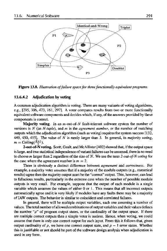
13.6. Numerical Software 291
Figure 13.8. Illustration of failure space for three functionally equivalent programs.
13.6.4.2 Adjudication by voting
A common adjudication algorithm is voting. There are many variants of voting algorithms,e.g., [295, 306, 473, 161, 297]. A voter compares results from two or more functionallyequivalent software components and decides which, if any, of the answers provided by thesecomponents is correct.
Majority voting. In an m-out-of-N fault-tolerant software system the number ofversions is N (an N-tuple), and m is the agreement number, or the number of matchingoutputs which the adjudication algorithm (such as voting) requires for system success [132,449, 450, 415]. The value of N is rarely larger than 3. In general, in majority voting,m = Ceiling(N+1/2).
2-out-of-N voting. Scott, Gault, and McAllister [402] showed that, if the output spaceis large, and true statistical independence of variant failures can be assumed, there is no needto choose m larger than 2 regardless of the size of N. We use the term 2-out-of-N voting forthe case where the agreement number is m = 2.
There is obviously a distinct difference between agreement and correctness. Forexample, a majority voter assumes that if a majority of the module outputs (e.g., numericalresults) agree then the majority output must be the "correct" output. This, however, can leadto fallacious results, particularly in the extreme case when the number of possible moduleoutputs is very small. For example, suppose that the output of each module is a singlevariable which assumes the values of either 0 or 1. This means that all incorrect outputsautomatically agree and it is very likely if modules have any faults there may be a majorityof LAW outputs. The behavior is similar to coincident and correlated failures.
In general, there will be multiple output variables, each one assuming a number ofvalues. The total number of allowed combinations of output variables and their values definesthe number "p" of program output states, or the cardinality of the output space. If thereare multiple correct outputs then a simple voter is useless. Hence, when voting, we couldassume that there is only one correct output for each input. From this it follows that, givenoutput cardinality of p, we have one correct output state, and p — 1 error states. Whetherthis is justifiable or not should be part of the software design analysis when adjudication isused in any form.

292 Chapter 13. Software-reliability Engineering of Numerical Systems
In that context, midvalue select (or simple median voting) is an interesting and simpleadjudication alternative whereby the median of all (numerical) output values is selected asthe correct answer. The philosophy behind the approach is that, in addition to being fast,the algorithm can handle multiple correct answers (and for small samples is less biased thanaveraging, or mean value voting), and it is likely to pick a value which is at least in thecorrect range. This technique has been applied successfully in aerospace applications.
A generalization of majority voting is consensus voting described in McAllister et al.[306, 307]. The consensus voting strategy is particularly effective in small output spacesbecause it automatically adjusts the voting to the changes in the effective output spacecardinality.
13.6.4.3 Tolerance
Closely related to voting is the issue of tolerance to which comparisons are made. LetTOL be the comparison tolerance, and consider an N-tuple of versions. The following twomutually exclusive events do not depend on whether the answers are correct or not.
1. All N components agree on an answer. In this case we have an "AGREEMENT"event.
2. There is at least one disagreement among the NC2 comparisons of alternate outputs,where NC2 denotes the number of combinations of N objects taken two at a time (2-tuples). We will call this case a "CONFLICT" event. All 2-tuples need to be evaluatedbecause agreement may not be transitive, that is, |a — b| TOL and |b — c| TOLdoes not always imply that |a — c| TOL (see Figure 13.9).
It is very important to realize that use of an inappropriate tolerance value, TOL,may either completely mask failure events (that is, too large a tolerance will always returnAGREEMENT events) or cause an avalanche of CONFLICT events (the tolerance is toosmall and therefore many answer pairs fail the tolerance test). Assume that we have an"oracle," so that we can tell the correctness of an answer.57 The following mutually exclusiveevents depend on the knowledge of the correctness of the output, or agreement with thecorrect answer:
1. All N components agree with the correct (call it "golden") answer. Then a"NO_FAILURE" event occurs.
2. One or more of the versions disagree with the correct answer. Then a "FAILURE"event occurs.
The following events are examples of subevents of the FAILURE event:
1. The majority of the versions disagree with the correct answer. We then say that a"MAJORITY_FAILURE" event has occurred. All but one of the versions disagreewith the correct answer.
2. Exactly k of the N (l k N) components disagree with the correct answer. Thisis a "k_ FAILURE" event.
57 For example, an "oracle" can take the form of an external consistency check.

13.6. Numerical Software 293
3. All the components disagree with the correct answer. Then an "N_FAILURE" eventhas occurred. If outputs are also identical, then comparisons will fail to signal anerror.
It is possible to define other states such as the majority of components agreeing withthe correct answer, two or more disagreeing, and exactly k agreeing. Combinations ofthe above "elementary" events produce the following mutually exclusive and collectivelyexhaustive multiversion comparison events:
1. An ALL_"CORRECT" event: a NO_FAILURE occurs with an AGREEMENT.
2. A "FALSE_ALARM" event: a NO_FAILURE occurs with a CONFLICT. Com-parison signals an error when one is not present which may or may not lead to afailure of the adjudication algorithm. Recall that agreement is not transitive, soFALSE_ALARM events are not inconsistent.
3. A "DETECTED_FAILURE" event: a FAILURE occurs together with a CON-FLICT. Comparison correctly detects a failure (fault).
4. A "UN_DETECTED_FAILURE" event: a FAILURE event occurs simultaneouslywith an AGREEMENT. This is the most significant event. A potential failure existsbut is not detected by comparison.
Consider again Figure 13.8 which shows responses from a hypothetical three versionsystem. A simplex failure (1_FAILURE) occurs when only one of the three versions fails(unshaded regions). A doublet failure (2-tuple, or 2_FAILURE) occurs when two compo-nents fail coincidentally (light shading). A triplet failure, or 3-tuple failure (N_FAILURE,N = 3), occurs when all three components fail coincidentally (dark shading). If the prob-ability that any of the shaded areas exceed or do not achieve the probability of overlapexpected by random chance, then the assumption of independence is violated [449, 450].That is,
or
where pi is the ith software variant.The most undesirable state of the system, UN_DETECTED_FAILURE, occurs when
the responses from three coincidentally failing versions are identical, in which case mutualcomparison of these answers does not signal that a failure has occurred.
Figure 13.9 provides an illustration of the events that may result from comparisonto tolerance TOL of floating-point outputs a, b, and c, from hypothetical programs P1, p2,and P3, respectively. Excessively small tolerances may produce an excessive incidence ofFALSE_ALARM events which may increase testing costs [470], while in operation this mayresult in degraded system operation, or even a critical system failure. The issue is discussedin more detail in [307].

294 Chapter 13. Software-reliability Engineering of Numerical Systems
Figure 13.9. Illustration of comparison events.
13.7 Basic Fault-tolerance TechniquesA principal way of introducing fault tolerance into a system is to provide a method todynamically determine if the system is behaving as it should, that is, an internal or externalresult verification, checking, or "oracle" capability. If unexpected and unwanted behavior(result) is detected, a fault-tolerant system then needs to provide a means of recovery orcontinuation of operation (preferably seamless from the perspective of the user). There aretwo basic ways of doing that: through partial, or complete, system state recovery and restarttechniques, and through forward recovery techniques. There is also the issue of safety, e.g.,[287].
It is important to understand that one can have a very safe system that has very littlefault tolerance in it. It is also possible to have a system that is highly fault tolerant, but whenit fails (rarely, one hopes), it can fail in an unsafe way. Hence, fault tolerance and safetyare not synonymous. Safety is concerned with failures (of any nature) that lead to failuresthat can result in unacceptable harm to the user; fault tolerance is primarily concerned withruntime prevention of failures in any shape and form (including prevention of safety-criticalfailures). When safety is defined properly and adequately in the system specifications, then awell-designed fault-tolerant system will also be a safe one. A fault-tolerant and safe systemwill both minimize overall failures and make sure that when a failure occurs it is a safe failure.
This section is intended only as a brief introduction into the world of fault-tolerantsoftware-based systems, including systems based on numerical software. For details, thereader is directed to key topic references such as [297] and [221].
13.7.1 Check-pointing and exception handling
A number of re-execution based methods exist (e.g., [297]). They include approachesthat periodically store known good states (and data) of the system and then roll back the

13.7. Basic Fault-tolerance Techniques 295
system to the closest check-pointed state if a problem is detected. Another set of methodsis concerned with trapping anomalies, transients, and exceptions and then handling theseevents in a graceful manner. Often recovery in both approaches includes partial or fullre-execution of the system software. If the recovery is reactive, i.e., it occurs as the resultof, and when, an immediate threat to system is detected, it may be disruptive.
The related term is software aging. It basically means that the state of a softwaresystem degrades with time [211]. Frequent causes of degradation are exhaustion of operatingsystem or application resources (such as memory leaks), data corruption, unreleased file-locks, and numerical error accumulation. Eventually, software aging may lead to systemperformance degradation, transient failures, and/or complete system stoppage. For example,popular and widely used software, such as the Web browser Netscape, is known to suffer fromserious memory leaks. Often, the only solution to this problem is to stop the applicationand restart it. This problem is particularly pronounced in systems low on swap space.Software aging has also been observed in specialized software used in high-availability andsafety-critical applications.
To counteract this phenomenon, a proactive approach of failure and fault manage-ment, called software rejuvenation, has been investigated by a number of researchers,e.g., [211, 434, 451]. It essentially involves detection of (anomalous) system parameterand variable patterns (fingerprints) and their correlation with undesirable system events (orfailures), i.e., detection of a growing A.( ). This is followed by occasional preventive, andwell-controlled, stoppage of the system, cleaning of its internal states, and system restart.This process removes the accumulated errors and frees up operating system and other re-sources, thus preventing in a proactive manner the unplanned and potentially expensivesystem outages due to software aging. Since the preventive action can be done at optimaltimes, for example, when the load on the system is low and noncritical, it reduces the cost ofsystem downtime compared to reactive recovery from failure. Thus, software rejuvenationis a cost-effective technique for dealing with software faults that include protection not onlyagainst hard failures but against performance degradation as well. Of course, its use has tobe judged against the need for continuity of services and similar factors.
13.7.2 Recovery through redundancy
Forward error recovery methods tend to be less disruptive from the end-user viewpoint.They detect an erroneous internal state of the system (that might lead to a failure), andtry to mask it, or on-the-fly transparently recover from it without resorting to stoppage ofthe system or excessive delays. Traditionally, they are used in information fault-tolerancecontexts—error coding being one example, e.g., [290, 103]. Two common fault-tolerantsoftware schemes that fall into the same general forward recovery class are the N-versionprogramming [21, 20] and the Recovery Block [373]. Both schemes are based on softwarecomponent redundancy and the assumption that coincident failures of components are rare,and when they do occur, responses are sufficiently dissimilar so that the mechanism fordeciding answer correctness is not ambiguous.
Fault-tolerant software mechanisms based on redundancy are particularly well suitedfor parallel processing environments where concurrent execution of redundant componentsmay drastically improve sometimes prohibitive costs associated with their serial execution[473, 27, 280]. The issue of fault tolerance will gain importance as computational, storage,

296 Chapter 13. Software-reliability Engineering of Numerical Systems
and application "Grids" become more prevalent [163]. Some hybrid techniques, suchas Consensus Recovery Block [401, 402], checkpoints [21], Community Error Recovery[454, 453], NVersion Programming variants [280, 435], and some partial fault-toleranceapproaches are also available [203,428, 316].
In this context, it is important to understand that redundancy in software, like inhardware, can take many forms. It may take the form of functionally equivalent softwaresolutions, but it can also take other forms. For example, use of redundant links in linkedlists is one form of fault tolerance that can help combat partial loss of list items [439].
13.7.2.1 Recovery blocks
One of the earliest fault-tolerant software schemes which used the multiversion softwareapproach is the Recovery Block (RB) [373,114]. The adjudication module is an acceptancetest (AT). The output of the first module is tested for acceptability. If the acceptance testdetermines that the output of the first module is not acceptable it restores, recovers, or "rollsback" the state of the system before the first or primary module is executed. It then allowsthe second module to execute and evaluates its output, etc. If all modules execute and noneproduce acceptable outputs, then the system fails.
A problem with this strategy in a uniprocessor environment is the sequential nature ofthe execution of the versions [280, 28]. In a distributed and/or multiprocessor environment,the modules and the acceptance tests can be executed in parallel. Distributed recovery blockis discussed in detail in [259,297]. Another potential problem is finding a simple, and highlyreliable, acceptance test which does not involve the development of an additional softwareversion.
The form of an acceptance test depends on the application. There may be a differentacceptance test for each module but in practice only one is usually used. An extreme case ofan acceptance test is another complete module, and the acceptance test would then consist ofa comparison of a given module output with the one computed by the acceptance test. Thiswould be equivalent to a staged 2-version programming scheme (see the following section)where one of the outputs in each stage is always from the same version (the acceptance test).
13.7.2.2 N-version programming
N-version programming (NVP) [21,91,20] proposes parallel execution of N independentlydeveloped functionally equivalent versions with adjudication of their outputs by a voter. N-version programming or multiversion programming (MVP) is a software generalization ofthe N-modular-redundancy (NMR) approach used in hardware fault tolerance [338]. The Nversions produce outputs to the adjudicator, which in this case is a voter. The voter acceptsall N outputs as inputs and uses these to determine the correct, or best, output if one exists.There is usually no need to interrupt the service while the voting takes place. We note thatthe approach can also be used to help during testing to debug the versions. This method,called back-to-back testing, is discussed further in [307].
Simple majority voting-based N-version fault-tolerant software has been investigatedby a number of researchers, both theoretically [21,180, 132,402,113, 293,469,250,297],and experimentally [403, 404, 34, 262, 411, 131, 299, 129, 474]. A reasonable alternativeto majority voting could be to use consensus voting as described earlier. Another simple

13.7. Basic Fault-tolerance Techniques 297
variation is median voting. There are also variants of the above architecture for distributedsystems. One such variant is the N-self-checking programming (NSCP) outlined below.
13.7.3 Advanced techniques
There are ways to combine the simple techniques to create hybrid techniques. Studies ofmore advanced models such as consensus recovery block [27,402,113,403,404], consensusvoting [306], or acceptance voting [27,19] are less frequent and mostly theoretical in nature.
13.7.3.1 Consensus recovery block
In [401] and [402] a hybrid system called consensus recovery block (CRB) was suggestedwhich combines NVP and RB in that order. If NVP fails the system reverts to RB (using thesame modules, the same module results can be used, or modules may be rerun if a transientfailure is suspected). Only in the case that both NVP and RB both fail does the system fail.CRB was originally proposed to treat the case of multiple correct outputs since appropriateacceptance testing can avoid that issue.
13.7.3.2 Acceptance voting
The "converse" of the CRB hybrid scheme, which we call acceptance voting (AV), wasproposed in [19, 157, 28]. As in NVP, all modules can execute in parallel. The output ofeach module is then presented to an acceptance test. If the acceptance test accepts the outputit is then passed to a voter.
The voter sees only those outputs which have been passed by the acceptance test. Thisimplies that the voter may not process the same number of outputs at each invocation andhence the voting algorithm must be dynamic. The system fails if no outputs are submitted tothe voter. If only one output is submitted, the voter must assume it to be correct and thereforepasses it to the next stage. Only if two or more outputs agree can the voter be used to makea decision. We then apply dynamic majority voting (DMV) or dynamic consensus voting(DCV). The difference between DMV and MV is that even if a small number of results arepassed to the voter, dynamic voting will try to find the majority among them. The concept issimilar for DCV and CV. Both Athavale [19] and Belli and Jedrzejowicz [27] have limitedtheir analytical work to DMV.
13.7.3.3 N self-checking programming
A variant of the N-version programming with recovery, that is, N self-checking program-ming, is used in the Airbus A310 system [280, 129]. In NSCP N modules are executed inpairs (for an even N) [280]. The outputs from the modules can be compared, or can be as-sessed for correctness in some other manner. Let us assume that comparison is used. Then,the outputs of each pair are tested and if they do not agree with each other, the response of thepair is discarded. If the outputs of both pairs agree then these outputs are compared again.Failure occurs if both pairs disagree or if the pairs agree but produce different outputs.

298 Chapter 13. Software-reliability Engineering of Numerical Systems
13.7.4 Reliability and performance
Although existing fault-tolerant software (FTS) techniques can achieve a significant im-provement over non-fault-tolerant software, they sometimes may not be sufficient for ensur-ing adequate reliability of critical systems and at the same time conform with the prevailingbusiness model, required timing and performance, and other constraints.
For example, experiments show that incidence of correlated failures of FTS systemcomponents may not be negligible in the context of current software development and testingtechniques, and this may result in a disaster [403, 472, 132, 262, 256, 255]. Furthermore,comparison tolerance issues [54] can also result in unexpected behavior unless they areproperly handled. This has led some researchers to question the validity of execution-timesoftware fault tolerance using the multiversion approach [262, 54]. Hence, it is importantto avoid, detect, and eliminate these errors as early as possible in the FTS life-cycle anddevelop FTS mechanisms that can adequately cope with any remaining faults.
Modeling different FTS mechanisms gives insight into their behavior and allowsquantification of their relative merits. Detailed FTS design, and reliability and performanceanalysis of fault-tolerant software systems, is beyond the scope of this tutorial. Interestedreaders are directed to the bibliography and the references in key references such as [280,297, 287, 298, 221].
13.8 SummaryThe day-to-day operation of our society is increasingly more dependent on software-basedsystems, and tolerance of failures of such systems is decreasing. Numerical software holdsone of the central positions in this context. Because of the high stakes involved, it is es-sential that the software be accurate, reliable, and robust. Numerical software has manycharacteristics of a general software system coupled with issues very specific to numericalalgorithms, their stability, their implementation in software, and the computational frame-work they run on. Hence, many software engineering techniques that apply to software ingeneral apply to numerical software as well.
In this paper we have first provided general information about the nature of softwarereliability engineering (SRE) and how it relates to software process, including factors suchas testing, cost, and benefits. This was followed by an overview of the SRE terminologyand modeling issues. Finally, SRE practice was addressed in both the general context andin the context of numerical software, as well as in the context of fault tolerance. We havediscussed specifics of SRE activities required during different software life-cycle phases,including an example of how to generate SRE-based test cases automatically. We have alsoillustrated issues that may arise in numerical software. Many other numerical issues exist,some very algorithm and application specific. We know enough today about the generalsoftware engineering technologies, as well as about the construction and implementation ofsound numerical algorithms, that we can make numerical software meet its specificationson time and within cost, provided a reasonable and realistic business model is employed.
Certainly, verification, validation, and testing of numerical software should be formal-ized. If diversity, or some other verification property, is relied upon, developers should striveto provide evidence that this property is present and preserved. It is also important to explic-itly show that appropriate and stable numerical algorithms have been implemented. With a

13.8. Summary 299
process that includes good specifications, realistic reliability, availability, and performanceparameters, careful inspection and testing of specifications, designs, and code, correct andfault-tolerant numerical software becomes a viable option for increasing reliability of anumerical software-based system.
More information, and access to SRE tools, can be obtained from the following site:http://renoir.csc.ncsu.edu/SRE/Tools/.

This page intentionally left blank

Bibliography
[ 1 ] J. A. ABRAHAM, G. METZE, R. K. IYER, AND J. H. PATEL, The evolution offault-tolerantcomputing at the University of Illinois, in Dependable Computing and Fault-TolerantSystems, A. Avizienis, H. Kopetz, and J.C. Laprie, eds., vol. 1, Springer- Verlag, Wienand New York, 1987, pp. 271-311.
[2] S. R. ABRAMSON, Customer satisfaction-based product development, in Proc. Intl.Switching Symp., vol. 2, Inst. Electronics, Information, Communications Engineers,Yokohama, Japan, 1992, pp. 65-69.
[3] F. S. ACTON, Numerical Methods that Usually Work, Harper & Row, New York, 1970.
[4] F. S. ACTON, REAL Computing Made REAL, .Preventing Errors in Scientific andEngineering Calculations, Princeton University Press, Princeton, New Jersey, 1996.
[5] E. ADAMS AND U. KULISCH, Scientific Computing with Automatic Result Verification,Academic Press, New York, 1993. See also the references therein.
[6] W. R. ADRION, M. A. BRANSTAD, AND J. C. CHERNIAVSKY, Validation, verification,and testing of computer software, ACM Comput. Surv., 14 (1982), pp. 159-192.
[7] AIAA, Guide for the verification and validation of computational fluid dynamicssimulations, Tech. Report AIAA-G-077-1998, American Institute for Aeronauticsand Astronautics, 1998.
[8] AIAA/ANSI, Recommended practice for software reliability, Tech. Report ANSI/AIAA, R-103-1992, American Institute of Aeronautics and Astronautics, 1993.
[9] M. AIGNER AND G. M. ZIEGLER, Proofs from THE BOOK, Springer-Verlag, Berlin,Heidelberg, 1998.
[10] G. ALEFELD, V. KREINOVICH, AND G. MAYER, On the shape of the symmetric, persym-metric, and skew-symmetric solution set, SIAM J. Matrix Anal. Appl., 18(3) (1997),pp. 693-705.
[11] G. ALEFELD AND G. MAYER, Interval analysis: Theory and applications, J. Comput.Appl. Math., 121 (2000), pp. 421-464.
301

302 BIBLIOGRAPHY
[12] E. ANDERSON, Z. BAI, C. H. BISCHOF, S. BLACKFORD, J. DEMMEL, J. J. DONGARRA,J. Du CROZ, A. GREENBAUM, S. HAMMARLING, A. MCKENNEY, AND D. C. SORENSEN,LAPACK Users' Guide, Software Environ. Tools 9. 3rd ed., SIAM, Philadelphia,1999.http://www.netlib.org/lapack/lug/.
[13] ANSI, American National Standard for Information Systems — Programming Lan-guage - C, ANSI X3 159-1989, ANSI, 1989.
[14] J. APPLEYARD, Comparing Fortran compilers, Fortran Forum, 20 (2001), pp. 6-10.See also the Fortran pages of http: / /www. polyhedron. com/.
[15] E. ARGE, A. M. BRUASET, P. B. CALVIN, J. F. KANNEY, H. P. LANGTANGEN, ANDC. T. MILLER, On the efficiency of C++ in scientific computing, in MathematicalModels and Software Tools in Industrial Mathematics, M. Daehlen and A. Tveito,eds., Birkhauser, Basel, 1997, pp. 91-118.
[16] M. ARIOLI, I. S. DUFF, AND D. RUIZ, Stopping criteria for iterative solvers, SIAM J.Matrix Anal. Appl., 13(1) (1992), pp. 138-144.
[17] ARUP, Summary report on the millennium bridge, 2003. http: //www.arup.com/MillenniumBridge.
[18] ASSOCIATED PRESS, Software disasters are often people problems, October 2004.http://www.msnbc.msn.com/id/6174622/.
[19] A. ATHAVALE, Performance evaluation of hybrid voting schemes, Tech. Report, M.S.Thesis, North Carolina State University, Department of Computer Science, December1989.
[20] A. AVIZIENlS, The N-version approach to fault-tolerant software, IEEE Transactionson Software Engineering, SE-11 (1985), pp. 1491-1501.
[21] A. AVIZIENlS AND L. CHEN, On the implementation of N-version programming forsoftware fault-tolerance during program execution, in Proc. COMPSAC 77, 1977,pp. 149-155.
[22] JOHN C. BAEZ, The octonions, Bull. Amer. Math. Soc., 39 (2002), pp. 145-205.http: / /math.ucr. edu/home/baez/Octonions/octonions .html.
[23] R. BARRETT, M. BERRY, T. CHAN, J. DEMMEL, J. DONATO, J. DONGARRA, V. EUKHOUT,R. Pozo, C. ROMINE, AND H. VAN DER VORST, Templates for the Solution of LinearSystems: Building Blocks for Iterative Methods, SIAM, Philadelphia, 1994.
[24] BBC, The Millennium bridge, 2000. http: / /news . bbc . co. uk/hi /english/static/in_depth/uk/2000/millennium_bridge/default.stm.
[25] H. BEHNKE, U. MERTINS, M. PLUM, AND CH. WIENERS, Eigenvalue inclusions viadomain decomposition, in Proc. Roy. Soc. London, A 456 (2000), pp. 2717-2730.
[26] BELLCORE, Reliability and quality measurements for telecommunications systems(RQMS), 1990. TR-TSY-000929, Issue 1, June 1990.

BIBLIOGRAPHY 303
[27] F. BELLI AND P. JEDRZEJOWICZ, Fault-tolerant programs and their reliability, IEEETrans. Rel., 29 (1990), pp. 184-192.
[28] , Comparative analysis of concurrent fault-tolerance techniques for real-timeapplications, in Proc. Intl. Symposium on Software Reliability Engineering, Austin,TX, 1991, pp. 202-209.
[29] M. BENNANI, T. BRACONNIER, AND J.-C. DUNYACH, Solving large-scale nonnor-mal eigenproblems in the aeronautical industry using parallel BIAS, in High-Performance Computing and Networking, W. Gentzsch and U. Harms, eds., vol. 796,Springer-Verlag, New York, 1994, pp. 72-77.
[30] K. BERKUN, London firms reportedly offer amnesty to "hacker thieves," TheRisks Digest, 8 (1989). http://catless.ncl.ac.uk/Risks/8-85.html#subj3.1.
[31] D. BERLEANT AND V. KREINOVICH, Intervals and probability distributions. h t t p: / /class.ee.iastate.edu/berleant/home/Servelnfo/Interval/intprob. html, 2003.
[32] M. BERZ AND K. MAKINO, Cosy infinity beam theory and dynamical systems group.http://cosy.pa.msu.edu/.
[33] D. BINDEL, J. DEMMEL, W. KAHAN, AND O. MARQUES, On computing Givens rotationsreliably and efficiently, ACM Trans. Math. Software, 28 (2002), pp. 206-238.
[34] P. G. BISHOP, D. G. ESP, M. BARNES, P. HUMPHREYS, G. DAHL, AND J. LAHTI, PODS-a project on diverse software, IEEE Trans. Soft. Eng., SE-12 (1986), pp. 929-940.
[35] R. H. BlSSELlNG, Parallel Scientific Computation: A Structured Approach Using BSPand MPI, Oxford University Press, Oxford, UK, 2004.
[36] L. S. BLACKFORD, A. CLEARY, J. DEMMEL, I. DHILLON, J. J. DONGARRA, S. HAMMAR-LING, A. PETTTET, H. REN, K. STANLEY, AND R. C. WHALEY. Practical experience inthe numerical dangers of heterogeneous computing. ACM Trans. Math. Software, 23(1997), pp. 133-147.
[37] R. M. BLOCH, Mark I calculator, in Proc. of a Symposium on Large-Scale DigitalCalculating Machinery, vol. 16 of The Annals of the Computation Laboratory ofHarvard University, Harvard University Press, Cambridge, MA, 1948, pp. 23-30.Reprinted, with a new introduction by William Aspray, Volume 7 in the Charles Bab-bage Institute Reprint Series for the History of Computing, MIT Press, Cambridge,MA, USA, 1985.
[38] B. W. BOEHM, Tutorial: Software Risk Management, IEEE Computer Society, LosAlamitos, CA, 1989.
[39] B. W. BOEHM, J. R. BROWN, H. KASPAR, M. LIPOW, G. J. MACLEOD, AND M. J.MERRTTT, Characteristics of software quality, Tech. Report TRW-SS-73-09, TRWSystems Group, December 1973.

304 BIBLIOGRAPHY
[40] G. BOHLENDER, Genaue Summation von Gleitkommazahlen, Computing, Suppl.l(1977), pp. 21-32.
[41] R. F. BOISVERT, J. MOREIRA, M. PHILlPPSEN, AND R. Pozo, Java and numericalcomputing, Computing in Science and Engineering, 3 (2001), pp. 18-24.
[42] R. F. BOISVERT, R. Pozo, K. REMINGTON, R. BARRETT, AND J. DONGARRA, TheMatrix Market, a Web repository for test matrix data, in The Quality of NumericalSoftware: Assessment and Enhancement, Ronald F. Boisvert, ed., Chapman & Hall,London, 1997.
[43] BOOST C++ LIBRARIES, Boost C++ libraries Web site. http: //www.boost,org/libs/libraries.htm.
[44] F. BORNEMANN, D. LAURIE, S. WAGON, AND J. WALDVOGEL, The SIAM 100-DigitChallenge: A Study in High-Accuracy Numerical Computing, SIAM, Philadelphia,2004. http: / /www. ec-securehost. com/SIAM/ot86 .html.
[45] G. E. P. Box, W. G. HUNTER, AND S. J. HUNTER, Statistics for Experimenters, JohnWiley & Sons, New York, 1978.
[46] T. BRACONNIER, Sur le calcul de valeurs propres en precision finie, Ph.D. Dissertation,Universite H. Poincare, Nancy, May 1994. TH/PA/94/24, CERFACS.
[47] T. BRACONNIER, F. CHATELIN, AND J.-C. DUNYACH, Highly nonnormal eigenvalueproblems in the aeronautical industry, Japan J. Ind. Appl. Math., 12 (1995), pp. 123-136.
[48] R. W. BRANKIN AND I. GLADWELL, Algorithm 771: rksuite_90: Fortran 90software for ordinary differential equation initial-value problems, ACM Trans. Math.Software, 23 (1997), pp. 402-15.
[49] R. W. BRANKIN, I. GLADWELL, AND L. F. SHAMPINE, RKSUITE: A suite of Runge-Kutta codes for the initial value problem for ODEs, Softreport 92-S1, MathematicsDepartment, Southern Methodist University, Dallas, TX, 1992.
[50] , RKSUITE: A suite of explicit Runge-Kutta codes, in Contributions to Nu-merical Mathematics, R. P. Agarwal, ed., World Scientific, River Edge, NJ, 1993,pp. 41-53.
[51] K. D. BRAUNE, Hochgenaue Standardfunktionen fur reelle und komplexe Punkte undIntervalle in beliebigen Gleitpunktrastern, dissertation, Universitat Karlsruhe, 1987.
[52] R. P. BRENT, Algorithms for Minimization without Derivatives, Prentice-Hall,Englewood Cliffs, NJ, 1973.
[53] L. C. BRIAND, W. M. THOMAS, AND C. J. HETSMANSKI, Modeling and managing riskearly in software development, in Proc. 15th ICSE, 1993, pp. 55-65.

BIBLIOGRAPHY 305
[54] S. S. BRILLIANT, J. C. KNIGHT, AND N. G. LEVESON, The consistent comparisonproblem in N-version software, ACM SIGSOFT Software Engineering Notes, 12(1987), pp. 29-34.
[55] S. BROCKLEHURST AND B. LITTLEWOOD, New ways to get accurate reliability mea-sures, IEEE Software, (1992), pp. 34-42.
[56] B. M. BROWN, D. K. R. McCORMACK, AND A. ZETTL, On the existence of an eigen-value below the essential spectrum, Proc. Roy. Soc. London, 455 (1999), pp. 2229-2234.
[57] C. G. BROYDEN, A new method of solving nonlinear simultaneous equations, Comput.J., 12 (1969), pp. 94-99.
[58] B. BUCHBERGER, Ein Algorithmus zum Auffinden der Basiselemente des Restklassen-ringes nach einem nulldimensionalen Polynomideal, Ph.D. Thesis, Universitat Ins-bruck, 1965.
[59] , Grobner bases: An algorithmic method in polynomial ideal theory, in RecentTrends in Multidimensional System Theory, N.K. Bose, ed., Reidel, Boston, 1985.
[60] J. M. BULL, L. A. SMITH, L. POTTAGE, AND R. FREEMAN, Benchmarking Javaagainst C and Fortran for scientific applications, in Proceedings of the 2001 JavaGrande/ISCOPE Conference, ACM, New York, 2001, pp. 97-105.
[61] C++THREADS, C++ Threads Web site. http: / /threads. sourcef orge. net.
[62] CALGO, Collected Algorithms of the ACM. http: / /www. acm. org/calgo.
[63] C. CAMACHO AND L. H. DE FIGUEIREDO, The dynamics of the Jouanolou foliationon the complex projective 2-space, Ergodic Theory and Dynamical Systems, 21(2001), pp. 757-766. ftp://ftp.tecgraf.puc-rio.br/pub/lhf/doc/etds .ps .gz.
[64] W. C. CARTER, Architectural considerations for detecting run-time errors in pro-grams, in Proc. 13th Int Symp. On Fault-Tolerant Computing (FTCS-13), Milano,Italy, IEEE Computer Society, Los Alamitos, CA, 1983, pp. 249-256.
[65] B. CHABAT, Introduction a l'Analyse Complexe, Tome 1, Mir, Moscow, Russia, 1990.
[66] G. J. CHAITIN, Exploring Randomness, Springer-Verlag, Singapore, 2001.
[67] F. CHAITIN-CHATELIN, Is nonnormality a serious computational difficulty in prac-tice ?, in Quality of Numerical Software, R. Boisvert, ed., Chapman and Hall, London,1997, pp. 300-314.
[68] , About singularities in Inexact Computing, Technical Report TR/PA/ 02/106,CERFACS, Toulouse, France, 2002.
[69] , The Arnoldi method in the light of Homotopic Deviation theory, TechnicalReport TR/PA/03/15, CERFACS, Toulouse, France, 2003.

306 BIBLIOGRAPHY
[70] , Computing beyond Analyticity. Matrix algorithms in Inexact and UncertainComputing, Technical Report TR/PA/03/110, CERFACS, Toulouse, France, 2003.
[71 ] , Elements of Hypercomputations on R and Z2 with the Dickson-Albert inductiveprocess, Technical Report TR/PA/03/34, CERFACS, Toulouse, France, 2003.
[72] , On a recursive hierarchy for Numbers algorithmically emerging from process-ing binary sequences, Technical Report TR/PA/03/08, CERFACS, Toulouse, France,2003.
[73] , The dynamics of matrix coupling with an application to Krylov methods,Technical Report TR/PA/04/29, CERFACS, Toulouse, France, 2004.
[74] F. CHAITIN-CHATELIN, S. DALLAKYAN, AND V. FRAYSSE, An overview of CarrierPhase Differential GPS, Contract Report IR/PA/99/50, CERFACS, 1999.
[75] F. CHAITIN-CHATELIN AND V. FRAYSSE, Lectures on Finite Precision Computa-tions, Software Environ. Tools 1. SIAM, Philadelphia, 1996. http://www.ec-securehost.com/SIAM/SE01.html#SE01.
[76] F. CHAITIN-CHATELIN, V. FRAYSSE, AND S. GRATTON, Fiabilite des calculs en pre-cision finie: Principes et mise en ceuvre, Contract Report FR/PA/97/55, CERFACS,1997.
[77] F. CHAITIN-CHATELIN AND S. GRATTON, Convergence of successive iteration methodsin finite precision under high nonnormality, BIT, 36 (1996), pp. 455-469.
[78] , Etude de la non convergence de Gauss-Newton, Contract Report IR/PA/97/14,CERFACS, 1997.
[79] F. CHAITIN-CHATELIN, A. HARRABI, AND A. ILAHI, About Holder condition numbersand the stratification diagram for defective eigenvalues, in 1999 International Sympo-sium on Computational Science, 54, North-Holland, Amsterdam, 2000, pp. 397-402.
[80] F. CHAITIN-CHATELIN AND T. MESKAUSKAS, Inner-outer iterations for mode solverin structural mechanics application to Code Aster, Contract Report FR/PA/02/06,CERFACS, Toulouse, France, 2002.
[81] F. CHAITIN-CHATELIN, T. MESKAUSKAS, AND A. N. ZAOUI, Hypercomplex division inthe presence of zero divisors on R and Z2, Technical Report TR/PA/02/29, CERFACS,Toulouse, France, 2002.
[82] F. CHAITIN-CHATELIN AND E. TRAVIESAS, PRECISE, a toolbox for assessing thequality of numerical methods and software, Tech. Report TR/PA/00/12, CERFACS,Toulouse, France, 2000. Special session on Recommender systems (N. Ramakrishnanorganizer), 16th IMACS World Congress, Lausanne, Switzerland, 2000.
[83] F. CHAITIN-CHATELIN AND E. TRAVIESAS, Homotopic perturbation—unfolding thefield of singularities of a matrix by a complex parameter: A global geometric ap-proach, Technical Report TR/PA/01/84, CERFACS, Toulouse, France, 2001.

BIBLIOGRAPHY 307
[84] F. CHAITIN-CHATELIN AND M. VAN GIJZEN, Homotopic Deviation theory with anapplication to Computational Acoustics, Technical Report TR/PA/04/05, CERFACS,Toulouse, France, 2004.
[85] T. F. CHAN, G. H. GOLUB, AND R. J. LEVEQUE, Algorithms for computing the samplevariance: Analysis and recommendations, The American Statistician, 37 (1983),pp. 242-247.
[86] C. CHARALAMBOUS AND J. W. BANDLER, Non-linear Minimax Optimization as aSequence of Least pth Optimization with Finite Values of p, J. Comput. System Sci.,7 (1976), pp. 377-391.
[87] F. CHATELIN, Spectral Approximation of Linear Operators, Academic Press, NewYork, 1983.
[88] , Valeurs propres de matrices, Masson, Paris, 1988.
[89] , Les ordinateurs calculent faux et c'est tant mieux, Juin 1991. Journees Ob-servatoire de Paris.
[90] , Eigenvalues of Matrices, Wiley, Chichester, U.K., 1993. Enlarged translationof the French publication [88] with Masson.
[91] L. CHEN AND A. AVIZIENIS, N-version programming: A fault-tolerance approach toreliability of software operation, in Proc. FTCS 8, Toulouse, France, 1978, pp. 3-9.
[92] D. A. CHRISTENSON, S. T. HUANG, AND A. J. LAMPEREZ, Statistical quality controlapplied to code inspections, IEEE J. on Selected Areas in Communications, 8 (1990),pp. 196-200.
[93] E. M. CLARKE AND J. M. WING, Formal methods: State of the an and future directions,ACM Computing Surveys, 28 (1996), pp. 626-643.
[94] D. M. COHEN, S. R. DALAL, M. L. FREDMAN, AND G. C. PATTON, TheAETG system:An approach to testing based on combinatorial design, IEEE Trans. Soft. Eng., 23(1997), pp. 437-444.
[95] D. M. COHEN, S. R. DALAL, A. KAJLA, AND G. C. PATTON, The automatic efficient testgenerator (AETG) system, in Proc. IEEE Int. Symp. Software Reliability Engineering,1994, pp. 303-309.
[96] D. M. COHEN, S. R. DALAL, J. PARELIUS, AND G. C. PATTON, Combinatorial designapproach to test generation, IEEE Software, (1996), pp. 83-88.
[97] M. COHEN, Information technology - Programming languages - Fortran - Enhanceddata type facilities, ISO/IEC 15581:2001, 2001.
[98] L. COLLATZ, Einschlieftungssatz fur die charakteristischen Zahlen von Matrizen,Math. Z., 48 (1942), pp. 221-226.

308 BIBLIOGRAPHY
[99] G. E. COLLINS, Quantifier elimination for real closed fields by cylindrical algebraicdecompositon, in Automata Theory and Formal Languages, B.F. Caviness, ed., Lec-ture Notes in Comput. Sci. 33, Springer-Verlag, Berlin, 1975, pp. 134-183.
[100] R. COOLS, Approximating integrals, estimating errors and giving the wrong solutionfor deceptively easy problems, 2003. MATLAB program as a zip-file, http: //www. cs .kuleuven.be/~ronald/perfprof iles/scripts . zip.
[101] R. P. CORBETT, Enhanced arithmetic for Fortran, SIGPLAN Notices, 17 (1982),pp. 41-48.
[102] G. F. CORLISS, Comparing software packages for interval arithmetic. Preprint pre-sented at SCAN'93, Vienna, 1993.
[103] D. J. COSTELLO, J. HAGENAUER, H. IMAI, AND S.B. WICKER, Applications of error-control coding, IEEE Trans. Inform. Theory, 44 (1998), pp. 2531-2560.
[104] M. G. Cox, M. P. DAINTON, AND P. M. HARRIS, Testing spreadsheets and otherpackages used in metrology: Testing functions for the calculation of standard devia-tion, NPL Report CMSC 07/00, Centre for Mathematics and Scientific Computing,National Physical Laboratory, Teddington, Middlesex, U.K., 2000.
[105] R. CRAMP, M. A. VOUK, AND W. JONES, On operational availability of a largesoftware-based telecommunications system, in Proc. Third Intl. Symposium on Soft-ware Reliability Engineering, IEEE Computer Society, Los Alamitos, CA, 1992,pp. 358-366.
[106] D. E. CULLER, R. M. KARP, D. A. PATTERSON, A. SAHAY, K. E. SCHAUSER, E. SANTOS,R. SUBRAMONIAN, AND T. VON ElCKEN, LogP: Towards a realistic model of parallelcomputation, ACM SIGPLAN Notices, 28 (1993), pp. 1-12.
[107] D. E. CULLER, J. P. SINGH, AND A. GUPTA, Parallel Computer Architecture: A Hard-ware/Software Approach, Morgan Kaufmann, San Francisco, 1999.
[108] G. DAHLQUIST AND A. BJORCK, Numerical methods, Prentice-Hall, EnglewoodCliffs, NJ, 1980. Second heavily expanded edition Numerical Mathematics andScientific Computation to be published in three volumes by SIAM, Philadelphia. Thefirst edition reprinted by Dover, 2003.
[109] S. R. DALAL AND C. L. MALLOWS, Factor-covering designs in testing software, Tech-nometrics, 40 (1998), pp. 234-243.
[110] B. K. DANIELS AND M. HUGHES, A literature survey of computer software reliability,Tech. Report NCSR R16, National Centre of Systems Reliability, UKAEA, WigshawLane, Culcheth, Warrington, U.K., 1979.
[1ll] DARPA, High Productivity Computer Systems. http://www.highproductivity.org/.
[112] R. DAVIES, Newmat C++ matrix library, http://www.robertnz.net/nm__intro.htm.

BIBLIOGRAPHY 309
[113] A. K. DEB, Stochastic Modelling for Execution Time and Reliability of Fault-TolerantPrograms Using Recovery Block and N-Version Schemes, Ph.D. Thesis, SyracuseUniversity, 1988.
[114] A. K. DEB AND A. L. GOEL, Model for execution time behavior of a recovery block,in Proc. COMPSAC 86, 1986, pp. 497-502.
[115] B. DEVOLDER, J. GLIMM, J. W. GROVE, Y. KANG, Y. LEE, K. PAO, D. H. SHARP,AND K. YE, Uncertainty quantification for multiscale simulations, Journal of FluidsEngineering, 124 (2002), pp. 29-41.
[116] C. F. DIETRICH, Uncertainty, Calibration and Probability: The Statistics of Scientificand Industrial Measurement, 2nd ed., Adam Hilger, Bristol, England, 1991.
[117] DIFFPACK SOFTWARE PACKAGE, Diffpack software package Web site, http: / /www.diffpack. com.
[118] D. S. DODSON, Corrigendum: Remark on "Algorithm 539: Basic Linear AlgebraSubroutines for Fortran usage," ACM Trans. Math. Software, 9 (1983), p. 140.
[119] D. S. DODSON AND R. G. GRIMES, Remark on "Algorithm 539: Basic Linear AlgebraSubprograms for Fortran usage," ACM Trans. Math. Software, 8 (1982), pp. 403-404.
[ 120] J. J. DONGARRA, J. J. DU CROZ, S. J. HAMMARLING, AND R. J. HANSON, Algorithm 656.An extended set of Fortran basic linear algebra subprograms: Model implementationand test programs, ACM Trans. Math. Software, 14 (1988), pp. 18-32.
[121] J. DONGARRA, I. FOSTER, G. Fox, W. GROPP, K. KENNEDY, AND L. TORCZON, eds.,The Sourcebook of Parallel Computing, Morgan Kaufmann, San Francisco, 2002.
[122] J. J. DONGARRA, J. Du CROZ, I. S. DUFF, AND S. HAMMARLING, A set of Level 3 BasicLinear Algebra Subprograms, ACM Trans. Math. Software, 16 (1990), pp. 1-28.(Article on pp. 1-17, Algorithm 679 on pp. 18-28.)
[123] J. J. DONGARRA, J. Du CROZ, S. HAMMARLING, AND R. J. HANSON, Corrigenda: "Anextended set of FORTRAN Basic Linear Algebra Subprograms," ACM Trans. Math.Software, 14 (1988), p. 399.
[124] , An extended set of FORTRAN Basic Linear Algebra Subprograms, ACMTrans. Math. Software, 14 (1988), pp. 1-32, 399. (Algorithm 656. See also [123].)
[125] C. C. DOUGLAS, M. HEROUX, G. SLISHMAN, AND R. M. SMITH, GEMMW: A portablelevel 3 BIAS Winograd variant of Strassen 's matrix-matrix multiply algorithm, J.Comput. Phys., 110 (1994), pp. 1-10.
[126] C. C. DOUGLAS, J. Hu, W. KARL, M. KOWARSCHIK, U. RUEDE, AND C. WEISS, Cacheoptimization for structured and unstructured grid multigrid, Electron. Trans. Numer.Anal., 10 (2000), pp. 25-40.

310 BIBLIOGRAPHY
[127] C. C. DOUGLAS, J. Hu, M. KOWARSCHIK, AND U. RUEDE, Very high performancecache based techniques for solving iterative methods. http: //www.mgnet.org/~douglas/ml-dddas .html.
[128] I. S. DUFF, R. G. GRIMES, AND J. G. LEWIS, User's guide for Harwell-Boeing sparsematrix test problems collection, Tech. Report RAL-92-086, Computing and Informa-tion Systems Department, Rutherford Appleton Laboratory, Didcot, U.K., 1992.
[129] J. B. DUGAN AND R. VAN BUREN, Reliability evaluation of fly-by-wire computersystems, J. Systems and Safety, (1993), pp. 109-124.
[130] P. S. DWYER, Computation with approximate numbers, in Linear Computations, P. S.Dwyer, ed., Wiley, New York, 1951, pp. 11-34.
[131] D. E. ECKHARDT, A. K. CAGLAYAN, J. R J. KELLY, J. C. KNIGHT, L. D. LEE, D. F.MCALLISTER, AND M.A. VOUK, An experimental evaluation of software redundancyas a strategy for improving reliability, IEEE Trans. Soft. Eng., 17 (1991), pp. 692-702.
[132] D. E. ECKHARDT AND L. D. LEE, A theoretical basis for the analysis of multi-version software subject to coincident errors, IEEE Trans. Soft. Eng., SE-11 (1985),pp. 1511-1517.
[133] J.-P. ECKMANN AND P. WlTTWER, Computer Methods and Borel Summability Appliedto Feigenbaum's Equation, Lecture Notes in Phys. 227. Springer-Verlag, Berlin,Heidelberg, New York, Tokyo, 1985.
[134] W. EHRLICH, B. PRASANNA, J. SAMPFEL, AND J. Wu, Determining the cost of stop-testdecisions, IEEE Software, 10 (1993), pp. 33-42.
[135] M. EMBREE AND N. TREFETHEN, Pseudospectra gateway. http: / /web. comlab.ox.ac.uk/projects/pseudospectra/.
[136] D. ENGLER, B. CHELF, A. CHOU, AND S. HALLEM, Checking system rules usingsystem-specific, programmer-written compiler extensions, in Proceedings of theFourth Symposium on Operating Systems Design and Implementation (OSDI2000),San Diego, Berkeley, 2000. http://www.usenix.org/publications/library/proceedings/osdi2000/engler.html.
[137] W. H. ENRIGHT, K. R. JACKSON, S. P. N0RSETT, AND P. G. THOMSEN, Interpolants forRunge-Kutta formulas, ACM Trans. Math. Software, 12 (1986), pp. 193-218.
[138] F2PY SOFTWARE PACKAGE, F2PY- Fortran to Python interface generator. http: / /cens.ioc.ee/projects/f2py2e.
[139] R. FAIRLEY, Software Engineering Concepts, McGraw-Hill, New York, 1985.
[140] W. H. FARR, Statistical modeling and estimation of reliability functions for software(SMERFS)—library access guide, Tech. Report TR84-371 (Rev.l), Naval SurfaceWarfare Center, Dahlgren VA, 1988. Also SMERFS User's Guide, TR84-373 (Rev.l).

BIBLIOGRAPHY 311
[141] FCC, Notification by common carriers of service disruptions, Tech. Report 47 CFRPart 63, Federal Register, Vol. 57 (44), March 5, Federal Communications Commis-sion, 1992.
[142] C. A. FLOUDAS, Handbook of Test Problems for Local and Global Optimization,Kluwer Academic Publishers, Dordrecht, 1999.
[143] G. E. FORSYTHE, What is a satisfactory quadratic equation solver, in ConstructiveAspects of the Fundamental Theorem of Algebra. B. Dejon and P. Henrici, eds., Wiley,New York, 1969, pp. 53-61.
[144] , Pitfalls in computation, or why a math book isn't enough, Amer. Math.Monthly, 9 (1970), pp. 931-995.
[145] L. D. FOSDICK AND L. J. OSTERWEIL, Dataflow analysis in software reliability, ACMComputing Surveys, 8 (1976), pp. 305-330.
[146] L. V. FOSTER, Gaussian elimination with partial pivoting can fail in practice, SIAMJ. Matrix Anal. Appl., 15 (1994), pp. 1354-1362.
[147] R.FowLER,HPCToolkit.http: //www.hipersof t. rice. edu/hpctoolkit.
[148] L. Fox, How to get meaningless answers in scientific computation (and what to doabout it), IMA Bulletin, 7 (1971), pp. 296-302.
[149] E. G. FRANKEL, Systems Reliability and Risk Analysis, Kluwer Academic Publishers,Dordrecht, 1988.
[150] V. FRAYSSE, L. GIRAUD, AND V. TOUMAZOU, Parallel computation of spectral portraitson the Meiko CS2, in High-Performance Computing and Networking, H. Liddell,A. Colbrook, B. Hertzberger, and P. Sloot, eds., Lecture Notes in Comput. Sci. 1067,Springer-Verlag, New York, 1996, pp. 312-318.
[151] V. FRAYSSE AND S. GRATTON, Moindres carres pour Vorbitographie - Etude destabilite - Partie II, Contract Report FR/PA/95/28, CERFACS, 1995.
[152] V. FRAYSSE, S. GRATTON, AND V. TOUMAZOU, Structured backward error and condi-tion number for linear systems of the type A* Ax = b, BIT, 40 (2000), pp. 74-83.
[153] V. FRAYSSE, M. GUEURY, F. NICOUD, AND V. TOUMAZOU, Spectral portraits for matrixpencils: A physical application, Tech. Report TR/PA/96/19, CERFACS, 1996.
[154] V. FRAYSSE AND G. W. STEWART, References on the Vancouver Stock Exchange,2000. (1) The Wall Street Journal, November 8, 1983, p. 37. (2) The TorontoStar, November 19, 1983. (3) B.D. McCullough and H.D. Vinod, The Numer-ical Reliability of Econometric Software, Journal of Economic Literature, VolXXXVII (June 1999), pp. 633-665. http://www.aeaweb.org/journal/contents/june1999.html#AN0494689.

312 BIBLIOGRAPHY
[155] A. FROMMER, Proving Conjectures by Use of Interval Arithmetic, in Perspectiveson enclosure methods. SCAN 2000, GAMM-IMACS international symposium onscientific computing, computer arithmetic and validated numerics, Univ. Karlsruhe,Germany, 2000. U. Kulisch et al., ed., Springer, Wien, 2001.
[156] W. A. FULLER, Measurement Error Models, John Wiley & Sons, New York, 1987.
[157] R.E. GANTENBEIN, S.Y. SHIN, AND J.R. COWLES, Evaluation of combined approachesto distributed software-based fault tolerance, in Pacific Rim International Symposiumon Fault Tolerant Systems, 1991, pp. 70-75.
[158] GAO, GAO Report, Patriot Missile Defense—software problem led to system fail-ure at Dhahran, Saudi Arabia, Tech. Report B-247094, United States General Ac-counting Office, February 1992. http://www.fas.org/spp/starwars/gao/ im92026.htm.
[159] I. GARGANTINI AND P. HENRICI, Circular arithmetic and the determination of poly-nomial zeros, Numer. Math., 18 (1972), pp. 305-320.
[160] F. GASPERONI AND G. DISMUKES, Multilanguage programming on the JVM, in TheAda 95 Benefits, Proceedings of the Sig'Ada Conference, 2000.
[161] J. GERSTING, R. L. NIST, D. R. ROBERTS, AND R. L. VAN VALKENBURG, A comparisonof voting algorithms for n-version programming, in Proc. 24th Ann. Hawaii Intl.Conf. on System Sciences, vol. II, 1991, pp. 253-262. Reprinted in Fault-TolerantSoftware Systems: Techniques and Applications, Hoang Pham, ed., IEEE ComputerSociety, Los Alamitos, CA, 1992, pp. 62-71.
[162] D. GERT, Euro page: Conversion arithmetics. Webpage no longer available but asimilar page is http: / / ta . twi . tudelft.nl/nw/users/vuik/wi211/disasters .html#euro. Background information is available in EuropeanCentral Bank, Fixed euro conversion rates. http://www.ecb.int/bc/intro/html/index, en.html#fix, 2001.
[163] GGF, Global Grid Forum. http: / /www. gridf orum. org/ and references andlinks therein. Also available as http: / /www. ggf. org/.
[164] W. GIVENS, Numerical computation of the characteristic values of a real symmetricmatrix, Technical Report ORNL-1574, Oak Ridge National Laboratory, Oak Ridge,TN, 1954.
[165] GNU, GNU Compiler Collection. http: / /gcc . gnu. org/.
[166] S. GODET-THOBIE, Eigenvalues of large highly nonnormal matrices (Valeurs pro-pres de matrices hautement non normales en grande dimension), Ph.D. Dissertation,Universite Paris IX Dauphine, 1992.
[167] S. GOEDECKER AND A. HOISIE, Performance Optimization of Numerically IntensiveCodes, Software Environ. Tools 12, SIAM, Philadelphia, 2001.

BIBLIOGRAPHY 313
[168] A. L. GOEL AND K. OKUMOTO, Time-dependent error-detection rate model for soft-ware reliability and other performance measures, IEEE Trans. Reliability, R-28(1979), pp. 206-211.
[169] G. H. GOLUB, Numerical methods for solving linear least squares problems, Numer.Math., 7 (1965), pp. 206-216.
[170] G. H. GOLUB AND C. F. VAN LOAN, Matrix Computations, 3rd ed. Johns HopkinsStudies in the Mathematical Sciences, The Johns Hopkins University Press, Balti-more, MD, 1996.
[171] R. E. GOMORY, Outline of an algorithm for integer solution to linear programs., Bull.Amer. Math. Soc., 64 (1958), pp. 275-278.
[172] J. GOSLING, B. JOY, G. STEELE, AND G. BRACHA, The Java Language Specification,2nd ed. Addison-Wesley, Reading, MA, 2000.
[173] J. GRABMEIER, E. KALTOFEN, AND V. WEISPFENNIG, Computer Algebra Handbook,Springer-Verlag, New York, 2003.
[174] S. GRATTON, On the condition number of linear least squares problems in a weightedFrobenius norm, BIT, 36 (1996), pp. 523-530.
[175] , Outils theoriques d'analyse du calcul a precision finie, Ph.D. Dissertation,Institut National Polytechnique de Toulouse, 1998. TH/PA/98/30, CERFACS.
[176] J. GRAY, A census of tandem system availability between 1985 and 1990, IEEE Trans.Reliability, 39 (1990), pp. 409-418.
[177] D. GRIES, Science of Programming, Springer-Verlag, Berlin, 1984.
[178] A. GRIEWANK, Evaluating Derivatives: Principles and Techniques of AlgorithmicDifferentiation, Frontiers Appl. Math., 19. SIAM, Philadelphia, 2000.
[179] A. GRIEWANK AND G. F. CORLISS, eds., Automatic Differentiation of Algorithms:Theory, Implementation, and Application, SIAM, Philadelphia, 1991.
[180] A. GRNAROV, J. ARLAT, AND A. AVIZIENIS, On the performance of software fault-tolerance strategies, in Proc. FTCS 10, 1980, pp. 251-253.
[181] W. GROPP, Exploiting existing software in libraries: Successes, failures, and rea-sons why, in Object Oriented Methods for Interoperable Scientific and EngineeringComputing, Michael Henderson, Christopher Anderson, and Stephen L. Lyons, eds.,Proc. Appl. Math. 99, SIAM, Philadelphia, 1999, pp. 21-29.
[182] S. J. GROTZINGER, Supports and Convex Envelopes, Math. Programming, 31 (1985),pp. 339-347.
[183] MUPAD RESEARCH GROUP, Interval arithmetic. http://research.mupad.de/doc30+M554e9f 5985d.html, 2003.

314 BIBLIOGRAPHY
[184] J. A. GUNNELS, F. G. GUSTAVSON, G. M. HENRY, AND R. A. VAN DE GEIJN, FLAME:Formal Linear Algebra Methods Environment, ACM Trans. Math. Software, 27(2001), pp. 422-455. http: / /www. cs .utexas . edu/users/flame/.
[185] E. GUNTHNER AND M. PHILIPPSEN, Complex numbers for Java, Concurrency: Practiceand Experience, 23 (2000), pp. 477-491.
[186] E. HAIRER AND G. WANNER, Solving Ordinary Differential Equations II. Stiff andDifferential-Algebraic Problems, Springer Series in Comput. Mathematics 14,Springer-Verlag, New York, 1996.
[187] J. G. HAJAGOS, Modeling uncertainty in population biology: How the model is writ-ten does matter. http://www.stat.lanl.gov/SAM02004/abstracts/pdf_files/Abs_046%20J_Hajagos.pdf, 2003.
[188] T. C. HALES, Cannonballs and honeycombs, Notices of the AMS, 47 (2000), pp. 440-449.
[189] R. HAMMER, M. HOCKS, U. KULISCH, AND D. RATZ, C++ Toolbox for Verified Com-puting: Basic Numerical Problems, Springer-Verlag, Berlin, 1995.
[190] J. HANDY, The Cache Memory Book, Academic Press, New York, 1998.
[191] E. HANSEN AND G. W. WALSTER, Global Optimization Using Interval Analysis, Mar-cel Dekker, New York, 2003.
[192] E. R. HANSEN, Global optimization using interval analysis—the one dimensionalcase, J. Optim. Theory Appl., 29 (1979), pp. 331-334.
[193] E. R. HANSEN, Global Optimization Using Interval Analysis, Marcel Dekker, NewYork, 1992.
[194] , Publications related to early interval work of R. E. Moore, 2001. http: / /interval.louisiana.edu/Moores_early_papers/bibliography,html.
[195] P. B. HANSEN, An evaluation of the Message-Passing Interface, ACM SIGPLANNotices, 33 (1998), pp. 65-72.
[196] G. HARGREAVES, Interval Analysis in MATLAB, master's thesis, University of Manch-ester, 2002.
[197] J. HARRISON, Formal verification of floating point trigonometric functions, in Pro-ceedings of the 3rd International Conference on Formal Methods in Computer-AidedDesign (FMCAD), Warren A. Hunt and Steven D. Johnson, eds., 1954, Springer-Verlag, New York, 2000, pp. 217-233.
[198] , Formal verification of square root algorithms, Formal Methods in SystemDesign, 22 (2003), pp. 143-153.

BIBLIOGRAPHY 315
[199] J. MASS, M. HUTCHINGS, AND R. SCHLAflY, The Double Bubble Conjecture, Elec.Res. Announcement of the Am. Math. Soc., 1(3) (1995), pp. 98-102.
[200] L. HATTON, Safer C: Developing Software for High-Integrity and Safety-CriticalSystems, McGraw-Hill, New York, 1995. http://www.oakcomp.co.uk/TP_Books.html.
[201] , The T-experiments: Errors in scientific software, in Quality of Numerical Soft-ware: Assessment and Enhancement, Proceedings of the IFTPTC 2/WG 2.5 WorkingConference in Oxford, England, 8-12 July 1996, R. F. Boisvert, ed., Chapman &Hall, London, New York, 1997, pp. 12-31.
[202] A. M. HAYASHI, Rough sailing for smart ships, Scientific American, 1998.
[203] H. HECHT, Fault tolerant software, IEEE Trans. Reliability, R-28 (1979), pp. 227-232.
[204] D. J. HICHAM AND N. J. HIGHAM, MATLAB Guide, 2nd ed., SIAM, Philadelphia,2005. http://www.ec-securehost.com/SIAM/ot92.htmlttOT92.
[205] N. J. HIGHAM, Accuracy and Stability of Numerical Algorithms, 2nd ed., SIAM,Philadelphia, 2002. http://www.ec-securehost.com/SIAM/ot80.html#ot80.
[206] N. J. HIGHAM, Can you "count" on your computer? Public lecture for Science Week1998, http: //www.ma.man.ac.uk/~higham/talks/.
[207] J. M. D. HILL, B. MCCOLL, D. C. STEFANESCU, M. W. GOUDREAU, K. LANG, S. B.RAO, T. SUEL, T. TSANTILAS, AND R. H. BlSSELING, BSPlib: The BSP programminglibrary, Parallel Computing, 24 (1998), pp. 1947-1980.
[208] P. HOFFMAN, The Man Who Loved Only Numbers, Hyperion, New York, 1998.
[209] J. J. Hu, Cache BasedMultigrid on Unstructured Grids in Two and Three Dimensions,Ph.D. Thesis, Department of Mathematics, University of Kentucky, Lexington, KY,2000.
[210] K.-H. HUANG AND J. A. ABRAHAM, Algorithms-based fault-tolerance for matrix op-erations, IEEE Trans. Computers, C-33 (1984), pp. 518-528.
[211] Y. HUANG, C. KINTALA, N. KOLETTIS, AND N. D. FULTON, Software rejuvena-tion: Analysis, module and applications, in Twenty-Fifth International Symposiumon Fault-Tolerant Computing, IEEE Computer Society, Los Alamitos, CA, 1995,pp. 381-390.
[212] T. HUCKLE, Collection of Software Bugs, 2002. http://www5.in.tum.de/~huckle/bugse.html.
[213] J. HUDAK, B. SUH, D. SIEWlOREK, AND Z. SEGALL, Evaluation and comparison offault-tolerant software techniques, IEEE Trans. Reliability, 42 (1993), pp. 190-204.

316 BIBLIOGRAPHY
[214] T. E. HULL, T. F. FAIRGRIEVE, AND P. T. P. TANG, Implementing complex elementaryfunctions using exception handling, ACM Trans. Math. Software, 20 (1994).
[215] IEEE, ANSI/IEEE standard 754-1985, 1985. Standard for Binary Floating-PointArithmetic, usually called IEEE 754, officially now IEC 60559.
[216] , IEEE standard 1012-1986, 1986. Software Verification and Validation Plans.
[217] , ANSI/IEEE standard 854-1987, 1987. Standard for Radix-IndependentFloating-Point Arithmetic, usually called IEEE 854.
[218] IEEE, IEEE standard 982.1-1988,1988. Dictionary of Measures to Produce ReliableSoftware.
[219] , IEEE standard 982.2-1988, 1988. IEEE Guide for the Use of IEEE StandardDictionary of Measures to Produce Reliable Software.
[220] IEEE, IEEE standard 610.12-1990,1990. Glossary of Software Engineering Termi-nology.
[221] IEEE, Special issue on fault-tolerance. IEEE Software Magazine, July/August 2001.
[222] A. ILAHI, Validation du calcul sur ordinateur: Application de la theorie des singular-ites algebriques, Ph.D. Dissertation, Universite Toulouse I, June 1998. TH/PA/98/31,CERFACS.
[223] INTERMETRICS, Ada 95 rationale, tech. report, Intermetrics, 1995.
[224] E. ISAACSON AND H. B. KELLER, Analysis of Numerical Methods, Wiley, New York,1966. (Reprinted with corrections and new Preface by Dover Publications, New York,1994.)
[225] D. ISBELL, Mars polar lander, Mars climate orbiter failure, Tech. Report 99-134,NASA, 1999. http://mars.jpl-nasa.gov/msp98/news/mco991110.html.
[226] ISO, Binary floating-point arithmetic for microprocessor systems, 1989. IEC559:1989, also known as IEC 60559 and IEEE 754.
[227] , Information technology—programming languages—Ada semantic interfacespecification (asis), 1989. ISO/IEC 15291:1999.
[228] , ISO/IEC 8652:1995 Information technology—Programming languages—Ada,1995.
[229] , ISO/IEC 1539-1:1997 Information technology—Programming languages—Fortran—Part 1: Base language, 1997. see also ISO/IEC 1539-2:2000 (Part 2:Varying length character), 1539-3:1999 (Part 3: Conditional compilation), TR15580:2001 (Floating-point exception handling), and TR 15581:2001 (Enhanceddata type facilities).

BIBLIOGRAPHY 317
[230] , Generic packages of real and complex vector and matrix type declarationsand basic operations for Ada, 1998. ISO/IEC 13813:1998, being revised.
[231] , ISO/IEC 9899—Programming Language—C, ISO, CH-1211 Geneve 20,Switzerland, 1999.
[232] , Guide for the use of the Ada programming language in high integrity systems,2000. ISO/IEC TR 15942:2000.
[233] , ISO/IEC 14882—Programming Language—C++, ISO, CH-1211 Geneve 20,Switzerland, 2003.
[234] , ISO/IEC 18015—Technical Report on C++ Performance, ISO, CH-1211Geneve 20, Switzerland, 2003.
[235] J3, Fortran Standards Technical Committee, http: / /www. j 3 -Fortran. org/.
[236] C. JANSSON, Zur linearen Optimierung mit unscharfen Daten, dissertation, Univer-sitat Kaiserslautern, 1985.
[237] , Interval linear systems with symmetric matrices, skew-symmetric matrices,and dependencies in the right hand side, Computing, 46 (1991), pp. 265-274.
[238] , Convex-concave extensions, BIT, 40 (2000), pp. 291-313. http: //www.ti3.tu-harburg.de/paper/jansson/extension.ps.
[239] , Quasiconvex relaxations based on interval arithmetic, Linear AlgebraAppl., 324 (2001), pp. 27-53. http: //www. ti3 . tu-harburg.de/paper/jansson/quasiconvex.ps.
[240] C. JANSSON AND O. KNUPPEL, A Global Minimization Method: The Multi-dimensional Case, Tech. Report 92.1, Forschungsschwerpunkt Informations- undKommunikationstechnik, TU Hamburg-Harburg, 1992.
[241] , A branch-and-bound algorithm for bound constrained optimization problemswithout derivatives, J. Glob. Optim., 7(3) (1995), pp. 297-331.
[242] L. JAULIN, M. KEIFFER, O. DIDRIT, AND E. WALTER, Applied Interval Analysis,with Examples in Parameter and State Estimation, Robust Control and Robotics,Springer-Verlag, New York, 2001. http://www.springer.de/cgi-bin/search_book.pl?isbn=l-85233-219-0. Book review in SIAM Rev.,44(4):736-739, 2002.
[243] JAVA GRANDE FORUM, Web site, http: / /www. javagrande. org/.
[244] JAVA GRANDE FORUM NUMERICS WORKING GROUP, Web site, http://math.nist.gov/javanumerics/.
[245] G. JOHNSON, At Los Alamos, two visions of supercomputing, The NewYork Times, 2002. http://query.nytimes.com/gst/abstract.html?res=F70D!6FA3D5AOC768EDDAF0894DA404482.

318 BIBLIOGRAPHY
[246] W. JONES AND M. A. VOUK, Software reliability field data analysis, in Handbookof Software Reliability Engineering. M. Lyu, ed., McGraw-Hill, New York, 1996,pp. 439-489.
[247] W. D. JONES AND D. GREGORY, Infinite failure models for a finite world: A simulationof the fault discovery process, in Proceedings of the Fourth International Symposiumon Software Reliability Engineering, 1993, pp. 284-293.
[248] W. KAHAN, A survey of error analysis, in Proc. IFIP Congress, Ljubljana, InformationProcessing 71, North-Holland, Amsterdam, 1972, pp. 1214-1239.
[249] , The Improbability of PROBALISTIC ERROR ANALYSIS for Numerical Com-putations. Talk given at the UCB Statistics Colloquium, 1996.
[250] K. KANOUN, M. KAANICHE, C. BEOUNES, J.-C. LAPRIE, AND J. ARLAT, Reliabilitygrowth of fault-tolerant software, IEEE Trans. Reliability, 42 (1993), pp. 205-219.
[251] K. KANOUN, M. KAANICHE, AND J.-C. LAPRIE, Experience in software reliability:From data collection to quantitative evaluation, in Proc. Fourth Intl. Symposium onSoftware Reliability Engineering, Denver, Colorado, 1993, pp. 234-245.
[252] K. KANOUN, M. KAANICHE, J.-C. LAPRIE, AND S. METGE, SoRel: A tool for SoftwareReliability analysis and evaluation from statistical failure data, in Proc. 23rd IEEEintl. Symp. on Fault-Tolerant Computing, Toulouse, France, 1993, pp. 654-659.
[253] G. E. KARNIADAKIS AND R. M. KIRBY, Parallel Scientific Computing in C++ andMPI: A Seamless Approach to Parallel Algorithms, Cambridge University Press,Cambridge, U.K., 2002.
[254] I. H. KAZI, H. H. CHEN, B. STANLEY, AND D. J. LilJA, Techniques for obtaininghigh performance in Java programs, ACM Computing Surveys (CSUR), 32 (2000),pp. 213-240.
[255] J. KELLY, D. ECKHARDT, A. CAGLAYAN, J. KNIGHT, D. MCALLISTER, AND M. VOUK, Alarge scale second generation experiment in multi-version software: Description andearly results, in Proc. 18th Ann. Intl. Symp. on Fault-Tolerant Computing (FTCS-18),Tokyo, Japan, 1988, pp. 9-14.
[256] J. P. J. KELLY, A. AVIZIENIS, B. T. ULERY, B. J. SWAIN, R. T. LYU, A. T. TAI, AND K. S.Tso, Multiversion software development, in Proc. IFAC Workshop SAFECOMP'86,Sarlat, France, 1986, pp. 43-49.
[257] B. W. KERNIGHAN AND D. M. RITCHIE, The C Programming Language, Prentice-Hall,Englewood Cliffs, NJ, 1978.
[258] T. M. KHOSHGOFTAAR AND J. C. MUNSON, Predicting software development errorsusing software complexity metrics, IEEE J. Selected Areas in Communications, 8(1990), pp. 253-261.

BIBLIOGRAPHY 319
[259] K. H. KIM AND H. O. WELCH, Distributed execution of recovery blocks: An approachfor uniform treatment of hardware and software faults in real-time applications, IEEETrans. Computers, 38 (1989), pp. 626-636.
[260] R. KLATTE, U. KULISCH, CH. LAWO, M. RAUCH, AND A. WiETHOFF, C-XSC—Language Description with Examples, Springer- Verlag, New York, 1992.
[261] R. KLATTE, U. KULISCH, M. NEAGA, D. RATZ, AND CH. ULLRICH, PASCAl-XSC—Language Description with Examples, Springer-Verlag, New York, 1991.
[262] J. C. KNIGHT AND N. G. LEVESON, An experimental evaluation of the assumption ofindependence in multiversion programming, IEEE Trans. Soft. Eng., SE-12 (1986),pp. 96-109.
[263] O. KNUPPEL, BIAS—Basic Interval Arithmetic Subroutines, Tech. Report 93.3,Forschungsschwerpunkt Informations- und Kommunikationstechnik, Inst. f. Infor-matik III, TU Hamburg-Harburg, 1993.
[264] , PROFIL—Programmer's Runtime Optimized Fast Interval Library, Tech.Report 93.4, Forschungsschwerpunkt Informations- und Kommunikationstechnik,TUHH, 1993.
[265] , PROFIL /BIAS—a fast interval library., Computing, 53 (1994), pp. 277-287.
[266] L. KNUSEL, On the accuracy of statistical distributions in Microsoft Excel 97, Comput.Statist. Data Anal., 26 (1998), pp. 375-377.
[267] W. KRAMER, Inverse Standardfunktionenfur reelle und komplexe Intervallargumentemit a priori Fehlerabschatzung fur beliebige Datenformate, dissertation, UniversitatKarlsruhe, 1987.
[268] R. KRAWCZYK, Newton-Algorithmen zur Bestimmung von Nullstellen mit Fehler-schranken, Computing, 4 (1969), pp. 187-201.
[269] R. KRAWCZYK AND A. NEUMAIER, Interval slopes for rational junctions and associ-ated centered forms, SLAM J. Numer. Anal., 22 (1985), pp. 604-616.
[270] V. KREINOVICH, D. J. BERLEANT, AND M. KOSHELEV, Applications of interval com-putations, http://www.cs.utep. edu/interval-comp/appl.html.
[271] , Bibliographies on interval and related methods. http: / /www. cs . utep.edu/interval-comp/bibl .html.
[272] U. KULISCH, A New Vector Arithmetic Coprocessor Chip for the PC, October 1995.Presented at the IFIP WG 2.5 workshop in Kyoto, Japan.ht tp: / /www. nsc. 1iu.se/~boein/ifip/kyoto/workshop-info/proceedings/kulisch/kulischl. html (navigate with the next/up at the far bottom).
[273] , Advanced arithmetic for the digital computer—interval arithmetic revisited,in Perspectives on Enclosure Methods, U. Kulisch, R. Lohner, and A. Facius, eds.,Springer-Verlag, Vienna, 2001, Also available as http://webserver.iam.uni-karlsruhe.de/documents/kulisch/advarith.ps . gz.

320 BIBLIOGRAPHY
[274] U. KULISCH, Advanced Arithmetic for the Digital Computer—Design of ArithmeticUnits, Springer-Verlag, New York, 2002.
[275] U. KULISCH AND W. L. MIRANKER, Arithmetic operations in interval spaces, Com-puting, Suppl., 2 (1980), pp. 51-67.
[276] U. KULISCH AND W. L. MIRANKER, Computer Arithmetic in Theory and Practice,Academic Press, New York, 1981 (and references therein).
[277] U. KULISCH AND L. B. RALL, Numerics with Automatic Result Verification. Preprint,1993.
[278] J. LAHMANN AND M. PLUM, A computer-assisted instability proof for the Orr-Sommerfeld equation with Blasiusprofile, ZAMMZ. Angew Math. Mech., 84 (2004),pp. 188-204.
[279] L. LAMPORT, How to make a multiprocessor computer that correctly executes multi-process programs, IEEE Trans. Computers, C-28 (1979), pp. 690-691.
[280] J. C. LAPRIE, J. ARLAT, AND K. KANOUN C. BEOUNES, Definition and analysis ofhardware- and software-fault-tolerant architectures, IEEE Computer, 23 (1990),pp. 39-51. Reprinted in Fault-Tolerant Software Systems: Techniques and Ap-plications, Hoang Pham, editor, IEEE Computer Society, Los Alamitos, CA, 1992,pp. 5-17.
[281] J. C. LAPRIE, K. KANOUN, C. BEOUNES, AND M. KAANICHE, The KAT (Knowledge-Action-Transformation) approach to the modeling and evaluation of reliability andavailability growth, IEEE Trans. Software Engineering, 18 (1991), pp. 701-714.
[282] C. L. LAWSON, R. J. HANSON, D. KINCAID, AND F. T. KROGH, Basic linear algebrasubprograms for FORTRAN usage, ACM Trans. Math. Soft., 5 (1979), pp. 308-323.
[283] C. L. LAWSON AND R. J. HANSON, Solving Least Squares Problems, Prentice-Hall,Englewood Cliffs, NJ, 1974. (Republished as [284].)
[284] , Solving Least Squares Problems, Classics Appl. Math., 15, SIAM, Philadel-phia, 1995. (Revised version of [283].)
[285] C. L. LAWSON, R. J. HANSON, D. KINCAID, AND F. T. KROGH, Basic linear algebrasubprograms for FORTRAN usage, ACM Trans. Math. Software, 5 (1979), pp. 308-323. (Algorithm 539. See also [119] and [118].)
[286] Y. LEI AND K. C. TAI, In-parameter-order: A test generation strategy for pairwisetesting, in Proc. 3rd IEEE High-Assurance Systems Engineering Symposium, 1998,pp. 254-261.
[287] N. LEVENSON, Software System Safety and Computers, Addison-Wesley, Reading,MA, 1995.
[288] P. LEVY, L'addition des variables aleatoires definies sur une circonference, Bull. Soc.Math. France, 67 (1939), pp. 1-41.

BIBLIOGRAPHY 321
[289] X. LI, J. DEMMEL, D. BAILEY, G. HENRY, Y. HIDA, J. ISKANDAR, W. KAHAN, S. KANG,A. KAPUR, M. MARTEN, B. THOMPSON, T. TUNG, AND D. Yoo, Design, implementationand testing of extended and mixed precision BIAS, ACM Trans. Math. Software, 28(2002), pp. 152-205. http: / /crd. Ibl. gov/~xiaoye/XBLAS/.
[290] S. LlN AND D. J. COSTELLO, Error Control Coding—Fundamentals and Applications,Prentice-Hall, Englewood Cliffs, NJ, 1983.
[291] T. LINDHOLM AND F. YELLLN, The Java Virtual Machine Specification, 2nd edition.Addison-Wesley, Reading, MA, 1999.
[292] J. L. LlONS, Ariane 501—presentation of inquiry board report, tech. re-port, ESA, Paris, 1996. http://www.esa.int/export/esaCP/Pr_3 3_19 9 6_p_EN.html.
[293] B. LlTTLEWOOD AND D. R. MILLER, Conceptual modeling of coincident failures inmultiversion software, IEEE Trans. Soft. Eng., 15 (1989), pp. 1596-1614.
[294] R. LOHNER, Einschliefiung der Losung gewohnlicher Anfangs- und Randwertauf-gaben und Anordnungen, Ph.D. Thesis, University of Karlsruhe, 1988.
[295] P. R. LORCZAK, A. K. CAGLAYAN, AND D. E. ECKHARDT, A theoretical investigationof generalized voters for redundant systems, in Proc. 19th Ann. Intl. Symp. on Fault-Tolerant Computing (FTCS-19), Chicago, IL, 1989, pp. 444-451.
[296] J. N. LYNESS, When not to use an automatic quadrature routine, SIAM Rev., 25(1983), pp. 63-87.
[297] M. R. LYU, Software Fault Tolerance. Trends-in-Software Book Series, Wiley, Chich-ester, U.K., 1995.
[298] , Handbook of Software Reliability Engineering, McGraw-Hill, New York,1996.
[299] M. R. LYU AND Y. HE, Improving the N-version programming process through theevolution of design paradigm, IEEE Trans. Reliability, 42 (1993), pp. 179-189.
[300] M. R. LYU AND A. NIKORA, Applying reliability models more effectively, IEEE Soft-ware, (1992), pp. 43-45.
[301] Y. K. MALAIYA, Software Reliability Models: Theoretical Developments, Evaluationand Application, IEEE Computer Society, Los Alamitos, CA, 1991.
[302] T. A. MANTEUFFEL, An interval analysis approach to rank determination in linearleast squares problems, SIAM J. Sci. Statist. Comput, 2 (1981), pp. 335-348.
[303] MAPLESOFT, Interval arithmetic. http://www.mapleapps.com/powertools/interval/Interval. shtml, 2004.
[304] R. S. MARTIN AND J. H. WILKINSON, Similarity reduction of a general matrix toHessenbergform, Numer. Math., 12 (1968), pp. 349-368. (See also [490, pp. 339-358].)

322 BIBLIOGRAPHY
[305] THE MATHWORKS, MATLAB 6.0, The MathWorks, Inc., Natick, MA, 2000.http: //www.mathworks .com/.
[306] D. F. MCALLISTER, C. E. SUN, AND M. A. VOUK, Reliability of voting in fault-tolerantsoftware systems for small output spaces, lEEETrans. Reliability, 39 (1990), pp. 524-534.
[307] D. F. MCALLISTER AND M. A. VOUK, Software fault-tolerance engineering. In M. Lyu,editor, Handbook of Software Reliability Engineering, McGraw-Hill, New York,1996, pp. 567-614.
[308] W. F. McCOLL, BSP programming, in Proc. DIMACS Workshop on Specificationof Parallel Algorithms, G. Blelloch, M. Chandy, and S. Jagannathan, eds., Prince-ton, 1994. AMS, Providence, RI, 1994. http://www.comlab.ox.ac.uk/oucl/users/bill.mccoll/p6.ps.Z.
[309] R. A. MCCOY AND V. TOUMAZOU, PRECISE User's Guide—Version 1.0, Tech. Rep.TR/PA/97/38, CERFACS, 1997.
[310] B. D. McCuLLOUGH AND B. WILSON, On the accuracy of statistical procedures inMicrosoft Excel 97, Comput. Statist. Data Anal., 31 (1999), pp. 27-37.
[311] , On the accuracy of statistical procedures in Microsoft Excel 2000 and Ex-cel XP, Comput. Statist. Data Anal., 40 (2002), pp. 713-721.
[312] MERSENNE. http: //primes .utm. edu/top20/page.php?id=4.
[313] MESSAGE PASSING INTERFACE FORUM, MPI: A message passing interface standard,International Journal of Supercomputer Applications, 8 (1994), pp. 159—416.
[314] , MPI2: A message passing interface standard, High Performance ComputingApplications, 12 (1998), pp. 1-299.
[315] M. METCALF AND J. K. REID, Fortran 90/95 Explained, 2nd ed. Oxford UniversityPress, Oxford, U.K., 1999. New version Fortran 95/2003 Explained published June2004.
[316] A. MILI, An Introduction to Program Fault-Tolerance—A Structured ProgrammingApproach, Prentice-Hall, London, 1990.
[317] D. MONTGOMERY, Design and Analysis of Experiments, Wiley, New York, 2001.
[318] R. E. MOORE, Interval Analysis, Prentice-Hall, Englewood Cliffs, NJ, 1966.
[319] , Methods and Applications of Interval Analysis, SIAM Stud. Appl. Math. 2.SIAM, Philadelphia, 1979.
[320] R. E. MOORE, E. HANSEN, AND A. LECLERC, Rigorous methods for global opti-mization, in Recent Advances in Global Optimization, Princeton Series in ComputerScience, Princeton University Press, Princeton, NJ, 1992, pp. 321-342.

BIBLIOGRAPHY 323
[321] R. E. MOORE, The dawning, Reliable Computing, 5 (1999), pp. 423-424.
[322] J. E. MOREIRA, S. P. MIDKIFF, AND M. GUPTA, From flop to megaflops: Java fortechnical computing, ACM Transactions on Programming Languages and Systems(TOPLAS), 22 (2000), pp. 265-295.
[323] , A comparison of three approaches to language, compiler, and library supportfor multidimensional arrays in Java, in Proceedings of the 2001 Java Grande/ISCOPEConference, ACM, New York, 2001, pp. 116-125.
[324] J. MORO, J. V. BURKE, AND M. L. OVERTON, On the Lidskii-Vishik-Lyusternikperturbation theory for eigenvalues of matrices with arbitrary Jordan struc-ture, SIAM J. Matrix Anal. Appl., 18 (1997), pp. 793-817. http: //epubs.siam.org/sam-bin/dbq/article/29466.
[325] P. J. MUCCI, PAPI, Performance Application Programming Interface, http: //icl.cs.utk.edu/papi/.
[326] J. C. MUNSON AND T. M. KHOSHGOFTAAR, The detection of fault-prone programs,IEEE Trans. Software Engineering, 18 (1992), pp. 423-433.
[327] J. D. MUSA, Software Reliability Engineering Web site, http://members.aol.com/JohnDMusa/index.htm. http://members.aol.com/JohnDMusa/ARTweb.htm.
[328] , Operational profiles in software-reliability engineering, IEEE Software, 10(1993), pp. 14-32.
[329] , Software Reliability Engineering, McGraw-Hill, New York, 1998.
[330] J. D. MUSA AND W. W. EVERETT, Software-Reliability Engineering: Technology forthe 1990s, IEEE Software, 7 (1990), pp. 36-43.
[331] J. D. MUSA, A. IANNINO, AND K. OKUMOTO, Software Reliability: Measurement,Prediction, Application, McGraw-Hill, New York, 1987.
[332] NAG, The NAG Library. NAG Ltd. http://www.nag.com/numeric/numerical_libraries.asp http://www.nag.co.uk/numeric/numerical_libraries.asp.
[333] , The NAG Fortran Library Manual, Mark 21, The Numerical Algo-rithms Group Ltd., Oxford, U.K., 2004. http: //www.nag.com/numeric/f1/manual/html/FLlibrarymanual.asp http://www.nag.co.uk/numeric/f1/manual/html/FLlibrarymanual.asp.
[334] M. R. NAKAO, A numerical approach to the proof of existence of solutions for ellipticproblems, Japan J. Appl. Math., 5 (1988), pp. 313-332.
[335] M. T. NAKAO, Y WATANABE, N. YAMAMOTO, AND T. NISHIDA, Some computer as-sisted proofs for solutions of the heat convection problems, Reliable Computing, 9(2003), pp. 359-372.

324 BIBLIOGRAPHY
[336] R. E. NANCE AND J. D. ARTHUR, Managing Software Quality, A Measurement Frame-work for Assessment and Prediction, Springer-Verlag, Heidelberg, 2002.
[337] N. S. NEDIALKOV AND K. R. JACKSON, ODE software that computes guaranteedbounds on the solution, in Advances in Software Tools for Scientic Computing, H.P.Langtangen, A.M. Bruaset, and E. Quak, eds., Springer-Verlag, New York, 2000,pp. 197-224.
[338] V. P. NELSON AND B. D. CARROLL, Tutorial: Fault-Tolerant Computing, 1987.
[339] A. NEUMAIER, Rigorous sensitivity analysis for parameter-dependent systems ofequations, J. Math. Anal. Appl. 144, 1989, pp. 16-25.
[340] , Interval Methods for Systems of Equations, Encyclopedia of Mathematics andits Applications 37, Cambridge University Press, Cambridge, U.K., 1990.
[341] , NOP—a compact input format for nonlinear optimization problems, in De-velopments in Global Optimization. I. M. Bomze et al., eds., Proceedings of the 3rdWorkshop, Szeged, Hungary, 1995. Kluwer Academic Publishers, Dordrecht, TheNetherlands, 1997, pp. 1-18.
[342] , Grand challenges and scientific standards in interval analysis, Reliable Com-puting, 8 (2002), pp. 313-320.
[343] A. NEUMAIER AND T. RAGE, Rigorous chaos verification in discrete dynamical sys-tems, Phys. D, 67 (1993), pp. 327-346.
[344] J. VON NEUMANN AND H. H. GOLDSTTNE, Numerical inverting of matrices of highorder, Bull. Amer. Math. Soc., 53 (1947), pp. 1021-1099.
[345] NEW SCIENTIST, Bad vibrations, how could the designers of a revolutionary bridgemiss something so obvious? New Scientist Magazine, 2000.
[346] NIST, NIST Physics Laboratory, The NIST Reference on Constants, Units, and Un-certainty. http://physics.nist.gov/cuu/index.html.
[347] NUMERICAL COMPUTING RESOURCES, Web site, http: / /www. Indiana. edu/~rac/hpc/numerics.html.
[348] NUMERICAL PYTHON SOFTWARE PACKAGE, Web site. http: //sourceforge.net/projects/numpy.
[349] W. L. OBERKAMPF AND T. G. TRUCANO, Validation methodology in computationalfluid dynamics, in Fluids 2000, Reston, VA, 2000, pp. 1-34. American Institute ofAeronautics and Astronautics, AIAA 2000-2549, invited paper.
[350] OBJECT-ORIENTED NUMERICS, Scientific Computing in Object-Oriented Languages.http://www.oonumerics.org/.
[351] T. OGITA, S. M. RUMP, AND S. OISHI, Accurate sum and dot product, SIAM J. Sci.Comput., 26 (2005), pp. 1955-1988.

BIBLIOGRAPHY 325
[352] M. OHBA, Software reliability analysis models, IBM J. of Res. and Development, 28(1984), pp. 428-443.
[353] S. OISHI AND S. M. RUMP, Fast verification of solutions of matrix equations, Numer.Math., 90 (2002), pp. 755-773.
[354] OPENMP, OpenMP Fortran Application Program Interface, Version 2.0. http: / /www.openmp.org/drupal/mp-documents/fspec20 .pdf, November2000.
[355] M. L. OVERTON, Numerical Computing with IEEE Floating Point Arithmetic, SIAM,Philadelphia, 2001.
[356] D. A. PATTERSON AND J. L. HENNESSY, Computer Architecture: A Quantative Ap-proach, Morgan-Kaufmann, San Mateo, CA, 1996.
[357] M. C. PAULK, B. CURTIS, M. B. CHRISSIS, AND C. V. WEBER, Capability maturitymodel, version 1.1, IEEE Software, (1993), pp. 18-27.
[358] M. PAYNE AND R. HANEK, Radian reduction for trigonometric functions, SIGNUMNewsletter, 18 (1983), pp. 19-24.
[359] H. PHAM (Editor). Fault-tolerant software systems: Techniques and applications,IEEE Computer Society, Los Alamitos, CA, 1992.
[360] G. PHIPPS, Comparing observed bug and productivity rates for Java and C++,Software—Practice and Experience, 29 (1999), pp. 345-358.
[361] R. PIESSENS, E. DE DONCKER-KAPENGA, C. W. UBERHUBER, AND D. K. KAHANER,QUADPACK—A Subroutine Package for Automatic Integration, Springer-Verlag,Berlin, 1983.
[362] M. PLUM, Computer assisted existence proofs for two point boundary value problems,Computing, 46 (1991), pp. 19-34.
[363] , Computer-assisted enclosure methods for elliptic differential equations, LinearAlgebra Appl., 324 (2001), pp. 147-187.
[364] M. PLUM AND C. WIENERS, New solutions of the Gelfand problem, J. Math. Anal.Appl., 269 (2002), pp. 588-606.
[365] S. POLJAK AND J. ROHN, Radius ofNonsingularity, no. 88-117, Universitas CarolinaPragensis, 1988.
[366] T. POTOK AND M. VOUK, The effects of the business model on the object-orientedsoftware development productivity, IBM Systems Journal, 36 (1997), pp. 140—161.
[367] W. H. PRESS, S. A. IEUKOLSKY, W. T. VERTTERLING, AND B. P. FLANNERY, Nu-merical Recipes in C, 2nd ed. Cambridge University Press, Cambridge, U.K.,1992. Also available on the web from http: //www. numerical-recipes .com/nronline switcher.html.

326 BIBLIOGRAPHY
[368] R. S. PRESSMAN, Software Engineering: A Practitioner's Approach, 5th ed. McGraw-Hill, New York, 2000.
[369] PYTHON PROGRAMMING LANGUAGE, Python programming language Web site.http://www.python.org.
[370] L. B. RALL, Automatic Differentiation: Techniques and Applications, Lecture Notesin Computer Science, 120, Springer-Verlag, Berlin, 1981.
[371] N. RAMAKRISHNAN AND C. J. RIBBENS, Mining and visualizing recommendationspaces for PDE solvers: The continuous attributes case, in Computational Science,Mathematics and Software, R. Boisvert and E. Houstis (eds.), Purdue UniversityPress, West Lafayette, IN, 2002, pp. 171-196.
[372] N. RAMAKRISHNAN, J. R. RICE, AND E. N. HOUSTIS, GAUSS: An online algorithm rec-ommender system for one-dimensional numerical quadrature, Adv. Engr. Software,23 (2002), pp. 27-36.
[373] B. RANDELL, System structure for software fault-tolerance, IEEE Trans. SoftwareEng., SE-1 (1975), pp. 220-232.
[374] H. RATSCHEK AND J. ROKNE, Computer Methods for the Range of Functions, HalstedPress, New York, 1984.
[375] , New Computer Methods for Global Optimization, John Wiley & Sons, NewYork, 1988.
[376] J. REID, Information technology—programming languages—Fortran—Floating-point exception handling, ISO/IEC 15580:2001, 2001.
[377] J. R. RICE AND R. F. BOISVERT, Solving Elliptic Equations Using ELLPACK, Springer-Verlag, New York, 1985.
[378] C. RILEY, S. CHATTERJEE, AND R. BISWAS, High-performance Java codes for compu-tational fluid dynamics, in Proceedings of the 2001 Java Grande/ISCOPE Conference,ACM, New York, 2001, pp. 143-152.
[379] R. H. RlSCH, The problem of integration infinite terms, Trans. Amer. Math. Soc., 139(1969), pp. 167-189.
[380] D. M. RITCHIE, The development of the C language, in History of ProgrammingLanguages-II, ACM, New York, 1993, pp. 201-208. Also available on line fromhttp://cm.bell-labs.com/cm/cs/who/dmr/chist.html.
[381] A. RIVERS, Software Reliability Modeling During Non-Operational Testing, Ph.D.Thesis, North Carolina State University, 1998.
[382] A. T: RIVERS AND M. A. VOUK, Resource-constrained non-operational testing ofsoftware, in Proceedings ISSRE 98, 9th International Symposium on Software Re-liability Engineering, Paderborn, Germany, IEEE Computer Society, Los Alamitos,CA, 1998, pp. 154-163.

BIBLIOGRAPHY 327
[383] P. J. ROACHE, Verification and Validation in Computational Science and Engi-neering, Hermosa Publishers, Albuquerque, NM, 1998. http: //kumo. swcp.com/hermosa/html /books. html#WCSE.
[384] N. ROBERTSON, D. P. SANDERS, P. D. SEYMOUR, AND R. THOMAS, A new proof of thefour colour theorem, Electron. Res. Announc. Amer. Math. Soc., 2 (1996), pp. 17-25.
[385] RTI, The Economic Impacts of Inadequate Infrastructure for Software Testing,Tech. Report RTI Project Number 7007.011, RTI; Health, Social and EconomicsResearch, Research Triangle Park, NC, 2002. http://www.nist.gov/director/prog-ofc/report02-3.pdf.
[386] S. M. RUMP, Solving algebraic problems with high accuracy. Habilitationsschrift, inA New Approach to Scientific Computation, U.W. Kulisch and W.L. Miranker, eds.,Academic Press, New York, 1983, pp. 51-120.
[387] , Verification methods for dense and sparse systems of equations, in Topics inValidated Computations—Studies in Computational Mathematics, J. Herzberger, ed.,Elsevier, Amsterdam, 1994, pp. 63-136.
[388] , Expansion and estimation of the range of nonlinear functions, Math. Comp.,65 (1996), pp. 1503-1512.
[389] , INTLAB—INTerval LABoratory, in Developments in Reliable Computing,Tibor Csendes, ed., Kluwer Academic Publishers, Dordrecht, The Netherlands, 1999,pp. 77-104. http: //www. ti3 .tu-harburg.de/~rump/intlab/.
[390] , Computational error bounds for multiple or nearly multiple eigenvalues, Lin-ear Algebra Appl., 324 (2001), pp. 209-226.
[391] , Rigorous and portable standard Junctions, BIT, 41 (2001), pp. 540-562.
[392] , Self-validating methods, Linear Algebra Appl., 324 (2001), pp. 3-13.
[393] , Ten methods to bound multiple roots of polynomials, J. Comput. Appl. Math.,156 (2003), pp. 403-432.
[394] G. H. SANDLER, Systems Reliability Engineering, Prentice-Hall, Englewood Cliffs,NJ, 1963.
[395] A. SARD, The measure of the critical values of differentiate maps, Bull. AMS, 48(1942), pp. 883-896.
[396] C. A. SCHNEPPER AND M. A. STADTHERR, Application of a parallel interval New-ton/generalized bisection algorithm to equation-based chemical process flowsheet-ing, Interval Computations, 4 (1993), pp. 40-64.
[397] M. SCHULTE, V. ZELOV, G. W. WALSTER, AND D. CHIRIAEV, Single-number intervalI/O, in Developments in Reliable Computing, T. Csendes, ed., Kluwer AcademicPublishers, Dordrecht, The Netherlands, 1999, pp. 141-148.

328 BIBLIOGRAPHY
[398] SCIENTIFICPYTHON SOFTWARE PACKAGE, ScientificPython software package Web site.http://starship.python.net/crew/hinsen.
[399] SCIMARK, The Scimark benchmark for scientific and numerical computing.http://math.nist.gov/scimark/.
[400] SCIPY SOFTWARE PACKAGE, SciPy—Scientific tools for Python, http: //www.scipy.org.
[401] R. K. SCOTT, J. W. GAULT, AND D. F. MCALLISTER, The consensus recovery block,in Proc. The Total Systems Reliability Symposium, IEEE, Gaithersburg, MD, 1983,pp. 74-85.
[402] , Fault-tolerant reliability modeling, IEEE Trans. Soft. Eng., SE-13 (1987),pp. 582-592.
[403] R. K. SCOTT, J. W. GAULT, D. F. MCALLISTER, AND J. WIGGS, Experimental validationof six fault-tolerant software reliability models, in IEEE FTCS 14, 1984.
[404] , Investigating version dependence in fault-tolerant software, 1984. AGARD361, pp. 21.1-21.10.
[405] J. SEWARD, Valgrind, a system for debugging and profiling x86-Linux programs.http://valgrind.kde.org/.
[406] L. F. SHAMPINE AND I. GLADWELL, The next generation of Runge-Kutta codes, inComputational Ordinary Differential Equations, Cash J. R. and I. Gladwell, eds.,Inst. Math. Appl. Conf. Ser. New Ser. 39, Oxford University Press, New York, 1992,pp. 145-164.
[407] L. F. SHAMPINE, I. GLADWELL, AND S. THOMPSON, Solving ODEs with MATLAB,Cambridge University Press, Cambridge, U.K., 2003.
[408] L. F. SHAMPINE AND M. W. REICHELT, The MATLAB ODE suite, SIAM J. Sci. Corn-put, 18 (1997), pp. 1-22.
[409] F. T. SHELDON, Software reliability engineering case studies, in 8th Intl. Symposiumon Software Reliability Engineering, IEEE Computer Society, Los Alamitos, CA,1997.
[410] T. SHEPARD, M. LAMB, AND D. KELLEY, More testing should be taught, Commu-nications of the ACM, 44 (2001), pp. 103-108. http: //portal. acm.org/citation. cfm?id=376180 (requires a subscription).
[411] T. J. SHMEALL AND N. G. LEVESON, An empirical comparison of software fault-tolerance and fault elimination, in 2nd Workshop on Software Testing, Verifica-tion and Analysis, Banff, 1988, IEEE Computer Society, Los Alamitos, CA, 1988,pp. 180-187.
[412] M. L. SHOOMAN, Software Engineering, McGraw-Hill, New York, 1983.

BIBLIOGRAPHY 329
[413] SIAM, Inquiry board traces Ariane 5 failure to overflow error, SIAM News,29 (1996), pp. 1, 12, 13. http://www.siam.org/siamnews/general/ariane.htm.
[414] J. SIEK AND A. LUMSDAINE, A modern framework for portable high-performancenumerical linear algebra, in Advances in Software Tools for Scientific Computing,E. Arge, A. M. Bruaset, and H. P. Langtangen, eds., Springer-Verlag, New York, 1999.
[415] D. P. SIEWlOREK AND R. S. SWARZ, Reliable Computer Systems—Design and Eval-uation, Digital Press, Bedford, MA, 1992.
[416] N. D. SINGPURWALLA AND R. SOYER, Nonhomogenous auto-regressive process fortracking (software) reliability growth, and their Bayesian analysis, J. of the RoyalStatistical Society, B 54 (1992), pp. 145-156.
[417] SINTEF, SLEIPNER A GBS Loss, Reports 1-17, tech. report, SINTEF,1998. Available from SINTEF, Biblioteket, PB 124, Blindern, NO-0314Oslo, Norway. A popular summary is available at http://www.ima.umn.edu/~arnold/disasters/sleipner.html.
[418] R. SKEEL, Iterative refinement implies numerical stability for Gaussian elimination,Math. Comp., 35 (1980), pp. 817-832.
[419] R. SKEEL, Roundoff error cripples Patriot missile, SIAM News, 25 (1992), p. 11.http://www.siam.org/siamnews/general/patriot.htm.
[420] G. SLABODKIN, Software glitches leave navy smart ship dead in the water,Government Computer .News, (1998). http://www.gcn.com/archives/gen/1998/july13/cov2 .htm.
[421] R. L. SMITH, Algorithm 116: Complex division, Communications of the ACM, 5(1962), p. 435.
[422] D. SPINELLIS, The decay and failures of Web references, Communications ofthe ACM, 46 (2003), pp. 71-77. http://portal.acm.org/citation.cfm?id=602422 (requires a subscription).
[423] M. A. STADTHERR, Computing in Chemical Engineering Award for Work Using In-tervals, http://www.cs.utep.edu/interval-comp/chem98.html.
[424] D. E. STEVENSON, A critical look at quality in large-scale simulations, IEEEComputing in Science & Engineering, 1 (1999), pp. 53-63. http://csdl.computer. org/ comp/mags /cs/1999/03 / c3 toc. htm (full text requires asubscription).
[425] G. W. STEWART, A note on complex division, ACM Trans. Math. Software, 11 (1985),pp. 238-241.
[426] , Matrix Algorithms: Basic Decompositions, SIAM, Philadelphia, 1998.

330 BIBLIOGRAPHY
[427] G. W. STEWART AND J. SUN, Matrix Perturbation Theory, Academic Press, London,1990.
[428] L. STRIGINI AND A. AVIZIENIS, Software fault-tolerance and design diversity: Pastexperience and future evolution, in Proc. IFAC SAFECOMP '85, Como, Italy, 1985,pp. 167-172.
[429] B. STROUSTRUP, The C++ Programming Language, 3rd ed., Addison-Wesley, Read-ing, MA, 1997.
[430] K. STRUBECKER, Einfuhrung in die ho'here Mathematik, Band IV: Grundziige derlinearen Algebra, Oldenbourg Verlag, Munchen, 1984.
[431] SUN, Forte™ Developer 7: Fortran and C++ Interval Arithmetic ProgrammingReference, http: //docs . sun.com/db/doc/816-2462, http: //docs .sun. c om / db /doc/816-2465 Sun C+ + Interval Arithmetic Programming Ref-erence, http: //docs . sun. com/db/doc/806-7998 Sun Fortran 95 Inter-val Arithmetic Programming Reference, http: / /docs . sun. com/db/doc/806-7994.
[432] T. SUNAGA, Theory of an interval algebra and its application to numerical analysis,RAAG Memoirs, 2 (1958), pp. 29-46.
[433] SWIG SOFTWARE PACKAGE, http: / /www. swig. org. (SWIG is a software de-velopment tool that connects programs written in C and C++.)
[434] A. T. TAI, L. ALKALAI, AND S. N. CHAU, On-boardpreventive maintenance: A design-oriented analytic study for long-life applications, Performance Evaluation, 35(1999),pp. 215-232.
[435] A. T.TAI, J. F. MEYER, AND A. AVIZIENIS, Performability enhancement offault-tolerantsoftware, IEEE Trans. Reliability, 42 (1993), pp. 227-237.
[436] K. C. TAI AND Y. LIE, A test generation strategy for pairwise testing, IEEE Trans.Software Eng., 28(1) (2002), pp. 109-111.
[437] A. TARSKI, A Decision Method for Elementary Algebra and Geometry, RAND Corp.,Santa Monica, CA, 1948.
[438] A. TARSKI, La completude de I'algebre et la geometric elementaires, In Logique,semantique, metamathematique, Memoires ecrits entre 1923 et 1944, Armand Colin,Paris, 2 (1974), pp. 203-242.
[439] D. J. TAYLOR, D. E. MORGAN, AND J. P. BLACK, Redundancy in data structures: Im-proving software fault-tolerance, IEEE Trans. Software Eng., SE-6 (1980), pp. 585-594.
[440] M. TELLES ANDY. HSIEH, The Science of Debugging, Coriolis, Scottsdale, AZ, 2001.
[441] T. TEUFEL, Genauer und trotzdem schneller - Ein neuer Coprozessorfiir hochgenaueMatrix- und Vektoroperationen, Elektronik, Heft 26 (1994).

BIBLIOGRAPHY 331
[442] , A novel VLSI vector arithmetic coprocessor for advanced DSP applications,in Proceedings of ICSPAT '96, volume 2, Boston, MA, 1996, pp. 1894-1898.
[443] D. T. THORNE, Multigrid with Cache Optimizations on Adaptive Mesh RefinementHierarchies, Ph.D. Thesis, Department of Computer Science, University of Kentucky,Lexington, KY, 2003.
[444] TNT SOFTWARE PACKAGE, Template Numerical Toolkit, An Interface for ScientificComputing in C++. http: / /math. nist. gov/tnt/.
[445] V. TOUMAZOU, Portraits spectraux de matrices: Un outil d'analyse de la stabilite,Ph.D. Dissertation, Universite H. Poincare, Nancy, 1996. TH/PA/96/46, CERFACS.
[446] N. TREFETHEN, The $100,100-Digit Challenge, SIAM News, 35(6) (2002).
[447] , A Hundred-dollar, Hundred-digit Challenge, SIAM News, 35(1) (2002).
[448] TRILINOS SOFTWARE PROJECT, Trilinos software project web site, http://software.sandia.gov/trilinos.
[449] K. S. TRTVEDI, Probability & Statistics with Reliability, Queuing, and ComputerScience Applications, Prentice-Hall, Englewood Cliffs, NJ, 1982.
[450] , Probability and Statistics with Reliability, Queueing and Computer ScienceApplications, 2nd ed. John Wiley & Sons, New York, 2001.
[451] K. S. TRIVEDI, K. VAIDYANATHAN, AND K. GOSEVA-POPSTOJANOVA, Modeling andanalysis of software aging and rejuvenation, in Proceedings of the 33rd AnnualSimulation Symposium (SS 2000), IEEE Computer Society, Los Alamitos, CA, 2000,pp. 270-279.
[452] T. TRUCANO AND D. POST, Guest editors' introduction: Verification and validationin computational science and engineering, Computing in Science and Engineering,6 (2004), pp. 8-9.
[453] K. S. TSO AND A. AVIZIENIS, Community error recovery in N-version software: Adesign study with experimentation, in Proc. IEEE 17th International Symposium onFault-Tolerant Computing, Pittsburgh, PA, 1987, pp. 127-133.
[454] K. S. TSO, A. AviZffiNis, AND J. P. J. KELLY, Error recovery in multi-version software,in Proc. IFAC SAFECOMP '86, Sarlat, France, 1986, pp. 35-41.
[455] W. TUCKER, The Lorenz attractor exists, C. R. Acad. Sci, Paris, Ser. I Math., 328(1999), pp. 1197-1202.
[456] B. TUCKERMAN, The 24thMersenne Prime, in Proc. Natl. Acad. Sci., USA, 68 (1971),pp. 2319-2320.
[457] J. TUPPER, GrafEq. http://www.peda.com/grafeq/.
[458] A. M. TURING, Rounding-off errors in matrix processes, Q. J. Mech. Appl. Math., 1(1948), pp. 287-308.

332 BIBLIOGRAPHY
[459] S. UPADHYAYA AND K. SALUJA, A watchdog processor based general rollback tech-nique with multiple retries, IEEE Trans. Software Eng., SE-12 (1986), pp. 87-95.
[460] US-CERT, Technical Cyber Security Alert TA04-041A, Multiple Vulnerabilities inMicrosoft ASN.l Library, 2004. February 10. http://www.us-cert.gov/cas/techalertsXTA04-041A.html.
[461 ] P. VAN HENTENRYCK, P. MICHEL, ANDY. DEVILLE, Numerica: A Modelling Languagefor Global Optimization, MIT Press, Cambridge, MA, 1997.
[462] VAULTS OF PARNASSUS, Web site with Python resources, http: / /www. vex. net /parnassus.
[463] T. L. VELDHUIZEN, Blitz++: The library that thinks it is a compiler, in Advances inSoftware Tools for Scientific Computing, E. Arge, A. M. Bruaset, and H. P. Langtan-gen, eds.,. Springer-Verlag, New York, 1999, pp. 57-88.
[464] T. L. VELDHUIZEN AND M. E. JERNIGAN, Will C+ + be faster than Fortran ? in ScientificComputing in Object-Oriented Parallel Environments, Y. Ishikawa, R. R. Oldehoeft,J. V. W. Reynders, and M. Tholburn, eds., Lecture Notes in Comput. Sci., Springer-Verlag, New York, 1997, pp. 49-56.
[465] B. VENNERS, A Conversation with Guido van Rossum, Artima.com, (2002).http: / /www. artima. com/intv.
[466] F. M. VERZUH, The solution of simultaneous linear equations with the aid of the 602calculated punch, M.T.A.C., 3 (1949), pp. 453-462.
[467] J. VlGNES, A stochastic arithmetic for reliable scientific computation, Math. Comput.Simulation, 35 (1993), pp. 233-261.
[468] J. VOAS, K. KANOUN, J. DUGAN, L. HATTON, AND M. VOUK, Fault-tolerance—roundtable, IEEE Software, 18 (2001), pp. 54-47.
[469] U. VOGES, Software Diversity in Computerized Control Systems, Dependable Com-puting and Fault-Tolerant Systems 2, A. Avizienis, H. Kopetz, and J. C. Laprie, eds.,Springer-Verlag, Wien, New York, 1987.
[470] M. A. VOUK, On engineering of fault-tolerant software, in 10th International Sym-posium "Computer at the University," Cavtat, Croatia, 1988.
[471] , Software reliability engineering, 1998. A tutorial presented at the 1998,1999,and 2000 Annual Reliability and Maintainability Symposiums, Anaheim, CA, Jan-uary 1998; Washington, DC, January 1999; Los Angeles, January 2000.
[472] M. A. VOUK, D. F. MCALLISTER, AND K. C. TAI, Identification of correlated failuresof fault-tolerant software systems, in Proc. IEEE COMPSAC '85, Chicago, IL, 1985,pp. 437-444.

BIBLIOGRAPHY 333
[473] M. A. VOUK, A. PARADKAR, AND D. MCALLISTER, Modeling execution time of multi-stage Nversionfaulttolerantsoftware, in Proc. IEEE COMPSAC '90,1990, pp. 505-511. Reprinted in Fault-Tolerant Software Systems: Techniques and Applications,Hoang Pham, eds. IEEE Computer Society, Los Alamitos, CA, 1992, pp. 55-61.
[474] M. A. VOUK AND K. C. TAI, Some issues in multi-phase software reliability modeling,in Proc. IBM GASCON '93, Toronto, ON, Canada, October 1993, pp. 513-523.
[475] G. W. WALSTER, Philosophy and practicalities of interval arithmetic, in Reliabilityin Computing, R. E. Moore, ed., Academic Press, San Diego, 1988, pp. 309-323.
[476] , Widest-need expression processing, ht tp: / /wwws. sun. com/ software /sundev/whitepapers/widest-need, pdf, 1999.
[477] , Implementing the "simple" closed interval system, http: / /wwws . sun.com/software/sundev/whitepapers/closed.pdf, 2000.
[478] G. W. WALSTER, E. R. HANSEN, AND J. D. PRYCE, Extended real intervalsand the topological closure of extended real relations, http://wwws.sun.com/software/sundev/whitepapers/extended-real .pdf, 2000.
[479] M. WARMUS, Calculus of approximations, Bulletin de L'Academic Polonaise desSciences, IV (1956), pp. 253-259.
[480] , Approximations and inequalities in the calculus of approximations. Classifi-cation of approximate numbers, Bulletin de L'Academic Polonaise des Sciences, IX(1961), pp. 241-245.
[481] D. WEBER-WULFF, Rounding error changes parliament makeup, The Risks Digest,13(1992). http://catless.ncl.ac.uk/Risks/13.37.htmlttsubj4.
[482] R. C. WHALEY, A. PETTTET, AND J. J. DONGARRA, Automated empirical optimizationof software and the ATLAS project, Parallel Comput., 27 (2001), pp. 3-25.
[483] J. H. WILKINSON, Error analysis of floating point computation, Numer. Math., 2(1960), pp. 219-340.
[484] J. H. WILKINSON, Error analysis of direct methods of matrix inversion, J. ACM, 8(1961), pp. 281-330.
[485] , Rounding Errors in Algebraic Processes, Notes on Applied Science, 32,HMSO, London, 1963. (Also published by Prentice-Hall, Englewood Cliffs, NJ,1964, translated into Polish as Bledy Zaokraglefi w Procesach Algebraicznych byPWW, Warsaw, Poland, 1967, and translated into German as Rundungsfehler bySpringer-Verlag, Berlin, Germany, 1969. Reprinted by Dover, New York, 1994.)
[486] , The Algebraic Eigenvalue Problem, Oxford University Press, Oxford, U.K.,1965. (Also translated into Russian by Nauka, Russian Academy of Sciences, 1970.)
334 BIBLIOGRAPHY
[487] , The perfidious polynomial, in Studies in Numerical Analysis, Volume 24, G. H.Golub, ed., The Mathematical Association of America, Washington, DC, 1984, pp. 1-28. (Awarded the Chauvenet Prize of the Mathematical Association of America.)
[488] , The state of the art in error analysis, NAG Newsletter, 2/85 (1985), pp. 5-28.(Invited lecture for the NAG 1984 Annual General Meeting.)
[489] , Error analysis revisited, IMA Bulletin, 22 (1986), pp. 192-200. (Invitedlecture at Lancaster University in honor of C. W. Clenshaw, 1985.)
[490] J. H. WILKINSON AND C. REINSCH, eds., Handbook for Automatic Computation, Vol. 2,Linear Algebra, Springer-Verlag, Berlin, Germany, 1971.
[491] S. WOLFRAM, The Mathematica Book, Fifth Edition, Wolfram Media, Champaign,IL, 2003. http://www.wolfram.com/.
[492] A. WRIGHT, On Sapphire and Type-Safe Languages, Communications of the ACM, 46(2003), p. 120. http://portal.acm.org/citation. cfm?id=641237(requires a subscription).
[493] S. J. WRIGHT, A collection of problems for which Gaussian elimination with partialpivoting is unstable, SIAM J. Sci. Comput., 14(1) (1993), pp. 231-238.
[494] P. Wu, S. MIDKIFF, J. MOREIRA, AND M. GUPTA, Efficient support for complex num-bers in Java, in Proceedings of the ACM 1999 Conference on Java Grande, ACM,New York, 1999, pp. 109-118.
[495] M. XIE, Software Reliability Modeling, World Scientific, Singapore, 1991.
[496] S. YAMADA, J. HISHITANI, AND S. OSAKI, Software-reliability growth with Weibulltest-effort: A model and application, IEEE Trans. Reliability, R-42 (1993), pp. 100-106.
[497] S. YAMADA, M. OHBA, AND S. OSAKI, S-shaped reliability growth modeling for soft-ware error detection, IEEE Trans. Reliability, R-32 (1983), pp. 475-478.
[498] K. YAMAMURA, An algorithm for representing nonseparable functions by separablefunctions, IEICE Trans. Fundamentals, E79-A (1996), pp. 1051-1059.
[499] D.YANG, C++ and Object Oriented Numeric Computing for Scientists and Engineers,Springer-Verlag, New York, 2001.
[500] J. M. YOKE, Interval analysis comes of age, SIAM News, 13 (1980), p. 1, 8.
[501] R. C. YOUNG, The algebra of multi-valued quantities, Mathematische Annalen, 104(1931), pp. 260-290.
[502] P. E. ZADUNAISKY, On the estimation of errors propagated in the numerical integra-tion of ordinary differential equations, Numer. Math., 27 (1976), pp. 21-39.

Index
absolute error, 21, 36, 73, 114,115accuracy, accurate, 3,7,9-11,13,14,17,
21-23, 31, 35-37, 40-42, 48,49, 54-56, 70, 71, 73-75, 82,84,96,98,99, 101, 108, 110,111, 123, 125, 126, 128, 130,133-135, 140, 158, 175, 176,185, 186, 190, 191, 202-204,211, 214, 219, 220, 227, 228,237, 238, 250, 251, 253, 254,257, 260, 265, 270, 271, 284-287, 289, 298
Ada, 125-128, 131-136, 138,153, 178Algol, 178APL, 145
backward compatible, 20, 165backward error, 60-63,71,74,75,88,89,
97-99, 101, 105, 106backward stable, 63,65,66,95,228,230Bayesian inference, 32benchmark, 27, 31, 158-161
C, 125, 126, 128, 133, 135-150, 152-154, 156, 158, 159, 161-171,178, 179, 221, 260, 262, 286
C++, 126,136, 138, 140,142-150,153-155, 159, 162-171, 173, 178,179, 186, 190, 194, 262
C#, 166Cobol, 135code verification, 15-17, 24, 26, 27, 30compiler, 9, 24, 25, 46, 126, 128, 131-
133, 135, 136, 138-149, 156,157, 159, 163, 173, 177-180,183-186, 189-191, 193, 202,
221, 222, 246, 247, 254, 260,262
component testing, 25convergence rate, 29, 220convergence testing, 29convergent, 5, 14, 15, 23, 28-30, 82, 85,
87,91,99,181,191,220CPU, central processing unit, 28, 170,
171, 222, 241-244, 246, 247,249, 260, 267, 271
design of experiments, 25, 31divergence portrait, 100dynamic code analysis, 24
error, 4, 5, 10, 11, 17-19, 24-27, 29, 30,32, 36-38, 40, 42, 43, 45, 96,126, 130, 133, 137-139, 141,143-146, 151, 154, 155, 161,165, 167, 174-177, 180, 182,186, 190, 196, 197, 199, 200,202, 210, 229, 230, 237, 238,242, 259, 260, 262, 267, 268,271, 285-287, 290, 291, 293,295, 298
absolute, 21, 36, 37, 73, 114, 115backward, 60-63,71,74,75,88,89,
97-99, 101,105,106,108bound, 69-73, 75, 89, 95, 97, 102,
132, 177, 203, 204control, 110conversion, 10, 19, 217estimate, 30, 32, 38,40,42, 202forward, 60, 62, 63, 71, 75, 89, 99,
213, 295function, 197global, 109, 111, 112,115,116,118
335

336 Index
growth, 4,57,69,100,278,286-288handling, 138, 145, 155, 165interface, 127linear law of, 99programming, 9, 18, 258relative, 4, 8, 11, 21, 42, 47, 64, 71,
114, 115, 199, 201, 214, 229,234
rounding, 4, 23, 56, 60, 133, 174,203,204,211,213,225
sensitivity, 267truncation, 5, 10, 58, 60
error analysis, 43,50,60,62-64,89,103,174, 194
backward, 60, 88, 89, 92, 96-98,100, 105,106
forward, 60example, 3-5, 9, 20, 34, 43, 45, 46, 48,
49, 56, 57, 59, 60, 63, 68-71,74, 78, 81, 87, 102, 105, 128,140, 141, 143, 144, 167, 175,178-180, 188, 196-200, 202-204, 209, 211, 213, 214, 217,220, 222, 227, 229-233, 235,236, 239, 242, 245-248, 254,257-260, 262, 265, 271, 277,285, 286, 288, 292, 295, 298
cancellation, 4, 5,46,47, 66, 75complex arithmetic, 48, 49condition, 50, 52, 53conversion, 11cubic equation, 50, 54eigenvalue, 50, 72exponential function, 5floating-point system, 44, 64, 65Fortran, 22, 191, 192Gaussian elimination, 71hypotenuse, 48interval arithmetic, 75Kepler conjecture, 197linear algebra, 51,54, 55,60,61,68loop, 18, 221nonsingularity, 204ODE, 5, 58, 73,112,113, 115-121optimization, 135overflow, 6, 47, 49
overloading, 131, 178PDE, 26polynomial, 63product, 65quadratic equation, 4, 56, 63quadrature, 27, 33, 41, 51, 73,
197recurrence, 56, 57rounding, 4, 10sample mean, 49sample variance, 46spectral norm, 108stable, 57sum, 65tool, 272trigonometric function, 53unstable, 56, 58
failure rate, 269, 275, 276, 278floating point, 6, 7, 9-11, 20-22, 25, 30,
44-47, 49, 55, 64, 65, 80, 91,92, 101, 102, 128, 130, 132-135, 139, 150, 155, 157, 158,164, 175-178, 183, 191, 199-204, 206, 207, 209, 214, 217-220, 225, 226, 228, 229, 238,240, 254-257, 262, 285, 286,288, 293
floating-point arithmetic, 6, 7, 9, 15, 22-24, 44, 46, 49, 64, 139, 150,201-203, 207, 240, 256, 287,288
FLOPS, floating-point operations per sec-ond, 158, 159, 176, 222, 223,225, 227, 228
formal methods, 24formal process, 154Fortran, 8,18,19, 22,46,47,73,74, 125,
126, 135, 137, 139-142, 144,145, 148-156, 159-164, 166-171, 173, 176, 178-186, 191-194, 262, 286
forward error, 60,62,63,71,75,99, 213,228, 295
forward stable, 63, 65, 66

Index 337
homotopic deviation, 83, 84, 86, 87, 89,91,92
IEEE 754, 4-9, 23, 44-48, 55-57, 101,133, 134, 139, 150, 155, 157,175,177,201,202,262,286
IEEE 854, 7, 9,45ill-conditioned, 23ill-posed, 203, 204inservice time, 267, 276integration testing, 25interval, 22, 30, 34, 38, 56, 73, 75, 110,
113, 115, 116, 126, 173-194,203-211,213-215,217-220,223-228, 230-234, 239, 240, 266,271, 274, 287
interval arithmetic, 30,75,161,173-179,185, 186, 190, 193, 204, 205,209, 213, 220, 289
INTLAB, 195, 207, 211, 214, 216-219,226, 228, 229, 232, 236, 240
IVP, initial value problem, 28, 111-113
Java, 125, 126, 128, 132, 133, 136, 138,145, 147, 148, 153-166, 169,170, 179, 284
Java performance, 156, 159John Backus, 149JVM,JavaVirtual Machine, 153,155,156,
158, 159
KTPV, kind type parameter value, 183,186, 189, 190, 193
machine precision, 27,45,86,96,98,99,101, 103, 237
Maple, 109, 125, 178Mathematica, 125, 178MATLAB, 4, 22, 33, 34, 36, 38, 40, 42,
46,47,73,75, 107, 109, 111,112, 120, 121, 125, 162, 163,170, 171, 178, 195, 207, 211,213, 216, 217, 219, 221, 225-230, 236-238
method of manufactured solutions, 27MIMD, multiple instruction multiple data,
253
Modula, 141, 162MPI, message passing interface, 250,254,
261-263mutation testing, 25
NaN, Not-a-Number, 7, 8, 45, 133, 134,185, 262, 286
normwise bounds, 70normwise perturbation, 89normwise psedospectrum, 89
ODE, ordinary differential equation, 5,28-30,58,59,73,74,109-114,120, 121, 167
operational profile, 266-268, 270, 272,276, 278-284
optimally reliable, 82, 83order of convergence, 29
parallel computing, 15, 142, 250, 253,254, 256-260, 262, 263
Pascal, 127, 141, 178PDE, partial differential equation, 14,26,
28,58,121,242,244,245,249,250
Perl, 163, 166portability, portable, 22, 71, 127, 128,
132, 133, 136, 137, 140, 142,145, 153, 155, 156, 161, 162,241, 245-247
PRECISE, 30, 74, 83, 95, 96, 99-103,105,107, 108
module-1, 100module-2,100
precision, 4, 7-9, 21-23, 28, 44-48, 55-57,71,72,82,87,89,95-101,117, 126, 139, 149, 150, 152,161, 164, 175-178, 186, 191,200, 208, 209, 227-230, 261,287, 289
double, 4-6, 8,9,22,102,131,139,140, 157, 164, 186, 214, 217,228
quadruple, 9, 228single, 5-7,102,131,139, 157,164
PSE, problem solving environment, 109-111,115,121,125
338 Index
Python, 126, 147,162-171
quality, 21, 30, 43, 50, 71, 72, 75, 77, 83,92,95-99,101,107,108,110,119, 120, 125, 126, 180, 203,204, 231, 233, 238, 265-269,271, 272, 274, 277, 284
index, 98,100of implementation, 184, 186
quantum computing, 81
regression testing, 25relative error, 4, 8, 11, 21,42,47, 64, 71,
114, 115, 199,201, 214,229,234
reliability growth, 266, 269, 273, 281,284
reliability target, 277, 278reliability, reliable, 3, 13, 21, 22, 30, 38-
40, 42, 43, 71, 74, 75, 82, 83,95-101,104,107,108,110,119,123, 125-128, 132, 136, 137,140, 142, 144-149, 153-156,162, 163, 165, 167, 169, 170,193, 195, 199, 201, 202, 242,250, 253, 262, 265-272, 276-279, 281, 284, 287, 296, 298,299
repair rate, 275, 276, 278robustness, 22, 23, 75, 91, 95, 99, 100,
110, 127, 136, 138, 142, 238,263,265, 298
rounding, 3,4,7,8,10,11,21,23,45,56,60, 63, 97, 126, 133, 134, 174,175, 177, 201, 203, 204, 206-209, 211, 213, 224-226, 228,238, 287-289
roundoff, 22,89,92,96,98,108,139,278
Scimark, 158-161self-adaptive, 30sensitivity, 100, 101, 231, 237, 238sensitivity analysis, 97, 100SIMD, same instruction multiple data, 253SMP, symmetric multiprocessors, 73,253,
254software testing, 25solution verification, 15-17, 21, 26-30SRE, software-reliability engineering, 265,
266, 268, 269, 272, 277, 278,284, 298, 299
stable, 5, 23, 27, 30, 48, 56, 57, 60, 276,298
static code analysis, 24
test problems, 26-28
ulp, unit in the last place, 158, 183, 185,202
unit roundoff u, 7, 8, 21, 45-47, 64-66,68-70,72,101,201,209
unit testing, 25, 272, 278
validation, 15, 17, 21, 23, 30, 31, 104,195,200,202, 203,208, 211,214, 215, 219, 228-230, 233,235, 236, 238-240, 257, 261,277, 280, 284, 285, 298
verification, 15, 21, 23-25, 27, 30, 74,110-113, 115, 119-121, 199,213, 229, 230, 236, 239, 240,265, 274, 277, 280, 285-287,289, 294, 298
voting, 290-292, 296, 297
Wilkinson principle, 97
Copyright © 2022 FDOKUMEN