AN ALGORITHM FOR FINDING SPURIOUS POINTS IN TURBULENT SIGNALS

D. Aaron Roberts

NASA Goddard Space Flight Center, Laboratory for Extraterrestrial Physics, Code 692,

Greenbelt, MD 20771

{Roberts, D.A., 1993; An algorithm for finding spurious points in turbulent

signals, Computers in Physics, V. 7 No. 5, pp. 599 - 607

Source code available: http://www.aip.org/cip/source.htm AUTOBADN.FOR}

Abstract: An algorithm is presented for finding spurious points in time series consisting of

data from a turbulent process. The usual statistical criterion of eliminating points a certain

number of standard deviations (σ) from the mean is shown to work well provided that:

(1) running means and standard deviations of about 100 points are used, (2) the interval for

testing is moved by one point at a time, and (3) spurious points are eliminated from the statistics

as the run progresses. This procedure allows the use of a criterion that points be 4 or 5σ from the

running mean, and it preserves near discontinuities and other desired features in the time series.

An automated procedure such as this is essential for the processing of certain types of data, such

as those obtained from some spacecraft instruments.

2

INTRODUCTION

A common problem in interpreting the results of experimental observations is that of

deciding which points represent real information and which are spurious due to some

interference with or failure of the apparatus. Typically, books on data analysis1 recommend

either keeping all points, if possible making many more measurements to decrease the influence

of spurious points, or using a statistical criterion to reject points. For example, if a point is more

than three standard deviations (3σ) from the mean of the measured points for some value

supposed to be a constant, then it may be reasonable to assume that some error led to the

anomalous value. This problem is compounded when the set of values being checked for

spurious points is not a constant but rather a time series associated with a turbulent process. For

example, the data from spacecraft in interplanetary space reveal a medium in which the velocity

and other fields have broad band power spectra and in which shocks and other discontinuities are

common. The observations are often subject to noise that leads to spurious points that stand out

to the eye as being anomalous, but simple criteria such as looking for large jumps between pairs

of points result in the “flagging” of many points as “bad” that the eye sees as not particularly

unusual. The direct solution of eliminating points by hand is unwieldy for the multi-gigabyte

data sets obtained even from early spacecraft, and thus some automated criterion for identifying

spurious points is needed for the proper interpretation of large amounts of data. Designing such

an algorithm is a process of trial and error guided by subjective criteria; the result of such a

process is reported on here.

This analysis assumes that we have independent confirmation, from independent instruments,

known sources of interference, and general physical principles, that the “spiky” signals we wish

to eliminate are indeed spurious; unless we have this, we might miss some exciting new

discovery. This concern will not be pursued at length here but should always be born in mind

when using the methods suggested below. For example, in the space plasma data sets that

motivated this work, a spurious spike in a magnetic field time series would have an enormous

3

overpressure with respect to its surroundings such that it would be impossible for it to persist

dynamically. Similarly, velocity spikes represent unphysical tiny jets of material that would

certainly have been slowed with respect to their surroundings by the time they reach the

spacecraft. Such unusual structures, if they were real, should also exhibit systematic correlations

with other quantities measured at the same time, and these correlations are not observed. Such

criteria, specific to each physical situation, should be applied any time an algorithm such as that

described here is used.

I. ARTIFICIAL TEST DATA SET

Since the ultimate test of a spurious point editor is the eye, an example data set is invaluable

in its development. The development of the algorithm described below relied on the analysis of

a large number of actual spacecraft data sets. This has the advantage of demonstrating the

subjective success of the method for real cases, but it has the important limitation that for such

data sets there is no way of being sure which points are truly spurious. Thus, both as a stringent

test of the method and for illustrative purposes, this paper will use an artificially constructed data

set that contains the most significant problems generally encountered in the analysis of field

variables from spacecraft and in which the spurious points are known from the start. The

artificial set is based very closely on real data sets, and in fact is difficult to distinguish form

observed time series. In fact, the conclusions below on the ability of the method to eliminate

points correctly without, for example, removing many points at shocks are quantitatively the

same for real data sets as for this artificial one. The analysis of a real data set is included (see

Figure 12) to illustrate the ability of the algorithm to handle an especially difficult case.

The interval consists of three subintervals of 512, 512, and 1028 points respectively, all with

a basic power law spectrum with a spectral index of –5/3 characteristic of the turbulent signals

seen in real data. The standard deviation of all three subintervals is about 0.4, but the second is

shifted in its mean by 2.0 (5σ) from its neighbors. This jump occurs over one point, and is thus

much steeper and larger than those typically encountered. Spurious points from a white noise

4

distribution were added to each subinterval such that the percentages of “bad” points were about

5%, 20%, and 5% respectively, with maximum amplitudes of ±10, ±50, and ±5. In the first

segment the spurious points are paired, with one triple. This data set thus presents the

simultaneous difficulties of sharp jumps, “spikes” with large amplitude that are densely spaced,

and spikes with amplitudes frequently near a few standard deviations of the data. The resulting

data set is shown in Fig. 1 in which the ordinate is labeled “VT” suggesting that it is

representative of actual data sets consisting of values of a component of the velocity of a space

plasma. The trace in the center of the graph, readily discerned by the eye, is the original signal.

The ultimate aim is to recover as much of this signal as possible, without any distortion or

smoothing of the real variations, while eliminating the spurious points.

II. MANUAL AND SIMPLE AUTOMATED METHODS

For comparison, an “editor” with an interactive graphical interface (using MATLAB2) was

used to find the spurious points. All but 5 or so of the 165 spurious points were eliminated in

about 5 minutes using such filters as the removal of all points within a certain range of values of

the ordinate (chosen by clicking on the graph) and by individually flagging points interactively

on close-up views of the data set. A closer examination of the resulting data set showed that

some of the remaining points might well have been eliminated by more careful scrutiny, but

others were not readily distinguished from the original signal. Such ambiguities will always

remain for real data since we never have access to the “true” signal. The difficulties are

illustrated in Fig. 2 which shows the original data as a solid line with the data that includes the

spurious points shown (offset by 1) as the dashed line. The dotted line that generally follows the

solid line is the hand-edited data, linearly interpolated across edited gaps, and it shows that not

all the spurious points were removed. In particular the two peaks occurring before point 1500

and the one just after 1580 are spurious points that were not edited. If these peaks were twice as

high, there would be no question about their being anomalous, and if they were half as high, they

would seem to be part of the data stream. Examination of other time series associated with the

5

same interval is often helpful in identifying truly anomalous points, but there will always be a

residue of uncertain cases.

The next figures illustrate the effect of a variety of algorithms for automating the editing

process. Algorithms that depend on comparing pairs or triples of points and looking for large

differences do not work well. Many such attempts within our Lab have revealed that they will

find the more obvious spurious points but that they are readily fooled not only by sharp jumps

but also by, for example, unusual but not anomalous points within regions of generally large

fluctuations. For example, a criterion that looks for jumps of a certain size or for derivatives

larger than some value may work well in a region of small amplitude fluctuations but eliminate

far too many points in regions of larger fluctuations. In general we have found that the textbook

use of a statistical criterion for finding spurious points is sound: outlying points are far from the

mean compared to typical fluctuations. This viewpoint is retained in the current algorithms, and

thus two central issues are how many points to use for the statistics and how unlikely a point has

to be to be eliminated. The region for finding statistics has to be long enough to make the local

mean relatively unaffected by spurious points, but short enough to have a meaningful local

standard deviation.

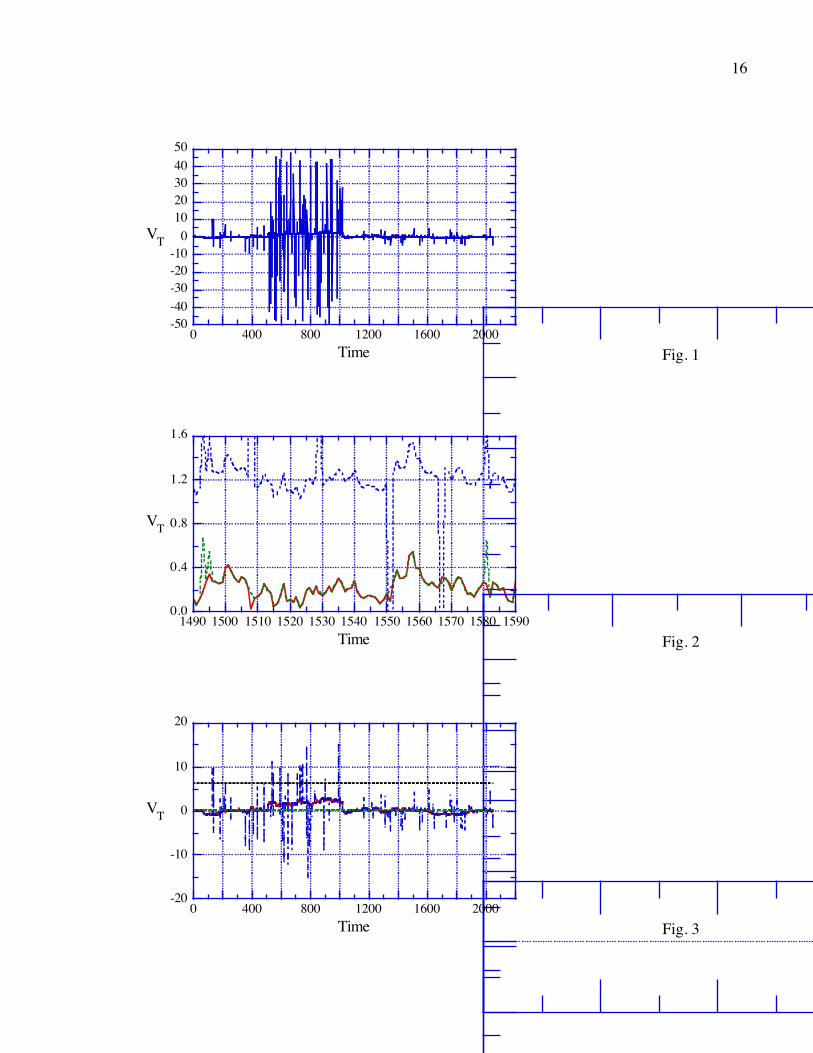
The choice of the whole data set for finding statistics is not appropriate, as shown in Fig. 3.

The large number of large-valued spurious points leads to a standard deviation of about 6, as

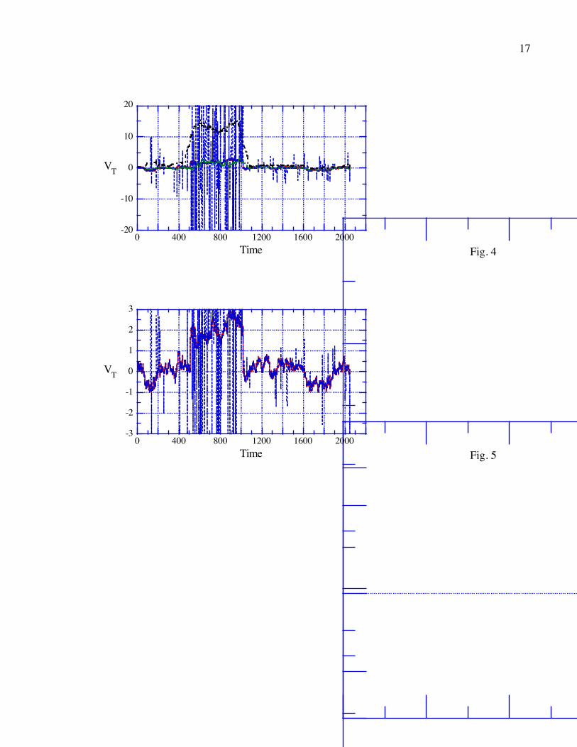
indicated by the dotted line at 1σ from the mean shown by a dashed line. Fig. 4 shows the

improvement provided by using a local running mean and standard deviation based on 100

points. The mean lies nearly on top of the data at this scale of presentation, and the dot-dashed

line is at 1σ from the running mean. Note that the 1σ line is generally above the data, but

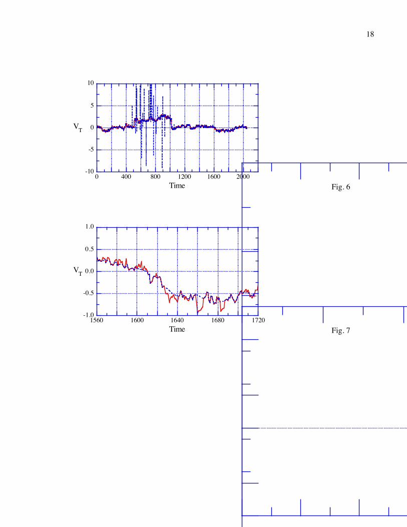
reflects local structure. Figs. 5 and 6 show the effect of removing points at 3σ and 1σ from the

mean, respectively, and while many spurious points are eliminated in this way, the region with

dense spurious points of large amplitude is still not well handled. Moreover, while the 1σ

criterion seems to do well outside this region, it will eliminate far too many points in general.

Fig. 7 shows a segment of the original (“good”) data edited with a 1σ criterion, showing that this

6

criterion will, as expected, eliminate far too many points. The algorithm described next solves

this and a number of other problems to a large extent, and represents our best attempt to date for

developing a spurious point editor.

III. RECOMMENDED AUTOMATED METHOD

One major problem with the local criteria used above is that they are not well suited to

intervals in which σ is greatly increased by spurious points compared to the true value. One way

around this problem is to pass the data though the automatic editor many times to get

successively closer to the ideal set of points. This process does not converge very effectively,

and thus the approach adopted here is to generate a running mean and standard deviation and to

take any points found to be spurious out of the sums as the run progresses. Thus the procedure

used here is as follows:

(1) The first available 100 points are used to find a mean and standard deviation. Whenever

data gaps are encountered at this or any other stage they are simply ignored and the data

either side of the gap is concatenated. This leads at times to sharp jumps that cause the

elimination of a few points either side of the gap, but interpolation across the gaps leads to

more serious problems with the running sums and thus to the elimination of even more

points. It is best to start with 100 points that are noise free so that the initial sums are

representative of the data. When this is not the case it may take a few hundred points for the

editing to become fully effective. Using less than 100 points can help to find spurious points

in troughs of the data, but this also increases the likelihood of eliminating points at jumps.

(2) A criterion is applied to find spurious points in the first 100 points. The basic procedure

is still to eliminate points a certain number of standard deviations from the mean, but the

testing of all the values of the ordinate Yi in the interval (not just the central one, as in Figure

5-7) according to

7

|(Yi – Yave)| > Mσ => spurious (1)

(where M is a multiplying factor) allows the use of a larger value of M than the usual value of

3. This procedure treats the 100 point subset in the same manner as the whole data set was

treated in Figure 3, but with a larger M value. Testing all the points in the interval leads to a

more complete elimination of spurious points while using a large M tends to retain more

“good” points, especially at jumps. The use of a running test to some extent counteracts the

latter advantage, but for real data sets this is rarely a significant problem (see below). In

terms of the usual statistical criteria, the probability of a point being 4σ from the mean of a

normal distribution is about 6×10–5, and thus even with 100 tests per point M = 4 provides

quite a stringent statistical test. At M = 5 the corresponding probability is two orders of

magnitude lower, thus providing a very restrictive test. Of course the data are not normally

distributed for the cases considered here, but this discussion is still qualitatively relevant.

(3) The interval is moved over by one point, as many new points as needed are added to the

end of the interval to obtain another 100 point set, and the mean and σ are updated. Points

found to be spurious in the previous pass are dropped from the sums so that to the extent

possible the mean and σ are always representative of the data. For efficiency, the sums

needed for the statistics are modified by subtracting out the dropped points and adding in the

new ones, rather than summing over all 100 points each time. The skipping of gaps and

previously eliminated points leads to an increased complexity involving many special cases

for updating subscripts, but this problem need only be solved once and the results make this

worthwhile. An attempt to speed up the algorithm by moving the starting point by more than

one point does lead to a time savings, but the results are often less accurate.

(4) The criterion (1) is applied again as in step (2).

(5) Steps (3) and (4) are repeated until the end of the data set is reached.

8

(6) The entire procedure (1)-(5) may be repeated. Most points are edited on the first pass, but

subsequent passes will eliminate some missed points.

A Fortran program to implement this procedure is included in the Appendix. The program is

set up to read up to 8 parallel time series, and is set to automatically take spurious points out of

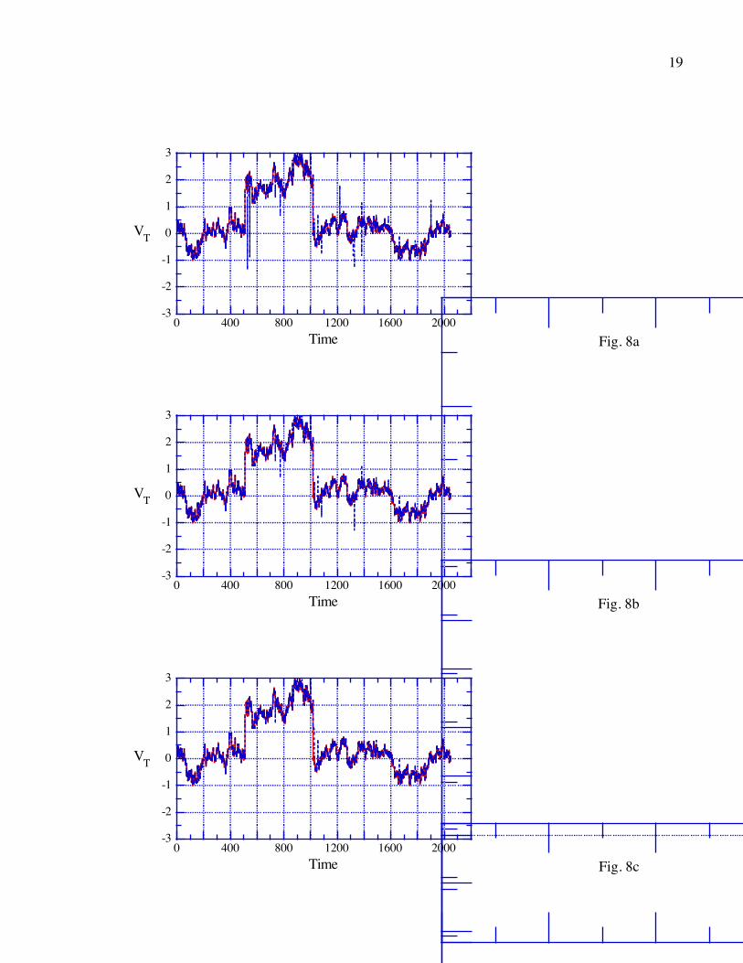
the parallel series when found in a tested series. The results of applying this algorithm to the

artificial data set are shown in Fig. 8a-c for M = 6, 5, and 4 respectively. Note that even with a

6σ criterion most of the spurious points are eliminated (140 out of 165). The 4σ criterion

eliminates a few too many points (175 total) and still fails to edit a few obvious outlying points.

The ones it misses are generally embedded in troughs or peaks of the original series so that the

standard deviation of 100 points of data is increased. Our eye uses a local criterion that changes

in width according to the context, but it is difficult to make a program reproduce this ability.

Overall, however, the time series generated by the above algorithm are very close to the ideal

generated by hand, and the time required is about 1 second per thousand points on a VAX 8810;

many current workstations would perform the calculations significantly faster.

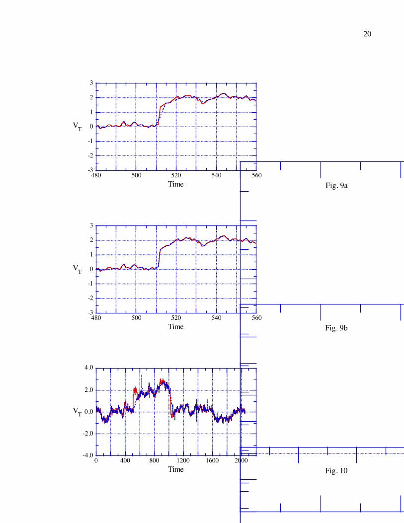
The major compromise that must be made in applying this algorithm is illustrated in Fig. 9.

Fig. 9a shows that the 4σ criterion tends to see the jumps as spurious points as it first encounters

them, and thus it will tend to eliminate a few points next to the jump. By contrast, Fig. 9b shows

that the 5σ criterion is much better for retaining jump points, but (see Fig. 8) not as effective at

removing spurious points in general. Most real time series have at least a few points in the

transition across a “discontinuity” and thus the elimination of points at jumps is less of a problem

in practice than in the case shown here.

IV. FURTHER ALTERNATIVES AND APPLICATION TO REAL DATA

Generally speaking we have found that a good interactive screen editor is the most effective

way for working with modest numbers of points, but other schemes have proven useful for some

9

purposes. For very quick editing of modest size data sets a criterion based on using a fixed value

of σ for the entire data set is sometimes useful. To produce Fig. 10 the test for spurious points

was whether a 100 point running mean of the input data set was within 1.0 of the measured

value. The value of 1.0 was found by trial and error based on a visual inspection of the data set

and the results of using different values. This criterion does very poorly at the jumps, but very

well for more well behaved portions of the data. The use of a 7 point running median rather than

a mean leads to nearly perfect fidelity at the jumps, and thus a quite respectable quick editing of

the data set, but it leaves essentially the same set of unedited spurious points in the latter half of

the data set. The main drawback of these methods is that the standard deviation of the points in

real data sets can vary by large factors so that without a priori information the technique will not

be effective. The requirement for finding local variances also makes the advantage of the

median-based methods much less, although the use of a running median calculated in an initial

step in place of the mean found in each step in the algorithm recommend here might speed up

processing somewhat. Such a procedure might also introduce errors, however. For example, if

the noise is all on one side of the signal, then the median may be far from the desired value for

testing for spurious points, and this could imply a need for calculating local medians at each step.

The median requires a sort, and thus this could be costly in CPU time. Nonetheless, median-

based methods do have their uses,3 and further development of them in this context may be

worthwhile.

The last two figures show the application of the above algorithm to real data. Fig. 11 shows

the time series of a measured velocity component from Voyager 2 spacecraft data at a resolution

of 12 seconds per point. This interval is unusually riddled with spurious points; the signal is the

line in the middle of the graph, as in Fig. 1. Fig. 12a shows an expanded view of the interval,

and Figs. 12b and c show the M = 6 and 4 edited versions of the data set, respectively. The

dramatic change in the appearance of the data set was achieved with the removal of only 6% of

the points for the 4σ criterion. A close look will reveal a few points in Fig. 12c that should have

been removed and an occasional peak that perhaps should not have been eliminated, but the main

10

features, including jumps and relatively isolated regions different from their surroundings, are

preserved, just as they were with the artificial data set. The time series that results is very similar

to time series that are typically observed for this component of the velocity field in less noisy

conditions, and thus it is reasonable to assume that the method was successful in retaining nearly

all of the useful information in this interval. Based on results such as these, this method for

eliminating spurious points is now being used routinely in the processing of magnetometer data

from the Voyager spacecraft as well as for post-processing many other spacecraft data sets which

did not have such an algorithm in the main processing program.

V. CONCLUSION

This work demonstrates that a local statistical criterion is capable of attaining nearly the same

fidelity as the eye in eliminating spurious points from turbulent time series with embedded jumps

and large noise signals. The central features of the algorithm are the testing of all the points in a

given subinterval against the mean and σ for that subinterval, the use of a 100 point subinterval

that moves by 1 point at a time, and the elimination of any point found to be spurious from

further calculations of the statistics. It is quite possible that further modification of this

algorithm would lead to increased efficiency and accuracy, but various attempts to change the

parameters described above have been found to degrade the performance. For small data sets a

screen oriented interactive editor is somewhat superior, but for large data sets an algorithm such

as that described here is indispensable. The present work focuses on applications to spacecraft

measurements, but the method should be applicable to a wide range of nonconstant signals (e.g.,

images in two-dimensions) in which spurious spikes occur, although the particular parameters

used here might well have to be modified for other applications.

Acknowledgments: I thank many people for encouraging and indicating a need for this effort,

or assisting in the work, including F. Ottens, W. Mish, L. Burlaga, M. Goldstein, C. W. Smith,

and W. Matthaeus. I thank J. Belcher for the use of the Voyager plasma data.

11

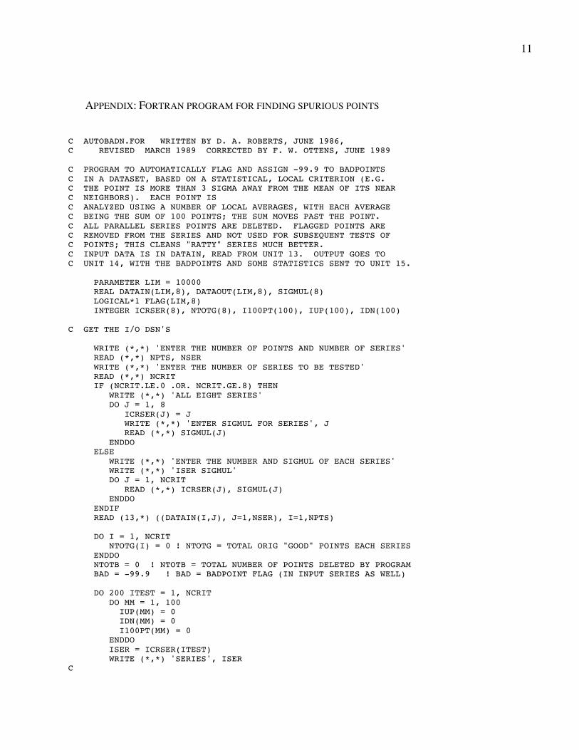
APPENDIX: FORTRAN PROGRAM FOR FINDING SPURIOUS POINTS

C AUTOBADN.FOR WRITTEN BY D. A. ROBERTS, JUNE 1986, C REVISED MARCH 1989 CORRECTED BY F. W. OTTENS, JUNE 1989 C PROGRAM TO AUTOMATICALLY FLAG AND ASSIGN -99.9 TO BADPOINTS C IN A DATASET, BASED ON A STATISTICAL, LOCAL CRITERION (E.G. C THE POINT IS MORE THAN 3 SIGMA AWAY FROM THE MEAN OF ITS NEAR C NEIGHBORS). EACH POINT IS C ANALYZED USING A NUMBER OF LOCAL AVERAGES, WITH EACH AVERAGE C BEING THE SUM OF 100 POINTS; THE SUM MOVES PAST THE POINT. C ALL PARALLEL SERIES POINTS ARE DELETED. FLAGGED POINTS ARE C REMOVED FROM THE SERIES AND NOT USED FOR SUBSEQUENT TESTS OF C POINTS; THIS CLEANS "RATTY" SERIES MUCH BETTER. C INPUT DATA IS IN DATAIN, READ FROM UNIT 13. OUTPUT GOES TO C UNIT 14, WITH THE BADPOINTS AND SOME STATISTICS SENT TO UNIT 15. PARAMETER LIM = 10000 REAL DATAIN(LIM,8), DATAOUT(LIM,8), SIGMUL(8) LOGICAL*1 FLAG(LIM,8) INTEGER ICRSER(8), NTOTG(8), I100PT(100), IUP(100), IDN(100) C GET THE I/O DSN'S WRITE (*,*) 'ENTER THE NUMBER OF POINTS AND NUMBER OF SERIES' READ (*,*) NPTS, NSER WRITE (*,*) 'ENTER THE NUMBER OF SERIES TO BE TESTED' READ (*,*) NCRIT IF (NCRIT.LE.0 .OR. NCRIT.GE.8) THEN WRITE (*,*) 'ALL EIGHT SERIES' DO J = 1, 8 ICRSER(J) = J WRITE (*,*) 'ENTER SIGMUL FOR SERIES', J READ (*,*) SIGMUL(J) ENDDO ELSE WRITE (*,*) 'ENTER THE NUMBER AND SIGMUL OF EACH SERIES' WRITE (*,*) 'ISER SIGMUL' DO J = 1, NCRIT READ (*,*) ICRSER(J), SIGMUL(J) ENDDO ENDIF READ (13,*) ((DATAIN(I,J), J=1,NSER), I=1,NPTS) DO I = 1, NCRIT NTOTG(I) = 0 ! NTOTG = TOTAL ORIG "GOOD" POINTS EACH SERIES ENDDO NTOTB = 0 ! NTOTB = TOTAL NUMBER OF POINTS DELETED BY PROGRAM BAD = -99.9 ! BAD = BADPOINT FLAG (IN INPUT SERIES AS WELL) DO 200 ITEST = 1, NCRIT DO MM = 1, 100 IUP(MM) = 0 IDN(MM) = 0 I100PT(MM) = 0 ENDDO ISER = ICRSER(ITEST) WRITE (*,*) 'SERIES', ISER C

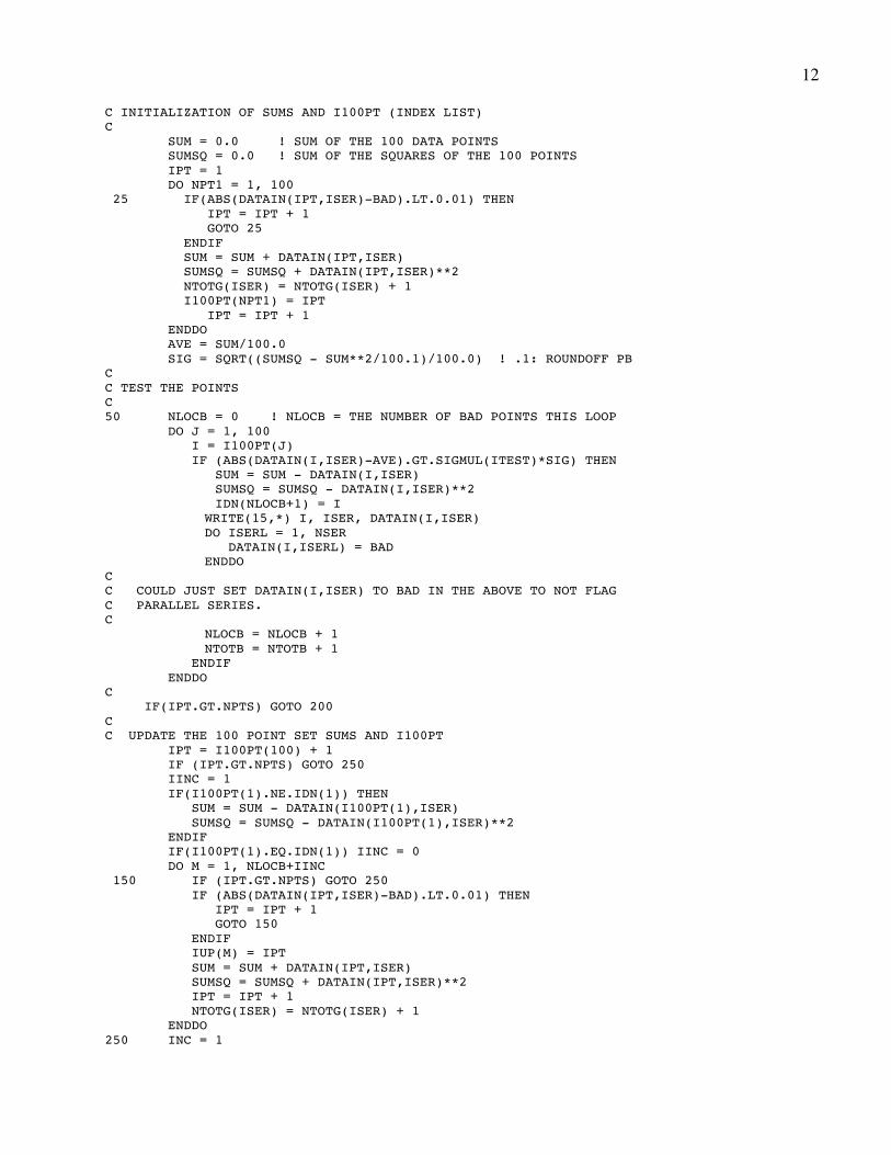
12

C INITIALIZATION OF SUMS AND I100PT (INDEX LIST) C SUM = 0.0 ! SUM OF THE 100 DATA POINTS SUMSQ = 0.0 ! SUM OF THE SQUARES OF THE 100 POINTS IPT = 1 DO NPT1 = 1, 100 25 IF(ABS(DATAIN(IPT,ISER)-BAD).LT.0.01) THEN IPT = IPT + 1 GOTO 25 ENDIF SUM = SUM + DATAIN(IPT,ISER) SUMSQ = SUMSQ + DATAIN(IPT,ISER)**2 NTOTG(ISER) = NTOTG(ISER) + 1 I100PT(NPT1) = IPT IPT = IPT + 1 ENDDO AVE = SUM/100.0 SIG = SQRT((SUMSQ - SUM**2/100.1)/100.0) ! .1: ROUNDOFF PB C C TEST THE POINTS C 50 NLOCB = 0 ! NLOCB = THE NUMBER OF BAD POINTS THIS LOOP DO J = 1, 100 I = I100PT(J) IF (ABS(DATAIN(I,ISER)-AVE).GT.SIGMUL(ITEST)*SIG) THEN SUM = SUM - DATAIN(I,ISER) SUMSQ = SUMSQ - DATAIN(I,ISER)**2 IDN(NLOCB+1) = I WRITE(15,*) I, ISER, DATAIN(I,ISER) DO ISERL = 1, NSER DATAIN(I,ISERL) = BAD ENDDO C C COULD JUST SET DATAIN(I,ISER) TO BAD IN THE ABOVE TO NOT FLAG C PARALLEL SERIES. C NLOCB = NLOCB + 1 NTOTB = NTOTB + 1 ENDIF ENDDO C IF(IPT.GT.NPTS) GOTO 200 C C UPDATE THE 100 POINT SET SUMS AND I100PT IPT = I100PT(100) + 1 IF (IPT.GT.NPTS) GOTO 250 IINC = 1 IF(I100PT(1).NE.IDN(1)) THEN SUM = SUM - DATAIN(I100PT(1),ISER) SUMSQ = SUMSQ - DATAIN(I100PT(1),ISER)**2 ENDIF IF(I100PT(1).EQ.IDN(1)) IINC = 0 DO M = 1, NLOCB+IINC 150 IF (IPT.GT.NPTS) GOTO 250 IF (ABS(DATAIN(IPT,ISER)-BAD).LT.0.01) THEN IPT = IPT + 1 GOTO 150 ENDIF IUP(M) = IPT SUM = SUM + DATAIN(IPT,ISER) SUMSQ = SUMSQ + DATAIN(IPT,ISER)**2 IPT = IPT + 1 NTOTG(ISER) = NTOTG(ISER) + 1 ENDDO 250 INC = 1

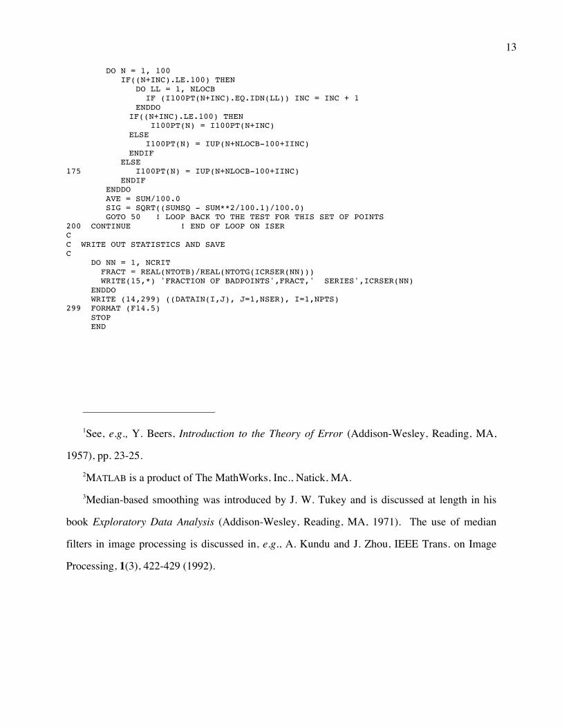
13

DO N = 1, 100 IF((N+INC).LE.100) THEN DO LL = 1, NLOCB IF (I100PT(N+INC).EQ.IDN(LL)) INC = INC + 1 ENDDO IF((N+INC).LE.100) THEN I100PT(N) = I100PT(N+INC) ELSE I100PT(N) = IUP(N+NLOCB-100+IINC) ENDIF ELSE 175 I100PT(N) = IUP(N+NLOCB-100+IINC) ENDIF ENDDO AVE = SUM/100.0 SIG = SQRT((SUMSQ - SUM**2/100.1)/100.0) GOTO 50 ! LOOP BACK TO THE TEST FOR THIS SET OF POINTS 200 CONTINUE ! END OF LOOP ON ISER C C WRITE OUT STATISTICS AND SAVE C DO NN = 1, NCRIT FRACT = REAL(NTOTB)/REAL(NTOTG(ICRSER(NN))) WRITE(15,*) 'FRACTION OF BADPOINTS',FRACT,' SERIES',ICRSER(NN) ENDDO WRITE (14,299) ((DATAIN(I,J), J=1,NSER), I=1,NPTS) 299 FORMAT (F14.5) STOP END

1See, e.g., Y. Beers, Introduction to the Theory of Error (Addison-Wesley, Reading, MA,

1957), pp. 23-25. 2MATLAB is a product of The MathWorks, Inc., Natick, MA. 3Median-based smoothing was introduced by J. W. Tukey and is discussed at length in his

book Exploratory Data Analysis (Addison-Wesley, Reading, MA, 1971). The use of median

filters in image processing is discussed in, e.g., A. Kundu and J. Zhou, IEEE Trans. on Image

Processing, 1(3), 422-429 (1992).

FIGURE CAPTIONS

Fig. 1: The artificial data set used to illustrate the effects of various algorithms. The original

data can be seen as a time series running through the middle of the panel.

Fig. 2: A portion of the time series in Fig. 1, showing the original series (solid), the series

with spurious points added (dashed and offset), and the results of manual editing of the points

(dots).

Fig. 3: The original series (solid), its mean (dashed), a line 1σ from the mean based on the

whole data set (dotted) and the edited series based on taking points less than 3σ from the mean

(dot-dashed).

Fig. 4: A close-up view of Fig. 1 with a dot-dashed line 1σ from the mean with the mean and

σ calculated from running 100 point sets of points.

Fig. 5: The original time series (solid) and the edited series based on a 3σ test with σ as

shown in Fig. 4.

Fig. 6: The original time series (solid) and the edited series based on a 1σ test with σ as

shown in Fig. 4.

Fig. 7: The original series (solid) and the result of a local 1σ test applied to it.

Fig. 8: The original series (solid) and the result the algorithm recommended in the text for

(a) M = 6, (b) M = 5, (c) M = 4.

15

Fig. 9: (a) A detailed subset of Fig. 8c. (a) A detailed subset of Fig. 8b.

Fig. 10: The original series (solid) and the result of the quick editing method described in the

text.

Fig. 11: Data for a component of the interplanetary plasma velocity from the Voyager

spacecraft.

Fig. 12: (a) An expanded view of Fig. 11, and the result of the algorithm recommended in

the text for (b) M = 6 and (c) M = 4.

16

-50-40-30

VT

-20-10010203040

Time

50

0 400 800 1200 1600 2000 Fig. 1

0.0

0.4

0.8VT

1.2

1.6

1490 1500 1510 1520 1530Time1540 1550 1560 1570 1580 1590

Fig. 2

-20

-10

0VT

10

20

0 400 800 1200 1600Time

2000 Fig. 3

17

-20

-10

0VT

10

20

0 400 800 1200 1600Time

2000 Fig. 4

-3

-2

-1

VT 0

1

2

3

0 400 800Time1200 1600 2000

Fig. 5

18

-10

-5

0VT

5

10

0 400 800 1200 1600Time

2000 Fig. 6

-1.0

-0.5

0.0VT

0.5

1.0

1560 1600 1640 1680 1720Time Fig. 7

19

-3

-2

-1

VT 0

1

2

3

0 400 800Time1200 1600 2000

Fig. 8a

-3

-2

-1

VT 0

1

2

3

0 400 800Time1200 1600 2000

Fig. 8b

-3

-2

-1

VT 0

1

2

3

0 400 800Time1200 1600 2000

Fig. 8c

20

-3

-2

-1

VT 0

1

2

3

480 500 520Time

540 560 Fig. 9a

-3

-2

-1

VT 0

1

2

3

480 500 520Time

540 560 Fig. 9b

-4.0

-2.0

0.0VT

2.0

4.0

0 400 800 1200 1600Time

2000 Fig. 10

21

Fig. 11

Fig. 12