An algorithm for calculating atomic D states with explicitly correlated GaussianfunctionsKeeper L. Sharkey, Sergiy Bubin, and Ludwik Adamowicz Citation: The Journal of Chemical Physics 134, 044120 (2011); doi: 10.1063/1.3523348 View online: http://dx.doi.org/10.1063/1.3523348 View Table of Contents: http://scitation.aip.org/content/aip/journal/jcp/134/4?ver=pdfcov Published by the AIP Publishing

This article is copyrighted as indicated in the abstract. Reuse of AIP content is subject to the terms at: http://scitation.aip.org/termsconditions. Downloaded to IP:

150.135.239.97 On: Mon, 25 Nov 2013 17:16:16

THE JOURNAL OF CHEMICAL PHYSICS 134, 044120 (2011)

An algorithm for calculating atomic D states with explicitly correlatedGaussian functions

Keeper L. Sharkey,1 Sergiy Bubin,2 and Ludwik Adamowicz1,3

1Department of Chemistry and Biochemistry, University of Arizona, Tucson, Arizona 85721, USA2Department of Physics and Astronomy, Vanderbilt University, Nashville, Tennessee 37235, USA3Department of Physics, University of Arizona, Tucson, Arizona 85721, USA

(Received 21 September 2010; accepted 10 November 2010; published online 27 January 2011)

An algorithm for the variational calculation of atomic D states employing n-electron explicitly corre-lated Gaussians is developed and implemented. The algorithm includes formulas for the first deriva-tives of the Hamiltonian and overlap matrix elements determined with respect to the Gaussian nonlin-ear exponential parameters. The derivatives are used to form the energy gradient which is employedin the variational energy minimization. The algorithm is tested in the calculations of the two lowest Dstates of the lithium and beryllium atoms. For the lowest D state of Li the present result is lower thanthe best previously reported result. © 2011 American Institute of Physics. [doi:10.1063/1.3523348]

I. INTRODUCTION

Very accurate quantum mechanical calculations of theground and excited states of small atoms have alwaysprovided the testing ground for new computational meth-ods for atomic calculations. The testing has been pos-sible due to the availability of very accurate gas-phasespectra of these systems. An important group of statesfor which such high accuracy experimental data are avail-able are D states. For example, the NIST atomic spec-tra database1 among the 182 states of the lithium atomlists ten 2 D states which correspond to the electron con-figurations 1s2nd, where n = 3, 4, . . . , 12. For the beryl-lium atom among the 219 levels listed there are 11 1 Dstates and 10 3 D states. The lowest 1 D state corresponds tothe electron configuration 1s22p2 and the rest to the config-urations 1s2nd2, n = 3, 4, . . . , 12. The 3 D states correspondto the configurations 1s2nd2, n = 3, 4, . . . , 12.

A literature search reveals that only the lowest 2 D stateof lithium has been calculated with high accuracy. The best todate variational energy for this state was reported by Yan andDrake2 and it is equal to −7.335 523 541 10(43) a.u. (an ex-trapolated result). There are no calculations with similar ac-curacy for the D states of beryllium. Part of the reason forthe lack of calculations of these states is due to the basis set,which for most works concerning atomic levels has involvedHylleraas type functions. These functions, while very effec-tive in the calculations of two- and three-electron atoms,2–7

have not yet been extended to four-electron atoms due to dif-ficulties with calculating the Hamiltonian matrix elements.

Another type of basis function that has been very popularin high-accuracy atomic calculations are correlated Gaussianfunctions that explicitly depend on the interelectron distances.The most accurate results for four- and five-electron atomshave been obtained with those functions.8–11 The main ad-vantage of using Gaussians in atomic calculations is due tothe simplicity of the Hamiltonian and overlap integrals withthose functions, which can be evaluated analytically for an ar-bitrary number of electrons. However, these functions cannot

satisfy the Kato cusps conditions and are too fast decaying atlarge distances. As the calculations have shown8–11 these de-ficiencies can be effectively remedied by using longer expan-sions and by performing extensive optimization of the Gaus-sian nonlinear parameters using the variational approach.

In this work we have derived and implemented algo-rithms for calculating the Hamiltonian matrix elements withexplicitly correlated Gaussian functions for describing Dstates of small atomic systems. We also derived and im-plemented algorithms for calculating first derivatives of thematrix elements determined with respect to the Gaussianexponents. These derivatives are used to calculate the energygradient, which is employed in the variational optimization ofthe Gaussian parameters. The variational energy minimiza-tion is greatly accelerated if the energy gradient is available.To test the algorithms, we have performed calculations oftwo lowest 2 D states of lithium and two lowest 1 D states ofberyllium.

In the approach we use in this work we explicitly accountfor the finite mass of the nucleus in the variational nonrela-tivistic calculations. This is done by means of using a Hamil-tonian that explicitly depends on the masses of all particlesincluding the mass of the nucleus (see Sec. I A). In this waythe results change when a different isotope is considered. Theapproach also allows us to obtain results corresponding to aninfinite mass of the nucleus. Such results generated here forlithium in the present work allow for a direct comparison withthe calculations performed by Yan and Drake.2

A. The Hamiltonian

We consider an atom with N particles (i.e., N − 1 elec-trons and a nucleus). We start with the laboratory-framenonrelativistic Hamiltonian and we separate out the center-of-mass motion. This is done by introducing an internalCartesian coordinate system centered at the nucleus. The sep-aration of the center-of-mass motion is rigorous and results inthe laboratory Hamiltonian becoming a sum of the operator

0021-9606/2011/134(4)/044120/9/$30.00 © 2011 American Institute of Physics134, 044120-1

This article is copyrighted as indicated in the abstract. Reuse of AIP content is subject to the terms at: http://scitation.aip.org/termsconditions. Downloaded to IP:

150.135.239.97 On: Mon, 25 Nov 2013 17:16:16

044120-2 Sharkey, Bubin, and Adamowicz J. Chem. Phys. 134, 044120 (2011)

representing the kinetic energy of the center-of-mass motionand the following “internal” Hamiltonian:

H = −1

2

⎛⎜⎝ n∑

i=1

1

μi∇2

ri+ 1

m0

n∑i, j=1i �= j

∇ri · ∇r j

⎞⎟⎠

+n∑

i=1

q0qi

ri+

n∑i> j=1

qi q j

ri j, (1)

where n = N − 1, ri is the distance between the i th electronand the nucleus, m0 is the nucleus mass and q0 is its charge,qi are electron charges, and μi = m0mi/ (m0 + mi ) are elec-tron reduced masses. The Hamiltonian (1) describes themotion of n (pseudo)electrons, whose masses have beenchanged to the reduced masses, in the central field of thecharge of the nucleus. This motion is coupled through theCoulombic interactions,

n∑i=1

q0qi

ri+

n∑i> j=1

qi q j

ri j,

where ri j = |r j − ri |, and through the mass polarization term,

−1

2

n∑i, j=1i �= j

(1/m0) ∇ri · ∇r j .

II. THE BASIS SET

In this work we consider atomic D states correspond-ing to electronic configurations where one or two electronsof the n electron atom is occupying a non-s state. Examples ofsuch states include the above-mentioned 2 D 1s2nd1 states oflithium and the 1 D and 3 D 1s22s1nd1 states of beryllium. Todescribe an atomic state with a single d electron one, in princi-ple, needs to use the following explicitly correlated Gaussianfunction:

φk = (x2

ik+ y2

ik− 2z2

ik

)exp[−r′ (Ak ⊗ I3) r], (2)

where ik is an electron label whose value can vary from 1 ton and is unique for each basis function. The prime indicatesthe matrix/vector transpose; this notation is used throughoutthis work. Ak in Eq. (2) is an n × n symmetric matrix, ⊗ isthe Kronecker product, I3 is a 3 × 3 identity matrix, and r isa 3n vector that has the form

r =

⎛⎜⎜⎜⎝

r1

r2...

rn

⎞⎟⎟⎟⎠ =

⎛⎜⎜⎜⎜⎜⎜⎜⎜⎜⎝

x1

y1

z1...

xn

yn

zn

⎞⎟⎟⎟⎟⎟⎟⎟⎟⎟⎠

. (3)

We will denote (Ak ⊗ I3) in Eq. (2) as Ak . However, in thewave functions of some of the D states there can be com-ponents corresponding to two electrons being in p statescoupling to a D state. For example, the lowest 1 D state of

beryllium is dominated by the 1s22p2 configuration. Also, thelowest 2 D state of lithium has a non-negligible contributionfrom a similar configuration (1s12p2).2 Thus, the Gaussianbasis set that can best capture all the angular coupling effectsin D states is the following basis:

φk = (xik x jk + y jk yik − 2zik z jk

)exp[−r′(Ak ⊗ I3)r], (4)

where electron indices ik and jk are either equal or not equalto each other.

We use a general quadratic form r′Wkr in place of(xik x jk + yik y jk − 2zik z jk ) allowing for a more generalized ap-proach in deriving the matrix elements. With that, our basisfunctions are

φk = (r′Wkr) exp[−r′Akr], (5)

where Wk is a sparse 3n × 3n symmetric matrix thatfor ik = jk comprises only three nonzero elements:W3(ik−1)+1,3(ik−1)+1 = 1, W3(ik−1)+2,3(ik−1)+2 = 1, andW3(ik−1)+3,3(ik−1)+3 = −2, and for ik �= jk it comprisessix elements: W3(ik−1)+1,3( jk−1)+1 = W3( jk−1)+1,3(ik−1)+1 = 1

2 ,W3(ik−1)+2,3( jk−1)+2 = W3( jk−1)+2,3(ik−1)+2 = 1

2 , andW3(ik−1)+3,3( jk−1)+3 = W3( jk−1)+3,3(ik−1)+3 = 1. It shouldbe noted that, in general, we could have used a nonsymmetricmatrix (for ik �= jk) Wk with only three nonzero elements(yielding the same quadratic form) since there are onlythree terms in Eq. (4). However, in practice it is muchmore convenient to deal with symmetric Wk matrices as thederivations of matrix elements becomes considerably simplerin this case.

As the basis functions used in describing bound statesmust be square integrable, restrictions must be imposed on theAk matrices. Each Ak matrix must be positive definite. Ratherthan restricting the Ak matrix elements, which usually leads tocumbersome constraints, we use the following Cholesky fac-tored form of Ak : Ak = Lk L ′

k , where Lk is a lower triangularmatrix. With this representation, Ak is automatically positivedefinite for any values of Lk ranging from ∞ to −∞. Thus,the variational energy minimization with respect to the Lk pa-rameters can be carried out without any restrictions. It shouldbe noted that the Lk L ′

k representation of Ak matrix does notlimit the flexibility of basis functions, because any symmet-ric positive matrix can be represented in a Cholesky factoredform.

The linear expansion coefficients of the wave function interms of the basis functions and the elements of the Lk matri-ces are optimization variables. Also, for each basis functionthe ik and jk indices are optimized. This optimization is onlydone once for each basis function when the function is firstadded to the basis set.

III. THE HAMILTONIAN INTEGRALS AND THEGRADIENT

In order to fully exploit the sparsity of the Wk matricesand make the calculation more efficient, three cases have beendistinguished in the calculation of the Hamiltonian and over-lap integrals. The first case concerns the integrals between thebasis functions with ik �= jk , the second case the integrals forfunctions with ik = jk , and the third case the mixed integrals.

This article is copyrighted as indicated in the abstract. Reuse of AIP content is subject to the terms at: http://scitation.aip.org/termsconditions. Downloaded to IP:

150.135.239.97 On: Mon, 25 Nov 2013 17:16:16

044120-3 An algorithm for calculating atomic D states J. Chem. Phys. 134, 044120 (2011)

Similar separation is applied in the calculation of the energygradient. As the integrals and the gradient are similar to thosepublished before for atomic states with two p electrons,12, 13

we only present the final formulas in the Appendix.As the total atomic wave function must be antisymmet-

ric with respect to the permutation of the electron labels anappropriate symmetry projection needs to be applied to eachbasis function. In this work we use the spin-free formal-ism. The Young projection operator, Y , which imposes propersymmetry, has to be applied only to the spatial part of thewave function and thus to each basis function, Yφk . Y is a lin-ear combination of permutational operators, Pγ , and, as theHamiltonian is invariant with respect to all permutations ofthe electrons, in the calculation of the overlap and Hamil-tonian matrix elements it is easy to arrange that the per-mutational operators are applied to the ket only. In brief,the ket functions in those matrix elements are operated onwith the permutation operator P = Y †Y (the dagger standsfor conjugate), where the Y operator can be derived usingthe appropriate Young tableaux for the state under consid-eration. For lithium in a 2 D and beryllium in a 1 D statethe Young operators can be chosen as Y = (1 + P34)(1 − P23)and Y = (1 − P45)(1 − P23)(1 + P24)(1 + P35), respectively,where the nucleus is labeled as 1, and the electrons are labeledas 2, 3, 4, 5, 1 is the identity operator, and Pi j is the permuta-tion of the the i th and j th electron.

A. Total energy and energy gradient

The optimization of the linear expansion coefficients, theLk Gaussian parameters, and the ik and jk indices, is per-formed in this work through the minimization of the standardRayleigh–Ritz variational energy functional. In the minimiza-tion the energy gradient is employed. The calculation for eachstate is performed independently from other states and the pa-rameters of the basis functions are optimized specifically forthat particular state. In the process of generating the basis set,we start with a small randomly selected set of functions andthis set is then grown by incremental additions of small groupsof functions. The added functions are generated randomlybased on the actual distribution of nonlinear parameters ofthe functions already present in the basis set. At this step asignificant number of random candidates are generated andonly those that give the best improvement of the total energyare selected. When a new group of functions is added to theset their nonlinear parameters are optimized with the gradient-based method. After this is finished the nonlinear parametersof the entire basis set (one function at a time) are reoptimized.

IV. NUMERICAL TESTS

The first test of the approach developed in this workconcerns the lowest 2 D state of lithium. As mentioned thisstate was calculated before by Yan and Drake.2 As their cal-culation was performed with an infinite mass of the lithiumnucleus, we also first carried a calculation setting the massof the nucleus (m0) to infinity. The convergence of the to-tal energy with the number of Gaussian functions in the ba-

TABLE I. The convergence of the total variational energy of the lowest 2 Dstate of lithium with the number of Gaussians obtained in the present infinite-nuclear mass variational calculations. The energies are in hartrees.

Basis set size Energy

1900 −7.335 523 530 702300 −7.335 523 538 222700 −7.335 523 540 893100 −7.335 523 541 963500 −7.335 523 542 513900 −7.335 523 542 821673a −7.335 523 540 35∞a,b −7.335 523 541 10(43)

aFrom Ref. 2.bThe energy obtained by extrapolating to infinity in terms of the parameter � used inthe integral formulas by Yan and Drake (Ref. 2).

sis set is shown in Table I. As one notices, the energy isconverged to about ten significant figures. The energy valueobtained in the present calculations with 3900 Gaussians of–7.335 523 542 82(60) a.u. is lower than the previous bestvariational upper bound of Yan and Drake2 by about 2 × 10−9

hartree. The Yan and Drake energy is obtained in our calcula-tions with about 2600 Gaussians in the basis set. The lithiumtest clearly shows that Gaussians can effectively describe theD states of small atomic systems. Also, the agreement be-tween Yan and Drake’s and our results give us confidence thatthe algorithm and its implementation works correctly.

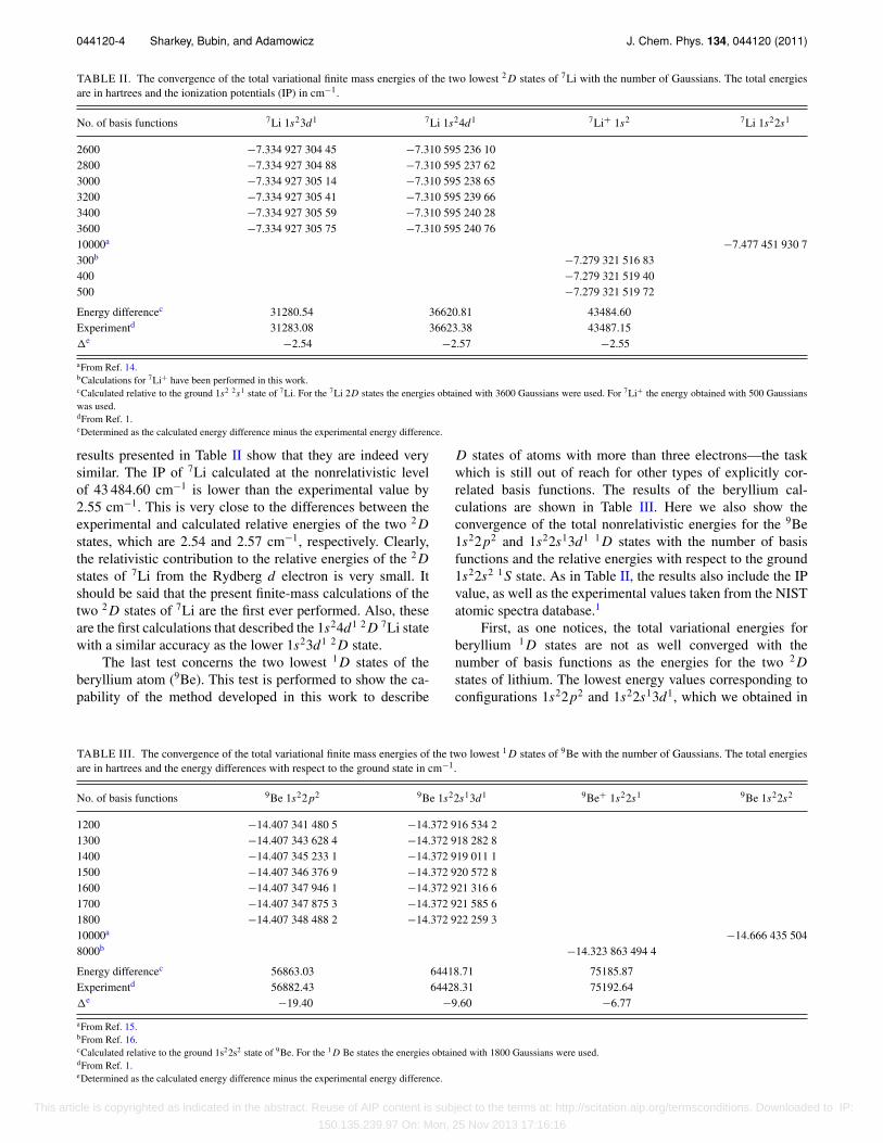
The next test concerns the energy differences betweenthe energies of the two lowest 2 D states of 7Li correspond-ing to the electron configurations 1s23d1 and 1s24d1 and the7Li 1s22s1 ground state energy. These energy differences canbe compared with the experimental values taken from theNIST atomic spectra database.1 Here we used a finite nuclearmass approach, which is possible in our scheme. The con-vergence of the total nonrelativistic energies with the numberof basis functions obtained in those calculations are shown inTable II. We also show in Table II the energy of the 7Li groundstate obtained in our previous work14 and the energy of 7Li+

calculated in this work. The latter value is used to determinethe 7Li nonrelativistic ionization potential (IP). The reasonwe need the 7Li IP is to compare it with the relative ener-gies of the 2 D states determined with respect to the energyof the ground state. Such a comparison must show that in thelimit of exciting the d electron in 7Li to increasingly higher2 D states, the relative energy should converge to the 7Li IPas the electron becomes removed from the atom. Naturally,as only two 2 D states are calculated in this work and not awider range of the Rydberg 1s2nd1 states is considered, theconsistency of the results and not the convergence will betested.

It should also be mentioned that, as the present results donot include relativistic corrections, the agreement with the ex-perimental values is not expected to be perfect. This is why weneed the IP value. If the algorithm implemented in this workis correct, the difference between the experimental and calcu-lated nonrelativistic IPs should be similar to the differencesbetween the calculated relative energies of the two 2 D statesof 7Li and their corresponding experimental counterparts. The

This article is copyrighted as indicated in the abstract. Reuse of AIP content is subject to the terms at: http://scitation.aip.org/termsconditions. Downloaded to IP:

150.135.239.97 On: Mon, 25 Nov 2013 17:16:16

044120-4 Sharkey, Bubin, and Adamowicz J. Chem. Phys. 134, 044120 (2011)

TABLE II. The convergence of the total variational finite mass energies of the two lowest 2 D states of 7Li with the number of Gaussians. The total energiesare in hartrees and the ionization potentials (IP) in cm−1.

No. of basis functions 7Li 1s23d1 7Li 1s24d1 7Li+ 1s2 7Li 1s22s1

2600 −7.334 927 304 45 −7.310 595 236 102800 −7.334 927 304 88 −7.310 595 237 623000 −7.334 927 305 14 −7.310 595 238 653200 −7.334 927 305 41 −7.310 595 239 663400 −7.334 927 305 59 −7.310 595 240 283600 −7.334 927 305 75 −7.310 595 240 7610000a −7.477 451 930 7300b −7.279 321 516 83400 −7.279 321 519 40500 −7.279 321 519 72

Energy differencec 31280.54 36620.81 43484.60Experimentd 31283.08 36623.38 43487.15�e −2.54 −2.57 −2.55

aFrom Ref. 14.bCalculations for 7Li+ have been performed in this work.cCalculated relative to the ground 1s2 2s1 state of 7Li. For the 7Li 2D states the energies obtained with 3600 Gaussians were used. For 7Li+ the energy obtained with 500 Gaussianswas used.dFrom Ref. 1.eDetermined as the calculated energy difference minus the experimental energy difference.

results presented in Table II show that they are indeed verysimilar. The IP of 7Li calculated at the nonrelativistic levelof 43 484.60 cm−1 is lower than the experimental value by2.55 cm−1. This is very close to the differences between theexperimental and calculated relative energies of the two 2 Dstates, which are 2.54 and 2.57 cm−1, respectively. Clearly,the relativistic contribution to the relative energies of the 2 Dstates of 7Li from the Rydberg d electron is very small. Itshould be said that the present finite-mass calculations of thetwo 2 D states of 7Li are the first ever performed. Also, theseare the first calculations that described the 1s24d1 2 D 7Li statewith a similar accuracy as the lower 1s23d1 2 D state.

The last test concerns the two lowest 1 D states of theberyllium atom (9Be). This test is performed to show the ca-pability of the method developed in this work to describe

D states of atoms with more than three electrons—the taskwhich is still out of reach for other types of explicitly cor-related basis functions. The results of the beryllium cal-culations are shown in Table III. Here we also show theconvergence of the total nonrelativistic energies for the 9Be1s22p2 and 1s22s13d1 1 D states with the number of basisfunctions and the relative energies with respect to the ground1s22s2 1S state. As in Table II, the results also include the IPvalue, as well as the experimental values taken from the NISTatomic spectra database.1

First, as one notices, the total variational energies forberyllium 1 D states are not as well converged with thenumber of basis functions as the energies for the two 2 Dstates of lithium. The lowest energy values corresponding toconfigurations 1s22p2 and 1s22s13d1, which we obtained in

TABLE III. The convergence of the total variational finite mass energies of the two lowest 1 D states of 9Be with the number of Gaussians. The total energiesare in hartrees and the energy differences with respect to the ground state in cm−1.

No. of basis functions 9Be 1s22p2 9Be 1s22s13d1 9Be+ 1s22s1 9Be 1s22s2

1200 −14.407 341 480 5 −14.372 916 534 21300 −14.407 343 628 4 −14.372 918 282 81400 −14.407 345 233 1 −14.372 919 011 11500 −14.407 346 376 9 −14.372 920 572 81600 −14.407 347 946 1 −14.372 921 316 61700 −14.407 347 875 3 −14.372 921 585 61800 −14.407 348 488 2 −14.372 922 259 310000a −14.666 435 5048000b −14.323 863 494 4

Energy differencec 56863.03 64418.71 75185.87Experimentd 56882.43 64428.31 75192.64�e −19.40 −9.60 −6.77

aFrom Ref. 15.bFrom Ref. 16.cCalculated relative to the ground 1s22s2 state of 9Be. For the 1 D Be states the energies obtained with 1800 Gaussians were used.dFrom Ref. 1.eDetermined as the calculated energy difference minus the experimental energy difference.

This article is copyrighted as indicated in the abstract. Reuse of AIP content is subject to the terms at: http://scitation.aip.org/termsconditions. Downloaded to IP:

150.135.239.97 On: Mon, 25 Nov 2013 17:16:16

044120-5 An algorithm for calculating atomic D states J. Chem. Phys. 134, 044120 (2011)

our calculations are –14.407 348 488 2 and –14.372 922 259 3a.u., respectively. We estimate that the remaining uncertaintyfor these values is of the order of 10−6 a.u. It would take sev-eral thousand Gaussians to converge them to the level of accu-racy reached for lithium and such calculations will be carriedout in the future. However, even with the present results, theagreement with the experiment for the relative energies is verygood. Also the difference between the calculated relative en-ergies and the experimental energies seems to converge to theIP calculated based on very accurate total energies of 9Be and9Be+ taken from our previous works.15, 16 The results showthat, unlike for lithium, the relativistic correction to IP of 9Beis almost three times smaller than for the relative energy ofthe lowest 1 D state of this atom.

V. SUMMARY

The following has been accomplished in this work.

1. An algorithm for nonrelativistic variational calculationsof atomic D states has been developed and implemented.

2. The approach has been used to obtain new improved up-per bound to the variational infinite-mass energy of thelowest 2 D state of lithium.

3. High-accuracy lithium calculations have also been per-formed for the two lowest 2 D states of the 7Li isotopeusing the finite-mass regime enabled by the approach.The results show very good agreement with the experi-ment.

4. It has been demonstrated that the approach can be usedto carry out calculations of D states of an atomic systemwith more than three electrons.

The work presented here will be extended in the future tostudy wider range of Rydberg D states of the leading isotopesof lithium and beryllium. The approach will also be used incalculations of D states of atoms and atomic ions with morethan four electrons.

APPENDIX A: MATRIX ELEMENTS AND THEGRADIENT

Below, we show the expressions for the Hamilto-nian and overalp matrix elements and the corresponding

derivatives with respect to the Lk matrix elements. We donot show how those quantities have been derived because theprocedure was very similar to that presented in our previousworks.12, 13

Let us first define a quantity common to the overlap, ki-netic, and potential energy matrix elements:

η = tr[A−1

kl WkA−1kl Wl

], (A1)

and a quantity common only to the kinetic energy matrix ele-ment:

τ = tr[A−1

kl Ak M Al]. (A2)

In Eq. (A2) M is the mass matrix whose diagonal elements areset to 1/(2m1), 1/(2m2), . . . , 1/(2mn), while the off-diagonalelements are set to 1/(2m0). Again, m0 is the mass of thenucleus and m1, . . . , mn are the electron masses. Next wedefine

λ = tr[A−1

kl J], (A3)

common only to the potential energy matrix element, wherematrix J has the following simple structure:

J ={

Eii , i = j for ri

Eii + E j j − Ei j − E ji , i �= j for ri j

, (A4)

and Ei j is a matrix with 1 in the i, j th position and 0’s else-where.

In addition to these quatities we also define opera-tions used to determine the gradient formulas. First, the“vech” operation transforms an n × n matrix into an n(n +1)/2-component vector and, second, the transformation ma-trix, T , formed by the first derivatives of the elementsof vech of a 3n × 3n matrix Lk (Ll) with respect tothe elements of vech of n × n matrix Lk (Ll). T isdefined as

T = d vech Lk (vech Lk)

d (vech Lk)′≡ d vech Ll (vech Ll)

d (vech Ll )′ . (A5)

The overlap integral for φk and φl basis functions is

〈φk |φl〉 = 12π3n/2|Akl |−3/2η, (A6)

and its derivatives with respect to vech Lk and vech Ll are

∂〈φk |φl〉∂ vech Lk

= −1

2π3n/2|A−1

kl |3/2

{3

2vech

((A−1

kl + A−1′kl

)Lk

)η

+ vech((

A−1kl WkA−1

kl WlA−1kl + (

A−1kl WkA−1

kl WlA−1kl

)′)Lk

)T

+ vech((

A−1kl WlA−1

kl WkA−1kl + (

A−1kl WlA−1

kl WkA−1kl

)′)Lk

)T

}, (A7)

∂〈φk |φl〉∂ vech Ll

= −1

2π3n/2|A−1

kl |3/2

{3

2vech

((A−1

kl + A−1′kl

)Ll

)η

+ vech((

A−1kl WkA−1

kl WlA−1kl + (

A−1kl WkA−1

kl WlA−1kl

)′)Ll

)T

+ vech((

A−1kl WlA−1

kl WkA−1kl + (

A−1kl WlA−1

kl WkA−1kl

)′)Ll

)T

}. (A8)

This article is copyrighted as indicated in the abstract. Reuse of AIP content is subject to the terms at: http://scitation.aip.org/termsconditions. Downloaded to IP:

150.135.239.97 On: Mon, 25 Nov 2013 17:16:16

044120-6 Sharkey, Bubin, and Adamowicz J. Chem. Phys. 134, 044120 (2011)

The kinetic energy matrix element is

Tkl = 〈φk | − ∇′rM∇′

r|φl〉 = π3n/2|Akl |−3/2{3ητ + 2

(tr

[A−1

kl WkA−1kl WlA−1

kl AkMAl] + tr

[A−1

kl WkMWl]

− tr[A−1

kl WkA−1kl AkMWl

] − tr[A−1

kl WlA−1kl WkMAl

]+ tr

[A−1

kl WlA−1kl WkA−1

kl AkMAl])}

, (A9)

and its derivative with respect to vech Lk and vech Ll are

∂Tkl

∂ vech Lk= ∂〈φk | − ∇′

rM∇′r|φl〉

∂ vech(Lk)

= −π3n/2|Akl |−3/2

{3

2vech

((A−1

kl + A−1′kl

)Lk

) (3ητ + 2

(tr

[A−1

kl WkA−1kl WlA−1

kl AkMAl] + tr

[A−1

kl WkMWl]

+ tr[A−1

kl WkA−1kl AkMWl

] + tr[A−1

kl WlA−1kl WkMAl

]+ tr

[A−1

kl WlA−1kl WkA−1

kl AkMAl]))

+3τ(

vech((

A−1kl WkA−1

kl WlA−1kl + (

A−1kl WkA−1

kl WlA−1kl

)′)Lk

)+ vech

((A−1

kl WlA−1kl WkA−1

kl + (A−1

kl WlA−1kl WkA−1

kl

)′)Lk

))T

+3η(

vech((

A−1kl Ak M Al A−1

kl + (A−1

kl Ak M Al A−1kl

)′)Lk

)− vech

((M Al A−1

kl + (M Al A−1

kl

)′)Lk

))+ 2

(vech

((A−1

kl WkA−1kl WlA−1

kl AkMAlA−1kl + (

A−1kl WkA−1

kl WlA−1kl AkMAlA−1

kl

)′)Lk

)+ vech

((A−1

kl WlA−1kl AkMAlA−1

kl WkA−1kl + (

A−1kl WlA−1

kl AkMAlA−1kl WkA−1

kl

)′)Lk

)+ vech

((A−1

kl AkMAlA−1kl WkA−1

kl WlA−1kl + (

A−1kl AkMAlA−1

kl WkA−1kl WlA−1

kl

)′)Lk

)− vech

((MAlA−1

kl WkA−1kl WlA−1

kl + (MAlA−1

kl WkA−1kl WlA−1

kl

)′)Lk

)+ vech

((A−1

kl WlA−1kl WkA−1

kl AkMAlA−1kl + (

A−1kl WlA−1

kl WkA−1kl AkMAlA−1

kl

)′)Lk

)+ vech

((A−1

kl WkA−1kl AkMAlA−1

kl WlA−1kl + (

A−1kl WkA−1

kl AkMAlA−1kl WlA−1

kl

)′)Lk

)+ vech

((A−1

kl AkMAlA−1kl WlA−1

kl WkA−1kl + (

A−1kl AkMAlA−1

kl WlA−1kl WkA−1

kl

)′)Lk

)− vech

((MAlA−1

kl WlA−1kl WkA−1

kl + (MAlA−1

kl WlA−1kl WkA−1

kl

)′)Lk

)+ vech

((A−1

kl WkA−1kl AkMWlA−1

kl + (A−1

kl WkA−1kl AkMWlA−1

kl

)′)Lk

)+ vech

((A−1

kl AkMWlA−1kl WkA−1

kl + (A−1

kl AkMWlA−1kl WkA−1

kl

)′)Lk

)− vech

((MWlA−1

kl WkA−1kl + (

MWlA−1kl WkA−1

kl

)′)Lk

)+ vech

((A−1

kl WlA−1kl WkMAlA−1

kl + (A−1

kl WlA−1kl WkMAlA−1

kl

)′)Lk

)+ vech

((A−1

kl WkMAlA−1kl WlA−1

kl + (A−1

kl WkMAlA−1kl WlA−1

kl

)′)Lk

)+ vech

((A−1

kl WkMWlA−1kl + (

A−1kl WkMWlA−1

kl

)′)Lk

))T

}, (A10)

This article is copyrighted as indicated in the abstract. Reuse of AIP content is subject to the terms at: http://scitation.aip.org/termsconditions. Downloaded to IP:

150.135.239.97 On: Mon, 25 Nov 2013 17:16:16

044120-7 An algorithm for calculating atomic D states J. Chem. Phys. 134, 044120 (2011)

∂Tkl

∂ vech Ll= ∂〈φk | − ∇′

rM∇′r|φl〉

∂ vech Ll

= −π3n/2|Akl |−3/2

{3

2vech

((A−1

kl + A−1′kl

)Ll

) (ητ + 2

(tr

[A−1

kl WkA−1kl WlA−1

kl AkMAl] + tr

[A−1

kl WkMWl]

+ tr[A−1

kl WkA−1kl AkMWl

] + tr[A−1

kl WlA−1kl WkMAl

] + tr[A−1

kl WlA−1kl WkA−1

kl AkMAl]))

+3τ(

vech((

A−1kl WkA−1

kl WlA−1kl + (

A−1kl WkA−1

kl WlA−1kl

)′)Ll

)+ vech

((A−1

kl WlA−1kl WkA−1

kl + (A−1

kl WlA−1kl WkA−1

kl

)′)Lk

))T

+3η(

vech((

A−1kl Ak M Al A−1

kl + (A−1

kl Ak M Al A−1kl

)′)Ll

)− vech

((A−1

kl Ak M + (A−1

kl Ak M)′)

Ll))

+2(

vech((

A−1kl WkA−1

kl WlA−1kl AkMAlA−1

kl + (A−1

kl WkA−1kl WlA−1

kl AkMAlA−1kl

)′)Ll

)+ vech

((A−1

kl WlA−1kl AkMAlA−1

kl WkA−1kl + (

A−1kl WlA−1

kl AkMAlA−1kl WkA−1

kl

)′)Ll

)+ vech

((A−1

kl AkMAlA−1kl WkA−1

kl WlA−1kl + (

A−1kl AkMAlA−1

kl WkA−1kl WlA−1

kl

)′)Ll

)− vech

((A−1

kl WkA−1kl WlA−1

kl AkM + (A−1

kl WkA−1kl WlA−1

kl AkM)′)

Ll)

+ vech((

A−1kl WlA−1

kl WkA−1kl AkMAlA−1

kl + (A−1

kl WlA−1kl WkA−1

kl AkMAlA−1kl

)′)Ll

)+ vech

((A−1

kl WkA−1kl AkMAlA−1

kl WlA−1kl + (

A−1kl WkA−1

kl AkMAlA−1kl WlA−1

kl

)′)Ll

)+ vech

((A−1

kl AkMAlA−1kl WlA−1

kl WkA−1kl + (

A−1kl AkMAlA−1

kl WlA−1kl WkA−1

kl

)′)Ll

)− vech

((A−1

kl WlA−1kl WkA−1

kl AkM + (A−1

kl WlA−1kl WkA−1

kl AkM)′)

Ll)

+ vech((

A−1kl WkA−1

kl AkMWlA−1kl + (

A−1kl WkA−1

kl AkMWlA−1kl

)′)Ll

)+ vech

((A−1

kl AkMWlA−1kl WkA−1

kl + (A−1

kl AkMWlA−1kl WkA−1

kl

)′)Ll

)+ vech

((A−1

kl WlA−1kl WkMAlA−1

kl + (A−1

kl WlA−1kl WkMAlA−1

kl

)′)Ll

)+ vech

((A−1

kl WkMAlA−1kl WlA−1

kl + (A−1

kl WkMAlA−1kl WlA−1

kl

)′)Ll

)− vech

((A−1

kl WlA−1kl WkM + (

A−1kl WlA−1

kl WkM)′)

Ll)

+ vech((

A−1kl WkMWlA−1

kl + (A−1

kl WkMWlA−1kl

)′)Ll

))T

}. (A11)

And finally, the potential energy matrix element is

Vkl = 〈φk | 1

ri j|φl〉 = 2π (3n−1)/2|Akl |−3/2λ−1/2

{1

2η−

1

6λ−1

(tr

[A−1

kl WkA−1kl WlA−1

kl J] + tr

[A−1

kl WlA−1kl WkA−1

kl J])

+ 1

20λ−2

(2 tr

[A−1

kl WkA−1kl JA−1

kl WlA−1kl J

] + tr[A−1

kl WkA−1kl J

]tr

[A−1

kl WlA−1kl J

])}, (A12)

and its derivatives with respect to vech Lk and vech Ll are

∂Vkl

∂ vech Lk=

∂〈φk | 1ri j

|φl〉∂ vech Lk

= 2π (3n−1)/2|Akl |−3/2λ−1/2

{(1

2λ−1 vech

((A−1

kl J A−1kl + (

A−1kl J A−1

kl

)′)Lk

) − 3

2vech

((A−1

kl + A−1′kl

)Lk

)) This article is copyrighted as indicated in the abstract. Reuse of AIP content is subject to the terms at: http://scitation.aip.org/termsconditions. Downloaded to IP:

150.135.239.97 On: Mon, 25 Nov 2013 17:16:16

044120-8 Sharkey, Bubin, and Adamowicz J. Chem. Phys. 134, 044120 (2011)

×(

1

2η − 1

6λ−1

(tr

[A−1

kl WkA−1kl WlA−1

kl J] + tr

[A−1

kl WlA−1kl WkA−1

kl J]))

+1

2

(vech

((A−1

kl WkA−1kl WlA−1

kl + (A−1

kl WkA−1kl WlA−1

kl

)′)Lk

)+ vech

((A−1

kl WlA−1kl WkA−1

kl + (A−1

kl WlA−1kl WkA−1

kl

)′)Lk

))T

+1

6λ−1

(vech

((A−1

kl WkA−1kl WlA−1

kl JA−1kl + (

A−1kl WkA−1

kl WlA−1kl JA−1

kl

)′)Lk

)+ vech

((A−1

kl WlA−1kl JA−1

kl WkA−1kl + (

A−1kl WlA−1

kl JA−1kl WkA−1

kl

)′)Lk

)+ vech

((A−1

kl JA−1kl WkA−1

kl WlA−1kl + (

A−1kl JA−1

kl WkA−1kl WlA−1

kl

)′)Lk

)+ vech

((A−1

kl WlA−1kl WkA−1

kl JA−1kl + (

A−1kl WlA−1

kl WkA−1kl JA−1

kl

)′)Lk

)+ vech

((A−1

kl WkA−1kl JA−1

kl WlA−1kl + (

A−1kl WkA−1

kl JA−1kl WlA−1

kl

)′)Lk

)+ vech

((A−1

kl JA−1kl WlA−1

kl WkA−1kl + (

A−1kl JA−1

kl WlA−1kl WkA−1

kl

)′)Lk

))T

−1

6λ−2 vech

((A−1

kl J A−1kl + (

A−1kl J A−1

kl

)′)Lk

)(

tr[A−1

kl WkA−1kl WlA−1

kl J] + tr

[A−1

kl WlA−1kl WkA−1

kl J])}

, (A13)

∂Vkl

∂ vech Ll=

∂〈φk | 1ri j

|φl〉∂ vech Ll

= 2π (3n−1)/2|Akl |−3/2λ−1/2

{(1

2λ−1 vech

((A−1

kl J A−1kl + (

A−1kl J A−1

kl

)′)Ll

) − 3

2vech

((A−1

kl + A−1′kl

)Ll

))

×(

1

2η − 1

6λ−1

(tr

[A−1

kl WkA−1kl WlA−1

kl J] + tr

[A−1

kl WlA−1kl WkA−1

kl J]))

+ 1

2

(vech

((A−1

kl WkA−1kl WlA−1

kl + (A−1

kl WkA−1kl WlA−1

kl

)′)Ll

)+ vech

((A−1

kl WlA−1kl WkA−1

kl + (A−1

kl WlA−1kl WkA−1

kl

)′)Ll

))T

+ 1

6λ−1

(vech

((A−1

kl WkA−1kl WlA−1

kl JA−1kl + (

A−1kl WkA−1

kl WlA−1kl JA−1

kl

)′)Ll

)+ vech

((A−1

kl WlA−1kl JA−1

kl WkA−1kl + (

A−1kl WlA−1

kl JA−1kl WkA−1

kl

)′)Ll

)+ vech

((A−1

kl JA−1kl WkA−1

kl WlA−1kl + (

A−1kl JA−1

kl WkA−1kl WlA−1

kl

)′)Ll

)+ vech

((A−1

kl JA−1kl WkA−1

kl WlA−1kl + (

A−1kl JA−1

kl WkA−1kl WlA−1

kl

)′)Ll

)+ vech

((A−1

kl WlA−1kl WkA−1

kl JA−1kl + (

A−1kl WlA−1

kl WkA−1kl JA−1

kl

)′)Ll

)+ vech

((A−1

kl WkA−1kl JA−1

kl WlA−1kl + (

A−1kl WkA−1

kl JA−1kl WlA−1

kl

)′)Ll

)+ vech

((A−1

kl JA−1kl WlA−1

kl WkA−1kl + (

A−1kl JA−1

kl WlA−1kl WkA−1

kl

)′)Ll

))T

− 1

6λ−2 vech

((A−1

kl J A−1kl + (

A−1kl J A−1

kl

)′)Ll

)(

tr[A−1

kl WkA−1kl WlA−1

kl J] + tr

[A−1

kl WlA−1kl WkA−1

kl J])}

. (A14)

This article is copyrighted as indicated in the abstract. Reuse of AIP content is subject to the terms at: http://scitation.aip.org/termsconditions. Downloaded to IP:

150.135.239.97 On: Mon, 25 Nov 2013 17:16:16

044120-9 An algorithm for calculating atomic D states J. Chem. Phys. 134, 044120 (2011)

1Yu. Ralchenko, A. E. Kramida, and J. Reader, NIST Atomic SpectraDatabase, version 3.1.5 (April 2008), URL http://physics.nist.gov/asd.

2Z.-C. Yan and G. W. F. Drake, Phys. Rev. A 52, 3711 (1995).3P. J. Pelzl, G. J. Smethells, and F. W. King, Phys. Rev. E 65, 036707 (2002).4D. M. Feldmann, P. J. Pelzl, and F. W. King, J. Math. Phys. 39, 6262 (1998).5Z.-C. Yan, M. Tambasco, and G. W. F. Drake, Phys. Rev. A 57, 1652(1998).

6Z.-C. Yan, W. Nörtershäuser, and G. W. F. Drake, Phys. Rev. Lett. 100243002 (2008).

7M. Puchalski and K. Pachucki, Phys. Rev. A 73, 022503 (2006).8M. Stanke, D. Kedziera, S. Bubin, and L. Adamowicz, Phys. Rev. Lett. 99,043001 (2007).

9S. Bubin, J. Komasa, M. Stanke, and L. Adamowicz, Phys. Rev. A 81,052504 (2010).

10S. Bubin, J. Komasa, M. Stanke, and L. Adamowicz, J. Chem. Phys. 132,114109 (2010).

11S. Bubin, M. Stanke, and L. Adamowicz, J. Chem. Phys. 131, 044128(2009).

12K. L. Sharkey, M. Pavanello, S. Bubin, and L. Adamowicz, Phys. Rev. A80, 062510 (2009).

13K. L. Sharkey, S. Bubin, and L. Adamowicz, J. Chem. Phys. 132, 184106(2010).

14S. Bubin, J. Komasa, M. Stanke, and L. Adamowicz, J. Chem. Phys. 131,234112 (2009).

15M. Stanke, J. Komasa, S. Bubin, and L. Adamowicz, Phys. Rev. A 80,022514 (2009).

16M. Stanke, J. Komasa, D. Kedziera, S. Bubin, and L. Adamowicz, Phys.Rev. A 77, 062509 (2008).

This article is copyrighted as indicated in the abstract. Reuse of AIP content is subject to the terms at: http://scitation.aip.org/termsconditions. Downloaded to IP:

150.135.239.97 On: Mon, 25 Nov 2013 17:16:16