arX

iv:1

311.

0460

v1 [

cs.N

E]

3 N

ov 2

013

An Adaptive Amoeba Algorithm for Shortest Path Tree

Computation in Dynamic Graphs

Xiaoge Zhang a,f, Qi Liub,c,g, Yong Hud, Felix T. S. Chane, Sankaran Mahadevanf, Zili Zhanga,g, Yong Deng a,f*

aSchool of Computer and Information Science, Southwest University, Chongqing 400715,China; bDepartment of Biomedical Informatics, Medical Center, Vanderbilt University,Nashiville, 37235, USA; cSchool of Life Sciences and Biotechnology, Shanghai Jiao TongUniversity, Shanghai, 200030, China; dInstitute of Business Intelligence and Knowledge

Discovery, Guangdong University of Foreign Studies, Guangzhou 510006, China; eDepartmentof Industrial and Systems Engineering, The Hong Kong Polytechnic University, Hung Hum,Kowloon, Hong Kong fSchool of Engineering, Vanderbilt University, Nashiville, 37235, USA g

These authors contribute equally*Correspondence and requests for materials should be addressed to Y. D.

(prof.deng@hotmail.com)

This paper presents an adaptive amoeba algorithm to address the shortest path tree (SPT) problem indynamic graphs. In dynamic graphs, the edge weight updates consists of three categories: edge weight increases,edge weight decreases, the mixture of them. Existing work on this problem solve this issue through analyzingthe nodes influenced by the edge weight updates and recompute these affected vertices. However, when thenetwork becomes big, the process will become complex. The proposed method can overcome the disadvantagesof the existing approaches. The most important feature of this algorithm is its adaptivity. When the edgeweight changes, the proposed algorithm can recognize the affected vertices and reconstruct them spontaneously.To evaluate the proposed adaptive amoeba algorithm, we compare it with the Label Setting algorithm andBellman-Ford algorithm. The comparison results demonstrate the effectiveness of the proposed method.

The shortest path tree problem (SPT) is one of the basic network optimization problems and it is a varianceof the shortest path problem (SPP), which has been widely used in many fields, such as multicast routing,1

Route Information Protocol (RIP),2 wireless network,3 network design,4, 5 IS-IS,6 and complex networks.7–9 Itsobjective is to find the set of edges which connect all the nodes in the network so that the sum of the edgelengths from the source to the other nodes is minimized. As the SPT problem is frequently as subproblem whensolving many combinatorial and network optimization problems, many researchers payed their attention to thisproblem.10, 11

In practical environment, the network is changing with time. It lead to the occurence of the variance ofSPTs named Dynamic Shortest Path (DSP) problem. Assume G (V,E, ω) be a simple network and the edge

weights in this network are nonnegative numbers. Let G′

(

V,E, ω′

)

be another network obtained from G in

which some edge weights change. Suppose Ts and T′

s are the SPTs rooted at s in G and G′

. The DSP problem isto compute T

′

s from Ts. Many methods have been proposed to deal with this problem. For example, the classicalDijkstra algorithm12 and Bellman algorithm solve this problem through recalculating the SPTs whenever there isa change to edge weights. Due to the high computational time, it cannot meet the requirement of the emergentaccidents. After the idea of using an SPTs update program which only reconstruct on the affected verticesproposed by Frigioni13 appeared, many dynamic SPTs approaches have implemented this concept into real-world applications10, 11 to reduce the computational time. They have divided the edge weight updates into threecategories: edge weight increase, edge weight decreases, the mixture of them. For the edge updates belongingto different categories, various operations are processed. The main feature of these approaches is recognize the

affected vertices, such as the intelligent semidynamic DSP algorithm named BallString in,14 the fully dynamicalgorithm called DynamicSWSF-FP proposed in.15

However, the above algorithms have obvious disadvantages. When the scale of the network becomes very bigor the weights of multiple edges decrease while that of other multiple edges increase, the procedure analyzing theaffected vertices will become very complex. Secondly, from the practical viewpoint, this will cost lots of time.Especially in recent years, the networks with big scale become more and more. This may still cause long latencyand unnecessary overheads. As a consequence, it is meaningful to explore new methods to handle the SPTsproblem. Recently, a large amoeboid organism, the plasmodium of Physarum polycephalum, has been shown tobe capable of solving many graph theoretical problems,16–19 including finding the shortest path,20–23 networkdesign,24–26 population migration27 and others.28–32 Moreover, this organism has been shown to be able to formnetworks with features comparable to or better than the Tokyo rail network.18 In addition, Baumgarten hasproved the mass of mold will eventually convergence to the shortest path of the network that the mold lies on.17

Inspired by this intelligent organism, a path finding mathematical model has been established.33 To the best ofknowledge, the amoeba model is not used to deal with SPTs by now.

In what follows, based on the amoeba model, an adaptive amoeba appraoch to SPTs in dynamic graphs ispresented. The main characteristic of the propose method is its adaptivity. More specially, the algorithm canrecognize the affected vertices and reconstruct them spontaneously. Those unaffected nodes will not be computedagain. We will introduce how to implement amoeba model to deal with SPTs in the following sections.

Results

System Environment and Data Sets. In order to evaluate the performance of the proposed method, we in-troduce the experimental environment and the problem instance generator is presented. Besides, the performanceof our algorithm is compared with the Label Setting algorithm34 and Bellman-Ford algorithm.35

The proposed adaptive amoeba algorithm for shortest path tree in dynamic graphs is tested on networkswith random and varying topologies through computer simulations using Matlab on an Intel Pentium Dual-CoreE5700 processor (3.00 GHz) with 2 GB of RAM under Windows Seven. The random directed graphs can begenerated using the erdos.renyi.game function of the igraph package in R language (for details, please referto http://igraph.sourceforge.net/doc/R/erdos.renyi.game.html). The weight for an edge is randomly generatedranging from 1 to 1000. The data for random graph is shown in Table 1.

Performance Indicators. In each testing graph, the first node in the random generated graph is denotedas the source node. Then, a set λ of edges is randomly selected to decrease or increase their edge weights. If boththe increased case and the decreased case associated with the edge weights appear in the network, we denoteλ as mixed. In this paper, we pay attention to the CPU runtime for each algorithm. In order to examine theefficiency of the presented method, the following parameters are taken into consideration.

• Graph size (graphsize). It denotes the size of the network. We will focus on how the CPU runtime changeswith the change of network size.

• Ratio of updated edges (rue). This parameter represents the percentage of updated edges occupied in thewhole network. For instance, in a network with 1000 edges, when 100 edges get their weight updated, thenwe will say rue is 0.1.

• Ratio of changed weight (rcw). This variable reflects the degree of the changed weight which is decreasedor increased from its original value. As for this parameter, in the increased case, the rcw for the edgeweight ranges from 1 to a large number 10. For example, assume the original weight value associated withthe edge is 100. If the parameter rcw is 1, the updated weight for this edge will be 200. In the decreasedcase, the rcw for the edge weight ranges from 0 to 0.9.

In order to evaluate the performance of the proposed method, we compare it with modified Dijkstra algorithm.We will show how the parameter rue affects the investigated algorithms. For the following computational results,the program is run for 10 times for each instance.

Edge Weight Increases. For the increase case, Fig. 1 shows the influence of rue on the networks withdifferent sizes when the parameter rue changes from 0.1 to 0.6 (here, the parameter rcw is set a constant value0.1). As can be seen in Fig. 1, in the increase cases, regardless of the change of the parameter rue, the CPU timeof all the three algorithms remain constant. On the other hand, considering CPU runtime, the Bellman-Fordalgorithm has less computational time than the Label Setting algorithm in the four networks. The proposedadaptive amoeba algorithm outperforms when compared with the Label Setting algorithm and Bellman-Fordalgorithm. The reason for this phenomenon is due to the change of the edge weights. When the weightsassociated with the edge change, the proposed adaptive amoeba algorithm can recognize the affected verticesand reconstruct them spontaneously. However, for the Label Setting Algorithm and Bellman-Ford Algorithm,it must reconstruct the whole network, which consumes more time. As a result, there is a big gap between theCPU runtime of the proposed method and that of Label Setting algorithm and Bellman-Ford algorithm.

0.1 0.15 0.2 0.25 0.3 0.35 0.4 0.45 0.5 0.55 0.60.5

1

1.5

2

2.5

3

3.5

4

rue

CP

U T

ime/

SP

T (

s)

graphsize=500

Label Setting AlgorithmBellman−Ford AlgorithmAdaptive Amoeba Algorithm

0.1 0.15 0.2 0.25 0.3 0.35 0.4 0.45 0.5 0.55 0.65

10

15

20

25

30

rueC

PU

Tim

e/S

PT

(s)

graphsize=1000

0.1 0.15 0.2 0.25 0.3 0.35 0.4 0.45 0.5 0.55 0.60

20

40

60

80

100

120

rue

CP

U T

ime/

SP

T (

s)

graphsize=1500

0.1 0.15 0.2 0.25 0.3 0.35 0.4 0.45 0.5 0.55 0.60

50

100

150

200

250

300

rue

CP

U T

ime/

SP

T (

s)

graphsize=2000

Figure 1. Comparison in edge weight increases when the parameter rue changes from 0.1 to 0.6 (here, the parameter rcwis set a constant value 0.1)

In what follows, we focus on how the change of the parameter rcw affects the CPU runtime of the differentalgorithms in the increase case. As shown in Fig. 2, it shows the influence of the parameter rcw on the threealgorithms’ computational time when the parameter rcw changes from 0.1 to 0.6 (here, the parameter rue is seta constant value 0.2). As we can see, the parameter rcw has different influences on the three algorithms. For theLabel Setting algorithm and Bellman-Ford algorithm, the computational time remains relatively constant, whichis shown as straight lines in Fig. 2. On the contrary, for the proposed adaptive amoeba algorithm, it is influencedstrongly by the parameter rcw, especially when the graph size is greater than 1500. From Fig. 2, it can be seenthat the CPU runtime of the presented method becomes more and more with the increase of parameter rcw.The reason lies that when the parameter rcw becomes bigger and bigger, the edge length is increased a lot fromits original value. As a result, most of the paths in the SPT need to be recomputed. Although the CPU time ofthe proposed adaptive amoeba algorithm increases a lot, it is still less than that of the Label Setting algorithmand Bellman-Ford algorithm.

In summary, in the increase case, the change of the parameter rue has little influence on these algorithms. Theadaptive amoeba algorithm proposed in this paper has the least CPU runtime when dealing with the networks

0.1 0.15 0.2 0.25 0.3 0.35 0.4 0.45 0.5 0.55 0.60

1

2

3

4

5

rue

CP

U T

ime/

SP

T (

s)

graphsize=500

Label Setting AlgorithmBellman−Ford AlgorithmAdaptive Amoeba Algorithm

0.1 0.15 0.2 0.25 0.3 0.35 0.4 0.45 0.5 0.55 0.60

5

10

15

20

25

30

35

rue

CP

U T

ime/

SP

T (

s)

graphsize=1000

0.1 0.15 0.2 0.25 0.3 0.35 0.4 0.45 0.5 0.55 0.60

20

40

60

80

100

120

rue

CP

U T

ime/

SP

T (

s)

graphsize=1500

0.1 0.15 0.2 0.25 0.3 0.35 0.4 0.45 0.5 0.55 0.60

50

100

150

200

250

300

rue

CP

U T

ime/

SP

T (

s)

graphsize=2000

Figure 2. Comparison in edge weight increases when the parameter rcw changes from 0.1 to 0.6 (here, the parameter rueis set a constant value 0.2)

with different sizes. On the contrary, the change of the parameter rcw has great influence on the CPU runtime ofthe proposed method. The CPU runtime of the presented method becomes bigger with the increase of parameterrcw.

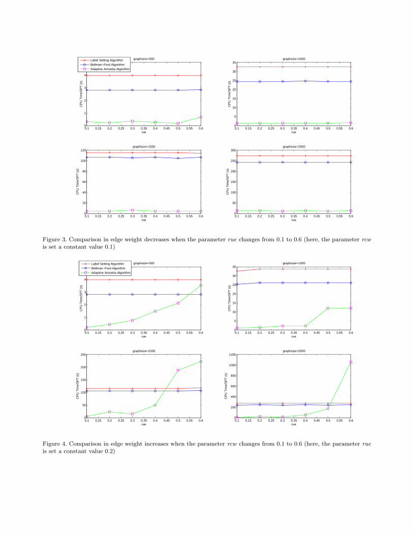
Edge Weight Decreases. Similarly, in the decrease case, we have observed the influence of the twoparameters on the CPU runtime of the above three algorithms. Figs. 3 and 4 show the experimental results,when the parameters rue, rcw change respectively.

As can be seen in Fig. 3, the parameters are set the same as that of the edge weight increases. From Fig. 3, itcan be concluded that, in the decrease case, when the parameter rue changes from 0.1 to 0.6, the CPU runtimeof the three algorithms fluctuates slightly in the networks with different sizes. In other words, the parameterrcw has very little effect on the computational efficiency of these algorithms. The proposed method has obviousadvantage over the Label Setting algorithm and Bellman-Ford algorithm when dealing with the SPT in dynamicgraphs.

As shown in Fig. 4, when the parameter rcw changes from 0.1 to 0.6, the CPU runtime of the proposedmethod fluctuates strongly. When rcw increases from 0.1 to 0.6, the CPU runtime for the adaptive amoebaalgorithm deteriorates rapidly. In the network with graph size equal to 500, 1500, 2000, when rcw reaches 0.6,it can be observed that the performance of the Label Setting algorithm and Bellman-Ford algorithm outperformcompared to the proposed method. It can be observed that when rcw is less than a certain threshold value, theproposed method has better performance. The threshold value varies with the size of a graph. When rcw isbigger than 0.4, it is more appropriate to adopt the Label Setting algorithm and Bellman-Ford algorithm. Thereason why the performance of the proposed algorithm gets worse when rcw is bigger than the threshold value isthat more edges are influenced, and more time is spent to reconstruct the SPT and reallocate the flux associatedwith each edge in the amoeba algorithm.

In summary, in the decreased case, the situation is similar to that of the increased case. The parameterrcw has different effect with that of parameter rue. Besides, the performance of the adaptive amoeba algorithm

0.1 0.15 0.2 0.25 0.3 0.35 0.4 0.45 0.5 0.55 0.60

1

2

3

4

5

rue

CP

U T

ime/

SP

T (

s)

graphsize=500

Label Setting AlgorithmBellman−Ford AlgorithmAdaptive Amoeba Algorithm

0.1 0.15 0.2 0.25 0.3 0.35 0.4 0.45 0.5 0.55 0.60

5

10

15

20

25

30

35

rue

CP

U T

ime/

SP

T (

s)

graphsize=1000

0.1 0.15 0.2 0.25 0.3 0.35 0.4 0.45 0.5 0.55 0.60

20

40

60

80

100

120

rue

CP

U T

ime/

SP

T (

s)

graphsize=1500

0.1 0.15 0.2 0.25 0.3 0.35 0.4 0.45 0.5 0.55 0.60

50

100

150

200

250

300

rue

CP

U T

ime/

SP

T (

s)

graphsize=2000

Figure 3. Comparison in edge weight decreases when the parameter rue changes from 0.1 to 0.6 (here, the parameter rcwis set a constant value 0.1)

0.1 0.15 0.2 0.25 0.3 0.35 0.4 0.45 0.5 0.55 0.60

1

2

3

4

5

rue

CP

U T

ime/

SP

T (

s)

graphsize=500

Label Setting AlgorithmBellman−Ford AlgorithmAdaptive Amoeba Algorithm

0.1 0.15 0.2 0.25 0.3 0.35 0.4 0.45 0.5 0.55 0.60

5

10

15

20

25

30

35

rue

CP

U T

ime/

SP

T (

s)

graphsize=1000

0.1 0.15 0.2 0.25 0.3 0.35 0.4 0.45 0.5 0.55 0.60

50

100

150

200

250

rue

CP

U T

ime/

SP

T (

s)

graphsize=1500

0.1 0.15 0.2 0.25 0.3 0.35 0.4 0.45 0.5 0.55 0.60

200

400

600

800

1000

1200

rue

CP

U T

ime/

SP

T (

s)

graphsize=2000

Figure 4. Comparison in edge weight increases when the parameter rcw changes from 0.1 to 0.6 (here, the parameter rueis set a constant value 0.2)

gets worse when rcw is more than a threshold value. As a consequence, it is appropriate to carry out differentalgorithms according to the specific value of this parameter.

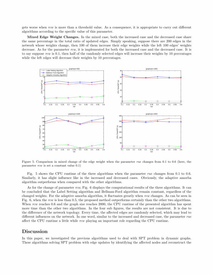
Mixed Edge Weight Changes. In the mixed case, both the increased case and the decreased case sharethe same percentage in the total ratio of updated edges. Simply speaking, suppose there are 200 edges in thenetwork whose weights change, then 100 of them increase their edge weights while the left 100 edges’ weightsdecrease. As for the parameter rcw, it is implemented for both the increased case and the decreased case. It isto say suppose rcw is 0.1, then half of the randomly selected edges will increase their weights by 10 percentageswhile the left edges will decrease their weights by 10 percentages.

0.1 0.15 0.2 0.25 0.3 0.35 0.4 0.45 0.5 0.55 0.60

1

2

3

4

5

rue

CP

U T

ime/

SP

T (

s)

graphsize=500

Label Setting AlgorithmBellman−Ford AlgorithmAdaptive Amoeba Algorithm

0.1 0.15 0.2 0.25 0.3 0.35 0.4 0.45 0.5 0.55 0.65

10

15

20

25

30

rue

CP

U T

ime/

SP

T (

s)

graphsize=1000

0.1 0.15 0.2 0.25 0.3 0.35 0.4 0.45 0.5 0.55 0.620

30

40

50

60

70

80

90

100

rue

CP

U T

ime/

SP

T (

s)

graphsize=1500

0.1 0.15 0.2 0.25 0.3 0.35 0.4 0.45 0.5 0.55 0.60

50

100

150

200

250

300

rue

CP

U T

ime/

SP

T (

s)

graphsize=2000

Figure 5. Comparison in mixed change of the edge weight when the parameter rue changes from 0.1 to 0.6 (here, theparameter rcw is set a constant value 0.1)

Fig. 5 shows the CPU runtime of the three algorithms when the parameter rue changes from 0.1 to 0.6.Similarly, it has slight influence like in the increased and decreased cases. Obviously, the adaptive amoebaalgorithm outperforms when compared with the other algorithms.

As for the change of parameter rcw, Fig. 6 displays the computational results of the three algorithms. It canbe concluded that the Label Setting algorithm and Bellman-Ford algorithm remain constant, regardless of thechanged weights. For the adaptive amoeba algorithm, it fluctuates greatly when rcw changes. As can be seen inFig. 6, when the rcw is less than 0.5, the proposed method outperforms certainly than the other two algorithms.When rcw reaches 0.6 and the graph size reaches 2000, the CPU runtime of the presented algorithm has spentmore time than the other two algorithms. In the four sub figures, the results are not consistent. It is due tothe difference of the network topology. Every time, the affected edges are randomly selected, which may lead todifferent influences on the network. In one word, similar to the increased and decreased case, the parameter rueaffect the CPU runtime a little while rcw playing an important role regarding the CPU runtime.

Discussion

In this paper, we investigated the previous algorithms used to deal with SPT problem in dynamic graphs.These algorithms solving SPT problem with edge updates by identifying the affected nodes and reconstruct the

0.1 0.15 0.2 0.25 0.3 0.35 0.4 0.45 0.5 0.55 0.60

1

2

3

4

5

rue

CP

U T

ime/

SP

T (

s)

graphsize=500

Label Setting AlgorithmBellman−Ford AlgorithmAdaptive Amoeba Algorithm

0.1 0.15 0.2 0.25 0.3 0.35 0.4 0.45 0.5 0.55 0.60

5

10

15

20

25

30

35

rue

CP

U T

ime/

SP

T (

s)

graphsize=1000

0.1 0.15 0.2 0.25 0.3 0.35 0.4 0.45 0.5 0.55 0.60

20

40

60

80

100

120

rue

CP

U T

ime/

SP

T (

s)

graphsize=1500

0.1 0.15 0.2 0.25 0.3 0.35 0.4 0.45 0.5 0.55 0.640

60

80

100

120

140

160

180

200

220

rue

CP

U T

ime/

SP

T (

s)

graphsize=2000

Figure 6. Comparison in mixed change of the edge weight when the parameter rcw changes from 0.1 to 0.6 (here, theparameter rue is set a constant value 0.2)

shortest path among these nodes. However, when these algorithms are faced with the network with big scale,on the one hand, this procedure becomes very complicated. On the other hand, it cost much time. In orderto address the above problems, we proposed a fully adaptive amoeba algorithm for solving SPT in dynamicgraphs. The efficiency of the presented algorithm is demonstrated by implementing it in all the edge updatesincluding the increase, decrease, mixed change of the edge weight. In order to evaluate the performance of theproposed method, we conducted experiments on randomly generated graphs, in terms of the CPU execution time.Moreover, we compared our algorithm with the existing algorithms, such as the Label Setting algorithm, Bellman-Ford algorithm. The purpose of the experiment is to obverse how these algorithms behave for different graph sizesand various mixes of changed edges. We randomly generate four graphs with different sizes: 500, 1000, 1500, 2000.

We evaluate the performance of the three algorithms according to three factors: graphsize, ratio of updatededges (rue), ratio of changed weight (rcw). For the increased case, the change of the parameter rue has littleinfluence on these algorithms while the change of the parameter rcw has great influence on the CPU runtime ofthe proposed method. For the decreased case, the influence of parameter rue is similar to that of the increasedcase. On the other hand, the performance of the adaptive amoeba algorithm gets worse when rcw is more thana threshold value. As for the other left algorithms, they are slightly influenced by parameter rcw. For the mixedchange of the edge weights, the influences of parameters rue and rcw on the computational time are consistentwith that of the increased and decreased cases. We conclude the following for the above three algorithms. Forthe increased case, decreased case, and mixed change case, in spite of the ratio of updated edges, the proposedmethod has the best overall performance. On the contrary, when the parameter rcw changes, it is appropriateto carry out different algorithms according to the specific value of rcw.

Methods

Physarum Polycephalum Inspired Shortest Path Finding Model. Physarum Polycephalum is a large,single-celled amoeboid organism forming a dynamic tubular network connecting the discovered food sources

during foraging. The mechanism of tube formation can be described as: tubes thicken in a given direction whenshuttle streaming of the protoplasm persists in that direction for a certain time. It implies positive feedbackbetween flux and tube thickness, as the conductance of the sol is greater in a thicker channel. With thismechanism, a mathematical model illustrating the shortest path finding has been constructed.33

Suppose the shape of the network formed by the Physarum is represented by a graph, in which a plasmodialtube refers to an edge of the graph and a junction between tubes refers to a node. Two special nodes labeledas N1, N2 act as the starting node and ending node respectively. The other nodes are labeled as N3, N4, N5, N6

etc. The edge between node Ni and Nj is expressed as Mij . The parameter Qij denotes the flux through tubeMij from node Ni to Nj . Regard the flow along the tube as an approximately poiseuille flow, the flux Qij canbe expressed as:

Qij =Dij

Lij

(pi − pj) (1)

where pi is the pressure at the node Ni, Dij is the conductivity of the tube Mij , Lij is its length.

By considering that the inflow and outflow must be balanced, we have:

∑

Qij = 0(j 6= 1, 2) (2)

For the source node N1 and the sink node N2 the following two equations hold

∑

i

Qi1 + I0 = 0 (3)

∑

i

Qi2 − I0 = 0 (4)

where I0 is the flux flowing from the source node and I0 is a constant value here.

In order to describe such an adaptation of tubular thickness we assume that the conductivity Dij changesover time according to the flux Qij . The following equation for the evolution of Dij(t) can be used

d

dtDij = f(|Qij |)− rDij (5)

where r is a decay rate of the tube. It can be obtained that the equation implies that the conductivity endsto vanish if there is no flux along the edge, while it is enhanced by the flux. The f is monotonically increasingcontinuous function satisfying f(0) = 0.

Then the network poisson equation for the pressure can be obtained from the Eq. (8-4) as follows:

∑

i

Dij

Lij

(pi − pj) =

+1 for j = 1,−1 for j = 2,0 otherwise

(6)

By setting p2=0 as a basic pressure level, all pi can be determined by solving Eq. (6) and Qij can also beobtained.

In this paper, f(Q) = |Q| is used. With the flux calculated, the conductivity can be derived, where Eq. (7)is used instead of Eq. (5), adopting the functional form f(Q) = |Q|.

Dn+1ij −Dn

ij

δt= |Q| −Dn+1

ij (7)

The amoeba model is modified to solve SPTs in dynamic graphs. The algorithm is composed of three parts.First of all, the amoeba model is extended to solve the shortest path in the directed networks. Then a modified

model is presented to handle SPTs in static directed networks. Finally, we analyze the changing trend of theamoeba algorithm is applied to deal with SPTs in dynamic graphs.

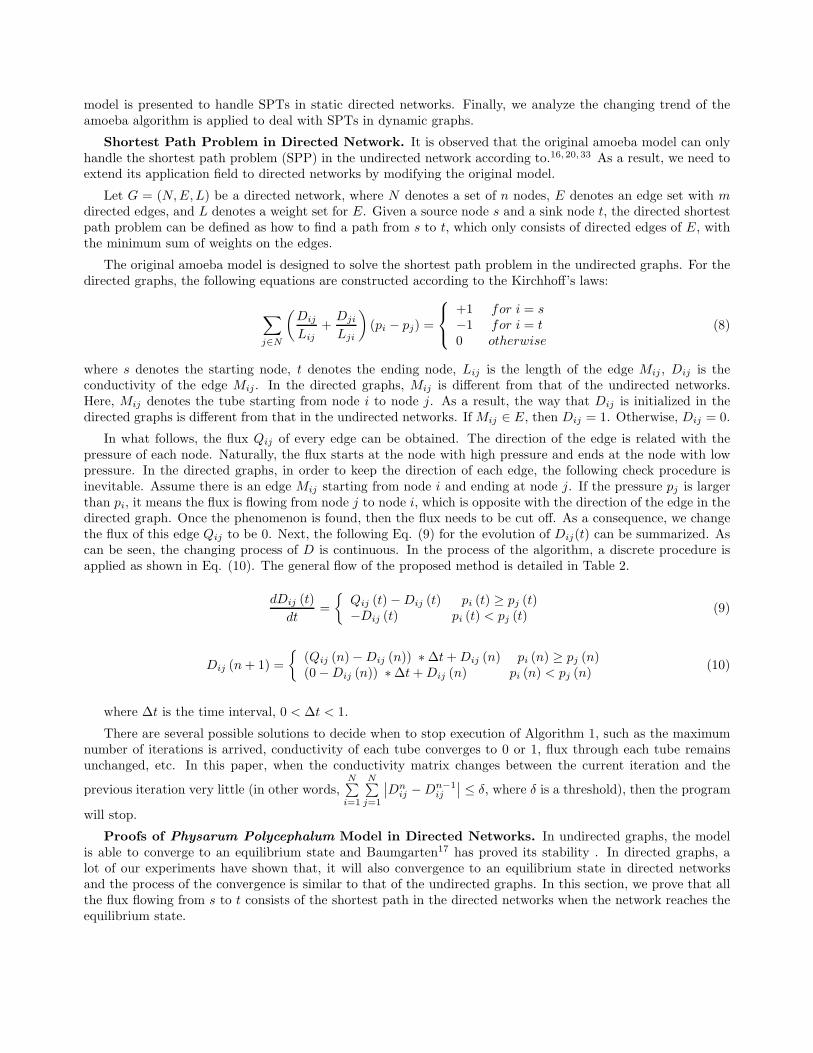
Shortest Path Problem in Directed Network. It is observed that the original amoeba model can onlyhandle the shortest path problem (SPP) in the undirected network according to.16, 20, 33 As a result, we need toextend its application field to directed networks by modifying the original model.

Let G = (N,E,L) be a directed network, where N denotes a set of n nodes, E denotes an edge set with m

directed edges, and L denotes a weight set for E. Given a source node s and a sink node t, the directed shortestpath problem can be defined as how to find a path from s to t, which only consists of directed edges of E, withthe minimum sum of weights on the edges.

The original amoeba model is designed to solve the shortest path problem in the undirected graphs. For thedirected graphs, the following equations are constructed according to the Kirchhoff’s laws:

∑

j∈N

(

Dij

Lij

+Dji

Lji

)

(pi − pj) =

+1 for i = s

−1 for i = t

0 otherwise

(8)

where s denotes the starting node, t denotes the ending node, Lij is the length of the edge Mij , Dij is theconductivity of the edge Mij . In the directed graphs, Mij is different from that of the undirected networks.Here, Mij denotes the tube starting from node i to node j. As a result, the way that Dij is initialized in thedirected graphs is different from that in the undirected networks. If Mij ∈ E, then Dij = 1. Otherwise, Dij = 0.

In what follows, the flux Qij of every edge can be obtained. The direction of the edge is related with thepressure of each node. Naturally, the flux starts at the node with high pressure and ends at the node with lowpressure. In the directed graphs, in order to keep the direction of each edge, the following check procedure isinevitable. Assume there is an edge Mij starting from node i and ending at node j. If the pressure pj is largerthan pi, it means the flux is flowing from node j to node i, which is opposite with the direction of the edge in thedirected graph. Once the phenomenon is found, then the flux needs to be cut off. As a consequence, we changethe flux of this edge Qij to be 0. Next, the following Eq. (9) for the evolution of Dij(t) can be summarized. Ascan be seen, the changing process of D is continuous. In the process of the algorithm, a discrete procedure isapplied as shown in Eq. (10). The general flow of the proposed method is detailed in Table 2.

dDij (t)

dt=

{

Qij (t)−Dij (t) pi (t) ≥ pj (t)−Dij (t) pi (t) < pj (t)

(9)

Dij (n+ 1) =

{

(Qij (n)−Dij (n)) ∗∆t+Dij (n) pi (n) ≥ pj (n)(0−Dij (n)) ∗∆t+Dij (n) pi (n) < pj (n)

(10)

where ∆t is the time interval, 0 < ∆t < 1.

There are several possible solutions to decide when to stop execution of Algorithm 1, such as the maximumnumber of iterations is arrived, conductivity of each tube converges to 0 or 1, flux through each tube remainsunchanged, etc. In this paper, when the conductivity matrix changes between the current iteration and the

previous iteration very little (in other words,N∑

i=1

N∑

j=1

∣

∣Dnij −Dn−1

ij

∣

∣ ≤ δ, where δ is a threshold), then the program

will stop.

Proofs of Physarum Polycephalum Model in Directed Networks. In undirected graphs, the modelis able to converge to an equilibrium state and Baumgarten17 has proved its stability . In directed graphs, alot of our experiments have shown that, it will also convergence to an equilibrium state in directed networksand the process of the convergence is similar to that of the undirected graphs. In this section, we prove that allthe flux flowing from s to t consists of the shortest path in the directed networks when the network reaches theequilibrium state.

First of all, the following parameters are defined:

F (t): F (t) is one set of edges whose Qij is non-negative number at time t. Let F = limt→∞

F (t).

B (t): B (t) is another set of edges whose Qij is is negative number at time t. Let B = limt→∞

B (t).

uij (t): uij (t) is the pressure difference between node i and node j at time t. uij (t) = pi (t) − pj (t). Letuij = lim

t→∞

uij (t).

lemma 3.1. For any directed edge Mij , limt→∞

(Qij (t)−Dij (t)) = 0.

Proof When t goes to a infinite number, the network reaches stable. As a result, for anyMij , limt→∞

dDij(t)dt

= 0.

According to Eq. (9), it can be seen that:

{

limt→∞

(Qij (t)−Dij (t)) = 0 Mij ∈ F

limt→∞

Dij (t) = 0 Mij ∈ B

When j ∈ B, limt→∞

Qij (t) = limt→∞

Dij(t)uij(t)Lij

= 0.

Lemma 3.1 is established.

lemma 3.2. For any Mij , if limt→∞

Qij (t) 6= 0, then Mij ∈ F and ue = Le.

Proof According to lemma 3.1, if limt→∞

Qij (t) 6= 0, then limt→∞

Dij (t) = limt→∞

Qij (t) 6= 0.

Based on Eq. (8), it can be seen that uij = Lij > 0 and Mij ∈ F .

Lemma 3.2 is established.

lemma 3.3. If Mij ∈ F , then uij ≤ Lij .

Proof According to lemma 3.2, when limt→∞

Qij (t) 6= 0, lemma 3.3 is established.

When limt→∞

Qij (t) = 0 and Mij ∈ F , then limt→∞

Dij (t) = 0, ∃T, ∀t > T,dDij(t)

dt< 0. Thus, Mij ∈ F (t).

According to Eq. (9), we can obtain Qij (t) < Dij (t).

According to Eq. (8), it can be seen uij (t) < Lij .

In summary, uij ≤ Lij . Therefore, lemma 3.3 is established.

lemma 3.4. When the model reaches the equilibrium state:

(i) All the flow converges to some paths from s to t.

(ii) These directed paths have the same path length and their length is equal to ust.

(iii) These directed paths have the shortest path length.

Proof

(i) According to lemma 3.1 and lemma 3.2, in the equilibrium state, the directions of all the edges are inaccordance with the flow directions. Consequently, the flow converges to the paths existing in the directedgraph G.

(ii) Assume v is one directed path which the flow converges to, Lv is the length of v. According to lemma 3.2,there are ust =

∑

Mij∈v

uij =∑

Mij∈v

Lij = Lv.

(iii) Assume v is one path from s to t, it is known to us that ust =∑

Mij∈v

uij . For any edge Mij , if uij ≥ 0,

then Mij ∈ F . According to lemma 3.3, uij ≤ Lij . If uij < 0, it is obviously seen that uij ≤ Lij .Consequently, ust =

∑

Mij∈v

uij ≤∑

Mij∈v

Lij = Lv. It means that all the other paths’ length is not less than

ust. Incorporating with (ii), these paths are the shortest ones.

Based on the above proofs, lemma 3.4 is established.

Shortest Path Tree Problem in Directed Networks. The above algorithm can only compute theshortest path between two nodes at a time. Assume there are N nodes in the network, if we want to constructthe shortest path tree, the algorithm must be run for N − 1 times. However, this will consume lots of time. Inthis section, after we modify the above model further, the shortest path tree can be constructed by running thealgorithm one time. In what follows, the modified model used to find the shortest path tree is introduced.

In the original amoeba model, there are only one starting node s and one ending node t in it. If there are onestarting node s and all the other nodes are the ending nodes, the Kirchhoffs laws can be transformed as below:

∑

i

(

Dij

Lij

+Dji

Lji

)

(pi − pj) =

{

+1 for j = s−1N−1 for j 6= s

(11)

The general flow of the modified model used to construct SPTs rooted at node s are shown in Table 3. Bythis way, SPT can be constructed through running the program once.

(a) An SPT Ts rooted at node s. In this figure, the vertex

are represented by letters and the numbers along the arcs

denote the path length. The arrow from the tail to the

head means the direction of the edge.

(b) The SPTs rooted at node s constructed by the adaptive

amoeba algorithm for shortest path tree

Figure 7. The amoeba algorithm for SPT

Example 0.1. In order to illustrate the algorithm shown in Table 3, an example is shown in Fig. 7(a). Thereare 16 nodes in this network. In this example, the amoeba model is applied to construct SPT rooted at nodes. According to Algorithm 2, first of all, initialize the parameters, such as the length matrix L, the initialconductivity matrix D, the initial pressure matrix Q etc. Then, according to Eq. (11), the pressure of each nodecan be obtained during the first iteration. In turn, the flux of each node can be computed according to Eq. (8).Next, the conductivity matrix during the following iteration can be constructed based on Eq. (7). This procedurewill continue until the flux of each arc do not change any more. Fig. 8 shows the flux variation of each edgeduring different iterations in the graph shown in Fig. 7(a) using the adaptive amoeba model. As we can see, theflux of some edges converges to 0 during the iterations. Those edges whose flux are not equal to zero constitutesthe following graph shown in Fig. 7(b).

0 10 20 30 40 50 600

0.1

0.2

0.3

0.4

0.5

0.6

0.7

0.8

0.9

1

Iteration

Flu

x

Edge(S,d)

Edge(S,c)

Edge(g,k) Edge(b,f)

Edge(S,b)Edge(d,h) Edge(g,j)

Edge(c,g)

Figure 8. Flux variation during different iterations in the graph shown in Fig. 7(a) using the adaptive amoeba model.

Fig. 7(b) shows the SPTs rooted at vertex s. The trees represented by the edges in blue color are consistentwith the result in.10 The edges with red color appear in the adaptive amoeba algorithm, but not in.10 The reasonlies that there are more than one shortest paths between the rooted node s and nodes e, k. For example, the lengthof the path S → b → e is equal to that of the path S → b → f → e. Similarly, the length of path S → d → h → k

is equal to that of S → c → g → k. This is the first advantage of our presented method.

The edge weight change can be divided into three categories: increase only, decrease only, the mixture ofthem. In this section, the adaptive amoeba algorithm for SPTs in dynamic graphs will be analyzed from thethree perspectives.

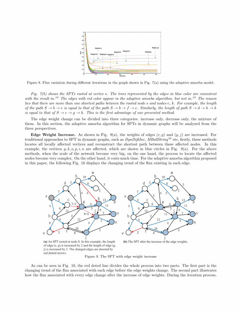
Edge Weight Increase. As shown in Fig. 9(a), the weights of edges (c, g) and (g, j) are increased. Fortraditional approaches to SPT in dynamic graphs, such as DynDijkInc, MBallString10 etc, firstly, these methodslocates all locally affected vertices and reconstruct the shortest path between these affected nodes. In thisexample, the vertices g, k, o, p, i, n are affected, which are shown in blue circles in Fig. 9(a). For the abovemethods, when the scale of the network become very big, on the one hand, the process to locate the affectednodes become very complex. On the other hand, it costs much time. For the adaptive amoeba algorithm proposedin this paper, the following Fig. 10 displays the changing trend of the flux existing in each edge.

(a) An SPT rooted at node S. In this example, the length

of edge (c, g) is increased by 2 and the length of edge (g,

j) is increased by 3. The changed edges are denoted by

red dotted arrows.

(b) The SPT after the increase of the edge weights.

Figure 9. The SPT with edge weight increase

As can be seen in Fig. 10, the red doted line divides the whole process into two parts. The first part is thechanging trend of the flux associated with each edge before the edge weights change. The second part illustrateshow the flux associated with every edge change after the increase of edge weights. During the iteration process,

0 50 100 150 200 2500

0.1

0.2

0.3

0.4

0.5

0.6

0.7

0.8

0.9

1

Iteration

Flu

x

Edge(S,d)

Edge(S,b)

Edge(d,h)

Edge(g,j)

Edge(c,g)Edge(b,f)

Edge(f,j)

Edge(S,c)

Edge(g,k)

Part 1 Part 2

Figure 10. The changing trend of the flux when the length of edge (c, g) is increased by 2 and the length of edge (g, j) isincreased by 3

the flux of the edge (g, j) decreases to 0 while that of the edge (f, j) become one of the edges constructingSPT. This example shows the adaptivity of the presented algorithm. It can recognize the affected vertices andreconstruct them spontaneously after the increase of the edge weights. Fig. 9(b) displays the SPT after theincrease of the edge weights and the result is consistent with that of.10

Edge Weight Decrease. Given a graph shown in Fig. 11(a), there are a source vertex S, an SPT rootedat node S. The weights of edge (c, g) and edge (g, j) are decreased by 3, 1 respectively. Different from theincrease case, the locally affected nodes can be predicted. In the decrease case, the traditional algorithms suchas DynDijkstra, MBallString recognize the all affected heads and then recompute the shortest path among theaffected heads. When the network becomes very big, the traditional algorithms are faced with the same problemsmentioned in the increase case. For the adaptive amoeba algorithm, the following Fig. 12 illustrates the changingtrend of the flux of each edge when the edge weights decrease.

(a) An SPT rooted at node S. In this example, the length

of edge (c, g) is decreased by 3 and the length of edge (g,

j) is decreased by 1. The changed edges are denoted by

red dotted arrows.

(b) The SPT after the decrease of the edge weights.

Figure 11. The SPT with edge weight decrease

As can be seen in Fig. 12, the whole process can be separated into two procedures by the red dotted line: thepart before edge weight decrease, the part after edge weight decrease. It can be seen that the flux associated withevery edge changes when the edge weights decrease. All the edges can be divided into 2 categories: the edgeswhich is not influenced by the edge weights decrease, such as edges (k, p) and (b, e) shown in Fig. 12 belongs tothe first category; the second category includes the edges that are influence by the edge weights decrease, suchas edges (h, k), (S, d), (S, c) etc. From Fig. 12, it can be concluded that the adaptive amoeba algorithm have the

0 20 40 60 80 100 120 1400

0.1

0.2

0.3

0.4

0.5

0.6

0.7

0.8

0.9

1

Iteration

Flu

x

Edge(S,d)

Edge(S,c)

Edge(d,h)

Edge(b,f)

Edge(g,j)

Edge(c,g)

Edge(b,e)Edge(k,p)Edge(g,k)

Edge(h,k)

Edge(S,b)

Part 1 Part 2

Figure 12. The changing trend of the flux when the length of edge (c, g) is decreased by 3 and the length of edge (g, j) isdecreased by 1

advantage of recognizing all the affected vertices spontaneously over traditional algorithms such as DynDijkstra,MBallString. Fig. 11(b) displays SPT after the edge weights decrease and the result is the same as that of.10

Mixed Edge Weight Changes. In Fig. 13(a), the weights of the following edges updates: edge (c, g) isdecreased by 1, the weight of edge (g, j) is increased by 3, and the weight of edge (f, i) is decreased by 8. Basedon this example, we will pay attention to the changing trend of the flux associated with each edge in the adaptiveamoeba algorithm when both the decrease and increase of the edges appear in the graph.

(a) An SPT rooted at node S. In this example, the weight

of edge (c, g) is decreased by 1, the weight of edge (g, j)

is increased by 3, and the weight of edge (f, i) is

decreased by 8. The changed edges are denoted by red

dotted arrows.

(b) The SPT after the update of the edge weights.

Figure 13. The SPT with mixed edge weight changes

As can be seen in Fig. 14, the changing trend of the flux associated with every edge is shown. Several edgessuch as edge (h, k) disappear from the SPT while edges (f, i) and (i, n) become the elements constructing SPTafter the update of edge weight. The other edges such as edges (k, p) and (b, e) are not affected by the updateof the edge weight. Fig. 13(b) gives the final SPT after the update of the edge weights. From Fig. 13(b), it canbe concluded that the amoeba algorithm can distinguish all the nodes adaptively.

In summary, all the edge updates including the increase, decrease, mixed change of the edge weight can behandled efficiently by the adaptive amoeba algorithm.

0 20 40 60 80 100 120 140 160 1800

0.1

0.2

0.3

0.4

0.5

0.6

0.7

0.8

0.9

1

Iteration

Flu

x

Part 1 Part 2

Edge(S,d)

Edge(g,k)

Edge(S,c)Edge(S,b)

Edge(c,g)Edge(d,h)

Edge(g,j)Edge(b,f)

Edge(h,k)

Edge(k,p)

Edge(b,e) Edge(i,n)

Edge(j,n)

Figure 14. The changing trend of the flux associated with each edge when the length of edge (c, g) is decreased by 1, thelength of edge (g, j) is increased by 3, and the weight of edge (f, i) is decreased by 810

Acknowledgment

All the authors of the cited papers for providing their network data. The work is partially supported byChongqing Natural Science Foundation, Grant No. CSCT, 2010BA2003, National Natural Science Foundationof China, Grant No. 61174022, 61364030, National High Technology Research and Development Program ofChina (863 Program) (No.2013AA013801), the Fundamental Research Funds for the Central Universities, GrantNo. XDJK2012D009.

1. Bauer, F., Varma, A. Distributed algorithms for multicast path setup in data networks. IEEE/ACM Trans.Networking 4, 181–191 (1996).

2. Rescigno, A. Optimally balanced spanning tree of the star network. IEEE Trans. Comput. 50, 88–91(2001).

3. Zhao, M., Yang, Y. Bounded relay hop mobile data gathering in wireless sensor networks. IEEE Trans.Comput. 61, 265–277 (2012).

4. Wang, P., Hunter, T., Bayen A.M., Schechtner, K., Gonzalez M.C. Understanding road usage patterns inurban areas. Sci. Rep. 2 (2012).

5. Barthelemy, M., Bordin, P., Berestycki, H., Gribaudi, M. Self-organization versus top-down planning inthe evolution of a city. Sci. Rep. 3 (2013).

6. Perlman, R. A comparison between two routing protocols: OSPF and IS-IS. IEEE Network 5, 18–24 (1991).

7. Estrada, E., Vargas-Estrada, E. How peer pressure shapes consensus, leadership, and innovations in socialgroups. Sci. Rep. 3 (2013).

8. Wei, D.J. et al. Box-covering algorithm for fractal dimension of weighted networks. Sci. Rep. 3 (2013).

9. Szell, M., Sinatra, R., Petri, G., Thurner, S., Latora, V. Understanding mobility in a social petri dish. Sci.Rep. 2 (2012).

10. Chan, E., Yang, Y. Shortest path tree computation in dynamic graphs. IEEE Trans. Comput. 58, 541–557(2009)

11. Chen, H., Tseng, P. A low complexity shortest path tree restoration scheme for IP networks. IEEECommun. Lett. 14, 566–568 (2010).

12. Dijkstra, E. A note on two problems in connection with graphs. Numerische Mathematik 1, 269C271(1959).

13. Frigioni, D., Marchetti-Spaccamela, A., Nanni, U. Incremental algorithms for the single-source shortestpath problem. Foundation of Software Technology and Theoretical Computer Science 14, 113–124 (1994).

14. Narvaez, P., Siu, K., Tzeng, H. New dynamic spt algorithm based on a ball-and-string model. IEEE/ACMTrans. Networking 9, 706–718 (2001).

15. Nguyen, S., Pallottino, S., Scutella, M.G. A new dual algorithm for shortest path reoptimization. Trans-portation and Network Analysis: Current Trends: Miscellanea in honor of Michael Florian 63, 221–221(2002).

16. Tero, A., Kobayashi, R., Nakagaki, T. Physarum solver: A biologically inspired method of road-networknavigation. Physica A 363, 115–119 (2006).

17. Baumgarten, W., Ueda, T., Hauser, M. Plasmodial vein networks of the slime mold physarum polycephalumform regular graphs. Phys. Rev. E 82, 046113 (2010).

18. Tero, A. et al. Rules for biologically inspired adaptive network design. Science Signalling 327, 439 (2010).

19. Watanabe, S., Tero, A., Takamatsu, A., Nakagaki, T. Traffic optimization in railroad networks using analgorithm mimicking an amoeba-like organism, physarum plasmodium. BioSystems 105, 225–232 (2011).

20. Nakagaki, T. et al. Minimum-risk path finding by an adaptive amoebal network. Phys. Rev. Lett. 99,068104 (2007).

21. Adamatzky, A., Prokopenko, M. Slime mould evaluation of australian motorways. Int. J. Parallel EmergentDistrib. Syst. 27, 275–295 (2012).

22. Zhang, X. et al. Solving 0-1 knapsack problems based on amoeboid organism algorithm. Appl. Math.Comput. 219, 9959–9970 (2013)

23. Zhang, X., Zhang, Z., Zhang, Y., Wei, D., Deng, Y. Route selection for emergency logistics management:A bio-inspired algorithm. Saf. Sci. 54, 87–91.

24. Gunji, Y.P., Shirakawa, T., Niizato, T., Haruna, T. Minimal model of a cell connecting amoebic motionand adaptive transport networks. J. Theor. Biol. 253, 659–667 (2008).

25. Adamatzky, A., Martınez, G.J., Chapa-Vergara, S.V., Asomoza-Palacio, R., Stephens, C.R. Approximatingmexican highways with slime mould. Natural Computing 10, 1195–1214 (2011).

26. Adamatzky, A., de Oliveira, P.P. Brazilian highways from slime molds point of view. Kybernetes 40,1373–1394 (2011).

27. Adamatzky, A. The worlds colonization and trade routes formation as imitated by slime mould. Int. J.Bifurcation Chaos 22 (2012).

28. Adamatzky, A. Growing spanning trees in plasmodium machines. Kybernetes 37, 258–264 (2008).

29. Aono, M., Hara, M., Aihara, K., Munakata, T. Amoeba-based emergent computing: combinatorial opti-mization and autonomous meta-problem solving. International Journal of Unconventional Computing 6,89–108 (2010).

30. Jones, J. Characteristics of pattern formation and evolution in approximations of physarum transportnetworks. Artificial Life 16, 127–153 (2010).

31. Aono, M., Zhu, L., Hara, M. Amoeba-based neurocomputing for 8-city traveling salesman problem. Inter-national Journal of Unconventional Computing 7, 463–480 (2011).

32. Shirakawa, T., Yokoyama, K., Yamachiyo, M., Gunji, Y.P., Miyake, Y. Multi-scaled adaptability in motilityand pattern formation of the physarum plasmodium. International Journal of Bio-Inspired Computation4, 131–138 (2012).

33. Tero, A., Kobayashi, R., Nakagaki, T. A mathematical model for adaptive transport network in pathfinding by true slime mold. J. Theor. Biol. 244, 553–564 (2007).

34. Meyer, U. Average-case complexity of single-source shortest-paths algorithms: lower and upper bounds.Journal of Algorithms 48, 91–134 (2003).

35. Nguyen, U.T., Xu, J. Multicast routing in wireless mesh networks: Minimum cost trees or shortest pathtrees? IEEE Commun. Mag. 45, 72–77 (2007).

Table 1. The related parameters of the erdos.renyi.game function. In this function, the parameter p denotes the probabilityfor drawing an edge between two arbitrary vertices.

Dataset Number of Nodes p Number of Edges

dataset 1 500 0.0200 5000dataset 2 1000 0.0100 9921dataset 3 1500 0.0060 13475dataset 4 2000 0.0050 19903

Table 2. Adaptive Amoeba Algorithm(L, V, E) for Directed Networks

// L is an N ×N matrix, Lij denotes the length between node i andnode j

// V denote the set of nodes, E denotes the set of edges// s is the starting node, t is the ending nodeDij ← (0, 1] (∀i, j = 1, 2, . . . , N ∧ Lij 6= 0)Qij ← 0 (∀i, j = 1, 2, . . . , N)pi ← 0 (∀i = 1, 2, . . . , N)count← 1repeat

pt ← 0 // the pressure at the ending node t

Calculate the pressure of every node using Eq. (8)

∑

i

(

Dij

Lij

+Dji

Lji

)

(pi − pj) =

+1 for j = s

−1 for j = t

0 otherwise

Qij ← Dij × (pi − pj)/Lij // Using Eq. (8)if Qij < 0 then

Qij = 0end if

Dij ← Qij +Dij // Using Eq. (7)count← count + 1

until a termination criterion is met

Author contributions

X. Z., Q. L., Z. Z. designed and performed research. X. Z. wrote the paper. Y. H. performed the computation. S.M., F. T.S. C. and Y. D. analyzed the data. All authors discussed the results and commented on the manuscript.

Additional information

Competing financial interests: The authors declare no competing financial interests.

Table 3. Adaptive Amoeba Algorithm(L, V, E) for Shortest Path Tree

// L is an N ×N matrix, Lij denotes the length between node i andnode j

// V denote the set of nodes, E denotes the set of edges// s is the root nodeDij ← (0, 1] (∀i, j = 1, 2, . . . , N ∧ Lij 6= 0)Qij ← 0 (∀i, j = 1, 2, . . . , N)pi ← 0 (∀i = 1, 2, . . . , N)count← 1repeat

Calculate the pressure of every node using Eq. (11)

∑

i

(

Dij

Lij

+Dji

Lji

)

(pi − pj) =

{

+1 for j = s−1

N−1for j 6= s

Qij ← Dij × (pi − pj)/Lij // Using Eq. (8)if Qij < 0 then

Qij = 0end if

Dij ← Qij +Dij // Using Eq. (7)count← count + 1

until a termination criterion is met