Planar Graphs, Negative Weight Edges, Shortest Paths, Near Linear Time

Journal of Computer and System Sciences 72 (2006) 868–889

www.elsevier.com/locate/jcss

Planar graphs, negative weight edges, shortest paths,and near linear time

Jittat Fakcharoenphol a,∗,1, Satish Rao b

a Department of Computer Engineering, Kasetsart University, Bangkok, Thailandb Computer Science Division, University of California, Berkeley, CA 94720, USA

Received 17 May 2002; received in revised form 6 May 2004

Available online 7 February 2006

Abstract

In this paper, we present an O(n log3 n) time algorithm for finding shortest paths in an n-nodeplanar graph with real weights. This can be compared to the best previous strongly polynomial timealgorithm developed by Lipton, Rose, and Tarjan in 1978 which runs in O(n3/2) time, and the bestpolynomial time algorithm developed by Henzinger, Klein, Subramanian, and Rao in 1994 whichruns in O(n4/3) time. We also present significantly improved data structures for reporting distancesbetween pairs of nodes and algorithms for updating the data structures when edge weights change.© 2006 Elsevier Inc. All rights reserved.

Keywords: Planar graphs; Negative edge weights; Shortest paths; Algorithms

1. Introduction

The shortest path problem with real (positive and negative) weights is the problem offinding the shortest distances from a specified source node to all the nodes in the graph. Forthis paper, we assume that the graph has no negative cycles since the shortest path betweentwo nodes will be undefined in the presence of negative cycles. In general, algorithms for

* Corresponding author.E-mail addresses: [email protected] (J. Fakcharoenphol), [email protected] (S. Rao).

1 Supported by the Fulbright scholarship and the scholarship from the Faculty of Engineering, KasetsartUniversity, Thailand. Work done while at CS Division, University of California, Berkeley.

0022-0000/$ – see front matter © 2006 Elsevier Inc. All rights reserved.doi:10.1016/j.jcss.2005.05.007

J. Fakcharoenphol, S. Rao / Journal of Computer and System Sciences 72 (2006) 868–889 869

the shortest path problem can, however, easily be modified to output a negative cycle, ifone exists. This also holds for the algorithms in this paper.

The shortest path problem has long been studied and continues to find applicationsin diverse areas. The problem has wide application even when the underlying graph isa grid. For example, there are recent image segmentation approaches that use negativecycle detection [1,2]. Some of our other favorite applications for planar graphs includeseparator algorithms [3], multi-source multi-sink flow algorithms [4], or algorithms forfinding minimum weighted cuts [5].

In 1958, Bellman and Ford [6,7] gave an O(mn) algorithm for finding shortest paths onan m-edge, n-node graph with arbitrary real edge weights. Gabow and Tarjan [8] showedthat this problem could indeed be solved in O(

√nm logC),2 where C denotes the largest

absolute weights in the graph. Their algorithm depends on the values of the edge weights.For strongly polynomial algorithms, Bellman–Ford remains the best known.

As for graphs with non-negative edge weights, the problem is much easier. For example,Dijkstra’s shortest path algorithm [9] can be implemented in O(m + n logn) time.

For planar graphs, upon the discovery of planar separator theorems [10], an O(n3/2)

algorithm was given by Lipton, Rose, and Tarjan [11]. Their algorithm is based on parti-tioning the graph into pieces and recursively computing distances between the borders ofeach piece using numerous invocations of Dijkstra’s algorithm to build a dense graph. Thenthey use the Bellman–Ford algorithm on the resulting dense graph to construct a global so-lution. Their algorithms works not only for planar graphs but for any

√n-separable one.3

Combining a similar approach with a weakly polynomial algorithm of Goldberg [12]for general graphs, Henzinger et al. [13] gave an O(n4/3 logC) algorithm for the shortestpath problem on planar graphs or any graphs with an O(

√n) sized separator, where C

denotes the largest absolute weights.In this paper, we present an O(n log3 n) time algorithm for finding shortest paths in a

planar graph with real weights. We also present algorithms for query and dynamic versionsof the shortest path problems.

1.1. The idea

Our approach is similar to the approaches discussed above in that, give a planar graph G,it constructs a rather dense non-planar graph GD on a subset of nodes and then computesa shortest path tree GD .

We observe that there exists a shortest path tree in GD that must obey a non-crossingproperty in the geometric embedding of the graph inherited from the embedding of theoriginal planar graph G. Using this non-crossing condition, we can compute a shortest pathtree of the GD in time that is nearly linear in the number of nodes in GD and significantlyless than linear in the number of edges. Specifically, we decompose our dense graph GD

into a set of bipartite graphs whose distance matrices obey a non-crossing condition (calledthe Monge condition; see definitions in Section 2.3).

2 The O(·) notation ignores logarithmic factors.3 Assuming that they are given a recursive decomposition of the graph.

870 J. Fakcharoenphol, S. Rao / Journal of Computer and System Sciences 72 (2006) 868–889

Our algorithm proceeds by combining Dijkstra’s and the Bellman–Ford algorithms withmethods for searching Monge matrices in sublinear time. We use an on-line method forsearching Monge arrays with our version of Dijkstra’s algorithm on the dense graph.

We note that our algorithms rely heavily on planarity, whereas some of the previousmethods only require that the graphs are O(

√n)-separable. Recently, Smith [14] suggests

that our algorithm works with the same time and space bound as well on graphs of boundedgenus, by using the result of Hutchinson and Miller [15] and Djidjev and Venkatesan [16]on finding planarizing separators for bounded genus graphs at the topmost level of thedecomposition.

1.2. Our results

We give the following results.

• An O(n log3 n) algorithm for finding shortest paths in planar graphs with real weights.• An algorithm that requires O(n log3 n) preprocessing time and answers distance

queries between pairs of nodes in time O(√

n log2 n). The best previous algorithmshad an Θ(n2) query-preprocessing time product, whereas ours is O(n3/2).

• An algorithm that supports distance queries and update operations that change edgeweights in amortized O(n2/3 log7/3 n) time per operation. This algorithm works forpositive edge weights.

• An algorithm that supports distance queries and update operations that change edgeweights in amortized O(n4/5 log13/5 n) time per operation. This algorithm works fornegative edge weights as well.

We also present an on-line Monge searching problem and methods to solve it that maybe novel and of independent interest.

1.3. More related work

For planar graphs with positive edge weights, Henzinger et al. [13] gave an O(n) timealgorithm to compute single-source shortest paths. Their work improves on work of Fred-erickson [17] who had previously given O(n

√logn ) algorithms for this problem.

For non-negative integer weights, if the distance queries are for ε-approximate an-swers, Thorup [18] gave two algorithms. His first algorithm preprocesses the input intime O(nε−1 log2 n logΔ) and builds a data structure supporting each query in timeO(log logΔ + ε−1 logn), where Δ is an upper bound on the largest finite distance. Hissecond algorithm gives a faster query time of O(log logΔ + 1/ε) while the preprocessingtime becomes O(n log3 logΔ/ε2).

Recently, Klein [19] gives an O(n logn)-time algorithm for planar graphs with non-negative edge weights that construct a data structure supporting each distance query intime O(logn). Using this algorithm, he derives faster algorithms for constructing the datastructure for distance query for graphs with non-negative weights, which runs in timeO(n log2 n), and for the dynamic case with the amortized running time of O(n2/3 log5/3 n)


per operation. His technique also improve the preprocessing time of Thorup’s first algo-rithm mentioned in the previous paragraph.

Frederickson [20] gave an improved all-pairs shortest path algorithm for planar graphswith small hammock decompositions. Djidjev et al. [21] gave dynamic algorithms whosecomplexity are linear in the size of the hammock decomposition. This could be quite effi-cient in certain cases, e.g., when the graph is outerplanar. But for general planar graphs—even grid graphs—their algorithms are no better than those in [11].

Efficient algorithms for searching for minima in Monge arrays have been developedpreviously. See, for example, [22,23].

A binary searching technique similar to the one we use in the Monge searching problemalso appeared in an algorithm for finding shortest paths on a three-dimensional polygon byMitchell et al. [24].

2. Preliminaries

In this section, we give backgrounds on shortest paths, algorithms for finding them, andMonge arrays. Subsection 2.1 describes two basic algorithms that we use, namely, Dijk-stra’s algorithm and the Bellman–Ford algorithm. We discuss price functions and reducedcosts as tools for speeding up shortest path computations when there are many sources inSubsection 2.2. Finally, in Subsection 2.3, we give an introduction to the Monge property.We begin with the definition of shortest path labellings.

Given a directed graph G = (V ,E), and a weight function w :E → R on the directededges, a distance labeling for a source node s is a function d :V → R such that d(v) is theminimum over all s to v paths P of P ’s length, i.e.,

∑e∈P w(e).

2.1. Algorithms

The algorithms we use work through a sequence of edge relaxations. They start witha labeling d(·) and choose an edge to relax. The relax operation proceeds for an edgee = (u, v) by setting the distance label d(v) to the minimum of d(v) and d(u) + d(e).

Dijkstra’s algorithm (described below) correctly computes a distance labeling when theweights on the edges are non-negative, i.e., d(e) � 0 for all e ∈ E.

Algorithm Dijkstra(G = (V ,E), w, s)

d(v) = ∞, ∀v �= s.

d(s) = 0.

S = {s}.while S �= V do

u = findMind (V \ S)

foreach e = (u, v)

d(v) = min(d(v), d(u) + w(e)) /* This is an edge relaxation */

S = S ∪ {u}.


For distance functions where d(e) could be less than zero, Bellman and Ford suggestedthe following algorithm, which is guaranteed to compute a distance labeling if there is nocycle in the graph whose total weight under d(·) is negative. The algorithm is as follows.

Algorithm Bellman–Ford (G = (V ,E), w, s)

d(v) = ∞, ∀v �= s.

d(s) = 0.

phase = 0.

while phase � n do

relax all edges.

phase ← phase + 1.

2.2. Feasible price functions and relabellings

A price function p is a function from V to the set of real numbers. The reduced costfunction wp over the edge set induced by the price function p is defined as

wp(u, v) = p(u) + w(u,v) − p(v).

It is well known that the reduced cost function preserves negative cycles and also the short-est paths [25].

We say that the price function p is feasible if and only if for all edges e = (u, v),wp(u, v) � 0. Hence, for any feasible price function p, we can find a distance labelingfrom any source node using Dijkstra’s algorithm on the modified graph with wp as weights(called the relabeled graph). The distance labeling for the original graph can be easilyrecovered from the relabeled one. We note that a valid set of distance labels for any sourcenode is a feasible price function.

Thus, computing shortest paths from k sources in a graph with negative weight edgescan be accomplished with only one application of the Bellman–Ford algorithm and k − 1applications of Dijkstra’s algorithm.

2.3. Monge arrays

Given ordered sets A and B and a distance function d :A × B → R between pairs ofelement in A and B , we say that d has the Monge property if for all u,v ∈ A and x, y ∈ B ,u � v and x � y implies that

d(u, x) + d(v, y) � d(v, y) + d(u, x),

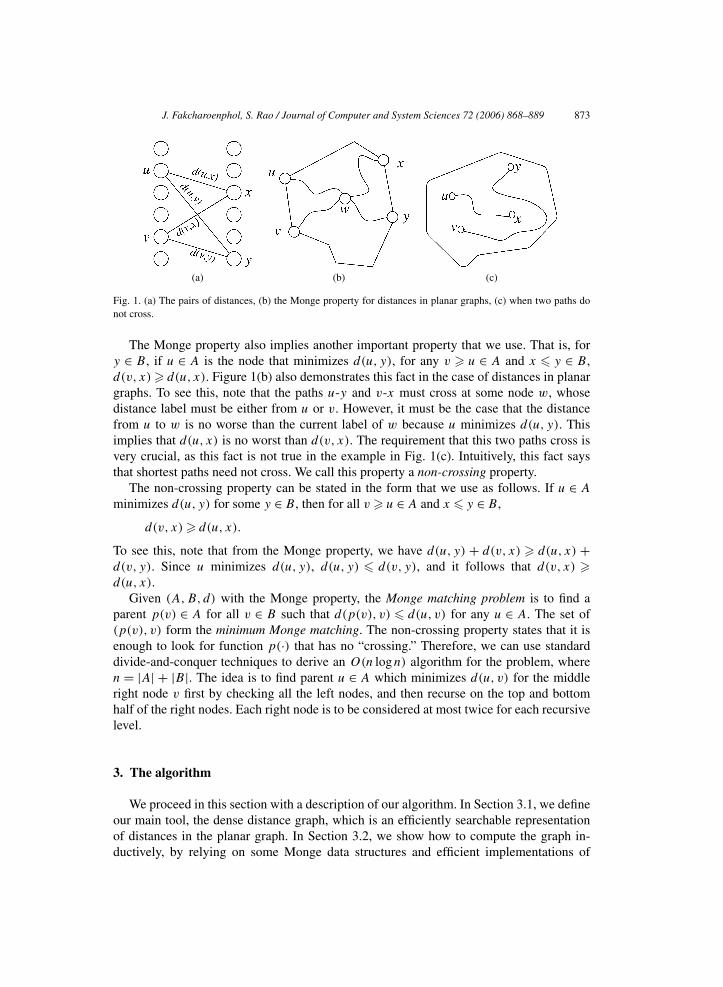
i.e., the sum of the distances when the pairs do not cross is at most the sum when thepairs cross (see Fig. 1(a)). We can also view the triplet (A,B,d) as a metric on a complete“ordered” bipartite graph. Naturally, we call each element in A and B a node. Nodes in A

are left nodes, and nodes in B are right nodes.An example of distance functions with the Monge property is the shortest distances

between border nodes in planar graphs. Figure 1(b) gives an example. Since any pathsfrom u to x and from v to y always cross at some node w, we can break up the distance onthe left-hand side and derive the inequality.


(a) (b) (c)

Fig. 1. (a) The pairs of distances, (b) the Monge property for distances in planar graphs, (c) when two paths donot cross.

The Monge property also implies another important property that we use. That is, fory ∈ B , if u ∈ A is the node that minimizes d(u, y), for any v � u ∈ A and x � y ∈ B ,d(v, x) � d(u, x). Figure 1(b) also demonstrates this fact in the case of distances in planargraphs. To see this, note that the paths u-y and v-x must cross at some node w, whosedistance label must be either from u or v. However, it must be the case that the distancefrom u to w is no worse than the current label of w because u minimizes d(u, y). Thisimplies that d(u, x) is no worst than d(v, x). The requirement that this two paths cross isvery crucial, as this fact is not true in the example in Fig. 1(c). Intuitively, this fact saysthat shortest paths need not cross. We call this property a non-crossing property.

The non-crossing property can be stated in the form that we use as follows. If u ∈ A

minimizes d(u, y) for some y ∈ B , then for all v � u ∈ A and x � y ∈ B ,

d(v, x) � d(u, x).

To see this, note that from the Monge property, we have d(u, y) + d(v, x) � d(u, x) +d(v, y). Since u minimizes d(u, y), d(u, y) � d(v, y), and it follows that d(v, x) �d(u, x).

Given (A,B,d) with the Monge property, the Monge matching problem is to find aparent p(v) ∈ A for all v ∈ B such that d(p(v), v) � d(u, v) for any u ∈ A. The set of(p(v), v) form the minimum Monge matching. The non-crossing property states that it isenough to look for function p(·) that has no “crossing.” Therefore, we can use standarddivide-and-conquer techniques to derive an O(n logn) algorithm for the problem, wheren = |A| + |B|. The idea is to find parent u ∈ A which minimizes d(u, v) for the middleright node v first by checking all the left nodes, and then recurse on the top and bottomhalf of the right nodes. Each right node is to be considered at most twice for each recursivelevel.

3. The algorithm

We proceed in this section with a description of our algorithm. In Section 3.1, we defineour main tool, the dense distance graph, which is an efficiently searchable representationof distances in the planar graph. In Section 3.2, we show how to compute the graph in-ductively, by relying on some Monge data structures and efficient implementations of


Dijkstra’s algorithm and the Bellman–Ford algorithm. In Section 3.3, we show how touse it to compute a shortest path labeling of the graph. In Sections 3.4 to 3.6, we use thedense distance graph as the basis for query and dynamic shortest path algorithms.

3.1. The dense distance graph

A decomposition of a graph is a set of subsets P1,P2, . . . ,Pk (not necessarily disjoint)such that the union of all the sets is V and for all e = (u, v) ∈ E, there is a unique Pi

that contains e. A node v is a border node of a set Pi if v ∈ Pi and there exists an edgee = (v, x) where x /∈ Pi . We refer to the subgraph induced on a subset Pi as a piece of thedecomposition.

We assume that we are given a recursive decomposition where at each level, a piecewith n nodes and r border nodes is divided into two subpieces such that each subpiece hasno more than 2n/3 nodes and at most 2r/3 + c

√n border nodes, for some constant c. (The

recursion stops when a piece contains a single edge.)In this recursive context, we define a border node of a subpiece to be any border node of

the original piece or any new border node introduced by the decomposition of the currentpiece.

It is convenient to define the level of a decomposition in the natural way, with the entiregraph being the only piece in the level 0 decomposition, the pieces of the decomposition ofthe entire graph being the level 1 pieces in the decomposition, and so on. A node is a leveli border node if it is a border node of a level i piece. Note that a node may be a bordernode for many levels. Indeed, any level i border node is also a level j border node for allj > i.

Given an embedding of the piece, a hole is a bounded face where all adjacent nodes areborder nodes. For simplicity, we assume inductively that there is a planar embedding ofany piece in the recursive decomposition where all the border nodes are on a single faceand are circularly ordered. This assumption implies that no piece of the decomposition hasa hole. Although this assumption is true for interesting classes of planar graphs, e.g., gridgraphs, it is not true in general. In Section 5, we show how to generalize the algorithmto work with a piece with a constant number of holes and describe how one can find arecursive decomposition of that form in O(n logn) time.

We assume, without loss of generality, that the graph is a bounded-degree graph and,for simplicity, that each piece is connected. If some piece is not connected, the algorithmworks with each connected component separately.

For each piece of the decomposition, we recursively compute the all-pairs shortest pathdistances between all its border nodes along paths that lie entirely inside the piece. Theseall-pair distances form the edge set of a non-planar graph representing shortest paths be-tween border nodes. Taking the union of these graphs over all the levels, we have the densedistance graph of the planar graph.

The level i dense distance graph is the subgraph of the dense distance graph on the leveli border nodes. We refer to the level i dense distance graph of piece P as the subgraph ofthe level i dense distance graph whose edges correspond to paths that lie in P . Note that inthis definition, piece P might not be a level i piece.


This graph underlies previous algorithms for shortest paths in planar graphs. We give abetter algorithm to construct and use it.

3.2. Computing the dense distance graph

We assume (recursively) while computing the level i dense distance graph that we havethe level i + 1 graph and the distances between all the border nodes of each piece in thatlevel. We will show how to find the edges of the level i dense distance graph that correspondto a particular piece P , which has n nodes and r border nodes.

Recall that the level i dense distance graph for P consists of the all-pairs shortest pathdistances between border nodes within each of its subpieces in the level i+1 dense distancegraph.

Also, note that the level i + 1 dense distance graph may contain negative edges. Byfinding a feasible price function using a single Bellman–Ford computation from any source,however, we can find the shortest path distances from any other source using only theDijkstra computation as stated in Section 2.2.

We proceed by doing a single Bellman–Ford computation in the level i + 1 dense dis-tance graph of P from one border node, and then doing r − 1 Dijkstra computations on therelabeled graph to compute the shortest path distances from the remaining border nodes.

This, again, is exactly what previous researchers did. Their algorithms, however, usedimplementations for the Bellman–Ford and Dijkstra’s algorithms which depended linearlyon the number of edges that are present in the level i + 1 dense distance graph.

Our methods depend near linearly on the number of nodes in the dense distance graphlevel i + 1 of piece P , which is proportional to the square root of the number of its edges.

We assume that P contains n nodes and r = c√

n border nodes. By a property of thedecomposition, we assume that each of the two subpieces of P contain at most c′√n bordernodes. Thus, the level i + 1 dense distance graph contains at most r ′ = O(

√n) nodes.

3.2.1. The Bellman–Ford stepThe Bellman–Ford algorithm that we run proceeds as in Fig. 2.The total number of border nodes in every subpiece of P is r ′ = O(

√n), so the number

of edges is O(n). Therefore, if we relax every edge directly as in [11], the running timefor each step of edge relaxation would be O(n) for all of P . The total running time for theBellman–Ford step would then be O(n3/2).

However, we will relax the edges in time that is nearly linear in the number of nodes,i.e., in O(

√n log2 n) time. This gives a running time of O(n log2 n) for the Bellman–Ford

step.

Algorithm Bellman–Ford (P,w, s)d(s) = 0.d(v) = ∞, ∀v �= s.phase = 0.while phase � r ′ do

relax all edges.phase ← phase + 1.

Fig. 2. The implementation of the Bellman–Ford algorithm.


(a) (b) (c)

Fig. 3. Partitions of nodes to form O(logn) Monge arrays: (a) the first and second arrays, (b) the third and fortharrays, and (c) the fifth and sixth arrays.

We accomplish this by maintaining the edges of each subpiece of P in O(logn) levelsof Monge arrays. After the definition of the Monge arrays, we describe how all edges ineach Monge array with k nodes can be relaxed in O(k log k) time, where k is the numberof nodes in the data structure.

The first Monge array that we define is formed as follows. Divide the border nodes insome subpiece into two halves, the first (or left) half in the circular order (with an arbitrarystarting point) and the second (or right) half. Consider the set of edges in the dense distancegraph that go from the left border nodes to the right ones. The edges obey the Mongeproperty, since there is an underlying shortest path tree in which the corresponding pathsdo not cross.

Using the same left–right partitioning, we can define another Monge array with thedirection of edges reversed (i.e., edges in the array go from the right border nodes to theleft border nodes).

Successive Monge arrays are constructed by recursively dividing the left and righthalves further. Each node will occur in at most O(logn) data structures, and each edgewill occur in one data structure. Figure 3 shows how we partition nodes and edges betweenthem.

We can relax all the edges in a Monge array as follows. The nodes on the left have alabel associated with them, and a node v on the right must choose a left node u whichminimizes d(u) + w(u,v). We say that u is the parent of v and edge (u, v) is the parentedge of v. However, because of the planarity of the piece, the parent edges of two rightnodes need not cross, and this gives us the Monge property. For this special case, we canuse a the Monge matching algorithm, described in Subsection 2.3, to find all the parents intime O(r log r), where the number of nodes in the Monge array is r .

The total number of nodes in all the data structures is O(√

n logn) for each subpiece ofP in the decomposition.

In P we have two subpieces. Therefore, the time for relaxing all of P ’s edges isO(

√n log2 n). The number of phases the Bellman–Ford runs is the number of nodes in

the longest path, which is O(√

n). Thus, the time for the Bellman–Ford step is O(n log2 n)

on an n-node piece.

3.2.2. The Dijkstra stepAfter one invocation of Bellman–Ford, we have a shortest path tree from some border

node of P . Now, using the relabeling property, we can modify all edge weights so that they


Algorithm Dijkstra (P, {P ′i}, s)

d(v) ← ∞, ∀v �= s.d(s) ← 0.S ← {s}.for all P ′

i� s do

AddToHeap(H,(d(s),P ′i)).

while H is not empty doP ′

min ← ExtractMin(H).v ← ExtractMinInSubpiece(P ′

min).if v /∈ S,

for all P ′i� v do

ScanInSubpiece(P ′i, v, dv ).

vmin ← FindMinInSubpiece(P ′i)

UpdateHeap(H,(d(vmin),P ′i)).

elsevmin ← FindMinInSubpiece(P ′

min)

UpdateHeap(H,(d(vmin),P ′min)).

S ← S ∪ {v}.Fig. 4. Pseudocode for Dijkstra implementation.

are all positive and the shortest paths remain unchanged. With these modified weights, werepeatedly apply Dijkstra’s algorithm to compute all-pairs shortest distances among theborder nodes in P .

In order to compute the shortest path distances from each border node s of P , we pro-ceed as in Dijkstra.

While working at level i of the decomposition, we view each subpiece of level i + 1separately. Each subpiece maintains a data structure that allow us to scan a node (relaxall edges in the dense distance graph adjacent to that node in that subpiece) and find theminimum labeled node in the subpiece efficiently.

As in Dijkstra’s algorithm, we will maintain a set of scanned nodes S and a global heapH for keeping minimum labeled nodes from all subpieces. A node is extracted from theglobal heap. This node can belong to many subpieces, so we scan it in all the subpiecescontaining it. After we scanned the node, the minimum labeled node in subpieces mightchange, so we have to update the entry of these subpieces in the global heap H .

The primary difference between our implementation of Dijkstra’s algorithm and thenormal one is that in our implementation a node that is already scanned can appear againin the heap. This is because the data structure in each subpiece does not guarantee that aminimum border node after being scanned will never reappear as a minimum node again.The data structure does, however, guarantee that node can reappear at most O(log r) times.

Let {P ′i } denote the set of subpieces in P . The pseudocode in Fig. 4 describes the algo-

rithm for computing the shortest path tree starting at a border node s. It uses the followingoperations on data structures that are maintained for each of the subpieces.

• ScanInSubpiece(P ′i , v, dv): Relax all edges of v in the dense distance graph at level

i + 1 in piece P ′i conditioned on d(v) = dv .

A sequence of l calls to ScanInSubpiece can be implemented in O(l log2 r) time.


• FindMinInSubpiece(P ′i ): Return the border node (which might already be scanned) in

piece P ′i whose label is no greater than all unscanned nodes in the piece.

This procedure can be implemented in O(1) time.• ExtractMinInSubpiece(P ′

i ): Return the border node (which might already be scanned)in piece P ′

i whose label is no greater than all unscanned nodes in the piece, and attemptto remove it from the heap in the piece. We say ‘attempt’ because the extracted nodecan be returned as the minimum node again, however no node can be returned by thisprocedure more than O(log r) times.A sequence of l calls to ExtractMinInSubpiece can be implemented in O(l log r) time.

We will show how to implement this data structure in Section 4.1. At this point weassume the bounds stated above and use them to bound the running time of the Dijkstrastep.

The algorithm also use heap H which stores references to subpieces. It supportsthe following operations: AddToHeap(H,(k,P ′

i )) which adds subpiece P ′i with key k;

ExtractMin(H ) which returns the subpiece with the minimum key, and delete it from H ;and UpdateHeap(H,(k,P ′

i )) which updates P ′i ’s key.

We stress that an already scanned node might be returned from FindMinInSubpiece andExtractMinInSubpiece. The data structure does, however, guarantee that any border nodeswill not be returned from ExtractMinInSubpiece more than O(log r) times.

When the data structure for each subpiece returns a minimum labeled unscanned node,it is the minimum unscanned node in the subpiece. Also, the algorithm only scans a nodewhich is the minimum over all nodes returned from all the subpieces. Therefore, every timethe algorithm scans a node v, v has the minimum distance label over all unscanned nodes.

Thus, our algorithm is a valid implementation of Dijkstra’s algorithm in that it onlyscans the minimum labeled nodes. Thus, it correctly computes a shortest path labeling.

3.2.3. Analysis of the running time of the Dijkstra stepFor piece P , there are O(r) + O(

√n) = O(

√n) border nodes in consideration, includ-

ing those from the level i + 1 dense distance graph of P .The number of calls to ScanInSubpiece is bounded by the number of nodes in the level

i + 1 dense distance graph. (Because the degree for each node is bounded, the node be-longs to a constant number of subpieces.) Since each node is scanned once as in Dijkstra’salgorithm, there are O(r) calls to ScanInSubpiece.

ExtractMinInSubpiece is called at most O(log r) times on each node in the level i + 1dense distance graph. So the total number of operations is O(r log r) for a total cost ofO(r log2 r).

Finally, the number of calls to FindMinInSubpiece is bounded by the number of calls toScanInSubpiece for a subpiece and to ExtractMinInSubpiece.

The time for each operation on heap H is O(1) because there are a constant number ofsubpieces.

Therefore, the running time for computing each shortest path tree is O(r log2 r) =O(

√n log2 n), and the total running time for computing all trees is O(r

√n log2 n) =

O(√

n√

n log2 n) = O(n log2 n).


3.2.4. The running time for constructing the dense distance graphFor each level of the decomposition, the time for doing the Bellman–Ford step is

O(n log2 n), and the time for all Dijkstra computations is O(n log2 n). Since there are atmost O(logn) levels in the decomposition, the time to construct the whole dense distancegraph is O(n log3 n).

3.3. Shortest path

To actually solve the shortest path problem for a source s, we use the dense distancegraph as follows.

Assume that s lies on the outer face of the embedding; if it does not, one can transformthe embedding in linear time. Then, we add s as a “border” node to all the pieces that con-tain it and compute the dense distance graph on the resulting decomposition. We computea shortest path labeling for the source s in the level 1 dense distance graph to the bordernodes using the Bellman–Ford algorithm above.

We then extend the distances to the internal nodes recursively, again, using the Bellman–Ford algorithm.

The Bellman–Ford computation costs O(n log2 n) for each level. Therefore, the runningtime for computing all the distances is O(n log3 n).

3.4. Supporting queries when the graph is static

The dense distance graph and the Dijkstra procedure above can be used to answer short-est path queries between a pair of nodes. In this section we show how to use the densedistance graph to find the shortest distance between any pair of nodes in O(

√n log2 n)

time.The algorithm for this is very similar to the one for the Dijkstra step in the shortest

path algorithm. Suppose the query is for the distance of a pair (u, v). The shortest (u, v)

path can be viewed as a sequence of paths between border nodes of the nested pieces thatcontain u and v. The lengths of these paths are represented in the dense distance graphas an edge between border nodes and the higher level border nodes or as an edge amongborder nodes of a piece. Thus, we can perform a Dijkstra computation on this subgraph ofthe dense distance graph to compute the shortest (u, v) path.

We derive the bound on the number of border nodes in the pieces containing u as fol-lows. Each piece, except the first one, which is G, is a piece in the decomposition of anotherpiece. Hence the number of nodes goes down geometrically. Also, the number of bordernodes, which is bounded above by the square root of the number of nodes in the piece,goes down geometrically. Therefore the number of border nodes involved is O(

√n).

We use the same algorithm as in the Dijkstra step, but now we work with many piecesfrom many levels of the decomposition. The algorithm in the Dijkstra step continues towork in time O(k log2 n) where k is the total number of nodes involved in the Dijkstrastep.

Since the total number of nodes in the graph that we are searching is O(√

n), the runningtime is bounded by O(

√n log2 n).


3.5. Dynamic algorithms for graphs with only positive edge weights

A dynamic data structure answers shortest path queries and allows edge cost updates,where the cost of an edge may be decreased or increased. (Edge additions and deletionsare not addressed in this paper.)

The query algorithm in the previous subsection works only with the pieces in the recur-sive decompositions that contain the query pair. It can avoid the other pieces because allthe distances in those pieces are reflected in the distances among the border nodes of thepieces containing them.

In the dynamic version, we will use the same algorithm as in the query-only case. Sinceour query step uses Dijkstra’s algorithm, it is crucial that all weights are non-negative.However, some update might introduce a negative edge in the relabeled graph. To simplifythe presentation, we first discuss the case that all edges have positive weights in this section.In the following section we extend the idea to the general case.

We do not know how to efficiently maintain an explicit representation of the densedistance graph when an update occurs. But, only the pieces containing an updated edgewill not have the correct distances among their border nodes. That is, an edge in the densedistance graph between two border nodes of a region containing an updated edge may havean accurate distance label. However, edges in other pieces in the dense distance graph havethe correct label.

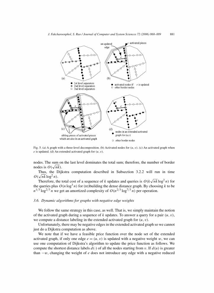
We call the pieces that contain updated edges activated pieces and call the border nodesof these pieces activated nodes. (See Fig. 5(b) for example.)

To properly recompute the distance for piece P that contains an updated edge, we needto consider the distances among all the border nodes of pieces that are contained in P .Thus, we define the activated graph to be all the valid edges between border nodes of thepieces containing an updated edge and their sibling pieces. (See Fig. 5(c).)

We answer a query for a pair (u, v) by adding the valid edges of border nodes of piecescontaining u and v to the activated graph and running a Dijkstra’s computation on theresulting graph. We call this graph the extended activated graph for (u, v). (See Fig. 5(d).)

We proceed by deriving a bound on the number of nodes involved in the computationassuming that we allow a maximum of k updates before rebuilding the entire data structure.

For each update, the number of border nodes on the pieces that need to be in Dijkstra’scomputation is O(

√n). Naively, one can bound the total number of activated nodes by

O(k√

n). However, if we consider a top-down process that divides any piece that containsan updated edge, we can show that the total number of activated nodes is O(

√nk) as

follows.Consider the decomposition tree. There are at most k leaves that are activated. Hence,

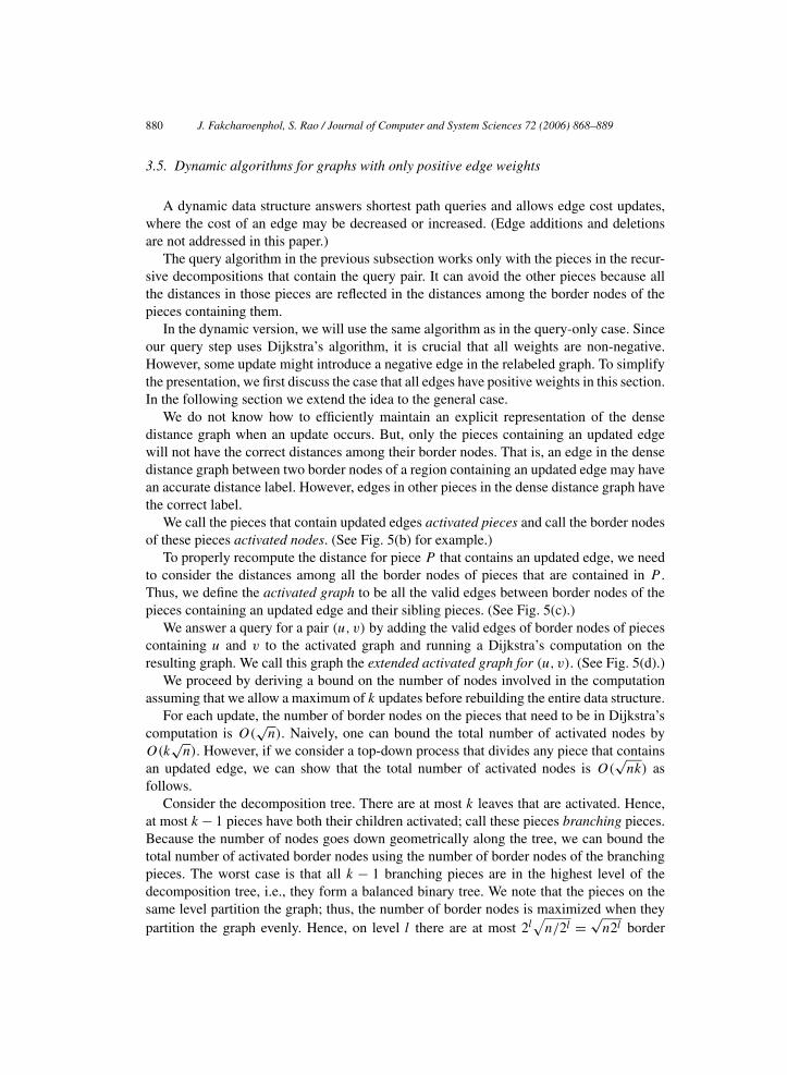
at most k − 1 pieces have both their children activated; call these pieces branching pieces.Because the number of nodes goes down geometrically along the tree, we can bound thetotal number of activated border nodes using the number of border nodes of the branchingpieces. The worst case is that all k − 1 branching pieces are in the highest level of thedecomposition tree, i.e., they form a balanced binary tree. We note that the pieces on thesame level partition the graph; thus, the number of border nodes is maximized when theypartition the graph evenly. Hence, on level l there are at most 2l

√n/2l = √

n2l border


Fig. 5. (a) A graph with a three-level decomposition. (b) Activated nodes for (u, v). (c) An activated graph whene is updated. (d) An extended activated graph for (u, v).

nodes. The sum on the last level dominates the total sum; therefore, the number of bordernodes is O(

√nk).

Thus, the Dijkstra computation described in Subsection 3.2.2 will run in timeO(

√nk log2 n).

Therefore, the total cost of a sequence of k updates and queries is O(k√

nk log2 n) forthe queries plus O(n log3 n) for (re)building the dense distance graph. By choosing k to ben1/3 log2/3 n we get an amortized complexity of O(n2/3 log7/3 n) per operation.

3.6. Dynamic algorithms for graphs with negative edge weights

We follow the same strategy in this case, as well. That is, we simply maintain the notionof the activated graph during a sequence of k updates. To answer a query for a pair (u, v),we compute a distance labeling in the extended activated graph for (u, v).

Unfortunately, there may be negative edges in the extended activated graph so we cannotjust do a Dijkstra computation as above.

We note that if we have a feasible price function over the node set of the extendedactivated graph, if only one edge e = (u, v) is updated with a negative weight w, we canuse one computation of Dijkstra’s algorithm to update the price function as follows. Wecompute the shortest distance labels d(·) of all the nodes starting from v. If d(u) is greaterthan −w, changing the weight of e does not introduce any edge with a negative reduced


cost on the graph with d(·) as a price function; hence, we can update e and update the pricefunction to be d(·). If, however, d(u) is less than −w, the shortest path from v to u togetherwith the updated edge (u, v) would form a negative cycle.

Therefore, if we already have k updates, we can compute a feasible price function inthe extended activated graph by performing k Dijkstra computations by starting with theoriginal price function on the extended activated graph, and for each update, we update theprice function as described above.

After we have the feasible price function for the extended activated graph which in-cludes all the updates, we can proceed as in the previous section.

After k queries and updates, we rebuild the dense distance graph. Thus, the total timefor a sequence of k queries and updates is O(k2

√nk log2 n) for recomputing the price

function and O(n log3 n) for (re)building the dense distance graph. By choosing k to ben1/5 log2/5 n, we get an amortized complexity of O(n4/5 log13/5 n) per operation.

4. Monge searching data structures

Recall that given a complete ordered bipartite graph (A,B,E) with edge weights d sat-isfying the Monge property, the Monge matching problem is to find a parent p(v) ∈ A forall v ∈ B that minimizes d(p(v), v). The non-crossing property ensure that there exists asolution where p(·) do not “cross.” Subsection 2.3 describes a divide-and-conquer algo-rithm for finding the minimum Monge matching in time O(n logn), where n = |A| + |B|.

In this section, we develop the on-line data structure that underlies the algorithms inSection 4.1. The data structure is extended to handle the non-bipartite case in Section 4.2.We note that the interface of this data structure is rather involved. The data structure wasused mainly in the Dijkstra step of the algorithms. Also, the technique for reducing thegeneral case to the bipartite case is used in the edge relaxation step in our implementationof Bellman–Ford.

4.1. On-line bipartite Monge searching

Given ordered sets A and B and a distance function d :A × B → R between pairs ofelement in A and B , the Monge property ensures that for all u,v ∈ A and x, y ∈ B , u � v

and x � y implies that d(u, x)+d(v, y) � d(v, y)+d(u, x). This condition on the distancefunction still holds when an offset distance D(u) on each left node u is given, i.e., the costfor an edge e = (u, v) becomes D(u) + d(u, v).

We now consider an on-line version of this problem in which the offset distances on theleft-side nodes are to be specified on-line.

We are given a complete ordered bipartite graph G = (A,B,E) with a distance functiond having the Monge property and a not-fully-specified initial distance D for every nodein A; the cost for an edge (u, v) is now D(u) + d(u, v). Initially the distance D(u) = ∞for every u ∈ A, and D(u) will be specified once for each u, over the life of the datastructure. We want the data structure to maintain the minimum Monge matching, i.e., theparent p(v) for each v ∈ B .


To make the interface suitable for the application of the data structure, we introduce agrowing subset S ⊆ B . Initially, S = ∅. Given S, the best matched node is node v ∈ B \ S

which minimizes D(p(v)) + d(p(v), v). We only allow the user to (1) query for the bestmatched node v and (2) add the current best matched node v to S. Basically, the set S

denotes the set of nodes in B that have the “correct” matches, i.e., if v ∈ S, v’s best parent,p(v), would remain the same after this point.

One of the interpretations for a node to have the correct match in the on-line setting is thefollowing. In the context of Dijkstra’s algorithm, the minimum node v in B \ S certainlyhas the correct match (or correct label) when v itself is scanned, because that means itslabel will never decrease.

When the current minimum node has the correct match, the user must add it to S to beable to query for other best matched nodes, since the data structure only allows queries forthe current best matched node outside the correctly matched set.

Without loss of generality, assume that |A| = |B| = n; otherwise we can add dummynodes to the one smaller. Let A be the ordered set {a1, . . . , an} and B be the ordered set{b1, . . . , bn}. The data structure maintains the initial distance variables D(u) for all u ∈ A

and the subset S ⊆ B , and supports the following operations.

• ActivateLeft(u,du): for u ∈ A, set D(u) = du.• FindMin( ): return a node v ∈ B \S such that v = arg minv∈B\S minu∈A D(u)+d(u, v).• ExtractMin( ): let v = FindMin( ), set S ← S ∪ {v}, and return v.

To build this data structure, we will use a range search tree data structure (see, e.g., [26]),which, for an ordered set Q = {q1, . . . , ql}, supports a query of the form mins�i�t qi , forany given 1 � s, t � l. The interval tree can be implemented using a balanced binary tree,whose leaves are Q and of which each internal node keeps the minimum value over all itschildren. The time for each query is O(log l), where l is the size of the ordered set.

For each active left node ai , we let s(ai) denote the start index of the interval of theright nodes of which ai is the best left node. Also, we let t (ai) denote the index of the lastnode in ai ’s interval plus one.

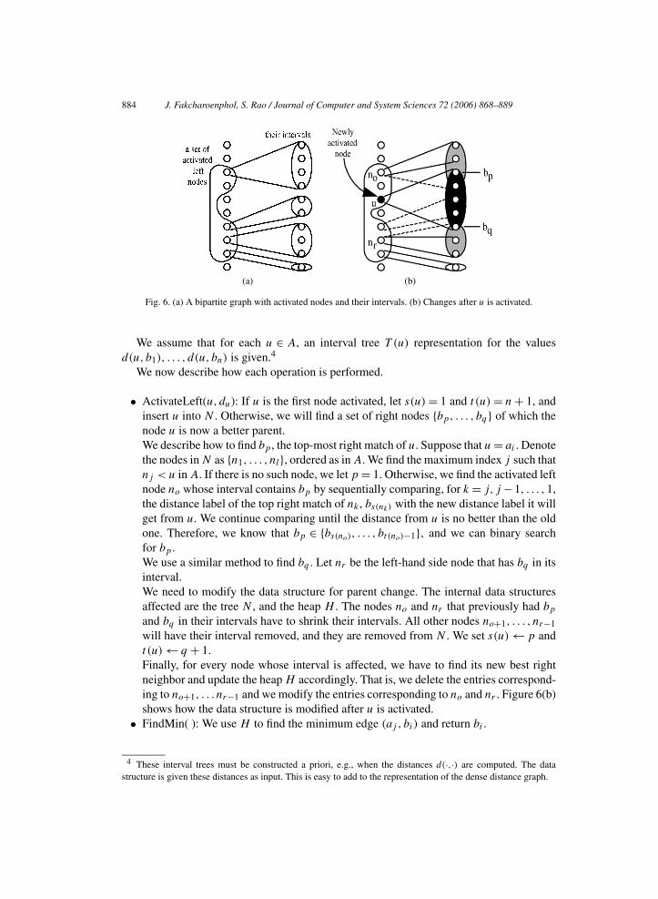
The algorithm maintains the invariant that for every ai ∈ A which has the initial distanceD(ai) �= ∞, the node ai is the best left node for the right nodes bs(ai ), bs(ai )+1, . . . , bt (ai )−1,i.e., D(ai) + d(ai, bj ) � D(a) + d(a, bj ) for all s(ai) � j < t(ai) and a ∈ A. Note thatthis implies that the ranges [s(ai), t (ai)) are non-overlapping. (For example, see Fig. 6(a).)

The data structure maintains:

• for each node in A, whether it is active;• the left neighbor tree N , an ordered (by index) binary tree for nodes in A which are

the best left neighbors for some right node;• the heap H for the minimum edges (ai, bj ) of every ai ∈ N .

Also, for each active node ai ∈ A, the data structure maintains the range [s(ai), t (ai)).


(a) (b)

Fig. 6. (a) A bipartite graph with activated nodes and their intervals. (b) Changes after u is activated.

We assume that for each u ∈ A, an interval tree T (u) representation for the valuesd(u, b1), . . . , d(u, bn) is given.4

We now describe how each operation is performed.

• ActivateLeft(u,du): If u is the first node activated, let s(u) = 1 and t (u) = n + 1, andinsert u into N . Otherwise, we will find a set of right nodes {bp, . . . , bq} of which thenode u is now a better parent.We describe how to find bp , the top-most right match of u. Suppose that u = ai . Denotethe nodes in N as {n1, . . . , nl}, ordered as in A. We find the maximum index j such thatnj < u in A. If there is no such node, we let p = 1. Otherwise, we find the activated leftnode no whose interval contains bp by sequentially comparing, for k = j, j −1, . . . ,1,the distance label of the top right match of nk , bs(nk) with the new distance label it willget from u. We continue comparing until the distance from u is no better than the oldone. Therefore, we know that bp ∈ {bs(no), . . . , bt (no)−1}, and we can binary searchfor bp .We use a similar method to find bq . Let nr be the left-hand side node that has bq in itsinterval.We need to modify the data structure for parent change. The internal data structuresaffected are the tree N , and the heap H . The nodes no and nr that previously had bp

and bq in their intervals have to shrink their intervals. All other nodes no+1, . . . , nr−1

will have their interval removed, and they are removed from N . We set s(u) ← p andt (u) ← q + 1.Finally, for every node whose interval is affected, we have to find its new best rightneighbor and update the heap H accordingly. That is, we delete the entries correspond-ing to no+1, . . . nr−1 and we modify the entries corresponding to no and nr . Figure 6(b)shows how the data structure is modified after u is activated.

• FindMin( ): We use H to find the minimum edge (aj , bi) and return bi .

4 These interval trees must be constructed a priori, e.g., when the distances d(·,·) are computed. The datastructure is given these distances as input. This is easy to add to the representation of the dense distance graph.


• ExtractMin( ): We use H to find the minimum edge (aj , bi). Then we create twonew nodes a′

j and a′′j and put them next to aj in N such that a′

j < aj < a′′j . We set

s(a′j ) ← s(aj ); t (a′

j ) ← i; s(a′′j ) ← i + 1; and t (a′′

j ) ← t (aj ). Also we set s(aj ) ← i

and t (aj ) ← i + 1, and remove (aj , bi) from the heap H .Finally, for a′

j and a′′j , we use aj ’s range search tree to find their best right neighbors

and add them to H .

4.1.1. Analysis of the running timeWe note that the size of N might be greater than n during the execution of the algorithm

because we create some nodes every time ExtractMin is called. However, it is called atmost n times; thus, we create no more than 2n = O(n) nodes.

We now analyze the running time for each operation.

• ActivateLeft(u,du): First, searching for the index j in N takes time O(logn).To find bp we do a sequential search and a binary search. Every node in N that weexamined during the sequential search is removed except the last one. We charge thecost for the sequential search to the cost for removing and updating these nodes. Thecost for the binary search is O(logn). The search for the lower end costs the same.Next, u has to pick its best right neighbor and add it to H . This can be done in O(logn)

time by querying the range search tree T (u) for the minimum right node of u over therange {bp, . . . , bq}.After the interval is found, some other node in N must update its data structure. Atmost two nodes have to change their intervals, pick their best right neighbors, andupdate their entries in H ; this takes O(logn) time. All other nodes are deleted andwill never reappear. Each delete takes time O(logn) and we charge this to the time thenode was inserted to the data structure.Therefore, the operation takes O(logn) amortized time.

• FindMin( ): We can read the top-most item in H in O(1) time.• ExtractMin( ): We can find the current minimum node bi in O(1) time. It takes

O(logn) time to find the left matched node aj for bi . We then do a constant num-ber of operations on N and H which take O(logn) time. Therefore, ExtractMin runsin time O(logn).

4.2. Non-bipartite on-line Monge searching

We generalize our data structure to support the case when the graph is not bipartite inthis section. We have the graph G = (V ,E) with the distance function d :E → R. Thenodes in V are in a circular order, and the distance function d satisfies the property that

d(u,w) + d(v, x) � d(u, x) + d(v,w), (1)

for every u,v,w,x ∈ V such that u � v � w � x in V . Notice that the sign of the inequalityis reversed because in this case (u,w) crosses (v, x), contrary to the bipartite case that(u, x) crosses (v,w).

We note the difficulties in this case. In the bipartite case, the set of nodes which hasa particular node as their parent is consecutive, i.e., that particular node owns a single


interval. This is not true in the non-bipartite case. However, we show in this section how toreduce this problem to O(logn) bipartite problems. The idea is to partition the edges as inSection 3.2.1.

From the graph G, we create 2�logn� bipartite graphs, because for each left–right par-tition, edges between them can go in two directions. We denote these bipartite graphs asG0,G1, . . . ,G2�logn�−1. Under this reduction, each edge belongs to one and only one bi-partite graph. We refer to each bipartite graph Gj as a level of G. Let G denote the set ofthese O(logn) bipartite graphs.

The operations that we need from this non-bipartite data structure are the following. Wewant to be able to set the initial offset distance D as in the bipartite case, and also, we wantto find a labeled node which is the minimum one over all the levels. However, the notionof the set S is different now. Suppose that currently a node v on level i is the minimumnode. When v is extracted, the level i label of v is definitely correct, but its labels on theother levels can still change. Therefore, we only add the node v to the set S of the level i

bipartite graph. This has a drawback: a call to FindMin can return v again. However, sinceeach node belongs to at most O(logn) levels, the node v can reappear at most O(logn)

times.The data structure for the non-bipartite case consists of O(logn) data structures for the

bipartite case, for all Gj ∈ G. It maintains a heap H ′ of minimum nodes over all levels,and initially the distance offset D(v) = ∞ for all v in all levels. To make the names of theprocedures consistent with the algorithm that constructs the dense distance graph, we callthese procedures ScanInSubpiece, FindMinInSubpiece, and ExtractMinInSubpiece insteadof ActivateNode, FindMin, and ExtractMin, respectively. We now describe the operationsthat the data structure supports together with their implementations and running times.

• ScanInSubpiece(v, dv): let D(v) = dv .This operation can be done by calling ActivateLeft(v, dv) on every Gj ∈ G of whichv is in the left-hand side node. On those affected levels, we call FindMin and updatetheir entries in the heap H ′. This operation can be done in O(log2 n) amortized time,because there are O(logn) levels and each call to ActivateLeft costs O(logn) amor-tized time. The time for finding the minimum nodes and updating the heap is onlyO(logn log logn), because the heap H ′ is of size O(logn).

• FindMinInSubpiece( ): find the minimum distance node over all levels.This can be done in O(1) time by returning the minimum entry in the heap H ′.

• ExtractMinInSubpiece( ): find the minimum distance node over all levels, remove thatnode from its level, and attempt to add the node to the set S of the data structure.For this operation, we do as in FindMinInSubpiece, but after the minimum node isfound, we call ExtractMin once on the bipartite data structure of the level to which theminimum node belongs and update that level’s entry in H ′. The cost for ExtractMin isO(logn) time, and the cost for updating H ′ is O(log logn), because the size of H ′ isO(logn). Therefore, this operation can be done in O(logn) time.

As noted in the discussion above, after O(logn) attempts to extract a node, it will neverbe returned as the minimum node again.


5. Dealing with holes

It is not difficult to work with a piece with holes if only a constant number of holesare present. We will describe the algorithm for finding such a decomposition in Subsec-tion 5.1. Here, we continue to discuss how one can modify the algorithm given the requireddecomposition.

We assume that there are at most h holes on each piece. For each hole, the edges betweentwo border nodes adjacent to it can be handled using the method described in previoussections. Thus, we need h copies of the on-line Monge data structures.

For edges between border nodes adjacent to different holes, we need to modify the datastructure. First note that the on-line bipartite Monge data structure in Section 4.1 can bemodified to work with edges going between two holes. In this case, we need to considerthe nodes in circular order, which can be done by allowing the intervals of left-hand sidenodes to wrap around. Therefore, since there are at most h(h − 1) pair of holes, we needanother h(h − 1) data structures for edges. category.

The running time for data structure operations increases by a factor of at most O(h2),which is a constant. Therefore, if every piece has O(1) holes, we can implement the algo-rithm to run in the same time bound.

5.1. Graph decomposition

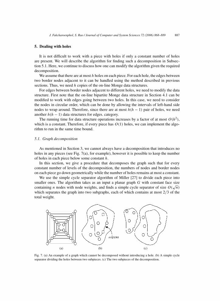
As mentioned in Section 3, we cannot always have a decomposition that introduces noholes in any pieces (see Fig. 7(a), for example), however it is possible to keep the numberof holes in each piece below some constant h.

In this section, we give a procedure that decomposes the graph such that for everyconstant number of levels of the decomposition, the numbers of nodes and border nodeson each piece go down geometrically while the number of holes remains at most a constant.

We use the simple cycle separator algorithm of Miller [27] to divide each piece intosmaller ones. The algorithm takes as an input a planar graph G with constant face sizecontaining n nodes with node weights, and finds a simple cycle separator of size O(

√n)

which separates the graph into two subgraphs, each of which contains at most 2/3 of thetotal weight.

(a) (b) (c)

Fig. 7. (a) An example of a graph which cannot be decomposed without introducing a hole. (b) A simple cycleseparator dividing the holes between two subpieces. (c) The two subpieces of the decomposition.


We show how to use the simple cycle separator algorithm to divide the graph so thatwe introduce at most one hole each time. We assume first that the graph is connected. Toget the face size to be a constant, we triangulate the graph. The edges added during thetriangulation process allow the cycle to jump over some faces, and because of these edges,the resulting subgraphs might contain many connected components. However, at most onehole gets introduced to at most one of the subgraphs.

For the piece with many connected components, we will apply Miller’s algorithm on atmost one of the components; hence, at most one hole is created. We proceed as follows.We note that if no component has more than 2/3 of the weights, we can divide the piece,without introducing any separator nodes, into two subpieces each with at most 2/3 fractionof the total weight. Now assume that there exists a unique component C that has more than2/3 of the weight. We run the Miller algorithm only on C, introducing at most one hole.Now, we are left with components each having at most 2/3 fraction of the weights, so wecan divide them without introducing new separator nodes.

With different weight assignments, we can divide the piece so that the subpieces satisfyvarious constraints. It is a standard application of the algorithm to divide the graph so thatthe number of nodes or border nodes in the subpieces drops by a factor of 2/3.

To divide the piece so that the number of holes decreases, we contract the border nodeson each hole into a super node and place uniform weights on the super nodes. After apply-ing the Miller algorithm, each subgraph contains at most a 2/3 fraction of all super nodes.In other words, it contains at most 2/3 of the original holes. For any super node on theseparator, the hole corresponding to that super node is broken into two parts and the bordernodes of that hole become parts of the newly introduced hole. However, we introduce atmost one hole during the process. Figures 7(b) and (c) illustrate the way we divide theholes.

We now describe how to obtain a decomposition with the property claimed in the be-ginning of Section 5. We divide a piece in the way that depends on which level of thedecomposition it belongs to. More specifically, at level 3i we reduce the number of nodes,at level 3i + 1 we reduce the number of border nodes, and at level 3i + 2 we reduce thenumber of holes.

On every 3ith level, the number of nodes decreases by a factor of 2/3. At each levelwe introduce at most new O(

√n) border nodes. The number of nodes in each subpiece

decreases geometrically, and the number border nodes in each subpiece with n nodes is atmost O(

√n).

On each level that we decompose a piece, we introduce at most one new hole. Since forevery 3 levels, the number of holes drops by a factor of 2/3, the number of holes remainsat most a constant.

The Miller algorithm runs in linear time; thus, the time for decomposing the graph isO(n logn).

Acknowledgments

We thank Chris Harrelson for his careful reading of this paper. We also greatly thankthe anonymous referees for numerous suggestions that help improving the presentation ofthe paper.


References

[1] I.J. Cox, S.B. Rao, Y. Zhong, ‘Ratio regions’: A technique for image segmentation, in: Proceedings Interna-tional Conference on Pattern Recognition, IEEE, 1996, pp. 557–564.

[2] L.C.D. Geiger, A. Gupta, J. Vlontzos, Dynamic programming for detecting, tracking and matching elasticcontours, IEEE Trans. Pattern Anal. Mach. Intell. 17 (3) (1995) 294–302.

[3] S.B. Rao, Faster algorithms for finding small edge cuts in planar graphs, extended abstract, in: Proceedingsof the Twenty-Fourth Annual ACM Symposium on the Theory of Computing, 1992, pp. 229–240.

[4] G. Miller, J. Naor, Flow in planar graphs with multiple sources and sinks, SIAM J. Comput. 24 (1995)1002–1017.

[5] P. Chalermsook, J. Fakcharoenphol, D. Nanongkai, A deterministic near-linear time algorithm for findingminimum cuts in planar graphs, in: SODA ’04: Proceedings of the Fifteenth Annual ACM–SIAM Sym-posium on Discrete Algorithms, Society for Industrial and Applied Mathematics, Philadelphia, PA, 2004,pp. 828–829.

[6] R.E. Bellman, On a routing problem, Quart. Appl. Math. 16 (1958) 87–90.[7] L.R. Ford, D.R. Fulkerson, Flows in Networks, Princeton Univ. Press, Princeton, NJ, 1962.[8] H.N. Gabow, R.E. Tarjan, Faster scaling algorithm for network problems, SIAM J. Comput. 18 (5) (1989)

1013–1036.[9] E.W. Dijkstra, A note on two problems in connexion with graphs, Numer. Math. 1 (1959) 269–271.

[10] R.J. Lipton, R.E. Tarjan, A separator theorem for planar graphs, SIAM J. Appl. Math. 36 (1979) 177–189.[11] R. Lipton, D. Rose, R.E. Tarjan, Generalized nested dissection, SIAM J. Numer. Anal. 16 (1979) 346–358.[12] A.V. Goldberg, Scaling algorithms for the shortest path problem, SIAM J. Comput. 21 (1) (1992) 140–150.[13] M.R. Henzinger, P.N. Klein, S. Rao, S. Subramanian, Faster shortest-path algorithms for planar graphs,

J. Comput. System Sci. 55 (1) (1997) 3–23.[14] W.D. Smith, private communication, 2005.[15] J.P. Hutchinson, G.L. Miller, Deleting vertices to make graphs of positive genus planar, in: Discrete Algo-

rithms and Complexity Theory, Academic Press, Boston, 1986, pp. 81–98.[16] H. Djidjev, S.M. Venkatesan, Planarization of graphs embedded on surfaces, in: WG ’95: Proceedings of the

21st International Workshop on Graph-Theoretic Concepts in Computer Science, Springer-Verlag, London,UK, 1995, pp. 62–72.

[17] G.N. Frederickson, Fast algorithms for shortest paths in planar graphs, with applications, SIAM J. Com-put. 16 (6) (1989) 1004–1022.

[18] M. Thorup, Compact oracles for reachability and approximate distances in planar digraphs, J. ACM 51 (6)(2004) 993–1024.

[19] P.N. Klein, Multiple-source shortest paths in planar graphs, in: Proceedings, 16th ACM–SIAM Symposiumon Discrete Algorithms, 2005, pp. 146–155.

[20] G.N. Frederickson, A new approach to all pairs shortest paths in planar graphs, extended abstract, in: Pro-ceedings of the Nineteenth Annual ACM Symposium on Theory of Computing, 1987, pp. 19–28.

[21] H.N. Djidjev, G.E. Pantziou, C.D. Zaroliagis, Computing shortest paths and distances in planar graphs, in:Proc. 18th ICALP, Springer-Verlag, 1991, pp. 327–339.

[22] A. Aggarwal, A. Bar-Noy, S. Khuller, D. Kravets, B. Schieber, Efficient minimum cost matching and trans-portation using the quadrangle inequality, J. Algorithms 19 (1) (1995) 116–143.

[23] S.R. Buss, P.N. Yianilos, Linear and O(n logn) time minimum-cost matching algorithms for quasi-convextours, SIAM J. Comput. 27 (1) (1998) 170–201.

[24] J.S.B. Mitchell, D.M. Mount, C.H. Papadimitriou, The discrete geodesic problem, SIAM J. Comput. 16 (4)(1987) 647–668.

[25] D. Johnson, Efficient algorithms for shortest paths in sparse networks, J. Assoc. Comput. Mach. 24 (1977)1–13.

[26] M. de Berg, M. van Kreveld, M. Overmars, O. Schwarzkopt, Computational Geometry: Algorithms andApplications, second ed., Springer-Verlag, 2000, pp. 96–99 (Chapter 5).

[27] G.L. Miller, Finding small simple cycle separators for 2-connected planar graphs, J. Comput. SystemSci. 32 (3) (1986) 265–279.

Planar Graphs, Negative Weight Edges, Shortest Paths, Near Linear Time

Documents

Transcript of Planar Graphs, Negative Weight Edges, Shortest Paths, Near Linear Time