EDGES Beam modelling and data comparison - McGill Physics

EDGES Beam modelling and data comparison

Nivedita Mahesh, Tom Mozdzen, Alan Rogers, Raul Monsalve, Judd Bowman

McGill 21-cm Workshop Nivedita Mahesh10/07/2019

Introduction

● If the antenna beam pattern is frequency dependent:○ spatial structure in the foreground would couple into the spectral domain ○ result in a non-smooth spectral response to structure in the continuum sky emission, ○ which can be difficult to model to the accuracy needed for 21 cm signal detection.

● With this effort we hope to answer the following questions:○ How do solutions from different EM solvers compare? ○ How chromatic is the EDGES Beam?○ Is it the chromaticity within acceptable levels?○ Do our beam modelling solutions match expectations?

2


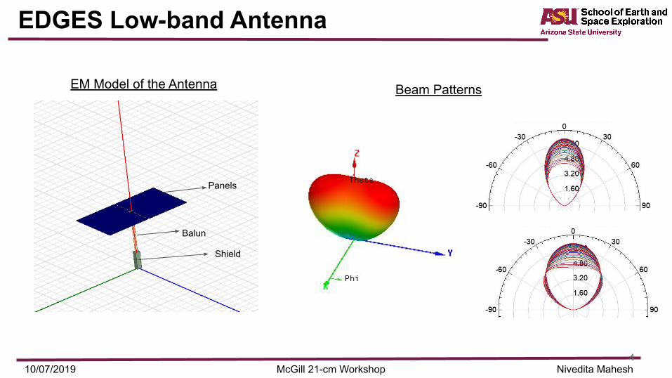
EDGES Low-band Antenna

3

Panels

Balun

Shield

EM Model of the AntennaParameter Value

Panel Width 125.2 cm

Panel Length 96.4 cm

Gap between panels 1.3 cm

Height from the ground 104 cm

Ground plane dimensions 10m X 10m

Extended Ground plane 30m X 30m

Frequency 40-100MHz


EDGES Low-band Antenna

4

Beam Patterns

Panels

Balun

Shield

EM Model of the Antenna


Simulation Set-up

Method of Moments(MoM) - FEKO, CST-I, HFSS-IE

Has the capability to model infinite real ground

Finite Element Method (FEM) - HFSS, CST - F

Finite Difference Time Domain (FDTD) - CST-T

5

Available techniques How Chromatic is the Beam?

● Derivative along the frequency axis● Residues of the beam to low order

polynomial at certain viewing angles


Question #1:

Simple Case:

Antenna + PEC ground

Do solutions from all the solvers match?

6


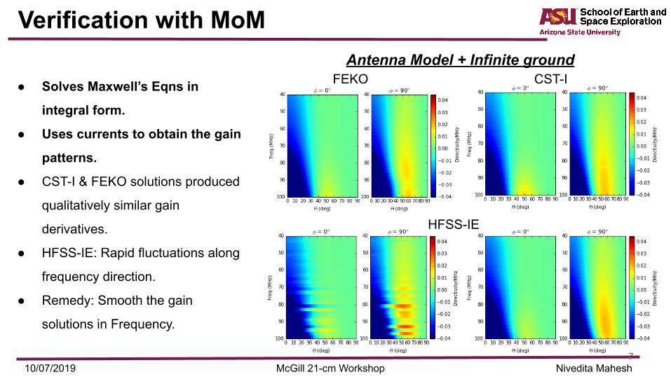
Verification with MoM

CST-IAntenna Model + Infinite ground

● Solves Maxwell’s Eqns in

integral form.

● Uses currents to obtain the gain

patterns.

● CST-I & FEKO solutions produced

qualitatively similar gain

derivatives.

● HFSS-IE: Rapid fluctuations along

frequency direction.

● Remedy: Smooth the gain

solutions in Frequency.

HFSS-IE

FEKO


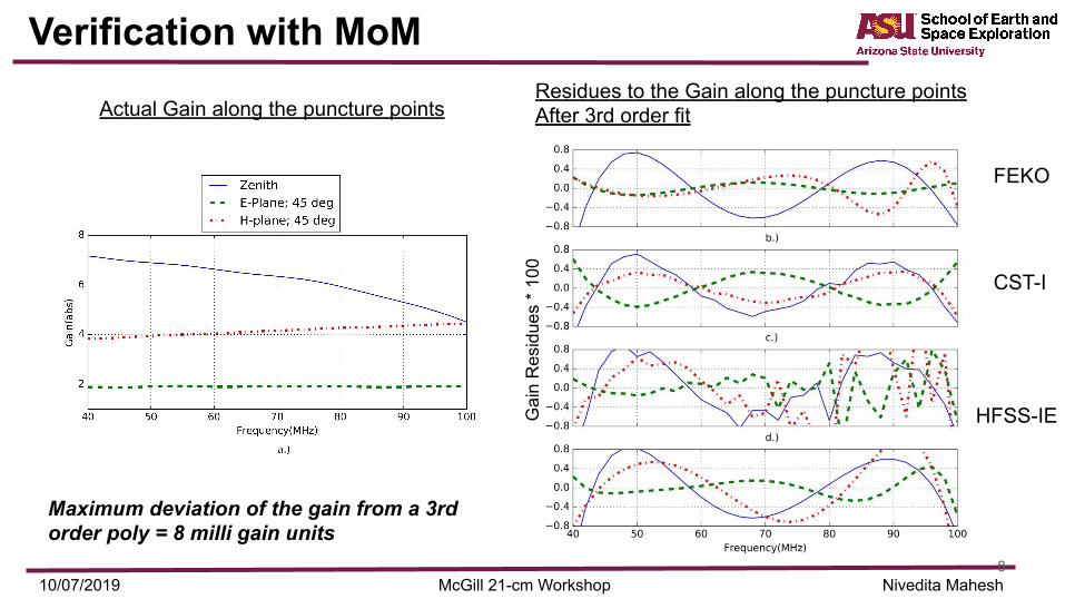
Verification with MoM

8

FEKO

CST-I

Actual Gain along the puncture pointsResidues to the Gain along the puncture pointsAfter 3rd order fit

HFSS-IE

Maximum deviation of the gain from a 3rd order poly = 8 milli gain units

Gai

n R

esid

ues

* 10

0


Question #2:

9

Simple Case:

Antenna + PEC ground

Do solutions from all the solvers match? Yes!

Now,

Real case:

Antenna + 10m X 10m PEC + Soil Below

9


Real ground: Model Comparisons

10

● The only solution technique: MOM● Soil Parameters: 𝝐r = 3.5 & 𝞂 = 0.02

S/m● Qualitatively FEKO and CST-I are

similar● The HFSS-IE solutions were

smoothened like in the PEC case● HFSS-IE: Predicts higher

chromaticity.● Caveat: This could still be residual

numerical errors

Antenna Model + 10m X 10m metal plate + SoilFEKO HFSS-IE

CST-I


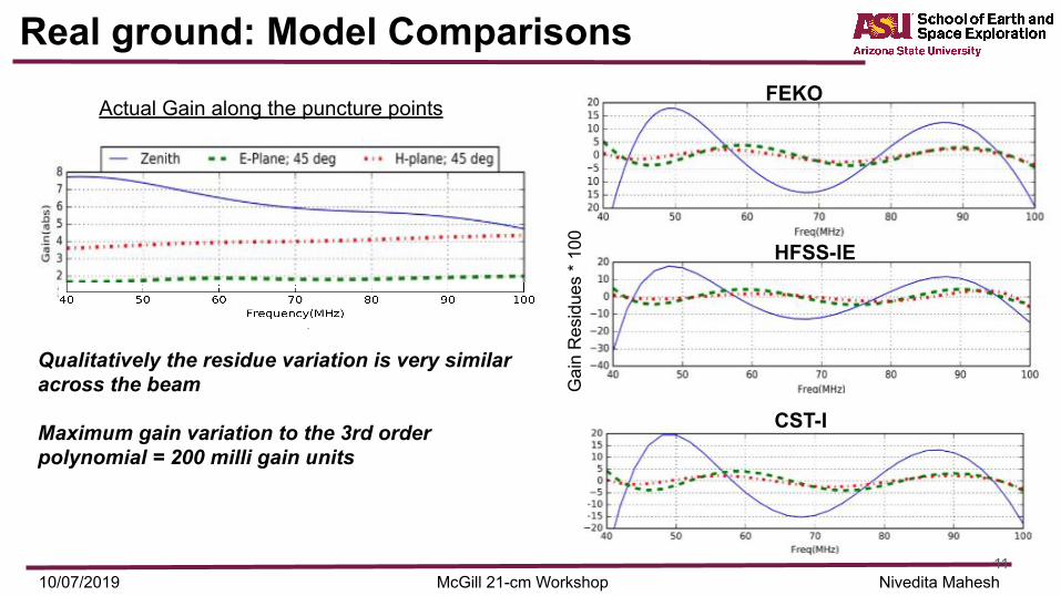
Real ground: Model Comparisons

Qualitatively the residue variation is very similar across the beam

Maximum gain variation to the 3rd order polynomial = 200 milli gain units

FEKO

HFSS-IE

CST-I

Actual Gain along the puncture points

Gai

n R

esid

ues

* 10

0


Question #3:

Is the chromaticity of the model beam solutions acceptable?

Can the cosmological signal still be detected?

12


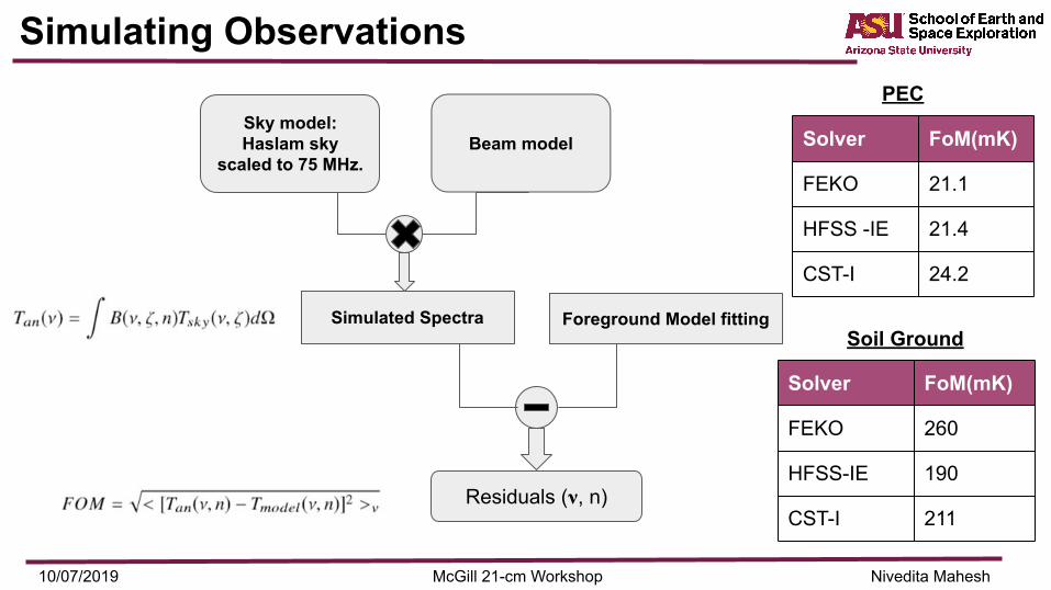
Simulating Observations

Sky model: Haslam sky

scaled to 75 MHz. Beam model

Simulated Spectra Foreground Model fitting

Residuals (𝛎, n)

Solver FoM(mK)

FEKO 21.1

HFSS -IE 21.4

CST-I 24.2

PEC

Soil Ground

Solver FoM(mK)

FEKO 260

HFSS-IE 190

CST-I 211


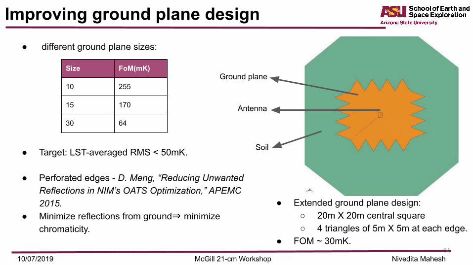
Improving ground plane design

14

● different ground plane sizes:

● Target: LST-averaged RMS < 50mK.

● Perforated edges - D. Meng, “Reducing Unwanted Reflections in NIM’s OATS Optimization,” APEMC 2015.

● Minimize reflections from ground⇒ minimize chromaticity.

● Extended ground plane design:○ 20m X 20m central square ○ 4 triangles of 5m X 5m at each edge.

● FOM ~ 30mK.

Size FoM(mK)

10 255

15 170

30 64

Ground plane

Antenna

Soil


Extended Ground Plane Design

15

FEKO

CST-I

● Soil: 𝝐r = 3.5 & 𝞂 = 0.02 S/m● HFSS-IE not used: The

chromaticity may be confused with numerical errors

● Derivative Metric: similar; CST-I more fluctuations along Φ =90

● Residual metric: maximum fluctuation of order 40 gain milli units

Gai

n R

esid

ues

* 10

0


Question #4:

Do our beam modelling solutions match expectations?

How close to reality?

16


Comparison with data: Drift Scan

17

10x10 meter Ground Plane

● Data (268 days) and simulated spectra averaged over 2 hr LST bins and plotted for certain frequency points.

The agreement between the data and simulated spectra is within 15%Possible disagreement ⇒ Sky model uncertainty


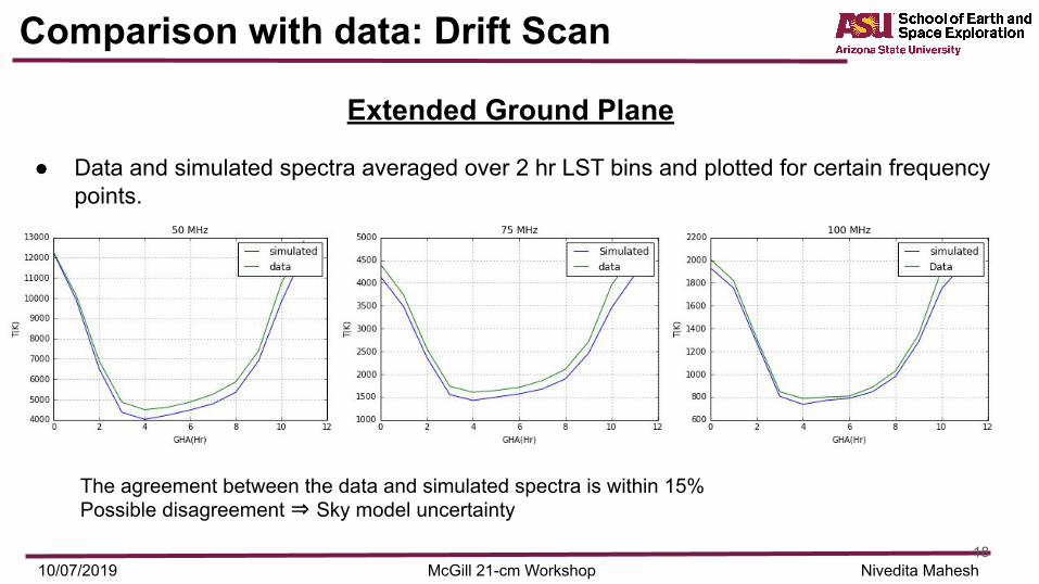
Comparison with data: Drift Scan

Extended Ground Plane

● Data and simulated spectra averaged over 2 hr LST bins and plotted for certain frequency points.

The agreement between the data and simulated spectra is within 15%Possible disagreement ⇒ Sky model uncertainty


Comparison to Data: residues after foreground fits

19

10x10 meterGround Plane

Rows are 2hr GHA binned data

5 term Loglog Model

5 term Linlog Model

5 term Linlog Model

● Simulated Residues to both the model fits capture the data residues similarly ● Adding the absorption feature to the simulation does very little improvement because the residues

are of the order of the feature


Comparison to Data: residues after foreground fits

20

Extended Ground Plane

Rows are 2hr GHA binned data

5 term Loglog Model 5 term Linlog Model

● Adding the absorption feature to the simulation improves the agreement with data; at these level of residues the feature is significant


Soil Properties Confirmation

21

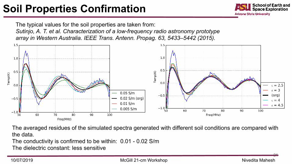
The typical values for the soil properties are taken from:Sutinjo, A. T. et al. Characterization of a low-frequency radio astronomy prototypearray in Western Australia. IEEE Trans. Antenn. Propag. 63, 5433–5442 (2015).

The averaged residues of the simulated spectra generated with different soil conditions are compared with the data.The conductivity is confirmed to be within: 0.01 - 0.02 S/mThe dielectric constant: less sensitive


Summary

22

➢ How do solutions from different EM solvers compare?

○ FEKO and CST-I gains are within 5%

➢ How chromatic is the EDGES Beam?

○ Compared to the ideal case:

■ the 10m X 10m is 10 times greater

■ Extended is 2 times greater

➢ Is it the chromaticity within acceptable levels?

○ The extended ground plane resulted in residues with an RMS ~50mK

➢ Do our beam modelling solutions match expectations?

○ Drift scan comparisons indicated within 15%

➢ The MRO soil properties quoted in Sutinjo paper is confirmed.


EXTRA SLIDES

23


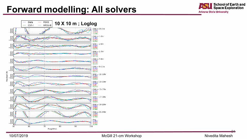
Forward modelling: All solvers

24

10 X 10 m ; Loglog


Verification with FEM

25


Verification with FDTD

26


Different ground Shapes

27


PEC Ground: Gain along Excitation axis

28


PEC Ground: Gain Perpendicular to Excitation axis


Summary

31

➢ The realistic scenario was modelled using FEKO and HFSS-IE (MoM)

➢ Simulated residues from the new ground plane is lesser than the expected amplitude of

the signature in that frequency regime.

➢ The simulation captured the residues from the actual data quite accurately.

➢ Different soil properties were simulated and beam solutions compared to data.

EDGES Beam modelling and data comparison - McGill Physics

Documents

Transcript of EDGES Beam modelling and data comparison - McGill Physics