ALPS-GPS_QUAKENET_Project_booklet.pdf - EPIC
127
ALPS GPSQUAKENET Interreg III B Project- Alpine Space ALPS GPSQUAKENET Alps-GPSquakeNet has promoted transanational co-operation in the field of space geodesy applied to natural hazards. It has set a transanational network of more than 35 continuous Global Positioning System (GPS) stations across the Alps. It has investigated the continental deformation and the earthquake hazard within the Alpine space, mountains and surrounding foothills, where are concentrated attractive European metropolitan areas and rapidly growing urban centres with extensive infrastructures. It has developed pilot projects on the use of GPS in meteorology, landslide studies and active faulting monitoring. It has favored transnational know-how exchange between regional authorities and alpine universities and research centres. For the first time in the Alpine geology, Alps- GPSquakeNet through its continuous GPS network "GAIN" (Geodetic Alpine Integrated Network) will allow the quantification of the crustal deformation of the whole mountain range. This will open new research initiatives in earth and environmental sciences, therefore rising the value of the Alps as a natural laboratory. The direct result will be an improvement in the knowledge of earthquake potential and hazard, and this will allow a better land use in terms of a safe living space. GAIN is giving the ground for a higher resolution space-based coverage of urban and mountain areas in the Alpine space offering therefore a robust tool for future infrastructure investment, land use harmonization and industrial planning. Alps-GPSquakeNet started catalyzing space geodetic applications in the Alps (meteorology, landslide monitoring, agriculture, navigation, transportation, mapping, surveying…). GPS nowadays is a must in navigation. The possibility of real- time positioning will undoubtedly play an increasing role in the EC during the next decades in the field of automation, traffic guidance and real-time hazard detection. Alpine Integrated GPS Network: Real-Time Monitoring and Master Model for Continental Deformation and Earthquake Hazard www.alps-gps.units.it Università degli Studi di Trieste Dipartimento di Scienze della Terra www.dst.units.it Agencija Republike Slovenije Za Okolje www.arso.gov.si ARPA Regione Piemonte www.arpa.piemonte.it ARPA Regione del Veneto www.arpa.veneto.it Bayerische Akademie der Wissenschaften Bayerische Kommission für die Internationale Erdmessung www.bek.badw-muenchen.de Deutsches Geodaetisches Forschungsinstitut www.dgfi.badw.de Regione Liguria Direzione Centrale Affari Organizzativi Servizio Sistemi Informatici www.regione.liguria.it Regione Lombardia Direzione Generale Territorio e Urbanistica Infrastruttura per l’Informazione Territoriale www.regione.lombardia.it Servizio Geologico, Provincia Autonoma di Bolzano – Alto Adige www.provincia.bz.it Servizio Geologico Provincia Autonoma di Trento www.provincia.tn.it Université Joseph Fourier Laboratoire de Géophysique Interne et Tectonophysique UMR 5559 du CNRS www-lgit.obs.ujf-grenoble.fr Fondazione Montagna Sicura-Valle d’Aosta www.fondazionemontagnasicura.org Ecole et Observatoire des Sciences de la Terre eost.u-strasb.fr Interreg IIIB This project has received European Regional Development Funding through the INTERREG IIIB Community Initiative Sub-contractors Galileian Plus S.r.l. www.galileianplus.it Università degli Studi di Genova Dipartimento di Macchine, Sistemi energetici e Trasporti (DIMSET) Facolta' di Ingegneria www.unige.it Politecnico di Milano Dipartimento di Ingegneria Idraulica, Ambientale, Infrastrutture Viarie, Rilevamento (DIIAR) - sezione Rilevamento www.rilevamento.polimi.it Politecnico di Torino Dipartimento di Ingegneria del Territorio, dell'Ambiente e delle Geotecnologie Politecnico di Torino II Facolta' di Ingegneria sede di Vercelli www.vercelli.polito.it Università degli Studi di Milano Dipartimento di Scienze della Terra "Ardito Desio" www.gp.terra.unimi.it IREALP Istituto di Ricerca per l'Ecologia e l'Economia Applicate alle Aree Alpine www.irealp.it LGCA Laboratoire de Geodynamique des Chaines Alpines, Chambery www.univ-savoie.fr/labos/lgca/ UNIVERSITÀ DEGLI STUDI DI GENOVA
-
Upload
khangminh22 -
Category
Documents
-
view
0 -
download
0
Transcript of ALPS-GPS_QUAKENET_Project_booklet.pdf - EPIC

ALPSGPSQUAKENET
Interreg III B Project- Alpine Space
ALP
S G
PSQ
UA
KEN
ET
Alps-GPSquakeNet has promotedtransanational co-operation in the field ofspace geodesy applied to natural hazards.It has set a transanational network of morethan 35 continuous Global PositioningSystem (GPS) stations across the Alps. It hasinvestigated the continental deformationand the earthquake hazard within the Alpinespace, mountains and surrounding foothills,where are concentrated attractive Europeanmetropolitan areas and rapidly growingurban centres with extensive infrastructures.It has developed pilot projects on the useof GPS in meteorology, landslide studies andactive faulting monitoring. It has favoredtransnational know-how exchange betweenregional authorities and alpine universitiesand research centres.
For the first time in the Alpine geology, Alps-GPSquakeNet through its continuous GPSnetwork "GAIN" (Geodetic Alpine IntegratedNetwork) will allow the quantification ofthe crustal deformation of the wholemountain range. This will open new researchinitiatives in earth and environmentalsciences, therefore rising the value of theAlps as a natural laboratory. The direct resultwill be an improvement in the knowledgeof earthquake potential and hazard, andthis will allow a better land use in terms ofa safe living space. GAIN is giving the groundfor a higher resolution space-based coverageof urban and mountain areas in the Alpinespace offering therefore a robust tool forfuture infrastructure investment, land useharmonization and industrial planning.
Alps-GPSquakeNet started catalyzing spacegeodetic applications in the Alps(meteorology, landslide monitoring,agriculture, navigation, transportation,mapping, surveying…). GPS nowadays is amust in navigation. The possibility of real-time positioning will undoubtedly play anincreasing role in the EC during the nextdecades in the field of automation, trafficguidance and real-time hazard detection.
Alpine IntegratedGPS Network:Real-Time Monitoringand Master Model forContinental Deformationand Earthquake Hazard
www.alps-gps.units.it
Università degli Studi di TriesteDipartimento di Scienze della Terrawww.dst.units.it
Agencija Republike Slovenije Za Okoljewww.arso.gov.si
ARPARegione Piemontewww.arpa.piemonte.it
ARPARegione del Venetowww.arpa.veneto.it
Bayerische Akademie der WissenschaftenBayerische Kommission für dieInternationale Erdmessungwww.bek.badw-muenchen.de
Deutsches Geodaetisches Forschungsinstitutwww.dgfi.badw.de
Regione LiguriaDirezione Centrale Affari OrganizzativiServizio Sistemi Informaticiwww.regione.liguria.it
Regione LombardiaDirezione Generale Territorio e UrbanisticaInfrastruttura per l’Informazione Territorialewww.regione.lombardia.it
Servizio Geologico,Provincia Autonoma di Bolzano – Alto Adigewww.provincia.bz.it
Servizio GeologicoProvincia Autonoma di Trentowww.provincia.tn.it
Université Joseph FourierLaboratoire de GéophysiqueInterne et TectonophysiqueUMR 5559 du CNRSwww-lgit.obs.ujf-grenoble.fr
Fondazione Montagna Sicura-Valle d’Aostawww.fondazionemontagnasicura.org
Ecole et Observatoire des Sciences de la Terreeost.u-strasb.fr
Interreg IIIBThis project has received European Regional DevelopmentFunding through the INTERREG IIIB Community Initiative
Sub-contractors
Galileian Plus S.r.l.www.galileianplus.it
Università degliStudi di GenovaDipartimento di Macchine,Sistemi energetici e Trasporti(DIMSET)Facolta' di Ingegneriawww.unige.it
Politecnico di MilanoDipartimento di IngegneriaIdraulica, Ambientale,Infrastrutture Viarie,Rilevamento (DIIAR) -sezione Rilevamentowww.rilevamento.polimi.it
Politecnico di TorinoDipartimento di Ingegneriadel Territorio, dell'Ambientee delle GeotecnologiePolitecnico di TorinoII Facolta' di Ingegneriasede di Vercelliwww.vercelli.polito.it
Università degliStudi di MilanoDipartimento di Scienzedella Terra "Ardito Desio"www.gp.terra.unimi.it
IREALPIstituto di Ricerca perl'Ecologia e l'EconomiaApplicate alle Aree Alpinewww.irealp.it
LGCALaboratoire deGeodynamique des ChainesAlpines, Chamberywww.univ-savoie.fr/labos/lgca/
UNIVERSITÀ DEGLI STUDIDI GENOVA


Located in the north of the italian peninsula near the Swiss
border, lying at a major junction of the great East-West and
North-South communication corridors, Lombardy is one of
the main gateways to Italy.
The intense development of virtually all activities, from tradi-
tional sectors as agricolture to industry and service, together
with its high density of 382 inhabitants per sqkm, make
Lombardy the leading region of Italy.
Nevertheless, the region’s morphology (53% hills and moun-
tains) and the typically continental climate with its intense and
prolonged rainy season, make natural disasters - as landslides
and flooding - very common (more than 130.000 landslides
surveyed in Lombardy). Recent events (earthquake of Salò,
lake of Garda, November 2004) remembered us that regional
territory is also active from a seismic point of view.
Within this scenery, the regional authority has developed risk
prevention policies and action plans to mitigate the effects of
natural disasters, that are costly both in terms of damages and
human life. Hence the need to invest in advanced tools, inclu-
ding satellite technology, to improve monitoring and rational
land management.
Moreover, Regione Lombardia coordinates the Region’s parti-
cipation in the INTERREG IIIB and IIIC, the European Funding
Programmes to support a common approach to the sustaina-
ble development of the territory. INTERREG programmes are a
basic aspect of the Structural Funds and conform the European
Union’s principle of common economic and social policy.
Regione Lombardia participated to the INTERREG IIC “South
Zone” and has been involved in three areas within INTERREG
IIIB programme: Alpine Space, Western Mediterranean Space
and Cadses Space (Adriatic Danube). Lombardia has been
strongly committed to taking advantage of all the opportu-
nities offered by such cooperative programmes, with over 30
projects approved in different sectors.
With this background, Regione Lombardia - Direzione Generale
Territorio e Urbanistica, in cooperation with IREALP (Research
Institute for Ecology and Applied Economics in Alpine Areas),
Politecnico of Milano and University of Milano participates in
the ALPS-GPSQUAKENET Interreg IIIB Alpine Space Project,
led by the University of Trieste -Department of Earth Sciences
in collaboration with the International Centre for Theoretical
Physics.
This project has realized a high-precision Global Positioning
System (GPS) network in the Alps. This network, besides re-
presenting a monitoring tool for continental deformation, will
support the development of space based techniques, since it
satisfies the performance required by all the GPS applications
(crustal deformation for earthquake potential, meteorology,
landslide monitoring, agriculture, navigation, transportation,
mapping, surveying, recreation & sport).
In this perspective, looking for investments optimization and
service improvement , the 4 ALPS-GPSQuakenet receivers lo-
cated in Lombardia are directly integrated in the regional GPS
permanent stations network GPSLombardia, the first regional
network, realized in Italy.
This experience also represents an example of excellence in
the cooperation between regional governments, research in-
stitutions and universities, sharing experience and resources
to achieve a common goal: to improve the knowledge of our
land.
Davide BoniRegione Lombardia
“Territorio e Urbanistica” District Councillor

INDEX
PREFACE
1 THE PROJECT1.1 Project abstract1.2 The partnership1.3 Background and objectives of the project1.4 Main activities and expected results1.5 Coherence with European policies and
Programme objectives
2 THE GAIN NETWORK2.1 Network design2.2 Monumentation2.3 GAIN stations2.4 GAIN Datacentre2.5 GAIN and referente frames2.6 The Geodetic Alpine Integrated Network (GAIN)
and its relation to EUREF2.7 Data analysis2.8 Outputs and Products2.9 GAIN and regional services
8
101111121213
14151920414445
454849
3 CONTINENTAL DEFORMATION IN THE ALPS3.1 First results from the GAIN network3.2 Active deformation in the western Alps3.3 Active Deformation in the South-Eastern Alps3.4 Glacier shrinkage and modeled uplift of the Alps3.5 Instrumental earthquakes in the Alpine region:
source parameters from moment tensor inversion
4 EARTHQUAKE HAZARD IN THE ALPS4.1 Unified Scaling Law for Earthquakes in the Alps:
a multiscale application4.2 Deterministic earthquake hazard assessment in the Alps
5 PILOT PROJECTS5.1 GPS and Meteorology5.2 GPS and Landslides5.3 GPS and active faults5.4 Active tectonics and Paleoseismology
PARTNERS LIST
BIBLIOGRAPHY
525355576467
7273
95
104105109113115
120
122

Interreg Project ALPS-GPS Quake Net
�
More than its Roman ruins and Renaissance cities, more than its medieval castles and meticulously manicured agricultural landscape, more than its matchstick forests and endlessly varied coastli-nes, the Alps - Europe’s majestic mountain chain that stretches some 1100 kilometres from sou-thern France in the west to Slovenia in the east - symbolizes Europe’s permanence and solidity. In fact, when you think of an immovable object, the Alps would certainly qualify. Or so it seems. But the truth is that the Alps are in constant mo-tion shifting about few millimeters each year, as Africa continues to creep northward towards Europe in an endless display of nature’s raw and relentless energy.In spring 2004, the European Union’s Interreg III-B Alpine Space Programme funded a 3-year € 2.424.638 grant, the ALPS-GPSQUAKENET, to stu-dy and monitor the continental deformation and the earthquake hazard over the Alps blending sei-smology and space geodesy through the Global Positioning System (GPS) technology. The Alps being a single geological entity required an ob-serving space geodetic network whose geometry should be built without any cross-border relevan-ce and the characteristics of the single observing station identical for the whole network. The exi-sting GPS networks were either national or regio-nal, heterogeneously distributed, with different characteristics and precisions accordingly with the required singular and specific application. The ALPS-GPSQUAKENET project aimed at the bui-ld-up of a high-performance transnational space geodetic network of Global Positioning System (GPS) receivers in the Alpine Space. This GPS array denominated “GAIN” (Geodetic Alpine Integrated Network), within the millimeter-per-year preci-sion, represents the first ever installed transna-
tional space geodetic network in the Alps. GAIN, through the availability of higher resolution spa-ce geodetic data will contribute in advancing na-tural disasters prevention in the Alps. GAIN sa-tisfies the performance required by all the GPS applications and further increase the precision of existing stations.Another important and long-term investment of the ALPS-GPSQUAKENET project stands in partner-ship build-up. The partnership brought to bear on the project objectives is of public typology. It is represented by research institutions with power-ful internationally recognized education and ou-treach programmes, national and governmen-tal agencies, regional public departments. This transnational structure with both the geoscien-ce and end-users communities provided an excel-lent means for the cross training and interaction of governmental and regional employees involved in GPS applications and public policy, and young research scientists within the Alpine space. The project has contributed with new research initiatives in earth and environmental sciences, therefore rising the value of the Alps as a natural laboratory. The project has favoured transnatio-nal and national know-how exchange between re-gional authorities and alpine universities and re-search centres.
This project volume is one part of the final output of the ALPS-GPSQUAKENET project. It reports on some of the principal activities and pilot projects carried out by the partnership of the project. Major issues discussed in this volume are: the transnational space geodetic network, GAIN
and all its components; the Alpine continental deformation over diffe-
rent spatial and temporal scales;
PREFACE

Interreg Project ALPS-GPS Quake Net
�
the Alps-wide multiscale and deterministic ear-thquake hazard assessment; the GPS Pilot Projects spanning active fault
and transient deformations monitoring, me-teorology and landslides, active tectonics and paleoseismologyThree years of successful collaboration within a partnership made by participants from twen-ty different institutions represent an experien-ce that is difficult, if not impossible, to fully de-scribe in words. Though we would like to report every single activity that has been performed, every meeting that has taken place and every presentation that has been given, in this final publication of the ALPS-GPSQUAKENET project we have chosen to focus our attention to the most relevant results that we have achieved and tried to give a flavour of the whole project experience. The main output is represented by the creation of the Geodetic Alpine Integrated Network (GAIN), which has been fully realized within the project. One of the basic requiremen-ts to obtain reliable measurements of crustal de-formation in continental areas, especially slow-deforming ones, is that the observations span a minimum of 3-4 years, in order to account for seasonal effects contained in the data. Since the whole duration of the project has been of about three years and most GPS stations have been installed in the last two years, it is too ear-ly to present here significant deformation pat-terns for the whole Alpine Space. Therefore, in chapter 2 we have focused our attention to a detailed description of the GAIN network, from site monumentation to data management (col-lection, storage, reduction and analysis). In the years to come, the collected data will be regu-larly processed, leading to a continuous impro-
vement in our knowledge of the geodynamics of the Alps and their surroundings. Nonetheless, a large amount of scientific research on the Alpine Space has been carried on by the univer-sities and research centers participating to the project. Thanks to the funds made available by the Alpine Space programme, it has been possi-ble to make progress into a number of multi-di-sciplinary research studies, making use of the available resources in terms of existing experti-se and structures. Chapters 3 and 4, with their collection of scientific papers about continental deformation and earthquake hazard in the Alps, show a sample of the variety of issues that can be addressed once different groups share their knowledge and exploit the newly available data provided by the GAIN network. The last chap-ter concerns the outcome of the four main pilot projects, which have all obtained successful re-sults. Therefore, they open the way to a broader spreading of the newly applied techniques, and to a further exploitation of GAIN, to the fields of meteorology, landslide and active faults mo-nitoring and their paleoseismicity.
The success of the ALPS-GPSQUAKENET project would not have been possible without the conti-nuous support of the different programme bodies: the Joint Technical Secretariat, the Managing Authority and the different National and regio-nal Contact Points. I wish to thank all the partners and sub-con-tractors of the project for their contributions and endeavours to have made of the ALPS-GPSQUAKENET project a successful contribution. I am particularly grateful to Marco Scuratti, Michela Fioroni and Riccardo Riva. Without their help, this document would not exist.
Karim Aoudia Project Coordinator
Department of Earth Sciences, University of Trieste - Trieste, Italy &
Earth System Physics Section, the Abdus Salam International Centre for Theoretical Physics - Trieste, Italy

Interreg Project ALPS-GPS Quake Net
101 - THE PROJECT

Interreg Project ALPS-GPS Quake Net
11
1.1 - Project abstractThe use of modern space based techniques gives us new potential to monitor and prevent natural risk, reduce economic losses, and save lives.The main output of the ALPS-GPSQUAKENET is the installation of a high-performance transnatio-nal space geodetic network of Global Positioning System (GPS) receivers in the Alpine Space. This GPS array, called Geodetic Alpine Integrated Network (GAIN), is capable to measure deforma-tions within the millimetre-per-year precision, and represents the first ever installed transnational space geodetic network involving Italy, Austria, France, Germany, Switzerland and Slovenia. This will support the use of space-based techniques since it will satisfy the performance required by all the GPS applications (crustal deformation for earthquake potential, meteorology, landslide mo-nitoring, agriculture, navigation, transportation, mapping, surveying, recreation & sports…).The transnational structure comprising both the geoscientists and end-users will provide an excel-lent means for the cross training and interaction of regional employees and young scientists.
1.2 - The partnership
1.2.1 - Presentation of the partnershipThe ALPS-GPSQUAKENET Partnership is of public typology, including the sub-contractors.It is represented by research institutions with powerful internationally recognized education and outreach programs, national and governmen-tal agencies, and regional public departments.
This transnational structure with both the geo-science and end-users communities provides an excellent means for the cross training and interac-tion of governmental and regional employees in-volved in GPS applications and public policy, and young research scientists within the Alpine space.
The partnership is made of the most outstanding European expertise in space geodesy. The sub-contracting activities are handled in close co-operation with different universities and regio-nal or national agencies. For LGIT: Laboratoire de Geodynamique des Chaines Alpines. For RLB: IREALP coordinating Politecnico of Milano and University of Milan. For RLG: University of Genova. For ARPA-P and FondMS: Politecnico of Torino.
Former contacts already exist between the Universities and the regional departments throu-gh regional and national projects. All the universities and governmental agencies co-operate in the framework of national and in-ternational projects, under the umbrella of the EUREF (http://www.epncb.oma.be/) that repre-sents the European Reference System (ETRS89) that coordinates the activities related to exi-
sting local permanent GPS networks in Europe since 1995.
1.2.2 Composition of thepartnership
Lead partner: DST-UNITS: Università degli Studi di Trieste
- Dipartimento di Scienze della Terra, Trieste, Italy.Project manager: A. Aoudia.Sub-contractor: Galileian Plus S.r.l., Roma, Italy. Contact: A. Amodio.
Project partners: ARPA-P: Agenzia Regionale Per la Protezione
Ambientale del Piemonte, Torino, Italy. Manager: C. Troisi.Sub-contractor: POLITO (Politecnico di Torino), Dipartimento di Ingegneria del Territorio, del-l’Ambiente e delle Geotecnologie - II Facolta’ di Ingegneria, Vercelli, Italy.Contact: A. Manzino. ARPA-V: Agenzia Regionale per la Prevenzione e
Protezione Ambientale del Veneto, Padova, Italy.Manager: A. Luchetta. BEK: Bayerische Akademie der Wissenschaften
/ Bayerische Kommission für die Internationale Erdmessung, München, Germany.Manager: C. Völksen. DGFI: Deutsches Geodäetisches Forschungsinstitut,
München, Germany.Manager: H. Drewes. EARS: Environmental Agency of the Republic of
Slovenia, Ljubljana, Slovenia.Manager: M. Zivcic. EOST-IPGS: Ecole et Observatoire des Sciences
de la Terre - Institut de Physique du Globe de Strasbourg CNRS/ULP UMR7516GSB, Strasbourg, France. Manager: J. Van der Woerd. FondMS: Fondazione Montagna Sicura - Montagne
Sûre, Courmayeur, Italy.Manager: J.P. Fosson.Sub-contractor: POLITO. GSB: Geological Survey of the Autonomous
Province of Bolzano - South Tyrol, Kardaun, Italy.Manager: C. Carraro. GST: Servizio Geologico, Provincia Autonoma di
Trento, Trento, Italy.Manager: G. Zampedri. LGIT: Université Joseph Fourier, Laboratoire de
Géophysique Interne et Tectonophysique, UMR 5559 du CNRS, Grenoble Cedex 9, France.Manager: A. Walpersdorf.Sub-contractor: LGCA (Laboratoire de Geodynamique des Chaines Alpines), Chambery, France. RLB: Regione Lombardia, Direzione Terriotrio Urba-
nistica, Sistema Informativo Territoriale, Milano, Italy.

Interreg Project ALPS-GPS Quake Net
12
Manager: R. Laffi.Sub-contractor: IREALP (Istituto di Ricerca per l’Ecologia e l’Economia Applicate alle Aree Alpine), Milano, Italy.Contact: M. Fioroni.Sub-contractor: POLIMI (Politecnico di Milano), Dipartimento di Ingegneria Idraulica, Ambientale, Infrastrutture Viarie, Rilevamento - sezioneRilevamento, Milano, Italy.Contact: R. Barzaghi.Sub-contractor: UNIMI (Universita’ degli studi di Milano), Dept. of Earth Sciences “A. Desio” -Geophysics section, Milano, Italy.Contact: R. Sabadini. RLG: Regione Liguria - Direzione Centrale AffariI
Organizativi - Servizio Sistemi Informatici, Geno-va, Italy.Manager: L. Pasetti.Sub-contractor: UNIGE (Universita’ degli Studi di Genova), Dipartimento di Macchine, Sistemi ener-getici e Trasporti, Facolta’ di Ingegneria, Genova, Italy.Contact: D. Sguerso.
1.3 - Background and objectives of the projectAdvances in natural disasters prevention, are dri-ven by the availability of higher-resolution spa-ce geodetic data than were previously available. This is achieved with a GPS network observing the entire area of interest with a homogenous distri-bution and identical station characteristics. The Alps represent a single geological entity, therefore the geometry of the observing network should be built without any cross-border relevan-ce and the characteristics of the single observing GPS station should be identical for the whole network. The existing GPS networks are either na-tional or regional, heterogeneously distributed, with different characteristics and precisions.The ALPS-GPSQUAKENET unprecedented precision, millimeter-per-year objective, satisfies the perfor-mance required by all the GPS applications and fur-ther increase the precision of existing stations.The primary goals of ALPS-GPSQUAKENET are: ear-thquake hazard reduction, landslides monitoring, and meteorology.Solutions as overall objectives: Install the first transnational GPS network (~29
stations) for the entire Alps; Test innovative continental deformation models
for earthquake risk reduction; Provide an excellent means for cross training
& interaction of regional employees in GPS ap-plications and public policy, and young resear-ch scientists; Catalyze multidisciplinary applications (meteo-
rology, landslide monitoring, agriculture, naviga-tion, transportation, mapping, surveying, recrea-tion - sports).
1.4 - Main activities and expected resultsThe project partnership ensures innovative methodologies and a direct transfer of knowledge to the local and regional authorities through an-nual meetings and workshops.
Four main activities:1 Set-up of the transnational GPS network (in-frastructure investment) and quality check of its performance.The activities of the infrastructure investment have consisted in: network design study; eva-luation of the already operational GPS receivers (compliant or not); procurement of the new GPS receivers; site construction; logistic and set up of the new receivers; acceptance test and operation start; realization of the projet Datacentre; reali-zation of the procedure and standard for data col-lection, transfer and archiving.The validation and quality check control consists in analysis on the collected data itself in particu-lar to evaluate: data noise; receiver clock perfor-mance; multipath or interference effects.Output: real-time broadcasting GPS network, co-vering the Alps, among all the PPs, real-time data collection, real-time monitoring of the transna-tional natural disasters. Result: knowledge transfer to the regional ope-rators, change of behaviour among the operators since involved in a transnational network, increa-se in know-how exchange among PP, real-time la-boratory for students and post-docs.Impact: improve public services with a policy of transnational commitment, creation of new jobs through other sub-nets, improvement of modern technologies in real-time mode, support European Space Agency missions, sustain environmental management and planning.2 Continental deformation and time-variable earthquake hazard assessment of the Alps.The time series of the ALPS-GPSQUAKENET are converted in strain to evaluate the full deforma-tion pattern in the Alps. This part consists in: Modelling the Earth Structure of the Alps from Geophysical data; Real-time monitoring: seismicity – GPS – InSAR;Geodetic strain from GPS observations;Dynamic modelling of the Alps: present day defor-mation and stress pattern.Output: structure of the earth beneath the Alps, master model for continental deformation, reco-gnition of zones of high seismogenic potential and earthquake deficit in the Alps.Result: Scientific excellence (publications), trai-ning of PhDs and post-docs, development of inte-grated methodologies, grants and fellowships for young research scientists.Impact: Change in earthquake risk policy by in-forming the decision makers, reduction of ear-thquake disasters, increase of the worldwide

Interreg Project ALPS-GPS Quake Net
13
excellence and opportunities of the European geo-science community.3 Pilot projects in test sites.GPS network is not limited to earthquake risk re-duction. Four pilot projects have been realized to establish procedures and methodologies whi-ch can be implemented in user friendly software packages, or standard approaches ready to be used by Regional and Local Services for day by day mo-nitoring of: meteo, landslides, and active faults.Output: know-how transfer, software packages for regional authorities, regional databases.Result: modern technologies and real-time ac-tions for prevention, export experiences in the Alpine space.Impact: reduction of natural risks, develop and efficient emergency response.4 Databases, website, networking, information and publicity.The project website represents as a major instru-ment of information, database archiving-han-dling and results distribution among the project partners. Output: project Web site, databases ready to use, real-time data collection, project dissemination, information and publicity, download open access.Result: networking regional authorities, catalyze other sub-networks, attract beginning students, and promote European Space Geodesy at the wor-ldwide level.Impact: promote Alpine Space co-operation at the worldwide level.
1.5 - Coherence withEuropean policies and Programme objectivesALPS-GPSQUAKENET promotes transnational co-operation in the field of Space geodesy applied to natural hazards. It delineates the seismogenic potential within the Alpine space, mountains and surrounding foothills, where are concentrated the most attractive European metropolitan areas and rapidly growing urban centres with extensive in-frastructures. It favours transnational know-how exchange between regional authorities and alpi-ne universities and research centres. It reinfor-ces the European Space geodetic and geoscience communities and support European Space Agency missions. For the first time in the Alpine geology, ALPS-GPSQUAKNET provides values for the crustal shortening of the whole mountain range. This opens new research initiatives in earth and en-vironmental sciences, therefore rising the value of the Alps as a natural laboratory. These results are changing the state of the knowledge in terms of earthquake hazard and constrain earthquake hazard scenarios therefore better harmonise the land use in terms of a safe living space.ALPS-GPSQUAKENET gives for the first time the ground for a higher resolution space based cove-rage of urban and mountains areas in the Alpine space, better resolves satellite imagery, and the-
refore offers a robust tool for future infrastructu-re investment, land use harmonisation and indu-strial planning. Highly resolving remote sensing methods (InSAR), give us new potential to mo-nitor and prevent environmental degradation and limit the impacts of natural disasters. ALPS-GPSQUAKENET is a catalyser of space geodetic ap-plications in the Alps (meteorology, landslides monitoring, agriculture, navigation, transporta-tion, mapping, surveying, recreation & sports…). GPS nowadays is a must in navigation. The ALPS-GPSQUAKENET contributes to better resolve the simple and handy GPS used for classical routing, thus attracting recreation & sports purposes even in isolated areas. This possibility of regional real-time positioning will undoubtedly play an increa-sing role in the EC during the next decade (e.g. GALILEO) and will dictate the forth-coming cen-tury in the field of automation, traffic guidance and real-time hazard detection.
Contribution to the improvement of insti-tutional setting and to the decision making processThis project has the goal of making regional au-thorities talking and interacting at the national and transnational level, therefore it gives more weight and credibility to the institutions. The in-teraction of the regional authorities with univer-sities and research centres has opened job oppor-tunities to newly graduated students during the project span. The GPS reference network supports the creation of local and regional sub-networks with direct access to ALPS-GPSQUAKENET softwa-re and databases.This project supports transnational natural risk prevention actions avoiding singular adapted ac-tions and assists the decision-making authorities in law and legislation proposal and implementa-tion. ALPS-GPSQUAKENET contributes to delinea-ting areas of high earthquake potential, providing maps of maximum credible earthquake occurrence that may change the earthquake hazard zoning at regional, national and transnational scale.
Contribution to multisectoral integration and co-operationThe ALPS-GPSQUAKENET Partnership with univer-sities, research institutions and governmental agencies with powerful, nationally and interna-tionally recognized education and outreach pro-grams, regional public sections and departments directed by regional authorities, and the diffe-rent hazard lines and aspects tackled, highlights the cross-sectoral approach and favour the ver-tical and horizontal co-operation. The benefits added by our cross-sectoral approach and mul-tisectoral integration reside in the proposal of concrete measures to reduce the natural hazards informing straightforwardly the institution sin-ce directly involved, and driving towards transna-tional preventive actions and dismissing adapted and regional actions. This contributes to reinfor-cing the cross-interaction and the emergence of new ideas both in natural hazard reduction and also in the emergency response.

Interreg Project ALPS-GPS Quake Net
142 - THE GAIN NETWORK

Interreg Project ALPS-GPS Quake Net
152 - THE GAIN NETWORK
2.1 Network designDST-UNITS, POLITO-ARPAP, POLIMI-RLB
The first step to realize the GAIN network consi-sted in gathering the partnership to discuss the location of the GPS stations. At this level, consi-derations were only made on the basis of geologi-cal and tectonic aspects, and taking into account the administrative boundaries of each project partner.In Figure 2.1.1, we show the map used during the first partnership meeting in Trieste, where black lines indicate national boundaries, red li-nes Italian regional boundaries and the purple line the Transalp seismic section. Red starts re-present existing CGPS stations, while yellow stars are the preliminary locations of the GAIN sites; note that, since EOST-IPGS and FondMS had not yet joined the partnership, no station was fore-seen in regions Alsace and Valle d’Aosta.A major effort was put into locating the new sta-tions within the plate boundary and at the same time obtaining a station distribution as homoge-neous as possible, for both tectonic and geode-tic purposes.The proposed sites location were afterwar-ds explored by each project partner, in order to find the suitable location for station installa-tion, where a number of other technical and logi-stic factors had to be considered (bedrock type, sky view, background noise, safety, accessibility, power availability, data transmission).
The final network design is displayed in Figure 2.1.2.
2.1.1 Quality control of candidate sites: methodologyAn important aspect when looking for candidate
sites location, besides all the previously mentio-ned elements, is represented by the analysis of preliminary GPS observations. In this section, we explain how this quality control has been perfor-med at a number of sites.
Twenty-four hours of preliminary GPS observa-tions have been acquired in the candidate sites, with sampling rate of 10 sec. The cutoff angle, or the elevation under which all the observation are neglected, has been fixed to 0°, in order to have e complete description of obstructions and of signal quality at low elevations. However, be-cause of the observation under an elevation an-
Fig. 2.1.2 - the GAIN network.
Fig. 2.1.1 - Geological map of the Alps and preliminary location of the GAIN sites (yellow stars). Red stars indicate existing CGPS stations.

Interreg Project ALPS-GPS Quake Net
16
gle of 10° are neglected by the processing, we distinguished the quality control parameters for two observation subsets, over and under the cut off line.
2.1.2 Error sourcesIn quality control we find observations characte-rized by a dysfunctional behaviour, caused mainly by receiver clock jump, cycle slip, quasi-random error or outlier. We will briefly examine the origin of these errors, focusing on the site dependent ones, cycle slips and quasi-random errors.
Clock jumpsThe majority of the receivers maintain their in-ternal clock synchronized to GPS time, adjusting periodically the clock by inserting a clock jump. These errors are completely dependent on the re-ceiver model, in fact the synchronization proce-dure is proprietary, and it depends on the firmwa-re. However the effects of clock jump on code and carrier phase observations are well known and can be simply recovered or removed by means of appropriate algorithms, before looking for cycle slips and multi-path.
Cycle slipsThe GPS receiver, after the start of the acquisi-tion, observes the difference between the recei-ved signal and its internal duplicate, measures the fractionary part of carrier phase and initia-lizes an integer counter. During the observation session the counter will be incremented of one cycle every time that the fractionary part chan-ge from 2 to 0. So the carrier phase observation is the sum of phase fraction j plus a counter n. The initial number N of integer cycles between the satellite and the receiver is unknown. This carrier phase ambiguity N remain a constant va-lue until a loss of signal happens. In this case the counter n is reinitialized, causing in carrier phase observation a jump of an integer number of cycles.The cycle slips have many causes. The most com-mon is the loss of signal due to obstructions, such as trees, buildings or other obstacles. Cycle slips can be due also to a low signal to noise ra-tio, caused by bad ionospheric conditions, multi-path, low satellite elevation or receiver dynamic. The last cause can be the firmware fails, quite un-common in modern receivers. We must underline that in modern receivers, thanks to the good al-gorithms implemented in the firmware, the cycle slip rejection and recovering is quite good. In fact usually we found cycle slips of the first type only, cause by obstructions; this type of cycle slip is characterized by a zeroing of n counter, produ-cing a large and easily detectable carrier phase jump. The cycle slips can occur on one or both frequencies, in particular on that one with lower
signal to noise ratio. However usually, if cycle sli-ps are caused by loss of signal, they occur on both frequencies.
Quasi-random errorsMulti-path, diffraction, ionospheric scintillation, etc. are the main sources of quasi random errors, usually neglected by the functional and stocha-stic models used in data processing. The LMS adjustment leads to reduce and to distribute their effect over the entire set of observations, so it is preferable to treat the quasi random errors sepa-rately by cycle slips and clock jumps.The multi-path, or the multiple reflection of the signal, happens when the received signal is re-flected by some obstacles. The terrain, buildin-gs, or the objects can be reflecting surfaces in the 1.6 GHz band. The multi-path is an error or di-sturbance that depends on the observation site, so it must be monitored in the choice of candi-date sites. Two important characteristic of mul-ti-path are: The multi-path signal reach the antenna always
after the direct signal, because of the longer pro-pagation path. The power is usually lower than the direct si-
gnal, because of the loss of power due to absorp-tion and diffraction.The multi-path signal distorts the correlation function of the signal, producing measurement errors. The effect of diffraction causes a droop (drop) of the signal to noise ratio in the direc-tions near to the obstacles. It can be mistaken
Tab. 2.1.1
Receiver tracking capability
Maximum ionospheric rate (L1)
Report data gap greater than
Expected rms level of P1 multi-path
Expected rms level of P2 multi-path
Multi-path slip sigma threshold
% increase in MP rms for C/A | A/S
Points in MP moving averages
Minimum signal to noise for L1
Minimum signal to noise for L2
Elevation mask (cut-off)
Elevation comparison threshold
Orbit path spline fit sample time
SVs w/ code data for position try
Width of ASCII summary plot
Data indicators on summary plot
Do ionospheric observable
Do ionospheric derivative
Do high-pass ionosphere observable
Do multi-path observables
Do 1-ms receiver clock slips
Tolerance for 1-ms clock slips
Do receiver LLI slips
Do plot file(s)
12 SVs
400 cm/min
10 min
50 cm
65 cm
4 cm
100 %
50
0
0
10°
25°
10 min
5
72
yes
yes
yes
no
yes
yes
1.e-02 ms
yes
yes

Interreg Project ALPS-GPS Quake Net
17
with other effects due to the shape of anten-na gain at low elevation and to the atmosphe-re. The effect of quasi random errors spans over some epochs of observation with not foreca-sting behaviour. They make more difficult to fix the correct value for carrier phase integer ambiguities.
2.1.3 TEQC softwareTEQC software (pronounced “tek”) is a simple yet powerful and unified approach to solving many pre-processing problems with GPS, GLONASS, and SBAS (Satellite Based Augmentation System) data. It includes data translation, data edi-ting and quality control functions (Translation, Editing, Quality Check). It is available at http://www.unavco.org/facility/software/teqc/
teqc.html
A short TEQC tutorial for quality control procedu-res is available at http://www.unavco.org/facility/software/teqc/
tutorial.html#sec_11 http://www.unavco.org/facility/software/teqc/
tutorial.html#sec_21
The quality control has been performed with the following processing parameters for all the can-didate sites:
We will explain some of these parameters.Maximum ionospheric rate: threshold value on ionospheric rate; it is used to search for cycle slips.
Multipath slip sigma threshold: threshold value
on multi-path variance; it is used to search for cycle slips.
Points in MP moving averages: the multi-path is estimated as difference from a moving avera-ge value. It is necessary to set the dimension of the time window used to compute the moving average.
Elevation comparison threshold: threshold va-lue defined to distinguish low elevation observa-tions. Some quality control parameters are com-puted separately for low elevation observations.Orbit path spline fit sample time: the satellite position is computed using the keplerian para-meters reported in the ephemeris files; the com-putation is quite slow, so the satellite positions are not computed at every observation epoch but only at fixed intervals, then they are interpolated by spline curves.
Do receiver LLI slips: it finds cycle slip previou-sly marked by receiver with Loss of Lock Indicator, LLI.
Do plot file: output plot files of SNR (*.sn1, *.sn2) and multi-path (*.mp1, *.mp2) of both frequencies, of ionospheric delay and its va-riation (*.ion, *.iod), of azimuth and elevation (*.azi, *.ele). These files can be used to produ-ce output sky-plots using the QC2SKY softwa-re or others.
2.1.4 Quality control of candidate sites: examples In order to clarify the above described strategy,
Tab. 2.1.2 - Some results from Teqc summary file.
Fig. 2.1.3 - Pseudorange mul-tipath at Sondrio for L1 and L2 frequencies respectively.
Cut off angle % obs [expected/have] Obs / cycle slips IOD or MP slips Average MP on L1 [m] Average MP on L2 [m]
0° 69 % 35853 0 0.53 0.45
10° 88 % 35113 0 0.49 0.41

Interreg Project ALPS-GPS Quake Net
1�
we will show the results for two sites located in Regione Lombardia, namely SOND and PORA.
SOND - SondrioTeqc summary file provides some preliminary re-sults which can be divided into two catego-ries: cut off angle fixed to 0 degree and to 10 degrees.Looking at Figure 2.1.3 and Figure 2.1.5, it is clear that Sondrio site is affected by a significant ob-struction with an azimuth between 250 and 330 degrees, till an elevation of about 25 degrees: this obstruction matches with the peak of the surrounding mountains. The rural buildings, whi-ch accommodates the receiver, cover the sky with an azimuth between 30 and 65-70 degrees, till an elevation of about 20 degrees.At lower elevation angle the amount of pseudo-range multipath is greater than at upper eleva-
Fig. 2.1.4 - Signal to Noise Ratio at Sondrio for L1 and L2
frequencies respectively.
Fig. 2.1.5 - Loss of Lock (yellow line) and Visibility Obstruction at
Sondrio for L1 and L2 frequen-cies respectively.
Fig. 2.1.6 - Signal to Noise Ratio at Mt. Pora for L1 and L2
frequencies respectively.

Interreg Project ALPS-GPS Quake Net
1�
tion angle: it also can indicate how susceptible a GPS antenna is to ground bounce.As it can be seen there are no observations at elevation less then 10 degrees, but once the si-gnal is locked the antenna do not loose the sa-tellite signal. Looking at Figure 2.1.4 it is possible to see how SNR on L2 is higher than on L1 frequency, where the ratio is good.
PORA - Mount PORA, BergamoTeqc summary file provides some preliminary re-sults which can be divided into two catego-ries: cut off angle fixed to 0 degree and to 10
Cut off angle % obs [expected/have] Obs / cycle slips IOD or MP slips Average MP on L1 [m] Average MP on L2 [m]
0° 90 % 13095 4 0.31 0.36
10° 100 % 11241 4 0.21 0.21
Tab. 2.1.3 - Some results from Teqc summary file.
Fig. 2.1.7 - Signal to Noise Ratio at Mt. Pora for L1 and L2 frequencies respectively.
Fig. 2.1.8 - Loss of Lock and Visi-bility Obstruction at Mt. Pora.
Fig. 2.2.1 - The antenna mount device.

Interreg Project ALPS-GPS Quake Net
20
degrees.Looking at Figure 2.1.6 and Figure 2.1.8, it resul-ts clear that Mount Pora site is not affected by any significant obstructions as we can seen from Tab.2.1.3.At lower elevation angle the amount of pseudo-range multipath is greater than at upper eleva-tion angle, which is a quite standard effect.Looking at Figure 2.1.7 it is possible to see how SNR on L2 is higher than on L1 frequency, where the ratio is good.
2.2 MonumentationDST-UNITS, POLITO-ARPAP, POLIMI-RLB
The international standards for permanent GPS stations involved in geodynamical studies, and the fact that tectonic motions in the Alps are only a few millimetres per year, require achieving the highest possible stability of the monument.The best choice to increase monument stability is to tie a concrete pillar to the bedrock: this mini-mizes the risk for the monument to be affected by motions not strictly connected with crustal deformation. The very common practice of instal-ling stations on building roofs is in this case not advised, because the observations could be af-fected by oscillations or seasonal building mo-tions related to thermal expansion.
The following guidelines to monument the per-manent GPS stations have been followed whene-ver possible (other designs have been devised for particular situations):
1 The pillar of the GPS stations must be well anchored into solid bedrock. In order to defi-ne whether exposed rocks have optimal featu-res it is mandatory to perform inspections with a geologist.
2 The anchorage between pillar and bedrock must be done by means of iron bars of suita-ble suitability section, which must be inserted into the ground for 2-3 meters in depth. The iron bars, which are usually fixed to the bedrock by means of special glues, have to emerge from the ground to allow the coupling of the pillar’s framework.
3 The square base of the pillar must have a len-gth of about 100 centimetres, while its height can be 20-30 centimetres.
4 The pillar’s framework should be cylin-drical and centered with respect to the base, with a diameter of about 40 centimetres. The cylindrical pillar should be about 150 centime-tres high. In any case, the height of the pillar should be greater than the average registered snow height.
5 The concrete used to build the pillar must have optimal properties and be able to withstand temperature variability and weather change.
6 The GPS antenna and the concrete pillar must be linked by means of an iron mount devi-ce (Fig. 2.2.1) inserted in the pillar by bi-com-ponent glue. This device must be levelled upon installation.
2.2.1 Local control network setupSite effects and monument stability at permanent GPS stations are controlled by monitoring a local control network, formed by three or more GPS and levelling points. These control points have usual-ly been materialized on sub-horizontal rock sur-faces by means of steel geodetic markers. Where it has not been possible to find suitable surfacing bedrock, the control points have been set up on the foundations of massive and stable buildings. In some cases only sub-vertical surfaces are avai-lable to set up the control points, or the only pos-sible locations for the control points are not sui-table to acquire GPS observations: in these cases the control points can be used only for levelling. The distance of the control points from the GPS station depends on the wavelength of the local phenomena to be monitored. Moreover this di-stance must be a compromise between different factors as: bedrock availability, GPS satellite vi-sibility, time necessary to reach the control point or to perform the levelling, chance to preserve the control point.Local control network set up and monitoring is of primary importance. However the monitoring is quite expensive in terms of time and human re-sources in the field. The GAIN network stations will be generally monitored by levelling and GPS survey campaigns once per year.
An additional very important role of the control network is represented by the possibility to deter-mine on-site the previous location of the GPS an-tenna, in case the pillar is damaged or destroyed by natural causes, accidents or acts of vandali-sms. If it would ever be necessary to substitute or relocate the monument, in fact, control points are the only way to link the new antenna location to the previous position and avoid wasting pre-vious measurements. For referencing reasons, it is very important that the control points are also observed by GPS.
2.3 GAIN stations
2.3.1 Station monographies
21
Interreg Project ALPS-GPS Quake Net
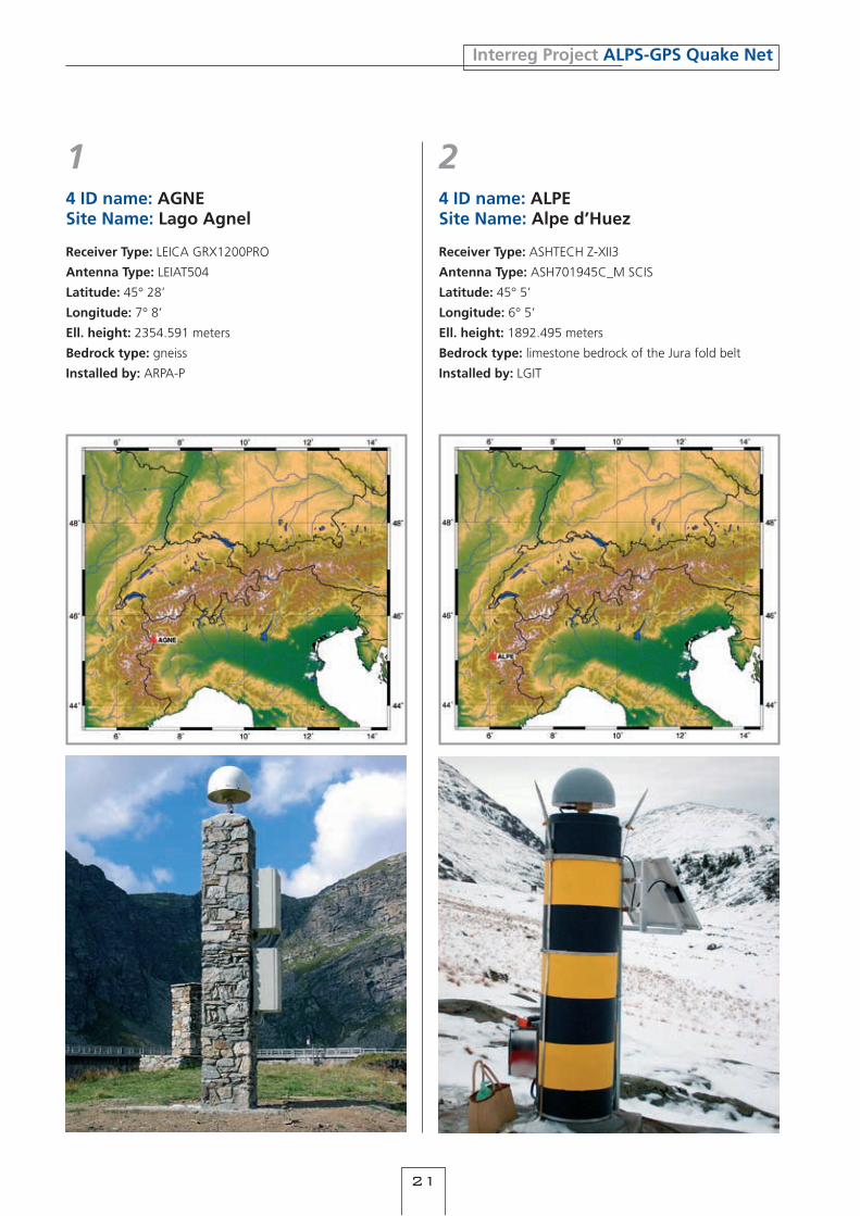
4 ID name: AGNESite Name: Lago Agnel
Receiver Type: LEICA GRX1200PRO
Antenna Type: LEIAT504
Latitude: 45° 28’
Longitude: 7° 8’
Ell. height: 2354.591 meters
Bedrock type: gneiss
Installed by: ARPA-P
14 ID name: ALPESite Name: Alpe d’Huez
Receiver Type: ASHTECH Z-XII3
Antenna Type: ASH701945C_M SCIS
Latitude: 45° 5’
Longitude: 6° 5’
Ell. height: 1892.495 meters
Bedrock type: limestone bedrock of the Jura fold belt
Installed by: LGIT
2

22
Interreg Project ALPS-GPS Quake Net
4 ID name: AUBUSite Name: Aubure
Receiver Type: TRIMBLE NetRS
Antenna Type: Dorne Margolin choke ring antenna
Latitude: 48° 12’
Longitude: 7° 12’
Ell. height: 970.139 meters
Bedrock type: granitic bedrock of the Palaeozoic of the Vosges massif
Installed by: EOST
34 ID name: BASOSite Name: Basoviza
Receiver Type: LEICA GRX1200Pro
Antenna Type: LEIAT504
Latitude: 45° 38’
Longitude: 13° 52’
Ell. height: 448.501 meters
Bedrock type: limestone bedrock
Installed by: UNITS
4

23
Interreg Project ALPS-GPS Quake Net
4 ID name: BOSCSite Name: Bosco Chiesa Nuova
Receiver Type: LEICA GRX1200pro
Antenna Type: LEIAT504
Latitude: 45° 35’
Longitude: 11° 2’
Ell. height: 910.177 meters
Bedrock type: sedimentary
Installed by: ARPAV-B
5 64 ID name: BREISite Name: Breitenberg
Receiver Type: LEICA GRX1200PRO
Antenna Type: LEIAT504
Latitude: 47° 32’
Longitude: 10° 33’
Ell. height: 1887.912 meters
Bedrock type: dolomite
Installed by: DGFI

24
Interreg Project ALPS-GPS Quake Net
74 ID name: BURESite Name: Bure (Haute-Marne)
Receiver Type: TRIMBLE NetRS
Antenna Type: Dorne Margolin choke ring antenna
Latitude: 48° 29’
Longitude: 5° 21’
Ell. height: 365.274 meters
Bedrock type: mesozoic sedimentary limestone and marls
Installed by: EOST
84 ID name: CARZSite Name: Monte Carza
Receiver Type: LEICA GRX1200PRO
Antenna Type: LEIAT504
Latitude: 46° 2’
Longitude: 8° 40’
Ell. height: 1164.497 meters
Bedrock type: gneiss-amphibolites
Installed by: ARPA-P

25
Interreg Project ALPS-GPS Quake Net
94 ID name: CLTNSite Name: Monte Coltignone
Receiver Type: TPS ODYSSEY_E
Antenna Type: TPSCR3_GGD CONE
Latitude: 45° 53’
Longitude: 9° 23’
Ell. height: 1440.037 meters
Bedrock type: igneous
Installed by: IREALP - RLB
104 ID name: DEVESite Name: Alpe Devero
Receiver Type: LEICA GRX1200PRO
Antenna Type: LEIAT504
Latitude: 46° 18’
Longitude: 8° 15’
Ell. height: 1679.418 meters
Bedrock type: calcareous schist
Installed by: ARPA-P

26
Interreg Project ALPS-GPS Quake Net
114 ID name: EOSTSite Name: Strasbourg
Receiver Type: TRIMBLE NetRS
Antenna Type: ‘Trimble Zephyr Geodetic
Latitude: 48° 34’
Longitude: 7° 45’
Ell. height: 137.327 meters
Bedrock type: (building)
Installed by: EOST
124 ID name: ELMOSite Name: Monte Elmo
Receiver Type: LEICA GRX1200PRO
Antenna Type: LEIAT504
Latitude: 46° 42’
Longitude: 12° 23’
Ell. height: 2397.875 meters
Bedrock type: quartzite
Installed by: GSB

27
Interreg Project ALPS-GPS Quake Net
4 ID name: FAHRSite Name: Fahrenberg
Receiver Type: LEICA GRX1200PRO
Antenna Type: LEIAT504
Latitude: 47° 36’
Longitude: 11° 18’
Ell. height: 1674.298 meters
Bedrock type: dolomite
Installed by: DGFI
13 144 ID name: FDOSSite Name: Fort Dossaccio
Receiver Type: LEICA GRX1200PRO
Antenna Type: LEIAT504
Latitude: 46° 18’
Longitude: 11° 43’
Ell. height: 1888.929 meters
Bedrock type: outcropping bedrock formed by rhyolitic
ignimbrites of the atesina volcanic platform
Installed by: Geological Survey of Provincia Autonoma di
Trento

2�
Interreg Project ALPS-GPS Quake Net
15 164 ID name: FERRSite Name: Ferret valley
Receiver Type: LEICA GRX1200PRO
Antenna Type: LEIAT504
Latitude: 45° 52’
Longitude: 7° 1’
Ell. height: 2404.873 meters
Bedrock type: granitic rocks
Installed by: FondMS
4 ID name: GORSSite Name: Gorjuse
Receiver Type: LEICA GRX1200Pro
Antenna Type: LEIAT504
Latitude: 46° 19’ 2.604”
Longitude: 13° 59’ 59.532”
Ell. height: 1048 meters
Bedrock type: bed rock
Installed by: UNITS - EARS

2�
Interreg Project ALPS-GPS Quake Net
4 ID name: HGRASite Name: Hochgrat
Receiver Type: LEICA SR520
Antenna Type: LEIAT504
Latitude: 47° 29’
Longitude: 10° 4’
Ell. height: 1764.160 meters
Bedrock type: conglomerate
Installed by: DGFI
17 184 ID name: HRIESite Name: Hochries
Receiver Type: LEICA SR520
Antenna Type: LEIAT504
Latitude: 47° 44’
Longitude: 12° 14’
Ell. height: 1615.181 meters
Bedrock type: limestone
Installed by: DGFI

30
Interreg Project ALPS-GPS Quake Net
19 204 ID name: JANUSite Name: Fort du Janus
Receiver Type: ASHTECH µZ-CGRS
Antenna Type: ASH700936A_M SCIS
Latitude: 44° 54’
Longitude: 6° 42’
Ell. height: 2583.061 meters
Bedrock type: limestone
Installed by: LGIT
4 ID name: JAVSSite Name: Javornik
Receiver Type: LEICA GRX1200Pro
Antenna Type: LEIAT504
Latitude: 45° 53’ 36.24”
Longitude: 14° 3’ 51.48”
Ell. height: 1100 meters
Bedrock type: bed rock
Installed by: UNITS - EARS

31
Interreg Project ALPS-GPS Quake Net
21 224 ID name: LEBESite Name: Col de Lebe
Receiver Type: ASHTECH Z-XII3
Antenna Type: ASH710945.02B SCIS
Latitude: 45° 54’
Longitude: 5° 37’
Ell. height: 940.487 meters
Bedrock type: fresh bedrock (limestone)
Installed by: LGIT
4 ID name: LFAZSite Name: Le Faz
Receiver Type: ASHTECH micro-Z CGRS
Antenna Type: ASH701945C_M SCIS
Latitude: 45° 6’
Longitude: 5° 23’
Ell. height: 1071.398 meters
Bedrock type: metamorphic
Installed by: LGIT

32
Interreg Project ALPS-GPS Quake Net
23 244 ID name: MARKSite Name: Le Markstein, Oderen
Receiver Type: “TRIMBLE NetRS”
Antenna Type: Dorne Margolin choke ring antenna
Latitude: 47° 55’
Longitude: 7° 1’
Ell. height: 1180.280 meters
Bedrock type: granitic bedrock of the Palaeozoic of the
Vosges massif
Installed by: EOST
4 ID name: LUCESite Name: Lucelle
Receiver Type: “TRIMBLE NetRS”
Antenna Type: Dorne Margolin choke ring antenna
Latitude: 47° 25’
Longitude: 7° 14’
Ell. height: 620.100 meters
Bedrock type: limestone bedrock of the Jura fold belt
Installed by: EOST

33
Interreg Project ALPS-GPS Quake Net
25 264 ID name: MATASite Name: Mount Matahur
Receiver Type: LEICA GRX1200PRO
Antenna Type: LEIAT504
Latitude: 46° 12’
Longitude: 13° 31’
Ell. height: 1629.062 meters
Bedrock type: flysch bed rock
Installed by: UNITS
4 ID name: MAVESite Name: Monte Avena
Receiver Type: LEICA GRX1200pro
Antenna Type: LEIAT504
Latitude: 46° 1’
Longitude: 11° 49’
Ell. height: 1465.510 meters
Bedrock type: sedimentary
Installed by: ARPAV-B

34
Interreg Project ALPS-GPS Quake Net
27 284 ID name: MITTSite Name: Kleine Mittagerspitze – Loc. Merano 2000
Receiver Type: LEICA GRX1200PRO
Antenna Type: LEIAT504
Latitude: 46° 41’
Longitude: 11° 17’
Ell. height: 2305.675 meters
Bedrock type: quartzite
Installed by: GSB
4 ID name: MBELSite Name: Montebelluna
Receiver Type: LEICA GRX1200pro
Antenna Type: LEIAT504
Latitude: 45° 46’
Longitude: 12° 2’
Ell. height: 214.453 meters
Bedrock type: sedimentary
Installed by: ARPAV-B

35
Interreg Project ALPS-GPS Quake Net
29 304 ID name: MOCASite Name: Mount Calisio
Receiver Type: LEICA GRX1200PRO
Antenna Type: LEIAT504
Latitude: 46° 5’
Longitude: 11° 8’
Ell. height: 1146.372 meters
Bedrock type: outcropping bedrock formed by dolomite
Installed by: GST
4 ID name: NIDESite Name: Niedersteinbach
Receiver Type: TRIMBLE NetRS
Antenna Type: Dorne Margolin choke ring antenna
Latitude: 49° 1’
Longitude: 7° 44’
Ell. height: 445.845 meters
Bedrock type: pink sandstone of the Triassic sedimentary
cover of the Vosges
Installed by: EOST

36
Interreg Project ALPS-GPS Quake Net
31 324 ID name: PALASite Name: Palazzolo
Receiver Type: LEICA GRX1200PRO
Antenna Type: LEIAT504
Latitude: 45° 47’
Longitude: 13° 2’
Ell. height: 4.942 meters
Bedrock type: alluvial sediments, test monumentation in
unconsolidated material
Installed by: UNITS
4 ID name: OATOSite Name: Osservatorio Astronomico di Torino
Receiver Type: LEICA GRX1200PRO
Antenna Type: LEIAT504
Latitude: 45° 2’
Longitude: 7° 45’
Ell. height: 658.815 meters
Bedrock type: arenite
Installed by: ARPA-P

37
Interreg Project ALPS-GPS Quake Net
33 344 ID name: POGGSite Name: Poggio Grande
Receiver Type: LEICA GRX1200PRO
Antenna Type: LEIAT504
Latitude: 44° 6’
Longitude: 8° 9’
Ell. height: 855.578 meters
Bedrock type: limestone
Installed by: RLG
4 ID name: PAROSite Name: Paroldo
Receiver Type: Ashtech Z – FX CORS
Antenna Type: Ashtech Dorne Margolin
Latitude: 44° 26’
Longitude: 8° 4’
Ell. height: 848.778 meters
Bedrock type: tertiary flish
Installed by: ARPA-P

3�
Interreg Project ALPS-GPS Quake Net
35 364 ID name: PUYASite Name: Puy Aillaud
Receiver Type: ASHTECH Z12-CGRS
Antenna Type: ASH700936A_M SCIS
Latitude: 44° 51’
Longitude: 6° 28’
Ell. height: 1689.702 meters
Bedrock type: limestone
Installed by: LGIT
4 ID name: PORASite Name: Monte Pora
Receiver Type: TPS ODYSSEY_E
Antenna Type: TPSCR3_GGD CONE
Latitude: 45° 53’
Longitude: 10° 6’
Ell. height: 1926.518 meters
Bedrock type:
Installed by: IREALP - RLB

3�
Interreg Project ALPS-GPS Quake Net
37 384 ID name: SERLSite Name: Serle
Receiver Type: TPS ODYSSEY_E
Antenna Type: TPSCR3_GGD CONE
Latitude: 45° 35’
Longitude: 10° 20’
Ell. height: 942.919 meters
Bedrock type: igneous
Installed by: IREALP - RLB
4 ID name: ROSDSite Name: Roselend
Receiver Type: ASHTECH Z12-CGRS
Antenna Type: LEIAT504 SCIS
Latitude: 45° 41’
Longitude: 6° 37’
Ell. height: 1693.313 meters
Bedrock type: gneiss
Installed by: LGIT

40
Interreg Project ALPS-GPS Quake Net
39 404 ID name: WARTSite Name: Wartsteinkopf
Receiver Type: LEICA GRX1200PRO
Antenna Type: LEIAT504
Latitude: 47° 39’
Longitude: 12° 48’
Ell. height: 1749.424 meters
Bedrock type: limestone
Installed by: Deutsches Geodaetisches Forschungsinstitut
4 ID name: SONDSite Name: Sondrio
Receiver Type: TPS ODYSSEY_E
Antenna Type: TPSCR3_GGD CONE
Latitude: 46° 10’
Longitude: 9° 51’
Ell. height: 529.015 meters
Bedrock type: igneous
Installed by: IREALP - RLB

Interreg Project ALPS-GPS Quake Net
41
2.3.2 Recommendations
The realization of a network of 40 CGPS stations capable of providing measurements with millime-ter precision requires maximum care about every single step involved in the process.For this reason, we are listing here a number of minimum technical requirements and practical measures that we consider important and that have allowed us to successfully realize the GAIN.
The first set of recommendations regards mini-mum requirements for the GPS kit, as they were agreed upon during the project scientific meeting held in Munch in February 2004.
Receiver: geodetic receivers recognized by the IGS that
could handle a meteo data logger; dual frequency ; memory size up to needs; embedded with a computer according to site
characteristics; external frequency input for real time purpo-
se (according to the needs of the of the project partner); possibility of remote control; lightening protector; UPS.
Antenna: geodetic antenna with a ground plane; phase center variations must be officially
certified; spherical radome.
The second set of recommendations regards ge-neral criteria for site selection: it has been com-piled by ARPA-P and is representative of the way most project partners have handled their sites.
Technical and scientific requirements: The site must allow the foundation of the monu-
ment in the bedrock. The site must be optically unobstructed, over
the cut-off angle of 15°, 360° around. In order to be significant at the alpine scale,
from the geologic point of view, the site has to be:- relevant, at a regional scale, from the general geologic, tectonic and structural point of view;- out of landslide and out of deep-seated-defor-mations. The point is critical; while it is quite easy to locate and define landslides, deep-sea-ted-deformations are often overlooked and ab-sent on landslide maps and inventories. Since, in the alpine area, deep-seated-deformations may cover entire mountain flanks for extremely large areas the geological investigation must include a thorough analysis aimed to be sure that the se-lected site is located in a totally stable area. The site has to be far from any source of electro-
magnetic disturbs (power lines, repeaters etc.).
Practical requirements: The site must preferably be on a public proper-
ty and it is advisable to provide strong and good contacts with the local communal authorities. The site must be easily reachable for mainte-
nance and should also be somehow sheltered, in order to prevent theft and vandalism. These two requirements may be mutually exclusive. Connection to the mains is advisable but not
indispensable. Power may easily be supplied by means of a unit consisting of solar panels and buffer batteries (allowing at least a one week au-tonomy), which is also less lightning-sensitive than mains connection. In case of connection to the mains, the ground-fault-device (compulsory in most countries) has to be of the self-retrigge-rable type, in order to prevent power blackouts due to lightnings. A proper, insulated, shelter must be provided
for power supply, modems and receiver electroni-cs. A double-case is to be preferred: an inner wa-terproof case and an outer ventilated one, to pro-tect for direct sun, rain and snow. A wire telephone connection is to be preferred
to GSM connection, which is a common source of technical troubles. If available, a DSL connection is the best choice.
2.4 GAIN DatacentreGalileianPlus for DST-UNITS
The GAIN Data Centre is a host computer with server architecture performing the following major functionalities: Data archiving for the whole GAIN network; FTP data distribution to authorized users (typi-
cally to Processing Centres); Internet server for the web site of the project; Web front-end for the Data Quality Evaluation
(DQETM) process.
These functionalities are described in the next sections.
2.4.1 SpecificationsThe physical characteristics of the GAIN Data Centre are:
HW: Dell PowerEdge 1800 with server architecture Processor Intel Xeon 3.0GHz; RAM: 1GB DDR2 Memory, (2x512MB); 3.5 inch 1.44MB Floppy Drive; 3 x 146GB SCSI Ultra320 (10,000rpm) Hard Drive
in SCSI 5 configuration, offering about 280GB of user-available disk size; RAID Disk Controller PERC 4/SC single channel
RAID card, 64MB cache, 1 int channels (U320)

Interreg Project ALPS-GPS Quake Net
42
20/48X IDE CD-ROM Redundant power supply 3 years of Dell Next Business Day Premier
Enterprise support
SW environment: Operating System: Linux Fedora Core 4 with ker-
nel 2.6.14 Scripting Language: PHP 5.0.4 Database Management System: MySQL 4.1.14
Web server: Apache HTTP Server 2.0.54 FTP server: ProFTPd 1.210 Firewall: Iptables 1.3.0 Connection to Windows system: Samba Server
3.0142
As can be seen in figure 2.4.1, the GAIN Data Centre has interfaces with the following items: Processing Centres: to send GAIN GPS data via
the Internet (using ftp) Data Receiving Centre (DST-UNITS local data
store) to retrieve DST-UNITS GPS data and to receive DQETM output via the LAN (using SMB protocol) Partners Data Centres: to receive GAIN GPS data
via the Internet (using ftp) The World Wide Web (WWW) to host the project
web site and to distribute GPS data to authorised users using common web browsers
2.4.2 Alps-GPS network data archiving capabilitiesThe GAIN Data centre provides the interface among Project Partners that collects GPS data and the Project Partners in charge of GPS data processing.Data retrieval from the remote GPS local networks (Partner Data Centres) is made using ftp over the Internet, with two different modalities available: ftp-push and ftp-get.In the ftp-push modality, the GAIN Data cen-tre makes available an ftp server to receive the GPS data ftp-pushed by the Project Partners. Only the hosts of the Project Partners are allowed to upload data.In the ftp-get modality, scheduled scripts con-nect to the Project Partners ftp servers to retrie-ve data.The retrieved data are then available to Processing Centres, that can retrieve them using ftp. Scheduled scripts are in charge of avoiding corrupted data to be available for the download.
2.4.3 FTP data distribution to authorized usersThe GPS data are downloadable by authorised users also using a web interface, that allows a ea-sier retrieving of data. An example of the query web interface is shown in figure 2.4.2, while the output of the query is shown in figure 2.4.3.The organization of the archive has been designed according to the FTP structure of the IGS data centres, available at CDDIS-GNSS Data References official web site: http://cddis.gsfc.nasa.gov/gnss_datasum.html
2.4.4 Internet server for the official web site of the projectThe GAIN Data Centre acts as web server for the official web site of the project. Goals of the web site are:
Fig. 2.4.1.
Fig. 2.4.2.
Fig. 2.4.3.

Interreg Project ALPS-GPS Quake Net
43
to distribute to the World Wide Web users all the information relevant to the project and its deve-lopment state to allow data browsing and their downloading to
authorised users to publish the results of the GPS data quality
ranking for all the active stations to allow the sharing of ideas, information and
comments using a forum
2.4.5 Web front-end for the Data Quality Evaluation (DQETM) processOne of the most important task problems arising in controlling the GAIN network efficiency is to evaluate continuously and automatically the re-liability of the retrieved GPS data. The GAIN Data Centre, through the software called Data Quality Evaluation (DQETM), accomplishes this task.The output of the DQE is processed by a proper script that updates the WEB pages containing a quality ranking of all the active GAIN stations.The output quality parameters of the DQE module published on the WEB site are: Acquired data versus expected data (Acq/Exp (%)):
ratio between the number of data acquired (Acq) and the expected data (Exp):
Acq / Exp = Acq
* 100Exp
Acquired data are the GPS data collection found on RINEX file fulfilling the nominal session tem-poral range and within the receiver cut-off an-gle. Expected data are computed according to the navigation RINEX data within the same nominal temporal session range and the same receiver cut-off angle. This parameter is important to check that the re-ceiver is acquiring data properly or that there is no obstruction over the cut-off angle. Double frequency-acquired data versus acqui-
red data (DF/Acq (%)): ratio between double fre-quency acquired data (DF) and total number of ac-quired data (Acq):
DF / Acq = Acq - SF
* 100Acq
DF is the difference between the acquired data and the single frequency data (SF) acquired that are edited.This parameter is useful to check that both fre-quencies are acquiring data correctly, during the satellite visibility period over the receiver. Total edited data versus double frequency ac-
quired data (Ed/DF (%)): data editing is also due to short satellite passages, i.e. when a satelli-te is locked to the receiver for less then ten epo-
ch. The total edited data is thus the sum of two contributions:1 Single-frequency acquired data editing (SF);2 Short satellite passage data editing (Shrt).This parameter is the ratio between the differen-ce of double frequency-acquired data and total edited data, and the double frequency-acquired data:
Cycle Slips (CS): this value represents the to-tal number of loss of satellites lock followed by a sudden relock of the same satellite. When the loss of lock and the relock happens, a cycle slip occurs. In terms of acquired data it means that phase observables show a sudden jump due to the reset of the ‘initial ambiguity’ value, since ‘ini-tial ambiguity’ is an unknown integration integer constant summed by the receiver to its own inter-nal clock integration, representing the phase ob-servable. Initial ambiguity can be estimated only on double differenced data. Noise on L1, L2, P1, P2 (N/L1, N/L2, N/P1, N/
P2): the parameters representing the noise on the phases and codes observable are the residuals standard deviation coming from an Euler-Goad al-gorithm based estimation process. Euler-Goad al-gorithm is used for obtaining, via a least square estimation with undifferenced single satellite-single receiver data, the following variables:i the total non-dispersive delay at each epo-ch( (t));ii the total dispersive delay at each epch (Î(t));iii the initial ambiguity estimation for both L1 and L2 (N1, N2).The observations model, according to the Euler-Goad algorithm, is, for each epoch a for a given satellite:
L1 = ~ - I + l1 N1 + e1
L2 = ~ - aI + l2 N2 + e2
P1 = ~ + I + e3
P2 = ~ + aI + e4
Where a = f1
f1
, the frequencies ratio, the four
unknowns are above displayed, and each ei repre-sents the sum of the whole mismodeled signals and instrumental noise. Once the estimation in performed, the evaluation of ei is straightforward, and it is possible to compute their distribution around their mean value. High value of noise parameters are the clear indi-cation that mismodeled signals, for instance due to multipath phenomena, have a great impact on data reception.
Ed / DF = Acq - Shrt - SF
* 100DF

Interreg Project ALPS-GPS Quake Net
44
2.5 GAIN and referenceframesHermann Drewes for DGFI
The objectives of the ALPS-GPS Quakenet project (see 1.1) call for highest precision in the deter-mination of station positions and position chan-ges of the entire station network (millimetres and tenth of millimetres per year, respectively). In order to achieve this extreme requirements, a unique and consistent reference system has to be used in all steps of the data processing for coor-dinate determination. Position coordinates refer always to a coordinate system that has to be de-fined unequivocally, and position changes need a stable origin to which the motions refer. If space geodetic observations are used, like in the pre-sent project the measurements between GPS sa-tellites and terrestrial points, it is necessary that the reference system for the coordinates in space (of the satellites) and on ground (terrestrial sta-tions) must be completely identical. The referen-ce system is realized in practice by a reference frame, i.e., a set of stations with coordinates ac-cording to the definition of the reference system. The global stations which are tracking the satel-lites and used for the orbit computations form a fundamental part of the reference frame.
There are, in principle, two types of coordinates publicly available for the orbits of all GPS satel-lites (satellite ephemeris). One of those are the
broadcast ephemeris provided in real time by the system operator (National Geospatial-Intelligence Agency, NGA, on behalf of the United States Department of Defense, DoD). They are continuo-usly computed from the observations of a small network of about a dozen global tracking stations and given in the World Geodetic System (WGS84). Another type are the ephemeris provided by the International GNSS Service (IGS). They are compu-ted from observations of a large network of global tracking stations and given in the International Terrestrial Reference Frame (ITRF). There are dif-ferent orbit products of the IGS, e.g., broadcast ephemeris (real time, daily updated,
~160 cm precision), ultra-rapid ephemeris (real time, four times dai-
ly updated, ~10 cm precision), final ephemeris (~13 days delayed, weekly upda-
ted, <5 cm precision).
The global IGS network used as the reference fra-me for the orbit computations consisted until end of 2006 of 98 tracking stations (IGb00) with coordinates in the ITRF2000. Since end of 2006 it includes 132 stations with coordinates in the ITRF2005, corrected for the absolute phase cen-tre variations. The complete ITRF2005 as well as the global IGS network includes about 350 sta-tions with given position coordinates and ve-locities caused by crustal movements (figure 2.5.1). The global networks are densified by re-gional networks, e.g., in Europe by the European Reference Frame (EUREF).
The GPS observations are measurements of travel times of microwave signals transmitted by the sa-tellites and received by the instruments on ground with different clocks. As the clocks are not syn-chronized with an accuracy sufficient to reach for the highest precision in point positioning (milli-metres), only relative positions (baselines) can be computed between stations in short distances, where the clock errors are estimated in an adjust-ment procedure. For coordinate determination we need thus terrestrial stations with coordinates in the same reference system as the satellite orbi-ts as a reference frame close to the network sta-tions. The WGS84 has not such a dense reference frame. The ITRF and its densification (EUREF) as well as the IGS offer a large set of stations in the alpine region. Due to crustal deformation (tecto-nic plate motions and regional deformations) the coordinates of the stations change with time re-lative to the satellite orbits. Therefore, we have to transform the coordinates of the reference fra-me by the station velocities to the observation epoch in the data processing. The velocities are shown in figure 2.5.1. The computed station posi-tions of new stations refer then always to the ob-servation epoch.
In summary we conclude that the GAIN referen-ce frame has to be the same as the reference fra-me of the satellites, and needs a dense spacing
Fig. 2.6.1 - The distribution of GNNS sites of the EPN network.
Fig. 2.6.2 - The distribution of the GAIN sites and the adjacent
EPN sites.

Interreg Project ALPS-GPS Quake Net
45
in the region of the measurements. This is only fulfilled by the ITRF, at present in its realization ITRF2005. For GPS users the ITRF2005 is reali-zed by the IGS05, where the GPS receiver phase centre variations are corrected according to the IGS conventions of 2006. In order to get a dense terrestrial reference frame we may also use sta-tions of the ITRF/IGS densification in the alpi-ne region.
2.6 The Geodetic Alpine Integrated Network (GAIN) and its relation to EUREFChristof Völksen for BEK
During the centuries each country, each fede-ral state or even each municipality developed its own reference system for mapping or land regi-ster. Mapping at the boundary between two sy-stems was always and is in part still difficult sin-ce one had to work with two different coordinate systems. EUREF is aiming at an uniform reference systems that can be used at any place in Europe for many different purposes.
The acronym EUREF stands for European Reference System and is integrated in the Sub-Commission 1.3, Regional Reference Frames, of the International Association for Geodesy (IAG). It has been founded in 1987 at the General Assembly of the International Union of Geophysics and Geodesy (IUGG) in Vancouver. The main objectives of EUREF are the definition, rea-lisation and maintenance of a geodetic reference system for Europe.
In close cooperation with the International GNSS Service (IGS) a network of permanently instal-led GNSS receivers has been established on vo-luntary basis by universities, research institutes and other groups. This network, which is known as the EUREF Permanent Network (EPN), obser-ves continuously the signals of the GNSS satel-lites. The EPN consists currently of more than 180 stations and covers Europe almost comple-tely (see Figure 2.6.1). It serves as a densifica-tion of the IGS network in Europe and also plays a major role in the realisation of the European Terrestrial Reference System 89 (ETRS89). This system is defined as connected to the stable part of the Eurasian plate and as identical to the International Terrestrial Reference System (ITRS) at epoch 1989.0. The ETRS89 is the EU-recommended frame of reference for geodata in Europe. Therefore it is used as the standard for precise positioning, surveying and geodyna-mic studies throughout Europe. It is supported by EuroGeographics, which represents nearly all European national mapping and cadastral agen-cies (NMCA), and is therefore the dominating re-ference system in Europe.
The main objective of the GAIN network is the monitoring of crustal deformation caused by pla-te tectonics or by earthquakes, land slide moni-toring and meteorology. These studies request a solid and well defined reference system such as the ITRF2000 (International Terrestrial Reference Frame 2000) or its subset IGb00. The network can also be used for some applications in navi-gation, agriculture, mapping and surveying, whi-ch also need a unified reference system. It is the-refore obvious to integrate stations of the EUREF network into the gain network and consequently in the data analysis. The selection of suitable re-ference station from the EUREF network is gover-ned by the following arguments covering the area of interest (the ALPS) well known station behaviour coordinates should be available in the reference
frame IGb00 and ETRS89 data availability / data access.
A selection of EPN sites are shown in Figure 2.6.2. Almost 15 sites cover the ALPS with a concentra-tion in Italy and Austria. This number of sites is more than sufficient for the integration of the GAIN network into the ETRS.
Although the GAIN network is processed in the IGb00 the integration of the EUREF sites with their well known coordinates in the ETRS89 allows the transformation between the two systems. An additional advantage of the integration of EPN sites is the study of continental deformation ou-tside the Alpine region. This study is currently under investigation by the Bavarian Comittee for International Geodesy (BEK), but is not directly linked to this project.
2.7 Data analysisPOLIMI-RLB, BEK, LGIT, POLITO-ARPAP
The monumentation of most part of the GAIN sta-tions and the availability of continuous GPS ob-servations in the data centre, have been the star-ting point for the data analysis.Different aspects have been considered by the three analysis centres of the project.The Bavarian Comittee for International Geodesy (BEK) and Polytechnic of Milano (POLIMI) analy-sis differ from each other for the GPS stations in-cluded in their analysis and for the reference sta-tions taken into account, whereas the Université Joseph Fourier, Laboratoire de Géophysique Interne et Tectonophysique (LGIT) analysis also differs for the GPS Software used.Briefly, the purpose of each analysis centre could be summarized as follows: 1 The aim of the BEK has been the analysis and the integration of the GAIN Network in the EUREF Permanent Network (fig.2.6.2). GPS data have been processed by means of the scientific Bernese Software v.5.0 [Beutler et al., 2007].

Interreg Project ALPS-GPS Quake Net
46
Fig. 2.7.1 - LGIT processed network over the Alps.
Fig. 2.7.2 - The POLIMI proces-sed Network over the Alps. The
EUREF stations MATE, NOT1 and CAGL, used with the other EU-
REF stations as reference frame, are not plotted.

Interreg Project ALPS-GPS Quake Net
47
2 The aim of the LGIT has been the analysis and the integration of the GAIN Network with 17 European IGS sites and with other stations belon-ging to the RENAG/OSUG Network, taking care of the Western part of the Alps (fig.2.7.1). GPS data have been processed by means of the scientific program GAMIT/GLOBK [Herring et al, 2006].3 The aim of POLIMI was the analysis and the in-tegration of the GAIN Network with the FReDNet Network [Zuliani et al., 2002] and some RING sta-tions [Selvaggi et al., 2006] taking care of the Eastern part of the Alps (fig. 2.7.2). GPS data have been processed by means of the scientific Bernese Software v. 5.0.
The GPS data processing strategy selected in the Bernese GPS Software v.5.0 by BEK and POLIMI analysis centres is based on the following assumptions: Precise satellite orbits and Earth Rotation
Parameter provided by IGS – International GPS Service [http://igscb.jpl.nasa.gov/] Absolute Phase Centre Variation (PCV) both of
satellites and antennas, provided by IGS. Global ionospheric modelling provided by CODE
[ftp://ftp.unibe.ch/aiub/CODE] Ocean tide loading provided by OSO – Onsala
Space Observatory [http://www.oso.chalmers.se/~loading/] – was applied. Processing of the phase double difference ob-
servations . Tropospheric modelling was realised applying
Niell mapping function and estimating tropo-
Fig. 2.7.3 - The POLITO proces-sed Network.
Fig. 2.7.4 - TORI coordinate time series. The red dots are the adjusted coordinates obtained removing less reliable stations. Note that the jump in week 1412 have been removed.
spheric parameters every hour with one gradient per station. QIF (Quasi Ionosphere Free). ambiguity resolu-
tion strategy is applied. Cut-off angle has been fixed to 10 degrees. According to the processed network, different
IGS stations have been used as reference sta-tions, constraining the latest coordinate realiza-tion of the IGS Reference Frame (IGb00/IGS05)
The GPS data processing strategy selected in the GAMIT/GLOBK by LGIT is based on the following choices: IGS final orbits adjusted Cut-off angle fixed to 10º

Interreg Project ALPS-GPS Quake Net
4�
A priori meteorological values GPT (Boehm et al., 2007) Mapping function VMF1 (Boehm et al., 2006) Ocean loading model FES2004 (Letellier, 2004) Absolute Phase Centre Variation (PCV) both of sa-
tellites and antennas, provided by IGS (IGS_05).
Daily solutions have been computed obtaining coordinates and variance-covariance matrix of the GPS stations
Polytechnic of Torino (POLITO) was also inte-rested in elaborating GAIN Network. Its purpo-se was the analysis and the integration of the GAIN Network with other Italian GPS Permanent Network (fig. 2.7.3) for mapping and surveying and the implementation of an automatic proce-dure for data quality control, based on Bernese Software v.5.0. GPS data have been processed by means of the scientific Bernese Software v. 5.0 following the same standards quoted above. Moreover POLITO has realised a software called NetDownload [[email protected]], whi-ch retrieves and prepares data for the Bernese Processing Engine (BPE) The output of this pro-cedure is the improvement of time series stabi-lity, as shown for the EUREF TORI station in fig. 2.7.4
2.8 Outputs and ProductsPOLIMI-RLB, BEK, LGIT, POLITO-ARPAP
The most important results of the performed data analysis described in Paragraph 2.7 are the daily coordinates of the GPS Permanent Stations.The time series of daily solutions are then analy-sed to get estimates of station velocities, as ex-plained in Paragraph 3.1.
In this paragraph some coordinate time series of GAIN stations are shown.In Fig. 2.8.1 and Fig. 2.8.2 the computed daily coordinates (X,Y,Z) of the WART and CANV sta-tions are respectively plotted: these time series are quite long as compared to those of other sta-tions (about one years).Green points are the coordinate in the IGS05 Reference Frame, introduced at day 309 of 2006, whereas purple points are the coordinate in the IGb00 Reference Frame. From DoY 309 of 2006 the points are double (green and purple points) because IGS05 coordinates are transformed into IGb00 coordinates applying the IGS transforma-tion parameters (for further explanations see Paragraph 3.1).
A problem in the time series analysis can occur in case of Reference Frame change. Even thou-gh coordinate transformation is applied with pro-per parameters, residual discontinuities can be present after datum shift compensation (see Fig. 2.8.1, Fig. 2.8.2).The residual discontinuities are further estimated
Fig. 2.8.1 - WART coordinate time series for the year 2006.
Fig. 2.8.2 - CANV coordinate time series for the year 2006.

Interreg Project ALPS-GPS Quake Net
4�
and removed from the time series. In this way re-fined time series are obtained suitable for reliable velocity estimates.As an example of this procedure the coordinate time series (North, East, Up) of WART station are shown in Fig. 2.8.3 after the recovering of the re-sidual jumps.
2.9 GAIN and regionalservicesIREALP-RLB, ARPAP, FondMS, UNIGE-RLG
2.9.1 Lombardia regionIn Italy, the first example of GNSS regional ser-vice is given by GPSLombardia, the GNSS positio-ning service of Regione Lombardia.The network project started in 2003 and involved Regione Lombardia, Politecnico di Milano, and IREALP, the regional research institute that final-ly created GPSLombardia (http://www.gpslombar-dia.it)The network now consists of 18 permanent sta-tions and covers 75% of the population of the re-gion; it will cover all the territory after the for-thcoming new installation of a permanent station in the city of Chiavenna.Starting from July 2005, GPSLombardia offers the users both RINEX data for post-processing posi-tioning and real time corrections. RINEX data are available 24/365 from all the stations: through a web interface, the user has the possibility to retrieve the data by selecting the station, the time period and the data decimation of interest. Real time differential corrections are distributed in different ways (also known as “mountpoint”) through a NTRIP server (http://131.175.88.151:2101), allowing a real time accuracy of few de-cimetres if using a GIS rover and few centime-tre accuracy if using a geodetic double frequen-cy receiver. The GPS hardware of permanent stations consists of TPSCR3_GGD + CONE antenna and TPS Odissey receiver, from Topcon, and tracks data of both GPS and GLONASS constellations. All stations are provided with long duration backup battery.Most of the stations are installed on the roofs of civil buildings while the 4 permanent stations in-stalled in the framework of ALPS – GPSQuakenet project were installed on concrete pillar on rock. Some more details are given below: PORA: installed on the top of Monte Pora,
between the provinces of Brescia and Bergamo. Data are retrieved using a wireless link, hiper-lan standard; SOND: installed in the vicinities of the city of
Sondrio. Data are retrieved using a wireless link with HI-FI standard. Solar panels were used; CLTN: installed on Monte Coltignone, in the vi-
cinities of the city of Lecco. Data are retrieved
using a wireless link and hiperlan standard. Solar panels were used. SERL: installed in the “Parco Naturale di
Cariadeghe” (province of Brescia). Data will be retrieved using a wireless link, hiperlan standard. Solar panels are used.
All permanent stations are daily monitored by se-veral automatic procedures: Daily and weekly adjustment using RINEX
data, performed by Politecnico di Milano, Polo Regionale di Como; Real time control over communication lines; Real time control over GPS data availability; Controls over percentage of lost GPS data vs.
expected data; Comparison of active GPS and GLONASS satelli-
tes vs expected ones; Controls over “low level” state of software (ca-
ster server, RINEX server, etc);
Coordinates of the stations are distributed in IGB00 reference frame; moreover, 7 parameters for the transformation in the Italian local ETRF89-IGM95 system are available on the website.The website (http://www.gpslombardia.it) offers a wide range of interesting pages for GPS users working in Lombardia region. First of all, there is a list of most-used GPRS contracts, allowing the
Fig. 2.8.3 - WART coordinate time series after jump recove-ring.

Interreg Project ALPS-GPS Quake Net
50
user to select his best one choice in order to use GPSLombardia real time corrections.Moreover, some interesting planning tools are available: the GPS user can see, for example, how many satellites are expected to be available in the next hours and their elevation, for both GPS and GLONASS constellation.An expected value of GDOP and PDOP is also gi-ven. All these information are available for all the permanent stations of GPSLombardia and are updated 4 times a day, using ultra rapid epheme-ris from CODE. The website also offers the real time status of the software that distributes dif-ferential corrections (GNSMART from GEO++): it is therefore possible to see how many satellites are seen and if any station is temporarily unavailable for TLC problems. A password limited section is also available: GPSLombardia users can see their total traffic, for both RINEX data and connections to NTRIP server.
Regione Lombardia will soon contribute to the creation of an Italian permanent GPS network, created and managed by IGM (Istituto Geografico Militare), whose aim will be the update of the Italian ETRF89-IGM95 reference system.
2.9.2 Liguria RegionServices distributed on the whole territory allow integrating data with spatially correlated effects especially for Real Time applications. Obviously they required a strong synergy with neighbouring networks for the congruency of data at the bor-der, and the continuity of the service. A national coordination about Reference Frame and manage-ment aspects is recommended.
In particular for Liguria Region, the POGG Permanent Station will be the first of a planned GNSS regional network. The institution of a Survey Regional Service con-cerns the realization, management and analysis of a GNSS permanent stations network on the re-gional territory. Foreseen activities regard the realisation of a data collection centre, elabora-tion and analysis of the regional data. Primary importance is give not only to data quality, but also to continuity and guaranty of the services offered to the territory in the different institu-tional activities.
A brief review on possible applications, for diffe-rent level of their precisions, is:a High precision applications (sub-centime-tre precision level), to monitor continental de-formation and landslides, and for meteorological modelling.b Medium precision applications (sub-decime-tre precision level) for Real Time positioning: real time tracking and searching targets for techni-cal applications (technologic network, roads, …), updating cartography, cadastral applications and many others.
c Low precision applications (sub-meter pre-cision level) in particular for navigation purpo-ses (e.g. aircraft positioning), and for specialized users (ambulances, firemen, etc.).
Several categories of people are potential users of a regional Positioning Service:1 Professional categories: Surveyors, Geologist, Engineers, Architects.2 Cartographic agencies: IGMI, Agenzia del Territorio.3 Local territorial administrative agencies, in different sectors like civil protection (prevention and management of risk and emergency), urban and transport planning, tourism, cadastral, envi-ronment and energy services.4 Association of management of territorial di-stricts (Autorità di bacino, Comunità Montane).5 Public and private company of transport ma-nagement (terrestrial, sea, aerial)6 Private users.
Several people like scientist researcher, admini-strative and technical staff of Regional Public Administration, University, local Public structures are involved. Thus, a dedicated staff for the GNSS Services is very important to guarantee optimal results and this requires to create new expertise for young scientists.
In synthesis, the Services has to provide to the local users the necessary tools to make the use of satellite survey techniques easier and more eco-nomic, assist the final users, study and develop new applications.
2.9.3 Piemonte RegionArpa Piemonte has created a unit, which is part of the Centro regionale per le ricerche territoriali e geo-logiche in order to manage and maintain the five permanent GAIN receivers installed in Piemonte in the framework of the AlpsGPSQuakenet project. The related costs will be covered by ARPA annual budget. Arpa Piemonte is currently preparing an internet site in order to distribute the data ac-quired by the receivers. The data will be available to everybody, free of charge, and may be useful for surveyors, engineers, geologists and to the lo-cal administration for several applications (topo-graphic surveys; surveys related to the register of landed property; local networks etc.).
2.9.4 Valle d’Aosta RegionThe permanent GPS station and the GAIN network supply an additional instrument to the glaciologi-sts in their monitoring activities: glaciers tongue variation and ice-flow veloci-
ty measurements with differential GPS techniques can be lead with high accuracy; during summer activities the tongue position is measured and compared with the previous one in order to reveal annual displacement. Superficial sensors on the

Interreg Project ALPS-GPS Quake Net
51
glacier measure the rate displacement of the ice. hanging glaciers displacement rate; hanging
glacier dynamic is a matter of study, in some case the fall down of enormous ice blocks can be dan-gerous for downhill settlements or alpine path. An experimental study can be implemented posi-tioning a chain of economical remote GPS recei-vers along the front and recording the displace-ment until the falling.
The Civil Protection of the Aosta Valley Autonomous Region investigates some alpine re-scue applications of the GPS station. An exam-ple is the precise positioning of the rescue teams over the territory, their portable GPS receivers transmit via radio their position to the central station that elaborates the correction and loca-tes them. Another application under study is the alpine path mapping with the help of the local al-pine guides.

Interreg Project ALPS-GPS Quake Net
52
3 - CONTINENTAL DEFORMATION IN THE ALPS

Interreg Project ALPS-GPS Quake Net
53
3.1 First results from the GAIN networkBEK, POLIMI-RLB, LGITThe main product of the EU co-funded project ALPS-GPSQUAKENET is the permanently installed GAIN network in the Alps that tracks continuously the signals of GNSS satellites. Apart from collecting the data it is of course necessary to process the ob-servations and estimate precise coordinates. Only the monitoring of the coordinates allows drawing conclusions on the tectonics of the Alps.The collected GNSS data of the whole GAIN network are processed by three different analysis centres: BEK: Bayerische Kommission für die Internationale
Erdmessung (Munich, Germany) LGIT: Université Joseph Fourier, Laboratoire de
Géophysique Interne et Tectonophysique (Grenoble, France) POLIMI-RLP: Politecnico di Milano (Milan, Italy).
While BEK and POLIMI-RLB are using the GNSS analysis package BERNESE 5.0, LGIT exerts GAMIT for the data processing. The data of the network are evaluated independently applying identical standards like correction models for the anten-na (absolute), realising the same reference frame (ITRF) and applying similar models for the correc-tion of the troposphere and for example the effects of ocean loading. These standards have been defi-ned by the three groups beforehand to ensure that comparable results will be achieved. The networks of the different analysis centres are slightly diffe-rent due to the selection of different GNSS sites that are added to the network (e.g. stations of the EUREF Permanent Network [EPN]). Nevertheless, the independently estimated solutions of the three analysis centres agree quite well.
Data are available for each day and therefore dai-ly solutions for the coordinates are computed for the whole network. The coordinates for each sta-tion change with time due to plate tectonics, ear-thquakes and possibly due to local movements of the monument. The strongest signal seen in the po-sition changes is of course caused by plate tecto-nics. But also snow on top of the antenna, which usually stays only for a couple of days, can have an impact on the coordinate solution. These unde-sirable effects like local movements of the monu-ment carrying the antenna or snow on top of the antenna compromise the signal, which is of course the change of position due to tectonics. One has to be extremely careful with the interpretation of position changes. It is therefore very important to exclude all these undesirable effects. This ensures that the detected signals are truly dependent on tectonics only.
In order to estimate the precision of the coordina-te components it is necessary to remove a linear trend from the time series of the position changes, which is mainly caused by plate tectonics. And in some cases it is also necessary to remove jumps (e.g. snow on the antenna etc.). The mean root mean square of these residuals is given in table 3.1.1 for the three coordinate components in the GAIN network. The achieved precision is very sati-sfying. Already daily position changes in the order of a few millimetres are detectable. This indicates that the impact of rather small earthquakes in the vicinity of the station should be visible.
The GAIN network has just recently been comple-ted. Some GNSS sites are installed for more than two years. Others are operational only for a few months. It is quite obvious that the precision of the estimated velocities for each site depend very much on the length of the observation period. Sites like ACOM, BASO, HRIE and ZOUF are opera-tional for the entire observation period of almost two years, while sites like SOND, POGG, MOCA and
Tab. 3.1.1 - Average precision achieved in the GAIN network.
HeightEast
RMS [mm]
GAIN Network
North
3.741.441.43
Vj Vl Vh sVj sVl sVhSTATIONmm/a
ACOM 14.7 22.2 2.8 0.7 0.5 0.7AFAL 14.5 16.2 2.2 0.7 0.6 0.7
AGNE 10.7 22.1 2.1 1.1 0.8 1.1BASO 18.5 23.1 -1.7 0.7 0.5 0.7
BOSC 17.5 21.1 3.8 1.0 0.7 1.0BREI 15.6 23.0 1.3 0.7 0.6 0.7
CANV 15.9 21.3 2.2 0.7 0.5 0.7CARZ 14.1 23.9 -5.3 1.0 0.6 1.0
DEVE 18.8 19.1 -6.9 2.5 2.5 2.5FAHR 12.7 25.0 4.3 0.7 0.5 0.7
FDOS 12.9 23.8 4.8 0.9 0.6 0.9GROG 21.8 18.4 -- 1.3 0.9 1.3
HGRA 18.2 12.5 0.1 0.8 0.6 0.8HRIE 20.1 22.1 7.1 0.7 0.6 0.7
JANU 15.3 27.4 -- 3.0 1.7 3.0LEBE 16.3 21.7 1.3 1.4 0.9 1.4
LFAZ 16.1 19.3 -0.2 0.8 0.6 0.8MAVE 19.0 22.3 -6.2 1.0 0.7 1.0
MBEL 19.3 16.8 -- 1.1 0.7 1.1MDEA 16.3 21.2 0.7 0.7 0.5 0.7
MOCA 13.8 15.2 3.7 1.6 1.0 1.6MONC 14.0 23.4 -6.1 0.9 0.6 0.9
MPRA 15.9 22.5 1.6 0.6 0.5 0.6OATO 14.2 20.6 -2.7 0.7 0.5 0.7
POGG 11.6 27.3 -- 1.9 1.3 1.9PUYA 14.2 23.3 -1.2 0.8 0.6 0.8
ROSD 15.2 15.6 3.2 0.9 0.7 0.9SOND 18.7 14.6 0.8 1.4 0.9 1.4WART 16.3 20.4 4.5 0.7 0.5 0.7ZOUF 12.8 23.5 2.8 0.7 0.5 0.7
Tab. 3.1.2 - Estimated velocities in the GAIN network.

Interreg Project ALPS-GPS Quake Net
54
others have observation periods as little as half a year. Significant estimates for the site movement cannot be expected as long as the observation pe-riod is rather short. Table 3.1.2 shows the estima-tes for the horizontal and vertical velocities for a number of sites from the GAIN network.
Table 3.1.2 shows clearly that the accuracy of the estimated components increases with time. The best results were achieved with stations, which are operational close to two years [BASO, HRIE etc.]. The opposite is visible for the above mentioned stations with rather short observation periods. But other aspects are proven by this table as well. JANU has been covered by snow for some weeks. The re-ceiver was also not always operational. The analy-sis of the GPS data estimates a subsidence of more than 50 mm per year. It is quite clear that this can-not be the realistic vertical motion of the station.
Fig. 3.1.1 - The horizontal veloci-ties of the GAIN network in the
ITRF2005.
Fig. 3.1.2 - The velocities of a part of the Bavarian Real-time network SAPOS. The network
is fixed to the Eurasian plate (based on the NUVEL-NNR1A
model).
Experience has shown that it is in general not pos-sible to estimate significant vertical motion within a time span of less then 3 to 4 years. Heights esti-mated with GPS are the weakest of all three coor-dinate components as table 3.1.1 shows. Therefore the vertical motion of the sites GROG, JANU, MBEL and POGG are not presented in Table 3.1.2.
Table 3.1.2 shows also that the horizontal velo-cities of most stations are quite similar. This is of course no surprise since all the stations are affected by the plate motion of the Eurasian plate. This be-comes also visible by looking at figure 3.1.1, whi-ch shows the horizontal velocities only. The gene-ral trend of the motion points into east-north-east with a rate of 20 to 30 mm.
Figure 3.1.2 shows the Bavarian part of a network that belongs to the Satellite Positioning Service (SAPOS) of the German State Survey. This network has been analysed by the BEK for the last 2.5 years. Compared to figure 3.1.1 the horizontal residual ve-locities are much smaller because the network is fixed to the Eurasias plate. Most stations show the same residual velocity apart from some stations like the WANK, which is caused by the instability of the local marker. This shows again the importance of stable markers. But this figure gives us a good indi-cation of what to expect in one or two years time. The analysis of the gain network should produce velocities for the horizontal components with accu-racy better than 1 mm/a. Sudden position changes, as small as a few millimetres, should be detectable. The correlation with seismic events might give an indication for an earthquake.

Interreg Project ALPS-GPS Quake Net
55
3.2 Active deformation in the western AlpsAndrea Walpersdorf for LGIT
3.2.1 IntroductionThe western Alps result from the Europe-Africa col-lision which leads to the indentation of Europe by the Adriatic promontory (Tapponier, 1977). A pro-bable counterclockwise rotation of the indenter has been suggested (Anderson and Jackson, 1987; Ménard, 1988; Vialon et al., 1989) (Figure 3.2.1). The present day convergence velocity between Africa and Europe is less than 1 cm/yr and increa-ses from the western to the eastern Mediterranean (Figure 3.2.1).
Although the countries bordering the western Alps have low to moderate seismotectonic activi-ty (Figure 3.2.2), several earthquakes of Ml > 5 are recorded in historical catalogues (Beauval and Scotti, 2003) and by paleoearthquake evidence (e.g. Sébrier et al., 1997) (Figure 3.2.3). A mean of one magnitude 6 earthquake occurs in the we-stern Alps per century.
The Alpine region is the most deforming part of western and central Europe. A synthesis of fo-cal mechanisms by Sue et al. (1999) and Delacou et al. (2004) shows that the kinematics are cha-racterized by a continuous area of orogen-per-pendicular extension following closely the lar-ge-sclae topographic crest line of the Alpine arc (corresponding to E-W extension in the western Alps), while thrusting is observed locally, limi-ted to areas near the border of the Alpine chain (Figure 3.2.4). The complex current tectonics of the Western Alps would result from the interfe-
rence of the Europe-Adria collision and relative rotation at the limits of the belt, and buoyancy forces within the western Alpine lithosphere (Sue et al., 1999).
Fig. 3.2.1 - Global tectonic settings, showing the Africa-Eurasia collision with velocities increasing from west to east and the counter-clockwise rotation of the Adriatic micro-plate.
Fig. 3.2.2 - Seismicity along the Eurasian-African plate boundary.
Fig. 3.2.3 - Historical and Instru-mental seismicity in the western Alps.

Interreg Project ALPS-GPS Quake Net
56
S compression (which could have been associated to the motion of the Corsica-Sardenia-block), but is rather characterized by a dominating E-W exten-sion (Figure 3.2.5).
The third measurement campaign in 2004 has iden-tified measurement outliers for a certain number of sites. These errors could be due to blunders in the tripod installation, unidentified tribrach offsets, unidentified antenna phase center offsets, etc. and cannot be evidenced by only two campaign mea-surements. However, even after the third measure-ment, it is difficult to identify the epoch bearing the outlier. Therefore a forth campaign will be ne-cessary to confirm the velocity field of this dense GPS network.
Permanent measurementsVelocity estimates with an accuracy of less than 1 mm/yr have been obtained by measuremen-ts of a network of permanent GPS stations from 1996 to 2001 covering central and western Europe (Nocquet and Calais, 2003, Fig. 3.2.6). The au-thors have shown that central Europe behaves as a rigid block with internal deformation of no more than 0.4 mm/yr. There is almost no motion west of the Rhine Graben and on the Iberian pe-ninsula, and less than 0.6 mm/yr across the Rhine Graben and the Pyrenees. The current strain pat-tern in the western Alps combines E-W extension and right-lateral shear. There is some evidence for a counter-clockwise rotation of the Adriatic micro-plate which appears to control the strain pattern along its boundaries in the Friuli area, the Alps and the Apennines (Nocquet and Calais, 2003) (Fig. 3.2.6). The first permanent GPS network dedicated to the observation of the deformation of the western Alps has been installed in the French Alps and its fore-land from 1997 on (the REGAL network, now alpi-ne part of the French RENAG consortium, http://renag.unice.fr). By now, about 30 stations instal-led directly on the bedrock are operational (Figure 3.2.7). First results of this permanent network have been published by the initiators (Calais et al., 2002, Figure 3.2.8), based on data from 1997 to 2001. The authors find velocities in the French Alps of less than 2 mm/yr with respect to stable Europe, with uncertainties from 0.3 to 1.4 mm/yr depen-ding on the age of the station. The central part of the mountain belt is dominated by E-W extension. Compressional strain oriented N-S to NW-SE is no-ted in the southern Alps. These geodetic data as well as seismotectonic observations (Figure 3.2.8) are coherent with a model where the deformation of the western Alps is mainly controlled by the anti-clockwise rotation of the Adriatic micro-plate with respect to stable Europe. The comparison of these first velocity estimates ba-sed on the REGAL data up to 2001 with a more recent solution constrained by REGAL data up to
a
b
3.2.2 Existing GPS measurements covering the western Alps Campaign measurementsTo measure the present day deformation in the we-stern Alps, a 60 stations campaign GPS network has been established in 1993 covering the French, Italian and Swiss part of the western Alps (Figure 3.2.5, from Vigny et al., 2001). Three measure-ment campaigns have been done in 1993, 1998 and 2004. The two first campaigns have shown re-latively slow velocities (1-3 mm/yr) on all of the sites with respect to stable Europe. The uncertain-ties have been evaluated by the respective campai-gn repeatabilities to 1.3 mm/yr, which means that most of the velocities are close to or inside of the measurement error. The deformation pattern evi-denced by these measurements has no visible N-
Fig. 3.2.4 - a) Map of the strain/stress states in the Western Alps
(stress tensors represented by black and open arrows, P and T axes represented by red and
blue lines) and b) 3D view iden-tifying regions of dominating extension (blue), compression
(red) and strike-slip mechanisms (green) (from Delacou et al.,
2004).

Interreg Project ALPS-GPS Quake Net
57
2004 presented in Walpersdorf et al. (2006) (Figure 3.2.9) shows a general decrease of site velocities (from typically velocities of 2 mm/yr to 1 mm/yr). The compression in the southern Alps between sta-tions GRAS and MICH has not been confirmed, but seems to persist further west between sites MARS and MICH, and MTPL and SAUV.
Semi-permanent networksOne of the regions in the western Alps where the highest deformation rates have been expected is the Jura area, located between the alpine orogen and its foreland. The Jura is known to have been an active area during the Neogene. Some eviden-ce suggests that this is still the case, but preci-se knowledge of deformation and slip rates is still unavailable. A local semi-permanent GPS network was installed in 2000 to address this issue and to improve the seismic hazard assessment of the re-gion. The 6 sites are measured at least twice a year for about 10 days, to obtain position time series approaching the quality of permanent stations. This semi-permanent approach requests the use of a single GPS receiver for the 6 sites. The semi-per-manent sites have lower constraints for the site se-lection as permanent sites as they need no electri-city and telephone. Therefore, semi-permanent observations can be an efficient means of densi-fying permanent GPS networks for geodynamic pur-poses. Figure 3.2.10 shows the Jura velocity field obtained in Walpersdorf et al. (2006). The uncer-tainties are evaluated to about 0.3 mm/yr. Most of the Jura velocities with respect to stable Europe are lower than this error limit. The major feature in this velocity field is a 1 mm/yr relative velocity between sites JU02 and JU04, giving a hint of the present day activity of the Vuache fault, situated between the two sites.
3.2.3 Contribution of the ALPS-GPSQUAKENET project: the GAIN networkIn the framework of the Interreg IIIB project ALPS-GPSQUAKENET, 8 new permanent GPS stations have been installed in the western Alps, 6 in France and 2 in Italy (Figure 3.2.11), as part of the GAIN network covering the entire Alpine arc. These 8 sta-tions will contribute to quantify precisely the slow but complex deformation in the western part of
Fig. 3.2.5 - GPS velocities from 2 measurement campaigns in 1993 and 1998, and the domi-nating extensive strain pattern (from Vigny et al., 2001).
Fig. 3.2.6 - From Nocquet and Calais, 2003. The crustal velocity field of western Europe from permanent GPS array solutions, 1996-2001.
Fig. 3.2.7 - The French REGAL network (REseau Gps permanent dans les ALpes) in 2006.
Fig. 3.2.8 - From Calais et al. (2002). GPS velocity field and strain tensors in the western Alps compared to focal mechanisms.
Fig. 3.2.9 - REGAL velocity fields based on data from 1997 to 2001 (Calais et al., 2002) and on data from 1997 to 2004 (Walpersdorf et al., 2006).
the Alps. The resolution of displacement rates ex-pected to be inferior to 1 mm/yr requires however continuous observations during at least 5 years. For most of the GAIN stations a 1 to 2 years data span has been available at the end of the project (spring 2007). The velocities evaluated from these data have typical formal errors of the order of 2 to 1 mm/yr as seen on Figure 3.2.11. We need to pur-sue the measurements until 2010 at least to obtain significant displacement rates characterizing the slow deforming western part of the Alps.
3.3 Active Deformation in the South-Eastern AlpsRiccardo Riva and Alessandra Borghi for DST-UNITS, POLIMI-RLB and UNIMI-RLB
3.3.1 IntroductionThe South-Eastern Alps represent one of the most seismically active regions in Europe and an out-standing natural laboratory for the study of acti-ve deformation.Collision between the African and Eurasian plates, in fact, leads to deformation of the plate boundary, with consequent stress localization on active faul-ts that leads to a very high seismic activity.The largest reported earthquake in the region took place in Western Slovenia in 1511, with an estima-ted magnitude of 6.9 [Fitzko et al., 2005], while in the last three decades we have observed the 1976 Friuli sequence, where the largest shock had a ma-gnitude of 6.5 [Aoudia et al., 2000], and more re-cently the 1998 and 2004 earthquakes in Western Slovenia, with magnitude 5.7 and 5.3 respectively [Bajc et al, 2001].In order to study the complex geodynamics of the region, a dense GPS network has been established in the last few years, as it is possible to see in Figure 3.3.1, where blue dots represent the con-tinuous stations of the FreDNet, the red dots the newly installed GAIN stations and the black dots the campaign GPS sites initially installed in col-laboration by University of Trieste, Politecnico di Milano and University of Milano and later incorpo-rated in the ALPS-GPSQuakenet project.In Figure 3.3.1 we show a topographic map of the region, where the main mapped active faults are identified by blue lines and each dot represents a

Interreg Project ALPS-GPS Quake Net
5�
it has been added to our network. The Slovenian EUREF station GSR1 has been also integrated into the network.For each campaign site, the monumentation was carefully performed to ensure a sub-millimetre cen-tring at every occupation. At each station point, a 25 cm long still rod was fixed in solid rock and a properly designed steel pillar holding the anten-na was centred on this ground part, using toroidal levels calibrated before every campaign. For each GPS site, we installed networks of control poin-ts and performed spirit levelling measurements to check for spurious local site effects.During all campaigns, data were collected for four consecutive days, with daily sessions of eight hours, and at some safer sites we have measured continuously for four days. The sampling rate was 15” for non-permanent stations and 30” for CGPS.Data analysis was performed with the Bernese Software v.5.0 [Hugentobler et al., 2004], where the Quasi Iono Free (QIF) strategy for ambiguity fixing was selected. Tropospheric parameters were estimated on one hourly basis and wet delays were modelled as stochastic parameters, using the map-ping function Dry_Niell. The ionospheric disturban-ce has been treated using global ionospheric mo-dels estimated by CODE [Hugentobler et al., 2000] in the L1&L2 ambiguity estimation step and using the iono-free observations (L3) in the co-ordinate computation.Observations were first analysed on a daily ba-sis with multi-base approach, without constrai-ning any stations and saving the normal equa-tions. Subsequently, the daily normal equations were combined into multi-day solutions for each year with the ADDNEQ program of the Bernese sof-tware, fixing the co-ordinates of the five reference stations used in this network (GRAS, GRAZ, WTZR, ZIMM and MATE), which were propagated to the current epoch. These stations were selected be-cause they are the closest to the Friuli-Slovenia Region. In this way we have obtained a set of coor-dinates for each campaign station, which allows us
GPS station: it is evident how the regional geody-namics is extremely complex, so that a high den-sity distribution of GPS stations is absolutely ne-cessary to understand how internal deformation is allocated on the different faults.
3.3.2 GPS data processingIn 2002 a GPS non-permanent network has been set up in Friuli Region and in 2004 it has been en-larged with six sites in western Slovenia (Figure 3.3.2).The FreDNet GPS continuous stations have also been integrated in our network [http://www.crs.inogs.it/frednet/ItalianSite/XFReDNetHome.htm] to increase its spatial resolution and impro-ve the geodetic description of the area. Moreover, the use of continuous GPS stations allows a bet-ter link between our local network and a global re-ference frame (IGS05 for the late 2006, IGb00 for 2006, 2005 and 2004; ITRF00 for 2003 and 2002) and helps in connecting campaigns performed in Friuli Region with those in Slovenia, which typical-ly take place on different days. Since the new GAIN station BASO has been operating from July 2005,
Figure 3.2.10. From Walpersdorf et al. (2006). The velocity field
in the semi-permanent Jura network with respect to stable
Europe, based on measurements from 2000 to 2004.
Fig. 3.2.11 - First velocity estima-tes with respect to stable Europe,
including 1 to 2 years of data on most of the GAIN stations
installed in the framework of the ALPS-GPSQUAKENET project.

Interreg Project ALPS-GPS Quake Net
5�
Fig. 3.3.1 - topographic map of the South-Western Alps. Blue li-nes indicate mapped active faul-ts (strike-slip with red arrows, dip-slip with blue triangles). Red dots are GAIN stations, black dots campaign stations and light blue dots FreDNet stations.
Fig. 3.3.2 - map of the GPS sites of the Friuli-Slovenia non-perma-nent network (blue points), the FreDNet continuous stations (red points), the EUREF GSR1 station (green point) and the GAIN station BASO (pink point).

Interreg Project ALPS-GPS Quake Net
60
to estimate the displacement vectors between the different campaigns.For the CGPS stations we have elaborated the who-le available database, from installation to the end of 2006, with the use of Bernese Software v.5.0, selecting the same procedure used for the GPS campaign analysis up to the daily solution com-putation. The daily coordinate solutions constitu-te a time series for each station and allow a deeper analysis of the GPS site velocities. All the coor-dinates have been reported in the same referen-ce frame (IGb00) using the official transformation parameters. Each coordinate component (North, East, Up) has been fitted using the following deterministic mo-del: a linear trend plus a periodic signal with an-nual frequency. Due to the shortness of the time series, about three years, any estimate of the fre-quency of the periodic signal will not be reliable, and it has been fixed in accordance to standard GPS practice.
Y(ti) = a·ti + b + c·sinwt + d·coswt + ng
j=1 gjH(ti - Tgj)
where
Y(ti) is the daily coordinate at time ti, a is the site velocity in the coordinate compo-
nent taken into account b the interceptor with the ordinate axis w is the annual frequency c and d are the magnitude of the periodic signal H is the Heaviside step function, ng is the number of jump i.e. due to change in
reference frames, changes in antenna/receivers or co-seismic displacement etc.., gj are the amplitude of the jump accursed at time
Tgi.The unknown parameters (a, b, c, d and gj) have been computed by Least Squares Estimator using a proper stochastic model that takes into account of the time correlations existing in GPS time series [Barzaghi et al, 2004], applied to a dataset clea-ned from outliers.
3.3.3 GPS results for continuous stations The first results obtained by processing three years of data for the FredNet network give a picture of the large scale deformation of the whole area and are presented in Figure 3.3.3.In order to provide a clear representation of the motion of the GPS stations, we have taken as refe-rence the Eurasian velocity as provided by the geo-logical model NNR-NUVEL1A.In this way, any displacement different from zero means that the GPS site is actually moving with re-spect to the velocity field predicted by the geolo-gical model.Considering the error ellipses, we see how the three northernmost sites AFAL, ZOUF and ACOM, and the south-western site CANV, do not show significant motions. On the contrary, we can clearly observe compression in north-west direction along the line TRIE, MDEA and MPRA.The magnitude and direction of the observed mo-tion is consistent with the counter-clockwise ro-tation of the Italian peninsula, as an effect of the African plate moving northwards: the whole pro-cess is sketched in Figure 3.3.4.In the left cartoon, Plate A represents Eurasia, Plate B Africa, and the central part, where the faul-ts are located, the Alps. The combination of thrust faults and strike-slip faults arises from the presen-ce of a pole of rotation in the western part of the domain, as further clarified represented in the ri-ght cartoon of Figure 3.3.4.
3.3.4 GPS results for campaign measurements The analysis of the motion of the continuous sta-tions might be enough to depict the large-scale deformation of the whole region. However, consi-dering the density of mapped fault already descri-bed in Figure 3.3.1, a densification of the network
Fig. 3.3.3 - continuous GPS stations, horizontal displacement
rates for years 2003-2006 with respect to the Eurasian plate velocity as defined by model
NNR-NUVEL1A.
Fig. 3.3.4 - sketch of the geo-dynamics of the Western Alps,
explaining the formation of right-lateral and thrust faults as a consequence of the regional
tectonics.

Interreg Project ALPS-GPS Quake Net
61
is necessary in order to understand if and where the regional deformation is going to be localised, leading to potential seismic risk.Preliminary results, after the occupation of the GPS campaign sites in 2002, 2004 and 2005, are displayed in Figure 3.3.5. We can observe as lar-ge differences in displacement magnitude and di-rection arise between sites close to each other, meaning that deformation is not homogeneously spread over the whole region. Interpretation of those motions requires a further effort of campai-gn geology and modelling work, in order to under-stand which geological features are responsible for the local geodynamics. More GPS campaigns and the addition of other space-geodetic techniques, such as Interferometric Synthetic Aperture Radar (InSAR), will also help to increase the measure-ments accuracy.
3.3.5 Co- and post-seismic deformation of past earthquakes In this section we will study the effect of the lar-gest reported earthquakes in the area, where co-seismic deformation means the elastic (instanta-neous) deformation that follows the rupture, while postseismic deformation is the effect of stress re-laxation in the lower crust and upper mantle. The moment an earthquake takes place, in fact, a per-manent deformation occurs in the area around it, leading to a situation of non-equilibrium: the excess stress causes material to flow in deeper cru-stal layers, which results in a long-lasting defor-mation process.Starting from the largest reported seismic event, the 1511 Western Slovenia earthquake, we show coseismic deformation in the left panel of Figure 3.3.6, where the scale is in millimetres: we can see how some areas where displaced by more than one meter.After the earthquake, the accumulated stress be-
gins to relax, with a process that can last for se-veral centuries, depending on the intensity of the earthquake and the properties of the Earth crust. In the right panel of Figure 3.3.6, we show the ac-cumulated postseismic deformation between 1511 and the present: we see how the region affected by significant deformation is much wider than in the coseismic case, and that displacement amounts to
Fig. 3.3.5 - campaign GPS displacements accumulated between 2002 and 2005.
Fig. 3.3.6 - map view of horizon-tal displacement following the 1511 earthquake. Left panel: coseismic; right panel: postsei-smic relaxation between 1511 and 1976.

Interreg Project ALPS-GPS Quake Net
62
about 20 cm in the part where our GPS sites are lo-cated, i.e. around the yellow lobe at the centre of the picture. Most of this deformation has occurred in the first few centuries after the earthquake, but a small residual is still present today, as we will show later.Analogously, we can study co- and post-seismic de-formation for the main shock of the 1976 Friuli earthquake, displayed in Figure 3.3.7. Due to the smaller size of the earthquake, deformation is con-centrated in a much smaller area; nonetheless, we obtain up to 30 cm of maximum coseismic defor-mation and more than 4 cm of postseismic relaxa-tion between 1976 and today.In Figure 3.3.8 we show coseismic deformation for the last two relevant earthquakes, occurred near Bovec in western Slovenia in 1998 and 2004 (left panel 1998, right panel 2004): we neglect the po-stseismic signal, which is below the millimetre le-vel. Since the 2004 event took place after the first GPS campaign in western Slovenia, it might have affected later measurements: model results, howe-ver, indicate that only the site TRIG could have
experienced a noticeable displacement.Modelling postseismic relaxation from past ear-thquakes gives us the opportunity to evaluate their effect on the GPS measurements that we have been performing in the last few years. In Figure 3.3.9 we show model postseismic relaxation rates due to the cumulative effect of all the above discus-sed earthquakes. The small blue arrows show the expected motion of our GPS sites: we can see how all of them are at the sub-millimetre level, sugge-sting that we can consider postseismic deforma-tion as a second order effect when we interpret the GPS measurements, as those of Figures 3.3.3 and 3.3.5.
3.3.6 Stress transfer In the previous sections we have analysed what is the impact of past earthquakes on surface displa-cement. Here we want to discuss another impor-tant aspect of the interaction between earthquakes in the same region, namely Coulomb Failure Stress (CFS).
Fig. 3.3.7 - map view of horizon-tal displacement following the 1976 earthquake. Left panel:
coseismic; right panel: postsei-smic relaxation between 1976
and 1998.
Fig. 3.3.8 - map view of hori-zontal coseismic displacement following the 1998 (left panel)
and the 2004 (right panel) earthquakes.

Interreg Project ALPS-GPS Quake Net
63
The mathematical definition of CFS is the following:
CFS = t + m·sn
where t is tangential stress, sn normal stress and μ the friction coefficient: tangential stress is directly related to slip along the fault plane, while normal stress influences the degree of locking of the fault. A positive value means that an earthquake is faci-litated, while a negative value means that an ear-thquake is prevented. When an earthquake occurs, in fact, the stress field around it is modified and this can affect the behaviour of active faults loca-ted in the neighbourhoods. Modelling CFS does not tell where and when another earthquake will take place, but gives an indication about which regions will see an increase or a reduction of seismic risk.In order to see whether there has been a posi-tive interaction between past earthquakes in the South-Eastern Alps, we have modelled CFS starting from 1511 and accounting for both coseismic and postseismic effects.In Figure 3.3.10 we show the effect of the 1511 earthquake on the 1976 earthquake, identified by the westernmost black segment and focal mecha-nism. The colour scale portrays the logarithm of the Coulomb stress in Pascal: generally, values are considered significant when they are above 1 bar, equal to 105 Pa, here represented in orange and purple.Since the 1976 earthquake is located in the yellow region, where CFS has a value of about half a bar, we cannot say that this seismic event has really been triggered by the 1511 earthquake; however, it looks like there has been a positive interaction between the 1511 and 1976 events.
Next, we add the contribution of the 1976 Friuli earthquake and its relaxation up to 1998. In Figure 3.3.11 we plot CFS on the fault that ruptured du-ring the Bovec earthquake: the earthquake falls in an area where there has been definite interaction with the previous earthquakes, in particular with the 1511 event. The distance between the 1976 and the 1998 earthquakes, however, appears to be too large to implicate a noticeable stress transfer between the two events. The reason why Figure 3.3.10 and 3.3.11 are so different, even if both are dominated by the stress field induced by the 1511 earthquake, is in the fact that the 1976 and 1998 earthquakes have very different focal mecha-nisms, so that the result of the projection of shear
Fig. 3.3.9 - map view of present-day postseismic relaxation rates.
Fig. 3.3.10 - map view of CFS due to the 1511 earthquake and projected on the 1976 fault, computed at a depth of 5 km with μ=0.4. The three black solid segments indicate the surface traces of the 1976, 1998 and 1511 earthquakes, respectively, starting from the West.

Interreg Project ALPS-GPS Quake Net
64
The mechanism is similar to the1998 event, i.e. a right lateral strike-slip, with the addition of a dip-slip component. If the location is very close to the 1998 event, than the similarity between the two earthquakes leads to a negative CFS value, consi-stent with the fact that the first earthquake has released most of the tectonically accumulated stress. However, the is an uncertainty about the exact location of the 2004 event, that could put it outside the 1998 stress shadow, in an area whe-re the positive influence of the 1511 earthquake is still dominant.In conclusion, as far as Coulomb stress transfer is concerned, all major seismic activity in the South-Eastern Alps seems to be dominated by the long la-sting effect of the 1511 earthquake. The 1976 sei-smic event, though rather large in terms of surface motions and damage, is probably too far from the area of the 1998 and 2004 earthquakes to be able to influence them. The similarity between the 1998 and 2004 earthquakes, in turn, suggests that ei-ther the location of the 2004 event is not accura-tely determined, or that not all of the accumulated tectonic stress had been released during the 1998 seismic sequence.
3.4 Glacier shrinkage and modeled uplift of the AlpsValentina Barletta for UNIMI-RLB
3.4.1 IntroductionAlpine glaciers are subject to rapid decline star-ting from 1850 A.D., as inferred from analyses of regional and national glacier inventories, as done in the present study, or from comparison of gla-cier data obtained from Landsat Thematic Mapper (TM) data with previous glacier areas [Paul et al., 2004]. Alpine glacier shrinkage is consistent with worldwide large ice mass reductions [Paul et al., 2004; Haeberli et al., 1999] and can be conside-red an indicator of global climate change [IPCC, 2001]. Changes in volume of glacier masses in the Alps are expected to induce vertical uplift due to the Earth’s elastic and viscoelastic response to sur-face load redistribution, as modeled in this stu-dy. Uplift rates from Alpine glacier wasting can be compared with those predicted for larger ice com-plexes, for example the Patagonian ones treated by Ivins and James [2004], thus providing testable tools for modeling lithosphere-cryosphere interac-tion, within two different environments, the Alps and the Andes.
3.4.2 Alpine Glacier Mass LossWorld Glacier Inventory (WGI) data have been used to evaluate the mass loss affecting the Alpine gla-ciers on a known time interval. WGI reports gla-cier data (surface area, lenght and main dimen-sional parameters) collected between the 50’s and
Region Area Mass Balance m/yr, w.e.aYearly Reduction, %
Austria - 0.640.63
France - 0.970.47
Italy - 1.190.47
Switzerland - 0.400.84
Germany - 0.640.63
and normal stress on the fault plane is also very different.Last, we can study the combined effect of the 1511, 1976 and 1998 earthquakes on the most re-cent 2004 earthquake in western Slovenia; results are shown in Figure 3.3.12.
Fig. 3.3.11 - map view of CFS due to the 1511 and 1976 ear-thquakes and projected on the
1998 fault, computed at a depth of 5 km with μ=0.4.

Interreg Project ALPS-GPS Quake Net
65
the 80’s of the XX century: it has been necessary to apply an area reduction factor in order to estimate more recent glacier surface areas. Updated glacier areas are evaluated for the years 1996, 1997, 1998 and 1999 by applying a surface reduction factor specific for each glacier, considering the Alpine re-gion where it is located. This factor is obtained from the available literature dealing with glacier shrinkage rate in the different Alpine regions in Table 3.4.1. Main sources for calculating the re-duction factor are multitemporal national and re-gional glacier inventories, whose comparison per-mitted the evaluation of reliable glacier reduction over a time frame of one or two decades [Paul et al, 2004; Käab et al., 2002; Biancotti and Motta, 2001]. Besides, the numerical variation affecting the whole glacier sample is considered: glaciers indicated as ``Glacierets’’ in the WGI are removed from the data-set. This choice is due to the au-thors’ findings in the Italian Alps where all the gla-cierets reported in the WGI data base at the end of the nineties disappeared. Thus the glaciers con-sidered in this study covered in 1999 an area of 2215 km2. Moreover the choice of evaluating the glacier mass loss for the years 1996-1999 is also supported by the availability, for that time inter-val, of specific mass balance data of a represen-tative sample of Alpine glaciers. The mass balan-ce data published on FOG [IAHS-UNESCO, 2005] can be considered representative of the mass va-riations which affected Alpine Glaciers on the stu-died time frame. In fact, according to the “glacier regionalism’’ introduced by Reynaud et al., [1984], glaciers located in the same region show stronger
correlation among their mass balances. Since more than one mass balance for the period 1996-1999 has been published for each region, a mean mass balance value per year has been obtained by avera-ging the mass balances for each region. These year-ly values have then been averaged over the consi-dered four years to obtain a unique value for each Alpine region (second column, Table 3.4.1), to be used within a high spatial resolution normal mode scheme. The average of the values reported in Table 3.4.1 equals -0.71 m/yr water equivalent: this va-lue represents an estimate of the mean mass loss affecting the whole sample of Alpine glaciers and is used within the low spatial resolution calcula-tion. In this scheme it is necessary to include the water feeding the Mediterranean sea: by applying the above reported glacier loss value, the sea-le-vel rise (limited to the Mediterranean sea) of 0.46 mm/yr is obtained.
Fig. 3.3.12 - map view of CFS due to the 1511, 1976 and 1998 earthquakes and projected on the 2004 fault, computed at a depth of 5 km with μ=0.4.
Tab. 3.4.1 - Coefficient of Glacier Area Reduction Per Year and the Mass Balance, Averaged Over 1996-1999.
Fig. 3.4.1 - Caption: Low resolution map of the uplift rate caused by glacier mass balance of -0.71 m/yr.
Fig. 3.4.2 - Computed high resolution (elastic response) to ice mass loss. In the inset (corre-sponding to the the dashed box in main figure), our white con-tour lines are superimposed to the vertical rates obtained from the new national height system (LHN95) of Switzerland [Schlatter et al., 1999], for comparison.

Interreg Project ALPS-GPS Quake Net
66
3.4.3 Traditional Normal Mode ApproachUplift rates are based on a spherical and radially stratified, viscoelastic Earth model (linear Maxwell rheology, 7 layers, Table 3.4.2), similar to that used for post-seismic calculations, but tuned to the vi-scosity profile used by Burov et al. [1999], infer-red from ECORS profile, and with volume averaged rigidities from PREM [Dziewonski and Anderson, 1981]. In normal mode theory for a viscoelastic Earth model, the vertical displacement is expanded in spherical harmonics. Truncation of the expan-sion results into information loss, determining the spatial resolution. The Alpine glaciers have cha-racteristic lengths of about 1 Km, thus a harmo-nic decomposition up to 40,000 degrees should be exploited. A low resolution calculation can be car-ried out considering only an equivalent load spread over the area of the geographical region occupied by all the glaciers; we can thus limit the harmonic expansion to about 500 degrees. The effective mass balance (s_E) is smaller with re-spect to the real one (s_R) by a factor chosen to respect the total mass balance, s_E=(A_R/A_E)*s_R, for a real area A_R of 2215 Km2 and a mean mass balance s_R of -0.71 m/yr. Results of this low resolution calculation are shown in Figure 3.4.1, where the largest elastic uplift rate is about 0.1 mm/yr and the position of the maxi-mum is roughly located in the centre of the area, as expected. Besides the uplift rate localized in the surrounding of the alpine chain, we can also
take into account the effect of Mediteranean basin sinking caused by the melting water. In this cal-culation we used about 1.151 Gt/yr of water fee-ding the Mediterranean sea, obtaining a small su-bsidence down to -0.007 mm/yr in the southern Mediterranean basin. The value of 0.1 mm/yr obtained from this low resolution calculation, can be compared with the present-day uplift rate of 2 mm/yr obtained by Ivins and James [2004] for the Patgonian ice fields and a sub-cratonic mantle, prediction very similar to that for an elastic model, not shown in that article. The difference can be understood by considering that in Patagonia the mass loss considered by Ivins and James [2004], 38.4 Gt/yr for years 1990-2000 A.D, is 24 times larges than the Alpine 1.54 Gt/yr. The low resolution calculation of this section is appropriate for estimating long wavelength featu-res of the vertical displacement, but the need for more detailed uplift rates in correspondence with the largest ice complexes, requires accurate high resolution calculations.
3.4.4 High Resolution ApproachDifferently from the case of global problems, such as sea level computations where the load function is extended over the whole globe, loads now oc-cupy a very limited part of the sphere, and thus it is convenient to integrate straightforwardly over the load. Furthermore, the glaciers can be easily treated as a discrete ensemble of point-like sour-ces. A similar use of point-like source distribution can be found for co- and post-seismic deforma-tion problems as recentely done by Dalla Via et al. [2005]. Le Meur and Hindmarsh [1999] and Barletta and Sabadini, [2006] have shown that for a surface load the elastic part of the solution tends asymp-totically to a non-zero value for increasingly high harmonic degrees. Le Meur and Hindmarsh [1999] have shown how to overcome the Gibbs phenome-non due to truncation by making use of the sum of Legendre polynomials series. The Green function thus can be rewritten in a more suitable form and so we can compute the approxi-mate solution for one disk and compare with the highly accurate solution where the sum of the se-ries is carried out at 40,000 harmonic degrees to resolve 1 Km loads.
Tab. 3.4.2 - Rheologic Structure.
Fig. 3.4.3 - High resolution viscous contribution, for 155
Km^3 of ice volume loss 1850 A.D.
Layer
1
2
3
4
5
r kg/m3
2650.0
2750.0
2900.0
3439.3
3882.3
r km
6371.0
6352.5
6341.0
6331.0
5951.0
Pa
2.97*1010
5.58*1010
6.81*1010
7.27*1010
1.09*1011
u Pa s
1.00*1035
2.15*1019
5.00*1021
4.64*1020
4.64*1020
6
7
4890.6
1093.2
5701.0
348.0
2.21*1011
0.00
1.00*1021
0.00

Interreg Project ALPS-GPS Quake Net
67
The comparison shows that for distances from the load larger than three times the radius of the load our approximation overlaps the highly accurate so-lution. This indicate that use of the approxima-ted relation for uplift rates at points far from eve-ry glacier is correct, at least for distances larger than three times the radius of the load. When the distance of the observation point from a glacier is smaller than three times the radius of the load, the contribution of that specific glacier is treated with the highly accurate decomposition. Small size loa-ds can thus be accurately treated by means of the above computationally efficient technique, optimi-zing the traditional normal mode approach. To show the results over the whole Alpine chain of Figure 3.4.2, a regular 5 Km spaced grid resolu-tion has been used. Nonetheless, uplift rate can be evaluated correctly using a restricted set of points only, as benchmarks (leveling or GPS) in the inver-se problem scheme.
3.4.5 ResultsFigure 3.4.2 shows the modeled uplift rates for present-day mass balance of Table 3.4.1 and for the Earth model of Table 3.4.2, while the inset shows the measured uplift rate, from leveling and GPS, limited to Switzerland after Schlatter et al. [1999]. Uplift rates, in the range 0.1-0.2 mm/yr, characterize the response of the whole Alpine belt to present-day glacier reduction, in agreement with the findings of Figure 3.4.1, encircling pa-tches of high uplift rates, localized over the major glacial complexes. The largest uplift rate spot, of 0.9 mm/yr, indicated by the arrow, occurs in the French Alps, in proxi-mity of Mount Blanc Group, where the largest mass loss is located. Uplift values of about 0.4 mm/yr, a factor two lower than the maxima in the west, are located in Austria. In the inset the (white con-tours) modeled and measured uplift rate pattern, closely resemble in shape, indicating that pre-sent day glacier shrinkage contributes a substan-tial fraction of observed uplift rate. The 0.1 mm/yr white contour in the north almost overprints the 0.4 mm/yr measured, indicating a 20% contribu-tion from present day glacier shrinkage in the pe-riphery of the uplifting region. The largest patches of modeled uplift rate overlap the regions of lar-gest observed ones, although the highest modeled uplift rates of about 0.4-0.5 mm/yr, dark blue pa-tches in the main panel of Figure 3.4.2, are about a factor two lower than measured ones. Modeling fails to reproduce the northernmost part of the large measured uplift patch, right in the in-set. These findings suggest on one side that gla-cier shrinkage sensibly contributes to the Alpine chain uplift, on the other side that there are other phenomena, such as active tectonics, drainage and erosion [Schlunegger et al., 2001a, 2001b], affec-ting both the values of the largest uplift rates and their geographical distribution.
Figure 3.4.3 portrays the effects of viscous relaxa-tion in the lower crust and in the asthenosphere on uplift rates, assuming a constant volume loss sin-ce 1850 A.D. for a total of 155 Km3, equally distri-buted over the representative glacier distribution of the 1973, and rheological parameters in Table 3.4.2. According to Haeberli and Beniston [1998] the estimated total glacier volume in European Alps was about 130 Km3 for mid-1970s and since the end of the Little Ice Age the glacierization has lost around half of its original volume. This means 130 Km3 since 1850, plus 25 Km3 since 1973, accor-ding to Paul et al [2004]. The viscous uplift pattern is smoother than the ela-stic one. In the western Alps, where also the elastic part is most important, the largest viscous uplift rates are concentrated, hitting 0.32 mm/yr. The vi-scous part can be more than 50% of the elastic part, but it is generally smaller. Summing up the largest elastic contribution and the geographically corresponding viscous one, an uplift of 0.7-0.8 mm/yr is obtained in the western Alps, a substantial fraction (half) of the largest observed one of 1.5 mm/yr. The estimate of the viscous contribution, on the other hand, can be affected by uncertainties in the rheological para-meters, and must thus be taken with caution. The dimensions of the patches where uplift is con-centrated, of tens of kilometers, is comparable with the thickness of the crust, of 40 km, as in Table 3.4.2, indicating that contributions to uplift origi-nates from stress relaxation in the soft lower crust of 2.15* 1019 Pa s, as in Table 3.4.2.
3.4.6 ConclusionsAccording to our model, rapid glacier shrinkage gives a substantial contribution to Alpine chain uplift. The specialized normal mode technique we introduced here provides an high spatial resolution scheme, thus becoming a necessary tool within the forward problem, which will be the kernel of the in-verse problem for future work. Our results are the key for a correct interpretation of uplift data in the Alpine chain and for quantifying the contributions from different drivers of uplift, present-day glacier instability, active tectonics and drainage.
3.5 Instrumental earthquakes in the Alpine region: source parameters from moment tensor inversion Mariangela Guidarelli for DST-UNITS
We consider moment tensor inversion solutions for a set of earthquakes, with moment magnitu-de 4.8, that occurred in the Alpine region during

Interreg Project ALPS-GPS Quake Net
6�
the period 1998-2004. The source parameters have been retrieved using a robust methodology (INPAR method), that performs a dynamic relocation of the hypocentre (latitude, longitude and depth) si-multaneously with the determination of the focal mechanism (Šílený et al., 1992; Šílený, 1998). To help constrain stress conditions and tecto-nic features in the Italian region it is necessary to supplement the information provided by glo-bal seismology (e.g. CMT-Harvard solutions, USGS) with regional and local broad-band studies. In fact the Italian region is seismically very active but most of the relevant seismicity is concentrated in the magnitude range 5-6, with a little number of events with MW>6.0. The study of earthquakes with MW<6.0 is necessary to obtain information about the tectonic structures and it is important in the framework of seismic risk assessment, because even moderate magnitude events can contribute to the seismic risk due to the uniqueness of the cul-tural heritage of Italy.In this study we analyse a set of earthquakes, with magnitude between 4.8 and 5.7 that occur-red in the Alpine region during the period 1998-2004. To determine the source parameters, we ap-ply the methodology called INPAR (Šílený et al., 1992; Šílený, 1998) that performs a full waveform inversion to obtain the source moment tensor. The INPAR method had successfully been applied over a quite broad range of magnitudes (1.5-6.0) and within a wide variety of tectonic (Campus et al., 1996; Radulian et al., 1996; Vuan et al., 2001; Chimera et al., 2003; Guidarelli et al., 2003; Guidarelli et al. 2006a), volcanic, and geothermal environments (Campus et al., 1993; Cespuglio et al., 1996; Guidarelli et al., 2000; Kravanja et al., 2000; Saraò et al., 2001; Guidarelli et al., 2002; Guidarelli et al., 2006b) and it has been shown
Fig. 3.5.1 - Map with fault plane solutions determined for the events analysed in this study.
that it can handle earthquakes in a wide range of magnitudes, from MW=1.5-2.0 for events in volca-nic environments (Guidarelli et al., 2002), up to MW=6.0 in tectonic settings (Vuan et al., 2001; Guidarelli, 2004; Guidarelli et al., 2006a). A signifi-cant feature of the INPAR method is the possibility of retrieving useful information about the seismic source even in case of a limited number of records available (Vuan et al., 2001). Therefore the INPAR method is particularly useful for regional and local studies, especially when few stations are available because of logistic problems or sparse seismometric networks. It follows that such methodology can be complementary to global scale methodologies (e.g. CMT), mainly when it permits a reliable estimation of focal depth, fixed a priori in CMT inversion, and can confidentially be extended to the analysis of smaller events.INPAR method (Šílený et al., 1992; Šílený, 1998) uses the point source approximation and consists of two main steps. The first step is a linear in-version and the six moment tensor rate functions (MTRF) are retrieved. They are obtained extracting from the data, with a damped least squares algori-thm, the Green functions, in this case with a time dependence given by a Heaviside function, compu-ted by the modal summation method (e.g. Panza, 1985; Florsch et al., 1991; Panza et al., 2000). Therefore the procedure does not require the a prio-ri assumption of an initial source model.The broad-band modelling of local and regional sei-smic waveforms needs a quite precise location of the hypocentre: any mislocation affects the confi-dence of the source mechanism determination. For this reason, the INPAR method performs, whenever necessary, dynamic relocation of the hypocentre si-multaneously with the determination of the mecha-nism (Šílený et al., 1992). The base functions are

Interreg Project ALPS-GPS Quake Net
6�
thus computed for a set of values of the hypocen-tral coordinates lying between two extremes, de-fined on the basis of hypocentral estimates. We indicate the different values of the source coordi-nates with the variables (X1, X2, X3). In the course of the inversion intermediate values of the para-meters (X1, X2, X3) are computed, incrementing the initial values with steps chosen a priori. The base functions corresponding to intermediate values of the source coordinate are computed with a linear interpolation of the base functions evaluated at the grid defined by the assumed set of coordina-tes. The difference between the observed records and the synthetic seismograms, corresponding to a given source coordinate set is computed using a L2-norm. The norm can be considered as a func-tion of the parameters (X1, X2, X3) and its minimum is searched. The second step is non-linear, and the six MTRF, obtained after the first step of the inver-sion, are reduced to a constant moment tensor and the corresponding source time function taking only the correlated part from each MTRF. This is a ba-sic feature of the INPAR method since, when taking only the coherent part at different stations, the in-fluence on the solution of non-modelled structural details and of scattering by non-modelled hetero-geneities is reduced (Kravanja et al., 1999). The problem is non-linear and it is solved iteratively by imposing constraints such as positivity of the sour-ce time function and, when clear readings of first arrivals are available, consistency with polarities. A genetic algorithm is used in the search of solu-tions and in the estimate of the error areas for the
Event number
1
2
3
4
5
6
7
8
Date
12.4.1998
10.5.2000
21.8.2000
17.7.2001
14.2.2002
14.9.2003
12.7.2004
24.11.2004
Time
10:55:32.50
15:09:00.81
17:14:31.10
15:06:15.24
03:18:01.39
21:42:51.86
13:04:07.16
22:59:40.05
Lat
46.27±0.01
44.33±0.03
44.90±0.01
46.67±0.04
46.38±0.08
44.20±0.17
46.27±0.01
45.70±0.18
Lon
13.55±0.01
11.90±0.16
8.25±0.04
11.10±0.04
13.11±0.12
11.55±0.02
13.64±0.01
10.72±0.07
Depth
10±4
8±7
7±1
14±8
3±3
32±1
7±1
10±3
Mw
5.7
4.9
5.0
5.0
4.8
5.4
5.3
5.2
Event number
1
2
3
4
5
6
7
8
Nodal planes
216 67 - 20/314 72 - 156
106 82 75/350 17 153
343 50 - 105/187 42 - 73
207 64 - 5/299 85 - 154
50 62 74/262 32 118
227 56 89/49 34 91
101 36 122/243 60 69
231 47 64/87 49 115
DC (%)
31
36
68
74
71
44
89
82
CLVD (%)
69
64
32
26
29
56
11
18
N° of waveforms
14
13
8
11
15
8
8
6
Tab. 3.5.1 - Source parameters for the events analysed in this study. The values for latitude, longitude and depth are those retrieved after the inversion with dynamic relocation of the hypo-centre, as provided by the INPAR method. Mw is the magnitude from scalar seismic moment (Kanamori, 1977).
Tab. 3.5.2 - Nodal planes and moment tensor component per-centages for the studied events in the Italian Peninsula; DC(%): percentage of the double couple component; CLVD(%) percenta-ge of the CLVD component. In the last column is reported the number of records used in the inversion for each event.
different source parameters (Šílený, 1998).We report here the results of the inversion for a set of damaging events recorded within the Alpine region in the period 1998-2004 with magnitude Mw 4.8: we include also two events recorded in Slovenia, near the border with Italy, due to their relevance for the Italian tectonic setting. We used waveform data from IRIS consortium, ORFEUS, and MedNet network recorded at local and regional di-stance. The structural models used for the inver-sion are taken from the EUR-ID data set (Du et al., 1998) updated with recent surface wave tomo-graphic studies (Raykova et al., 2004; Pontevivo and Panza, 2006; Panza et al., 2006).We inverted a set of 8 events and the results of the inversions are reported in Table 3.5.1 and Table 3.5.2, while the fault plane solutions are plotted in Fig. 3.5.1.We performed the inversions using a maximum of 15 signals (vertical, NS and EW components). To retrieve information about the error of the solu-tion we use the posterior probability density fun-ction to mark confidence zones of the model para-meters (Šílený, 1998). From the size and shape of the confidence areas we can decide about the re-liability level of the solution. The MTRFs retrieved from the waveform inversion, and then the average mechanism and source time function, are conside-red to be affected by three types of errors, genera-ted respectively by:1 the noise present in the data;2 the horizontal mislocation of the hypocenter adopted to compute the base functions in the dep-

Interreg Project ALPS-GPS Quake Net
70
th grid used in the inversion;3 the improper structural models used to com-pute the base functions (Šílený et al., 1996). The variance is turned into confidence regions of the eigenvalues and eigenvectors of the moment ten-sor. From the confidence areas for each mechani-sm, shown in Fig. 3.5.2, we can see that most of the fault mechanisms are well resolved.Table 3.5.2 lists the nodal planes and the percen-tages of the moment tensor components, Double Couple (DC) and Compensated Linear Vector Dipole (CLVD), corresponding to each event. We observe in several cases a departure from a pure double couple mechanism and the presence of a signifi-cant CLVD component.
The active tectonic region localized at the border between Italy and Slovenia was affected by two earthquakes, recorded in 1998 and 2004, with mo-ment magnitude 5.7 and 5.3 (events 1 and 7) res-pectively. The mechanism for the event of 1998 is a strike slip and seems to correlate with the NW-SE trend of the Dinaric structures (Bajc et al., 2001); the fault plane solution of the 2004 event shows a dominant thrust component, that matches the mean focal mechanism for the area (ZS9 seismic zonation, ZS9 Working Group, 2004) that is cha-racterized by the convergence of the Adriatic and European plates. Both of the events are shallow, with a considerable CLVD component in case of event 1. Quite large confidence regions characteri-ze the mechanism of event 7; nevertheless the do-minant thrust component is confirmed.Two of the analysed earthquakes are located in north western Italy. Event 3, in the Monferrato area, is characterized by a normal source mechani-sm, but large confidence areas indicate uncertain-ty in the solution. Event 8 occurred near the city of Brescia and the Garda Lake with a dominantly thrust mechanism. Event 6 presents a thrust mechanism while event 2 a thrust mechanism with a small strike slip com-ponent. They evidence the compressional environ-ment of the Northern Apenninic chain that can ori-ginate thrust faulting earthquakes, in agreement with the indications contained in ZS9 seismic zo-nation (ZS9 Working Group, 2004). The 17 July 2001 event 4 fault plane solution is a well resolved strike-slip mechanism. For the 14 February 2002 event 5 is characterized by a thrust mechanism, in agreement with the thrust mechani-sms obtained for the 1976-1977 Northern Italy sei-smic sequence (Aoudia et al., 2000; Pondrelli et al., 2001) and the average focal mechanism proposed by the ZS9 seismogenetic zonation (ZS9 Working Group, 2004).
Fig. 3.5.2 - Fault plane solutions of the studied earthquakes with
their confidence error areas.

Interreg Project ALPS-GPS Quake Net
71

Interreg Project ALPS-GPS Quake Net
72
4 - EARTHQUAKE HAZARD IN THE ALPS

Interreg Project ALPS-GPS Quake Net
73
4.1 Unified Scaling Law for Earthquakes in the Alps: a multiscale applicationAnastasia Nekrasova for DST-UNITS
4.1.1 IntroductionThe evident heterogeneity of seismicity distribu-tion and dynamics (Mandelbrot, 1982; Turcotte, 1997, 1999) are apparently scalable according to the generalized Gutenberg-Richter recurrence law that accounts for the fractal nature of faulting (Kossobokov & Mazhkenov, 1988). The results of the global and regional analyses (Keilis-Borok et al., 1989; Kossobokov & Mazhkenov, 1994; Nekrasova & Kossobokov, 2002, 2003; Kossobokov & Nekrasova, 2003, 2004, 2005) imply that the recurrence of earthquakes in a seismically prone site, for a wide range of magnitudes M and sizes L, can be descri-bed by the following recurrence law
log10 N (M, L) = A + B · (5 – M) + C · log10 L where N(M, L) is the expected annual number of earthquakes at a seismically active site of li-near dimension L. Following Ba et al.(2002) and Christiansen et al. (2002) who gave an alternative formulation using the inter-event time distribution we denote the relationship as the Unified Scaling Law for Earthquakes or USLE.The characterization of the geometrical nature of the earthquake epicenters distribution is not an obvious question. When epicenters are uniformly distributed over the surface, their number will be proportional to the area, whereas when they are distributed along a narrow strip, e.g., along a li-ner fault zone, the number will be proportional to the length of a segment. There are other possibi-lities that cannot be excluded a priori. Seismic ac-tivity is by no means a uniform process. Therefore, the question of spatial and temporal scaling arises with the necessity in seismic hazard and risk asses-sment, as well as in the studies of earthquake se-quences prior to the largest earthquakes aimed at earthquake prediction, which require a transfer of estimates and/or criteria from one area to another. When the data available permits the evaluation of the USLE coefficients, a reliable answer to the que-stion posed above could be given. Here we apply the methodology to a three diffe-rent length scales defined as S1, S2 and S3. S1 co-vers the whole Central Mediterranean area inclu-ding Alps, Dinarides, and Apennines. S2 covers the Alps and surroundings. S3 covers the Friuli-Venezia Giulia region and Western Slovenia. We analyze two earthquake catalogues. The first one is the UCI2001 (Peresan et al., 2005) covering S1 and S2 scales. The second one, the Friuli-Venezia Giulia Seismometric Network bulletins (Dipartimento Centro di Ricerche Sismologiche) covering S3 sca-le. These catalogues are enough homogeneous and
do not require any kind of stability tests like in Molchan et al., (1997). We provide maps of the A, B, C coefficients, for the different scales and discuss their usage in seismic hazard assessment. We analyze the seismicity flow before major even-ts in the region. Furthermore, we provide seismic risk estimates for selected cities in the Alps and surroundings.
4.1.2 Motivations of the method (Kossobokov & Mazhkenov, 1988)The Gutenberg-Richter recurrence law (Gutenberg & Richter, 1954; 1956), the most reliable and gene-rally accepted law of similarity in seismology, esta-blishes the relation for a given space-time volume between the annual number of earthquakes, N, and magnitude, M,
log10 N(M) = a-b(M-5), M_ M M* (1),
where M_ and M* are lower and higher magnitu-de cutoffs. The coefficient a characterizes the ex-pected level of seismic activity in the area, and b reflects changes in the number of earthquakes in successive magnitude ranges. Evidently (1) does not provide any information on the size of the region considered. Let us assume that a sequence of earthquakes is self-similar in space, that is, there are no principal differences in the geometry of a set of epicenters, when conside-red at different scales. Let N(M, L) be the expected annual number of earthquakes in a seismic area of linear dimension L (note that spatial averaging is performed over the areas supporting earthquake epicenters; non-seismic areas, those where no ear-thquakes have been recorded in the period of in-vestigation, are excluded). In the case of similari-ty, the correspondence between N(M, L) and N(M) from the Gutenberg-Richter law can be presented as N(M, L) = N(M)(L/l)c where N(M) = N(M, l) and l is the characteristic length of the region. Thus, the recurrence law (1) can be rewritten as
log10 N(M, L) = A + B (5 – M) + C log10 L (2).
The objective of the study is to estimate the pa-rameters of this law over the Alps, assuming site specific homogeneity and similarity for the set supporting earthquake epicenters. The coefficients A and B are similar to a and b from equation (1). According to the concept of hierarchy and self-si-milarity in Earth dynamics, the coefficient C is the fractal dimension (Mandelbrot, 1982) of the set of epicenters which shows how the number of ear-thquakes, N, is changing with linear dimension, L, of an area.Generally speaking, the fractal dimension is a no-tion that can be defined only locally (unless, a spe-cial case of mono-fractal geometry is considered), that is, at a given point of a set. It is the same for all points in case of a homogeneous and self-simi-lar set. It is rather difficult to estimate the fractal

Interreg Project ALPS-GPS Quake Net
74
dimension of a set using a sample of points, becau-se, first of all, the fractal dimension of any finite (even very large, as well as of any infinite discre-te) set equals 0, and, second, the estimate can be biased by the inadequate choice of areas used for the computation.Usually, in the case where the fractal dimension of a set of epicenters is estimated from earthquake catalogs, statistics are only representative for areas with a linear size of about several tens of ki-lometers. A set of epicenters is approximated by a finite number of events from a catalog where the coordinates are subject to some error. Furthermore, it is obvious that the spatial distribution of ear-thquakes is not uniform, and it is clear that this di-stribution is regionally inhomogeneous.
4.1.3 Algorithm
Notwithstanding the abovementioned difficul-ties, here we accept the hypothesis that the sei-smic process is self-similar, at least locally, and estimate the coefficients of equation (2) using the following algorithm for accounting Scaling Coefficients Estimation, hence its name SCE:A catalogue of earthquakes is used as initial data source. A space-time-magnitude volume, S ×T × M, is considered. Here S is the territory, T is time in-terval from T0 to T1, and M is the magnitude range M M0; all events with M M0 are reported since time T0. The data are processed as follows:1 The magnitude range M is subdivided into m adjacent intervals of length DM without overlapping
M0 + (j - 1) DM Mj <M0 + j DM, j = l,2,...,m.
2 The entire area S is subdivided into a hierarchy of h levels. The 0-level corresponds to the entire S included in a square with side L0. (To specify the boundaries, a square here is a set {(x, y) : a x < a + L0, b y < b+L0}). In the two successive levels (i and i+1) of hierarchy Li+1 = 0.5Li, for i = 0, l,..., h-1. A square at the level h of this hierarchy will be denoted by wh.3 Using the earthquake catalog, for each one out of the m magnitude ranges and for each one out of the h levels of hierarchy, the following number Nji is computed
Nji = [ ( nj(Qi))2 ]/ Nj (3),
where summation extends over all areas {Qi} at the i-th level of hierarchy; nj(Qi) is the number of events from a magnitude range Mj in an area Qi of linear size Li; Nj is the total number of events from a magnitude range Mj. The number Nj i can be considered as a mean of the number of events in the magnitude range Mj in an area at the i-th level, where the mean is calculated over the Mj epicenter set. To show this, let us call a “telescope” a set of h+1 embedded squares, W =
{wo, wl,..., wh}, so that each wi belongs to the i-th level of hierarchy. Note that for the hierarchy defi-ned above, each “telescope” corresponds unambi-guously to a single square cell wh from the lowest level. Let us assume that the Mj epicenters’ set is defined by a sample of events from the catalog, Xj
= {x1 xNj}. Each xk defines a “telescope” W(xk) such that wh(xk) contains the epicenter xk. Let {W(xk)} be a set of “telescopes” defined by Xj. and nj(wi) be the number of events from Xj that fall within wi. Then, the mean number of events in an area of the i-th level of hierarchy over the sample Xj is
Nji = {k=1,…,Nj} nj (wi(xk)) / Nj .
Substituting the summation over the events with the summation over the areas wi(xk) for the i-th le-vel, we obtain equation (3).Thus, a set of numbers nj (wi(xk)), i = 0, 1,..., h provides data for an estimate of fractal dimension for an epicenter locus set at the point xk, and the numbers Nji are averages of these data.4 Estimates of A, B, and C in (2) are derived from the set of linear algebraic equations log10 Nji = A-B(Mj - 5) + Clog Li by the least squares method. Unlike many other recent applications (e.g., Bak et al., 2002) the method makes heuristic adjust-ments for heterogeneity of seismic distribution, as well as for consistency of the real data statistics in different magnitude ranges: specifically, the equa-tions that correspond to the evidently incomplete samples are excluded from computations. For this purpose a heuristic limitation requiring log10 (Nj,i / Nj+1,i) > const on transfer from the magnitude ran-ge Mj to Mj+1 (where const is a free parameter of the SCE algorithm, usually set to 2) is used. Similar li-mitation - log10 (Nj,i / Nj+1,i) > const - is introduced for the transfer from (i-1)-th to i-th level of spa-tial hierarchy.5 In addition to the original prototype algori-thm (Kossobokov & Mazhkenov, 1988), at each sei-smically active location, the steps 1-4 are applied many (usually 100) times with randomized box counting settings (Nekrasova & Kossobokov, 2002). The resulting series of estimates are used to deter-mine the final A, B, and C averages and their stan-dard errors sA, sB, and sC.Nji are normalized in time and space: they are com-puted for unit of time of 1 year and unit of length of 1 degree of the Earth meridian.The estimate of C, as suggested here, is very clo-se to the definition of the correlation dimension D2 (Atmanspacher & Scheingraber, 1988) althou-gh our reasoning aims originally at estimation of the Hausdorff capacity dimension D0 (Mandelbrot, 1982).
4.1.4 Implications for seismic hazard and seismic risk estimatesAny kind of risk estimates results from a convolu-tion of the hazard with the exposed object under

Interreg Project ALPS-GPS Quake Net
75
consideration along with its vulnerability –
R(g)=H(g) · O(g) · V(O(g)),
where H(g) is natural hazard at point g, O(g) is the exposure of objects of risk at point g, and V(O) is the vulnerability of objects of risk. Note that di-stribution of risks, as well as objects of concern and their vulnerability could be time-dependent.In the case of seismic phenomenon the key role in the risk assessment is related to the choice of a probability model describing the occurrence of earthquakes in a specified space-magnitude-time volume V = {g, M, t}. A rough description of the leading features for long-term seismic activity is usually provided by assuming the flow of events (g, M, t) V to be a stationary point Poisson pro-cess with annual rate of N(M), which according to the well-established Gutenberg-Richter law (1) is parameterized in a log-linear form (Molchan et. al.,1996). Seismic reality evidences many contra-dictions to this assumption that have led to com-plications of the existing hypotheses by introdu-cing declustered sequences of main events and their associates (fore- and after-shocks) superim-posed with hypothetical distributions of the asso-ciate size, time and location. In any case, the esti-mation of N(M) at a given site of interest remains the basic source of seismic risk assessment, as well as the basic source of inadequate seismic enginee-ring decisions. Following the Unified Scaling Law for Earthquakes, USLE, that generalizes Gutenberg-Richter recurren-ce relation, one can demonstrate that the tradi-tional estimations of seismic risk for cities and ur-ban agglomerations are usually underestimated. In fact, any estimate of seismic hazard rate (e.g., N(M)) depends on the size of territory that is used for averaging and, therefore, may differ dramati-cally when scaled down in the proportion to the area of interest.Let us consider a city located at g which area equals S and supports seismic locations. In this case, in accordance with USLE, the rate N(M) equals:
N(M)=10A×10B×(5-M)SC/2 (3)
If the USLE coefficients are estimated from scaling that starts with seismic region of linear dimension L0 >> S0.5, then underestimation of N(M) by tradi-tional proportion S/L0
2 will account to the factor of (L0
2/S)C/2, implying “surprises” of inadequate sca-ling from large to small size area.The following two estimates of seismic risk are among the most simplest and natural. Of course, they do not use complicated procedures that mi-ght be more realistic and adequate convolutions of hazard, objects and their vulnerability and are used here to illustrate the general approach. The first one, rc, estimates for a given city the rate of hits by earthquakes of magnitude M0 and, therefo-re, equals to N(M0) at the city location g. In this
case, the city is the object of concern and the con-volutions are trivial unity factors. The second one, rp, considers the city inhabitants as objects of con-cern. In a city, where citizens are equal in vulnera-bility, with the population of Pc the suggested risk estimates the annual number of city inhabitants affected by earthquakes of magnitude M0, which makes rp = N(M0) × Pc.We shall use both rc and rp estimates for selected cities in the Alps. Evidently, more appropriate esti-mates of seismic risks of different nature would re-quire involvement of the specialists in social scien-ces and economics.
4.1.5 Data We have performed the analysis of basic parame-ters of seismic activity in the Alps at the three le-vels of geographical scale (Figure 4.1.1) – (i) a scale, S1, covering: Alps, Apennines and Central Mediterranean (ii) a scale, S2, covering Alps and surroundings, and (iii) a regional scale, S3, cove-ring the Friuli-Venezia-Giulia and western Slovenia regions. Specifically, we were trying to get an insi-ght into the hierarchical scaling of sizes and ear-thquake magnitudes on transition from 4° - 1/4° to 1° - 1/16° and magnitude range from 3 down to the to-date level of the regional earthquake ca-talog completeness of 2.2. As concerning the time scale we have investigated the entire periods of the complete data coverage, i.e., 136, 32, and 29 years as well as sliding time windows down to 6 years.Note that all catalogues considered are not homo-geneous either in space or in time. Therefore the reliability of the results we present below varies in space and time, which fact complicates strai-ghtforward interpretations and conclusions. We try avoiding this difficulty by setting formal a priory li-mitations on an acceptable estimation of the USLE parameters as well as by additional joint analysis of these parameters computed at locations from extended uniform seismogenic zones.The ultimate purpose of our study is related to seismic risk estimates for large cities and urban agglomerations. Therefore, we (i) apply the obtai-ned local estimates of seismic hazard for assess-ments of seismic risk at selected cities in Italy and surrounding countries and (ii) demonstra-te the importance of specificity of geometrical structure and scaling properties of seismic acti-vity distribution in this case. Such an applica-tion requires specifying data on urban population and city areas.
Joint data for the S1 scale (Alps + Apennines + Dinarides + Central Mediterranean), 1870-2005We consider the territory of Italy and adjacent area as a whole within the boundaries from 36°N to 50°N and from 2°E to 20°E (Figure 4.1.1). To cha-racterize the USLE parameters we apply the method described in section 3 to the Italian seismic acti-vity data from 1870 to the end of 2005 as repor-

Interreg Project ALPS-GPS Quake Net
76
Fig. 4.1.1 - Map of epicenters of earthquakes with M=3 or
larger in 1870-2005. Light curve outlines the region of S2 scale,
while the heavy one encloses the S3 scale region.
Fig. 4.1.2 - Map of epicenters of earthquakes with M=2.6 or
larger in 1974-2005 in the Alps and surroundings.

Interreg Project ALPS-GPS Quake Net
77
ted in the Updated Catalogue of Italy (UCI2001). This is the same UCI2001 catalogue as in the regio-nal studies aimed at real-time prediction of strong earthquakes (Peresan et al., 2005) restricted to the end of 2005. The UCI2001 catalog is a com-pilation composed from the CCI1996 (Peresan et al., 1997) for the period 1900-1985 and updated form the USGS/NEIC Preliminary Determinations of Epicenters (PDE data) since 1986. According to Peresan & Panza (2002), since 1950 the composi-te catalogue provides a rather complete coverage of the territory under study. The magnitudes of re-ported events in this period are usually above ma-gnitude 3 determined with the accurately to the first decimal digit. In addition to it we have used the historical part of the Current Catalogue of Italy (CCI1996), which compliments information on ear-thquakes of practically the same completeness
from 1870 to 1900. This part of the CCI1996 data is based on “Catalogo dei Forti Terremoti in Italia dal 461 a. C. al 1980” (Boschi et al., 1995). As a result, we have obtained the join catalogue that covers the entire period from 1870 to the end of 2005. We have used the whole time span of the ca-talogue except for the data affected by the Second World War.The epicenters of earthquakes with magnitude 3 or larger for the entire period are plotted in Figure 1. The joint catalog data for magnitudes 3.0 or larger permit calculation of the USLE parameters that uses 5 bisecting steps of the spatial hierarchy from the linear size L0=4° down to L4=1/4°. The territory of the catalogue completeness differs in time due to the evident re-arrangements of the sei-smographic networks and will be specified in the analysis of the results.
Fig. 4.1.3 - Annual number of earthquakes of different magnitudes in the DCRS/OGS catalogue, 1900-2005.
Fig. 4.1.4 - Map of epicenters of earthquakes with M=2.2 or larger reported by DCRS/OGS in 1977-2005 in Friuli-Venezia Giu-lia and western Slovenia regions.

Interreg Project ALPS-GPS Quake Net
7�
Scale S2 (Alps and surroundings), 1974-2005Figure 4.1.2 displays the epicenters of magnitude 2.6 or larger earthquakes reported in the UCI2001 data set from 1974 through 2005 within the boun-daries from 43.5°N to 48.5°N and from 5°E to 16°E (outlined rectangle in Figure 4.1.1). According to Peresan et al. (2005) this set of earthquakes ap-pear to be reasonably complete. The completeness of data permits us to use 5 bisecting steps of the spatial hierarchy from the linear size L0=2° down to L4=1/8° for characterizing the USLE parame-ters in Northern Italy and surrounding territories in another ranges of scales than those specified in section 5.1.
Scale S3 (Friuli-Venezia Giulia region and Western Slovenia), 1994-2005 The earthquake database of the National Institute of Oceanography and Experimental Geophysics, Centre of Seismological Research, consists of network bulletins, 1977-1999 (published on CD-ROM), and preliminary bulletins, 2000-2001 (both available on web-site http://www.crs.inogs.it/). To characterize the USLE parameters for the Friuli-Venezia-Giulia region we have used the corrected version of the OGS catalogue kindly provided by Dipartimento Centro di Ricerche Sismologiche, Istituto Nazionale di Oceanografia e di Geofisica Sperimentale updated to the end of 2005. The ma-gnitudes in the revised catalogue have been esti-mated all with the same most recent relation thou-gh the entire time span and updated through 2005.
According to our observation that confirms the re-sults of a previous study (Romashkova, 2006), the completeness of the OGS data set depends stron-gly on the territory and appears the best in the Tolmezzo-Gemona-Bovec region within much wider limits from 45.5°N to 46.7°N and from 11.7°E to 14°E (the rectangle outlined with a heavy line in Figure 4.1.1). Figure 4.1.3 displays annual num-ber of earthquakes of different magnitude ranges and demonstrates that from the mid-nineties the OGS catalog reports presumably most of the ear-thquakes about magnitude 2 or even smaller. Figure 4.1.4 shows the map of epicenters of magnitude 2.2 or larger earthquakes from the middle of 1977 to the end of 2005 in Friuli-Venezia-Giulia region. We accepted magnitude 2.2 cutoff as the level of the catalogue completeness since 1977. For the fine scale analysis the OGS catalogue permits cal-culation of the USLE parameters making use of the 5 bisecting steps of the spatial hierarchy from the linear size L0=1° down to L4=1/16°.
Variability of the USLE parameters in the eight major seismogenic zonesAs it was mentioned above the catalogues are not homogeneous either in space or in time. Therefore the reliability of the results we present below varies in space and time, which fact complicates strai-ght forward interpretations and conclusions. We try avoiding this difficulty by additional joint analy-sis of the basic parameters of seismic activity com-puted at many locations from extended seismo-genic zones, for example, the same large unions of seismogenic zones (GNDT, 1992), as defined in (Molchan et. al., 1996): Eastern Alps, Western Alps, Northern, Central and Southern Apennines, Calabria, Sicilia and Etna Volcano zones (Figure 4.1.5).
Seismic risk estimates for selected citiesThe seismic risk for the largest cities of the ter-ritories under investigation was calculated. The Italian cities population and areas data were re-trieved from the web site http://www.comunidita-lia.biz/dati/ (Comuni d’Italia). For other cities we used the data from the Internet free encyclopedia (Wikipedia).
4.1.6 The results of analysis citiesIn this section we present the results of our inve-stigation of the USLE parameters at the three sca-les of spatial accuracy, from large to small. We also try to search for patterns of temporal variability, as well as to understand the importance and limita-tions of brining the data from lower magnitude le-vels for obtaining finer resolution.
Long-term (1870-2005) estimates of A, B, and C for S1 scaleWe start from the analysis the entire territory of Italy and surroundings and the largest available time span of 136 years (from 1870 through 2005). Each plate of the three ones in Figure 4.1.6 consi-sts of the map (on the left), the probability den-sity distribution functions of the USLE coefficient
Fig. 4.1.5 - The eight major seismogenic zones combined by Molchan et. al. (1996) from the 79 smaller ones (GNDT, 1994).
Yellow dots mark the grid points inside the regions.

Interreg Project ALPS-GPS Quake Net
7�
Fig. 4.1.6 - The USLE coefficients of S1 scale, 1870-2005: (A) Logarithm of the annual number of magnitude 5 earthquakes in 1°×1°, A; (B) magnitude balance, B; (C) fractal dimension of the epicenter locus, C.

Interreg Project ALPS-GPS Quake Net
�0
(on the right, top, vertical abscissa) and its stan-dard error (on the right, bottom, horizontal abscis-sa) and corresponds to the one of A, B, and C coef-ficients, respectively.The reliable estimations of the USLE parameters were possible in 2352 grid points of the 1/4° mesh
covering the entire region considered. The standard errors of the coefficients do not exceed 0.08 and confirm claimed accuracy of the values plotted on the maps. The density bulk of the logarithm of seismic acti-vity (Figure4.1.6, A) normalized to recurrence of a
Fig. 4.1.7 - 2-D projections of the 858 combinations of A,
B, C coefficients for S1 scale, 1870-2005.
Fig. 4.1.8 - 2-D projections (a) of the 147 combinations of A, B, C coefficients in the eight seismo-genic zones, 1870-2005. Larger
symbols on 2-D projections mark the center of gravity of the grid
points from a single seismogenic zone.

Interreg Project ALPS-GPS Quake Net
�1
moderate magnitude 5.0 earthquake, at a unit area of 1°×1° in a unit time of one year is distributed from –0.7 to –1.8, which values correspond to the recurrence rates from one event in five years to one event in 60 years. The highest values are being ob-served in Central Apennines, Calabria and Sicily. The recurrence of moderate earthquakes is much lower in the Western Alps. As can be judged from Figure 4.1.6, B, the density bulk of the coefficient of magnitude balance B con-centrates mainly around 0.8. Higher values of B are observed in northern Sicily and Western Alps where they reach 1.2 or more. One can find from Figure 4.1.6, C that the esti-mate of fractal dimension of the earthquake epi-centers’ locus C has a smooth density distribution
widespread from 0.9 to 1.5. The highest values of C are located mainly in the Swiss Alps and Northern Apennines, while the lowest ones are found in Sicily. Figure 4.1.7 displays the observed combinations of the USLE parameters in the three projections on A - B, A - C, and C - B planes and in 3D, respec-tively. The USLE parameters in Italy and adjacent areas do not display any evident correlation al-though their distribution is far from being random. Let us follow the ABC values when their location points move along the eight seismogenic zones from Eastern Alps down to Sicily (Figure 4.1.8). When the points move from more seismically active Eastern though less active Western Alps they enter and remain in the highly fractured regions (indi-
Fig. 4.1.9 - Intermediate-term va-riations of the USLE coefficients for S1 scale, 1870-2005.

Interreg Project ALPS-GPS Quake Net
�2
Tab. 4.1.1 - Strong magnitude 6 or larger earthquakes inside or
next to the three regions.
Fig. 4.1.10 - Intermediate-term variations of the USLE coeffi-
cients in the three seismogenic zones, 1870-2005: (a) Eastern
Alps; (b) Western Alps; (c) Northern Apennines; (d) map of epicenters of strong, magnitude
6 or larger, earthquakes.
Magnitude
6.3
6.0
6.2
6.5
6.1
6.1
6.0
6.0
6.0
25
40
18
12
14
35
12
2
Depth, km
10
Location
°N °E
46.15 12.38
45.55 11.17
46.05 12.42
46.23 13.13
46.08 12.93
46.45 13.50
46.30 13.18
46.25 13.13
46.24 13.65
6.3 046.50 7.40
1873-06-29
1891-06-07
1936-10-18
1976-05-06
1976-06-17
1976-06-17
1976-09-15
1976-09-15
1998-04-12
Date
1961-01-17
1920-09-07 6.7 1844.20 10.25
1. Eastern Alps
Region
2. Western Alps
3. Northern Apennines
a

Interreg Project ALPS-GPS Quake Net
�3
cated by high values of C about 1.4) while making a loop to join via Northern Apennines the domain of the most active areas of Central Apennines. This move is better observed on A - C plane. The balan-ce of magnitudes B on this move is mostly wonde-ring around 0.77 except an excursion to higher va-lues about 0.92 on the Western Alps loop (see C – B plane). The points enter the domain of modera-te activity when passing Southern Apennines, and then migrate to the linear fracture zone of Calabria and Sicily. At the same time the values of magni-tude balance demonstrate a transfer from the do-main of stable values within 0.72-0.82 to an un-stable one where the values of B alternate from 0.65 in Calabria and from 0.78 in Sicily to just be-low 1. As could be judged from this example the values of the USLE parameters are hardly related to
an arbitrary seismotectonic zonation and, therefo-re, contribute yet unexplored information to the description of seismic activity at regional and lo-cal scales.
Intermediate-term variability of the A, B, and C estimates in the three seismoge-nic zones of S1 and magnitude 6 or larger earthquakesThe joint data from CCI1996 and UCI2001 catalo-gues permits to investigate the temporal variabi-lity of the USLE parameters at the intermediate-term scale from 1870. For reliable estimations the SCE algorithm requires substantial number of ear-thquakes, for example, in the long-term estima-tes this number is larger than 128 in all cases and more than 256 in 95% cases. Of course, it is not possible to investigate temporal variability of the
b

Interreg Project ALPS-GPS Quake Net
�4
c
are above one thousand possibly due to the better seismic survey of the territory in the recent years.Same as in Figure 4.1.9, each of the plates in Figure 4.1.10 displays the trailing sexennial estimates of the A, B, C medians (top three graphs) along with the trailing number of points that contribute to the average in the region considered (bottom). The me-dians are embraced by 75 and 25 percentiles, which span characterizes the variability of the coefficient estimate in the region.The red vertical lines in Figure 4.1.10 mark the ti-mes of strong magnitude 6 or larger earthquakes that happen in or next to the region and, there-fore, might be associated with the observed chan-ges of the USLE coefficients. Their magnitudes and, if possible, names are provided on the top of the plate. The green dotted lines indicate the times of the smaller moderate earthquakes (magnitudes
USLE parameters with the same level of reliabili-ty. To regularize the temporal analysis and stabili-ze the results of the A, B, C estimates we accepted the level of 32 events, which seems a reasonable retreat from the standard, and considered the ave-raging, applied to the points from a single seismo-genic zone, which presumably improves the accu-racy. The accepted limitations permitted us to plot the sexennial maps of USLE coefficients, which, ac-cording to graph at the bottom of Figure 4.1.9, seems to be about the lowest admissible limit. In fact, the numbers of the grid points that allow ap-plication of the SCE algorithm in the time span of the analysis is usually less than one half of the grid points of the long-term estimation (i.e., 2352). This is the reason for an additional averaging in a systematic study of intermediate-term variabili-ty of the USLE parameters. Since 1970 the numbers

Interreg Project ALPS-GPS Quake Net
�5
between 5.5 and 5.9). The parameters of the ear-thquakes from each of the eight regions are listed in Table 4.1.1.Figure 4.1.10a characterizes temporal changes of the USLE parameters in the Eastern Alps seismo-genic zone. The region trajectory wanders most of the time within the following ranges: A between –1.0 and -0.5, B between 0.6 and 0.8, C between 0.7 and 1.2. In the last four decades the sexen-nial averages of A raised above -0.5 in 1972-1974, i.e., two years in advance of the 1976 Friuli ear-thquakes, and right after it, then in 1996-1997, i.e., a year in advance the 1998 Bovec earthquake and right after it. At the same times except for ri-ght after the Friuli events, B was in its low values about 0.6 or less, while C remained about 1.2. The occurrence of the 1976 Friuli earthquake resulted in a dramatic drop of C from its maximum about 1.3 down to about 0.6. In the years between the two strong earthquakes A and B graphs were anti-cor-related demonstrating a substantial steady growth of activity from -1.5 to -0.5 and decline of the ma-gnitude balance from 1 to 0.6 in the fifteen years before the 1998 Bovec earthquake.The temporal changes of the USLE coefficien-ts in the Western Alps seismogenic zone (Figure 4.1.10b) do not compare with the occurrence of strong earthquakes here due to transient abundan-ce of data. On the other hand, the behavior of the USLE coefficients in the last four decades are ap-parently similar to the one between the two strong earthquakes in the Eastern Alps seismogenic zone, i.e., anti-correlated changes of A and B accompa-nied with a small variation of C.In the Northern Apennines (Figure 4.1.10c) A rose above -0.3 in 1917-1918, i.e., two years in advan-ce of the 1920 magnitude 6.7 strong earthquake. At the same time B was in its low values of 0.5-
0.6, while the sexennial C wandered just above 0.9. Similar to the two regions described earlier, in the absence of strong earthquakes we observe once again anti-correlated changes of A and B ac-companied with a small variation of C. The rise of A from -0.5 to about 0 and the drop of C from 1.2 to under 0.9 in 1998 is hardly inflicted from a ma-gnitude 5.9 earthquake in 1996, but might be rela-ted to extended activity associated with the 1997 Umbria, magnitude 6.4 earthquake in the adjacent Central Apennines. It should be noted that the dra-matic difference of the sexennial average (C = 1) and the long-term one (C = 1.44; see Figure 4.1.8 above) is not a contradiction, but indicates partial involvement of the complex multitude of fractures of different ranks and orientations into seismic ac-tivity at the intermediate-term scale, which even-tually combines into overall involvement at the long-term scales.
The long-term (1974-2005) estimates of A, B, and C coefficients for the Alps and surroundingsWe continue our analysis of the USLE in lower sca-les. Specifically, we consider about one third of the S1, seismic events from lower magnitude range, smaller time span of 32 years and, finally, smal-ler linear size of the spatial hierarchy from L0=2° down to L4=1/8°. Similarly to Figure 4.1.6, Figure 4.1.11 displays the maps and distributions of the USLE coefficients for the Alps and surroundings being computed by the same SCE algorithm though applied in the lower ranges of scales in 2533 grid points of the 1/8° mesh covering the region. The standard errors of the coefficients shown on the ri-ght bottom of each plate confirm high accuracy of the values plotted on the maps.Figure 4.1.11, A evidences the four modes of sei-smic activity distribution characterized with the
d

Interreg Project ALPS-GPS Quake Net
�6
Fig. 4.1.11 - The USLE coefficien-
ts in Alps and surroundings,
1974-2005: (A) Logarithm of the
annual number of magnitude
5 earthquakes in 1°×1°, A;
(B) magnitude balance, B; (C)
fractal dimension of the epicenter
locus, C.
a
b
c

Interreg Project ALPS-GPS Quake Net
�7
Magnitude
6.5
6.1
6.1
5.8
6.0
6.0
6.0
5.7
5.5
12
14
35
24
2
12
10
7
Depth
17
Locus
°N °E
46.23 13.13
46.08 12.93
46.45 13.50
46.28 13.20
46.30 13.18
46.25 13.13
46.30 13.64
46.24 13.65
45.63 10.56
1976-05-06
1976-06-17
1976-06-17
1976-09-11
1976-09-15
1976-09-15
1998-04-12
2004-07-12
2004-11-24
Data
1996-10-15 5.8 1044.79 10.78
1. Eastern Alps
Region
2. Western Alps
3. Northern Apennines2003-09-14 5.6 1044.33 11.45
Tab. 4.1.2 - Moderate and strong earthquakes of magnitude 5.5 or larger in the three regions of S2.
Fig. 4.1.12 - Intermediate-term variations of the USLE coefficien-ts in the three seismogenic zo-nes, 1974-2005: (a) Eastern Alps; (b) Western Alps; (c) Northern Apennines; (d) map of epicenters of moderate, magnitude 5.5 or larger, earthquakes.
a

Interreg Project ALPS-GPS Quake Net
��
b
d

Interreg Project ALPS-GPS Quake Net
��
values of A about -0.2, -0.7, -1.1, and -1.8. These levels of activity are observed in Central Apennines at the southern limits of the region, at the north-eastern borders of Italy and Northern Apennines, in between these regions and the north-western borders of Italy, and at the north-western borders of Italy, respectively. The density distribution of the B values has also the four modes about 1.3, 1.1, 0.95, and 0.8, however, these modes are re-lated to different locations except for the areas of the highest B values that coincides with areas of the lowest estimates of seismic activity situa-ted in the north-eastern Switzerland and at the French-Italian border. The density distribution of C has one skewed mode with the maximum 4% abo-ve 1.4 and the “long tail” about 0.5% ranging from 1.1 to 0.8 and below. This tail is evidently inflicted by the 1976 Friuli sequence of strong earthquakes, which is the dominant feature of seismic activity in the entire 32-year period considered and could
also explain the location of the high values of A at the north-eastern borders of Italy. The highest va-lues of C are observed in the most fractured moun-tain territories of the region, i.e., in Northern Apennines and Swiss Alps.
Intermediate-term variability of the A, B, and C estimates in the three seismogenic zones of S2 and magnitude 5.5 or larger earthquakesThe level completeness of the UCI2001 data from 1974 through 2005 is substantially better than for the other times covered by this catalogue. Following the same rules and limitations that we accepted in section 6.2 it is possible to apply the SCE algorithm systematically in the three seismo-genic regions of the Alps and surroundings. Similar to Figure 4.1.10, the three plates of Figure 4.1.12 display temporal variability of the A, B, C values in seismogenic zones of Eastern and Western Alps and Northern Apennines along with the dates of the
c

Interreg Project ALPS-GPS Quake Net
�0
a
b
c
Fig. 4.1.13 - The USLE coeffi-cients in Friuli-Venezia Giulia and western Slovenia regoin,
1977-2005: (A) Logarithm of the annual number of magnitude 5 earthquakes in 1°×1°, A; (B)
magnitude balance, B; (C) fractal dimension of the epicenter
locus, C.
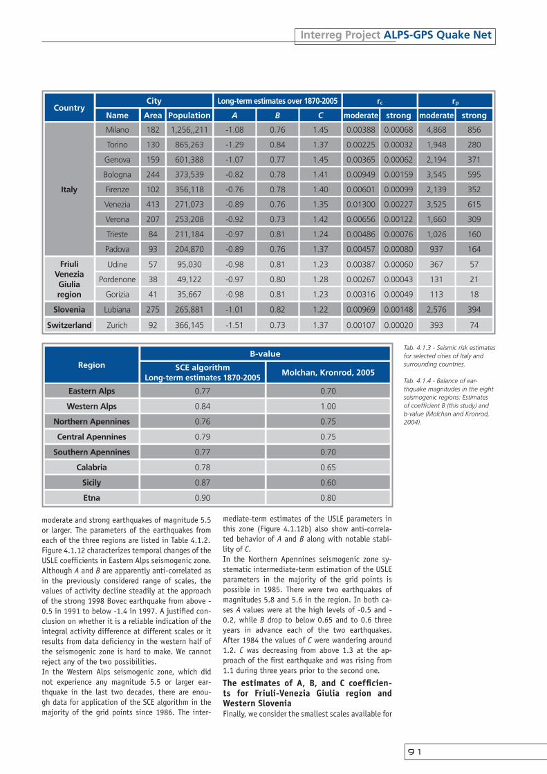
Interreg Project ALPS-GPS Quake Net
�1
Tab. 4.1.3 - Seismic risk estimates for selected cities of Italy and surrounding countries.
Tab. 4.1.4 - Balance of ear-thquake magnitudes in the eight seismogenic regions: Estimates of coefficient B (this study) and b-value (Molchan and Kronrod, 2004).
Area
182
Population
1,256,,211
Long-term estimates over 1870-2005
A B C
-1.08 0.76 1.45
rc
moderate strong
0.00388 0.00068
rp
moderate strong
4,868 856
130 865,263 -1.29 0.84 1.37 0.00225 0.00032 1,948 280
159 601,388 -1.07 0.77 1.45 0.00365 0.00062 2,194 371
244 373,539 -0.82 0.78 1.41 0.00949 0.00159 3,545 595
102 356,118 -0.76 0.78 1.40 0.00601 0.00099 2,139 352
413 271,073 -0.89 0.76 1.35 0.01300 0.00227 3,525 615
207 253,208 -0.92 0.73 1.42 0.00656 0.00122 1,660 309
84 211,184 -0.97 0.81 1.24 0.00486 0.00076 1,026 160
93 204,870 -0.89 0.76 1.37 0.00457 0.00080 937 164
275 265,881 -1.01 0.82 1.22 0.00969 0.00148 2,576 394
Italy
Country
Friuli Venezia Giulia region
Slovenia
Switzerland 92 366,145 -1.51 0.73 1.37 0.00107 0.00020 393 74
57 95,030 -0.98 0.81 1.23 0.00387 0.00060 367 57
38 49,122 -0.97 0.80 1.28 0.00267 0.00043 131 21
City
Name
Milano
Torino
Genova
Bologna
Firenze
Venezia
Verona
Trieste
Padova
Lubiana
Zurich
Udine
Pordenone
Gorizia 41 35,667 -0.98 0.81 1.23 0.00316 0.00049 113 18
moderate and strong earthquakes of magnitude 5.5 or larger. The parameters of the earthquakes from each of the three regions are listed in Table 4.1.2.Figure 4.1.12 characterizes temporal changes of the USLE coefficients in Eastern Alps seismogenic zone. Although A and B are apparently anti-correlated as in the previously considered range of scales, the values of activity decline steadily at the approach of the strong 1998 Bovec earthquake from above -0.5 in 1991 to below -1.4 in 1997. A justified con-clusion on whether it is a reliable indication of the integral activity difference at different scales or it results from data deficiency in the western half of the seismogenic zone is hard to make. We cannot reject any of the two possibilities.In the Western Alps seismogenic zone, which did not experience any magnitude 5.5 or larger ear-thquake in the last two decades, there are enou-gh data for application of the SCE algorithm in the majority of the grid points since 1986. The inter-
mediate-term estimates of the USLE parameters in this zone (Figure 4.1.12b) also show anti-correla-ted behavior of A and B along with notable stabi-lity of C.In the Northern Apennines seismogenic zone sy-stematic intermediate-term estimation of the USLE parameters in the majority of the grid points is possible in 1985. There were two earthquakes of magnitudes 5.8 and 5.6 in the region. In both ca-ses A values were at the high levels of -0.5 and -0.2, while B drop to below 0.65 and to 0.6 three years in advance each of the two earthquakes. After 1984 the values of C were wandering around 1.2. C was decreasing from above 1.3 at the ap-proach of the first earthquake and was rising from 1.1 during three years prior to the second one.
The estimates of A, B, and C coefficien-ts for Friuli-Venezia Giulia region and Western Slovenia Finally, we consider the smallest scales available for
Region
Eastern Alps
B-value
0.70
Molchan, Kronrod, 2005SCE algorithm
Long-term estimates 1870-2005
0.77
Western Alps 1.000.84
Northern Apennines 0.750.76
Central Apennines 0.750.79
Southern Apennines 0.700.77
Calabria 0.650.78
Sicily 0.600.87
Etna 0.800.90

Interreg Project ALPS-GPS Quake Net
�2
the Friuli-Venezia Giulia and Western Slovenia (S3) region in 1977-2005 within the area of about 120 by 200 km, spatial resolution of 1/16°, and magni-tudes down to 2.2. Figures 4.1.13a and 4.1.13b de-monstrate predominance of the characteristic va-lues of A about -1.5 and B about 1.15, each of which appears in 12% of the obtained estimates. These values are localized mainly in the Tolmezzo-Gemona-Bovec area of linear dimension about 40 km where the completeness of the OGS data set ap-pears to be the best as mentioned above in sec-tion 5.3. The values of C here are evidently biased due to the 1998 Bovec sequence. The seismic ac-tivity associated with the 1976 Friuli sequence of earthquakes might be still in effect in 1977 and, therefore, could have affected the estimates in the western areas of the region.In comparison with the long-term estimates given in Figure 4.1.6 the fine scale maps of the USLE pa-rameters plotted in Figure 4.1.13 do not match, confirming a banality that the data sets covering hundreds of years are essential for a reliable ade-quate estimation of seismic hazard and seismic risk. The high quality data of a few recent decades is not enough and its use could be misleading without bringing in historical and/or even paleoseismolo-gical evidence. On the other hand the variability of the USLE parameters computed at different scales appears to be rich enough for an objective descrip-tion of seismic activity and its scaling properties in a given region.
Seismic risk estimates for selected citiesWe have used the long-term estimates of the USLE coefficients determined by using the SCE algorithm to characterize seismic risk for the major Alpine ci-ties (more than 200,000 inhabitants), for selected cities in surrounding countries and for the three principal cities of the Friuli-Venezia-Giulia region. Specifically, we have considered the values of A, B, and C at the grid points inside the 1/4° vicinity of the cities and have calculated the values of rc and rp twice, for “moderate” (magnitude 5.0 or larger) and “strong” (magnitude 6.0 or larger) earthquakes. The results are given in Table 4.1.3 below.It is interesting to compare the obtained estimates of risk with those achieved previously when using the NEIC Global Hypocenters Database, 1964-2002 (Nekrasova, A., V. Kossobokov, 2005). The global estimates for Milan (mega-citie of Italy) are as fol-lows: Milan, A=-0.76, B=1.24, C=1.22. These values imply overestimation of seismic risk (either rc or rp) for moderate earthquakes about magnitude 5.5 in the citie by the factors of 3.4. For strong ear-thquakes about magnitude 6, the risk is slightly overestimated (by factor 1.1). The example shows explicitly the importance of bringing into conside-ration prolonged regional data on earthquakes for accurate and reliable estimates of seismic risks.
4.1.7 Discussion and conclusions Thus, the parameters of USLE for the Alps and sur-roundings were evaluated making use of the diffe-
Fig. 4.1.14 - The USLE B coefficient for S1
scale: (a) 1870-2005; (b) 1870-1976.11.1;
(c) 1870-1980.5.1.
a
b
c

Interreg Project ALPS-GPS Quake Net
�3
rent earthquake data and different ranges of ma-gnitude and scaling dimensions. Of course, this is just the beginning of understanding the complexi-ty of earthquake recurrence and many other com-putations could be suggested for clarification of different aspects of seismic energy release at diffe-rent scales of space, time and energy. Nevertheless some conclusions are already evident from the pre-sent analysis.The results confirm high accuracy of the USLE coef-ficient estimates obtained with the help of the SCE algorithm at different scales from regional to local ones, as well as from long-term to intermediate-term ones. The accuracy along with overall concor-dance of the USLE parameters in the calculations at different spatial, temporal and magnitude sca-les permits a few comparisons with the estimates of the basic parameters of seismic activity in Italy
published earlier. For example, Table 4.1.4 com-pares the values of B coefficient obtained as an overall average computed for the points inside the eight seismogenic regions with the b-value com-puted earlier by Molchan and Kronrod (2004) for the same regions. Except for the Western Alps, B is slightly larger than b. The average difference B and b is about 0.07 with the standard deviation 0.12, which values imply insignificant differences for each of the eight regions but Sicily (at the con-fidence level about 95%). The difference observed for Sicily might be due to the above mentioned instability of the B determinations in the region (6.1, Fig. 4.1.10), which could not be observed in a single determination of b-value (Molchan and Kronrod, 2004).For analyzing the spatial distribution of B coeffi-cient values one may find useful to redraw Figure
a
Fig. 4.1.15 - Intermediate-term variations of the USLE coefficien-ts in the CN regions, (S1 scale, 1870-2005): (a) Northern; (b) Central; (c) Southern.

Interreg Project ALPS-GPS Quake Net
�4
4.1.6-B in a form of Figure 4.1.14, which outli-nes more clearly the areas of the magnitude ba-lance extremes, i.e., Po Valley and Switzerland for low and Western Alps and Tyrrhenian Sea for high values. It should be noted, however, that such a sharp differentiation carry a certain degree of ar-bitrariness and might lead to illusory perception of the anomaly extent in space. Therefore, it should not substitute, but rather supplement the conti-nuous mapping of the USLE coefficients. As shown in 6.1 the USLE parameters are contributing to an arbitrary seismotectonic zonation yet unexplored information on seismic activity at regional and lo-cal scales. The monitoring of the long- and intermediate-term trailing estimates of the A, B, C coefficients may
b
contribute to the analysis aimed at earthquake fo-recast and or prediction. Essentially, the trailing A rescaled to a target magnitude of interest deliver the observed expectation of the rate for such even-ts, which could be used by itself as a forecast tool. On the other hand our analysis of the A, B, C varia-bility suggests a finer candidate for being used as a precursory signature: rise of A to its high values ac-companied with low values of B appears to indica-te at intermediate-term scale of years the approa-ch of strong earthquakes. Figures 4.1.15 and 4.1.16 show a possibility to supplement the on-going test of earthquake prediction algorithms with informa-tion either on the overall average of the observed values of the USLE coefficients inside the CN re-gions of investigation (Figure 4.1.15) and/or with

Interreg Project ALPS-GPS Quake Net
�5
those derived locally, e.g., from a set of neighbors on a regular grid (Figure 4.1.16). As could be jud-ged from the figures the observed variability sug-gests further investigations into the problem of the A, B, C predictive power and efficiency.The analysis of the USLE in Italy and surrounding regions are to be continued in the future.
4.2 Deterministic earthquake hazard assessment in the Alps Franco Vaccari for DST-UNITS
A deterministic procedure (Panza et al., 2001) for seismic hazard assessment has been applied to the
Alpine region. This approach addresses some issues largely neglected in probabilistic hazard analysis, namely how crustal properties affect attenuation: ground motion parameters are not derived from overly simplified attenuation functions, but rather from synthetic time histories.Starting from the available information on the Earth’s structure, seismic sources, and the level of seismicity of the investigated area, it is possible to estimate maximum ground displacement, velo-city, and acceleration or any other parameter re-levant to seismic engineering, which can be ex-tracted from the computed theoretical signals. This procedure allows us to obtain a realistic estima-te of the seismic hazard in those areas for which scarce (or no) historical or instrumental informa-tion is available and to perform the relevant para-
Fig. 4.1.16 - Intermediate-term variations of the USLE coefficien-ts for the set of neighbors on a regular grid, (S2 scale, 1974-2005): (a) A, B, C coefficients; (b) map of point set.

Interreg Project ALPS-GPS Quake Net
�6
metric analyses.Synthetic seismograms can be constructed to mo-del ground motion at sites of interest, using know-ledge of the physical process of earthquake gene-ration and wave propagation in realistic media. The signals are efficiently generated by the mo-
Fig. 4.2.1 - Flow-chart of the de-terministic procedure for seismic
hazard assessment at regional scale. The vertical component is
routinely not used.
Figure 4.2.4. Flowchart of the algorithm adopted to determine
the structural model of the Alpine region (modified from
Farina, 2006).
Fig. 4.2.2 . Regional poly-gons associated with average
structural models. GNDT: model previously defined in the
framework of GNDT activities. ALPS: structural boundaries
defined in the framework of the ALPS-GPSQUAKENET project.
On the left, a sample of the digital data extracted from the
database is shown.

Interreg Project ALPS-GPS Quake Net
�7
Fig. 4.2.3 - An example of structural model obtained after the application of the algorithm shown in Figure 4.2.4. A sample of the digital data extracted from the database is shown.
Fig. 4.2.5 - Discretized seismicity (0.2° x 0.2° cells) obtained from Italian earthquake catalogue CPTI (2004), merged with the Slove-nian catalogue used by Zivcic et al. (2000) and the Croatian catalogue used by Markusic et al. (2000). The yellow polygons show the areas where the Italian (CPTI), Slovenian (S) and Croatian (C) catalogues have been used.
dal summation technique (Panza, 1985; Florsch et al., 1991), so it becomes possible to perform de-tailed parametric analyses at reasonable costs. For instance, different source and structural models can be taken into account to create a wide range of possible scenarios from which to extract essen-tial information for decision making. The flowchart of the deterministic procedure is shown in Figure 4.2.1.
4.2.1 Structural modelsIn first-order zoning, average structural models are defined, representing the lithospheric properties at a regional scale. Synthetic seismograms are com-puted, taking into account the effects of lateral heterogeneities in a rough way: if the source-recei-ver path crosses one or more boundaries between adjacent structural models, the signal is computed assuming the model of the receiver as representa-

Interreg Project ALPS-GPS Quake Net
��
tive of the whole path.In Figure 4.2.2 the regional polygons associated with average structural models are shown. The map marked GNDT (top) shows the boundaries between different structures as they were defined in pre-vious studies carried on mainly in the framework of the Italian GNDT group activities. The map marked ALPS shows the new boundaries corresponding to the structural models defined in the framework of the ALPS-GPSQUAKENET project. On the left, a sam-ple of the digital data extracted from the databa-se, defined during the project activities, is shown. An example of structural model is given in Figure
4.2.3. The physical properties of the models have been obtained according to the scheme shown in Figure 4.2.4.
4.2.2 Seismic sourcesThe first problem to tackle in the definition of sei-smic sources is the handling of seismicity data. Basically, what is needed is an evenly spaced di-stribution of the maximum magnitude over the territory, but the data available from earthquake catalogues are widely scattered. Furthermore, ear-thquake catalogues are both incomplete and af-
Fig. 4.2.6 - Seismogenic zones das defined in ZS9 (Meletti and
Valensise, 2004). On the left, a sample of the digital data
extracted from the database is shown.
Fig. 4.2.7 - Focal mechanisms associated with the seismogenic zones, as defined in ZS9 (Meletti
and Valensise, 2004). On the left, a sample of the digital data
extracted from the database is shown.

Interreg Project ALPS-GPS Quake Net
��
fected by errors, so a smoothed distribution is pre-ferable (Panza et al., 1990). For the Alpine region, three earthquake catalogues have been considered: the Slovenian catalogue used by Zivcic et al. (2000), the Croatian catalogue used by Markusic et al (2000) and the Italian cata-logue CPTI (2004). The image of seismicity obtai-ned after discretization into 0.2° x 0.2° cells is shown in Figure 4.2.5.The punctual distribution of epicenters is discreti-zed into cells and the maximum magnitude of the events pertinent to each cell is retained. In the case where the earthquake catalogue contains different estimates of magnitude (e.g., magnitude computed from body waves, from surface waves, or from ma-croseismic intensity), the maximum between them is considered. In most cases, the smoothing obtai-ned by considering just the discretized cells is not enough. To account for errors in the location of the source and for its extension in space a centered smoothing window (radius = 3 cells) is then consi-dered, so that earthquake magnitudes are analyzed not only in the central cell but also in the neighbo-ring ones. The smoothed image of seismicity is fi-nally intersected with the seismogenic zones and only the cells located within a seismogenic zone are retained and constitute the set of sources used for the generation of the synthetic seismograms. ZS9 seismic zones have been considered (Meletti and Valensise, 2004), shown in Figure 4.2.6. The focal mechanism is equal for all the sources belon-ging to the same seismogenic zone, as defined in ZS9, and are shown in Figure 4.2.7. They compare rather well with the source parameters of the in-
strumental earthquakes studied in the framework of the ALPS-GPSQUAKENET and reported in chapter 3.5. The sources identified with the above mentio-ned algorithm are shown in Figure 4.2.8.
Fig. 4.2.8 - Sources identified in the Alpine region, within the seismogenic zones defined in ZS9 (Meletti and Valensise, 2004) that have been used for the generation of synthetic seismograms. The magnitude is obtained by discretizing and smoothing the seismicity reported in the CPTI (2004) earthquake catalogue.
Fig. 4.2.9 - Map showing the peak displacements obtained from the synthetic seismograms (top) and the period of the peak of the Fourier spectrum (bottom). Structural model ALPS, earthquake catalogue CPTI. A set of synthetic seismograms (80 s duration, peak value 4.1 cm), extracted from the database at a single site and generated by different sources is shown as well (right).

Interreg Project ALPS-GPS Quake Net
100
Fig. 4.2.10 - Same as Figure 4.2.9, considering velocities
(peak value 8 cm/s).
4.2.3 ComputationsOnce the structures and the sources have been de-fined, sites are considered on a grid (0.2° X 0.2°) that covers the whole territory. The synthetic si-gnals are computed for an upper frequency content of 1 Hz, and the scaled point-source approximation (Gusev, 1983) is still acceptable. This is fully ju-stified by practical considerations, as several-story buildings have a peak response in the frequen-cy range below 1 Hz (Manos and Demosthenous,
Fig. 4.2.11 - Same as Figure 4.2.9, considering accelerations
(peak value 25 cm/s2). Clearly the period saturation at 1Hz
indicates that acceleration values are underestimated. This limit is overcome by estimating the De-
sign Ground Acceleration (DGA), as shown in Figure 4.2.12.
Fig. 4.2.12 - Distribution of DGA, obtained as a result of
deterministic zonation extended to high frequencies using the design spectra of EC8 for soil
A. Structural model ALPS, earthquake catalogue CPTI. The increase of values when compa-red with the 1 Hz accelerations
of Figure 4.2.11 (top) is evident.

Interreg Project ALPS-GPS Quake Net
101
1992), and by the fact that modern seismic design approaches and technologies, such as seismic iso-lation, tend to lower the free oscillation frequen-cies of buildings. As a rule of thumb (in Italian le-gislation) the resonance period (in seconds) of a building can be expressed as 0.1H/B0.5, where H is the height and B is the maximum lateral exten-sion, in meters. When shorter periods are conside-red, it is no longer possible to neglect the finite dimensions of the faults and the rupturing process at the source.To reduce the number of computed seismograms, the source-receiver distance is kept below an up-per threshold, which is taken to be a function of the magnitude associated with the source. The ma-ximum source-receiver distance has been set equal to 25, 50, and 90 km, respectively, for M < 6, 6 M < 7 and M 7. All seismograms are computed for a hypocentral depth which is a function of magni-tude (10 km for M < 7, 15 km for M 7). Keeping the hypocentral depth fixed (for classes of magni-tude) and shallow is important due to the large er-rors generally affecting hypocentral depth reported in the earthquake catalogues and due to the fact that strong ground motion is mainly controlled by shallow sources (Vaccari et al., 1990).Synthetic seismograms for P-SV-waves (radial and vertical components) and SH-waves (transver-se component) are originally computed for a sei-smic moment of 10-7 Nm. The amplitudes are then properly scaled according to the smoothed ma-gnitude associated with the cell of the source. For the moment-magnitude relation, the one gi-ven by Kanamori (1977) has been used. The finite-ness of the source is accounted for by scaling the spectrum using the spectral scaling law proposed by Gusev (1983) as reported in Aki (1987). At each site, the horizontal components are first rotated to a reference system common to the whole territory (North-South and East-West directions) and then the vector sum is computed.Among the parameters representative of strong ground motion we have focused our attention on maximum ground acceleration, velocity, and displacement. The Fourier spectra of displacements and veloci-ties show that an upper frequency limit of 1 Hz is sufficient to take into account the dominant part of seismic waves, while this is definitely not true for accelerations (Panza et al., 1999). On the other hand, the required knowledge about seismic sour-ces and lateral heterogeneities, which might ju-stify the choice of a higher frequency limit in the computations, is not available at the scale of the entire Alpine region. The maps of peak displacement, velocity and ac-celeration, and the period associated with the peak in the Fourier spectrum, are shown in Figures 4.2.9, 4.2.10 and 4.2.11 respectively. Wherever long periods in the range between 20 and 30 s do-minate in the displacements, it means that are re-lated to signals generated by strong earthquakes
Fig. 4.2.13 - Map showing the peak velocities obtained for the structural model ALPS (top) and the structural model GNDT (bottom). The map of the dif-ferences is shown on the right, where triangles pointing up indi-cate values bigger for the ALPS model, while triangles pointing down indicate values bigger for the GNDT model.
Fig. 4.2.14 - Map showing the magnitude assigned to the sei-smic sources for the earthquake catalogue CPTI (top) and for the earthquake catalogue UCI (bottom). The map of the differences is shown on the right, where triangles pointing up indicate values bigger for the CPTI catalogue, while triangles pointing down indicate values bigger for the UCI catalogue.

Interreg Project ALPS-GPS Quake Net
102
occurring at large distances from the site (about 90 km), while the magnitude of the closer even-ts, which are responsible for the higher frequencies (between 2 and 5 s in our computations), is not big enough to let these frequencies dominate the ground motion scenario.For accelerations, deterministic results has been extended to frequencies higher than 1 Hz by using the Eurocode 8 design response spectrum for soil A (EC8, 1993), which defines the normalized ela-stic acceleration response spectrum of the ground motion, for 5% critical damping. The procedure to obtain the Design Ground Acceleration (DGA) is de-scribed in detail in Panza et al. (1996).The results of the deterministic procedure are parti-cularly suitable for civil engineers as seismic input for the design of special buildings. In fact, the re-levance of the displacements at periods on the or-der of 10 s or so is a key issue for seismic isolation and in general for lifelines with large linear dimen-sions, such as bridges and pipelines, where diffe-rential motion plays a relevant role in their stabili-ty (Monti et al., 1996).
4.2.4 Parametric tests and conclusionsA couple of parametric tests have been performed to check the stability of the results to variations of the input data. One test has been done on the influence of the structural model properties, adopting the GNDT model instead of the ALPS model, both shown in Figure 4.2.2. Not only the regional polygons differ, but also the properties of the layered models asso-ciated with them. The comparison of the results in terms of peak velocities is shown in Figure 4.2.13.In Figure 4.2.14 two maps with the sources used to generate the synthetic seismograms are shown. The map on the top has been obtained using the CPTI catalogue, and corresponds to the map of Figure 4.2.8. The map on the bottom is the corresponding map of sources that is the result of the discretiza-tion and smoothing of the UCI earthquake cata-logue (Peresan and Panza, 2002). The map of the magnitude difference is shown on the right. The maps of peak velocities obtained for the sources of Figure 4.2.14 are shown in Figure 4.2.15.The results of the parametric tests show how impor-tant the definition of the input data is. Wherever the differences in the ground shacking scenarios are relevant, a better understanding of the struc-tural models, and of the properties of the seismic sources, is desirable. Further investigations and developments in the methodology might be considered for a possible continuation of the project, like an improved de-finition of the seismogenic zones based on the analysis of the GPS data that will be made avai-lable by the network installed during the ALPS-GPSQUAKENET project.Another area where improvements might be achie-ved is in the definition of the structural model. The LSO smoothing algorithm (Farina, 2006) mi-ght be applied to smaller cells, wherever possible, so that the boundaries between the Alps and the surrounding plains could be better respected in the modeling.Finally, the possibility of applying a more realistic scaling of the seismic source for the magnitude should be considered. If the peak values obtained with the deterministic approach compare sati-sfactorily with observations (Panza et al., 2001), the signal duration in the synthetic seismograms may underestimate the duration of the recordings, if the rupturing process at the source is a compli-cated one, like the Irpinia 1980 earthquake (e.g. Vaccari et al., 1990).
Fig. 4.2.15 - Map showing the peak velocities obtained for the earthquake catalogue CPTI (top) and for the earthquake catalo-gue UCI (bottom). The map of the differences is shown on the right, where triangles pointing up indicate values bigger for the run made using the CPTI cata-logue, while triangles pointing down indicate values bigger for the run made using the UCI catalogue.

Interreg Project ALPS-GPS Quake Net
103

Interreg Project ALPS-GPS Quake Net
1045 - PILOT PROJECTS

Interreg Project ALPS-GPS Quake Net
105
5.1 GPS and MeteorologyAndrea Walpersdorf for LGIT
5.1.1 IntroductionPredictability of the atmosphere and particularly of precipitation is of extraordinary societal, eco-nomic, and social significance. Its improvement re-presents a task of provident character for our fu-ture existence. Agriculture and water resources management, air and shipping traffic, road tran-sport and energy economy directly depend on the state of the atmosphere. Damage caused by extre-me precipitation events heavily burdens the bud-gets of industry, national governments and inter-national organizations. People affected by extreme precipitation events often face economic ruin.Susceptibility to extreme events, e.g. strong preci-pitations, hailstorms or storms, will further increase in the industrialized nations due to the increasing accumulation of material assets and the optimiza-tion of economic processes. In Europe, this beca-me obvious in 2002 again during the catastrophic flash flood event in Saxonia, which caused an eco-nomic loss of 10B US$ (Munich Re Group 2002). The devastating hurricane season 2005 demonstra-ted that even the most developed countries such as the US can hardly handle these events.Quantitative forecast of non-extreme precipita-tion events is of comparable value, although the avoidable losses mostly do not appear to be that spectacular. Complemented by estimates of their potential uncertainties, such forecasts are of ine-stimable value as input for hydrological applica-tions or for consulting in agriculture and the con-struction sector. In spite of this strong societal demand for quan-titative precipitation forecasting (QPF), progress during the last two decades has been very slow. While many aspects of numerical weather foreca-sting have made great advances, model skills for precipitation remain much lower than for other atmospheric parameters. Among the reasons ex-plaining QPF failures, the following arguments are usually mentioned: Inaccuracy of the model initial states due to a
bad quality or lack of observations – this is parti-cularly true for moisture which has a strong spa-tial variability Sub-optimal use of the observations or a lack of
assimilated systems suited for the existing but non standard observations Deficiencies in the parameterization of the phy-
sical processes Too coarse resolution of the models and also re-
maining problems in their dynamical coresNowadays, to measure water vapour in the atmo-sphere, meteorological services rely on standard sy-noptic radiosoundings. However, even though such devices provide reasonably accurate measurements of water vapour profiles, they are far too sparsely distributed in space and time to support reliable
forecasting of such rain events. However, Global Positioning System (GPS) data, from stations with well known coordinates, permit to estimate tropo-spheric delays which can be transformed into pre-cipitable water vapour (PWV). Methodological stu-dies of meteorological GPS applications have been carried out since more than 10 years (e.g. Bevis et al., 1992, Businger et al., 1996, Tregoning et al., 1998, Bock and Doerflinger, 2001) and enable us now to infer PWV from GPS observations with the same precision as conventional meteorological measurements, such as radiosondes and microwave radiometers (WVR), to about 1-2 mm PWV. GPS tropospheric delay or PWV estimation has se-veral advantages over traditional meteorologi-cal measurements of water vapour: It can be done at low cost (either by using already existing GPS stations or by installing new GPS stations which are less expensive than other instruments), it is performing under all weather conditions and the method is intrinsically stable. Effectively, GPS PWV measurements are based on the exploitation of propagation delays excluding any instrumental drifts. Nevertheless, modifications of the analy-sis strategy or the change of instruments (recei-ver and/or antenna) can induce instantaneous off-sets in the coordinate time series, an effect which is however reduced on the tropospheric parameter estimates. The GPS performances have been te-sted mainly for mid-latitude networks where they have shown high efficiency. As more and more GPS are being deployed and operated in a continuous mode for geodetic purposes, they offer the poten-tial for a dense and reliable water vapour measu-rement network. Presently, applications in meteo-rological analysis and weather forecast are widely spread in e.g. European, US and Japanese weather services (Gendt et al., 2004, Guerova et al., 2006, Gutman et al., 2004, Nakamura et al., 2004).Examining potential meteorological applications of the permanent GPS stations installed in the fra-mework of ALPS-GPSQUAKENET is part of the Work Package “Pilot Projects” proposed in this study. To illustrate the capacities of our network, we re-call the principles of tropospheric measurements by GPS, show existing applications in comparable networks and present the results of a test period which has been scheduled in November 2006.
5.1.2 Principles of tropospheric measurements by GPSThe GPS signals at radio frequencies (1575 and 1228 MHz) are delayed when travelling throu-gh the Earth’s atmosphere, in a dispersive way by the charged part (the ionosphere) and in a non-dispersive way by the neutral part of the atmo-sphere (the troposphere). While the ionospheric delay can be identified by comparing the different influence on the two wavelengths of the GPS si-gnals, the effect of the troposphere on the two GPS signals is the same and can only be deter-mined by independent measurements or by indi-

Interreg Project ALPS-GPS Quake Net
106
rect methods. The tropospheric delay has a typi-cal value of 2.30 m at zenith, which can vary by several cm in a few hours, mainly due to the ra-pidly varying water vapour along the travel path. This delay must be precisely known to achieve high precision positioning (sub-centimetric). Model pre-dictions or estimations from meteorological ground measurements have shown to be not precise enou-gh to correct efficiently for the tropospheric delay. Therefore, an additional parameter has been intro-duced in the GPS data inversion representing the temporally and spatially varying troposphere, the tropospheric delay. To distinguish the troposphe-ric delay from the geometric distance between sa-tellite and antenna, a simple model is applied to characterize the troposphere: a mapping function describing the increase of the tropospheric delay for decreasing satellite elevations. The troposphe-ric parameter represents the average delay over all available satellites in a defined time interval, at-tributed to the zenith direction: the zenith total delay (ZTD) (Figure 5.1.1). A typical time resolu-tion of ZTD evaluations is 15 min. Permanent GPS stations can therefore provide ZTD evaluations eve-ry 15 min continuously, independently of daytime, season or weather conditions.The primary GPS observable ZTD can be conver-ted into an observation of water vapour via simple ground measurements of pressure and temperatu-re. ZTD is the sum of two components, the Zenith Hydrostatic Delay (ZHD) and the Zenith Wet Delay (ZWD). In fact, ZHD can be determined from ground pressure measurements. Then, ZWD can be isolated by subtracting ZHD from GPS observed ZTD. The ZWD is almost proportional to Precipitable Water
Vapour (PWV). The relation between ZWD and PWV can be approximated by a function of ground tem-perature. Typically, PWV = 0.15 ZWD with ZWD and PWV in mm. The precision which can be reached for the evaluation of ZTD is 6 - 12 mm. This means that PWV estimations by GPS are precise to 1 - 2 mm, reaching the precisions of standard meteoro-logical measurements (radio soundings, water va-pour radiometers). Radio sound and water vapour radiometer measurements are the main sources of water vapour observations over the continents, but they are expensive and therefore sparse in time and space. The persistent lack of water vapour observa-tions for the characterization of the water cycle in the atmosphere could be filled by the exploitation of data from GPS permanent stations.
5.1.3 Applications of GPS tropo-spheric parameter monitoringGPS meteorological applications can be divided in three classes:1 Climatology (long stable time series of PWV/ZTD)2 Meteorological analysis (detailed PWV field for the study of precipitation events, 3D PWV fields from tropospheric tomography)3 Numerical weather prediction (continuous PWV observations in near real time for assimilation in numerical weather prediction models)
For the first two applications, GPS ZTD is provi-ded by the most precise, post processing solution using precise satellite orbits published 2 weeks after the measurement date. The time delay cho-sen for a post processing also generally permits to wait until the data transmission of all stations in-cluded in the network is completed. ZTD observa-tions from the GAIN network obtained in a post processing analysis are shown in Figure 5.1.2. The upper, middle and lower boxes represent the we-stern, central and eastern stations. The domina-ting feature is the annual signal with high ZTD va-lues in summer and low values in winter, related to the amount of tropospheric humidity. Not only the annual trend but also variations over shorter time scales seem to be correlated between sta-tions, which however show a constant offset, due to the different station heights resulting in diffe-rent hydrostatic delays (the higher the station the lower the hydrostatic delay). The zoom on a pe-riod of 15 days presented in Figure 5.1.3 (western, central and eastern stations again in upper, mid-dle and lower box) shows in fact time offsets and differences in amplitude in the time series even between close-by stations. Also complete de-corre-lation can be observed between more distant sta-tions. Most of the variability in ZTD is related to the tropospheric water vapour. The differences and the de-correlation of the time series are due to the limited spatial and temporal scale of the water va-pour distribution.The spatial and temporal resolution of ZTD obser-
Fig. 5.1.1 - Schematic repre-sentation of the Zenith Total
Delay (ZTD), estimated from all simultaneously available satellite
observations.
Fig. 5.1.2 - GAIN ZTD time series (units of the vertical scale are
metres).
Fig. 5.1.3 - GAIN ZTD time series. Zoom on 15 days in
2006 (day of year 165 to 179). The ZTD on the vertical axis is
indicated in metres.

Interreg Project ALPS-GPS Quake Net
107
vations in GPS networks can be used to establish precise instantaneous PWV maps and their tempo-ral evolution. Figure 5.1.4 shows the example of PWV monitored by GPS during the flash-flood event in SE France on 8-9 September 2002 (Champollion et al., 2004)The precise knowledge of the amount and varia-tion of tropospheric water vapour is substantial for the understanding of the water cycle in the atmo-sphere as well as for the prediction of precipita-tions. Important advances could be made in both fields by exploiting the water vapour observations from the still increasing GPS permanent networks. However, the relation between Precipitable Water Vapour and precipitations is not direct. Figure 5.1.5 presents PWV time series for a precipitation event in SE France in 2004. The onset of heavy rain is marked by the arrow and corresponds to the end of a 2 days interval with high PWV. The rain dries out the troposphere as attested by a rapid drop of PWV. This shows that the presence of high PWV does not lead instantaneously to precipitations. Figure 5.1.6 illustrates the spatial offset between regions of high PWV and zones of rain, by compa-ring maps of PWV and rain for the same epoch, the 9th September 2002 at 6 h (during the flash-flood event of 2002). While the zone of high humidity is spread in a V shape from the Mediterranean coast to the first reliefs of the Cevennes mountains, the strongest precipitation cells are seen at the nor-thern extremity of the humidity zone. Accounting for the complex relationship between tropospheric humidity and precipitations, the assi-milation of GPS ZTD or PWV in Numerical Weather Prediction (NWP) is probably the most efficient way of exploiting the tropospheric information of GPS measurements. NWP models can be implemen-ted with the physical rules describing the water cycle in the atmosphere, and in particular with the detailed topography constraining upward motion of the air which can lead to condensation. Also, all necessary information is contained in NWP mo-dels to extract the water vapour observation di-rectly from ZTDs without converting them first into PWV passing by empirical formulations increasing (however slightly) the uncertainties. The technical challenge to provide significant ob-servations from GPS measurements for assimilation is the short life time of water vapour in the tropo-sphere (some hours). The European project COST 716 has studied the GPS capacities for NWP and emits the recommendation to provide GPS ZTD 1 h 45 after the measurement. This implies a data analysis done in “near real time”, through hour-ly data download and by a rapid analysis adapted to the short delay between the acquirement and the analysis of the data. The rapid analysis has to deal with ultra rapid (and therefore less precise) orbit solutions instead of final solutions published 2 weeks after the measurement date. Moreover, a precise ZTD value needs to be constrained by a few hours of data before and after the time tag of the
parameter. However, the near real time ZTD is eva-luated for the most recent (1 hour) observation session (Figure 5.1.7). This means the data after the time tag of the ZTD evaluation are missing. For both reasons (orbits and sessions) the near real time ZTD is less precise than the post processed ZTD, but some methodological developments can help limiting the errors. Our tests have shown that most precise solutions are obtained from an analy-sis calculating every hour a session of 7 hours en-ding with the most recent just downloaded hour of data. ZTDs are estimated every 30 min, so in par-ticular at the beginning, in the middle and at the end of the last hour of data. The middle value cor-responds to the time tag of the hourly data file and is the one representing best the ZTD of this data span. This hourly analysis has to be rapid enough to leave some time (e.g. 20 min) for the stations to upload their data and to be terminated before 1 h 15 after the end of the hourly measurement ses-sion (Figure 5.1.7) so that the results are available for assimilation within 1 h 45 after the time tag of the session.
5.1.4 Near real time test period in the GAIN networkThe hourly data download is an operational chal-lenge and needs stable data transfer lines. The per-formance of the GAIN network to this account has been tested during a near real time test period scheduled in November 2006. To have time enough for the hourly data analysis, a data upload within 20 min after the end of the hourly session has been required. 12 stations from the GAIN network have
Fig. 5.1.4 - From Champollion et al., 2004. 2D PWV fields infer-red from GPS ZTD observations in the French REGAL/RENAG network during the flash-flood event of September 2002.
Fig. 5.1.5 - GPS PWV time series during a precipitation event in SE France in 2004.
Fig. 5.1.6 - Precipitations and rain in SE France during the flash-flood event of 2002. Both maps are established by meteo-rological modelling.
Fig. 5.1.7 - Near real time data analysis strategy.

Interreg Project ALPS-GPS Quake Net
10�
participated in this test period, 8 of them provi-ding more than 90 % of data in due time (Figure 5.1.8). The participation rate and the rate of “suc-cess” shows that operational hourly data download of geodynamic GPS sites (more often on bedrock than on internet) is non trivial. The data of this test period have been analyzed to test the influence of the near real time mode com-pared with a post processing strategy. Figure 5.1.9 shows ZTD differences between a solution with ul-tra rapid orbits and a solution with final IGS orbi-ts. The differences are less than 10 mm (correspon-ding to 1.5 mm PWV). A second test aimed at evaluating the loss of pre-cision due to ZTD evaluation at the end of the ses-sion. Figure 5.1.10 displays ZTD calculated with a post processing strategy shifting 12 h sessions by 4 hours and keeping only the middle 4 hours in the ZTD solution (graph “post processing” in the bottom of Figure 5.1.10). This post processed ZTD is compared to near real time ZTD, evaluated in the last hour of 7 h sessions shifted by 1 hour (graph “near real time processing” in the bottom of Figure 5.1.10). Momentary offsets of up to 20 mm (3 mm PWV) are observed between the two time series which seem to be related to the lack of constrain-ts on the ZTD evaluation at the end of the obser-vation session.In collaboration with Météo France, assimilation tests are done to prepare the use of GPS ZTD in the new French operational weather forecast mo-del (AROME). The influence of the assimilation of a single ZTD observation (GPS site AXPV of the French RGP network) is shown in Figure 5.1.11 (V. Ducrocq, personal communication, 2006). Assimilation of GPS ZTD is already done operatio-
nally in Germany and Switzerland. For the GAIN stations, providing hourly data would be a (relati-vely) simple means to valorise the data by making them available for operational meteorological ap-plications. A dedicated water vapour application is scheduled for summer 2007, where the GAIN GPS stations located in Alsace will be included into the COPS experiment (Convective and Orographically-induced Precipitation Study).
5.2 GPS and LandslidesCarlo Troisi for ARPA-P, Giorgio Zampedri for GST
Landslide monitoring by means of GPS system de-veloped rapidly in the past few years. GPS mea-suring proved to be an effective and reliable tool especially for measuring large and slow-moving landslides; application for small and/or fast moving landslides is not so widespread for, in such cases, other monitoring systems are to be preferred.Each GPS monitoring system consists of a number of benchmarks on the landslides the positions of which is measured vs. the position of some referen-ce benchmarks located off-slide. The ideal num-ber of reference points should be four, geometrical-ly disposed around the slide, but the usual number is two (which is also the minimum) or three. Since locating off-slide reference point is no easy matter, the presence of permanent GPS stations (within 7-10 km from the landslide to me monitored) can gre-atly help.The following paragraphs shortly report the GPS landslide monitoring experience of two partners of the Alps Gps Quakenet project: Arpa Piemonte and Servizio Geologico della Provincia di Trento.
Fig. 5.1.8 - Examples of near real time data upload performances
in the GAIN network.
Fig. 5.1.9 - ZTD estimation with final IGS orbits compared to
ultra rapid orbits.
Fig. 5.1.10 - Comparison between ZTD evaluation in post
processing sessions (triangles, from 12 hour sessions shifted
by 4 hours with only the middle 4 hours kept) and in near real
time sessions (dots, from 7 hour sessions shifted by 1 hour with
only the last hour kept).
Fig. 5.1.11 - Map of specific humidity (kg/kg, see color code) for the 4th of November 2004.
Superposed dark lines delimit zones of increased specific
humidity due to assimilation of one GPS observation (ZTD). Increment between successive
lines is 0.1 g/kg. The maximum increase is located at the GPS
site (AXPV) and is 0.8 g/kg.
Fig. 5.2.1 - Distribution of monitored landslides (red dots)
in Piemonte.

Interreg Project ALPS-GPS Quake Net
10�
5.2.1 GPS for landslide monitoring in PiemonteThe Centro Regionale per le ricerche territoriali e geologiche of Arpa Piemonte (The Regional agency for environmental protection) manages a landslide-monitoring network including about 300 landsli-des (fig. 5.2.1). Most of the monitored landslides threaten built-up areas or important structures. The network includes about 680 inclinometers; 400 piezometers; 120 automated data recording units; conventional tacheometric surveys on monumen-ted benchmarks; GPS systems; extensometers and joint-meters.Large landslides and deep-seated-deformations are very common along the Alps; about 600 of them are mapped in Piemonte. Monitoring this kind of slope movements may be extremely expensive and poses several technical problems such as: conventional tacheometric surveys are often
inapplicable for, given the wide area, monitoring points are not normally intervisible; conventional local monitoring devices, such as
inclinometers, may be representative of a minimum portion of the deformation only.
Given this framework GPS is, up to now, the best technique (and, by far, the cheapest one also) for monitoring very large landslides and deep-seated-deformations. Several benchmarks, scattered over a wide area, may be effectively measured in one workday. Moreover, in areas with many rock ou-tcrops (which is common on large alpine landsli-des and deformations) installation of GPS bench-marks is easy and can be made directly from the surveying Arpa personnel, without need to have re-course to any building enterprises. A GPS monitoring system is presently active on fif-teen landslides in Piemonte. Apart from one site, monitored since 2000, GPS monitoring is active since 2005. Definite displacements, up to 8 cm/yr, were measured in seven cases. Each system consists of a number (three to twenty) of on-sli-de benchmarks and two or three off-slide referen-ce points. GPS data are acquired on the field by personnel of Arpa Piemonte, with double-frequency recei-vers in static mode, acquisition times of 1-1.5 h and 15 s epoch. Data post-processing is made with Leica™ LGO software. The displacement , between the zero-reference survey and each displacement survey, is calculated along for all the baselines
between each reference station and each on-slide benchmark. The measuring network works in “lo-cal” mode, i.e. is not connected to topographic vertex related permanent geodetic networks; only relative positions of points, on and out of the lan-dslide, are evaluated. Overall precision is in sub-centimetric order; resulting displacement vectors, in order to be validated, are to be consistent with slope attitude and with the general conceptual mo-del of the slide.A good example of GPS monitoring is the “Cima
Fig. 5.2.3 - The map shows four large landslides in the area of Ceresole Reale (TO). The landsli-des are monitored by means of GPS benchmarks (blue dots); the AGNE GAIN receiver is used as reference station.
Fig. 5.2.4 - The map shows a large deep-seated-deformation in the area of Baceno (VB). The deformation is monitored by means of GPS benchmarks (blue dots); the DEVE GAIN receiver is used as reference station.
Fig. 5.2.5 - Benchmark bolts for GPS monitoring.
4
N. of gps monitored landslides using the permanent receiver as reference station
2
1
0
7
CODE
AGNE
DEVE
CARZ
OATO
PARO
Permanent receiver
Ceresole Reale Agnel
Baceno Alpe Devero
Trarego Viggiona Carza
Torino Osservatorio
Paroldo
Fig. 5.2.2 - Map of the Cima Brenvetto Landslide. Displace-ment vectors on GPS bench-marks (red arrows) are shown; blue figures (mm) refers to the 2004-2006 period.

Interreg Project ALPS-GPS Quake Net
110
Brenvetto Landslide” (Valprato Soana, Provincia di Torino) which is a large deep-seated-deformation extending for about 1 km2 from Cima Brenvetto to the Soana stream (fig. 5.2.2).The crown is clearly defined by prominent upward-facing slopes a feature which, in the alpine area, is typical of deep-seated-deformations. Toe erosion by the stream often triggers large debris slides.
GPS techniques are the best way to monitor such a landslide, for steep slope angles and terrain rou-ghness makes a hard field for conventional instru-ments. On the other hand, it was easy and cheap to install a monitoring GPS network consisting of eight benchmarks: three off-slide grouted-in-pla-ce reference monuments and five on-landslide ben-chmarks, simply bolted in place in hand-drill-made holes on large boulders or exposed rock. An Arpa field team measures the benchmarks once a year. Results of the measurements shows displacements between 3 and 8 cm/yr; displacement vectors are consistent with slope attitude.One critical feature of GPS monitoring systems is the position and the characteristics of reference off-slide benchmarks; having permanent ones stron-gly helps so that, as part of the WP6 of the ALPS Quakenet project, Arpa Piemonte identified seve-ral landslides in the range of 7 km about from the five permanent receivers installed for the project, which can thus be used as reference stations (see table). A benchmark for a second non-permanent reference station was also installed for each lan-dslide. Several GPS benchmarks were installed on each landslide and zero-reference measurements were made on all of the landslides. Displacement measurements will start in 2007; the foreseen fre-quency is 1 or 2 measurements per year.Figure 5.2.3 and 5.2.4 show large GPS monitored landslides close to the Ceresole Reale and Baceno receivers respectively. Figure 5.2.5 shows the benchmarks bolts custom-made for GPS landslide monitoring. They can easi-ly bolted in place on hard rocks or boulders (fig. 5.2.6) in hand-drill-made holes (fig. 5.2.7) or placed on a monument (fig. 5.2.8). Around the Paroldo GAIN permanent receiver there are several large permanent, soft-rock translational landslides.
Fig. 5.2.6 - A benchmark bolted in place.
Fig. 5.2.7 - On rock outcrops the benchmarks can be easily
and cheaply installed by simple hand-drilling.

Interreg Project ALPS-GPS Quake Net
111
The slides are currently monitored by means of se-veral inclinometers. Since, on these sites, it’s both unadvisable and technically difficult to install per-manent monuments, we devised and made a simple device in order to use the inclinometers wellheads as reference benchmarks (fig. 5.2.9).
5.2.2 GPS for landslide monito-ring in the Province of TrentoThe Geological Survey of Provincia Autonoma di Trento manages a landslide-monitoring network in-cluding about 15 landslides. The network includes about 174 inclinometers; 125 piezometers; 10 au-tomated data recording units; conventional topo-graphic benchmarks; GPS systems, extensometers and joint-meters. Remote data acquisition sy-stems, optical systems and GPS are also used to monitor landslides’ dynamics.Use of GPS for landslide monitoring proved to be extremely useful when used in association with
Fig. 5.2.8 - GPS receiver on monumented benchmark.
Fig. 5.2.9 - Brass device (right) made in order to use the incli-nometers wellheads as reference benchmarks. The lower, large diameter, part exactly enters the pipe of a conventional alumi-nium inclinometer casing (diam. 76 mm, shown on the left), thus providing a stable and reliable stand for a GPS receiver.
Fig. 5.2.10 - Campodenno landslide; GPS network and displacement vectors.

Interreg Project ALPS-GPS Quake Net
112
other monitoring techniques. This integrated ap-proach allowed optimal use of the advantages offe-red by GPS, such as measure repeatability, com-parability and use of long baselines (> 1.5 km) . Some of the results from GPS monitored landslides in Trentino are hereinafter described.
Campodenno landslideThe landslide develops in Campodenno, Val di Non, at an elevation of about 550 m a.m.s.l.; it’s about 350 m wide and about 300 m long along a gen-tly dipping slope. Most of the landslide surface is built-up. At the moment about 15 buildings are severely fissured (three of which evacuated by mayors’ ordinance); minor fissuring affects other 25 buildings about. The landslide was classified as “area a rischio idrogeologico elevato” (eleva-ted landslide risk area) by force of a national law (D.P.C.M. 29/9/998). The landslide affects a thick cover deposit consisting of glacial clays and over-lying detritic coarse carbonatic debris 2 to 20 m
thick. The sliding surface is located around the top of the glacial deposits, at an average depth of 8 m, and the movement is mainly translational. Recorded surface displacements are about 1-2 cm/yr . The landslide is monitored by means of three inclino-meters, six piezometers, three GPS benchmarks and about sixty levelling benchmarks. In recent times the GPS system was partly replaced by a conven-tional topographic survey system; this was made in order to increase the monitoring points, which are now about 35. Fig. 5.2.10 shows the GPS network and the related displacement vectors.
Peio landslideThe landslide develops around the Peio village, and affects a steep slope below the built-up area. The elements at risk are the Peio village itself, a cam-ping site and some houses on the valley bottom. The landslide was classified as “area a rischio idro-geologico elevato” (elevated landslide risk area) by force of a national law (D.P.C.M. 29/9/998). The active landslide occupies about 500000 m2 , maximum depth of the sliding surface is about 45 m . Landslide materials are mainly heterogeneous loose glacial deposits, mainly consisting of limy sands with decimetric to metric size clasts.The slope is constantly monitored by means of 10 inclinometers, 4 piezometers, a conventional topo-graphic survey network, a GPS network (fig. 5.2.11; fig. 5.2.12) and 3 automated extensometers. Recorded displacements are in the order of 10-15
Fig. 5.2.11 - Peio landslide; GPS network and displacement
vectors.
Fig. 5.2.12 - Peio landslide; pla-nimetric displacements of GPS
benchmarks.

Interreg Project ALPS-GPS Quake Net
113
cm/yr, with clear acceleration in rainy periods. The GPS recorded displacements are strongly consistent both with the results from the others monitoring techniques and with the general conceptual land-slide model.
Prezzo landslideThe landslide develops along the slope of Mt. Melino and affects: the whole village of Prezzo (Val Giudicarie), whe-
re several buildings are damaged; the provincial road S.P. n. 122 and some local
roads.The landslide could also dam the underling Chiese torrent; damming could cause an overflow which could threaten an industrial area and the Pieve di Bono village.The landslide was classified as “area a rischio idro-geologico elevato” (elevated landslide risk area) by force of a national law (D.P.C.M. 29/9/998). The landslide is about 340 m wide and about 1200 m long; the thickness varies between 50 and 80 m, the average being around 68-70 m .It’s an old reactivated landslide, mainly consisting of clayey deposits with fragments, blocks and len-ticular rock bodies consisting of marly limestones and dolomites (Wengen Formation).The landslide is monitored by means of inclinome-ters, GPS benchmarks, conventional topographic benchmarks and piezometers. Recorded displace-ments are in the order of 3-6 cm/yr . Foreseen re-medial works include a deep drainage tunnel, at the base of the slope, whit branching micro-drains.GPS recorded displacements (fig. 5.2.13; fig. 5.2.14) perfectly dovetail with the results from the other monitoring systems and allow a proper defi-nition of landslide dynamics and extension.
5.3 GPS and active faultsLGIT, EOST
One particular application of permanent GPS mea-surements for geodynamics is the monitoring of active faults. In the complex Alpine tectonics, the observation of low magnitude earthquakes by dedicated seismological networks like Sismalp (Thouvenot, 2002) helps a lot to identify which of the numerous faults in the mountain belt could be presently active. In the French Alps and their fo-reland, three fault zones with characteristic sei-smicity are instrumented by permanent GPS, the Durance fault, the Belledonne fault and a zone of more diffuse seismicity in the Briançon region (Figure 5.3.1). The GAIN network established in this project contributes with 3 GPS stations to the monitoring of the Belledonne fault and the Briançon zone.The oldest GPS monitoring site is set up on the Durance fault, to complement a dense seismolo-gical network and seismotectonic studies initia-ted by IRSN (Institut de Radioprotection et Sureté Nucléaire, Fontenay-aux-Roses) (Figure 5.3.2). The two GPS stations GINA and MICH have been instal-
Fig. 5.2.13 - Prezzo landslide; GPS network and displacement vectors.
Fig. 5.2.14 - Prezzo landslide; planimetric displacements of the GPS benchmarks.

Interreg Project ALPS-GPS Quake Net
114
led in 1998, as some of the first stations of the REGAL/RENAG network (http://renag.unice.fr).The results of the permanent GPS measurements across the Durance fault are shown in Figure 5.3.3, in form of time series of the components of the GINA-MICH baseline. Note the jump in the horizon-tal components at the end of each year, probably due to hydrological phenomena, while the vertical component shows an increase of noise each sum-mer, probably due to higher water vapour content of the atmosphere. These features contribute to the noise of the positioning and increase the observa-tion duration needed to obtain significant velocity measurements across the Durance fault. A numeri-cal test of the degree of convergence of the baseli-ne rate has been performed and is shown on the ri-ght graph in Figure 3. The relative velocity between the two GPS sites has been calculated over increa-sing observation lengths, from 1 year to 5.5 years after the start of the measurements, 4 times per year. The graphs show dispersion of the velocity results during the first 4 years of data, and a final convergence in the 5th year to a value of 0.2 mm/yr of shortening on the north component, while the eastern velocity component is insignificant. The N-S shortening corresponds to transpressive left-late-ral strike-slip motion across the Durance fault and is compatible with the tectonic observations of the Durance fault. The first active fault which has been instrumented with GPS permanent stations by the LGIT Grenoble is the Belledonne fault, a dextral strike-slip fault producing about one earthquake of magnitude 2-4 per year (Figure 5.3.4). Two GPS stations have been installed on each side of the fault, STEY on the Chartreuse mountain belt (in May 2003) and CHAM on the Belledonne massif (in December 2003). A third station installed in the Vercors mountain belt completes the monitoring of slow deformation around Grenoble since December 2004. This third station LFAZ is part of the GAIN network. Today, 3 years of data are available on the baseline between STEY and CHAM, crossing the Belledonne fault. The time evolution of the baseline compo-nents of this 17 km baseline is shown in Figure 5.3.5. As for the Durance fault monitoring, a con-vergence test has been done, estimating the base-line rates after one year of data and then every 3 months up to the end of 2006 (vertical lines in the left graph of Figure 5.3.5). The right graph shows the variations of the inferred velocities and the fi-nal values after 3 years in red. These baseline rates (-0.20 mm/yr on the north component, 0.74 mm/yr on the east component and 0.73 mm/yr on the up component) are calculated considering the disper-sion of the time series as white noise. Another cal-culation has been done to infer linear station velo-cities using a noise model of coloured noise, which is supposed to better take into account the corre-lated noise in the positioning time series (green numbers in the right graph). Both results indica-te a fault velocity below 1 mm/yr but still differ
Fig. 5.3.1 - Seismicity in the western Alps registered by the
Sismalp network. The green fra-mes indicate the location of the
3 active fault zones monitored by permanent GPS.
Fig. 5.3.2 - Location of the GINA and MICH permanent GPS sta-
tions (red triangles) to each side of the Durance left lateral strike-slip fault (red line). Seismological stations are indicated by yellow
and blue squares.
Fig. 5.3.3 - The left graph shows the de-trended time series of baseline components of the
GINA-MICH baseline of 28 km length, from mid 1998 to end
of 2003. The north, east and up components are in the upper
3 boxes and the total baseline length in the lower box. The
average baseline rates are indicated for each component
on the top of the corresponding box. The right graph represents
the convergence test of the velocity estimates based on
increasing amounts of data. The final values are the average
rates of the complete time series shown in the left graph.
Fig. 5.3.4 - The 3 GPS sites around Grenoble on the three mountain belts bordering the
town. The alignment of seismi-city along the Belledonne massif indicates the present day activity
of this fault.

Interreg Project ALPS-GPS Quake Net
115
on the sub-millimeter level. Figure 5.3.6 compa-res the convergence tests done for the Belledonne fault with the Durance fault monitoring. After a three years time span (the available observation span on the Belledonne fault), the Durance fault velocities were still at about 1 mm/yr from their fi-nal values on the horizontal baseline components, and at 3 mm/yr on the vertical component. One or two years of additional observations will be neces-sary on the Belledonne fault to obtain significant displacement rates at the level of a tenth of a mil-limetre per year. In the framework of the ALPS-GPSQUAKENET pro-gram, LGIT had the opportunity to instrument the Briançon zone where an alignment of extensive seismic activity is localized (Figure 5.3.7, from Sue et al., 2000). These extensional earthquake mecha-nisms are coherent with the prevailing deforma-tion pattern in the western Alps, the E-W exten-sion localized in the centre of the mountain belt. The comparison of GPS measurements in 1996 with classical triangulation observations yielded a first velocity field, indicating an E-W extension of about 10 mm/yr with uncertainties of the same order of magnitude (Sue et al., 2000). Two permanent GPS stations (PUYA, JANU, right graph in Figure 5.3.7) installed in 2005 on each side of the seismically active belt could quantify precisely in a few years which part of the global Alpine extension is localized in the Briançon ex-tensive zone. Moreover, the local temporary GPS network of 30 sites measured first in 1996 has been reoccupied in July 2006 (right graph in Figure 5.3.7). For this new measurement campaign, the classical geodetic bold markers have been doubled by new screw markers, increasing the measurement precision by forced antenna centring. This implied the measurement of local ties between the old and the new marker to establish the link to the 1996 measurements. A first analysis of the 2006 data re-veals repeatabilities (a measure of positioning pre-cision) of 2-3 mm on the horizontal baseline com-
ponents between the stations. Supposing the local ties have a precision of 3 mm and the 1996 cam-paign has a precision of 6 mm, we obtain a for-mal uncertainty for the velocity estimates infer-red from the 1996 and the 2006 campaigns of 1.2 mm/yr. This is probably a conservative value whi-ch implies that displacements of the order of 1 mm/yr (the maximum displacement rate expected in the Briançon zone) will be at the limit of reso-lution. However, after 5 years of measurement, the two permanent GPS stations will quantify the lo-cal velocity field with a resolution of probably bet-ter than 0.2 mm/yr, and a second measurement campaign on the screw markers at that time (in 2011) will hopefully provide some significant in-formation about the local distribution of the de-formation field.
5.4 Active tectonics and PaleoseismologyJerome van der Woerd for EOST
5.4.1 IntroductionThe region of high relief in western Europe are
Fig. 5.3.5 - Left graph: De-tren-ded time series and average rates of the baseline components of the 17 km STEY-CHAM baseline across the Belledonne fault. Ri-ght graph: Results of the velocity convergence test and compari-son with velocities established by a coloured noise model.
Fig. 5.3.6 - Comparison of the velocity convergences on the Bel-ledonne fault (left graph) and the Durance fault (right graph). The vertical line in the Durance plot indicates the presently available observation span of 3 years on the Belledonne fault.
Fig. 5.3.7 - From Sue et al., 2000. Left graph: Fault traces and earthquake focal mechani-sms in the Briançon zone. Right graph: Temporary (red triangles) and permanent (blue triangles) GPS networks. The velocity vectors have been established by comparing triangulation and GPS measurements and have maxi-mum amplitudes of 10 mm/yr (Sue et al.).

Interreg Project ALPS-GPS Quake Net
116
Figure 5.4.1 : seismicity across western Europe (after Nocquet
et al., 2003).
Figure 5.4.2 : Main structural units in western Europe after
Ziegler and Dezes (2005).
Figure 5.4.3 : same as figure 5.4.2 with blocks represented in different colours and faults
at their boundaries (convergent boundaries or reverse faults in
blue, strike-slip faults in red, divergent or normal faults in
green, purple when combined strike-slip and normal) (modified
from Ziegler and Dezes, 2005).
clearly areas that accommodate most of the strain due to the collision between Africa and Europe. These ranges are mainly the Alps, the Pyrenees, and the Apennines. However, the regions that sur-round these ranges, while far less deformed and with less relief, are also characterized by a cer-tain level of seismicity that reflect slow strain ra-tes (Figure 5.4.1). These regions are in part the Tertiary grabens that follow the south western
Alpine arc and continue through the Upper and Lower Rhine Graben to the North Sea. Other regions include reactivated structures from the Paleozoic orogenies (Figure 5.4.1). The intracontinental regions or large collision zo-nes like western Europe, which is the place whe-re Africa collides with Eurasia, do accommodate slow rates of strain over large areas. At the longi-tude range of the Alps, the collision zone extends from the High Atlas in Morocco and Maghrebides in Algeria to the North Sea in The Netherlands and Germany, over a zone of 2000-2500 km. Plate tectonics model (Demets et al., 1994) as well as recent geodetic models from GPS (Nocquet et al., 2003) confirm that Africa and Eurasia collide at a rate of several mm/yr. How and where this conver-gence is accommodated remains the main issues in the description and understanding of the strain field in Europe. It is important to note that these questions are debated also for the India-Asia col-lision zone, which is, nevertheless, characterized by higher rates of deformation (Tapponnier et al., 2001; England and Molnar, 2005). In Europe, the tectonic strain rates may equal or be slower than other processes, like post-glacial isostatic rebound (in the Pyrenees, Alps and northern Europe)(Beck et al., 1996; Sue et al., 2000) or mantel upwel-ling (in the Eifel massif)(Walker et al., 2005), for example. The main geological structures that characteri-ze the present geomorphology and landscapes of Europe, as well as the reactivated structures during the Tertiary may be used to distinguish regions that deform more than others (Figure 5.4.2). Seismicity and focal mechanisms can also be used to discuss coherent pattern of strain within slow deforming regions. In Figure 5.4.3 we suggest a large sca-le frame with blocks that may be more rigid and with strain mostly occurring on their boundaries. For such models, where the block sizes are almost as large as the block boundaries, the definition of region with coherent strain is rather subjective. However, we think that this kind of first order ap-proach allows proposing a pattern of deformation that can be tested against other models. To test this model GPS data can be compared to the modelled strain field of the blocks. For exam-ple, a four block model (Tesauro et al., 2003) with a simplified block geometry indicates that coherent strain is accommodated within the blocks and may explain the abrupt changes in GPS vectors direction close to their boundaries (Figure 5.4.4). To better understand the deformation across we-stern Europe it is therefore important to combi-ne different methods that link local observations of deformation to the regional movement of blocks across the collision zone. For this purpose, the per-manent monitoring of strain with GPS stations is a step towards documenting the strain field across wide areas. In the Rhine Graben area (Figure5.4.5), north of the Alps and the Jura fold belt, the natu-re and amount of strain accommodated is still de-

Interreg Project ALPS-GPS Quake Net
117
bated. In particular, the recent instrumental sei-smicity may not reflect the long-term strain of the region. The historical earthquakes enhances the knowledge of zones exposed to seismic risk but co-vers still a short period compared to the characte-ristic time periods of geological processes (Figure 5.4.6). To further enlarge our knowledge of past ear-thquakes and strain accommodation, the geolo-gical study of past events or paleoseismology is necessary (Meghraoui et al., 2001; Sébrier et al., 1997; Peters et al., 2005, 2007). However, this method is limited to the largest earthquakes as most of the seismic events do not have primary surface breaks, but only secondary indirect conse-quences of ground shaking that may cause certain damages to man-made constructions or geological strata (Beck et al., 1996).
5.4.2 Example of active fault monitoring In the southern Upper Rhine Graben : the Basel earthquake of 1356The historical earthquake of 1356 occurred in the region of Basel (Figure 5.4.6). Despite historical records of damages and several recent investiga-tions the possible source of this large earthquake of magnitude over six remains controversial (Meyer et al., 1994; Meghraoui et al., 2001; Nivière et al., 2002; Ferry et al., 2005; Lambert et al., 2005). It is located at the intersection of two main struc-tures, namely, the north-northeast trending Upper Rhine Graben, and the east-west trending Jura fold belt (Figure 5.4.7). Trenching south of the city of Basel have lead to propose that the fault responsible of the 1356 earthquake is a north-south trending normal fault (Meghraoui et al., 2001; Ferry et al., 2005). Radiocarbon and thermoluminescence dating of successively buried colluvial wedges have been in-terpreted as the traces of the recurrence time for Mw 6.5 earthquakes every 2500 years. The avera-ge rate of displacement is on the order of 0.1-0.3 mm/yr.Historical records of damages caused by the 1356 events to the castle of the region are numerous but sometimes ambiguous. Recent re-interpreta-tions of the historical records have lead to a new evaluation of the damaged area and therefore to the possible source of the earthquake (Lambert et al., 2005) (Figure 5.4.8). The macroseismic data suggests an east-west elongated seismic source (Meyer et al., 1994; Lambert et al., 1997) under the folded Jura front.
In the northern Upper Rhine Graben : uplifted Rhine terracesThe northern Upper Rhine Graben is characterized to the west by a set of normal faults that separate it from the Mainz basin. These western border faul-ts are at present sub-parallel to the main strike of the Rhine River and recent as well as past Rhine
river beds have partially or completely remodeled the geomorphic expression of the faults. Depicting possible displacements caused by these faults have been possible by careful mapping of the terrace treads and by local paleoseismological trenching (Peters et al., 2005, 2007). The terraces treads can be followed over large di-
Figure 5.4.4 : A simplified four block model is consistent with GPS vectors from the blocks (after Tesauro et al., 2003).
Figure 5.4.5 : instrumental (yellow) and historical (red) ear-thquake in the Upper and Lower Rhine Graben north of the Alps. Black lines are mostly normal faults bouding the Upper and Lower Rhine Graben (after Ferry et al., 2005).
Figure 5.4.6 : Historical earthquakes across the alpine domain with intensity I0 7. Source : Sirène, ECOS and Grün-thal (2003).

Interreg Project ALPS-GPS Quake Net
11�
stances and clearly show that the normal faults were active during the Quaternary. The several tens of meters of displacement in the Quaternary allow to put bounds on the slip-rates of these faults on the order of 0.01-0.1 mm/yr. While terraces can be indicators of recent fault activity and can be used to quantify the amounts of displacements, elsewhe-re, the absence of terraces does not mean absence
Fig. 5.4.7 - main structural units of the Rhine Graben (after Peters et al., 2007). Red square is Basel
area.
Fig. 5.4.8 - Trench wall interpre-tation across the western border
of the Birs valley south of Basel proposed as the locus of the
Basel-Reinach Fault responsible of the 1356 Basel earthquake
(Ferry et al., 2005; Meghraoui et al., 2001).
Fig. 5.4.9 - re-evaluation of the damaged zone due to the 1356
event in the Basel area (after Lambert et al., 2005).
Fig. 5.4.10 - The northern Upper Rhine Graben is characterized by sup-parallel mostly normal faults. These fault cut and offset aban-
doned terrace levels of the Rhine. To the right, example of trench wall interpretations dug across
one of these normal fault reveals repeated normal displacements.
Fig. 5.4.11 - Terrace levels across the different faults of the western border of the northern
Upper Rhine Graben south of Mainz. Clearly, the terraces have been displaced relatively by the
fault activities.
of tectonic activity. In particular, the eastern side of the Upper Rhine Graben, which is geomorpholo-gically one of the most spectacular stretch along the Rhine Graben follows one of the deepest trou-gh of Quaternary sediments in the graben. Both the geomorphic expression of the Rhine Graben shoul-der and the depth of the sediments are indicator of long-term tectonic activity that most probably oc-curs along the East Border Fault. Quantifying the amount and rate of displacements in this area re-veals to be difficult in the absence of clear geomor-phological markers.
The Remua fault near Chamonix In 1905 two earthquakes have struck the re-gion around the Mont-Blanc massif in France and Switzerland (Figure 5.4.12). As of today, the pos-sible sources of these earthquakes are unknown (Alasset, 2005; Cara et al., 2006; van der Woerd et al., 2006). A combined approach of seismological modeling and geological investigation has lead to suggest different potential scenarios for these ear-thquakes. Recent magnitude 5 earthquakes in the area indicate a consistent pattern of deformation characterized by left-lateral movements along NW trending faults, right-lateral movements along NE trending faults and thrusting along NNE trending folds. Synthetic modeling of some of the rare re-cords of the 1905 events are not constrained enou-gh to decide the type of faulting involved in the events. In addition to the possible mechanisms expressed by the recent seismicity, a prominent fault scarp of the Remua fault has been explored (Figure 5.4.13). This several tens of meters high scarp is very steep and exhibits in its central part recently exhumed rocks. Weather this exhumation is due to tectonic displacements or local slope instability is deba-ted. If tectonic, then this fault is a left-lateral nor-theast-trending normal faults as attested by stria-tions on the fault scarp. To constrain the timing of possible displacement we have conducted cosmo-genic Be10 dating of rock outcrops on both side of the scarp. The dating of glacially polished quartz veins indicate that this part of the valley was free of ice around 17 ka, shortly after the Last Glacial Maximum (Coutterand and Nicoud, 2005). If the 5m of exhumed bedrock at the base of the scarp are of tectonic origin, then the ages provide an upper bound of tectonic movement and allow to determi-ne a rate of 0.3 mm/yr.
5.4.3 Future workOther regions like the transition zone between the Alps and the Dinarides show clear evidence of active faulting. The Cividale and Idria faults are right-la-teral strike-slip faults that accommodate northward displacement of the Adriatic towards the Alps. Both faults were the site of large historical earthquakes that may have produced surface breaks. Remote sensing techniques and high accuracy di-gital elevation models obtained from radar mea-surements (SRTM or LiDAR) help in the identifica-

Interreg Project ALPS-GPS Quake Net
11�
tion of fault scarps. The analysis of topography and high accuracy images have then to be combined with geological field work to constrain the timing of movements and the possible size of events. Among the techniques used in the active fault cha-racterization, continuous GPS measurements allow to determine both the type and rate of displace-ments in active tectonic regions. The network in-stalled during the Alps-GPSQuakenet project in the Rhine Graben area will allow to better under-stand the type of deformation occurring in this re-gion and precise the locations of the most acti-ve faults.
Fig. 5.4.12 - regional seismo-tectonic map of the northwe-stern Alps. Intensity map of the 1905 events are indicated as well as the recent focal mechanisms of magnitude 5 events.
Fig. 5.4.13 - View to northwest in the Chamonix-Mont Blanc valley towards the Aiguilles Rouges massif. Below the upper level reached by the glaciers during the Last Glacial Maximum, a clear linear and steep cliff marks the trace of the Remua fault (after Alasset, 2005).
Fig. 5.4.14 - Active fault map of western Slovenia. Idria and Cividale faults are clean cuts through the landscape indicating recent activity.
Fig. 5.4.16 - Map of permanent GPS stations installed by the ALPS-GPSQuakenet project in the upper Rhine Graben to monitor present strain across the Vosges and Black Forest massifs.
Fig. 5.4.15 - Remote sensing images allow to map active fault traces. A) active fault traces revealed by high precision digital elevation model in Buttrio along the Cividale Fault. B) Active fault traces mapping by high precision radar topography (LiDAR) reveals as a useful tools in forested area of western Slovenia along the Idria fault (Cunningham et al., 2006).

Interreg Project ALPS-GPS Quake Net
120
Partners list
LEAD PARTNERAcronym Institution People involved
UNITSUniversità degli Studi di Trieste - Dipartimento di Scienze del-la Terra
Karim Aoudia Riccardo RivaFranco VaccariNastia NekrasovaMariangela GuidarelliGiuliano Panza
PROJECT PARTNERSAcronym Institution People involved
ARPA-P Agenzia Regionale Per la Protezione Ambientale del Piemonte
Carlo TroisiErnesto BenazzoMichele MorelliGiacomo Re Fiorentin
ARPA-V Agenzia Regionale Per la Protezione Ambientale del Veneto
Alberto LuchettaRodolfo BassanAntonio CavinatoMirco Pollet
BEKBayerische Akademie der Wissenschaften / Bayerische Kommis-sion für die Internationale Erdmessung
Christof Völksen
DGFI Deutsches Geodaetisches Forschungs Institut Hermann Drewes
EARS Environmental Agency of the Republic of Slovenia Mladen Zivcic
EOST-IPGSEcole et Observatoire des Sciences de la Terre, Institut de Physi-que du Globe de Strasbourg, UMR CNRS/ULP 7516, 5, Rue De-scartes 67084 Strasbourg Cédex, France.
Jérôme van der WoerdGilbert FerhatMatthieu FerryMustapha MeghraouiJean-Paul BoyFrédéric MassonPascal GégoutJacques HindererPatrice UlrichPhilippe Kah
FondMS Fondazione Montagna Sicura
Fabrizio DiotriClaudio LucianazJean Pierre FossonIris Voyat
GSBGeological Survey of the Autonomous Province of Bolzano - South Tyrol
Claudio Carraro
GST Servizio Geologico Provincia Autonoma di Trento
Giorgio ZampedriSaverio Cocco Francesca De FranceschFulvia DemattèMauro DegasperiOscar GroazGiovanni MerlerFranco Rippa

Interreg Project ALPS-GPS Quake Net
121
LGITUniversité Joseph Fourier, Laboratoire de Géophysique Interne et Tectonophysique, UMR 5559 du CNRS
Andrea WalpersdorfNathalie Cotte
RLBRegione Lombardia, Direzione Territorio Urbanistica, Sistema In-formativo Territoriale
Stefania CrottaRoberto LaffiAndrea Piccin
RLGRegione Liguria – Direzione Centrale Affari Organizativi – Servi-zio Sistemi Informatici
Pier Giorgio GerbinoLucia PasettiEnrica De Micheri
SUB-CONTRACTORSAcronym Institution People involved
GALILEIAN Galileian plus srlAngelo AmodioMassimiliano ChersichAndrea Francia
UNIGEDipartimento di Macchine, Sistemi energetici e Trasporti (DIM-SET) Facolta’ di Ingegneria - Universita’ degli Studi di Genova
Bianca FedericiDomenico Sguerso
POLIMIDipartimento di Ingegneria Idraulica, Ambientale, Infrastruttu-re Viarie, Rilevamento (DIIAR) - sezione Rilevamento Politecnico di Milano
Riccardo BarzaghiAlessandra BorghiLetizia Cannizzaro
POLITODipartimento di Ingegneria del Territorio, dell’Ambiente e del-le Geotecnologie Politecnico di Torino - II Facolta’ di Ingegneria - sede di Vercelli
Ambrogio ManzinoManuele PesentiMarco Roggero
UNIMIDipartimento di Scienze della Terra “Ardito Desio” Universita’ degli Studi di Milano
Valentina BarlettaRoberto Sabadini
IREALPIREALP (Istituto di Ricerca per l’Ecologia e l’Economia Applicate alle Aree Alpine)
Paolo BelluominiLuca GrimaldiMarco ScurattiMichela Fioroni
LGCALGCA (Laboratoire de Geodynamique des Chaines Alpines), Chambery
Francois Jouanne

122
Interreg Project ALPS-GPS Quake Net
Bibliography Aki, K, 1987, Strong motion seismology, in M. Erdik and M. Toksöz (eds) Strong
ground motion seismology, NATO ASI Series, Series C: Mathematical and Physical Sciences, D. Reidel Publishing Company, Dordrecht, Vol. 204, pp. 3-39.
Anderson, H. and J. Jackson, Active tectonics in the Adriatic region, Geophys. J. R. astr. Soc., 91, 937-983, 1987.
Aoudia A., Saraó A., Bukchin B., and Suhadolc P., 2000. The 1976 Friuli (NE Italy) Thrust Faulting Earthquake: A Reappraisal 23 Years Later, Geophys. Res. Lett., 27 (4), 573-576.
Aoudia, A., Saraò, A., Bukchin. B., and Suhadolc, P., 2000. The 1976 Friuli (NE Italy) thrust faulting earthquake: a reappraisal 23 years later. Geophys. Res. Lett., 27(4): 577-580.
Atmanspacher, H., & H. Scheingraber, W. Voges, 1988. Global scaling properties of a chaotic attractor reconstructed from experimental data, Phys. Rev. A., 37(4), 1314-1322.
Bajc J., Aoudia A., Saraó A., and Suhadolc P., 2001. The 1998 Bovec-Krn mountain (Slovenia) earthquake sequence, Geophys. Res. Lett., 28 (9), 1839-1842.
Bajc, J., Aoudia, A., Saraò, A., and Suhadolc, P., 2001. The 1998 Bovec-Krn moun-tain (Slovenia) earthquake sequence. Geophys. Res. Lett., 28: 1839-1842.
Bak, P., K. Christensen, L. Danon, & T. Scanlon, 2002. Unified Scaling Law for Ear-thquakes. Phys. Rev. Lett. 88: 178501-178504.
Barletta V. R. and R. Sabadini, (2006), Investigating superswells and sea level changes caused by superplumes via normal mode relaxation theory, J. Geophys. Res, 111, B04404, doi:10.1029/2005JB003926
Barzaghi R., Borghi A., Crespi M., Pietrantonio G., Riguzzi F. (2004). GPS permanent network solution: the impact of temporal correlations, Proceedings of the IV Hotine-Marussi Symposium on Mathematical Geodesy, Matera, Italy, 17-21 June 2002, F. San-sò editor, pp 179-183, Springer-Verlag, 2004.
Beauval, C., and O. Scotti, Mapping b-values in France using two different magni-tude ranges: possible non power-law model ? Geophys. Res. Lett., 30 (17), 1892, doi:10.1029/2003GL017576, 2003.
Beutler G., Bock H., Dach R., Fridez P., Gäde A., Hugentobler U., Jäggi A., Meindl M., Mervart L., Prange L., Schaer S., Springer T., Urschl C., Walser P., Bernese GPS Sof-tware Version 5.0 (2007), Astronomical Institute, University of Bern.
Bevis, M., S. Businger, T.A. Herring, C. Rocken, R.A. Anthes and R.H. Ware, GPS Me-teorology: Remote Sensing of Atmospheric Water Vapor Using the Global Positioning System, J. Geophys. Res., 97, 15,787-15,801, 1992.
Biancotti A. and M. Motta, (2001), L’evoluzione recente ed attuale dei ghiacciai ita-liani, Bollettino geofisico 3-4 , 27 – 36;
Bock, O., and E. Doerflinger, Atmospheric modeling in GPS data analysis for high ac-curacy positioning, Phys. Chem. Earth, Vol. 26, Iss. 6-8, 373-383, 2001.
Boehm J., Heinkelmann R. and Schuh H., Short Note: A global model of pressure and temperature for geodetic applications, Journal of Geodesy, DOI 10.1007/s00190-007-0135-3 (2007)
Boehm J., Niell A., Tregoning P., Schuh H., Global Mapping Function (GMF): A new empirical mapping function based on data from numerical weather model data, Geophysical Research Letters, Vol. 33, L07304, doi:10.1029/2005GL025546, 2006.
Boschi, E., Ferrari, G., Gasperini, P., Guidoboni, E., Smiriglio, G. ans Valensise, G., 1995, Catalogo dei Forti Terremoti in Italis dal 461 a C. al 1980. Istituto Nazionale di Geogisica SGA storia geofisica ambiente.
Burov, E., Podladchkov, Y., Grandjean, G. and Burg, J.P., (1999), Thermo-mechani-cal approach to validation of deep crustal and lithospheric structures inferred from multidisciplinary data: application to the Western and Northern Alps, Terra Nova 11 (2-3) , 124-131.doi: 10.1046/j.1365-3121.1999.00236.x
Businger, S., S.R. Chiswell, M. Bevis, J. Duan, R.A. Anthes, C. Rocken, R.H. Ware, M. Exner, T. VanHove and F. Solheim, The Promise of GPS in Atmospheric Monitoring, Bull. Amer. Meteor. Soc., Vol. 77, No. 1, 5-18, 1996.
C. Vigny, J. Chéry, T. Duquesnoy, F. Jouanne, J. Ammann, M. Anzidei, J.-P. Avouac, F. Barlier, R. Bayer, P. Briole, E. Calais, F. Cotton, F. Duquenne, K. L. Feigl, G. Ferhat, M. Flouzat, J.-F. Gamond, A. Geiger, A. Harmel, M. Kasser, M. Laplanche, M. Le Pape, J. Martinod, G. Ménard, B. Meyer, J.-C. Ruegg, J.-M. Scheubel, O. Scotti, and G. Vidal, GPS network monitors the Western Alps’ deformation over a five-year period: 1993-1998, J. Geodesy, 76, no. 2, 63-76, 2002.
Calais, E., J.-M. Nocquet, F. Jouanne, and M. Tardy, Current strain regime in the We-stern Alps from continuous Global Positioning Sytem measurements, 1996-2001, Geo-logy, 30-7, 651-654, 2002.
Campus, P., Cespuglio G., and Panza, G.F., 1993. Full moment tensor retrieval and fluid dynamics in volcanic areas: the case of Phlegraean Fields (south Italy). Atti del-l’Accademia dei Lincei of the International Conference Large Explosive Eruptions (The problem of eruptions, forecasting and warning; limits and possibilities), pp. 81-101, Accademia dei Lincei, Rome.
Campus, P., Suhadolc, P., Panza, G.F., and Šílený, J., 1996. Complete moment ten-sor retrieval for weak events: application to orogenic and volcanic areas. In Sei-smic source parameters; from microearthquakes to large events. Tectonophysics, 261: 147-163.
Cespuglio, G., Campus, P. and Šílený, J., 1996. Seismic moment tensor resolution by waveform inversion of a few local noisy records. II. Application to Phlegraean Fields (southern Italy) volcanic tremors. Geophys. J. Int., 126: 620-634.
Chimera, G., Aoudia, A., Saraò, A., and Panza, G.F., 2003. Active tectonics in Cen-tral Italy: constraints from surface wave tomography and source moment tensor in-version. Phys. Earth Planet. Int., 138: 241-262.
Christensen, K., L. Danon, T. Scanlon, & P. Bak, 2002. Unified Scaling Law for Ear-thquakes. Proc. National Acad. Sci. 99, suppl. 1: 2509-2513.Comuni d’Italia, 2005, Istituto Enciclopedico Italiano, http//www.comuniditalia.biz/dati.
CPTI, 2004. Catalogo Parametrico dei Terremoti Italiani, versione 2004 (CPTI04), INGV, Bologna.
Dalla Via, G., R. Sabadini, G. De Natale and F. Pingue, (2005), Lithospheric rheology in southern Italy inferred from postseismic viscoelastic relaxation following the 1980 Irpinia earthquake, J. Geophys. Res. , 110 , B06311, doi:10.1029/2004JB003539
Delacou, B., C. Sue, J.-D. Champagnac and M. Burkhard, Present-day geodynamics in the bend of the western and central Alps as constrained by earthquake analysis, Geophys. J. Int., 158, 753-774, 2004.
Du, Z.J., Michelini, A., and Panza, G.F., 1998. EurID: a regionalized 3-D seismolo-gical model of Europe. Phys. Earth Planet. Int., 105. 31-62.
Dziewonski, A.M., and D.L. Anderson, (1981), Preliminary reference Earth model, Phys. Earth Planet Inter. , 25 , 297-356, doi: 10.1016/0031-9201(81)90046-7.EC 8, 1993. Eurocode 8 structures in seismic regions - design - part 1 general and bui-lding, Doc TC250/SC8/N57A.
Farina, B., 2006, Lithosphere-asthenosphere system in Italy and surrounding areas: optimized non-linear inversion of surface-wave dispersion curves and modelling of gravity Bouguer anomalies. PhD thesis, Università degli studi di Trieste.
Fitzko F., Suhadolc P., Aoudia A., Panza G.F., 2005. Constraints on the location and mechanism of the 1511 Western-Slovenia earthquake from active tectonics and mo-deling of macroseismic data, Tectonophysics, 404, 77-90.
Florsch, N., Fäh, D., Suhadolc, P. and Panza, G. F., 1991. Complete synthetic sei-smograms for high-frequency multimode SH-waves, PAGEOPH, 136, 529-560.
Florsch, N., Fäh, D., Suhadolc, P., and Panza, G.F., 1991. Complete synthetic sei-smograms for high-frequency multimode SH-waves. Pageoph, 136: 529-560.
Gendt, G., G. Dick, C. Reigber, M. Tomassini, Y. Liu and M. Ramatschi, Near Real Time GPS Water Vapour Monitoring for Numerical Weather Prediction in Germany, J. Meteorol. Soc. Japan, Vol. 82, No. 1b, 361-370, 2004.
GNDT, Gruppo Nazionale per la Difesa dai terremoti, 1992, GL Seismotettonica (zone sismogenetiche), Modello seismotettonico del terremoto italino, versione aggiorna-ta al Maggio 1992.
Guerova, G., J.-M. Bettems, E. Brockmann and C. Matzler, Assimilation of COST 716 Near-real Time GPS data in the nonhydrostatic limited area model used at MeteoSwiss, Meteorology and Atmospheric Physics, Vol. 91 Nr. 1-4, 149-164, 2006.
Guidarelli, M., 2004. Models of lithosphere and seismic sources in the Scotia sea re-gion. Ph.D. Thesis, University of Trieste, Trieste, Italy.
Guidarelli, M., and Panza, G.F., 2006a. Determination of the seismic moment ten-sor for local events in the South Shetland Islands and Bransfield Strait. Geophys. J. Int., 167, 684-692.
Guidarelli, M., Russi, M., Plasencia Linares, M.P., and Panza, G.F., 2003. The An-tarctic Seismographic Argentinean-Italian Network and the progress in the study of structural properties and stress conditions in the Scotia Sea region. Terra Antartica Reports, 9: 25-34.
Guidarelli, M., Saraò, A, and Panza, G.F., 2000. Analysis of seismicity by seismic moment tensor: the Phlegraean Fields (Southern Italy) case. Internal Report IC/IR/2000/5, The Abdus Salam International Centre for Theoretical Physics, 69 pp.
Guidarelli, M., Saraò, A., and Panza, G.F., 2002. Surface wave tomography and sei-smic source studies at Campi Flegrei (Italy). Phys. Earth Planet. Int., 134: 157-173.
Guidarelli, M., Zille, A., Saraò, A., Natale, M., Nunziata, C., and Panza, G.F., 2006b. Shear-wave velocity models and seismic sources in Campanian volcanic areas: Vesu-vio and Campi Flegrei. VESUVIUS: Education, Security and Prosperity. Editor Flavio Dobran, Elsevier, Amsterdam.
Gusev, A. A., 1983, Descriptive statistical model of earthquake source radiation and its application to an estimation of short period strong motion, Geophys. J. R. Astron. Soc. 74, 787-800.
Gutman, S. I., S. R. Sahm, S. G. Benjamin, B. E. Schwarz, K. L. Holub, J. Q., Stewart, and T. L. Smith, Rapid Retrieval and Assimilation of Ground Based GPS Precipitable Water Observations at the NOAA Forecast Systems Laboratory: Impact on Weather Fo-recasts, J. Meteorol. Soc. Japan, Vol. 82, No. 1b, 351-360, 2004.
Haeberli W., R. FraunFelder, M. Hoelzle and M. Maish, (1999), Rates and accelera-tion trend of global mass changes, Geografiska Annaler 810 , 585-591.
Haeberli, W. and M. Beniston (1998), Climate change and its impacts on glaciers and permafrost in the Alps, AMBIO 27 (4): 258-265
Herring T.A., King R.W., McClusky S.C., Introduction to GAMIT/GLOBK Release 10.3, Department of Earth, Atmospheric and Planetary Sciences, Massachussetts Institute of Technology, 28 September 2006

123
Interreg Project ALPS-GPS Quake Net
Hugentobler U., Dach R., Fridez P., 2004. Bernese GPS Software, Version 5.0, Uni-versity of Bern, Draft.
Hugentobler U., Shaer S., Springer T., Beutler G., Bock H., Dach R., Ineichen D., Mervart L., Rothacher M., Wild U., Wiget A., Brockmann E., Weber G., Habrich H., Bou-cher C., 2000. CODE IGS Analysis Center Technical Report 2000.
IPCC, 2001: Climate Change 2001: Synthesis Report, A Contribution of Working Groups I, II, and III to the Third Assessment Report of the Integovernmental Panel on Climate Change [Watson, R.T. and the Core Writing Team (eds.)]. Cambridge Universi-ty Press, Cambridge, United Kingdom, and New York, NY, USA, 398 pp.
IUGG (CCS)-UNEP-UNESCO, (2005), Fluctuations of Glaciers 1995-2000, World Gla-cier
Ivins E.R. and T.S. James, (2004), Bedrock response to Llanquihue Holocene and present-day glaciation in southernmost South America, Geophys. Res. Lett. , 31 , L24613, doi:10.1029/2004GL021500.
J.-M. Nocquet and E. Calais, Crustal velocity field of western Europe from permanent GPS array solutions, 1996-2001, Geophysical Journal International, 154 (1), 72–88, doi:10.1046/j.1365-246X.2003.01935.x, 2003.
Kääb, A., F. Paul, M. Maisch, M. Hoelzle, and W. Haeberli (2002), The new remo-te-sensing-derived Swiss glacier inventory: II. First results, Ann. Glaciol. , 34 , 362– 366.
Kanamori, H., 1977. The energy release in great earthquakes, J. Geophys. Res. 82, 2981-2987.
Kanamori, H., 1977. The energy release in great earthquakes. J. Geophys. Res., 82: 2981-2987.
Keilis-Borok, V.I., V.G. Kossobokov & S.A. Mazhkenov, 1989. On similarity of spa-tial distribution of seismic activity. In: Theory and algorithms of interpretation of geophysical data, Moscow: Nauka, p. 28-40. (Computational Seismology 22, in Rus-sian).
Kossobokov V.G. & Mazhkenov S.A., 1988. Spatial characteristics of similarity for earthquake sequences: Fractality of seismicity. Lecture Notes of the Workshop on Glo-bal Geophysical Informatics with Applications to Research in Earthquake Prediction and Reduction of Seismic Risk (15 Nov.-16 Dec., 1988), ICTP, Trieste, 15 p.
Kossobokov, V., & A. Nekrasova, Generalized Gutenberg-Richter recurrence law. Geophysical Research Abstracts, 5, 2003. Abstracts of the Contributions of the EGS-AGU-EGU Joint Assembly, Nice, France, 06-11 April, 2003 (CD-ROM): EAE03-A-06597.
Kossobokov, V.G., & A.K. Nekrasova, 2004. Unified scaling law for earthquakes: glo-bal map of parameters. In: Analysis of geodynamical and seismic processes. Moscow: Geos, p. 160-175 (Computational Seismology 35, in Russian).
Kossobokov, V.G., V.I. Keilis-Borok, D.L. Turcotte, and B.D. Malamud, 2000. Impli-cations of a statistical physics approach for earthquake hazard assessment and fore-casting. Pure Appl. Geophys., 157: 2323-2349
Kravanja, S., Batini, F., Fiordelisi, A., and Panza, G.F., 2000. Full moment tensor retrieval from waveform inversion in the Larderello geothermal area. Pure and Appl. Geophys., 157: 1379-1392.
Kravanja, S., Panza, G.F., and Šílený, J., 1999. Robust retrieval of seismic point source time function. Geophys. J. Int., 136: 385-394.
Le Meur, E., and R.C.A Hindmarsh (2000), A comparison of tow spectral approaches for computing the Earth response to surface loads, Geophys. J. Int. , 141 , 282-298, doi:10.1046/j.1365-246x.2000.00068.x.
Letellier T., Etude des ondes de marée sur les plateux continentaux. Thèse doctora-le, Université de Toulouse III, Ecole Doctorale des Sciences de l’Univers, de l’Environ-nement et de l’Espace, 237pp, 2004.
Mandelbrot, B.B., 1982. The Fractal Geometry of Nature. Freeman, New York, 488 p.
Manos, G.C. and Demosthenous, M., 1992. Design of R.C. structures according to the Greek Seismic Code Provisions. Bull. of IISEE, 26, 559-578.
Markusic, S., Suhadolc, P., Herak, M. and Vaccari, F., 2000. A contribution to sei-smic hazard assessment in Croatia from deterministic modelling, PAGEOPH., 157, 185-204.
Meletti, C. and Valensise, G., 2004. Zonazione sismogenetica ZS9 – App.2 al Rap-porto Conclusivo. In: Gruppo di Lavoro MPS (2004). Redazione della mappa di peri-colosità sismica prevista dall’Ordinanza PCM 3274 del 20 marzo 2003. Rapporto Con-clusivo per il Dipartimento della Protezione Civile, INGV, Milano-Roma, aprile 2004, 65 pp. + 5 enclosures.
Ménard, G., Structure et cinématique d’une chaîne de collision: les Alpes occi-dentales et centrales, Thèse de doctorat d’état, Université Joseph Fourier, Greno-ble, 1988.
Molchan, G.; Kronrod, 2004, Frequency–magnitude relation for Italy. SAND group internal report, ICTP, Trieste. Italy.
Molchan, G.; Kronrod, T.L.; Panza, G.F. 1996 Hazard oriented multiscale seismicity model: Italy. International Centre for Theoretical Physics. Internal report IC/96/23, ICTP, Trieste, Italy.
Monitoring Service, Zurich, http://www.geo.unizh.ch/wgms/
Monti, G., Nuti, C. and Pinto, P. E., 1996. Non-linear response of bridges under mul-ti-support excitation, J. of Structural Engineering, ASCE, 122, 10.
Nakamura, H., K. Koizumi, and N. Mannoji, Data assimilation of GPS precipitable water vapor into the JMA mesoscale numerical weather prediction model and its im-pact on rainfall forecasts, J. Meteorol. Soc. Japan, Vol. 82, No. 1b, 441-452, 2004.
Nekrasova, A., V. Kossobokov, 2002. Generalizing the Gutenberg-Richter scaling law. EOS Trans. AGU, 83 (47), Fall Meet. Suppl., Abstract NG62B-0958.
Nekrasova, A., V. Kossobokov, 2003. Generalized Gutenberg-Richter recurrence law: Global map of parameters. Geophysical Research Abstracts, 5, 2003. Abstracts of the Contributions of the EGS-AGU-EGU Joint Assembly, Nice, France, 06-11 April, 2003 (CD-ROM): EAE03-A-03801.
Nekrasova, A., V. Kossobokov, Unified Scaling Law for Earthquakes: Mega-cities and urban agglomerations, Eos Trans. AGU, 86(52), Fall Meet. Suppl., Abstract S23A-0229, 2005.
Panza G.F., Romanelli F. and Vaccari F., 2001. Seismic wave propagation in lateral-ly heterogeneus anelastic media: theory and applications to seismic zonation. Advan-ces in Geophysics, Academic Press, 43, 1-95.
Panza, G.F., 1985. Synthetic seismograms: the Rayleigh waves modal summation, J. Geophys., 58, 125-145.
Panza, G.F., 1985. Synthetic Seismograms: the Rayleigh Waves Modal Summation. J. of Geophys., 58: 125-145.
Panza, G.F., and Saraò, A., 2000. Monitoring volcanic and geothermal areas by full seismic moment tensor inversion: are non-double-couple components always arte-facts of modelling? Geophys. J. Int., 143: 353-364.
Panza, G.F., Peccerillo, A., Aoudia, A., and Farina, B., 2006. Geophysical and petro-logical modelling of the structure and composition of the crust and upper mantle: the case of the Tyrrhenian Sea and surroundings. Earth Science Review, in press.
Panza, G.F., Prozorov, A. and Suhadolc, P., 1990. Is there a correlation between li-thosphere structure and statistical properties of seismicity? In: R. Cassinis and G. F.
Panza (Editors), The structure of the Alpine - Mediterranean area: contribution of geophysical methods. Terra nova, 2, 585-595.
Panza, G.F., Romanelli F., and Vaccari, F., 2000, Seismic wave propagation in la-terally heterogeneous anelastic media: theory and applications to seismic zonation. Adv. Geophys., 43: 1-95.
Panza, G.F., Vaccari, F. and Cazzaro, R., 1999. Deterministic seismic hazard assess-ment. In F. Wenzel et al. (Eds), Vrancea Earthquakes: Tectonics, Hazard and Risk Mi-tigation, 269-286. Kluwer Academic Publishers, The Netherlands.
Panza, G.F., Vaccari, F., Costa, G., Suhadolc, P. and Fäh, D., 1996. Seismic input mo-delling for zoning and microzoning, Earthquake Spectra 12, 529-566.
Paul F., A. Kääb, M. Maisch, T. Kellenberger and W. Haeberli, (2002), The new re-mote-sensingderived Swiss glacier Inventory:I.Methods, Annals of Glaciology , 34 , 355-361
Paul F., A. Kääb, M. Maisch, T. Kellenberger, and W. Haeberli, (2004), Rapid disin-tegration of Alpine glaciers observed with satellite data, Geophys. Res. Lett. , 31 , L21402, doi:10.1029/2004GL020816.
Peresan, A. and Panza, G.F., 2002. UCI2001: The updated catalogue of Italy, ICTP, Trieste, Italy, Internal report, IC/IR/2002/3.
Peresan, A., Costa, G., Vaccari, F., 1997. CCI1996: the current catalog of Italy, In-ternal report IC/IR/97/9. International Centre for Theoretical Physics, Trieste, Italy.
Peresan, A., Panza, G.F., 2002. UCI2001: The updated catalogue of Italy, Internal report IC/IR/2002/3, ICTP, Trieste, Italy.
Peresan, A., V. Kossobokov, L. Romashkova & G.F. Panza, 2005. Intermediate-term middle range earthquake predictions in Italy: a review. Earth-Science Reviews 69, (1-2), 97-132.
Pondrelli, S., Ekström, G., and Morelli, A., 2001. Seismotectonic re-evaluation of the 1976 Friuli, Italy, seismic sequence. Journal of Seismology, 5: 73-83.
Pontevivo, A., and Panza, G.F., 2006. The lithosphere-asthenosphere system in the Calabrian Arc and surrounding seas – Southern Italy. Pageoph, in press.
Postpischl, D. (1985), Catalogo dei terremoti italiani dall’anno 1000 al 1980. C.N.R.-Progetto Finalizzato Geodinamica.
Radulian, M., Ardeleanu, L., Campus, P., Šílený, J., and Panza, G.F., 1996. Waveform inversion of weak Vrancea (Romania) earthquakes. Stud. Geoph. Geod., 40: 367-380.
Raykova, R., Chimera, G., Farina, B., and Panza, G.F., 2004. S-wave velocity structu-re of the lithosphere-asthenosphere system in Mediterranean region, 32nd Int. Cong., Abs. Vol., Pt. 2, abs 208-5, 970 pp.
Reynaud L., M. Vallon, S. Martin, and A. Letreguilly, (1984), Spaziotemporal distri-bution of the glacial mass balance in the Alpine, Scandinavian and Tien Shan areas, Geografiska Annaler 66A , 3 , pp. 239-47.
Romashkova L., 2006, Analysis of the Friuli-Venezia Giulia regional earthquake da-tabase, SAND group internal report, ICTP, Trieste, Italy.
Saraò, A., Panza, G.F., Privitera, E., and Cocina, O., 2001. Non double couple mechanisms in the seismicity preceding 1991-1993 Etna volcano eruption. Geophys. J. Int., 145: 319-335.
Schlatter A., U. Marti and D. Schneider, (1999), The new national height system (LHN95) of Switzerland, EUCOR-URGENT , Annual Reports 1999, Subproject 1.1 , http://comp1.geol.unibas.ch/report99/reportindex.htm

124
Interreg Project ALPS-GPS Quake Net
Schlunegger F., J. Melzer and G.E. Tucker, (2001b), Climate, exposed source-rock lithologies, crustal uplift and surface erosion: a theoretical analysis calibrated with data from the Alps/North Alpine Foreland Basin system, Int J Earth Sci , 90 484–499, doi:10.1007/s005310100174
Schlunegger, F. and H. Matthias (2001a), Crustal uplift in the Alps: why the drainage pattern matters, Terra Nova 13 (6) , 425-432. doi: 10.1046/j.1365-3121.2001.00374.x
Sébrier, M., A. Ghafiri, and J.L. Blès, Paleoseismicity in France : fault trench studies in a region of moderate seismicity, J. Geodyn., 24, 207-217, 1997.
Selvaggi G. et al., La “Rete Integrata Nazionale GPS” (RING) dell’INGV:
Šílený, J., 1998. Earthquake source parameters and their confidence regions by a genetic algorithm with a “memory”. Geophys. J. Int., 134: 228-242.
Šílený, J., Campus, P., and Panza, G.F., 1996. Seismic moment tensor resolution by waveform inversion of a few local noisy records-I. Synthetic tests. Geophys. J. Int., 126: 605-619.
Šílený, J., Panza, G.F., and Campus, P., 1992. Waveform inversion for point source moment tensor retrieval with optimization of hypocentral depth and structural mo-del. Geophys. J. Int., 109: 259 274.
Sue, C., Martinod, J., Tricart, P., Thouvenot, F., Gamond, J.-F., Fréchet, J., Mari-nier, D., Glot, J.-P. & Grasso, J.-R. 2000. Active deformation in the inner western Alps inferred from comparison between 1972-classical and 1996-GPS geodetic sur-veys, Tectonophysics 320, 17-29.
Sue, C., Thouvenot, F., Frechet, J. & Tricart, P., Widespread extension in the core of the western Alps revealed by earthquake analysis, J. Geophys. Res., 104 (B11), 25 611-25 622, 1999.
Tapponnier, P., Evolution tectonique du système alpin en Méditerranée: poinçonne-ment et écrasement rigide-plastique, Bull. Soc. Géol. Fr., 7, 437-460, 1977.
Thouvenot, F., La surveillance sismique du Sud-Est de la France. Risques Infos 13, 5-7, 2002.
Tregoning, P., R. Boers, D. O’Brien and M. Hendy, Accuracy of Absolute Precipita-ble Water Vapor Estimates from GPS Observations, J. Geophys. Res., 103, 28,701-28,710, 1998.
Turcotte, D. L., 1997. Fractals and Chaos in Geology and Geophysics, 2nd edition, Cambridge University Press, Cambridge
Turcotte, D. L., 1999. Seismicity and self-organized criticality. Phys. Earth Planet. Int., 111: 275–294.
una infrastruttura aperta per la ricerca scientifica. Atti 10a Conferenza Nazionale ASITA, 2006, 1749-1754
Vaccari, F., Suhadolc, P. and Panza, G.F., 1990. Irpinia, Italy, 1980 earthquake: wa-veform modelling of strong motion data, Geophys. J. Int. 101, 631-647.
Vialon, P., P. Rochette et G. Ménard, Indentation and rotation in the Alpine arc, in Alpine Tectonics, Geological Society of London Special Publication 45, pp. 329-339, eds. M. Coward, D. Dietrich and R. Park, 1989.
Vuan A., Russi, M., Costa, G., and Panza, G.F., 2001. Moment tensor waveform in-version in the sub-Antarctic Scotia Sea region: feasibility tests and preliminary resul-ts. Terra Antartica, 8(2): 55-62.
Walpersdorf, A., S. Baize, P. Tregoning, E. Calais and J.-M. Nocquet, Deformation in the Jura Mountains (France): First Results from Semi-Permanent GPS Measurements, Earth Planet. Sci. Lett., Vol. 245, 365-372, 2006.
Wikipedia, 2006, Wikipedia, L’enciclopedia libera. http://it.wikipedia.org/.
Zivcic, M., Suhadolc, P. and Vaccari, F., 2000. Seismic zoning of Slovenia based on deterministic hazard computations, PAGEOPH, 157, 171-184.
ZS9 working group (2004). Redazione della mappa di pericolosità sismica prevista dall’Ordinanza PCM del 20 marzo 2003. Rapporto conclusivo per il Dipartimento della Protezione Civile, INGV, Milano-Roma, aprile 2004, appendice 2.
Zuliani D., Battaglia M., Murray M.H., Michelini A., Burgmann R., Marson I., FRED-Net:A continuous GPS geodetic network monitoring crustal deformation in NE Italy. AGU Fall Meeting, poster presentation, 2002