Epic Reconstructions: Homeric Palaces & Mycenaean Architecture (2007)
Upload
khangminh22Category
view
1download
0
Evaluation and application of GPS and altimetry data
over central Dronning Maud Land, Antarctica: annual
elevation change, a digital elevation model, and surface
flow velocity
Dissertation
zur Erlangung des Grades Dr. rer. nat
vorgelegt dem Fachbereich Geowissenschaften
der Universitat Bremen
von
Christine Wesche
Alfred-Wegener-Institut fur Polar- und Meeresforschung
Bremerhaven
August 26, 2008


Gutachter
Prof. Dr. H. Miller
Prof. Dr. K. Huhn
Prufer
Prof. Dr. T. Morz
Prof. Dr. T. von Dobeneck
Promotionskolloquium
am 16. Januar 2009


Name:............................................ Datum:................................................
Anschrift:....................................................................................................
Erklarung
Hiermit versichere ich, dass ich
1. die Arbeit ohne unerlaubte fremde Hilfe angefertigt habe,
2. keine anderen als die von mir angegebenen Quellen und Hilfsmittel benutzt habe
und
3. die den benutzten Werken wortlich oder inhaltlich entnommenen Stellen als solche
kenntlich gemacht habe.
, den
(Unterschrift)


Wussten sie schon,
dass der Gipfel der Zugspitzeam oberen Ende des Berges abgebracht ist?
Loriot


Contents
Contents i
List of Figures iii
List of Tables v
Kurzfassung viii
Abstract x
1. Introduction 1
1.1. Antarctica and area of investigation . . . . . . . . . . . . . . . . . . . . . . . . . . . . . . . 1
1.2. Existing elevation models . . . . . . . . . . . . . . . . . . . . . . . . . . . . . . . . . . . . 3
1.2.1. JLB97 . . . . . . . . . . . . . . . . . . . . . . . . . . . . . . . . . . . . . . . . . . . 4
1.2.2. RAMP . . . . . . . . . . . . . . . . . . . . . . . . . . . . . . . . . . . . . . . . . . . 5
1.3. Motivation . . . . . . . . . . . . . . . . . . . . . . . . . . . . . . . . . . . . . . . . . . . . . 6
2. Scope of papers 9
3. Data and Methods 11
3.1. Global Positioning System (GPS) . . . . . . . . . . . . . . . . . . . . . . . . . . . . . . . . 11
3.1.1. Positioning with GPS . . . . . . . . . . . . . . . . . . . . . . . . . . . . . . . . . . . 11
3.1.2. GPS errors . . . . . . . . . . . . . . . . . . . . . . . . . . . . . . . . . . . . . . . . 12
3.1.3. Differential GPS processing . . . . . . . . . . . . . . . . . . . . . . . . . . . . . . . 13
3.2. Airborne altimetry . . . . . . . . . . . . . . . . . . . . . . . . . . . . . . . . . . . . . . . . 16
3.2.1. Radar altimetry . . . . . . . . . . . . . . . . . . . . . . . . . . . . . . . . . . . . . . 17
3.2.2. Radio echo sounding . . . . . . . . . . . . . . . . . . . . . . . . . . . . . . . . . . 19
3.3. Ice, Cloud and land Elevation Satellite (ICESat) . . . . . . . . . . . . . . . . . . . . . . . . 20
4. Applications of the Data 25
4.1. Annual elevation change . . . . . . . . . . . . . . . . . . . . . . . . . . . . . . . . . . . . . 25
4.2. Generating a DEM . . . . . . . . . . . . . . . . . . . . . . . . . . . . . . . . . . . . . . . . 31
i

4.3. Re-location of the ice divides . . . . . . . . . . . . . . . . . . . . . . . . . . . . . . . . . . 34
4.4. Determining ice flow and strain rates . . . . . . . . . . . . . . . . . . . . . . . . . . . . . . 35
5. Summary and Outlook 39
Bibliography 43
Danksagung 47
Appendix 49
A. Reference stations 49
B. Elevation changes 51
B.1. Coast . . . . . . . . . . . . . . . . . . . . . . . . . . . . . . . . . . . . . . . . . . . . . . . 51
B.2. Plateau . . . . . . . . . . . . . . . . . . . . . . . . . . . . . . . . . . . . . . . . . . . . . . 52
C. Maps of DML 55
D. Publications 57
Paper I . . . . . . . . . . . . . . . . . . . . . . . . . . . . . . . . . . . . . . . . . . . . . . . . . 59
Paper II . . . . . . . . . . . . . . . . . . . . . . . . . . . . . . . . . . . . . . . . . . . . . . . . . 69
Paper III . . . . . . . . . . . . . . . . . . . . . . . . . . . . . . . . . . . . . . . . . . . . . . . . . 93
Paper IV . . . . . . . . . . . . . . . . . . . . . . . . . . . . . . . . . . . . . . . . . . . . . . . . . 109
ii

List of Figures
1.1. Overview of the Antarctic continent . . . . . . . . . . . . . . . . . . . . . . . . . . . . . . . 2
1.2. Area of investigation . . . . . . . . . . . . . . . . . . . . . . . . . . . . . . . . . . . . . . . 3
1.3. The JLB97 DEM . . . . . . . . . . . . . . . . . . . . . . . . . . . . . . . . . . . . . . . . . 4
1.4. The RAMP DEM . . . . . . . . . . . . . . . . . . . . . . . . . . . . . . . . . . . . . . . . . 5
3.1. GPS pseudorange positioning . . . . . . . . . . . . . . . . . . . . . . . . . . . . . . . . . . 12
3.2. DGPS concept . . . . . . . . . . . . . . . . . . . . . . . . . . . . . . . . . . . . . . . . . . 13
3.3. GPS reference stations . . . . . . . . . . . . . . . . . . . . . . . . . . . . . . . . . . . . . 14
3.4. Reference station network . . . . . . . . . . . . . . . . . . . . . . . . . . . . . . . . . . . . 15
3.5. Kinematic GPS profiles . . . . . . . . . . . . . . . . . . . . . . . . . . . . . . . . . . . . . 16
3.6. Airborne altimetry . . . . . . . . . . . . . . . . . . . . . . . . . . . . . . . . . . . . . . . . 17
3.7. ARA data . . . . . . . . . . . . . . . . . . . . . . . . . . . . . . . . . . . . . . . . . . . . . 18
3.8. RES data . . . . . . . . . . . . . . . . . . . . . . . . . . . . . . . . . . . . . . . . . . . . . 20
3.9. ICESat altimetry . . . . . . . . . . . . . . . . . . . . . . . . . . . . . . . . . . . . . . . . . 21
3.10.2D-profile of a ICESat ground track . . . . . . . . . . . . . . . . . . . . . . . . . . . . . . . 22
3.11.Cloud residuals . . . . . . . . . . . . . . . . . . . . . . . . . . . . . . . . . . . . . . . . . . 22
3.12.Standard deviations against the elevation differences of GLA12 data at crossover point
with regard to the three areas (A) and the different slopes (B). . . . . . . . . . . . . . . . . 24
4.1. Mean elevation change . . . . . . . . . . . . . . . . . . . . . . . . . . . . . . . . . . . . . 27
4.2. Standard deviation of elevation change . . . . . . . . . . . . . . . . . . . . . . . . . . . . . 28
4.3. Mean annual elevation change at Ekstromisen . . . . . . . . . . . . . . . . . . . . . . . . 29
4.4. Standard deviation of annual elevation change at Ekstromisen . . . . . . . . . . . . . . . 29
4.5. Annual elevation change from JLB97 minus GLA12 L3h . . . . . . . . . . . . . . . . . . . 30
4.6. The improved DEM . . . . . . . . . . . . . . . . . . . . . . . . . . . . . . . . . . . . . . . . 32
4.7. DEM comparisons . . . . . . . . . . . . . . . . . . . . . . . . . . . . . . . . . . . . . . . . 33
4.8. Ice divides in DML . . . . . . . . . . . . . . . . . . . . . . . . . . . . . . . . . . . . . . . . 35
4.9. Strain field and velocity around EDML . . . . . . . . . . . . . . . . . . . . . . . . . . . . . 37
B.1. Elevation differences at coast in winter . . . . . . . . . . . . . . . . . . . . . . . . . . . . . 51
iii

B.2. Elevation differences at coast in spring . . . . . . . . . . . . . . . . . . . . . . . . . . . . . 51
B.3. Elevation differences at coast in fall . . . . . . . . . . . . . . . . . . . . . . . . . . . . . . . 52
B.4. Elevation differences at plateau in winter . . . . . . . . . . . . . . . . . . . . . . . . . . . . 52
B.5. Elevation differences at plateau in spring . . . . . . . . . . . . . . . . . . . . . . . . . . . . 53
B.6. Elevation differences at plateau in fall . . . . . . . . . . . . . . . . . . . . . . . . . . . . . 54
C.1. Slope map . . . . . . . . . . . . . . . . . . . . . . . . . . . . . . . . . . . . . . . . . . . . 55
C.2. Direction of the slopes . . . . . . . . . . . . . . . . . . . . . . . . . . . . . . . . . . . . . . 56
iv

List of Tables
3.1. GPS errors . . . . . . . . . . . . . . . . . . . . . . . . . . . . . . . . . . . . . . . . . . . . 13
3.2. Used GLA12 data . . . . . . . . . . . . . . . . . . . . . . . . . . . . . . . . . . . . . . . . 21
3.3. GLA12 errors . . . . . . . . . . . . . . . . . . . . . . . . . . . . . . . . . . . . . . . . . . . 23
4.1. DEM accuracy . . . . . . . . . . . . . . . . . . . . . . . . . . . . . . . . . . . . . . . . . . 33
4.2. Velocity measurements . . . . . . . . . . . . . . . . . . . . . . . . . . . . . . . . . . . . . 36
A.1. Permanent GPS reference stations . . . . . . . . . . . . . . . . . . . . . . . . . . . . . . . 49
A.2. Non-permanent GPS reference stations . . . . . . . . . . . . . . . . . . . . . . . . . . . . 49
A.3. Static GPS points . . . . . . . . . . . . . . . . . . . . . . . . . . . . . . . . . . . . . . . . . 50
v


Kurzfassung
Die polaren Eisschilde der Erde sind einzigartige Palaoklimaarchive und spielen im rezenten und zu-
kunftigen Klimageschehen eine große Rolle. Ein Abschmelzen dieser großen Sußwasserreservoire
ließe nicht nur den Meeresspiegel deutlich ansteigen, sondern hatte veranderte Meeresstromungen zur
Folge. Daher ist es von großem Interesse, die derzeitig vorhandenen numerischen Klimamodelle standig
zu verbessern, um Klimaveranderungen und deren Folgen so genau wie moglich darstellen zu konnen.
In dieser Arbeit wird die Evaluierung von GPS- und Altimeterdaten, sowie deren Anwendungen hin-
sichtlich der Verbesserungen von Modellen beschrieben. Das antarktische Untersuchungsgebiet, Dron-
ning Maud Land (DML), spielt fur die deutsche Polarforschung eine große Rolle, da sich sowohl die
Uberwinterungsstation Neumayer als auch die Sommerstation Kohnen in diesem Gebiet befinden. Im
Umkreis dieser Stationen wurden in verschiedenen Messkampagnen hochgenaue kinematische GPS
Messungen durchgefuhrt, welche die Grundlagen fur das hier prasentierte Hohenmodell bilden. Da
diese jedoch nur sehr kleinraumig vorliegen, werden sie mit verschiedenen Fernerkundungsdaten erganzt.
Dazu gehoren zwei Methoden der flugzeuggestutzten Altimetrie, sowie satellitengestutzte Laserhohen-
messungen des Ice, Cloud, and land Elevation Satellite (ICESat). Wichtigstes Werkzeug fur die Kom-
bination dieser Datensatze ist die Kreuzungspunktanalyse. Hierbei werden Hohendifferenzen zwischen
zwei Datensatzen an gleichen Positionen (sogenannten Kreuzungspunkten) ermittelt. Mit Hilfe dieses
Verfahrens werden zum einen die Genauigkeiten der Datensatze und zum anderen die Hohendifferenzen
der Fernerkundungsdaten zu den hochgenauen GPS Daten ermittelt. Diese berechneten Werte werden
dann zur Anpassung der Fernerkundungsdaten an die hochgenauen kinematischen GPS Daten verwen-
det. Mit Hilfe des geostatistischen Interpolationsverfahrens ”Ordinary Kriging” entstand ein verbessertes
Hohenmodell mit der Auflosung von 2.5 km × 2.5 km im Gebiet zwischen 20° W und 20° O sowie 69° S
bis 86° S. Vergleiche mit bereits existierenden Hohenmodellen fur die komplette Antarktis zeigen, dass
gerade in der Kustenregion des Untersuchungsgietes sehr große Hohenunterschiede von teilweise
mehreren 100 m existieren. Durch die Verwendung von bodengebundenen GPS Daten wird gerade
in den Kustenregionen DMLs die Genauigkeit erheblich verbessert.
Eine Anwendung des Hohenmodells ist die Neupositionierung der im Untersuchungsgebiet existieren-
den Eisscheiden. Eisscheiden sind die Grenzen ziwschen benachbarten Einzugsgebieten und konnen
mit Hilfe der aus dem Hohenmodell ermittelten Exposition der Topographie bestimmt werden. Erganzend
dazu wurden statische GPS Messungen ausgewertet, um die Oberflachengeschwindigkeit und daraus
vii

die Deformation des Eises im Umkreis der Kohnen Station zu ermitteln. Diese Ergebnisse tragen dazu
bei, die Interpretation des zwischen 2001 und 2006 an der Kohnen Station im Rahmen des European
Project for Ice Coring in Antarctica (EPICA) gebohrten Eiskerns (EDML) zu verbessern.
Mit Hilfe der ICESat Altimeterdaten aus verschiedenen Messperioden zwischen 2003 und 2007 wurde
zusatzlich zu den oben beschriebenen Arbeiten der Trend der jahrlichen Hohenanderungen im Un-
tersuchungsgebiet berechnet. Aus Kreuzungspunktanalysen wurde das jahrliche Mittel der Hohen-
anderungen in der Kustenregion und auf dem Plateau im Inneren Dronning Maud Lands ermittelt. Die
mittleren jahrlichen Hohenanderungen von 0.06 m (Kustenregion) bzw. -0.02 m (Plateau) zeigen einen
abnehmenden Trend der Hohe im Untersuchungsgebiet.
Die neu gewonnenen Datensatze geben Aufschluss uber die Gegebenheiten im Untersuchungsgebiet
und konnen als Eingangsgroßen der numerische Modellierung diese verbessern.
viii
Abstract
The polar ice sheets are unique paleoclimatic archives and play an important role in recent and future
climate. The melting of the big freshwater reservoirs will not only increase the global sea level, but will
also influence the ocean currents. Therefore, it will be of particular interest to improve the currently
available numeric climate models to achieve more accurate statements about climatic change and its
consequences.
In this work, the evaluation and the different applications of GPS and altimetry data will be described
in respect to enhance models. The antarctic area of investigation, Dronning Maud Land (DML), is of
particular interest for German polar research, because both the overwintering station Neumayer and
the summer station Kohnen are located within it. In the surroundings of these two stations, highly
accurate kinematic GPS measurement were made, which will be the basis for the digital elevation model
presented here. Because these data are spatially limited, they are supplemened with remotely sensed
data. For this purpose, two airborne altimetry data sets and spaceborne laser altimetry data of the
Ice, Cloud, and land Elevation Satellite (ICESat) are used. The basic tool for the combination of these
data sets is the crossover-point analysis. In this process, the elevation differences at equal positions
(crossover points) of two different data sets are determined. On the basis of this process, the vertical
accuracy of the different data sets and the elevation differences to the ground-based kinematic GPS
data are determined. These differences are used to shift the remotely sensed data to the highly accurate
ground-based GPS data. With the aid of the geostatistical interpolation method ”Ordinary Kriging” an
improved digital elevation model with a resolution of 2.5 km × 2.5 km of the region within 20° W to 20° E
and 69° S up to 86° S was generated. A comparison with commonly used digital elevation models,
covering the whole continent, shows high elevation differences up to several 100 m in the coastal region.
Due to the use of ground-based highly accurate GPS data, the elevation model could be significantly
improved above all for the coastal region of DML.
An application of this elevation model is the re-locating of the ice divides in the area of investigation.
Ice divides are the lines between two neighboring catchment areas. Their location is determined by
the aspect of the topography. Additionally, static GPS measurements are processed to determine the
surface flow velocity of the ice, which is further used for the calculation of the strain rate in the vicinity
of Kohnen station. These results will improve the interpretation of climate proxies of the deep ice core
(EDML), which was drilled between 2001 and 2006 at Kohnen station within the European Project for
ix

Ice Coring in Antarctica (EPICA).
On the basis of ICESat ice sheet altimetry data from different measurement periods between 2003 and
2007, the mean annual elevation change trend was calculated. From crossover-point analyses mean
annual elevation change was determined for the coastal region and the plateau. The mean annual
elevation change trend shows decreasing elevations in the coastal region (0.06 m) as well as at the
plateau (-0.02 m).
The data sets presented here give an explanation about the natural facts in the area of investigation and
may be used as input parameter, to improve numeric modeling.
x

1. Introduction
Ice sheets are unique archives for reconstructing the paleoclimate and play an important role in the
Earth’s past, present and future climate system. They have direct and indirect impacts on patterns of
oceanic and atmospheric circulation worldwide. Furthermore, they are sensitive indicators and modu-
lators of climate variability and change. Changes in mass balance of the polar ice sheets resulted in
global sea level change of 1.8 mm a-1 since 1961 and 3.1 mm a-1 since 1993 (Intergovernmental Panel
on Climate Change (IPCC), 2007). Several investigations on elevation changes of the Antarctic ice sheet
were carried out for estimating the mass loss and gain (Wingham and others, 1998; Davis and Ferguson,
2004; Zwally and others, 2005; Helsen and others, 2008) and thus estimate Antarctica’s contribution to
sea level change (Arthern and Hindmarsch, 2006; van den Broeke and others, 2006).
Numerical modeling of ice sheets plays a big role in understanding past and future climate and offers
estimations to key questions in geoscience, e.g. estimating the consequence of climate variability, re-
constructing and forecasting of the global sea level. Digital elevation models (DEMs) provide important
boundary conditions for accurate numerical ice sheet modeling (Paterson, 1994; Huybrechts and others,
2000; Huybrechts, 2003). Their accuracy and resolution have a high impact on the quality of ice dynamic
modeling (Alley and others, 2005).
This chapter gives a short introduction in the world’s largest ice sheet and the area of investigation. An
overview of two commonly used digital elevation models and the motivation of this work is also given in
the following sections.
1.1. Antarctica and area of investigation
The world’s southernmost continent Antarctica is nearly completely covered with ice and snow and
stores ∼90 % of the world’s ice which equivalents to ∼70 % of its freshwater. The ice sheet covers an
area of ∼12.4 × 10⁶ km2 and has an average ice thickness of ∼2.4 km. The maximum ice thickness is
4.776 km (www.scar.org/information/statistics/). A melting of the whole Antarctic ice sheet would result
in a global sea level rise of about 65 m (Massom and Lubin, 2006).
Antarctica is divided into three parts: (i) East Antarctica, (ii) West Antarctica, which are separated by
the Transantarctic Mountains, and (iii) Antarctic Peninsula. The three largest floating ice masses (ice
shelves) are: Filcher-Ronne Ice Shelf and Ross Ice Shelf in West Antarctica, and the Amery Ice Shelf in
1
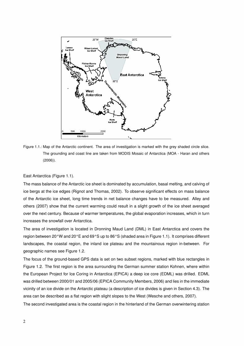
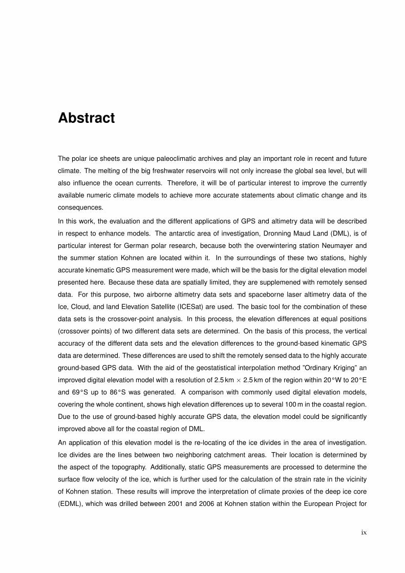
Figure 1.1.: Map of the Antarctic continent. The area of investigation is marked with the grey shaded circle slice.
The grounding and coast line are taken from MODIS Mosaic of Antarctica (MOA - Haran and others
(2006)).
East Antarctica (Figure 1.1).
The mass balance of the Antarctic ice sheet is dominated by accumulation, basal melting, and calving of
ice bergs at the ice edges (Rignot and Thomas, 2002). To observe significant effects on mass balance
of the Antarctic ice sheet, long time trends in net balance changes have to be measured. Alley and
others (2007) show that the current warming could result in a slight growth of the ice sheet averaged
over the next century. Because of warmer temperatures, the global evaporation increases, which in turn
increases the snowfall over Antarctica.
The area of investigation is located in Dronning Maud Land (DML) in East Antarctica and covers the
region between 20° W and 20° E and 69° S up to 86° S (shaded area in Figure 1.1). It comprises different
landscapes, the coastal region, the inland ice plateau and the mountainous region in-between. For
geographic names see Figure 1.2.
The focus of the ground-based GPS data is set on two subset regions, marked with blue rectangles in
Figure 1.2. The first region is the area surrounding the German summer station Kohnen, where within
the European Project for Ice Coring in Antarctica (EPICA) a deep ice core (EDML) was drilled. EDML
was drilled between 2000/01 and 2005/06 (EPICA Community Members, 2006) and lies in the immediate
vicinity of an ice divide on the Antarctic plateau (a description of ice divides is given in Section 4.3). The
area can be described as a flat region with slight slopes to the West (Wesche and others, 2007).
The second investigated area is the coastal region in the hinterland of the German overwintering station
2
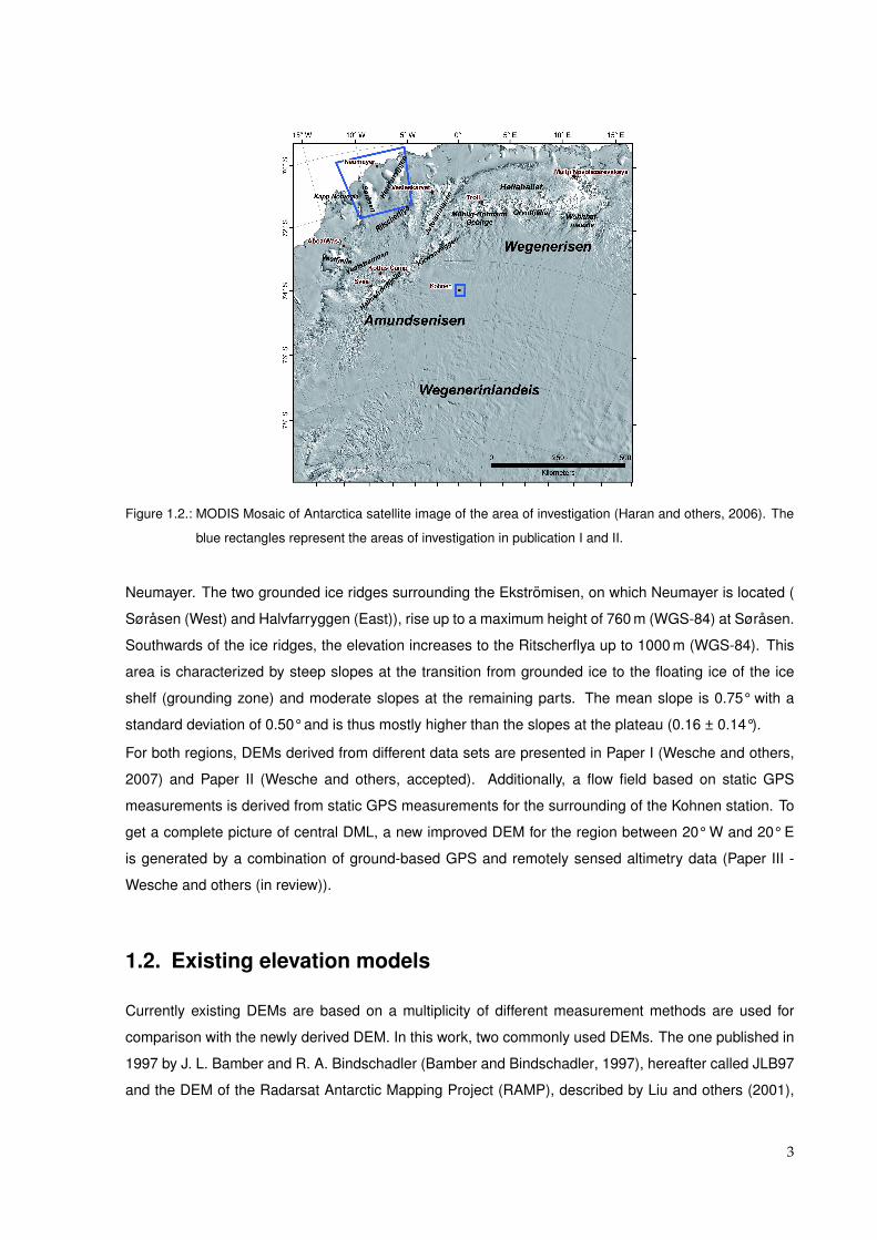
Figure 1.2.: MODIS Mosaic of Antarctica satellite image of the area of investigation (Haran and others, 2006). The
blue rectangles represent the areas of investigation in publication I and II.
Neumayer. The two grounded ice ridges surrounding the Ekstromisen, on which Neumayer is located (
Sørasen (West) and Halvfarryggen (East)), rise up to a maximum height of 760 m (WGS-84) at Sørasen.
Southwards of the ice ridges, the elevation increases to the Ritscherflya up to 1000 m (WGS-84). This
area is characterized by steep slopes at the transition from grounded ice to the floating ice of the ice
shelf (grounding zone) and moderate slopes at the remaining parts. The mean slope is 0.75° with a
standard deviation of 0.50° and is thus mostly higher than the slopes at the plateau (0.16 ± 0.14°).
For both regions, DEMs derived from different data sets are presented in Paper I (Wesche and others,
2007) and Paper II (Wesche and others, accepted). Additionally, a flow field based on static GPS
measurements is derived from static GPS measurements for the surrounding of the Kohnen station. To
get a complete picture of central DML, a new improved DEM for the region between 20° W and 20° E
is generated by a combination of ground-based GPS and remotely sensed altimetry data (Paper III -
Wesche and others (in review)).
1.2. Existing elevation models
Currently existing DEMs are based on a multiplicity of different measurement methods are used for
comparison with the newly derived DEM. In this work, two commonly used DEMs. The one published in
1997 by J. L. Bamber and R. A. Bindschadler (Bamber and Bindschadler, 1997), hereafter called JLB97
and the DEM of the Radarsat Antarctic Mapping Project (RAMP), described by Liu and others (2001),
3
are used for comparison with the newly derived DEM. Both data sets are available at the National Snow
and Ice Data Center (NSIDC - http://nsidc.org/).
1.2.1. JLB97
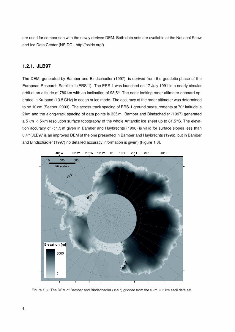
The DEM, generated by Bamber and Bindschadler (1997), is derived from the geodetic phase of the
European Research Satellite 1 (ERS-1). The ERS-1 was launched on 17 July 1991 in a nearly circular
orbit at an altitude of 780 km with an inclination of 98.5°. The nadir-looking radar altimeter onboard op-
erated in Ku-band (13.5 GHz) in ocean or ice mode. The accuracy of the radar altimeter was determined
to be 10 cm (Seeber, 2003). The across-track spacing of ERS-1 ground measurements at 70° latitude is
2 km and the along-track spacing of data points is 335 m. Bamber and Bindschadler (1997) generated
a 5 km × 5 km resolution surface topography of the whole Antarctic ice sheet up to 81.5° S. The eleva-
tion accuracy of < 1.5 m given in Bamber and Huybrechts (1996) is valid for surface slopes less than
0.4° (JLB97 is an improved DEM of the one presented in Bamber and Huybrechts (1996), but in Bamber
and Bindschadler (1997) no detailed accuracy information is given) (Figure 1.3).
Figure 1.3.: The DEM of Bamber and Bindschadler (1997) gridded from the 5 km × 5 km ascii data set.
4
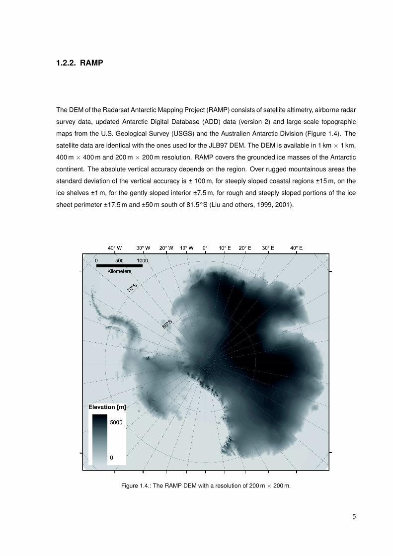
1.2.2. RAMP
The DEM of the Radarsat Antarctic Mapping Project (RAMP) consists of satellite altimetry, airborne radar
survey data, updated Antarctic Digital Database (ADD) data (version 2) and large-scale topographic
maps from the U.S. Geological Survey (USGS) and the Australien Antarctic Division (Figure 1.4). The
satellite data are identical with the ones used for the JLB97 DEM. The DEM is available in 1 km × 1 km,
400 m × 400 m and 200 m × 200 m resolution. RAMP covers the grounded ice masses of the Antarctic
continent. The absolute vertical accuracy depends on the region. Over rugged mountainous areas the
standard deviation of the vertical accuracy is ± 100 m, for steeply sloped coastal regions ±15 m, on the
ice shelves ±1 m, for the gently sloped interior ±7.5 m, for rough and steeply sloped portions of the ice
sheet perimeter ±17.5 m and ±50 m south of 81.5° S (Liu and others, 1999, 2001).
Figure 1.4.: The RAMP DEM with a resolution of 200 m × 200 m.
5
1.3. Motivation
The EDML deep-drilling site is situated on the plateau of DML, in the direct vicinity of an ice divide.
Being drilled in the Atlantic sector of Antarctica, the deep ice core is used to study the teleconnection of
northern and southern hemisphere climate variability in the past (EPICA Community Members, 2006).
For accurate paleoclimatic interpretation of the ice core, the knowledge of past and present ice dynamics
is essential. The mean flow velocity at the EDML deep-drilling site is 0.76 m a-1 (Wesche and others,
2007) and by an estimated age of 128 ka at a depth of 2366 m of the ice drilled at EDML (Ruth and others,
2007), the snow would have been deposited 96.8 km upstream (assuming a constant flow velocity).
Based on an accurate DEM the location of topographic ice divides can be determined (see Section 4.3)
and ice dynamic modeling and thus a localization of the deposition area of the snow can be improved.
The surface topography and surface slopes at the steep margins are a crucial input parameter for climate
modeling. Krinner and others (2007) show, that the gradient of decreasing precipitation, towards the
interior of an ice sheet, is bounded by three effects: (i) orographic effect of the steep margins of the
ice sheets, (ii) decreasing oceanic moisture by increasing distance to the coast and (iii) the temperature
gradient towards the plateau regions. To reduce uncertainties of climate modeling and thus improve the
estimation of future mass balance and sea level change an accurate elevation model is an important
boundary condition (Paterson, 1994; Huybrechts and others, 2000; Huybrechts, 2003). Both DEMs
described in the previous section have shortcomings in the mountainous and coastal regions as shown
by Bamber and Gomez-Dans (2005). Elevation differences up to 1000 m between the JLB97 and RAMP
DEM make the need of an improved DEM very clear.
In this work, four different data sets were used to generate an improved DEM: (i) ground-based kine-
matic GPS, (ii) airborne radar altimetry, (iii) airborne radio echo sounding, and (iv) spaceborne laser
altimetry. By combining different altimetry measurement methods disadvantages of single data sets can
be reduced. For example, highly accurate ground-based GPS data are not affected by cloud cover or
penetration of the signal into the snow surface, which cause false readings by applying laser, respec-
tively radar altimetry. They are recorded near the surface and give the best approximation of the true
surface. But these data are very limited in their spatial extent due to the time consuming survey speed,
and are therefore be supplemented with remotely sensed data, if larger regions are investigated.
The core of this work is the combination of these data sets with different typical features to a highly
accurate elevation data set for central DML. Furthermore, ice divides were localized in DML and the
spaceborne laser altimetry is used to estimate the mean elevation change between 2003 and 2007.
This thesis answers the following questions:
1. Is it possible to determine annual elevation change from spaceborne laser altimetry data?
2. How can different elevation data sets be combined into one to obtain an improved DEM?
6

3. Are there elevation differences between the improved regional DEM and currently existing conti-
nental DEMs?
4. Can the location of the ice divides in DML be confirmed or improved with the new DEM?
5. How fast does the ice move and how large are the strain rates around the EDML deep-drilling site?
7


2. Scope of papers
Paper I: Wesche, C., Eisen, O., Oerter, H., Schulte, D. and D. Steinhage. Surface topography and
ice flow in the vicinity of the EDML deep-drilling site, Antarctica.
Journal of Glaciology, Vol. 53, No. 182, pp. 442-448, 2007.
This paper investigates the surface topography in the vicinity of the EDML deep-drilling site derived
from highly accurate ground-based kinematic GPS measurements and spaceborne laser altimetry from
NASA’s Ice, Cloud, and land Elevation Satellite (ICESat). Because of the data point coverage in the
area of investigation, the surface topography has a horizontal resolution of 5 km x 5 km. Additionally,
static GPS measurements were used to determine the flow field around the deep-drilling site. Based on
the surface velocities, a strain-field for the area around the drilling site could be established and con-
tribute to an improved interpretation of EDML ice-core data. I processed most of the data and wrote the
manuscript, which was improved by the co-authors who also contributed to the data base.
Paper II: Wesche, C., Riedel, S. and D. Steinhage. Precise surface topography of the grounded
ice tongues at the Ekstromisen, Antarctica, based on several geophysical data sets.
ISPRS Journal of Photogrammetry and Remote Sensing, accepted.
This publication describes the method of combining different data sets to a DEM. The grounded part of
a coastal region in the hinterland of the German overwintering station Neumayer II is investigated with
highly accurate ground-based kinematic GPS, ICESat laser altimetry and airborne radar altimetry. A new
precise surface topography was generated with a spatial resolution of 1 km x 1 km. The comparison with
existing DEMs show obvious differences. Most of the data were processed by myself. The co-authors
helped with interpreting the data and improved the manuscript I wrote.
Paper III: Wesche, C., Riedel, S., Eisen, O., Oerter, H., Schulte, D. and D. Steinhage. An improved
DEM and refined locations of ice divides for Dronning Maud Land, Antarctica
Journal of Glaciology, in review
In this paper the combination of four altimetry data sets to an accurate elevation data sets in DML is pre-
9
sented. The methods established in the first two publications were applied to generate a new improved
DEM for DML within 20° W and 20° E and 69° S to 86° S. Due to the use of ground-based GPS data, the
DEM could be improved, which is shown by a comparison with commonly used DEMs. The DEM has
a resolution of 2.5 km × 2.5 km and was used for the localization of the ice divides in DML. A flow field,
consisting of 18 velocity measurements, shows the flow conditions near the German summer station
Kohnen and the wider surroundings. I processed and interpreted the data and wrote the manuscript.
The co-authors contributed to the data base and improved the manuscript.
Paper IV: Drews, R., Rack, W., Wesche, C. and V. Helm. A new digital elevation model in western
Dronning Maud Land (Antarctica), based on differential SAR Interferometry.
IEEE Transactions on Geoscience and Remote Sensing, accepted.
This study describes the methodology of interferometric SAR analyses and presents a high resolution
(50 m × 50 m) DEM for the grounded part of coastal DML within 5° to 20° W and up to 76° S. The paper
shows also an accuracy assessment of generated DInSAR DEM, checked by ground-based kinematic
GPS data, laser scanner data, and ICESat data and the JLB97 DEM and RAMP DEM.
Own contributions to Paper IV:
• processing of the GLA12 (see section 3.3) release 24 data, which were used as ground control
points
• processing of the GLA12 release28 data, which were used for comparison with the final DInSAR
DEM
• processing of the ground based kinematic GPS data, including the interpolation of the reference
stations
• contributions to the text
10

3. Data and Methods
The focus of this work is the generation of an improved DEM. To achieve an optimal result, four measure-
ment methods are combined in a way that uses the advantages and compensates for the disadvantages
of the single methods.
The DEM consists of four different data sets:
(i) highly accurate ground-based kinematic GPS measurements
(ii) airborne radar altimetry (ARA)
(iii) airborne radio echo sounding (RES)
(iv) spaceborne laser altimetry (ICESat).
In the following sections, the different GPS, ARA, RES and ICESat are presented and discussed with
respect to their advantages and disadvantages.
3.1. Global Positioning System (GPS)
The Global Positioning System (GPS) is part of the Global Navigation Satellite System (GNSS) and
was developed by the US Department of Defense in 1973. The present GPS, which is used here,
is a navigation system with timing and ranging (NAVSTAR) GPS. A detailed description is given in
Hofmann-Wellenhof and others (2008). In the following sections, the principle of positioning, possible
error sources, and the different processing methods are described.
3.1.1. Positioning with GPS
The core of the NAVSTAR GPS are 32 operational satellites in 20200 km altitude above the Earth’s
surface. Together with a dual frequency GPS receiver, operating with the L1 carrier frequency at
1575.42 MHz and L2 at 1227.60 MHz, it is possible to determine the precise position of every point
at the Earth’s surface. For position determination, at least four simultaneously operating satellites have
to be visible for the GPS receiver. Basically, the distances (range) between the satellites (equipped with
an atomic clock) and the GPS receiver (equipped with a quartz clock) are determined by the signal run
11
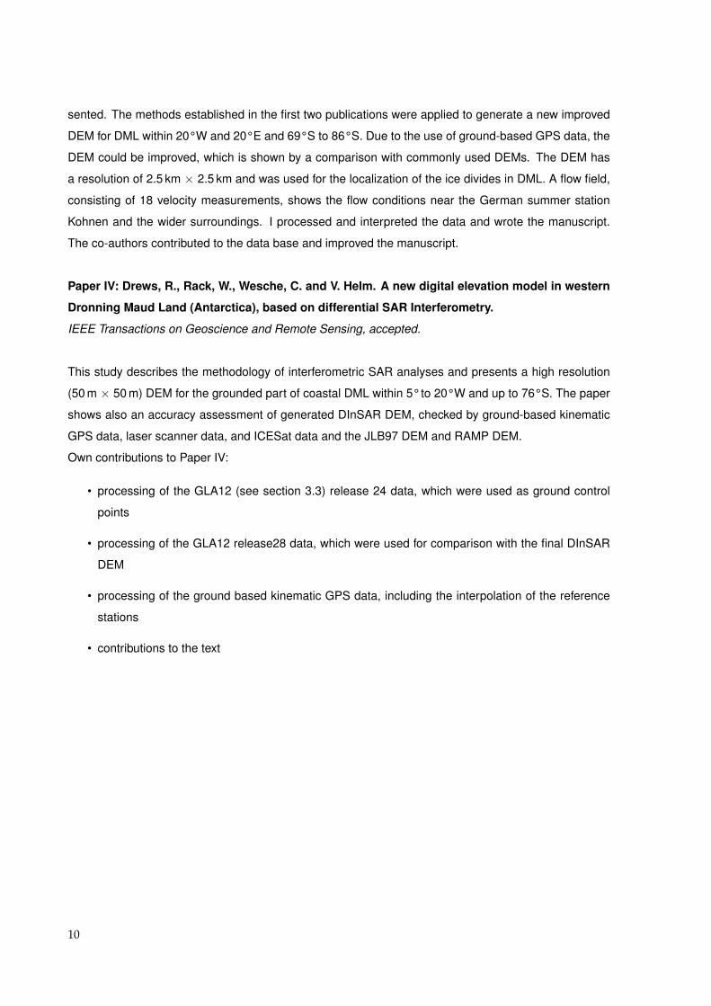
Figure 3.1.: Principle of pseudorange positioning with three satellites.
time, whereas the positions of the satellites are always known. The range is defined as the radius of
a sphere, which has the center point at the satellite position. In Figure 3.1 the positioning is presented
schematically. Three satellites (S1-3) are needed for estimating the position (longitude, latitude and el-
evation). Because of the clock offset of the GPS receiver at the Earth’s surface to the satellite’s clock,
the measured range (R’) differs from the true range (R), which results in three possible solutions for
the position (P’). If a fourth satellite is included, the time difference between the measured and the true
range and thus the true position at the surface (P) can be calculated.
3.1.2. GPS errors
GPS measurements are affected by several systematic errors, which can be separated into three groups:
(i) satellite-related errors (clock bias and orbital errors), (ii) propagation-medium-related errors (iono-
spheric and tropospheric refraction) and (iii) receiver related errors (antenna phase center variation,
clock bias and multipath). Table 3.1 shows a short summary of the systematic errors and their contribu-
tion to uncertainties of the calculated position. Satellite and receiver specific errors can be eliminated by
differential GPS (DGPS) processing (see following section) and most of the systematic errors are mini-
mized by including precise ephemerides (highly accurate orbital information) and atmospheric models.
Multipath errors are signal delays caused by buildings, surface reflections etc. Because of the use of
a Choke Ring antenna and the typically flat surface, they can be neglected in the area of investigation,
but were mentioned here for the sake of completeness. A more detailed description of the error sources
and their minimization is given for example in Hofmann-Wellenhof and others (2008).
12
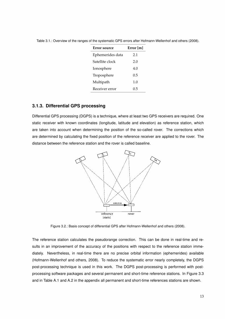
Table 3.1.: Overview of the ranges of the systematic GPS errors after Hofmann-Wellenhof and others (2008).
Error source Error [m]
Ephemerides data 2.1
Satellite clock 2.0
Ionosphere 4.0
Troposphere 0.5
Multipath 1.0
Receiver error 0.5
3.1.3. Differential GPS processing
Differential GPS processing (DGPS) is a technique, where at least two GPS receivers are required. One
static receiver with known coordinates (longitude, latitude and elevation) as reference station, which
are taken into account when determining the position of the so-called rover. The corrections which
are determined by calculating the fixed position of the reference receiver are applied to the rover. The
distance between the reference station and the rover is called baseline.
Figure 3.2.: Basis concept of differential GPS after Hofmann-Wellenhof and others (2008).
The reference station calculates the pseudorange correction. This can be done in real-time and re-
sults in an improvement of the accuracy of the positions with respect to the reference station imme-
diately. Nevertheless, in real-time there are no precise orbital information (ephemerides) available
(Hofmann-Wellenhof and others, 2008). To reduce the systematic error nearly completely, the DGPS
post-processing technique is used in this work. The DGPS post-processing is performed with post-
processing software packages and several permanent and short-time reference stations. In Figure 3.3
and in Table A.1 and A.2 in the appendix all permanent and short-time references stations are shown.
13
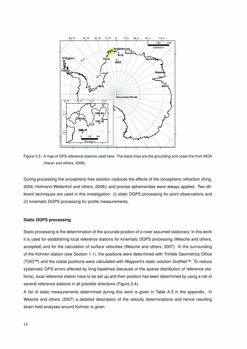
Figure 3.3.: A map of GPS reference stations used here. The black lines are the grounding and coast line from MOA
(Haran and others, 2006).
During processing the ionospheric-free solution (reduces the effects of the ionospheric refraction (King,
2004; Hofmann-Wellenhof and others, 2008)) and precise ephemerides were always applied. Two dif-
ferent techniques are used in this investigation: (i) static DGPS processing for point observations and
(ii) kinematic DGPS processing for profile measurements.
Static DGPS processing
Static processing is the determination of the accurate position of a rover assumed stationary. In this work
it is used for establishing local reference stations for kinematic DGPS processing (Wesche and others,
accepted) and for the calculation of surface velocities (Wesche and others, 2007). In the surrounding
of the Kohnen station (see Section 1.1), the positions were determined with Trimble Geometrics Office
(TGO™) and the costal positions were calculated with Waypoint’s static solution GrafNet™. To reduce
systematic GPS errors affected by long baselines (because of the sparse distribution of reference sta-
tions), local reference station have to be set up and their position has been determined by using a net of
several reference stations in all possible directions (Figure 3.4).
A list of static measurements determined during this work is given in Table A.3 in the appendix. In
Wesche and others (2007) a detailed description of the velocity determinations and hence resulting
strain-field analyses around Kohnen is given.
14
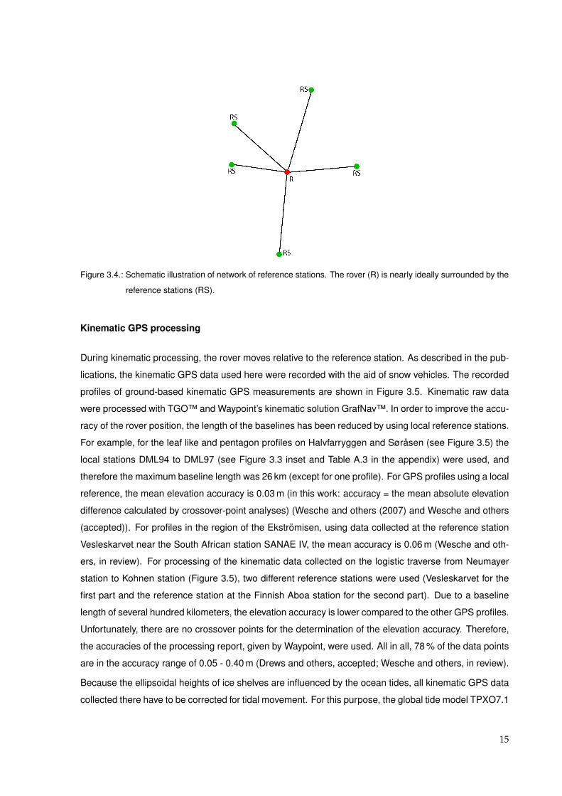
Figure 3.4.: Schematic illustration of network of reference stations. The rover (R) is nearly ideally surrounded by the
reference stations (RS).
Kinematic GPS processing
During kinematic processing, the rover moves relative to the reference station. As described in the pub-
lications, the kinematic GPS data used here were recorded with the aid of snow vehicles. The recorded
profiles of ground-based kinematic GPS measurements are shown in Figure 3.5. Kinematic raw data
were processed with TGO™ and Waypoint’s kinematic solution GrafNav™. In order to improve the accu-
racy of the rover position, the length of the baselines has been reduced by using local reference stations.
For example, for the leaf like and pentagon profiles on Halvfarryggen and Sørasen (see Figure 3.5) the
local stations DML94 to DML97 (see Figure 3.3 inset and Table A.3 in the appendix) were used, and
therefore the maximum baseline length was 26 km (except for one profile). For GPS profiles using a local
reference, the mean elevation accuracy is 0.03 m (in this work: accuracy = the mean absolute elevation
difference calculated by crossover-point analyses) (Wesche and others (2007) and Wesche and others
(accepted)). For profiles in the region of the Ekstromisen, using data collected at the reference station
Vesleskarvet near the South African station SANAE IV, the mean accuracy is 0.06 m (Wesche and oth-
ers, in review). For processing of the kinematic data collected on the logistic traverse from Neumayer
station to Kohnen station (Figure 3.5), two different reference stations were used (Vesleskarvet for the
first part and the reference station at the Finnish Aboa station for the second part). Due to a baseline
length of several hundred kilometers, the elevation accuracy is lower compared to the other GPS profiles.
Unfortunately, there are no crossover points for the determination of the elevation accuracy. Therefore,
the accuracies of the processing report, given by Waypoint, were used. All in all, 78 % of the data points
are in the accuracy range of 0.05 - 0.40 m (Drews and others, accepted; Wesche and others, in review).
Because the ellipsoidal heights of ice shelves are influenced by the ocean tides, all kinematic GPS data
collected there have to be corrected for tidal movement. For this purpose, the global tide model TPXO7.1
15

Figure 3.5.: Location of the ground based kinematic GPS profiles. The black lines indicate data processed with a
local reference station (max. baseline length 26 km, except for the long profile around Kohnen station),
whereas the thin grey profiles were processed with remote reference stations (baseline length greater
100 km). The grounding and coast line (bold grey lines) were derived from MOA (Haran and others,
2006). Stations and camps are marked with black rhombi.
(http://www.coas.oregonstate.edu/research/po/research/tide/global.html) was applied by using the Ohio
State University Tidal Prediction Software (OTPS) (Wesche and others, in review).
3.2. Airborne altimetry
Airborne altimetry data were recorded with sensors installed on the AWI research aircraft POLAR2. To
determine the surface elevation from altimetry, several on-board instruments were used: (i) two Trimble
4000SSI GPS receivers with roof mounted GPS antennas each for determining the exact flight track, (ii)
a HONEYWELL AA-300 radar altimeter system for determining the flying altitude above ground and (iii)
a radio echo sounding system, which is specially designed for the use in polar regions.
The airborne data used here are a byproduct of the pre-site survey for the EPICA project, respectively
the VISA survey (Validation, densification, and Interpretation of Satellite data in Antarctica using airborne
and groundborne measurements for the determination of gravity field, magnetic field, ice-mass balance
and crustal structure). Because of their independence of weather conditions, the data are suitable for
extending the ground-based kinematic GPS data.
The basic principle of airborne altimetry is to determine the aircrafts flying altitude above ground and
16

subtract it from the GPS heights recorded during the flight (Figure 3.6).
Figure 3.6.: Schematic figure of the basics of airborne altimetry. The solid wave lines represent the emitted radar
signal and the dashed wave lines the backscattered signal.
The different approaches of airborne radar altimetry (ARA) and radio-echo sounding (RES) will be de-
scribed in the following two sections.
3.2.1. Radar altimetry
The basic of this airborne radar altimetry is to calculate the height of the aircraft above surface by
measuring the travel time of the radar signal from its emission to arrival of the backscattered signal.
Since the altimeter emits microwave radiation (C-band, 4.3 GHz), the signal penetrates clouds and is
therefore independent of weather conditions. But there are serious limitations of this method. Brenner
and others (1983) show that slopes are influencing the vertical accuracy of the radar altimeters. The so
called ’slope-induced error’ is caused by the reflection of the radar signal from the antenna nearest point
instead of the nadir point. The measured surface lies over the true surface (for more information on the
slope-induced error, see Brenner and others (1983)). Another error source of the radar altimetry is the
penetration of the signal into the snow surface. The absorption of the radar signal is mainly controlled by
the snow temperature and decreases from the coast to the interior of Antarctica. This yields to a spatial
and temporal variation of the penetration depth (Legresy and Remy, 1998).
The operational altitude range above the surface of the HONEYWELL-AA 300 radio altimeter system is
0-2500 ft, which is equivalent to 0-760 m (Honeywell AA-300 Manual, 1998). According to the ground
speed of the aircraft of about 240 km h-1 and a measurement interval of one second, the along track
17

Figure 3.7.: Location of the ARA profiles. The grounding and coast line, derived from MOA, are presented in bold
grey lines (Haran and others, 2006). Stations and camps are marked with black rhombi.
spacing of data points is 66.7 m. Because of the limited operational range of the radar altimeter, only
two campaigns (1998/99 and 2000/01) with usable data are available (Figure 3.7).
The first step of processing the ARA data is the kinematic DGPS processing (see Section 3.1.3) of the
GPS data, recorded during flight by using TGO™. Reference stations were chosen depending on the
location of the starting point of the flight track and the availability of reference data during the whole flight.
In campaign 1998/99, all profiles were processed with reference data of Vesleskarvet. Data of campaign
2000/01 were processed with reference data collected at the Japanese station Syowa, Vesleskarvet and
Kohnen Reference Station (KRS). Because of the range of the aircraft and the sparse distribution of
reference stations, long baselines could not be avoided during processing, which reduced the accuracy
of the kinematic DGPS processing.
Processing (with TGO™) resulted in a root-mean-square of the positioning accuracy of 0.01 m, but this
value is overoptimistic. This software reported error has to be multiplied by 5 to 20 to get a realistic value
for the positioning accuracy (personal communication M. King, 2006).
The mean positioning accuracy of the airborne kinematic GPS can be assumed to range between 0.2
and 0.4 m. Because of the aircrafts orientation (roll, pitch and yaw angle) and the resulting elevation
errors, the ARA data have to be processed with regard to the aircrafts orientation. This is done with
a modified Airborne SAR Interferometric Altimeter System (ASIRAS) processor, which was developed
by V. Helm and S. Hendricks from AWI. The processor requires the post-processed GPS data and the
according raw navigation file of the flight. Based on the installation coordinates of the radar altimeter on-
18

board the aircraft and the navigation file, which includes the orientation angles, the error of the reflected
radar signal can be estimated. With the aid of the operating time (seconds per day), the GPS height is
corrected by the determined altitude above the ground of the aircraft. However, the elevation accuracy
still depends on the surface slope. The slope-induced-error (∆H) over a slope (α) with a flying altitude
(H) above ground can be estimated by:
∆H =Hα2
2(3.1)
For α = 0.026rad (1.5°) and H = 760 m (flying altitude above ground), the slope-induced error amounts to
0.26 m. The maximum slope in the area of investigation is 12° (0.078 rad), which results in a maximum
slope-induced error of 16.59 m. To avoid a high slope-induced error, all ARA data recorded over a
surface topography with a slope over 1.5° were removed from this investigation. The vertical accuracy
(2σ corrected) of 1.8 m is determined by a crossover-point analysis.
3.2.2. Radio echo sounding
During gravimetry measurements of the VISA campaigns, between 2001 and 2005, the flying altitude
had to be constant during the whole flight. Depending on the surface height along the flight track, the
flight level was chosen between 3600 and 4800 m, a.s.l. which was mostly too high above ground to
obtain usable ARA data. Therefore, the radio-echo-sounding system on-board the AWI research aircraft
is used to get surface elevation information over large parts of DML. The RES uses a carrier frequency
of 150 MHz and pulse lengths of 60 ns and 600 ns. The system is able to measure in ”toggle mode”, thus
the pulse length is switched between 60 ns and 600 ns for a different vertical resolution (5 m, respectively
50 m). A measurement interval of 20 Hz at a ground speed of the aircraft of 240 km h-1 results in an
along-track data point distance of 3.25 m, or rather 6.5 m for the individual pulse length (Steinhage and
others, 1999). For more details about the RES system see Nixdorf and others (1999).
Analog to the ARA data, the RES data were processed using the kinematic GPS data recorded during
the flight. Because of the different propagation velocities of electromagnetic waves in air, snow and ice,
the onset of the snow surface is clearly visible as a first reflection in the radargram. The result of this
investigations is the ”thickness” of the medium air, i.e. the flying altitude of the aircraft above the surface.
Afterwards, the airborne kinematic GPS data and the altitude were synchronized using the operation
time. The altitude is subtracted from the GPS heights to obtain the surface topography.
In Figure 3.8 the VISA flight lines are shown, but not for every line RES elevation data are available.
The RES data were recorded in a pattern of parallel lines with a profile separation of 10 km, respectively
20 km. Flight lines crossing the parallel lines (tie lines) were flown to obtain crossover points for cor-
rection of magnetic and gravity data and can be used for determining the quality of the RES elevation
measurements. To avoid elevation branches within the RES campaigns, the data were corrected with a
block shift using these tie lines. This first correction was only a statistical approach and may not show
19
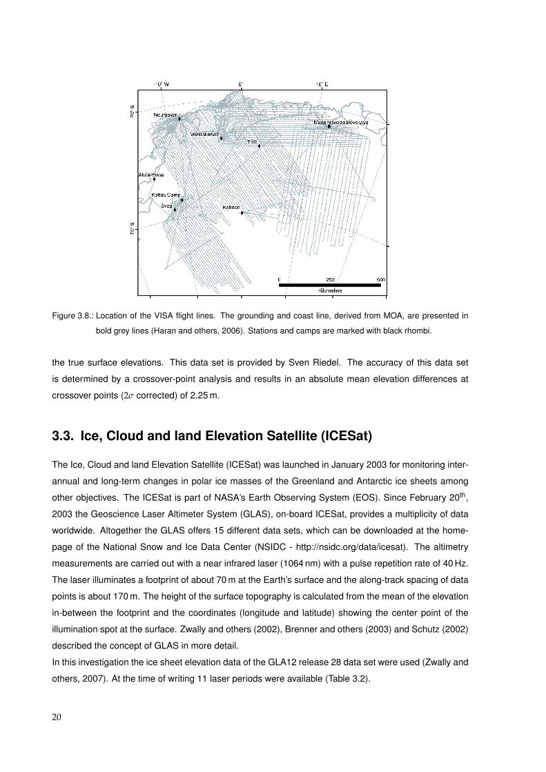
Figure 3.8.: Location of the VISA flight lines. The grounding and coast line, derived from MOA, are presented in
bold grey lines (Haran and others, 2006). Stations and camps are marked with black rhombi.
the true surface elevations. This data set is provided by Sven Riedel. The accuracy of this data set
is determined by a crossover-point analysis and results in an absolute mean elevation differences at
crossover points (2σ corrected) of 2.25 m.
3.3. Ice, Cloud and land Elevation Satellite (ICESat)
The Ice, Cloud and land Elevation Satellite (ICESat) was launched in January 2003 for monitoring inter-
annual and long-term changes in polar ice masses of the Greenland and Antarctic ice sheets among
other objectives. The ICESat is part of NASA’s Earth Observing System (EOS). Since February 20th,
2003 the Geoscience Laser Altimeter System (GLAS), on-board ICESat, provides a multiplicity of data
worldwide. Altogether the GLAS offers 15 different data sets, which can be downloaded at the home-
page of the National Snow and Ice Data Center (NSIDC - http://nsidc.org/data/icesat). The altimetry
measurements are carried out with a near infrared laser (1064 nm) with a pulse repetition rate of 40 Hz.
The laser illuminates a footprint of about 70 m at the Earth’s surface and the along-track spacing of data
points is about 170 m. The height of the surface topography is calculated from the mean of the elevation
in-between the footprint and the coordinates (longitude and latitude) showing the center point of the
illumination spot at the surface. Zwally and others (2002), Brenner and others (2003) and Schutz (2002)
described the concept of GLAS in more detail.
In this investigation the ice sheet elevation data of the GLA12 release 28 data set were used (Zwally and
others, 2007). At the time of writing 11 laser periods were available (Table 3.2).
20

Figure 3.9.: A schematic illustration of the basic concept of ICESat laser altimetry.
Table 3.2.: Overview of the GLA12 release 28 laser measurement periods available at the time of writing.
Laser identifier Days in operation Start date End date
1 38 2003-02-20 2003-03-29
2a 55 2003-09-24 2003-11-18
2b 34 2004-02-17 2004-03-21
3a 37 2004-10-03 2004-11-08
3b 36 2005-02-17 2005-03-24
3c 35 2005-05-20 2005-06-23
3d 35 2005-10-21 2005-11-24
3e 34 2006-02-22 2006-03-27
3f 33 2006-05-24 2006-06-26
3g 34 2006-10-25 2006-11-27
3h 34 2007-03-12 2007-04-14
For the final GLA12 data, the IDLreadGLAS tool offered by the NSIDC was used to convert the binary
raw file to an ascii file. Afterwards, a simple shell script extracts all necessary information (longitude,
latitude, elevation, time of measuring, ocean tide, ocean load tide and saturation correction factor). The
saturation correction factor has to be applied to the elevation data, if the return energy is higher than
predicted. The elevation error caused by detector saturation is shown in Fricker and others (2005).
After adding the saturation correction factor to the elevation data, the ocean tide and ocean load tide
correction (component of ocean tides, which is propagated a few kilometer inland on the grounded
ice masses (Riedel, 2003)) is removed from the elevation data. Based on the laser shot time, the
global tide model of TPXO7.1, recommended by King and Padmann (2005), was applied by using
OTPS (http://www.coas.oregonstate.edu/research/po/research/tide/global.html), replacing the routinely
21
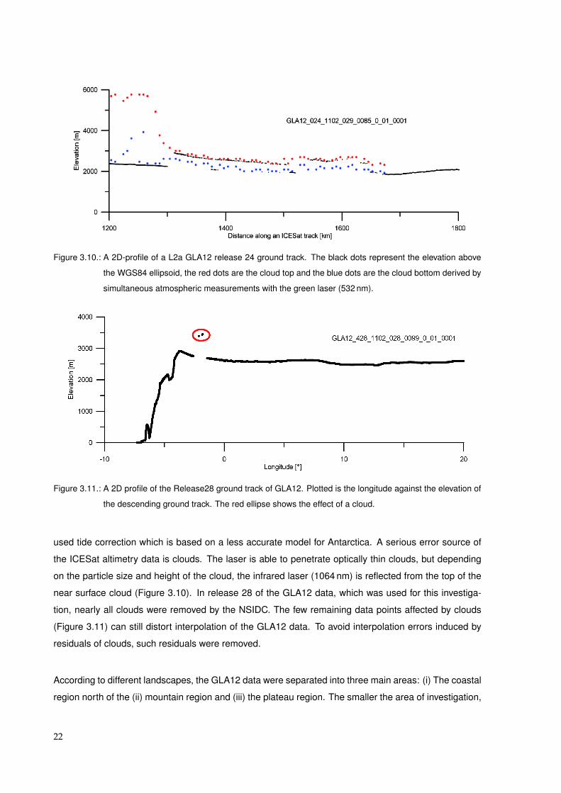
Figure 3.10.: A 2D-profile of a L2a GLA12 release 24 ground track. The black dots represent the elevation above
the WGS84 ellipsoid, the red dots are the cloud top and the blue dots are the cloud bottom derived by
simultaneous atmospheric measurements with the green laser (532 nm).
Figure 3.11.: A 2D profile of the Release28 ground track of GLA12. Plotted is the longitude against the elevation of
the descending ground track. The red ellipse shows the effect of a cloud.
used tide correction which is based on a less accurate model for Antarctica. A serious error source of
the ICESat altimetry data is clouds. The laser is able to penetrate optically thin clouds, but depending
on the particle size and height of the cloud, the infrared laser (1064 nm) is reflected from the top of the
near surface cloud (Figure 3.10). In release 28 of the GLA12 data, which was used for this investiga-
tion, nearly all clouds were removed by the NSIDC. The few remaining data points affected by clouds
(Figure 3.11) can still distort interpolation of the GLA12 data. To avoid interpolation errors induced by
residuals of clouds, such residuals were removed.
According to different landscapes, the GLA12 data were separated into three main areas: (i) The coastal
region north of the (ii) mountain region and (iii) the plateau region. The smaller the area of investigation,
22
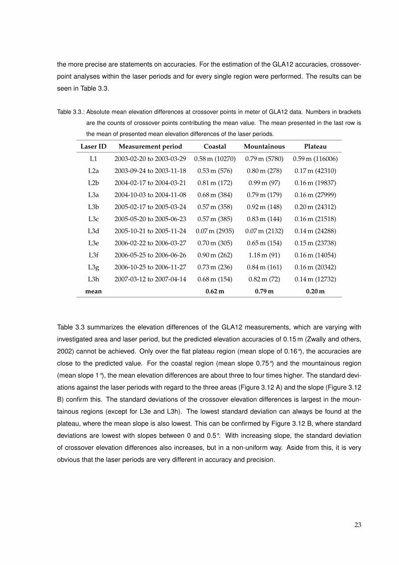
the more precise are statements on accuracies. For the estimation of the GLA12 accuracies, crossover-
point analyses within the laser periods and for every single region were performed. The results can be
seen in Table 3.3.
Table 3.3.: Absolute mean elevation differences at crossover points in meter of GLA12 data. Numbers in brackets
are the counts of crossover points contributing the mean value. The mean presented in the last row is
the mean of presented mean elevation differences of the laser periods.
Laser ID Measurement period Coastal Mountainous Plateau
L1 2003-02-20 to 2003-03-29 0.58 m (10270) 0.79 m (5780) 0.59 m (116006)
L2a 2003-09-24 to 2003-11-18 0.53 m (576) 0.80 m (278) 0.17 m (42310)
L2b 2004-02-17 to 2004-03-21 0.81 m (172) 0.99 m (97) 0.16 m (19837)
L3a 2004-10-03 to 2004-11-08 0.68 m (384) 0.79 m (179) 0.16 m (27999)
L3b 2005-02-17 to 2005-03-24 0.57 m (358) 0.92 m (148) 0.20 m (24312)
L3c 2005-05-20 to 2005-06-23 0.57 m (385) 0.83 m (144) 0.16 m (21518)
L3d 2005-10-21 to 2005-11-24 0.07 m (2935) 0.07 m (2132) 0.14 m (24288)
L3e 2006-02-22 to 2006-03-27 0.70 m (305) 0.65 m (154) 0.15 m (23738)
L3f 2006-05-25 to 2006-06-26 0.90 m (262) 1.18 m (91) 0.16 m (14054)
L3g 2006-10-25 to 2006-11-27 0.73 m (236) 0.84 m (161) 0.16 m (20342)
L3h 2007-03-12 to 2007-04-14 0.68 m (154) 0.82 m (72) 0.14 m (12732)
mean 0.62 m 0.79 m 0.20 m
Table 3.3 summarizes the elevation differences of the GLA12 measurements, which are varying with
investigated area and laser period, but the predicted elevation accuracies of 0.15 m (Zwally and others,
2002) cannot be achieved. Only over the flat plateau region (mean slope of 0.16°), the accuracies are
close to the predicted value. For the coastal region (mean slope 0.75°) and the mountainous region
(mean slope 1°), the mean elevation differences are about three to four times higher. The standard devi-
ations against the laser periods with regard to the three areas (Figure 3.12 A) and the slope (Figure 3.12
B) confirm this. The standard deviations of the crossover elevation differences is largest in the moun-
tainous regions (except for L3e and L3h). The lowest standard deviation can always be found at the
plateau, where the mean slope is also lowest. This can be confirmed by Figure 3.12 B, where standard
deviations are lowest with slopes between 0 and 0.5°. With increasing slope, the standard deviation
of crossover elevation differences also increases, but in a non-uniform way. Aside from this, it is very
obvious that the laser periods are very different in accuracy and precision.
23

0
0.5
1
1.5
2
2.5
3
L1 L2a L2b L3a L3b L3c L3d L3e L3f L3g L3h
Laser period
Sta
nd
ard
devia
tio
n [
m]
Coast
Mountain
Plateau
0
1
2
3
4
5
6
L1 L2a L2b L3a L3b L3c L3d L3e L3f L3g L3h
Laser periods
Sta
nd
ard
devia
tio
ns [
m]
0 - 0.5°
0.5 - 1°
1 - 1.5°
1.5 - 2°
2 - 2.5°
A
B
Figure 3.12.: Standard deviations against the elevation differences of GLA12 data at crossover point with regard to
the three areas (A) and the different slopes (B).
24
4. Applications of the Data
In this chapter the applications of the above presented altimetry and GPS data are presented. The
annual elevation change was calculated from the GLA12 data presented in Section 3.3. The two latest
laser operation periods of the GLA12 data were combined with the airborne altimetry data (ARA and
RES) and the ground-based kinematic GPS data to elevation data sets, which were used to generate an
improved digital elevation model (DEM) for central Dronning Maud Land (DML). Based on this DEM, the
ice divides in the area of investigation were re-located and static GPS data were used to determined a
flow and strain field in the vicinity of the Kohnen station. In the following sections, these applications are
described and results are presented.
4.1. Annual elevation change
Recent elevation-change studies of Antarctica (Wingham and others, 1998; Davis and Ferguson, 2004;
Zwally and others, 2005; Helsen and others, 2008) are based on spaceborne radar-altimetry measure-
ments. Wingham and others (1998) calculated the mean annual elevation change between 1992 and
1996 from ERS-1 and ERS-2 data. Davis and Ferguson (2004) present the mean annual elevation
change from 1995 to 2000 from ERS-2 data. Both investigations have data gaps in the coastal regions
and south of 81.5° S. Furthermore the firn compaction rate is neglected in both cases. Zwally and others
(2005) and Helsen and others (2008) show the elevation changes derived from ERS-1/2 data as well,
but pay attention to the firn compaction. These investigations show different elevation changes in DML.
Zwally and others (2005) calculate increasing or very slightly decreasing elevation, whereas Helsen and
others (2008) show an obvious decreasing elevation in the coastal region of DML and a slightly increas-
ing at the plateau. This shows that firn correction is crucial for the determination of mass balance trends
from altimetry and a different firn-correction techniques yield different elevation change results.
In this work, a first approach is presented to estimate the mean annual elevation changes in central
DML from 2003 to 2007 based on laser-altimetry data from ICESat. For this purpose, crossover-point
analyses between laser periods (Table 3.2) of an annual interval were performed (L1 minus L2b or L2a
minus l3a, etc.). The annual interval is chosen to investigate always the same seasonal conditions.
The elevation differences at crossover points were then interpolated to a 5 km × 5 km resolution grid to
show annual elevation changes (chapter B, see appendix). Because of the small number of crossover
25
points containing data of the L1 laser period (about 10% of the other laser periods) L1 measurements
were not used for further investigations. To calculate the mean annual elevation change and to minimize
the relative errors of this estimation, a crossover-point analysis between L2a and L3h laser periods
was made. The results were divided by the time span between the measurements (3.5 years) and
interpolated on a 5 km × 5 km raster. In Figure 4.1 the annual elevation change derived from GLA12
altimetry data are shown. In addition, the standard deviation was calculated from the annual elevation
changes presented in the appendix (Figure 4.2).
A few regions in the elevation change map are conspicuous due to elevation decreases at the plateau.
Looking at the annual elevation change maps (in the appendix), it is obvious that these locations are
characterized by very high elevation change estimations. The high standard deviations (over 10 m) in
elevation changes point to measurement errors (e.g. the reflection of the laser signal on snow particles
in the air during snow drift) of the GLA12 L2a data in these regions, thus the elevation changes in these
areas are not correct.
Detailed information on measured elevation changes in the surrounding of the German Antarctic over-
wintering station (see section 1.1.1) are presented in Figure 4.3 and 4.4. Evidently, this area is divided
into an increasing part, the Halvfarryggen, and a decreasing part, the Sørasen. The main wind direction
in this region is from east to west (Konig-Langlo and others, 1998), hence air masses reach the Halvfar-
ryggen first. Because of the peninsula character of the Halvfarryggen, it builds a barrier for air masses
coming from the eastern ice shelf region. The body of humid air will snow first over Halvfarryggen. Be-
cause of the closed ice cover of the Ekstromisen, the air masses are not able to restore new humidity
on their way westwards to the Sørasen. The mean elevation change for coastal DML is 0.06 ± 0.20 m
(min:-1.06 m, max:0.72 m) and for the plateau of central DML -0.02 ± 0.10 m (min:-2.00 m, max:1.41 m).
This results in a mass gain of 13.5 Gt a-1 at the coast and a mass loss of 19.3 Gt a-1 at the plateau (both
values were determined with an assumed ice density of 910 kg m-3). Because the laser is reflected at
the surface and under the assumption that the firn compaction does not change with time, the firn com-
paction is neglected here, because the laser signal does not penetrate into the snow surface and thus
changes in density do not affect the elevation change estimation. Nevertheless, the elevation accuracy
of the GLA12 data at the plateau is 0.20 m, which is only slightly smaller than the elevation changes
estimated for this region. The same is true for the coastal region. However, by calculating the mean
annual elevation change from different time spans, a trend of the elevation change could be estimated.
An additional estimation of annual elevation change can be given by calculating the differences between
the JLB97 DEM and the latest GLA12 data (L3h), to get the longest time span possible. The JLB97 DEM
consists of ERS-1 radar altimetry data from the geodetic phase, which provided elevation data between
April 1994 and May, 1995. The L3h data were derived between March 12th and April 14th, 2007. Thus,
there is a time span of 12 years. The calculated elevation differences between these two data were
divided by the time span, to obtain annual elevation change. Afterwards, the annual elevation change
26
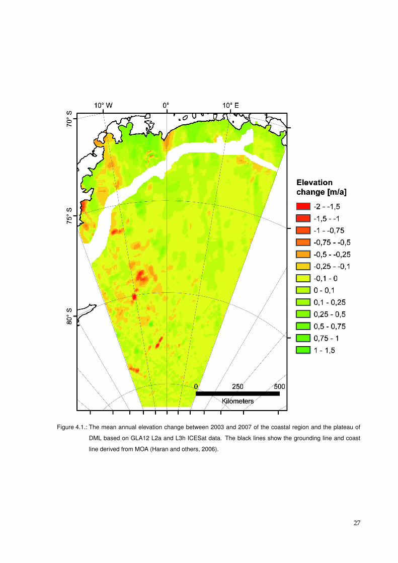
Figure 4.1.: The mean annual elevation change between 2003 and 2007 of the coastal region and the plateau of
DML based on GLA12 L2a and L3h ICESat data. The black lines show the grounding line and coast
line derived from MOA (Haran and others, 2006).
27
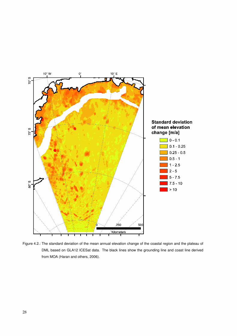
Figure 4.2.: The standard deviation of the mean annual elevation change of the coastal region and the plateau of
DML based on GLA12 ICESat data. The black lines show the grounding line and coast line derived
from MOA (Haran and others, 2006).
28
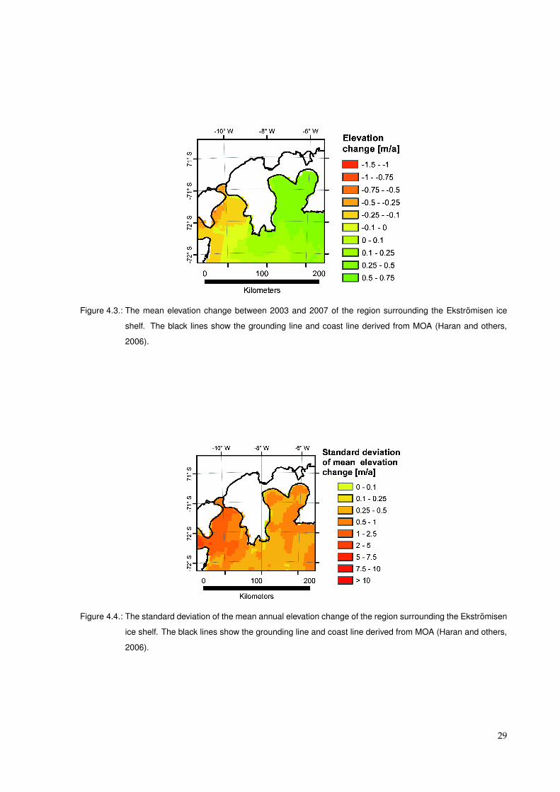
Figure 4.3.: The mean elevation change between 2003 and 2007 of the region surrounding the Ekstromisen ice
shelf. The black lines show the grounding line and coast line derived from MOA (Haran and others,
2006).
Figure 4.4.: The standard deviation of the mean annual elevation change of the region surrounding the Ekstromisen
ice shelf. The black lines show the grounding line and coast line derived from MOA (Haran and others,
2006).
29
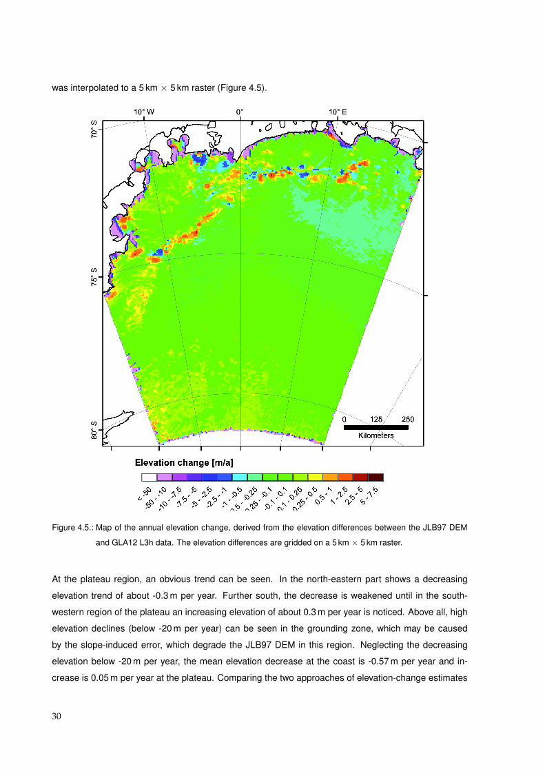
was interpolated to a 5 km × 5 km raster (Figure 4.5).
Figure 4.5.: Map of the annual elevation change, derived from the elevation differences between the JLB97 DEM
and GLA12 L3h data. The elevation differences are gridded on a 5 km × 5 km raster.
At the plateau region, an obvious trend can be seen. In the north-eastern part shows a decreasing
elevation trend of about -0.3 m per year. Further south, the decrease is weakened until in the south-
western region of the plateau an increasing elevation of about 0.3 m per year is noticed. Above all, high
elevation declines (below -20 m per year) can be seen in the grounding zone, which may be caused
by the slope-induced error, which degrade the JLB97 DEM in this region. Neglecting the decreasing
elevation below -20 m per year, the mean elevation decrease at the coast is -0.57 m per year and in-
crease is 0.05 m per year at the plateau. Comparing the two approaches of elevation-change estimates
30
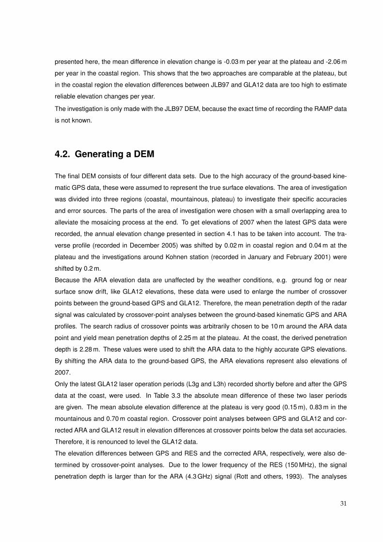
presented here, the mean difference in elevation change is -0.03 m per year at the plateau and -2.06 m
per year in the coastal region. This shows that the two approaches are comparable at the plateau, but
in the coastal region the elevation differences between JLB97 and GLA12 data are too high to estimate
reliable elevation changes per year.
The investigation is only made with the JLB97 DEM, because the exact time of recording the RAMP data
is not known.
4.2. Generating a DEM
The final DEM consists of four different data sets. Due to the high accuracy of the ground-based kine-
matic GPS data, these were assumed to represent the true surface elevations. The area of investigation
was divided into three regions (coastal, mountainous, plateau) to investigate their specific accuracies
and error sources. The parts of the area of investigation were chosen with a small overlapping area to
alleviate the mosaicing process at the end. To get elevations of 2007 when the latest GPS data were
recorded, the annual elevation change presented in section 4.1 has to be taken into account. The tra-
verse profile (recorded in December 2005) was shifted by 0.02 m in coastal region and 0.04 m at the
plateau and the investigations around Kohnen station (recorded in January and February 2001) were
shifted by 0.2 m.
Because the ARA elevation data are unaffected by the weather conditions, e.g. ground fog or near
surface snow drift, like GLA12 elevations, these data were used to enlarge the number of crossover
points between the ground-based GPS and GLA12. Therefore, the mean penetration depth of the radar
signal was calculated by crossover-point analyses between the ground-based kinematic GPS and ARA
profiles. The search radius of crossover points was arbitrarily chosen to be 10 m around the ARA data
point and yield mean penetration depths of 2.25 m at the plateau. At the coast, the derived penetration
depth is 2.28 m. These values were used to shift the ARA data to the highly accurate GPS elevations.
By shifting the ARA data to the ground-based GPS, the ARA elevations represent also elevations of
2007.
Only the latest GLA12 laser operation periods (L3g and L3h) recorded shortly before and after the GPS
data at the coast, were used. In Table 3.3 the absolute mean difference of these two laser periods
are given. The mean absolute elevation difference at the plateau is very good (0.15 m), 0.83 m in the
mountainous and 0.70 m coastal region. Crossover point analyses between GPS and GLA12 and cor-
rected ARA and GLA12 result in elevation differences at crossover points below the data set accuracies.
Therefore, it is renounced to level the GLA12 data.
The elevation differences between GPS and RES and the corrected ARA, respectively, were also de-
termined by crossover-point analyses. Due to the lower frequency of the RES (150 MHz), the signal
penetration depth is larger than for the ARA (4.3 GHz) signal (Rott and others, 1993). The analyses
31
result in mean penetration depths of 24.02 m (plateau), 25.35 m (mountain range) and 21.97 m (coastal
region). These values were also used to shift the RES data to the other data sets.
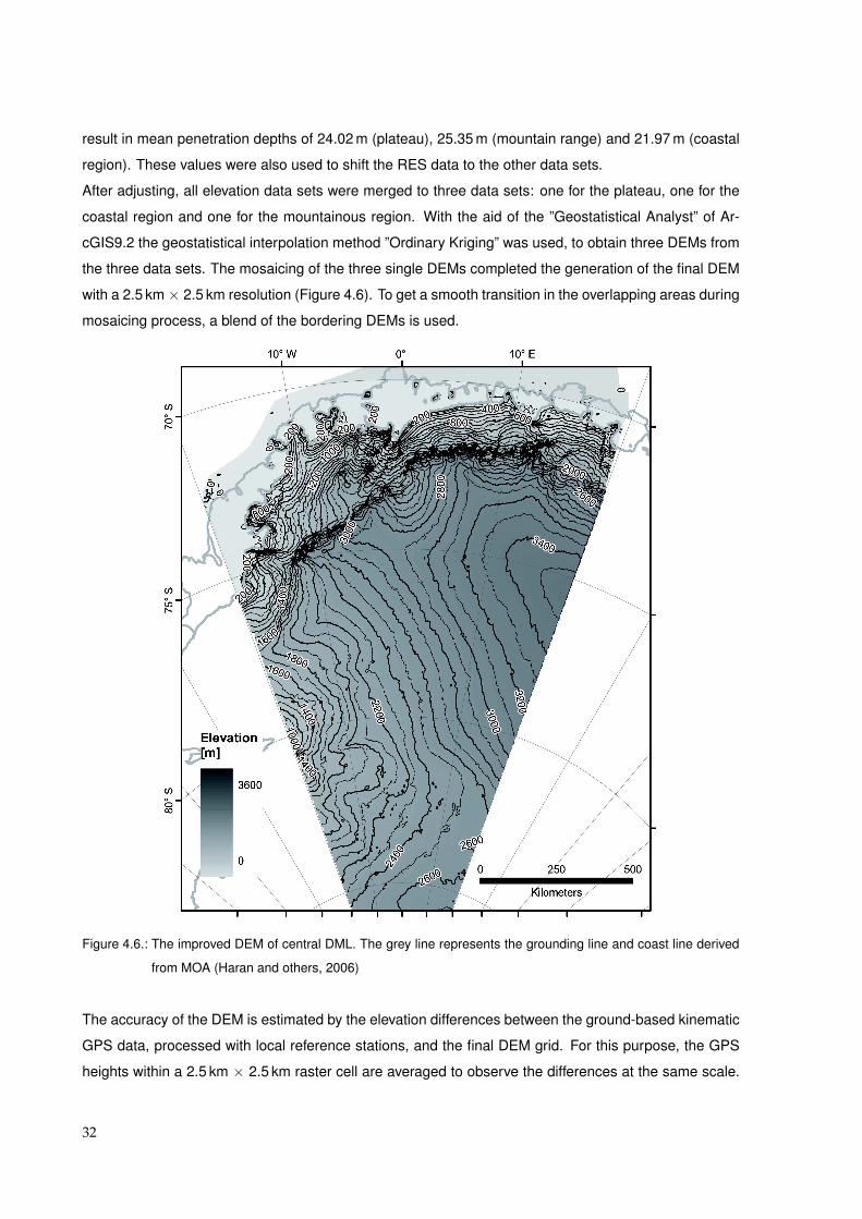
After adjusting, all elevation data sets were merged to three data sets: one for the plateau, one for the
coastal region and one for the mountainous region. With the aid of the ”Geostatistical Analyst” of Ar-
cGIS9.2 the geostatistical interpolation method ”Ordinary Kriging” was used, to obtain three DEMs from
the three data sets. The mosaicing of the three single DEMs completed the generation of the final DEM
with a 2.5 km × 2.5 km resolution (Figure 4.6). To get a smooth transition in the overlapping areas during
mosaicing process, a blend of the bordering DEMs is used.
Figure 4.6.: The improved DEM of central DML. The grey line represents the grounding line and coast line derived
from MOA (Haran and others, 2006)
The accuracy of the DEM is estimated by the elevation differences between the ground-based kinematic
GPS data, processed with local reference stations, and the final DEM grid. For this purpose, the GPS
heights within a 2.5 km × 2.5 km raster cell are averaged to observe the differences at the same scale.
32

Figure 4.7.: A comparison of the new DEM with JLB97 (A) and the new DEM with RAMP (B). The black lines are
showing the grounding and coast line derived from MOA (Haran and others, 2006).
Another investigation was the standard deviation of the GPS heights within a raster cell. In the coastal
region, the height of the leaf like profiles on Halvfarryggen and Sørasen were compared with the raster
values of the final DEM. On the plateau, the ground-based kinematic GPS profiles in the vicinity of
the EDML deep-drilling site were used. In Table 4.1 the results are shown and a detailed description is
given in Wesche and others (in review). Because of the insufficient comparative values, the mountainous
region is neglected in this investigation.
Table 4.1.: The accuracy of the improved DEM determined by height comparison with highly accurate ground-based
GPS data.
Region Mean difference [m] Standard deviation [m] Minimum [m] Maximum [m]
Coast -2.66 4.45 -33.49 58.29
Plateau -0.65 0.26 -1.77 0.11
A comparison of the new generated with the currently available DEMs presented in section 1.2 was done
by subtracting the JLB97 or RAMP DEM from the new DEM presented here. The results are shown in
Figure 4.7 A and B.
The elevation differences on the plateau north of 81.5° S are small in comparison to the coastal or
mountainous region. However, both commonly used DEMs consist of ERS-1 altimetry data in this region,
but in the north-eastern part, the elevation differences between the improved DEM and JLB97 are larger
than between the improved DEM and RAMP. South of 81.5° S and in the coastal region the RAMP DEM
33
consists of ADD data (Liu and others, 1999, 2001). There are larger positive and negative heights than
determined in the improved DEM. In the JLB97 DEM, the variations in lower and higher surface elevation
than the improved DEM are not as large. For more details see Wesche and others (in review).
4.3. Re-location of the ice divides
Ice divides, i.e. ice ridges separating catchment areas, are next to the domes preferred drilling locations,
because the interpretation of paleoclimatic records is simplified by the known origin of the ice (Paterson,
1994). In DML several ice divides are known from former investigations using the DEM of Bamber and
Huybrechts (1996). One distinguishes between two types of ice divides: (i) symmetric or topographic
ice divide and (ii) asymmetric or flow ice divide. The topographic ice divide can be determined by the
surface topography and is located at the highest surface elevation along a cross section of the DEM,
while the asymmetric ice divide is not necessarily at the highest surface elevation. The ice flow near the
topographic ice divide is characterized by a slow flow parallel to the course of the ice divide in-between
a buffer of three to five times the ice thickness around the ice divide (Raymond, 1983; van der Veen,
1999). Apart from this region, the flow velocity becomes faster and more divergent to the course of the
ice divide. The flow ice divide is characterized by a divergent flow at the border of two adjoined catchment
areas. This type of ice divide is not necessarily at the top of the surface topography (Paterson, 1994).
The focus of this work lies on the topographic ice divides. ArcGIS offers several investigation methods,
which help to obtain the location of the ice divides in DML. Based on the calculated aspect of the surface
topography in DML, the inclination of the slopes is illustrated (see appendix, Figure C.2). The aspect of
the topography was mainly used for the localization of the ice divides. Additionally, the theoretical ice
flow direction and the catchment basins were determined also with the ArcGISToolBox. The result is a
new map of ice divides in central DML (Figure 4.8). In most regions the course of the ice divide is only
a few kilometers away from the ones derived from the DEM of Bamber and Bindschadler (1997). Due to
the higher resolution of the improved DEM, it was possible to derive new ice divides, e.g. at the coast
on Halvfarryggen and Kapp Norvegia (see Figure 4.8). The course of the ice divide in the east of the
region of interest could not be confirmed, but a completely new one at ∼12° E was identified. Two ice
divides end at the mountain range, their course through the mountains could not be reliably identified.
The biggest outlet glacier in central DML is the Jutulstraumen. The outlet glacier is fed by ice masses
flowing from the plateau through a deep valley glacier between Kirwanveggen and Muhlig-Hofmann
Gebirge. The Jutulstraumen flows to the north into the Fimbulisen ice shelf. Another big outlet glacier
is the Veststraumen, which is fed by ice masses flowing from the Heimefrontfjiella to the north-west
and ice masses from the Ritscherflya flowing to the west. The Veststraumen drains to the west into the
Riiser-Larsen ice shelf. There are some smaller catchment areas between the Jutulstraumen and the
Veststraumen. They are all draining to the north into small ice shelves. The southern part of central
34

DML is draining to the south-west and the western part to the north. Of particular interest is the change
of the ice divide location in the vicinity of the EDML deep-drilling site (see small map in Figure 4.8). This
ice divide is forking in the east of EDML. The southern ice divide based on the DEM is about 12 km
north compared to the one determined with JLB97. The location of the northern ice divide is nearly
unchanged. That means EDML lies directly within two ice divides, only 3 km (southern ice divide) and
4 km (northern ice divide) apart from the location of the ice divides. A more detailed investigation of the
ice divides around EDML is given in Wesche and others (in review).
Figure 4.8.: A map showing the courses of the ice divides in DML. The dark grey lines show the ice divides derived
from the new DEM and for comparison, the light grey dashed line the ice divides derived from JLB97.
The contour lines are from the new DEM, the black lines representing a contour interval of 200 m and
the grey 100 m. The black lines are showing the grounding and coast line derived from MOA (Haran
and others, 2006). In the inset map, the region around the EDML drilling site (white dot) is shown. The
contour lines intervals are 10 m (grey) and 50 m (black).
4.4. Determining ice flow and strain rates
The ice flow in central DML is calculated from 18 static GPS measurements. The mean annual surface
velocity is calculated by averaging the flow velocities of different time periods. The results are shown
35

in Table 4.2. The accuracy of the velocity measurements is calculated by the propagation of errors and
has a maximum of 0.06 m a-1. A detailed description of the calculation of the precision of the velocity is
given in Wesche and others (2007).
Table 4.2.: The flow velocities of various point measurements on the Antarctic plateau.
Name Longitude Latitude Flow [m a-1] Flow direction [°] Period of averaging
DML01 2.5493° E 74.8564° S 0.54 293.2 Jan. 1997 - Jan. 1999
DML02 3.9185° E 74.9683° S 3.18 153.5 Jan. 1997 - Jan. 1999
DML03 1.9609° E 74.4995° S 7.40 128.9 Jan. 1997 - Jan. 1999
DML05 0.0072° E 75.0024° S 0.66 270.4 Jan. 2001 - Dec. 2005
DML07 3.4306° W 75.5816° S 4.28 229.6 Jan. 1997 - Jan. 2001
DML19 0.9951° W 75.1674° S 1.87 213.3 Jan. 1999 - Jan. 2001
DML25 0.0818° E 75.0060° S 0.83 274.2 Jan. 2004 - Dec. 2005
DML26 0.0099° E 74.8393° S 1.07 335.9 Jan. 2001 - Dec. 2005
DML27 0.7040° E 75.0560° S 0.96 287.5 Feb. 2003 - Dec. 2005
BA01 0.0678° E 75.0017° S 0.68 272.6 Jan. 2003 - Dec. 2005
HM01 0.0078° E 74.9939° S 0.64 273.7 Jan. 2000 - Dec. 2005
HM02 0.0394° E 75.0069° S 0.68 270.0 Jan. 2000 - Dec. 2005
HM03 0.0229° W 75.0074° S 0.67 266.6 Jan. 2000 - Dec. 2005
PEN1 0.0819° E 74.9654° S 0.64 291.3 Jan. 2000 - Dec. 2005
PEN2 0.2296° E 74.9945° S 0.77 282.9 Jan. 2000 - Dec. 2005
PEN3 0.1728° E 75.0393° S 0.86 265.9 Jan. 2000 - Dec. 2005
PEN4 0.0121° W 75.0388° S 0.84 257.9 Jan. 2000 - Dec. 2005
PEN5 0.0659° W 74.9937° S 0.62 269.8 Jan. 2000 - Dec. 2005
Strain is a dimensionless parameter of deformation and the strain rate is a time dependent deformation
of a material. Deformation is caused by stresses acting on e.g. ice masses (Paterson, 1994). The flow of
ice masses causes such stresses and therefore the surface velocities calculated from static GPS mea-
surements were used for the determination of the strain rates. Of particular interest is the deformation
rate around the EDML deep-drilling site. Therefore, five aluminium stakes (PEN1-5) in shape of a pen-
tagon network around the drilling site were fixed in the snow surface in January 2000. Since then, the
stakes were observed in several austral summer campaigns. Simultaneously, a sixth aluminium stake in
the center of the pentagon was observed (BA01). The strain field is shown in Figure 4.9 and a detailed
description is given in Wesche and others (2007) (Paper I).
Because the center point of the pentagon-shaped network is only 93 m north-east to the drilling location
of the EDML ice core, the determined weighted mean strain rates (εx = −1.54× 10⁻⁵ a−1 - strain rate in
north direction, εy = −5.64× 10⁻⁵ a−1 - strain rate in east direction and εz = 1.09× 10⁻⁴ a−1 - vertical
36
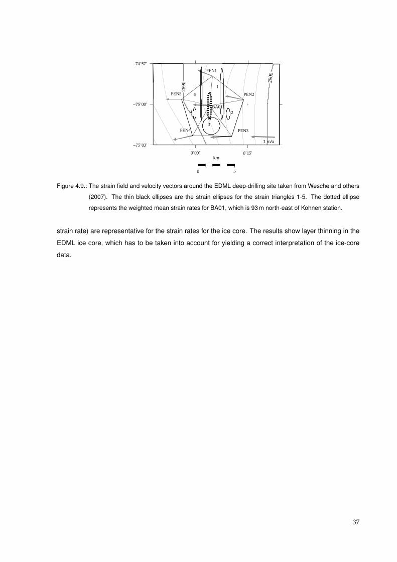
0˚00' 0˚15'
−75˚03'
−75˚00'
−74˚57'
0 5
km
2890 2
900
1 m/a
BA01
PEN1
PEN2
PEN3PEN4
PEN5
1
2
3
4
5
Figure 4.9.: The strain field and velocity vectors around the EDML deep-drilling site taken from Wesche and others
(2007). The thin black ellipses are the strain ellipses for the strain triangles 1-5. The dotted ellipse
represents the weighted mean strain rates for BA01, which is 93 m north-east of Kohnen station.
strain rate) are representative for the strain rates for the ice core. The results show layer thinning in the
EDML ice core, which has to be taken into account for yielding a correct interpretation of the ice-core
data.
37

5. Summary and Outlook
The evaluation of annual elevation changes between 2003 and 2007, derived from crossover-point anal-
yses between different laser periods of the GLA12 is a first approach for estimating annual changes of
the elevation. By calculating the mean annual elevation change from seven different time spans, a trend
could be determined. However, the GLA12 accuracy is only slightly below the elevation changes and
therefore it is necessary to use longer time spans to minimize the relative errors of elevation change
determination. Nevertheless, the preliminary estimation of annual elevation change shows interesting
results. In coastal DML, the mean elevation change is positive with 0.06 m with a standard deviation
of 0.20 m. Looking at the area of the Ekstromisen, one can see that the elevation change varies over
this small area. The Halvfarryggen near the Neumayer station shows an increasing surface elevation,
while the Sørasen, located in the west of the Halvfarryggen, shows decreasing elevations. Because
the main wind direction in the coastal region near Neumayer station is east, the Halvfarryggen can be
seen as a barrier for humid air masses. On the plateau, the mean annual elevation change is negative
by -0.02 m ± 0.10 m, which is contrary to the investigations of Zwally and others (2005) and Helsen and
others (2008). The trend analysis of mean annual elevation change results in a mass loss for the plateau
region of -19.3 Gt a-1 and a mass gain of 13.5 Gt a-1 for the coastal region.
Other elevation change investigations are predicting an increasing elevation on the plateau and a con-
trary evolution at the coast. Similar results are obtained by investigating JLB97 and GLA12 L3h data, but
the values of elevation change are nearly the same for the plateau region. However, the mean annual
elevation change in the coastal region is dependent on the elevation accuracy of the JLB97 DEM. Firn
compaction is also a factor of high uncertainty in the calculation of elevation change using radar altimetry
as shown in the different results of Zwally and others (2005) and Helsen and others (2008). Therefore,
the comparison of two different altimetry data sets in terms of calculating the annual elevation change
is limited. In regions with relatively constant firn compaction and thus penetration of the radar signal the
results are very good, but in highly variable regions, the annual elevation change should be calculated
with identical sensors.
The improved DEM for central DML presented in this work was derived from a combination of ground-
based kinematic GPS, two types of airborne radar altimetry, and spaceborne laser altimetry. To achieve
the best possible data accuracy and density, the different elevation data were compared to each other,
corrected and combined. Because the ground-based kinematic GPS data are not affected by clouds
39
(as laser altimetry) or signal penetration into the snow surface (as radar altimetry) and their high vertical
accuracy of 0.03 m, these heights are used as a reference elevation for the remotely sensed altimetry
data.
With regard to the very different surface topography and to obtain a good interpolation result, the area
of investigation was divided into three parts: (i) the coastal region north of the mountain range with its
varying topography, (ii) the mountain range with the steep slopes and outcrops, and (iii) the plateau with
its wide flat topography. Based on several crossover-point analyses, the remotely sensed elevation data
were investigated with regard to the elevation differences to the ground-based kinematic GPS elevations.
Because the ground-based data are spatially limited, the ARA data were used to enlarge the number
of crossover points to the other altimetry data. The ARA data were leveled to the GPS data by the
mean penetration depth. Afterwards, the GLA12 elevation data were investigated with regard to the
height differences to the GPS and ARA data. These differences are below the accuracy of the data set
and thus, the GLA12 data do not need to be shifted to the other data. The RES signal has a higher
penetration depth than the ARA, therefore a crossover-point analysis between the ARA profiles and the
RES data was performed. The obtained elevation differences were used to shift the RES data to the
ARA data. After leveling the remotely sensed data to the ground-based GPS data, the data were merged
into elevation data sets for the coastal, mountainous and plateau region. The geostatistical interpolation
technique ”Ordinary Kriging” was used to interpolate the heights to a 2.5 km × 2.5 km raster for the three
investigation areas. Afterwards, a mosaic of the three separated DEMs was generated. The accuracy
of the improved DEM is checked by the elevation differences between the ground-based GPS profiles
and the DEM grid. The mean elevation differences are -0.65 m at the plateau and -2.66 m in the coastal
region. The accuracy of this DEM could be further improved by using more ground-based kinematic
GPS data which should be equally distributed over the whole area of investigation. Especially in the
coastal region, where the penetration depth of the radar signal varies, ground-based measurement are
needed to estimate such variations and to improve the radar altimeter data. But the advancement in
accuracy of this DEM compared to the commonly used DEMs is obvious, due to use of highly accurate
ground-based kinematic GPS data (even if they are spatially limited) contributing significantly to the
quality of the DEM.
Elevation difference estimations between the new DEM presented here and the DEMs commonly used
for modeling, JLB97 and RAMP, show very high spatial variations. On the plateau north of 81.5° S,
the elevation differences are within a few meters. North of this region, the elevation differences are
increasing very fast up to several hundred meters. Especially in the coastal region, where the elevation
of large parts was underestimated in earlier DEMs, the improved DEM is a definite advance for numerical
modeling of ice dynamic and mass balance.
Because the new DEM has a higher resolution, the location of ice divides can be determined more
accurately. The location of the ice divides in DML has been calculated from investigations based on the
40
DEM of Bamber and Huybrechts (1996). A comparison between the improved and the old ice divides
shows variations mostly within very few kilometers. In the coastal region, the courses of old the ice
divides are complemented by some new ice divides. Altogether, only small changes in the courses
of the ice divides were found. Nevertheless, the knowledge of the ice-divide locations in the area of
investigation is improved by the new DEM.
As presented in Wesche and others (2007), static GPS measurements were not only used for local
reference stations, but also for the calculation of surface velocities. These velocities were used to de-
termine the strain field in the surrounding of the EDML deep-drilling site, which has to be accounted for
to yield a correct interpretation of ice-core data. During the International Partnerships on Ice Core Sci-
ence (IPICS) pre-site survey in the beginning of 2007, four pentagon-shaped deformation figures were
established around possible coastal drilling sites. These deformation figures will be re-surveyed during
the next austral summer campaign in Antarctica. The new positions will be used to determine surface
strain fields around these possible drilling sites. In addition to the accurate DEM presented here, ground
penetrating radar measurements and shallow ice and firn cores, as well as the deformation studies will
give an advice to select a suitable drilling site for a deep coastal ice core.
With the launch of the CryoSat-2, planned for November 2009, a new era of satellite radar altimetry
over ice sheets will begin. The onboard Synthetic-Apertur Interferometric Radaraltimeter (SIRAL) is
specially designed for the measurement above ice sheets. Due to the small footprint of 250 m (16 - 20 km
ERS - http://earth.esa.int/object/index.cfm?fobjectid=3999), the elevation radar-altimeter measurements
of elevation will be improved. The footprint of the GLAS on board the ICESat is even smaller (70 m),
but the laser is not able to penetrate clouds. The independence from weather conditions and the (for
a spaceborne radar altimeter) small footprint are the big advantages of the CryoSat-2. However, the
SIRAL will also be affected by the slope-induced error and the penetration of the radar signal into the
snow surface. Therefore, it will be essential to validate the CryoSat-2 altimetry data with ground-based
measurements. This improved DEM provides a suitable data set to validate the CryoSat-2 altimetry
products.
41


Bibliography
Alley, R. B., P. U. Clark, P. Huybrechts and I. Joughin, 2005. Ice-sheet and sea level changes, Science,
310, 456–460.
Alley, R. B., M. K. Spencer and S. Anandakrishnan, 2007. Ice-sheet mass balance: assessment, attri-
bution and prognosis, Annals of Glaciology , 46, 1–7.
Arthern, R. J. and R. C. A. Hindmarsch, 2006. Determining the contribution of Antarctica to sea-level
rise using data assimilation methods, Royal Society of London Transactions Series A, 364(1844),
1841–1865.
Bamber, J. L. and R. A. Bindschadler, 1997. An improved elevation dataset for climate and ice-sheet
modelling: validation with satellite imagery, Annals of Glaciology , 25, 439–444.
Bamber, J. L. and J. L. Gomez-Dans, 2005. The accuracy of digital elevation models of the Antarctic
continent, Earth and Planetary Science Letters, 237, 516–523.
Bamber, J. L. and P. Huybrechts, 1996. Geometric boundary conditions for modelling the velocity field
of the Antarctic ice sheet, Annals of Glaciology , 23, 364–373.
Brenner, A. C., R. A. Bindschadler, R. H. Thomas and H. J. Zwally, 1983. Slope-induced errors in radar
altimetry over continental ice sheets, Journal of Geophysical Research, 88(C3), 1617–1623.
Brenner, A. C., H. J. Zwally, C. R. Bentley, B. M. Csatho, D. J. Harding, M. A. Hofton, J.-B. Minster,
A. Roberts, Saba J. L., R. H. Thomas and D. Yi, 2003. Derivation of range and range distribution from
laser pulse waveform analysis for surface elevations, roughness, slope, and vegetation heights, GLAS
Algorithm Theoretical Basis Document Version 4.1, Greenbelt, MD, Goddard Space Flight Center.
van den Broeke, M., W. J. van de Berg and E. van Meijgaard, 2006. Snowfall in coastal West Antarctica
much greater than previously assumed, Geophysical Research Letters, 33(L02505), 1–4.
Davis, C. H. and A. C. Ferguson, 2004. Elevation Change of the Antarctic Ice Sheet, 1995-2000, From
ERS-2 Satellite Radar Altimetry, IEEE Transactions on Geoscience and Remote Sensing, 42(11),
2437–2445.
43
Drews, R., W. Rack, C. Wesche and V. Helm, accepted. A spatially adjusted elevation model in Dronning
Maud Land, Antarctica, based on differential SAR Interferometry, IEEE Transactions on Geoschience
and Remote Sensing.
EPICA Community Members, 2006. One-to-one coupling of glacial climate variability in Greenland and
Antarctica, Nature, 444(7116), 195–198.
Fricker, H. A., A. Borsa, B. Minster, C. Carabajal, K. Quinn and B. Bills, 2005. Assessment of ICESat
performance at the salar de Uyuni, Bolivia, Geophysical Research Letters, 32(L21S06).
Haran, T., J. Bohland, T. Scambos, T. Painter and M. Fahnestock, 2006. MODIS mosaic of Antarctica
(MOA) image map, Boulder, Colorado, National Snow and Ice Data Center, Digital media.
Helsen, M. M., M. R. van den Broeke, R. S. W. van de Wal, W. J. van de Berg, E. van Meijgaard, C. H.
Davis, Y. Li and I. Goodwin, 2008. Elevation changes in Antarctica mainly determined by accumulation
variability, Science, 320, 1626–1629.
Hofmann-Wellenhof, B., H. Lichtenegger and E. Wasle, 2008. GNSS - Global Navigations Satellite Sys-
tem: GPS, GLONASS, Galileo & more, Springer Wien New York.
Honeywell AA-300 Manual, 1998. System description and installation manual - AA-300 Radion Altimeter
System.
Huybrechts, P., 2003. Antarctica: modelling, In: Mass Balance of the Cryosphere: Observations and
Modeling of Contemporary and Furture Changes, eds. Bamber. J. L. and A. J. Payne, Cambrigde
University Press, chap. 13, 491–524.
Huybrechts, P., D. Steinhage, F. Wilhelms and J. Bamber, 2000. Balance velocities and measured prop-
erties of the Antarctic ice sheet from a new compilation of gridded data for modeling, Annals of Glaciol-
ogy , 30, 52–60.
Intergovernmental Panel on Climate Change (IPCC), 2007. Climate Change 2007: Synthesis Report.
King, M., 2004. Rigorous GPS data-processing strategies for glaciological applications, Journal of
Glaciology , 50(171), 601–607.
King, M. and L. Padmann, 2005. Accuracy assessment of ocean tide models around Antarctica, Geo-
physical Research Letters, 32(L23608).
Konig-Langlo, G., J. C. King and P. Pettre, 1998. Climatology of the three coastal Antarctic stations
Dumont d’Urville, Neumayer, and Halley, Journal of Geophysical Research, 103(D9), 10935–10946.
Krinner, G., O. Magand, I. Simmonds, C. Genthon and J.-L. Dufresne, 2007. Simulated Antarctic pre-
cipitation and surface mass balance at the end of the twentieth and twenty-first centuries, Climate
Dynamics, 28, 215–230.
44

Legresy, B. and F. Remy, 1998. Using the temporal variability of satellite radar altimetric observations to
map surface properties of the Antarctic ice sheet, Journal of Glaciology , 44(147), 197–206.
Liu, H., K. C. Jezek and B. Li, 1999. Development of an Antarctic digital elevation model by integrating
cartographic and remotely sensed data: A geographic information system based approach, Journal
of Geophysical Research, 104(B10), 23199–23213.
Liu, H., K. C. Jezek, B. Li and Z. Zhao, 2001. Radarsat Antarctic Mapping Project digital elevation model
version 2, Boulder CO, National Snow and Ice Data Center, Digital media.
Massom, R. and D. Lubin, 2006. Polar Remote Sensing, vol. II Ice Sheets, Springer Verlag, Berlin
Heidelberg New York.
Nixdorf, U., D. Steinhage, U. Meyer, L. Hempel, M. Jenett, P. Wachs and H. Miller, 1999. The newly de-
veloped airborne radio-echo sounding system of the AWI as a glaciological tool, Annals of Glaciology ,
29, 231–238.
Paterson, W.S.B., 1994. The physics of glaciers, Butterworth Heinemann, Oxford, UK, 3 ed.
Raymond, C.F., 1983. Deformation in the vicinity of ice divides, Journal of Glaciology , 29(103), 357–373.
Riedel, B., 2003. The elastic behaviour of Ekstroemisen grounding zone, FRISP Report , (14), 1–5.
Rignot, E. and R. H. Thomas, 2002. Mass balance of polar ice sheets, Science, 297, 1502–1506.
Rott, H., K. Sturm and H. Miller, 1993. Active and passive microwave signatures of Antarctica firn by
means of field measurements and satellite data, Annals of Glaciology , 17, 337–343.
Ruth, U., J.-M. Barnola, J. Beer, M. Bigler, T. Blunier, E. Castellano, H. Fischer, F. Fundel, P. Huybrechts,
P. Kaufmann, S. Kipfstuhl, A. Lambrecht, A. Morganti, H. Oerter, F. Parrenin, O. Rybak, M. Severi,
R. Udisti, F. Wilhelms and E.Wolff, 2007. EDML1: a chronology for the EPICA deep ice core from
Dronning Maud Land, Antarctica, over the last 150 000 years, Climate of the Past , 3, 475–484.
Schutz, B. E., 2002. Laser footprint location (geolocation) and surface profiles, GLAS Algorithm The-
oretical Basis Document version 3.0, Austin, TX: Center of Space Research, University of Texas at
Austin.
Seeber, G., 2003. Satellite Geodesy, de Gruyter, 2nd ed.
Steinhage, D., U. Nixdorf, U. Meyer and H. Miller, 1999. New maps of the ice thickness and subglacial to-
pography in Dronning Maud Land, Antarctica, determined by means of airborne radio echo sounding,
Annals of Glaciology , 29, 267–272.
van der Veen, C. J., 1999. Fundamentals of Glacier Dynamics, Balkema, Rotterdam u.a.
45

Wesche, C., O. Eisen, H. Oerter, D. Schulte and D. Steinhage, 2007. Surface topography and ice flow in
the vicinity of the EDML deep-drilling site, Antarctica, Journal of Glaciology , 53(182), 442–448.
Wesche, C., S. Riedel, O. Eisen, H. Oerter, D. Schulte and D. Steinhage, in review. An improved DEM
and refined ice divides for central Dronning Maud Land, Antarctica, Journal of Glaciology .
Wesche, C., S. Riedel and D. Steinhage, accepted. Precise surface topography of the grounded ice
tongues at the Ekstromisen, Antarctica, based on several geophysical data sets, ISPRS Journal of
Photogrammetry and Remote Sensing.
Wingham, D.J., A.J. Ridcout, R. Scharroo, R.J. Arthern and C.K. Shum, 1998. Antarctic elevation change
from 1992 to 1996, Science, 282, 456–458.
Zwally, H.J., B. Schutz, W. Abdalati, J. Abshire, C. Bentley, A. Brenner, J. Bufton, J. Dezio, D. Hancock,
D. Harding, T. Herring, B. Minster, K. Quinn, S. Palm, J. Spinhirne and R. Thomas, 2002. ICESat’s
laser measurements of polar ice, atmosphere, ocean, and land, Journal of Geodynamics, 34, 405–
445.
Zwally, H. J., M. B. Giovinetto, J. Li, H. G. Cornejo, M. A. Beckley, A. C. Brenner, J. L. Saba and D. Yi,
2005. Mass changes of the Greenland and Antarctic ice sheets and shelves and contributions to
sea-level rise: 1992-2002, Journal of Glaciology , 51(175), 509–527.
Zwally, H. J., R. Schutz, C. Bentley, T. Bufton, T. Herring, J. Minster, J. Spinhirne and R. Thomas, 2007.
GLAS/ICESat L2 Antarctic and Greenland Ice Sheet Altimetry Data V028, Boulder, CO, National
Snow and Ice Data Center, Digital media.
46

Danksagung
Mein erster Dank gilt Herr Prof. Dr. Heinrich Miller fur die Betreuung und die Begutachtung dieser Arbeit,
sowie Prof. Dr. Katrin Huhn fur die Ubernahme des Zweitgutachtens und die motivierenden Gesprache.
Ein besonderer Dank geht an Dr. Daniel Steinhage, der sich mehrfach durch die Arbeit gekampft hat,
mir immer mit Rat und Tat zur Seite stand und mir eine tolle Expedition ermoglichte. Weiterhin gilt mein
Dank Dr. Olaf Eisen, der mir gerade das Schreiben der Veroffentlichungen erleichtert hat und ebenfalls
in der Endphase dieser Arbeit immer bereit war mir zu helfen. Dr. Helgard Anschutz danke ich fur
die Unterstutzung wahrend der Endphase und Daniela Jansen danke ich fur die Therapiesitzungen bei
Kaffee und Kuchen. Weiterhin mochte ich mich bei der gesamten Arbeitsgruppe Glaziologie bedanken,
besonders bei Maria, die immer ein offenes Ohr hatte. Naturlich darf ich meine Freunde in Nah und
Fern nicht vergessen, die fur die notige Abwechslung gesorgt haben. Zum Schluss mochte ich mich
auch noch bei meiner Familie bedanken. Meinen Eltern danke ich fur die moralische Unterstutzung und
das Interesse an meiner Arbeit, Anne und Pete fur die Aufmunterungen und netten Abende bei Werner
und last but not least Melanie, danke fur alles!
47


A. Reference stations
Table A.1.: Table of the permanent GPS reference stations, which were described in section 3.1.3. The coordinates
are taken from the Scripps Orbit and Permanent Array Center (SOPAC - http://sopac.ucsd.edu/)
.
Station IGS site code Longitude Latitude Elevation
O’Higgins ohi2 57.90133° W 63.32108° S 32.55 m
Palmer palm 64.05112° W 64.77509° S 31.06 m
Sanae IV vesl 2.84178° W 71.67380° S 862.36 m
Syowa syog 39.58374° E 69.00696° S 50.00 m
Mawson maw1 62.87071° E 67.60477° S 59.13 m
Davis dav1 77.97261° E 68.57732° S 44.39 m
Amundsen/Scott amun 139.19009° E 89.99780° S 2816.26 m
Table A.2.: Table of the non-permanent GPS reference stations, which were described in section 3.1.3.
Station Longitude Latitude Elevation
Aboaa 13.40714° W 73.04377° S 468.64 m
Trollb 2.53808° E 72.01203° S 1313,53 m
Forsterc 11.82506° E 70.77794° S 125.93 m
aFinnish Station, data provided by Hannu Koivula of the Finnish Geodetic InstitutebNorwegian Station, data provided by Axel Rulke of the Technical University Dresdencsurvey point next to the former overwintering base Forster, data collected by the Technical University of Dresden
and provided by Axel Rulke
49

Table A.3.: Static GPS points in DML. KRS is the Kohnen Reference Station near the EDML deep-drilling site. The
sixth column shows the person in charge of the data processing.
Name Longitude Latitude Elevation Observation period
KRS 0.0667° E 75.0018° S 2897.8 m Jan. 2000 - Dec. 2005 D. Schultea, Ch. Wesche
DML01 2.5493° E 74.8564° S 2831.1 m Jan. 1997 - Jan. 1999 B. Riedelb, Ch. Wesche
DML02 3.9185° E 74.9683° S 3027.3 m Jan. 1997 - Jan. 1999 B. Riedel, Ch. Wesche
DML03 1.9609° E 74.4995° S 2855.4 m Jan. 1997 - Jan. 1999 B. Riedel, Ch. Wesche
DML05 0.0072° E 75.0024° S 2890.2 m Jan. 2001 - Dec. 2005 Ch. Wesche
DML07 3.4306° W 75.5816° S 2680.1 m Jan. 1997 - Jan. 1999 B. Riedel, Ch. Wesche
DML19 0.9951° W 75.1674° S 2849.5 m Jan. 1999 - Jan. 2001 Ch. Wesche
DML25 0.0818° E 75.0060° S 2889.2 m Jan. 2004 - Dec. 2005 Ch. Wesche
DML26 0.0099° E 74.8393° S 2881.9 m Jan. 2001 - Dec. 2005 Ch. Wesche
DML27 0.7040° E 75.0560° S 2909.0 m Feb. 2003 - Dec. 2005 Ch. Wesche
DML94 6.6989° W 71.1621° S 690.4 m Jan. 2007 Ch. Wesche
DML95 6.6670° W 71.5680° S 538.8 m Jan. 2007 Ch. Wesche
DML96 9.9167° W 71.4083° S 654.6 m Jan. 2007 Ch. Wesche
DML97 9.5583° W 72.0640° S 760.2 m Feb. 2007 Ch. Wesche
BA01 0.0678° E 75.0017° S 2891.1 m Jan. 2003 - Dec. 2005 Ch. Wesche
HM01 0.0078° E 74.9939° S 2889.6 m Jan. 2000 - Dec. 2005 Ch. Wesche
HM02 0.0394° E 75.0069° S 2889.6 m Jan. 2000 - Dec. 2005 Ch. Wesche
HM03 0.0229° W 75.0074° S 2889.4 m Jan. 2000 - Dec. 2005 Ch. Wesche
PEN1 0.0819° E 74.9654° S 2891.4 m Jan. 2000 - Dec. 2005 Ch. Wesche
PEN2 0.2296° E 74.9945° S 2894.8 m Jan. 2000 - Dec. 2005 Ch. Wesche
PEN3 0.1728° E 75.0393° S 2892.5 m Jan. 2000 - Dec. 2005 Ch. Wesche
PEN4 0.0121° W 75.0388° S 2887.8 m Jan. 2000 - Dec. 2005 Ch. Wesche
PEN5 0.0659° W 74.9937° S 2888.7 m Jan. 2000 - Dec. 2005 Ch. Wesche
aAlfred Wegener Institute for Polar and Marine ResearchbTechnical University of Braunschweig
50
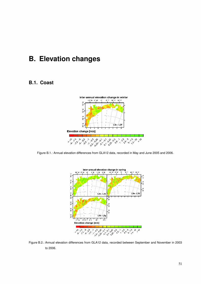
B. Elevation changes
B.1. Coast
Figure B.1.: Annual elevation differences from GLA12 data, recorded in May and June 2005 and 2006.
Figure B.2.: Annual elevation differences from GLA12 data, recorded between September and November in 2003
to 2006.
51

Figure B.3.: Annual elevation differences from GLA12 data, recorded between February and April in 2003 to 2007.
B.2. Plateau
Figure B.4.: Annual elevation differences from GLA12 data, recorded in May and June 2005 and 2006.
52

Figure B.5.: Annual elevation differences from GLA12 data, recorded between September and November in 2003
to 2006.
53

Figure B.6.: Annual elevation differences from GLA12 data, recorded between February and April in 2003 to 2007.
54

C. Maps of DML
Figure C.1.: The surface slopes in DML based on the improved DEM.
55
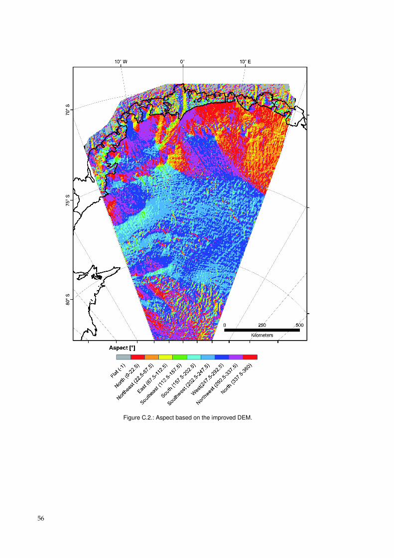
Figure C.2.: Aspect based on the improved DEM.
56

D. Publications
57


PAPER I
Surface topography and ice flow in the vicinity of the EDML
deep-drilling site, Antarctica
Published in Journal of Glaciology 2007, Vol. 153, No. 182, pages 442-448
Paper I is reprinted from the Journal of Glaciology with permission of the International Glaciological
society
59


Surface topography and ice flow in the vicinity of the EDMLdeep-drilling site, Antarctica
Christine WESCHE,1 Olaf EISEN,1,2 Hans OERTER,1 Daniel SCHULTE,1
Daniel STEINHAGE1
1Alfred Wegener Institute for Polar and Marine Research, PO Box 120161, D-27515 Bremerhaven, GermanyE-mail: [email protected]
2Laboratory of Hydraulics, Hydrology and Glaciology (VAW), ETH Zurich, CH-8092 Zurich, Switzerland
ABSTRACT. Interpretation of ice-core records requires accurate knowledge of the past and presentsurface topography and stress–strain fields. The European Project for Ice Coring in Antarctica (EPICA)drilling site (75.002588 S, 0.06848 E; 2891.7m) in Dronning Maud Land, Antarctica, is located in theimmediate vicinity of a transient and forking ice divide. A digital elevation model is determined from thecombination of kinematic GPS measurements with the GLAS12 datasets from the ICESat. Based on anetwork of stakes, surveyed with static GPS, the velocity field around the drilling site is calculated. Theannual mean velocity magnitude of 12 survey points amounts to 0.74ma–1. Flow directions mainly varyaccording to their distance from the ice divide. Surface strain rates are determined from a pentagon-shaped stake network with one center point close to the drilling site. The strain field is characterized byalong-flow compression, lateral dilatation and vertical layer thinning.
INTRODUCTIONWithin the framework of the European Project for Ice Coringin Antarctica (EPICA) a deep ice core (EDML) was drilled inDronning Maud Land (DML), Antarctica, near the Germansummer station, Kohnen (EPICA Community Members,2006). To obtain high-resolution climate information of thelast glacial cycle, a drilling site was chosen that providescomparatively high accumulation rates, large ice thicknessand nearly undisturbed layering of the ice. The EDMLdrilling site (75.00258 S, 0.06848 E; 2891.7m above theWorld Geodetic System 1984 (WGS84) ellipsoid) is locatedin the Atlantic sector of Antarctica (Fig. 1) and is used toinvestigate the connection between Northern and SouthernHemisphere climate variability in the past. The areasurrounding the EDML drilling site is situated between twotransient ice divides which fork at approximately 75.18 S,18 E, according to the elevation model of Bamber andBindschadler (1997). The deep ice-core drilling was carriedout in the austral summer seasons 2000/01 to 2005/06. Theice thickness in this region is 2782�5m, as measured byairborne radio-echo sounding, and the total recovered corelength was 2774.15m (personal communication fromF. Wilhelms, 2006). The drilling finished when subglacialwater entered the borehole. The recent accumulation rate inthe surroundings of the EDML drilling site is 64 kgm–2 a–1
(Eisen and others, 2005), with small-scale spatial variabilityof �10%.
Accurate interpretation of the EDML ice-core data (e.g.past accumulation from annual layer thicknesses) requiresknowledge of the complete strain field to correct for dynamiclayer thickness variation. In this paper, we determine thetopography, flow and strain field in the wider surroundings ofthe drilling site. Similar investigations were previously madeat several drilling sites in Antarctica and Greenland. Forexample, Vittuari and others (2004) present a velocity field atDome C (the first EPICA deep-drilling site (EPICA CommunityMembers, 2004)) in the Indo-Pacific sector of the Antarcticice sheet. In Greenland, Hvidberg and others (2002) investi-gated the ice flow at NorthGRIP, a drilling site that is also
located in the vicinity of a transient ice divide. For the EDMLsite, a digital elevation model (DEM) is derived from thecombination of ground-based kinematic GPS (global pos-itioning system) and ICESat (Ice, Cloud and land ElevationSatellite) laser altimetry, providing highly accurate surfacetopography in the region of interest. This forms, together withice velocity data, the basis for estimating and interpretingdeformation in the upper part of the ice sheet.
DATA AND METHODSStatic and kinematic GPS measurements were used for ourinvestigation. The elevation data derived from the kinematicGPS data were complemented by NASA’s ICESat satellitelaser altimetry data (US National Snow and Ice Data Center(NSIDC) http://nsidc.org/data/icesat/).
Kohnen Reference Station (KRS)Kohnen Reference Station (KRS), which is located at theGerman summer station Kohnen (75.00188 S, 0.06678 E), isused for processing our GPS measurements. This is a non-permanent GPS station, providing data at 1 s intervals onlyduring the drilling campaigns 2000/01 to 2005/06 (withinterruptions in the season 2004/05). The KRS GPS antennawas mounted on the northern corner of the Kohnen station.With the aid of the International Global Navigation SatelliteSystems Service (IGS) network, the daily position of KRSwas determined using the GPS stations Mawson, Sanae IV,Syowa, Davis, Casey and O’Higgins (Fig. 1). The KRSpositions were determined with the post-processing soft-ware GAMIT, assuming motion of the site was negligibleduring the processing window (Scripps Institution of Ocean-ography, http://sopac.ucsd.edu/processing/gamit/).
Surface profiles from kinematic GPS measurementsKinematic GPS measurements combined with ground-penetrating radar (GPR) recorded during the 2000/01 fieldcampaign (Eisen and others, 2005) form the basis forgenerating a DEM with a higher accuracy and resolution
Journal of Glaciology, Vol. 53, No. 182, 2007442
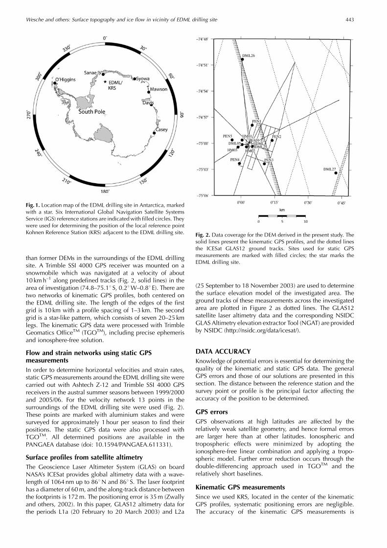
than former DEMs in the surroundings of the EDML drillingsite. A Trimble SSI 4000 GPS receiver was mounted on asnowmobile which was navigated at a velocity of about10 kmh–1 along predefined tracks (Fig. 2, solid lines) in thearea of investigation (74.8–75.18 S, 0.28W–0.88 E). There aretwo networks of kinematic GPS profiles, both centered onthe EDML drilling site. The length of the edges of the firstgrid is 10 km with a profile spacing of 1–3 km. The secondgrid is a star-like pattern, which consists of seven 20–25 kmlegs. The kinematic GPS data were processed with TrimbleGeomatics OfficeTM (TGOTM), including precise ephemerisand ionosphere-free solution.
Flow and strain networks using static GPSmeasurementsIn order to determine horizontal velocities and strain rates,static GPS measurements around the EDML drilling site werecarried out with Ashtech Z-12 and Trimble SSI 4000 GPSreceivers in the austral summer seasons between 1999/2000and 2005/06. For the velocity network 13 points in thesurroundings of the EDML drilling site were used (Fig. 2).These points are marked with aluminium stakes and weresurveyed for approximately 1 hour per season to find theirpositions. The static GPS data were also processed withTGOTM. All determined positions are available in thePANGAEA database (doi: 10.1594/PANGAEA.611331).
Surface profiles from satellite altimetryThe Geoscience Laser Altimeter System (GLAS) on boardNASA’s ICESat provides global altimetry data with a wave-length of 1064nm up to 868N and 868 S. The laser footprinthas a diameter of 60m, and the along-track distance betweenthe footprints is 172m. The positioning error is 35m (Zwallyand others, 2002). In this paper, GLAS12 altimetry data forthe periods L1a (20 February to 20 March 2003) and L2a
(25 September to 18 November 2003) are used to determinethe surface elevation model of the investigated area. Theground tracks of these measurements across the investigatedarea are plotted in Figure 2 as dotted lines. The GLAS12satellite laser altimetry data and the corresponding NSIDCGLAS Altimetry elevation extractor Tool (NGAT) are providedby NSIDC (http://nsidc.org/data/icesat/).
DATA ACCURACYKnowledge of potential errors is essential for determining thequality of the kinematic and static GPS data. The generalGPS errors and those of our solutions are presented in thissection. The distance between the reference station and thesurvey point or profile is the principal factor affecting theaccuracy of the position to be determined.
GPS errorsGPS observations at high latitudes are affected by therelatively weak satellite geometry, and hence formal errorsare larger here than at other latitudes. Ionospheric andtropospheric effects were minimized by adopting theionosphere-free linear combination and applying a tropo-spheric model. Further error reduction occurs through thedouble-differencing approach used in TGOTM and therelatively short baselines.
Kinematic GPS measurementsSince we used KRS, located in the center of the kinematicGPS profiles, systematic positioning errors are negligible.The accuracy of the kinematic GPS measurements is
Fig. 2. Data coverage for the DEM derived in the present study. Thesolid lines present the kinematic GPS profiles, and the dotted linesthe ICESat GLAS12 ground tracks. Sites used for static GPSmeasurements are marked with filled circles; the star marks theEDML drilling site.
Fig. 1. Location map of the EDML drilling site in Antarctica, markedwith a star. Six International Global Navigation Satellite SystemsService (IGS) reference stations are indicatedwith filled circles. Theywere used for determining the position of the local reference pointKohnen Reference Station (KRS) adjacent to the EDML drilling site.
Wesche and others: Surface topography and ice flow in vicinity of EDML drilling site 443

estimated by a crossover-point analysis. The histogram inFigure 3 shows the elevation differences at the 1615 cross-over points. The mean elevation difference is 0.03m with astandard deviation of 0.12m.
Static GPS measurementsAll stakes (Fig. 2) were occupied for an observation period of�1 hour in several campaigns. The length of the baselines toKRS varied between 0.03 km (BA01) and 19.4 km (DML27).The positions of all stakes were computed using TGOTM, andthe formal horizontal and vertical errors (Table 1) werederived for every point in a processing report. The formalerrors issued by GPS software are usually over-optimistic.Experience shows that these errors need to be scaled by afactor of 5–20, to be closer to the true uncertainty of thestatic GPS (personal communication from M. King, 2007).We take a factor of 20 as a conservative estimate of theprecision of the GPS positions. As the accuracy depends onthe baseline length, we use the points BA01 and DML27 toestimate the accuracy of the static GPS measurements.
The positions of these two points were calculated againstKRS for two campaigns. They have quite different horizontaland vertical errors, which can be attributed to the longer
baseline length between KRS and DML27. However, thereare also significant differences between campaigns for thesame point. For DML27, the horizontal and vertical errorsin 2002/03 are almost an order of magnitude larger than in2005/06. This may stem from the high sunspot activity in2002/03 (http://solarscience.msfc.nasa.gov/SunspotCycle.shtml) in combination with the baseline length, despiteusing the ionosphere-free solution of TGOTM. We assumethat the maximum horizontal and vertical errors for oursolutions are given by the values for DML27 of 0.30m and0.82m, respectively, from the campaign in 2002/03.
GLAS dataICESat’s positioning precision is stated as 35m and the pre-dicted elevation data accuracy is 0.15m (Zwally and others,2002). Shuman and others (2006) presented a new elevationaccuracy assessment of �0.02m for low-slope and clear-skyconditions. Our area of investigation is a low-slope region,but clouds during the observation period cannot beexcluded over the whole period. The elevation measure-ments of the ICESat laser altimeter refer to the TOPEX/Poseidon ellipsoid. Differences in elevation between theTOPEX/Poseidon ellipsoid and the WGS84 ellipsoid areapproximately 0.71m in the region of interest (personalcommunication from T. Haran, 2005). When transforming tothe WGS84 ellipsoid we subtract this value from all GLAS12elevation data.
RESULTSSurface topographyThe derived surface topography in the area of investigationrefers to the WGS84 ellipsoid and is a combination ofthe GPS and the GLAS12 datasets (Fig. 4, contours). Acrossover-point analysis was performed before combiningthe datasets to identify systematic offsets and to estimate theuncertainties. As crossover points for the GPS data we usethe average of all GPS measurements within the diameter ofthe GLAS footprint of about 60m. Considering all crossoverpoints, the GLAS12 data (transformed to the WGS84ellipsoid) are found to be 0.119m lower than the GPS data,on average. This elevation difference was added to theGLAS12 data, i.e. we corrected the elevations to the GPS
Table 1. Error estimates for BA01 and DML27
Point Campaign Horizontal1� � error�
Vertical1� � error�
Baselinelength
m m m
BA01 2002/03 0.01 0.04 29.4BA01 2005/06 0.01 0.02 29.7DML27 2002/03 0.30 0.82 19359.7DML27 2005/06 0.04 0.10 19358.9
�Based on formal errors issued by the GPS software, TGOTM, scaled by afactor of 20.
Fig. 3. Histogram of elevation differences at 1615 crossover pointsof the surveyed kinematic GPS profiles.
Table 2. Calculated mean annual horizontal ice-flow velocities
Point Magnitude Direction Period of averaging
ma–1 8
BA01 0.682 272.6 Jan. 2003–Dec. 2005DML05 0.660 270.4 Jan. 2001–Dec. 2005DML25 0.830 274.2 Jan. 2004–Dec. 2005DML26 1.066 335.9 Jan. 2001–Dec. 2005DML27 0.963 287.5 Feb. 2003–Dec. 2005HM01 0.642 273.7 Jan. 2000–Dec. 2005HM02 0.684 270.0 Jan. 2000–Dec. 2005HM03 0.674 266.6 Jan. 2000–Dec. 2005PEN1 0.643 291.3 Jan. 2000–Dec. 2005PEN2 0.767 282.9 Jan. 2000–Dec. 2005PEN3 0.859 265.9 Jan. 2000–Dec. 2005PEN4 0.841 257.9 Jan. 2000–Dec. 2005PEN5 0.624 269.8 Jan. 2000–Dec. 2005
Wesche and others: Surface topography and ice flow in vicinity of EDML drilling site444

profiles. To get sufficient spatial coverage of elevation dataover the whole area of investigation, we interpolated thecombined dataset with a minimum-curvature algorithm(Wessel and Smith, 1991) on a 5 km�5 km grid (Fig. 4).With this grid size, at least one data point was available foreach gridcell, even several tens of kilometers away from thedrilling site.
Surface velocityThe velocity magnitude at the survey points between the twoice divides varies between 0.62ma–1 (PEN5) and 0.96ma–1
(DML27). The flow direction varies between 257.98 (PEN4)and 291.38 (PEN1). The flow velocity of DML26, north of thedivide, is outside this range, moving in a direction of 335.98with a magnitude of 1.07ma–1 (Table 2; Fig. 4).
The location of the EDML drilling site was surveyed on10 January 2001, before the drilling operation started,yielding 75.00258 S, 0.0688 E and 2891.7m at the snowsurface. As excavation of the drill trench does not allowaccurate remeasurements, we use the mean velocities of thepoints next to it, DML25 and BA01. We thus obtain a valueof 0.756ma–1 in the direction of 273.48 for the ice velocityat the drilling site. The precision of the velocity measure-ments differs, depending on the period and data used (seeTable 1). We therefore perform a propagation of errors by
dv2 ¼ vsdsm
� �2þ v
tdt
� �2: ð1Þ
Only the horizontal errors are used; the vertical errors areneglected for calculating the propagated error (dv) of theannual movement. Here, v is the velocity magnitude and
s the horizontal offset of the survey point over the measure-ment interval (t ). The term dsm is the mean of the horizontalerrors for the survey point of the two campaigns used for thedetermination of the velocities. The time error, dt, is assumedto be a constant of 1 day (1/365.25 years), because the startand end time is rounded by the day. The resulting errors forsites DML27 and BA01 are 0.059 and 0.003ma–1, respect-ively. As discussed above, we take the error at DML27 as themaximum error of the velocity determination, as it has thelongest baseline.
Surface strain ratesStrain rates were determined from a pentagon-shapednetwork (PEN1–PEN5) with BA01 as the center referencepole (Fig. 5). Using the horizontal surface velocities inTable 2, with the geodetical nomenclature of y as theeastward and x as the northward components, we determinethe strain-rate components from (Paterson, 1994)
_"x ¼ �vx�x
, _"y ¼�vy�y
, ð2Þ
and the combined strain rate as
_"xy ¼ 12
�vx�y
þ�vy�x
� �, ð3Þ
where �vx and �vy are the differences of the x and yvelocity components of the considered pair of survey points,and �x and �y are the distances between the stakes in the xand y directions. Distances from the reference pole to eachpentagon point vary between 3961.85m (BA01–PEN5) and5173.28m (BA01–PEN3). Using Equation (3) the combinedsurface strain rate is calculated for every pair of neighboringpoints (west–east and south–north), yielding ten values(Table 3).
To determine the strain rates, we divide the pentagon intofive strain triangles (Fig. 5) and assume the strain is constantover the area of the triangle. We calculate the average of thestrain for each triangle (e.g. the mean of BA01/PEN1, BA01/PEN2 and PEN1/PEN2 for the northeastern triangle, num-bered 1). The principal components are calculated using the
Fig. 5. Velocity vectors of the pentagon-shaped network (PEN1–PEN5) and BA01. Strain ellipses are plotted for the five straintriangles, indicated by numbers 1–5. The mean strain ellipse(dotted) is centered on BA01. See text for the calculation of themean strain ellipse. The elevation contour interval is 2m.
Fig. 4. Surface flow-velocity vectors in the area of interest, plottedon the contour map of the combined and gridded (5 km� 5 km)GPS/GLAS12 elevation model. The contour interval is 2m. Thedotted curves indicate the ice divide corresponding to the DEM ofBamber and Bindschadler (1997).
Wesche and others: Surface topography and ice flow in vicinity of EDML drilling site 445
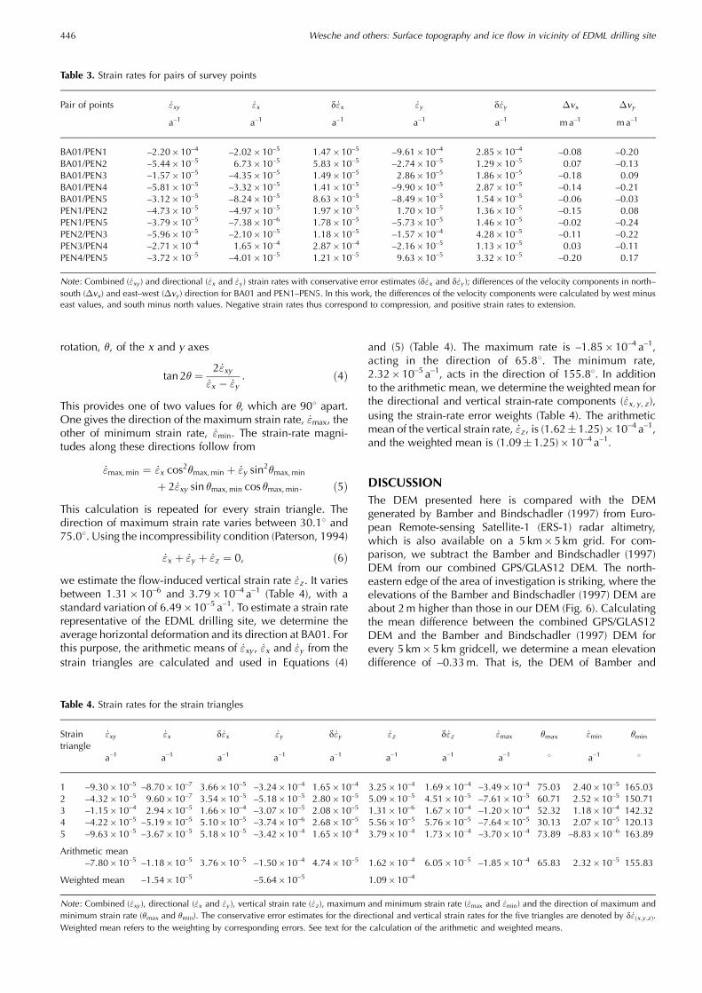
rotation, �, of the x and y axes
tan 2� ¼ 2 _"xy_"x � _"y
: ð4Þ
This provides one of two values for �, which are 908 apart.One gives the direction of the maximum strain rate, _"max, theother of minimum strain rate, _"min. The strain-rate magni-tudes along these directions follow from
_"max,min ¼ _"x cos2�max,min þ _"y sin2�max,min
þ 2 _"xy sin �max,min cos �max,min: ð5ÞThis calculation is repeated for every strain triangle. Thedirection of maximum strain rate varies between 30.18 and75.08. Using the incompressibility condition (Paterson, 1994)
_"x þ _"y þ _"z ¼ 0, ð6Þwe estimate the flow-induced vertical strain rate _"z . It variesbetween 1.31�10–6 and 3.79�10–4 a–1 (Table 4), with astandard variation of 6.49� 10–5 a–1. To estimate a strain raterepresentative of the EDML drilling site, we determine theaverage horizontal deformation and its direction at BA01. Forthis purpose, the arithmetic means of _"xy , _"x and _"y from thestrain triangles are calculated and used in Equations (4)
and (5) (Table 4). The maximum rate is –1.85�10–4 a–1,acting in the direction of 65.88. The minimum rate,2.32� 10–5 a–1, acts in the direction of 155.88. In additionto the arithmetic mean, we determine the weighted mean forthe directional and vertical strain-rate components ( _"x, y, z ),using the strain-rate error weights (Table 4). The arithmeticmean of the vertical strain rate, _"z , is (1.62� 1.25)�10–4 a–1,and the weighted mean is (1.09�1.25)� 10–4 a–1.
DISCUSSIONThe DEM presented here is compared with the DEMgenerated by Bamber and Bindschadler (1997) from Euro-pean Remote-sensing Satellite-1 (ERS-1) radar altimetry,which is also available on a 5 km� 5 km grid. For com-parison, we subtract the Bamber and Bindschadler (1997)DEM from our combined GPS/GLAS12 DEM. The north-eastern edge of the area of investigation is striking, where theelevations of the Bamber and Bindschadler (1997) DEM areabout 2m higher than those in our DEM (Fig. 6). Calculatingthe mean difference between the combined GPS/GLAS12DEM and the Bamber and Bindschadler (1997) DEM forevery 5 km�5 km gridcell, we determine a mean elevationdifference of –0.33m. That is, the DEM of Bamber and
Table 3. Strain rates for pairs of survey points
Pair of points _"xy _"x d _"x _"y d _"y �vx �vy
a–1 a–1 a–1 a–1 a–1 ma–1 ma–1
BA01/PEN1 –2.20� 10–4 –2.02�10–5 1.47�10–5 –9.61�10–4 2.85� 10–4 –0.08 –0.20BA01/PEN2 –5.44� 10–5 6.73�10–5 5.83�10–5 –2.74�10–5 1.29� 10–5 0.07 –0.13BA01/PEN3 –1.57� 10–5 –4.35�10–5 1.49�10–5 2.86�10–5 1.86� 10–5 –0.18 0.09BA01/PEN4 –5.81� 10–5 –3.32�10–5 1.41�10–5 –9.90�10–5 2.87� 10–5 –0.14 –0.21BA01/PEN5 –3.12� 10–5 –8.24�10–5 8.63�10–5 –8.49�10–5 1.54� 10–5 –0.06 –0.03PEN1/PEN2 –4.73� 10–5 –4.97�10–5 1.97�10–5 1.70�10–5 1.36� 10–5 –0.15 0.08PEN1/PEN5 –3.79� 10–5 –7.38�10–6 1.78�10–5 –5.73�10–5 1.46� 10–5 –0.02 –0.24PEN2/PEN3 –5.96� 10–5 –2.10�10–5 1.18�10–5 –1.57�10–4 4.28� 10–5 –0.11 –0.22PEN3/PEN4 –2.71� 10–4 1.65�10–4 2.87�10–4 –2.16�10–5 1.13� 10–5 0.03 –0.11PEN4/PEN5 –3.72� 10–5 –4.01�10–5 1.21�10–5 9.63�10–5 3.32� 10–5 –0.20 0.17
Note : Combined ( _"xy ) and directional ( _"x and _"y ) strain rates with conservative error estimates (d _"x and d _"y ); differences of the velocity components in north–south (�vx) and east–west (�vy) direction for BA01 and PEN1–PEN5. In this work, the differences of the velocity components were calculated by west minuseast values, and south minus north values. Negative strain rates thus correspond to compression, and positive strain rates to extension.
Table 4. Strain rates for the strain triangles
Straintriangle
_"xy _"x d _"x _"y d _"y _"z d _"z _"max �max _"min �min
a–1 a–1 a–1 a–1 a–1 a–1 a–1 a–1 8 a–1 8
1 –9.30�10–5 –8.70� 10–7 3.66�10–5 –3.24�10–4 1.65� 10–4 3.25�10–4 1.69� 10–4 –3.49�10–4 75.03 2.40� 10–5 165.032 –4.32�10–5 9.60� 10–7 3.54�10–5 –5.18�10–5 2.80� 10–5 5.09�10–5 4.51� 10–5 –7.61�10–5 60.71 2.52� 10–5 150.713 –1.15�10–4 2.94� 10–5 1.66�10–4 –3.07�10–5 2.08� 10–5 1.31�10–6 1.67� 10–4 –1.20�10–4 52.32 1.18� 10–4 142.324 –4.22�10–5 –5.19� 10–5 5.10�10–5 –3.74�10–6 2.68� 10–5 5.56�10–5 5.76� 10–5 –7.64�10–5 30.13 2.07� 10–5 120.135 –9.63�10–5 –3.67� 10–5 5.18�10–5 –3.42�10–4 1.65� 10–4 3.79�10–4 1.73� 10–4 –3.70�10–4 73.89 –8.83� 10–6 163.89
Arithmetic mean–7.80�10–5 –1.18� 10–5 3.76�10–5 –1.50�10–4 4.74� 10–5 1.62�10–4 6.05� 10–5 –1.85�10–4 65.83 2.32� 10–5 155.83
Weighted mean –1.54� 10–5 –5.64�10–5 1.09�10–4
Note : Combined ( _"xy ), directional ( _"x and _"y ), vertical strain rate ( _"z ), maximum and minimum strain rate ( _"max and _"min) and the direction of maximum andminimum strain rate (�max and �min). The conservative error estimates for the directional and vertical strain rates for the five triangles are denoted by d _" x;y;zð Þ.Weighted mean refers to the weighting by corresponding errors. See text for the calculation of the arithmetic and weighted means.
Wesche and others: Surface topography and ice flow in vicinity of EDML drilling site446

Bindschadler (1997) is about 0.3m higher than our com-bined GPS/GLAS12 DEM.
The topography in the region of interest shows a smoothsurface, slightly sloping down to the west. One major featureis a transient ice divide, which splits �20 km upstream of thedrilling location, thus separating three drainage basins. Ofour 13 survey points, 12 are located between the twobranches of the ice divide; only DML26 is located north ofboth ice branches (Fig. 4). As it represents a differentdrainage basin and flow regime, we exclude DML26 fromfurther analysis. The ice divide and the local surfaceelevation are the largest factors determining the flow andstrain field. This is evident from comparison of the meanslope direction at the drilling site with the mean flowdirection of 273.58 from the GPS-based velocity measure-ments. Small differences in magnitude and direction of thehorizontal ice-flow velocities of the survey points arelikewise mainly caused by the relative location of the surveypoint in respect to the ice divide. Points very close to the icedivide are generally slower and the direction of movement isnearly parallel to the course of the divide (Fig. 4 and Table 2,e.g. PEN1). The magnitude of the flow velocity increaseswith increasing distance from the divide, and the northwardflow component is reduced (Fig. 4; Table 2). An exception isPEN5, which has a slightly lower velocity (0.624ma–1) thanPEN1 (0.643ma–1) despite the greater distance from thedivide. Although this difference is smaller than the estimatedconservative maximum velocity error of 0.059ma–1, we tryto identify the origin of this variation.
Investigating the local bedrock topography in the vicinityof PEN5, available from airborne radio-echo soundings(Steinhage and others, 1999), PEN5 is found to be locatedabove a depression of the subglacial topography (Fig. 7). Thedepression is �5 km wide and several tens of meters deep,with respect to the surrounding average bedrock elevation.Because of the smoothing effect of ice dynamics, the surfaceelevation is much smoother than the bedrock topography.Surface topography varies only in the order of meters. Thedepression therefore simply causes locally increased icethickness, but not a significant feature at the surface. Theslightly lower velocity at PEN5, compared to the otherstakes, is thus a consequence of the flux balance required bythe larger ice thickness.
The surface strain rate at BA01, averaged from the straintriangles of the five pentagon points (PEN1–PEN5), isconsidered to be representative for the EDML ice core, asBA01 is only 93m to the northeast of the drilling site. Mosterror estimates for the strain rates (Tables 3 and 4) are aboutequal to or smaller than the nominal value of the strain rate.For some strain rates with very small nominal values, theerror is more than one order of magnitude larger (e.g. _"xtriangle 3, Table 4). We emphasize that the velocity errorsare very conservative estimates, so the strain-rate errors arealso conservative estimates. The average maximum principalcomponent of the strain rate at BA01 is negative (–1.85�10–4 a–1). It acts as a compressing force in the direction of65.88. The minimum principal component of the strain rateat BA01 is positive (2.32� 10–5 a–1). It therefore correspondsto a dilatational force and acts along an axis in the directionof 155.88. This results from the low magnitude of thevelocity at PEN5. Both BA01 and PEN2 (upstream of PEN5)are moving faster than PEN5, which induces the along-flowcompression of the ice mass. The average vertical strain rate,as calculated above, shows that the compression in thenorthwest–southeast direction only partly compensates thedilatational component of the strain field in the northeast–southwest direction, perpendicular to the ice flow at EDML,and layer thinning is required in the vertical component toachieve balance.
Fig. 6. Elevation differences of our GPS/GLAS12 DEM minus theBamber and Bindschadler (1997) DEM. The contour interval is 1m.Kinematic GPS and GLAS12 data coverage used in this paper(Fig. 2) are plotted as white dotted (GLAS12) and solid (GPS) lines.
Fig. 7. Subglacial topography of the area of investigation gridded ona 500m� 500m raster after Steinhage and others (1999). Thespacing between the contours is 50m. The dotted line representsthe ice divide corresponding to Bamber and Bindschadler (1997).
Wesche and others: Surface topography and ice flow in vicinity of EDML drilling site 447

CONCLUSIONWe provide an improved dataset for the surface topographyand flow velocity in the vicinity of the EDML drilling site. ADEM of high accuracy was derived from a combination ofkinematic surface GPS measurements and satellite laseraltimetry from ICESat’s GLAS12 data. Static GPS measure-ments at 13 stakes between the austral summer seasons1997/98 and 2005/06 provided the basis for deriving the flowvelocity field and resulting strain rates. The flow velocity fieldis, in general, divergent along the course of and in betweenthe two branches of the ice divide. On top of this generalfield, small velocity variations are superimposed, which arecaused by local variations in ice thickness resulting fromundulations in bedrock topography. The horizontal strainfield, calculated from the velocities, shows lateral extensionand smaller longitudinal compression. This results in layerthinning in the EDML ice core, which has to be accounted forto yield a correct interpretation of ice-core data.
ACKNOWLEDGEMENTSThe data of GPS reference stations were allocated byA. Rulke of the Institute for Planetary Geodesy of theTechnical University of Dresden (http://www.tu-dresden.de/ipg/). Satellite altimetry data were provided by the USNational Snow and Ice Data Center, Boulder, CO (http://nsidc.org/data/icesat/). The authors thank D. Jansen forhelpful discussions. This work is a contribution to theEuropean Project for Ice Coring in Antarctica (EPICA), a jointEuropean Science Foundation (ESF)/European Commission(EC) scientific program, funded by the EC and by nationalcontributions from Belgium, Denmark, France, Germany,Italy, The Netherlands, Norway, Sweden, Switzerland andthe UK. The main logistic support at Dronning Maud Landwas provided by AWI. This is EPICA publication No. 177.
Preparation of this work was supported by DeutscheForschumgsgemeinschaft with the ‘Emmy Noether’ scholar-ship EI-672/1 to O.E. This paper was enhanced significantlyby the comments of M. King, R. Jacobel and R. Bindschadler.
REFERENCESBamber, J.L. and R.A. Bindschadler. 1997. An improved elevation
dataset for climate and ice-sheet modelling: validation withsatellite imagery. Ann. Glaciol., 25, 439–444.
Eisen, O., W. Rack, U. Nixdorf and F. Wilhelms. 2005. Character-istics of accumulation around the EPICA deep-drilling site inDronning Maud Land, Antarctica. Ann. Glaciol., 41, 41–56.
EPICA Community Members. 2004. Eight glacial cycles from anAntarctic ice core. Nature, 429(6992), 623–628.
EPICA Community Members. 2006. One-to-one coupling of glacialclimate variability in Greenland and Antarctica. Nature,444(7116), 195–198.
Hvidberg, C.S., K. Keller and N.S. Gundestrup. 2002. Mass balanceand ice flow along the north-northwest ridge of the Greenlandice sheet at NorthGRIP. Ann. Glaciol., 35, 521–526.
Paterson, W.S.B. 1994. The physics of glaciers. Third edition.Oxford, etc., Elsevier.
Shuman, C.A. and 6 others. 2006. ICESat Antarctic elevation data:preliminary precision and accuracy assessment. Geophys. Res.Lett., 33(L7), L07501. (10.1029/2005GL025227.)
Steinhage, D., U. Nixdorf, U. Meyer and H. Miller. 1999. Newmaps of the ice thickness and subglacial topography inDronning Maud Land, Antarctica, determined by means ofairborne radio-echo sounding. Ann. Glaciol., 29, 267–272.
Vittuari, L. and 6 others. 2004. Space geodesy as a tool formeasuring ice surface velocity in the Dome C region and alongthe ITASE traverse. Ann. Glaciol., 39, 402–408.
Wessel, P. and W.H.F. Smith. 1991. Free software helps map anddisplay data. Eos, 72(41), 441, 445–446.
Zwally, H.J. and 15 others. 2002. ICESat’s laser measurements ofpolar ice, atmosphere, ocean and land. J. Geodyn., 34(3–4),405–445.
MS received 26 October 2006 and accepted in revised form 15 April 2007
Wesche and others: Surface topography and ice flow in vicinity of EDML drilling site448

PAPER II
Precise surface topography at the Ekstromisen, Antarctica, based
on several geophysical data sets
ISPRS Journal of Photogrammetry and Remote Sensing, accepted
69

Precise surface topography of the grounded ice
tongues at the Ekstromisen, Antarctica, based on
several geophysical data sets
C. Wesche ∗, S. Riedel, D. Steinhage
Alfred Wegener Institute for Polar and Marine Research Bremerhaven, Germany
Abstract
As part of the CryoSat Cal/Val activities and the pre-site survey for an ice core
drilling contributing to the International Partnerships in Ice Core Sciences (IPICS),
ground based kinematic GPS measurements were conducted in early 2007 in the
vicinity of the German overwintering station Neumayer (8.25° W and 70.65° S).
The investigated area comprises the regions of the ice tongues Halvfarryggen and
Sørasen, which rise from the Ekstromisen to a maximum of about 760 m surface
elevation, and have an areal extent of about 100 km x 50 km each. Available digital
elevation models (DEMs) from radar altimetry and the Antarctic Digital Database
show elevation differences of up to hundreds of meters in this region, which ne-
cessitated an accurate survey of the conditions on-site. An improved DEM of the
Ekstromisen surroundings is derived by a combination of highly accurate ground
based GPS measurements, satellite derived laser altimetry data (ICESat), airborne
radar altimetry (ARA), and radio echo sounding (RES). The DEM presented here
achieves a vertical accuracy of about 1.3 m and can be used for improved ice dy-
namic modeling and mass balance studies.
Key words: GPS, ICESat, radar altimetry
Preprint submitted to Journal of Photogrammetry and Remote Sensing11 April 2008
1 Introduction
Ice sheets play a major role in the climate system and changes in their mass
balance affect the global sea level. Currently, the absolute mass balances of
the ice sheets are only slightly above the measurement uncertainties and
changes in mass balance may even be below the precision of the measure-
ments (Wingham et al., 1998; Abdalati et al., 2002; Zwally et al., 2002). The
Antarctic ice sheet covers an area of about 12.4×10⁶ km2 with an average
ice thickness of about 2.4 km (Massom and Lubin, 2006). The steep margins
of the Antarctic ice sheet form the transition zone between the grounded
flat interior and the floating ice shelves which are very sensitive for cli-
mate variability. The knowledge of the surface topography of the Antarc-
tic ice sheet is an important input parameter for ice dynamic modeling
and mass balance studies. Recent mass balance studies (Alley et al., 2007;
Krinner et al., 2007) and ice dynamic modeling (Bamber and Huybrechts,
1996; Huybrechts et al., 2000) use digital elevation models (DEMs) derived
from satellite and airborne altimetry. For the grounded part of Dronning
Maud Land (DML), these models are not in agreement with each other, at
least in coastal Dronning Maud Land (DML).
The area of investigation comprises the two grounded ice tongues of Halv-
farryggen and Sørasen (Fig. 1) surrounding the Ekstromisen and reaches
inland up to 72.3° S. In the past, this region has been rarely surveyed by
∗ Corresponding author.Email address: [email protected] (D. Steinhage).
2
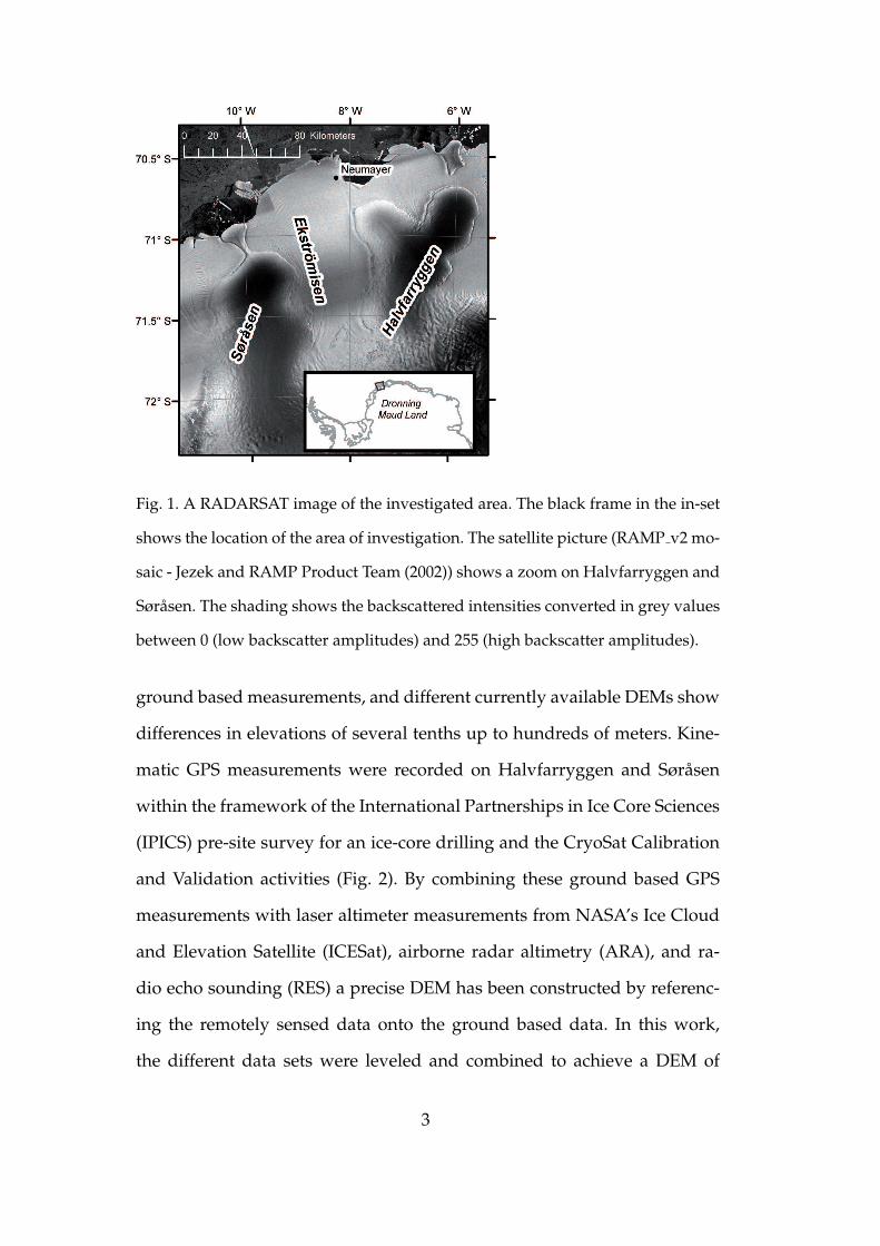
Fig. 1. A RADARSAT image of the investigated area. The black frame in the in-set
shows the location of the area of investigation. The satellite picture (RAMP v2 mo-
saic - Jezek and RAMP Product Team (2002)) shows a zoom on Halvfarryggen and
Sørasen. The shading shows the backscattered intensities converted in grey values
between 0 (low backscatter amplitudes) and 255 (high backscatter amplitudes).
ground based measurements, and different currently available DEMs show
differences in elevations of several tenths up to hundreds of meters. Kine-
matic GPS measurements were recorded on Halvfarryggen and Sørasen
within the framework of the International Partnerships in Ice Core Sciences
(IPICS) pre-site survey for an ice-core drilling and the CryoSat Calibration
and Validation activities (Fig. 2). By combining these ground based GPS
measurements with laser altimeter measurements from NASA’s Ice Cloud
and Elevation Satellite (ICESat), airborne radar altimetry (ARA), and ra-
dio echo sounding (RES) a precise DEM has been constructed by referenc-
ing the remotely sensed data onto the ground based data. In this work,
the different data sets were leveled and combined to achieve a DEM of
3

the area of investigation. The extent of the ice tongues was defined us-
ing the grounding line derived from SAR interferometry (pers. comm. R.
Drews, 2007). For the north-east flank of Halvfarryggen, the grounding line
(dashed grey line) was taken from the Antarctic Digital Database 4.0 (ADD4
- http://www.add.scar.org). To evaluate the quality of the new DEM, a
comparison with already existing DEMs is shown later beside a crossover
analysis of the various leveled input data.
2 Data and Methods
2.1 Kinematic GPS measurements
The kinematic GPS measurements were recorded during the field cam-
paign in January and February of 2007. A Trimble SSI 4000 GPS receiver
was mounted on a snow vehicle which was navigated along predefined
tracks at a velocity between 10 and 12 km h-1 (Fig. 2 - black lines). Using 1 s
observation intervals, the along track distance between the data points is
approximately 3 m, which is slightly larger than the length of the vehicle.
All kinematic GPS measurements were processed using local reference sta-
tions (Tab. 1). The local reference stations (DML94 to DML97, Tab. 1) were
non-permanent GPS stations, which provided reference data with a record-
ing interval of 1 s only for local survey period. The position of each local
reference station was determined with the aid of the International GNSS
Service (IGS) network data and commercial post-processing software, in-
cluding precise ephemerides, and the ionosphere-free solution. In order to
check the stationarity of the local reference stations, a kinematic process-
4
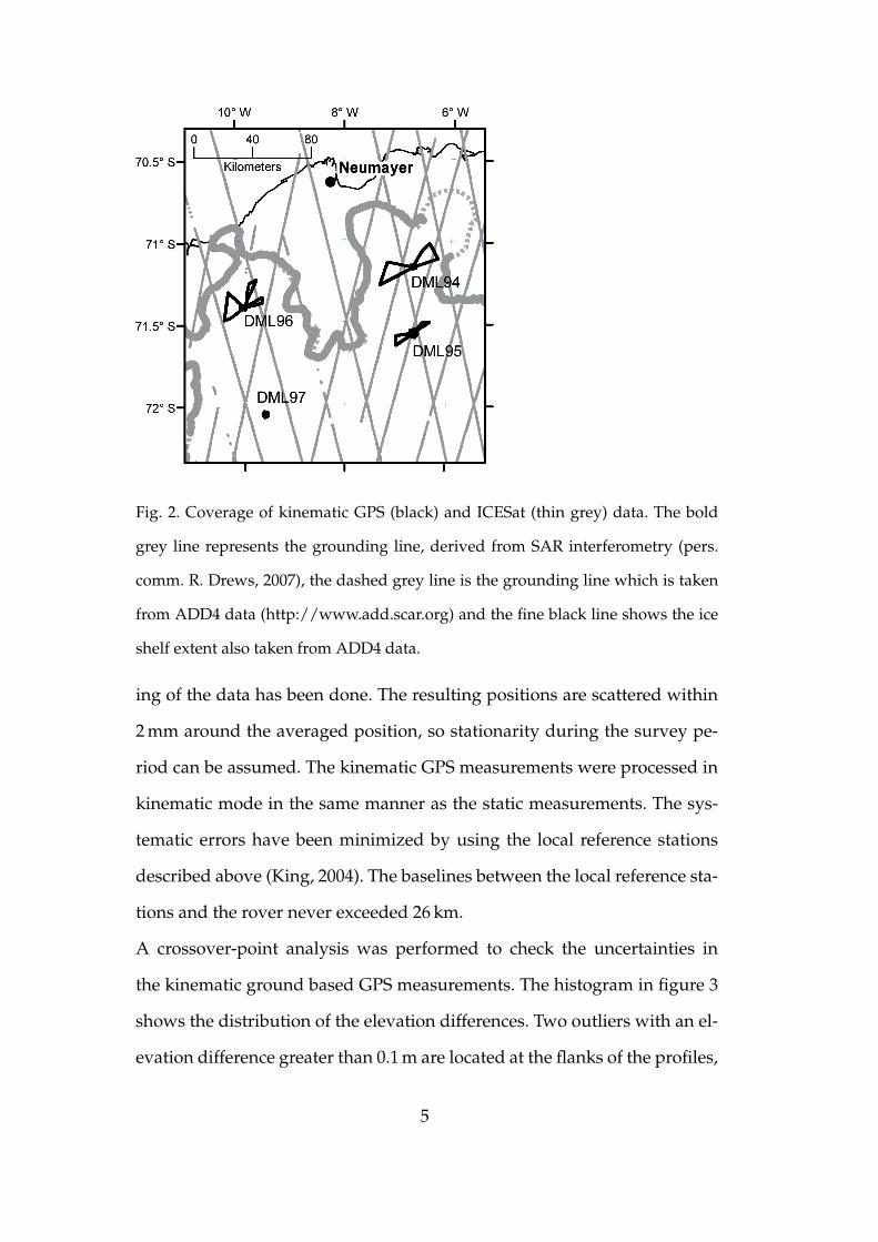
Fig. 2. Coverage of kinematic GPS (black) and ICESat (thin grey) data. The bold
grey line represents the grounding line, derived from SAR interferometry (pers.
comm. R. Drews, 2007), the dashed grey line is the grounding line which is taken
from ADD4 data (http://www.add.scar.org) and the fine black line shows the ice
shelf extent also taken from ADD4 data.
ing of the data has been done. The resulting positions are scattered within
2 mm around the averaged position, so stationarity during the survey pe-
riod can be assumed. The kinematic GPS measurements were processed in
kinematic mode in the same manner as the static measurements. The sys-
tematic errors have been minimized by using the local reference stations
described above (King, 2004). The baselines between the local reference sta-
tions and the rover never exceeded 26 km.
A crossover-point analysis was performed to check the uncertainties in
the kinematic ground based GPS measurements. The histogram in figure 3
shows the distribution of the elevation differences. Two outliers with an el-
evation difference greater than 0.1 m are located at the flanks of the profiles,
5
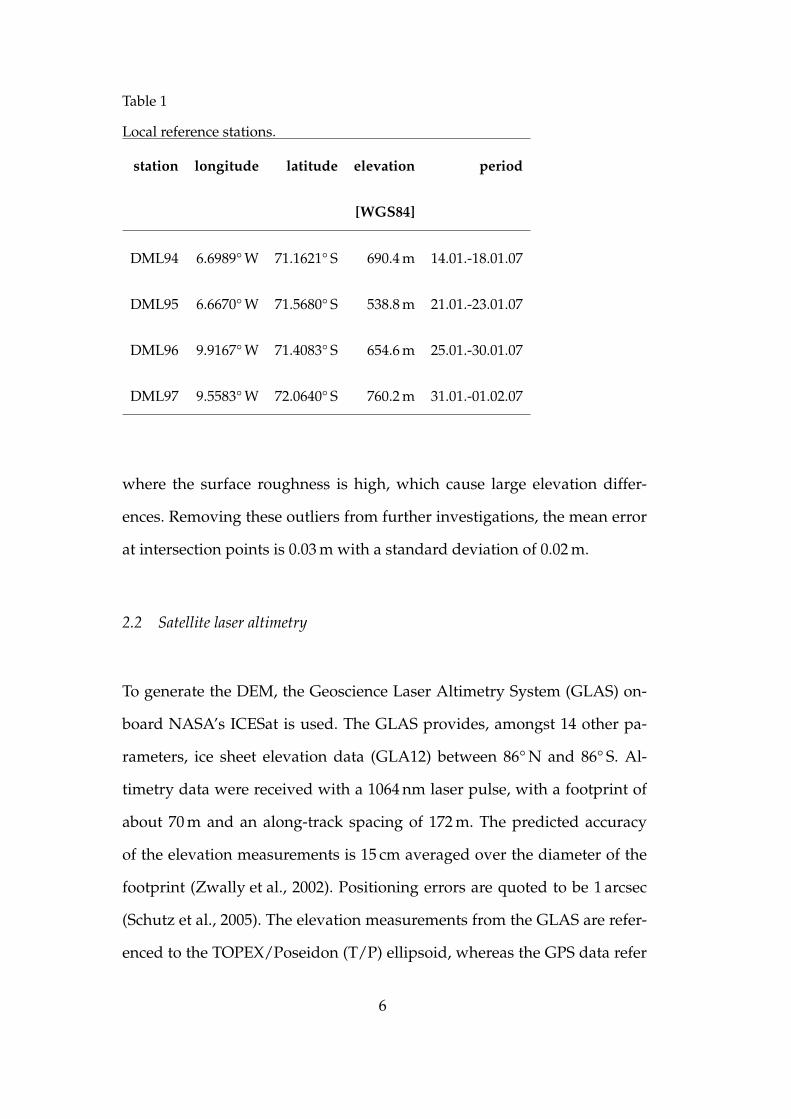
Table 1
Local reference stations.
station longitude latitude elevation period
[WGS84]
DML94 6.6989° W 71.1621° S 690.4 m 14.01.-18.01.07
DML95 6.6670° W 71.5680° S 538.8 m 21.01.-23.01.07
DML96 9.9167° W 71.4083° S 654.6 m 25.01.-30.01.07
DML97 9.5583° W 72.0640° S 760.2 m 31.01.-01.02.07
where the surface roughness is high, which cause large elevation differ-
ences. Removing these outliers from further investigations, the mean error
at intersection points is 0.03 m with a standard deviation of 0.02 m.
2.2 Satellite laser altimetry
To generate the DEM, the Geoscience Laser Altimetry System (GLAS) on-
board NASA’s ICESat is used. The GLAS provides, amongst 14 other pa-
rameters, ice sheet elevation data (GLA12) between 86° N and 86° S. Al-
timetry data were received with a 1064 nm laser pulse, with a footprint of
about 70 m and an along-track spacing of 172 m. The predicted accuracy
of the elevation measurements is 15 cm averaged over the diameter of the
footprint (Zwally et al., 2002). Positioning errors are quoted to be 1 arcsec
(Schutz et al., 2005). The elevation measurements from the GLAS are refer-
enced to the TOPEX/Poseidon (T/P) ellipsoid, whereas the GPS data refer
6
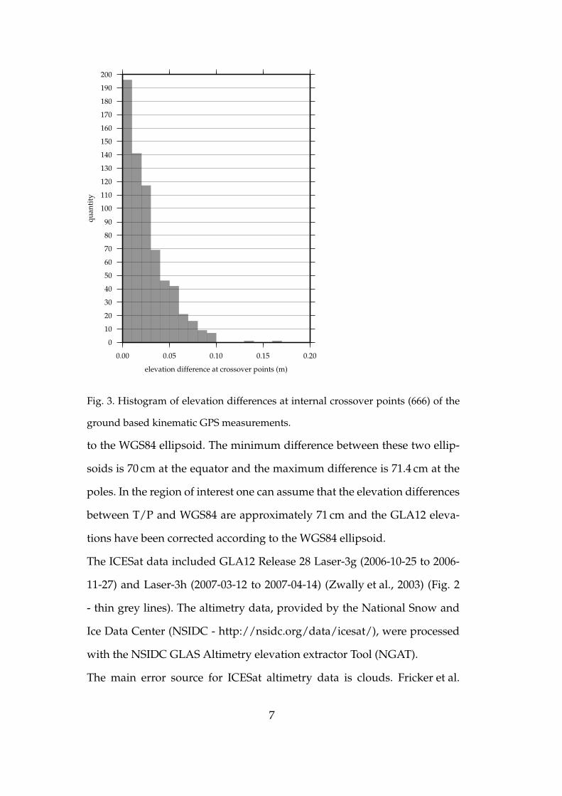
0
10
20
30
40
50
60
70
80
90
100
110
120
130
140
150
160
170
180
190
200
qu
an
tity
0.00 0.05 0.10 0.15 0.20
elevation difference at crossover points (m)
Fig. 3. Histogram of elevation differences at internal crossover points (666) of the
ground based kinematic GPS measurements.
to the WGS84 ellipsoid. The minimum difference between these two ellip-
soids is 70 cm at the equator and the maximum difference is 71.4 cm at the
poles. In the region of interest one can assume that the elevation differences
between T/P and WGS84 are approximately 71 cm and the GLA12 eleva-
tions have been corrected according to the WGS84 ellipsoid.
The ICESat data included GLA12 Release 28 Laser-3g (2006-10-25 to 2006-
11-27) and Laser-3h (2007-03-12 to 2007-04-14) (Zwally et al., 2003) (Fig. 2
- thin grey lines). The altimetry data, provided by the National Snow and
Ice Data Center (NSIDC - http://nsidc.org/data/icesat/), were processed
with the NSIDC GLAS Altimetry elevation extractor Tool (NGAT).
The main error source for ICESat altimetry data is clouds. Fricker et al.
7
(2005) show that the quality of ICESat measurements with the 1064 nm laser
is highly degraded by cloudy conditions, because the infrared laser pulses
were unable to penetrate clouds. The GLA12 data used here were split into
ascending and descending ground tracks. A simple script is used, to find
and remove elevation leaps greater than 50 m comparing neighbouring data
points along track with a maximum space of 500 m between each other. Af-
terwards, an additional visual check was made. Hence, the cloud degrading
factor can be barred from this investigation.
Another accuracy degrading feature is the surface slopes in the region of in-
terest. A 2° slope, combined with the 1 arcsec positioning error results in an
elevation error of 10 cm (Martin et al., 2005). Based on the new DEM pre-
sented here, the slopes at Halvfarryggen and Sørasen were calculated for
1 km x 1 km grid cells. The GLA12 data were recorded over a mean slope
of 0.77° and 77 % of the data points were recorded over slopes smaller than
1°. According to this the slope induced error is between 4 and 5 cm, which
has to be added to the predicted elevation accuracy of 15 cm of Zwally et al.
(2002). Therefore, the predicted elevation accuracy is about 20 cm on aver-
age.
After the cloud correction, crossover-point analyses within and between the
various GLA12 laser measurement periods were performed. The arithmetic
means of the absolute elevation differences at crossover points of the laser
periods are 0.24 m (L3g) and 0.22 m (L3h). For determining the accuracy of a
combined GLA12 elevation data set, the number of crossover points, which
were involved in determining the arithmetic means above, were used to
calculate a weighting factor. The weighted mean of the arithmetic means
is calculated, resulting in a crossover error of 0.23 m. For further investiga-
tions, the mean of elevations at crossover point is used.
8

Fig. 4. Coverage of the ARA (black) and RES (thin grey) data. The bold grey line
represents the grounding line, derived from SAR interferometry (pers. comm. R.
Drews, 2007) and the dashed grey line is the grounding line which is taken from
ADD4 data (http://www.add.scar.org) and the fine black line shows the ice shelf
extent also taken from ADD4 data.
2.3 Airborne radar altimetry and radio echo sounding
Airborne kinematic GPS combined with ARA and RES provides almost
complete coverage for DML. In order to generate a reference DEM of the
grounded ice surrounding the Ekstromisen, data from several campaigns
(1998/99 to 2004/05 - Fig. 4) were used. The AWI research aircraft POLAR2
is equipped with Trimble SSI 4000 GPS receivers, a HONEYWELL AA-300
radar altimeter (4.3 GHz carrier frequency - ARA) and a RES system op-
erating at 150 MHz, which was specially designed for the use in polar re-
gions (Nixdorf et al., 1999). For generating an elevation model, available
post-processed airborne kinematic GPS and ARA data from the campaigns
9
1998/99 and 2000/01 were used. For this purpose, the radar altimeter data
were corrected with regard to the attitude of the aircraft using a modi-
fied Airborne SAR Interferometric Altimeter System (ASIRAS) processor
(pers. comm. V. Helm, 2006). The derived flight altitude of the aircraft was
then subtracted from the GPS height. A crossover-point analysis was per-
formed and results in a mean elevation precision of the ARA measurements
of 0.44 m.
On the campaigns for the ”Validation, densification, and Interpretation of
Satellite data in Antarctica using airborne and groundborne measurements
for the determination of gravity field, magnetic field, ice-mass balance, and
crustal structure” (VISA) 2001/02 to 2004/05, (see Fig.4), the ARA could
not be applied due to the flight level of about 4000 m of the aircraft (the
HONEYWELL radar altimeter has an operation altitude of 0 to 760 m above
ground). In these cases data from surface reflections of the ice thickness
measurements of the RES data were used. A detailed description of the
RES equipment is given in Nixdorf et al. (1999). The absolute position of
the aircraft is determined from post-processed kinematic GPS data. The
distance from the RES antenna to the surface was determined by the on-
set of the reflected electromagnetic wave (Steinhage et al., 2001) and was
then subtracted from the GPS height to obtain the surface topography. This
calculation was done for every campaign and by means of crossover-point
analyses, the data were leveled to minimize elevation branches between the
different campaigns. Afterwards, a second crossover-point analysis of the
leveled RES data over grounded ice was made, and an elevation uncertainty
of 0.60 m was obtained.
10
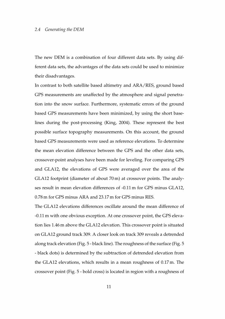
2.4 Generating the DEM
The new DEM is a combination of four different data sets. By using dif-
ferent data sets, the advantages of the data sets could be used to minimize
their disadvantages.
In contrast to both satellite based altimetry and ARA/RES, ground based
GPS measurements are unaffected by the atmosphere and signal penetra-
tion into the snow surface. Furthermore, systematic errors of the ground
based GPS measurements have been minimized, by using the short base-
lines during the post-processing (King, 2004). These represent the best
possible surface topography measurements. On this account, the ground
based GPS measurements were used as reference elevations. To determine
the mean elevation difference between the GPS and the other data sets,
crossover-point analyses have been made for leveling. For comparing GPS
and GLA12, the elevations of GPS were averaged over the area of the
GLA12 footprint (diameter of about 70 m) at crossover points. The analy-
ses result in mean elevation differences of -0.11 m for GPS minus GLA12,
0.78 m for GPS minus ARA and 23.17 m for GPS minus RES.
The GLA12 elevations differences oscillate around the mean difference of
-0.11 m with one obvious exception. At one crossover point, the GPS eleva-
tion lies 1.46 m above the GLA12 elevation. This crossover point is situated
on GLA12 ground track 309. A closer look on track 309 reveals a detrended
along track elevation (Fig. 5 - black line). The roughness of the surface (Fig. 5
- black dots) is determined by the subtraction of detrended elevation from
the GLA12 elevations, which results in a mean roughness of 0.17 m. The
crossover point (Fig. 5 - bold cross) is located in region with a roughness of
11
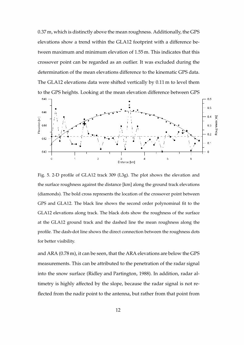
0.37 m, which is distinctly above the mean roughness. Additionally, the GPS
elevations show a trend within the GLA12 footprint with a difference be-
tween maximum and minimum elevation of 1.55 m. This indicates that this
crossover point can be regarded as an outlier. It was excluded during the
determination of the mean elevations difference to the kinematic GPS data.
The GLA12 elevations data were shifted vertically by 0.11 m to level them
to the GPS heights. Looking at the mean elevation difference between GPS
Fig. 5. 2-D profile of GLA12 track 309 (L3g). The plot shows the elevation and
the surface roughness against the distance [km] along the ground track elevations
(diamonds). The bold cross represents the location of the crossover point between
GPS and GLA12. The black line shows the second order polynominal fit to the
GLA12 elevations along track. The black dots show the roughness of the surface
at the GLA12 ground track and the dashed line the mean roughness along the
profile. The dash-dot line shows the direct connection between the roughness dots
for better visibility.
and ARA (0.78 m), it can be seen, that the ARA elevations are below the GPS
measurements. This can be attributed to the penetration of the radar signal
into the snow surface (Ridley and Partington, 1988). In addition, radar al-
timetry is highly affected by the slope, because the radar signal is not re-
flected from the nadir point to the antenna, but rather from that point from
12

the surface, which is nearest to the antenna (Brenner et al., 1983). For this
reason the ARA data were filtered for slopes larger than 1.5 °.
The HONEYWELL radar altimeter of the aircraft has a maximum squint an-
gle of 6° in flight direction and this causes a divergence between true and
measured elevation at the position of the aircraft. In case the flight direction
is inland with increasing elevations, the radar altimeter looks uphill. This
results in an error in determining the vertical distance of the aircraft at a
particular position to the ground and an error in determining the elevation
at this point. If the flight direction is from grounded to floating ice with de-
creasing elevations, the radar altimeter looks downhill, which results also
in large elevation differences.
The elevation differences between GPS and RES data are much larger
(23.17 m) than between GPS and ARA data. This is simply due to the fact,
that the electromagnetic waves of the RES penetrate deeper into the firn
than the higher frequency signal of the ARA (Hofer and Matzler, 1980).
Other limiting factors are on the one hand the small-scale variability in sur-
face properties, which also changes the penetration depth of the signal, and
on the other hand the subjective definition of the onset of the surface re-
flectance signal. These two factors affect the elevation accuracy, but to a
minor degree than the penetration depth in total. Both, ARA and RES were
leveled to the GPS measurements by the determined mean elevation differ-
ences (0.78 m for ARA and 23.17 m for RES).
After these corrections, all data sets were combined into one. The evalua-
tion of crossover points of different periods of GLA12 measurements do not
reveal any temporary trend. Therefore, the elevations of the ARA and RES
were leveled to the ground based GPS elevations even though they have
been acquired in different austral summer seasons. The final data set was
13
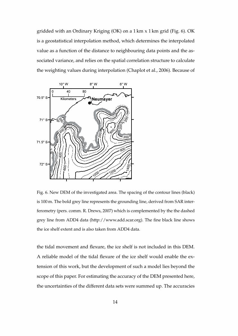
gridded with an Ordinary Kriging (OK) on a 1 km x 1 km grid (Fig. 6). OK
is a geostatistical interpolation method, which determines the interpolated
value as a function of the distance to neighbouring data points and the as-
sociated variance, and relies on the spatial correlation structure to calculate
the weighting values during interpolation (Chaplot et al., 2006). Because of
Fig. 6. New DEM of the investigated area. The spacing of the contour lines (black)
is 100 m. The bold grey line represents the grounding line, derived from SAR inter-
ferometry (pers. comm. R. Drews, 2007) which is complemented by the the dashed
grey line from ADD4 data (http://www.add.scar.org). The fine black line shows
the ice shelf extent and is also taken from ADD4 data.
the tidal movement and flexure, the ice shelf is not included in this DEM.
A reliable model of the tidal flexure of the ice shelf would enable the ex-
tension of this work, but the development of such a model lies beyond the
scope of this paper. For estimating the accuracy of the DEM presented here,
the uncertainties of the different data sets were summed up. The accuracies
14
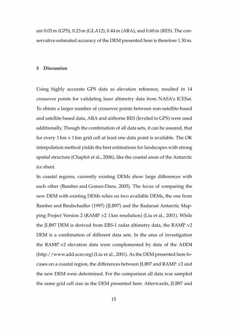
are 0.03 m (GPS), 0.23 m (GLA12), 0.44 m (ARA), and 0.60 m (RES). The con-
servative estimated accuracy of the DEM presented here is therefore 1.30 m.
3 Discussion
Using highly accurate GPS data as elevation reference, resulted in 14
crossover points for validating laser altimetry data from NASA’s ICESat.
To obtain a larger number of crossover points between non-satellite-based
and satellite based data, ARA and airborne RES (leveled to GPS) were used
additionally. Though the combination of all data sets, it can be assured, that
for every 1 km x 1 km grid cell at least one data point is available. The OK
interpolation method yields the best estimations for landscapes with strong
spatial structure (Chaplot et al., 2006), like the coastal areas of the Antarctic
ice sheet.
In coastal regions, currently existing DEMs show large differences with
each other (Bamber and Gomez-Dans, 2005). The focus of comparing the
new DEM with existing DEMs relies on two available DEMs, the one from
Bamber and Bindschadler (1997) (JLB97) and the Radarsat Antarctic Map-
ping Project Version 2 (RAMP v2 1 km resolution) (Liu et al., 2001). While
the JLB97 DEM is derived from ERS-1 radar altimetry data, the RAMP v2
DEM is a combination of different data sets. In the area of investigation
the RAMP v2 elevation data were complemented by data of the ADD4
(http://www.add.scar.org) (Liu et al., 2001). As the DEM presented here fo-
cuses on a coastal region, the differences between JLB97 and RAMP v2 and
the new DEM were determined. For the comparison all data was sampled
the same grid cell size as the DEM presented here. Afterwards, JLB97 and
15
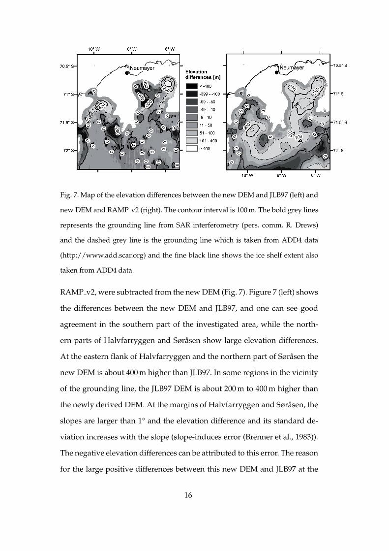
Fig. 7. Map of the elevation differences between the new DEM and JLB97 (left) and
new DEM and RAMP v2 (right). The contour interval is 100 m. The bold grey lines
represents the grounding line from SAR interferometry (pers. comm. R. Drews)
and the dashed grey line is the grounding line which is taken from ADD4 data
(http://www.add.scar.org) and the fine black line shows the ice shelf extent also
taken from ADD4 data.
RAMP v2, were subtracted from the new DEM (Fig. 7). Figure 7 (left) shows
the differences between the new DEM and JLB97, and one can see good
agreement in the southern part of the investigated area, while the north-
ern parts of Halvfarryggen and Sørasen show large elevation differences.
At the eastern flank of Halvfarryggen and the northern part of Sørasen the
new DEM is about 400 m higher than JLB97. In some regions in the vicinity
of the grounding line, the JLB97 DEM is about 200 m to 400 m higher than
the newly derived DEM. At the margins of Halvfarryggen and Sørasen, the
slopes are larger than 1° and the elevation difference and its standard de-
viation increases with the slope (slope-induces error (Brenner et al., 1983)).
The negative elevation differences can be attributed to this error. The reason
for the large positive differences between this new DEM and JLB97 at the
16
east flank of Halvfarryggen and Sørasen can not be explained.
In figure 7 (right) RAMP v2 DEM was subtracted from the newly derived
DEM. The highest differences are about 300 m in large parts of Halvfar-
ryggen and the southern part of Sørasen. The new DEM and RAMP v2
agree only with each other in small parts of the grounded ice in the
south of the investigated area. As mentioned before, in the region of in-
terest the RAMP v2 DEM is supplemented with ADD4 data (Liu et al.,
2001). Bamber and Gomez-Dans (2005) compared the RAMP v2 DEM with
GLA12 and found, that the errors in the coastal regions of the ice sheet are
in the order of ± 100 m. This investigation shows, that the discrepancies are
even more, between -200 m to 300 m.
4 Conclusion
The usage of remote sensing data (especially for altimetry) requires ground
based data for validation. The coastal regions of the Antarctic continent
are not well covered with ground based elevation measurements, but in
combination with airborne data, reliable reference measurements for satel-
lite data are available. The new DEM is a combination of ground based
GPS measurements, airborne, and satellite altimetry. By combining differ-
ent data sets the inherent errors of the single data sets can be reduced by
taking advantage of the unique features of the individual data sets, and an
accurate DEM can be constructed.
Airborne and satellite data have to be validated with ground based mea-
surements, especially in sloped regions, where airborne and satellite al-
timetry is imprecise due to the prevailing surface slopes. A combination
17

of ground based measurements with remote sensing data provides suffi-
cient data coverage for the construction of a reliable digital elevation model
of the surface topography.
Comparisons with already existing DEMs show large elevation differences
on Halvfarryggen and Sørasen. Current available DEMs do not provide the
accuracy requirements for reliable ice sheet modeling, because they show
very high elevation differences with each other in coastal regions. By using
highly accurate ground based GPS data as true reference elevations, the ap-
proximation of the real surface of the DEM presented here is much higher
than at the RAMP v2 DEM. JLB97 shows, apart from Halvfarryggen and
Sørasen, a very good agreement with the new DEM.
The aim is to generate an accurate DEM of whole DML from geophysical
data sets. Both mass balance studies and ice dynamic modeling with respect
to the sea level change and paleoclimatic reconstruction, will benefit from
the in the future derived and improved surface topography.
5 Acknowledgement
The authors thank Dr. Doris and Martin Bertges for their support. Prepara-
tion of this work was supported by the Bundesministerium fur Wirtschaft
(BMWi) through the CryoVEx activities 50EE0505. The airborne data
mapped within the VISA project were supported by Deutsche Forschungs-
gemeinschaft (DFG), founded under grants Di 473/17-1 and Jo 191/8-1.
Thanks to the National Snow and Ice Data Center (NSIDC) for providing
the ICESat data, the NGAT elevation extraction tool and the RAMP v2 data.
18

The authors also thank the editor O. Hellwich and the two anonymous re-
viewers for their helpful comments.
References
Abdalati, W., Krabill, W., Frederick, E., Manizade, S., Martin, C., Sonntag,
J., Swift, R., Thomas, R., Wright, W., Yungel, J., 2002. Airborne laser al-
timetry mapping of the Greenland ice sheet: application to mass balance
assessment. Journal of Geodynamics 34, 391–403.
Alley, R. B., Spencer, M. K., Anandakrishnan, S., 2007. Ice-sheet mass bal-
ance: assessment, attribution and prognosis. Annals of Glaciology 46, 1–7.
Bamber, J. L., Bindschadler, R. A., 1997. An improved elevation dataset for
climate and ice-sheet modelling: validation with satellite imagery. Annals
of Glaciology 25, 439–444.
Bamber, J. L., Gomez-Dans, J. L., 2005. The accuracy of digital elevation
models of the Antarctic continent. Earth and Planetary Science Letters
237, 516–523.
Bamber, J. L., Huybrechts, P., 1996. Geometric boundary conditions for
modelling the velocity field of the Antarctic ice sheet. Annals of Glaciol-
ogy 23, 364–373.
Brenner, A. C., Bindschadler, R. A., Thomas, R. H., Zwally, H. J., 1983. Slope-
induced errors in radar altimetry over continental ice sheets. Journal of
Geophysical Research 88 (C3), 1617–1623.
Chaplot, V., Darboux, F., Bourennane, H., Leguedois, S., Silvera, N., Pha-
chomphon, K., 2006. Accuracy of interpolation techniques for the deriva-
tion of digital elevation models in relation to landform types and data
density. Geomorphology 77, 126–141.
19
Fricker, H. A., Borsa, A., Minster, B., Carabajal, C., Quinn, K., Bills, B., 2005.
Assessment of ICESat performance at the salar de Uyuni, Bolivia. Geo-
physical Research Letters 32 (L21S06).
Hofer, R., Matzler, C., 1980. Investigations of snow parameters by radiom-
etry in the 3-to 60-mm wavelength region. Journal of Geophysical Re-
search 85 (C1), 453–459.
Huybrechts, P., Steinhage, D., Wilhelms, F., Bamber, J., 2000. Balance veloc-
ities and measured properties of the Antarctic ice sheet from a new com-
pilation of gridded data for modeling. Annals of Glaciology 30, 52–60.
Jezek, K., RAMP Product Team, 2002. RAMP AMM-1 SAR Image Mosaic of
Antarctica. Fairbanks, AK Alaska Satellite Facility, in association with the
National Snow and Ice Data Center, Boulder, CO, Digital media.
King, M., 2004. Rigorous GPS data-processing strategies for glaciological
applications. Journal of Glaciology 50 (171), 601–607.
Krinner, G., Magand, O., Simmonds, I., Genthon, C., Dufresne, J.-L., 2007.
Simulated Antarcitc precipitation and surface mass balance at the end of
the twentieth and twnty-first centuries. Climate Dynamics 28, 215–230.
Liu, H., Jezek, K. C., Li, B., Zhao, Z., 2001. Radarsat antarctic mapping
project digital elevation model version 2. Boulder CO National Snow and
Ice Data Center, Digital media.
Martin, C. F., Thomas, R. H., Krabill, W. B., Manizade, S. S., 2005. ICE-
SAT range and mounting bias estimation over precisely-surveyed terrain.
Geophysical Research Letters 32 (L21S07), doi:10.1029/2005GL023800.
Massom, R., Lubin, D., 2006. Polar Remote Sensing. Vol. II Ice Sheets.
Springer Verlag, Berlin Heidelberg New York.
Nixdorf, U., Steinhage, D., Meyer, U., Hempel, L., Jenett, M., Wachs, P.,
Miller, H., 1999. The newly developed airborne radio-echo sounding sys-
20

tem of the AWI as a glaciological tool. Annals of Glaciology 29, 231–238.
Ridley, J. K., Partington, K. C., 1988. A model of satellite radar altimeter
return from ice sheets. International Journal of Remote Sensing 9 (4), 601–
624.
Schutz, B. E., Zwally, H. J., Shuman, C. A., Hancock, D., DiMarzio, J. P.,
2005. Overview of the ICESat Mission. Geophysical Research Letters
32 (L21S01), doi:10.1029/2005GL024009.
Steinhage, D., Nixdorf, U., Meyer, U., Miller, H., 2001. Subglacial topogra-
phy and internal structure of central and western Dronning Maud Land,
Antarctica, determined from airborne radio echo sounding. Journal of
Applied Geophysics 47, 183–189.
Wingham, D., Ridcout, A., Scharroo, R., Arthern, R., Shum, C., 1998. Antarc-
tic elevation change from 1992 to 1996. Science 282, 456–458.
Zwally, H., Schutz, B., Abdalati, W., Abshire, J., Bentley, C., Brenner, A.,
Bufton, J., Dezio, J., Hancock, D., Harding, D., Herring, T., Minster, B.,
Quinn, K., Palm, S., Spinhirne, J., Thomas, R., 2002. ICESat’s laser mea-
surements of polar ice, atmosphere, ocean, and land. Journal of Geody-
namics 34, 405–445.
Zwally, H. J., Schutz, R., Bentley, C., Bufton, T., Herring, T., Minster, J., Spin-
hirne, J., Thomas, R., 2003. GLAS/ICESat L2 Antarctic and Greenland
Ice Sheet Altimetry Data V001. Boulder, CO National Snow and Ice Data
Center, Digital media.
21

PAPER III
An improved DEM and refined ice divides location for central
Dronning Maud Land, Antarctica
In review at Journal of Glaciology
93

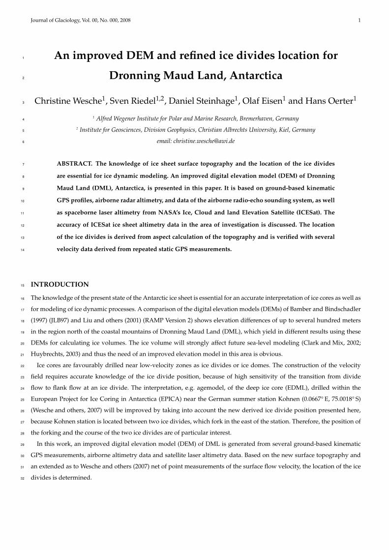
Journal of Glaciology, Vol. 00, No. 000, 2008 1
An improved DEM and refined ice divides location for1
Dronning Maud Land, Antarctica2
Christine Wesche1, Sven Riedel1,2, Daniel Steinhage1, Olaf Eisen1 and Hans Oerter13
1 Alfred Wegener Institute for Polar and Marine Research, Bremerhaven, Germany4
2 Institute for Geosciences, Division Geophysics, Christian Albrechts University, Kiel, Germany5
email: [email protected]
ABSTRACT. The knowledge of ice sheet surface topography and the location of the ice divides7
are essential for ice dynamic modeling. An improved digital elevation model (DEM) of Dronning8
Maud Land (DML), Antarctica, is presented in this paper. It is based on ground-based kinematic9
GPS profiles, airborne radar altimetry, and data of the airborne radio-echo sounding system, as well10
as spaceborne laser altimetry from NASA’s Ice, Cloud and land Elevation Satellite (ICESat). The11
accuracy of ICESat ice sheet altimetry data in the area of investigation is discussed. The location12
of the ice divides is derived from aspect calculation of the topography and is verified with several13
velocity data derived from repeated static GPS measurements.14
INTRODUCTION15
The knowledge of the present state of the Antarctic ice sheet is essential for an accurate interpretation of ice cores as well as16
for modeling of ice dynamic processes. A comparison of the digital elevation models (DEMs) of Bamber and Bindschadler17
(1997) (JLB97) and Liu and others (2001) (RAMP Version 2) shows elevation differences of up to several hundred meters18
in the region north of the coastal mountains of Dronning Maud Land (DML), which yield in different results using these19
DEMs for calculating ice volumes. The ice volume will strongly affect future sea-level modeling (Clark and Mix, 2002;20
Huybrechts, 2003) and thus the need of an improved elevation model in this area is obvious.21
Ice cores are favourably drilled near low-velocity zones as ice divides or ice domes. The construction of the velocity22
field requires accurate knowledge of the ice divide position, because of high sensitivity of the transition from divide23
flow to flank flow at an ice divide. The interpretation, e.g. agemodel, of the deep ice core (EDML), drilled within the24
European Project for Ice Coring in Antarctica (EPICA) near the German summer station Kohnen (0.0667° E, 75.0018° S)25
(Wesche and others, 2007) will be improved by taking into account the new derived ice divide position presented here,26
because Kohnen station is located between two ice divides, which fork in the east of the station. Therefore, the position of27
the forking and the course of the two ice divides are of particular interest.28
In this work, an improved digital elevation model (DEM) of DML is generated from several ground-based kinematic29
GPS measurements, airborne altimetry data and satellite laser altimetry data. Based on the new surface topography and30
an extended as to Wesche and others (2007) net of point measurements of the surface flow velocity, the location of the ice31
divides is determined.32
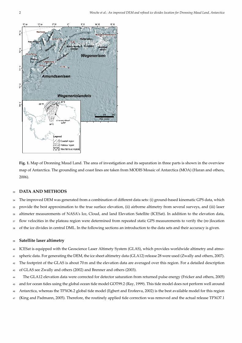
2 Wesche et al.: An improved DEM and refined ice divides location for Dronning Maud Land, Antarctica
Fig. 1. Map of Dronning Maud Land. The area of investigation and its separation in three parts is shown in the overview
map of Antarctica. The grounding and coast lines are taken from MODIS Mosaic of Antarctica (MOA) (Haran and others,
2006).
DATA AND METHODS33
The improved DEM was generated from a combination of different data sets: (i) ground-based kinematic GPS data, which34
provide the best approximation to the true surface elevation, (ii) airborne altimetry from several surveys, and (iii) laser35
altimeter measurements of NASA’s Ice, Cloud, and land Elevation Satellite (ICESat). In addition to the elevation data,36
flow velocities in the plateau region were determined from repeated static GPS measurements to verify the (re-)location37
of the ice divides in central DML. In the following sections an introduction to the data sets and their accuracy is given.38
Satellite laser altimetry39
ICESat is equipped with the Geoscience Laser Altimety System (GLAS), which provides worldwide altimetry and atmo-40
spheric data. For generating the DEM, the ice sheet altimetry data (GLA12) release 28 were used (Zwally and others, 2007).41
The footprint of the GLAS is about 70 m and the elevation data are averaged over this region. For a detailed description42
of GLAS see Zwally and others (2002) and Brenner and others (2003).43
The GLA12 elevation data were corrected for detector saturation from returned pulse energy (Fricker and others, 2005)44
and for ocean tides using the global ocean tide model GOT99.2 (Ray, 1999). This tide model does not perform well around45
Antarctica, whereas the TPXO6.2 global tide model (Egbert and Erofeeva, 2002) is the best available model for this region46
(King and Padmann, 2005). Therefore, the routinely applied tide correction was removed and the actual release TPXO7.147
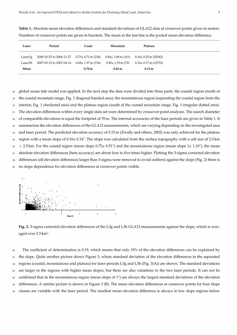
Wesche et al.: An improved DEM and refined ice divides location for Dronning Maud Land, Antarctica 3
Table 1. Absolute mean elevation differences and standard deviations of GLA12 data at crossover points given in meters.
Numbers of crossover points are given in brackets. The mean in the last line is the pooled mean elevation difference.
Laser Period Coast Mountain Plateau
Laser3g 2006-10-25 to 2006-11-27 0.73± 0.71 m (236) 0.84± 1.08 m (161) 0.16± 0.25 m (20342)
Laser3h 2007-03-12 to 2007-04-14 0.68± 1.97 m (154) 0.82± 1.33 m (72) 0.14± 0.17 m (12732)
Mean 0.70 m 0.83 m 0.15 m
global ocean tide model was applied. In the next step the data were divided into three parts, the coastal region (north of48
the coastal mountain range, Fig. 1 diagonal banded area), the mountainous region (separating the coastal region from the49
interior, Fig. 1 checkered area) and the plateau region (south of the coastal mountain range, Fig. 1 irregular dotted area).50
The elevation differences within every single data set were determined by crossover-point analyses. The search diameter51
of comparable elevations is equal the footprint of 70 m. The internal accuracies of the laser periods are given in Table 1. It52
summarizes the elevation differences of the GLA12 measurements, which are varying depending on the investigated area53
and laser period. The predicted elevation accuracy of 0.15 m (Zwally and others, 2002) was only achieved for the plateau54
region with a mean slope of 0.16± 0.14°. The slope was calculated from the surface topography with a cell size of 2.5 km55
× 2.5 km. For the coastal region (mean slope 0.75± 0.51°) and the mountainous region (mean slope 1± 1.10°), the mean56
absolute elevation differences (here accuracy) are about four to five times higher. Plotting the 3-sigma corrected elevation57
differences (all elevation differences larger than 3-sigma were removed to avoid outliers) against the slope (Fig. 2) there is58
no slope dependence for elevation differences at crossover points visible.59
Fig. 2. 3-sigma corrected elevation differences of the L3g and L3h GLA12 measurements against the slope, which is aver-
aged over 2.5 km2.
The coefficient of determination is 0.19, which means that only 19% of the elevation differences can be explained by60
the slope. Quite another picture shows Figure 3, where standard deviation of the elevation differences in the separated61
regions (coastal, mountainous and plateau) for laser periods L3g and L3h (Fig. 3(A)) are shown. The standard deviations62
are larger in the regions with higher mean slopes, but there are also variations in the two laser periods. It can not be63
confirmed that in the mountainous region (mean slope of 1°) are always the largest standard deviations of the elevation64
differences. A similar picture is shown in Figure 3 (B). The mean elevation differences at crossover points for four slope65
classes are variable with the laser period. The smallest mean elevation difference is always in low slope regions below66
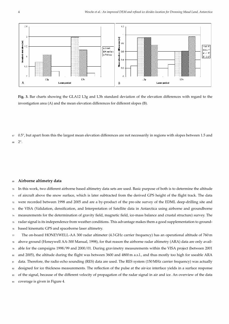
4 Wesche et al.: An improved DEM and refined ice divides location for Dronning Maud Land, Antarctica
Fig. 3. Bar charts showing the GLA12 L3g and L3h standard deviation of the elevation differences with regard to the
investigation area (A) and the mean elevation differences for different slopes (B).
0.5°, but apart from this the largest mean elevation differences are not necessarily in regions with slopes between 1.5 and67
2°.68
Airborne altimetry data69
In this work, two different airborne based altimetry data sets are used. Basic purpose of both is to determine the altitude70
of aircraft above the snow surface, which is later subtracted from the derived GPS height of the flight track. The data71
were recorded between 1998 and 2005 and are a by-product of the pre-site survey of the EDML deep-drilling site and72
the VISA (Validation, densification, and Interpretation of Satellite data in Antarctica using airborne and groundborne73
measurements for the determination of gravity field, magnetic field, ice-mass balance and crustal structure) survey. The74
radar signal is its independence from weather conditions. This advantage makes them a good supplementation to ground-75
based kinematic GPS and spaceborne laser altimetry.76
The on-board HONEYWELL-AA 300 radar altimeter (4.3 GHz carrier frequency) has an operational altitude of 760 m77
above ground (Honeywell AA-300 Manual, 1998), for that reason the airborne radar altimetry (ARA) data are only avail-78
able for the campaigns 1998/99 and 2000/01. During gravimetry measurements within the VISA project (between 200179
and 2005), the altitude during the flight was between 3600 and 4800 m a.s.l., and thus mostly too high for useable ARA80
data. Therefore, the radio echo sounding (RES) data are used. The RES system (150 MHz carrier frequency) was actually81
designed for ice thickness measurements. The reflection of the pulse at the air-ice interface yields in a surface response82
of the signal, because of the different velocity of propagation of the radar signal in air and ice. An overview of the data83
coverage is given in Figure 4.84
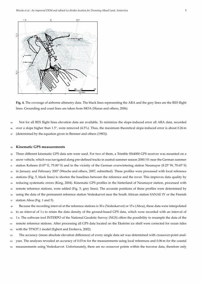
Wesche et al.: An improved DEM and refined ice divides location for Dronning Maud Land, Antarctica 5
Fig. 4. The coverage of airborne altimetry data. The black lines representing the ARA and the grey lines are the RES flight
lines. Grounding and coast lines are taken from MOA (Haran and others, 2006).
Not for all RES flight lines elevation data are available. To minimize the slope-induced error all ARA data, recorded85
over a slope higher than 1.5°, were removed (4.5%). Thus, the maximum theoretical slope-induced error is about 0.26 m86
(determined by the equation given in Brenner and others (1983)).87
Kinematic GPS measurements88
Three different kinematic GPS data sets were used. For two of them, a Trimble SSi4000 GPS receiver was mounted on a89
snow vehicle, which was navigated along pre-defined tracks in austral summer season 2000/01 near the German summer90
station Kohnen (0.07° E, 75.00° S) and in the vicinity of the German overwintering station Neumayer (8.25° W, 70.65° S)91
in January and February 2007 (Wesche and others, 2007, submitted). These profiles were processed with local reference92
stations (Fig. 5, black lines) to shorten the baselines between the reference and the rover. This improves data quality by93
reducing systematic errors (King, 2004). Kinematic GPS profiles in the hinterland of Neumayer station, processed with94
remote reference stations, were added (Fig. 5, grey lines). The accurate positions of these profiles were determined by95
using the data of the permanent reference station Vesleskarvet near the South African station SANAE IV or the Finnish96
station Aboa (Fig. 1 and 5).97
Because the recording interval at the reference stations is 30 s (Vesleskarvet) or 15 s (Aboa), these data were interpolated98
to an interval of 1 s to retain the data density of the ground-based GPS data, which were recorded with an interval of99
1 s. The software tool INTERPO of the National Geodetic Survey (NGS) offers the possibility to resample the data of the100
remote reference stations. After processing all GPS data located on the Ekström ice shelf were corrected for ocean tides101
with the TPXO7.1 model (Egbert and Erofeeva, 2002).102
The accuracy (mean absolute elevation difference) of every single data set was determined with crossover-point anal-103
yses. The analyses revealed an accuracy of 0.03 m for the measurements using local references and 0.06 m for the coastal104
measurements using Vesleskarvet. Unfortunately, there are no crossover points within the traverse data, therefore only105
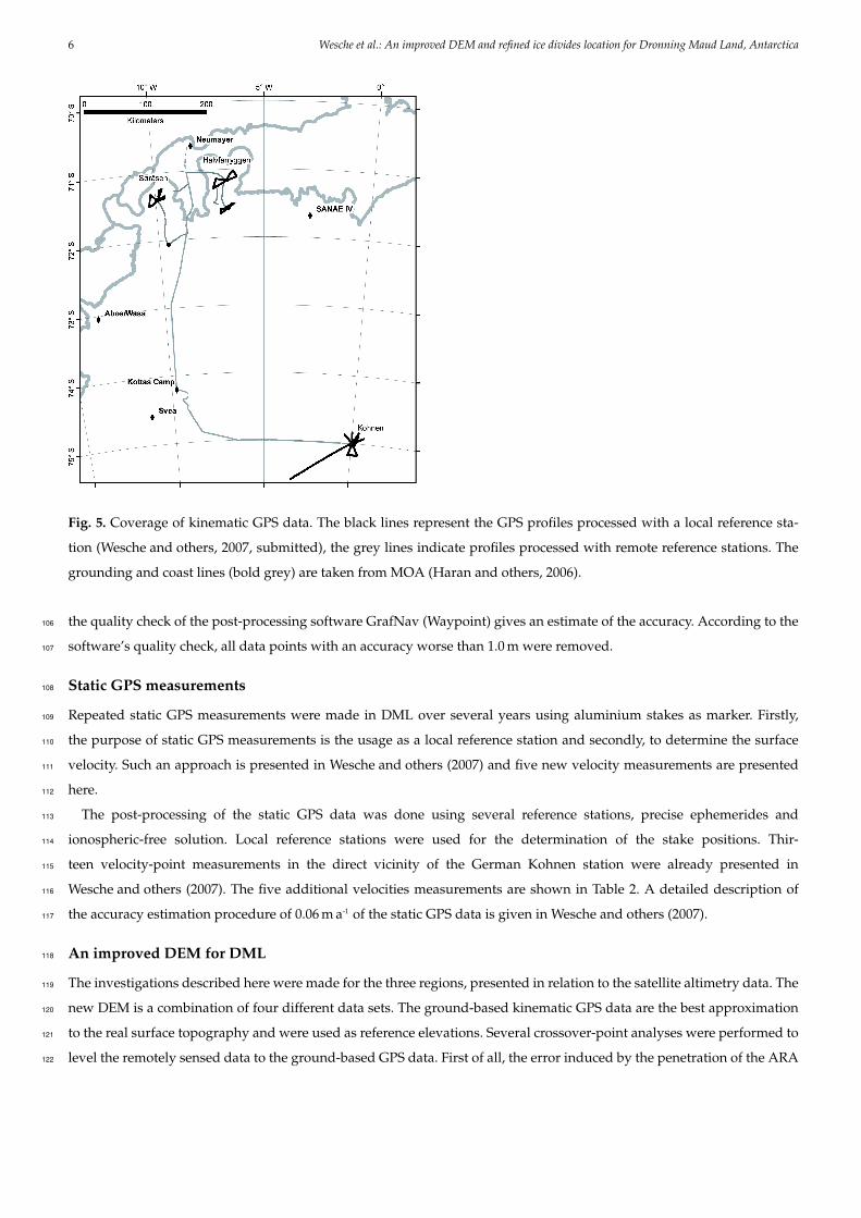
6 Wesche et al.: An improved DEM and refined ice divides location for Dronning Maud Land, Antarctica
Fig. 5. Coverage of kinematic GPS data. The black lines represent the GPS profiles processed with a local reference sta-
tion (Wesche and others, 2007, submitted), the grey lines indicate profiles processed with remote reference stations. The
grounding and coast lines (bold grey) are taken from MOA (Haran and others, 2006).
the quality check of the post-processing software GrafNav (Waypoint) gives an estimate of the accuracy. According to the106
software’s quality check, all data points with an accuracy worse than 1.0 m were removed.107
Static GPS measurements108
Repeated static GPS measurements were made in DML over several years using aluminium stakes as marker. Firstly,109
the purpose of static GPS measurements is the usage as a local reference station and secondly, to determine the surface110
velocity. Such an approach is presented in Wesche and others (2007) and five new velocity measurements are presented111
here.112
The post-processing of the static GPS data was done using several reference stations, precise ephemerides and113
ionospheric-free solution. Local reference stations were used for the determination of the stake positions. Thir-114
teen velocity-point measurements in the direct vicinity of the German Kohnen station were already presented in115
Wesche and others (2007). The five additional velocities measurements are shown in Table 2. A detailed description of116
the accuracy estimation procedure of 0.06 m a-1 of the static GPS data is given in Wesche and others (2007).117
An improved DEM for DML118
The investigations described here were made for the three regions, presented in relation to the satellite altimetry data. The119
new DEM is a combination of four different data sets. The ground-based kinematic GPS data are the best approximation120
to the real surface topography and were used as reference elevations. Several crossover-point analyses were performed to121
level the remotely sensed data to the ground-based GPS data. First of all, the error induced by the penetration of the ARA122
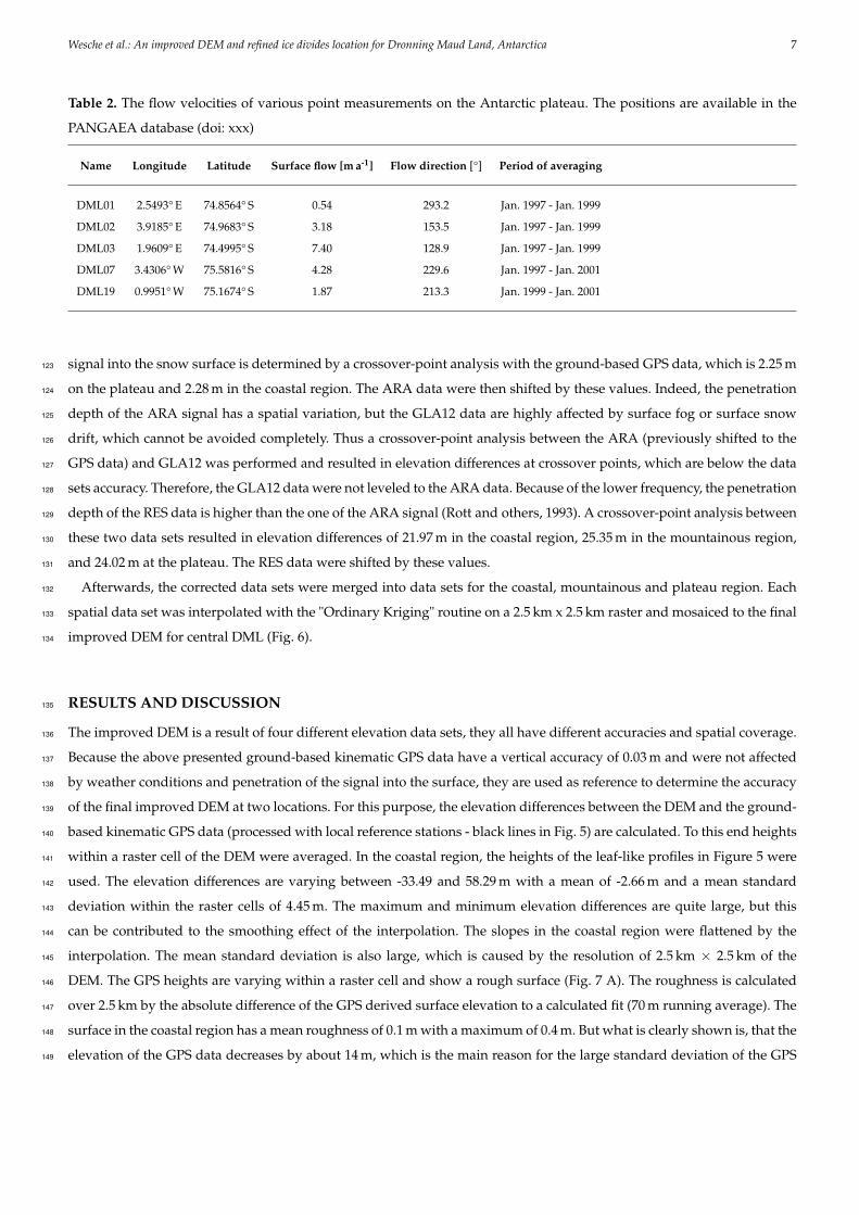
Wesche et al.: An improved DEM and refined ice divides location for Dronning Maud Land, Antarctica 7
Table 2. The flow velocities of various point measurements on the Antarctic plateau. The positions are available in the
PANGAEA database (doi: xxx)
Name Longitude Latitude Surface flow [m a-1] Flow direction [°] Period of averaging
DML01 2.5493° E 74.8564° S 0.54 293.2 Jan. 1997 - Jan. 1999
DML02 3.9185° E 74.9683° S 3.18 153.5 Jan. 1997 - Jan. 1999
DML03 1.9609° E 74.4995° S 7.40 128.9 Jan. 1997 - Jan. 1999
DML07 3.4306° W 75.5816° S 4.28 229.6 Jan. 1997 - Jan. 2001
DML19 0.9951° W 75.1674° S 1.87 213.3 Jan. 1999 - Jan. 2001
signal into the snow surface is determined by a crossover-point analysis with the ground-based GPS data, which is 2.25 m123
on the plateau and 2.28 m in the coastal region. The ARA data were then shifted by these values. Indeed, the penetration124
depth of the ARA signal has a spatial variation, but the GLA12 data are highly affected by surface fog or surface snow125
drift, which cannot be avoided completely. Thus a crossover-point analysis between the ARA (previously shifted to the126
GPS data) and GLA12 was performed and resulted in elevation differences at crossover points, which are below the data127
sets accuracy. Therefore, the GLA12 data were not leveled to the ARA data. Because of the lower frequency, the penetration128
depth of the RES data is higher than the one of the ARA signal (Rott and others, 1993). A crossover-point analysis between129
these two data sets resulted in elevation differences of 21.97 m in the coastal region, 25.35 m in the mountainous region,130
and 24.02 m at the plateau. The RES data were shifted by these values.131
Afterwards, the corrected data sets were merged into data sets for the coastal, mountainous and plateau region. Each132
spatial data set was interpolated with the "Ordinary Kriging" routine on a 2.5 km x 2.5 km raster and mosaiced to the final133
improved DEM for central DML (Fig. 6).134
RESULTS AND DISCUSSION135
The improved DEM is a result of four different elevation data sets, they all have different accuracies and spatial coverage.136
Because the above presented ground-based kinematic GPS data have a vertical accuracy of 0.03 m and were not affected137
by weather conditions and penetration of the signal into the surface, they are used as reference to determine the accuracy138
of the final improved DEM at two locations. For this purpose, the elevation differences between the DEM and the ground-139
based kinematic GPS data (processed with local reference stations - black lines in Fig. 5) are calculated. To this end heights140
within a raster cell of the DEM were averaged. In the coastal region, the heights of the leaf-like profiles in Figure 5 were141
used. The elevation differences are varying between -33.49 and 58.29 m with a mean of -2.66 m and a mean standard142
deviation within the raster cells of 4.45 m. The maximum and minimum elevation differences are quite large, but this143
can be contributed to the smoothing effect of the interpolation. The slopes in the coastal region were flattened by the144
interpolation. The mean standard deviation is also large, which is caused by the resolution of 2.5 km × 2.5 km of the145
DEM. The GPS heights are varying within a raster cell and show a rough surface (Fig. 7 A). The roughness is calculated146
over 2.5 km by the absolute difference of the GPS derived surface elevation to a calculated fit (70 m running average). The147
surface in the coastal region has a mean roughness of 0.1 m with a maximum of 0.4 m. But what is clearly shown is, that the148
elevation of the GPS data decreases by about 14 m, which is the main reason for the large standard deviation of the GPS149
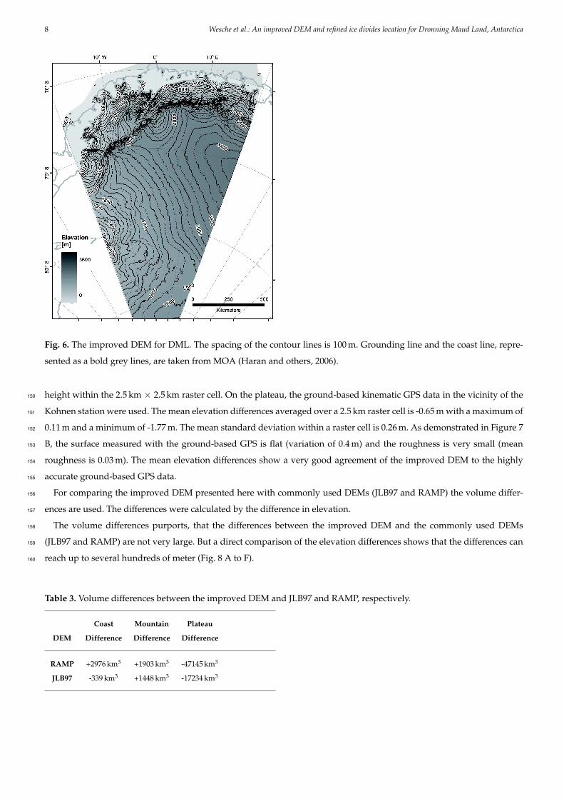
8 Wesche et al.: An improved DEM and refined ice divides location for Dronning Maud Land, Antarctica
Fig. 6. The improved DEM for DML. The spacing of the contour lines is 100 m. Grounding line and the coast line, repre-
sented as a bold grey lines, are taken from MOA (Haran and others, 2006).
height within the 2.5 km × 2.5 km raster cell. On the plateau, the ground-based kinematic GPS data in the vicinity of the150
Kohnen station were used. The mean elevation differences averaged over a 2.5 km raster cell is -0.65 m with a maximum of151
0.11 m and a minimum of -1.77 m. The mean standard deviation within a raster cell is 0.26 m. As demonstrated in Figure 7152
B, the surface measured with the ground-based GPS is flat (variation of 0.4 m) and the roughness is very small (mean153
roughness is 0.03 m). The mean elevation differences show a very good agreement of the improved DEM to the highly154
accurate ground-based GPS data.155
For comparing the improved DEM presented here with commonly used DEMs (JLB97 and RAMP) the volume differ-156
ences are used. The differences were calculated by the difference in elevation.157
The volume differences purports, that the differences between the improved DEM and the commonly used DEMs158
(JLB97 and RAMP) are not very large. But a direct comparison of the elevation differences shows that the differences can159
reach up to several hundreds of meter (Fig. 8 A to F).160
Table 3. Volume differences between the improved DEM and JLB97 and RAMP, respectively.
Coast Mountain Plateau
DEM Difference Difference Difference
RAMP +2976 km3 +1903 km3 -47145 km3
JLB97 -339 km3 +1448 km3 -17234 km3
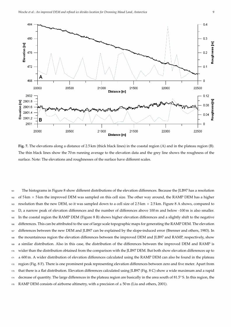
Wesche et al.: An improved DEM and refined ice divides location for Dronning Maud Land, Antarctica 9
Fig. 7. The elevations along a distance of 2.5 km (thick black lines) in the coastal region (A) and in the plateau region (B).
The thin black lines show the 70 m running average to the elevation data and the grey line shows the roughness of the
surface. Note: The elevations and roughnesses of the surface have different scales.
The histograms in Figure 8 show different distributions of the elevation differences. Because the JLB97 has a resolution161
of 5 km × 5 km the improved DEM was sampled on this cell size. The other way around, the RAMP DEM has a higher162
resolution than the new DEM, so it was sampled down to a cell size of 2.5 km × 2.5 km. Figure 8 A shows, compared to163
D, a narrow peak of elevation differences and the number of differences above 100 m and below -100 m is also smaller.164
In the coastal region the RAMP DEM (Figure 8 B) shows higher elevation differences and a slightly shift to the negative165
differences. This can be attributed to the use of large scale topographic maps for generating the RAMP DEM. The elevation166
differences between the new DEM and JLB97 can be explained by the slope-induced error (Brenner and others, 1983). In167
the mountainous region the elevation differences between the improved DEM and JLB97 and RAMP, respectively, show168
a similar distribution. Also in this case, the distribution of the differences between the improved DEM and RAMP is169
wider than the distribution obtained from the comparison with the JLB97 DEM. But both show elevation differences up to170
± 600 m. A wider distribution of elevation differences calculated using the RAMP DEM can also be found in the plateau171
region (Fig. 8 F). There is one prominent peak representing elevation differences between zero and five meter. Apart from172
that there is a flat distribution. Elevation differences calculated using JLB97 (Fig. 8 C) show a wide maximum and a rapid173
decrease of quantity. The large differences in the plateau region are basically in the area south of 81.5° S. In this region, the174
RAMP DEM consists of airborne altimetry, with a precision of ± 50 m (Liu and others, 2001).175
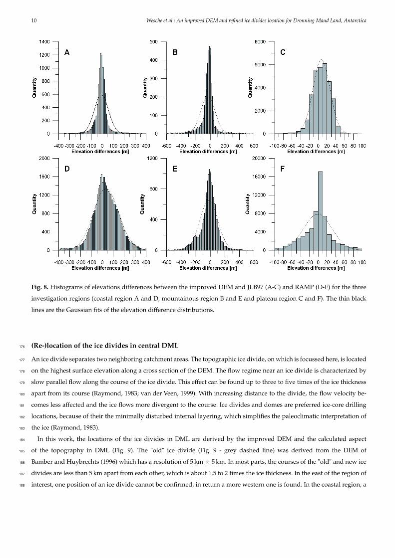
10 Wesche et al.: An improved DEM and refined ice divides location for Dronning Maud Land, Antarctica
Fig. 8. Histograms of elevations differences between the improved DEM and JLB97 (A-C) and RAMP (D-F) for the three
investigation regions (coastal region A and D, mountainous region B and E and plateau region C and F). The thin black
lines are the Gaussian fits of the elevation difference distributions.
(Re-)location of the ice divides in central DML176
An ice divide separates two neighboring catchment areas. The topographic ice divide, on which is focussed here, is located177
on the highest surface elevation along a cross section of the DEM. The flow regime near an ice divide is characterized by178
slow parallel flow along the course of the ice divide. This effect can be found up to three to five times of the ice thickness179
apart from its course (Raymond, 1983; van der Veen, 1999). With increasing distance to the divide, the flow velocity be-180
comes less affected and the ice flows more divergent to the course. Ice divides and domes are preferred ice-core drilling181
locations, because of their the minimally disturbed internal layering, which simplifies the paleoclimatic interpretation of182
the ice (Raymond, 1983).183
In this work, the locations of the ice divides in DML are derived by the improved DEM and the calculated aspect184
of the topography in DML (Fig. 9). The "old" ice divide (Fig. 9 - grey dashed line) was derived from the DEM of185
Bamber and Huybrechts (1996) which has a resolution of 5 km × 5 km. In most parts, the courses of the "old" and new ice186
divides are less than 5 km apart from each other, which is about 1.5 to 2 times the ice thickness. In the east of the region of187
interest, one position of an ice divide cannot be confirmed, in return a more western one is found. In the coastal region, a188
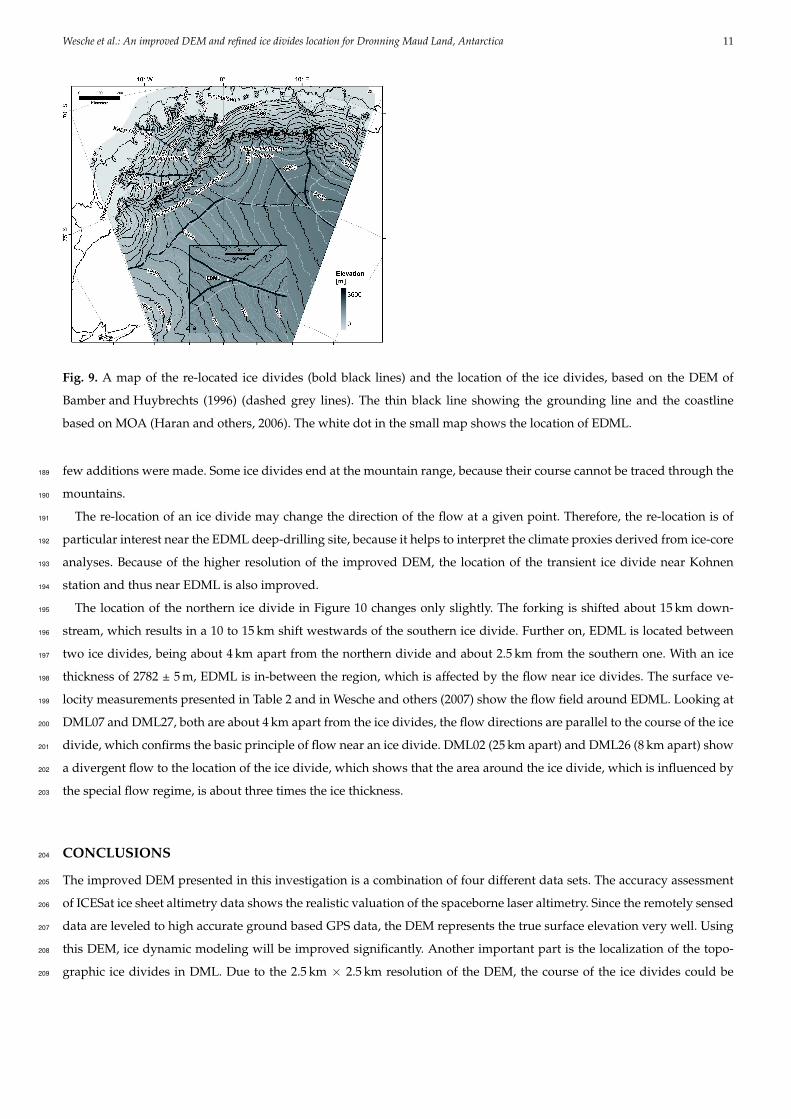
Wesche et al.: An improved DEM and refined ice divides location for Dronning Maud Land, Antarctica 11
Fig. 9. A map of the re-located ice divides (bold black lines) and the location of the ice divides, based on the DEM of
Bamber and Huybrechts (1996) (dashed grey lines). The thin black line showing the grounding line and the coastline
based on MOA (Haran and others, 2006). The white dot in the small map shows the location of EDML.
few additions were made. Some ice divides end at the mountain range, because their course cannot be traced through the189
mountains.190
The re-location of an ice divide may change the direction of the flow at a given point. Therefore, the re-location is of191
particular interest near the EDML deep-drilling site, because it helps to interpret the climate proxies derived from ice-core192
analyses. Because of the higher resolution of the improved DEM, the location of the transient ice divide near Kohnen193
station and thus near EDML is also improved.194
The location of the northern ice divide in Figure 10 changes only slightly. The forking is shifted about 15 km down-195
stream, which results in a 10 to 15 km shift westwards of the southern ice divide. Further on, EDML is located between196
two ice divides, being about 4 km apart from the northern divide and about 2.5 km from the southern one. With an ice197
thickness of 2782 ± 5 m, EDML is in-between the region, which is affected by the flow near ice divides. The surface ve-198
locity measurements presented in Table 2 and in Wesche and others (2007) show the flow field around EDML. Looking at199
DML07 and DML27, both are about 4 km apart from the ice divides, the flow directions are parallel to the course of the ice200
divide, which confirms the basic principle of flow near an ice divide. DML02 (25 km apart) and DML26 (8 km apart) show201
a divergent flow to the location of the ice divide, which shows that the area around the ice divide, which is influenced by202
the special flow regime, is about three times the ice thickness.203
CONCLUSIONS204
The improved DEM presented in this investigation is a combination of four different data sets. The accuracy assessment205
of ICESat ice sheet altimetry data shows the realistic valuation of the spaceborne laser altimetry. Since the remotely sensed206
data are leveled to high accurate ground based GPS data, the DEM represents the true surface elevation very well. Using207
this DEM, ice dynamic modeling will be improved significantly. Another important part is the localization of the topo-208
graphic ice divides in DML. Due to the 2.5 km × 2.5 km resolution of the DEM, the course of the ice divides could be209

12 Wesche et al.: An improved DEM and refined ice divides location for Dronning Maud Land, Antarctica
Fig. 10. A zoom to the static GPS measurements. The graduated arrows present the flow velocities of the 18 static points.
In the small map it is zoomed to the rectangle marked in the big map. The black lines represent the new ice divide, the
dashed grey lines the old. In the background, the new DEM with 100 m contour lines.
determined more precisely than using JLB97 with an resolution of 5 km × 5 km (Bamber and Bindschadler, 1997). With210
the aid of the new ice divides, the estimation of the origin of the ice, drilled at Kohnen station (Huybrechts and others,211
2007), can be improved, which contributes to the accurate paleoclimatic interpretation of the climate proxies.212
ACKNOWLEDGMENTS213
This work was supported by the Bundesministerium für Wirtschaft (BMWi) through the CryoVEx activities 50EE0505.214
The authors thank the National Snow and Ice Data Center for providing the ICESat data and a special thank to Jennifer215
Bohlander, for providing the MOA grounding and coast lines.216
References217
Bamber, J. L. and R. A. Bindschadler, 1997. An improved elevation dataset for climate and ice-sheet modelling: validation218
with satellite imagery, Annals of Glaciology, 25, 439–444.219
Bamber, J. L. and P. Huybrechts, 1996. Geometric boundary conditions for modelling the velocity field of the Antarctic ice220
sheet, Annals of Glaciology, 23, 364–373.221
Brenner, A. C., R. A. Bindschadler, R. H. Thomas and H. J. Zwally, 1983. Slope-induced errors in radar altimetry over222
continental ice sheets, Journal of Geophysical Research, 88(C3), 1617–1623.223
Brenner, A. C., H. J. Zwally, C. R. Bentley, B. M. Csatho, D. J. Harding, M. A. Hofton, J.-B. Minster, A. Roberts, Saba J. L.,224
R. H. Thomas and D. Yi, 2003. Derivation of range and range distribution from laser pulse waveform analysis for surface225
elevations, roughness, slope, and vegetation heights, GLAS Algorithm Theoretical Basis Document Version 4.1, Greenbelt,226
MD, Goddard Space Flight Center.227
Wesche et al.: An improved DEM and refined ice divides location for Dronning Maud Land, Antarctica 13
Clark, P. U. and A. C. Mix, 2002. Ice sheet and sea level of the Last Glacial Maximum, Quatenary Science Reviews, 21, 1–7.228
Egbert, G. D and S. Y. Erofeeva, 2002. Efficient inverse modeling of barotropic ocean tides, Journal of Atmospheric and229
Oceanic Technology, 19(2), 183–204.230
Fricker, H. A., A. Borsa, B. Minster, C. Carabajal, K. Quinn and B. Bills, 2005. Assessment of ICESat performance at the231
salar de Uyuni, Bolivia, Geophysical Research Letters, 32(L21S06).232
Haran, T., J. Bohland, T. Scambos, T. Painter and M. Fahnestock, 2006. MODIS mosaic of Antarctica (MOA) image map,233
Boulder, Colorado, National Snow and Ice Data Center, Digital media.234
Honeywell AA-300 Manual, 1998. System description and installation manual - AA-300 Radion Altimeter System.235
Huybrechts, P., 2003. Antarctica: modelling, In: Mass Balance of the Cryosphere: Observations and Modeling of Contem-236
porary and Furture Changes, eds. Bamber. J. L. and A. J. Payne, Cambrigde University Press, chap. 13, 491–524.237
Huybrechts, P., O. Rybak, F. Pattyn, U. Ruth and D. Steinhage, 2007. Ice thinning, upstream advection, and non-climatic238
biases for the upper89EDML ice core from a nested model of the Antarctic ice sheet, Climate of the Past, 3, 577–589.239
King, M., 2004. Rigorous GPS data-processing strategies for glaciological applications, Journal of Glaciology, 50(171), 601–240
607.241
King, M. and L. Padmann, 2005. Accuracy assessment of ocean tide models around Antarctica, Geophysical Research Letters,242
32(L23608).243
Liu, H., K. C. Jezek, B. Li and Z. Zhao, 2001. Radarsat Antarctic Mapping Project digital elevation model version 2, Boulder244
CO, National Snow and Ice Data Center, Digital media.245
Ray, R. D., 1999. A global ocean tide model from TOPEX/Poseidon altimetry: GOT99.2, NASATechnical Memo, (209478).246
Raymond, C.F., 1983. Deformation in the vicinity of ice divides, Journal of Glaciology, 29(103), 357–373.247
Rott, H., K. Sturm and H. Miller, 1993. Active and passive microwave signatures of Antarctica firn by means of field248
measurements and satellite data, Annals of Glaciology, 17, 337–343.249
van der Veen, C. J., 1999. Fundamentals of Glacier Dynamics, Balkema, Rotterdam u.a.250
Wesche, C., O. Eisen, H. Oerter, D. Schulte and D. Steinhage, 2007. Surface topography and ice flow in the vicinity of the251
EDML deep-drilling site, Antarctica, Journal of Glaciology, 53(182), 442–448.252
Wesche, C., S. Riedel and D. Steinhage, submitted. Precise surface topography of the grounded ice tongues at the Ek-253
strömisen, Antarctica, based on several geophysical data sets, ISPRS Journal of Photogrammetry and Remote Sensing.254
Zwally, H.J., B. Schutz, W. Abdalati, J. Abshire, C. Bentley, A. Brenner, J. Bufton, J. Dezio, D. Hancock, D. Harding, T. Her-255
ring, B. Minster, K. Quinn, S. Palm, J. Spinhirne and R. Thomas, 2002. ICESat’s laser measurements of polar ice, atmo-256
sphere, ocean, and land, Journal of Geodynamics, 34, 405–445.257
Zwally, H. J., R. Schutz, C. Bentley, T. Bufton, T. Herring, J. Minster, J. Spinhirne and R. Thomas, 2007. GLAS/ICESat258
L2 Antarctic and Greenland Ice Sheet Altimetry Data V028, Boulder, CO, National Snow and Ice Data Center, Digital259
media.260


PAPER IV
A new digital elevation model in western Dronning Maud Land
(Antarctica), based on differential SAR Interferometry
IEEE Transactions on Geoscience and Remote Sensing, accepted
109

For Peer Review
JOURNAL OF LATEX CLASS FILES, VOL. 6, NO. 1, JANUARY 2007 1
A spatially adjusted elevation model in DronningMaud Land, Antarctica, based on differential
SAR InterferometryReinhard Drews, Wolfgang Rack, Member, IEEE Christine Wesche, Veit Helm
Abstract —In this study we derived a new digital elevation model (DEM) in western Dronning Maud Land (Antarctica) byusing differential interferometric SAR (DInSAR). It is based on acquisitions from the European Remote Sensing satellitesERS-1/2 in combination with IceSAT’s geoscience laser altimeter (GLAS). The DEM is compiled out of 116 scenes fromthe ERS-1 ice phase and the ERS-1/2 (tandem) mission between 1994 and 1997. Profiles from laser altimetry of theIceSAT satellite were taken in 2003 and served as ground control for the DEM generation. By using three different SARprocessors we separate internal processing errors from external errors such as an unknown atmospheric contribution.The mosaicked DEM includes the grounded ice sheet on the gently sloped catchment basins of the Ekstromisen andthe Veststraumen as well as parts of the Heimefront Fjella mountain range. It covers an area of approximately 130 000km2 on a (50x50) m grid. For the uncertainty estimation independent IceSAT tracks from 2004-2007 were used togetherwith GPS and airborne LIDAR data. The height error varies spatially in average from 1-2 meters up to 15-20 meters. Nosystematic changes were detected over the 10 year period. Also the data set does not allow easily to assess variationsin radar penetration depth into snow. The DEM was filtered and resampled iteratively in order to account for the spatialvariation of noise. It mostly outperforms other DEMs currently available in the region and will serve for future elevationmodels from the Cryosat and the Terra SAR-X tandem mission as the late 1990s baseline to monitor temporal changesin ice sheet elevation.
Index Terms —Digital Elevation Model, Differential SAR Interferometry, Dronning Maud Land, Antarctica, GLAS, IceSAT
✦
1 INTRODUCTION
THE surface elevation on the coastal mar-gins of the Antarctic ice sheet is largely
unknown at the required accuracy to mon-itor short term temporal changes. Currentlyavailable Digital Elevation Models (DEMs) inour area of interest are the RAMPv2 [14], theGLAS/IceSAT-model [6], and the JBL97-model[10]. The RAMPv2 originates from the RadarsatMapping Project and is mainly deduced fromERS-1’s radar altimeter. It is gridded to 200meters. In areas of steep relief it is combined
• R. Drews, C.Wesche, and V. Helm are at the Alfred WegenerInstitute for Polar and Marine Research, Am Handelshafen 12,Bremerhaven, Germany.E-mail: [email protected]
• W. Rack is at the Gateway Antarctica Centre for Antarctic Studiesand Research, Canterbury University, Christchurch, New Zealand
Manuscript received XXXX XX, XXXX; revised XXXX XX,XXXX.
with terrestrially derived data like airbornedata and GPS measurements from the AntarcticDigital Database. JBL97 is a DEM with 5 kmpostings and is based on ERS-1 radar altimetryas well [3]. The GLAS/IceSAT DEM is deducedfrom IceSAT’s laser altimeter and was releasedfrom the National Snow and Ice Data Cen-ter (NSIDC) in 2007. In our area of interestRAMPv2 deviates partly more than 150 metersfrom JBL97, GLAS/IceSAT and GPS profiles(see Fig. 1). Glas/IceSAT performs better thanJBL97 especially in the vicinity of underlyingIceSAT tracks.
Precise and highly resolved DEMs areneeded for a variety of glaciological applica-tions, such as mass balance and accumulationstudies [1], input for numerical flow models,mapping of displacement fields, or ice coreanalysis [18]. The previously mentioned DEMsoften do not offer the needed horizontal res-
Page 1 of 12 Transactions on Geoscience and Remote Sensing
123456789101112131415161718192021222324252627282930313233343536373839404142434445464748495051525354555657585960
For Peer Review
JOURNAL OF LATEX CLASS FILES, VOL. 6, NO. 1, JANUARY 2007 2
olution and vertical accuracy. This motivatesthe derivation of a DEM through a differ-ential interferometric approach. Satelliteborneinterferometric SAR (InSAR) is a well knowntechnique to derive area-wide, fine resolutionDEMs and velocity fields. Detailed introduc-tions can be found for example in [15], [7] or[17]. Similar studies with respect to icesheetswere previsously performed in [13], [11], or [2].
The authors in [2] reported localized residualelevation discrepancies between the DInSARDEMs and IceSAT altimetry and speculated onthe origins such as atmospheric contributionand varying penetration depth. Our interestis to derive a larger scale DEM using thesame technique, quantify the obtainable accu-racy, and link deviations to two kinds of er-rors: Firstly internal errors due to uncertaintieswithin the radar/INSAR processing and sec-ondly to external errors such as an atmosphericcontribution. Secondly, we present a DEM witha varying spatial resolution which accounts forthe spatial variation of noise.
2 METHODOLOGY
In an interferometric multipass procedure twoacquisitions are combined to derive a mixedinterferogram which contains a topographicalcontribution as well as a contribution from theice sheet’s displacement in-between the twoacquisitions. In order to separate these twoparameters a differential approach (DInSAR) asdescribed in [13] is chosen: Under the assump-tion of a constant velocity flow, the displace-ment is canceled by differencing two interfero-grams of the same scene. The main processingsteps comprise the SAR processing of the rawdata, coregistration of the scenes, interferogramformation, phase unwrapping, differencing ofthe interferograms, the baseline refinement andthe rectification to the resulting height map. Aspreviously done in [21], the baseline refinementuses GCPs from IceSAT’s laser altimeter (GLA12 Release 24, Laser 1 (20.02.2002 - 29.02.2002)and Laser 2a (24.09.2003 - 18.11.2003) [22]) astiepoints. Limitations are the restricted avail-ability of coherent SAR image pairs and thelack of real GCPs. An unknown atmosphericcontribution as well as a varying penetration
depth may deteriorate the quality of the result-ing DEM.
Following a user based approach we in-vestigate the robustness and sensitivity of theSAR raw data processing by analyzing SLCdata from three different SAR processors withvarying scene length in azimuth. Some DEMswere derived from SLC frames from the Ger-man Processing and Archiving Facility (D-PAF;processing date between 2003 and 2007). Re-sulting DEMs often show phase discontinuitieson the boarder of adjacent frames which cannotfully be explained by baseline inaccuracies. Inorder to enable strip-line processing we usedGamma’s Modular SAR processor (MSP), andfor comparison EarthView’s advanced preci-sion processor (APP). All other steps were per-formed with Gamma’s interferometry software[19].
Fig. 1 displays the ERS frames which wereused in this study. Alltogether 19 DEMs wereseparately derived and mosaicked to a finalDEM. In overlapping areas, a weighted averagewas applied which reduced the overall noiselevel. The weights cc were given by the es-timated coherence of the respective DEM. Indetail:
DEM(i,j) =
∑Nk cck
(i,j)demk(i,j)
∑Nk cck
(i,j)
(1)
with
ccki,j =
{
ccki,j if cck
i,j > 0.60 otherwise.
}
where k indexes the individual DEMs and Nis the number of DEMs that overlap at thelocation (i,j). Usually N is in between 2 and 4.A threshold for coherence was chosen to avoidareas of high noise where phase unwrappingerrors are likely.
For the uncertainty estimation the final DEMis compared to IceSAT tracks as well as in-dependent GPS and LIDAR profiles. Whereasthese cover only a relatively small area, thedifferencing of the individual DEMs in over-lapping areas gives an estimate of the DEM’saccuracy on a larger scale. In order to isolateprocessing errors we compare independentlyprocessed raw data. This will be investigatedin the next section.
Page 2 of 12Transactions on Geoscience and Remote Sensing
123456789101112131415161718192021222324252627282930313233343536373839404142434445464748495051525354555657585960

For Peer Review
JOURNAL OF LATEX CLASS FILES, VOL. 6, NO. 1, JANUARY 2007 3
3 ACCURACY ANALYSIS
3.1 SAR raw-data and DInSAR processingThe SAR raw-data processing aims to recon-structs an image out of several reflected pulses,by using the Doppler history of the individ-ual targets (see for example [8] or [9]). Theresulting high resolution image is a single lookcomplex (SLC) file which stores a complexnumber (in-phase and quadrature) correspond-ing to phase and amplitude. After the double-differencing of 4 SLCs the conversion from dif-ferential phase to height can be approximatedby [16]:
z =λr0 sin(θ0)
4π
∆φf
B⊥,0(2)
where the unwrapped and flattened phase φf
is turned into height z (above a reference el-lipsoid) by using the perpendicular componentof the refined baseline B, as well as the lookangle θ0, the slant range distance r0 and thewavelength λ. Apart from the wavelength allparameters have a range and azimuth depen-dency which is not marked explicitly.
Processing uncertainties can be visualized(1) by comparing overlapping areas of adjacentframes which were processed individually or(2) by comparing DEMs which are based ona set of SLCs from different SAR processors.In both cases the resulting DEMs rely on thesame raw data and deviations can be entirelyattributed to the SAR processing.
As a specific example we consider two adja-cent frames (5157 and 5175) in track 407 whichis marked with 4 in Fig. 1. From this raw datastrip we derived 5 DEMs (D1,D2,Ev1,Ev2,G)which are listed in table 1. D1 and D2 are based
TABLE 1Comparison of IceSAT GCPs to DEMs fromtrack 407 based on SLCs from different SAR
processors
id SLCs frame sIce [m]D1 D-PAF 5157 −0.32 ± 3.1
D2 D-PAF 5175 −0.35 ± 7.0
Ev1 APP 5157 0.29 ± 2.0
Ev2 APP 5175 0.40 ± 5.1
G MSP 5157-5175 0.00 ± 3.7
on 8 SLCs from the german D-PAF, Ev1 and
Ev2 are based on 8 SLCs from Earth-View’sAPP. G is based on 4 SLCs from the MSPwhere the raw data of the two frames wasconcatenated.
At first, the individual DEMs are comparedwith the corresponding GCPs which were usedfor the baseline refinement. The mean deviationsIce in all cases scatters around zero with astandard deviation of 2 to 7 meters (see table1). Many long IceSAT tracks show randomdeviations from 1 to 2 meters which points outthe generally high quality of those particuarDEMs. However, in some localized areas thedeviations are systematic and reach up to 10 to15 meters which is illustrated in Fig. 2. Char-acteristic dents are for instance visible in theupper right and lower left corner of D2. Thesedents are evident in many DEMs and cannot beremoved with low order polynoms in a globalfit over an entire frame. From a perspective ofa user it is interesting to know whether theselocalized deviations have geophysical reasonsor if they are due to the processing. In our casemany of them are due to the processing, sincedepending on which set of SLCs has been usedthey appear in different places. This can be seenin Fig. 2 where the previously mentioned dentsfrom D2 are not visible in G.
For further investigation the 5 DEMs are dif-ferenced. The difference fields of D1, Ev1,andG as well as the difference fields of D2,Ev2,and G show deviations of up to 15 meters insome areas. Similar deviations can be seen inthe overlapping area of D1 and D2. This em-phasizes that most of the localized deviationsalong the IceSAT tracks are processing artifacts.
The magnitude of processing uncertaintiescan be explained with deviations in the differ-ential phase and baselinemodels. The typicalINSAR approach to correct for both inaccura-cies in the state vectors and phase tilts due toSAR processing is an overall fit of GCPs to theunwrapped differential phase. This alters thebaseline in a way that the resulting orbit modelcomplies best to the used set of GCPs. As aresult, deviations in the final baseline modelare partly interconnected with SAR process-ing phase uncertainties. As an example servesFig. 3 where the deviations in the differentialphase, differential baseline, and height are plot-
Page 3 of 12 Transactions on Geoscience and Remote Sensing
123456789101112131415161718192021222324252627282930313233343536373839404142434445464748495051525354555657585960

For Peer Review
JOURNAL OF LATEX CLASS FILES, VOL. 6, NO. 1, JANUARY 2007 4
ted along a range profile (indicated in Fig. 2)which intersects D1,D2, Ev2, and G. It becomesevident that the various DEMs are tilted withrespect to each other. The largest tilts can beseen in the pairs D2-G and D2-D1. Similarresults are obtained for the case that the twoframes in G are processed seperatly.
The height differences from Fig. 3 can bemodeled using equation 2. If only differencesof the refined differential baseline and the dif-ferential phase are considered, the height devi-ation z − z′ can be approximated as
z − z′ =λr0 sin Θ0
4π·
(
∆φfB′
⊥,0 − ∆φ′
fB⊥,0
B′
⊥,0B⊥,0
)
(3)
by using formula 2. The + in the lowest plotof Fig. 3 indicate that this analytical deviationpredicts the observed height deviation well.It supports the idea that differences in thebaseline model and phase are in fact the mainparameters for the deviation.
The deviations in the differential phase arerooted in the SAR processing. If SLCs from dif-ferent SAR processors are compared (as donein [4]) they sometimes exhibit a small residualphase ramp in our case. This can be shownvia auto-interferograms between APP and D-PAF SLCs ( the MSP SLCs are not processedto a zero Doppler geometry and thus are notdirectly comparable to APP and D-PAF SLCs).Also some parameters, as for example theDoppler Centroid and its range dependency,are estimated for each individual frame so thatphase discontinuities can be observed on theboarders, even if the same SAR processor hasbeen used. In case of G we processed the SLCpairs to a common Doppler for maximum spec-tral overlap. Possibly tilts and dents in phaseof the single SLCs are caused by differencesin the estimation of the Doppler Centroid andits range dependency. For the latter, the D-PAF SLCs are usually based on a quadraticfunction whereas MSP’s representation tendsto be linear. The low contrast within the scenesas well as larger squint angles in the southernhemisphere [19] may be an explanation whythe precise estimation of the Doppler Centroidis limited. What is seen in Fig. 3 as the devia-tion in differential phase is the summation oftilts from the individual SLCs.
It should be noted that in other examples thedifferences in a similar comparison did not ex-ceed the general noise level. Also a comparisonwith independent GCPs which is shown in asection below points to a higher accuracy inother areas of the DEM. However, from a per-spective of a user it must be assumed that pro-cessing uncertainties are not always negligible.Although strip-line processing removes discon-tinuities between frame boundaries it does notnecessarily raise the overall accuracy. Also theglobal comparison with IceSAT GCPs alonedoes not reflect the DEMs accuracy. We alsoinvestigated if localized deviations between theDEM and GCPs may be attributed to the levelof backscattered power and penetration depth.The absence of any dependence may be anindication that a varying depth of the effectivepoint of scattering cannot be detected or isonly of minor importance compared to thepreviously mentioned processing artifacts.
We globally adjusted each individual DEMwith a third order polynomial to the GCPs,which generally improves the DEM’s qualityand diminishes differences in overlapping ar-eas. However, only in few cases it is possibleto completely remove dents using polynomialfits.
3.2 Atmospheric Contribution
Variations in tropospheric water vapour con-tent are a source of lateral inhomogenities inrefractivity ([20], [7]) which is often neglectedfor the comparable dry polar atmosphere. Thisis illustrated in Fig. 4 showing a residual DEMwhich was derived from frame 5661 of track 31and track 45. The mean elevation of that areais 1800 m. Track 31 was recorded several timesin March 1994 (ERS-1 ice phase), track 45 is acombination from interferograms of 1996 and1997. A wave like pattern with an amplitudeof about 20 meters and a wavelength of about10 km can be seen in the difference field. Inthis obvious case the pattern can be recognizedin single interferograms from track 31 (9-12and 12-15 March 1994), and the pattern can betraced to the data acquisition of 12 March 1994,1:40 UTC. A NOAA AVHRR satellite image(11 March 1994, 23:17 UTC) shows a dominant
Page 4 of 12Transactions on Geoscience and Remote Sensing
123456789101112131415161718192021222324252627282930313233343536373839404142434445464748495051525354555657585960
For Peer Review
JOURNAL OF LATEX CLASS FILES, VOL. 6, NO. 1, JANUARY 2007 5
high cloud band in the area of the image frame,which is related to a deep pressure systemwith its centre located off the coast at about12W/68S (24 hour polar MM5 reanalysis fore-cast, Byrd Polar Research Center). It causesa strong south-easterly flow over the Heime-frontfjella mountain range. Wavelike structuresin the AVHRR image with similar spatial scalescannot be spotted exactly in the area of theERS SAR image but in the area to the north-west. This is probably because the two hourtime difference in data acquisition betweenthe AVHRR and the SAR image. Temperaturedifferences indicate a close sequence of highand low clouds with significant differences inwater vapour content and precipitable water.The wave amplitude in the March 12 SARimage corresponds to a total path delay of 9mm. This particular frame was not consideredfor the DEM, but it is a showcase that in gen-eral atmospheric contributions could be largeand cannot be neglected, especially for lowbaselines. Because the data base for differentialinterferograms in this area is limited, we cannotassume that this contribution is cancelled outby our stacking procedure.
3.3 Validation with GCPs from IceSAT, kine-matic GPS, and airborne laser altimetryFor the comparison the DEM is sampled toa 50 m grid. As GCPs serve IceSAT tracks,profiles from Airborne Laser Altimetry andGPS measurements.
IceSAT · The comparison includes indepen-dent IceSAT tracks from GLA12 Release 28(L3b - L3h) which were recorded in 2004-2007.A comparison with the individual laser peri-ods in each year does not reveal a systematicchange in surface elevation compared to ourDEM. Therefore we combine all laser periodsfor further comparison. The height error of thelaser altimetry varies in-between 14 to 59 cmas a function of surface slope [5]. The meandeviation compared to our DEM is sIceSAT =(−0.9 ± 9.6) m. For the comparison areas witha coherence below 0.8 were masked. This ex-cluded about 10% of the GCPs. Additionally aminor part (∼ 0.01%) of the points with devi-ations larger than 50 m were excluded and re-garded as outliers caused for example by phase
unwrapping errors in areas with high noise.The corresponding histogramm is displayed inFig. 5. The deviations do not follow a Gaussdistribution, but have longer tails in the posi-tive and negative domain. This can be causedamongst others by hidden phase unwrappingerrors, unnoticed atmospheric contributions, orby an actual change of heights in between theacquisitions of the ERS scenes and the Ice-SAT tracks. Generally the deviations to IceSATtracks in areas of good coherence (> 0.9) areabout 1-2 meters, whereas in areas of lowercoherence the standard deviation increases upto 15-20 m. The localized nature of deviationswhich was already considered in section 3.1is still apparent in the mosaicked DEM andare probably often due to residual processingerrors. Further independent measurements aregiven by GPS and airborne laser altimetry. Bothdata sets enable the evaluation of the DEM in-between IceSAT tracks.
Airborne Laser Altimetry · The airbornelaser scanner altimetric survey took place De-cember 2007. The position of the profile isillustrated in Fig. 1. It was flown with thePOLAR5, the new polar scientific aircraft ofthe Alfred Wegener Institute. Apart from theprimary laser scanner instrumentation (RIEGLLMS-Q280), the POLAR5 was equipped witha Honeywell inertial navigation system (INS),4 GPS receivers and ASIRAS (ESA’s AirborneSAR Interferometric Altimeter System). Thelaser instrumentation scanned at an approxi-mate off nadir angle of +/-22.5 with a scanrate of 80 Hz. Each scan consisted of 113 singlelaser shots. The average flight level of 700 mabove ground together with an average groundspeed of 67 m/s result in an along- and across-track laser point seperation of 1 m and 6 mrespectively. As reference for the differentialGPS post-processing a GPS ground station wasset up at Novo station, Sanae. The geocodedlaser scanner DEM of the 115 km long profilewas determined using post-processed GPS, INSand the calibrated laser scanner range measure-ments. The accuracy of the DEM, including theGPS uncertainty, is within 10 cm, with smallererrors at the vicinity of the nadir scan angle.This is a similar to the results obtained by [12]over Greenland.
Page 5 of 12 Transactions on Geoscience and Remote Sensing
123456789101112131415161718192021222324252627282930313233343536373839404142434445464748495051525354555657585960

For Peer Review
JOURNAL OF LATEX CLASS FILES, VOL. 6, NO. 1, JANUARY 2007 6
After filtering the DInSAR DEM with a co-herence threshold of 0.8, which excluded 10%of the DInSAR grid points, the difference ofthe laser scanner DEM and the DInSAR DEMreveals a deviation of sALS = (2.9± 4.1) m. Theconstant offset may be due to the processing orpossibly to a real change of height as the ALSdata is from 2007. The small standard deviationemphasizes the good quality of the DInSARDEM in that region. Local deviations are notapparent. A corresponding histogram is illus-trated in Fig. 5 and shows that the deviationsfollow a Gauss distribution.
GPS · An approximately 400 km long GPStraverse is illustrated in Fig. 1. It connects thegerman over-wintering station Neumayer withKohnen and was collected in 2005. The GPSantenna was mounted on top of a draggedliving container. A recording interval of 1 sand the along track velocity of about 10 - 12km/h results in an along track spacing of 3 m.The GPS data was processed with a commercialpost-processing software including referencestations, precise ephemerides, and ionospheric-free solutions. As reference stations served theSouth African station Sanea IV (2.84◦W and71.67◦S) and the Finnish station Aboa (13.41◦Wand 73.04◦S). Because of their recording in-terval of 30 s and 15 s, the reference datawas interpolated to an 1 s interval by usingINTERPO from the National Geodetic Survey.The mean accuracy is taken from the process-ing report of the software, since no crossoverpoints can be found. Overall 78 % of the datapoints have an accuracy in between (0.05 - 0.40)m and all data points have have deviationssmaller than 1 m. For the comparison the GPSpoints are sampled to the respective cell sizesof the DInSAR DEM, JBL97, GLAS/IceSAT,and RAMPv2. The DInSAR DEM was filteredwith a threshold in coherence of 0.8 whichexcluded approximately 10 % of the avail-able grid points. In this example JBL97 andGLAS/IceSAT show smaller variances (0-30)m compared to RAMPv2 which deviates overlarge areas more than 100 m. The DInSAR DEMshows localized deviations as already observedin the comparison with IceSAT tracks, how-ever it approximates the GPS traverse betterin shape as well as absolute value compared
to the other DEMs. The deviation is sGPS =(−1.2 ± 8.0)m. A corresponding histogram isillustrated in figure 5. The longer tails in thepositive and negative domain are likely to becaused by the same effects as already men-tioned during the comparison with the IceSATdata.
4 SPATIAL VARIATION OF NOISE
As discussed above, the quality of the DEMvaries spatially with the present coherence,atmospheric contribution and possibly varyingpenetration depth. With decreasing coherencethe general noise level increases. Averagingthe DEM by a factor of n × n decreases thestandard deviation by a factor of n at the cost ofspatial resolution. We chose a simple algorithmto resample the DEM iteratively to lower thestandard deviation under a threshold of 5 m.Therefore we estimated the standard deviationon the 50 meter grid in detrended 750x750 mwindows. If the standard deviation was belowthe threshold the sub-windows were excluded,otherwise the DEM was resampled with a 50m increment up to a maximum cell size of 500m. This results in a DEM with a varying spatialresolution which is shown in Fig. 6. Especiallyareas with steep relief in the Heimefront Fjellamountain range and some coastal areas had alower coherence and needed higher resamplingor were completely masked out. The largestpart of the DEM however remains on a 50 mgrid.
5 CONCLUSION
In this study 19 independent DEMs were de-rived through a differential interferometric ap-proach. The mosaicked DEM covers an area ofapproximately 1.30 ·105km2. Overlapping partsof the adjacent frames and auto-interferogramswere used to separate different error sources.In that process a cross comparison betweenDEMs, which are based on the same raw databut on different SLCs was performed. It couldbe shown that processing errors are not alwaysnegligible, and often depend on the process-ing history of the used SLCs. From a userperspective it is difficult to evaluate and ad-just possible inaccuracies within the processing
Page 6 of 12Transactions on Geoscience and Remote Sensing
123456789101112131415161718192021222324252627282930313233343536373839404142434445464748495051525354555657585960

For Peer Review
JOURNAL OF LATEX CLASS FILES, VOL. 6, NO. 1, JANUARY 2007 7
which superimpose geophysical effects suchas a varying penetration depth. Large obviouserrors from atmospheric contributions are onlyvisible in a small part of the DEM. The over-all coherence is high, but also areas of lowercoherence are well mapped. The DEM wasresampled iteratively with a spatially varyingresolution and an estimated standard deviationbelow 5 m. The largest part of the DEM is on a50-m grid. For future work more sophisticatedmethods will be applied to smooth the DEM.
A comparison with an approximately 400 kmlong GPS traverse on the 50-m grid reveals anerror of sGPS = (−1.2 ± 8) meters. The devia-tions to the airborne laser altimetry profiles aresALS = (2.9 ± 4.1) meters and towards IceSATGCPs sIce = (0.7±9.7) meters. Since other avail-able DEMs show larger deviations, this DEMcan be considered to have the best horizontaland vertical resolution currently available inthat region. Although the overall accuracy ishigh, the used data sets and methods do noteasily allow to assess a variation of radar pen-etration depth into snow.
ACKNOWLEDGMENTS
The ERS SAR data were made available byESA through the project AO3108. Airbornelaser data were acquired for the DLR project50EE0505.
The authors would like to thank C. Wernerfrom Gamma Remote Sensing for help dur-ing the processing and M. Bassler from theTU Dresden for the provision of sample data.Further we thank the Gateway Antarctica forenabling a six month internship for R. Drews.The stay was financed by the ”EvangelischesStudienwerk e.V. Villigst”.
IceSAT, RAMP, and AVHRR satellite datawere provided through NSIDC. MM5 reanal-ysis data were provided by D. Steinhoff, Po-lar Meteorology Group, Byrd Polar ResearchCenter. Thanks to H. Koivula and J. Makinen,Finnish Geodetic Institute, for providing theAboa GPS reference data.
REFERENCES
[1] H. Anschutz, O. Eisen, H. Oerter, D. Steinhage, andM. Scheinert, “Investigating small-scale variations of the
recent accumulation rate in coastal dronning maud land,east antarctica,” Annals of Glaciology, vol. 46, pp. 14–21,2007.
[2] S. Baek, O. Kwoun, A. Braun, L. Zhong, and C. Shum,“Digital elevation model of king edward vii peninsula,west antarctica, from sar interferometry and icesat laseraltimetry,” IEEE Geoscience and Remote Sensing Letters,vol. 2, no. 4, pp. 413–417, Oct. 2005.
[3] J. Bamber and J. Gomez-Dans, “The accuracy of digitalelevation models of the antarctic continent,” Earth andPlanetary Science Letters, vol. 237, pp. 516–523, sep 2005.
[4] A. Barmettler, P. Pasquali, D.Small, and D. Nuesch,“Cross-compatibility of ers-slc-products,” ProceedingsFRINGE SAR Interferometry Working Group: 2nd Workshop,Zurich, October 1996.
[5] A. C. Brenner, J. P. DiMarzio, and H. J. Zwally, “Precisionand accuracy of satellite radar and laser altimeter dataover the continental ice sheets,” IEEE Transactions onGeoscience and Remote Sensing, vol. 45, no. 2, pp. 321 –331, Feburary 2007.
[6] J. DiMarzio, A. Brenner, R. Schutz, C. Shuman, andH. Zwally, “Glas/icesat 500 m laser altimetry digitalelevation model of antarctica.” Boulder, Colorado USA:National Snow and Ice Data Center. Digital media., 2007.
[7] R. Hanssen, Radar Interferometry, Data Interpretation andError Analysis. Kluwer Academic Publishers, 2001.
[8] A. Hein, Processing of SAR Data. Springer, 2004.
[9] F. W. I. Cumming, digital processing of Synthetic ApertureRadar data. Artech House, 2005.
[10] R. B. J. Bamber, “An improved elevation dataset forclimate and ice-sheet modelling: validation with satelliteimagery,” Annals of Glaciology, vol. 25, pp. 438–444, 2001.
[11] I. Joughin, D. Winebrenner, M. Fahnestock, R. Kwok,and W. Krabill, “Measurements of ice-sheet topographyusing satellite radar interferometry,” Journal of Glaciology,vol. 42, no. 140, pp. 10 – 22, 2005.
[12] W. B. Krabill, W. Abdalati, E. B. Frederick, S. S. Manizade,C. F. Martin, J. G. Sonntag, R. N. Swift, R. H. Thomas,and J. G. Yungel, “Aircraft laser altimetry measurementof elevation changes of the greenland ice sheet: Techniqueand accuracy assessment,” J. Geodyn., vol. 34, no. 3-4, p.357, 2002.
[13] R. Kwok and M. Fahnestock, “Ice sheet motion andtopography from radar interferometry,” IEEE Transactionson Geoscience and Remote Sensing, vol. 34, no. 1, pp. 189–200, Januar 1996.
[14] H. Liu, K. Jezek, B.Li, and Z.Zhao, “Radarsat antarcticmapping project digital elevation model version 2,” Boul-der, CO: National Snow and Ice Data Center. Digital media.,2001.
[15] J. Mohr, N. Reeh, and S. Madsen, “Three-dimensionalglacial flow and surface elevation measured with radarinterferometry,” Nature, vol. 391, January 1998.
[16] P. A. Rosen, S. Hensley, H. A. Zebker, F. H.Webb, andE. J. Fielding, “Surface deformation and coherence mea-surements of kilauea volcano, hawai, from sir-c radarinterferometry,” Journal of Geophysical Research, vol. 101,pp. 23 109–23 125, 1996.
[17] R. Rosen, S. Hensley, I. Joughin, S. F. Li, E. Rodrıguez, andR. Goldstein, “Synthetic aperture radar interferometry,”Proceedings of the IEEE, vol. 88 No. 3, march 2000.
[18] G. Rotschky, W. Rack, W. Dierking, and H. Oerter, “Re-trieving snowpack properties and accumulation estimatesfrom combination of sar and scatterometer measure-
Page 7 of 12 Transactions on Geoscience and Remote Sensing
123456789101112131415161718192021222324252627282930313233343536373839404142434445464748495051525354555657585960

For Peer Review
JOURNAL OF LATEX CLASS FILES, VOL. 6, NO. 1, JANUARY 2007 8
ments,” IEEE Transactions on Geoscience and Remote Sens-ing, vol. 44, no. 4, pp. 943–956, April 2006.
[19] C. Werner, U. Wegmuller, T. Strozzi, and A. Wiesmann,“Gamma sar and interferometric processing software,”ERS-EnviSAT Symposium, Gotheburg, Sweden, May 2002.
[20] S. Williams, Y. Bock, and P. F., “Integrated satellite inter-ferometry: Tropospheric noise, gps estimates and impli-cations for interferometric synthetic aperture radar prod-ucts,” Journal of geophysical research, vol. 103, pp. 27 051–27 068, November 1998.
[21] H. A. Zebker, C. L. Werner, P. A. Rosen,and S. Hensley, “Accuracy of topographic mapsderived from ers-1 interferometric radar,” IEEETransactions on Geoscience and Remote Sensing, vol. 32,no. 4, pp. 823–836, July 1994. [Online]. Available:citeseer.ist.psu.edu/zebker94accuracy.html
[22] H. J. Zwally, R. Schutz, C. Bentley, J. Bufton, T. Herring,J. Minster, J. Spinhirne, and R. Thomas, “Glas/icesat l2antarctic and greenland ice sheet altimetry data v001,”Boulder, Colorado USA: National Snow and Ice Data Center.Digital media., 2003.
Page 8 of 12Transactions on Geoscience and Remote Sensing
123456789101112131415161718192021222324252627282930313233343536373839404142434445464748495051525354555657585960
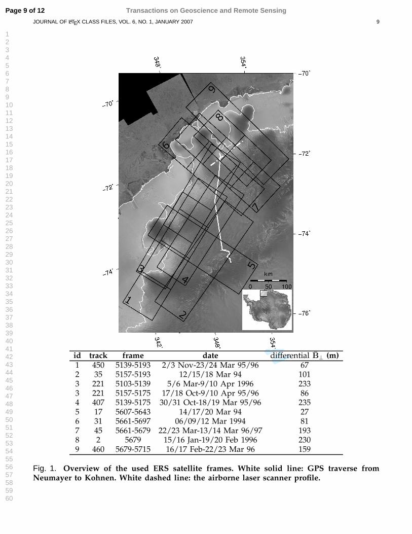
For Peer Review
JOURNAL OF LATEX CLASS FILES, VOL. 6, NO. 1, JANUARY 2007 9
id track frame date differential B⊥ (m)1 450 5139-5193 2/3 Nov-23/24 Mar 95/96 672 35 5157-5193 12/15/18 Mar 94 1013 221 5103-5139 5/6 Mar-9/10 Apr 1996 2333 221 5157-5175 17/18 Oct-9/10 Apr 95/96 864 407 5139-5175 30/31 Oct-18/19 Mar 95/96 2355 17 5607-5643 14/17/20 Mar 94 276 31 5661-5697 06/09/12 Mar 1994 817 45 5661-5679 22/23 Mar-13/14 Mar 96/97 1938 2 5679 15/16 Jan-19/20 Feb 1996 2309 460 5679-5715 16/17 Feb-22/23 Mar 96 159
Fig. 1. Overview of the used ERS satellite frames. White solid line: GPS traverse fromNeumayer to Kohnen. White dashed line: the airborne laser scanner profile.
Page 9 of 12 Transactions on Geoscience and Remote Sensing
123456789101112131415161718192021222324252627282930313233343536373839404142434445464748495051525354555657585960

For Peer Review
JOURNAL OF LATEX CLASS FILES, VOL. 6, NO. 1, JANUARY 2007 10
Fig. 2. Comparison of IceSAT ground control points with DEMs based on different SARprocessors. Localized dents appear as processing artifacts for instance in the upper left andlower right corner of D2.
Page 10 of 12Transactions on Geoscience and Remote Sensing
123456789101112131415161718192021222324252627282930313233343536373839404142434445464748495051525354555657585960
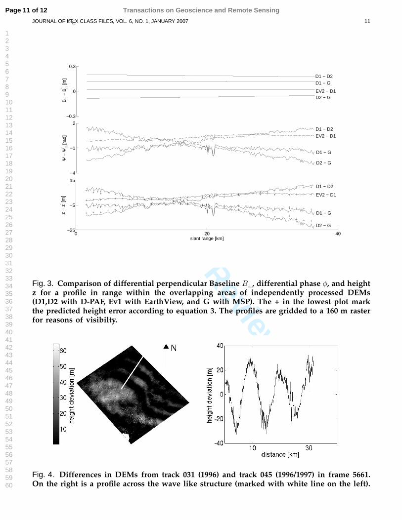
For Peer Review
JOURNAL OF LATEX CLASS FILES, VOL. 6, NO. 1, JANUARY 2007 11
−0.3
0
0.3B
⊥ −
B‘ ⊥ [m
]
−4
−1
2
Ψ −
Ψ‘ ⊥ [r
ad]
0 20 40−25
−5
15
z −
z‘ [m
]
slant range [km]
D1 − D2D1 − G
D2 − G
D1 − D2
EV2 − D1
D1 − G
D2 − G
D1 − D2
D1 − G
D2 − G
EV2 − D1
EV2 − D1
Fig. 3. Comparison of differential perpendicular Baseline B⊥, differential phase φ, and heightz for a profile in range within the overlapping areas of independently processed DEMs(D1,D2 with D-PAF, Ev1 with EarthView, and G with MSP). The + in the lowest plot markthe predicted height error according to equation 3. The profiles are gridded to a 160 m rasterfor reasons of visibilty.
Fig. 4. Differences in DEMs from track 031 (1996) and track 045 (1996/1997) in frame 5661.On the right is a profile across the wave like structure (marked with white line on the left).
Page 11 of 12 Transactions on Geoscience and Remote Sensing
123456789101112131415161718192021222324252627282930313233343536373839404142434445464748495051525354555657585960

For Peer Review
JOURNAL OF LATEX CLASS FILES, VOL. 6, NO. 1, JANUARY 2007 12
−50 0 50
1166
2333
3500
ALS − DInSAR [m]−50 0 50
143
290
440
GPS − DInSAR [m]−50 0 500
17500
35000
52500
IceSAT − DInSAR [m]
s =(2.9 +/− 4.1) m
Number of GCPs Number of GCPs
s =(−1.2 +/− 8.0) m s =(0.7 +/− 9.7) m
Number of GCPs
Fig. 5. Histogram of the DInSAR DEM compared to IceSAT, GPS and ALS ground controlpoints. The DInSAR data was filtered with a threshold of 0.8 in coherence, which excludedapproximately 15 percent of the IceSAT GCPs and less than 10 percent of the ALS and GPSpoints. The black line represents the corresponding Gaussian distribution.
(a) (b)
Fig. 6. Horizontal resolution (a) and resampled final DEM for Dronni ng Maud Land (b). Areasin (b) with a standard deviation higher than 5 m are masked out .
Page 12 of 12Transactions on Geoscience and Remote Sensing
123456789101112131415161718192021222324252627282930313233343536373839404142434445464748495051525354555657585960
Copyright © 2022 FDOKUMEN