WinAPEX Users Guide

Version 1.0

WinAPEXEvaporation

and Transpiration

Rain, Snow, & Chemicals

Surface Flow

Below Root Zone

Subsurface Flow

Title page

by

M. Magre, Dr. J.R. Williams, Dr. W.L. Harman, Dr. T. Gerik,

J. Greiner, L. Francis, E. Steglich, A. Meinardus

Blackland Research and Extension Center

Temple, Texas

August 2006

(i)

Table of Contents I. INTRODUCTION.............................................................................................................................................................1 II. MAIN MENU FUNCTIONS .......................................................................................................................................2

A. USER INPUT FILES ...........................................................................................................................................................2 1. Owners Files ..............................................................................................................................................................2

a) Add New Owner....................................................................................................................................................................... 3 b) Add New Livestock Herd by Owner ........................................................................................................................................ 4 c) Edit Owner ............................................................................................................................................................................... 5

2. Create New Watershed...............................................................................................................................................5 a) Watershed Parameters .............................................................................................................................................................. 5 b) Create Subarea File(s) .............................................................................................................................................................. 8

3. Edit Watershed Files ................................................................................................................................................15 a) Edit General Watershed Variables.......................................................................................................................................... 15 b) Edit Subarea ........................................................................................................................................................................... 16 c) Delete Watershed.................................................................................................................................................................... 17

4. Control Files ............................................................................................................................................................17 a) Add Control File..................................................................................................................................................................... 18 b) Add Using or Edit Existing Control File ................................................................................................................................ 19 c) Parameters for Revision in Control File ................................................................................................................................. 20 d) Delete Control File ................................................................................................................................................................. 22

5. Edit All Files - Managing the User Input files .........................................................................................................23 a) Data/Setup Selections and About Setup ................................................................................................................................. 23 b) Backgrounds........................................................................................................................................................................... 24 c) Control Table Editor............................................................................................................................................................... 26 d) Crop Data ............................................................................................................................................................................... 26 e) Cropping Systems................................................................................................................................................................... 27 f) Equipment/Activities .............................................................................................................................................................. 28 g) Fertilizers................................................................................................................................................................................ 32 h) Location.................................................................................................................................................................................. 33 i) Management ........................................................................................................................................................................... 34 j) Pesticides................................................................................................................................................................................ 46 k) Owner ..................................................................................................................................................................................... 47 l) Settings ................................................................................................................................................................................... 47 m) Soil..................................................................................................................................................................................... 48 n) Weather .................................................................................................................................................................................. 50 o) Watershed Editor .................................................................................................................................................................... 52

B. FILE SELECTION FOR PROGRAM EXECUTION .................................................................................................................52 C. MANAGING THE OUTPUT...............................................................................................................................................54

1. Open WinApexOut.mdb............................................................................................................................................54 2. View Customized Output ..........................................................................................................................................56

III. APPENDICES.............................................................................................................................................................60 A. APPENDIX A—WATERSHED DEFINITIONS.....................................................................................................................60 B. APPENDIX B—SUBAREA DEFINITIONS..........................................................................................................................61 C. APPENDIX C—WATERSHED NAME DEFINITIONS ..........................................................................................................67 D. APPENDIX D—WATERSHED SUBAREA DEFINITIONS.....................................................................................................68 E. APPENDIX E—ADDING SUBAREA(S) .............................................................................................................................71 F. APPENDIX F—MANNING’S N SURFACE ROUGHNESS (UPN).........................................................................................73 G. APPENDIX G—ROUTING REACH & CHANNEL MANNING’S N (RCHN & CHN)............................................................74 H. APPENDIX H—PARM DEFINITIONS................................................................................................................................75

(1)

I. Introduction WinAPEX is a user-friendly Windows® interface designed to assist users in executing APEX v. 0604. It contains a watershed builder subroutine in which users can delineate individual field (subarea) attributes including the upland slope, soil characteristic, land infiltration condition (curve number), routing reach and channel characteristics, cropping system, livestock activity, and one or more weather stations. These attributes can be edited for alternative analyses and comparisons of watershed losses. Losses are analyzed for runoff, sediment, nutrients and pesticides. Results are summarized in several ACCESS tables, each of which can be customized to include user-selected output for importing to an EXCEL spreadsheet. From there graphics, statistical analyses, and other options are provided the user as part of EXCEL.

(2)

II. Main Menu Functions The WinAPEX Main Menu serves four purposes for the user: creating and editing watershed files, accessing database files for editing, file selection for executing the program or making WinAPEX runs, and managing the output (Figure 1). These primary areas will be presented in the natural order or progression.

Main Menu

Figure 1: Main Menu Screen

A. User Input Files WinAPEX provides a means for specifying parameters for a watershed directly from the Main Menu screen: Owners Files, Create New Watershed, Edit Watershed Files, and Control Files (Figure 1). All of the files, once created, may be edited by clicking Edit All Files from the Main Menu screen; these will be discussed following those accessed directly from the Main Menu screen. Either method used produces the same result regardless of the manner in which the files are accessed.

1. Owners Files

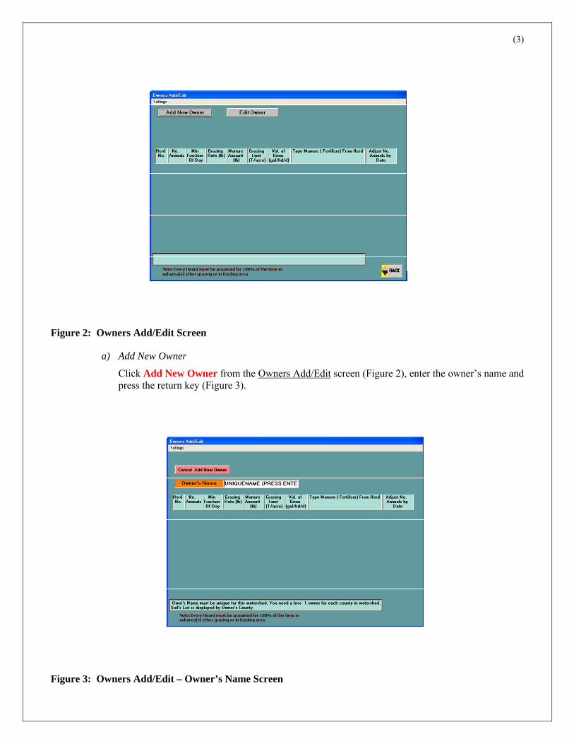
The user must create a unique owner name for each watershed and at least one owner for each county within a watershed. The user may click Owners Files from the Main Menu screen to manage owner(s) (Figure 2).

(3)

Owners Add/Edit Screen

Figure 2: Owners Add/Edit Screen

a) Add New Owner

Click Add New Owner from the Owners Add/Edit screen (Figure 2), enter the owner’s name and press the return key (Figure 3).

Owner’s Name

Figure 3: Owners Add/Edit – Owner’s Name Screen

(4)

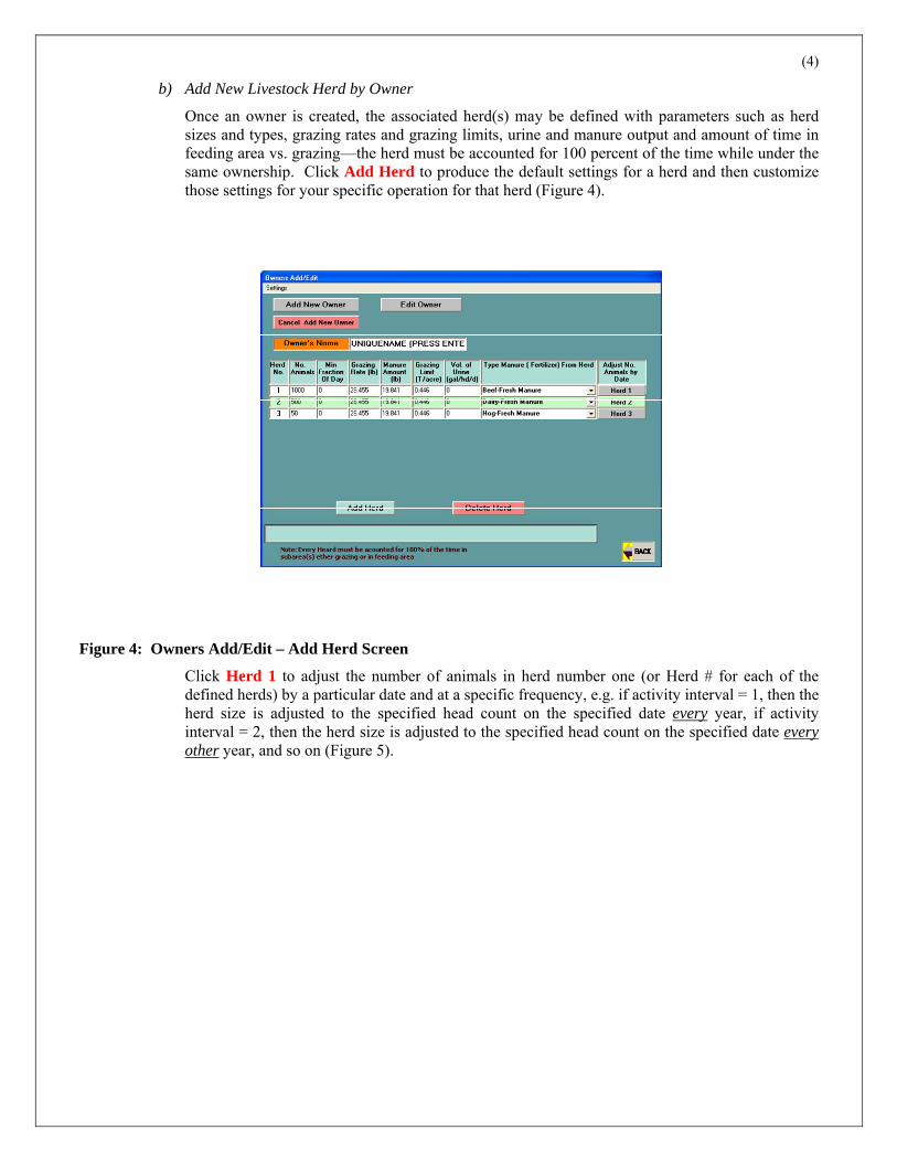
b) Add New Livestock Herd by Owner

Once an owner is created, the associated herd(s) may be defined with parameters such as herd sizes and types, grazing rates and grazing limits, urine and manure output and amount of time in feeding area vs. grazing—the herd must be accounted for 100 percent of the time while under the same ownership. Click Add Herd to produce the default settings for a herd and then customize those settings for your specific operation for that herd (Figure 4).

Add Herd

Figure 4: Owners Add/Edit – Add Herd Screen

Click Herd 1 to adjust the number of animals in herd number one (or Herd # for each of the defined herds) by a particular date and at a specific frequency, e.g. if activity interval = 1, then the herd size is adjusted to the specified head count on the specified date every year, if activity interval = 2, then the herd size is adjusted to the specified head count on the specified date every other year, and so on (Figure 5).

(5)

Adjust Herd Size

Figure 5: Owners Add/Edit – Adjust Herd Size Screen

This is used to adjust the head count or herd size on specific calendar dates, i.e. when animals are typically bought and sold or otherwise change in number. Select the month and day from the drop down menus then enter the total number of head existing in the herd. After final selections are made, the user is given the option to Save or Delete the adjustment. After all entries are made, click Back to return to the Owners Add/Edit – Add Herd screen (Figure 4). Up to ten herds may be added; herds may also be removed but note they are removed successively in reverse order by clicking Delete Last Herd so it’s important to review the herd specifications before entering the information.

c) Edit Owner

Once the owner(s) has/have been added, the user may make adjustments to existing owners. Click Edit Owner from the Owner Add/Edit screen to edit an existing owner (Figure 2). Select the owner from the drop down menu and proceed as when adding a new owner. Continue clicking Back until the Main Menu screen appears. Alternately, the user may edit or add owners as discussed in II.A.5.k).

2. Create New Watershed

The watershed is the area of land that captures rain and snow which drains or seeps into a marsh, stream, river, lake or an underground water supply. Many types of areas can make up watersheds including home sites, farms, ranches, forests, small towns, big cities, etc. Some watersheds cross county, state, and even international borders. Watersheds come in all shapes and sizes. Some are as large as many square miles while others are just a few acres. Just as creeks are smaller tributaries of rivers, watersheds are parts of larger water basins. General watershed variables include name, weather station, latitude, longitude, elevation, peak runoff rate, etc. A list of these and their explanations can be found in Appendix A—Watershed Definitions.

a) Watershed Parameters

(6)

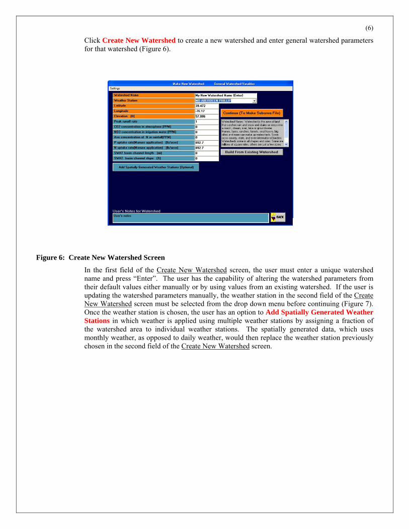
Click Create New Watershed to create a new watershed and enter general watershed parameters for that watershed (Figure 6).

Create New Watershed

Figure 6: Create New Watershed Screen

In the first field of the Create New Watershed screen, the user must enter a unique watershed name and press “Enter”. The user has the capability of altering the watershed parameters from their default values either manually or by using values from an existing watershed. If the user is updating the watershed parameters manually, the weather station in the second field of the Create New Watershed screen must be selected from the drop down menu before continuing (Figure 7). Once the weather station is chosen, the user has an option to Add Spatially Generated Weather Stations in which weather is applied using multiple weather stations by assigning a fraction of the watershed area to individual weather stations. The spatially generated data, which uses monthly weather, as opposed to daily weather, would then replace the weather station previously chosen in the second field of the Create New Watershed screen.

(7)

Spatially Gn WS

Figure 7: Spatially Generated Weather Stations

This procedure is optional and not commonly practiced. However, up to 10 stations may be used for spatially generated weather within a given watershed. This is done using the following sequence for each weather station assigned to a fraction of the watershed: click Add, select the weather station from the drop down menu which appears, and then assign a fraction of the watershed to this station. Repeat this process until the entire area of the watershed has been accounted, i.e. the summed fractions of area must equal 1.0 as noted on screen or an error message will appear. The user will be prevented from continuing until the total fractions sum to 1.0 or 100 percent of the watershed area. To change the weather station(s) used to generate spatial weather, change the selection in the drop down menu or click Delete Last to remove each of the previous and subsequent listing(s). Spatially generated weather stations are used if the variable NGN in the Control file is equal to zero. To remove all spatial weather assignments, click Remove all Spatially Generated Weather Stations and the original weather station chosen in the second field of the Create New Watershed screen will be used.

The user may want to build the new watershed based on the parameters of a watershed previously created as opposed to manually updating the watershed parameters. Click Build From Existing Watershed and select the watershed from which to base the new watershed values (Figure 8).

(8)

Build From Existing WSd

Figure 8: Build From Existing Watershed

For example, if the user wants to run a comparative analysis on the effects of a buffer strip, the first watershed or field could be created and then used as the basis for the second (which would be a duplication of the first except for the buffer strip area). After building the second watershed from the first, the user would simply add the subarea representing the buffer strip to the second watershed, run them and compare the two outcomes, changing the routing if necessary.

The watershed parameters onscreen will be updated using these base values from the selected watershed for the basic parameters as well as the subarea file for the new watershed. The information for the subarea file will be discussed in section II.A.2.b). The user may further fine tune these watershed parameters to their desired specifications. At any time, the user may cancel all by clicking the Back button and by choosing “Yes” when prompted.

b) Create Subarea File(s)

Once the user has set up the basic watershed parameters and selected the weather, the next step is to define the subareas. The user may click Continue (To Make the Subarea File) to create one or more subareas (up to 500). The basic subarea screen enables the user to set up the subarea files systematically (Figure 9).

(9)

Basic Subarea Screen

Figure 9: Create Subarea Files

The farm or watershed study may involve several fields, or subareas, or as generally called homogenous hydrologic landuse units (HLU). Each subarea is homogenous in climate, soil, landuse (operation schedule), topography and channel and routing reach characteristics. Therefore, the heterogeneity of a watershed/farm is determined by the number of subareas. Each subarea may be linked with each other according to the water routing direction in the watershed, starting from the most distant subarea towards the watershed outlet. The subareas are designated by number in the first field line.

To define the first subarea, the user must make selections in each of the orange fields either from the drop down menu selections or enter a number. These fields require specific information before the user may proceed. Entry is done sequentially but if the user omits any of the required information, a message will appear stating the step at which the user should return to enter the required information. Before proceeding with multiple subareas or watershed routing, the user will need more detailed information on subareas to aid in defining subareas.

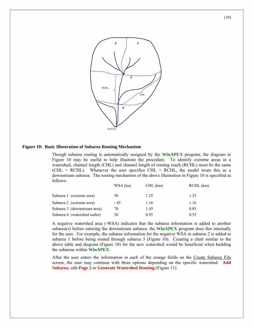
Generally speaking, the first subareas are characterized as being the farthest from the outlet; as water is routed through each subarea toward the outlet, the distance to the outlet gradually decreases on average. The primary variables which must be specified to determine the routing mechanism of every watershed include channel length, channel length of routing reach and watershed area (CHL, RCHL, and WSA, respectively). CHL is defined as the distance from the subarea outlet to the most distant point of the subarea. RCHL is defined as the distance of the routing reach of water flow through the subarea. Figure 10 illustrates a simple watershed with four subareas, which should help the user to understand how the routing mechanism is used in WinAPEX.

(10)

Basic Routing

1

4

2

RCHL

CHL

OUTLET

3

Figure 10: Basic Illustration of Subarea Routing Mechanism

Though subarea routing is automatically assigned by the WinAPEX program, the diagram in Figure 10 may be useful to help illustrate the procedure. To identify extreme areas in a watershed, channel length (CHL) and channel length of routing reach (RCHL) must be the same (CHL = RCHL). Whenever the user specifies CHL > RCHL, the model treats this as a downstream subarea. The routing mechanism of the above illustration in Figure 10 is specified as follows: WSA (ha) CHL (km) RCHL (km)

Subarea 1 (extreme area) 50 1.25 1.25

Subarea 2 (extreme area) - 45 1.16 1.16 Subarea 3 (downstream area) 70 1.45 0.85 Subarea 4 (watershed outlet) 30 0.95 0.55

A negative watershed area (-WSA) indicates that the subarea information is added to another subarea(s) before entering the downstream subarea; the WinAPEX program does this internally for the user. For example, the subarea information for the negative WSA in subarea 2 is added to subarea 1 before being routed through subarea 3 (Figure 10). Creating a chart similar to the above table and diagram (Figure 10) for the new watershed would be beneficial when building the subareas within WinAPEX.

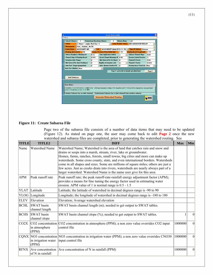
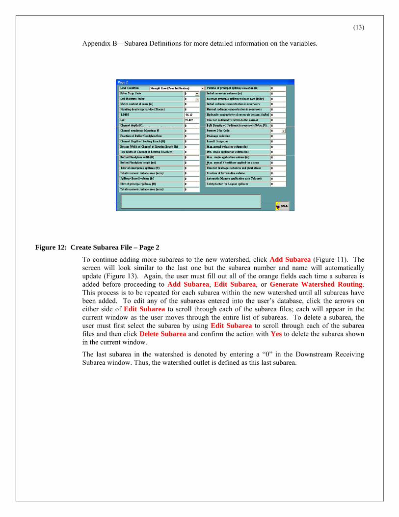
After the user enters the information in each of the orange fields on the Create Subarea File screen, the user may continue with three options depending on the specific watershed: Add Subarea, edit Page 2 or Generate Watershed Routing (Figure 11).

(11)

Subarea A1

Figure 11: Create Subarea File

Page two of the subarea file consists of a number of data items that may need to be updated (Figure 12). As stated on page one, the user may come back to edit Page 2 once the new watershed and subarea files are completed, prior to generating the watershed routing. See

TITLE TITLE2 DIFF Max MinName Watershed Name Watershed Name; Watershed is the area of land that catches rain and snow and

drains or seeps into a marsh, stream, river, lake or groundwater. Homes, farms, ranches, forests, small towns, big cities and more can make up watersheds. Some cross county, state, and even international borders. Watersheds come in all shapes and sizes. Some are millions of square miles; others are just a few acres. Just as creeks drain into rivers, watersheds are nearly always part of a larger watershed. Watershed Name is the name user give for this area.

APM Peak runoff rate Peak runoff rate; the peak runoff-rate-rainfall energy adjustment factor (APM); provides a means for fine tuning the energy factor used in estimating water erosion. APM value of 1 is normal range is 0.5 - 1.5

YLAT Latitude Latitude; the latitude of watershed in decimal degrees range is -90 to 90 YLOG Longitude Longitude; the longitude of watershed in decimal degrees range is -180 to 180 ELEV Elevation Elevation; Average watershed elevation BCHL SWAT basin

channel length SWAT basin channel length (m); needed to get output to SWAT tables.

BCHS SWAT basin channel slope

SWAT basin channel slope (%); needed to get output to SWAT tables. 1 0

CO2X CO2 concentration in atmosphere (PPM)

CO2 concentration in atmosphere (PPM); a non zero value overrides CO2 input control file

1000000 0

CQNX NO3 concentration in irrigation water (PPM)

NO3 concentration in irrigation water (PPM); a non zero value overrides CNO30 input control file

1000000 0

RFNX Ave concentration of N in rainfall

Ave concentration of N in rainfall (PPM) 1000000 0

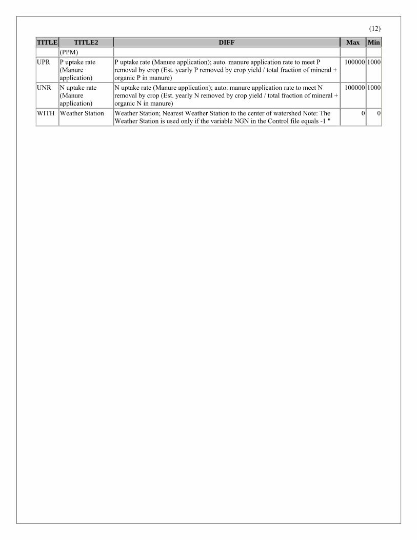
(12)

TITLE TITLE2 DIFF Max Min(PPM)

UPR P uptake rate (Manure application)

P uptake rate (Manure application); auto. manure application rate to meet P removal by crop (Est. yearly P removed by crop yield / total fraction of mineral + organic P in manure)

100000 1000

UNR N uptake rate (Manure application)

N uptake rate (Manure application); auto. manure application rate to meet N removal by crop (Est. yearly N removed by crop yield / total fraction of mineral + organic N in manure)

100000 1000

WITH Weather Station Weather Station; Nearest Weather Station to the center of watershed Note: The Weather Station is used only if the variable NGN in the Control file equals -1 "

0 0

(13)

Appendix B—Subarea Definitions for more detailed information on the variables.

Subarea A1-page2

Figure 12: Create Subarea File – Page 2

To continue adding more subareas to the new watershed, click Add Subarea (Figure 11). The screen will look similar to the last one but the subarea number and name will automatically update (Figure 13). Again, the user must fill out all of the orange fields each time a subarea is added before proceeding to Add Subarea, Edit Subarea, or Generate Watershed Routing. This process is to be repeated for each subarea within the new watershed until all subareas have been added. To edit any of the subareas entered into the user’s database, click the arrows on either side of Edit Subarea to scroll through each of the subarea files; each will appear in the current window as the user moves through the entire list of subareas. To delete a subarea, the user must first select the subarea by using Edit Subarea to scroll through each of the subarea files and then click Delete Subarea and confirm the action with Yes to delete the subarea shown in the current window.

The last subarea in the watershed is denoted by entering a “0” in the Downstream Receiving Subarea window. Thus, the watershed outlet is defined as this last subarea.

(14)

Add next Subarea

Figure 13: Add Additional Subarea(s)

After all of the subareas have been added to the new watershed, the user is ready to Generate Watershed Routing. This is done internally and the user simply confirms by clicking OK when the program confirms that the subarea file has been generated (Figure 14).

Add next Subarea

Figure 14: Generate Watershed Routing

The user will see the Main Menu screen after the subarea file is generated.

(15)

3. Edit Watershed Files

The user can manage previously defined watersheds and/or subareas by clicking Edit Watershed files from the Main Menu screen. After selecting the watershed name, the user may Edit General Watershed Variables, Edit Subarea or Delete Watershed (Figure 15).

Edit WShed

Figure 15: Select Watershed

a) Edit General Watershed Variables

The general watershed variables may be changed by entering new values directly into the table fields (Figure 16). This includes the option of adding or removing spatially generated weather stations to the watershed as discussed previously in section II.A.2.a). To save these changes, click Save Change or to cancel click Cancel Change. Click the Back button to return to the previous screen.

(16)

Edit WShed 2

Figure 16: Edit General Watershed Variables

b) Edit Subarea

Click Edit Subarea to edit the subarea files. Click the variable title name of any of the parameters listed in the table; use the drop down menus or enter the desired value in the box to the right (Figure 17). To save these changes, click Save Changes or to cancel click Cancel Changes.

(17)

Edit WShed 3

Figure 17: Edit Subarea Files

c) Delete Watershed

After selecting the watershed name as in Figure 15, the user may click Delete Watershed to remove all files and data for the selected watershed. Confirm selection with Yes or No.

4. Control Files

The control file or control table will determine when and under what circumstances the WinAPEX run will be made. Within the control table editor, the user is able to specify the starting year of the simulation, as well as the duration of the simulation. Automatic irrigation and fertilization parameters among numerous other control parameters are also set within the control table, including the auto irrigation trigger. In order to make runs using different years of simulation or irrigation strategies, several control tables must be created. From the Main Menu screen, click Control Files to Add/Edit Control File or Delete Control File (Figure 18).

(18)

Control File Menu

Figure 18: Control File Menu

The user is able to manage control files using the Control File Menu. Control files may be added, updated or deleted. Click Add/Edit Control File to enter the Control File Editor (Figure 19).

Control File Editor

Figure 19: Control File Editor

a) Add Control File

(19)

The data on the screen will remain locked until one of the three buttons is clicked: Add, Add Using or Edit. Upon selection, the user may add or change the parameter values in the “Current” column. For convenience, the default value is listed in the “Default” column. Click Default to refresh the “Current” values back to the “Default” values. The description of the parameters within the control file may be viewed by performing a right mouse click on each parameter name. Use the Next Page and Previous Page buttons to move through the parameter list in the file. Click Cancel or Back at any time to return to the Main Menu screen.

Click Add to add a new control record and a new number will be assigned automatically as the record number (Figure 20).

Control File Add

Figure 20: Add Control Record Screen

Name the control record (up to eight-characters) in the “Control Record Name” field and proceed with entering the values for the specific control record in the “Current” column. The user may enter values in each of the cells in the “Current” column or click Default to replace the “Current” values with the “Default” values for all of the parameters on the current page, i.e. if only a few of the parameters are different from the values in the default control file, this will quickly add the default values into the “Current” values column and those few parameters can be entered individually. Note: The start date of the simulation in the control table must be identical to (or later than) the initial date of the daily weather history. Otherwise, all weather will be generated as a random process. Also, entering a start date beyond the ending date of daily weather history will initiate generated weather.

Click Save to complete the process. NOTE: When creating a new run, the last control record saved will appear along with previous ones saved as different record numbers; otherwise, only one will appear for selection. Changing the name has no effect on the data being used in the control record—only the record number affects the data used.

b) Add Using or Edit Existing Control File

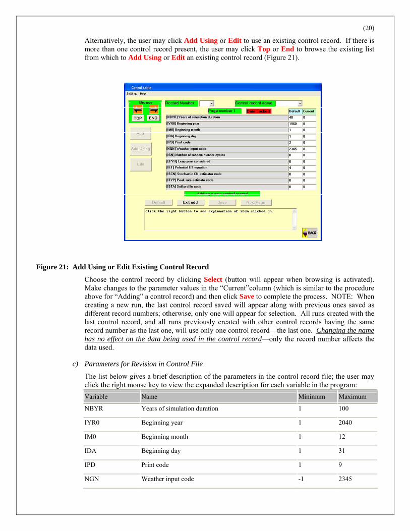
(20)

Alternatively, the user may click Add Using or Edit to use an existing control record. If there is more than one control record present, the user may click Top or End to browse the existing list from which to Add Using or Edit an existing control record (Figure 21).

Control File Add Using

Figure 21: Add Using or Edit Existing Control Record

Choose the control record by clicking Select (button will appear when browsing is activated). Make changes to the parameter values in the “Current”column (which is similar to the procedure above for “Adding” a control record) and then click Save to complete the process. NOTE: When creating a new run, the last control record saved will appear along with previous ones saved as different record numbers; otherwise, only one will appear for selection. All runs created with the last control record, and all runs previously created with other control records having the same record number as the last one, will use only one control record—the last one. Changing the name has no effect on the data being used in the control record—only the record number affects the data used.

c) Parameters for Revision in Control File

The list below gives a brief description of the parameters in the control record file; the user may click the right mouse key to view the expanded description for each variable in the program: Variable Name Minimum Maximum

NBYR Years of simulation duration 1 100

IYR0 Beginning year 1 2040

IM0 Beginning month 1 12

IDA Beginning day 1 31

IPD Print code 1 9

NGN Weather input code -1 2345

(21)

Variable Name Minimum Maximum

IGN Number of random number cycles 0 100

LPYR Leap year considered 0 1

IET Potential ET equation 0 5

ISCN Stochastic CN estimator code 0 1

ITYP Peak rate estimate code 0 4

ISTA Soil profile code 0 1

IHUS Automatic Heat Unit scheduling 0 1

ISLF Slope length/steepness factor 0 1

INFL0 Runoff Q estimation methodology 0 3

MSNP Nutrient/Pesticide output file 0 365

LBP Soluble Phosphorus runoff estimate 0 1

NAQ Air Quality Analysis 0 1

MSCP Solid manure scraping 0 365

MNUL Manure application code 0 2

NVCN0 Variable daily CN or non-varying CN 0 4

NUPC N and P plant uptake concentraion code 0 1

LPD Lagoon pumping 0 365

IERT Enrichment Ratio method for EPIC or GLEAMS 0 1

ICO2 Atmospheric CO2 0 1

RCN0 Average concentration of nitrogen in rainfall (ppm) 0.5 1.5

CO20 CO2 concentratiion in atmosphere (ppm) 50 10000

CQN0 Conc. of N in irrigation water (ppm) 0 10000

QG Channel Capacity Flow Rate 1 100

PSTX Pest damage scaling factor 0 10

YWI Number years of max. monthly .5 hour rainfall record 0 20

BTA Coeff. used to est. wet-dry prob. given mon. wet days 0 1

EXPK Parameter used to modify exp rain distribution 0 2

QCF Exponent in vatershed area flow rate EQ 0.4 0.6

IHY 0 for no flood routing, 1 for flood routing 0 1

ISW Soil water calculation code 0 2

FCW Floodplain width/channel width 2 50

(22)

Variable Name Minimum Maximum

BWD Channel bottom width/depth 1 20

FL Wind run Length 0.001 12

FW Wind run width 0.001 12

ANG0 Clockwise angle of field length from North 0 360

UXP Power parameter of modified exp dist of wind speed 0.1 0.5

SATO Saturated Conductivity adjustment factor 0.01 10

FPSC Floodplain saturated hydraulic conductivity 0.0001 10

RFPO Return Flow / (Return Flow + Deep Percolation) 0 1

RFTO Ground water residence time in days 0 365

GWSO Maximum ground water storage 5 200

CHSO Average upland slope in watershed 0.001 0.7

DIAM Soil particle diameter (UM) 100 500

ACW Wind erosion control factor 0 10

RTNO Number of years of cultivation at start of simulation 0 10000

GZLO Above ground plant material grazing limit 0.01 5

DRV Equation for water erosion 0 6

BUS1 1st input parm for MUSI 0 10

BUS2 2nd input parm for MUSI 0 0.9

QTH Routing Threshold - VSC routing used on QVOL>QTH 0 200000

STND - VSC Routing used when reach storage > STND 0 200000

BXCT Linear coefficient of change in rainfall from E to W (PI/PO/KM)

0 1

BYCT Linear coefficient of change in rainfall from S to N (PI/PO/KM)

0 1

DTHY Time interval for flood routing 0.05 12

BUS3 3rd input parm for MUSI 0 0.9

BUS4 4th input parm for MUSI 0 1.2

Note: If the grazing limit, GZLO, is greater than zero, it will be used only if the minimum grazing limit in the owners herd table is zero for any and all herds (see section II.A.1.b)).

d) Delete Control File

Control files may be deleted by clicking Delete Control File from the Control File Menu (Figure 18). The user must select the record number and control name of the control file from the list and then click Delete Selected Control Record (Figure 22).

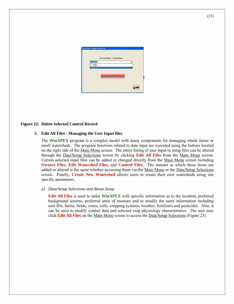
(23)

Control Fl Delete

Figure 22: Delete Selected Control Record

5. Edit All Files - Managing the User Input files

The WinAPEX program is a complex model with many components for managing whole farms or small watersheds. The program functions related to data input are executed using the buttons located on the right side of the Main Menu screen. The entire listing of user input or setup files can be altered through the Data/Setup Selections screen by clicking Edit All Files from the Main Menu screen. Certain selected input files can be added or changed directly from the Main Menu screen including Owners Files, Edit Watershed Files, and Control Files. The manner in which these items are added or altered is the same whether accessing them via the Main Menu or the Data/Setup Selections screen. Finally, Create New Watershed allows users to create their own watersheds using site specific parameters.

a) Data/Setup Selections and About Setup

Edit All Files is used to tailor WinAPEX with specific information as to the location, preferred background screens, preferred units of measure and to modify the users information including user IDs, farms, fields, zones, soils, cropping systems, weather, fertilizers and pesticides. Also, it can be used to modify control data and selected crop physiology characteristics. The user may click Edit All Files on the Main Menu screen to access the Data/Setup Selections (Figure 23).

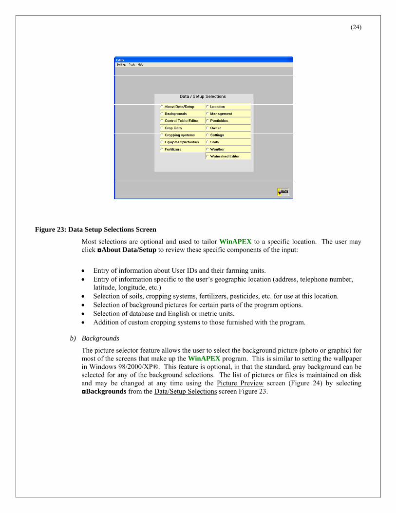
(24)

Data Setup Selections

Figure 23: Data Setup Selections Screen

Most selections are optional and used to tailor WinAPEX to a specific location. The user may click ◘About Data/Setup to review these specific components of the input:

• Entry of information about User IDs and their farming units. • Entry of information specific to the user’s geographic location (address, telephone number,

latitude, longitude, etc.) • Selection of soils, cropping systems, fertilizers, pesticides, etc. for use at this location. • Selection of background pictures for certain parts of the program options. • Selection of database and English or metric units. • Addition of custom cropping systems to those furnished with the program.

b) Backgrounds

The picture selector feature allows the user to select the background picture (photo or graphic) for most of the screens that make up the WinAPEX program. This is similar to setting the wallpaper in Windows 98/2000/XP®. This feature is optional, in that the standard, gray background can be selected for any of the background selections. The list of pictures or files is maintained on disk and may be changed at any time using the Picture Preview screen (Figure 24) by selecting ◘Backgrounds from the Data/Setup Selections screen Figure 23.

(25)

Backgrounds

Figure 24: Picture Preview Screen

There are two parts to the operation of the picture selector. First, the user is able to add, limit or delete the available pictures, photos or graphics for the individual screens. Second, the user may change backgrounds from each individual screen at any time without having to go to another part of the program. The latter option is found in the menu bar on the Main Menu screen under Settings/Background Picture. This feature allows each user to customize the background screens by selecting one of the screens provided or using their own custom photos or graphics. Either method used achieves the same result.

Selecting the background pictures available for the program is done via the Data/Setup Selections screen. The picture files, either photos or graphics, should be in the Windows® Metafile Format (.wmf). Bitmap formatted files (.bmp) may be used, however, Windows® Metafile Format is preferred because they are resizable. Utility programs are available which convert various types of files to Windows® Metafile Format. These optional, user-generated graphic files must be placed in the same directory as WinAPEX files. Up to 40 pictures can be placed on the selection list; however, 4 to 10 are sufficient. The Windows® Metafile Format files supplied with the program average around 350,000 bytes each and are photographs. Graphic files rather than photo-based files take less disk space (8,000 to 200,000 bytes, depending on the resolution of the graphic). The size, in bytes, of any picture file depends on its initial size, resolution and graphic format and can range from 1,000 to over 2 million bytes.

The ◘Backgrounds option from the Data/Setup Selections screen allows the user to build a list of graphic files to be made available to the program for use as screen backgrounds. Files may be added to and deleted from this list at any time. The program can only use the files in this list. If they are deleted, or otherwise made unavailable, the program cannot use them and the default screen, called “none” will be used. The file called “none.wmf” cannot be deleted.

The user may scroll the available graphic files on the far right in the “Choose From:” list and select one of them. The image will appear on the left side in the “Picture Preview screen”. Any of the images may be previewed or selected.

Operations for adding, limiting or deleting an image is as follows:

(26)

(1) Adding a Picture to the List

Scroll the image list by clicking on the down arrow (scroll) button under the “Choose From:” list. The user may select an image by clicking on the name of the picture (with the left mouse button) in the “Choose From:” list. If the picture has a valid file name, it will be displayed in the “Picture Preview screen”. The user may add it to the list by clicking on Add a picture to the list. Note: A message will appear if the desired picture file is already in the list.

(2) Deleting a Picture from the List

The center of the screen has a drop down menu entitled “Selected Pictures”. Scroll down the “Selected Picture” list and click on the graphic file chosen to delete from the list. The image will be displayed in the “Picture Preview screen”. Click on Delete a picture from the list and it will be removed from the “Picture Preview screen”. Note: This action does not remove the picture file from the hard disk; it will still be shown in the “Choose from:” list and can be added back to the list at any time. For permanent removal of the file from the hard disk, use normal file deletion techniques.

(3) Completing Picture Selection Maintenance

Click Back when finished adding or deleting pictures to the “Selected Pictures” list.

(4) Setting a Background Picture for Each screen

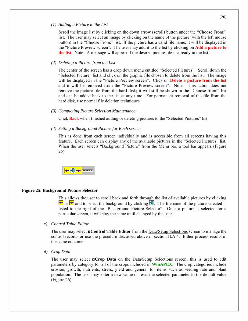
This is done from each screen individually and is accessible from all screens having this feature. Each screen can display any of the available pictures in the “Selected Pictures” list. When the user selects “Background Picture” from the Menu bar, a tool bar appears (Figure 25).

Figure 25: Background Picture Selector

This allows the user to scroll back and forth through the list of available pictures by clicking or and to select the background by clicking . The filename of the picture selected is

listed to the right of the “Background Picture Selector”. Once a picture is selected for a particular screen, it will stay the same until changed by the user.

c) Control Table Editor

The user may select ◘Control Table Editor from the Data/Setup Selections screen to manage the control records or use the procedure discussed above in section II.A.4. Either process results in the same outcome.

d) Crop Data

The user may select ◘Crop Data on the Data/Setup Selections screen; this is used to edit parameters by category for all of the crops included in WinAPEX. The crop categories include erosion, growth, nutrients, stress, yield and general for items such as seeding rate and plant population. The user may enter a new value or reset the selected parameter to the default value (Figure 26).

(27)

Figure 26: Crop Data Screen

e) Cropping Systems

Cropping systems are defined as unique combinations of the rotation (crop order), as well as the type, timing, rate and method for each operation associated with the rotation. The user may either select or add cropping systems for the specific location by clicking ◘Cropping Systems on the Data/Setup Selections screen.

Click ◘Select cropping systems for this location to select one, several or all cropping systems from the entire list for use in the WinAPEX program. Alternatively, by clicking ◘Add a cropping system the user may create a new cropping system from various combinations of three components: irrigation method, tillage type and crop (Figure 27).

(28)

Figure 27: Adding a Cropping System Screen

f) Equipment/Activities

Click ◘Equipment/Activities on the Data/Setup Selections screen to edit tillage and irrigation equipment information; for example, the user may indicate grazing quantity and manure deposited each day using this option. Select the activity category and then click Add or Edit (Figure 28).

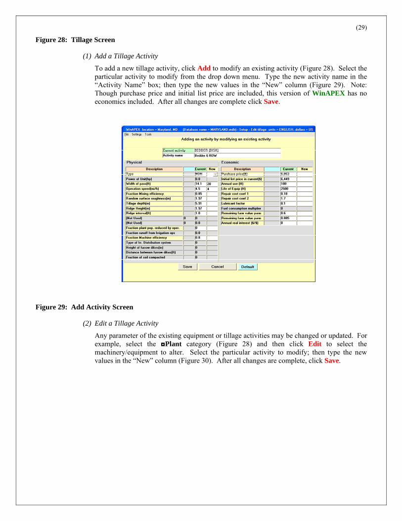
(29)

Figure 28: Tillage Screen

(1) Add a Tillage Activity

To add a new tillage activity, click Add to modify an existing activity (Figure 28). Select the particular activity to modify from the drop down menu. Type the new activity name in the “Activity Name” box; then type the new values in the “New” column (Figure 29). Note: Though purchase price and initial list price are included, this version of WinAPEX has no economics included. After all changes are complete click Save.

Figure 29: Add Activity Screen

(2) Edit a Tillage Activity

Any parameter of the existing equipment or tillage activities may be changed or updated. For example, select the ◘Plant category (Figure 28) and then click Edit to select the machinery/equipment to alter. Select the particular activity to modify; then type the new values in the “New” column (Figure 30). After all changes are complete, click Save.

(30)

Drill Air Delivery

Figure 30: Edit Activity Screen

In the case of irrigation systems with efficiencies indicated in their titles, the percentage runoff and percentage distribution efficiency cannot be changed. If, after reviewing the various systems, a center pivot system does not exist with the correct combination of runoff and distribution efficiency, there is a center pivot system with no efficiency in its title for customizing percentage runoff and percentage distribution efficiency.

For rice production, there is an equipment item typically used for rice flood irrigation: “Puddle Rice Paddy” which causes layer 2 of the soil profile to reduce infiltration significantly. To return soil to normal condition, include “Stop Puddle” as an operation.

(3) Specialized Categories

The Equipment Editor has some specialized categories including specific custom operations, grazing, plastic cover, and manure scraping, for example:

(a) Custom Operations

Certain custom operations are available; however, the program does not include costs at this time. In the future these costs will be added and may be altered to reflect specific expenses for certain custom operations. These include expenses for operations such as bagging and ties for cotton processing; cotton ginning; grain drying for seed grains, peanuts and rice; and hauling equipment. The procedure to update or alter these categories is the same as for adding or editing a tillage activity as discussed above in II.A.5.f)(2). Once activated, these custom costs may be changed, e.g. the user may enter the amount in “custom hire” which is the expense of the custom operation.

(b) Grazing

When using grazing as an enterprise, the amount of dry forage grazed is set in the “Daily Forage Consumption” (dry lbs/ac per head/day) (Figure 31). For this activity to be

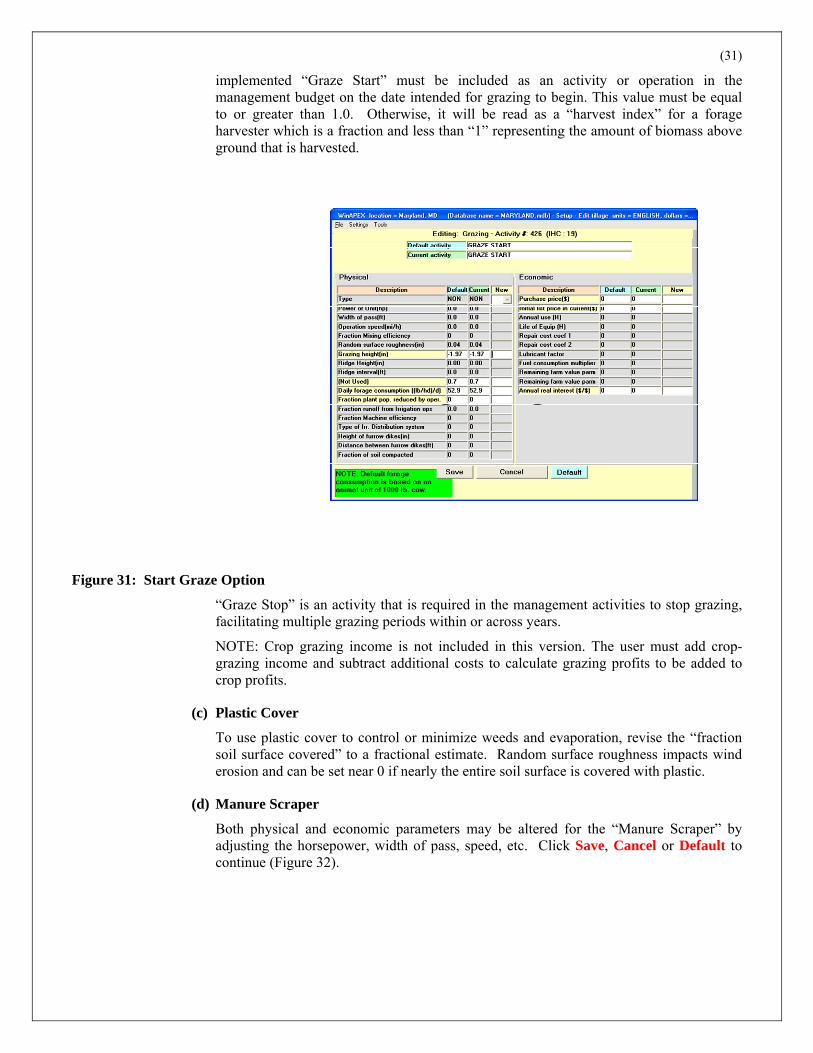
(31)

implemented “Graze Start” must be included as an activity or operation in the management budget on the date intended for grazing to begin. This value must be equal to or greater than 1.0. Otherwise, it will be read as a “harvest index” for a forage harvester which is a fraction and less than “1” representing the amount of biomass above ground that is harvested.

Graze Start

Figure 31: Start Graze Option

“Graze Stop” is an activity that is required in the management activities to stop grazing, facilitating multiple grazing periods within or across years.

NOTE: Crop grazing income is not included in this version. The user must add crop-grazing income and subtract additional costs to calculate grazing profits to be added to crop profits.

(c) Plastic Cover

To use plastic cover to control or minimize weeds and evaporation, revise the “fraction soil surface covered” to a fractional estimate. Random surface roughness impacts wind erosion and can be set near 0 if nearly the entire soil surface is covered with plastic.

(d) Manure Scraper

Both physical and economic parameters may be altered for the “Manure Scraper” by adjusting the horsepower, width of pass, speed, etc. Click Save, Cancel or Default to continue (Figure 32).

(32)

Manure Scraper

Figure 32: Manure Scraper

g) Fertilizers

To edit or select fertilizers for use in WinAPEX, select ◘Fertilizers on the Data/Setup Selections screen. Choose ◘Select Fertilizers for this location; select (or deselect certain unnecessary fertilizer products) from the list provided to add or remove specific fertilizer products to be listed when building management files. To modify any of the specific fertilizer products, choose ◘Edit Selected Fertilizers, select the specific fertilizer to edit from the drop down menu and make the desired changes. Fertilizer prices and costs of the amount applied are not yet included in the current version of WinAPEX (Figure 33).

(33)

Figure 33: Editing a Fertilizer Screen

Fertilizer price data listed under the "Current" column may be changed by entry of new data under the "New" column. However, until the economics module of the program is added, this change will not affect the user’s results. Cancel and Save appear when a change is entered in the "New" column. Note: The gray fields may not be altered.

h) Location

◘Location contains name, address, latitude, longitude and other miscellaneous data about the location or database (Figure 34).

(34)

Figure 34: Location Information

The latitude and longitude define the boundaries of the database. Maximum and minimum latitude and longitude are used for error checking when the latitude and longitude for individual run units (farms, fields and cells) are entered. If the run unit does not fall within the bounds specified under Data/Setup Selections/Location, the user is warned as the run unit data is entered.

i) Management

The files used to maintain farm operations and farm equipment for a particular crop may be managed to replicate a specific farm operation. To manipulate these management files or crop budgets, click ◘Management on the Data/Setup Selections screen. The user can Edit Existing Budgets, or add budget(s): 1 to 4 Annual Crop(s), Double Annual Crop(s), Annual Mono with Annual Cover Crop and 1 to 4 Perennial Crop(s) (Figure 35).

(35)

Management

Figure 35: Management Editor Screen

(1) Add 1 to 4 Annual Crop Budgets

From the Management Editor screen, click 1 to 4 Annual Crop(s) to make a budget for one to four crops per year (Figure 35). Select the number of crops to add and click Continue. Adding more than one crop assumes these crops are successive crops or are intercropped as opposed to double cropped which is restricted to two successive crops. Fill in the required fields: enter a new budget ID number to the new budget, identify the type of tillage and irrigation regimen, select the crop(s), and enter a new crop name and crop ID for each of the crops (Figure 36).

(36)

Mgmt 1 to 4 Annual

Figure 36: Add 1 to 4 Crop Budgets

Note: The new budget ID is limited to 10 alphanumeric characters. Click Continue and the budget operations for the new selection(s) is displayed in the Edit Budgets screen (Figure 37).

Continued

Figure 37: Edit Budgets/Add 1 to 4 Crop Budgets Screen

Essentially, this creates a new budget and it is treated from this point as an existing budget, i.e. the user may make other additions or changes to an existing budget in the same manner

(37)

used to Edit Existing Budgets which will be discussed later in section II.A.5.i)(5). A warning message may appear prompting the user to check the dates of operations or sequencing of operations so as to prevent errors from occurring. Click OK and proceed with adding operations if desired. To exit the Edit Budgets screens, the user must click the Back button and then Yes to save or No to cancel changes.

(2) Add a Double Annual Crop Budget

To add a new budget with a double annual crop, click Double Annual Crop(s) from the Management Editor screen (Figure 35). Fill in the required fields: assign a budget ID for the new budget, identify the type of tillage and determine whether dryland or some other type of irrigation system will be used. Select the first cropping system that will act as a starting point for the first crop in the new budget. The user may either use the crop already present in the database or create a new crop by clicking Make New Crop and fill in the new crop name and crop ID. Enter the second crop in the same manner as the first (Figure 38).

Double Annual Crop

Figure 38: Add a Double Crop Budget Screen

The new budget ID is limited to 10 alphanumeric characters. Click Continue and the budget operations for the new selections are displayed in the Edit Budgets screen since the budget just added is now treated as an existing budget which may be edited (Figure 39). A warning message may appear prompting the user to check the dates of operations or sequencing of operations so as to prevent errors from occurring. Click OK and proceed with adding operations if desired. To exit the Edit Budgets screens, the user must click the Back button and then Yes to save or No to cancel changes.

(38)

Contd

Figure 39: Edit Budgets/Add a Double Crop Budget Screen

(3) Add Annual Mono with Annual Cover Crop Budget

To add a new single crop budget with an annual cover crop, click Annual Mono with Annual Cover Crop from the Management Editor screen (Figure 35). Fill in the required fields: assign a budget ID for the new budget, identify the type of tillage and define what type of irrigation will be used. Select the cover cropping system that will act as a starting point for the new budget. The user may either use the crop already present in the database or create a new crop by clicking Make New Crop and fill in the new crop name and crop ID. Select the second crop in the same manner as the first (Figure 40).

(39)

Mono with Cover Crop

Figure 40: Add a Mono with Cover Crop Budget Screen

Click Continue and the budget operations for the new selections are displayed in the Edit Budgets screen since the budget just added is now treated as an existing budget which may be edited (Figure 41).

contd

Figure 41: Edit Budgets/Add a Mono with Cover Crop Budget Screen

(40)

A warning message may appear prompting the user to check the dates of operations or sequencing of operations so as to prevent errors from occurring. Click OK and proceed with adding operations if desired. To exit the Edit Budgets screens, the user must click the Back button and then Yes to save or No to cancel changes.

(4) Add 1 to 4 Perennial Crops Budget

To add one to four perennial crop budgets for up to 50 years, click Add 1 to 4 Crops (Perennial) from the Management Editor screen (Figure 35). Select the number of crops and the number of years in the budget. Fill in the required fields: assign a budget ID for the new budget, identify the type of tillage and determine whether dryland or some type of irrigation system will be used. Select the first crop that will act as a starting point for the new budget. The user may either use the crop already present in the database or create a new crop by checking “New Crop Name” and filling in the new crop name and crop ID. Select the proxy crop in the same manner as the first (Figure 42).

1 to 4 Perennial Crops

Figure 42: Add 1 to 4 Perennial Crops Screen

If the user wants the same crop in subsequent years, and wants to automatically add operations for the remaining years, repetitive operations which occur on a yearly basis can be added with this single action and the program will automatically add the operations every year of the budget. This will save time from having to enter the repetitious operations one by one.

Click Continue and if no proxy template is selected, answer yes or no (Figure 42). If yes is selected, a budget screen appears to build year 1 to be used as a repetitive process for years 2, 3…n. If no is selected, a generic budget including only a plant operation will appear to be used for years 2, 3…n to this planting operation. The user will only need to add operations that are repetitive. Click Continue after all operations are added. A harvest operation is required to get yields.

The number of years in a perennial crop budget in Setup must be equal to or an exact multiple of the number of years being simulated in the Control Table. If less, and the crop is harvested

(41)

in the last year only, no yield will be reported in the Crop Summary or Crop Yearly output Access tables. Additionally, if the simulated years are longer than in the perennial crop budget, yields will be reported for the first rotation of crop years but not necessarily for all of the years of the 2nd, 3rd, or nth rotations if the simulated years are not an exact multiple of the budget years in Setup.

By selecting one year more than the template budget, a screen will display year 1 operations of the template to allow major modifications, which are to be repetitive each year in the new crop budget. Make the necessary changes here and they will be repeated in all years after clicking Continue. Because the wrong number of years (one too many) was originally selected, several operations at the end may need to be deleted to restore the correct number of years to the rotation (change the final year of the kill but do not delete it).

When editing the final budget for repetitive operations with the same name, select the operation and hit the “Enter” button to register the change then click Change All (Figure 43).

Change All

Figure 43: Edit Budgets/Change All Feature

For irrigation and fertilizer amounts, select the amount or rate and type in the correct amount in the rate field below the budget table and hit the “Enter” key to register the change, and then click Change All. A message will appear requesting if the new amount is to replace all of the entries with the old amount. If so, click Yes.

Click Continue and OK to warning of checking dates on each operation. The budget operations for the new selections are displayed in the Edit Budgets screen since the budget just added is now treated as an existing budget that may be edited. See section II.A.5.i)(5) for more on editing a budget. Scroll to the next page to view years 2 and 3 in this three-year alfalfa crop budget (Figure 44).

(42)

contd

Figure 44: Edit Budgets/Add 1 to 4 Perennial Crops Screen

A perennial hay crop (e.g. alfalfa) will be harvested at the specified GDU fraction(s) of the growing season each year if and only if it is planted in YEAR 0 and harvested thereafter in YEARS 0 or 1 at one or more GDUs. If it is planted in YEAR 1 and harvested in YEAR 2, it will be planted every other year and harvested every other year at the specified GDUs. If a perennial hay crop is NOT to be harvested, the user must create a new perennial crop budget of the same crop. However, in the new crop budget all harvest operations must be deleted. This will cause the crop to grow until the end of the period, e.g. 20 years, without being harvested anytime. In perennial cropping systems, harvest(s) will occur every year for the number of years simulated (indicated in the control table) if planted in YEAR 1 despite the number of years in the crop budget.

If a fall-seeded perennial is to be reseeded after the last harvest, change all operations in YEAR 0 to YEAR 1. Then, move the kill operation to follow harvest in YEAR 1, but it must precede planting. Otherwise, if it is not to be reseeded after harvest, delete all operations in YEAR 1 and change operations in YEAR 0 to YEAR 1.

If a fall-seeded perennial is put into a rotation with an annual crop, make a seeded perennial template seed in YEAR 0 instead of YEAR 1 by these suggested steps:

• Develop a fake perennial budget called “ZZZZ” through the normal process of making a single crop, perennial for n years. This process will automatically renumber the fall seeding YEAR to 0 if the correct number of years in the template rotation are selected, i.e. if the template is for 3 years (years 1-3), selecting 2 years will renumber it 0-2 years.

• Develop the new perennial budget named the desired name, using the appropriate crop, and using “ZZZZ” as the template budget. The new fall-seeded budget will then be numbered 0,1,2...n.

(43)

• When making the rotation in Cropping Systems, always select the annual crop first followed by the new perennial crop numbered 0,1,2…n. This facilitates planting the perennial after the annual crop and harvesting both in sequential years.

To exit the Edit Budgets screens, the user must click Back through several screens until the Data/Setup Selections screen reappears.

(5) Edit an Existing Budget

To edit an existing budget by modifying it, click Edit Existing Budget from the Management Editor screen and select the crop budget to edit from the drop down menu. The operations for the selected budget will be displayed in the Edit Budgets screen (Figure 45).

Edit Mgmt

Figure 45: Edit Budgets Screen

To edit an existing operation type and/or change the attributes of an existing budget item, i.e. application amounts, application rates, depths of deposition, etc., the user may enter data directly to the on-screen table by selecting the cell(s) and then making the desired change(s) to the entry box beneath the data table (Figure 46).

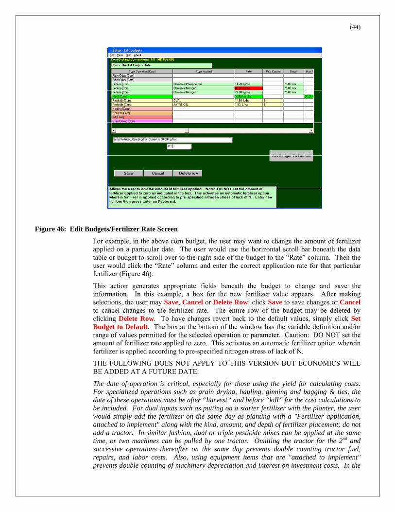
(44)

Edit Budgets/Fertilizer Rate Screen

Figure 46: Edit Budgets/Fertilizer Rate Screen

For example, in the above corn budget, the user may want to change the amount of fertilizer applied on a particular date. The user would use the horizontal scroll bar beneath the data table or budget to scroll over to the right side of the budget to the “Rate” column. Then the user would click the “Rate” column and enter the correct application rate for that particular fertilizer (Figure 46).

This action generates appropriate fields beneath the budget to change and save the information. In this example, a box for the new fertilizer value appears. After making selections, the user may Save, Cancel or Delete Row: click Save to save changes or Cancel to cancel changes to the fertilizer rate. The entire row of the budget may be deleted by clicking Delete Row. To have changes revert back to the default values, simply click Set Budget to Default. The box at the bottom of the window has the variable definition and/or range of values permitted for the selected operation or parameter. Caution: DO NOT set the amount of fertilizer rate applied to zero. This activates an automatic fertilizer option wherein fertilizer is applied according to pre-specified nitrogen stress of lack of N.

THE FOLLOWING DOES NOT APPLY TO THIS VERSION BUT ECONOMICS WILL BE ADDED AT A FUTURE DATE:

The date of operation is critical, especially for those using the yield for calculating costs. For specialized operations such as grain drying, hauling, ginning and bagging & ties, the date of these operations must be after “harvest” and before “kill” for the cost calculations to be included. For dual inputs such as putting on a starter fertilizer with the planter, the user would simply add the fertilizer on the same day as planting with a "Fertilizer application, attached to implement" along with the kind, amount, and depth of fertilizer placement; do not add a tractor. In similar fashion, dual or triple pesticide mixes can be applied at the same time, or two machines can be pulled by one tractor. Omitting the tractor for the 2nd and successive operations thereafter on the same day prevents double counting tractor fuel, repairs, and labor costs. Also, using equipment items that are "attached to implement" prevents double counting of machinery depreciation and interest on investment costs. In the

(45)

event of an operation such as spot spraying in which there is no specific machine or tractor used, select the "no cost operation" and include the kind and estimated amount of input per land unit, i.e. Roundup Ultra, 0.01 gal/ac.

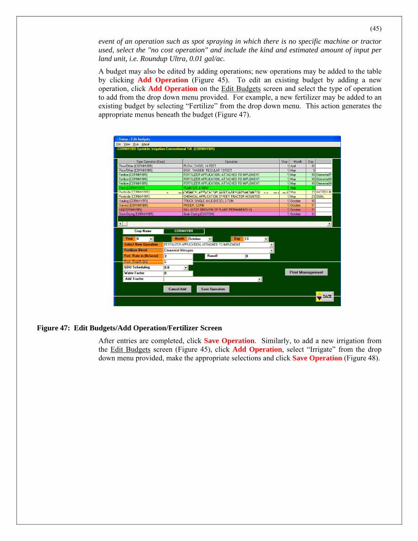
A budget may also be edited by adding operations; new operations may be added to the table by clicking Add Operation (Figure 45). To edit an existing budget by adding a new operation, click Add Operation on the Edit Budgets screen and select the type of operation to add from the drop down menu provided. For example, a new fertilizer may be added to an existing budget by selecting “Fertilize” from the drop down menu. This action generates the appropriate menus beneath the budget (Figure 47).

Edit Budgets/Add Operation/Fertilizer Screen

Figure 47: Edit Budgets/Add Operation/Fertilizer Screen

After entries are completed, click Save Operation. Similarly, to add a new irrigation from the Edit Budgets screen (Figure 45), click Add Operation, select “Irrigate” from the drop down menu provided, make the appropriate selections and click Save Operation (Figure 48).

(46)

Edit Budgets/Add Operation/Irrigation Screen

Figure 48: Edit Budgets/Add Operation/Irrigation Screen

Several sprinkler systems of various application efficiencies can be selected but the furrow (row) irrigation application efficiency with gated pipe is set at 75% of which 20% is runoff loss and 5% is distribution loss. To revise this and other irrigation system efficiencies, the user may edit the appropriate irrigation system in ◘Equipment/Activities on the Data/Setup Selections screen.

The user may at any time click the Set Budget to Default to cancel all changes to the budget and reset the budget values back to the original budget values for all operations. After all of the operations have been changed or added, click Save to save the new information in the datasheet. Click Back to exit the budget. The user will either click Yes to save all changes to the budget before exiting or No.

j) Pesticides

◘Pesticides on the Data/Setup Selections screen is used to edit or select pesticides for use and to turn on or off the pesticide fate and transport by checking the box in WinAPEX . To select/deselect specific pesticide products to be used, click ◘Select Pesticide products for this location then select pesticides (or deselect certain unnecessary pesticide products) from the list provided. To modify any of the specific pesticide products, click ◘Edit Selected Pesticides, choose specific pesticide(s) to edit from the drop down menu and make the desired changes. The user can modify the prices of the existing pesticides but until the economics module is added to the program, these changes will not affect the user’s results (Figure 49).

(47)

Edit Pesticide

Figure 49: Editing a Pesticide Screen

Pesticide price data listed under the "Current” column may be changed by entry of new data under the "New” column. Cancel and Save appear when a change is entered in the "New" column. Note: The gray fields may not be altered.

k) Owner

The user may add or edit the owner files by choosing ◘Owner on the Data/Setup Selections screen or by following the steps previously discussed in II.A.1. The procedure is identical.

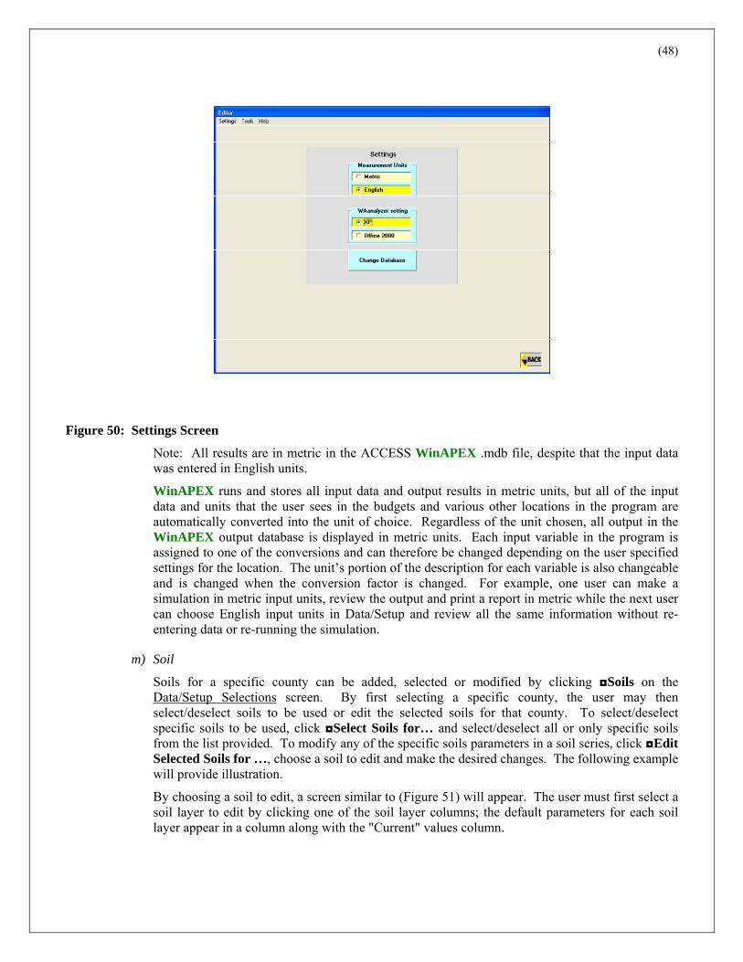
l) Settings

The ◘Settings option allows the user to set general parameters for a WinAPEX run. The user may select whether measurement units will be expressed in metric or English units and change the database. To convert from metric to English, or vice versa, choose ◘Settings on the Data/Setup Selections screen and make the appropriate choice (Figure 50). To change the database, click Change Database, and select the desired .mdb file. Additionally, the user may make these same changes using the menu bar: to change measurement units select “Settings” from the menu bar and select either “English” or “Metric”; to change databases, select “File” from the menu bar and select “Change Database”, select the .mdb and click Back.

(48)

Settings

Figure 50: Settings Screen

Note: All results are in metric in the ACCESS WinAPEX .mdb file, despite that the input data was entered in English units.

WinAPEX runs and stores all input data and output results in metric units, but all of the input data and units that the user sees in the budgets and various other locations in the program are automatically converted into the unit of choice. Regardless of the unit chosen, all output in the WinAPEX output database is displayed in metric units. Each input variable in the program is assigned to one of the conversions and can therefore be changed depending on the user specified settings for the location. The unit’s portion of the description for each variable is also changeable and is changed when the conversion factor is changed. For example, one user can make a simulation in metric input units, review the output and print a report in metric while the next user can choose English input units in Data/Setup and review all the same information without re-entering data or re-running the simulation.

m) Soil

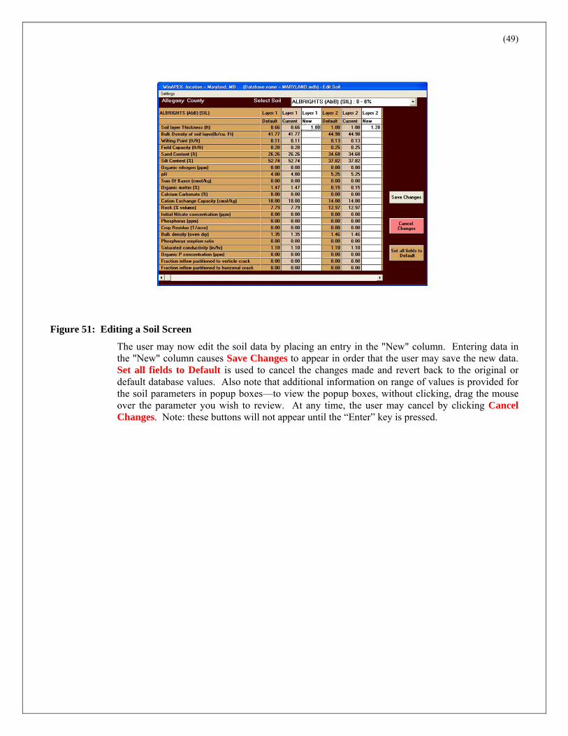
Soils for a specific county can be added, selected or modified by clicking ◘Soils on the Data/Setup Selections screen. By first selecting a specific county, the user may then select/deselect soils to be used or edit the selected soils for that county. To select/deselect specific soils to be used, click ◘Select Soils for… and select/deselect all or only specific soils from the list provided. To modify any of the specific soils parameters in a soil series, click ◘Edit Selected Soils for …, choose a soil to edit and make the desired changes. The following example will provide illustration.

By choosing a soil to edit, a screen similar to (Figure 51) will appear. The user must first select a soil layer to edit by clicking one of the soil layer columns; the default parameters for each soil layer appear in a column along with the "Current" values column.

(49)

Edit a Soil Screen

Figure 51: Editing a Soil Screen

The user may now edit the soil data by placing an entry in the "New" column. Entering data in the "New" column causes Save Changes to appear in order that the user may save the new data. Set all fields to Default is used to cancel the changes made and revert back to the original or default database values. Also note that additional information on range of values is provided for the soil parameters in popup boxes—to view the popup boxes, without clicking, drag the mouse over the parameter you wish to review. At any time, the user may cancel by clicking Cancel Changes. Note: these buttons will not appear until the “Enter” key is pressed.

(50)

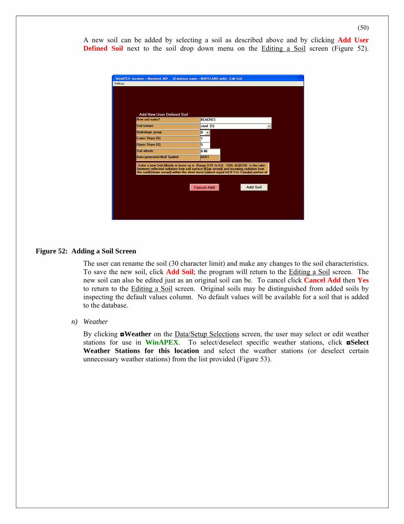
A new soil can be added by selecting a soil as described above and by clicking Add User Defined Soil next to the soil drop down menu on the Editing a Soil screen (Figure 52).

Add a Soil Screen

Figure 52: Adding a Soil Screen

The user can rename the soil (30 character limit) and make any changes to the soil characteristics. To save the new soil, click Add Soil; the program will return to the Editing a Soil screen. The new soil can also be edited just as an original soil can be. To cancel click Cancel Add then Yes to return to the Editing a Soil screen. Original soils may be distinguished from added soils by inspecting the default values column. No default values will be available for a soil that is added to the database.

n) Weather

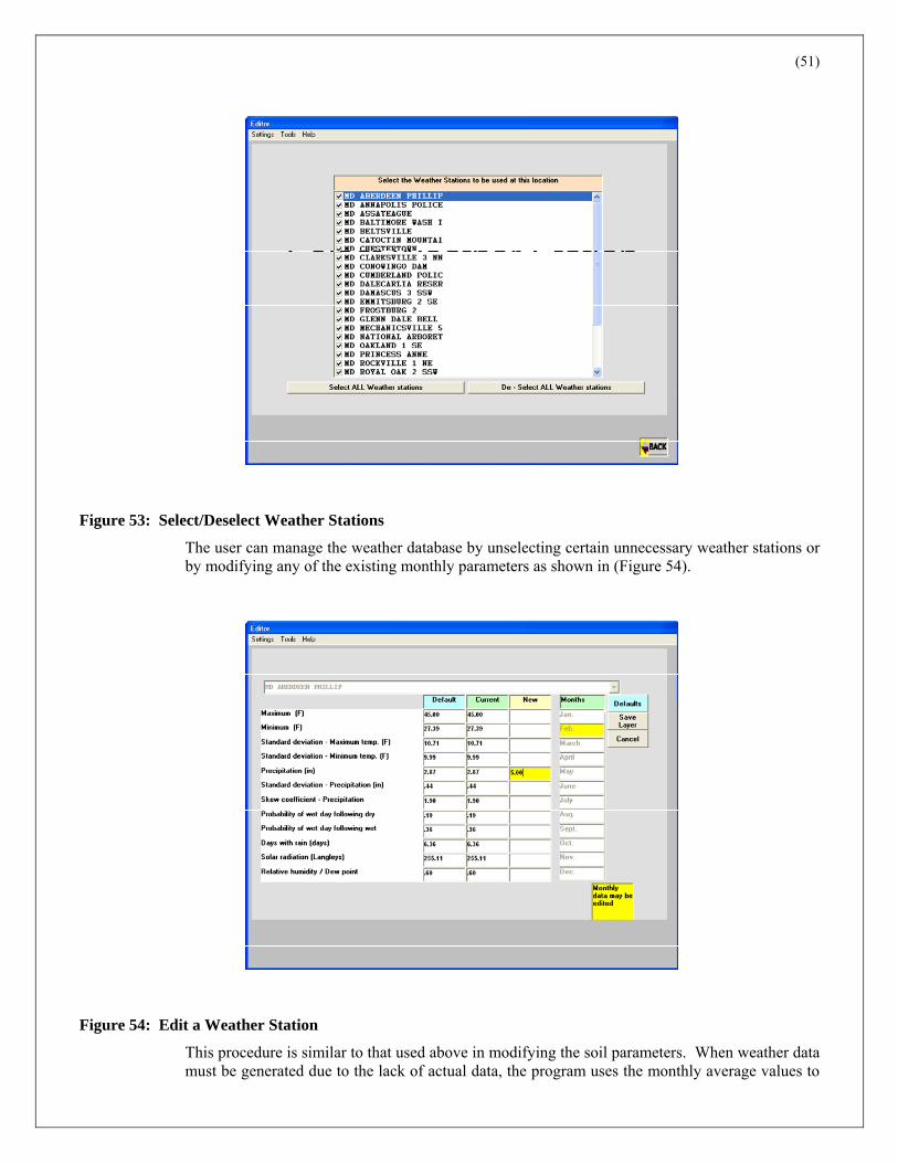
By clicking ◘Weather on the Data/Setup Selections screen, the user may select or edit weather stations for use in WinAPEX. To select/deselect specific weather stations, click ◘Select Weather Stations for this location and select the weather stations (or deselect certain unnecessary weather stations) from the list provided (Figure 53).

(51)

Select Weather Station

Figure 53: Select/Deselect Weather Stations

The user can manage the weather database by unselecting certain unnecessary weather stations or by modifying any of the existing monthly parameters as shown in (Figure 54).

Edit Weather Station

Figure 54: Edit a Weather Station

This procedure is similar to that used above in modifying the soil parameters. When weather data must be generated due to the lack of actual data, the program uses the monthly average values to

(52)

generate weather data. Therefore, increasing or decreasing the average monthly precipitation for a given period, for example, can simulate using relatively wetter or dryer periods than normal. To modify any of the specific weather stations, click ◘Select and Edit Monthly Weather, choose a weather station to edit from the drop down menu and make the desired changes. The form will remain locked until a month is chosen. Then the user may click the “New” column for the specific parameter and enter the new value for that particular month. To save, click Save or click Cancel to cancel all changes. At any time, the user may click Default to reset the “Current” values back to the original values.

o) Watershed Editor

The user may edit watersheds by choosing ◘Watershed Editor on the Data/Setup Selections screen or by following the steps previously discussed in section II.A.3. The procedure is identical.

B. File Selection for Program Execution To make a WinAPEX run, the user must select the watershed and the control file from the drop down menus on the Main Menu screen. These items would have been created earlier as discussed in sections II.A.2 and II.A.4.a) (Figure 55).

File selection and exe

Figure 55: Select Watershed / Select Control File

Typically, before each run is made, the user will clear the output from any previous runs; otherwise, output will be appended to the bottom of the output file. Press Clear WinApexOut.mdb to delete all output in the WinApexOut.mdb file (Figure 56).

(53)

Delete output file

Figure 56: Clear Output Files

Before a run is made, the user may also want to consider changing the output variables contained in the output. The user may select specific tables of data to be output in order to minimize run time. Click Change Output Files to specify the output files needed for the next run (Figure 57).

Change output options

Figure 57: Change Output Tables

(54)

The description box gives a brief review of the file types produced by the program. The user may select only certain files and information to be placed into the output file for viewing. Specific output files may be checked to minimize the amount of time it takes to complete a run. When all files have been chosen, press Save Changes.

The user may run WinAPEX by pressing Run WinAPEX; the confirmation screen will appear when the run is completed (Figure 58).

Run Completed

Figure 58: Run Completed

C. Managing the Output

1. Open WinApexOut.mdb

The user may save separate runs by renaming the WinApexOut.mdb file before it is cleared each time the program is run and use the output from these runs outside the WinAPEX program. The user would use the standard procedure with the Windows file manager to copy the output file to another file using copy and paste and then renaming the file (Figure 59).

(55)

Rename output file

Figure 59: Renaming the Output File Using Windows Explorer

The WinApexOut.mdb file is found in the WinAPEX parent directory. After a file is renamed, the user must use Windows Explorer and Microsoft Access to open, edit or delete the file. If the file is not renamed or cleared, all the data from each successive run is placed into the same file: WinApexOut.mdb. This file may be accessed directly from WinAPEX by pressing Open WinApexOut.mdb (Figure 55). The user is essentially accessing the output via the WinAPEX by invoking the Microsoft Access program from within the WinAPEX program. Therefore, the user must use standard operations for handling the file in Microsoft Access.

(56)

Open output file

Figure 60: Open WinApexOut.mdb Output File

2. View Customized Output

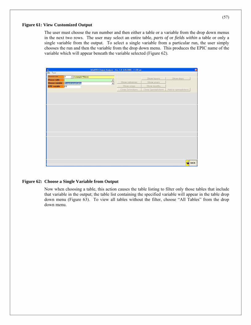
Oftentimes the user needs to compile or review the generated output for further analysis. This is facilitated using a search engine incorporated into the WinAPEX program. Simply click View Customized Output from the Run Completed screen (Figure 58) to access the search engine and select the run number containing the output from which the user would like to analyze (Figure 61).

View Custom Output

(57)

Figure 61: View Customized Output

The user must choose the run number and then either a table or a variable from the drop down menus in the next two rows. The user may select an entire table, parts of or fields within a table or only a single variable from the output. To select a single variable from a particular run, the user simply chooses the run and then the variable from the drop down menu. This produces the EPIC name of the variable which will appear beneath the variable selected (Figure 62).

ET Variable from Output

Figure 62: Choose a Single Variable from Output

Now when choosing a table, this action causes the table listing to filter only those tables that include that variable in the output; the table list containing the specified variable will appear in the table drop down menu (Figure 63). To view all tables without the filter, choose “All Tables” from the drop down menu.

(58)

Table filter

Figure 63: Table Filter

The user selects the table of choice and all of the fields are displayed on the bottom left portion of the screen with the variable selected automatically highlighted (Figure 64).

Table Fields List

Figure 64: Table Fields Listing

The user may also select the entire table or parts of it, which may be done at this point or initially before selecting a single variable by simply selecting a table from the drop down menu after selecting

(59)

the run. Either way, the fields within the table are shown on the bottom left portion of the screen where the user may check selected fields from the entire table.

Depending on the type of output the table contains, the user may subset this dataset further by selecting only specific subareas, crops, soil layers, years, months and/or days with the buttons to the right of the run and table drop down menus. Once selected, the information within may be used to again subset the data from a larger set of output and then added to a spreadsheet to minimize the amount of data the user must handle. This is done by selecting the “show” buttons. For example, our sample has two subareas so we can click Show Subarea to select only one of the two subareas output (Figure 65).

Show subareas

Figure 65: Show Subareas and Add to Spreadsheet

The user selects subarea “1” and then clicks Add to Spreadsheet; the ET data for subarea one is added to a spreadsheet in “spreadsheet format” on the screen. The user may use the data onscreen to perform analyses or export the data to Excel using the icons at the top of the spreadsheet. Alternately, the user may click Clear Spreadsheet at any time to change variables, tables and or fields and repeat the process above to view and/or export additional data.

Additionally, the user may want to view ET for subarea one for individual years. This may be done in a similar manner by clicking Show Years. This is not illustrated but may be done to further subset the data. The same is true for data formatted such that the other buttons may be used: Show Crops, Show Months, Show Days, and Show Layers. At any time, the ◘View Table bullet is available to view the original and complete ACCESS table directly from the output file, WinApexOut.mdb.

(60)

III. Appendices

A. Appendix A—Watershed Definitions TITLE TITLE2 DIFF Max MinName Watershed Name Watershed Name; Watershed is the area of land that catches rain and snow and

drains or seeps into a marsh, stream, river, lake or groundwater. Homes, farms, ranches, forests, small towns, big cities and more can make up watersheds. Some cross county, state, and even international borders. Watersheds come in all shapes and sizes. Some are millions of square miles; others are just a few acres. Just as creeks drain into rivers, watersheds are nearly always part of a larger watershed. Watershed Name is the name user give for this area.

APM Peak runoff rate Peak runoff rate; the peak runoff-rate-rainfall energy adjustment factor (APM); provides a means for fine tuning the energy factor used in estimating water erosion. APM value of 1 is normal range is 0.5 - 1.5

YLAT Latitude Latitude; the latitude of watershed in decimal degrees range is -90 to 90 YLOG Longitude Longitude; the longitude of watershed in decimal degrees range is -180 to 180 ELEV Elevation Elevation; Average watershed elevation BCHL SWAT basin

channel length SWAT basin channel length (m); needed to get output to SWAT tables.

BCHS SWAT basin channel slope

SWAT basin channel slope (%); needed to get output to SWAT tables. 1 0

CO2X CO2 concentration in atmosphere (PPM)

CO2 concentration in atmosphere (PPM); a non zero value overrides CO2 input control file

1000000 0

CQNX NO3 concentration in irrigation water (PPM)

NO3 concentration in irrigation water (PPM); a non zero value overrides CNO30 input control file

1000000 0

RFNX Ave concentration of N in rainfall (PPM)

Ave concentration of N in rainfall (PPM) 1000000 0

UPR P uptake rate (Manure application)

P uptake rate (Manure application); auto. manure application rate to meet P removal by crop (Est. yearly P removed by crop yield / total fraction of mineral + organic P in manure)

100000 1000

UNR N uptake rate (Manure application)

N uptake rate (Manure application); auto. manure application rate to meet N removal by crop (Est. yearly N removed by crop yield / total fraction of mineral + organic N in manure)

100000 1000

WITH Weather Station Weather Station; Nearest Weather Station to the center of watershed Note: The Weather Station is used only if the variable NGN in the Control file equals -1 "

0 0

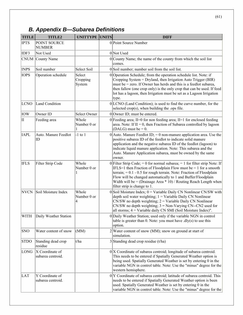
(61)

B. Appendix B—Subarea Definitions TITLE TITLE2 UNITTYPE UNITS DIFF IPTS POINT SOURCE

NUMBER 0 Point Source Number

IDF3 Not Used 0 Not Used CNUM County Name 0 County Name; the name of the county from which the soil list

comes. INPS Soil number Select Soil 0 Soil number; number soil from the soil list. IOPS Operation schedule Select

Cropping System

0 Operation Schedule; from the operation schedule list. Note: if Cropping System = Dryland, then Irrigation Auto Trigger (BIR) must be = zero. If Owner has herds and this is a feedlot subarea, then fallow (one crop only) is the only crop that can be used. If feed lot has a lagoon, then Irrigation must be set as a Lagoon Irrigation type.

LCNO Land Condition 0 LCNO (Land Condition); is used to find the curve number, for the selected crop(s), when building the .ops file.

IOW Owner ID Select Owner 0 Owner ID; must be entered. II Feeding area Whole

Number 0 or 1

0 Feeding area; II=0 for non feeding area; II=1 for enclosed feeding area. Note: If II = 0, then Fraction of Subarea controlled by lagoon (DALG) must be = 0.

IAPL Auto. Manure Feedlot ID

-1 to 1 0 Auto. Manure Feedlot ID; = 0 non-manure application area. Use the positive subarea ID of the feedlot to indicate solid manure application and the negative subarea ID of the feedlot (lagoon) to indicate liquid manure application. Note: This subarea and the Auto. Manure Application subarea, must be owned by the same owner.

IFLS Filter Strip Code Whole Number 0 or 1

0 Filter Strip Code; = 0 for normal subarea; = 1 for filter strip Note: If IFLS=1 then Fraction of Floodplain Flow must be = 1 for a smooth terrain; = 0.1 - 0.5 for rough terrain. Note: Fraction of Floodplain Flow will be changed automatically to 1 and Buffer/Floodplain Width will be = (Drainage Area * 10) / Routing Reach Length when filter strip is change to 1.

NVCN Soil Moisture Index Whole Number 0 or 4

0 Soil Moisture Index; 0 = Variable Daily CN Nonlinear CN/SW with depth soil water weighting; 1 = Variable Daily CN Nonlinear CN/SW no depth weighting; 2 = Variable Daily CN Nonlinear CN/SW no depth weighting; 3 = Non-Varying CN--CN2 used for all storms; 4 = Variable daily CN SMI (Soil Moisture Index)".

WITH Daily Weather Station 0 Daily Weather Station; used only if the variable NGN in control table is greater than 0. Note: you must have .dly(s) to use this option.

SNO Water content of snow (MM) 2 Water content of snow (MM); snow on ground at start of simulation.

STDO Standing dead crop residue

t/ha 3 Standing dead crop residue (t/ha)

LONG X Coordinate of subarea centroid.

0 X Coordinate of subarea centroid; longitude of subarea centroid. This needs to be entered if Spatially Generated Weather option is being used. Spatially Generated Weather is set by entering 0 in the variable NGN in control table. Note: Use the "minus" degree for the western hemisphere.

LAT Y Coordinate of subarea centroid.

0 Y Coordinate of subarea centroid; latitude of subarea centroid. This needs to be entered if Spatially Generated Weather option is been used. Spatially Generated Weather is set by entering 0 in the variable NGN in control table. Note: Use the "minus" degree for the

(62)

TITLE TITLE2 UNITTYPE UNITS DIFF western hemisphere.

WSA Subarea size (ha) 11 Size of Subarea (ha), Note: If this is a second extreme and it's flow joins the first extreme area flow but does not flow through the first extreme area, a "minus" sign is added to the front of the second extreme area. WSA makes it a negative number (this tells the program to add the second area WSA to the first extreme area as it relates to water flow).

CHL Longest Distance From Outlet

(km) 13 Distance From Outlet to Most Distant Point in Subarea (CHL) (km or miles) The channel length is the distance along the channel from the most distant point on the subarea to the outlet. Often in small areas (approx. 1 ha) there is no defined channel. In such cases the length is measured along a concentrated flow path or it can simply be estimated from the length-width ratio of the subarea. For areas < 20 ha, the channel length measurement is not critical. In such cases, enter 0. Units are kilometers (metric) or miles (English). If this is a EXTREME subarea then Channel Length of Routing Reach MUST EQUAL Distance from Outlet. If this is a DOWNSTREAM subarea then Channel Length of Routing Reach can NOT BE EQUAL to Distance from Outlet.

CHD Channel depth m 6 Channel depth (m) CHS Channel slope. m/m 15 Mainstream channel slope (m/m), the average channel slope is

computed by dividing the difference in elevation between the watershed outlet and the most distant point by CHL. For small areas this measurement is not critical because CHL and CHS are only used in estimating the watershed time of concentration. The dominant portion of the time of concentration is involved with overland rather than channel flow in small watersheds.

CHN Channel roughness Manning’s N

0 See Appendix G—Routing Reach & Channel Manning’s N (RCHN & CHN)

STP Average Upland Slope m/m 15 Average Upland Slope (m/m); must be entered. The average watershed slope can be estimated from field measurement or by using the Grid-Contour Method (Williams and Berndt 1977).

SPLG Ave Upland Slope Length

m 6 Ave Upland Slope Length (m); Must be entered. The watershed slope length can be estimated by field measurement as described by Wischmeier and Smith (1978) or from topographic maps using the Contour-Extreme Point Method (Williams and Berndt 1977).

UPN The surface roughness Manning’s N

0 Appendix F—Manning’s N Surface Roughness (UPN)

FFPQ Fraction of Buffer/floodplain flow

0 Fraction of buffer/floodplain flow; Partitions flow through filter strips.

RCHL Routing Reach Length km 13 Length of Routing Reach (RCHL) in (km or miles); The length (distance) between where channel starts or enters the subarea and where it exits the subarea. If this is an EXTREME subarea, then Routing Reach Length MUST EQUAL Longest Distance from Outlet (CHL). If this is a DOWNSTREAM subarea, then Routing Reach Length can not be equal to Longest Distance from Outlet.

RCHD Channel Depth of Routing Reach

m 6 Channel Depth of Routing Reach (m)

RCBW Bottom Width of Channel of Routing Reach

m 6 Bottom Width of Channel of Routing Reach (m)

RCTW Top Width of Channel of Routing Reach

m 6 Top Width of Channel of Routing Reach (m)

(63)

TITLE TITLE2 UNITTYPE UNITS DIFF RCHS Channel Slope of

Routing Reach m/m 15 Channel Slope of Routing Reach (m/m); Must be entered.

RCHN Channel Mannings N of Routing Reach.

0 See Appendix G—Routing Reach & Channel Manning’s N (RCHN & CHN)

RCHC USLE Crop Mangement Channel Factor

0 USLE Crop Management Channel Factor. For example, with bare channel condition, RCHC should be 0.1- 0.6 and if the channel has very good land cover, it should take on a value of 0. 0001 (0.0001 - 0.6).

RCHK USLE Erodibility Channel factor

0 USLE Erodibility Channel factor. For example, with a rock condition, RCHK should be 0.0001; with loess (silt/mud) condition, it should take on a value of 0.30. (0.0001 - 0.5).

RFPW Buffer/Floodplain width

m 6 Buffer/Floodplain width = (Drainage Area (WSA) X 10000) / (Floodplain length (RFPL) X 1000).

RFPL Buffer/Floodplain length

km 13 Buffer/Floodplain length (km)

RSEE Elev of emergency spillway

M 6 Elevation at emergency spillway elevation (m).

RSAE Total reservoir surface area

ha 11 Total reservoir surface area at emergency spillway elevation (km).

RSVE Runoff volume mm 2 Runoff volume at emergency spillway elevation (mm). RSEP Elev of principal

spillway M 6 Elevation at principal spillway elevation (m).

RSAP Total reservoir surface area

ha 11 Total reservoir surface area at principle spillway elevation (ha).

RSV0 Volume at principal spillway elevation

mm 2 Volume at principal spillway elevation (mm).

RSV Initial reservoir volumes

mm 2 Initial reservoir volumes (mm).

RSRR Average principle spillway release rate

mm/hr 61 Average principle spillway release rate (mm/hr).

RSYS Initial sediment concentration in reservoirs

0 Initial sediment concentration in reservoirs (ppm).

RSYN Normal sediment concentration in reservoirs

0 Normal sediment concentration in reservoirs (ppm).

RSHC Hydraulic conductivity of reservoir bottoms

mm/hr 61 Hydraulic conductivity of reservoir bottoms (mm/hr).

RSDP Time required for the sediment to return to normal

0 Time required for the sediment to return to normal; time required in days for the sediment in the reservoir to return to the normal concentrations following a runoff event.

RSBD Bulk Density of Sediment in reservoir

T/M^3 36 Bulk Density of Sediment in Reservoir (T/M^3)

NIRR Rigidity of irrigation code

0 Rigidity of irrigation code; for flexible applications. Applies minimum of FC-SW and ARMX. 1 for rigid applications; Applies input amount or ARMX. The irrigation code is used to specify the irrigation strategy. There are two mode of irrigating -- manual and automatic. If manual irrigation is selected, irrigation occurs on user specified dates and volumes. 0 = the irrigation is applied when needed and only as much as is needed;. 1 = the application is according to the amounts specified, either by automatic application (ARMX) or by user input amounts and restrictions.

(64)

TITLE TITLE2 UNITTYPE UNITS DIFF IRR Irrigation Code 0 Irrigation Code; IRR is set by change Operation schedule (IOPS)

Irrigation Code 0 = dryland, 1 = sprinkler irrigation, 2 = flood/furrow irrigation, 3 = fertigation, 4 = lagoon, and 5 = Drip irrigation. The irrigation code is used to specify whether irrigation is used and the type of irrigation. If flood/furrow irrigation is specified irrigation induced erosion is calculated. If fertigation is specified, IDFT identifies the type of fertilizer and FNP the amount of fertilizer with each irrigation. If lagoon is specified the concentration in tons of soils per m**3 of effluent is specified by FNP and the nutrient fraction by creating a fertilizer in the Fert1310.dat file with the appropriate nutrients and selecting it with IDFT.

IRI Min.application interval for auto. Irrigation

days 0 Minimum Application Interval for automatic irrigation (days); If IRR = 0 then set IRI = 0.

IFA Min. fertilizer application interval

days 0 Minimum fertilizer application interval (days); for auto option.

LM Liming Code 0 Liming Code; 0 = applies lime automatic; 1 = applies no lime. IFD Furrow Dike Code 0 Furrow Dike Code; 0 = does not use a furrow dike system; 1 =

considers a furrow dike system. IDR Drainage code mm 2 Drainage code; 0 = no drainage or enter depth to drainage system

(mm). IDF01 Liquid Fertilizer

Number 0 Liquid Fertilizer Number; from Lagoon, Select fertilizer from lists

provided (FERT.dat) or NONE. (MUNL in Control File MUST BE SET).

IDF02 Solid Manure From Feeding Area Stock Pile

0 Solid Manure From Feeding Area Stock Pile; automatic solid manure application from feeding area stock pile only. Fertilizer number or NONE. (FNP5 must be set and MUNL in Control File MUST BE SET).

IDF04 Automatic comercial Fertizer Application

0 Automatic commercial application; fertilizer number or NONE. (defaults to ELEM N) (BFT must be set), (FNP5 must be set).

IDF05 Automatic Solid Manure Application

0 Automatic solid manure application; fertilizer number or NONE. (As needed) (FNP5 must be set and MUNL in Control File MUST BE SET).

BIR Irrigation Auto Trigger 0 Irrigation Auto Trigger; Water stress factor to trigger automatic irrigation. To trigger automatic irrigation, the water stress factor is set: BIR= 0.0 Allows plants to be affected water stress; 0.8 BIR > 0.0 AND BIR < 1.0 fraction of plant stress; BIR = 1.0 Does not allow water stress; BIR < 0.0 Plant available water deficit in root zone (-mm); BIR > 1.0 For soil water tension Kilopascals in top 200mm - 1000.0 Sets water deficit high enough that only manual irrigations will occur.

EFI Runoff Irrigation 0 Runoff Irrigation; runoff vol/vol irrigation water applied. The irrigation runoff ratio specifies the fraction of each irrigation application that is lost to runoff.

VIMX Max.annual irrigation volume

mm 2 Maximum annual irrigation volume (mm); allowed for each crop.

ARMN Min. single application volume

mm 2 Minimum single application volume (mm); allowed for auto irrigation .

ARMX Max. single application volume

mm 2 Maximum single application volume (mm); allowed for auto irrigation.

BFT Auto Fert. Trigger (proportion)

0 Auto Fert. Trigger; N stress factor to trigger auto fertilization. When the plant nitrogen stress level reaches BFT, nitrogen fertilizer may be applied automatically. 0.00 For manual fertilizer. 0.80 0. <

(65)

TITLE TITLE2 UNITTYPE UNITS DIFF bft < 1.0 allows percentage of stress 1.00 no N stress, auto-fertilization when needed. If BFT is greater than 1, BFT is the PPM (G/T) N in soil at which automatic fertilizer is triggered. (Activated only if IDF0 = 4)

FNP4 Auto Fert. Application Rate (N)

km 32 Auto Fert. Application Rate (N); 0 variable rate of automatic commercial application (amount of fert applied as need to lower N stress); fixed rate of automatic commercial application (set amount of fert. applied each time N stress is reached). Note: BFT (Auto Fert. Trigger (proportion)) must be set, IDF0 (Auto Fert. Type) must be set to 4 and IDF04 (Automatic commercial fertilizer Application) can not be 0 for this variable to work.

FMX Max. annual N fertilizer applied for a crop

kg/ha 4 Maximum annual N fertilizer applied for a crop (kg/ha).

DRT Time requirement for drainage system to end plant stress

0 Time requirement for drainage system to end plant stress (days).

FDSF Fraction of furrow dike volume

0 Fraction of furrow dike volume available for water storage.

PEC Erosion control practice factor

0 Erosion control practice factor; The erosion-control-practice factor normally ranges from about 0.1 to 1.0 depending upon the effectiveness of the conservation practice. Default = 1.0 for non-contoured fields.

DALG Fraction of Feed Lot Subarea controlled by lagoon.

0 Fraction of Feed Lot Subarea controlled by lagoon. (Needed only when IRR = 4).

VLGN Normal Lagoon Volume

0 Normal Lagoon Volume/Maximum (fraction); Normal Lagoon Volume as a fraction of Maximum Lagoon Volume. (Needed only when IRR = 4) Note: If Fraction of Subarea controlled by lagoon (DALG) = 0 then VLGN must = 0.

COWW Lagoon input from wash water

0 Lagoon input from wash water in m**3/animal unit/day. (Needed only when IRR = 4 and owner has at least one head) (Average Normal is .015) Note: If Fraction of Subarea controlled by lagoon (DALG) = 0 then COWW must = 0.

DDLG Time to reduce lagoon storage from maximum to normal in days.

days 0 Time to reduce lagoon storage from maximum to normal in days. (Needed only when IRR = 4) Note: If Fraction of Subarea controlled by lagoon (DALG) = 0 then DDLG must = 0.

SOLQ Ratio Liquid/Total manure applied

0 Ratio Liquid/Total manure applied in this Feed Lot Subarea; fraction of total manure produced that goes into a lagoon. (Needed only when IRR = 4) Note: If Fraction of Subarea controlled by lagoon (DALG) = 0 then SOLQ must = 0.

FNP5 Automatic Manure application rate

kg/ha 4 Automatic Manure application rate. (Activated only if IDF0 = 2 or 4).

SFLG Safety factor for Lagoon spillover

0 Safety factor for Lagoon spillover (fraction 0_1). (Needed only when IRR = 4).

NY Select Herd(s) Eligible For Grazing This Crop

0 Select herd (s) eligible for grazing this crop; Select none for no herd used in this Subarea or select herd (s) eligible to feed in area. If herd is selected set the grazing lower limit of feed in the pasture area (Grazing limit for each herd Min. Plant Material (t/ha))...Grazing lower limit of feed in pasture for this herd before supplementary feed, what the Minimum Plant Material can be. Note: Management budget must have a Start Graze operation for this Crop before head graze. If Owen has no herds (from Owner table) then NY and XTP field can not be set….. If Min Fraction Of Day is set to 1 (in Owner table) the herd will not show up in select list.

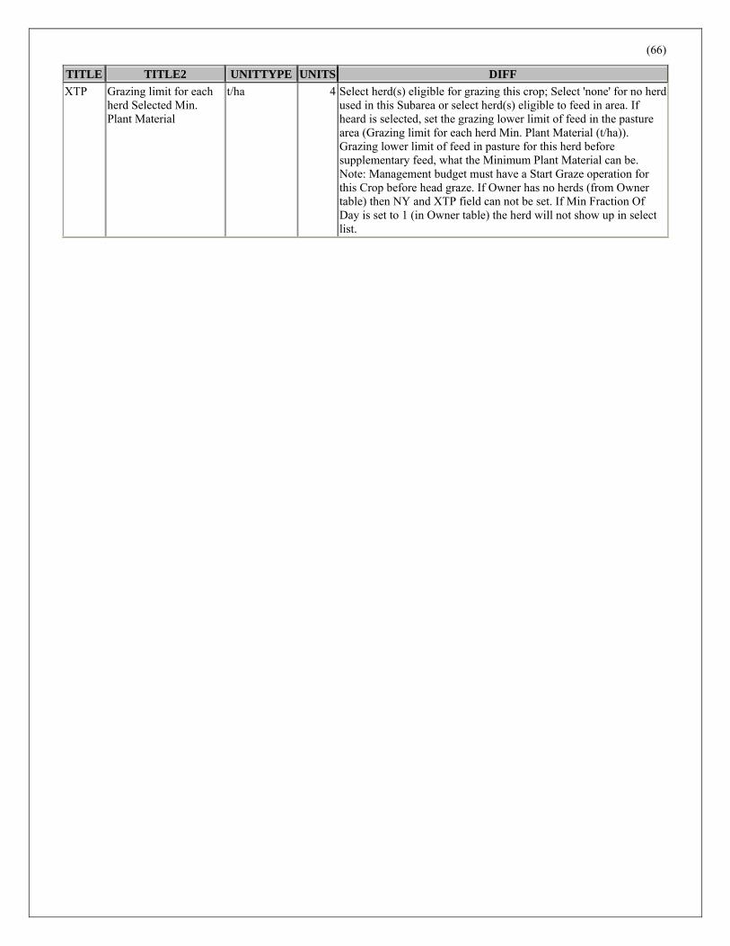
(66)

TITLE TITLE2 UNITTYPE UNITS DIFF XTP Grazing limit for each

herd Selected Min. Plant Material

t/ha 4 Select herd(s) eligible for grazing this crop; Select 'none' for no herd used in this Subarea or select herd(s) eligible to feed in area. If heard is selected, set the grazing lower limit of feed in the pasture area (Grazing limit for each herd Min. Plant Material (t/ha)). Grazing lower limit of feed in pasture for this herd before supplementary feed, what the Minimum Plant Material can be. Note: Management budget must have a Start Graze operation for this Crop before head graze. If Owner has no herds (from Owner table) then NY and XTP field can not be set. If Min Fraction Of Day is set to 1 (in Owner table) the herd will not show up in select list.

(67)

C. Appendix C—Watershed Name Definitions TITLE TITLE2 DIFF DALG Feed Lot Subarea

Controlled By Lagoon

Fraction of Feed Lot Subarea controlled by lagoon (0 - 1); if not a Feed Lot Subarea then Fraction of Subarea controlled by lagoon (DALG) must be 0.

VLGN Normal Lagoon Volume

Normal Lagoon Volume (VLGN) (mm); Lagoon storage at normal level in mm of runoff from the drainage area of a Feed Lot Subarea. Note: if Fraction of Subarea controlled by lagoon (DALG) = 0 then VLGN must = 0.

COWW Lagoon Input from Wash Water

Lagoon Input from Wash Water (COWW); Wash water for milking parlor that drains into lagoon in cubic meters per cow per day. Lagoon input from wash water in m**3/animal unit/day. Note: if Fraction of Subarea controlled by lagoon (DALG) = 0 then COWW must = 0.

DDLG Time To Reduce Lagoon Storage

Time To Reduce Lagoon Storage; from Max To Norm (DDLG) (Days). Note: if Fraction of Subarea controlled by lagoon (DALG) = 0 then DDLG must = 0.

SOLQ Ratio Liquid/Total manure applied

Ratio Liquid/Total manure applied; in this Feed Lot Subarea. Fraction of total manure produced that goes into a lagoon. Note: if Fraction of Subarea controlled by lagoon (DALG) = 0 then SOLQ must = 0.

(68)

D. Appendix D—Watershed Subarea Definitions

TITLE TITLE2 DIFF UNITSIE Current Subarea Current Subarea Number IO Downstream

Receiving Subarea

Receiving Subarea Number is the Downstream Subarea the Current Subarea drain into or 0 = Outlet to Watershed.

ISOL Soil Soil number; soil selected from soil list. IOP Management Management (Operation schedule file); Selected Rotation of Cropping system. Note: if

Cropping System is type Dryland then Irrigation Auto Trigger (BIR) must be 0. If Owner has herds and this is a feed lot subarea then fallow (one crop only) is the only crop that can be used. If feed lot has a lagoon then Irrigation must be a Lagoon Irrigation type.

IOW Owner OWNER NUMBER; Owner Of Land In Subarea (set up in owners screen). IFED Time Herd In

Feed Lot Fraction Of Time Herd In Feeding Area (Feed Lot)(II); 0 = Non Feeding Area; 0.001 - 1 = Fraction of Time Herd is in Feeding Area.

NGZ Grazing Area / Feed Lot

Grazing Area; 0 = For Non Grazing Area or Feeding Area; 1= Grazing Area 2 = Feed Lot (Feeding Area) Note: Feed Lot = Non grazing feeding area.

IAPL Auto. Manure FeedLot ID

Auto. Manure Feedlot ID.; 0 non manure application area; Use the positive subarea ID of the feedlot to indicate solid manure application; the negative subarea ID of the feedlot (lagoon) to indicate liquid manure application. Note: To use this option correctly, this subarea being build and the Auto. Manure Application subarea be entered, must be own by the same owner.

IRR Irrigation Code Irrigation Code; 0 = dryland 1 = sprinkler irrigation 2 = furrow irrigation 3 = fertigation 4 = lagoon The irrigation code is used to specify whether irrigation is used and the type of irrigation. If furrow irrigation is specified irrigation induced erosion is calculated. If Fertigation is specified IDFT identifies the type of FERT and FNP the amount of FERT with each irrigation. If lagoon is specified, the concentration in tons of soils per m**3 of effluent is specified by FNP and the nutrient fraction by creating a FERT in the FERT file with the appropriate nutrients and selecting it with IDFT.

LM Lime Application Switch

Lime Application Switch; 0 = APPLIES LIME AS NEEDED AUTOMATICALLY; 1 = NO LIME APPLIED. EPIC enables the user to simulate application of agricultural limestone to increase soil pH and/or reduce soil aluminum saturation. For many soils and applications of EPIC, this feature is not needed; therefore, it can be turned off.

WSA Drainage Area Subarea Drainage Area (WSA) (ha or acres); As a general rule, as fields become larger, the amount of sediment leaving per unit field area decreases. EPIC uses WSA to estimate soil erosion at the edge of the field. The units of WSA are hectares (metric) or acres (English). Usually WSA is small because EPIC assumes homogeneous soils and management Note: if this is a second extreme and it flow join the first extreme area flow but dose not flow throw first extreme area a - sign is add the front of the second extreme area WSA make it a negative number (this tills the program to add the second area WSA to the first extreme area when it has to do with water flow).

HA

CHL Longest Distance From Outlet

Distance From Outlet to Most Distant Point in Subarea (CHL) (km or miles) The channel length is the distance along the channel from the most distant point on the subarea to the outlet. Often in small areas (approx. 1 ha) there is no defined channel. In such cases the length is measured along a concentrated flow path or it can simply be estimated from the length-width ratio of the subarea. For areas < 20 ha, the channel length measurement is not critical. In such cases, enter 0. Units are kilometers (metric) or miles (English). If this is a EXTREME subarea then Channel Length of Routing Reach MUST EQUAL Distance from Outlet. If this is a DOWNSTREAM subarea then Channel Length of Routing Reach can NOT BE EQUAL to Distance from Outlet.

KM

CHS Subarea Channel Slope

Subarea channel slope (CHS) in m/m (Fraction); For small areas this measurement is not critical because CHS is only used in estimating the watersheds time of

M/M

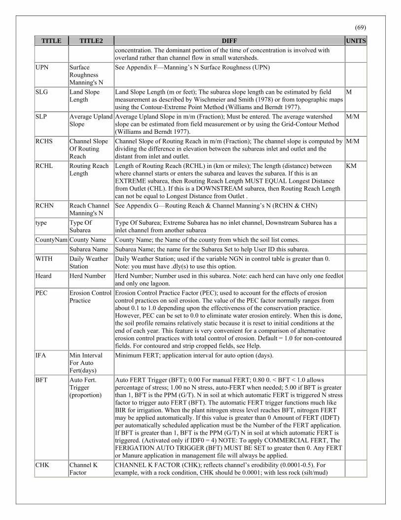
(69)

TITLE TITLE2 DIFF UNITSconcentration. The dominant portion of the time of concentration is involved with overland rather than channel flow in small watersheds.

UPN Surface Roughness Manning's N

See Appendix F—Manning’s N Surface Roughness (UPN)

SLG Land Slope Length

Land Slope Length (m or feet); The subarea slope length can be estimated by field measurement as described by Wischmeier and Smith (1978) or from topographic maps using the Contour-Extreme Point Method (Williams and Berndt 1977).

M

SLP Average Upland Slope

Average Upland Slope in m/m (Fraction); Must be entered. The average watershed slope can be estimated from field measurement or by using the Grid-Contour Method (Williams and Berndt 1977).

M/M

RCHS Channel Slope Of Routing Reach

Channel Slope of Routing Reach in m/m (Fraction); The channel slope is computed by dividing the difference in elevation between the subareas inlet and outlet and the distant from inlet and outlet.

M/M

RCHL Routing Reach Length

Length of Routing Reach (RCHL) in (km or miles); The length (distance) between where channel starts or enters the subarea and leaves the subarea. If this is an EXTREME subarea, then Routing Reach Length MUST EQUAL Longest Distance from Outlet (CHL). If this is a DOWNSTREAM subarea, then Routing Reach Length can not be equal to Longest Distance from Outlet .

KM

RCHN Reach Channel Manning's N

See Appendix G—Routing Reach & Channel Manning’s N (RCHN & CHN)

type Type Of Subarea

Type Of Subarea; Extreme Subarea has no inlet channel, Downstream Subarea has a inlet channel from another subarea

CountyNam County Name County Name; the Name of the county from which the soil list comes. Subarea Name Subarea Name; the name for the Subarea Set to help User ID this subarea. WITH Daily Weather

Station Daily Weather Station; used if the variable NGN in control table is greater than 0. Note: you must have .dly(s) to use this option.

Heard Herd Number Herd Number; Number used in this subarea. Note: each herd can have only one feedlot and only one lagoon.

PEC Erosion Control Practice

Erosion Control Practice Factor (PEC); used to account for the effects of erosion control practices on soil erosion. The value of the PEC factor normally ranges from about 0.1 to 1.0 depending upon the effectiveness of the conservation practice. However, PEC can be set to 0.0 to eliminate water erosion entirely. When this is done, the soil profile remains relatively static because it is reset to initial conditions at the end of each year. This feature is very convenient for a comparison of alternative erosion control practices with total control of erosion. Default = 1.0 for non-contoured fields. For contoured and strip cropped fields, see Help.

IFA Min Interval For Auto Fert(days)

Minimum FERT; application interval for auto option (days).

BFT Auto Fert. Trigger (proportion)

Auto FERT Trigger (BFT); 0.00 For manual FERT; 0.80 0. < BFT < 1.0 allows percentage of stress; 1.00 no N stress, auto-FERT when needed; 5.00 if BFT is greater than 1, BFT is the PPM (G/T). N in soil at which automatic FERT is triggered N stress factor to trigger auto FERT (BFT). The automatic FERT trigger functions much like BIR for irrigation. When the plant nitrogen stress level reaches BFT, nitrogen FERT may be applied automatically. If this value is greater than 0 Amount of FERT (IDFT) per automatically scheduled application must be the Number of the FERT application. If BFT is greater than 1, BFT is the PPM (G/T) N in soil at which automatic FERT is triggered. (Activated only if IDF0 = 4) NOTE: To apply COMMERCIAL FERT, The FERIGATION AUTO TRIGGER (BFT) MUST BE SET to greater then 0. Any FERT or Manure application in management file will always be applied.

CHK Channel K Factor

CHANNEL K FACTOR (CHK); reflects channel’s erodibility (0.0001-0.5). For example, with a rock condition, CHK should be 0.0001; with less rock (silt/mud)

(70)

TITLE TITLE2 DIFF UNITScondition, it should be 0.30.

BIR Irrigation Auto Trigger

Water stress factor; to trigger automatic irrigation (BIR). To trigger automatic irrigation, the water stress factor is set: 0.0 Allows plants to be affected water stress 0.8 BIR > 0.0 AND BIR < 1.0 fraction of plant stress 1.0 Does not allow water stress BIR < 0.0 Plant available water deficit in root zone (-mm) BIR > 1.0 For soil water tension Kilopascals in top 200mm -1000.0 Sets water deficit high enough that only manual irrigations will occur Note: if Cropping System Type is Dryland, BIR must be 0.

IRI Min Interval For Irr.(days)

Minimum Application Interval (Automatic Irrigation) (IRI) [days]; Some irrigation systems can apply water only so often. The variable IRI enables the user to specify the minimum number of days between automatic irrigation applications. For our example, this will be set to 0 since irrigation is not used. (max 365 days)

CHC Channel C Factor

CHANNEL C FACTOR (CHC); (0.0001- 0.6); With bare channel condition, CHC should be set 0.1- 0.6 and if the channel has very good land cover, it should take a value of 0. 0001.

NIRI Rigidity of irrigation code

Rigidity of irrigation code; for flexible applications. Applies minimum of FC-SW and ARMX. 1 for rigid applications. Applies input amount or ARMX. The irrigation code is used to specify the irrigation strategy. There are two mode of irrigating -- manual and automatic. If manual irrigation is selected, irrigation occurs on user specified dates and volumes. 0 = the irrigation is applied when needed and only as much as is needed. 1 = the application is according to the amounts specified, either by automatic application (ARMX) or by user input amounts and restrictions.

IDF0 Auto Fert. Number

Auto FERT Number (IDF0); 0 for NO AUTOMATIC FERT OR MANURE applications; 1 for FERTIGATION FROM LAGOON; 2 for AUTOMATIC SOLID MANURE application from FEEDING AREA STOCK PILE; 4 for AUTOMATIC Commercial FERT application (defaults to ELEM N); 5 for AUTOMATIC SOLID MANURE application. NOTE: To apply AUTO MANURE application, MUNL in Control File MUST BE SET. To apply COMMERCIAL FERT, The FERTIGATION AUTO TRIGGER (BFT) MUST BE SET to greater than 0. Any FERT or Manure application in management file will always be applied.

IDFX Fert./ Manure FNP4 Auto Fert.

Application Rate (N)

Auto FERT Application Rate (N); 0 variable rate of automatic commercial application (amount of FERT applied as need to lower N stress); fixed rate of automatic commercial application (set amount of FERT applied each time N stress is reached). Note: BFT (Auto FERT Trigger (proportion)) must be set, IDF0 (Auto FERT Type) must be set to 4 and IDF04 (Automatic commercial FERT Application) can not be 0 for this variable to work.

km

(71)

E. Appendix E—Adding Subarea(s) TITLE TITLE2 UNITTYPE UNITS DIFF LCNO Land Condition 0 LCNO (Land Condition); is used to find the curve number, for the

selected crop(s), when building the. ops file. IFLS Filter Strip Code Whole

Number 0 or 1

0 Filter Strip Code; 0 for normal subarea; 1 for filter strip Note: if Filter Strip Code = 1 then Fraction of floodplain flow must be set to 1 for a smooth terrain; 0.1 - 0.5 for rough terrain. Note: Fraction of floodplain flow will be changed auto to 1 and Buffer/Floodplain width will be set to (Drainage Area * 10) / Routing Reach Length when filter strip is change to 1.

NVCN Soil Moisture Index Whole Number 0 or 4

0 Soil Moisture Index; 0 Variable daily CN Nonlinear CN/SW with depth soil water weighting; 1 = Variable daily CN Nonlinear CN/SW no depth weighting; 2 = Variable daily CN Linear CN/SW no depth weighting; 3 = Non-Varying CN--CN2 used for all storms; 4 = Variable daily CN SMI (Soil Moisture Index)".

SNO Water content of snow

(MM) 2 Water content of snow; snow on ground at start of simulation.

STDO Standing dead crop residue

t/ha 3 Standing dead crop residue

XCT LONG 0 X Coordinate of subarea centroid; longitude of subarea centroid. It need to be entered if Spatially Generated Weather option is been used. Spatially Generated Weather is set by entering 0 in the variable NGN in control table. Note: A minus degree for western hemisphere.

YCT LAT 0 Y Coordinate of subarea centroid; latitude of subarea centroid. It need to be entered if Spatially Generated Weather option is been used. Spatially Generated Weather is set by entering 0 in the variable NGN in control table. Note: A minus degree for southern hemisphere.

CHD Channel depth m 6 Channel depth CHN Channel roughness

Manning’s N 0 See Appendix G—Routing Reach & Channel Manning’s N (RCHN &

CHN) FFPQ Fraction of

Buffer/floodplain flow

0 Fraction of Buffer/ floodplain flow; Partitions flow through filter strips.

RCHD Channel Depth of Routing Reach

m 6 Channel Depth of Routing Reach

RCBW Bottom Width of Channel of Routing Reach

m 6 Bottom Width of Channel of Routing Reach

RCTW Top Width of Channel of Routing Reach

m 6 Top Width of Channel of Routing Reach

RFPW Buffer/Floodplain width

m 6 Buffer/Floodplain width = (Drainage Area(WSA) X 10000) / (Floodplain length (RFPL) X 1000)

RFPL Buffer/Floodplain length

km 13 Buffer/Floodplain length

RSEE Elev of emergency spillway

M 6 Elevation at emergency spillway elevation

RSAE Total reservoir surface area

ha 11 Total reservoir surface area at emergency spillway elevation

RSVE Spillway Runoff volume

mm 2 Runoff volume at emergency spillway elevation.

RSEP Elev of principal M 6 Elevation at principal spillway elevation.

(72)

TITLE TITLE2 UNITTYPE UNITS DIFF spillway

RSAP Total reservoir surface area

ha 11 Total reservoir surface area at principle spillway elevation.

RSV0 Volume at principal spillway elevation

mm 2 Volume at principal spillway elevation.

RSV Initial reservoir volumes

mm 2 Initial reservoir volumes.

RSRR Average principle spillway release rate

mm/hr 61 Average principle spillway release rate.

RSYS Initial sediment concentration in reservoirs

0 Initial sediment concentration in reservoirs (ppm)

RSYN Normal sediment concentration in reservoirs

0 Normal sediment concentration in reservoirs (ppm).

RSHC Hydraulic conductivity of reservoir bottoms

mm/hr 61 Hydraulic conductivity of reservoir bottoms.

RSDP Time for sediment to return to the normal

0 Time required for the sediment to return to the normal; time required in days for the sediment in the reservoir to return to the normal concentrations following a runoff event.

RSBD Bulk Density of Sediment in reservoir

T/M^3 36 Bulk Density of Sediment in Reservoir.

IFD Furrow Dike Code 0 Furrow Dike Code; 0 does not use a furrow dike system; 1 considers a furrow dike system.

IDR Drainage code mm 2 Drainage code; no drainage 0 enter depth to drainage system. EFI Runoff Irrigation 0 Runoff Irrigation; runoff vol/vol irrigation water applied. The

irrigation runoff ratio specifies the fraction of each irrigation application that is lost to runoff.

VIMX Max. annual irrigation volume

mm 2 Maximum annual irrigation volume; allowed for each crop.

ARMN Min. single application volume

mm 2 Minimum single application volume; allowed for auto irrigation.

ARMX Max. single application volume

mm 2 Maximum single application volume; allowed for auto irrigation.

FMX Max. annual N fertilizer applied for a crop

kg/ha 4 Maximum annual N fertilizer applied for a crop.

DRT Time for drainage system to end plant stress

0 Time requirement for drainage system to end plant stress (days).

FDSF Fraction of furrow dike volume

0 Fraction of furrow dike volume available for water storage.

FNP5 Automatic Manure application rate

kg/ha 4 Automatic Manure application rate. (Activated only if IDF0 = 2 or 4)

SFLG Safety factor for Lagoon spillover

0 Safety factor for Lagoon spillover (fraction 0_1). (Needed only when IRR = 4)

(73)

F. Appendix F—Manning’s N Surface Roughness (UPN) Surface Roughness Manning’s N for Upland; the surface roughness factor is Manning's N.

Values of Manning's N for various conditions:

Overland flow Value chosen Range

Fallow, no residue [.0100] 0.008-0.012

Conventional tillage, no residue [.0900] 0.06-0.12

Conventional tillage, residue [.1900] 0.16-0.22

Chisel plow, no residue [.0900] 0.06-0.12

Chisel plow, residue [.1300] 0.10-0.16

Fall disking, residue [.4000] 0.30-0.50

No till, no residue [.0700] 0.04-0.10

No till (0.5-1.0 t/ha) [.1200] 0.07-0.17

No till (2.0-9.0 t/ha) [.3000] 0.17-0.47

Rangeland (20% cover) [.6000]

Short grass prairie [.1500] 0.10-0.20

Dense grass [.2400] 0.17-0.30

Bermuda grass [.4100] 0.30-0.48

(1) Blank if unknown (enter zero) [.0000]

(74)

G. Appendix G—Routing Reach & Channel Manning’s N (RCHN & CHN) Reach Channel Manning’s N (RCHN); if set to 0 will be calculated.

Type of Channel Value Chosen Range

A. Excavated or dredged

1. Earth, straight and uniform .0250 .016-.033

2. Earth, winding and sluggish .0350 .023-.050

3. Not maintained, weeds and brush .0750 .040-.140

B. Natural Streams

1. Few trees, stones or brush .0500 .025-.065

2. Heavy timber and brush .1000 .050-.150

If the channel conducting runoff to the edge of the field is winding and/or contains obstructions, water flow rates will be reduced, and sediment will have an opportunity to settle. The channel roughness factor is referred to as the Manning's N value. The table contains suggested values of Manning's N for various conditions of channel flow.

(75)

H. Appendix H—Parm Definitions PARM(1) = CROP CANOPY-PET(1_2)

FACTOR USED TO ADJUST CROP CANOPY RESISTANCE IN THE PEN-

MAN-MONTEITH PET EQ.

PARM(2) = ROOT GROWTH-SOIL STRENGTH(1_2)

NORMALLY 1.15<PARM(2)<1.2. SET TO 1.5 TO MINIMIZE SOIL

STRENGTH CONSTRAINT ON ROOT GROWTH. PARM(2)>2. ELIMINATES

ALL ROOT GROWTH STRESS.

PARM(3) = WATER STRESS-HARVEST INDEX(0_1)

SETS FRACTION OF GROWING SEASON WHEN WATER STRESS STARTS

REDUCING HARVEST INDEX.

PARM(4) = WATER STORAGE-N LEACHING(0_1)

FRACTION OF SOIL POROSITY THAT INTERACTS WITH PERCOLATING

WATER AS N LEACHING OCCURS.

PARM(5) = SOIL WATER LOWER LIMIT(0_1)

LOWER LIMIT OF WATER CONTENT IN THE TOP 0.5 M SOIL DEPTH

EXPRESSED AS A FRACTION OF THE WILTING POINT WATER CON-

TENT.

PARM(6) = WINTER DORMANCY(H)(0_1)

CAUSES DORMANCY IN WINTER GROWN CROPS. GROWTH DOES NOT

OCCUR WHEN DAY LENGTH IS LESS THAN ANNUAL MINIMUM DAY

LENGTH + PARM(6).

PARM(7) = N FIXATION(0_1)

AT 1. FIXATION IS LIMITED BY SOIL WATER OR NITRATE CON-

TENT OR BY CROP GROWTH STAGE. At 0 FIXATION MEETS CROP N

UPTAKE DEMAND. A COMBINATION OF THE 2 FIXATION ESTIMATES

IS OBTAINED BY SETTING 0 < Parm(7)< 1.

PARM(8) = SOLUBLE P ADSORPTION COEF(.1*M^3/T)(10_20)

P CONCENTRATION IN SEDIMENT DIVIDED BY THAT OF THE WATER.

PARM(9) = PEST DAMAGE MOISTURE THRESHOLD(MM)(25_150)

PREVIOUS 30-DAY RAINFALL MINUS RUNOFF.

PARM(10) = PEST DAMAGE COVER THRESHOLD(T/HA)(1_10)

CROP RESIDUE + ABOVE GROUND BIOMASS.

PARM(11) = MOISTURE REQUIRED FOR SEED GERMINATION(MM)(10_30)

SOIL WATER STORED MINUS WILTING POINT STORAGE IN THE PLOW

DEPTH (PMX = PARM(43).

(76)

PARM(12) = SOIL EVAPORATION COEF(1.5_2.5)

GOVERNS RATE OF SOIL EVAPORATION FROM TOP 0.2 M OF SOIL.

PARM(13) = WIND ERODIBILITY COEF(0_3)

ADJUSTS WIND SOIL ERODIBILITY FACTOR DOWNWARD AS LOOSE

MATERIAL IS ERODED.

PARM(14) = NITRATE LEACHING RATIO(0.1_1)

NITRATE CONCENTRATION IN SURFACE RUNOFF TO NITRATE CON-

CENTRATION IN PERCOLATE.

PARM(15) = RUNOFF CN WEIGHTING FACTOR(0.0_1.0)

WEIGHTS CURRENT AND PREVIOUS DAYS CN--1.0 USES CURRENT

ESTIMATE; 0.0 USES PREVIOUS DAYS CN.

PARM(16) = EXPANDS CN RETENTION PARAMETER(1.0_1.5)

VALUES > 1.0 EXPAND CN RETENTION PARAMETER AND REDUCE

RUNOFF.

PARM(17) = SOIL EVAPORATION-PLANT COVER FACTOR(0.01_0.5)

REDUCES EFFECT OF PLANT COVER AS RELATED TO LAI IN

REGULATING SOIL EVAPORATION.

PARM(18) = SEDIMENT ROUTING EXPONENT(1_1.5)

EXPONENT OF WATER VELOCITY FUNCTION FOR ESTIMATING

POTENTIAL SEDIMENT CONCENTRATION.

PARM(19) = SEDIMENT ROUTING COEF(T/M^3)(0.01_0.05)

POTENTIAL SEDIMENT CONC WHEN FLOW VELOCITY = 1. M/S.

PARM(20) = RUNOFF CURVE NUMBER INITIAL ABSTRACTION(0.05_0.4)

PARM(21) = SOLUBLE C ADSORPTION COEF(.1*M^3/T)(10_20)

C CONCENTRATION IN SEDIMENT DIVIDED BY THAT IN WATER.

PARM(22) = REDUCES NRCS RUNOFF CN RETENTION PARM FOR FROZEN SOIL.

FRACTION OF S FROZEN SOIL(0.05_0.5)

PARM(23) = HARGREAVES PET EQ COEF(0.0023_0.0032)

ORIGINAL VALUE = 0.0023

PARM(24) = PESTICIDE LEACHING RATIO(0.1_1)

PESTICIDE CONCENTRATION IN SURFACE RUNOFF TO PESTICIDE

CONCENTRATION IN PERCOLATE.

PARM(25) = NOT USED.

PARM(26) = FRACTION OF MATURITY AT SPRING GROWTH INITIATION(0_1)

ALLOWS FALL GROWING CROPS TO RESET HEAT UNIT INDEX TO A

VALUE GREATER THAN 0 WHEN PASSING THROUGH THE MINIMUM

(77)

TEMP MONTH.

PARM(27) = CEC EFFECT ON NITRIFICATION & VOLATILIZATION(0_1)

SETS LOWER LIMIT OF CEC CORRECTION FACTOR IN NIT/VOL

FUNCTION. AT 0 CEC SHOULD PREVENT NIT/VOL PROCESS. AT 1

CEC HAS NO EFFECT ON NIT/VOL.

PARM(28) = NOT USED

PARM(29) = BIOLOGICAL MIXING EFFICIENCY(0.1_0.5)

SIMULATES MIXING IN TOP SOIL BY EARTH WORMS ETC. PARM(31)

SETS DEPTH.

PARM(30) = SOLUBLE P RUNOFF EXPONENT(1_1.5)

PROVIDES NONLINEAR EFFECT FOR SOLUBLE P/RUNOFF EQ.

PARM(31) = MAXIMUM DEPTH FOR BIOLOGICAL MIXING(M)(0.1_0.3)

PARM(32) = ORGANIC P LOSS EXPONENT(1_1.2)

PROVIDES NONLINEAR EFFECT FOR ORGANIC P LOSS EQ.

PARM(33) = COEFFICIENT IN MUST EQ(2.0_3.0)

ORIGINAL VALUE = 2.5.

PARM(34) = HARGREAVES PET EQ EXP(0.5_0.6)

ORIGINAL VALUE=0.5. MODIFIED TO 0.6 TO INCREASE PET.

PARM(35) = DENITRIFICATION SOIL-WATER THRESHOLD(.9_1.1)

FRACTION OF FIELD CAPACITY SOIL WATER STORAGE TO TRIGGER

DENITRIFICATION.

PARM(36) = DENITRIFICATION RATE CONSTANT(.1_2)

CONTROLS DENITRIFICATION RATE. TRADITIONAL VALUE = 1.4.

PARM(37) = NOT USED.

PARM(38) = WATER STRESS WEIGHTING COEF(0_1)

AT 0 PLANT WATER STRESS IS STRICTLY A FUNCTION OF SOIL

WATER CONTENT; AT 1 PLANT WATER STRESS IS STRICTLY A

FUNCTION OF ACTUAL ET DIVIDED BY POTENTIAL ET.

0<PARM(38)<1 CONSIDERS BOTH APPROACHES.

PARM(39) = NOT USED.

PARM(40) = GROUNDWATER STORAGE THRESHOLD(.001_1.)

FRACTION OF GROUNDWATER STORAGE THAT INITIATES RETURN

FLOW.

PARM(41) = PLANT ROOT TEMPERATURE STRESS EXP(.1_2.)

EXP OF RATIO OF SOIL LAYER TEMP TO AVE OF PLANT OPTIMAL

AND BASE TEMPS.

(78)

PARM(42) = SCS CURVE NUMBER INDEX COEF(.3_2.5)

REGULATES THE EFFECT OF PET IN DRIVING THE SCS CURVE

NUMBER RETENTION PARAMETER.

PARM(43) = PLOW LAYER DEPTH(M)

USED TO TRACK SOLUBLE P CONCENTRATION OR WEIGHT.

PARM(44) = NOT USED

PARM(45) = SEDIMENT ROUTING TRAVEL TIME COEF(.5_10.)

BRINGS INFLOW SEDIMENT CONC TO TRANSPORT CAPACITY

CONC AS A FUNCTION OF TRAVEL TIME AND MEAN PARTICLE SIZE.

PARM(46) = RUSLE C FACTOR COEF(.5_1.5)

COEF IN EXPONENTIAL RESIDUE FUNCTION IN RESIDUE FACTOR.

PARM(47) = RUSLE C FACTOR COEF(.5_1.5)

COEF IN EXPONENTIAL CROP HEIGHT FUNCTION IN BIOMASS

FACTOR.

PARM(48) = ADJUSTS CLIMATIC STRESS FACTOR (AAP/AAT)/PARM(48) (50_80)

SET TO 0.0 GIVES CLF=1.

PARM(49) = MAXIMUM RAINFALL INTERCEPTION BY PLANT CANOPY(MM) (2._15.)

PARM(50) = RAINFALL INTERCEPTION COEF(.05_.3)

PARM(51) = WATER STORAGE CAPACITY OF LITTER (RESIDUE) COEF (.1_.9)

FRACTION OF LITTER WEIGHT.

PARM(52) = EXPONENTIAL COEF IN EQ EXPRESSING TILLAGE EFFECT ON RESIDUE

DECAY RATE(5._15.)

PARM(53) = COEF IN OXYGEN EQ USED IN MODIFYING MICROBIAL ACTIVITY WITH

SOIL DEPTH(0.8_0.95)

PARM(54) = N ENRICHMENT RATIO COEF FOR ROUTING (.4_.7)

PARM(55) = N ENRICHMENT RATIO EXP FOR ROUTING (.1_.3)

PARM(56) = FRACTION DESTROYED BY BURN OPERATION (.5_1.)

PARM(57) = P ENRICHMENT RATIO COEF FOR ROUTING (.05_.2)

PARM(58) = P ENRICHMENT RATIO EXP FOR ROUTING (.2_.4)

PARM(59) = P UPWARD MOVEMENT BY EVAPORATION COEF (1_20)

PARM(60) = MAXIMUM NUMBER OF DAYS A PASTURE IS GRAZED BEFORE

ROTATION (1-365)

PARM(61) = SOIL WATER TENSION WEIGHTING FACTOR(0._1.)

REGULATES UPWARD WATER FLOW AS A FUNCTION OF SOIL WATER

TENSION IN THE LAYER OF INTEREST AND THE ONE ABOVE IT.

0.0 ONLY CONSIDERS ABOVE LAYER TENSION. 1.0 ONLY CONSID-

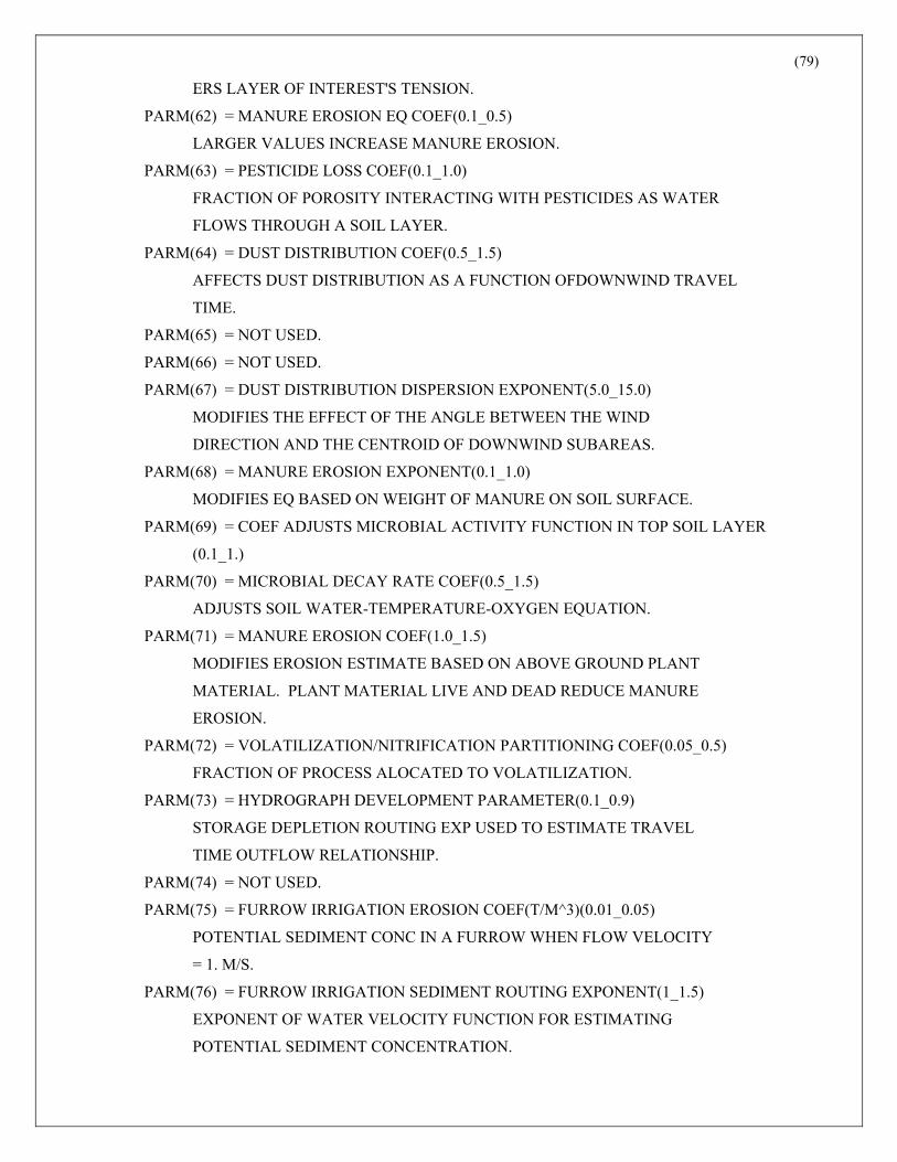
(79)

ERS LAYER OF INTEREST'S TENSION.

PARM(62) = MANURE EROSION EQ COEF(0.1_0.5)

LARGER VALUES INCREASE MANURE EROSION.

PARM(63) = PESTICIDE LOSS COEF(0.1_1.0)

FRACTION OF POROSITY INTERACTING WITH PESTICIDES AS WATER

FLOWS THROUGH A SOIL LAYER.

PARM(64) = DUST DISTRIBUTION COEF(0.5_1.5)

AFFECTS DUST DISTRIBUTION AS A FUNCTION OFDOWNWIND TRAVEL

TIME.

PARM(65) = NOT USED.

PARM(66) = NOT USED.

PARM(67) = DUST DISTRIBUTION DISPERSION EXPONENT(5.0_15.0)

MODIFIES THE EFFECT OF THE ANGLE BETWEEN THE WIND

DIRECTION AND THE CENTROID OF DOWNWIND SUBAREAS.

PARM(68) = MANURE EROSION EXPONENT(0.1_1.0)

MODIFIES EQ BASED ON WEIGHT OF MANURE ON SOIL SURFACE.

PARM(69) = COEF ADJUSTS MICROBIAL ACTIVITY FUNCTION IN TOP SOIL LAYER

(0.1_1.)

PARM(70) = MICROBIAL DECAY RATE COEF(0.5_1.5)

ADJUSTS SOIL WATER-TEMPERATURE-OXYGEN EQUATION.

PARM(71) = MANURE EROSION COEF(1.0_1.5)

MODIFIES EROSION ESTIMATE BASED ON ABOVE GROUND PLANT

MATERIAL. PLANT MATERIAL LIVE AND DEAD REDUCE MANURE

EROSION.

PARM(72) = VOLATILIZATION/NITRIFICATION PARTITIONING COEF(0.05_0.5)

FRACTION OF PROCESS ALOCATED TO VOLATILIZATION.

PARM(73) = HYDROGRAPH DEVELOPMENT PARAMETER(0.1_0.9)

STORAGE DEPLETION ROUTING EXP USED TO ESTIMATE TRAVEL

TIME OUTFLOW RELATIONSHIP.

PARM(74) = NOT USED.

PARM(75) = FURROW IRRIGATION EROSION COEF(T/M^3)(0.01_0.05)

POTENTIAL SEDIMENT CONC IN A FURROW WHEN FLOW VELOCITY

= 1. M/S.

PARM(76) = FURROW IRRIGATION SEDIMENT ROUTING EXPONENT(1_1.5)

EXPONENT OF WATER VELOCITY FUNCTION FOR ESTIMATING

POTENTIAL SEDIMENT CONCENTRATION.

(80)

PARM(77) = RUNOFF AMOUNT TO DELAY PEST APPLICATION(MM)(0.0_25.0)

PESTICIDE IS NOT APPLIED ON DAYS WITH RUNOFF GREATER THAN

PARM(77).

PARM(78) = SOIL WATER VALUE TO DELAY TILLAGE(0.0_1.0)

TILLAGE DELAYED WHEN PDSW/FCSW>PARM(78).