WHP Cruise Summary Information - EPIC
206
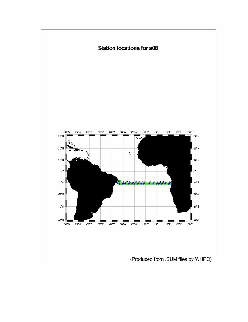
WHP Cruise Summary Information WOCE section designation A08 Expedition designation (EXPOCODE) 06MT28_1 Chief Scientist(s) and their affiliation Thomas Müller, IfMK Dates 1994.03.29 – 1994.05.11 Ship METEOR Ports of call Recife, Brazil to Walvisbay, Namibia Number of stations 126 Geographic boundaries of the stations 08º16.31’’S 05º45.08’’W 13º32.42’’E 11º40.50’’S Floats and drifters deployed see 4.1 Moorings deployed or recovered none Contributing Authors (in order of appearance) U. Beckmann P. Beining C. Dieterich U. Koy P. Meyer W.H. Pinaya D.J. Hydes S. Kohrs R. Meyer S. Müller A. Putzka K. Bulsiewicz H. Düßmann W. Plep J. Sültenfuß K. Johnson K. Wills D. Hydes G. Siedler O. Boebel C. Schmid W. Zenk J. Pätzold W. Krauß T. Knutz C. Zelck H.-Ch. John J. Brinkmann G. Schebeske W. Emery M. Suarez R. Cordes J. Funk R. Rieger M. Schneider K. Ballschmiter K. Flechsenhar W. Roether J.C. Jennings L.I. Gordon
-
Upload
khangminh22 -
Category
Documents
-
view
2 -
download
0
Transcript of WHP Cruise Summary Information - EPIC
WHP Cruise Summary Information
WOCE section designation A08Expedition designation (EXPOCODE) 06MT28_1
Chief Scientist(s) and their affiliation Thomas Müller, IfMKDates 1994.03.29 – 1994.05.11
Ship METEORPorts of call Recife, Brazil to Walvisbay, Namibia
Number of stations 126Geographic boundaries of the stations 08º16.31’’S
05º45.08’’W 13º32.42’’E11º40.50’’S
Floats and drifters deployed see 4.1Moorings deployed or recovered none
Contributing Authors(in order of appearance)
U. BeckmannP. BeiningC. DieterichU. KoyP. MeyerW.H. PinayaD.J. HydesS. KohrsR. MeyerS. MüllerA. PutzkaK. BulsiewiczH. DüßmannW. PlepJ. SültenfußK. JohnsonK. WillsD. HydesG. SiedlerO. Boebel
C. SchmidW. ZenkJ. PätzoldW. KraußT. KnutzC. ZelckH.-Ch. JohnJ. BrinkmannG. SchebeskeW. EmeryM. SuarezR. CordesJ. FunkR. RiegerM. SchneiderK. BallschmiterK. FlechsenharW. RoetherJ.C. JenningsL.I. Gordon
WHP Cruise and Data Information
Instructions: Click on items below to locate primary reference(s) or use navigationtools above.
Table of Contents:
Cruise Track
AbstractZusammenfassung
1 Research Objectives
2 Participants
3 Research Programme3.1 WOCE Hydrographic Programme (WHP): Section A83.2 WOCE Deep Basin Experiment (DBE)3.3 Near-Surface Circulation from Drifters3.4 GEK Observations3.5 Taxonomy and Distribution of Fish Larvae in the Tropical South Atlantic
3.5.1 Introduction3.5.2 Plankton Sampling
3.6 Atmospheric Physics and Chemistry3.7 Radiative Physics - Skin Sea Surface Temperature Investigation3.8 Marine Geology3.9 Environmental Chemistry
4 Narrative of the Cruise4.1 Leg M 28/1 (T.J. Müller)4.2 Leg M 28/2 (W. Zenk)
5 Preliminary Results5.1 The WHP Section A8 along 11˚30'S
5.1.1 Hydrography and Currents (T.J. Müller, U. Beckmann, P. Beining,C. Dieterich, U. Koy, P. Meyer, W.H. Pinaya)
5.1.2 Dissolved Oxygen and Nutrients (D.J. Hydes, S. Kohrs, R. Meyer,S. Müller)
5.1.3 Tracers (A. Putzka, K. Bulsiewicz, H. Düßmann, W. Plep, J.Sültenfuß)
5.1.4 CO2 -Measurements (K. Johnson, K. Wills)5.1.5 First Results from WHP A8 (T.J. Müller, P. Beining, D. Hydes, K.
Johnson, A. Putzka, G. Siedler)5.2 Deep Basin Experiment
5.2.1 Water Mass Distribution in the Subtropical South Atlantic (O.Boebel, C. Schmid, W. Zenk)
5.2.2 Water Exchange through Hunter Channel (T.J. Müller, J. Pätzold,G. Siedler, C. Schmid, W. Zenk)
5.3 Near Surface Circulation from Satilite Tracked Drifters (W. Krauß)5.4 GEK Observations (T. Knutz)5.5 Biological Oceanography and Taxonomy along 11˚30'S (C. Zelck, H.-
Ch. John)5.5.1 Quantitative Data
5.5.1.1 General5.5.1.2 Taxonomy5.5.1.3 Cross-slope Ecological Patterns
5.5.1.3.1 Abundance Patterns5.5.1.3.2 Diversity and Species Composition5.5.1.3.3 Vertical Distribution and Implication for Cross -
slope Zonations5.5.2 The Plankton Material from the Central Atlantic to Angola:
Findings, Hints and Expectations5.5.2.1 General5.5.2.2 Plankton Biomass Volumes and Micronekton Numbers5.5.2.3 The Juvenile Life Stage of Bathylagus argyrogaster
5.6 Atmospheric Physics and Chemistry along 11˚30 S (J. Brinkmann, G.Schebeske)
5.7 Radiative Physics (W. Emery, M. Suarez)5.8 Marine Geology (R. Cordes, J. Funk)
5.8.1 Sediment Sampling5.8.2 Water Sampling
5.9 Environmental Chemistry (R. Rieger, M. Schneider, K. Ballschmiter)5.9.1 Compounds of Interest5.9.2 Sampling Methods
5.9.2.1 Sampling of Surface Seawater5.9.2.2 Sampling of Surface Micro Layer5.9.2.3 High Volume Air Sampling5.9.2.4 Low Volume Sampling
5.9.3 Analytical Methods5.9.4 Preliminary Results
5.9.4.1 Chlorinated Paraffins5.9.4.2 Alkyl Nitrates in Air Samples5.9.4.3 Polychlorinated Biphenyls (PCB)
6 Ship's Meteorological Station (K. Flechsenhar)6.1 Weather and Meteorological Conditions during Leg M 28/16.2 Weather and Meteorological Conditions during Leg M 28/2
7 Lists7.1 Leg M 28/1
7.1.1 List of Stations7.1.2 List of XBT Drops7.1.3 List of Drifter Launches
7.2 Leg M 28/27.2.1 CTD Stations7.2.2 List of XBT Drops7.2.3 List of Drifter Launches7.2.4 Mooring Activities7.2.5 List of RAFOS Float Launches and MAFOS Deployments7.2.6 List of Plankton Stations during M 28 and Respective Haul
Numbers7.2.7 Sample List of Sediment- and Water Samples for Geological
Investigations7.2.8 List of Surface Seawater Samples (sampled on XAD-2)7.2.9 List of Surface Seawater Samples (sampled on XAD-7)7.2.10 List of Micro Layer Samples7.2.11 List of High Volume Air Samples7.2.12 List of Low Volume Air Samples
8 Concluding Remarks
9 References
Tritium-HeliumCFCCTD DQE ReportNutrients DQE ReportData Status Notes
(Produced from .SUM files by WHPO)

Abstract
From 29 March to 14 June 1994 the German research vessel METEOR performed its28th cruise, a journey in the subtropical South Atlantic divided into two legs. Themain objectives were hydrographical and tracer observations in the frame work of theinternationally coordinated World Ocean Circulation Experiment (WOCE). The cruisecontributed to the WOCE Hydrographic Programme (WHP) and to the Deep BasinExperiment (DBE) in the Brazil Basin. Physical observations were supplemented bybiological, air and environmental chemical and geological components, including acontribution to the Joint Global Ocean Flux Studies (JGOFS).
The present cruise report contains a summary of the research objectives andcomprises the research programme, a cruise narrative and preliminary observationalresults. The report was funded by the Deutsche Forschungsgemeinschaft (DFG) andthe Bundesministerium für Bildung, Wissenschaft, Forschung and Technologie(BMBF).
Zusammenfassung
Vom 29. März bis 14. Juni 1994 fand die 28. Reise des deutschenForschungsschiffes METEOR statt. Die Reise führte in den subtropischenS0datlantik, und sie war in zwei Abschnitte unterteilt. Der Schwerpunkt lag beihydrographischen und Spurenstoffbeobachtungen. Sie wurden im Rahmen desinternational koordinierten Programms "World Ocean Circulation Experiment"(WOCE) durchgeführt. Die Expedition lieferte Beiträge zum "WOCE HydrographicProgramme" (WHP) und zum "Deep Basin Experiment" (DBE), einer Studie imBrasilianischen Becken. Die physikalischen Untersuchungen wurden ergänzt durchbiologische, luft- und umweltchemische sowie geologische Beobachtungen, zu denenauch Beiträge zur "Joint Global Ocean Flux Study" (JGOFS) gehören.
Der vorliegende Expeditionsbericht enthält eine Zusammenfassung derwissenschaftlichen Ziele und des Programms. Außerdem enthält er dieFahrtbeschreibung sowie vorläufige Beobachtungsergebnisse. Der Bericht umfaßtferner ausführliche Tabellen zu allen Stationsarbeiten. Die Reise wurde von derDeutschen Forschungsgemeinschaft (DFG), sowie vom Bundesministerium fürBildung, Wissenschaft, Forschung und Technologie (BMBF) gefördert.
1 Research Objectives
The German research vessel METEOR operated under the auspices of the WorldOcean Experiment (WOCE) from March 29 - June 14, 1994 in the subtropical SouthAtlantic (Fig. 1, Tab. 1). WOCE is a major component of the World Climate ResearchProgramme, which was established in 1979 by the World MeteorologicalOrganisation (WMO) and the International Council of Scientific Unions (ICSU) incooperation with the UNESCO and the Scientific Committee in Oceanic Research(SCOR). WOCE encompasses planning, implementing and coordinating the globalfieldwork and extensive modeling studies. The information gained will allow to betterunderstand the ocean's role in climate and its changes resulting from both naturaland anthropogenic causes.
The WOCE Hydrographic Programme (WHP) includes a large set of sections in alloceans, with measurements of temperature, salinity, oxygen, nutrients andanthropogenic tracers. Its aim is the determination of global water mass distributionand geostrophic mass and heat transports. The zonal WHP section A8 on 11˚S wasselected for leg 1, Recife - Walvis Bay. In the beginning and at the end of thistransatlantic CTD-section additional measurements were conducted in the sourceregion of the Brazil Current and in the Angola Dome. The hydrographicinvestigations were supplemented by observations of the carbonate system as acontribution to the Joint Global Flux Study (JGOFS), by the biological sampling forthe determination of near-surface plankton, and by measurements of aerosols andprecipitation analyses.
During leg 2 studies of the Deep Basin Experiment (DBE), a subprogramme ofWOCE was continued between Walvis Bay and Buenos Aires. The main subjectdealt with water mass distribution and spreading within the Brazil Basin. Theadvection of Antarctic Intermediate Water on its west- and northward paths wasinvestigated in combination with the southward transport of North Atlantic DeepWater and Antarctic Bottom Water. Special attention was given to the overflowphenomenon across the Rio Grande Rise at the Hunter Channel. Direct currentobservations by moored instruments and drifting buoys near the surface and at 1000m depth were initiated. Seven deep-sea current meter and thermistor chain mooringshad been deployed by METEOR in December 1992. The programme included therecovery of this instrument array in the Hunter Channel region.
The investigation further included radiative measurements at the sea surface, anenvironmental chemistry component and sediment sampling in combination withCTD.
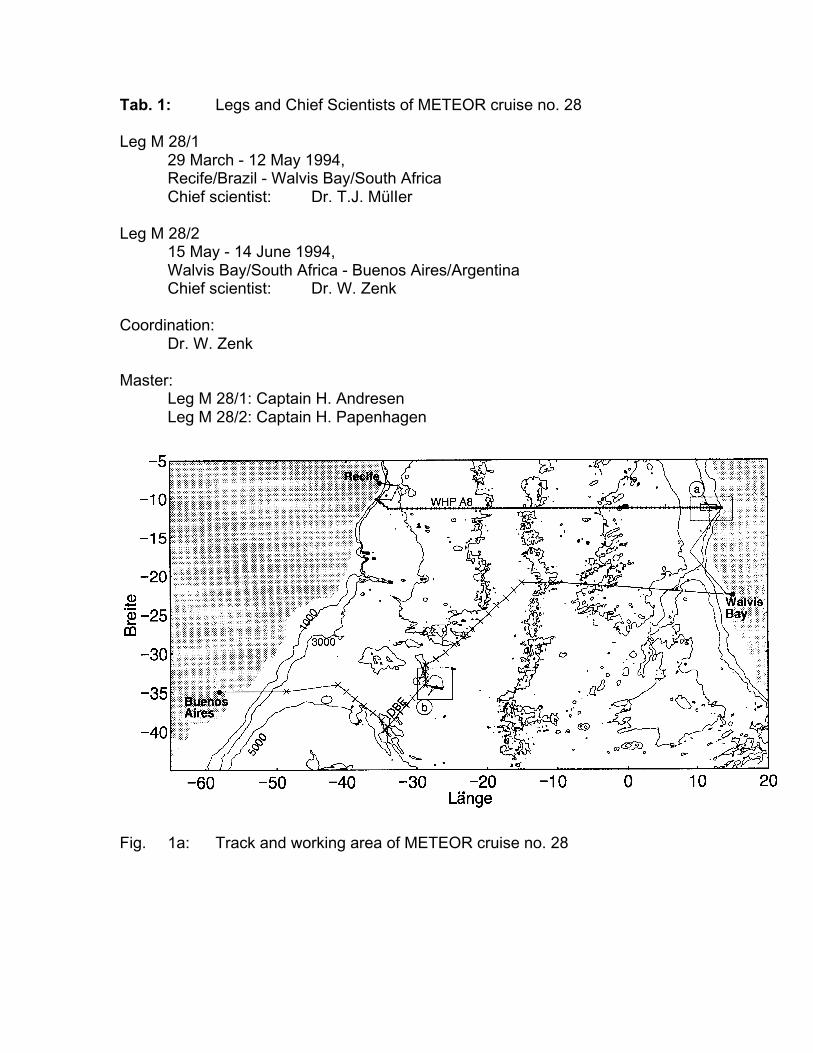
Tab. 1: Legs and Chief Scientists of METEOR cruise no. 28
Leg M 28/129 March - 12 May 1994,Recife/Brazil - Walvis Bay/South AfricaChief scientist: Dr. T.J. MülIer
Leg M 28/215 May - 14 June 1994,Walvis Bay/South Africa - Buenos Aires/ArgentinaChief scientist: Dr. W. Zenk
Coordination:Dr. W. Zenk
Master:Leg M 28/1: Captain H. AndresenLeg M 28/2: Captain H. Papenhagen
Fig. 1a: Track and working area of METEOR cruise no. 28
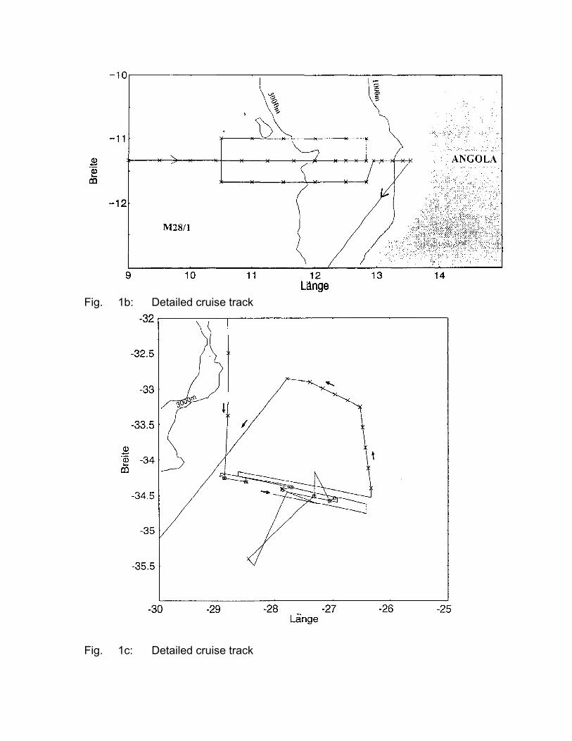
Fig. 1b: Detailed cruise track
Fig. 1c: Detailed cruise track
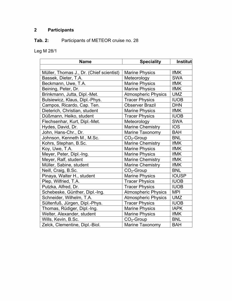
2 Participants
Tab. 2: Participants of METEOR cruise no. 28
Leg M 28/1
Name Speciality Institute
Müller, Thomas J., Dr. (Chief scientist) Marine Physics IfMKBassek, Dieter, T.A. Meteorology SWABeckmann, Uwe, T.A. Marine Physics IfMKBeining, Peter, Dr. Marine Physics IfMKBrinkmann, Jutta, Dipl.-Met. Atmospheric Physics UMZBulsiewicz, Klaus, Dipl.-Phys. Tracer Physics IUOBCampos, Ricardo, Cap. Ten. Observer Brazil DHNDieterich, Christian, student Marine Physics IfMKDüßmann, Heiko, student Tracer Physics IUOBFlechsenhar, Kurt, Dipl.-Met. Meteorology SWAHydes, David, Dr. Marine Chemistry IOSJohn, Hans-Chr., Dr. Marine Taxonomy BAHJohnson, Kenneth M., M.Sc. CO2-Group BNLKohrs, Stephan, B.Sc. Marine Chemistry IfMKKoy, Uwe, T.A. Marine Physics IfMKMeyer, Peter, Dipl.-Ing. Marine Physics IfMKMeyer, Ralf, student Marine Chemistry IfMKMüller, Sabine, student Marine Chemistry IfMKNeill, Craig, B.Sc. CO2-Group BNLPinaya, Walter H., student Marine Physics IOUSPPlep, Wilfried, T.A. Tracer Physics IUOBPutzka, Alfred, Dr. Tracer Physics IUOBSchebeske, Günther, Dipl.-Ing. Atmospheric Physics MPISchneider, Wilhelm, T.A. Atmospheric Physics UMZSültenfuß, Jürgen, Dipl.-Phys. Tracer Physics IUOBThomas, Rüdiger, Dipl.-Ing. Marine Physics IAPKWelter, Alexander, student Marine Physics IfMKWills, Kevin, B.Sc. CO2-Group BNLZelck, Clementine, Dipl.-Biol. Marine Taxonomy BAH
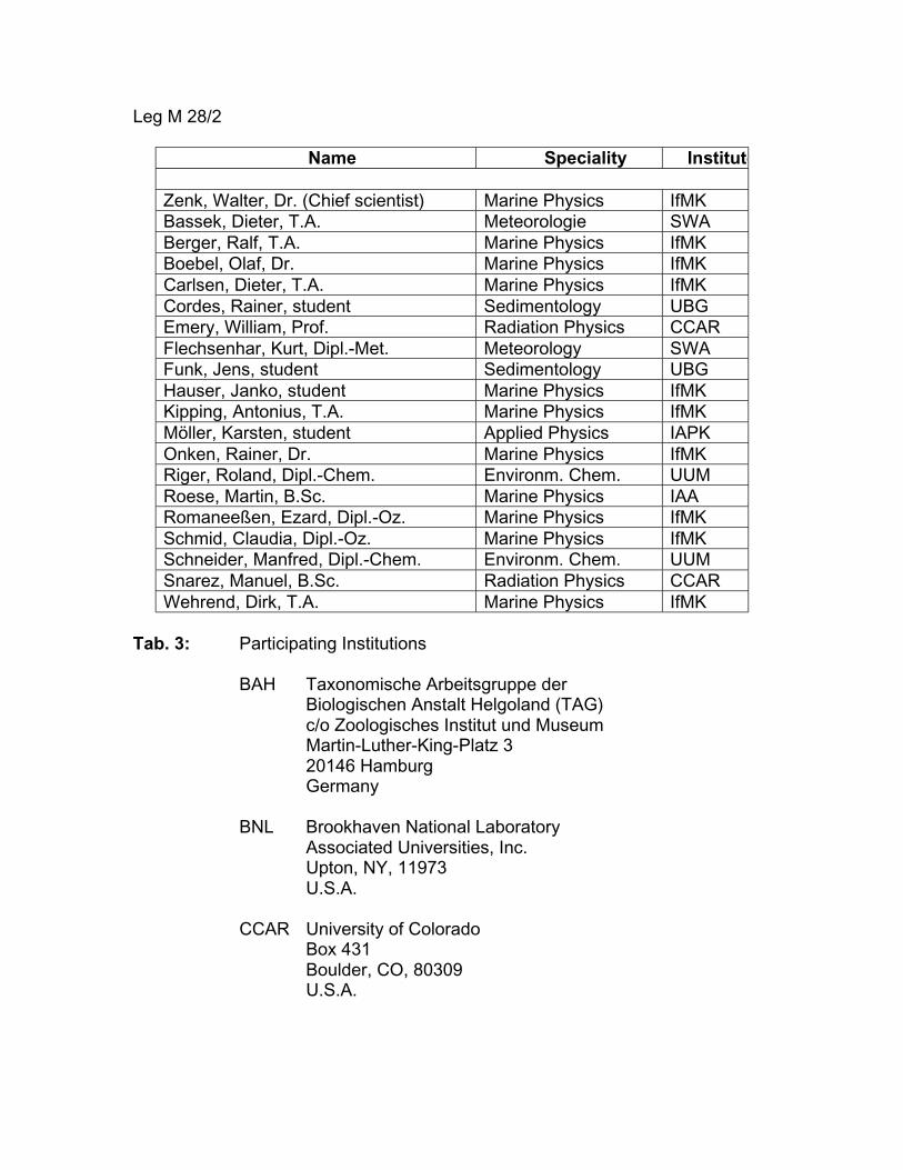
Leg M 28/2
Name Speciality Institute
Zenk, Walter, Dr. (Chief scientist) Marine Physics IfMKBassek, Dieter, T.A. Meteorologie SWABerger, Ralf, T.A. Marine Physics IfMKBoebel, Olaf, Dr. Marine Physics IfMKCarlsen, Dieter, T.A. Marine Physics IfMKCordes, Rainer, student Sedimentology UBGEmery, William, Prof. Radiation Physics CCARFlechsenhar, Kurt, Dipl.-Met. Meteorology SWAFunk, Jens, student Sedimentology UBGHauser, Janko, student Marine Physics IfMKKipping, Antonius, T.A. Marine Physics IfMKMöller, Karsten, student Applied Physics IAPKOnken, Rainer, Dr. Marine Physics IfMKRiger, Roland, Dipl.-Chem. Environm. Chem. UUMRoese, Martin, B.Sc. Marine Physics IAARomaneeßen, Ezard, Dipl.-Oz. Marine Physics IfMKSchmid, Claudia, Dipl.-Oz. Marine Physics IfMKSchneider, Manfred, Dipl.-Chem. Environm. Chem. UUMSnarez, Manuel, B.Sc. Radiation Physics CCARWehrend, Dirk, T.A. Marine Physics IfMK
Tab. 3: Participating Institutions
BAH Taxonomische Arbeitsgruppe derBiologischen Anstalt Helgoland (TAG)c/o Zoologisches Institut und MuseumMartin-Luther-King-Platz 320146 HamburgGermany
BNL Brookhaven National LaboratoryAssociated Universities, Inc.Upton, NY, 11973U.S.A.
CCAR University of ColoradoBox 431Boulder, CO, 80309U.S.A.
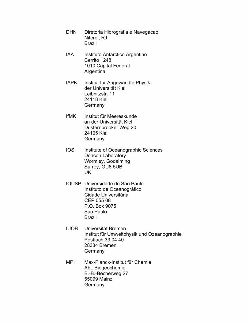
DHN Diretoria Hidrografia e NavegacaoNiteroi, RJBrazil
IAA Instituto Antarctico ArgentinoCerrito 12481010 Capital FederalArgentina
IAPK Institut für Angewandte Physikder Universität KielLeibnitzstr. 1124118 KielGermany
IfMK Institut für Meereskundean der Universität KielDüsternbrooker Weg 2024105 KielGermany
IOS Institute of Oceanographic SciencesDeacon LaboratoryWormley, GodalmingSurrey, GU8 5UBUK
IOUSP Universidade de Sao PauloInstituto de OceanográficoCidade UniversitáriaCEP 055 08P.O. Box 9075Sao PauloBrazil
IUOB Universität BremenInstitut für Umweltphysik und OzeanographiePostfach 33 04 4028334 BremenGermany
MPI Max-Planck-Institut für ChemieAbt. BiogeochemieB.-B.-Becherweg 2755099 MainzGermany
SWA Deutscher Wetterdienst- Seewetteramt -Bernhard-Nocht-.Str. 7620359 HamburgGermany
UBG Universität BremenFachbereich 5 - GeowissenschaftenPostfach 33 04 4028334 BremenGermany
UMZ Institut für Physik der AtmosphäreJohannes -Gutenberg-UniversitätSaarstr. 2155122 MainzGermany
UUM Universität UlmAbt. Analytische Chemie und UmweltchemieAlbert-Einstein-Allee 1189069 UlmGermany
3 Research Programme
3.1 WOCE Hydrographic Programme (WHP): Section A8
The main programme of leg M 28/1 was devoted to the World Ocean CirculationExperiment (WOCE) which is internationally coordinated by the World MeteorologicalOrganisation (WMO) and the International Council of Scientific Unions (ICSU).Within the fieldwork of WOCE, for the first time in history the present state anddynamics of the ocean will be observed world wide within less than ten years.Closely related to WOCE is the Joint Ocean Global Flux Studies (JGOFS) withinwhich sampling of CO2 components is requested on WOCE hydrographic sections.
One major component of WOCE is the Hydrographic Programme (WHP). Germaninstitutes took responsibility to occupy three zonal transatlantic hydrographic sectionsin the South Atlantic: Sections A9 along 19˚S and A10 along 30˚S were obtainedduring METEOR cruises no. 15/3 in 1991 and no. 22/5 in 1993, respectively. Duringthe present METEOR cruise no. 28/1, section A8 along nominal 11˚20 S wasoccupied with a total of 110 hydrographic stations with CTD and up to 40 small (10 l)volume rosette samples per station. The nominal station spacing was decreaseddown to 10 p.m. and 5 n.m. over the shelf and continental breaks, to 24 n.m. over theMid-Atlantic Ridge, and increased to 38 n.m. over the deep Pernambuco Basin and
Angola Basin. Bottle samples to analyze for oxygen, nutrients and salinity weretaken on each station, samples for anthropogenic tracers and CO2 on every otherstation.
In addition, four test stations and a survey with ADCP were performed off theBrazilian shelf before the WHP section began, and a box around the eastern tail ofthe section was occupied.
Underway measurements of currents down to 200 m with a ship borne AcousticDoppler Current Profiler (ADCP) and with a Geomagnetic Electro Kinetograph (GEK),satellite tracked drifting buoys and expendable current profilers as well as near-surface temperature and salinity and meteorological parameters supplemented thestation work.
As part of a long-term Atlantic wide survey on the distribution and ecology of fishlarvae, biological stations with 69 plankton hauls from the surface and in 5 levelsbetween the surface and 200 m depth were performed.
Aerosols determine the formation of clouds. Over the South Atlantic several sourcesmay be expected: Aerosols of sea salt and remainders of continental aerosols ofmostly desertal origin as well as particles which result from decomposition ofdimethylsulfide (DMS) formed by chlorophyll in the sea. All types of these aerosolswere filtered from air and are to be correlated to DMS concentrations in seawater andair.
3.2 WOCE Deep Basin Experiment (DBE)
During leg M 28/2 earlier work, performed in the Brazil Basin by METEOR in 1991and 1992, was continued and extended towards a larger area. These activitiescontributed to the Deep Basin Experiment of WOCE implemented by scientists fromBrazil, France, Germany and the USA. Certified knowledge of the regional watermass circulation as well as the distribution of horizontal divergence and convergencezones are essential for appropriate modelling, one of the research targets of WOCE.
Besides XBT, CTD and GEK measurements (chap. 3.4) circulation studies of thenear-surface Central Water were conducted on a quasi-meridional section throughthe Brazil Basin across the Rio Grande Rise towards the northern Argentine Basin.Among other instrumentation satellite tracked drift buoys from Kiel were used forthese observations (chapter 3.3).
Within the deeper levels (800 - 1000 m) of the Antarctic Intermediate WaterLagrangian current observation with RAFOS floats were performed. Results from theprevious METEOR cruise No. 22 have impressively confirmed the westwardcirculation pattern above the Rio Grande Rise. However, we definitely still need moreobservations of the Intermediate Water in the central part of the Brazil Basin and nearthe Subtropical Convergence in the Argentine Basin.
The RAFOS sound array has been enlarged by two more sound sources moored atthe northern rim of the Argentine Basin. In fact, the whole array in the South Atlanticconsists of nine American and six German sound sources (status: Nov. 1994). Wedeployed 27 floats, built and ballasted by the Institut für Meereskunde at Kiel. Therecovery of seven current meter and thermistor chain moorings in the Hunter Channelwas another research topic. These Eulerian long-term observations began duringMETEOR cruise No. 22 in December 1992. The obtained data supplement anexisting set of observations monitoring the more westerly part of the water exchangebetween the Argentine and the Brazil Basin.
Near-bottom CTD casts were utilized for taking bottom samples by means of aminicorer of the University of Bremen (chapter 3.8). Results are analyzed in terms ofpaleoceanographic objectives.
3.3 Near-Surface Circulation from Drifters
Within the framework of WOCE about 135 satellite tracked drifting buoys (droguedepth 100 m) have been deployed in the South Atlantic by the Institut fürMeereskunde at Kiel since 1990. The objective is to deduce near-surface circulationproperties in the South Atlantic. Analysis of the eddy statistics was already started inselected areas. But up to now the data density is insufficient for a basin-widedetermination of physical parameters like mean velocity and eddy kinetic energy.Therefore the data set has been supplemented by deploying 80 new buoys - 30 ofthem during M 28.
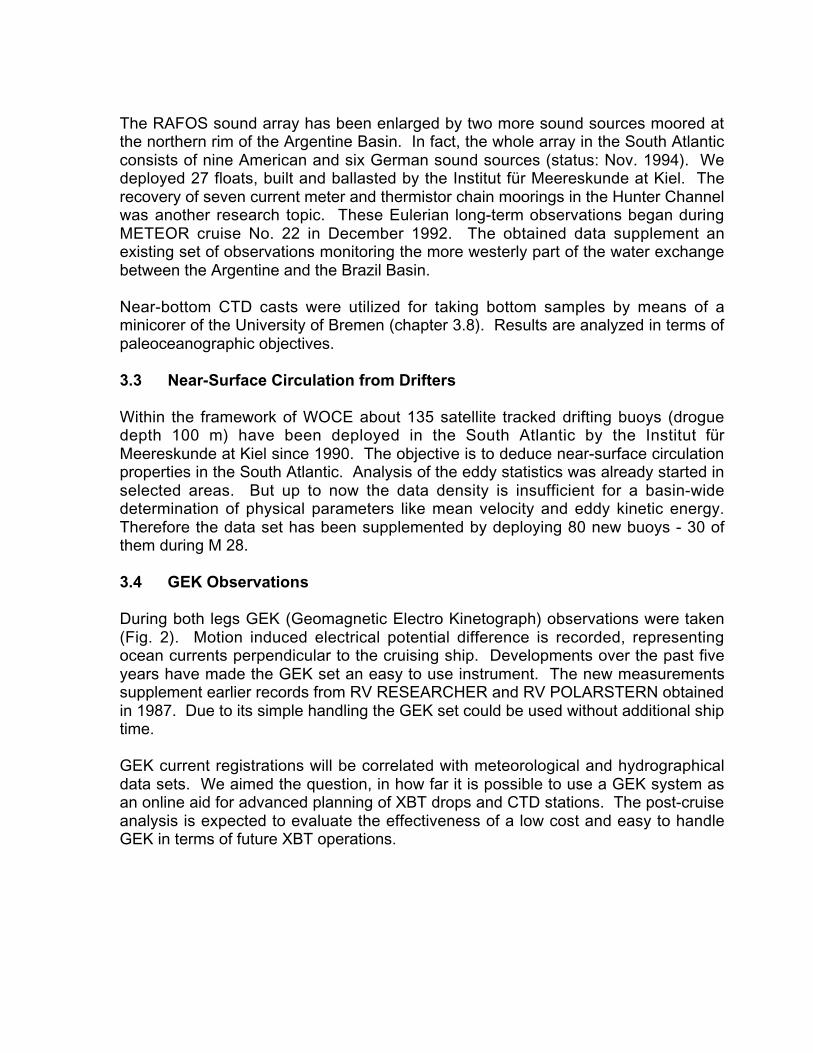
3.4 GEK Observations
During both legs GEK (Geomagnetic Electro Kinetograph) observations were taken(Fig. 2). Motion induced electrical potential difference is recorded, representingocean currents perpendicular to the cruising ship. Developments over the past fiveyears have made the GEK set an easy to use instrument. The new measurementssupplement earlier records from RV RESEARCHER and RV POLARSTERN obtainedin 1987. Due to its simple handling the GEK set could be used without additional shiptime.
GEK current registrations will be correlated with meteorological and hydrographicaldata sets. We aimed the question, in how far it is possible to use a GEK system asan online aid for advanced planning of XBT drops and CTD stations. The post-cruiseanalysis is expected to evaluate the effectiveness of a low cost and easy to handleGEK in terms of future XBT operations.

3.5 Taxonomy and Distribution of Fish Larvae in the Tropical South Atlantic
3.5.1 Introduction
The zonal transect surveyed during the M 28/1 is part of a long-term programme todescribe fish larvae (taxonomy), investigate their distribution (ichthyogeography) andtheir environmental requirements (ecology) in the entire Atlantic Ocean.
Ichthyogeography can be studied more easily and more economically by larvalcatches (ichthyoplankton) than by fisheries on adult fish. Larvae cover a verticallymore restricted space, are much more abundant, are less capable of escapemovements and can be stored more easily (e.g. LASKER, 1981). Some potentialdisadvantages may be seasonality in occurrence (JOHN, 1979) and the still limitedknowledge of larvae taxonomy. World wide the knowledge is most restricted intropical seas (AHLSTROM and MOSER, 1981).
Quantitative plankton samples can, even after coarse taxonomic analysis only, reveallarge scale regional differences in biogeography (JOHN, 1976/77). The spatialresolution increases with taxonomic precision. Additionally such quantitative studiescan indicate those environmental parameters limiting the specific distributions (JOHN,1985). The ranges of most vulnerable youngest stages generally conform withoptimum conditions for reproduction, whilst gradients of abundance and age indicatethe paths of dispersal and areas of decay (JOHN, 1984). Combining results of othermarine sciences, parameters of relevance can be revealed and quantified (e.g.HAMANN et al., 1981). In spite of many uncertainties, fish are among the bestinvestigated marine organisms and provide some regional comparative data coveringdecades. Comparison of such data can allow an assessment of the effects ofclimatic changes (e.g. EHRICH et al., 1987). Therefore, in light of the recentdiscussion concerning Global Change, such quantitative studies should be continuedand intensified.
3.5.2 Plankton Sampling
Samples were taken on a total of 69 biological stations, strictly following the box orlines of the CTD stations shown in the reports above, which made the hydrographicalparameters available. However, distances between plankton tows in the biologicallysomewhat more uniform oceanic realm were wider than for CTD stations.Nevertheless, at the continental slopes off Brazil and Angola smaller scalehydrographical features, particularly bottom depths and bottom types, wereanticipated to cause small scale heterogeneities in species composition andabundance. There a finer resolution of sometimes only 3 n.m. between stationscould be achieved, neglecting likely diurnal differences in light-sensitive neustonicorganisms. In the open ocean daylight and nighttime stations were taken in similarnumbers.
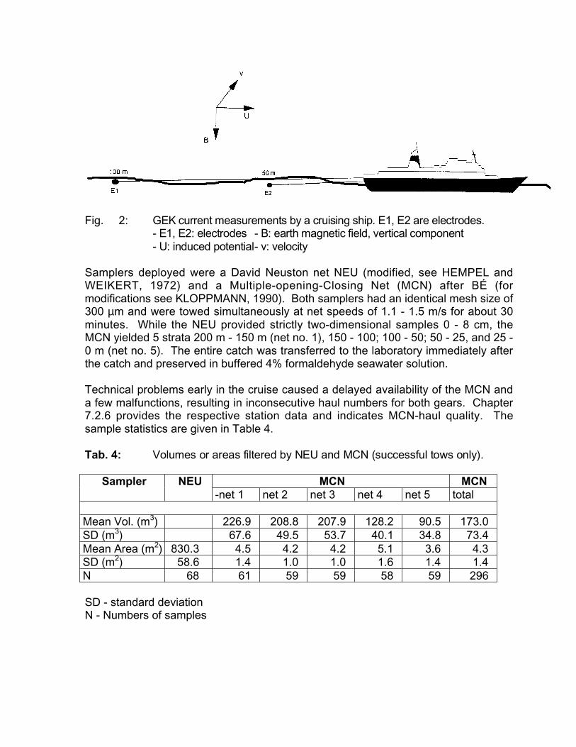
Fig. 2: GEK current measurements by a cruising ship. E1, E2 are electrodes.- E1, E2: electrodes - B: earth magnetic field, vertical component- U: induced potential- v: velocity
Samplers deployed were a David Neuston net NEU (modified, see HEMPEL andWEIKERT, 1972) and a Multiple-opening-Closing Net (MCN) after BÉ (formodifications see KLOPPMANN, 1990). Both samplers had an identical mesh size of300 µm and were towed simultaneously at net speeds of 1.1 - 1.5 m/s for about 30minutes. While the NEU provided strictly two-dimensional samples 0 - 8 cm, theMCN yielded 5 strata 200 m - 150 m (net no. 1), 150 - 100; 100 - 50; 50 - 25, and 25 -0 m (net no. 5). The entire catch was transferred to the laboratory immediately afterthe catch and preserved in buffered 4% formaldehyde seawater solution.
Technical problems early in the cruise caused a delayed availability of the MCN anda few malfunctions, resulting in inconsecutive haul numbers for both gears. Chapter7.2.6 provides the respective station data and indicates MCN-haul quality. Thesample statistics are given in Table 4.
Tab. 4: Volum es or a r ea s filte re d b y NEU a nd MCN (su ccessfu l to ws on ly) .
MCN MCNSampler NEU-net 1 net 2 net 3 net 4 net 5 total
Mean Vol. (m3) 226.9 208.8 207.9 128.2 90.5 173.0SD (m3) 67.6 49.5 53.7 40.1 34.8 73.4Mean Area (m2) 830.3 4.5 4.2 4.2 5.1 3.6 4.3SD (m2) 58.6 1.4 1.0 1.0 1.6 1.4 1.4N 68 61 59 59 58 59 296
SD - standard deviationN - Numbers of samples
3.6 Atmospheric Physics and Chemistry
Aerosol particles over the subtropical South Atlantic are mainly influenced by twosources: The sea salt aerosol and aged continental background aerosol with acontribution of the Sahara or Namib desert.
During M 28/1 the size distribution of the marine aerosol particles ranged from 0.005µm to about 50 ~m radius.
The ocean is an important source of biological aerosol particles. These are able tocontribute to cloud forming processes. Thus particles of this type were determined inthe radius range > 0.2 ~m. Measurements during METEOR cruise no. 9/2-4 and 22/5showed discrepancies in the biological content. Therefore dimethylsulfide (DMS) wasmeasured additionally during M 28/1.
In presence of sun light marine phytoplancton is able to produce a compound whichdecomposes in seawater and enters the atmosphere as DMS. This component inturn is unstable in the atmosphere and oxidizes to sulfate which forms particles andthus influences the cloud condensation nuclei density.
The DMS concentration will be correlated with the concentration of the biologicalaerosol particles on one hand and with the concentration of the aerosol particles onthe other hand. The latter were measured continuously during leg 1.
Additional information will be given by filter samples that were done simultaneously.The filters will be analyzed in order to determine the carbonaceous part of theaerosol.
3.7 Radiative Physics - Skin Sea Surface Temperature Investigation
The purpose of the measurements collected during M 28/2 in the South Atlanticocean is to examine the radiative skin sea surface temperature (SST) and itsrelationship to simultaneous measurement of bulk SST. It is the radiative skin SSTthat is viewed by satellite infrared radiometers and we wish to develop newcalibration procedures for the satellite sensors. We have used systems similar to thatto be installed on METEOR for cruises in the North Atlantic (on the old METEOR inthe fall of 1984), in the Arctic (from VALDIVIA in 1988) in the South Pacific (RV MBALDRIGE in 1990) and in the tropical Pacific (RV VICKERS in spring 1993). Thusmeasurements from the South Atlantic compliment some of our other measurementsof skin and bulk temperature. We have yet to collect a set of skin, bulk SSTmeasurements in the North Pacific.
The new radiometer (Fig. 3) has only been used once before in the tropical Pacificlast year. It is a unique system designed for this measurement and the radiometerhas 6 different infrared channels for the measurement of skin SST. Four of these 6channels are the same channels that are available from the satellite radiometer. The
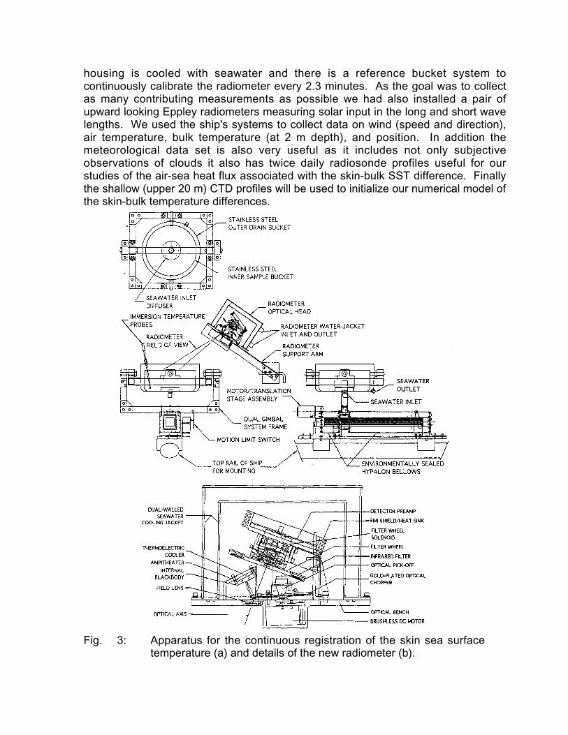
housing is cooled with seawater and there is a reference bucket system tocontinuously calibrate the radiometer every 2.3 minutes. As the goal was to collectas many contributing measurements as possible we had also installed a pair ofupward looking Eppley radiometers measuring solar input in the long and short wavelengths. We used the ship's systems to collect data on wind (speed and direction),air temperature, bulk temperature (at 2 m depth), and position. In addition themeteorological data set is also very useful as it includes not only subjectiveobservations of clouds it also has twice daily radiosonde profiles useful for ourstudies of the air-sea heat flux associated with the skin-bulk SST difference. Finallythe shallow (upper 20 m) CTD profiles will be used to initialize our numerical model ofthe skin-bulk temperature differences.
Fig. 3: Apparatus for the continuous registration of the skin sea surfacetemperature (a) and details of the new radiometer (b).
Using previous data we have been able to parameterize the night relationshipbetween skin and bulk SSTs which at that time are strictly a function of the local windspeed driving the ocean turbulence. During the day a more complex numericalmodel must be coupled to our paratermization to model conditions when solarinsolation occurs along with the local wind stress.
3.8 Marine Geology
During leg 2 sediment samples up to 20 cm depth as well as water samples weretaken on the whole profile across the Atlantic. A minicorer with four sampling tubeshas been used to sample the sediment.
The aim of the geological sampling during the second leg is to obtain core materialfor paleoceanographic studies of the time span from the last glacial to recent times.Furthermore the expressiveness of the proxy parameter should be improved.
On the water samples measurements of the stable oxygene-isotopes 18O/16O and ofnutrients as well as measurements of the 13C/12C compositions of ∑CO2 have beencarried out. These measurements will enlarge the Geochemical Ocean SectionStudy (GEOSECS) data set of the Atlantic.
3.9 Environmental Chemistry
The Department of Analytical and Environmental Chemistry joined M 28/2 toinvestigate the global occurrence and distribution of organic xenobiotics. Thesepersistent compounds are mainly produced in the northern hemisphere and reach theenvironment, where they are transported and distributed in the atmosphere,hydrosphere and biosphere by the global mass flow of these compartments. Theinter-hemispheric exchange however occurs very slowly resulting in very lowconcentrations of xenobiotics in the southern hemisphere. Thus data of persistentorganic compounds in the southern hemisphere reflect the global distribution of thesecompounds. Level and pattern of multi-component mixtures of xenobiotics indicateformation or global translocation.
During M 28/2 samples from the surface seawater, micro layer and air from the lowertroposphere were sampled for analysis of organic xenobiotics, namely chlorinatedparaffins (PC) and alkyl nitrates. Chlorinated paraffins were detected in all seawatersamples and surface micro layer samples in ng/I concentrations, whereas in airsamples CP were not detectable. These data confirm the global occurrence anddistribution of chlorinated paraffins. High volatile as well as long-chain alkyl nitrateswere detected in air samples of the lower troposphere. Levels and patterns can bediscussed in order to investigate the origin of these xenobiotics.
4 Narrative of the Cruise
4.1 Leg M 28/1 (T.J. Müller)
METEOR sailed from Recife on March 29, at 14:15 lt (19:15 UTC), T.J. Müller beingchief scientist. Heading eastwards (see Fig. 1), outside the 12 n.m. zone of Brazil atposition 8˚17 S/34˚30 W the continuously re-coding systems were switched on: Theintegrated system DVS to acquire navigational data, the ship borne 150 KHz ADCP,and the towed GEK. The first two days were designed to test both CTD systems,each equipped with a 24x10 I rosette sampler, on four deep water stations (Sta. 165to 168). Also, the analyzing systems for oxygen, nutrients, freons and CO2 were setup. At 11˚20 S/34˚W we began a section along A8 shore-wards with XBT and XCPthereby achieving a box with ADCP and GEK in the divergence zone of the westernbranch of the South Equatorial Current.
On April 1, WHP section A8 started on position 10˚03 S/35˚46 W on the 200 in depthcontour outside the 12 n.m. zone of Brazil normal to the continental break with Sta.169. On each of the following stations, together with the first CTD rosette, a 150 kHzself-containing ADCP was lowered (LADCP) to maximal 1000 in depth. The bottleswere used to increase the number of samples up to 40, where the bulk came from themain CTD which always went down until 10 m above the bottom. At 34˚W thenominal latitude 11˚20 S was reached again (Sta. 181), 13 stations at 5 n.m. to 20n.m. spacing were obtained. Station spacing now was increased to 30 n.m. until32˚W (Sta. 185).
Here, outside the 200 n.m. economic zone of Brazil, measurements with the multi-beam echo-sounding system Hydrosweep, surface meteorological data, andsampling of aerosols began. Over the Pernambuco Basin, station spacing wasincreased to 38 n.m. with XBTs of type T5 (nominal depth 1800 m at 6 kn) launchedhalfway in between. Until Sta. 190 at 25˚20 W, all stations were biological, too. Fromthen on, spacing for biological hauls was 70 to 90 n.m. Four satellite tracked surfacedrifters which are drogued at 100 m depth were launched between 20˚W and 15˚45W. Approaching the Mid-Atlantic Ridge, from 22˚W on (Sta. 200) spacing wasdecreased to 30 n.m. until 17˚W (Sta. 210) and down to 24 n.m. over the ridge until12˚W (Sta. 222).
Spacing was increased again towards the Angola Basin to 28 n.m. until 1˚W wherethe section ran close to the Dampier Seamount. Expecting higher hydrographicvariability and different species of fish larvae, two extra CTD stations (Sta. 245, Sta.247, no bottles) and plankton hauls were obtained.
From 0˚E on station spacing increased over the Angola Basin to 38 n.m. until wereached the African continental break at 8˚E (Sta. 260). Again, on this wider spacedpart of the section XBT T5 probes were launched halfway between stations. Also,four more satellite drifting buoys were launched between 1˚20 E and 5˚20 E.
With 28 n.m. station spacing we reached 10˚E (Sta. 264) where we entered the 200n.m. economic zone of Angola. Since no clearance had been applied for planktonhauls, XBT, XCP, and GEK, we had to continue with CTD measurements only.Station spacing was reduced first to 25 n.m. and then to 10 n.m. until we reached the50 n.m. zone at 12˚57 E (Sta. 274). Waiting for an extension of the clearance to 12n.m. and plankton hauls within 200 n.m. which was to be arranged by the GermanEmbassy in Luanda, Angola, we surveyed the northern part of a box around theeastern tail of A8 using the CTD/LADCP system down to 1000 in depth (Sta. 275 to281 along 11˚S). We completed this box in the south (Sta. 282 to Sta. 286 along11˚40 S) after the extension of the clearance came with plankton hauls as well. Wejoined A8 again after two days interruption on 11˚20 S at 13˚05 E (Sta. 287) andcompleted it on the 200 m depth contour at 13˚33 E with Sta. 290 on May 07, 1994.
4.2 Leg M 28/2 (W. Zenk)
In Walfish Bay, Namibia, W. Zenk took over as chief scientist at midday of May 13,1994. Previously Captain H. Papenhagen and both chief scientists had briefed thepress on board the ship. This meeting had been carefully arranged by H. Hoffmannfrom the German Embassy in Windhoek. In addition to the Regional Governor of theErongo Region, Mr. A. Kapere, we enjoyed the company of Mayor B. Edwards andMayor D. Kambo, representing the cities of Walfish Bay and Swakopmund,respectively.
In his introductory remarks H. Hofmann remembered the days 68 years ago, whenMETEOR's predecessor, the old METEOR, made a port call in Walfish Bay duringher famous cruise, the "Deutsche Atlantische Expedition". W. Zenk welcomed theguests on behalf of the Deutsche Forschungsgemeinschaft and T.J. Müllerintroduced some of the very first results of the WOCE section A8 that the METEORhad just completed.
Initiated by a press release issued by the coordinator's office in Kiel and the GermanEmbassy in Windhoek, the arrival of the METEOR was well received in Namibia. Thecity and habour of Walfish Bay had been peacefully incorporated by the Republic ofNamibia only 74 days earlier. A respectable number of German speaking inhabitantsvisited METEOR informally. Among them were a few elderly guests whoenthusiastically reported their unforgotten impressions of the old METEOR they hadvisited as school kids. Our port call at Walfish Bay exceeded everybody'sexpectation. We highly recommend this efficient port for future needs of the Germanresearch fleet.
Early Sunday morning on May 15, METEOR left Namibia and sailed directly towardstarget point "A" at 21˚S/10˚W, situated on the eastern flank of the Mid-Atlantic Ridge.Until early February 1994, we had planned to reach "A" coming from Pointe Noire,Republic of Congo, passing the island of St. Helena. However, due to official travelwarnings from the American Secretary of State and the German Foreign Ministry wewere forced to reorganize the cruise track on short notice.
On May 21, METEOR crossed the Mid-Atlantic Ridge and occupied the first stationsin the eastern Brazil Basin. Until then, all continuously recording systems, i.e.Geomagnetic Electro Kinetograph (GEK), ADCP, radiation and environmentalchemistry loggers, had become and remained fully operational for most of theexpedition time. The first surface drifters and RAFOS floats were launched at thecorner Sta. 295. All drifters were equipped with drogues at a depth of 100 m. Thecourse then changed to 223˚.
Further CTD/RO stations partly in combination with minicorer deployments, morefloat and drifter deployments and zodiac based chemical sampling followed till wereached mooring "R", at Sta. 305 on the eastern flank of the Rio Grande Rise on May25. This as all other mooring had been deployed by METEOR in mid December1992 as a component of the 'Deep Basin Experiment', a subprogramme of WOCE.
On May 27, we reached the western side of the 200 km wide zonal cross HunterChannel array at moorings "H1-6", being 200 km wide. Favoured by excellentweather conditions all moorings were recovered (Sta. 309-319, 27-30 May) after a 17month deployment duration. The remaining time in the region was utilized forHydrosweep surveys and GEK tracks at night. The systematic survey of the bottomtopography of the Hunter Channel is a long-term project of the Alfred -Wegener-Institut, Bremerhaven, the University of Bremen and the Institut für Meereskunde atKiel. Selected CTD stations with minicorer deployments will allow more precisehydrographic and sedimentological descriptions of this important passage forAntarctic Bottom Water on its equatorward drift.
We expected serious problems with mooring "K0". This sound source rig broke loosein mid February 1994, when signals from the watch dog top buoy were reported byService ARGOS. Upon several release commands no remainders showed up at themooring site of "K0" in the Hunter Channel. However, to our greatest surprise wewere able to locate the sound source's shifted position at approximately 35˚22S/28˚28 W by listening with two MAFOS monitors on the hydrographic wire. Thelistening procedure was repeated five nights from different spots resulting in a searchradius of < 8 n.m. Despite of a 36 hour intensive search METEOR was unable to findthe lost mooring on the sea surface.
On June 1, the search was discontinued. The ship returned to the Hunter Channeland set the replacement sound source mooring "K0 2" (Sta. 322). After a finalhydrosweep leg across the Hunter Channel a narrowly spaced deep CTD-sectionwas occupied at the eastern and northern exits of the channel area (Sta. 323-332).Because of rough weather conditions we had to skip further minicorer deployments,which were otherwise performed regularly under the CTD probe on deep stations.Chemical samples from the surface (University of Ulm) were taken regularly from thezodiac during CTD operations whenever the weather conditions allowed.
On June 4, METEOR left the well measured Hunter region and headed for itssouthernmost position at 40˚S/35˚W. Here sound source mooring "K4" was launchedat Sta. 338. Sound sources are an integral component of the RAFOS system. Theirsignals are sensed by drifting floats. Arrival times of the coded transmissions arerecorded in the floats. After the floats surface, typically after 10-15 months, thestored information is transmitted by a satellite link and converted in Kiel into a seriesof float positions.
The sound source "K4" was a brand-new instrument that had been shipped from themanufacturer WRC directly to METEOR in Hamburg. It was only the qualifiedassistance of the ship’s electronic technician B. James that we were able to solve aproblem that remained undiscovered until we unpacked the instrument on board ofMETEOR. The passage towards "K4" was combined with more float and drifterlaunches and GEK observations, resulting in a quasi -continuous section from thecentre (21˚S) of the subtropical gyre to its southern extend north of the confluenceregion (35˚S).
On station 338 an extended CTD cast was taken. Samples include, as in otherselected cases, probes of helium, tritium, nutrients (University of Bremen) andsulfurhaxaflouride (Woods Hole Oceanographic Institution). After METEOR hadoccupied this southern corner station she cruised northwestward towards the outerVema Channel. Additional drifters and floats were launched between shallow CTDstation 338 and 344.
After the last drifter and float were deployed on Sta. 342 and 343, respectively, theship cruised to the final position at the 200 n.m.-zone off the Brazilian coast line.Here, at Sta. 34S more water samples were taken in the western boundary currentsystem before METEOR called at Buenos Aires on 14 June 1994.
When approaching the South American shelf METEOR had occupied 44 CTDstations, 23 of them included joint minicorer deployments. 89 XBT probes weredropped. Seven moorings had been recovered, two were deployed. 27 RAFOSfloats, two MAFOS monitors and 20 satellite tracked surface drifters with drogues at100 m depth could be launched. Quasi-continuous measurements of solar radiationand skin sea surface temperature as well as nearly uninterrupted GEK records werecollected.
Fig. 4a: Participants of M 28/1
Fig. 4b: Participants of M 28/2
5 Preliminary Results
In this chapter, methods of sampling and calibration, and preliminary results arediscussed from the WOCE Hydrographic Programme (WHP) section A8 along 11˚20S, from the Deep Basin Experiment (DBE), and other projects of the cruise.
5.1 The WHP Section A8 along 11˚20'S
The backbone of the station work were two MKIIIB CTDs to measure continuousprofiles of pressure, temperature, salinity and dissolved oxygen. Attached to themain CTD was a General Oceanic rosette sampler with 24x10 I Niskin bottles. Withthis main CTD, all stations were profiled down to 5 m to 10 m above the bottom toachieve a consistent set of high resolution hydrographic data along the section.
To take samples for chemical analysis, during the all upcasts the first two bottleswere closed at nominally 10 m above the bottom, and the last two bottles were closedin the mixed layer at nominally 10 m depth. This, together with the remaining bottlesclosed in between assured full depth calibration values for the CTD. The remainingbottles in between were closed according to a sampling scheme that took intoaccount that zonal variations along this zonal section were expected to be small:During two successive stations, bottles were closed at fixed depths, during the nexttwo stations the closing depths were set midth between those of the preceeding twoprofiles. Then the scheme was repeated. In order to fulfill the WHP requirements forhigh resolution sampling in the vertical, over the deep basins bottles from a secondCTD/Rosette with up to 18x10 l bottles were added.
When on deck after a profile, samples were drawn in the following order: CFCs,helium, oxygen, CO2, nutrients, tritium, salinity.
The second CTD/Rosette system carried a self contained 150 kHz Acoustic DopplerCurrent Profiler (ADCP) that was lowered (LADCP) down to 1000 m on all but twostations to measure currents in the upper ocean. These LADCP data together withdata from a ship borne 150 kHz ADCP and 8 profiles taken with Expandable CurrentProfilers (XCP) in the western boundary, will provide estimates of absolute currents.
Due to reasons mentioned in chapter 4, underway measurements of near-surfacetemperature and salinity, the multibeam echo sounding system Hydrosweep, andcontinuously recorded meteorological parameters are available only outside the 200n.m. economic zone of Brazil.
Table 5 summarizes the most important events of the WHP section A8. Chapters5.1.1 to 5.1.4 describe methods, calibrations and instruments used for analysis onboard in more detail while in chapter 5.1.5 we present sections of hydrographic andtracer parameters as measured along A8.
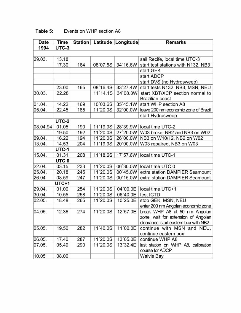
Table 5: Events on WHP section A8
Date Time Station Latitude Longitude Remarks1994 UTC-3
29.03. 13.18 sail Recife, local time UTC-317.30 164 08˚07.5S 34˚16.6W start test stations with N132, NB3
start GEKstart ADCPstart DVS (no Hydrosweep)
23.00 165 08˚16.4S 33˚27.4W start tests N132, NB3, MSN, NEU30.03. 22.28 11˚14.1S 34˚08.3W start XBT/XCP section normal to
Brazilian coast01.04. 14.22 169 10˚03.6S 35˚45.1W start WHP section A805.04. 22.45 185 11˚20.0S 32˚00.0W leave 200 nm economic zone of Brazil
start HydrosweepUTC-2
08.04.94 01.05 190 11˚19.9S 28˚39.9W local time UTC-219.50 192 11˚20.0S 27˚20.0W W03 broke , NB2 and NB3 on W02
09.04. 16.22 194 11˚20.0S 26˚00.0W NB3 on W10/12, NB2 on W0213.04. 14.53 204 11˚19.9S 20˚00.0W W03 repaired, NB3 on W03
UTC-115.04. 01.31 208 11˚18.6S 17˚57.6W local time UTC-1
UTC 022.04. 03.15 233 11˚20.0S 06˚30.0W local time UTC 025.04. 20.18 245 11˚20.0S 00˚45.0W e xt ra st at io n DAM PI ER Sea mo un t 26.04 08.59 247 11˚20.0S 00˚15.0W e xt ra st at io n DAM PI ER Sea mo un t
UTC+129.04. 01.00 254 11˚20.0S 04˚00.0E local time UTC+130.04. 10.55 258 11˚20.0S 06˚40.0E test ICTD02.05. 18.48 265 11˚20.0S 10˚25.0E stop GEK, MSN, NEU
enter 200 nm Angolan economic zone04.05. 12.36 274 11˚20.0S 12˚57.0E break WHP A8 at 50 nm Angolan
zone, wait for extension of Angolanclearance, start eastern box with NB2
05.05. 19.50 282 11˚40.0S 11˚00.0E continue with MSN and NEU,continue eastern box
06.05. 17.40 287 11˚20.0S 13˚05.0E continue WHP A807.05. 05.49 290 11˚20.0S 13˚32.4E last station on WHP A8, calibration
course for ADCP10.05 08.00 Walvis Bay
Notations:
ADCP shipmounted 150 KHz acoustic Doppler Current Profiler, RDIDVS ship's online data acquiring systemGEK towed Geomagnetic Electro KinetographNB3 combined CTD˚O2, 24 x 10 l rosetteNB2 combined CTD˚O2, 20 x 10 l rosette, 150 KHz ADCPMSN towed multiple opening and closing net, maximum depth 200 mNEU Neuston plankton surface netDR satellite tracked surface drifterW02/03 CTD winches 2 and 3W10/12 winches 10 and 12
5.1.1 Hydrography and Currents(T.J. Müller, U. Beckmann, P. Beining, C. Dieterich, U. Koy, P. Meyer, W.H. Pinaya)
The measurements to be made and controlled were: Two CTD/Rosette systems andtwo salinometers; XBT and XCP drops; Lowered Acoustic Doppler Profiling (LADCP)for vertical profiling of currents deeper than 300 in. Support came from the crew'selectronic group running the ship borne ADCP and other underway measurements:Near-surface temperature (T0) and salinity (S0) which were distributed by the ship'sdata collection and distribution system DVS along with data from the ship's navigationand echo sounding system and from the automatic weather station.
CTD/RosetteTwo MKIIIB CTDO2/Rosette systems were used with the sampling scheme describedin chapter 5.1 above. Both CTDs were made by Neil Brown Instruments (NBIS)(BROWN and MORRISON, 1978). No technical changes were made, because theinstruments were known to have relative smooth outputs. Thus, precision and fasttemperature have a combined output resulting in a priori weak salinity spiking,pressure is measured with a strain gauge sensor which is capsulated in steel andwhich is temperature compensated. Attached to both CTDs were Clark type oxygensensors.
The main CTD (IfMK code NB3) was used on all stations along with a 24x10 l bottleGeneral Oceanics rosette down to the bottom. The second CTD (IfMK code NB2)went down to 1000 in on almost each station to increase bottle samplings depths toWHP requirements. Attached to this second system was a 150 kHz LADCP tomeasure vertical current profiles.
Pre-cruise calibrations of both CTDs were performed in November 1993 at IfMK'scalibration laboratory before shipping the instruments (SAUNDERS et al., 1991;MOLLER et al., 1994, for details in the procedure). First, the correction of the CTD'stemperature output to the international temperature scale of 1990 (ITS90) wasdetermined with a Rosemount Pt25 resistance as part of a high precision bridgemade by 'Sensoren Instrumente Systeme' SIS in Kiel. Two triple point cells of water
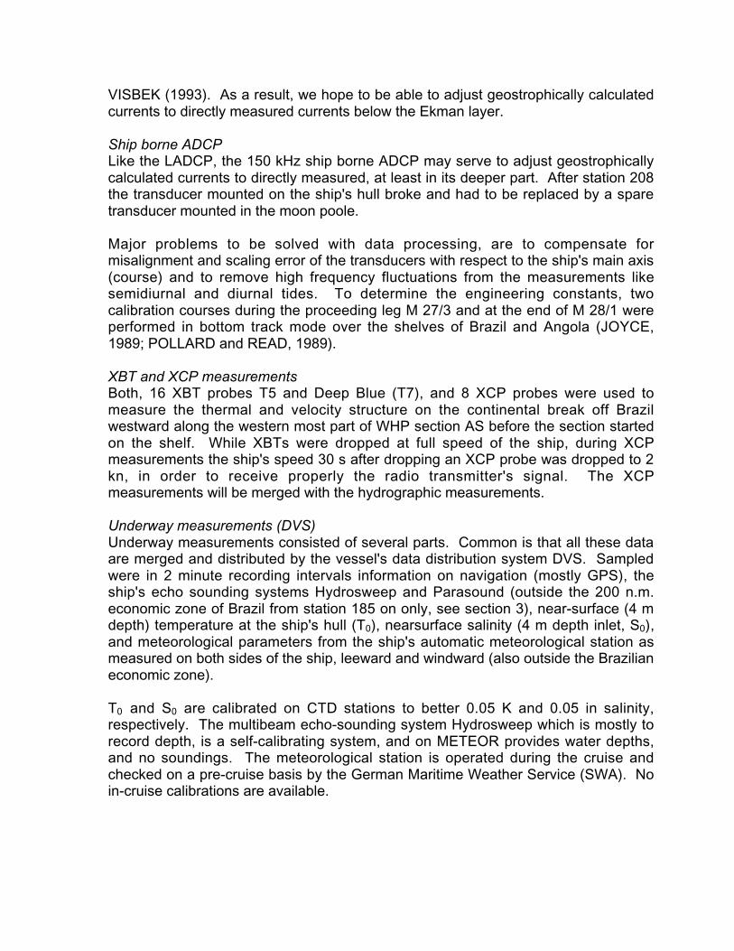
and two melting point cells of gallium defined the fix-points of the reference bridge at0.01˚C and close to 28˚C. The quadratic term for the Pt25 was taken from theoriginal calibration certificate. The drift between the two calibrations of the main CTD(N133) was less 1 mK (Fig. 5). Comparisons made during the cruise with the mainCTD (NB3) and three electronic reversing thermometers which have 1 mK resolutionand were turned on the same frame (depth) on almost each station also showed nodrift or jump. Thus, the accuracy for A8 over the whole range is better than 2 mK.
For both CTDs, the pressure sensors static correction at three different temperatures(ca. 0.5˚C, 10˚C, and 25˚C) were determined over the whole range, 0 dbar to 6000dbar, in loading mode, and in unloading mode with three maximum pressures at 6000dbar, 4000 dbar and 2000 dbar. A Budenberg dead weight tester with certifiedmasses corresponding to 500 dbar increments served as reference. The drift for bothsensors is less 1 dbar (Fig. 6), the accuracy for the static calibration is better than 1.5dbar over the whole range. For both sensors, fast temperature changes at fixedpressure result in sensor responses of order 0.3 dbar/K with time constants of theorder of 1.5 h. A simple model can reduce this error to less than 30% (MÜLLER etal., 1994). Observing static and dynamic corrections, the overall accuracy ofpressure measurements during A8 is better 2 dbar.
Conductivity is calibrated using the salinity of water samples taken during each castand analyzed on an Guildline Autosal salinometer along with calibrated CTDtemperature and pressure. The salinometer was calibrated with standard seawaterbatch P120. Double samples from two rosette bottles were taken 10 in above thebottom and within the mixed layer. All other samples for calibration stem from weakgradient layers at 2000 m, 3000 m, 4000 m and 5000 in depth giving a total of 1000samples for CTD calibration. At stations 165 and 166, the bottles of the main rosettewere closed at same depths to achieve an estimate of 0.0005 as mean precision ofreference salinities. The drift of the Autosal was less 0.0005 over the whole cruise, ifsome obvious instabilities due to noise in the power supply and radio operations areignored. After full evaluation we expect an accuracy of better 0.0015 in salinometersalinity and better 0.002 in CTD salinity.
Since the response of the oxygen sensor is known to be sensitive to uniform flowconditions, the calibration procedure at IfMK uses oxygen sensor and CTD valuesfrom the down cast and compares them to titrated values from the upcast on potentialdensity surfaces in high gradient levels up to a pressure of 2000 dbar, and onpressure surface for higher pressures where oxygen gradients are weak. Theformula for conversion of the sensor output to physical units is essentially that ofOWENS and MILLARD (1985).
Lowered ADCPA 150 kHz self-contained ADCP made by RD Instruments was attached to thesecond CTD/Rosette system to measure the vertical distribution of currents down to1000 m depth on stations. The instrument worked on all stations except stations 181,209, and 270. Data processing follows the method described by FISCHER and
VISBEK (1993). As a result, we hope to be able to adjust geostrophically calculatedcurrents to directly measured currents below the Ekman layer.
Ship borne ADCPLike the LADCP, the 150 kHz ship borne ADCP may serve to adjust geostrophicallycalculated currents to directly measured, at least in its deeper part. After station 208the transducer mounted on the ship's hull broke and had to be replaced by a sparetransducer mounted in the moon poole.
Major problems to be solved with data processing, are to compensate formisalignment and scaling error of the transducers with respect to the ship's main axis(course) and to remove high frequency fluctuations from the measurements likesemidiurnal and diurnal tides. To determine the engineering constants, twocalibration courses during the proceeding leg M 27/3 and at the end of M 28/1 wereperformed in bottom track mode over the shelves of Brazil and Angola (JOYCE,1989; POLLARD and READ, 1989).
XBT and XCP measurementsBoth, 16 XBT probes T5 and Deep Blue (T7), and 8 XCP probes were used tomeasure the thermal and velocity structure on the continental break off Brazilwestward along the western most part of WHP section AS before the section startedon the shelf. While XBTs were dropped at full speed of the ship, during XCPmeasurements the ship's speed 30 s after dropping an XCP probe was dropped to 2kn, in order to receive properly the radio transmitter's signal. The XCPmeasurements will be merged with the hydrographic measurements.
Underway measurements (DVS)Underway measurements consisted of several parts. Common is that all these dataare merged and distributed by the vessel's data distribution system DVS. Sampledwere in 2 minute recording intervals information on navigation (mostly GPS), theship's echo sounding systems Hydrosweep and Parasound (outside the 200 n.m.economic zone of Brazil from station 185 on only, see section 3), near-surface (4 mdepth) temperature at the ship's hull (T0), nearsurface salinity (4 m depth inlet, S0),and meteorological parameters from the ship's automatic meteorological station asmeasured on both sides of the ship, leeward and windward (also outside the Brazilianeconomic zone).
T0 and S0 are calibrated on CTD stations to better 0.05 K and 0.05 in salinity,respectively. The multibeam echo-sounding system Hydrosweep which is mostly torecord depth, is a self-calibrating system, and on METEOR provides water depths,and no soundings. The meteorological station is operated during the cruise andchecked on a pre-cruise basis by the German Maritime Weather Service (SWA). Noin-cruise calibrations are available.
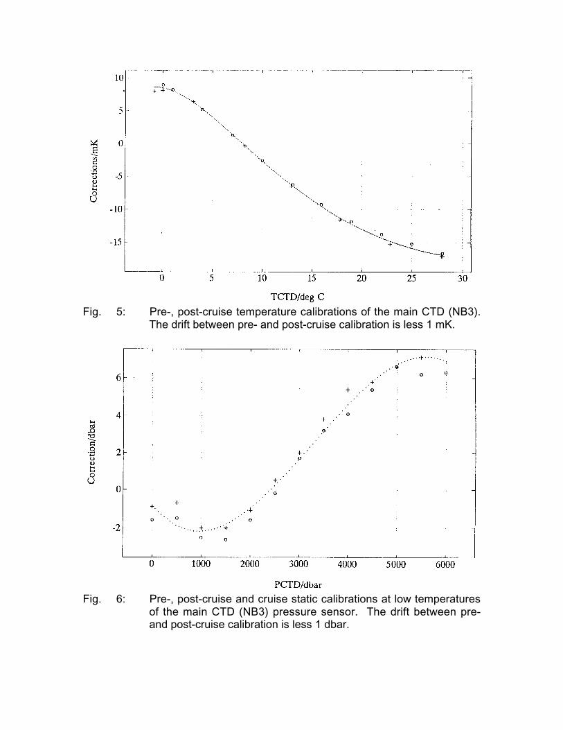
Fig. 5: Pre-, post-cruise temperature calibrations of the main CTD (NB3).The drift between pre- and post-cruise calibration is less 1 mK.
Fig. 6: Pre-, post-cruise and cruise static calibrations at low temperaturesof the main CTD (NB3) pressure sensor. The drift between pre-and post-cruise calibration is less 1 dbar.
5.1.2 Dissolved Oxygen and Nutrients (D.J. Hydes, S. Kohrs, R. Meyer, S. Müller)
Samples to measure dissolved oxygen and the nutrients phosphate, nitrate andsilicate were taken from each bottle closed on A8, and amount to more than analyzed3700 probes not including double probes to determine precision. Whereas themeasurements of oxygen, nitrate and silicate are of high quality, it was not possible tomeasure phosphate because of irreparable malfunction of the apparatus.
Dissolved oxygenBottle oxygen sub-samples were taken in calibrated clear glass bottles with groundglass stoppers from all WOCE section water samples collected on the cruise.Samples were taken immediately after the rosette was on deck or following thedrawing of tracer samples of CFCs and helium. At the time of chemical fixation thetemperature of the water was measured on a separate sample collected in the samemanner as the oxygen samples themselves. This information was used to correct thechange in density of the sample between the closure of the rosette bottle and thefixing of the dissolved oxygen. Duplicate samples were taken on every cast. Thesewere the first four bottles on the deep rosette, and the first two bottles on the shallowrosette.
Analysis followed the Winkler whole bottle method. The thiosulphate titrations werecarried out in an air conditioned laboratory, the temperature varied between 25˚C and21˚C over the period of the cruise. Potassium Iodate standards were determined inconjunction with most of the analytical runs. A mean value of the standardmeasurement was used to calibrate the titration of oxygen. The titration wascontrolled at the end point using a Metrohm Titrino (a combined automated buretteand micro-processor unit). The end point was determined amperometrically titratingto a dead stop (CULBERSON and HUANG, 1987). The concentration of thethiosulphate was 25 g/l this gives a titration volume close to 1 ml for oxygen saturatedwater. The thiosulphate solution is dispensed from a 5 ml exchange unit on theTitrino. The calculation of oxygen concentration in the solutions followed theprocedure outlined in the WOCE Manual of Operations and Methods (CULBERSON,1991) committing the unnecessary intermediate conversion to volumetric units.Appropriate corrections for density of samples and reagents and volumes of glass-ware were applied as well as for impurities in the reagents (as outlined inCULBERSON, 1991).
Bottle oxygen titrations are calibrated against a Potassium Iodate standard solution.These were prepared on board by dissolving amounts of the dried salt weighed to aprecision of 0.0001 g, in a calibrated volumetric flask. Before weighing the salt wasdried over night in an oven at 110˚C. The dried salt was cooled over silica gel beforeweighing. The accuracy of these solutions was checked against a Sagami PotassiumIodate standard which is certified to be a 0.0100 normal solution. These comparisonsagreed within the precision of the titrations. The precision of the measurements asindicated by the determination of the difference between duplicate samples takenfrom the same Niskin bottle were calculated as the mean of the absolute difference
between duplicate measurements for groups of ten stations. The results arepresented in Table 6, which includes the number of observations in each group ofstations and the number and percent of the duplicate differences greater than 1 µmoland greater than 2 µmol.
NutrientsNutrient samples were drawn from all the Niskin bottles closed on the WOCE sectionstations. Sampling followed that for oxygen and CO2 on those stations where CO2
samples were taken. Samples were collected into virgin polystyrene 30 ml Vials(Coulter Counter type). These were rinsed three times before filling. The sampleswere then stored in a refrigerator at 4˚C, until they were analyzed. The tests carriedout on WOCE leg A11 showed that samples from all depths stored for a week in arefrigerator at 4˚C were not detectably effected by storage. Actual storage times onM 28/1 were up to 12 hours before being analyzed.
The nutrient analyses were performed on a Chemlab AAII type Auto Analyser,coupled to a Digital -Analysis Microstream data capture and reduction system. Dueto problems with noise in the ship's electricity, supply the Chemlab Colorimeter wasmodified at the start of the cruise so that the detectors and light source were drivenfrom stabilized DC supplies. For silicate, the standard AAII molybdate-ascorbic acidmethod with the addition of a 37˚C heating bath was used (HYDES, 1984), and fornitrate the standard AAII method using sulphanilamide and naphtylethylenediamine-dihydrochloride was applied (GRASSHOFF, 1976), with a Cadmium-Copper alloyreduction column (HYDES and HELL, 1985).
As for phosphate it was intended to use the standard AAII phosphate method(HYDES, 1984) which follows the method of MURPHY and RILEY (1962). However,when the apparatus was set up the sensitivity of the method was so low as to makemeasurements meaningless.
The calibration of all the volumetric flasks and pipettes used on the cruise werechecked before packing and were rechecked on return to the laboratory.
Nutrient primary standards were prepared on board from weighed dry salts. Thesalts were dried at 110˚C for two hours and cooled over silica gel in a desiccatorbefore weighing. Precision of the weighings was better than 1 part per thousand.For nitrate 0.510 g of potassium nitrate was dissolved in 500 ml of distilled water in acalibrated glass volumetric flask. Four different solutions were prepared in threedifferent flasks. No detectable difference could be found between these solutions.For silicate 0.960 g of sodium silica fluoride was dissolved in 500 ml of distilled waterin a calibrated plastic (PMP) volumetric flask. No detectable difference could befound between this solution and a standard solution which had been prepared onshore.
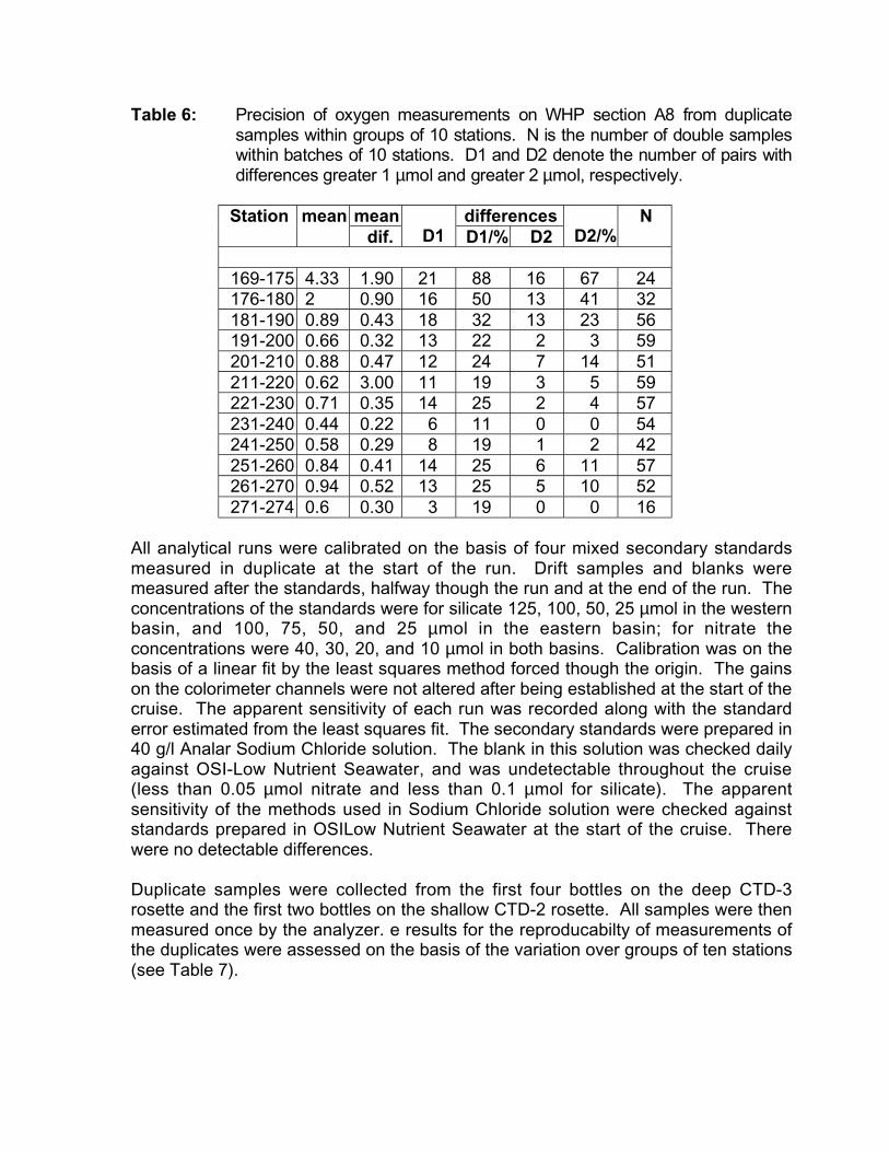
Table 6: Pre cision of oxygen measure ments on WHP section A8 from duplica tesam ples within groups of 10 stations. N is the num ber of double samp leswit hin ba tches of 10 statio ns. D1 and D2 den ote th e numb er of pairs withdif ferences gre ater 1 µmo l and greate r 2 µmo l, respectively.
mean differencesStation meandif. D1 D1/% D2 D2/%
N
169-175 4.33 1.90 21 88 16 67 24176-180 2 0.90 16 50 13 41 32181-190 0.89 0.43 18 32 13 23 56191-200 0.66 0.32 13 22 2 3 59201-210 0.88 0.47 12 24 7 14 51211-220 0.62 3.00 11 19 3 5 59221-230 0.71 0.35 14 25 2 4 57231-240 0.44 0.22 6 11 0 0 54241-250 0.58 0.29 8 19 1 2 42251-260 0.84 0.41 14 25 6 11 57261-270 0.94 0.52 13 25 5 10 52271-274 0.6 0.30 3 19 0 0 16
All analytical runs were calibrated on the basis of four mixed secondary standardsmeasured in duplicate at the start of the run. Drift samples and blanks weremeasured after the standards, halfway though the run and at the end of the run. Theconcentrations of the standards were for silicate 125, 100, 50, 25 µmol in the westernbasin, and 100, 75, 50, and 25 µmol in the eastern basin; for nitrate theconcentrations were 40, 30, 20, and 10 µmol in both basins. Calibration was on thebasis of a linear fit by the least squares method forced though the origin. The gainson the colorimeter channels were not altered after being established at the start of thecruise. The apparent sensitivity of each run was recorded along with the standarderror estimated from the least squares fit. The secondary standards were prepared in40 g/l Analar Sodium Chloride solution. The blank in this solution was checked dailyagainst OSI-Low Nutrient Seawater, and was undetectable throughout the cruise(less than 0.05 µmol nitrate and less than 0.1 µmol for silicate). The apparentsensitivity of the methods used in Sodium Chloride solution were checked againststandards prepared in OSILow Nutrient Seawater at the start of the cruise. Therewere no detectable differences.
Duplicate samples were collected from the first four bottles on the deep CTD-3rosette and the first two bottles on the shallow CTD-2 rosette. All samples were thenmeasured once by the analyzer. e results for the reproducabilty of measurements ofthe duplicates were assessed on the basis of the variation over groups of ten stations(see Table 7).
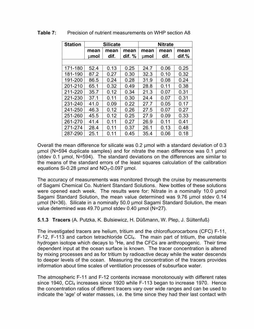
Table 7: Precision of nutrient measurements on WHP section A8
Silicate NitrateStationmeanµmol
meandif.
meandif. %
meanµmol
meandif.
meandif.%
171-180 52.4 0.13 0.25 24.7 0.06 0.25181-190 87.2 0.27 0.30 32.3 0.10 0.32191-200 86.5 0.24 0.28 31.9 0.08 0.24201-210 65.1 0.32 0.49 28.8 0.11 0.38211-220 35.7 0.12 0.34 21.3 0.07 0.31221-230 37.1 0.11 0.30 24.4 0.07 0.31231-240 41.0 0.09 0.22 27.7 0.05 0.17241-250 46.3 0.12 0.26 27.5 0.07 0.27251-260 45.5 0.12 0.25 27.9 0.09 0.33261-270 41.4 0.11 0.27 26.9 0.11 0.41271-274 28.4 0.11 0.37 26.1 0.13 0.48287-290 25.1 0.11 0.45 35.4 0.06 0.18
Overall the mean difference for silicate was 0.2 µmol with a standard deviation of 0.3µmol (N=594 duplicate samples) and for nitrate the mean difference was 0.1 µmol(stdev 0.1 µmol, N=594). The standard deviations on the differences are similar tothe means of the standard errors of the least squares calculation of the calibrationequations Si-0.28 µmol and NO3-0.097 µmol.
The accuracy of measurements was monitored through the cruise by measurementsof Sagami Chemical Co. Nutrient Standard Solutions. New bottles of these solutionswere opened each week. The results were for: Nitrate in a nominally 10.0 µmolSagami Standard Solution, the mean value determined was 9.76 µmol stdev 0.14µmol (N=36). Silicate in a nominally 50.0 µmol Sagami Standard Solution, the meanvalue determined was 49.70 µmol stdev 0.40 µmol (N=27).
5.1.3 Tracers (A. Putzka, K. Bulsiewicz, H. Düßmann, W. Plep, J. Sültenfuß)
The investigated tracers are helium, tritium and the chlorofluorocarbons (CFC) F-11,F-12, F-113 and carbon tetrachloride CCl4. The main part of tritium, the unstablehydrogen isotope which decays to 3He, and the CFCs are anthropogenic. Their timedependent input at the ocean surface is known. The tracer concentration is alteredby mixing processes and as for tritium by radioactive decay while the water descendsto deeper levels of the ocean. Measuring the concentration of the tracers providesinformation about time scales of ventilation processes of subsurface water.
The atmospheric F-11 and F-12 contents increase monotonously with different ratessince 1940, CCl4 increases since 1920 while F-113 began to increase 1970. Hencethe concentration ratios of different tracers vary over wide ranges and can be used toindicate the 'age' of water masses, i.e. the time since they had their last contact with
the surface. 'Younger' water is tagged with higher CFC concentration compared with'older' water. Combining concentrations and concentration ratios in the ocean withcorresponding input functions at the sea surface provides information about mixingprocesses in the ocean.
SamplingSamples were taken according to the WOCE scheme. About 1700 samples for CFCanalysis were taken from all bottle depths of each other station over the deep oceanand of each station close to the continental margins. Samples were stored in glasssyringes and measured on board.
Helium samples were extracted on board from 630 glass pipets. Another 520 heliumsamples in copper tubes and 645 tritium samples in glass tubes were taken for latershore based analysis. Therefore, in chapter 5.1.5, only the CFC and CCl4measurements are discussed.
Onboard measurements of CFCsThe Bremen system measures the CFCs F-11, F-12, F-113 and carbon tetrachlorideCCl4 concentrations of seawater samples. It consists of a gas chromatograph madeby Hewlett Packard which is equipped with a capillary column and a special noncommercial sample preparation unit. The latter is to prepare gas aliquots forcalibration purposes and to handle water samples, especially the stripping ofessentially all gases from water samples of about 30 cc.
The gases are transferred to a trap which is cooled with liquid CO2 down to -40˚C.The trap is filled with a special packing material to accumulate the compounds we areinterested in. During the next step these compounds are released by heating the trapto about (100˚C) and transferred through the capillary column by a steady carrier gasflow to separate the compounds.
The gases are detected using an electron capture detector (ECD). Temperatureprogramming facilities of the gas chromatograph is applied to accelerate the wholeanalytic procedure. All main parts of the system are controlled by a standard PCdriven by self developed software while the acquisition and integration of thechromatograms is done using commercial software on the same PC. Thepreparation unit is equipped with a multi sampler device which allows to analyze 7water samples without further attendance together with one gas standard and twoblanks within about 3 hour. Within 24 hours, 50 water samples can be processed.Every other day a calibration curve has to be measured, since the detector is non-linear and its sensitivity might change with time. This has to be taken into account forthe evaluation of the raw data.
The measurements for F-11, F-12 and CCl4 cover the range from the detection limitof 0.002 pmol/kg to about 2 pmol/kg. While the reproducibility of gas standards isbelow 0.5% standard deviation the values for the water measurements is slightlygreater of about 0.8% or 0.003 pmol/kg whichever is greater. The analytic resolution
for F-113 was not as sufficient as for the other compounds, but further evaluation ofthe chromatograms will recover some reasonable figures for this parameter.
5.1.4 CO2-Measurements (K. Johnson, K. Wills)
Research cruise M 28/1 (WOCE section A8) continues a tradition whereby personnelfrom the Brookhaven National Laboratory, Upton, N.Y., U.S.A., have made CO2
measurements aboard METEOR. This cruise is the fourth WOCE line involving theBrookhaven group and the Institut für Meereskunde at Kiel. The A8 section data jointhe results for WOCE sections A9 (M 15) and A10 (M 22) completed by the CO2
group, and with its completion Brookhaven is now in possession of data from threecontiguous latitude lines 11˚S, 19˚S, and 30˚S, respectively. This gives Brookhavenchemical oceanographers and oceanographic co-workers from Kiel, Warnemünde,and Wormley a unique opportunity to validate the calculation of CO2 transport in amanner analogous to that done for heat transport.
Dur in g M 2 8/ 1 t wo p a ra me ter s of th e car bo na t e syste m we r e me asu re d. T he first, to ta lcar bo n dio xid e (CT) , was me asur e d by co nt in u ou s gas ext r actio n of acid if ied sea wat er wit h th e resu lt an t CO2 de te rm ine d by cou lo me t ric tit ra tio n. The seco nd , the discre te p ar tial pr essur e of CO 2 (p CO 2) , wa s mea su r ed by equ ilibr at in g kno wn vo lu m es of aliq uid pha se (sea wa t er ) and a ga s ph a se (air of kno wn CO 2 co ncen t ra tio n) by sha kin gf or thr e e ho u rs at con st a nt tem p er at u re . Fo llowing equ ilibr a tion , the CO 2 in the ga sp ha se wa s de t er mine d on a gas ch ro ma t og ra ph eq uip pe d wit h a fla me io niza t io nd et ecto r (FI D) af te r the ca ta lyt ic co nver sio n of CO 2 to CH4. Th e pCO 2, at th e in sit ut em pe ra t ur e and the sa mp le alka lin it y wer e calcu lat ed fr om th e an cilla ry nu tr ie n t an d o xyge n dat a and fro m the th er mo d yn am ic co nside ra t io ns an d co n st an ts of th ecar bo na t e syste m. Unlike pre vio us cr uise s whe re co nt in u ou s und er wa y pCO 2, wasd et er min ed in t he su rf ace wat er s, th e d iscr e te m e th od a b ove was use d t o mea su re th ep CO 2 th ro ug h ou t the wat e r co lum n, an d to ou r kn o wled g e th is is th e first WOCEsection fo r which a co mp let e se t o f pCO 2 da ta e xit s.
The precision of the total carbon dioxide duplicate analyses during the cruise was0.80 mol/kg (0.04%), while preliminary calculations indicate that the precision of thepCO2 determinations was 1.0%. In addition, 76 samples of 'Certified ReferenceMaterials' (CRM) were analyzed for total carbon dioxide as a check on accuracy. TheCRM, seawater samples spiked with sodium bicarbonate, were analyzed before thecruise for CT in the laboratory of Dr. C.D. Keeling at the Scripps Institution ofOceanography (SIO) by vacuum extraction and manometry. The certified mean of 9samples was 1991.94 mol/kg. For the 76 samples CRM analyzed by coulometryduring M 28/1, the mean was 1991.37 mol/kg with standard deviation 1.27 mol/kg.As a further precaution, forty (40) samples were collected during the cruise andpreserved for later analysis in the laboratory of Dr. Keeling at SIO.
During M 28/1 some 51 stations (nearly 50% of the WOCE stations) were sampled for theCO2 parameters. Approximately, 1,588 individual total carbon dioxide samples and 1,549individual pCO2 samples (duplicates not included) were drawn and analyzed. Counting
the duplicates adds another 200 samples and analyses. Because the data set is verylarge and there are still some uncertainties in the final depths and associated nutrientvalues, analysis of the data set in chapter 5.1.5 still is preliminary.
5.1.5 First Results from WHP A8(T.J. Müller, P. Beining, D. Hydes, K. Johnson, A. Putzka, G. Siedler)
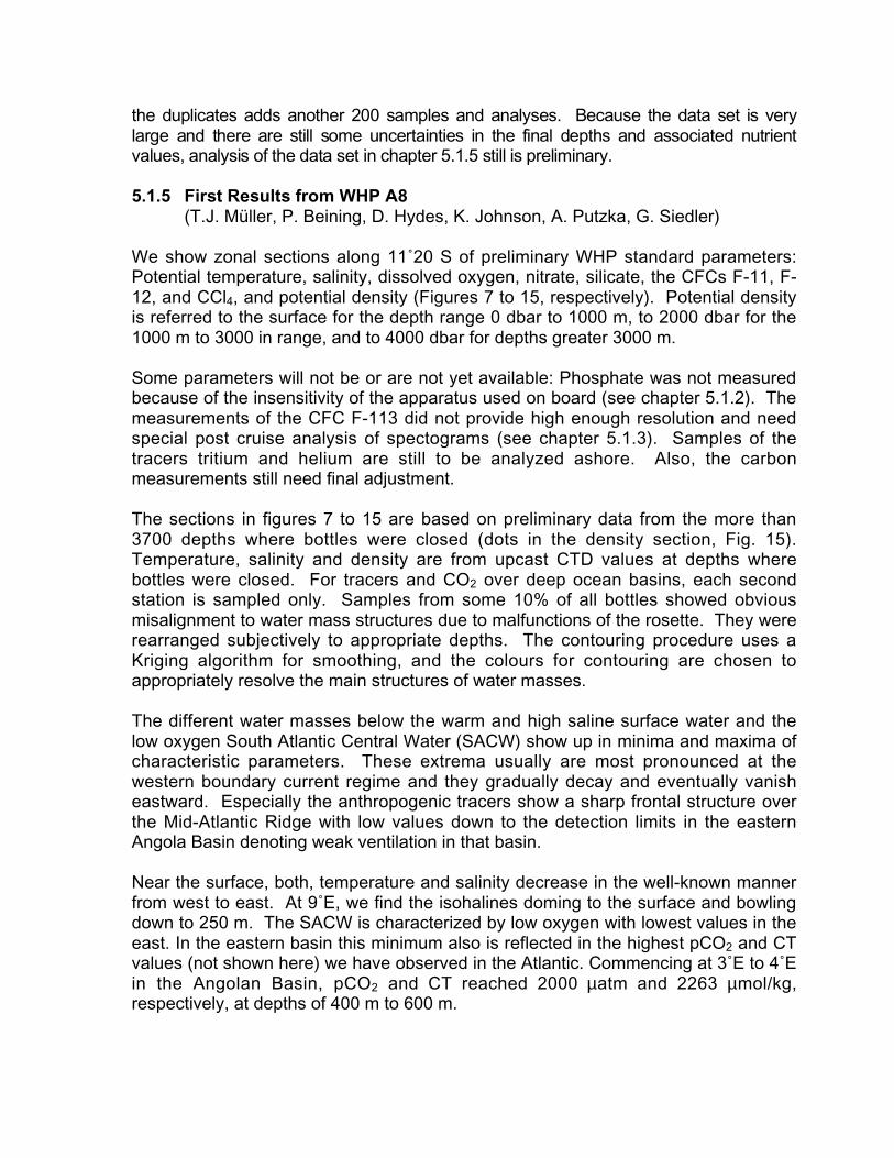
We show zonal sections along 11˚20 S of preliminary WHP standard parameters:Potential temperature, salinity, dissolved oxygen, nitrate, silicate, the CFCs F-11, F-12, and CCl4, and potential density (Figures 7 to 15, respectively). Potential densityis referred to the surface for the depth range 0 dbar to 1000 m, to 2000 dbar for the1000 m to 3000 in range, and to 4000 dbar for depths greater 3000 m.
Some parameters will not be or are not yet available: Phosphate was not measuredbecause of the insensitivity of the apparatus used on board (see chapter 5.1.2). Themeasurements of the CFC F-113 did not provide high enough resolution and needspecial post cruise analysis of spectograms (see chapter 5.1.3). Samples of thetracers tritium and helium are still to be analyzed ashore. Also, the carbonmeasurements still need final adjustment.
The sections in figures 7 to 15 are based on preliminary data from the more than3700 depths where bottles were closed (dots in the density section, Fig. 15).Temperature, salinity and density are from upcast CTD values at depths wherebottles were closed. For tracers and CO2 over deep ocean basins, each secondstation is sampled only. Samples from some 10% of all bottles showed obviousmisalignment to water mass structures due to malfunctions of the rosette. They wererearranged subjectively to appropriate depths. The contouring procedure uses aKriging algorithm for smoothing, and the colours for contouring are chosen toappropriately resolve the main structures of water masses.
The different water masses below the warm and high saline surface water and thelow oxygen South Atlantic Central Water (SACW) show up in minima and maxima ofcharacteristic parameters. These extrema usually are most pronounced at thewestern boundary current regime and they gradually decay and eventually vanisheastward. Especially the anthropogenic tracers show a sharp frontal structure overthe Mid-Atlantic Ridge with low values down to the detection limits in the easternAngola Basin denoting weak ventilation in that basin.
Near the surface, both, temperature and salinity decrease in the well-known mannerfrom west to east. At 9˚E, we find the isohalines doming to the surface and bowlingdown to 250 m. The SACW is characterized by low oxygen with lowest values in theeast. In the eastern basin this minimum also is reflected in the highest pCO2 and CTvalues (not shown here) we have observed in the Atlantic. Commencing at 3˚E to 4˚Ein the Angolan Basin, pCO2 and CT reached 2000 µatm and 2263 µmol/kg,respectively, at depths of 400 m to 600 m.
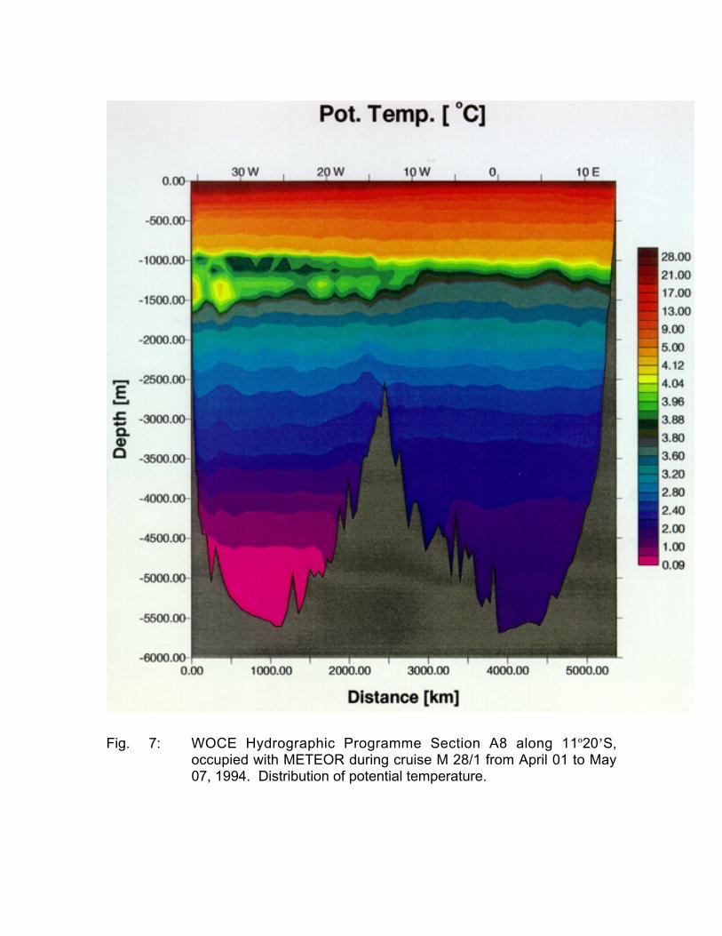
Fig. 7: WOCE Hydrographic Programme Section A8 along 11º20’S,occupied with METEOR during cruise M 28/1 from April 01 to May07, 1994. Distribution of potential temperature.
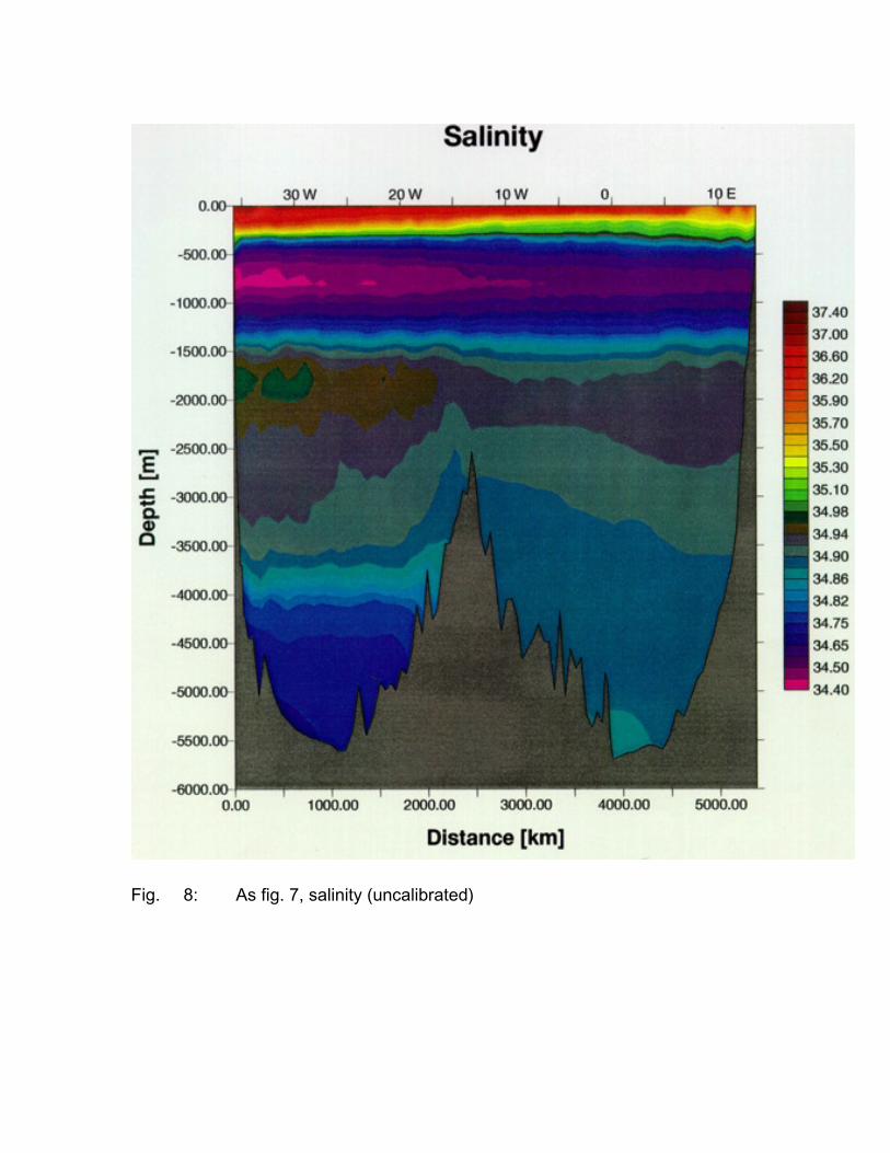
Fig. 8: As fig. 7, salinity (uncalibrated)
Fig. 9: As fig. 7, dissolved oxygen
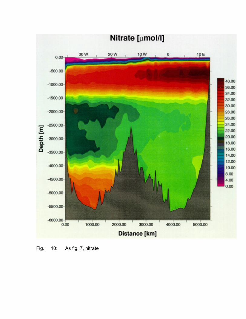
Fig. 10: As fig. 7, nitrate
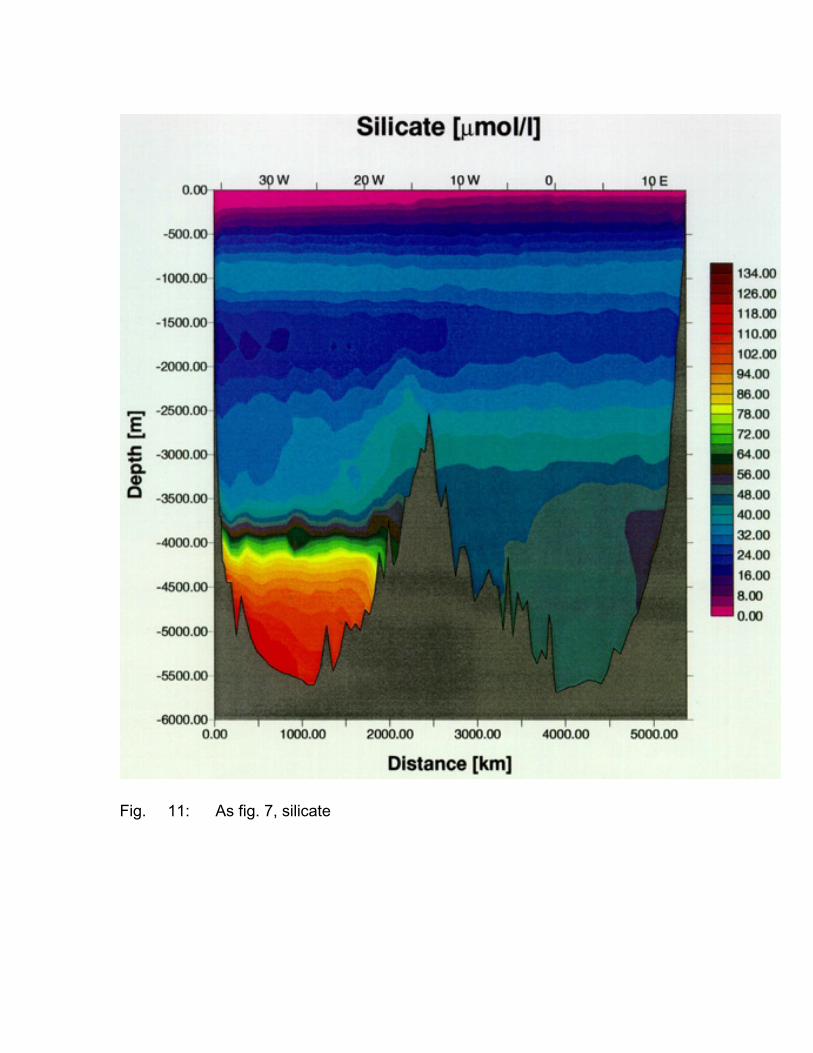
Fig. 11: As fig. 7, silicate
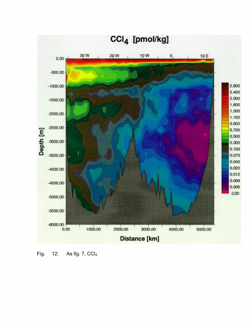
Fig. 12: As fig. 7, CCl4
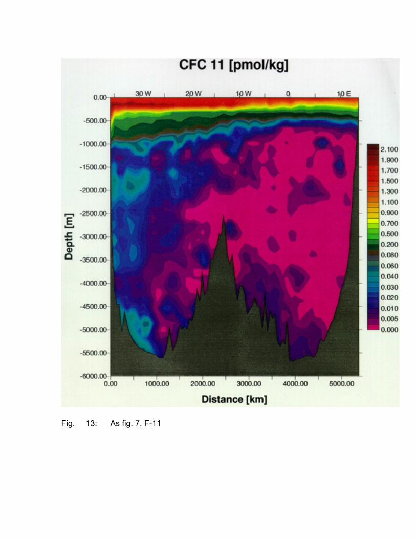
Fig. 13: As fig. 7, F-11
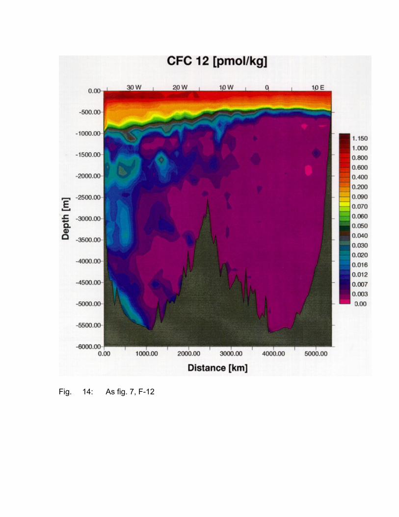
Fig. 14: As fig. 7, F-12
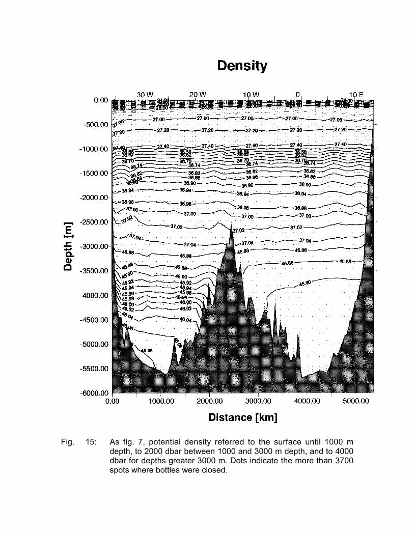
Fig. 15: As fig. 7, potential density referred to the surface until 1000 mdepth, to 2000 dbar between 1000 and 3000 m depth, and to 4000dbar for depths greater 3000 m. Dots indicate the more than 3700spots where bottles were closed.
Below the SACW, two cores of waters of antarctic origin are identified: At 800 mdepth the Antarctic Intermediate Water (AAIW) with its salinity minimum, and at 1000m depth the Upper Circumpolar Deep Water (UCPDW) with its temperature minimumand silicate maximum. They can be traced throughout the section until the Africanshelf break. While these water masses origin from the south, note that, both, thetongues of the AAIW and of the UCPDW are cut by the above mentioned fronts inanthropogenic tracers F-11 and CCl4 at about 5˚W which indicates their relativelyweak renewal rates in the eastern basin as compared to that in the western basin.
Next, all three components of North Atlantic Deep Water (NADW) are identified: At 1300 mdepth the core of the Upper North Atlantic Deep Water (UNADW) with its temperaturemaximum, at 1900 m the Mid North Atlantic Deep Water (MNADW) with its salinitymaximum and silicate minimum, and at 3200 m the oxygen rich Lower North Atlantic DeepWater (LNADW). Note some lenses of NADW just east of the western boundary; theymay indicate re-circulation cells discussed recently (De MADRON and WHEATHERLY,1994). In the west, the CFC values are relatively low within the UNADW because of its'old' components of Mediterranean origin. A maximum in CFCs is found in the MNADW,and they still have high values in the LNADW. Again, a front in CFC values separates theNADWs in the western from those of the eastern basin.
Lower Circumpolar Deep Water (LCPDW) is formed when Weddell Sea Deep Watermixes with Circumpolar Deep Water on its way north. Formerly denoted as AntarcticBottom Water (AABW) (PETERSON and WHITWORTH, 1989), it carries lowtemperature and salinity bottom water along the western boundary northward.Because of its Weddell Sea compound, it is also marked by relatively high CFCvalues. A slight increase of the F-11 concentration at the western slope of the Mid-Atlantic Ridge seems to indicate a re-circulation cell of bottom water. LCPDW alsowas clearly distinguishable in the CO2 parameters (not shown here).
Two further interesting result are found in the deep Angola Basin. First, we observean increase of, both, CCl4 and F-11 values at the bottom which is intensified at thewestern side of the basin. Thus there is evidence that the bottom water of the AngolaBasin is ventilated by a western boundary current (WARREN and SPEER, 1991)which carries compounds of bottom waters that have been at the surface within thelast 30 years. While other hydrographic and chemical parameters indicate a fairlyhomogenous water mass below 4000 m, F-11 and CCl4 outline a structure thatindicates a circulation and slow upwelling of bottom waters within the basin. Onlyvery few samples measured at about 3000 m depth in the eastern part of the AngolaBasin show CCl4 concentrations below their detection limit.
The second interesting feature in the Angola Basin is observed at 4000 m depth onthe continental break: A low oxygen and high silicate water mass with a smallincrease of CCl4 and extremely slight increase only of F-11. Whereas in the CFCsthe signal is confined to only very few samples just above the bottom, it is broaderand therefore significant in oxygen and silicate. Maybe the idea of a Congo Riverturbidity plume is evident here (BENNEKOM and BERGER, 1984).
5.2 Deep Basin Experiment
5.2.1 Water Mass Distribution in the Subtropical South Atlantic(O. Boebel, C. Schmid, W. Zenk)
The data base for this paragraph consists of two quasi-meridional hydrographic sections(Fig. 16) occupied between 21˚ and 39˚S during M 28/2. The longer section (Fig. 17)contains 21 CTD stations covering the east side of the Brazil Basin, crossing HunterChannel, running right into the central Argentine Basin. The supplementing shortersection (Fig. 18), featuring 7 CTD stations, connects the southern end of the long sectionbetween the Subtropical Convergence at roughly 40˚S with the southern extend of VemaChannel. Thermosalinograph records also shown in Fig. 17 and 18, are reproducedwithout further corrections. Comparisons with near-surface CTD data revealed nosystematic differences for temperature data. However, a significant shift of 0.038 ± 0.050PSU between 35 salinity samples (taken during CTD stations) and the displayedcontinuous salinity record was determined. The shown surface salinity needs to bereduced by the calculated offset for future analyses.
CTD stations were taken (a) for a detailed investigation of the vertical structure andzonal flow of the Antarctic Intermediate Water (AAIW) at approximately 900 m depthand (b) for the determination of in situ density at float launch sites (see chapter 7.2.5).Due to ship time limitations both sections had to be compiled from CTD profiles notexceeding 1500 dbar. Only selected stations cover tile whole water column. Theircomplete data are processed in our θ/S-diagram (Fig. 19). Nominally all deepstations were taken with a sediment sampler as described in chapter 5.8.
Both CTD-sections are shown jointly with continuous thermosaIinograph data and theirbelonging bottom profiles. Gaps in these data (DVS) were linearly interpolated, or in caseof bathymetry eliminated by soundings from CTD stations (Profile 36-33, 32-16). Fig. 16shows the track lines of the long (Profile 37-2) and the short section (Profile 37-43)embedded in the local bathymetry. Please note, station notation is given by CTD profilenumbers. An equivalence Stat. No. vs Profile contains chapter 7.2.1. The central box inFig. 46 contains CTD stations at Hunter Channel as displayed in Fig. 20 and describedfurther down.
The most pronounced structure of both sections shown in Figs. 17 and 18, is given by theSubtropical Convergence at their common southern end (<-38˚ = > 38˚S). North of 38˚Sthermosalinograph records with their strong fluctuations (horizontal interleaving) confirm theabrupt transition between the southern rim of the subtropical gyre of the South Atlantic at 38˚Sand the northern extend of the Southern Ocean (see Fig. 18e). The deep reaching front at theconvergence is most developed in the upper 500 dbar. Nevertheless, it can be traced down tothe bottom of our sections (1500 dbar), though with reduced horizontal gradients. Slopingisopygnals associated with the frontal region, represent the dynamical signature of theeastward flowing South Atlantic Current (STRAMMA and PETERSON, 1990).
Farther north we identify the well-known variety of water masses in the subtropical SouthAtlantic: In the centre of the subtropical gyre, i.e., north of 28˚S, we find the characteristicshallow salinity maximum at approximately 60 dbar. The next deeper extremum on theθ/S-diagram (Fig. 19) occurs below the main thermocline. It is marked by the salinityminimum of the Antarctic Intermediate Water (AAIW). The Smin core at approximately σθ= 27.18 or σ1 = 31.75 kg m3 drops from < 600 dbar at the Subtropical Convergence toalmost 1000 dbar between 36' and 37˚S, from where on we observe a slow decrease ofthe pressure level to 700 dbar at the northern end of the long section. The core salinity islowest in the frontal region (< 34.2 PSU). It increases up to 34.4 PSU towards the north.Temperatures range from 3-4˚C in the south , where 3.5-4˚C are more characteristic forthe northern end. In terms of potential density Intermediate Water ranges from 27.00 < σθ< 7.35 kg m3 or 31.50 < σ1 < 31.90 kg m3.
Fig. 16: Dur ing M 28/2 METEOR occupied two quasi-mer idiona l hydr ograph icsections in the Brazil Basin and in the Argen tine Basin. Number sind icate CTD pr ofiles, corr espond ing st ation number s are listed incha pter 7.2.1. Most of the CTD st ations cover only the up per 15 00dba r, suf ficien tly de ep eno ugh fo r the invest igatio n of the Ant arcticInt ermediate Wa ter. Station s in the box were taken in the Hunte rCha nnel r egion as described in ch apter 5.2.2.

Fig. 17a-b: CTD-sections (p ≤ 1500 dbar) through the southern subtropicalgyre of the western South Atlantic. The long section (A2) wastaken en route to Hunter Channel and farther to the SubtropicalConvergence.a) Potential temperature (ºC),b) Salinity (PSU),
Fig. 17c-f: CTD-sections (p ≤ 1500 dbar) through the southern subtropicalgyre of the western South Atlantic. The long section (A2) wastaken en route to Hunter Channel and farther to the SubtropicalConvergence.c) Density σ1 (kg m-3),d) thermosalinograph records of temperature,e) uncorrected salinity,f) bathymetry recorded simultaneously by METEOR.
Fig. 18a-f: CTD-sections (p ≤ 1500 dbar) through the southern subtropicalgyre of the western South Atlantic. The short section (A3) wastaken on the north-westbound track towards the Vema Channelextention.a) Potential temperature (ºC),b) Salinity (PSU),c) Density σ1 (kg m-3),d) thermosalinograph records of temperature,e) uncorrected salinity,f) bathymetry recorded simultaneously by METEOR.
Fig. 19: Potential temperature (ºC) vs salinity (PSU) from all deep stationsof M 28/2 (chapter 7.2.1). Lines of equal densities (kg m-3) arereferred to 1000 dbar (σ1).
Three different low temperature gradient regions were observed. The first at 36˚Sreaches down to 400 dbar at 14˚C. It resembles Maderia Mode Water (SIEDLER etal., 1987) found in the eastern North Atlantic. This thermocline mode water is formedat the northern boundary of the subtropical gyre by deep wintertime convection and isdegenerated during the course of the year. Deeper down at ~38˚S (Fig. 17 and 18)we identify remainders of the upper Circumpolar Water (2.7˚C, 34.4 PSU) beneaththe deep core of Antarctic Intermediate Water. Unfortunately no oxygen data forfurther identification of this water mass are available from M 28/2. The third and mostextended thermostat (~3.4˚C) layer is found between 21˚ and 26˚S (Fig. 17a) atpressures >1000 dbar. The concurrent increase of salinity from 34.40 to > 34.80PSU indicates a mixture of upper Circumpolar Water with North Atlantic Deep Water(NADW). While vertical mixing in this water mass cannot have much effect on thetemperature since the vertical temperature gradient is small, strong fluxes of salinitypresumably exist between layers (K. SPEER in SIEDLER and ZENK, 1992). Finallywe point out two submesoscale pygnocline depressions (Profiles 11, 14) and/or threedomes (Profiles 12, 13, 16, 34) which cannot be interpreted by the available CTDdata (Fig. 17c) alone. Perhaps RAFOS floats launched every degree of latitudeconcurrently with CTD stations along both sections, will allow a conclusive analysis ofthese dynamical signals. Float deployment locations are summarized in chapter7.2.5.
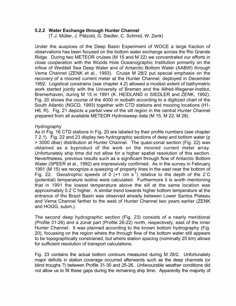
5.2.2 Water Exchange through Hunter Channel(T.J. Müller, J. Pätzold, G. Siedler, C. Schmid, W. Zenk)
Under the auspices of the Deep Basin Experiment of WOCE a large fraction ofobservations has been focused on the bottom water exchange across the Rio GrandeRidge. During two METEOR cruises (M 15 and M 22) we concentrated our efforts inclose cooperation with the Woods Hole Oceanographic Institution primarily on theinflow of Weddell Sea Deep Water and of Antarctic Bottom Water (AABW) throughVema Channel (ZENK et al., 1993). Cruise M 28/2 put special emphasis on therecovery of a moored current meter at the Hunter Channel, deployed in December1992. Logistical constrains (see chapter 4.2) allowed a modest extent of bathymetricwork started jointly with the University of Bremen and the Alfred-Wegener-Institut,Bremerhaven, during M 15 in 1991 (K. HEIDLAND in SIEDLER and ZENK, 1992).Fig. 20 shows the course of the 4000 m isobath according to a digitized chart of theSouth Atlantic (NGCD, 1993) together with CTD stations and mooring locations (H1-H6, R). Fig. 21 depicts a partial view of the sill region in the central Hunter Channelprepared from all available METEOR Hydrosweep data (M 15, M 22, M 28).
HydrographyAs in Fig. 16 CTD stations in Fig. 20 are labeled by their profile numbers (see chapter7.2.1). Fig. 22 and 23 display two hydrographic sections of deep and bottom water (p> 3000 dbar) distribution at Hunter Channel. The quasi-zonal section (Fig. 22) wasobtained as a byproduct of the work on the moored current meter array.Unfortunately ship time did not allow for a higher spatial resolution of this section.Nevertheless, previous results such as a significant through flow of Antarctic BottomWater (SPEER et al., 1992) are impressively confirmed. As in the survey in February1991 (M 15) we recognize a queezing of property lines in the east near the bottom ofFig. 22. Geostrophic speeds of 0 (+1 cm s-1) relative to the depth of the 2˚C(potential) temperature isoline were calculated. Furthermore it is worth mentioningthat in 1991 the lowest temperature above the sill at the same location wasapproximately 0.2˚C higher. A similar trend towards higher bottom temperature at theentrance of the Brazil Basin was observed already between Lower Santos Plateauand Vema Channel farther to the west of Hunter Channel two years earlier (ZENKand HOGG, subm.).
The second deep hydrographic section (Fig. 23) consists of a nearly meridional(Profile 31-26) and a zonal part (Profile 26-22) north, respectively, east of the innerHunter Channel. It was planned according to the known bottom hydrography (Fig.20), focussing on the region where the through flow of the bottom water still appearsto be topographically constrained, but where station spacing (nominally 25 km) allowsfor sufficient resolution of transport calculations.
Fig . 23 contain s the actual botto m cont ours measure d during M 28/2. Unfort unatelymajor def icits in sta tion coverag e occu rred afterwa rds su ch as the de ep cha nnels (orblind tro ughs ?) between Pr ofile 31-30 and 25 -26. Unf avoura ble we ather condit ions didnot allow us to fill these gaps during the re mainin g ship time. Appa rently the majorit y of

bot tom wa ter le aves the Hun ter re gion towards the east be tween Profile 25-2 4. On lymin or con tribut ions at more inter mediat e dept hs (< 4000 m) are advected northwardthr ough Profile 27-26 , which at least p artially see ms to recircula te bet ween Profile 28-27 .Dur ing M 28/2 we have obser ved no significant deep northward flow west of Profile 29.Such a flow has previously been suggest ed as part of an ant icyclo nic circulat ion ar oundRio Grand e Rise (see Fig. 9 in SPEER an d ZENK, 1993 ). Actually mooring R (Fig. 20)at Profile 13 (Sta t. 306 ) had been launche d in Decembe r 1993 with the in tentio n tomon itor this in terior weste rn bou ndary curren t. Re sults from moored curren t mete rs are sho wn in the fo llowin g para graph.
Moored Current Meter ArrayBetween 1991 and 1992 (M 15, M 22) an array of current meters had monitored deepadvection along the western segment of the southern boundary of the Brazil Basin. Ajoint data report by the Woods Hole Oceanographic Institution and the Institut fürMeereskunde Kiel summarizes the obtained results (TARBELL et al., 1994). Afterthe recovery of this large array parts of it were re-moored farther to the east in theHunter Channel and on the Rio Grande Ridge (Fig 24). Data presented here arecomplimentary to the former data set from the Vema Channel and the other morewesterly regions. A total of 25 Aanderaa Current Meters, two 200 m long thermistorchains and an Acoustic Doppler Current Meter operated in seven moorings (CodeH1-6 for Hunter Channel, R for Rio Grande Rise).
Fig. 20: Zoomed distributions of stations from the Hunter Channel region in thecenter box of Fig. 16. Isolines represent the 4000 m line as available indigital form (NGDC, 1993). Crosses denote deep CTD stations labeledby their profile numbers. Station numbers are listed in chapter 7.2.1.H1-6 stands for a moored current meter array across Hunter Channel.Mooring R was situated in the eastern flank of the Rio Grande Ridge.

Fig. 21: 3-dimensional representation of the Hunter Channel. The synthesis ofthe bathymetry was compiled according to three METEOR surveys (M15, M 22, M 28) by Hydrosweep in cooperation with the University ofBremen and the Alfred-Wegener-Institut, Bremerhaven (SIEDLER andZENK, 1992).
Fig. 22: a) Potential temperature (ºC)

Fig. 22: b) Salinity (PSU)
Fig. 22: c) Density σ4 (kg m-3) referred to 4000 dbar
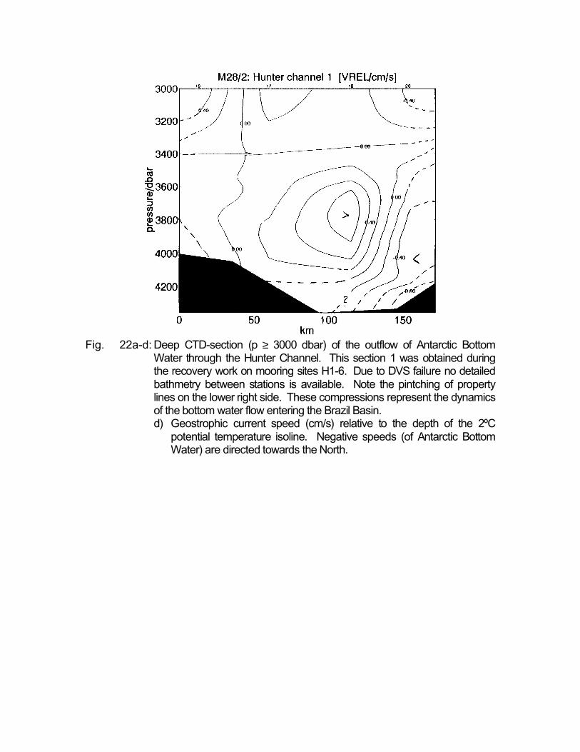
Fig. 22a-d: Deep CTD-section (p ≥ 3000 dbar) of the outflow of Antarctic BottomWater through the Hunter Channel. This section 1 was obtained duringthe recovery work on mooring sites H1-6. Due to DVS failure no detailedbathmetry between stations is available. Note the pintching of propertylines on the lower right side. These compressions represent the dynamicsof the bottom water flow entering the Brazil Basin.d) Geostrophic current speed (cm/s) relative to the depth of the 2ºC
potential temperature isoline. Negative speeds (of Antarctic BottomWater) are directed towards the North.
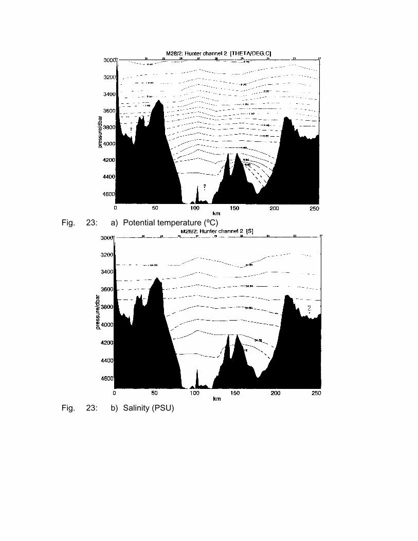
Fig. 23: a) Potential temperature (ºC)
Fig. 23: b) Salinity (PSU)

Fig. 23: c) Density σ4 (kg m-3) referred to 4000 dbar
Fig. 23a-d: Dee p CTD- sectio n (p ≥ 3000 dba r) of the ou tflow of Ant arctic Botto mWat er just nort h of the Hun ter Ch annel. This section 2 was plo ttedfro m prof iles 31-22. Bat hmetry betwe en sta tions was me asured byMET EOR. The ma in out flow across the Hu nter Sill in to the BrazilBasin was obtained be tween profiles 27, 26 an d 25, 24.d) Geostrophic current speed (cm/s) relative to the depth of the
2ºC potential temperature isoline. Negative speeds (of AntarcticBottom Water) are directed towards the North (Profiles 31-26) ortowards the East (Profiles 26-22).
Chapter 7.2.4 contains all mooring durations and locations. The latter are alsodisplayed in Figs. 20 and 21. Locations of related CTD stations from the deployment(M 22) and the recovery cruises (M 28) are summarized in Table 6. The tablecontains three different estimated depths which must be explained by the roughbottom topography, characteristic for the Hunter Channel (see Fig. 22). In selectedcases we therefore give two numbers for the vertical position of our instruments:Clearance from bottom and instrument depth. The more reliable vertical distancerelative to the surface or to the bottom is labeled by bold numbers.
Data from moored instruments were processed in the usual fashion (MOLLER, 1981).Problems occurred with larger numbers of Aanderaa Current Meters (RCM8): Bothvector averaged components in slow current regimes appeared to have a strongeruncorrelated tendency towards zero. In order to conserve a rough estimate of therecorded direction, zeros in calculated speed series were artificially set to 1 cm s-1,the threshold speed of the instruments. Besides other operational details, Table 7displays the percentage of changed threshold values of the Aanderaa CurrentMeters. Since we were forced to shift identical instruments from the Vema to theHunter regime during METEOR cruise M 22/4, time did not allow for a detailed shipborne analysis of the obtained data sets. Unfortunately this did not prevent us fromrunning into problems we had encountered before with vector averaging AanderaaCurrent Meters. (TARBELL et al., 1994).
The data from the moored Acoustic Doppler Current Meter (ADCP) in H6 weredownloaded from the instrument to a personal computer aboard METEOR. Thesebinary data later were transferred to the VAX of the Institut für Meereskundecomputer centre in Kiel, where they were converted into time series of MK4 andASCII coded vertical current profiles. The processing of auxiliary parameters likepitch, roll, heading and instrument depth followed. The latter quantity is displayed inFigs. 25-54. It represents a pseudo-pressure time series inferred from the strongestbin echo of the ADCP. A detail comparison of the upper real pressure record with thecalculated depths reveals an excellent agreement between both methods (VIESBEKand FISCHER, 1995).
All thermistor chain data from H4 and H5 in Fig. 37 and 39 were adjusted to theavailable CTD profiles. Since these moored instruments stopped due to a lack ofdata storage capabilities earlier then the adjacent Aanderaa Current Meters, theirtemperature time series were used as transfer standards for the recovery calibrationchecks of the thermistor chains. The biggest problem with this calibration fine tuningappeared to be the determination of equal observation levels of the thermistor chainsand the CTD profiles. As is shown in Table 6 and Fig. 21 the Hunter Channel is fullof strong gradients in the bottom topography. A pre-cruise laboratory calibration ofboth thermistor chains did not deliver accuracies desirable and necessary for abyssalapplications.
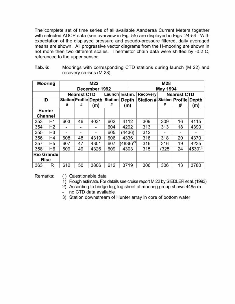
The complete set of time series of all available Aanderaa Current Meters togetherwith selected ADCP data (see overview in Fig. 55) are displayed in Figs. 24-54. Withexpectation of the displayed pressure and pseudo-pressure filtered, daily averagedmeans are shown. All progressive vector diagrams from the H-mooring are shown innot more then two different scales. Thermistor chain data were shifted by -0.2˚C,referenced to the upper sensor.
Tab. 6: Moorings with corresponding CTD stations during launch (M 22) andrecovery cruises (M 28).
Mooring M22 M28December 1992 May 1994
Nearest CTD Launch Estim. Recovery Nearest CTDID Station
#Profile
#Depth
(m)Station
#Depth
(m)Station # Station
#Profile
#Depth
(m)Hunter
Channel353 H1 603 46 4031 602 4112 309 309 16 4115354 H2 - - - 604 4292 313 313 18 4390355 H3 - - - 605 (4436) 312 - - -356 H4 608 48 4319 606 4336 318 318 20 4370357 H5 607 47 4301 607 (4836)2) 316 316 19 4235358 H6 609 49 4326 609 4303 315 (325 24 4530)3)
Rio GrandeRise
363 R 612 50 3806 612 3719 306 306 13 3780
Remarks: ( ) Questionable data1) Rough estimate. For details see cruise report M 22 by SIEDLER et al. (1993)2) According to br idge log, lo g shee t of m ooring group shows 4485 m.- no CTD data available3) Station downstream of Hunter array in core of bottom water
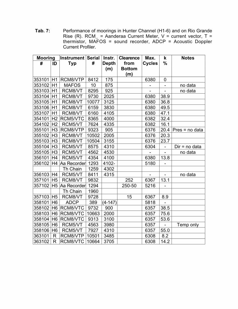
Tab. 7: Performance of moorings in Hunter Channel (H1-6) and on Rio GrandeRise (R). RCM_ = Aanderaa Current Meter, V = current vector, T =thermistor, MAFOS = sound recorder, ADCP = Acoustic DopplerCurrent Profiler.
Mooring# ID
InstrumentTyp
Serial#
Instr.Depth
(m)
Clearencefrom
Bottom(m)
Max.Cycles
k%
Notes
353101 H1 RCM8/VTP 8412 175 6380 0353102 H1 MAFOS 10 875 - - no data353103 H1 RCM8/VT 8295 925 - - no data353104 H1 RCM8/VT 9730 2025 6380 38.9353105 H1 RCM8/VT 10077 3125 6380 36.8353106 H1 RCM8/VT 6159 3830 6380 49.5353107 H1 RCM8/VT 6160 4105 6380 47.1354101 H2 RCM5/VTC 8365 4000 6382 32.4354102 H2 RCM5/VT 7624 4335 6382 16.1355101 H3 RCM8/VTP 9323 905 6376 20.4 Pres = no data355102 H3 RCM8/VT 10502 2005 6376 20.3355103 H3 RCM8/VT 10504 3155 6376 23.7355104 H3 RCM5/VT 8575 4310 6304 - Dir = no data355105 H3 RCM5/VT 4562 4530 - - no data356101 H4 RCM5/VT 4354 4100 6380 13.8356102 H4 Aa Record er 1293 4102- 5180 -
Th Chain 1259 4302356103 H4 RCM5/VT 8411 4315 - - no data357101 H5 RCM8/VT 9832 252 6367 13.1357102 H5 Aa Record er 1294 250-50 5216 -
Th Chain 1960357103 H5 RCM8/VT 9728 15 6367 8.9358101 H6 ADCP 389 (4-147) 5818 -358102 H6 RCM8/VTC 9732 900 6357 38.5358103 H6 RCM8/VTC 10663 2000 6357 75.6358104 H6 RCM8/VTC 9313 3100 6357 53.6358105 H6 RCM5/VT 4563 3980 6357 - Temp only358106 H6 RCM5/VT 7927 4310 6357 55.0363101 R RCM8/VTP 10501 3485 6308 8.2363102 R RCM8/VTC 10664 3705 6308 14.2
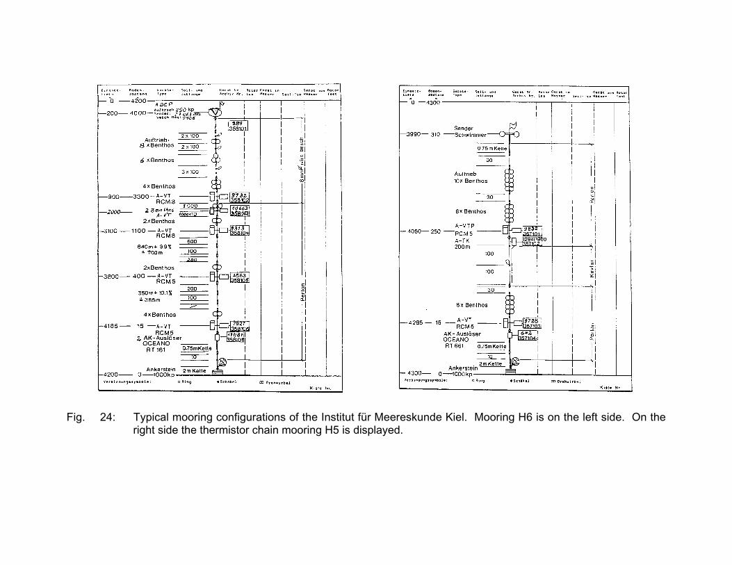
Fig. 24: Typical mooring configurations of the Institut für Meereskunde Kiel. Mooring H6 is on the left side. On theright side the thermistor chain mooring H5 is displayed.
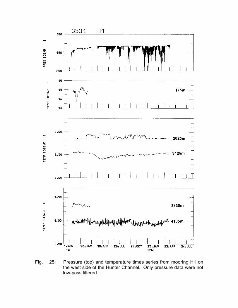
Fig. 25: Pressure (top) and temperature times series from mooring H1 onthe west side of the Hunter Channel. Only pressure data were notlow-pass filtered.
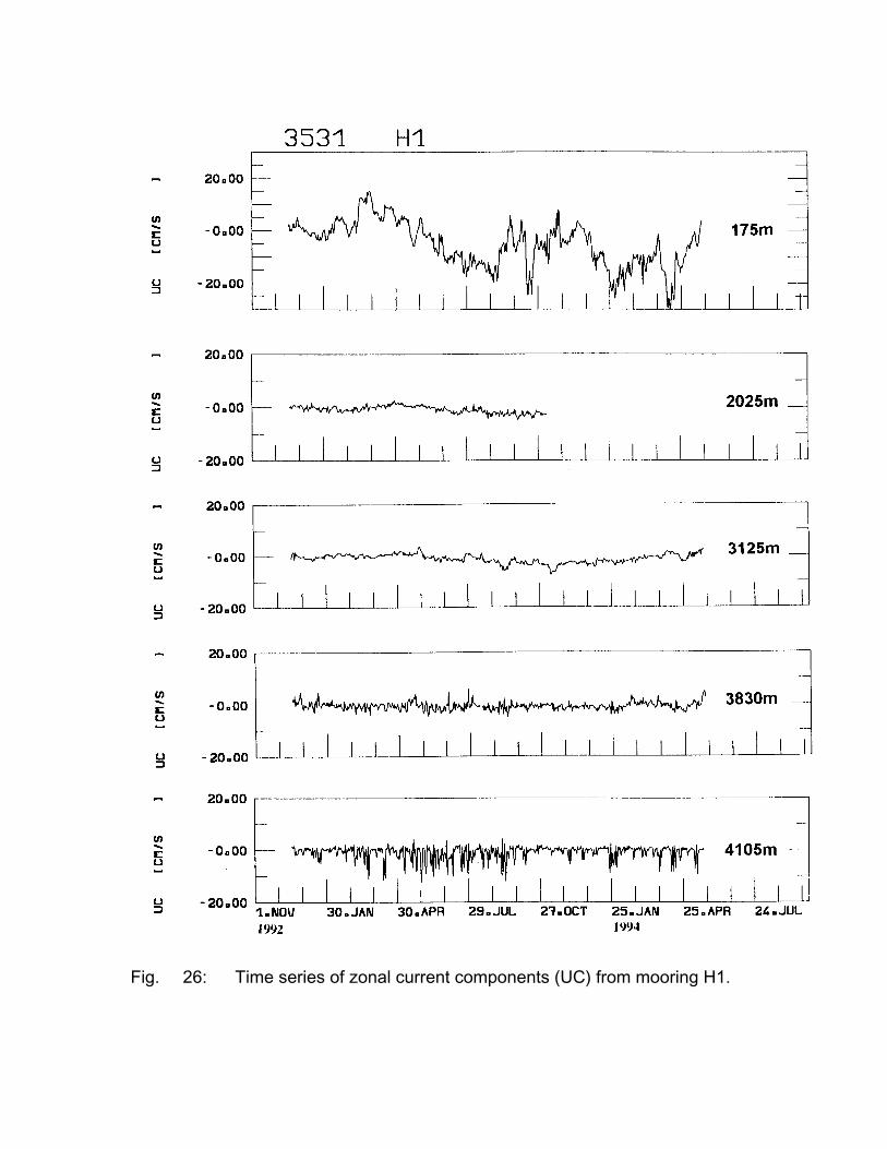
Fig. 26: Time series of zonal current components (UC) from mooring H1.
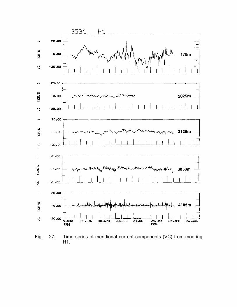
Fig. 27: Time series of meridional current components (VC) from mooringH1.
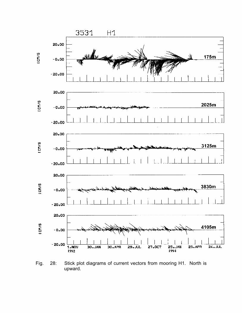
Fig. 28: Stick plot diagrams of current vectors from mooring H1. North isupward.
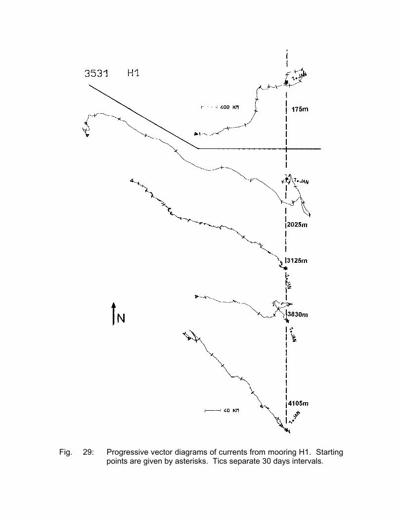
Fig. 29: Progressive vector diagrams of currents from mooring H1. Startingpoints are given by asterisks. Tics separate 30 days intervals.
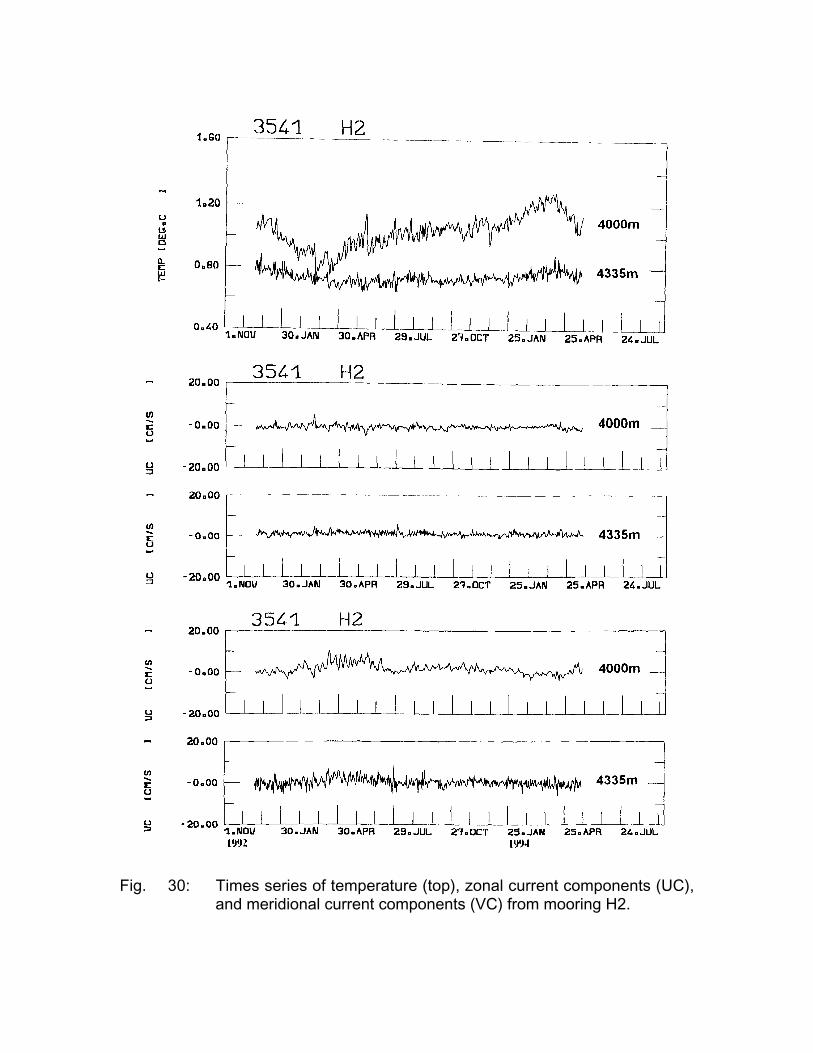
Fig. 30: Times series of temperature (top), zonal current components (UC),and meridional current components (VC) from mooring H2.
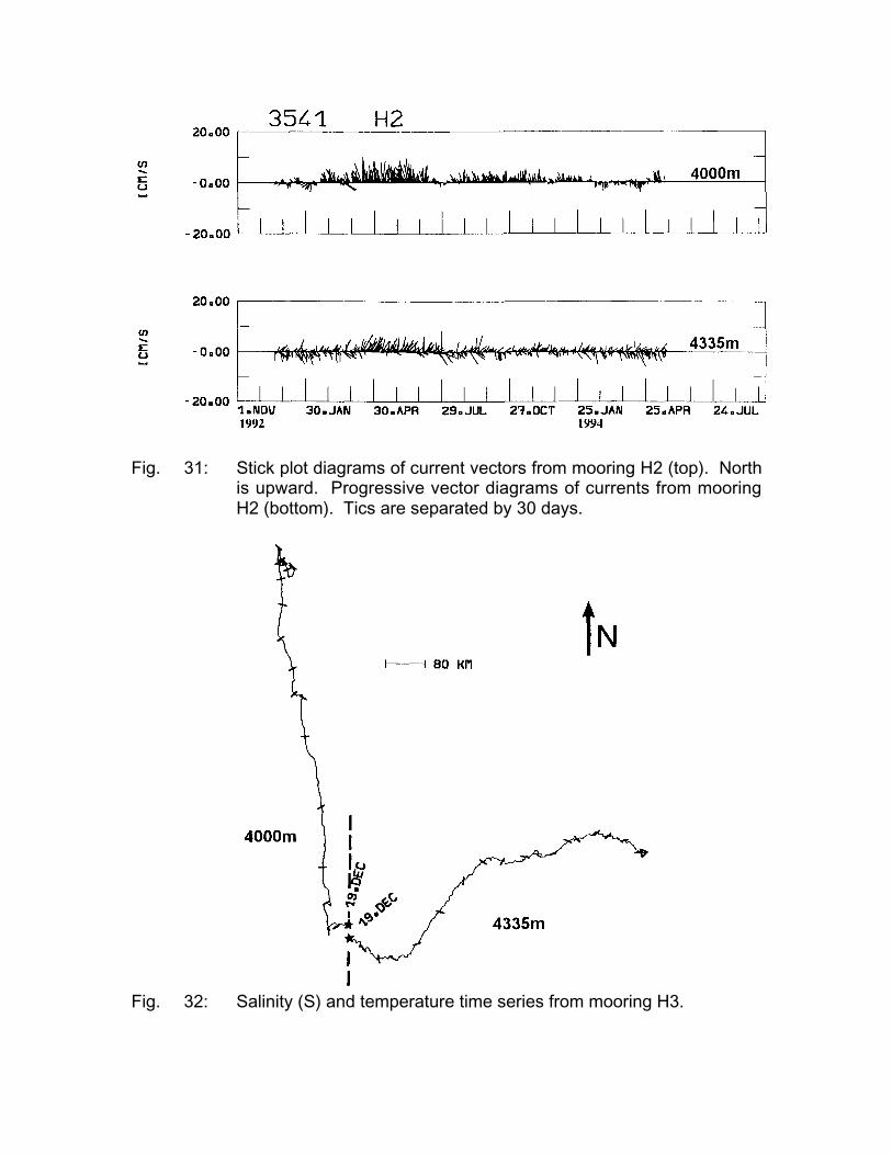
Fig. 31: Stick plot diagrams of current vectors from mooring H2 (top). Northis upward. Progressive vector diagrams of currents from mooringH2 (bottom). Tics are separated by 30 days.
Fig. 32: Salinity (S) and temperature time series from mooring H3.
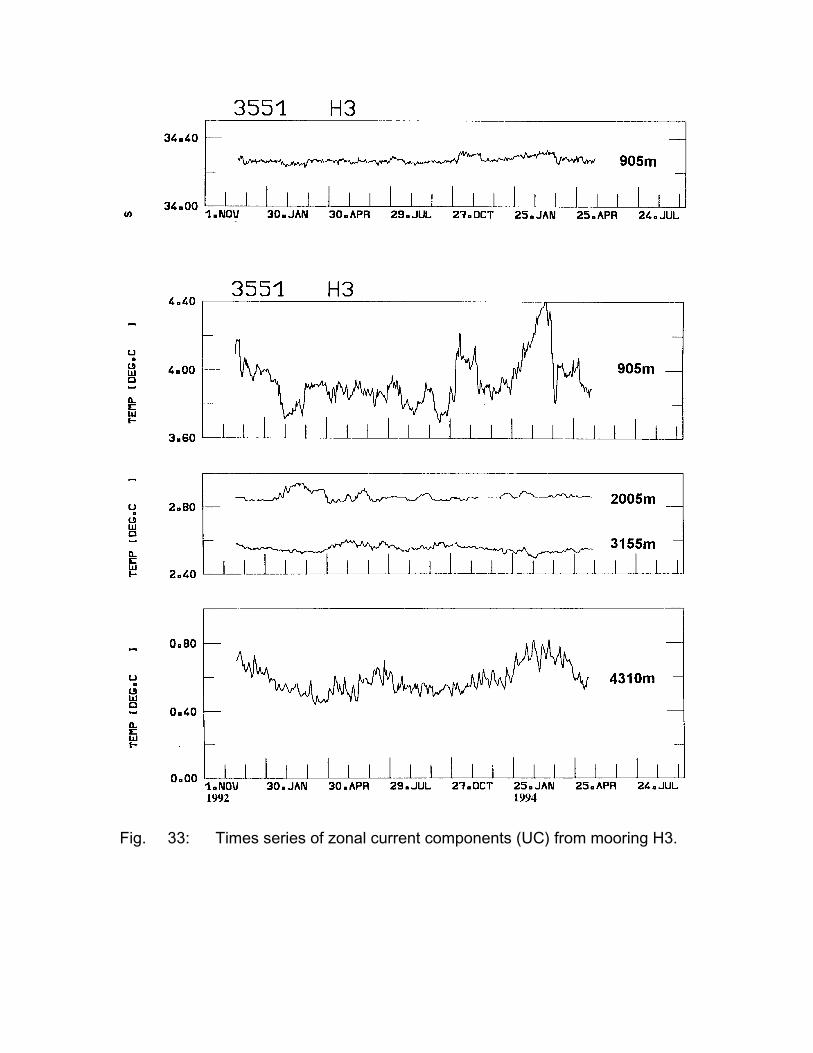
Fig. 33: Times series of zonal current components (UC) from mooring H3.
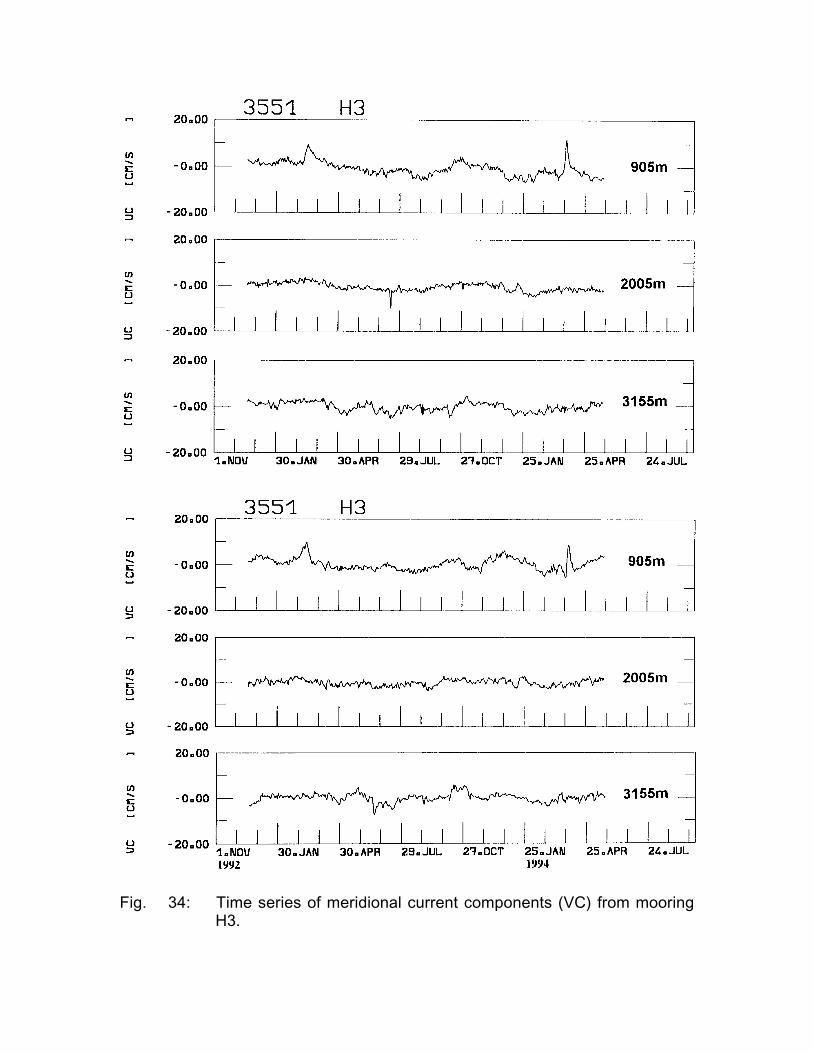
Fig. 34: Time series of meridional current components (VC) from mooringH3.
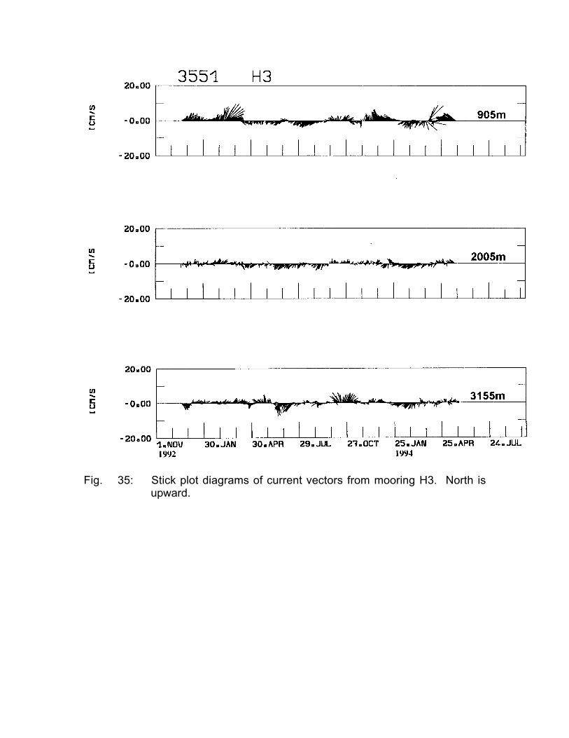
Fig. 35: Stick plot diagrams of current vectors from mooring H3. North isupward.
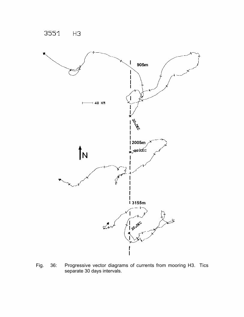
Fig. 36: Progressive vector diagrams of currents from mooring H3. Ticsseparate 30 days intervals.
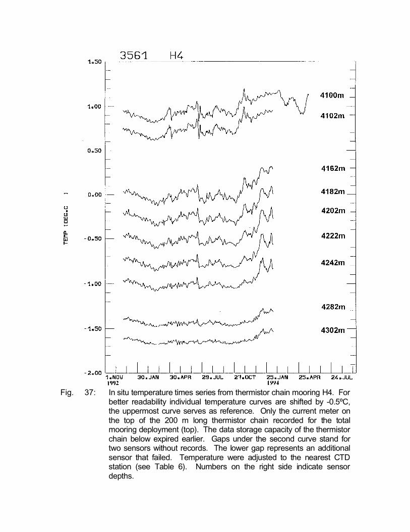
Fig. 37: In situ temperature times series from thermistor chain mooring H4. Forbetter readability individual temperature curves are shifted by -0.5ºC,the uppermost curve serves as reference. Only the current meter onthe top of the 200 m long thermistor chain recorded for the totalmooring deployment (top). The data storage capacity of the thermistorchain below expired earlier. Gaps under the second curve stand fortwo sensors without records. The lower gap represents an additionalsensor that failed. Temperature were adjusted to the nearest CTDstation (see Table 6). Numbers on the right side indicate sensordepths.
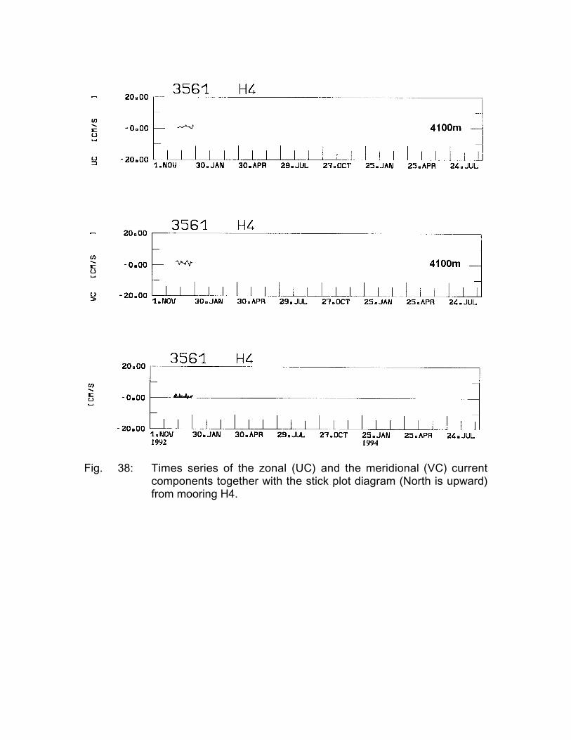
Fig. 38: Times series of the zonal (UC) and the meridional (VC) currentcomponents together with the stick plot diagram (North is upward)from mooring H4.
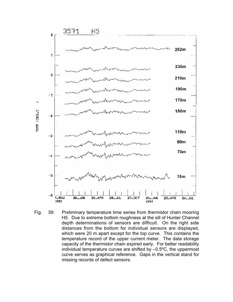
Fig. 39: Preliminary temperature time series from thermistor chain mooringH5. Due to extreme bottom roughness at the sill of Hunter Channeldepth determinations of sensors are difficult. On the right sidedistances from the bottom for individual sensors are displayed,which were 20 m apart except for the top curve. This contains thetemperature record of the upper current meter. The data storagecapacity of the thermistor chain expired early. For better readabilityindividual temperature curves are shifted by –0.5ºC, the uppermostcurve serves as graphical reference. Gaps in the vertical stand formissing records of defect sensors.
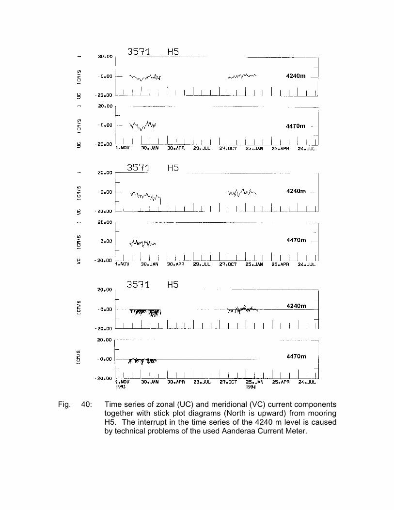
Fig. 40: Time series of zonal (UC) and meridional (VC) current componentstogether with stick plot diagrams (North is upward) from mooringH5. The interrupt in the time series of the 4240 m level is causedby technical problems of the used Aanderaa Current Meter.
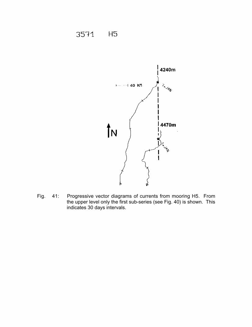
Fig. 41: Progressive vector diagrams of currents from mooring H5. Fromthe upper level only the first sub-series (see Fig. 40) is shown. Thisindicates 30 days intervals.

Fig. 42: Temperature (top) and auxiliary parameters of the Acoustic DopplerCurrent Profiler on the top of mooring H6. Only the temperaturetime series has been low-passed filtered.
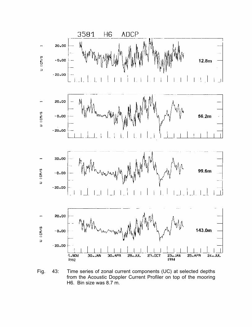
Fig. 43: Time series of zonal current components (UC) at selected depthsfrom the Acoustic Doppler Current Profiler on top of the mooringH6. Bin size was 8.7 m.
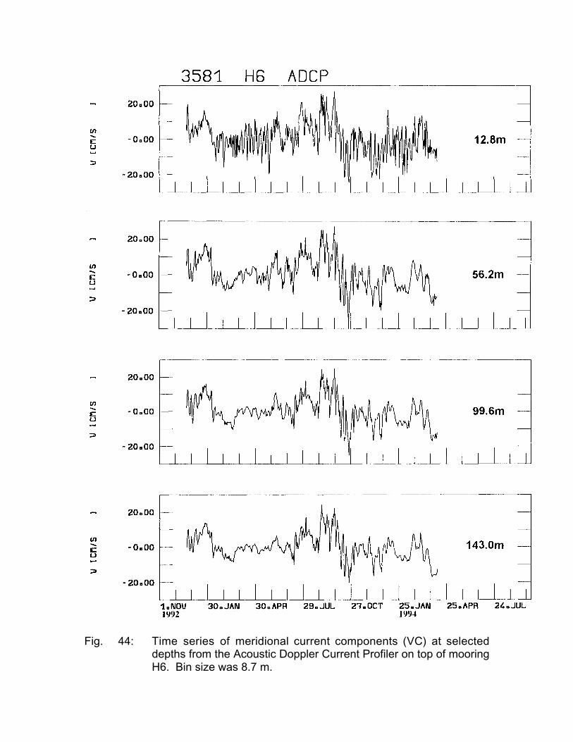
Fig. 44: Time series of meridional current components (VC) at selecteddepths from the Acoustic Doppler Current Profiler on top of mooringH6. Bin size was 8.7 m.
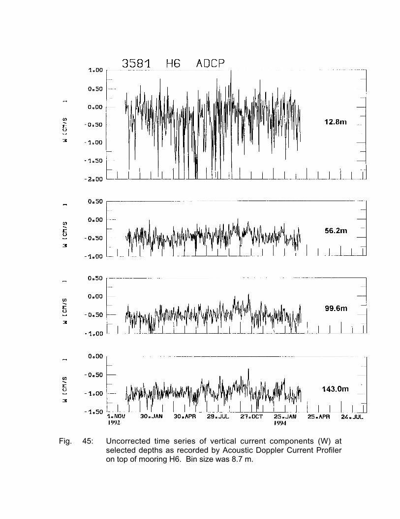
Fig. 45: Uncorrected time series of vertical current components (W) atselected depths as recorded by Acoustic Doppler Current Profileron top of mooring H6. Bin size was 8.7 m.

Fig. 46: Pseudo-pressure (PRESS) time series for the ADCP in mooring H6as inferred from the backscatter record (according to VIESBEK andFISCHER, 1995). Below PRESS stick plot diagrams of ADCPcurrent vectors at selected depth above the top instrument (ADCP)of mooring H6 is displayed. North is upward.
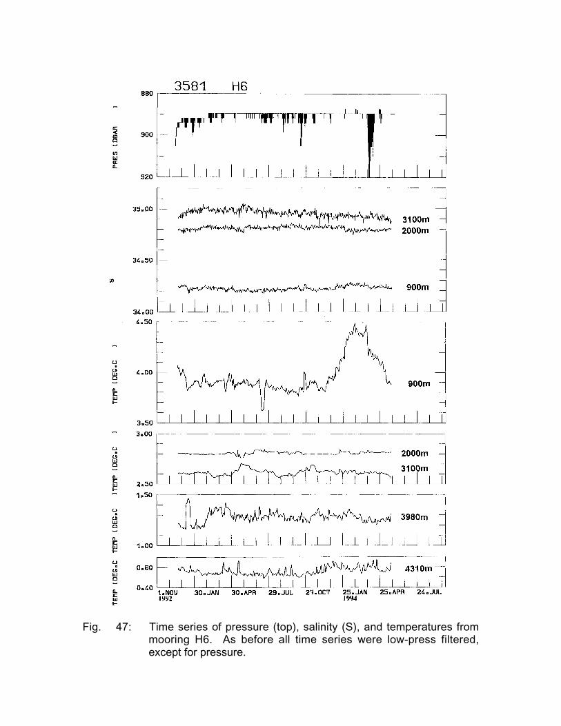
Fig. 47: Time series of pressure (top), salinity (S), and temperatures frommooring H6. As before all time series were low-press filtered,except for pressure.
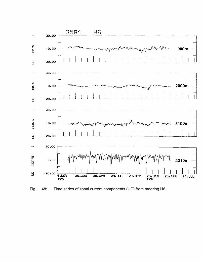
Fig. 48: Time series of zonal current components (UC) from mooring H6.
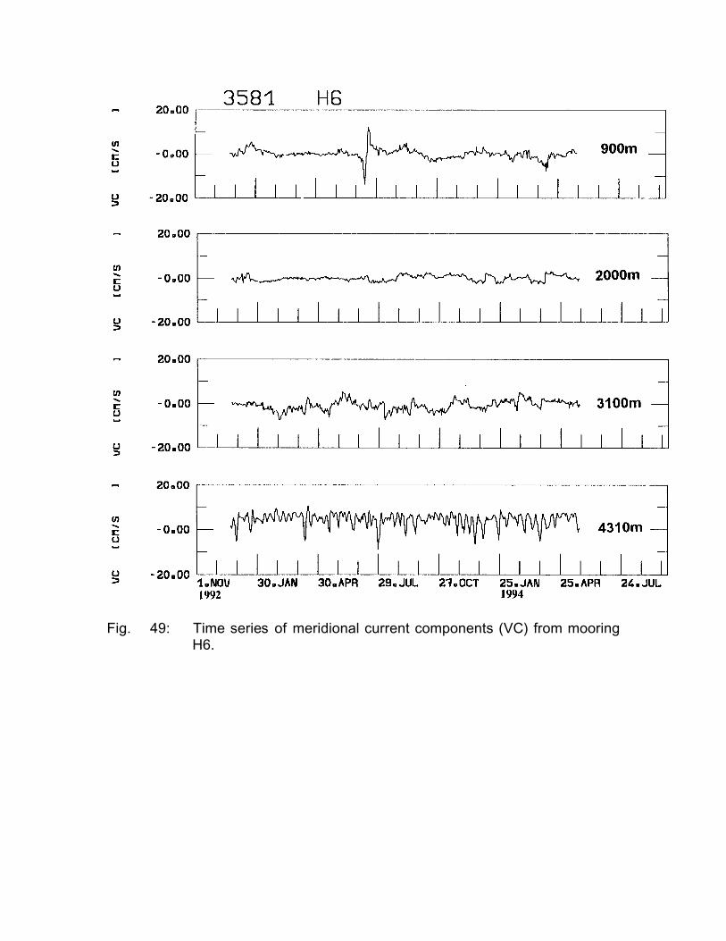
Fig. 49: Time series of meridional current components (VC) from mooringH6.

Fig. 50: Stick plot diagrams of current vectors from mooring H6. North isupward.
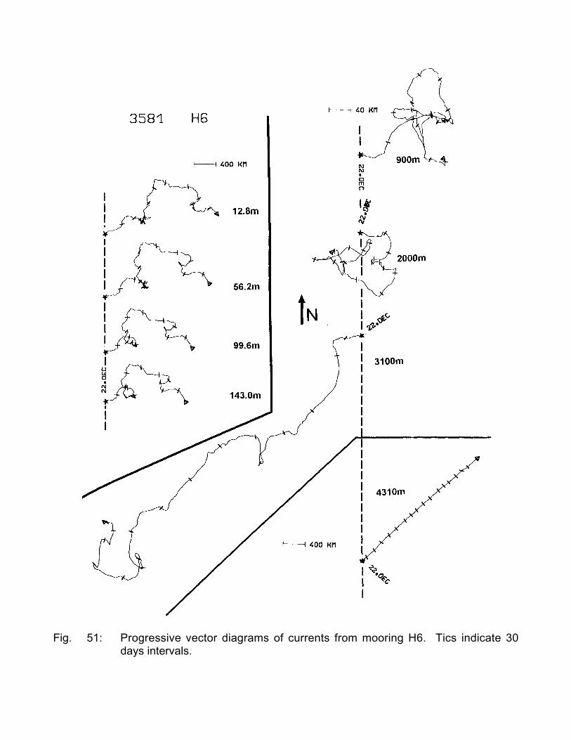
Fig. 51: Progressive vector diagrams of currents from mooring H6. Tics indicate 30days intervals.

Fig. 52: Time series of pressure (top), salinity (S), and temperatures from mooring R atthe eastern flank of the Rio Grande Rise. As before all time series were low-pass filtered, except for pressure.
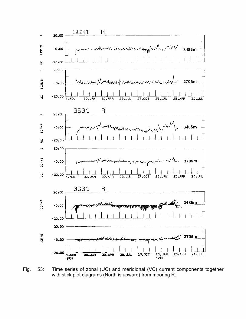
Fig. 53: Time series of zonal (UC) and meridional (VC) current components togetherwith stick plot diagrams (North is upward) from mooring R.
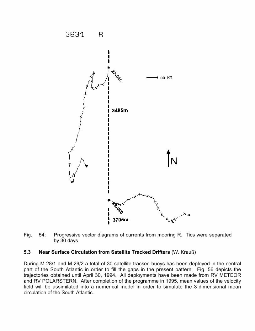
Fig. 54: Progressive vector diagrams of currents from mooring R. Tics were separatedby 30 days.
5.3 Near Surface Circulation from Satellite Tracked Drifters (W. Krauß)
During M 28/1 and M 29/2 a total of 30 satellite tracked buoys has been deployed in the centralpart of the South Atlantic in order to fill the gaps in the present pattern. Fig. 56 depicts thetrajectories obtained until April 30, 1994. All deployments have been made from RV METEORand RV POLARSTERN. After completion of the programme in 1995, mean values of the velocityfield will be assimilated into a numerical model in order to simulate the 3-dimensional meancirculation of the South Atlantic.
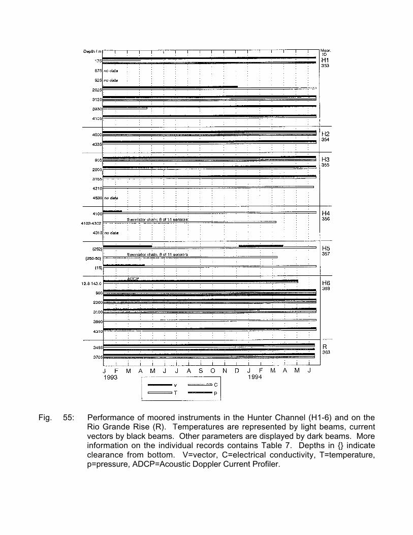
Fig. 55: Performance of moored instruments in the Hunter Channel (H1-6) and on theRio Grande Rise (R). Temperatures are represented by light beams, currentvectors by black beams. Other parameters are displayed by dark beams. Moreinformation on the individual records contains Table 7. Depths in {} indicateclearance from bottom. V=vector, C=electrical conductivity, T=temperature,p=pressure, ADCP=Acoustic Doppler Current Profiler.
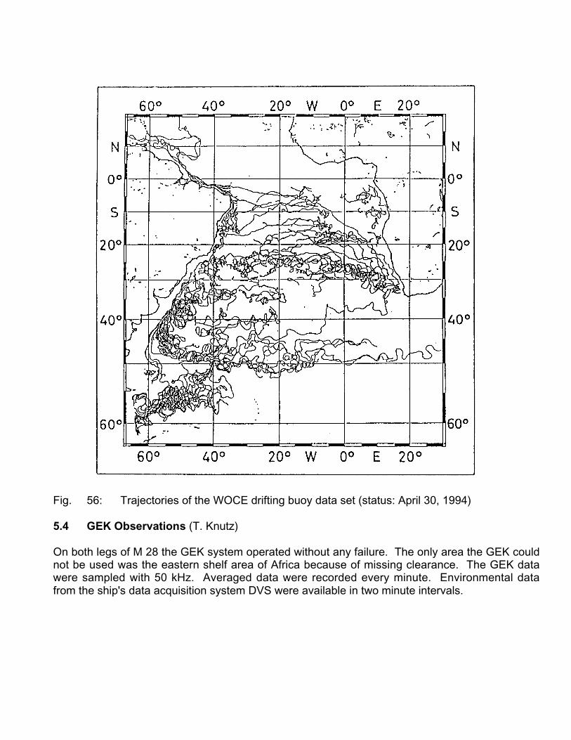
Fig. 56: Trajectories of the WOCE drifting buoy data set (status: April 30, 1994)
5.4 GEK Observations (T. Knutz)
On both legs of M 28 the GEK system operated without any failure. The only area the GEK couldnot be used was the eastern shelf area of Africa because of missing clearance. The GEK datawere sampled with 50 kHz. Averaged data were recorded every minute. Environmental datafrom the ship's data acquisition system DVS were available in two minute intervals.
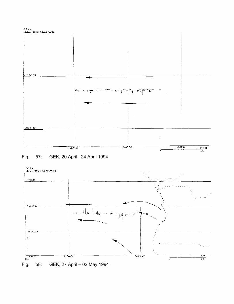
Fig. 57: GEK, 20 April –24 April 1994
Fig. 58: GEK, 27 April – 02 May 1994
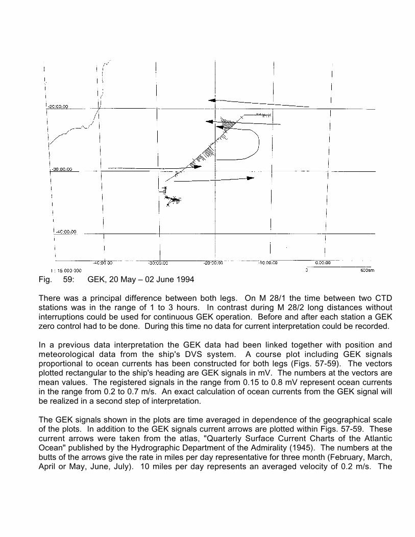
Fig. 59: GEK, 20 May – 02 June 1994
There was a principal difference between both legs. On M 28/1 the time between two CTDstations was in the range of 1 to 3 hours. In contrast during M 28/2 long distances withoutinterruptions could be used for continuous GEK operation. Before and after each station a GEKzero control had to be done. During this time no data for current interpretation could be recorded.
In a previous data interpretation the GEK data had been linked together with position andmeteorological data from the ship's DVS system. A course plot including GEK signalsproportional to ocean currents has been constructed for both legs (Figs. 57-59). The vectorsplotted rectangular to the ship's heading are GEK signals in mV. The numbers at the vectors aremean values. The registered signals in the range from 0.15 to 0.8 mV represent ocean currentsin the range from 0.2 to 0.7 m/s. An exact calculation of ocean currents from the GEK signal willbe realized in a second step of interpretation.
The GEK signals shown in the plots are time averaged in dependence of the geographical scaleof the plots. In addition to the GEK signals current arrows are plotted within Figs. 57-59. Thesecurrent arrows were taken from the atlas, "Quarterly Surface Current Charts of the AtlanticOcean" published by the Hydrographic Department of the Admirality (1945). The numbers at thebutts of the arrows give the rate in miles per day representative for three month (February, March,April or May, June, July). 10 miles per day represents an averaged velocity of 0.2 m/s. The
averaged currents described by the arrows are in the same scale as the GEK signals. In all plotsa good correlation between the GEK signals and global current field is given. Differences can becaused by local effects as sudden wind changes or superimposed eddy motion. In Fig. 57 nosignificant current rectangular to the ship's heading could be recorded. The shown GEK signalsrepresent currents in the range of 0.1 m/s. This is in good agreement with the global current indirection of the ship’s course. In Fig. 58 is given a southern component by the 0.8 mV signal inthe eastern area and a northern current (0.5 mV) component in the western part of the courseplot. The signals plotted in Fig. 59 give a good example for GEK measurements as frontal zonedetection system. The measurements have been taken in the area of subtropical convergence(United States Naval Oceanographic Office (1955)) with high seasonal variability. The reversingcurrent as described by the arrows could be registrated with high geographical resolution by theGEK system.
In the future data processing the GEK signals will be calculated with the earth magnetic field andcompared with meteorological observations, ship drift, ADCP data and CTD measurements.
5.5 Biological Oceanography and Taxonomy along 11˚30'S(C. Zelck, H.-Ch. John)
5.5.1 Quantitative Data
5.5.1.1. General
Microscopic analysis was possible on board for 25 NEU upper net samples and 10 complete MCNstations from the Brazilian slope and adjacent oceanic area (see chapter 7.2.6). Analysis includesquantitative extraction of taxa Gammaridea and Hyperiidae, Hexapoda and fish, plus a qualitativerecord on the coarse taxonomic composition of the remaining plankton. The following chapterswill exclusively focus on fish from the station sequence 169 - 189 (see Fig. 60). From thesesamples, the total catch of fish amounts to 3843 specimens, and a still insufficient identification of79 taxa.
5.5.1.2 Taxonomy
From this station sequence alone, larval forms of 4 taxa appear to be undescribed, further 10 taxaare known to science, but are new for the team and the larval collection of the ZoologischesMuseum Hamburg. These species belong to the complex of coastal (neritic) species, which areextremely difficult to identify. It is anticipated that further analysis might yield additional taxonomicfindings.
5.5.1.3 Cross-slope Ecological Patterns
5.5.1.3.1 Abundance Patterns
NEU and MCN samples provide conforming results, though there is very little overlap in thespecies composition obtained by each sampler (Scaridae type 1, parrot fish, making the only
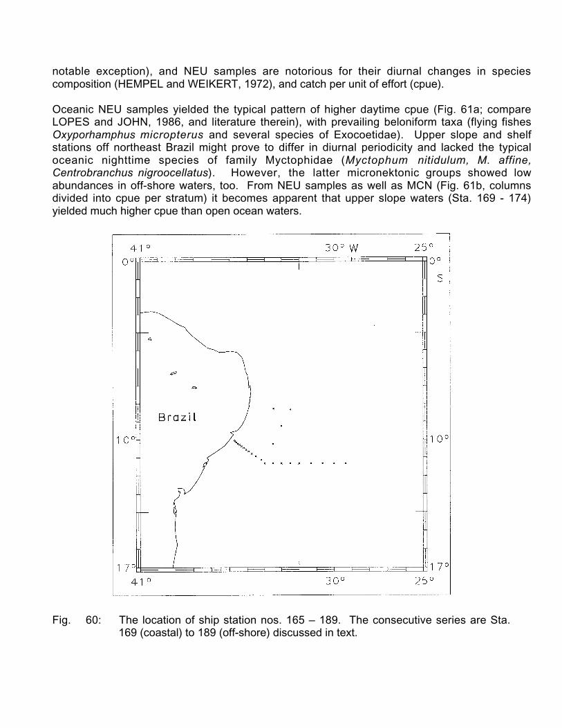
notable exception), and NEU samples are notorious for their diurnal changes in speciescomposition (HEMPEL and WEIKERT, 1972), and catch per unit of effort (cpue).
Oceanic NEU samples yielded the typical pattern of higher daytime cpue (Fig. 61a; compareLOPES and JOHN, 1986, and literature therein), with prevailing beloniform taxa (flying fishesOxyporhamphus micropterus and several species of Exocoetidae). Upper slope and shelfstations off northeast Brazil might prove to differ in diurnal periodicity and lacked the typicaloceanic nighttime species of family Myctophidae (Myctophum nitidulum, M. affine,Centrobranchus nigroocellatus). However, the latter micronektonic groups showed lowabundances in off-shore waters, too. From NEU samples as well as MCN (Fig. 61b, columnsdivided into cpue per stratum) it becomes apparent that upper slope waters (Sta. 169 - 174)yielded much higher cpue than open ocean waters.
Fig. 60: The location of ship station nos. 165 – 189. The consecutive series are Sta.169 (coastal) to 189 (off-shore) discussed in text.
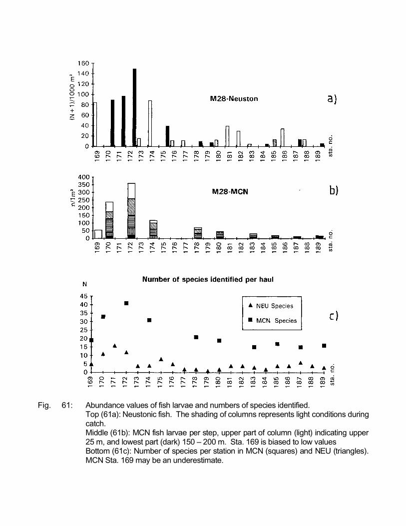
Fig. 61: Abundance values of fish larvae and numbers of species identified.Top (61a): Neustonic fish. The shading of columns represents light conditions duringcatch.Middle (61b): MCN fish larvae per step, upper part of column (light) indicating upper25 m, and lowest part (dark) 150 – 200 m. Sta. 169 is biased to low valuesBottom (61c): Number of species per station in MCN (squares) and NEU (triangles).MCN Sta. 169 may be an underestimate.
5.5.1.3.2 Diversity and Species Composition
A similar relation is revealed by the number of species identified (the MCN-values are likely to beunderestimates due to identification problems) shown in Fig. 61c, neritic ecosystems being morediverse than oceanic ones. The neustonic realm is, due to its environmental stress, a habitatsuited only for especially adapted organisms (HEMPEL and WEIKERT, 1972), and has thus alower diversity than the epipelagic and mesopelagic layer sampled by the MCN. It seems to bean advection-related ecological signal, that diversity in the MCN decreases further off-shore thanin the NEU (see below).
A preliminary calculation of the percentages of neritic and oceanic species among total catch (Fig.62) yields some differences between NEU and MCN. For NEU there is a sharp decline of oceanicspecies from Sta. 178 - 176, while such a decline in MCN only amounts to some 20 % (there areless identification problems and consequently more precise values for oceanic elements). On thecontrary, neritic species reach further off-shore in MCN samples than NEU samples (the entireneritic curve in Fig. 62b is likely to increase by some 20 % after better taxonomic analysis andinclusion of less conspicuous elements into the group).
The boundary between the neritic and oceanic regime was much sharper and closer to the shorethan found for the South Brazil Current, but there too oceanic elements are found in shelf waters(compare ANDRES et al., 1992; ZELCK, 1993).
It is furthermore noteworthy, that species like tropical oceanic-ubiquitous Diogenichthys atlanticusor Vinciguerria nimbaria were expected, but in fact proved absent or rare off Brazil (and somewhatdeeper than in the NE Atlantic). On the other hand, catches of Sudis atrox, Evermanella or tunaexceeded by far previous catches.
5.5.1.3.3 Vertical Distribution and Implication for Cross-slope Zonations
An overall relative vertical distribution of fish larvae is given in Fig. 63. Generally some 50 % of alllarvae were caught in the upper 50 m, and almost consistently some 80 % were contributed in theupper 100 m (Sta. 169 is an exception and biased as only half the bottom depth was sampled dueto opening-closing problems).
As for the defined station sequence so far only about half of the samples with vertical resolutioncould be sorted, a detailed analysis on species level and differing individual depth preferenceswas hardly feasible. Differing vertical patterns are exemplified by species Scaridae type I, havingan extended-shallow pattern (Fig. 64), and an oceanic deep group. Scaridae I occurred also inNEU samples seawards up to Sta. 175. However, in the MCN this species was encounteredregularly up to and including Sta. 180, and with a shift towards deeper occurrences there. As wehave a general pattern of a more restricted coastal regime in the NEU than in the MCN, wepresume that off-shore displacement of surface plankton is restricted by the westward flowingSouth Equatorial Current, while at mid-depths an eastward transport (by a South EquatorialUndercurrent?) apparently takes place to some 120 n.m. from the shelf edge. Nevertheless,considerable advection of oceanic species also occurred up to the shelf edge (Fig. 62), andperhaps at depths of between 50 and 200 m (Fig. 64) by along-slope currents.
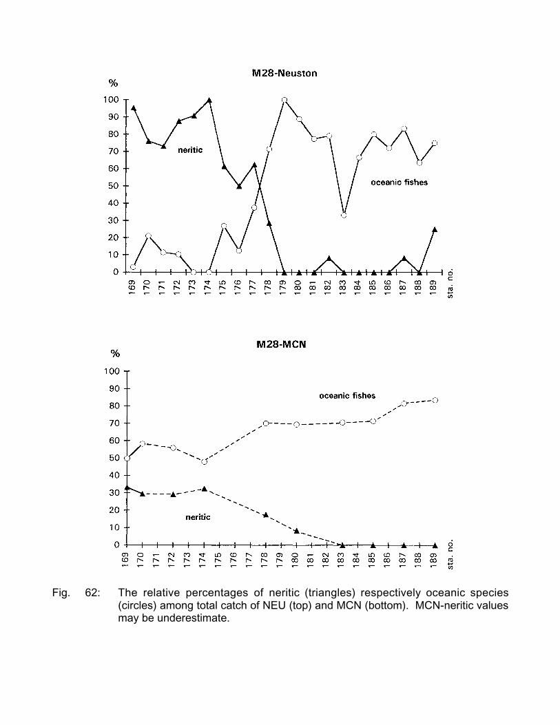
Fig. 62: The relative percentages of neritic (triangles) respectively oceanic species(circles) among total catch of NEU (top) and MCN (bottom). MCN-neritic valuesmay be underestimate.
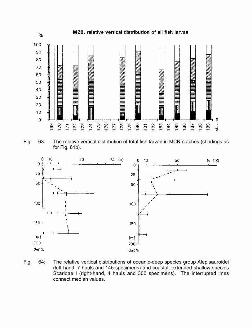
Fig. 63: The relative vertical distribution of total fish larvae in MCN-catches (shadings asfor Fig. 61b).
Fig. 64: The relative vertical distributions of oceanic-deep species group Alepisauroidei(left-hand, 7 hauls and 145 specimens) and coastal, extended-shallow speciesScaridae I (right-hand, 4 hauls and 300 specimens). The interrupted linesconnect median values.
5.5.2 The Plankton Material from the Central Atlantic to Angola:Findings, Hints and Expectations
5.5.2.1 General
It was impossible to microscopically analyze any further plankton sample. All followingstatements are based on macroscopical investigation during preservation of the sample, thoughsome individual species or specimens in question had been picked out for closer identificationunder the microscope. Any numerical estimates may become void after microscopical analysis oflarval numbers. Hoping that the team can be maintained as it is, a thorough analysis of the entire,huge load of material will take about four years. The priority to work from the Brazilian coasteastwards was set a long time ago.
5.5.2.2 Plankton Biomass Volumes and Micronekton Numbers
As already stated for Brazil, from Sta. 189 onwards and until having crossed the Mid-AtlanticRidge, plankton biomass and numbers of adult Myctophidae remained at a comparatively lowlevel. Myctophids were mainly "slendertails" and Myctophum affine, considered by us as typicalfor the low productive central gyre zones.
I mm ed ia t ely aft er cr ossin g th e Mid -At la nt ic Ridg e , bo th va lu e s in cr e ased dist in ctly. Ch eckin gr eg ular ly ad u lt M ycto ph ida e (fo llowing a re qu est of m ycto ph id ta xon om ist s de m an ding L ep id op h an es sp ecim e ns), we wer e able to id e nt if y and de ep fr ee ze 4 L . g ue nt he r i im me dia te lya ft er ca tch for gen et ica l an a lysis (St a. 24 2 an d 247 ) . T he se sp e cime ns we re tr an sfe rr ed from b o ar dd ir ectly to P.A. Hulle y in Ca p e To wn . Ot h er M ycto ph ida e (e. g. Dia ph us sp .) wer e oft en id en tif ie d tog en er ic le ve l o nly, as t h er e wa s n ot en ou gh time (a nd lite ra t ur e) f o r th o ro ug h ide nt ifica tio n.
Somewhat down current of the Dampier/Cardno Seamount group we caught a tiny but adultdragonet (Callionymidae, Sta. 218, 200 - 150 m). Though not acquainted with this complex anddifficult family, it might prove to become a new species. At Sta. 257 a beautiful larva of Loweinarara made a nice addition to our existing series of smaller larvae of this species, an amendeddescription is in progress.
In the samples adjacent to the mentioned seamounts, plankton biomass and numbers ofmicronekton increased furthermore. Apparently this was less a seamount effect than a generalEast Atlantic feature, as both values remained high towards the slope of Angola. We estimatedboth figures to be two orders of magnitude higher than in the Brazilian off-shore area, sometimeswe had problems to hose down the plankton in the nets. Sta. 264 yielded high numbers oftransforming V. nimbaria and will perhaps reveal even higher larval numbers. While highnumbers of myctophids occurred until the very last and shallow station (Sta. 290) above theAngola shelf edge, plankton volumes decreased distinctly at stations 289 and 290. Angolanichthyoplankton obtained a neritic characteristic (larvae of Serranidae, Scorpaenidae andCarangidae becoming abundant) from Sta. 285 onwards. These stations seemed to differ also invertical distribution, as plankton biomasses decreased sharply below 50 in depth, conforming withsharp density gradients below 30 m.
5.5.2.3 The Juvenile Life Stage of Bathylagus argyrogaster
Excit in g resu lt s yie ld ed St a. 28 3. The MCN ca ug h t 3 ju ven ile spe cim en s of Bat hyla g usa rg yr og a st er (d ee p- sea sm elt) a t d ep t hs 1 50 - 10 0 m , 50 - 25 m, a nd 25 - 0 m. The y wer e colou re d u nlike lar va e or ad u lt s, bu t like typ ical e pipe la g ic sp ecie s, with blue do rsum an d silve r ven tr al side . Accor din g to lite ra t ur e the dor sal colou r of ad u lt s is black or br o wn (BLACHE, 19 64 ; NORMAN,1 93 0) . Th e spe cies is ge ne ra lly con sid er ed to be end em ic of th e Gu lf of Gu in ea an d b at hype lag ic( BL ACHE, 196 4 ), but KO BYL YANSKI Y (19 8 5) sta t ed a m esop ela gic ran ge . BL ACHE (1 96 4 )p ro vide d e vid en ce th at ju ve nile s m ig h t ha ve a sh a llower dist r ib ut io n tha n a du lt s. L a rvae ha ve b e en d escr ib e d on th e ba sis of MET EO R mat e rial (HERMES and OL IVAR, 198 7) , and ar e kn o wn to beswe pt with th e NE At la nt ic Up we lling Un de rcu rr en t up to Ca pe Bla nc. Th re e lar va e have bee nr ep or te d fro m off Na mibia (HERM ES an d OLI VAR, 19 8 7) , an d at lea st on e ad d it io na l lar g er Sou t hAtlan tic lar va wa s cau gh t now at M 28 , St a. 28 3. In th e mea n tim e we le a rn ed , tha t lar va e are ste no ba t hic 60 - 90 in , and follow de flectio ns of the un de rcu rr en t cau se d by gyr es like the Gu in e aDom e or th e M au rita n ia n Cen tr al Gyre (o wn , unp ub lishe d dat a) . We t h in k this ne w f in d in g mig ht b e con ne ct e d wit h th e Ang ola Dom e plu s the sou t hwar d u nd er cur re n t, a nd it will she d n ew ligh t upo n ap re viou sly u n kn own e pipe la g ic life sta g e of th is o t he rwise d ee p -sea sp ecie s.
5.6 Atmospheric Physics and Chemistry along 11˚30S(J. Brinkmann, G. Schebeske)
Although needed for a better understanding of the atmosphere as well as input information fordifferent theoretical models (for example on cloud formation and radiation balance) the amount ofdata on marine aerosol is very crude.
During M 28/1 measurements of different physical and chemical properties of the marineatmosphere have been carried out. Furthermore investigations of the oceanic surface layer hadbeen made. These measurements have to be seen in comparison to previous measurementsmade during the last few years in other areas of the Atlantic Ocean.
As we did not have any permission to work within the 200 sm-zone off-shore from the Braziliancoast our measurements began on April 6, after having left that zone and were finished on May 6,near the Angolan coast.
The preliminary conclusions are described below:
1 Two optical particle counters in combination with a diffusion box and two impactors were usedto measure the number size distribution of the marine aerosol particles in the size range of0.002 micrometer to about 50 micrometer radius. Initial results show relatively homogeneousconcentrations during most of the time of the cruise. First investigations of our data in thelower particle size range are shown in Fig. 65. The spectrum is an average of all themeasurements done during the cruise in that particular range of particle size. Incorrespondence with the model distribution of marine aerosole (JAENICKE, 1987) thespectrum is of bimodal nature. The absolute values of our mean size distribution have to bevalidated in further tests. However, the shift of both of the models seems to be of specialinterest. This phenomenon will be investigated in detail in future examination of our data.
The particles in the super micrometer range show a clear diel behaviour with higherconcentrations during the night.
A noticeable increase in the concentrations measured next to the coast took place very late, i.e.about 500 km off-shore, which is probably due to the southerly winds next to the African coast.We also observed a slight rise in the aerosol particle concentration while crossing the shippingroute South Africa - Europe.
Besides these effects we also found an increase in the concentration in the upper size range ofthe particles from April 27 to April 28. Comparing Fig. 66a and 66b it can be seen that there hadbeen a doubling of particle concentration in both of the two channels measuring the biggerparticles while the channel counting the small ones remained indicating a relatively constantnumber concentration. This effect took place when we had a slight change in the weatherconditions: The sky became more cloudy, the wind strengthened. So reasons might be the minorconvection and an enhanced production of big particles due to the wind. Examinations of the filtersamples will give more information of the nature of these additional particles.
Fig. 65: Marine aerosole; number size distribution of aerosol particles; symboles: Meandistribution, measured during M 28/1, South Atlantic; solid line: Model distribution,calculated by means of the parameters and equations given in JAENICKE, 1987.
Fig. 66: Number concentration of aerosol particles in different size ranges, 10 min.means, measured during M 28/1;a) April 27, 1994;b) April 28, 1994.
2 Soot is a very effective absorber and thus of great importance for the radiation balance of theatmosphere. Nevertheless the amount of particulate carbon in an unpolluted area is poorlyknown, although recently some measurements have been made. We measured articulatecarbon measured in various ways. Different sets of filters will be analyzed with optical andpyrolytic methods in order to get some information on the total and the black carbon. Firstinvestigations of the deposits on the filters, i.e. the degree of greyish-ness, showed an obviousdependence from the distance to the coast. The filters will also be used to compare thedifferent analytical methods because up to now there is no standardized procedure fordetermining particulate carbon in the atmosphere.
3 During the period given above we sampled aerosol particles daily in three size classes bymeans of two different impactors. These specimens will be analyzed by energy dispersive
X-ray analysis and a protein dye technique in order to determine the amount of biological orbiologically contaminated particles. The analysis can not be done on board in detail but, asexpected, the relative amount of soil derived particles seems to be distinctly higher in front of theAngolan coast than in the middle of the South Atlantic.
Analogous investigations had been made with samples got on two previous cruises showingdiffering results. At the moment we cannot explain this behaviour but hopefully these newmeasurements give some further information. The differences might be due to dimethylsulfide.
4 Dimethylsulfide (DMS) is unstable in air and oxidizes to sulfate to form particles. So it is ofsome interest to correlate DMS with the total particle concentration as well as with the particlesof biological origin. DMS in air has been sampled and analyzed automatically. During thecruise 1400 samples have been analyzed. The concentration was between 150 ng and 400ng per cubic meter air. It was found a slight increase in the concentration while approachingthe African coast. The diurnal course of DMS with an afternoon minimum could be confirmed.
5 DMS in ocean water was sampled by means of a membrane pump four times a day at 00, 06,12, and 18 local time. All together 120 samples were analyzed. The water contained between120 ng and 480 ng DMS per liter. We also found a slight increase while getting closer to theAngolan coast.
6 The above mentioned samples had been analyzed for chlorophyll and phaeophytin, too.Because there had been no way to calibrate the measurements on board the absoluteamounts can not given here but will follow. An increase of the measured signal of chlorophyllconcentration in oceanic water increased parallel with the atmospheric DMS.
5.7 Radiative Physics (W. Emery, M. Suarez)
The world's ocean serve as an vast reservoir of heat in the ocean/atmosphere engine. For thisreason, it is impossible to accurately model global climate without first understanding the heatexchanges between the ocean and atmosphere. Since the advent of weather satellites, scientistshave been allowed to gather data from around the world in a matter of hours or days. One of thekey quantities measured in this fashion is global sea surface temperature (SST).
In the past, satellite radiometric measurements have been calibrated using SST measurementstaken from drifting buoys or ships which is not physically correct. These methods measure thetemperature of the seawater at a depth of a meter or more, that is, bulk temperature. Satellites,however, only measure the radiation emitted from the upper few microns, or skin temperature.Due to the latent heat released by evaporation, sensible heat and the net long wave radiativeemission, the skin temperature is generally cooler than the bulk temperature. It is possiblethough, during periods of high wind or strong solar insulation, that the skin may be of the same orhigher temperature than the water below. The difference between the bulk and skin temperaturescan occasionally be as large as 1˚C or more (SCHLUESSEL et al., 1990; WICK et al., 1992).While this difference may seem negligible, ROBINSON et al. (1984) suggests that an accuracy of0.2˚C is necessary for satellite measurements to be useful in global climate prediction. For thisreason a more accurate, radiometric method of sea surface temperature calibration has beendeveloped.
As part of M 28/2 we employed a prototype multi-channel infrared sea-truth calibration radiometer(MISTRC) designed and built by OPHIR Corp., Littleton, Colorado. The experimental set up waspatterned after a system developed by scientists in Hamburg and Kiel, Germany. Key aspects ofthe system include a bucket of continuously circulating ocean water which serves as a continuouscalibration reference, and that the radiometer views the ocean at approximately the Brewsterangle in order to minimize reflected radiation.
The radiometer has two independent optical trains, one operating in the short wave infrared (IR)and one operating in the thermal IR. The short wave head has filters at 3.7 and 4.0 µm andadditional vertically polarized filters to further suppress the effects of reflected radiation. In thelong wave region, the MISTRC has filters at 10.8 and 11.8 µm which are closer to the standardBarnes PRT-5 and Heimann KT-19 radiometers. These wave lengths are also similar to those onthe advanced very high resolution radiometer (AVHRR) flying on the NOAA satellites and thealong track scanning radiometer (ATSR) flying aboard ERS-1.
In addition to using the radiometric SST measurements to calibrate space borne radiometers,these measurements also give the opportunity to study the bulk-skin temperature difference. Byunderstanding this difference, it may be possible to determine the bulk temperature from satellitemeasured skin temperature, or alternately to predict the temperatures calculated from satellitesbased on bulk measurements.
In order to help better our understanding of the temperature difference and the heat fluxesinvolved, an entire suite of atmospheric, oceanographic and radiometric measurements are taken.Atmospheric variables include dry and wet bulb temperature, pressure and surface wind as wellas the profiles taken by radiosonde balloons. The primary oceanographic variable used is thebulk temperature from the hull mounted sensors and the thermosalinograph, however salinity andtemperature profiles are also taken for their importance in upper ocean stability. Upward lookingpyranometers and pyrgeometers are used to measure the down-welling solar and terrestrialirradiance.
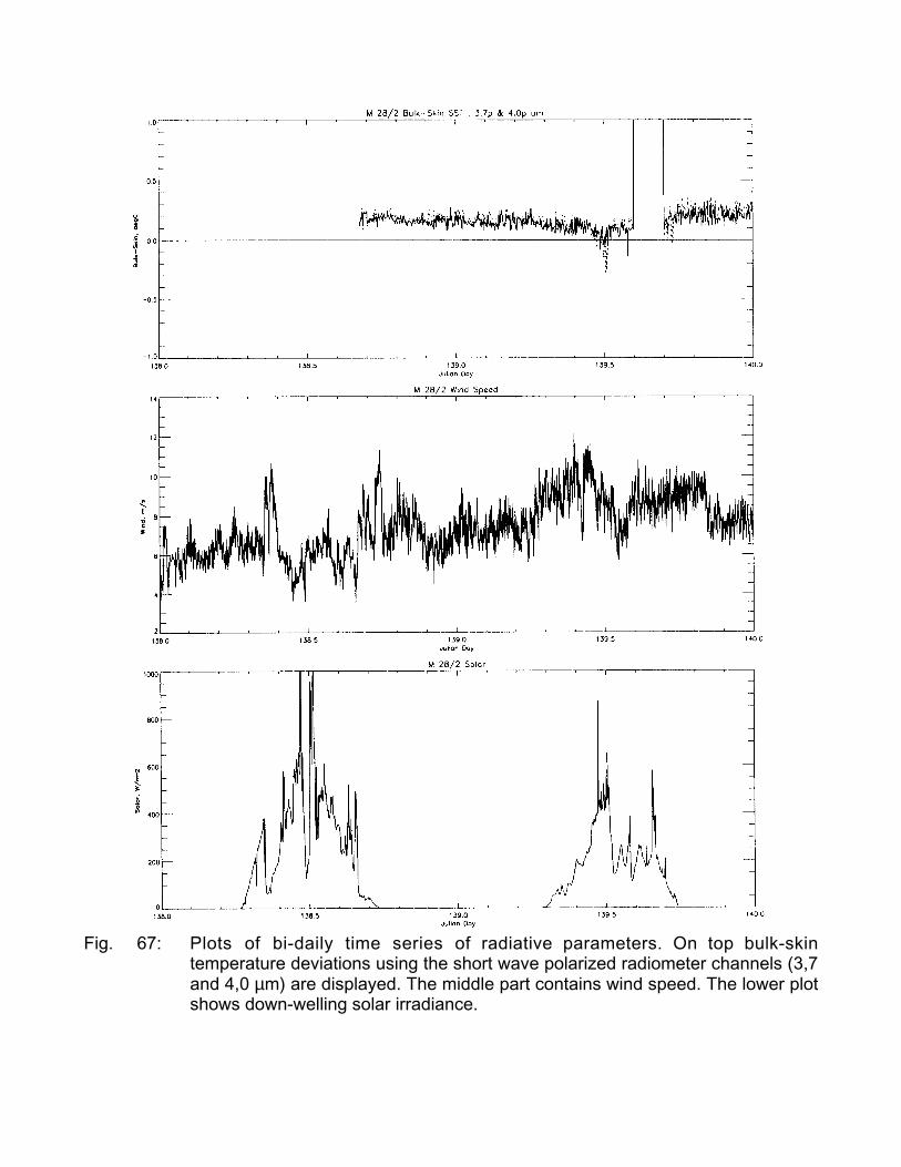
Fig. 67: Plots of bi-daily time series of radiative parameters. On top bulk-skintemperature deviations using the short wave polarized radiometer channels (3,7and 4,0 µm) are displayed. The middle part contains wind speed. The lower plotshows down-welling solar irradiance.
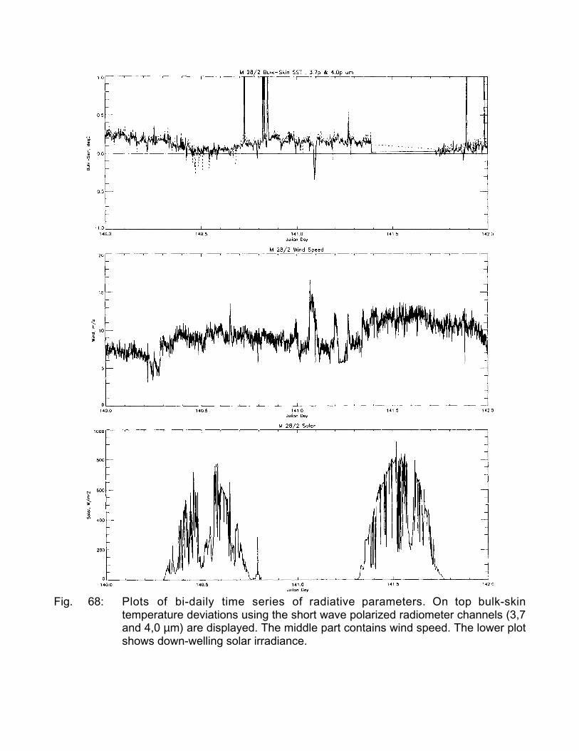
Fig. 68: Plots of bi-daily time series of radiative parameters. On top bulk-skintemperature deviations using the short wave polarized radiometer channels (3,7and 4,0 µm) are displayed. The middle part contains wind speed. The lower plotshows down-welling solar irradiance.

Fig. 69: Plots of bi-daily time series of radiative parameters. On top bulk-skintemperature deviations using the short wave polarized radiometer channels (3,7and 4,0 µm) are displayed. The middle part contains wind speed. The lower plotshows down-welling solar irradiance.
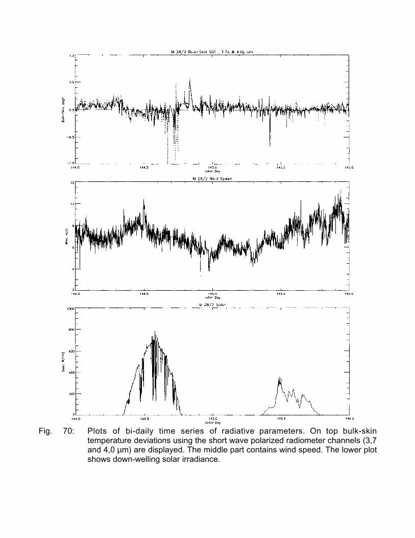
Fig. 70: Plots of bi-daily time series of radiative parameters. On top bulk-skintemperature deviations using the short wave polarized radiometer channels (3,7and 4,0 µm) are displayed. The middle part contains wind speed. The lower plotshows down-welling solar irradiance.
Preliminary results from the first eight days of system operation are shown in Figs. 67-70 in theform of four bi-daily time series plots. The Julian day, 138 corresponds to May 18, 1994 and soforth. On each page, the top plot is of the bulk-skin temperature deviation using the short wavepolarized radiometer channels, the middle plot is of surface wind speed and the bottom plot is ofdown-welling solar irradiance.
Important things to note are that the surface temperature deviation is generally positive, that is,the skin temperature is cooler than the bulk temperature. Also note that this difference changessign (i.e., a warm skin) during periods of intense insulation. A notable exception to the latter is atthe beginning of Julian day 141, May 21, when the temperature deviation dips below zero shortlyafter midnight. This dip corresponds with a large wind event which may have disturbed the skinlayer. Whether this was, in fact, the case or whether the wind simply caused an inaccuracy in thecalibration is difficult to say, but this behavior is not typical. Towards the end of day 144, May 24,the data begins to behave poorly. This was approximately the time we began having mechanicaland electrical problems with our data.
For the last two weeks of M 28/2, the preliminary results of our data do not look good.Unfortunately, this is often the case with prototypical instruments. Our radiometer is currentlyback home at OPHIR for post-cruise inspection and recalibration. It is hoped that with the help ofthe scientists and technicians at OPHIR we may be able to salvage data from the final two weeks.It should be duly noted that this was the second experiment using the MISTRC radiometer and onits first voyage it performed flawlessly. Every time radiometric SST measurements are made, itadds to the wealth of knowledge about bulk-skin temperature deviation and improves thefoundation for further research.
5.8 Marine Geology (R. Cordes, J. Funk)
Sediment and water samples have been taken during the M28/2 (see chapter 7.2.7) on a sectionacross the subtropical South Atlantic (Angola Basin, Brazil Basin, Hunter Channel and ArgentineBasin).
On 22 stations a minicorer was used to sample the sediment surface. The corer (Fig. 71) workssimilar to the multicorer which was successfully used on a number of cruises before. Theminicorer, however, only has four tubes and is of low weight so that it is possible to use it below aCTD probe. The big advantage is only to need a few minutes extra time per station to get a deepwater profile in combination with sediment samples from the uppermost 10 - 30 cm of theunderlying sediments at the same time.
The aim of the geological sampling during leg 2 was to obtain core material and water samples forpaleo-oceanographic studies from the last glacial to recent times. The studies are carried outwithin the framework of the "Sonderforschungsbereich 261" at the Department of Geosciences ofthe University of Bremen.
On the water samples, stable oxygen isotopes, isotope composition of ∑CO2 and nutrients will bemeasured to improve the GEOSECS-data set (Geochemical Ocean Section Study) of the Atlanticand to investigate the relationship between nutrients and the 12C/13C-ratio.

Fig. 71: Scheme of the minicorer. It is fixed by a 10 in rope below the rosette. As theoutrigger of the main crane is not high enough, it has to be fixed to an auxiliarycrane by an additional rope. It is brought out before the rosette, the auxiliaryrope is unhooked and fixed to the rosette as soon as the 10 m main rope comestight. It is recovered the reversed way. Bringing out and recovering the rosettewith the minicorer using the auxiliary crane takes about 10 minutes additionaltime per sampling station compared to the rosette without minicorer.
5.8.1 Sediment Sampling
The four tubes of the minicorer were sampled as follows:First tube: The uppermost 5 cm were cut in 1 cm thick slices, which were filled in Kautex-bottlesand than preserved with Rose Bengal. Below that depth each 5 cm a one 1 cm thick slice wastaken and filled up unpreserved. These samples will be used to determine the foraminiferalassemblage and the stable oxygen and carbon isotope-composition of the foraminifera.
Second tube: These samples were completely frozen up. Diatom and radiolaria assembleges willbe studied on the sediment.
Third tube: Here also the uppermost 5 cm were cut in 1 cm slices. Each was filled into a petridishand then frozen to -20˚C. The C/N-ratio of the organic material will be measured on thesesamples.
Fourth tube: This tube was completely frozen for the archives.
5.8.2 Water Sampling
The water samples were taken with a CTD-rosette including 24 Niskin bottles (10 l) which wereclosed at different water depths.
All water samples will be analyzed for the stable oxygen isotopes composition of the water and13C/12C -ratio of the ∑CO2. Besides measurements of nutrients are planned, to study the couplingbetween the 13C/12C-ratio of the ∑CO2 and the nutrients.
For the measurement of 13C/12C-ratio the water was carefully filled into 250 ml glass bottles toavoid contamination with air, and immediately poisoned with 1 ml of a saturated HgCl2 solution.Later the bottle was sealed air tight with wax and stored in the cooling storage at 4˚C. Thesamples for the measurement 18O/16O-ratio were prepared in the same way but were notpoisoned. Both samples were returned to the laboratory at the Department of Geosciences atBremen for further preparation.
Samples for nutrient measurements were taken twice from each depth to test differentpreservation methods. The water was filled into 10 ml scintillation bowls. One series was frozen to-20˚C the other one was poisoned with HgCl2 and stored at 4˚C. Both series were returned to theDepartment of Geosciences at Bremen and will be analyzed there.
5.9 Environmental Chemistry (R. Rieger, M. Schneider, K. Ballschmiter)
5.9.1 Compounds of Interest
Chlorinated paraffins (CP) are known as complex mixtures of polychlorinated n-alkanes, whichare characterized by the chain length of the food stocks and the grade of chlorination. Thesecompounds are synthesized in industrial scale (100000 t/year Europe) for various products, i.e.lubricants, plasticizers and fire retardants. Thus a significant input into the environment occurs.
Due to the high stability of CP under environmental conditions they are not biodegradable butpersistent. Only less data is available about the global occurrence and distribution of CP. Insewage sludge of different European cities CP levels are known in the µg/kg range and in the ng/lrange in the South Atlantic. This project aimed at the confirmation of the occurrence of CP in themarine environment of the South Atlantic. Furthermore a temporary change in the level and/orpattern of CP might be determined.
Alkyl nitrates are, besides the more investigated molecules ozone and peroxyacetyl nitrate,components of the photochemical smog. Their atmospheric occurrence is related to the photooxidation of anthropogenic and biogenic hydrocarbons and the steady increase in NOX emission.The atmospheric life times are in the range of some weeks and allow therefore a long rangetransport to the unpolluted marine troposphere. Only little information is available about levelsand pattern of alkyl nitrates in the South Atlantic region in relation of anthropogenic and biogenichydrocarbon sources. Due to the relative high hydrolytic resistance of alkyl nitrates samples ofsurface water and water from the micro layer have been taken to investigate the distribution tothese compartments. The micro layer possesses in order to higher temperatures increasedactivity of marine micro organisms. Biotic transformation of alkyl nitrates could be possibly seenby determining the enantiomeric ratios of chiral alkyl nitrates.
Furthermore the polychlorinated biphenyls (PCBs) have been analyzed as well as which serve astrace components.
5.9.2 Sampling Methods
5.9.2.1 Sampling of Surface Seawater
For sampling of surface seawater a solid phase extraction technique was employed whichenables sampling of volumes up to 1000 liters. Surface seawater was provided by a bulk waterinlet at the bow of the ship, two meters below the sea surface, and was served directly by a watertap in the laboratory. The seawater sampling apparatus consisted of two glass cartridges with avolume of 200 ml which were connected to the seawater tap. For solid phase extraction variouspolymeric materials are available which are appropriate to the sampling of the different molecules.Chlorinated paraffins were extracted on "Amberlite XAD-2", a cross-linked styrene-divinylbenzenecopolymer with slight polar properties suitable for sampling chlorinated paraffins showing thesame attributes. Alkyl nitrates contain more polarity and therefore "Amberlite XAD-7", an acrylester polymer with medium polarity, has to be used.
The cartridges were packed with 90 g of XAD-2 or XAD-7 respectively, conditioned with 4 liters ofseawater and spiked for quantification with internal standards (1,1,1,2,2,3,3-heptachloro propane,ε-hexachloro cyclo-hexane and tetrachloro naphthalene). A flow rate of approximately 400 ml perminute lead to sampling volumes of 300 to 550 liters which were determined by a water gauge.The first cartridge performs the sampling part, while the second should indicate the break throughof the compounds. To exclude any contamination of the ship, no water samples were takenduring stops. The essential blank tests were also carried out by performing the same procedureswith an XAD cartridge (filling, conditioning, spiking with internal standard) except sampling,
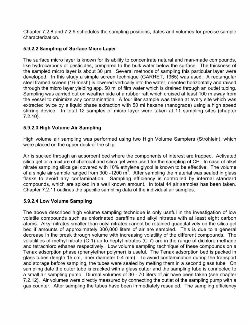
Chapter 7.2.8 and 7.2.9 schedules the sampling positions, dates and volumes for precise samplecharacterization.
5.9.2.2 Sampling of Surface Micro Layer
The surface micro layer is known for its ability to concentrate natural and man-made compounds,like hydrocarbons or pesticides, compared to the bulk water below the surface. The thickness ofthe sampled micro layer is about 30 µm. Several methods of sampling this particular layer weredeveloped. In this study a simple screen technique (GARRET, 1965) was used. A rectangularsteel framed screen (16-mesh) is lowered vertically into the water, oriented horizontally and raisedthrough the micro layer yielding app. 50 ml of film water which is drained through an outlet tubing.Sampling was carried out on weather side of a rubber raft which cruised at least 100 m away fromthe vessel to minimize any contamination. A four liter sample was taken at every site which wasextracted twice by a liquid phase extraction with 50 ml hexane (nanograde) using a high speedstirring device. In total 12 samples of micro layer were taken at 11 sampling sites (chapter7.2.10).
5.9.2.3 High Volume Air Sampling
High volume air sampling was performed using two High Volume Samplers (Ströhlein), whichwere placed on the upper deck of the ship.
Air is sucked through an adsorbent bed where the components of interest are trapped. Activatedsilica gel or a mixture of charcoal and silica gel were used for the sampling of CP. In case of alkylnitrate sampling silica gel covered with 10% ethylene glycol is known to be effective. The volumeof a single air sample ranged from 300 -1200 m3. After sampling the material was sealed in glassflasks to avoid any contamination. Sampling efficiency is controlled by internal standardcompounds, which are spiked in a well known amount. In total 44 air samples has been taken.Chapter 7.2.11 outlines the specific sampling data of the individual air samples.
5.9.2.4 Low Volume Sampling
The above described high volume sampling technique is only useful in the investigation of lowvolatile compounds such as chlorinated paraffins and alkyl nitrates with at least eight carbonatoms. Alkyl nitrates smaller than octyl nitrates cannot be retained quantitatively on the silica gelbed if amounts of approximately 300,000 liters of air are sampled. This is due to a generaldecrease in the break through volume with increasing volatility of the different compounds. Thevolatilities of methyl nitrate (C-1) up to heptyl nitrates (C-7) are in the range of dichloro methaneand tetrachloro ethanes respectively. Low volume sampling technique of these compounds on aTenax adsorption phase (phenylether polymer) is useful. The Tenax adsorption bed is packed inglass tubes (length 15 cm, inner diameter 0.4 mm). To avoid contamination during the transportand storage before sampling, the tubes were sealed by melting them in a second glass tube. Onsampling date the outer tube is cracked with a glass cutter and the sampling tube is connected toa small air sampling pump. Diurnal volumes of 30 - 70 liters of air have been taken (see chapter7.2.12). Air volumes were directly measured by connecting the outlet of the sampling pump with agas counter. After sampling the tubes have been immediately resealed. The sampling efficiency
can be proved, because most samples are taken using two Tenax glass tubes in a row. The firsttube represents the sample while the second will show a possible break through. Moreoverblanks of this sampling technique will be checked. Therefore two Tenax tubes were opened onthe ship and sealed afterwards without sampling. On M 28/2 twenty one low volume air sampleshave been taken. Explicit sample characterization (position, date, volumes) is depicted in chapter7.2.12. Sampling locations are displayed in Fig. 72.
Fig. 72: Locations of environmental chemistry samples
5.9.3 Analytical Methods
All samples were spiked with internal standards, sealed and carried to Germany. Organic traceanalysis requires high sensitive instrumentation (e.g. mass spectrometer) and the exclusion ofany sample contamination. Several control samples (blanks) document the background level.Thus sample preparation and analysis were not carried out on METEOR but at the University ofUlm under controlled background conditions (clean benches).
In cases of High Volume Air Sampling and Surface Seawater Sampling the adsorbents are elutedby organic solvents, cleaned-up and concentrated to a volume of 100 - 500 µl prior to analyticalmeasurement. For analysis high resolution gas chromatography with electron capture detection(HRGC-ECD) and mass selective detection (HRGC-MSD) were applied. The sensitive detectionof CP in negative chemical ionization mass spectrometry (NCI-MS) opens a classification intoshort-chain, intermediate and long-chain CP which gives more detailed information about thecomposition of a particular CP mixture.
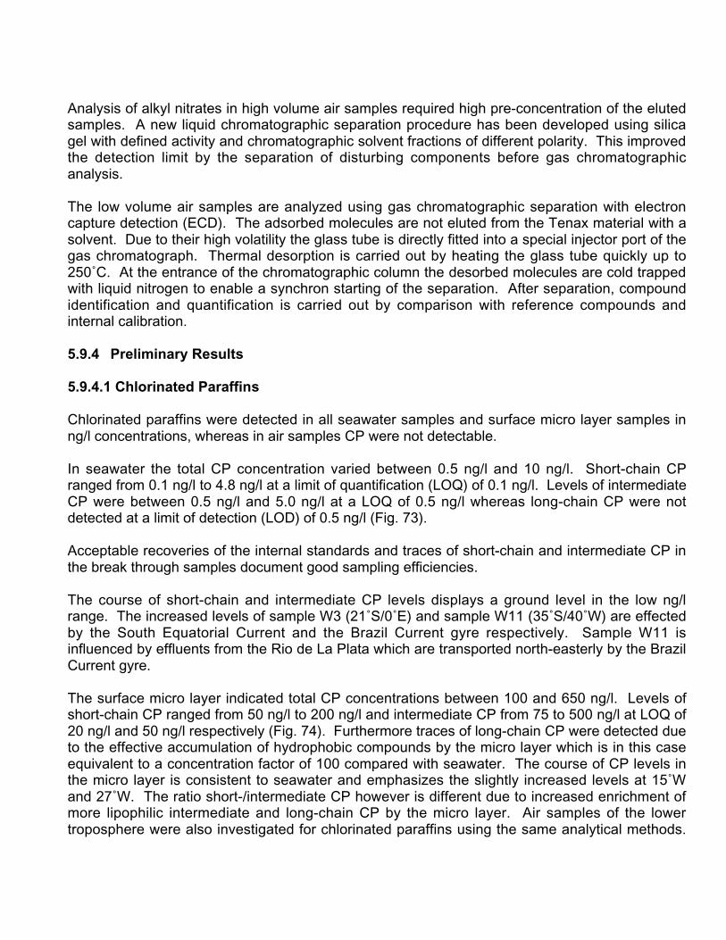
Analysis of alkyl nitrates in high volume air samples required high pre-concentration of the elutedsamples. A new liquid chromatographic separation procedure has been developed using silicagel with defined activity and chromatographic solvent fractions of different polarity. This improvedthe detection limit by the separation of disturbing components before gas chromatographicanalysis.
The low volume air samples are analyzed using gas chromatographic separation with electroncapture detection (ECD). The adsorbed molecules are not eluted from the Tenax material with asolvent. Due to their high volatility the glass tube is directly fitted into a special injector port of thegas chromatograph. Thermal desorption is carried out by heating the glass tube quickly up to250˚C. At the entrance of the chromatographic column the desorbed molecules are cold trappedwith liquid nitrogen to enable a synchron starting of the separation. After separation, compoundidentification and quantification is carried out by comparison with reference compounds andinternal calibration.
5.9.4 Preliminary Results
5.9.4.1 Chlorinated Paraffins
Chlorinated paraffins were detected in all seawater samples and surface micro layer samples inng/l concentrations, whereas in air samples CP were not detectable.
In seawater the total CP concentration varied between 0.5 ng/l and 10 ng/l. Short-chain CPranged from 0.1 ng/l to 4.8 ng/l at a limit of quantification (LOQ) of 0.1 ng/l. Levels of intermediateCP were between 0.5 ng/l and 5.0 ng/l at a LOQ of 0.5 ng/l whereas long-chain CP were notdetected at a limit of detection (LOD) of 0.5 ng/l (Fig. 73).
Acceptable recoveries of the internal standards and traces of short-chain and intermediate CP inthe break through samples document good sampling efficiencies.
The course of short-chain and intermediate CP levels displays a ground level in the low ng/lrange. The increased levels of sample W3 (21˚S/0˚E) and sample W11 (35˚S/40˚W) are effectedby the South Equatorial Current and the Brazil Current gyre respectively. Sample W11 isinfluenced by effluents from the Rio de La Plata which are transported north-easterly by the BrazilCurrent gyre.
The surface micro layer indicated total CP concentrations between 100 and 650 ng/l. Levels ofshort-chain CP ranged from 50 ng/l to 200 ng/l and intermediate CP from 75 to 500 ng/l at LOQ of20 ng/l and 50 ng/l respectively (Fig. 74). Furthermore traces of long-chain CP were detected dueto the effective accumulation of hydrophobic compounds by the micro layer which is in this caseequivalent to a concentration factor of 100 compared with seawater. The course of CP levels inthe micro layer is consistent to seawater and emphasizes the slightly increased levels at 15˚Wand 27˚W. The ratio short-/intermediate CP however is different due to increased enrichment ofmore lipophilic intermediate and long-chain CP by the micro layer. Air samples of the lowertroposphere were also investigated for chlorinated paraffins using the same analytical methods.
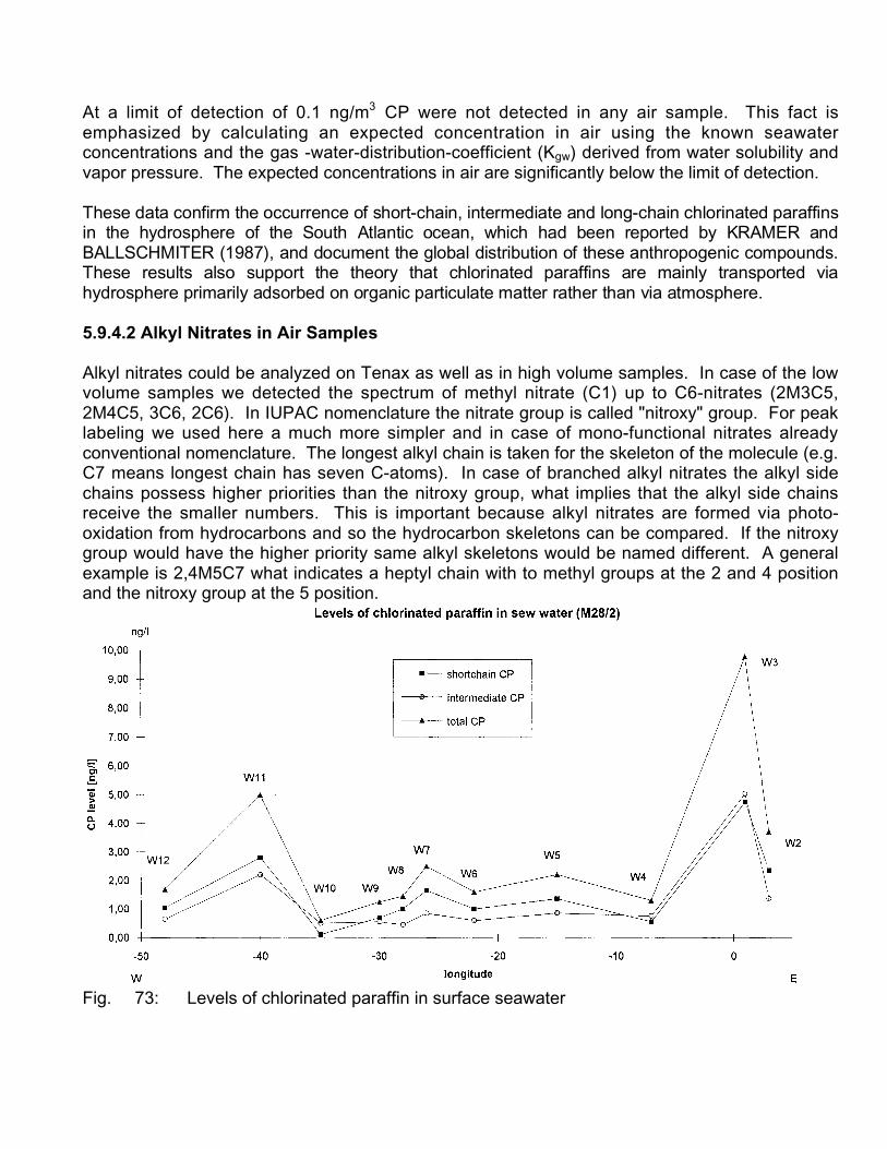
At a limit of detection of 0.1 ng/m3 CP were not detected in any air sample. This fact isemphasized by calculating an expected concentration in air using the known seawaterconcentrations and the gas -water-distribution-coefficient (Kgw) derived from water solubility andvapor pressure. The expected concentrations in air are significantly below the limit of detection.
T he se d a ta co nf ir m the o ccu rr en ce of sh or t- cha in , int er m ed ia t e an d lon g- cha in ch lo rin at ed p ar af fin sin th e hyd ro sph er e of th e Sou th At la n tic oce an , which ha d be e n re po r te d by KRAM ER an d BAL LSCHM IT ER (1 98 7) , and do cu me n t th e glo ba l dist ribu tio n of th ese a nt hr op o ge nic com po u nd s. T he se re su lt s also sup po r t th e the or y tha t chlor ina te d p ar af fin s ar e mainly tra n sp or te d via h yd ro sp h er e prima rily ad sor be d on or g an ic p a rt icu la te m a tt er ra th er th an via at m osph e re .
5.9.4.2 Alkyl Nitrates in Air Samples
Alkyl nitrates could be analyzed on Tenax as well as in high volume samples. In case of the lowvolume samples we detected the spectrum of methyl nitrate (C1) up to C6-nitrates (2M3C5,2M4C5, 3C6, 2C6). In IUPAC nomenclature the nitrate group is called "nitroxy" group. For peaklabeling we used here a much more simpler and in case of mono-functional nitrates alreadyconventional nomenclature. The longest alkyl chain is taken for the skeleton of the molecule (e.g.C7 means longest chain has seven C-atoms). In case of branched alkyl nitrates the alkyl sidechains possess higher priorities than the nitroxy group, what implies that the alkyl side chainsreceive the smaller numbers. This is important because alkyl nitrates are formed via photo-oxidation from hydrocarbons and so the hydrocarbon skeletons can be compared. If the nitroxygroup would have the higher priority same alkyl skeletons would be named different. A generalexample is 2,4M5C7 what indicates a heptyl chain with to methyl groups at the 2 and 4 positionand the nitroxy group at the 5 position.
Fig. 73: Levels of chlorinated paraffin in surface seawater
Fig. 74: Levels of chlorinated paraffin in the micro layer
Figure 75 depicts the separation of a 52.2 liter low volume air sample (LOW15) with highresolution gas chromatography and electron capture detection (HRGC-ECD) after thermaldesorption from the Tenax material. The detected alkyl nitrate peaks are marked by asterisks andpainted black. Beside the alkyl nitrates we determined high volatile halogenated hydrocarbonsespecially tetrachloro methane, tetrachloro ethylene and bromoform. Following table explains theabbreviations used in Figure 75 for halogenated hydrocarbons.
CH2BrCl Bromo-chloro methaneCHCl3 Chloroform111TCE 111-Trichloro ethaneCC14 carbon tetrachlorideTri Trichloro ethyleneCHBrCl2 Bromo-dichloro methanePer Tetrachloro ethyleneCHBr2Cl Dibromo-chloro methaneCHBr3 BromoformTCP (Int.St.) 123Trichloro propane (internal standard)PCE Pentachloro ethaneHCE Hexachloro ethane
Nevertheless the sample includes several unknown components predominantly in the mediumvolatile region (C6 - C8 nitrates). In case of an immense increase in the complexity of possiblebranched alkyl nitrates, reference compounds have to be synthesized for further identification.

Fig. 75: HRGC/ECD: Alkyl nitrates in a low volume air sample (LOW 15; aliquot 52.2 1)
The analysis of the high volume samples required intense effort in pre-separation before apossible gas chromatographic analysis of alkyl nitrates. Figure 76 exhibits an excellent highresolution gas chromatogram with mostly alkyl nitrates. We detected alkyl nitrates from C-6 up toC-14 with the typical separation pattern deriving from the n-alkanes, e.g. all n-nonyl nitrates arepresent in their correct relative concentrations. We obtained a maximum at C-11 nitrates.Interpretation of this result is yet very difficult. Detailed results are potential if the separationtechnique of C-15 - C-25 alkyl nitrates can be improved.
It must be noted that Figure 76 only depicts a fraction of the high volume air sample. The wholeair sample consists of a very complex composition. Gas chromatographic analysis without pre-separation would lead to no quantitative determination of alkyl nitrates. Furthermore we couldprove that also the branched alkyl nitrates are present in this fraction. Hence, several of theunlabeled peaks should represent branched alkyl nitrates.
Alkyl nitrates are not commercially available, therefore nearly all compounds have to besynthesized and reference standards have to be prepared for quantitative analysis. Firstquantitative estimations can be made. The concentrations of high volatile alkyl nitrates (lowvolume sampling) range in the medium to upper pg/m3, while the long-chain alkyl nitrates arepresent in the lower pg/m3 region. The much higher concentrations of short-chain alkyl nitratesare conform with present results. Only high volume sampling makes the detection of long-chainalkyl nitrates possible, because it involves an enrichment factor of approximately 100 relative to
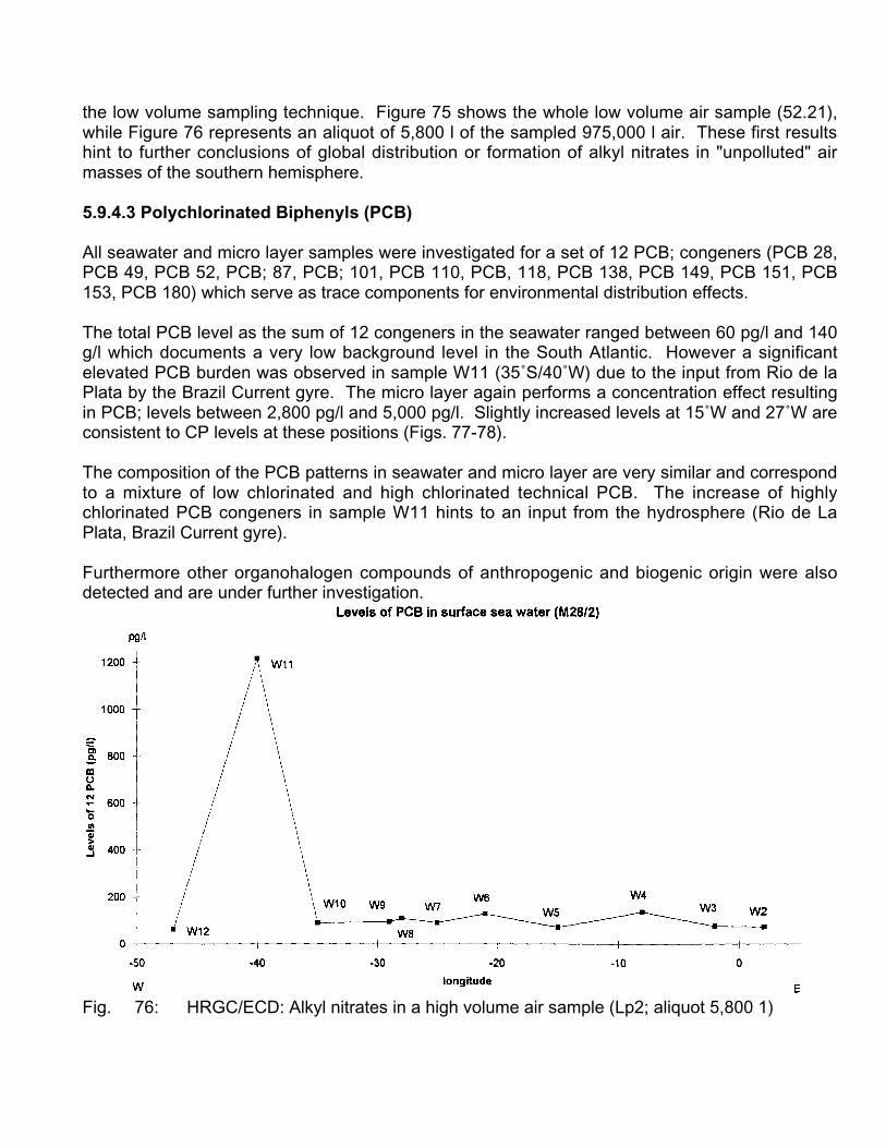
the low volume sampling technique. Figure 75 shows the whole low volume air sample (52.21),while Figure 76 represents an aliquot of 5,800 l of the sampled 975,000 l air. These first resultshint to further conclusions of global distribution or formation of alkyl nitrates in "unpolluted" airmasses of the southern hemisphere.
5.9.4.3 Polychlorinated Biphenyls (PCB)
All seawater and micro layer samples were investigated for a set of 12 PCB; congeners (PCB 28,PCB 49, PCB 52, PCB; 87, PCB; 101, PCB 110, PCB, 118, PCB 138, PCB 149, PCB 151, PCB153, PCB 180) which serve as trace components for environmental distribution effects.
The total PCB level as the sum of 12 congeners in the seawater ranged between 60 pg/l and 140g/l which documents a very low background level in the South Atlantic. However a significantelevated PCB burden was observed in sample W11 (35˚S/40˚W) due to the input from Rio de laPlata by the Brazil Current gyre. The micro layer again performs a concentration effect resultingin PCB; levels between 2,800 pg/l and 5,000 pg/l. Slightly increased levels at 15˚W and 27˚W areconsistent to CP levels at these positions (Figs. 77-78).
The composition of the PCB patterns in seawater and micro layer are very similar and correspondto a mixture of low chlorinated and high chlorinated technical PCB. The increase of highlychlorinated PCB congeners in sample W11 hints to an input from the hydrosphere (Rio de LaPlata, Brazil Current gyre).
Furthermore other organohalogen compounds of anthropogenic and biogenic origin were alsodetected and are under further investigation.
Fig. 76: HRGC/ECD: Alkyl nitrates in a high volume air sample (Lp2; aliquot 5,800 1)
Fig. 77: Level of ∑12 PCB in surface seawater
Fig. 78: Level of ∑12 PCB in surface micro layer
6 Ship's Meteorological Station (K. Flechsenhar)
6.1 Weather and Meteorological Conditions during Leg M 28/1
METEOR left the northeast Brazilian harbor Recife on March 29, 1994, steered south tosoutheastward doing station operations in coastal waters and reached the position 11˚20S/34˚W,which is the starting point of the projected WOCE section, on April 4. From this position on it wasto steer exactly east, doing all projected station operations on the same latitude. On April 4, thelongitude 30˚W was crossed.
Until April 9, METEOR sailed through the region of weak pressure gradients, which lies betweenthe subtropical South Atlantic high centered at 28˚S/5˚W and the equatorial low pressure zone.The Intertropical Convergence Zone (ITC) was placed in the western Atlantic just north of theequator and curved eastward up to 15˚N over Central Africa. Just south of the equator weaktropical disturbances moved westward, which could be noticed by some short showers nearMETEOR. Here weak easterly winds were dominating, height of swell 1.5 to 2 m.
From April 10 on, the eastsoutheasterly winds increased up to Bft 5, temporarily 6 at the northernparts of the above mentioned high, swell 2 to -3 in. On April 13, 20˚W and on April 19, 10˚W waspassed with east to southeast winds of 4 to 5 Bft and 2.5 m swell. On April 26, the Meridian 0was crossed with southeast winds of 3 to 4 Bft and a long swell of about 3 in from the southeast.On May 2, METEOR passed the Meridian 10˚E. Here the wind veered south to southwest anddecreased, caused by a stationary low over the Congo Basin. The swell decreased to 1 m. OnMay 4, 11˚20 S was left at 13˚E in the coastal waters of Angola for the first time. Until May 7,METEOR cruised near the coast of Angola doing station operations and then started her voyagedown to Walvis Bay, Namibia. In the last part of the voyage the dominating cold up-welling waterscaused fog and low clouds. The wind increased too. On May 11, METEOR moored in WalvisBay.
6.2 Weather and Meteorological Conditions during Leg M 28/2
METEOR left the harbor of Walvis Bay, Namibia, on May 15, 1994, and sailed first to the position21˚S/10˚W, where the station operations started. From this position on they steered west tosouthwest, doing all the projected station operations, and reached the Hunter Channel area(34˚S/28˚W) on May 27, where further station and mooring operations were done. Until May 25,the weather was fair, influenced by the stable subtropical South Atlantic high. But a steady 2 to 3m high swell made the ship roll, specially at the stations, disturbing the participants and causingsome lack of sleep. On May 25, a cyclogenetic process occurred near South Brazil, creating astorm centre, which moved eastsoutheast and caused winds Bft 6 to 7. After a rather calm periodon May 28/29, another storm cyclone created in the same area, bringing gale Bft 9 with gusts of11 to the heaving ship on May 30. From May 31 to the 3rd of June, a high was dominating, so thesearch operations for a trifting sound-producer on May 31/June I could be done under goodweather conditions, good sight and clear sky, but with a swell of 2 to 3 m. On June 4, anotherstorm cyclone approached from the Northwest, meeting METEOR at the position 33˚S/27˚W.After a while of high pressure influence with fair weather, METEOR reached the position40˚S/35˚W on June 7. There the ship found itself at the edge of a large storm cyclone with centre

between the Falkland Islands/Malvinas and the South Sandwich Islands. Here the wind increasedto Bft 7 to 8, becoming 4 to 6 later, and the swell increased up to 4 m, causing heavy pitching androlling. From June 6 on, the influence of a large high over Argentina was to be noticed by stableweather and a rather cool and steady southwest to west wind. This high moved graduallyeastward. So from June 10 on, METEOR met winds (Bft 6 to 7) from ahead. On June 12, thewind became weak, on June 13, they arrived at the Rio de la Plata with moderate winds fromsoutheast to east and a rainy weather. On June 14, METEOR moored in Buenos Aires,Argentina.

7 Lists
7.1 Leg M 28/1
7.1.1 List of Stations
StationNo.
Date Time Device Activity Length ofwire
Speed Winch Latitude Longitude
Station # 16429.03.94 UTC-3 GEK z/W, Schiff ADCP 08º07.5S 34º16.6W
17.30 (Kontinuierliches Messen mit ADCP; GEK - Messungenzwischen den einzelnen Stationen)
Station # 16523.12 CTD/Ro/WS z/W SL 4648 m W 03 08º16.9S 33º28.0W
30.03.94 01.52 CTD/Ro/WS a/D 08º16.5S 33º27.4W02.05 CTD/Ro/WS/ADCP z/W SL 991 m W 02 08º16.5S 33º27.4W02.49 CTD/Ro/WS/ADCP a/D 08º16.5S 33º27.4W02.55 NEUSS z/W V =2.3 Kn 08º16.3S 33º27.3W03.30 NEUSS a/D 08º14.7S 33º26.2W
Station # 16610.01 CTD/Ro/WS/ADCP z/W SL 999 m W 02 08º19.9S 32º29.9W10.55 CTD/Ro/WS/ADCP a/D 08º20.0S 32º29.7W11.10 CTD/Ro/WS z/W SL 4800 m W 03 08º19.8S 32º29.9W12.23 CTD/Ro/WS a/D 08º19.4S 32º29.8W13.59 NEUSS z/W V = 2.3 Kn 08º19.1S 32º29.7W14.32 NEUSS a/D 08º17.5S 32º29.4W
Station # 16721.06 CTD/Ro/WS z/W SL 4079 m W 03 09º15.1S 33º00.0W23.37 CTD/Ro/WS a/D 09º14.8S 32º59.9W23.58 CTD/Ro/WS/ADCP z/W SL 995 m W 02 09º14.9S 33º00.0W
31.03.94 00.28 CTD/Ro/WS/ADCP a/D 09º14.9S 33º00.0W00.58 MSN z/W SL 400 m V = 2.3 Kn W 09 09º14.7S 32º59.9W02.00 MSN a/D 09º11.2S 32º59.6W01.18 NEUSS z/W V = 2.3 Kn 09º13.4S 32º59.8W01.44 NEUSS a/D 09º11.9S 32º59.7W
Station # 16808.52 CTD/Ro/WS/ADCP z/W SL 994 m W 02 10º15.1S 33º30.1W09.43 CTD/Ro/WS/ADCP a/D 10º15.1S 33º29.9W

StationNo.
Date Time Device Activity Length ofwire
Speed Winch Latitude Longitude
10.00 CTD/Ro/WS z/W SL 4801 m W 03 10º15.0S 33º30.0W12.46 CTD/Ro/WS a/D 10º15.3S 33º29.3W13.01 MSN z/W SL 70 m V = 2.3 Kn W 09 10º14.9S 33º29.3W13.22 MSN a/D 10º14.1S 33º29.3W13.04 NEUSS z/W V = 2.3 Kn 10º14.8S 33º29.3W13.36 NEUSS a/d 10º13.6S 33º29.2W14.07 MSN z/W SL 375 m V = 2.3 Kn W 09 10º13.2S 33º28.8W14.53 MSN a7D 10º11.6S 33º28.3W
Wetter: SE 4 See 2 1012.7hPa c L 27.7ºW 28.9Station # 169
01.04.94 14.22 CTD/R o/WS/ADCP z/W SL 80 m W 02 10º03.6S 35º45.1W14.29 CTD/R o/WS/ADCP a/D 10º03.6S 35º45.0W14.37 CTD/R o/WS z/W SL 187 m W 03 10º03.6S 35º44.9W15.05 CTD/R o/WS a/D 10º03.6S 35º44.9W15.09 MSN z/W SL 127 m V = 2.3 Kn W 09 10º03.5S 35º44.9W15.30 MSN a/D 10º02.8S 35º44.7W15.12 NEUSS z/W V = 2.3 Kn 10º03.3S 35º44.8W15.42 NEUSS a/D 10º02.2S 35º44.4W
Station # 17016.35 CTD/Ro/WS/ADCP z/W SL 499 m W 02 10º06.2S 35º42.5W17.06 CTD/Ro/WS/ADCP a/D 10º05.9S 35º42.4W17.28 CTD/Ro/WS z/W SL 763 m W 03 10º06.2S 35º42.5W18.51 CTD/Ro/WS a/D 10º05.1S 35º41.9W18.58 MSN z/W SL 342 m V = 2.3 Kn W 09 10º05.0S 35º41.8W19.45 MSN a/D 10º02.9S 35º41.2W19.03 NEUSS z/W V = 2.3 Kn 10º04.8S 35º41.8W19.33 NEUSS a/D 10º03.3S 35º41.4W
Station # 17121.00 MSN z/W SL 280 m V = 2.3 Kn W 09 10º12.7S 35º38.3W21.42 MSN a/D 10º11.0S 35º37.7W21.04 NEUSS z/W V = 2.3 Kn 10º12.8S 35º38.1W21.33 NEUSS a/D 10º11.4S 35º37.8W22.03 CTD/Ro/WS/ADCP z/W SL 999 m W 02 10º10.2S 35º36.9W22.45 CTD/Ro/WS a/D 10º09.7S 35º36.5W23.09 CTD/Ro/WS z/W SL 2196 m W 03 10º10.2S 35º37.0W
02.04.94 01.07 CTD/Ro/WS a/D 10º09.2S 35º36.0W
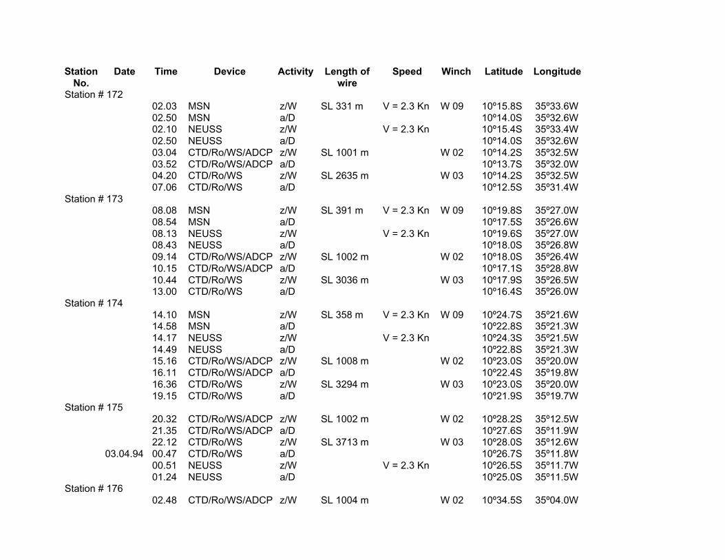
StationNo.
Date Time Device Activity Length ofwire
Speed Winch Latitude Longitude
Station # 17202.03 MSN z/W SL 331 m V = 2.3 Kn W 09 10º15.8S 35º33.6W02.50 MSN a/D 10º14.0S 35º32.6W02.10 NEUSS z/W V = 2.3 Kn 10º15.4S 35º33.4W02.50 NEUSS a/D 10º14.0S 35º32.6W03.04 CTD/Ro/WS/ADCP z/W SL 1001 m W 02 10º14.2S 35º32.5W03.52 CTD/Ro/WS/ADCP a/D 10º13.7S 35º32.0W04.20 CTD/Ro/WS z/W SL 2635 m W 03 10º14.2S 35º32.5W07.06 CTD/Ro/WS a/D 10º12.5S 35º31.4W
Station # 17308.08 MSN z/W SL 391 m V = 2.3 Kn W 09 10º19.8S 35º27.0W08.54 MSN a/D 10º17.5S 35º26.6W08.13 NEUSS z/W V = 2.3 Kn 10º19.6S 35º27.0W08.43 NEUSS a/D 10º18.0S 35º26.8W09.14 CTD/Ro/WS/ADCP z/W SL 1002 m W 02 10º18.0S 35º26.4W10.15 CTD/Ro/WS/ADCP a/D 10º17.1S 35º28.8W10.44 CTD/Ro/WS z/W SL 3036 m W 03 10º17.9S 35º26.5W13.00 CTD/Ro/WS a/D 10º16.4S 35º26.0W
Station # 17414.10 MSN z/W SL 358 m V = 2.3 Kn W 09 10º24.7S 35º21.6W14.58 MSN a/D 10º22.8S 35º21.3W14.17 NEUSS z/W V = 2.3 Kn 10º24.3S 35º21.5W14.49 NEUSS a/D 10º22.8S 35º21.3W15.16 CTD/Ro/WS/ADCP z/W SL 1008 m W 02 10º23.0S 35º20.0W16.11 CTD/Ro/WS/ADCP a/D 10º22.4S 35º19.8W16.36 CTD/Ro/WS z/W SL 3294 m W 03 10º23.0S 35º20.0W19.15 CTD/Ro/WS a/D 10º21.9S 35º19.7W
Station # 17520.32 CTD/Ro/WS/ADCP z/W SL 1002 m W 02 10º28.2S 35º12.5W21.35 CTD/Ro/WS/ADCP a/D 10º27.6S 35º11.9W22.12 CTD/Ro/WS z/W SL 3713 m W 03 10º28.0S 35º12.6W
03.04.94 00.47 CTD/Ro/WS a/D 10º26.7S 35º11.8W00.51 NEUSS z/W V = 2.3 Kn 10º26.5S 35º11.7W01.24 NEUSS a/D 10º25.0S 35º11.5W
Station # 17602.48 CTD/Ro/WS/ADCP z/W SL 1004 m W 02 10º34.5S 35º04.0W
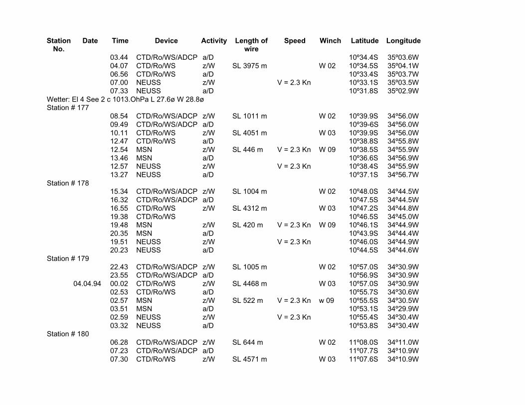
StationNo.
Date Time Device Activity Length ofwire
Speed Winch Latitude Longitude
03.44 CTD/Ro/WS/ADCP a/D 10º34.4S 35º03.6W04.07 CTD/Ro/WS z/W SL 3975 m W 02 10º34.5S 35º04.1W06.56 CTD/Ro/WS a/D 10º33.4S 35º03.7W07.00 NEUSS z/W V = 2.3 Kn 10º33.1S 35º03.5W07.33 NEUSS a/D 10º31.8S 35º02.9W
Wetter: El 4 See 2 c 1013.OhPa L 27.6ø W 28.8øStation # 177
08.54 CTD/Ro/WS/ADCP z/W SL 1011 m W 02 10º39.9S 34º56.0W09.49 CTD/Ro/WS/ADCP a/D 10º39-6S 34º56.0W10.11 CTD/Ro/WS z/W SL 4051 m W 03 10º39.9S 34º56.0W12.47 CTD/Ro/WS a/D 10º38.8S 34º55.8W12.54 MSN z/W SL 446 m V = 2.3 Kn W 09 10º38.5S 34º55.9W13.46 MSN a/D 10º36.6S 34º56.9W12.57 NEUSS z/W V = 2.3 Kn 10º38.4S 34º55.9W13.27 NEUSS a/D 10º37.1S 34º56.7W
Station # 17815.34 CTD/Ro/WS/ADCP z/W SL 1004 m W 02 10º48.0S 34º44.5W16.32 CTD/Ro/WS/ADCP a/D 10º47.5S 34º44.5W16.55 CTD/Ro/WS z/W SL 4312 m W 03 10º47.2S 34º44.8W19.38 CTD/Ro/WS 10º46.5S 34º45.0W19.48 MSN z/W SL 420 m V = 2.3 Kn W 09 10º46.1S 34º44.9W20.35 MSN a/D 10º43.9S 34º44.4W19.51 NEUSS z/W V = 2.3 Kn 10º46.0S 34º44.9W20.23 NEUSS a/D 10º44.5S 34º44.6W
Station # 17922.43 CTD/Ro/WS/ADCP z/W SL 1005 m W 02 10º57.0S 34º30.9W23.55 CTD/Ro/WS/ADCP a/D 10º56.9S 34º30.9W
04.04.94 00.02 CTD/Ro/WS z/W SL 4468 m W 03 10º57.0S 34º30.9W02.53 CTD/Ro/WS a/D 10º55.7S 34º30.6W02.57 MSN z/W SL 522 m V = 2.3 Kn w 09 10º55.5S 34º30.5W03.51 MSN a/D 10º53.1S 34º29.9W02.59 NEUSS z/W V = 2.3 Kn 10º55.4S 34º30.4W03.32 NEUSS a/D 10º53.8S 34º30.4W
Station # 18006.28 CTD/Ro/WS/ADCP z/W SL 644 m W 02 11º08.0S 34º11.0W07.23 CTD/Ro/WS/ADCP a/D 11º07.7S 34º10.9W07.30 CTD/Ro/WS z/W SL 4571 m W 03 11º07.6S 34º10.9W
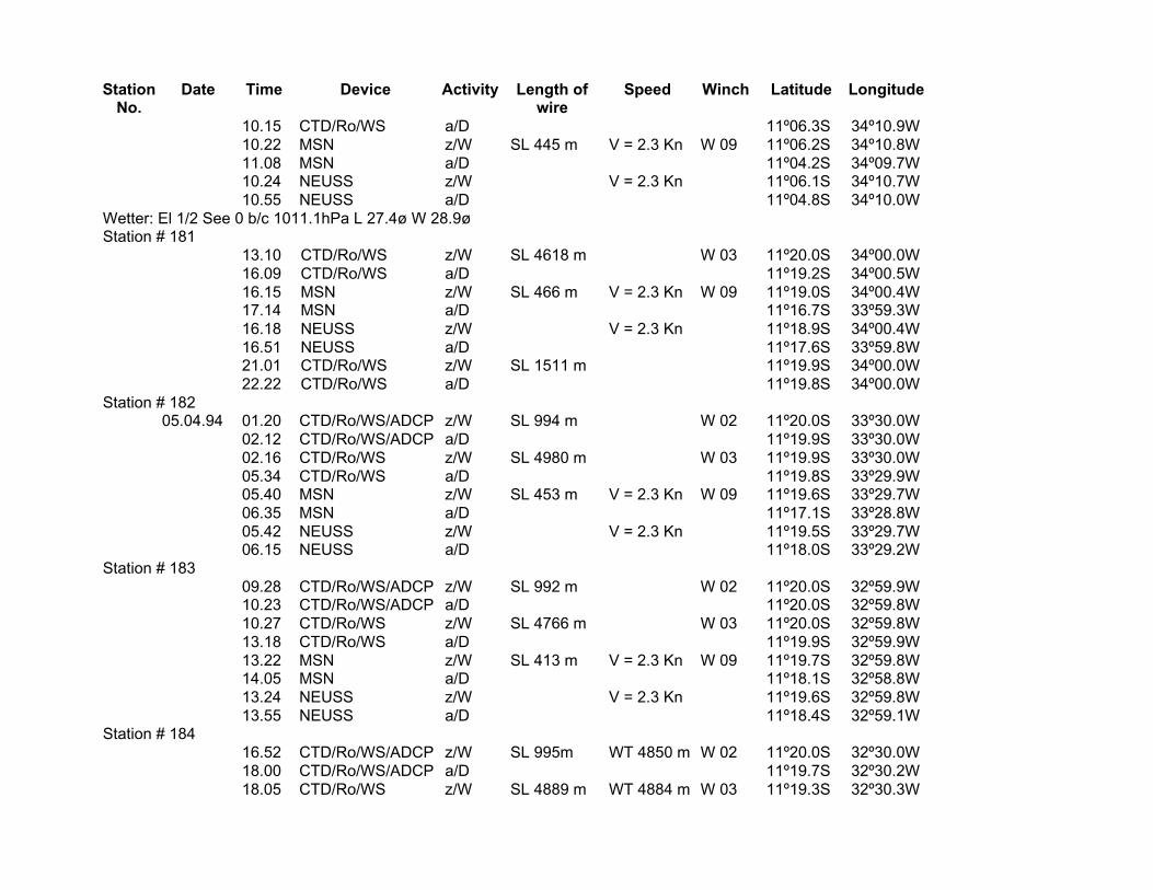
StationNo.
Date Time Device Activity Length ofwire
Speed Winch Latitude Longitude
10.15 CTD/Ro/WS a/D 11º06.3S 34º10.9W10.22 MSN z/W SL 445 m V = 2.3 Kn W 09 11º06.2S 34º10.8W11.08 MSN a/D 11º04.2S 34º09.7W10.24 NEUSS z/W V = 2.3 Kn 11º06.1S 34º10.7W10.55 NEUSS a/D 11º04.8S 34º10.0W
Wetter: El 1/2 See 0 b/c 1011.1hPa L 27.4ø W 28.9øStation # 181
13.10 CTD/Ro/WS z/W SL 4618 m W 03 11º20.0S 34º00.0W16.09 CTD/Ro/WS a/D 11º19.2S 34º00.5W16.15 MSN z/W SL 466 m V = 2.3 Kn W 09 11º19.0S 34º00.4W17.14 MSN a/D 11º16.7S 33º59.3W16.18 NEUSS z/W V = 2.3 Kn 11º18.9S 34º00.4W16.51 NEUSS a/D 11º17.6S 33º59.8W21.01 CTD/Ro/WS z/W SL 1511 m 11º19.9S 34º00.0W22.22 CTD/Ro/WS a/D 11º19.8S 34º00.0W
Station # 18205.04.94 01.20 CTD/Ro/WS/ADCP z/W SL 994 m W 02 11º20.0S 33º30.0W
02.12 CTD/Ro/WS/ADCP a/D 11º19.9S 33º30.0W02.16 CTD/Ro/WS z/W SL 4980 m W 03 11º19.9S 33º30.0W05.34 CTD/Ro/WS a/D 11º19.8S 33º29.9W05.40 MSN z/W SL 453 m V = 2.3 Kn W 09 11º19.6S 33º29.7W06.35 MSN a/D 11º17.1S 33º28.8W05.42 NEUSS z/W V = 2.3 Kn 11º19.5S 33º29.7W06.15 NEUSS a/D 11º18.0S 33º29.2W
Station # 18309.28 CTD/Ro/WS/ADCP z/W SL 992 m W 02 11º20.0S 32º59.9W10.23 CTD/Ro/WS/ADCP a/D 11º20.0S 32º59.8W10.27 CTD/Ro/WS z/W SL 4766 m W 03 11º20.0S 32º59.8W13.18 CTD/Ro/WS a/D 11º19.9S 32º59.9W13.22 MSN z/W SL 413 m V = 2.3 Kn W 09 11º19.7S 32º59.8W14.05 MSN a/D 11º18.1S 32º58.8W13.24 NEUSS z/W V = 2.3 Kn 11º19.6S 32º59.8W13.55 NEUSS a/D 11º18.4S 32º59.1W
Station # 18416.52 CTD/Ro/WS/ADCP z/W SL 995m WT 4850 m W 02 11º20.0S 32º30.0W18.00 CTD/Ro/WS/ADCP a/D 11º19.7S 32º30.2W18.05 CTD/Ro/WS z/W SL 4889 m WT 4884 m W 03 11º19.3S 32º30.3W

StationNo.
Date Time Device Activity Length ofwire
Speed Winch Latitude Longitude
20.58 CTD/Ro/WS a/D 11º18.9S 32º30.3W21.05 MSN z/W SL 458 m V = 2.3 Kn W 09 11º18.6S 32º30.2W21.57 MSN a/D V = 2.3 Kn 11º18.6S 32º30.1W21.40 NEUSS a/D 11º17.3S 32º29.4W
Station # 18506.04.94 00.44 CTD/Ro/WS/ADCP z/W SL 993 m WT 5060 m W 02 11º20.0S 32º00.0W
01.43 CTD/Ro/Ws/ADCP a/D 11º20.0S 32º00.0W01.47 CTD/Ro/WS z/W SL 5067 m WT 5060 m W 03 11º20.0S 32º00.0W04.58 CTD/Ro/WS a/D 11º19.9S 31º59.6W05.05 MSN z/W SL 466 m V = 2.3 Kn W 09 11º19.8S 31º59.5W06.05 MSN a/D 11º17.3S 31º58.3W05.07 NEUSS z/W V = 2.3 Kn 11º19.7S 31º59.4W05.40 NEUSS a/D 11º18.3S 31º58.8W
Station # 18609.49 CTD/Ro/WS/ADCP z/W SL 994 m WT 5220 m W 02 11º20.0S 31º19.9W10.44 CTD/Ro/WS/ADCP a/D 11º19.7S 31º20.0W10.49 CTD/Ro/WS z/W SL 5256 m WT 5220 m W 03 11º19.6S 31º20.0W13.57 CTD/Ro/WS a/D 11º19.3S 31º20.0W14.02 MSN z/W SL 459 m V = 2.3 Kn W 09 11º19.1S 31º19.9W14.54 MSN a/D 11º17.2S 31º18.7W14.02 NEUSS z/W V = 2.3 Kn 11º19.1S 31º19.9W14.36 NEUSS a/D 11º17.9S 31º19.1W
Wetter: E'l 1/2 S 0 b/C 1010.6hPa L 27.1ø W 28.7øStation # 187
18.55 CTD/Ro/WS/ADCP z/W SL 997 m WT 5296 m W 02 11º20.0S 30º40.0W20.02 CTD/Ro/WS/ADCP a/D 11º20.0S 30º40.0W20.09 CTD/Ro/WS z/W SL 5327 m WT 5296 m W 03 11º20.0S 30º40.0W23.05 CTD/Ro/WS a/D 11º20.1S 30º40.0W23.12 MSN z/W SL 474 m V = 2.3 Kn W 09 11º19.9S 30º39.8W00.04 MSN a/D 11º17.2S 30º39.5W23.16 NEUSS z/W V = 2.3 Kn 11º19.7S 30º39.9W23.46 NEUSS a/D 11º18.1S 30º39.6W
Station # 18802.05.94 04.10 CTD/Ro/WS/ADCP z/W SL 993 m WT 5382 m W 02 11º20.0S 30º00.0W
05.22 CTD/Ro/WS/ADCP a/D 11º20.1S 30º00.0W05.32 CTD/Ro/WS z/W SL 5412 m WT 5382 m W 03 11º20.1S 29º59.9W08.33 CTD/RO/WS a/D 11º19.9S 29º59.9W
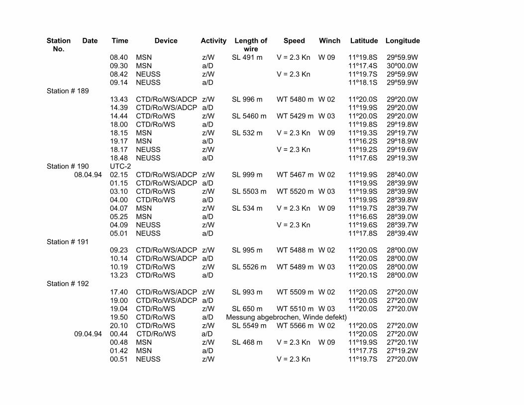
StationNo.
Date Time Device Activity Length ofwire
Speed Winch Latitude Longitude
08.40 MSN z/W SL 491 m V = 2.3 Kn W 09 11º19.8S 29º59.9W09.30 MSN a/D 11º17.4S 30º00.0W08.42 NEUSS z/W V = 2.3 Kn 11º19.7S 29º59.9W09.14 NEUSS a/D 11º18.1S 29º59.9W
Station # 18913.43 CTD/Ro/WS/ADCP z/W SL 996 m WT 5480 m W 02 11º20.0S 29º20.0W14.39 CTD/Ro/WS/ADCP a/D 11º19.9S 29º20.0W14.44 CTD/Ro/WS z/W SL 5460 m WT 5429 m W 03 11º20.0S 29º20.0W18.00 CTD/Ro/WS a/D 11º19.8S 29º19.8W18.15 MSN z/W SL 532 m V = 2.3 Kn W 09 11º19.3S 29º19.7W19.17 MSN a/D 11º16.2S 29º18.9W18.17 NEUSS z/W V = 2.3 Kn 11º19.2S 29º19.6W18.48 NEUSS a/D 11º17.6S 29º19.3W
Station # 190 UTC-208.04.94 02.15 CTD/Ro/WS/ADCP z/W SL 999 m WT 5467 m W 02 11º19.9S 28º40.0W
01.15 CTD/Ro/WS/ADCP a/D 11º19.9S 28º39.9W03.10 CTD/Ro/WS z/W SL 5503 m WT 5520 m W 03 11º19.9S 28º39.9W04.00 CTD/Ro/WS a/D 11º19.9S 28º39.8W04.07 MSN z/W SL 534 m V = 2.3 Kn W 09 11º19.7S 28º39.7W05.25 MSN a/D 11º16.6S 28º39.0W04.09 NEUSS z/W V = 2.3 Kn 11º19.6S 28º39.7W05.01 NEUSS a/D 11º17.8S 28º39.4W
Station # 19109.23 CTD/Ro/WS/ADCP z/W SL 995 m WT 5488 m W 02 11º20.0S 28º00.0W10.14 CTD/Ro/WS/ADCP a/D 11º20.0S 28º00.0W10.19 CTD/Ro/WS z/W SL 5526 m WT 5489 m W 03 11º20.0S 28º00.0W13.23 CTD/Ro/WS a/D 11º20.1S 28º00.0W
Station # 19217.40 CTD/Ro/WS/ADCP z/W SL 993 m WT 5509 m W 02 11º20.0S 27º20.0W19.00 CTD/Ro/WS/ADCP a/D 11º20.0S 27º20.0W19.04 CTD/Ro/WS z/W SL 650 m WT 5510 m W 03 11º20.0S 27º20.0W19.50 CTD/Ro/WS a/D Messung abgebrochen, Winde defekt)20.10 CTD/Ro/WS z/W SL 5549 m WT 5566 m W 02 11º20.0S 27º20.0W
09.04.94 00.44 CTD/Ro/WS a/D 11º20.0S 27º20.0W00.48 MSN z/W SL 468 m V = 2.3 Kn W 09 11º19.9S 27º20.1W01.42 MSN a/D 11º17.7S 27º19.2W00.51 NEUSS z/W V = 2.3 Kn 11º19.7S 27º20.0W
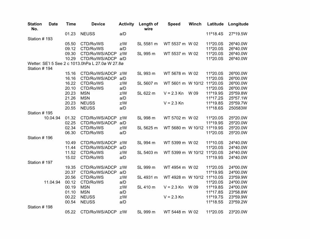
StationNo.
Date Time Device Activity Length ofwire
Speed Winch Latitude Longitude
01.23 NEUSS a/D 11º18.4S 27º19.5WStation # 193
05.50 CTD/Ro/WS z/W SL 5581 m WT 5537 m W 02 11º20.0S 26º40.0W09.12 CTD/Ro/WS a/D 11º20.0S 26º40.0W09.30 CTD/Ro/WS/ADCP z/W SL 995 m WT 5537 m W 02 11º20.0S 26º40.0W10.29 CTD/Ro/WS/ADCP a/D 11º20.0S 26º40.0W
Wetter: SE’I 5 See 2 c 1013.0hPa L 27.0ø W 27.8øStation # 194
15.16 CTD/Ro/WS/ADCP z/W SL 993 m WT 5678 m W 02 11º20.0S 26º00.0W16.16 CTD/Ro/WS/ADCP a/D 11º20.0S 26º00.0W16.22 CTD/Ro/WS z/W SL 5607 m WT 5601 m W 10/12 11º20.0S 26º00.0W20.10 CTD/Ro/WS a/D 11º20.0S 26º00.0W20.23 MSN z/W SL 622 m V = 2.3 Kn W 09 11º19.9S 25º59.8W21.26 MSN a/D 11º17.2S 25º57.1W20.23 NEUSS z/W V = 2.3 Kn 11º19.8S 25º59.7W20.55 NEUSS a/D 11º18.6S 250583W
Station # 19510.04.94 01.32 CTD/Ro/WS/ADCP z/W SL 998 m WT 5702 m W 02 11º20.0S 25º20.0W
02.25 CTD/Ro/WS/ADCP a/D 11º19.9S 25º20.0W02.34 CTD/Ro/WS z/W SL 5625 m WT 5680 m W 10/12 11º19.9S 25º20.0W06.30 CTD/Ro/WS a/D 11º20.0S 25º20.0W
Station # 19610.49 CTD/Ro/WS/ADCP z/W SL 994 m WT 5399 m W 02 11º10.0S 24º40.0W11.44 CTD/Ro/WS/ADCP a/D 11º20.0S 24º40.0W11.52 CTD/Ro/WS z/W SL 5403 m WT 5399 m W 10/12 11º20.0S 24º40.0W15.02 CTD/Ro/WS a/D 11º19.9S 24º40.0W
Station # 19719.35 CTD/Ro/WS/ADCP z/W SL 999 m WT 4954 m W 02 11º20.0S 24º00.0W20.37 CTD/Ro/WS/ADCP a/D 11º19.9S 24º00.0W20.56 CTD/Ro/WS z/W SL 4931 m WT 4928 m W 10/12 11º10.0S 23º59.9W
11.04.94 00.12 CTD/Ro/WS a/D 11º20.0S 24º00.0W00.19 MSN z/W SL 410 m V = 2.3 Kn W 09 11º19.8S 24º00.0W01.10 MSN a/D 11º17.8S 23º58.8W00.22 NEUSS z/W V = 2.3 Kn 11º19.7S 23º59.9W00.54 NEUSS a/D 11º18.5S 23º59.2W
Station # 19805.22 CTD/Ro/WS/ADCP z/W SL 999 m WT 5448 m W 02 11º20.0S 23º20.0W
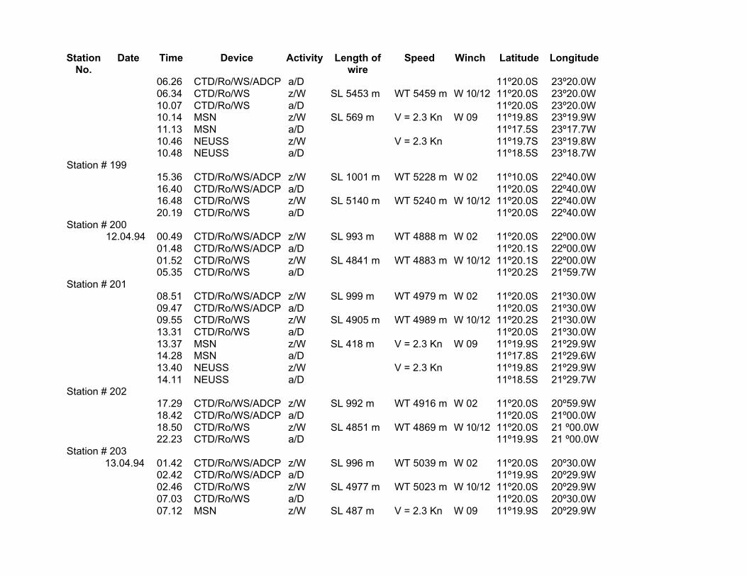
StationNo.
Date Time Device Activity Length ofwire
Speed Winch Latitude Longitude
06.26 CTD/Ro/WS/ADCP a/D 11º20.0S 23º20.0W06.34 CTD/Ro/WS z/W SL 5453 m WT 5459 m W 10/12 11º20.0S 23º20.0W10.07 CTD/Ro/WS a/D 11º20.0S 23º20.0W10.14 MSN z/W SL 569 m V = 2.3 Kn W 09 11º19.8S 23º19.9W11.13 MSN a/D 11º17.5S 23º17.7W10.46 NEUSS z/W V = 2.3 Kn 11º19.7S 23º19.8W10.48 NEUSS a/D 11º18.5S 23º18.7W
Station # 19915.36 CTD/Ro/WS/ADCP z/W SL 1001 m WT 5228 m W 02 11º10.0S 22º40.0W16.40 CTD/Ro/WS/ADCP a/D 11º20.0S 22º40.0W16.48 CTD/Ro/WS z/W SL 5140 m WT 5240 m W 10/12 11º20.0S 22º40.0W20.19 CTD/Ro/WS a/D 11º20.0S 22º40.0W
Station # 20012.04.94 00.49 CTD/Ro/WS/ADCP z/W SL 993 m WT 4888 m W 02 11º20.0S 22º00.0W
01.48 CTD/Ro/WS/ADCP a/D 11º20.1S 22º00.0W01.52 CTD/Ro/WS z/W SL 4841 m WT 4883 m W 10/12 11º20.1S 22º00.0W05.35 CTD/Ro/WS a/D 11º20.2S 21º59.7W
Station # 20108.51 CTD/Ro/WS/ADCP z/W SL 999 m WT 4979 m W 02 11º20.0S 21º30.0W09.47 CTD/Ro/WS/ADCP a/D 11º20.0S 21º30.0W09.55 CTD/Ro/WS z/W SL 4905 m WT 4989 m W 10/12 11º20.2S 21º30.0W13.31 CTD/Ro/WS a/D 11º20.0S 21º30.0W13.37 MSN z/W SL 418 m V = 2.3 Kn W 09 11º19.9S 21º29.9W14.28 MSN a/D 11º17.8S 21º29.6W13.40 NEUSS z/W V = 2.3 Kn 11º19.8S 21º29.9W14.11 NEUSS a/D 11º18.5S 21º29.7W
Station # 20217.29 CTD/Ro/WS/ADCP z/W SL 992 m WT 4916 m W 02 11º20.0S 20º59.9W18.42 CTD/Ro/WS/ADCP a/D 11º20.0S 21º00.0W18.50 CTD/Ro/WS z/W SL 4851 m WT 4869 m W 10/12 11º20.0S 21 º00.0W22.23 CTD/Ro/WS a/D 11º19.9S 21 º00.0W
Station # 20313.04.94 01.42 CTD/Ro/WS/ADCP z/W SL 996 m WT 5039 m W 02 11º20.0S 20º30.0W
02.42 CTD/Ro/WS/ADCP a/D 11º19.9S 20º29.9W02.46 CTD/Ro/WS z/W SL 4977 m WT 5023 m W 10/12 11º20.0S 20º29.9W07.03 CTD/Ro/WS a/D 11º20.0S 20º30.0W07.12 MSN z/W SL 487 m V = 2.3 Kn W 09 11º19.9S 20º29.9W

StationNo.
Date Time Device Activity Length ofwire
Speed Winch Latitude Longitude
08.05 MSN a/D 11º18.1S 20º28.3W07.15 NEUSS z/W V = 2.3 Kn 11º19.9S 20º29.9W07.45 NEUSS a/D 11º18.8S 20º29.0W
Station # 20411.15 CTD/Ro/WS/ADCP z/W SL 997 m WT 4753 m W 02 11º20.0S 20º00.0W12.07 CTD/Ro/WS/ADCP a/D 11º20.0S 20º00.0WWetter E 4/5 See 2 c 1012.9hPa L 26.4ø W 27.5ø12.18 Test mit Dummy SL 4415 m WT 4710 m W 03 11º20.0S 20º00.0W14.48 Dummy a/D 11º19.9S 20º00.0W14.54 CTD/Ro/WS z/W SL 4713 m WT 4751 m W 03 11º19.9S 20º00.0W18.15 CTD/Ro/WS a/D 11º20.0S 19º59.9W18.25 Drifter m. Segel z/W 11º19.8S 19º59.7W
Station # 20521.32 CTD/Ro/WS/ADCP z/W SL 993 m WT 4837 m W 02 11º20.0S 19º30.0W22.00 CTD/Ro/WS/ADCP a/D 11º20.0S 19º30.0W22.39 CTD/Ro/WS z/W SL 4743 m WT 4796 m W 03 11º20.0S 19º30.0W
14.04.94 01.39 CTD/Ro/WS a/D 11º20.0S 19º29.9W01.46 MSN z/W SL 485 m V = 2.3 Kn W 09 11º19.8S 19º29.9W02.43 MSN a/D 11º17.2S 19º29.3W01.49 NEUSS z/W V = 2.3 Kn 11º19.7S 19º29.8W02.20 NEUSS a/D 11º18.1S 19º29.5W
Station # 20605.40 CTD/Ro/WS/ADCP z/W SL 1001 m WT 4573 m W 02 11º10.0S 19º00.0W06.43 CTD/Ro/WS/ADCP a/D 11º20.0S 19º00.0W06.50 CTD/Ro/WS z/W SL 4542 m WT 4565 m W 03 11º20.0S 19º00.0W09.47 CTD/Ro/WS a/D 11º20.1S 18º59.9W09.54 Drifter m. Segel z/W 11º20.1S 18º59.8W
Station # 20712.48 CTD/Ro/WS/ADCP z/W SL 995 m WT 4115 m W 02 11º20.0S 18º30.0W13.45 CTD/Ro/WS/ADCP a/D 11º20.1S 18º29.9W13.54 CTD/Ro/WS z/W SL 4083 m WT 4114 m W 03 11º20.0S 18º30.0W16.40 CTD/Ro/WS a/D 11º20.1S 18º29.8W
Station # 20819.30 CTD/Ro/WS/ADCP z/W SL 994 m WT 4411 m W 02 11º20.0S 18º00.0W20.28 CTD/Ro/WS/ADCP a/D 11º20.0S 18º00.0W20.34 CTD/Ro/WS z/W SL 4326 m WT 4417 m W 03 11º20.0S 18º00.0W23.55 CTD/Ro/WS a/D 11º19.9S 17º59.8W
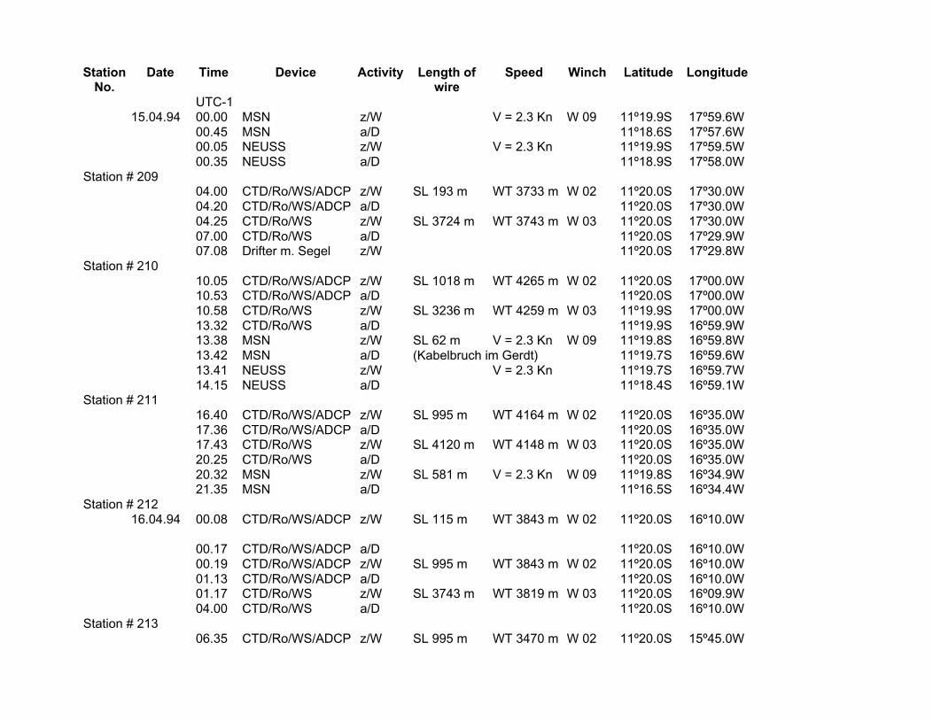
StationNo.
Date Time Device Activity Length ofwire
Speed Winch Latitude Longitude
UTC-115.04.94 00.00 MSN z/W V = 2.3 Kn W 09 11º19.9S 17º59.6W
00.45 MSN a/D 11º18.6S 17º57.6W00.05 NEUSS z/W V = 2.3 Kn 11º19.9S 17º59.5W00.35 NEUSS a/D 11º18.9S 17º58.0W
Station # 20904.00 CTD/Ro/WS/ADCP z/W SL 193 m WT 3733 m W 02 11º20.0S 17º30.0W04.20 CTD/Ro/WS/ADCP a/D 11º20.0S 17º30.0W04.25 CTD/Ro/WS z/W SL 3724 m WT 3743 m W 03 11º20.0S 17º30.0W07.00 CTD/Ro/WS a/D 11º20.0S 17º29.9W07.08 Drifter m. Segel z/W 11º20.0S 17º29.8W
Station # 21010.05 CTD/Ro/WS/ADCP z/W SL 1018 m WT 4265 m W 02 11º20.0S 17º00.0W10.53 CTD/Ro/WS/ADCP a/D 11º20.0S 17º00.0W10.58 CTD/Ro/WS z/W SL 3236 m WT 4259 m W 03 11º19.9S 17º00.0W13.32 CTD/Ro/WS a/D 11º19.9S 16º59.9W13.38 MSN z/W SL 62 m V = 2.3 Kn W 09 11º19.8S 16º59.8W13.42 MSN a/D (Kabelbruch im Gerdt) 11º19.7S 16º59.6W13.41 NEUSS z/W V = 2.3 Kn 11º19.7S 16º59.7W14.15 NEUSS a/D 11º18.4S 16º59.1W
Station # 21116.40 CTD/Ro/WS/ADCP z/W SL 995 m WT 4164 m W 02 11º20.0S 16º35.0W17.36 CTD/Ro/WS/ADCP a/D 11º20.0S 16º35.0W17.43 CTD/Ro/WS z/W SL 4120 m WT 4148 m W 03 11º20.0S 16º35.0W20.25 CTD/Ro/WS a/D 11º20.0S 16º35.0W20.32 MSN z/W SL 581 m V = 2.3 Kn W 09 11º19.8S 16º34.9W21.35 MSN a/D 11º16.5S 16º34.4W
Station # 21216.04.94 00.08 CTD/Ro/WS/ADCP z/W SL 115 m WT 3843 m W 02 11º20.0S 16º10.0W
00.17 CTD/Ro/WS/ADCP a/D 11º20.0S 16º10.0W00.19 CTD/Ro/WS/ADCP z/W SL 995 m WT 3843 m W 02 11º20.0S 16º10.0W01.13 CTD/Ro/WS/ADCP a/D 11º20.0S 16º10.0W01.17 CTD/Ro/WS z/W SL 3743 m WT 3819 m W 03 11º20.0S 16º09.9W04.00 CTD/Ro/WS a/D 11º20.0S 16º10.0W
Station # 21306.35 CTD/Ro/WS/ADCP z/W SL 995 m WT 3470 m W 02 11º20.0S 15º45.0W
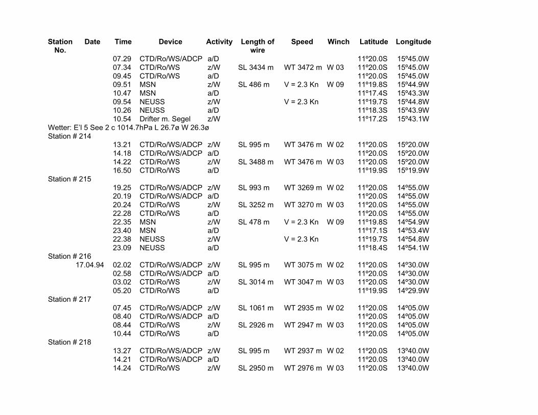
StationNo.
Date Time Device Activity Length ofwire
Speed Winch Latitude Longitude
07.29 CTD/Ro/WS/ADCP a/D 11º20.0S 15º45.0W07.34 CTD/Ro/WS z/W SL 3434 m WT 3472 m W 03 11º20.0S 15º45.0W09.45 CTD/Ro/WS a/D 11º20.0S 15º45.0W09.51 MSN z/W SL 486 m V = 2.3 Kn W 09 11º19.8S 15º44.9W10.47 MSN a/D 11º17.4S 15º43.3W09.54 NEUSS z/W V = 2.3 Kn 11º19.7S 15º44.8W10.26 NEUSS a/D 11º18.3S 15º43.9W10.54 Drifter m. Segel z/W 11º17.2S 15º43.1W
Wetter: E’l 5 See 2 c 1014.7hPa L 26.7ø W 26.3øStation # 214
13.21 CTD/Ro/WS/ADCP z/W SL 995 m WT 3476 m W 02 11º20.0S 15º20.0W14.18 CTD/Ro/WS/ADCP a/D 11º20.0S 15º20.0W14.22 CTD/Ro/WS z/W SL 3488 m WT 3476 m W 03 11º20.0S 15º20.0W16.50 CTD/Ro/WS a/D 11º19.9S 15º19.9W
Station # 21519.25 CTD/Ro/WS/ADCP z/W SL 993 m WT 3269 m W 02 11º20.0S 14º55.0W20.19 CTD/Ro/WS/ADCP a/D 11º20.0S 14º55.0W20.24 CTD/Ro/WS z/W SL 3252 m WT 3270 m W 03 11º20.0S 14º55.0W22.28 CTD/Ro/WS a/D 11º20.0S 14º55.0W22.35 MSN z/W SL 478 m V = 2.3 Kn W 09 11º19.8S 14º54.9W23.40 MSN a/D 11º17.1S 14º53.4W22.38 NEUSS z/W V = 2.3 Kn 11º19.7S 14º54.8W23.09 NEUSS a/D 11º18.4S 14º54.1W
Station # 21617.04.94 02.02 CTD/Ro/WS/ADCP z/W SL 995 m WT 3075 m W 02 11º20.0S 14º30.0W
02.58 CTD/Ro/WS/ADCP a/D 11º20.0S 14º30.0W03.02 CTD/Ro/WS z/W SL 3014 m WT 3047 m W 03 11º20.0S 14º30.0W05.20 CTD/Ro/WS a/D 11º19.9S 14º29.9W
Station # 21707.45 CTD/Ro/WS/ADCP z/W SL 1061 m WT 2935 m W 02 11º20.0S 14º05.0W08.40 CTD/Ro/WS/ADCP a/D 11º20.0S 14º05.0W08.44 CTD/Ro/WS z/W SL 2926 m WT 2947 m W 03 11º20.0S 14º05.0W10.44 CTD/Ro/WS a/D 11º20.0S 14º05.0W
Station # 21813.27 CTD/Ro/WS/ADCP z/W SL 995 m WT 2937 m W 02 11º20.0S 13º40.0W14.21 CTD/Ro/WS/ADCP a/D 11º20.0S 13º40.0W14.24 CTD/Ro/WS z/W SL 2950 m WT 2976 m W 03 11º20.0S 13º40.0W
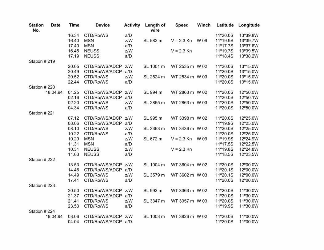
StationNo.
Date Time Device Activity Length ofwire
Speed Winch Latitude Longitude
16.34 CTD/Ro/WS a/D 11º20.0S 13º39.8W16.40 MSN z/W SL 582 m V = 2.3 Kn W 09 11º19.9S 13º39.7W17.40 MSN a/D 11º17.7S 13º37.6W16.45 NEUSS z/W V = 2.3 Kn 11º19.7S 13º39.5W17.19 NEUSS a/D 11º18.4S 13º38.2W
Station # 21920.05 CTD/Ro/WS/ADCP z/W SL 1001 m WT 2535 m W 02 11º20.0S 13º15.0W20.49 CTD/Ro/WS/ADCP a/D 11º20.0S 13º15.0W20.52 CTD/Ro/WS z/W SL 2524 m WT 2534 m W 03 11º20.0S 13º15.0W22.44 CTD/Ro/WS a/D 11º20.0S 13º15.0W
Station # 22018.04.94 01.25 CTD/Ro/WS/ADCP z/W SL 994 m WT 2863 m W 02 11º20.0S 12º50.0W
02.16 CTD/Ro/WS/ADCP a/D 11º20.0S 12º50.1W02.20 CTD/Ro/WS z/W SL 2865 m WT 2863 m W 03 11º20.0S 12º50.0W04.34 CTD/Ro/WS a/D 11º20.0S 12º50.0W
Station # 22107.12 CTD/Ro/WS/ADCP z/W SL 995 m WT 3398 m W 02 11º20.0S 12º25.0W08.06 CTD/Ro/WS/ADCP a/D 11º19.9S 12º25.0W08.10 CTD/Ro/WS z/W SL 3363 m WT 3436 m W 02 11º20.0S 12º25.0W10.22 CTD/Ro/WS a/D 11º20.0S 12º25.0W10.29 MSN z/W SL 672 m V = 2.3 Kn W 09 11º19.9S 12º24.9W11.31 MSN a/D 11º17.5S 12º22.5W10.31 NEUSS z/W V = 2.3 Kn 11º19.8S 12º24.8W11.03 NEUSS a/D 11º18.5S 12º23.5W
Station # 22213.53 CTD/Ro/WS/ADCP z/W SL 1004 m WT 3604 m W 02 11º20.0S 12º00.0W14.46 CTD/Ro/WS/ADCP a/D 11º20.1S 12º00.0W14.49 CTD/Ro/WS z/W SL 3579 m WT 3602 m W 03 11º20.1S 12º00.0W17.41 CTD/Ro/WS a/D 11º20.0S 12º00.0W
Station # 22320.50 CTD/Ro/WS/ADCP z/W SL 993 m WT 3363 m W 02 11º20.0S 11º30.0W21.37 CTD/Ro/WS/ADCP a/D 11º20.0S 11º30.0W21.41 CTD/Ro/WS z/W SL 3347 m WT 3357 m W 03 11º20.0S 11º30.0W23.53 CTD/Ro/WS a/D 11º19.9S 11º30.0W
Station # 22419.04.94 03.06 CTD/Ro/WS/ADCP z/W SL 1003 m WT 3826 m W 02 11º20.0S 11º00.0W
04.04 CTD/Ro/WS/ADCP a/D 11º20.0S 11º00.0W
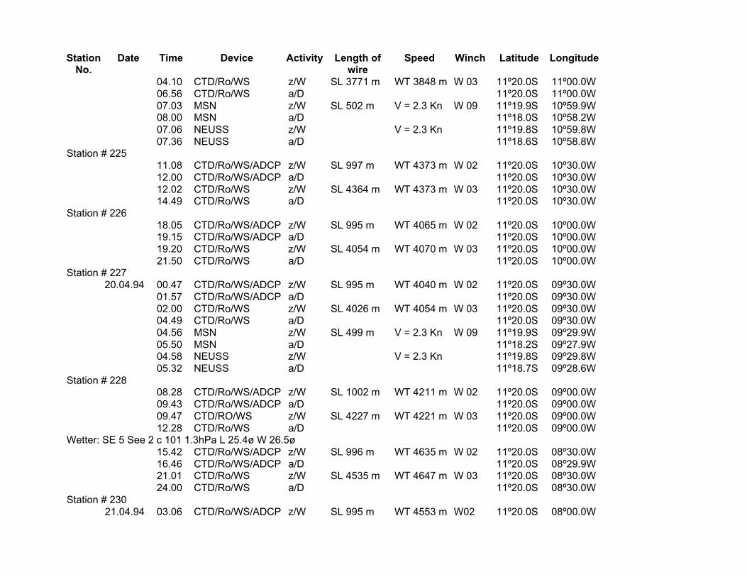
StationNo.
Date Time Device Activity Length ofwire
Speed Winch Latitude Longitude
04.10 CTD/Ro/WS z/W SL 3771 m WT 3848 m W 03 11º20.0S 11º00.0W06.56 CTD/Ro/WS a/D 11º20.0S 11º00.0W07.03 MSN z/W SL 502 m V = 2.3 Kn W 09 11º19.9S 10º59.9W08.00 MSN a/D 11º18.0S 10º58.2W07.06 NEUSS z/W V = 2.3 Kn 11º19.8S 10º59.8W07.36 NEUSS a/D 11º18.6S 10º58.8W
Station # 22511.08 CTD/Ro/WS/ADCP z/W SL 997 m WT 4373 m W 02 11º20.0S 10º30.0W12.00 CTD/Ro/WS/ADCP a/D 11º20.0S 10º30.0W12.02 CTD/Ro/WS z/W SL 4364 m WT 4373 m W 03 11º20.0S 10º30.0W14.49 CTD/Ro/WS a/D 11º20.0S 10º30.0W
Station # 22618.05 CTD/Ro/WS/ADCP z/W SL 995 m WT 4065 m W 02 11º20.0S 10º00.0W19.15 CTD/Ro/WS/ADCP a/D 11º20.0S 10º00.0W19.20 CTD/Ro/WS z/W SL 4054 m WT 4070 m W 03 11º20.0S 10º00.0W21.50 CTD/Ro/WS a/D 11º20.0S 10º00.0W
Station # 22720.04.94 00.47 CTD/Ro/WS/ADCP z/W SL 995 m WT 4040 m W 02 11º20.0S 09º30.0W
01.57 CTD/Ro/WS/ADCP a/D 11º20.0S 09º30.0W02.00 CTD/Ro/WS z/W SL 4026 m WT 4054 m W 03 11º20.0S 09º30.0W04.49 CTD/Ro/WS a/D 11º20.0S 09º30.0W04.56 MSN z/W SL 499 m V = 2.3 Kn W 09 11º19.9S 09º29.9W05.50 MSN a/D 11º18.2S 09º27.9W04.58 NEUSS z/W V = 2.3 Kn 11º19.8S 09º29.8W05.32 NEUSS a/D 11º18.7S 09º28.6W
Station # 22808.28 CTD/Ro/WS/ADCP z/W SL 1002 m WT 4211 m W 02 11º20.0S 09º00.0W09.43 CTD/Ro/WS/ADCP a/D 11º20.0S 09º00.0W09.47 CTD/RO/WS z/W SL 4227 m WT 4221 m W 03 11º20.0S 09º00.0W12.28 CTD/Ro/WS a/D 11º20.0S 09º00.0W
Wetter: SE 5 See 2 c 101 1.3hPa L 25.4ø W 26.5ø15.42 CTD/Ro/WS/ADCP z/W SL 996 m WT 4635 m W 02 11º20.0S 08º30.0W16.46 CTD/Ro/WS/ADCP a/D 11º20.0S 08º29.9W21.01 CTD/Ro/WS z/W SL 4535 m WT 4647 m W 03 11º20.0S 08º30.0W24.00 CTD/Ro/WS a/D 11º20.0S 08º30.0W
Station # 23021.04.94 03.06 CTD/Ro/WS/ADCP z/W SL 995 m WT 4553 m W02 11º20.0S 08º00.0W
StationNo.
Date Time Device Activity Length ofwire
Speed Winch Latitude Longitude
04.18 CTD/Ro/WS/ADCP a/D 11º20.0S 08º00.0W04.22 CTD/Ro/WS z/W SL 4514 m WT 4553 m W 03 11º20.0S 08º00.0W07.21 CTD/Ro/WS a/D 11º20.0S 08º00.0W07.27 MSN z/W SL 510 m V = 2.3 Kn W 09 11º19.8S 07º59.8W08.20 MSN a/D 11º17.8S 07º58.0W07.30 NEUSS z/W V = 2.3 Kn 11º19.7S 07º59.7W08.00 NEUSS a/D 11º18.5S 07º58.8W
Station # 23111.24 CTD/Ro/WS/ADCP z/W SL 995 m WT 4464 m W 02 11º20.0S 07º30.0W12.22 CTD/Ro/WS/ADCP a/D 11º20.0S 07º30.0W12.25 CTD/Ro/WS z/W SL 4439 m WT 4452 m W03 11º20.0S 07º30.0W15.07 CTD/Ro/WS a/D 11º20.0S 07º30.0W
Station # 23218.28 CTD/Ro/WS/ADCP z/W SL 997 m WT 4999 m W 02 11º20.0S 07º00.0W19.26 CTD/Ro/WS/ADCP a/D 11º20.0S 07º00.0W19.32 CTD/Ro/WS z/W SL 4283 m WT 4304 m W03 11º20.0S 07º00.0W22.53 CTD/Ro/WS a/D 11º20.0S 07º00.0W22.59 MSN z/W SL 497 m V = 2.3 Kn W 09 11º19.8S 06º59.9W23.54 MSN a/D 11º17.6S 06º58.7W23.12 NEUSS z/W V = 2.3 Kn 11º19.7S 06º59.9W23.34 NEUSS a/D 11º18.3S 06º59.1W
Station # 233 UTC 022.04.94 03.24 CTD/Ro/WS/ADCP z/W SL 998 m WT 4479 m W 02 11º20.0S 06º30.0W
04.28 CTD/Ro/WS/ADCP a/D 11º20.0S 06º30.0W04.35 CTD/Ro/WS z/W SL 4469 m WT 4477 m W 03 11º20.0S 06º30.0W07.31 CTD/Ro/WS a/D 11º20.0S 06º30.0W
Station # 23410.38 CTD/Ro/WS/ADCP z/W SL 998 m WT 4514 m W 02 11º20.0S 06º00.0W11.26 CTD/Ro/WS/ADCP a/D 11º20.0S 06º00.0W11.33 CTD/Ro/WS z/W SL 4505 m WT 4504 m W 03 11º20.0S 06º00.0W14.25 CTD/Ro/WS a/D 11º20.0S 06º00.0W
Station # 23517.35 CTD/Ro/WS/ADCP z/W SL 994 m WT 5002 m W 02 11º20.0S 05º30.0W18.37 CTD/Ro/WS/ADCP a/D 11º20.0S 05º30.0W18.44 CTD/Ro/WS z/W SL 5009 m WT 5001 m W 03 11º20.0S 05º30.0W21.37 CTD/Ro/WS a/D 11º20.0S 05º30.0W21.45 MSN z/W SL 613 m V = 2.3 Kn W 09 11º19.8S 05º29.8W
StationNo.
Date Time Device Activity Length ofwire
Speed Winch Latitude Longitude
22.47 MSN a/D 11º17.7S 05º27.0W21.48 NEUSS z/W V = 2.3 Kn 11º19.8S 05º29.7W22.18 NEUSS a/D 11º18.7S 05º28.2W
Station # 23623.04.94 01.38 CTD/Ro/WS/ADCP z/W SL 1007 m WT 4145 m W 02 11º20.0S 05º00.0W
02.35 CTD/Ro/WS/ADCP a/D 11º20.0S 05º00.0W02.41 CTD/Ro/WS z/W SL 4131 m WT 4166 m W 03 11º20.0S 05º00.0W05.32 CTD/Ro/WS a/D 11º20.0S 05º00.0W
Station # 23708.37 CTD/Ro/WS/ADCP z/W SL 997 m WT 5057 m W 02 11º20.0S 04º30.0W09.32 CTD/Ro/WS/ADCP a/D 11º19.9S 04º30.0W09.37 CTD/Ro/WS z/W SL 5061 m WT 5062 m W 03 11º19.9S 04º30.0W12.46 CTD/Ro/WS a/D 11º20.0S 04º30.0W
Wetter: SSE 5 See 2 c 1015.51lPa L 24.7ø W 25.9øStation # 238
16.48 CTD/Ro/WS/ADCP z/W SL 994 m WT 4552 m W 02 11º20.0S 04º00.0W17.53 CTD/Ro/WS/ADCP a/D 11º20.0S 04º00.0W17.58 CTD/Ro/WS z/W SL 4528 m WT 4554 m W 03 11º20.0S 04º00.0W20.49 CTD/Ro/WS a/D 11º20.0S 03º59.9W20.58 MSN z/W SL 585 m V = 2.3 Kn W 09 11º19.9S 03º59.5W21.31 MSN a/D 11º18.8S 03º56.1W21.00 NEUSS z/W V = 2.3 Kn 11º19.8S 03º59.4W21.31 NEUSS a/D 11º19.3S 03º57.7W
Station # 23924.04.94 00.42 CTD/Ro/WS/ADCP z/W SL 996 m WT 4762 m W 02 11º20.0S 03º30.0W
01.38 CTD/ro/WS/ADCP a/D 11º20.0S 03º30.0W01.41 CTD/Ro/WS z/W SL 4770 m WT 4762 m W 03 11º20.0S 03º30.0W04.49 CTD/Ro/WS a/D 11º20.0S 03º30.0W
Station # 24007.50 CTD/Ro/WS/ADCP z/W SL 1002 m WT 4650 m W 02 11º20.0S 03º00.0W08.47 CTD/Ro/WS/ADCP a/D 11º20.0S 03º00.0W08.52 CTD/Ro/WS z/W SL 4645 m WT 4652 m W 03 11º20.0S 03º00.0W11.40 CTD/Ro/WS a/D 11º20.0S 02º59.9W11.46 MSN z/W SL 447 m V = 2.3 Kn W 09 11º19.9S 02º59.8W12.37 MSN a/D 11º19.3S 02º57.6W11.48 NEUSS z/W V = 2.3 Kn 11º19.9S 02º59.6W12.20 NEUSS a/D 11º19.5S 02º58.2W

StationNo.
Date Time Device Activity Length ofwire
Speed Winch Latitude Longitude
Station # 24115.18 CTD/ro/WS/ADCP z/W SL 996 m WT 5210 m W 02 11º20.0S 02º30.0W16.24 CTD/ro/WS/ADCP a/D 11º20.0S 02º29.7W16.45 CTD/Ro/WS z/W SL 5220 m WT 5225 m W 03 11º20.0S 02º30.0W20.03 CTD/Ro/WS a/D 11º20.0S 02º30.0W
Station # 24222.52 CTD/Ro/WS/ADCP z/W SL 999 m WT 5383 m W 02 11º20.0S 02º00.0W23.50 CTD/Ro/WS/ADCP a/D 11º19.9S 01º59.7W
25.04.94 00.15 CTD/Ro/WS z/W SL 5381 m WT 5382 m W 03 11º20.0S 01º59.9W03.41 CTD/Ro/WS a/D 11º20.0S 02º00.0W03.46 MSN z/W SL 560 m V = 2.3 Kn W 09 11º19.9S 01º59.8W04.40 MSN a/D 11º19.3S 01º56.9W03.49 NEUSS z/W V = 2.3 Kn 11º19.9S 01º59.6W04.20 NEUSS a/D 11º19.5S 01º58.0W
Station # 24307.11 CTD/Ro/WS/ADCP z/W SL 996 m WT 5211 m W 02 11º20.0S 01º30.0W08.12 CTD/Ro/WS/ADCP a/D 11º20.0S 01º30.0W08.17 CTD/Ro/WS z/W SL 5216 m WT 5219 m W 03 11º20.0S 01º29.8W11.19 CTD/Ro/WS a/D 11º20.0S 01º29.9W
Station # 24414.12 CTD/Ro/WS/ADCP z/W SL 1014 m WT 5326 m W 02 11º20.0S 01º00.0W15.12 CTD/Ro/WS/ADCP a/D 11º20.0S 01º00.0W15.15 CTD/Ro/WS z/W SL 5327 m WT 5322 m W 03 11º20.0S 01º00.0W18.37 CTD/Ro/WS a/D 11º20.0S 01º00.0W
Station # 24520.18 CTD/Ro/WS/ADCP z/W SL 997 m WT 4798 m W 02 11º20.0S 00º45.0W21.04 CTD/Ro/WS/ADCP a/D 11º20.0S 00º45.0W21.09 CTD/Ro/WS z/W SL 4720 m WT 4780 m W 03 11º20.0S 00º45.0W23.53 CTD/Ro/WS a/D 11º20.0S 00º45.0W
26.04.94 00.00 MSN z/W SL 455 m V = 2.3 Kn W 09 11º20.0S 00º44.8W00.53 MSN a/D 11º20.0S 00º42.3W00.05 NEUSS z/W V = 2.3 Kn 11º20.1S 00º44.5W00.36 NEUSS a/D 11º20.1S 00º43.1W
Station # 24602.15 CTD/Ro/WS/ADCP z/W SL 995 m WT 4930 m W 02 11º20.0S 00º30.0W03.12 CTD/Ro/WS/ADCP a/D 11º20.0S 00º30.0W03.16 CTD/Ro/WS z/W SL 4916 m WT 4930 m W 03 11º20.0S 00º30.0W
StationNo.
Date Time Device Activity Length ofwire
Speed Winch Latitude Longitude
06.30 CTD/Ro/WS a/D 11º20.0S 00º30.0W06.35 MSN z/W SL 572 m V = 2.3 Kn W 09 11º19.9S 00º29.8W07.37 MSN a/D 11º18.0S 00º27.6W06.38 NEUSS z/W V = 2.3 Kn 11º19.8S 00º29.7W07.10 NEUSS a/D 11º18.7S 00º28.5W
Station # 24708.59 CTD/Ro/WS/ADCP z/W SL 996 m WT 5462 m W 02 11º20.0S 00º15.0W09.47 CTD/Ro/WS/ADCP a/D 11º20.1S 00º15.0W09.51 CTD/Ro/WS z/W SL 5469 m WT 5473 m W 03 11º20.1S 00º15.0W13.06 CTD/Ro/WS a/D 11º20.2S 00º14.9W13.13 MSN ZIW SL 471 m V = 2.3 Kn W 09 11º20.2S 00º14.7W14.00 MSN a/D 11º19.9S 00º12.4W13.16 NEUSS ZIW V = 2.3 Kn 11º20.1S 00º14.5W13.48 NEUSS a/D 11º20.0S 00º13.1W
Station # 24815.35 CTD/Ro/WS/ADCP z/W SL 994 m WT 5701 m W 02 11º20.0S 00º00.1W16.40 CTD/Ro/WS/ADCP a/D 11º20.0S 00º00.016.44 CTD/Ro/WS z/W SL 5697 m WT 5694 m W 03 11º20.0S 00º00.020.41 CTD/Ro/WS a/D 11º20.1S 00º00.0
Station # 24927.04.94 00.40 CTD/Ro/WS/ADCP z/W SL 5605 m WT 5608 m W 02 11º20.0S 00º40.0E
04.25 CTD/Ro/WS/ADCP a/D 11º20.0S 00º40.0E0433 MSN z/W SL 480 m V = 2.3 Kn W 09 11º19.9S 00º40.3E05.22 MSN a/D 11º18.9S 00º42.6E04.36 NEUSS z/W V = 2.3 Kn 11º19.9S 00º40.4E05.07 NEUSS a/D 11º19.2S 00º42.0E
Station # 25009.03 CTD/Ro/WS/ADCP z/W SL 1094 m WT 5590 m W 02 11º20.0S 01º20.0E10.02 CTD/Ro/WS/ADCP a/D 11º20.0S 01º20.0E10.06 CTD/Ro/WS z/W SL 5590 m WT 5627 m W 03 11º20.0S 01º19.9E13.23 CTD/Ro/WS a/D 11º20.0S 01º20.0E13.31 Drifter m. Segel z/W 11º19.9S 01º20.0E
Station # 25119.20 CTD/Ro/WS/ADCP z/W SL 993 m WT 5621 m W 02 11º20.0S 02º00.0E20.21 CTD/Ro/WS/ADCP a/D 11º20.0S 02º00.0E20.25 CTD/Ro/WS z/W SL 5589 m WT 5574 m W 03 11º20.0S 02º00.0E23.48 CTD/Ro/WS a/D 11º20.0S 02º00.0W

StationNo.
Date Time Device Activity Length ofwire
Speed Winch Latitude Longitude
23.57 MSN z/W SL 525 m V = 2.3 Kn W 09 11º19.9S 02º00.0E28.04.94 00.51 MSN a/D 11º18.2S 02º02.0E
00.01 NEUSS z/W V = 2.3 Kn 11º19.8S 02º00.0E00.31 NEUSS a/D 11º18.8S 02º01.4E
Station # 25204.50 CTD/Ro/WS/ADCP z/W SL 994 m WT 5570 m W 02 11º20.0S 02º40.0E05.55 CTD/Ro/WS/ADCP a/D 11º20.0S 02º40.0E06.01 CTD/Ro/WS z/W SL 5585 m WT 5572 m W 03 11º20.0S 02º40.0E09.17 CTD/Ro/WS a/D 11º20.0S 02º40.0E09.24 Drifter m. Segel z/W 11º20.0S 02º40.0E
Station # 25313.25 CTD/Ro/WS/ADCP z/W SL 995 m WT 5558 m W 02 11º20.0S 03º20.0E14.28 CTD/Ro/WS/ADCP a/D 11º20.0S 03º20.0E14.32 CTD/Ro/WS z/W SL 5588 m WT 5566 m W 03 11º20.0S 03º20.0E18.08 CTD/Ro/WS a/D 11º20.0S 03º20.0E18.13 MSN z/W SL 512 m V = 2.3 Kn W 09 11º19.9S 03º20.2E19.08 MSN a/D 11º18.6S 03º22.5E18.16 NEUSS z/W V = 2.3 Kn 11º19.8S 03º20.3E18.46 NEUSS a/D 11º19.0S 03º21.5E
Station # 25423.03 CTD/Ro/WS/ADCP z/W SL 1094 m WT 5554 m W 02 11º20.0S 04º00.0EUTC+1
29.04.94 01.00 CTD/Ro/WS/ADCP a/D 11º20.0S 04º00.0E01.05 CTD/Ro/WS z/W SL 5573 m WT 5556 m W 03 11º20.0S 04º00.0E04.52 CTD/Ro/WS a/D 11º20.1S 04º00.0E05.00 Drifter m. Segel z/W 11º20.2S 04º00.1E
Station # 25509.01 CTD/Ro/WS/ADCP z/W SL 995 m WT 5596 m W 02 11º20.0S 04º40.0E09.56 CTD/Ro/WS/ADCP a/D 11º20.0S 04º40.0E10.00 CTD/Ro/WS z/W SL 5560 m WT 5590 m W03 11º20.0S 04º40.0E13.17 CTD/Ro/WS a/D 11º20.1S 04º39.9E13.22 MSN z/W SL 470 m V = 2.3 Kn W 09 11º20.1S 04º40.1E14.13 MSN a/D 11º19.4S 04º42.5E13.26 NEUSS z/W V = 2.3 Kn 11º20.0S 04º40.3E13.57 NEUSS a/D 11º19.6S 04º41.8E
StationNo.
Date Time Device Activity Length ofwire
Speed Winch Latitude Longitude
Wetter: S 4 See 2 c 1013.2hPa L 24.1ø W 25.5øStation # 256
18.00 CTD/Ro/WS/ADCP z/W SL 995 m WT 5452 m W 02 11º20.0S 05º20.0E19.02 CTD/Ro/WS/ADCP a/D 11º20.0S 05º20.0E19.08 CTD/Ro/WS z/W SL 5403 m WT 5452 m W 03 11º20.0S 05º20.0E22.10 CTD/Ro/WS a/D 11º20.0S 05º20.0E22.17 Drifter m. Segel z/W 11º20.1S 05º20.1E
Station # 25702.15 CTD/Ro/WS/ADCP z/W SL 995 m WT 5190 m W 03 11º20.0S 06º00.0E03.11 CTD/Ro/WS/ADCP a/D 11º20.0S 06º00.0E03.14 CTD/Ro/WS z/W SL 5137 m WT 5185 m W 02 11º20.0S 06º00.0E06.28 CTD/Ro/WS a/D 11º20.0S 06º00.0E06.31 MSN z/W SL 469 m V = 2.3 Kn W 09 11º20.1S 06º00.1E07.20 MSN a/D 11º20.0S 06º02.6E06.35 NEUSS z/W V = 2.3 Kn 11º20.0S 06º00.3E07.06 NEUSS a/D 11º20.0S 06º01.9E
Station # 25810.55 CTD/Ro/WS z/W SL 5228 m WT 5256 m W 03 11º20.0S 06º40.0E14.08 CTD/Ro/WS a/D 11º20.0S 06º40.0E14.12 CTD/Ro/WS/ADCP z/W SL 1014 m WT 5256 m W 02 11º20.0S 06º40.0E15.14 CTD/Ro/WS/ADCP a/D 11º20.0S 06º40.0E15.19 CTD/Ro/WS z/W SL 5217 m WT 5259 m W 03 11º20.0S 06º40.0E18.34 CTD/Ro/WS a/D 11º20.0S 06º40.0E
Station # 25922.33 CTD/Ro/WS/ADCP z/W SL 995 m WT 5060 m W 02 11º20.0S 07º20.0E23.32 CTD/Ro/WS/ADCP a/D 11º20.0S 07º20.0E23.36 CTD/Ro/WS z/W SL 5029 m WT 5055 m W 03 11º20.0S 07º19.9E
01.05.94 02.37 CTD/Ro/WS a/D 11º20.0S 07º20.0E02.43 MSN z/W SL 499 m V = 2.3 Kn W 09 11º19.9S 07º20.0E03.35 MSN a/D 11º20.7S 07º22.9E02.46 NEUSS z/W V = 2.3 Kn 11º20.0S 07º20.3E03.18 NEUSS a/D 11º20.5S 07º22.0E
Station # 26007.12 CTD/Ro/WS/ADCP z/W SL 993 m WT 4864 m W 02 11º20.0S 08º00.0E08.10 CTD/Ro/WS/ADCP a/D 11º20.0S 08º00.0E08.13 CTD/Ro/WS z/W SL 4834 m WT 4860 m W 03 11º20.0S 08º00.0E

StationNo.
Date Time Device Activity Length ofwire
Speed Winch Latitude Longitude
11.25 CTD/Ro/WS a/D 11º20.0S 08º00.0EWetter: SSE 3 See 1 c 1013.8hPa L 23.9ø W 26.8øStation # 261
14.30 CTD/Ro/WS/ADCP z/W SL 995 m WT 4787 m W 02 11º20.0S 08º30.0E15.25 CTD/Ro/WS/ADCP a/D 11º20.0S 08º30.0E15.31 CTD/Ro/WS z/W SL 4775 m WT 4786 m W 03 11º20.0S 08º30.0E18.32 CTD/Ro/WS a/D 11º20.0S 08º30.0E18.37 MSN z/W SL 525 m V = 2.3 Kn W 09 11º20.0S 08º30.0E19.32 MSN a/D 11º20.6S 08º32.8E18.41 NEUSS z/W V = 2.3 Kn 11º20.0S 08º30.3E19.14 NEUSS a/D 11º20.4S 08º31.9E
Station # 26222.06 CTD/Ro/WS/ADCP z/W SL 997 m WT 4589 m W 02 11º20.0S 09º00.0E22.56 CTD/Ro/WS/ADCP a/D 11º20.0S 08º59.9E23.00 CTD/Ro/WS z/W SL 4578 m WT 4586 m W 03 11º20.0S 09º00.0E
02.05.94 01.41 CTD/Ro/WS a/D 11º20.0S 09º00.0EStation # 263
04.35 CTD/Ro/WS/ADCP z/W SL 995 m WT 4406 m W 02 11º20.0S 09º30.0E05.38 CTD/Ro/WS/ADCP a/D 11º20.0S 09º30.0E05.47 CTD/Ro/WS z/W SL 4380 m WT 4408 m W 03 11º20.0S 09º30.0E08.30 CTD/Ro/WS a/D 11º20.0S 09º30.0E08.39 MSN z/W SL 588 m V = 2.3 Kn W 09 11º20.0S 09º30.2E09.40 MSN a/D 11º20.0S 09º33.8E08.41 NEUSS z/W V = 2.3 Kn 11º20.0S 09º30.0E09.13 NEUSS a/D 11º20.0S 09º32.1E
Station # 26412.00 CTD/Ro/ WS/ ADCO z/W SL 1007 m WT 4153 m W 02 11º20.0S 10º00.0E12.57 CTD/Ro/WS/ADCP a/D 11º20.0S 10º00.0E12.59 CTD/Ro/WS z/W SL 4141 m WT 4150 m W 03 11º20.0S 10º00.0E15.37 CTD/Ro/WS a/D 11º20.0S 10º00.0E15.44 MSN z/W SL 551 m V = 2.3 Kn W 09 11º20.1S 09º59.9E16.46 MSN a/D 11º22.4S 10º02.6E15.47 NEUSS z/W V = 2.3 Kn 11º20.2S 09º59.9E16.20 NEUSS a/D 11º21.5S 10º01.6E
Station # 26518.48 CTD/Ro/WS/ADCP z/W SL 999 m WT 4069 m W 02 11º20.0S 10º25.0E19.54 CTD/Ro/WS/ADCP a/D 11º20.0S 10º25.0E
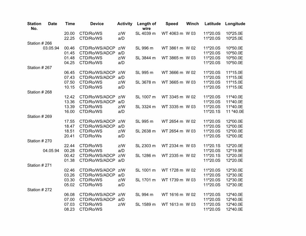
StationNo.
Date Time Device Activity Length ofwire
Speed Winch Latitude Longitude
20.00 CTD/Ro/WS z/W SL 4039 m WT 4063 m W 03 11º20.0S 10º25.0E22.25 CTD/Ro/WS a/D 11º20.0S 10º25.0E
Station # 26603.05.94 00.46 CTD/Ro/WS/ADCP z/W SL 996 m WT 3861 m W 02 11º20.0S 10º50.0E
01.45 CTD/Ro/WS/ADCP a/D 11º20.0S 10º50.0E01.48 CTD/Ro/WS z/W SL 3844 m WT 3865 m W 03 11º20.0S 10º50.0E04.25 CTD/Ro/WS a/D 11º20.0S 10º50.0E
Station # 26706.45 CTD/Ro/WS/ADCP z/W SL 995 m WT 3666 m W 02 11º20.0S 11º15.0E07.43 CTD/Ro/WS/ADCP a/D 11º20.0S 11º15.0E07.50 CTD/Ro/WS z/W SL 3678 m WT 3665 m W 03 11º20.0S 11º15.0E10.15 CTD/Ro/WS a/D 11º20.0S 11º15.0E
Station # 26812.42 CTD/Ro/WS/ADCP z/W SL 1007 m WT 3345 m W 02 11º20.0S 11º40.0E13.36 CTD/Ro/WS/ADCP a/D 11º20.0S 11º40.0E13.39 CTD/Ro/WS z/W SL 3324 m WT 3335 m W 03 11º20.0S 11º40.0E16.00 CTD/Ro/WS a/D 11º20.1S 11 º40.0E
Station # 26917.55 CTD/Ro/WS/ADCP z/W SL 995 m WT 2654 m W 02 11º20.0S 12º00.0E18.47 CTD/Ro/WS/ADCP a/D 11º20.0S 12º00.0E18.51 CTD/Ro/WS z/W SL 2638 m WT 2654 m W 03 11º20.0S 12º00.0E20.41 CTD/Ro/Ws a/D 11º20.0S 12º00.0E
Station # 27022.44 CTD/Ro/WS z/W SL 2303 m WT 2334 m W 03 11º20.1S 12º20.0E
04.05.94 00.28 CTD/Ro/WS a/D 11º20.0S 12º19.9E00.42 CTD/Ro/WS/ADCP z/W SL 1286 m WT 2335 m W 02 11º20.1S 12º20.0E01.38 CTD/Ro/WS/ADCP a/D 11º20.0S 12º20.0E
Station # 27102.46 CTD/Ro/WS/ADCP z/W SL 1001 m WT 1728 m W 02 11º20.0S 12º30.0E03.26 CTD/Ro/WS/ADCP a/D 11º20.0S 12º30.0E03.30 CTD/Ro/WS z/W SL 1701 m WT 1739 m W 03 11º20.0S 12º30.0E05.02 CTD/Ro/WS a/D 11º20.0S 12º30.0E
Station # 27206.08 CTD/Ro/WS/ADCP z/W SL 994 m WT 1616 m W 02 11º20.0S 12º40.0E07.00 CTD/Ro/WS/ADCP a/D 11º20.0S 12º40.0E07.03 CTD/Ro/WS z/W SL 1589 m WT 1613 m W 03 11º20.0S 12º40.0E08.23 CTD/Ro/WS 11º20.0S 12º40.0E
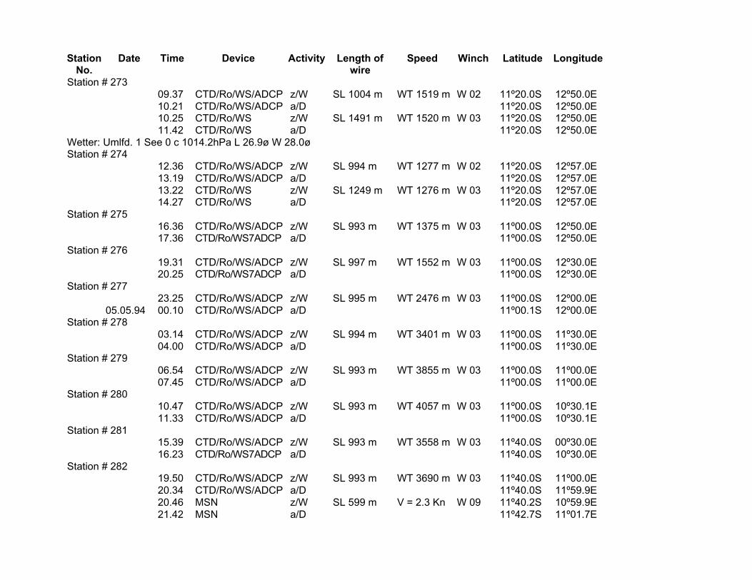
StationNo.
Date Time Device Activity Length ofwire
Speed Winch Latitude Longitude
Station # 27309.37 CTD/Ro/WS/ADCP z/W SL 1004 m WT 1519 m W 02 11º20.0S 12º50.0E10.21 CTD/Ro/WS/ADCP a/D 11º20.0S 12º50.0E10.25 CTD/Ro/WS z/W SL 1491 m WT 1520 m W 03 11º20.0S 12º50.0E11.42 CTD/Ro/WS a/D 11º20.0S 12º50.0E
Wetter: Umlfd. 1 See 0 c 1014.2hPa L 26.9ø W 28.0øStation # 274
12.36 CTD/Ro/WS/ADCP z/W SL 994 m WT 1277 m W 02 11º20.0S 12º57.0E13.19 CTD/Ro/WS/ADCP a/D 11º20.0S 12º57.0E13.22 CTD/Ro/WS z/W SL 1249 m WT 1276 m W 03 11º20.0S 12º57.0E14.27 CTD/Ro/WS a/D 11º20.0S 12º57.0E
Station # 27516.36 CTD/Ro/WS/ADCP z/W SL 993 m WT 1375 m W 03 11º00.0S 12º50.0E17.36 CTD/Ro/WS7ADCP a/D 11º00.0S 12º50.0E
Station # 27619.31 CTD/Ro/WS/ADCP z/W SL 997 m WT 1552 m W 03 11º00.0S 12º30.0E20.25 CTD/Ro/WS7ADCP a/D 11º00.0S 12º30.0E
Station # 27723.25 CTD/Ro/WS/ADCP z/W SL 995 m WT 2476 m W 03 11º00.0S 12º00.0E
05.05.94 00.10 CTD/Ro/WS/ADCP a/D 11º00.1S 12º00.0EStation # 278
03.14 CTD/Ro/WS/ADCP z/W SL 994 m WT 3401 m W 03 11º00.0S 11º30.0E04.00 CTD/Ro/WS/ADCP a/D 11º00.0S 11º30.0E
Station # 27906.54 CTD/Ro/WS/ADCP z/W SL 993 m WT 3855 m W 03 11º00.0S 11º00.0E07.45 CTD/Ro/WS/ADCP a/D 11º00.0S 11º00.0E
Station # 28010.47 CTD/Ro/WS/ADCP z/W SL 993 m WT 4057 m W 03 11º00.0S 10º30.1E11.33 CTD/Ro/WS/ADCP a/D 11º00.0S 10º30.1E
Station # 28115.39 CTD/Ro/WS/ADCP z/W SL 993 m WT 3558 m W 03 11º40.0S 00º30.0E16.23 CTD/Ro/WS7ADCP a/D 11º40.0S 10º30.0E
Station # 28219.50 CTD/Ro/WS/ADCP z/W SL 993 m WT 3690 m W 03 11º40.0S 11º00.0E20.34 CTD/Ro/WS/ADCP a/D 11º40.0S 11º59.9E20.46 MSN z/W SL 599 m V = 2.3 Kn W 09 11º40.2S 10º59.9E21.42 MSN a/D 11º42.7S 11º01.7E
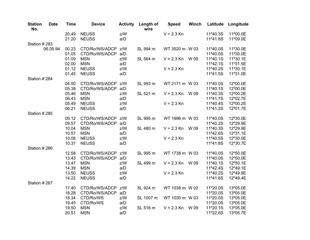
StationNo.
Date Time Device Activity Length ofwire
Speed Winch Latitude Longitude
20.49 NEUSS z/W V = 2.3 Kn 11º40.3S 11º00.0E21.20 NEUSS a/D 11º41.8S 11º09.0E
Station # 28306.05.94 00.23 CTD/Ro/WS/ADCP z/W SL 994 m WT 3520 m W 03 11º40.0S 11º30.0E
01.05 CTD/Ro/WS/ADCP a/D 11º40.0S 11º30.0E01.09 MSN z/W SL 564 m V = 2.3 Kn W 09 11º40.1S 11º30.1E02.00 MSN a/D 11º42.1S 11º31.5E01.12 NEUSS z/W V = 2.3 Kn 11º40.2S 11º30.1E01.45 NEUSS a/D 11º41.5S 11º31.0E
Station # 28404.50 CTD/Ro/WS/ADCP z/W SL 993 m WT 2171 m W 03 11º40.0S 12º00.0E05.38 CTD/Ro/WS/ADCP a/D 11º40.1S 12º00.0E05.46 MSN z/W SL 521 m V = 2.3 Kn W 09 11º40.3S 12º00.2E06.43 MSN a/D 11º41.7S 12º02.7E05.49 NEUSS z/W V = 2.3 Kn 11º40.4S 12º00.2E06.21 NEUSS a/D 11º41.2S 12º01.7E
Station # 28509.12 CTD/Ro/WS/ADCP z/W SL 995 m WT 1996 m W 03 11º40.0S 12º30.0E09.57 CTD/Ro/WS/ADCP a/D 11º40.2S 12º29.9E10.04 MSN z/W SL 480 m V = 2.3 Kn W 09 11º40.3S 12º29.9E10.57 MSN a/D 11º42.6S 12º31.1E10.06 NEUSS z/W V = 2.3 Kn 11º40.5S 12º30.0E10.37 NEUSS a/D 11º41.8S 12º30.7E
Station # 28612.58 CTD/Ro/WS/ADCP z/W SL 995 m WT 1738 m W 03 11º40.0S 12º50.0E13.43 CTD/Ro/WS/ADCP a/D 11º40.0S 12º50.0E13.47 MSN z/W SL 499 m V = 2.3 Kn W 09 11º40.1S 12º50.1E14.39 MSN a/D 11º42.4S 12º49.1E13.50 NEUSS z/W V = 2.3 Kn 11º40.2S 12º49.9E14.22 NEUSS a/D 11º41.6S 12º49.4E
Station # 28717.40 CTD/Ro/WS/ADCP z/W SL 924 m WT 1038 m W 02 11º20.0S 13º05.0E18.28 CTD/Ro/WS/ADCP a/D 11º20.0S 13º05.0E18.34 CTD/Ro/WS z/W SL 1007 m WT 1030 m W 03 11º20.0S 13º05.0E19.45 CTD/Ro/WS a/D 11º20.0S 13º05.0E19.50 MSN z/W SL 516 m V = 2.3 Kn W 09 11º20.1S 13º05.0E20.51 MSN a/D 11º22.6S 13º05.7E
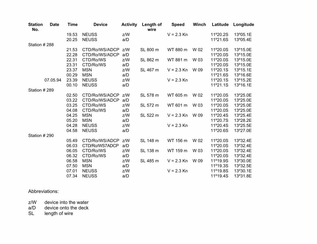
StationNo.
Date Time Device Activity Length ofwire
Speed Winch Latitude Longitude
19.53 NEUSS z/W V = 2.3 Kn 11º20.2S 13º05.1E20.25 NEUSS a/D 11º21.6S 13º05.4E
Station # 28821.53 CTD/Ro/WS/ADCP z/W SL 800 m WT 880 m W 02 11º20.0S 13º15.0E22.28 CTD/Ro/WS/ADCP a/D 11º20.0S 13º15.0E22.31 CTD/Ro/WS z/W SL 862 m WT 881 m W 03 11º20.0S 13º15.0E23.31 CTD/Ro/WS a/D 11º20.0S 13º15.0E23.37 MSN z/W SL 467 m V = 2.3 Kn W 09 11º20.1S 13º15.1E00.29 MSN a/D 11º21.6S 13º16.6E
07.05.94 23.39 NEUSS z/W V = 2.3 Kn 11º20.1S 13º15.2E00.10 NEUSS a/D 11º21.1S 13º16.1E
Station # 28902.50 CTD/Ro/WS/ADCP z/W SL 578 m WT 605 m W 02 11º20.0S 13º25.0E03.22 CTD/Ro/WS/ADCP a/D 11º20.0S 13º25.0E03.25 CTD/Ro/WS z/W SL 572 m WT 601 m W 03 11º20.0S 13º25.0E04.08 CTD/Ro/WS a/D 11º20.0S 13º25.0E04.25 MSN z/W SL 522 m V = 2.3 Kn W 09 11º20.4S 13º25.4E05.20 MSN a/D 11º20.7S 13º28.2E04.28 NEUSS z/W V = 2.3 Kn 11º20.4S 13º25.5E04.58 NEUSS a/D 11º20.6S 13º27.0E
Station # 29005.49 CTD/Ro/WS/ADCP z/W SL 148 m WT 156 m W 02 11º20.0S 13º32.4E06.03 CTD/Ro/WS7ADCP a/D 11º20.0S 13º32.4E06.05 CTD/Ro/WS z/W SL 138 m WT 159 m W 03 11º20.0S 13º32.4E06.32 CTD/Ro/WS a/D 11º20.0S 13º32.4E06.58 MSN z/W SL 485 m V = 2.3 Kn W 09 11º19.9S 13º30.0E07.50 MSN a/D 11º19.3S 13º32.5E07.01 NEUSS z/W V = 2.3 Kn 11º19.8S 13º30.1E07.34 NEUSS a/D 11º19.4S 13º31.8E
Abbreviations:
z/W device into the watera/D device onto the deckSL length of wire
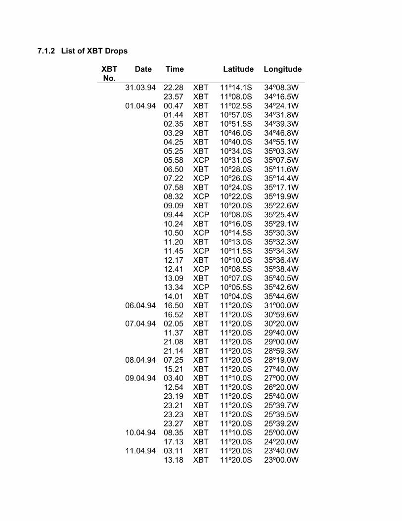
7.1.2 List of XBT Drops
XBTNo.
Date Time Latitude Longitude
31.03.94 22.28 XBT 11º14.1S 34º08.3W23.57 XBT 11º08.0S 34º16.5W
01.04.94 00.47 XBT 11º02.5S 34º24.1W01.44 XBT 10º57.0S 34º31.8W02.35 XBT 10º51.5S 34º39.3W03.29 XBT 10º46.0S 34º46.8W04.25 XBT 10º40.0S 34º55.1W05.25 XBT 10º34.0S 35º03.3W05.58 XCP 10º31.0S 35º07.5W06.50 XBT 10º28.0S 35º11.6W07.22 XCP 10º26.0S 35º14.4W07.58 XBT 10º24.0S 35º17.1W08.32 XCP 10º22.0S 35º19.9W09.09 XBT 10º20.0S 35º22.6W09.44 XCP 10º08.0S 35º25.4W10.24 XBT 10º16.0S 35º29.1W10.50 XCP 10º14.5S 35º30.3W11.20 XBT 10º13.0S 35º32.3W11.45 XCP 10º11.5S 35º34.3W12.17 XBT 10º10.0S 35º36.4W12.41 XCP 10º08.5S 35º38.4W13.09 XBT 10º07.0S 35º40.5W13.34 XCP 10º05.5S 35º42.6W14.01 XBT 10º04.0S 35º44.6W
06.04.94 16.50 XBT 11º20.0S 31º00.0W16.52 XBT 11º20.0S 30º59.6W
07.04.94 02.05 XBT 11º20.0S 30º20.0W11.37 XBT 11º20.0S 29º40.0W21.08 XBT 11º20.0S 29º00.0W21.14 XBT 11º20.0S 28º59.3W
08.04.94 07.25 XBT 11º20.0S 28º19.0W15.21 XBT 11º20.0S 27º40.0W
09.04.94 03.40 XBT 11º10.0S 27º00.0W12.54 XBT 11º20.0S 26º20.0W23.19 XBT 11º20.0S 25º40.0W23.21 XBT 11º20.0S 25º39.7W23.23 XBT 11º20.0S 25º39.5W23.27 XBT 11º20.0S 25º39.2W
10.04.94 08.35 XBT 11º10.0S 25º00.0W17.13 XBT 11º20.0S 24º20.0W
11.04.94 03.11 XBT 11º20.0S 23º40.0W13.18 XBT 11º20.0S 23º00.0W
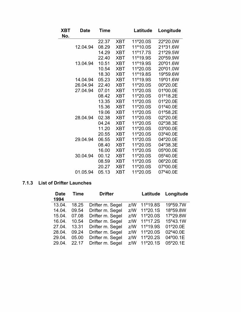
XBTNo.
Date Time Latitude Longitude
22.37 XBT 11º20.0S 22º20.0W12.04.94 08.29 XBT 11º10.0S 21º31.6W
14.29 XBT 11º17.7S 21º29.5W22.40 XBT 11º19.9S 20º59.9W
13.04.94 10.51 XBT 11º19.9S 20º01.6W10.54 XBT 11º20.0S 20º01.0W18.30 XBT 11º19.8S 19º59.6W
14.04.94 05.23 XBT 11º19.9S 19º01.6W26.04.94 22.40 XBT 11º20.0S 00º20.0E27.04.94 07.01 XBT 11º20.0S 01º00.0E
08.42 XBT 11º20.0S 01º18.2E13.35 XBT 11º20.0S 01º20.0E15.36 XBT 11º20.0S 01º40.0E19.06 XBT 11º20.0S 01º58.2E
28.04.94 02.38 XBT 11º20.0S 02º20.0E04.24 XBT 11º20.0S 02º38.3E11.20 XBT 11º20.0S 03º00.0E20.55 XBT 11º20.0S 03º40.0E
29.04.94 06.55 XBT 11º20.0S 04º20.0E08.40 XBT 11º20.0S 04º38.3E16.00 XBT 11º20.0S 05º00.0E
30.04.94 00.12 XBT 11º20.0S 05º40.0E08.59 XBT 11º20.0S 06º20.0E20.27 XBT 11º20.0S 07º00.0E
01.05.94 05.13 XBT 11º20.0S 07º40.0E
7.1.3 List of Drifter Launches
Date Time Drifter Latitude Longitude199413.04. 18.25 Drifter m. Segel z/W 11º19.8S 19º59.7W14.04. 09.54 Drifter m. Segel z/W 11º20.1S 18º59.8W15.04. 07.08 Drifter m. Segel z/W 11º20.0S 17º29.8W16.04. 10.54 Drifter m. Segel z/W 11º17.2S 15º43.1W27.04. 13.31 Drifter m. Segel z/W 11º19.9S 01º20.0E28.04. 09.24 Drifter m. Segel z/W 11º20.0S 02º40.0E29.04. 05.00 Drifter m. Segel z/W 11º20.2S 04º00.1E29.04. 22.17 Drifter m. Segel z/W 11º20.1S 05º20.1E
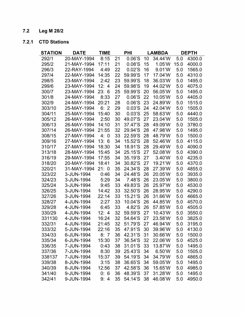
7.2 Leg M 28/2
7.2.1 CTD Stations
STATION DATE TIME PHI LAMBDA DEPTH292/1 20-MAY-1994 8:15 21 0.06’S 10 34.44’W 5.0 4300.0295/2 21-MAY-1994 17:11 21 0.08’S 15 1.05’W 15.0 4000.0296/3 22-RAY-1994 4:49 22 0.02’S 16 9.01’W 5.0 1565.0297/4 22-MAY-1994 14:35 22 59.99’S 17 17.04’W 5.0 4310.0298/5 23-MAY-1994 2:42 23 59.99’S 18 36.03’W 5.0 1495.0299/6 23-MAY-1994 12: 4 24 59.98’S 19 44.02’W 5.0 4075.0300/7 23-MAY-1994 23: 6 25 59.99’S 20 56.05’W 5.0 1495.0301/8 24-MAY-1994 8:33 27 0.06’S 22 10.05’W 5.0 4405.0302/9 24-MAY-1994 20:21 28 0.06’S 23 24.89’W 5.0 1515.0303/10 25-MAY-1994 6: 2 29 0.03’S 24 42.04’W 5.0 1505.0304/11 25-MAY-1994 15:40 30 0.03’S 25 58.63’W 5.0 4440.0305/12 26-MAY-1994 2:50 30 49.07’S 27 23.04’W 5.0 1505.0306/13 26-MAY-1994 14:10 31 37.47’S 28 49.09’W 5.0 3780.0307/14 26-MAY-1994 21:55 32 29.94’S 28 47.98’W 5.0 1495.0308/15 27-MAY-1994 4: 0 33 22.59’S 28 48.79’W 5.0 1500.0309/16 27-MAY-1994 13: 6 34 15.52’S 28 52.46’W 5.0 4115.0310/17 27-MAY-1994 18:30 34 18.91’S 28 29.49’W 5.0 4090.0313/18 28-MAY-1994 15:45 34 25.15’S 27 52.08’W 5.0 4390.0316/19 29-MAY-1994 17:55 34 35.19’S 27 3.40’W 5.0 4235.0318/20 20-MAY-1994 18:41 34 30.82’S 27 19.21’W 5.0 4370.0320/21 31-MAY-1994 21: 0 35 24.34’S 28 27.39’W 5.0 4855.0323/22 3-JUN-1994 0:46 34 24.48’S 26 20.05’W 5.0 3935.0324/23 3-JUN-1994 5:29 34 7.48’S 26 23.05’W 5.0 3800.0325/24 3-JUN-1994 9:45 33 49.83’S 26 25.97’W 5.0 4530.0326/25 3-JUN-1994 14:42 33 32.50’S 26 28.95’W 5.0 4290.0327/26 3-JUN-1994 22:14 33 15.21’S 26 31.66’W 5.0 4665.0328/27 4-JUN-1994 2:27 33 10.04’S 26 44.85’W 5.0 4570.0329/28 4-JUN-1994 6:45 33 4.82’S 26 57.85’W 5.0 4505.0330/29 4-JUN-1994 12: 4 32 59.59’S 27 10.43’W 5.0 3550.0331130 4-JUN-1994 16:24 32 54.64’S 27 23.58’W 5.0 3825.0332/31 4-JUN-1994 21:45 32 51.79’S 27 46.94’W 5.0 3195.0333/32 5-JUN-1994 22:16 35 47.91’S 30 39.96’W 5.0 4130.0334/33 6-JUN-1994 8: 7 36 42.31’S 31 30.66’W 5.0 1500.0335/34 6-JUN-1994 15:30 37 36.54’S 32 22.06’W 5.0 4525.0336/35 7-JUN-1994 0:43 38 31.01’S 33 13.87’W 5.0 1495.0337/36 7-JUN-1994 8:30 39 25.43’S 34 6.50’W 5.0 1505.0338137 7-JUN-1994 15:37 39 54.19’S 34 34.79’W 5.0 4865.0339/38 8-JUN-1994 3:15 38 36.65’S 34 59.05’W 5.0 1495.0340/39 8-JUN-1994 12:56 37 42.58’S 36 15.65’W 5.0 4985.0341/40 9-JUN-1994 0: 6 36 48.39’S 37 31.28’W 5.0 1495.0342/41 9-JUN-1994 9: 4 35 54.14’S 38 46.08’W 5.0 4950.0

STATION DATE TIME PHI LAMBDA DEPTH343/42 9-JUN-1994 20: 5 34 59.97’S 40 0.02’W 5.0 1505.0344/43 10-JUN-1994 4:50 34 5.93’S 41 13.16’W 20.0 1510.0345/44 11-JUN-1994 17: 3 34 57.52’S 48 38.97’W 5.0 4540.0
7.2.2 List of XBT Drops
STATION DATE TIME PHI LAMBDA DEPTH1 20-MAY-1994 0: 0 21 4.90’S 8 55.20’W 5.0 895.02 20-MAY-1994 1: 0 21 3.90’S 9 8.00’W 5.0 870.03 20-MAY-1994 2: 0 21 3.00’S 9 20.60’W 5.0 895.04 20-MAY-1994 3: 0 21 2.60’S 9 33.30’W 5.0 870.05 20-MAY-1994 4: 0 21 1.10’S 9 46.10’W 5.0 895.06 20-MAY-1994 5: 0 21 0.10’S 9 58.60’W 5.0 885.07 20-MAY-1994 6: 0 21 0.00’S 10 7.20’W 5.0 880.08 20-MAY-1994 7: 0 20 60.00’S 10 19.90’W 5.0 905.09 20-MAY-1994 8: 0 21 0.10’S 10 32.80’W 5.0 875.0
10 20-MAY-1994 20: 1 20 59.90’S 10 45.50’W 5.0 905.011 20-MAY-1994 21: 0 20 60.00’S 10 57.70’W 5.0 895.012 20-MAY-1994 22: 0 21 0.00’S 10 10.30’W 5.0 915.013 20-MAY-1994 23: 0 20 60.00’S 11 22.60’W 5.0 910.014 21-MAY-1994 0: 0 21 0.00’S 11 34.90’W 5.0 890.015 21-MAY-1994 1: 0 21 0.00’S 11 47.00’W 5.0 890.016 21-MAY-1994 3: 0 21 0.00’S 12 19.40’W 5.0 865.017 21-MAY-1994 5: 0 21 0.00’S 12 32.30’W 5.0 880.018 21-MAY-1994 6: 0 21 0.00’S 12 44.40’W 5.0 885.019 21-MAY-1994 7: 3 21 0.00’S 12 57.40’W 5.0 880.020 21-MAY-1994 8: 0 21 0.00’S 13 9.30’W 5.0 905.021 21-MAY-1994 9: 0 21 0.10’S 13 20.90’W 5.0 900.022 21-MAY-1994 10: 0 21 0.20’S 13 31.60’W 5.0 905.023 21-MAY-1994 11: 0 21 0.00’S 13 44.10’W 5.0 880.024 21-MAY-1994 12: 0 21 0.00’S 13 56.80’W 5.0 885.025 21-MAY-1994 13: 0 21 0.20’S 14 9.40’W 5.0 855.026 21-MAY-1994 14: 0 21 0.10’S 14 22.40’W 5.0 895.027 21-MAY-1994 15: 0 21 0.10’S 14 35.30’W 5.0 925.028 21-MAY-1994 16: 0 21 0.10’S 14 48.00’W 5.0 900.029 21-MAY-1994 17: 0 20 59.80’S 15 0.50’W 5.0 865.030 21-MAY-1994 22: 0 21 6.10’S 15 8.30’W 5.0 870.031 21-MAY-1994 23: 0 21 14.20’S 15 17.00’W 5.0 890.032 22-MAY-1994 0: 0 21 22.00’S 15 25.90’W 5.0 890.033 22-MAY-1994 1: 0 21 30.20’S 15 35.20’W 5.0 900.034 22-MAY-1994 2: 0 21 38.80’S 15 44.80’W 5.0 885.035 22-MAY-1994 3: 0 21 45.80’S 15 52.10’W 5.0 885.036 22-MAY-1994 4: 0 21 54.00’S 16 2.20’W 5.0 890.037 22-MAY-1994 8: 0 22 7.30’S 16 17.30’W 5.0 905.038 22-MAY-1994 9: 0 22 15.80’S 16 26.80’W 5.0 875.0
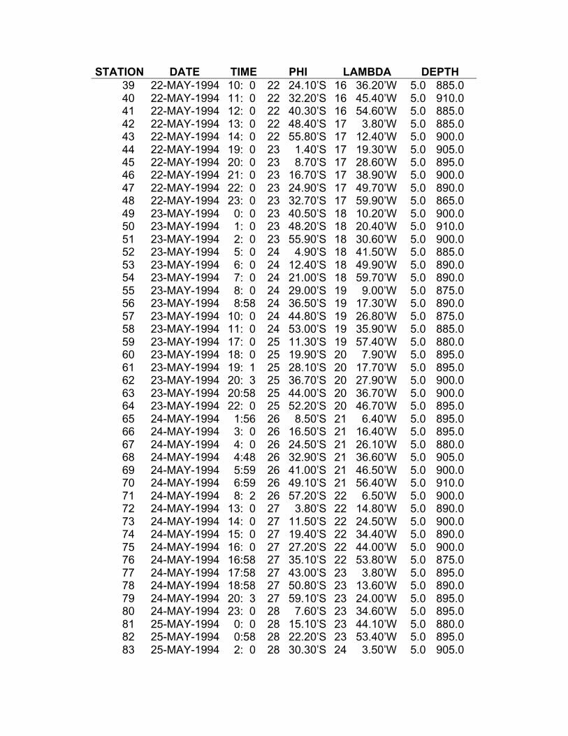
STATION DATE TIME PHI LAMBDA DEPTH39 22-MAY-1994 10: 0 22 24.10’S 16 36.20’W 5.0 885.040 22-MAY-1994 11: 0 22 32.20’S 16 45.40’W 5.0 910.041 22-MAY-1994 12: 0 22 40.30’S 16 54.60’W 5.0 885.042 22-MAY-1994 13: 0 22 48.40’S 17 3.80’W 5.0 885.043 22-MAY-1994 14: 0 22 55.80’S 17 12.40’W 5.0 900.044 22-MAY-1994 19: 0 23 1.40’S 17 19.30’W 5.0 905.045 22-MAY-1994 20: 0 23 8.70’S 17 28.60’W 5.0 895.046 22-MAY-1994 21: 0 23 16.70’S 17 38.90’W 5.0 900.047 22-MAY-1994 22: 0 23 24.90’S 17 49.70’W 5.0 890.048 22-MAY-1994 23: 0 23 32.70’S 17 59.90’W 5.0 865.049 23-MAY-1994 0: 0 23 40.50’S 18 10.20’W 5.0 900.050 23-MAY-1994 1: 0 23 48.20’S 18 20.40’W 5.0 910.051 23-MAY-1994 2: 0 23 55.90’S 18 30.60’W 5.0 900.052 23-MAY-1994 5: 0 24 4.90’S 18 41.50’W 5.0 885.053 23-MAY-1994 6: 0 24 12.40’S 18 49.90’W 5.0 890.054 23-MAY-1994 7: 0 24 21.00’S 18 59.70’W 5.0 890.055 23-MAY-1994 8: 0 24 29.00’S 19 9.00’W 5.0 875.056 23-MAY-1994 8:58 24 36.50’S 19 17.30’W 5.0 890.057 23-MAY-1994 10: 0 24 44.80’S 19 26.80’W 5.0 875.058 23-MAY-1994 11: 0 24 53.00’S 19 35.90’W 5.0 885.059 23-MAY-1994 17: 0 25 11.30’S 19 57.40’W 5.0 880.060 23-MAY-1994 18: 0 25 19.90’S 20 7.90’W 5.0 895.061 23-MAY-1994 19: 1 25 28.10’S 20 17.70’W 5.0 895.062 23-MAY-1994 20: 3 25 36.70’S 20 27.90’W 5.0 900.063 23-MAY-1994 20:58 25 44.00’S 20 36.70’W 5.0 900.064 23-MAY-1994 22: 0 25 52.20’S 20 46.70’W 5.0 895.065 24-MAY-1994 1:56 26 8.50’S 21 6.40’W 5.0 895.066 24-MAY-1994 3: 0 26 16.50’S 21 16.40’W 5.0 895.067 24-MAY-1994 4: 0 26 24.50’S 21 26.10’W 5.0 880.068 24-MAY-1994 4:48 26 32.90’S 21 36.60’W 5.0 905.069 24-MAY-1994 5:59 26 41.00’S 21 46.50’W 5.0 900.070 24-MAY-1994 6:59 26 49.10’S 21 56.40’W 5.0 910.071 24-MAY-1994 8: 2 26 57.20’S 22 6.50’W 5.0 900.072 24-MAY-1994 13: 0 27 3.80’S 22 14.80’W 5.0 890.073 24-MAY-1994 14: 0 27 11.50’S 22 24.50’W 5.0 900.074 24-MAY-1994 15: 0 27 19.40’S 22 34.40’W 5.0 890.075 24-MAY-1994 16: 0 27 27.20’S 22 44.00’W 5.0 900.076 24-MAY-1994 16:58 27 35.10’S 22 53.80’W 5.0 875.077 24-MAY-1994 17:58 27 43.00’S 23 3.80’W 5.0 895.078 24-MAY-1994 18:58 27 50.80’S 23 13.60’W 5.0 890.079 24-MAY-1994 20: 3 27 59.10’S 23 24.00’W 5.0 895.080 24-MAY-1994 23: 0 28 7.60’S 23 34.60’W 5.0 895.081 25-MAY-1994 0: 0 28 15.10’S 23 44.10’W 5.0 880.082 25-MAY-1994 0:58 28 22.20’S 23 53.40’W 5.0 895.083 25-MAY-1994 2: 0 28 30.30’S 24 3.50’W 5.0 905.0

STATION DATE TIME PHI LAMBDA DEPTH84 25-MAY-1994 3: 0 28 37.80’S 24 13.00’W 5.0 900.085 25-MAY-1994 4: 0 28 45.40’S 24 23.00’W 5.0 900.086 25-MAY-1994 5: 0 28 53.00’S 24 33.00’W 5.0 890.087 25-MAY-1994 8:59 29 8.60’S 24 53.90’W 5.0 885.088 25-MAY-1994 10: 0 29 16.90’S 25 3.30’W 5.0 895.089 25-MAY-1994 11: 0 29 25.00’S 25 13.40’W 5.0 870.0
7.2.3 List of Drifter Launches
Sta. Drifter Date Time Latitude Longitude Temp Drogue RemarksNo. (ARGOS) 1994 UTC South West (ºC) (m)291 00652 20/5 5:20 21º00.0 10º00.1 23.6 100 Drift Sta. only292 00665 20/5 19:00 20º59.9 10º34.5 23.8 100 Test Sta.293 00671 21/5 2:15 20º59.8 12º00.0 24.0 100 Drift Sta. only294 00650 21/5 9:50 21º00.1 13º30.1 24.3 100 Drift Sta. only295 00626 21/5 21:04 20º59.1 15º01.1 24.5 100 w2 Float Depl.297 00670 22/5 18:34 22º59.9 17º17.0 24.2 100 w Float Depl.299 00630 23/5 15:23 25º00.0 19º43.9 24.1 100 w Float Depl.301 00654 24/5 12:22 26º59.2 22º09.9 22.2 100 w Float Depl.303 00639 25/5 7:49 28º59.9 24º42.0 21.2 100 w Float Depl.305 00668 26/5 4:26 30º48.8 27º22.9 21.4 100 w Float Depl.307 00672 26/5 22:40 32º29.9 28º48.0 20.6 100 w Float Depl.309 00673 27/5 21:48 34º19.2 28º29.8 19.2 100 H1 w Fl Dep.313 00653 28/5 19:07 34º25.4 27º52.4 17.4 100 H2º Hunter Ch.321 00669 1/6 13:59 35º29.8 28º21.4 17.7 100 search for K0327 00628 3/6 00:46 33º15.4 26º31.9 18.6 100 Hunter Ch East334 00663 6/6 5:05 36º42.3 31º30.6 16.7 100 SR im Subtr. Gyre336 00624 7/6 1:46 38º31.0 33º14.0 16.2 100 SR im Subtr. Gyre338 00647 7/6 19:17 39º54.2 34º34.8 11.5 100 Subtropr. Front341 00649 8/6 1:20 36º48.1 37º31.3 17.0 100 towards Vema Ch.343 00635 9/6 21:16 35º00.2 40º00.1 18.9 100 outer Vema Ch.
7.2.4 Mooring Activities
Sta. Ext Int Date Latitude Longitude Depth Instrum. RemarksNo. No. No. dd/mm/yy South West (m) TypeCurrent Meter Moorings*612 R 363 16/12/92 31º37.1 28º48.6 3719 2ACM DWBC at Rio
G Rise306 26/05/94 CB 100% recvd
*602 H1 353 11/12/92 34º15.5 28º52.3 4112 6ACM, CB Hunter West309 27/5/94 IMAFOS 100% recvd
*605 H3 355 12-14/12/92 approximately 1 (4436) 5ACM launch interrup,34º23.5 27º42.7 dual release,
no CB
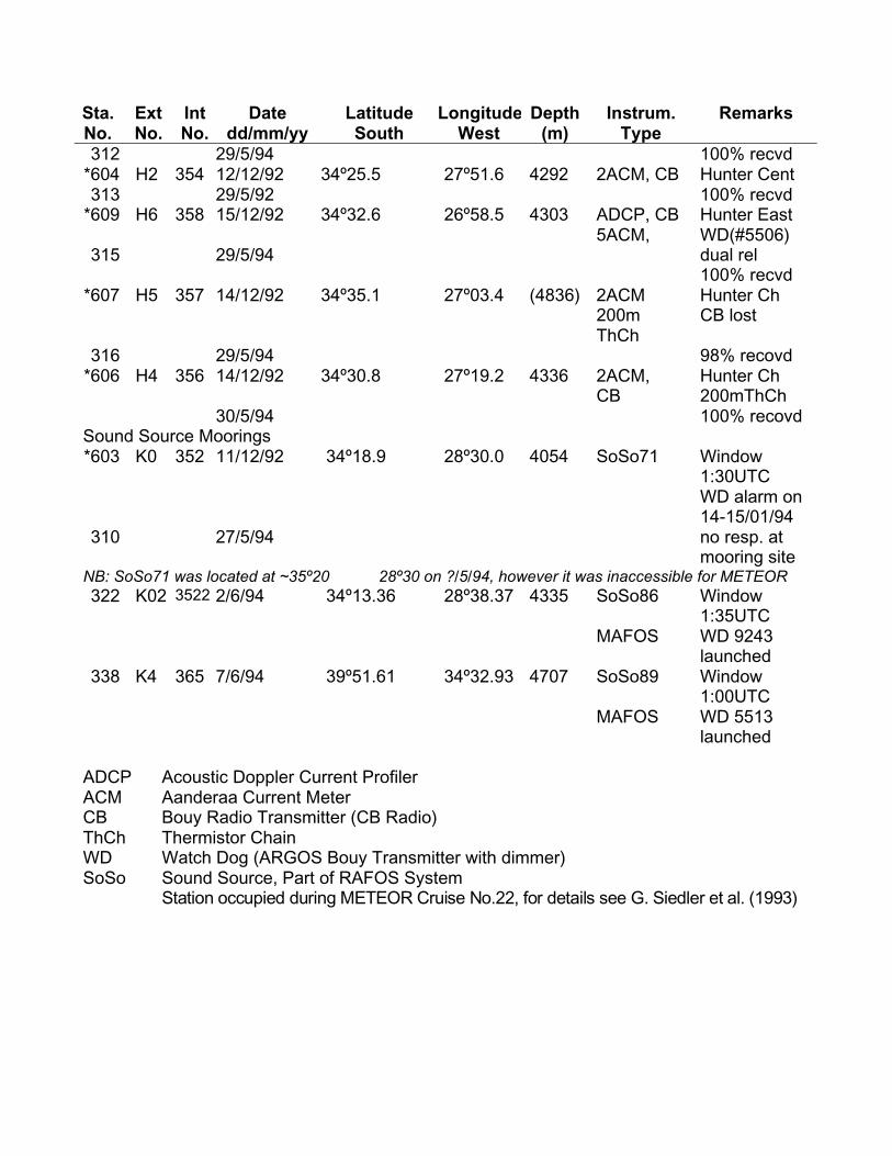
Sta. Ext Int Date Latitude Longitude Depth Instrum. RemarksNo. No. No. dd/mm/yy South West (m) Type312 29/5/94 100% recvd
*604 H2 354 12/12/92 34º25.5 27º51.6 4292 2ACM, CB Hunter Cent313 29/5/92 100% recvd
*609 H6 358 15/12/92 34º32.6 26º58.5 4303 ADCP, CB Hunter East5ACM, WD(#5506)
315 29/5/94 dual rel100% recvd
*607 H5 357 14/12/92 34º35.1 27º03.4 (4836) 2ACM Hunter Ch200m CB lostThCh
316 29/5/94 98% recovd*606 H4 356 14/12/92 34º30.8 27º19.2 4336 2ACM, Hunter Ch
CB 200mThCh30/5/94 100% recovd
Sound Source Moorings*603 K0 352 11/12/92 34º18.9 28º30.0 4054 SoSo71 Window
1:30UTCWD alarm on14-15/01/94
310 27/5/94 no resp. atmooring site
NB: SoSo71 was located at ~35º20 28º30 on ?/5/94, however it was inaccessible for METEOR322 K02 3522 2/6/94 34º13.36 28º38.37 4335 SoSo86 Window
1:35UTCMAFOS WD 9243
launched338 K4 365 7/6/94 39º51.61 34º32.93 4707 SoSo89 Window
1:00UTCMAFOS WD 5513
launched
ADCP Acoustic Doppler Current ProfilerACM Aanderaa Current MeterCB Bouy Radio Transmitter (CB Radio)ThCh Thermistor ChainWD Watch Dog (ARGOS Bouy Transmitter with dimmer)SoSo Sound Source, Part of RAFOS System
Station occupied during METEOR Cruise No.22, for details see G. Siedler et al. (1993)
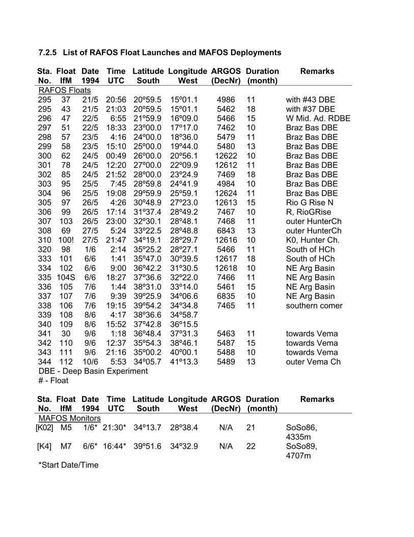
7.2.5 List of RAFOS Float Launches and MAFOS Deployments
Sta. Float Date Time Latitude Longitude ARGOS Duration RemarksNo. IfM 1994 UTC South West (DecNr) (month)RAFOS Floats295 37 21/5 20:56 20º59.5 15º01.1 4986 11 with #43 DBE295 43 21/5 21:03 20º59.5 15º01.1 5462 18 with #37 DBE296 47 22/5 6:55 21º59.9 16º09.0 5466 15 W Mid. Ad. RDBE297 51 22/5 18:33 23º00.0 17º17.0 7462 10 Braz Bas DBE298 57 23/5 4:16 24º00.0 18º36.0 5479 11 Braz Bas DBE299 58 23/5 15:10 25º00.0 19º44.0 5480 13 Braz Bas DBE300 62 24/5 00:49 26º00.0 20º56.1 12622 10 Braz Bas DBE301 78 24/5 12:20 27º00.0 22º09.9 12612 11 Braz Bas DBE302 85 24/5 21:52 28º00.0 23º24.9 7469 18 Braz Bas DBE303 95 25/5 7:45 28º59.8 24º41.9 4984 10 Braz Bas DBE304 96 25/5 19:08 29º59.9 25º59.1 12624 11 Braz Bas DBE305 97 26/5 4:26 30º48.9 27º23.0 12613 15 Rio G Rise N306 99 26/5 17:14 31º37.4 28º49.2 7467 10 R, RioGRise307 103 26/5 23:00 32º30.1 28º48.1 7468 11 outer HunterCh308 69 27/5 5:24 33º22.5 28º48.8 6843 13 outer HunterCh310 100! 27/5 21:47 34º19.1 28º29.7 12616 10 K0, Hunter Ch.320 98 1/6 2:14 35º25.2 28º27.1 5466 11 South of HCh333 101 6/6 1:41 35º47.0 30º39.5 12617 18 South of HCh334 102 6/6 9:00 36º42.2 31º30.5 12618 10 NE Arg Basin335 104S 6/6 18:27 37º36.6 32º22.0 7466 11 NE Arg Basin336 105 7/6 1:44 38º31.0 33º14.0 5461 15 NE Arg Basin337 107 7/6 9:39 39º25.9 34º06.6 6835 10 NE Arg Basin338 106 7/6 19:15 39º54.2 34º34.8 7465 11 southern comer339 108 8/6 4:17 38º36.6 34º58.7340 109 8/6 15:52 37º42.8 36º15.5341 30 9/6 1:18 36º48.4 37º31.3 5463 11 towards Vema342 110 9/6 12:37 35º54.3 38º46.1 5487 15 towards Vema343 111 9/6 21:16 35º00.2 40º00.1 5488 10 towards Vema344 112 10/6 5:53 34º05.7 41º13.3 5489 13 outer Vema ChDBE - Deep Basin Experiment# - Float
Sta. Float Date Time Latitude Longitude ARGOS Duration RemarksNo. IfM 1994 UTC South West (DecNr) (month)MAFOS Monitors
[K02] M5 1/6* 21:30* 34º13.7 28º38.4 N/A 21 SoSo86,4335m
[K4] M7 6/6* 16:44* 39º51.6 34º32.9 N/A 22 SoSo89,4707m
*Start Date/Time
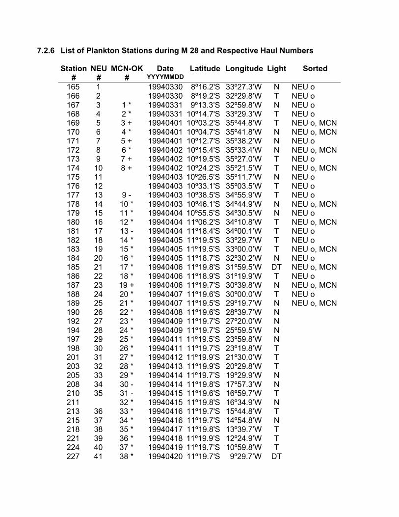
7.2.6 List of Plankton Stations during M 28 and Respective Haul Numbers
Station NEU MCN-OK Date Latitude Longitude Light Sorted# # # YYYYMMDD
165 1 19940330 8º16.2'S 33º27.3’W N NEU o166 2 19940330 8º19.2'S 32º29.8’W T NEU o167 3 1 * 19940331 9º13.3’S 32º59.8’W N NEU o168 4 2 * 19940331 10º14.7'S 33º29.3’W T NEU o169 5 3 + 19940401 10º03.2'S 35º44.8’W T NEU o, MCN170 6 4 * 19940401 10º04.7'S 35º41.8’W N NEU o, MCN171 7 5 + 19940401 10º12.7'S 35º38.2’W N NEU o172 8 6 * 19940402 10º15.4'S 35º33.4’W N NEU o, MCN173 9 7 + 19940402 10º19.5'S 35º27.0’W T NEU o174 10 8 + 19940402 10º24.2'S 35º21.5’W T NEU o, MCN175 11 19940403 10º26.5’S 35º11.7’W N NEU o176 12 19940403 10º33.1'S 35º03.5’W T NEU o177 13 9 - 19940403 10º38.5'S 34º55.9’W T NEU o178 14 10 * 19940403 10º46.1'S 34º44.9’W N NEU o, MCN179 15 11 * 19940404 10º55.5’S 34º30.5’W N NEU o180 16 12 * 19940404 11º06.2'S 34º10.8’W T NEU o, MCN181 17 13 - 19940404 11º18.4'S 34º00.1’W T NEU o182 18 14 * 19940405 11º19.5'S 33º29.7’W T NEU o183 19 15 * 19940405 11º19.5’S 33º00.0’W T NEU o, MCN184 20 16 * 19940405 11º18.7'S 32º30.2’W N NEU o185 21 17 * 19940406 11º19.8'S 31º59.5’W DT NEU o, MCN186 22 18 * 19940406 11º18.9'S 31º19.9’W T NEU o187 23 19 + 19940406 11º19.7'S 30º39.8’W N NEU o, MCN188 24 20 * 19940407 11º19.6'S 30º00.0’W T NEU o189 25 21 * 19940407 11º19.5'S 29º19.7’W N NEU o, MCN190 26 22 * 19940408 11º19.6'S 28º39.7’W N192 27 23 * 19940409 11º19.7'S 27º20.0’W N194 28 24 * 19940409 11º19.7'S 25º59.5’W N197 29 25 * 19940411 11º19.5’S 23º59.8’W N198 30 26 * 19940411 11º19.7'S 23º19.8’W T201 31 27 * 19940412 11º19.9’S 21º30.0’W T203 32 28 * 19940413 11º19.9'S 20º29.8’W T205 33 29 * 19940414 11º19.7’S 19º29.9’W N208 34 30 - 19940414 11º19.8'S 17º57.3’W N210 35 31 - 19940415 11º19.6'S 16º59.7’W T211 32 * 19940415 11º19.8'S 16º34.9’W N213 36 33 * 19940416 11º19.7'S 15º44.8’W T215 37 34 * 19940416 11º19.7'S 14º54.8’W N218 38 35 * 19940417 11º19.8'S 13º39.7’W T221 39 36 * 19940418 11º19.9’S 12º24.9’W T224 40 37 * 19940419 11º19.7’S 10º59.8’W T227 41 38 * 19940420 11º19.7'S 9º29.7’W DT
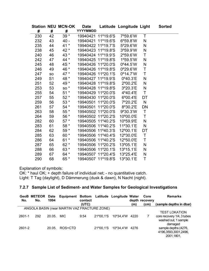
Station NEU MCN-OK Date Latitude Longitude Light Sorted# # # YYYYMMDD
230 42 39 * 19940421 11º19.6'S 7º59.6’W T232 43 40 - 19940421 11º19.6'S 6º59.8’W N235 44 41 * 19940422 11º19.7’S 5º29.6’W N238 45 42 * 19940423 11º19.8'S 3º59.9’W N240 46 43 * 19940424 11º19.9’S 2º59.6’W T242 47 44 * 19940425 11º19.8'S 1º59.5’W N245 48 4S * 19940426 11º20.0'S 0º44.5’W N246 49 46 * 19940426 11º19.8'S 0º29.6’W T247 so 47 * 19940426 11º20.1'S 0º14.7’W T249 S1 48 * 19940427 11º19.9’S 0º40.3’E N251 52 49 * 19940428 11º19.8'S 2º00.2'E N253 53 so * 19940428 11º19.8'S 3º20.3’E N255 54 51 * 19940429 11º20.0'S 4º40.4'E T257 55 52 * 19940430 11º20.0'S 6º00.4'E DT259 56 53 * 19940501 11º20.0'S 7º20.2'E N261 57 54 * 19940501 11º20.0'S 8º30.2'E DN263 58 55 * 19940502 11º20.0'S 9º30.3’W T264 59 56 * 19940502 11º20.2'S 10º00.0'E T282 60 57 * 19940505 11º40.2'S 10º59.9'E N283 61 58 * 19940506 11º40.2'S 11º30.1’E N284 62 59 * 19940506 11º40.3’S 12º00.1’E DT285 63 60 * 19940506 11º40.4'S 12º30.0'E T286 64 61 * 19940506 11º40.2'S 12º50.0'E T287 65 62 * 19940506 11º20.2'S 13º05.1’E N288 66 63 * 19940506 11º20.1'S 13º15.1’E N289 67 64 * 19940507 11º20.4'S 13º25.4'E N290 68 65 * 19940507 11º19.8'S 13º30.1’E T
Explanation of symbols:OK: * haul OK; + depth failure of individual net; - no quantitative catch.Light: T Tag (daylight), D Dämmerung (dusk & dawn), N Nacht (night).
7.2.7 Sample List of Sediment- and Water Samples for Geological Investigations
GeoB METEOR Date Equipment Bottom Latitude Longitude Water Core RemarksNo. No. 1994 contact depth recovery
(UTC) (m) (cm) (sample depths in dbar)ANGOLA BASIN (near MARTIN VAZ FRACTURE ZONE)
TEST LOKATION2601-1 292 20.05. MIC 9:54 21º00,1'S 10º34,4'W 4220 7 core recovery 1/4, 3 tubes
washed out, 1 sampledamaged
2601-2 20.05. ROS+CTD 21º00,1'S 10º34,4’W 4276 sample depths (4276,4196,3593,3001,2496,
2001,1801,
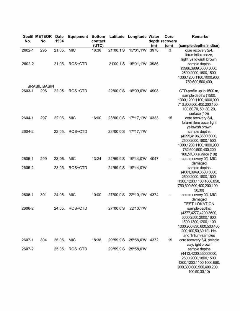
GeoB METEOR Date Equipment Bottom Latitude Longitude Water Core RemarksNo. No. 1994 contact depth recovery
(UTC) (m) (cm) (sample depths in dbar)2602-1 295 21.05. MIC 18:38 21º00,1'S 15º01,1'W 3978 3 core recovery 2/4,
foraminifere ooze,light yellowish brown
2602-2 21.05. ROS+CTD 21'00,1'S 15º01,1’W 3986 sample depths(3986,3909,3600,3000,2500,2000,1800,1500,
1300,1200,1100,1000,900,750,600,500,400,
BRASIL BASIN2603-1 296 22.05. ROS+CTD 22º00,0'S 16º09,0’W 4908 CTD-profile up to 1500 m,
sample depths (1500,1300,1200,1100,1000,900,710,600,500,400,200,150,
100,80,70, 50, 30, 20,surface (10))
2604-1 297 22.05. MIC 16:00 23º00,0'S 17º17,1’W 4333 15 core recovery 3/4,foraminifere ooze, light
yellowish brown2604-2 22.05. ROS+CTD 23º00,0'S 17º17,1’W sample depths
(4295,4196,3600,3000,2500,2000,1800,1500,
1300,1200,1100,1000,900,782,600,500,400,200
100,50,30,surface (10))2605-1 299 23-05. MIC 13:24 24º59,9'S 19º44,0’W 4047 - core recovery 0/4, MIC
damaged2605-2 23.05. ROS+CTD 24º59,9'S 19º44,0’W sample depths
(4061,3949,3600,3000,2500,2000,1800,1500,
1300,1200,1100,1000,850,750,600,500,400,200,100,
50,30)2606-1 301 24.05. MIC 10:00 27º00,0'S 22º10,1’W 4374 - core recovery 0/4, MIC
damagedTEST LOKATION
2606-2 24.05. ROS+CTD 27º00,0'S 22'10,1’W sample depths;(4377,4277,4200,3600,3000,2500,2000,1800,1500,1300,1200,1100,
1000,900,830,600,500,400200,100,50,30,10), He-and Tritium-samples
2607-1 304 25.05. MIC 18:38 29º59,9'S 25º58,0’W 4372 19 core recovery 3/4, pelagicclay, light brown
2607-2 25.05. ROS+CTD 29º59,9'S 25º58,0’W sample depths(4413,4200,3600,3000,2500,2000,1800,1500,
1300,1200,1100,1000,980,900,800,600,500,400,200,
100,50,30,10)
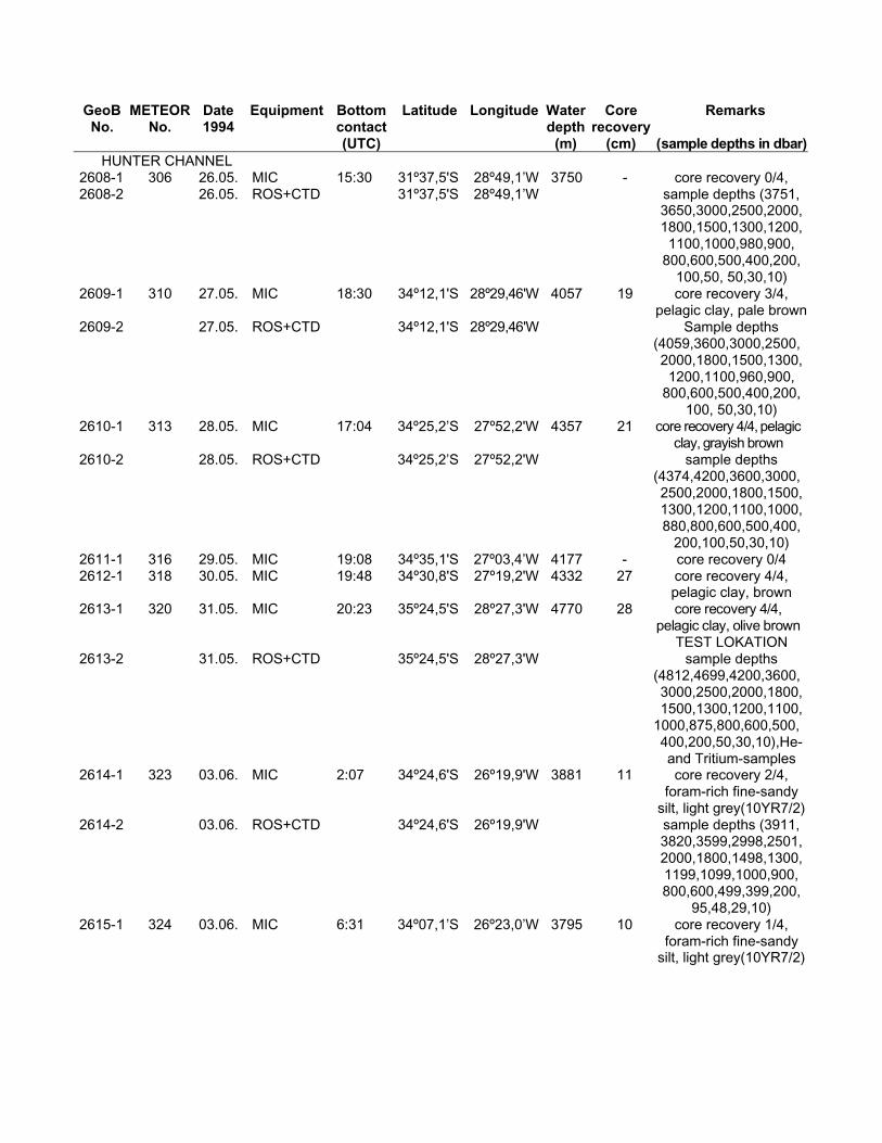
GeoB METEOR Date Equipment Bottom Latitude Longitude Water Core RemarksNo. No. 1994 contact depth recovery
(UTC) (m) (cm) (sample depths in dbar)HUNTER CHANNEL
2608-1 306 26.05. MIC 15:30 31º37,5'S 28º49,1’W 3750 - core recovery 0/4,2608-2 26.05. ROS+CTD 31º37,5'S 28º49,1’W sample depths (3751,
3650,3000,2500,2000,1800,1500,1300,1200,
1100,1000,980,900,800,600,500,400,200,
100,50, 50,30,10)2609-1 310 27.05. MIC 18:30 34º12,1'S 28º29,46'W 4057 19 core recovery 3/4,
pelagic clay, pale brown2609-2 27.05. ROS+CTD 34º12,1'S 28º29,46'W Sample depths
(4059,3600,3000,2500,2000,1800,1500,1300,
1200,1100,960,900,800,600,500,400,200,
100, 50,30,10)2610-1 313 28.05. MIC 17:04 34º25,2’S 27º52,2'W 4357 21 core recovery 4/4, pelagic
clay, grayish brown2610-2 28.05. ROS+CTD 34º25,2’S 27º52,2'W sample depths
(4374,4200,3600,3000,2500,2000,1800,1500,1300,1200,1100,1000,880,800,600,500,400,
200,100,50,30,10)2611-1 316 29.05. MIC 19:08 34º35,1'S 27º03,4’W 4177 - core recovery 0/42612-1 318 30.05. MIC 19:48 34º30,8'S 27º19,2'W 4332 27 core recovery 4/4,
pelagic clay, brown2613-1 320 31.05. MIC 20:23 35º24,5'S 28º27,3'W 4770 28 core recovery 4/4,
pelagic clay, olive brownTEST LOKATION
2613-2 31.05. ROS+CTD 35º24,5'S 28º27,3'W sample depths(4812,4699,4200,3600,3000,2500,2000,1800,1500,1300,1200,1100,
1000,875,800,600,500,400,200,50,30,10),He-and Tritium-samples
2614-1 323 03.06. MIC 2:07 34º24,6'S 26º19,9'W 3881 11 core recovery 2/4,foram-rich fine-sandy
silt, light grey(10YR7/2)2614-2 03.06. ROS+CTD 34º24,6'S 26º19,9'W sample depths (3911,
3820,3599,2998,2501,2000,1800,1498,1300,1199,1099,1000,900,800,600,499,399,200,
95,48,29,10)2615-1 324 03.06. MIC 6:31 34º07,1’S 26º23,0’W 3795 10 core recovery 1/4,
foram-rich fine-sandysilt, light grey(10YR7/2)
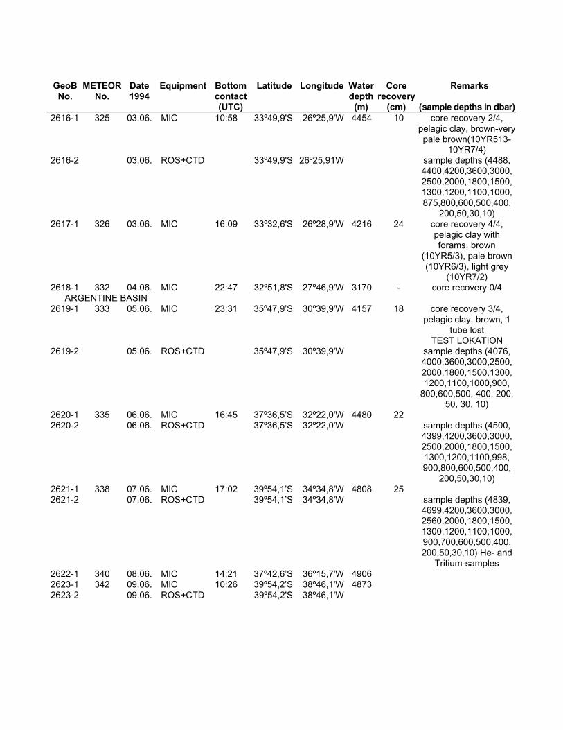
GeoB METEOR Date Equipment Bottom Latitude Longitude Water Core RemarksNo. No. 1994 contact depth recovery
(UTC) (m) (cm) (sample depths in dbar)2616-1 325 03.06. MIC 10:58 33º49,9'S 26º25,9'W 4454 10 core recovery 2/4,
pelagic clay, brown-verypale brown(10YR513-
10YR7/4)2616-2 03.06. ROS+CTD 33º49,9'S 26º25,91W sample depths (4488,
4400,4200,3600,3000,2500,2000,1800,1500,1300,1200,1100,1000,875,800,600,500,400,
200,50,30,10)2617-1 326 03.06. MIC 16:09 33º32,6'S 26º28,9'W 4216 24 core recovery 4/4,
pelagic clay withforams, brown
(10YR5/3), pale brown(10YR6/3), light grey
(10YR7/2)2618-1 332 04.06. MIC 22:47 32º51,8'S 27º46,9'W 3170 - core recovery 0/4
ARGENTINE BASIN2619-1 333 05.06. MIC 23:31 35º47,9’S 30º39,9'W 4157 18 core recovery 3/4,
pelagic clay, brown, 1tube lost
TEST LOKATION2619-2 05.06. ROS+CTD 35º47,9’S 30º39,9'W sample depths (4076,
4000,3600,3000,2500,2000,1800,1500,1300,1200,1100,1000,900,
800,600,500, 400, 200,50, 30, 10)
2620-1 335 06.06. MIC 16:45 37º36,5’S 32º22,0'W 4480 222620-2 06.06. ROS+CTD 37º36,5’S 32º22,0'W sample depths (4500,
4399,4200,3600,3000,2500,2000,1800,1500,1300,1200,1100,998,900,800,600,500,400,
200,50,30,10)2621-1 338 07.06. MIC 17:02 39º54,1’S 34º34,8'W 4808 252621-2 07.06. ROS+CTD 39º54,1’S 34º34,8'W sample depths (4839,
4699,4200,3600,3000,2560,2000,1800,1500,1300,1200,1100,1000,900,700,600,500,400,200,50,30,10) He- and
Tritium-samples2622-1 340 08.06. MIC 14:21 37º42,6’S 36º15,7'W 49062623-1 342 09.06. MIC 10:26 39º54,2’S 38º46,1'W 48732623-2 09.06. ROS+CTD 39º54,2'S 38º46,1'W
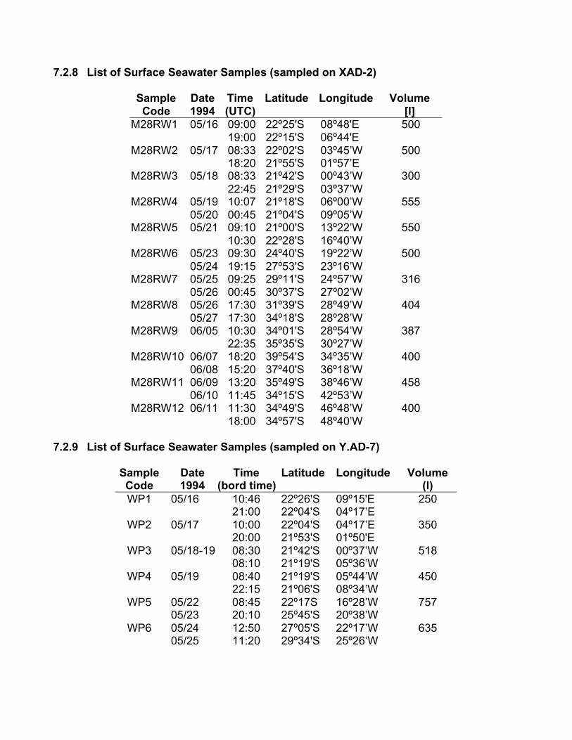
7.2.8 List of Surface Seawater Samples (sampled on XAD-2)
Sample Date Time Latitude Longitude VolumeCode 1994 (UTC) [l]
M28RW1 05/16 09:00 22º25'S 08º48'E 50019:00 22º15'S 06º44'E
M28RW2 05/17 08:33 22º02'S 03º45’W 50018:20 21º55'S 01º57’E
M28RW3 05/18 08:33 21º42'S 00º43’W 30022:45 21º29'S 03º37’W
M28RW4 05/19 10:07 21º18'S 06º00’W 55505/20 00:45 21º04'S 09º05’W
M28RW5 05/21 09:10 21º00'S 13º22’W 55010:30 22º28'S 16º40’W
M28RW6 05/23 09:30 24º40'S 19º22’W 50005/24 19:15 27º53'S 23º16’W
M28RW7 05/25 09:25 29º11'S 24º57’W 31605/26 00:45 30º37'S 27º02’W
M28RW8 05/26 17:30 31º39'S 28º49’W 40405/27 17:30 34º18'S 28º28’W
M28RW9 06/05 10:30 34º01'S 28º54’W 38722:35 35º35'S 30º27’W
M28RW10 06/07 18:20 39º54'S 34º35’W 40006/08 15:20 37º40'S 36º18’W
M28RW11 06/09 13:20 35º49'S 38º46’W 45806/10 11:45 34º15'S 42º53’W
M28RW12 06/11 11:30 34º49'S 46º48’W 40018:00 34º57'S 48º40’W
7.2.9 List of Surface Seawater Samples (sampled on Y.AD-7)
Sample Date Time Latitude Longitude VolumeCode 1994 (bord time) (l)WP1 05/16 10:46 22º26'S 09º15'E 250
21:00 22º04'S 04º17’EWP2 05/17 10:00 22º04'S 04º17’E 350
20:00 21º53'S 01º50'EWP3 05/18-19 08:30 21º42'S 00º37’W 518
08:10 21º19'S 05º36’WWP4 05/19 08:40 21º19'S 05º44’W 450
22:15 21º06'S 08º34’WWP5 05/22 08:45 22º17S 16º28’W 757
05/23 20:10 25º45'S 20º38’WWP6 05/24 12:50 27º05'S 22º17’W 635
05/25 11:20 29º34'S 25º26’W
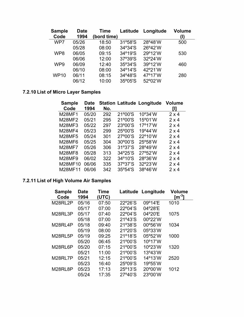
Sample Date Time Latitude Longitude VolumeCode 1994 (bord time) (l)WP7 05/26 18:50 31º58'S 28º48’W 500
05/28 08:00 34º34'S 26º42’WWP8 06/05 09:15 34º19'S 29º12’W 530
06/06 12:00 37º39'S 32º24’WWP9 06/09 12:40 35º34'S 39º12’W 460
06/10 08:00 34º14'S 42º21’WWP10 06/11 08:15 34º48'S 47º17’W 280
06/12 10:00 35º05'S 52º02’W
7.2.10 List of Micro Layer Samples
Sample Date Station Latitude Longitude VolumeCode 1994 No. [l]
M28MF1 05/20 292 21º00'S 10º34’W 2 x 4M28MF2 05/21 295 21º00'S 15º01’W 2 x 4M28MF3 05/22 297 23º00’S 17º17’W 2 x 4M28MF4 05/23 299 25º00'S 19º44’W 2 x 4M28MF5 05/24 301 27º00’S 22º10’W 2 x 4M28MF6 05/25 304 30º00’S 25º58’W 2 x 4M28MF7 05/26 306 31º37’S 28º49’W 2 x 4M28MF8 05/28 313 34º25’S 27º52’W 2 x 4M28MF9 06/02 322 34º10'S 28º36’W 2 x 4M28MF10 06/06 335 37º37’S 32º23’W 2 x 4M28MF11 06/06 342 35º54'S 38º46’W 2 x 4
7.2.11 List of High Volume Air Samples
Sample Date Time Latitude Longitude VolumeCode 1994 (UTC) [m-3]
M28RL2P 05/16 07:50 22º26’S 09º14'E 101005/17 07:00 22º04’S 04º28'E
M28RL3P 05/17 07:40 22º04’S 04º20'E 107505/18 07:00 21º43’S 00º22’W
M28RL4P 05/18 09:40 21º38’S 00º56’W 103405/19 08:00 21º20’S 05º33’W
M28RL5P 05/19 09:25 21º18’S 05º52’W 100005/20 06:45 21º00’S 10º17’W
M28RL6P 05/20 07:15 21º00’S 10º23’W 132005/21 11:00 21º00’S 13º43’W
M28RL7P 05/21 12:15 21º00’S 14º13’W 252005/23 16:40 25º09’S 19º55’W
M28RL8P 05/23 17:13 25º13’S 20º00’W 101205/24 17:35 27º40’S 23º00’W
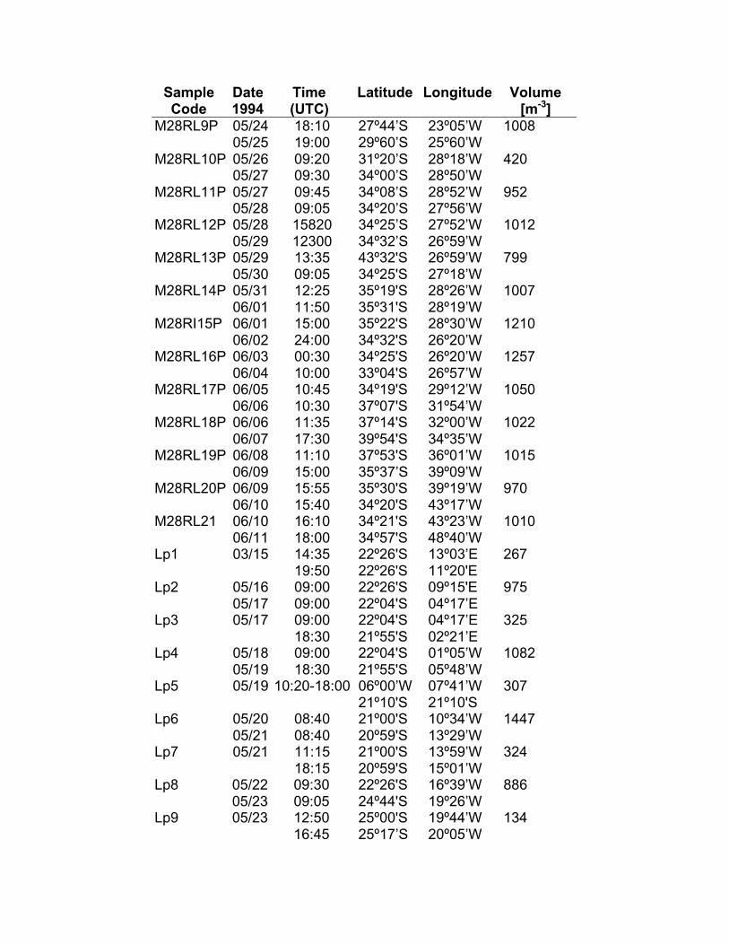
Sample Date Time Latitude Longitude VolumeCode 1994 (UTC) [m-3]
M28RL9P 05/24 18:10 27º44’S 23º05’W 100805/25 19:00 29º60’S 25º60’W
M28RL10P 05/26 09:20 31º20’S 28º18’W 42005/27 09:30 34º00’S 28º50’W
M28RL11P 05/27 09:45 34º08’S 28º52’W 95205/28 09:05 34º20’S 27º56’W
M28RL12P 05/28 15820 34º25’S 27º52’W 101205/29 12300 34º32’S 26º59’W
M28RL13P 05/29 13:35 43º32'S 26º59’W 79905/30 09:05 34º25'S 27º18’W
M28RL14P 05/31 12:25 35º19'S 28º26’W 100706/01 11:50 35º31'S 28º19’W
M28RI15P 06/01 15:00 35º22'S 28º30’W 121006/02 24:00 34º32'S 26º20’W
M28RL16P 06/03 00:30 34º25'S 26º20’W 125706/04 10:00 33º04'S 26º57’W
M28RL17P 06/05 10:45 34º19'S 29º12’W 105006/06 10:30 37º07'S 31º54’W
M28RL18P 06/06 11:35 37º14'S 32º00’W 102206/07 17:30 39º54'S 34º35’W
M28RL19P 06/08 11:10 37º53'S 36º01’W 101506/09 15:00 35º37’S 39º09’W
M28RL20P 06/09 15:55 35º30'S 39º19’W 97006/10 15:40 34º20'S 43º17’W
M28RL21 06/10 16:10 34º21'S 43º23’W 101006/11 18:00 34º57'S 48º40’W
Lp1 03/15 14:35 22º26'S 13º03’E 26719:50 22º26'S 11º20'E
Lp2 05/16 09:00 22º26'S 09º15'E 97505/17 09:00 22º04'S 04º17’E
Lp3 05/17 09:00 22º04'S 04º17’E 32518:30 21º55'S 02º21’E
Lp4 05/18 09:00 22º04'S 01º05’W 108205/19 18:30 21º55'S 05º48’W
Lp5 05/19 10:20-18:00 06º00’W 07º41’W 30721º10'S 21º10'S
Lp6 05/20 08:40 21º00'S 10º34’W 144705/21 08:40 20º59'S 13º29’W
Lp7 05/21 11:15 21º00'S 13º59’W 32418:15 20º59'S 15º01’W
Lp8 05/22 09:30 22º26'S 16º39’W 88605/23 09:05 24º44'S 19º26’W
Lp9 05/23 12:50 25º00'S 19º44’W 13416:45 25º17’S 20º05’W
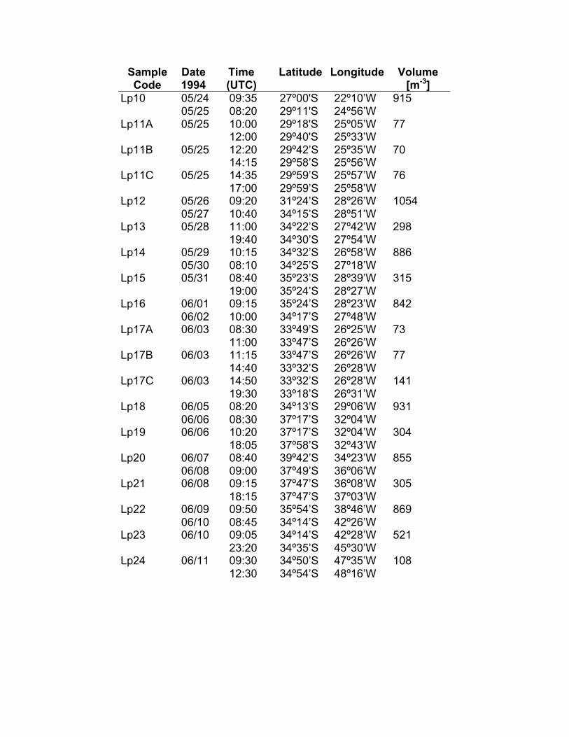
Sample Date Time Latitude Longitude VolumeCode 1994 (UTC) [m-3]
Lp10 05/24 09:35 27º00'S 22º10’W 91505/25 08:20 29º11'S 24º56’W
Lp11A 05/25 10:00 29º18'S 25º05’W 7712:00 29º40'S 25º33’W
Lp11B 05/25 12:20 29º42’S 25º35’W 7014:15 29º58’S 25º56’W
Lp11C 05/25 14:35 29º59’S 25º57’W 7617:00 29º59’S 25º58’W
Lp12 05/26 09:20 31º24’S 28º26’W 105405/27 10:40 34º15’S 28º51’W
Lp13 05/28 11:00 34º22’S 27º42’W 29819:40 34º30’S 27º54’W
Lp14 05/29 10:15 34º32’S 26º58’W 88605/30 08:10 34º25’S 27º18’W
Lp15 05/31 08:40 35º23’S 28º39’W 31519:00 35º24’S 28º27’W
Lp16 06/01 09:15 35º24’S 28º23’W 84206/02 10:00 34º17’S 27º48’W
Lp17A 06/03 08:30 33º49’S 26º25’W 7311:00 33º47’S 26º26’W
Lp17B 06/03 11:15 33º47’S 26º26’W 7714:40 33º32’S 26º28’W
Lp17C 06/03 14:50 33º32’S 26º28’W 14119:30 33º18’S 26º31’W
Lp18 06/05 08:20 34º13’S 29º06’W 93106/06 08:30 37º17’S 32º04’W
Lp19 06/06 10:20 37º17’S 32º04’W 30418:05 37º58’S 32º43’W
Lp20 06/07 08:40 39º42’S 34º23’W 85506/08 09:00 37º49’S 36º06’W
Lp21 06/08 09:15 37º47’S 36º08’W 30518:15 37º47’S 37º03’W
Lp22 06/09 09:50 35º54’S 38º46’W 86906/10 08:45 34º14’S 42º26’W
Lp23 06/10 09:05 34º14’S 42º28’W 52123:20 34º35’S 45º30’W
Lp24 06/11 09:30 34º50’S 47º35’W 10812:30 34º54’S 48º16’W
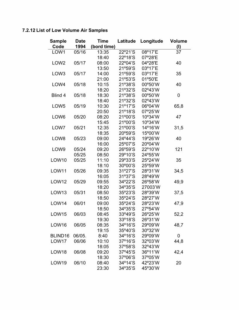
7.2.12 List of Low Volume Air Samples
Sample Date Time Latitude Longitude VolumeCode 1994 (bord time) (l)LOW1 05/16 13:35 22º21’S 08º17’E 37
18:40 22º18’S 07º28'ELOW2 05/17 08:00 22º04’S 04º28'E 40
13:50 21º59’S 03º17’ELOW3 05/17 14:00 21º59’S 03º17’E 35
21:00 21º53’S 01º50'ELOW4 05/18 10:15 21º38’S 00º50’W 40
18:20 21º32’S 02º43’WBlind 4 05/18 18:30 21º38’S 00º50’W 0
18:40 21º32’S 02º43’WLOW5 05/19 10:30 21º17’S 06º04’W 65,8
20:50 21º18’S 07º25’WLOW6 05/20 08:20 21º00’S 10º34’W 47
15:45 21º00’S 10º34’WLOW7 05/21 12:35 21º00’S 14º16’W 31,5
18:35 20º59’S 15º00’WLOW8 05/23 09:00 24º44’S 19º26’W 40
16:00 25º07’S 20º04’WLOW9 05/24 09:20 26º59’S 22º10’W 121
05/25 08:50 29º10’S 24º55’WLOW10 05/25 11:10 29º33’S 25º24’W 35
18:10 30º00’S 25º59’WLOW11 05/26 09:35 31º27’S 28º31’W 34,5
16:05 31º37’S 28º49’WLOW12 05/29 09:55 34º22’S 26º58’W 49,9
18:20 34º35’S 27003’WLOW13 05/31 08:50 35º23’S 28º39’W 37,5
18:50 35º24’S 28º27’WLOW14 06/01 09:00 35º24’S 28º23’W 47,9
18:50 34º35’S 27º54’WLOW15 06/03 08:45 33º49’S 26º25’W 52,2
19:30 33º18’S 26º31’WLOW16 06/05 08:35 34º16’S 29º09’W 48,7
19:15 35º40’S 30º32’WBLIND16 06/05. 8:40 34º16’S 29º09’W 0LOW17 06/06 10:10 37º16’S 32º03’W 44,8
18:05 37º58’S 32º43’WLOW18 06/08 09:20 37º45’S 36º11’W 42,4
18:30 37º06’S 37º05’WLOW19 06/10 08:40 34º14’S 42º23’W 20
23:30 34º35’S 45º30’W
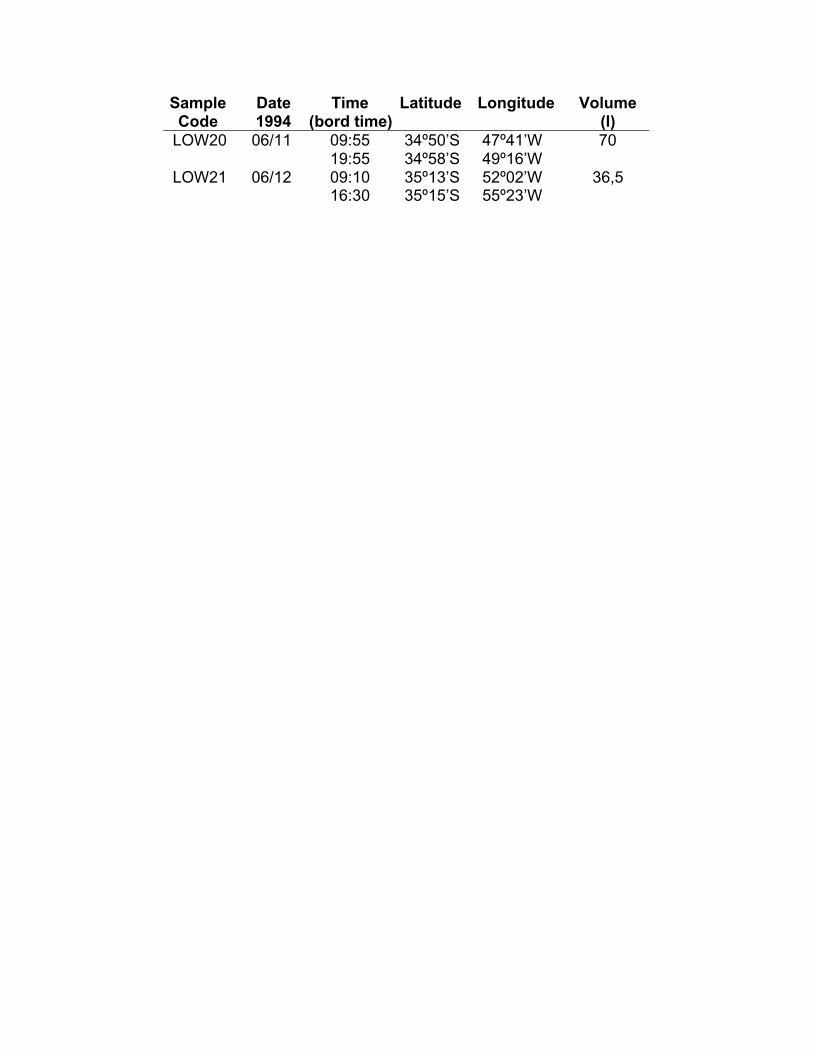
Sample Date Time Latitude Longitude VolumeCode 1994 (bord time) (l)
LOW20 06/11 09:55 34º50’S 47º41’W 7019:55 34º58’S 49º16’W
LOW21 06/12 09:10 35º13’S 52º02’W 36,516:30 35º15’S 55º23’W
8 Concluding Remarks
Foremost we thank the captains and the crew of RV METEOR for their skilled work. Specialthanks go to Mrs. S. Drews. She run the coordinator's office in Kiel with great competence andpatience. We all appreciate the professional travel services provided by Mrs. I. Weigert ofContiways Reisen, Hamburg. Not forgotten are the excellent co-operations with the staff of theGerman diplomatic representatives in Brasilia, Luanda, Walfish Bay, and Buenos Aires.
Financial support for the cruise and the scientific data analysis come from the 'DeutscheForschungsgemeinschaft' (DFG) (Ze 145/7-1) and the 'Bundesministerium Bir Bildung,Wissenschaft, Forschung und Technologie' (BMBF) (FKZ 03F0121A).
9 References
AHLSTROM, E. and H.G. MOSER (1981): Systematic's and development of early life historystages of marine fishes: Achievements during the past century, present status andsuggestions for the future. Rapp. P.-v. Réun. Cons. CIEM 178, 541 - 546.
ANDRES, H.G., H.-Ch. JOHN and C. ZELCK (1992): Biologische Ozeanographie und marineTaxonornie. In: SIEDLER, G. and W. ZENK (1992): WOCE Sildatlantik 1991, Reise Nr. 15,30. Dezember 1990 - 23. März 1991. METEOR -Berichte, Universität Hamburg 92-1, 74 -85.
BENNEKOM, A.J. and G.W. BERGER (1984): Hydrography and silica budget of the AngolaBasin. Netherl. Journ. Sea Res. 17, 149-200.
BLACHE, J. (1964): Le genre Bathylagus dans I'Atlantique tropical oriental sud (Teleostei,Clupeiformi, Opistoproctoidei, Bathylagidae). Cah. ORSTOM (océanogr.) 2 (1), 7-16.
BROWN, N. and G.K. MORRISON (1978): WHOI/Brown Conductivity, temperature, and depthprofiler. Woods Hole Oceanographic Inst. Techn. Rep. No. WHOI-78-23.
CULBERSON, C.H. (1991): 15 pp in the WOCE Operations Manual (WHP Operations andMethods) WMPO 91/1, Woods Hole.
CULBERSON, C.H. and S. HUANG (1987): An automated amperometric oxygen titration. DeepSea Research, 34, 875-880.
De MADRON, X.D. and G. WHEATHERLY (1994): Circulation, transport and bottom boundarylayers of the deep currents in the Brazil Basin. Journ. Mar. Res. 52, 583-638.
EHRICH, S., H.-Ch. JOHN and P. WESTHAUS-EKAU (1987): Southward extension of thereproductive range of Macroramphosus scolopax in the up-welling area off North-WestAfrica. S. Afr. J. Mar. Sci. 5, 95 - 105.

FISCHER, J. and M. VISBEK (1993): Deep Profiling with Self-contained ADCPs. Journ. Atmos.Oean. Techn., 10, 5, 764-773.
GARRETT, W.D. (1965): Surface chemistry of the sea. Limnol. and Oceanogr., 10, 602-610.
GRASSHOFF, K. (1976): Methods of seawater analysis. Verlag Chemie, Weinheim, 305pp
HAMAN, I., H.-Ch. JOHN and E. MITTELSTAEDT (1981): Hydrography and its effect on fishlarvae in the Mauritanian up-welling area. Deep-Sea Res. 28 A(6), 561 - 575.
HEMPEL, G. and H. WEIKERT (1972): The neuston of the subtropical and boreal NortheasternAtlantic Ocean. A review. Mar. Biol. 13 (1), 70 - 88.
HERMES, R. and M.P. OLIVAR (1987): Larval development of Bathylagus argyrogaster Norman1930 (Teleostei, Bathylagidae). Pesq. 51 (4), 483 - 489.
HYDES, D.J. (1984): A manual of methods for the continuous flow determination of ammonia,nitrate-nitrite, phosphate and silicate in seawater. Institute of oceanographic SciencesReport No. 177, 40pp.
HYDES, D.J. and N.C. HILL. (1985): Use of Copper Cadmium Alloy in the determination ofdissolved nitrate. Est. Coastal Shelf Sci. 21, 27-31.
Hydrographic Department of the Admirality (1945): Quarterly Surface Current Charts of theAtlantic Ocean. Prepared in the Marine Branch of the Meteorological Office and publishedby the authority of the Meteorological Committee, 25.
JAENICKE, R. (1987): Aerosol physics and chemistry. In: G. FISCHER (ed.): Landolt Bbrnstein,Volume 4 'Meteorology', 391-457, Springer Verlag, Berlin.
JOHN, H.-Ch. (1976/77): Die Hdufigkeit des Ichthyoplanktons an der Oberfldche des mittlerenund südlichen Atlantischen Ozeans. Meeresforsch. 25 (1-2), 23 - 36.
JOHN, H-Ch. (1979): Regional and seasonal differences in ichthyoneuston off Northwest Africa."METEOR" Forsch.-Ergebn. D 29, 30 - 47.
JOHN, H.-Ch. (1984): Drift of larval fishes in the ocean: Results and problems from previousstudies and a proposed field experiment. P. 39-60 in: MCCLEAVE, J.D.; G.P. ARNOLD,J.J. DODSON and W.H. NEILL (eds): Mechanisms of migration in fishes. Plenum Publ.Corp., New York, 574 pp.
JOHN, H.-Ch. (1985): Horizontal and vertical distribution patterns of fish larvae off NW Africa inrelation to the environment. P. 489-512 in: BAS, C., R. MARGALEF and P. RUBIES (eds.):Simposio internacional sobre las areas de afloramiento mas importantes del oeste africano(Cabo Blanco y Benguela). Vol. 1. Inst. In. Pesqueras, Barcelona.
JOYCE, T.M. (1989): On in situ "calibration" of shipboard ADCP. Journ. Atmos. and Ocean.Techn. 6, 169-172.
JOYCE, T., C. CORRY and M. STALCUP (1991): Requirements for WOCE hydrographicprogramme data reporting, WHPO 90-1, 71pp.
KLOPPMANN, M. (1990): The sampling efficiency of a horizontally towed BE multiple-opening-closing-net. ICES 1990, C.M. 1990/L, 97, 11 pp.
KOBYLYANSKIY, S.G. (1985): Material for the revision of the genus Bathylagus Giinther(Bathylagidae): The group of "light" deep sea smelts. J. Ichthyol. 25 (1), 1 - 17.
KRÄMER, W. and K. BALLSCHMITER (1987): Detection of a new class of organochlorinecompounds in the marine environment: The chlorinated paraffins. Fresenius z. Anal.Chem., 327, 47-48.
LASKER, R. (1981): Marine fish larvae. Washington Sea Grant Program, Seattle, 131 pp.
LOPES, P.C. and H.-Ch. JOHN (1986): Ichthyoplankton at the surface of the Equatorial Atlantic.Bol. Soc. Port. Cienc. Nat. 23, 83 - 111.
MOLLER, T. (1981): Current and temperature measurements in the North-East Atlantic duringNEADS. Ber. Inst. Meereskunde, Nr. 90, 98 pp.
MOLLER et al. (1994): Improving MKIII measurements. In: WOCE Operations Manual, Part 3.1.3:WFIP Operations and methods. WOCE Hydrographic Programme Office, Woods HoleOceanographic Institution (update July 1993 in press).
MURPHY J. and J.P. RILEY (1962): A modified single solution method for the determination ofphosphate in natural waters. Anal. Chim. Acta, 27, 31-36.
NGCD (1993): Global relief data, CD-ROM, National Geophysical Data Center.
NORMAN, J.R. (1930): Oceanic fishes and flatfishes collected in 1925 - 27. Discovery Rep. 2,261 - 370.
OWENS, B. and R. MILLARD (1985): A new algorithm for CTD Oxygen calibration. Journ. Phys.Oceanogr. 15, 621-631.
PETERSON, R.G. and T. WHITWORTH 111 (1989): The Subantarctic and Polar Fronts in relationto deep water masses through the Southwestern Atlantic. Journ. Geophys. Res. 94, 10817-10838.
POLLARD, R. and J. READ (1989): A method for calibrating ship-mounted acoustic Dopplerprofilers and the limitations of gyro compasses. Journ. Atmos. Ocean. Techn., 6, 6, 859-865.
ROBINSON, I.S., N.S. WELLS and H. CHARNOCK (1984): The sea surface thermal boundarylayer and its relevance to the measurement of sea surface temperature by airborne andspace-borne radiometers. International Journal of Remote Sensing, 5, (n1), 19-45.
SAUNDERS, P.M., K.-H. MAHRT and R.T. WILLIAMS (1991): Standards and laboratorycalibrations. In: WOCE Operations Manual, Part 3.1.3: WHP Operations and methods.WOCE Hydrographic Programme Office, Woods Hole Oceanographic Institution (updateJuly 1993 in press).
SCHLUESSEL, P., W.J. EMERY, H. GRASSL, and T. MAMMEN (1990): On the bulk-skintemperature difference and its impact on satellite remote sensing of sea surfacetemperature. Journal of Geophysical Research, 95(C8), 13341-13356.
SIEDLER, G., A. KUHL and W. ZENK (1987): The Madeira Mode Water. J. Phys. Oceanogr., 17(10), 1561-1570.
SIEDLER, G. and W. Zenk (1992): WOCE Sddatlantik 1991, Reise Nr. 15, 30. Dezember - 23.März 1991. METEOR -Berichte, Universität Hamburg, 92-1, 126 S.
SIEDLER, G., W. BALZER, T.J. MOLLER, R. ONKEN, M. RHEIN and W. ZENK (1993): WOCESouth Atlantic 1992, Cruise No. 22, 22 September 1992 - 31 January 1993. METEOR -Berichte, Universität Hamburg, 93-5, 131pp.
SPEER, K.G., W. ZENK, G. SIEDLER, J. PATZOLD and C. HEIDLAND (1992): First resolution offlow through the Hunter Channel in the South Atlantic. Earth and Planeary Science Letters,113, 287-292.
SPEER, K.G. and W. ZENK (1993): The flow of Antarctic Bottom Water into the Brazil Basin. J.Phys. Oceanogr. 23, 2667-2682.
STRAMMA, L. and R.G. PETERSON (1990): The South Atlantic Current, J. Phys. Oc., 20, 846-859.
TARBELL, S., R. MEYER, N. HOGG and W. ZENK (1994): A moored array along the southernboundary of the Brazil Basin for the Deep Basin Experiment - Report on a joint experiment1991-1992. Ber. Inst. f. Meereskunde Kiel, Nr. 243.
UNITED STATES NAVAL OCEANOGRAPHIC OFFICE, 1955: Atlas of Pilot Charts CentralAmerican Waters and South Atlantic Ocean. Published by the Defense Mapping AgencyHydrographic Center, Washington D.C.
VIESBEK, M. and J. FISCHER (1995): Sea surface conditions remotely sensored byupwardlooking ADCPs. J. Atmos. a. Oceanic Techn., in press.
WARREN, B.A. and K.G. SPEER (1991): Deep circulation in the eastern South Atlantic. Deep-Sea Res. 38 (Suppl. 1), 5281-5322.
WICK, G.A., W.J. EMERY and P. SCHLUSSEL (1992): A comprehensive comparison betweenskin and multi-channel sea surface temperature. Journal of Geophysical Research, 97(C4),5569-5595.
ZELCK, C. (1993): Biological oceanography and marine taxonomy. In: SIEDLER, G., W. BALZER,T.J. MÜLLER, R. ONKEN, M. RHEIN and W. ZENK (1993): WOCE South Atlantic 1992.Cruise No. 22, 22 September 1992 - 31 January 1993. METEOR-Berichte, UniversitdtHamburg 93-5, 73 - 76.
ZENK, W. and N.G. HOGG (1994): Climate changes of Antarctic Bottom Water flowing into theBrazil Basin? Deep-Sea Res. (submitted).
ZENK, W., K.G. SPEER and N.G. HOGG (1993): Bathymetry at the Vema Sill. Deep-Sea Res.40(9), 1925-2933.
Tritium HELIUM ISOTOPE DATA DOCUMENTATION
CRUISE METEOR 28 WHP A8
The data was aquired by
Prof. Dr. Wolfgang RoetherTracer-OzeanographieFB1Universitaet BremenPO.Box. 330 44028334 BremenTel.: 0421/218-3511 / 4221Fax: 0421/218-7018email: [email protected]
for questions about measurement and data processing please contact
Birgit KleinTel: 0421/210-2931email: [email protected]
In the data file we enclose final (tritium corrected delhe3 data) and final tritium data.
Final delhe3 data:
Two different sets of helium samples have been taken during the cruise:
1. Most samples were taken in the usual manner with pinched- off copper tubes. After thegas extraction in Bremen they were measured in the Laboratory with a dedicatedHelium - Neon Isotope Mass Spectrometer.
2. Another set was sampled into glass-pipettes and extracted at sea. The glass ampouleswith the extracted gas were then transported back to Bremen for measurement.
All samples were calibrated using an air standard (regular air) in the Bremen laboratory.The Copper tube samples are now corrected for tritium decay during storage time!Because of the very low tritium concentrations in the South Atlantic the tritium correctionwas very small. For samples from the upper layer, the maximum reduction in delta 3He ofabout 0.24% and on average 0.05%. The samples which had been extracted at sea didnot need a correction for delhe3 because their storage time was zero.
Tritium data:Tritium was sampled in 1l glass bottles which were analyzed after the cruise in thelaboratory at bremen. Tritium was measured through in-growth of helium3 from radioactivedecay. For this procedure the water samples are degassed and transferred into special
glass containers which are sealed off and placed into freezers. After a storage time of 6month to about a year to allow for sufficient in-growth of helium3 the samples aremeasured with a special noble gas spectrometer.
Tritium concentrations are scaled to 1 April 1994 and individual errors have beenassigned. The quality flags follow WOCE standard.
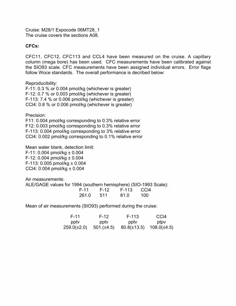
Cruise: M28/1 Expocode 06MT28_1The cruise covers the sections A08.
CFCs:
CFC11, CFC12, CFC113 and CCL4 have been measured on the cruise. A capillarycolumn (mega bore) has been used. CFC measurements have been calibrated againstthe SIO93 scale. CFC measurements have been assigned individual errors. Error flagsfollow Woce standards. The overall performance is decribed below:
Reproducibility:F-11: 0.3 % or 0.004 pmol/kg (whichever is greater)F-12: 0.7 % or 0.003 pmol/kg (whichever is greater)F-113: 7.4 % or 0.006 pmol/kg (whichever is greater)CCl4: 0.8 % or 0.006 pmol/kg (whichever is greater)
Precision:F11: 0.004 pmol/kg corresponding to 0.3% relative errorF12: 0.003 pmol/kg corresponding to 0.3% relative errorF-113: 0.004 pmol/kg corresponding to 3% relative errorCCl4: 0.002 pmol/kg corresponding to 0.1% relative error
Mean water blank, detection limit:F-11: 0.004 pmol/kg ± 0.004F-12: 0.004 pmol/kg ± 0.004F-113: 0.005 pmol/kg ± 0.004CCl4: 0.004 pmol/kg ± 0.004
Air measurements:ALE/GAGE values for 1994 (southern hemisphere) (SIO-1993 Scale):
F-11 F-12 F-113 CCl4261.0 511 81.0 100
Mean of air measurements (SIO93) performed during the cruise:
F-11 F-12 F-113 CCl4pptv pptv pptv ptpv
259.0(±2.0) 501.(±4.5) 80.8(±13.5) 108.0(±4.5)
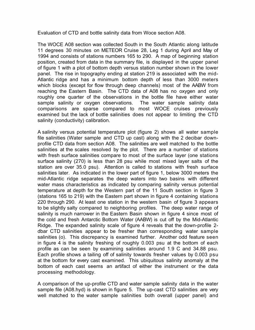
Evaluation of CTD and bottle salinity data from Woce section A08.
The WOCE A08 section was collected South in the South Atlantic along latitude11 degrees 30 minutes on METEOR Cruise 28, Leg 1 during April and May of1994 and consists of stations numbers 165 to 290. A map of beginning stationposition, created from data in the summary file, is displayed in the upper panelof figure 1 with a plot of bottom depth versus station number shown in the lowerpanel. The rise in topography ending at station 219 is associated with the mid-Atlantic ridge and has a minimum bottom depth of less than 3000 meterswhich blocks (except for flow through deep channels) most of the AABW fromreaching the Eastern Basin. The CTD data of A08 has no oxygen and onlyroughly one quarter of the observations in the bottle file have either watersample salinity or oxygen observations. The water sample salinity datacomparisons are sparse compared to most WOCE cruises previouslyexamined but the lack of bottle salinities does not appear to limiting the CTDsalinity (conductivity) calibration.
A salinity versus potential temperature plot (figure 2) shows all water samplefile salinities (Water sample and CTD up cast) along with the 2 decibar down-profile CTD data from section A08. The salinities are well matched to the bottlesalinities at the scales resolved by the plot. There are a number of stationswith fresh surface salinities compare to most of the surface layer (one stationssurface salinity (270) is less than 28 psu while most mixed layer salts of thestation are over 35.0 psu). Attention is called to stations with fresh surfacesalinities later. As indicated in the lower part of figure 1, below 3000 meters themid-Atlantic ridge separates the deep waters into two basins with differentwater mass characteristics as indicated by comparing salinity versus potentialtemperature at depth for the Western part of the 11 South section in figure 3(stations 165 to 219) with the Eastern part shown in figure 4 containing stations220 through 290. At least one station in the western basin of figure 3 appearsto be slightly salty compared to neighboring profiles. The deep water range ofsalinity is much narrower in the Eastern Basin shown in figure 4 since most ofthe cold and fresh Antarctic Bottom Water (AABW) is cut off by the Mid-AtlanticRidge. The expanded salinity scale of figure 4 reveals that the down-profile 2-dbar CTD salinities appear to be fresher than corresponding water samplesalinities (o). This discrepancy is examined further. Another odd feature seenin figure 4 is the salinity freshing of roughly 0.003 psu at the bottom of eachprofile as can be seen by examining salinities around 1.9 C and 34.88 psu.Each profile shows a tailing off of salinity towards fresher values by 0.003 psuat the bottom for every cast examined. This ubiquitous salinity anomaly at thebottom of each cast seems an artifact of either the instrument or the dataprocessing methodology.
A comparison of the up-profile CTD and water sample salinity data in the watersample file (A08.hyd) is shown in figure 5. The up-cast CTD salinities are verywell matched to the water sample salinities both overall (upper panel) and
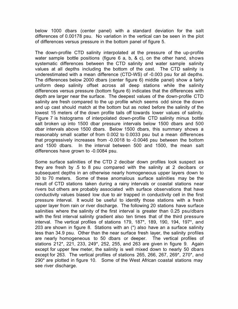
below 1000 dbars (center panel) with a standard deviation for the saltdifferences of 0.00178 psu. No variation in the vertical can be seen in the plotof differences versus pressure in the bottom panel of figure 5.
The down-profile CTD salinity interpolated at the pressure of the up-profilewater sample bottle positions (figure 6 a, b, & c), on the other hand, showssystematic differences between the CTD salinity and water sample salinityvalues at all depths including the bottom of the cast. The CTD salinity isunderestimated with a mean difference (CTD-WS) of -0.003 psu for all depths.The differences below 2000 dbars (center figure 6) middle panel) show a fairlyuniform deep salinity offset across all deep stations while the salinitydifferences versus pressure (bottom figure 6) indicates that the differences withdepth are larger near the surface. The deepest values of the down-profile CTDsalinity are fresh compared to the up profile which seems odd since the downand up cast should match at the bottom but as noted before the salinity of thelowest 15 meters of the down profile tails off towards lower values of salinity.Figure 7 is histograms of interpolated down-profile CTD salinity minus bottlesalt broken up into 1500 dbar pressure intervals below 1500 dbars and 500dbar intervals above 1500 dbars. Below 1500 dbars, this summary shows areasonably small scatter of from 0.002 to 0.0033 psu but a mean differencesthat progressively increases from -0.0018 to -0.0046 psu between the bottomand 1500 dbars. In the interval between 500 and 1500, the mean saltdifferences have grown to -0.0084 psu.
Some surface salinities of the CTD 2 decibar down profiles look suspect asthey are fresh by .5 to 8 psu compared with the salinity at 2 decibars orsubsequent depths in an otherwise nearly homogeneous upper layers down to30 to 70 meters. Some of these anomalous surface salinities may be theresult of CTD stations taken during a rainy intervals or coastal stations nearrivers but others are probably associated with surface observations that haveconductivity values biased low due to air trapped in conductivity cell in the firstpressure interval. It would be useful to identify those stations with a freshupper layer from rain or river discharge. The following 20 stations have surfacesalinities where the salinity of the first interval is greater than 0.25 psu/dbarswith the first interval salinity gradient also ten times that of the third pressureinterval. The vertical profiles of stations 179, 187*, 189, 190, 194, 197*, and203 are shown in figure 8. Stations with an (*) also have an a surface salinityless than 34.9 psu. Other than the near surface fresh layer, the salinity profilesare nearly homogeneous to 50 dbars or deeper. The vertical profiles ofstations 212*, 221, 233, 249*, 252, 255, and 263 are given in figure 9. Againexcept for upper few meter, the salinity is well mixed down to nearly 50 dbarsexcept for 263. The vertical profiles of stations 265, 266, 267, 269*, 270*, and290* are plotted in figure 10. Some of the West African coastal stations maysee river discharge.
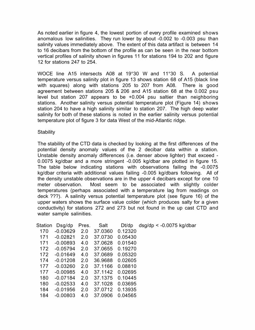
As noted earlier in figure 4, the lowest portion of every profile examined showsanomalous low salinities. They run lower by about -0.002 to -0.003 psu thansalinity values immediately above. The extent of this data artifact is between 14to 16 decibars from the bottom of the profile as can be seen in the near bottomvertical profiles of salinity shown in figures 11 for stations 194 to 202 and figure12 for stations 247 to 254.
WOCE line A15 intersects A08 at 19°30 W and 11°30 S. A potentialtemperature versus salinity plot in figure 13 shows station 68 of A15 (black linewith squares) along with stations 205 to 207 from A08. There is goodagreement between stations 205 & 206 and A15 station 68 at the 0.002 psulevel but station 207 appears to be +0.004 psu saltier than neighboringstations. Another salinity versus potential temperature plot (Figure 14) showsstation 204 to have a high salinity similar to station 207. The high deep watersalinity for both of these stations is noted in the earlier salinity versus potentialtemperature plot of figure 3 for data West of the mid-Atlantic ridge.
Stability
The stability of the CTD data is checked by looking at the first differences of thepotential density anomaly values of the 2 decibar data within a station.Unstable density anomaly differences (i.e. denser above lighter) that exceed -0.0075 kg/dbar and a more stringent -0.005 kg/dbar are plotted in figure 15.The table below indicating stations with observations failing the -0.0075kg/dbar criteria with additional values failing -0.005 kg/dbars following. All ofthe density unstable observations are in the upper 4 decibars except for one 10meter observation. Most seem to be associated with slightly coldertemperatures (perhaps associated with a temperature lag from readings ondeck ???). A salinity versus potential temperature plot (see figure 16) of theupper waters shows the surface value colder (which produces salty for a givenconductivity) for stations 272 and 273 but not found in the up cast CTD andwater sample salinities.
Station Dsg/dp Pres. Salt Dt/dp dsg/dp < -0.0075 kg/dbar170 -0.03629 2.0 37.0360 0.12320171 -0.02821 2.0 37.0730 0.05430171 -0.00893 4.0 37.0628 0.01540172 -0.05794 2.0 37.0655 0.19270172 -0.01649 4.0 37.0689 0.05320174 -0.01208 2.0 36.9688 0.02605177 -0.03260 2.0 37.1166 0.08810177 -0.00985 4.0 37.1142 0.02695180 -0.07184 2.0 37.1375 0.10445180 -0.02533 4.0 37.1028 0.03695184 -0.01956 2.0 37.0712 0.13935184 -0.00803 4.0 37.0906 0.04565
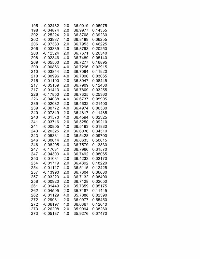
195 -0.02482 2.0 36.9019 0.05975198 -0.04874 2.0 36.9977 0.14355202 -0.25224 2.0 36.8708 0.39230202 -0.03987 4.0 36.8189 0.06255206 -0.07383 2.0 36.7953 0.46225206 -0.03339 4.0 36.8793 0.20250208 -0.12524 2.0 36.7671 0.26340208 -0.02346 4.0 36.7489 0.05140209 -0.05500 2.0 36.7277 0.16895209 -0.00866 4.0 36.7296 0.02915210 -0.03844 2.0 36.7094 0.11920210 -0.00996 4.0 36.7090 0.03065216 -0.01100 2.0 36.8047 0.08445217 -0.05139 2.0 36.7909 0.12430217 -0.01413 4.0 36.7809 0.03255226 -0.17850 2.0 36.7325 0.25360226 -0.04088 4.0 36.6737 0.05905239 -0.02082 2.0 36.4632 0.21400239 -0.00772 4.0 36.4974 0.06580240 -0.07849 2.0 36.4817 0.11485240 -0.01570 4.0 36.4594 0.02325241 -0.03716 2.0 36.5250 0.09210241 -0.00805 4.0 36.5193 0.01880243 -0.20325 2.0 36.6036 0.34510243 -0.05331 4.0 36.5428 0.09700246 -0.30014 2.0 36.8635 0.50015246 -0.08295 4.0 36.7579 0.13830247 -0.17031 2.0 36.7966 0.31570247 -0.04303 4.0 36.7492 0.08065253 -0.01081 2.0 36.4233 0.02170254 -0.01719 2.0 36.4392 0.18220254 -0.01117 4.0 36.5115 0.12425257 -0.13990 2.0 36.7304 0.36680257 -0.03223 4.0 36.7132 0.08400258 -0.00920 2.0 36.7128 0.02050261 -0.01449 2.0 35.7359 0.05175262 -0.04595 2.0 35.7187 0.11445262 -0.01129 4.0 35.7088 0.02390272 -0.29981 2.0 36.0977 0.55450272 -0.06197 4.0 36.0367 0.12040273 -0.26208 2.0 35.9994 0.38260273 -0.05137 4.0 35.9276 0.07470
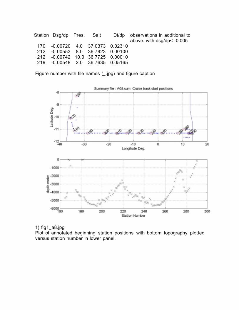
Station Dsg/dp Pres. Salt Dt/dp observations in additional toabove. with dsg/dp< -0.005
170 -0.00720 4.0 37.0373 0.02310212 -0.00553 8.0 36.7923 0.00100212 -0.00742 10.0 36.7725 0.00010219 -0.00548 2.0 36.7635 0.05165
Figure number with file names (_.jpg) and figure caption
1) fig1_a8.jpgPlot of annotated beginning station positions with bottom topography plottedversus station number in lower panel.
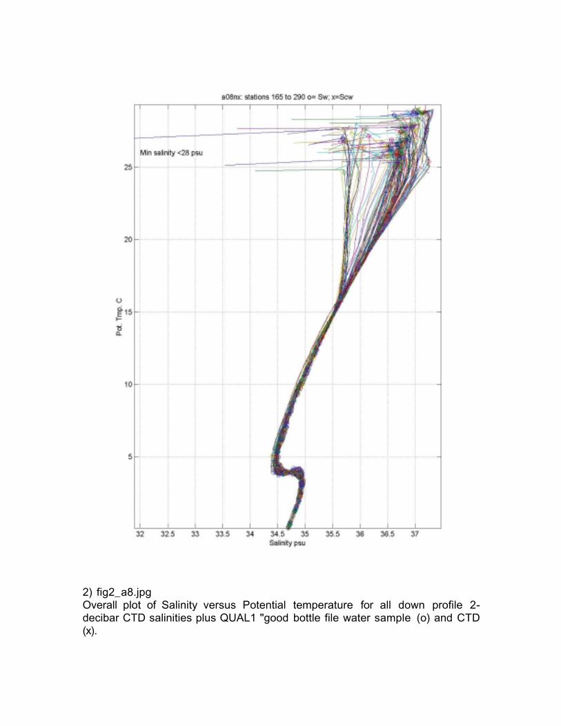
2) fig2_a8.jpgOverall plot of Salinity versus Potential temperature for all down profile 2-decibar CTD salinities plus QUAL1 "good bottle file water sample (o) and CTD(x).
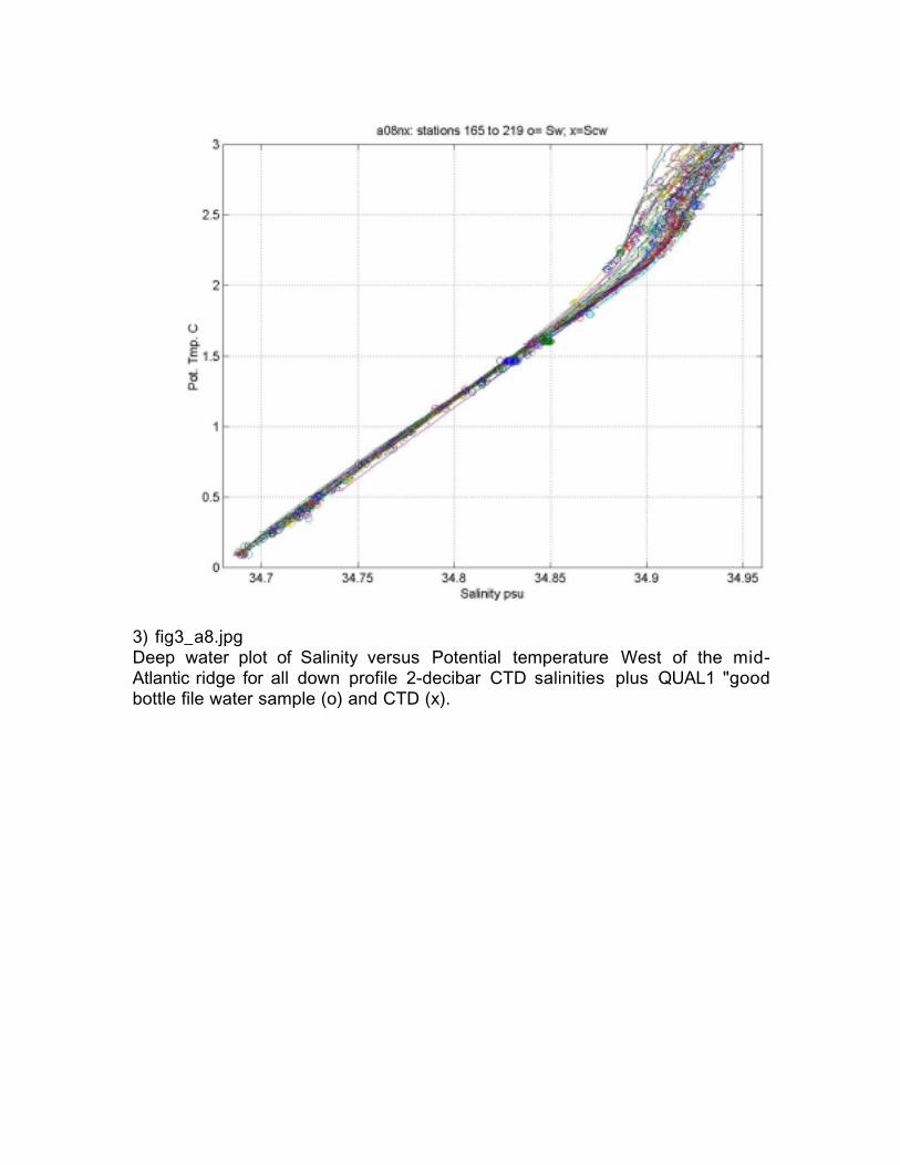
3) fig3_a8.jpgDeep water plot of Salinity versus Potential temperature West of the mid-Atlantic ridge for all down profile 2-decibar CTD salinities plus QUAL1 "goodbottle file water sample (o) and CTD (x).
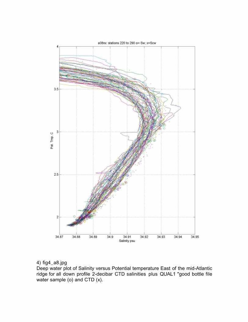
4) fig4_a8.jpgDeep water plot of Salinity versus Potential temperature East of the mid-Atlanticridge for all down profile 2-decibar CTD salinities plus QUAL1 "good bottle filewater sample (o) and CTD (x).

5) fig5_a8.jpg3 Plot panels of up cast salinity differences Ds=(CTD-WS) psu versus stationnumber (a) all pressures (b) below 1000 dbars and (c) versus pressure.
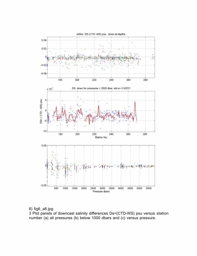
6) fig6_a8.jpg3 Plot panels of downcast salinity differences Ds=(CTD-WS) psu versus stationnumber (a) all pressures (b) below 1000 dbars and (c) versus pressure.
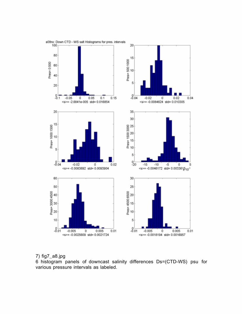
7) fig7_a8.jpg6 histogram panels of downcast salinity differences Ds=(CTD-WS) psu forvarious pressure intervals as labeled.
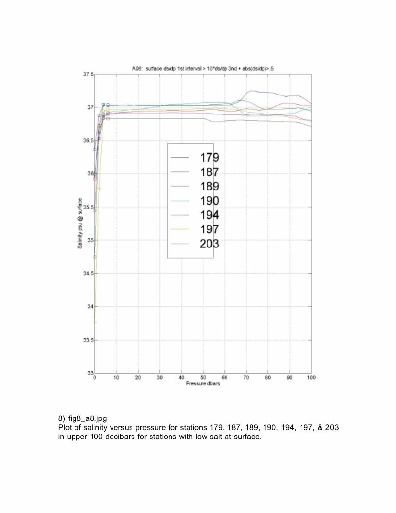
8) fig8_a8.jpgPlot of salinity versus pressure for stations 179, 187, 189, 190, 194, 197, & 203in upper 100 decibars for stations with low salt at surface.

9) fig9_a8.jpgPlot of salinity versus pressure for stations 212, 221, 233, 249, 252, 255, & 263in upper 100 decibars for stations with low salt at surface.
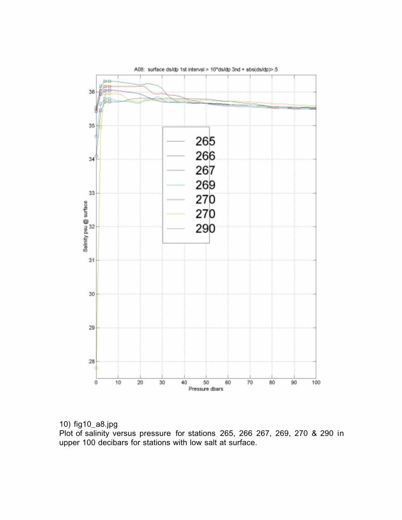
10) fig10_a8.jpgPlot of salinity versus pressure for stations 265, 266 267, 269, 270 & 290 inupper 100 decibars for stations with low salt at surface.
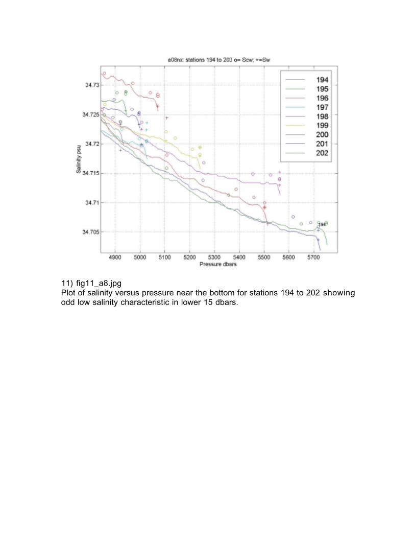
11) fig11_a8.jpgPlot of salinity versus pressure near the bottom for stations 194 to 202 showingodd low salinity characteristic in lower 15 dbars.
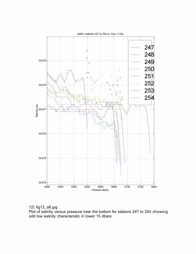
12) fig12_a8.jpgPlot of salinity versus pressure near the bottom for stations 247 to 254 showingodd low salinity characteristic in lower 15 dbars.
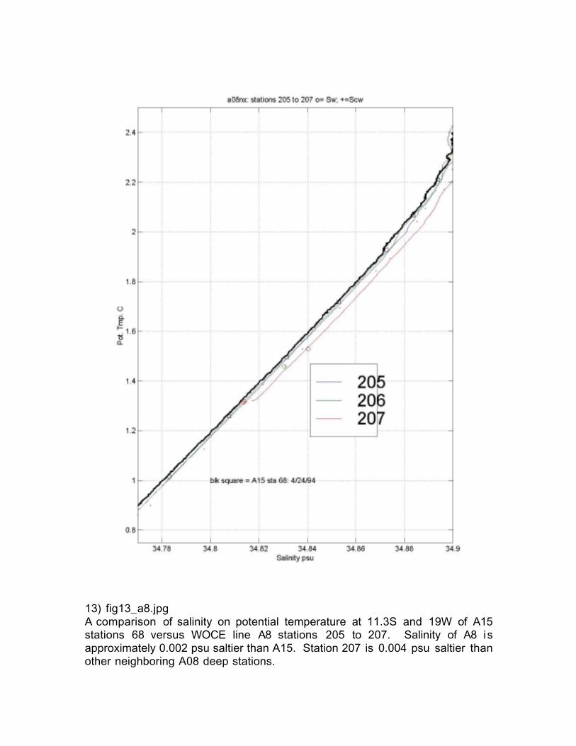
13) fig13_a8.jpgA comparison of salinity on potential temperature at 11.3S and 19W of A15stations 68 versus WOCE line A8 stations 205 to 207. Salinity of A8 isapproximately 0.002 psu saltier than A15. Station 207 is 0.004 psu saltier thanother neighboring A08 deep stations.
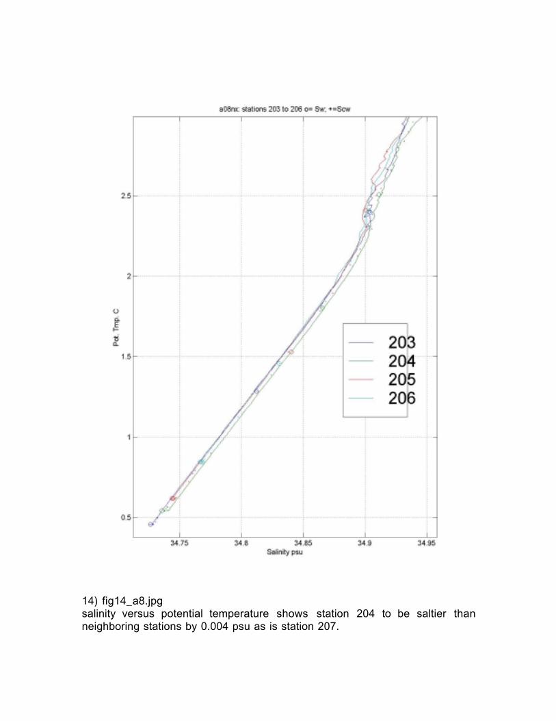
14) fig14_a8.jpgsalinity versus potential temperature shows station 204 to be saltier thanneighboring stations by 0.004 psu as is station 207.
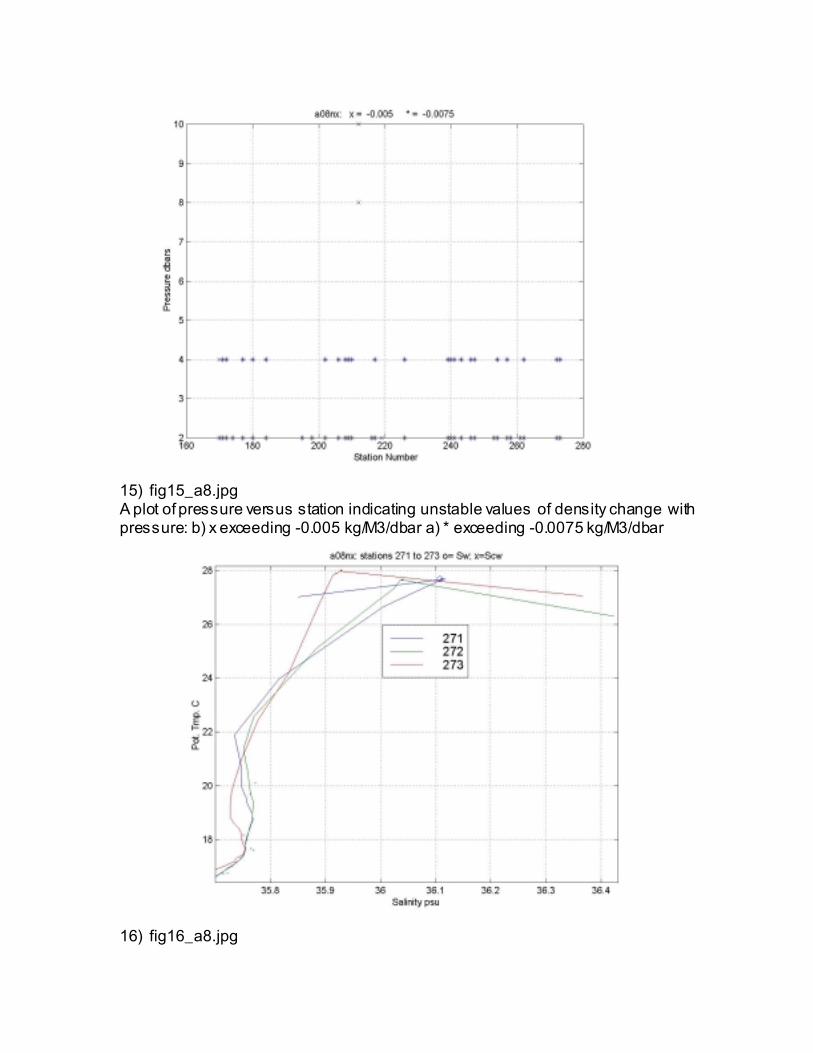
15) fig15_a8.jpgA plot of pressure versus station indicating unstable values of density change withpressure: b) x exceeding -0.005 kg/M3/dbar a) * exceeding -0.0075 kg/M3/dbar
16) fig16_a8.jpg
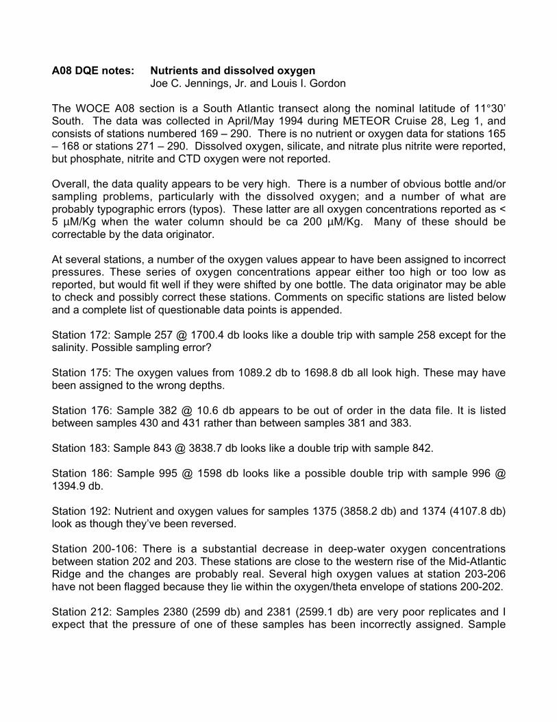
A08 DQE notes: Nutrients and dissolved oxygenJoe C. Jennings, Jr. and Louis I. Gordon
The WOCE A08 section is a South Atlantic transect along the nominal latitude of 11°30’South. The data was collected in April/May 1994 during METEOR Cruise 28, Leg 1, andconsists of stations numbered 169 – 290. There is no nutrient or oxygen data for stations 165– 168 or stations 271 – 290. Dissolved oxygen, silicate, and nitrate plus nitrite were reported,but phosphate, nitrite and CTD oxygen were not reported.
Overall, the data quality appears to be very high. There is a number of obvious bottle and/orsampling problems, particularly with the dissolved oxygen; and a number of what areprobably typographic errors (typos). These latter are all oxygen concentrations reported as <5 µM/Kg when the water column should be ca 200 µM/Kg. Many of these should becorrectable by the data originator.
At several stations, a number of the oxygen values appear to have been assigned to incorrectpressures. These series of oxygen concentrations appear either too high or too low asreported, but would fit well if they were shifted by one bottle. The data originator may be ableto check and possibly correct these stations. Comments on specific stations are listed belowand a complete list of questionable data points is appended.
Station 172: Sample 257 @ 1700.4 db looks like a double trip with sample 258 except for thesalinity. Possible sampling error?
Station 175: The oxygen values from 1089.2 db to 1698.8 db all look high. These may havebeen assigned to the wrong depths.
Station 176: Sample 382 @ 10.6 db appears to be out of order in the data file. It is listedbetween samples 430 and 431 rather than between samples 381 and 383.
Station 183: Sample 843 @ 3838.7 db looks like a double trip with sample 842.
Station 186: Sample 995 @ 1598 db looks like a possible double trip with sample 996 @1394.9 db.
Station 192: Nutrient and oxygen values for samples 1375 (3858.2 db) and 1374 (4107.8 db)look as though they’ve been reversed.
Station 200-106: There is a substantial decrease in deep-water oxygen concentrationsbetween station 202 and 203. These stations are close to the western rise of the Mid-AtlanticRidge and the changes are probably real. Several high oxygen values at station 203-206have not been flagged because they lie within the oxygen/theta envelope of stations 200-202.
Station 212: Samples 2380 (2599 db) and 2381 (2599.1 db) are very poor replicates and Iexpect that the pressure of one of these samples has been incorrectly assigned. Sample
2380 also has an oxygen value so low it must be a typo. The value of 2.30 should probablybe ca. 223 uM/Kg.
Station 214: Sample 2450 (130.3 db) has oxygen so low that it may be a typo. The value of1.80 should probably be 180 uM/Kg.
Station 218: Oxygen values for samples 2675 (49 db) and 2714 (2951 db) are both so lowthat they are probably typos.
Station 220: Oxygen values for samples 2808 (1296.3 db) and 2800 (2850.4 db) are both solow they are probably typos.
Station 242: Silicate values for samples 268 (3101 db) and 269 (2856.3 db) may have beenreversed. As assigned, 268 looks low and 269 looks high.
Station 256: Sample 1624 (1598 db) has an oxygen value of –0.7. This must be a typo.
Station 262: Oxygen values from 921 db to 2098.3 db (samples 2398, 2400 – 2405) all lookas though they have been mis-assigned pressures by one bottle. If shifted up, they would fitwell.
Station 263: Oxygen values from 496.8 db to 996 db all look low. If shifted up by one bottlethey would fit well. Could be a sampling error or a data entry error.
Cruise A08METEOR Cruise 28 / Leg 1 Comments
Sta. Samp. Press. O2 O2 Si Si N+N N+N No Phosphate or nitrite dataFlag Flag Flag
172 257 1700.4 Low y High y High y Looks like double trip except forsalt.
253 2480 High y175 384 3707.5 V Low y
342 1089.2 High y335 1298 High y397 1497.3 High y398 1698.8 High y
176 382 10.6 Looks like surface sample butdoesn't fit tripping sequence.
434 452.9 High y178 490 397.6 High y179 575/576 650.8 y Poor replicates of O2, flagged
both180 650 2351.6 Low y
599/600 650.8 High y Low y Low y Poor replicate.
Cruise A08METEOR Cruise 28 / Leg 1 Comments
Sta. Samp. Press. O2 O2 Si Si N+N N+N No Phosphate or nitrite dataFlag Flag Flag
181 676 199.6 Low y High y High y675 2249.5 Low y High y High y685 600.4 Low y Poor replicate of O2
182 711 696.7 High y712 698.6 Low y Compare with 711, poor
replicates.766 1997.7 High y 752 - 766: O2 looks high vs Z
and theta.765 2250 High y O2 looks high vs Z and theta.764 2500.2 High y “ " " " " "763 2749.5 High y “ " " " " "762 3001.5 High y “ " " " " "761 3252.6 High y “ " " " " "760 3550.2 High y “ “ “ “ “ “759 3754.6 High y “ “ “ “ “ “758 4005.5 High y “ “ “ “ “ “757 4254.2 High y “ “ “ “ “ “756 4504.8 High y “ “ “ “ “ “755 4754.5 High y “ “ “ “ “ “754 4936 High y “ “ “ “ “ “753 5005.9 High y “ “ “ “ “ “752 5038.6 High y
183 843 3838.7 Low y High y High y Looks like double trip withsample 842, except for salinity.
184 875 2600.7 Low y185 905 1997.7 Low y186 991 2499.1 High y
995 1598 Low y y High y Looks like dbl-trip with [email protected], except for salinity.
188 1099 3101.6 Low y No nutrient shift1106 1496.7 High y1110 924.1 Low y1157 4605.9 Low y No nutrient shift
189 1140 398.5 High y Ok y Low y Sil flagged due to O2 & N+N190 1227 500.7 Low y
1225 699 High y1224 847.7 High y1222 1003.8 High y
192 1375 3858.2 High y High y Looks like nutrients reversed1374 4107.8 Low y Low y Looks like nutrients reversed
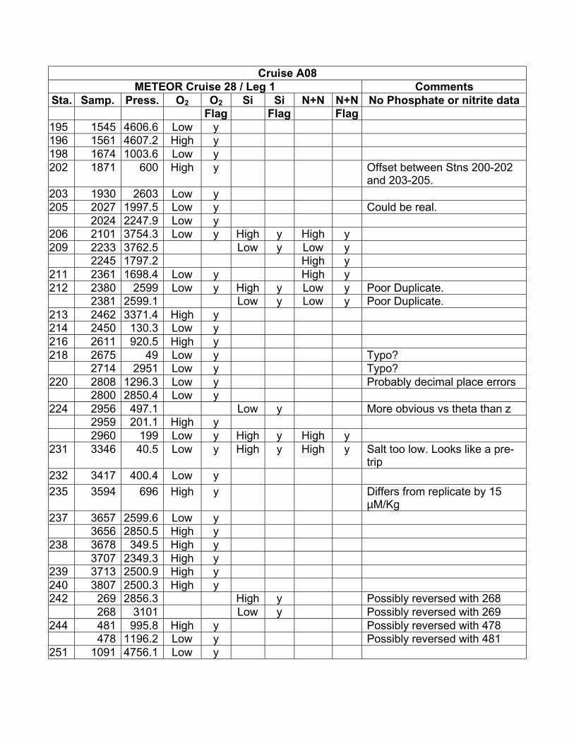
Cruise A08METEOR Cruise 28 / Leg 1 Comments
Sta. Samp. Press. O2 O2 Si Si N+N N+N No Phosphate or nitrite dataFlag Flag Flag
195 1545 4606.6 Low y196 1561 4607.2 High y198 1674 1003.6 Low y202 1871 600 High y Offset between Stns 200-202
and 203-205.203 1930 2603 Low y205 2027 1997.5 Low y Could be real.
2024 2247.9 Low y206 2101 3754.3 Low y High y High y209 2233 3762.5 Low y Low y
2245 1797.2 High y211 2361 1698.4 Low y High y212 2380 2599 Low y High y Low y Poor Duplicate.
2381 2599.1 Low y Low y Poor Duplicate.213 2462 3371.4 High y214 2450 130.3 Low y216 2611 920.5 High y218 2675 49 Low y Typo?
2714 2951 Low y Typo?220 2808 1296.3 Low y Probably decimal place errors
2800 2850.4 Low y224 2956 497.1 Low y More obvious vs theta than z
2959 201.1 High y2960 199 Low y High y High y
231 3346 40.5 Low y High y High y Salt too low. Looks like a pre-trip
232 3417 400.4 Low y235 3594 696 High y Differs from replicate by 15
µM/Kg237 3657 2599.6 Low y
3656 2850.5 High y238 3678 349.5 High y
3707 2349.3 High y239 3713 2500.9 High y240 3807 2500.3 High y242 269 2856.3 High y Possibly reversed with 268
268 3101 Low y Possibly reversed with 269244 481 995.8 High y Possibly reversed with 478
478 1196.2 Low y Possibly reversed with 481251 1091 4756.1 Low y
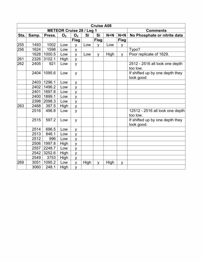
Cruise A08METEOR Cruise 28 / Leg 1 Comments
Sta. Samp. Press. O2 O2 Si Si N+N N+N No Phosphate or nitrite dataFlag Flag Flag
255 1493 1002 Low y Low y Low y256 1624 1598 Low y Typo?
1628 1000.5 Low y Low y High y Poor replicate of 1629.261 2326 3102.1 High y262 2405 921 Low y 2512 - 2516 all look one depth
too low.2404 1095.6 Low y If shifted up by one depth they
look good.2403 1296.1 Low y2402 1496.2 Low y2401 1697.8 Low y2400 1899.1 Low y2398 2098.3 Low y
263 2468 397.5 High y2516 496.8 Low y 12512 - 2516 all look one depth
too low.2515 597.2 Low y If shifted up by one depth they
look good.2514 696.5 Low y2513 846.1 Low y2512 996 Low y2506 1997.8 High y2557 2248.7 Low y2542 3252.6 High y2549 3753 High y
269 3051 1095.2 Low y High y High y3060 248.1 High y
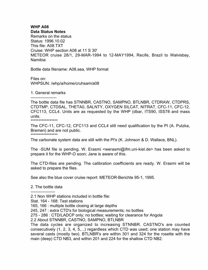
WHP A08Data Status NotesRemarks on the statusStatus: 1996.10.02This file: A08.TXTCruise: WHP section A08 at 11 S 30'METEOR cruise 28/1, 29-MAR-1994 to 12-MAY1994, Recife, Brazil to Walvisbay,Namibia
Bottle data filename: A08.sea, WHP format
Files on:WHPSUN: /whp/a/home/cruhsam/a08
1. General remarks-------------------The bottle data file has STNNBR, CASTNO, SAMPNO, BTLNBR, CTDRAW, CTDPRS,CTDTMP, CTDSAL, THETA0, SALNTY, OXYGEN SILCAT, NITRAT, CFC-11, CFC-12,CFC113, CCL4. Units are as requested by the WHP (dbar, ITS90, ISS78 and massunits.*****************The CFC-11, CFC-12, CFC113 and CCL4 still need qualification by the PI (A. Putzka,Bremen) and are not public.*****************The carbonate system data are still with the PI's (K. Johnson & D. Wallace, BNL).
The -SUM file is pending. W. Erasmi <[email protected]> has been asked toprepare it for the WHP-O soon; Jane is aware of this.
The CTD-files are pending. The calibration coefficients are ready. W. Erasmi will beasked to prepare the files.
See also the blue cover cruise report: METEOR-Berichte 95-1, 1995.
2. The bottle data------------------2.1 Non WHP stations included in bottle file:Stat. 164 - 168: Test stations165, 166 : multiple bottle closing at large depths245, 247 : extra CTD's for biological measurements; no bottles275 - 286 : CTD/LADCP only; no bottles; waiting for clearance for Angola2.2 About STNNBR, CASTNO, SAMPNO, BTLNBRThe data cycles are organized to increasing STNNBR. CASTNO's are countedconsecutively (1, 2, 3, 4, 5,...) regardless which CTD was used; one station may haveseveral casts (mostly two). BTLNBR's are within 301 and 324 for the rosette with themain (deep) CTD NB3, and within 201 and 224 for the shallow CTD NB2.
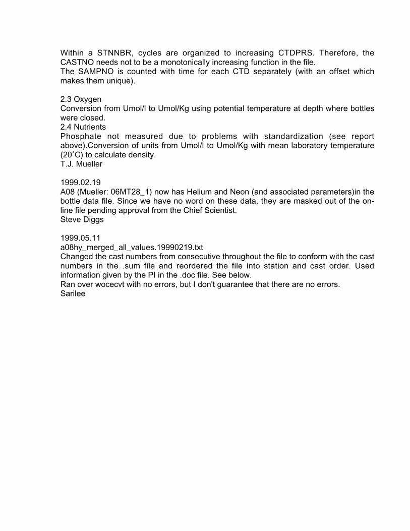
Within a STNNBR, cycles are organized to increasing CTDPRS. Therefore, theCASTNO needs not to be a monotonically increasing function in the file.The SAMPNO is counted with time for each CTD separately (with an offset whichmakes them unique).
2.3 OxygenConversion from Umol/l to Umol/Kg using potential temperature at depth where bottleswere closed.2.4 NutrientsPhosphate not measured due to problems with standardization (see reportabove).Conversion of units from Umol/l to Umol/Kg with mean laboratory temperature(20˚C) to calculate density.T.J. Mueller
1999.02.19A08 (Mueller: 06MT28_1) now has Helium and Neon (and associated parameters)in thebottle data file. Since we have no word on these data, they are masked out of the on-line file pending approval from the Chief Scientist.Steve Diggs
1999.05.11a08hy_merged_all_values.19990219.txtChanged the cast numbers from consecutive throughout the file to conform with the castnumbers in the .sum file and reordered the file into station and cast order. Usedinformation given by the PI in the .doc file. See below.Ran over wocecvt with no errors, but I don't guarantee that there are no errors.Sarilee