Barcelona GSE Working Paper Series

Working Paper nº 631

Catchment Areas and Access to Better Schools

Caterina Calsamiglia Antonio Miralles

This version: December 2014

May 2012

Catchment Areas andAccess to Better Schools

Caterina Calsamiglia and Antonio Miralles∗

December 23, 2014

Abstract

We compare popular school choice mechanisms in terms of children’s access tobetter schools (ABS) than their catchment area school, in districts with school strati-fication and where priority is given for residence in the catchment area of the school.In a large market model with two good schools and one bad school, we calculateworst-case and best-case bounds of the Boston Mechanism (BM). We find that bothBM and DA convey a non-negligible risk that catchment area priority fully deter-mines the final assignment regardless parents’ preferences. Top-Trading Cycles is analternative that provides more access to better schools than DA.

Key words: priorities, bad school, school choiceJEL classification numbers: D78 C40

∗Universitat Autonoma de Barcelona and Barcelona GSE. First version (2012): All About Priorities? NoSchool Choice with Bad Schools. We thank Atila Abdulkadiroglu, Eduardo Azevedo, Guillaume Haeringer,Onur Kesten, Tayfun Sonmez, Utku Unver, seminar participants at MIE meeting in Chicago, at the“Frontiers in Market Design” Conference in Monte Verita, Switzerland, and seminars in Duke, CarnegieMellon, Madison-Wisconsin, Barcelona, Budapest, Helsinki, Istanbul and Bonn for their comments andsuggestions. Both authors acknowledge financial support by the Fundacion Ramon Areces, from the Ramony Cajal contract of the Spanish Ministerio de Ciencia y Tecnologia, from the Spanish Plan Nacional I+D+I(SEJ2005-01481, SEJ2005-01690 and FEDER), and from the “Grupo Consolidado de tipo C” (ECO2008-04756), the Generalitat de Catalunya (SGR2014-505) and the Severo Ochoa program.

1

1 Introduction

The importance of allowing for school choice has been greatly emphasized in the literatureand in the policy debate. In the past, children were systematically assigned to theirneighborhood school. School choice, then, referred to residential choice or Tiebout choice–see Hoxby(2003), Black (1999), Cullen, Jacob and Levitt (2006). A large fraction of OECDcountries has expanded choice in various ways in the last two decades. As described inthe Friedman Foundation for Educational Choice’s website: “School Choice is a commonsense idea that gives parents the power and freedom to choose their child’s education [. . . ]School Choice is a public policy that allows parents/guardians to choose a school regardlessof residence and location”. Hence, school choice aims to improve Access to Better Schools(ABS) for families beyond their neighborhood school.

The main problem when introducing school choice is resolving excess demands forcertain schools and defining the alternatives for applicants rejected from those schools. Inmost cases local authorities define priority rules that determine how applicants shall beprioritized in case of overdemand. Priority is often given to families that have a sibling inthe school, that live in the school’s catchment area or that have particular socioeconomiccircumstances. The norms describing how applicants rejected from their first choice arereallocated define the different mechanisms that the market design literature on schoolchoice, starting with Abdulkadiroglu and Sonmez (2003), has analyzed extensively.

In this paper we study the most common mechanisms, the Gale Shapley DeferredAcceptance (DA), the Boston mechanism (BM), and the Top Trading Cycles (TTC), withcoarse priorities defined by residence in the neighborhood of the school to break ties foroverdemanded schools.1 We introduce vertical differentiation between schools: there is abad school, a school that all families believe is the worst. We study the extent to whichfamilies can move away from their neighborhood school, the school they are given priorityfor by the authorities (the default school when there is no school choice). For this purposewe define Access to Better School (ABS), which is the expected fraction of individuals whoare allocated a school that is better than their neighborhood school.

We show that priorities may limit ABS drastically, both under DA and BM. But theinstances under which DA and BM do worst in terms of ABS differ. BM does worst whenthe bad school is (cardinally) substantially worse than the other schools, forcing familiesto apply for their neighborhood school to avoid the bad school. But when the bad school isnot (cardinally) too different, then truthful revelation can be optimal, leading to maximalABS. Instead, under DA the cardinality of the bad school plays no role, but the number ofchildren living in the good neighborhood as compared to capacity in the school does. Onone extreme, when both good schools are overprioritized (i.e. they have no less studentsliving in the neighborhood than capacity), all students will, at best, be allocated to theirneighborhood school, independently of their preferences. To understand why DA fails in

1In some cities only a fraction of the seats are reserved for prioritized students. The seats for whichno priorities apply, overdemands are resolved randomly and so our results will be relaxed. We discuss thiscase in the discussion at the end of the paper.

2

this case, consider the simple example where all schools have equal capacity and equalmass of prioritized students, that is 1/3. Clearly, no student in the catchment area of agood school can end up in the bad school under DA (access to neighborhood school isguaranteed). In other words, all student living in the catchment area of the bad school arecondemned to stay there, regardless of their lottery number. Students with priority in thedifferent good schools may want to “exchange” their slots. Nevertheless, when applyingfor their preferred school, since they do not have priority for it, they will have to get ahigher lottery number than any of the individuals living in the bad neighborhood. In abig economy, the individual with highest lottery number in the bad neighborhood wouldsystematically win, blocking ABS for individuals in the good neighborhoods. Only whenthe bad school is more prioritized than both good schools (i.e. it has a larger studentsliving in the neighborhood-capacity ratio), will there be increased ABS. Students with thebest lottery numbers from the bad neighborhood obtain access to a good school, and thisin turn allows for an increased exchange of slots. However, DA never reaches the upperbound in ABS that BM does. This result is true for any stable mechanism, a property thathas been greatly emphasized in the literature– see Roth (2008). Importantly, the result inBM stems from risk avoidance and not from stability.2

On the other hand TTC can be proven to dominate DA in terms of ABS. In TTCindividuals preferring each others’ schools can always trade (this is precisely how the mech-anism operates), and so a minimum level of ABS, always higher than that under DA, isguaranteed. As will become clear TTC does not always dominate BM.

Empirical evidence on the performance of these mechanisms is scarce. The main chal-lenge is that preferences are unobservable. When DA or TTC are implemented strat-egyproofness facilitates inferring preferences, but under the BM preferences need to beestimated.3 He (2014) uses data from Beijing to perform such exercise, but his frameworkis not useful for our purpose since there are no residential priorities. Calsamiglia and Guell(2014) show that priorities play a large role in determining the list submitted by par-ents under the BM. They exploit a change in the definition of neighborhoods in the city ofBarcelona to identify that a large fraction of parents apply for the neighborhood school, in-dependently of their preferences. Calsamiglia, Fu and Guell (2014) model and structurallyestimate the preferences of individuals in Barcelona and do counterfactual analysis of theallocation that would result if DA or TTC were implemented instead. Table 18 in theirpaper shows the results from their simulations for specific subgroups of the population.We are particularly interested in the last line which presents the assignment for familieswho’s favorite school is not their neighborhood school. As we can see both BM and DAassign them to their neighborhood school more often then TTC. For DA, despite the fact

2Recall that the set of NE assignments in BM necessarily coincides with the set of stable assignmentsonly if priorities are strict.

3Dur, Kominers, Pathak and Sonmez (2014) analyze data from the city of Boston, where the DA isused with neighborhood priorities, but only for half of the seats in each school. There, all schools fill theirprioritized seats with neighborhood students except for the worst three schools. This is obviously no proofof our theory, but provides some indication that our results may be relevant.

3

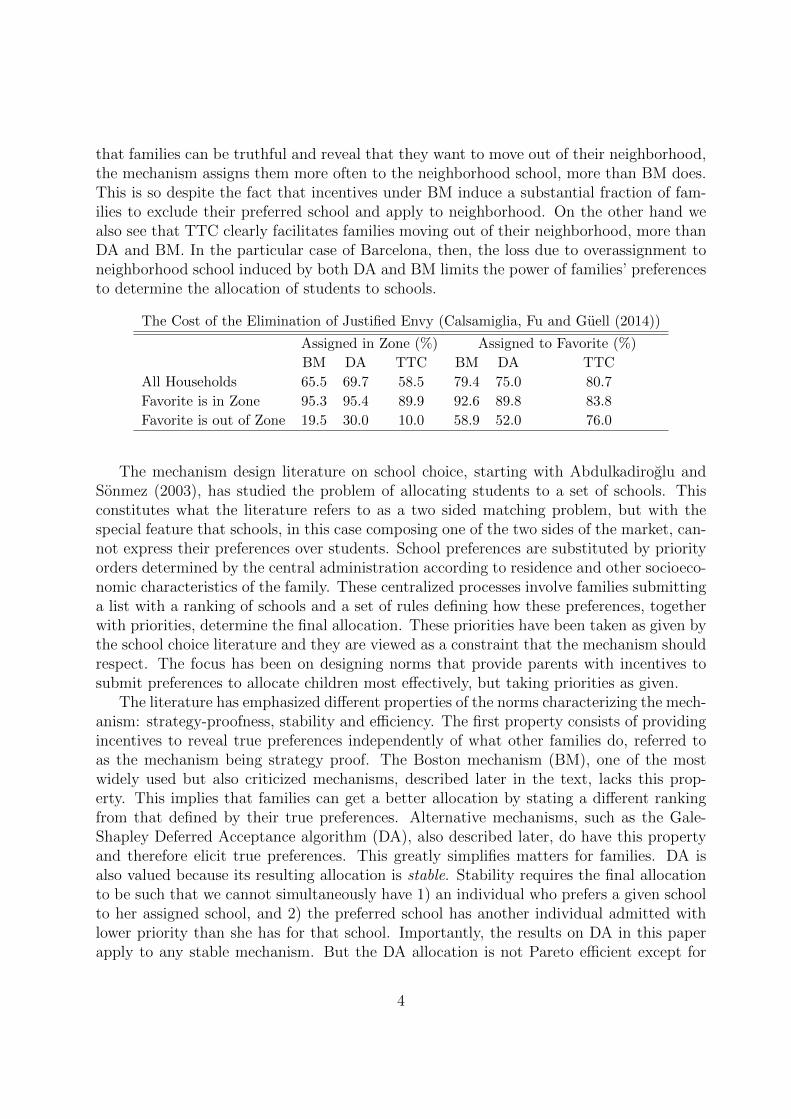
that families can be truthful and reveal that they want to move out of their neighborhood,the mechanism assigns them more often to the neighborhood school, more than BM does.This is so despite the fact that incentives under BM induce a substantial fraction of fam-ilies to exclude their preferred school and apply to neighborhood. On the other hand wealso see that TTC clearly facilitates families moving out of their neighborhood, more thanDA and BM. In the particular case of Barcelona, then, the loss due to overassignment toneighborhood school induced by both DA and BM limits the power of families’ preferencesto determine the allocation of students to schools.

The Cost of the Elimination of Justified Envy (Calsamiglia, Fu and Guell (2014))

Assigned in Zone (%) Assigned to Favorite (%)

BM DA TTC BM DA TTC

All Households 65.5 69.7 58.5 79.4 75.0 80.7

Favorite is in Zone 95.3 95.4 89.9 92.6 89.8 83.8

Favorite is out of Zone 19.5 30.0 10.0 58.9 52.0 76.0

The mechanism design literature on school choice, starting with Abdulkadiroglu andSonmez (2003), has studied the problem of allocating students to a set of schools. Thisconstitutes what the literature refers to as a two sided matching problem, but with thespecial feature that schools, in this case composing one of the two sides of the market, can-not express their preferences over students. School preferences are substituted by priorityorders determined by the central administration according to residence and other socioeco-nomic characteristics of the family. These centralized processes involve families submittinga list with a ranking of schools and a set of rules defining how these preferences, togetherwith priorities, determine the final allocation. These priorities have been taken as given bythe school choice literature and they are viewed as a constraint that the mechanism shouldrespect. The focus has been on designing norms that provide parents with incentives tosubmit preferences to allocate children most effectively, but taking priorities as given.

The literature has emphasized different properties of the norms characterizing the mech-anism: strategy-proofness, stability and efficiency. The first property consists of providingincentives to reveal true preferences independently of what other families do, referred toas the mechanism being strategy proof. The Boston mechanism (BM), one of the mostwidely used but also criticized mechanisms, described later in the text, lacks this prop-erty. This implies that families can get a better allocation by stating a different rankingfrom that defined by their true preferences. Alternative mechanisms, such as the Gale-Shapley Deferred Acceptance algorithm (DA), also described later, do have this propertyand therefore elicit true preferences. This greatly simplifies matters for families. DA isalso valued because its resulting allocation is stable. Stability requires the final allocationto be such that we cannot simultaneously have 1) an individual who prefers a given schoolto her assigned school, and 2) the preferred school has another individual admitted withlower priority than she has for that school. Importantly, the results on DA in this paperapply to any stable mechanism. But the DA allocation is not Pareto efficient except for

4

some specific priority structures (Ergin, 2002). Pareto-efficiency is defined as the lack ofan alternative allocation that makes an individual better off without making another in-dividual worse off. The Top Trading Cycles (TTC), also described in the next section, isstrategy proof and efficient, but is not stable. There is no mechanism that has the threeproperties. But the efficiency costs of DA, as measured in experiments, such as Chen andSonmez (2006), are small and so DA has actually been adopted in cities like New Yorkand Boston, substituting the former mechanism, referred to as the Boston Mechanism.4

Both DA and Boston, or a combination of the two (see Chen and Kesten (2013)) are themost debated alternatives (Abdulkadiroglu and Sonmez (2003); Abdulkadiroglu, Pathak,Roth and Sonmez (2006); Ergin and Sonmez (2006); Miralles (2008); Pathak and Sonmez(2008); Abdulkadiroglu, Che and Yasuda (2011)). TTC was only used in New Orleans forthe year 2012.

This paper suggests that, unless certain priorities are questioned, the choice betweenthese two main mechanisms may be less important, given that in both cases the final al-location of students is largely determined by priority rules. Similarly to Miralles (2008),Abdulkadiroglu, Che and Yasuda (2011), we follow Auman (1964) and assume that there isa continuum of individuals to be allocated to a finite number of seats in schools. Neverthe-less, we include a preliminary section containing a leading example with a finite number ofstudents. There it can be seen that our insights hold even for relatively small assignmentproblems.

Our base model contains a binomial priority structure (families either have priority ornot) that we intuitively connect to residential priorities (or walking-zone priorities).5 Thiskind of reasonable coarse priority structures lie in between two rather extreme models inthe theoretical literature: the strict priority model (e.g. Ergin and Sonmez, 2006; Pathakand Sonmez, 2008) and the no-priorities model (Abdulkadiroglu, Che and Yasuda, 2011;Miralles, 2008).6 In our model all seats follow the same priority structure. In cities likeBoston or New Orleans only a fraction of the seats are prioritized. For the remainingseats, overdemands are resolved randomly. We do not consider these non-prioritizes seatsexplicitly in our model, but clearly the larger the fraction of non-prioritized seats, the lessrelevant are our results.7 The objective in this paper is to illustrate that priorities createproblems that the literature had not emphasized enough. Hence, for ease of exposition wefocus on the case where all seats are prioritized.

The key additional element in our model is the existence of some degree of vertical

4Experiments evaluating the efficiency cost have been done in the lab, and the simulated environmentsused did not contain bad schools, as we model them here or are found in the data. This paper suggeststhat under the presence of bad schools efficiency losses may be very large, since preferences may have arather small effect on the final allocation.

5Extensions including sibling priorities and low-income / bad-neighborhood priorities can easily beincluded and are available upon request.

6All these papers discuss their models beyond the adopted extreme assumption, yet their most illustra-tive proofs rely on them. See Ergin and Erdil (2008) for an exception that formally analyzes weak prioritystructures.

7We explicitly discuss the the case with a fraction of prioritized seats at the end of the paper.

5

differentiation across schools, so that there is at least one bad school that is homogeneouslythought to be the worst. We argue that this is an element that we typically find in schoolchoice realities. In most cities where school choice is implemented there is a set of so-calledfailing schools, schools that are explicitly considered bad by local authorities. In the USthe requirement of the federal No Child Left Behind Public Choice Program requires thatlocal school districts allow students in academically unacceptable schools (F-rated schools)to transfer to higher performing, non-failing schools in the district– if there is capacityavailable.8

This paper emphasizes that the two most debated and used mechanisms in the litera-ture and in the policy debate may both be very limited in their capacity to allocate childrenaccording to their preferences whenever there are coarse priorities to break ties that imposea different ordering across different schools. Priorities limit the extent to which families’preferences determine the final allocation. The mechanism design literature should incor-porate the design of the priority structure explicitly, since it may deem crucial for theproperties of the final allocation.

The results of this paper are also important for the empirical literature in the economicsof education that evaluates the impact of school choice on school outcomes– see Lavy(2010), Hastings, Kane and Staiger (2010). This literature assumes that implementingchoice implies that preferences will affect the allocation of children to schools. But theseempirical papers ignore how allocation mechanisms are affected by the priority structureand therefore they may be attributing the effects to the wrong source of variation.

The results in this paper are presented in a rather stylized model for ease of exposition.The model should facilitate understanding the intuition for the results without harmingits perceived robustness. Next we present the mechanisms and an example that illustratesthe main intuitions underlying our general results . Section 4 presents the main results,evaluating the performance of the different mechanisms. Section 5 provides some discussionand section 6 concludes. Appendix A contains a discussion of the discrete model andAppendix B contains all proofs.

2 The Mechanisms

The mechanisms we compare are the Deferred Acceptance (DA), the Boston Mechanism(BM) and the Top-Trading Cycles (TTC). In all these mechanisms, parents (students) arerequested to submit a ranked list of schools. The student’s strategy space is the set of allrankings among the schools. Each student may belong to the catchment area of a school.Belonging to a school’s catchment area is the main priority criterion when resolving excessdemands. Additionally, a unique lottery number per agent breaks any other eventual tie.The outcome of the lottery is uncertain at the moment students submit their lists.

8See Title I Public School Choice for schools identified as Low Performing:http://www.ncpie.org/nclbaction/publicchoice.html.

6

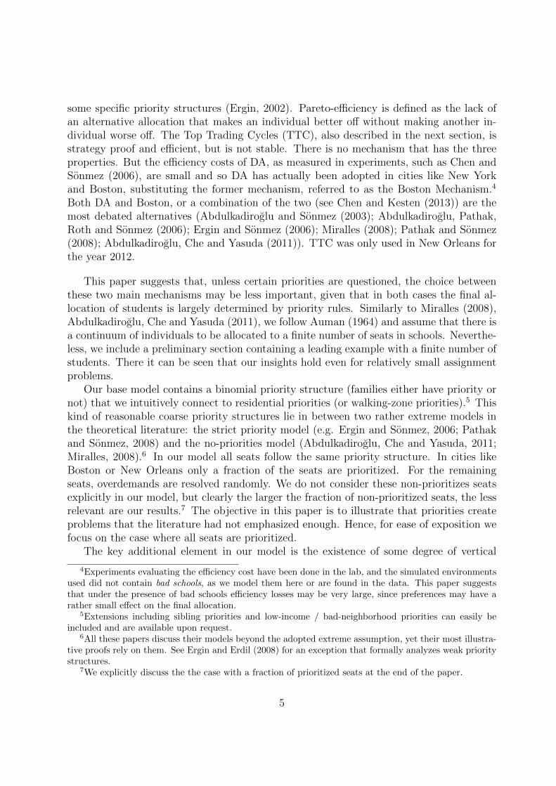
Deferred Acceptance (DA):

• In every round, each student applies for the highest school in its submitted list thathas not rejected her yet.

• For every round k, k ≥ 1: Each school tentatively assigns seats to the students thatapply to it or that were preaccepted in the previous round following its priority order(breaking ties through a fair lottery)9. When the school capacity is attained theschool rejects any remaining students that apply to it in that round.

• The DA mechanism terminates when no student is rejected. The tentative matchingbecomes final.10

Boston Mechanism (BM):

• In every round, each students applies for the highest school in its submitted list thathas not rejected her yet.

• For every round k, k ≥ 1: Each school assigns its remaining seats to the studentsthat apply to it following its priority order, and breaking ties through a randomlottery when necessary. If the school capacity is or was attained, the school rejectsany remaining students that point to it.

• The Boston mechanism algorithm terminates when all students have been assignedto a school, in at most three rounds.

Top-Trading Cycles (TTC):

• In each round, we find a cycle as follows. Taking a school s, we choose its firststudent in the priority list, i. This student points at her most preferred school s′,which points at its highest-priority student i′, etc. A cycle is always found becausethere is a finite number of schools.

• We assign to each student of the cycle a slot of the school she points at. We removethese students and slots.

• We repeat the process round by round (having erased completely filled schools fromstudents’ lists and assigned students from schools’ priority lists) until we have as-signed all the students.

9We assume that there is a single tie-breaker that serves to break ties when necessary at all schools. Wejustify this assumption on Abdulkadiroglu, Che and Yasuda (2014), which shows that a multiple tie-breaker(one for each school) in DA would lead to Pareto inefficient assignments.

10Abdulkadiroglu, Che and Yasuda (2014) show that this algorithm converges to an assignment in bigcontinuum economies, even though not necessarily in finite time.

7

3 A Finite Economy Example

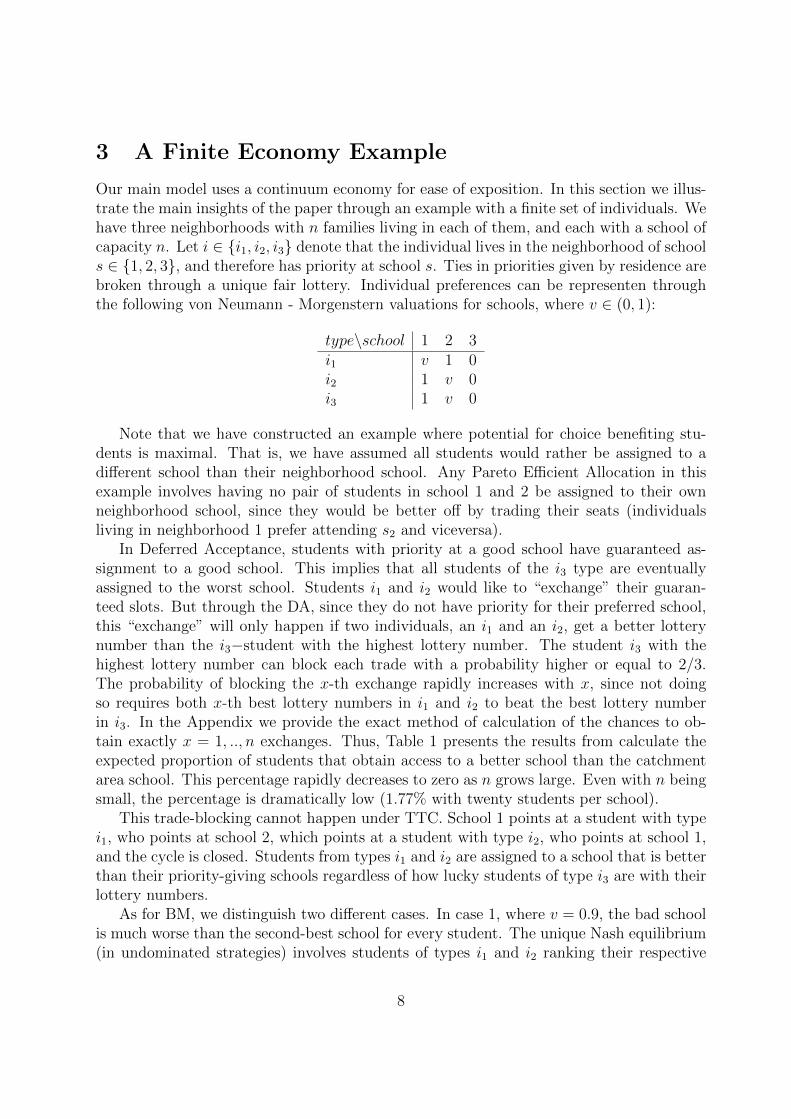
Our main model uses a continuum economy for ease of exposition. In this section we illus-trate the main insights of the paper through an example with a finite set of individuals. Wehave three neighborhoods with n families living in each of them, and each with a school ofcapacity n. Let i ∈ {i1, i2, i3} denote that the individual lives in the neighborhood of schools ∈ {1, 2, 3}, and therefore has priority at school s. Ties in priorities given by residence arebroken through a unique fair lottery. Individual preferences can be representen throughthe following von Neumann - Morgenstern valuations for schools, where v ∈ (0, 1):

type\school 1 2 3i1 v 1 0i2 1 v 0i3 1 v 0

Note that we have constructed an example where potential for choice benefiting stu-dents is maximal. That is, we have assumed all students would rather be assigned to adifferent school than their neighborhood school. Any Pareto Efficient Allocation in thisexample involves having no pair of students in school 1 and 2 be assigned to their ownneighborhood school, since they would be better off by trading their seats (individualsliving in neighborhood 1 prefer attending s2 and viceversa).

In Deferred Acceptance, students with priority at a good school have guaranteed as-signment to a good school. This implies that all students of the i3 type are eventuallyassigned to the worst school. Students i1 and i2 would like to “exchange” their guaran-teed slots. But through the DA, since they do not have priority for their preferred school,this “exchange” will only happen if two individuals, an i1 and an i2, get a better lotterynumber than the i3−student with the highest lottery number. The student i3 with thehighest lottery number can block each trade with a probability higher or equal to 2/3.The probability of blocking the x-th exchange rapidly increases with x, since not doingso requires both x-th best lottery numbers in i1 and i2 to beat the best lottery numberin i3. In the Appendix we provide the exact method of calculation of the chances to ob-tain exactly x = 1, .., n exchanges. Thus, Table 1 presents the results from calculate theexpected proportion of students that obtain access to a better school than the catchmentarea school. This percentage rapidly decreases to zero as n grows large. Even with n beingsmall, the percentage is dramatically low (1.77% with twenty students per school).

This trade-blocking cannot happen under TTC. School 1 points at a student with typei1, who points at school 2, which points at a student with type i2, who points at school 1,and the cycle is closed. Students from types i1 and i2 are assigned to a school that is betterthan their priority-giving schools regardless of how lucky students of type i3 are with theirlottery numbers.

As for BM, we distinguish two different cases. In case 1, where v = 0.9, the bad schoolis much worse than the second-best school for every student. The unique Nash equilibrium(in undominated strategies) involves students of types i1 and i2 ranking their respective

8

neighborhood school first, and each student is assigned his neighborhood school. HenceABS in this case is equal to 0.

In case 2, where v = 0.1 the bad school is similar to the second-best school for everystudent. Even though the former Nash equilibrium still exists, another Nash equilibrium(in undominated strategies) exists in which all students submit a truthful ranking overschools. For any n, all students of type i1 obtain a slot at school 2, while students of typesi2 and i3 have fifty per cent chances of obtaining a slot at school 1, and fifty per cent toobtain a slot at the worst school. In case 2 then, an equilibrium exists in which all theslots at good schools are given to students who prefer these more than their priority-givingschools. Hence, in this case ABS is maximal and equal to 67%.

Table 1 summarizes the expected number of students who obtain a better placementthan the school for which they had priority (weighted by the size 3n of the market).

Table 1: Expected percentage of students who get Access to Better School (ABS)

Mechanism \ n 1 2 5 10 20 ∞BM (v = 0.9) 0 0 0 0 0 0

DA 22 13.3 6.3 3.4 1.77 0

BM (v = 0.1) 66.7 66.7 66.7 66.7 66.7 66.7

TTC 66.7 66.7 66.7 66.7 66.7 66.7

BM (case 1) obtains the worst performance possible in terms of access to a better school.The assignment is fully determined by the priority structure. BM (case 1) performs worsethan DA, although insignificantly so as n goes large. In fact both perform extremelybad. Notice how the expected percentage of students who improve upon their catchmentareas rapidly decreases to zero under DA. With ten students per school, only 3.4% ofthem are expected to obtain a better assignment outside their catchment areas. Withtwenty students per school, this percentage is 1.77%. This exemplifies that the bad resultsobtained by DA later in the model are not an artifact of the continuum.

In contrast, BM (case 2), which performs as good as TTC, obtain maximum access tobetter schools for any n. The comparison between DA and BM crucially depends on theintensity of students’ preferences between the second-best school and the worst school. Incase 1, preferences lead to a (bad) equilibrium in BM where agents manipulate preferencesand use safe options. In case 2, students do not strategize, hence reaching a “good”equilibrium that outperforms DA.

Although TTC and BM (case 2) are similar in terms of ABS, they are very differentin other respects. While TTC ensures that students with priority at good schools do notworsen their positions, BM (case 2) involves a risk of ending in the worst school. At thesame time, BM (case 2) gives chances to i3, the student with priority the bad school, ofgetting access to a better school. In the discussion at the end of the paper we commenton the limitations of our ABS measure.

9

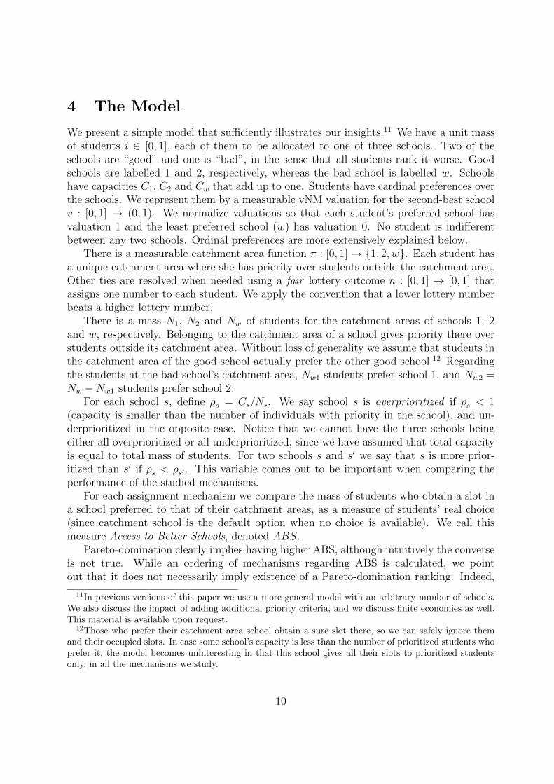
4 The Model

We present a simple model that sufficiently illustrates our insights.11 We have a unit massof students i ∈ [0, 1], each of them to be allocated to one of three schools. Two of theschools are “good” and one is “bad”, in the sense that all students rank it worse. Goodschools are labelled 1 and 2, respectively, whereas the bad school is labelled w. Schoolshave capacities C1, C2 and Cw that add up to one. Students have cardinal preferences overthe schools. We represent them by a measurable vNM valuation for the second-best schoolv : [0, 1] → (0, 1). We normalize valuations so that each student’s preferred school hasvaluation 1 and the least preferred school (w) has valuation 0. No student is indifferentbetween any two schools. Ordinal preferences are more extensively explained below.

There is a measurable catchment area function π : [0, 1]→ {1, 2, w}. Each student hasa unique catchment area where she has priority over students outside the catchment area.Other ties are resolved when needed using a fair lottery outcome n : [0, 1] → [0, 1] thatassigns one number to each student. We apply the convention that a lower lottery numberbeats a higher lottery number.

There is a mass N1, N2 and Nw of students for the catchment areas of schools 1, 2and w, respectively. Belonging to the catchment area of a school gives priority there overstudents outside its catchment area. Without loss of generality we assume that students inthe catchment area of the good school actually prefer the other good school.12 Regardingthe students at the bad school’s catchment area, Nw1 students prefer school 1, and Nw2 =Nw −Nw1 students prefer school 2.

For each school s, define ρs = Cs/Ns. We say school s is overprioritized if ρs < 1(capacity is smaller than the number of individuals with priority in the school), and un-derprioritized in the opposite case. Notice that we cannot have the three schools beingeither all overprioritized or all underprioritized, since we have assumed that total capacityis equal to total mass of students. For two schools s and s′ we say that s is more prior-itized than s′ if ρs < ρs′ . This variable comes out to be important when comparing theperformance of the studied mechanisms.

For each assignment mechanism we compare the mass of students who obtain a slot ina school preferred to that of their catchment areas, as a measure of students’ real choice(since catchment school is the default option when no choice is available). We call thismeasure Access to Better Schools, denoted ABS.

Pareto-domination clearly implies having higher ABS, although intuitively the converseis not true. While an ordering of mechanisms regarding ABS is calculated, we pointout that it does not necessarily imply existence of a Pareto-domination ranking. Indeed,

11In previous versions of this paper we use a more general model with an arbitrary number of schools.We also discuss the impact of adding additional priority criteria, and we discuss finite economies as well.This material is available upon request.

12Those who prefer their catchment area school obtain a sure slot there, so we can safely ignore themand their occupied slots. In case some school’s capacity is less than the number of prioritized students whoprefer it, the model becomes uninteresting in that this school gives all their slots to prioritized studentsonly, in all the mechanisms we study.

10

mechanisms that may induce higher access to better schools may do so in exchange ofplacing prioritized students from good schools’ catchment areas to bad schools. At the sametime, mechanisms that perform poorly in terms of ABS may be protecting these studentsfrom being assigned to the bad school. Finally, we also observe that rank-domination(Featherstone, 2014) does not imply (or is implied by) ABS domination. A mechanismmay be good in placing students from the worst school’s catchment area in either one ofthe good schools, while being bad in placing them to her favorite good school. Anothermechanism could rank-dominate the former and at the same time it could be dominatedby it in terms of ABS.

4.1 Worst and Best Cases under the Boston Mechanism

It is well known that both DA and TTC are strategy-proof: there is a dominant strategyequilibrium in which all students submit the true ranking of schools according to theirpreferences. It is also known that agents have incentives to manipulate their rankings inBM, depending on their cardinal preferences– see for example Abdulkadiroglu and Sonmez(2003), Miralles (2008) or Abdulkadiroglu, Che and Yausda (2011). We illustrate twoextreme cases that may constitute part of a Nash equilibrium (in undominated strategies)for limit preference structures.

The first extreme, which we call Boston Mechanism (worst case), involves everystudent manipulating her preferences in order to minimize the probability of being assignedthe bad school. More precisely, for each underprioritized good school, all the prioritizedstudents rank it first. And for every overprioritized good school, the number of prioritizedstudents who rank it first exceeds the school’s capacity. This maximum manipulation arisesas the unique Nash equilibrium outcome when the valuation of the bad school is sufficientlybad for every student. It is also one, yet not necessarily unique, Nash equilibrium predictionwhen both good schools are overprioritized, regardless of how worse the bad school is(compared to the second school). It is easy to envision that this maximal manipulationequilibrium leads to a dreadful level of access to better schools, since prioritized studentsuse their safest options, resigning from achieving a slot in a better school while blockingothers from getting access to good schools.

Lemma 1: There is v ∈ (0, 1) such that if the range of v lies strictly above v, everyNash equilibrium (undominated strategies) of the game induced by BM meets the worstcase of the Boston Mechanism.

Appendix A contains the proofs to all lemmas and propositions.

On the other extreme we have the Boston Mechanism (best case), where agentssubmit a ranking according their true preferences. This is a limit Nash equilibrium pre-diction when the valuation every agent has for the worst school is almost as good as thevaluation for her second-best school. That is, there is almost no punishment for being re-jected in the first round of the assignment algorithm, thus being sincere is optimal. In thiscase it is clear that access to better schools is dramatically increased. Prioritized students

11

at good schools make no use of this privilege, aiming to better schools and thereby lettingothers get access to their preferred schools.13

Lemma 2: There exists v ∈ (0, 1) such that if the range of v lies strictly below v, thereis a Nash equilibrium (undominated strategies) of the game induced by BM that coincideswith the best case of the Boston Mechanism.

The Nash equilibrium (in undominated strategies) outcome of the Boston Mechanism isneither unique nor predictable without knowing the distribution of cardinal von Neumann- Morgenstern utilities. Fortunately, we can state that the access to better schools measurewould stay between the lower bound and the upper bound provided by the worst case andbest case scenarios. Interestingly, this is also true if there is a proportion of nonstrategicstudents that compulsory rank the schools according to their true preferences.

We calculate ABS under BM (worst case and best case). In the worst-case scenario,agents aim to minimize the probability of ending assigned at the bad school. A school sis overdemanded if the mass of students ranking it in first position exceeds its capacity.School s is underdemanded otherwise. Notice that since ranking the bad school other thanlast is part of a dominated strategy, it cannot be the case that both two good schools areunderdemanded. Here is our result. Let ABS=

∑s∈{1,2}max{0, Cs − Ns} be the lower

bound for the access to better schools that can be attained by any mechanism. Essentially,every slot at each good school is given to a prioritized student, until either all students ofits catchment area have been already assigned or the school capacity is filled.

Proposition 1 ABSBMworst =ABS.

In the Boston Mechanism (best case), all the students truthfully rank their schoolsaccording to their preferences. As in the previous case, it cannot be that both two goodschools are underdemanded in the first round of the assignment algorithm. Thus, eitherN1 + Nw2 > C2 or N2 + Nw1 > C1 (or both). Let ABS = C1 + C2 be the obvious upperbound for the access to better schools that can be attained by any mechanism. If bothschools have sufficient number of students who have it as its first best, then maximal accessto better schools is attained, since both good schools are filled by students who desire itmost. If one of the schools does not have a sufficient amount of students who prefer it,No +Nwo < Cu, then the remaining capacity after the first round, Cu −No +Nwo, will befilled by those who have priority at it that did not get their preferred school. If there isstill capacity after that, then it will be filled by individuals from the bad neighborhood.Therefore, the only seats that will not be used to improve access to better schools will bethe capacity available in the second round occupied by applicants to the overdemendedschool that did not get in and that live in the underdemanded school.

Proposition 2 1) If both schools are filled when all students who have it as their first bestdemand it, that is, N1 +Nw2 > C2 and N2 +Nw1 > C1, then ABSBMbest = ABS.

13See Kojima and Unver (2014) for a characterization of the Boston Mechanism under truthtelling.

12

2) If one school is not filled when all students who have it as their first best demandit (label this school as u and the other school as o), that is, if No + Nwo < Cu, then

ABSBMbest = ABS −min{Nu

(1− Co

Nu+Nwo

), Cu −No −Nwu

}.

4.2 Access to better schools under Deferred Acceptance

The properties derived from DA in this paper are direct implications of it being stable. Inother words, the results in DA would result from any stable mechanism. Stability in ourframework limits ABS largely, because it leads to individuals in the bad neighborhoodsblocking pareto improving exchanges between individuals in the good schools. Individualsin the good neighborhoods will apply for their first best and if they do not get in theywill apply and get their neighborhood school, capacity permitting. Therefore no individualliving in a good neighborhood will be placed in the bad school, unless her neighborhoodschool is overprioritized. If both schools are overprioritized, then clearly no individualfrom the bad neighborhood will have access to a good school. But by stability then, noindividual from a good neighborhood can get better access, since, lacking priority to theirpreferred school requires that they get a higher lottery number than any student in thebad neighborhood. Therefore ABS in that case is 0.

On the other hand, if one school is underprioritized, Ch − Nh > 0, then some trademay arise. The intuition is as follows. Since Ch > Nh some seats at h are available thatno individual living in h will “claim” back. This implies that some individuals from thebad and from the other good neighborhood will access those seats and thereby achieveimproved access. Additional access may be provided if the individuals from the other goodschool that access school h do not fill their own school, creating some leftover capacityto be filled by non-prioritized students (this will depend on how overprioritized the othergood school is). This process may lead to ABS being substantial in this case. The followingproposition formally states these results.

Proposition 3 1) If both good schools are (weakly) overprioritized, ABSDA = 0.2) If one school (h) is underprioritized and the other one is (weakly) more prioritized

than the bad school, ABSDA = Ch −Nh.3) If one school is underprioritized and the other one is less prioritized than the bad

school, ABSDA = ABS −Nh(1− c2)−N2(1− ch).

where cs ∈ [0, 1], are cut-offs such that no non-prioritized student with lottery numberabove the cut-off can obtain access to school s. The Appendix provides the exact analyticalexpressions for these cut-offs. Notice that in cases 1 and 2 DA reaches the lower boundof ABS, that is, ABSDA = ABS. More generally, this “trade blocking” systematicallyhappens as long as min{ρ1, ρ2} ≤ ρw. Performance under DA improves when schools areless prioritized. As long as more slots at good schools can be given to students fromthe catchment area of the bad school, access to better schools is less blocked. Satisfyingstudents with best lottery numbers from the bad school catchment area allows studentsfrom the catchment area of good schools to “exchange slots”, as long as they also havesufficiently good lottery numbers. However, DA never reaches the upper bound ABS.

13

4.3 Access under Boston versus Deferred Acceptance

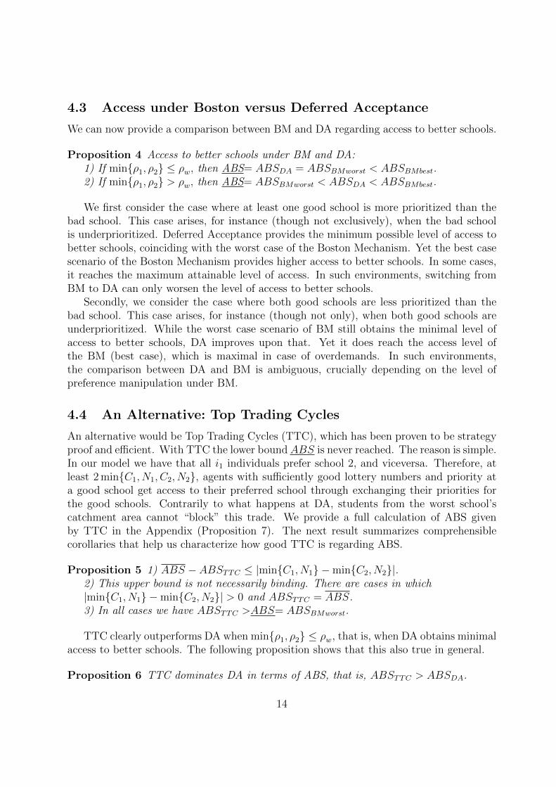
We can now provide a comparison between BM and DA regarding access to better schools.

Proposition 4 Access to better schools under BM and DA:1) If min{ρ1, ρ2} ≤ ρw, then ABS= ABSDA = ABSBMworst < ABSBMbest.2) If min{ρ1, ρ2} > ρw, then ABS= ABSBMworst < ABSDA < ABSBMbest.

We first consider the case where at least one good school is more prioritized than thebad school. This case arises, for instance (though not exclusively), when the bad schoolis underprioritized. Deferred Acceptance provides the minimum possible level of access tobetter schools, coinciding with the worst case of the Boston Mechanism. Yet the best casescenario of the Boston Mechanism provides higher access to better schools. In some cases,it reaches the maximum attainable level of access. In such environments, switching fromBM to DA can only worsen the level of access to better schools.

Secondly, we consider the case where both good schools are less prioritized than thebad school. This case arises, for instance (though not only), when both good schools areunderprioritized. While the worst case scenario of BM still obtains the minimal level ofaccess to better schools, DA improves upon that. Yet it does reach the access level ofthe BM (best case), which is maximal in case of overdemands. In such environments,the comparison between DA and BM is ambiguous, crucially depending on the level ofpreference manipulation under BM.

4.4 An Alternative: Top Trading Cycles

An alternative would be Top Trading Cycles (TTC), which has been proven to be strategyproof and efficient. With TTC the lower bound ABS is never reached. The reason is simple.In our model we have that all i1 individuals prefer school 2, and viceversa. Therefore, atleast 2 min{C1, N1, C2, N2}, agents with sufficiently good lottery numbers and priority ata good school get access to their preferred school through exchanging their priorities forthe good schools. Contrarily to what happens at DA, students from the worst school’scatchment area cannot “block” this trade. We provide a full calculation of ABS givenby TTC in the Appendix (Proposition 7). The next result summarizes comprehensiblecorollaries that help us characterize how good TTC is regarding ABS.

Proposition 5 1) ABS − ABSTTC ≤ |min{C1, N1} −min{C2, N2}|.2) This upper bound is not necessarily binding. There are cases in which|min{C1, N1} −min{C2, N2}| > 0 and ABSTTC = ABS.3) In all cases we have ABSTTC >ABS= ABSBMworst.

TTC clearly outperforms DA when min{ρ1, ρ2} ≤ ρw, that is, when DA obtains minimalaccess to better schools. The following proposition shows that this also true in general.

Proposition 6 TTC dominates DA in terms of ABS, that is, ABSTTC > ABSDA.

14

We are not able to provide a clear characterization of the ordering between TTC andBM with respect to ABS. There are environments in which TTC reaches maximal ABSwhereas BM (best case) does not, and cases in which the opposite happens. We provideexamples illustrating both possibilities.

Example 1: When N1 = N2 < min{C1, C2} and some good school is underdemandedunder BM (best case), we have ABS = ABSTTC > ABSBMbest. �

Example 2: When min{N1, N2} > max{C1, C2} and C1 6= C2, we have: ABS =ABSBMbest > ABSTTC = 2 min{C1, C2}. �

ABS is an aggregate measure of choice that abstracts from potentially important aspectswhen allowing families to choose. For instance, BM (best case) may outperform TTC orvice versa, but qualitatively there are differences in the identity of the agents who obtaina better choice outside their catchment area. In TTC, no prioritized student from anunderprioritized good school could ever be assigned to a bad school. Hence, access tobetter schools arises primarily because students with priority at good schools exchangetheir positions. Note that students from the bad school’s catchment area get no indirectbenefit from this. Conditional on not having traded a good school seat, the prioritizedstudent’s lottery number is worse than that of the students from the bad school’s catchmentarea. This way the latter students may obtain access to better schools as well. In BM (bestcase), the first round works as if no priorities existed. Prioritized students at good schoolsapply for a different school, directly emptying a slot for other students. Consequently,chances are that a student from a good school’s catchment area ends assigned at the badschool. The good side of this is that students from the bad school’s catchment area havemore chances to get access to a good school.

5 Discussion

5.1 Reducing the Number of Prioritized Seats

In cities such as Boston, it is well-known that for almost every school only half of avail-able seats are prioritized according to the catchment area priority criterion. That is, thecatchment area only has a bite in allocating half of the slots. The other half is assignedaccording to the lottery number only. The assignment process in Boston lies between ourbase model, where all the slots are prioritized, and a school assignment problem with nocatchment area priorities. Not surprisingly, one would expect that access to better schoolsis enhanced by lowering the proportion of prioritized seats.

For each good school we can distinguish three cases. In the first case, the number ofprioritized students ultimately applying for a slot at the school is lower than the number ofprioritized seats. The outcome becomes identical to that of the base model. In the secondcase, the number of prioritized students applying for a slot at the school exceeds the numberof prioritized seats, and the minimum lottery number among rejected students is too high

15

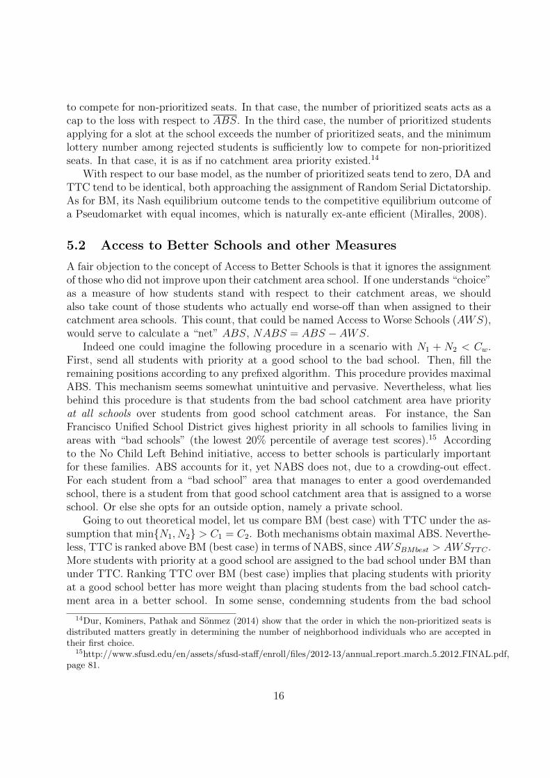
to compete for non-prioritized seats. In that case, the number of prioritized seats acts as acap to the loss with respect to ABS. In the third case, the number of prioritized studentsapplying for a slot at the school exceeds the number of prioritized seats, and the minimumlottery number among rejected students is sufficiently low to compete for non-prioritizedseats. In that case, it is as if no catchment area priority existed.14

With respect to our base model, as the number of prioritized seats tend to zero, DA andTTC tend to be identical, both approaching the assignment of Random Serial Dictatorship.As for BM, its Nash equilibrium outcome tends to the competitive equilibrium outcome ofa Pseudomarket with equal incomes, which is naturally ex-ante efficient (Miralles, 2008).

5.2 Access to Better Schools and other Measures

A fair objection to the concept of Access to Better Schools is that it ignores the assignmentof those who did not improve upon their catchment area school. If one understands “choice”as a measure of how students stand with respect to their catchment areas, we shouldalso take count of those students who actually end worse-off than when assigned to theircatchment area schools. This count, that could be named Access to Worse Schools (AWS),would serve to calculate a “net” ABS, NABS = ABS − AWS.

Indeed one could imagine the following procedure in a scenario with N1 + N2 < Cw.First, send all students with priority at a good school to the bad school. Then, fill theremaining positions according to any prefixed algorithm. This procedure provides maximalABS. This mechanism seems somewhat unintuitive and pervasive. Nevertheless, what liesbehind this procedure is that students from the bad school catchment area have priorityat all schools over students from good school catchment areas. For instance, the SanFrancisco Unified School District gives highest priority in all schools to families living inareas with “bad schools” (the lowest 20% percentile of average test scores).15 Accordingto the No Child Left Behind initiative, access to better schools is particularly importantfor these families. ABS accounts for it, yet NABS does not, due to a crowding-out effect.For each student from a “bad school” area that manages to enter a good overdemandedschool, there is a student from that good school catchment area that is assigned to a worseschool. Or else she opts for an outside option, namely a private school.

Going to out theoretical model, let us compare BM (best case) with TTC under the as-sumption that min{N1, N2} > C1 = C2. Both mechanisms obtain maximal ABS. Neverthe-less, TTC is ranked above BM (best case) in terms of NABS, since AWSBMbest > AWSTTC .More students with priority at a good school are assigned to the bad school under BM thanunder TTC. Ranking TTC over BM (best case) implies that placing students with priorityat a good school better has more weight than placing students from the bad school catch-ment area in a better school. In some sense, condemning students from the bad school

14Dur, Kominers, Pathak and Sonmez (2014) show that the order in which the non-prioritized seats isdistributed matters greatly in determining the number of neighborhood individuals who are accepted intheir first choice.

15http://www.sfusd.edu/en/assets/sfusd-staff/enroll/files/2012-13/annual report march 5 2012 FINAL.pdf,page 81.

16

catchment area to stay there is rewarded, if NABS is used as an aggregate measure ofchoice.

Another alternative aggregate measure of school choice is the mass of students thatobtain Access to their Favorite School (AFS). This approximation to students’ satisfactiontakes into account that ending in the actual top choice should not count equally as endingin the second-best school. Incidentally, in the context of the base model, AFS dominationis equivalent to rank domination (since the mass of agents who obtain a slot in the least-preferred school is the same in every mechanism). However, we chose ABS because itcounts students’ chances to escape from their catchment areas towards a preferred school.The quantitative difference between AFS and ABS is the number of students from the badschool’s catchment area that are assigned to their second-best schools.16

6 Conclusions

Since Abdulkadiroglu and Sonmez (2003) the Boston Mechanism has been widely criti-cized in the school choice literature. Since then many cities around the world have sub-stituted this mechanism by the Gale Shapley Deferred Acceptance mechanism.17DeferredAcceptance has been adapted from matching theory as a good alternative, since it is notmanipulable, it protects nonstrategic parents and provides more efficient assignments insetups with strict priorities. The debate between these two mechanisms was based uponmodels that assumed extreme scenarios in the priority structure: either no priorities orstrict priorities, and did not incorporate some important realities about the schools sys-tem, such as the vertical differentiation among schools. We solve a simple model of schoolchoice with coarse residential priorities and vertical differentiation separating good frombad schools. We show that if school choice aims to improve access to better schools thanthe neighborhood school, then both mechanisms are likely to perform very poorly. Weillustrate that the priority structure, under the presence of a stratified school system, candetermine the final allocation to a great extent in both of these mechanisms.

The range of possible ABS outcomes of the Boston Mechanism is very wide, covering thelower and the upper bound of all possible ABS levels. The outcome depends on the degree ofpreference manipulation among participating parents. Manipulation harms access to betterschools via the use of safe options, while sincerity is good because it makes improvementspossible directly, but also because it empties a slot in a school (the neighborhood school)that is better preferred by other students. In districts where some schools are perceivedas very bad, avoiding them becomes a primary objective, manipulation naturally arises.In school districts where vertical differentiation is rather low, sincere school applicationstrategies are less punished, and ABS can be large.

We have seen that Deferred Acceptance unambiguously provides less access to better

16Incidentally, Table 1 in the preceding example would also report a measure of AFS. Both AFS andABS may coincide numerically in several scenarios.

17See Pathak and Sonmez (2013) for evidence on the number of cities around the word where the Bostonmechanims has been banned.

17

schools than the Boston Mechanism when some good school is relatively more prioritized (interms of number of prioritized students divided by school capacity) than the bad school/s.ABS, in that case, reaches the lower bound of all possible outcomes. ABS improves underDA when all good schools are less prioritized than the bad school/s. The opportunity forstudents from a bad school’s catchment area to occupy slots at good schools makes prioritytrading among prioritized students at good schools possible. However, access to betterschools under Deferred Acceptance is always inferior to that of the Boston Mechanism ifparents rank schools according to their true preferences.

We have also discussed a third, natural alternative in this debate, which is Top-TradingCycles. TTC is more immune to the priority structure because prioritized students at goodschools are allowed to trade their slots with no interferences from students of a bad school’scatchment area. Top-Trading Cycles obtains higher access to better schools than DeferredAcceptance. It therefore constitutes a safe mechanism with respect to both the BostonMechanism and Deferred Acceptance, in school choice problems where coarse zone prioritiesexist.

More generally this paper puts forth the extreme relevance that neighborhood prioritiescan have on the final allocation of students to schools, inhibiting the role that preferencesmay have in determining the final allocation. The literature has deemed these prioritiesas exogenous, but ultimately they constitute a key feature of the final assignment that theadministration can a do change whenever needed.18 Future work should incorporate thedesign of these priorities as a fundamental part of the mechanism design problem.

7 Appendix

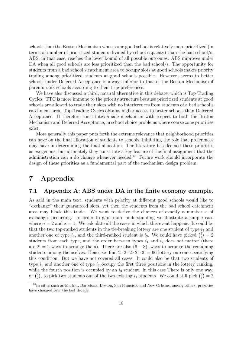
7.1 Appendix A: ABS under DA in the finite economy example.

As said in the main text, students with priority at different good schools would like to“exchange” their guaranteed slots, yet then the students from the bad school catchmentarea may block this trade. We want to derive the chances of exactly a number x ofexchanges occurring. In order to gain more understanding we illustrate a simple casewhere n = 2 and x = 1. We calculate all the cases in which this event happens. It could bethat the two top-ranked students in the tie-breaking lottery are one student of type i1 andanother one of type i2, and the third-ranked student is i3. We could have picked

(21

)= 2

students from each type, and the order between types i1 and i2 does not matter (thereare 2! = 2 ways to arrange them). There are also (6 − 3)! ways to arrange the remainingstudents among themselves. Hence we find 2 · 2 · 2 · 2! · 3! = 96 lottery outcomes satisfyingthis condition. But we have not covered all cases. It could also be that two students oftype i1 and another one of type i2 occupy the first three positions in the lottery ranking,while the fourth position is occupied by an i3 student. In this case There is only one way,or(

22

), to pick two students out of the two existing i1 students. We could still pick

(21

)= 2

18In cities such as Madrid, Barcelona, Boston, San Francisco and New Orleans, among others, prioritieshave changed over the last decade.

18

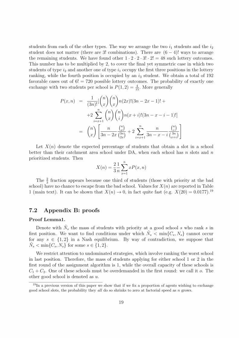
students from each of the other types. The way we arrange the two i1 students and the i2student does not matter (there are 3! combinations). There are (6 − 4)! ways to arrangethe remaining students. We have found other 1 · 2 · 2 · 3! · 2! = 48 such lottery outcomes.This number has to be multiplied by 2, to cover the final yet symmetric case in which twostudents of type i2 and another one of type i1 occupy the first three positions in the lotteryranking, while the fourth position is occupied by an i3 student. We obtain a total of 192favorable cases out of 6! = 720 possible lottery outcomes. The probability of exactly oneexchange with two students per school is P (1, 2) = 4

15. More generally

P (x, n) =1

(3n)![

(n

x

)(n

x

)n(2x)!(3n− 2x− 1)! +

+2n∑

i=x+1

(n

x

)(n

i

)n(x+ i)!(3n− x− i− 1)!]

=

(n

x

)[n

3n− 2x

(nx

)(3n2x

) + 2n∑

i=x+1

n

3n− x− i

(ni

)(3nx+i

)]

Let X(n) denote the expected percentage of students that obtain a slot in a schoolbetter than their catchment area school under DA, when each school has n slots and nprioritized students. Then

X(n) =2

3

1

n

n∑x=1

xP (x, n)

The 23

fraction appears because one third of students (those with priority at the badschool) have no chance to escape from the bad school. Values for X(n) are reported in Table1 (main text). It can be shown that X(n)→ 0, in fact quite fast (e.g. X(20) = 0.0177).19

7.2 Appendix B: proofs

Proof Lemma1.

Denote with Ns the mass of students with priority at a good school s who rank s infirst position. We want to find conditions under which Ns < min{Cs, Ns} cannot occurfor any s ∈ {1, 2} in a Nash equilibrium. By way of contradiction, we suppose thatNs < min{Cs, Ns} for some s ∈ {1, 2}.

We restrict attention to undominated strategies, which involve ranking the worst schoolin last position. Therefore, the mass of students applying for either school 1 or 2 in thefirst round of the assignment algorithm is 1, while the overall capacity of these schools isC1 + C2. One of these schools must be overdemanded in the first round: we call it o. Theother good school is denoted as u.

19In a previous version of this paper we show that if we fix a proportion of agents wishing to exchangegood school slots, the probability they all do so shrinks to zero at factorial speed as n grows.

19

Suppose u is underdemanded in the first round. Then, among those students applyingfor school o in the first round without priority there, the chances of ending assigned at ware at least Cw = 1 − C1 − C2, since the bad school is filled only with students that usedthis strategy. The payoff from this latter strategy for these agents is no more than C1 +C2.Instead, the payoff from applying for the underdemanded school is higher than v.

Setting v ≥ C1 +C2 we force every Nash equilibrium to have both good schools overde-manded. Otherwise all students without priority at o would best respond by ranking theunderdemanded school u first. Since all students with priority at o would also best respondby ranking the preferred underdemanded school u first, we would contradict the fact thatu is underdemanded.

Since both good schools are overdemanded, every rejected student at the first roundis eventually assigned at the bad school. Use qs for the Nash equilibrium probability ofbeing accepted at s ∈ {1, 2} for a student without priority at s that applies there in thefirst round of the BM algorithm. WLOG assume qu ≥ qo and notice that it must be thecase that qo ≤ C1 + C2. Let 0 < ε < Cw. We find conditions under which every Nashequilibrium meets qu ≤ 1− ε. Suppose the contrary, thus applying for this school rendersa payoff of more than (1 − ε)v. Applying for the other school renders a payoff boundedby qo ≤ C1 + C2. Set v ≥ C1+C2

1−ε . Under this condition all non-prioritized students at o

(a mass Nu + Nw) would best respond by ranking u first. But then, since Nu = Nu, ourinitial assumption implies No < min{Co, No}, yielding o underdemanded, a contradiction.

Finally, we fix ε ∈ (0, Cw) and we use qo ≤ qu ≤ 1 − ε. Let Ns < min{Cs, Ns} forsome s ∈ {o, u}. For a prioritized student at school s applying for the other good school,the payoff is not more than 1− ε, whereas applying for school s gives payoff above v. Setv = max{C1+C2

1−ε , 1 − ε}. With this, the best response for all students with priority at s is

to rank s in first position, contradicting Ns < min{Cs, Ns} as part of a Nash equilibrium.�

Proof Lemma2.

We restrict attention to undominated strategies, where all students rank the worstschool in last position. Suppose that the profile of submitted rankings coincides with theprofile of ordinal preferences. We show that the best response for all students is preciselyto rank the schools sincerely, when valuations for second-best schools are sufficiently low(capped by a properly chosen v).

First, consider the case where both good schools (labelled s and s′) are overdemandedin the first round. For a student i who prefers s and abides by the sincere ranking strategythe payoff is Cs

Ns′+Nws. Instead, the payoff from the best alternative, putting s′ first in the

ranking, cannot exceed v(i). Setting v ≤ v1 = min{ C1

N2+Nw1, C2

N1+Nw2} we make sure that all

such i best respond by ranking schools truthfully.

Consider now the case in which one school, labelled u, is underdemanded in the firstround (the other one, o, must be overdemanded). For a student who prefers u the most,

20

truthful ranking is obviously a best response. Consider a student i who prefers o the most.If she ranks o in first position according to her true preferences, she obtains a payoff higherthan Co

Nu+Nwo. If she instead ranks u first she obtains a payoff v(i). Setting v ≤ v2 = Co

Nu+Nwo

we make sure that all such i best respond by ranking o in first position. Notice that v1 = v2,thus v = min{ C1

N2+Nw1, C2

N1+Nw2} suffices to obtain the desired result. �

Proof Proposition 1.

In BM (worst case), if some good school s is underprioritized, all of its prioritizedstudents optimally rank the school of their catchment area first. If a good school s isoverprioritized, no Nash equilibrium (undominated strategies) exists where the number ofprioritized students that rank s first does not exceed its capacity. Altogether we obtainABSBMworst =

∑s∈{1,2}max{0, Cs −Ns} =ABS. �

Proof Proposition 2.

Clear for overdemanded schools (all good slots are given to students that prefer themthe most). When u is underdemanded (hence o is overdemanded), Cu − No − Nwu slotsof u are still available after the first assignment round. This is the maximum number ofslots that students with priority at u who were rejected from o in the first round, a total

of Nu

(1− Co

Nu+Nwo

), can occupy. All other slots are occupied by agents who had priority

at a less-preferred school. �

Proof Proposition 3.

Following in Abdulkadiroglu, Che and Yasuda (2014), the outcome of DA can be char-acterized via cutoffs c1 and c2. Provided a student i with π(i) 6= s applies at some point forschool s, she would be definitely accepted if her lottery number meets n(i) ≤ cs. Obviouslythe cut-off for the worst school is 1. We easily adapt Abdulkadiroglu, Che and Yasuda’smethod of calculus to the existence of a zone priority structure. Let l be the good schoolwith lowest cut-off, and h the good school with highest cut-off. Then cl and ch meet

cl(Nh +Nwl) = max{0, Cl − (1− ch)Nl}ch(Nl +Nwh) + (ch − cl)Nwl = max{0, Ch − (1− cl)Nh}

1) Ch− (1− cl)Nh ≤ 0. Then cl and ch are both zero. This case arises when both goodschools are (weakly) overprioritized.

2) Cl − (1 − ch)Nl ≤ 0 and Ch − (1 − cl)Nh > 0. In such a case we have cl = 0 andch = Ch−Nh

Nl+Nw. This case arises when Ch > Nh (that is, ρh > 1) and, after some algebra,

ρl ≤ ρw. This algebra goes as follows. Cl − (1 − ch)Nl ≤ 0 iff Cl − (1 − Ch−Nh

Nl+Nw)Nl ≤ 0,

or Cl − Nl+Nw+Nh−Ch

Nl+NwNl ≤ 0, or Cl − 1−Ch

Nl+NwNl ≤ 0, or Cl − Cl+Cw

Nl+NwNl ≤ 0, or Cl

Nl≤ Cl+Cw

Nl+Nw,

which happens if and only if Cl

Nl≤ Cw

Nw.

3): Cl − (1 − ch)Nl > 0 and Ch − (1 − cl)Nh > 0. Solving for the system of equations

gives cl = Nl(ρl−ρw)Nh+Nwl

and ch = 1− ρw. We have, of course, that this is met when ρh > 1 andρl > ρw. Notice that this implies ρw < 1.

21

In this case ABSDA = N1c2 + N2c1 + Nw max{c1, c2} = N1c2 + N2c1 + Nw(1 − ρw) =N1c2 +N2c1 +Nw − Cw = N1c2 +N2c1 + C1 + C2 −N1 −N2. �

Proof Proposition 4.

We already saw that ABSBMworst =ABS. From the preceding Proposition it is clearthatABSDA =ABS in its cases 1 and 2 (summarized as min{ρ1, ρ2} ≤ ρw), whileABSDA >ABSif min{ρ1, ρ2} > ρw. It is also clear that ABSBMbest = ABS > ABSDA if both good schoolsare overdemanded under BM (best case). It remains to check that ABSBMbest > ABSDAalso when there is one underdemanded good school under BM (best case). We use the la-belling from previous propositions: u for the underdemanded good school under BM (bestcase), o for the overdemanded good school under BM (best case), l for the good schoolwith lowest cut-off under DA, and h for the good school with highest cut-off under DA.

If min{ρ1, ρ2} ≤ ρw, we show that ABSBMbest > max{Cu − Nu, Co − No} (≥ ABS).On the one hand, ABSBMbest ≥ Cu +Co−{Cu −No −Nwu} = Co +No +Nwu > Co−No.

On the other hand, ABSBMbest ≥ Cu + Co −Nu

(1− Co

Nu+Nwo

)> Cu −Nu.

If min{ρ1, ρ2} > ρw, we need to show that min{Nu

(1− Co

Nu+Nwo

), Cu −No −Nwu} <

Nl(1− ch) +Nh(1− cl).

Case 1: u = h, o = l. It is enough to show Nu

(1− Co

Nu+Nwo

)= Nh

(1− Cl

Nh+Nwl

)<

Nh(1− cl), or cl <Cl

Nh+Nwl. This follows immediately since cl = Cl−Nlρw

Nh+Nwl.

Case 2: u = l, o = h. It suffices to show Cu−No−Nwu = Cl−Nh−Nwl < Nl(1− ch) =Nlρw. We use the fact that cl = Cl−Nlρw

Nh+Nwl< 1 (since cl ≤ ch = 1 − ρw < 1). This implies

exactly Cl −Nh −Nwl < Nlρw.�

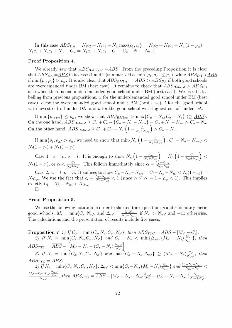
Proof Proposition 5.

We use the following notation in order to shorten the exposition: s and s′ denote genericgood schools, Ms = min{Cs, Ns}, and ∆ss′ = NsNw

Ns′−Nws′if Ns′ > Nws′ and +∞ otherwise.

The calculations and the presentation of results include five cases.

Proposition 7 1) If Cs = min{Cs, Ns, Cs′ , Ns′}, then ABSTTC = ABS − [Ms′ − Cs].2) If Ns = min{Cs, Ns, Cs′ , Ns′} and Cs − Ns < min{∆ss′ , (Ms′ − Ns)

Nw

Nws′}, then

ABSTTC = ABS −[Ms′ −Ns − (Cs −Ns)

Nws′Nw

].

3) If Ns = min{Cs, Ns, Cs′ , Ns′} and max{Cs − Ns,∆ss′} ≥ (Ms′ − Ns)Nw

Nws′, then

ABSTTC = ABS.4) If Ns = min{Cs, Ns, Cs′ , Ns′}, ∆ss′ < min{Cs−Ns, (Ms′−Ns)

Nw

Nws′} and

Cs−Ns−∆ss′Nws+Ns

<

Ms′−Ns−∆ss′Nws′Nw

Nws′, then ABSTTC = ABS − [Ms′ −Ns−∆ss′

Nws′Nw− (Cs−Ns−∆ss′)

Nws′Nws+Ns′

].

22

5) If Ns = min{Cs, Ns, Cs′ , Ns′}, ∆ss′ < min{Cs−Ns, (Ms′−Ns)Nw

Nws′} and

Cs−Ns−∆ss′Nws+Ns

≥Ms′−Ns−∆ss′

Nws′Nw

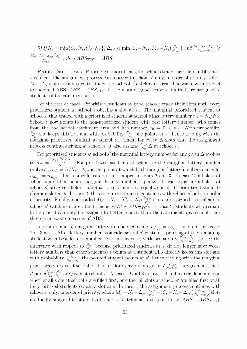
Nws′, then ABSTTC = ABS.

Proof. Case 1 is easy. Prioritized students at good schools trade their slots until schools is filled. The assignment process continues with school s′ only, in order of priority, whereMs′−Cs slots are assigned to students of school s′ catchment area. The waste with respectto maximal ABS, ABS − ABSTTC , is the mass of good school slots that are assigned tostudents of its catchment area.

For the rest of cases. Prioritized students at good schools trade their slots until everyprioritized student at school s obtains a slot at s′. The marginal prioritized student atschool s′ that traded with a prioritized student at school s has lottery number n0 = Ns/Ns′ .School s now points to the non-prioritized student with best lottery number, who comesfrom the bad school catchment area and has number n0 = 0 < n0. With probabilityNws

Nwshe keeps this slot and with probability

Nws′Nw

she points at s′, hence trading with themarginal prioritized student at school s′. Then, for every ∆ slots that the assignmentprocess continues giving at school s, it also assigns

Nws′Nw

∆ at school s′.

For prioritized students at school s′ the marginal lottery number for any given ∆ evolves

as n∆ =Ns+

Nws′Nw

∆

Ns′. For prioritized students at school w the marginal lottery number

evolves as n∆ = ∆/Nw. ∆ss′ is the point at which both marginal lottery numbers coincide,n∆ss′

= n∆ss′. This coincidence does not happen in cases 2 and 3. In case 2, all slots at

school s are filled before marginal lottery numbers equalize. In case 3, either all slots atschool s′ are given before marginal lottery numbers equalize or all its prioritized studentsobtain a slot at s. In case 2, the assignment process continues with school s′ only, in orderof priority. Finally, non-traded Ms′ −Ns− (Cs −Ns)

Nws′Nw

slots are assigned to students of

school s′ catchment area (and this is ABS − ABSTTC). In case 3, students who remainto be placed can only be assigned to better schools than the catchment area school, thusthere is no waste in terms of ABS.

In cases 4 and 5, marginal lottery numbers coincide, n∆ss′= n∆ss′

, before either cases2 or 3 arise. After lottery numbers coincide, school s′ continues pointing at the remainingstudent with best lottery number. Yet in this case, with probability

Nws+Ns′Nw+Ns′

(notice the

difference with respect to Nws

Nwbecause prioritized students at s′ do not longer have worse

lottery numbers than other students) s points at a student who directly keeps this slot andwith probability

Nws′Nw+Ns′

the pointed student points at s′, hence trading with the marginal

prioritized student at school s′. In sum, for every δ slots given, δNws′

Nw+Ns′are given at school

s′ and δNws+Ns′Nw+Ns′

are given at school s. As cases 2 and 3 do, cases 4 and 5 arise depending on

whether all slots at school s are filled first, or either all slots at school s′ are filled first or allits prioritized students obtain a slot at s. In case 4, the assignment process continues withschool s′ only, in order of priority, where Ms′−Ns−∆ss′

Nws′Nw−(Cs−Ns−∆ss′)

Nws′Nws+Ns′

slots

are finally assigned to students of school s′ catchment area (and this is ABS −ABSTTC).

23

In case 5, as in case 3, slots that remain to be placed belong to school s, that is betterthan the catchment area school for all unassigned students, thus there is no waste in termsof ABS. �

Proof Proposition 6.

We omit cases where min{ρ1, ρ2} ≤ ρw, that is, when ABSDA =ABS. Consider thecase where Cs = min{Cs, Ns, Cs′ , Ns′}. Then ABS−ABSDA = Ns(1− cs′)+ Ns′(1− cs) >Ns′(1− cs) ≥ Ns′−Cs ≥ min{Cs′ , Ns′}−Cs = ABS−ABSTTC . The first inequality arisesfrom the fact that no cutoff equals 1. The second inequality is a feasibility condition (atleast Ns′ − Cs students with priority at school s′ cannot enter at school s).

We next consider the case where Ns = min{Cs, Ns, Cs′ , Ns′}, and we assume thatABS − ABSTTC > 0. Otherwise we would be done because DA never reaches this upperbound. Since all students with priority at school s obtain a slot at s′, ABS−ABSTTC > 0implies that a positive mass of students with priority at school s′ are assigned at school s′

under TTC (thus they cannot obtain access to the more preferred school s).

Focus then on TTC. Let ns′s be the maximum lottery number among the students with

priority at school s′ that are assigned at school s. Let nwss be the maximum lottery numberamong the students with priority at school w who prefer s among all schools and areassigned at school s. Notice that ns

′s ≥ nwss . The reason is that the latter students can

only gain access to school s by directly being pointed by school s. They cannot be pointedby school s′ before s fills all slots. Simply because not all students with priority at s′ arepointed by s′ as part of a trading cycle either (before s fills all positions). On the contrary,students with priority at s′ can gain access to school s either by directly being pointed byschool s or by being part of a trading cycle.

Moreover, notice that only students of the latter and the former types are assigned toschool s. All students with priority at school s obtain a slot at s′. No student with priorityat school w who prefers s′ among all schools is assigned to s. If they are pointed by schools, they must be part of a trading cycle (this is implied by the fact that a positive mass ofstudents with priority at school s′ cannot obtain access to the more preferred school s).Therefore we have ns

′s Ns′ + nwss Nws = Cs.

But in DA where min{ρ1, ρ2} > ρw, the cutoff for school s meets cs(Ns′ + Nws) =

Cs−(1−cs′)Ns− max{0, (cs−cs′)Nws′}, implying cs <ns′s Ns′+n

wss Nws

Ns′+Nws. Given that ns

′s ≥ nwss

we obtain ns′s > cs. But then ABS −ABSDA = Ns(1− cs′)+ Ns′(1− cs) > Ns′(1− cs) >

Ns′(1− ns′s ) = ABS − ABSTTC . �

References

[1] Abdulkadiroglu A., Che Y. and Yasuda Y. (2014) “Expanding “Choice” in SchoolChoice”, forthcoming at American Economic Journal: Microeconomics.

24

[2] Abdulkadiroglu A., Che Y. and Yasuda Y. (2011) “Resolving Conflicting Preferences inSchool Choice: The ‘Boston’ Mechanism Reconsidered.” American Economic Review101, 399–410.

[3] Abdulkadiroglu A., Pathak P.A., Roth A.E. and Sonmez T. (2006), “Changing theBoston School Choice Mechanism”, unpublished manuscript.

[4] Abdulkadiroglu A. and Sonmez T. (2003) “School Choice: a Mechanism Design Ap-proach.” American Economic Review 93, 729–747.

[5] Aumann R.J. (1964) ”Markets with a Continuum of Traders”, Econometrica, 1964,39-50.

[6] Azevedo E.M. and Leshno J.D. (2011) “A Supply and DemandFramework for Two-Sided Matching Markets” mimeo Harvard:http://www.people.fas.harvard.edu/ azevedo.

[7] Black S.E. (1999). “Do Better Schools Matter? Parental Valuation of ElementaryEducation.” Quarterly Journal of Economics, 114, 577-599.

[8] Calsamiglia C. and Guell M. (2014) “What schools parents choose under the Bostonmechanism: evidence from Barcelona” CEPR discussion paper 10011.

[9] Calsamiglia C., Fu C., and Guell M. (2014) “Structural Estimation of a Modelof School Choices: the Boston Mechanism vs Its Alternatives”, mimeo UAB.http://pareto.uab.es/ caterina/research.

[10] Chen Y. and Sonmez T. (2006) “School Choice: an Experimental Study”, Journal ofEconomic Theory 127, 202-231.

[11] Chen Y. and Kesten O. (2013) “From Boston to Chinese Parallel to Deferred Accep-tance: Theory and Experiments on a Family of School Choice Mechanisms”, mimeoCMU.

[12] Cowen Institute for Public Education Initiative, Research brief, November 2011, “CaseStudies of School Choice and Open Enrollment in Four Cities”.

[13] Cullen J.B., Jacob B.A. and Levitt S. (2006) “The Effect of School Choice on Partic-ipants: Evidence from Randomized Lotteries.” Econometrica 74, 1191–1230.

[14] Ergin H. (2002) “Efficient Resource Allocation on the Basis of Priorities,” Economet-rica 70, 2489-2497

[15] Ergin H. and Erdil A. (2008), “What’s the Matter with Tie-Breaking? ImprovingEfficiency in School Choice.” American Economic Review 98, 669–689.

[16] Ergin H. and Sonmez T. (2006) “Games of School Choice under the Boston Mecha-nism.” Journal of Public Economics 90, 215-237.

25

[17] Featherstone C.R. (2014) Rank Efficiency: Investigating a Widespread Ordinal Wel-fare Criterion, unpublished manuscript.

[18] Hastings J., Kane T. and Staiger D. (2010) “Heterogeneous Preferences and the Effi-cacy of School Choice” combines and replaces National Bureau of Economic ResearchPaper Working Papers No. 12145 and No. 11805.

[19] He, Y. (2014) “Gaming the Boston School Choice Mechanism in Beijing”, mimeoToulouse.

[20] Hoxby C.M. ed. (2003) The Economics of School Choice, University of Chicago Press:Chicago.

[21] Kojima F. and Unver U. (2014) “The ‘Boston’ School Choice Mechanism”, forthcom-ing at Economic Theory.

[22] Lavy V. (2010) “Effects of Free Choice Among Public Schools.” The Review of Eco-nomic Studies 77, 1164–1191.

[23] Miralles A. (2008) School choice: The Case for the Boston Mechanism, unpublishedmanuscript.

[24] Pathak P.A. and Sonmez T. (2008) “Leveling the Playing Field: Sincere and StrategicPlayers in the Boston Mechanism.” American Economic Review 98, 1636-1652.

[25] Pathak P.A. and Sonmez T. (2013) “School Admissions Reform in Chicago and Eng-land: Comparing Mechanisms by their Vulnerability to Manipulation.” American Eco-nomic Review forthcoming.

[26] Roth A. (2008) “What have we learned from Market Design?” Economic Journal, 118,285-310.

26