
Alessandro Tolomiotte Rivello Essays on Decision Theory
46
Instrução Normativa nº 01/19, de 09/07/19 - Pró-Reitoria FGV Em caso de participação de Membro(s) da Banca Examinadora de forma não-presencial*, o Presidente da Comissão Examinadora assinará o documento como representante legal, delegado por esta I.N. *Skype, Videoconferência, Apps de vídeo etc Alessandro Tolomiotte Rivello Essays on Decision Theory Tese apresentado(a) ao Curso de Doutorado em Economia do(a) EPGE Escola Brasileira de Economia e Finanças - FGV EPGE para obtenção do grau de Doutor(a) em Economia. Data da defesa: 18/12/2020 ASSINATURA DOS MEMBROS DA BANCA EXAMINADORA Presidente da Comissão Examinadora: Profº/ª Leandro Gorno Lucas Jóver Maestri Antonio de Araujo Freitas Junior Coordenador Pró-Reitor de Ensino, Pesquisa e Pós-Graduação FGV Leandro Gorno Paulo Klinger Monteiro Kazuhiro Hara Jose Heleno Faro Gil Riella
-
Upload
khangminh22 -
Category
Documents
-
view
4 -
download
0
Transcript of Alessandro Tolomiotte Rivello Essays on Decision Theory

Instrução Normativa nº 01/19, de 09/07/19 - Pró-Reitoria FGV Em caso de participação de Membro(s) da Banca Examinadora de forma não-presencial*, o Presidente da Comissão Examinadora assinará o documento como representante legal, delegado por esta I.N. *Skype, Videoconferência, Apps de vídeo etc
Alessandro Tolomiotte Rivello
Essays on Decision Theory
Tese apresentado(a) ao Curso de Doutorado em Economia do(a) EPGE Escola Brasileira de Economia e
Finanças - FGV EPGE para obtenção do grau de Doutor(a) em Economia.
Data da defesa: 18/12/2020
ASSINATURA DOS MEMBROS DA BANCA EXAMINADORA
Presidente da Comissão Examinadora: Profº/ª Leandro Gorno
Lucas Jóver Maestri Antonio de Araujo Freitas Junior Coordenador Pró-Reitor de Ensino, Pesquisa e Pós-Graduação FGV
Leandro Gorno
Paulo Klinger Monteiro
Kazuhiro Hara
Jose Heleno Faro
Gil Riella

Dados Internacionais de Catalogação na Publicação (CIP) Ficha catalográfica elaborada pelo Sistema de Bibliotecas/FGV
Rivello, Alessandro Tolomiotte Essays on Decision Theory / Alessandro Tolomiotte Rivello. – 2020.
44 f.
Tese (doutorado) - Fundação Getulio Vargas, Escola Brasileira de
Economia e Finanças. Orientador: Leandro Gorno Inclui bibliografia. 1. Teoria axiomática dos conjuntos. 2. Equações diferenciais estocásticas. 3.
Economia - Modelos matemáticos. 4. Principios de maximo (Matematica). I. Gorno, Leandro. II. Fundação Getulio Vargas. Escola Brasileira de Economia e Finanças. III. Título.
CDD – 511.3
Elaborada por Rafaela Ramos de Moraes – CRB-7/6625

FUNDACAO GETULIO VARGASESCOLA de POS-GRADUACAO em ECONOMIA
Essays on Decision Theory
Alessandro Tolomiotte Rivello
Advisor: Leandro Gorno
Rio de Janeiro2020

Acknowledgements
I would like to start by thanking my parents Rafael Rivello and Miriam Rivello fortheir continuous support and effort to give me access to the best education possible.All those little steps in my academic life were essential for the completion of thisthesis.
I will always be indebted to my advisor Leandro Gorno. Our almost weekly 3-4hours meetings provided me with the insights necessary to keep advancing. In manyoccasions I thought that I would not be able to finish this thesis and those meetingswere my life boat. I should also thank you for the support on personal matters,especially in the year of 2020 marked by the Covid-19 pandemics.
I extend my appreciation to all members of the Microeconomics Theory workshopfor insightful discussions, and the Coordenacao de Aperfeicoamento de Pessoal deNıvel Superior (CAPES) for the financial support.
Last but not least, I would like to mention my partner Raianny Rodrigues andmy friends Diogo Dias, and Davi Gimenes. Most of the time that I was not thinkingabout this thesis I was with one of you. These moments of relief were indispensableto give me the strength to complete this work.
1

Abstract
Even though completeness is a standard axiom for economic preferences, it is alsoa very strong assumption. According to von Neumann and Morgenstern (1953) (p.631) “It is very dubious, whether the idealization of reality which treats this postulateas a valid one, is appropriate or even convenient.” in the same vein Aumann (1962)said “Of all the axioms of utility theory, the completeness axiom is perhaps themost questionable”. This thesis aims to advance the study of incomplete preferencesthrough three chapters.
Chapter 1 extends the notion of stochastic dominance to dynamic environments.Its main result is a clean characterization of the dominance orders between stochasticpayoff processes given by unanimity within groups of discounted expected utility max-imizers. A measure that quantifies the intensity of the dominance of a payoff processover another is defined and used to derive robust bounds on asset price differentials.
Chapter 2 extends Berge’s Maximum Theorem to allow for incomplete prefer-ences. A simple version of the Maximum Theorem is provided for convex feasible setsand a fixed preference. Then, it shows that if, in addition to the traditional continu-ity assumptions, a new continuity property for the domains of comparability holds,the limits of maximal elements along a sequence of decision problems are maximalelements in the limit problem. While this new continuity property for the domainsof comparability is sufficient, it is not generally necessary. However, conditions aregiven under which it is necessary and sufficient for maximality and minimality to bepreserved by limits.
Chapter 3 defines and studies the class of “connected preferences”, that is, pref-erences that may fail to be complete but have connected maximal domains of compa-rability. It offers four new results. Theorem 3.1 identifies a basic necessary conditionfor a continuous preference to be connected in the sense above, while Theorem 3.2provides sufficient conditions. Building on the latter, Theorem 3.3 characterizes themaximal domains of comparability. Finally, Theorem 3.4 presents conditions that en-sure that maximal domains are arc-connected. Building on these results it is proven,for the case of compact spaces, a tight relationship between connectedness of thespace and axioms on a preference defined on that space, in the spirit of the celebratedtheorem of Schmeidler (1971).
2
Contents
Acknowledgements 1Abstract 2
List of Figures 5
Chapter 1. Dynamic Stochastic Dominance 71.1. Introduction 71.2. Related literature 81.3. Dynamic Stochastic Dominance 91.4. Robust premium 131.5. Discussion 17
Chapter 2. Maximum Theorem for Incomplete Preferences 192.1. Introduction 192.2. Preliminaries 202.3. A Simple Maximum Theorem 212.4. A General Maximum Theorem 232.5. A Characterization 242.6. Related literature 272.7. Discussion 28
Chapter 3. Connected Incomplete Preferences 293.1. Introduction 293.2. Preliminaries 303.3. Connected preferences 303.4. Characterization of maximal domains 323.5. Arc-connected preferences 343.6. Applications 34
Appendix A. Technical lemmas 37
Bibliography 41
3


List of Figures
1.1 Example 1.2: FODSD between X and Y 13
1.2 Example 1.3: representation of GX and GY 15
1.3 Example 1.4: representation of GX and GY 16
5


CHAPTER 1
Dynamic Stochastic Dominance
1.1. Introduction
First order stochastic dominance provides a robust decision rule for static eco-
nomic models with uncertainty. If money lottery F first order stochastically domi-
nates money lottery G, then any decision maker who maximizes expected utility and
prefers more money to less would choose F over G. As a result, if several individuals
with monotone preferences decide via consensus between lotteries F and G, we can
expect them to choose F .
While the notion of first order stochastic dominance is essentially static, intertem-
poral trade-offs play a major role in economics. The main goal of this chapter is to
bridge this gap by studying a class of orders between stochastic payoff processes
which are naturally associated with robust decision rules for standard dynamic envi-
ronments.
In most economic models, agents facing uncertainty make dynamic decisions by
maximizing an objective function of the form V (X|u, r) = E{r∫ +∞0
e−rtu(Xt)dt}
,
where X is a stochastic process which represents the payoff flow and r > 0 is a
constant discount rate. Such agents will choose X over Y whenever V (X|u, r) is
larger than V (Y |u, r). However, it is clear that specific hypothesis about u will affect
choice behavior.
In order to identify comparisons which are robust to perturbations on vNM util-
ity indexes, we define a class of a dynamic stochastic orders which essentially say
that X dominates Y whenever V (X|u, r) exceeds V (Y |u, r) for every vNM index
u satisfying certain conditions. Our main results reduce the analysis of dynamic
stochastic dominance to static stochastic dominance of the relevant type, using an
“average” probability distribution which combines the statistical properties of the
payoffs processes and the intertemporal weighting (i.e., discounting) encoded in the
agent’s preferences. More specifically, Theorem 1.1 provides a clean characterization
of the first order dynamic stochastic dominance order associated with nondecreasing
7

8 1. DYNAMIC STOCHASTIC DOMINANCE
vNM utility indexes, while Theorem 1.2 offers the same kind of characterization under
the additional assumption of concavity.
Since the dynamic stochastic dominance orders we study naturally imply robust
decision rules within groups of individuals, we can elicit how much we need to add to
a payoff process X in order to dominate Y . The formalization of this idea leads to a
family of “robust premia” that measure the intensity of dominance. These notions are
useful because they provide a way to connect theoretical assumptions on preferences
with observable data. Proposition 1.1 demonstrates this by using robust premia to
obtain bounds on asset price differentials.
1.2. Related literature
The use of stochastic dominance as a decision rule to rank uncertain prospects in
finance and economics originated in the 70’s with Hadar and Russell (1971), Whitmore
(1970) and Rothschild and Stiglitz (1970). Many developments have been made since
then (see Levy (1992) and Levy and Kroll (1980) for an extensive review).
There exists some work that attempts to extend the notion of stochastic domi-
nance to dynamic frameworks. Magnac and Robin (1999) define an alternative notion
of dynamic stochastic dominance that also involves a general set of vNM utility in-
dexes, but requires the existence of a transformation inducing static stochastic dom-
inance for all t. Our definition seems more natural because it evaluates stochastic
payoff flows using the most common model of preferences under uncertainty and does
not require the existence of an abstract transformation. Arcand et al. (2020) propose
a simple dynamic extension of the integral conditions that characterize static second
order stochastic dominance. Their approach is limited, though, in that they only
deal with second order stochastic dominance for Ito diffusions with constant volatil-
ity coefficient. In contrast, our approach is more general since it can accommodate
dynamic stochastic dominance relations of any order and stochastic payoff processes
of any kind.
This chapter is also related to the literature on model robustness regarding the
specification of utility functions. Dubra et al. (2004a) axiomatization yields a prefer-
ence that have a multi-utility representation, therefore in their framework a choice of
one alternative over another is also represented by unanimity of that decision among
a group of agents. Ok et al. (2012) axiomatize a preference that is robust to mis-
specification in distribution or in the utility function, whereas Galaabaatar and Karni
(2012) allow for robustness in both dimensions at the same time. However, the main

1.3. DYNAMIC STOCHASTIC DOMINANCE 9
goal in this strand of literature is to axiomatize preferences and establish represen-
tation results. Instead, the present chapter starts from a discounted expected utility
representation and uses it to define dynamic stochastic orders associated with robust
decision rules.
1.3. Dynamic Stochastic Dominance
For a stochastic process X ≡ {Xt}t≥0 we define
V (X|u,D) := E{∫ +∞
0
u(Xt)dD(t)
},
where u : R → R is a vNM utility index and D : [0,+∞) → R+ is a general
intertemporal aggregator (i.e., the CDF associated to a probability measure weighting
the different dates). We say that V (X|u,D) is well defined when V (X|u+, D) < +∞or V (X|u−, D) < +∞, where u+ and u− are the positive and negative parts of u,
respectively.
Example 1.1. Let D(t) := 1− e−rt for some fixed 0 < r < 1. Then we have the
standard expected discounted utility model with exponential discounting. That is,
V (X|u,D) := E{r
∫ +∞
0
e−rtu(Xt)dt
}.
Moreover, if u is bounded V (X|u,D) is well defined.
Our first result shows that the expected discounted utility is equal to the expected
utility taken with respect to a special CDF.
Lemma 1.1. Let FX(·|t) be the CDF of Xt. The discounted distribution of X is
represented by the CDF
GX(x|D) :=
∫ +∞
0
FX(x|t)dD(t).
Then
V (X|u,D) =
∫ +∞
−∞u(x)dGX(x|D)
for all measurable u such that V (X|u,D) is well defined.
Proof. Let ν be the measure induced by GX(·|D) and, for each t, µt be the
measure induced by FX(·|t). We start establishing a result for simple functions. Let
n ∈ N and {Ai}ni=1 be a collection of measurable sets. Define I(x) :=∑n
i=1 ai1Ai(x),

10 1. DYNAMIC STOCHASTIC DOMINANCE
then
EνI =n∑i=1
aiν(Ai) =n∑i=1
ai
∫ +∞
0
µt(Ai)dD(t)
=
∫ +∞
0
n∑i=1
aiµt(Ai)dD(t)
=
∫ +∞
0
(EµtI) dD(t).
Now let u be a measurable nonnegative function and In an increasing sequence of
nonnegative simple functions such that limn→∞ In(x) = u(x) for every x. Thus, by
definition and the previous result
Eνu = limn→∞
EνIn = limn→∞
∫ +∞
0
(EµtIn) dD(t).
Using the monotone convergence theorem we can pass the limit inside the inte-
gral to obtain Eνu =∫ +∞0
(Eµtu) dD(t). Finally, for any measurable u such that
V (X|u+, D) < +∞ or V (X|u−, D) < +∞
V (X|u,D) = E{∫ +∞
0
u+(Xt)dD(t)
}− E
{∫ +∞
0
u−(Xt)dD(t)
}=
∫ +∞
0
Eu+(Xt)dD(t)−∫ +∞
0
Eu−(Xt)dD(t)
= Eνu+ − Eνu− = Eνu,
where the second equality is an application of Tonelli’s theorem, the third equality
was proved in the previous step, and the last equality follows from the definition of
the Lebesgue integral. �
Using this result we define an order on the space of stochastic processes.
Definition 1.1. Let X and Y be two stochastic processes and U be a subset
of functions u : R → R. We say that X U-dynamically stochastically dominates Y
(X ≥U Y ) whenever
V (X|u,D) ≥ V (Y |u,D)
holds for every u ∈ U such that V (X|u,D) and V (X|u,D) are well defined.
Because V (X|u,D) and V (Y |u,D) need to be well defined, it is possible that only
a proper subset of vNM utility indexes in U is used to check V (X|u,D) ≥ V (Y |u,D).
More significantly, this subset may depend on the pair of stochastic processes that

1.3. DYNAMIC STOCHASTIC DOMINANCE 11
one wants to compare. This is an unfortunate feature of our definition, but one that
is unrelated to dynamics (it is already present in the general versions of static first
and second order stochastic dominance). Moreover, as we shall see, a single subset of
U suffices to characterize the associated order in some contexts.
In the following subsections we discuss important instances of the general order,
specified through restrictions on the set U .
1.3.1. Dynamic first order stochastic dominance. Define
U1 := {u : R→ R|u is nondecreasing} .
Whenever X ≥U1 Y , we say that X first order dynamically stochastically dominates
(FODSD) Y . The next theorem is the main result of this subsection.
Theorem 1.1. The following are equivalent:
(1) X first order dynamically stochastically dominates Y .
(2) GX(·|D) first order stochastically dominates GY (·|D).
Proof. Note that GX(·|D) first order stochastically dominates GY (·|D) if and
only if∫ +∞−∞ u(x)dGX(x|D) ≥
∫ +∞−∞ u(x)dGY (x|D), for all nondecreasing u such that
both integrals are well defined, then Lemma 1.1 yields the conclusion. �
Remark 1.1. If process X is nonnegative we have V (X|u−, D) < +∞ for all
u ∈ U1. Hence, for nonnegative stochastic processes the comparison between any pair
of payoff processes relies on the same set of vNM utility indexes.
Theorem 1.1 establishes that first order dynamic stochastic dominance is equiva-
lent to first order stochastic dominance between discounted CDFs. Theorem 1.1 also
implies that having first order stochastic dominance between Xt and Yt, for every t, is
a sufficient condition for first order dynamic stochastic dominance. The next exam-
ple illustrates how Theorem 1.1 can be used to check first order dynamic stochastic
dominance while showing that having first order stochastic dominance between Xt
and Yt, for every t, is not a necessary condition for first order dynamic stochastic
dominance.
Example 1.2. Let X be a stochastic process such that X0 = 1 and
Xt =
1, with probability e−t
0, with probability 1− e−t

12 1. DYNAMIC STOCHASTIC DOMINANCE
for t > 0. Let Y be a a stochastic process such that Y0 = 1 and
Yt =
1, with probability e−T
0, with probability 1− e−T
for t > 0 and some fixed T > 0. Let D(t) = 1− e−rt for some fixed 0 < r < 1. Note
that
FX(x|t) =
1 , if x ≥ 1
1− e−t , if 0 ≤ x < 1
0 , if x < 0
and
FY (x|t) =
1 , if x ≥ 1
1− e−T , if 0 ≤ x < 1
0 , if x < 0.
Then FX(·|t) dominates FY (·|t) in first order stochastic sense for every t ≤ T and
vice versa for t > T . Evaluating the discounted distribution of each process we obtain
GX(x|D) =
1 , if x ≥ 1
1− rr+1
, if 0 ≤ x < 1
0 , if x < 0
and
GY (x|D) =
1 , if x ≥ 1
1− e−T , if 0 ≤ x < 1
0 , if x < 0.
Define GX(r) := 1− rr+1
and GY (T ) := 1−e−T . Figure 1.1 shows in red the region
where the combination of parameters r and T makes X FODSD Y and in blue the
region where Y FODSD X.
Hence, we can see that there are parameters T and r such that the worse initial
distributions of payoffs Y are compensated by the worsen in distribution that happens
with payoff X, in a way that every monotonic decision maker would prefer Y over X.
1.3.2. Dynamic second order stochastic dominance. Define
U2 := {u : R→ R|u is nondecreasing and concave} .

1.4. ROBUST PREMIUM 13
Figure 1.1. Example 1.2: FODSD between X and Y
Whenever X ≥U2 Y , we say that X second order dynamically stochastically dominates
(SODSD) Y . We can establish a result that parallels Theorem 1.1.
Theorem 1.2. The following are equivalent:
(1) X second order dynamically stochastically dominates Y .
(2) GX(·|D) second order stochastically dominates GY (·|D).
Proof. We know that GX(·|D) second order stochastically dominates GY (·|D)
if and only if∫ +∞−∞ u(x)dGX(x|D) ≥
∫ +∞−∞ u(x)dGY (x|D), for all nondecreasing and
concave u such that both integrals are well defined, then we only need to apply Lemma
1.1. �
1.4. Robust premium
In this section, we use first order dynamic stochastic dominance to construct a
measure that quantifies relative dominance between stochastic payoff processes.
Definition 1.2. Let X and Y be two stochastic processes. We define the robust
premium as
RP (X, Y ) := inf {ε > 0| (Y + ε) FODSD X} .

14 1. DYNAMIC STOCHASTIC DOMINANCE
Intuitively, the robust premium is the minimum annuity that one needs to add
to the payoff flow Y , such that the resulted shifted process FODSD X. Because of
Theorem 1.1, the robust premium is the minimum shift to the right on GY that makes
it first order stochastically dominates GX .
Remark 1.2. Let Y and Z be two stochastic payoff processes. If Y FODSD
Z, then RP (Y,X) ≥ RP (Z,X), for any process X. This is so because Theorem 1.1
implies that first order dynamic stochastic dominance is a transitive order. Moreover,
X + RP (Y,X) FODSD Y by the definition of robust premium. These two facts
together imply that X +RP (Y,X) FODSD Z.
We could have defined the robust premium in terms of the general U -dynamic
dominance, but much of its interpretation would be lost, since without restricting
ourselves to nondecreasing u adding a positive annuity to a payoff flow could harm
the decision maker.
Another possibility would be to use second order dynamic stochastic dominance
instead of first order dynamic stochastic dominance. Since its interpretation and the
relation with second order dynamic stochastic dominance are completely analogous
to the case of first order dynamic stochastic dominance, we omit the details.
The next example shows how Theorem 1.1 makes simple the assessment of the
robust premium.
Example 1.3. Keep X, Y and D as defined in Example 1.2. We can choose r
and T such that GY (T ) > GX(r). We plot these two CDFs together in Figure 1.2.
Since the discounted CDF of Y + ε is just the discounted CDF of Y shifted to the
right by ε, RP (X, Y ) will be the minimum shift to the right that makes the shifted
CDF stays below GX for every point. Hence, RP (X, Y ) = 1.
On the other hand, GX already dominates GY in first order stochastic sense, then
no shift to the right is necessary implying RP (Y,X) = 0.
Another interesting aspect of the robust premium is that it allows for compar-
ison between stochastic processes that could not be ordered in first order dynamic
stochastic sense before.

1.4. ROBUST PREMIUM 15
Figure 1.2. Example 1.3: representation of GX and GY
Example 1.4. Let’s keep process X and D as in Example 1.2, but change Y to
be Y0 = 1 and
Yt =
1.3, with probability e−T
0.3, with probability 1− e−T
for t > 0 and some fixed T > 0. Of course GX is the same as before, but
GY (x|D) =
1 , if x ≥ 1.3
1− e−T , if 0.3 ≤ x < 1.3
0 , if x < 0.3.
Note that this new GY is the former one shifted to the right by 0.3. Figure 1.3
shows the graph of GX and GY when we choose r and T such that GY > GX . Using
again Theorem 1.1 it is easy to see that RP (X, Y ) = 0.7 and RP (Y,X) = 0.3. Note
that RP (X, Y ) is less than in Example 1.3, because GY here dominates in first order
stochastic sense the GY from Example 1.3. By the same reasoning RP (Y,X) is larger
now.
The next result shows that the robust premium can be used to bound the difference
between asset prices.

16 1. DYNAMIC STOCHASTIC DOMINANCE
Figure 1.3. Example 1.4: representation of GX and GY
Proposition 1.1. Consider a Lucas economy in continuous time, with complete
markets, risk free rate r > 0, unlimited short sales, infinitely many agents, and posi-
tive endowments for everyone. Each individual i preference can be represented by
Vi(S) := E{r
∫ +∞
0
e−rtui(Sit)dt
},
where Sit is his consumption for each t and ui is nondecreasing for all i. Let X =
{Xt}t>0 and Y = {Yt}t>0 be two assets with prices PX ={PXt
}t>0
and P Y ={P Yt
}t>0
respectively. Then,
P Y0 −
RP (Y,X)
r≤ PX
0 ≤ P Y0 +
RP (X, Y )
r.
Proof. Note that if RP (Y,X) = +∞ or RP (X, Y ) = +∞ the corresponding
inequalities hold trivially. Thus, assume that both premia are finite. Given our setup,
arbitrage cannot exist in equilibrium. First we will prove that PX0 ≤ P Y
0 + RP (X,Y )r
.
Suppose, seeking a contradiction, that PX0 − P Y
0 > RP (X,Y )r
, then agent i∗, at t = 0,
could sell short one unit of asset X and buy one unit of asset Y . The same agent can
propose to any other agent, say i, to pay Yt+RP (S, Y ) to i, for all t > 0, in exchange
for receiving St each period from i. Since Vi(Y + RP (S, Y )) ≥ Vi(S), for all i, any
agent in this economy would accept this deal. In the end, the net position of agent
i∗ is an annuity of RP (S, Y ) that he has to pay, which has present value of RP (S,Y )r
.
Hence, in t = 0, he gains P S0 − P Y
0 −RP (S,Y )
r> 0, a contradiction with no arbitrage.

1.5. DISCUSSION 17
To prove P Y0 −
RP (Y,S)r≤ P S
0 , one could reverse the strategy already described, also
yielding a contradiction. �
It is important to note that the robust premium can be +∞, because first or-
der dynamic stochastic dominance is equivalent to the static first order stochastic
dominance and there are distributions that are incomparable in first order stochastic
dominance sense, no matter how much we shift to the right one of the CDFs. Normal
distributions with different volatilities are a good example. In this case, Proposition
1.1 imposes no bounds on the difference of asset prices.
If we have used second order dynamic stochastic dominance in the definition of
Robust Premium there would be less cases of it being +∞, since first order stochastic
dominance implies second order stochastic dominance, but the converse does not hold.
Moreover, because of this relation between stochastic dominance orders, a Robust
Premium based on second order dynamic stochastic dominance would be lower than
a Robust Premium based on first order stochastic dominance. Hence, using second
order dynamic stochastic dominance to define the Robust Premium would imply
tighter bounds on price differentials.
1.5. Discussion
In this chapter we define general orders on the space of stochastic processes that
naturally represent a decision rule among payoff processes and we offer a full charac-
terization to two of these orders, namely first (and second) order dynamic stochastic
dominance, which are natural extensions of first (and second) order stochastic domi-
nance. We also define a measure of the relative dominance between stochastic payoff
processes and Proposition 1.1 shows that this measure disciplines the relation of the-
oretical preference assumptions and observable data on asset prices.
As we have established, our dynamic stochastic orders imply decision rules that
are robust to specific assumptions about vNM utility indexes. One extension is to
define orders that not only relate to utility function robustness, but also relate to
discounting function robustness. More concretely,
Definition 1.1′. Let X and Y be two stochastic processes. Let U and B be,
respectively, a subset of functions u : R→ R and a subset of CDFs D : [0,+∞)→ R+.
We say that X U-dynamically stochastically dominates Y (X ≥U Y ) whenever
V (X|u,D) ≥ V (Y |u,D)

18 1. DYNAMIC STOCHASTIC DOMINANCE
holds for every u ∈ U and every D ∈ B such that V (X|u,D) and V (Y |u,D) are well
defined.
Then the content of Theorem 1.1 could be rewritten as
Theorem 1.1′. The following are equivalent:
(1) X first order dynamically stochastically dominates Y .
(2) GX(·|D) first order stochastically dominates GY (·|D), for all D ∈ B.
With the same sort of adaptation to Theorem 1.2. A natural route for further re-
search is to investigate what are the implications of first and second orders dynamic
stochastic dominance to optimal stopping problems and control problems in a dy-
namic framework. Related to that, still is an open question if our dynamic stochastic
orders allow comparative statics of optimal stopping times in the spirit of Quah and
Strulovici (2013).

CHAPTER 2
Maximum Theorem for Incomplete Preferences
2.1. Introduction
An important issue arising in the study of models involving optimization is whether
optimal choices depend continuously on parameters affecting the objective function
and the constraints. The main tool to address this question is the Maximum Theorem
by Berge (1963), which can be stated as follows:
Maximum Theorem. Let X and Θ be topological spaces; let u : X × Θ →R be a continuous function; let K : Θ ⇒ X be a continuous and compact-valued
correspondence. Then, the correspondence M : Θ ⇒ X defined by setting M(θ) :=
arg maxx∈K(θ) u(x, θ) for each θ ∈ Θ is upper hemicontinuous and compact-valued.
This result can be easily modified to dispense with utility functions and deal di-
rectly with complete (continuous) preferences and also with incomplete preferences
with open asymmetric parts (see Walker (1979)). However, to the best of our knowl-
edge, none of the existing generalizations of the Maximum Theorem applies to some of
the most standard types of incomplete preferences such as Pareto orderings based on
continuous utility functions, preferences over lotteries admitting an expected multi-
utility representation as in Dubra, Maccheroni, and Ok (2004b), or ordinal preferences
possessing a continuous multi-utility representation studied by Evren and Ok (2011).
The following example shows that obtaining a maximum theorem that covers these
types of preferences requires additional conditions:
Example 2.1. Consider a consumer choosing bundles of two goods: apples (A)
and bananas (B). Her preferences are fixed, but incomplete. They can be represented
with two utilities: u1(qA, qB) = qA + qB and u2(qA, qB) = qA + 2qB, in the sense that
a bundle (qA, qB) is considered at least as good as another bundle (q′A, q′B) if and only
if u1(qA, qB) ≥ u1(q′A, q
′B) and u2(qA, qB) ≥ u2(q
′A, q
′B). The price of apples, pA, is
normalized to 1 and there is sequence of prices for bananas pB,n = 1 + 1/n. Note
that, if the consumer’s wealth is w = 1, bundle (1, 0) is optimal for every n ∈ N: there
is no feasible bundle that the consumer strictly prefers to (1, 0). However, in the limit
19

20 2. MAXIMUM THEOREM FOR INCOMPLETE PREFERENCES
n→ +∞, the bundle (1, 0) is no longer optimal because the consumer strictly prefers
the bundle (0, 1), which is feasible when the prices are (pA, pB,+∞) = (1, 1).
The example above is fairly simple and suggests that, when weak preferences are
continuous but incomplete, we should not be surprised to find sequences of maximal
elements that converge to suboptimal alternatives. With this observation in mind, the
main contributions of the present chapter are: 1) to provide conditions which ensure
that limits of optimal choices are optimal in the limit problem, and 2) to shed light
on how the nature of preference incompleteness may interfere with the preservation
of optimality when taking limits.
The rest of the paper is organized as follows. We present basic definitions in Sec-
tion 2.2. We state and prove a simple Maximum Theorem for incomplete preferences
in Section 2.3. This result is somewhat restrictive since it requires a fixed prefer-
ence and convex feasible sets. In Section 2.4, we establish a more general Maximum
Theorem based on a new continuity condition for the domains of comparability of
the preferences involved. In Section 2.5, we investigate assumptions under which this
new condition is not only sufficient but also essentially necessary. Finally, Section 2.6
briefly relates our results to the existing literature and Section 2.7 offers some con-
cluding remarks. We relegated all auxiliary lemmas and their proofs to Appendix A.
2.2. Preliminaries
Let (X, d) be a metric space. In this thesis, a preference, generically denoted by
%, is a reflexive and transitive binary relation on X. As usual, ∼ and � denote the
symmetric and asymmetric parts of %, respectively. For every x ∈ A ⊆ X, the set
{y ∈ A|y ∼ x} is the indifference class of % in A.
We say that % is complete on a set A ⊆ X if either x % y or y % x holds for all
x, y ∈ A. The set A is a %-domain if % is complete on A. If A ⊆ B ⊆ X and A is a
%-domain such that there exists no %-domain contained in B and strictly containing
A, then A is a maximal %-domain relative to B. Denote by D (%, B) the collection
of all maximal %-domains relative to B.
A point x ∈ A is %-maximal in A if, for every y ∈ A, y % x implies x % y. The
set of all %-maximal elements in A is denoted by Max(%, A). Analogously, a point
x ∈ A is %-minimal in A if, for every y ∈ A, x % y implies y % x. The set of all
%-minimal elements in A is denoted by Min(%, A).
A preference % is continuous if it is a closed subset of X×X. Let P be the collec-
tion of continuous preferences on X. A set U ⊆ RX is a multi-utility representation

2.3. A SIMPLE MAXIMUM THEOREM 21
for % whenever, for every x, y ∈ X, x % y holds if and only if u(x) ≥ u(y) for all
u ∈ U .
Let KX be the collection of nonempty compact subsets of X. Consider both KXand P equipped with the Hausdorff metric topology derived from X and X × X,
respectively. Finally, for any sequence {An}n∈N of nonempty subsets of KX , denote
by LSn→+∞An the collection of accumulation points of all sequences {An}n∈N, where
An ∈ An for each n ∈ N.
2.3. A Simple Maximum Theorem
In this section, we introduce a new continuity condition that is compatible with
interesting classes of incomplete preferences and allows us to prove a simple Maximum
Theorem. Throughout this section, we will assume that X is convex.
Definition 2.1. A preference % is midpoint continuous if, for every x, y ∈X satisfying y � x, there exists α ∈ [0, 1) and open sets V,W ⊆ X such that
(αx+ (1− α)y, x) ∈ V ×W and z′ � x′ for all (z′, x′) ∈ V ×W .
Every complete and continuous preference satisfies midpoint continuity.1 The
following result establishes that a significant class of incomplete preferences also does:
Proposition 2.1. If % admits a finite multi-utility representation U ⊆ RX with
each u ∈ U continuous and strictly quasiconcave, then % satisfies midpoint continuity.
Proof. Take x, y ∈ X such that x � y. By definition of multi-utility repre-
sentation, we have u(x) ≥ u(y) for all u ∈ U . Define z := (1/2)x + (1/2)y. Since
each u ∈ U is strictly quasi-concave, u(z) > u(y) holds for all u ∈ U . For each
u ∈ U , there are open sets Vu,Wu such that (z, y) ∈ Vu×Wu and u(z′) > u(y′) for all
(z′, y′) ∈ Vu×Wu. Define V :=⋂u∈U Vu and W :=
⋂u∈UWu. Clearly (z, y) ∈ V ×W ,
so V and W are nonempty. Moreover, since U is finite, V and W are open. By
construction, we have u(z′) > u(y′) for all z′ ∈ V , y′ ∈ W , and u ∈ U . Since U is a
multi-utility representation, (z′, y′) ∈ V ×W implies z′ � y′, showing that % satisfies
midpoint continuity. �
Using the concept of midpoint continuity, we can establish the first major result
of this chapter, a simple Maximum Theorem:
1If a preference is complete and continuous, its asymmetric part is open in X ×X. As a result, wecan always take α = 0 to satisfy the de�nition of midpoint continuity.
22 2. MAXIMUM THEOREM FOR INCOMPLETE PREFERENCES
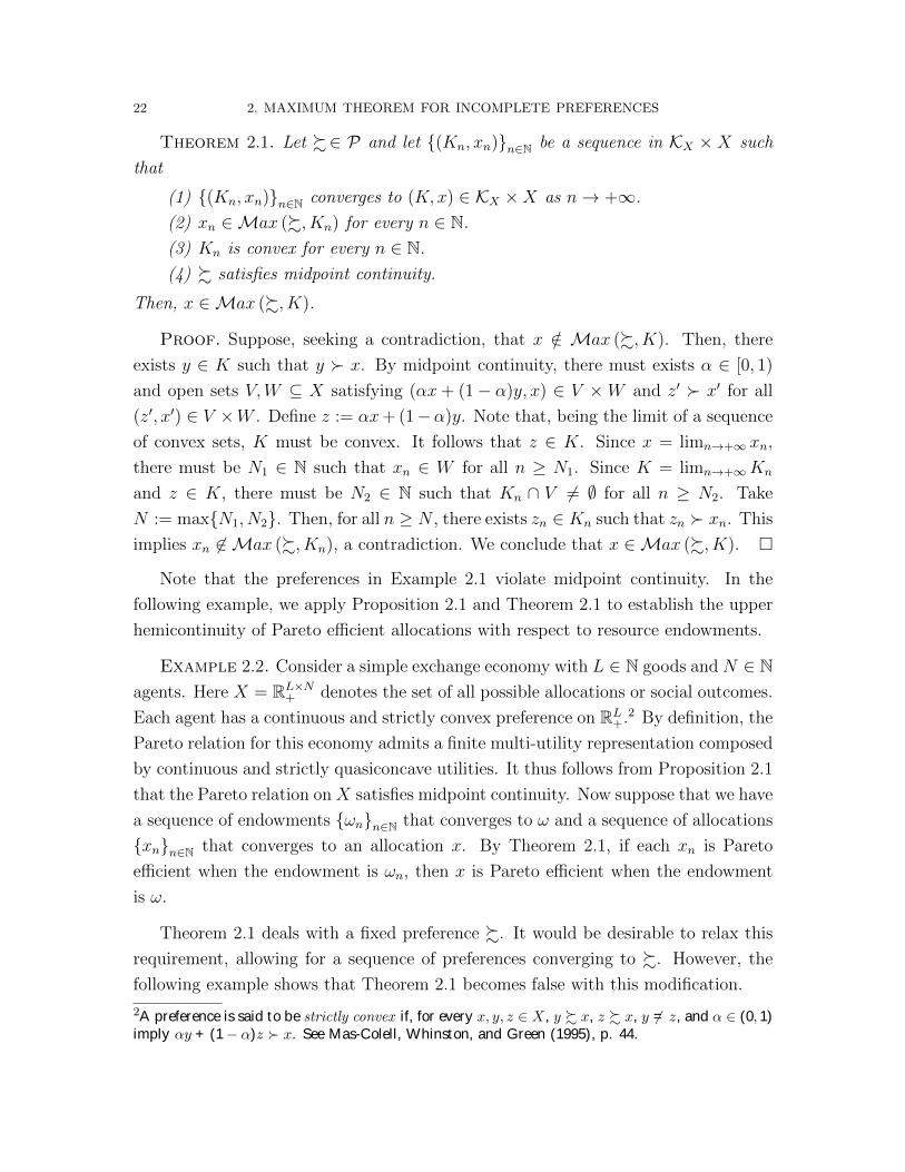
Theorem 2.1. Let %∈ P and let {(Kn, xn)}n∈N be a sequence in KX × X such
that
(1) {(Kn, xn)}n∈N converges to (K, x) ∈ KX ×X as n→ +∞.
(2) xn ∈Max (%, Kn) for every n ∈ N.
(3) Kn is convex for every n ∈ N.
(4) % satisfies midpoint continuity.
Then, x ∈Max (%, K).
Proof. Suppose, seeking a contradiction, that x /∈ Max (%, K). Then, there
exists y ∈ K such that y � x. By midpoint continuity, there must exists α ∈ [0, 1)
and open sets V,W ⊆ X satisfying (αx+ (1− α)y, x) ∈ V ×W and z′ � x′ for all
(z′, x′) ∈ V ×W . Define z := αx+ (1−α)y. Note that, being the limit of a sequence
of convex sets, K must be convex. It follows that z ∈ K. Since x = limn→+∞ xn,
there must be N1 ∈ N such that xn ∈ W for all n ≥ N1. Since K = limn→+∞Kn
and z ∈ K, there must be N2 ∈ N such that Kn ∩ V 6= ∅ for all n ≥ N2. Take
N := max{N1, N2}. Then, for all n ≥ N , there exists zn ∈ Kn such that zn � xn. This
implies xn 6∈ Max (%, Kn), a contradiction. We conclude that x ∈Max (%, K). �
Note that the preferences in Example 2.1 violate midpoint continuity. In the
following example, we apply Proposition 2.1 and Theorem 2.1 to establish the upper
hemicontinuity of Pareto efficient allocations with respect to resource endowments.
Example 2.2. Consider a simple exchange economy with L ∈ N goods and N ∈ Nagents. Here X = RL×N
+ denotes the set of all possible allocations or social outcomes.
Each agent has a continuous and strictly convex preference on RL+.2 By definition, the
Pareto relation for this economy admits a finite multi-utility representation composed
by continuous and strictly quasiconcave utilities. It thus follows from Proposition 2.1
that the Pareto relation on X satisfies midpoint continuity. Now suppose that we have
a sequence of endowments {ωn}n∈N that converges to ω and a sequence of allocations
{xn}n∈N that converges to an allocation x. By Theorem 2.1, if each xn is Pareto
efficient when the endowment is ωn, then x is Pareto efficient when the endowment
is ω.
Theorem 2.1 deals with a fixed preference %. It would be desirable to relax this
requirement, allowing for a sequence of preferences converging to %. However, the
following example shows that Theorem 2.1 becomes false with this modification.
2A preference is said to be strictly convex if, for every x, y, z ∈ X, y % x, z % x, y 6= z, and α ∈ (0, 1)imply αy + (1− α)z � x. See Mas-Colell, Whinston, and Green (1995), p. 44.

2.4. A GENERAL MAXIMUM THEOREM 23
Example 2.3. Let X = [0, 1] and let %n be represented by Un := {u, vn}, where
u(x) = x and vn(x) =(x− n+1
2n
)2. Clearly, %n converges to %, the preference repre-
sented by U := {u, v}, where v(x) =(x− 1
2
)2. Moreover, every preference considered
is continuous and satisfies midpoint continuity because of Proposition 2.1. However,
even though 0 ∈Max (%n, X) for each n ∈ N, 0 6∈ Max (%, X).
2.4. A General Maximum Theorem
A significant limitation of Theorem 2.1 is that it requires a fixed preference and
convex feasible sets. The second major result of this chapter replaces these restrictions
with a continuity condition on maximal domains of comparability:
Theorem 2.2. Let {(%n, Kn, xn)}n∈N be a sequence in P ×KX ×X such that
(1) {(%n, Kn, xn)}n∈N converges to (%, K, x) ∈ P ×KX ×X as n→ +∞.
(2) xn ∈Max (%n, Kn) for every n ∈ N.
(3) LSn→+∞D (%n, Kn) ⊆ D (%, K).
Then, x ∈Max (%, K).
Proof. For each n ∈ N, there exists Dn ∈ D (%n, Kn) such that xn ∈ Dn.
Since Kn ∈ KX converges to K ∈ KX and Dn is closed in Kn, we have Dn ∈ KX .
By Lemma A.1, there exists a convergent subsequence (Dnh)h∈N. As a result, there
is no loss of generality in assuming that {Dn}n∈N itself converges. Define D :=
limn→+∞Dn. By Lemma A.3, xn ∈ Dn for all n ∈ N and limn→+∞(Dn, xn) = (D, x)
together imply that x ∈ D. Moreover, condition (3) implies that D ∈ D (%, K).
We now claim that x is a %-best in D. To prove this, suppose, seeking a contra-
diction, that there exists y ∈ D such that y � x. Since limn→+∞Dn = D, there must
exist a sequence {yn}n∈N such that limn→+∞ yn = y and yn ∈ Dn for every n ∈ N.
Moreover, since limn→+∞ %n =%, by the second part of Lemma A.3, there must exist
N ∈ N such that yN �N xN . This contradicts that xN is %N -maximal in KN , as
assumed.
Since x is %-best in D ∈ D (%, K), Theorem 1 of Gorno (2018) implies that x is
%-maximal in K. �
Theorem 2.2 generalizes the upper-hemicontinuity of the arg max correspondence
in Berge’s Maximum Theorem by weakening the completeness implied by the exis-
tence of a utility representation to condition (3). Roughly, this condition says that
limits of maximal %n-domains should be maximal %-domains, relative to the relevant
feasible sets. In the particular case in which all preferences in the sequence {%n}n∈N

24 2. MAXIMUM THEOREM FOR INCOMPLETE PREFERENCES
are complete, the limit preference % must also be complete and condition (3) holds
trivially. However, condition (3) is also compatible with incomplete preferences.
Example 2.4. Suppose there is a finite partition D∗ of X such that D (%n, X) =
D∗ for all n ∈ N. Note that this assumption nests the case of complete prefer-
ences as the particular case in which D∗ = {X}. Convergence of preferences im-
plies that D (%, X) = D∗ as well. Moreover, since all maximal domains relative
to X are disjoint, we also have D (%, K) = {D ∩K|D ∈ D∗} and D (%n, Kn) =
{D ∩Kn|D ∈ D∗} for every n ∈ N. We conclude that LSn→+∞D (%n, Kn) ⊆ D (%, K)
and condition (3) holds.
2.5. A Characterization
Even though condition (3) in Theorem 2.2 constitutes a general sufficient condition
for optimality to be preserved by limits, it is not necessary:
Example 2.5. Let X = [0, 1]. Consider the following preference
%={
(x, y) ∈ [0, 0.5)2∣∣x = y
}∪ [0.5, 1]2.
Consider the sequence {Kn}n∈N, where Kn := [0.5− 0.5/n, 1] for each n ∈ N. On the
one hand, Dn = {0.5 − 0.5/n} is a maximal %-domain relative to Kn, while the se-
quence {Dn}n∈N converges to D = {0.5}, which is not a maximal %-domain relative to
K := limn→+∞Kn = [0.5, 1]. On the other hand, Max (%n, Kn) =Min (%n, Kn) =
Kn for all n ∈ N and Max (%, K) = Min (%, K) = K, so all convergent sequences
composed by %-maximal and %-minimal elements in each Kn converge to %-maximal
and %-minimal elements in K.
However, condition (3) is indeed necessary and sufficient for maximal and minimal
elements to be preserved by limits in more specific settings. In this section, we obtain
a characterization by restricting attention to limit preferences that are antisymmetric
(i.e., partial orders) and sets that are “order dense”.
Formally, a set A ⊆ X is %-dense if, for every x, y ∈ A, x � y implies that there
exists z ∈ A such that x � z � y. %-dense sets are quite common in applications.
For instance, if % is a preference over lotteries that admits an expected multi-utility
representation3, then every convex set of lotteries is %-dense. We can now state the
main result of this section.
3Dubra, Maccheroni, and Ok (2004b) show that a preference over lotteries has an expected multi-utility representation if and only if it is continuous and satis�es the independence axiom.

2.5. A CHARACTERIZATION 25
Theorem 2.3. Denote by G ⊆ P the collection of continuous partial orders on X.
Let {(%n, Kn)}n∈N be a converging sequence in P × KX with limit (%, K) ∈ G × KXand such that, for every n ∈ N, Kn is a %n-dense set and all indifference classes of
%n in Kn are connected. Then, K is %-dense. Moreover, the following are equivalent:
(1) LSn→+∞D (%n, Kn) ⊆ D (%, K)
(2) LSn→+∞Max(%n, Kn) ⊆Max(%, K) and
LSn→+∞Min(%n, Kn) ⊆Min(%, K).
Proof. (1)⇒ (2). The convergence of the maximal elements is a direct implica-
tion of Theorem 2.2. To see the convergence of the minimal elements let {yn}n∈N be a
convergent sequence such that limn→+∞ yn = y and, for all n ∈ N, yn is a %n-minimal
element. If we define %∗n := {(x, y) ∈ X ×X|y %n x}, then D (%∗n, Kn) = D (%n, Kn)
for every n ∈ N. Moreover, every yn is a %∗n-maximal. Thus we can apply Theorem
2.2 to conclude that y is a %∗-maximal which is equivalent to it be a %-minimal.
(1) ⇐ (2). Take a sequence {Dn}n∈N such that Dn ⊆ Kn, Dn ∈ D (%n, Kn), and
limn→+∞Dn = D. Since limn→+∞ %n =%, D is a %-domain. For each n ∈ N, %n is
a continuous preference such that %n ∩ (Kn ×Kn) has connected indifference classes
and Kn is %n-dense. Thus, by Lemma A.4, Dn is connected for every n ∈ N. It
follows that D is also connected by Lemma A.5 and %-dense by Lemma A.6.
We claim that D has no exterior bounds. Suppose, seeking a contradiction, there
is x ∈ K such that x % y for every y ∈ D and x /∈ D. In fact, we must have x � y
because % is a partial order. For each Dn take yn ∈ Dn such that yn %n z for all
z ∈ Dn. By Theorem 1 in Gorno (2018) each yn is a maximal element in Kn. Note
that {yn} ⊂ Kn and {yn} is compact for every n ∈ N, thus by Lemma A.1 there
is no loss of generality in assuming that {yn}n∈N converges to some y ∈ K. Since
yn ∈ Dn for every n and {(Dn, yn)}n∈N converges to (D, y), we must have y ∈ D.
By hypothesis we have x � y and y is a maximal element in K, a contradiction. An
analogous argument guarantees that there is no x ∈ K such that y % x for every
y ∈ D and x /∈ D. This means that D has no exterior bounds.
Furthermore, since % is a partial order, D contains all its indifferent alternatives.
Thus, by Lemma A.4, we conclude that D ∈ D (%, K). �
Theorem 2.3 provides assumptions under which condition (3) in Theorem 2.2 is
necessary and sufficient for all limits of maximal or minimal elements to be maximal
or minimal, respectively. An immediate application is to show that, in the case
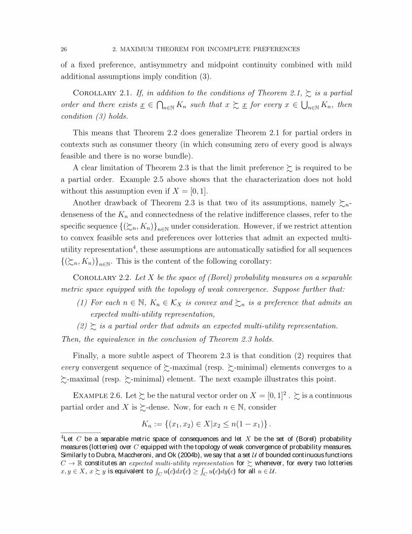
26 2. MAXIMUM THEOREM FOR INCOMPLETE PREFERENCES
of a fixed preference, antisymmetry and midpoint continuity combined with mild
additional assumptions imply condition (3).
Corollary 2.1. If, in addition to the conditions of Theorem 2.1, % is a partial
order and there exists x ∈⋂n∈NKn such that x % x for every x ∈
⋃n∈NKn, then
condition (3) holds.
This means that Theorem 2.2 does generalize Theorem 2.1 for partial orders in
contexts such as consumer theory (in which consuming zero of every good is always
feasible and there is no worse bundle).
A clear limitation of Theorem 2.3 is that the limit preference % is required to be
a partial order. Example 2.5 above shows that the characterization does not hold
without this assumption even if X = [0, 1].
Another drawback of Theorem 2.3 is that two of its assumptions, namely %n-
denseness of the Kn and connectedness of the relative indifference classes, refer to the
specific sequence {(%n, Kn)}n∈N under consideration. However, if we restrict attention
to convex feasible sets and preferences over lotteries that admit an expected multi-
utility representation4, these assumptions are automatically satisfied for all sequences
{(%n, Kn)}n∈N. This is the content of the following corollary:
Corollary 2.2. Let X be the space of (Borel) probability measures on a separable
metric space equipped with the topology of weak convergence. Suppose further that:
(1) For each n ∈ N, Kn ∈ KX is convex and %n is a preference that admits an
expected multi-utility representation,
(2) % is a partial order that admits an expected multi-utility representation.
Then, the equivalence in the conclusion of Theorem 2.3 holds.
Finally, a more subtle aspect of Theorem 2.3 is that condition (2) requires that
every convergent sequence of %-maximal (resp. %-minimal) elements converges to a
%-maximal (resp. %-minimal) element. The next example illustrates this point.
Example 2.6. Let % be the natural vector order on X = [0, 1]2 . % is a continuous
partial order and X is %-dense. Now, for each n ∈ N, consider
Kn := {(x1, x2) ∈ X|x2 ≤ n(1− x1)} .4Let C be a separable metric space of consequences and let X be the set of (Borel) probabilitymeasures (lotteries) over C equipped with the topology of weak convergence of probability measures.Similarly to Dubra, Maccheroni, and Ok (2004b), we say that a set U of bounded continuous functionsC → R constitutes an expected multi-utility representation for % whenever, for every two lotteriesx, y ∈ X, x % y is equivalent to
∫Cu(c)dx(c) ≥
∫Cu(c)dy(c) for all u ∈ U .
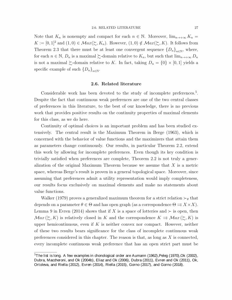
2.6. RELATED LITERATURE 27
Note that Kn is nonempty and compact for each n ∈ N. Moreover, limn→+∞Kn =
K := [0, 1]2 and (1, 0) ∈Max(%, Kn). However, (1, 0) /∈Max(%, K). It follows from
Theorem 2.3 that there must be at least one convergent sequence {Dn}n∈N, where,
for each n ∈ N, Dn is a maximal %-domain relative to Kn, but such that limn→+∞Dn
is not a maximal %-domain relative to K. In fact, taking Dn = {0} × [0, 1] yields a
specific example of such {Dn}n∈N.
2.6. Related literature
Considerable work has been devoted to the study of incomplete preferences.5.
Despite the fact that continuous weak preferences are one of the two central classes
of preferences in this literature, to the best of our knowledge, there is no previous
work that provides positive results on the continuity properties of maximal elements
for this class, as we do here.
Continuity of optimal choices is an important problem and has been studied ex-
tensively. The central result is the Maximum Theorem in Berge (1963), which is
concerned with the behavior of value functions and the maximizers that attain them
as parameters change continuously. Our results, in particular Theorem 2.2, extend
this work by allowing for incomplete preferences. Even though its key condition is
trivially satisfied when preferences are complete, Theorem 2.2 is not truly a gener-
alization of the original Maximum Theorem because we assume that X is a metric
space, whereas Berge’s result is proven in a general topological space. Moreover, since
assuming that preferences admit a utility representation would imply completeness,
our results focus exclusively on maximal elements and make no statements about
value functions.
Walker (1979) proves a generalized maximum theorem for a strict relation �θ that
depends on a parameter θ ∈ Θ and has open graph (as a correspondence Θ⇒ X×X).
Lemma 9 in Evren (2014) shows that if X is a space of lotteries and � is open, then
Max (%, K) is relatively closed in K and the correspondence K ⇒ Max (%, K) is
upper hemicontinuous, even if K is neither convex nor compact. However, neither
of these two results bears significance for the class of incomplete continuous weak
preferences considered in this chapter. The reason is that, as long as X is connected,
every incomplete continuous weak preference that has an open strict part must be
5The list is long. A few examples in chonological order are Aumann (1962),Peleg (1970),Ok (2002),Dubra, Maccheroni, and Ok (2004b), Eliaz and Ok (2006), Dubra (2011), Evren and Ok (2011), Ok,Ortoleva, and Riella (2012), Evren (2014), Riella (2015), Gorno (2017), and Gorno (2018).

28 2. MAXIMUM THEOREM FOR INCOMPLETE PREFERENCES
trivial (see Schmeidler (1971)) and, as a result, satisfy Max (%, K) = K for every
K ⊆ X.
2.7. Discussion
The present chapter provides three major results that expand the scope of Berge’s
Maximum Theorem to allow for incomplete preferences. Theorem 2.1 is based on a
simple continuity condition, but its applicability is somewhat limited since it requires
convex feasible sets and a fixed preference.
Theorem 2.2 does not have the aforementioned limitations. The result depends
crucially on its condition (3), a form of upper hemicontinuity of the mapping between
preferences-feasible sets pairs and the corresponding collection of maximal domains
of comparability. Since Gorno (2018) shows that every maximal element is the best
element in some maximal domain and vice-versa, convergence of maximal domains
permits the application of a Berge-type of argument to ensure the convergence of
maximal elements through the convergence of local best elements, where the term
“local” here means “relative to a maximal domain”.
Finally, Theorem 2.3 describes a more specific setting in which condition (3) in
Theorem 2.2 is necessary and sufficient for minimality and maximality to be preserved
when taking limits.
We believe that these results constitute a step forward towards understanding
convergence of maximal elements without completeness and open at least three av-
enues for future research. First, the abstract nature Theorem 2.2 suggests to look for
additional sets of assumptions which are sufficient for its condition (3) to hold. Sec-
ond, the equivalence in Theorem 2.3 might be true under weaker assumptions. Third,
we currently do not know whether our results remain true in a general topological
space (which is the environment in which Berge’s Maximum Theorem is formulated).

CHAPTER 3
Connected Incomplete Preferences
3.1. Introduction
The standard model of choice in economics is the maximization of a complete and
transitive preference relation over a fixed set of alternatives. While completeness of
preferences is usually regarded as a strong assumption, weakening it requires care
to ensure that the resulting model still has enough structure to yield interesting
results. This chapter takes a step in this direction by studying the class of “connected
preferences”, that is, preferences that may fail to be complete but have connected
maximal domains of comparability.1
We offer four new results. Theorem 3.1 identifies a basic necessary condition for a
continuous preference to be connected in the sense above, while Theorem 3.2 provides
sufficient conditions. Building on the latter, Theorem 3.3 characterizes the maximal
domains of comparability. Finally, Theorem 3.4 presents conditions that ensure that
maximal domains are arc-connected.
Methodologically, our contribution provides an incomplete preference perspective
on a theoretical literature relating basic assumptions on preferences and the space of
alternatives over which these preferences are defined. For example, Schmeidler (1971)
shows that every nontrivial preference on a connected topological space which satisfies
seemingly innocuous continuity conditions must be complete. In a recent article, Khan
and Uyank (2019) revisit Schmeidler’s theorem and link it to the results in Eilenberg
(1941), Sonnenschein (1965), and Sen (1969), providing a thorough analysis of the
logical relations between the form of continuity assumed by Schmeidler, completeness,
transitivity, and the connectedness of the space.
In particular, Theorem 4 in Khan and Uyank (2019) implies a converse to Schmei-
dler’s theorem: if every strongly nontrivial Schmeidler preference is complete, the
underlying space must be connected. We provide a different kind of converse: every
compact space that admits at least one complete and gapless Schmeidler preference
with connected indifference classes must be connected.
1Gorno (2018) examines the maximal domains of comparability of a general preorder.
29

30 3. CONNECTED INCOMPLETE PREFERENCES
3.2. Preliminaries
Let X be a (nonempty) set of alternatives equipped with some topology. A pref-
erence is a reflexive and transitive binary relation on X. For the rest of this chapter,
we consider a fixed preference %.
% is complete on a set A ⊆ X if A × A ⊆% ∪ -. The set A is a domain if % is
complete on A. If A is a domain such that there exists no larger domain containing
it, then A is a maximal domain.
% is Debreu continuous if {y ∈ X|y % x} and {y ∈ X|x % y} are closed sets for
every x ∈ X. % has connected indifference classes if {y ∈ X|y ∼ x} is connected for
every x ∈ X.
The set A ⊆ X contains every indifferent alternative if x ∈ A, y ∈ X, and x ∼ y
implies y ∈ A. A has no exterior bound if x % A % y implies x, y ∈ A.
3.3. Connected preferences
The main concept of this chapter is embedded in the following definition:
Definition 3.1. % is connected if every maximal domain is connected.
We will restrict attention to preferences that are not only connected, but also
Debreu continuous. As a result, maximal domains will be necessarily closed (see
Theorem 1 in Gorno (2018)).
3.3.1. A necessary condition. A natural first step towards a characterization
of connected preferences is to obtain a simple necessary condition.
Definition 3.2. % is gapless if, for every x, y ∈ X, x � y implies that there
exists z ∈ X such that x � z � y.
The notion of gapless preferences is not really new; its content coincides with a
specific definition of order-denseness for sets.2 We now prove our first result:
Theorem 3.1. If % is Debreu continuous and connected, then % is gapless.
Proof. Suppose, seeking a contradiction, that % is not gapless. Then, there
exist alternatives x, y ∈ X such that x � y and no z ∈ X satisfies x � z � y. By
Lemma 1 in Gorno (2018), there exists a maximal domain D such that {x, y} ⊆ D.
2X is said to be %-dense if for every x, y ∈ X satisfying x � y there exists z ∈ X such that x � z � y(see Ok (2007), p. 92). Evidently, X is %-dense if and only if % is gapless. We should perhapsnote that there are multiple distinct de�nitions of order-denseness in the literature and that theterminology has not necessarily been consistent.

3.3. CONNECTED PREFERENCES 31
Define A := {z ∈ D|z % x} and B := {z ∈ D|y % z}. Clearly, A and B are nonempty,
A ∩ B = ∅, and A ∪ B = D. Moreover, since % is Debreu continuous, A and B are
closed relative to D. It follows that D is not connected, a contradiction. �
It is easy to see that not every Debreu continuous and gapless preference is con-
nected:
Example 3.1. LetX = [−1, 1] and%= {(x, y) ∈ X2|x = y ∨ x2 = y2 = 1}. Then,
the preference % is Debreu continuous and gapless, but not connected (the maximal
domain {−1, 1} is not a connected set).
3.3.2. A sufficiency theorem. We already know that every Debreu continu-
ous and connected preference must be gapless. In this section, we provide a set of
assumptions which constitute a sufficient condition for a preference to be connected.
Theorem 3.2. If X is compact and % is a Debreu continuous and gapless pref-
erence with connected indifference classes, then % is connected.
Proof. Suppose, seeking a contradiction, that there is a maximal domain D that
is not connected. Then, there exist disjoint nonempty sets A and B such that A∪B =
D and both are closed relative to D. Since % is Debreu continuous Proposition 1
in Gorno (2018) implies that D is closed in X, hence A and B are also closed in
X. Moreover, since X is compact, A and B are compact as well. Let xA and xB
be the best elements in A and B, respectively. Since D is a domain, xA and xB are
comparable, which means that either xA ∼ xB, xA � xB, or xB � xA. Suppose first
that xA ∼ xB and consider the indifference class I := {x ∈ X|x ∼ xA}. Note that
I ⊆ D, because D is a maximal domain. Hence, the sets I1 := A∩ I and I2 := B ∩ Iare nonempty, disjoint, and closed relative to I, which contradicts the assumption
that % has connected indifference classes. Suppose now that xA � xB (the remaining
case is symmetric). Define the set C := {x ∈ A|x % xB}. C is nonempty (as xA ∈ C)
and compact. Let xC be the worst element in C. It is easy to check that xC � xB.
Since % is gapless, there exists z ∈ X such that xC � z � xB. It is easy to verify
that z 6∈ A and z 6∈ B. Hence, z 6∈ D. Moreover, D ∪ {z} is a domain, contradicting
the assumption that D is a maximal domain. �
The following example identifies an important class of connected preferences:
Example 3.2. Let X be the set of Borel probability measures (lotteries) on a
compact metric space of prizes Z, equipped with the topology of weak convergence.

32 3. CONNECTED INCOMPLETE PREFERENCES
Following Dubra, Maccheroni, and Ok (2004b), we say that the preference % is an
expected multi-utility preference if there exists a set U of continuous functions Z → Rsuch that x % y if and only if ∫
Z
udx ≥∫Z
udy
holds for all u ∈ U . It is easy to verify that all the assumptions of Theorem 3.2 hold.
Thus, % is connected.
3.4. Characterization of maximal domains
Building on Theorem 3.2, we can offer a useful characterization of the maximal
domains:
Theorem 3.3. Assume X is compact and % is Debreu continuous, gapless, and
has connected indifference classes. Then, a set A ⊆ X is a maximal domain if and
only if it is a connected domain that contains every indifferent alternative and has no
exterior bound.
Proof. We start establishing sufficiency through the following lemma:
Lemma 3.1. Every connected domain that contains every indifferent alternative
and has no exterior bound is a maximal domain.
Proof. Suppose, seeking a contradiction, that D is a domain that contains every
indifferent alternative, has no exterior bound, but it is not a maximal domain, then
by Lemma 1 in Gorno (2018) exists D′, a maximal domain, such that D ⊂ D′. Take
x ∈ D′\D. Since D has no exterior bounds there are y, z ∈ D such that y � x � z.
Define D1 := {w ∈ D|w % x} and D2 := {w ∈ D|x % w}. D1 and D2 are nonempty
since y ∈ D1 and z ∈ D2. Also, D1 ∪ D2 = D because x ∈ D′ and D′ is a domain
that contains D. Moreover, D1 ∩ D2 = ∅. If this intersection was not empty, there
would be w ∈ D such that x ∼ w, which would contradict that D contains every
indifferent alternative. Finally, D1 and D2 are closed relative to D because % is
Debreu continuous. It follows that {D1, D2} is a nontrivial partition of D by closed
sets. We conclude that D is not connected, which is a contradiction. �
Now we turn to necessity. It is easy to show that every maximal domain contains
every indifferent alternative and has no exterior bound. Moreover, since % satisfies
the assumptions of Theorem 3.2, every maximal domain is connected. �

3.4. CHARACTERIZATION OF MAXIMAL DOMAINS 33
We finish this section, discussing the two additional assumptions employed in
Theorem 3.3.
3.4.1. X is compact. Compactness of X cannot be dispensed with, as the fol-
lowing example shows.
Example 3.3. Let X = {−1}∪ [0, 1) and %= {(x, y) ∈ X2|x = −1 ∨ x ≥ y ≥ 0}.Then, X is bounded, locally compact and σ-compact, but fails to be compact. More-
over, % is complete, Debreu continuous, and gapless. However, the only maximal
domain is X itself that is not connected.
3.4.2. Connected indifferent classes. On the one hand, the assumption that
indifferent classes are connected is not strictly necessary for the conclusion of Theo-
rem 3.3. That is, there are examples failing this condition in which the equivalence
in the theorem holds:
Example 3.4. Let X = [−1, 1] and %= {(x, y) ∈ X2|x2 ≥ y2}.
On the other hand, it is a tight condition: there are examples that violate it,
satisfy the remaining conditions, and for which the equivalence in the theorem fails
to hold:
Example 3.5. Let X = {−1} ∪ [0, 1] and %= {(x, y) ∈ X2|x2 ≥ y2}.
There is a well-known axiom introduced by Dekel (1986) that ensures that indif-
ference classes are connected. Assuming that X is convex, we say that % satisfies
betweenness if x % y implies x % αx + (1 − α)y % y for all x, y ∈ X and α ∈ [0, 1].
Prominent examples of preferences satisfying betweenness include preferences satis-
fying the independence axiom (such as expected utility or the expected multi-utility
preferences studied in Dubra, Maccheroni, and Ok (2004b)) and also preferences ex-
hibiting disappointment aversion as in Gul (1991). The following lemma shows that
betweenness implies connected indifference classes.
Lemma 3.2. If X is convex and % satisfies betweenness, then % has connected
indifference classes.
Proof. Take any x, y ∈ X such that x ∼ y and α ∈ [0, 1]. Define z := αx+ (1−α)y. Since x % y and y % x, by betweenness, we have x % z % y and y % z % x and,
so z ∼ y. It follows that each indifference class is convex, thus connected. �

34 3. CONNECTED INCOMPLETE PREFERENCES
We should note that, if X is convex and % is a Debreu continuous preference
that satisfies betweenness, then % does not only possess connected indifferent classes,
but is also necessarily gapless. This fact makes the application of Theorem 3.2 and
Theorem 3.3 to preferences satisfying betweenness quite direct.
3.5. Arc-connected preferences
In some cases, it can be useful to strengthen the notion of connectedness to arc-
connectedness:
Definition 3.3. % is arc-connected if every maximal domain is arc-connected.
Every arc-connected preference is connected, but the converse does not generally
hold. To see this it suffices to take X to be any space that is connected but not
arc-connected3 and consider %= X ×X, that is, universal indifference.
In the particular case of antisymmetric preferences (i.e., partial orders) on a
metrizable space, we can strengthen the conclusion of Theorem 3.2:
Theorem 3.4. If X is a compact metrizable space and % is a Debreu continuous,
gapless, and antisymmetric preference, then % is arc-connected.
Proof. Let D be a maximal domain. Since % is Debreu continuous and X is
compact and metrizable, Theorem 1 in Gorno (2018) implies that D is compact and
metrizable, hence second countable. Because % is complete and Debreu continuous
on D, there exists a continuous utility representation u : D → R.
Since % is antisymmetric, its indifference classes are singletons, hence connected.
By Theorem 3.2, D is connected. It follows that u(D) is connected and compact, thus
a compact interval. Without loss of generality, we can assume that u(D) = [0, 1].
Since % is antisymmetric, u is a continuous bijection. Since X is compact and [0, 1]
is Hausdorff, u is actually an homeomorphism between D and [0, 1]. It follows that
D is arc-connected. as desired. �
3.6. Applications
3.6.1. First-order stochastic dominance. Suppose X is the set of cumula-
tive distribution functions (CDFs) over a compact interval [0, z] (endowed with the
topology of weak convergence of the associated probability measures). Let ≥1 denote
the first-order stochastic dominance relation on X, that is, F ≥1 G if and only if
F (z) ≤ G(z) for all z ∈ [0, z].
3A well-known example is the closed topologist’s sine curve, which is also compact.

3.6. APPLICATIONS 35
Proposition 3.1. ≥1 is arc-connected. Moreover, a subset of X is a maximal
domain of ≥1 if and only if it is the image of a ≥1-increasing arc joining the degenerate
CDFs associated with 0 and z.
Proof. X is a compact metrizable space (it is metrized by the Levy metric) and
≥1 is Debreu continuous, gapless, and antisymmetric. Thus, by Theorem 3.4, ≥1 is
arc-connected. Since every arc-connected set is connected, Theorem 3.3 implies the
desired equivalence. �
An analogous result holds for second-order stochastic dominance.
3.6.2. Schmeidler preferences. Schmeidler (1971) shows that, in a connected
space, every nontrivial preference satisfying seemingly innocuous continuity condi-
tions must be complete. In this section, we explore the implications of his assumptions
in spaces that are not connected.
We start by formulating the class of preferences which are the subject of Schmei-
dler’s theorem:
Definition 3.4. A preference % is a Schmeidler preference if it is Debreu con-
tinuous and the sets {y ∈ X|x � y} and {y ∈ X|y � x} are open for all x ∈ X.
The following definition captures a property that generalizes the conclusion of
Schmeidler’s theorem in terms of maximal domains:
Definition 3.5. A preference is decomposable if every maximal domain is either
a connected component or an indifference class.
Note that, when X is connected, every nontrivial decomposable preference is
complete. More generally, any two distinct maximal domains of a decomposable
preference must necessarily be disjoint. As a result, if a decomposable preference is
locally nonsatiated, then no maximal domain can be trivial or, equivalently, every
maximal domain must be a connected component.
We can now state the main result of this section:
Proposition 3.2. Let X be compact and let % be a Schmeidler preference with
connected indifference classes. Then, % is decomposable if and only if % is gapless.
Proof. To prove necessity, assume that % is gapless. Since % is a Schmeidler
preference, Proposition 10 in Gorno (2018) implies that every nontrivial connected
component is contained in a maximal domain. Moreover, because % is a gapless

36 3. CONNECTED INCOMPLETE PREFERENCES
preference on a compact space, every maximal domain is connected by Theorem 3.3.
It follows that every nontrivial maximal domain is a connected component. Finally,
since trivial maximal domains must be indifference classes, % is decomposable.
For sufficiency, note that, since % is decomposable and has connected indifference
classes, every maximal domain is connected. Thus, Theorem 3.1 implies that % is
gapless. �
Note that every Debreu continuous and complete preference is a Schmeidler pref-
erence. In that particular case, we have the following
Corollary 3.1. Let X be compact and let % be a Debreu continuous and complete
preference with connected indifference classes. Then, % is gapless if and only if X is
connected.
Schmeidler (1971) shows that if X is connected, then every nontrivial Schmeidler
preference must be complete. Khan and Uyank (2019) prove the converse and obtain
the following characterization: X is connected if and only if every nontrivial Schmei-
dler preference is complete. The corollary above implies a different characterization
for compact spaces: provided X is compact, X is connected if and only if there ex-
ists at least one complete, gapless, and Debreu continuous preference with connected
indifference classes.4
4Note that, if X is connected, the trivial preference that declares all alternatives indi�erent satis�esall the desired properties.

APPENDIX A
Technical lemmas
The proof of Theorem 2.2 requires some results about Hausdorff convergence.
In the following two lemmas (M,d) is any metric space and KM (resp. FM) is the
collection of all nonempty compact (resp. closed) subsets of M .
Lemma A.1. Let {Kn}n∈N be a convergent sequence in KM with limit K ∈ KM .
Then, every sequence {An}n∈N in KM such that An ⊆ Kn for all n ∈ N has a subse-
quence which converges to a nonempty compact subset of K.
Proof. Let dH : KM × KM → R+ denote the Hausdorff distance and let KK be
the collection of all nonempty compact subsets of K. Note that(KM , dH
)is a metric
space, KK is compact in the (relative) Hausdorff metric topology, and dH(An, ·) is
continuous on KK . For each n ∈ N, let Bn ∈ arg minB∈KKdH(An, B). I now claim
that, for each n ∈ N, we have
dH(An, Bn) ≤ dH(Kn, K).
To prove this claim, note that, since {y} ∈ KK for all y ∈ K, we have
dH(An, Bn) ≤ dH(An, {y}) = maxx∈An
d(x, y)
for all y ∈ K. Defining y∗(x) ∈ arg miny∈K d(x, y) for each x ∈ An, we have
dH(An, Bn) ≤ maxx∈An
d(x, y∗(x)) = maxx∈An
miny∈K
d(x, y),
≤ maxx∈Kn
miny∈K
d(x, y) ≤ dH(Kn, K)
as desired. It follows that limn→+∞ dH(An, Bn) ≤ limn→+∞ d
H(Kn, Kn) = 0.
Since KK is compact, the sequence {Bn}n∈N has a convergent subsequence, say
{Bnh}h∈N. Let A := limh→+∞Bnh
∈ KK . Since limn→+∞ dH(An, Bn) = 0 and
limh→+∞Bnh= A, the triangle inequality dH(Anh
, A) ≤ dH(Anh, Bnh
) + dH(Bnh, A)
implies limh→+∞ dH(Anh
, A) = 0. This means that {Anh}h∈N converges to A, com-
pleting the proof. �
37

38 A. TECHNICAL LEMMAS
Lemma A.2. Denote by FM the collection of all nonempty closed subsets of M and
let {(Fn, xn)}n∈N be a convergent sequence on FM ×M with limit (F, x) ∈ FM ×Mand such that xn ∈ Fn for every n ∈ N. Then, x ∈ F .
Proof. Suppose, seeking a contradiction, that x /∈ F . Since F is closed, there
exists ε > 0 such that {y ∈M |d(x, y) ≤ ε} ∩ F = ∅. Hence, infy∈F d(x, y) > ε/2. By
the triangule inequality, we have
d(x, y) ≤ d(x, xn) + d(xn, y)
for all y ∈ F and all n ∈ N. Therefore
infy∈F
d(x, y) ≤ infy∈F{d(x, xn) + d(xn, y)} = d(x, xn)+ inf
y∈Fd(xn, y) ≤ d(x, xn)+dH(Fn, F )
for all n ∈ N, where we used
infy∈F
d (xn, y) ≤ supx∈Fn
infy∈F
d(x, y) ≤ dH(Fn, F )
Taking limits we conclude that infy∈F d(x, y) = 0, a contradiction. �
Lemma A.3. Consider a convergent sequence {(%n, Kn, xn, yn)}n∈N in P ×KX ×X ×X with limit (%, K, x, y) ∈ P ×KX ×X ×X. Then:
(1) xn ∈ Kn for all n ∈ N implies x ∈ K.
(2) xn %n yn for all n ∈ N implies x % y.
Proof. The first part follows from Lemma A.1 by taking M = X and An = {xn}for each n ∈ N, since every subsequence of {xn}n∈N converges to x ∈ K. The second
part follows from Lemma A.2 by taking M = X×X and noting that xn %n yn means
(xn, yn) ∈%n. �
The next three lemmas are used in the proof of Theorem 2.3. In what follows, K
is an element of KX and % is a continuous preference on X. A set A ⊆ K has no
exterior bound in K if, for every x, y ∈ K, x % A % y implies x, y ∈ A.
Lemma A.4. Assume that K is %-dense and the indifference classes of % in K
are connected. Then, a subset of K is a maximal %-domain relative to K if and only
if it is a connected %-domain relative to K which has no exterior bound in K.
Proof. Since K is compact and % ∩ (K ×K) is a continuous preference on K
with connected indifference classes, the result follows from Theorem 4 in Gorno and
Rivello (2020). �

A. TECHNICAL LEMMAS 39
Lemma A.5. Let {Kn}n∈N be a sequence in KX such that Kn is connected for
every n and limn→+∞Kn = K, then K is connected.
Proof. Suppose, seeking a contradiction, that K is not connected. Then, there
exist disjoint nonempty sets A and B which are closed in K and satisfy A ∪B = K.
For any ε > 0, define Aε := {x ∈ X|d(x,A) < ε} and Aε as its closure. Define Bε and
Bε analogously. Define Kε := Aε ∪Bε and Kε as its clousure.
Since K is closed, A and B are also closed in X, which is a normal space. Then,
there exists ε > 0 such that, for every ε ∈ (0, ε], we have Aε ∩ Bε = ∅. Fix ε = ε/2,
then Aε ∩ Bε = ∅. Because limn→+∞Kn = K there is Nε ∈ N such that n ≥ Nε
implies Kn ⊆ Kε. Now define An := Kn ∩ Aε and Bn := Kn ∩ Bε. It is easy to
see that An ∩ Bn = ∅, An ∪ Bn = Kn, and An, Bn ∈ KX . It follows that Kn is not
connected, a contradiction. �
Lemma A.6. Let {(%n, Kn)}n∈N be a converging sequence in P × KX with limit
(%, K) ∈ G ×KX . If, for every n ∈ N, Kn is %n-dense and all indifference classes of
%n in Kn are connected, then K is %-dense.
Proof. Suppose, seeking a contradiction, that K is not %-dense. Then, there
exist x, y ∈ K such that x � y and there is no z ∈ K that satisfies x � z � y. Take
{xn}n∈N and {yn}n∈N such that xn, yn ∈ Kn for every n ∈ N, limn→+∞ xn = x, and
limn→+∞ yn = y. Define Mn := {z ∈ Kn|xn %n z %n yn}. Note that Mn ∈ KX and
Mn ⊆ Kn for every n ∈ N, so Lemma A.1 implies that {Mn}n∈N has a convergent
subsequence. Thus, we can assume without loss of generality that {Mn}n∈N itself
converges and define M := limn→+∞Mn.
We claim that Mn is connected for each n ∈ N. Suppose, seeking a contradiction,
that Mn is not connected for some n ∈ N. Then there should exist disjoint nonempty
sets A and B which are closed in Mn and satisfy A∪B = Mn. Without loss, assume
that xn ∈ A. Since B is compact and %n is continuous, there exists at least one
%n-maximal element in B, call it xB. Define C := {z ∈ A|z %n xB}. Note that C
is also compact and nonempty (xn ∈ C), so we can take xC , one of its %n-minimal
elements. We will now show that xC �n xB. Define I := {z ∈ Kn|z ∼n xB}. Since
I ⊆Mn, both I ∩B and I ∩A are closed sets which satisfy (I ∩ A)∪ (I ∩B) = I and
(I ∩ A) ∩ (I ∩B) = ∅. Since I is assumed to be connected and xB ∈ I ∩ B it must
be that I ∩A = ∅, proving that xC �n xB. Define D := {z ∈Mn|xC �n z �n xB}. If
there is z ∈ D, then z �n xB implies z /∈ B. Moreover xC �n z �n xB implies that

40 A. TECHNICAL LEMMAS
z /∈ C, so z /∈ A either. It follows that D must be empty, which is a contradiction
with Kn being %n-dense. We conclude that Mn is connected.
On the one hand, since {Mn}n∈N is a sequence of connected sets in KX , M is
connected by Lemma A.5. On the other hand, we claim that M = {x, y}. It is easy
to see that {x, y} ⊆ M . To prove the other inclusion take any sequence {zn}n∈Nconverging to z ∈ M and such that zn ∈ Mn for every n ∈ N. Then xn %n zn %n ynimplies x % z % y. But, since we initially assumed that there is no z ∈ K that satisfies
x � z � y, we must necessarily have that either x ∼ z or z ∼ y. Furthermore, %
antisymmetric implies that x = z or z = y. Hence, M must be equal to {x, y}.We conclude that M must simultaneously be connected and equal to {x, y}, which
yields the desired contradiction. �

Bibliography
J.-L. Arcand, M.-O. Hongler, and D. Rinaldo. Increasing risk: Dynamic mean-
preserving spreads. Journal of Mathematical Economics, 86:69–82, 2020.
R. J. Aumann. Utility theory without the completeness axiom. Econometrica, 30(3):
445–462, 1962.
C. Berge. Topological Spaces. Oliver and Boyd, 1963.
E. Dekel. An axiomatic characterization of preferences under uncertainty: Weakening
the independence axiom. Journal of Economic Theory, 40(2):304 – 318, 1986.
J. Dubra. Continuity and completeness under risk. Mathematical Social Sciences, 61
(1):80–81, 2011.
J. Dubra, F. Maccheroni, and E. A. Ok. Expected utility theory without the com-
pleteness axiom. Journal of Economic Theory, 115(1):118–133, 2004a.
J. Dubra, F. Maccheroni, and E. A. Ok. Expected utility theory without the com-
pleteness axiom. Journal of Economic Theory, 115(1):118–133, 2004b.
S. Eilenberg. Ordered topological spaces. American Journal of Mathematics, 63(1):
39–45, 1941.
K. Eliaz and E. A. Ok. Indifference or indecisiveness? choice-theoretic foundations
of incomplete preferences. Games and Economic Behavior, 56(1):61–86, 2006.
O. Evren. Scalarization methods and expected multi-utility representations. Journal
of Economic Theory, 151:30–63, 2014.
O. Evren and E. A. Ok. On the multi-utility representation of preference relations.
Journal of Mathematical Economics, 47(4-5):554–563, 2011.
T. Galaabaatar and E. Karni. Subjective expected utility with incomplete preferences.
Econometrica, 81:255–288, 2012.
L. Gorno. A strict expected multi-utility theorem. Journal of Mathematical Econom-
ics, 71:92–95, 2017.
L. Gorno. The structure of incomplete preferences. Economic Theory, 66(1):159–185,
2018.
L. Gorno and A. Rivello. Connected incomplete preferences. 2020.
F. Gul. A theory of disappointment aversion. Econometrica, 59(3):667–686, 1991.
41

42 Bibliography
J. Hadar and W. Russell. Stochastic dominance and diversification. Journal of Eco-
nomic Theory, 3:288–305, 1971.
M. Khan and M. Uyank. Topological connectedness and behavioral assumptions on
preferences: a two-way relationship. Economic Theory, pages 1–50, 2019.
H. Levy. Stochastic dominance and expected utility: Survey and analysis. Manage-
ment Science, 38(4), 1992.
H. Levy and Y. Kroll. Smaple vs. population mean variance, efficient portifolios.
Management Science, 26:1108–1116, 1980.
T. Magnac and J.-M. Robin. Dynamic stochastic dominance in bandit decision prob-
lems. Theory and Decision, 47:267295, 1999.
A. Mas-Colell, M. D. Whinston, and J. R. Green. Microeconomic Theory. Oxford
University Press, 1995.
E. A. Ok. Utility representation of an incomplete preference relation. Journal of
Economic Theory, 104(2):429–449, 2002.
E. A. Ok. Real analysis with economic applications. 2007.
E. A. Ok, P. Ortoleva, and G. Riella. Incomplete preferences under uncertainty:
Indecisiveness in beliefs versus tastes. Econometrica, 80(4):1791–1808, 2012.
B. Peleg. Utility functions for partially ordered topological spaces. Econometrica, 38
(1):93–96, 1970.
J. K.-H. Quah and B. Strulovici. Discounting, values and decisions. Journal of
Political Economy, 121(5):896–939, 2013.
G. Riella. On the representation of incomplete preferences under uncertainty with
indecisiveness in tastes and beliefs. Economic Theory, 58(3):571–600, 2015.
M. Rothschild and J. Stiglitz. Increasing risk i: A definition. Journal of Economic
Theory, 2:225–243, 1970.
D. Schmeidler. A condition for the completeness of partial preference relations. Econo-
metrica, 39(2):403–404, 1971.
A. Sen. Quasi-transitivity, rational choice and collective decisions. The Review of
Economic Studies, 36(3):381–393, 1969.
H. Sonnenschein. The relationship between transitive preference and the structure of
the choice space. Econometrica, pages 624–634, 1965.
J. von Neumann and O. Morgenstern. The Theory of Games and Economic Behavior.
Princeton University Press, third edition, 1953.
M. Walker. A generalization of the maximum theorem. International Economic
Review, 20:267–272, 1979.

Bibliography 43
G. Whitmore. Third-degree stochastic dominance. American Economic Review, 60:
457–459, 1970.