
AGRICULTURAL SITUATION IN INDIA NOVEMBER, 2012
58
AGRICULTURAL SITUATION IN INDIA NOVEMBER, 2012 PUBLICATION DIVISION DIRECTORATE OF ECONOMICS AND STATISTICS DEPARTMENT OF AGRICULTURE AND CO-OPERATION MINISTRY OF AGRICULTURE GOVERNMENT OF INDIA
-
Upload
khangminh22 -
Category
Documents
-
view
10 -
download
0
Transcript of AGRICULTURAL SITUATION IN INDIA NOVEMBER, 2012

AGRICULTURAL SITUATIONIN
INDIA
NOVEMBER, 2012
PUBLICATION DIVISIONDIRECTORATE OF ECONOMICS AND STATISTICS
DEPARTMENT OF AGRICULTURE AND CO-OPERATIONMINISTRY OF AGRICULTURE
GOVERNMENT OF INDIA

Agricultural Situationin India
VOL. LXIX NOVEMBER, 2012 No. 8
CONTENTS
PART I
PAGES
A. GENERAL SURVEY 401
B. ARTICLES
1. Agroforestry in Climate Change Adaptation and Miti- 405gation—A. Abdul Haris, Vandna Chhabra andB. P. Bhatt
2. Growth in foodgrain production in India is technology 409led or policy led: Special reference to Andhra Pradeshwith district wise economic analysis—I. V. Y. RamaRao, N. Vasudev and G. Sunil Kumar Babu
3. Do Market Facilities Influence Market Arrivals ? Evi- 419dence from Karnataka—Soumya Manjunath andElumalai Kannan
4. Inter-District Analysis of Production Instability of 427Cotton in Tamil Nadu State—Dr. R. Meenakshi
C. AGRO-ECONOMIC RESEARCH
Impact of Emerging Marketing Channels in Agricultural 437Marketing in Uttar Pradesh—A.E.R.C. University ofAllahabad-211002
D. COMMODITY REVIEWS
(i) Foodgrains 444
(ii) COMMERCIAL CROPS :
Oilseeds and Vegetables 446
Fruits and Vegetables 446
Potato 446
Onion 446
Condiments and Spices 446
Raw Cotton 446
Raw Jute 446
Editorial Board
Chairman
SHRI R. VISWANATHAN
Members
Dr. B.S. BhandariDr. Sukhpal SinghDr. Pramod KumarProf. Brajesh Jha
Narain Singh
Publication DivisionDIRECTORATE OF ECONOMICS
AND STATISTICSDEPARTMENT OF AGRICULTURE
AND CO-OPERATIONMINISTRY OF AGRICULTURE
GOVERNMENT OF INDIA
C-1, HUTMENTS, DALHOUSIE ROAD,NEW DELHI-110001PHONE : 23012669
Subscription
Inland ForeignSingle Copy : ����� 40.00 £ 2.9 or $ 4.5
Annual : ����� 400.00 £ 29 or $ 45
Available from :
The Controller of Publication,Ministry of Urban Development,
Deptt. of Publications,Publications Complex (Behind Old Secretariat),
Civil Lines, Delhi-110 054.Phone : 23817823, 23817640, 23819689
©Articles published in the Journal cannotbe reproduced in any form without thepermission of Economic and StatisticalAdviser.
688 Agri/2012—1 ( i )

The Journal is brought out by the Directorateof Economics and Statistics, Ministry ofAgriculture. It aims at presenting a factual andintegrated picture of the Food and AgriculturalSituation in India on month to month basis.The views expressed, if any, are notnecessarily those of the Government of India.
PART II
STATISTICAL TABLES
PAGES
A. WAGES
1. Daily Agricultural Wages in Some States— 448Category-wise.
1.1. Daily Agricultural Wages in Some States— 448Operation-wise.
B. PRICES
2. Wholesale Prices of Certain Important Agricultural 450Commodities and Animal Husbandry Productsat Selected Centres in India.
3. Month-end Wholesale Prices of Some Important 452Agricultural Commodities in International Marketsduring the Year 2012
C. CROP PRODUCTION
4. Sowing and Harvesting Operations Normally in 454Progress during the month of December, 2012.
( ii )
Officials of the Publication Division,Directorate of Economics and Statistics,Department of Agriculture and Co-operation,New Delhi associated in preparations of thispublication :
B. B. S.V. Prasad—Sub-EditorD. K. Gaur —Technical AssttUma Rani —Technical Asstt. (Printing).
Abbreviations used
N.A. —Not Available.N.Q. —Not Quoted.N.T. —No Transactions.N.S. —No Supply/No Stock.R. —Revised.M.C. —Market Closed.N.R. —Not Reported.Neg. —Negligible.Kg. —Kilogram.Q. —Quintal.(P) —Provisional.Plus (+) indicates surplus or increase.Minus (–) indicates deficit or decrease.
NOTE TO CONTRIBUTORS
Articles on the State of Indian Agricultureand allied sectors are accepted for publication in theDirectorate of Economics & Statistics, Departmentof Agriculture & Cooperation’s monthly Journal“Agricultural Situation in India”. The Journalintends to provide a forum for scholarly work andalso to promote technical competence for researchin agricultural and allied subjects. The articles, notexceeding five thousand words, may be sent induplicate, typed in double space on one side offullscape paper in Times New Roman font size 12,addressed to the Economic & Statistical Adviser,Room No.145, Krishi Bhawan, New Delhi-11 0001,alongwith a declaration by the author(s) that thearticle has neither been published nor submitted forpublication elsewhere. The author(s) should furnishtheir e-mail address, Phone No. and their permanentaddress only on the forwarding letter so as tomaintain anonymity of the author while seekingcomments of the referees on the suitability of thearticle for publication.
Although authors are solely responsible forthe factual accuracy and the opinion expressed intheir articles, the Editorial Board of the Journal,reserves the right to edit, amend and delete anyportion of the article with a view to making it morepresentable or to reject any article, if not foundsuitable. Articles which are not found suitable willnot be returned unless accompanied by a self-addressed and stamped envelope. No corres-pondence will be entertained on the articles rejectedby the Editorial Board.

November, 2012 401
A. General Survey
ALL INDIA CROP SITUATION - RABI (2011-12) AS ON 30-11-2012
Crop Name Normal Area Average Areaas on date Area sown reported Absolute Change over (+/–1)
(in lakh hectares)30-11-2012 % of 30-11-2011 Average as Last Year
Normal on date
Wheat 282.62 144.05 157.89 55.9 162.50 13.8 –4.6
Rice 44.99 1.57 0.85 1.9 1.05 –07 –02
Jowar 44.99 40.44 35.65 79.2 34.48 –4.8 1.2
1. Trends in Foodgrain Prices :
During the month of October, 2012, the All IndiaIndex Number of Wholesale Price (2004-05=100) ofFoodgrains decreased by 0.33 per cent from 211.9 inSeptember, 2012 to 211.2 in October. 2012.
Similarly, the Wholesale Price Index Number ofCereals showed an increase of 0.15 per cent from 201.3 to201.6 and Pulses showed an increase of 1.68 per cent from261.4 to 265.8.
There is no change in Wholesale Price Index Numberof Wheat and remained at 198.0 where as that of Riceincreased by 0.82 per cent during the same period.
The Government of India has fixed the MinimumSupport Prices for the Rabi Crops of 2012-13 season ofFair Average Quality as under :—
Rs. per quintal
Commodity MSP
Wheat Not AnnouncedBarley 980Gram 3000Masur (Lenti1) 2900Rapeseed / Mustard 3000Safflower 2800
2. Weather, Rainfall and Reservoir situation duringOctober, 2012
• Cumulative Post-Monsoon Rainfall for thecountry as a whole during the period 1st Octoberto 28th November, 2012 is 19% less than LP A.Rainfall in the four broad geographical divisionsof the country during the above period was (-)87% in North West India, (-) 25% in Central India,
1% in South Peninsula and (-) 17% in East andNorth East India.
• Out of a total of 36 meteorological subdivisions,15 subdivisions constituting 38% of the tota areaof the country received excess/normal rainfall andthe remaining 21 subdivision constituting 62% ofthe total area of the country received deficient/scanty rainfall.
• Central Water Commission monitors 84 majorreservoirs in the country which have a total livecapacity of 154.42 BCM at Full Reservoir Level(FRL). Current live storage in these reservoirs ason 29th November,. 2012 was 103.12 BCM asagainst 112.22 BCM on 29-11.2011(last year) and96.74 BCM of normal storage (average storage ofthe last 10 years). Current year’s storage in 92%of the last year’s and 107% of the normal storage.Major States reporting lower than normal storageare Jharkhand, West Bengal, Tripura, AndhraPradesh, Karnataka, Kerala, Maharashtra andTamil Nadu.
• As per latest information available on sowing ofcrops, around 61 % of the normal area under Rabicrops have been sown upto 30-11-2012. Area sownunder all rabi crops taken together has beenreported to be 374.22 lakh hectares at All Indialevel as compared to 384.70 lakh hectares in thecorresponding period of 2011-12. Area coveragewas higher by 1.2 lakh ha. under Jowar and lowerby 4.6 lakh ha. under Wheat and 3.2 lakh ha underGram.
• A statement indicating comparative position ofarea coverage under major Rabi crops during 2012-13 (upto 30-11-2012) and the corresponding periodof last year is given in the following table.

402 Agricultural Situation in India
Agriculture :
All India production of foodgrains: As per the 1stadvance estimates (Kharif only) released by Ministry ofAgriculture on 24-09-2012, production of foodgrains during2012-13 is estimated at 117.18 million tonnes compared to123.88 million.tonnes (1st advance estimates) in 2011-12.
TABLE 1— PROCUREMENT IN MILLION TONNES
2009-10 2010-11 2011-12 2012-13
Rice (Oct.-Sept.) 32.03 34.20 35.04* 9.41*Wheat (Apr.-Mar.) 25.38 22.51 28.34 38.15**
Total 57.41 56.71 63.38 47.56* Position as on 5-11-2012.** Position as on 02-08-2012
Procurement: Procurement of rice as on 1st October,2012 (Kharif Marketing Season 2011-12) at 34.92 milliontonnes represents an increase of 3.65 per cent compared tothe corresponding date last year. Wheat procurementduring Rabi Marketing Season 2012-13 is 38.15 milliontonnes as compared to 28.15 million tonnes during thecorresponding period last year.
Maize 11.36 4.91 5.10 44.9 4.50 0.2 0.6Barley 6.57 5.15 4.79 72.8 5.54 –04 –08Total Coarse Cereals 62.92 50.80 46.15 73.3 44.83 –4.7 1.3Total Cereals 390.53 196.42 204.89 52.5 208.38 8.5 –3.5Gram 80.57 73.14 72.40 89.9 75.58 –0.7 –3.2Lentil 14.46 13.25 10.81 74.7 11.93 –2.4 –1.1Peas 7.15 6.60 6.33 88.6 6.95 –0.3 –0.6Kulthi(Horse Gram) 2.36 3.92 3.57 151.5 3.71 –0.3 –0.1Urad 7.46 2.98 2.36 31.7 3.26 –0.6 –0.9Moong 6.40 1.33 0.89 13.9 0.97 .04 –0.1Lathyrus 5.46 3.58 2.86 52.4 3.76 –0.7 –0.9Others 3.61 3.91 3.27 90.6 3.42 –0.6 –0.1Total Pulses 127.46 108.70 102.49 80.4 109.56 –6.2 –7.1Total Foodgrains 518.00 305.12 307.38 59.3 317.94 2.3 –10.6Rapeseed & Mustard 62.80 56.65 57.10 90.9 56.43 0.5 0.7Groundnut 8.87 2.40 2.51 28.3 2.05 0.1 0.5Safflower 3.05 2.22 1.16 38.0 1.56 –1.1 –0.4Sunflower 10.26 5.69 3.39 33.1 3.37 –2.3 0.0Sesamum 2.56 0.40 0.24 9.3 0.38 –0.2 –0.1Linseed 4.03 2.93 2.17 53.8 2.62 –0.8 –0.5Others 0.00 0.58 0.28 #DIV/01 0.36 –0.3 –0.1Total Oilseed (Nine) 91.56 70.87 66.84 73.0 66.76 –4.0 0.1
All-Crops 609.55 375.99 374.22 61.4 384.70 –1.8 –10.5
Source Crops and TMOP Divisions DAC
ALL INDIA CROP SITUATION - RABI (2011-12) AS ON 30-11-2012
Crop Name Normal Area Average Areaas on date Area sown reported Absolute Change over (+/–1)
(in lakh hectares)30-11-2012 % of 30-11-2011 Average as Last Year
Normal on date
November, 2012 403
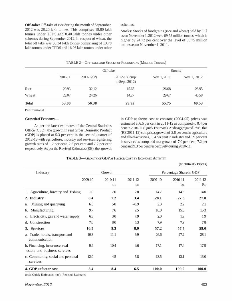
Growth of Economy —
As per the latest estimates of the Central StatisticsOffice (CSO), the growth in real Gross Domestic Product(GDP) is placed at 5.3 per cent in the second quarter of2012-13 with agriculture, industry and services registeringgrowth rates of 1.2 per eent, 2.8 per cent and 7.2 per centrespectively. As per the Revised Estimates (RE), the, growth
in GDP at factor cost at constant (2004-05) prices wasestimated at 6.5 per cent in 2011-12 as compared to 8.4 percent in 2010-11 (Quick Estimate). At disaggregated level, this(RE 2011-12) comprises growth of 2.8 per cent in agricultureand allied activities, 3.4 per cent in industry and 8.9 per centin services as compared to a growth of 7.0 per cent, 7.2 percent and 9.3 per cent respectively during 2010-11.
TABLE 2—OFF-TAKE AND STOCKS OF FOODGRAINS (MILLION TONNES)
Off-take Stocks
2010-11 2011-12(P) 2012-13(P) up Nov. 1, 2011 Nov. 1, 2012to Sept. 2012)
Rice 29.93 32.12 15.65 26.08 28.95
Wheat 23.07 24.26 14.27 29.67 40.58
Total 53.00 56.38 29.92 55.75 69.53
P=Provisional
TABLE 3— GROWTH OF GDP AT FACTOR COST BY ECONOMIC ACTIVITY
(at 2004-05 Prices)
Industry Growth Percentage Share in GDP
2009-10 2010-11 2011-12 2009-10 2010-11 2011-12QE RE QE RE
1. Agriculture, forestry and fishing 1.0 7.0 2.8 14.7 14.5 14.02. Industry 8.4 7.2 3.4 28.1 27.8 27.0a. Mining and quarrying 6.3 5.0 –0.9 2.3 2.2 2.1b. Manufacturing 9.7 7.6 2.5 16.0 15.8 15.3c. Electricity, gas and water supply 6.3 3.0 7.9 2.0 1.9 1.9d. Construction 7.0 8.0 5.3 7.9 7.9 7.83. Services 10.5 9.3 8.9 57.2 57.7 59.0a. Trade, hotels, transport and 10.3 11.1 9.9 26.6 27.2 28.1
communicationb. Financing, insurance, real 9.4 10.4 9.6 17.1 17.4 17.9estate and business services
c. Community, social and personal 12.0 4.5 5.8 13.5 13.1 13.0 services
4. GDP at factor cost 8.4 8.4 6.5 100.0 100.0 100.0(QE): Quick Estimates; (RE): Revised Estimates
Off-take: Off-take of rice during the month of September,2012 was 28.20 lakh tonnes. This comprises 19.80 lakhtonnes under TPDS and 8.40 lakh tonnes under otherschemes during September 2012. In respect of wheat, thetotal off take was 30.34 lakh tonnes comprising of 13.78lakh tonnes under TPDS and 16.96 lakh tonnes under other
schemes.
Stocks: Stocks of foodgrains (rice and wheat) held by FClas on November 1, 2012 were 69.53 million tonnes, which ishigher by 24.72 per cent over the level of 55.75 milliontonnes as on November 1, 2011.

404 Agricultural Situation in India
TABLE 4—QUARTERLY ESTIMATE OF GDP
(Year-on-year in per cent)
2010-11 2011-12 2012-13
Industry Q l Q 2 Q 3 Q 4 Q l Q 2 Q 3 Q 4 Q l Q 2
1. Agriculture, forestry & fishing 3.1 4.9 11.0 7.5 3.7 3.1 2.8 1.7 2.9 1.2
Industry 8.3 5.7 7.6 7.0 5.6 3.7 2.5 1.9 3.6 2.8
2. Mining & quarrying 6.9 7.3 6.1 0.6 –0.2 –5.4 –2.8 4.3 0.1 1.9
3. Manufacturing 9.1 6.1 7.8 7.3 7.3 2.9 0.6 -0.3 0.2 0.8
4. Electricity, gas & water supply 2.9 0.3 3.8 5.1 8.0 9.8 9.0 4.9 6.3 3.4
5. Construction 8.4 6.0 8.7 8.9 3.5 6.3 6.6 4.8 10.9 6.7
Services 10.0 9.1 7.7 10.6 10.2 8.8 8.9 7.9 6.9 7.2
6. Trade, hotels, transport & communication 12.6 10.6 9.7 11.6 13.8 9.5 10.0 7.0 4.0 5.5
7. Financing, insurance, real estate & buss. 10.0 10.4 11.2 10.0 9.4 9.9 9.1 10.0 10.8 9.4Services
8. Community, social & personal services 4.4 4.5 –0.8 9.5 3.2 6.1 6.4 7.1 7.9 7.5
9. CDP at factor cost (total I to 8) 8.5 7.6 8.2 9.2 8.0 6.7 6.1 5.3 5.5 5.3
Source: CSO

November, 2012 405
B. Articles
Agroforestry in Climate Change Adaptation and MitigationA. ABDUL HARIS1, VANDNA CHHABRA2 AND B. P. BHATT3
1. Sr. Scientist, Agronomy, ICAR Research Complex for Eastern Region, Patna2. Senior Research Fellow, ICAR Research Complex for Eastern Region, Patna3. Director, ICAR Research Complex for Eastern Region, Patna
It is the popular phrase “climate is what you expect,while weather is what you get” weather refers -day to dayatmospheric condition resulting from changes intemperature, rain, sunshine and wind etc. Climate refers tothe average weather condition for a certain period—monthsto thousands or millions of years. A classical period of 30years average changes in surface variables can be taken asstable climatic condition. Climate change is a matter ofglobal concern which means any significant change inclimatic parameters lasting for an extended period of time.Climate variability refers to short-term changes in climatesuch as longer dry or rainy season, intense heat duringsummer, more rains during rainy months, and many more.Evidences of climate change are; increasing mean surfacetemperature and associated changes like variability inrainfall, increased frequency of extreme events,unpredictable weather, uncertain water availability, foodscarcity, increasing the incidence of pests and diseases,altering cropping seasons etc.
Studies have shown that climate change is due tothe increasing emission and accumulation of greenhousegasses, such as carbon dioxide and other gases with highglobal warming potential, in the atmosphere. Greenhousegases are released from human activities such asdeforestation, burning of fossil fuels, chemical use, andmany others. These gases trap heat in the atmosphere andprevent it from being released into space. This increasesglobal temperature which changes both weather and climateconditions. Global warming increases ocean temperatureand rate of evaporation. Climate change, through globalwarming, increased the number, frequency, and intensityof extreme weather events in the country over the years.Increasing global temperature causes glaciers and polarice caps to melt hence making sea levels rise. Climatechange can extend El Nino or bring more rains than usualduring La Nina. Farmers become confused as to when theyshould plant crops, thereby affecting length of croppingseason, time of harvest, and food supply. Water shortageduring dry months can also affect crop growth and overallfood production.
Climate change can vary the life cycle of pests-increasing their population. Diseases can also becomeprevalent based on the environmental conditions resulting
from climate change. Climate change can make summermonths warmer or cold months cooler than usual. Thesechanges in temperature can cause animals to migrate tomore suitable places, or force them to adapt with adverseeffects on their physical conditions. Biodiversity is thus atmore risk now than ever because of climate change.
Forest destruction for agriculture and industrypurpose is a major threat to the biodiversity in India. Forestsare the sinks of carbon dioxide which is the major greenhouse gas apart from maintaining a favourable bioclimate.As public forests become all the time more depleted, thepressure towards forests will increase. Agroforestry is aperfect choice to reduce pressure on forests by increasingtree cover and productivity of wastelands and to preventand mitigate climate-change effects (Dhyani et.al, 2009).
Currently worldwide area under agroforestry is 1,023million ha (Nair, 2009), and areas that could be broughtunder agroforestry is estimated to be 630 M ha (IPCC, 2000)with the potential to sequester 586 Gg C yr-1 by 2040.Pandey, 1998 reported that agroforestry systems in Indiahave trees in farms and a variety of forest management andethnoforestry practices. In India, area under natural forestshas reduced to 19.39%, lower than recommended thresholdof 33% (SFR, 1993). It needs minimum of 100 million haunder forest or other tree plantations to maintain theecological balance. The National Agriculture Policy-2000sets a goal to bring one third of the total area of the countryunder the tree cover. Indeed, numerous regions of Indiacan be designated as agricultural biodiversity,heritage sitesbased on the crop diversity and numerous tree species intraditional agroforestry' systems to enhance food securityand adaptation to climate change (Singh, 2011).Agroforestry can improve the lives of farmers, help reducepoverty, and maintain ecological stability.
Agroforestry is an art and science that has beenpracticed traditionally. It combines the production of trees,food crops, and forage crops for animals on the same land.It can even integrate mini-forests, orchards, andaquaculture systems. Some of the agroforestry species thatcan be grown for various purposes include Sesbaniasesban, Calliandra species, Leucaena species, Jatrophacurcus, Tephrosia vogeli, Cajanus cajan, Eucalyptus

406 Agricultural Situation in India
species, Acacia species and some fruit trees. Based on thenature of composition, agroforestry can be classified asagrosilvicultural, silvipastoral, agrosilvipastoral andmultipurpose tree plantation system.
Agrosilvi -cultural system
In this system, agricultural crops are intercroppedwith trees in the interspace between the trees. The treesare grown in agricultural fields, on farm boundaries orseparately. The species generally grown include Prosopiscineraria, Zizyphus nummularia; Eucalyptus globulus,Jatropha curcus, etc. Wheat, mustard, sugarcane, potato,maize and paddy are crops that can be grown along withtrees.
Silvipastoral system
The production of woody plants combined withpasture is referred to Silvipasture system. The trees andshrubs may be used primarily to produce fodder for livestockor they may be grown for timber, fuelwood, and fruit or toimprove the soil. Tree species under this system are Tectonagrandis, Gmelina arborea, Terminalia myriocarpa Acacianilotica, Albizia lebbeck, Azadirachta indica, Leucaenaleucocephala, Gliricidia sepium, Sesbania grandifloraand grasses like red clover, white clover and Setaria etc arecultivated.
Agrosilvipastoral and Agrihortisilvipastoral system
The production of woody perennials combined withannuals and pastures is called as Agrisilvipastoral system.Many species of trees, bushes, vegetables and otherherbaceous plants are grown in dense and in random orspatial and temporal arrangements. Fodder grass andlegumes are also grown to meet the fodder requirement ofcattle. Woody species like Dalbergia sissoo, Ficus spp,Anacardium occidentale,Artocarpus heterophyllus, Citrusspp, Psiduim guajava, Mangifera indica, Azadirachtaindica, Cocus nucifera,and herbaceous species like Bhindi,Onion, cabbage, Pumpkin, Sweet potato, Banana, Beans,etc.are grown in this system.
Plantation based Agroforestry systems
Modern commercial plantation crops like rubber,coffee, poplar, eucalypts and oil palm represent a well-managed and profitable stable land-use activity in tropics.Some of the plantation crops like coconut, palms have beencultivated since very early times but their economic yieldremained low. However, the research attention andcommercial yields of these crops have increasedsubstantially.
Other systems
Apiculture with trees: In this system various honeyproducing trees frequently visited by honeybees areplanted on the boundary of the agricultural fields.
Aquaforestry: Various trees and shrubs preferred by fishare planted on the boundary and around fish ponds. Treeleaves are used as feed for fish.
Mixed wood lots: In this system, special location specificMulti purpose trees are grown mixed or separately plantedfor various purposes such as wood, fodder, soilconservation, soil reclamation etc.
Adaptation to climate change through Agroforestry
Adaptation is the adjustment of natural and man-made systems to environmental stimuli. Main corridorthrough which agroforestry may qualify as an adaptationto climate change is through diversifying productionsystems. The role of agroforestry in reducing thevulnerability of agroecosystems-and the people thatdepend on them-to climate change and climate variabilityneeds to be understood more clearly. Because of itspotentials, agroforestry is not only unique from agricultureand forestry; it may also be a key strategy in mitigating andadapting to climate change.
Food security: Agroforestry ensures food security bygenerating direct benefits to farmers such as food, fodder,feed for fish and livestock, fuel wood, live fences, andother products. The diversity of crops provides multipleharvests at different times of the year, thereby reducingthe risk of crop loss and food shortage. In northeast Indianstate of Meghalaya the guava and Assam lemon based agrihorticultural agroforestry systems (farming systems thatcombine domesticated fruit trees and forest trees) gave 2.96and 1.98-fold higher net return respectively in comparisonto farmlands without trees (Bhatt and Mishra, 2003).
Ecological balance: Agroforestry helps in maintainingecological balance by water conservation, improved soilfertility, and improved microclimate conditions.Agroforestry systems such as intercropping and mixedlivestock systems, involving legume-based rotations,reduce runoff and improve soil fertility.
Improvement of quality of life: Agroforestry improvesquality of life of farmers by increasing income due tomultiple harvests and sale of products from the systemsdifferent components, thereby providing regular incomethroughout the year. About 76% of the human populationwas dependent on 21% of land suitable for agriculture inthe Garhwal hills for livelihood almost 20 years ago(Dadhwal et al. 1989).
Mitigation of climate change through Agroforestry
Mitigation is the process of reducing the impact ofclimate change through interventions which remove thecarbon dioxide and other green house gases from theatmosphere. It can be through reducing the source ofemission or creating improved sink capacity. An agro-forestry system not only supports the livelihood but alsomitigates the impact of climate change through carbon

November, 2012 407
sequestration (Pandey 2002, 2007). Carbon sequestrationoccur through forestation, reforestation and restoration ofdegraded lands, agroforestry, cropland and grazingmanagement and silviculture, promoting increase carbonstocks in biomass or soil carbon. Biological carbonsequestration is the process of fixing atmospheric carbonin plants through photosynthesis and its assimilation intissues and storage organs as structural and metaboliccomponents which ultimately enrich soil carbon. Carbonconservation through conservation of biomass and soilcarbon, improved forest management practices, carbonsubstitution through increased transfer of forest biomassinto durable wood, sustainable use of biofuels, andenhanced harvesting and utilization of waste as bio fuelare some of the activities helpful to mitigate climate change.The interactions of the different components ofagroforestry systems can help absorb and sequester carbondioxide and other greenhouse gasses from the atmosphere.In India, average sequestration potential in agroforestryhas been estimated to be 25tC per ha over 96 million ha, butthere is substantial variation in different regions dependingupon the biomass production (Sathaye and Ravindranath,1998). The net annual carbon sequestration rates for fastgrowing short rotation agroforestry crops such as poplarand Eucalyptus have been reported to be 8 Mg C ha-1 yr-1 and 6 Mg C ha-1yr-1 respectively (Kaul et al., 2010).However, a poorly designed agroforestry system canenhance global warming and further contribute to climatechange. Undertaking agroforestry systems involves properimplementation of soil and water conservation measures,particularly along steep slopes. Putting these measures inplace enable agroforestry systems to efficiently minimizeerosion, floods, and landslides. The canopy of trees, treelitter, and humus also filter sunlight thereby maintainingsoil moisture. An efficient agroforestry system not onlymaximizes the benefits it provides but also ensures the linkto climate change mitigation.
Limitations of Agroforestry
An integrated food-tree farming system, whileadvantageous, does have certain negative aspects likecompetition of trees with food crops for space, sunlight,moisture and nutrients may reduce food crop yield; damageto food crop during tree harvest operation; potential oftrees to serve as hosts to insect pests that are harmful tofood crops, which may displace food crops and take overentire fields. Requirement for more labour inputs, whichmay causes scarcity at times in other farm activities andresistance by farmers to displace food crops with trees,especially where land is scarce are also some of thelimitations to agroforestry.
Researchable issues
To use agroforestry systems as an important optionfor climate change mitigation and adaptation, livelihoodsimprovement and sustainable development, research and
policy will have to progress towards
(i) Effective communication to enhanceagroforestry practices with multifunctionalvalues
(ii) Maintenance of the traditional agroforestrysystems and creation of new systems
(iii) Selection of more useful trees for livelihoodsimprovement
(iv) Designing silvicultural and farming systems tooptimize food production, carbon sequestrationand biodiversity conservation
(v) Maintaining a continuous cycle of regeneration-harvest and regeneration
(vi) Domestication of useful fruit tree speciescurrently growing in the wilderness to providemore options for livelihoods improvement
(vii) Strengthening the markets for non timber forestproducts
(viii) Addressing the research needs and policy forlinking knowledge to action.
Policy Issues
Appropriate policy issues can strengthen adaptationand resilience of communities to local and global change.On the recommendations of the National Commission onAgriculture (GOI, 1976) the farm forestry programmes inIndia, along with other social forestry programme, startedin late 1970s to meet rural people's subsistence needs. TheNational Forest Policy (GOI, 1988) stipulated that forestbased industries should meet their raw materialrequirements by establishing a direct relationship with thefarmers. The Amendment to the Forest (Conservation) Actin 1988 restricted leasing of forestlands to private sectorfor industrial plantations. The National Agriculture Policy(2000) emphasized the role of agroforestry for, nitrogenfixation, efficient nutrient cycling and organic matteraddition and for improving drainage. The Task Force onGreening India for Livelihood Security and SustainableDevelopment of Planning Commission (2001) has alsorecommended that agroforestry may be introduced overan area of 14 million ha out of 46 m ha irrigated areas thatare degrading due to water-logging, salinization and soilerosion for sustaining agriculture.
A Committee on 'Development of Bio-fuels' wasconstituted in July 2002 under which Jatropha plantationis promoted for production of Biodiesel. With a view tosubstituting diesel for biodiesel, the Government of Indiahas launched the National Mission on Biodiesel. TheNational Environmental Policy 2006 also emphasised thepromotion of private and farm forestry in environmentalconservation and management.

408 Agricultural Situation in India
Government of India stresses on biofuels, likebiodiesel to meet the energy requirements of the country.Bio-diesel production can be integrated with theagroforestry with suitable incentives and policy initiatives.The country’s bio-diesel programme is based on non-edibleoil seeds, like Jatropha curcas and Pongamia pinnata. ANational Mission on Biodiesel (NMB) has been constitutedwith Ministry of Rural Development as the nodal agency.
Conclusion
Agroforestry is an art and science that has been practicedtraditionally that combines the production of trees, foodcrops, and forage crops for animals from the limited landavailable to small and marginal farmers in diverse agroecosystems. Diversifying the production system byincluding agroforestry may reduce the risks associated withclimatic variability in synergy with climate changemitigation. The interactions of the different components ofagroforestry systems can help absorb and sequester carbondioxide and other greenhouse gasses from the atmosphere.However while planning such systems, complimentarity ofdifferent enterprises in the farm and competing requirementsof land, labour, capital and management aspects needs tobe looked into. If agroforestry systems are properly plannedand implemented, more carbon dioxide and othergreenhouse gases can be sequestered every year.Appropriate research and policy interventions canstrengthen adaptation and resilience of communities tolocal and global change.
References
Bhatt, B. P. and Misra, L. K. 2003. Production potential andcost-benefit analysis of agrihorticultureagroforestry systems in Northeast India, Journalof Sustainable Agriculture, 22,99-108.
Dadhwal K.S., Narain P., Dhyani S.K. 1989. Agroforestrysystems in the Garhwal Himalayas of India.Agroforestry Systems, 7: 213-225.
Dhyani, S. K., Ram Newaj and Sharma, A. P. 2009.Agroforestry: its relation with agronomy,
challenges and opportunities. Indian J. Agron.,54(3),249-266.
GOI, 1976, Report of the National Commission on Agriculture,Part IX, Forestry, Department of Agriculture andCooperation, Government of India, New Delhi.
GOI, 1988. The National Forest Policy, Department ofEnvironment, Forests & Wildlife, Government ofIndia, New Delhi.
IPCC, 2000. Land Use, Land-use Change, and Forestry. ASpecial Report of the IPCC, Cambridge UniversityPress, Cambridge, UK.
Kaul, M., G. Mohren and V. Dadhwa1. 2010. Carbon storageand sequestration potential of selected treespecies in India, Mitigation and AdaptationStrategies for Global Change, 15(5): 489-510.
Nair, P. K. R., B. M. ,Kumar and D. N. Vimala. 2009.Agroforestry as a strategy for carbonsequestration, Journal of Plant Nutrition andSoil Science, 172(1): 10-23.
Pandey, D.N. 1998. Ethnoforestry: Local Knowledge forSustainable Forestry and Livelihood Security,Himanshui/AFN, New Delhi.
Pandey D.N. 2002. Global climate change and carbonmanagement in multifunctional forests. CurrentScience, 83: 593-602.
Pandey D.N. 2007. Multifunctional agroforestry systemsin India. Current Science, 92: 455-463.
Sathaye, J.A. and Ravindranath, N.H. 1998. Climate changemitigation in the energy and forestry sectors ofdeveloping countries, Annual Review of Energy& Environment, 1998, 23, 387-437.
SFR, 1993. The State of Forest Report. Forest Survey ofIndia, Dehra Dun.
Singh, A. K. 2011. Probable agricultural biodiversityheritage Sites in India: X. The BundelkhandRegion, Asian Agri-History, 15(3): 179-197.

November, 2012 409
*Scientist (Agril Economics), Cost of Cultivation Scheme, R.A.R.S., Anakapalle, Visakhapatnam, Andhra Pradesh-531001 email:[email protected]**Professor & Head (Department of Agril Economics) and Honorary Director, Cost of Cultivation Scheme, College of Agriculture,Rajendra Nagar, AndhraPradesh-500030***Principal Scientist (Agril Economics), Regional Agricultural Research Station, Anakapalle, Visakhapatnam, Andhra Pradesh-531 001.
Growth in Foodgrain Production in India is Technology led or Policy led : Special Reference toAndhra Pradesh with District wise Economic Analysis
I. V. Y. RAMA RAO* N. VASUDEV** AND G. SUNIL KUMAR BABU***
Abstract
This study is to assess the impact of Technologyand policy on production of foodgrains in India in generalalong with district wise analysis of Andhra Pradesh inparticular. Time senes data for the period 1990-91 to 2009-10 were collected from Bureau of Economics and Statistics,Government of India and Andhra Pradesh. Analytical toolslike Hierarchical and K-Means Clustering, Compoundgrowth rate (CGR), Coppock’s Instability Index (C.I.l),Decomposition of change in average production wereemployed.
Growth in production was higher during period-1than period-II, along with low degree of instability. Effectof technology was higher than the policy effect on theproduction differential in both Andhra Pradesh and in India.So, growth in production should mainly come from yieldattributing factors like development of farming systemspecific high yielding varieties, input use efficiency andtechnology etc.
Growth in production was higher during period-I thanperiod-II, along with low degree of instability. Effect oftechnolopgy was higher than the policy effect on theproduction differential in both Andhra Pradesh and in India.So, growth in production should mainly come from yieldattributing factors like development of farming systemspecific high yelding varieties, input use efficiency andtechnology etc.
India is the one of the largest producer, consumerand importer of food grains in the world. During 2010-11,food grains were grown in 125.73 Million hectares with aproduction of 24l.77 Million tonnes and productivity of1,921 kg/ha . The major food grains grown in India are Rice,Wheat, Red gram, Bengal gram etc. During 2009-10, AndhraPradesh ranks sixth in Food grains production, with 6.67(5.3%) Million hectares of area, 15.30 (6.33%) Million tonnesof production and 2,294 kg/ha productivity (AgriculturalStatistics at a glance 2011). Growth in crop productionduring the post-green revolution period has beenaccompanied with increased instability and yield
fluctuation turned out to be the major source of productioninstability (Hazell 1984; Jayadevan 1991). In Andhra Pradeshinter period comparison between period I (1980-81 to1990-91 )and period II (1991- 92 to 2001-02) revealed thatgrowth in area and production in period II has performedwell over period I, contrastingly, there was decline inproductivity growth during period II over period I (Ramaraoand Raju 2005). With this background to find out whethergrowth in food grain production is technology led or policyled, an attempt has been made in the present study withthe following specific objectives:
1. To calculate growth rates in area, production andproductivity
2. To estimate the extent of instability in production
3. To assess the technology effect and policy effecton change in average production
4. To Identify the productivity clusters
5. To examine the growth and instability clustersbased on production
Materials and Methods
The study pertains to India (country as a whole),Andhra Pradesh (state as a whole), three geographicalregions of Andhra Pradesh viz; Coastal Andhra,Rayalaseema and Telangana and all districts ie., 22 districts(Because data for Hyderabad district is negligible). Here,the food grains means summing up total cereals and milletswith total pulses. The time series data for period (1990-91to 2009-10) on area, production and productivity werecollected from various publications of the Bureau ofEconomics and Statistics, Government of India and AndhraPradesh. In order to analyse the technology and policyeffect, productivity was taken as proxy for technology andarea was taken as policy variables. Because, technology willaffect the yields of the crops, where as policy parameterprice will lead to area expansion. For the purpose of analysisdata period was divided into two sub periods viz.Period -I (1990-91 to 1999-2000) and Period -II (2000-01 to2009-10). Analysis was conducted separately for each period.

410 Agricultural Situation in India
Analytical Tools: Following analytical techniqueswere employed to achieve the objectives.
Estimation of growth rates: Compound growth rateswere estimated by fitting an exponential function of thefollowing form.
Y=A.bt
Log Y = Log A + t. log b
Where,
Y = Area/Production/Productivity A= Constantb= (1 +r)
r = Compound Growth Rate t = Time variable in years(1, 2, 3 ... n)
The value of antilog of 'b' was estimated by usingLOGEST function in MS-Excel. Then, the percentCompound Growth Rate is calculated as below;
CGR (%) = [LOGEST (Yt : Y10) - 1] × 100
Estimation of extent of instability : For the calculation ofextent of instability, Coppock’s. Instability Index (Cll) wasemployed. Cll is a close approximation of the average year-to-year percentage variation adjusted for trend. In algebraicform:
C.I.I = [Antilog v √√√√√log V -1] × 100[Log (Xt+1/Xt) -m ]2
Log V = -----------------------N-l
Where,
Xt = Areal productionl Productivity in the year ‘t’N= Number of years
log V = Logarithm ic variance m = Arithmetic mean ofdifference between the logs of Xt+1 etc.,
Decomposition of Change in Average Production: Changein average production between the periods arises fromchanges in mean area and mean yield (productivity),interaction . between changes in mean yield and mean areaand change in yield-area covariance (Hazell, 1984).
The change in average production , ΔE (P) betweenthe periods can be obtained as follows:
ΔE (P) = Al. ΔY + Y1 . ΔA+ ΔA. , ΔY + ΔCov (A,Y)
Where,
A1, ΔY, Y 1. ΔA, ΔA. ΔY and Δ Cov (A,Y) are change inmean area, change in mean yield, changes in mean area andmean yield and changes in area & yield covariancerespectively
Clustering: Cluster analysis is a multivariate procedureideally suited to segmentation application. Clustering is
the technique, which groups the objects of interest basedon the proximities of the concerned character. Two-stageclustering technique was employed by using theHierarchical and K-Means Clustering techniques.Hierarchical Clustering gives the number of groups to beformed. Where as, K-Means Clustering will decide themembership in each cluster.
(1) Based on productivity:
Hierarchical Cluster analysis given three clusters ofdistricts based on yield (kg/ha). These clusters were namedas low (1,500), medium (1,500-2,000) and high (> 2,000).
Based on growth vis-a-vis instability
Based on the production growth (CGR) HierarchicalCluster analysis classified the districts into three clustersviz., Low (< 0 %), Medium (0.1-2.0%) and High (> 2.1%).Similarly, based on production instability (CII) districts werecategorised into three clusters viz; Low (< 1 0%), Medium(l 0-20%) and High (> 20%). Then, these three clusterseach in growth and instability were cross tabulated andresulted in nine clusters Viz., L-L (Low-Low), L-M,L-H,M-L,M-M,M-H,H-L,H-M, and H-H (High-High) clusters, andpresented in the form of 3× 3 tables (tables 6 and 7). Further,analysis was carried for the both periods.
Results and Discussion
Magnitude of Growth:
During the period -I, country as a whole, growth ratewas negative in area (-0.32%), growth rate in production(3.18%) and productivity (3.51 %) were high (Table 1). So,growth in productivity contributed more towards growthin production than by growth in area. Similar trend wasnoticed in state as a whole also. Among the regions, rangesof growth rates in area varied between -5.34 per cent(Rayalaseema) and 0.41 per cent (Coastal Andhra), inproduction they were from - 0.52 per cent (Rayalaseema) to2.94 per cent (Telangana) and in productivity variedbetween 1.90 per cent (Coastal Andhra) and 5.64 per cent(Telangana). Growth in productivity contributed moretowards growth in production in all regions. Among thedistricts, range of growth rates in area was between -7.78per cent (Kadapa) and 4.16 per cent (Srikakulam), inproduction the lowest was -2.43 per cent (Ananthapur)and the highest was 6.11 per cent (Srikakulam), inproductivity growth rates varied from -0.1 per cent (Krishna)to 8.06 per cent (Warangal). All districts in Rayalaseemaand Telangana regions shows negative trend in area. Outof 22 districts, in 19 districts growth in productivity washigher than growth in area and likewise contributed towardsproduction growth.
During the period -II, among the districts, highestgrowth rates in area (3.31 %), production (4.72%) andproductivity (5.92%) were recorded in Kurnool,Mahaboobnagar and Ranga reddy respectively. Lowest

November, 2012 411
growth rates in area (-4.79 %) and production (-4.88%) werenoticed in Chittoor, in productivity (-2.82) was observed inKadapa. Lowest growth rates in all variables were recordedamong the districts of Rayalaseema region, while highestin production and productivity were noticed in districts ofTelangana. Further, 13, three, four districts registered withnegative growth rates in area, production and productivityrespectively. Among the regions, growth rates in area variedbetween -0.72 per cent (Coastal Andhra) and 1.62 per cent(Rayalaseema), in production varied from 1.40 per cent(Coastal Andhra) to 3.20 per cent (Telangana), inproductivity varied between 0.67 per cent (Rayalaseema)and 3.31 per cent (Telangana). Growth in area contributedmore towards growth in production than growth inproductivity in Rayalaseema, vice versa was noticed inCoastal Andhra and Telangana.
State as a whole, growth in productivity (2.42%)contributed more towards growth in production (3.3%) thanby growth in area (- 0.20%). Similarly, Country as a whole,growth in productivity (0.84%) had higher influence onproduction (0.63%) than by growth in area (- 0.22%).
Shah and Shah (1997) reported that foodgrainproduction during 1977-76 to 1990- 91 has increasedsubstantially but has brought in uneven developmentacross the region and crops in India. In present study amongthe regions of Andhra Pradesh, during the period -1 growthin production varied between -0.52 (Rayalaseema) to 2.94(Telangana) shows high difference (3.46 %) among theregions, where as, this difference (1.80 %) was loweredduring period -II. Further, uneven growth was noticedacross districts also. During period -I all the districts inRayalaseema and Telangana has showed negative growthrate in area, whereas, during period -II seven districts (outof 9) in Coastal region recorded negative growth rate inarea. It conveys that improved technology and improvedvarieties are locally biased.
Extent of Instability:
Country as a whole, during the period -I, productivityvariability (4.40%) had more influence on productionfluctuations (4.44%) than by instability in area (0.97%)(Table 2). During the period -II also instability in productivity(1.78%) has more influence on production variability(2.74%) than by instability in area (1.14%). Inter periodcomparison revealed that instability in production andproductivity during the period-II was less than period-I.
State as a whole, during both periods, productivityvariability had more influence on production fluctuationsthan by instability in area. Inter period comparison revealedthat instability in production and productivity during theperiod-II was less than period-I.
Among the regions, during the period -I, the lowestinstability in area (2.18%), production (5.02%) andproductivity (4.11%) were recorded in Coastal Andhra.
Highest instability in area (6.61 %) and productivity (8.88%)were recorded in Rayalaseema, while, in production (6.54%)was observed in Telangana. In all regions contributiontowards production fluctuations was more by variability inproductivity. During the period -II, the lowest instability inarea (2.67 %), production (4.72%) and productivity (3.21%)were recorded in Coastal Andhra. Highest in area (3.85%)and production (8.98%) was noticed in Telangana and inproductivity (7.64%) was recorded in Rayalaseema.Contribution towards production variability was more byproductivity variability in all regions.
Among the districts, during the period -I, the lowestin area (1.53%), production (4.04%) and productivity(3.82%) were recorded in Khammam, Krishna and Gunturrespectively. Highest instability in area (12.51%) andproduction (23.93%) were noticed in Srikakulam and inproductivity (13.35%) was recorded in Vizianagaram.Highest in all variables were noticed in among the districtsof Coastal Andhra. In 18 districts, out of 22, contribution ofinstability in productivity in relation to variability in areawas more towards production fluctuations. During theperiod -II, the lowest instability in area (2.83%) was noticedin Medak, in production (4.66%) and productivity (3.61%)were observed in West Godavari. Highest instability inarea (9.04%), production (15.68%) and productivity (12.73%)were registered respectively in and Karimnagar, Nalgondaand Kadapa. In 19 districts, out of 22, production fluctuationwas more influenced by instability in productivity thanvariability in area.
Technology effect and Policy effect on change in averageproduction:
Between period -I and II, country as a whole, effectof technology (213.97%) was higher than policy (-11.29).Similar trend was noticed in State as a whole, wheretechnology (154.12%) had very high effect on averageproduction differential between the periods, than otherfactors (Table-3).
Among the regions, technology effect has highereffect on production differential than other components ofchange in all regions. When compared about magnitude, itwas highest in Rayalaseema (848.04%) followed byTelangana (141.13%) and Coastal Andhra (138.04%).
Among the districts, in 19 districts (7 in CoastalAndhra, 3 in Rayalaseema and All in Telangana) technologyhad more effect on average production differential than byother components of change. The highest technology effectwas recorded in Krishna (449.49%). While, highest policyeffect (1465.68%) was noticed in Nalgonda.
Clustering based on productivity:
During period -I, 36.44%, 29.31 % and 34.24% of stateaverage production was in low, medium and high clustergroups respectively (Table 4). During, period -II, a good
412 Agricultural Situation in India
amount (59.72%) was in high cluster group (Table 5). Thatshows the definite effct of technology in some districtsover the time. In the districts where productivity wasdecreased magnitude was low, whereas, in the districtswhere productivity increased the magnitude was high. Thiswas reflected in average productivity level in period-II (2.02tonnes/ha) which is higher than period -I (1.53 tonnes/ha).During period-I, 12, six and four districts were in low,medium and high clusters respectively. Duringperiod-II, eight, six and eight districts were in low, mediumand high clusters respectively. This shows technologyled the movements of the some districts from low tomedium and to high clusters from period 1 to II. That isto say that three districts Viz., Srikakulam, Prakasam andKhammam moved from low cluster to medium cluster,one district Viz., Warangal moved from low to highclusters, three districts Viz., East Godavari, Nizamabadand Karimnagar moved from medium to high clusters.But, point of concern is that productivity levels of 15districts were stagnant.
Clustering based on Growth vis-a-vis Instability:
Production growth was 2.25% and 2.21 % in periods-Iand II respectively for state as a whole (Table 1). Theaverage foodgrains production increased from period-I(11.48 Million tonnes) to period -II (14.13 Million tonnes)by 25% in the state.
During period -I, looking in isolated manner (Table6), first from growth rates angle there was 62.17% ofproduction base was in high clusters followed by 34 % inmedium and 4% in low clusters. Looking from instabilityangle 80% of production base was in low cluster followedby 13.8% in medium and 6.28% in high clusters.
Looking from both Viz., growth and instability, themost desirable combination is the district with high growthand low instability (Top-Right corner group), where as,opposite (Bottom-Left corner group) is most undesirablegroup.
Tables 6 show that in period -I, there was 47.69% ofstates' production base was in H-L (High growth and LowInstability) cluster followed by 28.42% in M-L cluster and8.2% in H-M clusters.
During period -II, 45.97% of state production was inhigh growth cluster, followed by 39.3% in medium clusterand 6% in low cluster (Table 7). In instability clusters 69.81% of the state production was in low clusters followed by30.19% in medium cluster. In joint situation of growth andinstability, 30.03% of production was in M-L (Mediumgrowth and Low instability) clusters followed by 29.89% inH-L (High growth and Low instability) cluster. It revealsthat growth and instability are going in opposite direction.Further, nearly 60% of state production is in Medium andHigh growth clusters with low instability.
Looking through tables 6 and 7 reveals that exceptthree districts Viz., Ananthapur (L-L cluster) and Guntur(M-L Cluster) and East Godavari (H-L group) all the districtsmoved from one cluster to another cluster from periods -Ito II. Majority of the districts moved from low growthclusters to medium and towards high clusters, in instabilityreverse trend was observed. The fact established here isthat growth and instability are going in opposite direction.
Positive movements were observed inVisakhapatnam, Adilabad (from H-M to H-L) andSrikakulam (from H-M to H-L). Among these districtsgrowth was high and production was moving frominstabilised to stabilised condition.
Most undesirable movement is in the direction fromTop-Right corner (H-L Cluster) to Down-Left corner (L-Hcluster) like Nalgonda moved from L-H cluster to M-Mcluster. Other undesirable movements are from right to leftHorizontally like Krishna (from M-L to L-L), West Godavari,Nellore and Medak (from H-L to M-L) etc., and movementfrom top to bottom vertically like Kadapa (from L-L toL-M), Nizamabad (from M-L to M-M) etc.
Concern about movement from top-left corner tobottom-right corner and opposite direction depends uponproduction base. That is, if production base is highgenerally then low instability at the cost of growth isdesirable, whereas, at low production base high growth isdesirable at the cost of fluctuations.
Policy Implications
1. Production was more contributed by productivityin Foodgrains this indicates the growth inproduction should come from yield attributingfactors like development of High Yielding farmingsystem specific varieties and improvement in inputuse efficiency.
2. Yield stabilisation efforts should be given primeimportance, like assured supply of farm inputsand providing the remunerative prices.
3. Identified high and low growth rate districts andregions for foodgrains will be better utilised inthe local specific and crop specific researchschemes and growth oriented developmentprogrammes.
4. Though area has less effect on Foodgrainproduction, but for overall improvement inFoodgrain production for supplying staple foodto people, the area attributing factors like adequatesupply of farm inputs for area expansion shouldalso be given importance.
ReferencesAgricultural Statistics at a glance (2011) available at
http://agricoop.nic.in

November, 2012 413
Hazell P. B. R. (1984): “Sources of increased instability inIndia and US cereal production”, AmericanJournal of Agricultural Economics, 66: 302-311.
Jayadevan C. M. (1991): “Instability in wheat productionin M.P”, Agricultural Situation in India, 46(4):219-223.
Ramarao l. V. Y. and Raju V.T. (2005): 'Scenario of agriculturein Andhra Pradesh, Daya publishing house, NewDelhi, ISBN 81-7035-349-1, pp: 195-215.
Shah D and Shah D (1997): “Foodgrain production in India:a drive towards self-sufficiency.” Artha Vijnana,39(2): 219-239.
TABLE 1—COMPOUND GROWTH RATES OF AREA, PRODUCTION AND PRODUCTIVITY OF FOODGRAINS IN INDIA AND ANDHRA
PRADESH DURING PERIOD —I AND II
(values in percentages)
Districts, Period —I Period —IIRegions andState Area Production Productivity Area Production Productivity
Srikakulam 4.16 6.11 1.87 –0.04 2.82 2.86
Vizianagaram 2.73 4.99 2.20 –2.70 0.08 2.86
Visakhapatnam 1.25 3.94 2.66 –2.90 1.73 4.77
East Godavari 2.15 2.48 0.33 –0.56 3.46 4.03
West Godavari –0.82 2.81 3.67 –0.03 1.97 2.00
Krishna –0.64 1.14 1.79 –1.79 –3.21 –1.45
Guntur 1.27 1.18 –0.10 –1.43 1.27 2.74
Prakasam –3.31 2.93 6.46 2.25 2.74 0.48
Nellore –1.08 2.37 3.48 0.11 2.00 1.89
Coastal Andhra 0.41 2.32 1.90 –0.72 1.40 2.14
Kurnool –4.94 0.48 5.70 3.31 7.33 3.89
Ananthapur –6.46 –2.43 4.31 1.05 –1.07 –2.09
Kadapa –7.78 –1.19 7.14 2.98 0.07 –2.82
Chittoor –2.61 0.36 3.05 –4.79 –4.88 –0.10
Rayalaseema –5.34 –0.53 5.08 1.62 2.30 0.67
Ranga Reddy –1.08 1.82 2.93 –3.40 2.33 5.92
Nizamabad –2.16 1.72 3.96 –0.27 1.97 2.25
Medak –0.62 4.79 5.45 0.10 2.05 1.95
Mahaboob Nagar –4.18 0.51 4.89 0.07 4.72 4.65
Nalgonda –3.05 3.29 6.54 –0.75 0.96 1.72
Warangal –4.25 3.47 8.06 2.09 7.03 4.84
Khammam –1.95 4.45 6.52 –0.23 2.99 3.22
Karim Nagar –2.53 2.11 4.77 1.85 2.81 0.95
Adilabad –2.17 4.82 7.14 –2.52 2.77 5.43
Telangana –2.55 2.94 5.64 –0.10 3.20 3.31
Andhra Pradesh –1.57 2.25 3.88 –0.20 2.21 2.42
INDIA –0.32 3.18 3.51 —0.22 0.63 0.84

414 Agricultural Situation in India
TABLE 2—COPPOCK’S INSTABILITY INDICES (CII) OF AREA, PRODUCTION AND PRODUCTIVITY OF FOODGRAINS IN INDIA AND
ANDHRA PRADESH DURING PERIOD —I AND II
(values in percentages)
Districts, Period —I Period —IIRegions andState Area Production Productivity Area Production Productivity
Srikakulam 12.51 23.93 10.66 3.60 8.61 5.58
V izianagaram 7.93 21.97 13.35 5.18 12.35 8.10
Visakhapatnam 3.78 11.06 7.62 5.41 9.30 6.43
East Godavari 2.74 7.73 6.31 3.57 6.37 5.98
West Godavari 2.52 8.37 8.66 3.30 4.66 3.61
Krishna 1.72 4.04 4.37 4.17 10.78 6.79
Guntur 2.43 5.85 3.82 4.02 8.12 6.92
Prakasam 4.87 7.15 8.79 5.53 14.16 11.68
Nellore 2.16 5.35 5.60 5.85 9.27 5.27
Coastal Andhra 2.18 5.02 4.11 2.67 4.72 3.21
Kurnool 6.50 6.08 10.45 3.93 10.51 8.15
Ananthapur 9.81 8.53 8.28 4.08 9.98 10.02
Kadapa 10.55 7.10 9.32 3.94 12.01 12.73
Chittoor 5.72 12.78 8.29 8.66 14.17 6.75
Rayalaseema 6.61 6.35 8.88 2.87 8.61 7.64
Ranga Reddy 2.13 5.51 4.79 6.11 6.32 8.45
Nizamabad 4.00 6.00 5.73 6.50 11.70 5.98
Medak 2.67 10.44 9.31 2.83 6.25 5.41
Mahaboob Nagar 9.52 13.24 7.11 4.02 9.09 8.41
Nalgonda 5.12 7.42 8.76 7.26 15.68 8.19
Warangal 7.31 11.33 11.68 4.73 9.43 6.52
Khammam 1.53 7.81 7.94 5.65 13.51 8.47
Karim Nagar 5.94 7.84 5.96 9.04 15.09 5.73
Adilabad 2.95 11.75 12.92 4.21 8.36 6.93
Telangana 4.28 6.54 6.94 3.85 8.98 5.91
Andhra Pradesh 2.59 4.88 5.49 2.86 5.86 3.93
INDIA 0.97 4.44 4.40 1.14 2.74 1.78

November, 2012 415
TABLE 3—EFFECT OF TECHNOLOGY AND POLICY ON AVERAGE PRODUCTION IN FOODGRAINS BETWEEN PERIOD—I AND II ININDIA AND ANDHRA PRADESH
(values in percentage)Districts, Sources of EffectRegions and Technology Policy Combined Technology and policyState Effect Effect Effect covariance
Srikakulam –7.17 88.75 0.35 18.07
Vizianagaram 79.07 74.33 –0.43 –52.97
Visakhapatnam –91. 70 194.11 16.00 –18.41
East Godavari 83.90 10.09 2.49 3.53
West Godavari 112.27 –9.30 –3.52 0.56
Krishna 449.49 –323.88 –59.16 33.54
Guntur 128.82 –20.35 –2.29 –6.18
Prakasam 137.50 –26.22 –6.50 –4.78
Nellore 149.57 –23.39 –6.36 –19.81
Coastal Andhra 138.04 –32.57 –6.85 1.38
Kurnool 139.23 –26.53 –9.61 –3.09
Ananthapur –622.05 553.28 115.22 53.55
Kadapa 47.06 17.57 –0.94 36.31
Chittoor –66.52 150.88 20.85 –5.21
Rayalaseema 848.04 –570.81 –110.84 –66.39
Rangareddy 201.33 –83.45 –25.45 7.57
Nizamabad 109.53 –0.38 –0.11 –9.03
Medak 78.07 17.54 6.40 –2.02
Mahaboob Nagar 161.49 –28.22 –14.53 –18.75
Nalgonda –1600.03 1465.68 296.47 –62.12
Warangal 109.43 –4.18 –2.69 –2.57
Khammam 210.30 –81.62 –43.78 15.11
Karim Nagar 101.73 8.58 3.98 –14.30
Adilabad 179.86 –49.67 –38.05 7.86
Telangana 142.13 –26.72 –11.91 –3.50
Andhra Pradesh 154.12 –37.70 –11.40 –5.02
INDIA 213.97 –11.29 –2.76 –99.82

416 Agricultural Situation in India
TABLE 4—PRODUCTIVITY (TONNES/HA) CLUSTERS OF DIFFERENT DISTRICTS IN ANDHRA PRADESH DURING PERIOD—I
S.N Cluster—I (Low) Cluster—II (Medium) Cluster—III (High)
Name Yield Name Yield Name Yield
1. Ranga Reddy 0.96 East Godavari 1.98 West Godavari 2.51
2. Mahaboobnagar 0.77 Kadapa 1.74 Krishna 2.02
3. Adilabad 0.69 Chittoor 1.63 Guntur 2.01
4. Srikakulam 1.46 Nizamabad 1.77 Nellore 2.19
5. Vizianagaram 1.37 Nalgonda 1.58
6. Visakhapatnam 1.01 Karimanagar 1.96
7. Prakasam 1.41
8. KurnooI 1.04
9. Ananthapur 1.08
10. Medak 1.04
11. Warangal 1.37
12. Khammam 1.31
Average 1.13 1.78 2.18
% to State productivity 1.53 1.53 1.53
Share in State production (%) 36.44 29.31 34.24
NOTE 1 : State average productivity during period —I is 1.53 tonnes/ha
NOTE 2 : State average production during period —I is 1, 14, 83, 891 tones
.
TABLE 5—PRODUCTIVITY (TONNES/HA) CLUSTERS OF DIFFERENT DISTRICTS IN PERIOD —II
S.N Cluster—I (Low) Cluster—II (Medium) Cluster—III (High)
Name Yield Name Yield Name Yield
1. Vizianagaram 1.43 Srikakulam 1.52 East Godavari 2.58
2. Visakhapatnam 1.13 Prakasam 1.78 West Godavari 3.44
3. Kurnool 1.49 Kadapa 1.56 Krishna 2.35
4. Ananthapur 1.32 Chittoor 1.85 Guntur 2.33
5. Ranga Reddy 1.31 Nalgonda 1.90 Nellore 2.76
6. Medak 1.43 Khammam 1.99 Nizamabad 2.29
7. Mahaboobnagar 1.21 Warangal 2.25
8. Adilabad 1.23 Karimanagar 2.90
Average 1.32 1.76 2.61
% to State productivity 2.02 2.02 2.02
Share in State production (%) 19.08 18.56 59.72
NOTE 1: State average productivity during period —II is 2.02 tonnes/haNOTE 2: State average production during period —II is 1,41,27,359 tones

November, 2012 417
TABLE 6—CROSS TABULATED GROWTH AND INSTABILITY CLUSTERS IN PERIOD —I(production in tones)
Growth All Clusters Cluster-I Cluster-II Cluster-III groups’
(Low) (Medium) (High) share inDistrict A.P* District A.P* District A.P* state
Instability Name Name Name productioClusters n (%)
WestAnanthapur 218692 Krishna 1150591 Godavari 1201578
Kadapa 216888 Guntur 1026178 Prakasam 464176Kurnool 407399 Nellore 554259
Cluster—I Ranga(Low) Reddy 217068 Medak 385903
Nizamabad 462641 Nalgonda 690818Khammam 435564
EastGodavari 1003513
Karimanagar 741221Each groups' share in 3.79 28.42 47.69 79.91state production (%)
VisakhaCluster—II Chittoor 251321 patnam 248879(Medium) Nil Mahabub Warangal 427887
Nagar 393189Adilabad 264848
Each groups' share in 0.00 5.61 8.20 13.81state production (%)Cluster—III Nil Srikakulam 435714(High) Vizia
Nagaram 285089Each groups' share in 0.00 0.00 6.28 6.28state production (%)All groups' share in 3.79 34.03 62.17 100state production (%)NOTE: State average production during period —I IS 1, 14,83,891 tones.* A.P = Average production (tonnes) in period —I for the respective districts.
TABLE 7—CROSS TABULATED GROWTH AND INSTABILITY CLUSTERS IN PERIOD —II(production in tones)
Growth Cluster—I Cluster—II Cluster—III All groups’Clusters (Low) (Medium) (High) share (%)
in stateInstability Name A.P* Name A.P* Name A.P* productionCluster
117434 VisakhaKrishna 5 patnam 226550 Srikakulam 421414
West 1599308 East 1341734Ananthapur 222277 Godavari 8 Godavari 4

418 Agricultural Situation in India
TABLE 7—CROSS TABULATED GROWTH AND INSTABILITY CLUSTERS IN PERIOD —II—Contd.(production in tones)
Growth Cluster—I Cluster—II Cluster—III All groups’Clusters (Low) (Medium) (High) share (%)
in stateInstability Name A.P* Name A.P* Name A.P* productionCluster
Cluster—I(Low) Guntur 1164696 Kurnool 564242
Nellore 673358 Ranga Reddy 253634Mahaboob
Medak 578714 nagar 560373Warangal 708690Adilabad 372669
Each groups’ share in 9.89 30.03 29.89 69.81state production (%)
ViziaCluster—II nagaram 289073 Nizamabad 611478 Prakasam 571570(Medium) Kadapa 197966 Nalgonda 697974 Khammam 535676
Chittoor 197700 Karimnagar 1163847
Each groups' share in 4.85 9.27 16.08 30.19state production (%)Cluster—III(High) Nil Nil NilEach groups’ share in 0 0 0 0state production (%)All groups’ share in 14.73 39.30 45.97 100state production (%)Note: State average production during period —II is 1,41,27,359 tones* A.P = Average production (tonnes) in period —II for the respective districts

November, 2012 419
Do Market Facilities Influence Market Arrivals? Evidence From KarnatakaSOUMYA MANJUNATH AND ELUMALAI KANNAN*
*Ph.D. Scholar and Associate Professor respectively, Institute for Social and Economic Change (ISEC), Bangalore-560 072.
Introduction
A dynamic agricultural sector is crucial for overalleconomic development. There are various factors affectthe performance of agricultural sector in the state ofKarnataka. Among others,agricultural marketing plays acrucial role in stimulating production and consumption ofagricultural produce as it acts as a critical link betweenfarm production sector and the non-farm sector. A lack ofan efficient marketing system can affect the welfare of bothproducers and consumers. The distance to the market,manipulation of weighing machines, lack of proper grading,and proliferation of middlemen who charge enormous'commissions can be listed as some of the problems thatfarmers who choose to sell the produce at the unregulatedmarkets (Acharya, 2004). Higher agricultural productiondoes not necessarily mean high returns to the farmer unlessthere is an orderly marketing system that ensures fair prices.The absence of such a fair system could also deprive theconsumer of the benefits of a good cropping season.Recognizing the importance of marketing for developmentof agriculture, the Government of India emphasized theneed for taking steps to make the marketing system moreefficient. The government intervention was initially thoughtto be necessary to protect the interests of farmers from thevagaries of market regime, trade malpractices and highmarketing cost. But, in view of the emergence of globalmarkets, development of a competitive marketing systemwith adequate infrastructure facilities and professionalmanagement of existing market yards has become imperativein the country.
Building up of new market complexes with modernamenities would influence the market structure and pricingmechanism by increasing efficiency of the market (Kerur etal, .2008). Further, provision of market amenities wouldassist in better handling of the produce and reduce storagelosses, thereby offering higher prices to growers. Anefficient regulated marketing system would, therefore,attract greater market arrivals due to effectiveness in pricingand efficiency in the movement of agricultural commodities(Shilpi and Umali-Deininger, 2007). On the other hand, inthe absence of a fair marketing system, farmers would sellagricultural produce either at the farmgate or at the privatemarkets risking aplethora of problems. Nevertheless,Agricultural Produce Market Committees (APMC) havegreater role in motivating the farmers to sell their produceat the regulated market yard. This could be achieved by
offering better accessibility, remunerative prices, andinfrastructure for trading. The success of the APMCmarkets, therefore, needs to be measured in terms ofquantity of market arrival, which is basically the marketedsurplus of various' agricultural produce. It is important notehere that the marketed surplus and market arrivals do notalways match. This is because the farmer may choose tostore part of the produce for sale at a later date. An efficientAPMC marketing system could help in reducing this gapbetween marketed surplus and market arrivals for a givenperiod.
Farmers’ desire to sell any agricultural produce atregulated markets depends on the facilities/amenitiesavailable rather than just the presence of regulated marketsper se in the area. But, empirical evidences available in thisregard are not comprehensive and are mixed in nature.Khunt and Gajipara (2008) reported that Rajkot market inRajasthan could attract consistently high quantity ofarrivals due to both the high rate of investment in providingsuperior infrastructural facilities and transport-connectivityof the market (Khunt and Gajipara, 2008). An analysis offour regulated markets in northern Karnataka revealed thatproducer-sellers experienced problems due to improperweighing of products and inadequate grading facilities(Vaikunthe, 2000).
A World Bank study in Tamil Nadu concluded thatthe likelihood of sales at the market increased significantlywith an improvement in market facilities and with decreasein travel time from the village to the market (Shilpi andUmali-Deininger, 2007). Studies have also emphasized thepositive relationship between market arrivals and price(Gote et aI, 2010; Atteri and Bisaria, 2003). Better marketinfrastructure helps in curbing marketing losses (Rangi etaI, 2002; Atteri and Bisaria, 2003). However, few empiricalstudies have analysed the influence of market facilities inattracting market arrivals of agricultural commodities inIndia. In this context, the present study makes an attemptto understand the role of market facilities in attractingarrivals of agricultural commodities in the state ofKarnataka.
Data and Methodology
The present study is based on the secondary datacompiled from various published sources. Data on area,production and yield of major agricultural crops werecollected from Statistical Abstract of Karnataka. The

420 Agricultural Situation in India
marketed surplus ratios (MSR) of major agriculturalcommodities were collected from the Agricultural Statisticsat a Glance for various years. Since data on marketed surplusratios were not available at the district level inKarnataka"three years average (2006-07, 2007-08 and 2008-09) of state marketed surplus ratios were used to estimatethe district marketed surpluses of major crops viz., paddy,jowar, maize and ragi. The district level quantity of marketedsurplus, thus estimated was used to work out the per centmarket arrival of respective commodities in various marketsfalling in a particular district. Data on monthly quantity of
arrivals and wholesale prices of these crops were collectedfor 144 APMCs from AGMARKNET portal(www.agmarknet.nic.in) for the year 2009-10. The details ofmarket physical infrastructures and facilities across APMCswere also compiled from the same source. To examine therelationship between market facilities and market arrival, amultiple regression analysis was carried out with marketarrival as percentage of marketed surplus as the dependentvariable and number of market facilities, price, district roadlength and area of the principal market yard (ha) as theexplanatory variables.
Growth Performance of Major Crops in Karnataka
TABLE 1—COMPOUND ANNUAL GROWTH RATES OF AREA, PRODUCTION AND YIELD OF MAJOR CROPS IN KARNATAKA
(Per cent)
Period 1980-81 to 1989-90 1990-91 to 2007-08 1980-81 to 2007-08
Crops Area Produc- Yield Area Produc- Yield Area produc- Yieldtion tion tion
Rice 0.25 0.01 –0.24 0.31 1.11 0.7 0.79*** 2.05*** 1.20***
Bajra –2.89** 0.37 3.17* 0.09 1.86 1.42 1.98*** –0.14 1.73***
Jowar 1.43 –0.05 –1.47 –2.49 –1.45 0.71 1.60*** –0.76* 0.69
Maize 6.14*** 7.02*** 0.82 8.60*** 7.82*** –0.97 7.75*** 8.06*** 0.16
Ragi 0.90* 0.64 –1.72 1.87*** –0.72 1.08 1.26*** 0.41 1.32***
Small Millets –6.86*** –5.76** 1.17 6.81 *** –6.14*** 0.79 –8.20*** –6.78*** 1.58***
Wheat –3.77*** –6.44** 5.51 *** 1.31 *** 1.94 0.63 –0.66** 0.78 1.65***
Cereals 0.19 0.42 0.24 –0.28 1.59* 1.50** –0.43*** 1.85*** 2.11 ***
Arhar 4.22*** 2.03 –2.09 2.66*** 6.17*** 3.42** 1.69*** 2.51 *** 0.84
Gram 6.13*** 3.04 3.93*** 5.74*** 8.11 *** 3.29*** 5.28*** 6.8*** 1.84***
Pulses 1.71** 0.07 –1.05 2.16** 3.09*** 1.22 1.42*** 2.16*** 1.01 ***
Foodgrains 0.36 0.41 0.05 0.345* 1.712** 1.19 –0.003 1.87*** 1.78***
Groundnut 5.04*** 7.10*** 1.97 2.69*** –4.32*** –2.15** –0.12 –0.35 –0.5
Sunflower 32.07*** 26.77*** –4.001 * 0.18 1.29 1.36 7.05*** 6.83*** –0.1
Total Oilseeds 7.73*** 9.17*** 0.83 –1.75** –1.89** –0.43 1.25** 1.23* –0.2
Cotton –7.31 1.72 9.74*** 3.06*** –3.07** 3.05 –2.79*** –0.49 3.68***
Sugarcane 4.72*** 5.36*** 0.59 –0.33 –1.41 –0.57 2.46*** 2.48*** 0.22
Tobacco –0.62 1.42 1.93 4.61 *** 1.57** 2.95*** 3.25*** 2.52*** –0.75*
Fruits and nuts — — — 10.83* 15.96 18.16** — — —
Vegetables — — — 1.24 15.9 16.27* — — —
NOTE: (*=p<0.l, **=p<0.05, ***=p<0.0l)
Source: Statistical Abstract of Karnataka (Various issues), Government of Karnataka

November, 2012 421
The compound annual growth rates of area,production and yield of major agricultural commoditiesworked out for the period of 1980-81 to 2007-08 are shownin Table 1. The entire period has been divided into twosub-periods viz., 1980-81 to 1989-90 and 1990-91 to 2007-08to examine the differential performance of various crops indifferent periods in Karnataka. Among crops, rice, jowar,ragi, wheat, gram, and sunflower registered negative growthin yield during 1980-81 to 1989-90. Growth in area for bajra,small millets, wheat and cotton was negative and statisticallysignificant during the same period. It is important to notethat maize recorded growth rate of about 7 per cent inproduction and this was contributed by growth in area (6.1per cent). The compound annual growth in area under foodgrains was 0.3 per cent during 1980-81 to 1989-90 and itsgrowth in production was low and not significant at 0.4 percent. A cursory look at the performance of other cropsindicates that the period 1980-81 to 1989-90 witnessedstagnation in production as has been discussed in theReport of the Expert Committee (1993). The production ofcereals grew from 0.4 per cent per annum during 1980-81 to1989-90 to 1.59 per cent per annum during 1990-91 to 2007-08. This growth has been contributed by increases in yieldas the expansion in area for cereals was almost stagnant.
Notwithstanding, growth in area and yield waspositive and significant for most other crops during 1990-91 to 2007-08. The compound annual growth rate in areaunder foodgrains remained at around 0.3 per cent during1990-91 to 2007-08. However, growth in food grainsproduction was high at 1.7 per cent compared to the earlierperiod. This comparatively high growth rate was due togrowth in area under food grains (0.35 per cent). Despite afall in area, cereals registered a significant growth inproduction at 1.6 per cent mainly contributed by growth in
yield at 1.5 per cent. Maize continued to perform well inthis period as well with growth in production at around 7.8per cent contributed by growth in area (8.6 per cent) despitenegative yield growth.
During the overall period from 1980-81 to 2007-08,the performance of agriculture in Karnataka was relativelygood. Notable achievements were made on the fronts ofproduction and yield growth. Overall growth in productionof cereals, pulses, foodgrains, and total oilseeds wascommendable. Rice registered approximately 2 per centgrowth in production during this period contributed bothby growth in area (0.8 per cent) and yield (1.2 per cent).Unfortunately, growth in area was negative for bajra, jowar,ragi, wheat, small millets, groundnut, and cotton. Thougharea under foodgrains recorded a negative growth, itsproduction registered annual growth rate of 1.8 per centwhich was mainly contributed by growth in yield. Thus, itcan be understood from the analysis of growth performancethat increased production leads to increased marketedsurplus. However, arrivals at the market yards depend onthe willingness of the producer to sell it at the regulatedmarkets which, of course, depend on a variety of factorssuch as price, infrastructures, accessibility and finance.
Marketed Surplus Ratios (MSR) of Major AgriculturalCommodities
Table 2 depicts the comparison of marketed surplusratios of major agricultural products in Karnataka and India.The marketed surplus ratios of paddy, jowar, maize,. ragi,arhar, and groundnut have been fluctuating over the yearsin Karnataka. Nevertheless, the marketed surplus ratios ofthese major grains were higher than all India weightedaverage. Any increase in marketed surplus always placesdemands for better transport, storage and grading facilities.
TABLE 2—MARKETED SURPLUS RATIOS OF MAJOR AGRICULTURAL COMMODITIES IN KARNATAKA
(Percent)
Karnataka All India
Crops 2000- 2004- 2005- 2006- 2007- 2000 2004- 2005- 2006- 2007-01 05 06 07 08 -01 05 06 07 08
Paddy 92.9 84.41 94.35 94.59 85.47 73.8 71.37 71.25 79.17 72.64Jowar 71.5 51.01 96.85 55.33 98.79 62.7 53.44 80.01 61.02 82.87Maize 96.4 93.47 41.19 96.54 58.84 69.1 76.22 46.25 78.56 61.46Ragi 33.6 57.54 66.33 27.58 22.17 35.1 57.74 80.9 30.02 22.17Arhar 72.7 73.7 90.93 98.13 93.98 — 85.26 77.78 83.61 79.16Groundnut 93.8 97.5 65.77 85.35 82.56 — 88.75 80.2 91.6 88.61Sugarcane — 97.17 100 100 100 — 98.23 76.8 100 100Cotton 98.8 82.91 100 100 100 — 94.94 94.1 96.23 96.15Onion 96.9 82.91 99.46 99.62 99.46 — 82.91 — 99.62 42.13Source: Agricultural Statistics at a Glance (various issues), Government of India.

422 Agricultural Situation in India
Distribution of Regulated Markets by Districts inKarnataka
Table 3 presents the distribution of regulated marketsby districts during 2007-08. The density of regulated market,which is measured in terms of the number of regulatedmarkets per lakh hectare of geographical area, is alsopresented. There are a total of 498 regulated markets in
Karnataka which are well distributed between Northernand Southern districts. The districts Tumkur, Belgaum,Gulbarga and Uttara Kannada have greater number ofregulated markets than others. It can be noticed thatNorthern Karnataka has around 53 per cent of the totalregulated markets in the state. However, the main marketsin the state do not seem to be distributed uniformly acrossthe districts.
TABLE 3—DISTRIBUTION OF AGRICULTURAL REGULATED MARKETS BY DISTRICTS IN KARNATAKA: 2007-08
Districts Main Sub- Total Distribution of MarketMarket Market Markets Markets (%) density
Southern KarnatakaBangalore (U) 2 7 9 1.81 4.14Bangalore(R) 1 5 6 1.2 2.39Chitradurga 4 10 14 2.81 1.82Davanagere 6 8 14 2.81 '2.34Kolar 5 7 12 2.41 3.08Shimoga 4 18 22 4.42 .2.6Tumkur 9 25 34 6.83 3.19Chikmagalur 6 9 15 3.01 2.08D. Kannada 5 9 14 2.81 2.93Udupi 3 3 6 1.2 1.68Hassan 6 17 23 4.62 3.47Kodagu 3 4 7 1.41 1.7Mandya 6 10 16 3.21 3.21Mysore 7 8 15 3.01 2.22Chamarajanagar 3 4 7 1.41 1.23Total 70 144 214 42.97 2.53Northern KarnatakaBelgaum 10 37 47 9.44 3.5Bijapur 3 14 17 3.41 1.61Bagalkot 5 15 20 4.02 3.04Dharwad 5 11 16 3.21 3.74Gadag 5 17 22 4.42 4.72Haveri 7 12 19 3.82 3.92U. Kannada 8 20 28 5.62 2.73Bellary 6 14 20 4.02 2.46Bidar 5 9 14 2.81 2.58Gulbarga 7 22 29 5.82 1.8Raichur 4 11 15 3.01 1.79Koppal 4 13 17 3.41 3.08Total 69 195 264 53.01 2.69State 146 352 498 100 2.61Source: Director of Agriculture Marketing, Government of Karnataka and Authors’ calculation.

November, 2012 423
Distribution of Physical Market Infrastructures andFacilities
Table 4 reveals the distribution of regulated marketswith respect to the percentage of markets having physicalinfrastructure and facilities. The study has classified thefacilities provided in the APMC markets into two groupson the basis of the type of facilities, namely ‘physicalinfrastructure’ and ‘market facilities’. Physical infrastructurerefers to those facilities that are required during the actualprocess of sale of produce at the regulated market. They
include items such as input/sundry shops, auctionplatforms, grading and analysing laboratory, mechanicalgraders, sieves, market office building and warehouse.Physical infrastructure must be present in any market forsmooth conduct of transactions. Market facilities refer tothose amenities/conveniences that are provided in theAPMC market including information notice board/electricdisplay board, canteen, toilets, internal roads, parking,fencing, post office, bank, fire extinguishers, rest housesfor farmers, drinking water, electricity, garbage disposalsystem, sweeping facilities and extension unit.
TABLE 5—PERCENTAGE OF APMC MARKETS HAVING PHYSICAL INFRASTRUCTURE AND FACILITIES
Physical Infrastructure Northern Karnataka Southern Karnataka
Input/Sundry Shops 86.9 71.1Auction Platform 78.7 83.1Grading and Analysing Laboratory 21.3 9.6Mechanical Graders 4.9 6.0Sieves 21.3 15.7Market office building 98.4 91.6Storage facilities (Warehouse) 60.7 57.8Market FacilitiesInformation Notice Board/Electric Display Board 100 96.4Canteen 68.9 68.7Toilets 86.9 90.4Internal Roads 98.4 91.6Parking 86.9 81.9Fencing 85.2 77.1Post office 47.5 16.9Bank 47.5 25.3Fire extinguishers 47.5 21.7Rest houses for farmers 82.0 74.7Drinking water 98.4 92.8Electricity 100 95.2Garbage Disposal System 31.1 38.6Sweeping facilities 57.4 69.9Extension unit 21.3 19.3Source: agmarknet.nic.in
The number of market facilities was higher thanphysical infrastructures in both Northern and SouthernKarnataka. Physical infrastructure such as mechanicalgraders, grading and analysing laboratory and sieves arevery poorly developed in both the regions though theseare very basic to the proper functioning of the market.Among market facilities, extension unit and garbagedisposal system are poorly developed in the regulated
markets. It is commendable to note that in both theregions, internal roads that are crucial for market accessare well developed. Market amenities such as parking,fencing, rest houses for farmers, and toilets are fairly welldeveloped in both the regions. Banks, post offices andfire extinguishers are better developed in NorthernKarnataka when compared to South. Further, it isimportant to note that by and large markets in Northern

424 Agricultural Situation in India
Karnataka are better ernuipped with market facilities thanthe markets in Southern region.
Analysis of Relation between Facilities and Market Arrival
Table 6 presents the results of the regressionanalysis. The market-level regression analysis was carriedout to examine the relationship between the arrivals andmarket facilities. For this purpose, the study has estimatedtwo models. In Model 1, market arrivals as percentage ofmarketed surplus was regressed on market facilities. Inmodel 2 we regress on market facilities by inclusion ofother variables such as price, district road length, area ofthe principal market yard. Price has been one of the mostimportant determinants of the market arrivals in theregulated markets. An efficient marketing system can helpin stabilizing the price level.
In the case of paddy in model 1, the coefficient ofmarket facility was positive and significant. It implies thatbetter market facilities enable greater arrival of paddy inAPMC yards. However, when other explanatory variablesincluded as shown in model 2, the coefficient of market
facilities was positive, but turned insignificant. Area ofprincipal yard and price showed expected positive relationand were significant, indicating that they played animportant role in determining the quantity of market arrivals.Similar results were obtained in the case of jowar too. Inmodel 1, market facilities were positive and significant. Inmodel 2, all the explanatory variables were statistically notsignificant. It would be interesting to note that thecoefficient of district road length showed a negative signindicating that better transport might not necessarily leadto greater market arrivals. However, in both the models, noexplanatory variable turned out significant in case of maize.In fact, as observed in jowar, district road length recordeda negative sign. Price, market facilities, and area of principalyard showed positive relation but were found to bestatistically not significant. In the case of ragi, model 1showed market facilities as significant and positive therebystressing that facilities at the market yard attracted greatermarket arrivals. In Model 2, the regression results showedthat all the explanatory variables were significant. However,coefficients of district road length and area of the principalyard turned out negative.
TABLE 6—REGRESSION ANALYSIS OF MARKET FACILITIES AND MARKET ARRIVAL
Dependent variable : Market arrival as percentage of marketed surplus
Variables Paddy Jowar Maize Ragi
Model 1 Model 2 Model 1 Model 2 Model 1 Model 2 Model 1 Model 2
Market 1.017* 0.632 2.324* 2.009 1.953 1.376.. 0.999** 0.738**facility (1. 77) (1.11) (1.97) (1.61) (1.19) (0.81) (2.64) (2.1)
Price 0.014* 0.167 0.051 0.011 **(1.92) (0.14) (1.6) (2.53)
District road 0.001 –0.007 –0.013 –0.008***length (0.21) (–1.45) (–1.45) (–3.36)
Area of 0.156** 0.012 0.044 –0.048*principal yard (2.41) (0.09) (.29) (–1.68)
Constant –3.864 –14.854 –27.876 –15.616 –3.297 –7.099 –7.912 7.610( –0.49) (–1.25) (–1.58) (–0.75) (–0.14) (–0.18) (–1.45) (1.08)
No of observations 81 81 49 49 86 86 39 39
R2 0.0381 0.1549 0.0766 0.1360 0.0165 0.0754 0.1582 0.4157
NOTE: Figures in parenthesis are't' values; *** significant at 1 % level, ** significant at 5% level and * significant at 10% level.
Overall, regression results indicated a positiverelationship between market facilities and market arrivals.The differentials in the influence could be due to absenceof produce-specific facilities, geographic location of themarkets, and the cropping pattern of areas served bydifferent markets. Further, coefficient of district roadlength, a proxy for market access, was expected to be
positive and significant. However, unfortunately itturned out to be negative in most cases, which might bedue to data problems as consistent data on road lengthat district level are not available. Further, the presentstudy considered only the district road length, whichdid not include national and state highways, and villageroads.

November, 2012 425
Conclusions
The study indicates that the regulated foodgrainmarkets within the state are beset with a number ofimperfections and are found wanting in amenities andinfrastructural facilities for promoting orderly and efficientmarketing. Consequently, the regulated markets have beenattracting low arrivals despite substantial increase inmarketed surpluses over time. The present study hasattempted to examine the relationship between marketfacilities and arrival in the APMC markets of Karnataka byusing regression analysis at market level. The analysis ofthe distribution of market infrastructure reveals that themain markets are fairly distributed equally betweenNorthern and Southern Karnataka. However, markets inNorthern Karnataka are better equipped with marketfacilities than the markets in Southern region.
Regression analysis has showed that the coefficientof market facilities was positive but its statisticalsignificance varied across crops. Market facilities differedin their effectiveness in inducing market arrivals ofdifferent crops. The differentials in the influence couldbe due to absence of produce-specific market facilities,geographic location of the markets, and the croppingpattern of areas served by different markets. Nevertheless,it is important to note that higher production need notlead to higher market arrivals in a district. Despite relativelylower production in a given year, market arrivals couldstill remain high due to delayed sale of crops made possibleby better storage facilities.
Thus, the study shows that the regulated marketshave greater capacity to attract market arrivals and therefore,there is scope for large scale increase in agriculturalproduction. It needs to be stated here that only a few majorcrops have been considered in this analysis. Also, inclusionof more explanatory variables could have strengthenedthe analysis. Further analysis could cover more periods oftime to examine the possibility of a trend in the marketarrivals since any improvement in market facilities couldhave long-term impacts on the market arrivals. The dataavailable on the public domain with regard to the marketinfrastructure is provided on ‘as-on-date’ basis whichrestricts the possibility of a time-series analysis of theadvancement of market facilities. Nevertheless, there is aneed to strengthen the functioning of these regulatedmarkets by the state government and market committees ina way that the knowledge is disseminated on profitablemarketing to the farmers and at the same time facilitateavailability of produce to the non-farming population ataffordable prices.
References
Acharya, S. (1998). Agricultural Marketing in India: SomeFacts and Emerging Issues. Indian Journal ofAgricultural Marketing, Vol.53(3), 311-332.
Acharya, S. (2004). Agricultural Marketing-State of theIndian Farmer-A Millenium Study (Vol. 17). NewDelhi: Academic Foundation.
Atteri, B., & Bisaria, G. (2003). Marketable Surplus of Riceand Wheat and Benefits of Storage to the Farmersin India. Agricultural Marketing, Vol.XLVI(1),27-31.
Fafchamps, M., & Hill, R. V. (2004). Selling at the farm-gateor travelling to market. Centre for the Study ofAfrican Economies.
Gote, M., Khodiar, M., Shekhar, S., & Sadhu, B. (2010).Market Arrival and Prices of Groundnut.International Research Journal, Vol. 1 (II),77-79.
Kerur, N., Banakar, B., Vijayakumar, H., & Manjunath,L. (2008). Documentation of Different SchemesOperated in Regulated Markets in Karnataka.-Karnataka Journal of Agricultural Sciences,Vol.21(1),78-82.
Kerur, N., Banakar, B., VijayaKumar, H., Manjunath, L., &Basavaraj, H. (2008). Performance Analysis ofRegulated Markets in Karnataka. KarnatakaJournal of Agricultural Sciences, Vol. 21 (1),74-77.
Khunt, K., Vekariya, S., & Gajipara, H. (2008). Performanceand Problems of Regulated Markets in Gujarat.Indian Journal of Agricultural Marketing,Vol.22(1), 82-98.
Kumar, B., & Mishra, S. (1985). Are Agricultural MarketsLocation-Optimal? A Case Study of Gaya District(Bihar). Retrieved from http://mpra.ub.uni-muenchen.de/3297/
Mangahas, M., Recto, A. E., & Ruttan, V. (1966). Price andMarket Relationships for Rice and Corn in thePhilippines. Journal of Farm Economics,VoI.48(No. 3, Part 1),685-703.
Minten, B. (1999). Infrastructure, Market Access, andAgricultural Prices: Evidence from Madagascar.Washington D.C.: International Food PolicyResearch Institute.
Rai, K., Singh, S., Singh, S., & Mehta, V. (2000). Growth andDevelopment of Regulated Markets in Haryana.Indian Journal of Agricultural Marketing, Vol.1(3), 25-32.
Ram, S., Singh, R., & Yadav, R. K. (2007). Impact of MarketInfrastructural Development on Market Arrivalsin Uttar Pradesh-An Economic Analysis. IndianJournal of Agricultural Economics, Vol.L(1),36-39.
426 Agricultural Situation in India
Rangi, P., Sidhu, M., & Singh, H. (2002). A study on MarketInfrastructure in Punjab. Agricultural Marketing,Vol.XLV(3).
Report of the Expert Committee. (1993). Stagnation ofAgricultural Productivity in Karnataka during1980’s. Government of Karnataka.
Shilpi, F., & Umali-Deininger, D. (2007). Where to Sell?Market Facilities and Agricultural Marketing.Policy Research Working Paper 4455. The WorldBank.
Sukhsanjam, Chahal, S., & Toor, M. (2000). An Impact of
Market Regulation.on Adequacy of MarketInfrastructure in Punjab. Indian Journal ofAgricultural Marketing, Vol. 14(3), 18-24.
Vaikunthe, L. (2000). Regulatory Framework for AgriculturalMarketing-A Case Study of APMCs in Karnataka.Indian Journal of Agricultural Marketing,Vol.14(3), 1-7.
Wanmali, S. (1980). The Regulated and Periodic Marketsand Rural Development in India. Transactions ofthe Institute of British Geographers, New Series,Vol. 5,(4),466-486.

November, 2012 427
*Head and Associate Professor of Economics, Sri Sarada College for Women, Salem - 16. The Authoress is grateful to the project fellowMrs. S.Deepalakshmi for data collection.
Inter-district Analysis of Production Instability of Cotton in Tamil Nadu StateDR. R. MEENAKSHI*
Introduction
Instability in cotton production has been a matter ofconcern in the context of agricultural development in TamilNadu state in recent years. The growth of cotton in districtsof Tamil Nadu does not follow a smooth path but showsirregularities that can be described as deviations from orfluctuations around such a smooth path. This kind ofinstability can be observed and measured. For exampleproduction may show irregular changes during some years(apart from seasonal variations) or over a period of yearsthere may be changes in area or yearly changes that deviatefrom some yield trend. Sometimes there may betechnological changes causing instability in supply anddemand conditions. Hence, one has to be careful aboutthese changes for understanding the nature of instabilityin cotton production at the Tamil Nadu level. A number ofattempts have been made earlier on time series analysis ofcotton production and also on examining the extent ofinstability in crop production. But, so far, one has not comeacross any study on the instability in cotton production indistricts of Tamil Nadu in recent times. It is in this contextan attempt has been made to study cotton productioninstability in districts of Tamil Nadu. The relevantmethodology is built upon the line of work by Mehra andHazell.
Methodology and Data
The instability in cotton production in Tamil Nadu ismeasured in the two time periods namely in pre-reformperiod (1971-72 to 1989-90) and post-reform period (1990-91 to 2009-10). Here an attempt is made to break down thegrowth of production during the pre-reform period from1971-72 to 1979-80 and from 1980-81 to 1989-90. Again thegrowth of production during the post-reform period isdivided into two time periods from 1990-91 to 1999-2000and from 2000-01 to 2009-10.
Zt=a+bt+et
Where Zt denotes the dependent variable (area oryield), t is time, a, b are constants and et residual term withzero mean and variance σ2. Separate regressions are run foreach of the two time periods to ensure that ∑ tet = 0 for eachperiod.
LInear relations are deliberately used as they do notassume a deterministic part to any relation between the
variance of Z and time t. The variance of Z is simply σ2 andby estimating separate equations for the two periods, theestimated variances can take on any relation to each other.The variances of Z, as well as the covariances between Zsfor the cotton crop are obtained from the variance,covariance matrix of the residuals et. Specifically
Cov (zi, Zj) = Cov (ei, ej)
After detrending, the residuals were centered around theirmean areas or yields for each period z resulting in detrendedtime—series data of the form.
∧ –Zt = et + Z
Time series data on detrended production are thencalculated as the product of the detrended area and yieldfor districts of Tamil Nadu for two time periods. In order toanalyse the problem more completely a formaldecomposition procedure is developed. The procedure canbe used to separate the components of the changes inproduction variability.
The variance of aggregate production of cotton indistricts of Tamil Nadu was decomposed into tencomponents. These components are analysed to know theaccurate ideas on the sources of instability in the productionof cotton in Tamil Nadu. The following variables are takeninto account to explain the meas.ures of instability inproduction.
Let Q denote production. A—Area sown and Y—Yield. Then total production Q=Ay.
The variance of production can be expressed as
– – – –V(Q) = A2 V(y) + Y2 V(A)+2A Y Cov(A, Y)-Cov(A,Y)2
+R...........(1)
Where
A = average area
Y = average yield
R = residual term
The objective of the decomposition analysisis to part i t ion the changes in V(Q) and E(Q)between the first and second period into constitu-ent parts which can be attributed separately to

428 Agricultural Situation in India
changes in means, variances and co-variances of ar-eas and yields.
The average production in the first period is ex-pressed as
E(Q1) = Al Y1 + Cov(A1, Y1) .........(2)
Similarly the avarage production in the secondperiod becomes
E(Q2) = A2 Y 2 + Cov(A2, Y2) .......(3)For convenience each variable in the second period
can be expressed in terms of its counterpart in the firstperiod plus the change in the variables between the twoperiods.
For exampleA2 =A2 +ΔA ......(4)
Where
ΔA=A2 -A1 ......(5)
The equation 3 can be written as
– – – –E(Q2) = (A1 + ΔA) (Y1 + ΔY) + Cov(A1, Y1) + ΔCov
(A, Y).......(6)
ΔE(Q) is then obtained by subtracting equation (2)from (6)
ΔE(Q) = E(Q2) - E(Q1) .....(7)
– – – – – –= A1ΔY + Y1 ΔA+ΔA ΔY +ΔCov(A, Y)
There are four sources of changes in E(Q). Two partsΔA1 ΔY and ΔY1 ΔA arise from the changes in mean yieldand mean area which are called pure effects. The term ΔYΔA is an interaction effect which arises from simultaneousoccurrence of change in mean yield and mean area. Thelast term ΔCov (A, Y) arises from change in variability ofarea and yield. The following Table identifies the pureeffects and interaction effects of the components of changein variance of production.
COMPONENTS OF CHANGE IN THE VARIANCE OF PRODUCTION IN TAMIL NADU
S. Sources of ChangeNo. Description Symbol Components of Change
1. Change in mean yield ΔY 2A1ΔY Cov(Y1A1)+
[2Y1ΔY +(ΔY )2]V(A1)
2. Change in mean area ΔΑ 2Y1ΔA Cov(Y1A1) +
[2A1ΔA + (ΔA)2]V(Y1)
3. Change in yield variance ΔV(Y) (A1)2 ΔV(Y)
4. Change in area variance ΔV(A) (Y1)2 ΔV(A)
5. Interaction between changes ΔY, ΔA 2Δ Y ΔACov(Y1A1)in mean yield and mean area
6. Change in area-yield co-variance ΔCov(Y,A) [2A1 Y1 - 2Cov(Y1A1)ΔCov(Y,A)]
-[ΔCov(YA)]2
7. Interaction between changes in mean ΔA,ΔV(Y) [2A1ΔA+(ΔA)2]ΔV(Y)area and yield variance
8. Interaction between changes in mean ΔY, ΔV(A) [2Y1ΔY +(ΔY)2]ΔV(A)yield and area variance
9. Interaction between changes in mean area ΔY,, ΔA, [2Y1 ΔA+2A1 ΔY +2ΔAΔY]and yield and changes in area -yield co-varIance ΔCov(Y,A) ΔCov(Y,A)
10. Change in residual ΔR ΔV(A Y) - sum of the othercomponents
Source: Compiled by the Principal Investigator from Peter B.R. Hazell’s work on “Instability in Indian Foodgrains Production” Researchreport 30, International Food Policy Research Institute, Washington, D.C. May, 1982.

November, 2012 429
At present there are 32 districts in Tamil Nadu state.Because of the non-availability of data these 32 districtshave been merged into 10 districts in pre-reform periodand 13 districts in post-reform period. District-Wisedecomposition analysis is carried out to find the magnitudeof fluctuations in cotton production in pre and post reformperiods in Tamil Nadu.
Pre-Reform Period Chengalpattu-MGR
Table-I presents a summary of the components ofchange in the variance of cotton crop in Chengalpattu-MGR region. Interaction between changes in mean areaand yield and changes in area- yield covariance accountsfor a considerable share of changes in the variance ofproduction of cotton. The change in residual appears tohave a more stabilising influence on cotton in Chengalpatturegion. The interaction between changes in mean yieldand mean area is very low followed by interaction betweenchanges in mean yield and area variance. Contrary to this,change in mean area and the interaction between changesin mean area and yield variance account for large share ofchange in the variance of cotton in this region in pre reformperiod.
South Arcot
It can be seen from Table-I that the interactionsbetween changes in mean area and yield and changes inarea - yield covariance account for large share of the changein the variance of cotton in South Arcot district. Change inresidual, change in mean area, change in mean yield andthe interaction between changes in mean yield and meanarea are the important components of the stability of cottonproduction in this district. The maximum stability in cottonwas mainly due to the change in residual. Change in areavariance and the interaction between changes in mean areaand yield and changes in area—yield covariance are notconsidered as important components of the variance ofproduction of cotton in pre reform period in South Arcotdistrict of Tamil Nadu.
North Arcot—Ambedkar—Thiruvannamalai—Sambuvarayar
It is evident from Table I that is region the interactionbetween changes in mean area and yield and changes inarea—yield covariance was the important factor responsiblefor instability in cotton. The effect of change in yieldvariance, interaction between changes in mean area yieldvariance and the interaction between changes in meanyields and mean areas are very low for variance ofproduction of cotton in this region. The change in residualappears to have a more stabilising influence on cottonproduction. All other components account for large shareof the changes in the variance of production of cotton inthis study area.
Salem—Dharmapuri
Table I shows that, by and large, production stabilityfor cotton was more in these districts. Change in residualappears to have a more stabilising influence for cottonproduction. Similarly when the change in mean yield, changein mean area, change in yield variance, interactions between(i) changes in mean yield and mean area and (ii) changes inmean area and yield variance are considered together, theyaccount for a positive effect towards increase in cottonproduction. It can further be seen that change in area —yield co-variance accounts for substantial share of theincrease in the variance of production of cotton. All othercomponents are very important in explaining the changesin the variance of cotton production in this region andthese components together account for instability of cottonproduction.
Coimbatore—Periyar
The results indicate a summary of the componentsof change in the variance of cotton crop in this area.Interaction between changes in mean area and yield andchanges in area—yield covariance accounts for large shareof the change in the variance of cotton. Change in meanarea, change in area variance and interaction betweenchanges in mean area and yield variance had a good effecton the variance of cotton production. A comparison of theinfluence of interaction between changes in mean yieldand mean area and interaction between changes in meanarea and yield variance showed that both these interactionterms do not contribute significantly in the variance ofcotton production. Change in area yield covariance appearsto have a more stable influence on cotton. Cottonproduction stable was also due to change in yield variancefollowed by change in residual in this region.
Tiruchirappalli—Pudukottai.
It may be recalled from Table I that the factorscontributing to the highest reduction in variability ofproduction of cotton were the change in area variance,change in mean area, change in mean yield and to a littleextent interaction between changes in mean yield andarea variance. Interaction between changes in mean yieldand mean area and change in residual, account for a smallshare of the increase in the stability of cotton crop.Contrary to change in area variance, change in area yieldcovariance contributes to the stability of cottonproduction. Along with this component, change in yieldvariance and interaction between changes in mean areaand yield and changes in area - yield covariance accountfor stability of cotton production in this study region.Interaction between changes in mean area and yieldvariance contributes a small share of the change in thevariance of production of cotton.

430 Agricultural Situation in India
TAB
LE I—
CO
MPO
NEN
TS O
F CH
AN
GE I
N TH
E VA
RIA
NC
E OF P
RO
DU
CTI
ON
OF C
OTT
ON
CR
OP I
N P
RE-
REF
OR
M P
ERIO
D IN
ALL
DIS
TRIC
TS O
F TA
MIL
NA
DU
AN
D S
TATE
AS A
WH
OLE
Des
crip
tion
Chen
gal-
Sout
hN
orth
Salem
-Co
imba
-Ti
ruch
ira-
Than
javu
rM
adur
ai-
Ram
anat
ha-
Tiru
nelv
eli-
Tam
ilM
GR
Arc
otA
meb
ed-
Dha
rma-
tore
-pp
alli-
Din
digu
lpu
ram
Chid
am-
Nad
uka
r-pu
riPe
riyar
Pudu
kotta
i-K
amar
ajar
-ba
rana
rTh
iruva
n-Pa
sum
pon
nam
alai
-M
uthu
r-Sa
mbu
-ra
mlin
gam
vara
yar
Cha
nge i
n m
ean
yiel
d5.
08-2
.71
126.
16-2
08.2
2-1
9.55
-24.
314.
3214
5.11
194.
5149
.80
-113
7.62
Cha
nge i
n m
ean
area
19.0
1-6
.73
16.4
7-4
9.35
331.
06-3
6.67
37.0
1-7
5.77
-111
.59
-12.
6413
23.5
7
Cha
nge i
n yi
eld
varia
nce
7.01
18.0
08.
45-9
4.25
-110
.39
100.
587.
3527
.07
66.6
078
.62
-114
0.71
Cha
nge i
n ar
ea v
aria
nce
11.2
34.
8629
.79
68.9
827
1.17
-356
.08
42.2
47.
87-5
.50
-0.8
626
2.00
Inte
ract
ion
betw
een
chan
ges
1.52
-3.5
615
.33
-10.
654.
48-0
.52
4.28
-11.
93-4
4.63
-7.4
517
3.18
in m
ean
yiel
d an
d m
ean
area
Cha
nge i
n ar
ea y
ield
co v
aria
nce
7.82
93.6
774
.52
865.
92-9
49.8
834
8.99
4.02
-323
.46
-153
.57
-4.8
023
90.8
8
Inte
ract
ion
betw
een
chan
ges
12.3
915
.35
12.7
3-3
3.11
153.
685.
2216
5.20
-8.0
6-2
9.12
-25.
9838
8.62
in m
ean
area
and
yiel
d va
rianc
e
Inte
ract
ion
betw
een
chan
ges
2.45
5.19
31.1
356
.85
9.68
-13.
2121
.59
3.63
-8.4
9-2
.09
86.0
3in
mea
n yi
eld
and
area
var
ianc
e
Inte
ract
ion
betw
een
chan
ges
133.
6318
4.10
155.
4945
0.60
599.
1876
.30
68.9
0-4
.71
-43.
11-3
.92
-167
.89
in m
ean
area
and
yiel
d an
dch
ange
s in
area
- yi
eld
cova
rianc
e
Cha
nge i
n re
sidua
l-1
00.1
4-2
08.1
7-3
70.0
7-9
46.7
7-1
89.4
3-0
.33
-254
.91
340.
2323
5.90
29.3
2-2
078.
06
Tota
l10
0.00
100.
0010
0.00
100.
0010
0.00
100.
0010
0.00
100.
0010
0.00
100.
0010
0.00
Sour
ce :
Com
pile
d by
the
Aut
hore
ss.

November, 2012 431
Thanjavur
As regards cotton production it can been seen thatchange in residual is the only component associated withstability of cotton production. All other componentstogether are associated with instability in cottonproduction. The highest instability of cotton productionwas due to interaction between changes in mean area andyield variance followed by interaction between changes inmean area and yield and changes in area yield covariance,change in area variance, change in mean area and interactionbetween changes in mean yield and area variance. Theremaining components showed a very little effect onchange in the variance of production.
Madurai—Dindigul
It can been seen from Table I that, change in residualaccounts for substantial share of the increase in the varianceof production of cotton. The change in area yieldcovariance acted very well to reduce the variability ofproduction of cotton. Change in mean yield is veryimportant in explaining the changes in the variance ofcotton production. Again change in yield variance revealsa negative effect on the stability of production of cotton.Components like change in mean area, interaction betweenchanges in mean yield and mean area, interaction betweenmean area and yield variance and finally interaction betweenchanges in mean area and yield and changes in area yieldcovariance account for stability in cotton production. Allother components do not have significant influence in thechange in the variance of production of cotton crop inthese districts.
Ramanathapuram—Kamarajar—PasumponMuthuramalingam
With regard to the results of Ramanathapuram—Kamarajar—Pasumpon Muthuramalingam districts that byand large production instability in cotton was mainly dueto the influence of the change in residual followed bychange in mean yield. To a certain extent change in yieldvariance also contributes to change in the variance ofcotton production. The remaining components accountfor stabilising effect on cotton production. Of theseremaining components interaction between changes inmean yield and mean area and interaction between changesin mean area and yield and changes in area—yieldcovariance almost equally contribute towards stability incotton production. Change in area-yield covariance andchange in mean area are the major components accountingfor stabilising effect on cotton production.
Tirunelveli—Chidambaranar
Table I presents a summary of the components ofchange in .the variance of cotton crop in this study area.Interaction between changes in mean area and yield varianceis the main factor responsible for stability in cotton
production. The negative entries of change in mean area,interaction between changes in mean yield and mean area,change in area —yield covariance, interaction betweenchanges in mean area and yield and changes in area —yield covariance and interaction between changes in meanyield and area variance contribute to production stabilityof cotton. Change in yield variance, change in mean yieldand change in residual are the three componentsresponsible for change in the variance of production. Theremaining components showed insignificant effect towardsstability in cotton crop in this region.
Tamil Nadu
For the state as a whole, change in area - yieldcovariance accounts for substantial share of the increasein the variance of production of cotton crop. Change inmean area accounts for large share of the changes in thevariance of production of cotton. With the exception ofinteraction between changes in mean area and yield andchanges in area -yield covariance, all other interaction termsare very important in explaining the changes in the varianceof cotton production and these interactions togetherassociated with instability of production. Change in residualfollowed by change in yield variance and change in meanyield explain the positive effect on the stability of productionof cotton. Interaction between changes in mean area andyield and changes in area—yield covariance is the fourthcomponent of stability for cotton production.
Components Of Change in the Variance of Production ofCotton Crop in All Districts of Tamil Nadu and State asa Whole in Pre-reform Period
Components of change in variance of production ofcotton crop in pre-reform period defect from district todistrict in Tamil Nadu. It may be noted from Table valuesthat Change in mean yield, Interaction between changes inmean area and yield variance and Change in residual inSalem - Dharmapuri, Change in mean area, Interactionbetween changes in mean yield and mean area, Interactionbetween changes in mean area and yield and changes inarea - yield covariance in Ramanathapuram - Kamarajar—Pasumpon Muthuramalingam, Change in yield variance andChange in area yield co variance in Coimbatore—Periyar,Change in area variance and Interaction between changesin mean yield and area variance in Tiruchirappalli—Pudukottai districts are found to be highly stable in TamilNadu and for the state as a whole change in residual bringsstability in cotton production.
Thus the decomposition model enables to measurethe contribution of different components of change in thevariance of cotton crop production in all districts of TamilNadu state in pre-reform period.

432 Agricultural Situation in India
Post-Reform Period Chengalpattu—Chennai—Kancheepuram—Thiruvallur
The contribution of different components of changein the variance of production of cotton in this region isshown in Table II. Change in area - yield covariance appearsto have more destabilising influence of the change in thevariance of production of cotton. Change in mean area,interaction terms (i) between changes in mean area andyield variance and (ii) between changes in mean yield andmean area are also the components responsible to theincrease in the variability of cotton production, Change inresidual contributes to the highest reduction in variabilityof cotton production in this study region. Interactionbetween changes in mean area and yield and changes inarea - yield covariance is also responsible for the decreasein variability of cotton production. Again change in areavariance, change in yield variance, change in mean yieldand the interaction between changes in mean yield andarea variance do have a more stabilising influence onproduction of cotton crop. The remaining components havecaused in stability in cotton crop.
South Arcot—Cuddalore—Villupuram
The results in Table II shows that the factorcontnbuting to the highest reduction in variability of cottonproduction was a change in area - yield covariance followedby change in mean area. Change in residual is associatedwith an increase in variance of production. Interactionbetween changes in mean area and yield and changes inarea—yield covariance also accounts for instability incotton production in this region. The change in productionvariance was noticed for change in yield variance,Interaction between changes in mean yield and mean area,change in area variance and change in yield variancecontribute to the increase in the variability of cottonproduction. Contrary to this change in mean yield,interaction between changes in mean area and yield varianceand interaction between changes in mean yield and areavariance are responsible for the decrease in the variabilityof cotton production.
North Arcot—Vellore—Thiruvannamalai
It is evident from the Table II that change in residualappears to have more stabilising influence on cottonproduction. The negative entries of Interaction betweenchanges in mean area and yield and changes in area —yield covariance, Change in mean yield, Change in yieldvariance have contributed to stability in production growth.Change in area—yield covariance has contributed thelargest share in the variance of cotton production. Next tothis component, change in area variance accounts forinstability in production. The components namely changein mean area, interaction between changes in mean areaand yield variance account for more or less same percentageshare contributing to the increase in variability of
production. The last component namely Interactionbetween changes in mean yield and mean area isresponsible for the lowest change in production variance.
Salem—Namakkal
Table II presents a summary of the components ofchange in- variance of production of cotton in this studyarea. Change in area-yield co variance appears to havemore destabilising effect on cotton crop. Contrary to thischange in residual is responsible for the decrease in thevariability of cotton production. Change in mean area,Interaction between changes in mean area and yield varianceand Interaction between changes in mean yield and meanarea are also associated with the reduction in variability ofcotton production. As against this, Change in mean yield,Interaction between changes in mean area and yield andchanges in area—yield covariance, and Change in yieldvariance are associated with instability in production.Though components like Change in area variance andInteraction between changes in mean yield and area varianceare associated with the instability in production, thepercentage share of these components is found to be lowin this region.
Dharmapuri—Krishnagiri
Table II it can be seen that change in residualaccounts for substahtial share of the increase in the varianceof production. In addition, Interaction between changes inmean area and yield and changes in area—yield covarianceand Change in area variance are together associated withinstability in cotton production. The maximum stability incotton production was due to the influence of Change inarea-yield co variance. The negative entries of theInteraction between changes in mean yield and areavariance, Change in mean yield and to a limited extentInteraction between changes in mean yield and mean areaexhibit stability in cotton production. The remainingcomponents namely Change in yield variance, Change inmean area and Interaction between changes in mean areaand yield variance has also contributed to stability irncotton production growth.
Coimbatore—Thiruppur
Table II shows that by and large productioninstability is mainly due to the influence of Interactionbetween changes in mean area and yield variance. Contraryto this almost equal but negative entry of Change in yieldvariance has contributed to stability in production growth.The other negative entries of Interaction between changesin mean area and yield and changes in area—yieldcovariance, Change in residual, Interaction betweenchanges in mean yield and mean area and to a minimumextent of Interaction between changes in mean yield andarea variance have contributed to stability in cottonproduction. Change in area—yield co variance, Change inmean area, Change in mean yield and Change in area variance

November, 2012 433
TAB
LE II
—C
OM
PON
ENTS
OF C
HA
NG
E IN
THE V
AR
IAN
CE O
F PR
OD
UC
TIO
N O
F CO
TTO
N C
RO
P IN
PO
ST-R
EFO
RM
PER
IOD
IN A
LL D
ISTR
ICTS
OF T
AM
IL N
AD
U A
ND
STA
TE A
S A W
HO
LE
Des
crip
tion
Cha
nge
in m
ean
yiel
d–1
7.42
–544
.60
–127
.38
35.9
3–3
1.36
94.4
4–1
35.0
3–9
.43
20.7
0–1
2.87
–19.
5064
.19
–52.
94–0
.49
Cha
nge
in m
ean
area
28.7
6–1
291.
9646
.23
–39.
1811
.91
149.
4337
3.71
32.1
7–2
21.0
85.
55–1
14.5
313
6.94
217.
31–6
9.73
Cha
nge
in y
ield
var
ianc
e–2
8.22
301.
70–8
9.57
19.0
08.
56–7
94.1
626
1.51
5.20
–26.
87–3
.58
–532
.56
21.4
29.
75–3
6.12
Cha
nge
in a
rea
varia
nce
–78.
9614
8.45
290.
679.
0511
8.04
27.6
412
2.19
30.2
117
6.92
–953
.04
–12.
3810
4.89
159.
17–3
.23
Inte
ract
ion
betw
een
chan
ges
in0.
8626
7.27
4.78
–3.8
5–5
.05
–25.
5012
1.07
6.81
20.8
7–0
.48
20.6
0–3
.94
12.6
30.
29m
ean
yiel
d an
d m
ean
area
Cha
nge
in a
rea
yiel
d co
var
ianc
e61
3.26
–559
0.75
530.
8749
2.63
–784
.06
304.
6824
25.9
933
4.54
–168
.12
1387
.43
342.
0129
5.49
38.0
91.
65
Inte
ract
ion
betw
een
chan
ges
in14
.09
–171
.01
48.4
8–7
.97
0.79
715.
14–2
01.8
9–2
.98
21.1
2–0
.08
424.
87–1
7.55
–9.0
727
.51
mea
n ar
ea a
nd y
ield
var
ianc
e
Inte
ract
ion
betw
een
chan
ges
in–7
.41
–45.
5985
.94
8.08
–62.
90–1
0.89
78.9
79.
68–3
0.0
134.
251.
87–3
0.61
32.9
80.
02m
ean
yiel
d an
d ar
ea v
aria
nce
Inte
ract
ion
betw
een
chan
ges
inm
ean
area
and
yie
ld a
nd c
hang
es–1
40.3
723
01.1
5–1
15.3
127
.54
227.
56–2
30.4
1–1
065.
47–8
9.55
80.2
1–7
4.77
–191
.47
–186
.08
–28.
5918
3.95
in a
rea
– yi
eld
cova
rianc
e
Cha
nge
in r
esid
ual
–284
.59
4725
.34
–574
.71
–441
.23
616.
53–1
30.3
7–1
881.
05–2
16.6
722
6.24
–382
.47
181.
11–2
84.7
5–2
79.2
9–3
.85
Tota
l10
0.00
100.
0010
0.00
100.
0010
0.00
100.
0010
0.00
100.
0010
0.00
100.
0010
0.00
100.
0010
0.00
100.
00
Sour
ce:
Com
pile
d by
the
Aut
hore
ss.
Chengalpattu-Chennai-Kancheepuram-Thiruvallur
South Arcot-Cuddalore-Villupiram
North Arcot-Vellore-Thiruvannamalai
Salem-Namakkal
Dhamapuri-Krishnagiri
Coimbatore-Thiruppur
Erode
Tiruchirappalli-Karur-Perambalur-Ariyalur
Pudukottai
Thanjavur-Thiruvarur- NagaiQuid-e-milleth-Nagapattinam
Madurai-Theni-Dindigul
Ramanathapuram-Virudhunagar-Kamarajar-PasumponMuthuramalingam-Sivagangai
Thirunelveli-Thoothukudi
State

434 Agricultural Situation in India
are together associated with stability in cotton productionand hence these components do not account for change inthe variance of production of cotton.
Erode
Table II presents a summary of the components ofchange in the variance of cotton crop in Erode district.Change in residual and Interaction between changes inmean area and yield and changes in area - yield covarianceaccount for stability in cotton production. In additionChange in mean yield and Interaction between changes inmean area and yield variance are also associated withstability in cotton production. On the other hand Changein area—yield covariance accounts for a considerable shareof changes in the variance of production of cotton. Theremaining components namely Change in mean area,Change in yield variance, Change in area variance,Interaction between changes in mean yield and mean areaand Interaction between changes in mean yield and areavariance have contributed stability in cotton production inthe post reform period in this district of Tamil Nadu.
Tiruchirappalli—Karur—Perambalur—Ariyalur
It can be seen from tneTable II that the Change inarea-yield co variance accounts for large share of the changein the variance of cotton in this region. Change in residual,Interaction between changes in mean area and yield andchanges in area - yield covariance are the importantcomponents of the stability of cotton production in thisregion. The maximum stability in cotton was mainly due tothe Change in residual. Change in mean yield and Interactionbetween changes in mean area and yield variance are notconsidered as very important components of stability incotton production for the simple reason that the percentageshare of these components is found to be low. All othercomponents are associated with the instability ofproduction of cotton.
Pudukottai
It can be seen from the Table II that the Change inmean area accounts for stability of cotton production inthis region. Change in area-yield covariance is also theimportant component of the stability of cotton production.With these two components, Change in yield variance andInteraction between changes in mean yield and area variancehave more stabilising effect on cotton crop. Change inresidual accounts for large share of the change in thevariance of cotton. Change in area variance has alsosignificantly contributed for change in the variance ofproduction. This is followed by the positive entry ofInteraction between changes in mean area and yield andchanges in area - yield covariance. Components like Changein mean yield, Interaction between changes in mean yieldand mean area and Interaction between changes in meanarea and yield variance have equally contributed to theincrease in percentage variability of cotton production.
Thanjavur—Thiruvarur—Nagai—Quide-Milleth—Nagapattinam
It is evident from the Table II that the Change in area-yield co variance was the important factor responsible forinstability in cotton. As against this change in area variancefollowed by Change in residual are the factors responsiblefor stability in cotton. In addition Interaction betweenchanges in mean area and yield and changes in area - yieldcovariance, Change in mean yield, Change in yield variance,Interaction between changes in mean yield and mean areaand Interaction between changes in mean area and yieldvariance are associated with the stability of production ofcotton. Components like Change in mean area andInteraction between changes in mean yield and area varianceare associated with instability of production of cotton inthis study region.
Madurai—Theni—Dindigul
Table II shows that, by and large, production stabilityfor cotton was more due to the influence of the componentChange in yield variance. Similarly when the Interactionbetween changes in mean area and yield and changes inarea - yield covariance and Change in mean area areconsidered together they account for a positive effecttowards increase in cotton production. It can further beseen that Change in mean yield and Change in area varianceaccount for stability in production of cotton. Interactionbetween changes in mean area and yield variance andChange in area-yield co variance contribute a substantialshare of the increase in the variance of production of cotton.The other two components namely Interaction betweenchanges in mean yield and mean area and Interactionbetween changes in mean yield and area variance are alsoimportant in explaining the changes in the variance ofcotton production in this region.
Ramanathapuram—Virudhunagar—Kamarajar—Pasumpon Muthuramalingam—Sivagangai
Table II presents a summary of the components ofchange in the variance of cotton crop in this area. Changein area-yield co-variance accounts for large share of thechange in the variance of cotton. Change in mean area andChange in area variance had a good effect on the varianceof cotton production. The positive entry of change in meanyield reveals a small change in the variance of productionof cotton crop. A comparison of the influence of Change inresidual and Interaction between changes in mean areaand yield and changes in area - yield covariance showedthat both these components contribute significantly to thestability of cotton production. The other interaction termsnamely (i) Interaction between changes in mean yield andarea variance, (ii) Interaction between changes in meanarea and yield variance and (iii) Interaction betweenchanges in mean yield and mean area appear to have amore stability influence on cotton.

November, 2012 435
Tirunelveli—Thoothukudi
Table II shows that the factor contributing to thehighest reduction in variability of production of cottonwas the change in residual. Change in mean yield,Interaction between changes in mean area and yield andchanges in area - yield covariance and Interaction betweenchanges in mean area and yield variance account for asmall share of the increase in the stability of cotton crop.The highest instability of cotton production was due toChange in mean area followed by Change in area variance.Components like Change in area-yield co-variance andInteraction between changes in mean yield and area variancealmost equally contribute to the change in the variance ofproduction. Interaction between changes in mean yieldand mean area and Change in yield variance showed a verylittle effect on change in the variance of production.
Tamil Nadu
Table II shows that the factors contributing to thehighest reduction in variability of production of cottonwere Change in mean area and Change in yield variance.Change in area variance, Change in residual and Changein mean yield account for a small share of the increase inthe stability of cotton crop. Contrary to thesecomponents, Interaction between changes in mean areaand yield and changes in area - yield covariancecontributes to the highest instability of cotton production.Along with this component, Interaction between changesin mean area and yield variance is responsible for thechange in the variance of production. The remainingcomponents namely Change in area-yield co variance,Interaction between changes in mean yield and mean areaand Interaction between changes in mean yield and areavariance contribute a small share of the change in thevariance of production of cotton.
Components of Change in the Variance of Production ofCotton Crop in Post-reform Period in all Districts of TamilNadu and State as a Whole
Table II reveals that components of change invariance or production of cotton crop in post-reform periodare different in different districts of Tamil Nadu. It may berecalled from the table values that Change in mean yield,Change in mean area and Change in area yield co variancein South Arcot—Cuddalore—Villupuram, Change in yieldvariance and Interaction between changes in mean yieldand mean area in Coimbatore—Thiruppur, Change in areavariance in Thanjavur—Thiruvarur—Nagai -Quid-e-milleth—Nagapattinam, Interaction between changes in mean areaand yield variance, Interaction between changes in meanarea and yield and changes in area—yield covariance inErode district, Interaction between changes in mean yieldand area variance in Dharmapuri—Krishnagiri andcomponent Change in residual in North Arcot—Vellore—Thiruvannamalai are found to be stable in Tamil Nadu state.
For the state as a whole change in mean area is stable forcotton production.
Conclusion
Thus the instability model measures the contributionof different components of change in the variance of cottonproduction in different districts of Tamil Nadu state in preand post-reform periods. But it does not specify why theyarose. It explains change in yield variance, change in meanarea and change in residual were the important componentsin generating production instability. But a large part of theincrease in instability has to be accepted as a necessaryconsequence of total cotton growth.
The conclusion from this study is that cropproduction instability is an inevitable consequence ofgrowth of crop and there is little that can effectively bedone about it with the existing crop pattern. Becausecontinued growth in cotton crop is of paramountimportance to Tamil Nadu state, the most promisingapproach is to change the crop plan in the most efficientway so that desired crop reallocations consistent withpolicy objectives bring beneficial results.
References
1. Ashok K. Mitra: “Agricultural Production inMaharashtra Growth and Instability in the contextof New Technology”, Economic and PoliticalWeekly (Review of Agriculture) December 29,1990.
2. Bohmstede, G.W. and Goldberger, A.S.: “On theExact covariance of Products of RandomVariables”, Journal of American StatisticalAssociation, Vol. 64, No. 328, December, 1969.
3. Deshpande, R.S.: “Growth and Instability inMaharashtra Agriculture”, Artha Vijnana, Vol.XXX No. (4) December, 1968.
4. R. Meenakshi and J.Gayathri : “Instability inCereals Production: an Analysis of Tamil Nadu”,Agricultural Situation in India, Vol. LXIII, No.7,October 2006,
5. Hazell, P.B.R.: “Instability in Indian FoodgrainsProduction”, Research Report No. 30, IFPRI,Washington D.C., 1987.
6. Lalith Achoth and et al :“Output Growth Stabilityof Natural Rubber in India”, Margin, January,1986.
7. Mahendradev, S.: “Growth and Instaihility in Foodgrains Production. An Inter-state Analysis”,Economic and Political Weekly, (Review ofAgriculture), September, 1987.
8. Mebra Shakuntala: “Instability in IndianAgriculture in the Context of the New

436 Agricultural Situation in India
Technology”, International Food Policy ResearchInstitute, Research Paper, 25, July, 1981.
9. Riy, S. K.: “An Empirical Investigation of theNature and causes for Growth and Instability inIndian Agriculture: 1950-80”, Indian Journal ofAgricultural Economics, Vol. 38, No, 4, October-December, 1983.
10. Rao, C. H. H.: “Fluctuations in Foodgrains output,1950-51 to 1979-80: Implications for Policy”,Economic Times, February 8, 1980.
11. Rae, C. H. H., Subba Rao, K. and Ray, S. K.:“Unstable Agriculture and Draught”, Vikas, NewDelhi, 1988.
12. Vaidyanathan A.: “On Analysing AgriculturalGrowth”, Journal of the Indian Society ofAgricultural Statistics, April, 1980.

November, 2012 437
C. Agro-Economic Research
Impact of Emerging Marketing Channels in Agricultural Marketing in Uttar Pradesh
A.E.R.C. University of Allahabad-211002
1. Backdrop
Indian fanning is characterized by small and marginalholdings. They contribute about 54 per cent of marketablesurplus. Hence, they should be protected by providing theremunerative prices of their produces. On account ofconvenience, the producers had used to dispose off theirproduces at door step at unreasonable price instead ofgoing to the markets. Under this process, the middle menwere swallowing off major part of price paid by theconsumers. Prior to implementation of APMC Act 1963, themalpractices were peak in rural markets. Different type ofdeductions was also taken by buyers in rural markets. Thecorrect weight of commodities was also not done properly.The rural markets were only buyers markets. The paymentwas also not made at time of purchase of commodities. Theproducers were much exploited by different purchasingagents. After independence, it was prime priority ofGovernment of India to provide reasonable prices to thefarmers of their produces. In order to eliminate theexploitation from market functionaries, the Government ofIndia has passed Agricultural Produce MarketingCommittee (APMC) Act 1963. Under this act, all ruralmarkets across the country is being governed by stateGovernments and has come under ambit of APMC. All thestates and union territorys were asked to implement theAPMC Act 1963 in their respective states to safeguard theinterest of producers. The sale and purchase activities havebeen chanelized through regulated markets and licensedtraders. In order to increase the marketing efficiency, 7161markets were covered under APMC Act 1963 by the 27state Governments of the country.
With the passage of time, there have been manifoldchanges in agricultural marketing system. The regulatedmarkets were not able to fulfill the total requirements anddemands of producers and market functionaries due tolack of effective implementation of market regulations inregulated markets. The public control on functioning ofregulated markets was not upto the mark and marketinfrastructural facilities were also inadequate. In order toimprove the regulated market system and functions, theGovernment of India felt necessary to reform and changein market legislation of APMC Act, 1963. In order to changein various provisions in APMC Act 1963, the InterMinisterial Task Force had recommended for remodeling inAPMC Act 1963. The Model Act 2003, encourages theprocurement of agricultural commodities from farmers field
and also establish effective forward and backward linkages.As per provision of Model Act 2003, corporate sectorswere also allowed to purchase direct from producers. Thisalso facilitates the promotion of Public Private Partnership(PPP) in the development of agricultural market across thecountry.
In order to know the benefit of remodeling of APMCAct 1963, which has been amended (Model Act 2003) in2006. The Ministry of Agriculture, Government of Indiahad allotted a study on “Impact of Emerging MarketingChannels in Agricultural Marketing, Benefit to Producerssellers and Marketing Costs and Margins of MajorAgricultural Commodities” to all the Agro-EconomicResearch Centres located across the country undercoordinatorship of Institute of Economic Growth, NewDelhi.
2. Objectives
The objectives that have been framed for this studyto compare the economic benefits of Emerging MarketingChannels (EMC) over Traditional Marketing Channels(TMC) are:
(i) To observe the share of the farmers in the finalconsumers rupee in an emerging marketing modelvis-a-vis the traditional marketing channel.
(ii) To observe the degree of market efficiency andincidence of post harvest losses in emergingmarketing channel vis-a-vis traditional marketingchannel.
(iii) To note market practices and services of agenciesinvolved in emerging channel and observe if theyare superior to that of traditional channels.
(iv) To observe the constraints faced by farmers andmarket functionaries in the emerging marketingchannel as compared to the traditional marketingchannel.
3. Methodology
As per guideline of coordinator, Institute of EconomicGrowth, New Delhi of this study, the research methodologyof this study had been adopted by this centre. Twohorticultural crops namely potato and aonla were selectedfrom U.P. for this study because both crops have verymuch economic potential in U.P. Since, area and production
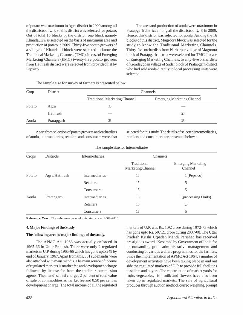
438 Agricultural Situation in India
of potato was maximum in Agra district in 2009 among allthe districts of U.P. so this district was selected for potato.Out of total 15 blocks of the district, one block namelyKhandauli was selected on the basis of maximum area andproduction of potato in 2009. Thirty-five potato growers ofa village of Khandauli block were selected to know theTraditional Marketing Channels (TMC). In case of EmergingMarketing Channels (EMC) twenty-five potato growersfrom Hathrash district were selected from provided list byPepsico.
The area and production of aonla were maximum inPratapgarh district among all the districts of U.P. in 2009.Hence, this district was selected for aonla. Among the 16blocks of this district, Magroora block was selected for thestudy to know the Traditional Marketing Channels.Thirty-five orchardists from Narharpur village of Magroorablock of Pratapgarh district were selected for TMC. In caseof Emerging Marketing Channels, twenty-five orchardistsof Goadaygoan village of Sadar block of Pratapgarh districtwho had sold aonla directly to local processing units wereselected.
The sample size for survey of farmers is presented below
Crop District Channels
Traditional Marketing Channel Emerging Marketing Channel
Potato Agra 35 —
Hathrash — 25
Aonla Pratapgarh 35 25
Apart from selection of potato growers and orchardistsof aonla, intermediaries, retailers and consumers were also
selected for this study. The details of selected intermediaries,retailers and consumers are presented below :
The sample size for Intermediaries
Crops Districts Intermediaries Channels
Traditional Emerging MarketingMarketing Channel Channel
Potato Agra/Hathrash Intermediaries 15 1 (Pepsico)
Retailers 15 5
Consumers 15 5
Aonla Pratapgarh Intermediaries 15 1 (processing Units)
Retailers 15 .5
Consumers 15 5Reference Year: The reference year of this study was 2009-2010
4. Major Findings of the Study
The following are the major findings of the study.
The APMC Act 1963 was actually enforced in1965-66 in Uttar Pradesh. There were only 2 regulatedmarkets in U.P. during 1965-66 which has gone upto 249 byend of January, 1967. Apart from this, 381 sub mandis werealso attached with main mandis. The main source of incomeof regulated markets is market fee and development chargefollowed by license fee from the traders / commissionagents. The mandi samiti charges 2 per cent of total valueof sale of commodities as market fee and 0.50 per cent asdevelopment charge. The total income of all the regulated
markets of U.P. was Rs. 1.92 crore during 1972-73 whichhas gone upto Rs. 507.21 crore during 2007-08. The UttarPradesh Krishi Utpadan Mandi Parishad has receivedprestigious award “Kosamb” by Government of India forits outsanding good administrative management andconducting of various welfare programmes for the farmers.Since the implementation of APMC Act 1964, a number ofdevelopment activities have been taking place in and outside the regulated markets of U.P. to provide full facilitiesto sellers and buyers. The construction of market yards forfruits vegetables, fish, milk and flowers have also beentaken up in regulated markets. The sale of agriculturalproduces through auction method, correc weighing, prompt

November, 2012 439
payment without undue deductions, availability ofamenities etc, are basic activities of regulated markets ofUttar Pradesh.
The Interference of bureaucrats is more prevalentbecause the election could not be held up for a long time inalmost all the regulated markets of Uttar Pradesh. Most ofregulated markets of the state were not fully equipped asper norm of APMC Act 1963.
As far as sample farmers are concerned, the analysisreveals that the majority of sample farmers of potato aswell as aonla of both channels belonged to small andmarginal categories. The agriculture was main occupationof all the selected households of potato and aonla. Thearea under potato as well as aonla was fully irrigated. Noneof the sample farmers of both crops had micro irrigationdevices. Per hectare paid out cost of potato in TMC washigher by 13.04 per cent over Rs. 72,776 in case of EMC.Out of total paid out costs, seed alone accounted for 46.55per cent and 52.21 per cent in TMC and EMC respectively.Two varieties of potato namely chipsona and LR have beenonly preferred by Pepsico.
As far as aonla is concerned, the analysis revealsthat per hectare paid out cost was Rs. 59,633 in case ofTMC against Rs. 51,961 in case of EMC. Out of total perhectare paid out costs, maximum cost in both channelswas incurred for hired labour.
The productivity of potato in case of TMC was 299quintals against 296 quintals in case of EMC. Theproductivity of aonla was 249 quintal in case of EMC against246 quintal in case of TMC. The sample farmers of potatohad received the price of 512 per quintal under TMC againstRs. 588 under EMC. The per quintal net profit on paid out
cost was Rs. 253 under TMC against Rs. 342 per quintalunder EMC. The sample farmers of potato had gained muchhigher price sold through EMC than sold through TMC.
The per quintal price of aonla was Rs. 544 in TMC ascompared to price of Rs. 553 per quintal ir case of TMC.The per quintal net profit of aonla on paid out cost was Rs.311 in case of EMC against Rs. 290 in case of TMC. Theanalysis shows that sample farmers of potato and aonla,were getting better price sold through EMC than that ofTMC in the study areas during the reference year.
5. Price Spread and Marketing Costs
As far as price spread and marketing cost of potatoare concerned table-l reveals that producer share inconsumer's rupee in case of TMC was 75.55 per cent andtotal marketing costs incurred by a producer accounted for3.02 per cent of consumer’s price. The price spread in caseof TMC was 165.70 per quintal of which, the share ofwholesaler was 3.32 per cent from producer price and 2.51per cent retailer's price. The net margin retained bywholesaler and retailer in APMC was estimated at 2.51 percent and 3.60 per cent of consumer's price respectively.The marketing efficiency was worked out of 0.36 in case ofTMC.
As far as price spread in marketing of potato throughEMC is concerned, Pepsico had purchased potato only fortheir own processing units. Hence, Pepsico neither soldthe potato in Super Market/ Big Bazar nor through mall.The retailers were not involved in the marketing of potatoin EMC in the study area. The producers had sold potatoat the rate of Rs. 588 per quintal to Pepsico against Rs. 512in APMC Agra. Thus, the producer received net margin of76 per quinta in case of EMC than sold through TMC.
TABLE 1—PRICE SPREAD AND MARKETING COST FOR POTATO (2009)
Sr. No. Price Spread TMC EMC
I Price received by farmer 512 588II Total marketing costs of farmer 20.50 —
(a) Transport to APMC 15.00 —(b) Loading and Unloading 3 —(c) Weighing & other related expenses 1.50 —(d) Commission, sorting etc. 1.00 —(e) Standard deduction considered as wastage 00 —Net price received by farmer 491.50 588Net profit (Net price received on paid out cost) 208.50 336
III Marketing costs of wholesalers 51.30 —(a) Market fee 12.80 —
(b) Gunny bags 36.00 —
(c) Stitching gunny bag 0.50 —

440 Agricultural Situation in India
(d) Hamali 2.00 —
( e) Wastage during transport 00 —
(t) Transport to terminal market 00 —
(g) Wholesaler's margin 17.00 —
Purchase price of wholesaler plus marketing cost 563.30 —
IV Marketing cost of retailers 73.00 —
(a) Hamali from point of purchase to tempo 2.00 —
(b) Transport to retail outlet 15.00 —
(c) Miscellaneous expenses such as cess to corporation, watchman for unsold 46.00 — stock, supermarket overheads, etc.
(d) Wastage 10.00 —
(e) Retailer's margin 24.40 —
sale price of retailers 677.70 —
V Share of farmer % in retailer’s price 75.55 —
VI Marketing Costs as % of retailer's price 21.37 —
VII Marketing margins as % of retailer’s price 6.11 —
VIII Modified Measure of Marketing Efficiency 0.36 —Source: computed from field survey data.
TABLE 1—PRICE SPREAD AND MARKETING COST FOR POTATO (2009)—Contd.
Sr. No. Price Spread TMC EMC
TABLE 2—PRICE SPREAD AND MARKETING COST FOR AONLA (2009)
Sr. No. Price Spread TMC EMC
I Price received by farmer 544.00 533.00
II Total marketing costs of farmer 35.50 —
(a) Transport to APMC 30.00 —
(b) Loading and Unloading 3.00 —
(c) Weighing & other related expenses 1.50 —
(d) Commission, sorting and stacking 1.00 —
(e) Standard deduction considered as wastage 0.00 —
Net price received by farmer 508.50 533.00
In spite of this, the producer had incurred Rs. 20.50per quintal as marketing cost under TMC while it was nil incase of EMC. Besides this, the producers had not paidcommission to commission agents and also free fromexploitation from irtermediaries when he had sold potato toPepsico.
As far as price spread of aonla is concerned a numberof deductions either in kind or cash are made in aonla byvarious intermediaries in regulated market of Pratapgarh.
The Producers share in consumer's rupee of aonla was72.53 per cent in case of TMC. The marketing costs andmargins accounted for 15.08 per cent and 17.12 per cent ofretailer's price respectively. The marketing cost incurredon consumer's price by sample farmers was 4.73 per cent ascompared to 7.01 per cent and 3.33 per cent by wholesalerand retailer respectively. The retailer margin was higherbeing 14.73 per cent than wholesaler margin of 2.39 percent of the consumer's price. (Table-2)

November, 2012 441
Net profit (Net price received on paid out cost) 242.50 —
III Marketing costs of wholesalers 52.60 —
(a) Market fee 13.60 —
(b) Gunny bags 36.00 —
(c) Stitching gunny bag 1.00 —
(d) Hamali 2.00 —
( e) Wastage during transport 0.00 —
(f) Transport to terminal market 0.00 —
(g) Wholesaler's margin 17.90 —
Purchase price of wholesaler plus marketing cost
IV Marketing cost of retailers 25.00 —
(a) Hamali from point of purchase to tempo 5.00 —
(b) Transport to retail outlet 10.00 —
(c) Miscellaneous expenses such as cess to corporation, watchman for unsold 10.00 — stock, supermarket overheads, etc.
(d) Wastage 0.00 —
(e) Retailer's margin 110.50 —
(f) sale price of retailer 750.00 —
V Share of farmer % in retailer's price 72.53 —
VI Marketing Costs as % of retailer's price 15.08 —
VII Marketing margins as % of retailer's price 17.12 —
VIII Modified Measure of Marketing Efficiency 0.44 —Source: computed from field survey data.
TABLE 2—PRICE SPREAD AND MARKETING COST FOR AONLA (2009)—Contd.
Sr. No. Price Spread TMC TMC
With respect to sale of aonla through EMC, retailerswere also not involved. The total purchased quantity ofaonla by processing units was utilized for preparation ofprocessed products. The producer had received the priceof Rs. 533 per quintal of aonla from processing units against
Rs. 544 per quintal from traders in regulated market ofPratapgarh. In this way, the producer received net profit ofRs. 533 per quintal under EMC against Rs. 508.50 underTMC. The reason of the higher profit in case of EMC wasno involvement of marketing costs.
TABLE-3—BENEFIT COST RATIO FOR POTATO AND AONLA
Particulars TMC (cost of EMC (cost of TMC (cost of EMC (cost ofproduction production production' production
includes only includes only includes family includes familypaid out costs) paid out costs) labour) labour)
BCR for Potato 1.86 2.39 1.83 2.34
BCR for Aonla 2.25 2.49 2.14 2.43
Source: Computed from field survey data
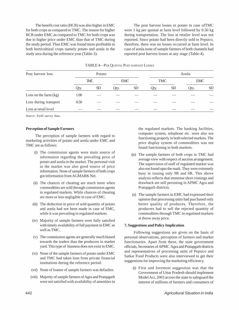
442 Agricultural Situation in India
The benefit cost ratio (HCR) was also higher in EMCfor both crops as compared to TMC. The reason for higherBCR under EMC as compared to TMC for both crops wasdue to higher price under EMC than that of TMC duringthe study period. Thus EMC was found more profitable inboth horticultural crops namely potato and aonla in thestudy area during the reference year (Table-3).
The post harvest losses in potato in case ofTMCwere 1 kg per quintal at farm level followed by 0.50 kgduring transportation. The loss at retailer level was notreported. Since potato had been directly sold to Pepsico,therefore, there was no losses occurred at farm level. Incase of aonla none of sample farmers of both channels hadreported post harvest losses at any stage (Table-4).
TABLE 4—PER QUINTAL POST HARVEST LOSSES
Post harvest loss Potato Aonla
TMC EMC TMC EMC
Qty. SD Qty. SD Qty. SD Qty. SD
Loss on the farm (kg) 1.00 — — — — — — —
Loss during transport 0.50 — — — — — — —
Loss at retail level — — — — — — — —
Source: Field survey data.
Perception of Sample Farmers
The perception of sample farmers with regard tomarketing activities of potato and aonla under EMC andTMC are as follows:
(i) The commission agents were main source ofinformation regarding the prevailing price ofpotato and aonla in the market. The personal visitin the market was also good source of priceinformation. None of sample farmers of both cropsgot information from AGMARK Net.
(ii) The chances of cheating are much more whencommodities are sold through commission agentsin regulated markets. While chances of cheatingare more or less negligible in case of EMC.
(iii) The deduction in price of sold quantity of potatoand aonla had not been made in case of EMC,while it was prevailing in regulated markets.
(iv) Majority of sample farmers were fully satisfiedwith timely availability of full payment in EMC aswell as TMC.
(v) The commission agents are generally much biasedtowards the traders than the producers in marketyard. This type of biasness does not exist in EMC.
(vi) None of the sample farmers of potato under EMCand TMC had taken loan from private financialinstitutions during the reference period.
(vii) None of loanee of sample farmers was defaulter.
(viii) Majority of sample farmers of Agra and Pratapgarhwere not satisfied with availability of amenities in
the regulated markets. The banking facilities,computer system, telephone etc. were also notfunctioning properly in both selected markets. Theprice display system of commodities was notfound functioning in both markets.
(ix) The sample farmers of both crops in TMC hadaverage view with respect of auction arrangement.The supervision of staff of regulated market wasalso not found upto the mark. They were extremelybusy in issuing only 9R and 6R. This aboveanalysis reflects that immense short comings anddrawback are still persisting in APMC Agra andPratapgarh districts.
(x) The sample farmers in EMC had expressed theiropinion that processing units had purchased onlybetter quality of produces. Therefore, theproducers had to sell the rejected quantity ofcommodities through TMC in regulated marketsat throw away price.
7. Suggestions and Policy Implication
Following suggestions are given on the basis ofpersonal observations, perception of farmers and marketfunctionaries. Apart from these, the state governmentofficials, Secretaries of APMC Agra and Pratapgarh districtsand representatives of processing units of Pepsico andSatkar Food Products were also interviewed to get theirsuggestions for improving the marketing efficiency.
(i) First and foremost suggestion was that theGovernment of Uttar Pradesh should implementModel Act, 2003 across the state to safeguard theinterest of millions of farmers and consumers of

November, 2012 443
the state. This would not only increase the incomeof farmers but also open new avenues for exportof agricultural and horticultural produces from thestate. The Private and Public Partnership will alsodevelop to improve the marketing efficiency ofagricultural and horticultural produces.
(ii) The State Government should also motivate theprivate sectors to establish the processing unitsin potential pockets of the state to avoid distresssale of agricultural and horticultural producesduring bumper production of crops.
(iii) Almost all the APMCs of the state have beenearning good income throughout the year but theinvestment on the infrastructural facilities andbasic amenities is not being done properly neitheroutside the markets nor inside the market. Theinvestment according to income of the marketshould be made on the development ofinfrastructure facilities to provide better facilitiesto sellers and buyers during marketing ofcommodities.
(iv) The mini cold storages should be constructed inmarket yard or near by the market to protect thelosses of unsold fruits, vegetables, flowers etc.for a long duration.
(v) The deduction practices in cash or kind is stillpersisting in market yard. This should not beallowed at any cost.
(vi) The rules and regulations of APMC Act 1963,should be totally enforced in the regulatedmarkets. Any type of harassment of farmers shouldnot be done by commission agents, traders andothers. The staff of regulated market should keepvigilant watch on these imbroglio to protect thefarmers.
(vii) The auction of commodities and fixation of itsprices should be made more transparent Totalaccountability should be fixed on the staff ofregulated market in this regard.
(viii) The state intervention is also needed in case ofhorticultural produces when its price goes downquite low during the huge arrival in the market.The state government should take immediate step
to supply these commodities to deficit places tomaintain the price equilibrium.
(ix) Since a long time, election of Marketing Boardhas not been held in almost all regulated marketsof the state, hence the election of Marketing Boardshould take place as soon as possible across thestate to provide public representation in thedecision making process
(x) The farmers are still cheated and exploited in theregulated markets by the market functionaries indifferent ways. Therefore, the authorities ofregulated markets should be more vigilant andactive to eliminate the foul activities andoperations in the market.
(xi) Since, the association of intermediaries is verystrong and well united, therefore authority ofregulated market should give more protection toproducers rather than intermediaries.
(xii) The commission agents and wholesalers are wellacquainted with price of different commodities indifferent markets of places outside the state. Theyare getting information of prices of differentcommodities through land line telephone, mobile,internet etc. while the producers are generallyignorant in this regard. Therefore, the StateGovernment should take concrete step to providethe upto date information of prices of commoditiesto the farmers through print and electronic media.The proper display of latest price list of prices ofdifferent commodities should be posted on thegate of market.
(xiii) The maximum attention is needed to develop therural roads to facilitate the farmers of remotevillages to bring their produces in Mandi withoutany botheration.
(xiv) The Central and U.P. Governments should allotmaximum amount to establish cold chains systemacross the state to protect the quality and quantitylosses of horticultural produces.
(xv) The farmers of Uttar Pradesh should get pledgeloan from APMCs to get higher prices of theircommodities during the lean period.

444 Agricultural Situation in India
D. Commodity Reviews
(i) Foodgrains
ALL INDIA INDEX NUMBER OF WHOLESALE PRICES
(Base : 2004-2005=100)
Commodity Weight WPI for the WPI for the WPI Percentage change(%) Month of Month of A year ago during
October September A A2012 2012 month year
(1 ) (2) (3) (4) (5) (6) (7)
Rice 1.793 196.4 194.8 176.3 0.82 11 .40Wheat 1.116 198.0 198.0 165.3 0.00 19.78Jowar 0.096 234.5 234.8 248.7 –0.13 –5.71Bajra 0.115 219.0 232.3 184.5 –5.73 18.70Maize 0.217 231.4 235.1 194.1 –1.57 19.22Barley 0.017 198.2 200.6 174.6 –1.20 13.52Ragi 0.019 284.8 269.9 208.7 5.52 36.46Cereals 3.373 201.6 201.3 176.3 0.15 14.35Pulses 0.717 265.8 261.4 214.0 1.68 24.21Foodgrains 4.09 211.2 211.9 182.9 –0.33 15.47Source : Office of the Economic Adviser, M/o Commerce and Industry.
During the month of October, 2012 the WholesalePrices of food grains displayed a declining trend.Wholesale Price Index (Base 2004-05=100) of Food grains
fell by 0.33% while that of pulses and cereals rose by1.68% and 0.15% respectively over the previous month.
Behaviour of Wholesale PricesThe following Table indicates the State wise trend
of Wholesale Prices of Cereals during the month ofOctober, 2012.
Commodity Main Rising Falling Mixed SteadyTrend
Rice Mixed Jharkhand AssamHaryana GujaratKerala West BengalUttar PradeshKarnatakaTamil Nadu
Wheat Mixed M.P. Kamataka GujaratHaryana Jharkhand Rajasthan
Uttar PradeshJowar Falling Maharashtra Gujarat Rajasthan U.P.
Karnataka A.P.Tamil Nadu
Bajra Steady & A.P. Tamil Nadu Gujarat U.P.Falling Rajasthan Karnataka
Maize Falling U.P. Gujarat Haryana M.P.Jharkhand A.P. Rajasthan
Karnataka

November, 2012 445
PROCUREMENT OF RICE
(in thousand tonnes)
State Marketing Season Corresponding Marketing Year2012-13 Period of last Year (October-September)
(up to 31-10-2012) 2011-12 2011-12 2010 -11Procure- Percentage Procure- Percentage Procure- Percentage Procure- Percentagement to Total ment to Total ment to Total ment to Total
(1) (2) (3) (4) (5) (6) (7) (8) (9)
Andhra Pradesh 0 0.00 0 0.00 7540 22.05 9610 30.00Chhatisgarh 0 0.00 0 0.00 4115 12.03 3746 11.69Haryana 2101 26.47 1715 20.91 2007 5.87 1687 5.27Maharashtra 0 0.00 0 0.00 178 0.52 308 0.96Punjab 5825 73.38 6297 76.79 7731 22.61 8635 26.96Tamil Nadu 1 0.01 161 1.96 1596 4.67 1543 4.82Uttar Pradesh 1 0.01 6 0.07 3355 9.81 2554 7.97Uttarakhand 1 0.01 1 0.01 378 1.11 422 1.32Others 9 0.11 20 0.24 8131 23.78 5693 17.77
Total 7938 100.00 8200 100.00 35031 100.00 34198 100.00Source: Department of Food & Public Distribution.
Procurement of Rice
7938 thousand tonnes of Rice (including paddyconverted into rice) was procured during October, 2012, asagainst 8200 thousand tonnes of Rice (including paddyconverted into rice) procured during October 2011.The total
procurement of Rice in the current marketing season i.e2012-2013, upto 31.10.2012 stood at 7938 thousand tonnes,as against 8200 thousand tonnes of rice procured, duringthe corresponding period of last year. The details are givenin the following table.
Procurement of Wheat
The total procurement of wheat in the current marketingseason i.e 2012-2013 upto August, 2012 is 38148 thousand
tonnes against a total of 28148 thousand tonnes of wheatprocured during last year. The details are given in the followingtable :
PROCUREMENT OF WHEAT
(in thousand tonnes)
State Marketing Season Corresponding Marketing Year2012-13 Period of last Year (April-March)
(up to 2-08-2012) (2011-12) 2011-12 2010-11 Procure- Percentage Procure- Percentage Procure- Percentage Procure- Percentagement to Total ment to Total ment to Total ment to Total
(1 ) (2) (3) (4) (5) (6) (7) (8) (9)Haryana 8665 22.71 6882 24.45 6928 24.45 6347 28.19Madhya Pradesh 8493 22.26 4905 17.43 4965 17.52 3539 15.72Punjab 12834 33.64 10957 38.93 10958 38.67 10209 45.35Rajasthan 1964 5.15 1303 4.63 1303 4.60 476 2.11Uttar Pradesh 5063 13.27 3461 12.30 3461 12.21 1645 7.31Others 1129 2.96 640 2.27 720 2.54 298 1.32
Total 38148 100.00 28148 100.00 28335 100.00 22514 100.00Source: Department of Food & Public Distribution.
446 Agricultural Situation in India
(ii) Commercial Crops
OIL SEEDS AND EDIBLE OILS :
The Wholesale Price Index (WPI) of nine majoroilseeds as a group stood at 196.6 in October, 2012 showinga fall of 5.0 per cent over the previous month.However, itincreased by 27.2 per cent over the previous year.
The Wholesale Price Index (WPI) of all individualoilseeds showed a mixed trend. The WPI of Rape & Mustard(4.5 per cent), Sunflower (2.7 per cent) and Cottonseed (1.0per cent) increased over the previous month. However, theWPI of Soyabean (-21.7 per cent), Niger Seed (-9.1 percent), Gingelly seed (-5.1 per cent), Safflower seed (-2.5 percent), Copra ( -1.7 per cent) and Groundnut seed (-0.7 percent) decreased over the previous month. The WholesalePrice Index (WPI) of Edible Oils as a group stood 148.1 inOctober, 2012 showing a fall of 1.9 per cent over theprevious month. However, it increased by 9.4 per cent overthe previous year. The, WPI of Groundnut Oil (4.6 percent), Soyabean Oil (3.1 per cent), Mustard Oil (1.5 percent), Sunflower Oil (1.3 per cent), Gingelly Oil (1.2 percent), Cottonseed Oil (1.0 per cent) and Copra oil (0.8 percent) decreased over the previous month.
FRUITS AND VEGETABLE :
The Wholesale Price Index (WPI) of Fruits &Vegetable as a group stood at 192.9 in October, 2012showing a fall of 1.0 per cent and 2.9 per cent over theprevious month and over the previous year.
POTATO :
The Wholesale Price Index (WPI) of Potato stood at231.0 in October, 2012 showing a fall of 4.8 per cent over
the previous month. However, it increased by 49.1 per centover the previous year.
ONION :
The Wholesale Price Index (WPI) of Onion stood210.2 in October, 2012 showing an increase of 8.4 per centover the previous month. However, it decreased by 9.1 percent over the previous year.
CONDIMENTS AND SPICES :
The Wholesale Price Index (WPI) of Condiments &Spices (Group) stood at 208.8 in October, 2012 showing afall of 0.7 per cent and 18.3 per cent over the previousmonth and over the previous year.
The Wholesale Price Index of Black Pepper, Chillies(Dry) and Turmeric decreased by 0.2 per cent, 1.7 per centand 1.3 per cent, respectively over the previous month.
RAW COTTON :
The Wholesale Price Index (WPI) of Raw Cottonstood at 200.9 in October, 2012 showing a fall of 5.1 percent and 9.5 per cent over the previous month and over theprevious year.
RAW JUTE :
The Wholesale Price Index (WPI) of Raw Jute stoodat 241.9 in October, 2012 showing a fall of 5.2 per cent overthe previous month. However, it increased by 15.4 per centover the previous year.

November, 2012 447
WHOLESALE PRICE INDEX OF COMMERCIAL CROPS FOR THE MONTH OF OCTOBER, 2012
(Base Year : 2004-05=100)
Commodity Latest Month Year Percent Variation over the
Oct., 2012 Sep., 2012 Oct., 2011 Month Year
Oil Seeds 196.6 207.0 154.5 –5.0 27.2
Groundnut Seed 241.3 243.0 196.9 –0.7 22.5
Rape and Mustard Seed 224.4 214.8 150.4 4.5 49.2
Cotton Seed 174.6 172.8 148.0 1.0 18.0
Copra (Coconut) 88.4 89.9 111.0 –1.7 –20.4
Gingelly Seed (Sesamum) 300.4 316.6 201.4 –5.1 49.2
Niger Seed 191.8 210.9 174.9 –9.1 9.7
Safflower (Kardi Seed) 150.4 154.2 126.8 –2.5 18.6
Sunflower 184.3 179.5 156.5 2.7 17.8
Soyabean 189.1 241.4 124.8 –21.7 51.5
Edible Oils 148.1 150.9 135.4 –1.9 9.4
Groundnut Oil 183.2 192.0 161.1 –4.6 13.7
Cotton Seed Oil 186.7 188.6 150.9 –1.0 23.7
Mustard and Rapeseed Oil 154.8 157.2 136.7 –1.5 13.2
Soyabean Oil 163.4 168.6 147.0 –3.1 11.2
Copra Oil 111.6 112.5 123.7 –0.8 –9.8
Sunflower Oil 137.1 138.9 134.8 –1.3 1.7
Gingelly Oil 163.9 165.9 143.2 –1.2 14.5
Fruits and Vegetables 192.9 194.9 198.7 –1.0 –2.9
Potato 231.0 242.7 154.9 –4.8 49.1
Onion 210.2 194.0 231.3 8.4 –9.1
Condiments and Spices 208.8 210.2 255.5 –0.7 –18.3
Black Pepper 530.3 531.1 433.7 –0.2 22.3
Chillies (Dry) 226.4 230.4 295.6 –1.7 –23.4
Turmeric 169.1 171.4 190.1 –1.3 –11.0
Raw Cotton 200.9 211.7 222.1 –5.1 –9.5
Raw Jute 241.9 255.3 209.6 –5.2 15.4

448 Agricultural Situation in India
PART II—Statistical TablesA. Wages
1. DAILY AGRICULTURAL WAGES IN SOME STATES (CATEGORY-WISE)(in Rupees)
State/Distt. Village Month Normal Field Labour Other Agri. Labour Herdsman Skilled Labourand DailyYear Working Man Wo- Non Man Wo- Non Man Wo- Non Car- Black- Cob-
Hours man Adult man Adult man Adult penter smith bler
(1) (2) (3) (4) (5) (6) (7) (8) (9) (10) (11) (12) (13) (14) (15) (16)
Andhra PradeshKrishna Ghantasala Dec., 2011 8 250.00 100.00 NA 250.00 130.00 NA NA NA NA NA NA NA
Guntur Tadikonda Dec., 2011 8 200.00 175.00 110.00 200.00 160.00 110.00 160.00 NA NA NA NA NA
Rangareddy Arutla Dec., 2011 8 200.00 120.00 NA 150.00 120.00 NA 150.00 120.00 NA 220.00 200.00 NA
Karnataka
Bangalore Harisandra May to 8 200.00 150.00 NA 200.00 150.00 NA 250.00 180.00 NA 300.00 300.00 NAJune, 2012
Tumkur Gedlahali May to 8 160.00 160.00 NA 180.00 160.00 NA 180.00 160.00 NA 180.00 180.00 NAJune, 2012
Maharashtra
Nagpur Mauda Dec., 2009 8 100.00 80.00 NA NA NA NA NA NA NA NA NA NA
Ahmednagar Akole June, 2009 8 80.00 70.00 NA NA NA NA NA NA NA 83.5 85.00 85.00
Jharkhand
Ranchi Gaintalsood April, 2012 8 100.00 100.00 NA 90.00 90.00 NA 58.00 58.00 NA 170.00 150.00 NA
1.1 DAILY AGRICULTURAL WAGES IN SOME STATES (OPERATION-WISE)(in Rupees)
State/Distt. Centre Month Type Normal Skilled Labourand of Daily Plough- Sow- Weed- Harvest- Other Herds- Car- Black- Cob-Year Lab- Work- ing ing ing ing Agri. man penter smith bler
our ing LabourHours
(1) (2) (3) (4) (5) (6) (7) (8) (9) (10) (11) (12) (13) (14)
Assam
Barpeta Loharapara March, 12 M 8 180.00 180.00 180.00 180.00 180.00 180.00 180.00 180.00 180.00W 8 NA NA 160.00 160.00 160.00 NA NA NA NA
Bihar
Muzaffarpur Bhalui Rasul Feb. and, M 8 104.00 104.00 104.00 104.00 104.00 NA 150.00 150.00 150.00March, 2010 W 8 NA 104.00 104.00 104.00 104.00 NA NA NA NA
Shekhpura Kutaut May and M 8 150.00 NA NA NA 150.00 NA 220.00 NA NAJune, 2010 W 8 NA NA NA NA NA NA NA NA NA
ChhattisgarhDhamtari Sihaba July, 2012 M 8 350.00 100.00 100.00 NA 80.00 80.00 200.00 100.00 80.00
W 8 NA 80.00 80.00 NA 60.00 NA NA NA NA
GujaratRajkot Rajkot March, 2012 M 8 247.00 270.00 164.00 197.00 168.00 140.00 408.00 358.00 240.00
W 8 NA 182.00 142.00 167.00 167.00 100.00 NA NA NA
Dahod Dahod March, 2012 M 8 71.00 71.00 71.00 71.00 71.00 NA 143.00 150.00 150.00W 8 NA 71.00 71.00 71.00 71.00 NA NA NA NA
Haryana
Panipat Ugarakheri May and M 8 180.00 180.00 180.00 200.00 180.00 NA NA NA NAJune, 2012 W 8 NA 150.00 150.00 180.00 150.00 NA NA NA NA

November, 2012 449
1.1 DAILY AGRICULTURAL WAGES IN SOME STATES (OPERATION-WISE)—Contd.0 (in Rupees)
State/Distt. Centre Month Type Normal Skilled Labourand of Daily Plough- Sow- Weed- Harvest- Other Herds- Car- Black- Cob-Year Lab- Work- ing ing ing ing Agri. man penter smith bler
our ing LabourHours
(1) (2) (3) (4) (5) (6) (7) (8) (9) (10) (11) (12) (13) (14)
Himachal Pradesh
Mandi Mandi Nov., to M 8 300.00 110.00 110.00 110.00 110.00 110.00 200.00 200.00 NADec. 2010 W 8 NA 110.00 110.00 110.00 110.00 110.00 NA NA NA
Kerala
Kozhikode Koduvally Feb., and M 4 to 8 720.00 450.00 NA 450.00 572.05 NA 500.00 NA NAMarch, 2012 W 4 to 8 NA NA 350.00 350.00 350.00 NA NA NA NA
Palakkad Elappally Feb., and M 4 to 8 400.00 300.00 NA 275.00 368.75 NA 400.00 NA NAMarch, 2012 W 4 to 8 NA NA 150.00 200.00 160.00 NA NA NA NA
Madhya Pradesh
Hoshangabad Sangarkhera Aug., 2012 M 8 150.00 130.00 150.00 150.00 125.00 100.00 350.00 350.00 NAW 8 NA 130.00 150.00 150.00 125.00 100.00 NA NA NA
Satna Kotar Aug., 2012 M 8 NA NA NA NA NA NA NA NA NAW 8 NA NA NA NA NA NA NA NA NA
Shyopur Kala Vijaypur Aug., 2012 M 8 NA NA NA NA NA NA NA NA NAW 8 NA NA NA NA NA NA NA NA NA
Orissa
Bhadrak Chandbali May, 2012 M 8 220.00 150.00 NA NA 166.66 150.00 250.00 140.00 140.00W 8 NA NA NA NA 106.66 100.00 NA NA NA
Ganjam Aska May, 2012 M 8 250.00 150.00 150.00 150.00 168.33 150.00 300.00 150.00 150.00W 8 NA 100.00 100.00 100.00 100.00 100.00 NA NA NA
Punjab
Ludhiana Pakhowal June, 2008 M 8 NA NA 90.00 95.00 NA 99.44 NA NA NAW 8 NA NA NA NA NA NA NA NA NA
Rajasthan
Barmer Vishala July, 2012 M 8 —NA—
W 8 —NA—
Jalore Panwa July, 2012 M 8 NA NA NA NA NA 50.00 100.00 50.00 NAW 8 NA NA NA NA NA NA NA NA NA
Tamil Nadu
Thanjavur Pulvarnatham Aug., 2012 M 6 —NA—M 5
Tirunelveli Malayakulam Aug., 2012 M 8 NA NA NA NA NA NA NA NA NA(Kurvikulam) W 8 NA NA 100.00 NA NA NA NA NA NA
Tripura
Agartala Govt. Agri. M —NA—Farm W
Uttar Pradesh*
Meerut Ganeshpur July, 2012 M 8 208.00 205.00 205.00 207.00 204.00 NA 306.00 NA NAW 8 NA 175.00 175.00 177.00 176.00 NA NA NA NA
Aurraiya# Aurraiya July, 2012 M 8 120.00 120.00 120.00 132.9 120.00 NA 257.1 NA NAW 8 NA NA 120.00 132.9 120.00 NA NA NA NA
Chandauli Chandauli July, 2012 M 8 NA NA NA 125.00 125.00 NA 236.00 NA NAW 8 NA NA NA 125.00 125.00 NA NA NA NA
M-Man, W-Woman,
N. A. —Not Available N. R. —Not Reported
*- Uttar Pradesh reports its district-wise average rural wage data rather than from selected centre/village.
# New district is opted to replace Chandbali.

450 Agricultural Situation in India
B. PRICES
2. WHOLESALE PRICES OF CERTAIN IMPORTANT AGRICULTURAL COMMODITIES AND ANIMAL HUSBANDRY
PRODUCTS AT SELECTED CENTRES IN INDIA
(Month-end Prices in Rupees)
Commodity Variety Unit State Centre Oct.-12 Sep.-12 Oct.-11
(1) (2) (3) (4) (5) (6) (7) (8)
Wheat PBW 343 Quintal Punjab Amritsar 1450 1450 1155
Wheat Dara Quintal Uttar Pradesh Chandausi 1400 1450 1050
Wheat — Quintal Madhya Pradesh Sagar 2000 2000 1500
Jowar — Quintal Maharashtra Mumbai 2000 2100 2100
Gram — Quintal Punjab Abohar NA NA NA
Maize Yellow Quintal Uttar Pradesh Bahraich 1165 1120 1035
Gram Split — Quintal Maharashtra Mumbai 6350 5800 4500
Gram Split — Quintal Bihar Patna 5400 5460 4560
Arhar Split — Quintal NCT of Delhi Delhi 6700 7000 N T
Arhar Split — Quintal Maharashtra Mumbai 6625 6250 6000
Arhar Split Sort-II Quintal Tamil Nadu Chennai 6000 6100 5200
Arhar Split — Quintal Bihar Patna 5900 5850 5750
Gur Balti Quintal Uttar Pradesh Hapur 2675 3050 2350
Gur Sort-II Quintal Tamil Nadu Chennai NA 3200 3000
Gur — Quintal Maharashtra Mumbai 3400 3350 2800
Mustard Seed Rai UP Quintal West Bengal Kolkata 4300 4425 3300
Mustard Seed Raira Quintal West Bengal Kolkata NA NA NA
Mustard Seed Black(S) Quintal Uttar Pradesh Kanpur 4120 4190 2925
Linseed — Quintal Maharashtra Nagpur 4100 4000 2950
Linseed Bada Dana Quintal Uttar Pradesh Kanpur 4350 4270 3100
Cotton Seed Superior Quintal Maharashtra Jalgaon NA NA NQ
Castor Seed — Quintal Andhra Pradesh Badepalli NA NA NA
Sesamum Seed Black Quintal Tamil Nadu Chennai NA 4500 4500
Cotton Seed — Quintal Maharashtra Mumbai NA NA NA
Copra FAQ Quintal Kerala Alleppey 4100 4050 5450
Groundnut — Quintal Maharashtra Mumbai 8200 7900 5600
Groundnut TMV-7 Quintal Tamil Nadu Chennai NA 4280 4280
Mustard Oil Ordinary 15 Kg. West Bengal Kolkata 1403 1395 1175
Mustard Oil — 15 Kg. Uttar Pradesh Kanpur 1335 1328 1065
Groundnut Oil — 15 Kg. Maharashtra Mumbai 1695 1688 1290
Groundnut Oil — 15 Kg. Tamil Nadu Chennai 1725 1650 1320
Linseed Oil — 15 Kg. Uttar Pradesh Kanpur 1467 1455 1197
Castor Oil — 15 Kg. Uttar Pradesh Kanpur NA NA NA
Sesamum Oil Agmark 15 Kg. Tamil Nadu Chennai 2400 2400 1875
Sesamum Oil — 15 Kg. Maharashtra Mumbai NA NA NA
Coconut Oil — 15 Kg. Kerala Cochin 900 885 1170
Mustard Cake — Quintal Uttar Pradesh Kanpur 2170 2150 1130
Groundnut Cake — Quintal Uttar Pradesh Kanpur NA NA NA
Cotton/Kapas F-414 Quintal Punjab Abohar NA NA NA
Cotton/Kapas LR-A Quintal Tamil Nadu Thiruppur NA NA NA
Wool Fine Quintal Madhya Pradesh Dabra NA NA NA
Jute Raw TD-5 Quintal West Bengal Kolkata 2450 2500 2150

November, 2012 451
2. WHOLESALE PRICES OF CERTAIN IMPORTANT AGRICULTURAL COMMODITIES AND ANIMAL HUSBANDRY
PRODUCTS AT SELECTED CENTRES IN INDIA —Contd.(Month-end Prices in Rupees)
Commodity Variety Unit State Centre Oct.-12 Sept.-12 Oct.-11
(1) (2) (3) (4) (5) (6) (7) (8)
Jute Raw W-5 Quintal West Bengal Kolkata 2450 2500 2150
Oranges — 100 No. Maharashtra Mumbai NA NA NA
Oranges Nagpuri 100 No. West Bengal Kolkata NA NA NA
Oranges Big 100 No. Tamil Nadu Chennai 600 540 640
Banana Basarai 100 No. Maharashtra Jalgaon 220 210 NA
Banana Singapore 100 No. West Bengal Kolkata 350 350 NA
Cashewnuts — Quintal Maharashtra Mumbai 50000 52500 60000
Almonds — Quintal Maharashtra Mumbai 45500 45000 45000
Walnuts — Quintal Maharashtra Mumbai 51250 52500 70000
Kishmish — Quintal Maharashtra Mumbai 11000 11000 15250
Peas Green — Quintal Tamil Nadu Chennai NA NA 10000
Tomatoes — Quintal Tamil Nadu Chennai 1500 1200 2300
Ladyfinger — Quintal Tamil Nadu Chennai 2000 2000 1800
Cauliflower — 100 No. Tamil Nadu Chennai 1100 1100 1000
Potatoes Red Quintal Bihar Patna 1200 1230 650
Potatoes Deshi Quintal West Bengal Kolkata 1200 1060 530
Potatoes Sort-I Quintal Tamil Nadu Mettuppalayam 2365 NA 1333
Onions Bombay Quintal West Bengal Kolkata NA NA NA
Turmeric Erode Quintal West Bengal Kolkata 8200 8000 NA
Turmeric Nadan Quintal Kerala Cochin 8200 7850 8500
Chillies — Quintal Bihar Patna 7100 6800 9400
Black Pepper Palai Quintal Kerala Alleppey N T N T N T
Ginger Dry Quintal Kerala Cochin 11250 11100 12200
Cardamom Big Quintal West Bengal Kolkata 82000 82000 110000
Cardamom Small Quintal West Bengal Kolkata 100000 100000 80000
Milk Cow 100 NCT of Delhi Delhi 3600 3600 3400
Milk Buffalo 100 West Bengal Kolkata 3200 3200 3000
Ghee Deshi Agmark Quintal West Bengal Kolkata 33000 33000 NA
Ghee Deshi — Quintal Uttar Pradesh Khurja 23950 NA NA
Ghee Deshi — Quintal Maharashtra Mumbai NA 25250 28000
Fish Rohu Quintal West Bengal Kolkata 14000 13000 NA
Fish Sea Prawns Quintal Tamil Nadu Chennai — 15000 21000
Eggs Madras 1000 No. West Bengal Kolkata 4000 4000 3000
Tea Medium Quintal Assam Guwahati 21000 20000 14000
Tea Atti Kunna Quintal Tamil Nadu Coimbatore NA NA 13000
Coffee Plant-A Quintal Tamil Nadu Coimbatore 26000 26000 30000
Coffee Rubusta Quintal Tamil Nadu Coimbatore 14000 14000 12400
Tobacco Kampila Quintal Uttar Pradesh Farukhabad 2700 2500 2300
Tobacco Raisa Quintal Uttar Pradesh Farukhabad 2530 2400 2200
Tobacco Bidi /Tobacco Quintal West Bengal Kolkata 4000 4000 3200
Rubber — Quintal Kerala Kottayam 16700 18200 20200
Arecanut Rashi Quintal Tamil Nadu Chennai NA 30000 29500
NA :—Not Available
NT :—Not Transaction

452 Agricultural Situation in India
3. MONTH-END WHOLESALE PRICES OF SOME IMPORTANT AGRICULTURAL COMMODITIES IN INTERNATIONAL
MARKETS DURING YEAR, 2012
Commodity Variety Country Centre Jan. Feb. Mar. Apr. May June Jul. Aug. Sep.
Barley Canada Winni- Dollar/M.T. 213.00 214.00 216.00 220.00 220.00 220.00 220.00 — —peg Rs./Qtl. 1072.88 1048.81 1100.30 1175.68 1183.38 1203.40 1211.54 — —
Cardamom Guatmala Bold U.K. — Dollar/M.T. 15000.00 11000.00 12500.00 12500.00 12500.00 12500.00 12500.00 12500.00 12500.00Green Rs./Qtl. 118395.06 85536.00 101825.00106650.00108412.50109250.00108737.50110125.00110062.50
Cashew Spot U.K. 320s U.K. — Dollar/1bs 4.12 4.03 4.00 4.06 4.03 3.80 3.65 3.55 3.53Kerrnels Rs./Qtl. 71672.23 69067.37 71815.14 76346.38 77034.63 73199.25 69979.98 68931.20 68503.96
Castor Oil Any Origin ex Nether- — Dollar/M.T. 1880.00 1875.00 1700.00 1600.00 1500.00 1500.00 1680.00 1760.00 1600.00
tank Rotterdam lands Rs./Qtl. 9687.64 9185.63 8649.60 8392.00 8305.50 8346.00 9282.00 9771.52 8688.00Celery Seed ASTA cif India — Dollar/M.T. 1500.00 1500.00 1500.00 1500.00 1500.00 1500.00 1500.00 1500.00 1500.00
Rs./Qtl. 7729.50 7348.50 7632.00 7867.50 8305.50 8346.00 8287.50 8328.00 8145.00
Chillies Birds eye 2005 Africa — Dollar/M.T. 5500.00 6500.00 5900.00 5900.00 5650.00 5650.00 5650.00 5650.00 5650.00crop Rs./Qtl. 28341.50 31843.50 30019.20 30945.50 31284.05 31436.60 31216.25 31368.80 30679.50
Cinnamon Mada- — Dollar/M.T. 1100.00 1100.00 1100.00 1100.00 1100.00 1100.00 1100.00 1100.00 1100.00 Bark gascar Rs./Qtl. 5668.30 5388.90 5596.80 5769.50 6090.70 6120.40 6077.50 6107.20 5973.00
Cloves Singapore Mada- — Dollar/M.T. 10875.00 12000.00 12000.00 12000.00 12000.00 10300.00 10500.00 9500.00 9500.00gascar Rs./Qtl. 56038.88 58788.00 61056.00 62940.00 66444.00 57309.20 58012.50 52744.00 51585.00
Coconut Crude Nether- — Dollar/M.T. 1430.00 1430.00 1315.00 1325.00 1030.00 1095.00 1000.00 995.00 990.00Oil Phillipine/ lands Rs./Qtl. 7368.79 7005.57 6690.72 6949.63 5703.11 6092.58 5525.00 5524.24 5375.70
Indonesia
Copra Phillipines cif Philli — Dollar/M.T. 901.50 905.00 835.00 825.50 648.00 692.00 616.00 648.00 609.50Rotterdam pine Rs./Qtl. 4645.43 4433.60 4248.48 4329.75 3587.98 3850.29 3403.40 33597.70 3309.59
Corriander India — Dollar/M.T. 1150.00 1150.00 1150.00 1150.00 1150.00 1150.00 1150.00 1150.00 1150.00Rs./Qtl. 5925.95 5633.85 5851.20 6031.75 6367.55 6398.60 6353.75 6384.80 6244.50
Cummin India — Dollar.M.T. 3800.00 3800.00 3800.00 3800.00 3800.00 2800.00 2800.00 2800.00 2800.00Seed Rs./Qtl. 19581.40 18616.20 19334.40 19931.00 21040.60 15579.20 15470.00 15545.60 15204.00
Fennel seed India — Dollar/M.T. 2600.00 2600.00 2600.00 2600.00 2600.00 2600.00 2600.00 2600.00 2600.00Rs./Qtl. 13397.80 12737.40 13228.80 13637.0 14396.20 14466.40 14365.00 14435.20 14118.00
Ginger Split Nigeria — Dollar/M.T. 3800.00 3400.00 2550.00 2550.00 2550.00 2550.00 2550.00 2550.00 2550.00Rs./Qtl. 19581.40 16656.60 12974.40 13374.75 14119.35 14188.20 14088.75 14157.60 13846.50
Groundnut US 2005, 40/50 European — Dollar/M.T - - - 2400.00 1725.00 1650.00 1595.00 1555.00 1400.00kerrnels cif Rotterdam Ports Rs./Qtl. - - - 12588.00 9551.33 9180.60 8812.38 6412.56 7602.00
Groundnut Crude Any Ori U.K. — Dollar/M.T - 2200.00 2200.00 2200.00 2200.00 2200.00 2200.00 — 2200.00Oil gin cif Rotterdam Rs./Qtl. - 17107.20 17921.20 18770.40 19080.60 19228.00 1917.80 — 19371.00
Lentils Turkish Red Split U.K. — Pound/M.T 587.57 567.02 562.08 553.32 574.59 572.94 571.55 519.93 508.84Crop 1+1 water Rs./Qtl. 4637.69 4409.15 4578.70 4720.93 4983.42 5007.50 4971.91 4580.58 4480.34
Maize U.S.A Chic- C/56 lbs. 658.00 630.00 630.50 607.00 601.25 645.50 790.00 789.75 782.50
ago Rs./Qtl 1332.53 1212.94 1260.74 1251.20 1308.34 1411.48 1715.35 1723.58 1669.85
Oats Canada Winni-Dollar/M.T. 209.31 211.40 211.23 207.59 217.72 215.14 212.19 370.30 375.82peg Rs./Qtl. 1054.29 1036.07 1076.01 1109.36 1171.12 1176.82 1168.53 2084.79 2101.59
Palm Kernal Crude Nether- — Dollar/M.T. 1355.00 1410.00 1370.00 1375.00 1180.00 1070.00 1000.00 1040.00 990.00Oil Malaysia/ lands — Rs./Qtl. 6982.32 6907.59 6970.56 7211.88 6533.66 5953.48 5525.00 5774.08 5375.70
Indonesia
Palm Oil Crude Nether- — Dollar/M.T. 1063.00 1125.00 1163.00 1178.00 1015.00 1013.00 990.00 998.00 1000.00

November, 2012 453
3. MONTH-END WHOLESALE PRICES OF SOME IMPORTANT AGRICULTURAL COMMODITIES IN INTERNATIONAL
MARKETS DURING YEAR, 2012—Contd.
Commodity Variety Country Centre Jan. Feb. Mar. Apr. May June Jul. Aug. Sep.
Malaysian/ lands — Rs./Qtl. 5477.64 5511.38 5917.34 6178.61 5620.06 5636.33 5469.75 5540.90 5430.00Sumatra
Rapeseed Canola Canada Winni- Can 524.80 559.50 606.90 620.50 610.80 632.10 605.00 621.40 627.30
peg Dollar/M.T 2643.42 2742.11 3091.55 3315.95 3285.49 3457.59 3331.74 3498.48 3507.86
U.K. delivered U.K. — Pound/M.T. 365.00 372.00 394.00 397.00 364.00 378.00 390.00 393.00 385.00rapeseed, delivered Rs./Qtl. 2880.95 2892.67 3209.52 3387.20 3156.97 3303.72 3392.61 3462.33 3389.93
Rapeseed UK produced HP U.K. — Pound/M.T. 171.00 176.00 166.00 178.00 197.00 199.00 221.00 — —Meal 37% DO, Resell Rs/Qtl. 1349.70 1368.58 1352.24 1518.70 1708.58 1739.26 1922.48 — —
Erith
Rapeseed Refined bleached U.K. — Pound/M.T. 911.00 914.00 909.00 913.00 851.00 870.00 870.00 873.00 894.00 Oil and deodorised Rs/Qtl. 7190.52 7107.26 7404.71 7789.72 7380.72 7603.80 7568.13 7691.13 7871.67
Soyabean U.K. produced U.K. — Pound/M.T. 264.00 269.00 302.00 292.00 354.00 365.00 459.00 49800 487.00
Meal 49% oil & protein Rs./Qtl. 2083.75 2091.74 2460.09 2491.34 3070.24 3190.10 3992.84 4387.38 4288.04
Soyabean U.S.A. — C/lbs Rs./Qtl. 52.15 54.00 55.02 55.72 50.40 50.87 51.73 55.87 56.10Oil 5922.79 5830.59 6169.92 6441.22 6150.59 6238.22 6299.21 6824.36 6713.89
Refined bleached U.K. — Pound/M.T. 843.00 874.00 875.00 871.00 823.00 834.00 864.00 865.00 867.00and deodorised Rs/Qtl. 6653.80 6796.22 7127.75 7431.37 7137.88 72.89.16 7515.94 7620.65 7633.94
Soyabeans U.S.A. — C/60 lbs 1208.50 1267.75 1370.75 1465.00 1382.50 1471.50 1645.50 1736.00 1700.25Rs./Qtl 2285.46 2279.33 2559.60 2820.00 2809.35 3004.79 3336.54 3537.25 3388.28
US No. 2 yellow Nether- Chi- Dollar/M.T. 503.90 527.50 558.20 591.70 556.40 606.30 676.10 707.50 700.40lands cago Rs./Qtl 2596.60 2584.22 2840.12 3103.47 3080.79 3373.45 3735.45 3928.04 3803.17
Sunflower US hulled U.K. — Pound/M.T. 979.28 945.03 936.80 922.20 957.64 — — — —Seed ex-store Rs./Qtl 7729.46 7348.55 7631.17 7868.21 8305.61 — — — —
Sunflower Refined bleached U.K. — Pound/M.T. 964.00 985.00 981.00 1004.00 1038.00 1026.00 981.00 988.00 995.00Seed Oil and deodorised Rs./Qtl 7608.85 7659.36 7991.23 8566.13 9002.57 8967.24 8533.72 8704.28 8760.98
Tallow High grade U.K. Lon- Pound/M.T. 550.00 550.00 550.00 550.00 570.00 570.00 570.00 570.00 600.00delivered don Rs./Qtl 4341.15 4276.80 4480.30 4692.60 4943.61 4981.80 4958.43 5021.70 5283.00
Turmeric Madras finger India — Dollar/M.T. 4100.00 4100.00 4100.00 4100.00 4100.00 850.00 850.00 850.00 850.00spot/cif Rs./Qtl 21127.30 20085.90 20860.80 21504.50 22701.70 4729.40 4696.25 4719.20 4615.50
Walnuts Indian light U.K. — Pound/M.T. 6750.0 6300.00 6350.00 6350.00 6350.00 6775.00 5900.00 5900.00 5900.00halves Rs./Qtl 53277.75 48988.80 51727.10 54178.20 55073.55 59213.50 51324.10 51979.00 51949.50
Wheat U.S.A. Chic- C/60 lbs 646.50 633.00 639.50 624.50 683.00 727.50 880.25 854.75 864.00ago Rs../Qtl 1222.63 1138.09 1194.14 1202.11 1387.91 1485.55 1784.86 1741.62 1721.79
Source : Public Ledger. Exchange Rate
Jan. Feb. Mar. Apr. May June Jul Aug. Sep.
US Dollar 51.53 48.99 50.88 52.45 55.37 55.64 55.25 55.52 54.30
CAN Dollar 50.37 49.01 50.94 53.44 53.79 54.70 55.07 56.30 55.92
UK 78.93 77.76 81.46 85.32 86.73 87.40 86.99 88.10 88.05
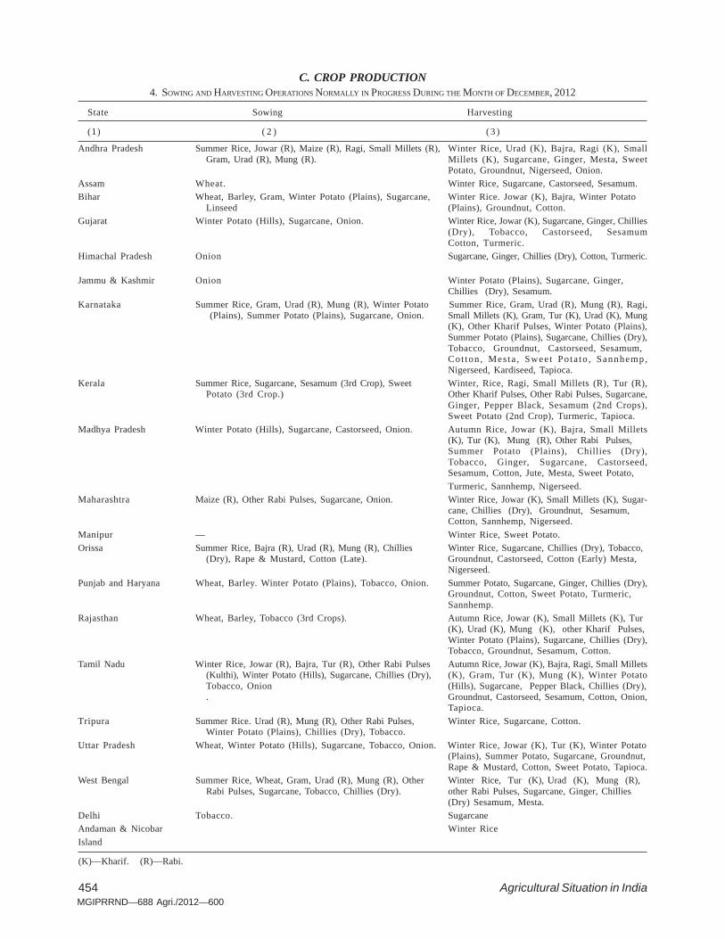
454 Agricultural Situation in IndiaMGIPRRND—688 Agri./2012—600
C. CROP PRODUCTION4. SOWING AND HARVESTING OPERATIONS NORMALLY IN PROGRESS DURING THE MONTH OF DECEMBER, 2012
State Sowing Harvesting
(1) ( 2 ) ( 3 )
Andhra Pradesh Summer Rice, Jowar (R), Maize (R), Ragi, Small Millets (R), Winter Rice, Urad (K), Bajra, Ragi (K), SmallGram, Urad (R), Mung (R). Millets (K), Sugarcane, Ginger, Mesta, Sweet
Potato, Groundnut, Nigerseed, Onion.Assam Wheat. Winter Rice, Sugarcane, Castorseed, Sesamum.Bihar Wheat, Barley, Gram, Winter Potato (Plains), Sugarcane, Winter Rice. Jowar (K), Bajra, Winter Potato
Linseed (Plains), Groundnut, Cotton.Gujarat Winter Potato (Hills), Sugarcane, Onion. Winter Rice, Jowar (K), Sugarcane, Ginger, Chillies
(Dry), Tobacco, Castorseed, SesamumCotton, Turmeric.
Himachal Pradesh Onion Sugarcane, Ginger, Chillies (Dry), Cotton, Turmeric.
Jammu & Kashmir Onion Winter Potato (Plains), Sugarcane, Ginger,Chillies (Dry), Sesamum.
Karnataka Summer Rice, Gram, Urad (R), Mung (R), Winter Potato Summer Rice, Gram, Urad (R), Mung (R), Ragi, (Plains), Summer Potato (Plains), Sugarcane, Onion. Small Millets (K), Gram, Tur (K), Urad (K), Mung
(K), Other Kharif Pulses, Winter Potato (Plains),Summer Potato (Plains), Sugarcane, Chillies (Dry),Tobacco, Groundnut, Castorseed, Sesamum,Cot ton , Mes ta , Sweet Pota to , Sannhemp,Nigerseed, Kardiseed, Tapioca.
Kerala Summer Rice, Sugarcane, Sesamum (3rd Crop), Sweet Winter, Rice, Ragi, Small Millets (R), Tur (R),Potato (3rd Crop.) Other Kharif Pulses, Other Rabi Pulses, Sugarcane,
Ginger, Pepper Black, Sesamum (2nd Crops),Sweet Potato (2nd Crop), Turmeric, Tapioca.
Madhya Pradesh Winter Potato (Hills), Sugarcane, Castorseed, Onion. Autumn Rice, Jowar (K), Bajra, Small Millets(K), Tur (K), Mung (R), Other Rabi Pulses,Summer Potato (Plains), Chillies (Dry),Tobacco, Ginger, Sugarcane, Castorseed,Sesamum, Cotton, Jute, Mesta, Sweet Potato,Turmeric, Sannhemp, Nigerseed.
Maharashtra Maize (R), Other Rabi Pulses, Sugarcane, Onion. Winter Rice, Jowar (K), Small Millets (K), Sugar-cane, Chillies (Dry), Groundnut, Sesamum,Cotton, Sannhemp, Nigerseed.
Manipur — Winter Rice, Sweet Potato.Orissa Summer Rice, Bajra (R), Urad (R), Mung (R), Chillies Winter Rice, Sugarcane, Chillies (Dry), Tobacco,
(Dry), Rape & Mustard, Cotton (Late). Groundnut, Castorseed, Cotton (Early) Mesta,Nigerseed.
Punjab and Haryana Wheat, Barley. Winter Potato (Plains), Tobacco, Onion. Summer Potato, Sugarcane, Ginger, Chillies (Dry),Groundnut, Cotton, Sweet Potato, Turmeric,Sannhemp.
Rajasthan Wheat, Barley, Tobacco (3rd Crops). Autumn Rice, Jowar (K), Small Millets (K), Tur(K), Urad (K), Mung (K), other Kharif Pulses,Winter Potato (Plains), Sugarcane, Chillies (Dry),Tobacco, Groundnut, Sesamum, Cotton.
Tamil Nadu Winter Rice, Jowar (R), Bajra, Tur (R), Other Rabi Pulses Autumn Rice, Jowar (K), Bajra, Ragi, Small Millets(Kulthi), Winter Potato (Hills), Sugarcane, Chillies (Dry), (K), Gram, Tur (K), Mung (K), Winter PotatoTobacco, Onion (Hills), Sugarcane, Pepper Black, Chillies (Dry),. Groundnut, Castorseed, Sesamum, Cotton, Onion,
Tapioca.Tripura Summer Rice. Urad (R), Mung (R), Other Rabi Pulses, Winter Rice, Sugarcane, Cotton.
Winter Potato (Plains), Chillies (Dry), Tobacco.Uttar Pradesh Wheat, Winter Potato (Hills), Sugarcane, Tobacco, Onion. Winter Rice, Jowar (K), Tur (K), Winter Potato
(Plains), Summer Potato, Sugarcane, Groundnut,Rape & Mustard, Cotton, Sweet Potato, Tapioca.
West Bengal Summer Rice, Wheat, Gram, Urad (R), Mung (R), Other Winter Rice, Tur (K), Urad (K), Mung (R),Rabi Pulses, Sugarcane, Tobacco, Chillies (Dry). other Rabi Pulses, Sugarcane, Ginger, Chillies
(Dry) Sesamum, Mesta.Delhi Tobacco. SugarcaneAndaman & Nicobar Winter RiceIsland
(K)—Kharif. (R)—Rabi.

ISSN 0002—167 P. Agri. 21-11-2012Regn. No. : 840 600
LIST OF PUBLICATIONS
Journal
Agricultural Situation in India (Monthly)
Periodicals
Agricultural Prices in India
Agricultural Wages in India
Cost of Cultivation of Principal Crops
Land Use Statistics at a Glance
District-wise Area and Production of Principal Crops in India
Year Book of Agro-Economic Research Studies
Farm Harvest Prices of Principal Crops in India
Agricultural Statistics at a Glance
Copies are available from : The Controller of Publications, Civil Lines, Delhi-110054. (Phone 23817640)
PRINTED BY THE MANAGER, GOVERNMENT OF INDIA PRESS, RING ROAD, MAYAPURI, NEW DELHI-110064AND PUBLISHED BY THE CONTROLLER OF PUBLICATIONS, DELHI-110054—2013.