Agricultural Household Models - World Bank Document
354
AGRICULTURAL HOUSEHOLD MODELS Extensions, Applications, acnd Policy INDERJITSINGGH LYN SQUIRE JOF_L STRAUSS EDITORS FITLE COPY Report; No](a: >-11179D lx,8; ; Auho' LU NQI (j 2i-Ctr S!_?( O rO,E tlI CAT ' ON I I7 9 -3 Public Disclosure Authorized Public Disclosure Authorized Public Disclosure Authorized Public Disclosure Authorized
-
Upload
khangminh22 -
Category
Documents
-
view
0 -
download
0
Transcript of Agricultural Household Models - World Bank Document
AGRICULTURALHOUSEHOLD
MODELS
Extensions,Applications,
acnd Policy
INDERJIT SINGGHLYN SQUIRE
JOF_L STRAUSSEDITORS
FITLE COPY
Report; No](a: >-11179D lx,8; ;
Auho' LU NQI (j 2i-Ctr S!_?(O rO,E tlI CAT ' ON I I7 9 -3
Pub
lic D
iscl
osur
e A
utho
rized
Pub
lic D
iscl
osur
e A
utho
rized
Pub
lic D
iscl
osur
e A
utho
rized
Pub
lic D
iscl
osur
e A
utho
rized

iSl..:N .-..:i ;r;:I4 ... ... :.. :° i. .. .. .. .
~~~~~~~~~~~~~~~~~~~~~~~~~~~~~~~~~~~~~~.. .... ..... ... , .,,
j :.: .'. t.i ,. .L ' .... ' i::. , :'i ....... iT.:. L CL i:,j;::i ! :f !2'i .1 ........ Si. :) t. '5'.J.... . .. .... ... " .... ..... .1.~~~~~~~~~~.P
L:i::' ;c:: .it ' I L i ', a ! ai::, : I c:tai .... . ... i .... ... ... .S. .. :..-. ...... 7. ... .....

AgriculturalHousehold Models
A World Bank Research Publication

AgriculturalHousehold Models
Extensions, Applications, and Policy
Inderjit SinghLyn Squire
John StraussEditors
Published for The World Bank
THE JOHNS HOPKINS UNIVERSITY PRESS
Baltimore and London
Copyright © 1986 by The International Bankfor Reconstruction and Development/The World Bank1818 H Street, N.W., Washington, D.C. 20433, U.S.A.
All rights reservedManufactured in the United States of America
First printing February 1986
The Johns Hopkins University PressBaltimore, Maryland 21211, U.S.A.
The World Bank does not accept responsibility for the views expressed herein, which are those ofthe authors and should not be attributed to the World Bank or to its affiliated organizations.The findings, interpretations, and conclusions are the results of research supported by the Bank;they do not necessarily represent official policy of the Bank.
Library of Congress Cataloging-in-Publication DataMain entry under title:
Agricultural household models.
"Published for the World Bank."Bibliography: p.Includes index.1. Agricultural laborers-Developing countries-Case
studies. 2. Rural families-Developing countries-Casestudies. 3. Agricultural industries-Developing coun-tries-Case studies. 4. Developing countries-Ruralconditions-Case studies. 5. Agricultural laborers-Government policy-Developing countries-Case studies.I. Singh, Inderjit, 1941- . II. Squire, Lyn,1946- . Ill. Strauss, John, 1951-IV. International Bank for Reconstruction andDevelopment.HD1542.A34 1986 331.7'63'091724 85-45102ISBN 0-8018-3149-0
Contents
Contributors ixAcknowledgments xiIntroduction 3
Inderjit Singh, Lyn Squire, and John StraussModeling Agricultural Household Models: Why and How 3Structure of the Analysis 9References 14
PART I. AN OVERVIEW OF AGRICULTURAL HOUSEHOLD MODELS
1. The Basic Model: Theory, Empirical Results,and Policy Conclusions 17Inderjit Singh, Lyn Squire, and John Strauss
The Basic Model 17Estimation Issues 20Empirical Results 22Do Agricultural Household Models Matter? 25Policy Results 30Some Extensions 35Appendix: Detailed Elasticities from Studies
of Agricultural Household Models 42References 47
2. Methodological Issues 48Inderjit Singh, Lyn Squire, and John Strauss
Nonseparability 48Multimarket Analysis 59Data Requirements and Implications for Data Collection 62Agenda for Future Research 66References 69
V
VI CONTENTS
Appendix. The Theory and Comparative Staticsof Agricultural Household Models: A General Approach 71John Strauss
A Basic Model: The Household as Price-Taker 71Deriving Virtual (Shadow) Prices 76Models with Absent Markets: Labor 79Models with Absent Markets: Z-Goods 85Partly Absent Markets: Commodity Heterogeneity 88Recursive Conditions Summarized 89References 90
PART 11. CASE STUDIES
3. Agricultural Household Modeling in a MulticropEnvironment: Case Studies in Korea and Nigeria 95Inderjit Singh and Janakiram Subramanian
The Theoretical Model 97Model Results for Agricultural Households
in Korea and Nigeria 100Policy Implications 108Conclusions 112Appendix: Data Sources 113Notes 114References 114
4. Estimating the Determinants of Food Consumptionand Caloric Availability in Rural Sierra Leone 116John Strauss
Policy Issues 117Model Specification and Estimation 119Consumption, Labor Supply, and Marketed Surplus Responses 124Price and Income Effects for Caloric Availability 137Policy Implications 140Appendix: Data Sources 142Notes 148References 151
5. Agricultural Prices, Food Consumption, and theHealth and Productivity of Indonesian Farmers 153Mark M. Pitt and Mark R. Rosenzweig
Determinants and Consequences of Changes in Healthin Farm Households 154
The Multiperson Household, Consumption Aggregation,and Intrafamily Resource Allocation 161
CONTENTS Vil
Estimation of the Relationships between Health, Food Prices,Farm Profits, and Aggregate Food Consumption: Indonesia 166
Conclusions 177Appendix: Data Sources 179References 181
6. The Demand and Supply of Funds among Agricultural
Households in India 183
Farrukh lqbalStructure and Selected Features of the Model 184Data, Estimation Issues, and Empirical Results 192Summary 203Appendix: Data and Sample 204References 204
7. Simulating the Rural Economy in a Subsistence
Environment: Sierra Leone 206
Victor E. Smith and John StraussA Comparison of Microsimulation
and Direct Population Estimates 207Point Elasticities versus Microsimulation 211Microsimulation and Partial Equilibrium 213Microsimulation and General Equilibrium 217Microsimulation and the Interhousehold Distribution
of Calories 225Conclusion 228Appendix: Estimates of Rural per Capita Aggregates
from Observed Data 230Notes 231References 232
8. Multimarket Analysis of Agricultural Pricing Policies
in Senegal 233
Avishay Braverman and Jeffrey S. HammerThe Senegalese Problem 234Structure of the Model 235Results 243Conclusions 250Appendix: Mathematical Formulation 251References 253
9. Yield Risk in a Dynamic Model of the
Agricultural Household 255
Terry Roe and Theodore Graham-TomasiBackground 256The Conceptual Framework 258
Vill CONTENTS
Characterizing a Solution 260Increases in Risk 263Duality and Risk Aversion 269Discussion 271Notes 273References 274
10. Using a Farm-Household Model to Analyze LaborAllocation on a Chinese Collective Farm 277Terry Sicular
Model of a Collective Farm 279Empirical Model of a Production Team 287Results 292Conclusion 300Appendix: Constraints and Activities of the Basic Model 303Notes 304References 305
11. Structural Models of the Farm Household That Allowfor Interdependent Utility and Profit-Maximization Decisions 306Ramon E. Lopez
Farm-Household Models 307Testing Recursive Models 314Estimating a Nonrecursive Model 316Conclusions 323Notes 324References 324
Index 327
Contributors
Avishay Braverman, Agriculture and Rural Development Department,World Bank, Washington, D.C.
Theodore Graham-Tomasi, Department of Agriculture and Applied Eco-nomics, University of Minnesota, Minneapolis, Minn.
Farrukh Iqbal, East Asia and Pacific Country Programs Department,World Bank, Washington, D.C.
Subramanian Janakiram, Consultant, World Bank, Washington, D.C.
Jeffrey S. Hammer, Agriculture and Rural Development Department,World Bank, Washington, D.C.
Ramon E. Lopez, Agricultural Economics Department, University ofMaryland, College Park, Md.
Mark M. Pitt, Department of Economics, University of Minnesota, Min-neapolis, Minn.
Terry Roe, Department of Agriculture and Applied Economics, Univer-sity of Minnesota, Minneapolis, Minn.
Mark R. Rosenweig, Department of Economics, University of Minne-sota, Minneapolis, Minn.
Terry Sicular, Food Research Institute, Stanford University, Stanford,Calif.
Inderjit Singh, South Asia Projects Department, World Bank, Washing-ton, D.C.
Victor E. Smith, Department of Economics, Michigan State University,East Lansing, Mich.
Ix

X CONTRIBUTORS
Lyn Squire, Country Policy Department, World Bank, Washington,D.C.
John Strauss, Economic Growth Center, Yale University, New Haven,Conn.
Acknowledgments
THIS BOOK HAS BENEFITED from the financial support of the World Bank'sResearch Committee and from the encouragement, suggestions, and helpof many people. Special thanks are due to Dennis DeTray, whose invalu-able comments led to major improvements in the organization and pre-sentation of the book's materials. Jon Skinner provided very helpful com-ments on early versions of the material in Part I, which also benefitedfrom the careful reading of Robert Evenson and T. Paul Schultz. We werealso greatly assisted by the comments of a review panel.
We owe many thanks to Vicki Macintyre for very able and extremelyefficient copyediting. Finally, the book could not have come to fruitionwithout the skills and patience of Arlene Elcock, who not only did muchof the typing, but also handled much of the correspondence. Lois Van deVelde also provided invaluable help in typing.
xi

AgriculturalHousehold Models

Introduction
Inderjit Singh, Lyn Squire, and John Strauss
IN MOST DEVELOPING COUNTRIES, agriculture remains a principal source ofincome for the majority of the population, an important earner of foreignexchange, and a central concern of government policymakers. One of thegreat problems for these countries is that efforts to predict the conse-quences of agricultural policies are often confounded by the complex be-havioral patterns characteristic of households in semicommercialized, ru-ral economies. That is to say, most households in agricultural areasproduce partly for sale and partly for their own consumption. They alsopurchase some of their inputs (fertilizer, for example) and provide some(such as family labor) from their own resources. Any change in the poli-cies governing agricultural activities will therefore affect not only produc-tion, but also consumption and labor supply. These relations are whatanalysts attempt to capture in their efforts to model the behavior of agri-cultural households.
Modeling Agricultural Household Models: Why and How
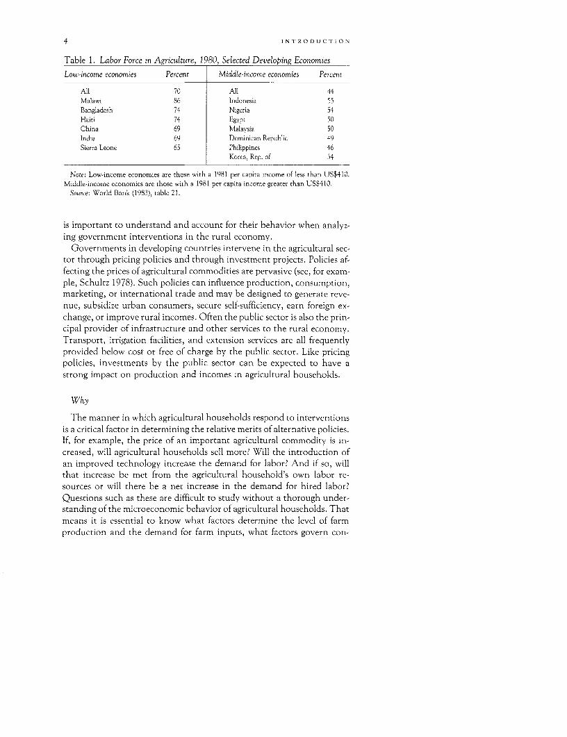
Agricultural households are the main form of economic organization indeveloping countries. Roughly 70 percent of the labor force in low-income developing countries was employed in the agricultural sector in1980. Even in the middle-income developing countries, almost 45 percentof the labor force was so employed (table 1). Although some members ofthe agricultural labor force are landless laborers, agricultural households,according to the information in table 1, are numerous. Consequently, it
3
4 INTRODU CTION
Table 1. Labor Force in Agriculture, 1980, Selected Developing Economies
Low-income economies Percent Middle-income economies Percent
All 70 All 44Malawi 86 Indonesia 55Bangladesh 74 Nigeria 54Haiti 74 Egypt 50China 69 Malaysia 50India 69 Dominican Republic 49Sierra Leone 65 Philippines 46
Korea, Rep. of 34
Note: Low-income economies are those with a 1981 per capita income of less than US$410.Middle-income economies are those with a 1981 per capita income greater than US$410.
Source: World Bank (1983), table 21.
is important to understand and account for their behavior when analyz-ing government interventions in the rural economy.
Governments in developing countries intervene in the agricultural sec-tor through pricing policies and through investment projects. Policies af-fecting the prices of agricultural commodities are pervasive (see, for exam-ple, Schultz 1978). Such policies can influence production, consumption,marketing, or international trade and may be designed to generate reve-nue, subsidize urban consumers, secure self-sufficiency, earn foreign ex-change, or improve rural incomes. Often the public sector is also the prin-cipal provider of infrastructure and other services to the rural economy.Transport, irrigation facilities, and extension services are all frequentlyprovided below cost or free of charge by the public sector. Like pricingpolicies, investments by the public sector can be expected to have astrong impact on production and incomes in agricultural households.
Why
The manner in which agricultural households respond to interventionsis a critical factor in determining the relative merits of alternative policies.If, for example, the price of an important agricultural commodity is in-creased, will agricultural households sell more? Will the introduction ofan improved technology increase the demand for labor? And if so, willthat increase be met from the agricultural household's own labor re-sources or will there be a net increase in the demand for hired labor?Questions such as these are difficult to study without a thorough under-standing of the microeconomic behavior of agricultural households. Thatmeans it is essential to know what factors determine the level of farmproduction and the demand for farm inputs, what factors govern con-
INTRODU C TI0 N 5
sumption and the supply of labor, and how the behavior of the house-hold as a producer affects its behavior as a consumer and supplier of la-bor, and vice versa.
Agricultural household models are designed to capture these relation-ships in a theoretically consistent fashion so that the results of the analy-sis can be applied empirically to illuminate the consequences of policyinterventions. Ideally, such models should enable the analyst to examinethe consequences of policy in three dimensions. First, it is important toexamine the effect of alternative policies on the well-being of representa-tive agricultural households. In this book well-being refers to meanhousehold income or some other measure such as nutritional status. Inexamining the effect of a policy designed to provide inexpensive food forurban consumers, for example, an agricultural household model wouldallow the analyst to assess the costs to farmers of depressed producerprices.
Second, the analyst will want to examine the "spillover" effects of gov-ernment policies on other segments of the rural population. Since mostrural investment strategies are designed to increase production, their pri-mary impact is on the incomes of agricultural households and thus someof them may not reach landless households or households engaged innonagricultural activities. A model that incorporates total labor demandand family labor supply allows the analyst to explore the effects of policyon the demand for hired labor and hence on the rural labor market andthe incomes of landless households. Similarly, a model that incorporatesconsumer behavior allows the analyst to explore the consequences of in-creased profits for agricultural households on the demand for productsand services provided by nonagricultural, rural households (see Ander-son and Leiserson 1980). Since the demand for nonagricultural commodi-ties is often thought to be much more responsive to an increase in incomethan the demand for agricultural staples, this spillover effect may well beimportant.
Third, the analyst is interested in the performance of the agriculturalsector from a multisectoral perspective since agriculture is often an impor-tant source of both revenue for the public budget and foreign exchange.In assessing the effects of pricing policy on the budget or the balance ofpayments, governments are obliged to consider the quantitative responsesof agricultural households. Reducing export taxes, for example, may in-crease earnings of foreign exchange and budget revenues provided house-holds market enough additional production. Since agricultural house-hold models capture both consumption and production behavior, theyare a natural vehicle for examining the effect of pricing policy on mar-keted surplus and hence foreign exchange earnings and budget revenues.

6 INTRODUCTION
Because of the importance of agricultural households in the total popu-lation of developing countries and the significance of agricultural sectorpolicies, the behavior of agricultural households warrants thorough theo-retical and empirical investigation. The analysis of agricultural house-holds has been approached from many different angles, each relevant inits own way and having its advantages and disadvantages. This volumereports the results of a large body of work that has followed a similar basicapproach, which we believe offers important policy insight that differssignificantly from the results of more traditional approaches.
How
Since 1975, researchers at the Food Research Institute of Stanford Uni-versity and at the World Bank have been developing microeconomicmodels of farm households that combine producer, consumer, and laborsupply decisions in a theoretically consistent manner. In true subsistencehouseholds, these decisions are made simultaneously. Without access totrade, a household can consume only what it produces and must rely ex-clusively on its own labor. A large part of agriculture, however, is madeup of semicommercial farms in which some inputs are purchased andsome outputs are sold. In these circumstances, producer, consumer, andlabor supply decisions are no longer made simultaneously, although theyare obviously connected because the market value of consumption can-not exceed the market value of production less the market value ofinputs.
Imagine a simple agricultural household that produces one crop, say,rice; has a fixed amount of land; and uses one variable input, labor. Thehousehold consumes some of the rice, and sells some in order to buy anonagricultural commodity. In addition to using its own labor, thehousehold hires labor. Assume further that the household can sell rice ata fixed price and buy labor at a fixed wage. How does this householdorganize its productive activities? Since income contributes positively tototal household utility or satisfaction, the household will attempt toachieve the largest profit possible from its fixed quantity of land. Thisimplies that the household will go on hiring labor until the marginal reve-nue product of labor equals the market wage. The household may not, ofcourse, achieve maximum profits exactly. Nevertheless, in setting thelevel of output and the quantity of inputs, the household will try to ap-proximate the profit-maximizing solution and will therefore require infor-mation on prices-in this case, the price of rice and the wage rate-and onthe technological relationships between inputs and outputs. These piecesof information are sufficient for the household to equate marginal reve-nue product to the wage. Notice that, in making its farm output and in-

INTRODUCTION 7
put calculations, the household does not need to know how much rice itplans to consume or how much labor it intends to supply. In other words,the household can make its production decisions independently of itsconsumption and labor-supply decision. (This proposition was developedby Krishna 1964 and by Jorgenson and Lau 1969.)
Consumption and labor-supply decisions, however, are not indepen-dent of production decisions. Consumption and labor supply depend onboth prices and income and, although prices are fixed by assumption,income is determined, at least to some extent, by the household's profitsfrom its farming activities. Thus, production decisions determine farmprofits, which are a component of household income, which in turn influ-ences consumption and labor-supply decisions. This one-way relation be-tween production on the one hand and consumption and labor supply onthe other hand is known as the profit effect; it will be referred to fre-quently throughout the volume.
This result-that the decisionmaking process of the agricultural house-hold has a recursive character is crucial for much of the work summarizedin this volume. It is based on the assumption that households are price-takers for every commodity, including labor, that is both produced andconsumed by the household. According to this line of reasoning, theamount of, say, rice to be produced can be determined independently ofthe amount of rice to be consumed because the household can always buyor sell rice at a fixed price. Similarly, the amount of labor applied to riceproduction can be determined independently of the amount of family la-bor to be used because the difference can be hired at a fixed wage. Theonly constraint on rice consumption or family labor supply arises fromtotal household income. The household cannot consume more rice ormore leisure (that is, reduce its labor supply and use more hired laborers)than is allowed by its total income. Since the household always prefersmore income, it makes sense to maximize profits and then allocate theresulting income to rice-the nonagricultural commodity-and leisure,given the prevailing market prices. With prices fixed, therefore, the twocomponents of the model are related only through income and only inone direction, from the production side of the model to the consumptionand labor-supply side.
If production decisions affect prices as well as household income, how-ever, the recursive property of the model is eliminated. If the household'sdecision to hire a certain amount of labor affects the wage rate, or if itsdecision to sell a quantity of rice affects the market price, then a theoreti-cally consistent treatment requires that production, consumption, andlabor-supply decisions be determined jointly. If we assume there is no la-bor market, for example, then there is no market wage and the householdmust equate its demand for labor with its own supply of labor. Despite
8 INTRODU CTION
the absence of a market wage, one can nevertheless focus on the shadow,or virtual, price-this being the price that would just secure the observedequality between the demand and supply of household labor. This pricewill depend on all the variables that influence household decisionmaking.
More important, since this shadow price will influence production,consumption, and labor-supply decisions, income will no longer be theonly connection between the two sides of the model and the recursiveproperty will be lost. Thus if there is an increase in the price of rice, pro-duction will increase and hence the demand for labor; at the same time,income will increase and hence the supply of labor will decrease. But, ifthere is no labor market, the supply and demand of household labor mustbe balanced. Balance will be achieved only if the shadow price of laborincreases. An increase in this price, however, will initiate second-roundeffects-production, for example, will be reduced in response to the in-crease in the price of a major input. In fact, when all the interactions arecomplete, one might observe a net decrease in production, despite theincrease in its price. Had the wage been fixed, on the other hand, second-round effects would have been eliminated.
The incorporation of endogenously determined prices obviously com-plicates the analyst's task considerably. The specification of price determi-nation in output and labor markets, therefore, is important. In outputmarkets, the assumption that households are price-takers may often bewarranted. Although many agricultural output markets are characterizedby extensive government intervention, for example, price fixing by thegovernment implies that agricultural households are price-takers. Simi-larly, if prices are determined in world markets, it seems perfectly reason-able to assume that any given agricultural household is a price-taker. Ob-viously, this assumption should be carefully investigated in each case,but, given the existence of many sellers, the assumption that any individ-ual seller is unable to influence the market price may often be the mostplausible description of market behavior.
The household must also be a price-taker in the labor market. Ruralwages, however, are less likely to be fixed by government intervention orin international markets. Thus the operation of the labor market be-comes an important ingredient in the specification of an agriculturalhousehold model. Circumstances will clearly differ from case to case, buttwo recent surveys of rural labor markets point to the existence of manybuyers and many sellers and to the general availability of informationon rural wage rates among participants in the labor market (Binswangerand Rosenzweig 1984; Squire 1982). The essential elements of a reason-ably competitive market may, therefore, often be found in rural areas. Inother words, before proceeding to a more complicated model in whichproduction and consumption are determined simultaneously, one ought
INTRODUCTION 9
to have a compelling argument with supporting empirical evidence tosubstantiate the notion that the behavior of one agricultural householdcan be expected to influence the market wage for rural labor in general.Accordingly, most, but not all, of the case studies in this volume treathouseholds as price-takers and consequently develop models of recursivedecisionmaking.
The approach to agricultural household modeling adopted here can bebetter understood if we look at the significance of the profit effect. Con-sider the effect of an increase in the price of rice. If the decisions of theagricultural household are recursive, then the traditional analysis of farmoutput supply and input demand using the theory of the firm will yieldthe same results as those of a fully specified agricultural household model.The same is not true, however, for consumption and labor supply. Thetraditional approach to consumer-demand analysis would allow for thesubstitution effect and the income effect of the change in the price of rice.The substitution effect is unambiguously negative. And for a normalcommodity such as rice, the income effect can be confidently expected tobe negative. The traditional approach, therefore, would predict an unam-biguous decrease in the consumption of rice following an increase in itsprice. An integrated agricultural household model, however, allows foran additional effect-the profit effect.
When the price of rice increases, farm profits increase. This means morehousehold income, which will, of course, tend to increase the demand forrice. In the framework of an agricultural household model, therefore, thedemand for rice is subject to two forces pulling in opposite directions. Onthe one hand, an increase in price will tend to reduce demand as a resultof the traditional substitution and income effects of consumer theory.On the other hand, the profit effect associated with the same increase inprice will tend to increase demand. The ultimate effect on demand is thusa matter for empirical investigation. In fact, the profit effect could out-weigh the other effects and thereby reverse the traditional conclusion.That is, an increase in the price of rice may result in increased demand.The studies reported in this volume provide empirical confirmation ofthis possibility.
Other examples could be cited. The essential principle, however, re-mains the same: the consistent incorporation of the profit effect canchange the direction and magnitude of results predicted by traditionalmodels of consumption and labor-supply behavior.
Structure of the Analysis
The book consists of two main parts: part I provides an overview ofempirical results, policy conclusions, and methodological issues; part II
10 INTRODUCTION
contains a series of recent applications of agricultural household modelingthat expands the range of policy issues subject to investigation within thisgeneral framework and explores several critical methodological issues.
Part I first presents the basic model of an agricultural household thatunderlies most of the case studies undertaken so far. The model assumesthat households are price-takers and is therefore recursive. The decisionsmodeled include those affecting production and the demand for inputsand those affecting consumption and the supply of labor. Comparativeresults on selected elasticities are presented for a number of economies(Japan, the Republic of Korea, Malaysia, Nigeria, Sierra Leone, Taiwan,and Thailand). The empirical significance of the approach is demon-strated in a comparison of models that treat production and consump-tion decisions separately and those in which the decisionmaking processis recursive. The opening chapter also summarizes the implications of ag-ricultural pricing policy for the welfare of farm households, marketed sur-plus, the demand for nonagricultural goods and services, the rural labormarket, budget revenues, and foreign exchange earnings. In addition, it isshown that the basic model can be extended in order to explore the ef-fects of government policy on crop composition, nutritional status,health, saving, and investment and to provide a more comprehensiveanalysis of the effects on budget revenues and foreign exchange earnings.
Chapter 2 concentrates on methodological topics, primarily the datarequirements of the basic model and its extensions, along with aggrega-tion, market interaction, uncertainty, and market imperfections. Themost important methodological issue-the question of the recursive prop-erty of these models-is also discussed. Part I concludes with a technicalappendix that develops a general model of an agricultural household andformally derives the conditions under which it is appropriate to treat thedecisions governing production, consumption, and labor supply recur-sively. The comparative statics of the general model are derived and thedifference between recursive and nonrecursive models is demonstrated byreference to certain well-known models such as the one that incorporatesZ-goods (or home-produced goods).
Part II contains nine case studies, each of which extends the basic ap-proach in some new direction. Chapters 3 and 4, for example, describeefforts to disaggregate commodities on both the production and con-sumption sides of the model. First, Singh and Janakiram use Koreanand Nigerian data to demonstrate how a linear programming character-ization of production can be used to investigate factors influencing theallocation of resources among several crops within the framework of anagricultural household model. Next, Strauss looks at disaggregation ofconsumed items. With data from Sierra Leone, he is able to show how afarm-household model can be used to examine the effects of pricing policy
I N T R O D U C T I0 N I1
for nutritional status. In this application, the profit effect becomes criticalbecause the direct effect of an increase in the price of food on consump-tion may be offset by an increase in farm profits and hence householdincome. Strauss provides empirical confirmation of this point.
In chapter 5, Pitt and Rosenzweig extend Strauss's analysis to the rela-tions between food intake and household health and that between healthand farm profits. According to their results, farm profits are relativelyimmune to the health status of the farmer because of access to a well-functioning labor market. Health status can be influenced by prices, how-ever; reductions in the price of sugar, for example, help to increase theincidence of illness, whereas reductions in the prices of vegetables andvegetable oil help to reduce it.
Iqbal extends the model in a completely different direction in chapter 6by focusing on the household's borrowing decision. Moreover, since hebelieves that households are not price-takers in the capital market, he isobliged to abandon the recursive characteristic of decisionmaking. Usingdata for rural India, Iqbal demonstrates that interest rates have an impor-tant effect on the amount borrowed. Furthermore, he finds that in pre-vious studies the interest rate variable has often proved insignificant be-cause of misspecification of the borrowing variable.
Most of the case studies up to this point in the book deal with repre-sentative households. Policy conclusions drawn from such analyses arepotentially misleading for at least two reasons. First, households are dif-ferent, and therefore simply scaling up the results for a representativehousehold may yield unsatisfactory results. Second, the approach ignoresgeneral equilibrium effects. Although the wage may be treated as givenfor any particular household, for example, if all households increase theirdemand for labor, the market wage may well be pushed upward.
Two chapters address these issues. Again relying on Sierra Leone data,Smith and Strauss use microsimulation to explore the consequences ofpolicy intervention for different types of households. Their results, re-ported in chapter 7, show that, although the nutritional benefit of ahigher rice price is negligible for the rural population at large, its impacton the poorest households is positive. Moreover, this is a direct outcomeof the operation of the profit effect. Low-income households have largermarketed surpluses of rice than other households. As a result, an increasein the price of this crop yields an increase in profits for low-income house-holds that is large enough to offset the direct impact on consumption(and hence nutrition) through the traditional substitution and incomeeffects.
Smith and Strauss also touch on the consequences of an induced in-crease in the rural wage following an increase in the price of rice. Thispreliminary effort to incorporate general equilibrium effects is taken one
12 INTRODUCTION
step further by Braverman and Hammer, who in chapter 8 aggregateresults at the household level and explicitly incorporate market-clearingconditions in the agricultural household model. In applying the model toSenegal, they assume that the prices of groundnuts, cotton, and rice arefixed by the government and that the market clears through adjust-ments-exports or imports-in international trade. For millet and maize,however, prices are determined endogenously by the interaction of do-mestic supply and demand. Endogenous prices for land and labor by re-gion are also modeled. The model must therefore be designed to ensurebalance in two output markets and two input markets through price ad-justments; furthermore, the production, consumption, and labor-supplydecisions of households must be consistent with the newly emergingprices. The authors suggest that in this way, the more important generalequilibrium effects in the model are captured.
The work of Braverman and Hammer offers the prospect of a usefultool for policy analysis that strikes a reasonable balance between the needto incorporate general equilibrium effects and the need to meet data andcomputational requirements. Their work also lends itself to the analysisof issues that often concern policymakers. Consider the effect of a de-crease in the producer price of groundnuts, a principal export in Senegal.The government may contemplate such a step because it is anxious toreduce the drain on the budget of large subsidies to groundnut producers.At the same time, however, it may be reluctant to jeopardize export earn-ings. Braverman and Hammer are able to show that, because of interac-tions with other markets, much of the reduction in export earnings fromgroundnuts is offset by other crops, whereas the budget savings fromgroundnuts are largely untouched by developments in other markets. Inaddition to results of this kind, their work also yields the usual microeco-nomic results-household incomes, labor supply, consumption, produc-tion-associated with agricultural household models. Their approach,however, allows fully for induced changes in market-clearing prices.
The models described so far have been deterministic. Agricultural pro-duction is subject to considerable uncertainty, however. Yields, for exam-ple, obviously depend on weather conditions that can be predicted withonly a limited degree of accuracy. In chapter 9, Roe and Graham-Tomasibegin the difficult task of incorporating production risk into agriculturalhousehold models. They demonstrate that, under certain very restrictivecircumstances, the recursive property of agricultural household modelssurvives the incorporation of production risk. These circumstances arethe existence of markets for contingent states of the future or, in the ab-sence of such markets, special assumptions concerning the household'sutility function. That recursiveness of production and consumption deci-
I N T R O D U C T I O N 13
sions might depend on preferences in addition to markets makes the caseof risk quite different from the certainty case. Roe and Graham-Tomasiwork out an example using a particular utility function and using illustra-tive data from the Dominican Republic. They show for this case that theproblem becomes separable using certainty equivalent income to replaceincome. They also show that when the analyst ignores risk in computingcomparative statics an extra income effect, which counters the profit ef-fect, is omitted. This is because a rise in price raises the variance of profits,so that certainty equivalent income falls for risk-averse households.
In principle, agricultural household modeling is relevant for economicagents other than households provided a discrete, decisionmaking unitcan be identified. In an imaginative application to a Chinese collective inchapter 10, Sicular demonstrates that the general approach can be usedto analyze the behavior of a group of farm households. Sicular exploresthe behavior of a Chinese production team subject to various state-imposed quotas and restrictions. One consequence of these restrictions-such as those on labor-market participation-is that Sicular is obliged toabandon the recursive property characteristic of most studies of agricul-tural households. In the absence of adequate data on consumption, Sicu-lar focuses on the production side of the model. The consumption-production interaction is then introduced by constraining productiondecisions so that certain optimal levels of consumption by commodity areachieved. Within this framework, Sicular is able to show the conse-quences of state-imposed restrictions on production and marketing bycomparing the results of a restricted model with those of an unrestrictedone.
The volume comes to a close in chapter 11 with a discussion of one ofthe first attempts to address statistically the appropriateness of the recur-sive characterization of decisionmaking common to most agriculturalhousehold models. Lopez argues that production, consumption, and la-bor-supply decisions may be interdependent because of differences inpreferences for off-farm and on-farm work or because of the costs of com-muting associated with off-farm work. Having demonstrated analyticallythat in these circumstances the agricultural household model can nolonger be treated recursively, Lopez uses data from Canada to test statisti-cally whether or not the nonrecursive model is preferred to the recursiveone. The results of this exercise do not support the use of a recursivemodel. The quantitative differences in the elasticities estimated by thetwo models are substantial. For example, the elasticity of total labor sup-ply is 0.04 in the nonrecursive model compared with 0.19 in the recursiveone. Although the particular reasons advanced by Lopez in favor of anonrecursive model may not seem especially relevant to developing coun-

14 INTRODUCTION
tries, the general thrust of his work is clearly important, and further testsusing data from developing countries are warranted. (Chapter 2 of thisvolume contains an evaluation of Lopez's results for future work on agri-cultural household models.)
It may be useful to conclude these introductory remarks with a briefreader's guide. The reader who is interested in understanding the basicidea behind agricultural household models and who wants a review of themain empirical results and policy conclusions should read chapter 1. Thereader who wants to go beyond this and see how the basic model mightbe extended to a much wider range of policy issues should also read thecase studies on crop-composition, nutrition, health, borrowing, and gov-ernment deficits in chapters 3, 4 and 7, 5, 6, and 8, respectively. Finally,the reader whose interests are methodological and who wants to identifyareas for further research should read chapter 2, the technical appendixto part I, and the case studies on aggregation, general equilibrium effects,production risk, market imperfections, and nonrecursive models in chap-ters 7, 8, 9, 10, and 11, respectively. Although progress to date on agricul-tural household modeling has been substantial, much remains to be doneto substantiate the orders of magnitude of critical elasticities and the pol-icy conclusions emerging from existing studies and to incorporate addi-tional decisions and realism into the models.
References
Anderson, Dennis, and Mark Leiserson. 1980. "Rural Nonfarm Employment inDeveloping Countries." Economic Development and Cultural Change, vol. 28, pp.227-48.
Binswanger, Hans, and Mark Rosenzweig. 1984. Contractual Arrangements, Employ-ment and Wages in Rural Labor Markets in Asia. New Haven, Conn.: Yale UniversityPress.
Jorgenson, Dale, and Lawrence Lau. 1969. "An Economic Theory of AgriculturalHousehold Behavior." Paper read at 4th Far Eastern Meeting of the EconometricSociety, Tokyo, Japan.
Krishna, Raj. 1964. "Theory of the Firm: Rapporteur's Report." Indian Economic Jour-nal, vol. 11, pp. 514-25.
Schultz, Theodore W. Distortion of Agricultural Incentives. 1978. Bloomington, Ind.:University of Indiana Press.
Squire, Lyn. 1981. Emplowment Policy in Developing Countries: A Survey of Issues andEvidence. New York: Oxford University Press.
World Bank. 1983. World Development Report. Washington, D.C.
Part I
An Overview ofAgricultural Household
Models

1The Basic Model: Theory, Empirical
Results, and Policy Conclusions
Inderjit Singh, Lyn Squire, and John Strauss
THE BASIC MODEL PRESENTED HERE is the analytical framework used in mostof the early empirical efforts to investigate the behavior of agriculturalhouseholds. A more general analytical framework is described in the ap-pendix to part I. Many of the case studies presented in part 11 illustratehow the basic model can be expanded to treat a wider range of policyissues and how it can be modified to reflect more accurately the realities ofagricultural production. For the present, however, attention is focused onfundamentals.
The Basic Model
For any production cycle, the household is assumed to maximize a util-ity function:
(1-1) U = U(Xa, Xm, X)
where the commodities are an agricultural staple (Xa), a market-purchased good (X ), and leisure (XI). Utility is maximized subject to acash income constraint:
PmXm = Pa(Q -Xa) - w(L - F)
where Pm and pa are the prices of the market-purchased commodity andthe staple, respectively, Q is the household's production of the staple (sothat Q - X, is its marketed surplus), w is the market wage, L is totallabor input, and F is family labor input (so that L - F, if positive, is hiredlabor and, if negative, off-farm labor supply).
17
18 AN OVERVIEW
The household also faces a time constraint-it cannot allocate moretime to leisure, on-farm production, or off-farm employment than the to-tal time available to the household:
XI + F = T
where T is the total stock of household time. It also faces a productionconstraint or production technology that depicts the relation betweeninputs and output:
Q = Q(L, A)
where A is the household's fixed quantity of land.In this presentation, various complexities have been omitted. For ex-
ample, other variable inputs-fertilizer, pesticide-have been omitted andthe possibility that more than one crop is being produced has also beenignored. In addition, it has been assumed that family labor and hiredlabor are perfect substitutes and can be added directly. Production is alsoassumed to be riskless. Finally, and perhaps most importantly, it will beassumed that the three prices in the model-Pa, pm, and w-are not af-fected by actions of the household. That is, the household is assumed tobe a price-taker in the three markets and, as argued in the Introduction,this will result in a recursive model. At various points in this volume,each of these assumptions will be abandoned, but for much of the discus-sion in this chapter they will be retained.
The three constraints on household behavior can be collapsed into asingle constraint. Substituting the production constraint into the cashincome constraint for Q and substituting the time constraint into thecash income constraint for F yields a single constraint of the form
(1-2) Pm Xm + Pa Xa + wXj = wT + 7r
where r = pa Q (L, A) - wL and is a measure of farm profits. In thisequation, the left-hand side shows total household "expenditure" onthree items-the market-purchased commodity, the household's "pur-chase" of its own output, and the household's "purchase" of its own timein the form of leisure. The right-hand side is a development of Becker'sconcept of full income in which the value of the stock of time (wT) ownedby the household is explicitly recorded. The extension for agriculturalhouseholds includes a measure of farm profits (Pa Q - wL) with all laborvalued at the market wage, this being a consequence of the assumption ofprice-taking behavior in the labor market. Equations 1-1 and 1-2 are thecore of all the studies of agricultural households reported in this volume.
In these equations, the household can choose the levels of consumptionfor the three commodities and the total labor input into agricultural pro-
THE BASIC MODEL 19
duction. We therefore need to explore the first-order conditions for maxi-mizing each of these choice variables. Consider labor input first. Thefirst-order condition is:
(1-3) pa8Q/dL = w.
That is, the household will equate the marginal revenue product of laborto the market wage. An important attribute of this equation is that itcontains only one endogenous variable, L. The other endogenous vari-ables-Xm, X,, Xi-do not appear and therefore do not influence thehousehold's choice of L. Accordingly, equation 1-3 can be solved for L asa function of prices (Pa and w), the technological parameters of the pro-duction function, and the fixed area of land. This result parallels thatdescribed in the Introduction in that production decisions can be madeindependently of consumption and labor-supply (or leisure) decisions.
Let the solution for L be
(1-4) L* = L*(w, Pa, A).
This solution can then be substituted into the right-hand side of the con-straint (equation 1-2) to obtain the value of full income when farm profitshave been maximized through an appropriate choice of labor input. Wecould, therefore, rewrite equation 1-2 as
PmXm + PaXa + wX1 = Y*
where Y* is the value of full income associated with profit-maximizingbehavior. Maximizing utility subject to this new version of the constraintyields the following first-order conditions:
(1-5) dU/elXm = xPmau/axa = XPaau/axl = Xw
and
Pm Xm + Pa Xa + wXl = Y*
which are the standard conditions from consumer-demand theory.The solution to equation 1-5 yields standard demand curves of the form
(1-6) Xi = X(pm, Pas w, Y*) i = m, a, 1.
That is, demand depends on prices and income. In the case of the agricul-tural household, however, income is determined by the household'sproduction activities. It follows that changes in factors influencing pro-duction will change Y* and hence consumption behavior. Consump-
20 AN OVERVIEW
tion behavior, therefore, is not independent of production behavior.This establishes the recursive property of the model described in theIntroduction.
To complete this section, we derive the "profit effect" also mentioned inthe Introduction. Assume that the price of the agricultural staple is in-creased. What is the effect on consumption of the staple? From equation1-6,
(1-7) dXa = aXa + aXa ay*dPa aPa dY* apa
The first term on the right-hand side is the standard result of consumer-demand theory and, for a normal good, is negative. The second term cap-tures the profit effect. A change in the price of the staple increases farmprofits and hence full income. From equation 1-7,
ay dpa = a7 dp, Q dp,ap,: p
That is, the profit effect equals output times the change in price and is,therefore, unambiguously positive. As noted in the Introduction, the pos-itive effect of an increase in profits-an effect that is totally ignored intraditional models of demand-will definitely dampen and may outweighthe negative effect of standard consumer-demand theory.
Estimation Issues
Given a recursive model, a set of output-supply and variable input-demand functions (equation 1-4) and a set of commodity-demand equa-tions including leisure or labor supply (see equation 1-6) can be derivedfrom the household's equilibrium. The output supplies and input de-mands are functions of input and output prices and of farm characteris-tics (including fixed inputs). They are derived from a profit function thatobeys the usual constraints from the theory of the firm: homogeneity ofdegree one in prices, and convexity with respect to prices. The commod-ity demands are functions of commodity prices, full income, and possiblyhousehold characteristics (see below). When full income is held constant,these demands satisfy the usual constraints of demand theory: adding upto total expenditure; zero homogeneity with respect to prices and exoge-nous income; and symmetry and negative semidefiniteness of the Slutsky-substitution matrix. These results can be used as a guide when specifyingthe model for estimation.
THE BASIC MODEL 21
If estimation is to be carried out by econometric means, errors have tobe added to the model. The issues involved in specifying a sensible errorstructure are outside the scope of this chapter. For simplicity, suppose theerrors are added to the demand and output-supply equations. If for agiven household the errors on the input-demand and output-supplyequations are uncorrelated with the errors on the commodity-demandequations, the entire system of equations is statistically block recursive. Inthis case, profits will be uncorrelated with the commodity-demand distur-bances so that the latter equations may be consistently estimated as asystem independent from the output-supply and input-demand equa-tions. The practical advantage of estimating the demand and productionsides of the model separately is that far fewer parameters need to be esti-mated for each. This can be important if the equations are nonlinear inparameters and have to be estimated using numerical algorithms, sinceexpense is greatly reduced and tractability increased. Thus models withgreater detail can be estimated.
Even though demand-side and production-side errors are uncorrelated,errors on diffcrent commodity-demand equations may still be correlated,as might errors of different output-supply and input-demand equations.This is intuitively plausible. Moreover, it is a necessary condition for thecommodity-demand equations, since they must satisfy the adding-upconstraint; that is, expenditures must add up to full income. If this con-straint is to be met for every household, the errors, or a linear combina-tion of them, must add up to zero for each household so that the result isnonzero correlations. This result is well known and is one reason for esti-mating either the commodity-demand equations or the output-supplyand input-demand equations as a system: accounting for the error covari-ances will improve the statistical efficiency of the estimates. A second rea-son for estimating these equations as a system (or, more properly, twoseparate systems, one for the commodity demands and one for the outputsupplies and input demands) is to account for cross-equation parameterrestrictions. These will occur because these equations are derived from acommon optimizing problem. In particular, the adding up and theSlutsky symmetry constraints will impose certain cross-equation con-straints on commodity-demand parameters, which, if used (and if theyare correct), will again improve the statistical efficiency of the estimates.These advantages are well known and have given rise to an econometricliterature on estimation of demand systems (see, for example, Brown andDeaton 1972; Barten 1977; Deaton and Muellbauer 1980).
One does not have to estimate a system of equations, since single,reduced-form equations can be consistently estimated as well. This will beadvantageous when the underlying model is not recursive (see chapter 2).
22 AN OVERVIEW
The disadvantage of this approach is that it is usually not possible to solvefor the reduced form analytically. Consequently, one cannot take full ad-vantage of economic theory in imposing (or testing) parameter restric-tions, although some of the restrictions may be readily apparent. Never-theless, it is possible to specify what variables belong in the reduced formand thus to estimate a least squares approximation to it. In general, bynot imposing parameter restrictions one sacrifices only statistical effi-ciency, and not consistency.
Even if the underlying model is recursive, estimating a single equationmay be advantageous because it can economize data requirements. Toestimate a complete set of commodity-demand, output-supply, and input-demand equations requires an enormous amount of data on consump-tion expenditures and prices for farm and nonfarm commodities; onhousehold time allocation to on-farm and off-farm work and relatedwages; and on inputs and outputs of the production activities. To esti-mate a single equation, however, the analyst needs data on only one en-dogenous variable and the proper exogenous variables, but not on all theendogenous variables. (Other aspects of estimation-data requirements,specification of variables-are discussed in chapter 2.)
Empirical Results
The first empirical studies to give estimates of agricultural householdmodels (Lau, Lin, and Yotopoulos 1978; Yotopoulos, Lau, and Lin 1976;Kuroda and Yotopoulos 1978, 1980; Adulavidhaya and others 1979;Adulavidhaya, Kuroda, Lau, and Yotopoulos 1984; and Barnum andSquire 1978, 1979a, b) are econometric studies that specify separablemodels and that estimate commodity demands and either output supplyand input demands or a production function. They are highly aggregativeon the demand side and use one agricultural commodity produced andconsumed by the household (our Xa), one nonagricultural commoditythat can only be purchased (our X,), and leisure (our XI). Kuroda andYotopoulos decompose leisure into leisure of family members who workon the farm and leisure of these working off the farm. Those working offthe farm are therefore different people with different labor quality thanthose working on the farm. To make the model separable they also im-plicitly assume hired labor is used on the farm. All the studies providemore detail on the production side and thus allow for several variable andfixed inputs.
Lau, Lin, and Yotopoulos (1978) look at Taiwanese household data av-eraged by farm size and by region for each of two years. Kuroda and Yoto-
THE BASIC MODEL 23
poulos (1978, 1980) use cross-sectional household data from Japan, alsogrouped by farm size and by region. Adulavidhaya and others (1979,1984) use cross-sectional household data from Thailand, but the cross sec-tions differ for the production and consumption sides of the model. Thisapproach considers that the two sets of households behave identicallyand is possible only because the model is recursive. Otherwise, data onthe same set of households would be necessary. Barnum and Squire(1978, 19 79 a, b) use cross-sectional household data from the Muda RiverValley in Malaysia. Both the Malaysian and Thai households practicemonoculture (rice cultivation), so that aggregation on the production sideis not a problem. It was possible to estimate price elasticities for Taiwan,Japan, and Thailand because prices vary by region (and over time in Tai-wan). In Malaysia only, wages vary. By making sufficiently strong as-sumptions about preferences, however, price elasticities could be calcu-lated.
These four studies use the systems approach to estimate commodity de-mands. Lau, Lin, and Yotopoulos (1978), Kuroda and Yotopoulos (1980),and Adulavidhaya and others (1984) use the Linear Logarithmic Expend-iture System (LLES), whereas Barnum and Squire (1979 a, b) use a LinearExpenditure System (LES). The LLES is derived from a translog indirectutility function that is homogeneous of degree minus one in prices. Thisimplies that every expenditure elasticity with respect to full income isone-which is a restrictive assumption, particularly if one specifies manycommodities. That fact that LLES is linear in parameters, however,makes estimation simpler. The LES is derived from an additive utilityfunction, the Stone-Geary. It has fewer parameters to estimate than anLLES, hut is nonlinear in parameters. Since the system is additive, Engelcurves must be linear and no Hicks-complementarity between commodi-ties is allowed for. As is true for the LLES, these conditions become lessrestrictive when commodities are highly aggregated. According toDeaton (1978), however, additivity should be rejected even then.
In all of these studies, household characteristics such as total size and itsdistribution are regarded as fixed, but they do affect commodity de-mands. The effects of demographic variables on demand can be modeledin different ways. Lau, Lin, and Yotopoulos (1978), for example, enterhousehold characteristics as separate arguments into the utility function.This implies that they will be independent variables in the expenditure aswell as indirect utility functions. Barnum and Squire use linear transla-tion (see Pollak and Wales 1981) to enter household characteristics. Thisinvolves subtracting commodity-specific indices from each commodity inthe utility function-that is, U(X 0 - y, . . ., - yj, where the X,'sare consumption of commodity i, and the -y's are the translation parame-
24 AN OVERVIEW
ters that depend linearly on household characteristics. The associated in-direct utility function looks like V(p, Y - Ei=l pi-yi). In other words,everywhere that full income, Y, appears, one subtracts the sum of thevalues of these commodity indices (the pi's being prices). Consequently,in this specification, the effect of household characteristics comesthrough full income. Other specifications of household characteristics arepossible and perhaps are preferable. (For an excellent review, see Pollakand Wales 1981.
When demographic variables are used, an LLES share equation is givenby
pj xi ce + k8- Ojk In Pi + E ail In a,y k=1 y ~~~~~1=1n ~~ ~~n n
Ij= -1; k Ik =0, Vj; jI = V
where pj, X,, and Y are defined as before, a, is the Ith household charac-teristic, and the 's, O's, and 's are parameters to be estimated. An LESexpenditure equation with linear translating is given by
n n
piXi = P (01 + -y) + o31[Y - E pi(0E + 'yM)1, o = 1.
Here the O's are the (constant) marginal budget shares, the 0's are parame-ters, and the -y's are the translation parameters that are a linear functionof household characteristics, that is, ;y = El., afjal.
For the production side, Yotopoulos, Lau, and Lin (1976), Kuroda andYotopoulos (1978), and Adulavidhaya and others (1979) estimate a profitfunction and associated input demand functions, which are derived froma Cobb-Douglas production function. Barnum and Squire (1978, 1979a)estimate a Cobb-Douglas production function directly since they do nothave the necessary price data to estimate the dual functions.
Two other studies must be included here since they also estimate com-plete systems on both the demand and production sides. One, by Singhand Janakiram (see chapter 3), is based on Korean and Nigerian data,and the other, by Strauss (chapter 4), looks at data from Sierra Leone.Singh and Janakiram specify a linear expenditure system for the con-sumption side and use a linear program to model the production side;Strauss characterizes consumption behavior by a quadratic expendituresystem and production behavior by a multiple output production func-tion in which outputs are related by a constant elasticity of transforma-tion and inputs by a Cobb-Douglas function.
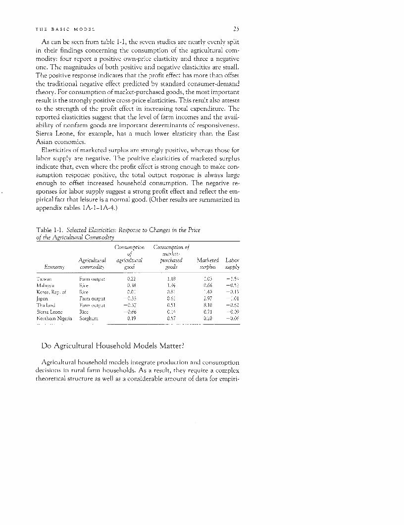
THE BASIC MODEL 25
As can be seen from table 1-1, the seven studies are nearly evenly splitin their findings concerning the consumption of the agricultural com-modity: four report a positive own-price elasticity and three a negativeone. The magnitudes of both positive and negative elasticities are small.The positive response indicates that the profit effect has more than offsetthe traditional negative effect predicted by standard consumer-demandtheory. For consumption of market-purchased goods, the most importantresult is the strongly positive cross-price elasticities. This result also atteststo the strength of the profit effect in increasing total expenditure. Thereported elasticities suggest that the level of farm incomes and the avail-ability of nonfarm goods are important determinants of responsiveness.Sierra Leone, for example, has a much lower elasticity than the EastAsian economies.
Elasticities of marketed surplus are strongly positive, whereas those forlabor supply are negative. The positive elasticities of marketed surplusindicate that, even where the profit effect is strong enough to make con-sumption response positive, the total output response is always largeenough to offset increased household consumption. The negative re-sponses for labor supply suggest a strong profit effect and reflect the em-pirical fact that leisure is a normal good. (Other results are summarized inappendix tables lA-1-lA-4.)
Table 1-1. Selected Elasticities: Response to Changes in the Priceof the Agricultural Commodity
Consumption Consumption ofof market-
Agricultural agricultural purchased Marketed LaborEconomy commodity good goods surplus supply
Taiwan Farm output 0.22 1.18 1.03 -1.54Malaysia Rice 0.38 1.94 0.66 -0.57Korea, Rep. of Rice 0.01 0.81 1.40 -0.13Japan Farm output -0.35 0.61 2.97 -1.01Thailand Farm output -C.37 0.51 8.10 -0.62Sierra Leone Rice -0.66 0.14 0.71 -0.09Northern Nigeria Sorghum 0.19 0.57 0.20 -0.06
Do Agricultural Household Models Matter?
Agricultural household models integrate production and consumptiondecisions in rural farm households. As a result, they require a complextheoretical structure as well as a considerable amount of data for empiri-
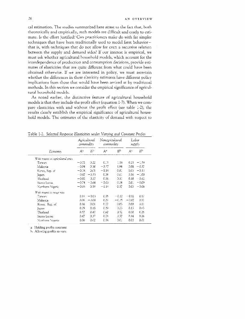
26 AN OVERVIEW
cal estimation. The studies summarized here attest to the fact that, boththeoretically and empirically, such models are difficult and costly to esti-mate. Is the effort justified? Can practitioners make do with far simplertechniques that have been traditionally used to model farm behavior-that is, with techniques that do not allow for even a recursive relationbetween the supply and demand sides? If our interest is empirical, wemust ask whether agricultural household models, which account for theinterdependence of production and consumption decisions, provide esti-mates of elasticities that are quite different from what could have beenobtained otherwise. If we are interested in policy, we must ascertainwhether the differences in these elasticity estimates have different policyimplications from those that would have been arrived at by traditionalmethods. In this section we consider the empirical significance of agricul-tural household models.
As noted earlier, the distinctive feature of agricultural householdmodels is that they include the profit effect (equation 1-7). When we com-pare elasticities with and without the profit effect (see table 1-2), theresults clearly establish the empirical significance of agricultural house-hold models. The estimates of the elasticity of demand with respect to
Table 1-2. Selected Response Elasticities under Varying and Constant Profits
Agricultural Nonagricultural Laborcommodity commodity supply
Economy Aa Bb Aa Bb Aa Bb
With respect to agricultural priceTaiwan -0.72 0.22 0.13 1.18 0.21 -1.59Malaysia -0.04 0.38 -0.27 1.94 0.08 -0.57Korea, Rep. of -0.18 0.01 -0.19 0.81 0.03 -0.13Japan -0.87 -0.35 0.08 0.61 0.16 -1.00Thailand -0.82 -0.37 0.06 0.51 0.18 -0.62Sierra Leone -0.74 -0.66 -0.03 0.14 0.01 -0.09Northern Nigeria -0.05 0.19 -0.14 0.57 0.03 -0.06
With respect to wage rateTaiwan 0.14 -0.03 0.05 -0.12 -0.12 0.17Malaysia 0.06 -0.08 0.29 -0.35 -0.07 0.11Korea, Rep. of 0.16 0.01 0.77 0.05 0.00 0.11Japan 0.29 0.15 0.39 0.25 0.15 0.45Thailand 0.57 0.47 0.62 0.52 0.08 0.26Sierra Leone 0.47 0.37 0.78 0.57 0.14 0.26Northern Nigeria 0.06 0.02 0.04 0.01 0.01 0.01
a. Holding profits constant.b. Allowinig profits to vary.
THE BASIC MODEL 27
own-price not only differ significantly in the cases of Japan, Thailand,and Sierra Leone, for example, but they also change sign in the case ofTaiwan, Malaysia, Korea, and northern Nigeria. Thus, whereas tradi-tional models of demand, as we would expect, predict a decline in own-consumption in response to an increase in agricultural commodity prices,for four cases, the agricultural household models predict an increase. Thisis because the profit effect-which is the result of the increase in incomewhen crop prices are raised-offsets the negative price effects. Farmhouseholds end up increasing their own consumption as prices are raised.Whether or not the amounts they offer on the market will be reduced willdepend on the elasticity of output, which we know remains positive inthese cases (see table 1-1). The marketed surplus response, however, isdampened by the profit effect.
The differences in the elasticity of demand for nonagricultural goodswith respect to the price of agricultural goods are also striking. The elas-ticities change sign in four cases, and in the other three cases the magni-tudes are much larger when the profit effect is included. Whereas cross-price elasticities estimated using traditional demand models tend to below or negative because of negative income effects, the estimates obtainedwith the agricultural household model are positive and large because ofthe positive profit effect. The elasticities of household labor supply withrespect to the price of the agricultural good also differ greatly. In the tradi-tional demand models, an increase in the price of the agricultural goodreduces the consumption of both that good and leisure, and thus impliesan increase in the family work effort (table 1-2). In contrast, agriculturalhousehold models predict a negative response of household labor supplyto increased output prices because households are willing to take a part oftheir increased incomes in increased leisure, thereby reducing their workeffort. Consequently, any increase in the demand for labor in agriculturalproduction will have considerable spillover effect on the demand forhired labor.
Although fewer signs change when responses to agricultural wage ratesare examined, the magnitudes change. In traditional demand models, anincrease in the wage rate implies an increase in real household incomes,which induces a positive-demand response with respect to agriculturaland nonagricultural goods and a negative or inelastic response wherehousehold labor supply is concerned. In agricultural household modelsthese effects are partly offset because an increase in wages also affects theproduction side and reduces total farm incomes. As a result, demand re-sponses for both agricultural and nonagricultural goods are either damp-ened or totally offset (as in Taiwan and Malaysia), and labor supply re-sponse becomes positive or more elastic.
28 AN OVERVIEW
Looking at the market (or off-farm) labor-supply responses of landedand landless households in rural India, Rosenzweig (1980) provides a dif-ferent type of evidence that agricultural household models matter. Afterseparately estimating reduced-form market-supply equations for landlessand agricultural households, Rosenzweig compares coefficients betweenthe two groups and finds that twenty-one out of twenty-two comparisonsconform to the predictions of the agricultural household framework. Forinstance, the off-farm male labor response of landless households to in-creases in the market male wage is less than for agricultural households,as would be predicted because of the negative profit effect of raising malewages.
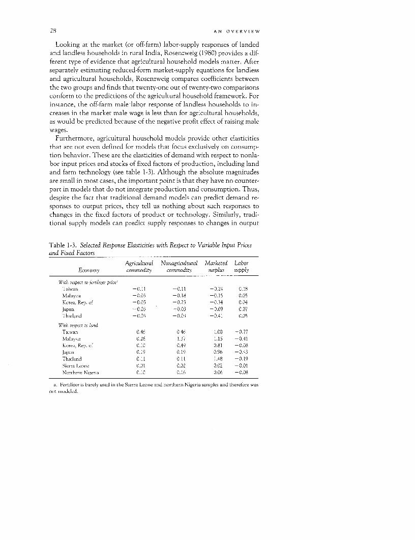
Furthermore, agricultural household models provide other elasticitiesthat are not even defined for models that focus exclusively on consump-tion behavior. These are the elasticities of demand with respect to nonla-bor input prices and stocks of fixed factors of production, including landand farm technology (see table 1-3). Although the absolute magnitudesare small in most cases, the important point is that they have no counter-part in models that do not integrate production and consumption. Thus,despite the fact that traditional demand models can predict demand re-sponses to output prices, they tell us nothing about such responses tochanges in the fixed factors of product or technology. Similarly, tradi-tional supply models can predict supply responses to changes in output
Table 1-3. Selected Response Elasticities with Respect to Variable Input Pricesand Fixed Factors
Agricultural Nonagricultural Marketed LaborEconomy commodity commodity surplus supply
With respect to fertilizer pricea
Taiwan -0.11 -0.11 -0.24 0.18Malaysia -0.03 -0.18 -0.15 0.05Korea, Rep. of -0.05 -0.23 -0.34 0.04Japan -0.03 -0.03 -0.09 0.07Thailand -0.03 -0.03 -0.41 0.05
With respect to land
Taiwan 0.46 0.46 1.00 -0.77
Malaysia 0.26 1.37 1.15 -0.41
Korea, Rep. of 0.10 0.49 0.81 -0.08
Japan 0.19 0.19 0.96 -0.43
Thailand 0.11 0.11 1.48 -0.19
Sierra Leone 0.01 0.02 0.02 -0.01
Norrhern Nigeria 0.10 0.16 0.06 -0.08
a. Fertilizer is barely used in the Sierra Leone and northern Nigeria samples and therefore was
not modeled.
THE BASIC MODEL 29
and input prices or in fix-ed factors of production and technology, butthey fail to tell us anything about the demand responses to these exoge-nous factors. Agricultural household models therefore provide a vital linkbetween the demand and supply-side responses to exogenous policychanges. Although these links can be established informally between tra-ditional supply-and-demand models, in agricultural household modelsthey are handled directly within a consistent theory and framework ofestimation.
When should a full agricultural household model be used? The answeris that, since the profit effect is its distinguishing feature, such a model isappropriate when the profit effect is likely to be important. Notice, how-ever, that changes in some exogenous prices have a small effect on farmprofits. The profit effect is much more important in Malaysia than in Si-erra Leone (table 1-6), for example, partly because the effect of a pricechange on profits is much larger in Malaysia, where a 10 percent increasein output price results in a 16 percent increase in profits. In Sierra Leone,the same percentage increase in output price increases profits by only 2percent.
Second, even if profits are affected by an exogenous price increase, theymay be only a small part of full income (equation 1-2), and it is full incomethat appears in the demand equations. For our sample of economies, theshare of profits in full income ranges from 0.5 in Malaysia to only 0.2 inThailand. It follows that a given percentage increase in profits will have amuch greater impact on total income in Malaysia than in Thailand.
Finally, the effect of full income on demand varies among commodities.It is much more important in the case of nonagricultural commoditiesthan agricultural ones, for example, since the demand for agriculturalcommodities tends to be inelastic with respect to income. In Malaysia, theelasticity of demand for rice with respect to full income is only 0.52 com-pared with 2.74 for market-purchased goods. As a result, the profit effectis much more significant in the case of nonagricultural goods (table 1-6).
These remarks suggest that, if profits are relatively insensitive to pro-ducer prices and constitute a relatively small part of full income and ifconsumption of a particular item is relatively insensitive to full income,then an agricultural household model will not necessarily make our anal-ysis more accurate. This proves to be the case, for example, with the elas-ticity of demand for agricultural goods with respect to changes in pro-ducer prices in Sierra Leone, although it is not true for low-incomehouseholds in that study (see chapter 4). If these three conditions are re-versed, however, a full agricultural household model is of critical impor-tance, as the elasticity of demand for nonagricultural goods with respectto producer prices in Malaysia reveals.
30 AN OVERVIEW
Policy Results
Agricultural household models provide insight into three broad areasof interest to policymakers: the welfare or real incomes of agriculturalhouseholds; the spillover effects of agricultural policies onto the rural,nonagricultural economy; and, at a more aggregate level, the interactionbetween agricultural policy and international trade or fiscal policy. Thepotential role of agricultural household models in this respect becomesevident when we look at these three dimensions in a "typical" agriculturalpolicy such as taxing output (either through export taxes or marketingboards) in order to generate revenue for the central exchequer and simul-taneously subsidizing a significant input (usually fertilizer) to restore, atleast in part, producer incentives. The model could just as easily be ap-plied to other policies, but this particular combination has been adoptedby many developing countries and illustrates well the type of issue thatcan be analyzed within the framework of the agricultural householdmodel.
Consider, first, the effect of pricing policy on the welfare or real fullincome of a representative agricultural household. For some pricechanges-for example, a change in the price of fertilizer-the resultingchange in nominal full income is an accurate measure of the change inreal income since the prices of all consumer goods have remained un-changed. In other cases, however, the commodity in question may beboth a consumer good and a farm output or input. If the price of, say, anagricultural staple is increased, the household will benefit as a producerbut lose as a consumer. As long as the household is a net producer of thecommodity, its net benefit will be positive (see the appendix to part I).Nevertheless, to quantify the net gain to the household, one must allowfor both the positive effect coming through farm profits and the negativeeffect coming through an increase in the price of an important consumergood.
Table 1-4 presents estimates of the elasticities of real full income withrespect to changes in output price and fertilizer price for the six studiesexamined earlier. For marginal changes, the decrease in real income fol-lowing an increase in the price of the agricultural output equals marketedsurplus times the price increase, and the increase following a reduction inthe price of an input equals the quantity of the input times the price re-duction. Thus, if prices, marketed surplus, and full income are known,these elasticities can be calculated without reference to price and incomeelasticities. For nonmarginal changes, however, it would be necessary to

THE BASIC MODEL 31
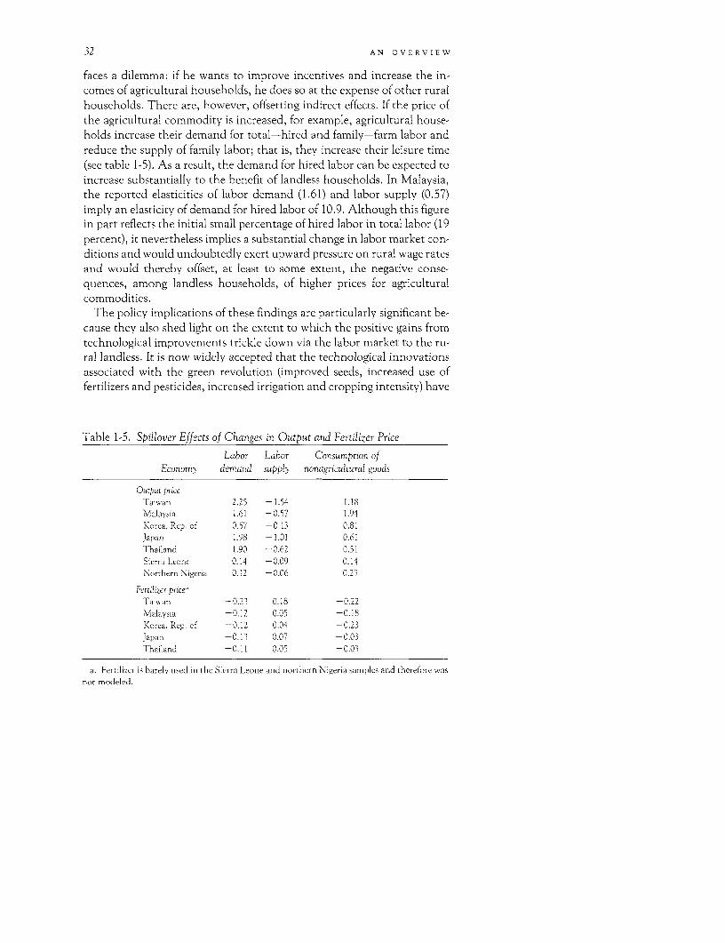
Table 1-4. Effect on Real Income of Changes in Output and Fertilizer Prices
Response to Response toEconomy- output price fertilizer price
Taiwan 0.90 -0.11Malaysia 0.67 -0.07Korea, Rep. of 0.40 -0.10Japan 0.34 -0.03Thailand 0.10 -0.03Sierra Leone 0.09 -
Northern Nigeria 0.12
- Not applicable. Fertilizer is barely used in the Sierra Leone and northern Nigeria samplesand therefore was not modeled.
use information on the underlying structure of preferences to calculateequivalent or compensating variation.
The percentage change in real income among the six countries underconsideration is less than the percentage change in either the output priceor the fertilizer price (table 1-4). In addition, it appears that the loss in realincome arising from a given percentage reduction in the output price canbe offset only if the price of fertilizer is reduced by a much larger percent-age. In Malaysia, for example, a 10 percent reduction in output pricewould reduce real income by almost 7 percent, whereas a 10 percent re-duction in the price of fertilizer would increase real income by only about1 percent. This difference arises from the relative magnitudes of marketedsurplus and fertilizer use. Thus, if policymakers are interested primarily inthe welfare of agricultural households, intervention in output markets islikely to be much more important than intervention in the markets forvariable, nonlabor inputs.
Policymakers are also concerned with the welfare of rural householdsthat do not own or rent land for cultivation. Landless households eithersell their labor to land-operating households or else engage in nonfarmactivities (see, for example, Anderson and Leiserson 1980). Althoughgovernments have few policy instruments by which to improve the wel-fare of these households directly, price interventions and investment pro-grams directed at land-operating households have spillover effects thatmay (or may not) be beneficial for these households. What can agricul-tural household models tell us about these effects?
An increase in the price of an important agricultural staple will obvi-ously hurt households that are net consumers of that item. The directeffect of a price increase will therefore be unambiguously negative forlandless households and nonfarm households. The policymaker thus
32 AN OVERVIEW
faces a dilemma: if he wants to improve incentives and increase the in-comes of agricultural households, he does so at the expense of other ruralhouseholds. There are, however, offsetting indirect effects. If the price ofthe agricultural commodity is increased, for example, agricultural house-holds increase their demand for total-hired and family-farm labor andreduce the supply of family labor; that is, they increase their leisure time(see table 1-5). As a result, the demand for hired labor can be expected toincrease substantially to the benefit of landless households. In Malaysia,the reported elasticities of labor demand (1.61) and labor supply (0.57)imply an elasticity of demand for hired labor of 10.9. Although this figurein part reflects the initial small percentage of hired labor in total labor (19percent), it nevertheless implies a substantial change in labor market con-ditions and would undoubtedly exert upward pressure on rural wage ratesand would thereby offset, at least to some extent, the negative conse-quences, among landless households, of higher prices for agriculturalcommodities.
The policy implications of these findings are particularly significant be-cause they also shed light on the extent to which the positive gains fromtechnological improvements trickle down via the labor market to the ru-ral landless. It is now widely accepted that the technological innovationsassociated with the green revolution (improved seeds, increased use offertilizers and pesticides, increased irrigation and cropping intensity) have
Table 1-5. Spillover Effects of Changes in Output and Fertilizer PriceLabor Labor Consumption of
Economy demand supply nonagricultural goods
Output price
Taiwan 2.25 -1.54 1.18Malaysia 1.61 -0.57 1.94Korea, Rep. of 0.57 -0.13 0.81Japan 1.98 -1.01 0.61Thailand 1.90 -0.62 0.51Sierra Leone 0.14 -0.09 0.14Northern Nigeria 0.12 -0.06 0.23
Fertilizer price'
Taiwan -0.23 0.18 -0.22Malaysia -0.12 0.05 -0.18Korea, Rep. of -0.12 0.04 -0.23Japan -0.13 0.07 -0.03Thailand -0.11 0.05 -0.03
a. Fertilizer is barely used in the Sierra Leone and northern Nigeria samples and therefore wasnot modeled.
THE BASIC MODEL 33
had a great deal to do with increasing the demand for total labor, but theconcern has been whether this increased demand would do much forhired labor, most of which comes from the smallest farms and the land-less. The empirical findings show that it could. When an increase, eitherin the fixed factors of production or technologies, boosts farm incomes,the amount of family (household's own) labor effort tends to decline (seetable 1-7). Therefore any increase in the demand for total labor means aneven larger increase in the demand for hired labor. The labor supply-and-demand elasticities emerging from empirical applications of agriculturalhousehold models provide strong support for the view that trickle-downeffects are both positive and significant.
A second indirect effect of increased output prices is a significant in-crease in the demand for nonagricultural goods (see table 1-5). The re-sponse elasticity is positive and greater than 1 in two economies (Taiwanand Malaysia) and is positive and greater than 0.5 in all economies exceptSierra Leone, though for low-income households in Sierra Leone it is alsohigh (0.9). Some of this demand will be for imports and urban-producedcommodities. But a large part will be for rurally produced goods and ser-vices and will therefore increase demand for the output of nonfarm, ruralhouseholds. Any increase in farm profits, whether caused by a pricechange or a technological improvement, can be expected to lead to a sub-stantial increase in the demand for goods and services produced by non-agricultural households. Thus, spillover effects through output marketswill, at least in part, offset the negative effects on nonfarm households ofan increase in agricultural prices and will ensure that the benefits of tech-nological improvements are dispensed throughout the rural community.
Table 1-5 also traces through the effects of a change in the price of fertil-izer. The results suggest that changes in fertilizer prices can be made with-out generating large negative or positive spillover effects.
As mentioned earlier, governments often tax agricultural output in or-der to generate revenue and at the same time subsidize essential inputssuch as fertilizer in order to restore production incentives. In this way,they hope to achieve self-sufficiency or earn foreign exchange. Can agri-cultural household models shed light on these and other policy options?Indeed, the information they provide with respect to the effect of pricingpolicy on marketed surplus and fertilizer demand can be used as inputs incalculations of self-sufficiency, balance of payment effects, and budgetaryeffects.
If a government's primary concern is self-sufficiency, it needs to knowthe marketed surplus available for procurement. When we look at theelasticity estimates for agricultural production, consumption, and mar-keted surplus (table 1-6), two points become clear. First, even where con-
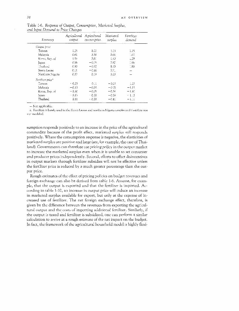
34 AN OVERVIEW
Table 1-6. Response of Output, Consumption, Marketed Surplus,and Input Demand to Price Changes
Agricultural Agricultural Marketed FertilizerEconomy output consumption surplus demand
Otaput priceTaiwan 1.25 0.22 1.03 2.25Malaysia 0.61 0.38 0.66 1.61Korea, Rep. of 1.56 0.01 1.40 1.29Japan 0.98 -0.35 2.97 1.98Thailand 0.90 -0.37 8.10 1.90Sierra Leone 0.11 -0.66 0.71 -Northern Nigeria 0.30 0.19 0.20 -
Fertilizer price'Taiwan -0.23 -0.11 -0.23 -1.23Malaysia -0.13 -0.03 -0.15 -1.13Korea, Rep. of -0.30 -0.05 -0.34 -1.10Japan -0.13 -0.03 -0.09 -1.13Thailand -0.11 -0.03 -0.41 -1.11
-Not applicable.a. Fertilizer is barely used in the Sierra Leone and northern Nigeria samples and therefore was
not modeled.
sumption responds positively to an increase in the price of the agriculturalcommodity because of the profit effect, marketed surplus still respondspositively. Where the consumption response is negative, the elasticities ofmarketed surplus are positive and large (see, for example, the case of Thai-land). Governments can therefore use pricing policy in the output marketto increase the marketed surplus even when it is unable to set consumerand producer prices independently. Second, efforts to offset disincentivesin output markets through fertilizer subsidies will not be effective unlessthe fertilizer price is reduced by a much greater percentage than the out-put price.
Rough estimates of the effect of pricing policies on budget revenues andforeign exchange can also be derived from table 1-6. Assume, for exam-ple, that the output is exported and that the fertilizer is imported. Ac-cording to table 1-10, an increase in output price will induce an increasein marketed surplus available for export, but only at the expense of in-creased use of fertilizer. The net foreign exchange effect, therefore, isgiven by the difference between the revenues from exporting the agricul-tural output and the costs of importing additional fertilizer. Similarly, ifthe output is taxed and fertilizer is subsidized, one can perform a similarcalculation to arrive at a rough estimate of the net impact on the budget.In fact, the framework of the agricultural household model is highly flexi-
THE BASIC MODEL 35
ble and can be adapted to fit many other circumstances and issues. Oneof the purposes of this volume is to present some of the extensions thathave recently been tested (see chapters 3, 4, 5, 6, and 7).
Some Extensions
Most of the early work on agricultural household models ignored ques-tions of choice among competing crops. These studies either examinedmonocultures or else treated farm output as an aggregate. Several impor-tant policy issues, however, are concerned with the choice among alterna-tive crops. Many governments, for example, are concerned with the effectof export taxation on production when export crops compete with foodcrops destined for the domestic market. Similarly, if fertilizer intensityvaries among crops, price-induced changes in the composition of outputmay have significant effects on the demand for fertilizer. The demand forhired labor can also be influenced by changes in crop composition.
The basic agricultural household model can be modified easily to ac-commodate multiple crops. Thus a production function for a single cropcan be replaced with an implicit production function linking inputs andoutputs:
G(Q1, Qni Vi, .V.. Vm, Al, ... Ak) = 0
where Q represents output, V is variable inputs, and A is fixed factors.Provided the household is a price-taker in the relevant markets, the intro-duction of multiple outputs does not affect the recursive property of themodel. Two of the studies covered in this volume-those by Singh andJanakiram and by Strauss-allow specifically for multiple crops.
This is an important policy extension since pricing policies are oftenoriented around specific commodities, but other crops will likely be af-fected as well. These studies cover three countries: the Republic of Korea,Nigeria, and Sierra Leone, and in each case cover crops grown primarilyfor consumption, for sale, and crops both consumed and exchanged. Thecountries cover three dissimilar environments. In Korea, farm house-holds are well integrated into product and factor markets. Crops aregrown under irrigated conditions and in single stands. Considerable tech-nological advance has occurred in rice production, with a consequenthigh-level use of purchased inputs. In addition, there are many sourcesfor nonfarm incomes. Households in Sierra Leone are also fairly well inte-grated into product and labor markets, but the level of income is far lowerthan for Korean households. There has been little technological changein paddy rice (or other crop) production so there is little use for nonpur-
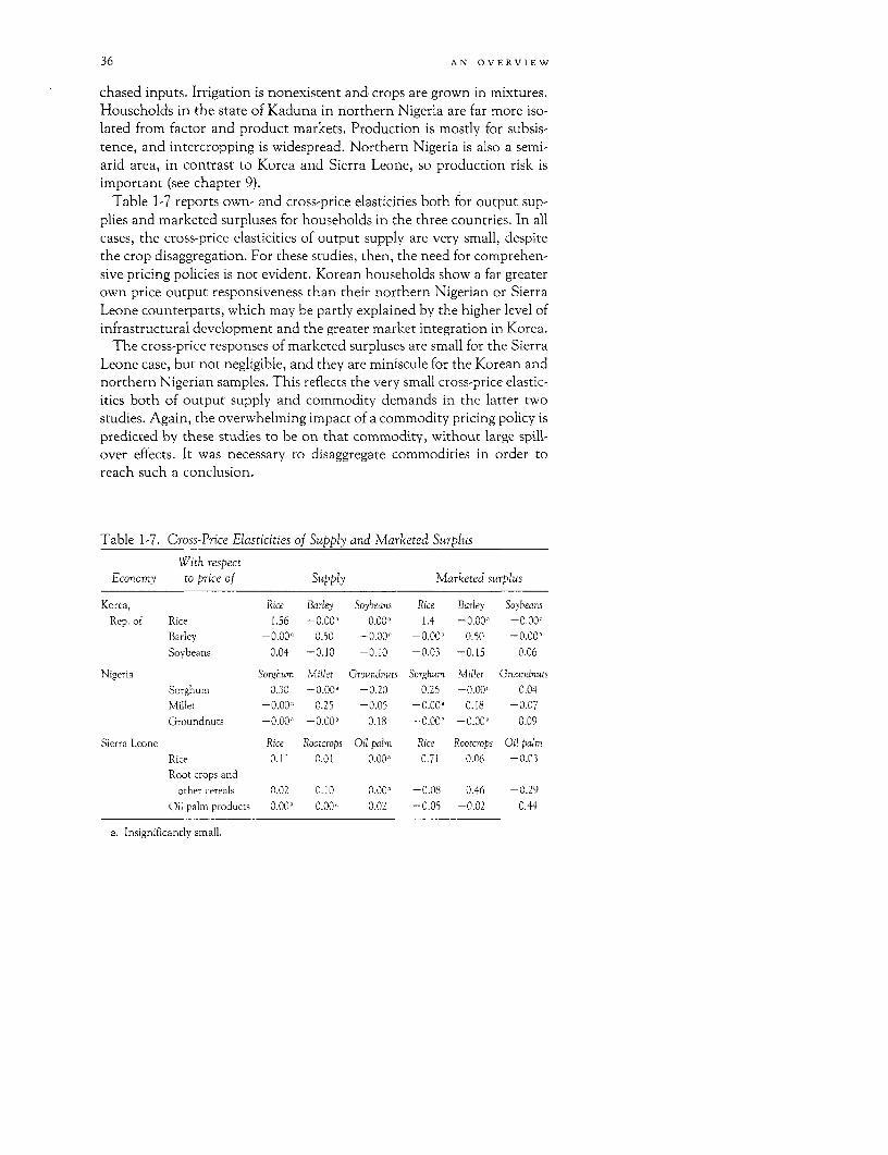
36 AN OVERVIEW
chased inputs. Irrigation is nonexistent and crops are grown in mixtures.Households in the state of Kaduna in northern Nigeria are far more iso-lated from factor and product markets. Production is mostly for subsis-tence, and intercropping is widespread. Northern Nigeria is also a semi-arid area, in contrast to Korea and Sierra Leone, so production risk isimportant (see chapter 9).
Table 1-7 reports own- and cross-price elasticities both for output sup-plies and marketed surpluses for households in the three countries. In allcases, the cross-price elasticities of output supply are very small, despitethe crop disaggregation. For these studies, then, the need for comprehen-sive pricing policies is not evident. Korean households show a far greaterown price output responsiveness than their northern Nigerian or SierraLeone counterparts, which may be partly explained by the higher level ofinfrastructural development and the greater market integration in Korea.
The cross-price responses of marketed surpluses are small for the SierraLeone case, but not negligible, and they are miniscule for the Korean andnorthern Nigerian samples. This reflects the very small cross-price elastic-ities both of output supply and commodity demands in the latter twostudies. Again, the overwhelming impact of a commodity pricing policy ispredicted by these studies to be on that commodity, without large spill-over effects. It was necessary to disaggregate commodities in order toreach such a conclusion.
Table 1-7. Cross-Price Elasticities of Supply and Marketed Surplus
With respectEconomy to price of Supply Marketed surplus
Korea, Rice Barley Soybeans Rice Barley SoybeansRep. of Rice 1.56 -0.00° 0.00' 1.4 -0.00' -0.Q00
Barley -0.00, 0.50 -0.00' -0.00, 0.50 -0.00'Soybeans 0.04 -0.10 -0.10 -0.03 -0.15 0.06
Nigeria Sorghum Millet Groundnuos Sorghum Millet GroundnutsSorghum 0.30 -0.00' -0.20 0.25 -0.00, 0.04Millet -0.00, 0.25 -0.05 -0.00' 0.18 -0.07Groundnuts -0.00' -0.00' 0.18 -0.00' -0.00' 0.09
Sierra Leone Rice Rootcrops Oil palm Rice Rootcrops Oil palmRice 0.11 0.01 0.00' 0.71 0.06 -0.03Root crops and
other cereals 0.02 0.10 0.00' -0.08 0.46 -0.29Oil palm products 0.00' 0.00 0.02 -0.05 -0.02 0.44
a. Insignificantly small.
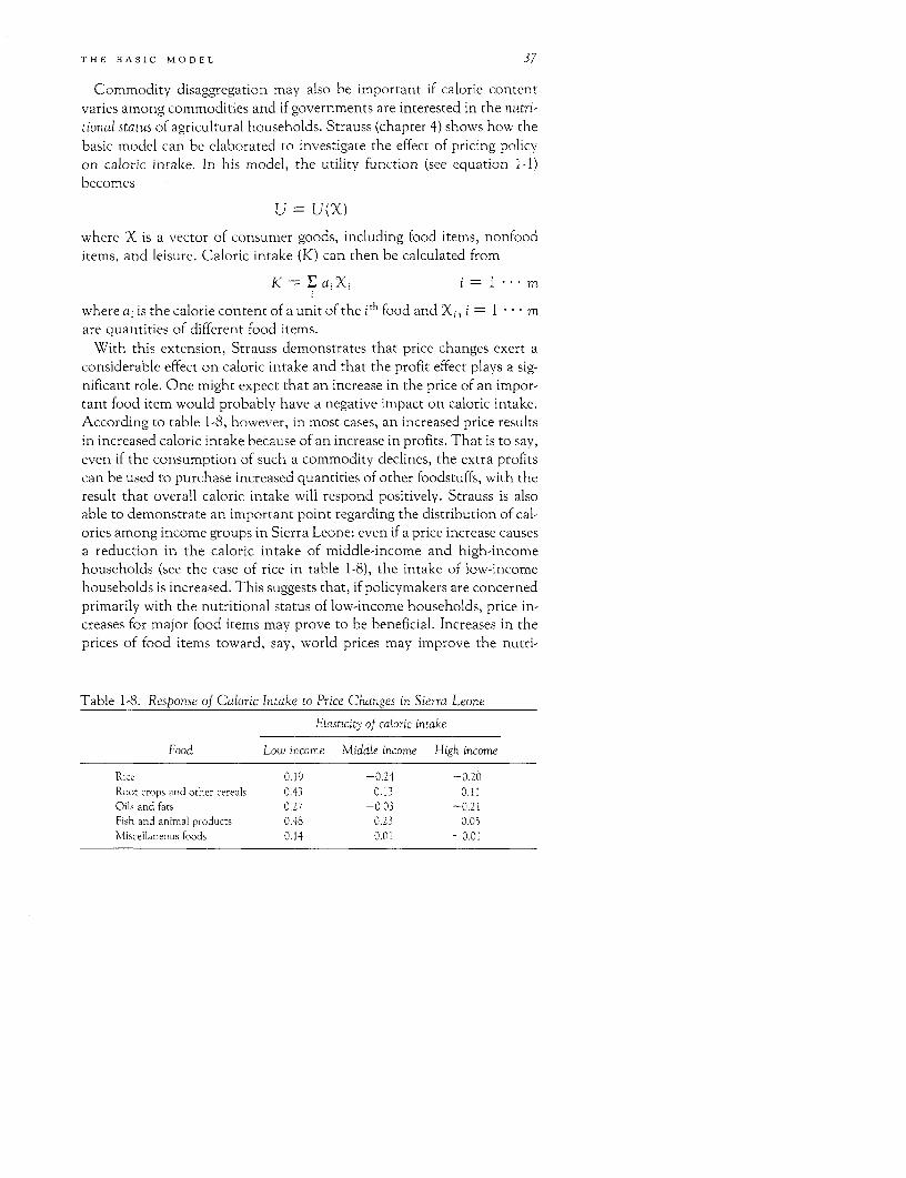
THE BASIC MODEL 37
Commodity disaggregation may also be important if calorie contentvaries among commodities and if governments are interested in the nutri-
tional status of agricultural households. Strauss (chapter 4) shows how thebasic model can be elaborated to investigate the effect of pricing policyon caloric intake. In his model, the utility function (see equation 1-1)becomes
U= U(X)
where X is a vector of consumer goods, including food items, nonfooditems, and leisure. Caloric intake (K) can then be calculated from
K = Ea aXi i=I***m
where ai is the calorie content of a unit of the ith food and Xi, i 1 ... mare quantities of different food items.
With this extension, Strauss demonstrates that price changes exert aconsiderable effect on caloric intake and that the profit effect plays a sig-nificant role. One might expect that an increase in the price of an impor-tant food item would probably have a negative impact on caloric intake.According to table 1-8, however, in most cases, an increased price resultsin increased caloric intake because of an increase in profits. That is to say,even if the consumption of such a commodity declines, the extra profitscan be used to purchase increased quantities of other foodstuffs, with theresult that overall caloric intake will respond positively. Strauss is alsoable to demonstrate an important point regarding the distribution of cal-ories among income groups in Sierra Leone: even if a price increase causesa reduction in the caloric intake of middle-income and high-incomehouseholds (see the case of rice in table 1-8), the intake of low-incomehouseholds is increased. This suggests that, if policymakers are concernedprimarily with the nutritional status of low-income households, price in-creases for major food items may prove to be beneficial. Increases in theprices of food items toward, say, world prices may improve the nutri-
Table 1-8. Response of Caloric Intake to Price Changes in Sierra Leone
Elasticity of caloric intake
Food Lou income Middle income High income
Rice 0.19 -0.24 -0.20Root crops and other cereals 0.43 0.13 0.11Oils and fats 0.27 -0.03 -0.21Fish and animal products 0.48 0.23 0.05Miscellaneous foods 0.14 0.01 -0.01
38 AN OVERVIEW
tional status of low-income households and provide appropriate signalsfor resource allocation. The usual equity-growth tradeoff may be absentin this case.
Policymakers are interested in nutritional status presumably because itaffects health and may also affect productivity at the individual level. Pittand Rosenzweig (chapter 5) take the analysis one step further, therefore,and examine the interaction between prices, health, and farm profits in thecontext of an agricultural household model. To do so, they incorporate ahealth variable directly in the utility function (people prefer to behealthy) and in the production function (a healthy individual is moreproductive). To complete their model, they introduce a production func-tion for health:
H = H(X", Xm, XI, Z)
which says that health (H) depends on consumption (X, and Xm) andhence on nutrition, leisure (or work effort, XI), and a vector (Z) of otherfactors that affect health, some of which are chosen by the household(boiling water) and some of which are community-level services (wellwater).
When this model is applied to data from Indonesia, it is found that a 10percent increase in the consumption of fish, fruit, and vegetables reducesthe probability of illness by 9, 3, and 6 percent, respectively, whereas a 10percent increase in the consumption of sugar increases the probability ofillness by almost 12 percent. These results suggest that increases in con-sumption cannot automatically be assumed to contribute to health sincethe composition of consumption may also change in a manner detrimen-tal to health.
In addition to estimating the health production function, Pitt and Ro-senzweig also estimate a reduced-form equation that produces a directlink between prices and health. They show that a 10 percent reduction inthe prices of vegetables and vegetable oil will decrease the probability ofthe household head being ill by 4 and 9 percent, respectively, whereas thesame percentage reduction in the prices of grains and sugar will increasethe probability of illness by 15 and 20 percent, respectively, albeit from avery low base. These results are calculated with profits held constant,however. In principle, when profits are allowed to vary, some of theseresults may be modified. In this particular application the coefficient onfarm profits proved statistically insignificant. The results reported aboveare therefore reasonably accurate measures of the total effect of pricechanges on health.
Changes in health may also affect productivity and farm profits. Pittand Rosenzweig demonstrate for their sample, however, that the effects of
THE BASIC MODEL 39
ill-health on labor supply are not reflected in reduced farm profits whenhouseholds have recourse to an active labor market. Thus, although fam-ily labor supply is significantly reduced by illness, total labor input, andhence farm profits, remain unaffected. In other words, in this Indonesiansample the benefits of improved health (or the costs of a deterioration inhealth) in agricultural households will be reflected in household income-if at all-only through labor-market supply.
Most of the policy issues mentioned thus far have been static in natureand have been couched in a single-period framework. Iqbal's work (chap-ter 6) represents a significant departure from previous studies in that itintroduces another period to accommodate borrowing, saving, and invest-ment decisions. Since governments and multinational agencies devotesubstantial quantities of funds to rural credit programs, this particularextension makes it possible to apply agricultural household models to anew set of policy issues of considerable importance in many countries.
In the first period of Iqbal's two-period model, the household may bor-row and invest in farm improvements. In the second period, the loanmust be repaid with interest and the household enjoys higher farm profitsas a result of its investment in period one. Accordingly, the single full-income constraint is replaced by two full-income constraints, one foreach period:
11(KI) + wLT, + B = Cl + I
and
Ul(KI + )+ W2 T2 = C,- + B(1 + r[B])
where K1 is capital in period one and I is investment, so that K1 + I iscapital in period two. B is borrowing in period one and B(1 + r[B]) isrepayment in period two. C is the value of consumption of goods andleisure. Iqbal draws a parallel between his treatment of household savingsand borrowing and the treatment of own-consumption and marketedsurplus or family labor supply and hired labor in the standard agriculturalhousehold model. He notes that the recursive property of the standardmodel carries over to his two-period extension, provided the householdcan borrow at a fixed rate of interest. In his application to Indian house-holds, Iqbal argues that the interest rate is influenced by household bor-rowing decisions (r is a function of B in the second-period constraint) andtherefore he adopts a nonrecursive specification.
lqbal finds that borrowing is significantly reduced by increases in theinterest rate, the elasticity being -1.2. His results support the view thatinterest rate policy can have a marked effect on the level of debt held byfarmers. Iqbal also shows that farmers owning more than three hectares
40 AN OVERVIEW
are highly sensitive to the interest rate, whereas the coefficient on bor-rowing by farmers owning less than three hectares is statistically insignifi-cant. It follows that the elimination or reduction of subsidies to programsproviding agricultural credit may serve the dual purpose of increasing effi-ciency in the capital market and simultaneously improving equity, sincethe reduction in borrowing by "large" farmers will exceed that by "small"ones.
As noted earlier, governments are also interested in the effects of agri-cultural pricing policy on more aggregate economic variables such asbudget deficits and foreign exchange earnings. In Senegal, for example, agri-cultural products generate 70 percent of total export earnings, and defi-cits arising from the government's policy on agricultural pricing amountto more than 20 percent of government expenditure and 2 percent ofGDP. Changes in agricultural prices can therefore be expected to have aconsiderable impact on these aggregates. Indeed, concern with the exist-ing levels of foreign exchange earnings and a budget deficit may be theprimary motivation for changing pricing policy in many countries. Thegovernment of Senegal has explored a number of ways, including pricingpolicy, to promote the production and consumption of millet in orderto reduce imports of rice and hence improve the country's balance ofpayments.
The effect of pricing policy on foreign exchange and budget revenuesdiscussed earlier in the chapter is further illuminated by Braverman andHammer (chapter 8) through their addition of market-clearing conditions(for the major outputs and inputs) to the basic model. The changes inconsumption, production, or labor supply at the household level follow-ing any change in an exogenous variable can then be aggregated and fedinto the market-clearing equations. In some cases, the market is clearedthrough adjustments in international trade, and prices remain fixed atlevels determined by the government, that is,
Q(P,) = X. (p) + E
where E represents net exports. In this event, a change in production orconsumption has an immediate effect on foreign exchange earnings. Al-ternatively, the market may clear through adjustments in price, that is,
Q(Pa) Xa(P,).
Now a policy-induced change in production or consumption will bringabout a change in price, which will generate second-round effects on pro-duction and consumption.
In their application to Senegal, Braverman and Hammer assume thefirst form of marketing clearing (quantity adjustment) for cotton, ground-
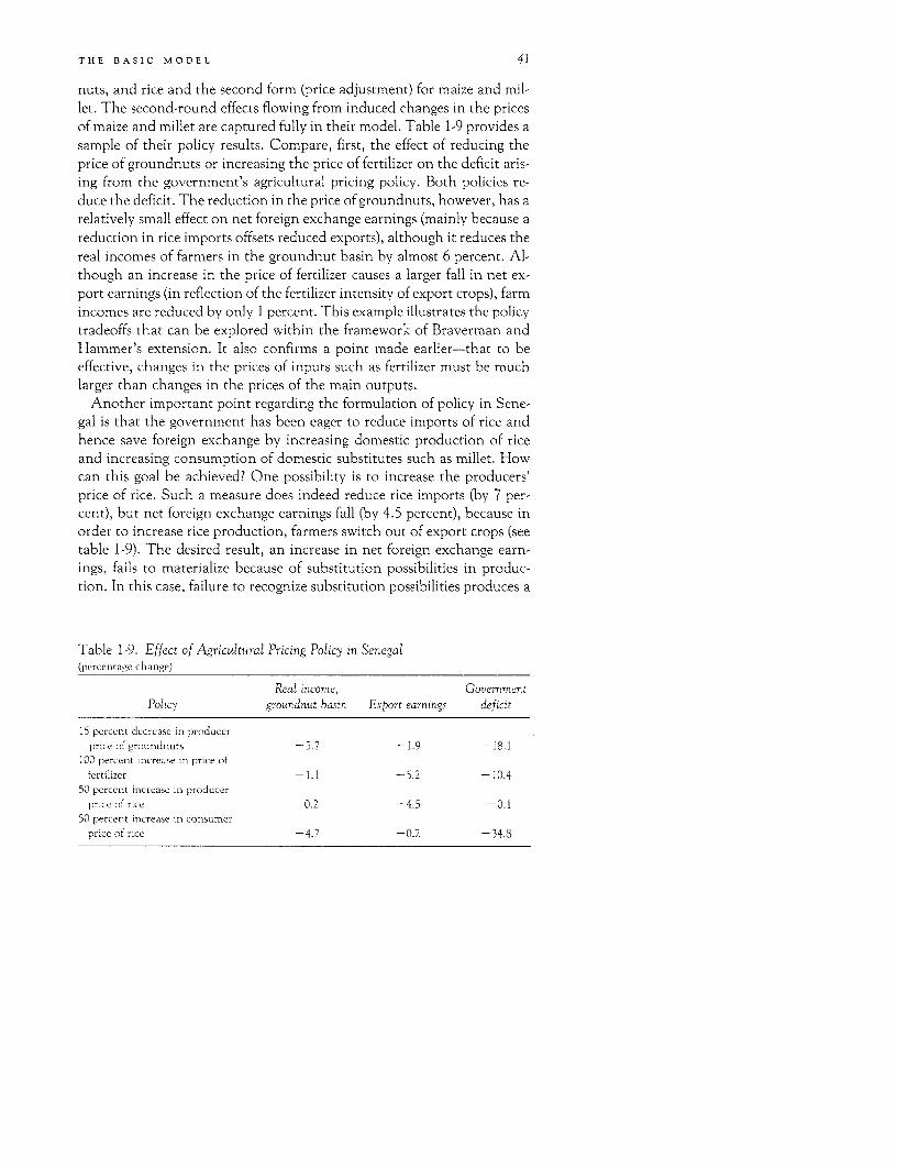
THE BASIC MODEL 41
nuts, and rice and the second form (price adjustment) for maize and mil-let. The second-round effects flowing from induced changes in the pricesof maize and millet are captured fully in their model. Table 1-9 provides asample of their policy results. Compare, first, the effect of reducing theprice of groundnuts or increasing the price of fertilizer on the deficit aris-ing from the government's agricultural pricing policy. Both policies re-duce the deficit. The reduction in the price of groundnuts, however, has arelatively small effect on net foreign exchange earnings (mainly because areduction in rice imports offsets reduced exports), although it reduces thereal incomes of farmers in the groundnut basin by almost 6 percent. Al-though an increase in the price of fertilizer causes a larger fall in net ex-port earnings (in reflection of the fertilizer intensity of export crops), farmincomes are reduced by only 1 percent. This example illustrates the policytradeoffs that can be explored within the framework of Braverman andHammer's extension. It also confirms a point made earlier-that to beeffective, changes in the prices of inputs such as fertilizer must be muchlarger than changes in the prices of the main outputs.
Another important point regarding the formulation of policy in Sene-gal is that the government has been eager to reduce imports of rice andhence save foreign exchange by increasing domestic production of riceand increasing consumption of domestic substitutes such as millet. Howcan this goal be achieved? One possibility is to increase the producers'price of rice. Such a measure does indeed reduce rice imports (by 7 per-cent), but net foreign exchange earnings fall (by 4.5 percent), because inorder to increase rice production, farmers switch out of export crops (seetable 1-9). The desired result, an increase in net foreign exchange earn-ings, fails to materialize because of substitution possibilities in produc-tion. In this case, failure to recognize substitution possibilities produces a
Table 1-9. Effect of Agricultural Pricing Policy in Senegal(percentage change)
Real income, GovernmentPolicx groundnut basin Export earnings deficit
15 percent decrease in producerprice of groundnuts -5.7 -1.9 -18.1
100 percent increase in price offertilizer -1.1 -5.2 -10.4
50 percent increase in producerprice of rice 0.2 -4.5 -0.1
50 percent increase in consumerprice of rice -4.7 -0.2 -34.8
42 AN OVERVIEW
perverse result. In other situations, however, policy may be designed totake advantage of substitution possibilities. The government might in-crease the consumer price of rice in the hope that people would changetheir pattern of consumption in favor of millet. According to Bravermanand Hammer's analysis, however, such a policy would have little impacton net export earnings, so that in this case a reliance on substitution pos-sibilities would have been misplaced (see table 1-9).
These examples from the work of Braverman and Hammer illustratethe importance of placing agricultural household models in a multi-market framework, particularly where foreign exchange earnings andgovernment revenues are of concern. Because the expansion of one cropis usually detrimental to another crop, changes in the quantities of inter-nationally traded items and in the quantities of taxed or subsidized itemswill influence the overall impact of policy on foreign exchange and gov-ernment revenue even if a change in a government-controlled price inone market leaves the prices in all other agricultural markets unchanged.More generally, changes in government-controlled prices will inducechanges in other prices so that even measures of output response, laborsupply response, consumer response, and changes in farm profits willhave to allow for general equilibrium effects (see chapter 2). Thus themultimarket extension may well emerge as the most useful vehicle forgenerating relevant policy results from agricultural household models.
Appendix: Detailed Elasticities from Studiesof Agricultural Household Models
The four tables in this appendix are on the following pages.
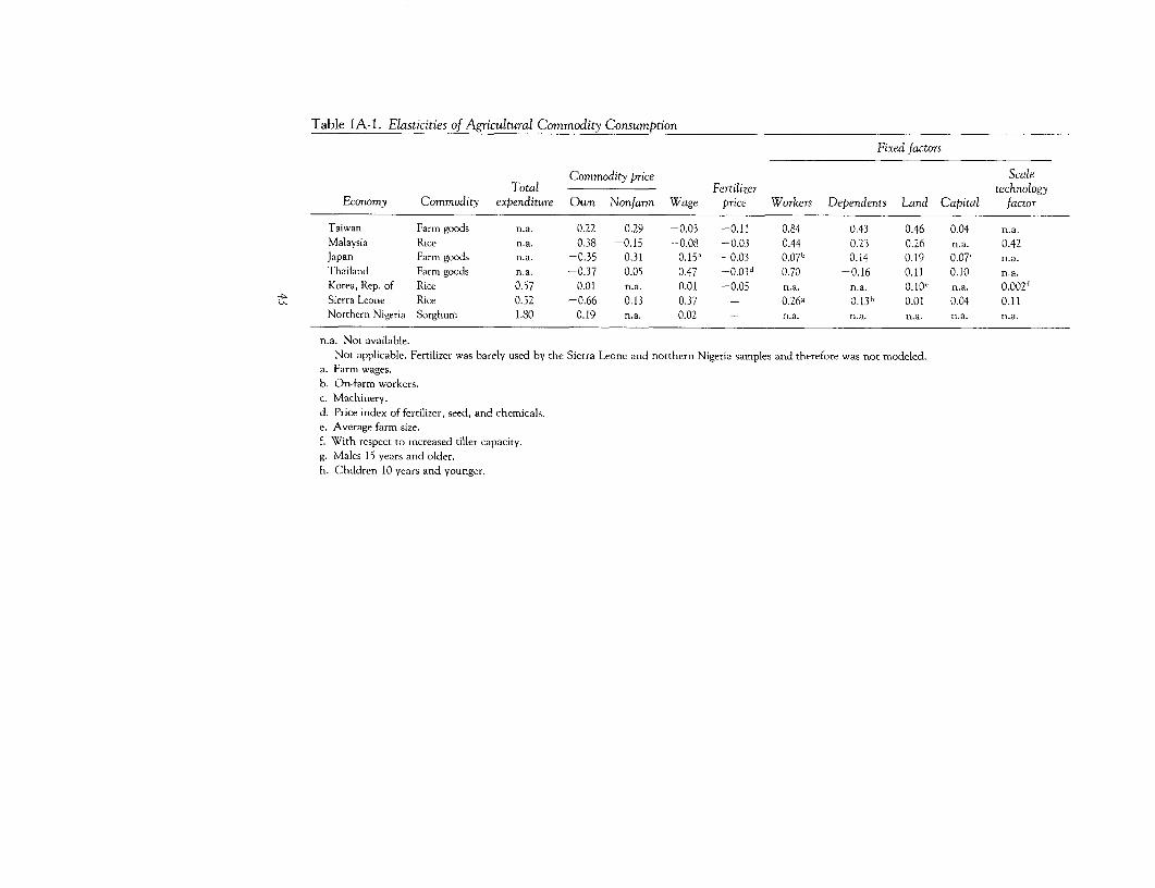
Table IA-1. Elasticities of Agricultural Commodity Consumption
Fixed factors
Commodity price ScaleTotal Fertilizer technology
Economy Commodity expenditure Own Nonfarn Wage price Workers Dependents Land Capital factor
Taiwan Farm goods n.a. 0.22 0.29 -0.03 -0.11 0.84 0.43 0.46 0.04 n.a.Malaysia Rice n.a. 0.38 -0.15 -0.08 -0.03 0.44 0.23 0.26 n.a. 0.42Japan Farm goods n.a. -0.35 0.31 0.15' -0.03 0.07b 0.14 0.19 0.07- n.a.Thailand Farm goods n.a. -0.37 0.05 0.47 -0.03d 0.70 -0.16 0.11 0.10 n.a.Korea, Rep. of Rice 0.57 0.01 n.a. 0.01 -0.05 n.a. n.a. 0.10, n.a. 0.002f
411 Sierra Leone Rice 0.52 -0.66 0.13 0.37 - 0.26g 0.13h 0.01 0.04 0.11Northern Nigeria Sorghum 1.80 0.19 n.a. 0.02 - n.a. n.a. n.a. n.a. n.a.
n.a. Not available.- Not applicable. Fertilizer was barely used by the Sierra Leone and northern Nigeria samples and therefore was not modeled.a. Farm wages.b. On-farm workers.c. Machinery.d. Price index of fertilizer, seed, and chemicals.e. Average farm size.f. With respect to increased tiller capacity.g. Males 15 years and older.h. Children 10 years and younger.
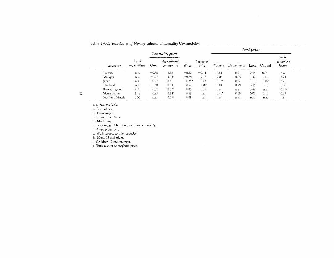
Table 1A-2. Elasticities of Nonagricultural Commodity ConsumptionFixed factors
Commodity prices Scale
Total Agricultural Fertilizer technology
Economy expenditure Own commodity Wage price Workers Dependents Land Capital factor
Taiwan n.a. -0.58 1.18 -0.12 -0.11 0.84 0.0 0.46 0.04 n.a.
Malaysia n.a. -0.77 1.94' -0.35 -0.18 -0.06 -0.05 1.37 n.a. 2.21
Japan n.a. -0.97 0.61 0.25b -0.03 -0.l12 0.02 0.19 0.07' n.a.
Thailand n.a. -0.89 0.51 0.52 -0.03, 0.69 -0.29 0.11 0.10 n.a.
Korea, Rep. of 2.76 -0.87 0.81' 0.05 -0.23 n.a. n.a. 0.49' n.a. 0.01'
41. Sierra Leone 1.18 -0.93 0.14' 0.57 n.a. 0.41h 0.09i 0.02 0.10 0.27
Northern Nigeria 3.30 n.a. 0.57i 0.01 n.a. n.a. n.a. n.a. n.a. na.
n.a. Not available.a. Price of rice.b. Farm wage.c. On-faTm workers.d. Machinery.e. Price index of fertilizer, seed, and chemicals.f. Average farm size.g. With respect to tiller capacity.h. Males 15 and older.i. Children 10 and younger.j. With respect to sorghum price.
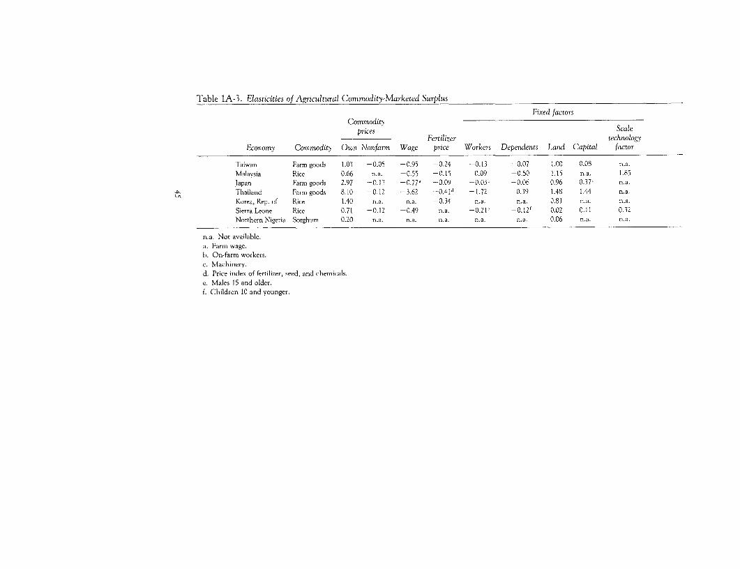
Table 1A-3. Elasticities of Agricultural Commodity-Marketed Surplus
Fixed factorsCommodity
prices ScaleFertilizer technology
Economy Commodity Own Nonfarm Wage price Workers Dependents Land Capital factor
Taiwan Farm goods 1.03 -0.05 -0.95 -0.24 -0.13 -0.07 1.00 0.08 n.a.Malaysia Rice 0.66 n.a. -0.55 -0.15 0.09 -0.50 1.15 n.a. 1.85Japan Farm goods 2.97 -0.13 -0.77' -0.09 -0.03b -0.06 0.96 0.37' n.a.
a1 Thailand Farm goods 8.10 -0.12 -3.62 -0.41d -1.72 0.39 1.48 1.44 n.a.Korea, Rep. of Rice 1.40 n.a. n.a. -0.34 n.a. n.a. 0.81 n.a. n.a.Sierra Leone Rice 0.71 -0.12 -0.49 n.a. -0.21' -0.12f 0.02 0.11 0.32Northern Nigeria Sorghum 0.20 n.a. n.a. n.a. n.a. in.a. 0.06 n.a. n.a.
n.a. Not available.a. Farm wage.b. On-farm workers.c. Machinery.d. Price index of fertilizer, seed, and chemicals.e. Males 15 and older.f. Children 10 and younger.

Table IA-4. Elasticities of Labor Supply
Fixed factorsCommodity prices
ScaleType of Agricultural Nonfarm Farm Off-farm Fertilizer technology
Economy labor commodity commodity wage wage price Workers Dependents Land Capital factor
Taiwan Total -1.54 0.58 0.17 n.a. 0.18 1.27 0.20 -0.77 -0.06 n.a.Malaysia Total -0.57T 0.24 0.11 n.a. 0.05 0.62 0.12 -0.41 n.a. -0.65Japan Farm -1.01 0.30 0.45 -1.97 0.07 -0.891" 0.34 -0.43 -0.17 in.a.Thailand Total -0.62 0.10 0.26 n.a. 0,05d 0.94 -0.28 -0.19 -0.19 n.a.Korea, Rep. of Total -0.13' n.a. 0.11 n.a. 0.04 n.a. n.a. -0.08, n.a. -0.002'
Oh Sierra Leone Total -0.09' -0.05 0.26 n.a. n.a. 0.55g 0.13h -0.01 -0.05 n.a.Sierra Leonie Off-farm -4.42' -1.85 17.18 n.a. n.a. 14.367 3.781" -0.94 -4.90 n.a.Northern Nigeria Total -0.06 n.a. 0.10 n.a. n.a. n.a. n.a. n.a. n.a. n.a.
n.a. Not available.a. Price of rice.b. On-farm workers.c. Machinery.d. Price index of fertilizer, seed, and chemicals.e. Average farm size.f. With respect to tiller capacity.g. Males 15 and older.h. Children 10 and younger.
THE BASIC MODEL 47
References
Adulavidhaya, Kamphol, Yoshimi Kuroda, Lawrence Lau, Pichit Lerttamrab, andPan Yotopoulos. 1979. "A Microeconomic Analysis of the Agriculture of Thai-land." Food Research Institute Studies, vol. 17, pp. 79-86.
Adulavidhaya, Kamphol, Yoshimi Kuroda, Lawrence Lau, and Pan Yotopoulos.1984. "The Comparative Statics of the Behavior of Agricultural Households inThailand." Singapore Economic Review, vol. 29, pp. 67-96.
Anderson, Dennis, and Mark Leiserson. "Rural Nonfarm Employment in Develop-ing Countries." Economic Development and Cultural Change, vol. 28, pp. 227-48.
Barnum, Howard, and Lyn Squire. 1978. "Technology and Relative Economic Effi-ciency." Oxford Economic Papers, vol. 30, pp. 181-98.
-_____ 1979a. "An Econometric Application of the Theory of the Farm House-hold." Journal of Development Economics, vol. 6, pp. 79-102.
______ 1979b. A Model of an Agricultural Household. Washington, D.C.: WorldBank.
Barten, Anton. 1977. "The Systems of Consumer Demand Functions Approach: AReview." Econometrica, vol. 45, pp. 23-52.
Brown, Alan, and Angus Deaton. 1972. "Surveys in Applied Economics: Models ofConsumer Behavior." Economic Journal, vol. 82, pp. 1145-1236.
Deaton, Angus, and John Muellbauer. 1980. Economics and Consumer Behavior. Cam-bridge, Mass.: Cambridge University Press.
Kuroda, Yoshimi, and Pan Yotopoulos. 1978. "A Microeconomic Analysis of Pro-duction Behavior of the Farm Household in Japan: A Profit Function Approach."The Economic Review (Japan), vol. 29, pp. 116-29.
___ . 1980. "A Study of Consumption Behavior of the Farm Household in Japan:An Application of the Linear Logarithmic Expenditure System." The Economic Re-view (Japan), vol. 31, pp. 1-15.
Lau, Lawrence, Wuu-Long Lin, and Pan Yotopoulos. 1978. "The Linear LogarithmicExpenditure System: An Application to Consumption Leisure Choice." Econo-metrica, vol. 46, pp. 843-68.
Pollak, Robert, and Terence Wales. 1981. "Demographic Variables in Demand Anal-ysis." Econometrica, vol. 49, pp. 1533-51.
Yotopoulos, Pan, Lawrence Lau, and Wuu-Long Lin. 1976. "Microeconomic OutputSupply and Factor Demand Functions in the Agriculture of the Province of Tai-wan." American Journal of Agricultural Economics, vol. 58, pp. 333-40.
2Methodological Issues
Inderjit Singh, Lyn Squire, and John Strauss
A NUMBER OF IMPORTANT METHODOLOGICAL ISSUES arise from the empiricalliterature on agricultural household models. Perhaps foremost amongthese is the question of the empirical validity of recursive models. Somewould argue (see Lopez chapter I1) that the principle of separability can-not be applied in some cases. (Separable and recursive are used inter-changeably here.) Nonseparability may be important when modeling cer-tain phenomena, for instance when sales and purchase prices differ forthe same commodity, or when markets are incomplete, as they might bein the face of risk and incentive problems. The first question to consider,then, is to what extent nonseparability is justified in agricultural house-hold modeling.
Nonseparability
Nonseparability affects empirical farm-household modeling in twoways: it changes the comparative statics, and it renders statistically incon-sistent the usual demand-and-supply parameter estimates. The compara-tive statics of a general, one-period nonseparable model are derived in theappendix to part I, where it is shown that a virtual (or shadow) price willexist if a commodity has an incomplete market or if the household is at acorner (that is, if it consumes all of its output). This virtual price will beendogenous to the household, and, if the commodity is both producedand consumed, the shadow price will be a function of both preferencesand technology.
48
METHODOLOGICAL ISSUES 49
In Lopez's model (chapter 11), for instance, on-farm and off-farm laborare imperfect substitutes in the household utility function. Members caredifferentially whether they work for themselves or for others. In addition,Lopez assumes that family and hired labor are imperfect substitutes in thefarm production function. Because of these two assumptions, his model isnonseparable; households have a supply of on-farm and off-farm labor,but, at the given market farm wage rate, it is unlikely that the supply ofhousehold on-farm labor will equal the demand for household farm la-bor. Since households will equate the two, they will act as if they faced avirtual farm wage different from the market wage. This virtual farm wageis derived implicitly from equating household on-farm household laborsupply and demand. It is therefore a function of both consumption-related and production-related variables and is endogenous to the house-hold. Meanwhile, if interior solutions are assumed, off-farm labor-supplydecisions will respond to the market off-farm wage, and hired-in farm la-bor demand will respond to the rnarket farm wage. Hence, the virtualfarm wage will be a function of both market-farm and off-farm wages.
The comparative statics will have extra terms similar to those derived inthe appendix to part I because the virtual farm wage will now change inresponse to exogenous variables. If the researcher wrongly believed themodel to be separable, elasticity calculations would be in error, even ifutility and production function parameters were known, because the vir-tual price would be wrongly treated as constant. How important thisomission will be depends on the responsiveness of the virtual price to thechanging exogenous variable and on the responsiveness of the variable ofpolicy interest to changes in the virtual price. These magnitudes can oftenbe guessed.
In Lopez's model, for example, the response of the uncompensated vir-tual farm wage (see the appendix for the distinction between uncompen-sated and compensated virtual prices) to an exogenous change in, say, theoff-farm wage is likely to be positive. As the off-farm wage increases, therewill be a positive substitution effect on the virtual farm wage, providedoff-farm and on-farm work are substitutes in the utility function. Thisresults from an upward shift of the on-farm labor-supply function (if util-ity is held constant) that accompanies the increase in the off-farm wage.In addition, full income rises with the off-farm wage rate, which, if weassume negative income effects on labor supply, should shift the on-farmlabor-supply function still further upward. The responsiveness of the vir-tual farm wage will depend on the magnitudes of the shifts of the on-farmlabor-supply function and on the steepness of the household farm-labor-demand functions. If family and hired labor are close substitutes, farmdemand for household laborers should be elastic, and the resulting effect
50 AN OVERVIEW
of the off-farm wage on the virtual farm wage should be small. This isclearly an empirical question, however.
If the policymaker is interested in the effect of a change in the off-farmwage on off-farm labor supply, the next step is to investigate the respon-siveness of off-farm labor supply to a rise in the virtual farm wage. Thisshould be negative because, if utility is held constant, off-farm labor sup-ply will respond negatively to the virtual farm wage (if we assume substi-tutability). Income effects will be nonexistent because household farm-labor demand equals on-farm labor supply. This suggests that ignoringthe endogeneity of the virtual farm wage in Lopez's model will create anupward bias in the off-farm labor-supply elasticity with respect to the off-farm wage rate, providing the true model parameters are known.
True model parameters are not known, however, and if a nonseparablemodel is wrongly estimated as separable, parameter estimates will be in-consistent. In general, the magnitude of the inconsistency cannot be de-termined analytically and as yet there is no Monte Carlo experimentalevidence in this regard. Consequently, the magnitude of the statisticalbias for estimating a separable model when a nonseparable model is validis not known. Of course, the combined effects of parameter inconsistencyand missing terms in the comparative statics may reinforce or offset eachother. The one piece of evidence on the combined effect-that providedby Lopez-suggests that total labor supply (off-farm plus on-farm labor) ismuch less responsive to a simultaneous change in off-farm and on-farmmarket wage rates when a nonseparable model is being used. This findingis consistent with the previous arguments concerning off-farm elasticity.The nonseparable model yields a total labor-supply elasticity of 0.04,whereas the separable model indicates an elasticity of 0.19. Standard er-rors are not provided, however, so it is not clear how much of the differ-ence is attributable to imprecision in the estimates.
It seems intuitively clear that, if the changing exogenous variable andthe variable of policy interest are far removed from the market that iscleared by a virtual price, the issue of separability becomes less important.In the above example, the exogenous variable was a wage rate, the vari-able of policy interest was labor supply, and the virtual price was also awage rate. In these circumstances, the difference between a separablespecification and a nonseparable specification is likely to be at its greatest.Consider a different example, say, the consequences for marketed surpluswhen the price of the agricultural output changes. Output price will havethree effects on the virtual farm wage rate. First, the farm-labor-demandschedule will be raised, and this will put upward pressure on the virtualwage. Second-provided on-farm labor and the agricultural commodityare substitutes-the income-compensated on-farm labor-supply schedule
METHODOLOGICAL ISSUES 51
will be raised. This shift will probably be small, however, since the degreeof substitutability between on-farm labor and food, far removed vari-ables, is likely to be low. Third, an increased farm output price will havean effect on real full income in proportion to the marketed surplus ofoutput. Provided this surplus is positive, the labor-supply schedule willshift upward still further. All three effects will tend to push the virtual on-farm wage higher.
The higher virtual farm wage will reduce output supply and increaseconsumption of the farm output. The effect on consumption is likely tobe small, however, coming as it will through substitution effects betweenfarm-labor and farm-output consumption. (Remember there will be noincome effects from the induced rise in the virtual farm wage since on-farm labor demand equals its supply in this model.) Consequently, thedifference between a separable and nonseparable specification, when weare considering the effect of the price of the agricultural output on mar-keted surplus, is likely to be confined to the effect on output of an in-duced rise in the on-farm virtual wage. The size of the increase will de-pend largely on the responsiveness of labor demand to output price andof on-farm labor supply to income. Accordingly, before abandoning sepa-rability, the analyst should carefully consider the interaction amongchanges in exogenous variables, changes in the virtual price, and changesin the variables of policy interest.
A few more points should be noted concerning potential generaliza-tions from Lopez's paper. First, the data are aggregate, being at the levelof the census division in Canada. To treat an average of households as ifit were a single household requires special assumptions concerning theutility function. Lopez assumes quasi homotheticity, which results in lin-ear Engel curves. Likewise, the commodities are highly aggregated, withall consumption (both food and nonfood) being grouped together; off-farm and on-farm labor constitute the other groups.
One reason for the limited commodity disaggregation on the demandside is the high cost of estimating such a nonseparable model, even withonly three commodities. Lopez's model is highly nonlinear in parameters;thus, if many equations were involved, it would be very difficult to esti-mate them with maximum likelihood techniques. As an alternative,equations could be consistently estimated by subgroups, for instance, bythose from the production side and those from the consumption side,provided instrumental variables techniques (such as nonlinear three-stage least squares) were used to account for endogeneity of certain vari-ables (for example, profits in the commodity-demand equations). The useof subgroups could reduce the expense of estimation at the cost of somestatistical efficiency, but the procedure would still be expensive. Estimat-
52 AN OVERVIEW
ing separable models is in general a much more tractable problem; henceit is useful to know roughly what is lost by incorrectly specifying a separa-ble model.
Unfortunately, it is impossible to assess the overall importance of sepa-rability, and, even in a specific case such as Lopez's, a useful prognosis isnot readily apparent to practitioners. For some types of analyses, the ba-sic model will probably be a good approximation, but under what condi-tions? The most that can be said at present is that it may be possible toassess the bias in comparative statics caused by ignoring nonseparability,as was done in this section, but even then, the potential bias dependsupon the hypothetical sources of the nonseparability, which the analystwill in general know only imperfectly.
Applications of Nonseparability: Differing Sales and Purchase Prices
Given the strong policy and empirical focus of the agricultural house-hold literature, it makes sense that methodological interest in nonsepara-bility should be directed at specific circumstances in which reasonablemodels ought to be nonseparable. The example of differing preferencesfor on-farm and off-farm work is a possible source of nonseparability, butits empirical relevance in developing countries is not clear. As Lopez ar-gues, differential preferences for on-farm and off-farm labor can arise fromtransportation costs of off-farm labor. Although Lopez does not use someof the testable implications of that idea (such as differing transportationcosts across households leading to differing labor supply decisions), hedoes illustrate how differences between sales and purchase prices can af-fect the basic assumptions used in formulating a model.
Differences between sales and purchase prices can arise because of com-modity heterogeneity. For instance, the quality of food consumed out ofhome production may differ from that of market-purchased food. Someof these differences may be related to different degrees of processing orother embodied market services. In a dynamic model under risk, de-mands for home-produced and market-purchased food might differ be-cause of differing attitudes toward risk. Allowing this kind of commodityheterogeneity seems to be a reasonable way to model the household ef-fects of certain government infrastructural investments such as roads.
Alternatively, sales and purchase prices might differ for labor. One po-tential reason might be the higher costs of supervising hired labor becauseof incentive problems connected with short-run fixed wage contracts.Such moral-hazard problems could give rise to imperfect substitutabilitybetween hired and family labor. Though it need not. Quality-adjusted
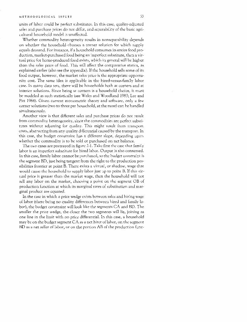
METHODOLOGICAL ISSUES 53
units of labor could be perfect substitutes. In this case, quality-adjustedsales and purchase prices do not differ, and separability of the basic agri-cultural household model is unaffected.
Whether commodity heterogeneity results in nonseparability dependson whether the household chooses a corner solution for which supplyequals demand. For instance, if a household consumes its entire food pro-duction, market-purchased food being an imperfect substitute, then a vir-tual price for home-produced food exists, which in general will be higherthan the sales price of food. This will affect the comparative statics, asexplained earlier (also see the appendix). If the household sells some of itsfood output, however, the market sales price is the appropriate opportu-nity cost. The same idea is applicable in the hired-versus-family laborcase. In many data sets, there will be households both at corners and atinterior solutions. Since being at corners is a household choice, it mustbe modeled as such statistically (see Wales and Woodland 1983; Lee andPitt 1984). Given current econometric theory and software, only a fewcorner solutions (two to three per household, at the most) can be handledsimultaneously.
Another view is that different sales and purchase prices do not resultfrom commodity heterogeneity, since the commodities are perfect substi-tutes without adjusting for quality. This might result from transportcosts, abstracting from any quality differential caused by the transport. Inthis case, the budget constraint has a different slope, depending uponwhether the commodity is to be sold or purchased on net balance.
The two cases are portrayed in figure 2-1. Take first the case that familylabor is an imperfect substitute for hired labor. Output is also consumed.In this case, family labor cannot be purchased, so the budget constraint isthe segment BD, just being tangent from the right to the production pos-sibilities frontier at point B. There exists a virtual, or shadow, wage thatwould cause the household to supply labor just up to point B. If this vir-tual price is greater than the market wage, then the household will notsell any labor on the market, choosing a point on the segment OB ofproduction function at which its marginal rates of substitution and mar-ginal product are equated.
In the case in which a price wedge exists between sales and hiring wageof labor (there being no quality differences between hired and family la-bor), the budget constraint will look like the segments CA and BD. Thesmaller the price wedge, the closer the two segments will lie, joining asone line in the limit with no price differential. In this case, a householdmay be on the budget segment CA as a net hirer of labor, on the segmentBD as a net seller of labor, or on the portion AB of the production func-
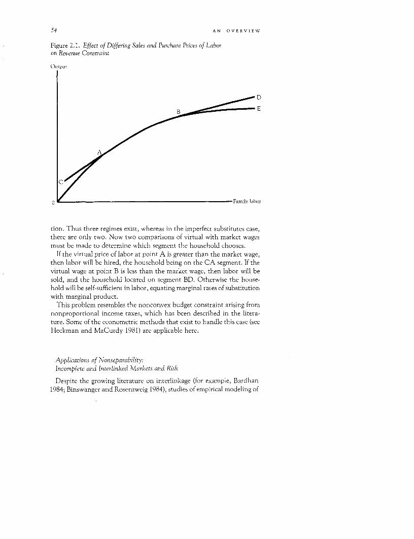
54 AN OVERVIEW
Figure 2.1. Effect of Differing Sales and Purchase Prices of Laboron Revenue Constraint
Output
D
E
O Familv labor
tion. Thus three regimes exist, whereas in the imperfect substitutes case,there are only two. Now two comparisons of virtual with market wagesmust be made to determine which segment the household chooses.
If the virtual price of labor at point A is greater than the market wage,then labor will be hired, the household being on the CA segment. If thevirtual wage at point B is less than the market wage, then labor will besold, and the household located on segment BD. Otherwise the house-hold will be self-sufficient in labor, equating marginal rates of substitutionwith marginal product.
This problem resembles the nonconvex budget constraint arising fromnonproportional income taxes, which has been described in the litera-ture. Some of the econometric methods that exist to handle this case (seeHeckman and MaCurdy 1981) are applicable here.
Applications of Nonseparability:Incomplete and Interlinked Markets and Risk
Despite the growing literature on interlinkage (for example, Bardhan1984; Binswanger and Rosenzweig 1984), studies of empirical modeling of
METHODOLOGICAL ISSUES 55
agricultural households have not yet considered the interlinking of mar-kets that may result from incomplete markets. The fact that householdsmay be rationed in the credit market because of potential default (Stiglitzand Weiss 1981) will affect their behavior in other markets. Credit ration-ing may give rise to share tenancy (Jaynes 1982), with tenants borrowingfrom landlords. Access to land rental markets may be constrained byownership of draft animals in cases where no rental markets exist for suchanimals. Renting out land may serve to secure more draft animals. Thenonseparability thereby induced will give rise to several phenomena: forexample, land lease or rental decisions may be affected by the stock ofhousehold laborers as households adjust land holdings to family size, orlabor-supply decisions may be affected by land ownership through virtualprices as well as through income.
In the case of credit rationing, the interest rate charged to the house-hold will be a function of how much has been borrowed, as well as ofother household characteristics (see chapter 6). Furthermore, the effectivewage rate may be affected by the number of hired laborers if supervisioncosts per worker are not constant. Such imperfections in markets will alsoresult in nonseparability.
Underlying many of the discussions of incomplete markets and marketinterlinkages is the notion of risk. Although risk in one market is not asufficient condition to cause such linkages, it is an important ingredientin the case of share tenancy (Newbery and Stiglitz 1979). Bardhan andSrinivasan (1971) use an agricultural household model in which land canbe sharecropped and households maximize expected utility. Their model,although it incorporates risk, has a one-period framework, as do mostmodels in the market-linkage literature. Yet, this approach ignores thetime dimension that is crucially related to risk.
The only truly dynamic model under risk is that formulated by Roe andGraham-Tomasi (chapter 9), who model risks in farm production, not inprices. The separability results they obtain are not only instructive, butthey also alert one to certain strong assumptions that have to be made ifthe result is to stand. Clearly, if perfectly competitive markets exist forfuture contingencies as well as for other markets, and given producthomogeneity, risk can be completely diversified away and so does notpresent a problem. If contingent markets do not exist, then special as-sumptions must be made about preferences and about the distribution ofyields in addition to markets before separability can result. Given theirmultiperiod framework, Roe and Graham-Tomasi must assume a per-fectly competitive market to exist for a financial asset. This assumption,on top of the assumptions for one-period static models, would result inseparability in an intertemporal model without risk, as Iqbal (chapter 6)
56 AN OVERVIEW
points out. Adding risk, however, requires further assumptions concern-ing preferences. Providing households maximize expected utility, riskneutrality along with the previously maintained assumptions plus a per-fectly competitive financial market would ensure separable productionand consumption decisions.
Under risk aversion, Roe and Graham-Tomasi show that if the utilityfunction is additively separable over time, with each period's subutilityfunction being of negative exponential form (as is often assumed in therisk literature), if the exponents are functions that are homothetic withrespect to consumption bundles (including leisure) and if production riskis multiplicative and normally distributed, then separability results. Inthis very special case, the household behaves as if it first maximizes cer-tainty equivalent full income with respect to input and output choices(which is equivalent to maximizing expected utility of full income), andthen maximizes utility subject its budget constraint, in which certaintyequivalent full income appears.
In this special case, the profit effect of a change in farm output price hastwo counteracting components, since it is certainty equivalent full in-come that is changing in response to output price. An increase in farmoutput price raises mean profits but also increases its variance. The firsteffect is analogous to the usual profits effect. The second effect, however,acts to reduce certainty equivalent full income for risk averters, thuscounteracting the positive effect on mean profits. Indeed, the combinedprofit effect of an increase in output price is no longer unambiguouslypositive, particularly if yields are sufficiently risky.
Past literature on the behavior of the pure firm under risk (for instance,Roumasset, Boussard, and Singh 1979) assumed that firms maximize ex-pected utility of profits; this idea is consistent with a farm householdframework, given risk aversion, under these special assumptions, but notnecessarily under more general conditions. Without any restrictions onpreferences other than a utility function-which is additively separableover time-Roe and Graham-Tomasi show that, conditional upon theoptimal consumption bundle, the first-order conditions for expected util-ity maximization are identical to those of the pure firm maximizing ex-pected utility of profits. Embedded in these first-order conditions, how-ever, are the levels of optimal commodity consumption, which areunknown, and therefore input choices do depend in general upon con-sumption bundles.
As noted, markets for contingent claims (that is, for consumption ineach period as a function of the realized state of the world), are absent inthis model. Given possibilities for complete diversification of productionrisk, attitudes toward risk will not matter in the determination of produc-
METHODOLOGICAL ISSUES 57
tion choices (whereas they do in Roe and Graham-Tomasi's model). Al-though complete risk diversification may not be possible in developingcountry agriculture, some means of diversification do exist; these rangefrom investment in human capital (through education and migration) toinvestment in livestock or other physical assets to the formation of largerhouseholds, and so on. Clearly, this initial attempt at incorporating riskdoes not allow for such possibilities.
The assumption of a perfect financial asset market is one of the pointsof departure for the literature on incomplete and interlinked markets dis-cussed above. If the interlinkage literature is correct, then the separabilityassumption under risk will not apply. Since much of this literature is the-oretical, further empirical research is needed to define the nature of inter-linked markets.
A second set of problems arises when we consider the particular specifi-cation of Roe and Graham-Tomasi's model, especially their assumptionthat the period-specific subutility function is homothetic. This restrictionon preferences is implied by either constant absolute or constant relativerisk aversion (Stiglitz 1969). Although this may be an empirically tracta-ble assumption, the homotheticity assumption is overly strong since itrestricts all income elasticities to unity.
Furthermore, this model overlooks possible randomness in futureprices. Roe and Graham-Tomasi assume that future prices are known byhouseholds but that future production is random. Yet there may be cir-cumstances in which production instability will cause price instability. Inall agricultural household modeling, the data on relative prices must varyover observations, say, regions, if commodity-demand systems are to beestimated. If markets are well integrated so that local production disturb-ances do not affect local prices and regional price variation is sufficientlygreat, then local production uncertainty is consistent with local price cer-tainty. Regional prices may vary because of other factors, however, suchas government prescriptions on interregional trade or extremely poortransportation facilities, which may make invalid a small region assump-tion (so that local production does affect local prices).
Incorporating random prices into the agricultural household model islikely to be a more complicated task and will probably involve privatestorage decisions (see Wright 1979) as well as price expectations formation(see Eckstein 1983).
In addition, just as in the literature on the pure firm under risk, as-sumptions concerning what decisions can be made before uncertainty isresolved may vary and thus can greatly affect the analytical results. InRoe and Graham-Tomasi's model, all input decisions are made before theuncertainty is resolved.
58 AN OVERVIEW
Applications of Nonseparability: Household Production Activities
For many policy applications, it will be necessary to consider bothhousehold production activities and agricultural production activities.When this new dimension is added to the model, separability will in somecases be affected. Pitt and Rosenzweig (chapter 5) argue that whether farmproduction decisions can be modeled independently of other decisions-such as health inputs, consumption, and labor supply-depends on thenature of the hired labor market and the degree of substitutability be-tween hired and family labor. Provided the two types of labor are perfectsubstitutes, separability between farm production and other decisionsstill holds because household demand for a certain quantity of a particu-lar quality of labor can be met by hiring at a constant wage in the market.Consequently, the health of family laborers does not affect demand forhealthy labor time. Clearly this would not be true if family and hiredlabor were imperfect substitutes.
A current concern of many policymakers is how to estimate the impactsof policy instruments such as food prices and health and education proj-ects on health outcomes of individual farm-household members. Forsome policies, it may be important to estimate certain household produc-tion processes empirically, such as the relationship between food intakes,other health inputs, and health outcomes (see chapter 5). If estimates ofthe health technology are to be consistent, attention must be given to thefact that certain health inputs-such as food consumed, time devoted tohealth care, or boiling water-are household decisions. This is an impor-tant area for future research.
Even if policymakers only need reduced-form estimates of policy im-pacts, it will be important to disaggregate male and female time use andwages. This has not been done in typical farm-household modeling (Ro-senzweig 1980 is an exception), but is important in this context because ofspecialization by gender in certain household activities. If health timecare is female-labor intensive, for example, the effects on health outcomeswithin the household will differ between a rise in female wages and a risein male wages. The substitution effect of an increase in female wagesshould lead to a greater decline in health than would the substitutioneffect of an equivalent increase in male wages. Of course, income effectswill also be important and will tend to raise the demand for health. Theimportance of distinguishing male and female wages when evaluating im-pacts of policies on household nonmarket, nonfarm activities is one of theprincipal messages of the literature on the so-called new household eco-nomics that needs to be incorporated into household production activi-ties of farm households as well.

METHODOLOGICAL ISSUES 59
Multimarket Analysis
If agricultural household models are to be used for policy analysis, inter-market relations need to be accounted for because of their potential im-portance. Such an accounting requires moving toward a general equilib-rium analysis. Yotopoulos and Lau (1974) suggested some types ofmacrolevel models that might be useful, but they did not have the dataneeded to test their ideas. Barnum and Squire (1979) and Smith andStrauss (chapter 7) allow rural wages to be endogenously determined byequilibrating net labor demand (supply) among agricultural householdswith net labor supply (demand) in the rest of the economy.
Even if a limited amount of market interaction is allowed, certainresults are significantly affected. Barnum and Squire find that in Malaysiaincreases in the price of rice cause such a large increase in the rural wagerate that output supply and marketed surplus of rice are both lowered inresponse. Consumption of paddy still increases, but by a smaller amountthan when wages are exogenous. Smith and Strauss show that the partialequilibrium results for Sierra Leone stand up in sign but not in magni-tude. Marketed surplus of rice remains positive, but the magnitude of thearc elasticity is more than halved, from 0.75 to 0.3.
Of course, the wage rate may not be the only endogenous price. Otherprices may be endogenous as a result of government trade policies (forexample, import or export quotas) or because of high transportationcosts. Which prices should be allowed to equilibrate will differ, of course,for each application.
Braverman, Ahn, and Hammer (1983) examine agricultural pricing pol-icies in Korea that were expected to reduce deficits in the government'sGrain Management Fund and Fertilizer Fund. This study allows the priceof the traditional variety of rice and rural wages to be endogenous whileprices of high-yielding rice, barley, and fertilizer are government con-trolled. Effects of policy changes are traced through to government budg-ets, incomes of different classes of rural and urban households, nationalincome, and marketed surpluses. The model's equations are based onagent optimizing behavior. For the rural sector, there are commodity andlabor-demand and labor-supply equations derived from an agriculturalhousehold model using the Almost Ideal Demand System (Deaton andMuellbauer 1980) and the translog profit function. Urban commodity de-mands are also derived using an Almost Ideal Demand System. Finally,market-clearing equations are specified, and it is through these that spe-cific government policies can be analyzed. For instance, the traditionalrice market in Korea is modeled as a closed system in which urban de-
60 AN OVERVIEW
mand equals rural marketed surplus. For a high-yielding variety of rice,imports are allowed, and the government supports the producer priceabove the world market price and subsidizes urban consumers. Becausethe structure of the model is general, it can be adapted to a variety ofcountry and policy contexts. Indeed, a number of such adaptations havebeen reported: in Senegal (see chapter 8), Sierra Leone (Braverman, Ham-mer, and Jorgenson 1983), Cyprus (Braverman, Hammer, and Jorgenson1984), and Malawi (Kirchner, Singh, and Squire 1984).
Several problems with respect to specification and data arise in thosemodels. The basic model demands a great deal of data, as does the agricul-tural household model. Ideally, parameters should be econometrically es-timated before being used in the simulation, but this ideal will not alwaysbe feasible because of the poor quality or lack of data. Hence, in practice,parameters are estimated, borrowed from other studies, or assumed. Thesystem of equations is then solved at one point in time, and the solvedvalues are compared with actual values for the economy at that particularmoment. If the difference is too large in some sense, parameters are thenchanged iteratively until a desired closeness of simulated to actual valuesis achieved. Once a baseline simulation has been achieved, policy experi-ments can be simulated and sensitivity analysis of some small number ofparameters performed. The lack of appropriate data manifests itself in pa-rameters that may be imprecise. The sensitivity of the model's policyshould therefore be carefully investigated. The Korea study, for example,has a relatively large number of parameters estimated from real worlddata. In the Senegal study, by contrast, many parameters are assumedand others (for instance, the price elasticities) are drawn from weaksources. This situation is largely a reflection of the stage of developmentof the data collection agencies in Korea versus those in Senegal. The as-sessment of the sensitivity of policy results to unprecise parameters istherefore especially important in the Senegalese model. This analysis ofsensitivity leads to different conclusions for different variables of policyinterest, and for different parameters. Parameters more directly related tothe policy outcomes of interest will need to be estimated more precisely.In Senegal, for example, the effect of a 50 percent increase in the con-sumer price of rice on net foreign exchange earnings from agriculture de-pends critically on the assumed cross-price elasticity between the price ofrice and millet consumption. Under high elasticity, much more millet isconsumed, millet prices go up, and acreage is switched from groundnuts,the export crop, to domestically consumed millet. A low elasticity raisesforeign exchange from agriculture, as tariffs from rice are increased,whereas rice consumption falls off only slightly. For government deficitsin the agricultural sector, the elasticity assumptions make much less dif-
METHODOLOGICAL ISSUES 61
ference. Although less government tariff revenue is gained from increasedconsumer prices of rice when rice price elasticities are assumed to be high,the subsidies to groundnut producers drop because fewer groundnuts areproduced-more acreage being switched over to millet than in the low-elasticity case.
Another practical problem has to do with how these models are solvednumerically. If the model is set up in levels-for instance, if the quantitiesof rice demanded by rural households are a function of prices, wage, fullincome, and so on-the system of equations is highly nonlinear, and re-quires a great deal of time and expertise to solve. If the nonlinear system istotally differentiated, however, the resulting linear approximation will berelatively easy to solve with existing computer hardware. Nonethelessthere is a tradeoff here because the approximation will be good only forvariable values close to the baseline values, and policy analysts may beinterested in the effects of large changes in certain variables, in which casethe differentiated system may approximate the real world poorly. It is ob-viously a relatively simple matter to test the reliability of linear approxi-mations by comparing their results with those of fully specified models.This is a high priority for future research and could be easily accom-plished using some of the existing multimarket models.
A further problem that arises in model specification but that is not pe-culiar to multimarket models has to do with the Almost Ideal DemandSystem, which allows commodities to be inferior goods, but only permitsa limited amount of nonlinearity in the Engel curves. It also restrictsEngel curves to zero intercepts. Although this might be intuitively accept-able, real world incomes, appropriately measured, are sufficiently far fromzero so that extending an approximation to an Engel curve in the rele-vant region will generally result in a nonzero intercept. If the functionalform used to fit the Engel curve has sufficient curvature, this will be less ofa problem. As already noted, however, the Almost Ideal Demand Systemdoes not have much curvature. The consequences of this are twofold:Engel curve slopes may be badly estimated even at the sample mean, andchanges in the slopes as income changes may be missed. These conse-quences will be most damaging when the real Engel curves are very non-linear, as might be expected when commodities are more highly disaggre-gated. This problem can be solved by using Engel curves with morecurvature or by introducing nonzero intercepts, or both. Clearly bothcan be easily incorporated into multimarket analysis. Deaton (1982) hasintroduced quadratic income terms into the Almost Ideal Demand Sys-tem, and Strauss (1982) has used the quadratic expenditure system ofHowe, Pollak, and Wales (1979). Moreover, Gorman (1981) has shownthat, in general, a second-order polynomial in income is as general as one
62 AN OVERVIEW
can be in modeling Engel curves and yet still be consistent with utilitymaximization.
A common approach in macroeconomic work, also followed by Braver-man and Hammer in their analyses, is to treat an aggregate of consumers(and producers) as an individual. For example, to relate aggregate com-modity consumption to prices and average income, individual Engelcurves must be both linear and parallel, as is well known. Otherwise thedistribution of income will also affect aggregate consumption. If the con-cept of representative income (which is not average income) is used, whererepresentative income depends on the income distribution and possiblyon prices, then somewhat more general behavior can be accommodated.
Smith and Strauss (chapter 8) simulate outcomes for individual house-holds in the Sierra Leone sample, as do Lau and others (1981) for theTaiwan sample. Knowledge of the regional sampling proportions allowsthe authors to convert the outcomes for individual households into re-gional and finally national aggregates. Comparing arc elasticities betweenthis method of microsimulation and that using the representative house-hold, Smith and Strauss find some large differences for both commodity-demand and output-supply elasticities. For example, a 10 percent increasein the price of rice raises the total national production of rice by only Ipercent when a representative household approach is used, comparedwith 3.4 percent under microsimulation. Rural rice consumption drops61/2 percent with the representative household approach, but only 5 per-cent with microsimulation. Although the results depend on both thedata and the commodity-demand and output-supply specifications, theysuggest that care should be taken when simulations are performed withfunctional forms that do not admit of perfect aggregation. As Smith andStrauss also point out, microsimulation allows the analyst to examine dis-tributional effects of policies more readily. Braverman and Hammer comepart way toward distributional disaggregation by allowing for representa-tive households of different income classes (for Korea) or for different re-gions (Senegal).
Data Requirements and Implications for Data Collection
To estimate a complete agricultural household model, the analyst musthave an extensive set of data on consumption expenditures (market pur-chased and subsistence), labor supply (possibly broken down by sex),farm and nonfarm outputs, purchased and household-supplied variableinputs, fixed farm assets, basic demographic characteristics, and prices,both for consumption and production inputs, including wages. It is obvi-
METHODOLOGICAL ISSUES 63
ously a massive undertaking to obtain data of reasonable quality on thisscale for a single household. That is why comparatively few such data setshave been collected. Sample size clearly has to be traded off against bothdata comprehensiveness and quality. Empirical studies conducted to dateindicate, however, that massive sample sizes, which many cross sectionscontain, are not needed to obtain plausible estimates of the structure ofthe basic farm household.
The precise nature of the potential tradeoffs between sample size, com-prehensiveness, and quality is not entirely clear. In separable models, forexample, commodity-demand and production-side equations can be esti-mated on different sets of data as long as each can be considered represen-tative of the area in question, as would be the case if each were from aprobability sample. Adulavidhaya and others (1984) did precisely this inthe Thailand study. Such a data collection strategy may be more expen-sive than using common households, however, if increasing returns toscale exist in the collection techniques. Nevertheless, existing, less com-prehensive sets of data can be combined. In particular, it is possible tosupplement prototypical farm management surveys with a special house-hold budget survey in which prices are also collected.
If complete nonseparable models are to be estimated, then this collec-tion strategy is no longer viable because data are needed for both con-sumption and production activities on identical households. Many coun-tries today conduct household budget surveys and farm management sur-veys. If the surveys could be coordinated so that household coveragecould at least overlap, and if some price and wage data could be added,the information available for policy analysis would greatly increase. Thepayoff would be sizable-since such policy analyses could be built onmuch better quality data.
One potential way to reduce the costs of collecting comprehensive dataon a moderately sized group is to obtain samples from only a limitednumber of geographical areas. This would be a grave mistake in farm-household modeling because then very little price variation would appearin the data. Yet the analyst relies on just such a variation in prices toexplain differing consumption and production patterns. Unfortunately,many existing farm management surveys suffer from this very problem.Although household budget surveys may cover an aciequate number ofgeographic regions, they often omit any price or wage data.
If longitudinal data are collected, then less geographical dispersion willbe necessary because prices will vary over time. Indeed, longitudinal dataon households circumvent a possible problem in the use of purely cross-sectional data-that is, that geographical price variation will be a proxyfor other regional variables that might affect consumption or production
64 AN OVERVIEW
outcomes. Collecting such panel data can be expensive, and some house-holds may drop out of the survey in a systematic way.
Alternatively, for separable models, it would be possible to use time-series cross-sectional data (which do not follow identical households overtime) as long as each cross section was from a representative sample. Inthat case, households would have to be averaged in groups, for example,by size of land owned within each geographic region. The observationsfor analysis would then be the group averages. Such a procedure was usedby Lau, Lin, and Yotopoulos (1978). The problem with this approach isthat the group average may no longer behave as if it were a single house-hold; that is, the distribution of income or assets within the group mayalso matter. This problem was covered above (see also Deaton andMuellbauer 1980 for an excellent survey).
A different type of aggregation problem has to do with the grouping ofcommodities and the computation of group price indices. Several stud-ies-for instance those in Taiwan, Japan, and Thailand-assume that allhouseholds in a region face the same prices for disaggregated commodi-ties, but allow the weights used in forming the indices to vary for eachobservation (household group). This technique enables the analyst to de-rive household (or household group) specific prices. At the same time, itintroduces two potentially serious problems: a spurious variation inprices, and a price index endogenous to the household. Suppose thatevery household in a market area (say, a region) faced the same set ofprices for each disaggregated commodity (that is, for different qualities ofthe same aggregate commodity). Even with a common utility function,different households will buy different amounts of each quality of the ag-gregate commodity because of differences in full income and in householdcharacteristics. Since the weights used are the share of household expend-iture on a particular commodity, the weights will differ by household.Thus the price variation seen by the researcher will be spurious. In addi-tion, these aggregate prices are endogenous to the household since ex-penditure decisions are endogenous. The endogeneity of prices wouldhave to be accounted for in the estimation procedure in order to produceconsistent statistical estimates, but the identifying instruments are lack-ing. All the variables that might affect the choice of quality are alreadyincluded in the demand equations, so there would not seem to be anyinstruments left. Consequently, the analytical framework would have tobe reformulated, for instance, into a model of probabilistic choice (see, forexample, McFadden 1981). A more practical approach, if choice of qual-ity is not the main focus of the research, is to use regional average weightsrather than household specific weights when constructing the price indi-ces. This approach is used in the Sierra Leone and Indonesian studies,
METHODOLOGICAL ISSUES 65
among others. Even by averaging the expenditure-share weights over aregion, however, it may not be possible to eliminate endogeneity if re-gions and full incomes are highly correlated.
Although, ideally, prices should be collected for all items consumed bya sample's households, this is both an impractical and unnecessary step inmany cases. For the empirical analysis, the researcher will decide on thelevel of commodity disaggregation and will compute price indices for eachgroup. In practice, prices will probably be required only for the most im-portant items (with respect to budget shares) for each group, but allgroups must be covered. If price indices cannot be computed for somegroups, price and income elasticities can still be estimated in separablemodels, but strong assumptions will then have to be made about house-hold preferences. If, for instance, we assume additivity of the direct utilityfunction, as the Linear Expenditure System does, then all price elasticitiescan be estimated, although not every parameter will be identified.Barnum and Squire (1979) use this property of the LES to estimate all theprice and income elasticities in a separable model for data from the MudaRiver valley in Malaysia when the only price variation in the data setapplies to wages. Given the empirical evidence that contradicts some ofthe implications of the LES (such as additivity of the utility function andlinear Engel curves), this is arguably a poor substitute for complete groupprice coverage. (See Deaton 1978 for a discussion of empirical evidence onadditivity; Strauss 1982 for a strong rejection of linear Engel curves forfarming households.)
Some comprehensiveness of data may be sacrificed if estimating a com-plete agricultural household model is not the objective of the analysis. Itmay be that only one or a few structural or reduced-form equations are ofinterest. To estimate reduced-form equations, the analyst needs data onall the exogenous variables, of course, but not on all endogenous vari-ables. Moreover, certain details may not be necessary. To estimate healthreduced-form equations, for instance, Pitt and Rosenzweig only need dataon farm profits (subtracting out the value of family labor as well as pur-chased inputs), and not on specific input usage. Provided it is easier toobtain expenditure data on inputs rather than quantity data, this is asmaller information requirement. Note, however, that data on consump-tion prices are needed, even though the focus is on health outcomes.Consequently, it is not enough to collect data on only health outcomes,prices of health inputs (for example, doctor's fees, distance to health facili-ties, and so on), and an appropriate definition of income such as farmprofits (that part of income uncorrelated with that equation's statisticalerror term) in order to obtain consistent estimates of the reduced-formhealth equation.
66 AN OVERVIEW
Iqbal, for example, does not need detailed data on consumption ex-penditure or input usage to estimate his reduced-form borrowing func-tion. Of course, more complete data would have aided the analysis sincefewer proxy variables would have been needed, and the interpretation ofthe coefficients of those contaminated variables would have been cleaner(for instance, the family size variable represents life cycle decisions, but italso affects current full income).
Furthermore, the traditional farm production, cost, or profit-functionanalysis is concerned only with a subset of the relevant household equa-tions. This traditional analysis, as already noted, is acceptable as long asone is working with a separable farm-household model. In that case, de-tailed consumption expenditure and price data are not needed. If one isdealing with a nonseparable model, however, estimating even reduced-form output-supply equations will require prices of consumptioncommodities.
How comprehensive the data set should be depends on whether thegoal is to estimate the complete farm-household system or just some partsof it. What data can be reasonably omitted also depends on whetherstructural or reduced-form equations are being estimated, and whetherthe household model assumes separability.
As for what can be accomplished with different degrees of shortfallfrom an ideal quality of data, that question has been only partly answeredin the existing studies. Clearly, data sets do not have to be perfect-theynever are-and in fact much insight has been gained from data that arefar from perfect in quality. Yet even these imperfect data sets are exten-sive in their variable coverage and contain geographical, and in some in-stances time-series variations in prices.
Agenda for Future Research
To organize an agenda for future research, we must first distinguish be-tween issues of household behavior and issues of policy analysis. (In mak-ing this delineation, we are not judging the relative importance of eachgroup of issues, both of which are very important.) The first question inthe household behavior category is what difference it makes if basic elas-ticity calculations wrongly assume separability. As we have seen, there islittle evidence with which to answer this question. Moreover, the ques-tion itself is inherently difficult because the answer is likely to depend onhow nonseparability enters the model, and there are many possible ways.Thus it may be more fruitful to pursue certain types of nonseparability
METHODOLOGICAL ISSUES 67
that are suggested by the policy issue of interest and by the economicinstitutions that characterize the data set.
With respect to the basic, static model, one of the most importantsources of nonseparability is likely to involve commodity heterogeneity,whether for consumption commodities or labor inputs. Such heteroge-neity may lead to differing sales and purchase prices for the same com-modity (whether there is a quality difference will need to be carefully con-sidered since it leads to differences in modeling, as argued earlier). Forlabor, potential differences between family and hired labor, or betweenmale, female, and child labor may be important (the latter distinctionapproaches the issue of intrahousehold distribution, treated below).
In some cases, but not all, it will be important to consider householdproduction activities, not only for health issues, as noted earlier, but alsofor issues such as fertility and household composition. Although house-hold production activities need not lead to nonseparability between farmproduction and household consumption, they may. Even if they do not,problems may arise in dealing with intrahousehold distribution, whethera reduced-form, or black box, approach is used in which the intrahouse-hold allocation mechanisms are not modeled explicitly, or whether morestructural approaches are employed. In the black box approach, it will becrucial to account differentially for the effect of male and female opportu-nity costs on intrahousehold distribution (at least between sexes), as doPitt and Rosenzweig.
One of the weak areas in the overall farm-household literature is thelack of empirical results on savings and investments. The little work thathas been done (for example, that of Iqbal) has used a static framework.No study, except the one by Roe and Graham-Tomasi, has attempted atruly dynamic analysis, and very few longitudinal data sets exist to ana-lyze these issues. Although this type of dynamic analysis could be carriedout by ignoring risk, this consideration surely adds a great deal. Withinsuch a framework, the analyst is able to consider not only issues con-nected with savings and investments (and perhaps their composition),but also those having to do with the adoption of new technologies. Mostwork on technology adoption under risk (for example, Feder, Just, andZilberman 1985) has ignored the composition side of household activitiesand has modeled the household as maximizing expected utility of wealthor income. As Roe and Graham-Tomasi show, the assumptions justifyingthis approach may be rather restrictive. Much remains to be done in thisarea; to begin with, much more empirical work is needed, some of therather restrictive assumptions such as homothetic preferences need to berelaxed, and price risk should be added. Unfortunately, the empirical
68 AN OVERVIEW
work will not be easy and may well involve tackling the household modelby parts rather than estimating a giant model, which is bound to be enor-mously expensive to test.
Just how restrictive are the assumptions underlying separability in dy-namic models under production risk? This is an area in which the marketinterlinkage literature and the agricultural household literature intersect.Much more empirical work needs to be done on the true nature of rurallabor, credit, and land markets in developing countries. In some areas ofthe world, farm-household models having a fixed land area will be verypoor approximations. Investigating the determinants of land lease andsales behavior within the framework of an agricultural household modelis likely to prove highly interesting, even if only reduced-form equationsor a subset of structural equations are estimated. In other areas, creditmay be rationed for some households and the effects of this on consump-tion and investment will have to be accounted for. All these issues aretheoretical possibilities. Just how prevalent they are empirically is animportant question with important consequences for farm-householdmodeling.
These aspects of household behavior must be considered whether one isattempting to improve the realism of agricultural household models or tomodel certain policy issues. Some other important research issues have todo with multimarket modeling and tradeoffs that can be made betweenthe quality of data and cost.
A high priority for multimarket policy analysis will be to experimentwith less costly solution algorithms and to investigate the adequacy ofapproximation with a fully differentiated system. In the absence of better-quality data, sensitivity analysis will remain quite important, but it wouldalso be interesting to see just how much difference better-quality datawould make.
The realism of the farm-household models used in multimarket analy-ses could be enhanced by introducing more highly nonlinear Engelcurves, for example, and this would be a useful extension, although prob-ably a less important one than the extensions noted above. Somewhatlower on the priority list would be experimenting with disaggregation (mi-crosimulation). Since microsimulation will raise the computational costsof finding equilibrium, it will be important to have some idea of what islost by wrongly treating groups of households as if they are individualhouseholds.
Finally, we need to know whether better-quality data would greatly af-fect elasticity estimates and which types of data are most crucial. If dataont farm profits are gathered in one-time retrospective interviews, for ex-ample, will this vastly reduce the quality of estimates compared with a
METHODOLOGICAL ISSUES 69
much more intensive (for example, biweekly or monthly) effort to obtaindetailed input data, including information on family labor, and outputdata? These questions have been addressed to some extent by those whocollect farm management or household expenditure surveys separately.They are of particular concern in agricultural household modeling sincethe expense of past surveys has discouraged many from undertaking thiskind of analysis.
References
Adulavidhaya, Kamphol, and others. 1984. "The Comparative Statics of the Behav-ior of Agricultural Households in Thailand." Singapore Economic Review, vol. 29,pp. 67-96.
Bardhan, Pranab. 1984. Land, Labor and Rural Povert-. New York: Columbia l'niver-sity Press.
Bardhan, Pranab, and T. N. Srinivasan. 1971. "Cropsharing Tenancy in Agriculture:A Theoretical and Empirical Analysis." American Economic Review, vol. 51, pp.48-64.
Barnum, Howard, and Lyn Squire. 1979. A Model of an Agricultural Household. Wash-ington, D.C.: World Bank.
Binswanger, Hans, and Mark Rosenzweig, eds. 1984. Contractual Arrangements, Em-plo-vment, and Wages in Rural Labor Markets in Asia. New Haven, Conn.: Yale Uni-versity Press.
Braverman, Avishay, C. Y. Ahn, and Jeffrey Hammer. 1983. Alternative AgriculturalPricing Policies in Korea: Their Implications for Government Def wits, Income Distribu-tion, and Balance of Payments. World Bank Staff Working Paper no. 621. Washing-ton, D.C.
Braverman, Avishay, Jeffrey Hammer, and Erika Jorgenson. 1983. "Agricultural Tax-ation and Trade Policies in Sierra Leone." World Bank Country Policy DepartmentPaper. Washington, D.C.
____. 1984. "An Economic Analysis of Reducing Input Subsidies to the LivestockSector in Cyprus." World Bank Country Policy Department Paper. Washington,D.C.
Deaton, Angus. 1978. "Specification and Testing in Applied Demand Analysis." Eco-nomic Journal, vol. 88, pp. 524-36.
Deaton, Angus, and John Muellbauer. 1980. Economics and Consumer Behavior. Cam-bridge, Mass.: Cambridge University Press.
Eckstein, Zvi. 1984. "A Rational Expectations Model of Agricultural Supply." Journalof Political Economy, vol. 92, pp. 1-19.
Feder, Gershon, Richard Just, and David Zilberman. 1985. "Adoption of Agricul-tural Innovations in Developing Countries: A Survey." Economic Development andCultural Change, vol. 33, pp. 255-98.
70 AN OVERVIEW
Heckman, James J., and Thomas MaCurdy. 1981. "New Methods for Estimating La-bor Supply Functions: A Survey." In Research in Labor Economics, vol. 4. Edited byR. Ehrenberg. New York: JAI Press.
Jaynes, Gerald, 1982. "Production and Distribution in Agrarian Economies." OxfordEconomic Papers, vol. 34, pp. 346-67.
Kirchner, James, I. J. Singh, and Lyn Squire. 1984. "Agricultural Pricing and Market-ing Policies in Eastern Africa." World Bank. Processed.
Lau, Lawrence, Wuu-Long Lin, and Pan Yotopoulos. 1978. "The Linear LogarithmicExpenditure System: An Application to Consumption Leisure Choice." Econome-trica, vol. 46, pp. 843-68.
Lau, Lawrence, Pan Yotopoulos, Erwin Chou, and Wuu-Long Lin. 1981. "The Mi-croeconomics of Distribution: A Simulation of the Farm Economy." Journal of Pol-icy Modeling, vol. 3, pp. 175-206.
Lee, Lung-Fei, and Mark Pitt. 1984. "Microeconometric Models of Consumer andProducer Demand with Limited Dependent Variables." Economic DevelopmentCenter Bulletin no. 84-4. University of Minnesota, Minneapolis.
McFadden, Daniel. 1981. "Econometric Models of Probabilistic Choice." In Struc-tural Analysis of Discrete Data with Econometric Applications. Edited by C. Manskiand D. McFadden. Cambridge, Mass.: MIT Press.
Muth, Richard. 1966. "Household Production and Consumer Demand Functions."Econometrica, vol. 34, pp. 699-708.
Newbery, David, and Joseph Stiglitz. 1979. "Sharecropping, Risk Sharing, and theImportance of Imperfect Information." In Risk, Uncertainty and Agricultural Develop-ment. Edited by J. Roumasset, J. M. Boussard, and I. J. Singh. New York: Agricul-tural Development Council.
Pollak, Robert, and Michael Wachter. 1975. "The Relevance of the Household Pro-duction Function for the Allocation of Time." Journal of Political Economy, vol. 83,pp. 255-77.
Roumasset, James, Marc Boussard, and Inderjit Singh. 1979. Risk, Uncertainty andAgricultural Development. New York: Agricultural Development Council.
Stiglitz, Joseph. 1969. "Behavior toward Risk with Many Commodities." Econo-metrica, vol. 37, pp. 660-67.
Stiglitz, Joseph, and Andrew Weiss. 1981. "Credit Rationing in Markets with Imper-fect Information." American Economic Review, vol. 71, pp. 393-410.
Strauss, John. 1982. "Determinants of Food Consumption in Rural Sierra Leone:Application of the Quadratic Expenditure System to the Consumption-LeisureComponent of a Household-Firm Model." Journal of Development Economics, vol.11, pp. 327-53.
Wales, Terence, and A. D. Woodland. 1983. "Estimation of Consumer Demand Sys-tems with Binding Non-Negativity Constraints." Journal of Econometrics, vol. 21,pp. 263-285.
Wright, Brian. 1979. "Effects of Ideal Production Stabilization: A Welfare Analysisunder Rational Behavior." Journal of Political Economy, vol. 87, pp. 1011-33.
Yotopoulos, Pan, and Lawrence Lau. 1974. "On Modeling the Agricultural Sector inDeveloping Economies." Journal of Development Economics, vol. 1, pp. 105-27.
AppendixThe Theory and Comparative Statics
of Agricultural Household Models:A General Approach
John Strauss
THIS APPENDIX DEVELOPS the basic model of the agricultural household in-troduced in chapter 1. The recursive property and comparative statics arederived first. The concept of a shadow or virtual price is then explicitlydefined, and it is shown how the response of the virtual price to exoge-nous variables can be obtained. It turns out that with a minimum of as-sumptions this response can be signed. Next, these results are used toexamine the comparative statics of various farm-household models, whenthe household faces virtual rather than parametric prices. During this ex-ercise, the difference in the comparative statics between recursive andnonrecursive models becomes clear. The next section presents the outlineof a model in which the market for labor is absent. This follows the earli-est modeling of an agricultural household, by Chayanov, and its latertechnical development by Japanese economists (for example, Nakajima).Models that incorporate Z-goods are subsequently discussed, along withthe previously neglected topic of models with certain types of commodityheterogeneity, which lead to corner solutions. Finally, conditions underwhich agricultural household models are recursive are summarized.
A Basic Model: The Household as Price-Taker
All prices in the static model developed here are taken as exogenous.Assume the household maximizes its utility subject to its constraints.Three constraints are specified at first: a production function, a time, anda budget constraint. Since agricultural household models have not gener-ally been used to address issues of intrafamily distribution (Pitt and Ro-
71
72 AN OVERVIEW
senzweig explore some of the conceptual problems involved), a householdutility function is assumed to exist. Let
(IA-1) U(XI, . . ., XL)
be the utility function, which is well behaved: quasi-concave with positivepartial derivatives. The arguments are household consumption of com-modity i, with XL denoting total leisure time. Clearly, the Xi's can be avector of commodity consumption for different members of the family aswell. For instance, we might want XL to include male, female, or chil-dren's leisure time separately. We could also allow household characteris-tics such as number of members to enter the utility function separately.As long as these are viewed as fixed, this will not change the analysis.
Utility is maximized subject to a budget constraint:L
(IA-2) Y pi x iX
where Y is the household's full income (see equation [IA-3]), and the pi'sare commodity prices (PL being the wage rate). Full income of an agricul-tural household equals the value of its time endowment, plus the value ofthe household's production less the value of variable inputs required forproduction of outputs, plus any nonwage, nonhousehold production in-come such as remittances:
M N
(IA-3) Y = PLT+ qj Qj- EqjV -pLL + Ej=1 i=1
where
T = time endowmentQj = output, for j = 1, ... , MVi = nonlabor variable inputs, for i = 1, ... , NL = labor demandqj = price of Qjqi = price of ViE = exogenous income.
For the moment, it is assumed that L is total labor demanded by thehousehold, both family and hired, which are assumed to be perfect substi-tutes, an assumption we relax later in the discussion on partly absentmarkets.
Outputs and inputs are related by an implicit production function
(IA-4) G(QI,., QM, VI,. , VN,, L, K, I , Ko) = 0
THEORY AND COMPARATIVE STATICS OF MODELS 73
where K,'s are fixed inputs. This is a general specification that allows forseparate production functions for different outputs, or for joint produc-tion. G is assumed to satisfy the usual properties for production func-tions: it is quasi-convex, increasing in outputs and decreasing in inputs.
If the household maximizes utility (IA-1) subject to its full-income (IA-2and IA-3) and production-function (IA-4) constraints and to prices (p, q)being fixed, then the household's choices can be modeled as recursivedecisions, even though the decisions are simultaneous in time (Jorgensonand Lau 1969; Nakajima 1969). The household behaves as though it max-imizes the revenue side of its full income, equation (IA-3), subject to itsproduction-function constraint, and then maximizes utility subject to itsfull-income constraint, equation (IA-2). Since neither the value of en-dowed time nor exogenous income are household choice variables, maxi-mizing full income is equivalent to maximizing the value of outputs lessvariable inputs (that is, profits).
To see that the model is separable between revenue and expenditure,the comparative statics are examined. Let the household consume threecommodities: leisure, XL; a good that is purchased on the market, Xm,;and a good, Xa, produced by the household. (Obviously all these scalarscould just as well be vectors.) The household uses labor, L, another vari-able input, V, and a fixed input K to produce both Qa and another crop,Qc. All Qc is sold on the market (a commercial crop). The Lagrangianfunction can be written as
(IA-5) £ = U(XL, Xm, Xa) + X [pLT + (qcQ, + PaQa- p L - q,V)+ E - PLXL - PmXm -PaXa] ± ,uG(Q, Qa, L, V, K).
If we assume interior solutions, the first-order conditions are:
(IA-6) - = UL-n PL = 0aXL
ax = Ua - XPa 0
- PL(T - XL L) ± qcQ, p± PaQa - X.)ax
- q,,V - PmXm + E = 0
1 d£ = qc + A Gc = °
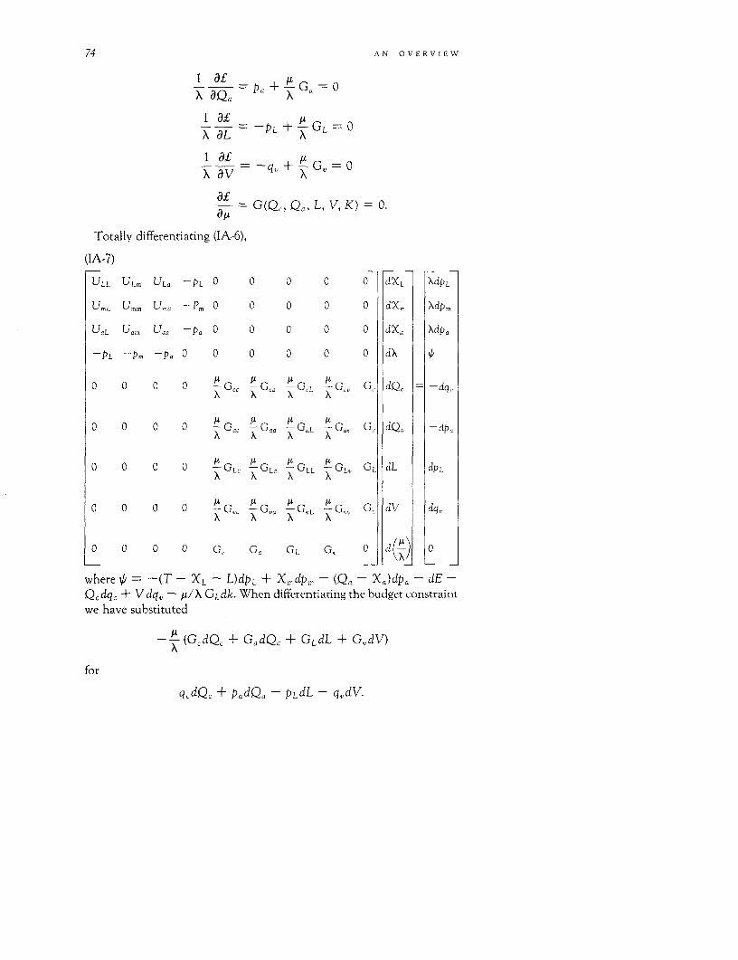
74 AN OVERVIEW
aQ = Pa + AGa = O
I aL PL +A GL = O
a£= _qv + GV = °
-= G(Qc, Qa, L, V, K) O.a,1
Totally differentiating (IA-6),
(IA-7)
ULL ULm ULa PL 0 0 0 0 0 dXL XdPL
U.L Umm Uma -Pm ° 0 0 0 dX, Xdpm
UaL U=m Uaa -Pa 0 0 0 0 0 dXa Xdpa
-PL -Pm.Pa 0 0 0 0 0 0 dX i
O 0 0 0 XG_ X G X GL X G G, dQ = - dq,
O 0 0 0 XG_ X Gaa - GaL - G., Ga, dQa -dp,
o 0 0 0 -GLC GL, GLL GLV GL dL dPL
o 0 0 0 - GVC - G,a -G,L -L G_ GC dV dqv
O 0 0 0 GC Ga GL G, ° -(X_ O
where -(T -XL- L)dPL + Xmdpm - (Qa - Xa)dPa- dE-Q,dq, + Vdqv - /L/X GCkdk. When differentiating the budget constraintwe have substituted
- (G,dQc + GadQa + GLdL + GAdV)
for
q,dQ. + PadQa- PLdL - qdV.
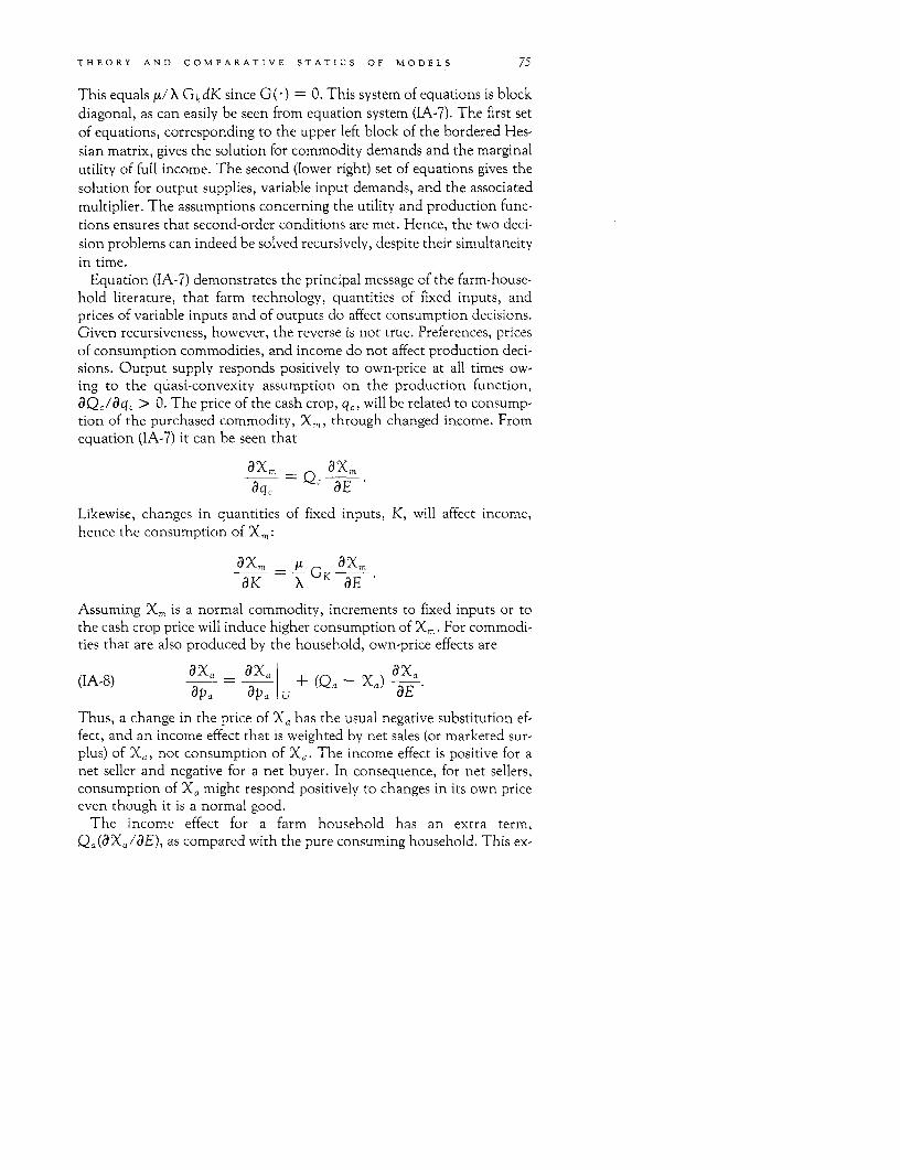
THEORY AND COMPARATIVE STATICS OF MODELS 75
This equals u/ X Gk dK since G(*) = 0. This system of equations is blockdiagonal, as can easily be seen from equation system (IA-7). The first setof equations, corresponding to the upper left block of the bordered Hes-sian matrix, gives the solution for commodity demands and the marginalutility of full income. The second (lower right) set of equations gives thesolution for output supplies, variable input demands, and the associatedmultiplier. The assumptions concerning the utility and production func-tions ensures that second-order conditions are met. Hence, the two deci-sion problems can indeed be solved recursively, despite their simultaneityin time.
Equation (IA-7) demonstrates the principal message of the farm-house-hold literature, that farm technology, quantities of fixed inputs, andprices of variable inputs and of outputs do affect consumption decisions.Given recursiveness, however, the reverse is not true. Preferences, pricesof consumption commodities, and income do not affect production deci-sions. Output supply responds positively to own-price at all times ow-ing to the quasi-convexity assumption on the production function,aQ,/aq, > 0. The price of the cash crop, q,, will be related to consump-tion of the purchased commodity, Xm, through changed income. Fromequation (IA-7) it can be seen that
axm Q axmaq, aE
Likewise, changes in quantities of fixed inputs, K, will affect income,hence the consumption of Xm:
ax, GKax
aK X aEKAssuming Xm is a normal commodity, increments to fixed inputs or tothe cash crop price will induce higher consumption of Xm. For commodi-ties that are also produced by the household, own-price effects are
(IA-8) axa Xax + (Q.-Xa) aEapa apa_ ±(a aE
Thus, a change in the price of Xa has the usual negative substitution ef-fect, and an income effect that is weighted by net sales (or marketed sur-plus) of Xa, not consumption of Xa. The income effect is positive for anet seller and negative for a net buyer. In consequence, for net sellers,consumption of Xa might respond positively to changes in its own priceeven though it is a normal good.
The income effect for a farm household has an extra term,Qa(aXa/aE), as compared with the pure consuming household. This ex-
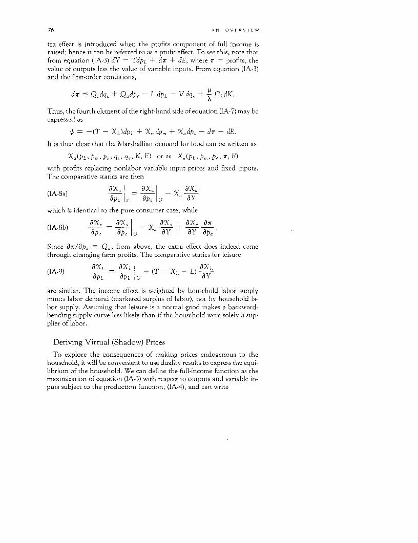
76 AN OVERVIEW
tra effect is introduced when the profits component of full income israised; hence it can be referred to as a profit effect. To see this, note thatfrom equation (IA-3) dY = TdPL + d7r + dE, where T = profits, thevalue of outputs less the value of variable inputs. From equation (IA-3)and the first-order conditions,
d7r = Qdq, + Qa.dpa - LdPL - Vdq, + - G1 dK.
Thus, the fourth element of the right-hand side of equation (IA-7) may beexpressed as
f = -(T - XL) dPL + Xmdpm + Xadpa - d7r - dE.
It is then clear that the Marshallian demand for food can be written as
Xa(PL, Pm, Pa, qc, qv, K, E) or as Xa(PL, Pm 5 Pa) ir, E)
with profits replacing nonlabor variable input prices and fixed inputs.The comparative statics are then
(IA-8a) ax, _a_ _ ax,apa apa L ay
which is identical to the pure consumer case, while
(IA-8b) ax - axd - Xa ax + axa adaPa aP u a y ay ape,
Since ax/apa = Qa, from above, the extra effect does indeed comethrough changing farm profits. The comparative statics for leisure
(IA-9) aXL - aXL + (T - XL - L) aXLaPL aPL U ay'
are similar. The income effect is weighted by household labor supplyminus labor demand (marketed surplus of labor), not by household la-bor supply. Assuming that leisure is a normal good makes a backward-bending supply curve less likely than if the household were solely a sup-plier of labor.
Deriving Virtual (Shadow) Prices
To explore the consequences of making prices endogenous to thehousehold, it will be convenient to use duality results to express the equi-librium of the household. We can define the full-income function as themaximization of equation (IA-3) with respect to outputs and variable in-puts subject to the production function, (IA-4), and can write
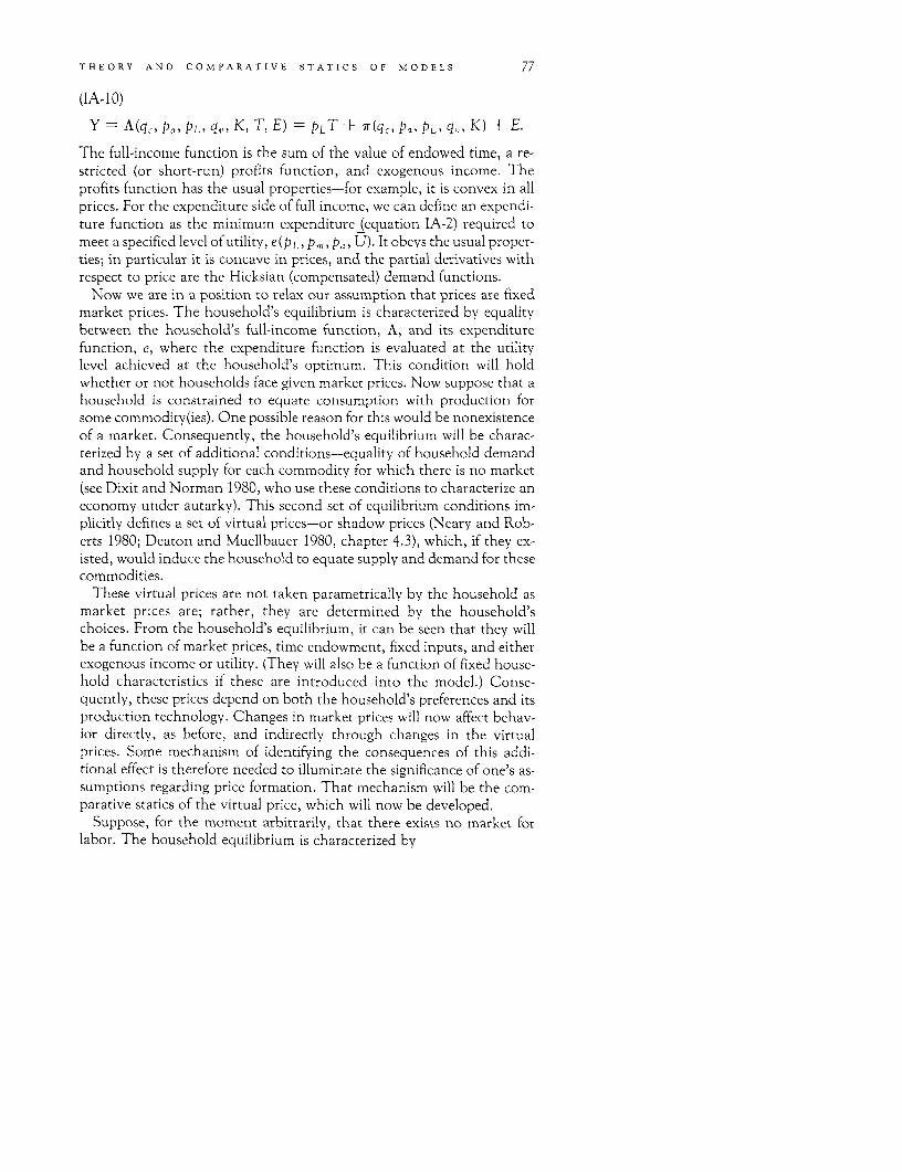
THEORY AND COMPARATIVE STATICS OF MODELS 77
(IA-10)
Y = A(qc, Pa, PL, q., K, T, E) = pLT + 1(qc, Pa) PL, qU, K) + E.
The full-income function is the sum of the value of endowed time, a re-stricted (or short-run) profits function, and exogenous income. Theprofits function has the usual properties-for example, it is convex in allprices. For the expenditure side of full income, we can define an expendi-ture function as the minimum expenditure (equation IA-2) required tomeet a specified level of utility, e(pL, Pm, Pa, U). It obeys the usual proper-ties; in particular it is concave in prices, and the partial derivatives withrespect to price are the Hicksian (compensated) demand functions.
Now we are in a position to relax our assumption that prices are fixedmarket prices. The household's equilibrium is characterized by equalitybetween the household's full-income function, A, and its expenditurefunction, e, where the expenditure function is evaluated at the utilitylevel achieved at the household's optimum. This condition will holdwhether or not households face given market prices. Now suppose that ahousehold is constrained to equate consumption with production forsome commodity(ies). One possible reason for this would be nonexistenceof a market. Consequently, the household's equilibrium will be charac-terized by a set of additional conditions-equality of household demandand household supply for each commodity for which there is no market(see Dixit and Norman 1980, who use these conditions to characterize aneconomy under autarky). This second set of equilibrium conditions im-plicitly defines a set of virtual prices-or shadow prices (Neary and Rob-erts 1980; Deaton and Muellbauer 1980, chapter 4.3), which, if they ex-isted, would induce the household to equate supply and demand for thesecommodities.
These virtual prices are not taken parametrically by the household asmarket prices are; rather, they are determined by the household'schoices. From the household's equilibrium, it can be seen that they willbe a function of market prices, time endowment, fixed inputs, and eitherexogenous income or utility. (They will also be a function of fixed house-hold characteristics if these are introduced into the model.) Conse-quently, these prices depend on both the household's preferences and itsproduction technology. Changes in market prices will now affect behav-ior directly, as before, and indirectly through changes in the virtualprices. Some mechanism of identifying the consequences of this addi-tional effect is therefore needed to illuminate the significance of one's as-sumptions regarding price formation. That mechanism will be the com-parative statics of the virtual price, which will now be developed.
Suppose, for the moment arbitrarily, that there exists no market forlabor. The household equilibrium is characterized by
78 AN OVERVIEW
(IA-11) e(T*L, P., Pa, U) = LT + 7r(q,, pa, L qv, K) + E
eL(PL) Pmr Pa, U) = T + 7rL(qc) Pa, F qv., K)
where eL = de/ap* and likewise TL = a7/ap*. The second equationgives the Hicksian leisure demand on the left-hand side and time endow-ment minus labor demand on the right. From this equation, PL*, the com-pensated virtual price, can be solved for as
(IA-12) FL =L*(Pm, Pa, qc, qv, K, U).
Note that the utility level is being held constant, and not exogenous in-come. Alternatively, the Marshallian leisure demand
XL(PL, Pm) Pa) pLT + iT + E)
can be set equal to time minus labor demand, and a solution obtained:
(IA- 13) PL* PL*(Pmr Pa) qc, qv, K, E).
To relate the functions PL* and PL, a somewhat different expenditurefunction is needed. Let
e'(PL, Pm, Pa, qc, qv, K, T, U)
(IA-14) xmx PLX L + PmXm + PaXa - PLT - q - pQQ~, Q, L, V
+ PLL + qvV st U( ) = U and G(-) = O.
This represents the minimum exogenous income, E, necessary to achieveutility level U, given the production function and prices. It is clear that e'meets all the conditions that a regular expenditure function does, andthat
(IA-15) e'(PL, Pm , Pa, qc, q,, K, T, U)
e(PL, P mn Pa, U) - PLT - ir(qc, Pa, PL, qv, K).
In equation (IA-13), if exogenous income E is evaluated at e' (hence fullincome, Y, at e) then Marshallian leisure demand equals the Hicksiandemand and pL* = PL. Using this equality
___ a __ ± z Z =P m , Pa, qc, q~, K.(IA-16) azL - azL| E aE daZ
With utility constant, the response of the virtual price can be expressedin terms of second partial derivatives of the expenditure and profit func-tions. Using the implicit function rule and equation (IA-1 1),
(IA-17) aT = -(eLz - 7rLZ)/(eLL - ItLL) Z = Pm i Pa, qc, qv, K.az
THEORY AND COMPARATIVE STATICS OF MODELS 79
The denominator is unambiguously negative owing to the concavity ofthe expenditure function and the convexity of the profits function. Thenumerator can be either sign, but often the sign will be determinate if oneis willing to assume that commodities are substitutes or complements inconsumption or production. For instance, if Z = Pm, the price of themarket-purchased commodity, Xm, the numerator is - eLm, which is neg-ative if leisure and Xm are substitutes. If Z = Pa, the numerator is 7La -
eLa. The first term is the response of output of Xa to wage, which shouldbe negative. The second term is negative if leisure and Xa are substitutes.For an input price, q,, the numerator is ItLV, which can be positive ornegative, depending on whether labor and input V are gross substitutesor complements.
Equation (IA-17) is a basic result that will be used repeatedly in thesubsequent discussion to illuminate the effects of totally or partly absentmarkets. It allows one to sign the partial derivatives of the compensatedvirtual price, making this device useful in looking at the comparative stat-ics. Moreover, it allows one to compare directly models that make differ-ing assumptions about the nature of prices the household faces.
The sign of the response of the compensated virtual price, P*, to exoge-nous variables can be given an intuitive interpretation. If, for instance,the price of the cash crop rises, the demand schedule for labor shouldshift upward. Given that other market prices, fixed inputs, and utility areconstant, the virtual wage has to rise in order to reequate compensatedlabor supply with demand. Such a rise will lower labor demand along thenew schedule, while raising compensated, or Hicksian, labor supply.
The virtual prices are functions of both household preferences and pro-duction technology. Because these prices help to determine both con-sumption and production choices-they belong in both the expenditureand the full-income functions-the household commodity demands willdepend on production technology, both through the virtual price andthrough full income. Output supplies and input demands will depend onpreferences through the virtual price. If, however, the household facesonly market prices or if it faces a virtual price for a commodity that isconsumed but not produced (or vice versa), then production choices willnot depend on household preferences, but consumption choices will de-pend on production technology through full income. The model is thenrecursive.
Models with Absent Markets: Labor
In the historical development of agricultural household models, par-tially autarkic behavior has been very important. One of the earliest
80 AN OVERVIEW
models can be traced to the Russian economist A. V. Chayanov (1925)(see Millar 1970 for a reinterpretation). Chayanov was concerned withexplaining the allocation of labor between work and leisure in Russianpeasant households given his observation that virtually no hired laborwas used in farm production activities. He recognized that such house-holds were not simply maximizing profits as in the theory of the firm;rather, they had a subjective equilibrium in which they equated the mar-ginal utility of household consumption with the marginal utility of lei-sure. His analysis was embellished by a group of Japanese economists, no-tably Tanaka (1951) and Nakajima (1957), during the 1950s and 1960s.Nakajima (1969), in particular, gave the model currency among English-speaking economists. He not only gave a mathematical formulation toChayanov's model, but also proposed some additional models. Nakaji-ma's (1969) model of a pure commercial family farm without a labor mar-ket assumed that households sold all of their output and purchased com-modities from the market, and that they produced the output with familylabor and a fixed amount of land. He also allowed for the possibility of aminimum subsistence consumption requirement as well as a target in-come. In a different version (his semisubsistence family farm), he allowsthe family to consume some of its output, and in another version intro-duces two outputs. Similar models of peasant households were advancedby Mellor (1963) and Sen (1966) and by economic anthropologists such asFisk and Shand (1969). These models are thus special cases of the generalform of the agricultural household model developed here.
These models in which the family supplied all of its labor were usedprimarily to explore the effects on labor supply (and hence output, sincefamily labor was assumed to be the only variable input) of changes indifferent variables. The effect of output price was of particular interestbecause of the seemingly perverse possibility that output might respondnegatively to output price. This might occur if the income effect, resultingin more leisure demand, was large enough. Nakajima showed that an ex-ogenous increase in land input might also reduce output, because it toowould have an income effect on leisure. Nakajima separated the responseof labor supply to output price into substitution and income effects,showing that the income-compensated response of labor supply to outputprice was positive. Sen showed that output response to output price couldbe negative, and that there could be no output response to the with-drawal of family workers if the remaining family laborers worked suffi-ciently hard to offset the reduced number of hours worked as workerswere withdrawn. This required that the virtual wage (or its ratio to out-put price, Sen's real cost of labor) be constant, as would be the case in
THEORY AND COMPARATIVE STATICS OF MODELS 81
Sen's model if the marginal utilities of both income and leisure wereroughly constant.
The possibility of a negative response of labor demand (and of outputsupply) to output price at the household level is dependent on the con-strained equality of labor demand and labor supply. At the market levellabor demand might respond negatively to output price if wage is bid upsufficiently (see Barnum and Squire 1980). If markets exist for all com-modities, then the model is recursive and labor demand will respond posi-tively to output price as long as it is not an inferior input. Nakajima notedthis when discussing his model with a labor market and a cash crop. BothJorgenson and Lau (1969) and Krishna (1964, 1969) proposed separablesemisubsistence models in which labor is marketed and output is partlyconsumed at home. Jorgenson and Lau's study has formed the basis onwhich most of the empirical work to date has been conducted.
Consumption and Leisure Responses
The difference that absence of a labor market makes to the comparativestatics of leisure and commodity demand can easily be seen by using thenotion of a virtual wage. Write the Marshallian demand as
Xi[PL, Pmn Pa pL*T + 7r(qc, Pa, Pt q, K) + E], i = L, M.
DiffeTentiate this with respect to qc to obtain
(IA-18) E=ax_ aXi apL + Q i = L, M.aqc - aPL* aqc ayCash output price has two effects on the demand for leisure or for themarket purchased good: it has an income effect by changing profits (thesecond term), and it changes the virtual price for labor. Clearly, when thehousehold is a price-taker in the labor market, the latter effect is zero.
Equation (IA-18) can be decomposed into substitution and income ef-fects, which will help in signing the uncompensated changes in the de-mand for leisure and the market-purchased commodity. First, it canbe shown that the uncompensated effect with respect to the virtualwage equals the compensated effect. To do this, it will be useful to equateMarshallian and Hicksian demands by evaluating full income, Y, ande and the virtual wage at PL (that is, if both hold utility constant):
(IA-19) Xi [L, Pm , Pa, e(L, Pm, Pa, U)] = Xci( PriPM Pa, U)i = L, M.
Differentiating both sides of (IA-19) with respect to the cash crops price,q,, and using ae/laL = XL results in
82 AN OVERVIEW
(1A~.2O) ax, aFy* axi a~i* ax§ a~4 *L M(IA-20) * L+ XL P= iPL =L, M.
apL ay +q X aY aq- apt aqcSince
(IA-21) adX a dXj + (T-L) dY
and since labor supply equals labor demand, so that XL = T - L, it canbe shown by means of equation (IA-20) that aX/dap* a aXc/ap*. Thusthe income effect of a change in the virtual wage equals zero, which isintuitive since the net marketed surplus is zero when no labor market
exists.
The term ap*/aq, in equation (IA-18) can be made more transparentby noting from (IA-16) that
___= a + QC- (recall that =Q - Q).aq, aqq dE aq,When this is substituted into (IA-18), one obtains
(IA-22) aXs aXi j + Q (aX + aM aPL) i=L,Maq, ap* aqc \aY apL aE/axi aTL axj ~
(IA-22a) a Qc aE i = L, M.
Equations (IA-22) and (IA-22a) show the decomposed income and substitu-tion effects. They also clarify the significance of one's view regarding the la-bor market. If the labor market does exist, then the household faces marketprices so the substitution effect-the first term in (IA-22a)-is zero and theentire effect of the change in output price is captured by the income effect
[Q,(aX/aY)l. This is positive, providing leisure or the purchased commod-ity are normal goods. When the labor market is absent, a substitution effect iscaused by the change in the income-compensated virtual wage. Using equa-tion (IA-17), we can rewrite this substitution effect as
(IA-23) ap aq eLt7rLAeLL - rLL) i = L, M.
If the compensated virtual wage rises-that is, if 7rL, < 0, in equation(IA-23)-then there is a substitution away from leisure or toward the pur-
chased commodity (if it is a substitute for leisure). The income effect comes intwo parts: first, a traditional looking income effect, and, second, a substitu-tion-type effect due to an induced change in the uncompensated virtual wage,
PL*. This two-part income effect is identical to equation (IA-24) of Neary and
THEORY AND COMPARATIVE STATICS OF MODELS 83
Roberts (1980), once their equation (IA-19) has been substituted in. From
equation (IA-22), we can see that when leisure is normal, apL*/aE > 0, theincome effect is smaller for leisure and larger for purchased goods (if we as-
sume substitutability with leisure) when the labor market does not exist thanwhen it does. An increase in exogenous income raises the uncompensatedvirtual wage, and this increase induces a substitution away from leisure ortoward the purchased commodity. If we assume that the entire income effect
is positive, the net effect of a rise in output price q, on leisure is indetermi-
nant, but it will be positive for the purchased commodity. This is the sameresult, of course, as is obtained by both Nakajima (1969) and Sen (1966).
Output Responses
If labor is the only variable input, then the sign of output response to out-
put price must be the opposite to the leisure response. More generally, we canwrite output supply Q, as
Q = (qc,p.,pL*,q_K)aq,consequently,
(IA-24) aQ= 7rc- + 7rcLaq, ~~~aq,
The first term is the output-supply response when the virtual wage is fixed,and is positive. The second term is negative, if we assume that output re-sponds negatively to the virtual wage (7rcL < 0), so that the sign of the entireexpression is indeterminant. It is possible to show that when household util-ity is held constant, the response is positive. (See Lopez 1980 for a somewhat
different demonstration of this.) Substituting for apt/laq from equation(IA-16),
(IA-25) aQ' + 7r AP) + Q 7r aPLaq, aYq7 aq,
The first two terms are the response of output supply when utility is heldconstant. The third term is an income effect, which is negative if 7r,L is nega-tive. The second term equals 7rcL/(eLL - 7rLL), so it is negative. However,summing it with 7r,, gives a nonnegative quantity because the function e'(equation [IA-151) is concave in prices, so that
a2 e' a2 e' ( a2 e' 2
aq,2 apL2 aq, p .
84 AN OVERVIEW
Straightforward algebra shows that this expression is simply the first twoterms in equation (IA-25) multiplied by -8 2 e'/8pt 2 . The magnitude ofTCL and consequently the likelihood of a negative output response will beinfluenced by the number of variable inputs and the partial elasticity ofsubstitution between labor and these other inputs. Presumably, the moreinputs and the more substitutable they are, the less negative rCL will beand the more likely will be a positive response to output price. Clearly,when the virtual wage is exogenous to the household, output responsewill be positive and greater than when the virtual wage is endogenous.
If the household consumes some of the output for which price is chang-ing, QC, the comparative statics have an additional substitution effect,and the income effect is weighted by net output sold (marketed surplus)and not by total output:
(IA-26) axi = x,, + ± Xd i-= L, M, A.apa aPa P L apt ap
Again using equation (IA-17), adL/ap0 = (7aL - eaL)/(eLL - TrLL),
which is positive if Qa and leisure are substitutes. Deriving the compara-tive statics as before, one finds
(____ axi, aj (IA-27) aX, = ax + apX apapa aP. p, apt a
+ (QaX.) ap~ dE ~ ~axc ap + ax) i L, M, A
ax, - axc a-E ayx,(IA-27a) apX aXi + (Qa- Xa) aE i L, M, A.
The substitution effect for leisure demand can be of either sign. It is notnecessarily positive, even if Xa and leisure are substitutes holding the vir-tual wage constant. The income-compensated response of Xa can also beof either sign when the wage is virtual, since an increase in the price, Pa,will increase the compensated virtual wage leading to a substitution to-ward Xa. The substitution effect for Xa will be less negative than whenthe labor market exists, as Neary and Roberts (1980) found in the purerationing case. The income effect has an extra term, which for Xa and Xmis positive if leisure is a substitute and is negative for leisure demand.
Marketed Surplus Responses
If we examine the response of marketed surplus of Xa, Qa - Xa, tochange in Pa, we obtain from (IA-25), (IA-16), and (IA-27)

THEORY AND COMPARATIVE STATICS OF MODELS 85
a(Qa - Xa) - aQ.(aa | aQ apL a_ X ax,aTLapa apa aL apL apa tPa P rPL aPa
(IA-28) + (Q. - XI) aQ p L_aaaP_L aE ap* aE ay
The first four terms (in brackets) hold utility constant, and therefore com-prise the substitution effect. It is straightforward to see that this effectequals
a2e' Le' a 2e' a _2e' 2
apL2 ap PL dPaaPIapL
and consequently is nonnegative (remember that e' is concave in prices).The last term equals
Q - Xa) (0Qa _ Xa)
and so is the income effect that should be negative if marketed surplus ispositive and Xa is a normal good. Consequently, marketed surplus of Xamight respond positively or negatively to an increase in its own price.Comparing this result with that when the labor market exists, one can seethat the extra substitution effects will be negative if Xa and leisure aresubstitutes, since the compensated virtual wage will then rise. The extraincome effects should also be negative, so that a greater possibility existsof obtaining a negative own-price response of marketed surplus of Xa.
The comparative statics with respect to changes in Pm, q,, K, and T aresimilar to equation (IA-22), except that the response of the compensatedvirtual wage is different, as is the term weighting the income effect. Spe-cific formulae are left for the interested reader to derive.
Models with Absent Markets: Z-Goods
The market that one assumes not to exist clearly does not affect theforegoing argument. Hence, the existence of a labor market is a necessarybut not a sufficient condition for an agricultural household model to beseparable. All markets must exist for separability, although this is not a suffi-cient condition, as is discussed in the next section. Historically, econo-mists thought that the labor market was the one least likely to exist forpeasant farms. That view has been changing, however, since active rurallabor markets have been found according to several studies (Rosenzweig1978; Spencer and Byerlee 1977; Bardhan 1979; Squire 1981; Binswanger
86 AN OVERVIEW
and Rosenzweig 1984), although they are not necessarily perfectly com-petitive ones. More recent studies have focused on the nonexistence of amarket for so-called Z-goods. This was first formalized by Hymer and Res-nick (1969), who refer to Z-goods as nonagricultural, nonleisure activities.In general the commodities Hymer and Resnick refer to, such as foodprocessing and metalworking, are commodities for which small-scale ru-ral industries have been found to exist (Anderson and Leiserson 1980;and Liedholm and Chuta 1976). Z-goods, however, refer equally as wellto nontraded outputs of household production activities such as thenumber and quality of children, home maintenance, or food preparation.In this way, the household production models of Becker (1965) and Gro-nau (1973, 1977) can be incorporated into agricultural household models.
Hymer and Resnick (1969) were concerned with the increasing speciali-zation of agricultural household activities, which they saw as occurringover time and resulting in an increasing marketed surplus from agricul-tural households. Rather than focus on the leisure-labor tradeoff, theyconcentrated on the Z-goods-food tradeoff. In terms of the general modelspecified here, households produce foods, Qa, which they consume andsell the surplus in exchange for manufactured commodities, Xm. Theyproduce Z-goods, our L, which they consume entirely at home, L = XL.Labor supply does not enter their model, but implicitly it is assumed to befixed in amount and to be equal to labor demand; thus it is not a choicevariable. In terms of this model, labor is one of the fixed inputs, K, and itdoes not appear in the utility function. Alternatively, leisure can enterthe utility as a fixed factor, similar to other fixed household characteris-tics such as household size and age distribution. In this case, the expendi-ture function will include leisure as a conditioning variable just as a short-run cost or profit function includes fixed inputs.
There are no other variable inputs, V = 0, nor does there exist a cashcrop, Q, = 0. These assumptions imply that the product transformationcurve between foods and Z-goods has the usual downward-sloping, con-cave shape. Consequently, to find the sign of the effect of a change in theprice of foods, Pa, on the output of foods, only the effect on demand(hence supply) of Z-goods needs to be considered, aXL/bpa, which isgiven by equation (IA-27). The substitution effect can be of either sign. IfZ-goods and foods are substitutes, a rise in food prices will increaseZ-goods consumption when the compensated virtual price of Z-goods isheld constant. This will force up the virtual price, however, and lead to asubstitution away from Z-goods consumption. The income effect isweighted by the marketed surplus of foods, which is presumed to be posi-tive. Hymer and Resnick assume that Z-goods consumption is inferiorand that the combined substitution effect is small, so that the net effect of
THEORY AND COMPARATIVE STATICS OF MODELS 87
a rise in the price of foods will be a fall in the consumption (and produc-tion) of Z-goods, and hence a rise in food production. Of course, if foodsare consumed by the household, the food consumption response to foodprice needs to be examined before what happens to marketed surplus offoods can be judged. As seen from equation (IA-28), marketed surplus offood can either rise or fall in response to an increase in food price, pro-vided the household has a positive marketed surplus and Z-goods are nor-mal (so apV/aE > O). However, if Z-goods are inferior, then its virtualprice falls when exogenous income rises, so that production of foods risesand compensated consumption of foods falls (provided foods and Z-goodsare substitutes), making it more likely that the response of marketed sur-plus is positive.
The Hymer and Resnick assumption that leisure and labor demand arenot choice variables can be relaxed. If it is assumed that no labor marketexists, then two virtual prices exist, one for labor and one for householdZ-goods. There are thus two equality constraints on supply and demandrather than one. Alternatively, the labor market may be assumed to exist.
As an alternative to the Hymer and Resnick interpretation, Z-goodsmight be interpreted as being synonymous with household productionactivities. The original work of Becker (1965), Lancaster (1966), andMuth (1966) emphasizes that the commodities that yield household util-ity are produced within the household by goods purchased in the marketand by labor. In terms of this general model, Xc is a vector of commodi-ties consumed and produced in the home. Market-purchased inputs aredenoted by V (Xm = 0), and labor demand, L, is a vector of time allo-cated to the production of each commodity. Leisure usually is not consid-ered, so total time is the sum of time spent in household production, plusmarket work. It is often assumed that Z-goods production is not joint andthat it exhibits constant returns to scale. If no fixed inputs exist, the sup-ply (and profit) functions will be ill-defined so that shadow (or implicit)prices cannot be defined in terms of equality between household supplyand demands. Rather, they are defined implicitly by the partial deriva-tives of the cost functions with respect to output (Pollak and Wachter1975). However if fixed inputs do exist, or the production functions arestrictly convex, shadow (or virtual) prices can be implicitly defined fromthe equality of household demand and supply functions.
An elaboration of the household production framework by Gronau(1973) provides results almost identical to the model of Hymer and Res-nick. Gronau's model amounts to relabeling food consumption as leisureand food production as labor demand. He, too, has a market-purchasedand a home-produced (Z) commodity, with home production using la-bor and purchased inputs. As in the Hymer and Resnick model, a virtual
88 AN OVERVIEW
price exists for the home-produced (Z) good. If no labor is supplied to themarket, there will exist a virtual (shadow) wage as well, and the analysis iscomparable to the Hymer and Resnick model when labor is a choice vari-able but no market for it exists. In a subsequent study, Gronau (1977)assumes that the market-purchased and the household-produced com-modities are perfect substitutes in consumption and so may be added. Aslong as market purchases are positive and labor is sold on the market, thismodel is recursive. If labor is not sold on the market, a virtual (shadow)price for labor exists, and if market purchases of the home-produced com-modity are zero, a virtual price for it exists. Huffman and Lange (1982)have a slightly different version of Gronau's model in which the house-hold is explicitly an agricultural household. The household jointly pro-duces a farm and a household commodity (Xc and Xa), selling the formerand consuming the latter. Labor is sold on the market, but the only mar-ket purchases are for production inputs. A virtual price exists for thehousehold commodity and the model is not separable. If, however, thefarm and household commodities have separate production functionsand fixed inputs could only be allocated to one enterprise, the modelwould be recursive between farm production decisions and the rest.
Partly Absent Markets: Commodity Heterogeneity
Even if all markets exist, households may face a virtual price that de-pends on both production technology and household preferences, so thatagain an agricultural household model would not be recursive. This canoccur because markets are partly absent or because constraints are insti-tutionally imposed (see Sicular, chapter 10, for an analysis of such con-straints imposed on a production team in the People's Republic ofChina). In particular, a household may be able to sell a commodity butnot buy it, or vice versa. If this commodity is both consumed and pro-duced by the household, then the household's optimum may be at a cor-ner at which consumption equals production. Such corner solutions arelikely to occur especially when commodities are heterogeneous. For ex-ample, hired and family labor may be imperfect substitutes because ofextra monitoring or search costs of hired labor. On-farm and off-farmlabor may give different levels of disutility (see Lopez, chapter 1 1). Alter-natively, a commodity consumed out of home production may have adifferent quality than the same commodity purchased on the market, andthus sales and purchase prices may differ.
Households can sell and consume family labor or home production,but they cannot purchase them. This suggests that, at the market price,supply might be less than demand, which is not possible. For such corner
THEORY AND COMPARATIVE STATICS OF MODELS 89
solutions, the commodity in question has a virtual price that wouldequate supply and demand. The virtual price will be higher than the mar-ket price provided that the compensated marketed surplus responds posi-tively to price.
If households have preferences between on-farm and off-farm labor,then even if hired and family labor are perfect substitutes in productionthere may exist excess supply of on-farm labor at the market wage, inwhich case the virtual wage will be lower.
It should be clear that the comparative statics for these equilibria areidentical to those considered earlier for the cases in which no market ex-ists. Also, if these corner solutions are not binding, then the model isseparable, the market prices being the opportunity costs. This will compli-cate empirical work since, if such heterogeneity exists, a sample is likely toinclude both households at corners and households at interior solutions.
Recursive Conditions Summarized
This appendix has reviewed the comparative statics of some basic, staticagricultural household models. A key modeling issue is under what cir-cumstances a model is recursive. This is very important for applied empir-ical work since it makes the problem far more tractable (see chapter 1). Ithas been shown that a sufficient condition for recursiveness is that allmarkets exist for commodities that are both produced and consumed,with the household being a price-taker in each one, and that such com-modities are homogeneous. As long as households can buy or sell asmuch as they want at given prices, production and consumption deci-sions can be treated as if they were sequential, production decisions beingmade first, even though they may be made simultaneously. Such strongconditions are not necessary, however. In particular, the homogeneityassumption can be dropped. In this case, however, the agricultural house-hold model remains recursive only if the household does not choose to beat a corner for a commodity that it both produces and consumes (forexample, consuming all of its output). If a corner solution is chosen, thena virtual price exists, which is a function of both preferences and tech-nology, so that the household's decision is no longer separable. Notethat even in the case of heterogeneity, it is still necessary to assumethat all markets exist and that prices are given to households to achieverecursiveness. If even one market does not exist (for a commodity that isconsumed and produced), then recursiveness from production to con-sumption decisions breaks down.
Historically, nonrecursive agricultural household models were thoughtto be relevant, primarily because labor markets were presumed not to
90 AN OVERVIEW
exist. As more has been learned about rural labor markets in developingcountries, this assumption has become increasingly questioned. This doesnot mean that empirically relevant models have to be recursive, but thereasons for nonrecursiveness need to be clearly spelled out (see chapter 2).
References
Anderson, Dennis, and Mark Leiserson. 1980. "Rural Nonfarm Employment in De-veloping Countries." Economic Development and Cultural Change, vol. 28, pp.227-48.
Bardhan, Pranab. 1979. "Wages and Unemployment in a Poor Agrarian Economy: ATheoretical and Empirical Analysis." Journal of Political Economy, vol. 87, pp.479-500.
Barnum, Howard, and Lyn Squire. 1980. "Predicting Agricultural Output Re-sponse." Oxford Economic Papers, vol. 32, pp. 284-95.
-_____ 1979. A Model of an Agricultural Household. Washington, D.C.: World Bank.
Becker, Gary. 1965. "A Theory of the Allocation of Time." Economic Journal, vol. 75,pp. 493-517.
Binswanger, Hans, and Mark Rosenzweig, eds. 1984. Contractual Arrangements, Em-ployment and Wages in Rural Labor Markets: A Critical Review. New Haven, Conn.:Yale University Press.
Chayanov, A. V. 1925. "Peasant Farm Organization." Moscow: Cooperative Pub-lishing House. Translated in A. V. Chayanov: The Theory of Peasant Economy, ed.D. Thorner, B. Kerblay, and R. E. F. Smith. Homewood, Ill.: Richard Irwin, 1966.
Deaton, Angus, and John Muellbauer. 1980. Economics and Consumer Behavior. Cam-bridge, Mass.: Cambridge University Press.
Dixit, Avinash, and Victor Norman. 1980. Theory of International Trade: A Dual,General Equilibrium Approach. Cambridge, Mass.: Cambridge University Press.
Fisk, E. K., and K. T. Shand. 1969. "The Early Stages of Development in a PrimitiveEconomy: The Evolution from Subsistence to Trade and Specializations." In Sub-sistence Agriculture and Economic Development, ed. C. F. Wharton, Jr. Chicago:Aldine.
Gronau, Reuben. 1973. "The Intrafamily Allocation of Time: The Value of theHousewives' Time." American Economic Review, vol. 68, pp. 634-51.
_ . 1977. "Leisure, Home Production and Work: The Theory of the Allocationof Time Revisited." Journal of Political Economy, vol. 85, pp. 1099-1124.
Huffman, Wallace, and Mark Lange. 1982. "Farm Household Production: Demandfor Wife's Labor, Capital Services and the Capital-Labor Ratio." Yale UniversityEconomic Growth Center Discussion Paper no. 408. New Haven, Conn.
Hymer, Stephan, and Stephen Resnick. 1969. "A Model of an Agrarian Economywith Nonagricultural Activities." American Economic Review, vol. 59, pp. 493-506.
Jorgenson, Dale, and Lawrence Lau. 1969. "An Economic Theory of AgriculturalHousehold Behavior." Paper read at 4th Far Eastern Meeting of the EconometricSociety.

THEORY AND COMPARATIVE STATICS OF MODELS 91
Krishna, Raj. 1964. "Theory of the Firm: Rappoteur's Report." Indian Economic Jour-nal, vol. 11, pp. 514-25.
_____. 1969. "Comment: Models of the Family Farm." In Subsistence Agriculture andEconomic Development, ed. C. F. Wharton, Jr. Chicago: Aldine.
Lancaster, Kelvin. 1966. "A New Approach to Consumer Theory." Journal of PoliticalEconomy, vol. 74, pp. 132-57.
Liedholm, Carl, and Enyinya Chuta. 1976. The Economics of Rural and Urban Small-Scale Industry in Sierra Leone. African Rural Economy Working Paper no. 14. EastLansing: Michigan State University.
Lopez, Ramon. 1980. "Economic Behaviour of Self-Employed Farm Producers."Ph.D. dissertation, University of British Columbia, Vancouver.
Mellor, J. 1963. "The Use and Productivity of Farm Labor in Early Stages of Agricul-tural Development." Journal of Farm Economics, vol. 45, pp. 517-34.
Millar, J. 1970. "A Reformulation of A. V. Chayanov's Theory of the Peasant Econ-omy." Economic Development and Cultural Change, vol. 18, pp. 219-29.
Muth, Richard. 1966. "Household Production and Consumer Demand Functions."Economet1ica, vol. 34, pp. 699-708.
Nakajima, Chihiro. 1957. "Over-Occupied and the Theory of the Family Farm."Osaka Daigaku Keizaigaku, vol. 6.
_- 1969. "Subsistence and Commercial Family Farms: Some TheoreticalModels of Subjecture Equilibrium." Subsistence Agriculture and Economic Develop-ment. Edited by C. F. Wharton, Jr. Chicago: Aldine.
Neary, J., and K. Roberts. 1980. "The Theory of Household Behavior under Ration-ing." European Economic Review, vol. 13, pp. 25-42.
Pollak, Robert, and Mvichael Wachter. 1975. "The Relevance of the Household Pro-duction Function for the Allocation of Time." Journal of Political Economy, vol. 83,pp. 255-77.
Rosenzweig, Mark. 1978. "Rural Wages, Labor Supply, and Land Reform." AmericanEconomic Review, vol. 68, pp. 847-61.
-_____ 1982. "Agricultural Development, Education and Innovation." In The The-ory and Experience of Economic Development. Edited by M. Gersovitz and others.London: George Allen & Unwin.
Sen, Amartya K. 1966. "Peasants and Dualism with and without Surplus Labor."Journal of Political Economy, vol. 74, pp. 425-50.
Spencer, Dunstan, and Derek Byerlee. 1977. Small Farms in West Africa: A DescriptiveAnalysis of Employment, Incomes and Productivity in Sierra Leone. African Rural Econ-omy Program Working Paper no. 19. East Lansing: Michigan State University.
Squire, Lyn. 1981. Employment Policy in Developing Countries: A Survey of Issues andEvidence. New York: Oxford University Press.
Tanaka, Osamu. 1951. "An Equilibrium Analysis of Peasant Economy." Nogyo Kei-zai Kenkyu (journal of Rural Economics), vol. 22.
\Vorld Bank. 1983. World Development Report. New York: Oxford University Press.


Part II
Case Studies

3Agricultural Household Modeling
in a Multicrop Environment:Case Studies in Korea and Nigeria
Inderjit Singh and Subramanian Janakiram
A CONSIDERABLE AMOUNT of both theoretical and applied wvork has nowbeen done to develop integrated models of behavior for the agriculturalhousehold such as those attested to by many studies in this volume. Mostof the models to date have been econometric in nature, however, andhave treated only single farm outputs on the production side. The deci-sion concerning crop composition has been neglected. It is obviously im-portant to treat multiple crop outputs on the production side of thesemodels because family farms in developing countries are seldom special-ized single-crop farms; instead they grow a variety of outputs, somemainly to meet family consumption needs, and others mainly for the mar-ket in varying degrees. Of course, linear programming models have beenused extensively to analyze the allocation of resources between variouscompeting crops on the farm, but these generally neglect the interdepen-dence between production and consumption decisions that characterizefamily farms. This chapter outlines an approach that extends the theoryof the agricultural household to multicrop economies by using program-ming models to characterize production decisions. Other chapters in thisvolume use multiple-output production functions (see chapters 4 and 7).
Farm-household data from two quite dissimilar environments, Koreaand Nigeria, are used to illustrate the use of this approach in multicropenvironments. The empirical results from this study are therefore of con-siderable interest. In Korea family farms are highly integrated into ruralfactor and product markets and, though not fully commercial, they pro-duce mainly for the market. It is a multicrop environment in which anumber of outputs are grown under irrigated conditions, which allowconsiderable control over expected outcomes. Crops are seasonal but are
95
96 CASE STUDIES
grown in single-crop stands. In addition, there are many sources of non-farm incomes for rural households engaged in farm production. In con-trast, farms in the state of Kaduna in northern Nigeria (where the data forthis study were collected) are more isolated from factor and product mar-kets and produce primarily for home-subsistence needs. Although thesefarms are semicommercial and hence linked to factor and product mar-kets, there are few opportunities for off-farm incomes. But most impor-tant, the region is semiarid. Thus a great deal of uncertainty exists aboutexpected outcomes that depend upon weather. To hedge against this typeof uncertainty, farmers plant a variety of crops, but intercropping is thedominant mode, and crops planted in rotation of various mixtures arethe rule and single crop stands are the exception.
This difference in environments leads to behavioral differences thatmight result in different models. The approach taken here, however, is touse the same model for both sets of households, although the implemen-tation is somewhat different in the two cases. The differences in the em-pirical results are fairly pronounced: the Nigerian households are moreresponsive to income where consumption is concerned, but less respon-sive to prices and to land where outputs and marketed surpluses are con-cerned. Given that the Nigerian households are far more subsistence ori-ented, poorer, and in a more land abundant environment than theirKorean counterparts, these results are not surprising.
There are several advantages to integrating programming with econo-metric techniques. First, many economists who deal with developmentprojects in rural areas tend to focus on farm activities rather than produc-tion functions when they analyze farm behavior. This is partly becausethey are primarily interested in cost-benefit analysis and thus tend to col-lect data for that purpose, which are easier to relate to a set of farm activi-ties than to inputs and outputs that are related through some form ofproduction function. The data collected for cost-benefit analysis can bereadily adapted for linear programming models. To do so, in many cases,we need only to specify the objective function with an optimizing ruleand organize the data into a set of farm activities with associated inputs,cost outputs, and returns. The widely used modeling routine calledFARMOD that the World Bank uses, for example, calculates parametricchanges to be made in the budget data used for cost-benefit analysis andthus makes it possible to calculate rates of return under varying assump-tions. These data have been readily adapted for use in programmingmodels of representative farms.
Second, project economists find it easier to work with an embodiedtechnology as defined by activities than with a disembodied technologyas represented in a production function. Thus, for example, it is easier to
MODELING IN A MULTICROP ENVIRONMENT 97
deal with an activity associated with "a high-yielding variety sown withtillers and tubewells" and to differentiate this from the activity of sowinga traditional variety with hand labor than it is to work with a productionfunction in which technological change is captured by a constant coeffi-cient that is higher for a set of observations in which "high-yielding vari-eties sown with tillers" have been included. The two are conceptuallysimilar (and given certain functional forms, the one can be mapped intothe other). Nonetheless, technology choices are treated more explicitly inlinear programming models and are easier to understand than produc-tion functions. Furthermore, activity analysis allows one to examine theimpact of technology changes in a piecemeal manner. Thus, for example,the impact of new varieties can be separated from that of mechanization,whereas this is more difficult to do with econometric techniques and de-composition methods unless all the relevant data are available.
Finally, programming models provide a link between the project econo-mists, who usually rely on budget data in their analyses and confine theirwork almost exclusively to examining production-side effects, and themacroeconomists, who use aggregate data and are more concerned withthe broader effects throughout the economy. This link cannot be estab-lished unless the analysis done with farm budget data at the representa-tive farm level is linked with demand analysis by tracing the impact offarm-level production changes on farm-sector incomes.
The Theoretical Model
The model of household behavior developed in this chapter extendsthe basic model set out in chapter 1 to multicrop economies. It describes asemicommercial family farm that operates in competitive product andfactor markets, and thus production and consumption decisions areseparable. This characterization seems to be quite suitable for theKorean sample. In rural Korea, product and factor markets are welldeveloped and agricultural households are active participants in all mar-kets. For the northern Nigeria sample, as will be seen, this characteriza-tion is less appropriate. Because that region is semiarid, production risksare much more important and product and factor markets are farless active, at least during some parts of the years. To model productionrisk and absent markets is beyond the scope of this chapter, however.(See chapter 9 for an explicit model of an agricultural household underproduction risk.)
The planning horizon for the model is assumed to be a single crop year.Thus decisions that relate to the total supply of household factors of pro-
98 CASE STUDIES
duction-such as family labor force, area of land operated, and otherfarm implements or animals-are treated as given. The fixed and quasi-fixed endowments available to the household are fixed in the short run.Similarly, it is assumed that the household has already made its decisionsconcerning the desired level of savings. The model therefore focuses onthe short-run allocation of expenditures to different goods (includingfarm goods for own-consumption and leisure and the allocation of fixedand variable inputs to different production activities. It is also assumedthat any incomes from nonfarm and nonwage sources are given and de-termined exogenously. (That is, any incomes from transfers or other thanfarm and labor assets are given.)
Further, it is assumed that there are markets for agricultural and othertypes of labor and that all households participate in labor markets either asbuyers or sellers of labor, or both, and that family labor and hired labor areperfect substitutes. Thus the use of family time and the disposal of outputsare determined with reference to market wages and prices. In input andoutput markets, the household is assumed to be a price-taker. In addition,it is assumed that production is riskless, that land, if rented, is rented onthe basis of fixed rents, and that there are no contractual arrangementsthat might lead to nonstandard profit-maximizing conditions.
With these points in mind, the model can be formulated as follows:For any production cycle, the agricultural household is assumed to
maximize the utility function.1
(3-1) max U = U(x) = U(x,, xm, xi)
subject to:
(3-2) [I]'Ai < i 1, .. KRl
and
(3-3) P'X = x'A + Z + E
where X is a (h x 1) vector of items consumed, composed of a vector ofagricultural staples (Xa), a vector of market-purchased goods (xm), andleisure (XI) and where
[1]' is an (I X n) unit vector;Ai is an (n X 1) vector of land use by crop and technologies on the
i'h type of land (or other quasi-fixed resource); and A is an(m X 1) vector of Ai;
Ri is the maximum available quantity of the ith type of land (orquasi-fixed resource);
p' is a (I X h) vector of prices of consumed goods including leisure;
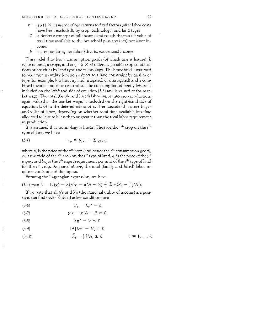
MODELING IN A MULTICROP ENVIRONMENT 99
T ' is a (1 X m) vector of net returns to fixed factors (after labor costshave been excluded), by crop, technology, and land type;
Z is Becker's concept of full income and equals the market value oftotal time available to the household plus any (net) nonlabor in-come.
E is any nonfarm, nonlabor (that is, exogenous) income.
The model thus has h consumption goods (of which one is leisure), ktypes of land, n crops, and m (= k X n) different possible crop combina-tions or activities by land type and technology. The household is assumedto maximize its utility function subject to a land constraint by quality ortype (for example, lowland, upland, irrigated, or unirrigated) and a com-bined income and time constraint. The consumption of family leisure isincluded on the left-hand side of equation (3-3) and is valued at the mar-ket wage. The total (family and hired) labor input into crop production,again valued at the market wage, is included on the right-hand side ofequation (3-3) in the determination of -T. The household is a net buyerand seller of labor, depending on whether total time available less timeallocated to leisure is less than or greater than the total labor requirementin production.
It is assumed that technology is linear. Thus for the rth crop on the ithtype of land we have
(3-4) 7ri, =- p,c, - qj birj
where Pr is the price of the rth crop (and hence the rth consumption good),ci, is the yield of the rth crop on the ith type of land, qj is the price of the jth
input, and b j, is the jth input requirement per unit of the ith type of landfor the rth crop. As noted above, the total (family and hired) labor re-quirement is one of the inputs.
Forming the Lagrangian expression, we have
(3-5) max L = U(x) - X(P'x - r'A - Z) + ; vi(Ri - [1]'Ai).
If we note that all x's and X's (the marginal utility of income) are posi-tive, the first-order Kuhn-Tucker conditions are
(3-6) Ux - Xp' = 0
(3-7) p'x - -'A -Z =: O
(3-8) XTr - V C 0
(3-9) IAr[Xi' - VI = 0
(3-10) Ri - [r]'Ai 2 0 i= k
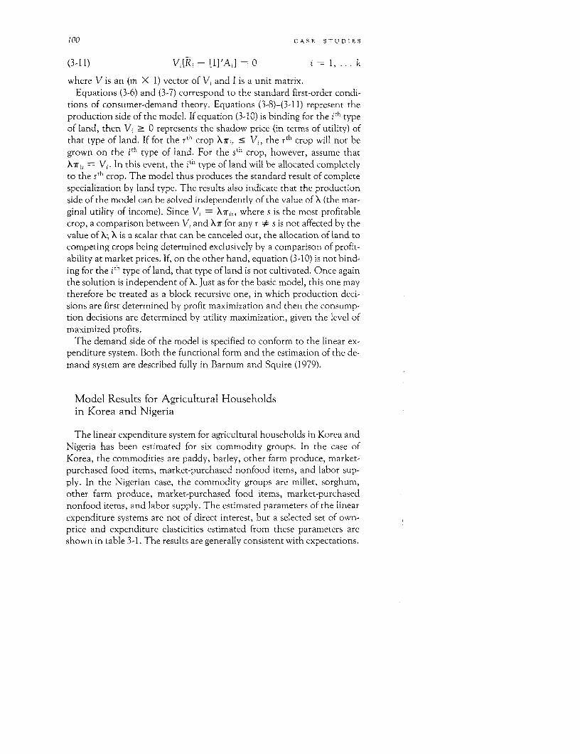
100 CASE STUDIES
(3-11) Vj[Ri - [I'Ai] = ° i = l, .. k
where V is an (m X 1) vector of Vi and I is a unit matrix.Equations (3-6) and (3-7) correspond to the standard first-order condi-
tions of consumer-demand theory. Equations (3-8)-(3-l 1) represent theproduction side of the model. If equation (3-10) is binding for the ith typeof land, then Vi 2 0 represents the shadow price (in terms of utility) ofthat type of land. If for the rth crop X7r_ < V., the rth crop will not begrown on the ith type of land. For the 5 th crop, however, assume thatXri, = Vi. In this event, the ith type of land will be allocated completelyto the 5th crop. The model thus produces the standard result of completespecialization by land type. The results also indicate that the productionside of the model can be solved independently of the value of X (the mar-ginal utility of income). Since Vi =X )7ris, where s is the most profitablecrop, a comparison between Vi and XTr for any r * s is not affected by thevalue of X; X is a scalar that can be canceled out, the allocation of land tocompeting crops being determined exclusively by a comparison of profit-ability at market prices. If, on the other hand, equation (3-10) is not bind-ing for the ith type of land, that type of land is not cultivated. Once againthe solution is independent of X. Just as for the basic model, this one maytherefore be treated as a block recursive one, in which production deci-sions are first determined by profit maximization and then the consump-tion decisions are determined by utility maximization, given the level ofmaximized profits.
The demand side of the model is specified to conform to the linear ex-penditure system. Both the functional form and the estimation of the de-mand system are described fully in Barnum and Squire (1979).
Model Results for Agricultural Householdsin Korea and Nigeria
The linear expenditure system for agricultural households in Korea andNigeria has been estimated for six commodity groups. In the case ofKorea, the commodities are paddy, barley, other farm produce, market-purchased food items, market-purchased nonfood items, and labor sup-ply. In the Nigerian case, the commodity groups are millet, sorghum,other farm produce, market-purchased food items, market-purchasednonfood items, and labor supply. The estimated parameters of the linearexpenditure systems are not of direct interest, but a selected set of own-price and expenditure elasticities estimated from these parameters areshown in table 3-1. The results are generally consistent with expectations.
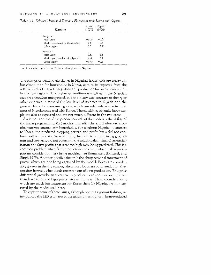
MODELING IN A MULTICROP ENVIRONMENT 101
Table 3-1. Selected Household Demand Elasticities from Korea and Nigeria
Korea NigeriaElasticitN (1970) (1976)
Ou n-priceMain crop' -0.18 -0.05Market purchased nonfood goods -0.87 -0.6Labor supply 0.0 0.01
ExpenditureMain crop' 0.57 1.8Market purchased non food goods 2.76 3.3Labor supply -0.45 -0.5
a. The main crop is rice for Korea and sorghum for Nigeria.
The own-price demand elasticities in Nigerian households are somewhatless elastic than for households in Korea, as is to be expected from therelative levels of market integration and production for own-consumptionin the two regions. The higher expenditure elasticities in the Nigeriancase are somewhat unexpected, but not in any way contrary to theory orother evidence in view of the low level of incomes in Nigeria and thegeneral desire for consumer goods, which are relatively scarce in ruralareas of Nigeria compared with Korea. The elasticities of family labor sup-ply are also as expected and are not much different in the two cases.
An important test of the production side of the models is the ability ofthe linear programming (LP) models to predict the actual observed crop-ping patterns among farm households. For northern Nigeria, in contrastto Korea, the predicted cropping pattern and profit levels did not con-form well to the data. Several crops, the most important being ground-nuts and cowpeas, did not come into the solution algorithm. Overspecial-ization and farm profits that were too high were being predicted. This is acommon problem when farm-production choices in which risk is an im-portant consideration are being modeled (see Roumasset, Boussard, andSingh 1979). Another possible factor is the sharp seasonal movement ofprices, which are not being captured by the model. Prices are consider-ably greater in the dry season, when more foods are purchased, than theyare after harvest, when foods are eaten out of own-production. This pricedifferential provides an incentive to produce more and to store it, ratherthan have to buy at high prices later in the year. These considerations,which are much less important for Korea than for Nigeria, are not cap-tured by the model used here.
To capture some of these issues, although not in a rigorous fashion, weintroduced the LES estimates of the minimum amounts of farm-produced
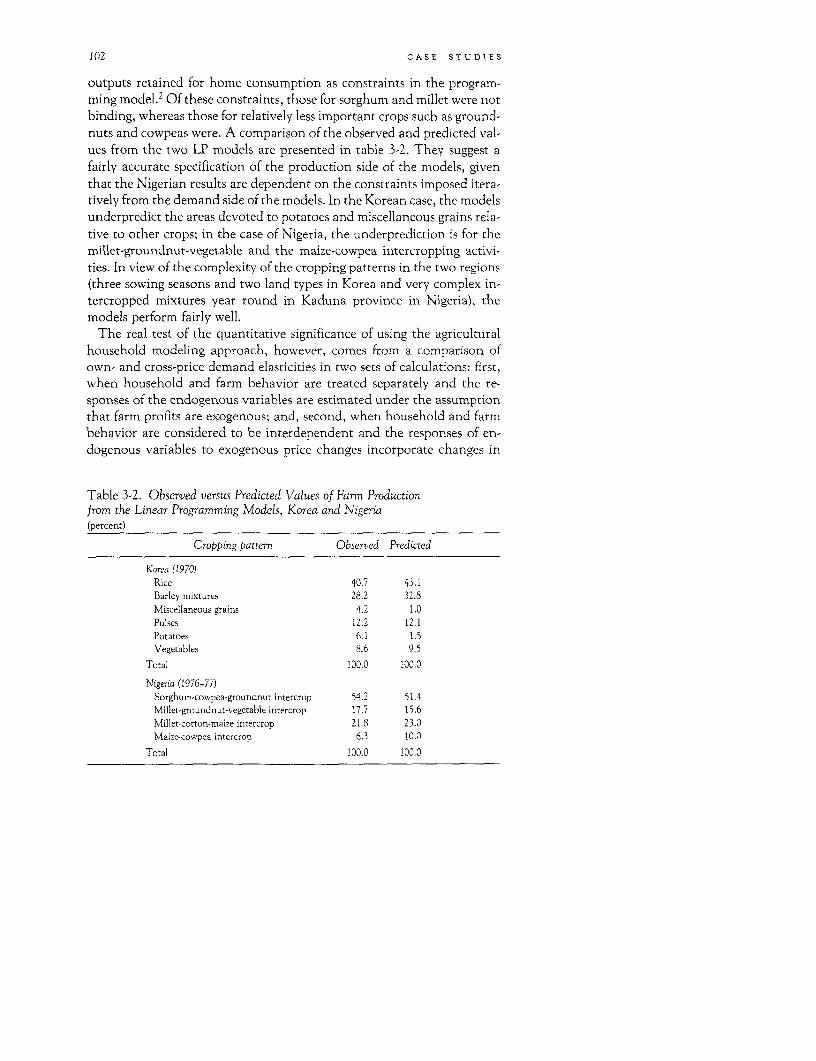
102 CASE STUDIES
outputs retained for home consumption as constraints in the program-ming model.2 Of these constraints, those for sorghum and millet were notbinding, whereas those for relatively less important crops such as ground-nuts and cowpeas were. A comparison of the observed and predicted val-ues from the two LP models are presented in table 3-2. They suggest afairly accurate specification of the production side of the models, giventhat the Nigerian results are dependent on the constraints imposed itera-tively from the demand side of the models. In the Korean case, the modelsunderpredict the areas devoted to potatoes and miscellaneous grains rela-tive to other crops; in the case of Nigeria, the underprediction is for themillet-groundnut-vegetable and the maize-cowpea intercropping activi-ties. In view of the complexity of the cropping patterns in the two regions(three sowing seasons and two land types in Korea and very complex in-tercropped mixtures year round in Kaduna province in Nigeria), themodels perform fairly well.
The real test of the quantitative significance of using the agriculturalhousehold modeling approach, however, comes from a comparison ofown- and cross-price demand elasticities in two sets of calculations: first,when household and farm behavior are treated separately and the re-sponses of the endogenous variables are estimated under the assumptionthat farm profits are exogenous; and, second, when household and farmbehavior are considered to be interdependent and the responses of en-dogenous variables to exogenous price changes incorporate changes in
Table 3-2. Observed versus Predicted Values of Farm Productionfrom the Linear Programming Models, Korea and Nigeria(percent)
Cropping pattern Observed Predicted
Korea (1970)Rice 40.7 43.1Barley mixtures 28.2 32.8Miscellaneous grains 4.2 1.0Pulses 12.2 12.1Potatoes 6.1 1.5Vegetables 8.6 9.5
Total 100.0 100.0
Nigeria (1976-77)Sorghum.cowpea-groundnut intercrop 54.2 51.4Millet-groundnut-vegetable intercrop 17.7 15.6Millet-cotton-maize intercrop 21.8 23.0Maize-cowpea intercrop 6.3 10.0
Total 100.0 100.0
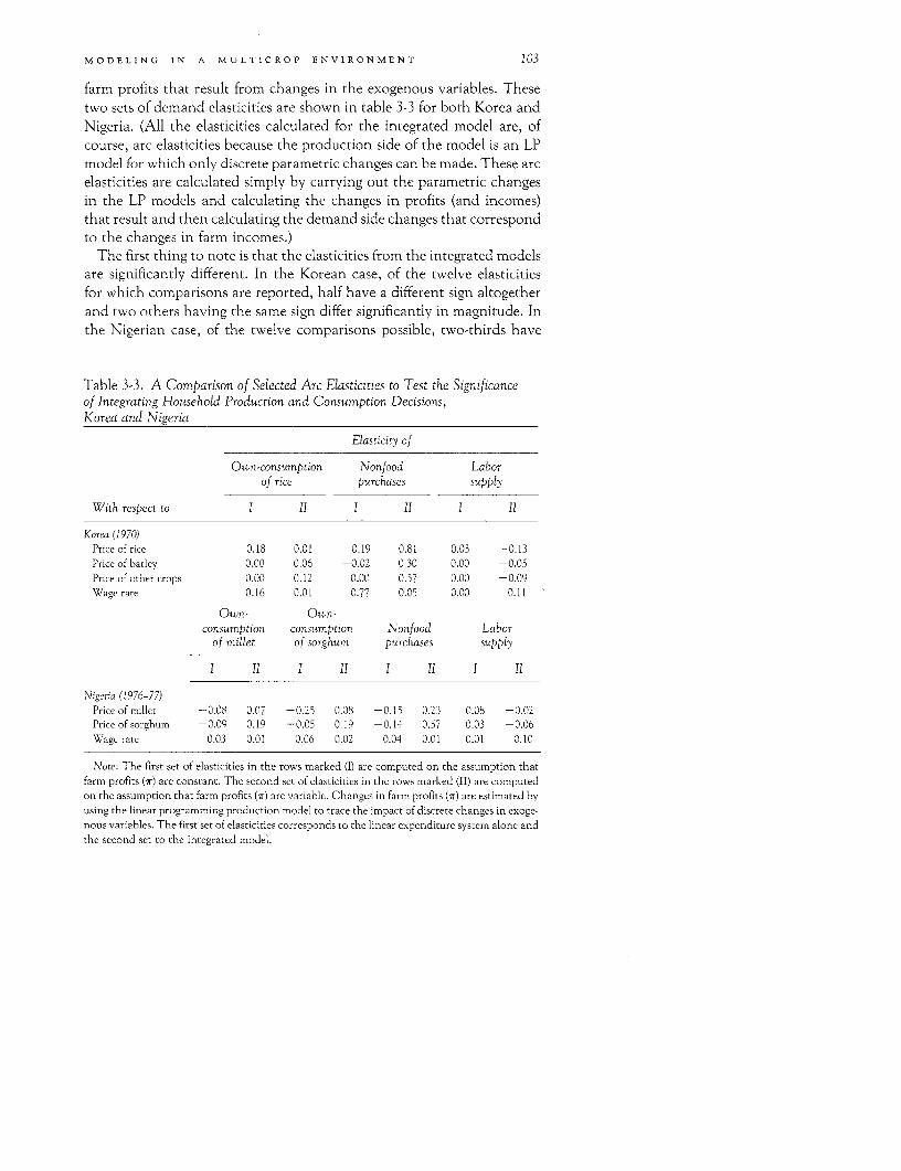
MODELING IN A MULTICROP ENVIRONMENT 103
farm profits that result from changes in the exogenous variables. Thesetwo sets of demand elasticities are shown in table 3-3 for both Korea andNigeria. (All the elasticities calculated for the integrated model are, ofcourse, arc elasticities because the production side of the model is an LPmodel for which only discrete parametric changes can be made. These arcelasticities are calculated simply by carrying out the parametric changesin the LP models and calculating the changes in profits (and incomes)that result and then calculating the demand side changes that correspondto the changes in farm incomes.)
The first thing to note is that the elasticities from the integrated modelsare significantly different. In the Korean case, of the twelve elasticitiesfor which comparisons are reported, half have a different sign altogetherand two others having the same sign differ significantly in magnitude. Inthe Nigerian case, of the twelve comparisons possible, two-thirds have
Table 3-3. A Comparison of Selected Arc Elasticities to Test the Significanceof Integrating Household Production and Consumption Decisions,Korea and Nigeria
Elasticity of
Own-consumption Nonfood Laborof rice purchases supply
With respect to 1 11 1 11 1 11
Korea (1970)Price of rice -0.18 0.01 -0.19 0.81 0.03 -0.13Price of barley 0.00 0.06 -0.02 0.30 0.00 -0.05Price of other crops 0.00 0.12 0.00 0.57 0.00 -0.09Wage rate 0.16 0.01 0.77 0.05 0.00 0.11
Own- Own-consumption consumption Nonfood Labor
of millet of sorghum purchases supply
Nigeria (1976-77)Price of millet -0.08 0.07 -0.25 0.03 -0.15 0.23 0.08 -0.02Price of sorghum -0.09 0.19 -0.05 0.19 -0.14 0.57 0.03 -0.06Wage rate 0.03 0.01 0.06 0.02 0.04 0.01 0.01 0.10
Note: The first set of elasticities in the rows marked (I) are computed on the assumption thatfarm profits (r) are constant. The second set of elasticities in the rows marked (1I) are computedon the assumption that farm profits (r) are variable. Changes in farm profits (7r) are estimated byusing the linear programming production model to trace the impact of discrete changes in exoge-nous variables. The first set of elasticities corresponds to the linear expenditure system alone andthe second set to the integrated model.
Table 3-4. Selected Elasticities to Illustrate the Impact of Changes in Farm Technology and Costs on Household Demand
in Integrated Models, Korea (1970)
With respect to
Fertilizer Interestand rate on Power Paddy Average
Wage Seed pesticide working tiller land Upland farrn°11 Elasticity of rate costs costs capital capacitya available available size
Own-consumption of rice 0.0097 -0.0111 -0.0484 -0.0155 0.0019 0.0691 0.0334 0.1013
Food purchases 0.0156 -0.0179 -0.078 -0.025 0.0031 0.1114 0.0538 0.1632
Nonfood purchases 0.047 -0.054 -0.2349 -0.0754 0.0094 0.3353 0.1620 0.4913
Labor suipply 0.105 0.0088 0.0383 0.0123 -0.0015 -0.0547 -0.0264 -0.0802
a. Obtained by increasing the capacity of power tillers available per household; the elasticity should be read as a percentage change in the endogenous variable
for a I percent change in the available tiller capacity.
MODELING IN A MULTICROP ENVIRONMENT 105
different signs and the rest differ in magnitude. What accounts for thisdifference?
Consider, for example, the own-price consumption elasticities of themain crops grown by agricultural households-rice in Korea and sor-ghum in Nigeria. Both these crops are the most important food items(and hence nutrition source) in the consumption bundle and the mostimportant crops on the farms. Traditional demand theory would suggestthat the own-consumption of these crops would decrease if their priceswere increased (the estimated elasticities are -0.18 and -0.05 for riceand sorghum, respectively), a result totally consistent with theory if agri-cultural households are to be treated solely as consumers. The integratedmodels, however, predict that own-consumption of these commoditieswill increase (the estimated elasticities are 0.01 and 0.19 in this case).
Consider another example, that of the elasticities of family labor supplywith respect to the wage rate. Again, in traditional demand theory, anincrease in wage rates implies an increase in real household incomes, andthe result is a negative or inelastic response of household labor supply.(These elasticities are not significantly different from zero for both Koreaand Nigeria.) These effects are offset in the case of the integrated agricul-tural household models because an increase in agricultural wages also af-fects farm costs on the production side and reduces total farm incomes.As a result, labor-supply responses become positive or more elastic. (Thisis the case with an elasticity of 0.11 and 0.1 in Korea and Nigeria,respectively.)
Another set of elasticities can be estimated only for the integratedmodels-those with respect to input costs and other technologicalchanges in farm production. This point can be illustrated for Korea bythe selected set of elasticities in table 3-4. The Korean model is more ap-propriate for illustration purposes because it is much richer on the pro-duction side owing to the widespread adoption of new high-yielding vari-eties, the extensive use of nonfarm inputs in agriculture, and the use ofirrigation and tillers. The Kaduna region in Nigeria has seen few of thesetechnological innovations, nor is the use of nonfarm inputs significant.
Consider, first, the elasticities with respect to the costs of seeds, fertil-izers, and pesticides. As input costs go up, the model correctly predictsthat farm incomes and hence outlays on all commodities will be reducedand work effort on part of households will be increased. Increased tillercapacities or the availability of additional land (of different qualities) orincreases in family size, which increases farm-family labor, have the oppo-site effects. Similarly, with increased input costs, farm incomes are re-duced and thus the amount of family labor supply forthcoming from thehouseholds increases, whereas increases in the capacities of land and
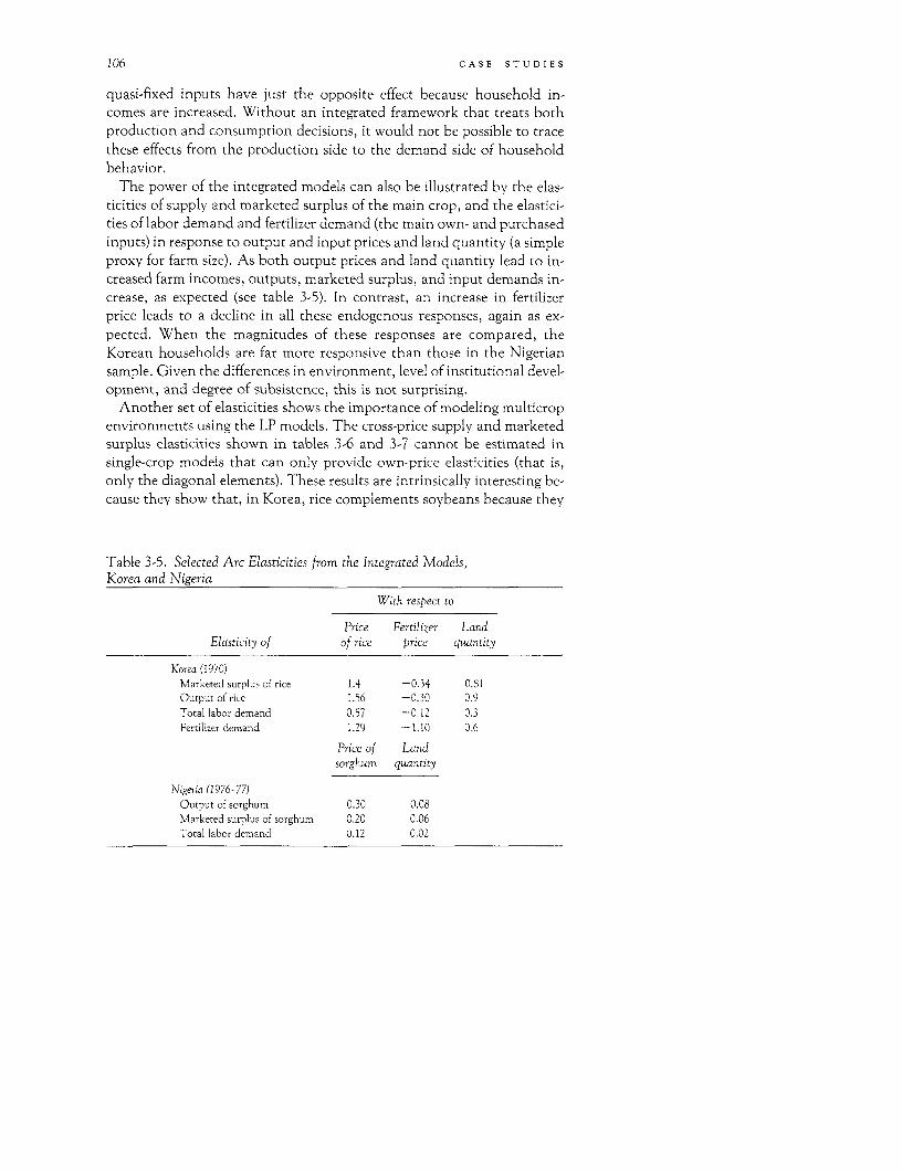
106 CASE STUDIES
quasi-fixed inputs have just the opposite effect because household in-comes are increased. Without an integrated framework that treats bothproduction and consumption decisions, it would not be possible to tracethese effects from the production side to the demand side of householdbehavior.
The power of the integrated models can also be illustrated by the elas-ticities of supply and marketed surplus of the main crop, and the elastici-ties of labor demand and fertilizer demand (the main own- and purchasedinputs) in response to output and input prices and land quantity (a simpleproxy for farm size). As both output prices and land quantity lead to in-creased farm incomes, outputs, marketed surplus, and input demands in-crease, as expected (see table 3-5). In contrast, an increase in fertilizerprice leads to a decline in all these endogenous responses, again as ex-pected. When the magnitudes of these responses are compared, theKorean households are far more responsive than those in the Nigeriansample. Given the differences in environment, level of institutional devel-opment, and degree of subsistence, this is not surprising.
Another set of elasticities shows the importance of modeling multicropenvironments using the LP models. The cross-price supply and marketedsurplus elasticities shown in tables 3-6 and 3-7 cannot be estimated insingle-crop models that can only provide own-price elasticities (that is,only the diagonal elements). These results are intrinsically interesting be-cause they show that, in Korea, rice complements soybeans because they
Table 3-5. Selected Arc Elasticities from the Integrated Models,Korea and Nigeria
With respect to
Price Fertilizer LandElasticity of of rice price quantity
Korea (1970)Marketed surplus of rice 1.4 -0.34 0.81Output of rice 1.56 -0.30 0.9Total labor demand 0.57 -0.12 0.3Fertilizer demand 1.29 -1.10 0.6
Price of Landsorghum quantity
Nigeria (1976-77)Output of sorghum 0.30 0.08Marketed surplus of sorghum 0.20 0.06Total labor demand 0.12 0.02
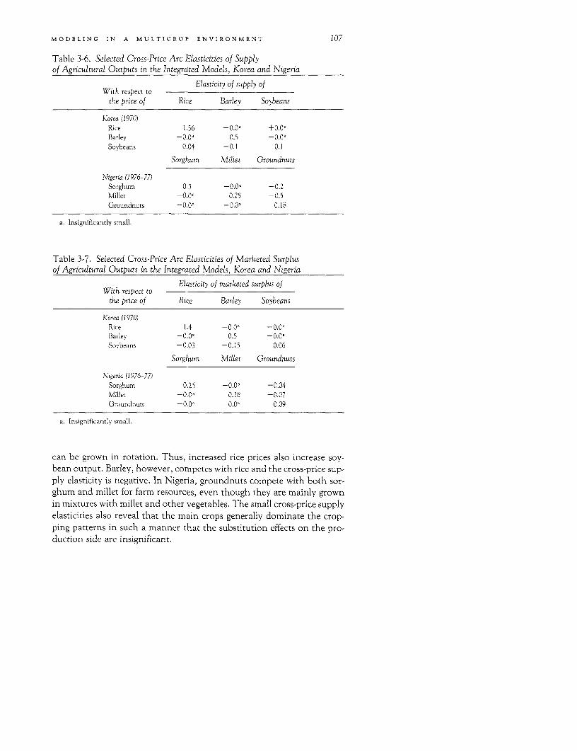
MODELING IN A MUJLTICROP ENVIRONMENT 107
Table 3-6. Selected Cross-Price Arc Elasticities of Supplyof Agricultural Outputs in the Integrated Models, Korea and Nigeria
Elasticity of supply ofWith respect to
the price of Rice Barley Soybeans
Korea (1970)Rice 1.56 -0.0' +0.OaBarley -0.0° 0.5 -0.0'Soybeans 0.04 -0.1 0.1
Sorghum Millet Groundnuts
Nigeria (1976-77)Sorghum 0.3 - 0.0' -0.2Millet -0.0' 0.25 -0.5Groundnuts -0.0P -0.0' 0.18
a. Insignificantly small.
Table 3-7. Selected Cross-Price Arc Elasticities of Marketed Surplusof Agricultural Outputs in the Integrated Models, Korea and Nigeria
Elasticity of marketed surplus ofWith respect to
the price of Rice Barley Soybeans
Korea (1970)Rice 1.4 -0.0a -0.0'Barley -0.0a 0.5 -0.0'Soybeans -0.03 -0.15 0.06
Sorghum Millet Groundnuts
Nigeria (1976-77)Sorghum 0.25 -0.0 -_0.04Millet -0.0' 0.18 -0.07Groundnuts - 0.0' -0.0° 0.09
a. Insignificantly small.
can be grown in rotation. Thus, increased rice prices also increase soy-bean output. Barley, however, competes with rice and the cross-price sup-ply elasticity is negative. In Nigeria, groundnuts compete with both sor-ghum and millet for farm resources, even though they are mainly grownin mixtures with millet and other vegetables. The small cross-price supplyelasticities also reveal that the main crops generally dominate the crop-ping patterns in such a manner that the substitution effects on the pro-duction side are insignificant.
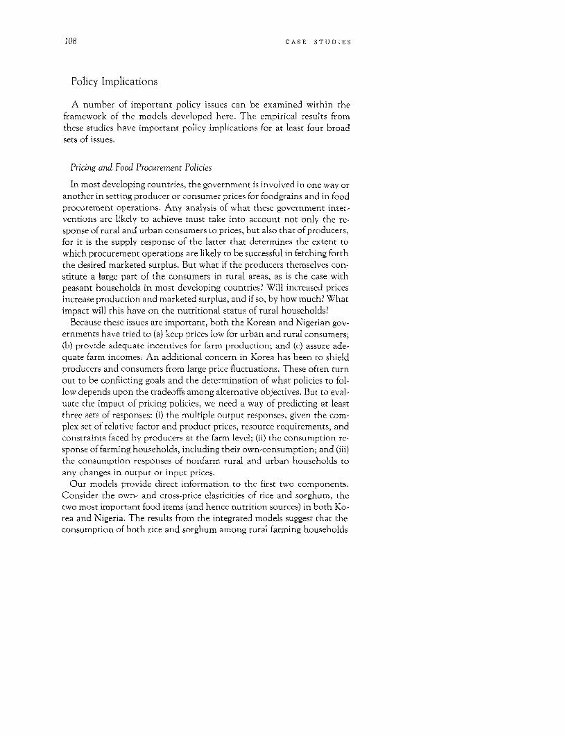
108 CASE STUDIES
Policy Implications
A number of important policy issues can be examined within theframework of the models developed here. The empirical results fromthese studies have important policy implications for at least four broadsets of issues.
Pricing and Food Procurement Policies
In most developing countries, the government is involved in one way oranother in setting producer or consumer prices for foodgrains and in foodprocurement operations. Any analysis of what these government inter-ventions are likely to achieve must take into account not only the re-sponse of rural and urban consumers to prices, but also that of producers,for it is the supply response of the latter that determines the extent towhich procurement operations are likely to be successful in fetching forththe desired marketed surplus. But what if the producers themselves con-stitute a large part of the consumers in rural areas, as is the case withpeasant households in most developing countries? Will increased pricesincrease production and marketed surplus, and if so, by how much? Whatimpact will this have on the nutritional status of rural households?
Because these issues are important, both the Korean and Nigerian gov-ernments have tried to (a) keep prices low for urban and rural consumers;(b) provide adequate incentives for farm production; and (c) assure ade-quate farm incomes. An additional concern in Korea has been to shieldproducers and consumers from large price fluctuations. These often turnout to be conflicting goals and the determination of what policies to fol-low depends upon the tradeoffs among alternative objectives. But to eval-uate the impact of pricing policies, we need a way of predicting at leastthree sets of responses: (i) the multiple output responses, given the com-plex set of relative factor and product prices, resource requirements, andconstraints faced by producers at the farm level; (ii) the consumption re-sponse of farming households, including their own-consumption; and (iii)the consumption responses of nonfarm rural and urban households toany changes in output or input prices.
Our models provide direct information to the first two components.Consider the own- and cross-price elasticities of rice and sorghum, thetwo most important food items (and hence nutrition sources) in both Ko-rea and Nigeria. The results from the integrated models suggest that theconsumption of both rice and sorghum among rural farming households
MODELING IN A MULTICROP ENVIRONMENT 109
is likely to increase marginally (the relevant elasticities are 0.01 and 0.19,respectively). Although the predicted output responses of these crops arehigher-much more so for Korea (the output elasticities are 1.56 for riceand 0.3 for sorghum)-the increase in household consumption dampensthis response, so that the response of marketed surpluses is lower (therelevant elasticities are 1.4 for rice and 0.2 for sorghum in table 3-3). Thedifferences in the estimated responses for marketed surplus in Korea andnorthern Nigeria suggest much less scope for government pricing policyin generating food production in northern Nigeria, a finding that is con-sistent with the relatively low levels of technology there.
Similarly, the cross-price demand elasticities are not only positive forother food crops, but are also positive and fairly high for nonfood pur-chases. This suggests that although raising farm output prices may have anegative impact on the nutritional status of nonfarming rural house-holds, it has a positive impact on agricultural households. The net impactin rural areas depends, of course, upon the relative weights of the twogroups in the rural population. In both Korea and Nigeria, farminghouseholds are by far the most dominant, and hence increased outputprices are likely to enhance the nutritional status in rural areas.
The cross-price effects are both on the production and consumptionside. Thus, for example, increased sorghum prices in Nigeria reduce theproduction of groundnuts and millet as sorghum displaces them in thecrop mix, but increased prices, because they increase incomes, have a posi-tive effect on their consumption. An opposite effect occurs when inputprices are increased. Thus a 10 percent increase in fertilizer prices in Koreareduces the fertilizer demand by 11 percent and the output of rice by 3percent, but as incomes decline, so does own-consumption of rice (by 0.1percent). The decline in the marketed surplus is the outcome of these twooffsetting effects. It is important to be able to trace this type of production-consumption interaction in evaluating the impact of input subsidypolicies.
The ability to predict accurately the marketed surplus response to gov-ernment pricing policies is an essential ingredient in developing effectiveprocurement programs and in evaluating their costs and their impact ondifferent groups of the population. Government procurements often de-termine the level of food imports (exports), which in turn affect foreignexchange.
Farm Technologies and Farm Employment
If rapid technological change in the agricultural sector is both land in-tensive and labor saving, what is the likely impact on the demand for
110 CASE STUDIES
labor? More important, how will family versus hired labor be affected bythis increased demand? This matter is of great interest to policymakers,especially in areas where rural households rely upon wage employment asa major source of income. Such households include not only the landlessbut also small and marginal farmers with very small land holdings. Howwould such households fare under different pricing policies and techno-logical regimes? We cannot provide an answer to these questions unlesswe can establish how agricultural households respond to technologicalchanges in allocating family labor to farm production. Our results pro-vide some insight.
To begin with, all land intensification programs in Korea and Nigeriadefinitely increase the demand for total labor. The demand for hired la-bor increases at an even higher rate. This is because increased land avail-ability, by increasing farm incomes, also decreases the supply of familylabor. The slack is taken up by the increased demand for hired labor.Thus, land-intensification strategies greatly increase the employment op-portunities for rural wage earners. The same effect occurs when new high-yielding varieties are introduced because they also increase the demandfor total labor inputs (not shown), but, by increasing income, they in-crease the demand for hired labor even faster.
The impact of labor-displacing technologies such as power tillers onhired labor in Korea is more complicated, however. We have used para-metric changes in the LP model to trace the changes. The results showthat, on one hand, the tillers displace labor and thus reduce the totallabor demand (the relevant elasticity not shown in the tables is -0.025;that is, a 1 percent increase in tiller capacity reduces total labor demandby 0.25 percent). On the other hand, they also substantially increase farmincomes so that the supply of family labor to farm production is reduced(the relevant elasticity is -0.00 15). The net effect on hired labor is posi-tive and the relevant elasticity is 3.8! This is because a small reduction infamily labor, which accounts for nearly 96 percent of the total labor usein Korean farming households (using the mean farm size of 1.89 hectaresin the sample), means a large increase in the demand for hired labor, eventhough the total demand for labor has decreased.
Pricing Policies and Farm Employment
Nonfarm households may also benefit considerably from increasedwages and employment opportunities related to increased output pricesbecause they not only increase output and the demand for total labor,but they also decrease the supply of family labor as profits and incomesincrease. The demand for hired labor thus increases faster than the de-
MODELING IN A MULTICROP ENVIRONMENT 1I1
mand for total labor as farmers use more labor per unit of output. Therelevant elasticities for labor demand with respect to the prices of themain crops are 0.57 for Korea and 0.12 for Nigeria; for labor supply, theyare -0.13 for Korea and -0.06 for Nigeria. Once again, these relation-ships are stronger in Korea than in Nigeria.
These results have important policy implications because they showthat benefits of new technologies spill over into increased employment forrural wage earners. Increased output prices may also have the same im-pact, but whether or not they result in a net gain in welfare for the land-less depends on two offsetting effects-on the one hand, they obtainincreased employment (and perhaps increased wages and incomes, de-pending on how tight rural labor markets are and how they operate), but,on the other hand, they face higher prices for farm goods because theyrespond as pure consumers (not having any land at all, by definition, theyare not affected by the production side of the model). The debate overwhich effects dominate is still going strong, and these models can helpaddress the issues more clearly with the relevant empirical elasticities.
Nonfarm Employment and Demand Linkages
Ultimately, the question of what happens to the demand for the laborof the landless cannot be resolved by looking at the demand for farmlabor only. The extent to which agricultural growth induces employmentin the rural nonfarm sector and the industrial sector depends upon theextent to which the growth (and distribution) of farm incomes increasesthe demand for nonfarm consumer goods and services. How do techno-logical change and changes in farm output prices affect this demand? Ourresults show that this demand increases tremendously. The elasticities ofdemand for nonfarm purchased goods in response to increased outputprices is positive, as expected, but the expenditure elasticity of demandfor these goods is both positive and very high (2.76 in Korea and 3.3 inNigeria). Thus, as farm incomes and farm employment increase, so doesthe final demand for nonfarm and industrial goods. Our results allow usto explicitly trace these final demand linkages from the productionchanges all the way to changes in the final demand for nonfarm goods.Expenditure elasticities for nonfarm goods in the order of 2.5-3.0 as pre-dicted by our results mean that a 10 percent increase in farm and ruralincomes would increase the demand for nonfarm goods by about 20 to 30percent.
Farm household incomes in Korea grew at an annual rate of 5 percent(at constant prices) between 1965 and 1976. The implied growth in de-mand for nonfarm products is 14 percent per annum. This has, of course,

112 CASE STUDIES
been the reason why high rates in the growth of the labor force in Koreahave not been accompanied by unemployment or underemployment.The growth in farm employment generates secondary induced effects thatlead to the rapid growth of nonfarm employment. If this is accompaniedby high rates of outmigration to the urban sector in response to growingemployment opportunities, as in the case of Korea (and Nigeria more re-cently), real rural wage rates rise quite rapidly and rural poverty is sub-stantially reduced. This linkage between high rates of agricultural growthaccompanied by high rates of growth in nonfarm employment and re-duced incidence of rural poverty can also be found in other developingeconomies-most notably, Taiwan and the Indian and Pakistani Punjabs.
The policy implications of the results discussed here illustrate the im-portance of developing an integrated approach to modeling agriculturalhousehold decisions in a multicrop environment.
Conclusions
This chapter extends the theory of an agricultural household to multi-crop environment and provides results for two rather diverse agriculturalregions at quite different levels of development. The results clearly indi-cate the value of such models in tracing the impact of price, technology,and other policy changes in rural areas that are dominated by peasanthouseholds that make production and consumption decisions jointly.They also clearly show the quantitative significance of using this ap-proach, as the predicted responses differ not only in magnitude but alsoin direction when compared with the traditional approaches to demandand supply response.
The approach to modeling agricultural household behavior describedhere has several limitations, however. Most of these stem from the simpli-fying assumptions made in developing the theoretical framework. Thetwo that are most troubling (at least for the Nigerian context) are the wayin which labor markets are handled and the risk-free environment pos-ited for household decisions. Although evidence shows that most ruralhouseholds operate in rural factor markets-particularly in labor mar-kets, where they are both buyers and sellers of labor-considerable evi-dence also shows that these markets are interlinked. Thus, credit, land,and labor contractual relations may not be independent. This linkageimplies that the standard type of profit-maximization conditions usedhere may not hold. This is the case, for example, where tenancy prevailsand labor contracts are conditional on land contracts. In such cases thetheories would have to be extended and reformulated.
MODELING IN A MULTICROP ENVIRONMENT 113
The assumption of a risk-free environment is also a matter of some con-cern, especially when intercropping decisions are being modeled, as in thecase of Nigeria. We know that intercropping is a response to risk in envi-ronments with uncertain rainfall. Clearly, the production side of themodels could be improved by incorporating risk. This can be done byeither using the focus-loss method developed by Boussard and Petit (1967)or by using one or another version of the mean-variance approaches torisk programming. The one that has proved fairly robust is the one devel-oped by Hazell (1971). The real challenge, however, is to integrate thisexplicitly into an expected utility-maximization framework. An initial at-tempt in this direction is made by Roe and Graham-Tomasi (see chapter9). An integrated approach that would both remove the assumptions ofindependent factor markets and include uncertainty remains a challengeto future research work.
The ultimate value of the modeling approach developed in this chapterlies in its ability to use farm management and farm family budget datathat can be collected by project economists and that are often readilyavailable for the analysis of a number of important policy issues. Thus,despite their limitations, these models should find increasing use in proj-ect and policy work.
Appendix: Data Sources
The data for Korea are from a series of extensive farm household sur-veys carried out by the Ministry of Agriculture and Fisheries beginning in1962. The surveys took in farms that were included in a representativenational random sample of farm households throughout the country. Asfar as possible, the same households were surveyed each year, exceptwhen replacements were necessary owing to death, retirement, or migra-tion of the farm operators. From 1962 to 1973, the surveys included ap-proximately 1,200 farm households each year. (The number was in-creased to 2,500 in 1974.) These surveys cover data on farm production(including area planted to rice and other information on farm operationsand expenditures) as well as household data (including family size, laboruse, household expenditures, and other sources of income).
We used 1970 data to estimate the linear expenditure systems and de-rive the parameters for the programming models. After accounting formissing variables and data errors, we had a sample of 524 households. Inaddition, we used data from the Yearbook of Agriculture and Forestry, 1971,to test cropping patterns from a nationwide survey. The survey data ap-pear in the Report on the Results of Farm Household Economy Survey and
114 CASE STUDIES
Production Cost Survey of Agricultural Products (various years) published bythe Ministry of Agriculture and Fisheries. The data were made availableto us through the courtesy of The National Agricultural Research Insti-tute, Seoul, and the data tapes were provided by the Department of Agri-cultural Economics and Rural Sociology, Ohio State University.
The Nigerian data come from three large agricultural projects fundedby the World Bank. The project areas-Funtua, Gombe, and Gusau-arein the state of Kaduna. So that progress in these project areas could bemonitored, a Monitoring and Evaluation Unit was funded under theBank projects and given the responsibility of collecting farm-level produc-tion and expenditure data. The project areas lie in the semidry northernregion of Kaduna state and are populated mainly by the Hausa and Fu-lani. The predominant crops in the region are sorghum, millet, ground-nuts, cowpeas, and cotton. More than half the area in this region is culti-vated mainly by hand in a mixed intercropping system with practicallyno modern inputs.
The projects began in 1975 and we were able to obtain data for the1976-77 cropping season. This information consisted of household size,family labor use, farm income and expenditures, and household expendi-tures. The data were collected on a weekly basis for 42 weeks and coveredsome 24 villages and 24 households in each village. After validation, asample size of 312 households from the Funtua project area was selectedand the data for the 1976-77 cropping year were used for analysis (fordetails, see World Bank, 1980).
Notes
1. This model was first presented in a study by Ahn, Singh, and Squire (1981), where theresults from the Korean study were first reported.
2. Using the Stone-Geary form of the utility function U = EU, = n Ei ln(xi - -y), where xis the per capita consumption of the i,h commodity, n the number of family members, and f,i -ythe parameters. The estimates of yj can be interpreted as minimum amounts retained for own-consumption.
References
Ahn, Choong Yong, Inderjit Singh, and Lyn Squire. 1981. "A Model of an Agricul-tural Household in Multi-crop Economy: The Case of Korea." The Review of Eco-
nomics and Statistics, vol. 63, no. 4 (November), pp. 520-25.
Barnum, Howard N., and Lyn Squire. 1979. A Model of an Agricultural Household:Theor) and Evidence. Washington, D.C.: World Bank.
MODELING IN A MULTICROP ENVIRONMENT 115
Boussard, Jean Marc, and Michele Petit. 1967. "Representation of Farmer's Behaviorunder Uncertainty with Focus-Loss Constraint." Journal of Farm Economics, vol. 49,no. 4, pp. 869-80.
Hazell, P. B. R. "A Linear Alternative to Quadratic and Semi-Variance Programmingfor Farm Planning Under Uncertainty." 1971. American Journal of Agricultural Eco-nomics, vol. 53, no. 1, pp. 53-62.
Roumasset, James, Jean Marc Boussard, and Inderjit Singh, eds. 1979. Risk, Uncer-tainty and Agricultural Development. New York: Agricultural Development Council,New York.
World Bank. 1980. "The Monitoring and Evaluation of the Funtua, Gusau, andGombe Agricultural Development Projects: A Guide to Statistical Tabulations."West African Region Projects Department. Washington, D.C.
4Estimating the Determinants of FoodConsumption and Caloric Availability
in Rural Sierra Leone
John Strauss
THE NUTRITIONAL WELL-BEING OF HOUSEHOLDS, particularly those with lowincomes, has become an important consideration for governments of de-veloping countries. Policy planners seldom have much indication of howdifferent policies will affect household food consumption and thereby nu-tritional well-being, however, particularly among agricultural house-holds. For such households, a change in price or technology, by affectingprofits from home production, will shift the budget constraint andthereby result in a profit effect (see chapter 1). The resultant increase infoods consumed may lead to increased or decreased nutrient availabilityat the household level.
To explore the effects of prices and of income on household nutrient(hereafter) calorie availability, disaggregation of foods is required. Themodel estimation reported in this chapter does just that. Consumptionand marketed surplus responses are estimated for five food items, non-foods, and labor supply for rural households in Sierra Leone. The re-sponses are obtained by means of a farm-household model with multipleoutputs. The data are from a cross-sectional survey of households in ruralSierra Leone. Since price variation for all commodities exists by region, itis possible to estimate complete systems of commodity demand and ofoutput-supply and variable input demands.
The basic farm-household model, which has already been estimated,assumes that households produce a single crop (Lau, Lin, and Yotopoulos1978; Barnum and Squire 1979). These earlier studies used demand sys-
Note: The research described in this chapter was funded under USAID contract no. AID/DSAN-C-0008.
116
DETERMINANTS OF FOOD CONSUMPTION 117
tems that impose severely restrictive assumptions concerning the effect offull income on expenditures (see chapter 1). Although such assumptionsas linear Engel curves may not be completely unreasonable when a highlevel of commodity aggregation is used, they seem questionable when oneis interested in more disaggregated commodities.
This study uses a Quadratic Expenditure System (QES), which allowsfor quadratic Engel curves. Demographic variables are explicitly incorpo-rated into the model to allow for a richer specification than can be ob-tained by means of per capita variables. Output and variable input alloca-tion is determined by a system of output-supply and input-demandequations. These equations are derived from a multiple output produc-tion function assumed to be separable between outputs and inputs-con-stant elasticity of transformation is assumed for outputs and Cobb-Douglas for inputs. Thus the analyst is able to use regional price data andcan avoid problems of endogeneity with respect to variables on the right-hand side, which would be encountered if a multiple-output productionfunction were estimated directly. Household specialization in productionis such, however, that some commodities are not produced by somehouseholds. If the censored nature of the data is ignored, parameter esti-mates become inconsistent. Perhaps this is one reason why econometricapproaches to estimating the production side of multiple-output farm-household models have not previously been attempted. (See chapter 3 fora discussion of the use of linear programming to determine crop alloca-tion in a multiple-output agricultural model.)
The results of the study show that for most crops, the own-price effectson consumption remain negative when profits are allowed to vary. Cross-price consumption elasticities are both positive and sizable. Marketed sur-plus elasticities are sizable, even for the lowest-income households. Elastic-ities of caloric availability with respect to total expenditure are found to belarge, and vary little by expenditure group. Price elasticities of calorie avail-ability are generally positive, though very small, except for the price of thestaple food, rice, for which the calorie elasticities are moderately negative.This exception has several important policy implications.
Policy Issues
The potential effect of government policies that operate on the nutri-tional well-being of rural households in Sierra Leone through prices andincome can be explored. These may be targeted to specific groups, or not.Nonprice interventions such as food fortification or direct feeding pro-grams are not addressed here. The farm-household model provides the
118 CASE STUDIES
responses of food consumption to prices and income needed to derive thenutritional effects of government policies. Only partial equilibrium effectsare investigated in this study (for some limited general equilibrium effects,see chapter 7).
The principal symptoms of nutritional problems in rural Sierra Leoneseem to be underweight and stunted linear growth for age, and anemia. Ina national nutrition survey (University of California 1978), almost one-third of rural children aged 0-5 were found to be underweight (weighedless than 80 percent of the expected weight for a reference child of thesame age), and slightly more than one-fourth of rural children in the sameage group were found to be stunted (less than 90 percent of the expectedheight of a reference child of the same age). Anemia was found to affectroughly half of the rural children.
This study focuses on calorie availability to the household in the lightof evidence that caloric deficiency is a serious problem and of Sukhatme's(for example, 1970) work indicating that protein deficiency tends to beaccompanied by calorie deficiency, and protein sufficiency by calorie suf-ficiency. Two important issues for government policymakers are, first, thedegree of responsiveness of calorie availability to changes in income, and,second, the calorie elasticities with respect to food prices.
There is some controversy regarding the calorie elasticity with respectto income. Reutlinger and Selowsky (1976) believe 0.15 and 0.3 to be therelevant bounds. Behrman and Wolfe (1984) find this elasticity to bearound 0.05 for households in Nicaragua. If these low estimates are cor-rect, then programs attempting to increase caloric intake by increasingincomes are unlikely to be successful. Rather, programs targeted at spe-cific groups are likely to be more cost effective in this case than generalpricing policies or policies focusing on income generation. Even if higherestimates are correct, very large income interventions may be requiredwhen caloric targets are substantially greater than existing intakes. Thefollowing are estimates reported for some other areas: 0.3 to 0.5 for a sam-ple of northeast Brazilian households (Ward and Sanders 1980); upwardsof 0.5 for all households and 0.6 for low-income households in Colombia(Pinstrup-Andersen and Caicedo 1978); and an average of about 0.5 forrural households and as high as 0.75 for low-income households in Indo-nesia (Timmer and Alderman 1979). The food coverage in the Timmerand Alderman study is incomplete, but the authors argue that their esti-mates may be a lower bound to the true elasticities since the omittedfoods (dairy products, meats, eggs, fish) are likely to be income elastic andhigh in calories per kilogram. In addition, Pitt (1983) finds an incomeelasticity of roughly 0.8 for rural Bangladesh households. The fact thatthe income elasticity falls for higher-income households in several ofthese studies may help to explain why these estimates vary.

DETERMINANTS OF FOOD CONSUMPTION 119
Estimates of elasticities of calorie availability with respect to prices ofgoods for rural households are rare. Some estimates exist for elasticities ofcalories with respect to calorie price. In general, the price of a calorie de-pends on prices of foods and on caloric intake. Since caloric intake resultsfrom a household choice, calorie price is endogenous to the household.Many econometric estimates of this elasticity are thus suspect, since theydo not account for the endogeneity of calorie price. In addition, it makessense to inquire about the calorie responsiveness to food prices since theseprices correspond much more directly to government policy than do calo-rie prices. Pitt's (1983) estimates are generally negative but small in magni-tude, except for rice, the staple crop in Bangladesh, for which the esti-mates (around -0.5) are sizable. A shortcoming of Pitt's study is thatproduction data are lacking and thus the farm-household aspect of theproblem is not properly accounted for. Whether his price elasticities ofcaloric intake would remain negative when profits are varied in responseto price changes is unclear.
Model Specification and Estimation
Model Specification
The model used is a static, separable, semisubsistence farm-householdmodel (see chapter 1 for a detailed review). Assume that each householdhas a well-behaved utility function with arguments being household con-sumption of various goods and of leisure. Goods may be either producedor bought or sold in the market, and labor may be bought or sold in themarket. Goods are produced using labor, land, and fixed capital.' Land isassumed to be fixed in total amount but must be distributed betweenuses. A time constraint exists equating household leisure plus labor timeto total time available. Finally, a budget constraint exists equating thevalue of net product transactions plus exogenous income plus the value ofnet labor transactions to zero. Product prices and wages are exogenous tothe household, and markets are assumed to be perfectly competitive.Family and hired labor are assumed to be perfect substitutes, as are con-sumption from home production and market purchases. Under these as-sumptions, the household behaves as though its production and con-sumption decisions are separable, the differences between quantitiesproduced and consumed being bought or sold on the market.
A Quadratic Expenditure System (QES) is used for the demand side ofthe model (see Howe, Pollak, and Wales 1979). A closed-form solution forthe direct utility function cannot in general be obtained analytically. Forthe Linear Expenditure System (LES) special case, the direct utility func-
120 CASE STUDIES
tion is additively separable. For small departures from the LES specialcase, there are presumably small departures from additivity in the directutility function. What the direct utility looks like for large departuresfrom the LES is not clear, however, nor is it clear how to measure largedepartures since the utility function is ordinal.
The QES meets the neoclassical restrictions (except for the negativesemidefiniteness of the Slutsky matrix) and is parsimonious in parame-ters, yet is not so restrictive as some other systems. In particular, it allowsfor quadratic Engel curves and inferior goods. The QES is actually a classof demand systems that are derived from a class of indirect utility func-tions (Howe, Pollak, and Wales 1979; for more details, see Strauss 1982).This model uses the indirect utility function
N N N(4-1) V = 11 pak/(E + PNT + Tr - a pkck) + H pk-dk)
k= k Ik=
k=j ak =k= dk = 1, where leisure is treated as the Nth good. The Ck,
dk, and ak are parameters to be determined from the data2 and
E -exogenous income,Pk prices of goods, k = 1, .. ., - 1,PN 5 price of labor,T total time available to the household,7r = short-run profits = value of all outputs less the value of variable
inputs (including family labor).
The term E + PNT + Ir is the household's full income, which is "spent"on consumption of goods and of leisure. Consistent with the farm-household model, full income has replaced the more commonly used to-tal expenditure in the indirect utility function. The demand functionscan be derived by Roy's identity, again replacing total expenditure by fullincome in the derivations. The expenditure functions are given by
N
(4-2) PiXi = Pici + ai(pNT + 7r + E - L PkCk)k=l
N N
k=1 k (PNT + 7r + E krlIPkCk 1, N
X i-consumption of good i, i = 1, ... , N - 1XN household leisure.
This has as a special case the linear expenditure system, provided a,di, Vi.
Equation 4-2 is an expenditure equation for total household expendi-ture on good i. It is specified independently of household characteristics
DETERMINANTS OF FOOD CONSUMPTION 121
such as size and age distribution. Such characteristics may enter the util-ity function as separate goods (see Lau, Lin, and Yotopoulos 1978) orthey may enter in other ways. In this discussion, household characteris-tics are entered into the demand system by the translation method. Theindirect utility function associated with this specification is V(p, E +7r + PNT - k=I Pkbk), where the bk are commodity specific translationparameters. Thus, everywhere that full income appears in the indirectutility function (1) and the demand function (2), one subtracts from it thesum of values of these commodity indices (see note 4).3 Using a linearlyhomogeneous specification for the translation parameters,
R
bi = 0 virtr)r=l
where Z., r = 1, . . ., R are household characteristics and the aj,'s areparameters.
Total time available to the household, T, is also modeled as being de-pendent on household characteristics. This circumvents the need to im-pose values for -y, such as a male having exactly 16 hours per day availablefor work and leisure. Let
s
T = SaYrMr
where m., r = 1, . . ., S are household characteristics (some possibly iden-tical to the zr's) and the -y's are parameters. With N commodities, R trans-lation demographic variables, and S demographic variables for total time,this system has at most (3 + R)N - 2 + S parameters to estimate. Ifsome of the z,'s and mr's are identical there will be fewer parameters sincein that case we may combine parameters as
R'
PN 1 mr(Y, - NA
where R' the number of common m's and z's. Clearly, only the differ-ence Yr -ONr is identified, not both parameters separately.
The production side is specified by assuming that the production func-tion is separable into all outputs as a group and all inputs as a group. Thismeans fewer parameters need to be estimated than when separate produc-tion functions are assumed for each output. Such parsimony will be im-portant in view of the estimation difficulties encountered later. In addi-tion, jointness probably exists for at least some of the outputs (there isintercropping); for those that may be nonjoint, the data are inadequateto pursue that approach. For example, some households report no capitalor labor use for fishing and animal product activities, yet report positive
122 CASE STUDIES
outputs. Many households reporting zero production of nonfoods reportpositive labor use to produce nonfoods. When inputs are aggregated, as isdone here, into total labor, total capital, and total land, there is a greaterchance that such errors will cancel each other out than when using disag-gregated inputs. A constant elasticity of transformation (CET) functionwas used to specify the outputs (see Powell and Gruen 1968) and a Cobb-Douglas function to specify the inputs. This gives the production func-tion as
/N-1I l/p
(43) (ei 6QP) a LTLAAKIK,
Q= production of good i, i = 1, . . ., N - 1,LT=labor demand (family plus hired),A total land area,K capital flow.
The bi's, Oi's, and p are parameters, with p > 1 to ensure convexity. Theconstant elasticity of transformation between outputs is 1/(p - 1). Thisproduction function requires one of two normalizations, either a = 1 orEibi = 1.
Maximizing profits subject to (3) (normalizing ax = 1) and to A, and Kbeing fixed, the output-supply and labor-demand equations are
(4-4) -Qi = L 'L/1
ILoIl/(P-) P1/(p-1)
(E 5k1Pkl)PI(P 1))(P3L l)/p(l FL)kk k
(AOAKOK)1I/(I PL) p-ILA(I-00]
LT =
( ai )piP (8l)(P l)/[P(lUSL)]
Data and Model Estimation
The data are from a cross-sectional survey of households in rural SierraLeone conducted during the 1974-75 cropping year (May-April). SierraLeone was divided into eight geographical regions chosen to conformwith agroclimatic zones, and those were used to stratify the sample.Within these regions, three enumeration areas were randomly picked andthe households within each were sampled. Households were visited twiceeach week to obtain information on production, sales, and labor use,
DETERMINANTS OF FOOD CONSUMPTION 123
among other variables. Half the households were visited twice during oneweek per month to obtain market-purchase information.
Prices vary regionally in Sierra Leone because of poor transportationfacilities. Relative price variation may arise in the face of such difficultiesbecause transportation costs differ by commodity and some regions spe-cialize in providing different commodities because of soil and climatecharacteristics, and because some commodities become nontradablesacross regions. (See Jones [1972] and Mutti et al. [1968] for evidence onpoor market integration in Sierra Leone.)
The QES was estimated using seven commodities, three demographicvariables for the translation parameters, and three for total time availableto the household. The commodities are rice, root crops and other cereals,oils and fats, fish and animal products, miscellaneous foods, nonfoods,and labor supply (see table 4A-1). Household size, children younger than10, and a dummy equal to 1 if the household lived in the northern regionwere the variables used for the translation parameters; persons older than10 years, females older than 15, and children aged 11-15 were the vari-ables used to model total time. (In this sample, children younger than 10did not work and so were excluded.) These variables were chosen partlyon the basis of single-demand equation estimation (for details, see Strauss1982).4 The number of parameters is forty-two.
One must assume that demand-side and production-side disturbancesare uncorrelated in order to consistently estimate parameters of the de-mand system separately from the production system. Otherwise, profitswill be correlated with demand-side disturbances and thus parameter esti-mates will be inconsistent. (For details of the specification of the distur-bances, the estimation procedures, and the parameter estimates seeStrauss 1982).
Wald tests were conducted for different hypotheses. A test of whetherthe LES special case (a; = di, Vi) holds was rejected under the 0.005 level.Tests of the demographic parameters were highly significant. Householdcharacteristics-notably size, age distribution, and location in the north-ern regions of Sierra Leone-do affect consumption.
The system of output-supply and input-demand equations, equation(4-4), derived from a constant elasticity of transformation-Cobb-Douglas(CET-CD) multiple-output production function, are modified to allowthe &i parameters to vary for households living near the capital, Free-town. That is, &i = bio + $il D, where D = 1 for such households. Thesehouseholds are primarily fishing households, and are quite unlike otherhouseholds in their production characteristics (though this is not true oftheir consumption characteristics). A statistical problem emerges becausemany households do not produce several of the six outputs. Three house-
124 CASE STUDIES
holds do not produce rice, nineteen produce no root crops and othercereals, twenty-four no oils and fats, thirty-five no fish and animal prod-ucts, twelve no miscellaneous foods, and fifty-nine no nonfoods. Hence, iferror terms are added to equation (4-4), the estimates of these equationswill be inconsistent, since the error terms have a nonzero mean and arenot normally distributed. This problem can be overcome by using a Tobitapproach. 5 When this is done, the system of output supplies and labordemand is estimated using numerical maximum likelihood techniques(see Strauss 1984a for details and parameter estimates).
Consumption, Labor Supply,and Marketed Surplus Responses
Now that the demand system and production system components ofthe farm-household model have been estimated separately, the model canbe examined in its entirety. Consumption demand may be written Xi =f (p, z, pNT(m) + 7r(p, A, K)), where p e prices, z e household charac-teristic variables affecting taste, T e time available to the household,m - household characteristic variables determining T (some of whichmay be identical to some of those in z), and T - profits. Differentiatingwith respect to pj,
(4-5) pj axi - pj axi ± pjaxia7Xi ap1 Xi apj dr=0 XiTrap3
The first term is simply the usual uncompensated elasticity of demand ofgood i with respect to price j. The second term is what might be called theprofit effect in elasticity form.
When deriving profit effects, we need aXi/air, which is easily foundfrom the marginal expenditures out of full income derived from the QESestimates. The more commonly used shares of marginal expenditure arereported here, however (see table 4-1).6 These estimates are reported atmean values for a representative low-, middle-, and high-expenditurehousehold as well as for the sample mean values. The dividing lines be-tween expenditure groups are less than 350 Leones total expenditure, be-tween 350 and 750 Leones inclusive, and greater than 750 Leones. In1974-75 one Leone = US$1.1. The sample sizes for these groups are 44,51, and 53, respectively. From table 4A-2, it is evident that the lowerexpenditure group faces lower prices for root crops and other cereals andfor nonfoods, but higher prices for oils and fats and fish and animal prod-ucts. Household size tends to be smaller for the lower expenditure group,as does the proportion of family members younger than 10 years.
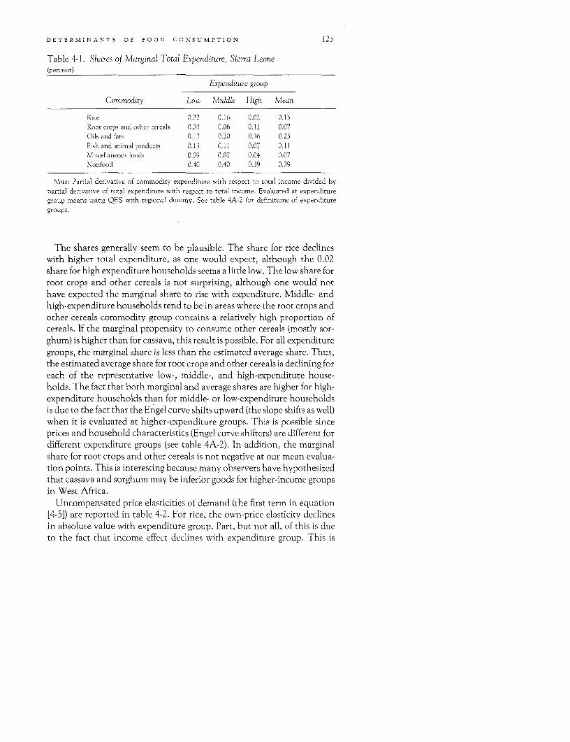
DETERMINANTS OF FOOD CONSUMPTION 125
Table 4-1. Shares of Marginal Total Expenditure, Sierra Leone(percent)
Expenditure group
Commodity Low Middle High Mean
Rice 0.22 0.16 0.02 0.13Root crops and other cereals 0.03 0.06 0.12 0.07Oils and fats 0.13 0.20 0.36 0.23Fish and animal products 0.13 0.11 0.07 0.11Miscellaneous foods 0.09 0.07 0.04 0.07Nonfood 0.40 0.40 0.39 0.39
Note: Partial derivative of commodity expenditure with respect to total income divided bypartial derivative of total expenditure with respect to total income. Evaluated at expendituregroup means using QES with regional dummy. See table 4A-2 for definitions of expendituregroups.
The shares generally seem to be plausible. The share for rice declineswith higher total expenditure, as one would expect, although the 0.02share for high expenditure households seems a little low. The low share forroot crops and other cereals is not surprising, although one would nothave expected the marginal share to rise with expenditure. Middle- andhigh-expenditure households tend to be in areas where the root crops andother cereals commodity group contains a relatively high proportion ofcereals. If the marginal propensity to consume other cereals (mostly sor-ghum) is higher than for cassava, this result is possible. For all expendituregroups, the marginal share is less than the estimated average share. Thus,the estimated average share for root crops and other cereals is declining foreach of the representative low-, middle-, and high-expenditure house-holds. The fact that both marginal and average shares are higher for high-expenditure households than for middle- or low-expenditure householdsis due to the fact that the Engel curve shifts upward (the slope shifts as well)when it is evaluated at higher-expenditure groups. This is possible sinceprices and household characteristics (Engel curve shifters) are different fordifferent expenditure groups (see table 4A-2). In addition, the marginalshare for root crops and other cereals is not negative at our mean evalua-tion points. This is interesting because many observers have hypothesizedthat cassava and sorghum may be inferior goods for higher-income groupsin West Africa.
Uncompensated price elasticities of demand (the first term in equation[4-5]) are reported in table 4-2. For rice, the own-price elasticity declinesin absolute value with expenditure group. Part, but not all, of this is dueto the fact that income effect declines with expenditure group. This is
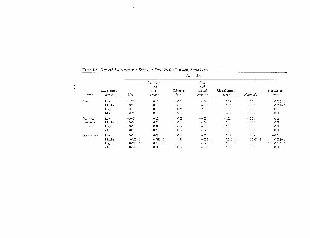
Table 4-2. Demand Elasticities with Respect to Price, Profits Constant, Sierra Leone
Commodity
Root crops Fishand and
Expenditure other Oils and animal Miscellaneous HouseholdPrice group Rice cereals fats products foods Nonfoods labor
Rice Low -1.26 -0.16 -0.23 0.02 0.03 -0.01 0.01E- IMiddle -0.78 -0.13 -0.31 0.02 0.02 -0.02 0.01E-IHigh -0.45 -0.12 -0.38 0.05 0.07 -0.04 0.01Mean -0.74 -0.10 -0.29 0.03 0.03 -0.03 0.01
Root crops Low -0.02 -0.15 -0.02 -0.02 -0.02 -0.02 0.01and other Middle -0.02 -0.26 -0.04 -0.02 -0.01 -0.02 0.01cereals High -0.01 -0.31 -0.02 -0.01 -0.01 -0.01 0.01
Mean -0.01 -0.22 -0.02 -0.02 -0.01 -0.02 0.01
Oils and fats Low 0.04 0.04 -0.82 0.05 0.03 0.05 -0.02Middle 0.01E- I 0.04E- I -1.10 0.02E-I 0.01E- I 0.04E-I -0.02E- IHigh -0.01E- I 0.05E- 1 -1.25 0.02E- 1 0.01E- I 0.01 -0.03E- IMean 0.04E- I 0.01 -0.97 0.01 0.01 0.01 -0.01
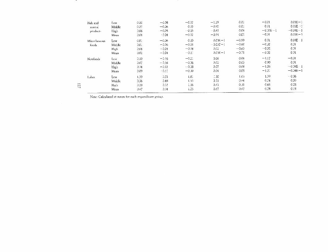
Fish and Low 0.02 -0.08 -0.12 -1.29 0.01 -0.01 O.OlE-I
animal Middle 0.03 -0.06 -0.15 -0.92 0.01 -0.01 0.03E-I
products High 0.06 -0.05 -0.15 -0.81 0.04 -0.03E-1 -0.04E-I
Mean 0.04 -0.04 -0.12 -0.95 0.02 -0.01 0.01E-3
Miscellanieous Low 0.01 -0.06 -0.10 -0.03E- 1 -0.99 -0.01 0.04E -I
foods Middle 0.01 -0.06 -0.14 -0.03E-1 -0.60 -0.02 0.01High 0.04 -0.04 -0.14 0.02 -0.63 -0.02 0.01
Mean 0.02 -0.04 -0.11 0.03E-1 -0.71 -0.02 0.01
Nonfoods Low 0.10 -0.16 -0.21 0.06 0.06 -1.17 -0.01Middle 0.07 -0.16 -0.36 0.02 0.03 -0.90 0.01High 0.14 -0.12 -0.38 0.07 0.08 -1.05 -0.04E- I
Mean 0.09 -0.11 -0.30 0.04 0.05 -1.01 -0.04E-I
Labor Low 1.30 0.72 1.81 1.30 1.03 1.39 -0.06Middle 0.56 0.48 1.53 0.71 0.44 0.74 0.09
High 0.20 0.31 1.16 0.43 0.31 0.65 0.28Mean 0.47 0.34 1.25 0.67 0.47 0.78 0.14
Note: Calculated at mean for each expeniditure group.

Table 4-3. Demand Elasticities with Respect to Price, Profits Variable, Sierra Leone
Commodity
Root crops Fishand and
°0 Expenditure other Oils and animal Miscellaneous HouseholdPrice group Rice cereals fats products foods Nonfoods labor
Rice Low -0.44 0.47 1.21 0.93 0.69 0.93 -0.32Middle -0.67 0.02 0.15 0.18 0.12 0.16 -0.11High -0.44 -0.04 -0.12 0.10 0.10 0.07 -0.06Mean) -0.66 -0.01 0.06 0.17 0.12 0.14 -0.09
Root crops Low 0.47 0.23 0.84 0.52 0.38 0.54 -0.18and other Middle 0.12 -0.07 0.52 0.17 0.11 0.20 -0.12cereals High 0.01E-1 -0.15 0.56 0.11 0.06 0.23 -0.14
Mean 0.11 -0.06 0.53 0.19 0.13 0.25 -0.14
Oils and fats Low 0.40 0.32 -0.19 0.45 0.32 0.46 -0.16Middle 0.08 0.11 -0.79 0.11 0.06 0.13 -0.07High 0.02E- 1 0.05 -1.08 0.03 0.02 0.08 -0.04Mean 0.06 0.08 -0.73 0.10 0.07 0.13 -0.07
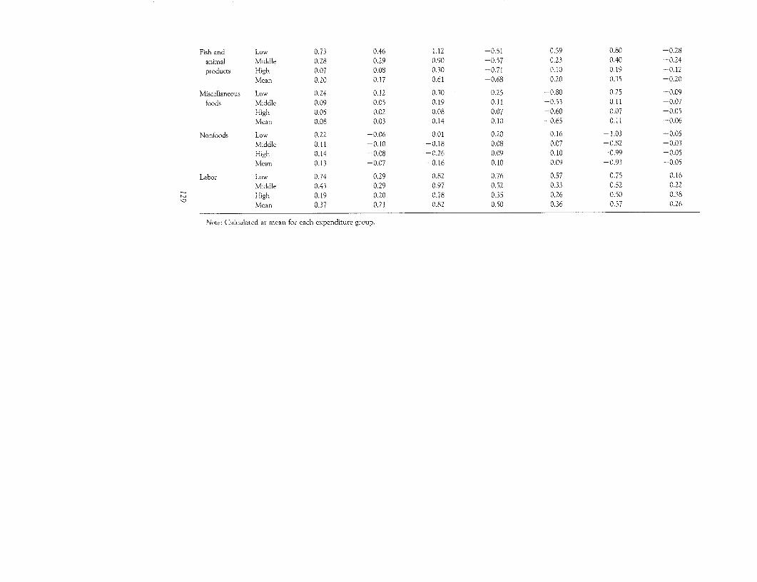
Fish and Low 0.73 0.46 1.12 -0.51 0.59 0.80 -0.28
animal Middle 0.28 0.29 0.90 -0.57 0.23 0.40 -0.24
products High 0.07 0.08 0.30 -0.71 0.10 0.19 -0.12Mean 0.20 0.17 0.61 -0.68 0.20 0.35 -0.20
Miscellaneous Low 0.24 0.12 0.30 0.25 -0.80 0.25 -0.09
foods Middle 0.09 0.05 0.19 0.11 -0.53 0.11 -0.07High 0.05 0.02 0.08 0.07 -0.60 0.07 -0.05Mean 0.08 0.03 0.14 0.10 -0.65 0.11 -0.06
Nonfoods Low 0.22 -0.06 0.01 0.20 0.16 -1.03 -0.05Middle 0.11 -0.10 -0.18 0.08 0.07 -0.82 -0.03High 0.14 -0.08 -0.26 0.09 0.10 -0.99 -0.05Mean 0.13 -0.07 -0.16 0.10 0.09 -0.93 -0.05
Labor Low 0.74 0.29 0.82 0.76 0.57 0.75 0.16Middle 0.43 0.29 0.97 0.52 0.33 0.52 0.22
High 0.19 0.20 0.78 0.35 0.26 0.50 0.38Mean 0.37 0.21 0.82 0.50 0.36 0.57 0.26
Note: Calculated at mcan for each cxpenditure group.
130 CASE STUDIES
certainly not surprising. Root crops do not seem to be price responsive.The relative unresponsiveness of total household labor supplied to wagerate changes (-0.06 to 0.28) is not really surprising either, since this ismeasuring total supply, not its allocation between uses. The negative signfor the low expenditure group is due to the income effect and gives someslight evidence for a backward-bending supply curve.
The cross-price effects with respect to the price of rice are negative, ex-cept for fish and miscellaneous foods. This is to be expected because thelarge budget share of rice leads to a relatively large income effect.
Income-compensated price elasticities of demand are reported inStrauss (1982). Two points are worth noting here. First, negative semidef-initeness of the Slutsky substitution matrix was tested after estimationand was found to hold for 113 out of 138 observations and for all threeexpenditure group averages, as well as the sample average. Second, thecompensated own-price elasticities tended to be sizable.
Price elasticities of demand when profits are allowed to vary (equation[4-5]) are reported in table 4-3. In deriving these elasticities, care has to betaken to obtain consistent estimates of a7r/lapj (see Strauss 1984a) becauseof the censoring in the data. A comparison with table 4-2 tests the signifi-cance of the agricultural household model approach. The total own-priceeffects for commodities remain negative when profit effects are added, ex-cept for root crops and other cereals at the low-expenditure group. How-ever, the profit effect does change the magnitudes of the price elasticities.An interesting consequence, especially for the low-income households, isthat the total own-price elasticities for several commodities such as rice,oils and fats, and fish and animal products no longer drop in absolutevalue with higher expenditure levels. This is because the profit effects-when expressed as an elasticity-are larger, often much larger, for thelowest expenditure households. There are two reasons why profit effectstend to decline with higher total expenditure levels. First, for some goods,marginal expenditures out of full income decline with higher expenditure(see table 4-1). Second, because the profit effect is an elasticity, it de-creases as expenditure levels increase, because mean consumption levelsincrease. Thus, when expressed as a marginal change, the profit effectdoes increase with expenditure group for some commodities, for instance,for oils and fats and root crops and other cereals.
Labor Supply
For labor supply, the own-price elasticity is positive for all expendituregroups. Although income effects might tend to cause the supply curve tobend backward, as it does for low-expenditure households, the profits ef-
DETERMINANTS OF FOOD CONSUMPTION 131
fect partly offsets this, since higher wages imply lower profits. The labor-supply elasticity with respect to the wage increases with expendituregroup, since the classical substitution effects increase with expendituregroup.
In general, the total cross-price effects on labor supply are negative. Thepositive signs of the cross-price effects, when profits are held constant, arereversed because of the profit effect. Cross-price responses generally de-cline with expenditure group for the same reason as before, namely thatthe profit effect decreases. The cross-price effects on labor supply are neg-ative since leisure is a normal good. The cross-price effects on commodityconsumption with respect to the wage rate are smaller in magnitude thanwhen profits are constant, but remain positive. An increased wage ratedecreases profits and therefore decreases expenditure on goods. However,a comparison of the uncompensated and compensated elasticities showsthat the (positive) income effect exceeds the (negative) profits effect.
Marketed Surplus
Price elasticities of marketed surpluses can be written as
p1 aMsi Q, pi aQi - X, pi ax,
iMSi ap, MS,I Q, ap MS, I X, apj
It is a weighted difference of output elasticities and of total (profits vari-able) price elasticities of quantities consumed. The weights are the ratio ofquantity produced to surplus, for production, and quantity consumed tosurplus, for consumption. The marketed surplus elasticities with respectto changes in the production technology or household characteristic vari-ables (which will only affect consumption) may be similarly derived.
Price elasticities of marketed surplus are presented in table 4-4. Giventhe Tobit estimation of the production side, aE(Qi)/apj is used in thefirst term of equation (4-6) and aE(7r)/apj in the second (see Strauss1984a). Also, the divisor is the absolute value of marketed surplus. This isused so that one can easily recognize the sign of aMSj/dpj, that is,whether production increases more or less than consumption.
If the sign of the elasticity is positive and the net surplus is positive,then an increase in price will result in more being sold on the market. Ifthe elasticity is positive and the household is a net purchaser (a negativesurplus), then an increase in price will lead to less being purchased on themarket. A negative elasticity and a positive surplus will lead to less beingsold to the market and negative elasticity, and a negative surplus meansmore will be purchased. (Quantities of marketed surpluses by expendituregroup are given in table 4A-4.)
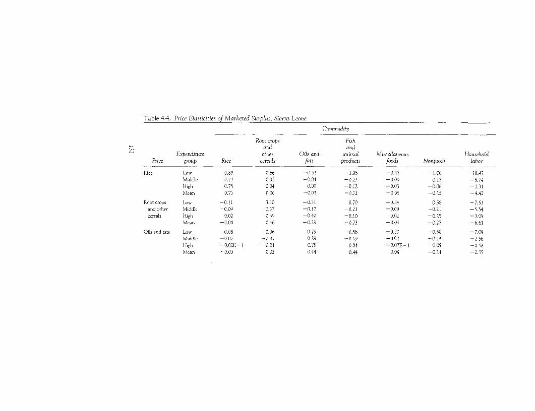
Table 4-4. Price Elasticities of Marketed Surplus, Sierra Leone
Commodity
Root crops Fishand and
Expenditure other Oils and animal Miscellaneous HouseholdPrice group Rice cereals fats products foods Nonfoods labor
Ricc Low 0.89 0.66 -0.32 -1.05 -0.47 -1.00 -18.45Middle 0.73 0.05 -0.04 -0.23 -0.09 -0.17 -5.74High 0.75 0.04 0.09 -0.12 -0.03 -0.08 -1.31Mean 0.71 0.06 -0.03 -0.72 -0.05 -0.15 -4.42
Root crops Low -0.11 3.10 -0.31 -0.70 -0.34 -0.58 -7.53and other Middle -0.09 0.37 -0.17 -0.23 -0.09 -0.21 -5.54cereals High 0.02 0.39 -0.40 -0.10 0.02 -0.25 -3.09
Mean) -0.08 0.46 -0.29 -0.73 -0.04 -0.27 -6.61
Oils anid fats Low -0.08 0.06 0.79 -0.58 -0.27 -0.50 -7.09Middle -0.07 -0.01 0.29 -0.19 -0.07 -0.14 -2.56High -0.02E -I -0.01 0.78 -0.04 -0.07E- 1 -0.09 -0.58Mean -0.05 -0.02 0.44 -0.44 -0.04 -0.14 -2.35
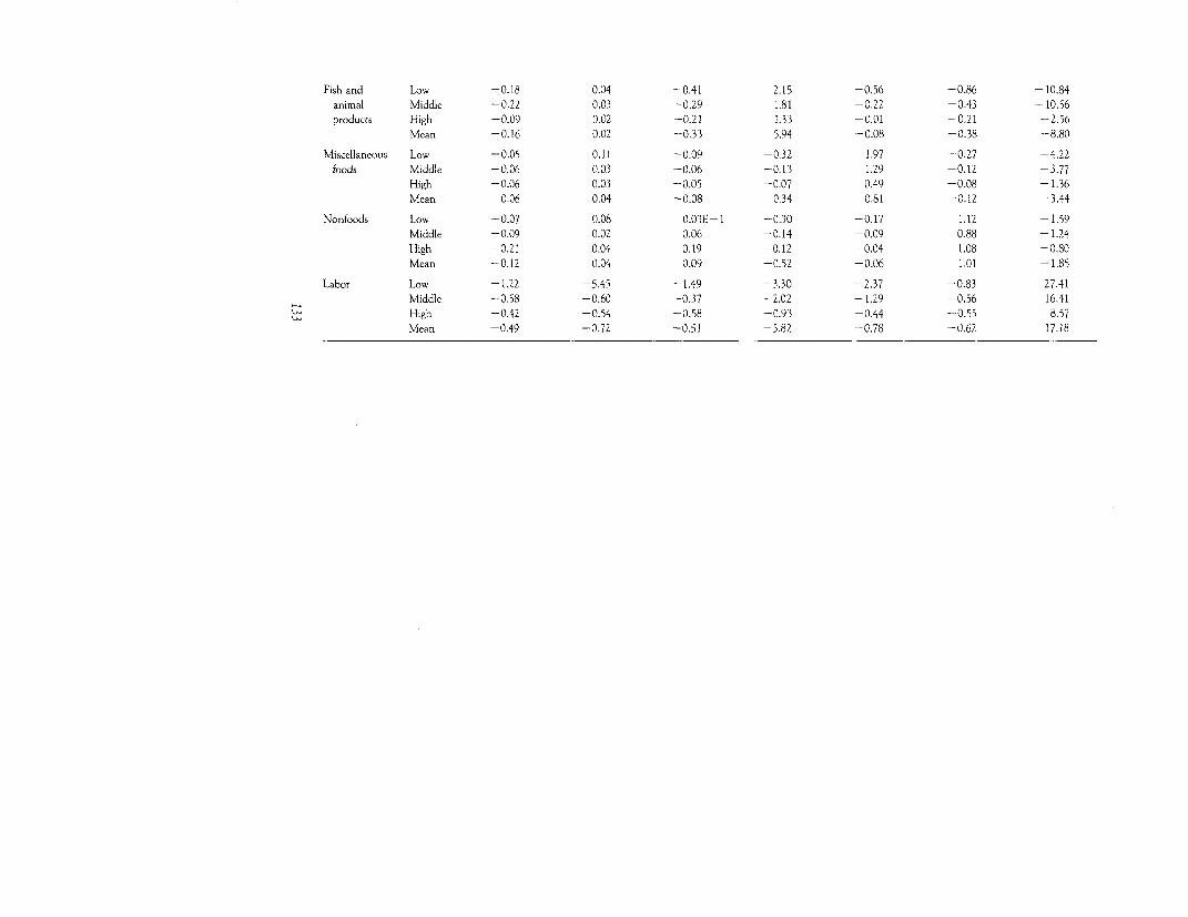
Fish and Low -0.18 0.04 -0.41 2.15 -0.56 -0.86 - 10.84
animal Middle -0.22 0.03 -0.29 1.81 -0.22 -0.43 -10.56
products High -0.09 0.02 -0.21 1.33 -0.01 -0.21 -2.56
Mean -0.16 0.02 -0.33 5.94 -0.08 -0.38 -8.80
Miscellaneous Low -0.05 0.11 -0.09 -0.32 1.97 -0.27 -4.22
foods Middle -0.06 0.03 -0.06 -0.13 1.29 -0.12 -3.77
High -0.06 0.03 -0.05 -0.07 0.49 -0.08 - 1.36
Mean -0.06 0.04 -0.08 -0.34 0.81 -0.12 -3.44
Nonfoods Low -0.07 0.08 0.03E- 1 -0.30 -0.17 1.12 -1.59
Middle -0.09 0.02 0.06 -0.14 -0.09 0.88 - 1.24
High -0.21 0.04 0.19 -0.12 -0.04 1.08 -0.80
Mean -0.12 0.04 0.09 -0.52 -0.06 1.01 -1.85
Labor Low -1.22 -5.45 -1.49 -3.30 -2.37 -0.83 27.41
Middle -0.58 -0.60 -0.37 -2.02 -1.29 -0.56 16,41
High -0.42 -0.54 -0.58 -0.93 -0.44 -0.55 8.57
Mean -0.49 -0.72 -0.51 -5.82 -0.78 -0.62 17.18
134 CASE STUDIES
All the own-price elasticities are positive and some are reasonably high.The positive sign is not surprising since the only total price elasticity ofquantity consumed that is positive (a necessary condition to obtain a neg-ative marketed surplus response) is for root crops and other cereals, and itis only positive when evaluated at the average for low-expenditure house-holds. The mean own-price elasticity for rice, the major staple, is 0.71,which is comparable to the elasticity of 1.03 reported for an aggregateagricultural commodity (Lau, Lin, and Yotopoulos 1978) and to the elas-ticity reported for rice, 0.66 (Barnum and Squire 1979). The price elastic-ity of marketed surplus tends to decline at higher expenditure levels,largely because the absolute value of marketed surplus, part of the de-nominator, increases at higher expenditure levels. The low marketed sur-plus is the reason for the high magnitude of the own-price elasticity forroot crops and other cereals among low-expenditure households. If abso-lute changes in kilograms marketed due to an infinitesimal proportionateincrease in price were shown, they would be roughly equal for the low-and middle-expenditure groups, and would rise for the high-expendituregroup. Nonetheless, low expenditure households do seem to respond intheir marketed surplus to price, contrary to the allegations of many. Thisis a very important policy conclusion, since many governments rely intheir policies only on larger farms to be responsive in their marketed out-put. This supposition is often used to rationalize policies that discriminateagainst or have a benign neglect of small holders. In the Sierra Leonecase, it is worth noting that the response of marketed surplus comeslargely through changes in consumption rather than changes in output(see Strauss 1984b). This may reflect the low level of agricultural technol-ogy and infrastructure development in Sierra Leone.
For household labor, the extremely large (positive) values of the mar-keted surplus (off-farm labor) elasticity with respect to wage rate are sim-ply the result of the very small base, the average household being nearlyself-sufficient in labor when labor sold and labor hired are netted out overa period of a year. The absolute change in hours supplied to the marketwill not be so large. These off-farm labor results contrast markedly withthose reported by Rosenzweig (1980). He separated male and female laborsupply (which are combined here using relative wages as weights) andfound the former's marketed surplus responds negatively to wage.
The cross-price elasticities of marketed surplus tend to be negative be-cause of the strong profit effect in the cross-price elasticity of demand.Indeed, when profits are held constant, most of the cross-price elasticitiesare positive. For instance, the elasticity of oils and fats surplus to rice priceis 0.32 when profits are held constant but -0.32 when it varies (see
DETERMINANTS OF FOOD CONSUMPTION 1I 5
Strauss 1984b). The profit effect of an increase in the price of rice will leadto an increase in the consumption of oils and fats. Sales of oils and fatswill consequently decrease.
Some of the magnitudes of the cross-price elasticities are fairly large.Again, this is caused by the strong profit effect on consumption. Themagnitudes do tend to fall with the higher expenditure groups, as they dofor the own-price elasticities. They are not negligible, however, so it is notwise to ignore them, as was often done in the past.
Variables other than prices will affect the marketed surplus of a com-modity. In this model, two sets of factors stand out. First are householdcharacteristics such as size and age composition. These factors are mod-eled explicitly in the demand equations. They do not affect output di-rectly, because of the separability of the model, but they might affect itindirectly through their general equilibrium effect on wages. The secondset of factors are fixed inputs and the production technology. They willaffect both consumption and production directly, the former through theprofit effect.
The household characteristics used in this study are children youngerthan 10, children 11-15 years, males older than 15, and females olderthan 15. The latter three characteristics affect demand in two ways: theyaffect the commodity composition (including leisure) of demand given alevel of full income; and they change the level of full income, since per-sons of those ages can work or take leisure. Children younger than 10 inour sample do not work; hence they do not affect full income, but they dochange the commodity composition of goods and leisure demanded.
The first four columns of table 4-5 report elasticities of marketed surpluswith respect to the four age-group variables. These elasticities are re-ported at the sample mean only. For the higher age groups, the signs ofthe elasticities for goods are predominantly negative (that is consumptionincreases). This is not surprising; any negative composition impact onconsumption of a good is outweighed by the effect from increased fullincome. Exceptions exist for miscellaneous foods and root crops andother cereals for children aged 1 1 -15 and females older than 15, thoughthe magnitudes are quite small. Children younger than 10 change thehousehold commodity composition by lowering consumption of oils andfats, fish and animal products, and leisure, but they raise consumption ofeverything else. Marketed surplus of labor responds positively to changesin persons in the older age groups, as might be expected since total timeavailable to the household varies when the number of persons older than10 changes. It does indicate that if adult household size decreases, say,because of migration, that the remaining members do not work hard
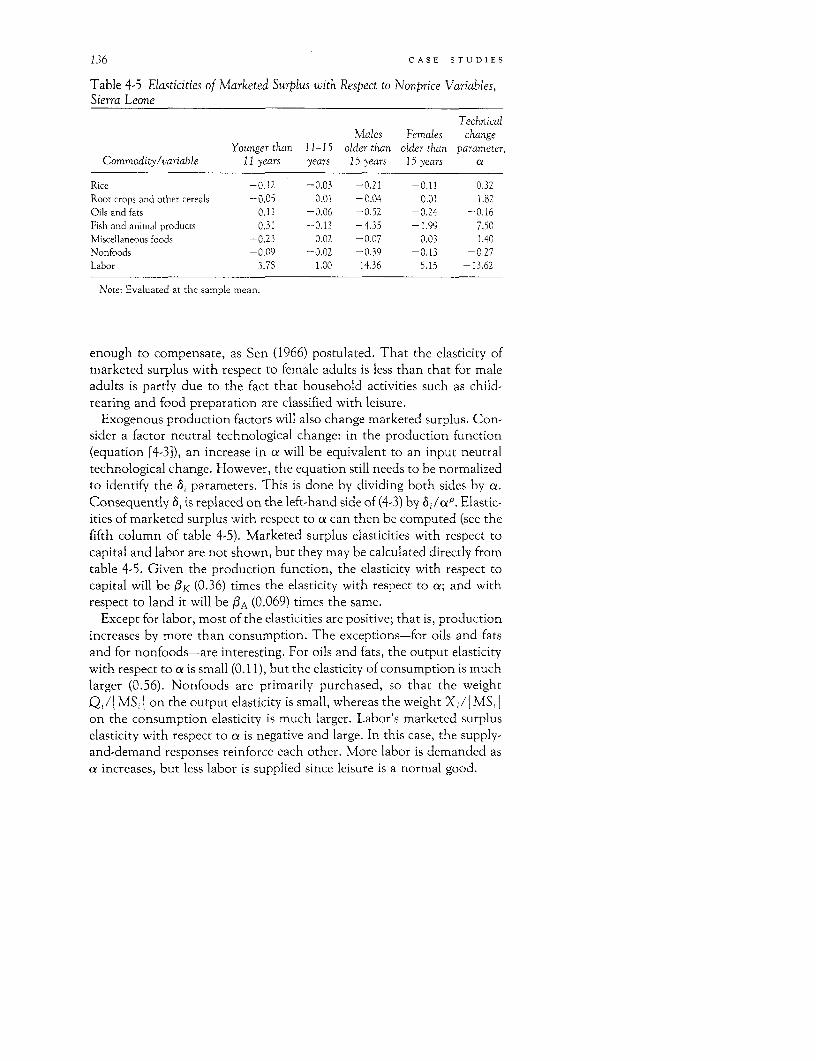
136 CASE STUDIES
Table 4-5 Elasticities of Marketed Surplus with Respect to Nonprice Variables,Sierra Leone
TechnicalMales Females change
Younger than 11-15 older than older than parameter,Commodity/variable 11 years years 15 years 15 years a
Rice -0.12 -0.03 -0.21 -0.11 0.32Root crops and other cereals -0.05 0.01 -0.04 0.01 1.82Oils and fats 0.11 -0.06 -0.52 -0.24 -0.16Fish and animal products 0.31 -0.13 -4.35 - 1.99 7.50Miscellaneous foods -0.23 0.02 -0.07 0.03 1.40Nonfoods -0.09 -0.02 -0.39 -0.13 -0.27Labor 3.78 1.00 14.36 5.15 -13.62
Note: Evaluated at the sample mean.
enough to compensate, as Sen (1966) postulated. That the elasticity ofmarketed surplus with respect to female adults is less than that for maleadults is partly due to the fact that household activities such as child-rearing and food preparation are classified with leisure.
Exogenous production factors will also change marketed surplus. Con-sider a factor neutral technological change: in the production function(equation [4-3]), an increase in a will be equivalent to an input neutraltechnological change. However, the equation still needs to be normalizedto identify the 6, parameters. This is done by dividing both sides by ae.Consequently 6i is replaced on the left-hand side of (4-3) by Si/aP. Elastic-ities of marketed surplus with respect to a can then be computed (see thefifth column of table 4-5). Marketed surplus elasticities with respect tocapital and labor are not shown, but they may be calculated directly fromtable 4-5. Given the production function, the elasticity with respect tocapital will be K (0.36) times the elasticity with respect to a; and withrespect to land it will be fA (0.069) times the same.
Except for labor, most of the elasticities are positive; that is, productionincreases by more than consumption. The exceptions-for oils and fatsand for nonfoods-are interesting. For oils and fats, the output elasticitywith respect to a is small (0.11), but the elasticity of consumption is muchlarger (0.56). Nonfoods are primarily purchased, so that the weightQi/j MSi I on the output elasticity is small, whereas the weight X /I MSi Ion the consumption elasticity is much larger. Labor's marketed surpluselasticity with respect to a is negative and large. In this case, the supply-and-demand responses reinforce each other. More labor is demanded asa increases, but less labor is supplied since leisure is a normal good.
DETERMINANTS OF FOOD CONSUMPTION 137
Price and Income Effects for Caloric Availability
This study is concerned ultimately with the determinants of food con-sumption. This can be further translated into the effects of prices andother variables on the availability to the household of different nutrients,particularly calories. The effect of price on calories is
acal a cal aX,ap; i=1 a Xi apj
where cal - calories and 1-5 are the food groups. In elasticity form
p, acal p, S acalaXical ap, cal =-I axd apj
Effects of price changes on calories are calculated both when profits areconstant and when they are variable. The difference will clearly point outthe effect on caloric availability of families producing the foods theyconsume.
Elasticities of caloric availability with respect to total expenditure aregiven below. The elasticities were calculated as (TEXP/Cal) 1 (dCal/aX) (aE(Xi)/aTEXP) (see table 4-1 for aE(pi X,)/aTEXP). Total expendi-ture, as opposed to full income, is endogenous in the model, but theresults will still be of interest. The magnitudes are around 0.85, and theyvary little among expenditure groups.
Low Middle High Mean0.85 0.83 0.93 0.86
The elasticity for the high-expenditure group is slightly higher than forthe low-expenditure group because the marginal total expenditure shareof oils and fats, an important contributor of calories, rises with the ex-penditure group. This apparently offsets the declining total expenditureshare on rice.
As mentioned earlier, these elasticity estimates are high compared withother results. One reason may be the relatively high level of aggregation ofthe food groups. As full income rises, expenditures undoubtedly shiftwithin these groups, not just between them. If foods with high costs percalorie are substituted for foods with low cost per calorie, then expendi-tures on a group can rise much more than calorie consumption from thegroup. A word of caution is in order here, however. First, the elasticitieshold only for small movements of total expenditure where intragroup sub-stitution may be small. Second, the calorie conversions from kilograms
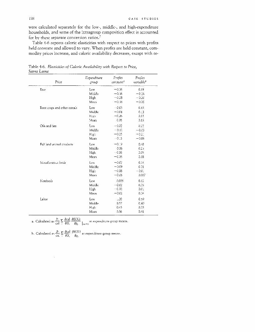
138 CASE STUDIES
were calculated separately for the low-, middle-, and high-expenditurehouseholds, and some of the intragroup composition effect is accountedfor by these separate conversion ratios.7
Table 4-6 reports caloric elasticities with respect to prices with profitsheld constant and allowed to vary. When profits are held constant, com-modity prices increase, and caloric availability decreases, except with re-
Table 4-6. Elasticities of Calorie Availability with Respect to Price,Sierra Leone
Expenditure Profits ProfitsPrice group constant' variableb
Rice Low -0.58 0.19Middle -0.38 -0.24High -0.28 -0.20Mean -0.38 -0.26
Root crops and other cereals Low -0.03 0.43Middle -0.04 0.13High -0.06 0.11Mean -0.05 0.15
Oils and fats Low -0.07 0.27Middle -0.12 -0.03High -0.25 -0.21Mean -0.15 -0.06
Fish 'and animal products Low -0.19 0.48Middle -0.08 0.23High -0.08 0.05Mean -0.08 0.18
Miscellaneous foods Low -0.07 0.14Middle -0.09 0.01High -0.08 -0.01Mean -0.08 0.007
Nonfoods Low 0.008 0.12Middle -0.02 0.03High -0.02 0.01 Mean -0.02 0.04
Labor Low 1.20 0.59Middle 0.57 0.40High 0.45 0.33Mean 0.56 0.41
a. Calculated as Pi acal aE(X) at expenditure group means.cal i aX, aP( i ed
h. Calculated as ~ cal r E(X,)6_ at expenditure group means.

DETERMINANTS OF FOOD CONSUMPTION 139
spect to the nonfoods price for the low-expenditure group. There is nogeneral pattern of elasticities across expenditure group, but the absolutechange in caloric availability often increases with expenditure group. Forcommodity prices, the largest response of caloric availability is to changesin the price of rice, the principal staple. These range from -0.58 to-0.28.
When profits can vary, the situation changes substantially. Now mostof the commodity price elasticities of calories are positive. If the price of agood increases, consumption of that good may decrease, but the increasein full income is distributed over the consumption of other foods, and theincrease is large enough to increase total caloric availability. The price ofrice and of oils and fats in all but the low-expenditure group is an excep-tion, as is the price of miscellaneous foods in the high-expenditure group.The magnitudes of the positive elasticities are not high for the samplemean, but some are sizable for the low-expenditure group.
For all commodities, the positive effect of a change in price, with prof-its variable, is greatest for low-expenditure households because of thefact that, for every commodity, own-price profit effects are greatestamong such households. For rice and for oils and fats, it is only amonglow-expenditure households that the profit effect is large enough to domi-nate the negative own-price effects upon calorie availability with profitsconstant. This is partly because in the middle- and high-expenditurehouseholds the negative own-price effects-with profits constant-arestronger for rice and for oils and fats than for other commodities.
Although caloric availability increases for low-expenditure households,with an increase in the price of rice or of oils and fats, it decreases formiddle- and high-expenditure households, and at the sample mean. Forrice price, the elasticities for the two higher expenditure groups are stillquite negative, between -0.2 and -0.25. Hence, when profit effects areaccounted for, increases in the price of rice seem to lessen the discrepancyin calories available to the rural expenditure groups. They increase avail-ability for very low expenditure households and decrease availability formiddle- and higher-expenditure households. The mean daily caloricavailability per capita for high-expenditure households is quite high(2,600 calories), and for the middle-expenditure households it is moremodest (2,130 calories). Although caloric availability will be lower thanthe group mean for some households in the high-expenditure group,lower availability may still allow these households to have sufficient calo-ries available for weight maintenance under normal activity levels.Whether this would be true of middle-expenditure households is morequestionable.
140 CASE STUDIES
Policy Implications
These results have significant implications for the development processin Sierra Leone. The estimates of the calorie elasticity with respect to to-tal expenditure suggest that promoting higher incomes may be an effi-cient way to reduce undernutrition. The present income levels for poorrural households are so low, however, that this process is likely to take along time. Before the representative low-expenditure household couldhave caloric availability even at the level of 1,900 calories per capita perday (actual daily availability is 1,188 calories per capita for such a house-hold), income would have to increase considerably. With prices andhousehold characteristics constant, an average low-expenditure house-hold would need an increase in annual full income of about 270 Leones toreach the availability level of 1,900 calories per capita per day. This newlevel of full income would result in total expenditures of roughly 445Leones. That figure is 88 percent higher than the existing expenditurelevel (237 Leones) of the representative low-expenditure household. If weassume, optimistically, an annual growth rate in real total expenditures of3 percent, it would take almost twenty-two years for an average low-expenditure family to reach this point. Of course, if family size grew alongwith total expenditure, as is likely, it would take even longer.
The usual caution is needed here. Caloric availability at the householdlevel says little about the intake of individuals. The intrahousehold distri-bution of food depends on household choices, which in turn may dependon household income, prices, and tastes. This discussion abstracts fromthat admittedly important issue.
In general, increased food prices in this model lead to increased caloricavailability owing to the profit effect for producers. Response by thehousehold in its role as a farm-firm does make a difference to consump-tion patterns. Despite the profit effect, however, caloric availability re-sponds negatively to rice price changes for middle- and high-expenditurehouseholds. This may indicate a tradeoff between long-run outputgrowth and short-run nutritional goals if output growth is pursued solelyby a policy of high producer prices. Policies that induce household in-vestments leading to higher full income would mitigate or reverse thistradeoff.
In the longer run, rice price may be lower than otherwise if productiongrowth has been stimulated. The distributional impacts of technicalchange have long been debated, but questions of access to technology are
DETERMINANTS OF FOOD CONSUMPTION 141
beyond the scope of this study. The results do have something to say,however, about the differential price effects of technical change.
The effect of a price change on household welfare can be shown to beproportional to net marketed surplus of the commodity. Indeed, the elas-ticity of real full income with respect to rice price can be quantified. It ispositive, but small, for all three expenditure groups; ranging from 0.13 forthe lowest group to 0.06 for the highest, being 0.09 at the sample mean.This result occurs because on the one hand marketed surplus of rice ishighest for the low expenditure group (table 4A-4), and on the otherhand full income (based on a sixteen-hour day) is lowest for this group.These magnitudes imply a small welfare loss because of potentially de-creased rice prices in rural Sierra Leone, with the largest losses being forthe lowest expenditure households. At the same time, the nutritional sta-tus of households, at least for the middle and higher expenditure groups,would be raised by such a price decrease, although it would be lowered forlow-income households. Of course, to the extent that there is an autono-mous increase in nominal full income caused by the technical change,welfare and nutritional status might both increase. However, the pointsremain that changes in nutritional status and changes in welfare may bein opposite directions, and that price increases are both a welfare andnutrition status equalizer in rural Sierra Leone, whereas price decreasesworsen distributional consequences.
Another question that has bearing on calorie availability is to whatextent a country should promote exports of cash crops such as palm oil,coffee, and cocoa. Some have argued that increasing the production ofcash crops at the expense of subsistence crops will have an adverse impacton nutritional status. According to the results of this study, an increase inown-price of oils and fats-of which palm products are the lion's share invalue-results in decreased calorie availability for high- and middle-expenditure groups but increased availability for the low-expendituregroup. Marketed surplus increases for all groups. Hence, increased reli-ance on the market for oils and fats as a consequence of a rise in the priceof oils and fats results in higher caloric availability for a typical low-expenditure household, but lower caloric availability for typical middle-and high-expenditure households.
Alternatively, an increase in the price of rice decreases the marketedsurplus of oils and fats for the low- and middle-expenditure groups. Sucha price increase will lead to increased calorie availability for the low-expenditure group and decreased availability for the middle-expendituregroup. This is contrary to the relationship often hypothesized. For lowexpenditure households, however, decreased market reliance is associated
142 CASE STUDIES
with higher calorie availability when the source of the change is an in-crease in the price of rice. Note that, for low- and middle-expenditurehouseholds, the relationships between the direction of change of mar-keted surplus of oils and fats and of calorie availability differ when theyare a result of changes in the price of rice compared with changes in theprice of oils and fats. Since both calorie availability and marketed surplusare endogenous variables, this situation is not surprising.
When greater market reliance does coincide with reduced caloric avail-ability, the causative factors underlying this relationship turn out to beopposite to the ones just suggested. More, not less, of the rice and rootcrops and other cereals is consumed when the price of oils and fats in-creases. This is primarily due to the profit effect in increasing full income.As a result, less of these foods is marketed, and less, not more, of the oilsand fats is consumed. That reduction in consumption is the source oflowered caloric availability.
When the price of rice increases, the consumption of oils and fats goesup and rice consumption decreases. For the low-expenditure group, a re-duction in reliance on the market for oils and fats due to rice-pricechanges results in the expected increases in caloric availability, but againfor different reasons than commonly assumed. In this case, calorie avail-ability increases because enough additional oils and fats, as well as othercommodities, are consumed to offset the reduced consumption of rice.
The foregoing partial-equilibrium implications are examples of the widervariety of policy questions that may be addressed by a farm-householdmodel having more commodity detail than the three-commodity modelscommonly used in the past. This research has shown that such multicom-modity farm-household models can be estimated econometrically usingcross-sectional household data if the functional forms allow for a widevariety of behavior. The results can then be fitted into a general equilib-rium analysis (see chapter 7).
Appendix: Data Sources
Estimates of quantities apparently consumed out of home productionwere derived by subtracting sales and wages in kind paid out (and seed usefor rice, the major crop) from production, and by adding wages in kindreceived. These were adjusted for processing (to avoid double-counting)and for storage losses. (Net changes in storage were assumed to be zero.)Quantities consumed out of own-production were multiplied by regionalfarm-gate sales prices to transform into values. Values of foods purchasedwere then added to calculate the total value of foods consumed. These
DETERMINANTS OF FOOD CONSUMPTION 143
were aggregated into five groups, which, with nonfoods and labor, consti-tute the seven commodities used in the study (see table 4A-1).
Values of production were derived by multiplying quantities producedby farm-gate sales price, and then added into the appropriate groups. Pro-duction of raw products was used; processed food production was notadded in order to avoid double-counting. For example, only estimates offresh and not dried fish production were used.
Household labor-supplied data were formed by summing hours workedfor agricultural and nonagricultural enterprises and for labor sold out.Labor supply includes such activities as work by women and children onvegetable production, for which women generally take responsibility, aswell as the cleaning of rice. Excluded are household production activitiessuch as food preparation, child care, and ceremonies. Units are in termsof male equivalents with weights I for males older than 15, 0.75 for fe-males older than 15, and 0.5 for children aged 10-15. The weights are de-rived from an analysis of variance of wage rates as reported by Spencerand Byerlee (1977). Household labor demand, also measured in maleequivalents, includes work on all agricultural and nonagricultural activi-ties in the household exclusive of processing agricultural products. Bothfamily and hired labor are included.
Prices used in estimating the demand system were formed on the basisof the eight geographical regions. Annual sales prices were formed usingthe larger sample of 328 households for which reliable production andlabor use data were available. The value of regional sales was divided bysales quantity for each of 195 commodities. Likewise, regional purchaseprices were formed for 113 commodities. A concordance between com-modities purchased and sold was established and a commodity price foreach region was then formed by taking a weighted average of sales andpurchase prices, with region-specific weights being the share of total ex-penditure for a commodity coming from either purchases or home pro-duction. Commodities were then aggregated into six groups, and regionalvalues consumed were used as weights to form arithmetically weightedprices.8 Wage is expressed in male equivalents.
Farm sales prices for the 128 foods were aggregated into the samegroups as were the weighted sales and purchase prices. In this case, theweights were the proportion of value of regional sales for the group repre-sented by each of its component foods. These were the prices used inestimating the system of output supplies and labor demands.
Data on household characteristics were available for total size and agecomposition by 0-5 years, 5-10 years, 11-15 years, 16-65 years, and olderthan 65 years. In addition, data on number of wives, years of English andArabic education by the household head, age of household head, ethnic
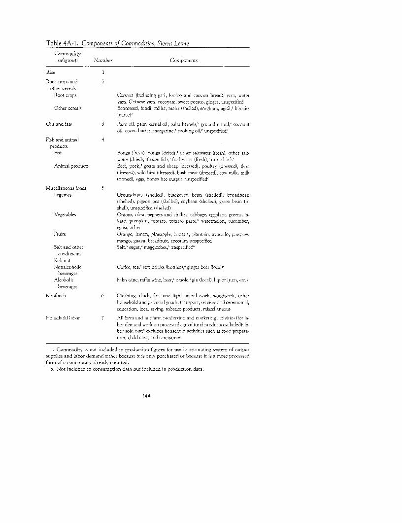
Table 4A-1. Components of Commodities, Sierra Leone
Commoditysubgroup Number Components
Rice 1
Root crops and 2other cereals
Root crops Cassava (including gari, foofoo and cassava bread), yam, wateryam, Chinese yam, cocoyam, sweet potato, ginger, unspecified
Other cereals Benniseed, fundi, millet, maize (shelled), sorghum, agidi,' biscuits(natco)'
Oils and fats 3 Palm oil, palm kernel oil, palm kernels,' groundnut oil,' coconutoil, cocoa butter, margarine,' cooking oil,' unspecified'
Fish and animal 4products
Fish Bonga (fresh), bonga (dried),, other saltwater (fresh), other salt-water (dried),' frozen fish,, freshwater (fresh),' tinned fish'
Animal products Beef, pork,' goats and sheep (dressed), poultry (dressed), deer(dressed), wild bird (dressed), bush meat (dressed), cow milk, milk(tinned), eggs, honey bee output, unspecified'
Miscellaneous foods 5Legumes Groundnuts (shelled), blackeyed bean (shelled), broadbean
(shelled), pigeon pea (shelled), soybean (shelled), green bean (inshell), unspecified (shelled)
Vegetables Onions, okra, peppers and chillies, cabbage, eggplant, greens, ja-kato, pumpkin, tomato, tomato paste,' watermelon, cucumber,egusi, other
Fruits Orange, lemon, pineapple, banana, plantain, avocado, pawpaw,mango, guava, breadfruit, coconut, unspecified
Salt and other Salt,'a sugar,' maggicubes,a unspecified'condiments
KolanutNonalcoholic Coffee, tea,' soft drinks (bottled),' ginger beer (local)a
beveragesAlcoholic Palm wine, raffia wine, beer,, omole,' gin (local), liquor (rum, etc.)'
beverages
Nonfoods 6 Clothing, cloth, fuel and light, metal work, woodwork, otherhousehoLd and personal goods, transport, services and ceremonial,education, local saving, tobacco products, miscellaneous
Household labor 7 All farm and nonfarm production and marketing activities (for la-bor demand work on processed agricultural products excluded); la-bor sold out;' excludes household activities such as food prepara-tion, child care, and ceremonies
a. Commodity is not included in production figUTes for use in estimating system of outputsupplies and labor demand either because it is only purchased or because it is a more processedform of a commodity already counted.
b. Not included in consumption data but included in production data.
144
DETERMINANTS OF FOOD CONSUMPTION 145
group (there are three principal ones in our sample), and region of resi-dence are available. Since ethnic groups tend to live in contiguous areas,this information is also regional in character (though not identical to theeight survey regions).
Land is measured as total land area cropped, in acres. It includes land inperennial as well as annual crops. It is a simple sum of acres. No weightingto reflect different qualities (for example, of swamp and of upland lands)was made because such data were unavailable. The rental markets arevery thin and rental prices reflect a household's standing in the commu-nity as much as the economic value of the land (Spencer and Byerlee1977, pp. 21-24). For a very few households, data on the land variablewere missing. Since these households had usable data for all other vari-ables, they were not dropped. Spencer and Byerlee had classified house-holds into many different farm types. From the production sample of 328households, average land-labor use ratios were computed for each farmtype. Knowing the farm type and the labor used for these householdsenabled us to estimate total land cropped.
Capital is measured as the value of its flow. For variable capital, thisrepresents no problem. For our sample, however, variable capital is mi-nuscule, mostly rice seed. Only a little fertilizer is used and a little machin-ery hired, and these were added into the total. Since there are some val-ues for variable capital, which is a flow, it was necessary to convert thestock of fixed capital into the equivalent flow in order to add the two.9
Sample characteristics of the variables that enter into the demand sys-tem are shown in table 4A-2. The sample is divided into three expendi-ture groups, and for each group simple averages are computed for eachcharacteristic. These groups are total expenditure under 350 Leones, be-tween 350 and 750 Leones, and greater than 750 Leones. Just how poorthese households are can be seen from the annual per capita expendituresin 1974-75, which in U.S. dollars amount to $54, $88, and $136 for thelow-, middle-, and high-expenditure groups, respectively. When the capi-tal city, Freetown, was divided into three groups for a migration compo-nent of this study, the average income of the middle group was found tobe $153. Hence, even the "high" expenditure households are quite poorcompared with both urban Sierra Leone and other countries.
As can be seen from the expenditures reported in table 4A-2, rice is theprincipal staple and cassava (included in "root crops and other cereals")the main substitute. Rice tends to be eaten with a sauce and boiled cas-sava with a stew, both cooked with palm oil. Both sauce and stew aremade with vegetables (onions, peppers, tomatoes, and leafy greens) andsome meats. Sauces tend to include dried fish and stews fresh fish.
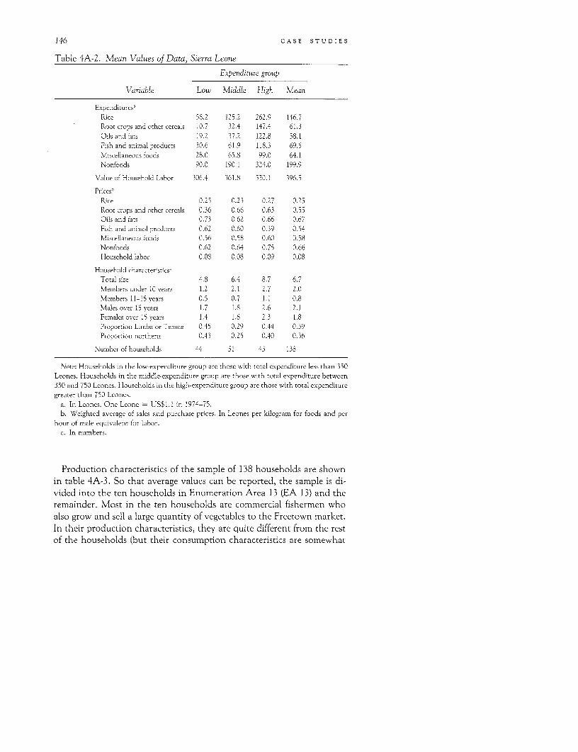
146 CASE STUDIES
Table 4A-2. Mean Values of Data, Sierra Leone
Expenditure group
Variable Low Middle High Mean
Expenditures'Rice 58.2 125.2 262.9 146.7Root crops and other cereals 10.7 32.4 147.4 61.3Oils and fats 19.2 37.2 122.8 58.1Fish and animal products 30.6 61.9 118.3 69.5Miscellaneous foods 28.0 65.8 99.0 64.1Nonfoods 90.0 190.1 324.0 199.9
Value of Household Labor 306.4 361.8 530.1 396.5
Prices'
Rice 0.25 0.23 0.27 0.25Root crops and other cereals 0.36 0.66 0.63 0.55Oils and fats 0.73 0.62 0.66 0.67Fish and animal products 0.62 0.60 0.39 0.54Miscellaneous foods 0.56 0.58 0.60 0.58Nonfoods 0.62 0.64 0.75 0.66Household labor 0.08 0.08 0.09 0.08
Household characteristics'Total size 4.8 6.4 8.7 6.7Members under 10 years 1.2 2.1 2.7 2.0Members 11-15 years 0.5 0.7 1.1 0.8Males over 15 years 1.7 1.8 2.6 2.1Females over 15 years 1.4 1.8 2.3 1.8Proportion Limba or Temne 0.45 0.29 0.44 0.39Proportion northern 0.43 0.25 0.40 0.36
Number of households 44 51 43 138
Note: Households in the low-expenditure group are those with total expenditure less than 350Leones. Households in the middle-expenditure group are those with total expenditure between350 and 750 Leones. Households in the high-expenditure group are those with total expendituregreater than 750 Leones.
a. In Leones. One Leone = US$1.1 in 1974-75.b. Weighted average of sales and purchase prices. In Leones per kilogram for foods and per
hour of male equivalent for labor.c. In numbers.
Production characteristics of the sample of 138 households are shownin table 4A-3. So that average values can be reported, the sample is di-vided into the ten households in Enumeration Area 13 (EA 13) and theremainder. Most in the ten households are commercial fishermen whoalso grow and sell a large quantity of vegetables to the Freetown market.In their production characteristics, they are quite different from the restof the households (but their consumption characteristics are somewhat
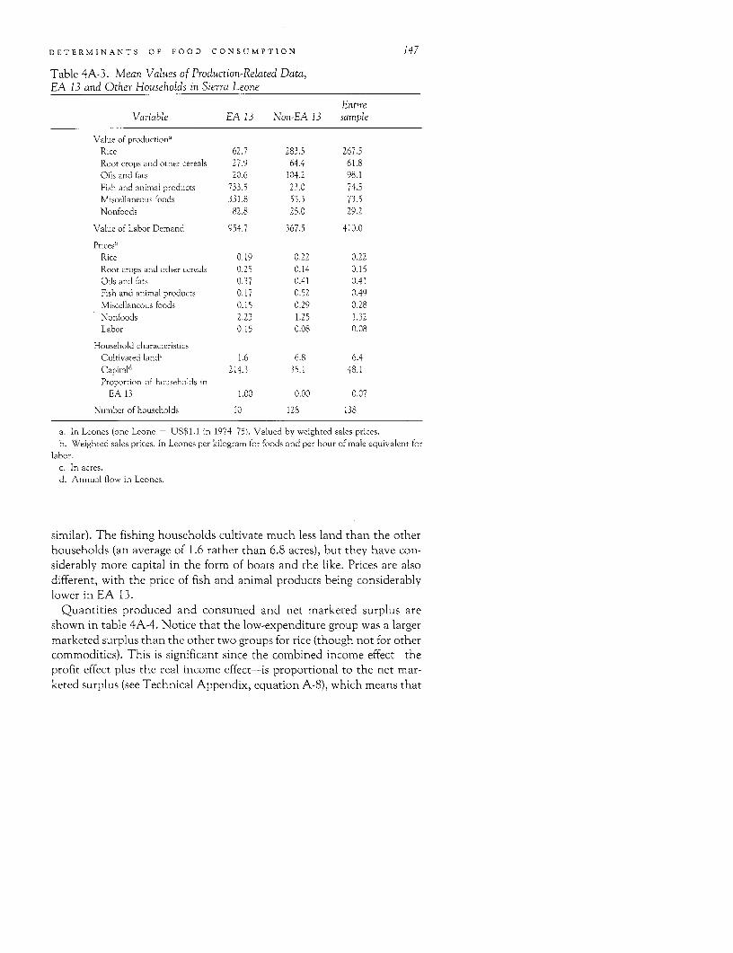
DETERMINANTS OF FOOD CONSUMPTION 147
Table 4A-3. Mean Values of Production-Related Data,EA 13 and Other Households in Sierra Leone
EntireVariable EA 13 Non-EA 13 sample
Value of production'Rice 62.7 283.5 267.5Root crops and other cereals 27.9 64.4 61.8Oils and fats 20.6 104.2 98.1Fish and animal products 733.5 23.0 74.5Miscellaneous foods 331.8 53.3 73.5Nonfoods 82.8 25.0 29.2
Value of Labor Demand 954.7 367.5 410.0
Prices5
Rice 0.19 0.22 0.22Root crops and other cereals 0.25 0.14 0.15Oils and fats 0.37 0.41 0.41Fish and animal products 0.17 0.52 0.49Miscellaneous foods 0.15 0.29 0.28Nonfoods 2.23 1.25 1.32Labor 0.15 0.08 0.08
Household characteristicsCultivated land' 1.6 6.8 6.4Capital' 214.3 35.1 48.1Proportion of households in
EA 13 1.00 0.00 0.07
Number of households 10 128 138
a. In Leones (one Leone = US$1.1 in 1974-75). Valued by weighted sales prices.b. Weighted sales prices. In Leones per kilogram for foods and per hour of male equivalent for
labor.c. In acres.d. Annual flow in Leones.
similar). The fishing households cultivate much less land than the otherhouseholds (an average of 1.6 rather than 6.8 acres), but they have con-siderably more capital in the form of boats and the like. Prices are alsodifferent, with the price of fish and animal products being considerablylower in EA 13.
Quantities produced and consumed and net marketed surplus areshown in table 4A-4. Notice that the low-expenditure group was a largermarketed surplus than the other two groups for rice (though not for othercommodities). This is significant since the combined income effect-theprofit effect plus the real income effect-is proportional to the net mar-keted surplus (see Technical Appendix, equation A-8), which means that
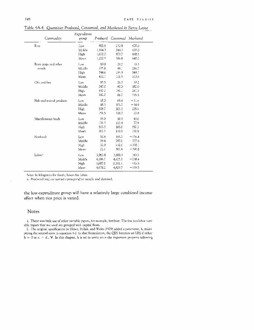
148 CASE STUDIES
Table 4A-4. Quantities Produced, Consumed, and Marketed in Sierra Leone
ExpenditureCommodity group Produced Consumed Marketed
Rice Low 902.8 232.8 670.0Middle 1,164.3 544.3 620.0High 1,622.2 973.7 648.5Mean 1,227.5 586.8 640.7
Root crops and other Low 69.0 29.7 39.3cereals Middle 335.8 49.1 286.7
High 744.6 194.9 549.7Mean 422.1 111.5 310.6
Oils and fats Low 85.5 26.3 59.2Middle 242.0 60.0 182.0High 447.2 186.1 261.1Mean 242.2 86.7 155.5
Fish and animal products Low 18.0 49.4 -31.4Middle 48.3 103.2 -54.9High 508.7 303.3 205.4Mean 151.5 128.7 22.8
Miscellaneous foods Low 93.0 50.0 43.0Middle 191.3 113.4 77.9High 515.3 165.0 350.3Mean 262.3 110.5 151.8
Nonfoods Low 10.8 145.2 -134.4Middle 19.4 297.0 -277.6High 33.9 432.0 -398.1Mean 22.1 302.9 -280.8
Labor' Low 3,963.8 3,800.3 163.5Middle 4,286.7 4,425.1 -138.4High 5,687.8 6,141.4 -453.6Mean 4,670.2 4,829.7 -159.5
Note: In kilograms for foods, hours for labor.a. Produced and consumed correspond to supply and demand.
the low-expenditure group will have a relatively large combined incomeeffect when rice price is varied.
Notes
1. There was little use of other variable inputs, for example, fertilizer. The few nonlabor vari-able inputs that are used are grouped with capital flows.
2. The original specification by Howe, Pollak, and Wales (1979) added a parameter, X, multi-plying the second term in equation 4-2. In that formulation, the QES becomes an LES if eitherX = 0 or a, = di, V. In this chapter, X is set to unity since the important property (allowing
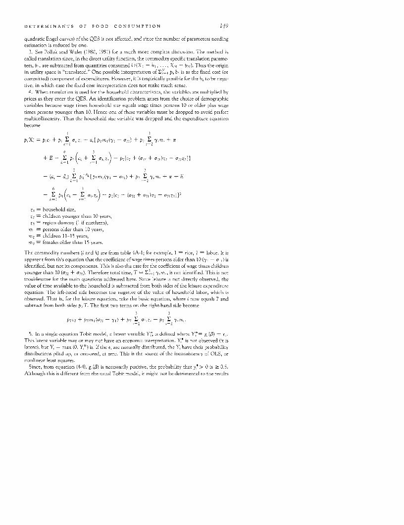
DETERMINANTS OF FOOD CONSUMAPTION 149
quadratic Engel curves) of the QES is not affected, and since the number of parameters needingestimation is reduced by one.
3. See Pollak and Wales (1980, 1981) for a much more complete discussion. The method iscalled translation since, in the direct utility function, the commodity specific translation parame-ters, b,, are subtracted from quantities consumed U(Xi -b .,..., X- bN). Thus the origin
in utility space is "translated." One possible interpretation of Ek=l Pkbk is as the fixed cost (or
committed) component of expenditures. However, it is empirically possible for the b2 to be nega-
tive, in which case the fixed cost interpretation does not make much sense.
4. When translation is used for the household characteristics, the variables are multiplied by
prices as they enter the QES. An identification problem arises from the choice of demographlc
variables because wage times household size equals wage times persons 10 or older plus wage
times persons younger than 10. Hence one of these variables must be dropped to avoid perfectmulticollinearity. Thus the household size variable was dropped and the expenditure equation
became
3 3
p,X = p,c, + P, 1 a,-rz + a{ p 7 m,(y 1 - aU) + p, E -y,m, + 3r
6 3
+ E-kEI P. (Ck + 'aElk,Z) - pM-, + (a,7 + a71)z2 + a7!Z3J}
7 3
(a, d,) E pdk l (p71 Y-71) + P7 E y,m,r + T + E
6 3
-E pt(c. + 1 oUaZ) -p7[C7 + (9712 + u71)Z2 + 973Z3]})
zi - household size,
Z2- children younger than 10 years,Z3-region dummy (I if northern),
ml-persons older than 10 years,
m, children 11-15 years,
m3 females older than 15 years.
The commodity numbers (i and k) are from table 4A-1; for example, I rice, 7 -labor. It is
apparent from this equation that the coefficient of wage times persons older than 10 (-y - a7,) is
identified, but not its components. This is also the case for the coefficient of wage times children
younger than 10 (072 + U71 ). Therefore total time, T = E 3y m_, is not identified. This is nottroublesome for the main questions addressed here. Since leisure is not directly observed, the
value of time available to the household is subtracted from both sides of the leisure expenditureequation. The left-hand side becomes the negative of the value of household labor, which is
observed. That is, for the leisure equation, take the basic equation, where i now equals 7 andsubtract from both sides p7 T. The first two terms on the right-hand side become
3 3
P7 C7 + p7m1(U71 - 'y1) + P7, Ea-,Z- P7 y,mr,.
5. In a single equation Tobit model, a latent variable Y*, is defined where Y*= gol) + e,.This latent variable may or may not have an economic interpretation. Y,* is not observed (it islatent), but Y, = max (0, Yl*) is. If the e, are normally distributed, the Y, have their probability
distributions piled up, or censored, at zero. This is the source of the inconsistency of OLS, or
nonlinear least squares.
Since, from equation (4-4), g(O) is necessarily positive, the probability that y*> 0 is 2 0.5.
Although this is different from the usual Tobit model, it might not be detrimental to the results
150 CASE STUDIES
reported here; when evaluated at the sample average for independent variables, the probabilityof having positive production is an estimator of the sample proportion with positive production,which is always greater than half for these data.
Because the output-supply and input-demand equations are a system, a multivariate Tobitmodel is applicable. In this case, e is an N vector with covariance matrix E, which is constrainedto be diagonal in order to keep estimation from being prohibitively expensive. Cross-equationparameter restrictions are still imposed, however. Had E not been constrained to be diagonal,the probability density for each household would have involved evaluating multiple integrals,one for each good not produced. In this study, there are many households not producing one ortwo goods and a few households not producing as many as four goods. For these households, thecorresponding density involves evaluating a quadruple integral. This is not only awkward toprogram, but also expensive to compute. When independence is assumed between each of theerror terms, the household density is the product of 7-K normal densities and K standard normaldistribution functions. If K outputs are not produced, only a single integral would have to beevaluated, but one for each of the normal distribution functions corresponding to the K outputsnot produced. Evaluating a single integral K times is a much less costly and less difficult proce-dure than evaluating a K-dimensional integral once.
It should be noted that for a demand system E cannot be diagonal since expenditures on goodsplus the value of household leisure equal full income. Thus error terms add up to zero, resultingin a singular covariance matrix, which it could not be if it were diagonal. However, this is nottrue for the values of output supply less the value of input demand, which sums to profits, be-cause profits contain an error term.
Moreover, ignoring cross-equation restrictions, maximum likelihood estimates assuming inde-pendence retain their consistency even if the assumption is violated. Hence, the assumptionremains attractive statistically. All that would be sacrificed is asymptotic efficiency.
Although there is a problem in using the CET output aggregator in representing this behavior,the alternatives create even greater problems. The trouble with the CET is that the marginal rateof transformation is infinite between a good not being produced and one that is. Hence a profitmaximizing firm would always produce an infinitesimal amount of every output. This character-istic is shared by other output aggregators that rely on few parameters, for instance, the transcen-dental (Mundlak 1963). An alternative might be to use a flexible form. For instance, one mightassume a translog profit function. Then, however, one would estimate share equations, whichmust add to unity. Hence the error terms must add to zero so they cannot be assumed to beindependent, as already mentioned. Another alternative might be a general quadratic produc-tion function, but in this case, the number of parameters to be estimated is a multiple of thesquare of the number of specified outputs. In this case, the Tobit estimation might be prohibi-tively expensive.
6. Write
apjXj/a(pNT - ir + E) = aP.Xi/8( pa PpX)/ N(PNT + -r + E)
from which ap Xl/a(N= pjXj), the marginal total expenditure for good i, can be solved for.7. The calorie conversion ratios were virtually identical for rice and for oils and fats (almost all
palm oil), both very homogeneous groups. The conversion factors differed substantially for theother three food groups, which are fairly heterogeneous. For example, the conversion factor formiscellaneous foods was twice as high for the representative high-expenditure household as forthe representative low-expenditure household (4,750 calories per kilogram to 2,430). Conversionfactors from kilograms to calories are available from the author.
8. In principle, separate prices could have been calculated for each household, but that wouldhave created serious statistical problems. Assume that every household in a region faced thesame set of sales and purchase prices (or the same set of prices for different qualities of goods).Even with a common utility function, different households would buy and sell foods at differenttimes during the year (or buy different qualities), because of differences in household characteris-

DETERMINANTS OF FOOD CONSUMPTION 151
tics and in full income. Since prices have a seasonal movement (quality differential), if an averageprice was calculated for each household, those averages would be different for each householdeven though the households actually faced the same set of prices. Not only would there be spuri-ous variation in such prices, but these prices would be endogenous to the farm-household modelwe use to explain household behavior. This is so since purchase and sales decisions are endoge-nous to the model. Hence, if these prices were used to estimate a system of demand- or output-supply equations, the parameter estimates would be inconsistent. The same problem would oc-cur if we used sales prices for net sellers and purchase prices for net purchasers. One way to avoidthe problems of spurious variation and endogeneity of prices is to average prices across house-holds. One interpretation of these prices is thus as a proxy for the constellation of true pricesfaced by a household. For this purpose, it is desirable to define the proxv prices over a marketarea. Region was chosen instead of enumeration area as the definition of market area because itwas feared that the latter might be too small. Also, region is the area used by Spencer and Byerlee(1977) in computing their prices.
9. Let K = rV/[1 - (I + r)-n], where K annual service user cost, V - acquisition cost ofcapital, and n- expected life of capital in years. In a perfect market, the acquisition cost of theasset equals the discounted sum of its annual flows. If we assume the annual flows to be constantin real value and to start in year 1, the equation for K is obtained. Spencer and Byerlee (1977) usea discount rate of 0.1 and expected lives that were different for different types of capital (1977, pp.47-48). The types of capital included are farm tools, animal equipment (including fishing equip-ment), nonfarm equipment, livestock, and tree crops.
References
Bardhan, Kalpana. 1970. "Price and Output Response of Marketed Surplus of Food-grains: A Cross-Sectional Study of Some North Indian Villages." American Journalof Agricultural Economics, vol. 52, pp. 51-61.
Barnum, Howard, and Lyn Squire. 1979. A Model of An Agricultural Household,Washington, D.C.: World Bank.
Behrman, Jere, and Barbara Wolfe. 1984. "More Evidence on Nutrition Demand:
Still Income Seems Overrated and Women's Schooling Underemphasized." Journalof Development Economics, vol. 14, pp. 105-28.
Howe, Howard, Robert Pollak, and Terence Wales. 1979. "Theory and Time SeriesEstimation of the Quadratic Expenditure System." Econometrica, vol. 47, pp.1231-47.
Jones, W. 0. 1972. Marketing Staple Food Crops in Tropical Africa. 1972. Ithaca, N.Y.:Cornell University Press.
Krishna, Raj. 1962. "A Note on the Elasticity of the Marketable Surplus of a Subsis-
tence Crop." Indian Journal of Agricultural Economics, vol. 17, pp. 79-84.
Lau, Lawrence, Wuu-Long Lin, and Pan Yotopoulos. 1978. "The Linear LogarithmicExpenditure System: An Application to Consumption Leisure Choice." Econo-metrica, vol. 46, pp. 843-68.
Mundlak, Yair. 1963. "Specification and Estimation of Multiproduct ProductionFunctions." Journal of Farm Economics, vol. 45, pp. 433-43.
Mutti, R., D. Atere-Roberts, and D. Spencer. 1968. Marketing Staple Food Cropsin Sierra Leone. Department of Agricultural Economics, University of Illinois,Urbana.
152 CASE STUDIES
Pinstrup-Andersen, P., and E. Caicedo. 1978. "The Potential Impact of Changes inIncome Distribution on Food Demand and Human Nutrition." American Journal ofAgricultural Economics, vol. 60, pp. 402-15.
Pitt, Mark. 1983. "Food Preferences and Nutrition in Rural Bangladesh." Review ofEconomics and Statistics, voi. 65, pp. 105-14.
Pollak, Robert, and Terence Wales. 1981. "Demographic Variables in Demand Anal-ysis." Econometrica, vol. 49, pp. 1533-51.
-______ 1980. "Comparison of the Quadratic Expenditure System and Translog De-mand Systems with Alternative Specifications of Demographic Effects." Econo-metrica, vol. 48, pp. 595-612.
Powell, Alan, and F. H. G. Gruen. 1968. "The Constant Elasticity of TransformationProduction Frontier and Linear Supply System." International Economic Review, vol.9, pp. 315-28.
Reutlinger, Shlomo, and Marcelo Selowsky. 1976. Malnutrition and Poverty, Magni-tude and Policy Options. Washington, D.C.: World Bank.
Rosenzweig, Mark. 1980. "Neoclassical Theory and the Optimizing Peasant: AnEconometric Analysis of Market Family Labor Supply in a Developing Country."Quarterly Journal of Economics, vol. 94, pp. 31-55.
Sen, A. K. 1966. "Peasant and Dualism with or without Surplus Labor." Journal ofPolitical Economy, vol. 74, pp. 425-50.
Spencer, Dunstan, and Derek Byerlee. 1977. "Small Farms in West Africa: A De-scriptive Analysis of Employment, Incomes and Productivity in Sierra Leone." Af-rican Rural Economy Program Working Paper no. 19. East Lansing. MichiganState University.
Strauss, John. 1982. "Determinants of Food Consumption in Rural Sierra Leone:Application of the Quadratic Expenditure System to the Consumption-LeisureComponent of a Household-Firm Model." Journal of Development Economics, vol.11, pp. 327-53.
-_____ 1984a. "Joint Determination of Food Consumption and Production in RuralSierra Leone: Estimates of a Household-Firm Model." Journal of Development Eco-nomics, vol. 14, pp. 77-103.
. 1984b. "Market Surpluses of Agricultural Households in Sierra Leone."American Journal of Agricultural Economics, vol. 66, pp. 321-3 1.
Sukhatme, P. V. 1970. "Incidence of Protein Deficiency in Relation to Different Dietsin India." British Journal of Nutrition, vol. 24, pp. 447-87.
Timmer, C. Peter, and Harold Alderman. 1979. "Estimating Consumption Parame-ters for Food Policy Analysis." American Journal of Agricultural Economics, vol. 61,pp. 982-87.
University of California at Los Angeles, Nutrition Assessment Unit, School of PublicHealth. 1978. Sierra Leone National Nutrition Survey. Washington, D.C.: Agency forInternational Development.
Ward, John, and John Sanders. 1980. "Nutritional Determinants and Migration inthe Brazilian Northeast: A Case Study of Rural and Urban Ceara." Economic Devel-opment and Cultural Change, vol. 29, pp. 141-63.
5Agricultural Prices, Food
Consumption, and the Health andProductivity of Indonesian Farmers
Mark M. Pitt and Mark R. Rosenzweig
THIS CHAPTER EXAMINES existing household survey data from Indonesia todetermine how food price changes and health program interventions affectthe health, nutritional status, and profits of farm households. Many poli-cies adopted by developing and developed countries serve to alter the pricestructure faced by consumers and food producers. Such macro price-inter-vention strategies as tariffs, support prices, ceilings, export taxes, and ex-change-rate policies directly alter relative prices and thus alter the distribu-tion of income and dietary patterns of the population. Food aid programs,depending on the manner in which they are implemented, also may affectthe price structure of foods. In addition, agricultural development policiesthat are crop specific, either by design or by consequence, and all projectsthat enhance employment opportunities affect the relative prices of notonly foods, but also nonfood resources supplied by family members to chil-dren-parental time and breastmilk.
Despite the well-recognized potential importance of the nutritional con-sequences of most programs and policies, there is little empirical evidenceon the linkages between price changes, food intake, and nutritional well-being. A great impediment to the acquisition of this knowledge has beenthe lack of data. Although a number of localized case studies have emerged,the small size of the samples, the lack of price variability, and the noncom-parability of sample designs and the analyses have made it difficult to drawdefensible inferences or generalities from such information (Martin 1983).Recently, however, sets of household data have been collected in develop-ing countries that have enabled analysts to compute estimates of the rela-tionship between relative food prices and household food consumptionpatterns (Pitt 1983; Strauss 1982). Although such studies provide the first
153
154 CASE STUDIES
theoretically based estimates of aggregate household food consumption bydisaggregated food groups from national probability samples, they do notprovide any insight into the health consequences of the observed altera-tions in nutritional intake for individuals. Nor do they provide any infor-mation on the income or productivity changes arising from alterations infood consumption and in health status.
To the extent that food consumption is only one direct determinant ofhealth and the rules by which households distribute their resources amongtheir members is unknown, estimates of the effects on household-level con-sumption of food price and programmatic interventions do not necessarilyprovide sufficient information on the health consequences of such initia-tives. The health of the population may also depend on the cost or avail-ability of medical services, on the sanitation conditions of the environ-ment, and, in the case of children, on the availability of parental care. Tothe extent that programs designed to alter the health status of populationsmay compete for donor funds with food-oriented projects and aid pro-grams, it is useful to assess from comparable data both the relative effects offood price changes and of health program interventions on health or nutri-tional status. In this chapter, we extend the now conventional model of theproducer-cum-consumer farm-household model by incorporating a house-hold health production sector in which the household-produced good,health, can both affect the production of farm output and provide directadditional utility to the household. We use farm household data from anIndonesian national probability sample to estimate the effects of the short-term illness of farmers and their spouses on farm profits and labor supply;the effects of changes in eleven food-group prices, health programs, andfarm profits on the probability and severity of illness of farmers and farmerspouses; and the effects of alterations in food consumption on the level ofhousehold health.
Determinants and Consequences of Changes in Healthin Farm Households
Consumption, Farm Production, and Health Production
To understand health determination and the consequences of changes inhealth or nutritional levels in the farm sector, it is necessary to specify theprocesses (technology) by which health is produced, the way in whichhealth is valued by the producer household, the effects of changes in healthon household constraints, the mechanisms by which changes in health

HEALTH AND PRODUCTIVITY OF FARMERS 155
directly affect farm production, and the efficiency of input and outputmarkets.
To illustrate how these relationships involving the market environment,health, production, and consumption influence the appropriate methodsof estimating health determinants and health effects as well as policy con-clusions, we consider first the simplest model of the farm household, inwhich the farm commodity is produced with one input, labor; there is oneadult member, the farmer; and the farmer's health is also produced. Thefarmer derives utility from his or her level of health, H, from the consump-tion of the produced food commodity X (at level XC) and purchased foodcommodity Y, and from leisure 1, such that
(5-1) U = U(H, X, Y, 1).
The level of health is assumed to be influenced by the levels of Xc and Yconsumed, a health input Z (which yields no direct utility), the farmer'swork time If and by environmental factors and the individual's health en-dowment, summarized by p, beyond the control of the household; that is,
(5-2) H = h(X', Y, Z, If) + / hi, h2, h3, > 0; h4 < O.
Expression (5-2) is the health production function, which depicts howchanges in food consumption, work, time, health goods (such as medicalservices), and the environment affect the farmer's health. Just as with con-ventional firm or farm production functions, the technology embodied in(5-2) may change over time and may be known more or less precisely bydifferent households.
The farm output production function is conventional, except that it alsodescribes how the farmer's health may affect production; that is,
(5-3) X = F(L; H)
where L = farm labor input, defined below. The level of health may affectthe productivity of farm inputs (a2X/aLaH > 0) but may have no directproductivity effect. That is, the health of the farmer may affect his or herability to utilize (supervise, allocate) resources. The level of health mightalso directly affect the quality of the labor input supplied by the farmer. Inother words, the "effective" labor units Lf the farmer supplies might beboth a function of health and time worked; that is,
(5-4) Lf = O(Qf, H) 01 > 0, 02 > 0.
If labor time can be hired in the market at a wage rate per unit of time Wand each unit of hired labor time provides a efficiency units of labor, thenthe labor input L in efficiency units is Lf + aLH, where LH is hired labor
156 CASE STUDIES
time. The price of an efficiency unit is thus X = W/l and labor costs ofproduction on the farm are Lw. We note that W (or w) may be determinedaccording to the "efficiency" wage models of Leibenstein (1957), Mirrlees(1975) or Stiglitz (1976), or may be the result of standard supply-demandequilibrium. The critical assumption, discussed below, is that hired andfarmer labor are perfect substitutes in farm production and the supply ofhired labor to an individual farm is perfectly elastic at the market (effi-ciency) wage.
As noted in Grossman's (1972) original work on health production, anincrease in the farmer's health may also increase the number of healthydays available for leisure I or work If; that is,
(5-5) If + I = Q(H), 6' > 0.
The income constraint of the household is thus
(5-6) pxXc + pyY + pzZ = Tw + cLf = X+ + wOO((H)-1, H) = I
where PX, py, pz are the market prices of X, Y, and Z; c is the market wagerate, I is income, and 7r = p,X - L = profits.
Separability and the Effects of Farmer's Health on Farm Profitsand Farm Income
As we have just seen, changes in the health status of the farmer can affectincome by altering the farmer's available time Q, managerial abilities, or theproductivity of work time. We now discuss more precisely the effects ofchanges in the farmer's health on potential output or income, farm profits,and actual family income, given that the world consists of households thatmaximize the utility function described by (5-1), subject to the constraintsand structural relations (5-2) through (5-6). Note that, since health is anendogenous choice variable in the model, it is necessary to distinguish theexogenous component of health (AL) from that part influenced by behavior(consumption choice and thus tastes) in order to draw causal conclusionsfrom relationships between observed health and other variables. We thusexamine how changes in IL-the health environment or endowment-which is exogenous to the farmer but possibly manipulable by policy, affectthese various components and concepts of incomes. To further simplify, forthe time being we ignore the managerial effect of health. The utility-maxi-mizing (necessary) first-order conditions for the optimal quantities of theconsumption and household production inputs X', Y, Z and I and the farmproduction input L are
(5-7) UxL + UHhXC = X[pA - WhA(, Q' + 02)]
HEALTH AND PRODUCTIVITY OF FARMERS 157
(5-8) Uy + UHhy = X[py - wh,(0, Q' + 02)]
(5-9) UHh = Xpz - whz(O, Q' + 02)]
(5-10) U1 + Ulh = Xw[01 - h2 (01 V + 02)]
(5-11) PxrL
where X = Lagrangian multiplier.Conditions (5-7), (5-8), and (5-10) indicate how changes in the consump-
tion of the food items as well as in leisure time augment utility both directlyand indirectly, by changing the level of health, and also influence incomeindirectly by altering the efficiency of the farmer's labor time and the timeavailable for leisure or work. Despite the interdependence between thefarmer's consumption and his labor productivity, however, the level of thefarm (labor) input L is independent of the farmer's consumption and leisurechoices. Expression (5-1 1) is the profit maximization condition for the useof the farm labor input; farm production and consumption allocations arethus separable. The reason is that, whatever the endogenously determinedefficiency per unit of time supplied by the farmer to farm production andwhatever the quantity of time supplied, labor time (and efficiency units)can be hired at constant cost per unit to perfectly substitute for changes inthe farmer's labor supply. Thus, farm profits will be independent of thefarmer's health status when market substitutes are easily available for laborinput, measured in efficiency units or time. Conversely, only if such substi-tution is imperfect will consumption decisions and health affect productiondecisions and farm productivity. If, for example, the farmer's health affectsmanagement performance and the market for management is absent orimperfect, then the separability between production and health will bebroken.
The independence of farm profits and farmer's health in the perfect (in-put and output) market case does not imply that potential income orhousehold income is unaffected by changes in the health environment. Wecan define the household's potential, or full, income F(H*) in the perfectmarket (separable) case, for a given health level H*, as the sum of the profit-maximizing level of profits 7r (independent of H*) and labor income whenthe farmer works full time (all available time = Q(H*); that is,
(5-12) F(H*) =7r + wO(Q(H*), H*).
The effect of a small change, dy, in the health environment on full incomeis thus
(5-13) d(F(H*) = (0l4 + 02) dH > 0.d,u d[t
158 CASE STUDIES
Since second-order conditions constrain dH/d1 > 0, increases in healthalways increase full income by altering the (potential) time available forwork and by augmenting efficiency per unit of labor time. Even though thefarmer's profits are unaffected by the healthiness of the environment, po-tential output to society is affected (hired labor time can be released for usein other productive pursuits).
Although full or potential income rises when the farmer's health envi-ronment improves, even in the separable case no prediction can be madefrom the model with respect to how actual or realized income will changein response to changes in I, since realized income depends on labor timesupplied:
(5-14) dI(H*) (0 dlfo + 0 dH)dju dtL dy,)
The effect of It on the level of the farmer's work time cannot be predictedbecause it depends on the properties of the unknown utility function aswell as on the characteristics of the health production and efficiency laborfunctions. Thus, changes in farm profits, actual or realized income, andpotential income in response to changes in health will generally not beidentical. Indeed, if health was purely a consumption good and had noeffects on time availability or on labor efficiency, farmer's income (via laborsupply) would be likely to change when the healthiness of the environmentchanges, but output and full or potential income would not.
It is clear that the effect of health on farm profits (which depends on thenature of input and output markets), or on income (which depends in parton the labor-leisure choices of the household), is not an appropriate mea-sure of the total costs to society (or benefits) from changes in the healthenvironment. In the absence of direct measures of efficiency units of labor,measures of health, labor time, and all farm inputs could be used in a pro-duction-function analysis to discern how farm output changes, given labortime, in response to changes in health. (Of course, this approach-that is,holding all inputs constant-would not capture any effects of health on theallocative ability of the farmer.) Additionally, if illness fully prevents anywork effort, then the cost of illness is simply lost earnings. The value ofmarginal changes in lost work days from severe (fully constraining) illness,however, although relatively easy to measure, will understate the total re-turns from investments in health when health also affects worker efficiency.
Finally, it can be easily demonstrated that the absence of markets for anyof the consumed commodities or inputs in health production, which leadto own-production of those factors, also breaks down the separability offarm production and consumption, as hired resources are diverted from thecash crop to produce nonmarketable commodities. Farm profits will thus
HEALTH AND PRODUCTIVITY OF FARMERS 159
be affected by the farmer's health even if input markets are perfect, al-though in the latter case, production of the cash crop will be efficient.
Food Prices and Health Programs: The Exogenous Determinants of Health
The reduced-form consumption-demand equations for the foods, otherhealth inputs, and leisure, conditional on farm profits, derived from themodel incorporating health production are
(5-15) Xc, Y, Z, I = D'(PX, P P, w, co, I,) i = Xc, Y, Z, 1.
These conditional-demand equations have all the usual properties of de-mand equations derived from models without household (health) produc-tion. Thus, own-compensated price effects are negative, cross-compensatedprice effects are symmetric, and so on. However, the functional form ofthese demand equations depends on (or implies) the characteristics of boththe household utility function (5-1) and the household production technol-ogy embodied in (5-2). Thus, the assumption that the utility function isStone-Geary, Extended Linear Expenditure System (ELES), or Cobb-Douglas, for example, does not, under most circumstances, result in theusual demand-system parameterizations derived from these specific func-tional forms, since the system will depend as well on the household tech-nology. In most cases, no exact closed-form solutions for the demand equa-tions in (5-15) can be obtained from explicit parameterizations of thepreference orderings and technology of the household. One special casewhere this is possible, considered in Rosenzweig and Schultz (1983), occurswhen the Cobb-Douglas form characterizes both the utility and householdproduction sector. Conversely, ad hoc specification of the reduced-formconsumption-demand equations does not generally allow retrieval of eitherthe underlying technological or utility parameters. Household health pro-duction and consumption are never separable, unlike consumption andfarm production with perfect input and output markets, because there is nomarket for the produced good, in this case, health.
Although the consumption-demand equations derived from the house-hold production model, as noted, do contain all the predictions of conven-tional utility maximizing models, the parallel reduced-form demand equa-tion for health, in (5-16), does not have any predictive content:
(5-16) H = DH(PX, P\,P) '' H, ).
To see why, consider the effects of a change in the price of the food good X,P,, on the household's health:
dH = dXc dY dZ dldP, d±- d, +h Ifd_~,
160 CASE STUDIES
Even if all inputs including the food good X in the health production func-tion have positive marginal products and contribute to improving health,it can be seen from (5-17) that a rise in the price of X or of any food goodmay increase or decrease health. The reason is that a change in any oneprice of food also (generally) affects the consumption of other foods andleisure (cross-price effects are nonzero) in directions that cannot be pre-dicted. In (5-17) for example, although dXc/dP, is likely to be negative, con-sumption of the Y good and the Z-input may increase (if Y and health aregross substitutes for X in consumption) and health may improve. For ex-ample, governmentally subsidized technological improvements in cashcrops, such as wheat, which result in higher relative prices for noninterna-tionally traded items such as some vegetables, could lower or raise healthlevels even if farm profits are unaltered and vegetables are healthier thanbread (consumption of butter, rich in vitamin A and a likely complementto bread, might increase).
The net effect of a food price change on health will thus depend on themagnitudes and signs of the own- and cross-price effects in consumptionand on the relative magnitudes of the marginal productivities of the inputsin the health production function. That is, food price effects on health de-pend on both the properties of the health production technology and theunderlying preference ordering of the household for foods and otherhealth-related goods. As a consequence, conclusions about the health im-pact of various food policies, which alter the relative prices of foods andother goods, cannot be known a priori without estimates of the health re-duced-form equation (5-16) or estimates of both the consumption (food andother health inputs) demand system (5-15) and the health technology, from(5-2).
Finally, the composition and nutrient level of the household diet reflectsnot only relative food costs and the constraints of income, but also the costor availability of health services Pz and the healthiness of the environment1. Moreover, just as a change in one food price may reduce or increasehealth levels because of theoretically ambiguous substitution among foodsof different health marginal productivities (nutritiousness), the health ef-fects of interventions that alter the cost of pure health inputs will be aug-mented or diminished by substitutions in health production and consump-tion. Thus, reductions in health service costs may induce a change in diettoward less nutritious (but more tasty?) foods, if nutritious foods and healthservices are substitutes in health production and such foods and health aresubstitutes in consumption. Similarly, programs aimed at improving thehealth environment (cleaner sources of water) will alter the composition ofdemand and the demand for health services in ways that may reinforce orattenuate the health effects of such interventions. Estimates of the health
HEALTH AND PRODUCTIVITY OF FARMERS 161
reduced-form equation provide information about the joint health effectsof food policies and health programs that reflect these household alloca-tions of resources.
The Multiperson Household, Consumption Aggregation,and Intrafamily Resource Allocation
An important element of unrealism in the model discussed so far is theassumption that the farm household consists of one person. Although one-person household models are extensively used in the development litera-ture (for example, Barnum and Squire 1979; Iqbal, chapter 6), analyses oflabor supply in developed countries (Ashenfelter and Heckman 1974;Schultz 1980) have demonstrated the importance of the interaction be-tween heterogeneous members residing in the same household (husbandand wife) as well as the differential intrahousehold responsiveness ofspouses' labor supply to price and wage changes. Since almost all house-holds in all developing societies consist of at least one adult female and oneadult male, and wage rates for males and females are not always in fixedproportion (see Rosenzweig 1984, for evidence from India; Hansen 1969,for evidence from Egypt), treatment of family members as one aggregateperson or as a collection of identical individuals (Sen 1966) facing a "uni-sex" wage would appear to be overly simplistic, at best. Moreover, in thearea of health and nutrition, the well-documented differentials and varia-tion in male and female infant survival rates across countries suggest thatchanges in income and prices may have significant distributional effects onthe health of individuals within families, given that most households con-tain children and adults of both sexes.
The question of how a household distributes its available resourcesamong its members is particularly important in the study of food price,food consumption, and nutrition relationships, because most availablehousehold data sets are likely to provide information only on householdconsumption aggregates, given the expense of collecting individual-specificconsumption data. To the extent that interest in aggregate (family-level)consumption or overall nutritional availability in low-income householdsis derived mainly from concern about the nutrition, health status, or pro-ductivity of members of such households, understanding how householdaggregates map into the well-being and health of individuals is critical.
In this section we consider three related questions: How does a change ina particular food or other price faced by a household affect the consump-tion and health of individual household members? What inferences regard-ing the health of individual members of a household can be drawn from
162 CASE STUDIES
information on total household food consumption or nutritional availabil-ity? Given data on the health of individual family members and the totalhousehold intake of food, what inferences can be made about the relation-ship between food intake and health; that is, when can the health technol-ogy be retrieved, given data on the health of individuals and household-level input information?
We first generalize the model discussed in the previous section by addingn - 1 family members, whose individual-specific vectors of consumptiongoods, leisure, and health enter the household utility function such that:
(5-18) U = U(H', Xi, Y, li) i 1 * n
(5-19) H = h(Xci, yi, ZI' 1) + !
(5-20) Li = 0i(1, Hi)
(5-21) X =(L)
(5-22) P-Z + PxXc + PY = 7r + E W'Ll1=1 f
where Z = £z, Xc EXc, y = EY, L' = Li + LH, and superscriptsdenote individuals. Note that the ,lt term includes both household-specificfactors-the health environment-and individual-specific factors-thehealth endowment. As constructed, the model allows each person to haveunique health and efficiency unit production functions and assumes thateach type of person has an equivalent market substitute, at wage rate w', infarm production. Thus the model retains its separability between the profitand consumption sections.
The first-order condition, derived from maximization of (5-18) subject to(5-19) through (5-22) for the intrahousehold allocation of, say, good X be-tween person j and person k, is
(5-23) UX} + UHj hXi PX - cohjiO2(5-23) U~~~ ± UH0k h'k ph- ehk'~
U,k + UH -X Wk@hxk 2
As can be seen from (5-23), the allocation of resources between members ofthe household will depend on how the household values the health andconsumption of each member (UHi, Uxi); how the relationships betweenhealth and consumption (the health technology) and between productivityand health (0) differ among members; and how the pecuniary returns toinvestments in the health of individual family members (the wi) differ.
HEALTH AND PRODUCTIVITY OF FARMERS 163
The reduced-form demand equations for the multiperson model are
ycl
(5-24) Z = R'i(PX, Fk, Pz, O, ,) j X, Y, Z, 1, H; i = 1 ... njijwhere w, it are the household vectors of individual-specific wages and en-dowments containing the elements wi, pi, i =1 ... n.
Comparing the single-person model to its multiple-person counterpart,we see that each has the same number of exogenous food and input prices,but the number of endogenous consumption variables to be determined(solved for) in the multiperson model is greater by n - 1 times the numberof choice variables. As a consequence, no additional predictions can bemade from the multiperson model regarding the effects of changes in thefood and health input prices beyond those for foods and health inputs ag-gregated over individuals; that is, own-compensated price effects for X', Z,Y are negative. Thus, no predictions can be derived from the multipersonmodel as to how changes in food prices alter the distribution of food con-sumption across members of the household without the imposition of agreat deal of additional structure.
Because, however, there is a unique price of time coi corresponding toeach individual in the model, the compensated effects of person-specificwage changes on the consumption of individual household members andthus on the intrahousehold allocation of foods can be discerned with littleadditional structure imposed. For example, a compensated increase in thewage of person type j can be shown to increase the allocation of food toperson j and decrease the allocation of food to person k, if the health, foodconsumption, and leisure of j and k are Hicksian substitutes. Thus, thehousehold will tend to distribute more resources to persons with higherearnings capacities, as given by the market wage per labor efficiency unit,when the individual-specific goods in the household welfare function aresubstitutes. This feature of the multiperson household is exploited in Ro-senzweig and Schultz (1982) to show how differences in economic opportu-nities for women could account for the variation in male-female infant sur-vival ratios across India.
To examine the relationships between the aggregate quantity of house-hold consumption and the consumption and health of individual familymembers, we employ a simpler multiperson model in which there are onlytwo persons. For simplicity, we also ignore labor/leisure decisions and farmproduction. The household's utility thus depends on the health status H
164 CASE STUDIES
and consumption of food good X of each individual as well as on a jointlyconsumed good Y. The health of each individual depends in turn on own-consumption of the X good.Thus,
(5-25) U = U(H1, H2, XI, X - XI, Y)
(5-26) H1 = h'(X1) hi > 0, hxi,i < 0
(5-27) H2 = h2(X - XI)
(5-28) p,X + PxY = I
where X2 = X-Xl and I is total income, assumed exogenous.To facilitate the comparison between aggregate household consumption
X and person-specific consumption, we treat the aggregate food X and theconsumption of X by individual one, X', as control variables. Determina-tion of X and X' obviously determines the consumption of X by person 2,X2, in this two-person case. The necessary first-order condition for the allo-cation of X between household members 1 and 2, the intrafamily alloca-tion "rule,' given the optimal aggregate consumption of X, is
(5-29) UHihtl i+ Uxi = UH2hX2 + Ux2
that is, allocate resources across family members to equate their marginalcontributions to household welfare. These marginal values will depend onboth the unique utility-generating traits of each individual and on individ-ual-specific differences in the health technology.
The relevant first-order conditions for the aggregate household con-sumption of X2 and Y are given by:
(5-30) UH2h22 + Ux2 = )px
(5-31) U, =Xp.
where X is the Lagrangian multiplier.We now consider how member one's health status, H' changes when
there is an exogenous change in the total amount of X, the commodityaffecting health, consumed by the household. That is, we wish to knowhow a change in the availability of total or per capita X, x = X/2, alters X'(and X2) and thus the individual health levels of 1 and 2. Using rationingtheory (Tobin and Houthakker 1950-51) and assuming that the exogenouschange in the aggregate consumption of X occurs at the optimal level, asgiven by expressions (5-30) and (5-3 1), we know that dX'/dx is just (dX1/dp,)/dx/dp,), the ratio of the compensated effects of a change in the priceof the X commodity on individual one's consumption of X and the com-pensated effect of a change in the price of X on the total or per capita
HEALTH AND PRODUCTIVITY OF FARMERS 165
consumption of X in the household. In the two-person model, when theutility function is strongly separable, the relationships between a change inper-capita X, x, and the consumption of X by person one is thus:
(5-32) dX1 UHIH1(hI) + U1 phxx + Uxlxi +dx UH1H2(hx2)2 + UH2hXx + UjLXi 9
Only if the numerator and denominator of the first parenthetical term in(5-32) are equal will changes in per capita X consumption and changes inthe consumption of all individuals in the household be equal; a sufficientcondition is that the health production functions among individuals beidentical and the family consider all persons perfect substitutes for eachother. In the absence of blindness to individual traits by households andperfect biological homogeneity across family members, however, little canbe said a priori about how alterations in the per capita (or adult-equivalent)availability of food in the household affect any individual's health status inthat household, unless the intrafamily distributional rules are also known.
Lack of information on intrafamily allocations also means that little canbe said about the magnitude of the change in average family health statuswhen average family consumption changes, so long as individual food ornutrient consumption is not in fixed proportion to health. The effect of percapita X on average health (A = H/2) in the model is
dA dX1 dX2 d-] 1(5-33) = xi + h2 2 I-
dx I dx xdX j 2
which will depend on both the allocative rule dX'/dx and on the proper-ties of the health production functions. Expression (5-33) above shows thateven if the individual-specific health functions are identical, as long ashealth production functions exhibit diminishing returns in food and allo-cations of X across individuals are not equal, then
1. If the relationship between individual food consumption and health isknown, knowledge of per capita family food consumption will notyield the level of per capita household health, since dA/dx * I/nEn, hit;
2. If the relationship between individual food consumption and health(the health production function) is not known, it cannot be inferredfrom information on the health status of individuals and family percapita food consumption, since dH1/dx = h,idX'/dx * h,i.
Conversely, only if the relationship between individual consumptionand health is in fixed proportions, that is, if hi = h,2= a, then, indepen-dent of how the household distributes its resources:
166 CASE STUDIES
1. If the consumption-health coefficients are known, the average healthof the household can be inferred from knowledge only of per capitahousehold consumption, although individual-specific levels of healthor nutritional status cannot be known
2. If the health production coefficients are unknown, they can be in-ferred from information on the individual health levels of all familymembers and total family consumption, since, from (5-33), E2 dH'/dX = a E;dXi/dX = a.
Given the difficulty of directly estimating the health production functionowing to the need for individual-specific consumption (intake) informa-tion, it may be preferable to estimate individual-specific reduced-formhealth-demand equations (such as [5-24]). Although such reduced-form es-timates do not provide information on how the consumption of food itemsdirectly affect health, they do yield information on how changes in theprices of foods, medical services, and other goods result in changes inhealth or nutritional status. Since it is relatively more difficult for policy-makers to alter directly (dictate) how households allocate their resourcesthan to manipulate prices or provide services, the health-reduced formsmay provide more policy-relevant information than will estimation of thehealth technology, as long as technology (and tastes) remain unchanged.The reduced-form equations for health and other consumption items, in-cluding leisure, also can provide information on how changes in measur-able aspects of the health environment alter health, health practices (in-puts) and the supply of labor.
Finally, reduced-form health estimates obtained for different members ofthe same family also allow a test of whether family members can be (or are)considered to be identical, since, under the null hypothesis of perfect intra-family substitution and biological homogeneity, all coefficients in the per-son-specific reduced forms will be equal across household members. Rejec-tion of the null hypothesis, of course, does not reveal the underlying cause(biological or behavioral) of the observed differences in health responses tocommonly experienced price and income effects across members of thesame family in the absence of direct estimates of the health technology.
Estimation of the Relationships between Health, Food Prices,Farm Profits, and Aggregate Food Consumption: Indonesia
Heterogeneity, Separability, and Estimation Procedures
We estimate the relationships between health and food prices, consump-tion and production using household-level data from an Indonesian na-
HEALTH AND PRODUCTIVITY OF FARMERS 167
tional probability sample. These data provide information on short-termillness, labor supply, and earnings for all household members, detailed foodand other consumption data and farm profits at the household level, andfood and other price data at the village level. The data thus enable theestimation of
1. The effects of changes in farmer's and spouse's health on farm profitsand on labor supply.
2. The effects of changes in food prices and health infrastructure on thehealth of the farmer and spouse, on the demand for household-levelhealth inputs, and on differences in the illness incidence betweenfarmer and spouse.
3. The effects of changes in the level and composition of individual foodconsumption on individual health levels, under the fixed coefficientand homogeneity assumptions for the individual health productionfunction.
The estimation procedures used to obtain these estimates as well as theappropriate specifications of the profit function and health reduced formsdepend not only on whether the farm production and consumption(household production) sectors are separable, as noted, but also on the exis-tence of variations among individuals or households in exogenous charac-teristics that are unobserved or unrecorded in the data, that is, heteroge-neity. It is now well recognized (Mundlak 1961) that heterogeneity infarmer's managerial capacities may lead to bias in least squares estimates offarm production functions, as farmers of different abilities may choose dif-ferent input combinations and will obtain higher output from a given inputmix. Accordingly, in estimating the effects of farmer's health on farmprofits, a correlation between those unobserved farmer characteristics that(conditional on prices) augment profits and unobserved characteristics thatincrease health status (the ,) will also lead to bias in estimating the effects ofhealth on profits, even if changes in profit levels do not influence thehousehold's demand for health. Thus it is possible to find that health andprofits are correlated, even if health does not structurally affect farmprofits, solely because of heterogeneity bias. Since price changes are likelyto be uncorrelated with farmer characteristics, health input prices (P, in themodel) are suitable instruments for estimating the direct, structural effect offarmer health on farm profits.
Estimation of the reduced-form equations that include farm profit by or-dinary least squares will provide consistent estimates of food price andprofit effects on health and other goods (as long as unmeasured aspects of ttare independent of prices or farm profits). If exogenous changes in thefarmer's health or in y affect profits (nonseparability), however, profits and
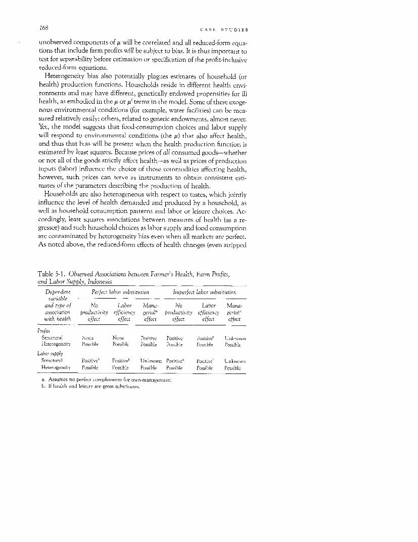
168 CASE STUDIES
unobserved components of yI will be correlated and all reduced-form equa-tions that include farm profits will be subject to bias. It is thus important totest for separability before estimation or specification of the profit-inclusivereduced-form equations.
Heterogeneity bias also potentially plagues estimates of household (orhealth) production functions. Households reside in different health envi-ronments and may have different, genetically endowed propensities for illhealth, as embodied in the ,. or /A' terms in the model. Some of these exoge-nous environmental conditions (for example, water facilities) can be mea-sured relatively easily; others, related to genetic endowments, almost never.Yet, the model suggests that food-consumption choices and labor supplywill respond to environmental conditions (the ,a) that also affect health,and thus that bias will be present when the health production function isestimated by least squares. Because prices of all consumed goods-whetheror not all of the goods strictly affect health-as well as prices of productioninputs (labor) influence the choice of those commodities affecting health,however, such prices can serve as instruments to obtain consistent esti-mates of the parameters describing the production of health.
Households are also heterogeneous with respect to tastes, which jointlyinfluence the level of health demanded and produced by a household, aswell as household consumption patterns and labor or leisure choices. Ac-cordingly, least squares associations between measures of health (as a re-gressor) and such household choices as labor supply and food consumptionare contaminated by heterogeneity bias even when all markets are perfect.As noted above, the reduced-form effects of health changes (even stripped
Table 5-1. Observed Associations between Farmer's Health, Farm Profits,and Labor Supply, Indonesia
Dependent Perfect labor substitution Imperfect labor substitutionvariable
and type of No Labor Mana- No Labor Mana-association productivity efficiency gerial' productivity efficiency gerialawith health effect effect effect effect effect effect
ProfitsStructural None None Positive Positive' Positive' UnknownHeterogeneity Possible Possible Possible Possible Possible Possible
Labor supplyStructural Positive' Positive' Unknown Positive' Positive' UnknownHeterogeneity Possible Possible Possible Possible Possible Possible
a. Assumes no perfect complements for own-management.b. If health and leisure are gross substitutes.
HEALTH AND PRODUCTIVITY OF FARMERS 169
of heterogeneity bias) on behavioral outcomes, controlling for prices, com-bine (and confound) the underlying utility and technological or biologicalparameters. Given the stability of those parameters, they do, however,yield information on the consequences of (if not the social returns to) im-provements in health.
Table 5-1 summarizes the expected types of relationships, and their signs,between health and farm profits and labor supply, when structural healthestimates are obtained using proxies for health input prices as identifyinginstruments. Although in some cases structural effects are signed, orknown to be absent, heterogeneity leads to a theoretically unknown rela-tionship between health, profits, and labor supply in all cases.
Results
Data. The household-level sample used to estimate the relationships be-tween health and food prices, food consumption and production are fromthe April-June 1978 subround of the National Socio-Economic Survey ofIndonesia (SUSENAS 1978) carried out by the Central Bureau of Statistics(Biro Pusat Statistik). This survey provides information on farm profits,itemized household consumption and expenditures, water sources, drink-ing water treatment, land ownership, cultivation, income and, for eachhousehold member, information on the incidence and severity of illness inthe previous seven days as well as age, education, labor supply, and wages.These data were augmented with information on the availability of healthprograms in local areas, irrigation quality and attributes of the nonfarmlabor market. In this analysis, the sample size for households cultivatingland and having both a head and spouse present is 2,347. Irrigation infor-mation, however, was only available for 2,175 households. Data sources forall the areal variables as well as sample characteristics and definitions of allvariables used in obtaining the estimates below are in the appendix.
Wages for the head (male in all sample households) and spouse were com-puted by means of wage equations estimated from a sample of all householdmembers aged 10 years and older, stratified by sex, and corrected for selec-tivity bias. The least squares correction for selectivity bias was applied(Olsen 1980). Variables measuring land ownership and marital status wereused to identify the selectivity correction in the wage equations. To achieveidentification of the health and profit equations using predicted wages, ka-bupaten (district)-specific measures of industrial capital and manufacturingworkers per capita, derived from the raw data tapes of a 1978 survey ofmanufacturing establishments (Survey Tahunan Perusahaan Industri1978), were included as regressors in the individual wage equations.
170 CASE STUDIES
To maintain tractability, the 112 separate expenditure items in theSUSENAS were aggregated into thirteen commodity groups, eleven foodsplus tobacco-betel and fuel. Consumption of the commodity aggregate to-bacco-betel-which includes the use of sirih, an intoxicating quid consist-ing of betel leaf, areca nut, gambier, and lime-may influence a respon-dent's perception of illness in addition to any actual effect. Thereforecaution is required in interpreting its estimated effects on the respondent'sreported health.
The principal shortcoming of the SUSENAS data is that they provideinformation only on short-term farm profits, labor supply, and illness. Thehealth status of family members is indicated by the occurrence of (self-reported) illness during the previous week; illness intensity is captured byinformation as to whether the illness required bed rest.
The Effects of Illness on Farm Profit and Farmer Labor Supply. We firstdetermine whether the allocation of resources in farm production can betreated as separable from household health and consumption decisions byestimating a farm-profit equation including the illness of the head of house-hold and his wife. First we tested whether the illness variables were inde-pendent of the profit function residuals. The Wu statistic (3.00) was lessthan the critical value for (2,2500) degrees of freedom. Thus the profit func-tion can be appropriately estimated by ordinary least squares (OLS). Theparameter estimates are presented in the first two columns of table 5-2. Theresults of our tests of the structural effects of illness and heterogeneity biasappear in table 5-3. The hypothesis that the illness of the farmer or thefarmer's spouse do not structurally influence farm profits cannot be re-jected (F[2,2144] = 1.62). Thus, we cannot reject the separability of farmproduction and consumption sectors.
The hypothesis that health is exogenous in the labor-supply equation forthe male head of household is, however, rejected (F[2,2144] = 7.16); leisureand the household production of health are not separable. Consistent withfarm production-consumption sector separability, however, farm profits areexogenous to labor-supply decisions by the farmer (F[1,2170] = 0.92). In-strumental variable estimates of the male labor-supply equation are re-ported in the second column of table 5-2, with health program variablesused as instruments. As predicted in table 5-1, we find that illness experi-enced by the farmer does significantly reduce his labor supply, even thoughhis illness does not reduce farm profits. The hypothesis that illness has nostructural effects on the amount of work performed by the male head isrejected at the 0.01 level of significance (X2 12] = 9.40). Thus, rural labormarkets in Indonesia appear to be operating smoothly enough so that mar-ket substitutes can be found for significant illness-induced reductions in the
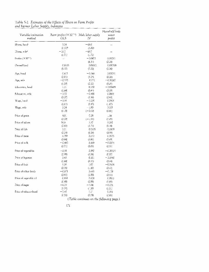
Table 5-2. Estimates of the Effects of Illness on Farm Profitsand Farmer Labor Supply, Indonesia
Household boilsVariable/estimation Farm profits (X 1-') Male labor supply water
method OLS IV probit
Illness, heada 3.24 -68.0(0,37)b (1.80)
Illness, wife' -16.7 -69.7 -(1.71) (1.72)
Profits (X 10- i) -0.0455 0.00211(6.34) (2.24)
Owned land 0.0115 0.00102 0.000106(9.32) (2.55) (2.36)
Age, head 0.615 -0.346 0.00231(2.01) (3.24) (0.26)
Age, wife -0.535 0.222 -0.00267(1.59) (2.12) (0.03)
Education, head 1.31 0.150 -0.00489(1.64) (0.44) (0.19)
Education, wife -3.52 -0.489 0.0861(0.37) (1.56) (2.60)
Wage, head -1.93 -0.205 0.0901(1.61) (0.47) (1.67)
Wage, wife 3.24 -1.90 0.325(0.18) (-0.30) (0.41)
Price of grain 4.01 -7.29 1.16(0.39) (-1.94) (3.85)
Price of tubers 16.6 3.37 0.262(2.83) (1.73) (1.34)
Price of fish 3.21 0.0335 -0.0439(2.24) (0.06) (0.98)
Price of meat 0.385 0.230 0.0975(0.44) (0.80) (3.69)
Price of milk -0.445 0.169 -0.0374(0.71) (0.85) (2.11)
Price of vegetables -8.55 0.597 -0.00725(2.98) (0.58) (0.07)
Price of legumes 3.43 0.101 -0.0360(1.44) (0.12) (0.44)
Price of fruit 1.09 1.07 -0.0416(0.36) (1.10) (0.42)
Price of other foods -0.871 0.483 -0.158(0.91) (1.59) (0.13)
Price of vegetable oil 0.668 0.424 0.0873(0.48) (0.88) (1.85)
Price of sugar -6.79 -3.04 -0.231(1.03) (1.30) (1.01)
Price of tobacco-betel -2.47 1.21 0.393(0.51) (0.78) (2.49)
(Table continues on the following page.)
171

172 CASE STUDIES
Table 5-2. (continued)
Household boilsVariable/estimation Farm profits (X 10-3) Male labor supply water
method OLS IV probit
Price of fuel -0.136 -0.0127 -0.0152(0.63) (0.19) (2.50)
Irrigation-i 25.6 -(3.06)
Irrigation-2 -16.0 -(2.01)
Irrigation-3 -21.5 - -(1.72)
Well - - 0.207(1.67)
River - - 0.0149(0.97)
Hospital - - 0.261(0.45)
Clinic - - 4.09(3.25)
Maternity hospitals - - 0.826(0.98)
Family planning - - 1.35(4.28)
Public lavatories - - 0.375(1.36)
Households in kabupaten - - -0.000687(3.34)
Intercept -3.91 55.2 -1.44(0.18) (8.40) (1.81)
d.f. 2,171 2,171 2,347
a. Endogenous variable in labor-supply equation. See text.b. Absolute values of t-ratios in parentheses.c. Absolute values of asymptotic t-ratios in parentheses.
farmer's cultivation time that leave levels of production unaffected, at leastin the short term.
The labor-supply parameter estimates indicate that the illness of the hus-band and wife jointly and significantly reduce the head's labor supply, re-flecting both the expected complementarity between health and leisureand intrafamily substitution of time in household production. The illnessreported in the sample appears to reduce labor supply strongly, by almostseventy hours a week. The low incidence of illness (2.6 to 3.4 percent) com-bined with this result suggests that only severely debilitating illness is re-
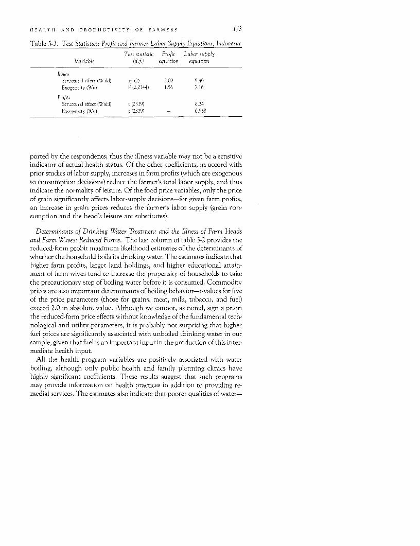
HEALTH AND PRODUCTIVITY OF FARMERS 173
Table 5-3. Test Statistics: Profit and Farmer Labor-Supply Equations, Indonesia
Test statistic Profit Labor supplyVariable (d.f.) equation equation
IllnessStructural effect (Wald) x2 (2) 3.00 9.40Exogeneity (Wu) F (2,2144) 1.56 7.16
ProfitsStructural effect (Wald) t (2319) - 6.34Exogeneitv (Wu) t (2319) 0.958
ported by the respondents; thus the illness variable may not be a sensitiveindicator of actual health status. Of the other coefficients, in accord withprior studies of labor supply, increases in farm profits (which are exogenousto consumption decisions) reduce the farmer's total labor supply, and thusindicate the normality of leisure. Of the food price variables, only the priceof grain significantly affects labor-supply decisions-for given farm profits,an increase in grain prices reduces the farmer's labor supply (grain con-sumption and the head's leisure are substitutes).
Determinants of Drinking Water Treatment and the Illness of Farm Heads
and Farm Wives: Reduced Forrns. The last column of table 5-2 provides thereduced-form probit maximum likelihood estimates of the determinants ofwhether the household boils its drinking water. The estimates indicate thathigher farm profits, larger land holdings, and higher educational attain-ment of farm wives tend to increase the propensity of households to takethe precautionary step of boiling water before it is consumed. Commodityprices are also important determinants of boiling behavior-t-values for fiveof the price parameters (those for grains, meat, milk, tobacco, and fuel)exceed 2.0 in absolute value. Although we cannot, as noted, sign a priorithe reduced-form price effects without knowledge of the fundamental tech-nological and utility parameters, it is probably not surprising that higherfuel prices are significantly associated with unboiled drinking water in oursample, given that fuel is an important input in the production of this inter-mediate health input.
All the health program variables are positively associated with waterboiling, although only public health and family planning clinics havehighly significant coefficients. These results suggest that such programsmay provide information on health practices in addition to providing re-medial services. The estimates also indicate that poorer qualities of water-
174 CASE STUDIES
that from wells and rivers rather than from springs and piped water sys-tems-tend to increase the propensity to boil water.
In Pitt and Rosenzweig (1985), we estimated sex-specific illness reducedforms for heads and their wives. A likelihood-ratio test indicated, however,that all the slope parameters in the equation for heads and wives werejointly different from zero at the 0.05 and 0.10 levels of significance, respec-tively. The patterns of signs for commodity prices were quite different inthe farm-head- and farm-wife-illness reduced forms. As noted, of course, itis not possible to infer to what extent these apparent differences representdifferences in sex-specific health technologies or the nature of intrahouse-hold allocation rules.
Among the more precisely estimated parameters for heads of households,the prices of grains and sugar were negatively related to illness, whereas theprices of vegetables and vegetable oil were positively related to illness. Al-though the popular notions that sugar is bad for health and vegetables aregood for health conform to these results, we reiterate that such conclusionscannot be drawn from the reduced form. The estimates do imply that re-ductions in the relative prices of vegetables will increase health levels,whereas subsidies to sugar, for given farm profits, will increase the incidenceof illness. At the sample means, the estimates indicated that a 10 percentreduction in the prices of vegetables and vegetable oil will decrease theprobability of illness by 4.2 and 9.3 percent, respectively. Similar propor-tional decreases in the prices of grains and sugars will increase the incidenceof illness by 15 and 25 percent, respectively.
A rigorous test of the joint hypotheses that there is both perfect intra-family substitution and identical health production functions across thefarm head and his wife is carried out by estimating a model obtained bysubtracting the wife's illness reduced form from that of her husband usingfixed-effect logit (Chamberlain 1980). A likelihood-ratio test failed to reject(at the 0.05 level) the hypothesis that the set of slope parameters of thehead's illness reduced form is different from that of the wife's reduced form.Among the individual food prices, however, the prices of fish and vegeta-bles had statistically different impacts on the differential incidence of illnessof heads and wives. Higher fish prices tend to make wives relatively more illand higher vegetable prices tend to make heads relatively more ill.
The Illness Production Function. As noted, we are unable to estimate di-rectly individual-specific health production functions because individual-specific consumption data are not available. If we assume that the relation-ship between individual consumption and health is in fixed proportionsand is the same for all individuals, however, we can estimate the person-specific health production function, formed by summing the linear health
HEALTH AND PRODUCTIVITY OF FARMERS 175
production functions for all the individuals residing in the household, evenif household resources are allocated differentially across individuals. Food-and tobacco-consumption levels in this aggregated, linear, household-ill-ness production function are now household totals; the intercept is repre-sented by the total number of household members and the age variable isthe sum of the ages of all household members. Possible differences in theindividual male and female health production functions are permitted byincluding an intercept dummy variable for sex (male = 1, female = 0),which, in summing to an aggregated function, becomes the total number ofmale household members.
Also included in the production-function specification are householdpublic good inputs, that is, household-level variables that are assumed toaffect the health of all individual family members net of their own con-sumption of foods. These are the (endogenous) boil variable, which affectsthe drinking water of all household members, the water sources, and theschooling attainment of the head and wife. The latter are included to test ifschooling improves health net of input levels, that is, to test for schoolingeffects in household production that are analogous to worker or efficiencyeffects in farm production.
All variables are divided by the size of the family in order to eliminate theheteroscedasticity caused by differences in household size. As a conse-quence, the illness-dependent variable, average illness incidence in thehousehold, has a large concentration of observations at zero but also obser-vations that may range up to a value of one (when there are no observa-tions). The Tobit estimation procedure is therefore employed. Because ofpossible heterogeneity in health endowments and environmental factors,which would bias these single-equation estimates, the health productionfunction is also estimated using two-stage Tobit, where the endogenousfood and other inputs are first regressed on the prices and programs. Al-though the two-stage Tobit estimates are consistent estimates of the (linear)production coefficients, the standard errors are not unbiased, so that cau-tion should be exercised in interpreting the two-stage results.
Table 5-4 presents both Tobit and two-stage Tobit estimates of the linearhousehold production function. As we have noted, heterogeneity bias aris-ing from differences in health environments and endowments, and tastes,potentially contaminate the single-stage estimates. The difference betweenthe Tobit and two-stage Tobit estimates is indeed quite striking. For exam-ple, the Tobit estimates indicate that fruit consumption is implausibly posi-tively and significantly associated with household illness, whereas the two-stage estimates suggest that the reverse pattern is more likely the case.
The consistent two-stage Tobit estimates indicate that six of eleven foodcommodities have negative production coefficients in the production of ill-
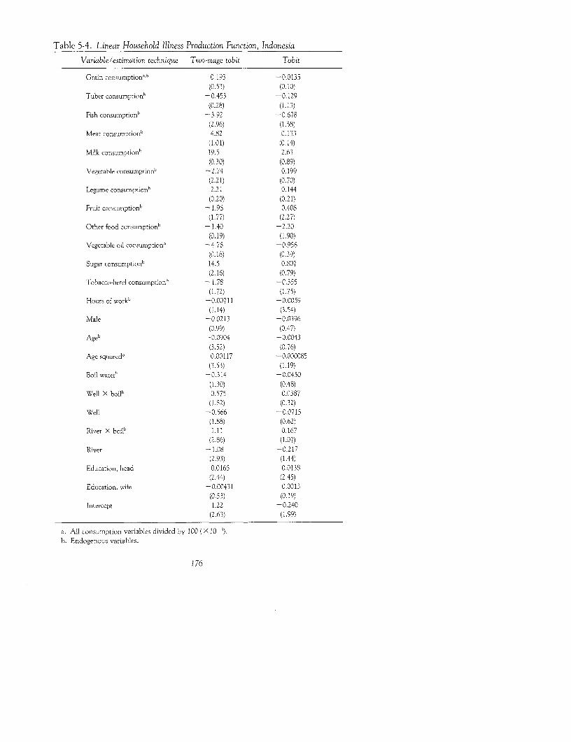
Table 5-4. Linear Household Illness Production Function, Indonesia
Variable/estimation technique Two-stage tobit Tobit
Grain consumptionr5 0.193 -0.0135(0.53) (0.10)
Tuber consumption' -0.453 -0.129(0.28) (1.13)
Fish consumption' -3.92 -0.678(2.96) (1.58)
Meat consumptionb 4.82 0.133(1.01) (0.14)
Milk consumption' 19.5 2.63(0.30) (0.89)
Vegetable consumption" -2.74 0.199(2.21) (0.70)
Legume consumption' 2.21 0.144(0.20) (0.21)
Fruit consumption5 -1.98 0.408(1.77) (2.27)
Other food consumptionb -1.40 -2.20(0.19) (1.90)
Vegetable oil consumptionb -4.78 -0.958(0.18) (0.39)
Sugar consumptionb 14.5 0.807(2.16) (0.79)
Tobacco-betel consumption5 -1.78 -0.355(1.72) (1.75)
Hours of work' -0.00711 -0.0059(1.14) (3.54)
Male -0.0213 -0.0396(0.99) (0.47)
Age' -0.0904 -0.0043(3.52) (0.76)
Age squaredb 0.00117 -0.000085(3.53) (1.19)
Boil water' -0.314 -0.0450(1.30) (0.48)
Well X boilb 0.575 0.0387(1.82) (0.32)
Well -0.566 -0.0715(1.88) (0.62)
River X boil5 1.11 0.167(2.86) (1.07)
River -1.08 -0.217(2.93) (1.44)
Education, head 0.0165 0.0138(2.44) (2.45)
Education, wife -0.00431 0.0013(0.53) (0. 19)
Intercept 1.22 -0.240(2.63) (1.99)
a. All consumption variables divided by 100 (X10 3).
b. Endogenous variables.
176
HEALTH AND PRODUCTIVITY OF FARMERS 177
ness. Of these, three are statistically significant at least at the 10 percentlevel of significance (fish, fruit, vegetables). The negative coefficient for to-bacco-betel suggests that consumption of this commodity reduces reportedillness. As noted earlier, however, the sirih (betel) component of this con-sumption aggregate is intoxicating and may distort perceptions of healthstatus. Sugar consumption, on the other hand, appears to increase signifi-cantly the production of illness. (It should be remembered, that the stan-dard errors of the two-stage Tobit model are not unbiased.) The (consistent)point estimates indicate that a 10 percent increase in vegetable, fruit, andfish consumption reduces the probability of illness by 9.1, 3.4, and 5.6 per-cent, respectively, and that a similar proportional increase in sugar intakeincreases this probability by 11.5 percent. The results also suggest that forany level of the specified health inputs, males are no less likely to become illthan are females, and that illness incidence declines with age up to age 38and then increases.
Of the household-level variables, the set of water-source and water-treat-ment variables are statistically significant. The educational level of thehousehold head, but not the wife, is also statistically significant. As in thehealth reduced forms, however, higher male educational attainment is asso-ciated with higher levels of reported illness incidence, perhaps because of agreater propensity among educated respondents to report illness in re-sponse to given illness symptoms. Although individual differences in ill-ness-reporting propensities may be uncorrelated with (village-level) pricesand programs, personal characteristics may influence both objectively mea-sured health conditions and reporting errors.
Conclusions
A number of recent studies have focused on the allocation of food nutri-ents across households and the response of household nutrient intake tochanges in food prices and income. Since nutrient intake itself cannot beconsidered an argument in the utility function or even a good indicator ofwelfare, it seems likely that implicit in this focus on nutrient intake is theview that food nutrients are an important set of inputs into the productionof health. In addressing the direct relationships between food (and otherhealth inputs) prices, income, and health, we demonstrate that policy im-plications derived from studying how the level and distribution of a subsetof health inputs (foods) changes with price subsidies or other interventionsmay be seriously flawed if the ultimate policy goal is to improve the levels ordistribution of health in the population.
178 CASE STUDIES
The traditional model of the producer-cum-consumer farm householdincorporating a household health production sector is used to demonstratethe difficulty in predicting the effects of policies on health or of the conse-quences of changes in health status. We show that theory offers no predic-tions for the signs of the effects of food price changes on health withoutcomplete knowledge of preferences and of the health technology. More-over, we show that the change in farm profits resulting from changes inhealth status is not a measure of the output loss resulting from illness, butrather an indicator of the imperfection of markets and the substitutabilityof inputs in farm production. Indeed, no prediction can be made from themodel with respect to how household income will change in response tochanges in health status.
Although in principle the health technology is estimable, estimation re-quires individual-specific information on health inputs consumed and in-struments such as prices. Available household data sets are likely to provideinformation only on household consumption aggregates. Thus, we con-sider how household aggregates map into the well-being and health of indi-viduals. In general, no predictions can be derived as to how changes inprices or per capita consumption affect the distribution of consumptionacross individuals, the health of individuals, or even the average health ofthe household. If the health technology is linear and homogeneous acrossindividuals, however, it is possible to estimate the relationship betweenhousehold consumption and an individual's health.
From a sample survey of farm households in Indonesia, we estimatedfarm profit and labor supply equations and reduced-form equations for onehousehold health input (the boiling of drinking water) and for the illness ofthe (male) head of household and his wife. Exogenous regressors includedthe prices of eleven food groups, tobacco and fuel, wage rates for the headand his wife, education, and measures of the availability of water and thehealth infrastructure.
Our estimates of the profit and labor supply equations suggested thatalthough the illness of either spouse decreased significantly the amount oflabor supplied by the farmer, there was little or no effect on farm profitsexclusive of family opportunity costs. Further tests were consistent with thehypothesis that the substitution of hired labor for illness-induced lost fam-ily labor time was fully compensating, as the production and consumptionsectors of the farm household were found to be separable owing to evi-dently well-functioning input and output markets.
With respect to the determinants of health, the estimates also suggestthat both the health environment and costs of inputs affect a household'schoice of precautionary health measures and that certain foods play partic-ularly important roles in determining the short-term illness propensities of
HEALTH AND PRODUCTIVITY OF FARMERS 179
adult farm-family members. In particular, households residing in areaswhere sanitary sources of water are limited and where fuel costs are low aremore likely to boil their drinking water. Furthermore, the consumption ofvegetables, fruit, and fish are significantly and negatively associated withthe incidence of adult illness, and increased sugar consumption appears tosignificantly increase the probability of illness. Alterations in the prices offoods also appear to have a significant effect on the illness probabilities ofadult males-reductions in the prices of vegetables and vegetable oil im-prove health and reductions in the price of sugar increase the incidence ofillness.
Although our theoretical framework implies that changes in actual orrealized income or farm profits associated with changes in health status arenot good measures of either the output loss due to illness or of changes inthe welfare of individuals, with appropriate data it may be possible to ob-tain at least boundary measures of health effects on output. One approachwould be to estimate a farm production function that includes the healthstatus of family workers as an additional input and to control for their la-bor input in units of time as well as other production factors. A secondapproach would be to estimate the relationship between (time) wages andhealth status, as implied by efficiency wage theories. Measurement of theproductivity gains associated with investments in health is a neglected butimportant area of research that may be useful in assessing the full conse-quences of both agricultural and "basic needs" policies.
Appendix: Data Sources
The basic data used in this study have already been described. A fewother details should be mentioned, however. First, a village is assumed torepresent a distinct market and the average village price of every item iscalculated as the average price of the commodity consumed by the sampledhouseholds in the village. All food prices are measured in rupiahs per kilo-gram and fuel prices in rupiah per British thermal unit. Price indices areformed by geometrically weighting component prices with the averagebudget shares of the relevant district (kabupaten) of residence. A quantityindex for each commodity group is formed by dividing expenditure by thisprice index.
The household-level information was augmented with data on the pro-portion of rural villages in each kabupaten in which there was at least onehospital, public health clinic, maternity hospital, family planning clinic,health personnel, or public lavatory (Biro Pusat Statistik 1979, 1980).
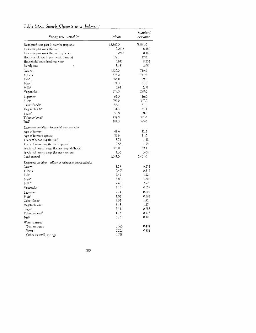
Table 5A-1. Sample Characteristics, Indonesia
StandardEndogenous variables Mean deviation
Farm profits in past 3 months (rupiahs) 13,860.0 75,041.0Illness in past week (farmer) 0.0336 0.180Illness in past week (farmer's spouse) 0.0267 0.161Hours employed in past week (farmer) 37.3 17.81Household boils drinking water 0.932 0.252Family size 5.16 3.95Grains' 1,420.0 749.0Tubers' 373.0 744.0Fish' 166.0 199.0Meat' 34.3 81.6Milk, 6.64 22.0Vegetables' 379.0 290.0Legumes' 67.0 116.0Fruit' 196.0 347.0Other Foodsa 96.1 83.4Vegetable Oila 31.3 34.1Sugar' 93.8 88.0Tobacco-betelb 237.0 382.0Fuelb 282.0 383.0
Exogenous variables-household characteristicsAge of farmer 42.6 12.2Age of farmer's spouse 36.0 11.0Years of schooling (farmer) 3.71 3.10Years of schooling (farmer's spouse) 2.58 2.79Predicted hourly wage (farmer, rupiah/hour) 103.0 59.1Predicted hourly wage (farmer's spouse) 4.30 3.04Land owned 1,047.0 1,401.0
Exogenous variables-village or kabupaten characteristicsGrain' 1.28 0.213Tubers' 0.493 0.315Fish, 3.41 1.22Meat' 8.80 2.20Milk, 7.65 2.72Vegetables' 1.15 0.652Legumes' 2.24 0.807Fruit' 1.07 0.582Other foods, 4.57 1.82Vegetable oil' 5.18 1.17Sugar' 2.33 0.288Tobacco-betel' 1.22 0.378Fueld 6.20 8.10Water sources
Well or pump 0.575 0.494River 0.203 0.402Other (rainfall, spring) 0.778
180
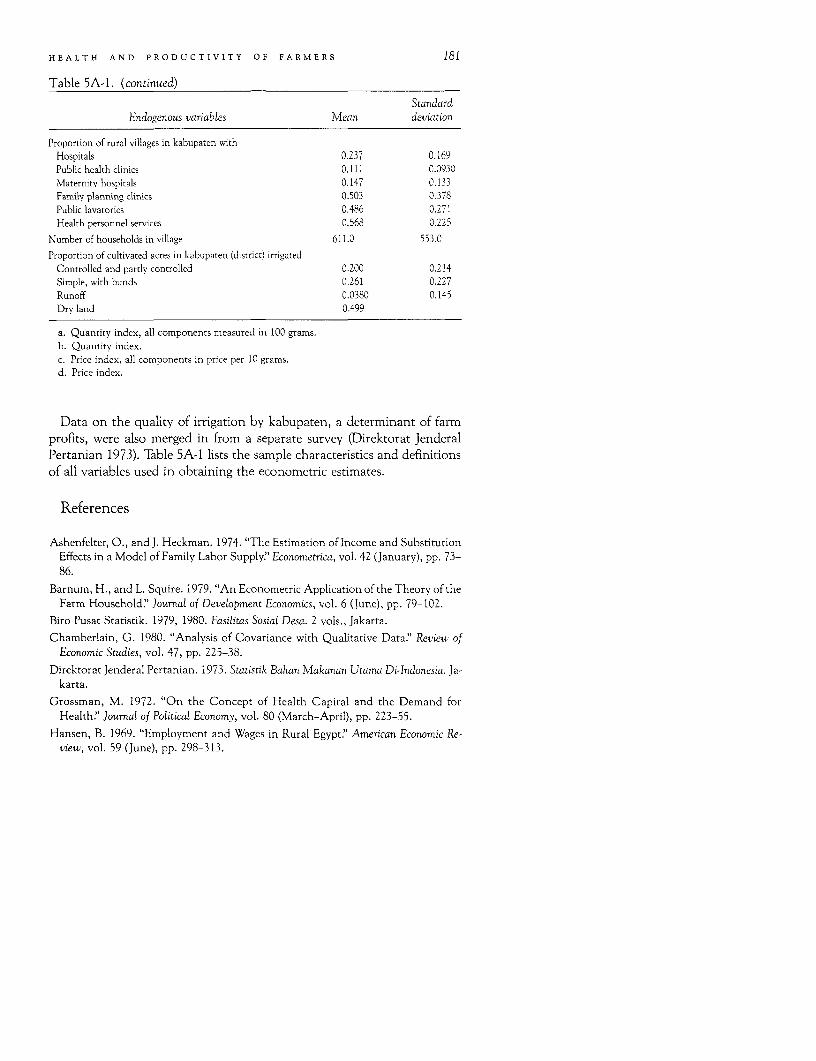
HEALTH AND PRODUCTIVITY OF FARMERS 181
Table 5A-1. (continued)
StandardEndogenous variables Mean deviation
Proportion of rural villages in kabupaten withHospitals 0.237 0.169Public health clinics 0.111 0.0930Maternity hospitals 0.147 0.133Family planning clinics 0.503 0.378Public lavatories 0.486 0.271Health personnel services 0.568 0.225
Number of households in village 611.0 553.0
Proportion of cultivated acres in kabupaten (district) irrigatedControlled and partly controlled 0.200 0.214Simple, with bunds 0.261 0.227Runoff 0.0380 0.145Dry land 0.499
a. Quantity index, all components measured in 100 grams.b. Quantity index.c. Price index, all components in price per 10 grams.d. Price index.
Data on the quality of irrigation by kabupaten, a determinant of farmprofits, were also merged in from a separate survey (Direktorat JenderalPertanian 1973). Table 5A-1 lists the sample characteristics and definitionsof all variables used in obtaining the econometric estimates.
References
Ashenfelter, O., and J. Heckman. 1974. "The Estimation of Income and SubstitutionEffects in a Model of Family Labor Supply." Econometrica, vol. 42 (January), pp. 73-
86.
Barnum, H., and L. Squire. 1979. "An Econometric Application of the Theory of theFarm Householtd" Journal of Development Economics, vol. 6 (June), pp. 79-102.
Biro Pusat Statistik. 1979, 1980. Fasilitas Sosial Desa. 2 vols., Jakarta.
Chamberlain, G. 1980. "Analysis of Covariance with Qualitative Data" Review ofEconomic Studies, vol. 47, pp. 225-38.
Direktorat Jenderal Pertanian. 1973. Statistik Bahan Makanan Utama Di-lndonesia. Ja-karta.
Grossman, M. 1972. "On the Concept of Health Capital and the Demand forHealth" Journal of Political Economy, vol. 80 (March-April), pp. 223-55.
Hansen, B. 1969. "Employment and Wages in Rural Egypt" American Economic Re-view, vol. 59 (June), pp. 298-313.
182 CASE STUDIES
Leibenstein, H. 1957. Economic Backwardness and Economic Growth. New York: JohnWiley & Sons.
Martin, Terence H. 1983. "Nutritional Consequences of Agricultural DevelopmentProjects: A Survey of the Evidence." Washington, D.C.: World Bank. Processed.
Mirrlees, J. A. 1975. "A Pure Theory of Underdeveloped Economies." In Agriculturein Development Theory. Edited by L. G. Reynolds. New Haven, Conn.: Yale Univer-sity Press.
Mundlak, Y. 1961. "Empirical Production Functions Free of Management Bias." Jour-nal of Farm Economics, vol. 43, pp. 44-56.
Olsen, R. J. 1980. "A Least Squares Correction for Selection Bias." Econometrica, vol.48, no. 7, pp. 1815-20.
Pitt, M. M. 1983. "Food Preferences and Nutrition in Rural Bangladesh" Review ofEconomics and Statistics, vol. 65 (February), pp. 105-14.
Pitt, M. M., and M. R. Rosenzweig. 1985. "Health and Nutrient Consumption acrossand within Farm Households." Review of Economics and Statistics, vol. 67 (May), pp.212-23.
Rosenzweig, M. R. 1984. "Determinants of Wage Rates and Labor Supply Behavior inthe Rural Sector of a Developing Country'" In Contractual Arrangements, Employ-ment and Wages in Rural Labor Markets in Asia. Edited by H. P. Binswanger andM. R. Rosenzweig. New Haven, Conn.: Yale University Press.
Rosenzweig, M. R., and T. P. Schultz. 1982. "Market Opportunities, Genetic Endow-ments and Intra-Family Resource Distribution: Child Survival in Rural India."American Economic Review, vol. 72 (September), pp. 803-15.
-______ 1983. "Estimating a Household Production Function: Heterogeneity, the De-mand for Health Inputs and Their Effects on Birthweight " Journal of Political Econ-omy, vol. 91 (October), pp. 723-46.
Sen, A. K. 1966. "Peasants and Dualism with or without Surplus Labor." Journal ofPolitical Economy, vol. 74, pp. 425-50.
Schultz, T P. 1980. "Estimating Labor Supply Functions for Married Women." In Fe-male Labor Supply. Edited by J. P. Smith. Princeton, N.J.: Princeton UniversityPress.
Stiglitz, J. E. 1976. "The Efficiency Wage Hypothesis, Surplus Labour, and the Distri-bution of Income in L.D.C.'s " Oxford Economic Papers. New Series, vol. 28, pp. 185-207.
Strauss, J. 1982. "Determinants of Food Consumption in Rural Sierra Leone: Appli-cation of the Quadratic Expenditure System to the Consumption-Leisure Compo-nent of a Household-Firm Model." Journal of Development Economics, vol. 11, no. 3,pp. 327-54.
Survai Sosial Ekonomi Nasional (Susenas) Data Tapes. 1978. Biro Pusat Statistik,Jakarta.
Tobin, J., and H. S. Houthakker. 1950-51. "The Effects of Rationing on DemandElasticities?" Review of Economic Studies, vol. 18, pp. 140-53.
6The Demand and Supply of Funds
among Agricultural Householdsin India
Farrukh Iqbal
AGRICULTURAL CREDIT PROGRAMS have become important components ofdevelopment strategy in most developing countries. More than US$30billion in rural credit is now disbursed annually by the governments inthese countries and more than US$5 billion has been spent on such pro-grams by international aid agencies over the past several decades (Adamsand Graham 1981). Since such programs have staked out substantialclaims upon national development budgets, it is important that theircosts and benefits be assessed. Such an assessment will not be possible,however, without a theoretical and empirical understanding of the deter-minants of the demand and supply for funds among agricultural house-holds. This study attempts to contribute toward that understanding.
Several dimensions of the demand-for credit are important for develop-ment policy. For example, there has been considerable technical changein agriculture in the developing countries (especially in populous SouthAsia) in recent decades and it is believed that the pace and spread of suchchange is dependent on the availability of funds and terms of financing. Ifthe momentum of agricultural innovation is to be maintained, its linkwith the borrowing, saving, and investment behavior of agriculturalhouseholds needs to be better understood. Similarly, interest rate policy
Note: This is a considerably revised version of a paper put out originally as Rand Note N-1631-
AID by the Rand Corporation. My research at Rand was supported by Grant no. AID/Otr-1822
from the Agency for International Development. I would like to record my gratitude for the
comments and suggestions of Kenneth Wolpin, Robert Evenson, Surjit Bhalla, Dennis De Tray,
and John Strauss. The views contained herein are to be attributed to me alone and not to any of
the individuals or agencies with whom I have been affiliated.
183

184 CASE STUDIES
could be another important determinant of this behavior and it has cer-tainly been accorded pride of place among relevant policy instruments bypolicymakers in the developing countries. The existing literature (re-viewed in David and Myer 1979) has little to offer in this area, however.A systematic statistical investigation of the interest elasticity of borrow-ing would shed light on many policy debates that have hitherto been con-ducted largely on the basis of conjecture.
This study departs from previous ones in that it analyzes the borrowingbehavior of farmers in the context of an agricultural household model. Asnoted elsewhere in this volume, the main reason for investigating suchmodels is that agricultural households combine in themselves the charac-teristics of both producers and consumers. Their production decisionsand outcomes affect their consumption decisions and outcomes, and viceversa. Up to now, attention has been focused on two activities of farmhouseholds where such interactions are important: the production-consumption of food and of labor. Among others, Barnum and Squire(1979) have demonstrated that the magnitudes of market food and laborsupply and the relevant elasticities with respect to important policy vari-ables depend substantially on whether or not we take an agriculturalhousehold approach to theoretical and empirical analysis. The objectiveof this study is to extend this framework to cover the borrowing and sav-ing behavior of farm households. Such an extension is both realistic andimportant. It is realistic because farmers make borrowing decisions notjust on the basis of market conditions defining their production, but alsoon the basis of their own savings or self-financing capacity (and viceversa). Just as such households supply part of the food and labor that theydemand, so also do they supply part of the funds needed to make invest-ments and intertemporal adjustments in consumption. The extension isimportant because it leads to some empirical results and implications thatare quite different from those available in the literature.
The data for the empirical analysis were obtained from a comprehen-sive national (panel) survey of approximately 3,000 farm households inIndia carried out from 1968 to 1971. This survey was conducted by theNational Council for Applied Economic Research (NCAER). Relevantdetails appear in the text and a general description is provided in theappendix.
Structure and Selected Features of the Model
Basic Structure
The basic structure of a farm-household model (see chapter 2 for de-tails) is as follows: the household is supposed to act as if it were maximiz-
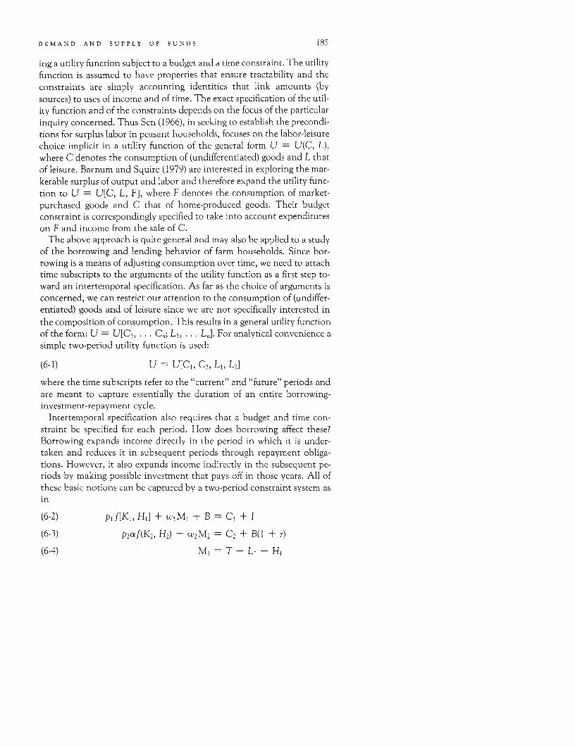
DEMAND AND SUPPLY OF FUNDS 185
ing a utility function subject to a budget and a time constraint. The utilityfunction is assumed to have properties that ensure tractability and theconstraints are simply accounting identities that link amounts (bysources) to uses of income and of time. The exact specification of the util-ity function and of the constraints depends on the focus of the particularinquiry concerned. Thus Sen (1966), in seeking to establish the precondi-tions for surplus labor in peasant households, focuses on the labor-leisurechoice implicit in a utility function of the general form U = U(C, L),where C denotes the consumption of (undifferentiated) goods and L thatof leisure. Barnum and Squire (1979) are interested in exploring the mar-ketable surplus of output and labor and therefore expand the utility func-tion to U = U[C, L, F], where F denotes the consumption of market-purchased goods and C that of home-produced goods. Their budgetconstraint is correspondingly specified to take into account expenditureson F and income from the sale of C.
The above approach is quite general and may also be applied to a studyof the borrowing and lending behavior of farm households. Since bor-rowing is a means of adjusting consumption over time, we need to attachtime subscripts to the arguments of the utility function as a first step to-ward an intertemporal specification. As far as the choice of arguments isconcerned, we can restrict our attention to the consumption of (undiffer-entiated) goods and of leisure since we are not specifically interested inthe composition of consumption. This results in a general utility functionof the form: U = U[CI, . . . C,; LI, . . . LJ. For analytical convenience a
simple two-period utility function is used:
(6-1) U = U[C1, C2, LI, L2]
where the time subscripts refer to the "current" and "future" periods andare meant to capture essentially the duration of an entire borrowing-investment-repayment cycle.
Intertemporal specification also requires that a budget and time con-straint be specified for each period. How does borrowing affect these?Borrowing expands income directly in the period in which it is under-taken and reduces it in subsequent periods through repayment obliga-tions. However, it also expands income indirectly in the subsequent pe-riods by making possible investment that pays off in those years. All ofthese basic notions can be captured by a two-period constraint system asin
(6-2) p1f[KI, Hi] + w1MI + B = C, + I
(6-3) P2olf(K2 , H2) + w2 M2 = C2 + B(1 + r)
(6-4) Ml = T-L - H
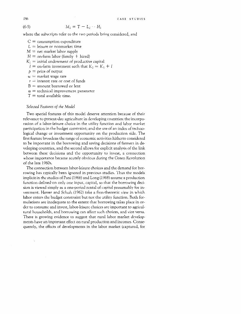
186 CASE STUDIES
(6-5) M 2 =T-L 2 -H2
where the subscripts refer to the two periods being considered, and
C consumption expenditureL leisure or nonmarket time
M net market labor supplyH on-farm labor (family + hired)
K,= initial endowment of productive capitalI on-farm investment such that K2 = K1 + Ip price of outputw market wage rater interest rate or cost of funds
B - amount borrowed or lent
u technical improvement parameterT total available time.
Selected Features of the Model
Two special features of this model deserve attention because of theirrelevance to present-day agriculture in developing countries: the incorpo-ration of a labor-leisure choice in the utility function and labor marketparticipation in the budget constraint; and the use of an index of techno-logical change or investment opportunity on the production side. Thefirst feature broadens the range of economic activities hitherto consideredto be important in the borrowing and saving decisions of farmers in de-veloping countries, and the second allows for explicit analysis of the linkbetween these decisions and the opportunity to invest, a connectionwhose importance became acutely obvious during the Green Revolutionof the late 1960s.
The connection between labor-leisure choices and the demand for bor-rowing has typically been ignored in previous studies. Thus the modelsimplicit in the studies of Pani (1966) and Long (1968) assume a productionfunction defined-on only one input, capital, so that the borrowing deci-sion is viewed simply as a one-period rental of capital presumably for in-vestment. Hesser and Schuh (1962) take a firm-theoretic view in whichlabor enters the budget constraint but not the utility function. Both for-mulations are inadequate to the extent that borrowing takes place in or-der to consume and invest, labor-leisure choices are important to agricul-tural households, and borrowing can affect such choices, and vice versa.There is growing evidence to suggest that rural labor market develop-ments have an important effect on rural production and incomes. Conse-quently, the effects of developments in the labor market (captured, for
DEMAND AND SUPPLY OF FUNDS 187
example, through movements in wage rates), on the demand and supplyof credit should be of interest.
The role of technical change in influencing the demand for credit hasalso been largely ignored in most previous studies in this area. Althoughit is generally agreed that credit availability affects the decision to adoptnew technology (Feder, Just, and Zilberman 1982), it is not known howagricultural technical change affects the demand for credit. One way toapproach this matter is to consider the effects of technical change on farmincomes and productivity. By and large, the technical change experi-enced by agriculture in the developing countries since the early 1960s hasraised average farm incomes and productivity. In particular, the seed-fertilizer-irrigation package of Green Revolution fame has tended to bescale-neutral and income-augmenting in its effects. Now, the greater thevalue of expected future income, the greater the tendency to borrow inanticipation of it. Similarly, the higher the rate of return to capital, thegreater the tendency to borrow and thereby employ more capital. Both ofthese effects can be captured by the use of a measure of investment oppor-tunity or the opportunity to shift from one possible income stream toanother.
In the case of farm households, an improvement in investment oppor-tunities could be thought of as an outward shift of the production-possi-bility frontier. This effect is captured in our model by a parameter, a,which shifts the production function in a manner analogous to Hicks-neutral technical change. Empirically, a is meant to be interpreted as avector containing all the factors that bring about differences in the invest-ment opportunities open to farmers. As such, it should include manage-rial ability, together with soil quality and differences in the availability ofgovernment extension services, irrigation services, and the like. The ac-tual empirical implementation of this hypothesis is discussed later.
The Truncation Issue
Perhaps the most important feature of our model is that it yields a flow-of-funds measure of the demand for credit that is theoretically superior tothe one used in previous studies. This measure is based on the first-periodconstraint (equation 6-2), which can be rewritten as
(6-6) [pif(KI, HI) + w Ml - C1] + B = I
and, by condensing the income terms on the left-hand side into an overallincome term YI, as
(6-7) (Yl-Cj) + B = 1.
188 CASE STUDIES
Our definition of borrowing is now seen to be simply the difference be-tween on-farm investment and current savings:
(6-8) B = I-(Y 1 -C 1 ) or B = I-S.
The difference between this measure and the conventional one can bestbe understood by examining the components of B. From the definition ofsavings, S, as the change in net worth from one period to the next, we canwrite
(6-9) S = I + CD + FA + EL-EB,
where I is on-farm investment, CD is the net change in consumer dura-bles, FA is the net change in financial assets, and EL and EB refer toexternal lending and external borrowing. Substituting for S in (6-8) givesus
(6-10) B = EB-EL-FA-CD.
This indicates that the demand for funds is simply the algebraic sum ofchanges in liabilities (EB - EL), changes in internal borrowing (-FA),and changes in the stock of consumer durables (-CD).
Previous studies have used EB rather than B as their measure of thedemand for credit. This leads to truncation bias, a problem formally akinto that arising in the case of female market labor supply, where nonmar-ket hours and wages (for housewives) are unobserved. In the borrowingcase, because the conventional definition is restricted to EB and does nottake into account borrowing from internal sources (for example, savingsaccounts) or lending, the dependent variable is effectively truncated atzero.
Truncation produces biased coefficient estimates for one or both of tworeasons. Suppose we assume that separating the sample into borrowersand lenders is correct because there are essentially two distinct popula-tions with different behaviors that should be estimated separately. It isthen important that the discrimination between the two populations bequite accurate; otherwise, biases are likely to be produced. In the case ofrural borrowing, it does not seem appropriate to use the level of currentborrowing to distinguish between populations of borrowers and nonbor-rowers, because current borrowing behavior is likely to vary for reasonsthat do not reflect the permanent status of a household. The second,more important, problem is that the assumption that two separate popu-lations exist may not be tenable. There may, in fact, be only one popula-tion, and it may contain some households that choose to borrow andothers that choose to lend in the face of a common set of exogenous deter-minants. Consider the relationship between the interest rate and the
DEMAND AND SUPPLY OF FUNDS 189
amount borrowed. This relationship is a stochastic and not a determinis-tic one-that is, some individuals will borrow more and others will bor-row less, even when faced with the same interest rate. By focusing only onthose who borrow, we increase the likelihood of observing a positive,rather than the expected negative, relationship between these two vari-ables, partly because those who reduce their borrowings by a largeamount (in response to an increase in the interest rate) are more likely toswitch from borrower to nonborrower status and therefore to be ex-cluded from the sample; those who reduce their borrowings by a smallamount are more likely to remain in the sample. The bias produced bystratifying along the dependent variable has been most commonly ob-served and discussed in the literature on the human-capital earningsfunction. In particular, it has been shown that looking at a subsample ofrelatively poor households alone tends to underestimate the true effect ofschooling on earning power.
Interest Rate Endogeneity
Thus far, the model has been developed as if the agricultural householdfaces a capital market in which it can borrow (or lend) all it wants at aconstant, exogenously given, interest rate. This is a convenient assump-tion because it allows us to invoke separability between production andconsumption-related determinants of borrowing-the household firstchooses a production level determined by the point of tangency betweenits production possibility frontier and the market opportunity line; hav-ing fixed a production level, it then borrows or lends to make up thedifference between production income and consumption expenditure. Inmost agricultural household models (for example, Barnum and Squire1979), a similar assumption is typically invoked with respect to the hiringin or out of labor.
The constant exogenous interest rate assumption, however, may not berealistic in the case of rural capital markets in developing countries. Itmight be more realistic to assume that in the informal lending arrange-ments that prevail in such markets, interest rates are household-specificand vary in accordance with household characteristics such as wealthand education. In fact, it can even be argued that the "effective" interestrate charged in the formal rural capital market (that is, cooperative creditsocieties and agricultural development banks) is also household-specific-whereas all borrowers are charged the same nominal rate by law, poorerclients may be subject to higher bribe demands. The possible endogeneityof the interest rate can also be depicted by considering its relationship tothe amount borrowed. There are several reasons why interest rates may
190 CASE STUDIES
vary directly with loan exposure. It is possible, for example, that individ-ual lenders may attach higher risk to larger loans and hence charge higherinterest rates as the loan amount demanded increases. It is also possiblethat households may have to draw funds away from more and more re-warding uses in order to lend more and more; if so, they will have to becompensated by higher and higher returns to lending. This would cer-tainly be a reasonable possibility in informal markets where householdsoften lend and compete, as it were, with professional moneylenders. Inthe case of borrowing from moneylenders, it is quite likely that differentmoneylenders have to be approached as borrowing needs increase, eachbeing more expensive than the previous one. In each of these cases anupward-sloping supply curve would be generated. This possibility has tobe set against the possibility that there may be economies of scale in lend-ing-the larger the loan, the lower the unit costs of administering it andhence the lower the interest charge. Whether an upward or downwardsloping cost of funds schedule is faced is ultimately an empirical matter.What is being asserted here is that agricultural households may face inter-est rates that are a function of household characteristics and loan de-mand and that may not, therefore, be exogenous.
Some Theoretical Results
The incorporation of an endogenous interest rate into the model isstraightforward. It requires replacing r by r(B) in equation (6-3), the sec-ond-period budget constraint. Assume also that r3 > 0 and rB3 < 0, thatis, that the supply-of-funds schedule slopes upward but at a decliningrate-these assumptions keep the model theoretically tractable.
The optimizing problem can now be stated as
(6-1 ') maximize U = UL[C, C2, Li, L21
(6-2') subject to pif(K 1 , HI) + w1M1 + B = C I
(6-3') P2 af(K2, H2 ) + w2 M2 = Cl + B[1 + r(B)]
(6-4') Ml = T -LI - H
(6-5') M 2 = T-L 2 -H 2 .
The optimal amount of borrowing and its variation with respect tochanges in exogenous variables can be derived from the model depictedby (6-1 ')-(6-5') in standard fashion by specifying the appropriate Lagran-gian and solving the differentials of the first-order conditions via Cra-mer's Rule. Readers interested in the algebraic exercises may turn to Iqbal(1981a). For the purposes of this paper, only the consequences of interest
DEMAND AND SUPPLY OF FUNDS 191
rate endogeneity and the coefficient signs derived from the model areelaborated.
One consequence of interest rate endogeneity is that the optimizingcondition for borrowing changes: that the marginal product of capital nolonger be equal to the interest rate but that it be equal to the term r(B) +BrB. The demand function for borrowing takes the form B = B[E, xi, r(B)Y,where E denotes all farm specific endowments, xi denotes prices of differ-ent inputs and outputs except capital, and r(B) denotes the endogenousprice of capital. A typical coefficient in the borrowing function could bewritten as
dB/dx, = dB/dxilr + aB/ara-Fr/j.It has been the practice to estimate agricultural household models by firstestimating the production-profit function, next estimating a system ofconsumption-demand equations, and then integrating the results of thetwo to obtain full coefficient and elasticity values. This practice cannot befollowed if the interest rate is considered endogenous because the produc-tion and consumption parts of the model are not theoretically separa-ble-the interest rate affects both decisions and is jointly determined bythese decisions. An alternative way to estimate this model is to adopt atwo-stage simultaneous-equations procedure involving a borrowing func-tion and an interest rate function as the structural equations. The exactprocedure followed and the reasons for it are discussed in a later section.
The following coefficient signs are derived from the model: dB/dr < 0for B > 0; dB/dpI < 0; dB/dp2 > 0; dB/dux > 0. The signs for dB/dw1,dB/dw2, and dB/dK, remain ambiguous. These results depend essentiallyon what may be called period-specific income effects. Thus, when varia-tions in an exogenous factor cause income to rise in period 1, the house-hold transfers some of this increase to consumption in period 2 by reduc-ing its borrowings; increases in period-2 income similarly lead to anincrease in borrowing as the household attempts to raise period-1 con-sumption. Thus dB/dct and dB/dp2 are positive in sign because increasesin ca and P2 amount to increases in second-period income, whereas dB/dpl is negative because an increase in Pi amounts to an increase in cur-rent-period income.
The results for dB/dw1 and dB/dw2 involve, in addition, what could becalled leisure substitution effects. An increase in wl, for example, in-creases the cost of Li, and if we assume LI and L2 are substitutes, theconsequence is a decrease in LI and an increase in L2. This intertemporaltransfer of leisure is accomplished by a decrease in borrowing, which re-duces repayment claims in period 2 and thereby permits greater consump-tion of goods and leisure. The case of an increase in w2-which, other
192 CASE STUDIES
things being equal, leads to an increase in borrowing-is similar. It shouldbe noted that the signs of dB/dw, and dB/dw2 also depend on whetherthe household is a net labor importer or exporter and also on the rela-tionship of on-farm labor (HI, H2) to leisure. Thus, in the case of an em-ployed but landless household, where Ml and M2 are always positive andHI = H2 = 0, it can be shown that dB/dw1 < 0 and dB/dw2 > 0.
The expression for dB/dK, contains both income effects and is there-fore ambiguous. An increase in K1 causes first-period income to rise(through the production-function relationship) and thereby induces a de-crease in borrowings. It also causes second-period income to rise (since K,is included in K2) and thereby induces an increase in borrowings. Thetwo effects oppose each other. Alternative models, by failing to take intoaccount future-period effects, conclude that an increase in assets musthave a negative effect on borrowing. Also, the expression dB/dKi con-tains terms pertaining to the cross-partial relationship of the arguments ofthe production function, and hence the sign will depend on the specificsof these relationships as well.
Data, Estimation Issues, and Empirical Results
Discussion of the Variables
The theoretical analysis calls for the following regressors in the borrow-ing function: initial endowment, current and expected wage, current andexpected output prices, investment opportunity measures, and the mar-ginal cost of borrowing. Since the model is specified intertemporally, weshould also include measures of life cycle stage as independent determi-nants. In the empirical analysis that follows, output prices are not in-cluded under the assumption that prices for identical outputs ought to beinvariant in the cross section. The same argument could have been ap-plied to remove input costs from consideration. There is, however, con-siderable geographical immobility in factor markets in India so that varia-tions in both wages and interest rates are observed in the cross section.The variables actually used in the empirical analysis (table 6-1) are dis-cussed below.
Borrowing
The data collected by NCAER provide information on each of thecomponents of B, that is, external borrowing and lending, changes infinancial assets, and changes in consumer durable stocks. The measure of
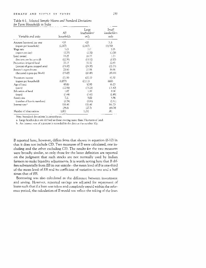
DEMAND AND SUPPLY OF FUNDS 193
Table 6-1. Selected Sample Means and Standard Deviationsfor Farm Households in India
Large SmallAll landholdersa landholders
Variable and units households only only
Amount borrowed per year 420 453 318(rupees per household) (2,207) (2,467) (1,050)
Wage rate 3.23 3.21 3.26(rupees per day) (1.25) (1.31) (1.08)
Land owned 11.25 14.33 1.73(hectares per household) (12.95) (13.52) (0.87)
Proportion irrigated land 33.15 33.32 32.65(percent of gross cropped area) (23.92) (24.30) (22.71)
Research expenditures 25.60 27.58 19.46(thousand rupees per block) (15.65) (16.48) (10.61)
Transitory income 371.90 470.30 67.30(rupees per household) (1,872) (2,111) (660)
Age of head 48.80 50.90 45.20(years) (12.90) (13.20) (11.40)
Education of head 1.07 1.09 0.98(years) (1.44) (1.43) (1.48)
Family size 7.51 9.00 5.96(number of live-in members) (3.74) (3.93) (2.51)
Interest rate' 155.40 153.40 161.70(39.6) (37.7) (44.74)
Number of observations 1,602 1,211 391
Note: Standard deviations in parentheses.a. Large landholders are defined as those owning more than 3 hectares of land.
b. An interest rate of y percent is recorded in the data as the number ION.
B reported here, however, differs from that shown in equation (6-10) inthat it does not include CD. Two measures of B were calculated, one in-cluding and the other excluding CD. The results for the two measureswere broadly similar, so only those for the latter definition are reportedon the judgment that such stocks are not normally used by Indianfarmers to make liquidity adjustments. It is worth noting here that B dif-fers substantially from EB in our sample-the mean level of B is one-thirdof the mean level of EB and its coefficient of variation is two and a halftimes that of EB.
Borrowing was also calculated as the difference between investmentand saving. However, reported savings are adjusted for repayment ofloans such that if a loan was taken and completely repaid within the refer-ence period, the calculation of B would not reflect the taking of the loan
194 CASE STUDIES
at all. Direct information on repayments is not available for many in thesample. Hence the component approach is preferred. It should also benoted that the data do not allow for a complete account of a household'sflow of funds. For example, no data are available on changes in the stocksof gold and jewelry. This could be an important item in the balancesheets of rural households in a country such as India and its omissioncould result in a significant measurement error. To the extent, however,that there is no reason to expect the error to be nonrandomly distributed,the coefficient estimates need not be biased.
Wage Rates
Because the NCAER data do not contain individual wage information,the average district agricultural wage per day for males (for 1970-71) isused as the measure of the opportunity cost of leisure. The theoreticalanalysis calls for an expected future wage in addition to the current wage;it is assumed that the future wage rate is simply a multiple of the currentone. This eliminates the separate role of the unobservable variable, butthe coefficient of w, must now be interpreted as the sum of the effects ofboth current and expected wages.
Initial Endowment
It is common to use a monetary measure of wealth or assets owned (forexample, land, livestock, implements) as a proxy for endowments (seePani 1966; Long 1968). If, however, we take the point of view that theasset accumulation and borrowing decisions are jointly made over thecourse of a household's life cycle, such a measure of current wealth be-comes inappropriate in the framework of an ordinary least squares equa-tion. The proxy that comes closest to measuring initial endowment and isalso less likely to introduce simultaneous bias is probably a physical mea-sure of the total land owned by the farm household. Owing to differencesin soil quality and terrain, however, the physical measure alone will notreflect the differences in endowment value across Indian farms.
It is also possible that the use of a physical measure of initial endow-ment rather than a monetary one may introduce some error. The qualityof land varies so much in India that a 10-hectare plot in, say, the Punjabarea may reflect a different endowment position than a plot of the samesize in, say, remote Madhya Pradesh. A monetary measure would capturedifferences in land quality, whereas a physical one does not. To the ex-tent that the value of land is affected by choices regarding irrigation and

DEMAND AND SUPPLY OF FUNDS 195
fertilizer use among other such endogenous land improvement measures,however, a monetary measure might introduce simultaneity bias in thesort of life cycle framework we are using here. For this reason, we haveretained the physical measure in spite of its possible disadvantages.
To account for such differences a district-level index of soil quality asmeasured by the proportion of irrigated area to total area is included asan additional regressor. Because this variable is not measured at the indi-vidual farm level, it is not as likely to involve simultaneity bias as a moredirect measure.
Investment Opportunity Measures
The investment opportunity index is supposed to capture differences inexpected future income. These differences could arise from two sources:environment-specific characteristics and farm-specific characteristics.Among the former one could list differences in soil quality and the avail-ability of credit, extension services, and fertilizer across regions. Abroader measure might be the magnitude of exogenous government ex-penditures on rural development (by region) in general and on agricul-tural technical change in particular. An approximation to such a measureis the level of annual expenditures on research on principal crops by eachstate and the federal govenment. The underlying assumption is that cropresearch expenditures in a region produce new investment opportunitieswithin a few years and also signify a commitment by the government tocontinued technical improvements in that region.
The research expenditure figures used here pertain to 1968 and aretaken from Evenson and Kislev (1975). Total research expenditures aredivided by the number of community development blocks in each state toobtain a measure of research intensity on a per farm basis. Communitydevelopment blocks are so demarcated as to contain an equal number offarms and they form the basic extension and village development units inIndia.
Among farm-specific characteristics that denote differences in invest-ment opportunities and expected future income, one could list manythings, including natural ability considerations and some investmentsmade by the farmer, such as the adoption of modern inputs. The problemwith measures such as modern inputs is that the adoption decision andthe borrowing decision may be jointly determined and thus a simultane-ity bias issue would arise. One measure that is not likely to involve asimultaneity bias and, at the same time, might even capture differences in
196 CASE STUDIES
natural ability, is the education (investment in human capital) of thefarmer. Better-educated farmers might be expected to face brighter fu-tures and be better able to exploit technical opportunities when theyarise. Education can be treated as exogenous because the original decisionto invest is most likely to have been taken by a person other than therecipient of the education (for example, by the farmer's father)-mostfarmers in India do not acquire much education (sample mean is 1.07years) and the little they do obtain is acquired in early years rather thanin adulthood. Two measures are therefore used to capture differences inexpected future incomes across farms: crop research expenditures (bystate) and farmer's education.
Life Cycle Variables
Age of the head of household is included as a measure of the farmhousehold's life cycle stage. In case age alone is not sufficient, we haveadded another variable, family size, which, in rural contexts, displays aregular pattern over the household's life cycle and can therefore serve as aproxy for it. Family size could also serve as a proxy for expected futureincome: a large family size would denote a family that expects a largerflow of income in the future as the children grow up and begin to work.Since family size is clearly a determinant of current income also, its effecton borrowing cannot be theoretically predicted.
Transitory Income
We have included a measure of transitory income in our analysis toaccount for variation in the demand for funds that arise simply from tran-sient and unanticipated variations in income. This variable is calculatedas the difference between current income and permanent income, wherethe latter is calculated as a weighted average of the incomes of the pastthree years. The technique used to derive the weights is employed byBhalla (1980) in an analysis of the savings behavior of Indian farmersbased on the same data set that is used here. The equation for permanentincome, Yp, is: Yp = 0.43Y3 + 0.32Y2 + 0.25Y1, where Y3 refers tocurrent income and the others to past incomes. Bhalla reports that therole of Yp in savings behavior is not greatly affected by the choice of dis-count rates.
Special characteristics of our data set affect the manner in which weintroduce the marginal cost of borrowing into the demand for funds re-gression. This issue is discussed in the next section.
DEMAND AND SUPPLY OF FUNDS 197
The Interest Rate Function
Information on interest rates paid is available only for those householdsin our sample that report positive levels of external borrowing-thisamounts to 1,080 households out of a total of 1,602 for which the non-truncated flow-of-funds measure of borrowing can be calculated. The re-sulting problem of missing interest rates for a large fraction of the sampleis similar to the missing-wage (for housewives) problem in the labor-sup-ply literature, and the solution adopted here is one that has been widelyused in that literature. For nonreporters, interest rates are imputed froman interest rate function regressed over a set of personal characteristicsand a set of locality-specific characteristics that denote differences intransaction costs of supply across districts and villages. An advantage ofthis procedure is that it accommodates interest rate endogeneity since theinterest rate enters as a predicted variable rather than a directly reportedvariable. Since this "conventional" regression is based only on informa-tion from the subsample that did report positive levels of external bor-rowing, the estimates could be subject to selection bias resulting from theconfounding of the behavioral function relating the interest rate to itsdeterminants with the sample-selection function relating the probabilityof borrowing to its determinants. This possibility is ignored in the presentanalysis.
Table 6-2 presents the interest rate equation. Since the purpose ismainly to obtain an instrumental variable and since a fuller discussion ofsuch an equation is available elsewhere (Iqbal 1981b), the discussion hereis brief. The dependent variable in table 6-2 is the highest nominal inter-est rate reported by a household from among all its current loans. Thisshould come closest to being a measure of the current marginal cost ofborrowing for the relevant household. It is an inexact measure of the lat-ter, however, to the extent that significant "other" costs of borrowingexist that are not captured by the nominal rate. Some evidence in theliterature, for example, suggests that small farmers in particular face fairlyhigh unobserved extra costs of borrowing in the form of bribes, fees tointermediaries, and the like, when applying for formal sector loans (Ad-ams and Nehman 1979).
As far as the independent variables are concerned, all included vari-ables, except transitory income, can be justified in terms of their affectingthe costs of lending in an uncertain environment. Transitory income isused as an identifying variable since it affects borrowing but not the inter-est rate. Similarly, the following four variables are used as identifiers onthe assumption that they affect the interest rate but not the individual
198 CASE STUDIES
Table 6-2. Interest Rate Equation for Farm Households in India
t-statistic(absolute
Variable Coefficient value)
Intercept 183 (17.1)Land owned -0.19 (1.96)Proportion irrigated land -0.19 (2.10)Research expenditures -1.00 (2.42)Wage rate 16.31 (1.78)
Education of head -10.22 (4.40)Age of head -0.0004 (0.52)Family size 3.12 (1.18)Source of loana -58.21 (10.82)Existence of bank' -14.10 (1.94)
Distance to market 0.39 (2.40)Village population. -0.008 (4.80)Transitory income 0.0005 (0.66)R2 0.18Number of observations 1,080
Note: A y percent interest rate is recorded in the data as the number lOy.a. Dummy variable, I is borrowed from official sources, 0 otherwise.b. Dummy variable, I if bank present in village, 0 otherwise.
amounts borrowed: source of loan, existence of bank, distance to market,and village population. The rationale for including the source-of-loanvariable is that official lending agencies (for example, banks or coopera-tive credit societies) are constrained to give subsidized loans and thereforethose who can borrow from such agencies pay lower interest rates. Be-cause the selection of clients by such agencies is based on certain cred-itworthiness indicators, this variable could also be a proxy for some of thecosts of lending pertaining to risk. The mere presence of such agencies ina village can reduce average interest rates partly by reducing possible mo-nopoly power margins of moneylenders. Residents of a village can benefitfrom the mere existence of a bank or cooperative even if they do notthemselves borrow from such agencies. This effect is captured by thedummy variable, which registers the existence or absence of banks in therespondent's village.
Distance of village from markets and towns can be thought of as affect-ing the riskiness of farming in the village or even the opportunity costsincurred by moneylenders in lending in such villages. Village size can bethought of as affecting the administrative cost of lending. The larger the
DEMAND AND SUPPLY OF FUNDS 199
village, the greater the demand for funds and the easier for the money-lender to spread his overhead costs across loans.
The remaining variables can be thought of as affecting the costs of lend-ing pertaining to risk and are also determinants of how much is bor-rowed. From a lender's point of view, such variables as quantity and qual-ity of land owned, age and education, wage faced, and the prospect ofincome growth through technical change all ought to be indicators ofhow risky it is to lend to a particular farmer.
The interest rate function regression results are broadly consistent withthe arguments made above. All included variables save transitory in-come, age, and family size turn out to be significant in their effects. Inter-est rates imputed from the results shown in table 6-2 are used in estimat-ing the borrowing functions reported in table 6-3.
Table 6-3. Borrowing Functions for Farm Households in IndiaVariable All households Large farmers Small farmers
Intercept 625.80 972.10 -521.32(1.91) (2.29) (1.34)
Land owned -14.84 -16.65 24.32(3.24) (3.05) (0.39)
Wage rate -158.20 -171.41 -114.50(2.56) (1.90) (2.08)
Proportion irrigated land -4.98 -6.82 2.24(1.86) (2.00) (0.82)
Research expenditures 26.44 29.46 12.61(5.60) (4.41) (2.38)
Education of head 68.33 60.98 83.24(1.48) (1.00) (1.89)
Age of head 0.84 1.31 0.30(1.10) (1.11) (0.88)
Family size 62.63 62.35 74.47(4.25) (3.52) (3.57)
Interest rate -3.23 -5.11 2.14(2.02) (2.32) (1.52)
Transitory income -0.23 -0.23 -0.27(7.77) (6.72) (3.36)
R' 0.08 0.08 0.09Number of observations 1,602 1,211 391F Ratio 16.70 13.17 5.00
Note: Absolute values of asymptotic t-statistics are in parentheses. Large landholders aredefined as those owning more than 3 hectares of land. The rest are considered small farmers. Theinterest rate is predicted (as an instrumental variable) from the regression reported in table 6-2. Ay percent rate is recorded in the data as the number lOy.

200 CASE STUDIES
Borrowing Function Results
Table 6-3 presents results for identical borrowing functions estimatedfor three different sample groups. The results in the first column are for allhouseholds for which a measure of B could be calculated as shown byequation (6-10). The second and third column results pertain to subsam-ples from this group obtained by separating the large landholders fromthe small ones. The purpose of this segmentation is to check the robust-ness of the results reported in column 1 and see if any nonlinearitiesmight be present.
Land owned, the proxy for initial endowment, is negatively related tothe demand for funds. This is also the case for proportion of irrigatedland, the proxy for the quality component of initial endowment. Al-though the theoretical analysis offered no unambiguous predictions forthis effect, the general presumption in the literature (Pani 1966; Long1968) is that of a negative relationship. None of the relevant empiricalstudies in this area have demonstrated such a relationship however; in-deed, most studies have tended to find a positive sign for this effect, afinding typically explained by an appeal to the effects of multicollinearityor scale. The results from this analysis suggest the incorrect definition ofthe dependent variable may have been responsible for the anomalousresults reported in previous studies.
The very different results obtained for small farmers-the coefficient onland owned is positive but quite insignificant-could indicate the pres-ence of a nonlinearity. It is possible that land ownership does not affectthe demand for credit noticeably until a sort of threshold farm size isreached, after which self-financing capability is strengthened and exter-nal borrowing needs lessen. An alternative explanation of the differencein statistical significance of the coefficient on "land owned" is that itarises from the segmentation procedure that sharply reduces the rangeover which this variable can move for small farmers while allowing alarger range in the case of large farmers. If the first explanation is valid, wecould draw an implication for land reform policy to the effect that redis-tribution would lead initially to an increased demand for funds thatwould have to be accommodated by an increased inflow of funds fromoutside the rural sector. If such an inflow is not forthcoming from theprivate sector, say, because of the high risks involved in lending to smallfarmers, it is possible that there will occur both a rise in informal ruralinterest rates and a drop in rural investment. A reformist governmentmight therefore need to link its redistribution strategy with an expansionof official lending in the rural sector.
DEMAND AND SUPPLY OF FUNDS 201
The wage rate effect is negative and, with an elasticity of 1.22, quitestrong. This effect does not change when the sample is separated intosmall and large farmers. It is hard to offer a clear explanation for thisresult. The theoretical model contains no unambiguous prediction forthis effect and, at the empirical level, it has not been possible to distin-guish either between current and expected wages or between labor-im-porting and labor-exporting households. Perhaps the most that can besaid for the moment is that interactions between the labor market andthe credit market appear to be empirically detectable in the latter: bothinterest rates and the demand for credit are affected by the district-leveldaily agricultural wage rate. The results support the view that factor mar-ket interactions are important, a view also stressed in the slightly differentcontext of the landlord-tenant relationship by Bardhan (1980) and Bra-verman and Srinivasan (1980). Policy implications cannot be drawn, how-ever, because it has not been possible to trace the exact linkages involved.
Both research expenditures and the education variable are positivelyrelated to the demand for funds, although the latter is not uniformly sig-nificant. This may be interpreted as confirming that increases in expectedincome owing to the prospect of technical change in agriculture leadfarmers to increase their demand for credit. It might also be noted thatthe proxies used here reduce the interest rates faced by farmers (see table6-2). Thus, there is evidence that the rural credit market is affected byagricultural technical change (and the ability to profit from such change)on both the demand and the supply sides. These findings are consistentwith the view that the sort of technical change that has been associatedwith the Green Revolution (which was based on fertilizer and new seedvarieties for wheat and rice) is risk-reducing in nature. Borrowers appar-ently see the prospect of higher future earnings on the average and henceincrease their demand for funds. Lenders apparently see a similar pros-pect for those of their clients who are in a position to benefit from suchtechnical change because of their location in an area receiving high levelsof government funds for agricultural research and also because of theirability to cope with the new opportunities being offered.
It might be noted that even small farmers raise their demand for funds ifthey happen to be located in a state with higher levels of crop researchexpenditures, although, in elasticity terms, their response is less strong(1.8 versus 0.8). This could suggest an interaction between land size andthe ability to benefit from agricultural research and technical change.When an interaction term was specified directly, however, it turned outnot to have a significant coefficient (results not shown here). Finally, wenote that education appears to play a stronger role for small farmers thanit does for large farmers with respect to stimulating demand for funds.
202 CASE STUDIES
Of the two life cycle variables included, only family size is consistentlysignificant. The larger the family size, the greater the household's demandfor funds. One could interpret this as indicating that relatively largerhouseholds have relatively higher present consumption requirements orrelatively higher levels of expected future income-both of these factorswould raise the household's desire to borrow now and pay later. Thisinterpretation is also consistent with the results of a related study (Iqbal198 1c) in which family size is shown to be negatively related to householdsavings. The results are consistent across farm size groups. Both large andsmall farmers display similar behavior as far as the borrowing-family sizeconnection is concerned, and thus it appears that the results are robust.For small farmers, in fact, this connection seems especially important: thedemand for funds rises by 1.4 percent for every 1 percent increase in fam-ily size. (Age was also entered in squared form so as to pick up the humppattern expected from life cycle savings theory; neither age nor agesquared was significant in any regression.)
The interest rate effect is quite revealing. It is significantly and stronglynegative for all households taken together and for large farmers takenseparately. It is positive, although not significant, for small farmers. Sev-eral comments are in order. First, it should be noted that the high level ofsignificance obtained for this variable in the full sample regression standsin contrast to the generally inconclusive results obtained in other studies.Neither Pani (1966) nor Long (1968), for example, find uniformly signifi-cant or strong interest rate effects on borrowing. Second, the strength ofthis effect, as measured by an elasticity of 1.2, suggests that interest ratescan be an important policy instrument in influencing the level of debtheld by farmers. Third, the pattern of response across size groups suggeststhat large farmers are more sensitive to interest rate changes; hence, in-creases in the interest rate are more likely to drive large farmers out of thecredit market. This has implications for official credit policy: by raisingthe official or formal interest rate, the government can improve efficiency(by coming closer to the market rate of interest) and equity (since therelative participation of small farmers in the concessional credit schemeswill increase as large farmers drop out disproportionately).
It is worth noting briefly the differences between the results reportedhere and those obtained from an alternative regression (see Iqbal 1983) inwhich the interest rate is entered exogenously and the dependent variableis defined conventionally as EB rather than B. In this case, all coefficientsare biased toward zero (relative to the coefficient values reported incolumn 1 of table 6-3), as is to be generally expected in regressions involv-ing truncated dependent variables. Two results are especially damaging tothe conventional case. The interest rate coefficient is positive (though not
DEMAND AND SUPPLY OF FUNDS 203
significant) in contradiction of theoretical prediction. The coefficient onland owned (proxy for initial endowment) is also positive (and signifi-cant), in contradiction of general expectation if not of theoretical predic-tion.
The R2 coefficients obtained in the regressions reported in table 6-3 areall uniformly low. Alternative specifications were tried to improve the fit:these consisted mainly of employing alternative proxies for investmentopportunity and regional dummies. The latter improve the R2 to about0.16 but pose new problems. It is difficult to interpret the economic mean-ing of a regional dummy in the absence of specific information about eachregion. In some cases the regional dummies appear to be conveying thesame information that our other aggregate variables, wage levels, and ag-ricultural research expenditures, convey. Alternative functional formswere not particularly helpful, either. Reasons for the low R2 comparedwith levels obtained in previous studies include the fact that the presentstudy is based on household-level observations, whereas previous oneshave been based on aggregate observations and the fact that the rede-fined dependent variable, B, turns out to have a coefficient of variationabout two and a half times that of the conventional dependent variable,EB.
Summary
In this study the borrowing behavior of farmers in rural India was in-vestigated within the context of the agricultural household modelingframework. It is shown here that this framework suggests two departuresfrom previous analyses that are both realistic and empirically important.The first consists of a redefinition of the demand for funds so as to takeinto account the possibility of self-financing and the second involves con-sideration of the cost of borrowing as an endogenous variable. Bothchanges lead to empirical results more in accord with theorv than ob-tained in earlier studies. Generally speaking, the following factors appearto influence developments in the rural finance market as far as both thedemand for funds and the determination of interest rates are concerned:labor market developments as captured by the agricultural wage rate, ag-ricultural technical change as indicated by the level of crop research ex-penditures, life cycle stage of the household as measured by current familysize, and farm-specific characteristics such as quantity and quality of landowned. It is also shown that interest rates have an important effect onamount borrowed and that this effect varies across farm size in a mannerthat suggests that raising formal interest rates may succeed in increasing
204 CASE STUDIES
the relative participation of small landowners in the official concessionalloan market.
Appendix: Data and Sample
In 1968-69, the National Council of Applied Economics Research(NCAER) undertook a national survey, known as the Additional RuralIncomes Survey, of approximately 5,000 agricultural households in India.This survey was repeated in 1969-70 and 1970-71 on the same house-holds, but in the final year a core group of approximately 3,000 cultivat-ing households were asked additional questions regarding borrowing,lending, interest rates, and interaction with formal lending agencies. Thesampling design of the survey resulted in oversampling of rich house-holds.
The present analysis is based on the core sample of households thatcomprised cultivators in 1970-71. Some exclusionary restrictions wereapplied to this group. Households with savings rates greater than 75 per-cent were excluded to eliminate some cases of logical inconsistency (sav-ings greater than income, which implies negative consumption) and alsoto eliminate some cases where transcription errors appeared to be highlyprobable. These restrictions reduced the working sample to 2,912 obser-vations.
Three categories can be distinguished within this group: the first andsecond comprising those households reporting positive (1,080) and zero(522) levels of external borrowing and the third those for which the rele-vant information is missing (1,310). The present analysis is based on asample size consisting of only the first two categories. Since the exclusionof the third category could have involved censoring problems, we also ranregressions over a larger sample by assuming that the third category alsoconsisted of zero-level borrowers. The results obtained were roughly simi-lar in terms of signs and t-statistics to those reported here. Some elastici-ties change considerably, however. In particular, the interest elasticity ofborrowing was found to be much greater in the larger sample.
References
Adams, D., and D. Graham. 1981. "A Critique of Traditional Agricultural Projectsand Policies." Journal of Development Economics, vol. 8, pp. 347-66.
Adams, D. W., and G. 1. Nehman. 1979. "Borrowing Costs and the Demand forRural Credit." The Joumal of Development Studies, vol. 15, no. 1 (January), pp. 165-76.

DEMAND AND SUPPLY OF FUNDS 205
Bardhan, P. K. 1980. "Interlocking Factor Markets and Agrarian Development: AReview of Issues." Oxford Economic Papers, vol. 32, no. 1, pp. 82-98.
Barnum, H., and L. Squire. 1979. A Model of An Agricultural Household. Washington,D.C.: World Bank.
Bhalla, S. S. 1980. "The Measurement of Permanent Income and Its Applications toSavings Behavior." Joumal of Political Economy, vol. 88, no. 4, pp. 722-44.
Braverman, A., and T. N. Srinivasan. 1980. "Credit and Sharecropping in AgrarianSocieties." Joumal of Development Economics, vol. 9, no. 3, pp. 289-312.
David, C. C., and R. L. Myer. 1979. A Review of Empirical Studies of the Demand forAgricultural Loans. Economics and Sociology Occasional Paper no. 603. Ohio StateUniversity, Columbus.
Evenson, R. E., and Y. Kislev. 1975. Agricultural Research and Productivity. New Ha-ven, Conn.: Yale University Press.
Feder, G., R. Just, and D. Zilberman. 1982. Adoption of Agricultural Innovations inDeveloping Countries: A Survey. World Bank Staff Working Paper no. 542. Washing-ton, D.C.
Hesser, L. F., and 0. C. Schuh. 1962. "The Demand for Agricultural MortgageCredit." Journal of Farm Economics, vol. 44, no. 5, pp. 1583-88.
Iqbal, F. 1981a. "The Demand and Supply of Funds among Agricultural House-holds." Ph.D. dissertation, Yale University, New Haven. Processed.
. 1981b. "Dualism, Technical Change, and Rural Finance Markets in Develop-ing Countries." Rand Note N-1723-AID. Santa Monica, Calif.: Rand Corporation.
. 1981c. "Rural Savings, Investment and Interest Rates in Developing Coun-tries: Evidence from India." Rand Note N-1763-AID. Santa Monica, Calif.: RandCorporation.
. 1983. "The Demand for Funds among Agricultural Households: Evidencefrom Rural India." Joumal of Development Studies (October), vol. 20, no. 1, pp. 68-86.
Long, M. G. 1968. "Why Peasant Farmers Borrow." American Journal of AgriculturalEconomics, vol. 50, no. 4, pp. 991-1008.
Pani, P. K. 1966. "Cultivator's Demand for Credit: A Cross-Section Analysis." lnter-national Economic Review, vol. 7, no. 2, pp. 176-203.
Sen, A. K. 1966. "Peasants and Dualism with or without Surplus Labor." Journal ofPolitical Economy, vol. 74, pp. 425-50.
7Simulating the Rural Economyin a Subsistence Environment:
Sierra Leone
Victor E. Smith and John Strauss
FOR POLICY PURPOSES, we often estimate the effects on household behaviorof exogenous changes in prices and other economic variables by usingpoint elasticities for a representative household (see chapter 4). Micro-simulation offers an alternative approach that may be preferred for sev-eral reasons. First, this method takes full account of nonlinearities in themodel and of the fact that each household faces a different set of indepen-dent variables and that therefore response elasticities vary among house-holds. It also allows us to see how outcomes vary when elasticities changeas price and other parameters go outside the range of the point estimates.Second, several prices can be varied at once, even though a change inonly one price may alter elasticities for several commodities-this is animportant advantage when examining general equilibrium effects. Andfinally, microsimulation is ideally suited for analyzing the distribution ofthe effects of economic policies, especially when the simulation is at thelevel of individual households.'
If effects upon the poor are particularly important, microsimulation al-lows us to classify the households so as to bring out those effects. Further-more, effects that depend upon the distribution of households within theclass are not lost because we look only at a representative household.(Those effects can be important. The distribution of low-expenditurehouseholds about their mean differs greatly from that for the high-ex-penditure households.) These advantages of microsimulation are illus-trated in this chapter by an analysis of household data from Sierra Leone.
Note: The research on which this paper is based was funded under USAID Contract No. AID/
DSAN-C-0008.
206

MICROSIMULATION OF THE RURAL ECONOMY 207
A Comparison of Microsimulationand Direct Population Estimates
Rural households in Sierra Leone are poor. In 1974-75, the mean an-nual expenditure per capita in our sample was 90 Leones (one Leoneequaled U.S.$1.10 at that time), of which 24 percent was spent for riceand 67 percent on all food (table 7-1). But some households are muchpoorer than others. Average per capita expenditure among the 32 per-cent of the sample households that had total annual expenditures below350 Leones was only 49 Leones. Calories available per capita in thatgroup were at an extremely low level-1,1 90 per day.
Under these circumstances, it is vitally important to know how the en-ergy content of rural diets would change if Sierra Leone should decide toraise producer prices for rice in order to reduce the use of foreign ex-change for rice imports. We begin by establishing a benchmark-simula-tion estimates of per capita production and consumption at 1974-75prices.
The model is a separable agricultural household model (see part 1, ap-pendix). The commodity-demand and household labor-supply equations
Table 7-1. Characteristics of Households by Expenditure Classes, Sierra LeoneWhole
Expenditure class Low Medium High sample
Range of annual expenditures <350 350 to 750 > 750 -(Leones)
Mean annual expenditure (Leones) 237 513 1,074 600Mean value of labor supplied (Leones) 306 362 530 397Number of households 44 51 43 138Household size 4.8 6.4 8.7 6.7
Percentage 10 years old or less 25 33 31 30Percentage 11-15 years old 10 11 13 12Percentage 15 and older 65 56 56 58Percentage of males among those 55 50 53 54
older than 15
Per capita expenditure (Leones) 49 80 123 90Percentage spent on rice 25 24 24 24Percentage spent on all food 62 63 70 67
Calories available per capita 1,188 2,132 2,608 2,109
-Not applicable.Note: These data are for the sample, not the population.Source: Strauss (chapter 4 herein) and Strauss and others (1981, table B.1).
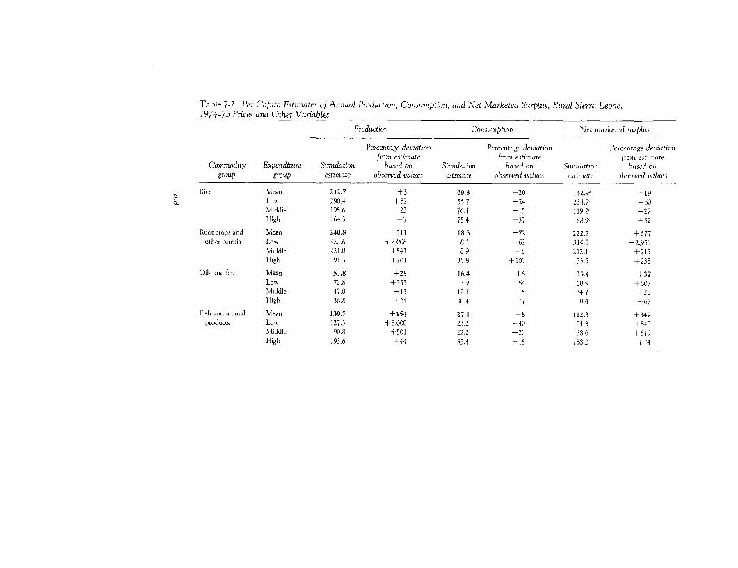
Table 7-2. Per Capita Estimates of Annual Production, Consumption, and Net Marketed Surplus, Rural Sierra Leone,1974-75 Prices and Other Variables
Production Consumption Net marketed surplus
Percentage deviation Percentage deviation Percentage deviationfrom estimate from estimate from estimate
Commodity Expenditure Simulation based on Simulation based on Simulation based ongroup group estimate observed values estimate observed values estimate observed values
Rice Mean 212.7 +3 69.8 -20 142.91 +19CD Low 290.4 +52 55.7 +24 234.7c +60
Middle 195.6 -23 76.4 -15 119.21 - 27High 164.3 -7 75.4 -37 88.9' +52
Root crops and Mean 240.8 +511 18.6 +72 222.2 +677other cereals Low 322.6 +2,008 8.1 +62 314.5 +2,953
Middle 221.0 +541 8.9 +6 212.1 +713High 191.3 +201 35.8 + 103 155.5 +238
Oils and fats Mean 51.8 +25 16.4 +5 35.4 +37Low 72.8 +355 3.9 -54 68.9 +807Middle 47.0 -13 12.3 +15 34.7 -20High 38.8 -24 30.4 +17 8.4 -67
Fish and animal Mean 139.7 +154 27.4 -8 112.3 +347products Low 127.5 +5,000 23.2 +40 104.3 +840
Middle 90.8 +501 22.2 -20 68.6 +649High 193.6 +44 35.4 -18 158.2 +74
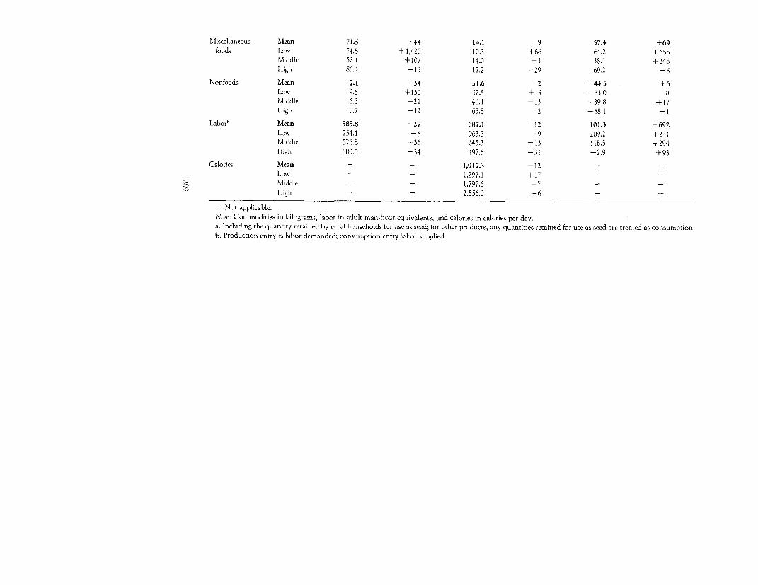
Miscellaneous Mean 71.5 +44 14.1 -9 57.4 +69foods Low 74.5 + 1,420 10.3 +66 64.2 +655
Middle 52.1 +107 14.0 -1 38.1 +246High 86.4 -13 17.2 -29 69.2 -8
Nonfoods Mean 7.1 +34 51.6 -2 -44.5 +6Low 9.5 +150 42.5 +15 -33.0 0Middle 6.3 +21 46.1 -13 -39.8 + 17High 5.7 -12 63.8 -2 -58.1 +1
Labor5 Mean 585.8 -27 687.1 -12 101.3 +692Low 754.1 -8 963.3 +9 209.2 +231Middle 526.8 -36 645.3 -13 118.5 +294High 500.5 -34 497.6 -31 -2.9 +93
Calories Mean - - 1,917.3 -12 - -
Low - - 1,297.1 + 17 -t- Middle - - 1,797.6 -7 -
'0 High - - 2,556.0 -6 - -
- Not applicable.Note: Commodities in kilograms, labor in adult man-hour equivalents, and calories in calories per day.a. Including the quantity retained by rural households for use as seed; for other products, any quantities retained for use as seed are treated as consumption.b. Production entry is labor demanded; consumption entry labor supplied.

210 CASE STUDIES
are specified by a quadratic expenditure system with variables for house-hold characteristics (see chapter 4). This permits the Engel curves to bequadratic if the data so determine. This is a potentially important consid-eration when commodities are disaggregated. Nonlinear Engel curves alsoprove to be important when the interest is in the differential responses ofexpenditure class groups. The multiple output-supply and input-demandequations are derived by assuming that the production function is separa-ble between all outputs and all inputs. A constant elasticity of transfor-mation function is used for the outputs and a Cobb-Douglas function forthe inputs.
Using this model, as estimated from the 1974-75 data, we predict pro-duction and consumption values for each of the 138 sample households,taking the exogenous variables at their 1974-75 levels. From the pre-dicted values for the dependent variables, we derive per capita populationestimates-by expenditure class and for rural Sierra Leone as a whole (ex-cept for the Northern Plateau)-for each of the quantities with which weare concerned: consumption and production, labor use and supply, andmarketed surpluses of goods and labor (table 7-2).2
The simulation estimates of aggregate consumption capture the ob-served behavior for 1974-75 very well for the region as a whole. Exceptfor one food group (root crops and other cereals), the percentage devia-tions between the simulated mean per capita figures and the estimatesbased directly on the observed data are modest. Predicted mean caloricavailability-the figure most important for policy-is within 12 percent ofthe estimate from the observed data. (For those estimates see appendixtable 7A-1.)
The simulations of mean per capita production do not accord as wellwith the figures from the observed data-except for rice, the most impor-tant food. For root crops and other cereals, as for fish and animal prod-ucts, the simulations are poor, yet that for rice is excellent (within 3 per-cent of the estimate based upon observed data). Our model, althoughincapable of handling every commodity as well as we would have liked,did perform well for rice, the commodity in which we were primarily in-terested-the estimate of rice production is the crucial one for the policyissues we discuss.
The mean marketed surplus estimates, which depend heavily on pro-duction simulations, also show some large deviations from the estimatesbased on observed data. Again, however, the overall estimate most im-portant for policy-that for rice-is quite good.
The simulation estimates are more successful in capturing the observedbehavior of the whole population than that of the different expendituregroups. To be sure, one usually expects better predictions for the average

MICROSIMULATION OF THE RURAL ECONOMY 211
of all households than for households restricted to the upper or lowerthird of the expenditure distribution. Yet our policy interest in the distri-bution of the effects of price changes requires us to look at each segmentof the population distribution, particularly at low-expenditure house-holds. Unfortunately, production estimates for the latter group are con-sistently high in comparison with estimates from observed data (as aremost of the marketed surplus estimates).
In part this is because measuring deviations as percentages of the esti-mates obtained from observed data exaggerates deviations in the low-ex-penditure group; almost without exception, those percentages are mea-sured from smaller bases than the others. But some of the productionestimates from simulation, particularly those for root crops and other ce-reals and for fish and animal products, are simply unreliable.
But the estimates for rice produced by low-expenditure households aremuch better than for other commodities, and the estimate for total calo-ries available, although 17 percent higher than the estimate derived fromobserved data, is still quite good. Thus we can proceed with a measure ofconfidence when examining the effects of rice-price policy on low-expend-iture households.
Point Elasticities versus Microsimulation
The standard approach to policy analysis is to apply point elasticities toa representative household (or households). This method may be reason-able when just one variable changes and the range of variation is small,but if we want to predict outcomes from a larger change, point elasticities,if they are not constant, will yield poor predictions. Simulation demandsno restrictive assumption about the behavior of elasticities.
To determine whether the two methods lead to different results in theSierra Leone situation, we simulate production and consumption re-sponses to several independent price changes: a 10 percent increase in theprice of rice, a 10 percent increase in the price of oils and fats, a 10 percentdecrease in the price of fish and animal products, and a 5 percent increasein the price of labor. The results for a representative sample householdare shown in arc elasticity form in the second column of table 7-3. Arcand point elasticities are virtually identical for outputs, but differ some-what for consumption and labor supplied and demanded.
Given that there are potential advantages from simulation a furtherquestion arises: whether to simulate for a representative household or foreach household in the sample, combining the results later as desired. Theconditions under which using a representative household generates the
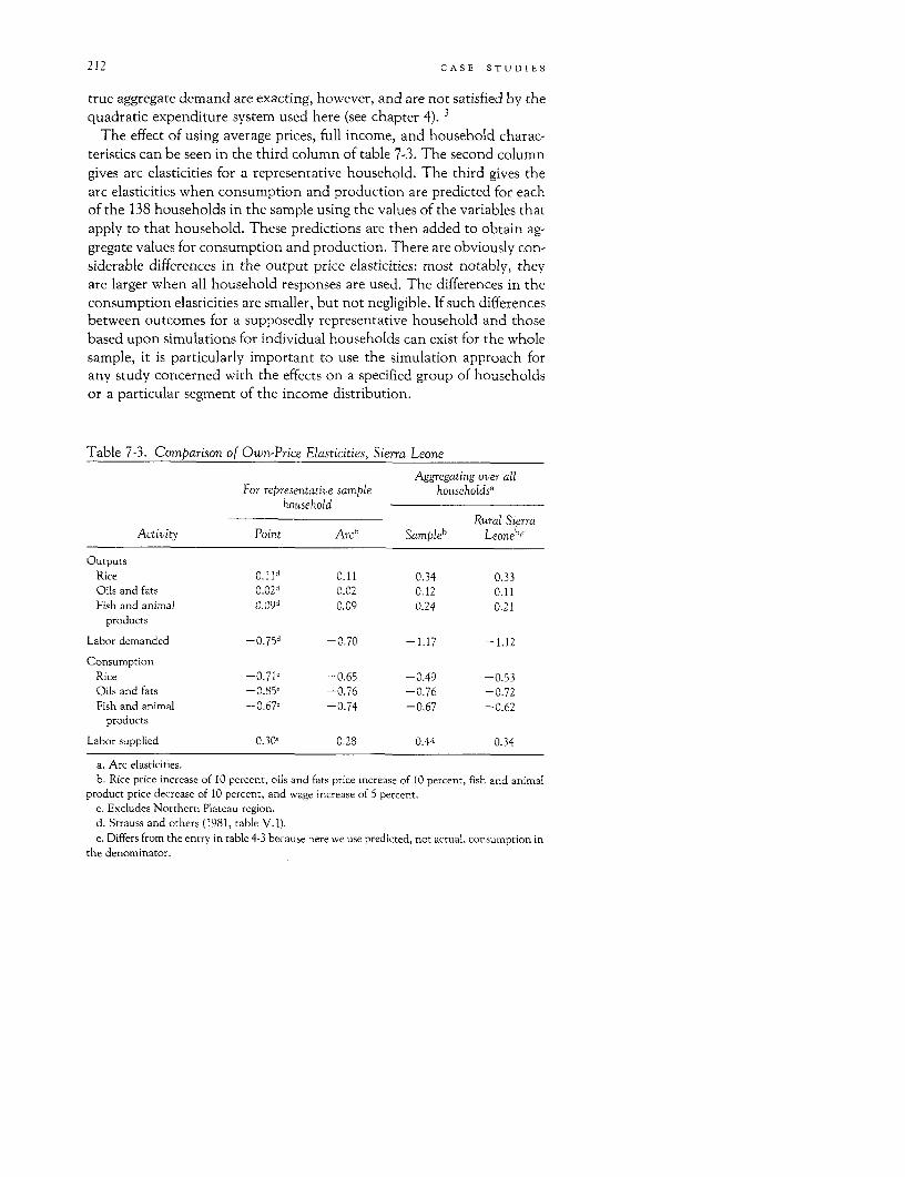
212 CASE STL'DIES
true aggregate demand are exacting, however, and are not satisfied by thequadratic expenditure system used here (see chapter 4). 3
The effect of using average prices, full income, and household charac-teristics can be seen in the third column of table 7-3. The second columngives arc elasticities for a representative household. The third gives thearc elasticities when consumption and production are predicted for eachof the 138 households in the sample using the values of the variables thatapply to that household. These predictions are then added to obtain ag-gregate values for consumption and production. There are obviously con-siderable differences in the output price elasticities: most notably, theyare larger when all household responses are used. The differences in theconsumption elasticities are smaller, but not negligible. If such differencesbetween outcomes for a supposedly representative household and thosebased upon simulations for individual households can exist for the wholesample, it is particularly important to use the simulation approach forany study concerned with the effects on a specified group of householdsor a particular segment of the income distribution.
Table 7-3. Comparison of Own-Price Elasticities, Sierra Leone
Aggregating over allFor representative sample households'
householdRural Sierra
Activity Point Arcb Sampleb Leoneb,c
OutputsRice 0.1ld 0.11 0.34 0.33Oils and fats 0.02d 0.02 0.12 0.11Fish and animal 0.09d 0.09 0.24 0.21
products
Labor demanded -0. 75d -0.70 -1.17 -1.12
ConsumptionRice -0.71e -0.65 -0.49 -0.53Oils and fats -0.85, -0.76 -0.76 -0.72Fish and animal -0.67' -0.74 -0.67 -0.62
products
Labor supplied 0.30, 0.28 0.44 0.34
a. Arc elasticities.b. Rice price increase of 10 percent, oils and fats price increase of 10 percent, fish and animal
product price decrease of 10 percent, and wage increase of 5 percent.c. Excludes Northern Plateau region.d. Strauss and others (1981, table V.1).e. Differs from the entry in table 4-3 because here we use predicted, not actual, consumption in
the denominator.
MICROSIMULATION OF THE RURAL ECONOMY 213
For the sake of completeness, arc elasticities are also reported when aprojection to the national level is made from the sample households(column 4). Although some differences exist between arc elasticities forthe sample observations and for rural Sierra Leone, they are not large.(The differences occur because the weights for each household differ inthe two cases and because the five households in the Northern Plateauregion are not included when projecting to the national level.)
In summary, for the representative household, there are small differ-ences between arc and point elasticities for consumption and for laborsupplied and demanded; for production, the differences are negligible.Using a representative household instead of aggregating the results forindividual households likewise affects consumption estimates; for the esti-mates of production and labor use, the differences are quite large.
Using simulation instead of point elasticities has another advantage,not dealt with in table 7-3. When several variables are allowed to changesimultaneously, looking at individual elasticities makes it considerablymore difficult to make projections, especially when the elasticities are notconstant or when interactions between changes in different variables canbe important. By allowing several variables to change simultaneously wecan also allow for some general equilibrium effects. If, for instance, therural labor supply curve is upward sloping, as it seems to be, then anincrease in an output price for the entire country raises labor demand andputs upward pressure on wages. As the effect of a wage increase on outputis to counteract the output price increase, one should take account of it.In our results, allowing wages to adjust makes a large difference in thepredictions.
Microsimulation and Partial Equilibrium
Since 1961, Sierra Leone has sought self-sufficiency in rice production.The government establishes official producers' prices through the SierraLeone Produce Marketing Board. Since the late 1970s, government priceshave usually been above the prices of imported rice, but the price thetrader actually pays the farmer is normally 20 to 40 percent below theofficial price (see Snodgrass and others 1980, pp. 44, 97-98, 100). Yet riceimports still remain a problem. How effective would an increase in theprice actually received by the producer be in expanding the marketedsurplus of rice? And what effects would a change in rice prices have on thenutritional status of rural households?
Suppose that government decree or an autonomous shift in the urbandemand for rice causes a 10 percent increase in the producer's price, and
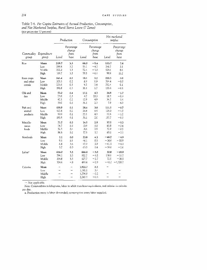
214 CASE STUDIES
Table 7-4. Per Capita Estimates of Annual Production, Consumption,and Net Marketed Surplus, Rural Sierra Leone (7 Zones)(rice prices rise 10 percent)
Net marketedProduction Consumption surplus
Percentage Percentage Percentagechange change change
Commodity Expenditure from from fromgroup group Level base Level base Level base
Rice Mean 219.7 3.3 66.0 -5.4 153.7 7.6Low 299.8 3.2 53.1 -4.7 246.7 5.1Middle 202.0 3.3 72.6 -5.0 129.4 8.6High 169.7 3.3 70.8 -6.1 98.9 11.2
Root crops Mean 241.4 0.2 19.1 2.7 222.3 0.0and other Low 323.3 0.2 8.9 9.9 314.4 -0.0cereals Middle 221.6 0.3 9.2 3.4 212.4 0.1
High 191.8 0.3 36.4 1.7 155.4 -0.1
Oils and Mean 52.0 0.4 17.1 4.3 34.8 -1.7fats Low 73.0 0.3 4.7 20.5 68.3 -0.9
Middle 47.1 0.2 12.9 4.9 34.2 -1.4High 39.0 0.5 31.1 2.3 7.9 -6.0
Fish and Mean 139.9 0.1 28.4 3.6 111.5 -0.7animal Low 127.8 0.2 24.8 6.9 103.0 -1.2products Middle 90.9 0.1 23.1 4.1 67.8 -1.2
High 193.8 0.1 36.1 2.0 157.7 -0.3
Miscella- Mean 71.7 0.3 14.5 2.8 57.2 -0.3neous Low 74.7 0.3 10.9 5.8 63.8 -0.6foods Middle 52.3 0.4 14.4 2.9 37.9 -0.5
High 86.6 0.2 17.5 1.7 69.1 -0.1
Nonfoods Mean 7.1 0.0 53.8 4.3 -46.7 -4.9Low 9.5 0.1 46.1 8.5 -36.6 -10.9Middle 6.4 1.6 47.9 3.9 -41.5 -4.3High 5.7 0.0 65.3 2.4 -59.6 -2.6
Labor' Mean 616.0 5.2 666.8 -3.0 50.8 -49.9Low 794.1 5.3 932.7 -3.2 138.6 -33.7Middle 554.8 5.3 627.7 -2.7 72.9 -38.5High 524.6 4.8 483.4 -2.9 -41.2 -1,320.7
Calories Mean - - 1,922.7 0.3 - -
Low - - 1,341.1 3.4 - -
Middle - - 1,794.0 -0.2 - -
High - - 2,547.2 -0.3 - -
- Not applicable.Note: Commodities in kilograms, labor in adult man-hour equivalents, and calories in calories
per day.a. Production entry is labor demanded; consumption entry labor supplied.
MICROSIMULATION OF THE RURAL ECONOMY 215
that consumer prices for rice consumed within the rural sector change inthe same proportion, but that neither wage rates nor other prices changeat all. Given that other exogenous variables are at the levels prevailing in1974-75, we see in table 7-4 that overall per capita rice production willrise 3.3 percent, consumption will fall 5.4 percent, and the marketed sur-plus of rice will rise 7.6 percent (by 16,700 metric tons, or 30 percent of1980 imports for all of Sierra Leone, estimated at 55,000 tons by Snod-grass et al. 1980, p. 100). The net effect on per capita calorie availability isnegligible for the rural population as a whole, as households counteractthe reductions in rice consumption by consuming more of the foods forwhich prices have not risen.
The higher prices of rice cause a significant reduction in rice imports,but do not appreciably affect the availability of food energy in rural SierraLeone as a whole. Sierra Leone now needs less foreign exchange for im-ported rice, but spends more on imported palm oil, dried fish, and otheritems of which the rural sector now provides smaller marketed surpluses.Of course, maintaining higher producers' prices puts a strain on the gov-ernment budget unless urban rice prices are allowed to rise.
Although the nutritional effects of the higher rice prices are negligiblefor the rural population as a whole, they are positively beneficial for low-expenditure households (the L households), which contain 30 percent ofthat population (Smith and others 1981, p. 38). These households in-crease their per capita calorie intake (availability) by 3.4 percent. Asonly 1,300 calories per capita are being consumed daily (table 7-2), even a3.4 percent increase constitutes significant nutritional gain. The remain-ing 70 percent of the population reduces its per capita calorie intake, butthe amounts are small (0.3 percent or less), and the high-expenditure (H)group, at least, appears able to support them. About the M group wemust be less complacent. There is a serious need for more calories amongperhaps half of those households as in the benchmark simulation the av-erage per capita caloric intake of all M-households was only 1,800 perday.
Both in absolute and percentage terms, L households reduce rice con-sumption less and increase their consumption of other foods more thanother households. The net effect is that, on balance, L households con-sume more calories when rice prices rise, whereas others consume slightlyfewer.
Why should this be so? Differences in the consumption responses ofdifferent expenditure groups are partly the result of differences among thegroups in income-consumption elasticities and in income-compensatedprice elasticities (see Strauss, Smith, and Schmidt 1981, pp. 23-28). But,in the present case, these differences are relatively inconsequential com-
216 CASE STUDIES
pared with the differences in the magnitude of the effective incomechange that occurs for a semisubsistence household when both producerand consumer prices change. If we hold profits constant for the moment,a rise in the consumption price has a negative income effect on rice con-sumption. But if the household produces all the rice it consumes and sellsnone, a rise of the same amount in the producer's price creates an oppo-site income effect exactly equal in size. If both producer and consumerprices are equal, and if a household has a positive net marketed surplus,there will be a net positive income effect when both prices rise.4 The mag-nitude of the effect will depend upon the size of the net marketed surplus.5
The primary reason that low-expenditure households in Sierra Leonegain nutritionally when rice prices rise is that they have large marketedsurpluses of rice. The mean marketed surplus among L households (235kilograms per capita, table 7-2) is approximately twice as great as in eitherof the other expenditure groups, so the net effect on household expendi-ture is about twice as great. This large net income effect is important notonly for rice consumption, but also for the consumption of all commodi-ties. When the effect of a higher rice-production price is taken into ac-count, the cross elasticities of consumption for other foods, with respectto a joint increase in the producer and consumer prices of rice, becomevery large for L households (see table 4-3). As a result, L households havea positive elasticity of 0.19 for calorie availability with respect to the priceof rice; for other expenditure groups, these calorie elasticities are negative(see table 4-6). In Sierra Leone, at least, it is useful to assert as a rule ofthumb that the amount of gain (or loss) in calorie availability dependsupon the size of a household's marketed surplus of rice. Although Lhouseholds in general benefit nutritionally when rice prices rise, individ-ual L households may be harmed, for it is not the level of household ex-penditure, but the size of the marketed surplus that appears to be crucialin predicting the effect upon caloric intake.
The observed data make it clear that L households produce large percapita marketed surpluses of rice, but they do not support the simulationestimate of a marketed surplus as large as 235 kilograms per capita (table7-2).6 According to the direct population estimates (table 7A-1) rice mar-keted surpluses are 147 and 164 kilograms per capita for the average L andM households, respectively. The simulation estimate exceeds the directpopulation estimate for the L households by about 100 kilograms per cap-ita, both for production and for the marketed surplus. Actually, the ob-served data for upland rice production may have been somewhat low incomparison with a normal year. In 1974-75, the rains came late and thusupland rice yields were reduced significantly (Spencer and Byerlee 1977,p. 54). We may assume that the direct population estimate for the mar-
MICROSIMULATION OF THE RURAL ECONOMY 217
keted surplus figure imposes a lower bound for the true effect of a 10 per-cent rise in rice prices on calorie availability. If the simulation estimatesare correct, calorie availability rises 3.4 percent for L households; if theysignificantly overstate the benefit to L households, it is still likely that theL households do no worse than the M households, so at least SierraLeone needs fear no significant reduction in calorie availability as theresult of a decision to increase the government's producer price for rice.
Microsimulation and General Equilibrium
When there is a change in the price of a staple product such as rice,other prices are also likely to change as factor and product markets moveto new equilibria. We do not have a full general equilibrium model, so wecannot predict those changes, but microsimulation makes it easy to ex-amine the consequences of induced price changes for any set of changesone may wish to consider.
An Induced Increase in Wages
We examine an induced wage change, asking how such a change wouldalter the effects of a 10 percent increase in rice prices on rice productionand calorie availability. At 1974-75 wage levels, a 10 percent change inrice prices would raise the use of rural labor by 5 percent and reduce laborsupply by 3 percent (table 7-4). This would put upward pressure on agri-cultural wages and reduce the marketed surplus of labor (the labor supplyto nonrural enterprises in the region) by 50 percent. If the nonrural de-mand function for this marketed surplus is given, the rural wage ratemust rise unless that demand function is infinitely elastic. We put an up-per bound on this induced rise by assuming zero elasticity of nonruraldemand; in this case, the wage must rise until the marketed surplus ofrural labor equals its amount before rice prices rose. According to ourdata, the upper bound is approximately 5 percent, which we establishedby experimental simulation runs. A 5 percent wage increase raises themarketed surplus of labor by 44 percent, substantially offsetting the nega-tive effect of a 10 percent increase in rice prices.
When a 5 percent induced wage increase occurs along with a 10 percentincrease in rice prices, the gain in the marketed surplus of rice is cut bymore than one-half, but there are nutritional gains for each expenditureclass, the largest being among L households. For them, calories availablerise twice as much as they do when wages do not rise. (Table 7-5 showsthe new levels of output and consumption.)
218 CASE STUDIES
Table 7-5. Per Capita Estimates of Annual Production, Consumption,and Net Marketed Surplus, Rural Sierra Leone (7 Zones)(rice prices rise 10 percent, wages 5 percent)
Net marketedProduction Consumption surplus
Percentage Percentage Percentagechange change change
Commodity Expenditure from from fromgroup group Level base Level base Level base
Rice Mean 215.0 1.1 67.5 -3.3 147.5 3.2Low 293.5 1.1 54.9 -1.4 238.6 1.7Middle 197.7 1.1 74.0 -3.1 123.7 3.8High 166.0 1.0 71.9 -4.6 94.1 5.8
Root crops Mean 239.8 -0.4 19.6 5.4 220.2 -0.9and other Low 321.5 -0.3 9.2 13.6 312.3 -0.7cereals Middle 220.1 -0.4 9.3 4.5 210.8 -0.6
High 190.3 -0.5 37.2 3.9 153.1 -1.5
Oils and Mean 51.5 -0.6 17.6 7.3 33.9 -4.2fats Low 72.4 -0.5 5.0 28.2 67.4 -2.2
Middle 46.7 -0.6 13.3 8.1 33.4 -3.7High 38.6 -0.5 31.7 4.3 6.9 -17.9
Fish and Mean 138.1 -1.1 29.0 5.8 109.1 -2.8animal Low 127.1 -0.3 25.4 9.5 101.7 -2.5products Middle 90.3 -0.6 23.6 6.3 66.7 -2.8
High 190.0 -1.9 36.8 4.0 153.2 -3.2
Miscella- Mean 70.6 -1.3 14.8 5.0 55.9 -Z.6neous Low 74.0 -0.7 11.2 8.7 62.8 -2.2food Middle 51.7 -0.8 14.6 4.3 37.1 -2.6
High 84.8 -1.9 17.8 3.5 67.0 -3.2
Nonfoods Mean 7.0 -0.2 54.9 6.4 -47.9 -7.6Low 9.5 -0.2 47.4 11.5 -37.9 -14.8Middle 6.3 -0.2 48.9 6.1 -42.6 -7.0High 5.6 -0.5 66.5 4.2 -60.9 -4.8
Labor' Mean 580.5 -0.9 679.7 -1.1 99.2 -2.1Low 749.8 -0.6 942.5 -2.2 192.7 -7.9Middle 523.3 -0.7 637.0 -1.3 113.7 -4.1High 492.7 -1.6 502.1 0.9 9.4 +424.1
Calories Mean - - 1,969.8 2.7 - -
Low - - 1,387.5 7.0 - -Middle - - 1,829.8 1.8 - -
High - - 2,592.8 1.4 - -
- Not applicable.Note: Commodities in kilograms, labor in adult man-hour equivalents, and calories in calories
per day.a. Production entry is labor demanded; consumption entry labor supplied.
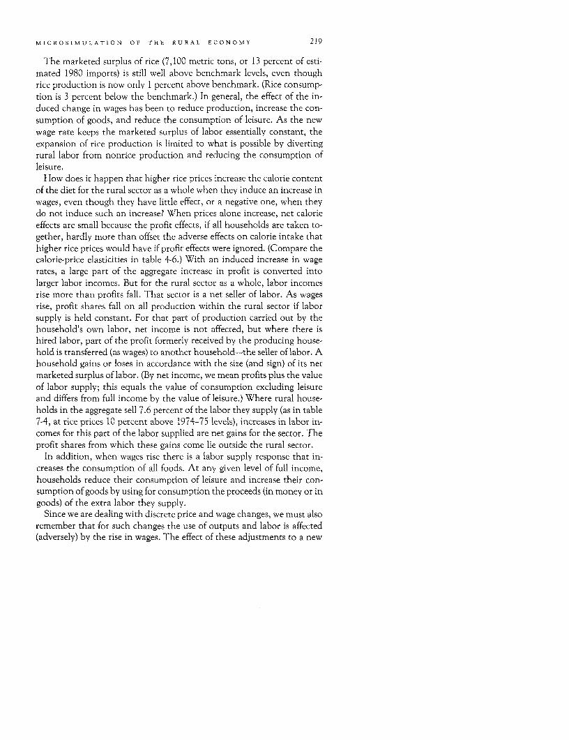
MICROSIMULATION OF THE RURAL ECONOMY 219
The marketed surplus of rice (7,100 metric tons, or 13 percent of esti-mated 1980 imports) is still well above benchmark levels, even thoughrice production is now only 1 percent above benchmark. (Rice consump-tion is 3 percent below the benchmark.) In general, the effect of the in-duced change in wages has been to reduce production, increase the con-sumption of goods, and reduce the consumption of leisure. As the newwage rate keeps the marketed surplus of labor essentially constant, theexpansion of rice production is limited to what is possible by divertingrural labor from nonrice production and reducing the consumption ofleisure.
How does it happen that higher rice prices increase the calorie contentof the diet for the rural sector as a whole when they induce an increase inwages, even though they have little effect, or a negative one, when theydo not induce such an increase? When prices alone increase, net calorieeffects are small because the profit effects, if all households are taken to-gether, hardly more than offset the adverse effects on calorie intake thathigher rice prices would have if profit effects were ignored. (Compare thecalorie-price elasticities in table 4-6.) With an induced increase in wagerates, a large part of the aggregate increase in profit is converted intolarger labor incomes. But for the rural sector as a whole, labor incomesrise more than profits fall. That sector is a net seller of labor. As wagesrise, profit shares fall on all production within the rural sector if laborsupply is held constant. For that part of production carried out by thehousehold's own labor, net income is not affected, but where there ishired labor, part of the profit formerly received by the producing house-hold is transferred (as wages) to another household-the seller of labor. Ahousehold gains or loses in accordance with the size (and sign) of its netmarketed surplus of labor. (By net income, we mean profits plus the valueof labor supply; this equals the value of consumption excluding leisureand differs from full income by the value of leisure.) Where rural house-holds in the aggregate sell 7.6 percent of the labor they supply (as in table7-4, at rice prices 10 percent above 1974-75 levels), increases in labor in-comes for this part of the labor supplied are net gains for the sector. Theprofit shares from which these gains come lie outside the rural sector.
In addition, when wages rise there is a labor supply response that in-creases the consumption of all foods. At any given level of full income,households reduce their consumption of leisure and increase their con-sumption of goods by using for consumption the proceeds (in money or ingoods) of the extra labor they supply.
Since we are dealing with discrete price and wage changes, we must alsoremember that for such changes the use of outputs and labor is affected(adversely) by the rise in wages. The effect of these adjustments to a new
220 CASE STUDIES
equilibrium position is to moderate the adverse effect of the wage increaseupon profits, so their effect upon food consumption and calorie intakecan only be positive. As employment falls and labor supply rises, the netresult is to shift some labor from less productive uses within the ruralsector to more productive activities outside.
In sum, for the rural sector as a whole, each of the mechanisms dis-cussed leads to greater food consumption and a larger calorie intake. Ag-gregate calorie availability, in response to these factors, rises nearly 2.5percent above its level when only the 10 percent change in rice pricesoccurs.
The induced wage increase brings calorie availability among L house-holds to 3.5 percent above its level when only rice prices rise; M and Hhouseholds gain by only 2 percent. (In absolute terms gains are essentiallyequal for the M and the H households.) The L-household gains reflecttheir relatively large net marketed surpluses of labor (table 7-4). Adverseeffects upon food consumption are possible only for net purchasers of la-bor. Some of those exist within the H group, but there is an offsettingfactor: the positive labor supply response is much stronger among Hhouseholds. (The 5 percent induced wage increase raises labor suppliedamong the L, M, and H households by 1.1 percent, 1.5 percent, and 3.9percent, respectively, as compared with the quantities supplied when riceprices rise but the wage remains constant.) The relatively strong supplyresponse among H households is enough to cause a gain in calorie avail-ability for the group as a whole.
The simulation analysis predicts that an induced wage increase willbring a net gain in calorie availability for the rural sector as a whole. Thisresults in part from its prediction of a positive marketed surplus of labor(101 man-hours per capita per year for the 1974-75 situation). Yet thedirect estimates from observed data (see table 7A-1) do not confirm thatsuch a surplus exists for the rural sector as a whole. Instead, they show asmall net marketed deficit (of 17 man-hours). The L households, how-ever, do have a net marketed surplus (63 man-hours per capita). Conse-quently, a conservative interpretation of our results would be that foodenergy consumption among L households would rise if induced wage in-creases occurred, whereas gains are possible, but not assured, among Mand H households.
The policy significance of all this, in a semisubsistence economy wheremost labor is used by the household that provides it, is that high productprices may or may not improve the energy content of the diet, but thatrural wage increases induced by high product prices do-except possiblyfor households that are net purchasers of labor. Moreover, benefits fromhigher product prices accrue only to households with net marketed sur-

MICROSIMULATION OF THE RURAL ECONOMY 221
pluses of those products, unless they lead to higher wages. In that case,producers of all products benefit, in amounts that depend partly upontheir net marketed surpluses of labor and the elasticities of householdlabor-supply responses to higher wages.
As wages rise, there will be complaints about high wages and shortagesof labor, but, for the rural sector as a whole, induced wage increases are abeneficial mechanism, spreading the benefits of higher prices for particu-lar products throughout the economy. To be sure, some households maylose. Wage increases cause some reallocation of benefits-in the presentcase, away from all rice producers (as they cut back somewhat on riceoutput), particularly from those who are net buyers of labor. (In an econ-omy with landless laborers, they benefit from higher product prices onlyif more employment or higher wages occur.) In Sierra Leone, we expect atleast the L households to gain because they have relatively high marketedsurpluses of both rice and of labor.
Where calorie consumption rises although rice consumption declines inresponse to a higher relative price for rice, it is because the consumptionof other foods expands enough to more than offset the loss of caloriesfrom rice. This can occur because the prices of other foods remain con-stant, or at least lag behind rice prices and wage rates. If all prices andwage rates rose 10 percent, neither consumption nor output patternswould change from benchmark levels except for such minor effects asmight arise because the autonomous component of income remained un-changed. (In this model, both demand and production systems are homo-geneous of zero degree; see Smith and others 1981.)
In fact, however, the prices of many foods (including such importantitems as palm oil and fish) are determined partly in world markets, or atleast outside the rural sector of Sierra Leone, so some net change in therelative price of rice is likely to persist even after all induced effects onother prices have been fully felt. Thus, even in the long run, general equi-librium effects on prices of other foods are unlikely to nullify completelyany gains that a rise in the government buying price might bring.
Improved Productivity
What of measures to improve general agricultural productivity? With a5 percent improvement in overall productivity7 at benchmark prices andwages, calorie consumption increases 4.3 percent, labor use 6.1 percent,rice output 6.4 percent, and the outputs of other foods 2.0-4.3 percent(table 7-6). The quantity of labor supplied falls 2.3 percent, and thus themarketed surplus of labor falls. Consumption increases (more for oils andfats and for root crops and other cereals than for anything else), but rice
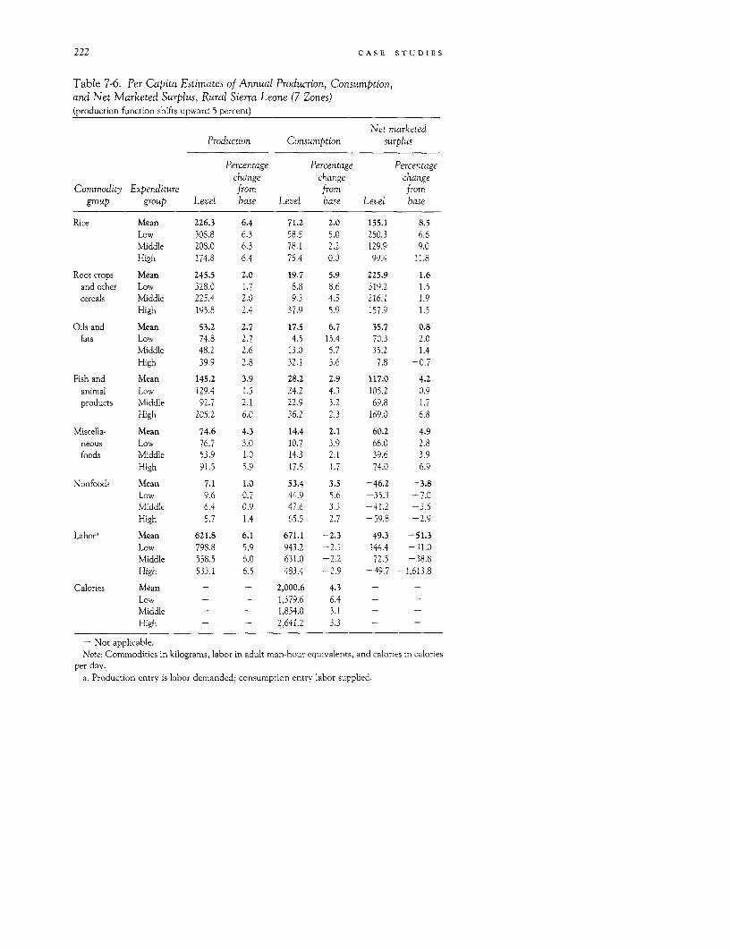
222 CASE STUDIES
Table 7-6. Per Capita Estimates of Annual Production, Consumption,and Net Marketed Surplus, Rural Sierra Leone (7 Zones)(production function shifts upward 5 percent)
Net marketedProduction Consumption surplus
Percentage Percentage Percentagechange change change
Commodity Expenditure from from fromgroup group Level base Level base Level base
Rice Mean 226.3 6.4 71.2 2.0 155.1 8.5Low 308.8 6.3 58.5 5.0 250.3 6.6Middle 208.0 6.3 78.1 2.2 129.9 9.0High 174.8 6.4 75.4 0.0 99.4 11.8
Root crops Mean 245.5 2.0 19.7 5.9 225.9 1.6and other Low 328.0 1.7 8.8 8.6 319.2 1.5cereals Middle 225.4 2.0 9.3 4.5 216.1 1.9
High 195.8 2.4 37.9 5.9 157.9 1.5
Oils and Mean 53.2 2.7 17.5 6.7 35.7 0.8fats Low 74.8 2.7 4.5 15.4 70.3 2.0
Middle 48.2 2.6 13.0 5.7 35.2 1.4High 39.9 2.8 32.1 5.6 7.8 -0.7
Fish and Mean 145.2 3.9 28.2 2.9 117.0 4.2animal Low 129.4 1.5 24.2 4.3 105.2 0.9products Middle 92.7 2.1 22.9 3.2 69.8 1.7
High 205.2 6.0 36.2 2.3 169.0 6.8
Miscella- Mean 74.6 4.3 14.4 2.1 60.2 4.9neous Low 76.7 3.0 10.7 3.9 66.0 2.8foods Middle 53.9 1.0 14.3 2.1 39.6 3.9
High 91.5 5.9 17.5 1.7 74.0 6.9
Nonfoods Mean 7.1 1.0 53.4 3.5 -46.2 -3.8Low 9.6 0.7 44.9 5.6 -35.3 -7.0Middle 6.4 0.9 47.6 3.3 -41.2 -3.5High 5.7 1.4 65.5 2.7 -59.8 -2.9
Labora Mean 621.8 6.1 671.1 -2.3 49.3 -51.3Low 798.8 5.9 943.2 -2.1 144.4 -31.0Middle 558.5 6.0 631.0 -2.2 72.5 -38.8High 533.1 6.5 483.4 -2.9 -49.7 -1,613.8
Calories Mean - - 2,000.6 4.3 - -
Low - - 1,379.6 6.4 - -
Middle - - 1,854.0 3.1 - -
High - - 2,641.2 3.3 - -
- Not applicable.Note: Commodities in kilograms, labor in adult man-hour equivalents, and calories in calories
per day.a. Production entry is labor demanded; consumption entry labor supplied.
MICROSIMULATION OF THE RURAL ECONOMY 223
consumption rises only 2.0 percent. The marketed surplus of rice rises 8.5percent (more than for any other commodity); it now amounts to 18,900metric tons, 34 percent of estimated 1980 imports.
The effect on the nutritional status of L households is especially impor-tant. A 5 percent increase in general productivity increases calorie avail-ability among L household by 6.4 percent. Their rice consumption risesby 5 percent and their intake of oils and fats by 15.4 percent. If low-expenditure households share equally in productivity improvement, theygain more than proportionally in nutritional well-being-presumably be-cause the largest percentage gains in output occur for rice, a relativelymore important product for L households than for others.
Higher agricultural productivity of course means greater demand forlabor and upward pressure on wages. Again, if we assume zero nonruralelasticity of demand for the marketed surplus of labor, we can define anupper bound for the wage increase (slightly more than 5 percent in thepresent case). A 5 percent increase restores labor use to the benchmarklevel, but does not quite return the marketed surplus to the benchmarkstate because the quantity of labor supplied remains slightly below thatlevel (table 7-7).
Transforming some of the gains in productivity into a 5 percent in-crease in wages reduces goods production and marketed surpluses, butstill leaves outputs above benchmark levels. Rice production, consump-tion, and marketed surplus remain 4 percent above the base situation.This gives a total seven-zone marketed surplus of 9,000 metric tons, 16percent of the country's estimated 1980 imports. On the average, calorieavailability improves, rising to 6.3 percent above the benchmark and 10.2percent for L households. (For those households, the elasticity of calorieavailability with respect to productivity is 2.0 when the effects of the wageincrease are included.)
This 10 percent increase in calorie availability among L households isnearly 50 percent more than was achieved by a 10 percent increase in riceprices plus the induced wage increase. For M and H households, the 5percent nutritional gains from productivity improvement with wage in-crease were some 200 percent greater than those from the change in riceprices with a wage increase.
The assumption that output prices do not change when productivityincreases is realistic where commodity prices are set in world markets, orperhaps by government policy. For at least two of the most importantfoods (rice and palm oil), this is the case. Of course, whatever happens toprices, the fundamental fact is that an increase in productivity reducesthe price of food in terms of labor. Thus, food consumption in generalshould increase. Yet if money prices decrease more for some foods than
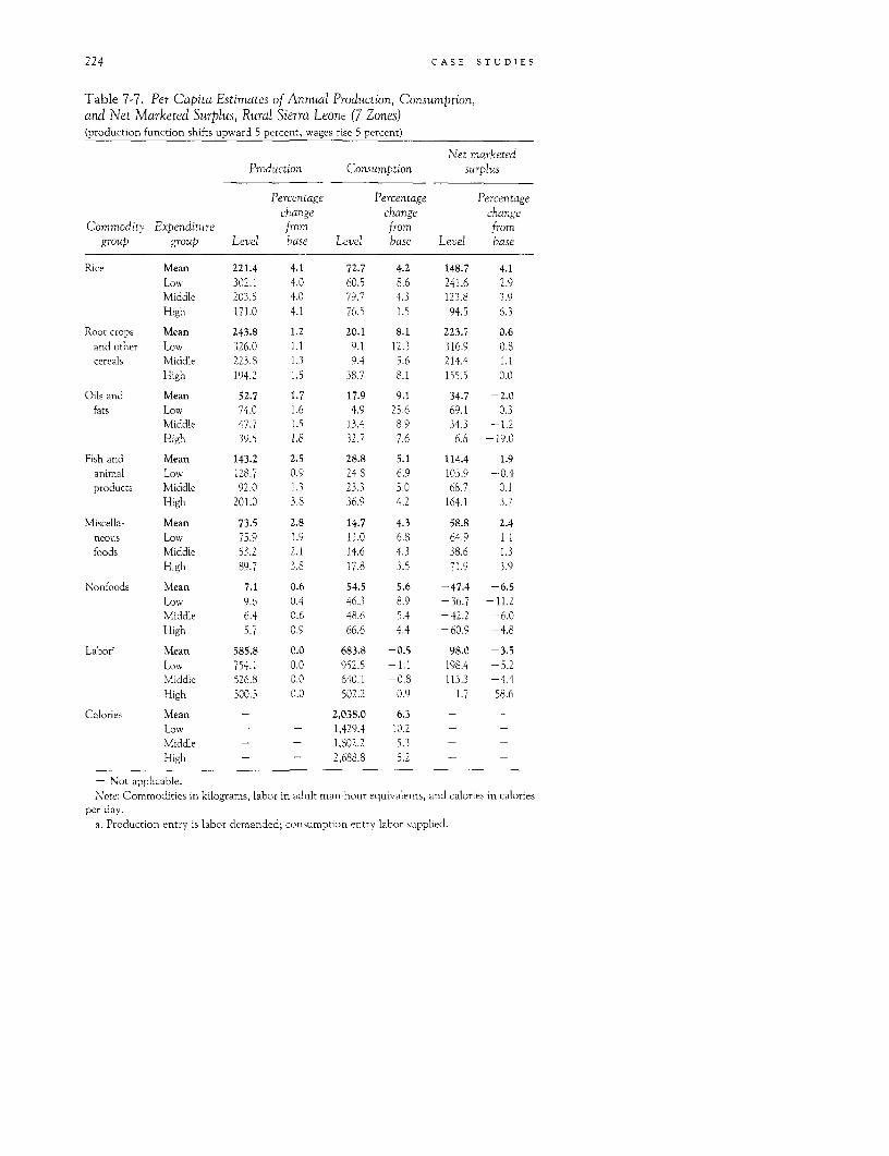
224 CASE STUDIES
Table 7-7. Per Capita Estimates of Annual Production, Consumption,and Net Marketed Surplus, Rural Sierra Leone (7 Zones)(production function shifts upward 5 percent, wages rise 5 percent)
Net marketedProduction Consumption surplus
Percentage Percentage Percentagechange change change
Commodity Expenditure from from fromgroup group Level base Level base Level base
Rice Mean 221.4 4.1 72.7 4.2 148.7 4.1Low 302.1 4.0 60.5 8.6 241.6 2.9Middle 203.5 4.0 79.7 4.3 123.8 3.9High 171.0 4.1 76.5 I.5 94.5 6.3
Root crops Mean 243.8 1.2 20.1 8.1 223.7 0.6and other Low 326.0 1.1 9.1 12.3 316.9 0.8cereals Middle 223.8 1.3 9.4 5.6 214.4 1.1
High 194.2 1.5 38.7 8.1 155.5 0.0
Oils and Mean 52.7 1.7 17.9 9.1 34.7 -2.0fats Low 74.0 1.6 4.9 25.6 69.1 0.3
Middle 47.7 1.5 13.4 8.9 34.3 -1.2High 39.5 1.8 32.7 7.6 6.8 -19.0
Fish and Mean 143.2 2.5 28.8 5.1 114.4 1.9animal Low 128.7 0.9 24.8 6.9 103.9 -0.4products Middle 92.0 1.3 23.3 5.0 68.7 0.1
High 201.0 3.8 36.9 4.2 164.1 3.7
Miscella- Mean 73.5 2.8 14.7 4.3 58.8 2.4neous Low 75.9 1.9 11.0 6.8 64.9 1.1foods Middle 53.2 2.1 14.6 4.3 38.6 1.3
High 89.7 3.8 17.8 3.5 71.9 3.9
Nonfoods Mean 7.1 0.6 54.5 5.6 -47.4 -6.5Low 9.6 0.4 46.3 8.9 -36.7 -11.2Middle 6.4 0.6 48.6 5.4 -42.2 -6.0High 5.7 0.9 66.6 4.4 -60.9 -4.8
Labora Mean 585.8 0.0 683.8 -0.5 98.0 -3.5Low 754.1 0.0 952.5 -1.1 198.4 -5.2Middle 526.8 0.0 640.1 -0.8 113.3 -4.4High 500.5 0.0 502.2 0.9 1.7 58.6
Calories Mean - - 2,038.0 6.3 - -Low - - 1,429.4 10.2 - -Middle - - 1,802.2 5.3 - -High - - 2,688.8 5.2 - -
- Not applicable.Note: Commodities in kilograms, labor in adult man-hour equivalents, and calories in calories
per day.a. Production entry is labor demanded; consumption entry labor supplied.
MICROSIMULATION OF THE RURAL ECONOMY 225
for others, it is at least conceivable that the new consumption patternmight contain fewer calories than the old.
Either higher rice prices or higher agricultural productivity (along withthe associated changes in rural wages) increases calorie availability, espe-cially for the L households. But the magnitudes of these effects promiseno easy solution for the 30 percent of the rural population whose percapita caloric intake needs to be increased by some 50 percent to ap-proach conventional nutritional standards. Even if rates of induced wagechange and elasticities of caloric intake do not change as rice prices orproductivity increase, it would take a 70 percent rise in rice prices or a 25percent increase in productivity to raise caloric intake by 50 percent forthe L household group. One hesitates to assume that these predictionswould remain valid for such large changes.
Microsimulation and the Interhousehold Distributionof Calories
Once microsimulation estimates have been made, one can classify thehouseholds in as many ways as one likes and examine the distributionaleffects of policy measures in detail. Grouping by household expenditures,as we have done so far, has shown that low-expenditure households reapthe largest percentage gains in calorie intake from each of the policy alter-natives discussed. Such households are typically poor and undernour-ished. Those in our sample had mean per capita expenditures of 49Leones per year and daily calorie availability per capita of only 1,188 calo-ries. But not all L households are poor and not all H households well-to-do. A two-person household with a per capita expenditure of 174 Leonesper year would be classified as an L household, and an H household withten members could be spending little more than 75 Leones per capita.
To reduce the effect of family size and to look at nutritional situationsin individual households, we array the households by predicted caloricavailability per capita at 1974-75 values of the independent variables (fig-ure 7-1). (Even calories per capita is not an ideal measure of nutritionaladequacy, however; the energy needs of a child of three months differfrom those of a fourteen-year-old boy.) We restrict ourselves to the 138households in the sample. For 100 households (72 percent of the sample)per capita availability lies between 800 and 2,800 calories per day, with nostrong concentration around any point in that range. As the distributionappears to be approximately flat over a wide range, more than one-thirdof which extends below 1,500 calories per day, we anticipate many nutri-tional problems. There are 48 households, comprising 370 persons, withan estimated per capita caloric intake of less than 1,500 per day. Yet the
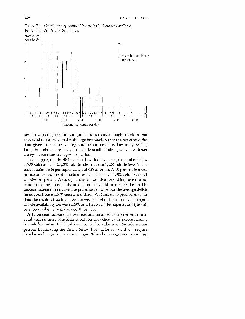
226 CASE STUDIES
Figure 7.1. Distribution of Sample Households by Calories Availableper Capita (Benchmark Simulation)
Number ofhouseholds8H
Mean household size
6- loriesfor inrerv al
4-
2.
4 4 8791010766949759695571724 2 4 33225 2 41 ~141n2 1 '1 K i
1,000 2,000 3,000 4,000 5,000 6,000Calories per capita per day
low per capita figures are not quite as serious as we might think in thatthey tend to be associated with large households. (See the household-sizedata, given to the nearest integer, at the bottoms of the bars in figure 7-1.)Large households are likely to include small children, who have lowerenergy needs than teenagers or adults.
In the aggregate, the 48 households with daily per capita intakes below1,500 calories fall 161,000 calories short of the 1,500 calorie level in thebase simulation (a per capita deficit of 435 calories). A 10 percent increasein rice prices reduces that deficit by 7 percent-by 11,400 calories, or 31calories per person. Although a rise in rice prices would improve the nu-trition of these households, at this rate it would take more than a 140percent increase in relative rice prices just to wipe out the average deficit(measured from a 1,500-calorie standard). We hesitate to predict from ourdata the results of such a large change. Households with daily per capitacalorie availability between 1,500 and 1,900 calories experience slight cal-orie losses when rice prices rise 10 percent.
A 10 percent increase in rice prices accompanied by a 5 percent rise inrural wages is more beneficial. It reduces the deficit by 12 percent amonghouseholds below 1,500 calories-by 20,000 calories or 54 calories perperson. Eliminating the deficit below 1,500 calories would still requirevery large changes in prices and wages. When both wages and prices rise,
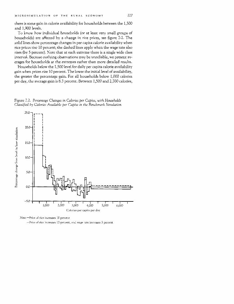
MICROSIMULATION OF THE RURAL ECONOMY 227
there is some gain in calorie availability for households between the 1,500and 1,900 levels.
To know how individual households (or at least very small groups ofhouseholds) are affected by a change in rice prices, see figure 7-2. Thesolid lines show percentage changes in per capita calorie availability whenrice prices rise 10 percent; the dashed lines apply when the wage rate alsorises (by 5 percent). Note that at each extreme there is a single wide classinterval. Because outlying observations may be unreliable, we present av-erages for households at the extremes rather than more detailed results.
Households below the 1,500 level for daily per capita calorie availabilitygain when prices rise 10 percent. The lower the initial level of availability,the greater the percentage gain. For all households below 1,000 caloriesper day, the average gain is 8.3 percent. Between 1,500 and 2,700 calories,
Figure 7.2. Percentage Changes in Calories per Capita, with HouseholdsClassified by Calories Available per Capita in the Benchmark Simulation
25.0-
l ll l
< 20.0- l I l
t 15.0-
E 10.0-
0.0 D 0 J U W +===
-.0 1- 7 - 7 1 1 1 1
-s.
1,000 2,000 3,000 4,000 5,000 6,000
Calories per capita per day
Note:-Price of rice increases 10 percent
---Price of rice increases 10 percent, and wage rate increases 5 percent
228 CASE STUDIES
average caloric intake is little affected; beyond 2,700 calories, almost allhouseholds reduce their calorie intake.
Practically all households benefit if the higher prices of rice induce a 5percent wage increase. Except at the highest and lowest ends of the distri-bution, the increments in percentage gain from the wage increases areabout the same at all calorie levels. At the lowest levels, the incrementsare greater; at the highest, less. The pattern of total gain is still a fallingone-the largest percentage gains accrue to the households most disad-vantaged in the benchmark simulation. In this case, the average gain incalorie availability is 12 percent for households with less than 1,000 calo-ries per capita before the price and wage changes.
Whether we look at households with low total expenditures or house-holds with low per capita calorie availability, an increase in rice pricesincreases availability for approximately the lowest one-third of the house-holds. (Total household expenditures and per capita caloric intake arehighly correlated.) The percentage gains are largest for the households atthe lowest caloric levels. On balance, households above the 1,500 calorielevel lose slightly when rice prices rise.
The benefits of an induced wage increase of 5 percent extend over thewhole range of calorie and expenditure levels, but they are smallest at thehigher ends of those ranges. (Although it is conceivable that net buyers oflabor might lose from the wage increase, we found no such households inthe sample.)
Conclusion
Point elasticities allow us to estimate the effects of a very small pricechange on the consumption of a representative household and, in princi-ple, by combining those effects for all foods, to estimate the net effects oncalorie availability for that household. But to cumulate those effects overthe range of a price change as large as 5 or 10 percent would be awkward(though perhaps not impossible), particularly in view of the fact that out-puts, marketed surpluses, and quantities of labor supplied are changingover the whole range of the price change. Furthermore the presumablyrepresentative household may not be characteristic of the total popula-tion, or even of its own expenditure group.
Microsimulation avoids these problems by going directly to the under-lying demand and supply functions to calculate the new consumptionand output levels-for every household in the sample, if we wish. Ouranalysis of the distributional effects of higher rice prices on individualhouseholds would not have been feasible without microsimulation. Nor
MICROSIMULATION OF THE RURAL ECONOMY 229
would our examination of the consequences of combining an inducedwage increase with higher rice prices or greater productivity. Indeed, itwas only by the use of microsimulation that we were able to determinewhat wage increase would occur if the nonrural demand for labor wereperfectly inelastic.
Microsimulation proved effective as a means of proceeding directly tothe policy issue of most interest to us-how a rice policy or improvementsin agricultural productivity would affect the caloric content of rural diets.Our analysis shows that a government policy of guaranteeing producershigh rice prices can increase the marketed surplus of rice without seriousadverse effects on the calorie content of rural diets, and with beneficialeffects for those households most at nutritional risk (those whose dailyper capita calorie intake is 1,500 or less). If induced wage increases follow,calorie availability increases for all households.
A 5 percent gain in general agricultural productivity raises calorie in-take among all rural households, but the largest percentage gains occuramong low-expenditure households. An induced wage increase againbenefits all households, especially those in the lowest-expenditure group.Any increase in the demand for rural labor benefits households in allexpenditure classes, whether it comes from outside the agricultural sector,from gains in the physical productivity of agriculture, or from an increasein the relative price of rice-or of other outputs. (Labor income is moreimportant than profits to most households.) In each case, the percentageof calorie availability rises most for the L households.
Unfortunately, neither higher rice prices nor greater productivity pro-vides an easy solution to undernutrition. Before the per capita caloricintake of the low-expenditure group could go up to 1,950 calories per day,the relative prices of rice would have to rise by 70 percent or more, oragricultural productivity would have to rise by at least 25 percent, even ifinduced wage increases that are near their upper bound were taken intoaccount. These policies help, but do not of themselves promise early suc-cess in the fight against malnutrition.
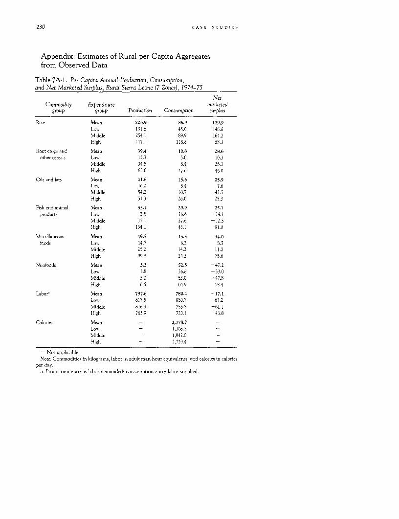
230 CASE STUDIES
Appendix: Estimates of Rural per Capita Aggregatesfrom Observed Data
Table 7A-1. Per Capita Annual Production, Consumption,and Net Marketed Surplus, Rural Sierra Leone (7 Zones), 1974-75
NetCommodity Expenditure marketed
group group Production Consumption surplus
Rice Mean 206.9 86.9 119.9Low 191.6 45.0 146.6Middle 254.1 89.9 164.2High 177.1 118.8 58.3
Root crops and Mean 39.4 10.8 28.6other cereals Low 15.3 5.0 10.3
Middle 34.5 8.4 26.1High 63.6 17.6 46.0
Oils and fats Mean 41.6 15.6 25.9Low 16.0 8.4 7.6Middle 54.2 10.7 43.5High 51.3 26.0 25.3
Fish and animal Mean 55.1 29.9 25.1products Low 2.5 16.6 -14.1
Middle 15.1 27.6 -12.5High 134.1 43.1 91.0
Miscellaneous Mean 49.5 15.5 34.0foods Low 14.7 6.2 8.5
Middle 25.2 14.2 11.0High 99.8 24.2 75.6
Nonfoods Mean 5.3 52.5 -47.2Low 3.8 36.8 -33.0Middle 5.2 53.0 -47.8High 6.5 64.9 58.4
Labor' Mean 797.6 780.4 -17.1Low 817.5 880.7 63.2Middle 816.9 755.8 -61.1High 763.9 720.1 -43.8
Calories Mean - 2,178.7 -
Low - 1,108.5 -Middle - 1,942.0 -
High - 2,729.4 -
- Not applicable.Note: Commodities in kilograms, labor in adult man-hour equivalents, and calories in calories
per day.a. Production entry is labor demanded; consumption entry labor supplied.
MICROSIMULATION OF THE RURAL ECONOMY 231
Notes
1. Lau and others (1981) used microsimulation applied to average households taken as repre-sentative of each of some forty region-size classes.
2. The underlying data were collected by Spencer and Byerlee (1977) in a survey of ruralhouseholds in Sierra Leone. They used a stratified sample with equal numbers of households ineach of eight ecological zones (agroclimatic resource regions). To make estimates for the popula-tion, we estimated per capita consumption or production levels in each zone, weighted eachzonal estimate by the proportion of the total rural population found in that zone, and combinedthese weighted consumption ratios into a single ratio for the whole rural population (see Smithand others 1981, pp. 3-7, 15-18). Because of problems in data collection, in one zone the samplecontained only five usable households. Thus the estimates presented here apply only to the re-maining seven zones, which have an estimated rural population of 1,546,600. The estimatedpopulation of the omitted zone (the Northern Plateau) was 495,500 in 1974-75 (Spencer andByerlee 1977, Table 3.1).
3. When a representative household is used, it is implicitly assumed that demand and output-supply functions aggregate perfectly over households in the sense that we can model aggregatedemand (or supply) as a function of prices and of aggregate, or average, income (fixed factors).Further, we might want the aggregate demand function to be consistent with some utility func-tion (of a representative household). For instance, the it' household's demand function for ricemight be R, = f(y,, p), where y, is full income and p is a price vector. Averaging rice demandsover N households we obtain
INR = N E if(y" P),
assuming all households face the same prices. The question is whether there exists a demandfunction gi ) such that g(y, p) = R, where y is average full income and g( ) is consistent withsome utility function. The well-known answer is yes, provided each household has the samemarginal propensity to consume rice, which implies linear Engel curves (see Deaton andMuellbauer 1980).
A weaker alternative (Muellbauer 1976; Deaton and Muellbauer 1980) is to let the averagerice budget share depend on prices and on some representative (not necessarily average) fullincome. This representative full income might even be a function of the distribution of incomesas well as of prices. In this case, we can still talk about average demand being generated by arepresentative consumer. Muellbauer derives conditions on the household cost (or expenditure)functions that are required if the representative consumer is to exist. Although the QuadraticExpenditure System does not satisfy these restrictions, the Almost Ideal Demand System (seechapter 8) does. When prices or wages vary over households, as they do in our data, however, theconditions under which the representative household exists are even more strict (Deaton andMuellbauer 1980).
4. Inasmuch as the average household in Sierra Leone produces 74 percent of the rice it con-sumes (Smith and others 1980, table 3.1) and this portion of its consumption is valued at theproducer price, the consumer price for all rice consumed does not normally differ greatly fromthe producer price.
5. If we were dealing only with point elasticities, we could leave the discussion at this point,but over the range defined by a finite price change, as in table 7-4, marketed surpluses changebecause the consumption elasticities just mentioned reduce rice consumption and because out-puts also respond to change in price. But the percentage of output changes differs little by ex-penditure group, so that such changes have little effect on consumption-response differencesamong expenditure classes.
232 CASE STUDIES
6. Apparently L households have such high marketed surpluses of rice because, having lowincomes, they consume much less rice per capita than others, and they concentrate their re-sources heavily on rice production. Snodgrass and others (1980, pp. 155-56) found that most riceproduction yielded negative returns in 1980 (see also Spencer, Byerlee, and Franzel 1979, p. 43).The L households produce relatively little of the more profitable crops, such as palm products,fish, and vegetables.
7. In the production function,
(E5jQP)I/P = OLBLAsAK8KT
the constant es is changed from 1.00 to 1.05. As this is a Hicks neutral production function, sucha shift does not of itself change the proportions among outputs. It does, however, affect bothlabor demand and the overall output level.
References
Deaton, Angus, and John Muellbauer. 1980. Economics and Consumer Behavior. Cam-bridge: Cambridge University Press.
Lau, Lawrence J., and others. 1981. "The Microeconomics of Distribution: A Simula-tion of the Farm Economy." Journal of Policy Modeling 3(2):175-206.
Muellbauer, John. 1976. "Community Preferences and the Representative Con-sumer." Econometrica 44(5):979-99.
Smith, Victor E., and others. 1980. "Non-Price Factors Affecting Household FoodConsumption in Sierra Leone." Rural Development Working Paper no. 12. EastLansing: Michigan State University.
- -. 1981. "Food Flows and Simulations: Rural Sierra Leone." Rural Develop-ment Working Paper no. 19. East Lansing: Michigan State University.
Snodgrass, Milton M., and others. 1980. Agricultural Sector Assessment Report for Si-erra Leone. Logan, Utah: Consortium for International Development.
Spencer, Dunstan S.C., and Derek Byerlee. 1977. "Small Farms in West Africa: ADescriptive Analysis of Employment, Incomes and Productivity in Sierra Leone."African Rural Economy Working Paper no. 19. East Lansing: Michigan State Uni-versity.
Spencer, Dunstan S.C., Derek Byerlee, and Steven Franzel. 1979. "Annual Costs,Returns, and Seasonal Labor Requirements for Selected Farm and Nonfarm Enter-prises in Sierra Leone." African Rural Economy Working Paper no. 27. East Lan-sing: Michigan State University.
Strauss, John, Victor E. Smith, and Peter Schmidt. 1981. "Determinants of FoodConsumption in Rural Sierra Leone: Application of the Quadratic ExpenditureSystem to the Consumption-Leisure Component of a Household Firm Model." Ru-ral Development Working Paper no. 14. East Lansing: Michigan State University.
Strauss, John, and others. 1981. "Joint Determination of Food Consumption andProduction in Rural Sierra Leone: Estimates of a Household-Firm Model." RuralDevelopment Working Paper no. 17. East Lansing: Michigan State University.
8Multimarket Analysis of Agricultural
Pricing Policies in Senegal
Avishay Braverman and Jeffrey S. Hammer
THIS CHAPTER PRESENTS an approach to analyzing the effects of agricul-tural pricing in less developed countries. The same general method underdifferent institutional constraints has been used in Korea, Sierra Leone,Cyprus, and Malawi (see Braverman, Ahn, and Hammer 1983; Braver-man, Hammer, and Jorgensen 1983, 1984; and Singh, Squire, and Kirch-ner 1984). Here we are concerned with the pricing policies of Senegal.The method presented is only a deterministic one; for an attempt at in-troducing uncertainty into such a framework see Braverman, Hammer,and Levinsohn (1983, chapter 5) and Hammer (forthcoming).
Our general method takes as a starting point the theory of the farmhousehold (Yotopoulos and Lau 1974; Barnum and Squire 1979) and in-corporates it into a simulation model that traces the short- to medium-run effects of pricing policies on a variety of outcomes of interest to pol-icymakers. These outcomes have to do with the distribution of income(between income groups or between regions), agricultural production andconsumption, and foreign trade. In many cases, pricing policies generatelarge deficits in the agricultural sector and the reduction of these deficitsis often a high-priority concern.
We are living in a quantitative era in which political debate necessitatessome quantitative assessments of evaluated policies for the sake of public
Note: For a detailed description of the studv on Senegal see Braverman, Hammer, and Levin-sohn (1983). We thank Jim Levinsohn and Erika Jorgensen for excellent research assistance.Many persons at the World Bank and in Senegal contributed to this study through discussionsand suggestions. In particular, we would like to thank Joseph Baah-Dwomoh and ChristopherRedfern. Special thanks are due to Sangone Amar, who joined our mission in Senegal and whoprovided us with invaluable support. We alone are responsible for all views expressed.
233
234 CASE STUDIES
accountability. Many economists use two standard operational tools intheir quantitative assessment of agricultural pricing policies. The mostcommonly used class of measures includes the domestic resource cost(DRC) and the effective protection rate (EPR), which are modified ratiosof domestic prices to international prices. (For agricultural pricing studiesusing EPR, see, for example, Scandizzo and Bruce 1980.) This type ofmeasure does not address the income distribution and public revenue is-sues, nor can it address the quantitative impact of taxes and subsidies onproduction and consumption. The second method, single-market calcu-lation of consumers' and producers' surplus, does not address the interac-tion among markets (that is, the substitution effects in consumption andproduction), and does not devote sufficient attention to income distribu-tion beyond classifying agents into consumers and producers. It also ig-nores the impact on and feedback from the rural labor market. In addi-tion, agricultural price reforms often include simultaneous changes in sev-eral prices, where interaction among the different commodities iscritical, and where the effects of policies may not be additive across com-modities.
The methodology presented here extends the single-market surplusmethod to include income distribution and some general equilibriumconsiderations. Balancing the need for more complete information on theconsequences of policy is the need for simplicity in operational work andthe need to maintain intuitive understanding of the system under investi-gation. For this reason, our method stops short of the computable generalequilibrium models, which often become cumbersome tools, especiallywhen institutional details are important in the structure of the economy.As with any model of economic activity, the appropriate boundaries ofthe analysis are a matter of judgment. The agricultural sector is consid-ered the proper unit of study and the urban sector (except for agrobusi-ness concerns) is taken to be exogenous. Market equilibrium includes theurban sector, however. Previous work that used the farm-householdmodel in a policy simulation study (Lau and others 1981) limited the anal-ysis to the agricultural sector alone. In the case of Senegal, this division isartificial and would ignore most of the important policy questions, suchas government deficits arising from urban consumption. Therefore, theboundaries of the problem were set to include urban consumption andthe cost of living, with nominal urban wages left exogenous.
The Senegalese Problem
The performance of the agricultural sector in Senegal is extremely im-portant to the national economy. Agriculture employs 77 percent of the
MULTIMARKET ANALYSIS OF PRICING POLICIES 235
labor force and contributes 26 percent of GDP. Agricultural productsgenerate 70 percent of export earnings. At the same time, governmentintervention in the agricultural sector has become costly. In 1982-83 defi-cits related to agricultural pricing funds amounted to 23 percent of gov-ernment expenditure and 2.6 percent of GDP.
A policy initiative discussed recently would promote the production,consumption, and marketing of millet, the main subsistence crop. Theadvantages envisioned for this approach were the saving of foreign ex-change (from reduced rice imports) and the creation of new income-gen-erating activities for farmers. The policy would be implemented by in-creasing the consumer price of rice, which is currently controlled. Thismight be accompanied by a reduction in the price of groundnuts, millet'smain competitor for cultivated land; such a measure would help to reducethe deficit in groundnut-marketing operations.
The policies selected for analysis are concerned with reducing govern-ment deficits and with addressing the millet problem. The market inter-ventions that are analyzed are reductions of 15 and 35 percent in theprice of groundnuts paid to farmers; increases of 10 and 50 percent in theprice of rice; increases of 50 and 118 percent in the price of cotton (thelatter representing world prices in 1981); and increases of 100, 200, and300 percent in the price of fertilizer (the last representing factory prices).
Since the agricultural sector is treated as a whole, integrated policypackages can also be analyzed. The multiple price changes to be examinedare reducing the price of fertilizer from 25 to 5 CFAF per kilogram andlowering the price of groundnuts to farmers by 5 CFAF (such a schemeunder consideration within Senegal would provide virtually free fertilizerthrough an added tax on groundnuts); reducing groundnut prices whileincreasing the price of rice to encourage millet production and pursuedeficit reductions; and simulating a devaluation by raising the prices oftraded commodities.
Structure of the Model
The model was constructed with two concerns in mind: it had to becomplex enough to capture the essential tradeoffs between competinggovernment goals, but it also had to be simple enough to highlight themost important features of the rural sector and not overtax the limitedinformation available. The model is quite straightforward. We model thedemand for four consumer goods: rice and groundnut oil (which are gener-ally taxed and subsidized, respectively) and millet and maize (which aremodeled as if in a free market). On the supply side, we model the produc-tion of five commodities: groundnuts, rice and cotton (which are subject
236 CASE STUDIES
to government-controlled prices), and millet and maize (which, as alreadymentioned, are traded freely in domestic markets).
The official marketing channels for millet and maize in Senegal havecontrolled prices. Very little of the millet and maize produced passesthrough these channels, however. Most is used for on-farm consumption,is traded in local village markets, or finds its way to urban areas throughprivate traders. An issue of critical concern at-present is the developmentof better marketing facilities for millet. Although they do not directlycontribute to government deficits, these crops are included in the modelbecause they are important substitutes for the other three crops in bothproduction and consumption. Policy changes will affect the production ofthese crops and their market prices. In consequence, farm incomes andthe cost of living will also be affected.
The country is divided into four regions according to the crops grown ineach. The Groundnut Basin, which is the largest region (it holds almosthalf the population), consists of the administrative districts of Sine-Sa-loum, Diorbel, Louga, and Thies. For the purposes of the model, it isassumed that the basin produces only groundnuts and millet. Land de-voted to other crops constitutes less than I percent of the total in theregion and is ignored. The southern region, which is made up of the ad-ministrative divisions of Casamance and Senegal Oriental, has the mostvaried agricultural system. Crops grown there are groundnuts, millet,rice, maize, and cotton (in the order of acreage in the base year). TheFlueve is assumed to grow millet, rice, and groundnuts. The final regionto be considered is Dakar, which is entirely a consuming area for agricul-tural products.
Each producing region is endowed with a fixed supply of land and laborthat may be allocated to the crops produced within it. Because we areusing a short-run model, we exclude interregional migration as well as theexpansion of total land farmed within a region. Various assumptions willbe made concerning the degree of substitution possibilities for land in theshort run. Labor is assumed to move freely between crops within a regionaccording to its marginal productivity in each use. Variable factors arefertilizer and a residual category consisting of other factors. These arechosen by profit maximization decisions and are not limited to any spe-cific amount.
Supply responses are derived from underlying production functions.The demand functions are derived from their underlying utility func-tions, which characterize preferences for consumer goods. The use of pro-duction and utility functions was preferred to the direct use of supply anddemand elasticities for a variety of reasons, even at the expense of compu-tational simplicity. In the tradition of the farm-household model that in-
MULTIMARKET ANALYSIS OF PRICING POLICIES 237
tegrates production and consumption decisions (Barnum and Squire1979; Yotopoulos and Lau 1974), aspects of the production structure in-fluence the consumption pattern of the household. Profits from farm pro-duction yield income that influences demand and marketed surplus offood crops. Information on supply response alone cannot easily be usedto generate this income gain. In addition, factor demand is an essentialfeature of the current model. Fertilizer is distributed directly by the gov-ernment and is a substantial contributor to the deficit. Also, the govern-ment is currently discussing the possibility of increasing the subsidies tofertilizer and financing them in part with lowered prices for crops, partic-ularly for groundnuts. A full production structure is necessary to ensureconsistency between factor demands and crop supply. This policy optioncould not be adequately analyzed without a consistent framework.
On the consumption side, demand curves are linked to their underly-ing utility functions in order to assess the welfare implications of con-sumer price changes involving a number of goods simultaneously. By us-ing a well-specified utility function, we can calculate the compensatingvariation of policy changes, giving a CFAF amount for the gain or loss ofeach person. This allows us to incorporate some of the insight providedby the new public economics literature (see, for example, Atkinson andStiglitz 1980).
Agricultural Production
The four regions of the model constitute the basic units of the analysis.Since data on income distribution and the size distribution of farms arescanty, we are unable to model the intraregional distribution effects ofpolicies. Within each of the three producing regions (that is, excludingDakar), the production structure of crops is characterized by use of thetranslog restricted profit function (Lau 1976). This functional form isquite flexible and can represent a wide variety of substitution possibilitiesbetween factors. Again, because data are scarce, the function is special-ized to correspond to the Cobb-Douglas form. The restricted profit func-tion is composed of two parts: one for variable factors of production andone for factors that are fixed to the region. Rents accruing to the fixedfactors (land and labor) become part of the income of the region.
All allocation decisions assume profit-maximizing behavior on the partof farmers. The profit function yields the appropriate amount of the vari-able factors (fertilizer and "other") as functions of their prices and thequantities of the fixed factors used. Although land and labor are fixed tothe region, they can be shifted between crops within the region. Landand labor are allocated so that the value of their marginal products are
238 CASE STUDIES
equated between uses. Since most production takes place on family farmsand the markets for both land and wage labor are quite thin in Senegal,this seemed the most appropriate way of modeling the allocation deci-sion. The alternative, which would be to discuss explicitly the determina-tion of wages and rental rates on land, does not seem to fit the generalpicture of Senegalese agriculture and would make it difficult to collectrelevant information.
Conventionally, production functions are assumed to be subject toconstant returns to scale. For the Groundnut Basin and the Flueve, thisposes no problem and the above structure is completely straightforward.Because so many crops are produced in the south, however, one addeddifficulty is that three of the crops-cotton, groundnuts, and rice-aresubject to fixed prices. Since there are only two fixed factors of produc-tion and constant returns to scale, the production possibility frontier forthese three goods contains "flats" or linear areas. This would imply thatonly two of these crops would ever be produced at the same time. If onecrop was more profitable than another, both land and labor would flowto it. With constant returns and fixed prices, the former crop would re-main more profitable even after this factor movement and would driveout the other crop. The fact remains, however, that all three crops areproduced in this region (as well as maize and millet, the price flexibility ofwhich avoids this problem). Therefore, one of the assumptions must beabandoned. We have decided to replace constant returns to scale withdecreasing returns. This can be justified in one of two ways. First, an ex-planation of the multiplicity of crops may be that the assumption of ho-mogeneous land is incorrect. Some land is simply more suitable for onecrop than another. Irrigated paddy land could conceivably be used forcrops other than rice but (in the short run, at least) is far more profitablein its present use. This type of land cannot be easily expanded in the shortrun. Therefore some of the land may be fixed not only to the region as awhole but also to its present use. More generally, the suitability of landfor different crops varies greatly and the substitution between crops can-not take place with equal ease at all levels of output. The decline in qual-ity of land as a crop acreage expands is precisely the justification given forthe assumption of decreasing returns in classical economic theory.
The second possible explanation for the variety of crops is that it is away of reducing riskiness of yields. Rainfall is erratic in Senegal and al-though little rain will hurt all crops, diversification is still advantageous aslong as yields are not perfectly correlated. A complete model of farmerbehavior under uncertainty is beyond the scope of this chapter, but sucha model would balance the additional gain of expanding the productionof a more profitable crop (in expected value) against the additional cost
MULTIMARKET ANALYSIS OF PRICING POLICIES 239
(in terms of increased variability in yields) of overspecialization. This deci-sion can also be modeled on an as-if basis by assuming decreasing returnsto scale in any one crop. The increased costs to scale are not technologicalin this case but are psychic costs resulting from a decline in the diversityof a farmer's portfolio of crops. For either of the above reasons, then, themodel adopts decreasing returns to scale in the underlying productionfunction as a means of ensuring the observed diversity of crops in pro-duction.
Incomes and Demand
Incomes in the three producing regions come from two sources, themore important being the profit generated by agricultural production.Profit is the joint return to the two fixed factors, labor and land, and isthe value of production minus payments to the two variable factors. Thisvalue is determined endogenously via the production system describedabove. The second source of income covers all nonagricultural receiptsand is held exogenous in the exercise. The value is determined by thedifference between computed agricultural income and actual income inthe base period. Since the three producing areas include some urbanareas without agricultural activities, this term is not trivial. Income inDakar is entirely nonagricultural and is held constant, in nominal terms,throughout.
The demand system used is based on a flexible functional form for theutility function similar to the translog form for the production function.It was devised by Deaton and Muellbauer (1980) and called the AlmostIdeal Demand System (AIDS). Certain features of this model make it at-tractive for the Senegal model. First, this functional form allows a greatervariety of price elasticities to be incorporated than most common de-mand systems (such as the Linear Expenditure System [LES]). Second, itis also flexible with respect to income elasticities. Since we are concernedwith substitution between basic grains, there is a good possibility that theEngel curve for some of these commodities will have an inverse U shape.Purchases increase rapidly with income at low levels of income. As in-comes rise, preferred foods substitute for the necessity items, and demandfor the latter begins to fall off. If the commodities are sufficiently disaggre-gated (as in this case), it is quite likely that demand will decline absolutelyfor the subsistence commodity. The AIDS system allows for this possibil-ity, whereas many alternative systems (LES, in particular) impose positiveincome elasticities. Since consumption of rice is an important variable inthis analysis for balance of payment purposes, the effect of incomechanges on consumption will be of central concern.
240 CASE STUDIES
Market-Clearing Conditions
Having defined the behavioral relations assumed to characterize pro-ducers and consumers, we can construct the market-clearing conditionsthat incorporate the institutional details of the Senegalese economy. Forthe crops directly controlled by government, the conditions that ensurematerials will balance are quite simple. For the cash crops groundnutsand cotton, the entire crop is purchased from the farmers at the govern-ment set price. This accords with the arrangement that SONACOS andSEIB (for groundnuts) and SODIFITEX (cotton) have with the govern-ment of Senegal. These companies then process the materials into oil andfiber and export their total production. Demand from world markets isthen perfectly elastic and absorbs the domestic supply.
In principle, the government also buys rice from producers at a fixedprice. The price of rice consumption is also set by the government; theseprices are usually lower than the (milled equivalent) producer price. Sincedomestic production is always short of consumption, the remaining rice isimported from Thailand. Again, international trade clears the market. Inmost years, however, the amount of marketed surplus is very small. Al-most the entire crop is consumed on the farm and the government han-dles very little domestic rice. Nonetheless, the opportunity to sell at thegovernment price is assumed to be present for the farmers, and that priceis assumed to be used by the farmers in their allocation decisions. Theproblem of arbitrage between high producer and relatively low consumerprices is removed by the fact that farmers sell paddy rice and the govern-ment sells milled grain.
Millet and maize are modeled as being traded on free markets isolatedfrom world markets. The prices of these goods vary endogenously toequate supply and demand. There are official government channels andgovernment prices for these crops. However, most of the production is foron-farm use and whatever is traded usually goes through unofficial chan-nels at prices above the government levels. Although the absence of adistribution system is frequently cited as a problem for farmers in dispos-ing of their crops, the fact remains that millet and (to some extent) maizefind their way to Dakar and other urban areas. The imperfection of thedistribution system is modeled by inserting a wedge between the prices inDakar and the producing regions to represent transport costs.
Deficits
The calculation of the deficits is not expected to match the actual ac-counting procedures of the CPSP (the government agricultural pricing
MULTIMARKET ANALYSIS OF PRIClNG POLICIES 241
board). Simplifications are made for each of the six funds that have beenof interest in recent years. Three of these funds relate to groundnuts. Themain component in the groundnut deficit corresponds to the subsidies toSONACOS and SEIB. It is calculated as the difference between the pro-ducer price of groundnuts and the implicit price paid by the companies(which includes transportation and handling costs), all multiplied by thetotal marketed surplus of the grain. The implicit price is derived fromtotal deficit figures for the 1981-82 crop year. The actual subsidy for theoperation of the groundnut companies is a matter of negotiation and usu-ally depends on the world price of oil, among other variables. For a givenset of world prices and an agreed cost structure for marketing, however,the above formula should reflect the fund costs adequately.
The second component of the deficit is associated with the distributionof seeds. The government currently sells seeds to the farmers by exactinga 10 CFAF per kilogram tax on groundnut production. The deficit is thedifference between the (fixed) total cost of seed distribution and the reve-nue from the tax. The last of the groundnut costs is the consumptionsubsidy for oil. This is the difference between the cost of the oil distrib-uted (a blend of groundnut and imported soybean oils) and the pricecharged the consumer, multiplied by total consumer demand.
The rice deficit is, in principle, composed of two parts. The first is thegap between relatively high producer prices and the consumer prices,multiplied by the marketed surplus. This is offset by the difference be-tween world prices of Thai 100 percent broken rice and (usually higher)consumer prices, multiplied by the level of imports derived in the model.The level of marketed surplus is usually negligible in reality, however,and, because of the regional aggregations, is always zero in the model.Therefore, the rice fund will generally be in surplus and be equal to theimplicit tariff revenue earned on imports.
The cotton fund is modeled the same way as the groundnut fund. Thedeficit per ton in 1981-82 is attributed to the difference between market-ing costs plus the implicit payment to SODIFITEX and the producerprice of cotton. In the simulation exercises, the producer prices and thetotal production will change, but the deficit will be computed the sameway.
Finally, the fertilizer deficit is calculated as the difference in the cost ofproduction of the principal fertilizers and the price charged to the farmer,multiplied by total fertilizer use.
Calibration of the Model
Rainfall, and consequently yields, fluctuate substantially from year toyear in Senegal. Therefore, picking a particular year from which to cali-
242 CASE STUDIES
brate the model runs the risk of generalizing results from a special case.To avoid this problem, we calibrated the model to match outputs, inputusage, and consumption patterns for a three-year period in which all theinformation needed was available. Thus, fluctuations can be smoothedout to obtain an average year on which to base comparisons. The threecrop years were 1976-77, 1977-78, and 1978-79. The years 1976-77 and1977-78 were slightly below average in rainfall, whereas 1978-79 was ayear with relatively high rainfall.
Basic data concerning prices, output, and acreage came from an ArthurAnderson study. Information concerning the production functions of thevarious crops was based on the study by SONED (1981). In this study,technical input-output coefficients and expenditure data are derived forlabor, fertilizer, and other inputs. When used in combination with pricedata, the share information required for the Cobb-Douglas profit func-tion can be recovered. Total production and acreage of each crop by re-gion are readily available from the Ministry of Agriculture, as is fertilizeruse.
Data concerning the demand side of the model were somewhat moreelusive. The main source of this information is a study by the Center forResearch in Economic Development (CRED 1982) at the University ofMichigan. Income and price elasticities, per capita consumption for theprincipal grains in the model, and some estimates of per capita incomewere obtained from that study. This information was then incorporatedinto the Almost Ideal Demand System framework. Although flawed in anumber of ways, this remains the only source of information available onconsumption patterns.
For some of the policy runs, especially the rice price increase used tospur millet consumption, this type of information is potentially impor-tant. In such cases, it is essential to use sensitivity analysis to see how faroff the conclusions can be with deficient data. Aggregate figures for themarket-clearing equations are fairly precise. Imports of rice, exports ofgroundnut oil and cotton fiber, and total production levels are measuredwith reasonable accuracy.
The method used to ensure consistency between these disparate sourcesof information and the structure of the model are discussed in detail inBraverman, Ahn, and Hammer (1983) and Braverman, Hammer, andJorgensen (1984). Briefly, a nonlinear programming model is constructedthat minimizes deviations of variables and behavioral parameters fromknown values, subject to various constraints. This yields all the parame-ter values needed for the base period of the model. Included are all thevariables for which information is available, such as levels of production,consumption, imports, and the like. Also included are behavioral param-
MULTIMARKET ANALYSIS OF PRICING POLICIES 243
eters such as price and income elasticities of demand, which are functionsof parameters in the AIDS demand system. The known values come fromvarious sources. Actual levels come from national statistics or the CPSPaccounts. Elasticities come from the CRED (1982) study for demand; sup-ply elasticities from simple Nerlove-style econometric exercises for farmerresponses.
The constraints that the programming model must satisfy are of twokinds. First, all of the model equations must be satisfied for the base pe-riod. Second, the theory of demand imposes a number of constraints onthe AIDS system. As with all flexible functional forms, the AIDS systemdoes not ensure the concavity of the underlying expenditure function.This requirement was imposed on the calibration exercise and took theform of restricting parameters such that the Slutsky matrix is negativesemidefinite.
Results
The analysis takes the model as derived in the calibration describedabove, changes prices as would be done in the proposed policies, and re-cords percentage changes in the supply of all five crops, in real incomes inthe four regions, in total export earnings, in government deficits (from1981 base), and in rice imports. Changes in real income are defined as the(negative of) compensating variation of the price change. The compensat-ing variation is the amount of money that must be paid to a person after apolicy change in order to make him or her as well off as before the policy.(The basic results of the model are presented in table 8-1.)
Groundnut Prices
The price of groundnuts is, rightfully, a sensitive topic. Since it repre-sents so large a share of agricultural production, we cannot tamper withthe price without making substantial changes in output and farm in-comes. Further, since prices are announced before the growing seasonand world prices of groundnut oil are fairly volatile, it is not easy to assessan appropriate border price that can be used as a base for efficiency com-parisons.
A 15 percent decline in the producer price of groundnuts has the fol-lowing consequences.
* Government deficits fall by 18.1 percent. This is composed of a 22percent fall in the three groundnut funds combined with a counter-
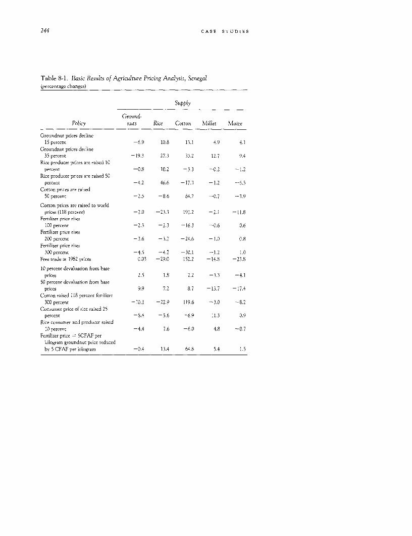
244 CASE STUDIES
Table 8-1. Basic Results of Agriculture Pricing Analysis, Senegal(percentage changes)
Supply
Ground-Policy nuts Rice Cotton Millet Maize
Groundnut prices decline15 percent -6.9 10.8 13.1 4.9 4.1
Groundnut prices decline35 percent -19.3 27.3 33.2 12.7 9.4
Rice producer prices are raised 10percent -0.8 10.2 -3.3 -0.2 -1.2
Rice producer prices are raised 50percent -4.2 46.6 -17.3 -1.2 -6.5
Cotton prices are raised50 percent -2.5 -8.6 84.7 -0.7 -3.9
Cotton prices are raised to worldprices (118 percent) -7.0 -23.3 191.2 -2.1 -11.8
Fertilizer price rises100 percent -2.3 -2.3 -16.3 -0.6 0.6
Fertilizer price rises200 percent -3.6 -3.7 -24.6 -1.0 0.8
Fertilizer price rises300 percent -4.5 -4.7 -30.1 -1.2 1.0
Free trade at 1982 prices 0.03 -29.0 152.2 -14.8 -23.8
10 percent devaluation from baseprices 2.5 1.8 2.2 -3.3 -4.1
50 percent devaluation from baseprices 9.9 7.2 8.7 -13.7 -17.4
Cotton raised 118 percent fertilizer300 percent -10.1 -22.9 119.6 -3.0 -8.2
Consumer price of rice raised 25percent -8.4 -5.6 -6.9 11.3 0.9
Rice consumer and producer raised10 percent -4.4 7.6 -6.0 4.8 -0.7
Fertilizer price = 5CFAF perkilogram groundnut price reducedby 5 CFAF per kilogram -0.4 13.4 64.8 5.4 1.5

MULTIMARKET ANALYSIS OF PRICING POLICIES 245
Real income Govern-Demand Agricul- ment
Ground, tural deficitnut Ground- export in agri- Rice
Basin South Flueve Dakar Rice Maize nut Millet earnings culture imports
-5.7 -4.7 1.2 0.6 -9.1 2.6 -3.9 5.3 -1.9 -18.1 -13.9
-13.1 -10.0 3.0 1.5 -21.2 6.0 -9.2 13.9 -7.9 -36.4 -33.0
0.03 1.5 0.7 -0.03 0.6 -0.7 0.3 -0.2 -0.7 -0.02 -1.7
0.2 9.3 3.5 -0.2 3.3 -4.2 1.8 - 1.3 -4.5 -0.1 -7.2
0.1 5.4 -0.3 -0.1 1.8 -2.5 0.9 -0.8 5.0 22.2 4.4
0.3 18.0 -0.9 -0.3 5.4 -7.5 2.9 -2.2 8.6 72.3 12.4
-1.1 -1.1 -0.4 -0.1 0.3 0.4 -0.3 -0.7 -5.2 -10.4 1.0
-1.7 -1.7 -0.6 -0.1 0.5 0.5 -0.5 -1.1 -8.1 -14.1 1.6
-2.1 -2.2 -0.8 -0.1 0.7 0.7 -0.7 -1.4 -10.1 -16.0 2.014.9 40.0 -2.4 -2.0 35.2 -15.2 14.7 -16.2 -1.9 133.6 50.8
3.7 5.3 -0.1 -0.4 6.9 -2.6 3.0 -3.6 13.3 24.8 8.1
18.9 26.6 0.4 -1.8 33.3 -11.2 14.3 -15.0 68.0 145.3 39.6
-1.9 11.1 -1.5 -0.4 5.2 -5.2 1.6 -3.2 -3.5 34.1 12.0
-1.6 -5.1 -7.8 -5.1 -6.7 0.6 -1.5 12.3 -8.8 -24.6 -7.0
-0.6 -0.7 -2.6 -2.2 -2.1 -0.4 -0.3 5.3 -4.6 - 10.2 -4.4
-2.3 -0.7 1.9 0.6 -8.1 1.0 -2.4 5.9 12.3 61.0 -13.3
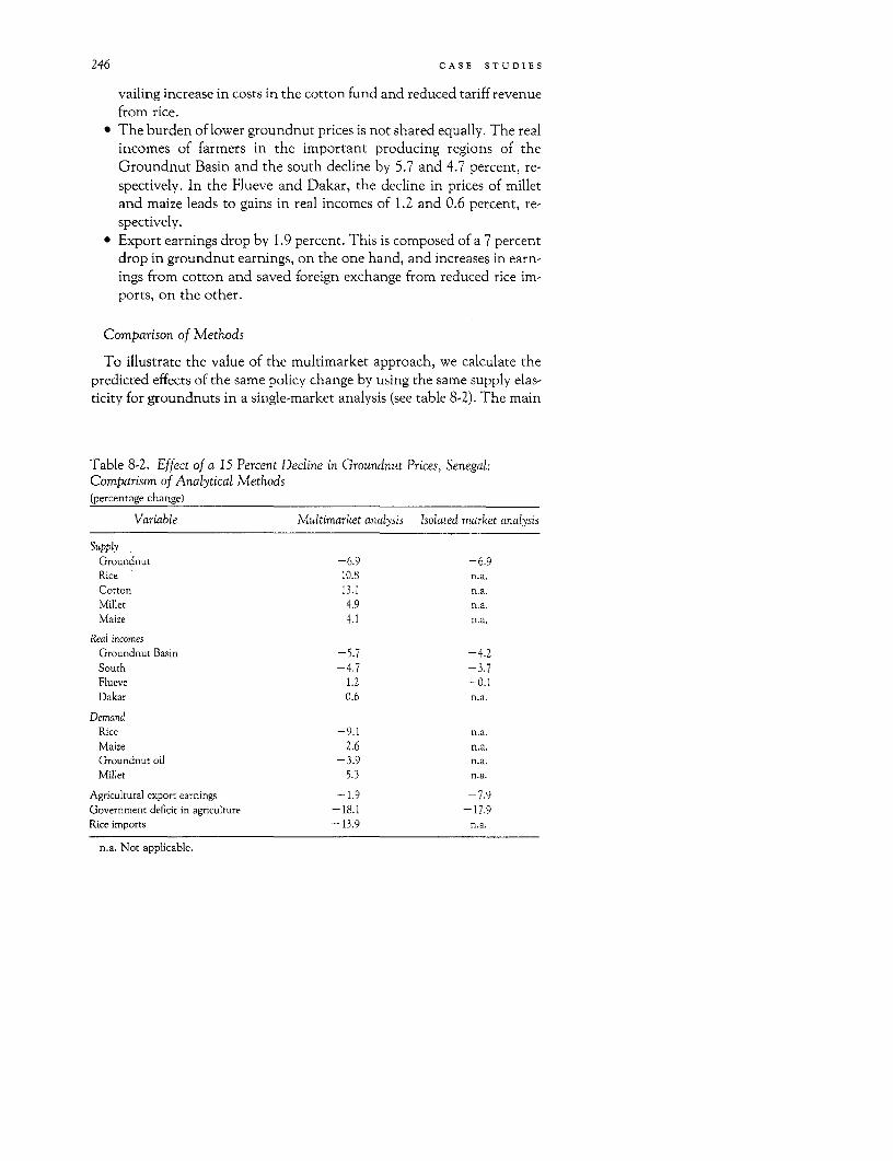
246 CASE STUDIES
vailing increase in costs in the cotton fund and reduced tariff revenuefrom rice.
* The burden of lower groundnut prices is not shared equally. The realincomes of farmers in the important producing regions of theGroundnut Basin and the south decline by 5.7 and 4.7 percent, re-spectively. In the Flueve and Dakar, the decline in prices of milletand maize leads to gains in real incomes of 1.2 and 0.6 percent, re-spectively.
* Export earnings drop by 1.9 percent. This is composed of a 7 percentdrop in groundnut earnings, on the one hand, and increases in earn-ings from cotton and saved foreign exchange from reduced rice im-ports, on the other.
Comparison of Methods
To illustrate the value of the multimarket approach, we calculate thepredicted effects of the same policy change by using the same supply elas-ticity for groundnuts in a single-market analysis (see table 8-2). The main
Table 8-2. Effect of a 15 Percent Decline in Groundnut Prices, Senegal:Comparison of Analytical Methods(percentage change)
Variable Multimarket analysis Isolated market analysis
SupplyGroundnut -6.9 -6.9Rice 10.8 n.a.Cotton 13.1 n.a.Millet 4.9 n.a,Maize 4.1 n.a.
Real incomesGroundnut Basin -5.7 -4.2South -4.7 -3.7Flueve 1.2 -0.1Dakar 0.6 n.a.
DemandRice -9.1 n.a.Maize 2.6 n.a.Groundnut oil -3.9 n.a.Millet 5.3 n.a.
Agricultural export earnings -1.9 -7.9Government deficit in agriculture -18.1 -17.9Rice imports -13.9 n.a.
n.a. Not applicable.

MULTIMARKET ANALYSIS OF PRICING POLICIES 247
advantage of the multimarket approach, of course, is that more issues canbe addressed and side effects examined in the more complete version.Supply responses of other crops, cost of living in Dakar, and demand forall consumption goods are simply beyond the scope of an analysis of thegroundnut market in isolation.
Although both methods provide answers, some differences remain.The multimarket analysis shows a larger fall in income in the GroundnutBasin and the south. This is due to the fall in prices of millet (in bothregions) and maize (in the south). With substitution possibilities avail-able, the reduction in groundnut prices induces substitution to othercrops. Prices for millet and maize fall as a result of the extra supply. Sincethese prices are inelastically demanded, net income from these crops falls.This reinforces the income loss. In the Flueve, there is a small decline inincome from groundnuts. When consumption effects of cheaper milletand maize are taken into account in the multimarket analysis, the realincomes actually increase.
The fact that the deficit figures are similar between the two versions iscoincidental. In the multimarket framework, the side effects of a ground-nut price reduction on other deficits operate in opposite directions. Fertil-izer costs are reduced, some extra seed costs are not recovered, cottondeficits rise, and rice imports fall. These add up to be within a percentagepoint of the direct effect captured in an isolated market analysis (this maynot be true in every case).
The principal difference between the two methods lies in the appraisalof the effect on foreign exchange earnings. The multimarket approachindicates that the fall in export earnings from groundnuts (the isolatedmarket figure) is mitigated substantially by the increase in cotton exportsand the decline in rice imports.
Cotton Prices
Cotton represents an important opportunity for the generation of ex-port earnings and provides an alternative source of income in rural areas.In general, producer prices have been kept lower than internationalprices. A 50 percent increase in cotton prices has the following effects:export earnings rise 5 percent; cotton output increases greatly butgroundnut production falls and rice imports increase; incomes increaseappreciably only in the south; reduced millet supplies raise the cost ofliving in Dakar and the Flueve.
Fertilizer Price
Fertilizer has traditionally been provided at a substantial discount.Prices are approximately one-fourth of the cost of production. Doubling
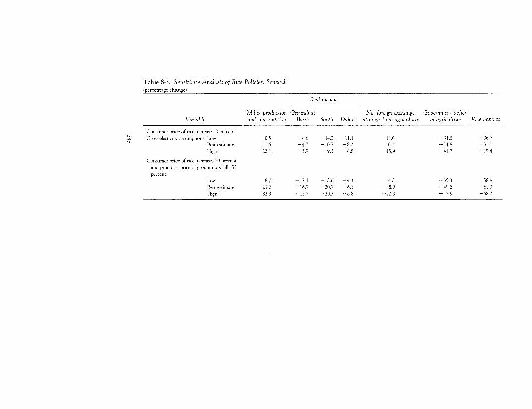
Table 8-3. Sensitivity Analysis of Rice Policies, Senegal(percentage change)
Real income
Millet production Groundnut Net foreign exchange Government deficitVariable and consumption Basin South Dakar earnings from agriculture in agriculture Rice imports
Consumer price of rice increasc 50 percent42 Cross-elasticity assumptions: Low 0.5 -8.6 -14.2 -11.1 13.6 -31.5 -36.7co Best estimate 11.6 -4.7 -10.7 -8.2 0.2 -34.8 -31.1
High 22.1 -3.9 -9.5 -8.8 -15.9 -41.7 -19.4
Consumer price of rice increases 50 percentand producer price of groundnuts falls 35percent:
Low 8.7 -17.4 -18.6 -4.3 4.05 -55.3 -58.4Best estimate 21.0 -16.9 -20.7 -6.1 -8.0 -49.8 -61.3High 32.3 -15.7 -20.3 -6.8 -22.3 -47.9 -58.2
MULTIMARKET ANALYSIS OF PRICING POLICIES 249
the price would reduce the total agricultural deficit by 10 percent, reducenet agricultural export earnings by 5 percent, and reduce rural incomes inthe main producing areas by 1 percent.
Rice Prices
Producer prices of rice are generally maintained above world prices.This may be to encourage self-sufficiency and to save foreign exchangefrom rice imports. The former goal is essentially noneconomic in naturebut its cost can be evaluated quantitatively. The latter must be evaluatedaccording to the substitution possibilities in production. Increasing theproducer price of rice will increase the income of farmers in the south atthe expense of urban dwellers (because of higher millet prices), and reducethe net foreign exchange earnings (because of the substitution of rice pro-duction for the production of important export crops such as groundnutand cotton).
Raising the consumer price of rice has recently been proposed to stimu-late millet consumption and, hence, production. The strength of this ar-gument rests on the cross-price elasticity of demand between rice and mil-let. Since this parameter is known only roughly, it is important to seehow sensitive the results are with regard to this variable. Table 8-3presents selected results for two policies: raising the consumer price of riceby 50 percent, and raising the price of rice in conjunction with a 35 per-cent decline in groundnut prices. Rice prices stimulate millet output fromthe demand side, but groundnut prices influence the supply side. Threeformulations of the demand system are tried for each policy. The elastic-ity of demand for millet with respect to the price of rice is assumed to beunity (follow the results of the CRED 1982 demand study), zero, and two.Further, in order to show the effects of the policy proposal in its bestlight, we changed some other assumptions of the model. Since the draw-back of these policies is likely to be losses in foreign exchange due to sub-stitution away from the export crops, the model was changed to lower thesubstitution possibilities. In this version, land allocated to each crop isfixed. Increases in output can be achieved only by increasing the intensityof cultivation using the other factors of production. The basic results canbe summarized as follows:
* Although sensitive to the assumption concerning cross elasticities,millet production can be stimulated by means of an increase in riceprices.
* The public deficit is reduced substantially by this policy, althoughthis is mostly due to the gain in tariff revenue from rice imports. Thisresult is relatively insensitive to the elasticity assumption.
250 CASE STUDIES
* These benefits come at a cost. Net foreign exchange earnings, verysensitive to the elasticity assumption, can be expected to fall withhigher elasticities because extra millet production comes at the ex-pense of groundnuts, the main export earner. Real incomes nation-wide fall substantially; this result is insensitive to the demand struc-ture. When combined with a reduction in groundnut prices, theabove remarks hold; the effects are merely strengthened.
Although some of the results are quite sensitive to the underlying de-mand system, proponents of raising the rice price are faced with a seriousproblem. There is no unambiguously good scenario. Real incomes anddeficits are reduced together and are not greatly affected by the uncer-tainty surrounding the cross-price parameter. However, the cases inwhich millet production is successfully stimulated by higher rice prices areprecisely the cases in which foreign exchange earnings are hurt most.Thus, even though the degree of substitution between rice and millet isunknown, the tradeoff between the goals of millet production and foreignexchange earnings is known quite well. The costs with respect to a loss inforeign exchange go up with the degree of success in increasing millet pro-duction through the use of prices alone with a given technology.
Conclusions
This chapter has presented an analysis of agricultural pricing policies ina multimarket framework for a data-scarce country. Even with limiteddata, a consistent framework of analysis brings into focus the short-runeconomic issues for an intelligent debate in the political arena. Most policy-makers would like to clarify the issues and probable outcomes. Without anassessment of the short-run impact of changes in taxes and subsidies, thecredibility of any position on a policy may be questioned. Numbers canalso be used out of context and models abused by political advocates.Nonetheless, we believe that the advantage of simple modeling of taxchanges providing a consistent framework and quantitative structure fordiscussion greatly outweighs this cost.
The method presented here will remain valid despite the scarcity ofdata if sensitivity analysis is properly used, as demonstrated here in theanalysis of rice price policies. It is important to know when gaps in one'sknowledge affect policy conclusions and when conclusions are relativelyrobust.
This method was designed to be an operational tool for economists.The elaborateness of the calibration technique requires sophisticated
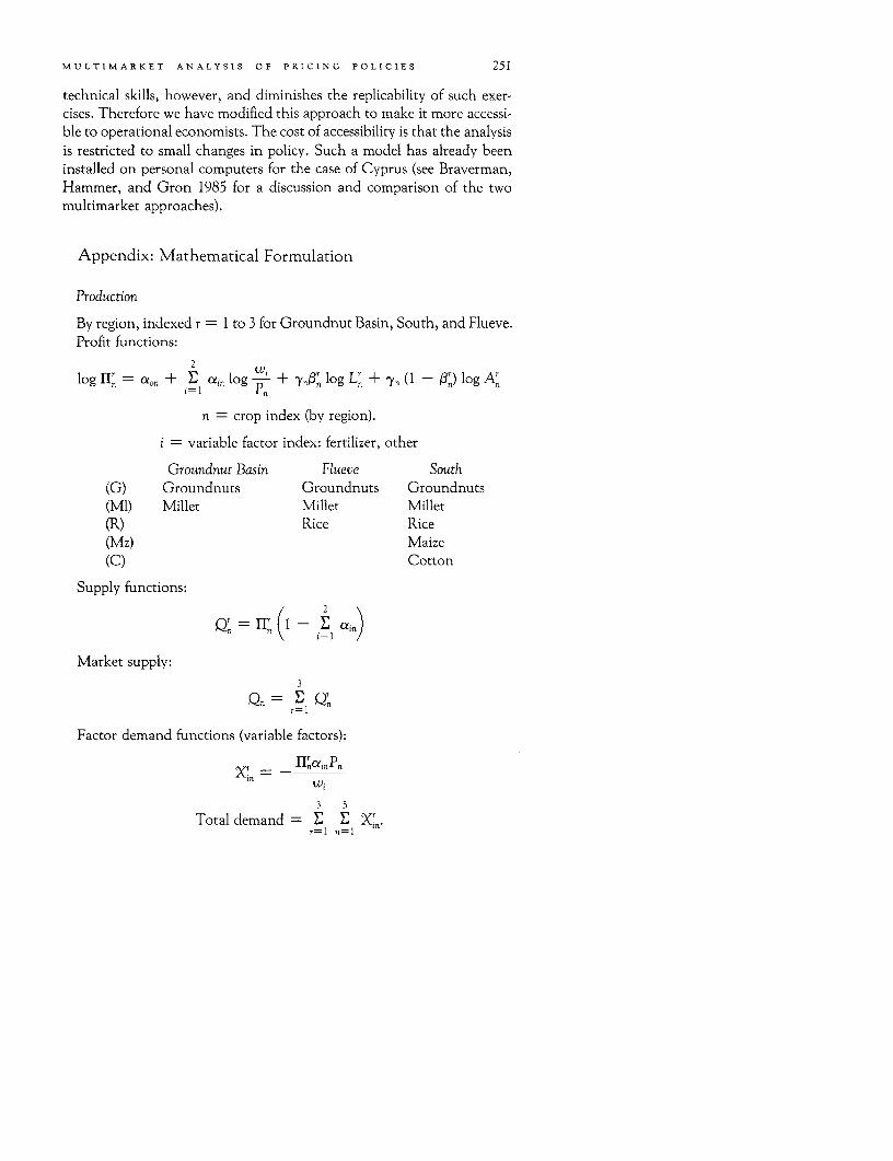
MULTIMARKET ANALYSIS OF PRICING POLICIES 251
technical skills, however, and diminishes the replicability of such exer-cises. Therefore we have modified this approach to make it more accessi-ble to operational economists. The cost of accessibility is that the analysisis restricted to small changes in policy. Such a model has already beeninstalled on personal computers for the case of Cyprus (see Braverman,Hammer, and Gron 1985 for a discussion and comparison of the twomultimarket approaches).
Appendix: Mathematical Formulation
Production
By region, indexed r = 1 to 3 for Groundnut Basin, South, and Flueve.Profit functions:
2
1og flcn = Con + E cejn log p + y,f3 log L' + ry (1 - ) log A'
n = crop index (by region).
i = variable factor index: fertilizer, other
Groundnut Basin Flueve South(G) Groundnuts Groundnuts Groundnuts(Ml) Millet Millet Millet(R) Rice Rice(Mz) Maize(C) Cotton
Supply functions:
Un = frn (1 - a i2n)
Market supply:3
Qn I QT
Factor demand functions (variable factors):
Cxr _ HnUinP._in w3 5
Total demand = 2 Xr.r=l n=1 m
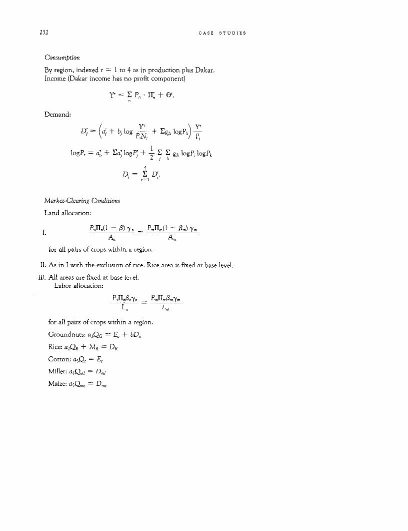
252 CASE STUDIES
Consumption
By region, indexed r = 1 to 4 as in production plus Dakar.Income (Dakar income has no profit component)
yr = E Pn, * HI + 0r.n
Demand:
D= (a; + bj log p + FgJk log Pk) yr
logP= a' + ra. logPT + 2 E E gjk logP1 logPk
4
Di = E, D;.r=l
Market-Clearing Conditions
Land allocation:
PJn(1 - 03) yYn _ PmIm(1 - 1m) 'YmI. A Am
for all pairs of crops within a region.
II. As in I with the exclusion of rice. Rice area is fixed at base level.
III. All areas are fixed at base level.Labor allocation:
PnIInf3n'yn - PmImlBmfmym
Ln Lm
for all pairs of crops within a region.
Groundnuts: a,QG= E0 + bD0
Rice: a2QR + MR = DR
Cotton: a3Q= E,
Millet: a4QmZ = Dmi
Maize: a5Qmz= Dmz
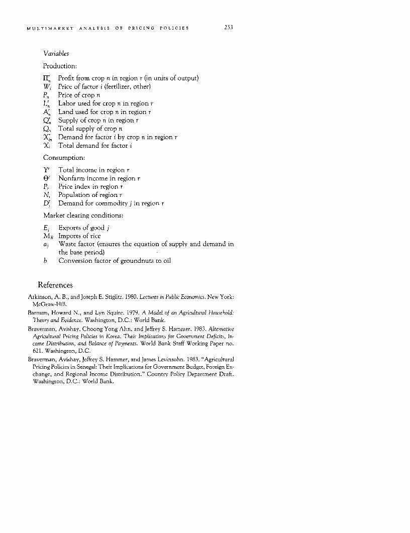
MULTIMARKET ANALYSIS OF PRICING POLICIES 253
Variables
Production:
IIr Profit from crop n in region r (in units of output)Wi Price of factor i (fertilizer, other)Pn Price of crop nL' Labor used for crop n in region rA' Land used for crop n in region rQn Supply of crop n in region rQ, Total supply of crop nX' Demand for factor i by crop n in region rXi Total demand for factor i
Consumption:
yr Total income in region rOr Nonfarm income in region rPr Price index in region rN, Population of region rD' Demand for commodity j in region r
Market clearing conditions:
Fj Exports of good jMR Imports of riceaj Waste factor (ensures the equation of supply and demand in
the base period)b Conversion factor of groundnuts to oil
References
Atkinson, A. B., and Joseph E. Stiglitz. 1980. Lectures in Public Economics. New York:McGraw-Hill.
Barnum, Howard N., and Lyn Squire. 1979. A Model of an Agricultural Household:Theory and Evidence. Washington, D.C.: World Bank.
Braverman, Avishay, Choong Yong Ahn, and Jeffrey S. Hammer. 1983. AltemativeAgricultural Pricing Policies in Korea: Their Implications for Government Deficits, In-come Distribution, and Balance of Payments. World Bank Staff Working Paper no.621. Washington, D.C.
Braverman, Avishay, Jeffrey S. Hammer, and James Levinsohn. 1983. "AgriculturalPricing Policies in Senegal: Their Implications for Government Budget, Foreign Ex-change, and Regional Income Distribution." Country Policy Department Draft.Washington, D.C.: World Bank.
254 CASE STUDIES
Braverman, Avishay, Jeffrey S. Hammer, and Erika Jorgensen. 1983. "AgriculturalTaxation and Trade Policies in Sierra Leone." Country Policy Department Draft.Washington, D.C.: World Bank.
. Forthcoming. An Economic Analysis of Reducing Input Subsidies to the LivestockSector in Cyprus. World Bank Staff Working Paper no. 782. Washington, D.C.
Braverman, Avishay, Jeffrey S. Hammer, and Anne Gron. 1985. "Multi-MarketAnalysis of Agricultural Pricing in an Operational Context: the Case of Cyprus."World Bank Agricultural and Rural Development Department Discussion Paper.Washington, D.C.
Braverman, Avishay, Jeffrey Hammer, and Choong Yong Ahn. Forthcoming."Multimarket Analysis of Agricultural Pricing Policies in Korea." In Modern TaxTheory for Developing Countries. Edited by David Newbery and Nicholas Stern.Washington, D.C.: World Bank,
Center for Research on Economic Development (CRED). 1982. "Consumption Ef-fects of Agricultural Policies: Cameroon and Senegal." Ann Arbor, Mich.: Univer-sity of Michigan.
Deaton, Angus, and John Muellbauer. 1980. "An Almost Ideal Demand System."American Economic Review, vol. 70, no. 3 (June), pp. 312-26.
Hammer, Jeffrey S. Forthcoming. "Subsistence First: Farm Allocation Decisions inSenegal." Journal of Development Economics.
Lau, Lawrence. 1976. "A Characterization of the Normalized Restricted Profit Func-tion." Journal of Economic Theory, vol. 12, no. 1 (February), pp. 131-63.
Lau, Lawrence, P. A. Yotopoulos, E. C. Chou, and W. L. Lin. 1981. "The Micro-economics of Distribution: A Simulation of the Farm Economy." Journal of PolicyModeling, vol. 3, pp. 175-206.
Scandizzo, P., and C. Bruce. 1980. Methodologies for Measuring Agricultural Price Inter-vention Effects. World Bank Staff Working Paper no. 394. Washington, D.C.
Singh, I., L. Squire, and J. Kirchner. 1984. "Agricultural Pricing Policies in Malawi."Country Policy Department Paper, preliminary draft. Washington, D.C.: WorldBank.
SONED. 1981. "Modelisation des Prix Agricoles." Processed.
Yotopoulos, P.A., and L. J. Lau. 1974. "On Modelling the Agricultural Sector inDeveloping Countries: An Integrated Approach of Micro and Macro-economics."journal of Development Economics, vol. 1, pp. 105-27.
9Yield Risk in a Dynamic Modelof the Agricultural Household
Terry Roe and Theodore Graham-Tomasi
NUMEROUS STUDIES HAVE FOUND that farmers in developing countries preferlower but certain levels of income to marginally higher uncertain incomelevels (Moscardi and de Janvry 1977; Dillon and Scandizzo 1978; andBinswanger 1980). Estimates of farmers' aversion to risk in these studiesrange from a measurement of 0.9 for absolute risk aversion in NortheasternBrazil to 0.316-1.74 for partial risk aversion among farmers in India. Sincecontingency markets are surely imperfect in developing economies, riskaverse farmers tend, in an effort to reduce income uncertainty, to allocateresources to activities with lower expected marginal value products thanthey would in the absence of uncertainty.1
The relationship between depressed income due to risk and householdconsumption has not been studied in models of the agricultural household.An implication of assuming the absence of risk when risk is present is thatinferences drawn from such models may be misleading. The problem is todetermine the nature of the misleading inferences that might otherwise bedrawn. Moreover, failure to consider the effect of risk on household choiceslimits the insight that can be gained into the welfare effects of market im-perfections, such as those that inhibit households from allocating resourcesto off-farm activities, crop insurance, or imperfections that provide limitedaccess to production technologies and other risk-reducing inputs.
In this chapter, we seek to incorporate production risk into a dynamicversion of the agricultural household model. We investigate a fairly simple
Note: The authors thank John Strauss, Cliff Hildreth, Bob Myers, and participants in the
Consumption Economics Workshop at the University of Minnesota for helpful comments on anearlier draft of this chapter.
255
256 CASE STUDIES
model in an effort to determine the impact of yield risk and the household'srisk preferences on its production and consumption decisions. Our modelgives the familiar result that consumption and production occur along thelocus of points formed by the tangency of marginal utilities and marginalproducts to their respective price ratios. An analogue of Roy's Identity isalso found that relates consumption and input demands to the derivativesof a dynamic version of the household's indirect utility function. At thispoint, the results depart from those of the traditional model. In general,separability between production and consumption decisions does not hold,although a special case is demonstrated in which a type of separability ex-ists. Even though relationships between the household's choices and in-creasing risk can be derived for this special case, parameters of the house-hold's direct utility function and prices of the arguments appearing in thisfunction are found to determine the "risk aversion parameter" appearing inthe product-supply and input-demand functions. Also, for this special case,demand is found to be a function of certainty-equivalent income. Hence,our findings suggest that parameter restrictions on estimating equations de-rived from models of the agricultural household that assume an absence ofrisk may be inappropriate if risk and risk aversion are important.
Background
The theory of the individual consumer provides some insight into theeffect of increasing income uncertainty on consumption levels. Results arenot easy to obtain, however, and generally depend on third-derivativeproperties of the utility function. In the case of a single-good, two-period,utility function with uncertain income in the second period, the third-de-rivative property implies the convexity of the marginal utility of the goodconsumed in the second period; this is compatible with decreasing absoluterisk aversion. In the models considered by Leland (1968), Mirman (1971),and others,2 the third-derivative property implies a decrease in first-periodconsumption or an increase in savings as uncertainty increases. The prob-lem faced by the agricultural household in our model is more complex thanthe problem studied in this literature in two ways.
First, income in these models is exogenous, and second, there is only oneconsumption good. Clearly, the essence of the agricultural householdmodel as outlined in chapter 1 is endogenous income and the existence ofboth a staple and a market good. With respect to the first issue, Block andHeineke (1973) study a static model in which utility is a function of incomeand labor. They show that if (-B2 U/a Y2)/(a U/a Y), where Y is income, isdecreasing in income for a given quantity of labor supply, then an increase
YIELD RISK IN A DYNAMIC MODEL 257
in risk increases labor supply when there is additive income risk (Y = wL+ Y). Thus, the individual self-insures against income risk by workingmore. With wage rate uncertainty (Y = Y + wL), Block and Heinekeshow that an increase in risk has an ambiguous effect. A dynamic modeltakes into account savings as well as labor effort, and thus it is not clearthat the Block and Heineke results will hold.
The definition and measurement of risk aversion in situations wherethere are several goods has been studied by Kihlstrom and Mirman (1974,1981). In addition, Stiglitz (1969) and Hanoch (1977) have investigated theimplications of risk aversion for demands for commodities. All of theseanalyses take place in static models, however. The most important resultsfor our purposes are those of Kihlstrom and Mirman, which indicate thatwith homothetic preferences and income risk, the risk preferences of theconsumer are reflected by the indirect utility function considered as a func-tion of income alone. Similarly, the dynamic, single-good models show thatthe value function in a dynamic programming approach to solving theproblem embodies the curvature properties of the direct utility function(Miller 1976).
Our efforts along these lines are complicated by the production activitiesof the agricultural household. If we consider production decisions alone,the most relevant study is one by Pope and Kramer (1979) that examinesproduction uncertainty for a competitive firm.3 They find that, if the pro-duction function is multiplicative in the random variable (a form we as-sume in this paper), then an increase in risk reduces output if absolute riskaversion is decreasing. Our research extends their model to a dynamicsetting.
The introduction of risk into a dynamic model of the agricultural house-hold has two significant implications: (1) in general, the model is no longerseparable into independent consumption and production activities, al-though a type of separability exists in one special case, and (2) restrictionson estimating equations derived from certainty theory are not appropriatewhen production is risky. These results hold even for our relatively simplespecial case, in which utility is additively separable over time, input andoutput prices are known, risk enters the production function multiplica-tively, and production shocks are distributed independently over time.
A basic reason for the lack of separability is that risk aversion in con-sumption induces risk aversion where profits are concerned.4 Thus, the ex-pected utility of profits must be maximized, The form of this function de-pends on the form of the consumption utility function and consumptiondecisions.
A more fundamental reason for the lack of separability is the absence of amarket. As discussed in chapter 1, separability of the static household pro-
258 CASE STUDIES
duction model obtains if a complete set of markets exists. Iqbal (chapter 6)extends this to a two-period model by introducing a capital market. In thischapter, with risk, separability does not hold because contingent claimsmarkets do not exist; if contingent claims markets were introduced, separa-bility would be restored. We believe, however, that positing such perfectinsurance markets is inappropriate.5
The Conceptual Framework
The household gains utility from a sequence of consumptions of goodsX, and leisure Xi, over its time horizon t = 0, 1, ... , T and from a be-quest. The household's utility is given by an additively separable, time-invariant utility function:
,=T) tTT(9-1) U({ X,, ,,, b, It) = i t u(Xt, XI,) + T+116(bT+ ).
Here, as in the basic model presented in chapter 1, there are two goods: anagricultural staple, Xqt, and a good purchased in a market, X,,t. The house-hold is assumed to hold a single financial asset, bt. The discount factor ce(1 + e)-', where e is the rate of utility discount; we assume that 0 < e < 1.
Farm production of the agricultural staple is given by the stochastic pro-duction function
(9-2) Qt+ = Q(L,, At; e,+j)
where L, and A, are labor and land inputs at t, and e, is a random variable.Note that both labor and land are variable here, and that there is a lag inproduction. L, and A, are the sum of allocations to production out of thehousehold's endowments, plus net market purchases of labor and land.
In contrast to the basic model of chapter 1, the model studied here isdynamic. The household consumes goods and leisure in period t from in-come generated by allocations of land and labor made in the previous pe-riod, t - 1. We assume that Q, is known when (X4,, X,m, XI,) are chosen. Inperiod t, the household also decides upon the resource allocation (L,, At),which determines output in the next period, t + 1. As with goods andleisure, we assume that Q, is known when choices of A, and L, are made.Another departure from the basic model is the existence of a financial assetwith rate of return, r. As we shall see, this asset serves to smooth intertem-poral household consumption by linking, over time periods, the house-hold's marginal utility of income. Note that b, represents beginning-of-period holdings of the asset.
Markets for commodities, land, and labor are assumed to exist. The mar-ket prices of X., and X,,t are Pqt and Pint respectively. The rental rate forland is a, and the wage is w,.
YIELD RISK IN A DYNAMIC MODEL 259
Full income in period t can be expressed as the value of the household'sendowment of land and time plus interest income plus profits, that is,
(9-3) 1t = a,A + w,L + PqtQ(Lt-1, A,-; t) -atAt - w,L + (1 + r)bt
= W, + 7rT + (1 + r)bt
where A and L represent endowments of land and labor, respectively. Ex-penditure on goods and leisure in period t is
(94) Ct = PqtXqt + PmtXmt + WtXft.
Then, the holdings of the financial asset evolve according to
(9-5) b -+, = It-Ct.
In summary, we have the following statement of the household's maximi-zation problem:
T
X: max E E Ctu(X", XI,) + T+l 6(bT+l)1ZJ] t
s.t. Q,+1 = Q(L,, A,; et+,)
b,+I = Wt + Tt-Ct + (1 + r)bt
where zt = (Xqt, Xmt, Xit, At) Lt).
Under an assumption that the stochastic process let] is a stationary Mar-kov process, the solution to X can usefully be studied using a dynamic pro-gramming approach. A Markov process is such that the probability distri-bution on et+1 is conditional only on et and not on the entire history ofthe process. Thus, we write the conditional distribution on the next pe-riod's realization of the random event (called the transition probability) as40et+I, et)
Let Vt(Q,, b,, et) be the value function for the household's problem atdate t. V'() gives the maximal expected present value of utility from date tto T + 1, starting with "initial" condition (Qt, b,, et). Thus, V° is the indi-rect objective function for the overall problem; it is the dynamic equivalentof the household's indirect utility function. The dynamic programming ap-proach to characterizing a solution to the problem makes use of the recur-sive relationship
(9-6) Vt(Q,, b,, et) =
sup [U(Xqt, Xmt, X) ± a Vt+1 (Qt+l± bt+1, et+l) dO(e,+1, et)
I Q,+I = Q(Lt, At; e,+ 1); b+l= WI + (1 + r)b, + rt - Ct].
260 CASE ST UDIES
In the terminology of dynamic programming, the state of the system att is the vector (Qt, b1, et). A plan is a map at each date giving the cur-rent action z, as a function of the history of the state until t, that is, z, =z,([QT, b,, E,]'_o). An optimal plan is a solution to X. An optimal plan, ifone exists, solves the functional equation in (9-6) at each date.
Under some fairly mild assumptions, it is possible to show that an opti-mal plan for our problem exists, is continuous, and depends only on thecurrent state and not on the history of states. Furthermore, if the functionsu(*) and Q(*) are strictly concave and p-times continuously differentiable,then if solutions are interior, it may be shown that the value function Vt()is p-times differentiable, and that the optimal plan zt*(Q,, b1, et) is (p - 1)-times differentiable. The optimal plan can be obtained by applying the Im-plicit Function Theorem to the first-order, necessary (and sufficient, owingto strict concavity) conditions for the problem
(9-7) max u(Xqt, Xmt, X,,) + aEVI+I (Qt+1, bt+1, 1 + ).[zI
The statements in the previous two paragraphs are asserted withoutproof in this chapter since the proofs involve technical details that are notparticularly interesting per se. (For a more formal analysis of a problemsimilar to the one stated here and for formal proofs of assertions in thischapter, see Graham-Tomasi and Roe 1985).
Characterizing a Solution
We turn now to a special case of the problem X in which the productionfunction for the agricultural staple takes the form
(9-8) Q(L,, A,; t+,) = f(L1, A,) e,+j
and where the process { et } is a sequence of independently and identicallydistributed random variables. For this special case, e, does not conditionthe distribution of et+ 1. Thus, et does not enter the value function directlyas part of the state at t.
Let the price of goods and inputs be summarized by the vector Pt = (Pqt,Pint, w, a,) and define
&1(Zt; Q1, b1, P1) = U(Xqt, Xm,, X,,) + otEVt+l(Qt+i, bt+i)
U(Xqt, X.t XI,) + aEVE+l (f(Lt, A,) e, W, + (1 + r)b,
+ PqtQt - wtL - aAt - PqtXqt - PmtXmt - WtXlt)-
Our discussion above indicates that Zt can be characterized by studying thefirst-order necessary conditions
YIELD RISK IN A DYNAMIC MODEL 261
(9-9) 0 ax d ax aPqt E(>)aqt q -a +
(940) 0 - aab au ~ aPmt 'ax,, ax,,, EK ab1+1
_aat au ~ (avt+(9-11) 0 = =a t E-ax 1,, ax,, ~ "ab, ab1 ±
(9-12) d = aat = ( davbt+l )f) E v+-aL, Ka Q,+ IaL4 ) wa -ab -1±
(9-13) o = da = /E av' af e)- oaE av'LAt, dQt,- a-A, /dabt+ 1I
We now offer some economic interpretations of these conditions. First,(9-9), (9-10), and (9-11) imply
(u/axqt au/axm, _ au/ax1 ,(9-14)=
Pqt Pm, W,
This, of course, is the familiar result from static certainty theory that goodsand leisure are consumed so as to equate marginal rates of substitution toprice ratios. Thus, the household allocates the amount it decides to spendon consumption in accordance with the usual efficiency principles.
Intertemporal allocations of goods can be characterized by consideringVt+1(*). By definition,
(9-15) Vt+l(Q,+±, b,+1) max a 6 t+1(-) = u(Xqt+l, Xmqt+lh Xlt+l)
± oLEVI+2 (Q,±2, b,+2 ).
As with choices of z, we have the following necessary condition for Xqt+ i:
(9-16) 0 = dd - -a - axP +I E( )ax,,+ I axq,±i qt K ab14-2 PFrom (9-15) we also have
(9-17) -+ b(V-,= El) (1 + r).dbt+,\dbt+ 21
Substituting (9-17) into (9-16) yields
(9-18) au (1 + r) aVt+'(9-18) ~~~~aXqt± I Pqt+ I at
When Xq,+I is chosen, b,+I is known. To compare this with the choice ofXq, so as to depict how the household plans to allocate consumption
262 CASE STUDIES
through time, we must take the expectation of (9-18), conditional on infor-mation available at date t, and substitute into (9-9). After rearrangement,we obtain
au/ax = E(au/aXqt+1)/(l + e)Pqt Pqt+i/(1 + r)
Thus, as in (9-14), the household equates the marginal rate of substitutionbetween current consumption and the expected present value of futureconsumption (discounting at the utility discount rate) of a good to the ratioof current price to present value future price (discounting at the rate ofreturn on the financial asset) of that good.
On the production side, our model can be given familiar interpretationsas well. From (9-15), we have
avt+l _ avt±2
(9- 1 9) 8Q,+ of =: CPqt+1 E( lb )
Substituting (9-17) into (9-19), taking expectations, and substituting the re-sulting expression into (9-13) yields
(9-20) E [aV+l ( Pq+1 af(. - at)] = 0.
This is a first-order condition for a firm with risk preferences represented bythe utility function Vt±+y() if it were to maximize the expected utility ofprofits. In our model, costs are incurred at date t and output sold at datet + 1; hence, the output price is discounted.6 Of course, a similar expres-sion holds for the labor input.
It is possible to show that the usual static efficiency conditions concern-ing the choice of inputs holds in our framework. To see this, divide (9-12) by(9-13) to get
/ avt+l df a ,V( dQ, f, aL ) _ __
E(:aQe) aAa e)
But, when evaluated at optimal choices L,* and At*, the derivatives af/aLtand af/aA, are constants. Thus, they can be taken out of the expectationsoperation to achieve
(92)aaL, = w,(9-21) fA, a
YIELD RISK IN A DYNAMIC MODEL 263
This is a direct consequence of using a multiplicative form for our produc-tion function, as stated in (9-8). A similar result was derived by Pope andKramer (1979) in a static model.
Returning to equation (9-20), we see why the model is not separable intoconsumption and production aspects of the household's problem. Thefunction V'(*) is a value function and therefore depends on the maximizedquantities of all choice variables, including consumption goods. The con-sumption goods enter V"'+(.) through the transition equation on assets.The risk preferences for solving the problem of maximizing the expectedutility of profit must be derived from the household's preferences for in-come risk and ultimately from their preferences concerning consumptionvariability. Moreover, the results available from the theory of the firm andthe theory of the consumer under uncertainty do not, in general, carryover to our nonseparable model.
Increases in Risk
It is apparent from the first-order condition stated in (9-9)-(9-13) thatgeneral comparative statics results with regard to changes in prices of goodsand inputs and changes in the interest rate can be obtained in the usualfashion. At the same time, obtaining these results will be tedious becausemany choice variables and parameters exist in our model. To see the issuesmore clearly, we focus on a specific functional form of the general modelpresented above. In this case, unambiguous results can be obtained andproblems of empirical application are more apparent.
A Specific Model
This simplification enables us to derive functional forms of the house-hold's output-supply and commodity- and factor-demand equations and avalue function exhibiting constant absolute risk aversion (CARA); it issimilar to the form of the indirect utility function derived by Stiglitz. Thisderivation also demonstrates a type of separability between the household'sproduction and consumption decisions. An empirical example of themodel is also presented. Although the model was initialized to householddata from the Dominican Republic, the empirical results are only intendedto illustrate and provide further insight into the relationship between yieldvariance, risk aversion, and the household's choices, and thus, by implica-tion, to suggest some of the likely consequences of not accounting for thistype of behavior in the more traditional nonstochastic model of the agricul-tural household.
264 CASE STUDIES
The specific form of the household's additively separable, time-invariantutility function corresponding to (9-1) is
U({ Xqtt Xmt. Xi,}t})
t-T
= 8 (-adexp{- riX'i}) + UT+'(-exp -K(bT+I)}),t~ 0
where i = q, m, 1. As shown below, it is important that the coefficients forui are positive and sum to unity. Hence, the direct utility function is a nega-tive exponential where the exponential is a Cobb-Douglas (C-D) function,homogeneous of degree 1.
No production is assumed to occur in the terminal period T + 1 so, withrespect to dynamic programming, the household's problem is to chooseXqt, Xn,, and XI, to maximize terminal period utility subject to a given levelof assets bT+ 1. In this case, it is easily shown that the terminal period utilityis given by
(9-22) -exp{ -kbT+l } -exp{ -1ri&i P i+lbT±l }
-exp{--k(bT+ ±) }
for i = q, m, 1. The exponent of bT+l on the LHS of (9-22) is unity becauseof the assumption that the values of oi sum to one.
To simplify the problem, we eliminate the production lag, and for con-venience, let production be given by the C-D production function
Qt = Qte = cLA'1-e, 0 < -YI < 1
wheree iidN(l, V[e]).7 The problem is further simplified by assuming that
prices remain unchanged-hence no time subscript appears on k in (9-22)-and by focusing on only two periods. The two-period assumption reducesthe number of arguments in the t-th period value function, but otherwise itdoes not alter the nature of the problem. The state variable b,+I is given by
b^+ = PqQt - aA - wL, ± (1 + r)b, + aA
+ wL-PqXqt -PmXmr - WXit.
Under the above assumptions, the two-period problem can be stated as
max - exp{ -iX1ti} + uE[-a exp{ -kb,+l}]
or, from the moment-generating function, it can be stated as
max - exp{ - irXlt}-c a exp -k(bt+ I - .5k(PqQt)2 V(E))}ith,
where b,+ I is the mean of b,+.
YIELD RISK IN A DYNAMIC MODEL 265
From the first-order necessary conditions, (9-14) implies the result, famil-iar to C-D forms, Xi, = (aiP,1/ajP)Xj, in the case of consumption, and (9-21) implies the result L = (-yya/(I - yI)w)A, in production. Moreover, theequivalent of (9-20) in this case is simply
Pq(aQ,/3Lt) - w - kPqQ, (aQ,/Lt)V(e) = 0
and similarly for A,. This result is obtained because of the restrictionsplaced on the ai. This result suggests a type of separability in the sense thatproduction choices can be made independently of consumption choices.Contrary to the traditional nonstochastic version of the household model,however, preferences over goods and leisure affect input choice through theparameters embodied in k. Furthermore, risk aversion, as determined by k,is also a function of prices Pq, Pm, and w. Hence, contrary to most treat-ments of decisionmaking under risk, the simple model illustrated hereserves to reinforce the point made in the preceding section that productiondepends on the properties of the direct utility function. Moreover, riskaversion (even in the case of constant absolute risk aversion) is not con-stant, but varies with changes in prices of the arguments appearing in thedirect utility function.
The demand and supply functions are derived from the first-order neces-sary conditions and the transversality condition. It can be verified that thehousehold functions are
(9-23) X,, = (ac/2PD)(Y, - (log c4/k), i = q, m; I
where Y, is the utility certainty-equivalent income given by
Y, = PqQt - aA, - wL, + (1 + r)b, + aA + wL - .5k(P,Q,)2 V[e].
The last term in (9-23) accounts for the substitution relationship betweenthe utility the household obtains from current (relative to future) consump-tion. Since the discount term (a) is a fraction, its log is negative and thusserves to augment certainty-equivalent income as preferences for currentutility from current (relative to future) consumption increases. The "2" inthe denominator "divides" certainty-equivalent income between the cur-rent and the next period. Otherwise, (9-23) bears a close resemblance to thefamiliar demand functions derived from a direct utility function of the C-Dform.
These results show more explicitly the nature of the empirical biases thatmight arise when the influence of risk aversion on the household's con-sumption choices is omitted. The compensated price elasticity terms de-rived from the demand equations (if we assume that they can be identified)are likely to be unaffected by risk attitudes. This result is also suggested by(9-14). However, the profit effect on consumption (equation [1-7], chapter1) from a change in the price of a good (staple) produced by the household
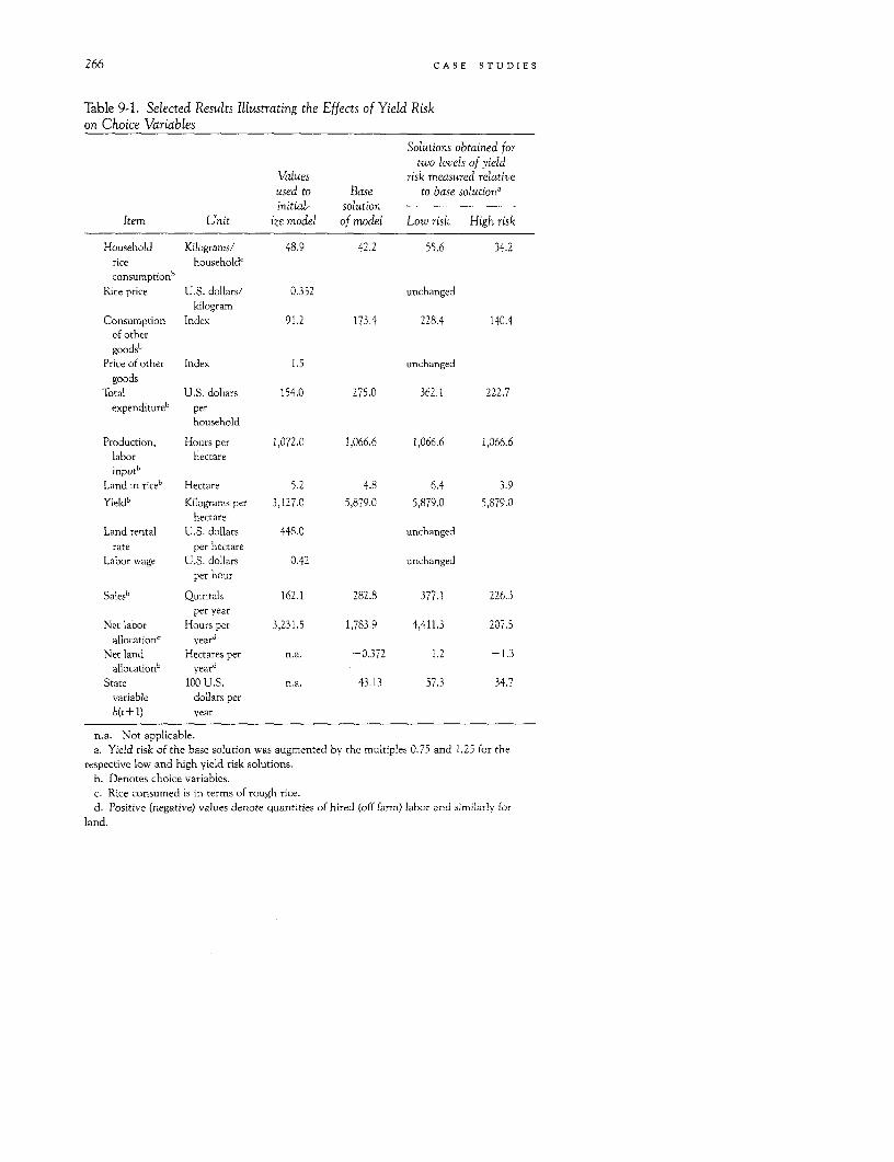
266 CASE STUDIES
Table 9-1. Selected Results Illustrating the Effects of Yield Riskon Choice Variables
Solutions obtained fortwo levels of yield
Values risk measured relativeused to Base to base solution'initial- solution
Item Unit ize model of model Low risk High risk
Household Kilograms/ 48.9 42.2 55.6 34.2rice household'consumption'
Rice price U.S. dollars/ 0.352 unchangedkilogram
Consumption Index 91.2 173.4 228.4 140.4of othergoodsb
Price of other Index 1.5 unchangedgoods
Total U.S. dollars 154.0 275.0 362.1 222.7expenditure" per
household
Production, Hours per 1,072.0 1,066.6 1,066.6 1,066.6labor hectareinputb
Land in riceb Hectare 5.2 4.8 6.4 3.9Yield" Kilograms per 3,127.0 5,879.0 5,879.0 5,879.0
hectareLand rental U.S. dollars 448.0 unchanged
rate per hectareLabor wage U.S. dollars 0.42 unchanged
per hour
Salesb Quintals 162.1 282.8 377.1 226.3per year
Net labor Hours per 3,231.5 1,783.9 4,411.3 207.5allocationb yeard
Net land Hectares per n.a. -0.372 1.2 -1.3allocation' yeard
State 100 U.S. n.a. 43.13 57.3 34.7variable dollars perb(t+l) year
n.a. Not applicable.a. Yield risk of the base solution was augmented by the multiples 0.75 and 1.25 for the
respective low and high yield risk solutions.b. Denotes choice variables.c. Rice consumed is in terms of rough rice.d. Positive (negative) values denote quantities of hired (off farm) labor and similarly for
land.
YIELD RISK IN A DYNAMIC MODEL 267
will likely be overestimated if risk is present in the form considered here.That is to say, the income effect of a price change in a good the householdproduces is likely to be overestimated because the traditional model ignoresthe risk discount term, which will increase in value (and thus decrease in-come) since a(.5k(PqQt)21VE])/aPq > 0.
The factor-demand functions can be verified to be of the form:
Lt = (Pq - lyf1Yfry 72 aY2W'YIc-)/kP' VE]yi 2Z2 2aYzw72c and
(9-24)
A, = (Pq- 2 arzwwlc )/kPq V[e]'ly'YaY2lw'Yc
where 72 = 1 - 'yI. Hence, planned supply is
Qt = (Pqc- 1-yFYly2 2aYZw'Yl)/ckP VtW,
As already pointed out, these production relationships include k, whichcontains the parameters and the prices of the arguments appearing in thedirect utility function. This is an important departure from the literature,where k is related to the Arrow-Pratt coefficient and, in the case of CARA,simply treated as a constant. In this sense, the problem is not separable.Because of the restrictions placed on the parameters (ai) of the direct utilityfunction, however, the problem can be treated as though the householdsought to maximize certainty-equivalent income (Yr), and then as though itsought to choose the levels of goods and leisure to consume, subject tocertainty-equivalent income adjusted for the discount factor log(a)/k.
The biases in empirical estimates of the household's production choicesfrom ignoring risk when it is present in the context of the model developedhere is to overestimate the quantity of output and the resources allocatedto production, and to underestimate the resources allocated to off-farm ac-tivities.
An Empirical Example
To provide some insight into the possible magnitudinal implications ofrisk aversion and yield variance on the household's choices, we initializedthe model to farm household data from the Dominican Republic for thecrop year 1975-76. Only those agricultural households reporting rice astheir sole cash crop were selected for this illustration.
The utility function parameters chosen were (aq, am, ai) = (0.01, 0.175,0.815), and the production parameters were (c, -yl) = (180, 0.5). The otherkey data used to initialize the model appear in the third column of table9-1. The base solution to which other solutions of the model are comparedis reported in the fourth column. The values reported in the remaining two
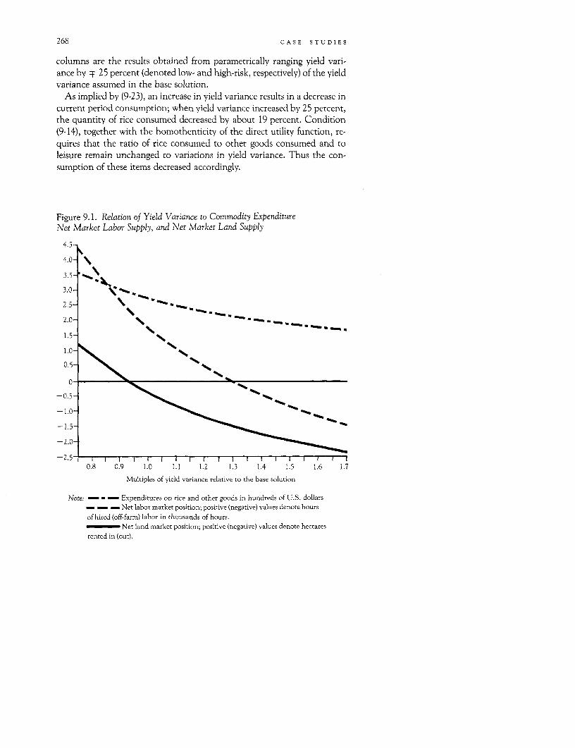
268 CASE STUDIES
columns are the results obtained from parametrically ranging yield vari-ance by T 25 percent (denoted low- and high-risk, respectively) of the yieldvariance assumed in the base solution.
As implied by (9-23), an increase in yield variance results in a decrease incurrent period consumption; when yield variance increased by 25 percent,the quantity of rice consumed decreased by about 19 percent. Condition(9-14), together with the homothenticity of the direct utility function, re-quires that the ratio of rice consumed to other goods consumed and toleisure remain unchanged to variations in yield variance. Thus the con-sumption of these items decreased accordingly.
Figure 9.1. Relation of Yield Variance to Commodity ExpenditureNet Market Labor Supply, and Net Market Land Supply
4.5-
4.0-\
3.5-
3.0-
2.5-
2.0-
1.5-.
1.0-
0-
-0.5-
-1.5-
-2.0-
-2.50.8 0.9 1.0 1.1 1.2 1.3 1.4 1.5 1.6 1.7
Multiples of yield variance relative to the base solution
Note: - - Expenditures on rice and other goods in hundreds of U.S. dollars- - - Net labor market position; positive (negative) values denote hoursof hired (off-farm) labor in thousands of hours.
Net land market position; positive (negative) values denote hectaresrented in (out).
YIELD RISK IN A DYNAMIC MODEL 269
An increase in yield variance also induces the household to decrease thequantity of rice produced by about 19 percent. Since the production func-tion is homogeneous of degree 1, it follows from (9-21) that the labor-landratio and rice yields remain unchanged. The increase in yield variance in-duces the household to increase the amount of land rented out and to de-crease the amount of labor hired, and at the same time to reduce theamount of leisure consumed. In spite of the household's efforts to avoid thedisutility of increases in the variance of yields (and hence income), assetstransferred to the next period (b,+ 1) decline.
It is clear from (9-23), (9-24), and the results reported in table 9-1 thatdeclining consumption and the transfer of resources to other activities arenot a linear function of changes in yield variance. The empirical nature ofthis nonlinearity for the example considered here can be gleaned from fig-ure 9-1, where numerous solutions of the model are charted showingchanges in the household's choices to various levels of yield risk. As yieldvariance increases, the welfare of the household becomes dependent onlabor, land, and asset markets. It is possible for the household to reach apoint where it withdraws all of its land and labor resources from rice pro-duction.
Asset holdings, certainty-equivalent income and the quantity of rice soldare charted in figure 9-2. Rice sales decline as resources are withdrawn fromrice production, in spite of the decline in the quantity of rice consumed bythe household. At a sufficiently high yield variance, the household willbecome a deficit producer of rice. The level of asset holdings will also de-pend on the "riskless" alternatives the household faces in the asset, land,and labor markets. Similarly, the level of certainty-equivalent income willtend to converge, though at diminishing rates, with the income earnedfrom the resources that the household allocates to these markets.
Duality and Risk Aversion
Duality results are useful for providing restrictions on parameters in em-pirical investigations. For example, Hotelling's Lemma (Varian 1978) andthe symmetry of cross second derivatives (Young's Theorem) establish thesymmetry of derivatives of input demands with respect to factor prices.
The value function V%(.) is a dynamic indirect utility function. As such,one would expect that an analogue of Roy's Identity would emerge relatingthe demand for goods and the derivatives of the value function.
Let
z*(P,) (Xq*r (P,) - Qt*, X,t (Pt), Lt* (Pr) + X* (PF)-L, A*(P,)-A).
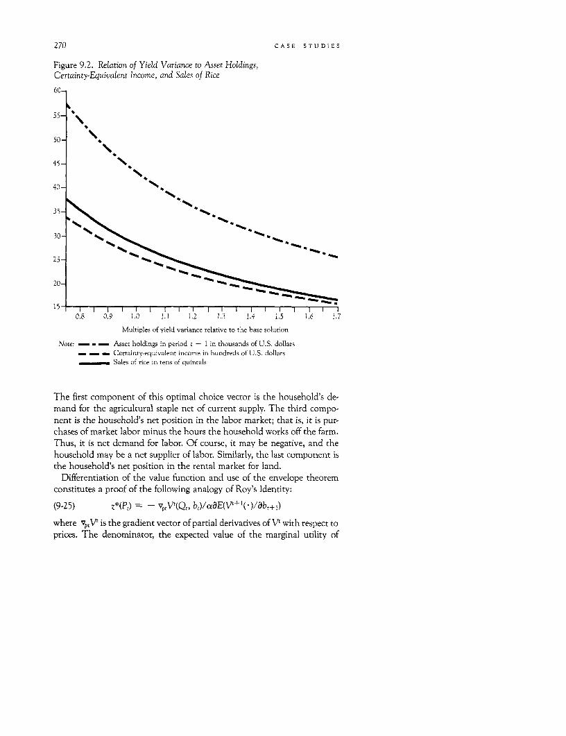
270 CASE STUDIES
Figure 9.2. Relation of Yield Variance to Asset Holdings,Certainty-Equivalent Income, and Sales of Rice
60-
55-
* o
150
45 -,
40 N
35 4
30 4
25
20-
0.8 0.9 1.0 1.1 1.2 1.3 1.4 1.5 1.6 1.7
Multiples of yield variance relative to the base solution
Note: - - _ Asset holdings in period t + 1 in thousands of U.S. dollars_ _ _ Certainty-equivalent income in hundreds of U.S. dollars
Sales of rice in tens of quintals
The first component of this optimal choice vector is the household's de-mand for the agricultural staple net of current supply. The third compo-nent is the household's net position in the labor market; that is, it is pur-chases of market labor minus the hours the household works off the farm.Thus, it is net demand for labor. Of course, it may be negative, and thehousehold may be a net supplier of labor. Similarly, the last component isthe household's net position in the rental market for land.
Differentiation of the value function and use of the envelope theoremconstitutes a proof of the following analogy of Roy's Identity:
(9-25) Z*(P') =- vp tV(Q,, b,)/1aaE(Vt`(*)/abr+ 1)
where vp,V' is the gradient vector of partial derivatives of V' with respect toprices. The denominator, the expected value of the marginal utility of
YIELD RISK IN A DYNAMIC MODEL 271
wealth, plays the role of the derivative of the indirect utility function withrespect to income in Roy's Identity.
Two points are worth noting. First, the market surplus and demand forpurchased goods correspond to similar results obtained from applying theequivalent of (9-25) to the static model. The component for labor reflectsnet positions in the market as well as leisure decisions and the household'sendowment.
Second, the results indicating net factor demand correspond to the dual-ity results obtained by Pope (1980, equation [8]) for the risk averse firmunder price uncertainty. As Pope (1978) has shown, no simple and generalcomparative static results are obtainable from the static model under un-certainty without additional restrictions on the form of the utility function.Thus, it is clear from (9-25) that no simple and general results can be de-rived from the general model. The efficiency in production results (9-21)suggests that properties of the cost function and the corresponding condi-tional factor demand functions are, with one exception, identical to thoseobtained from static efficiency theory. The exception is that the output (Qt)variable is planned (and hence not observable) rather than realized output.
For the type of separability that exists in the specific model discussed inthe preceding section, note that the first-order conditions are identical tothose obtained from maximizing certainty-equivalent income, Y,. In thiscase, the term E{ aV'+l(Q±+ 1, b±+ )/ab,+ I } does not appear, so that L* andAt* follow directly from the envelope theorem. However, Q* does not fol-low from the theorem because Pqt appears in the risk-premium term of Y,.From the Hessian of this problem, it can be shown that the sign of aA*/aatand aL*/aw, cannot be established, although symmetry of the cross partialderivatives holds.
It is important to point out that equation (9-25) greatly depends on ourassumptions that the production shocks are independently distributed andthat the prices are fixed and known. Suppose, to the contrary, that produc-tion shocks form a Markov process and that they induce a Markov processon prices. Then, the current prices will condition the distribution of thefuture prices. In this circumstance, a derivative of V'(*) with respect to priceaffects the choice variable both directly and indirectly through an altera-tion in the household's subjective probability estimate of future prices(Taylor 1984).
Discussion
In this brief chapter, we have attempted to introduce production risk intoa model of the agricultural household in as simple a manner as possible.
272 CASE STUDIES
Even then, the analysis of the model becomes difficult. The main problemis that, when risk is introduced, separability of the model into independentconsumption and production "sides" no longer obtains in most cases. Thislack of separability severely complicates both the analysis of the theoreticalmodel and the empirical estimation of the model's parameters.
It is important to estimate these parameters, however, since many policy-relevant results are ambiguous on a theoretical level and need to be deter-mined empirically. If risk and risk aversion are ignored, misleading infer-ence may be made. The specific model described here suggests that theincome effect of an increase in the price of a staple might significantly over-estimate the level of resources employed in its production. The consider-ation of risk also clearly establishes the importance of markets that permithouseholds to self-insure against increasing yield risk.
Our analysis raises several issues that suggest further research along theselines. We can mention only a few of these possibilities here. Obviously, itwould be useful to know what alternative forms for utility and productionfunctions, in combination with distributions on the random variable, im-ply for behavior toward risk and the effects of increases in risk. This type ofinformation would clarify the results of our model under plausible repre-sentations of household activities and thus have some bearing on policydecisions. If increases in risk reduce consumption and production intensity,for example, institutions that allow more efficient risk sharing could in-crease output and consumption. Furthermore, findings establishing rela-tionships between functional forms and comparative statics results (such asthe type of separability found in the specific model) could guide researcherstoward appropriate tests of the theory and away from imposing results byassumption.
The model could also be elaborated further with respect to the form ofthe production function. This should be generalized in two ways. First,work by Pope and Kramer (1979) demonstrates that the assumption of mul-tiplicative risk is quite special. In particular, this assumption allows us toconclude that factors are used in accord with static efficiency principles(equation [9-21]). As well, the multiplicative form implies that all inputsincrease risk. More general formulations that are tractable yet allow risk-reducing inputs have been proposed.8 Second, we have assumed that allinputs must be chosen before the realization of the random variable isknown. The literature on the firm under price uncertainty informs us thatthe timing of the resolution of uncertainty relative to the timing of inputchoices strongly influences what effect an increase in risk will have on pro-duction decisions.9
In this context, it would seem reasonable to allow the household some expost flexibility. Although inputs associated with planting are fixed, for ex-
YIELD RISK IN A DYNAMIC MODEL 273
ample, irrigation decisions can be altered in response to the current realiza-tion of rainfall. The substitution possibilities between these ex ante and expost inputs will be important in establishing the response of factor use toincrease in risk. This would also apply in a model with investment in dura-ble capital.
A third possible generalization of the model would be to provide for theproduction of multiple goods. This permits us to understand a household'schoice of crop portfolio. One would conjecture that covariances of yieldsacross crops would prove to be important for policy decisions where somecrops are grown for consumption and some for export.
It seems odd to construct a model with quantity risk but no price vari-ability, especially when production shocks are correlated across large num-bers of households. Price variability can be incorporated into the model byconsidering joint distributions on prices and production shocks. It is possi-ble to define and study increases in risk in this situation as well (see Epstein1978). As mentioned earlier, however, if prices are not independently dis-tributed, then duality results become difficult to interpret. If all of the riskin prices is due to production risk, independence may be a reasonable as-sumption.
In considering the relationship between price risk and production risk,we encounter one of the many issues involved in moving from a single-agent to a market model. In particular, and as is well-known, we have tomake some assessment of or assumption about how agents form expecta-tions. This, in turn, raises some controversial economic issues that mustsquarely be faced in future research.
Notes
1. For a description of how farmers diversify crop production activities in order to lower thevariation in their income associated with yield risk, see Walker and Jodha (1985).
2. Leland (1968) considers income uncertainty in a two-period model with a utility functionthat is not additively separable over time-that is, one of the form U(C1, Cz). He finds that if(a2U/aC2)/(aU/oC2) is increasing in Cl and decreasing in C2, then savings increase with increas-ing uncertainty. Sandmo (1970) also obtained this result for small risks. Mirman (1971) studies anadditively separable utility function U(Cl, Cz) = Ui(CI) + U2(C2) in a two-period model. Heshows that with rate of return uncertainty, period-I savings increase (decrease) with an increasein uncertainty if C2dU2(C2)/dC2 is a convex (concave) function. Dreze and Modigliani (1972)provide a comprehensive exploration of the two-period model, including income and substitu-tion effects of increasing uncertainty.
Phelps (1962) established, in an infinite horizon model with additively separable utility, that ifthe preperiod utility function exhibits decreasing absolute risk aversion, then an increase in in-come uncertainty increases savings. Miller (1976) generalizes the Phelps result somewhat. Millerdemonstrates that, with an infinite horizon and additively separable utility function, consump-tion decreases when the sequence of incomes becomes more risky in the sense of Rothschild and
274 CASE STUDIES
Stiglitz (1970) if the marginal utility of consumption is convex. A similar result is obtained bySibley (1975) for a finite horizon model. A more complete review is provided by Lippman andMcCall (1981).
3. There is a large literature on firms facing price uncertainty. A good summary and treat-ment can be found in Epstein (1978).
4. Many analyses of firms under price uncertainty posit some form of a utility function overprofits without explaining where such a utility function comes from. A virtue of the householdproduction model is that risk preferences concerning profit are deduced from risk preferencesover consumption. That the introduction of risk may eliminate separability was pointed out byBarnum and Squire (1979, p. 39, n. 16).
5. Thus, general equilibrium models (with consumer incomes tied to firm profits), in whichcontingent claims markets do not exist and risk neutral behavior on the part of firms is posited,may be inconsistent. A set of securities that spans the states of nature may replace contingentclaims markets (Arrow 1964).
6. To see this, consider the problem
maxEU(7r); 7r = pf(X) -w . x.x
First-order conditions are
E U'(I (70 af x, = C for all j.I ( aX.j ')
7. The normality assumption implies that a nonzero probability exists for negative and ex-tremely high yield. The alternative is to apply the formulas for the moments of a truncatednormal distribution (see Johnson and Kotz 1970, pp. 81-83) or to maintain that the variance of eis sufficiently small that our treatment leads to a good approximation of the actual distribution ofyields. Another alternative is to permit e to be distributed log normal. Levy (1973) shows thatmean variance analysis applied to a log normal distribution is a sufficient decision rule for allnondecreasing, strictly concave utility functions. In any case, the more rigorous approach ofemploying the formulas of a truncated normal distribution would seem to clutter unnecessarilythe key purpose of the task at hand. Hence, we proceed with the normality assumption.
8. Pope and Kramer (1979) suggest the form
F(A, L; e) = f(A, L) + h(A, L)e,
which admits risk-reducing inputs, depending on the shape of the function h(.). An input is riskreducing (increasing) if risk averse producers use more (less) of it than a risk neutral producer.One of the basic implications of our analysis is that risk neutrality does not make sense onceconsumers are added to the model explicitly, except under stringent assumptions.
9. For a review of earlier work in this area, see, for example, Epstein (1978).
References
Arrow, K. 1964. "The Role of Securities in the Optimal Allocation of Risk-Bearing."Review of Economic Studies, vol. 31, pp. 91-96.
Barnum, H., and L. Squire. 1979. A Model of an Agricultural Household: Theory andEvidence. Washington, D.C.: World Bank.
Binswanger, H. 1980. "Attitudes toward Risk: Experimental Measurement in RuralIndia." American Journal of Agricultural Economics, vol. 62, pp. 395-407.
YIELD RISK IN A DYNAMIC MODEL 275
Block, M., and ). Heineke. 1973. "The Allocation of Effort under Uncertainty: TheCase of Risk Averse Behavior." Journal of Political Economy, vol. 81, pp. 376-85.
Dillon, J., and P. Scandizzo. 1978. "Risk Attitudes of Subsistence Farmers in North-east Brazil" American JouTnal of Agricultural Economics, vol. 60, pp. 425-35.
Dreze, J., and F. Modigliani. 1972. "Consumption Decisions under Uncertainty."Joumal of Economic Theory, vol. 5, pp. 308-35.
Epstein, L. 1978. "Production Flexibility and the Behavior of the Competitive Firmunder Price Uncertainty!" Review of Economic Studies, vol. 45, pp. 251-61.
Graham-Tomasi, T., and T Roe. 1985. "Production Uncertainty and the Behavior ofthe Agricultural Household." University of Minnesota, St. Paul. Processed.
Hanoch, G. 1977. "Risk Aversion and Consumer Preferences" Econometrica, vol. 45,pp. 413-26.
Johnson, N. L. and S. Kotz. 1970. Distribution in Statistics: Continuous Univariate Dis-tributions. Vols. 1 and 2. Boston, Mass.: Houghton Mifflin.
Kihlstrom, R., and L. Mirman. 1974. "Risk Aversion with Many Commodities " Jour-nal of Economic Theory, vol. 8, pp. 361-88.
. 1981. "Constant, Increasing, and Decreasing Risk Aversion with Many Com-modities" Review of Economic Studies, vol. 48, pp. 271-80.
Leland, H. 1968. "Saving and Uncertainty: The Precautionary Demand for Saving."Quarterly Joumal of Economics, vol. 82, pp. 465-73.
Levy, H. 1973. "Stochastic Dominance among Log-Normal Prospects." IntemationalEconomic Review, vol. 14, pp. 601-14.
Lippman, S., and J. McCall. 1981. "The Economics of Uncertainty: Selected Topicsand Probabilistic Methods." In Handbook of Mathematical Economics, vol. 1. Editedby K. Arrow and M. Intriligator. Amsterdam: North-Holland.
Miller, B. 1976. "The Effect on Optimal Consumption of Increased Uncertainty inLabor Income in the Multiperiod Case." Journal of Economic Theory, vol. 13, pp.154-67.
Mirman, L. 1971. "Uncertainty and Optimal Consumption Decisions," Econometrica,vol. 39, pp. 179-85.
Moscardi, E., and A. de Janvry. 1977. "Attitudes towards Risk among Peasants: AnEconometric Approach." American Journal of Agricultural Economics, vol. 59, pp.710-16.
Phelps, E. 1962. "The Accumulation of Risky Capital: A Sequential Utility Analysis!'Econometrica, vol. 30, pp. 299-343.
Pope, Rulon D. 1978. "The Expected Utility Hypothesis and Supply Demand Restric-tion." American Journal of Agricultural Economics, vol. 62, pp. 619-27.
. 1980. "The Generalized Envelope Theorem and Price Uncertainty." Interna-tional Economic Review, vol. 21, pp. 75-86.
Pope, Rulon D., and R. Kramer. 1979. "Production Uncertainty and Factor Demandsfor the Competitive Firm." Southern Economics Journal, vol. 46, pp. 489-501.
276 CASE STUDIES
Rothschild, M., and J. Stiglitz. 1970. "Increasing Risk 1: A Definition." Journal of Eco-nomic Theory, vol. 2, pp. 225-43.
Sandmo, A. 1970. "The Effect of Uncertainty on Saving Decisions" Review of Eco-nomic Studies, vol. 37, pp. 353-60.
Sibley, D. 1975. "Permanent and Transitory Income Effects in a Model of Consump-tion with Wage Income Uncertainty" Journal of Economic Theory, vol. 11, pp. 68-82.
Stiglitz, J. 1969. "Behavior towards Risk with Many Commodities!" Econometrica, vol.3, pp. 660-67.
Taylor, C. 1984. "Stochastic Dynamic Duality: Theory and Empirical Applicability"American Journal of Agricultural Economics, vol. 66, pp. 351-57.
Varian, H. 1978. Microeconomic Analysis. New York: Norton.
Walker, T., and N. Jodha. 1985. "How Small Farm Households Adapt to Risk." InAgricultural Risks and Insurance: Issues in Policy. Edited by P. Hazell, C. Pomareda,and A. Valdes. Baltimore, Md.: Johns Hopkins University Press.
10
Using a Farm-Household Model toAnalyze Labor Allocation on a
Chinese Collective Farm
Terry Sicular
FARM-HOUSEHOLD MODELS are often used to analyze household labor allo-cation in agriculture in developing countries. Since these models incorpo-rate both the consumption and production aspects of household deci-sionmaking, they capture the essential considerations underlying theallocation of family time between leisure and work. Moreover, they pro-vide a framework for understanding household participation in labormarkets as suppliers of family labor or as employers of hired labor.
The farm-household approach is equally useful for analyzing labor allo-cation within Chinese collective farms. In the People's Republic of China,the basic collective farm unit has been the production team. Productionteams normally embraced the population and land surrounding a village.In 1979, the average number of households in a team was 34 and thepopulation 157 (Chang and Luo 1980, p. 5). Although collective farms inChina comprised a number of households, they were nonetheless farmunits making dual production and consumption decisions. On the pro-duction side, collective farms chose the patterns and methods of cultiva-tion on collective land and the mix between cultivation and other side-line activities. These production decisions implied certain deriveddemands for labor and a seasonal distribution of labor use. On the con-sumption side, collective farms planned for desired levels of collective in-come, both in kind and in cash, and for its distribution among members.
Note: This research was supported by a grant from the U.S.-China National Scholarly Ex-change Program and by generous assistance from Yale University and the University of Wiscon-sin-Madison. I would like to thank N. R. Lardy, R. E. Evenson, J. M. Montias, W. P. Falcon, andJ. Strauss for their helpful comments on earlier versions.
277

278 CASE STUDIES
In these respects, Chinese collective farms have resembled farm house-holds elsewhere and so lend themselves to farm-household analysis.
In other respects, however, Chinese collective farms have differed fromthe usual farm household. First, although the collective performed manyof the same functions as a farm household, it was not a household, but acollection of households. Member households supplied labor for collec-tive activities. Member households could also engage in private-produc-tion activities independently of the collective. Labor allocation within acollective farm therefore involved a choice among labor on the collective,labor in private household production, and leisure. Second, collectivefarms and their member households had no access to labor markets. Ac-cording to Marxist theory, employment of labor can lead to economicexploitation, class differentiation, and class conflict. Such socioeconomicprocesses were considered inappropriate under Chinese socialism. Thegovernment therefore did not permit exchange of labor. From the pointof view of the collective farm, government suppression of labor marketsforced self-sufficiency in labor: all labor employed in collective produc-tion had to be supplied by member households, and the only outside em-ployer for household labor was the collective. Third, the access of collec-tive farms to markets for nonlabor inputs, outputs, and consumer goodswas restricted. Until the late 19 70s, private exchange was discouraged, socollectives were more or less limited to trade with the state commercialsystem. In this trade, the state not only set prices (collectives were price-takers), but also fixed maximum quotas on collectives' purchases of cer-tain modern inputs and consumer goods, and minimum quotas on collec-tives' sales of farm products to the state. In general, collectives could sellas much output to the state as they desired at official prices. Fourth, col-lective farms faced certain production planning targets. These targets typ-ically specified minimum areas to be planted in crops such as grain andcotton. At times, they also specified yield levels or production methods,for example, chemical fertilizer applications per hectare. Together, mar-keting quotas and production targets formed a complex array of planningrestrictions. Collective farms had to take such targets and quotas intoaccount when deciding on a production plan. In the above respects, Chi-nese collective farms have differed from farm households observed inother countries. A farm-household analysis of Chinese collectives shouldpay attention to these specific characteristics of the Chinese case.
This chapter examines labor allocation within a Chinese collectivefarm by means of a modified farm-household model. First, it presents atheoretical model of the collective farm. This model is used to analyze theeffects of planning targets, planning quotas, and the absence of a labormarket on collective labor allocation. Next, it turns to an empirical linear
LABOR ALLOCATION ON A CHINESE COMMUNE 279
programming model of a case-study collective farm, a production team incentral China. The chapter concludes with a discussion of the implica-tions of the theoretical and empirical results for Chinese agriculture and,more generally, for agriculture in developing countries.
Model of a Collective Farm
Consider, first, a household-type theoretical model of a productionteam. The model answers the question: how do restrictions on trade,whether in the form of marketing quotas or in the form of trade prohibi-tions, affect team labor allocation? I begin by examining team labor allo-cation in an unrestricted market environment. The effects of market re-strictions on team labor allocation are revealed by comparing optimallabor allocation in the unrestricted environment with optimal labor allo-cation when marketing quotas or trade restrictions are imposed.
Like the usual farm household, the production team both consumesand produces. Thus its objective is to maximize the utility of its memberhouseholds subject to a budget constraint, where income is the sum of itsendowed wealth and that of its members plus net revenues from collectiveand individual production. Since the model is concerned with the effectof market restrictions and not group decisionmaking processes, I makethe simplifying assumptions that all member households have identicalpreferences and that the team and all its members face the same prices.These assumptions imply that the collective utility function is a simple,monotonic transformation of the household utility function and rule outlack of consensus. In addition, I assume that team members are indiffer-ent between participation in household and collective activities. Thus, inan unrestricted market environment, profitability considerations woulddetermine the optimal amounts of resources devoted to private as op-posed to collective endeavors. This latter assumption may appear to be atodds with the evidence. I would maintain, however, that the preferencefor private activities commonly observed in socialist agriculture is fre-quently no more than the desire to engage in activities that, because ofgovernment restrictions limiting their extent, are more profitable thancollective activities. Such a desire is completely consistent with thismodel.'
Under these assumptions, in an unrestricted market environment aproduction team would behave in more or less the same way as the usualfarm household. The team determines optimal levels of production, con-sumption, and marketing by maximizing collective utility U(x1, . . ., xI)subject to exogenous prices p = (Pi, .. , p), its production function
280 CASE STUDIES
(10-1) G(ql, . ,,) = O
and its budget constraint
(10-2) px' < pq' + pVw.
These utility and production functions are assumed to have the usualproperties (see the appendix to this volume). Full income in the team'sbudget constraint is the sum value of profits from production pq' andteam endowments piwi', where endowments include collectively culti-vated land, private plot land, the stock of available human time, and anyother financial and physical assets belonging to the team and its mem-bers.2 In this formulation, optimization causes consumption expendituresto exactly equal full income. Thus savings are not carried over betweenperiods. In other words, this is essentially a one-period model.
Solution of the above maximization problem leads the team to produceat optimal production levels q* and to consume the utility-maximizingconsumption bundle x*. As in the usual household model, productionand consumption decisions are recursive but separable. Moreover, for allgoods, the technical rates of substitution in production and marginalrates of substitution in consumption are equated to their respective priceratios. In other words,
aGlaqi _ au/lax, pi_(10-3) aG/aq aU/a-= P for all i, j.
The usual profit function Tr(p), net output supply functions yi(p) = a7r(p)/
api, Marshallian demand functions xj[p, 7r(p) + pW'], and net marketing(or sales) functions sj(p, w) = - xi can be derived for the team. Thederivation of these standard results can be found in the appendix to thisvolume.
Production teams differ from the usual farm household in that theycannot trade freely. In particular, they face two types of market restric-tions: absolute quantity limits on team purchases and sales, and inter-linked quantity limits on team purchases and sales, where those limits aretied to other variables. The former, which are referred to here as fixedquota restrictions, occur either when the state sets absolute quotas onprocurement from and sales to production teams, or when the state pro-hibits trade. (Prohibition of trade effectively sets a fixed quota limit ofzero on team sales and purchases.) The latter, which are referred to hereas variable quota restrictions, occur either when the state requires that acertain percentage of team output be sold to the state, or when rations ofconsumer and producer goods sold to the team by the state are set on thebasis of the team's production or marketing levels.
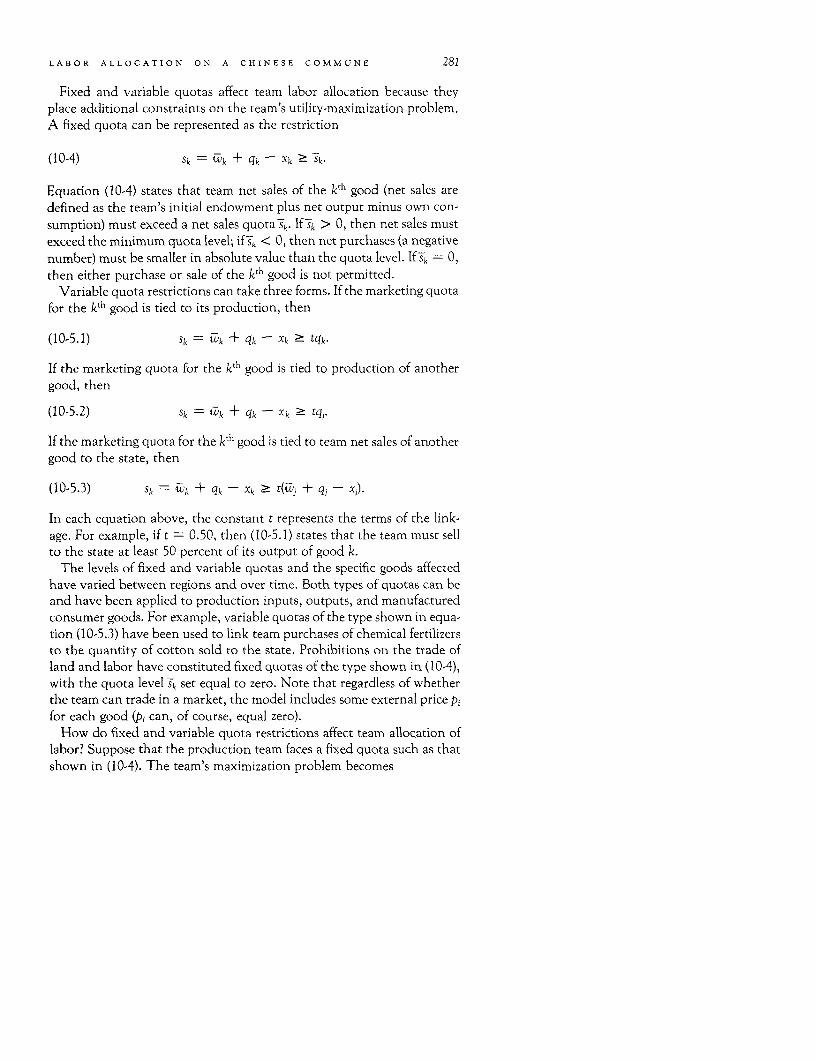
LABOR ALLOCATION ON A CHINESE COMMUNE 281
Fixed and variable quotas affect team labor allocation because theyplace additional constraints on the team's utility-maximization problem.A fixed quota can be represented as the restriction
(10-4) Sk = wk + qk Xk 2S
Equation (10-4) states that team net sales of the kth good (net sales aredefined as the team's initial endowment plus net output minus own con-sumption) must exceed a net sales quota Sk. If Sk > 0, then net sales mustexceed the minimum quota level; ifSk < 0, then net purchases (a negativenumber) must be smaller in absolute value than the quota level. IfSk = 0,then either purchase or sale of the kth good is not permitted.
Variable quota restrictions can take three forms. If the marketing quotafor the kth good is tied to its production, then
(10-5.1) Sk = Wk + qk - Xk > tqk.
If the marketing quota for the k' good is tied to production of anothergood, then
(10-5.2) Sk = wk + qk - Xk 2 tqj-
If the marketing quota for the k,h good is tied to team net sales of anothergood to the state, then
(10-5.3) Sk = Wk + qk- Xk 2t(Wj + qj - xi).
In each equation above, the constant t represents the terms of the link-age. For example, if t = 0.50, then (10-5.1) states that the team must sellto the state at least 50 percent of its output of good k.
The levels of fixed and variable quotas and the specific goods affectedhave varied between regions and over time. Both types of quotas can beand have been applied to production inputs, outputs, and manufacturedconsumer goods. For example, variable quotas of the type shown in equa-tion (10-5.3) have been used to link team purchases of chemical fertilizersto the quantity of cotton sold to the state. Prohibitions on the trade ofland and labor have constituted fixed quotas of the type shown in (10-4),with the quota level Sk set equal to zero. Note that regardless of whetherthe team can trade in a market, the model includes some external price pifor each good (Pi can, of course, equal zero).
How do fixed and variable quota restrictions affect team allocation oflabor? Suppose that the production team faces a fixed quota such as thatshown in (10-4). The team's maximization problem becomes
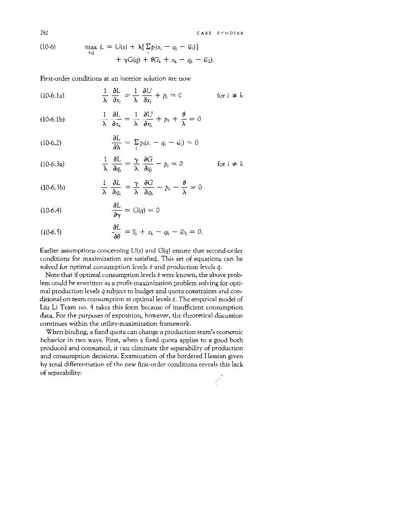
282 CASE STUDIES
(10-6) max L = U(x) + X{ Ep1 (x - qi-vi)x,q i
+ yG(q) + O(Mk + Xk - qk - Wk).
First-order conditions at an interior solution are now
(10-6.1a) _ _ I- + pi = 0 for i *k12 axi XSaxi
(10-6.lb) 1 aL Ia Pk +-= X aXk X aXk
(10-6.2) -= pi(xi -qi - ) - 0
(10-6.3a) 1 aL a' -Pi =0 for i * kX aqi X aqi
(10-6.3b) 1 a aq -Pk =-X aqk X ak
aL(10-6.4) a = G(q) = 0
aL(10-6.5) _ = Sk + Xk - qk -wk = 0.ao
Earlier assumptions concerning U(x) and G(q) ensure that second-orderconditions for maximization are satisfied. This set of equations can besolved for optimal consumption levels x and production levels q.
Note that if optimal consumption levels x were known, the above prob-lem could be rewritten as a profit-maximization problem solving for opti-mal production levels q subject to budget and quota constraints and con-ditional on team consumption at optimal levels x. The empirical model ofLiu Li Team no. 4 takes this form because of insufficient consumptiondata. For the purposes of exposition, however, the theoretical discussioncontinues within the utility-maximization framework.
When binding, a fixed quota can change a production team's economicbehavior in two ways. First, when a fixed quota applies to a good bothproduced and consumed, it can eliminate the separability of productionand consumption decisions. Examination of the bordered Hessian givenby total differentiation of the new first-order conditions reveals this lackof separability:
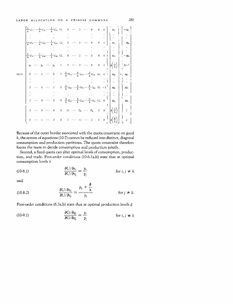
LABOR ALLOCATION ON A CHINESE COMMUNE 283
XUl ... XI Ulk ... Ui U, ...U 00 0 0 dxl -dp,
Ukl ''-.. Ukk ''. U Uk 0 ... 0 ... 0 0 I dxk -dpk
U, XUnk .Unn, Un, 0 0 0 0 0 dxn -dpn
Pi .. Pk - P. 0 0 0 0 o 0 0 d(X) K-3
(10-7) 0 0 0 0 -GiI- y Glk X GI, GI 0 dql dpi
0 °0. 0 0 ° XGkl ' XGkk ' X Gk, Gk -1 dqk dPk
0 ° 0 ... 0 0 n G X, Gnk X Gnn Gn 0 dqn dp,
0. 0 0 0 Gl Gk G, 00 d(-) 0
O--. 1-0 0 0 .. O... 0 00 d(.) 0
Because of the outer border associated with the quota constraint on goodk, the system of equations (10-7) cannot be reduced into distinct, diagonalconsumption and production partitions. The quota constraint thereforeforces the team to decide consumption and production jointly.
Second, a fixed quota can alter optimal levels of consumption, produc-tion, and trade. First-order conditions (10-6.1a,b) state that at optimalconsumption levels x
(10-8.1) aU/ax, = p for i,j kau/ax, - j
and
(10-8.2) au/aXk Pk 1 X forj k.
First-order conditions (6.3a,b) state that at optimal production levels q
(10-9.1) aG/aq, _ pp for i,j * kaGlaq1 pj
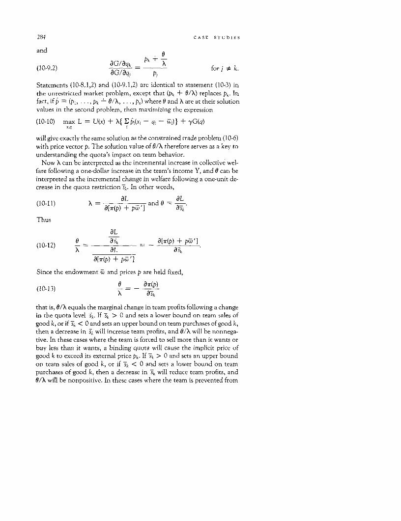
284 CASE STUDIES
and 0
Pk + (10-9.2) aG/aqk -1 X for k.
Statements (10-8.1,2) and (10-9.1,2) are identical to statement (10-3) inthe unrestricted market problem, except that (Pk + O/X) replaces Pk. Infact, if p = (PI, . -, Pk + O/X, . . ., P) where 0 and X are at their solutionvalues in the second problem, then maximizing the expression
(10-10) max L = U(x) + X{ E 1 (xj - q- iv)} + -yG(q)x,q
will give exactly the same solution as the constrained trade problem (10-6)with price vector p. The solution value of 0/A therefore serves as a key tounderstanding the quota's impact on team behavior.
Now X can be interpreted as the incremental increase in collective wel-fare following a one-dollar increase in the team's income Y, and 0 can beinterpreted as the incremental change in welfare following a one-unit de-crease in the quota restriction Sk. In other words,
(10-11) 3[()+p' and 0 = _ a[7r(p) + pvD] a Sk
Thus
aL(10-12) 0 aSk _ __ __ _a[7r(p) + p~'I(10-12) X =x - aL a-k
af[r(p) + pV' I
Since the endowment w and prices p are held fixed,
(10-13) 0 = _ d7r(p)
that is, 0/X equals the marginal change in team profits following a changein the quota level Sk. If Sk > 0 and sets a lower bound on team sales ofgood k, or if Sk < 0 and sets an upper bound on team purchases of good k,then a decrease in Sk will increase team profits, and 0/X will be nonnega-tive. In these cases where the team is forced to sell more than it wants orbuy less than it wants, a binding quota will cause the implicit price ofgood k to exceed its external price Pk. If Sk > 0 and sets an upper boundon team sales of good k, or if Sk < 0 and sets a lower bound on teampurchases of good k, then a decrease in Sk will reduce team profits, andO/X will be nonpositive. In these cases where the team is prevented from

LABOR ALLOCATION ON A CHINESE COMMUNE 285
selling as much as it wants or is forced to buy more than it wants, a bind-ing quota will cause the implicit price of good k to be lower than its exter-nal price Pk-
Consider the effect of a fixed quota on team labor allocation. Suppose afixed quota of zero applies to labor, and that labor is the first good (k =1). Moreover, suppose that in the absence of the quota, the team wouldbe a net hirer of labor. At an interior solution, then, O/X is positive.Therefore
(10-14) 0I = Pi + PI.
The amount of human time used in production is
(10-15) q y l YP).
Since ay/lapi > 0, the net output of human time will increase; that is, theteam will reduce the amount of labor it employs in production: 41 > q*I.On the consumption side, optimal team leisure is now
(10-16) xl = X[j, Ti(p) + pW'].
Since axilapi < 0, the team will substitute away from consumption ofleisure now that it faces a higher implicit price for human time. In addi-tion, team profits may change
(10-17) Tr(p) = ii * T7*(p)
and thus so may full team income Y. If income is reduced and leisure is anormal good, then the income effect will reinforce the decrease in teamleisure consumption owing to the substitution effect. In sum, a fixedquota on labor or suppression of labor markets could force productionteams that would hire labor in the absence of the constraint to decreaseboth their use of labor in production and the amount of leisure con-sumed. The pattern of production would then shift to less labor-intensiveactivities, and team members would increase the amount of time theyspend working.
In contrast, suppose that, in the absence of the quota, the team wouldbe a net exporter of labor. Then, at an interior solution, G/A is negative,and pj will be less than Pl. At this lower implicit wage, the team will in-crease the amount of labor used in production, but substitute in con-sumption toward leisure.
If the fixed quota applies to a good other than human time, then thequota's effect on team labor allocation depends on the elasticities of hu-man time with respect to the price of the other good. Suppose, for exam-
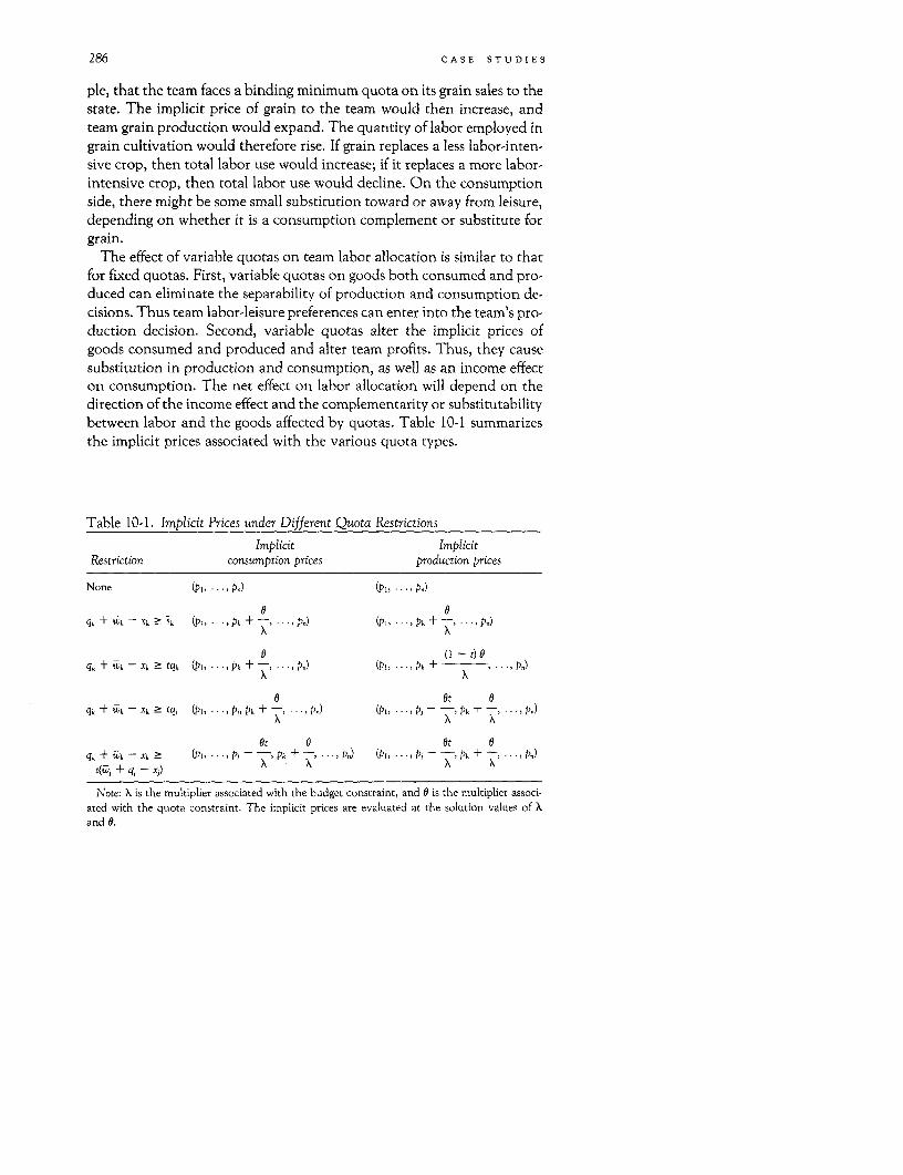
286 CASE STUDIES
ple, that the team faces a binding minimum quota on its grain sales to thestate. The implicit price of grain to the team would then increase, andteam grain production would expand. The quantity of labor employed ingrain cultivation would therefore rise. If grain replaces a less labor-inten-sive crop, then total labor use would increase; if it replaces a more labor-intensive crop, then total labor use would decline. On the consumptionside, there might be some small substitution toward or away from leisure,depending on whether it is a consumption complement or substitute forgrain.
The effect of variable quotas on team labor allocation is similar to thatfor fixed quotas. First, variable quotas on goods both consumed and pro-duced can eliminate the separability of production and consumption de-cisions. Thus team labor-leisure preferences can enter into the team's pro-duction decision. Second, variable quotas alter the implicit prices ofgoods consumed and produced and alter team profits. Thus, they causesubstitution in production and consumption, as well as an income effecton consumption. The net effect on labor allocation will depend on thedirection of the income effect and the complementarity or substitutabilitybetween labor and the goods affected by quotas. Table 10-1 summarizesthe implicit prices associated with the various quota types.
Table 10-1. Implicit Prices under Different Quota Restrictions
Implicit ImplicitRestriction consumption prices production prices
None (Pi., P) (P, Pn)
qk + W-k Xk 2Sh (P" P + P) (PI Pk + P)
qk + Wk -Xk tqk (PI Pk + P.,) (P, -P+ P.)
e et 0qk + Wk Xk 2! tq (P, Pi, Pk + , Pn) (PI, - h , Pk + ,.PJ)
et 9 Ot 9qk + Wk xk 2 (PI.p, Pi ,Pk + * PJ) (PI. I p , Pk + ,.PJ)
t(i-,j + q4j-Xj) X X X ..... X
Note: X is the multiplier associated with the budget constraint, and 0 is the multiplier associ-ated with the quota constraint. The implicit prices are evaluated at the solution values of Xand 9.
LABOR ALLOCATION ON A CHINESE COMMUNE 287
Empirical Model of a Production Team
The theoretical model just described shows the effects of quota restric-tions on team allocation of labor. In this section we look at a linear pro-gramming model used to illustrate empirically their effects on a case-studyproduction team in Hubei Province-Liu Li Team no. 4. Solution of theprogramming model will show that state planning restrictions affect thelevel and seasonal distribution of labor employed by the team. Moreover,the model demonstrates the interrelated nature of team production andconsumption decisions when markets are restricted.
Although the linear programming model incorporates the basic ele-ments of the theoretical framework, it differs from the usual empiricalhousehold model in that it does not estimate both the production andconsumption sides. Insufficient consumption data preclude estimation ofteam consumption. The model therefore estimates only the team's profitsand production behavior, where profits and production are conditionalon the optimal consumption bundle. Specifically, rather than solving foroptimal consumption and production levels by maximizing collective util-ity subject to the team's technological, resource, and planning con-straints, the empirical model solves for optimal production levels by max-imizing collective profits subject not only to technological, resource, andplanning constraints, but also subject to the restriction that consumptiontakes place at observed, and assumedly optimal, levels. The empiricalmodel is presented in more detail below.
The case-study production team Liu Li Team no. 4 is located in Mian-yang County, a commercial cotton and grain-growing county in HubeiProvince. The climate in this central region of China is temperate, aver-aging 170 Centigrade. Frost-free days number about 235 annually. Rain-fall is abundant, exceeding 1,000 millimeters a year.
Liu Li Team no. 4's pattern of cultivation is representative of the re-gion. In 1979, the year of this study, the team planted 40 percent of collec-tively cultivated land in double-crop rice, 10 percent in single-crop rice,and 37 percent in cotton. The remaining collective land was usuallyplanted in minor crops such as soybeans, sorghum, hemp, peanuts, andsesame. During the winter season, barley, naked barley, wheat, broad-beans, and green manure completed the annual rotations.
Production teams were permitted to devote a certain percentage of theirland to private plots. In 1979, Liu Li Team no. 4 set aside 3 hectares or 6percent of its total land area, the maximum allowed, for household pri-
288 CASE STUDIES
vate plots. On the average, each household privately cultivated 0.048hectare. Vegetables and small amounts of cash crops were usuallyplanted, as well as fodder for privately raised hogs. In 1979, team house-holds raised an average of 2.5 hogs each.
The team population in 1979 was 365, and its labor force 135. House-holds numbered 63. With a total cultivatable land area of 49 hectares, theteam's population density was 7.4 people per hectare (0.135 hectare perperson), which was about equal to the county average. The dependencyratio was high, 1.70 dependents per working adult, as compared with 1.37for the county as a whole.
In part because of the quality of its soil, Liu Li Team no. 4's yields wereconsistently higher than the county, provincial, and national averages. In1979, the team's rice yields were 5.3 tons per hectare of sown area, whichwas 10 percent higher than the county average and 25 percent higherthan the national average. Cotton yields were 995 kilograms per hec-tare of sown area, or 14 percent above the county average and morethan double the national average (see State Statistical Bureau 1982, pp.154-55).
As a result of these high yields, the team enjoyed high per capita out-put, which promoted high marketing rates and income. In 1979, the teamsold 36 percent of its grain to the state, compared with the county averageof 23 percent and national average of 20 percent. The team's cotton mar-keting rate was 98 percent, which was equal to the national but slightlyhigher than the county average (see Sicular 1983, pp. 18, 27). Team percapita distributed income from collective sources was 225 yuan, whichwas 57 percent higher than the county average of 143 yuan; the nationalaverage was 83.4 yuan (see Chang and Luo 1980, p. 41). These incomefigures include both cash and in-kind income distributed by collectives totheir members, but do not include income earned privately by house-holds or individuals.
Liu Li Team no. 4 was an above-average team by both county and na-tional standards. It was not, however, a model team; that is, it did notreceive preferential treatment in the form of superior access to markets,lower quota levels, special financial or technical support, and so on. LiuLi Team no. 4 was subject to the same types of institutional arrangementsand planning restrictions as other teams in the county. Thus an empiricalcase study of this team can usefully illustrate the general effects of suchrestrictions.
Agricultural planning restrictions in China fall into two categories: di-rect restrictions on production, and marketing restrictions. Direct restric-tions on production usually take the form of minimum crop area targets.In this part of China, area targets have applied to grain and cotton. Be-

LABOR ALLOCATION ON A CHINESE COMMUNE 289
fore 1979, teams in Mianyang County faced area targets for double-croprice and cotton. After 1979, rice area targets were eliminated and only thecotton targets remained. In 1979, Liu Li Team no. 4's cotton area targetwas 18.067 hectares, or 41 percent of its collective land area.
As noted earlier, market restrictions can take the form of quotas orresult from prohibition of trade. Trade prohibitions applied to land andlabor. Cotton and cotton products could be traded through state chan-nels, but not privately. Private trade of other items was tolerated to avarying degree. During the Cultural Revolution (1966-76), all privatetrade was discouraged. Since 1978, private exchange has been permittedand rural markets have gradually revived. As of 1979, Liu Li Team no. 4did not engage in private trade as a collective, although team membersprobably did so individually.
The system of quotas was quite complex. As mentioned above, quotascan be fixed or variable in form, and can apply to sales as well as pur-chases. Fixed quotas were set on collective deliveries of grain and vegeta-ble oil or oilseeds to the state. These quotas were set in weight and did notspecify type of grain or oil. Variable quotas were set on deliveries of grainand cotton. With respect to grain, in addition to the fixed quota, a sec-ond, variable above-quota quota was set annually on the basis of the ex-pected grain harvests of the teams. With respect to cotton, teams withyields exceeding 750 kilograms per hectare were required to deliver alltheir output except one kilogram ginned cotton per team member to thestate; teams with lower yields had to deliver all but 0.75 kilogram perteam member. In addition to these formal delivery quotas, an informalmaximum delivery quota applied to hog sales to the state. After the stateraised hog prices in 1979, households in Mianyang County increasedtheir production beyond the state's capacity to procure. The state re-sponded by informally limiting the number of hogs it would procure fromany particular household or team. (The delivery quotas faced by Liu LiTeam no. 4 in 1979 are summarized in table 1OA-1 in the appendix.)
Fixed and variable quotas have at times also restricted collective andhousehold opportunities to buy consumer and producer goods from thestate. In general, the state does not supply grain or vegetable oils to theagricultural population. Effectively, then, teams faced a fixed importquota of zero on these items; that is, they had to be self-sufficient in theseitems and produce what they consumed. Cotton cloth ration couponswere allocated to teams on a fixed quota per capita basis. Occasionally,additional coupons were awarded on a variable-quota basis for deliveriesof ginned cotton or hemp to the state. Supplies of producer goods wereallocated to teams in some cases according to crop areas, in others on thebasis of deliveries to the state. Diesel fuel was allocated on the basis of
290 CASE STUDIES
team-owned machine horsepower. The quantity of each item allocatedper capita, per unit sown area, per ton delivery to the state, and so on,was set more or less uniformly across teams within a county, but variedfrom year to year depending on the county's total allocation from thestate for that year. Since 1979, the county's total allocation of most pro-ducer goods has risen to the point where its quotas exceed team demand.Liu Li Team no. 4 reported that in 1979 it was able to buy as much of anymodern input as it desired.
The empirical model of Liu Li Team no. 4 captures the specifics of thiscase-study team. The team's production function G(q) takes the form of alinear, fixed-coefficient technology given by an input-output matrix A.Coefficients of the A matrix are calculated from 1979 field data. The Amatrix includes columns representing Liu Li Team no. 4's observed col-lective cultivation activities; observed collective sideline, mechanization,and processing activities; a number of cultivation activities not observed(corner solution activities in which the team did not engage in 1979, butin which it had previously engaged or in which neighboring teams en-gaged); and private household hog-raising and manure-collecting activi-ties. Because data on inputs used and outputs produced on private plotsare insufficient, household private-plot cultivation activities do not ap-pear in the model. (Activities included in the model are summarized intable IOA-2 in the appendix.) The A matrix includes alternate activitycolumns producing the same items, thus permitting some variation in rel-ative factor proportions. For example, cotton can be produced using lesschemical fertilizer per ton output in a cotton-broadbean rotation activity,or using more in a cotton-wheat rotation activity. (Broadbeans fix nitro-gen in the soil, whereas wheat depletes it.)
The rows of the A matrix represent use of various inputs across produc-tion activities. Inputs include collectively cultivated land, human labortime, animal draft time, machine time, fuels, chemical fertilizers, organicfertilizers, and pesticides. Land is differentiated by quality. Labor is differ-entiated by time of year to capture the seasonality of labor use.
Associated with the A matrix is a right-hand side vector b giving theteam's initial endowments of various inputs. The team has initial endow-ments of collective land, people, cows, and machinery. Since the endow-ments of these items cannot be augmented by production (the supplies ofpeople, cows, and machinery are assumed to be fixed in the short run), orby purchase (market restrictions prevent exchange of land or labor), theseinitial endowments effectively set maximum limits on their availability.
Planning and market restrictions are represented by an additional set ofrows R and its associated right-hand side vector k. Planning and marketrestrictions include a minimum acreage target of 18.07 hectares for cot-

LABOR ALLOCATION ON A CHINESE COMMUNE 291
ton; a minimum cotton sales quota of all output minus 1 kilogram perteam member; a minimum grain sales quota of 54.75 tons husked grainequivalents; and a minimum vegetable oil or oilseeds sales quota of 1.44tons oil equivalents. Neither grain nor vegetable oils can be purchased bythe team, only sold. Sales of hogs to the state are restricted to a maximumlimit of 126 head, or two per household, the observed level of householdhog sales in 1979. No formal maximum quota existed for hogs, but thisconstraint is necessary to capture the state's unwillingness to purchase asmany hogs as team households wished to sell.
In the theoretical model, the production team maximizes utility subjectto its income from production and its endowments and subject to plan-ning and marketing restrictions. If no market restrictions constrained theteam, then utility maximization would lead the team to select a profit-maximizing production plan. In this case, profits could be used as theobjective function in an empirical model of team production. If, however,one or more restrictions on the purchase of a consumed good is binding,then preferences may enter directly into the production decision andmust be specified as elements in either the objective function or body ofthe model. In view of the lack of data, I use the latter approach. Theempirical model maximizes team profits conditional on consumption atoptimal levels. Optimal consumption levels appear in R as a set of mini-mum consumption constraint rows for important consumer goods, specif-ically for grains, vegetable oils, and leisure. Consumption constraints donot specify type of grain or oil. In addition, leisure refers to all time notspent in collective work and private hog raising and manure collection.The labor-leisure choice depicted by the empirical model, therefore, is notstrictly a choice between labor and leisure, but a choice between collec-tive or hog-raising activities and leisure or labor in other household side-lines.
Consumption constraints are initially set equal to observed 1979 con-sumption levels, which I assume are the optimal consumption levels at1979 prices, given 1979 planning and market restrictions. The leisure con-sumption constraint is set equal to the lowest level of leisure time ob-served during peak seasons in 1979. When binding, consumption con-straints influence the model's optimal solution, and their associatedshadow prices give the marginal value of team consumption in terms offoregone profit income.
The empirical model's objective function Z = cy is defined as teamshort-run profits: the value of collectively produced output plus hogs mi-nus the cost of purchased variable inputs. Outputs valued into the objec-tive function include products marketed and retained for team consump-tion, but not products used as intermediate inputs in the production
292 CASE STUDIES
process. Inputs costed out of the objective function include only thosethat are purchased and variable in the short run, such as chemical fertil-izers, fuels, and pesticides. Land, human labor time, animal draft time,and machinery-inputs of which the team has an endowment but thatcannot be purchased or sold, or that are fixed in the short run-do notappear in the objective function. The scarcity values of these inputs to theteam, however, enter the model's calculation through shadow prices.
Prices c used to value inputs and outputs in the objective function are,in theory, expected marginal prices. Since in 1979 rural free markets werestill not fully developed in Mianyang County and since the productionteam did not participate in those markets, I use state prices. The statepricing system was multitiered; quota sales received a basic quota price,and above-quota sales received a price 30 to 50 percent higher than thequota price. Since the team had to fulfill the quota, the relevant price foran additional unit output was the above-quota price. Therefore, teamoutput is valued at 1979 state above-quota prices. Commercial inputssuch as chemical fertilizers and pesticides are valued at 1979 state retailsales prices.
The linear programming model of Liu Li Team no. 4 can be summa-rized in the following form:
(10-18) maximize Z cysubject to Ay ' b
Ry ' ky Ž 0.
Z is team net income, A represents the team's production technology,and b gives initial endowments. Ry c k includes additional constraintsdue to planning and marketing restrictions and consumption constraints.(Table lOA-1 in the appendix gives a summary of the price and planningregime used in this basic version of the model.) Altogether, the modelcontains approximately 180 rows and 4,000 nonslack columns. Solutionof the model will determine profit-maximizing production levels and theshadow prices for resource, planning, market, and consumption con-straints.
Results
Solutions of the linear programming model described here show theeffects of state planning restrictions on team income, cultivation patterns,and labor allocation. First, the solution of a basic model version that ex-actly replicates the team's price and planning environment in 1979 re-
LABOR ALLOCATION ON A CHINESE COMMUNE 293
veals which restrictions are binding and their respective shadow prices.The basic model solution can be compared with the team's observed be-havior in 1979 to check the accuracy of the model. Second, solution of anunrestricted version of the model, where the team faces no state-imposedplanning or market constraints, shows the level of team income and laboruse in an unrestricted environment. Examination of both the basic andunrestricted model solutions demonstrates the interrelatedness of teamconsumption and production decisions.
When the basic model solution is compared with the team's observedbehavior in 1979, the three major aspects of model-predicted and ob-served team behavior-patterns of land use, levels of production and in-put use, and the level of team profits-are consistent. In each of thesethree categories, the model predicts observed team behavior quite well.
Table 10-2 summarizes 1979 land use observed and predicted by thebasic model. In both cases, cotton occupies 41.3 percent of the team'ssummer season land area, which is exactly equal to the planned area tar-get. The balance between double-crop and single-crop rice differs betweenthe predicted and observed cases; the model substitutes single-crop ricefor some double-crop rice and for "other" minor crops (soybean-sorghumintercrop). In the winter season, observed and predicted cultivation pat-terns are also similar, except that the model eliminates naked barley andconsiderably reduces green manure cultivation, replacing them with bar-ley. Barley cultivation expands from an observed 20.4 percent to a pre-dicted 66.6 percent of team land.
Table 10-2. Land Use Summary, Liu Li Team No. 4:Predicted and Observed(percentages of collective land area)
Predicted PredictedObserved land use land use
Crop land use (1979) (basic model) (unrestricted model)
Summer
Cotton 41.3 41.3 33.7Double-crop rice 44.2 35.1 42.7Single-crop rice 12.2 23.6 23.6Other crops 2.3 0.0 0.0
WinterBroadbeans 13.7 15.4 12.9Naked barley 13.0 0.0 0.0Wheat 10.5 6.3 0.0Barley 20.4 66.6 76.8Green manure 42.4 11.6 10.3
294 CASE STUDIES
The above differences in observed and predicted land use reflect substi-tutions in cropping rotations. The elimination of naked barley is theresult of the model's substitution of a cotton-barley rotation for cotton-naked barley. The green manure area is reduced because the model re-places some of the double-crop rice-green manure rotation with double-crop rice-barley and single-crop rice-barley. Wheat, actually cultivated inrotation with cotton, is moved into rotation with single-crop rice. Broad-beans, actually cultivated in rotation with single-crop rice, are movedinto rotation with cotton.
The above similarities and differences between observed and predictedland use are manifested in levels of production and input use. Table 10-3gives 1979 production levels observed and predicted by the basic model.Despite the substitution of single-crop for double-crop rice cultivation,predicted total rice output is very close to the observed level. Increases insingle-crop rice production balance the decrease in early and late double-cropped rices. The expansion of barley onto land actually planted ingreen manure, as well as barley's substitution for lower-yielding nakedbarley and wheat, however, cause predicted winter grain and total grain
Table 10-3. Production, Liu Li Team No. 4: Basic and Unrestricted Models(tons)
Observed Predicted PredictedProduct (1979) (basic model) (unrestricted model)
Total grain 267.646 311.174 344.950Total rice 214.591 218.450 243.700
Early rice 87.488 69.368 81.683Late nonglutinous rice 75.785 66.202 79.137Late glutinous rice 10.601 0.000 0.000Single-crop rice 40.717 82.880 82.880
Total winter grains 50.784 92.724 101.250Broadbeans 9.405 9.091 7.642Naked barley 8.424 0.000 0.000Wheat 10.042 4.786 0.000Barley 22.913 78.847 93.608
Other grains 2.271 0.000 0.000
Cotton 17.977 19.602 18.028
Oilseed and oilOilseed (not pressed) 25.65 27.8 27.7Pressed oila 0.912 0.912 0.000
Hogsb (head) 126.0 126.0 983.0
a. Cottonseed yields 12 percent its weight in oil.b. Hogs are counted as the number of head raised and marketed. This number does not in-
clude the team breeding stock and immature hogs.
LABOR ALLOCATION ON A CHINESE COMMUNE 295
production to exceed their observed levels. Predicted cotton and oilseed(primarily cottonseed) production are slightly higher than observed. Thisdifference is explained entirely by higher predicted yields caused by themodel's substitution of nitrogen-fixing broadbeans for nitrogen-consum-ing wheat in the cotton rotation. Hog production, both predicted andobserved, is equal to the maximum hog-marketing limit of 126 head.
Levels of input use appear in table 10-4. Despite changes in croppingpatterns and production levels, predicted and observed input use are re-markably similar. The total labor used in collective production and hograising as predicted by the basic model is only 2 percent different from theobserved level. Predicted labor per capita adult laborer averages 302 workunits per year, or about 3.98 hours per adult laborer per day. At peakseasons, the labor contribution reaches its maximum limit of 6.76 hoursper adult laborer per day, which is equal to the observed maximum. Theprincipal discrepancies between predicted and observed input levels oc-
Table 10-4. Input Use, Liu Li Team No. 4: Predicted and Observed
Unre-Predicted Basic model stricted
Observed Predicted (unrestricted . observed basicInput (1979) (basic model) model) (percent) (percent)
LaborTotala 40,000 40,818 58,041 102.0 142.2Per adult laborerlb 296 302 430
Chemical fertilizersUrea 9,562 9,353 9,757 97.8 104.3Ammonium nitrate 155 155 155 100.0 100.0Ammonium bicarbonate 11,300 11,253 12,856 99.6 114.2Calcium superphosphate 4,250 3,964 4,118 95.5 103.9Compound fertilizer 1,350 1,350 1,067 100.0 79.0
Organic fertilizersOilcake 12,301 11,794 12,180 95.9 103.3Hog manurea 4,066 5,003 4,861 123.0 97.2Cow manure' 804 1,190 1,267 148.0 106.5Night soila 451 414 417 91.8 100.7
FuelsDiesel oil 4,144' 3,028 3,427 73.1 113.2Electricity (kilowatt-hours) 13,000W 11,977 13,233 92.1 110.5
Note: Kilograms, except where noted otherwise.a. Measured in work units, each equivalent to approximately 4.8 hours of labor time.b. The team had 135 adult laborers in 1979.c. The data for observed fuel use include fuel used by team households for consumption pur-
poses. These numbers therefore overstate fuel used as an input to production and so are notstrictly comparable to the values predicted by the model.

296 CASE STUDIES
cur for manure fertilizers: predicted applications of hog and cow manureare, respectively, 23 percent and 48 percent higher than observed. Thisincrease is due to the higher manure requirements following substitutionof barley for green manure on 9.4 hectares of the double-crop rice ro-tation.
What implications do the above differences between predicted and ob-served levels of production and input use hold for team profits? Predictedprofits are 170,027 yuan, which is 3.8 percent greater than the observed163,838 yuan. (Note that, in these calculations of predicted and observedprofits, all output is valued at above-quota prices; profits would be lowerif quota sales were valued at quota prices.) The model solution thereforegives profits very close to their observed level. Together with the basicconsistency between predicted and observed land use, production levels,and input applications, the similarity between predicted and observedprofits suggests that the linear programming model captures essential as-pects of Liu Li Team no. 4's economic environment. The model can thusbe usefully employed to analyze the effects of planning restrictions on theteam.
The planning and market restrictions faced by Liu Li Team no. 4 ap-pear in the linear programming model as row constraints on team pro-duction, sales, and consumption. A positive shadow price for one ormore of these constraints in the basic model solution indicates that thecorresponding restrictions are binding. Of the planning and market con-straints in the basic model, four show positive shadow prices: the cottonarea target, the hog-marketing limit, the vegetable oil self-sufficiency con-straint, and the leisure consumption (labor availability) constraint for theperiod May 11-15. (Binding planning and market restrictions and theirshadow prices are given in table 10-5.)
Table 10-5. Binding Planning and Marketing Restrictionsin the Basic Model Solution, Liu Li Team No. 4
Shadow priceConstraint Level (yuan)
Minimum cotton area target 18.067 hectares 1,385.26Maximum hog-marketing limit 126 head 38.50Minimum vegetable oil self-
sufficient consumption constraint 0.912 tons 90.00May 11-15 minimum leisure,
maximum labor constraint 11,640 hours leisure, 4,560 hours 4.18(950 work units) labor (per work unit)
LABOR ALLOCATION ON A CHINESE COMMUNE 297
A few points should be made concerning constraints that are not bind-ing in the basic model solution. Neither the minimum grain sales quotanor the minimum grain consumption constraint is binding. The basicmodel predicts team grain production more than adequate to meet theteam's livestock feed-grain requirements, grain sales quota, and desiredconsumption. The team's vegetable oil sales quota and cotton sales re-quirement are also nonbinding. The levels at which these quotas were setare also consistent with profit maximization. Leisure consumption con-straints are not binding except during the period May 11-15. During allother periods, adult workers consume free time (time not spent raisinghogs or working for the collective) greater than or equal to their mini-mum observed level of 17.28 hours per person per day. In other words,labor required for production is less than or equal to the 1.4 work units(6.72 hours) per laborer per day maximum implied by this level of leisure,and the shadow prices associated with the labor constraints are equal tozero.
Of the four binding constraints, two-the cotton area target and thehog-marketing limit-do not involve team consumption preferences. Theminimum cotton area target of 18.067 hectares is binding with a shadowprice of 1,385 yuan. The maximum hog sales limit of 126 head is bindingwith a shadow price of 38.50 yuan. Both these constraints reduce teamprofits and influence team behavior, but since they do not involve con-sumed items, they do not bring preferences directly into the productiondecision.
The binding vegetable oil consumption constraint and the May 11-15labor-leisure constraint involve items consumed by team members andtherefore make the team's production and consumption decisions inter-dependent. The minimum consumption constraint on vegetable oil isbinding at 0.912 ton with a shadow price of 90.00 yuan. This constraint isbinding even though the team produces enough cottonseed to more thanfulfill the state quota, feed its livestock, and feed team members. Thisconstraint is binding because at 1979 state prices it would cost the teamless to sell raw cottonseed to the state and buy back pressed oil than topress the oil itself. If the team were permitted to buy pressed oil at stateprices and eliminate its own oil-pressing activity, it would save 90.00 yuanper ton on oil consumed.
The May 11-15 labor-leisure constraint is binding at 950 work units(4,560 hours labor and 11,640 hours leisure) for the five-day period. Thisconstraint is binding because at this time in the double-crop rice-barleyrotation, barley must be harvested and early rice transplanted immedi-ately thereafter to minimize delay in the early and late rice crops that
298 CASE STUDIES
follow. The binding May 11-15 labor constraint effectively limits teamcultivation of this triple-grain rotation. An additional work unit of laborwould enable the team to expand double-crop rice-barley cultivation andthus increase team profits by 4.18 yuan. Team members forego this in-come, however, in order to maintain free time for leisure or private side-lines.
Comparing the basic model solution with the solution of an unre-stricted version of the model further clarifies the overall effect of the fourbinding constraints on team behavior and labor allocation. In the unre-stricted version of the model, the team faces no quotas or area targets, canpurchase desired amounts of grain and oil from the state at its above-quota procurement prices, and has an unlimited supply of free labor. Thisunrestricted version is, of course, a special case of an unrestricted eco-nomic environment. The unrestricted version of the model portrays asituation in which the team faces no area targets, is allowed to exchangeunlimited quantities of commodities with the state at state prices, and hasaccess to additional labor at zero cost. The unrestricted version of themodel does not predict team behavior in a free market environmentwhere prices can fluctuate in response to supply and demand or in anenvironment where prices reflect societywide scarcities.
The unrestricted model solution predicts a reduction in cotton areafrom the basic model level of 41.3 percent to 33.7 percent of team land(see table 10-2); this cotton is replaced by double-crop rice. Single-croprice area remains unchanged at 23.6 percent of team land. In the winter,barley expands from 66.6 percent to 76.8 percent of team land, replacingbroadbeans, wheat, and green manure. Part of this increase in barley cul-tivation reflects an expansion of the double-crop rice-barley rotationonto land formerly planted in cotton and onto some land formerlyplanted in the double-crop rice-green manure rotation in the basic modelsolution. These changes in cultivation are made possible by eliminationof the cotton area target and the maximum labor constraints. In addition,barley replaces wheat on 2.761 hectares of the single-crop rice rotation.The substitution of barley for wheat in rotation with single-crop rice oc-curs because barley yields more tons of livestock feed than wheat, andthat feed is now used to support expanded hog production. These shiftsin land use are reflected in the output levels shown in table 10-3.
The most dramatic change from the basic to unrestricted model solu-tion occurs for hog production. With the removal of the maximum hog-marketing limit, hog production soars from 126 head to 983 head, or 15.6hogs per household (see table 10-3). All grain produced except 79.14 tonsof late japonica rice, which is still sold to the state, now goes to feed live-
LABOR ALLOCATION ON A CHINESE COMMUNE 299
stock. It is more profitable for the team to use grain to raise hogs for saleto the state than to sell grain directly.
With the elimination of the minimum consumption constraint on vege-table oil, oil-pressing activities drop to zero. In the unrestricted modelsolution, all cottonseed is sold to the state in raw form. Any vegetable oilconsumed would be purchased.
The above changes in team production have a substantial impact on itsemployment of labor. Since market restrictions limit the labor-intensivehog production and triple-cropped grain activities, once they are re-moved, the team's total and peak-season labor use increases. The unre-stricted model solution requires 58,041 work units of labor, an increase of17,223 work units, or 42.2 percent over the basic model solution of 40,818work units. Work units per adult laborer jump from 302 to 430 per year,or from an average 3.98 hours to 5.66 hours per laborer per day (see table10-4). The expansion of hog production accounts for most of this increasein total labor use. Not only does total labor employment increase, but sodoes peak-season employment. Use of labor during the May 11-15 periodincreases by 54 percent, from 950 to 1,463 work units. This growth inpeak-season labor use reflects expansion of double-crop rice-barley culti-vation. Growth in both total and peak-season employment is exagger-ated, however, because additional labor is assumed to be available at zerowage. If additional labor were available at a positive wage, removal ofmarketing restrictions would probably cause less expansion in labor usethan that predicted by the unrestricted model version.
The above changes in production and employment lead to a significantincrease in the net income of the team. Profits in the unrestricted modelrise to 187,061 yuan, which is a net increase of 16,989 yuan, or 10.0 per-cent more than the basic model solution. At prevailing prices, then, 1979planning and marketing restrictions reduced Liu Li Team no. 4's abilityto earn income.
The impact of planning and market restrictions on Liu Li Team no. 4 asillustrated by the basic and unrestricted linear programming model solu-tions is consistent with the theoretical conclusions discussed earlier.Binding restrictions lower team profits and alter levels of production andlabor use. Although insufficient data on team preferences prevent the lin-ear programming model from demonstrating the impact of binding re-strictions on team consumption, theoretically one would expect differentlevels of consumption between the restricted and unrestricted cases. First,removal of restrictions would have a positive income effect on consump-tion. Since team profits are higher when planning restrictions are re-moved, team consumption of grain, oil, leisure, and other goods should
300 CASE STUDIES
increase. Second, since the implicit price of oil and peak-season leisure tothe team declines, consumption of these two goods should experience anadditional positive substitution effect. The planning restrictions imposedon Liu Li Team no. 4 therefore have a negative impact on team consump-tion, especially on the consumption of leisure and oil.
In addition to altering levels of team profits, production, and consump-tion, Liu Li Team no. 4's planning restrictions eliminate the separabilityof production and consumption concerns. Binding self-sufficiency con-straints on oil and labor-leisure force the team to choose its productionplan not just on the basis of profitability but also on the basis of its con-sumption preferences. Because of consumption preferences, the teammaintains unprofitable oil-pressing activities and reduces cultivation ofthe profitable double-crop rice-barley rotation.
Conclusion
Theoretical and empirical analyses demonstrate that China's state poli-cies restricting commercial exchange influence rural labor allocation aswell as production, consumption, and income levels. Their effect is illus-trated by the case of Liu Li Team no. 4. Commercial quotas and suppres-sion of markets caused this team to reduce cultivation of labor-intensivecrop rotations, maintain unprofitable oil-pressing activities, and raisefewer hogs. Total and peak-season labor use were reduced, as were teamprofits. Although the empirical model does not estimate team consump-tion, market restrictions should, in theory, also cause substitution amonggoods because the shadow prices of restricted goods differ from their ex-ternal prices.
Furthermore, the analyses suggest that planning restrictions influencenot only the levels of team production, consumption, and income, butalso the mix between collective and household employment. In the caseof Liu Li Team no. 4, restrictions on hog sales effectively suppressed aprofitable household production activity, thus reducing the amount oflabor devoted to private production. As a result, collective activities em-ployed an artificially high proportion of team labor time. In the past, Chi-nese planning restrictions have proscribed not only hog raising, but alsoprivate-plot cultivation and a wide range of other household productionand marketing activities. Recent reforms have lifted many of these restric-tions. To the extent that household enterprise is more profitable thancollective enterprise, these reforms should lead to a shift in labor alloca-tion away from collective and toward household employment.
LABOR ALLOCATION ON A CHINESE COMMUNE 301
Finally, policies restricting trade undermine the separability of produc-tion and consumption decisions. When a collective farm is unable totrade items both produced and consumed, consumption preferences mayenter directly into its production decisions. In the case of Liu Li Team no.4, this is demonstrated by the reduction of peak-season labor activities inorder to maintain desired leisure consumption, and by continued oilpressing in order to satisfy the team demand for vegetable oil. When con-sumption becomes a factor in production decisions, collective farms be-come less sensitive to external market signals; the price elasticities of bothsupply and demand may therefore be reduced. In such an environment,state pricing policy may be ineffective as a means of guiding resource allo-cation. Rural production and consumption may be responsive, however,to adjustments in quantity restrictions. Current research on Chinese ag-riculture supports this conclusion: in recent years agricultural productionhas apparently been more sensitive to quantity than price planning re-forms. (See Sicular 1983 for a discussion of supply responses to price andplanning reforms.)
Although Liu Li Team no. 4 provides a useful case study, the specificimpact of market restrictions on levels of production, consumption, andincome; on the mix between collective and private employment; and onthe interrelation between consumption and production decisions couldbe quite different for a production team in another region, or even foranother production team in the same region. For example, a team poorlyendowed for grain production would be more severely affected by grainself-sufficiency constraints than a team such as Liu Li Team no. 4, whichenjoyed a comparative advantage in grain and was able to produce largequantities of grain per team member. Thus, during the Cultural Revolu-tion when teams were forced to be self-sufficient, regions of China tradi-tionally known for their production of commercial crops such as cottonand sugar had no choice but to plant grain on land better suited to othercrops, and so experienced reduced incomes and living standards (seeLardy 1983). Similarly, variations in population density and dependencyratios can influence the particular effect of labor market restrictions onthe labor-leisure choice. A team with relatively abundant labor wouldhave a low shadow value for human time, and so would consume moreleisure and use more labor in production than a team in which labor wasin short supply. The marginal product of labor therefore differs acrossteams. Variation in the impact of market restrictions among teams iscaused by differences in the levels of restrictions relative to local resourceendowments. Since China is a large and agriculturally diverse country,the effect of market restrictions has not been uniform.
302 CASE STUDIES
The effect of market restrictions has varied not only across teams, butalso over time with shifts in economic policy. In recent years, the Chinesegovernment has instituted a number of reforms, including increased tol-erance of private exchange in free markets, reformulation of quota poli-cies, and implementation of the household responsibility system. In-creased opportunities for private exchange and reformulation of quotapolicies have in general reduced restrictions on exchange and so havesoftened the impact of commercial quotas. Household responsibility sys-tem reforms have replaced collectives with households as the basic farmunit. Households continue to face market constraints similar to thosethat formerly applied to collectives, however. The analyses of the effectsof market restrictions presented here should therefore apply equally wellto a Chinese household farm unit.
What lessons does analysis of Chinese agriculture contain for other de-veloping countries? First, it highlights some potential difficulties of statecommercial planning in the agricultural sector. In countries where farmsconsume a significant portion of their output-for example, in areas char-acterized by small-scale household farming-the use of marketing quotasto promote national production objectives may have unanticipated ef-fects. In such countries, marketing quotas will affect not only the quan-tity of farm output produced and marketed, but also consumption levelsand the relationship between consumption and production decisions.Second, incomplete or fragmented rural markets affect microeconomicagents in more or less the same way as commercial quotas: they restrictopportunities for exchange, and so maintain the interrelation betweenproduction and consumption behavior, dampen price responsiveness,and reduce incomes (see Bardhan 1980; McKinnon 1973). Incompletemarkets and market fragmentation are commonly observed in rural sec-tors of developing countries. Efforts to eliminate such obstacles to trademay promote rural employment, welfare, and the efficiency of agricul-tural production.
LABOR ALLOCATION ON A CHINESE COMMUNE 303
Appendix: Constraints and Activities of the Basic Model
Table IOA-1. Price and Planning Regime, Liu Li Team No. 4:The Basic Model
Level
Output prices 1979 state above-quota procurement prices
Input prices 1979 state retail sales prices
Marketing restrictionsMinimum grain sales quota 54.75 tons husked grain equivalentsMinimum vegetable oil sales quota 1.44 tons oil equivalentsMaximum hog sales limit 126 head (2 head per household)Minimum cotton sales requirement All output produced except 365 kilogramsSelf-sufficiency restrictions Grain, vegetable oils, and cotton cannot be
purchased by the team
Production planning restrictionsMinimum cotton area target 18.067 hectares
Consumption constraintsGrain 115.666 tons unhusked grain (317 kilograms per
capita)Vegetable oil 0.912 ton (2.5 kilograms per capita)Ginned cotton 365 kilograms (I kilogram per capita)
Labor-leisure constraintsMaximum labor availability 1.4 work units per laborer per day (6.72 hours per
laborer per day; labor cannot be hired in)Minimum leisure consumption 17.28 hours per laborer per day
304 CASE STUDIES
Table 1OA-2. Activities Included in the Linear Programming Modelof Liu Li Team No. 4
Cultivation activities: annual crop rotationsCotton: with broadbeans, wheat, barley, naked barley'Ambary hemp:' with barley,' naked barley'Jute:, with barley,' naked barleyaSesame:a with broadbeans,a wheat,' barley,a naked barley,Single-crop rice: with broadbeans, wheat,' barley, naked barleyDouble-crop rice (second crop japonica rice): with barley, naked barley,' green manureDouble-crop rice (second crop glutinous rice): with barley, naked barley,' green manureSorghum:' with broadbeans,' wheat,' barley,' naked barley'Soybeans:' with broadbeans,' wheat,' barley,' naked barley'Soybean-sorghum intercrop: with broadbeans,' wheat,' barley, naked barley'
Animal husbandry and manure productionCollective cow raising, and cow labor and cow manure productionCollective raising of breeding hogs, piglet production, and hog manure productionHousehold hog and hog manure productionHousehold human night soil manure productionHousehold chicken manure production
Mechanical and processing activitiesIrrigation: using 10-horsepower diesel engine, 12-horsepower diesel engine, 12-horsepower diesel
walking tractor, 10-kilowatt-hour electric engine, or 7.5-kilowatt-hour electric enginePloughing: using 12-horsepower diesel engine or 12-horsepower diesel walking tractorThreshing: using 10-horsepower diesel engine, 12-horsepower diesel engine, 12-horsepower diesel
walking tractor, 10-kilowatt-hour electric engine, 7.5-kilowatt-hour electric engine, or paying afee for brigade threshing
Transport: using 12-horsepower diesel walking tractorCotton ginning: paying a fee for brigade ginningOil pressing: paying a fee for brigade pressing
a. Crops and crop rotations not planted by Liu Li Team no. 4 in 1979 but included becausethey were planted in other years or by neighboring teams.
Notes
l. It is commonly observed that members of collective farms in socialist countries are notindifferent between collective and private activities, but prefer private activities. Preference forprivate activities can take two forms, one of which is economic preference, where the preferenceis due solely to differential returns in private and collective activities. In both the USSR and thePeople's Republic of China, restrictions on private enterprise have led to sustained profitabilitydifferentials between private and collective work. When private activities are more profitable,collective members will prefer them. Such economic preference due solely to differential returnsamong activities is allowed within the model. The second form of preference, pure preference,has nothing to do with relative profitabilities. If pure preference for private activities exists, col-lective members would prefer private to collective activities even if their returns were identical.The model assumes that this second type of preference does not exist. With the assumption of nopure preference for private activities, the model will predict that when private activities face norestrictions, they will expand to the point where their marginal profitability exactly equals that
LABOR ALLOCATION ON A CHINESE COMMUNE 305
of collective activities. If this assumption is incorrect, private activities could expand to a pointwhere their profitability is lower than that of collective activities, in which case the model wouldunderstate the extent of private activities and overstate the extent of collective activities.
2. Note that the notation in this chapter differs slightly from that in the appendix to thevolume. do not use different letters to distinguish outputs, labor inputs, variable inputs, andfixed inputs in the production function. All inputs and outputs are referred to as q, and distin-guished only by the subscript. If q, < 0, then the i'5 good is a net input; if q, > 0, then it is a netoutput. This formulation allows the same good to be either an input or output. For example,grain could be either a final output or a net input used for livestock production. In the utilityfunction n goods appear (including both the usual consumer goods and human time in the formof leisure). Finally, team endowments include the team's stock of human time valued at the priceof labor, as well as other items valued at their respective prices.
3. K = (i, + q, - x,)dp,.
References
Bardhan, P. K. 1980. "Interlocking Factor Markets and Agrarian Development: AReview of Issues." Oxford Economic Papers.
Chang, Zi-zhong, and Han-xian Luo, eds. 1981. Chinese Agricultural Yearbook, 1980(Zhongguo Nongye Nianjian). Beijing: Agricultural Publishing House.
Gotsch, Carl H., B. Ahmed, W. P. Falcon, M. Naseem, and S. Yusuf. 1975. "LinearProgramming and Agricultural Policy: Micro Studies of the Pakistan Punjab," FoodResearch Institute Studies, vol. 14, no. 1.
Heyer, Judith. 1971. "A Linear Programming Analysis of Constraints on PeasantFarms in Kenya," Food Research Institute Studies, vol. 10, no. 1, pp. 55-67.
Lardy, Nicholas R. 1983. Agriculture in China's Modern Economic Development. NewYork: Cambridge University Press.
McKinnon, R. 1. 1973. Money and Capital in Economic Development. Washington,D.C.: Brookings Institution.
Perkins, Dwight H. 1966. Market Control and Planning in Communist China. Cam-bridge, Mass.: Harvard University Press.
Sicular, Terry. 1983. "Market Restrictions in Chinese Agriculture: A MicroeconomicAnalysis." Ph.D. dissertation. Yale University, New Haven, Conn.
State Statistical Bureau. 1982. China Statistical Yearbook, 1981 (Zhongguo TongjiNianjian). Beijing: China Statistical Publishing House.
11
Structural Models of the FarmHousehold That Allow for
Interdependent Utility and Profit-Maximization Decisions
Ramon E. Lopez
THE EMPIRICAL LITERATURE on measuring the behavioral responses of farmhouseholds has typically used recursive models (see, for example, Lau,Lin, and Yotopoulos 1978; Barnum and Squire 1979; chapter 1). That is,it has been assumed that production conditions (farm technology, input,and output prices) affect consumption and labor-supply decisions exclu-sively via income levels and that production decisions are entirely inde-pendent of consumption and labor-supply decisions. Thus, these studiesconsider a one-way only effect (from the production to the consumptionsector), and, moreover, this relation is restricted to the income effect.Changes in the production sector have no implications for the shadowprices of labor or consumption. This assumption has allowed researchersto estimate the consumption and production sectors of the model inde-pendently or, more frequently, recursively.
The purpose of this chapter is to show that there are several plausiblesituations for which the above procedure may not be appropriate. Fur-thermore, a relatively simple structural model is developed that allows forthe measurement of interdependent utility- and profit-maximizing deci-sions, and a statistical test is proposed to discriminate between interde-pendent and recursive models. Finally, the working of the structuralmodel is illustrated by applying it to farm-household cross-sectional datafrom Canada.
Note: I wish to thank A. D. Woodland and W. E. Diewert for their comments on an earlierversion, and J. Strauss for helpful comments.
306
NONRECURSIVE MODELS OF THE FARM HOUSEHOLD 307
The main source of interdependence is the existence of endogenousshadow prices that would become a basic linkage between the productionand consumption sectors of the model. In particular, if time allocationsbetween on-farm and off-farm work have different utility connotations,then the shadow price of on-farm work is endogenously determinedwithin the farm-household unit, even if the farm-household's memberswork off the farm. What is more important is that explicit considerationof commuting time associated with off-farm work leads to a model inwhich households behave as if they maximize a utility function with dif-ferent preferences between on-farm and off-farm work even if preferencesare defined in terms of total leisure only.1
Farm-Household Models
Two models of the farm household are presented here. One of themassumes that preferences for on-farm and off-farm work are different andignores commuting time associated with off-farm work. The secondmodel is more conventional in the sense that it assumes identical prefer-ences for on-farm and off-farm time allocations, but it explicitly accountsfor commuting time to off-farm work. Both models yield similar nonre-cursive empirical specifications where utility- and profit-maximizing deci-sions are jointly determined.
A Model without Commuting Time and Different Preferencesfor On-Farm and Off-Farm Work
If we ignore commuting time and assume different preferences for on-farm and off-farm work, the utility-maximization model of the farmhousehold can be represented as
(11-1) max U(H - Li, H - L2, X)
N
s.t. (11-1.1) E PAXN < 7r(q; Lz) + w2L2 + yn=1
(11-1.2) LI + L2 ' H
(11-1.3) XN 2 0, Li, L2 2 0
where U is the household's utility function, X is the N dimensional vec-tor of consumption goods, LI is the number of hours of work supplied tothe family farm by household members, L2 is the number of hours of off-farm work, P, is the rental price of commodity n consumed by household
308 CASE STUDIES
members, y is net nonlabor income, q is the price vector of the s outputsand inputs used by the family farm, H is the total number of hours thathousehold members have available for all activities including leisure, wi isthe wage rate received by household members when they work off-farm,and ?r(q; LI) is the family farm's conditional profit function. The proper-ties of 7r(q; LI) are those of the variable profit function discussed byDiewert (1974).
The utility function U(-) may also be represented by a more conven-tional preference structure such as F(LI, Lz, X). Moreover, if F(-) is con-tinuous, quasi-concave, nondecreasing in X, and nonincreasing in LI andL 2, then U( ) will also have identical properties, except that it will benondecreasing in H - LI and H - L 2 (Diewert 1974). The advantage ofU(*) over F(*) is that the former is defined over the nonnegative orthant,and the corresponding budget constraint may be defined using nonnega-tive prices and positive full income.
The fact that the farm-profit function is dependent on L, and that pref-erences are allowed to be affected differently by on-farm and off-farm timeallocations signifies that farm-household utility and profit maximizationcannot in general be dichotomized. That is, labor-supply and productiondecisions are interdependent mainly because the shadow price of LI isendogenous (it is dependent on both the production and consumptionsides of the model). This interdependence is reduced if one assumes eitherthat the household's utility depends on total labor supply and not on theallocation of that supply between on-farm and off-farm employment, pro-vided that households work off-farm and that commuting time is negligi-ble; or that household labor and hired labor are perfect substitutes inproduction, provided that some hired labor is used.
Either of these assumptions makes it possible to consider the shadowprice of on-farm household work to be exogenous, equal to the off-farmrate if the first assumption is used, or equal to the hired labor wage rate ifthe second assumption is used. In either case, the interdependence of util-ity- and profit-maximization decisions is reduced to the effects of farmprofits on household income. That is, the model becomes recursive.
Both assumptions are likely to be unrealistic, however. It has long beenrecognized that the disutility associated with diverse working activities isdifferent (see, for example, Benewitz and Zucker 1968; Diewert 1971;Fieldings and Hoseck 1973; Rottenberg 1956). Utility differences associ-ated with different working activities are likely to be even greater whenone of the activities involves self-employment with a large component ofentrepreneurial WOTk and the other is a wage-earning activity. The sec-ond assumption is also dubious if one considers differences in requiredsupervision costs and in educational levels between farm operators and

NONRECURSIVE MODELS OF THE FARM HOUSEHOLD 309
hired labor. Furthermore, the absence of perfect substitutability betweenhired and nonhired labor has been empirically established in studies ap-plied to agriculture (see, for example, Barichello 1979).
Assume that constraint (11-1.2) is not binding. That is, assume that atall wage rates and commodity prices, households consume some leisure.Assume also that the production technology exhibits constant returns toscale. If this is the case and if there are no fixed factors of production,then the profit function is homogeneous of degree one in LI and can bedecomposed as follows:2
(11-2) 7r(q; LI) = Lli(q)
where *r(q) is nonnegative, convex, continuous, and linear homogeneousin q.
Using (11-2), we may now write the utility maximization problem (11-1)as
(11-3) max X) -(H LI, H - L2 , X)H4-L1 , H--L2, X)
s.t. (11-3.1)pX + t(q) (H - LI) + w2(H - L2) < H(iT + W2) + Y- Z
(11-3.2) (H-LI) 2 0; (H-L 2 )Ž2 0; X 2 0
(11-3.3) (H - LI) < H; (H - L2) < H.
The advantage of using (11-3) rather than (11-1), is that (11-3) is a stan-dard maximization problem with a linear constraint, provided that i*(q) isknown, and that constraint (11-3.3) is not binding. Thus, standard dual-ity theory (see, for example, Diewert 1974) can now be applied in order toderive the structural equations for household commodity demand andlabor supply to the household farm, and off-farm labor supply. The wagerate for on-farm work, ir(q), is determined by the farm production tech-nology, output and input prices.
An indirect utility function, G(p, i*, w2; Z) can therefore be definedfrom (11-3) in the standard manner. The function G(p, ir(q), W 2 ; Z) is
continuous, quasi-convex in p, ir, w2, and Z (Diewert 1974). From thefunction G, it is possible to derive the Marshallian demand functions forH - L1, H - L2, and X using Roy's identity:
(11-4.1) H-L 1 -L 8G/Pq) =k(p, T, W2, Z)
(11-4.2) H - L2- aG/aW2 =(P *, W2, Z)aG/aZ '(,i,w,2
310 CASE STUDIES
(11-4.3) X- aG/Z = e(p, *r, w, Z).
Furthermore, the set of conditional output-supply and factor-demandfunctions can be derived from the conditional profit function using Ho-telling's lemma (Hotelling 1932):
(11-5) Qj(q; LI) = LI a*(q) i s
where Qi is the conditional supply or demand for commodity i. The un-conditional output-supply and factor-demand functions are obtained byusing (11-4.1) in (11-5):
(11-6) Qi(q; p, w2, Z) = [H - (p, *(q), W2, Z)] a*(q)= 0(p,, q, w2, Z) i=1,...,s.
Equations (11-4) and (11-6) represent the set of supply-and-demand re-sponses obtained from a model that considers consumption and produc-tion activities of the farm household within an integrated framework.Changes on the consumption side are transmitted to the net output-sup-ply functions via the function c1(p, i(q), w2, Z) in (11-6). Similarly,changes on the production side affect utility maximization decisions notonly via Z but also by changing the shadow price of LI, that is, by chang-ing * in (11-4). Thus if output prices increase, for example, then thehousehold will reconsider its consumption and labor-supply allocationsbecause the increased output prices imply a higher level for the shadowprice of on-farm work [*(q)] as well as higher Z.
Modeling Commuting Time to Off-Farm Work
The model described above is nonrecursive because the assumption ofidentical preferences for time allocations between on-farm and off-farmwork is removed. Relaxation of this assumption might seem appropriatefor farm producers in developed countries but quite futile for developingcountries. One might argue that farm households in developing countriesface too many basic problems in procuring enough food, shelter, andhealth services to survive to be concerned about fine-tuning their prefer-ences for on-farm or off-farm work. One might also argue that their prin-cipal concern is simply the total labor supply, regardless of the distribu-tion of their work on and off the farm. This might seem a reasonableargument. It can be shown, however, that if off-farm work implies a timesacrifice in order to commute to work, then one can derive an interdepen-
NONRECURSIVE MODELS OF THE FARM HOUSEHOLD 311
dent model almost identical to the one presented earlier even if there areno time preferences for the distribution of work time among on-farmwork, off-farm work, and commuting time.
The crucial observation is that although off-farm work usually impliesthat household members should commute long hours, on-farm workneeds little or no additional commuting time cost. Each additional day ofoff-farm work implies further (commuting) time that is detrimental toproductive activities and leisure. Commuting time costs can be consid-ered important for rural families that usually live far away from urbanand rural centers of employment. Moreover, the lack or insufficiency ofmodern transportation facilities in developing countries makes commut-ing to off-farm work even more time-costly than it is for rural families indeveloped countries.
Apart from the commuting time considerations, there are at least twoother cases in which a nonrecursive model is required for the farm house-hold in developing countries. The first case exists where institutional re-strictions limit the off-farm work-time range of choice. When, for exam-ple, there are standard minimum weekly hours of work in off-farmactivities, the shadow price of on-farm and off-farm work becomes endog-enous and, in general, is different from the off-farm wage rate. This endo-geneity of the shadow price of labor makes an interdependent model nec-essary. Second, in subsistence agriculture where farm households do nottrade labor or produce certain goods to be entirely consumed by the farmhousehold (the Z goods), then farm-household production and consump-tion activities are also interdependent. These latter two cases will not beconsidered here. (For an empirically feasible model of subsistence agricul-ture, see Lopez 1982.)
Consider the following model of the farm household where commutingtime is explicitly accounted for:
(11-7) max UJ(H - LI - L2 - t, X)
s.t. (11-7.1) px < ir(q, LI) + w2L2 + y
(11-7.2) t = g(L2, M)
(11-7.3) H-LI-L 2 -t > 0, X 2 0
where t is commuting time required for off-farm work, M is distance tooff-farm work centers assumed to be an exogenous variable, g(L2, M) is amonotonic increasing function, and all other variables have been previ-ously defined.
It should first be pointed out that preferences are expressed in the con-ventional manner, that is, in terms of leisure (H - L -L2 - t) only.
312 CASE STUDIES
Thus, it is assumed that households are indifferent with respect to theirallocation of time among on-farm work, off-farm work, and commutingtime. Furthermore, commuting time is assumed to be an increasing func-tion of off-farm employment. Note that, in general, the function is non-linear. Although commuting time may be seen as a linear function of thenumber of days worked, the fact that the number of hours of daily workcan be changed implies that t is in general a nonlinear function of totalhours of off-farm work. The total number of hours of off-farm work is
(11-8) L2 Nh
where N is the number of days of off-farm work and h is the number ofhours of work per day.
If we assume that commuting time is a linear function of days of off-farm work, t can be defined as
(11-9) t = qN
where iq is a fixed coefficient. Using (11-8) and (11-9) we obtain
(11-10) t h L2.
In (11-10), commuting time is a nonlinear function, g, of L2 because h isalso likely to be affected by t. Substituting constraint (11-7.2) into theobjective function yields the following equivalent problem:
(11-11) max U(H - L- L2- g(L2, M), X)
s.t. pX < ir(q, LI) + W2L2 + y
H - L-L2- g(L2)> 0, X> 0.
The first-order conditions for an interior solution (if we assume also thatLI > 0 and L2 > 0) are
(11-12) (a) - U( + g ) + XW2 = 0aL2
(b)-U +X =0
where ? is the Lagrangian variable and
a cUl [H - L-L2- g(L2)]
is the marginal utility of leisure.
NONRECURSIVE MODELS OF THE FARM HOUSEHOLD 313
The marginal utility of off-farm work aU/aL 2 =- U(l + ag/aL2 ) isdifferent from the marginal utility of on-farm work, aU/aLl = -U 1.Therefore, in contrast with the models, the shadow price on on-farmwork is not equal to the off-farm wage rate. In general, the shadow priceof on-farm work is smaller than the off-farm wage rate. From (11-12) it isclear that
(11-13) 1 = wz 2
aL2
Thus, since ag/aL2 > 0 it follows that a7r/aL1 < w2. That is, in equilib-rium the value of the marginal productivity of on-farm work is equal tothe off-farm wage rate divided by an endogenous discount factor. Theshadow price of labor is thus endogenous and different from w2, andtherefore the off-farm wage rate cannot be used as the unique exogenousshadow price of labor, as is usually assumed when recursive models areused.3
The utility-maximization model (11-11) can be expressed exactly asmodel (11-1). That is, one may postulate that households behave as ifthey maximize a utility function with different preferences for on-farmand off-farm work. Given the ordinality of UJ( ) and the fact that H isfixed, the utility function U( ) can be written as
(11-14) U(H - L - L2 -g(L 2, M), X)-f(LI, L2 , X) = U(H - L1 , H - L2, X; M)
where U( ) is another monotonically increasing function of X and de-creasing function of LI and L2.4 Therefore, problem (11-13) can be writtenas
(11-15) max U(H - LI, H - L2, X; M)
s.t. (1 1-15. 1) pX c 7r(q, LI) + W2L2 + y
(11-15.2) LI + L2 < H
(11-15.3) LI 2 0, L2 2 0, X 2 0.
Problem (11-15) is almost identical to problem (11-1) except that theinequality in (11-15.2) is now strict and that M is now a variable affectingUC-2. Hence, one can perform the same transformations that were madeon model (11-1) to obtain an identical estimating model. Thus, nonrecur-siveness is important in modeling farm-household behavior even if house-holds do not have specific preferences for the allocation of time among
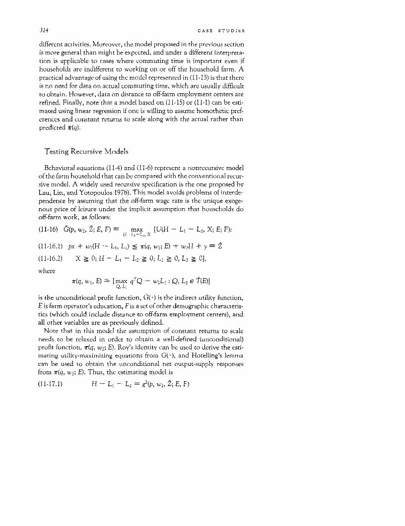
314 CASE STUDIES
different activities. Moreover, the model proposed in the previous sectionis more general than might be expected, and under a different interpreta-tion is applicable to cases where commuting time is important even ifhouseholds are indifferent to working on or off the household farm. Apractical advantage of using the model represented in (11-15) is that thereis no need for data on actual commuting time, which are usually difficultto obtain. However, data on distance to off-farm employment centers arerefined. Finally, note that a model based on (11-15) or (11-1) can be esti-mated using linear regression if one is willing to assume homothetic pref-erences and constant returns to scale along with the actual rather thanpredicted *(q).
Testing Recursive Models
Behavioral equations (11-4) and (11-6) represent a nonrecursive modelof the farm household that can be compared with the conventional recur-sive model. A widely used recursive specification is the one proposed byLau, Lin, and Yotopoulos 1978). This model avoids problems of interde-pendence by assuming that the off-farm wage rate is the unique exoge-nous price of leisure under the implicit assumption that households dooff-farm work, as follows:
(11-16) G(p, w2, 2; E, F) max [U(H - L- L2, X; E; F):H-LI 1- 2 , X
(11-16.1) px + w2(H - LI, L2) _ 7r(q, w2; E) + w2 H + y a Z
(11-16.2) X _ O; H-LI-L 2 > 0; LI > O, L2 >_ ],
where
7r(q, W2, E) [max qTQ - w 2LI : Q, Li e T(E)]Q, Li
is the unconditional profit function, G(*) is the indirect utility function,E is farm operator's education, F is a set of other demographic characteris-tics (which could include distance to off-farm employment centers), andall other variables are as previously defined.
Note that in this model the assumption of constant returns to scaleneeds to be relaxed in order to obtain a well-defined (unconditional)profit function, 7r(q, w2; E). Roy's identity can be used to derive the esti-mating utility-maximizing equations from G(-), and Hotelling's lemmacan be used to obtain the unconditional net output-supply responsesfrom ir(q, w2; E). Thus, the estimating model is
(11-17.1) H - L- = g2(p, W2, Z; E, F)
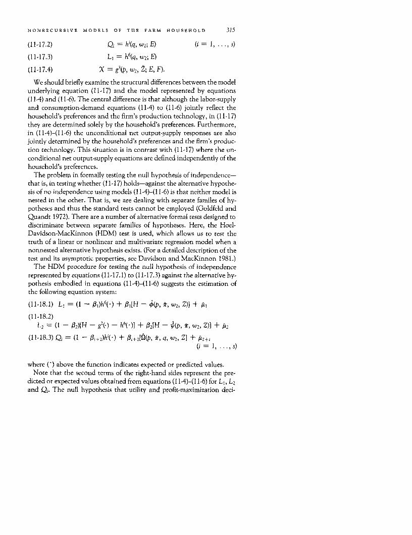
NONRECURSIVE MODELS OF THE FARM HOUSEHOLD 315
(11-17.2) Qi = hi(q,w2; E) (i 1, . . ., s)
(11-17.3) LI = h6(q, w2; E)
(11-17.4) X =g(P, w2, Z; E, F).
We should briefly examine the structural differences between the modelunderlying equation (11-17) and the model represented by equations(11-4) and (11-6). The central difference is that although the labor-supplyand consumption-demand equations (11-4) to (11-6) jointly reflect thehousehold's preferences and the firm's production technology, in (11-17)they are determined solely by the household's preferences. Furthermore,in (1 1-4)-(11-6) the unconditional net output-supply responses are alsojointly determined by the household's preferences and the firm's produc-tion technology. This situation is in contrast with (11-17) where the un-conditional net output-supply equations are defined independently of thehousehold's preferences.
The problem in formally testing the null hypothesis of independence-that is, in testing whether (11-17) holds-against the alternative hypothe-sis of no independence using models (11-4)-(11-6) is that neither model isnested in the other. That is, we are dealing with separate familes of hy-potheses and thus the standard tests cannot be employed (Goldfeld andQuandt 1972). There are a number of alternative formal tests designed todiscriminate between separate families of hypotheses. Here, the Hoel-Davidson-MacKinnon (HDM) test is used, which allows us to test thetruth of a linear or nonlinear and multivariate regression model when anonnested alternative hypothesis exists. (For a detailed description of thetest and its asymptotic properties, see Davidson and MacKinnon 1981.)
The HDM procedure for testing the null hypothesis of independencerepresented by equations (1 1-17.1) to (1 1-17.3) against the alternative hy-pothesis embodied in equations (1 1-4)-(11-6) suggests the estimation ofthe following equation system:
(11-18.1) LI = (I - I)h6 () + 11[H - ¢(p, *, w2, Z)] + [i
(11-18.2)12 =(1 - 2)[H - g2 () - h6(-)] + 023H- 1 4, *, W2, Z)] + A2
(11-18.3) Qi (1 - Oi+2)hi'() + 0i+2[PNP, fr, q, w2, Zl + ft2+i
(i = 1, . .. , s)
where (^) above the function indicates expected or predicted values.Note that the second terms of the right-hand sides represent the pre-
dicted or expected values obtained from equations (1 1-4)-(11-6) for LI, L2and Qi. The null hypothesis that utility and profit-maximization deci-
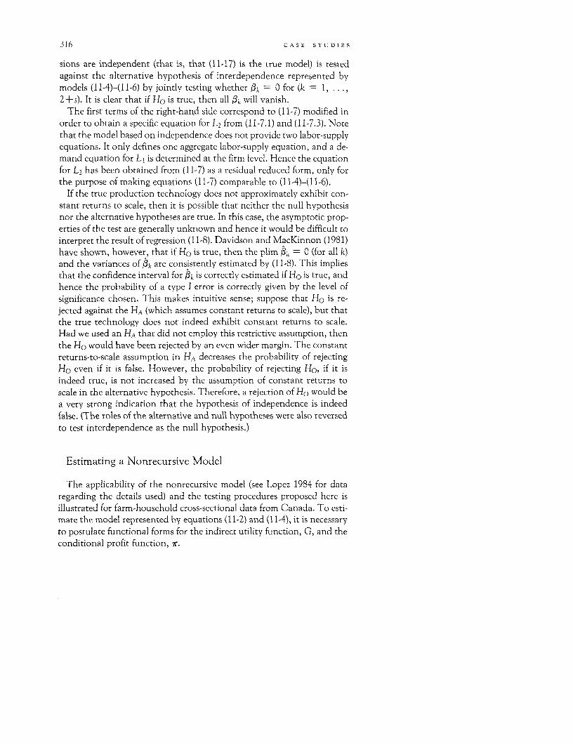
316 CASE STUDIES
sions are independent (that is, that (11-17) is the true model) is testedagainst the alternative hypothesis of interdependence represented bymodels (11-4)-(11-6) by jointly testing whether fk = 0 for (k = 1,2+s). It is clear that if Ho is true, then all Sk will vanish.
The first terms of the right-hand side correspond to (11-7) modified inorder to obtain a specific equation for L2 from (11-7.1) and (11-7.3). Notethat the model based on independence does not provide two labor-supplyequations. It only defines one aggregate labor-supply equation, and a de-mand equation for LI is determined at the firm level. Hence the equationfor L2 has been obtained from (11-7) as a residual reduced form, only forthe purpose of making equations (11-7) comparable to (11-4)-(11-6).
If the true production technology does not approximately exhibit con-stant returns to scale, then it is possible that neither the null hypothesisnor the alternative hypotheses are true. In this case, the asymptotic prop-erties of the test are generally unknown and hence it would be difficult tointerpret the result of regression (11-8). Davidson and MacKinnon (1981)have shown, however, that if Ho is true, then the plim k =0 (for all k)and the variances of Sk are consistently estimated by (1 1-8). This impliesthat the confidence interval for Sk is correctly estimated if Ho is true, andhence the probability of a type I error is correctly given by the level ofsignificance chosen. This makes intuitive sense; suppose that Ho is re-jected against the HA (which assumes constant returns to scale), but thatthe true technology does not indeed exhibit constant returns to scale.Had we used an HA that did not employ this restrictive assumption, thenthe Ho would have been rejected by an even wider margin. The constantreturns-to-scale assumption in HA decreases the probability of rejectingHo even if it is false. However, the probability of rejecting HO, if it isindeed true, is not increased by the assumption of constant returns toscale in the alternative hypothesis. Therefore, a rejection of HO would bea very strong indication that the hypothesis of independence is indeedfalse. (The roles of the alternative and null hypotheses were also reveisedto test interdependence as the null hypothesis.)
Estimating a Nonrecursive Model
The applicability of the nonrecursive model (see Lopez 1984 for dataregarding the details used) and the testing procedures proposed here isillustrated for farm-household cross-sectional data from Canada. To esti-mate the model represented by equations (11-2) and (11-4), it is necessaryto postulate functional forms for the indirect utility function, G, and theconditional profit function, 7r.
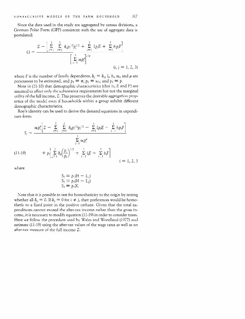
NONRECURSIVE MODELS OF THE FARM HOUSEHOLD 317
Since the data used in the study are aggregated by census divisions, aGorman Polar Form (GPF) consistent with the use of aggregate data ispostulated:
-3 3 3 3
Z -_ y31 ;p p1112 + r lipE + E bjPiF]
G =
(i, j = 1, 2, 3)
where F is the number of family dependents, 6j =6, b1 , b,, ci, and p areparameters to be estimated, and Pi =-; P2 w 2, and P3 3p
Note in (11-18) that demographic characteristics (that is, E and F) areassumed to affect only the subsistence requirements but not the marginalutility of the full income, Z. This preserves the desirable aggregation prop-erties of the model even if households within a group exhibit differentdemographic characteristics.
Roy's identity can be used to derive the demand equations in expendi-ture form:
3 3 3 3
xiPip Z - FI, E 6jP1'"Pj"' - iEl liPiE - iE bipiF]
Si = ~~~~~~~~~~~3
i- I Cop'
(11-19) + piW ±E ij + iE+ ElbiF]
i= 1, 2,3
where
S,- p(H - Li)S2 - p 2 (H - L2 )
S3 -p 3X.
Note that it is possible to test for homotheticity to the origin by testingwhether all ai1= 0. If 0ii = O for i * j, then preferences would be homo-thetic to a fixed point in the positive orthant. Given that the total ex-penditures cannot exceed the after-tax income rather than the gross in-come, it is necessary to modify equation (11-19) in order to consider taxes.Here we follow the procedure used by Wales and Woodland (1977) andestimate (11-19) using the after-tax values of the wage rates as well as anafter-tax measure of the full income Z.
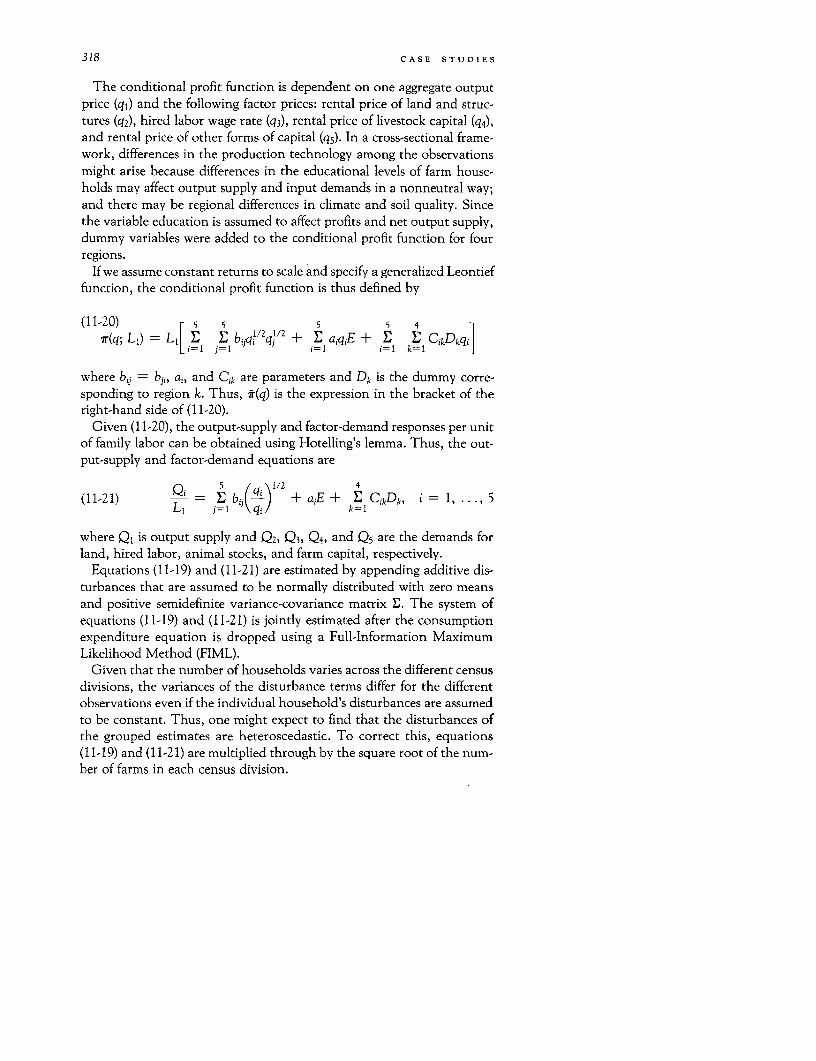
318 CASE STUDIES
The conditional profit function is dependent on one aggregate outputprice (ql) and the following factor prices: rental price of land and struc-tures (q2), hired labor wage rate (q3), rental price of livestock capital (q 4 ),
and rental price of other forms of capital (q 5 ). In a cross-sectional frame-work, differences in the production technology among the observationsmight arise because differences in the educational levels of farm house-holds may affect output supply and input demands in a nonneutral way;and there may be regional differences in climate and soil quality. Sincethe variable education is assumed to affect profits and net output supply,dummy variables were added to the conditional profit function for fourregions.
If we assume constant returns to scale and specify a generalized Leontieffunction, the conditional profit function is thus defined by
(11-20) 5 5 5 5 4
7r(q; LI) =L[ LI j bijqiII2qj '2 + il aiq,E + E k, CikDkq1i=J i=1 i=I ~~~~i=1 k-1
where b,j = bij, ai, and Cik are parameters and Dk is the dummy corre-sponding to region k. Thus, ii(q) is the expression in the bracket of theright-hand side of (11-20).
Given (11-20), the output-supply and factor-demand responses per unitof family labor can be obtained using Hotelling's lemma. Thus, the out-put-supply and factor-demand equations are
(11-21) - E bij + aiE + E CikDk, i = 1, 5LI j=1 qi ~~~k=1 Ckk
where Q, is output supply and Q2, Q3, Q4, and Q5 are the demands forland, hired labor, animal stocks, and farm capital, respectively.
Equations (11-19) and (11-21) are estimated by appending additive dis-turbances that are assumed to be normally distributed with zero meansand positive semidefinite variance-covariance matrix E. The system ofequations (11-19) and (11-21) is jointly estimated after the consumptionexpenditure equation is dropped using a Full-Information MaximumLikelihood Method (FIML).
Given that the number of households varies across the different censusdivisions, the variances of the disturbance terms differ for the differentobservations even if the individual household's disturbances are assumedto be constant. Thus, one might expect to find that the disturbances ofthe grouped estimates are heteroscedastic. To correct this, equations(11-19) and (11-21) are multiplied through by the square root of the num-ber of farms in each census division.
NONRECURSIVE MODELS OF THE FARM HOUSEHOLD 319
The data used were obtained from the 1971 agricultural and populationcensus in Canada, which covered approximately 240 census divisionsacross the country. The data consisted of averages per farm household ofnumber of days of off-farm work, number of days of on-farm work, theoff-farm wage rate, the household's nonlabor income, output and inputprices faced by the household's firm, output and input quantities, thefarm operator's years of schooling, and the number of family dependents.An aggregated output price index and three input price indices-namely,the hired labor wage rate, an animal stocks rental price index, and a landrental price index-are needed. The price index of farm capital (machin-ery, implements, and other intermediate inputs) is not available and isassumed to be constant across the observations. Farm machinery, fertil-izers, and spray materials, in contrast with other farm inputs (such as la-bor, land, and livestock), are traded by large firms that operate on a na-tional scale. It is reasonable to assume that these firms chargeapproximately homogeneous prices for their products in the different re-gions of the country, and thus the above assumption may not be toounrealistic.
The most important empirical result is the testing of the null hypothesisthat utility- and profit-maximizing decisions are independent. To test thenull hypothesis, we must test whether 3k =0 for k = 1, .. ., 7. Asymp-totic likelihood ratio tests were used for this purpose (Theil 1971). Thecalculated x2 value was 127.20, which is substantially higher than the crit-ical x2 values for 7 degrees of freedom (14.07 and 18.48 at a 5 percent and1 percent level of significance, respectively). Hence, the hypothesis of in-dependent production and consumption decisions (that is, that a recur-sive model is appropriate) is categorically rejected. Furthermore, whenthe roles of the null and alternative hypotheses were reversed (that is,when the null hypothesis was interdependent), the calculated x2 was9.89, which is not large enough to reject the hypothesis at a 1 percent or 5percent level of significance. These results strongly suggest that the recur-sive model considered is restrictive and that the nonrecursive model usedis superior.
The parameter estimates and asymptotic standard error obtained bythe joint estimation of the consumption and production sides of themodel are presented in table 11-1. Most coefficients in the consumptionand production sectors are significant. There is one degree of freedom forthe parameters of the CES function, which can be exhausted by any suit-able normalization (see Blackorby, Boyce, and Russell 1981). The normal-ization chosen is that the share parameter, (2, is equal to one. The good-ness-of-fit measure used is the generalized R2 originally proposed byBaxter and Cragg (1970).
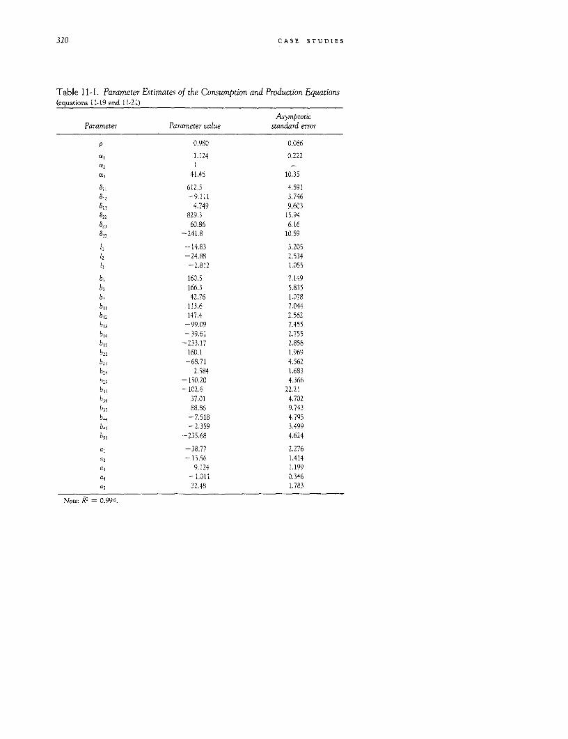
320 CASE STUDIES
Table 1 1-1. Parameter Estimates of the Consumption and Production Equations(equations 11-19 and 11-21)
AsymptoticParameter Parameter value standard error
p 0.980 0.086
at 1.124 0.222
02 I _
03 41.45 10.35
811 612.5 4.591812 -9.111 3.746
°13 4,749 9.603622 829.3 15.94623 60.86 6.16
833 -241.8 10.59
11 -14.83 3.20512 -24.88 2.53413 -2.812 1.055
b, 160.5 7.149b, 166.3 5.835b3 42.76 1.078bil 113.6 7.044b12 147.4 2.562b13 -99.09 7.455b14 -39.61 2.755b15 --233.17 2.858b22 160.1 1.969
b23 -68.71 4.562b24 2.584 1.683b25 -150.20 4.366b33 --102.6 22.21b34 37.01 4.702
b35 88.86 9.743b44 -7.518 4.795b45 --2.359 3.499b755 -235.68 4.624
a, -38.77 2.276a2 -15.56 1.414a3 9.124 1.199a4 -1.011 0.346a5 32.48 1.783
Note: R2 0.994.
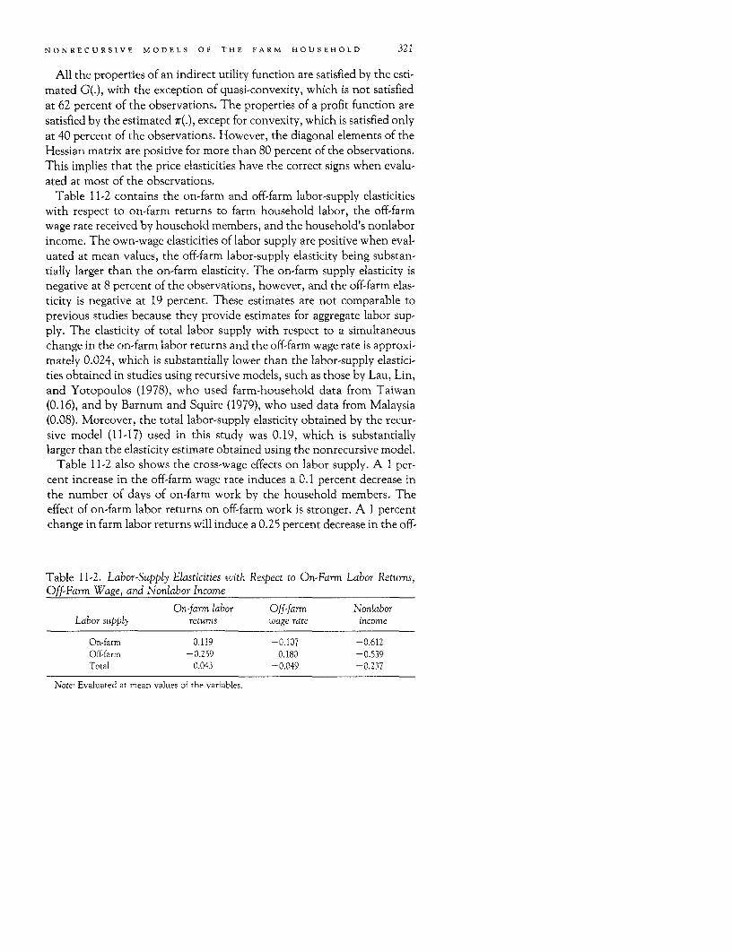
NONRECURSIVE MODELS OF THE FARM HOUSEHOLD 321
All the properties of an indirect utility function are satisfied by the esti-mated G(.), with the exception of quasi-convexity, which is not satisfiedat 62 percent of the observations. The properties of a profit function aresatisfied by the estimated Tr(.), except for convexity, which is satisfied onlyat 40 percent of the observations. However, the diagonal elements of theHessian matrix are positive for more than 80 percent of the observations.This implies that the price elasticities have the correct signs when evalu-ated at most of the observations.
Table 11-2 contains the on-farm and off-farm labor-supply elasticitieswith respect to on-farm returns to farm household labor, the off-farmwage rate received by household members, and the household's nonlaborincome. The own-wage elasticities of labor supply are positive when eval-uated at mean values, the off-farm labor-supply elasticity being substan-tially larger than the on-farm elasticity. The on-farm supply elasticity isnegative at 8 percent of the observations, however, and the off-farm elas-ticity is negative at 19 percent. These estimates are not comparable toprevious studies because they provide estimates for aggregate labor sup-ply. The elasticity of total labor supply with respect to a simultaneouschange in the on-farm labor returns and the off-farm wage rate is approxi-mately 0.024, which is substantially lower than the labor-supply elastici-ties obtained in studies using recursive models, such as those by Lau, Lin,and Yotopoulos (1978), who used farm-household data from Taiwan(0.16), and by Barnum and Squire (1979), who used data from Malaysia(0.08). Moreover, the total labor-supply elasticity obtained by the recur-sive model (11-17) used in this study was 0.19, which is substantiallylarger than the elasticity estimate obtained using the nonrecursive model.
Table 11-2 also shows the cross-wage effects on labor supply. A 1 per-cent increase in the off-farm wage rate induces a 0.1 percent decrease inthe number of days of on-farm work by the household members. Theeffect of on-farm labor returns on off-farm work is stronger. A 1 percentchange in farm labor returns will induce a 0.25 percent decrease in the off-
Table 11-2. Labor-Supply Elasticities with Respect to On-Farm Labor Returns,Off-Farm Wage, and Nonlabor Income
On-farm labor Off-farm NonlaborLabor supply returns wage rate income
On-farm 0.119 -0.107 -0.612Off-farm -0.259 0.180 -0.539Total 0.043 -0.049 -0.237
Note: Evaluated at mean values of the variables.
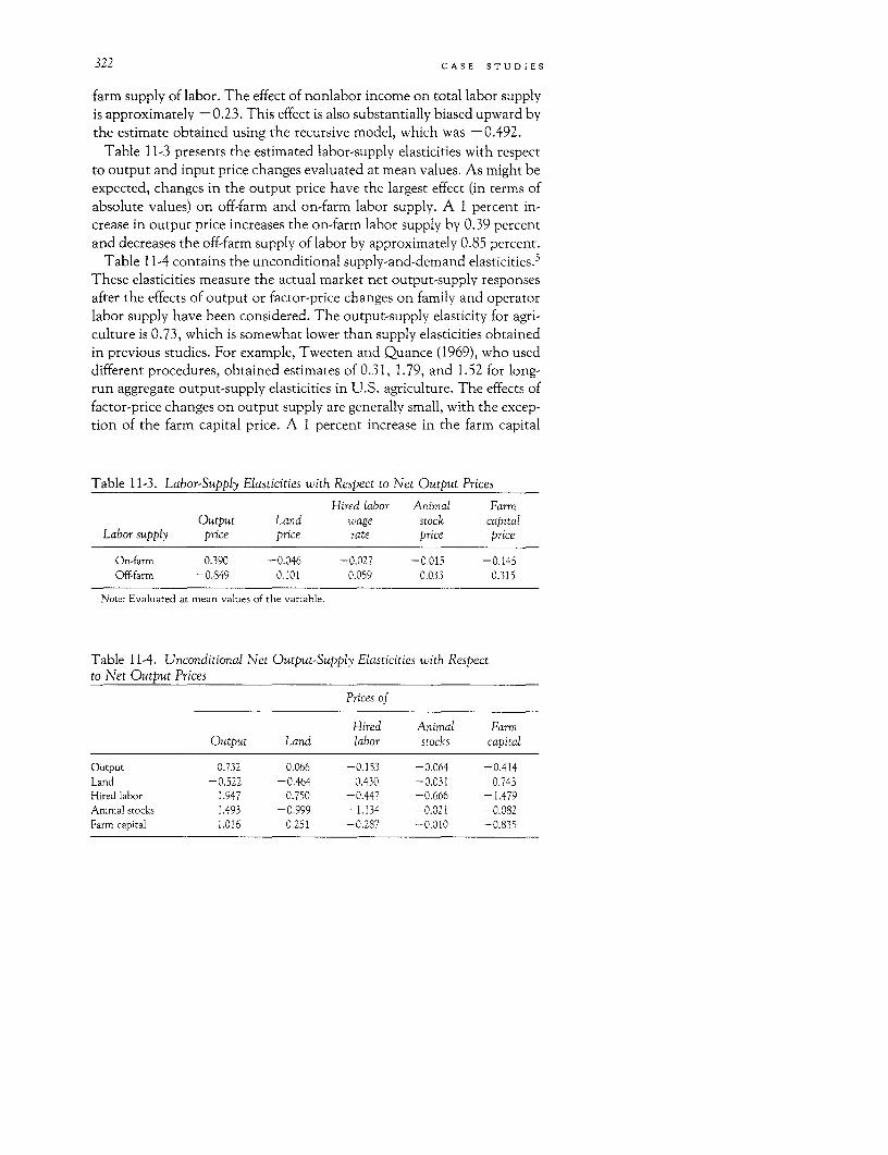
322 CASE STUDIES
farm supply of labor. The effect of nonlabor income on total labor supplyis approximately -0.23. This effect is also substantially biased upward bythe estimate obtained using the recursive model, which was -0.492.
Table 11-3 presents the estimated labor-supply elasticities with respectto output and input price changes evaluated at mean values. As might beexpected, changes in the output price have the largest effect (in terms ofabsolute values) on off-farm and on-farm labor supply. A 1 percent in-crease in output price increases the on-farm labor supply by 0.39 percentand decreases the off-farm supply of labor by approximately 0.85 percent.
Table 11-4 contains the unconditional supply-and-demand elasticities.5
These elasticities measure the actual market net output-supply responsesafter the effects of output or factor-price changes on family and operatorlabor supply have been considered. The output-supply elasticity for agri-culture is 0.73, which is somewhat lower than supply elasticities obtainedin previous studies. For example, Tweeten and Quance (1969), who useddifferent procedures, obtained estimates of 0.31, 1.79, and 1.52 for long-run aggregate output-supply elasticities in U.S. agriculture. The effects offactor-price changes on output supply are generally small, with the excep-tion of the farm capital price. A 1 percent increase in the farm capital
Table 11-3. Labor-Supply Elasticities with Respect to Net Output PricesHired labor Animal Farm
Output Land wage stock capitalLabor supply price price rate price price
On-farm 0.390 -0.046 -0.027 -0.015 -0.145Off-farm -0.849 0.101 0.059 0.033 0.315
Note: Evaluated at mean values of the variable.
Table 11-4. Unconditional Net Output-Supply Elasticities with Respectto Net Output Prices
Prices of
Hired Animal FarmOutput Land labor stocks capital
Output 0.732 0.066 -0.153 -0.064 -0.414Land -0.522 -0.464 0.430 -0.031 0.743Hired labor 1.947 0.750 -0.447 -0.666 -1.479Animal stocks 1.493 -0.999 -1.134 -0.021 -0.082Farm capital 1.016 0.251 -0.287 -0.010 -0.835
NONRECURSIVE MODELS OF THE FARM HOUSEHOLD 323
price induces a 0.4 percent decrease in output supply. Changes in theland price index have a small effect on the demand for all inputs, with theexception of hired labor. Factor demands are not very responsive tochanges in their own prices. Rather, all factors present inelastic demandschedules. These estimates can be compared with previous results forU.S. and Canadian agriculture. Binswanger's (1974) own-factor demandelasticity estimates for U.S. agriculture are -0.34 for land, -0.91 forlabor, -1.089 for machinery, and -0.95 for fertilizers. Lopez's (1980)estimates for Canadian agriculture are -0.52 for labor, -0.35 for farmcapital, -0.42 for land, and -0.41 for intermediate inputs. Thus, al-though the results are not entirely comparable-because the disaggrega-tion of inputs is different and because these studies estimated compen-sated price elasticities (that is, for a constant level of output)-the generalpattern of inelastic factor demands is consistent in the three studies.
Conclusions
This study has shown that under several circumstances the use of recur-sive models in estimating farm-household models may be quite restrictive.It is possible, however, to construct models that allow for interdependentproduction and consumption decisions and that are feasible to estimate.A statistical test to discriminate between an interdependent and a com-monly used recursive model has been implemented using Canadian data.The hypothesis that production and consumption decisions are indepen-dent was categorically rejected, and it was shown that important gains inexplanatory power result from estimating the consumption and produc-tion sectors jointly.
Some other important results emerge from the empirical estimation.First, the cross effects between the production equations and the labor-supply responses are quantitatively strong and thus suggest that interde-pendent models should be used for farm households. Second, the modelestimated explains the behavior of farm households reasonably well andgenerates results that are generally consistent with economic theory.Third, the estimated labor-supply elasticities for on-farm and off-farmwork are very different and thus suggest that the models for farm house-holds should allow for different behavior toward on-farm and off-farmwork. Finally, the total labor-supply elasticities obtained by using thenonrecursive and recursive models tend to be drastically different. Theempirical findings thus imply that nonseparable models are both theoreti-cally and empirically sounder than separable models.
324 CASE STUDIES
Notes
1. There are several other sources of interdependent utility- and profit-maximizing decisionsthat are not dealt with in this study. For example, imperfections in capital markets (that is, creditrationing) lead to the specification of an intertemporal dynamic model, which ultimately impliesthat utility-maximizing and production decisions are not separable. See Chambers and Lopez(1984) for the comparative dynamics of such a model.
2. The assumption of constant returns to scale in agriculture has often not been rejected. See,for example, Chan (1981).
3. Note that if hours worked per day were not affected by commuting costs, then the shadowprice of on-farm work would still be different from the off-farm wage rate. In this case, however,the discount factor would not be endogenous and, hence, the shadow price of on-farm workwould be proportional to the off-farm wage rate.
4. Without loss of generality, one can impose in the function U(LI, L2, X) weak separabilitybetween the two labor-supply variables and the vector of consumption X. This would allow oneto postulate the existence of a composite commodity L(LI, L2) and to estimate an aggregate laborsupply. This is not equivalent to a recursive model, however, because in order to estimate anaggregate labor-supply equation, one would have to construct an aggregate labor price that is ingeneral different from v 2. This aggregate labor price is a combination of the shadow price of LIand L2. Since the shadow price of LI is endogenous, the aggregate labor price will also be endoge-nous. Moreover, the shadow price of LI is usually not known and, hence, the aggregate laborprice would be extremely difficult to determine. Thus, although a composite aggregate laborsupply commodity exists, its estimation appears to be infeasible.
5. The unconditional effect of a change in net output price qj on Q can be readily derived:
aQ _ 82T L + dT aLaq, dqO&q, aq, aq,
References
Barichello, R. R. 1979. "The Schooling of Farm Youth in Canada." Ph.D. disserta-tion. University of Chicago, Chicago, 111. Processed.
Barnum, H. N., and L. Squire. 1979. "An Econometric Application of the Theory ofthe Farm-Household." Journal of Development Economics, vol. 6, pp. 79-102.
Baxter, N. D., and J. Cragg. 1970. "Corporate Choice among Long-Term FinancingInvestments." Review of Economic Studies, vol. 52, pp. 259-61.
Benewitz, M. C., and A. Zucker. 1968. "Human Capital and Occupational Choice:A Theoretical Model." Southern Economic Journal, vol. 33, pp. 406-9.
Binswanger, H. P. 1974. "The Measurement of Technical Change Biases with ManyFactors of Production." American Economic Review, vol. 64, pp. 964-76.
Blackorby, C., R. Boyce, and R. Russell. 1981. "Estimation of Demand Systems Gen-erated by the Gorman Polar Form: A Generalization of the S-Branch Utility Tree."Econometrica, vol. 46, pp. 265-82.
NONRECURSIVE MODELS OF THE FARM HOUSEHOLD 325
Chambers, R., and R. E. Lopez. 1984. "Equity Formation and the On-farm, Off-farmLabor Choice." University of Maryland, Department of Agricultural and ResourceEconomics, College Park, Md. Processed.
Chan, M. W. 1981. "An Econometric Model of the Canadian Agricultural Econ-omy." Canadian Journal of Agricultural Economics, vol. 29, pp. 265-82.
Davidson, R., and J. G. MacKinnon. 1981. "Several Tests for Model Specification inthe Presence of Alternative Hypotheses." Econometrica, vol. 49, pp. 781-93.
Diewert, W. E. 1971. "Choice on Labour Markets and the Theory of Allocation ofTime." Ottawa: Department of Manpower and Immigration.
. 1974. "Applications of Duality Theory." In Frontiers of Quantitative Economics,ed. M. D. Intriligator and D. A. Kenrick. Vol. 2. London: North-Holland.
Fieldings, G. S., and J. Hoseck. 1973. "Human Investment Decisions, Labour MarketChoice, and Unemployment." Rand #P-5144, Los Angeles, Calif.
Goldfeld, S. M., and R. E. Quandt. 1972. Nonlinear Methods in Econometrics. London:North-Holland.
Gorman, W. M. 1953. "Community Preference Field." Econometrica, vol. 21, pp.63-80.
Hotelling, H. 1932. "Edgeworth's Taxation Paradox and the Nature of Demand andSupply Functions." Journal of Political Economy, vol. 40, pp. 577-616.
Lau, L. J., W. L. Lin, and P. A. Yotopoulos. 1978. "The Linear Logarithmic Expendi-ture System: An Application to Consumption-Leisure Choice." Econometrica, vol.46, pp. 843-68.
Lopez, R. E. 1980. "The Structure of Production and the Derived Demand for Inputsin Canadian Agriculture." American Journal of Agricultural Economics, vol. 62, pp.38-45.
. 1982. "Applications of Duality Theory to Agriculture." Western Journal of Ag-ricultural Economics, vol. 7, pp. 353-66.
. 1984. "Estimating Labor Supply and Production Decisions of Self-EmployedFarm Producers." European Economic Review, vol. 24, pp. 61-82.
Malinvaud, E. 1976. Lectures on Microeconomic Theory. London: North-Holland.
Rottenberg, S. 1956. "On Choice in Labour Markets." In Readings in Labour Markets.Edited by J. Burton. London.
Theil, H. 1971. Principles of Econometrics. New York: John Wiley & Sons.
Tweeten, L. B., and L. C. Quance. 1969. "Positivistic Measures of Aggregate SupplyElasticities: Some New Approaches." American Journal of Agricultural Economics,Proceedings, vol. 51, pp. 475-89.
Wales, T. J., and A. D. Woodland. 1977. "Estimation of the Allocation of Time forWork, Leisure and Housework." Econometrica, vol. 45, pp. 115-25.

Index
Page numbers in italics indicate tables. Bangladesh, 118, 119Bardhan, Pranab, 55, 201
Adulavidhaya, Kamphol, 23, 24, 63 Barnum, Howard, 23, 24, 59, 65, 184, 185,Agricultural household models: appropriate 321
use and value of, 25-29; basic principles of, Baxter, N. D., 31917-20; of a Chinese collective farm, 279- Becker, Gary, 86, 87300; commuting time and work preferences Behrman, Jere, 118in, 307-14; data collection for, 62-66, 68- Betel consumption and health, 17769; elasticities and 28, 30, 31; empirical Bhalla, S. S., 196results of, 22-25; estimation issues in, 20- Binswanger, H. P., 32322; food consumption study for, 116-17, Block, M., 256, 257119-24; household as price-taker in basic, Borrowing, 39, 40; credit program study and,71-76; labor allocation in, 278-302; multi- 184, 185, 186, 188, 189, 192-94, 199, 200-crop environment study and, 95, 96, 100- 03, 20407, 112-13; multicrop environment theoret- Boussard, Jean Marc, 113ical model of, 97-100; multimarket analysis Braverman, Avishay, 40, 41, 42, 59, 62, 201,and, 59-62; multimarket pricing in, 235-43, 242251-53; nonseparability effects in, 48-58; Brazil, 118, 255policy extensions and, 35-42; policy results Budget deficits. See Deficits (government)of, 30-35 Budget surveys, 63, 113, 204
Agricultural households: complex behavior Byerlee, Derek, 143, 145patterns of, 3; credit and size of, 202; healthdeterminants in, 154-61; methodology formodeling of, 6-9; reasons for modeling of,4-6; simulation of rural economy and poor, Caloric availability: basic model and, 37; elas-206-29; structure of study of, 9-14 ticities of, 137-39; food consumption study
Ahn, Choong Yong, 59, 242 and, 118, 119, 137-39, 140, 141, 142; inAlderman, Harold, 118 foodstuffs, 37-38; microsimulation and in-Almost Ideal Demand System, 59, 61, 239, terhousehold distribution of, 207, 210, 215,
243 216, 219, 220, 221, 223, 225-28, 229Anderson, Arthur, 242 Canada, 51, 306, 316, 319, 323Autarkic behavior in models, 79-80; self-suffi- Capital, food consumption study and, 145,
ciency and, 33 147
327
328 INDEX
Center for Research in Economic Develop- Credit program study (India): assets and, 192-ment (CRED), 242, 243, 249 93; basic model and, 39-40; basic structure
Chayanov, A. V., 71, 80 of model for, 184-86; borrowing and, 184,Chinese farm collective. See Labor allocation 185, 186, 188, 189, 192-94, 199, 200-03,
study (Chinese collective farm) 204; data and, 194, 204; family size and,Cobb-Douglas production function, 24; food 202; farm size and, 200, 201; flow-of-funds
consumption study and, 117, 122, 123; measure and truncation issue and, 187-89;health production study and, 159; micro- income and, 187, 191, 196, 204; initial en-simulation and, 210; multimarket pricing dowment and, 194-95; interest rate and,and, 237 183-84, 188, 189-90, 197-99, 202-03, 204;
Colombia, 118 investment and, 187, 195-96, 203; laborCommodities: agricultural, 27, 43; data col- and, 186-87, 192; leisure and, 186-87, 191;
lection examples and, 64, 65; elasticities of life cycle variables and, 196, 203; purpose of,consumption for, 43, 44; empirical results of 183-84; savings and, 188, 196, 204; timemodels and, 22; food consumption study constraint in, 185; wage rates and, 188, 194,and, 123, 143, 144; health production study 201, 203and, 170, 173, 174; microsimulation and, Credit rationing, 55207, 210, 211; multimarket and demand for Crops: Braverman-Hammer case study and(example), 62; nonagricultural, 27, 29, 33, multimarket analysis and, 59; collective44; partly absent markets and heterogeneity farm, 287, 288, 289, 293, 294, 295, 297-98,of, 88-89; production decisions and, 75, 79; 299, 300; consumption and price of, 75; ex-sales and purchase price differences for, 52- penditures for research on, 195; food con-54 sumption study and, 116, 119, 124-25, 134,
Commodity-marketed surplus, agricultural, 144, 145, 146, 147, 148; policy and compet-45 ing, 35-36; price policy effects example
Consumption, 51, 56; agricultural household (Senegal) and exported and imported, 40-modeling and, 7, 8-9, 28; basic model and, 42; price of (Senegal), 238, 240, 242, 243-46,19-20; borrowing and, 185; Chinese collec- 247, 249-50; rural economic microsimula-tive study and, 279, 280, 282-83, 285, 286, tion and, 210, 211, 213-17. See aLso Multi-287, 291, 297, 299, 300, 301, 302; data col- crop environment case studylection examples and, 64-66; elasticities of Cyprus, 60commodity, 43, 44; empirical results and,25; food consumption study and, 124-30,135, 136, 139, 146; health and food, 38, Data: equation estimation and, 22; model re-153-54, 155, 157, 159, 160, 161-66, 168, quirements and collection of, 62-66; prob-169, 178; household as price-taker and, 75; lems with, 60; utility and profit-maximiza-modeling commuting time and work prefer- tion, 306, 316, 319, 323ences and, 308, 310; models with absent la- Davidson, R., 316bor market and, 81-83; multicrop study Deaton, Angus, 23, 61, 239and, 99, 102, 103, 105, 109; multimarket Debt, policy issues and, 39-40. See also Creditanalysis example and, 62; multimarket pric- program study (India)ing and, 237, 240, 241, 242, 252; nonsepara- Decisionmaking process, 7ble analysis and, 67; price rise and increase Deficits (government): agricultural pricingin, 27; production risk study and, 258, 262, policy and, 40-42; multimarket pricing263, 272; production separability and, 306, analysis and, 240-41, 243-44323; production technology and, 79; self- Demand: agricultural household models and,sufficiency and, 33-34; Sierra Leone rural, 28, 29; basic model and, 19-20; basic model207, 208-09, 210, 211, 212, 213, 214, 215- and commodity, 20, 21, 22, 23; commodity16, 218, 219, 222, 223, 224, 228; Z-goods demand in multimarket example and, 62;and, 87, 88 commuting time and work preference mod-
Cragg, J., 319 elingand,310;forcredit, 183, 187, 188,201;
INDEX 329
elasticities of, 26, 27, 28, 32-33; empirical Finance market. See Credit program studyresults and, 24; estimation issues and, 20, (India)21, 22; for fertilizer, 35; food consumption Fisk, E. K., 80study and, 120, 121, 123, 125-30, 135, 143, Food, 53, 76; consumption patterns and145; health production function and, 159, health production, 153-54, 155, 157, 159,160-61, 168; for labor, 27, 32-33, 81, 213; 160, 161-66, 168, 169, 175, 177, 178; policy,multicrop case study and, 100, 101, 102-05, 37-38, 58; procurement policies (multicrop108, 109, 111-12; in multimarket pricing case study), 108-09; rural economic micro-analysis, 235, 237, 239, 251, 252; produc- simulation and, 210, 213-14, 221; sales andtion risk study and, 265, 266, 271; profit purchase price differences and, 52, 53;and, 33. See also Almost Ideal Demand Sys- Z-goods and, 86, 87. See also Nutritiontem; Input demands Food consumption case study (Sierra Leone):
Developing countries: government interven- consumption and, 124-30; data 122-24,tion in, 4; importance of agricultural house- 142-48; labor supply and, 130-31; marketedholds in, 6; labor force in, 3-4 surplus and, 131-36; methodology and pur-
Diewert, W. E., 308 pose of, 116-17; model specification and,Dominican Republic, 263, 267 119-22; policy and, 117-19, 140-42; price
and income and, 137; time constraint in,121
Education: credit program study and, 196, Food Research Institute (Stanford Univer-201; of farm operators, 319; food consump- slty), 6tion study and, 143; labor and levels of, ForeignTexchange, 3, 33, 249, 250; pricing pol-308-09; policy and projects for, 58 icy and, 33, 40-42
Employment: multicrop farming and, 109-12. Freetown (Sierra Leone), 145, 146See also Labor Full-Information Maximum Likelihood
Engel curves, 23, 65, 68; food consumption Method (FIML), 318study and, 117, 125; microsimulation analy-sis and, 210; multimarket models and, 61-62; multimarket pricing and, 239; nonsepa- General equilibrium. See Equilibriumrability analysis and, 51 Government deficits. See Deficits (govern-
Equilibrium: general, 213, 217-25; microsim- ment)ulation and, 213-25; partial, 59, 142, 213- Government policy. See Policy17. See also Statics Graham-Tomasi, Theodore, 55, 56, 57, 67,
Estimation: issues, 21; process (health produc- 113tion function), 167 Grain Management Fund and Fertilizer Fund
Evenson, R. E., 195 (Korea), 59Exports, 12, 34; in agricultural pricing policy Green Revolution, 186, 187, 201
example (Senegal), 40-42, 235; taxation on, Gronau, Reuben, 86, 87, 8835 Grossman, M., 156
Extended Linear Expenditure System (ELES),159
Hammer, Jeffrey S., 40, 41, 42, 59, 62, 242Hanoch, G., 257
Families. See Agricultural households Hazell, P. B. R., 113Farm households. See Agricultural house- Health: data on, 65, 166-67, 169-70; estimat-
holds ing production function for, 38-39; foodFertilizer, 34, 35; on Chinese collective, 278, consumption patterns and, 153-54, 155,
290, 292, 296; food consumption study and, 157,159, 160, 161-66,168, 169, 178; policy,145; multimarket pricing analysis and, 237, 58; study and, 11. See also Caloric availabil-241, 247-49; self-sufficiency and price policy ity; Food consumption case study; Illness;and, 33 Nutrition
330 INDEX
Health determinants: consequences of 266, 269; rural economic microsimulationchanges in, 154-61; data on, 166-67, 169- and, 212, 215-16, 219, 221, 22970, 179-81; estimation procedures and, 167; India, 28, 255; credit program study concern-food consumption patterns and, 153-54, ing, 11, 39, 66, 183-204154-56, 157, 159, 160, 161-66, 168, 178; Indonesia: health and food consumption in,heterogeneity bias and, 167-69; income 38, 118; health production function dataand, 156-59, 161, 177, 178, 179; in Indone- for, 166-67, 169-70, 179-81sia, 166-79; intrafamily resource allocation Initial endowment: for Chinese collective pro-and, 161-66; labor and, 155-56, 157, 161, ductive team, 281, 290; in credit program168, 169, 170-73, 178; policy and, 153; study, 194-95prices and, 159-61, 163, 167, 173, 174, 177, Input costs (multicrop study), 105-06178, 179; profits and, 156-59, 162, 167, 169, Input demands: estimation issues and, 20, 21;170-73, 178; separability and, 156-59, 162, food consumption study and, 123; house-167 hold as a price-taker and, 75
Heineke, J., 256, 257 Input variables (basic model), 18Hesser, L. F., 186 Interest rates, 39-40; credit study and, 183-Heterogeneity bias and health production, 84, 188, 189-90, 197-99, 202-03, 204
167-69 Intervention (government): in a Chinese col-Hoel-Davidson-MacKinnon (HDM) test, 315 lective, 13; in developing countries, 4;Hog production (Chinese collective), 291, model and policy and, 30-42
295, 297, 298, 300 Investment, 39, credit and, 187, 195-96, 203Household budget surveys, 63, 113, 204 lqbal, Farrukh, 11, 39, 66, 190Household models. See Agricultural house- Irrigation, 238; health production function
hold models; Models analysis and, 169, 181; multicrop case studyHuffman, Wallace, 88 and, 95Hymer, Stephan, 86, 87, 88
Janakiram, Subramanian, 24, 35Japan, 23, 27, 64
Illness: drinking water and, 173-74; farm Jorgenson, Dale, 7, 81profits and, 170-73; production function of,174-77
Imperfect substitutes. See SubstitutionImports, 12, 33, 34, 240, 242, 243; policy for- Kihlstrom, R., 257
mation and agricultural, 41; Sierra Leone Kislev, Y., 195microsimulation and, 214, 223 Korea, 24, 27; crop choice example for, 35, 36;
Income: agricultural commodity consumption multicrop environment study of, 95-114;increase and, 27; agricultural household multimarket analysis of, 59models and, 13, 29, 30-31, 32; basic model Kramer, R., 257, 263, 267, 272and full, 24; in a Chinese collective, 279, Krishna, Raj, 7, 81280, 285, 288, 291, 293, 299, 301, 302; credit Kuroda, Yoshimi, 22, 23, 24program and, 39, 187, 191, 196, 204; deriv-ing virtual (shadow) prices and, 77; foodconsumption study and, 118, 120, 124,13i/- Labor: agricultural household, 6; agricultural39, 140, 141, 142, 145, 147-48; health pro- household modeling and supply of, 7, 25,duction function and, 156-59, 161, 177, 27-28; basic model and, 19; borrowing and178, 179; household as price-taker and, 72- savings and, 39; commodity price increase73, 75-76; labor-supply and consumption and demand for, 32; credit and, 186-87,decisions and, 306; multicrop case study 192; in developing countries, 3-4; elastici-and, 98, 105, 111-12; multimarket analysis ties of demand for, 27, 32-33; elasticities ofand, 61, 62; multimarket pricing and, 235, supply of, 27, 46, 321, 323; food consump-250; production risk and, 256-57, 259, 265, tion study and, 121-22, 130-31, 134, 135,
INDEX 331
136, 143; health and, 39, 155-56, 157, 161, MacKinnon, J. G., 316168, 169, 170, 178; models with absent mar- Malawi, 60ket in, 79-85; model without preferences for Malaysia, 23, 27, 29, 31, 33, 65, 321; labor de-commuting time and work and, 307-10; mand elasticities in, 32model with preferences for commuting time Marketed surplus, 36, 51, 59, 89; agriculturaland work and, 310-14; multicrop case study household models and, 30; basic model em-and, 98, 99, 105, 110, 111-12; multimarket pirical results and, 25; elasticities of agricul-pricing and, 238, 239; nonseparability and, tural commodity and, 45; food consump-49-52, 67; production risk and, 258, 259, tion study and, 116, 131-36, 141; models269, 270; rural economic microsimulation with absent market for labor and, 83-84;and, 213, 217, 219, 220, 221, 223, 229; sales multicrop study and, 106, 109; in rural Si-and purchase price difference (example of), erra Leone, 208-09, 210, 214, 218, 219,52, 53-54; testing a nonrecursive model of, 222, 223, 224; self-sufficiency calculations321, 322; Z-goods and, 86, 87, 88. See also and, 33-34Employment Markets: absent labor, 79-85; absent Z-goods,
Labor allocation study (Chinese collective 85-88; in Chinese collective study, 280,farm): collective farm model for, 279-86; 281, 288-89; multimarket analysis method-historical background on, 277-79; Marxist ology issues and, 59-62, 68; nonseparabilitytheory and, 278; model results of, 292-300; and incomplete and interlinked marketsproduction team empirical model for, 287- and risk and, 54-57. See also Pricing (multi-92; theoretical and empirical conclusions market) analysis (Senegal)concerning, 300-02; time constraint in, 285 Mellor, J., 80
Lancaster, Kelvin, 87 Microsimulation: data for, 206, 207, 208-09,Land, 318; on a collective farm, 287-88, 290, 212, 214, 218, 222, 224, 226, 227, 230; gen-
292, 293, 294; credit and, 200, 201; food eral equilibrium and, 217-25; income con-consumption study and, 145, 147; health sumption and, 215-16; interhousehold dis-production study and, 169; multicrop study tribution of calories and, 225-28, 229;and, 99, 100, 106, 107, 110; multimarket partial equilibrium and, 213-17; point elas-pricing and, 236, 238, 239; production risk ticities versus, 211-13, 228; policy and, 206,and, 258, 259, 269, 270 210-11, 229; the poor and, 206, 229; popu-
Lange, Mark, 88 lation estimates and, 207-11; productivityLau, Lawrence, 7, 22, 23, 24, 59, 62, 64, 81, and, 221-25, 229; wages and, 217-21, 229
314, 321 Mirman, L., 256, 257Leibenstein, H., 156 Mirrlees, J. A., 156Leisure, 73, 120; Chinese collective farm Models: appropriate use and value of, 25-29;
study and, 277, 285, 297, 301; credit study data collection and, 62-66, 68-69; govern-and, 186-87, 191; empirical results of model ment intervention in developing countriesand, 22; health production function and, and, 4; labor in developing countries and,156, 157; microsimulation analysis and, 3-4; methodology for, 6-9; nonrecursive,219; models with absent market for labor 71-89, 316-23; nonseparable, 48-58, 63,and, 80, 81-83; production risk study and, 66-67; reason for, 4-6; recursive, 48, 71-89;261; Z-goods and, 86 recursive properties of, 10, 11, 12, 13, 18,
Leland H., 256 20, 22, 89-90, 306, 314-16, 323; researchLinear Expenditure System (LES), 23, 24, 65, agenda for, 66-69; separable, 50, 51, 52, 56,
239; food consumption study and, 119-20, 63, 64, 68, 73; separable microsimulation,123; multicrop study and, 101-02 207; separability and Chinese collective
Linear Logarithmic Expenditure System study, 282, 286, 301; separability and exis-(LLES), 23, 24 tence of all markets, 85; separability and
Lin, Wuu-Long, 22, 23, 24, 64, 314, 321 health production and, 156-59, 162, 167;Long, M. G., 186, 202 solving multimarket (numerically), 61; timeLopez, Ramon E., nonseparability analysis constraint in basic, 18; See also Agricultural
and, 49-52 household models
332 INDEX
Muda River Valley (Malaysia), 23, 65 labor market and, 83-84; multimarket anal-Muellbauer, John, 239 ysis and elasticities in, 62; nonseparabilityMulticrop environment case study (Korea analysis and, 51
and Nigeria): data for, 95-96, 113-14; farm Output taxation, 33technology and farm employment and,109-10; linear programming and economet-ric technique integration, 95, 96; model Pani, P. K., 186, 202results, 100-07; models and, 95, 97-100, Parameter estimates: food consumption study112-13; nonfarm employment and demand and, 123; multicrop case study and, 100-01;linkages, 111-12; pricing and food procure- separable and nonseparable models and, 50;ment policies and, 108-09; pricing policies use in simulation, 60and farm employment, 110-11; technology Parameter restrictions, 22and, 96-97 Partial equilibrium. See Equilibrium
Multimarket analysis, 242; methodology is- Petit, Michele, 113sues in, 59-62, 68, 233-34, 246-47, 250 Pitt, Mark M., 38, 58, 65, 67, 118, 119, 174
Murth, Richard, 87 Policy: agricultural household models and,30-35; complex behavior patterns of agri-cultural households and, 3; farm employ-
Nakajima, Chihiro, 71, 80, 81, 83 ment, 110-11; food consumption studyNational Council for Applied Economic Re- and, 117-19, 140-42; food procurement,
search (NCAER) (India), 184, 192, 194, 204 108-09; health production function and,National Socio-Economic Survey of Indone- 153, 178; impact on health outcomes, 58;
sia (SUSENAS 1978), 169, 170 nutritional and health consequences of,Neary,J., 82, 84 153; pricing, 108-111, 233-34, 235, 242; rea-Nicaragua, 118 sons for modeling agricultural householdNigeria, 24, 27; multicrop environment study behavior and, 4-6; research and, 66; rural
in, 35, 36, 95-114 economic microsimulation and, 206, 210-Nonseparability: effects and, 48-52; differing 11, 229
sales and purchase prices for same commod- Pollak, Robert, 61ity, and, 52-54; household production ac- Pope, Rulon D., 257, 263, 267, 272tivities and, 58; incomplete and interlinked Preferences: Chinese collective model and,markets and risk and, 54-57 279, 299; commodity heterogeneity and, 88,
Nutrition: caloric content of foodstuffs and, 89; model with and without work, 307-14;37-38; food consumption study and, 118; nonseparability effects of virtual (orhealth policy consequences and, 153; multi- shadow) price analysis and, 48; nonsepara-crop study and, 109; rural economic micro- bility and on-farm and off-farm work, 52simulation and, 207, 210, 215, 216, 219, Price: agricultural policy for (Korea), 59-60; in220, 221, 223, 225-28, 229; study and, 11. basic model analysis, 18; caloric content ofSee also Caloric availability foodstuffs and, 37-38; changes and elastici-
ties, 206; Chinese collective study and, 292,293, 296, 298, 299-300, 301; data collection
Output markets (agricultural), 8; price in- and, 63, 64, 65; deriving virtual (shadow),creases and, 33 76-79; economic calculations and policy
Output price increase and increase in de- on, 33-34, 40-42; elasticities, 27, 28, 29; es-mand, 33 timation issues and, 20; in food consump-
Output supplies: commuting time and work tion study, 125, 126-29, 130, 131, 132-33,preference modeling and, 310; food con- 134-35, 137-39, 140, 141, 142, 143; healthsumption study and, 123-24; household as and, 38; health production function and,price-taker and, 75; microsimulation and, 159-61, 163, 167, 173, 174, 177; indirect ef-210; model empirical results and, 22; model fect of increased output, 33; modeling of ag-estimation issues and, 20, 21; model and ricultural households and, 7-8, 9, 28, 29,policy extensions and, 36; models without 30; modeling and policy issues and, 31-32;

INDEX 333
multicrop case study and, 102-03, 106, 107, tion for, 260-63; conceptual framework for,108-II; policy and food, 58; production in- 258-60: data, 263; duality and risk aversionstability causing instability in, 57; produc- and, 269-71; empirical example of, 266-69;tion risk and, 261, 264, 266, 273; rural eco- increasing, 263-69; in model, 255-56, 271-nomic microsimulation and, 211, 212, 213, 73; production choices (nonseparability215, 216-17, 221, 223, 225, 228; sales and analysis) and, 56-57; separability and, 68,purchase price difference for same commod- 256, 263, 271; specific model of, 263-66;ity (nonseparability) and, 52-54, 67; utility theoretical background on, 256-58and profit-maximization and, 307, 308, 310, Production team. See Labor allocation study313, 318, 319, 322; wage rates and increase (Chinese collective farm)in rice, 59 Productivity: farm, 187; health production
Price-taker: in the basic model, 18; household function and, 179; microsimulation and,
as (basic model), 71-76; model and assump- 221-25, 229; nutritional status and, 38-39tion of agricultural households as, 8, 9, 10, Profit, 76, 229; agricultural household model-
11 ing and, 6, 9; Chinese collective study and,Pricing (multimarket) analysis (Senegal): agri- 280, 284, 296, 297, 299, 300; estimating
cultural production and, 237-39; agricul- nonrecursive models and, 316-23; food con-tural sector and, 234-35; cotton prices and, sumption study and, 122, 123, 126-29, 130;247; deficits and, 240-41, 243-44; demand health and, 38-39; health production func-response and, 235, 239, 251, 252; fertilizer tion and, 156-59, 162, 167, 169, 170-73,
prices in, 247-49; groundnut prices in, 243- 178; increase in demand for goods and ser-
46; income and, 239; market-clearing condi- vices and, 33; model with and without com-
tions and, 240; methodology for, 233-34, muting time and work preferences, 307-14;246-47, 250; model calibration and, 241- multicrop study and, 112; multimarket pric-43; model structure for, 235-43, 251-53; ing and, 237; testing recursive models and,rice prices in, 249-50; supply response and, 314-16
235-37, 251, 252 Profit effect, 34, 56; in agricultural models,Production, 56; consumption separability 26-27, 29; in basic model, 20; food con-
and, 306, 323; empirical results and, 24; esti- sumption study and, 124, 130, 139, 140
mation issues and, 21; food consumptionstudy and, 121-22, 123, 136, 142, 143, 146-47; health and farm, 154-56, 169; modeling Quadratic Expenditure System, food con-
of agricultural households and, 6-9, 28; sumption study and, 117, 119, 120, 123, 124modeling commuting time and work prefer- Quance, L. C., 322
ences and, 308; multicrop case study and,100, 101, 102, 103, 105, 109; multimarkets
and agricultural, 237-39, 251; nonseparabil- Renting, 55, 145, 318ity and household, 58, 67; in rural Sierra Research: agenda for future, 66-69; credit and
Leone, 207, 208-09, 210, 211, 212, 213, crop, 195, 201; production risk study and,214, 218, 219, 222, 223, 224, 229; Z-goods, 272
86, 87 Resnick, Stephen, 86, 87, 88
Production cycle: basic model and, 17-18, 20; Resource allocation (intrafamily), health pro-
multicrop case study and, 98 duction function and, 161-66Production function: calculation of health, Reutlinger, Shlomo, 118
38; of Chinese collective, 279-80; health, Risk, 52; multicrop study and, 112-13; non-
155, 162, 166, 174, 175; household as price- separability and incomplete and interlinked
taker and, 72-75; of illness, 174-77; multi- markets and, 54-57; technology and, 67.
crop case study and, 96; production risk See also Production riskstudy and, 260. See also Cobb-Douglas pro- Roberts, K., 83, 84
duction function Roe, Terry, 55, 56, 57, 67, 113
Production risk: agricultural household Rosenzweig, Mark, 28, 38, 58, 65, 67, 159,models and, 13-14; characterizing a solu- 163, 174
334 INDEX
Savings, 39, 98; Chinese collective farm study Surveys, 63; credit program, 204; multicropand, 280; credit study and, 188, 196, 204 data and, 113
Schuh, G. C., 186Schultz, T. P., 159, 163Seasonality, 95-96, 101 Taiwan, 22, 27, 62, 64, 321Self-sufficiency, 33; models with autarkic be- Tanaka, Osamu, 80
havior and, 78-80 Taxes, 34; agricultural output, 33; crop choiceSelowsky, Marcelo, 118 and exports and, 35; in Senegal, 241Sen, Amartya K., 80, 83, 136 Technical change, credit demand and, 187,Senegal, 60; balance of payments in, 239; ex- 201, 203
port earnings and deficits example and, 40, Technology, 28, 67, 88, 135; consumption de-41; multimarket analysis of pricing in, 232- cisions and, 75; health and, 154, 159, 160,51 164, 178; household commodity demands
Shand, E. T., 80 and production, 79; multicrop compositionSierra Leone, 24, 25, 27, 29, 33, 62; food con- and, 96-97, 99, 104, 109-10, 111; nonsepa-
sumption study of, 11 6-48; microsimulation rability effects of virtual (or shadow) price
study of, 206-29; multimarket analysis of, analysis and, 48; policy and, 32; prices and59; multiple crop example of, 35, 36 distribution of, 33; production, 18, 309,
Simulation. See Microsimulation 316; rice production and crop choice poli-Singh, Inderjit, 24 cies and, 35Smith, Victor E., 59, 62 Thailand, 23, 27, 29, 33, 63, 64, 240Specification: in food consumption study, Time-series cross-sectional data, 64
119-22; in multimarket analysis, 60, 61 Timmer, C. Peter, 118Spencer, Dunstan, 143, 145 Tobacco consumption, 175, 177Squire, Lyn, 23, 24, 59, 65, 184, 185, 321 Trade: Chinese collectives and restrictionsSrinivasan, T. N., 55, 201 on, 279, 280, 281, 284, 289, 301-02; interna-Statics: in absent labor market analysis, 79- tional, 12
85; for derivation of virtual (shadow) prices, eet, .76-79; for household as price-taker, 71-76;nonseparability effects, and 48; summation Utility function, 65; average of householdsof recursive conditions and, 89-90. See also treated as single household and, 51; in basicEquilibrium model, 17; for a Chinese collective, 279-80;
Stiglitz, J. E., 156, 257 empirical results of basic model and, 23-24;Strauss, John, 24, 35, 37, 59, 61, 62 food consumption study and, 119, 120;Subsidies, 34; credit programs and, 40; price, health production function analysis and,
177; in Senegal, 241; taxes on output to cre- 158, 159, 177; labor as imperfect substituteate, 33 in household, 49; model with and without
Substitution: in Chinese collective study, 285, commuting rime and work preferences and,293, 296; health and food, 160; health and 307-14; multicrop case study and, 98, 99; inillness and, 174; health and labor, 157; la- a nonrecursive model, 316-23; productionbor as imperfect, 49; labor market absence risk study and, 258, 259, 264, 267, 268, 271;and, 81, 82, 83, 84; labor as perfect, 308; lei- in recursive models, 314-16; separabilitysure, 191; nonseparability and Lopez's and, 56model and, 49, 51; policy possibilities and,41-42; production risk study and, 261, 262
Sugar consumption and health, 177, 179 Wages, 6, 135, 143, 313; in agricultural house-Supply: agricultural models and, 28-29; com- hold models, 27, 28; in the credit study,
muting time and work preferences modeling 188, 194, 201, 203; data collection and, 63;and, 310; elasticities of, 106; of labor, 7, 25, health production function and, 161, 169,27-28, 39, 46; multimarket pricing and, 179; health and rise in female, 58; increase235-37, 251, 252; production risk study in rice price (Malaysia) and, 59; microsimu-and, 265 lation and, 217-21, 229; in a multicrop

INDEX 335
itudy, 105; in a nonseparability analysis, function analysis and, 177; policy and, 31,49-51; rural economic microsimulation 141
and, 213, 217, 219-21, 228, 229 Wolfe, Barbara, 118Wales, Terence, 61, 317 Woodland, A. D., 317Water (health production function study),
169,173-74,179 Yotopoulo, Pan, 22-23, Zi, 59, 6i, 314, 321Weathler, 2, 287; multicrop case study and,
95-96Welfare of rural households: food consump- Z-goods, 10, 71; models with absent market
tion study and, 141; health production in, 85-88
The most recent World Bank publications are described in theannual spring and fall lists.The latest edition is available free ofcharge from Publications Sales Unit, Department B, The World
Bank, Washington, D.C. 20433, U.S.A.


a9E
-fi¢a