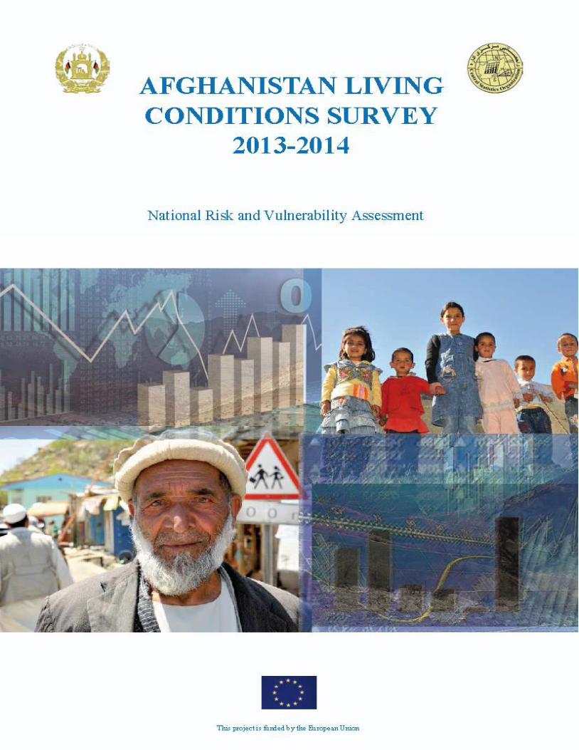
Afghanistan Living Conditions Survey 2013-14 - IHSN catalog
350
i
-
Upload
khangminh22 -
Category
Documents
-
view
0 -
download
0
Transcript of Afghanistan Living Conditions Survey 2013-14 - IHSN catalog
i
ii
The Afghanistan Living Conditions Survey 2013-14 was implemented by the Central Statistics Organization
(CSO) of the Government of the Islamic Republic of Afghanistan with technical assistance from ICON-
Institute Public Sector Gmbh.
This publication has been produced with the assistance of the European Union. The contents of this
publication is the sole responsibility of CSO and ICON-Institute, and can in no way be taken as to reflect
the views of the European Union.
For further information, please contact:
CSO
www.nrva.cso.gov.af
E-mail: [email protected]
ICON-Institute
www.icon-institute.de
E-mail: [email protected] (Project Manager) or
[email protected] (Chief Analyst/Editor)
Delegation of the European Union to Afghanistan
http://eeas.europa.eu/delegations/afghanistan/index_en.htm
E-mail: [email protected]
Recommended citation:
Central Statistics Organization (2016), Afghanistan Living Conditions Survey 2013-14. National Risk and
Vulnerability Assessment. Kabul, CSO.
ISBN: 978-9936-8050-0-2
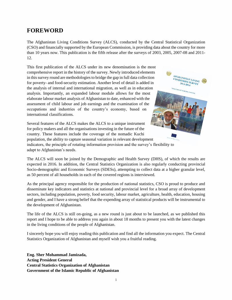
Cover page photos are used by courtesy of Mr. Sascha Oliver Rusch
Designed by: Mohammad Ashraf Abdullah
COPHEN ADVERTISING
www.cophenadvertising.af
Printed by: Jehoon Printing Press, Kabul, Afghanistan
i
FOREWORD
The Afghanistan Living Conditions Survey (ALCS), conducted by the Central Statistical Organization
(CSO) and financially supported by the European Commission, is providing data about the country for more
than 10 years now. This publication is the fifth release after the surveys of 2003, 2005, 2007-08 and 2011-
12.
This first publication of the ALCS under its new denomination is the most
comprehensive report in the history of the survey. Newly introduced elements
in this survey round are methodologies to bridge the gap in full data collection
for poverty- and food-security estimation. Another level of detail is added in
the analysis of internal and international migration, as well as in education
analysis. Importantly, an expanded labour module allows for the most
elaborate labour market analysis of Afghanistan to date, enhanced with the
assessment of child labour and job earnings and the examination of the
occupations and industries of the country’s economy, based on
international classifications.
Several features of the ALCS makes the ALCS to a unique instrument
for policy makers and all the organisations investing in the future of the
country. These features include the coverage of the nomadic Kuchi
population, the ability to capture seasonal variation in relevant development
indicators, the principle of rotating information provision and the survey’s flexibility to
adapt to Afghanistan’s needs.
The ALCS will soon be joined by the Demographic and Health Survey (DHS), of which the results are
expected in 2016. In addition, the Central Statistics Organization is also regularly conducting provincial
Socio-demographic and Economic Surveys (SDESs), attempting to collect data at a higher granular level,
as 50 percent of all households in each of the covered regions is interviewed.
As the principal agency responsible for the production of national statistics, CSO is proud to produce and
disseminate key indicators and statistics at national and provincial level for a broad array of development
sectors, including population, poverty, food security, labour market, agriculture, health, education, housing
and gender, and I have a strong belief that the expending array of statistical products will be instrumental to
the development of Afghanistan.
The life of the ALCS is still on-going, as a new round is just about to be launched, as we published this
report and I hope to be able to address you again in about 18 months to present you with the latest changes
in the living conditions of the people of Afghanistan.
I sincerely hope you will enjoy reading this publication and find all the information you expect. The Central
Statistics Organization of Afghanistan and myself wish you a fruitful reading.
Eng. Sher Mohammad Jamizada,
Acting President General
Central Statistics Organization of Afghanistan
Government of the Islamic Republic of Afghanistan
ii
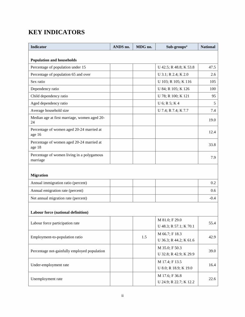
KEY INDICATORS
Indicator ANDS no. MDG no. Sub-groupsa National
Population and households
Percentage of population under 15 U 42.5; R 48.8; K 53.8 47.5
Percentage of population 65 and over U 3.1; R 2.4; K 2.0 2.6
Sex ratio U 103; R 105; K 116 105
Dependency ratio U 84; R 105; K 126 100
Child dependency ratio U 78; R 100; K 121 95
Aged dependency ratio U 6; R 5; K 4 5
Average household size U 7.4; R 7.4; K 7.7 7.4
Median age at first marriage, women aged 20-
24 19.0
Percentage of women aged 20-24 married at
age 16 12.4
Percentage of women aged 20-24 married at
age 18 33.8
Percentage of women living in a polygamous
marriage 7.9
Migration
Annual immigration ratio (percent) 0.2
Annual emigration rate (percent) 0.6
Net annual migration rate (percent) -0.4
Labour force (national definition)
Labour force participation rate M 81.0; F 29.0
U 48.3; R 57.1; K 70.1 55.4
Employment-to-population ratio 1.5 M 66.7; F 18.3
U 36.3; R 44.2; K 61.6 42.9
Percentage not-gainfully employed population M 35.0; F 50.3
U 32.8; R 42.9; K 29.9 39.0
Under-employment rate M 17.4; F 13.5
U 8.0; R 18.9; K 19.0 16.4
Unemployment rate M 17.6; F 36.8
U 24.9; R 22.7; K 12.2 22.6
iii
Indicator ANDS no. MDG no. Sub-groupsa National
Youth unemployment rate 17.a 42 M 22.1; F 40.5
U 34.3; R 26.4; K 12.1 27.4
Youth unemployment as percentage of total
unemployment
M 26.2; F 29.4
U 27.5; R 27.5; K 29.7 27.5
Proportion of own-account and contributing
family workers in total employment 1.7
M 76.2; F 88.7
U 60.0; R 83.2; K 94.1 78.8
Child labour rate (ILO definition) M: 32.7; F: 19.6
U: 10.2; R: 30.3; K: 46.9 26.5
Child labour rate (UNICEF definition) M: 34.1; F: 24.2 29.5
Agriculture and livestock
Percentage of households owning irrigated land 36.6
Percentage of households owning rain-fed land 16.3
Percentage of households owning a garden plot 12.6
Percentage of households having access to
irrigated land 36.2
Percentage of households having access to rain-
fed land 16.1
Percentage of households having access to a
garden plot 12.2
Mean size of owned irrigated land (in jeribsb) 6.1
Mean size of owned rain-fed land (in jeribsb) 13.2
Mean size of owned garden plot (in jeribsb) 1.9
Mean size of accessed irrigated land (in jeribsb) 6.6
Mean size of accessed rain-fed land (in jeribsb) 13.7
Mean size of accessed garden plot (in jeribsb) 1.9
Number of cattle (in thousands) 2,850
Number of goats (in thousands) 10,265
Number of sheep (in thousands) 21,629
Number of chickens (in thousands) 12,221
Poverty
Poverty headcount 1.a (alt) 39.1
iv
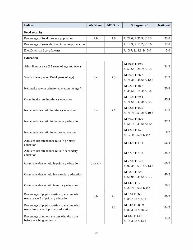
Indicator ANDS no. MDG no. Sub-groupsa National
Food security
Percentage of food insecure population 2.b 1.9 U 29.6; R 35.9; K 9.3 33.0
Percentage of severely food insecure population U 12.3; R 12.7; K 0.0 12.0
Diet Diversity Score (mean) U: 5.7; R: 4.8; K: 5.0 5.0
Education
Adult literacy rate (15 years of age and over) M 49.1; F 19.0
U 53.6; R 28.7; K 7.5 34.3
Youth literacy rate (15-24 years of age) 3.c 2.3 M 66.3; F 36.7
U 74.3; R 44.6; K 12.5 51.7
Net intake rate in primary education (at age 7) M 22.9; F 18.7
U 35.5; R 18.4; K 0.8 20.8
Gross intake rate in primary education M 51.4; F 39.4
U 71.6; R 41.3; K 6.5 45.4
Net attendance ratio in primary education 3.a 2.1 M 62.4; F 45.5
U 76.7; R 51.2; K 10.3 54.5
Net attendance ratio in secondary education M 46.7; F 26.9
U 56.1; R 31.6; K: 5.4 37.2
Net attendance ratio in tertiary education M 12.5; F 4.7
U 17.4; R 5.4; K 0.7 8.7
Adjusted net attendance ratio in primary
education M 64.5; F 47.1 56.4
Adjusted net attendance ratio in secondary
education M 47.8; F 27.8 38.2
Gross attendance ratio in primary education 3.a (alt) M 77.4; F 54.6
U 92.3; R 63.1; K 13.7 66.7
Gross attendance ratio in secondary education M 58.9; F 32.6
U 68.9; R 39.6; K 7.3 46.2
Gross attendance ratio in tertiary education M 14.3; F 5.9
U 20.7; R 6.2; K 0.7 10.1
Percentage of pupils starting grade one who
reach grade 5 of primary education 3.b 2.2
M 87.1 F 86.0
U 85.7 R+K 87.2 86.7
Percentage of pupils starting grade one who
reach last grade of primary education 2.2
M 84.4 F 883.9
U 82.3 R+K 885.2 84.2
Percentage of school starters who drop out
before reaching grade six
M 13.6 F 14.6
U 14.3 R+K 13.8 14.0
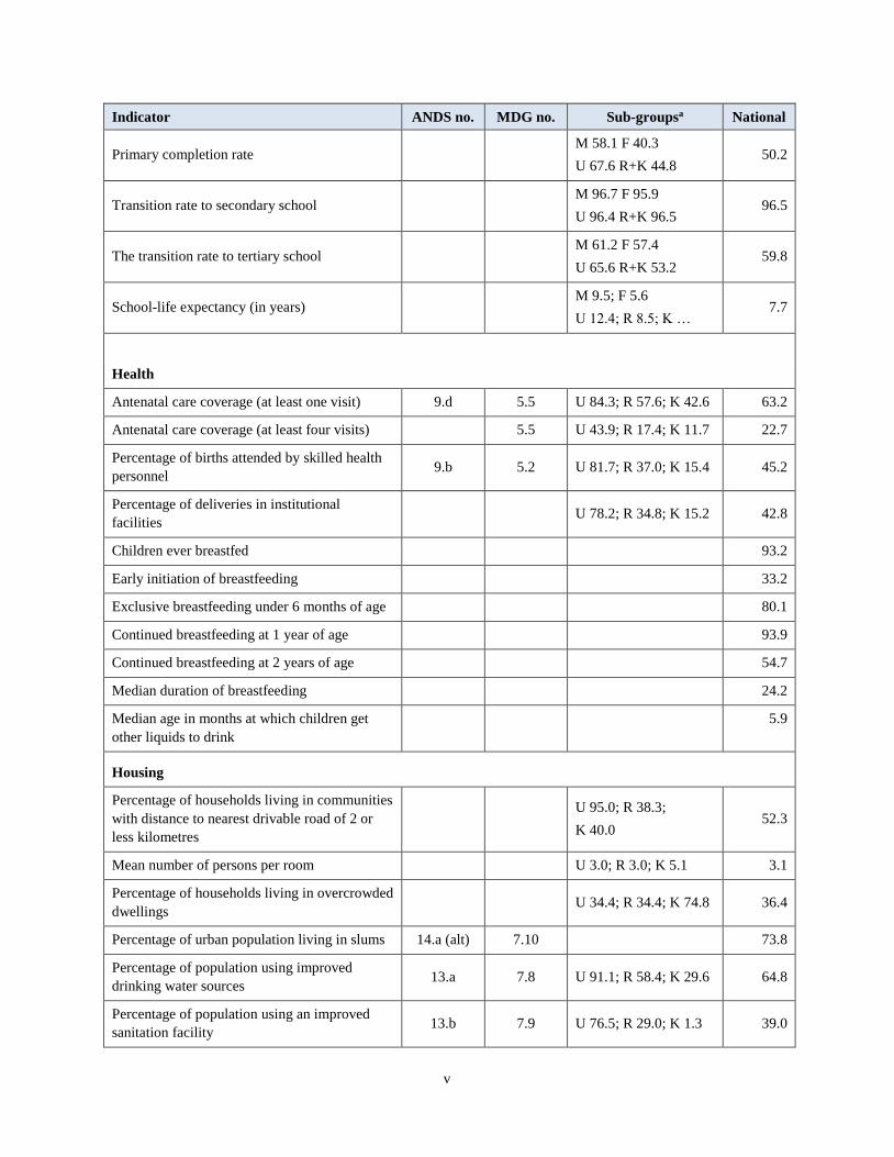
v
Indicator ANDS no. MDG no. Sub-groupsa National
Primary completion rate M 58.1 F 40.3
U 67.6 R+K 44.8 50.2
Transition rate to secondary school M 96.7 F 95.9
U 96.4 R+K 96.5 96.5
The transition rate to tertiary school M 61.2 F 57.4
U 65.6 R+K 53.2 59.8
School-life expectancy (in years) M 9.5; F 5.6
U 12.4; R 8.5; K … 7.7
Health
Antenatal care coverage (at least one visit) 9.d 5.5 U 84.3; R 57.6; K 42.6 63.2
Antenatal care coverage (at least four visits) 5.5 U 43.9; R 17.4; K 11.7 22.7
Percentage of births attended by skilled health
personnel 9.b 5.2 U 81.7; R 37.0; K 15.4 45.2
Percentage of deliveries in institutional
facilities U 78.2; R 34.8; K 15.2 42.8
Children ever breastfed 93.2
Early initiation of breastfeeding 33.2
Exclusive breastfeeding under 6 months of age 80.1
Continued breastfeeding at 1 year of age 93.9
Continued breastfeeding at 2 years of age 54.7
Median duration of breastfeeding 24.2
Median age in months at which children get
other liquids to drink
5.9
Housing
Percentage of households living in communities
with distance to nearest drivable road of 2 or
less kilometres
U 95.0; R 38.3;
K 40.0 52.3
Mean number of persons per room U 3.0; R 3.0; K 5.1 3.1
Percentage of households living in overcrowded
dwellings U 34.4; R 34.4; K 74.8 36.4
Percentage of urban population living in slums 14.a (alt) 7.10 73.8
Percentage of population using improved
drinking water sources 13.a 7.8 U 91.1; R 58.4; K 29.6 64.8
Percentage of population using an improved
sanitation facility 13.b 7.9 U 76.5; R 29.0; K 1.3 39.0
vi
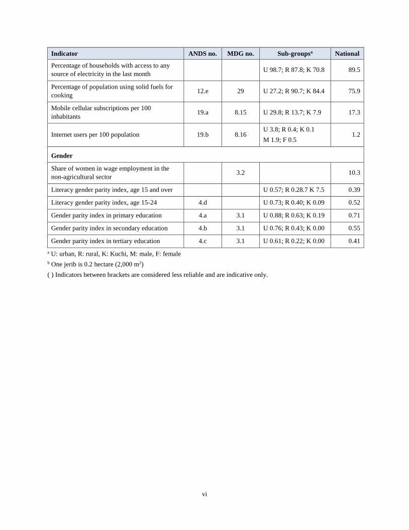
Indicator ANDS no. MDG no. Sub-groupsa National
Percentage of households with access to any
source of electricity in the last month U 98.7; R 87.8; K 70.8 89.5
Percentage of population using solid fuels for
cooking 12.e 29 U 27.2; R 90.7; K 84.4 75.9
Mobile cellular subscriptions per 100
inhabitants 19.a 8.15 U 29.8; R 13.7; K 7.9 17.3
Internet users per 100 population 19.b 8.16 U 3.8; R 0.4; K 0.1
M 1.9; F 0.5 1.2
Gender
Share of women in wage employment in the
non-agricultural sector 3.2 10.3
Literacy gender parity index, age 15 and over U 0.57; R 0.28.7 K 7.5 0.39
Literacy gender parity index, age 15-24 4.d U 0.73; R 0.40; K 0.09 0.52
Gender parity index in primary education 4.a 3.1 U 0.88; R 0.63; K 0.19 0.71
Gender parity index in secondary education 4.b 3.1 U 0.76; R 0.43; K 0.00 0.55
Gender parity index in tertiary education 4.c 3.1 U 0.61; R 0.22; K 0.00 0.41
a U: urban, R: rural, K: Kuchi, M: male, F: female
b One jerib is 0.2 hectare (2,000 m2)
( ) Indicators between brackets are considered less reliable and are indicative only.
vii
TABLE OF CONTENTS
Foreword ........................................................................................................................................................ i
Key indicators .............................................................................................................................................. ii
Table of contents ........................................................................................................................................ vii
List of tables .............................................................................................................................................. xiii
List of figures ........................................................................................................................................... xvii
List of text boxes ...................................................................................................................................... xxii
Abbreviations .......................................................................................................................................... xxiii
Map of Afghanistan ................................................................................................................................... xxv
Acknowledgements .................................................................................................................................. xxvi
Executive summary ............................................................................................................................... xxviii
1 Introduction ........................................................................................................................................... 1
2 Survey methodology and operations ..................................................................................................... 3
2.1 Introduction .................................................................................................................................... 3
2.2 Stakeholder involvement ............................................................................................................... 3
2.3 Questionnaire design ...................................................................................................................... 4
2.4 Pilot training and pilot survey ........................................................................................................ 5
2.5 Training and selection of field staff ............................................................................................... 5
2.6 Sampling design ............................................................................................................................. 6
2.7 Field operations .............................................................................................................................. 7
2.8 Data processing .............................................................................................................................. 9
2.8.1 Manual checking and coding ............................................................................................... 9
2.8.2 Data entry and data editing .................................................................................................. 9
2.9 Analysis ....................................................................................................................................... 10
2.10 Comparability of results ............................................................................................................... 10
2.11 Data limitations ............................................................................................................................ 11
2.12 Reporting ..................................................................................................................................... 12
3 Population and households .................................................................................................................. 13
3.1 Introduction .................................................................................................................................. 14
3.2 Population structure ..................................................................................................................... 14
3.2.1 Age distribution ................................................................................................................. 14
3.2.2 Sex ratio ............................................................................................................................. 16
3.2.3 Distribution by place of residence ..................................................................................... 18
3.3 Household composition ............................................................................................................... 19
3.3.1 Household structure ........................................................................................................... 19
viii
3.3.2 Head of household ............................................................................................................. 21
3.4 Marriage patterns ......................................................................................................................... 22
3.4.1 Marital status distribution .................................................................................................. 22
3.4.2 Age at first marriage .......................................................................................................... 24
3.4.3 The marriage age gap ........................................................................................................ 25
3.4.4 Polygamy ........................................................................................................................... 26
4 Migration ........................................................................................................................................... 28
4.1 Introduction .................................................................................................................................. 29
4.1.1 Afghanistan’s migration context ........................................................................................ 29
4.1.2 Migration concepts ............................................................................................................ 29
4.2 Internal migration in Afghanistan ................................................................................................ 31
4.2.1 Internal life-time migrants ................................................................................................. 31
4.2.2 Internal intermediate-time migrants .................................................................................. 34
4.2.3 Internal recent migrants ..................................................................................................... 36
4.2.4 Urban-rural linkages .......................................................................................................... 38
4.2.5 Who are the internal migrants? .......................................................................................... 39
4.2.6 Why do internal migrants move? ....................................................................................... 40
4.3 International migration................................................................................................................. 41
4.3.1 Immigrants and immigration ............................................................................................. 42
4.3.2 Emigrants and emigration .................................................................................................. 45
4.4 The migration balance.................................................................................................................. 47
4.5 Return from displacement ............................................................................................................ 49
4.5.1 Origins and destinations of returnees ................................................................................ 49
4.5.2 Living conditions of returnees ........................................................................................... 50
5 Labour market outcomes ..................................................................................................................... 53
5.1 Introduction .................................................................................................................................. 54
5.2 Labour force participation ............................................................................................................ 55
5.3 Employment, underemployment and unemployment .................................................................. 57
5.3.1 Overview of employment, underemployment and unemployment ................................... 57
5.3.2 Comparison over time ....................................................................................................... 62
5.3.3 Characteristics of the employed and underemployed ........................................................ 63
5.3.4 Hours of work and earnings ............................................................................................... 72
5.4 Labour migration ......................................................................................................................... 75
5.4.1 Origins and destinations of labour migration ................................................................... 75
5.4.2 Characteristics of labour migrants ..................................................................................... 77
5.4.3 Migrants’ labour market performance ............................................................................... 79
5.4.4 Kuchi labour migration ...................................................................................................... 81
ix
5.4.5 Seasonal migration ............................................................................................................ 81
5.5 Child labour ................................................................................................................................. 83
5.5.1 Introduction ....................................................................................................................... 83
5.5.2 Prevalence of child labour and their conditions of work ................................................... 84
5.5.3 Causes and consequences of child labour .......................................................................... 86
5.5.4 Household chores and child labour .................................................................................... 88
6 Farming and livestock ......................................................................................................................... 91
6.1 Introduction .................................................................................................................................. 91
6.2 Farming and horticulture.............................................................................................................. 92
6.2.1 Irrigated land ...................................................................................................................... 92
6.2.2 Rain-fed land ..................................................................................................................... 97
6.2.3 Farming input .................................................................................................................. 100
6.2.4 Horticulture ...................................................................................................................... 101
6.3 Livestock .................................................................................................................................... 103
6.3.1 Livestock numbers ........................................................................................................... 103
6.3.2 Sale of animals and animal products ............................................................................... 104
6.3.3 Livestock production factors ........................................................................................... 105
7 Poverty ......................................................................................................................................... 107
7.1 Introduction ................................................................................................................................ 107
7.2 Measuring poverty trends using survey to survey imputation ................................................... 109
7.3 Growth and distribution ............................................................................................................. 110
7.4 Poverty profile ........................................................................................................................... 110
7.4.1 Demographic characteristics ............................................................................................ 110
7.4.2 Household head characteristics ........................................................................................ 111
7.4.3 Characteristics of children in the household .................................................................... 113
7.4.4 Access to services ............................................................................................................ 114
7.5 Conclusion ................................................................................................................................. 115
8 Food security .................................................................................................................................... 116
8.1 Introduction ................................................................................................................................ 116
8.2 Current food security ................................................................................................................. 118
8.2.1 Distribution by residence ................................................................................................. 118
8.2.2 Distribution by region and province ................................................................................ 118
8.3 Characteristics of the food-insecure population ......................................................................... 120
8.3.1 Characterisation by main income source ......................................................................... 120
8.3.2 Characterisation by asset ownership ................................................................................ 122
8.3.3 Characterisation by demographics ................................................................................... 122
x
8.4 Seasonality and food insecurity ................................................................................................. 123
8.4.1 Afghan calendar seasonal differences ............................................................................. 123
8.4.2 Harvest and lean season’s differences ............................................................................. 124
8.5 Food access and supply .............................................................................................................. 126
8.5.1 Sources of food items by population group and food security status .............................. 126
8.5.2 Sources of food items by main income source ................................................................ 126
8.5.3 Sources of food items by season ...................................................................................... 127
8.6 Food consumption ...................................................................................................................... 127
8.6.1 Dietary diversity .............................................................................................................. 127
8.6.2 Food Consumption Score (FCS) ...................................................................................... 128
8.6.3 Household Hunger Scale (HHS) ...................................................................................... 130
8.7 Coping with shocks .................................................................................................................... 131
8.7.1 General coping ................................................................................................................. 131
8.7.2 Coping Strategy Index (CSI) ........................................................................................... 132
9 Education ......................................................................................................................................... 134
9.1 Introduction ................................................................................................................................ 135
9.2 Educational attendance .............................................................................................................. 136
9.2.1 Educational attendance in residence and gender perspective .......................................... 136
9.2.2 Developments in educational attendance ......................................................................... 139
9.2.3 Transitions in the education career .................................................................................. 142
9.2.4 School-life expectancy .................................................................................................... 145
9.2.5 Population not attending education ................................................................................. 145
9.2.6 Home schooling ............................................................................................................... 148
9.3 Educational attainment............................................................................................................... 149
9.4 Literacy ...................................................................................................................................... 151
9.4.1 Literacy in residential and gender perspective ................................................................ 151
9.4.2 Developments in literacy levels ....................................................................................... 154
10 Health .............................................................................................................................................. 157
10.1 Introduction ................................................................................................................................ 158
10.2 Access to health services and health-seeking behaviour ........................................................... 158
10.2.1 Travel time, travel costs and staff availability ................................................................. 158
10.2.2 Care-seeking behaviour ................................................................................................... 162
10.3 Maternal health .......................................................................................................................... 165
10.3.1 Ante-natal care .............................................................................................................. 165
10.3.2 Skilled birth attendance and place of delivery .............................................................. 168
10.4 Breastfeeding ................................................................................................................ 174
xi
11 Gender equity and women’s development......................................................................................... 179
11.1 Introduction ................................................................................................................................ 180
11.2 The position of women in the population .................................................................................. 181
11.2.1 Sex ratios ....................................................................................................................... 181
11.2.2 Head of household ........................................................................................................ 183
11.2.3 Child marriage ............................................................................................................... 183
11.2.4 Polygamy ...................................................................................................................... 184
11.3 The gender education gap .......................................................................................................... 186
11.3.1 Literacy ......................................................................................................................... 186
11.3.2 School attendance ......................................................................................................... 187
11.3.3 Educational attainment .................................................................................................. 188
11.4 Women in the labour force ........................................................................................................ 190
11.5 Decision making ........................................................................................................................ 191
11.6 Seclusion .................................................................................................................................... 194
11.7 Women and development .......................................................................................................... 198
12 Housing and household amenities ..................................................................................................... 202
12.1 Introduction ................................................................................................................................ 203
12.2 Tenancy and dwelling characteristics ........................................................................................ 203
12.2.1 Tenancy ......................................................................................................................... 203
12.2.2 Dwelling characteristics ................................................................................................ 205
12.3 Household amenities .................................................................................................................. 208
12.3.1 Water and sanitation ...................................................................................................... 208
12.3.2 Other household amenities ............................................................................................ 213
Annexes
I Persons involved in ALCS 2013-14 .................................................................................................. 219
I.1 CSO staff .................................................................................................................................... 219
I.2 ICON staff .................................................................................................................................. 219
I.3 Steering Committee ................................................................................................................... 220
I.4 Technical Advisory Committee ................................................................................................. 220
I.5 Chapter authors .......................................................................................................................... 221
II Subjects covered in NRVA 2007-08 to ALCS 2018-19 .................................................................... 221
III ALCS 2013-14 questionnaires ........................................................................................................... 223
III.1 ALCS Household questionnaire ................................................................................................ 223
III.2 ALCS Male shura questionnaire 262
xii
IV Sample design and implementation ................................................................................................... 268
IV.1 Introduction ................................................................................................................................ 268
IV.2 Sample frame ............................................................................................................................. 268
IV.3 Sample size ................................................................................................................................ 268
IV.4 Stratification ............................................................................................................................... 268
IV.5 Cluster size and number of clusters ........................................................................................... 269
IV.6 Sampling stages and selection process ...................................................................................... 269
IV.7 Sample design implementation .................................................................................................. 270
IV.8 Calculation of sampling weights and post-stratification ............................................................ 271
IV.8.1 Resident population ........................................................................................................ 271
IV.8.2 Kuchi population ............................................................................................................ 274
IV.8.3 Weights variables ............................................................................................................ 274
V Population tables ................................................................................................................................ 275
VI Technical note on survey to survey imputation: poverty projection for Afghanistan ....................... 281
VI.1 Data ......................................................................................................................................... 281
VI.2 Model development ................................................................................................................... 282
VI.3 Model selection: cross-validation .............................................................................................. 283
VI.4 Simulation and estimation of poverty rates ................................................................................ 285
VI.5 Estimation results ....................................................................................................................... 285
VI.6 Backward and contemporaneous imputation ............................................................................. 285
VII Quality assurance and quality assessment ......................................................................................... 292
VII.1 Introduction ..................................................................................................................... 292
VII.2 Quality assurance ............................................................................................................. 292
VII.3 Sampling errors ................................................................................................................ 297
VII.4 Non-sampling errors ........................................................................................................ 299
VII.4.1 Overview of possible non-sampling errors ...................................................................... 299
VII.4.2 Missing values ................................................................................................................. 302
VIII Concepts and definitions ................................................................................................................... 304
References ................................................................................................................................................. 310
xiii
LIST OF TABLES
Table 2.1 ALCS 2013-14 household questionnaire modules.................................................................... 4
Table 2.2 ALCS 2013-14 male Shura questionnaire modules .................................................................. 5
Table 3.1 Population, by residence, sex, and by age .............................................................................. 16
Table 3.2 Households, by residence, and by selected household structure indicators ............................ 19
Table 3.3 Households and population, by characteristics of the head of household (in percentages) .... 22
Table 3.4 Population, by marital status, and by sex, age (in percentages) .............................................. 23
Table 4.1 Life-time and recent internal migrants, by current residence, and by residence at
respective moments in the past ............................................................................................... 38
Table 4.2 Resident population born abroad and living abroad in 2002 and living abroad in 2012, by
country of residence abroad (in percentages) ......................................................................... 42
Table 5.1 Labour force definitions .......................................................................................................... 55
Table 5.2 Labour force, by sex, and by age ............................................................................................ 57
Table 5.3 Working-age population, by activity status, and by residence, sex ........................................ 58
Table 5.4 Labour market indicators, by survey, and by residence, sex .................................................. 64
Table 5.5 Gender ratios of mean and median monthly earnings, by occupational group ....................... 75
Table 5.6 Sedentary labour migrant populations, by place of current residence, and by place of
previous residence, urban-rural (in percentages) .................................................................... 77
Table 5.7 Mean and median monthly earnings of total male working population and male sedentary
labour-migrant workers, by status in employment (in Afghanis) ........................................... 80
Table 5.8 Children aged 5 to 17, by activity status, and by sex, age (ILO definition) (in thousands) .... 84
Table 5.9 Children aged 5 to 17, by activity status, and by sex, age (UNICEF definition)
(in thousands) .......................................................................................................................... 90
Table 6.1 Households, by (a) ownership of irrigated land and (b) access to irrigated land,
irrigated land size (in percentages); also stating mean and median irrigated land size (in
jeribs) ...................................................................................................................................... 93
Table 6.2 Crop production from irrigated land by harvesting season (in thousand tonnes) ................... 97
Table 6.3 Households, by (a) ownership of rain-fed land and (b) access to rain-fed land,
rain-fed land size (in percentages); also stating mean and median rain-fed land size
(in jeribs) ................................................................................................................................. 98
Table 6.4 Crop production from rain-fed land in spring cultivation season (in thousand tonnes) .......... 99
Table 6.5 Farming households, by farming costs ................................................................................. 100
Table 6.6 Households, by (a) ownership of garden plot and (b) access to garden plot, garden
plot size (in percentages); also stating mean and median garden plot size (in jeribs) .......... 102
xiv
Table 6.7 Fruit and crop production from garden plots (in thousand tonnes) ....................................... 102
Table 6.8 Livestock, by year, and by animal type (in thousands) ......................................................... 103
Table 6.9 Number of livestock sold in the year prior to the survey, by animal type (in thousands) .... 104
Table 7.1 List of candidate variables common across surveys ............................................................. 109
Table 7.2 Trends in actual and imputed poverty rate ............................................................................ 109
Table 7.3 Mean real per capita consumption (at 2011-12 prices), by poverty quintile ........................ 110
Table 7.4 Poverty headcount, share of poor and total population, by selected demographic
characteristics (in percentages) ............................................................................................. 111
Table 7.5 Poverty headcount, share of poor and total population, by selected household head
education (in percentages) .................................................................................................... 112
Table 7.6 Poverty headcount, share of poor and total population, by selected household head
labour market outcomes (in percentages) ............................................................................. 113
Table 7.7 Poverty headcount, share of poor and total population, by selected child characteristics
(in percentages) ..................................................................................................................... 114
Table 7.8 Poverty headcount, by selected access to services (in percentages) ..................................... 114
Table 8.1 Levels of food security ......................................................................................................... 117
Table 8.2 Population, by food security status, and by residence .......................................................... 118
Table 8.3 Food-insecure population, by food-security status, and by region ....................................... 119
Table 8.4 Households, by asset holding and food insecurity, and by main income group (in
percentages) .......................................................................................................................... 121
Table 8.5 Percentage of food-insecure households, by residence, and by selected household
characteristics........................................................................................................................ 123
Table 8.6 Percentage of food-insecure households, by harvest season, and by region
(in percentages), 2014 ........................................................................................................... 125
Table 8.7 Dietary diversity score (mean) and percentage of households with low dietary diversity
and lack of consumption of selected food groups, by residence and region and sex of
household head ..................................................................................................................... 128
Table 8.8 Households, by food consumption group, and by residence and region and sex of
household head (in percentages) ........................................................................................... 129
Table 8.9 Average number of days of protein consumption in the household, by food consumption
group ..................................................................................................................................... 130
Table 8.10 Percentage of households, by Household Hunger Scale and HHS components, by
residence and region (in percentages) ................................................................................... 131
Table 8.11 Household applying coping strategies, by residence, and by use of selected coping
strategies (in percentage) ...................................................................................................... 132
Table 8.12 Households, by level of Coping Strategy Index, and by residence and region and
sex of the household head (in percentages) .......................................................................... 133
xv
Table 9.1 Net attendance ratio (NAR) and gross attendance ratio (GAR), by residence, and by
education level, sex; Gender parity index, by residence, and by education level;
GAR/NAR ratio, by education level ..................................................................................... 138
Table 9.2 Education transition indicators, by sex and by residence (in percentages) ........................... 144
Table 9.3 Population 7-24 years not attending school, by school age, sex, and by residence,
reason for not attending (in percentages) .............................................................................. 148
Table 9.4 Population 25 years over, by sex, and by educational attainment ........................................ 150
Table 9.5 Adult literacy rate, by residence, and by sex (in percentages); Gender equity indicators,
by residence .......................................................................................................................... 152
Table 9.6 Youth literacy rate, by residence, and by sex (in percentages); Gender equity indicators,
by residence .......................................................................................................................... 154
Table 10.1 Population, by residence, and by (a) travel time to health facilities (in percentages) and
(b) one-way travel costs to health facilities (in Afs) ............................................................. 160
Table 10.2 Population, by residence, and by presence of different staff types in different health
facilities (in percentages) ...................................................................................................... 161
Table 10.3 Women 14 years and older who were ill or injured during the period of 30 days before
the survey and did not seek medical attention, by place of residence, and by (a) main
and (b) second reason why not seeking health care (in percentages) ................................... 164
Table 10.4 Women with a live birth in the five years preceding the survey, by type of birth
attendant, and by residence (in percentages) ........................................................................ 169
Table 10.5 Women with a live birth during the five years preceding the survey, by five-year
age-groups, and by reason for not breastfeeding the child (in percentages) ......................... 175
Table 10.6 Indicators breastfeeding and child feeding ........................................................................... 178
Table 11.1 Degree of happiness of ever married women by polygamous status .................................... 186
Table 11.2 Women 14 years of age and over by preference to work for money and place of residence 191
Table 11.3 Women 14 years of age and over, by person who decides how money earned by the
woman is spent, and by residence (in percentages) .............................................................. 192
Table 11.4 Women 14 years of age and over, by person who decides how money earned by selling
female's livestock is spent, and by residence (in percentages) ............................................. 193
Table 11.5 Percentage of women 14 years of age and over, by residence, and by being
accompanied/assisted when going out of the compound (in percentages) ........................... 194
Table 11.6 Women 14 years of age and over, by residence, and by person who usually accompanies
the woman when she leaves the compound (in percentages) ................................................ 195
Table 11.7 Perceptions of the senior female household member and the male head of the household
on the present economic situation of the household compared with one year ago (in
percentages) .......................................................................................................................... 199
Table 11.8 Perceptions of the senior female household member and the male head of the household
on the way the police in the district is doing its job of serving and protecting the people
(in percentages) ..................................................................................................................... 199
Table 11.9 Perceptions of the senior female household member and the male head of the household
on the security situation in the district (in percentages)........................................................ 200
xvi
Table 11.10 Priorities on type of government assistance to the community the household would most
benefit from, by order of priority, and by sex (in percentages) ............................................ 201
Table 12.1 Households, by tenancy status of the dwelling, and by residence type (in percentages) ...... 204
Table 12.2 Households, by type of dwelling, and by residence type (in percentages) ........................... 205
Table 12.3 Households, by main construction of material external walls, and by residence type (in
percentages) .......................................................................................................................... 206
Table 12.4 Population and households with access to improved sources of drinking water, by
residence type (in percentages); Time to reach drinking water source (all water sources),
by residence type .................................................................................................................. 209
Table 12.5 Population, by type of drinking water source, and by residence type (in percentages) ........ 210
Table 12.6 Population and households, by access to improved sanitation, and by residence type (in
percentages) .......................................................................................................................... 212
Table 12.7 Population, by use of improved sanitation, access privacy, and by residence type (in
percentages) .......................................................................................................................... 212
Table 12.8 Households, by use of solid fuels for cooking and heating in winter and no heating, and
by residence type (in percentages) ........................................................................................ 217
Annex tables
Table IV.1 Districts excluded from sample frame for reserve sample .................................................... 270
Table IV.2 Interviewed households, by year, and by season (Shamsi calendar) .................................... 271
Table V.1 Population, by residence, sex, and by five-year age groups (in thousands) .......................... 275
Table V.2 Population, by residence, sex, and by five-year age groups (in percentages) ....................... 275
Table V.3 Population, by sex, and by province, age groups (in thousands) .......................................... 276
Table VI.1 Validation results – actual and imputed poverty rate 2007-08 ............................................. 286
Table VI.2 Validation results – actual and imputed poverty rate 2011-12 ............................................. 286
Table VI.3 Estimated poverty rate for 2013-14 (in percentages) ............................................................ 286
Table VI.4 Summary Statistics of candidate variables ........................................................................... 287
Table VI.5 National consumption model ................................................................................................ 290
Table VII.1 Quality assurance dimensions and measures in the ALCS 2013-14 ..................................... 293
Table VII.2 Sampling errors and confidence intervals for selected indicators ......................................... 298
Table VII.3 Percentage missing values for selected variables ................................................................. 302
xvii
LIST OF FIGURES
Figure 2.1 Implementation of ALCS 2013-14 sampling clusters, by district .......................................... 8
Figure 3.1 Population, by sex, and by sex (in percentages)................................................................... 15
Figure 3.2 Smoothed age-specific sex ratios, by age ............................................................................. 17
Figure 3.3 Households and population, by household size (in percentages) ......................................... 20
Figure 3.4a Male population, by relation to the head of households, and by age group (in percentages)21
Figure 3.4b Female population, by relation to the head of households, and by age group
(in percentages) .................................................................................................................... 21
Figure 3.5 Male and female population, by marital status, and by age (in percentages) ....................... 24
Figure 3.6 Females aged 15 to 49, by current age group, and by age at first marriage (in percentages)25
Figure 3.7 Ever-married females, by current age, and by relative age of husband (in percentages) ..... 26
Figure 3.8 Percentage of married women in a polygamous marriage, by age ....................................... 27
Figure 4.1 Life-time in-migration ratio, by province (in percentages) .................................................. 33
Figure 4.2 Life-time out-migration rate, by province (in percentages) ................................................. 33
Figure 4.3 Intermediate-time in-migration ratio, by province (in percentages) .................................... 35
Figure 4.4 Intermediate -time out-migration rate, by province (in percentages) ................................... 35
Figure 4.5 Recent in-migration ratio, by province (in percentages) ...................................................... 37
Figure 4.6 Recent out-migration rate, by province (in percentages) ..................................................... 37
Figure 4.7 Total resident population and internal life-time and recent migrants, by age, and by sex
(in percentages) .................................................................................................................... 39
Figure 4.8 Internal migrants, by period of migration, and by reason for migration (in percentages) .... 41
Figure 4.9 Immigration ratio since 2002, by province (in percentages) ................................................ 43
Figure 4.10 Immigrant population, by sex, and by age (in percentages) ................................................. 44
Figure 4.11 Immigrants since 2002, by reason for immigration, and by period of immigration (in
percentages) .......................................................................................................................... 45
Figure 4.12 Emigrants departing in the 12 months before the survey, by sex, and by country of
destination (in thousands)..................................................................................................... 46
Figure 4.13 Emigrants departing in the 12 months before the survey, by age, and by sex (in
percentages) ......................................................................................................................... 47
Figure 4.14 Net overall migration effect on population size, by province (in percentages) .................... 48
Figure 4.15 Returned refugees, by country of refuge, and by residence in country of refuge (in
percentages) .......................................................................................................................... 49
Figure 4.16 Displacement and return of returned displaced households, by year of movement, and by
refugee-IDP status (in thousands) ........................................................................................ 50
Figure 4.17 Selected (a) individual-level and (b) household-level indicators, by returnee status (in
percentages) .......................................................................................................................... 51
xviii
Figure 5.1 Labour force participation, by sex, and by age (in percentages) .......................................... 56
Figure 5.2 Labour force participation, by sex, and by residence (in percentages) ................................ 56
Figure 5.3 Labour force, by age, and by sex ......................................................................................... 57
Figure 5.4 Working-age men and women, by age, and by activity status (in percentages)................... 60
Figure 5.5 Working-age men and women, by highest level of education attained, and by activity
status (in percentages) .......................................................................................................... 61
Figure 5.6 Proportion of the working-age population that is not gainfully employed, by season, and
sector (in percentages) .......................................................................................................... 62
Figure 5.7 Employed and underemployed men and women, by residence, and by educational
attainment (in percentages) .................................................................................................. 65
Figure 5.8 Employed and underemployed persons, by sex, and by job status (in percentages) ............ 66
Figure 5.9 Employed and underemployed persons, by age, and by job status (in percentages) ............ 67
Figure 5.10 Employed and underemployed persons, by highest level of education attained, and by
job status (in percentages) .................................................................................................... 68
Figure 5.11 Employed and underemployed persons, by sector of employment, and by sex (in
percentages) .......................................................................................................................... 69
Figure 5.12 Employed and underemployed persons, by sex, and by main economic sector (in
percentages) .......................................................................................................................... 70
Figure 5.13 Employed and underemployed persons, by sex, and by occupational category (in
percentages) .......................................................................................................................... 71
Figure 5.14 Employed and underemployed persons, by occupational category, and by sex (in
percentages) .......................................................................................................................... 72
Figure 5.15 Employed and underemployed persons, by hours of work a week, and by sex (in
percentages) .......................................................................................................................... 73
Figure 5.16 Mean and median monthly earnings, by age, and by sex (in Afghanis) .............................. 74
Figure 5.17 Mean and median monthly earnings, by job status, and by sex (in Afghanis) ..................... 74
Figure 5.18 Sedentary internal labour migrants, by province of previous residence (in percentages) .... 76
Figure 5.19 Sedentary labour migrant populations, by age, and by sex (in percentages)........................ 78
Figure 5.20 Labour migrants and total population, by highest level of education attained (in
percentages) .......................................................................................................................... 78
Figure 5.21 Total population and labour migrant populations, by sex, and by current activity status
(in percentages) .................................................................................................................... 79
Figure 5.22 Male employed total population and labour migrants, by status in employment (in
percentages) .......................................................................................................................... 80
Figure 5.23 Male and female seasonal labour migrants, by current residence, and by place of
migration for seasonal work (in percentages) ...................................................................... 82
Figure 5.24 Seasonal labour migrants, by sex, and by age (in percentages) ........................................... 82
Figure 5.25 Seasonal labour migrants, by sex, and by usual job status (in percentages) ........................ 83
Figure 5.26 Boys and girls aged 5 to 17, by age, and by activity status (in percentages) ....................... 85
Figure 5.27 Mean hours worked by children aged 5 to 16, by working status, and by sex ..................... 85
xix
Figure 5.28 Child labourers’ exposure to hazardous conditions, by sex (in percentages) ....................... 86
Figure 5.29 Children aged 6 to 17 attending school, by sex, and by activity status (in percentages) ..... 87
Figure 5.30 Children aged 5 to 17, by sex, residence, and by activity status (in percentages) ................ 88
Figure 5.31 Percentage of children aged 5 to 17 engaged in household chores, by sex, and by age....... 89
Figure 5.32 Percentage of children aged 5 to 17 engaged in chores, by task, and by sex ....................... 89
Figure 5.33 Boys and girls aged 5 to 17, by age, and by activity status (in percentages) ....................... 90
Figure 6.1 Percentage of households owning irrigated farm land, by province .................................... 94
Figure 6.2 Households owning land for irrigation left fallow, by reason for not cultivating the land,
and by residence (in percentages) ........................................................................................ 95
Figure 6.3 Main source of water for irrigated land (in percentages) ..................................................... 96
Figure 6.4 Percentage of households owning rain-fed farm land, by province ..................................... 98
Figure 6.5 Households owning rain-fed land left fallow, by reason for not cultivating the land, and
by residence (in percentages) ............................................................................................... 99
Figure 6.6 National annual farming input costs, by type of production input (in million Afghanis) .. 100
Figure 6.7 Percentage of households owning any cattle, by province ................................................. 104
Figure 6.8 Livestock-owning households with fully-vaccinated livestock, by type of livestock (in
percentages) ........................................................................................................................ 105
Figure 7.1 Poor and total population, by age group (in percentages) .................................................. 111
Figure 8.1 Percentage of food-insecure population, by province ........................................................ 119
Figure 8.2 Percentage of food insecure households, by residence, and by season .............................. 124
Figure 8.3 Households, by residence, food security status, and by source of cereals (in percentages)126
Figure 9.1 Education attendance rate of population aged 6-24, by sex, and by age (in percentages) . 137
Figure 9.2 Net primary attendance ratio, by sex, and by survey (in percentages) ............................... 140
Figure 9.3 Net secondary attendance ratio, by sex, and by survey (in percentages) ........................... 141
Figure 9.4 Ratio of girls to boys (gender parity index) by level of education, and by survey year
(in percentages) .................................................................................................................. 142
Figure 9.5 Net and gross intake rate in primary education, by residence, and by sex (in
percentages) ........................................................................................................................ 143
Figure 9.6 School-life expectancy for (a) total, (b) urban and (c) rural populations, by sex
(in years)............................................................................................................................. 145
Figure 9.7 Percentage of population aged 6 and older who participated in home schooling or
literacy school, by sex, and by age group .......................................................................... 147
Figure 9.8 Population 15 years and over, by educational attainment, and by age, for (a) males and
(b) females (in percentages) ............................................................................................... 151
Figure 9.9 Adult literacy rate, by province, for (a) males and (b) females (in percentages) ............... 153
Figure 9.10 Youth literacy rate, by sex, and by survey year (in percentages) ....................................... 155
xx
Figure 9.11 Literacy rate, by sex, and by age; Gender equity indicators, by age .................................. 156
Figure 10.1 Increase of female staff in (a) public and (b) private clinics since 2007-08, by residence,
and by staff type (in percentages) ...................................................................................... 162
Figure 10.2 Women 14 years and older who had been sick or injured during the month before the
survey, by age, and by treatment sought (in percentages); also women who sought help
among sick or injured women, by age (in percentages) ..................................................... 163
Figure 10.3 Women with a live birth in the five years preceding the survey who reported at least
one ante-natal examination by a skilled provider, by residence, and by survey (in
percentages) ........................................................................................................................ 166
Figure 10.4 Women with a live birth in the five years preceding the survey who reported at least one
ante-natal examination by a skilled provider, by highest educational attainment (in
percentages) ........................................................................................................................ 167
Figure 10.5 Mean number of visits to ante-natal care providers, by province ...................................... 168
Figure 10.6 Percentage of women with a live birth during the five years preceding the survey who
delivered with skilled birth attendance, by province (in percentages) ............................... 170
Figure 10.7 Utilisation of skilled birth attendants, by survey year (in percentages) ............................. 171
Figure 10.8 Women with a live birth during the five years preceding the survey who were attended
by a skilled provider during delivery, by type of provider, and by educational
attainment (in percentages) ................................................................................................ 172
Figure 10.9 Women with a live birth during the five years preceding the survey, by place of
delivery, and by residence (in percentages) ....................................................................... 173
Figure 10.10 Trends in selected reproductive health indicators (in percentages).................................... 174
Figure 10.11 Number of children in the life table population who are still breastfed at the beginning
of the age interval (month) without other liquids being given ........................................... 177
Figure 10.12 Number of children in the life table population who are still breastfed at the beginning
of the age interval (month) without supplementary food being given ............................... 177
Figure 10.13 Number of children in the life table population who are still breastfed at the beginning
of the age interval (month) ................................................................................................. 178
Figure 11.1 Smoothed age-specific sex ratios, by age ........................................................................... 182
Figure 11.2 Percentage of women 20-59 years of age who married before ages 16, 18 and 20, by
five-year age group ............................................................................................................ 184
Figure 11.3 Percentage of ever-married women who live in a polygamous union, by five-year age
group185
Figure 11.4 Age-specific literacy gender parity indices ........................................................................ 187
Figure 11.5 Main reasons given for persons aged 6-24 years who had ever attended school for not
attending school in the year of the survey, by sex ............................................................. 188
Figure 11.6 Educational attainment for (a) males and (b) females, by five-year age group, and by
educational level ................................................................................................................. 189
Figure 11.7 Economic activities of women by five year age group ...................................................... 191
xxi
Figure 11.8 Women 14 years of age and over, by age, and by possession of specified livestock (in
percentages) ........................................................................................................................ 193
Figure 11.9 Percentage of women aged 14 years of age and over who are usually
accompanied/assisted when they go outside of the dwelling, by age ................................. 195
Figure 11.10 Percentage of women 14 years of age and over who wear a burka when they leave the
dwelling, by place of residence .......................................................................................... 196
Figure 11.11 Mean number of days women left the dwelling during the month before the survey, by
age, and by place of residence ............................................................................................ 197
Figure 11.12 Places women went to the month before the survey, by place of residence ...................... 198
Figure 12.1 Households, by tenancy status, and by residence type (in percentages) ............................ 204
Figure 12.2 Percentage of households owning their dwelling, by province .......................................... 205
Figure 12.3 Percentage of dwellings constructed since 1995, by province ........................................... 206
Figure 12.4 Households, by number of rooms in the dwelling, and by residence type
(in percentages) .................................................................................................................. 207
Figure 12.5 Population, by access to improved drinking water sources, and by province (in
percentages) ........................................................................................................................ 211
Figure 12.6 Population, by access to improved sanitation, and by province (in percentages) .............. 213
Figure 12.7 Households, by distance to the nearest paved or unpaved road, and by residence type
(in percentages) .................................................................................................................. 214
Figure 12.8 Households, by distance to the nearest paved road, and by residence type (in
percentages) ........................................................................................................................ 214
Figure 12.9 Households, by residence type, and by changed road condition of road access to the
community, (in percentages) .............................................................................................. 215
Figure 12.10 Households with access to different sources of electricity, by residence type (in
percentages) ....................................................................................................................... 216
Annex figures
Figure VI.1 Illustration of cross-validation ........................................................................................... 284
Figure VI 2 Results of the cross-validation exercise ............................................................................. 284
Figure VII.1 Error rate of contingency checks with error rates above 1 percent (in percentages).......... 301
xxii
LIST OF TEXT BOXES
Quality of age reporting .............................................................................................................................. 14
Migration rates and ratios ............................................................................................................................ 31
MDG indicator 1.5 – Employment-to-population ratio ............................................................................... 58
Unemployment and underemployment ....................................................................................................... 59
ANDS target 17 – Youth unemployment rate ............................................................................................. 59
MDG indicator 1.7 – Proportion of own-account and contributing family workers in total employment .. 65
Decent work ................................................................................................................................................ 66
MDG indicator 3.2 – Share of women in wage employment in the non-agricultural sector ....................... 66
Minimum working age ................................................................................................................................ 83
UNICEF and child labour............................................................................................................................ 84
ANDS indicator 1.a (alt) – Poverty headcount rate ................................................................................... 109
Afghanistan’s education system ................................................................................................................ 136
ANDS indicator 3.a / MDG Indicator 2.1 – Net attendance in primary education, both sexes ................. 137
ANDS indicators 4.a-c / MDG Indicator 3.1 – Ratio of girls to boys in primary, secondary and tertiary
education ................................................................................................................................ 139
ANDS indicator 3.b / MDG indicator 2.2 – Percentage of pupils starting grade one who reach grade 5
(last grade) of primary education ........................................................................................... 143
ANDS Indicator 3.c / MDG Indicator 2.3 – Literacy rates of 15-24 year olds ......................................... 152
ANDS Indicator 4.d – Ratio of literate females to males (15-24 year olds) ............................................. 154
ANDS Indicator 9.d / MDG Indicator 5.5 – Antenatal care coverage ...................................................... 168
ANDS Indicator 9.b / MDG Indicator 5.2 – Proportion of births attended by skilled health personnel ... 169
MDG Indicator 3.2 – Share of women in wage employment in the non-agricultural sector .................... 190
MDG Indicator 7.10 – Percentage of urban population living in slums .................................................... 208
MDG Indicator 7.8 – Proportion of the population using improved drinking water sources .................... 209
MDG Indicator 7.9 – Proportion of population using an improved sanitation facility ............................. 212
ANDS Indicator 19.a / MDG Indicator 8.15 – Mobile cellular subscriptions per 100 inhabitants ........... 217
MDG Indicator 8.16 / ANDS Indicator 19.b – Internet users per 100 population .................................... 218
xxiii
ABBREVIATIONS
ADB - Asian Development Bank
AHS - Afghanistan Health Survey
MICS - Multiple Indicator Cluster Survey
ANC - Ante-Natal Care
ANDS - Afghanistan National Development Strategy
ANSP - Afghanistan National Statistical Plan
AUWSSC - Afghanistan Urban Water Supply Corporation
BPHS - Basic Package of Health Services
CBN - Cost of Basic Needs
CCPR - Convenant on Civil and Political Rights
CHW - Community Health Worker
CI - Confidence Interval
CSI - Coping Strategy Index
CSPro - Census and Survey Processing System
CSO - Central Statistics Organization
DDS - Diet Diversity Score
DfID - UK Department for International Development
EA - Enumeration Area
ELA - Enhancement of Literacy in Afghanistan
FAO - Food and Agriculture Organization
FCS - Food Consumption Score
GAR - Gross Attendance Ratio
GIR - Gross Intake Ratio
GIZ - German Gesellschaft für Internationale Zusammenarbeit
GoA - Government of Afghanistan
HHS - Household Hunger Scale
ICT - Information and Communication Technology
ILO - International Labour Organization
Kcal - Kilocalorie
MAIL - Ministry of Agriculture, Irrigation and Livestock
MDG - Millennium Development Goal
MMR - Maternal Mortality Ratio
MICS - Multiple Indicator Cluster Survey
MoE - Ministry of Education
MoEc - Ministry of Economy
MoF - Ministry of Finance
MoEW - Ministry of Energy and Water
MoLSAMD - Ministry of Labour, Social Affairs, Martyrs and Disabled
xxiv
MoPH - Ministry of Public Health
MoUA - Ministry of Urban Affairs
MoUDA - Ministry of Urban Development Affairs
MoWA - Ministry of Women Affairs
MRRD - Ministry of Rural Rehabilitation and Development
MSE - Mean Squared Errors
NAR - Net Attendance Ratio
NIR - Net Intake Ratio
NMAK - National Multi-sectoral Assessment of Kuchi
NRVA - National Risk and Vulnerability Assessment
OLS - Ordinary Least Square
PPS - Probability Proportional to Size
PSO - Provincial Statistical Officer
PSU - Primary Sampling Unit
RSO - Regional Statistical Officer
SBA - Skilled Birth Attendance
SDES - Socio-Demographic and Economic Survey
SE - Standard Error
SIOC - Security Information and Operation Center
SWIFT - Survey of Well-being via Instant, Frequent Tracking
TAC - Technical Advisory Committee
TBA - Traditional Birth Attendant
TFR - Total Fertility Rate
UAE - United Arab Emirates
UNFPA - United Nations Fund for Population Activities
UNICEF - United Nations Children’s Fund
UN SIOC - United Nations Security Information and Operation Center
USU - Ultimate Sampling Unit
WB - World Bank
WFP - World Food Programme
WHO - World Health Organization
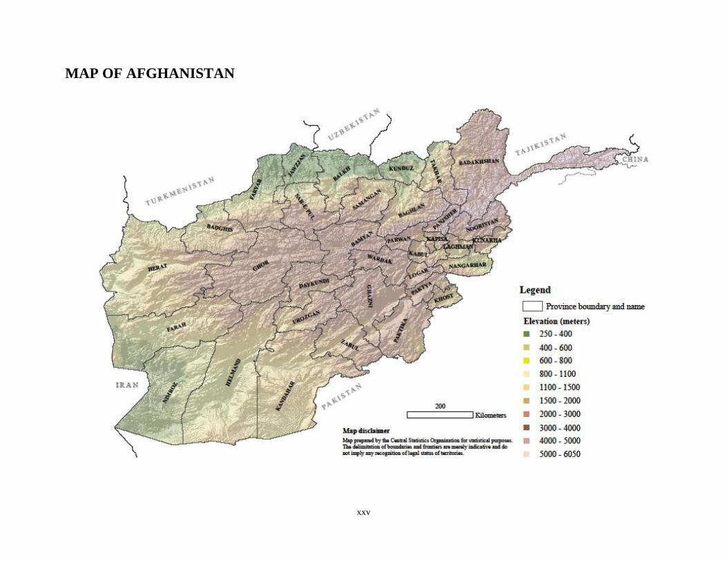
xxv
MAP OF AFGHANISTAN
xxvi
ACKNOWLEDGEMENTS
The Afghanistan Living Conditions Survey (ALCS) report has been through a long way to reach the hands
of the readers. It has been a very ambitious project in its objective and I am delighted to be able to present
the result of this hard work to you dear reader.
The ALCS is one of the flagships of the Central Statistical Organization, as it is the longest standing and
most comprehensive survey in the Afghan statistical system. It is now running for more than 10 years and
has provided the Afghan Government, civil society, researchers and the international community with
precious data on the living conditions of the Afghan population since its first iteration. During the course of
its implementation, the survey as changed in scope and purpose, following the country’s transformations,
what has prompted CSO to let its name evolve as well. It had started as the National Risk and Vulnerability
Assessment (NRVA) following a methodology of the United Nations Food and Agriculture Organisation,
focusing on food security and poverty prevalence and was then heavily supported by the United Nations
World Food Programme. Now, the survey is supported by the Delegation of the European Union to
Afghanistan and it has expanded to incorporate a large number of dimensions of life. This year, and for the
first time, it has implemented a full module on labour, similar to a Labour Force Survey, including child
labour.
In order to reflect this evolution, the publication is now called the Afghanistan Living Conditions Survey as
we, in CSO, together with stakeholders and the ALCS Steering Committee members, had the feeling that
its former name did not pay proper tribute to the wealth of statistical information the survey was collecting.
We also believe the ALCS represents a model for social statistical surveys of which Afghanistan can be
proud of, as it has proved to be a continued and undeniable success throughout the years.
Obviously, as this is the case for all the projects and publications of this scope, the list of persons who have
contributed and who made this publication a reality is very long and I will probably forget some persons. I
pray that they will forgive me.
First of all, I would like to thank the European Union Delegation to Afghanistan and in particular Mr. Wali
Mohammed Farhodi, Programme Manager - Rural Development for his constant and invaluable support in
implementing this project. The EU Delegation is our main donor in this project and this publication would
never have been published without their commitment.
I would also like to thank all the members of the Steering Committee and Technical Advisory Committee
of the ALCS for their support. Their contribution has been precious, and we much appreciated their support
and valuable comments during the numerous meetings regarding the conduct of the survey.
A special mention has to be addressed to the United Nations World Food Programme for their on-going
support to the ALCS. Their help was greatly appreciated, as well as their input in training and in a wide
range of survey issues. In this respect, the role of Mr. Amanullah Assil, Programme Officer VAM, has been
invaluable. From the same Organisation, I would like to thank Ms. Thi Van Hoang as well, for her assistance
and commitment throughout the survey.
xxvii
Several other international organisations were involved and provided assistance to the survey. I would like
to thank Ms. Silvia Redaelli, Economist from the World Bank for her contribution to the Technical Advisory
Committee and her contribution to the Poverty chapter in this report. I am also grateful to UNICEF and
especially Ms. Siping Wang, ILO and more specifically Mr. Hedeki Kagohashi.
This also enables me to thank other major contributors to the Steering Committee from the side of CSO,
namely Mr. Esmatullah Ramzi, Adviser to the President General, Prof. Hasibullah Mowahed, Deputy
President General of CSO and of course H.E Eng. Sher Mohammad Jamizada, President General of CSO
and Chair of the Steering Committee for their valuable input during the Steering Committee meetings, as
well as their knowledge of the country and its people.
This survey has benefited for a large support from the international community, but could also count on the
continuous commitment of the experts from ICON Institut Public Sector GmbH and especially from the
Team Leader Mr. Roberto Bianchini, who has showed a great capacity in supporting the ALCS team.
Another person whose invaluable commitment must be acknowledged is Mr. Bart de Bruijn, the Chief Editor
of this report. His assistance and work throughout the years has been a great asset to the office and he has
performed an unbelievable work in assisting CSO in the production of this report. I also would like to thank
Mr. Frank Eelens for his contribution to the data processing overhaul, as well as the project manager and
survey administrator, Mr. Christophe Dietrich, from ICON. They have never spared their efforts to make
this project a success. Allow me to also have kind word for ADE Consulting SA, and more particularly Ms.
Sylvie Skepi, project manager, for their contribution to the preparation of the data collection.
Of course, I would also like to thank the staff of CSO for the work they have done in conducting the survey
and in particular Mr. Esmatullah Hakimi, Mr. Ahmad Khalid Amarkhel, Mr. Muneer Jamshidi, Mr. Tamim
Shakeb from the ALCS Team, Mr. Whaheed Ibrahimi from the Database section, Mr. Zubair from the Data
entry section and Ms. Shakeeba from the GIS section for the hard work and commitment they have shown
during this round of the ALCS.
I would like to address a special thank to all the contributors to the present report Silvia Redaelli (World
Bank), Maya Sherpa (World Bank consultant), Thi Van Hoang (WFP), Amanullah Assil (WFP), Siemon
Hollema (WFP Bangkok), Ahmad Khalid Amarkhel (CSO), Esmatullah Hakimi (CSO), Roberto Bianchini
(ICON), Frank Eelens (ICON) and Bart de Bruijn (ICON).
Finally I would like to thank the field staff and the respondents to the survey without whom the survey
would not have been possible, and of course, I would like to thank you, the readers for getting interest for
the living conditions of the people of Afghanistan and the work of the Statistical Organization.
Mohamed Sami Nabi
Director of Field Operation Department
Central Statistical Organisation
xxviii
EXECUTIVE SUMMARY
Introduction
The 2013-14 Afghanistan Living Conditions Survey (ALCS; previously known as NRVA – National Risk
and Vulnerability Assessment) provides national and international stakeholders with information that is
required for the development of policies and programmes. The survey was conducted by the Central
Statistics Organization (CSO) of the Islamic Republic of Afghanistan and provides results that are
representative at national and provincial level. It covered 20,786 households and 157,262 persons across the
country, and is unique in the sense that it also includes the nomadic Kuchi population of Afghanistan.
Another distinguishing feature of the survey is the continuous data collection during a cycle of 12 months,
which captures important seasonal variation in a range of indicators. The survey is designed to cover a wide
scope of development themes and indicators that were agreed upon in series of consultations with
government departments and agencies, donors and international organisations. Building on previous survey
rounds in 2003, 2005, 2007-08 and 2011-12, ALCS is also the country’s main instrument for monitoring
progress in development. The present survey round was able to produce 19 ANDS indicators and 21 MDG
indicators.
The recent history of Afghanistan prior to 2001 was characterised by violent conflict, war and lawlessness,
which left the country with millions of displaced persons, a ruined economy, destroyed physical and
agricultural infrastructures, devastated health and education systems, and a complete setback in gender
equality. The period that followed the overthrow of the Taliban regime witnessed large-scale return of
refugees and IDPs and recovery in many development domains, based on massive international funding and
support. Despite several persistent problems, the successive NRVAs from 2003 to 2011-12 recorded
significant improvements in health, education, housing, infrastructure and basic services, such as provision
of drinking water, sanitation and electricity. The message from the present ALCS is that Afghanistan has
entered a new phase. The return of displaced persons has largely dried up and Afghanistan turned again
from an immigration country into an emigration country. A number of development indicators still show
improvement, but progress in several sectors seem to have slowed down or stagnated altogether. The
presence of foreign troops has diminished, donors funds were reduced and international organisations are
pulling out, with the effect of increasing unemployment and poverty. Political uncertainty, rampant
corruption and deteriorating security further aggravate these problems.
Despite significant achievements in the first decade of this century, Afghanistan remains among the most
poorly developed countries in the world according to almost all development indicators covered by the
survey. High rates of population growth driven by high fertility stifle progress in many areas and exceed the
country’s absorption capacity in, among others, the labour market, the education and health systems and the
agriculture sector. As in previous rounds, ALCS 2013-14 shows that national figures conceal dramatic
differences within the population. With only few exceptions, the situation in urban areas is much better than
that in rural areas and among the Kuchi population. And invariantly, gender-specific indicators show that
women and girls are far more disadvantaged than men and boys.
The remainder of this summary recapitulates the main findings of the thematic chapters of this report. An
in-depth analysis of the interaction between development indicators – and more specifically the apparent
nexus between poverty, food insecurity, poor labour market performance, low levels of education, high
xxix
fertility and mortality, and limited access to services – is beyond the scope of this report and will require
additional efforts.
Population
The age structure of Afghanistan’s population shows that population growth remains a critical element in
Afghanistan’s development process. The proportion of persons under age 15 (47.5 percent) is one of the
highest in the world. This very young age structure, driven by very high fertility, poses formidable
challenges to progress in many areas. It is the main component in the high dependency ratio of 100
dependent persons per 100 persons in the working age 15-65. This dependency ratio implies a heavy burden
on those who have to provide income and support, as much in individual households as in the economy at
large, and absorbs large shares of investments that could have been assigned to more productive ends. The
age structure also implies that in five years time Afghanistan has to cope with providing primary education
for 5.5 million children, while at the time of the survey the education system could offer primary education
to only 2.9 million. Similarly, in the next five years close to 4 million young people will reach working age
in a labour market that is already characterised by high levels of unemployment and underemployment. The
high fertility level underlying the young population composition also implies high risks for maternal and
child mortality, especially in view of the poor access to health services in the country. The ever-increasing
numbers of births, children and young adults exceed the absorption capacity of key institutions, such as the
health and education systems and the labour market, and would need serious attention of policy makers.
Various population parameters also show the vulnerable position of women in the Afghan society. The high
sex ratios at older age are indications of high maternal mortality and underreporting of women in statistics.
A sizeable share of 8 percent of married women – amounting to 388 thousand women – live in a polygamous
marriage, which creates inequality between spouses. Also the large age gap between spouses – on average
more than 6 years – tends to produce a subordinate position for women in marriage. However, the spousal
age gap reduces from older to younger generations, indicating a trend toward a more age-balanced marital
relation. Despite this trend, one third of female youth aged 20-24 was already married at age 18, the age that
distinguishes child marriage. Some 12 percent of these women were even already married at age 16,
indicating that they married below the legal minimum age at marriage. Also with regard to the proportion
married at a very young age, ALCS data suggest an improvement.
The average household size in Afghanistan remained around 7.4 persons, similar to previous NRVAs. Close
to half the Afghan people live in households with nine or more household members. The households are
almost exclusively headed by men. Female-headed households make up only one percent of the total
number.
Migration
Afghanistan has a complex migration situation, which in recent decades was dominated by large-scale
displacement – internally and to other countries – and subsequent return in the decade following the overturn
of the Taliban regime. These phases have now ended and a new migration phase has emerged. Results from
ALCS 2013-14 indicate that in the two years before the survey the return from displacement abroad is the
xxx
migration reason for only 39 percent of immigrants, and for internal migrants return from displacement has
reduced to a minor reason altogether. Labour migration has become the main migration trend, both internally
and to other countries. Iran has taken over the role of Pakistan as the dominant country of destination
(accommodating 61 percent of emigrants), but in addition the Gulf countries gain an increasingly prominent
place, as they received 18 percent of emigrants in the last year before the survey. Because of these shifting
migration patterns, Afghanistan has turned again from a net immigration country to a net emigration country.
ALCS information suggests that in recent years emigration exceeds immigration by more than 100 thousand
persons per year, implying a negative annual migration rate of 0.4 percent.
Both for immigrants and internal migrants, Kabul represents the main magnet of attraction. The capital
generates a recognisable migration system with its immediately surrounding provinces, in particular Parwan,
Panshjer and Wardak. Close to half of all migrations within Afghanistan happen in this area. Panshjer is the
province with the largest migration drain, having lost 28 percent of its population, mainly to Kabul.
Migration in general is strongly contributing to urbanisation: compared to an urban share of 24 percent in
the total population, 50 percent of immigrants and 82 percent of internal life-time migrants live in urban
areas. However, the pull toward urban areas – including Kabul – seemed to have lessened in the most recent
years, which may very well be related to the deteriorating labour market situation that particularly affects
the urban economy.
The living conditions of people returning from displacement has been a relevant issue for policy makers and
humanitarian organisations. Although more advanced analysis is in order, the ALCS 2013-14 suggests that
in many aspects – literacy, attained education, labour force participation, housing quality and access to
improved water and sanitation – returnees are better situated than non-returnees.
Labour market
The ALCS 2013-14 indicates that Afghanistan’s labour market is under considerable stress. The pressure of
increasingly large cohorts of young people entering the labour market in combination with a deteriorating
economic situation due to aid reduction and withdrawal of foreign employers are a likely cause for the high
proportion – 39 percent – of not-gainfully employed population. In particular the share of fully unemployed
has sharply increased compared to the situation in 2007-08: from 14 to 22 percent of the labour force if the
same definition were to be applied. The youth unemployment rate is as high as 30 percent. At the same time,
a large under-utilisation of the working-age population is observed, because of the low female labour force
participation rate: only 29 percent of working-age women is economically active. Among those men and
women who are working, a large majority – 79 percent – is working in vulnerable employment, lacking
formal work arrangements and access to benefits or social protection programmes. Around 90 percent of
the working population is employed in low-skilled occupations. Agriculture is by far the largest economic
sector (employing 44 percent of the work force), followed by the services sector (16 percent) and
construction (14 percent). Women’s work is much more concentrated, with 66 percent working in
agriculture and 24 percent in manufacturing.
There are large gender differences in labour market performance, and almost invariantly to the disadvantage
of women. Not only is labour force participation much lower among women (29 against 81 percent), also
their unemployment rate is double that of men (37 against 18 percent) and their share in vulnerable
xxxi
employment is higher (89 against 76 percent). Men earn significantly more than women, even if they hold
the same job. On average they earn 30 percent more than women.
Labour migration is largely directed towards urban areas, in particular Kabul: two thirds of non-Kuchi
labour migrants moved to the capital. Whereas internal labour migrants – mostly men – are relatively well
distributed across age groups, labour emigrants – exclusively men – are highly concentrated in the age group
20-29. Iran has become the most favoured destination of labour migrants, but the Gulf states attract an
increasing number of workers from Afghanistan.
The Afghan labour context is also characterised by high rates of child labour. Depending on the application
of the ILO or UNICEF definition of child labour, 26.5 or 29.5 percent of the 5 to 17 year olds are engaged
in child labour and thereby jeopardise their physical and mental development. These figures represent 2.7
or 3.0 million children, respectively. More boys are engaged in child labour than are girls, and the gender
difference increases with age. Regarding residence type, Kuchi children appear to be the most vulnerably,
as almost half of them – 47 percent – is performing child labour, compared to 30 percent of rural children
and 10 percent of urban children.
Poverty
The 2013-14 survey round did not collect information for a direct estimate of poverty indicators in the
country, but survey-to-survey imputation provided reliable and comparable results. These results show that
the share of the population living below the poverty line has increased from 36.5 percent in 2011-12 to 39.1
in the present survey. The results also indicate that the poorer segments of the population suffered more
from per-capita consumption decline than the better-off population, which suggests an increase in
inequality.
The present ALCS again confirmed the profile of the poor that was established by previous survey rounds.
Correlates of poverty are households relying on child labour and households with an illiterate head and a
head employed in informal labour arrangements – particularly in agriculture and construction sectors. Also
larger households and households with higher number of young children tend to be poorer, again indicating
the burden of high fertility on households.
Food security
Around one third of the Afghan population is estimated to suffer from food insecurity. The estimate, based
on the combination of the household’s food consumption score and food-based coping strategies, indicates
that 9.3 million people face chronic or transitory food insecurity. Some 3.4 million of them are even severely
food insecure. Food insecurity is strongly fluctuating by season. Winter and spring recorded the highest
levels of food insecurity (48 and 47 percent, respectively) and summer and autumn the lowest (23 and 26
percent, respectively).
Also in qualitative terms the diet of Afghans is frequently inadequate. The proportion of households with
low dietary diversity accounts for 36 percent of all Afghan households, often caused by a one-sided
xxxii
dependence on staple food. Both quantitative and qualitative food indicators suggest better conditions in
urban areas than in rural areas. Kuchi households recorded lower food insecurity, but also lower dietary
diversity.
Agriculture
Farming and animal husbandry remain to be the backbone of Afghanistan’s economy. Agriculture provides
a source of income for 61 percent of households, and for 28 percent it is the most important income source.
Similarly, it is the main sector of employment for 44 percent of the working population. Some 37 percent
of all households in Afghanistan – approximately 1.4 million households – own any irrigated farm land,
while around one in six households – 620 thousand – own the much less productive rain-fed land.
Wheat is by far the most important crop produced in Afghanistan. More than one million households grow
wheat on irrigated land. Fodder crops, potatoes and maize or sorghum were the next most frequently grown
crops on irrigated land. Farming on rain-fed land is even more concentrated on wheat production, but the
volume of wheat produced is only one third of that produced on irrigated land. Some 13 percent of all
households own a garden plot, which provides the opportunity to grow high-value and high-nutrition crops.
Grapes and apples are the crops grown most often on garden plots.
A considerable number of land owners have moved to urban areas and is no longer physically present on
their land. Mechanisms of leasing and renting land, sharecropping land and mortgaging land have the effect
of a net transfer of access to farm land from such land-owners living in urban areas to rural households that
cultivate the land. These mechanisms result in somewhat fewer households having access to somewhat
larger farming areas.
Problems faced by cultivating households are mostly related to poor soil, farming costs and particularly the
lack of water. The latter forces households to leave fallow around one third of land available for irrigated
and rain-fed farming. Fertiliser, seeds and machinery rent represent the largest production costs in farming.
Altogether, farming households spent 21 billion Afghanis (around 365 million USD) on farming inputs.
The ALCS 2013-14 reiterate that livestock is an important asset of Afghan households, either for own
household consumption or for market sale of animals and animal products. Some 38 percent of the
households in Afghanistan own one or more cattle, while goats and sheep are owned by 26 and 27 percent
of the households, respectively. Chicken-holding households represent 43 percent of households. This is
particularly important for women, as these are usually responsible for tending chicken and other birds, and
also may reap direct benefits from poultry products.
Farmers as well as livestock owners often lack access to relevant services. Levels of full vaccination of
livestock are low, varying from 15 percent for sheep and between 12 and 14 percent for goats, cattle, camels
and oxen and yaks, to 9 percent for chickens. As a result, large numbers of livestock and large amounts of
investments are lost because of animal diseases. No more than 37 percent of livestock owners could obtain
a sufficient amount of animal feed concentrate. Only one in five households involved in either farming or
livestock tending used agricultural extension services or veterinary support. Apart from voluntary reasons,
the most important reasons for non-use were the lack of knowledge of where or how to obtain the services,
the reluctance to offer services by the provider and the distance to the facility.
xxxiii
Education
The education picture presented by the ALCS 2013-14 is one of modest improvements in most areas, but
also with stagnation and even deterioration in other fields. This contrasts to survey rounds that covered
earlier periods when significant improvements were recorded in terms of literacy, educational attendance
and attainment, and gender equality.
Literacy indicators still show improvement, even though the advancement of the youth literacy rate (for
persons aged 15 to 24) from 47 percent in 2011-12 to 52 percent now is modest, and the increase of the
adult literacy rate from 31 to 34 percent is even smaller. The net attendance ratio for secondary and tertiary
education also maintained upward trends: respectively from 33 to 37 percent and from 5 to 9 percent since
the previous survey. However, the net attendance ratio for primary education showed a decline to 55 percent,
after a peak of 57 percent in 2011-12. The school attendance information suggests that 2.3 million primary
school age children and 2.0 million secondary school age children miss out on education and on the
opportunity to learn basic life skills.
The gross intake rate of 45 percent is an indication that the capacity of the educational system to absorb new
pupils is low, less than half of what would be required to provide every eligible child with a place at school.
On the other hand, the transition rates from one grade to the next are fairly high, resulting in a modest drop-
out percentage of 14 percent and an adequate 84 percent of school starters who reach the last grade of
primary education. Also the transition rate from primary to secondary education is fairly high (96 percent).
These transition rates indicate that the problem of Afghanistan’s education system is not so much retention
and drop out, but first and foremost starting school. Given the present age-specific attendance rates, an
Afghan child of 6 years old can expect to spend on average 7.7 years of his or her life in education, a very
short period in international perspective. The main reasons for not attending school are economic
considerations – particularly opportunity costs – and cultural barriers – especially for girls. In rural areas,
security concerns figured also prominently for girls.
Education is an area where gender inequality is clearly visible. Without exception, education gender
indicators show a very disadvantaged position of women and girls in Afghanistan. The present ALCS
indicates that the relatively high rates of improvement observed in the decade before 2011-12, cannot be
maintained. For youth and adult literacy, and for secondary school attendance, the parity indices still showed
some improvement, but the gender parity index for primary education declined from 74 to 71 percent.
Underlying the educational gender inequity is the very low education intake of girls. However, once in
school, the progression and dropout rates of girls and boys are very similar.
Residence is the other main inequity dimension in Afghanistan. For all education indicators, rural
populations score significantly poorer, and the Kuchi do even worse. This applies to levels of school
attendance and literacy, and equally to gender equity indicators.
xxxiv
Health
According to ALCS 2013-14, the health sector is the one that shows the most consistent improvement. The
most impressive improvements are observed for maternal health indicators. Afghanistan has achieved its
MDG target for ante-natal care coverage (50 percent in 2020) far ahead of schedule. The present survey
indicated that 63 percent of pregnant women made at least one visit to a skilled ANC provider, compared
to 51 percent in 2011-12. The recommended four ante-natal visits are realised by only 23 percent of pregnant
women, which, however, is a significant improvement from 10 percent in the previous survey. Also with
regard to the percentage of institutional deliveries (43 percent; up from 36 percent) and skilled birth
attendance (45 percent; up from 40 percent) ALCS 2013-14 indicates a consistent improvement in recent
years. The general trend in skilled birth attendance suggests that the MDG 2015 target of 50 percent is
within reach.
Breastfeeding practices in Afghanistan are generally beneficial for both mother and child in the sense that
breastfeeding is almost universal (for 93 percent of the newborns) and typically continues for a long
duration. However, substantial health and mortality gains can be achieved if more mothers start
breastfeeding within the first hour after birth (only 33 percent did so), if supplementary liquids and solid
food are only given after six months (more than half of the babies received other liquids before 6 months)
and if supplementary food is introduced soon after six months.
Whereas improvement of the health care system is still one of the highest priorities for the Afghan people,
physical access to health facilities and costs involved in obtaining health services remain major obstacles
for many people to obtain the care they need. The present survey indicates that medical needs of one in
every five women who were ill or injured, could not be met, mostly because of poverty and geographical
remoteness. Cultural responsiveness of the health system – for instance in terms of provision of female
health care providers – remains an obstacle for the effective use of health care, especially by women.
However, the availability of female care providers has significantly improved in the rural areas, especially
through private clinics and public health posts. Invariably, for the majority of Afghanistan’s rural
population, service delivery and health outcome indicators are significantly lower than for urban dwellers.
Moreover, the situation is generally even far worse for the nomadic Kuchi population.
Gender equality
Achieving gender equality remains one of the major challenges in Afghan society. Within an overall poor
development context, women and girls face especially deprived conditions. Various indicators signify a
subordinate and dependent position in the household, leaving little negotiating power in terms of household
decisions, sexuality and fertility. These indicators include women in polygamous marriages (8 percent),
those who married at a very young age (12 percent of women aged 20-24 were married before the legal
marriage age of 16), and those with much older husbands (21 percent of women are married to a husband
at least 10 years older; on average the age difference is 6 years). The proportions marrying before age 16
and with a large spousal age difference are decreasing though, probably indicating an improvement of the
position of married women.
xxxv
Also the underrepresentation of women in household listings – frequently reflected in high sex ratios – is
an indication of their low status and seclusion. Very high sex ratios at older ages probably also relate to high
maternal mortality. Three quarters of women do not leave the dwelling without the company of another
person and about half leave the house four times or less per month, while 12 percent of women indicate they
never left the house in an entire month. Female decision making on spending money is quite restricted: only
34 percent could independently decide how to spend money they earned themselves. The degree of
independence in this decision making is higher for urban women (48 percent) than for their rural and Kuchi
sisters (31 and 6 percent, respectively).
Despite improvements in recent years, education-related indicators still show large gender gaps. The literacy
level of women aged 15 and over stands at 39 percent of the level of men, although this literacy gender
parity index has improved for youth aged 15 to 24 (52 percent). The gender parity indices for primary,
secondary and tertiary education attendance are, respectively, 71, 55 and 41 percent. Also the labour market
indicators show the vulnerable position of women. First and foremost because of the low female labour
force participation rate of 29 percent, compared to 81 percent for men. But also because of the much higher
unemployment rate (37 against 18 percent for men), youth unemployment rate (44 against 24 percent),
higher engagement in vulnerable employment (89 against 76 percent) and lower payment, even for the same
type of jobs. The MDG indicator of the share of women in wage employment in the non-agricultural sector
is at a low 10 percent.
Housing
Housing conditions of the Afghan population are overall poor, but show substantial improvements in several
respects. Dwellings are typically single-family and traditionally-constructed mud houses, with external
walls made of mud bricks (68 percent) and roofs constructed with wood and mud (74 percent). Most
dwellings (60 percent) were built after 1995, but only less than 3 percent in the last three years before the
survey. Rural dwellings are generally owned (93 percent), either inherited or otherwise purchased or self-
constructed. A majority of urban dwellings is also owned (70 percent), but renting is a main second tenure
arrangement for 21 percent of households in urban areas.
Large progress has been made with regard to access to improved drinking water sources. The ALCS
estimated that 65 percent of the population has access to improved sources (up from 46 percent in NRVA
2011-12), thereby achieving the ANDS/MDG target of 61.5 percent in 2020 more than five years in advance.
Access to improved sanitation, on the other hand, lags behind with only 39 percent, compared to the target
of 66 percent in 2020.
Improvements are also observed in terms of a decreasing urban slum population (74 percent, down from 87
percent in 2011-12), lower use of solid fuels (76 percent, down from 80 percent) and an increase of use of
communication means: from 14 to 17 mobile cellular subscriptions per 100 population, and from 0.5 to 1.2
internet users per 100 population. In addition, the proportion of households with access to any source of
electricity has increased significantly, from 69 to 89 percent. The spread of solar panels is a main driving
force of this increase. Whereas NRVA 2007-08 recorded 2 percent of households with solar panels, NRVA
2011-12 recorded 22 percent and ALCS indicate that almost half of all households (48 percent) use solar
power.
1
1 INTRODUCTION
After decades of war and political instability, Afghanistan remains one of the poorest countries in the world.
In 2013 Afghanistan ranked 169th out of 185 countries in the UNDP Human Development Index, a summary
measure that is based on development dimensions of health, education and living standards (UNDP 2014).
This poor ranking represents the challenges faced by large parts of the country’s population, but at the same
time hides significant improvements in different sectors in the period since 2001. The present year 2015 is
especially important as it signifies the year in which the Millennium Development Goals (MDGs) should
be achieved that were established following the Millennium Summit of the United Nations in 2000.
Afghanistan endorsed the Millennium Declaration in 2004, but the time period for meeting the MDG targets
was extended from 2015 to 2020 in view of the years lost for development progress before 2004.
In order to address the information needs of the Government of Afghanistan and other parties to monitor
this development progress and to inform and prioritise development policies and programmes, the Central
Statistics Organization (CSO) conducts on a regular basis the Afghanistan Living Conditions Survey,
previously known as the National Risk and Vulnerability Assessment (NRVA). Initial NRVAs were
implemented in a combined effort by the Ministry of Rural Rehabilitation and Development (MRRD) and
the Central Statistics Organisation (CSO). Building on two survey rounds in 2003 and 2005, the instrument
developed into a full-blown multi-purpose survey in 2007-08 and subsequent rounds in 2011-12 and 2013-
14 were conducted under the sole responsibility of CSO. The survey captures a wide variety of development
indicators in such areas as poverty, food security, labour market performance, demography, education,
health, gender equality, housing and agriculture. As such, the ALCS is the major single source of socio-
economic statistics of the country. The survey is unique in the sense that – with inclusion of the nomadic
Kuchi – it represents the entire population of Afghanistan, and that – since the 2007-08 survey – year-round
data are collected in order to capture the seasonality of indicators like employment, food security and
poverty. The survey was designed to produce representative estimates for the national and provincial levels,
and for the Kuchi population.
Each survey round produces a standard set of core indicators that are prioritised by ALCS data users. Data
for additional indicators and more in-depth information are collected on a rotating basis in the successive
survey rounds. This rotating principle allows progress monitoring of a wide range of development indicators
with appropriate time intervals and at the same time preserves the manageability and sustainability of the
survey. The specific focus of ALCS 2013-14, for which data were collected from December 2013 to
December 2014, was on migration, gender equality and labour market outcomes, including child labour. In
addition, non-standard data about breastfeeding behaviour were collected and the education module was
expanded on a structural basis.
The present ALCS 2013-14 report is the most comprehensive to date. The information presented includes
19 indicators to monitor the implementation of the Afghanistan National Development Strategy (ANDS)
and 20 MDG indicators. The main focus in this report is on the national level, but information is frequently
disaggregated for residential populations (urban, rural and Kuchi). Provincial-level information is largely
outside the scope of the present report, although most chapters include thematic maps showing the
provincial distribution of selected indicators. The information provided in this report is also largely
descriptive in nature; cross-sectoral and more in-depths analyses – especially those aiming at cause-and-
effect relationships – will require additional efforts and reporting.
2
Chapter 2 describes the main methodological characteristics of the ALCS 2013-14, including brief
descriptions of the sampling design, survey questionnaires, data collection and processing, data limitations,
and comparison with the previous survey rounds and the related rotating principle applied to the successive
questionnaires. Several annexes provide further elaborations and technical details of the methodology.
Subsequent chapters cover the subject-matter of the survey. Population structure and change are addressed
first in chapter 3, as these factors permeate into every development aspect of the remaining report sections.
Afghanistan’s population composition by age and sex is analysed, as well as household and marriage
patterns. A separate chapter – chapter 4 – is devoted to migration, as this topic received additional attention
in the present survey round. Both internal and international migration is analysed, as well as urbanisation
and displacement.
Chapter 5 provides an analysis of the structure and dynamics of Afghanistan’s labour market. Based on an
extended labour module, it is the most comprehensive description of the labour market in the history of
ALCS. Besides indicators on employment, underemployment, unemployment, working hours, vulnerable
employment and gender analysis, the main new elements now covered include descriptions of occupations
and economic sectors based on newly developed ISCO and ISIC classifications, remuneration, labour
migration and child labour.
Agriculture, including farming and livestock production, is the subject of chapter 6. The chapter analyses
the agricultural sector with a view on access to land, land area size, cultivation problems, farm and garden
production, type and number of livestock, and sale of animals, as well as relevant production factors in this
sector.
The key chapters 7 and 8 present the results of, respectively, poverty and food-security analyses. Since
ALCS 2013-14 did not include extended modules on food consumption and market prices, alternative
methods for poverty and food-security estimation were developed and applied. Both chapters include
profiling of, respectively, the poor and the food insecure.
The twin chapters 9 and 10 are dedicated to the social sectors of education and health, and to the changes
occurring in these sectors. The former analyses literacy rates, school attendance and educational attainment,
and new elements of education transition rates and school expectancy. The chapter on health includes
information on the use of maternal health care services, access to health facilities, health care seeking
behaviour and breastfeeding practices.
ALCS 2013-14 included a dedicated module on work of women, female seclusion, household decision
making and women’s health care behaviour. These elements are covered in chapter 11 on gender equity
and women’s development. Besides the elaboration of these elements, this chapter uses a gender lens to
zoom in on the information covered in other subject-matter sections of the report, including education,
marriage and the position of women in the household.
The last chapter – chapter 12 – describes the housing situation, with a view on access to the community,
tenancy arrangements, physical characteristics of the dwelling and housing facilities, like electricity,
drinking water and sanitation, as well as fuel used for cooking and heating, and information and
communication means. It includes also a focus on slum dwellers living in the urban areas of Afghanistan.
3
2 SURVEY METHODOLOGY AND OPERATIONS
2.1 Introduction
The Afghanistan Living Conditions Survey 2013-14 continues the series of National Risk and
Vulnerabilities Assessments (NRVAs) that were conducted since 2003. The name NRVA was changed to
ALCS in order to reflect the full scope of development information that is covered by the survey. The
methodologies applied in the ALCS 2013-14 – in terms of questionnaire and sampling design, analysis, and
procedures for data collection, data capture and data processing – took into account the specific
circumstances of Afghanistan. These refer to issues such as fieldwork challenges, stakeholder information
needs, socio-cultural specificities, the statistical infrastructure and the implementation capacity at various
levels of the survey hierarchy. At the same time, methodologies were designed as to comply with
international survey recommendations and best practices. Experience gained from the previous rounds of
NRVA and application of international standards resulted in some methodological changes, but as much as
possible the rigour of previous achievements was maintained in order to ensure comparability over time.
This chapter provides an introduction to different methodology dimensions adopted in the present round of
ALCS for a better understanding of the survey results that are presented in the subject matter chapters 3 to
12. In this respect, the different sections will also highlight methodological changes compared with previous
rounds.
2.2 Stakeholder involvement
As the primary aim of ALCS is to serve the information needs of data users, consultation with stakeholders
has been carried out in several crucial stages of the survey to identify these needs. The stakeholders that
participated in the meetings organised by CSO included line ministries and government agencies,1 UN and
other international organisations,2 bilateral donors,3 and academic and research bodies. These meetings also
dealt with the sustainability and long-term perspective of the ALCS as Afghanistan’s most important
instrument for producing socio-economic information (see Section 2.3). Further stakeholder meetings were
organised to discuss the ALCS tabulation and analysis plan and the outline of this final report (January
2015).
In addition to these meetings, a number of key stakeholders were present in the ALCS Steering Committee
to supervise the work progress and recommend specific actions. Similarly, relevant stakeholders
participated in the Technical Advisory Committee (TAC) to scrutinise methodological and technical
matters and provide input if and when required. Members of the Steering Committee and TAC are
mentioned in Annex I.
1 MRRD, MAIL, MoPH, MoE, MoLSAMD, MoWA, MoEW, MoEc, MoF, MoUDA, AUWSSC 2 WFP, WB, UNICEF, UNFPA, UNDP, ILO, UNDP, UNHCR, WHO, FAO, ADB 3 EU, DfID, GIZ
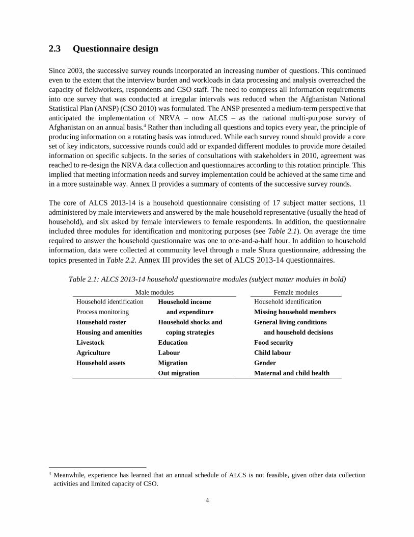
4
2.3 Questionnaire design
Since 2003, the successive survey rounds incorporated an increasing number of questions. This continued
even to the extent that the interview burden and workloads in data processing and analysis overreached the
capacity of fieldworkers, respondents and CSO staff. The need to compress all information requirements
into one survey that was conducted at irregular intervals was reduced when the Afghanistan National
Statistical Plan (ANSP) (CSO 2010) was formulated. The ANSP presented a medium-term perspective that
anticipated the implementation of NRVA – now ALCS – as the national multi-purpose survey of
Afghanistan on an annual basis.4 Rather than including all questions and topics every year, the principle of
producing information on a rotating basis was introduced. While each survey round should provide a core
set of key indicators, successive rounds could add or expanded different modules to provide more detailed
information on specific subjects. In the series of consultations with stakeholders in 2010, agreement was
reached to re-design the NRVA data collection and questionnaires according to this rotation principle. This
implied that meeting information needs and survey implementation could be achieved at the same time and
in a more sustainable way. Annex II provides a summary of contents of the successive survey rounds.
The core of ALCS 2013-14 is a household questionnaire consisting of 17 subject matter sections, 11
administered by male interviewers and answered by the male household representative (usually the head of
household), and six asked by female interviewers to female respondents. In addition, the questionnaire
included three modules for identification and monitoring purposes (see Table 2.1). On average the time
required to answer the household questionnaire was one to one-and-a-half hour. In addition to household
information, data were collected at community level through a male Shura questionnaire, addressing the
topics presented in Table 2.2. Annex III provides the set of ALCS 2013-14 questionnaires.
Table 2.1: ALCS 2013-14 household questionnaire modules (subject matter modules in bold)
Male modules Female modules
Household identification Household income Household identification
Process monitoring and expenditure Missing household members
Household roster Household shocks and General living conditions
Housing and amenities coping strategies and household decisions
Livestock Education Food security
Agriculture Labour Child labour
Household assets Migration Gender
Out migration Maternal and child health
4 Meanwhile, experience has learned that an annual schedule of ALCS is not feasible, given other data collection
activities and limited capacity of CSO.
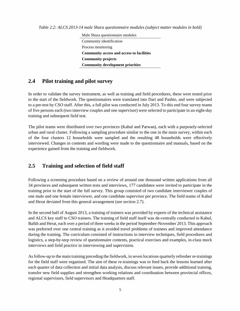
5
Table 2.2: ALCS 2013-14 male Shura questionnaire modules (subject matter modules in bold)
Male Shura questionnaire modules
Community identification
Process monitoring
Community access and access to facilities
Community projects
Community development priorities
2.4 Pilot training and pilot survey
In order to validate the survey instrument, as well as training and field procedures, these were tested prior
to the start of the fieldwork. The questionnaires were translated into Dari and Pashto, and were subjected
to a pre-test by CSO staff. After this, a full pilot was conducted in July 2013. To this end four survey teams
of five persons each (two interview couples and one supervisor) were selected to participate in an eight-day
training and subsequent field test.
The pilot teams were distributed over two provinces (Kabul and Parwan), each with a purposely-selected
urban and rural cluster. Following a sampling procedure similar to the one in the main survey, within each
of the four clusters 12 households were sampled and the resulting 48 households were effectively
interviewed. Changes in contents and wording were made to the questionnaire and manuals, based on the
experience gained from the training and fieldwork.
2.5 Training and selection of field staff
Following a screening procedure based on a review of around one thousand written applications from all
34 provinces and subsequent written tests and interviews, 177 candidates were invited to participate in the
training prior to the start of the full survey. This group consisted of two candidate interviewer couples of
one male and one female interviewer, and one candidate supervisor per province. The field teams of Kabul
and Herat deviated from this general arrangement (see section 2.7).
In the second half of August 2013, a training of trainers was provided by experts of the technical assistance
and ALCS key staff to CSO trainers. The training of field staff itself was de-centrally conducted in Kabul,
Balkh and Herat, each over a period of three weeks in the period September-November 2013. This approach
was preferred over one central training as it avoided travel problems of trainees and improved attendance
during the training. The curriculum consisted of instructions in interview techniques, field procedures and
logistics, a step-by-step review of questionnaire contents, practical exercises and examples, in-class mock
interviews and field practice in interviewing and supervision.
As follow-up to the main training preceding the fieldwork, in seven locations quarterly refresher re-trainings
for the field staff were organised. The aim of these re-trainings was to feed back the lessons learned after
each quarter of data collection and initial data analysis, discuss relevant issues, provide additional training,
transfer new field supplies and strengthen working relations and coordination between provincial offices,
regional supervisors, field supervisors and Headquarters staff.
6
After completion of the survey, a final series of regional debriefings was organised for field staff in order
to obtain their views on possible improvements in field procedures and questionnaire design and contents.
This feedback has been incorporated in the development of the next survey round in 2016.
2.6 Sampling design
The sampling design of the ALCS 2013-14 ensured results that were representative at national and
provincial level, as well as for Shamsi calendar seasons.5 In total 35 strata were identified, 34 for the
provinces of Afghanistan and one for the nomadic Kuchi population. Stratification by season was achieved
by equally distributing data collection over 12 months within the provinces. For the Kuchi population, the
design only provided sampling in winter and summer when communities tend to temporarily settle. The
distribution of sampling areas per province was based on an optimal trade-off between precision at the
national and provincial levels.6
The sampling frame used for the resident population in the ALCS 2013-14 was the pre-census household
listing conducted by CSO in 2003-05, updated in 2009. 7 Households were selected on the basis of a two-
stage cluster design within each stratum. In the first stage Enumeration Areas (EAs) were selected as
Primary Sampling Units (PSUs) with probability proportional to EA size (PPS). Subsequently, in the second
stage ten households were selected as the Ultimate Sampling Unit (USU).8 The design thus provided data
collection in on average 170 clusters (1,700 households) per month and 2,040 clusters (20,400 households)
in the full year of data collection.
The Kuchi sample was designed on basis of the 2003-04 National Multi-sectoral Assessment of Kuchi
(NMAK-2004). For this stratum a community selection was implemented with PPS and a second stage
selection with again a constant cluster size of ten households. The 60 clusters (600 households) for this
stratum were equally divided between the summer and winter periods within the survey period.
The reality of survey taking in Afghanistan imposed a number of deviations from the sampling design. In
the first six fieldwork months areas that were inaccessible due to insecurity were replaced by sampled areas
that were scheduled for a later month, in the hope that over time security conditions would improve and the
original cluster interviews could still be conducted. In view of sustained levels of insecurity, from the sixth
month of data collection onward, clusters in inaccessible areas were replaced by clusters drawn from a
reserve sampling frame that excluded insecure districts. Instead of collecting data among the Kuchi
population in winter 2013-14 (Shamzi calendar 1392), this was done in autumn of 2014 (1393).
5 The Shamsi years 1392 and 1393, in which the ALCS 2013-14 was conducted, run from, respectively, 21 March
2013 to 20 March 2014 and from 21 March 2014 to 20 March 2015, respectively. Season dates are given in Annex
VIII. 6 For an optimal sample allocation a balance was obtained between proportional allocation and equal-size allocation
with a Kish power allocation of I = 0.25. 7 For three provinces, the sampling frame consisted of the SDES household listings: Bamyan (data collected in 2010),
Ghor and Daykundi (both with data collected in 2012). 8 Some of the selected EAs in rural areas comprised more than one village. In those cases only one village has been
selected with probability proportional to the village size, thus creating a third sampling stage.
7
Sample weights were calculated for up-scaling the surveyed households and population to the total number
of households and population in Afghanistan. The calculation was based on the official CSO population
estimate by province for January 2014 and average provincial household size derived from the survey. In
view of the unequal implementation of the sample across seasons, a post-stratification adjustment was
imposed to give equal weight to the seasons.
Annex IV gives an account of the background and technical details of the sampling design and
implementation.
2.7 Field operations
The ALCS 2013-14 field staff consisted of two mixed interview couples and one field supervisor for most
of the 34 provinces of Afghanistan. The exceptions were Kabul – where the field staff consisted of two
supervisors and four interviewer couples – and Herat, with one supervisor and three interviewer couples.
The field operations were supervised by nine Regional Statistical Officers (RSOs), who were selected from
the Provincial Statistical Officers (PSOs). In addition, ALCS staff from CSO Headquarters performed
monthly monitoring missions for direct feedback to interviewers and supervisors.
The survey instrument consisted of paper questionnaires for households and the male Shura. The male
interviewers administered the interviews with the male household representative and the female
interviewers those with female household representative and other eligible female household members. The
supervisor usually administered the male Shura interviews and performed the household listing update prior
to the data collection.
Each of the field teams had a monthly interview target of on average 50 household interviews in 5 selected
clusters, resulting in a national monthly total of 1,700 household interviews. Data collection started in the
second half of December 2013 (Jadi 1392). Fieldwork delays were experienced during the months of the
presidential elections in April and June 2014 and during Ramazan in July 2014. However, the field staff
managed to catch up with the largest part of the interview backlog, and only few interview clusters were
completed after mid December 2014. In addition to surveying the resident population during the entire
survey period of 12 months, the nomadic Kuchi population was accessed in summer and autumn 2014.
The tasks of the RSOs included checking a sample of the completed questionnaires, as a second level of
quality control in the field after the checking by supervisors. For this purpose, specific check lists were
developed. On a monthly basis, they transported batches of completed questionnaires and other survey
documents back to CSO Headquarters and took new field supplies to the provinces. The PSOs were
responsible for the introduction of the field teams to the provincial and local authorities, for monitoring
fieldwork progress and the security situation, and for verification of survey results in the field. In four
provinces field staff was replaced due to underperformance. Furthermore, two supervisors and 11
interviewers dropped out during the year-long cycle of data collection due to other reasons.
Further quality assurance during data collection was provided by seven members of the ALCS team at CSO
Headquarters, who conducted field monitoring missions every survey quarter. These monitors focussed
specifically on those provinces from which questionnaires were returned with the most irregularities
according to manual checking at Headquarters.
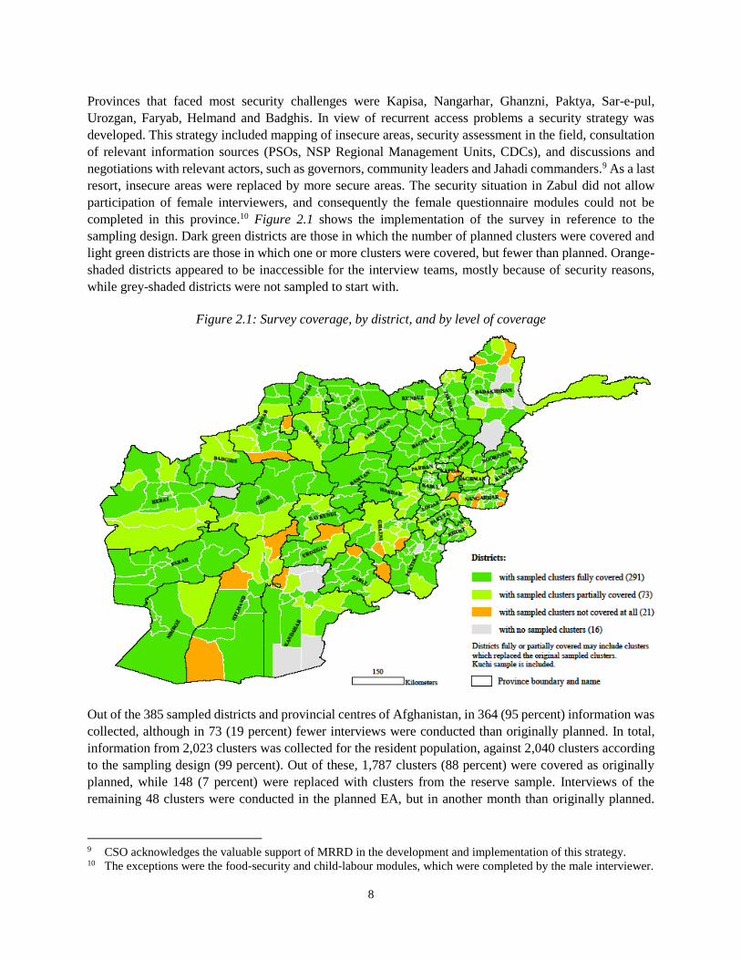
8
Provinces that faced most security challenges were Kapisa, Nangarhar, Ghanzni, Paktya, Sar-e-pul,
Urozgan, Faryab, Helmand and Badghis. In view of recurrent access problems a security strategy was
developed. This strategy included mapping of insecure areas, security assessment in the field, consultation
of relevant information sources (PSOs, NSP Regional Management Units, CDCs), and discussions and
negotiations with relevant actors, such as governors, community leaders and Jahadi commanders.9 As a last
resort, insecure areas were replaced by more secure areas. The security situation in Zabul did not allow
participation of female interviewers, and consequently the female questionnaire modules could not be
completed in this province.10 Figure 2.1 shows the implementation of the survey in reference to the
sampling design. Dark green districts are those in which the number of planned clusters were covered and
light green districts are those in which one or more clusters were covered, but fewer than planned. Orange-
shaded districts appeared to be inaccessible for the interview teams, mostly because of security reasons,
while grey-shaded districts were not sampled to start with.
Figure 2.1: Survey coverage, by district, and by level of coverage
Out of the 385 sampled districts and provincial centres of Afghanistan, in 364 (95 percent) information was
collected, although in 73 (19 percent) fewer interviews were conducted than originally planned. In total,
information from 2,023 clusters was collected for the resident population, against 2,040 clusters according
to the sampling design (99 percent). Out of these, 1,787 clusters (88 percent) were covered as originally
planned, while 148 (7 percent) were replaced with clusters from the reserve sample. Interviews of the
remaining 48 clusters were conducted in the planned EA, but in another month than originally planned.
9 CSO acknowledges the valuable support of MRRD in the development and implementation of this strategy. 10 The exceptions were the food-security and child-labour modules, which were completed by the male interviewer.
9
From the 60 Kuchi clusters, 58 were covered according to the sampling design, whereas for the two
remaining the targeted Kuchi population could not be found in the field.
2.8 Data processing
2.8.1 Manual checking and coding
Data processing in CSO Headquarters was done in parallel to the fieldwork and started upon arrival of the
first batch of completed questionnaires in February 2014. The first two data-processing stages consisted of
manual checking and coding by a team of eight questionnaire editors and coders. This team was trained by
the experts of the technical assistance and followed procedures that were provided in manuals for editing
and coding. The tasks of the questionnaire editors consisted of:
recording and archiving returned questionnaires
checking the completeness of the questionnaire batches and questionnaire forms
checking questionnaire answers for completeness, consistency, correctness and readability
correcting answers or completing missing answers for a limited and prescribed number of
questions, including identification fields and some key questions
adding codes for missing values
completing an evaluation form on the basis of which the questionnaire batch would be dispatched
to the questionnaire coders or returned to the field for renewed data collection.
The coders had the responsibility to add codes for textual answers to questions and variables about
occupations, industries, provinces and countries, following the guidelines given in the training and in the
provided coding manuals. Subsequently, the questionnaire batch was submitted for data entry.
2.8.2 Data entry and data editing
Data capture was done with a specially designed CSPro programme, which was piloted to ensure a smooth
performance in real time. The data-entry system applied first data entry and dependent verification through
double entry to avoid high levels of manual data capture errors. In addition, CSPro data-editing programmes
were developed to identify errors and either perform automatic imputation or manual screen editing, or
refer cases to data editors for further questionnaire verification and manual corrections.
CSO’s data-entry section started entering the first round of data in February 2014. Progress was slow in the
first weeks due to the operators’ unfamiliarity with the complex questionnaires and fine-tuning of the
elaborate data-processing programmes. With experience built up, the speed of data processing increased
and in later months all data were entered and verified within two weeks from reception of questionnaires
from the manual checking and coding section. Data capture and editing operations were completed in March
2015.
10
2.9 Analysis
Extensive programmes in Stata software package were revised or developed to perform final data
verification-, correction-, editing- and imputation procedures A full dataset was available in July 2015 and
a preliminary report with a limited set of key results was produced in the same month.11 A team of eleven
internal and external12 analysts contributed to the present Analysis report.
New methodological elements introduced in the analysis of ALCS 2013-14 include the following:
In view of the absence of a full module on food consumption and household expenditure in the
2013-14 round, alternative methods were developed and applied to estimate levels of poverty and
food security. In chapter 7, survey-to-survey imputation is used to estimate poverty on the basis of
a set of proxy indicators, which were calibrated with NRVA 2007-08 and 2011-12 data. In chapter
6, the Food Consumption Score (FCS) is used as a proxy indicator to measure caloric intake and
diet quality at household level. In combination with the Coping Strategy Index (CSI), this is
assumed to properly indicate the food security situation in Afghanistan.
For the purpose of labour market analysis, the ALCS 2013-14 questionnaire included questions on
occupation and industry. Context-specific occupation and industry codes were developed, based
on, respectively ISCO and ISIC classifications. An elaborate section on labour migration is
included in the analysis and for the first time an analysis of job earnings is added. Altogether,
chapter 5 provides the most elaborate labour market analysis of Afghanistan to date.
One notable component of chapter 5 is the section on child labour (section 5.5). The questionnaire
module that provided the information for this section is based on newly developed UNICEF
guidelines for measuring child labour and allows the production of child labour indicators
according to both UNICEF and ILO definitions.
For the first time, ALCS is able to produce education transition-, completion- and drop-out rates,
as well as the indicator of school life expectancy (chapter 9).
2.10 Comparability of results
Comparability between ALCS 2013-14 and previous NRVAs was maintained as much as possible by a
largely similar questionnaire design and content for reported indicators, training and data collection
procedures. A new and more appropriate sampling design was introduced for ALCS 2013-14. Whereas this
sampling design differed from earlier rounds, all surveys produced representative results at national and
provincial level. Comparability with NRVA 2005 is more limited due to major questionnaire revisions since
2007. In addition, data collection in 2005 was limited to three months, which prevented the seasonal
analysis that can be done on the basis of the latest three surveys. Any comparison with 2005 results in this
report should, therefore, be treated with caution.13
The ALCS questionnaire design partially built on major international survey practices, such as the DHS
and MICS surveys and standardised labour force surveys. Accordingly, data collection on and analysis of
11 Afghanistan Living Conditions Survey 2013-14. Preliminary report. Not published. 12 From WFP, World Bank and ILO. 13 As sampling design, survey design and questionnaire content of NRVA 2003 were very different from the
subsequent rounds, no effort is made here to include its results in any trend analysis.
11
education, water and sanitation supply, labour force, child labour and maternal health care are aligned with
international practices. In addition, for internationally agreed indicators, and especially MDG indicators,
ALCS applies the standard conceptualisation and definitions. Therefore, many indicators produced in this
report embody a high level of international comparability. The report text indicates if, for some reason,
applied definitions deviate from the internationally recommended ones. The annex with concepts and
definitions provides the specifications applied in the present analysis (Annex VIII).
Due to changes in national and international definitions and guidelines, as well as lessons learned in the
history of ALCS and specific data limitations, some indicators in the present report are not directly
comparable to those in previous reports. These notably include the following:
Labour-market indicators: the abbreviated labour module of NRVA 2011-12 introduced a specific
bias that prohibits a direct comparison with ALCS 2013-14. Also NRVA 2007-08 had specific
limitations that hamper straight comparison. However, chapter 5 includes a section that re-aligns
NRVA 2007-08 data with ALCS 2013-14 in order to produce a trend indication.
In order to align with national and international definitions of improved sanitation, ALCS adopted
a new classification. Consequently, the sanitation indicator presented in this report cannot be
compared with those in previous reports. However, the information gap for trend analysis is bridged
by producing the indicator according to the new and old definition.
The difference in methodology to estimate food security between ALCS 2013-14 and previous
NRVAs does not allow direct comparison.
2.11 Data limitations
The specific constraints in the Afghanistan context in terms of security problems, cultural barriers and local
survey capacity induced some data limitations. The following observations should be taken into account
when interpreting the results in this report:
In 152 out of 2,100 clusters (7.2 percent), originally sampled clusters could not be covered, in most
cases due to security reasons. For 148 of these cases, clusters were replaced. To the extent that the non-
visited clusters may have profiles different from visited clusters, the final sample will give a bias in the
results. This effect will have been larger at the provincial level for provinces with relatively large
numbers of replacement, such as Ghazni, Helmand and Badakhshan.
Analysis of the population structure by sex and age shows under-enumeration of women and girls, as
well as young children in general, especially infants. Coverage of the youngest age group was much
better than in previous surveys, but significant numbers are still omitted. Cultural backgrounds related
to the seclusion of women and high infant mortality are among likely reasons for these omissions.
The quality of age reporting in the Afghan population remains extremely poor, as indicated by large
age heaping on ages with digits ending on 5 and 0.14
Due to alleged security problems, work by female interviewers in Zabul was not allowed by the
authorities. Consequently, the information on general living conditions, maternal- and child health, and
gender is largely missing for this province. However, the food-security and child-labour modules in the
female questionnaire were completed by male interviewers interviewing male respondents.
14 The Myers' Blended Index is 21.8 and the Whipple's Index is 231.
12
2.12 Reporting
The source of all information presented in this report is the ALCS 2013-14, unless otherwise specified.
Presenting information from other sources than ALCS does not imply an endorsement by CSO, but should
merely be interpreted as a contextualisation of the present findings.
Titles of tables presented in this report follow a standard convention to exactly define the table contents and
structure: first, the title states the universe of elements presented in the table, then it defines the variable(s)
presented in the column headings, then the variable(s) presented in the row headings. In the title the universe
and the column variable(s) are separated by a comma (‘,’); the column variable(s) and the row variable(s)
are separated by ‘, and by’. Titles of line and bar charts first specify the universe of elements presented in
the figure, then the variable presented on the main axis, and then the variable presented in the legend (if
any). When presenting rounded figures in tables or graphs, the presented total figure may not correspond
to the sum of rounded figures.
In comparison to the report on the previous survey (NRVA 2011-12), this report is enriched with a larger
number of thematic maps, to provide more information on the geographical distribution of indicators at
provincial level, and to help the reader to quickly understand demographic and socioeconomic patterns
across the country, as evinced by 2013-14 ALCS data. Indeed, maps are used not only for dissemination
purposes, but also to indicate spatial correlations, proposing further investigation in some subjects and
geographical areas of the 2013-14 ALCS results.
Maps were prepared using Geographic Information System (GIS) software in which selected indicators of
ALCS data were associated with their corresponding administrative units of the country, and presented with
different colours and gradients on the basis of their values registered at provincial level. The statistical
method of data classification was the standard Jenks method called also ‘Natural breaks’ method. Class
breaks were defined in order to maximise differences in data values between classes. A minimal
customisation was applied to round class breaks and to show in the legend the national average of the
indicators presented at national level. An explanatory note was added below the legend when deemed
necessary to explain the mapped data.
In order to allow the reader further insight into the value of the presented data, an annex (Annex VII) is
added to the report on quality assurance and quality assessment. For the ANDS and MDG indicators
presented in this report, an overview of standard errors and 95 percent confidence limits are included in this
annex.
13
3 POPULATION AND HOUSEHOLDS
Summary. The population of Afghanistan is characterised by a very young age structure. The proportion
of 47.5 percent of the population under age 15 is one of the highest in the world. This young age structure,
driven by very high fertility, is the main component of the high dependency ratio of one dependent per
person in the most productive ages 15 to 64. The large number of young people pose formidable challenges
to various sectors of society. In five years time there will be more than 5.5 million children of primary
school age, while presently the education system offers primary education to only 2.9 million children of
this age. Similarly, in these next five years close to 4 million youth will reach working age in a labour
market that is already characterised by high levels of unemployment and underemployment. The typical
pyramid shape of Afghanistan’s population ensures that population growth will remain high for several
decades.
The sex ratio by age shows a very a-typical pattern. Instead of a situation where at older age women tend
to become more numerous compared to men, the opposite is observed in Afghanistan. Beyond age 70 men
outnumber women by 170 to 100. Likely explanations for this can be found in underreporting of women and
high maternal mortality. Both causes reflect the vulnerable position of women in society.
The vulnerable position of women and gender inequality is also witnessed in specific marriage patterns. A
sizable number of 388 thousand married women live in polygamous marriages, which places them in a
disadvantaged position. Polygamy also increases the age gap between spouses, which is again
disadvantageous for women. However, a positive trend towards a smaller age gap can be observed. For
married women aged 40 and older, the age of the husband is on average more than 7 years higher, but for
women aged 15 to 29, the difference is reduced to 4.6 years. Also the proportion of couples with a spousal
age gap of 10 years or more has declined from 36 percent among women 50 years and over, to 8 percent
among women under 20.
A major issue of concern is the large share of child marriages in the country. The ALCS 2013-14 indicates
that 34percent of female youth aged 20-24 were already married at age 18, the age that distinguishes child
marriage. Some 12 percent of these women were even already married at age 16, which is legally the
minimum age at marriage. At the positive side, these high figures for marriage at a young age imply an
improvement compared to older women who married in an earlier period. Thus, more than 50 percent of
women 30 and older were married at age 18 and more than 23 percent of them were even married at age
16.
The average household size in Afghanistan is 7.4 persons, of whom on average 3.5 persons – 48 percent –
are children under fifteen. On average, only one in five households has an elderly member of 65 years of
age or older. Close to half the Afghan people live in households with nine or more household members.
Households with just one or two persons make up 3.5 percent of all households, but the share of the
population that lives in these small households is less than 1 percent. The households are almost exclusively
headed by men. Female-headed households are only one percent of the total number.
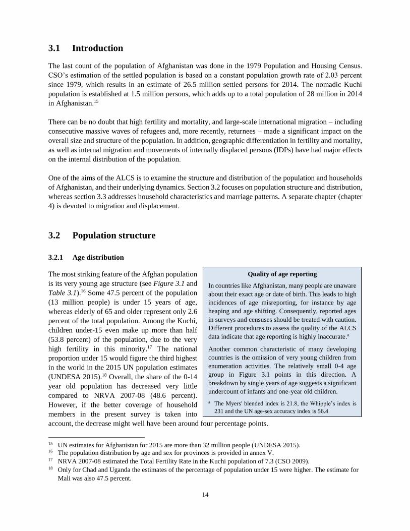
14
3.1 Introduction The last count of the population of Afghanistan was done in the 1979 Population and Housing Census.
CSO’s estimation of the settled population is based on a constant population growth rate of 2.03 percent
since 1979, which results in an estimate of 26.5 million settled persons for 2014. The nomadic Kuchi
population is established at 1.5 million persons, which adds up to a total population of 28 million in 2014
in Afghanistan.15
There can be no doubt that high fertility and mortality, and large-scale international migration – including
consecutive massive waves of refugees and, more recently, returnees – made a significant impact on the
overall size and structure of the population. In addition, geographic differentiation in fertility and mortality,
as well as internal migration and movements of internally displaced persons (IDPs) have had major effects
on the internal distribution of the population.
One of the aims of the ALCS is to examine the structure and distribution of the population and households
of Afghanistan, and their underlying dynamics. Section 3.2 focuses on population structure and distribution,
whereas section 3.3 addresses household characteristics and marriage patterns. A separate chapter (chapter
4) is devoted to migration and displacement.
3.2 Population structure
3.2.1 Age distribution
The most striking feature of the Afghan population
is its very young age structure (see Figure 3.1 and
Table 3.1).16 Some 47.5 percent of the population
(13 million people) is under 15 years of age,
whereas elderly of 65 and older represent only 2.6
percent of the total population. Among the Kuchi,
children under-15 even make up more than half
(53.8 percent) of the population, due to the very
high fertility in this minority.17 The national
proportion under 15 would figure the third highest
in the world in the 2015 UN population estimates
(UNDESA 2015).18 Overall, the share of the 0-14
year old population has decreased very little
compared to NRVA 2007-08 (48.6 percent).
However, if the better coverage of household
members in the present survey is taken into
account, the decrease might well have been around four percentage points.
15 UN estimates for Afghanistan for 2015 are more than 32 million people (UNDESA 2015). 16 The population distribution by age and sex for provinces is provided in annex V. 17 NRVA 2007-08 estimated the Total Fertility Rate in the Kuchi population of 7.3 (CSO 2009). 18 Only for Chad and Uganda the estimates of the percentage of population under 15 were higher. The estimate for
Mali was also 47.5 percent.
Quality of age reporting
In countries like Afghanistan, many people are unaware
about their exact age or date of birth. This leads to high
incidences of age misreporting, for instance by age
heaping and age shifting. Consequently, reported ages
in surveys and censuses should be treated with caution.
Different procedures to assess the quality of the ALCS
data indicate that age reporting is highly inaccurate.a
Another common characteristic of many developing
countries is the omission of very young children from
enumeration activities. The relatively small 0-4 age
group in Figure 3.1 points in this direction. A
breakdown by single years of age suggests a significant
undercount of infants and one-year old children.
a The Myers' blended index is 21.8, the Whipple’s index is
231 and the UN age-sex accuracy index is 56.4
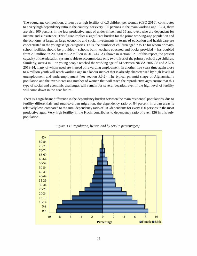
15
The young age composition, driven by a high fertility of 6.3 children per woman (CSO 2010), contributes
to a very high dependency ratio in the country: for every 100 persons in the main working age 15-64, there
are also 100 persons in the less productive ages of under-fifteen and 65 and over, who are dependent for
income and subsistence. This figure implies a significant burden for the prime working-age population and
the economy at large, as large economic and social investments in terms of education and health care are
concentrated in the youngest age categories. Thus, the number of children aged 7 to 12 for whom primary-
school facilities should be provided – schools built, teachers educated and books provided – has doubled
from 2.6 million in 2007-08 to 5.2 million in 2013-14. As shown in section 9.2.1 of this report, the present
capacity of the education system is able to accommodate only two-thirds of the primary school age children.
Similarly, over 4 million young people reached the working age of 14 between NRVA 2007-08 and ALCS
2013-14, many of whom need are in need of rewarding employment. In another five years time again close
to 4 million youth will reach working age in a labour market that is already characterised by high levels of
unemployment and underemployment (see section 5.3.2). The typical pyramid shape of Afghanistan’s
population and the ever-increasing number of women that will reach the reproductive ages ensure that this
type of social and economic challenges will remain for several decades, even if the high level of fertility
will come down in the near future.
There is a significant difference in the dependency burden between the main residential populations, due to
fertility differentials and rural-to-urban migration: the dependency ratio of 84 percent in urban areas is
relatively low, compared to the rural dependency ratio of 105 dependents for every 100 persons in the most
productive ages. Very high fertility in the Kuchi contributes to dependency ratio of even 126 in this sub-
population.
Figure 3.1: Population, by sex, and by sex (in percentages)
10 8 6 4 2 0 2 4 6 8 10
0-4
5-9
10-14
15-19
20-24
25-29
30-34
35-39
40-44
45-49
50-54
55-59
60-64
65-69
70-74
75-79
80-84
85+
Percentage Female Male
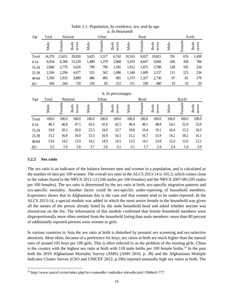
16
Table 3.1: Population, by residence, sex, and by age
a. In thousands
Age Total National Urban Rural Kuchi
Male
Fem
ale
Bo
th
sex
es
Male
Fem
ale
Bo
th
sex
es
Male
Fem
ale
Bo
th
sex
es
Male
Fem
ale
Bo
th
sex
es
Total 14,370 13,651 28,020 3,425 3,317 6,742 10,163 9,657 19,821 781 676 1,458
0-14 6,934 6,384 13,318 1,489 1,379 2,868 5,019 4,647 9,666 426 358 784
15-24 2,840 2,776 5,616 799 796 1,595 1,912 1,875 3,788 128 105 234
25-39 2,184 2,294 4,477 525 562 1,086 1,548 1,609 3,157 111 123 234
40-64 1,956 1,933 3,889 486 495 981 1,373 1,357 2,730 97 81 178
65+ 456 264 720 126 85 212 311 169 480 19 10 29
b. In percentages
Age Total National Urban Rural Kuchi
Male
Fem
ale
Bo
th
sex
es
Male
Fem
ale
Bo
th
sex
es
Male
Fem
ale
Bo
th
sex
es
Male
Fem
ale
Bo
th
sex
es
Total 100.0 100.0 100.0 100.0 100.0 100.0 100.0 100.0 100.0 100.0 100.0 100.0
0-14 48.3 46.8 47.5 43.5 41.6 42.5 49.4 48.1 48.8 54.5 52.9 53.8
15-24 19.8 20.3 20.0 23.3 24.0 23.7 18.8 19.4 19.1 16.4 15.5 16.0
25-39 15.2 16.8 16.0 15.3 16.9 16.1 15.2 16.7 15.9 14.2 18.2 16.1
40-64 13.6 14.2 13.9 14.2 14.9 14.5 13.5 14.1 13.8 12.4 12.0 12.2
65+ 3.2 1.9 2.6 3.7 2.6 3.1 3.1 1.7 2.4 2.4 1.4 2.0
3.2.2 Sex ratio
The sex ratio is an indicator of the balance between men and women in a population, and is calculated as
the number of men per 100 women. The overall sex ratio in the ALCS 2013-14 is 105.3, which comes close
to the values found in the NRVA 2011-12 (106 males per 100 females) and the NRVA 2007-08 (105 males
per 100 females). The sex ratio is determined by the sex ratio at birth, sex-specific migration patterns and
sex-specific mortality. Another factor could be sex-specific under-reporting of household members.
Experience shows that in Afghanistan this is the case and that women tend to be under-reported. In the
ALCS 2013-14, a special module was added in which the most senior female in the household was given
all the names of the person already listed by the male household head and asked whether anyone was
missed-out on the list. The information of this module confirmed that female household members were
disproportionally more often omitted from the household listing than male members: more than 80 percent
of additionally reported persons were women or girls.
In various countries in Asia the sex ratio at birth is disturbed by prenatal sex screening and sex-selective
abortions. Most often, because of a preference for boys, sex ratios at birth are much higher than the natural
ratio of around 105 boys per 100 girls. This is often referred to as the problem of the missing girls. China
is the country with the highest sex ratio at birth with 118 male births per 100 female births.19 In the past
both the 2010 Afghanistan Mortality Survey (AMS) (AMS 2010, p. 38) and the Afghanistan Multiple
Indicator Cluster Survey (CSO and UNICEF 2012, p.196) reported unusually high sex ratios at birth. The
19 http://www.unicef.cn/en/index.php?m=content&c=index&a=show&catid=196&id=777
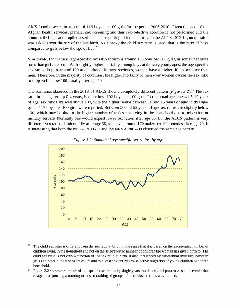
17
AMS found a sex ratio at birth of 116 boys per 100 girls for the period 2006-2010. Given the state of the
Afghan health services, prenatal sex screening and thus sex-selective abortion is not performed and the
abnormally high ratio implied a serious underreporting of female births. In the ALCS 2013-14, no question
was asked about the sex of the last birth. As a proxy the child sex ratio is used, that is the ratio of boys
compared to girls below the age of five.20
Worldwide, the ‘natural’ age-specific sex ratio at birth is around 105 boys per 100 girls, as somewhat more
boys than girls are born. With slightly higher mortality among boys at the very young ages, the age-specific
sex ratios drop to around 100 at adulthood. In most societies, women have a higher life expectancy than
men. Therefore, in the majority of countries, the higher mortality of men over women causes the sex ratio
to drop well below 100 usually after age 50.
The sex ratios observed in the 2013-14 ALCS show a completely different pattern (Figure 3.2).21 The sex
ratio in the age-group 0-4 years, is quite low: 102 boys per 100 girls. In the broad age interval 5-19 years
of age, sex ratios are well above 100, with the highest value between 10 and 15 years of age: in this age-
group 117 boys per 100 girls were reported. Between 20 and 55 years of age sex ratios are slightly below
100, which may be due to the higher number of males not living in the household due to migration or
military service. Normally one would expect lower sex ratios after age 55, but the ALCS pattern is very
different. Sex ratios climb rapidly after age 55, to a level around 170 males per 100 females after age 70. It
is interesting that both the NRVA 2011-12 and the NRVA 2007-08 observed the same age pattern.
Figure 3.2: Smoothed age-specific sex ratios, by age
20 The child sex ratio is different from the sex ratio at birth, in the sense that it is based on the enumerated number of
children living in the household and not on the self-reported number of children the woman has given birth to. The
child sex ratio is not only a function of the sex ratio at birth, it also influenced by differential mortality between
girls and boys in the first years of life and to a lesser extent by sex-selective migration of young children out of the
household. 21 Figure 3.2 shows the smoothed age-specific sex ratios by single years. As the original pattern was quite erratic due
to age misreporting, a running means smoothing of groups of three observations was applied.
0
20
40
60
80
100
120
140
160
180
200
0 5 10 15 20 25 30 35 40 45 50 55 60 65 70 75
Sex
rat
io
Age
18
The underrepresentation of female teenagers and older women is probably caused by the combination of
two factors. The most important is the cultural code of purdah which dictates the physical boundaries
between both sexes. To protect the honor of the woman and the reputation of the family, many women live
secluded. The secluded position of women may easily lead to them being omitted in the household roster
by the head of household. It is interesting that at teenage and older age the sex ratios are particularly high,
but not in the age-group 20-49 years. Perhaps this is due to the fact that (female) interviewers specifically
probed for women of these age groups to be interviewed for the reproductive health module. Another reason
why the sex ratio at older ages is so high may be the very high levels of maternal mortality, especially in
the past. The global report on maternal mortality by the interagency group estimated 460 maternal deaths
per 100,000 births for Afghanistan in 2010 (WHO, UNICEF, UNFPA and World Bank 2012). Although no
exact nationwide figures are available, there is no doubt that maternal mortality was much higher in earlier
days. Bartlett et al. (2005) estimated that in the period 1999-2002 the maternal mortality ratio (MMR) was
between 1,600 and 2,200. Assuming for the sake of argument that in the period 1970-2000 the MMR was
2,000 and the Total Fertility Rate (TFR)22 was around 7, then the lifetime risk of maternal mortality can be
estimated at 14,000 per 100,000 women. This would imply that in that period almost one in seven women
would have died during pregnancy and childbirth. Obviously, this would still be reflected in the number of
women who survive beyond age 50 and it would seriously distort the current sex ratios at older ages.
3.2.3 Distribution by place of residence
As is shown in Table 3.1, the population of Afghanistan is overwhelmingly rural: the 19.8 million rural
residents represent 70.7 percent of the total population. Only 24.1 percent (6.7 million) live in urban areas,
whereas 5.2 percent (1.5 million) of the population is classified as Kuchi. The CSO population projection
rates imply that since the NRVA 2007-08, the total population has increased with 3.0 million people, of
which close to 1.8 million in urban areas and 1.3 million in rural areas. Due to the assumed counterbalancing
effect of natural growth and settlement of the Kuchi, the size of the nomadic population remains stable at
just below 1.5 million people, which implies a steady decrease in terms of its share in the overall population
(down from 5.8 in 2007-08).
The urban, rural and Kuchi residence groups differ considerably in the age distribution of their populations,
especially in terms of the share of children under 15. The lowest share is observed in urban areas (less than
43 percent), while rural (49 percent) and Kuchi (54 percent) have considerable higher percentages of
children. Fertility differentials are likely to be the most important explanation for these differences. At
provincial level, the differences in the age structure of the population are even more pronounced. Whereas
Kabul – as expected, being the most urbanised province – records a low share of under-15 population (41.8
percent), eight provinces have shares of more than 52 percent (data not shown).23 The provinces with the
highest shares of young people – an indication of high fertility levels – are typically located in the south-
eastern Pashtun belt of the country.
22 The Population Reference Bureau estimates that the TFR for Afghanistan was around 7.5 in 1970
(http://www.prb.org/DataFinder) 23 These provinces are Urozgan, Zabul, Nangarhar, laghman, Kunhara, Nooristan, Helmand and Khost.
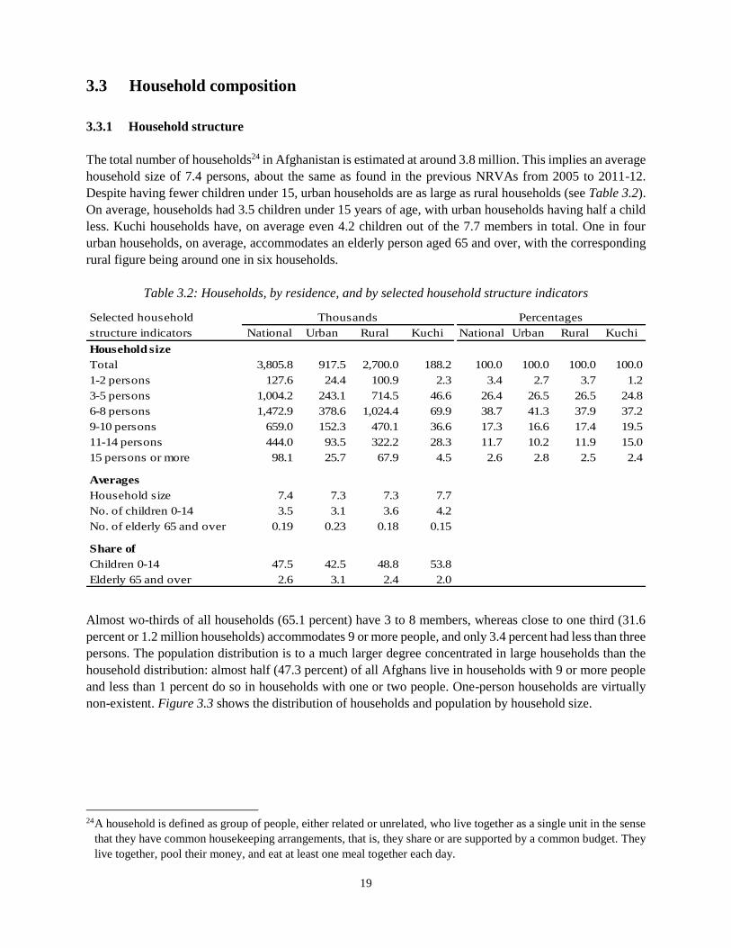
19
3.3 Household composition
3.3.1 Household structure
The total number of households24 in Afghanistan is estimated at around 3.8 million. This implies an average
household size of 7.4 persons, about the same as found in the previous NRVAs from 2005 to 2011-12.
Despite having fewer children under 15, urban households are as large as rural households (see Table 3.2).
On average, households had 3.5 children under 15 years of age, with urban households having half a child
less. Kuchi households have, on average even 4.2 children out of the 7.7 members in total. One in four
urban households, on average, accommodates an elderly person aged 65 and over, with the corresponding
rural figure being around one in six households.
Table 3.2: Households, by residence, and by selected household structure indicators
Selected household Thousands Percentages
structure indicators National Urban Rural Kuchi National Urban Rural Kuchi
Household size
Total 3,805.8 917.5 2,700.0 188.2 100.0 100.0 100.0 100.0
1-2 persons 127.6 24.4 100.9 2.3 3.4 2.7 3.7 1.2
3-5 persons 1,004.2 243.1 714.5 46.6 26.4 26.5 26.5 24.8
6-8 persons 1,472.9 378.6 1,024.4 69.9 38.7 41.3 37.9 37.2
9-10 persons 659.0 152.3 470.1 36.6 17.3 16.6 17.4 19.5
11-14 persons 444.0 93.5 322.2 28.3 11.7 10.2 11.9 15.0
15 persons or more 98.1 25.7 67.9 4.5 2.6 2.8 2.5 2.4
Averages
Household size 7.4 7.3 7.3 7.7
No. of children 0-14 3.5 3.1 3.6 4.2
No. of elderly 65 and over 0.19 0.23 0.18 0.15
Share of
Children 0-14 47.5 42.5 48.8 53.8
Elderly 65 and over 2.6 3.1 2.4 2.0
Almost wo-thirds of all households (65.1 percent) have 3 to 8 members, whereas close to one third (31.6
percent or 1.2 million households) accommodates 9 or more people, and only 3.4 percent had less than three
persons. The population distribution is to a much larger degree concentrated in large households than the
household distribution: almost half (47.3 percent) of all Afghans live in households with 9 or more people
and less than 1 percent do so in households with one or two people. One-person households are virtually
non-existent. Figure 3.3 shows the distribution of households and population by household size.
24 A household is defined as group of people, either related or unrelated, who live together as a single unit in the sense
that they have common housekeeping arrangements, that is, they share or are supported by a common budget. They
live together, pool their money, and eat at least one meal together each day.
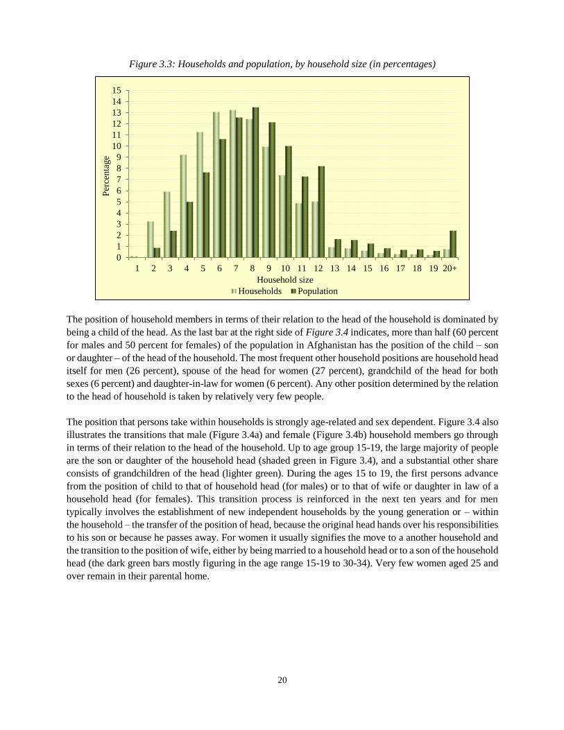
20
Figure 3.3: Households and population, by household size (in percentages)
The position of household members in terms of their relation to the head of the household is dominated by
being a child of the head. As the last bar at the right side of Figure 3.4 indicates, more than half (60 percent
for males and 50 percent for females) of the population in Afghanistan has the position of the child – son
or daughter – of the head of the household. The most frequent other household positions are household head
itself for men (26 percent), spouse of the head for women (27 percent), grandchild of the head for both
sexes (6 percent) and daughter-in-law for women (6 percent). Any other position determined by the relation
to the head of household is taken by relatively very few people.
The position that persons take within households is strongly age-related and sex dependent. Figure 3.4 also
illustrates the transitions that male (Figure 3.4a) and female (Figure 3.4b) household members go through
in terms of their relation to the head of the household. Up to age group 15-19, the large majority of people
are the son or daughter of the household head (shaded green in Figure 3.4), and a substantial other share
consists of grandchildren of the head (lighter green). During the ages 15 to 19, the first persons advance
from the position of child to that of household head (for males) or to that of wife or daughter in law of a
household head (for females). This transition process is reinforced in the next ten years and for men
typically involves the establishment of new independent households by the young generation or – within
the household – the transfer of the position of head, because the original head hands over his responsibilities
to his son or because he passes away. For women it usually signifies the move to a another household and
the transition to the position of wife, either by being married to a household head or to a son of the household
head (the dark green bars mostly figuring in the age range 15-19 to 30-34). Very few women aged 25 and
over remain in their parental home.
0
1
2
3
4
5
6
7
8
9
10
11
12
13
14
15
1 2 3 4 5 6 7 8 9 10 11 12 13 14 15 16 17 18 19 20+
Per
centa
ge
Household size
Households Population
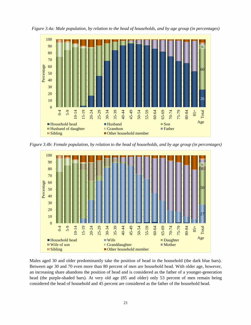
21
Figure 3.4a: Male population, by relation to the head of households, and by age group (in percentages)
Figure 3.4b: Female population, by relation to the head of households, and by age group (in percentages)
Males aged 30 and older predominantly take the position of head in the household (the dark blue bars).
Between age 30 and 70 even more than 80 percent of men are household head. With older age, however,
an increasing share abandons the position of head and is considered as the father of a younger-generation
head (the purple-shaded bars). At very old age (85 and older) only 53 percent of men remain being
considered the head of household and 45 percent are considered as the father of the household head.
26
60
6
0
10
20
30
40
50
60
70
80
90
100
0-4
5-9
10-1
4
15-1
9
20-2
4
25-2
9
30-3
4
35-3
9
40-4
4
45-4
9
50-5
4
55-5
9
60-6
4
65-6
9
70-7
4
75-7
9
80-8
4
85+
To
tal
Per
centa
ge
AgeHousehold head Husband SonHusband of daughter Grandson FatherSibling Other household member
27
50
66
0
10
20
30
40
50
60
70
80
90
100
0-4
5-9
10-1
4
15-1
9
20-2
4
25-2
9
30-3
4
35-3
9
40-4
4
45-4
9
50-5
4
55-5
9
60-6
4
65-6
9
70-7
4
75-7
9
80-8
4
85+
To
tal
Per
centa
ge
AgeHousehold head Wife DaughterWife of son Granddaughter MotherSibling Other household member
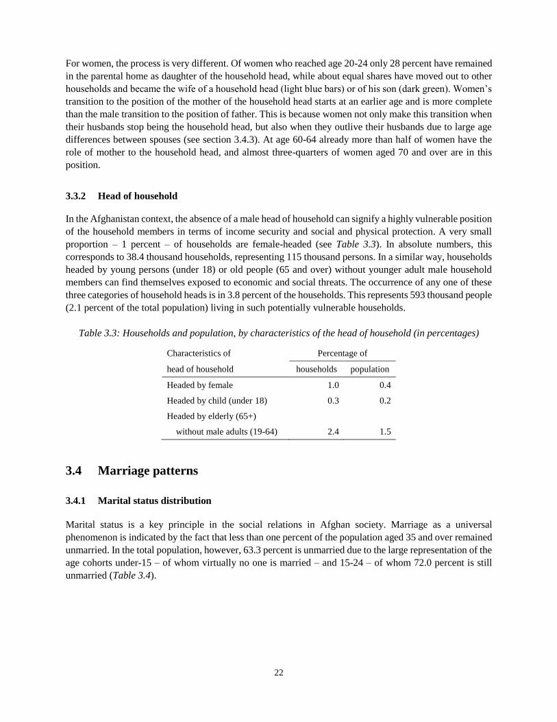
22
For women, the process is very different. Of women who reached age 20-24 only 28 percent have remained
in the parental home as daughter of the household head, while about equal shares have moved out to other
households and became the wife of a household head (light blue bars) or of his son (dark green). Women’s
transition to the position of the mother of the household head starts at an earlier age and is more complete
than the male transition to the position of father. This is because women not only make this transition when
their husbands stop being the household head, but also when they outlive their husbands due to large age
differences between spouses (see section 3.4.3). At age 60-64 already more than half of women have the
role of mother to the household head, and almost three-quarters of women aged 70 and over are in this
position.
3.3.2 Head of household
In the Afghanistan context, the absence of a male head of household can signify a highly vulnerable position
of the household members in terms of income security and social and physical protection. A very small
proportion – 1 percent – of households are female-headed (see Table 3.3). In absolute numbers, this
corresponds to 38.4 thousand households, representing 115 thousand persons. In a similar way, households
headed by young persons (under 18) or old people (65 and over) without younger adult male household
members can find themselves exposed to economic and social threats. The occurrence of any one of these
three categories of household heads is in 3.8 percent of the households. This represents 593 thousand people
(2.1 percent of the total population) living in such potentially vulnerable households.
Table 3.3: Households and population, by characteristics of the head of household (in percentages)
Characteristics of Percentage of
head of household households population
Headed by female 1.0 0.4
Headed by child (under 18) 0.3 0.2
Headed by elderly (65+)
without male adults (19-64) 2.4 1.5
3.4 Marriage patterns
3.4.1 Marital status distribution
Marital status is a key principle in the social relations in Afghan society. Marriage as a universal
phenomenon is indicated by the fact that less than one percent of the population aged 35 and over remained
unmarried. In the total population, however, 63.3 percent is unmarried due to the large representation of the
age cohorts under-15 – of whom virtually no one is married – and 15-24 – of whom 72.0 percent is still
unmarried (Table 3.4).
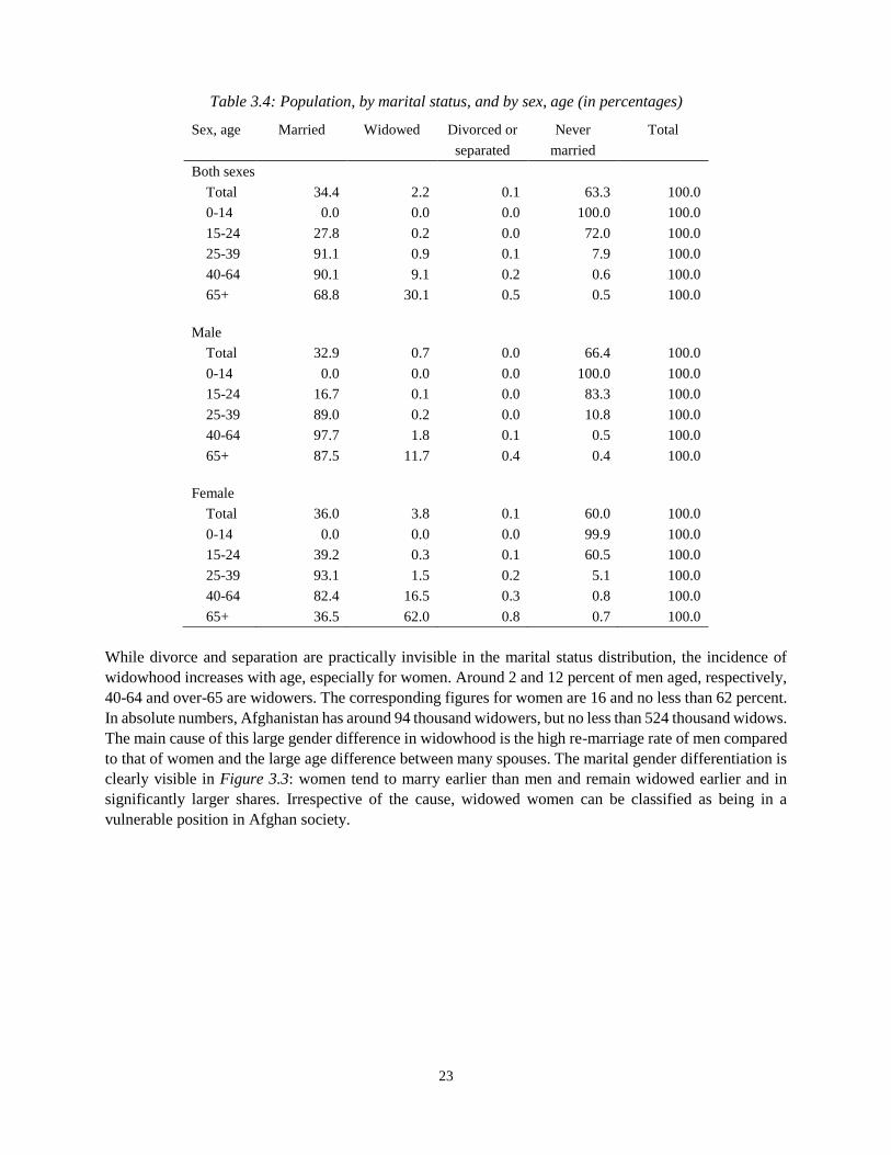
23
Table 3.4: Population, by marital status, and by sex, age (in percentages)
Sex, age Married Widowed Divorced or Never Total
separated married
Both sexes
Total 34.4 2.2 0.1 63.3 100.0
0-14 0.0 0.0 0.0 100.0 100.0
15-24 27.8 0.2 0.0 72.0 100.0
25-39 91.1 0.9 0.1 7.9 100.0
40-64 90.1 9.1 0.2 0.6 100.0
65+ 68.8 30.1 0.5 0.5 100.0
Male
Total 32.9 0.7 0.0 66.4 100.0
0-14 0.0 0.0 0.0 100.0 100.0
15-24 16.7 0.1 0.0 83.3 100.0
25-39 89.0 0.2 0.0 10.8 100.0
40-64 97.7 1.8 0.1 0.5 100.0
65+ 87.5 11.7 0.4 0.4 100.0
Female
Total 36.0 3.8 0.1 60.0 100.0
0-14 0.0 0.0 0.0 99.9 100.0
15-24 39.2 0.3 0.1 60.5 100.0
25-39 93.1 1.5 0.2 5.1 100.0
40-64 82.4 16.5 0.3 0.8 100.0
65+ 36.5 62.0 0.8 0.7 100.0
While divorce and separation are practically invisible in the marital status distribution, the incidence of
widowhood increases with age, especially for women. Around 2 and 12 percent of men aged, respectively,
40-64 and over-65 are widowers. The corresponding figures for women are 16 and no less than 62 percent.
In absolute numbers, Afghanistan has around 94 thousand widowers, but no less than 524 thousand widows.
The main cause of this large gender difference in widowhood is the high re-marriage rate of men compared
to that of women and the large age difference between many spouses. The marital gender differentiation is
clearly visible in Figure 3.3: women tend to marry earlier than men and remain widowed earlier and in
significantly larger shares. Irrespective of the cause, widowed women can be classified as being in a
vulnerable position in Afghan society.
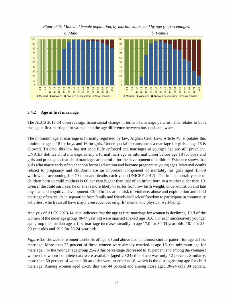
24
Figure 3.5: Male and female population, by marital status, and by age (in percentages)
a. Male b. Female
3.4.2 Age at first marriage
The ALCS 2013-14 observes significant social change in terms of marriage patterns. This relates to both
the age at first marriage for women and the age difference between husbands and wives.
The minimum age at marriage is formally regulated by law. Afghan Civil Law, Article 40, stipulates this
minimum age at 18 for boys and 16 for girls. Under special circumstances a marriage for girls at age 15 is
allowed. To date, this law has not been fully enforced and marriages at younger age are still prevalent.
UNICEF defines child marriage as any a formal marriage or informal union before age 18 for boys and
girls and propagates that child marriages are harmful for the development of children. Evidence shows that
girls who marry early often abandon formal education and become pregnant at young ages. Maternal deaths
related to pregnancy and childbirth are an important component of mortality for girls aged 15–19
worldwide, accounting for 70 thousand deaths each year (UNICEF 2012). The infant mortality rate of
children born to child mothers is 60 per cent higher than that of an infant born to a mother older than 19.
Even if the child survives, he or she is more likely to suffer from low birth weight, under-nutrition and late
physical and cognitive development. Child brides are at risk of violence, abuse and exploitation and child
marriage often results in separation from family and friends and lack of freedom to participate in community
activities, which can all have major consequences on girls’ mental and physical well-being.
Analysis of ALCS 2013-14 data indicates that the age at first marriage for women is declining. Half of the
women of the older age group 40-44 year old were married at exact age 16.6. For each successively younger
age group this median age at first marriage increases steadily to age 17.0 for 30-34 year olds, 18.1 for 25-
29 year olds and 19.0 for 20-24 year olds.
Figure 3.6 shows that women’s cohorts of age 30 and above had an almost similar pattern for age at first
marriage. More than 23 percent of these women were already married at age 16, the minimum age for
marriage. For the younger age group 25-29 this percentage decreased to 19 percent and among the youngest
women for whom complete data were available (aged 20-24) this share was only 12 percent. Similarly,
more than 50 percent of women 30 an older were married at 18, which is the distinguishing age for child
marriage. Among women aged 25-29 this was 44 percent and among those aged 20-24 only 34 percent.
0
10
20
30
40
50
60
70
80
90
1000
-4
5-9
10
-14
15
-19
20
-24
25
-29
30
-34
35
-39
40
-44
45
-49
50
-54
55
-59
60
-64
65
-69
70
-74
75
+
Married Widowed Divorced or separated Never married
0
10
20
30
40
50
60
70
80
90
100
0-4
5-9
10
-14
15
-19
20
-24
25
-29
30
-34
35
-39
40
-44
45
-49
50
-54
55
-59
60
-64
65
-69
70
-74
75
+
Married Widowed Divorced or separated Never married
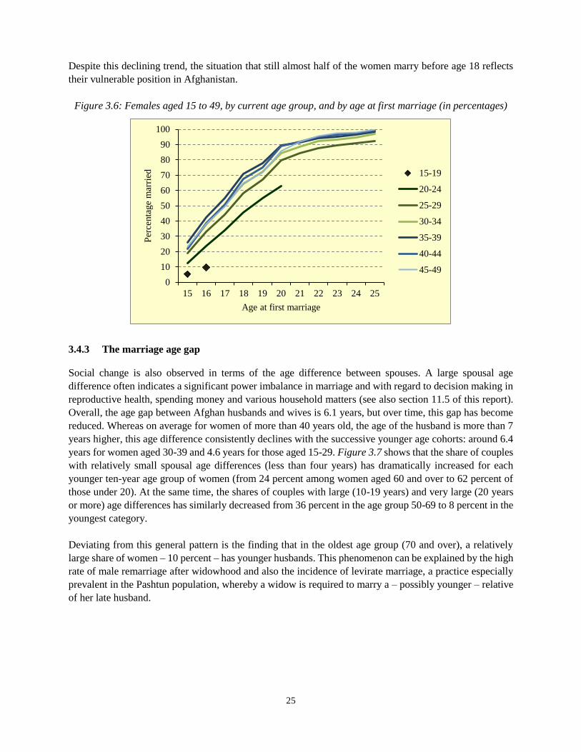
25
Despite this declining trend, the situation that still almost half of the women marry before age 18 reflects
their vulnerable position in Afghanistan.
Figure 3.6: Females aged 15 to 49, by current age group, and by age at first marriage (in percentages)
3.4.3 The marriage age gap
Social change is also observed in terms of the age difference between spouses. A large spousal age
difference often indicates a significant power imbalance in marriage and with regard to decision making in
reproductive health, spending money and various household matters (see also section 11.5 of this report).
Overall, the age gap between Afghan husbands and wives is 6.1 years, but over time, this gap has become
reduced. Whereas on average for women of more than 40 years old, the age of the husband is more than 7
years higher, this age difference consistently declines with the successive younger age cohorts: around 6.4
years for women aged 30-39 and 4.6 years for those aged 15-29. Figure 3.7 shows that the share of couples
with relatively small spousal age differences (less than four years) has dramatically increased for each
younger ten-year age group of women (from 24 percent among women aged 60 and over to 62 percent of
those under 20). At the same time, the shares of couples with large (10-19 years) and very large (20 years
or more) age differences has similarly decreased from 36 percent in the age group 50-69 to 8 percent in the
youngest category.
Deviating from this general pattern is the finding that in the oldest age group (70 and over), a relatively
large share of women – 10 percent – has younger husbands. This phenomenon can be explained by the high
rate of male remarriage after widowhood and also the incidence of levirate marriage, a practice especially
prevalent in the Pashtun population, whereby a widow is required to marry a – possibly younger – relative
of her late husband.
0
10
20
30
40
50
60
70
80
90
100
15 16 17 18 19 20 21 22 23 24 25
Per
centa
ge
mar
ried
Age at first marriage
15-19
20-24
25-29
30-34
35-39
40-44
45-49
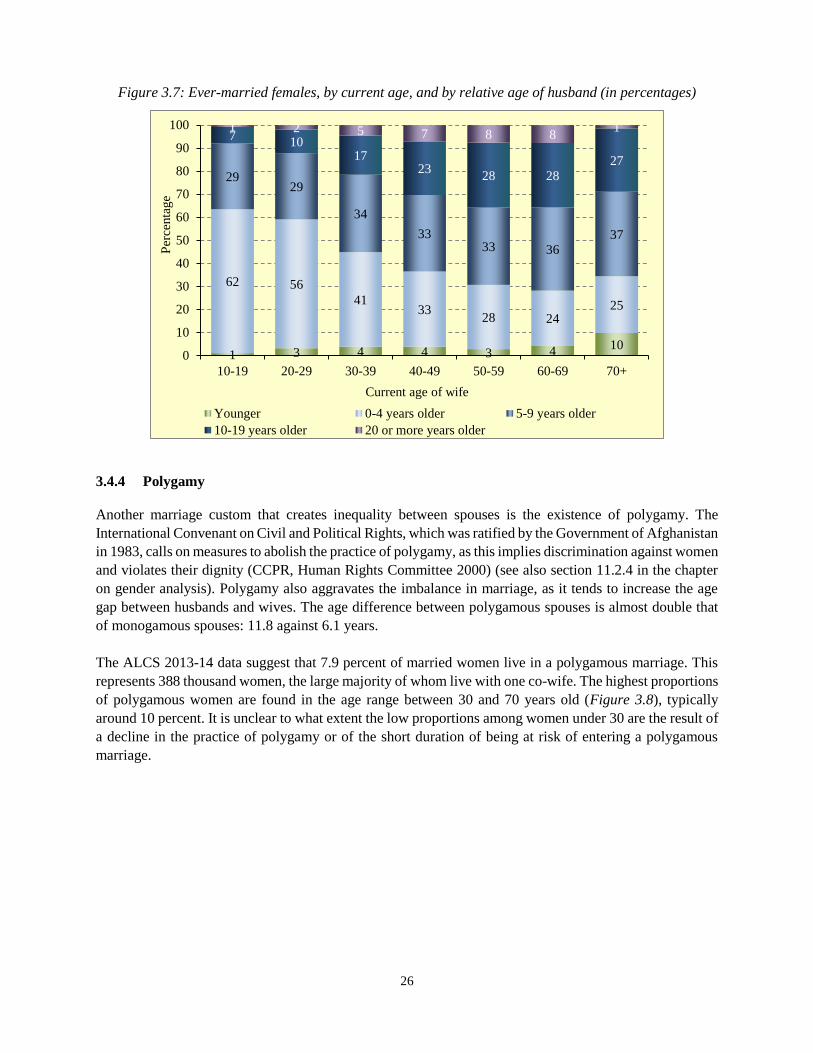
26
Figure 3.7: Ever-married females, by current age, and by relative age of husband (in percentages)
3.4.4 Polygamy
Another marriage custom that creates inequality between spouses is the existence of polygamy. The
International Convenant on Civil and Political Rights, which was ratified by the Government of Afghanistan
in 1983, calls on measures to abolish the practice of polygamy, as this implies discrimination against women
and violates their dignity (CCPR, Human Rights Committee 2000) (see also section 11.2.4 in the chapter
on gender analysis). Polygamy also aggravates the imbalance in marriage, as it tends to increase the age
gap between husbands and wives. The age difference between polygamous spouses is almost double that
of monogamous spouses: 11.8 against 6.1 years.
The ALCS 2013-14 data suggest that 7.9 percent of married women live in a polygamous marriage. This
represents 388 thousand women, the large majority of whom live with one co-wife. The highest proportions
of polygamous women are found in the age range between 30 and 70 years old (Figure 3.8), typically
around 10 percent. It is unclear to what extent the low proportions among women under 30 are the result of
a decline in the practice of polygamy or of the short duration of being at risk of entering a polygamous
marriage.
1 3 4 4 3 410
62 56
4133
28 2425
2929
34
3333 36
37
710
1723
28 28
27
1 2 5 7 8 81
0
10
20
30
40
50
60
70
80
90
100
10-19 20-29 30-39 40-49 50-59 60-69 70+
Per
centa
ge
Current age of wife
Younger 0-4 years older 5-9 years older
10-19 years older 20 or more years older
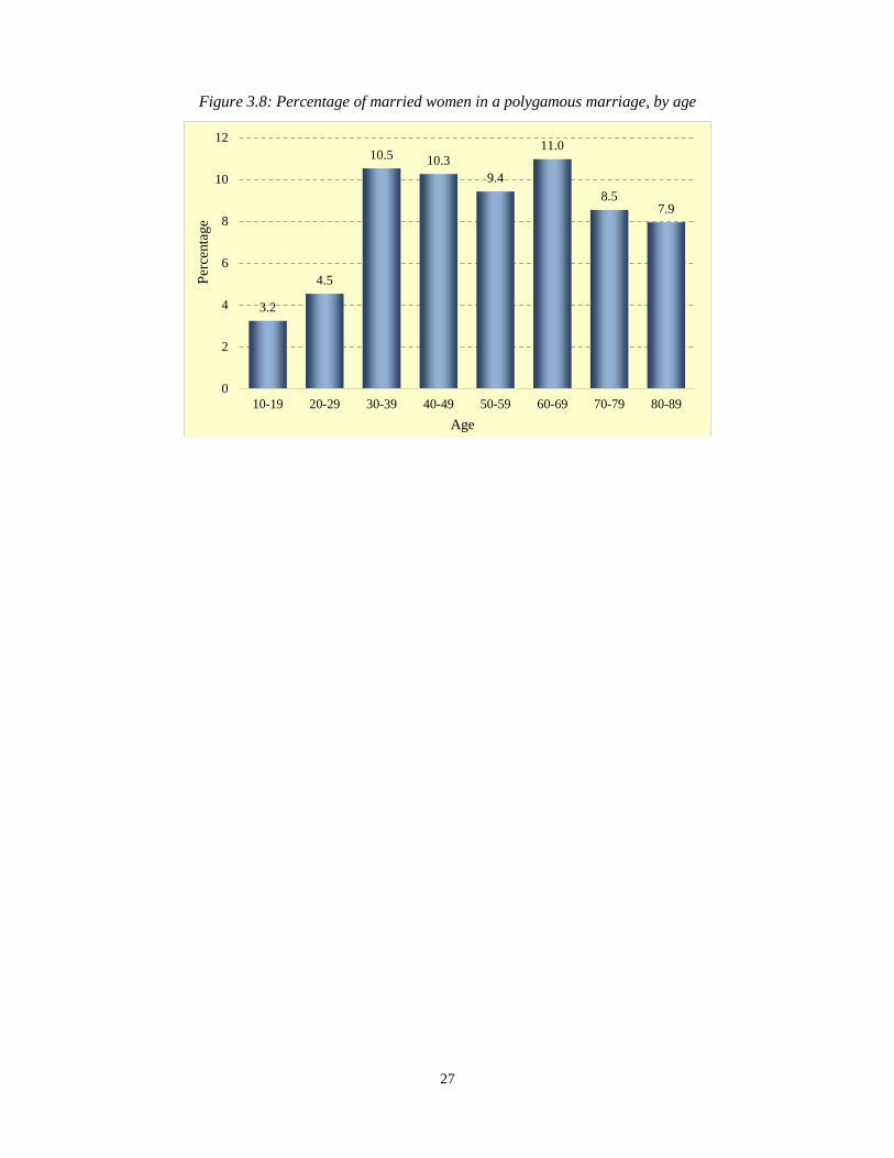
27
Figure 3.8: Percentage of married women in a polygamous marriage, by age
3.2
4.5
10.5 10.3
9.4
11.0
8.57.9
0
2
4
6
8
10
12
10-19 20-29 30-39 40-49 50-59 60-69 70-79 80-89
Per
centa
ge
Age
28
4 MIGRATION
Summary. Until the overturn of the Taliban regime the complex migration situation of Afghanistan has
been dominated by displacement flows – either within Afghanistan or across borders. The year 2002
marked the start of a ten-year period in which return from displacement was the main motive for migration: in this period 39 percent of internal migrants and even 82 percent of immigrants moved for this reason.
Overall, Kabul was the destination of half of the internal migrants (almost 500 thousand people) in the ten years after 2002. In international perspective, Pakistan was the country where most immigrants – 63
percent – came from and Kabul was by far the most important destination province, accommodating almost
half the immigrant stock: 45 percent (almost 600 thousand people) of all immigrants since 2002.
In more recent years, the migration patterns have changed substantially. Afghanistan has turned again
from a net immigration country to a net emigration country. The ALCS information suggests that in recent
years emigration is larger than immigration by more than 100 thousand persons per year. This would imply a negative annual migration rate of 0.4 percent. Return from displacement is reduced to a minor reason
for internal migration in the period 2012 to 2014 and for immigrants this reason is reduced to only 39 percent. With the returnee flows going down, labour migration becomes a leading motive for migration,
and is by far the most important reason for emigration. Kabul remains the most important destination for
internal migrants, but the proportion of 25 percent moving there is only half of that going to Kabul in the ten years before 2012. This may be related to the deteriorating employment situation in the capital. In
international migration, Iran has taken over the leading position from Pakistan, both as destination country for emigrants (61 percent) and as origin country for immigrants (63 percent). The Gulf states gain a
prominent place, as they generated 7 percent of immigrants into Afghanistan between 2012 and 2014, and
received 18 percent of emigrants in the last year before the survey.
Kabul and its immediately surrounding provinces form the main internal migration system in the country,
with Kabul acting as a strong gravitation centre for migrants from particularly Parwan, Panshjer and
Wardak. Close to half of all migrations within Afghanistan happen in this area. In absolute numbers, Kabul has by far the largest overall net gain due to migration, adding close to 900 thousand people to its
population. Also Balkh, Herat and Nangarhar have substantial net migration gains of around 100 thousand persons each. On the other hand, Laghman and Wardak are the provinces with the largest net population
loss due to migration, losing well over 100 thousand persons each. In relative terms Kabul and Nimroz are
the provinces with the largest population gain, each increasing with around one quarter due to migration. Pansjher is the province that lost relatively most population: it would have had 28 percent more population
without migration. Internal migration and immigration are strongly directed toward urban areas. Compared to an urban proportion of 24 percent in the total population, 50 percent of the immigrants live
in urban areas, 82 percent of internal life-time migrants and 67 percent of recent migrants.
The survey also indicated that for Afghans migration is more often a family event than an individual act. Family migration usually occurs when returning for displacement, but apparently families also often move
together if one or some household members seek employment elsewhere. The exception is emigration, which
almost exclusively consists of adult working-age males.
The living conditions of persons and households that returned from displacement seem to be somewhat
better than those of non-returnees. Literacy among returnees is significantly higher, as is the proportion with completed secondary and tertiary education. Also labour force participation is higher among
returnees, although the rate of returnee women that is gainfully employed is somewhat lower. Housing
quality and access to improved water and sanitation is also better for returnee households than for non-returnee households.
29
4.1 Introduction
4.1.1 Afghanistan’s migration context
The migration context of Afghanistan is particularly complex. Regular and traditional migrant flows
feature both internal and cross-border movements, permanent, seasonal and circularly migration –
including remaining nomadism of a sizable part of the population – and migration patterns that are highly
gender-specific and very different for the short and long distance (CSO 2014). These flows have become
mixed with the effects of one of the world’s largest and most protracted refugee situations, the largest
volume of returnees in recent history, large-scale internal displacement and newly emerging destinations
for labour migrants and asylum seekers. The number of Afghans involved in international migration – and
more particularly the number of refugees and returnees – is so large that it is critical to the population
equation in national estimates. However, displacement and other forms of internal and international
migration are so intertwined that the government of Afghanistan is now taking the first steps in developing
a migration policy that is going beyond refugee migration.
The ALCS 2013-14 included two modules on migration. The general migration module asked questions
about the place of usual residence at three different points in time: at birth, in 2002 (Shamsi calendar
1380) and two years before the survey (mostly 2012, Shamsi calender 1391). The year 2002 marks the
moment of the overthrow of the Taliban regime and the change from large-scale refugee flows to large-
scale return flows. The question on place of residence two years before the survey was included to assess
possible recent changes in migration. Although the survey is not primarily designed as a migration survey,
the information collected is relevant to add to the limited body of information on migrants and migration
flows. The information collected refers to migrant stocks. Consequently, information provided about the
volume of migration flows is an underestimation to the extent that people had other places of residence in
addition to those recorded on the questionnaire. It should be also emphasised that the strength of the ALCS
migration information is more in revealing patterns than in specifying absolute numbers.
This chapter dissects the migration analysis into information about internal migration (migration between
provinces in Afghanistan; section 4.2) and that about international migration (migration crossing
international borders; section 4.3). For these two types of migration, the number of migrants are estimated,
their origins and destinations, their main characteristics and the reasons for migration. Specific attention
is also paid to the urbanisation effect of migration. Section 4.4 attempts to assess the overall effect of
migration on the population distribution in Afghanistan. Separate sections of this report are devoted to
main migrant types in terms of reasons for migration. A section on labour migration is included in the
next chapter on labour outcomes (section 5.4), while section 4.5 of this chapter elaborates on returned
refugees and internally displaced persons (IDPs), which were the dominant migrant types in the first
decade of this century. The second section of this introduction, however, continues with an explanation
of the main migration concepts that are used in this chapter.
4.1.2 Migration concepts
Migration is defined by the act of crossing a border and going to live elsewhere for at least a year. Crossing
the international border between two countries represents international migration. People who enter a
country are immigrants and those who leave a country are emigrants. Crossing (administrative) boundaries
within a country represents internal migration. Persons moving into an area from within the same country
30
are labelled in-migrants; those who move to another area within the country are labelled out-migrants. Internal migration can be measured at different levels, such as province-, district- or even municipality
level. The ALCS 2013-14 was designed to measure migration between the provinces of Afghanistan.
In this report, migration analysis distinguishes three different time dimensions, which can apply to both
internal and international migration.
Life-time migration indicates a difference between the place of birth and the place of current
residence. It gives the net result of all moves a person has made during his or her life, and may
conceal possible consecutive migrations during the person’s life time. At the aggregate level, it
gives an indication of net loss and gain of the population in specific areas.
Intermediate-time migration in this report refers to a difference between the place of residence in
2002 and the place of current residence and gives the net result of all moves a person has made in
the twelve years between 2002 and the survey. The year 2002 was chosen as it is a landmark in the
migration history of Afghanistan, marking the onset of large returnee flows after the overthrow of
the Taliban regime.
Recent migration is measured as migration in the two years preceding the survey and gives the net
result of all moves a person has made in these two years. Measuring recent migration allows to
detect possible new migration patterns.
Current residence is the place of residence at the time of the ALCS 2013-14.
Refugee: A person who, owing to a well-founded fear of persecution for reasons of race, religion,
nationality, membership of a particular social group or political opinions, is outside the country of his or
her nationality and is unable or, owing to such fear, is unwilling to avail him- or herself of the protection
of that country.
Internally Displaced Person (IDP): A person who has been forced or obliged to flee or to leave his or her
home or place of habitual residence, in particular as a result of or in order to avoid the effects of armed
conflict, situations of generalised violence, violations of human rights or natural or human-made disasters,
and who have not crossed an internationally recognised state border
Although the absolute number of migrants provide relevant information, an equally relevant indicator is
this number in relation to the total population of the migrant-receiving area or to the population of the
migrant-sending area. These indicators are expressed as, respectively, migration rates and ratios. For
definitions of these indicators, see Text box Migration rates and ratios below.
31
4.2 Internal migration in Afghanistan
This section looks at the internal migrant stocks across the provinces of Afghanistan; international
migration is covered in more detail in section 4.3. The key question of this section is where migrants go
to and where they come from. In order to discover the main migration patterns, attention is paid to absolute
numbers, but more specifically to migration ratios – for the proportion of migrants in the resident
population – and rates – for the proportion of migrants who moved away from the place of origin. This
information is provided for three episodes in people’s lives in the next three sub-sections: migration since
birth (life-time migration), migration since 2002 when the regime change occurred in Afghanistan
(labelled intermediate-time migration), and migration in the two years before the survey (recent
migration). For detailed definitions of these concepts, see section 4.1.2.
4.2.1 Internal life-time migrants
Around 1.6 million residents in Afghanistan were born in another province than where they were living
at the time of the survey. This number of life-time migrants implies that at least 6 percent of the total
population of Afghanistan now lives in another province than where they were born. Zooming in from the
national to the province level, a large variation in this proportion of internal life-time migrants can be
observed (Figure 4.1).25 Kabul stands out with 869 thousand life-time migrants in its population, which
is more than half (55 percent) of all life-time migrants in the country. Also in relative terms, Kabul stands
out with a proportion of 21 percent of the population who were born elsewhere. Surprisingly, Nimroz is
the province with the next-highest in-migration ratio (13 percent), but the absolute number of internal life-
time migrants in this province is small (19 thousand).
A second group of provinces with above-average in-migration ratios includes Balkh and Bamyan (each
with around 10 percent life-time in-migrants in the population, and Nangarhar and Parwan (8 and 7
percent, respectively). It is likely the presence of major towns (Mazar-e-Sharif and Jalalabad) in some of
25 Including in-migrants and immigrants.
Migration rates and ratios
Immigration ratio. The number of people who now
live in Afghanistan or in a specific province of
Afghanistan but who were living in another country
previously, expressed as a percentage of the total
population living in Afghanistan or the specific
province of Afghanistan. This ratio is a measure of
the ‘burden’ of immigration to the region receiving
the migrants.
Emigration rate. The number of people who lived in
Afghanistan or a specific province of Afghanistan
previously, but are now living in another country,
expressed as a percentage of the total population living
in Afghanistan or the specific province of
Afghanistan. This rate measures the chance of people
moving abroad from a place of origin.
In-migration ratio. The number of people who
now live in a specific province, but who were
living in another province previously, expressed as
a percentage of the total population living in the
specific province. This ratio is a measure of the
‘burden’ of in-migration to the province receiving
the migrants.
Out-migration rate. The number of people who
lived in a specific province previously, but are now
living in another province, expressed as a
percentage of the total population living in the
specific province previously. This rate measures the
chance of people moving out from a province.
32
these provinces that attracts migrants who look for employment and education opportunities. On the other
hand, there is quite a large group of provinces that has very low in-migration ratios. This group includes
provinces like Badakhshan, Daykundi and Nooristan, which are not attractive to move to because of their
remoteness and few opportunities for livelihoods. Very low proportions of migrants in Wardak, Paktika,
Urozgan and Helmand may also be related to the security situation in those provinces.
The provinces where internal life-time migrants come from are very different from the main destination
provinces.26 Due to its total population size, Kabul generated one of the largest numbers of out-migrants
(105 thousand), but four other – in terms of population much smaller – provinces had even more out-
migrants, ranging from 122 to 183 thousand persons. However, it is not so much the absolute numbers,
but the out-migration rates that provide the key to understanding out-migration. Figure 4.2 shows that the
highest rates are found for provinces immediately surrounding Kabul, an indication of the very strong pull
force of the capital. Panshjer has the highest out-migration rate, with 34 percent, meaning that of all
persons born in Panshjer more than one third now live elsewhere. Also Laghman and Logar have very
high out-migration rates of more than 20 percent (28 and 21 percent, respectively), which is, however,
much affected by Kuchi migration. But without the Kuchi migration component the out-migration rates
of these provinces are still double the national average. Close-to-Kabul Wardak, Parwan and Kapisa have
relatively high rates as well (18, 17 and 11 percent, respectively). On the other hand, there is also a group
of provinces with very low out-migration, indicating that people tend to stay within the province because
either the province itself has sufficient to offer – like probably Kunduz and Herat – or because of a strong
connection with the place of origin. Kabul is among the provinces with the lowest out-migration rates (3
percent only).
26 It should be noted that information in this section only includes internal migrants, as no information is available
about place of birth of persons who emigrated.
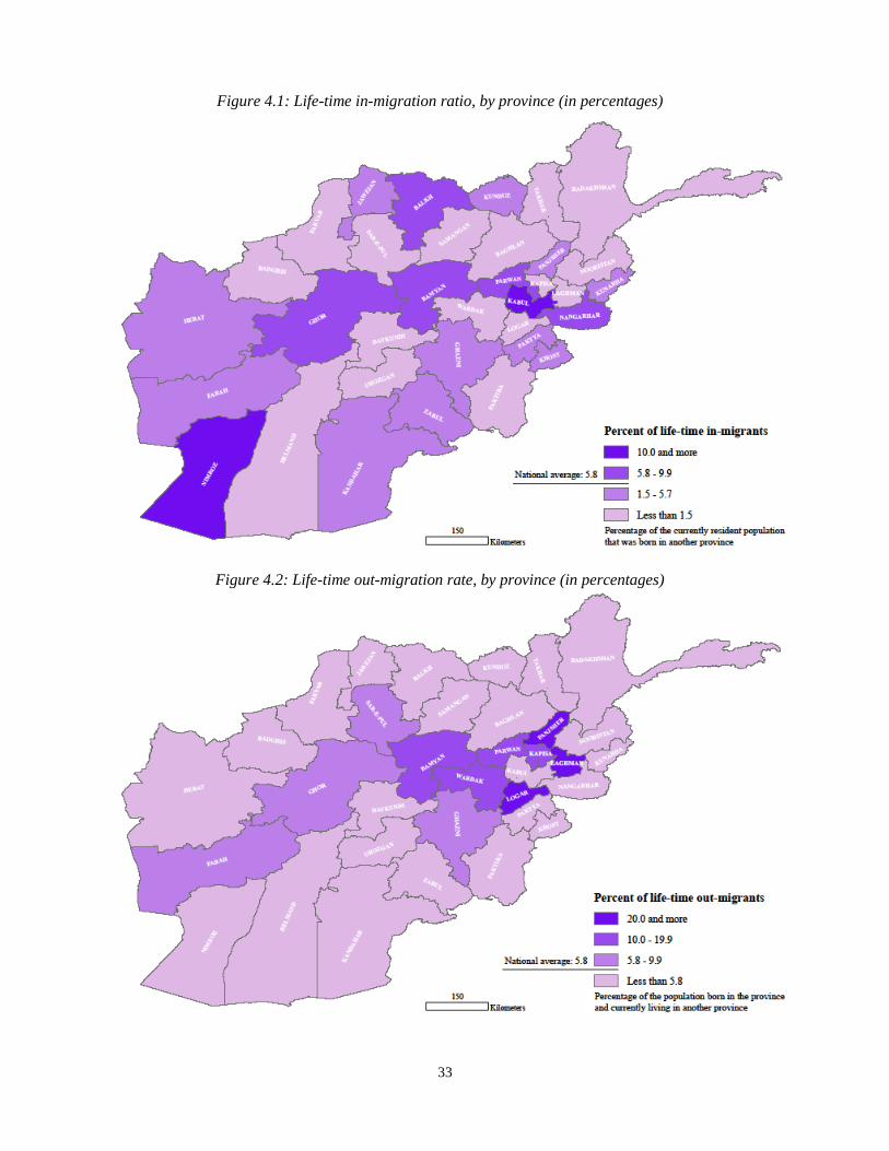
33
Figure 4.1: Life-time in-migration ratio, by province (in percentages)
Figure 4.2: Life-time out-migration rate, by province (in percentages)
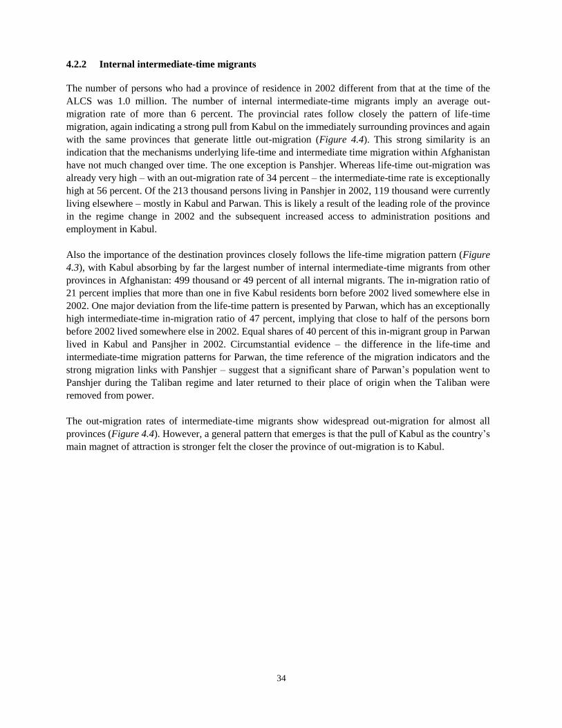
34
4.2.2 Internal intermediate-time migrants
The number of persons who had a province of residence in 2002 different from that at the time of the
ALCS was 1.0 million. The number of internal intermediate-time migrants imply an average out-
migration rate of more than 6 percent. The provincial rates follow closely the pattern of life-time
migration, again indicating a strong pull from Kabul on the immediately surrounding provinces and again
with the same provinces that generate little out-migration (Figure 4.4). This strong similarity is an
indication that the mechanisms underlying life-time and intermediate time migration within Afghanistan
have not much changed over time. The one exception is Panshjer. Whereas life-time out-migration was
already very high – with an out-migration rate of 34 percent – the intermediate-time rate is exceptionally
high at 56 percent. Of the 213 thousand persons living in Panshjer in 2002, 119 thousand were currently
living elsewhere – mostly in Kabul and Parwan. This is likely a result of the leading role of the province
in the regime change in 2002 and the subsequent increased access to administration positions and
employment in Kabul.
Also the importance of the destination provinces closely follows the life-time migration pattern (Figure
4.3), with Kabul absorbing by far the largest number of internal intermediate-time migrants from other
provinces in Afghanistan: 499 thousand or 49 percent of all internal migrants. The in-migration ratio of
21 percent implies that more than one in five Kabul residents born before 2002 lived somewhere else in
2002. One major deviation from the life-time pattern is presented by Parwan, which has an exceptionally
high intermediate-time in-migration ratio of 47 percent, implying that close to half of the persons born
before 2002 lived somewhere else in 2002. Equal shares of 40 percent of this in-migrant group in Parwan
lived in Kabul and Pansjher in 2002. Circumstantial evidence – the difference in the life-time and
intermediate-time migration patterns for Parwan, the time reference of the migration indicators and the
strong migration links with Panshjer – suggest that a significant share of Parwan’s population went to
Panshjer during the Taliban regime and later returned to their place of origin when the Taliban were
removed from power.
The out-migration rates of intermediate-time migrants show widespread out-migration for almost all
provinces (Figure 4.4). However, a general pattern that emerges is that the pull of Kabul as the country’s
main magnet of attraction is stronger felt the closer the province of out-migration is to Kabul.
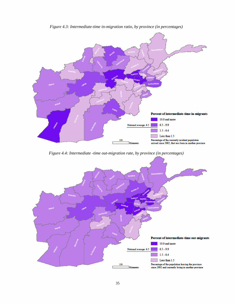
35
Figure 4.3: Intermediate-time in-migration ratio, by province (in percentages)
Figure 4.4: Intermediate -time out-migration rate, by province (in percentages)
36
4.2.3 Internal recent migrants
The stock of internal recent migrants – those who migrated in the two years before the survey – is much
smaller than that of the life-time and intermediate-time migrants (388 thousand), but their information
allows the detection of recent changes in migration patterns and can also give an indication of changes in
the intensity of migration.
Although Kabul is the most preferred destination for recent migrants as well, it is far less dominant than
for less-recent migration. Some 25 percent of internal recent migrants choose to come to Kabul, which
was followed by Nangarhar and Ghor as the main destination provinces (accommodating 19 and 12
percent of all internal recent migrants, respectively). This recent migration information implies that,
relative to the size of the resident population, Kabul drops down the list of destinations. With a recent in-
migration ratio of just over 2 percent, it is far below Bamyan that tops the list with close to 8 percent, and
Zabul and Ghor, each with over 7 percent (see Figure 4.5). In-migration has also become significantly
less pronounced in Parwan and Nimroz. More in-depth analysis will be required to identify the causes of
these shifts, but they are likely to include the receding effect of return from internal displacement and the
slow-down of the economy, which especially affects the labour absorption capacity of Kabul.
Also for out-migration significant changes in the pattern across the country are observed, compared to
less-recent migration. Besides Logar, Wardak, Panjsher and Laghman that maintained relatively high
levels of out-migration, Nimroz, Sar-e-Pul, Helmand and Kandahar have risen into the top-eight provinces
with the highest out-migration rates, with heavy out-migration from the south-western provinces (Figure
4.6). Wardak and Kandahar closely follow Kabul as the largest provider of internal migrants, with both
40 thousand recent out-migrants, compared to Kabul with 46 thousand. Helmand and Logar each
generated around 30 thousand migrants. As all these provinces – except Kabul – face severe security
problems, this might be a common cause for high out-migration from these areas.
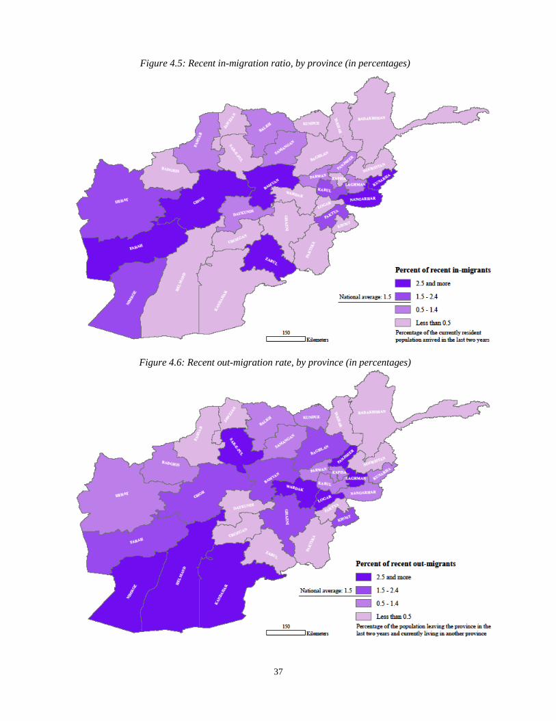
37
Figure 4.5: Recent in-migration ratio, by province (in percentages)
Figure 4.6: Recent out-migration rate, by province (in percentages)
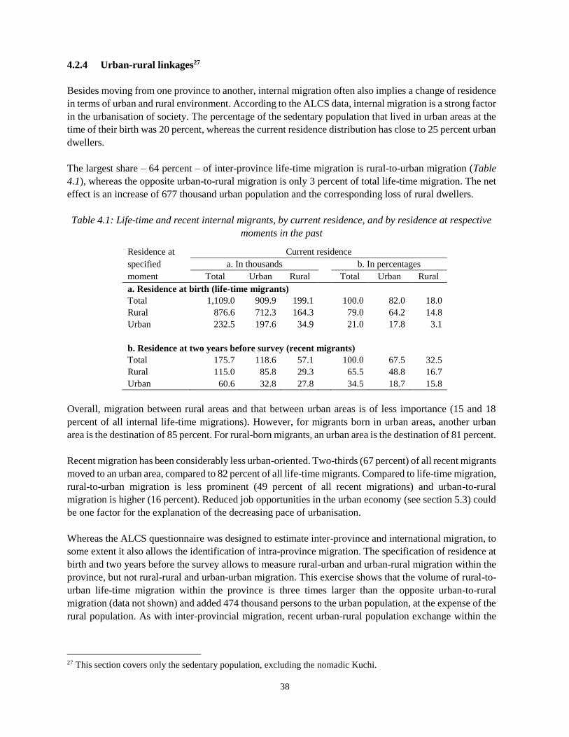
38
4.2.4 Urban-rural linkages27
Besides moving from one province to another, internal migration often also implies a change of residence
in terms of urban and rural environment. According to the ALCS data, internal migration is a strong factor
in the urbanisation of society. The percentage of the sedentary population that lived in urban areas at the
time of their birth was 20 percent, whereas the current residence distribution has close to 25 percent urban
dwellers.
The largest share – 64 percent – of inter-province life-time migration is rural-to-urban migration (Table
4.1), whereas the opposite urban-to-rural migration is only 3 percent of total life-time migration. The net
effect is an increase of 677 thousand urban population and the corresponding loss of rural dwellers.
Table 4.1: Life-time and recent internal migrants, by current residence, and by residence at respective
moments in the past
Residence at Current residence
specified a. In thousands b. In percentages
moment Total Urban Rural Total Urban Rural
a. Residence at birth (life-time migrants)
Total 1,109.0 909.9 199.1 100.0 82.0 18.0
Rural 876.6 712.3 164.3 79.0 64.2 14.8
Urban 232.5 197.6 34.9 21.0 17.8 3.1
b. Residence at two years before survey (recent migrants)
Total 175.7 118.6 57.1 100.0 67.5 32.5
Rural 115.0 85.8 29.3 65.5 48.8 16.7
Urban 60.6 32.8 27.8 34.5 18.7 15.8
Overall, migration between rural areas and that between urban areas is of less importance (15 and 18
percent of all internal life-time migrations). However, for migrants born in urban areas, another urban
area is the destination of 85 percent. For rural-born migrants, an urban area is the destination of 81 percent.
Recent migration has been considerably less urban-oriented. Two-thirds (67 percent) of all recent migrants
moved to an urban area, compared to 82 percent of all life-time migrants. Compared to life-time migration,
rural-to-urban migration is less prominent (49 percent of all recent migrations) and urban-to-rural
migration is higher (16 percent). Reduced job opportunities in the urban economy (see section 5.3) could
be one factor for the explanation of the decreasing pace of urbanisation.
Whereas the ALCS questionnaire was designed to estimate inter-province and international migration, to
some extent it also allows the identification of intra-province migration. The specification of residence at
birth and two years before the survey allows to measure rural-urban and urban-rural migration within the
province, but not rural-rural and urban-urban migration. This exercise shows that the volume of rural-to-
urban life-time migration within the province is three times larger than the opposite urban-to-rural
migration (data not shown) and added 474 thousand persons to the urban population, at the expense of the
rural population. As with inter-provincial migration, recent urban-rural population exchange within the
27 This section covers only the sedentary population, excluding the nomadic Kuchi.
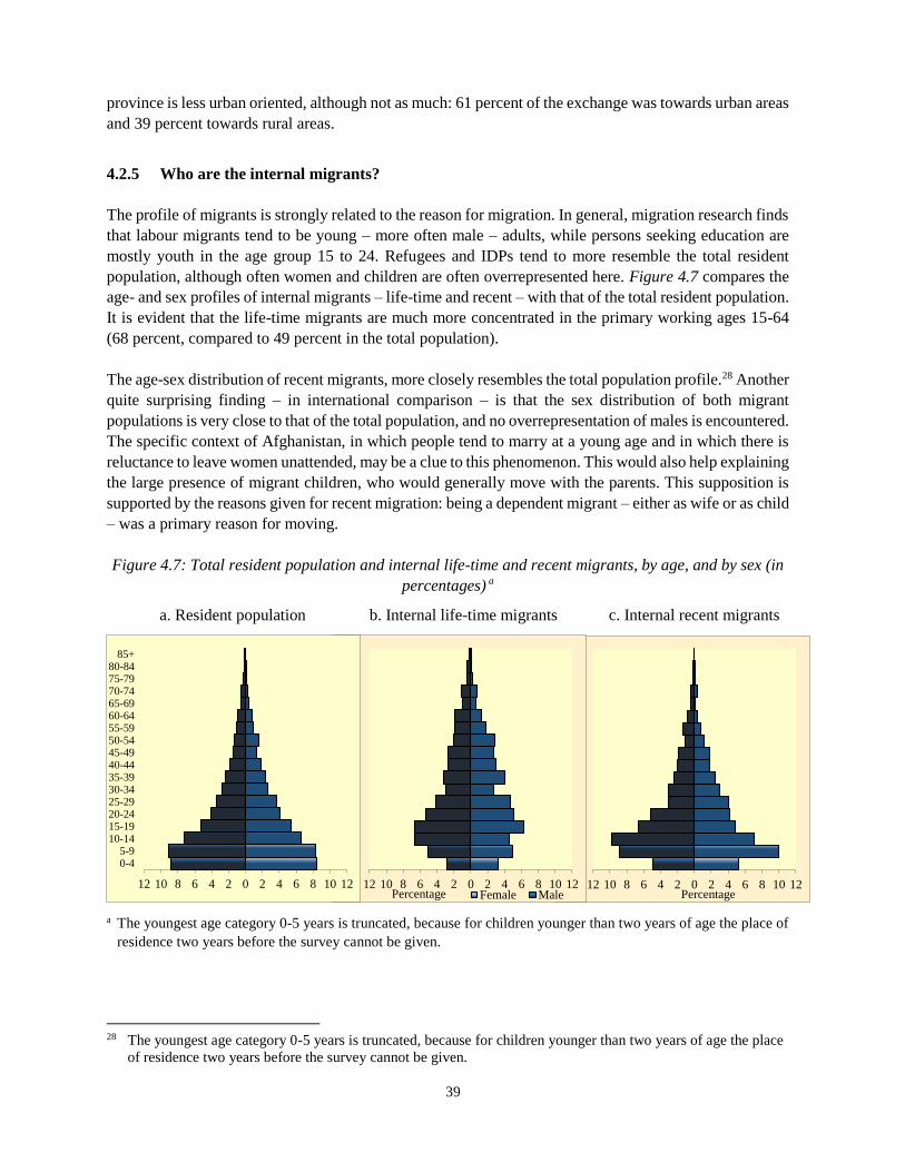
39
province is less urban oriented, although not as much: 61 percent of the exchange was towards urban areas
and 39 percent towards rural areas.
4.2.5 Who are the internal migrants?
The profile of migrants is strongly related to the reason for migration. In general, migration research finds
that labour migrants tend to be young – more often male – adults, while persons seeking education are
mostly youth in the age group 15 to 24. Refugees and IDPs tend to more resemble the total resident
population, although often women and children are often overrepresented here. Figure 4.7 compares the
age- and sex profiles of internal migrants – life-time and recent – with that of the total resident population.
It is evident that the life-time migrants are much more concentrated in the primary working ages 15-64
(68 percent, compared to 49 percent in the total population).
The age-sex distribution of recent migrants, more closely resembles the total population profile.28 Another
quite surprising finding – in international comparison – is that the sex distribution of both migrant
populations is very close to that of the total population, and no overrepresentation of males is encountered.
The specific context of Afghanistan, in which people tend to marry at a young age and in which there is
reluctance to leave women unattended, may be a clue to this phenomenon. This would also help explaining
the large presence of migrant children, who would generally move with the parents. This supposition is
supported by the reasons given for recent migration: being a dependent migrant – either as wife or as child
– was a primary reason for moving.
Figure 4.7: Total resident population and internal life-time and recent migrants, by age, and by sex (in
percentages) a
a. Resident population b. Internal life-time migrants c. Internal recent migrants
a The youngest age category 0-5 years is truncated, because for children younger than two years of age the place of
residence two years before the survey cannot be given.
28 The youngest age category 0-5 years is truncated, because for children younger than two years of age the place
of residence two years before the survey cannot be given.
12 10 8 6 4 2 0 2 4 6 8 10 12
0-45-9
10-1415-1920-2425-2930-3435-3940-4445-4950-5455-5960-6465-6970-7475-7980-84
85+
Percentage12 10 8 6 4 2 0 2 4 6 8 10 12
0-45-9
10-1415-1920-2425-2930-3435-3940-4445-4950-5455-5960-6465-6970-7475-7980-84
85+
Percentage Female Male12 10 8 6 4 2 0 2 4 6 8 10 12
0-45-9
10-1415-1920-2425-2930-3435-3940-4445-4950-5455-5960-6465-6970-7475-7980-84
85+
40
In terms of economic activity status, all internal migrant groups – life-time, intermediate-time and recent
– are quite similar to the profile of the general population. To the extent that differences can be observed,
migrants are slightly better-off, with generally a little higher labour-force participation and a little lower
un- and under-employment. Thus, it seems that internal migration is to a limited extent an effective
strategy for finding employment. A more detailed analysis on the association between labour-market
participation and migration is provided in section 5.4.
With regard to educational attainment, life-time and intermediate-time migrants perform better than the
general population. Adults of 18 years and older of these two groups less often lack any education (54
and 57 percent respectively against 64 percent in the general adult population), 14 percent has completed
upper secondary education against 11 percent in the total population, and 9 and 7 percent, respectively,
have obtained a university degree, compared to only 3 percent generally. Recent adult migrants, however,
more resemble the general population in terms of educational attainment.
4.2.6 Why do internal migrants move?
The ALCS allowed to identify the reasons for migration in two different periods, that between 2002 and
2012, and since two years before the survey, which is mostly the period 2012 to 2014. For both periods,
the most important reason was ‘Moving with parents or the family’, which usually refers to dependent
children who accompany their parents and dependent wives accompanying their husbands (Figure 4.8).
For the underlying motive of the migration, the reasons of the independent migrants can provide clues. In
the period between 2002 and 2012, the two most important of these other reasons were ‘Returning from
displacement’ and ‘Looking for work’, with 24 and 18 percent, respectively. Assuming that the category
of dependent migrants could be distributed pro rato to the other categories, these shares would even be 39
and 29 percent.
The picture that emerges from these results is that internal migration flows in the decade following the
overturn of the Taliban regime were to a large extent shaped by IDPs’ returning to their place of residence
before displacement. Kabul and Panshjer together generated half of the returning IDPs, with about equal
shares. Another quarter came from Baghlan, Balkh, Herat and Nangarhar. Kabul and Parwan were the
most important destinations of these returnees.
In the recent period 2012 to 2014, the share of returning IDPs was much smaller with 6 percent (9 percent
if adding dependent migrants). Migration for employment was about as important as in the decade before.
For the surprisingly high proportion of migrants who moved to join the family is no ready explanation.
In both periods, new violence-related IDP flows were generated, which accounted for 7 percent of all
internal migrants. Most of these fled from Wardak, but in 2012-2014, Ghor and Laghman also became
important origins of IDPs. Kabul is the most important destination of these new IDPs, receiving close to
40 percent of them in both periods.
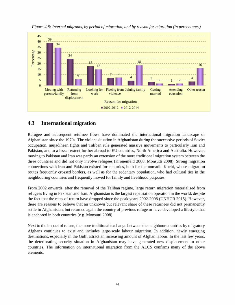
41
Figure 4.8: Internal migrants, by period of migration, and by reason for migration (in percentages)
4.3 International migration
Refugee and subsequent returnee flows have dominated the international migration landscape of
Afghanistan since the 1970s. The violent situation in Afghanistan during the successive periods of Soviet
occupation, mujadiheen fights and Taliban rule generated massive movements to particularly Iran and
Pakistan, and to a lesser extent further abroad to EU countries, North America and Australia. However,
moving to Pakistan and Iran was partly an extension of the more traditional migration system between the
three countries and did not only involve refugees (Kronenfeld 2008, Monsutti 2008). Strong migration
connections with Iran and Pakistan existed for centuries, both for the nomadic Kuchi, whose migration
routes frequently crossed borders, as well as for the sedentary population, who had cultural ties in the
neighbouring countries and frequently moved for family and livelihood purposes.
From 2002 onwards, after the removal of the Taliban regime, large return migration materialised from
refugees living in Pakistan and Iran. Afghanistan is the largest repatriation operation in the world, despite
the fact that the rates of return have dropped since the peak years 2002-2008 (UNHCR 2015). However,
there are reasons to believe that an unknown but relevant share of these returnees did not permanently
settle in Afghanistan, but returned again the country of previous refuge or have developed a lifestyle that
is anchored in both countries (e.g. Monsutti 2008).
Next to the impact of return, the more traditional exchange between the neighbour countries by migratory
Afghans continues to exist and includes large-scale labour migration. In addition, newly emerging
destinations, especially in the Gulf, attract an increasing amount of Afghan labour. In the last few years,
the deteriorating security situation in Afghanistan may have generated new displacement to other
countries. The information on international migration from the ALCS confirms many of the above
elements.
39
24
18
74 3
14
34
6
15
7
18
2 2
16
0
5
10
15
20
25
30
35
40
45
Moving with
parents/family
Returning
from
displacement
Looking for
work
Fleeing from
violence
Joining family Getting
married
Attending
education
Other reason
Per
centa
ge
Reason for migration
2002-2012 2012-2014
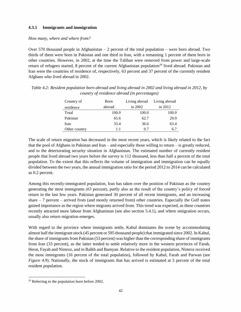
42
4.3.1 Immigrants and immigration
How many, where and where from?
Over 570 thousand people in Afghanistan – 2 percent of the total population – were born abroad. Two
thirds of them were born in Pakistan and one third in Iran, with a remaining 1 percent of them born in
other countries. However, in 2002, at the time the Taliban were removed from power and large-scale
return of refugees started, 8 percent of the current Afghanistan population29 lived abroad. Pakistan and
Iran were the countries of residence of, respectively, 63 percent and 37 percent of the currently resident
Afghans who lived abroad in 2002.
Table 4.2: Resident population born abroad and living abroad in 2002 and living abroad in 2012, by
country of residence abroad (in percentages)
Country of Born Living abroad Living abroad
residence abroad in 2002 in 2012
Total 100.0 100.0 100.0
Pakistan 65.6 62.7 29.9
Iran 33.4 36.6 63.4
Other country 1.1 0.7 6.7
The scale of return migration has decreased in the most recent years, which is likely related to the fact
that the pool of Afghans in Pakistan and Iran – and especially those willing to return – is greatly reduced,
and to the deteriorating security situation in Afghanistan. The estimated number of currently resident
people that lived abroad two years before the survey is 112 thousand, less than half a percent of the total
population. To the extent that this reflects the volume of immigration and immigration can be equally
divided between the two years, the annual immigration ratio for the period 2012 to 2014 can be calculated
as 0.2 percent.
Among this recently-immigrated population, Iran has taken over the position of Pakistan as the country
generating the most immigrants (63 percent), partly also as the result of the country’s policy of forced
return in the last few years. Pakistan generated 30 percent of all recent immigrants, and an increasing
share – 7 percent – arrived from (and mostly returned from) other countries. Especially the Gulf states
gained importance as the region where migrants arrived from. This trend was expected, as these countries
recently attracted more labour from Afghanistan (see also section 5.4.1), and where emigration occurs,
usually also return migration emerges.
With regard to the province where immigrants settle, Kabul dominates the scene by accommodating
almost half the immigrant stock (45 percent or 595 thousand people) that immigrated since 2002. In Kabul,
the share of immigrants from Pakistan (53 percent) was higher than the corresponding share of immigrants
from Iran (33 percent), as the latter tended to settle relatively more in the western provinces of Farah,
Herat, Fayab and Nimroz, and in Balkh and Bamyan. Relative to the resident population, Nimroz received
the most immigrants (16 percent of the total population), followed by Kabul, Farah and Parwan (see
Figure 4.9). Nationally, the stock of immigrants that has arrived is estimated at 5 percent of the total
resident population.
29 Referring to the population born before 2002.
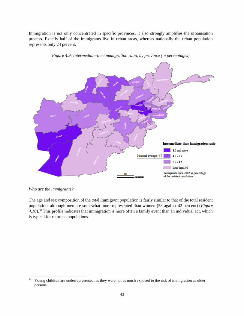
43
Immigration is not only concentrated in specific provinces, it also strongly amplifies the urbanisation
process. Exactly half of the immigrants live in urban areas, whereas nationally the urban population
represents only 24 percent.
Figure 4.9: Intermediate-time immigration ratio, by province (in percentages)
Who are the immigrants?
The age and sex composition of the total immigrant population is fairly similar to that of the total resident
population, although men are somewhat more represented than women (58 against 42 percent) (Figure
4.10).30 This profile indicates that immigration is more often a family event than an individual act, which
is typical for returnee populations.
30 Young children are underrepresented, as they were not as much exposed to the risk of immigration as older
persons.
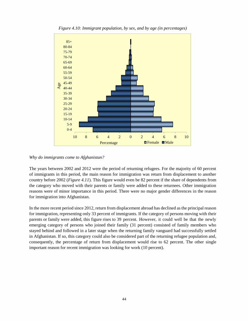
44
Figure 4.10: Immigrant population, by sex, and by age (in percentages)
Why do immigrants come to Afghanistan?
The years between 2002 and 2012 were the period of returning refugees. For the majority of 60 percent
of immigrants in this period, the main reason for immigration was return from displacement to another
country before 2002 (Figure 4.11). This figure would even be 82 percent if the share of dependents from
the category who moved with their parents or family were added to these returnees. Other immigration
reasons were of minor importance in this period. There were no major gender differences in the reason
for immigration into Afghanistan.
In the more recent period since 2012, return from displacement abroad has declined as the principal reason
for immigration, representing only 33 percent of immigrants. If the category of persons moving with their
parents or family were added, this figure rises to 39 percent. However, it could well be that the newly
emerging category of persons who joined their family (31 percent) consisted of family members who
stayed behind and followed in a later stage when the returning family vanguard had successfully settled
in Afghanistan. If so, this category could also be considered part of the returning refugee population and,
consequently, the percentage of return from displacement would rise to 62 percent. The other single
important reason for recent immigration was looking for work (10 percent).
10 8 6 4 2 0 2 4 6 8 10
0-4
5-9
10-14
15-19
20-24
25-29
30-34
35-39
40-44
45-49
50-54
55-59
60-64
65-69
70-74
75-79
80-84
85+
Percentage
Age
Female Male
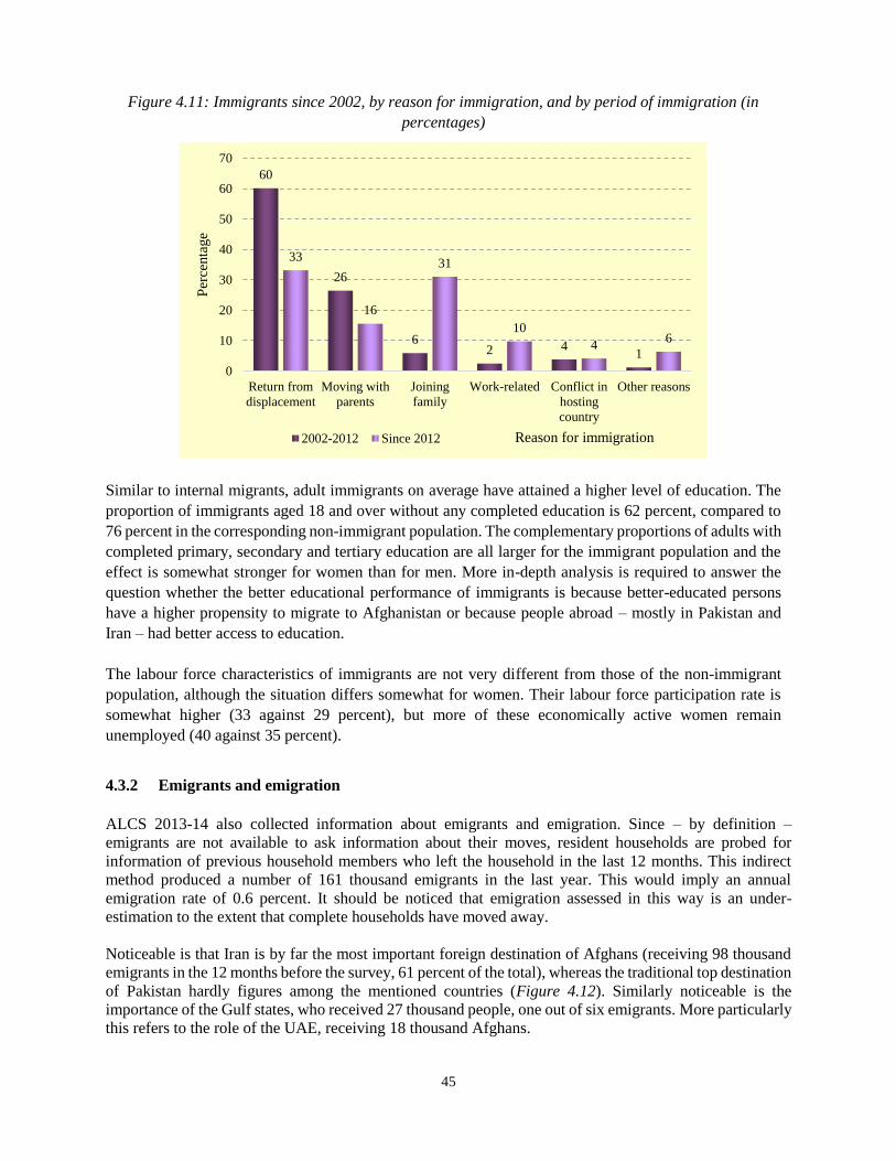
45
Figure 4.11: Immigrants since 2002, by reason for immigration, and by period of immigration (in
percentages)
Similar to internal migrants, adult immigrants on average have attained a higher level of education. The
proportion of immigrants aged 18 and over without any completed education is 62 percent, compared to
76 percent in the corresponding non-immigrant population. The complementary proportions of adults with
completed primary, secondary and tertiary education are all larger for the immigrant population and the
effect is somewhat stronger for women than for men. More in-depth analysis is required to answer the
question whether the better educational performance of immigrants is because better-educated persons
have a higher propensity to migrate to Afghanistan or because people abroad – mostly in Pakistan and
Iran – had better access to education.
The labour force characteristics of immigrants are not very different from those of the non-immigrant
population, although the situation differs somewhat for women. Their labour force participation rate is
somewhat higher (33 against 29 percent), but more of these economically active women remain
unemployed (40 against 35 percent).
4.3.2 Emigrants and emigration
ALCS 2013-14 also collected information about emigrants and emigration. Since – by definition –
emigrants are not available to ask information about their moves, resident households are probed for
information of previous household members who left the household in the last 12 months. This indirect
method produced a number of 161 thousand emigrants in the last year. This would imply an annual
emigration rate of 0.6 percent. It should be noticed that emigration assessed in this way is an under-
estimation to the extent that complete households have moved away.
Noticeable is that Iran is by far the most important foreign destination of Afghans (receiving 98 thousand
emigrants in the 12 months before the survey, 61 percent of the total), whereas the traditional top destination
of Pakistan hardly figures among the mentioned countries (Figure 4.12). Similarly noticeable is the
importance of the Gulf states, who received 27 thousand people, one out of six emigrants. More particularly
this refers to the role of the UAE, receiving 18 thousand Afghans.
60
26
62 4
1
33
16
31
10
46
0
10
20
30
40
50
60
70
Return from
displacement
Moving with
parents
Joining
family
Work-related Conflict in
hosting
country
Other reasons
Per
centa
ge
Reason for immigration2002-2012 Since 2012
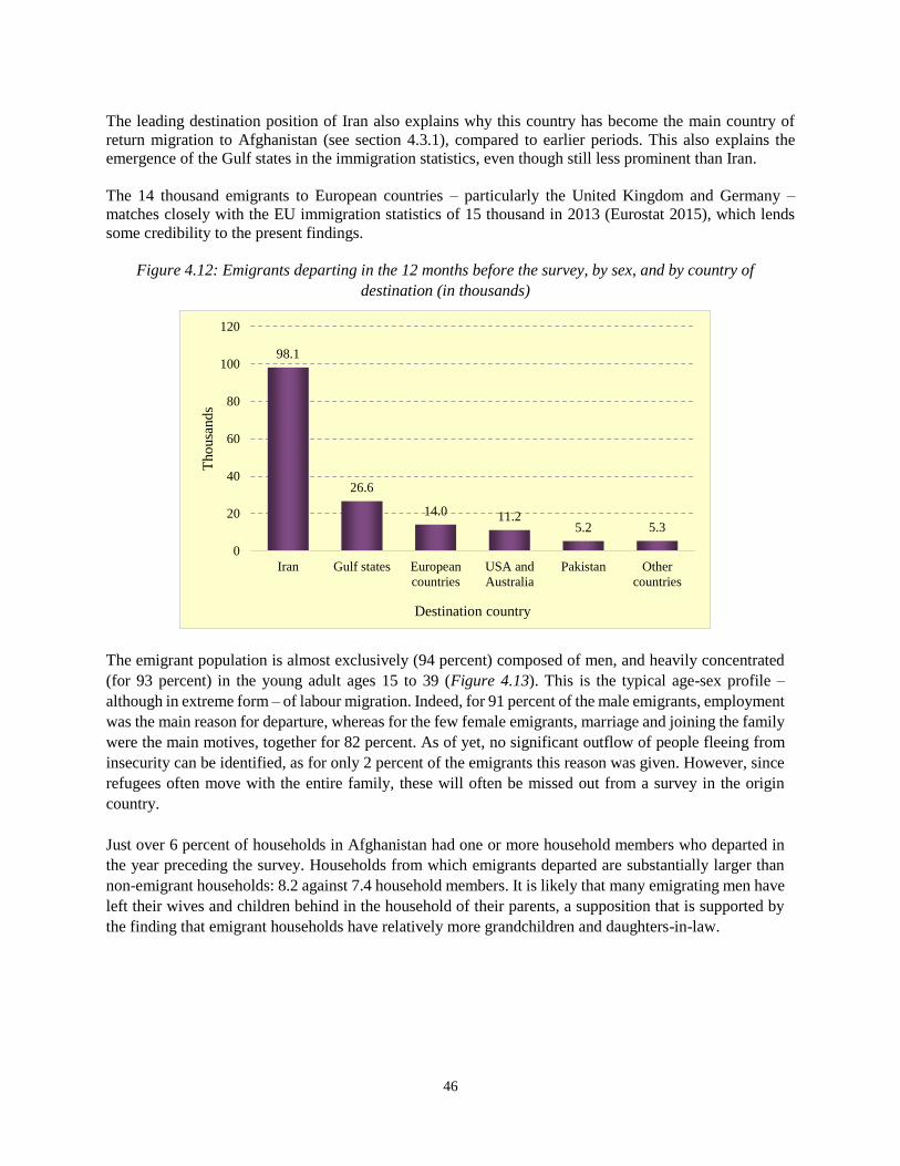
46
The leading destination position of Iran also explains why this country has become the main country of
return migration to Afghanistan (see section 4.3.1), compared to earlier periods. This also explains the
emergence of the Gulf states in the immigration statistics, even though still less prominent than Iran.
The 14 thousand emigrants to European countries – particularly the United Kingdom and Germany –
matches closely with the EU immigration statistics of 15 thousand in 2013 (Eurostat 2015), which lends
some credibility to the present findings.
Figure 4.12: Emigrants departing in the 12 months before the survey, by sex, and by country of
destination (in thousands)
The emigrant population is almost exclusively (94 percent) composed of men, and heavily concentrated
(for 93 percent) in the young adult ages 15 to 39 (Figure 4.13). This is the typical age-sex profile –
although in extreme form – of labour migration. Indeed, for 91 percent of the male emigrants, employment
was the main reason for departure, whereas for the few female emigrants, marriage and joining the family
were the main motives, together for 82 percent. As of yet, no significant outflow of people fleeing from
insecurity can be identified, as for only 2 percent of the emigrants this reason was given. However, since
refugees often move with the entire family, these will often be missed out from a survey in the origin
country.
Just over 6 percent of households in Afghanistan had one or more household members who departed in
the year preceding the survey. Households from which emigrants departed are substantially larger than
non-emigrant households: 8.2 against 7.4 household members. It is likely that many emigrating men have
left their wives and children behind in the household of their parents, a supposition that is supported by
the finding that emigrant households have relatively more grandchildren and daughters-in-law.
98.1
26.6
14.0 11.25.2 5.3
0
20
40
60
80
100
120
Iran Gulf states European
countries
USA and
Australia
Pakistan Other
countries
Tho
usa
nd
s
Destination country
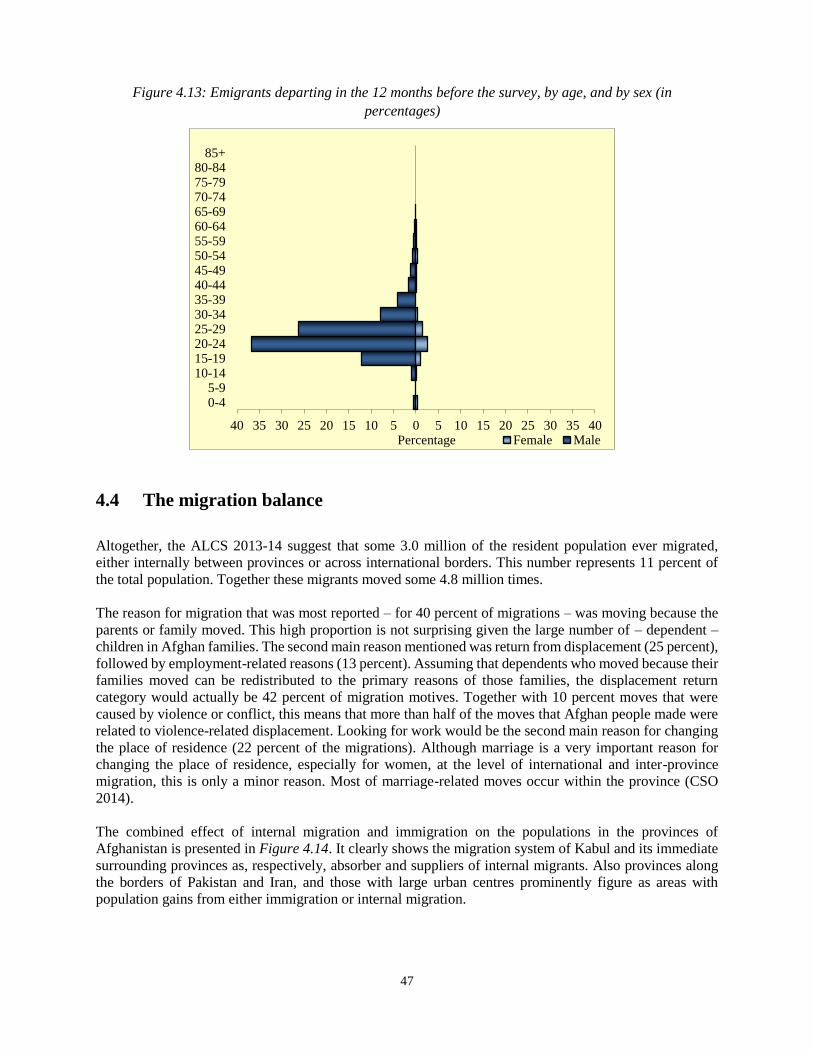
47
Figure 4.13: Emigrants departing in the 12 months before the survey, by age, and by sex (in
percentages)
4.4 The migration balance
Altogether, the ALCS 2013-14 suggest that some 3.0 million of the resident population ever migrated,
either internally between provinces or across international borders. This number represents 11 percent of
the total population. Together these migrants moved some 4.8 million times.
The reason for migration that was most reported – for 40 percent of migrations – was moving because the
parents or family moved. This high proportion is not surprising given the large number of – dependent –
children in Afghan families. The second main reason mentioned was return from displacement (25 percent),
followed by employment-related reasons (13 percent). Assuming that dependents who moved because their
families moved can be redistributed to the primary reasons of those families, the displacement return
category would actually be 42 percent of migration motives. Together with 10 percent moves that were
caused by violence or conflict, this means that more than half of the moves that Afghan people made were
related to violence-related displacement. Looking for work would be the second main reason for changing
the place of residence (22 percent of the migrations). Although marriage is a very important reason for
changing the place of residence, especially for women, at the level of international and inter-province
migration, this is only a minor reason. Most of marriage-related moves occur within the province (CSO
2014).
The combined effect of internal migration and immigration on the populations in the provinces of
Afghanistan is presented in Figure 4.14. It clearly shows the migration system of Kabul and its immediate
surrounding provinces as, respectively, absorber and suppliers of internal migrants. Also provinces along
the borders of Pakistan and Iran, and those with large urban centres prominently figure as areas with
population gains from either immigration or internal migration.
40 35 30 25 20 15 10 5 0 5 10 15 20 25 30 35 40
0-45-9
10-1415-1920-2425-2930-3435-3940-4445-4950-5455-5960-6465-6970-7475-7980-84
85+
Percentage Female Male
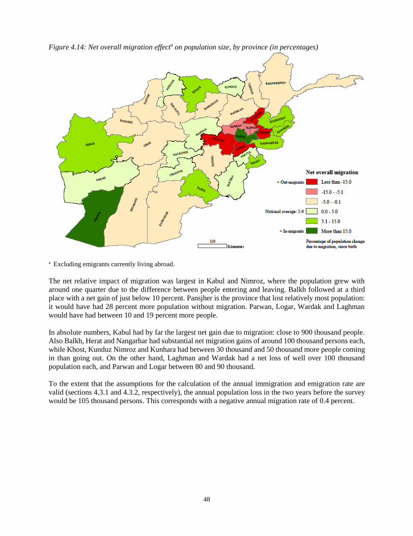
48
Figure 4.14: Net overall migration effecta on population size, by province (in percentages)
a Excluding emigrants currently living abroad.
The net relative impact of migration was largest in Kabul and Nimroz, where the population grew with
around one quarter due to the difference between people entering and leaving. Balkh followed at a third
place with a net gain of just below 10 percent. Pansjher is the province that lost relatively most population:
it would have had 28 percent more population without migration. Parwan, Logar, Wardak and Laghman
would have had between 10 and 19 percent more people.
In absolute numbers, Kabul had by far the largest net gain due to migration: close to 900 thousand people.
Also Balkh, Herat and Nangarhar had substantial net migration gains of around 100 thousand persons each,
while Khost, Kunduz Nimroz and Kunhara had between 30 thousand and 50 thousand more people coming
in than going out. On the other hand, Laghman and Wardak had a net loss of well over 100 thousand
population each, and Parwan and Logar between 80 and 90 thousand.
To the extent that the assumptions for the calculation of the annual immigration and emigration rate are
valid (sections 4.3.1 and 4.3.2, respectively), the annual population loss in the two years before the survey
would be 105 thousand persons. This corresponds with a negative annual migration rate of 0.4 percent.
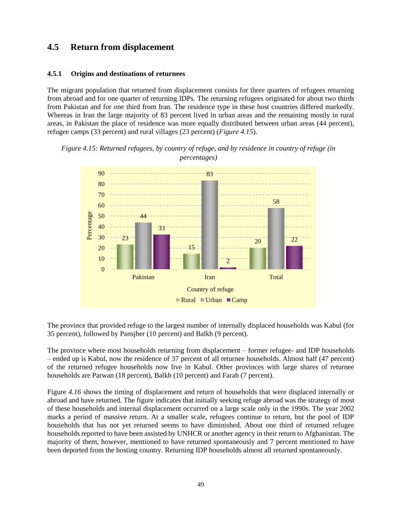
49
4.5 Return from displacement
4.5.1 Origins and destinations of returnees
The migrant population that returned from displacement consists for three quarters of refugees returning
from abroad and for one quarter of returning IDPs. The returning refugees originated for about two thirds
from Pakistan and for one third from Iran. The residence type in these host countries differed markedly.
Whereas in Iran the large majority of 83 percent lived in urban areas and the remaining mostly in rural
areas, in Pakistan the place of residence was more equally distributed between urban areas (44 percent),
refugee camps (33 percent) and rural villages (23 percent) (Figure 4.15).
Figure 4.15: Returned refugees, by country of refuge, and by residence in country of refuge (in
percentages)
The province that provided refuge to the largest number of internally displaced households was Kabul (for
35 percent), followed by Pansjher (10 percent) and Balkh (9 percent).
The province where most households returning from displacement – former refugee- and IDP households
– ended up is Kabul, now the residence of 37 percent of all returnee households. Almost half (47 percent)
of the returned refugee households now live in Kabul. Other provinces with large shares of returnee
households are Parwan (18 percent), Balkh (10 percent) and Farah (7 percent).
Figure 4.16 shows the timing of displacement and return of households that were displaced internally or
abroad and have returned. The figure indicates that initially seeking refuge abroad was the strategy of most
of these households and internal displacement occurred on a large scale only in the 1990s. The year 2002
marks a period of massive return. At a smaller scale, refugees continue to return, but the pool of IDP
households that has not yet returned seems to have diminished. About one third of returned refugee
households reported to have been assisted by UNHCR or another agency in their return to Afghanistan. The
majority of them, however, mentioned to have returned spontaneously and 7 percent mentioned to have
been deported from the hosting country. Returning IDP households almost all returned spontaneously.
23
1520
44
83
58
33
2
22
0
10
20
30
40
50
60
70
80
90
Pakistan Iran Total
Per
centa
ge
Country of refuge
Rural Urban Camp
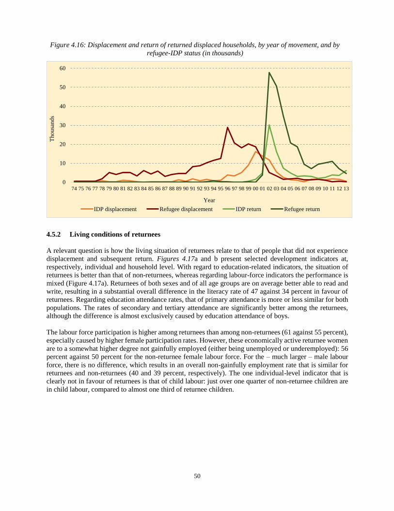
50
Figure 4.16: Displacement and return of returned displaced households, by year of movement, and by
refugee-IDP status (in thousands)
4.5.2 Living conditions of returnees
A relevant question is how the living situation of returnees relate to that of people that did not experience
displacement and subsequent return. Figures 4.17a and b present selected development indicators at,
respectively, individual and household level. With regard to education-related indicators, the situation of
returnees is better than that of non-returnees, whereas regarding labour-force indicators the performance is
mixed (Figure 4.17a). Returnees of both sexes and of all age groups are on average better able to read and
write, resulting in a substantial overall difference in the literacy rate of 47 against 34 percent in favour of
returnees. Regarding education attendance rates, that of primary attendance is more or less similar for both
populations. The rates of secondary and tertiary attendance are significantly better among the returnees,
although the difference is almost exclusively caused by education attendance of boys.
The labour force participation is higher among returnees than among non-returnees (61 against 55 percent),
especially caused by higher female participation rates. However, these economically active returnee women
are to a somewhat higher degree not gainfully employed (either being unemployed or underemployed): 56
percent against 50 percent for the non-returnee female labour force. For the – much larger – male labour
force, there is no difference, which results in an overall non-gainfully employment rate that is similar for
returnees and non-returnees (40 and 39 percent, respectively). The one individual-level indicator that is
clearly not in favour of returnees is that of child labour: just over one quarter of non-returnee children are
in child labour, compared to almost one third of returnee children.
0
10
20
30
40
50
60
74 75 76 77 78 79 80 81 82 83 84 85 86 87 88 89 90 91 92 93 94 95 96 97 98 99 00 01 02 03 04 05 06 07 08 09 10 11 12 13
Tho
usa
nd
s
Year
IDP displacement Refugee displacement IDP return Refugee return
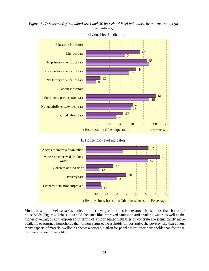
51
Figure 4.17: Selected (a) individual-level and (b) household-level indicators, by returnee status (in
percentages)
a. Individual-level indicators
b. Household-level indicators
Most household-level variables indicate better living conditions for returnee households than for other
households (Figure 4.17b). Household facilities like improved sanitation and drinking water, as well as the
higher dwelling quality expressed in terms of a floor sealed with tiles or concrete are significantly more
available to returnee households than to non-returnee households. Importantly, the poverty rate that covers
many aspects of material wellbeing shows a better situation for people in returnee households than for those
in non-returnee households.
26
39
55
8
37
55
34
32
40
61
12
44
53
47
0 10 20 30 40 50 60 70
Child labour rate
Not gainfully employment rate
Labour force participation rate
Labour indicators
Net tertiary attendance rate
Net secondary attendance rate
Net primary attendance rate
Literacy rate
Education indicators
PercentageReturnees Other population
15
31
13
62
36
15
40
27
73
62
0 10 20 30 40 50 60 70 80
Economic situation improved
Poverty rate
Concrete or tiled floor
Access to improved drinking
water
Access to improved sanitation
PercentageReturnee households Other households

52
It is likely that the type of residence is an important explanatory factor for the generally better situation of
returnees, as they live almost twice as often in urban areas than non-returnees.
53
5 LABOUR MARKET OUTCOMES
Summary. The chapter on labour market outcomes tabulates and analyses labour market indicators on the
basis of the new national definitions first used in the report on NRVA 2011-12 (CSO 2014). The analysis
suggests that Afghanistan’s labour market is under considerable stress. Slightly more than two thirds of the
labour force of 8.5 million is less than 40 years of age. Two fifths remains not gainfully employed
(underemployed or unemployed) and 79 percent is in vulnerable employment. Meanwhile, a total of 6.8
million Afghans in the working age, mainly women (5.3 million), do not participate at all. Agriculture
accounts for two fifths of all employment, manufacturing for less than a tenth, while the recently more
dynamic trade, transport, finance, real estate and insurance sectors account for a little less than a fifth. An
overwhelming 61 percent of all employed have not been to school and only ten percent have attended school
up to primary level. Consequently, nine tenths of the employed workforce is in unskilled occupations.
Gender differences in labour market outcomes are stark: while participation rates are low (29 percent),
unpaid family work and agriculture account for at least two thirds of female employment, and women’s
mean and median monthly earnings are much lower than men’s in equivalent occupations. Comparison of
labour indicators between 2007-08 and 2012-13 suggests that there has been a large shift of the labour
force from working to unemployed, particularly in the urban sector. A substantial slowdown in growth
constrained by persistent uncertainty surrounding political and security transition, increased levels of
conflict and a downturn in aid, are likely to be underlying factors.
Four percent of Afghans of working age have migrated to their current place of residence for employment,
either from within Afghanistan (87 percent) or from abroad. (13 percent). While a disproportionally large
share of internal labour migrants consists of the nomadic Kuchi, two thirds of the sedentary (non-Kuchi)
migrants have moved to Kabul province. Almost two-thirds of all sedentary internal migrants move from
rural to urban areas, with only a very small proportion of 4 percent moving in the opposite direction.
Internal labour migrants tend to be male (77 percent) and are distributed fairly evenly among different age
cohorts, while labour emigrants are almost all male, and more than two thirds of them are in their twenties.
Of the traditional labour migration destinations – Pakistan and Iran – the former has lost much of its appeal
to migrants. On the other hand, the Gulf states have emerged as important labour migration destinations.
Labour migrants appear to be better educated, and males at least perform much better in the labour market
than the general population: a greater proportion of internal male migrants were gainfully employed, found
better jobs, and earned more, although male immigrants were less successful in finding gainful employment
and had higher rates of unemployment. In contrast, women’s labour market prospects appear to have
worsened with migration: 74 percent of internal migrants and even 83 percent of immigrants remained
inactive after migration. Even the prospects of male Kuchi labour migrants are bleak. They earn only 45
percent of the earnings of sedentary labour migrants, likely because of very low levels of human capital.
High rates of child labour in Afghanistan also reflect the extent to which its labour market is stressed.
Slightly more than a quarter of all children between the ages of 5 and 17, that is 2.7 million children or 27
percent, are engaged in child labour according to ILO’s definitions. This is one of the highest rates of child
labour in the world. Of this number of children, 46 percent are between 5 and 11 years of age. In every age
cohort, more boys are engaged in child labour than are girls, and the gender difference increases with age.
Of course, if household work is also taken into account, as in the UNICEF definition, the child labour rate
among girls rises from 20 percent to 24 percent and for boys and girls together, it rises to 29 percent. While
a higher proportion of boys than girls are exposed to hazardous conditions, at least half of all child
labourers, more boys (61 percent) than girls (53 percent), are exposed to dust, gas and fumes. A similar
proportion of labouring boys, but a marginally higher proportion of girls is exposed to extreme cold, heat
or humidity. Meanwhile, 43 percent of boys and 38 percent of girls who have undertaken child labour have
been injured or have fallen ill as a result of the work he or she had been doing. While 40 percent of boys
54
who did not attend school cited the need to work as the main reason, 37 percent of girls who did not attend
school did not do so because they were not allowed to. While child labour is strongly associated with
household poverty, engaging in child labour perpetuates the cycle of poverty, as working children are
unable to acquire necessary skills and remain healthy, which are in turn likely to retard their capacity to
earn enough to get out of poverty themselves in the future.
The analysis suggests that both demand and supply side measures are necessary to promote the growth of
decent employment opportunities in Afghanistan. The demand for labour needs to be increased through the
aggressive promotion of entrepreneurship and small businesses catering to export markets as well as to
domestic and local markets. The agricultural sector needs to be made more productive by providing better
inputs, such as improved seeds and fertilizer; storage facilities; creating functioning local markets; and
rebuilding transport and communication networks to access more distant markets. At the same time,
workers must also be equipped with demand-driven skills so that they can create productive self-
employment opportunities, or else take up the job opportunities created by a growing business class.
5.1 Introduction
Most Afghan households depend on the market work of their members for income to meet basic needs.
Rent, forms of zakat and remittances from household members who have moved elsewhere for work are
also useful sources of additional income for some. But the vast majority of Afghans get by with subsistence-
level productive activities, family work, or precarious, informal work where very long or very few hours
are the norm. Therefore, standard labour market indicators used for international comparisons cannot
adequately capture the true nature of employment outcomes in Afghanistan. Hence, beginning with the
report National Risk and Vulnerability Assessment 2011-12 (CSO 2014), the CSO has developed and used
definitions that yield a more nuanced picture of Afghanistan’s labour market. Accordingly, this report too
tabulates and analyses labour market indicators on the basis of the new national definitions which are set
out in Table 5.1 below, along with the corresponding international definitions.
The most fundamental choice that Afghans of working age face in the labour market is whether to engage
in market work or not, that is, whether or not to participate in the labour market. Those who decide to
participate in the labour market face two outcomes: they may find employment that they are willing to take
up – in which case they become part of the employed workforce, or they may not, in which case they will
continue to seek work and will be regarded as unemployed. However, those who take up work experience
a further set of employment outcomes: they may be working at least eight hours a week and may be satisfied
with that, in which case they are regarded as being gainfully employed. Alternatively, they may be working
less than 40 hours a week and be willing and available to work additional hours, in which case they are
considered underemployed. All those who are willing and able to work more than their current levels of
engagement are those who are not gainfully employed. Thus, the underemployed and the unemployed
together constitute that part of the labour force which is not gainfully employed. In seeking employment,
however, individuals may migrate from either the place of their birth, or from other locations to which they
had previously migrated looking for work. They may also undertake to migrate seasonally for purposes of
employment. This migrant workforce is an important subset of the country’s labour force.
This chapter on labour market outcomes in Afghanistan is organised according to this basic framework of
participation decisions and employment outcomes. Thus, section 5.2 describes the initial choice that
Afghans of working age have made in whether or not to participate in the labour force, and estimates stocks
and shares by sex, age cohort and residence. Section 5.3 first presents an overview of employment,
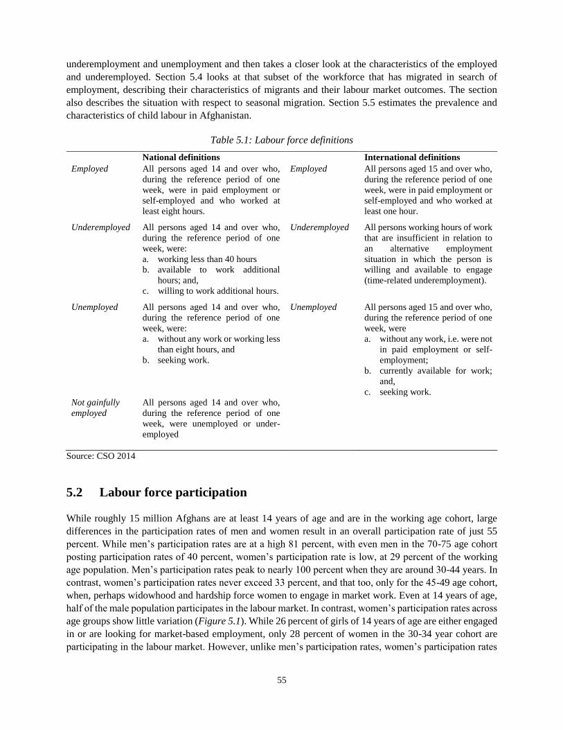
55
underemployment and unemployment and then takes a closer look at the characteristics of the employed
and underemployed. Section 5.4 looks at that subset of the workforce that has migrated in search of
employment, describing their characteristics of migrants and their labour market outcomes. The section
also describes the situation with respect to seasonal migration. Section 5.5 estimates the prevalence and
characteristics of child labour in Afghanistan.
Table 5.1: Labour force definitions
National definitions International definitions
Employed All persons aged 14 and over who,
during the reference period of one
week, were in paid employment or
self-employed and who worked at
least eight hours.
Employed All persons aged 15 and over who,
during the reference period of one
week, were in paid employment or
self-employed and who worked at
least one hour.
Underemployed All persons aged 14 and over who,
during the reference period of one
week, were:
a. working less than 40 hours
b. available to work additional
hours; and,
c. willing to work additional hours.
Underemployed All persons working hours of work
that are insufficient in relation to
an alternative employment
situation in which the person is
willing and available to engage
(time-related underemployment).
Unemployed All persons aged 14 and over who,
during the reference period of one
week, were:
Unemployed All persons aged 15 and over who,
during the reference period of one
week, were
a. without any work or working less
than eight hours, and
b. seeking work.
a. without any work, i.e. were not
in paid employment or self-
employment;
b. currently available for work;
and,
c. seeking work.
Not gainfully
employed
All persons aged 14 and over who,
during the reference period of one
week, were unemployed or under-
employed
Source: CSO 2014
5.2 Labour force participation While roughly 15 million Afghans are at least 14 years of age and are in the working age cohort, large
differences in the participation rates of men and women result in an overall participation rate of just 55
percent. While men’s participation rates are at a high 81 percent, with even men in the 70-75 age cohort
posting participation rates of 40 percent, women’s participation rate is low, at 29 percent of the working
age population. Men’s participation rates peak to nearly 100 percent when they are around 30-44 years. In
contrast, women’s participation rates never exceed 33 percent, and that too, only for the 45-49 age cohort,
when, perhaps widowhood and hardship force women to engage in market work. Even at 14 years of age,
half of the male population participates in the labour market. In contrast, women’s participation rates across
age groups show little variation (Figure 5.1). While 26 percent of girls of 14 years of age are either engaged
in or are looking for market-based employment, only 28 percent of women in the 30-34 year cohort are
participating in the labour market. However, unlike men’s participation rates, women’s participation rates
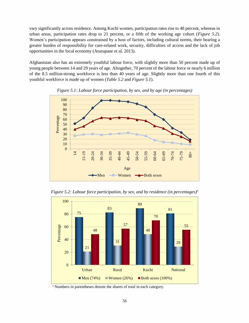
56
vary significantly across residence. Among Kuchi women, participation rates rise to 48 percent, whereas in
urban areas, participation rates drop to 21 percent, or a fifth of the working age cohort (Figure 5.2).
Women’s participation appears constrained by a host of factors, including cultural norms, their bearing a
greater burden of responsibility for care-related work, security, difficulties of access and the lack of job
opportunities in the local economy (Aturupane et al. 2013).
Afghanistan also has an extremely youthful labour force, with slightly more than 50 percent made up of
young people between 14 and 29 years of age. Altogether, 70 percent of the labour force or nearly 6 million
of the 8.5 million-strong workforce is less than 40 years of age. Slightly more than one fourth of this
youthful workforce is made up of women (Table 5.2 and Figure 5.1).
Figure 5.1: Labour force participation, by sex, and by age (in percentages)
Figure 5.2: Labour force participation, by sex, and by residence (in percentages)a
a Numbers in parentheses denote the shares of total in each category.
0
10
20
30
40
50
60
70
80
90
100
14
15-1
9
20-2
4
30-3
4
35-3
9
40-4
4
45-4
9
50-5
4
55-5
9
60-6
4
65-6
9
70-7
4
75-7
9
80+
Per
centa
ge
Age
Men Women Both sexes
75
8389
81
21
31
48
29
48
57
70
55
0
20
40
60
80
100
Urban Rural Kuchi National
Per
centa
ge
Men (74%) Women (26%) Both sexes (100%)
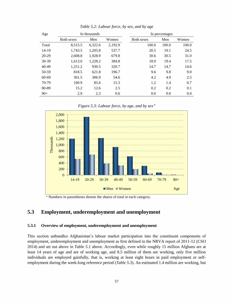
57
Table 5.2: Labour force, by sex, and by age
Age In thousands In percentages
Both sexes Men Women Both sexes Men Women
Total 8,515.5 6,322.6 2,192.9 100.0 100.0 100.0
14-19 1,743.5 1,205.8 537.7 20.5 19.1 24.5
20-29 2,608.8 1,928.9 679.8 30.6 30.5 31.0
30-39 1,613.0 1,228.2 384.8 18.9 19.4 17.5
40-49 1,251.2 930.5 320.7 14.7 14.7 14.6
50-59 818.5 621.8 196.7 9.6 9.8 9.0
60-69 361.5 306.9 54.6 4.2 4.9 2.5
70-79 100.9 85.6 15.3 1.2 1.4 0.7
80-89 15.2 12.6 2.5 0.2 0.2 0.1
90+ 2.9 2.3 0.6 0.0 0.0 0.0
Figure 5.3: Labour force, by age, and by sex a
a Numbers in parentheses denote the shares of total in each category.
5.3 Employment, underemployment and unemployment
5.3.1 Overview of employment, underemployment and unemployment
This section unbundles Afghanistan’s labour market participation into the constituent components of
employment, underemployment and unemployment as first defined in the NRVA report of 2011-12 (CSO
2014) and set out above in Table 5.1 above. Accordingly, even while roughly 15 million Afghans are at
least 14 years of age and are of working age, and 8.5 million of them are working, only five million
individuals are employed gainfully, that is, working at least eight hours in paid employment or self-
employment during the week-long reference period (Table 5.3). An estimated 1.4 million are working, but
0
200
400
600
800
1,000
1,200
1,400
1,600
1,800
2,000
14-19 20-29 30-39 40-49 50-59 60-69 70-79 80+
Tho
usa
nd
s
AgeMen Women
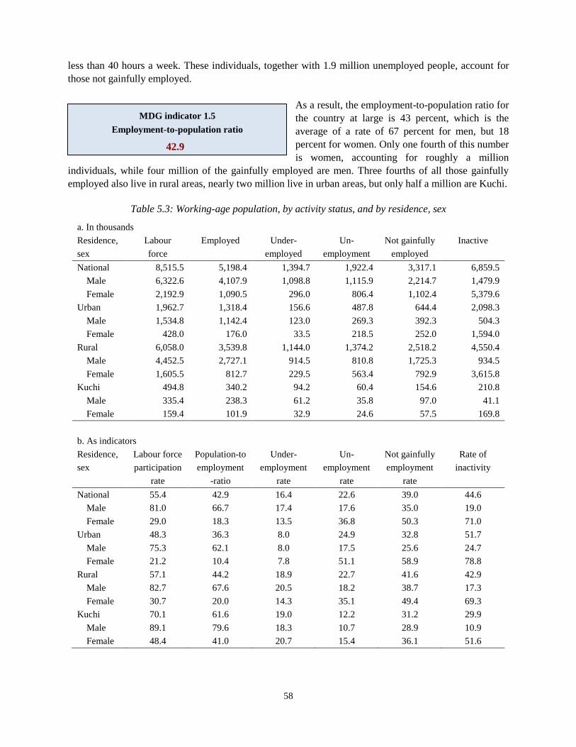
58
less than 40 hours a week. These individuals, together with 1.9 million unemployed people, account for
those not gainfully employed.
As a result, the employment-to-population ratio for
the country at large is 43 percent, which is the
average of a rate of 67 percent for men, but 18
percent for women. Only one fourth of this number
is women, accounting for roughly a million
individuals, while four million of the gainfully employed are men. Three fourths of all those gainfully
employed also live in rural areas, nearly two million live in urban areas, but only half a million are Kuchi.
Table 5.3: Working-age population, by activity status, and by residence, sex
a. In thousands
Residence, Labour Employed Under- Un- Not gainfully Inactive
sex force employed employment employed
National 8,515.5 5,198.4 1,394.7 1,922.4 3,317.1 6,859.5
Male 6,322.6 4,107.9 1,098.8 1,115.9 2,214.7 1,479.9
Female 2,192.9 1,090.5 296.0 806.4 1,102.4 5,379.6
Urban 1,962.7 1,318.4 156.6 487.8 644.4 2,098.3
Male 1,534.8 1,142.4 123.0 269.3 392.3 504.3
Female 428.0 176.0 33.5 218.5 252.0 1,594.0
Rural 6,058.0 3,539.8 1,144.0 1,374.2 2,518.2 4,550.4
Male 4,452.5 2,727.1 914.5 810.8 1,725.3 934.5
Female 1,605.5 812.7 229.5 563.4 792.9 3,615.8
Kuchi 494.8 340.2 94.2 60.4 154.6 210.8
Male 335.4 238.3 61.2 35.8 97.0 41.1
Female 159.4 101.9 32.9 24.6 57.5 169.8
b. As indicators
Residence, Labour force Population-to Under- Un- Not gainfully Rate of
sex participation employment employment employment employment inactivity
rate -ratio rate rate rate
National 55.4 42.9 16.4 22.6 39.0 44.6
Male 81.0 66.7 17.4 17.6 35.0 19.0
Female 29.0 18.3 13.5 36.8 50.3 71.0
Urban 48.3 36.3 8.0 24.9 32.8 51.7
Male 75.3 62.1 8.0 17.5 25.6 24.7
Female 21.2 10.4 7.8 51.1 58.9 78.8
Rural 57.1 44.2 18.9 22.7 41.6 42.9
Male 82.7 67.6 20.5 18.2 38.7 17.3
Female 30.7 20.0 14.3 35.1 49.4 69.3
Kuchi 70.1 61.6 19.0 12.2 31.2 29.9
Male 89.1 79.6 18.3 10.7 28.9 10.9
Female 48.4 41.0 20.7 15.4 36.1 51.6
MDG indicator 1.5
Employment-to-population ratio
42.9
59
In contrast, 39 percent of Afghanistan’s labour force is not gainfully employed, and this rate rises to 50
percent for women, and drops to 35 percent of the male workforce. These individuals were either
unemployed, that is looking for work, without having anything more than eight hours of work a week, or
underemployed, that is working less than 40 hours a week, but available and willing to work additional
hours. While the total number of males not gainfully employed is made up of almost equal numbers of
underemployed and unemployed individuals, proportionately more women were unemployed (37 percent)
than unemployed (14 percent). But this is because relatively more women in urban and rural areas are
unemployed than underemployed, whereas more Kuchi women were underemployed (21 percent) than
unemployed (15 percent). The problem of not being gainfully employed is most marked in rural areas,
where the rate jumps to 42 percent. It is somewhat lower for the Kuchi population at 31 percent, but the
proportion of individuals not gainfully employed even in urban areas is quite high at 33 percent.
Figure 5.4 shows how Afghan men and women of working age are distributed across the main economic
activities of employment, underemployment, unemployment and non-participation. Very high rates of non-
participation are evident across the age spectrum in the panel showing the female working-age population
by activity status. However, the proportion in each age cohort which is not gainfully employed is much
larger among males, significantly more of whom are, in any case, actively engaged in the labour market.
The ANDS uses the youth unemployment rate (the
unemployed persons aged 15-24 as a percentage of
the labour force in the corresponding age group) as
an indicator for the effectuation of decent work for
youth (MDG 8: Develop a global partnership for
development). Young people tend to be more vulnerable and disillusioned about livelihood opportunities,
which negatively affect the ability of young people to embark on an independent and full life course.
Widespread youth unemployment may also be an important cause of social unrest, affecting communities
and the society at large. In 2013-14, the youth unemployment rate was as high as 27 percent, 22 percent for
males and even 41 for females. These young unemployed individuals made up 28 percent of the total
unemployed population.
Unemployment and underemployment
In poor developing countries such as Afghanistan, being unemployed is not an option that the majority
of people can afford to be. Only those with financial resources or family support can manage to be openly
unemployed, that is being completely without work during the reference period but being available for
work and actually seeking it. Consequently only a small proportion of the labour force is usually found
to be unemployed according to this definition. In contrast, the vast majority of Afghans are forced to
take up any low-productivity employment without social security or unemployment insurance, even if it
is for a few hours no matter how poorly paid. Hence, in Afghanistan, underemployment rates are often
more relevant than unemployment rates, and the concept of being gainfully employed is more useful in
describing individuals who need more or other employment in order to provide for sufficient and
sustainable income or livelihood. In fact, the analysis of poverty in Chapter 7 of this report suggests that
that people living in households headed by an unemployed or underemployed person are significantly
more likely to be poor than those in households where the household head is employed.
ANDS target 17, MDG indicator 42
Youth unemployment rate
27.4 percent
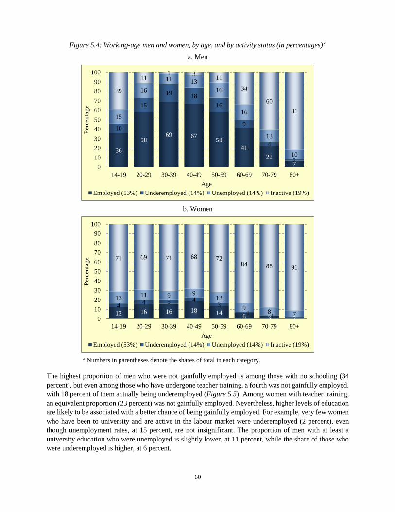
60
Figure 5.4: Working-age men and women, by age, and by activity status (in percentages) a
a. Men
b. Women
a Numbers in parentheses denote the shares of total in each category.
The highest proportion of men who were not gainfully employed is among those with no schooling (34
percent), but even among those who have undergone teacher training, a fourth was not gainfully employed,
with 18 percent of them actually being underemployed (Figure 5.5). Among women with teacher training,
an equivalent proportion (23 percent) was not gainfully employed. Nevertheless, higher levels of education
are likely to be associated with a better chance of being gainfully employed. For example, very few women
who have been to university and are active in the labour market were underemployed (2 percent), even
though unemployment rates, at 15 percent, are not insignificant. The proportion of men with at least a
university education who were unemployed is slightly lower, at 11 percent, while the share of those who
were underemployed is higher, at 6 percent.
36
5869 67
58
41
22
7
10
15
19 18
16
9
4
2
15
16
11 13
16
16
13
10
39
111 3
11
34
60
81
0
10
20
30
40
50
60
70
80
90
100
14-19 20-29 30-39 40-49 50-59 60-69 70-79 80+
Per
centa
ge
Age
Employed (53%) Underemployed (14%) Unemployed (14%) Inactive (19%)
12 16 16 18 146 3 2
44 5 4
3
11
13 11 9 912
98 7
71 69 71 68 7284 88 91
0
10
20
30
40
50
60
70
80
90
100
14-19 20-29 30-39 40-49 50-59 60-69 70-79 80+
Per
centa
ge
Age
Employed (53%) Underemployed (14%) Unemployed (14%) Inactive (19%)
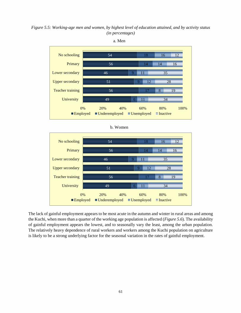
61
Figure 5.5: Working-age men and women, by highest level of education attained, and by activity status
(in percentages)
a. Men
b. Women
The lack of gainful employment appears to be most acute in the autumn and winter in rural areas and among
the Kuchi, when more than a quarter of the working age population is affected (Figure 5.6). The availability
of gainful employment appears the lowest, and to seasonally vary the least, among the urban population.
The relatively heavy dependence of rural workers and workers among the Kuchi population on agriculture
is likely to be a strong underlying factor for the seasonal variation in the rates of gainful employment.
54
56
46
51
56
49
18
14
9
9
17
6
16
14
11
12
8
11
12
16
35
28
19
34
0% 20% 40% 60% 80% 100%
No schooling
Primary
Lower secondary
Upper secondary
Teacher training
University
Employed Underemployed Unemployed Inactive
54
56
46
51
56
49
18
14
9
9
17
6
16
14
11
12
8
11
12
16
35
28
19
34
0% 20% 40% 60% 80% 100%
No schooling
Primary
Lower secondary
Upper secondary
Teacher training
University
Employed Underemployed Unemployed Inactive
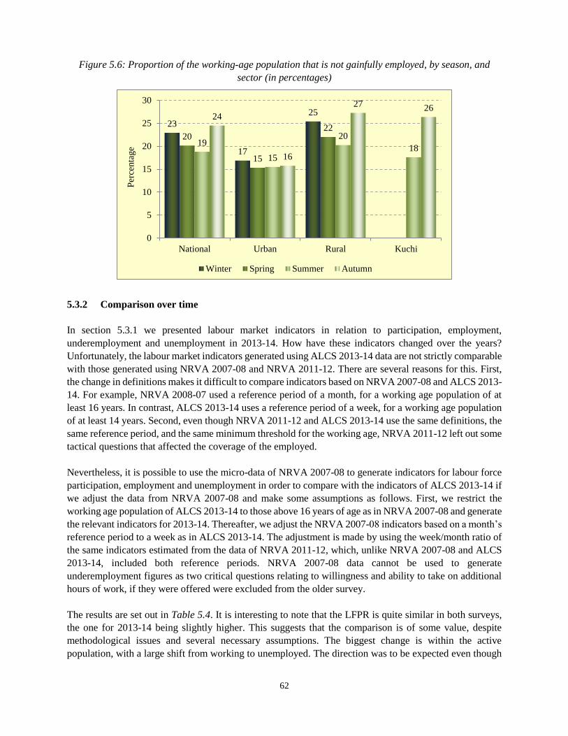
62
Figure 5.6: Proportion of the working-age population that is not gainfully employed, by season, and
sector (in percentages)
5.3.2 Comparison over time
In section 5.3.1 we presented labour market indicators in relation to participation, employment,
underemployment and unemployment in 2013-14. How have these indicators changed over the years?
Unfortunately, the labour market indicators generated using ALCS 2013-14 data are not strictly comparable
with those generated using NRVA 2007-08 and NRVA 2011-12. There are several reasons for this. First,
the change in definitions makes it difficult to compare indicators based on NRVA 2007-08 and ALCS 2013-
14. For example, NRVA 2008-07 used a reference period of a month, for a working age population of at
least 16 years. In contrast, ALCS 2013-14 uses a reference period of a week, for a working age population
of at least 14 years. Second, even though NRVA 2011-12 and ALCS 2013-14 use the same definitions, the
same reference period, and the same minimum threshold for the working age, NRVA 2011-12 left out some
tactical questions that affected the coverage of the employed.
Nevertheless, it is possible to use the micro-data of NRVA 2007-08 to generate indicators for labour force
participation, employment and unemployment in order to compare with the indicators of ALCS 2013-14 if
we adjust the data from NRVA 2007-08 and make some assumptions as follows. First, we restrict the
working age population of ALCS 2013-14 to those above 16 years of age as in NRVA 2007-08 and generate
the relevant indicators for 2013-14. Thereafter, we adjust the NRVA 2007-08 indicators based on a month’s
reference period to a week as in ALCS 2013-14. The adjustment is made by using the week/month ratio of
the same indicators estimated from the data of NRVA 2011-12, which, unlike NRVA 2007-08 and ALCS
2013-14, included both reference periods. NRVA 2007-08 data cannot be used to generate
underemployment figures as two critical questions relating to willingness and ability to take on additional
hours of work, if they were offered were excluded from the older survey.
The results are set out in Table 5.4. It is interesting to note that the LFPR is quite similar in both surveys,
the one for 2013-14 being slightly higher. This suggests that the comparison is of some value, despite
methodological issues and several necessary assumptions. The biggest change is within the active
population, with a large shift from working to unemployed. The direction was to be expected even though
23
17
25
20
15
22
19
15
20
18
24
16
27 26
0
5
10
15
20
25
30
National Urban Rural Kuchi
Per
centa
ge
Winter Spring Summer Autumn
63
the change appears rather large. This is because the economy has experienced a substantial slowdown in
growth constrained by persistent uncertainty surrounding political and security transition, increased levels
of conflict and a downturn in aid. The change is also more pronounced in urban areas than in rural areas,
and is insignificant for Kuchis. This urban-rural-Kuchi pattern is again plausible, given the reduction of
foreign aid, foreign organisations and troops, which is most likely to have first affected urban residents’
employment, and secondly, and often more indirectly, rural employment; the Kuchi, being much less
involved in the paid market economy were probably the least affected. Also, people who depended on the
employment related to foreign presence may also be better able to be – for some time at least – unemployed,
rather than underemployed. With time, however, we may expect the number of underemployed to rise if
the urban economy fails to pick up and re-employ the currently unemployed.
5.3.3 Characteristics of the employed and underemployed
This section looks more closely at the nature of employment in Afghanistan by describing the characteristics
of the employed in terms of education, job status, economic sector of employment, occupation, hours of
work and earnings. Note that in the discussion in this section, the characteristics of the underemployed are
described together with those who are employed.
Educational attainment
Since a worker’s skills endowment is critical to his or her capacity for productive work, which in turn
underlies earning potential and the likelihood of obtaining decent work, we first describe Afghanistan’s
employed workforce in terms of its educational attainment. Figure 5.7 shows the preponderance of those
who have not been to school at all in the workforce. But while 61 percent of the entire employed workforce
has not been to school, this proportion varies widely by sex and economic sector. Higher proportions of
urban men and women are considerably more educated than their rural and Kuchi counterparts, but in each
sector, women are far less educated than men. The gender gap is noticeably narrower in urban areas, but
rural women are proportionately slightly better educated than Kuchi men.
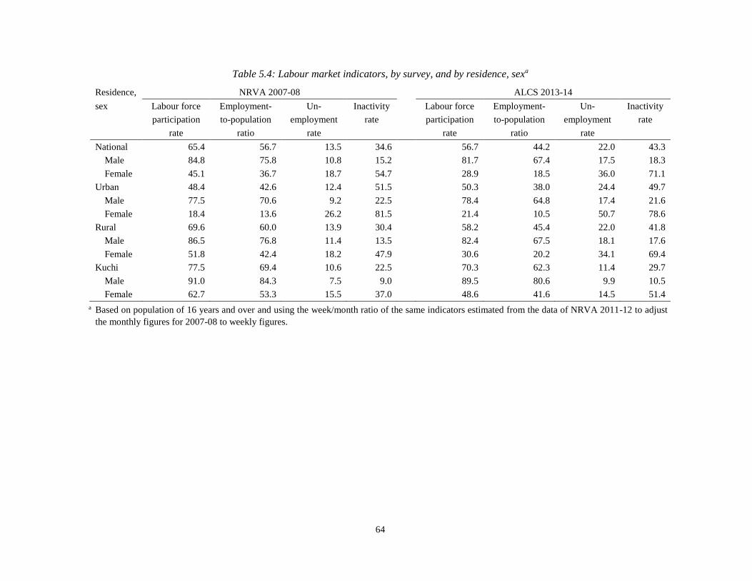
64
Table 5.4: Labour market indicators, by survey, and by residence, sexa
Residence, NRVA 2007-08 ALCS 2013-14
sex Labour force Employment- Un- Inactivity Labour force Employment- Un- Inactivity
participation to-population employment rate participation to-population employment rate
rate ratio rate rate ratio rate
National 65.4 56.7 13.5 34.6 56.7 44.2 22.0 43.3
Male 84.8 75.8 10.8 15.2 81.7 67.4 17.5 18.3
Female 45.1 36.7 18.7 54.7 28.9 18.5 36.0 71.1
Urban 48.4 42.6 12.4 51.5 50.3 38.0 24.4 49.7
Male 77.5 70.6 9.2 22.5 78.4 64.8 17.4 21.6
Female 18.4 13.6 26.2 81.5 21.4 10.5 50.7 78.6
Rural 69.6 60.0 13.9 30.4 58.2 45.4 22.0 41.8
Male 86.5 76.8 11.4 13.5 82.4 67.5 18.1 17.6
Female 51.8 42.4 18.2 47.9 30.6 20.2 34.1 69.4
Kuchi 77.5 69.4 10.6 22.5 70.3 62.3 11.4 29.7
Male 91.0 84.3 7.5 9.0 89.5 80.6 9.9 10.5
Female 62.7 53.3 15.5 37.0 48.6 41.6 14.5 51.4
a Based on population of 16 years and over and using the week/month ratio of the same indicators estimated from the data of NRVA 2011-12 to adjust
the monthly figures for 2007-08 to weekly figures.
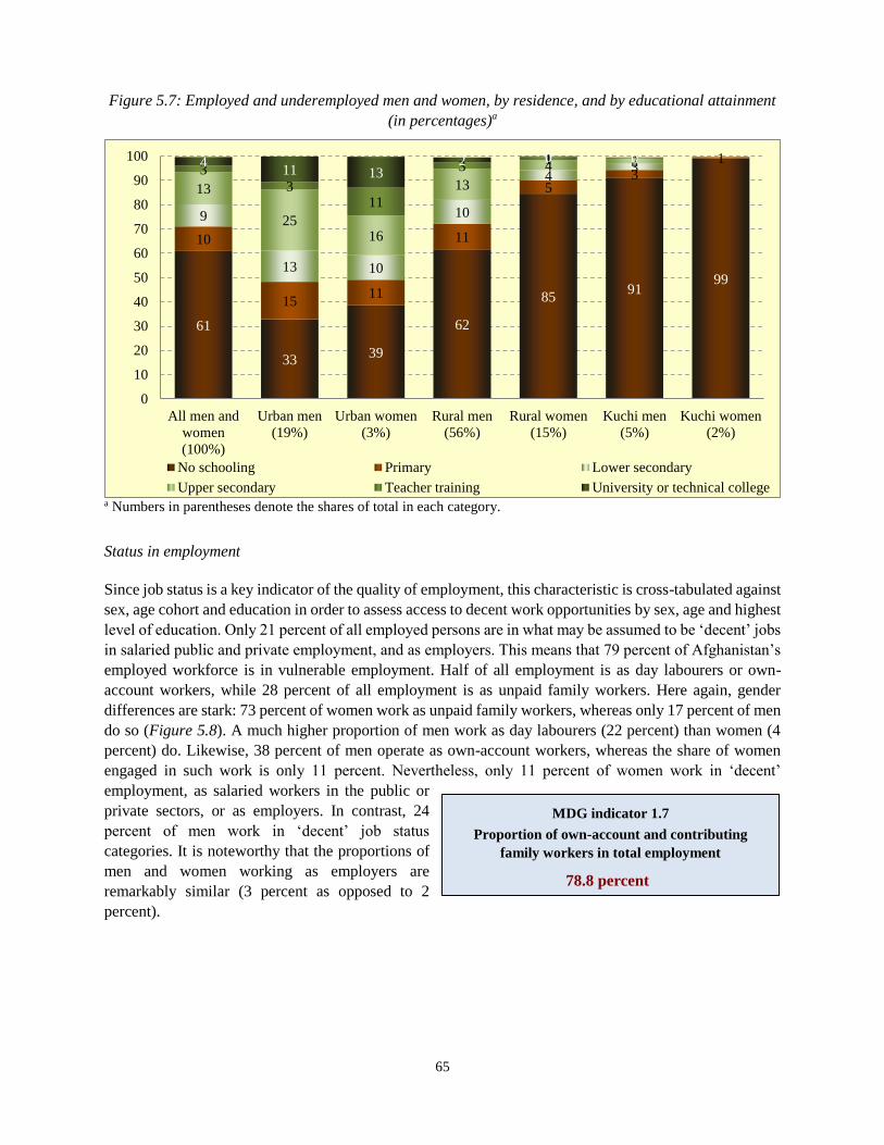
65
Figure 5.7: Employed and underemployed men and women, by residence, and by educational attainment
(in percentages)a
a Numbers in parentheses denote the shares of total in each category.
Status in employment
Since job status is a key indicator of the quality of employment, this characteristic is cross-tabulated against
sex, age cohort and education in order to assess access to decent work opportunities by sex, age and highest
level of education. Only 21 percent of all employed persons are in what may be assumed to be ‘decent’ jobs
in salaried public and private employment, and as employers. This means that 79 percent of Afghanistan’s
employed workforce is in vulnerable employment. Half of all employment is as day labourers or own-
account workers, while 28 percent of all employment is as unpaid family workers. Here again, gender
differences are stark: 73 percent of women work as unpaid family workers, whereas only 17 percent of men
do so (Figure 5.8). A much higher proportion of men work as day labourers (22 percent) than women (4
percent) do. Likewise, 38 percent of men operate as own-account workers, whereas the share of women
engaged in such work is only 11 percent. Nevertheless, only 11 percent of women work in ‘decent’
employment, as salaried workers in the public or
private sectors, or as employers. In contrast, 24
percent of men work in ‘decent’ job status
categories. It is noteworthy that the proportions of
men and women working as employers are
remarkably similar (3 percent as opposed to 2
percent).
61
3339
62
8591
99
10
1511
11
53
1
9
13 10
10
43
13
2516
13
4 23
311
314
11 132 0 0
0
10
20
30
40
50
60
70
80
90
100
All men and
women
(100%)
Urban men
(19%)
Urban women
(3%)
Rural men
(56%)
Rural women
(15%)
Kuchi men
(5%)
Kuchi women
(2%)
No schooling Primary Lower secondary
Upper secondary Teacher training University or technical college
MDG indicator 1.7
Proportion of own-account and contributing
family workers in total employment
78.8 percent
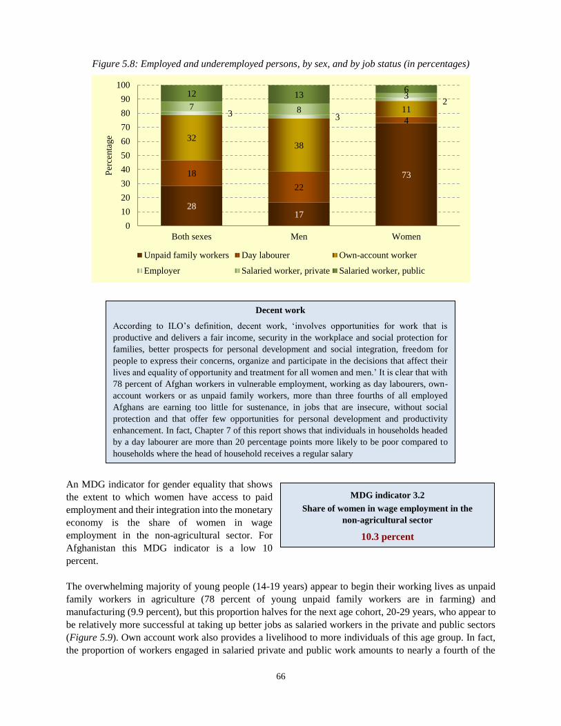
66
Figure 5.8: Employed and underemployed persons, by sex, and by job status (in percentages)
An MDG indicator for gender equality that shows
the extent to which women have access to paid
employment and their integration into the monetary
economy is the share of women in wage
employment in the non-agricultural sector. For
Afghanistan this MDG indicator is a low 10
percent.
The overwhelming majority of young people (14-19 years) appear to begin their working lives as unpaid
family workers in agriculture (78 percent of young unpaid family workers are in farming) and
manufacturing (9.9 percent), but this proportion halves for the next age cohort, 20-29 years, who appear to
be relatively more successful at taking up better jobs as salaried workers in the private and public sectors
(Figure 5.9). Own account work also provides a livelihood to more individuals of this age group. In fact,
the proportion of workers engaged in salaried private and public work amounts to nearly a fourth of the
2817
7318
22
4
3238
113 3
27 8
312 136
0
10
20
30
40
50
60
70
80
90
100
Both sexes Men Women
Per
centa
ge
Unpaid family workers Day labourer Own-account worker
Employer Salaried worker, private Salaried worker, public
Decent work
According to ILO’s definition, decent work, ‘involves opportunities for work that is
productive and delivers a fair income, security in the workplace and social protection for
families, better prospects for personal development and social integration, freedom for
people to express their concerns, organize and participate in the decisions that affect their
lives and equality of opportunity and treatment for all women and men.’ It is clear that with
78 percent of Afghan workers in vulnerable employment, working as day labourers, own-
account workers or as unpaid family workers, more than three fourths of all employed
Afghans are earning too little for sustenance, in jobs that are insecure, without social
protection and that offer few opportunities for personal development and productivity
enhancement. In fact, Chapter 7 of this report shows that individuals in households headed
by a day labourer are more than 20 percentage points more likely to be poor compared to
households where the head of household receives a regular salary
MDG indicator 3.2
Share of women in wage employment in the
non-agricultural sector
10.3 percent
67
population of employed persons of this age cohort, and thereafter these proportions decline slightly, only
to increase again to 24 percent for the 60-69 age group. It is possible that the end of the civil war opened
up relatively more of such decent work opportunities for younger people in recent times, though not in the
volumes that are necessary to make a significant dent in the proportion of Afghans forced to take up ‘bad
jobs’ as day labourers and own-account workers. In fact, the proportion of those in self-employment rises
to nearly half the population of employed and underemployed workers in the senior age cohort of 60-69
years, 56 percent in the 70-79 age category, and 60 percent in the 80-89 category. The figures suggest that
older workers’ prospects of finding decent work are extremely low, and that they are in fact forced to take
up any work that comes their way in the absence of effective social protection mechanisms.
Figure 5.9: Employed and underemployed persons, by age, and by job status (in percentages)
Prospects for getting decent work are strongly mediated by the level of education attained. Figure 5.10
suggests that education levels beyond upper secondary have a significant impact on the chances of finding
a good job as a salaried worker in the public or private sector. For example, of those with teacher training,
72 percent have found jobs in the public sector, while nearly 80 percent of those with university or technical
college training have jobs in the public or private sectors as salaried workers. In contrast, at least a third of
those educated up to upper secondary education levels or less, resort to own account work, while a fifth of
those with no schooling or primary level education only work as day labourers.
29
55
2722 22 22
17 20 23
18
16
1920 18 16
13 11 5
32
19
28 36 39 4047
56 64
3
2
33 2 2 2
2
4
7
5
88 6 5 6
3
412
315 12 12 14 16
8
0
10
20
30
40
50
60
70
80
90
100
Total 14-19 20-29 30-39 40-49 50-59 60-69 70-79 80+
Per
centa
ge
Age
Unpaid family workers Day labourer Own-account worker
Employer Salaried worker, private Salaried worker, public
68
Figure 5.10: Employed and underemployed persons, by highest level of education attained, and by job
status (in percentages)
Economic sector of work
Employment is dominated by the agricultural sector which accounts for two fifths of all jobs. A little less
than a tenth is in manufacturing. Construction accounts for 14 percent and trade, transport, financing and
real estate account for 18 percent. More striking are the stark gender differences in the distribution of
employment of men and women across the main economic sectors. While men account for 79 percent of
all employment, and women account for 21 percent, it is clearly evident from Figure 5.11 that job
opportunities for women are confined to only three out of nine sectors, agriculture, manufacturing, and
community, social and personal services. In fact, women are the overwhelming majority in the
manufacturing sector at 65 percent of all persons engaged in the sector.
35
21 2516
3 5 112
21
21 17
10
3 2
16
33
37 36
32
11 13
10
28
3
3 3
2
11
2
5
411 10
11
11
23 34
17
4 8 10
30
72
56 53
21
0
10
20
30
40
50
60
70
80
90
100
No
schooling
Primary Lower
secondary
Upper
secondary
Teacher
training
University
or technical
college
Postgraduate Any Islamic
school
Per
centa
ge
Highest level of education attained
Unpaid family workers Day labourer
Own-account worker Employer
69
Figure 5.11: Employed and underemployed persons, by sector of employment, and by sex (in
percentages)
Having looked at the relative concentrations of men and women in the main economic sectors, we turn next
to the distribution of men and women across them. It is evident from Figure 5.12 that proportionately more
women than men work in agriculture. In fact, while a little less than 40 percent of total male employment
is in agriculture, the sector accounts for two thirds of employed women with 21 percent of all employed
women in farming or crop growing, and 42 percent in livestock production. The second most important
sector for the employment of women is manufacturing, accounting for 24 percent of the employed and
underemployed female workforce, whereas the share of men in manufacturing is a mere 8 percent of the
employed and underemployed male workforce. However, in manufacturing, women are mostly found in
the manufacture of textiles (not clothes), and the manufacture of clothes (not footwear), and these two
sectors account for 16.4 percent and 2.9 percent of total female employment in across sectors. Men are
well-represented in the construction, wholesale and retail trade, and transport and communication sectors.
Their share in community, social and personal services is twice as large as the share of women’s
employment in the sector. In fact, women’s representation in community, social and personal services is in
the three-digit category of ‘other social and related services’ which accounts for 7.2 percent of total female
employment. The share of women employed in the health and education sectors is negligible. It can be seen
that women have hardly any representation in the sectors that have experienced higher economic growth
rates in recent years, such as construction, mining and quarrying, wholesale and retail trade and restaurants,
transport, storage and communication, and financing, insurance and real estate.
69
100
35
98
98
100
100
89
79
31
65
2
2
11
21
0 10 20 30 40 50 60 70 80 90 100
Agriculture
Mining and quarrying
Manufacturing
Construction
Wholesale and retail trade, restaurants and hotels
Transport storage communication and information
Financing, insurance, real estate and business…
Community, social and personal services
All sectors
PercentageMen (79%) Women (21%)
70
Figure 5.12: Employed and underemployed persons, by sex, and by main economic sector (in
percentages)a
a Numbers in parentheses denote the shares of total employment in each category.
Occupation
Given the predominance of the primary sectors in the Afghan economy, despite the expansion of the
services sectors in recent times, around 90 percent of the employed (and underemployed) workforce is in
low-skilled occupations of elementary, plant and machine assemblers and operators, craft and related trades,
and agriculture, forestry and fisheries workers (Figure 5.13). Gender differences in the distribution of
occupations are as striking. Among those in skilled occupations, the professionals dominate, at 4 percent
of the entire employed workforce, and women’s share in this category is equivalent to men’s. But two thirds
of the employed female workforce is in agriculture, fisheries and forestry-related occupations, compared to
36 percent of men. In fact, the two-digit occupation category of market-oriented agricultural workers, that
is farmers and animal keepers who sell part of their produce accounts for nearly 40 percent of all employed
women’s occupations, while 23 percent of women are engaged as sales workers or street sales workers.
Meanwhile a fourth of working women are in craft and related trades. In contrast, only 7 percent of males
are in the same trades.
0
10
20
30
40
50
60
70
80
90
100
Both sexes
(100%)
Men (79%) Women (21%)
Community, social and
personal services (16%)
Financing, insurance, real
estate and business
services (1%)
Transport storage
communication and
information (5%)
Wholesale and retail trade,
restaurants and hotels
(12%)
Construction (14%)
Manufacturing (8%)
Mining and quarrying
(0%)
Agriculture (44%)
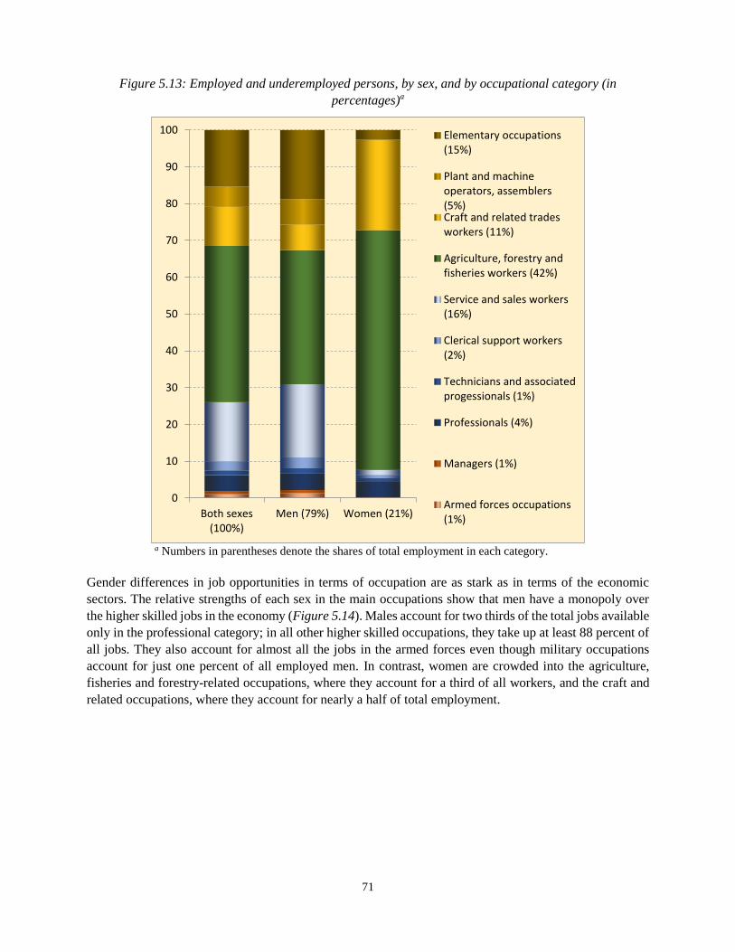
71
Figure 5.13: Employed and underemployed persons, by sex, and by occupational category (in
percentages)a
a Numbers in parentheses denote the shares of total employment in each category.
Gender differences in job opportunities in terms of occupation are as stark as in terms of the economic
sectors. The relative strengths of each sex in the main occupations show that men have a monopoly over
the higher skilled jobs in the economy (Figure 5.14). Males account for two thirds of the total jobs available
only in the professional category; in all other higher skilled occupations, they take up at least 88 percent of
all jobs. They also account for almost all the jobs in the armed forces even though military occupations
account for just one percent of all employed men. In contrast, women are crowded into the agriculture,
fisheries and forestry-related occupations, where they account for a third of all workers, and the craft and
related occupations, where they account for nearly a half of total employment.
0
10
20
30
40
50
60
70
80
90
100
Both sexes(100%)
Men (79%) Women (21%)
Elementary occupations(15%)
Plant and machineoperators, assemblers(5%)Craft and related tradesworkers (11%)
Agriculture, forestry andfisheries workers (42%)
Service and sales workers(16%)
Clerical support workers(2%)
Technicians and associatedprogessionals (1%)
Professionals (4%)
Managers (1%)
Armed forces occupations(1%)
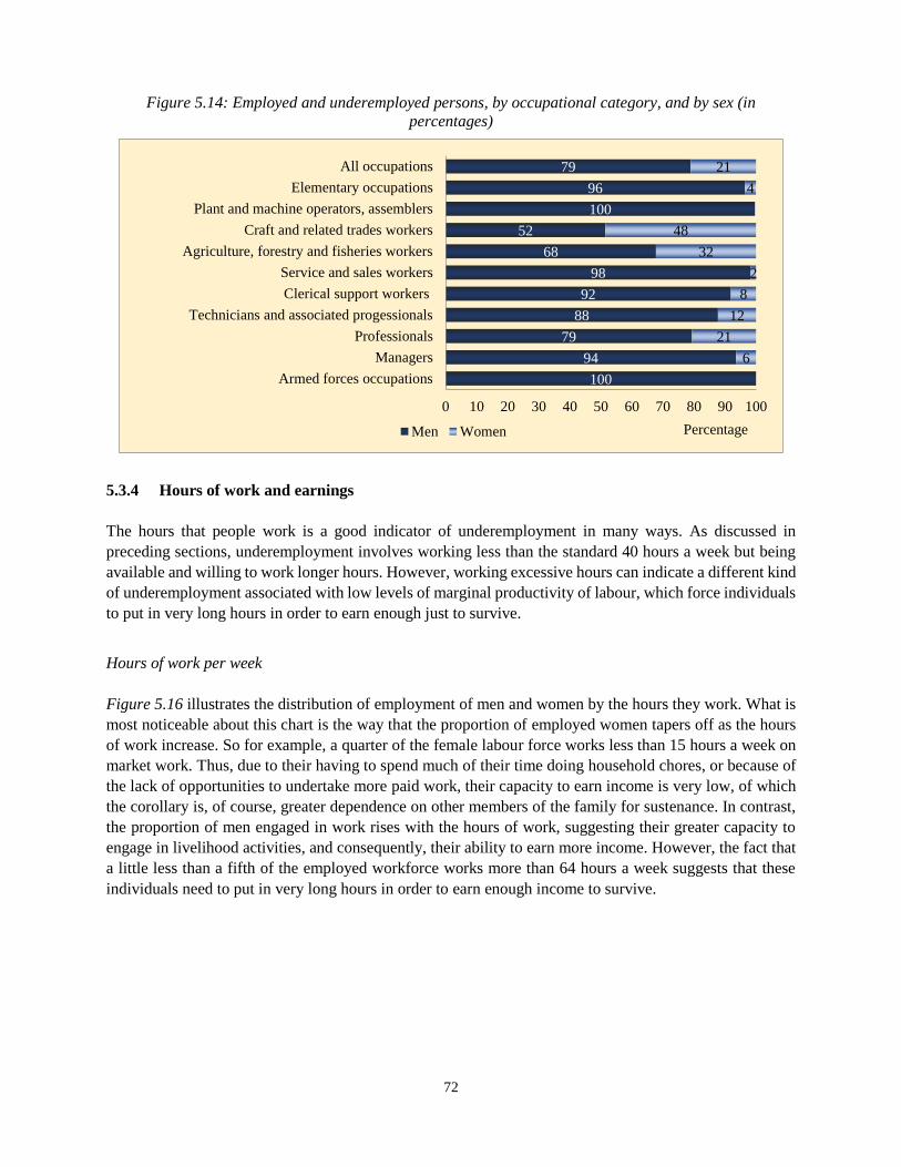
72
Figure 5.14: Employed and underemployed persons, by occupational category, and by sex (in
percentages)
5.3.4 Hours of work and earnings
The hours that people work is a good indicator of underemployment in many ways. As discussed in
preceding sections, underemployment involves working less than the standard 40 hours a week but being
available and willing to work longer hours. However, working excessive hours can indicate a different kind
of underemployment associated with low levels of marginal productivity of labour, which force individuals
to put in very long hours in order to earn enough just to survive.
Hours of work per week
Figure 5.16 illustrates the distribution of employment of men and women by the hours they work. What is
most noticeable about this chart is the way that the proportion of employed women tapers off as the hours
of work increase. So for example, a quarter of the female labour force works less than 15 hours a week on
market work. Thus, due to their having to spend much of their time doing household chores, or because of
the lack of opportunities to undertake more paid work, their capacity to earn income is very low, of which
the corollary is, of course, greater dependence on other members of the family for sustenance. In contrast,
the proportion of men engaged in work rises with the hours of work, suggesting their greater capacity to
engage in livelihood activities, and consequently, their ability to earn more income. However, the fact that
a little less than a fifth of the employed workforce works more than 64 hours a week suggests that these
individuals need to put in very long hours in order to earn enough income to survive.
100
94
79
88
92
98
68
52
100
96
79
6
21
12
8
2
32
48
4
21
0 10 20 30 40 50 60 70 80 90 100
Armed forces occupations
Managers
Professionals
Technicians and associated progessionals
Clerical support workers
Service and sales workers
Agriculture, forestry and fisheries workers
Craft and related trades workers
Plant and machine operators, assemblers
Elementary occupations
All occupations
PercentageMen Women
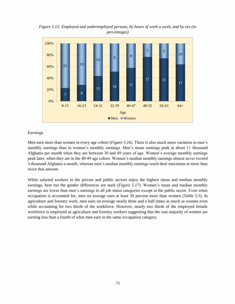
73
Figure 5.15: Employed and underemployed persons, by hours of work a week, and by sex (in
percentages)
Earnings
Men earn more than women in every age cohort (Figure 5.16). There is also much more variation in men’s
monthly earnings than in women’s monthly earnings. Men’s mean earnings peak at about 11 thousand
Afghanis per month when they are between 30 and 49 years of age. Women’s average monthly earnings
peak later, when they are in the 40-49 age cohort. Women’s median monthly earnings almost never exceed
3 thousand Afghanis a month, whereas men’s median monthly earnings reach their maximum at more than
twice that amount.
While salaried workers in the private and public sectors enjoy the highest mean and median monthly
earnings, here too the gender differences are stark (Figure 5.17). Women’s mean and median monthly
earnings are lower than men’s earnings in all job status categories except in the public sector. Even when
occupation is accounted for, men on average earn at least 30 percent more than women (Table 5.5). In
agriculture and forestry work, men earn on average nearly three and a half times as much as women even
while accounting for two thirds of the workforce. However, nearly two thirds of the employed female
workforce is employed as agriculture and forestry workers suggesting that the vast majority of women are
earning less than a fourth of what men earn in the same occupation category.
7 8
1510
11
17 1517
25 19
199
8
5 510
0%
20%
40%
60%
80%
100%
8-15 16-23 24-31 32-39 40-47 48-55 56-63 64+
Age
Men Women
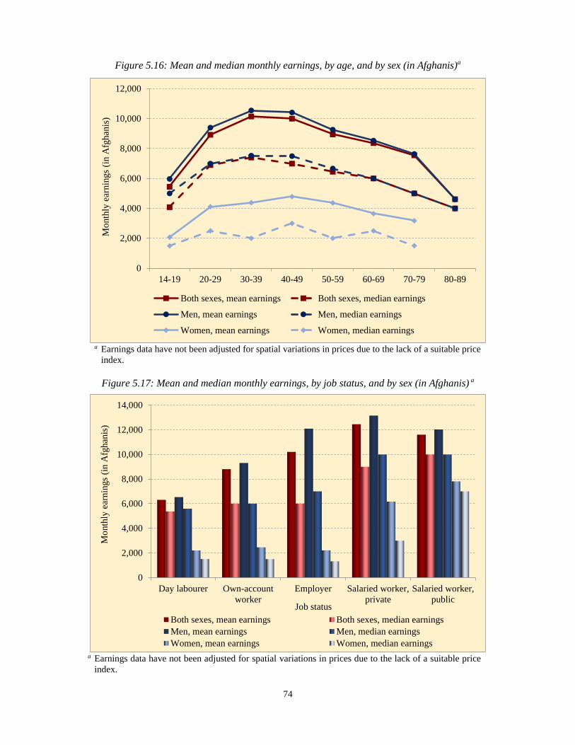
74
Figure 5.16: Mean and median monthly earnings, by age, and by sex (in Afghanis)a
a Earnings data have not been adjusted for spatial variations in prices due to the lack of a suitable price
index.
Figure 5.17: Mean and median monthly earnings, by job status, and by sex (in Afghanis) a
a Earnings data have not been adjusted for spatial variations in prices due to the lack of a suitable price
index.
0
2,000
4,000
6,000
8,000
10,000
12,000
14-19 20-29 30-39 40-49 50-59 60-69 70-79 80-89
Mo
nth
ly e
arnin
gs
(in A
fghan
is)
Both sexes, mean earnings Both sexes, median earnings
Men, mean earnings Men, median earnings
Women, mean earnings Women, median earnings
0
2,000
4,000
6,000
8,000
10,000
12,000
14,000
Day labourer Own-account
worker
Employer Salaried worker,
private
Salaried worker,
public
Mo
nth
ly e
arnin
gs
(in A
fghan
is)
Job status
Both sexes, mean earnings Both sexes, median earnings
Men, mean earnings Men, median earnings
Women, mean earnings Women, median earnings
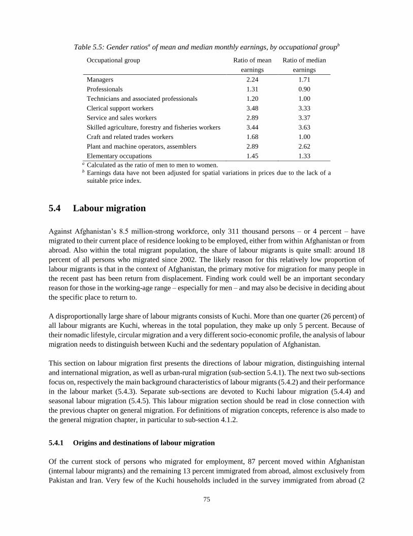
75
Table 5.5: Gender ratiosa of mean and median monthly earnings, by occupational groupb
Occupational group Ratio of mean Ratio of median
earnings earnings
Managers 2.24 1.71
Professionals 1.31 0.90
Technicians and associated professionals 1.20 1.00
Clerical support workers 3.48 3.33
Service and sales workers 2.89 3.37
Skilled agriculture, forestry and fisheries workers 3.44 3.63
Craft and related trades workers 1.68 1.00
Plant and machine operators, assemblers 2.89 2.62
Elementary occupations 1.45 1.33 a Calculated as the ratio of men to men to women. b Earnings data have not been adjusted for spatial variations in prices due to the lack of a
suitable price index.
5.4 Labour migration
Against Afghanistan’s 8.5 million-strong workforce, only 311 thousand persons – or 4 percent – have
migrated to their current place of residence looking to be employed, either from within Afghanistan or from
abroad. Also within the total migrant population, the share of labour migrants is quite small: around 18
percent of all persons who migrated since 2002. The likely reason for this relatively low proportion of
labour migrants is that in the context of Afghanistan, the primary motive for migration for many people in
the recent past has been return from displacement. Finding work could well be an important secondary
reason for those in the working-age range – especially for men – and may also be decisive in deciding about
the specific place to return to.
A disproportionally large share of labour migrants consists of Kuchi. More than one quarter (26 percent) of
all labour migrants are Kuchi, whereas in the total population, they make up only 5 percent. Because of
their nomadic lifestyle, circular migration and a very different socio-economic profile, the analysis of labour
migration needs to distinguish between Kuchi and the sedentary population of Afghanistan.
This section on labour migration first presents the directions of labour migration, distinguishing internal
and international migration, as well as urban-rural migration (sub-section 5.4.1). The next two sub-sections
focus on, respectively the main background characteristics of labour migrants (5.4.2) and their performance
in the labour market (5.4.3). Separate sub-sections are devoted to Kuchi labour migration (5.4.4) and
seasonal labour migration (5.4.5). This labour migration section should be read in close connection with
the previous chapter on general migration. For definitions of migration concepts, reference is also made to
the general migration chapter, in particular to sub-section 4.1.2.
5.4.1 Origins and destinations of labour migration
Of the current stock of persons who migrated for employment, 87 percent moved within Afghanistan
(internal labour migrants) and the remaining 13 percent immigrated from abroad, almost exclusively from
Pakistan and Iran. Very few of the Kuchi households included in the survey immigrated from abroad (2
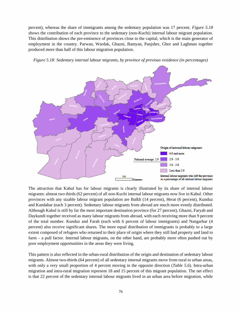
76
percent), whereas the share of immigrants among the sedentary population was 17 percent. Figure 5.18
shows the contribution of each province to the sedentary (non-Kuchi) internal labour migrant population.
This distribution shows the pre-eminence of provinces close to the capital, which is the main generator of
employment in the country. Parwan, Wardak, Ghazni, Bamyan, Panjsher, Ghor and Laghman together
produced more than half of this labour migration population.
Figure 5.18: Sedentary internal labour migrants, by province of previous residence (in percentages)
The attraction that Kabul has for labour migrants is clearly illustrated by its share of internal labour
migrants: almost two thirds (62 percent) of all non-Kuchi internal labour migrants now live in Kabul. Other
provinces with any sizable labour migrant population are Balkh (14 percent), Herat (6 percent), Kunduz
and Kandahar (each 3 percent). Sedentary labour migrants from abroad are much more evenly distributed.
Although Kabul is still by far the most important destination province (for 27 percent), Ghazni, Faryab and
Daykundi together received as many labour migrants from abroad, with each receiving more than 9 percent
of the total number. Kunduz and Farah (each with 6 percent of labour immigrants) and Nangarhar (4
percent) also receive significant shares. The more equal distribution of immigrants is probably to a large
extent composed of refugees who returned to their place of origin where they still had property and land to
farm – a pull factor. Internal labour migrants, on the other hand, are probably more often pushed out by
poor employment opportunities in the areas they were living.
This pattern is also reflected in the urban-rural distribution of the origin and destination of sedentary labour
migrants. Almost two-thirds (64 percent) of all sedentary internal migrants move from rural to urban areas,
with only a very small proportion of 4 percent moving in the opposite direction (Table 5.6). Intra-urban
migration and intra-rural migration represent 18 and 15 percent of this migrant population. The net effect
is that 22 percent of the sedentary internal labour migrants lived in an urban area before migration, while
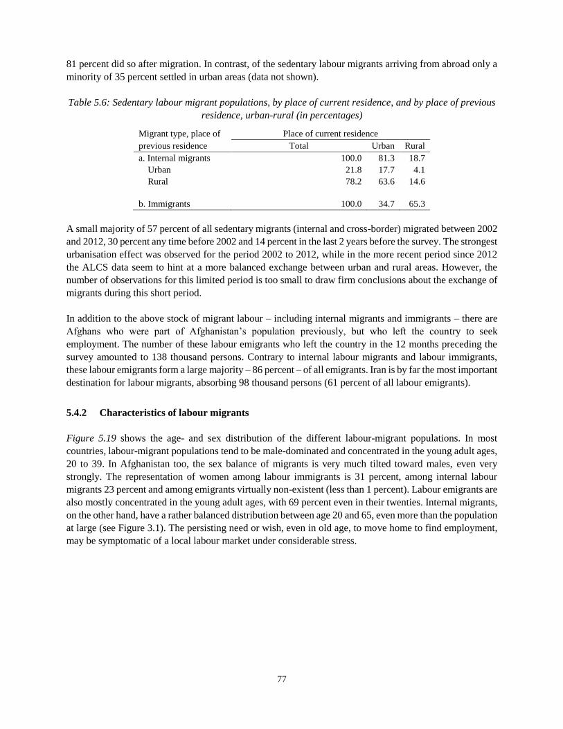
77
81 percent did so after migration. In contrast, of the sedentary labour migrants arriving from abroad only a
minority of 35 percent settled in urban areas (data not shown).
Table 5.6: Sedentary labour migrant populations, by place of current residence, and by place of previous
residence, urban-rural (in percentages)
Migrant type, place of Place of current residence
previous residence Total Urban Rural
a. Internal migrants 100.0 81.3 18.7
Urban 21.8 17.7 4.1
Rural 78.2 63.6 14.6
b. Immigrants 100.0 34.7 65.3
A small majority of 57 percent of all sedentary migrants (internal and cross-border) migrated between 2002
and 2012, 30 percent any time before 2002 and 14 percent in the last 2 years before the survey. The strongest
urbanisation effect was observed for the period 2002 to 2012, while in the more recent period since 2012
the ALCS data seem to hint at a more balanced exchange between urban and rural areas. However, the
number of observations for this limited period is too small to draw firm conclusions about the exchange of
migrants during this short period.
In addition to the above stock of migrant labour – including internal migrants and immigrants – there are
Afghans who were part of Afghanistan’s population previously, but who left the country to seek
employment. The number of these labour emigrants who left the country in the 12 months preceding the
survey amounted to 138 thousand persons. Contrary to internal labour migrants and labour immigrants,
these labour emigrants form a large majority – 86 percent – of all emigrants. Iran is by far the most important
destination for labour migrants, absorbing 98 thousand persons (61 percent of all labour emigrants).
5.4.2 Characteristics of labour migrants
Figure 5.19 shows the age- and sex distribution of the different labour-migrant populations. In most
countries, labour-migrant populations tend to be male-dominated and concentrated in the young adult ages,
20 to 39. In Afghanistan too, the sex balance of migrants is very much tilted toward males, even very
strongly. The representation of women among labour immigrants is 31 percent, among internal labour
migrants 23 percent and among emigrants virtually non-existent (less than 1 percent). Labour emigrants are
also mostly concentrated in the young adult ages, with 69 percent even in their twenties. Internal migrants,
on the other hand, have a rather balanced distribution between age 20 and 65, even more than the population
at large (see Figure 3.1). The persisting need or wish, even in old age, to move home to find employment,
may be symptomatic of a local labour market under considerable stress.
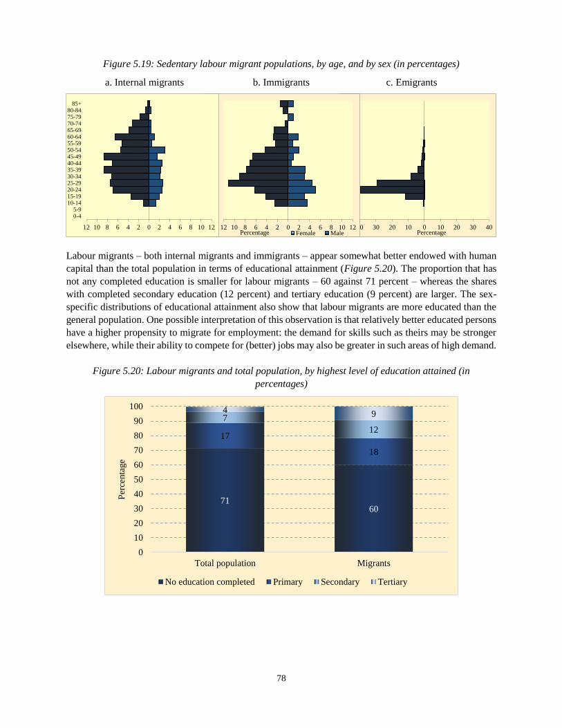
78
Figure 5.19: Sedentary labour migrant populations, by age, and by sex (in percentages)
a. Internal migrants b. Immigrants c. Emigrants
Labour migrants – both internal migrants and immigrants – appear somewhat better endowed with human
capital than the total population in terms of educational attainment (Figure 5.20). The proportion that has
not any completed education is smaller for labour migrants – 60 against 71 percent – whereas the shares
with completed secondary education (12 percent) and tertiary education (9 percent) are larger. The sex-
specific distributions of educational attainment also show that labour migrants are more educated than the
general population. One possible interpretation of this observation is that relatively better educated persons
have a higher propensity to migrate for employment: the demand for skills such as theirs may be stronger
elsewhere, while their ability to compete for (better) jobs may also be greater in such areas of high demand.
Figure 5.20: Labour migrants and total population, by highest level of education attained (in
percentages)
40 30 20 10 0 10 20 30 40
0-45-9
10-1415-1920-2425-2930-3435-3940-4445-4950-5455-5960-6465-6970-7475-7980-84
85+
Percentage12 10 8 6 4 2 0 2 4 6 8 10 12
0-45-9
10-1415-1920-2425-2930-3435-3940-4445-4950-5455-5960-6465-6970-7475-7980-84
85+
Percentage Female Male12 10 8 6 4 2 0 2 4 6 8 10 12
0-45-9
10-1415-1920-2425-2930-3435-3940-4445-4950-5455-5960-6465-6970-7475-7980-84
85+
7160
17
18
7
12
4 9
0
10
20
30
40
50
60
70
80
90
100
Total population Migrants
Per
centa
ge
No education completed Primary Secondary Tertiary
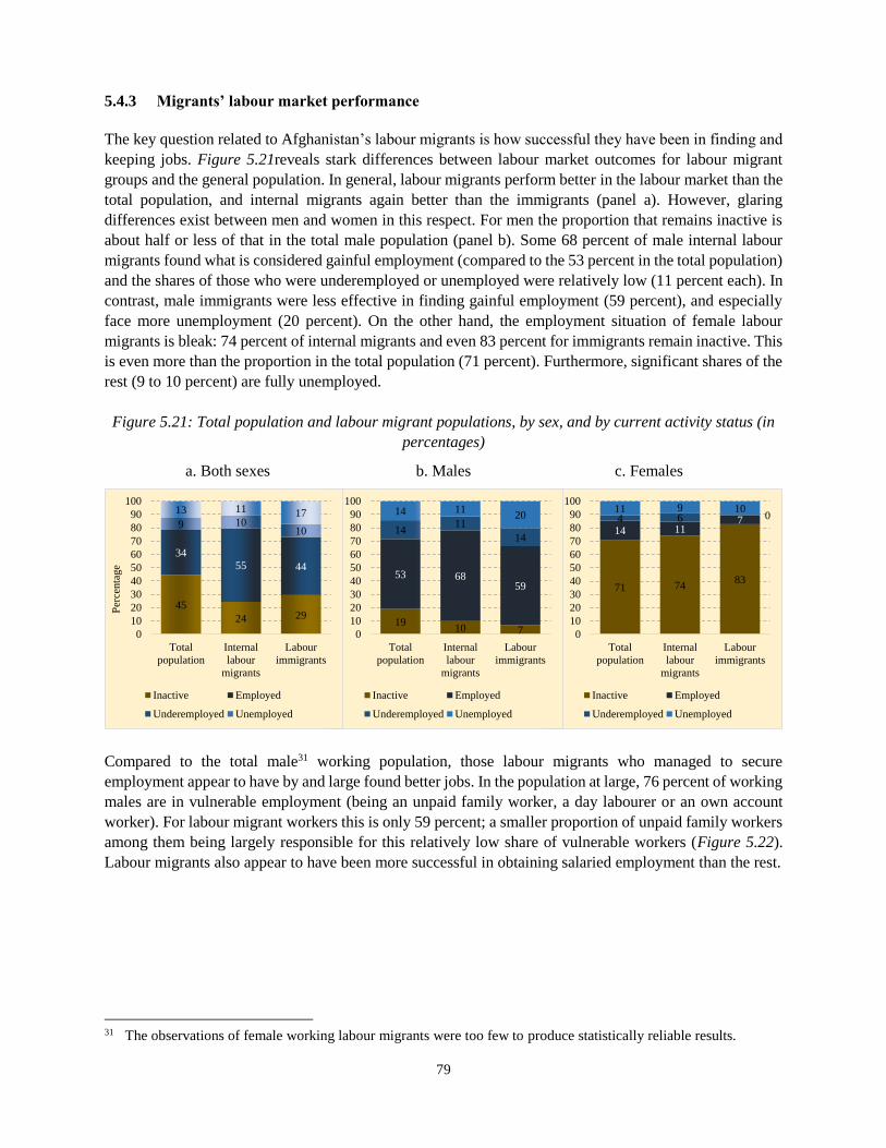
79
5.4.3 Migrants’ labour market performance
The key question related to Afghanistan’s labour migrants is how successful they have been in finding and
keeping jobs. Figure 5.21reveals stark differences between labour market outcomes for labour migrant
groups and the general population. In general, labour migrants perform better in the labour market than the
total population, and internal migrants again better than the immigrants (panel a). However, glaring
differences exist between men and women in this respect. For men the proportion that remains inactive is
about half or less of that in the total male population (panel b). Some 68 percent of male internal labour
migrants found what is considered gainful employment (compared to the 53 percent in the total population)
and the shares of those who were underemployed or unemployed were relatively low (11 percent each). In
contrast, male immigrants were less effective in finding gainful employment (59 percent), and especially
face more unemployment (20 percent). On the other hand, the employment situation of female labour
migrants is bleak: 74 percent of internal migrants and even 83 percent for immigrants remain inactive. This
is even more than the proportion in the total population (71 percent). Furthermore, significant shares of the
rest (9 to 10 percent) are fully unemployed.
Figure 5.21: Total population and labour migrant populations, by sex, and by current activity status (in
percentages)
a. Both sexes b. Males c. Females
Compared to the total male31 working population, those labour migrants who managed to secure
employment appear to have by and large found better jobs. In the population at large, 76 percent of working
males are in vulnerable employment (being an unpaid family worker, a day labourer or an own account
worker). For labour migrant workers this is only 59 percent; a smaller proportion of unpaid family workers
among them being largely responsible for this relatively low share of vulnerable workers (Figure 5.22).
Labour migrants also appear to have been more successful in obtaining salaried employment than the rest.
31 The observations of female working labour migrants were too few to produce statistically reliable results.
71 7483
14 1174 6 0
11 9 10
0
10
20
30
40
50
60
70
80
90
100
Total
population
Internal
labour
migrants
Labour
immigrants
Per
centa
ge
Inactive Employed
Underemployed Unemployed
1910 7
53 6859
1411
14
14 1120
0
10
20
30
40
50
60
70
80
90
100
Total
population
Internal
labour
migrants
Labour
immigrants
Per
centa
ge
Inactive Employed
Underemployed Unemployed
45
24 29
34
55 44
9 1010
13 11 17
0
10
20
30
40
50
60
70
80
90
100
Total
population
Internal
labour
migrants
Labour
immigrants
Per
centa
ge
Inactive Employed
Underemployed Unemployed
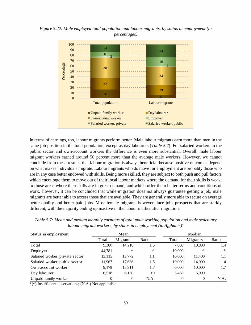
80
Figure 5.22: Male employed total population and labour migrants, by status in employment (in
percentages)
In terms of earnings, too, labour migrants perform better. Male labour migrants earn more than men in the
same job position in the total population, except as day labourers (Table 5.7). For salaried workers in the
public sector and own-account workers the difference is even more substantial. Overall, male labour
migrant workers earned around 50 percent more than the average male workers. However, we cannot
conclude from these results, that labour migration is always beneficial because positive outcomes depend
on what makes individuals migrate. Labour migrants who do move for employment are probably those who
are in any case better endowed with skills. Being more skilled, they are subject to both push and pull factors
which encourage them to move out of their local labour markets where the demand for their skills is weak,
to those areas where their skills are in great demand, and which offer them better terms and conditions of
work. However, it can be concluded that while migration does not always guarantee getting a job, male
migrants are better able to access those that are available. They are generally more able to secure on average
better-quality and better-paid jobs. Most female migrants however, face jobs prospects that are starkly
different, with the majority ending up inactive in the labour market after migration.
Table 5.7: Mean and median monthly earnings of total male working population and male sedentary
labour-migrant workers, by status in employment (in Afghanis)a
Status in employment Mean Median
Total Migrants Ratio Total Migrants Ratio
Total 9,380 14,218 1.5 7,000 10,000 1.4
Employer 44,781 * * 10,000 * *
Salaried worker, private sector 13,115 13,772 1.1 10,000 11,400 1.1
Salaried worker, public sector 11,967 17,636 1.5 10,000 14,000 1.4
Own-account worker 9,179 15,311 1.7 6,000 10,000 1.7
Day labourer 6,518 6,130 0.9 5,438 6,090 1.1
Unpaid family worker 0 0 N.A. 0 0 N.A.a (*) Insufficient observations; (N.A.) Not applicable
166
22
19
38
34
2
1
8
16
1424
0
10
20
30
40
50
60
70
80
90
100
Total population Labour migrants
Per
centa
ge
Unpaid family worker Day labourer
own-account worker Employer
Salaried worker, private Salaried worker, public
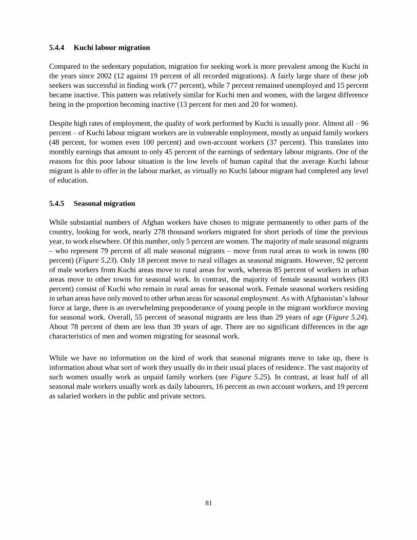
81
5.4.4 Kuchi labour migration
Compared to the sedentary population, migration for seeking work is more prevalent among the Kuchi in
the years since 2002 (12 against 19 percent of all recorded migrations). A fairly large share of these job
seekers was successful in finding work (77 percent), while 7 percent remained unemployed and 15 percent
became inactive. This pattern was relatively similar for Kuchi men and women, with the largest difference
being in the proportion becoming inactive (13 percent for men and 20 for women).
Despite high rates of employment, the quality of work performed by Kuchi is usually poor. Almost all – 96
percent – of Kuchi labour migrant workers are in vulnerable employment, mostly as unpaid family workers
(48 percent, for women even 100 percent) and own-account workers (37 percent). This translates into
monthly earnings that amount to only 45 percent of the earnings of sedentary labour migrants. One of the
reasons for this poor labour situation is the low levels of human capital that the average Kuchi labour
migrant is able to offer in the labour market, as virtually no Kuchi labour migrant had completed any level
of education.
5.4.5 Seasonal migration
While substantial numbers of Afghan workers have chosen to migrate permanently to other parts of the
country, looking for work, nearly 278 thousand workers migrated for short periods of time the previous
year, to work elsewhere. Of this number, only 5 percent are women. The majority of male seasonal migrants
– who represent 79 percent of all male seasonal migrants – move from rural areas to work in towns (80
percent) (Figure 5.23). Only 18 percent move to rural villages as seasonal migrants. However, 92 percent
of male workers from Kuchi areas move to rural areas for work, whereas 85 percent of workers in urban
areas move to other towns for seasonal work. In contrast, the majority of female seasonal workers (83
percent) consist of Kuchi who remain in rural areas for seasonal work. Female seasonal workers residing
in urban areas have only moved to other urban areas for seasonal employment. As with Afghanistan’s labour
force at large, there is an overwhelming preponderance of young people in the migrant workforce moving
for seasonal work. Overall, 55 percent of seasonal migrants are less than 29 years of age (Figure 5.24).
About 78 percent of them are less than 39 years of age. There are no significant differences in the age
characteristics of men and women migrating for seasonal work.
While we have no information on the kind of work that seasonal migrants move to take up, there is
information about what sort of work they usually do in their usual places of residence. The vast majority of
such women usually work as unpaid family workers (see Figure 5.25). In contrast, at least half of all
seasonal male workers usually work as daily labourers, 16 percent as own account workers, and 19 percent
as salaried workers in the public and private sectors.
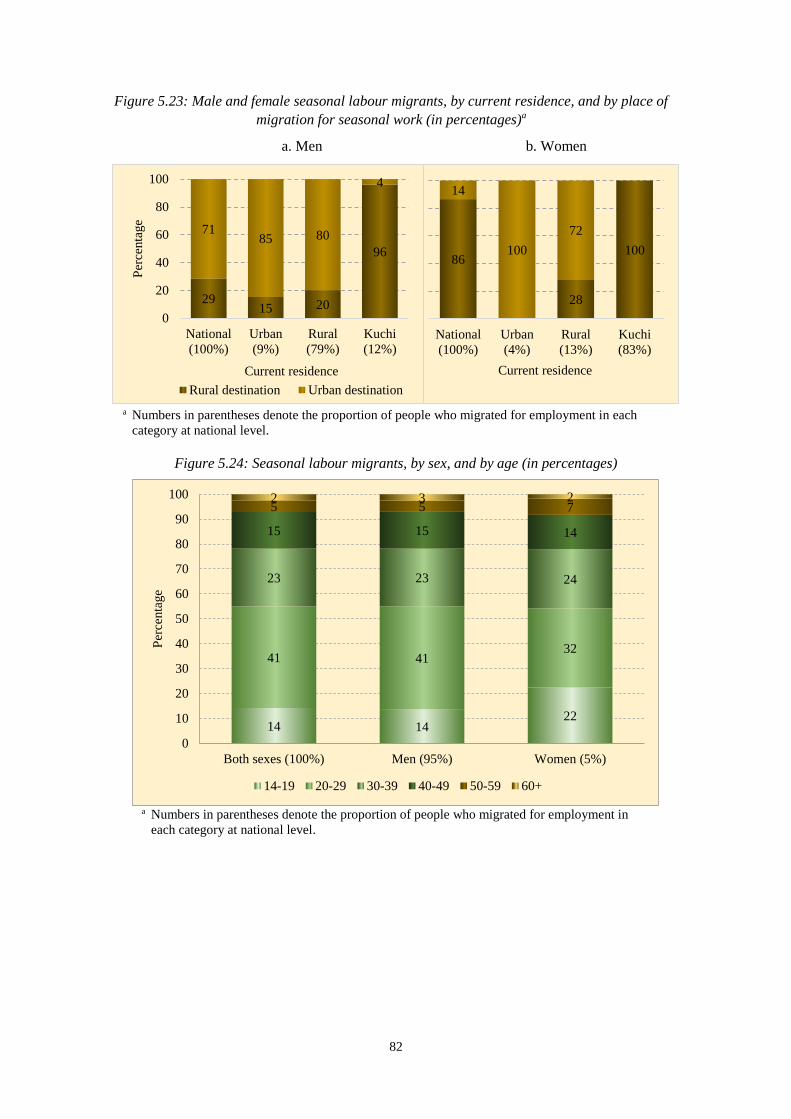
82
Figure 5.23: Male and female seasonal labour migrants, by current residence, and by place of
migration for seasonal work (in percentages)a
a. Men b. Women
a Numbers in parentheses denote the proportion of people who migrated for employment in each
category at national level.
Figure 5.24: Seasonal labour migrants, by sex, and by age (in percentages)
a Numbers in parentheses denote the proportion of people who migrated for employment in
each category at national level.
86
28
100
14
100
72
National
(100%)
Urban
(4%)
Rural
(13%)
Kuchi
(83%)
Current residence
2915 20
96
7185 80
4
0
20
40
60
80
100
National
(100%)
Urban
(9%)
Rural
(79%)
Kuchi
(12%)
Per
centa
ge
Current residence
Rural destination Urban destination
14 1422
41 4132
23 23 24
15 15 14
5 5 72 3 2
0
10
20
30
40
50
60
70
80
90
100
Both sexes (100%) Men (95%) Women (5%)
Per
centa
ge
14-19 20-29 30-39 40-49 50-59 60+
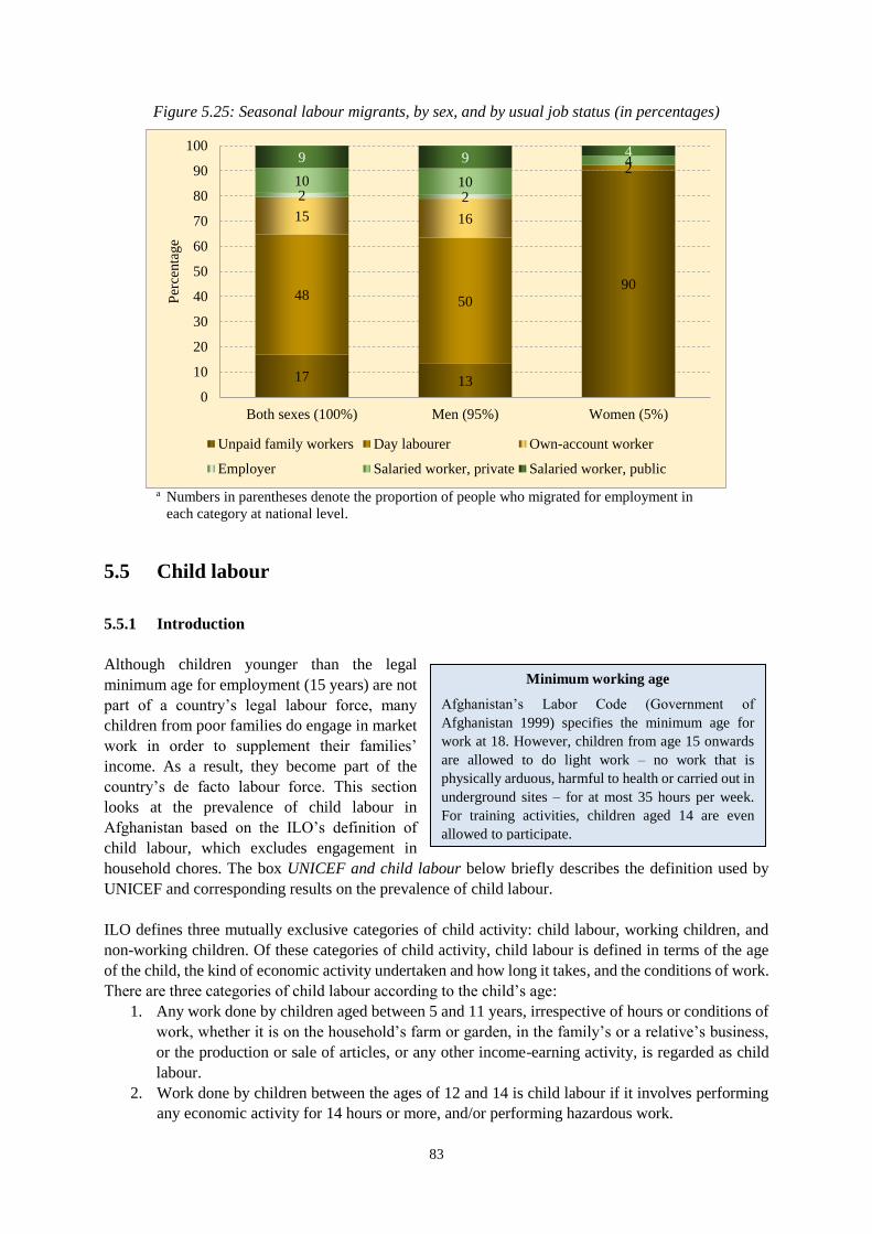
83
Figure 5.25: Seasonal labour migrants, by sex, and by usual job status (in percentages)
a Numbers in parentheses denote the proportion of people who migrated for employment in
each category at national level.
5.5 Child labour
5.5.1 Introduction
Although children younger than the legal
minimum age for employment (15 years) are not
part of a country’s legal labour force, many
children from poor families do engage in market
work in order to supplement their families’
income. As a result, they become part of the
country’s de facto labour force. This section
looks at the prevalence of child labour in
Afghanistan based on the ILO’s definition of
child labour, which excludes engagement in
household chores. The box UNICEF and child labour below briefly describes the definition used by
UNICEF and corresponding results on the prevalence of child labour.
ILO defines three mutually exclusive categories of child activity: child labour, working children, and
non-working children. Of these categories of child activity, child labour is defined in terms of the age
of the child, the kind of economic activity undertaken and how long it takes, and the conditions of work.
There are three categories of child labour according to the child’s age:
1. Any work done by children aged between 5 and 11 years, irrespective of hours or conditions of
work, whether it is on the household’s farm or garden, in the family’s or a relative’s business,
or the production or sale of articles, or any other income-earning activity, is regarded as child
labour.
2. Work done by children between the ages of 12 and 14 is child labour if it involves performing
any economic activity for 14 hours or more, and/or performing hazardous work.
17 13
9048 50
2
15 16
2 210 10
49 9 4
0
10
20
30
40
50
60
70
80
90
100
Both sexes (100%) Men (95%) Women (5%)
Per
centa
ge
Unpaid family workers Day labourer Own-account worker
Employer Salaried worker, private Salaried worker, public
Minimum working age
Afghanistan’s Labor Code (Government of
Afghanistan 1999) specifies the minimum age for
work at 18. However, children from age 15 onwards
are allowed to do light work – no work that is
physically arduous, harmful to health or carried out in
underground sites – for at most 35 hours per week.
For training activities, children aged 14 are even
allowed to participate.
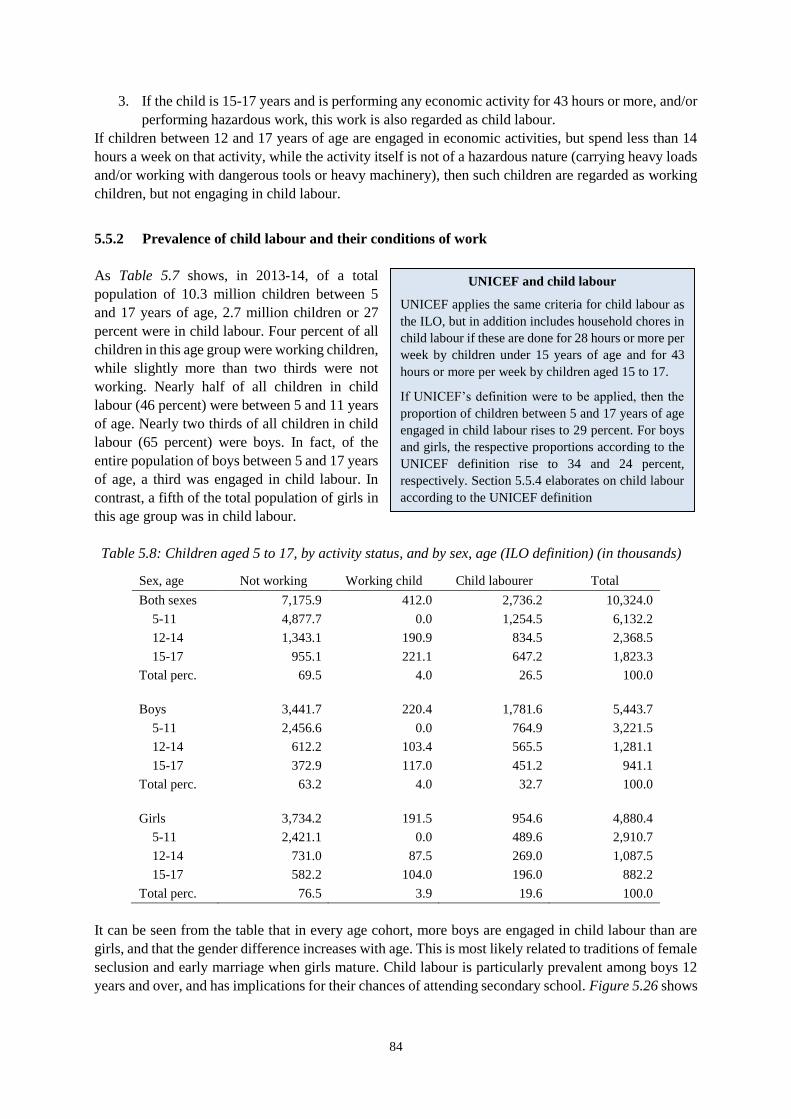
84
3. If the child is 15-17 years and is performing any economic activity for 43 hours or more, and/or
performing hazardous work, this work is also regarded as child labour.
If children between 12 and 17 years of age are engaged in economic activities, but spend less than 14
hours a week on that activity, while the activity itself is not of a hazardous nature (carrying heavy loads
and/or working with dangerous tools or heavy machinery), then such children are regarded as working
children, but not engaging in child labour.
5.5.2 Prevalence of child labour and their conditions of work
As Table 5.7 shows, in 2013-14, of a total
population of 10.3 million children between 5
and 17 years of age, 2.7 million children or 27
percent were in child labour. Four percent of all
children in this age group were working children,
while slightly more than two thirds were not
working. Nearly half of all children in child
labour (46 percent) were between 5 and 11 years
of age. Nearly two thirds of all children in child
labour (65 percent) were boys. In fact, of the
entire population of boys between 5 and 17 years
of age, a third was engaged in child labour. In
contrast, a fifth of the total population of girls in
this age group was in child labour.
Table 5.8: Children aged 5 to 17, by activity status, and by sex, age (ILO definition) (in thousands)
Sex, age Not working Working child Child labourer Total
Both sexes 7,175.9 412.0 2,736.2 10,324.0
5-11 4,877.7 0.0 1,254.5 6,132.2
12-14 1,343.1 190.9 834.5 2,368.5
15-17 955.1 221.1 647.2 1,823.3
Total perc. 69.5 4.0 26.5 100.0
Boys 3,441.7 220.4 1,781.6 5,443.7
5-11 2,456.6 0.0 764.9 3,221.5
12-14 612.2 103.4 565.5 1,281.1
15-17 372.9 117.0 451.2 941.1
Total perc. 63.2 4.0 32.7 100.0
Girls 3,734.2 191.5 954.6 4,880.4
5-11 2,421.1 0.0 489.6 2,910.7
12-14 731.0 87.5 269.0 1,087.5
15-17 582.2 104.0 196.0 882.2
Total perc. 76.5 3.9 19.6 100.0
It can be seen from the table that in every age cohort, more boys are engaged in child labour than are
girls, and that the gender difference increases with age. This is most likely related to traditions of female
seclusion and early marriage when girls mature. Child labour is particularly prevalent among boys 12
years and over, and has implications for their chances of attending secondary school. Figure 5.26 shows
UNICEF and child labour
UNICEF applies the same criteria for child labour as
the ILO, but in addition includes household chores in
child labour if these are done for 28 hours or more per
week by children under 15 years of age and for 43
hours or more per week by children aged 15 to 17.
If UNICEF’s definition were to be applied, then the
proportion of children between 5 and 17 years of age
engaged in child labour rises to 29 percent. For boys
and girls, the respective proportions according to the
UNICEF definition rise to 34 and 24 percent,
respectively. Section 5.5.4 elaborates on child labour
according to the UNICEF definition
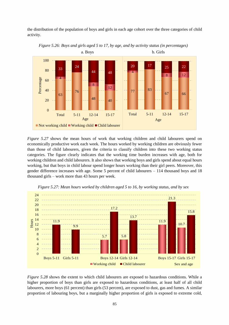
85
the distribution of the population of boys and girls in each age cohort over the three categories of child
activity.
Figure 5.26: Boys and girls aged 5 to 17, by age, and by activity status (in percentages)
a. Boys b. Girls
Figure 5.27 shows the mean hours of work that working children and child labourers spend on
economically productive work each week. The hours worked by working children are obviously fewer
than those of child labourers, given the criteria to classify children into these two working status
categories. The figure clearly indicates that the working time burden increases with age, both for
working children and child labourers. It also shows that working boys and girls spend about equal hours
working, but that boys in child labour spend longer hours working than their girl peers. Moreover, this
gender difference increases with age. Some 5 percent of child labourers – 114 thousand boys and 18
thousand girls – work more than 43 hours per week.
Figure 5.27: Mean hours worked by children aged 5 to 16, by working status, and by sex
Figure 5.28 shows the extent to which child labourers are exposed to hazardous conditions. While a
higher proportion of boys than girls are exposed to hazardous conditions, at least half of all child
labourers, more boys (61 percent) than girls (53 percent), are exposed to dust, gas and fumes. A similar
proportion of labouring boys, but a marginally higher proportion of girls is exposed to extreme cold,
77 8367 66
48 12
20 1725 22
Total 5-11 12-14 15-17
Age
6376
4840
4
812
3324
44 48
0
20
40
60
80
100
Total 5-11 12-14 15-17
Per
centa
ge
Age
Not working child Working child Child labourer
5.7 5.8
11.910.7
11.9
9.9
17.2
13.7
21.3
15.8
0
2
4
6
8
10
12
14
16
18
20
22
24
Boys 5-11 Girls 5-11 Boys 12-14 Girls 12-14 Boys 15-17 Girls 15-17
Ho
urs
Sex and ageWorking child Child labourer
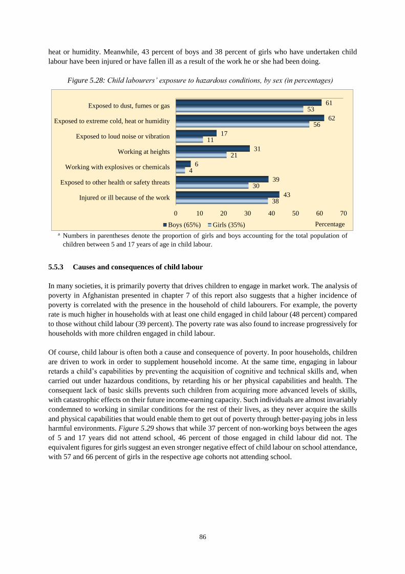
86
heat or humidity. Meanwhile, 43 percent of boys and 38 percent of girls who have undertaken child
labour have been injured or have fallen ill as a result of the work he or she had been doing.
Figure 5.28: Child labourers’ exposure to hazardous conditions, by sex (in percentages)
a Numbers in parentheses denote the proportion of girls and boys accounting for the total population of
children between 5 and 17 years of age in child labour.
5.5.3 Causes and consequences of child labour
In many societies, it is primarily poverty that drives children to engage in market work. The analysis of
poverty in Afghanistan presented in chapter 7 of this report also suggests that a higher incidence of
poverty is correlated with the presence in the household of child labourers. For example, the poverty
rate is much higher in households with at least one child engaged in child labour (48 percent) compared
to those without child labour (39 percent). The poverty rate was also found to increase progressively for
households with more children engaged in child labour.
Of course, child labour is often both a cause and consequence of poverty. In poor households, children
are driven to work in order to supplement household income. At the same time, engaging in labour
retards a child’s capabilities by preventing the acquisition of cognitive and technical skills and, when
carried out under hazardous conditions, by retarding his or her physical capabilities and health. The
consequent lack of basic skills prevents such children from acquiring more advanced levels of skills,
with catastrophic effects on their future income-earning capacity. Such individuals are almost invariably
condemned to working in similar conditions for the rest of their lives, as they never acquire the skills
and physical capabilities that would enable them to get out of poverty through better-paying jobs in less
harmful environments. Figure 5.29 shows that while 37 percent of non-working boys between the ages
of 5 and 17 years did not attend school, 46 percent of those engaged in child labour did not. The
equivalent figures for girls suggest an even stronger negative effect of child labour on school attendance,
with 57 and 66 percent of girls in the respective age cohorts not attending school.
61
62
17
31
6
39
43
53
56
11
21
4
30
38
0 10 20 30 40 50 60 70
Exposed to dust, fumes or gas
Exposed to extreme cold, heat or humidity
Exposed to loud noise or vibration
Working at heights
Working with explosives or chemicals
Exposed to other health or safety threats
Injured or ill because of the work
PercentageBoys (65%) Girls (35%)
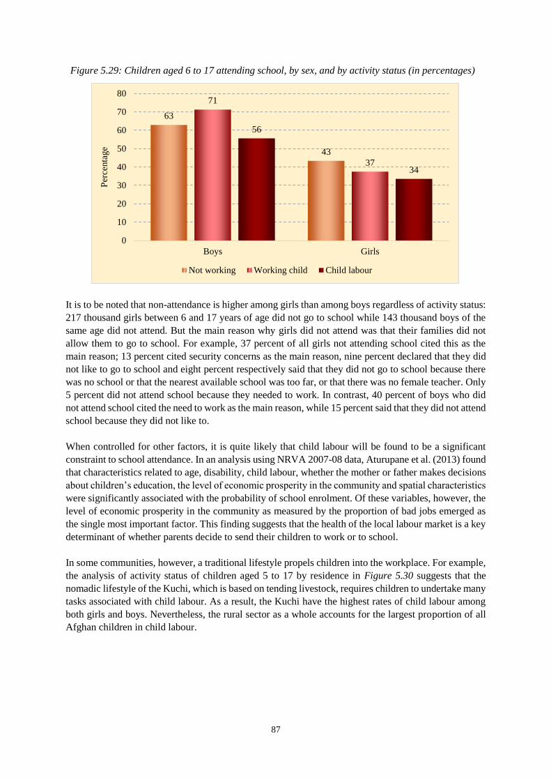
87
Figure 5.29: Children aged 6 to 17 attending school, by sex, and by activity status (in percentages)
It is to be noted that non-attendance is higher among girls than among boys regardless of activity status:
217 thousand girls between 6 and 17 years of age did not go to school while 143 thousand boys of the
same age did not attend. But the main reason why girls did not attend was that their families did not
allow them to go to school. For example, 37 percent of all girls not attending school cited this as the
main reason; 13 percent cited security concerns as the main reason, nine percent declared that they did
not like to go to school and eight percent respectively said that they did not go to school because there
was no school or that the nearest available school was too far, or that there was no female teacher. Only
5 percent did not attend school because they needed to work. In contrast, 40 percent of boys who did
not attend school cited the need to work as the main reason, while 15 percent said that they did not attend
school because they did not like to.
When controlled for other factors, it is quite likely that child labour will be found to be a significant
constraint to school attendance. In an analysis using NRVA 2007-08 data, Aturupane et al. (2013) found
that characteristics related to age, disability, child labour, whether the mother or father makes decisions
about children’s education, the level of economic prosperity in the community and spatial characteristics
were significantly associated with the probability of school enrolment. Of these variables, however, the
level of economic prosperity in the community as measured by the proportion of bad jobs emerged as
the single most important factor. This finding suggests that the health of the local labour market is a key
determinant of whether parents decide to send their children to work or to school.
In some communities, however, a traditional lifestyle propels children into the workplace. For example,
the analysis of activity status of children aged 5 to 17 by residence in Figure 5.30 suggests that the
nomadic lifestyle of the Kuchi, which is based on tending livestock, requires children to undertake many
tasks associated with child labour. As a result, the Kuchi have the highest rates of child labour among
both girls and boys. Nevertheless, the rural sector as a whole accounts for the largest proportion of all
Afghan children in child labour.
63
43
71
37
56
34
0
10
20
30
40
50
60
70
80
Boys Girls
Per
centa
ge
Not working Working child Child labour
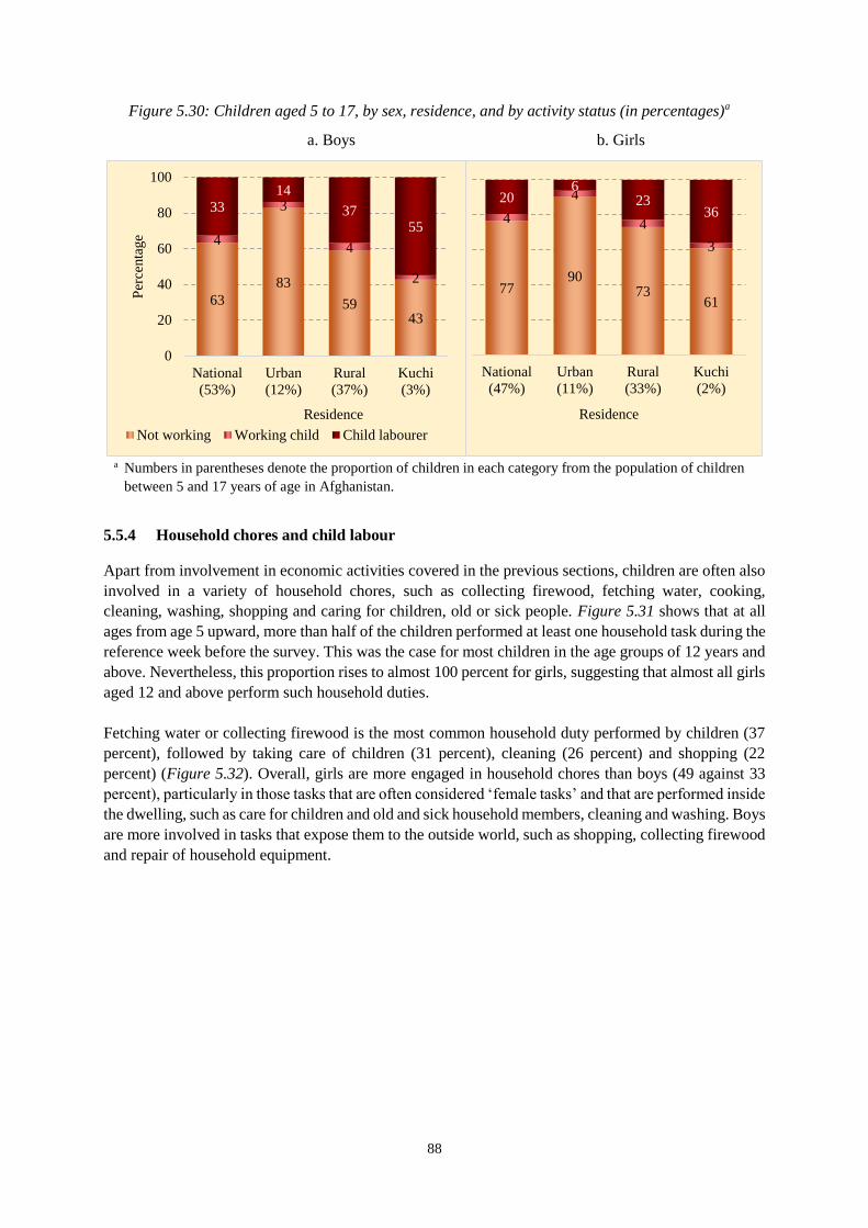
88
Figure 5.30: Children aged 5 to 17, by sex, residence, and by activity status (in percentages)a
a. Boys b. Girls
a Numbers in parentheses denote the proportion of children in each category from the population of children
between 5 and 17 years of age in Afghanistan.
5.5.4 Household chores and child labour
Apart from involvement in economic activities covered in the previous sections, children are often also
involved in a variety of household chores, such as collecting firewood, fetching water, cooking,
cleaning, washing, shopping and caring for children, old or sick people. Figure 5.31 shows that at all
ages from age 5 upward, more than half of the children performed at least one household task during the
reference week before the survey. This was the case for most children in the age groups of 12 years and
above. Nevertheless, this proportion rises to almost 100 percent for girls, suggesting that almost all girls
aged 12 and above perform such household duties.
Fetching water or collecting firewood is the most common household duty performed by children (37
percent), followed by taking care of children (31 percent), cleaning (26 percent) and shopping (22
percent) (Figure 5.32). Overall, girls are more engaged in household chores than boys (49 against 33
percent), particularly in those tasks that are often considered ‘female tasks’ and that are performed inside
the dwelling, such as care for children and old and sick household members, cleaning and washing. Boys
are more involved in tasks that expose them to the outside world, such as shopping, collecting firewood
and repair of household equipment.
7790
7361
4
4
4
3
206
2336
National
(47%)
Urban
(11%)
Rural
(33%)
Kuchi
(2%)
Residence
63
83
5943
4
3
4
2
33
14
3755
0
20
40
60
80
100
National
(53%)
Urban
(12%)
Rural
(37%)
Kuchi
(3%)
Per
centa
ge
Residence
Not working Working child Child labourer
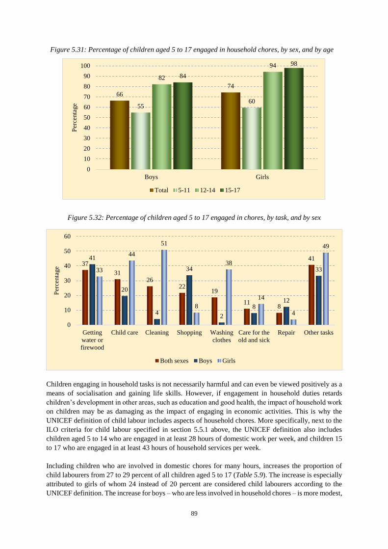
89
Figure 5.31: Percentage of children aged 5 to 17 engaged in household chores, by sex, and by age
Figure 5.32: Percentage of children aged 5 to 17 engaged in chores, by task, and by sex
Children engaging in household tasks is not necessarily harmful and can even be viewed positively as a
means of socialisation and gaining life skills. However, if engagement in household duties retards
children’s development in other areas, such as education and good health, the impact of household work
on children may be as damaging as the impact of engaging in economic activities. This is why the
UNICEF definition of child labour includes aspects of household chores. More specifically, next to the
ILO criteria for child labour specified in section 5.5.1 above, the UNICEF definition also includes
children aged 5 to 14 who are engaged in at least 28 hours of domestic work per week, and children 15
to 17 who are engaged in at least 43 hours of household services per week.
Including children who are involved in domestic chores for many hours, increases the proportion of
child labourers from 27 to 29 percent of all children aged 5 to 17 (Table 5.9). The increase is especially
attributed to girls of whom 24 instead of 20 percent are considered child labourers according to the
UNICEF definition. The increase for boys – who are less involved in household chores – is more modest,
66
74
5560
82
94
84
98
0
10
20
30
40
50
60
70
80
90
100
Boys Girls
Per
centa
ge
Total 5-11 12-14 15-17
37
3126
2219
118
4141
20
4
34
2
812
3333
44
51
8
38
14
4
49
0
10
20
30
40
50
60
Getting
water or
firewood
Child care Cleaning Shopping Washing
clothes
Care for the
old and sick
Repair Other tasks
Per
centa
ge
Both sexes Boys Girls
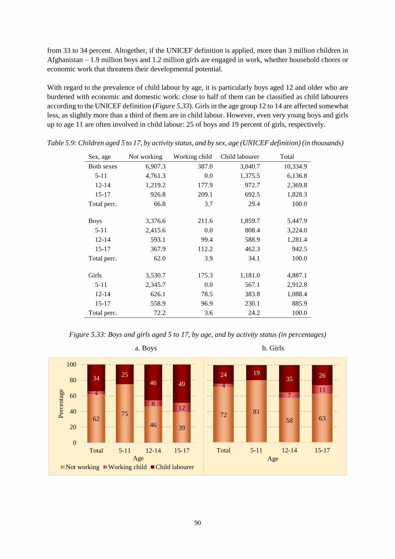
90
from 33 to 34 percent. Altogether, if the UNICEF definition is applied, more than 3 million children in
Afghanistan – 1.9 million boys and 1.2 million girls are engaged in work, whether household chores or
economic work that threatens their developmental potential.
With regard to the prevalence of child labour by age, it is particularly boys aged 12 and older who are
burdened with economic and domestic work: close to half of them can be classified as child labourers
according to the UNICEF definition (Figure 5.33). Girls in the age group 12 to 14 are affected somewhat
less, as slightly more than a third of them are in child labour. However, even very young boys and girls
up to age 11 are often involved in child labour: 25 of boys and 19 percent of girls, respectively.
Table 5.9: Children aged 5 to 17, by activity status, and by sex, age (UNICEF definition) (in thousands)
Sex, age Not working Working child Child labourer Total
Both sexes 6,907.3 387.0 3,040.7 10,334.9
5-11 4,761.3 0.0 1,375.5 6,136.8
12-14 1,219.2 177.9 972.7 2,369.8
15-17 926.8 209.1 692.5 1,828.3
Total perc. 66.8 3.7 29.4 100.0
Boys 3,376.6 211.6 1,859.7 5,447.9
5-11 2,415.6 0.0 808.4 3,224.0
12-14 593.1 99.4 588.9 1,281.4
15-17 367.9 112.2 462.3 942.5
Total perc. 62.0 3.9 34.1 100.0
Girls 3,530.7 175.3 1,181.0 4,887.1
5-11 2,345.7 0.0 567.1 2,912.8
12-14 626.1 78.5 383.8 1,088.4
15-17 558.9 96.9 230.1 885.9
Total perc. 72.2 3.6 24.2 100.0
Figure 5.33: Boys and girls aged 5 to 17, by age, and by activity status (in percentages)
a. Boys b. Girls
7281
58 63
4
711
24 1935
26
Total 5-11 12-14 15-17
Age
6275
46 39
4
812
3425
46 49
0
20
40
60
80
100
Total 5-11 12-14 15-17
Per
centa
ge
Age
Not working Working child Child labourer
91
6 FARMING AND LIVESTOCK
Summary. The ALCS 2013-14 confirms that agriculture – encompassing farming and animal husbandry
- makes up the backbone of Afghanistan’s economy. Agriculture provides a source of income for 61
percent of households, and for 28 percent it is the most important income source in the household.
Similarly, it is the main sector of employment for 44 percent of the working population. Some 37 percent
of all households in Afghanistan – approximately 1.4 million households – own any irrigated farm land,
while around one in six households – 620 thousand – own the much less productive rain-fed land.
Mechanisms of leasing and renting land, sharecropping land and mortgaging land have the effect of a
net transfer of access to farm land from land-owners living in urban areas to rural households that
cultivate the land. At the same time these mechanisms result in somewhat fewer households having
access to somewhat larger farming areas. On average, households engaged in irrigated cultivation have
on average access to 6.6 jeribs of irrigated land and those engaged in rain-dependent agriculture have
access to 13.7 jeribs of rain-fed land. Poor soil, farming costs and particularly the lack of water enforce
households to leave fallow around one third of land available for irrigated and rain-fed farming.
The large majority of households cultivating irrigated land – 85 percent, corresponding to more than
million households – grew wheat on their land for the spring harvesting season. Fodder crops, potatoes
and maize or sorghum were the next most frequently grown crops on irrigated land. The concentration
on wheat production is even stronger on rain-fed land, as 93 percent of the households involved grow
this crop. However, the total volume produced is only one third of the volume produced on irrigated
land. Farming households spent on average 14 thousand Afghanis on farming costs, especially on
fertiliser, seeds and machinery rent. Together, farming households spent 21 billion Afghanis (around
365 million USD) on farming inputs. Households owning a garden plot – 13 percent of all households
– are usually able to grow high-value and high-nutrition crops. Grapes and apples are the crops grown
most often.
Livestock is an important asset of Afghan households, either for own household consumption or for
market sale of animals and animal products. ALCS 2013-14 data suggest that the number of cattle has
reduced, but the number of sheep has increased since 2011-12. A large proportion of livestock owners
– 73 percent – had access to animal feed concentrate, but only 37 percent could obtain a sufficient
amount. Levels of full vaccination of livestock are low, running from 15 percent for sheep and between
12 and 14 percent for goats, cattle, camels and oxen and yaks, to 9 percent for chickens.
Only one in five households involved in either farming or livestock tending used agricultural extension
services or veterinary support. Apart from voluntary reasons, the most important reasons for non-use
were the lack of knowledge of where or how to obtain the services, the reluctance to offer services by
the provider and the distance to the facility.
6.1 Introduction
Agriculture – including farming and livestock-related activities – is the backbone of Afghanistan’s
economy. For 61 percent of households agriculture provides any source of income and for 28 percent
it is even the most important source. Similarly, with 44 percent of the employed engaged in agriculture,
it is the main sector for employment (see section 4.3.2 of this report). CSO estimates that the sector
contributes 25 percent to the country’s GDP in the solar year 1393 (2013-14) (CSO 2014). However,
the capacity of the agriculture sector is restricted by droughts, a partially destroyed infrastructure and
shrinking grazing land.
92
With a varied geography and topography, out of 652 thousand square kilometres of total land area, only
an estimated 12 percent is arable, 3 percent of the land is considered forest-covered, 46 percent is under
permanent pasture and 39 percent is mountainous, not usable for agriculture (CSO 2014).
This chapter deals with various aspects of Afghanistan’s agricultural sector and is divided into two main
parts: section 6.2 on farming and horticulture, and section 6.3 on livestock-related information.
6.2 Farming and horticulture
Land tenure in Afghanistan involves a complex system of ownership and access through renting,
sharecropping and mortgaging. Furthermore, significant differences exist between productivity of
irrigated and rain-fed land. Thus, the Ministry of Agriculture, Irrigation and Livestock (MAIL)
estimates that typically yield of wheat from irrigated fields is 2.7 times higher than that from rain-fed
fields (MAIL 2012). Horticulture involves again harvests that have high monetary value, even though
usually garden plots are small in terms of size. Consequently, this section on farming treats the different
types of land – irrigated, rain-fed and garden plot – separately, and distinguishes the different types of
land tenure.
6.2.1 Irrigated land
Irrigated land tenure
Some 37 percent of all households in Afghanistan – approximately 1.4 million households – own any
irrigated farm land. The majority of these land owners (63 percent) have a farm size of less than 4 jeribs
(0.8 ha.)32, whereas the median and mean irrigated land size is, respectively, 2.5 and 6.1 jeribs (1.2 and
0.5 ha.) (Table 6.1). The trend of an increasing share of land owners with small landholdings – below
four jeribs – that was observed in NRVA 2011-12, has continued. In 2007-08 the proportion with such
small landholdings was 54 percent and this increased to 58 percent in 2011-12. This trend towards
smaller land size is also reflected in the lower median size of owned irrigated land: half of land owners
have now less than 2.5 jeribs of land, compared to 3.0 jeribs in 2011-12. It is very likely that the
fragmentation of land is a result of the fast population growth that Afghanistan is experiencing (see
chapter 3), which results in an increasing pressure on the limited area of irrigable land.
A disproportionate share of irrigated land is owned by urban households: while urban households make
up 10 percent of all households that own irrigated land, they own almost 19 percent of the land. This is
also reflected in the larger average irrigated land size owned by urban households compared to rural
households: 11.1 against 5.4 jeribs. Apparently, irrigated land is accumulated by urban dwellers. The
proportion of rural households that own any irrigated land is 46 percent.
32 One jerib is 0.2 hectare (2,000 m2)
93
Table 6.1: Households, by (a) ownership of irrigated land and (b) access to irrigated land, irrigated
land size (in percentages); also stating mean and median irrigated land size (in jeribs)
a. Ownership b. Access
Ownership Percentage Access Percentage
Total 100.0 Total 100.0
No ownership 63.4 No access 63.8
Any ownership 36.6 Any access 36.2
Less than 2.0 jeribs 34.3 Less than 2.0 jeribs 30.4
2.0-3.9 jeribs 28.2 2.0-3.9 jeribs 27.6
4.0-5.9 jeribs 14.2 4.0-5.9 jeribs 15.4
6.0-9.9 jeribs 9.5 6.0-9.9 jeribs 10.7
10.0-19.9 jeribs 8.5 10.0-19.9 jeribs 10.1
20 jeribs or more 5.3 20 jeribs or more 5.8
Mean land size 6.1 Mean land size 6.6
Median land size 2.5 Median land size 3.0
Besides owning land, households can also access (additional) land for cultivation by renting- or leasing-
in, sharecropping-in or mortgaging-in. Vice versa, land owners can provide access to land to other
households by renting- or leasing-out, sharecropping-out or mortgaging-out. Some land owners transfer
access of all their land to others for land cultivation. Around 5 percent of households reported that they
had access to (additional) irrigated land without ownership of that land, by renting- or leasing-in,
sharecropping-in or mortgaging-in. For 3 percent (some 114 thousand households) this was the only
way of accessing irrigated land, the other 2 percent had also other land in ownership. On the other hand,
9 percent of households that owned irrigated land themselves provided access for cultivating to their
land or part of their land to other households. Most of the land (around three quarters) that was cultivated
by a household that did not own land itself was transferred in an arrangement of sharecropping between
the owner and cultivator, while another sizeable part (between one quarter and one fifth) was rented
and a negligible proportion was mortgaged.
The typical share that is given to the sharecropping landowner is 50 percent of the farm produce (by 57
percent of sharecroppers). One quarter (26 percent) gave less than 50 percent of the produce and 17
percent more than 50 percent.
The proportion of households owning any irrigated land (36.6 percent; Table 6.1, panel a) is almost the
same as the proportion having access to any irrigated land (36.3 percent; panel b). However, transfer of
access to land does affect the size of land being cultivated by farming households. Whereas the
proportion landholders owning at least 4 jeribs of irrigated land was 37 percent, the share of households
with access to at least 4 jerbs land was 42 percent. The transfer of access to land has the effect of
increasing the mean and median area of irrigated land that is accessed, becoming 6.6 and 3.0 jeribs,
respectively.
The transfer of irrigated land for cultivation occurred particularly from landowners living in urban areas
– usually detached from their land – to rural households. More than two fifth (41 percent) of the land
owned by urban households is transferred to other households for cultivation. In absolute land area, this
is more than rural land-owning households do, who transferred only 8 percent of irrigated land to others.
Compared to 46 percent of rural households that own any irrigated land, the proportion that has access
to land increases to 48 percent if renting, leasing and mortgaging arrangements are included. And the
share of rural households that has access to at least 4 jeribs of irrigated land is almost 3 percentage
points higher (at 20 percent) than the share that owns at least 4 jeribs.
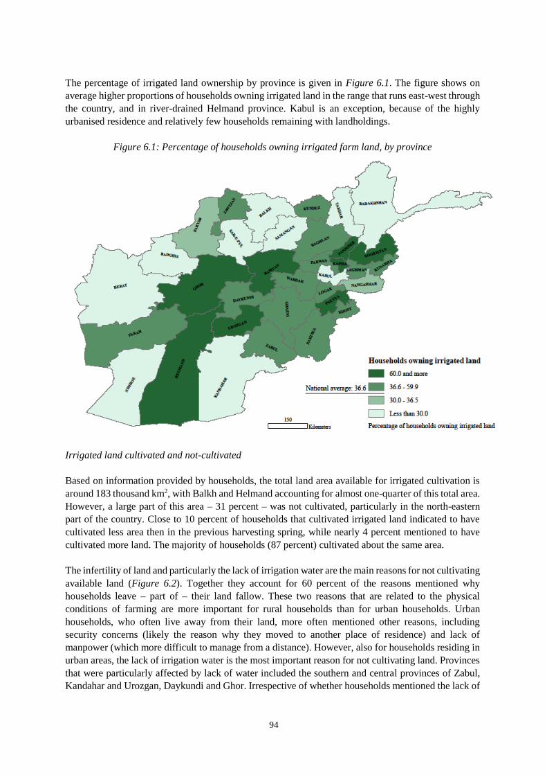
94
The percentage of irrigated land ownership by province is given in Figure 6.1. The figure shows on
average higher proportions of households owning irrigated land in the range that runs east-west through
the country, and in river-drained Helmand province. Kabul is an exception, because of the highly
urbanised residence and relatively few households remaining with landholdings.
Figure 6.1: Percentage of households owning irrigated farm land, by province
Irrigated land cultivated and not-cultivated
Based on information provided by households, the total land area available for irrigated cultivation is
around 183 thousand km2, with Balkh and Helmand accounting for almost one-quarter of this total area.
However, a large part of this area – 31 percent – was not cultivated, particularly in the north-eastern
part of the country. Close to 10 percent of households that cultivated irrigated land indicated to have
cultivated less area then in the previous harvesting spring, while nearly 4 percent mentioned to have
cultivated more land. The majority of households (87 percent) cultivated about the same area.
The infertility of land and particularly the lack of irrigation water are the main reasons for not cultivating
available land (Figure 6.2). Together they account for 60 percent of the reasons mentioned why
households leave – part of – their land fallow. These two reasons that are related to the physical
conditions of farming are more important for rural households than for urban households. Urban
households, who often live away from their land, more often mentioned other reasons, including
security concerns (likely the reason why they moved to another place of residence) and lack of
manpower (which more difficult to manage from a distance). However, also for households residing in
urban areas, the lack of irrigation water is the most important reason for not cultivating land. Provinces
that were particularly affected by lack of water included the southern and central provinces of Zabul,
Kandahar and Urozgan, Daykundi and Ghor. Irrespective of whether households mentioned the lack of
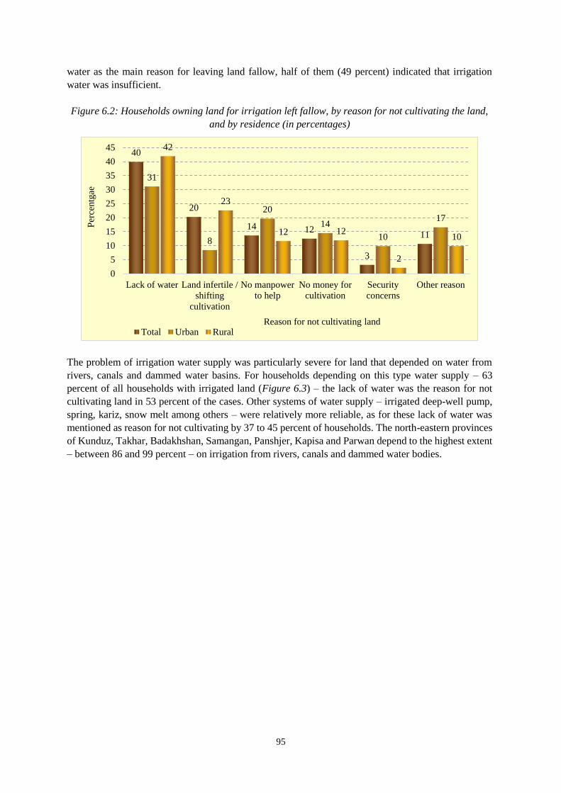
95
water as the main reason for leaving land fallow, half of them (49 percent) indicated that irrigation
water was insufficient.
Figure 6.2: Households owning land for irrigation left fallow, by reason for not cultivating the land,
and by residence (in percentages)
The problem of irrigation water supply was particularly severe for land that depended on water from
rivers, canals and dammed water basins. For households depending on this type water supply – 63
percent of all households with irrigated land (Figure 6.3) – the lack of water was the reason for not
cultivating land in 53 percent of the cases. Other systems of water supply – irrigated deep-well pump,
spring, kariz, snow melt among others – were relatively more reliable, as for these lack of water was
mentioned as reason for not cultivating by 37 to 45 percent of households. The north-eastern provinces
of Kunduz, Takhar, Badakhshan, Samangan, Panshjer, Kapisa and Parwan depend to the highest extent
– between 86 and 99 percent – on irrigation from rivers, canals and dammed water bodies.
40
20
14 12
3
11
31
8
20
14
10
17
42
23
12 12
2
10
0
5
10
15
20
25
30
35
40
45
Lack of water Land infertile /
shifting
cultivation
No manpower
to help
No money for
cultivation
Security
concerns
Other reason
Per
centg
ae
Reason for not cultivating landTotal Urban Rural
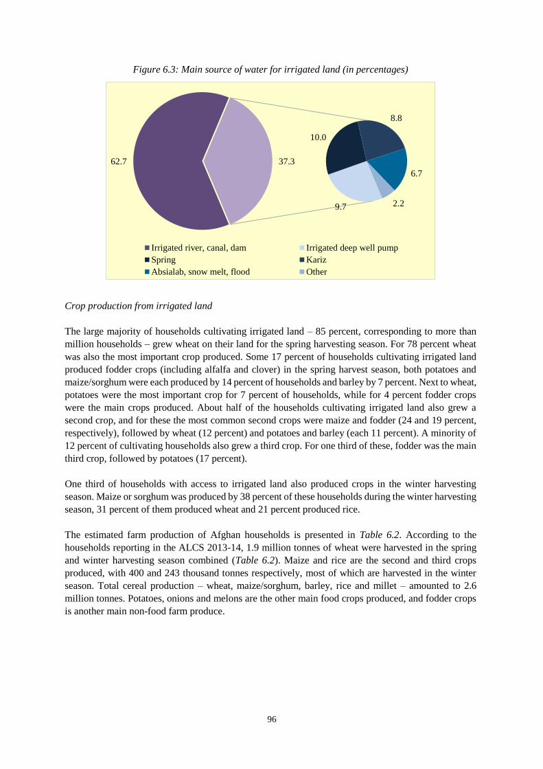
96
Figure 6.3: Main source of water for irrigated land (in percentages)
Crop production from irrigated land
The large majority of households cultivating irrigated land – 85 percent, corresponding to more than
million households – grew wheat on their land for the spring harvesting season. For 78 percent wheat
was also the most important crop produced. Some 17 percent of households cultivating irrigated land
produced fodder crops (including alfalfa and clover) in the spring harvest season, both potatoes and
maize/sorghum were each produced by 14 percent of households and barley by 7 percent. Next to wheat,
potatoes were the most important crop for 7 percent of households, while for 4 percent fodder crops
were the main crops produced. About half of the households cultivating irrigated land also grew a
second crop, and for these the most common second crops were maize and fodder (24 and 19 percent,
respectively), followed by wheat (12 percent) and potatoes and barley (each 11 percent). A minority of
12 percent of cultivating households also grew a third crop. For one third of these, fodder was the main
third crop, followed by potatoes (17 percent).
One third of households with access to irrigated land also produced crops in the winter harvesting
season. Maize or sorghum was produced by 38 percent of these households during the winter harvesting
season, 31 percent of them produced wheat and 21 percent produced rice.
The estimated farm production of Afghan households is presented in Table 6.2. According to the
households reporting in the ALCS 2013-14, 1.9 million tonnes of wheat were harvested in the spring
and winter harvesting season combined (Table 6.2). Maize and rice are the second and third crops
produced, with 400 and 243 thousand tonnes respectively, most of which are harvested in the winter
season. Total cereal production – wheat, maize/sorghum, barley, rice and millet – amounted to 2.6
million tonnes. Potatoes, onions and melons are the other main food crops produced, and fodder crops
is another main non-food farm produce.
62.7
9.7
10.0
8.8
6.7
2.2
37.3
Irrigated river, canal, dam Irrigated deep well pump
Spring Kariz
Absialab, snow melt, flood Other
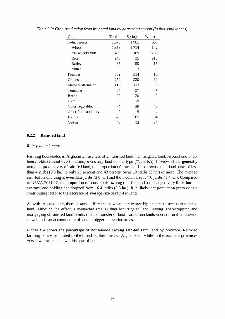
97
Table 6.2: Crop production from irrigated land by harvesting season (in thousand tonnes)
Crop Total Spring Winter
Total cereals 2,570 1,961 609
Wheat 1,856 1,714 142
Maize, sorghum 400 169 230
Rice 243 25 218
Barley 65 50 15
Millet 5 2 3
Potatoes 332 314 18
Onions 250 220 30
Melon/watermelon 119 113 6
Tomatoes 64 57 7
Beans 25 20 5
Okra 22 19 3
Other vegetables 74 29 45
Other fruits and nuts 9 5 4
Fodder 370 285 84
Cotton 46 12 34
6.2.2 Rain-fed land
Rain-fed land tenure
Farming households in Afghanistan use less often rain-fed land than irrigated land. Around one in six
households (around 620 thousand) owns any land of this type (Table 6.3). In view of the generally
marginal productivity of rain-fed land, the proportion of households that owns small land areas of less
than 4 jeribs (0.8 ha.) is only 23 percent and 43 percent owns 10 jeribs (2 ha.) or more. The average
rain-fed landholding is even 13.2 jeribs (2.6 ha.) and the median size is 7.0 jeribs (1.4 ha.). Compared
to NRVA 2011-12, the proportion of households owning rain-fed land has changed very little, but the
average land holding has dropped from 16.4 jeribs (3.3 ha.). It is likely that population pressure is a
contributing factor to the decrease of average size of rain-fed land.
As with irrigated land, there is some difference between land ownership and actual access to rain-fed
land. Although the effect is somewhat smaller than for irrigated land, leasing, sharecropping and
mortgaging of rain-fed land results in a net transfer of land from urban landowners to rural land users,
as well as in an accumulation of land in bigger cultivation areas.
Figure 6.4 shows the percentage of households owning rain-fed farm land by province. Rain-fed
farming is mostly limited to the broad northern belt of Afghanistan, while in the southern provinces
very few households own this type of land.
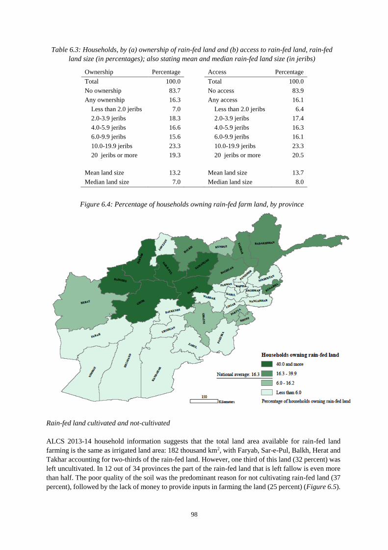
98
Table 6.3: Households, by (a) ownership of rain-fed land and (b) access to rain-fed land, rain-fed
land size (in percentages); also stating mean and median rain-fed land size (in jeribs)
Ownership Percentage Access Percentage
Total 100.0 Total 100.0
No ownership 83.7 No access 83.9
Any ownership 16.3 Any access 16.1
Less than 2.0 jeribs 7.0 Less than 2.0 jeribs 6.4
2.0-3.9 jeribs 18.3 2.0-3.9 jeribs 17.4
4.0-5.9 jeribs 16.6 4.0-5.9 jeribs 16.3
6.0-9.9 jeribs 15.6 6.0-9.9 jeribs 16.1
10.0-19.9 jeribs 23.3 10.0-19.9 jeribs 23.3
20 jeribs or more 19.3 20 jeribs or more 20.5
Mean land size 13.2 Mean land size 13.7
Median land size 7.0 Median land size 8.0
Figure 6.4: Percentage of households owning rain-fed farm land, by province
Rain-fed land cultivated and not-cultivated
ALCS 2013-14 household information suggests that the total land area available for rain-fed land
farming is the same as irrigated land area: 182 thousand km2, with Faryab, Sar-e-Pul, Balkh, Herat and
Takhar accounting for two-thirds of the rain-fed land. However, one third of this land (32 percent) was
left uncultivated. In 12 out of 34 provinces the part of the rain-fed land that is left fallow is even more
than half. The poor quality of the soil was the predominant reason for not cultivating rain-fed land (37
percent), followed by the lack of money to provide inputs in farming the land (25 percent) (Figure 6.5).
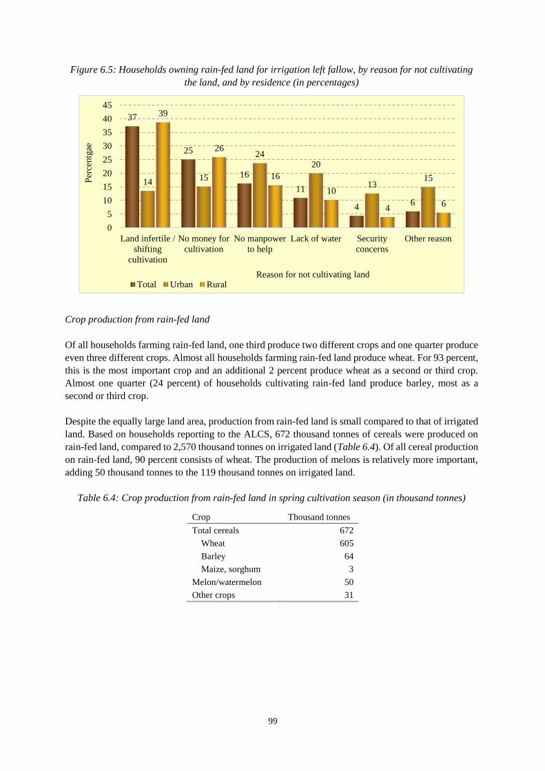
99
Figure 6.5: Households owning rain-fed land for irrigation left fallow, by reason for not cultivating
the land, and by residence (in percentages)
Crop production from rain-fed land
Of all households farming rain-fed land, one third produce two different crops and one quarter produce
even three different crops. Almost all households farming rain-fed land produce wheat. For 93 percent,
this is the most important crop and an additional 2 percent produce wheat as a second or third crop.
Almost one quarter (24 percent) of households cultivating rain-fed land produce barley, most as a
second or third crop.
Despite the equally large land area, production from rain-fed land is small compared to that of irrigated
land. Based on households reporting to the ALCS, 672 thousand tonnes of cereals were produced on
rain-fed land, compared to 2,570 thousand tonnes on irrigated land (Table 6.4). Of all cereal production
on rain-fed land, 90 percent consists of wheat. The production of melons is relatively more important,
adding 50 thousand tonnes to the 119 thousand tonnes on irrigated land.
Table 6.4: Crop production from rain-fed land in spring cultivation season (in thousand tonnes)
Crop Thousand tonnes
Total cereals 672
Wheat 605
Barley 64
Maize, sorghum 3
Melon/watermelon 50
Other crops 31
37
25
16
11
46
1415
2420
1315
39
26
16
10
46
0
5
10
15
20
25
30
35
40
45
Land infertile /
shifting
cultivation
No money for
cultivation
No manpower
to help
Lack of water Security
concerns
Other reason
Per
centg
ae
Reason for not cultivating landTotal Urban Rural
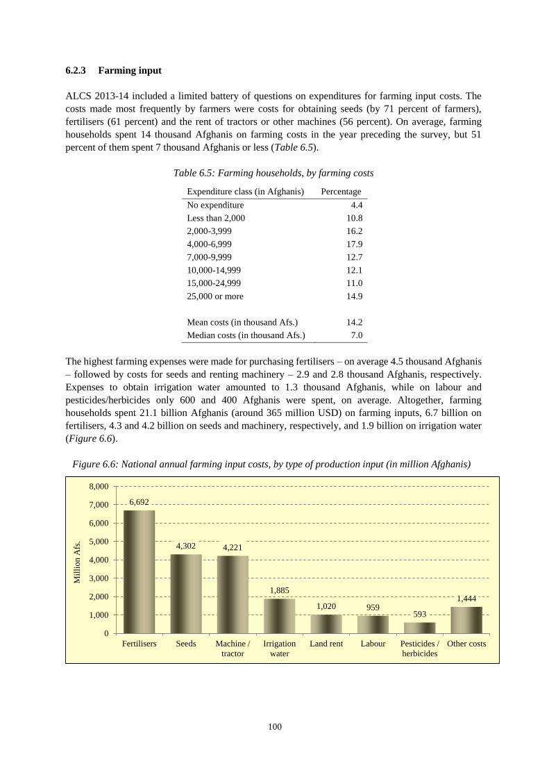
100
6.2.3 Farming input
ALCS 2013-14 included a limited battery of questions on expenditures for farming input costs. The
costs made most frequently by farmers were costs for obtaining seeds (by 71 percent of farmers),
fertilisers (61 percent) and the rent of tractors or other machines (56 percent). On average, farming
households spent 14 thousand Afghanis on farming costs in the year preceding the survey, but 51
percent of them spent 7 thousand Afghanis or less (Table 6.5).
Table 6.5: Farming households, by farming costs
Expenditure class (in Afghanis) Percentage
No expenditure 4.4
Less than 2,000 10.8
2,000-3,999 16.2
4,000-6,999 17.9
7,000-9,999 12.7
10,000-14,999 12.1
15,000-24,999 11.0
25,000 or more 14.9
Mean costs (in thousand Afs.) 14.2
Median costs (in thousand Afs.) 7.0
The highest farming expenses were made for purchasing fertilisers – on average 4.5 thousand Afghanis
– followed by costs for seeds and renting machinery – 2.9 and 2.8 thousand Afghanis, respectively.
Expenses to obtain irrigation water amounted to 1.3 thousand Afghanis, while on labour and
pesticides/herbicides only 600 and 400 Afghanis were spent, on average. Altogether, farming
households spent 21.1 billion Afghanis (around 365 million USD) on farming inputs, 6.7 billion on
fertilisers, 4.3 and 4.2 billion on seeds and machinery, respectively, and 1.9 billion on irrigation water
(Figure 6.6).
Figure 6.6: National annual farming input costs, by type of production input (in million Afghanis)
6,692
4,302 4,221
1,885
1,020 959593
1,444
0
1,000
2,000
3,000
4,000
5,000
6,000
7,000
8,000
Fertilisers Seeds Machine /
tractor
Irrigation
water
Land rent Labour Pesticides /
herbicides
Other costs
Mil
lio
n A
fs.
101
Just over half farming households (54 percent) use tractors or other motorised power as traction
power for ploughing. Somewhat less – 41 percent – use oxen or other animals and 5 percent use
human power for ploughing.
Agricultural extension services are used to a limited extent. The exception is Herat, where 90 percent
of farmers used these services. Other provinces with relatively widespread use are Wardak, Nangarhar,
Paktya and Jawzjan, where use ranges between 40 and 68 percent. On the other hand, 15 in provinces
use is less than 10 percent.33 The main reason why farmers did not use these extension was lack of
knowledge how to find or obtain the services (35 percent). Other reasons frequently mentioned included
reluctance from the service side to work with the farmer (20 percent) and the distance to the service (16
percent). Costs were mentioned as the main reason in 9 percent of the cases.
6.2.4 Horticulture
Tenure and size of garden plots
Produce from garden plots is important for many Afghanistan households, in terms of supplementation
of their consumption diet, as well as their household income. Valuable garden products with high-
nutrient content – especially fruits and nuts – are harvested from horticulture production. Overall, 13
percent of households own a garden plot. Having a garden plot is more widespread in rural areas –
where 16 percent of households own a plot – but even in urban areas, 5 percent have one. Especially in
the central-eastern provinces of Zabul, Paktika, Ghazni, Wardak, Bamyan and Parwan many households
– between 25 and 50 percent – own garden plots.
Garden plots are substantially smaller in size than normal farm land, irrigated or rain-fed. The mean
plot size is 1.9 jeribs (0.4 ha.) (Table 6.6a), but 55 percent of the garden-plot owners have one jerib or
less. The lease or rent, sharecropping and mortgage of garden plots is far less common than that of farm
land. Consequently, there is very little difference between the distribution of owning and accessing
garden plots. However, as with farm land, a noticeable transfer occurs from urban dwellers, who
probably own garden plots in their province of origin, to rural garden plot tillers.
33 These provinces are Zabul, Khost, Badakhshan, Nimroz, Takhar, Kandahar, Daykundi, Samangan, Ghor,
Faryab, Farah, Kapisa, Badghis, Sar-e-Pul and Parwan.
102
Table 6.6: Households, by (a) ownership of garden plot and (b) access to garden plot, garden plot
size (in percentages); also stating mean and median garden plot size (in jeribs)
Ownership Percentage Access Percentage
Total 100.0 Total 100.0
No ownership 87.4 No access 87.8
Any ownership 12.6 Any access 12.2
Less than 1.0 jerib 27.4 Less than 1.0 jerib 26.6
1.0-1.9 jeribs 34.6 1.0-1.9 jeribs 34.8
2.0-3.9 jeribs 28.1 2.0-3.9 jeribs 28.9
4.0-5.9 jeribs 6.0 4.0-5.9 jeribs 5.9
6.0-9.9 jeribs 1.9 6.0-9.9 jeribs 1.9
10 jeribs or more 2.0 10 jeribs or more 1.8
Mean plot size 1.9 Mean plot size 1.9
Median plot size 1.0 Median plot size 1.0
Horticulture production
The crops that were most commonly grown on garden plots are grapes (on 35 percent of garden plots)
and apples (on 29 percent). Grapes were mostly used for fresh consumption or marketing, but around
one third was dried before selling or consumption. Apricots and nuts were the third- and fourth-most
commonly grown crops, on 17 and 15 percent of garden plots, respectively. Also apricots are mostly
used fresh. Fodder was an important secondary crop, grown on 11 percent of garden plots. Table 6.7
gives the harvested produce from garden plots.
Table 6.7: Fruit and crop production from garden plots (in thousand tonnes)
Crop Total
Fresh grapes 304
Dried grapes 50
Apples 239
Fresh apricots 38
Dried apricots 8
Pommegrenades 62
Plums 18
Other fruit 19
Nuts 21
Fodder 88
Other crop 7
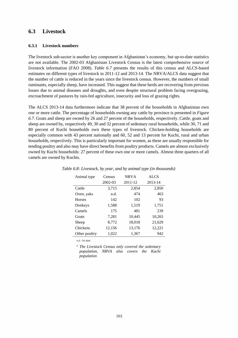
103
6.3 Livestock
6.3.1 Livestock numbers
The livestock sub-sector is another key component in Afghanistan’s economy, but up-to-date statistics
are not available. The 2002-03 Afghanistan Livestock Census is the latest comprehensive source of
livestock information (FAO 2008). Table 6.7 presents the results of this census and ALCS-based
estimates on different types of livestock in 2011-12 and 2013-14. The NRVA/ALCS data suggest that
the number of cattle is reduced in the years since the livestock census. However, the numbers of small
ruminants, especially sheep, have increased. This suggest that these herds are recovering from previous
losses due to animal diseases and droughts, and even despite structural problem facing overgrazing,
encroachment of pastures by rain-fed agriculture, insecurity and loss of grazing rights.
The ALCS 2013-14 data furthermore indicate that 38 percent of the households in Afghanistan own
one or more cattle. The percentage of households owning any cattle by province is presented in Figure
6.7. Goats and sheep are owned by 26 and 27 percent of the households, respectively. Cattle, goats and
sheep are owned by, respectively 49, 30 and 32 percent of sedentary rural households, while 30, 71 and
80 percent of Kuchi households own these types of livestock. Chicken-holding households are
especially common with 43 percent nationally and 60, 52 and 13 percent for Kuchi, rural and urban
households, respectively. This is particularly important for women, as these are usually responsible for
tending poultry and also may have direct benefits from poultry products. Camels are almost exclusively
owned by Kuchi households: 27 percent of these own one or more camels. Almost three quarters of all
camels are owned by Kuchis.
Table 6.8: Livestock, by year, and by animal type (in thousands)
Animal type Census NRVA ALCS
2002-03 2011-12 2013-14
Cattle 3,715 2,854 2,850
Oxen, yaks n.d. 474 463
Horses 142 102 93
Donkeys 1,588 1,519 1,751
Camels 175 481 239
Goats 7,281 10,445 10,265
Sheep 8,772 18,018 21,629
Chickens 12,156 13,176 12,221
Other poultry 1,022 1,367 942
n.d.: No data
a The Livestock Census only covered the sedentary
population, NRVA also covers the Kuchi
population
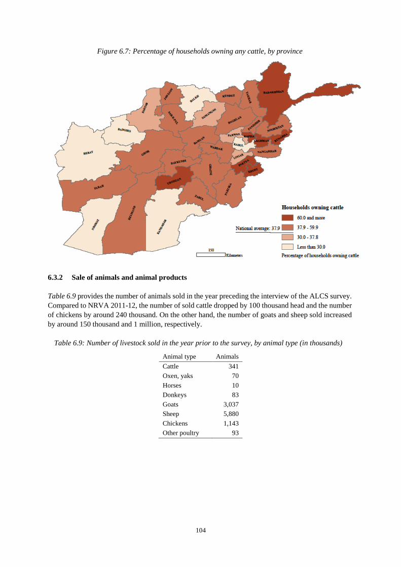
104
Figure 6.7: Percentage of households owning any cattle, by province
6.3.2 Sale of animals and animal products
Table 6.9 provides the number of animals sold in the year preceding the interview of the ALCS survey.
Compared to NRVA 2011-12, the number of sold cattle dropped by 100 thousand head and the number
of chickens by around 240 thousand. On the other hand, the number of goats and sheep sold increased
by around 150 thousand and 1 million, respectively.
Table 6.9: Number of livestock sold in the year prior to the survey, by animal type (in thousands)
Animal type Animals
Cattle 341
Oxen, yaks 70
Horses 10
Donkeys 83
Goats 3,037
Sheep 5,880
Chickens 1,143
Other poultry 93
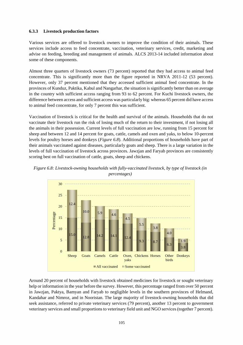
105
6.3.3 Livestock production factors
Various services are offered to livestock owners to improve the condition of their animals. These
services include access to feed concentrate, vaccination, veterinary services, credit, marketing and
advise on feeding, breeding and management of animals. ALCS 2013-14 included information about
some of these components.
Almost three quarters of livestock owners (73 percent) reported that they had access to animal feed
concentrate. This is significantly more than the figure reported in NRVA 2011-12 (53 percent).
However, only 37 percent mentioned that they accessed sufficient animal feed concentrate. In the
provinces of Kunduz, Paktika, Kabul and Nangarhar, the situation is significantly better than on average
in the country with sufficient access ranging from 93 to 62 percent. For Kuchi livestock owners, the
difference between access and sufficient access was particularly big: whereas 65 percent did have access
to animal feed concentrate, for only 7 percent this was sufficient.
Vaccination of livestock is critical for the health and survival of the animals. Households that do not
vaccinate their livestock run the risk of losing much of the return to their investment, if not losing all
the animals in their possession. Current levels of full vaccination are low, running from 15 percent for
sheep and between 12 and 14 percent for goats, cattle, camels and oxen and yaks, to below 10-percent
levels for poultry horses and donkeys (Figure 6.8). Additional proportions of households have part of
their animals vaccinated against diseases, particularly goats and sheep. There is a large variation in the
levels of full vaccination of livestock across provinces. Jawzjan and Faryab provinces are consistently
scoring best on full vaccination of cattle, goats, sheep and chickens.
Figure 6.8: Livestock-owning households with fully-vaccinated livestock, by type of livestock (in
percentages)
Around 20 percent of households with livestock obtained medicines for livestock or sought veterinary
help or information in the year before the survey. However, this percentage ranged from over 50 percent
in Jawzjan, Paktya, Bamyan and Faryab to negligible levels in the southern provinces of Helmand,
Kandahar and Nimroz, and in Nooristan. The large majority of livestock-owning households that did
seek assistance, referred to private veterinary services (79 percent), another 13 percent to government
veterinary services and small proportions to veterinary field unit and NGO services (together 7 percent).
15.012.8 14.2 14.1
12.49.3 8.7
6.33.8
12.4
10.0 5.94.6
4.5
5.53.8
4.0
1.9
0
5
10
15
20
25
30
Sheep Goats Camels Cattle Oxen,
yaks
Chickens Horses Other
birds
Donkeys
Per
centa
ge
All vaccinated Some vaccinated

106
Those households that did not seek assistance did not do so because they considered it not necessary
(15 percent) or had too few animals (23 percent). Major obstacles for not seeking assistance were lack
of knowledge of how or where to obtain the services (21 percent), reluctance to offer services by the
provider (17 percent), distance (15 percent) and costs (7 percent).
107
7 POVERTY
Summary: The analysis of ALCS 2013-14 indicates that poverty has increased over time, with about 39
percent of population living below the national poverty line. On average per capita consumption
declined between 2011-12 and 2013-14 with consumption of the poorer population declining faster. Per
capita consumption of the bottom two quintiles decreased at a faster rate than the top two quintiles
suggesting a possible increase in inequality.
In Afghanistan, the period between 2011-12 and 2013-14 is characterised by a substantial slowdown in
economic growth fuelled by persistent uncertainty surrounding political and security transition,
increased levels of conflict and downturn in aid. The slowdown in economic growth coupled with
decrease in aid is reflected in changes in labour market outcomes. Since NRVA 2007-08 and ALCS
2013-14, the unemployment rate has increased from 14 to 22 percent. As labour endowment is one of
the most critical assets for households, changes in labour market outcomes have had a significant impact
on poverty. Along with changes in labour market outcomes, negative shocks and an increased level of
conflict during this period have played a major role in driving up poverty.
Overall, the characteristics of poor have remained relatively stable over time and with a general upward
trend in poverty rate across different characteristics. The profile of the poor reveals that households
with certain characteristics, such as households with higher number of younger children, households
relying on child labour, households with an illiterate head and a head employed in informal labour
arrangements – particularly in agriculture or construction sectors – are more vulnerable to poverty
than others.
7.1 Introduction Poverty is multidimensional, and measurable from a variety of perspectives. Measuring poverty requires
defining a welfare or living standard measure and a threshold point – the ‘poverty line’ – which
represents the minimum welfare level below which we categorise a person as ‘poor’.
In Afghanistan the welfare measure used to define poverty is based on household consumption.
Consumption-based poverty measurement involves generating a ‘consumption aggregate’ at the
household level, using detailed food and non-food consumption data from household surveys, then
estimating the poverty line and applying the poverty line to the consumption aggregate value to identify
the poor, that is people who are consuming less than the poverty line. In line with international standards,
the poverty line in Afghanistan is estimated following the Cost of Basic Needs (CBN) approach.34 Past
poverty analysis of Afghanistan has shown that consumption-based poverty strongly correlates with
household size, dependency ratio, the educational attainment of head of household, as well as his or her
employment status and sector of work, and household access to basic services like safe drinking water,
improved sanitation, and electricity (CSO 2009, 2014).
Measuring and providing information on the evolution and distribution of living standards of the Afghan
population over time is one of the core objectives of the ALCS. However, because of the rotating module
methodology35, ALCS 2013-14 did not survey for food consumption. The absence of these data means
that the usual consumption-based approach cannot be applied to the ALCS 2013-14 data to estimate
34 Under the CBN approach, estimated poverty line represents the monetary value of consumption at which the
members of a household can be expected to meet their food and non-food needs. 35 See section 2.3 of this report.
108
poverty. In the absence of food consumption data, poverty for ALCS 2013-14 is estimated using an
alternative ‘survey-to-survey imputation’ technique.
Implementation of survey-to-survey imputation requires at least two comparable household surveys, one
with and one without consumption data, and a set of comparable data on household characteristics (e.g.,
household size, household head’s characteristics such as age, gender, ethnicity, education, occupation,
household assets, etc.) that correlate well with household consumption. In summary the technique,
explained in detail in Annex VI, entails to:
i) Develop a statistical model to estimate household consumption based on the household
characteristics in the survey where consumption data are available. Developing a statistical
model of household consumption means running a regression of household consumption on
household characteristics.
ii) Use this model to predict consumption for households in the survey with missing consumption
data. That is, apply the estimated model parameters (beta coefficients) of the consumption to the
same set of variables (household characteristics) in survey, which do not have consumption, to
predict consumption.
iii) Use the predicted household consumption to estimate poverty.
Thus, implementation of survey-to-survey imputation in Afghanistan entailed building a consumption
model using the previous survey, NRVA 2011-12, which has both actual consumption data and the
same non-consumption variables as the ALCS 2013-14. The estimated parameters of the 2011-12
consumption model are then applied to the ALCS 2013-14 data to impute the missing household
consumption. The imputed household consumptions are then used to estimate the poverty rate for
ALCS 2013-14. Table 7.1
Table 7.1 lists the categories and specific variables used in national consumption model.36 Annex VI.5
provides the final model.
Two validation tests are carried out to check the performance of the model. The purpose of the validation
is to see how well the imputation-based estimates compare with actual poverty rates. The first validation
test is the within-sample imputation, meaning the 2011-12 consumption model is applied to the NRVA
2011-12 data. The second is the out-of-sample imputation, where the 2011-12 model is applied the
NRVA 2007-08 data, for which actual consumption data are also available. The model performs
extremely well, delivering ‘imputed’ poverty rates within a 95% confidence interval of actual poverty
rates (Table 7.2).37
36 Not all variables listed are retained in the final model. See Annex VI for details on the variable selection
process. 37 Note however that the model lacks predictive accuracy on other poverty measures (such as poverty gap and
square of poverty gap). Working with a national model also limits subnational poverty analysis. In the case of
Afghanistan, although the national model yields accurate prediction of poverty incidence for the whole country,
the model cannot capture differences across regions or between urban and rural areas. For Afghanistan,
estimating poverty at the regional and urban-rural levels using the national model has resulted in poor
predictions both within sample (NRVA 2011-12) and across time (NRVA 2007-08), compared to direct
estimates from the two surveys. As such, subnational poverty analysis requires a model flexible enough to
capture spatial differences in the relationship between consumption and the correlates of consumption.
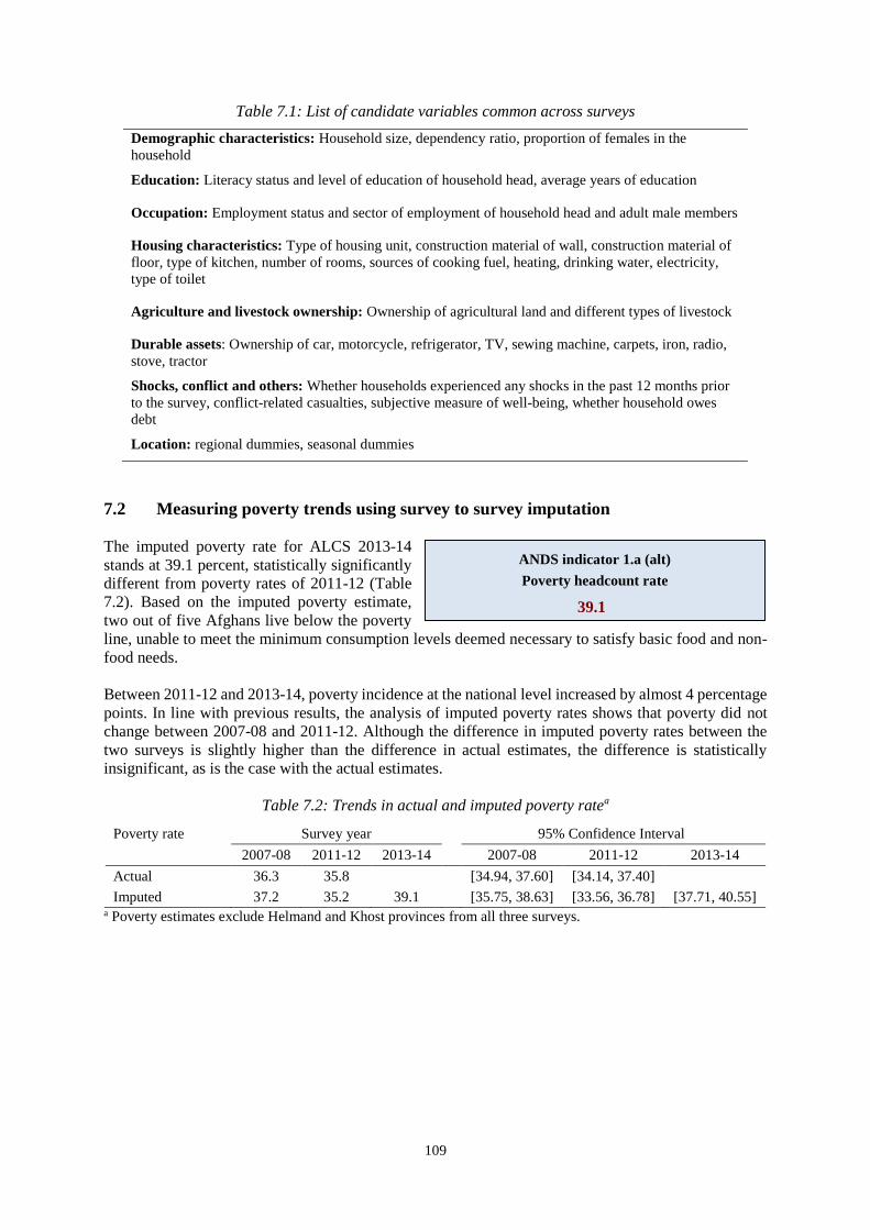
109
Table 7.1: List of candidate variables common across surveys
Demographic characteristics: Household size, dependency ratio, proportion of females in the
household
Education: Literacy status and level of education of household head, average years of education
Occupation: Employment status and sector of employment of household head and adult male members
Housing characteristics: Type of housing unit, construction material of wall, construction material of
floor, type of kitchen, number of rooms, sources of cooking fuel, heating, drinking water, electricity,
type of toilet
Agriculture and livestock ownership: Ownership of agricultural land and different types of livestock
Durable assets: Ownership of car, motorcycle, refrigerator, TV, sewing machine, carpets, iron, radio,
stove, tractor
Shocks, conflict and others: Whether households experienced any shocks in the past 12 months prior
to the survey, conflict-related casualties, subjective measure of well-being, whether household owes
debt
Location: regional dummies, seasonal dummies
7.2 Measuring poverty trends using survey to survey imputation
The imputed poverty rate for ALCS 2013-14
stands at 39.1 percent, statistically significantly
different from poverty rates of 2011-12 (Table
7.2). Based on the imputed poverty estimate,
two out of five Afghans live below the poverty
line, unable to meet the minimum consumption levels deemed necessary to satisfy basic food and non-
food needs.
Between 2011-12 and 2013-14, poverty incidence at the national level increased by almost 4 percentage
points. In line with previous results, the analysis of imputed poverty rates shows that poverty did not
change between 2007-08 and 2011-12. Although the difference in imputed poverty rates between the
two surveys is slightly higher than the difference in actual estimates, the difference is statistically
insignificant, as is the case with the actual estimates.
Table 7.2: Trends in actual and imputed poverty ratea
Poverty rate Survey year 95% Confidence Interval
2007-08 2011-12 2013-14 2007-08 2011-12 2013-14
Actual 36.3 35.8 [34.94, 37.60] [34.14, 37.40]
Imputed 37.2 35.2 39.1 [35.75, 38.63] [33.56, 36.78] [37.71, 40.55] a Poverty estimates exclude Helmand and Khost provinces from all three surveys.
ANDS indicator 1.a (alt)
Poverty headcount rate
39.1
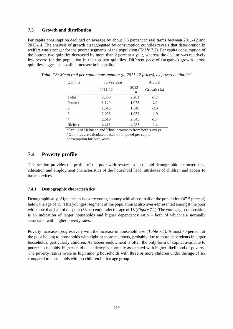
110
7.3 Growth and distribution
Per capita consumption declined on average by about 3.5 percent in real terms between 2011-12 and
2013-14. The analysis of growth disaggregated by consumption quintiles reveals that deterioration in
welfare was stronger for the poorer segments of the population (Table 7.3). Per capita consumption of
the bottom two quintiles decreased by more than 2 percent a year, whereas the decline was relatively
less severe for the population in the top two quintiles. Different pace of (negative) growth across
quintiles suggests a possible increase in inequality.
Table 7.3: Mean real per capita consumption (at 2011-12 prices), by poverty quintilea,b
Quintile Survey year Annual
2011-12 2013-
14 Growth (%)
Total 2,360 2,281 -1.7
Poorest 1,120 1,073 -2.1
2 1,615 1,540 -2.3
3 2,036 1,959 -1.9
4 2,619 2,545 -1.4
Richest 4,411 4,287 -1.4 a Excluded Helmand and Khost provinces from both surveys. b Quintiles are calculated based on imputed per capita
consumption for both years.
7.4 Poverty profile This section provides the profile of the poor with respect to household demographic characteristics,
education and employment characteristics of the household head, attributes of children and access to
basic services.
7.4.1 Demographic characteristics
Demographically, Afghanistan is a very young country with almost half of the population (47.5 percent)
below the age of 15. This youngest segment of the population is also over-represented amongst the poor
with more than half of the poor (53 percent) under the age of 15 (Figure 7.1). The young age composition
is an indication of larger households and higher dependency ratio – both of which are normally
associated with higher poverty rates.
Poverty increases progressively with the increase in household size (Table 7.4). Almost 70 percent of
the poor belong to households with eight or more members, probably due to more dependents in larger
households, particularly children. As labour endowment is often the only form of capital available to
poorer households, higher child dependency is normally associated with higher likelihood of poverty.
The poverty rate is twice as high among households with three or more children under the age of six
compared to households with no children in that age group.
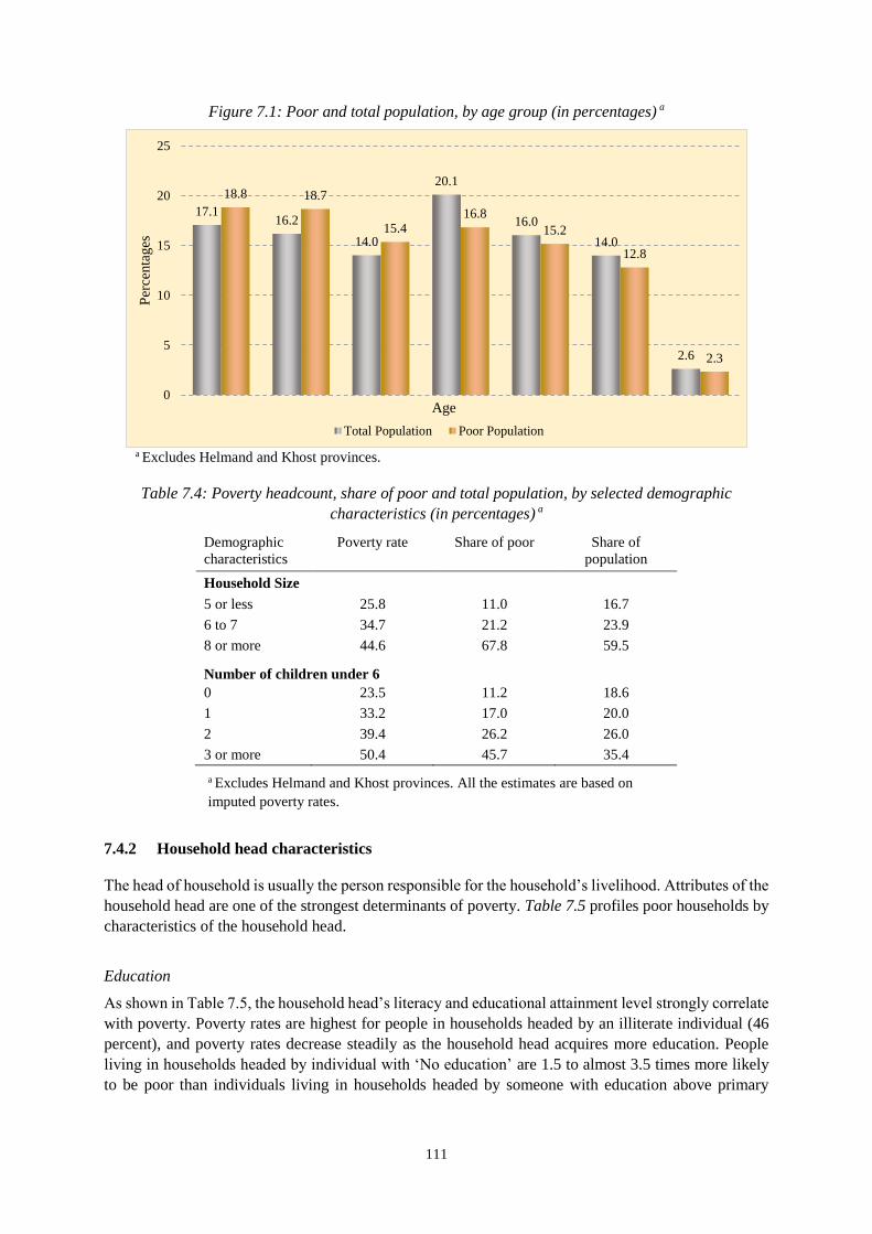
111
Figure 7.1: Poor and total population, by age group (in percentages) a
a Excludes Helmand and Khost provinces.
Table 7.4: Poverty headcount, share of poor and total population, by selected demographic
characteristics (in percentages) a
Demographic
characteristics
Poverty rate Share of poor Share of
population
Household Size
5 or less 25.8 11.0 16.7
6 to 7 34.7 21.2 23.9
8 or more 44.6 67.8 59.5
Number of children under 6
0 23.5 11.2 18.6
1 33.2 17.0 20.0
2 39.4 26.2 26.0
3 or more 50.4 45.7 35.4
a Excludes Helmand and Khost provinces. All the estimates are based on
imputed poverty rates.
7.4.2 Household head characteristics The head of household is usually the person responsible for the household’s livelihood. Attributes of the
household head are one of the strongest determinants of poverty. Table 7.5 profiles poor households by
characteristics of the household head.
Education
As shown in Table 7.5, the household head’s literacy and educational attainment level strongly correlate
with poverty. Poverty rates are highest for people in households headed by an illiterate individual (46
percent), and poverty rates decrease steadily as the household head acquires more education. People
living in households headed by individual with ‘No education’ are 1.5 to almost 3.5 times more likely
to be poor than individuals living in households headed by someone with education above primary
17.116.2
14.0
20.1
16.0
14.0
2.6
18.8 18.7
15.416.8
15.2
12.8
2.3
0
5
10
15
20
25P
erce
nta
ges
Age
Total Population Poor Population
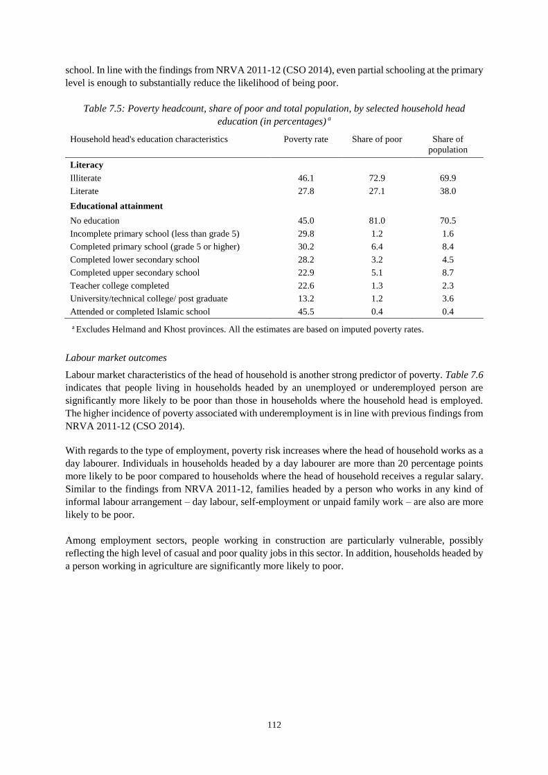
112
school. In line with the findings from NRVA 2011-12 (CSO 2014), even partial schooling at the primary
level is enough to substantially reduce the likelihood of being poor.
Table 7.5: Poverty headcount, share of poor and total population, by selected household head
education (in percentages) a
Household head's education characteristics Poverty rate Share of poor Share of
population
Literacy
Illiterate 46.1 72.9 69.9
Literate 27.8 27.1 38.0
Educational attainment
No education 45.0 81.0 70.5
Incomplete primary school (less than grade 5) 29.8 1.2 1.6
Completed primary school (grade 5 or higher) 30.2 6.4 8.4
Completed lower secondary school 28.2 3.2 4.5
Completed upper secondary school 22.9 5.1 8.7
Teacher college completed 22.6 1.3 2.3
University/technical college/ post graduate 13.2 1.2 3.6
Attended or completed Islamic school 45.5 0.4 0.4
a Excludes Helmand and Khost provinces. All the estimates are based on imputed poverty rates.
Labour market outcomes
Labour market characteristics of the head of household is another strong predictor of poverty. Table 7.6
indicates that people living in households headed by an unemployed or underemployed person are
significantly more likely to be poor than those in households where the household head is employed.
The higher incidence of poverty associated with underemployment is in line with previous findings from
NRVA 2011-12 (CSO 2014).
With regards to the type of employment, poverty risk increases where the head of household works as a
day labourer. Individuals in households headed by a day labourer are more than 20 percentage points
more likely to be poor compared to households where the head of household receives a regular salary.
Similar to the findings from NRVA 2011-12, families headed by a person who works in any kind of
informal labour arrangement – day labour, self-employment or unpaid family work – are also are more
likely to be poor.
Among employment sectors, people working in construction are particularly vulnerable, possibly
reflecting the high level of casual and poor quality jobs in this sector. In addition, households headed by
a person working in agriculture are significantly more likely to poor.
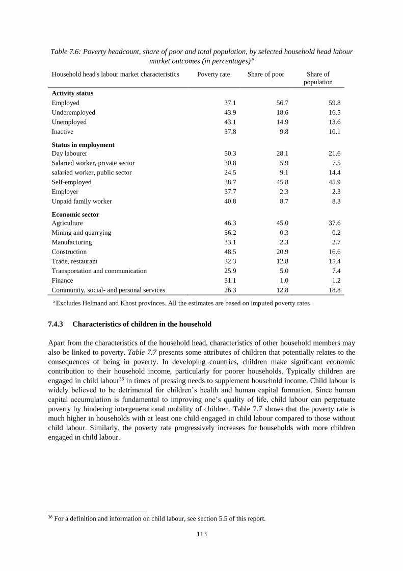
113
Table 7.6: Poverty headcount, share of poor and total population, by selected household head labour
market outcomes (in percentages) a
Household head's labour market characteristics Poverty rate Share of poor Share of
population
Activity status
Employed 37.1 56.7 59.8
Underemployed 43.9 18.6 16.5
Unemployed 43.1 14.9 13.6
Inactive 37.8 9.8 10.1
Status in employment
Day labourer 50.3 28.1 21.6
Salaried worker, private sector 30.8 5.9 7.5
salaried worker, public sector 24.5 9.1 14.4
Self-employed 38.7 45.8 45.9
Employer 37.7 2.3 2.3
Unpaid family worker 40.8 8.7 8.3
Economic sector
Agriculture 46.3 45.0 37.6
Mining and quarrying 56.2 0.3 0.2
Manufacturing 33.1 2.3 2.7
Construction 48.5 20.9 16.6
Trade, restaurant 32.3 12.8 15.4
Transportation and communication 25.9 5.0 7.4
Finance 31.1 1.0 1.2
Community, social- and personal services 26.3 12.8 18.8
a Excludes Helmand and Khost provinces. All the estimates are based on imputed poverty rates.
7.4.3 Characteristics of children in the household
Apart from the characteristics of the household head, characteristics of other household members may
also be linked to poverty. Table 7.7 presents some attributes of children that potentially relates to the
consequences of being in poverty. In developing countries, children make significant economic
contribution to their household income, particularly for poorer households. Typically children are
engaged in child labour38 in times of pressing needs to supplement household income. Child labour is
widely believed to be detrimental for children’s health and human capital formation. Since human
capital accumulation is fundamental to improving one’s quality of life, child labour can perpetuate
poverty by hindering intergenerational mobility of children. Table 7.7 shows that the poverty rate is
much higher in households with at least one child engaged in child labour compared to those without
child labour. Similarly, the poverty rate progressively increases for households with more children
engaged in child labour.
38 For a definition and information on child labour, see section 5.5 of this report.
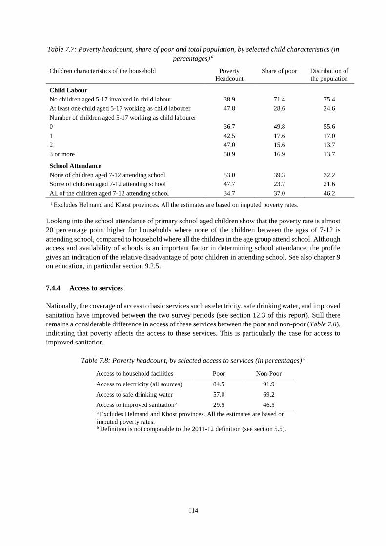
114
Table 7.7: Poverty headcount, share of poor and total population, by selected child characteristics (in
percentages) a
Children characteristics of the household Poverty
Headcount
Share of poor Distribution of
the population
Child Labour
No children aged 5-17 involved in child labour 38.9 71.4 75.4
At least one child aged 5-17 working as child labourer 47.8 28.6 24.6
Number of children aged 5-17 working as child labourer
0 36.7 49.8 55.6
1 42.5 17.6 17.0
2 47.0 15.6 13.7
3 or more 50.9 16.9 13.7
School Attendance
None of children aged 7-12 attending school 53.0 39.3 32.2
Some of children aged 7-12 attending school 47.7 23.7 21.6
All of the children aged 7-12 attending school 34.7 37.0 46.2
a Excludes Helmand and Khost provinces. All the estimates are based on imputed poverty rates.
Looking into the school attendance of primary school aged children show that the poverty rate is almost
20 percentage point higher for households where none of the children between the ages of 7-12 is
attending school, compared to household where all the children in the age group attend school. Although
access and availability of schools is an important factor in determining school attendance, the profile
gives an indication of the relative disadvantage of poor children in attending school. See also chapter 9
on education, in particular section 9.2.5.
7.4.4 Access to services
Nationally, the coverage of access to basic services such as electricity, safe drinking water, and improved
sanitation have improved between the two survey periods (see section 12.3 of this report). Still there
remains a considerable difference in access of these services between the poor and non-poor (Table 7.8),
indicating that poverty affects the access to these services. This is particularly the case for access to
improved sanitation.
Table 7.8: Poverty headcount, by selected access to services (in percentages) a
Access to household facilities Poor Non-Poor
Access to electricity (all sources) 84.5 91.9
Access to safe drinking water 57.0 69.2
Access to improved sanitationb 29.5 46.5 a Excludes Helmand and Khost provinces. All the estimates are based on
imputed poverty rates. b Definition is not comparable to the 2011-12 definition (see section 5.5).
115
7.5 Conclusion
Although the analysis of poverty is constrained by lack of consumption data, the use of alternative
poverty estimation method allows to track the changes in poverty over time. The analysis of ALCS
2013-14 data reveals an increase in poverty over the last two years. Increase in poverty is consistent
with the pattern of economic growth and different macroeconomic events taking place in the economy
during this period.
Political uncertainty, increasing conflict and downturn in aid have limited Afghanistan’s growth.
Compared to real per capita GDP growth of 11.3 percent in 2012, growth in 2014 is estimated to be
negative (-0.96 percent). The slowdown in economic growth and the downturn in aid39 has translated
into an overall deterioration in labour market opportunities. The proportion of individuals in the labour
force that is unemployed has increased since 2007-08 (see section 5.3.2). Deteriorating labour market
opportunities coupled with deteriorating security account for most of the estimated increase in poverty.
39 Looking at US funding alone, the amount appropriated by Congress for reconstruction efforts in Afghanistan
has more than halved between 2012 and 2014 (SIGAR 2015).
116
8 FOOD SECURITY
Summary. A high proportion of Afghanistan’s 28 million people face chronic and transitory food
insecurity. Food insecurity based on the food consumption score and food-based coping strategies is
estimated at 33 percent (9.3 million people) of total population. Among them, an estimated 3.4 million
(or 12 percent) are severely food insecure, and 5.9 million (or 21 percent) moderately food insecure.
The proportion of the food insecure is significantly higher in rural areas, with 36 percent of the rural
population being food insecure, compared to 30 percent of the urban population. The Kuchi
population is significantly better off compared to the rural and urban counterparts, with 9 percent or
about 140 thousand being food insecure. Food insecurity is mainly attributed to households’ lack of
access to sustainable income. The North-East, West and South-West regions of Afghanistan have
the highest proportions of food-insecure people, as well as the highest proportions of severely
food insecure people.
The diet of the Afghan population is not only quantitatively inadequate, but also qualitatively poor
and heavily cereal-based. Poor diet diversity is a serious problem across much of Afghanistan.
Most of the food consumed is made up of staples (wheat in particular). Overall, the proportion
of households with low dietary diversity accounts for 36 percent of all Afghan households (20
percent in urban, 42 percent in rural and 41 percent among the Kuchi households).
To cope with shocks, the majority of households mainly adopt short-term viable coping strategies.
However, some unviable (distressed) coping strategies are also used, which negatively impacts
food security in the future. Many more rural households than their urban and Kuchi counterparts
adopt coping strategies, particularly unviable strategies.
8.1 Introduction
Food security exists when all people, at all times have physical, social and economic access to
sufficient, safe and nutritious food for a healthy and active life. In this chapter, food consumption based
on the Food Consumption Score (FCS)40 as a description for the current short-term household food
security situation is triangulated with the food-based Coping Strategy Index (CSI)41 to provide an
40 The Food Consumption Score (FCS) is an acceptable proxy indicator to measure caloric intake and diet quality
at household level, giving an indication of food security status of the household if combined with other
household access indicators. It is a composite score based on dietary diversity, food frequency, and relative
nutritional importance of different food groups. The FCS is calculated based on the past 7-day food
consumption recall for the household and classified into three categories: poor consumption (FCS = 1.0 to 28);
borderline (FCS = 28.1 to 42); and acceptable consumption (FCS = >42.0). The FCS is a weighted sum of food
groups. The score for each food group is calculated by multiplying the number of days the commodity was
consumed and its relative weight. 41 The Coping Strategy Index (CSI) is often used as a proxy indicator of household food insecurity. Households
were asked about how often they used a set of five short-term food based coping strategies in situations in
which they did not have enough food, or money to buy food, during the one-week period prior to interview.
The information is combined into the CSI which is a score assigned to a household that represents the frequency
and severity of coping strategies employed. First, each of the five strategies is assigned a standard weight based
on its severity. These weights are: Relying on less preferred and less expensive foods (=1.0); Limiting portion
size at meal times (=1.0); Reducing the number of meals eaten in a day (=1.0); Borrow food or rely on help
from relatives or friends (=2.0); Restricting consumption by adults for small children to eat (=3.0). Household
CSI scores are then determined by multiplying the number of days in the past week each strategy was employed
by its corresponding severity weight, and then summing together the totals. The total CSI score is the basis to
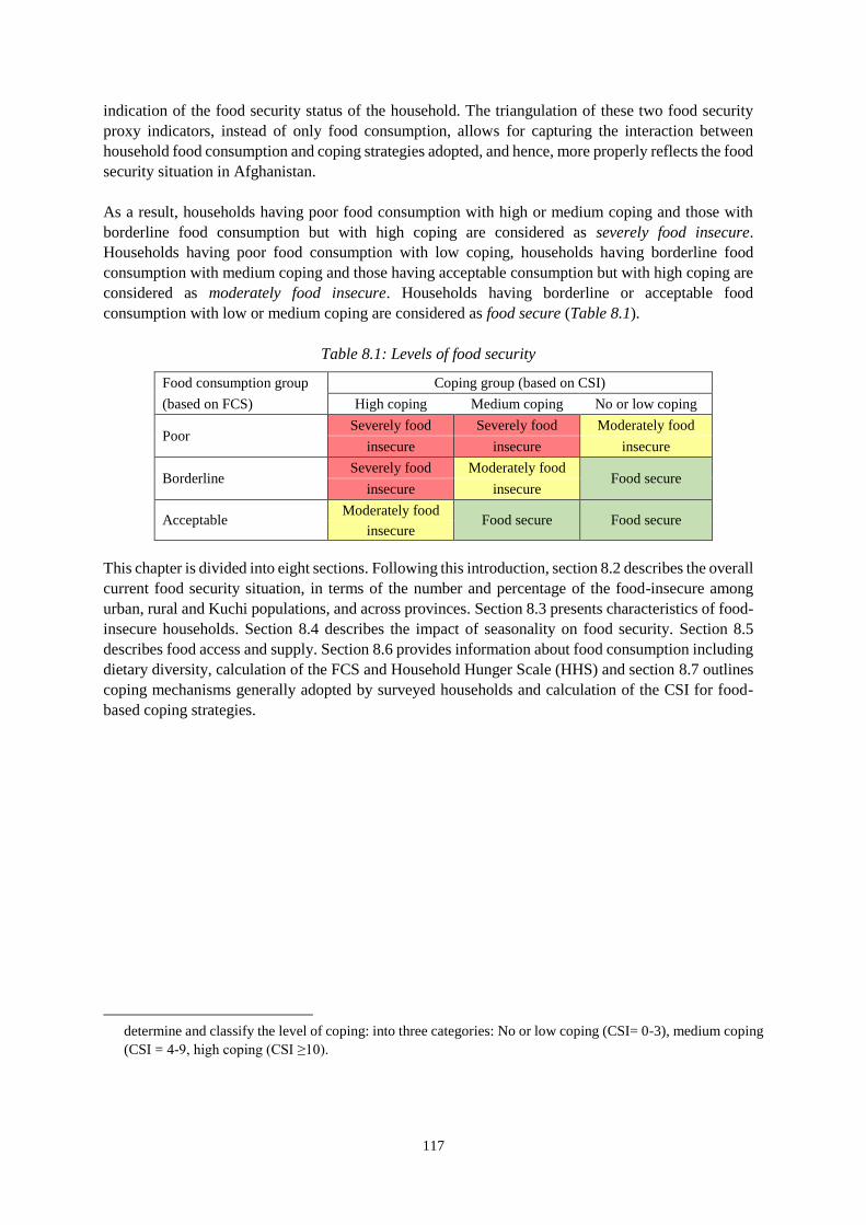
117
indication of the food security status of the household. The triangulation of these two food security
proxy indicators, instead of only food consumption, allows for capturing the interaction between
household food consumption and coping strategies adopted, and hence, more properly reflects the food
security situation in Afghanistan.
As a result, households having poor food consumption with high or medium coping and those with
borderline food consumption but with high coping are considered as severely food insecure.
Households having poor food consumption with low coping, households having borderline food
consumption with medium coping and those having acceptable consumption but with high coping are
considered as moderately food insecure. Households having borderline or acceptable food
consumption with low or medium coping are considered as food secure (Table 8.1).
Table 8.1: Levels of food security
Food consumption group Coping group (based on CSI)
(based on FCS) High coping Medium coping No or low coping
Poor Severely food Severely food Moderately food
insecure insecure insecure
Borderline Severely food Moderately food
Food secure insecure insecure
Acceptable Moderately food
Food secure Food secure insecure
This chapter is divided into eight sections. Following this introduction, section 8.2 describes the overall
current food security situation, in terms of the number and percentage of the food-insecure among
urban, rural and Kuchi populations, and across provinces. Section 8.3 presents characteristics of food-
insecure households. Section 8.4 describes the impact of seasonality on food security. Section 8.5
describes food access and supply. Section 8.6 provides information about food consumption including
dietary diversity, calculation of the FCS and Household Hunger Scale (HHS) and section 8.7 outlines
coping mechanisms generally adopted by surveyed households and calculation of the CSI for food-
based coping strategies.
determine and classify the level of coping: into three categories: No or low coping (CSI= 0-3), medium coping
(CSI = 4-9, high coping (CSI ≥10).
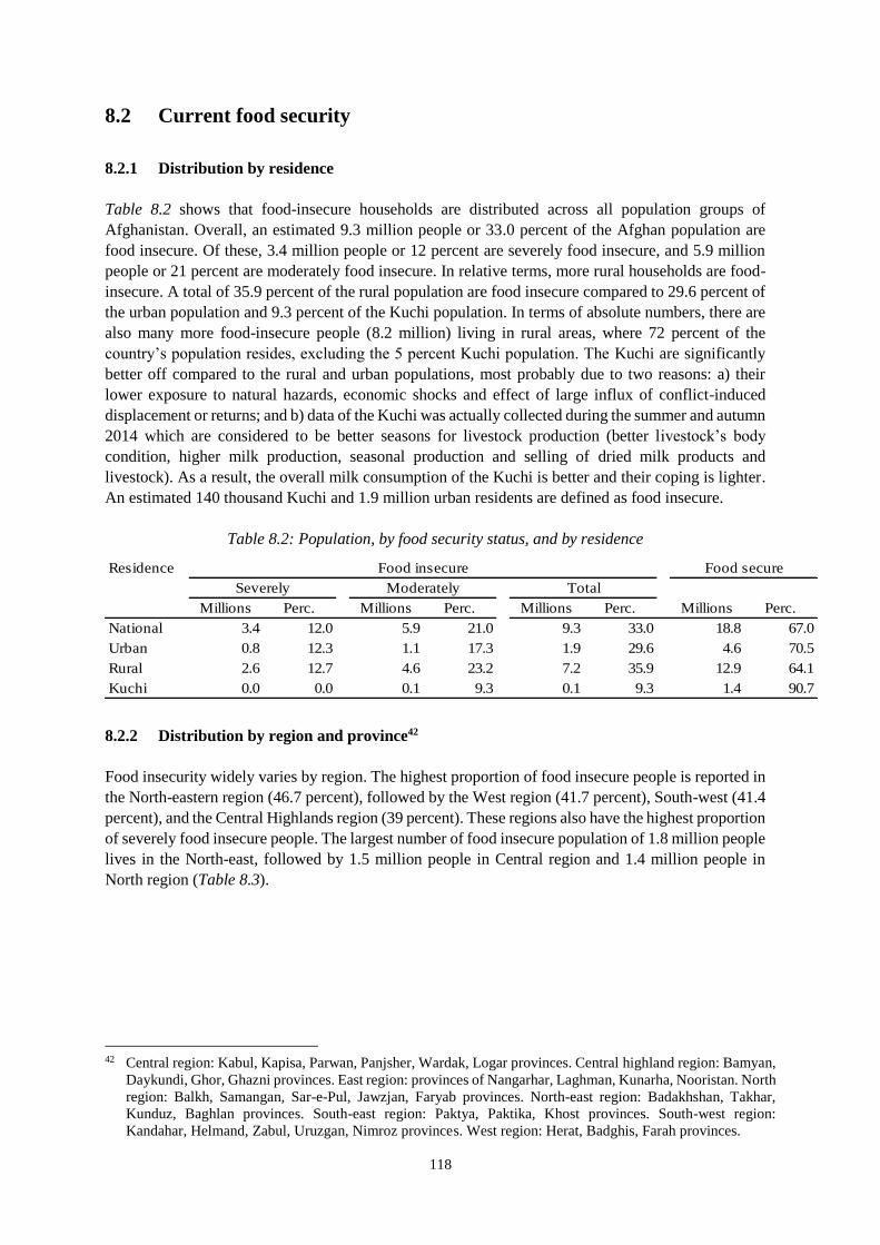
118
8.2 Current food security
8.2.1 Distribution by residence
Table 8.2 shows that food-insecure households are distributed across all population groups of
Afghanistan. Overall, an estimated 9.3 million people or 33.0 percent of the Afghan population are
food insecure. Of these, 3.4 million people or 12 percent are severely food insecure, and 5.9 million
people or 21 percent are moderately food insecure. In relative terms, more rural households are food-
insecure. A total of 35.9 percent of the rural population are food insecure compared to 29.6 percent of
the urban population and 9.3 percent of the Kuchi population. In terms of absolute numbers, there are
also many more food-insecure people (8.2 million) living in rural areas, where 72 percent of the
country’s population resides, excluding the 5 percent Kuchi population. The Kuchi are significantly
better off compared to the rural and urban populations, most probably due to two reasons: a) their
lower exposure to natural hazards, economic shocks and effect of large influx of conflict-induced
displacement or returns; and b) data of the Kuchi was actually collected during the summer and autumn
2014 which are considered to be better seasons for livestock production (better livestock’s body
condition, higher milk production, seasonal production and selling of dried milk products and
livestock). As a result, the overall milk consumption of the Kuchi is better and their coping is lighter.
An estimated 140 thousand Kuchi and 1.9 million urban residents are defined as food insecure.
Table 8.2: Population, by food security status, and by residence
Residence Food insecure Food secure
Severely Moderately Total
Millions Perc. Millions Perc. Millions Perc. Millions Perc.
National 3.4 12.0 5.9 21.0 9.3 33.0 18.8 67.0
Urban 0.8 12.3 1.1 17.3 1.9 29.6 4.6 70.5
Rural 2.6 12.7 4.6 23.2 7.2 35.9 12.9 64.1
Kuchi 0.0 0.0 0.1 9.3 0.1 9.3 1.4 90.7
8.2.2 Distribution by region and province42
Food insecurity widely varies by region. The highest proportion of food insecure people is reported in
the North-eastern region (46.7 percent), followed by the West region (41.7 percent), South-west (41.4
percent), and the Central Highlands region (39 percent). These regions also have the highest proportion
of severely food insecure people. The largest number of food insecure population of 1.8 million people
lives in the North-east, followed by 1.5 million people in Central region and 1.4 million people in
North region (Table 8.3).
42 Central region: Kabul, Kapisa, Parwan, Panjsher, Wardak, Logar provinces. Central highland region: Bamyan,
Daykundi, Ghor, Ghazni provinces. East region: provinces of Nangarhar, Laghman, Kunarha, Nooristan. North
region: Balkh, Samangan, Sar-e-Pul, Jawzjan, Faryab provinces. North-east region: Badakhshan, Takhar,
Kunduz, Baghlan provinces. South-east region: Paktya, Paktika, Khost provinces. South-west region:
Kandahar, Helmand, Zabul, Uruzgan, Nimroz provinces. West region: Herat, Badghis, Farah provinces.
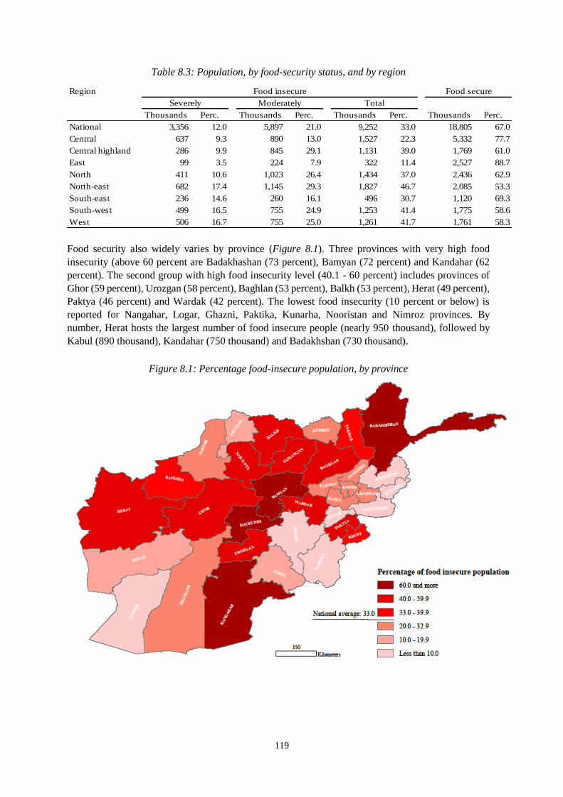
119
Table 8.3: Population, by food-security status, and by region
Region Food insecure Food secure
Severely Moderately Total
Thousands Perc. Thousands Perc. Thousands Perc. Thousands Perc.
National 3,356 12.0 5,897 21.0 9,252 33.0 18,805 67.0
Central 637 9.3 890 13.0 1,527 22.3 5,332 77.7
Central highland 286 9.9 845 29.1 1,131 39.0 1,769 61.0
East 99 3.5 224 7.9 322 11.4 2,527 88.7
North 411 10.6 1,023 26.4 1,434 37.0 2,436 62.9
North-east 682 17.4 1,145 29.3 1,827 46.7 2,085 53.3
South-east 236 14.6 260 16.1 496 30.7 1,120 69.3
South-west 499 16.5 755 24.9 1,253 41.4 1,775 58.6
West 506 16.7 755 25.0 1,261 41.7 1,761 58.3
Food security also widely varies by province (Figure 8.1). Three provinces with very high food
insecurity (above 60 percent are Badakhashan (73 percent), Bamyan (72 percent) and Kandahar (62
percent). The second group with high food insecurity level (40.1 - 60 percent) includes provinces of
Ghor (59 percent), Urozgan (58 percent), Baghlan (53 percent), Balkh (53 percent), Herat (49 percent),
Paktya (46 percent) and Wardak (42 percent). The lowest food insecurity (10 percent or below) is
reported for Nangahar, Logar, Ghazni, Paktika, Kunarha, Nooristan and Nimroz provinces. By
number, Herat hosts the largest number of food insecure people (nearly 950 thousand), followed by
Kabul (890 thousand), Kandahar (750 thousand) and Badakhshan (730 thousand).
Figure 8.1: Percentage food-insecure population, by province
120
8.3 Characteristics of the food-insecure population
8.3.1 Characterisation by main income source
Income sources are assessed and classified according to the proportion the source contributed to the
total household income. In general, income that contributes at least 50 percent of total household
income is considered as the main source of income. Some households in urban areas have income
sources which include rural activities, such as agriculture, because of the inclusion of the Nahias (peri-
urban locations) as urban centers. When combining the first, second and third most important income
sources in which the household is engaged, five major income sources emerge from which households
earn their income:
Production and sales of field crops (32 percent of the households)
Non-farm wage labour and other types of day labour (28 percent)
Borrowing (16 percent)
Production and sale of livestock (14 percent), and
Shop keeping /small business (12 percent).
Other activities are engaged in by less than 8 percent of the households.
On average, urban households earn a significantly higher amount of income from the main source
while rural households earn the lowest amount. Government/NGO/UN workers, traders, non-
government workers, doctors/nurse/medical personnel earn the largest amount from the main source.
Following this group are road construction workers, people engaged in other production work, military
service, government workers and shop keeping /small business. Those with the lowest average amount
of the main income source are households dependent on opium wage labour, Zakat, agricultural wage
labour, non-farm wage labour, pensions, shepherding wage labour, carpet weaving, and production
and sale of field crops or livestock.
The main source of household income is related to food security status.
Households dependent on opium wage labour, non-opium farm wage labour, borrowing and
Zakat have the highest proportion of the food insecure of 79 percent, 64 percent, 58 percent and
52 percent, respectively.
The second highest food insecurity group includes households relying on non-farm wage labour
or other types of day labour and street market sale, with 40 to 50 percent of them being food
insecure.
The third highest food insecurity group are households whose main income source is from
pensions, production and sale of field crops, sewing and embroidery, service work, other trade,
teaching, military services and police, with 30 to 40 percent of them being food insecure.
The fourth group with low food insecurity (20 to 30 percent) includes households dependent on
taxi/transport, production and sale of opium/orchard products/ livestock, carpet weaving,
mechanic and construction work, shepherding wage labour, government/UN/NGO work, rental
and shop keepers/small businessmen.
Non-government office workers and medical personnel have the lowest proportion of the food
insecure among them (20 percent or below) (Table 8.4).
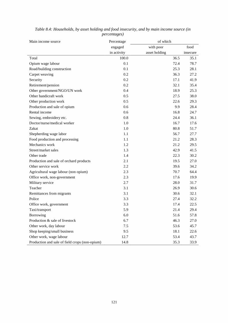
121
Table 8.4: Households, by asset holding and food insecurity, and by main income source (in
percentages)
Main income source Percentage of which
engaged with poor food
in activity asset holding insecure
Total 100.0 36.5 35.1
Opium wage labour 0.1 72.4 78.7
Road/building construction 0.1 25.3 28.1
Carpet weaving 0.2 36.3 27.2
Security 0.2 17.1 41.9
Retirement/pension 0.2 32.1 35.4
Other government/NGO/UN work 0.4 18.9 25.3
Other handicraft work 0.5 27.5 38.0
Other production work 0.5 22.6 29.3
Production and sale of opium 0.6 9.9 28.4
Rental income 0.6 16.8 24.7
Sewing, embroidery etc. 0.8 24.4 36.1
Doctor/nurse/medical worker 1.0 16.7 17.6
Zakat 1.0 80.8 51.7
Shepherding wage labor 1.1 56.7 27.7
Food production and processing 1.1 21.2 28.3
Mechanics work 1.2 21.2 29.5
Street/market sales 1.3 42.9 41.5
Other trade 1.4 22.3 30.2
Production and sale of orchard products 2.1 19.5 27.0
Other service work 2.2 39.6 34.2
Agricultural wage labour (non opium) 2.3 70.7 64.4
Office work, non-government 2.3 17.6 19.9
Military service 2.7 28.0 31.7
Teacher 3.1 26.9 30.6
Remittances from migrants 3.1 30.6 32.1
Police 3.3 27.4 32.2
Office work, government 3.3 17.4 22.5
Taxi/transport 5.9 21.4 29.4
Borrowing 6.0 51.6 57.8
Production & sale of livestock 6.7 46.3 27.0
Other work, day labour 7.5 53.6 45.7
Shop keeping/small business 9.5 18.1 22.6
Other work, wage labour 12.7 53.4 43.7
Production and sale of field crops (non-opium) 14.8 35.3 33.9
122
8.3.2 Characterisation by asset ownership43
Across residence groups, 37 percent of the households are regarded as having poor asset holding (22
percent in urban, 40 percent in rural and 60 percent among the Kuchi households).
Households dependent on Zakat, farm wage labour (opium and non-opium), non-farm wage labour,
shepherding wage labour and borrowing are among those with the highest proportion of asset poverty.
Across livelihood groups, the ownership of household assets closely correlate with the level of food
insecurity, except for those dependent on shepherding wage labour, and production and sale of
livestock who have a high percentage of households with poor asset holding, yet the proportion of
food-insecure households among them is relatively low (Table 8.4).
8.3.3 Characterisation by demographics
Food insecurity tends to decrease as household size increases. Overall, households with less than nine
members are more likely to be food-insecure than larger households (Table 8.5). The highest
proportion of food insecure is reported amongst households with 1-5 members. This trend is similar
across all residence groups, although the variation between household size categories is less
pronounced in urban areas than in rural areas and among the Kuchi. The reason is probably that larger
households have a higher number of working age adults who can deploy and earn a larger amount of
annual income than households with fewer members which then translates into their better food
consumption score and lower coping level.
The age of the household head seems to be related to food insecurity status. Overall, households headed
by adults under 20 years of age tend to be more food insecure than other groups, except for the Kuchi
where households headed by the elderly adults (65 years or above) tend to be more food insecure. The
higher food insecurity among the young headed households is similarly reported among rural and
urban households which could be related to their lower asset ownership, limited employment
opportunities and significantly lower income. As the households head’s age increases up to 64 years,
food insecurity generally reduces. However, after that food insecurity increases again, although this
surge is less remarkable in urban areas than in rural areas and among the Kuchi.
On marital status of the household head, across residence groups, the widowed, divorced or separated
tend to be more food insecure compared to other groups, although in urban areas food insecurity among
the engaged and those who never married is reported at a slightly higher level.
43 The information is combined into the Asset Score which is a score assigned to a household that represents the
number of assets they hold and the proxy weight of their importance to food security according to the common
perceptions of Afghan people and WFP knowledge of local context on the asset holding. This methodology
was applied in the asset analysis of the previous NRVA 2011-2012. The following weights are applied: weight
‘1’ is assigned for stove, gas balloon, sewing machine, iron, radio, tape recorder, electric fan, bicycle, blanket
and mobile phone. Weight ‘2’ is assigned for refrigerator, television, and ordinary carpets (gilim, satrangi,
namad, fash, others). Weight ‘3’ is assigned for computer, satellite disc, motorcycle, and better quality carpets
(khalin, other hand-made woven carpets). Weight ‘4’ is assigned for car, tractor, and thresher. Due to the fact
that gold and silver are likely to be reluctantly, and hence inaccurately reported by the respondents, these items
are excluded from the analysis.
Household Asset scores are then determined by multiplying the number of assets by its corresponding weight,
and then summing together the totals. The total Asset score is the basis to determine and classify the level of
asset holding into four categories: Poor (asset score = 1 – 19.99), Borderline (asset score = 20 – 29.99), Middle
(asset score = 30 –39.99), and Rich (asset score = 40 or above).
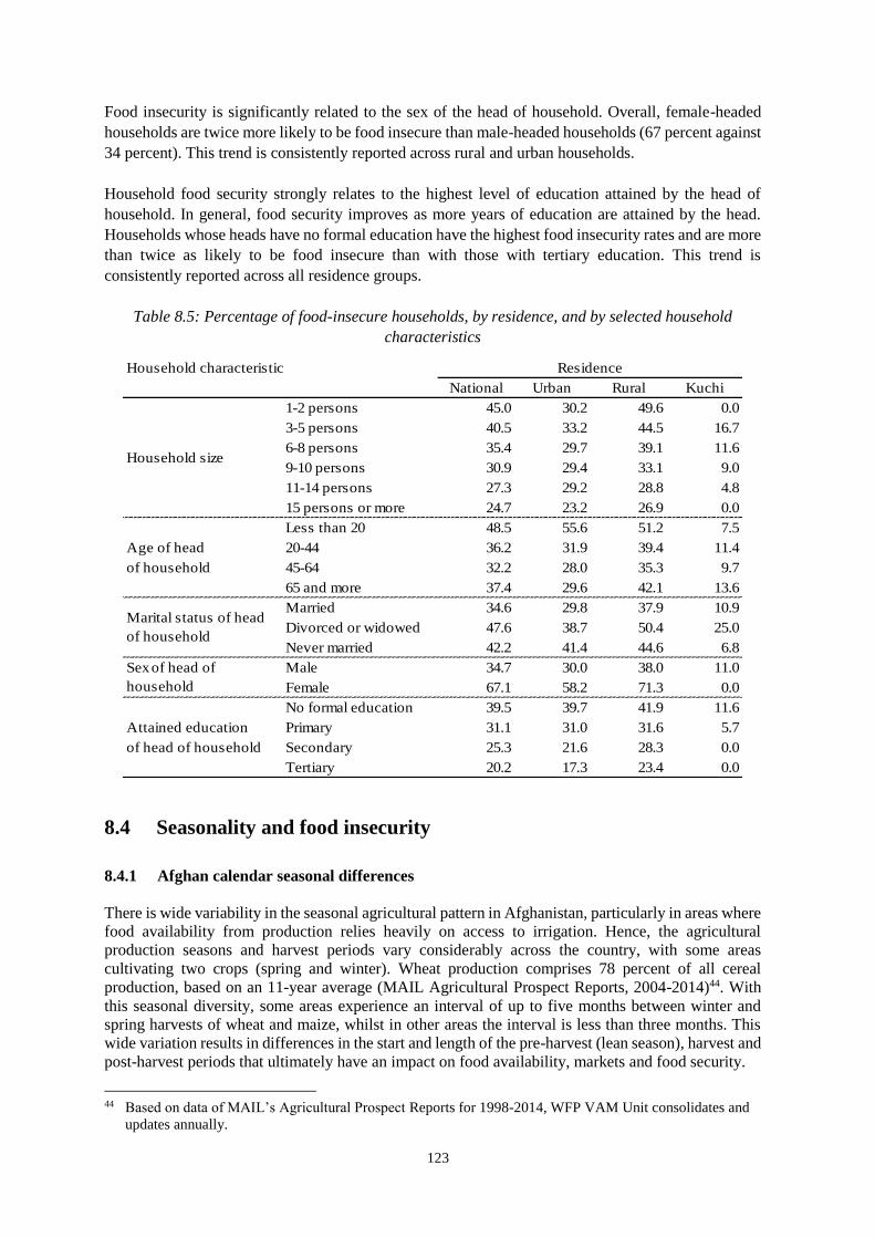
123
Food insecurity is significantly related to the sex of the head of household. Overall, female-headed
households are twice more likely to be food insecure than male-headed households (67 percent against
34 percent). This trend is consistently reported across rural and urban households.
Household food security strongly relates to the highest level of education attained by the head of
household. In general, food security improves as more years of education are attained by the head.
Households whose heads have no formal education have the highest food insecurity rates and are more
than twice as likely to be food insecure than with those with tertiary education. This trend is
consistently reported across all residence groups.
Table 8.5: Percentage of food-insecure households, by residence, and by selected household
characteristics
Household characteristic Residence
National Urban Rural Kuchi
1-2 persons 45.0 30.2 49.6 0.0
3-5 persons 40.5 33.2 44.5 16.7
6-8 persons 35.4 29.7 39.1 11.6
9-10 persons 30.9 29.4 33.1 9.0
11-14 persons 27.3 29.2 28.8 4.8
15 persons or more 24.7 23.2 26.9 0.0
Less than 20 48.5 55.6 51.2 7.5
Age of head 20-44 36.2 31.9 39.4 11.4
of household 45-64 32.2 28.0 35.3 9.7
65 and more 37.4 29.6 42.1 13.6
Married 34.6 29.8 37.9 10.9
Divorced or widowed 47.6 38.7 50.4 25.0
Never married 42.2 41.4 44.6 6.8
Male 34.7 30.0 38.0 11.0
Female 67.1 58.2 71.3 0.0
No formal education 39.5 39.7 41.9 11.6
Attained education Primary 31.1 31.0 31.6 5.7
of head of household Secondary 25.3 21.6 28.3 0.0
Tertiary 20.2 17.3 23.4 0.0
Household size
Marital status of head
of household
Sex of head of
household
8.4 Seasonality and food insecurity
8.4.1 Afghan calendar seasonal differences
There is wide variability in the seasonal agricultural pattern in Afghanistan, particularly in areas where
food availability from production relies heavily on access to irrigation. Hence, the agricultural
production seasons and harvest periods vary considerably across the country, with some areas
cultivating two crops (spring and winter). Wheat production comprises 78 percent of all cereal
production, based on an 11-year average (MAIL Agricultural Prospect Reports, 2004-2014)44. With
this seasonal diversity, some areas experience an interval of up to five months between winter and
spring harvests of wheat and maize, whilst in other areas the interval is less than three months. This
wide variation results in differences in the start and length of the pre-harvest (lean season), harvest and
post-harvest periods that ultimately have an impact on food availability, markets and food security.
44 Based on data of MAIL’s Agricultural Prospect Reports for 1998-2014, WFP VAM Unit consolidates and
updates annually.
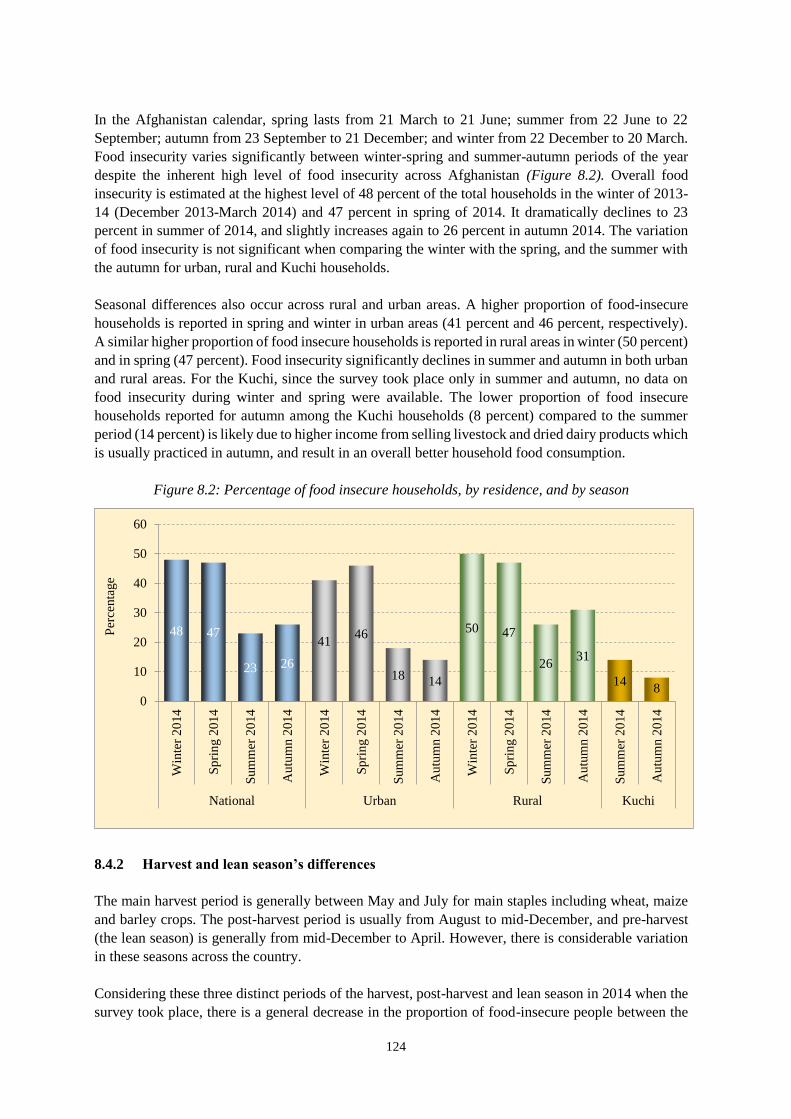
124
In the Afghanistan calendar, spring lasts from 21 March to 21 June; summer from 22 June to 22
September; autumn from 23 September to 21 December; and winter from 22 December to 20 March.
Food insecurity varies significantly between winter-spring and summer-autumn periods of the year
despite the inherent high level of food insecurity across Afghanistan (Figure 8.2). Overall food
insecurity is estimated at the highest level of 48 percent of the total households in the winter of 2013-
14 (December 2013-March 2014) and 47 percent in spring of 2014. It dramatically declines to 23
percent in summer of 2014, and slightly increases again to 26 percent in autumn 2014. The variation
of food insecurity is not significant when comparing the winter with the spring, and the summer with
the autumn for urban, rural and Kuchi households.
Seasonal differences also occur across rural and urban areas. A higher proportion of food-insecure
households is reported in spring and winter in urban areas (41 percent and 46 percent, respectively).
A similar higher proportion of food insecure households is reported in rural areas in winter (50 percent)
and in spring (47 percent). Food insecurity significantly declines in summer and autumn in both urban
and rural areas. For the Kuchi, since the survey took place only in summer and autumn, no data on
food insecurity during winter and spring were available. The lower proportion of food insecure
households reported for autumn among the Kuchi households (8 percent) compared to the summer
period (14 percent) is likely due to higher income from selling livestock and dried dairy products which
is usually practiced in autumn, and result in an overall better household food consumption.
Figure 8.2: Percentage of food insecure households, by residence, and by season
8.4.2 Harvest and lean season’s differences
The main harvest period is generally between May and July for main staples including wheat, maize
and barley crops. The post-harvest period is usually from August to mid-December, and pre-harvest
(the lean season) is generally from mid-December to April. However, there is considerable variation
in these seasons across the country.
Considering these three distinct periods of the harvest, post-harvest and lean season in 2014 when the
survey took place, there is a general decrease in the proportion of food-insecure people between the
48 47
23 26
4146
18 14
50 47
2631
148
0
10
20
30
40
50
60
Win
ter
20
14
Sp
rin
g 2
01
4
Su
mm
er 2
014
Au
tum
n 2
01
4
Win
ter
20
14
Sp
rin
g 2
01
4
Su
mm
er 2
014
Au
tum
n 2
01
4
Win
ter
20
14
Sp
rin
g 2
01
4
Su
mm
er 2
014
Au
tum
n 2
01
4
Su
mm
er 2
014
Au
tum
n 2
01
4
National Urban Rural Kuchi
Per
centa
ge
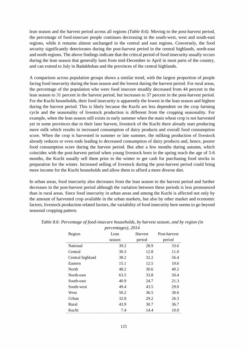
125
lean season and the harvest period across all regions (Table 8.6). Moving to the post-harvest period,
the percentage of food-insecure people continues decreasing in the south-west, west and south-east
regions, while it remains almost unchanged in the central and east regions. Conversely, the food
security significantly deteriorates during the post-harvest period in the central highlands, north-east
and north regions. The above findings indicate that the critical period of food insecurity usually occurs
during the lean season that generally lasts from mid-December to April in most parts of the country,
and can extend to July in Badakhshan and the provinces of the central highlands.
A comparison across population groups shows a similar trend, with the largest proportion of people
facing food insecurity during the lean season and the lowest during the harvest period. For rural areas,
the percentage of the population who were food insecure steadily decreased from 44 percent in the
lean season to 31 percent in the harvest period, but increases to 37 percent in the post-harvest period.
For the Kuchi households, their food insecurity is apparently the lowest in the lean season and highest
during the harvest period. This is likely because the Kuchi are less dependent on the crop farming
cycle and the seasonality of livestock production is different from the cropping seasonality. For
example, when the lean season still exists in early summer when the main wheat crop is not harvested
yet in some provinces due to their later harvest, livestock of the Kuchi there already start producing
more milk which results in increased consumption of dairy products and overall food consumption
score. When the crop is harvested in summer or late summer, the milking production of livestock
already reduces or even ends leading to decreased consumption of dairy products and, hence, poorer
food consumption score during the harvest period. But after a few months during autumn, which
coincides with the post-harvest period when young livestock born in the spring reach the age of 5-6
months, the Kuchi usually sell them prior to the winter to get cash for purchasing food stocks in
preparation for the winter. Increased selling of livestock during the post-harvest period could bring
more income for the Kuchi households and allow them to afford a more diverse diet.
In urban areas, food insecurity also decreases from the lean season to the harvest period and further
decreases in the post-harvest period although the variation between these periods is less pronounced
than in rural areas. Since food insecurity in urban areas and among the Kuchi is affected not only by
the amount of harvested crop available in the urban markets, but also by other market and economic
factors, livestock production related factors, the variability of food insecurity here seems to go beyond
seasonal cropping pattern.
Table 8.6: Percentage of food-insecure households, by harvest season, and by region (in
percentages), 2014
Region Lean Harvest Post-harvest
season period period
National 39.2 28.9 33.6
Central 30.3 12.8 11.0
Central highland 38.2 32.2 56.4
Eastern 15.1 12.5 10.6
North 48.2 30.6 40.2
North-east 63.5 33.8 50.4
South-east 40.9 24.7 21.3
South-west 49.4 43.5 29.0
West 50.2 36.5 30.6
Urban 32.8 29.2 26.3
Rural 43.9 30.7 36.7
Kuchi 7.4 14.4 10.0
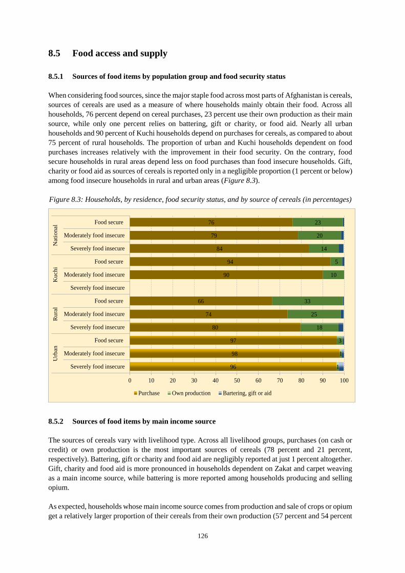
126
8.5 Food access and supply
8.5.1 Sources of food items by population group and food security status
When considering food sources, since the major staple food across most parts of Afghanistan is cereals,
sources of cereals are used as a measure of where households mainly obtain their food. Across all
households, 76 percent depend on cereal purchases, 23 percent use their own production as their main
source, while only one percent relies on battering, gift or charity, or food aid. Nearly all urban
households and 90 percent of Kuchi households depend on purchases for cereals, as compared to about
75 percent of rural households. The proportion of urban and Kuchi households dependent on food
purchases increases relatively with the improvement in their food security. On the contrary, food
secure households in rural areas depend less on food purchases than food insecure households. Gift,
charity or food aid as sources of cereals is reported only in a negligible proportion (1 percent or below)
among food insecure households in rural and urban areas (Figure 8.3).
Figure 8.3: Households, by residence, food security status, and by source of cereals (in percentages)
8.5.2 Sources of food items by main income source
The sources of cereals vary with livelihood type. Across all livelihood groups, purchases (on cash or
credit) or own production is the most important sources of cereals (78 percent and 21 percent,
respectively). Battering, gift or charity and food aid are negligibly reported at just 1 percent altogether.
Gift, charity and food aid is more pronounced in households dependent on Zakat and carpet weaving
as a main income source, while battering is more reported among households producing and selling
opium.
As expected, households whose main income source comes from production and sale of crops or opium
get a relatively larger proportion of their cereals from their own production (57 percent and 54 percent
96
98
97
80
74
66
90
94
84
79
76
1
1
3
18
25
33
10
5
14
20
23
0 10 20 30 40 50 60 70 80 90 100
Severely food insecure
Moderately food insecure
Food secure
Severely food insecure
Moderately food insecure
Food secure
Severely food insecure
Moderately food insecure
Food secure
Severely food insecure
Moderately food insecure
Food secure
Urb
an
Rura
lK
uch
iN
ati
on
al
Purchase Own production Bartering, gift or aid
127
of households, respectively). However, 42 percent of these households still depend on the market for
the balance of their cereal needs. Purchases from markets are the main source of cereals of the majority
of households (80 percent and above) engaged in production and manufacturing, services, trade, farm
and non-farm wage labors, borrowing and rental income.
8.5.3 Sources of food items by season
Within the year of 2014, sources of cereals vary slightly and purchases remain the main source of
around 77 percent of the households across all populations groups. Own production is the second
source of cereals for 22 percent of the households.
For the urban households, purchases remain high at 97 percent of the households all year round and
does not significantly vary by season. Among the Kuchi households, about 8 percent depend on their
own production in summer (June – September), but purchases are the main source of cereals for the
autumn months (September – December). In rural areas, about 30 percent of households depend on
their own production for their cereals throughout the year, and around 70 percent depend on purchases.
The proportion of households dependent on purchases in rural areas slightly increases from 66 percent
in winter (December 2013 - March 2014) to 72 percent in spring (March-June 2014) and summer
(June-September 2014).
8.6 Food consumption
8.6.1 Dietary diversity45
Even among households who satisfy their calorie requirements, those who consume a non-diversified,
unbalanced and unhealthy diet, can be classified as food insecure. Hungry people spend a larger share,
if not all, of their food budget on macronutrient dense staples, such as wheat and rice, which provide
cheap and accessible sources of calories. In doing so, they compromise more nutritious items and their
diet lacks adequate proteins and micro-nutrients.
Poor diet diversity is a serious problem across much of Afghanistan (Table 8.7). Most of the food
consumed is made up of staples (wheat in particular). The average household in Afghanistan consumes
food from 5.0 out of standard 8 food groups. The score for urban households is slightly higher than for
rural and Kuchi households (5.7 versus 4.8 and 5.0, respectively). The regions of the central highlands,
north-east, and west score below the national average and consume 4.3, 4.5, 4.5 food groups,
respectively. Female-headed households consume fewer food groups (4.1 groups) than male-headed
households (5.1 groups).
Overall, the proportion of households with low dietary diversity accounts for 36 percent of all Afghan
households, representing 20 percent in urban areas, 42 percent in rural areas and 41 percent among the
Kuchi households. Urban households tend to have higher consumption of meats, eggs and vegetables
compared to the rural and Kuchi households. As expected, the Kuchi households consume more dairy
products compared to other groups. The wider diversity of foods available in urban areas is likely
45 The Diet Diversity Score measures how many food groups (out of eight) are consumed during a week reporting
period. Households that over a seven day period consumed foods from four or fewer food groups out of eight
are classified as having low dietary diversity.
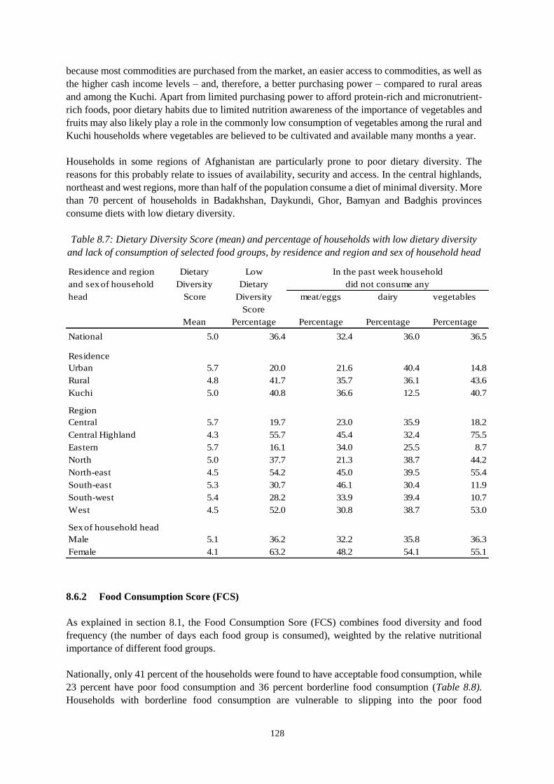
128
because most commodities are purchased from the market, an easier access to commodities, as well as
the higher cash income levels – and, therefore, a better purchasing power – compared to rural areas
and among the Kuchi. Apart from limited purchasing power to afford protein-rich and micronutrient-
rich foods, poor dietary habits due to limited nutrition awareness of the importance of vegetables and
fruits may also likely play a role in the commonly low consumption of vegetables among the rural and
Kuchi households where vegetables are believed to be cultivated and available many months a year.
Households in some regions of Afghanistan are particularly prone to poor dietary diversity. The
reasons for this probably relate to issues of availability, security and access. In the central highlands,
northeast and west regions, more than half of the population consume a diet of minimal diversity. More
than 70 percent of households in Badakhshan, Daykundi, Ghor, Bamyan and Badghis provinces
consume diets with low dietary diversity.
Table 8.7: Dietary Diversity Score (mean) and percentage of households with low dietary diversity
and lack of consumption of selected food groups, by residence and region and sex of household head
Residence and region Dietary Low In the past week household
and sex of household Diversity Dietary did not consume any
head Score Diversity meat/eggs dairy vegetables
Score
Mean Percentage Percentage Percentage Percentage
National 5.0 36.4 32.4 36.0 36.5
Residence
Urban 5.7 20.0 21.6 40.4 14.8
Rural 4.8 41.7 35.7 36.1 43.6
Kuchi 5.0 40.8 36.6 12.5 40.7
Region
Central 5.7 19.7 23.0 35.9 18.2
Central Highland 4.3 55.7 45.4 32.4 75.5
Eastern 5.7 16.1 34.0 25.5 8.7
North 5.0 37.7 21.3 38.7 44.2
North-east 4.5 54.2 45.0 39.5 55.4
South-east 5.3 30.7 46.1 30.4 11.9
South-west 5.4 28.2 33.9 39.4 10.7
West 4.5 52.0 30.8 38.7 53.0
Sex of household head
Male 5.1 36.2 32.2 35.8 36.3
Female 4.1 63.2 48.2 54.1 55.1
8.6.2 Food Consumption Score (FCS)
As explained in section 8.1, the Food Consumption Sore (FCS) combines food diversity and food
frequency (the number of days each food group is consumed), weighted by the relative nutritional
importance of different food groups.
Nationally, only 41 percent of the households were found to have acceptable food consumption, while
23 percent have poor food consumption and 36 percent borderline food consumption (Table 8.8).
Households with borderline food consumption are vulnerable to slipping into the poor food
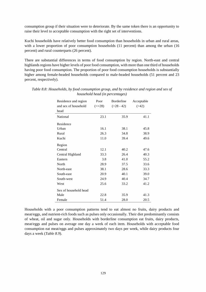
129
consumption group if their situation were to deteriorate. By the same token there is an opportunity to
raise their level to acceptable consumption with the right set of interventions.
Kuchi households have relatively better food consumption than households in urban and rural areas,
with a lower proportion of poor consumption households (11 percent) than among the urban (16
percent) and rural counterparts (26 percent).
There are substantial differences in terms of food consumption by region. North-east and central
highlands regions have higher levels of poor food consumption, with more than one third of households
having poor food consumption. The proportion of poor food consumption households is substantially
higher among female-headed households compared to male-headed households (51 percent and 23
percent, respectively).
Table 8.8: Households, by food consumption group, and by residence and region and sex of
household head (in percentages)
Residence and region Poor Borderline Acceptable
and sex of household (<=28) (>28 - 42) (>42)
head
National 23.1 35.9 41.1
Residence
Urban 16.1 38.1 45.8
Rural 26.3 34.8 38.9
Kuchi 11.0 39.4 49.6
Region
Central 12.1 40.2 47.6
Central Highland 33.3 26.4 40.3
Eastern 3.8 41.0 55.2
North 28.9 37.5 33.6
North-east 38.1 28.6 33.3
South-east 20.9 40.1 39.0
South-west 24.9 40.4 34.7
West 25.6 33.2 41.2
Sex of household head
Male 22.8 35.9 41.3
Female 51.4 28.0 20.5
Households with a poor consumption patterns tend to eat almost no fruits, dairy products and
meat/eggs, and nutrient-rich foods such as pulses only occasionally. Their diet predominantly consists
of wheat, oil and sugar only. Households with borderline consumption eat fruits, dairy products,
meat/eggs and pulses on average one day a week of each item. Households with acceptable food
consumption eat meat/eggs and pulses approximately two days per week, while dairy products four
days a week (Table 8.9).
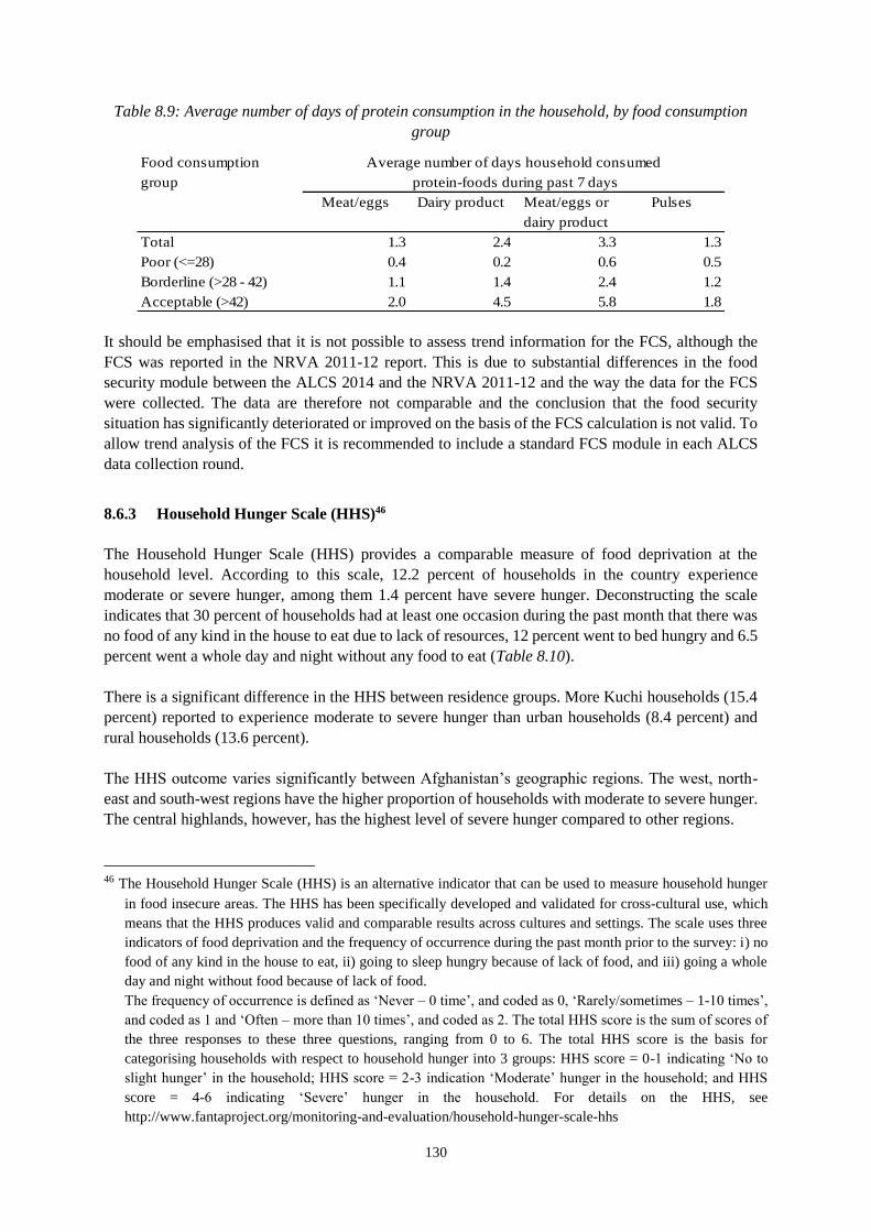
130
Table 8.9: Average number of days of protein consumption in the household, by food consumption
group
Food consumption Average number of days household consumed
group protein-foods during past 7 days
Meat/eggs Dairy product Meat/eggs or Pulses
dairy product
Total 1.3 2.4 3.3 1.3
Poor (<=28) 0.4 0.2 0.6 0.5
Borderline (>28 - 42) 1.1 1.4 2.4 1.2
Acceptable (>42) 2.0 4.5 5.8 1.8
It should be emphasised that it is not possible to assess trend information for the FCS, although the
FCS was reported in the NRVA 2011-12 report. This is due to substantial differences in the food
security module between the ALCS 2014 and the NRVA 2011-12 and the way the data for the FCS
were collected. The data are therefore not comparable and the conclusion that the food security
situation has significantly deteriorated or improved on the basis of the FCS calculation is not valid. To
allow trend analysis of the FCS it is recommended to include a standard FCS module in each ALCS
data collection round.
8.6.3 Household Hunger Scale (HHS)46
The Household Hunger Scale (HHS) provides a comparable measure of food deprivation at the
household level. According to this scale, 12.2 percent of households in the country experience
moderate or severe hunger, among them 1.4 percent have severe hunger. Deconstructing the scale
indicates that 30 percent of households had at least one occasion during the past month that there was
no food of any kind in the house to eat due to lack of resources, 12 percent went to bed hungry and 6.5
percent went a whole day and night without any food to eat (Table 8.10).
There is a significant difference in the HHS between residence groups. More Kuchi households (15.4
percent) reported to experience moderate to severe hunger than urban households (8.4 percent) and
rural households (13.6 percent).
The HHS outcome varies significantly between Afghanistan’s geographic regions. The west, north-
east and south-west regions have the higher proportion of households with moderate to severe hunger.
The central highlands, however, has the highest level of severe hunger compared to other regions.
46 The Household Hunger Scale (HHS) is an alternative indicator that can be used to measure household hunger
in food insecure areas. The HHS has been specifically developed and validated for cross-cultural use, which
means that the HHS produces valid and comparable results across cultures and settings. The scale uses three
indicators of food deprivation and the frequency of occurrence during the past month prior to the survey: i) no
food of any kind in the house to eat, ii) going to sleep hungry because of lack of food, and iii) going a whole
day and night without food because of lack of food.
The frequency of occurrence is defined as ‘Never – 0 time’, and coded as 0, ‘Rarely/sometimes – 1-10 times’,
and coded as 1 and ‘Often – more than 10 times’, and coded as 2. The total HHS score is the sum of scores of
the three responses to these three questions, ranging from 0 to 6. The total HHS score is the basis for
categorising households with respect to household hunger into 3 groups: HHS score = 0-1 indicating ‘No to
slight hunger’ in the household; HHS score = 2-3 indication ‘Moderate’ hunger in the household; and HHS
score = 4-6 indicating ‘Severe’ hunger in the household. For details on the HHS, see
http://www.fantaproject.org/monitoring-and-evaluation/household-hunger-scale-hhs
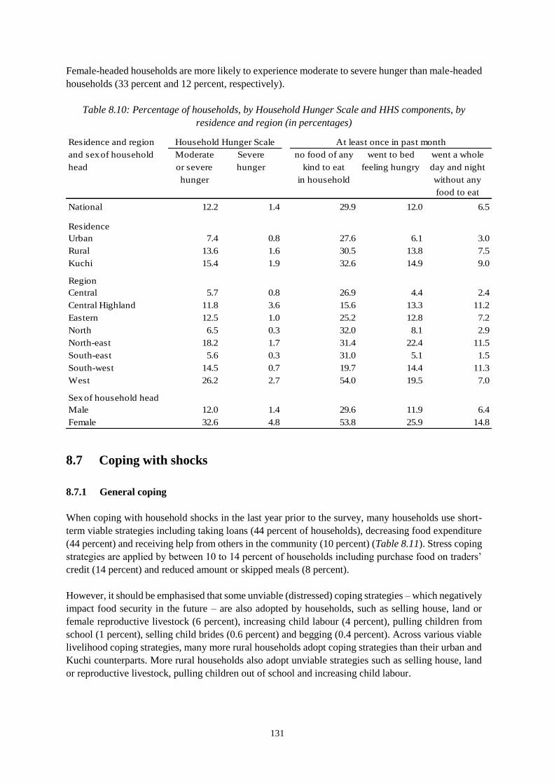
131
Female-headed households are more likely to experience moderate to severe hunger than male-headed
households (33 percent and 12 percent, respectively).
Table 8.10: Percentage of households, by Household Hunger Scale and HHS components, by
residence and region (in percentages)
Residence and region Household Hunger Scale At least once in past month
and sex of household Moderate Severe no food of any went to bed went a whole
head or severe hunger kind to eat feeling hungry day and night
hunger in household without any
food to eat
National 12.2 1.4 29.9 12.0 6.5
Residence
Urban 7.4 0.8 27.6 6.1 3.0
Rural 13.6 1.6 30.5 13.8 7.5
Kuchi 15.4 1.9 32.6 14.9 9.0
Region
Central 5.7 0.8 26.9 4.4 2.4
Central Highland 11.8 3.6 15.6 13.3 11.2
Eastern 12.5 1.0 25.2 12.8 7.2
North 6.5 0.3 32.0 8.1 2.9
North-east 18.2 1.7 31.4 22.4 11.5
South-east 5.6 0.3 31.0 5.1 1.5
South-west 14.5 0.7 19.7 14.4 11.3
West 26.2 2.7 54.0 19.5 7.0
Sex of household head
Male 12.0 1.4 29.6 11.9 6.4
Female 32.6 4.8 53.8 25.9 14.8
8.7 Coping with shocks
8.7.1 General coping
When coping with household shocks in the last year prior to the survey, many households use short-
term viable strategies including taking loans (44 percent of households), decreasing food expenditure
(44 percent) and receiving help from others in the community (10 percent) (Table 8.11). Stress coping
strategies are applied by between 10 to 14 percent of households including purchase food on traders’
credit (14 percent) and reduced amount or skipped meals (8 percent).
However, it should be emphasised that some unviable (distressed) coping strategies – which negatively
impact food security in the future – are also adopted by households, such as selling house, land or
female reproductive livestock (6 percent), increasing child labour (4 percent), pulling children from
school (1 percent), selling child brides (0.6 percent) and begging (0.4 percent). Across various viable
livelihood coping strategies, many more rural households adopt coping strategies than their urban and
Kuchi counterparts. More rural households also adopt unviable strategies such as selling house, land
or reproductive livestock, pulling children out of school and increasing child labour.
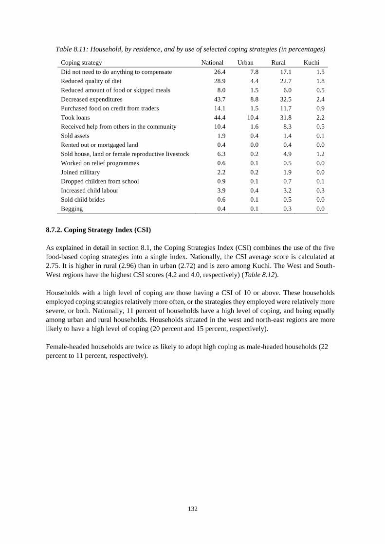
132
Table 8.11: Household, by residence, and by use of selected coping strategies (in percentages)
Coping strategy National Urban Rural Kuchi
Did not need to do anything to compensate 26.4 7.8 17.1 1.5
Reduced quality of diet 28.9 4.4 22.7 1.8
Reduced amount of food or skipped meals 8.0 1.5 6.0 0.5
Decreased expenditures 43.7 8.8 32.5 2.4
Purchased food on credit from traders 14.1 1.5 11.7 0.9
Took loans 44.4 10.4 31.8 2.2
Received help from others in the community 10.4 1.6 8.3 0.5
Sold assets 1.9 0.4 1.4 0.1
Rented out or mortgaged land 0.4 0.0 0.4 0.0
Sold house, land or female reproductive livestock 6.3 0.2 4.9 1.2
Worked on relief programmes 0.6 0.1 0.5 0.0
Joined military 2.2 0.2 1.9 0.0
Dropped children from school 0.9 0.1 0.7 0.1
Increased child labour 3.9 0.4 3.2 0.3
Sold child brides 0.6 0.1 0.5 0.0
Begging 0.4 0.1 0.3 0.0
8.7.2. Coping Strategy Index (CSI)
As explained in detail in section 8.1, the Coping Strategies Index (CSI) combines the use of the five
food-based coping strategies into a single index. Nationally, the CSI average score is calculated at
2.75. It is higher in rural (2.96) than in urban (2.72) and is zero among Kuchi. The West and South-
West regions have the highest CSI scores (4.2 and 4.0, respectively) (Table 8.12).
Households with a high level of coping are those having a CSI of 10 or above. These households
employed coping strategies relatively more often, or the strategies they employed were relatively more
severe, or both. Nationally, 11 percent of households have a high level of coping, and being equally
among urban and rural households. Households situated in the west and north-east regions are more
likely to have a high level of coping (20 percent and 15 percent, respectively).
Female-headed households are twice as likely to adopt high coping as male-headed households (22
percent to 11 percent, respectively).
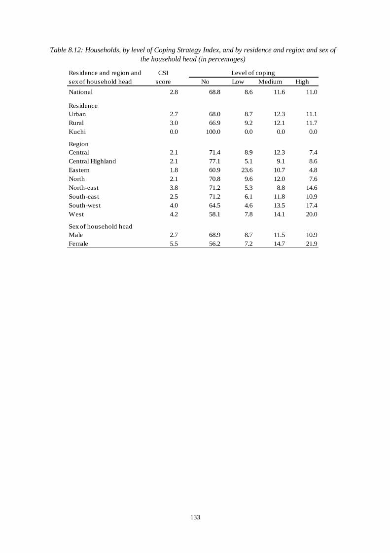
133
Table 8.12: Households, by level of Coping Strategy Index, and by residence and region and sex of
the household head (in percentages)
Residence and region and CSI Level of coping
sex of household head score No Low Medium High
National 2.8 68.8 8.6 11.6 11.0
Residence
Urban 2.7 68.0 8.7 12.3 11.1
Rural 3.0 66.9 9.2 12.1 11.7
Kuchi 0.0 100.0 0.0 0.0 0.0
Region
Central 2.1 71.4 8.9 12.3 7.4
Central Highland 2.1 77.1 5.1 9.1 8.6
Eastern 1.8 60.9 23.6 10.7 4.8
North 2.1 70.8 9.6 12.0 7.6
North-east 3.8 71.2 5.3 8.8 14.6
South-east 2.5 71.2 6.1 11.8 10.9
South-west 4.0 64.5 4.6 13.5 17.4
West 4.2 58.1 7.8 14.1 20.0
Sex of household head
Male 2.7 68.9 8.7 11.5 10.9
Female 5.5 56.2 7.2 14.7 21.9

134
9 EDUCATION
Summary. Despite major achievements in the last decade, education performance in Afghanistan is still
among the poorest in the world. Opportunities to attend education are few, especially for girls and
women, and rural and Kuchi populations in general. The education picture presented by the ALCS 2013-
14 is one of modest improvements in most areas, but also with stagnation and even deterioration in
other fields. The survey results suggest that the ANDS education and related gender-equity targets will
not be achieved by 2020.
Literacy indicators show steady, but modest increases. More than half (52 percent) of the youth
population aged 15 to 24 is now able to read and write, compared to 31 percent in 2005 and 47 percent
in the previous NRVA 2011-12. Continuous small increases are observed for the adult literacy rate,
from 26 percent in NRVA 2007-08 and 31 percent in 2011-12 to 34 percent in the ALCS 2013-14.
More disconcerting results are obtained with regard to the development of school attendance ratios.
Previous NRVAs already noted a slowdown of the rate of improvement of net attendance ratios and the
current ALCS confirms this negative tendency. The net attendance ratio for secondary and tertiary
education still maintained upward trends: for the secondary net attendance ratio from 16 percent in
2007-08 and 33 percent in 2011-12 to 37 percent now. However, the net attendance ratio for primary
education showed a decline to 55 percent, after a peak of 57 percent in 2011-12. The school attendance
information suggests that 2.3 million primary school age children in Afghanistan miss out on education
and on the opportunity to learn basic life skills. The absolute numbers of persons of secondary and
tertiary education age who are not participating in education are in the same order of magnitude: 2.0
and 2.3 million, respectively.
For the first time, ALCS was able to estimate education transition rates. The gross intake rate of 45
percent is an indication that the capacity of the educational system to absorb new pupils is low, less
than half of what would be required to provide every eligible child with a place at school. On the other
hand, the transition rates from one grade to the next are fairly high, resulting in a modest drop-out
percentage of 14 percent and an adequate 84 percent of school starters who reach the last grade of
primary education. The transition rate from primary to secondary education is also fairly high (96
percent), but the next transition to tertiary education is much more difficult, as indicated by the low 60
percent who start at this level. These transition rates indicate that the problem of Afghanistan’s
education system is not so much retention and drop out, but first and foremost starting school. Given
the present age-specific attendance rates, an Afghan child of 6 years old can expect to spend on average
7.7 years of his or her life in education, a very short period in international perspective.
Dominant reasons for school dropout are economic considerations – particularly opportunity costs –
and cultural barriers – especially for girls, family resistance against education and entering marriage.
In rural areas, security concerns figured also prominently for girls. To some extent, home schooling and
literacy schools can compensate inadequacies of the formal education system, but they are often not a
sufficient alternative for a full course of compulsory formal education.
Gender inequity remains a major concern in education. Without exception, education gender indicators
show a very disadvantaged position of women and girls in Afghanistan. In line with the increase of
literacy levels in the adult and youth population, the literacy gender parity indices are improving, but
at a slow pace. The youth literacy parity index increased from 0.52 in 2011-12 to 0.55 in the current
ALCS and the adult literacy parity index increased from 0.37 to 0.39 in the same period. The survey
suggests that for the ratio of girls to boys in education only in secondary education some progress is
made. Here, the ratio increase from 53 to 55 percent. But for tertiary education attendance the ender
parity index stagnated at a level of 41 percent and the ratio for primary education even declined from
74 to 71 percent.
Underlying the educational gender inequity is the very low education intake of girls. Once in school,
the progression and dropout rates of girls and boys are very similar. The disadvantage of girls and
135
women compared to boys and men is reflected in a low school-life expectancy (5.6 against 9.5 years of
expected education), low literacy rates (19 percent for adult women and 37 percent for female youth,
against 49 and 66 percent for male adults and youth, respectively) and low attendance ratios for all
levels of education: 45 against 62 percent in primary education, 27 against 47 percent in secondary
education and 5 against 13 percent in tertiary education.
Residence is the other main inequity dimension in Afghanistan. For all education indicators, rural
populations score significantly poorer, and the Kuchi do even worse. This applies to levels of school
attendance and literacy, and equally to gender equity indicators.
9.1 Introduction
Education is one of the most important aspects of human development. The Convention on the Rights
of the Child – the most widely ratified human rights treaty – enshrines the right of all children to a
primary education that will give them the skills they need to continue learning throughout life. It has
been well-established that increasing girls’ and women’s access to education improves maternal and
child health, improves their own children’s access to education, and promotes economic growth. Yet, a
large majority of Afghan people have been denied this right, most of them women and girls.
Consequently, they are bereft of many opportunities for personal development and contributions to
society.
Afghanistan is faced with a huge challenge to recover from thirty years of conflict and political unrest
that resulted in the destruction of the Afghan education system in terms of staffing, premises, curricula
and student attendance. During the Taliban rule girls were even prohibited from attending schools. Since
2001, a nationwide reconstruction process is being implemented with large support from the
international community. According to the Ministry of Education (MoE), only one million children
(almost all boys) were enrolled in schools in 2001, but over 8.6 million were enrolled in 2013 of whom
39 percent were girls (Ministry of Education 2014). Improvement of the education system was also
demonstrate by the results of the consecutive NRVAs (2005, 2007-08 and 2011-12), which showed
significant gains in the areas of literacy, educational attendance and educational attainment.
However, the latest NRVA also showed that there is still a long way to go to achieve the goals that are
set by the Afghan government in terms of literacy and enrolment, particularly for girls. Also, the pupil-
teacher ratio of 47 students per teacher is much higher than the Education Ministry’s norm (35 students
per teacher). Moreover, 58 percent of teachers do not have the minimum required qualification (14th
grade degree), which implies that the number pupil per qualified teacher is even much higher (111
students per teacher). The shortage of teachers is especially acute in rural areas and specific fields, like
mathematics and science. In addition, almost half the schools for primary and secondary education do
not have usable buildings and those with buildings often lack sufficient classrooms, proper sanitation,
drinking water or surrounding walls, and are frequently in bad repair (Ministry of Education 2014).
The latest ALCS covered again components for a situational analysis on education in the period 2013-
14. Section 9.2 addresses the present performance of Afghanistan’s educational system by reviewing
attendance and non-attendance, and some of their backgrounds. Section 9.3 is dedicated to the
accumulated human capital in terms of highest educational levels attained by Afghanistan’s adult
population. Finally, section 9.4 provides an assessment of the situation with regard to literacy, being one
of the key effects of education. The chapter also presents most of the education-related MDG indicators.
136
9.2 Educational attendance
9.2.1 Educational attendance in residence and gender perspective Although since 2008 education is supposed to start at age 6 (see text box Afghanistan’s education system
above), for various reasons, few children actually start schooling at this age. Figure 9.1 presents the age-
specific attendance rates and shows that only around one in nine 6-year olds (13 percent of boys and 9
percent of girls) actually started education. It also indicates that many children enter primary school
even at ages beyond 7 and highest attendance rates are achieved only in the late primary and early
secondary school ages.
Afghanistan’s education system
The education system in Afghanistan is being rebuilt and restructured. The Ministry of Education is responsible
for primary and secondary education levels, while the Ministry of Higher Education supervises tertiary education.
In principle, public education is free and primary and lower secondary education is compulsory.
Primary education lasts 6 years, from classes 1 through 6 and is intended for pupils aged 6 to 12. In the first 3
years of primary education, the curriculum comprises subjects such as art, theology, Dari or Pashtu (depending on
the region), mathematics, calligraphy and physics. Other subjects, such as sciences, geography and history, are
added to the curriculum at a later stage. Community-based education is provided in the less safe regions, such as
the southern provinces. Education of this type is often provided in mosques by an imam and the emphasis lies
primarily on religious subjects. Pupils complete their primary education with an examination which grants them
admission to lower secondary education.
Lower (or intermediate) secondary education has a duration of 3 years, from classes 7 to 9 for pupils aged 12-
14. The curriculum for lower secondary education comprises subjects such a mathematics, sciences, biology,
physics, chemistry and foreign languages (English, German French and Russian). Lower secondary education is
provided in preparation for higher secondary education. Lower secondary education also provides admission to
technical and secondary vocational education. Pupils complete their lower secondary education with an
examination, which grants admission to higher secondary education.
Higher secondary education consists of 3 years of senior secondary education, from classes 10 to 12 for pupils
aged 14-17. In senior secondary education, pupils can choose theoretical subjects, such as history, mathematics or
Islamic studies, or vocationally-oriented subjects, such as agriculture, education, art and culture and economics.
Both variants conclude with a national examination, on successful completion of which pupils are awarded a 12
Grade Graduation Certificate (NUFFIC 2015).
For various reasons (such as late start, temporary drop out, grade repetition or passing two grades in one year), the
actual age at which children attend different education levels often differs considerably with the official school
age. For practical reasons this report adopts age 7 to 12 as the primary school age, age 13 to 18 as secondary school
age and age 19 to 24 as tertiary school age (see section 9.2).
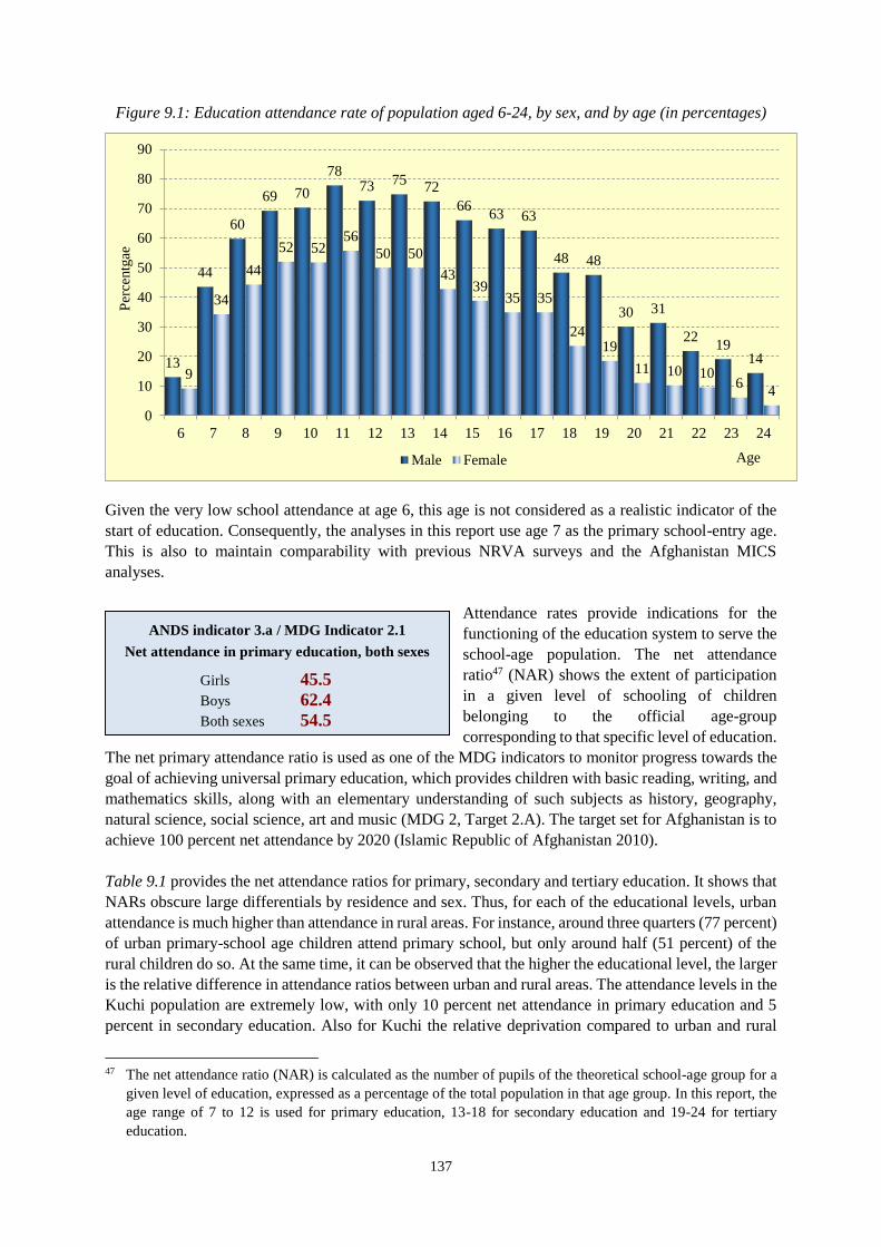
137
Figure 9.1: Education attendance rate of population aged 6-24, by sex, and by age (in percentages)
Given the very low school attendance at age 6, this age is not considered as a realistic indicator of the
start of education. Consequently, the analyses in this report use age 7 as the primary school-entry age.
This is also to maintain comparability with previous NRVA surveys and the Afghanistan MICS
analyses.
Attendance rates provide indications for the
functioning of the education system to serve the
school-age population. The net attendance
ratio47 (NAR) shows the extent of participation
in a given level of schooling of children
belonging to the official age-group
corresponding to that specific level of education.
The net primary attendance ratio is used as one of the MDG indicators to monitor progress towards the
goal of achieving universal primary education, which provides children with basic reading, writing, and
mathematics skills, along with an elementary understanding of such subjects as history, geography,
natural science, social science, art and music (MDG 2, Target 2.A). The target set for Afghanistan is to
achieve 100 percent net attendance by 2020 (Islamic Republic of Afghanistan 2010).
Table 9.1 provides the net attendance ratios for primary, secondary and tertiary education. It shows that
NARs obscure large differentials by residence and sex. Thus, for each of the educational levels, urban
attendance is much higher than attendance in rural areas. For instance, around three quarters (77 percent)
of urban primary-school age children attend primary school, but only around half (51 percent) of the
rural children do so. At the same time, it can be observed that the higher the educational level, the larger
is the relative difference in attendance ratios between urban and rural areas. The attendance levels in the
Kuchi population are extremely low, with only 10 percent net attendance in primary education and 5
percent in secondary education. Also for Kuchi the relative deprivation compared to urban and rural
47 The net attendance ratio (NAR) is calculated as the number of pupils of the theoretical school-age group for a
given level of education, expressed as a percentage of the total population in that age group. In this report, the
age range of 7 to 12 is used for primary education, 13-18 for secondary education and 19-24 for tertiary
education.
13
44
60
69 70
7873 75
72
6663 63
48 48
30 31
2219
149
34
44
52 5256
50 50
4339
35 35
2419
11 10 106
4
0
10
20
30
40
50
60
70
80
90
6 7 8 9 10 11 12 13 14 15 16 17 18 19 20 21 22 23 24
Per
centg
ae
AgeMale Female
ANDS indicator 3.a / MDG Indicator 2.1
Net attendance in primary education, both sexes
Girls 45.5
Boys 62.4
Both sexes 54.5
138
children is larger the higher the educational level. Overall, the NAR found for Afghanistan (55 percent
for primary education, 37 percent for secondary and 9 percent for tertiary) indicate that the country is
still among the poorest performers in providing adequate education to its population.
Table 9.1: Net attendance ratio (NAR) and gross attendance ratio (GAR), by residence, and by
education level, sex; Gender parity index, by residence, and by education level; GAR/NAR ratio, by
education level
Educational level, Net/gross attendance ratio, residence Ratio
sex and gender Net attendance ratio Gross attendance ratio GAR/NAR
parity index National Urban Rural Kuchi National Urban Rural Kuchi National
Primary
Both sexes 54.5 76.7 51.2 10.3 66.7 92.3 63.1 13.7 1.2
Male 62.4 80.1 61.2 15.7 77.4 97.9 76.1 20.7 1.2
Female 45.5 72.9 39.9 2.8 54.6 86.1 48.3 4.0 1.2
Gender parity index 0.73 0.91 0.65 0.18 0.71 0.88 0.63 0.19
Secondary
Both sexes 37.2 56.1 31.6 5.4 46.2 68.9 39.6 7.3 1.2
Male 46.7 62.8 43.2 9.3 58.9 78.4 54.6 12.4 1.3
Female 26.9 49.2 19.0 0.0 32.6 59.3 23.3 0.0 1.2
Gender parity index 0.58 0.78 0.44 0.00 0.55 0.76 0.43 0.00
Tertiary
Both sexes 8.7 17.4 5.4 0.7 10.1 20.7 6.2 0.7 1.2
Male 12.7 22.2 9.2 1.5 14.3 25.6 10.1 1.5 1.1
Female 4.7 12.4 1.7 0.0 5.9 15.6 2.3 0.0 1.3
Gender parity index 0.37 0.56 0.19 0.00 0.41 0.61 0.22 0.00
Given the large discrepancy between official and actual school ages, the standard net attendance ratio
may not be an adequate indicator for the performance of the education system in Afghanistan. An often-
used alternative is the adjusted attendance ratio, which also includes pupils attending a higher education
level than what would be in accordance with their age. Applying this definition, the adjusted NAR for
primary education (the percentage of children of primary school age attending primary or secondary
school) would be 56 percent (65 percent for boys and 47 percent for girls) and the adjusted NAR for
secondary education (the percentage of children of secondary school age attending secondary school or
higher) would be 38 percent (boys 48 percent and girls 29 percent).
The gross attendance ratio48 (GAR) is another measure of educational performance. It gives the total
number of school places per education level also provides an indication of whether the education system
has the capacity to provide education for all children of a specific school age. Table 9.1 (middle panel)
presents the GARs for the three main education levels. The overall GAR of 66.7 percent for primary
education means that the number of students attending primary education, whether or not they have the
age corresponding to primary education, is only two-thirds of the children of primary-school age.
In Afghanistan, many children may enter school late and stay at a specific educational level well past
the official school age due to late entry or grade repetition. In addition, children may also enter a specific
school level early, for instance if home schooling accelerated the learning process. A comparison of the
48 The gross attendance ratio is calculated as the number of pupils in a given level of education, regardless of age,
expressed as a percentage of the total population corresponding to the same level of education.
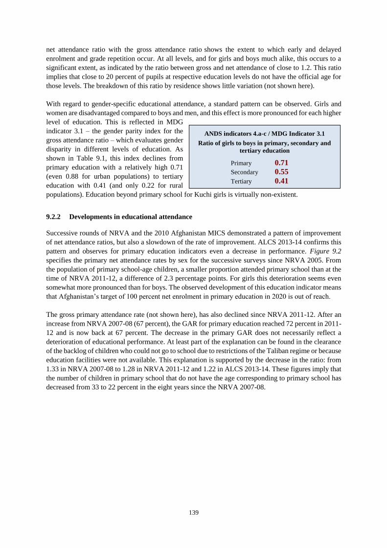
139
net attendance ratio with the gross attendance ratio shows the extent to which early and delayed
enrolment and grade repetition occur. At all levels, and for girls and boys much alike, this occurs to a
significant extent, as indicated by the ratio between gross and net attendance of close to 1.2. This ratio
implies that close to 20 percent of pupils at respective education levels do not have the official age for
those levels. The breakdown of this ratio by residence shows little variation (not shown here).
With regard to gender-specific educational attendance, a standard pattern can be observed. Girls and
women are disadvantaged compared to boys and men, and this effect is more pronounced for each higher
level of education. This is reflected in MDG
indicator 3.1 – the gender parity index for the
gross attendance ratio – which evaluates gender
disparity in different levels of education. As
shown in Table 9.1, this index declines from
primary education with a relatively high 0.71
(even 0.88 for urban populations) to tertiary
education with 0.41 (and only 0.22 for rural
populations). Education beyond primary school for Kuchi girls is virtually non-existent.
9.2.2 Developments in educational attendance
Successive rounds of NRVA and the 2010 Afghanistan MICS demonstrated a pattern of improvement
of net attendance ratios, but also a slowdown of the rate of improvement. ALCS 2013-14 confirms this
pattern and observes for primary education indicators even a decrease in performance. Figure 9.2
specifies the primary net attendance rates by sex for the successive surveys since NRVA 2005. From
the population of primary school-age children, a smaller proportion attended primary school than at the
time of NRVA 2011-12, a difference of 2.3 percentage points. For girls this deterioration seems even
somewhat more pronounced than for boys. The observed development of this education indicator means
that Afghanistan’s target of 100 percent net enrolment in primary education in 2020 is out of reach.
The gross primary attendance rate (not shown here), has also declined since NRVA 2011-12. After an
increase from NRVA 2007-08 (67 percent), the GAR for primary education reached 72 percent in 2011-
12 and is now back at 67 percent. The decrease in the primary GAR does not necessarily reflect a
deterioration of educational performance. At least part of the explanation can be found in the clearance
of the backlog of children who could not go to school due to restrictions of the Taliban regime or because
education facilities were not available. This explanation is supported by the decrease in the ratio: from
1.33 in NRVA 2007-08 to 1.28 in NRVA 2011-12 and 1.22 in ALCS 2013-14. These figures imply that
the number of children in primary school that do not have the age corresponding to primary school has
decreased from 33 to 22 percent in the eight years since the NRVA 2007-08.
ANDS indicators 4.a-c / MDG Indicator 3.1
Ratio of girls to boys in primary, secondary and
tertiary education
Primary 0.71
Secondary 0.55
Tertiary 0.41
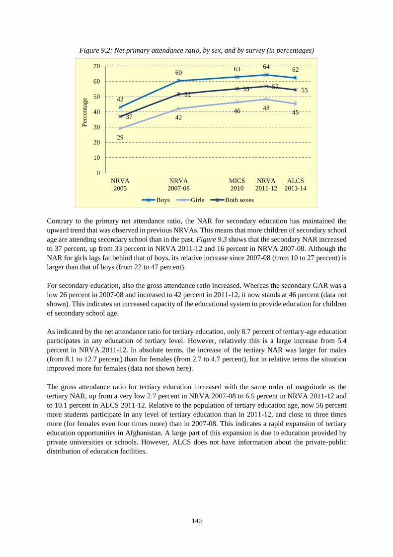
140
Figure 9.2: Net primary attendance ratio, by sex, and by survey (in percentages)
Contrary to the primary net attendance ratio, the NAR for secondary education has maintained the
upward trend that was observed in previous NRVAs. This means that more children of secondary school
age are attending secondary school than in the past. Figure 9.3 shows that the secondary NAR increased
to 37 percent, up from 33 percent in NRVA 2011-12 and 16 percent in NRVA 2007-08. Although the
NAR for girls lags far behind that of boys, its relative increase since 2007-08 (from 10 to 27 percent) is
larger than that of boys (from 22 to 47 percent).
For secondary education, also the gross attendance ratio increased. Whereas the secondary GAR was a
low 26 percent in 2007-08 and increased to 42 percent in 2011-12, it now stands at 46 percent (data not
shown). This indicates an increased capacity of the educational system to provide education for children
of secondary school age.
As indicated by the net attendance ratio for tertiary education, only 8.7 percent of tertiary-age education
participates in any education of tertiary level. However, relatively this is a large increase from 5.4
percent in NRVA 2011-12. In absolute terms, the increase of the tertiary NAR was larger for males
(from 8.1 to 12.7 percent) than for females (from 2.7 to 4.7 percent), but in relative terms the situation
improved more for females (data not shown here).
The gross attendance ratio for tertiary education increased with the same order of magnitude as the
tertiary NAR, up from a very low 2.7 percent in NRVA 2007-08 to 6.5 percent in NRVA 2011-12 and
to 10.1 percent in ALCS 2011-12. Relative to the population of tertiary education age, now 56 percent
more students participate in any level of tertiary education than in 2011-12, and close to three times
more (for females even four times more) than in 2007-08. This indicates a rapid expansion of tertiary
education opportunities in Afghanistan. A large part of this expansion is due to education provided by
private universities or schools. However, ALCS does not have information about the private-public
distribution of education facilities.
43
6063 64 62
29
4246 48
4537
5255 57
55
0
10
20
30
40
50
60
70
NRVA
2005
NRVA
2007-08
MICS
2010
NRVA
2011-12
ALCS
2013-14
Per
centa
ge
Boys Girls Both sexes
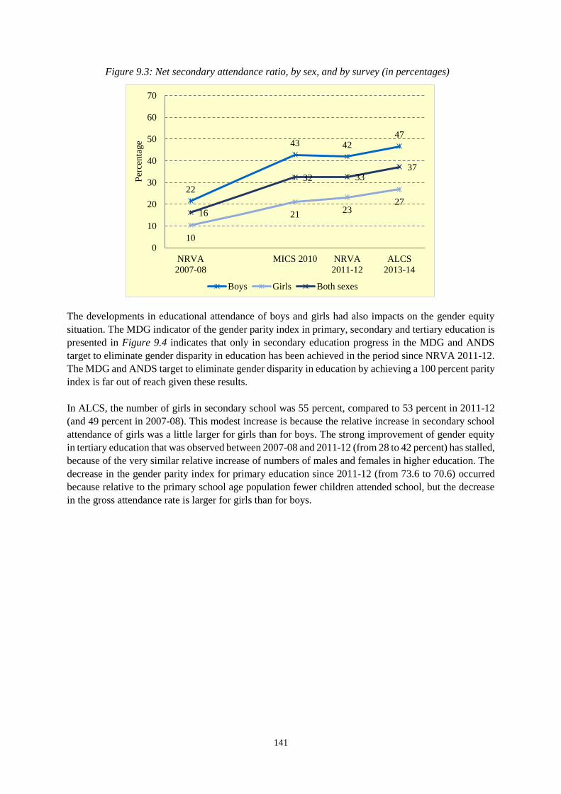
141
Figure 9.3: Net secondary attendance ratio, by sex, and by survey (in percentages)
The developments in educational attendance of boys and girls had also impacts on the gender equity
situation. The MDG indicator of the gender parity index in primary, secondary and tertiary education is
presented in Figure 9.4 indicates that only in secondary education progress in the MDG and ANDS
target to eliminate gender disparity in education has been achieved in the period since NRVA 2011-12.
The MDG and ANDS target to eliminate gender disparity in education by achieving a 100 percent parity
index is far out of reach given these results.
In ALCS, the number of girls in secondary school was 55 percent, compared to 53 percent in 2011-12
(and 49 percent in 2007-08). This modest increase is because the relative increase in secondary school
attendance of girls was a little larger for girls than for boys. The strong improvement of gender equity
in tertiary education that was observed between 2007-08 and 2011-12 (from 28 to 42 percent) has stalled,
because of the very similar relative increase of numbers of males and females in higher education. The
decrease in the gender parity index for primary education since 2011-12 (from 73.6 to 70.6) occurred
because relative to the primary school age population fewer children attended school, but the decrease
in the gross attendance rate is larger for girls than for boys.
22
43 4247
10
2123
27
16
32 3337
0
10
20
30
40
50
60
70
NRVA
2007-08
MICS 2010 NRVA
2011-12
ALCS
2013-14
Per
centa
ge
Boys Girls Both sexes
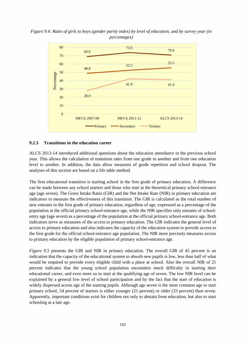
142
Figure 9.4: Ratio of girls to boys (gender parity index) by level of education, and by survey year (in
percentages)
9.2.3 Transitions in the education career
ALCS 2013-14 introduced additional questions about the education attendance in the previous school
year. This allows the calculation of transition rates from one grade to another and from one education
level to another. In addition, the data allow measures of grade repetition and school dropout. The
analyses of this section are based on a life table method.
The first educational transition is starting school in the first grade of primary education. A difference
can be made between any school starters and those who start at the theoretical primary school-entrance
age (age seven). The Gross Intake Ratio (GIR) and the Net Intake Rate (NIR) in primary education are
indicators to measure the effectiveness of this transition. The GIR is calculated as the total number of
new entrants in the first grade of primary education, regardless of age, expressed as a percentage of the
population at the official primary school-entrance age, while the NIR specifies only entrants of school-
entry age (age seven) as a percentage of the population at the official primary school-entrance age. Both
indicators serve as measures of the access to primary education. The GIR indicates the general level of
access to primary education and also indicates the capacity of the education system to provide access to
the first grade for the official school-entrance age population. The NIR more precisely measures access
to primary education by the eligible population of primary school-entrance age.
Figure 9.5 presents the GIR and NIR in primary education. The overall GIR of 45 percent is an
indication that the capacity of the educational system to absorb new pupils is low, less than half of what
would be required to provide every eligible child with a place at school. Also the overall NIR of 21
percent indicates that the young school population encounters much difficulty in starting their
educational career, and even more so to start at the qualifying age of seven. The low NIR level can be
explained by a general low level of school participation and by the fact that the start of education is
widely dispersed across age of the starting pupils. Although age seven is the most common age to start
primary school, 54 percent of starters is either younger (21 percent) or older (33 percent) than seven.
Apparently, important conditions exist for children not only to abstain from education, but also to start
schooling at a late age.
69.073.6
70.6
48.852.5
55.5
28.0
41.9 41.4
0
10
20
30
40
50
60
70
80
NRVA 2007-08 NRVA 2011-12 ALCS 2013-14
Per
centa
ge
Primary Secondary Tertiary
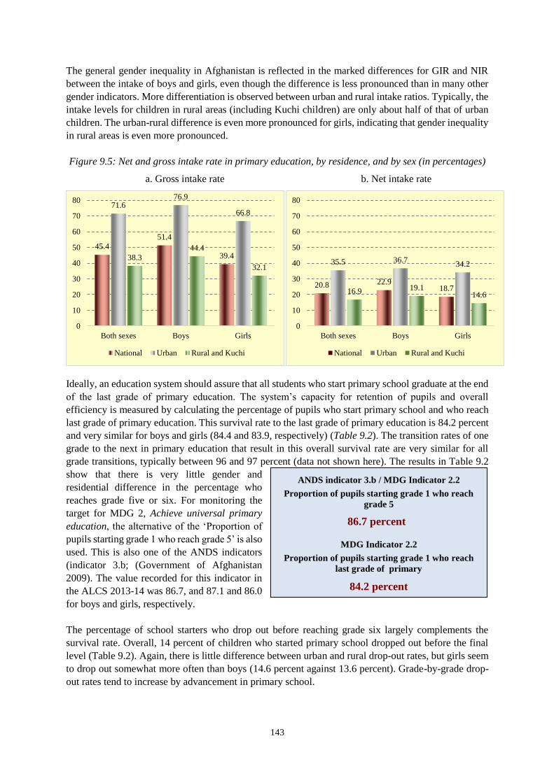
143
The general gender inequality in Afghanistan is reflected in the marked differences for GIR and NIR
between the intake of boys and girls, even though the difference is less pronounced than in many other
gender indicators. More differentiation is observed between urban and rural intake ratios. Typically, the
intake levels for children in rural areas (including Kuchi children) are only about half of that of urban
children. The urban-rural difference is even more pronounced for girls, indicating that gender inequality
in rural areas is even more pronounced.
Figure 9.5: Net and gross intake rate in primary education, by residence, and by sex (in percentages)
a. Gross intake rate b. Net intake rate
Ideally, an education system should assure that all students who start primary school graduate at the end
of the last grade of primary education. The system’s capacity for retention of pupils and overall
efficiency is measured by calculating the percentage of pupils who start primary school and who reach
last grade of primary education. This survival rate to the last grade of primary education is 84.2 percent
and very similar for boys and girls (84.4 and 83.9, respectively) (Table 9.2). The transition rates of one
grade to the next in primary education that result in this overall survival rate are very similar for all
grade transitions, typically between 96 and 97 percent (data not shown here). The results in Table 9.2
show that there is very little gender and
residential difference in the percentage who
reaches grade five or six. For monitoring the
target for MDG 2, Achieve universal primary
education, the alternative of the ‘Proportion of
pupils starting grade 1 who reach grade 5’ is also
used. This is also one of the ANDS indicators
(indicator 3.b; (Government of Afghanistan
2009). The value recorded for this indicator in
the ALCS 2013-14 was 86.7, and 87.1 and 86.0
for boys and girls, respectively.
The percentage of school starters who drop out before reaching grade six largely complements the
survival rate. Overall, 14 percent of children who started primary school dropped out before the final
level (Table 9.2). Again, there is little difference between urban and rural drop-out rates, but girls seem
to drop out somewhat more often than boys (14.6 percent against 13.6 percent). Grade-by-grade drop-
out rates tend to increase by advancement in primary school.
20.8 22.918.7
35.5 36.734.2
16.9 19.114.6
0
10
20
30
40
50
60
70
80
Both sexes Boys Girls
National Urban Rural and Kuchi
45.4
51.4
39.4
71.676.9
66.8
38.3
44.4
32.1
0
10
20
30
40
50
60
70
80
Both sexes Boys Girls
National Urban Rural and Kuchi
ANDS indicator 3.b / MDG Indicator 2.2
Proportion of pupils starting grade 1 who reach
grade 5
86.7 percent
MDG Indicator 2.2
Proportion of pupils starting grade 1 who reach
last grade of primary
84.2 percent
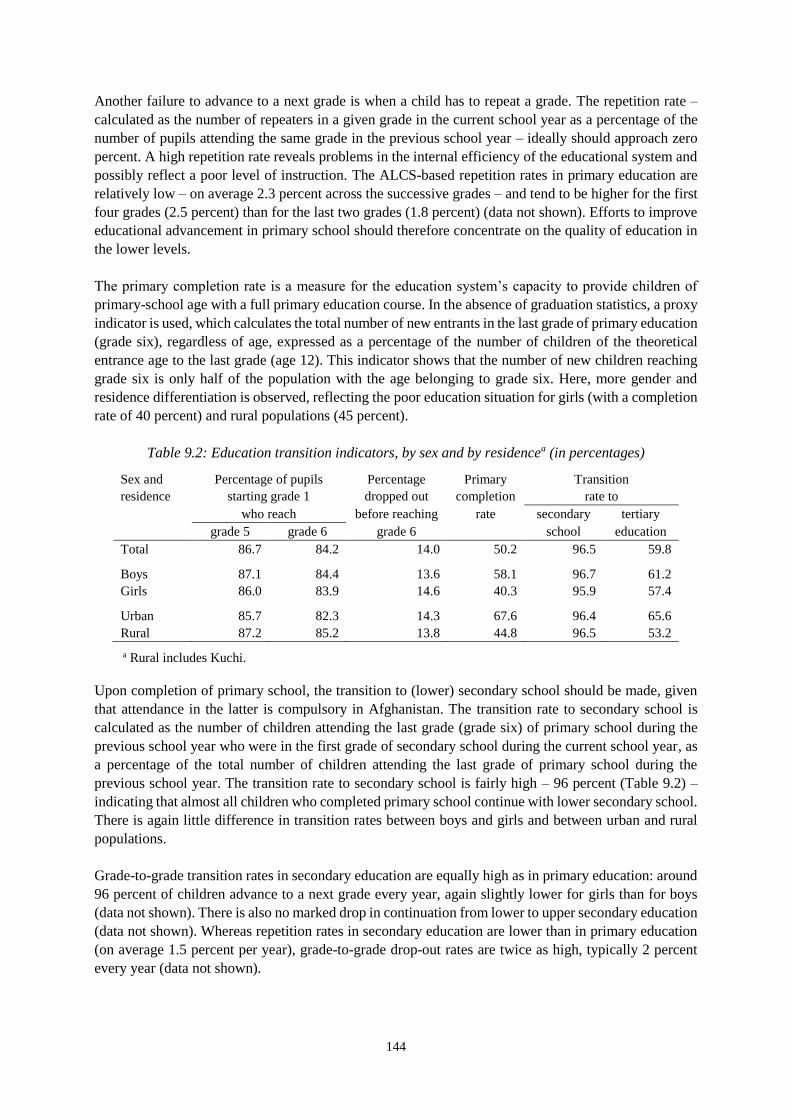
144
Another failure to advance to a next grade is when a child has to repeat a grade. The repetition rate –
calculated as the number of repeaters in a given grade in the current school year as a percentage of the
number of pupils attending the same grade in the previous school year – ideally should approach zero
percent. A high repetition rate reveals problems in the internal efficiency of the educational system and
possibly reflect a poor level of instruction. The ALCS-based repetition rates in primary education are
relatively low – on average 2.3 percent across the successive grades – and tend to be higher for the first
four grades (2.5 percent) than for the last two grades (1.8 percent) (data not shown). Efforts to improve
educational advancement in primary school should therefore concentrate on the quality of education in
the lower levels.
The primary completion rate is a measure for the education system’s capacity to provide children of
primary-school age with a full primary education course. In the absence of graduation statistics, a proxy
indicator is used, which calculates the total number of new entrants in the last grade of primary education
(grade six), regardless of age, expressed as a percentage of the number of children of the theoretical
entrance age to the last grade (age 12). This indicator shows that the number of new children reaching
grade six is only half of the population with the age belonging to grade six. Here, more gender and
residence differentiation is observed, reflecting the poor education situation for girls (with a completion
rate of 40 percent) and rural populations (45 percent).
Table 9.2: Education transition indicators, by sex and by residencea (in percentages)
Sex and Percentage of pupils Percentage Primary Transition
residence starting grade 1 dropped out completion rate to
who reach before reaching rate secondary tertiary
grade 5 grade 6 grade 6 school education
Total 86.7 84.2 14.0 50.2 96.5 59.8
Boys 87.1 84.4 13.6 58.1 96.7 61.2
Girls 86.0 83.9 14.6 40.3 95.9 57.4
Urban 85.7 82.3 14.3 67.6 96.4 65.6
Rural 87.2 85.2 13.8 44.8 96.5 53.2
a Rural includes Kuchi.
Upon completion of primary school, the transition to (lower) secondary school should be made, given
that attendance in the latter is compulsory in Afghanistan. The transition rate to secondary school is
calculated as the number of children attending the last grade (grade six) of primary school during the
previous school year who were in the first grade of secondary school during the current school year, as
a percentage of the total number of children attending the last grade of primary school during the
previous school year. The transition rate to secondary school is fairly high – 96 percent (Table 9.2) –
indicating that almost all children who completed primary school continue with lower secondary school.
There is again little difference in transition rates between boys and girls and between urban and rural
populations.
Grade-to-grade transition rates in secondary education are equally high as in primary education: around
96 percent of children advance to a next grade every year, again slightly lower for girls than for boys
(data not shown). There is also no marked drop in continuation from lower to upper secondary education
(data not shown). Whereas repetition rates in secondary education are lower than in primary education
(on average 1.5 percent per year), grade-to-grade drop-out rates are twice as high, typically 2 percent
every year (data not shown).
145
A main drop in continuation of education occurs after completion of secondary education. The transition
rate to tertiary education is only 60 percent (Table 9.2), indicating that of all students who reached grade
12, 40 percent dropped out from pursuing higher education. Contrary to the transition rate to secondary
school, here is a substantial difference between the continuation rates of urban and rural populations (66
and 53 percent, respectively). Also the female transition rate 57 percent) is lower than the male rate (61
percent).
9.2.4 School-life expectancy
The age- and level-specific attendance rates allow estimating the total number of years of schooling that
a child of a certain age can expect to receive in the future. For Afghanistan, this school-life expectancy
is a good proxy for the expected number of grades of education that will be completed, because of the
relatively low grade-repetition rates.49 Figure 9.6 shows the school-life expectancy by sex at national
level and for urban and rural populations. If current attendance ratios will be maintained, a six-year old
child can expect to remain in education for 7.7 years, an average that is built up from an expected 4.2
years in primary education, 3.0 years in secondary and 0.6 years in tertiary education. Boys can expect
to stay in education for 9.5 years, 1.7 times longer than girls, for whom the school-life expectancy is 5.6
years.
The urban school-life expectancy of 12.4 years is much higher than the rural version (8.5 years).
Figure 9.6 also indicates that the gender disadvantage for girls is larger in rural areas, both in absolute
and in relative terms. On average, a rural girl can expect to be in education for only 4.3 years.
Figure 9.6: School-life expectancy for (a) total, (b) urban and (c) rural populations, by sex (in years)
a. Total b. Urban c. Rural
9.2.5 Population not attending education
The school attendance information from the ALCS 2013-14 indicates that an estimated 2.3 million
primary school age children in Afghanistan miss out on education. The large majority of these (90
percent or 2.0 million) are from the rural or Kuchi populations. Girls are also overrepresented among
49 The school-life expectancy is calculated as the sum of the age-specific attendance ratios for primary,
secondary and tertiary education levels, assuming that prevailing attendance ratios will be maintained.
4.93.4
4.2
3.8
2.1
3.0
0.8
0.2
0.6
0
2
4
6
8
10
12
14
Male Female Both sexes
Yea
rs
Primary Secondary Tertiary
6.05.2 5.6
5.0
3.74.4
1.5
0.4
1.2
0
2
4
6
8
10
12
14
Male Female Both sexes
Primary Secondary Tertiary
4.62.9
3.8
3.4
1.4
2.4
0.6
0.1
0.3
0
2
4
6
8
10
12
14
Male Female Both sexes
Primary Secondary Tertiary
146
the non-attenders, with 1.3 million not in school, compared to 977 thousand boys not attending. The
absolute numbers of persons of secondary and tertiary education age who are not participating in
education are in the same order of magnitude – 2.0 and 2.3 million, respectively), due to the combination
of lower attendance ratios at these levels and smaller base populations. Whereas the number of primary
school age children who are attending education has remained stable since 2011-12, the number who
are not attending increased with 220 thousand.
Non-attendance in education is a multi-facetted issue, which involves – among others – economic,
cultural, security, health and distance considerations. ALCS 2013-14 collected information about
persons in the eligible ages 6 to 24 who ever attended education, but no longer attended at the time of
the survey. As can be seen in Table 9.3, the reasons why persons dropped out from education vary
considerably by age, residence and sex.
Economic considerations figure importantly as the main reason for no longer attending school. Their
prominence increases with the level of education: it was the main reason for 15 percent of primary
school age children, but twice as high (30 percent) for persons with tertiary education age. It is worth
noticing that from the mentioned economic reasons, it was not so much direct costs that were mentioned,
but foremost the need for the child to work. In economic terms, ‘opportunity costs’ – income foregone
if attending school – were more important than direct costs. This importance of opportunity costs was
especially observed for males. As shown in chapter 7, there is a noticeable relation between poverty and
child labour in the household (section 7.5.2).
Probably, the figures of Table 9.2 obscure the importance of economic considerations for girls, as for
them other reasons for no longer attending school – mostly cultural considerations – often take
precedence. In other words, even in the absence of additional obstacles, many girls would not attend
school because the need to contribute to household livelihoods or direct costs would prevent them from
going to school. For all education levels, cultural considerations were mentioned most frequently as the
main reason for girls dropping out from education, ranging from 29 percent for girls aged 7-12 to 50
percent for girls in the age range 13 to 18. Family members not allowing girls to go to school was the
most prominent reason mentioned, but for women in the age range 19 to 24, marriage was also often
mentioned (17 percent). The lack of female teachers seems to be of secondary importance, although this
was still mentioned for 7 percent of girls no longer attending school.
Security concerns are also obstacles for school attendance, but these seem to be concentrated in primary
school ages and especially among girls: overall, for 22 percent of girls aged 7 to 12, this was the main
reason to drop out from school. The targeted attacks on girls’ schools and female pupils that occur across
the country may play an important role for the observed gender difference.
Problems with school occur foremost in primary (14 percent of reasons for not attending) and secondary
(12 percent) education and predominantly relate to children who do not like school or who do not learn
enough. Unfortunately, no distinction can be made between these two reasons. Additional reasons
mentioned in this category are schools that do not accept children and schools that are temporarily out
of order. However, these reasons were of minor importance.
Two reasons for non-attendance that are closely related to age are the consideration that children are too
young for school and the one that sufficient education has been obtained. The first is almost exclusively
mentioned for primary school age children, but it is remarkable that many households consider the age
of seven – and sometimes even higher ages – too young to attend school. For around one in five persons
aged 19 to 24 (21 percent), further schooling is considered not necessary. As can be expected, this figure
is lower for children in secondary and primary school ages, 8 and 3 percent, respectively.
147
The problem of physical access to schools takes a low position among reasons mentioned for no longer
attending school. Obviously, problems with distance to school is mostly an issue in rural areas. The
reason of distance or access is virtually absent in urban areas. Also security considerations hardly figure
in urban areas, but are a major concern for primary school children in rural areas: for more than one in
five non-attenders (21 percent) and for even 30 percent of non-attending primary school girls this was
the major reason to drop out from school. The other main difference between urban and rural non-
attendance is in the category ‘Problems with school’ for primary school age children. The difference
can be traced back to the finding that schools that do not allow children are mostly found in urban areas.
An additional explanation could be that in rural areas other considerations take precedence when
mentioning the reason for drop out. Other reasons for dropping out are of similar importance in rural
and urban areas. These include economic and cultural reasons, and the consideration that a person has
obtained a sufficient level of education.
The pattern of reasons for drop out by Kuchi children is again somewhat different from other residential
populations. The most prominent differences are found in the high number of Kuchi children that do not
attend primary school because they do not like it and – obviously in a migratory population – the physical
access to school.
148
Table 9.3: Population 7-24 years not attending school, by school age, sex,
and by residence, reason for not attending (in percentages)
Residence, reason School-age, sex
for non-attendance Primary Secondary Tertiary
Both Male Female Both Male Female Both Male Female
sexes sexes sexes
National 100 100 100 100 100 100 100 100 100
Economic reasons 15 27 5 26 51 7 30 44 6
Cultural reasons 18 5 29 30 4 50 20 3 48
Problems with school 14 16 11 12 15 9 5 6 4
Studied as far as needed 3 3 2 8 9 6 21 23 19
Child too young 17 26 9 1 1 1 1 1 1
Insecurity 16 8 22 6 2 10 2 1 4
Distance / access 8 5 10 5 3 6 2 1 3
Other reasons 10 9 11 12 14 10 18 20 16
Urban 100 100 100 100 100 100 100 100 100
Economic reasons 16 28 8 25 54 6 28 47 6
Cultural reasons 20 12 25 31 4 48 22 2 44
Problems with school 21 27 18 16 17 16 4 5 4
Studied as far as needed 2 4 0 7 6 8 23 24 21
Child too young 17 17 17 0 1 0 1 1 1
Insecurity 0 0 0 2 0 3 2 0 3
Distance / access 0 0 0 1 0 1 1 0 1
Other reasons 25 12 32 18 17 19 20 20 20
Rural 100 100 100 100 100 100 100 100 100
Economic reasons 15 28 5 26 50 7 31 42 6
Cultural reasons 17 3 30 30 4 52 19 4 52
Problems with school 10 11 9 10 14 6 6 7 4
Studied as far as needed 3 4 3 8 11 6 20 22 16
Child too young 18 31 7 2 2 2 1 1 1
Insecurity 21 11 30 9 3 14 3 2 5
Distance / access 9 5 12 7 4 9 2 1 5
Other reasons 6 7 4 8 12 5 17 20 11
9.2.6 Home schooling
The formal education system does not adequately fulfil the education needs of the Afghan people. For
a variety of reasons – no schools available, not being allowed to go to school by the family or external
forces opposed to education, low quality of education, among others – people may decide to seek
alternative education. Home schooling and literacy schools have been very important in this respect.
The ALCS 2013-14 showed that no less than 25 percent of the population of 6 years and older have ever
participated in these types of education. In view of the practice of female seclusion, it could be expected
that this is more popular among girls and women, but the survey results show the opposite. Male
participation was 32 percent against only 19 percent female participation. Figure 9.7 shows that this
male dominance is found for every age group and is stronger at more mature adult age.
A second noticeable pattern that can be deduced from Figure 9.7 is that the share of people that had
home schooling or literacy school becomes larger with successively younger age groups (except for the
youngest age group 6 to 9). This is also somewhat surprising, given the wider opportunities for school
attendance for the youngest age groups.
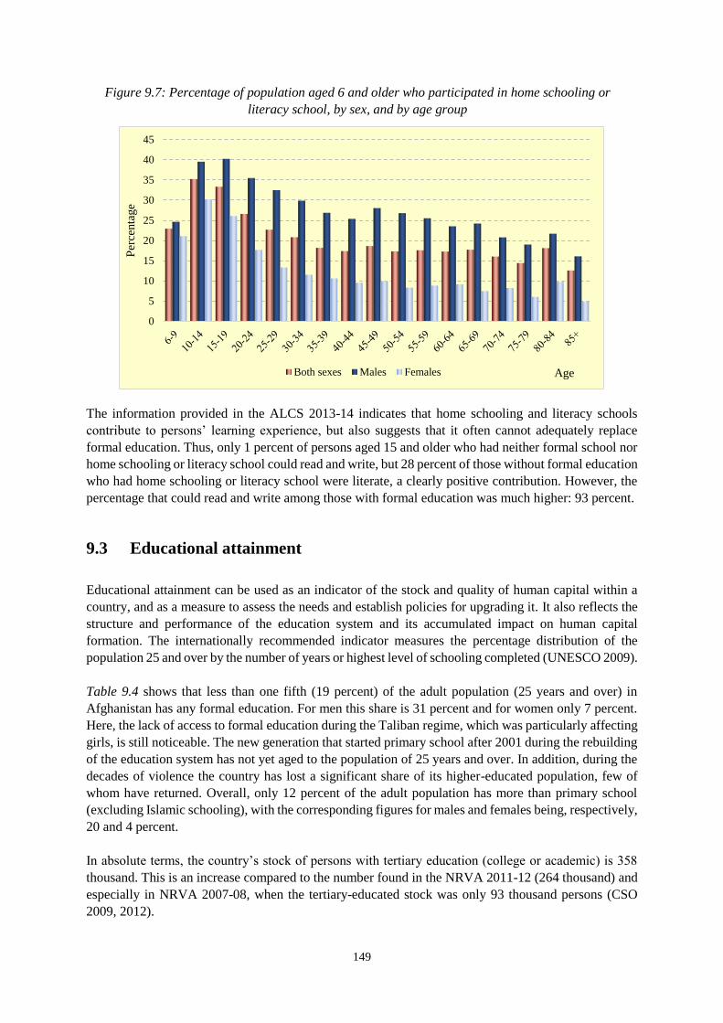
149
Figure 9.7: Percentage of population aged 6 and older who participated in home schooling or
literacy school, by sex, and by age group
The information provided in the ALCS 2013-14 indicates that home schooling and literacy schools
contribute to persons’ learning experience, but also suggests that it often cannot adequately replace
formal education. Thus, only 1 percent of persons aged 15 and older who had neither formal school nor
home schooling or literacy school could read and write, but 28 percent of those without formal education
who had home schooling or literacy school were literate, a clearly positive contribution. However, the
percentage that could read and write among those with formal education was much higher: 93 percent.
9.3 Educational attainment
Educational attainment can be used as an indicator of the stock and quality of human capital within a
country, and as a measure to assess the needs and establish policies for upgrading it. It also reflects the
structure and performance of the education system and its accumulated impact on human capital
formation. The internationally recommended indicator measures the percentage distribution of the
population 25 and over by the number of years or highest level of schooling completed (UNESCO 2009).
Table 9.4 shows that less than one fifth (19 percent) of the adult population (25 years and over) in
Afghanistan has any formal education. For men this share is 31 percent and for women only 7 percent.
Here, the lack of access to formal education during the Taliban regime, which was particularly affecting
girls, is still noticeable. The new generation that started primary school after 2001 during the rebuilding
of the education system has not yet aged to the population of 25 years and over. In addition, during the
decades of violence the country has lost a significant share of its higher-educated population, few of
whom have returned. Overall, only 12 percent of the adult population has more than primary school
(excluding Islamic schooling), with the corresponding figures for males and females being, respectively,
20 and 4 percent.
In absolute terms, the country’s stock of persons with tertiary education (college or academic) is 358
thousand. This is an increase compared to the number found in the NRVA 2011-12 (264 thousand) and
especially in NRVA 2007-08, when the tertiary-educated stock was only 93 thousand persons (CSO
2009, 2012).
0
5
10
15
20
25
30
35
40
45P
erce
nta
ge
AgeBoth sexes Males Females
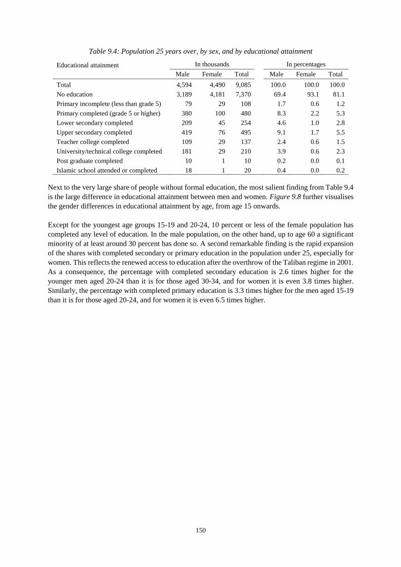
150
Table 9.4: Population 25 years over, by sex, and by educational attainment
Educational attainment In thousands In percentages
Male Female Total Male Female Total
Total 4,594 4,490 9,085 100.0 100.0 100.0
No education 3,189 4,181 7,370 69.4 93.1 81.1
Primary incomplete (less than grade 5) 79 29 108 1.7 0.6 1.2
Primary completed (grade 5 or higher) 380 100 480 8.3 2.2 5.3
Lower secondary completed 209 45 254 4.6 1.0 2.8
Upper secondary completed 419 76 495 9.1 1.7 5.5
Teacher college completed 109 29 137 2.4 0.6 1.5
University/technical college completed 181 29 210 3.9 0.6 2.3
Post graduate completed 10 1 10 0.2 0.0 0.1
Islamic school attended or completed 18 1 20 0.4 0.0 0.2
Next to the very large share of people without formal education, the most salient finding from Table 9.4
is the large difference in educational attainment between men and women. Figure 9.8 further visualises
the gender differences in educational attainment by age, from age 15 onwards.
Except for the youngest age groups 15-19 and 20-24, 10 percent or less of the female population has
completed any level of education. In the male population, on the other hand, up to age 60 a significant
minority of at least around 30 percent has done so. A second remarkable finding is the rapid expansion
of the shares with completed secondary or primary education in the population under 25, especially for
women. This reflects the renewed access to education after the overthrow of the Taliban regime in 2001.
As a consequence, the percentage with completed secondary education is 2.6 times higher for the
younger men aged 20-24 than it is for those aged 30-34, and for women it is even 3.8 times higher.
Similarly, the percentage with completed primary education is 3.3 times higher for the men aged 15-19
than it is for those aged 20-24, and for women it is even 6.5 times higher.
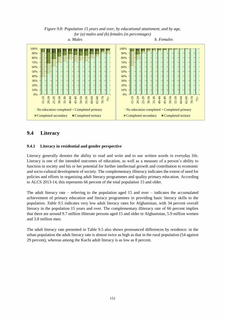
151
Figure 9.8: Population 15 years and over, by educational attainment, and by age,
for (a) males and (b) females (in percentages)
a. Males b. Females
9.4 Literacy
9.4.1 Literacy in residential and gender perspective
Literacy generally denotes the ability to read and write and to use written words in everyday life.
Literacy is one of the intended outcomes of education, as well as a measure of a person’s ability to
function in society and his or her potential for further intellectual growth and contribution to economic
and socio-cultural development of society. The complementary illiteracy indicates the extent of need for
policies and efforts in organizing adult literacy programmes and quality primary education. According
to ALCS 2013-14, this represents 66 percent of the total population 15 and older.
The adult literacy rate – referring to the population aged 15 and over – indicates the accumulated
achievement of primary education and literacy programmes in providing basic literacy skills to the
population. Table 9.5 indicates very low adult literacy rates for Afghanistan, with 34 percent overall
literacy in the population 15 years and over. The complementary illiteracy rate of 66 percent implies
that there are around 9.7 million illiterate persons aged 15 and older in Afghanistan, 5.9 million women
and 3.8 million men.
The adult literacy rate presented in Table 9.5 also shows pronounced differences by residence: in the
urban population the adult literacy rate is almost twice as high as that in the rural population (54 against
29 percent), whereas among the Kuchi adult literacy is as low as 8 percent.
0%
10%
20%
30%
40%
50%
60%
70%
80%
90%
100%
15-1
9
20-2
4
25-2
9
30-3
4
35-3
9
40-4
4
45-4
9
50-5
4
55-5
9
60-6
4
65-6
9
70-7
4
75+
No education completed Completed primary
Completed secondary Completed tertiary
0%
10%
20%
30%
40%
50%
60%
70%
80%
90%
100%
15-1
9
20-2
4
25-2
9
30-3
4
35-3
9
40-4
4
45-4
9
50-5
4
55-5
9
60-6
4
65-6
9
70-7
4
75+
No education completed Completed primary
Completed secondary Completed tertiary
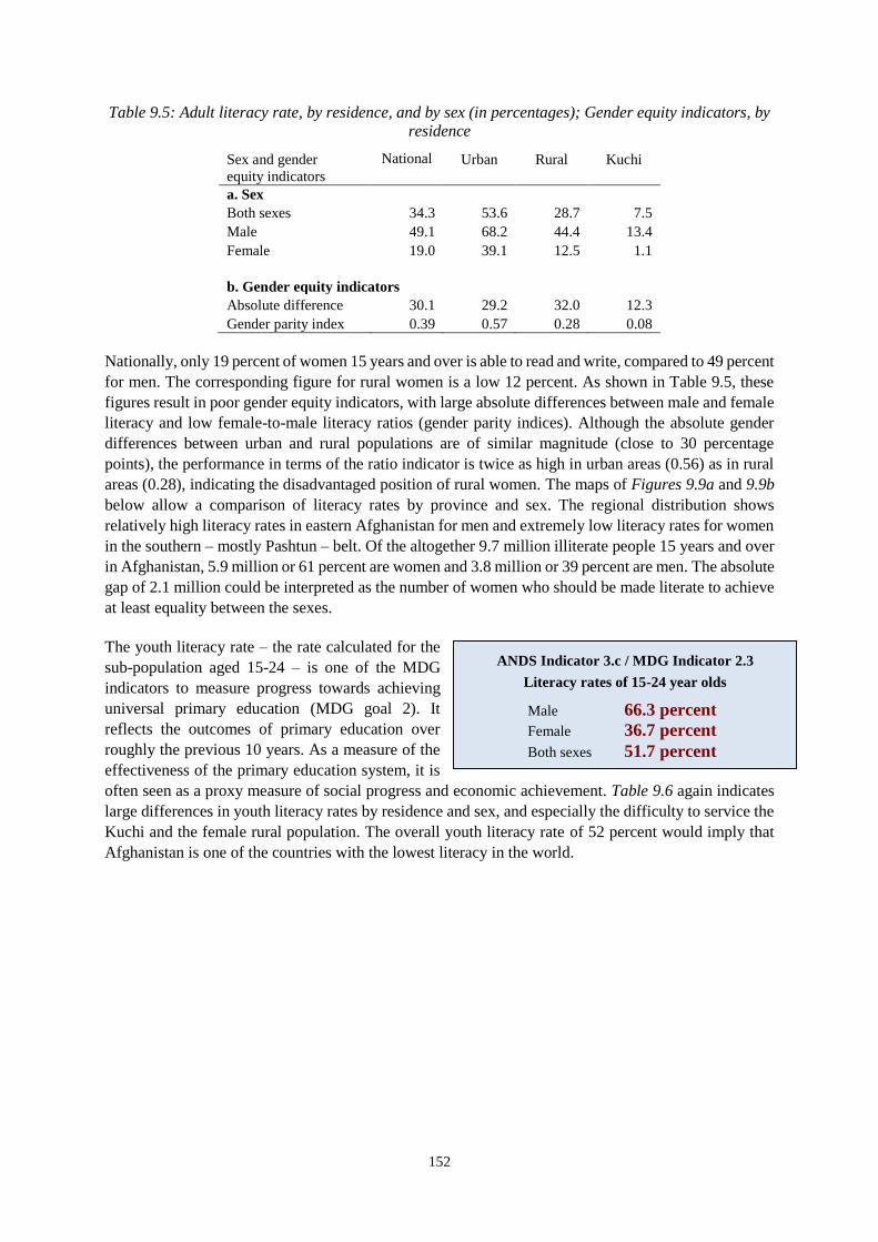
152
Table 9.5: Adult literacy rate, by residence, and by sex (in percentages); Gender equity indicators, by
residence
Sex and gender National Urban Rural Kuchi
equity indicators
a. Sex
Both sexes 34.3 53.6 28.7 7.5
Male 49.1 68.2 44.4 13.4
Female 19.0 39.1 12.5 1.1
b. Gender equity indicators
Absolute difference 30.1 29.2 32.0 12.3
Gender parity index 0.39 0.57 0.28 0.08
Nationally, only 19 percent of women 15 years and over is able to read and write, compared to 49 percent
for men. The corresponding figure for rural women is a low 12 percent. As shown in Table 9.5, these
figures result in poor gender equity indicators, with large absolute differences between male and female
literacy and low female-to-male literacy ratios (gender parity indices). Although the absolute gender
differences between urban and rural populations are of similar magnitude (close to 30 percentage
points), the performance in terms of the ratio indicator is twice as high in urban areas (0.56) as in rural
areas (0.28), indicating the disadvantaged position of rural women. The maps of Figures 9.9a and 9.9b
below allow a comparison of literacy rates by province and sex. The regional distribution shows
relatively high literacy rates in eastern Afghanistan for men and extremely low literacy rates for women
in the southern – mostly Pashtun – belt. Of the altogether 9.7 million illiterate people 15 years and over
in Afghanistan, 5.9 million or 61 percent are women and 3.8 million or 39 percent are men. The absolute
gap of 2.1 million could be interpreted as the number of women who should be made literate to achieve
at least equality between the sexes.
The youth literacy rate – the rate calculated for the
sub-population aged 15-24 – is one of the MDG
indicators to measure progress towards achieving
universal primary education (MDG goal 2). It
reflects the outcomes of primary education over
roughly the previous 10 years. As a measure of the
effectiveness of the primary education system, it is
often seen as a proxy measure of social progress and economic achievement. Table 9.6 again indicates
large differences in youth literacy rates by residence and sex, and especially the difficulty to service the
Kuchi and the female rural population. The overall youth literacy rate of 52 percent would imply that
Afghanistan is one of the countries with the lowest literacy in the world.
ANDS Indicator 3.c / MDG Indicator 2.3
Literacy rates of 15-24 year olds
Male 66.3 percent
Female 36.7 percent
Both sexes 51.7 percent
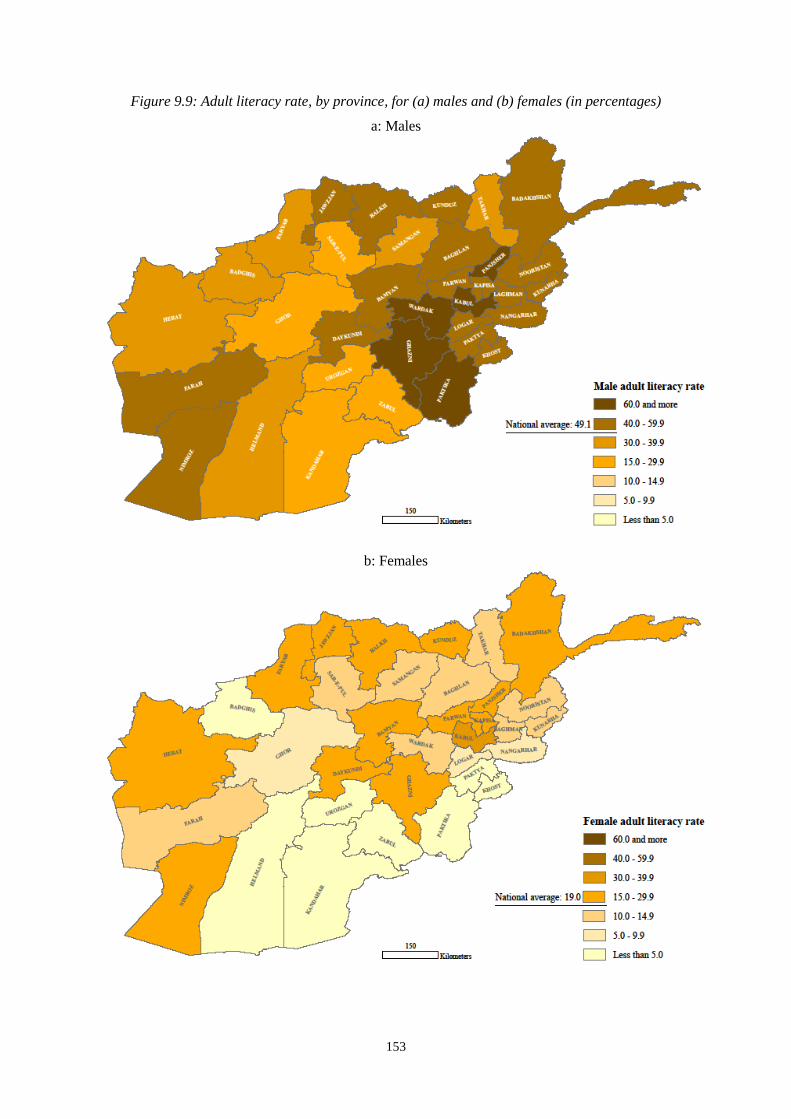
153
Figure 9.9: Adult literacy rate, by province, for (a) males and (b) females (in percentages)
a: Males
b: Females
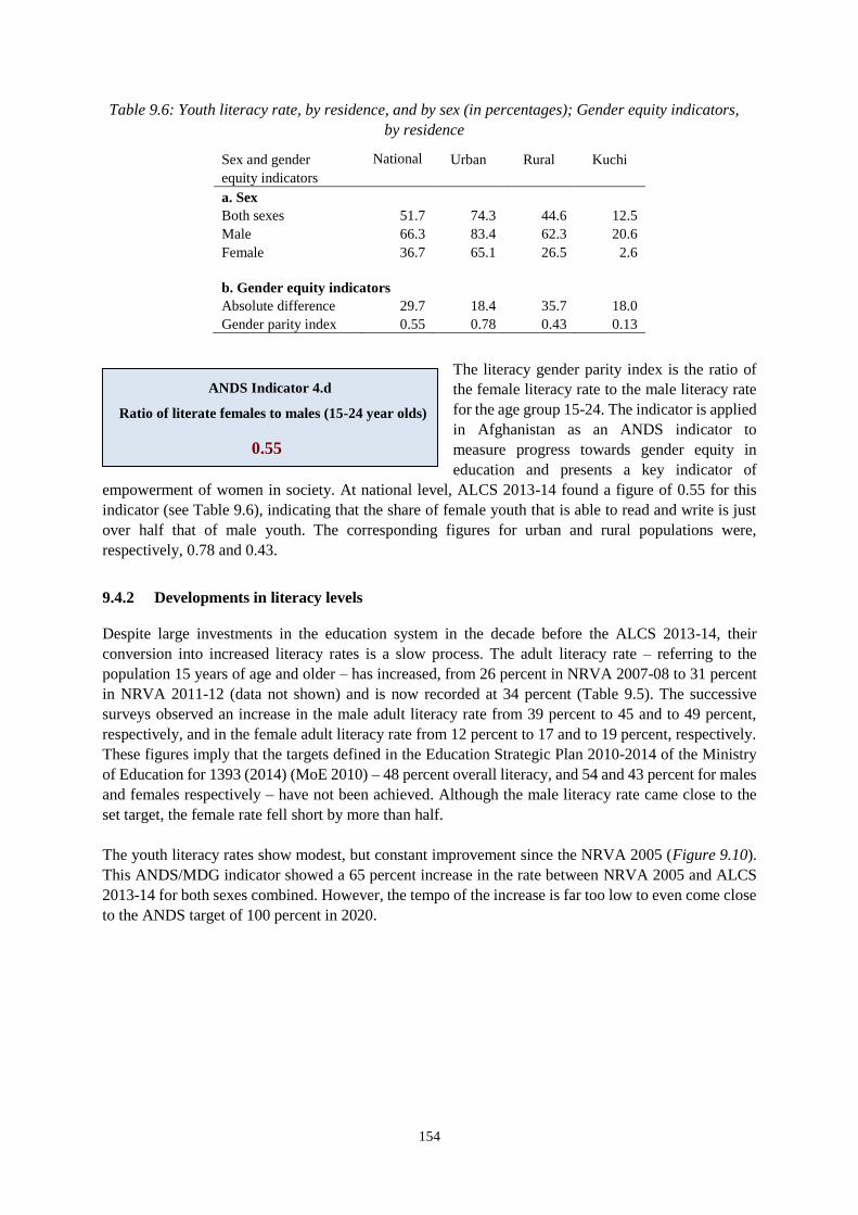
154
Table 9.6: Youth literacy rate, by residence, and by sex (in percentages); Gender equity indicators,
by residence
Sex and gender National Urban Rural Kuchi
equity indicators
a. Sex
Both sexes 51.7 74.3 44.6 12.5
Male 66.3 83.4 62.3 20.6
Female 36.7 65.1 26.5 2.6
b. Gender equity indicators
Absolute difference 29.7 18.4 35.7 18.0
Gender parity index 0.55 0.78 0.43 0.13
The literacy gender parity index is the ratio of
the female literacy rate to the male literacy rate
for the age group 15-24. The indicator is applied
in Afghanistan as an ANDS indicator to
measure progress towards gender equity in
education and presents a key indicator of
empowerment of women in society. At national level, ALCS 2013-14 found a figure of 0.55 for this
indicator (see Table 9.6), indicating that the share of female youth that is able to read and write is just
over half that of male youth. The corresponding figures for urban and rural populations were,
respectively, 0.78 and 0.43.
9.4.2 Developments in literacy levels Despite large investments in the education system in the decade before the ALCS 2013-14, their
conversion into increased literacy rates is a slow process. The adult literacy rate – referring to the
population 15 years of age and older – has increased, from 26 percent in NRVA 2007-08 to 31 percent
in NRVA 2011-12 (data not shown) and is now recorded at 34 percent (Table 9.5). The successive
surveys observed an increase in the male adult literacy rate from 39 percent to 45 and to 49 percent,
respectively, and in the female adult literacy rate from 12 percent to 17 and to 19 percent, respectively.
These figures imply that the targets defined in the Education Strategic Plan 2010-2014 of the Ministry
of Education for 1393 (2014) (MoE 2010) – 48 percent overall literacy, and 54 and 43 percent for males
and females respectively – have not been achieved. Although the male literacy rate came close to the
set target, the female rate fell short by more than half.
The youth literacy rates show modest, but constant improvement since the NRVA 2005 (Figure 9.10).
This ANDS/MDG indicator showed a 65 percent increase in the rate between NRVA 2005 and ALCS
2013-14 for both sexes combined. However, the tempo of the increase is far too low to even come close
to the ANDS target of 100 percent in 2020.
ANDS Indicator 4.d
Ratio of literate females to males (15-24 year olds)
0.55
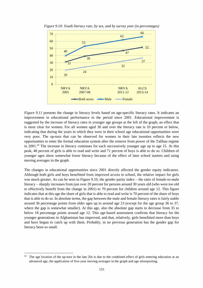
155
Figure 9.10: Youth literacy rate, by sex, and by survey year (in percentages)
Figure 9.11 presents the change in literacy levels based on age-specific literacy rates. It indicates an
improvement in educational performance in the period since 2001. Educational improvement is
suggested by the increase of literacy rates in younger age groups at the left of the graph, an effect that
is most clear for women. For all women aged 30 and over the literacy rate is 10 percent or below,
indicating that during the years in which they were in their school age educational opportunities were
very poor. The up-turn that can be observed for women in their late twenties reflects the new
opportunities to enter the formal education system after the remove from power of the Taliban regime
in 2001.50 The increase in literacy continues for each successively younger age up to age 15. At this
peak, 48 percent of girls is able to read and write and 71 percent of boys is able to do so. Children of
younger ages show somewhat lower literacy because of the effect of later school starters and using
moving averages in the graph.
The changes in educational opportunities since 2001 directly affected the gender equity indicators.
Although both girls and boys benefitted from improved access to school, the relative impact for girls
was much greater. As can be seen in Figure 9.10, the gender parity index – the ratio of female-to-male
literacy – sharply increases from just over 20 percent for persons around 30 years old (who were too old
to effectively benefit from the change in 2001) to 70 percent for children around age 12. This figure
indicates that at this age the share of girls that is able to read and write is 70 percent of the share of boys
that is able to do so. In absolute terms, the gap between the male and female literacy rates is fairly stable
around 36 percentage points from older ages up to around age 23 (except for the age group 36 to 37,
where the gap is somewhat smaller). At this age, also the absolute gap starts to decrease from 35 to
below 18 percentage points around age 12. This age-based assessment confirms that literacy for the
younger generations in Afghanistan has improved, and that, relatively, girls benefitted more than boys
and have begun to catch up with them. Probably, in no previous generation has the gender gap for
literacy been so small.
50 The age location of the up-turn in the late 20s is due to the combined effect of girls entering education at an
advanced age, the application of five-year moving averages in the graph and age misreporting.
31
39
47
52
40
53
6266
2024
32
37
0
10
20
30
40
50
60
70
NRVA
2005
NRVA
2007-08
NRVA
2011-12
ALCS
2013-14
Both sexes Male Female
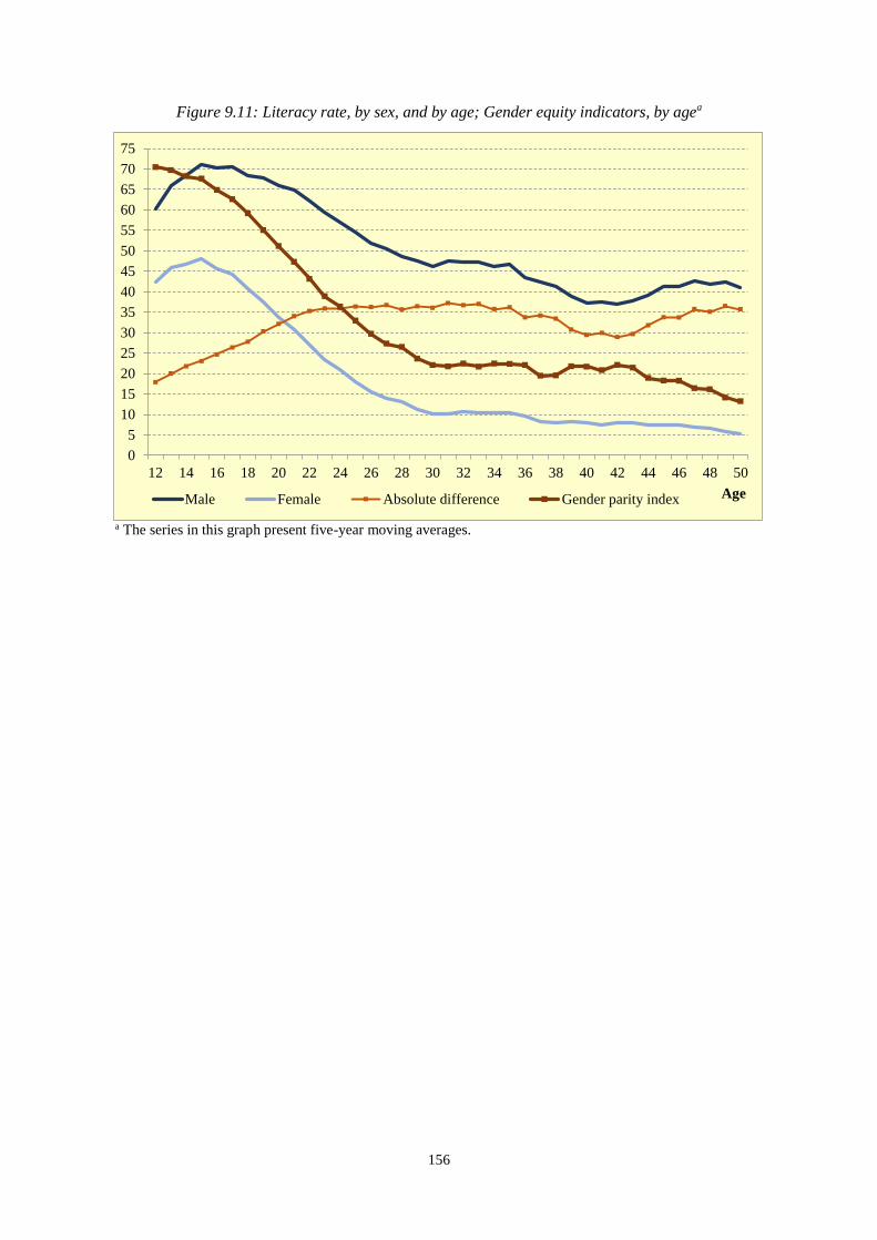
156
Figure 9.11: Literacy rate, by sex, and by age; Gender equity indicators, by agea
a The series in this graph present five-year moving averages.
0
5
10
15
20
25
30
35
40
45
50
55
60
65
70
75
12 14 16 18 20 22 24 26 28 30 32 34 36 38 40 42 44 46 48 50
AgeMale Female Absolute difference Gender parity index
157
10 HEALTH
Summary. The ALCS 2013-14 confirms the image of a recovering health system in Afghanistan since
the beginning of the century, even to the extent that in some areas it achieves performance levels not
previously recorded. Although Afghanistan’s health indicators are poor in an international perspective
and cultural barriers and financial and security constraints impede progress for many components of
health, significant improvement is evident from successive surveys in the post-Taliban period.
The present survey shows that improvement of the health care system remains one of the highest
priorities for the Afghan people. Whereas prior to NRVA 2011-12 much progress was made in access
to health care in terms of time required to reach different types of health facilities, this trend seems to
have continued only modestly for public and private clinics. Travel costs and other health-related
expenditures remain major obstacles for many people to obtain the care they need. ALCS 2013-14 shows
that medical needs of one in every five women who were ill or injured, could not be met, mostly because
of poverty and geographical remoteness. Costs and transportation to access health services are also
associated with cultural and social barriers at the demand side, which may limit the observed
improvement in the health sector. Cultural responsiveness of the health system – for instance in terms
of provision of female health care providers – remains an obstacle for the effective use of health care,
especially by women. However, the availability of female service providers has significantly improved
in the rural areas, especially through private clinics and public health posts.
The most consistent and impressive improvements are observed for maternal health indicators.
Afghanistan has achieved its MDG target for ante-natal care coverage ahead of schedule, and in 2011-
12 already surpassed its MDG 2020 target of 50 percent coverage. ALCS 2013-14 indicated that 63
percent of pregnant women made at least one visit to a skilled ANC provider. However, the
recommended four visits are realised by only 23 percent of pregnant women. Also with regard to the
percentage of institutional deliveries (43 percent) and skilled birth attendance (45 percent) ALCS 2013-
14 indicated a consistent improvement in recent years. The general trend in skilled birth attendance
suggests that the MDG 2015 target of 50 percent is within reach.
From the ALCS data, it is evident that breastfeeding in Afghanistan is almost universal (93 percent) and
typically continues for a long duration; practices that are very beneficial for both mother and child.
However, substantial health gains can be achieved by starting breastfeeding within the first hour after
birth (only one third of mothers did so), starting with supplementary liquids and solid food only after
six months (more than half of the babies received other liquids before 6 months) and introducing
supplementary food soon after six months (at age 9 months still 23 percent only received breastmilk and
at 12 months still 12.7 percent).
One of the main concerns with respect to Afghanistan’s health system performance remains the very
unequal health care provision between urban and rural populations and between provinces. Invariably,
for the majority of Afghanistan’s rural population, service delivery and health outcome indicators are
significantly lower than for urban dwellers. And the situation is generally even far worse for the nomadic
Kuchi population.
158
10.1 Introduction
Decades of conflict had a devastating effect on the health system of Afghanistan. At the time of the
overthrow of the Taliban regime in 2001, the country recorded some of the world’s worst health
statistics, including estimated infant mortality rates of 165 per thousand live births, under-five mortality
of more than 250 per thousand live births and maternal mortality of 1,600 per 100 thousand live births
(MoPH 2005). More than one-third of health facilities were severely damaged and the rest failed to meet
WHO standards (Ministry of Health 2002). In addition, many health professionals had fled the country
and the remaining lacked good clinical training and were severely underrepresented in rural areas.
Since then, the Ministry of Public Health (MoPH) has coordinated the efforts to rebuild the health
system. A strategy to deliver a Basic Package of Health Services (BPHS) was developed in 2002 and
updated in 2005 and 2010, with the aim to provide a core service delivery package in all primary health
care facilities, addressing the principal health problems of the population, especially the most vulnerable
groups – women and children – and the rural population (Ministry of Health 2003, MoPH 2005, MoPH
2010). Previous NRVAs and other health surveys showed that many of Afghanistan’s main health
indicators are rapidly improving, although they remain low by international standards. Other health-
related indicators show mixed results: the food security situation in the country remains fragile (see
chapter 9), but significant advance has been achieved with respect to access to safe drinking water (see
chapter 10) and to a lesser extent access to improved sanitation (chapter 12).
ALCS 2013-14, as its preceding NRVAs, provides information about specific health indicators. Previous
survey rounds covered maternal and child health, access to health facilities, health care expenditure and
use of health care providers. In line with the principle of rotating modules in successive surveys, the
present ALCS focused on maternal health (section 10.3), breastfeeding (10.4) and access to health
facilities (10.2). The next ALCS will again collect data on health care expenditure and disability, next
to some basic information about maternal and child health, family planning and health care access. In
addition, the 2015 DHS is expected to provide detailed health information in 2016.
10.2 Access to health services and care-seeking behaviour
10.2.1 Travel time, travel costs and staff availability
Access to health services is a multi-dimensional concept. It not only relates to the physical distance to
health facilities or the travel time involved, but also involves the costs of travel and services, as well as
opportunity costs, cultural responsiveness to clients’ needs, mobility of women, and even the ‘value’
attached to the health and survival of specific household members, such as children and women (the
demand-side barriers to access health services). As the previous NRVAs, the ALCS 2013-14 Shura
questionnaire provides information about travel time and travel costs required to reach health facilities,
as well as information about gender-specific availability of health care staff. These figures should be
treated with care because of high non-response rates, as well as the possible respondents’ inability to
identify the correct type of health care provider and position of health care staff.
Distance and costs to reach a health facility can be primary reasons for low use of health care, especially
in remote areas. Thus, the 2006 Afghanistan Health Survey (AHS) suggested that – after the absence of
urgency for seeking health care – the most important reason for not seeking care was distance (27
percent) and the fourth-most important reason mentioned was transport costs (11 percent). In line with
159
this, male and female Shuras responses to the successive rounds of NRVA invariantly mentioned
improved access to health facilities among the top priorities.
Table 10.1 panel a gives the percentage of population that is able to reach different types of health
facilities within a specified time by any means of transport. It is evident that the urban population has
almost universal access to health care of any type within two hours. For rural populations – including
Kuchi – access time is less favourable: only around three-quarters can reach a referral hospital or a
private clinic within two hours, but close to nine in ten has access to a health post or a public clinic
within this time. Compared to NRVA 2011-12, the situation for rural populations seems to have
improved with regard to access to public and private clinics (both around 83 percent then), but not so
with regard to health posts and district or provincial hospitals. However, a major improvement has
occurred since 2006, when only 60 percent of the total population – including urban residents – had
access to any health facility (MoPH 2007).
In terms of travel costs to reach different health providers, rural Afghans are much more disadvantaged
compared with urban dwellers. They typically pay around nine times as much for a one-way trip to a
health facility, on average around 350 Afs per person to a referral hospital or a private clinic, around
185 Afs to a public clinic or a private pharmacy and somewhat less to the nearest health post (Table
10.1, panel b). The median travel costs – the costs level below and above which half of rural households
has to pay – are usually much less than the average costs. This indicates that there is a large variation in
travel costs for rural dwellers, some of whom have to pay large sums to reach health care.
Among the modalities considered in the survey, the time to reach a health care provider and the costs
involved are by far the most important reasons for women not to use health care services. For 36 percent
of women who were in need of health care, the distance to the provider was the main reason not to seek
care and for 52 percent the costs were the main reason (see also section 10.2.2). Since women usually
have to be accompanied by a male family member, the cost for their travel to a health centre is often
even more than that for a male patient, making access to health care for women in many cases
prohibitively expensive.
In the gender-sensitive context of Afghanistan, another impeding factor to seek health care is the absence
of same-sex health care staff. Results from the ALCS 2013-14 show that within the public health system
only higher up in the referral system and in urban areas any presence of female staff reaches levels close
to full coverage (Table 10.2). For example, in rural areas only 43 percent of the population can consult
a female doctor in a public clinic and for 28 percent no female midwife is available there.
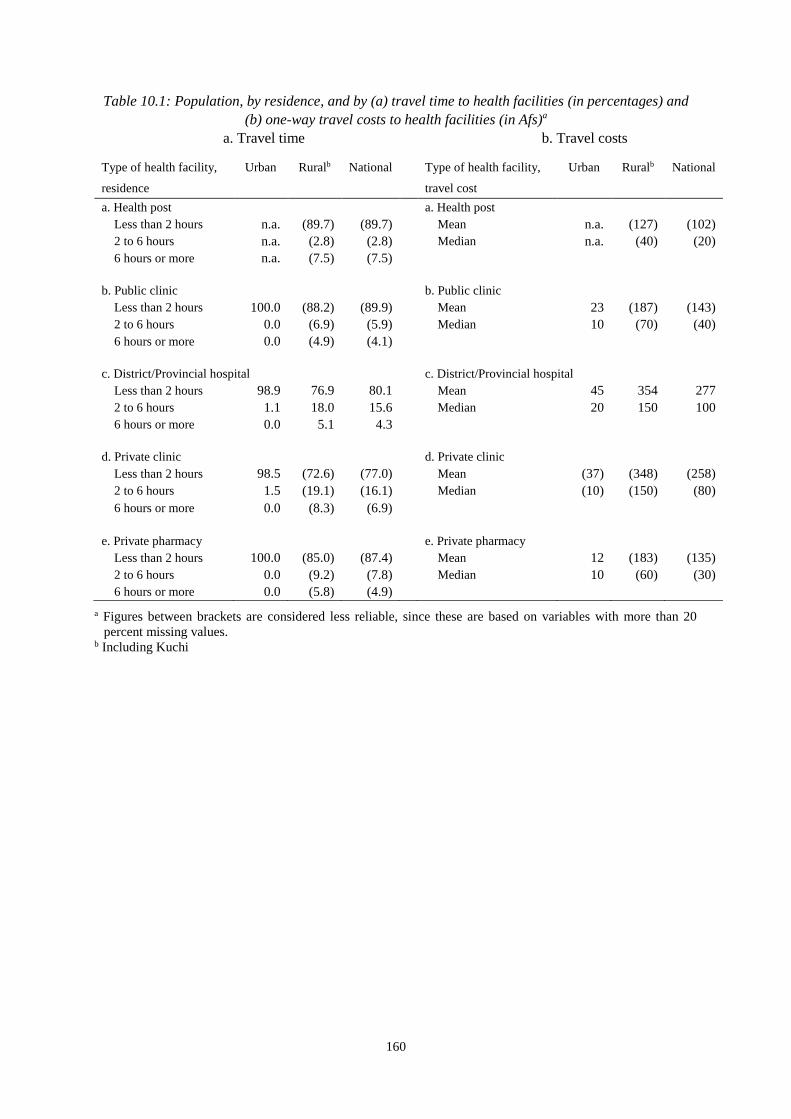
160
Table 10.1: Population, by residence, and by (a) travel time to health facilities (in percentages) and
(b) one-way travel costs to health facilities (in Afs)a
a. Travel time b. Travel costs
Type of health facility, Urban Ruralb National Type of health facility, Urban Ruralb National
residence travel cost
a. Health post a. Health post
Less than 2 hours n.a. (89.7) (89.7) Mean n.a. (127) (102)
2 to 6 hours n.a. (2.8) (2.8) Median n.a. (40) (20)
6 hours or more n.a. (7.5) (7.5)
b. Public clinic b. Public clinic
Less than 2 hours 100.0 (88.2) (89.9) Mean 23 (187) (143)
2 to 6 hours 0.0 (6.9) (5.9) Median 10 (70) (40)
6 hours or more 0.0 (4.9) (4.1)
c. District/Provincial hospital c. District/Provincial hospital
Less than 2 hours 98.9 76.9 80.1 Mean 45 354 277
2 to 6 hours 1.1 18.0 15.6 Median 20 150 100
6 hours or more 0.0 5.1 4.3
d. Private clinic d. Private clinic
Less than 2 hours 98.5 (72.6) (77.0) Mean (37) (348) (258)
2 to 6 hours 1.5 (19.1) (16.1) Median (10) (150) (80)
6 hours or more 0.0 (8.3) (6.9)
e. Private pharmacy e. Private pharmacy
Less than 2 hours 100.0 (85.0) (87.4) Mean 12 (183) (135)
2 to 6 hours 0.0 (9.2) (7.8) Median 10 (60) (30)
6 hours or more 0.0 (5.8) (4.9)
a Figures between brackets are considered less reliable, since these are based on variables with more than 20
percent missing values. b Including Kuchi
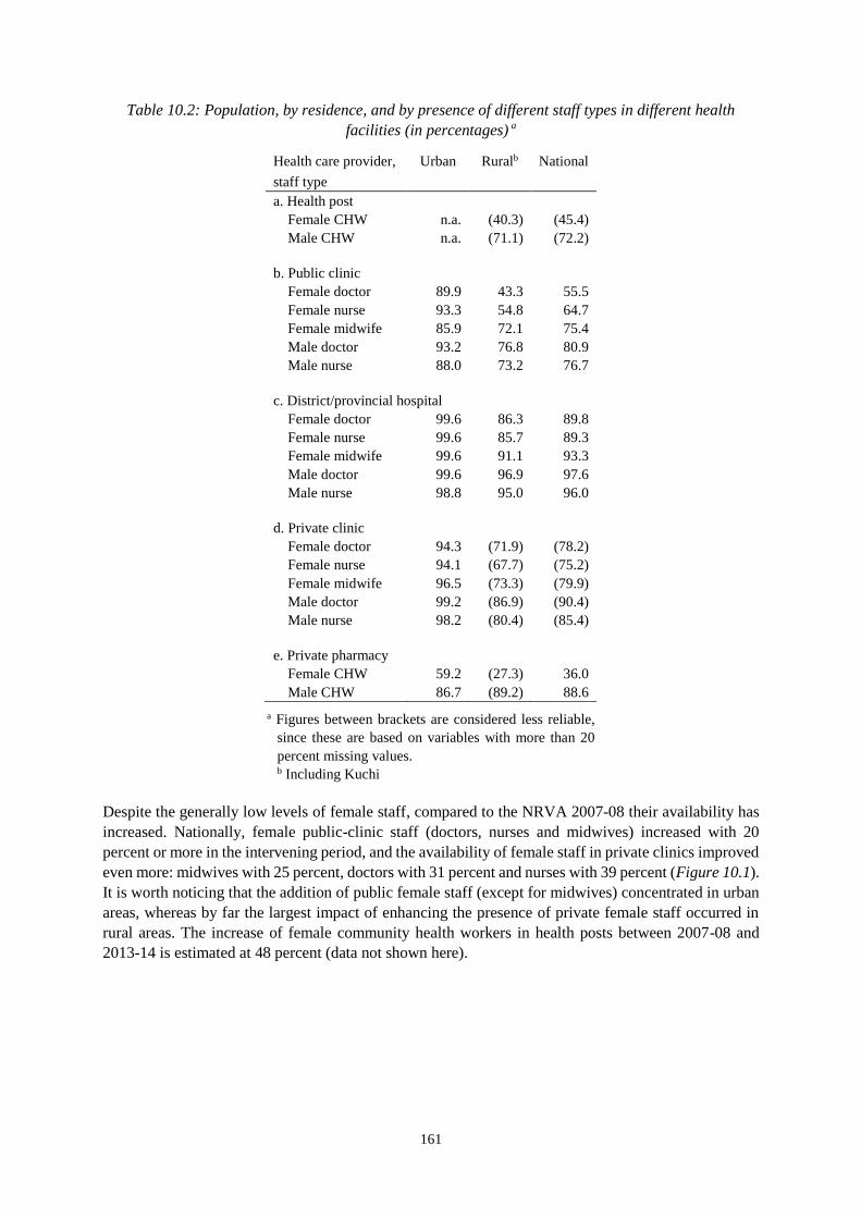
161
Table 10.2: Population, by residence, and by presence of different staff types in different health
facilities (in percentages) a
Health care provider, Urban Ruralb National
staff type
a. Health post
Female CHW n.a. (40.3) (45.4)
Male CHW n.a. (71.1) (72.2)
b. Public clinic
Female doctor 89.9 43.3 55.5
Female nurse 93.3 54.8 64.7
Female midwife 85.9 72.1 75.4
Male doctor 93.2 76.8 80.9
Male nurse 88.0 73.2 76.7
c. District/provincial hospital
Female doctor 99.6 86.3 89.8
Female nurse 99.6 85.7 89.3
Female midwife 99.6 91.1 93.3
Male doctor 99.6 96.9 97.6
Male nurse 98.8 95.0 96.0
d. Private clinic
Female doctor 94.3 (71.9) (78.2)
Female nurse 94.1 (67.7) (75.2)
Female midwife 96.5 (73.3) (79.9)
Male doctor 99.2 (86.9) (90.4)
Male nurse 98.2 (80.4) (85.4)
e. Private pharmacy
Female CHW 59.2 (27.3) 36.0
Male CHW 86.7 (89.2) 88.6
a Figures between brackets are considered less reliable,
since these are based on variables with more than 20
percent missing values. b Including Kuchi
Despite the generally low levels of female staff, compared to the NRVA 2007-08 their availability has
increased. Nationally, female public-clinic staff (doctors, nurses and midwives) increased with 20
percent or more in the intervening period, and the availability of female staff in private clinics improved
even more: midwives with 25 percent, doctors with 31 percent and nurses with 39 percent (Figure 10.1).
It is worth noticing that the addition of public female staff (except for midwives) concentrated in urban
areas, whereas by far the largest impact of enhancing the presence of private female staff occurred in
rural areas. The increase of female community health workers in health posts between 2007-08 and
2013-14 is estimated at 48 percent (data not shown here).
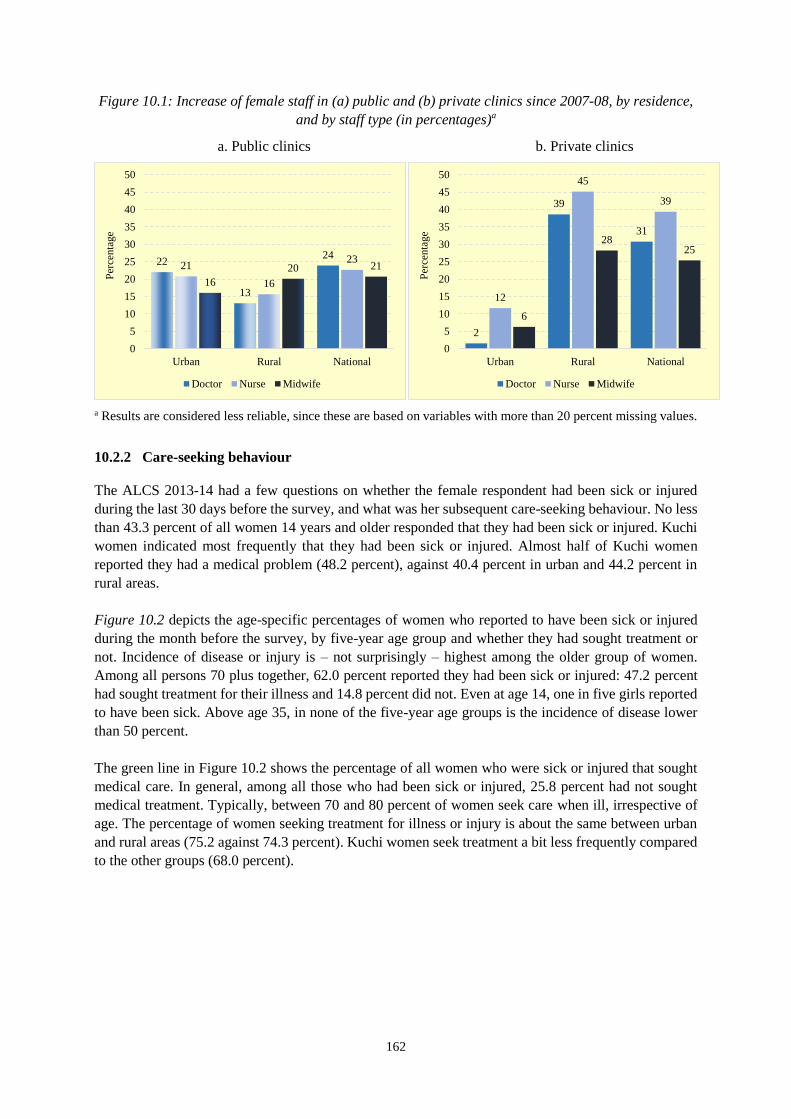
162
Figure 10.1: Increase of female staff in (a) public and (b) private clinics since 2007-08, by residence,
and by staff type (in percentages)a
a. Public clinics b. Private clinics
a Results are considered less reliable, since these are based on variables with more than 20 percent missing values.
10.2.2 Care-seeking behaviour
The ALCS 2013-14 had a few questions on whether the female respondent had been sick or injured
during the last 30 days before the survey, and what was her subsequent care-seeking behaviour. No less
than 43.3 percent of all women 14 years and older responded that they had been sick or injured. Kuchi
women indicated most frequently that they had been sick or injured. Almost half of Kuchi women
reported they had a medical problem (48.2 percent), against 40.4 percent in urban and 44.2 percent in
rural areas.
Figure 10.2 depicts the age-specific percentages of women who reported to have been sick or injured
during the month before the survey, by five-year age group and whether they had sought treatment or
not. Incidence of disease or injury is – not surprisingly – highest among the older group of women.
Among all persons 70 plus together, 62.0 percent reported they had been sick or injured: 47.2 percent
had sought treatment for their illness and 14.8 percent did not. Even at age 14, one in five girls reported
to have been sick. Above age 35, in none of the five-year age groups is the incidence of disease lower
than 50 percent.
The green line in Figure 10.2 shows the percentage of all women who were sick or injured that sought
medical care. In general, among all those who had been sick or injured, 25.8 percent had not sought
medical treatment. Typically, between 70 and 80 percent of women seek care when ill, irrespective of
age. The percentage of women seeking treatment for illness or injury is about the same between urban
and rural areas (75.2 against 74.3 percent). Kuchi women seek treatment a bit less frequently compared
to the other groups (68.0 percent).
22
13
2421
16
23
16
20 21
0
5
10
15
20
25
30
35
40
45
50
Urban Rural National
Per
centa
ge
Doctor Nurse Midwife
2
39
31
12
45
39
6
2825
0
5
10
15
20
25
30
35
40
45
50
Urban Rural National
Per
centa
ge
Doctor Nurse Midwife
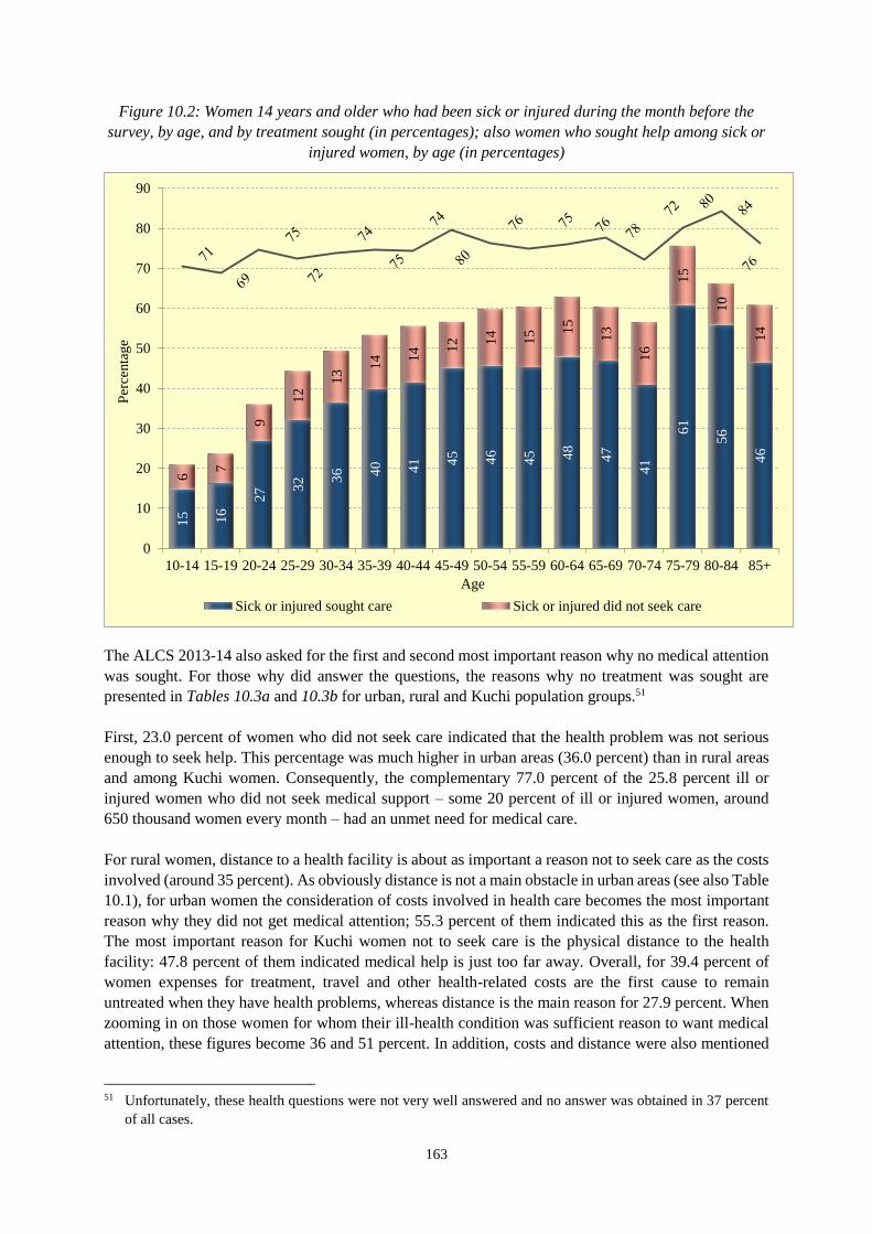
163
Figure 10.2: Women 14 years and older who had been sick or injured during the month before the
survey, by age, and by treatment sought (in percentages); also women who sought help among sick or
injured women, by age (in percentages)
The ALCS 2013-14 also asked for the first and second most important reason why no medical attention
was sought. For those why did answer the questions, the reasons why no treatment was sought are
presented in Tables 10.3a and 10.3b for urban, rural and Kuchi population groups.51
First, 23.0 percent of women who did not seek care indicated that the health problem was not serious
enough to seek help. This percentage was much higher in urban areas (36.0 percent) than in rural areas
and among Kuchi women. Consequently, the complementary 77.0 percent of the 25.8 percent ill or
injured women who did not seek medical support – some 20 percent of ill or injured women, around
650 thousand women every month – had an unmet need for medical care.
For rural women, distance to a health facility is about as important a reason not to seek care as the costs
involved (around 35 percent). As obviously distance is not a main obstacle in urban areas (see also Table
10.1), for urban women the consideration of costs involved in health care becomes the most important
reason why they did not get medical attention; 55.3 percent of them indicated this as the first reason.
The most important reason for Kuchi women not to seek care is the physical distance to the health
facility: 47.8 percent of them indicated medical help is just too far away. Overall, for 39.4 percent of
women expenses for treatment, travel and other health-related costs are the first cause to remain
untreated when they have health problems, whereas distance is the main reason for 27.9 percent. When
zooming in on those women for whom their ill-health condition was sufficient reason to want medical
attention, these figures become 36 and 51 percent. In addition, costs and distance were also mentioned
51 Unfortunately, these health questions were not very well answered and no answer was obtained in 37 percent
of all cases.
15 16
27 3
2 36 40 41 4
5 46
45 48
47
41
61
56
46
6
7
9
12
13
14 1
4 12 1
4
15 1
5
13
16
15
10
14
0
10
20
30
40
50
60
70
80
90
10-14 15-19 20-24 25-29 30-34 35-39 40-44 45-49 50-54 55-59 60-64 65-69 70-74 75-79 80-84 85+
Per
centa
ge
Age
Sick or injured sought care Sick or injured did not seek care
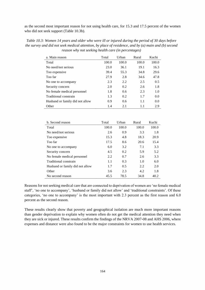
164
as the second most important reason for not using health care, for 15.3 and 17.5 percent of the women
who did not seek support (Table 10.3b).
Table 10.3: Women 14 years and older who were ill or injured during the period of 30 days before
the survey and did not seek medical attention, by place of residence, and by (a) main and (b) second
reason why not seeking health care (in percentages)
a. Main reason Total Urban Rural Kuchi
Total 100.0 100.0 100.0 100.0
No need/not serious 23.0 36.1 19.1 16.3
Too expensive 39.4 55.3 34.8 29.6
Too far 27.9 2.8 34.6 47.8
No one to accompany 2.3 2.2 2.5 0.5
Security concern 2.0 0.2 2.6 1.8
No female medical personnel 1.8 0.6 2.3 1.0
Traditional constrain 1.3 0.2 1.7 0.0
Husband or family did not allow 0.9 0.6 1.1 0.0
Other 1.4 2.1 1.1 2.9
b. Second reason Total Urban Rural Kuchi
Total 100.0 100.0 100.0 100.0
No need/not serious 2.6 0.9 3.3 1.8
Too expensive 15.3 4.8 18.3 20.9
Too far 17.5 8.6 20.6 15.4
No one to accompany 6.0 3.2 7.1 3.3
Security concern 4.5 0.2 5.9 5.2
No female medical personnel 2.2 0.7 2.6 3.3
Traditional constrain 1.1 0.3 1.0 6.0
Husband or family did not allow 1.7 0.5 2.2 2.0
Other 3.6 2.3 4.2 1.8
No second reason 45.5 78.5 34.8 40.2
Reasons for not seeking medical care that are connected to deprivation of women are ‘no female medical
staff’, ‘no one to accompany’, ‘husband or family did not allow’ and ‘traditional constraints’. Of these
categories, ‘no one to accompany’ is the most important with 2.3 percent as the first reason and 6.0
percent as the second reason.
These results clearly show that poverty and geographical isolation are much more important reasons
than gender deprivation to explain why women often do not get the medical attention they need when
they are sick or injured. These results confirm the findings of the NRVA 2007-08 and AHS 2006, where
expenses and distance were also found to be the major constraints for women to use health services.
165
10.3 Maternal health
In recent years, serious efforts have been made to reduce maternal mortality and to improve the
reproductive health status of women in Afghanistan. Despite these efforts, maternal mortality remains
one of the highest in the world. A cooperation research project between WHO, UNICEF, UNFPA and
the World Bank estimated the Maternal Mortality Ratio to be 460 maternal deaths per 100 thousand
births for Afghanistan in 2010. According to their estimates, the level of maternal mortality has come
down by 65 percent from a very high level of 1,300 in 1990 to 460 in 2010 (WHO, UNICEF, UNFPA
and World Bank 2012) A not fully representative survey in 2002 even suggested a Maternal Mortality
Ratio of at least 1,600 per 100,000 births, which would imply that the life-time risk of women dying to
pregnancy-related causes was at least one in nine (Bartlett et al. 2005).
The reproductive health situation in Afghanistan is a complicated synergy of social, demographic,
medical, economic, cultural and gender factors. The next sections will go deeper into some of the
components of reproductive health care. As much as possible comparisons will be made with conditions
observed in earlier surveys.
10.3.1 Ante-natal care
Ante-natal care (ANC) encompasses the total care a woman receives during pregnancy to ensure good
health for both herself and her child at the time of delivery. In general terms, during ANC visits, the
health of the mother and the unborn child is monitored, i.e. pre-existing health conditions are identified,
possible complications are detected, preventive actions are taken (through vaccinations, micronutrient
supplements, etc.), delivery for high risk births are planned and information is provided on family
planning, mother and child health, breastfeeding etc.
Since the beginning of the new millennium, important progress has been made in monitoring the health
of expectant mothers in Afghanistan. According to the Multiple Indicator Cluster Survey (MICS) in
2003, only 16 percent of women obtained ante-natal care. The NRVA in 2007-08 showed that 36 percent
of pregnant women made use of skilled ANC services. In 2013-14, according to the ALCS, 63.0 percent
of pregnant women made at least one visit to a skilled ante-natal care provider (doctor, nurse or
midwife); 34.8 percent of women did not see anyone at all for ante-natal care, while 2.2 percent relied
on a traditional birth attendant or a community health worker (0.6 percent) or ‘someone else’ (0.1
percent). The ALCS figures show that a further improvement has taken place since the NRVA 2011-12,
when 51 percent of expectant mothers reported at least one examination by a skilled medical provider.52
The National Reproductive Health Strategy of the Afghan Ministry of Public Health for 2010-2015
indicated that by 2013 the percentage of women receiving ante-natal care at least once should be
increased to 50 percent nationwide (MoPH n.d., p. 3). ALCS results show that this target has been clearly
reached and even significantly surpassed.
Large differences exist between urban and rural areas. In urban centers, 84.3 percent of pregnant women
made at least one visit to a skilled ANC provider, against 57.6 in rural areas. Among Kuchi women,
only 42.6 percent visit an ANC provider, which is only about half the percentage of urban women.
Among all three groups of expectant mothers, further improvement has been made during the last three
years (CSO 2014, p. 92; see Figure 10.3). Most progress has been made among the Kuchi, where the
number of pregnant women who received ante-natal care increased by almost 20 percentage points.
52 The figures of the NRVA 2011-12 come close to those of the 2010-2011 MICS, which showed a level of 47.9
percent of women using any skilled ANC (CSO and UNICEF 2012).
166
Ante-natal care by skilled health personnel is slightly higher among women in the younger age-groups:
65.7 of women in the age group 10-19 years and 64.6 percent of women aged 20-29 years old had an
ante-natal check by a skilled health professional, against 61.5 percent and 57.9 percent among women
30-39 and 40-49 years old.
Figure 10.3: Women with a live birth in the five years preceding the survey who reported at least one
ante-natal examination by a skilled provider, by residence, and by survey (in percentages)
Educational attainment is an important discriminatory factor whether expectant mothers receive ante-
natal care or not (Figure 10.4). Among women with no formal education, 60.3 percent made a visit to a
skilled medical provider during their last pregnancy. Women who had finished primary education scored
significantly higher (83.2 percent). Note that the difference between primary and secondary education
is only marginal. Women who had finished Teacher College or University (including post-graduate
studies) scored considerably higher; 94 percent of women with high education visited a skilled ante-
natal provider at least once during pregnancy. Although the figures for the highest educational levels
look very promising, one should keep in mind that these women only constitute a very small, privileged
minority among all women; 91.6 percent of women who had a live birth during the last five years before
the survey indicated they had no formal education.
Large differences exist between provinces in the provision of ante-natal care and the type of medical
professional who delivers the service. Among the 34 provinces in Afghanistan, in ten provinces more
than half of all pregnant women did not see a medical provider for a pre-natal check. In four provinces
even less than 20 percent of women saw a medical provider before childbirth (Nooristan, Kandahar,
Daykundi, Badakhshan). On the other hand, Kabul, Nangarhar and Kunduz compare favourably with
around 10 percent or more of women who had at least one ante-natal check during pregnancy.
51.0
78.4
46.3
23.4
63.2
84.3
57.6
42.6
0
10
20
30
40
50
60
70
80
90
National Urban Rural Kuchi
Per
centa
ge
NRVA 2011-12 ALCS-2013-14
167
Figure 10.4: Women with a live birth in the five years preceding the survey who reported at least one
ante-natal examination by a skilled provider, by highest educational attainment (in percentages)
According to the WHO’s recommendations, essential ante-natal care can be given to pregnant women
with no complications during four visits, at specified intervals during pregnancy (Villar and Bergsjø
2002). The WHO ante-natal care model clearly specifies what tests have to be performed during each
of the visits and is often referred to as ‘focused ante-natal care’. For 2011-12, the NRVA indicated that
only 9.9 percent of pregnant women made the recommended four visits to an ante-natal provider. In just
a few years this percentage has increased to 22.7 percent.53 In urban areas, 43.9 percent of women have
the minimum four visits, against 17.4 in rural areas. Only 11.7 percent of Kuchi pregnant women made
the four recommended ante-natal visits. On average, pregnant women residing in urban areas make 3.5
visits (both to skilled and unskilled providers) for ante-natal care, against 1.8 visits in rural areas and
1.3 among Kuchi women. The national average is 2.1 ante-natal visits.
Closely related to the type of provider of ante-natal care is the average number of visits paid to an ante-
natal care provider per province. Again large differences can be noted between the different provinces
(Figure 10.5) Kabul has the highest average number of ante-natal visits (4.1 visits per woman). Nine
provinces score less than 1 ante-natal visit per pregnant woman.
53 For the number of ante-natal visits, no distinction was made between skilled and unskilled providers, as the
data did not allow to calculate the number of visits to each type of provider. As only about 2 percent pregnant
women visited unskilled medical providers, the bias introduced is very limited.
60.3
83.2 81.6 86.694.2 93.4
0
10
20
30
40
50
60
70
80
90
100
None Primary Lower
secondary
Upper
secondary
Teacher
college
University
Per
centa
ge
168
Figure 10.5: Mean number of visits to ante-natal care providers, by province
Target 5.b of the Millennium Development
Goals aims to reach universal access to
reproductive health for all women in 2015.
Ante-natal care coverage is one of four
indicators to monitor progress towards Target
5.b. Measuring in terms of receiving at least one
visit, Afghanistan has achieved its target ahead
of schedule, and the NRVA 2011-12 indicator already surpassed its 2020 goal of 50 percent coverage.
ALCS figures show that even though significant progress has been made to increase the percentage of
women who receive ante-natal care, there is still a long way to go. Although serious improvements have
been made in the last few years, only slightly more than 1 in every 5 pregnant Afghan women makes
the recommended four visits to a skilled health provider for an ante-natal check.
10.3.2 Skilled birth attendance and place of delivery
The vast majority of obstetric complications can be prevented or dealt with by skilled birth attendants,
in a hygienic and safe health facility. To avert maternal mortality and reduce levels of neonatal mortality,
pregnant women should therefore have full access to skilled birth attendants in a safe and hygienic
environment at the time of childbirth. In the 2013-14 ALCS, a question was asked to measure the
proportion of births attended by a skilled health provider and another one to determine the place where
the delivery took place.
ANDS Indicator 9.d / MDG Indicator 5.5
Ante-natal care coverage
At least one visit: 63.2 percent
At least four visits: 22.7 percent
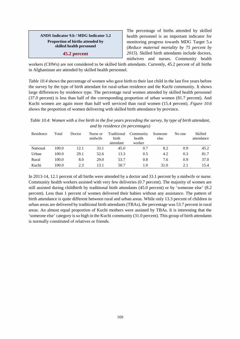
169
The percentage of births attended by skilled
health personnel is an important indicator for
monitoring progress towards MDG Target 5.a
(Reduce maternal mortality by 75 percent by
2015). Skilled birth attendants include doctors,
midwives and nurses. Community health
workers (CHWs) are not considered to be skilled birth attendants. Currently, 45.2 percent of all births
in Afghanistan are attended by skilled health personnel.
Table 10.4 shows the percentage of women who gave birth to their last child in the last five years before
the survey by the type of birth attendant for rural-urban residence and the Kuchi community. It shows
large differences by residence type. The percentage rural women attended by skilled health personnel
(37.0 percent) is less than half of the corresponding proportion of urban women (81.7 percent). And
Kuchi women are again more than half well serviced than rural women (15.4 percent). Figure 10.6
shows the proportion of women delivering with skilled birth attendance by province.
Table 10.4: Women with a live birth in the five years preceding the survey, by type of birth attendant,
and by residence (in percentages)
Residence Total Doctor Nurse or Traditional Community Someone No one Skilled
midwife birth health else attendance
attendant worker
National 100.0 12.1 33.1 45.0 0.7 8.2 0.9 45.2
Urban 100.0 29.1 52.6 13.3 0.5 4.2 0.3 81.7
Rural 100.0 8.0 29.0 53.7 0.8 7.6 0.9 37.0
Kuchi 100.0 2.3 13.1 50.7 1.0 31.0 2.1 15.4
In 2013-14, 12.1 percent of all births were attended by a doctor and 33.1 percent by a midwife or nurse.
Community health workers assisted with very few deliveries (0.7 percent). The majority of women are
still assisted during childbirth by traditional birth attendants (45.0 percent) or by ‘someone else’ (8.2
percent). Less than 1 percent of women delivered their babies without any assistance. The pattern of
birth attendance is quite different between rural and urban areas. While only 13.3 percent of children in
urban areas are delivered by traditional birth attendants (TBAs), the percentage was 53.7 percent in rural
areas. An almost equal proportion of Kuchi mothers were assisted by TBAs. It is interesting that the
‘someone else’ category is so high in the Kuchi community (31.0 percent). This group of birth attendants
is normally constituted of relatives or friends.
ANDS Indicator 9.b / MDG Indicator 5.2
Proportion of births attended by
skilled health personnel
45.2 percent
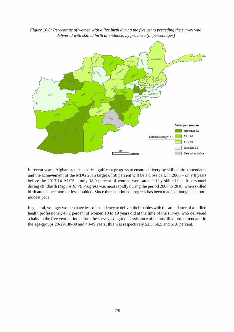
170
Figure 10.6: Percentage of women with a live birth during the five years preceding the survey who
delivered with skilled birth attendance, by province (in percentages)
In recent years, Afghanistan has made significant progress to ensure delivery by skilled birth attendants
and the achievement of the MDG 2015 target of 50 percent will be a close call. In 2006 – only 8 years
before the 2013-14 ALCS – only 18.9 percent of women were attended by skilled health personnel
during childbirth (Figure 10.7). Progress was most rapidly during the period 2006 to 2010, when skilled
birth attendance more or less doubled. Since then continued progress has been made, although at a more
modest pace.
In general, younger women have less of a tendency to deliver their babies with the attendance of a skilled
health professional; 48.2 percent of women 10 to 19 years old at the time of the survey, who delivered
a baby in the five year period before the survey, sought the assistance of an unskilled birth attendant. In
the age-groups 20-29, 30-39 and 40-49 years, this was respectively 52.5, 56,5 and 61.6 percent.
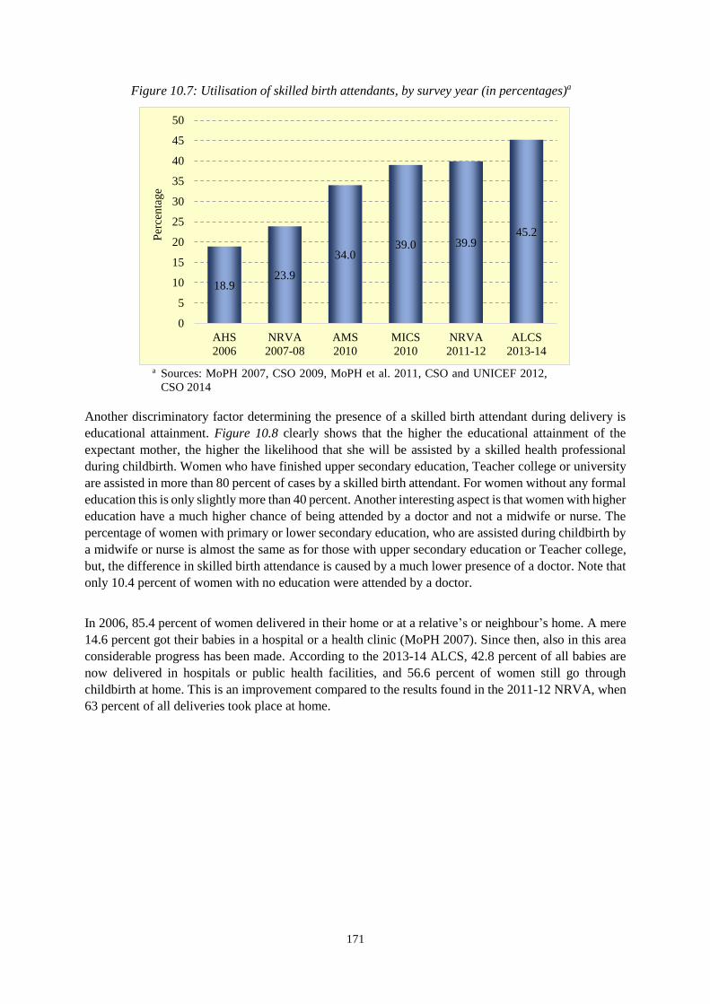
171
Figure 10.7: Utilisation of skilled birth attendants, by survey year (in percentages)a
a Sources: MoPH 2007, CSO 2009, MoPH et al. 2011, CSO and UNICEF 2012,
CSO 2014
Another discriminatory factor determining the presence of a skilled birth attendant during delivery is
educational attainment. Figure 10.8 clearly shows that the higher the educational attainment of the
expectant mother, the higher the likelihood that she will be assisted by a skilled health professional
during childbirth. Women who have finished upper secondary education, Teacher college or university
are assisted in more than 80 percent of cases by a skilled birth attendant. For women without any formal
education this is only slightly more than 40 percent. Another interesting aspect is that women with higher
education have a much higher chance of being attended by a doctor and not a midwife or nurse. The
percentage of women with primary or lower secondary education, who are assisted during childbirth by
a midwife or nurse is almost the same as for those with upper secondary education or Teacher college,
but, the difference in skilled birth attendance is caused by a much lower presence of a doctor. Note that
only 10.4 percent of women with no education were attended by a doctor.
In 2006, 85.4 percent of women delivered in their home or at a relative’s or neighbour’s home. A mere
14.6 percent got their babies in a hospital or a health clinic (MoPH 2007). Since then, also in this area
considerable progress has been made. According to the 2013-14 ALCS, 42.8 percent of all babies are
now delivered in hospitals or public health facilities, and 56.6 percent of women still go through
childbirth at home. This is an improvement compared to the results found in the 2011-12 NRVA, when
63 percent of all deliveries took place at home.
18.923.9
34.039.0 39.9
45.2
0
5
10
15
20
25
30
35
40
45
50
AHS
2006
NRVA
2007-08
AMS
2010
MICS
2010
NRVA
2011-12
ALCS
2013-14
Per
centa
ge
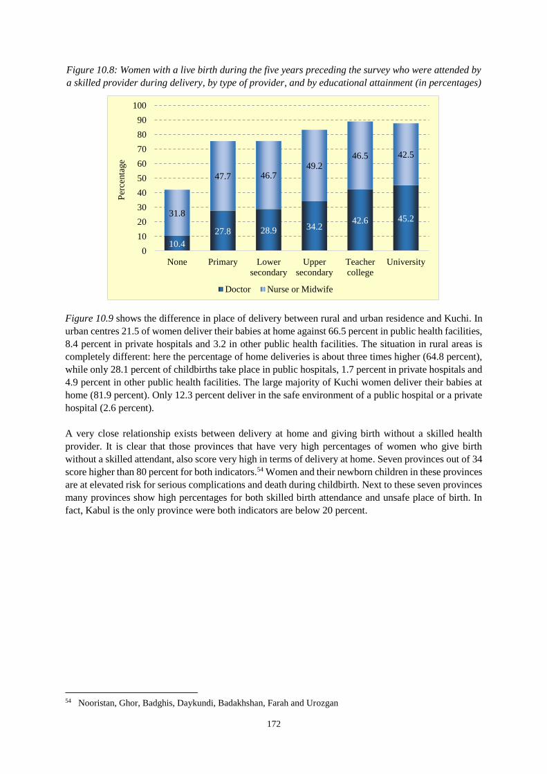
172
Figure 10.8: Women with a live birth during the five years preceding the survey who were attended by
a skilled provider during delivery, by type of provider, and by educational attainment (in percentages)
Figure 10.9 shows the difference in place of delivery between rural and urban residence and Kuchi. In
urban centres 21.5 of women deliver their babies at home against 66.5 percent in public health facilities,
8.4 percent in private hospitals and 3.2 in other public health facilities. The situation in rural areas is
completely different: here the percentage of home deliveries is about three times higher (64.8 percent),
while only 28.1 percent of childbirths take place in public hospitals, 1.7 percent in private hospitals and
4.9 percent in other public health facilities. The large majority of Kuchi women deliver their babies at
home (81.9 percent). Only 12.3 percent deliver in the safe environment of a public hospital or a private
hospital (2.6 percent).
A very close relationship exists between delivery at home and giving birth without a skilled health
provider. It is clear that those provinces that have very high percentages of women who give birth
without a skilled attendant, also score very high in terms of delivery at home. Seven provinces out of 34
score higher than 80 percent for both indicators.54 Women and their newborn children in these provinces
are at elevated risk for serious complications and death during childbirth. Next to these seven provinces
many provinces show high percentages for both skilled birth attendance and unsafe place of birth. In
fact, Kabul is the only province were both indicators are below 20 percent.
54 Nooristan, Ghor, Badghis, Daykundi, Badakhshan, Farah and Urozgan
10.4
27.8 28.9 34.242.6 45.2
31.8
47.7 46.749.2
46.5 42.5
0
10
20
30
40
50
60
70
80
90
100
None Primary Lower
secondary
Upper
secondary
Teacher
college
University
Per
centa
ge
Doctor Nurse or Midwife
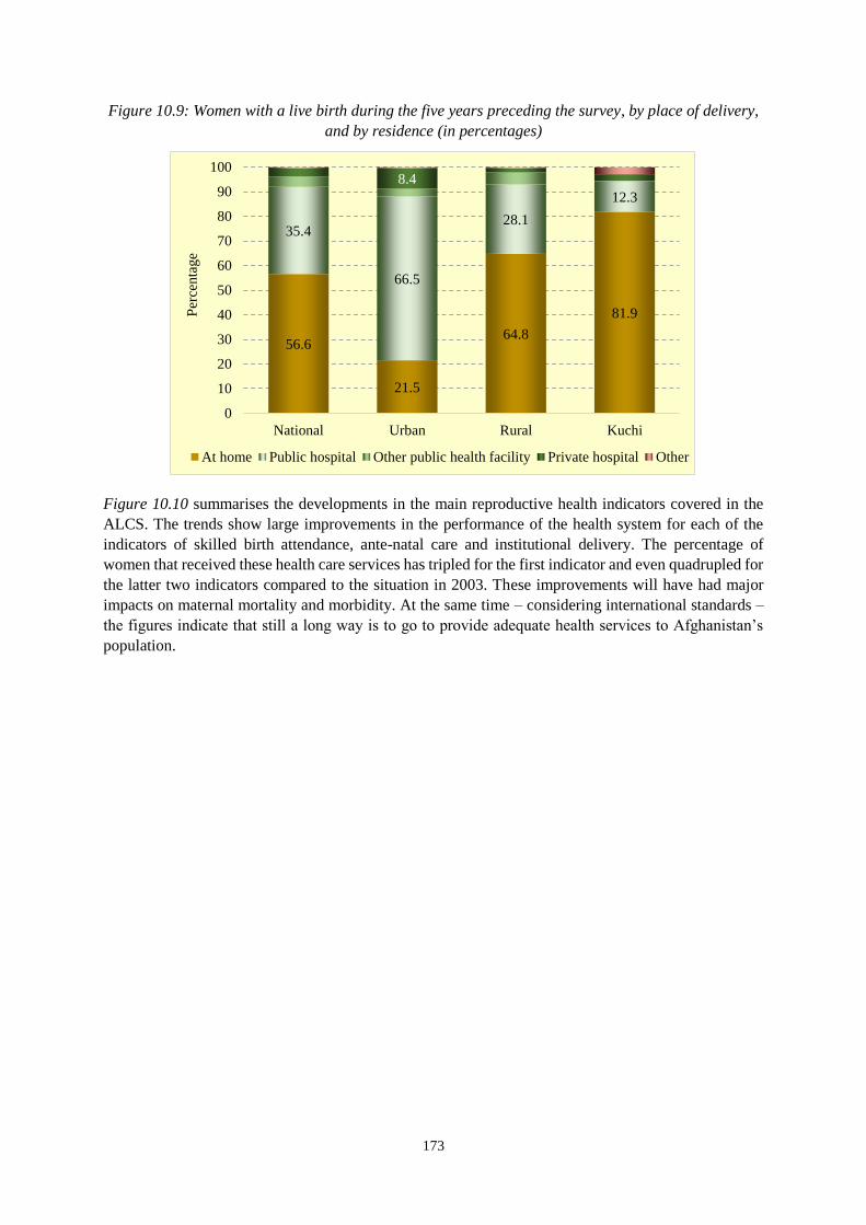
173
Figure 10.9: Women with a live birth during the five years preceding the survey, by place of delivery,
and by residence (in percentages)
Figure 10.10 summarises the developments in the main reproductive health indicators covered in the
ALCS. The trends show large improvements in the performance of the health system for each of the
indicators of skilled birth attendance, ante-natal care and institutional delivery. The percentage of
women that received these health care services has tripled for the first indicator and even quadrupled for
the latter two indicators compared to the situation in 2003. These improvements will have had major
impacts on maternal mortality and morbidity. At the same time – considering international standards –
the figures indicate that still a long way is to go to provide adequate health services to Afghanistan’s
population.
56.6
21.5
64.8
81.9
35.4
66.5
28.1
12.3
8.4
0
10
20
30
40
50
60
70
80
90
100
National Urban Rural Kuchi
Per
centa
ge
At home Public hospital Other public health facility Private hospital Other
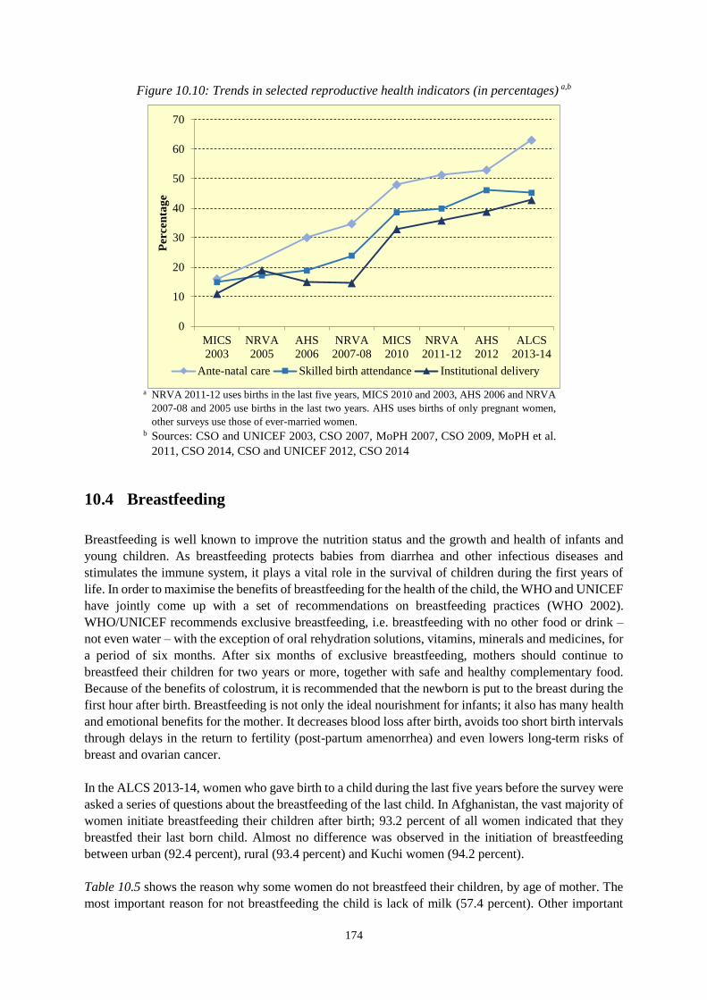
174
Figure 10.10: Trends in selected reproductive health indicators (in percentages) a,b
a NRVA 2011-12 uses births in the last five years, MICS 2010 and 2003, AHS 2006 and NRVA
2007-08 and 2005 use births in the last two years. AHS uses births of only pregnant women,
other surveys use those of ever-married women. b Sources: CSO and UNICEF 2003, CSO 2007, MoPH 2007, CSO 2009, MoPH et al.
2011, CSO 2014, CSO and UNICEF 2012, CSO 2014
10.4 Breastfeeding
Breastfeeding is well known to improve the nutrition status and the growth and health of infants and
young children. As breastfeeding protects babies from diarrhea and other infectious diseases and
stimulates the immune system, it plays a vital role in the survival of children during the first years of
life. In order to maximise the benefits of breastfeeding for the health of the child, the WHO and UNICEF
have jointly come up with a set of recommendations on breastfeeding practices (WHO 2002).
WHO/UNICEF recommends exclusive breastfeeding, i.e. breastfeeding with no other food or drink –
not even water – with the exception of oral rehydration solutions, vitamins, minerals and medicines, for
a period of six months. After six months of exclusive breastfeeding, mothers should continue to
breastfeed their children for two years or more, together with safe and healthy complementary food.
Because of the benefits of colostrum, it is recommended that the newborn is put to the breast during the
first hour after birth. Breastfeeding is not only the ideal nourishment for infants; it also has many health
and emotional benefits for the mother. It decreases blood loss after birth, avoids too short birth intervals
through delays in the return to fertility (post-partum amenorrhea) and even lowers long-term risks of
breast and ovarian cancer.
In the ALCS 2013-14, women who gave birth to a child during the last five years before the survey were
asked a series of questions about the breastfeeding of the last child. In Afghanistan, the vast majority of
women initiate breastfeeding their children after birth; 93.2 percent of all women indicated that they
breastfed their last born child. Almost no difference was observed in the initiation of breastfeeding
between urban (92.4 percent), rural (93.4 percent) and Kuchi women (94.2 percent).
Table 10.5 shows the reason why some women do not breastfeed their children, by age of mother. The
most important reason for not breastfeeding the child is lack of milk (57.4 percent). Other important
0
10
20
30
40
50
60
70
MICS
2003
NRVA
2005
AHS
2006
NRVA
2007-08
MICS
2010
NRVA
2011-12
AHS
2012
ALCS
2013-14
Per
cen
tag
e
Ante-natal care Skilled birth attendance Institutional delivery
175
reasons are death of the child (13.0 percent), baby too sick (12.0 percent) and mother too sick (14.7
percent). All these reasons are non-voluntarily; actually only 0.3 percent of women who did not
breastfeed their babies indicated they did not want too. This clearly shows the almost universal character
of breastfeeding in Afghanistan. Women, who did not breastfeed, do so because of external reasons.
Table 10.5: Women with a live birth during the five years preceding the survey, by five-year age-
groups, and by reason for not breastfeeding the child (in percentages)
Reason Total 15-19 20-24 25-29 30-34 35-39 40-44 45-49
Total 100.0 100.0 100.0 100.0 100.0 100.0 100.0 100.0
Baby died 13.0 30.1 12.0 8.7 13.0 15.4 14.6 14.1
Baby too sick 12.0 10.5 11.1 11.2 9.1 16.4 11.6 15.2
Did not have milk 57.4 47.4 58.3 60.5 61.0 52.9 57.7 47.1
Mother too sick 14.7 9.8 15.8 14.0 14.6 14.5 14.1 22.5
Did not want to 0.3 0.0 0.0 0.9 0.0 0.0 0.0 0.0
Had to work 0.1 0.0 0.0 0.2 0.0 0.0 0.0 0.0
Other reason 2.1 2.1 2.8 3.7 0.8 0.8 1.9 1.2
Don't know 0.5 0.0 0.0 0.8 1.5 0.0 0.0 0.0
There are many reasons why a baby should be put to the breast during the first hour of life: the baby
should receive the colostrum (first breast milk) as soon as possible after birth, as it is rich in nutrients
and protects against many infections, suckling stimulates the contraction of the uterus (which stimulates
the delivery of the placenta and reduces maternal bleeding), breastfeeding reduces stress in the newborn
baby and stimulates the immediate bonding between the mother and her newborn child (UNICEF 2007).
The ALCS 2013-14 indicates that about a third of all babies (33.2 percent) born in Afghanistan and who
receive breastfeeding are breastfed within the first hour after birth. Another 24.2 percent are put to the
breast between one and two hours after birth and another 14.9 percent between two and three hours.
Overall, breastfeeding is initiated for 90.5 percent of all babies during the first day of life, another 5.5
are breastfed for the first time during the second day of life and another 2.5 percent during the third day.
Little difference exists between rural and urban residence and the Kuchi population. It is interesting that
the results on the percentage of children who were first breastfed within an hour after birth is quite
different from the 2010-11 Multiple Indicator Cluster Survey (CSO and UNICEF 2012). Where ALCS
found that 33.2 percent of births were put to the breast within an hour after birth, the MICS found 53.6
percent for the same indicator.
The percentage of babies in MICS who were breastfed within the first day of life came much closer to
the ALCS figure: 84.5 percent (MICS) against 90.5 percent (ALCS). It is unclear what caused the
significant differences between both surveys. Questions in both surveys about the initiation of
breastfeeding were quite similar; the only difference is that the question in MICS is restricted to women
who had a baby in the last two years, while the ALCS question is asked to women with a birth in the
last five years before the survey.
Breastmilk contains all nutrients and liquids a young child needs. No other drinks are necessary during
the first six months of life. Providing a baby less than 6 months old with any other liquids (or food)
increases the risks of diarrhea and other serious infections. To measure the timing of adding other liquids
than breastfeeding to young children's diet, a question was asked whether during the first three days of
live, the child was given anything to drink other than breastmilk. In addition it was asked how many
days the mother fed the baby only breastmilk before giving other liquids. The proportion of young
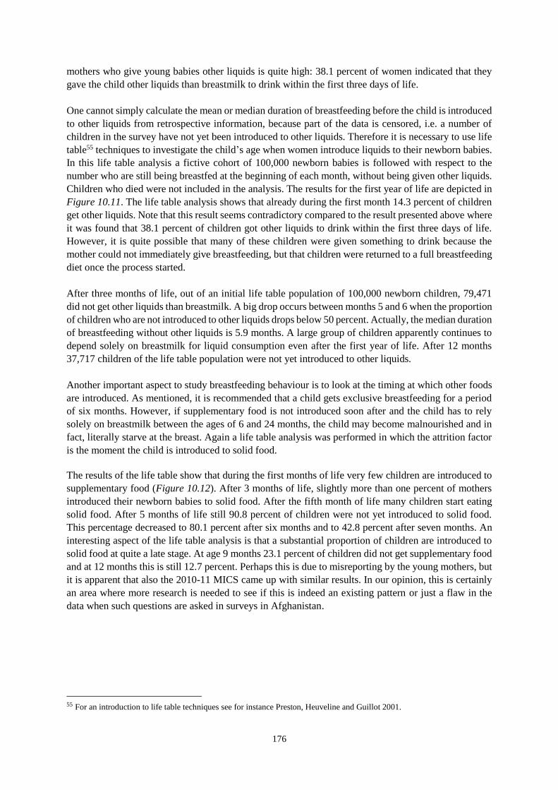
176
mothers who give young babies other liquids is quite high: 38.1 percent of women indicated that they
gave the child other liquids than breastmilk to drink within the first three days of life.
One cannot simply calculate the mean or median duration of breastfeeding before the child is introduced
to other liquids from retrospective information, because part of the data is censored, i.e. a number of
children in the survey have not yet been introduced to other liquids. Therefore it is necessary to use life
table55 techniques to investigate the child’s age when women introduce liquids to their newborn babies.
In this life table analysis a fictive cohort of 100,000 newborn babies is followed with respect to the
number who are still being breastfed at the beginning of each month, without being given other liquids.
Children who died were not included in the analysis. The results for the first year of life are depicted in
Figure 10.11. The life table analysis shows that already during the first month 14.3 percent of children
get other liquids. Note that this result seems contradictory compared to the result presented above where
it was found that 38.1 percent of children got other liquids to drink within the first three days of life.
However, it is quite possible that many of these children were given something to drink because the
mother could not immediately give breastfeeding, but that children were returned to a full breastfeeding
diet once the process started.
After three months of life, out of an initial life table population of 100,000 newborn children, 79,471
did not get other liquids than breastmilk. A big drop occurs between months 5 and 6 when the proportion
of children who are not introduced to other liquids drops below 50 percent. Actually, the median duration
of breastfeeding without other liquids is 5.9 months. A large group of children apparently continues to
depend solely on breastmilk for liquid consumption even after the first year of life. After 12 months
37,717 children of the life table population were not yet introduced to other liquids.
Another important aspect to study breastfeeding behaviour is to look at the timing at which other foods
are introduced. As mentioned, it is recommended that a child gets exclusive breastfeeding for a period
of six months. However, if supplementary food is not introduced soon after and the child has to rely
solely on breastmilk between the ages of 6 and 24 months, the child may become malnourished and in
fact, literally starve at the breast. Again a life table analysis was performed in which the attrition factor
is the moment the child is introduced to solid food.
The results of the life table show that during the first months of life very few children are introduced to
supplementary food (Figure 10.12). After 3 months of life, slightly more than one percent of mothers
introduced their newborn babies to solid food. After the fifth month of life many children start eating
solid food. After 5 months of life still 90.8 percent of children were not yet introduced to solid food.
This percentage decreased to 80.1 percent after six months and to 42.8 percent after seven months. An
interesting aspect of the life table analysis is that a substantial proportion of children are introduced to
solid food at quite a late stage. At age 9 months 23.1 percent of children did not get supplementary food
and at 12 months this is still 12.7 percent. Perhaps this is due to misreporting by the young mothers, but
it is apparent that also the 2010-11 MICS came up with similar results. In our opinion, this is certainly
an area where more research is needed to see if this is indeed an existing pattern or just a flaw in the
data when such questions are asked in surveys in Afghanistan.
55 For an introduction to life table techniques see for instance Preston, Heuveline and Guillot 2001.
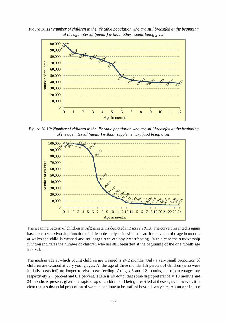
177
Figure 10.11: Number of children in the life table population who are still breastfed at the beginning
of the age interval (month) without other liquids being given
Figure 10.12: Number of children in the life table population who are still breastfed at the beginning
of the age interval (month) without supplementary food being given
The weaning pattern of children in Afghanistan is depicted in Figure 10.13. The curve presented is again
based on the survivorship function of a life table analysis in which the attrition event is the age in months
at which the child is weaned and no longer receives any breastfeeding. In this case the survivorship
function indicates the number of children who are still breastfed at the beginning of the one month age
interval.
The median age at which young children are weaned is 24.2 months. Only a very small proportion of
children are weaned at very young ages. At the age of three months 1.5 percent of children (who were
initially breastfed) no longer receive breastfeeding. At ages 6 and 12 months, these percentages are
respectively 2.7 percent and 6.1 percent. There is no doubt that some digit preference at 18 months and
24 months is present, given the rapid drop of children still being breastfed at these ages. However, it is
clear that a substantial proportion of women continue to breastfeed beyond two years. About one in four
0
10,000
20,000
30,000
40,000
50,000
60,000
70,000
80,000
90,000
100,000
0 1 2 3 4 5 6 7 8 9 10 11 12
Num
ber
of
chil
dre
n
Age in months
0
10,000
20,000
30,000
40,000
50,000
60,000
70,000
80,000
90,000
100,000
0 1 2 3 4 5 6 7 8 9 10 11 12 13 14 15 16 17 18 19 20 21 22 23 24
Num
ber
of
chil
dre
n
Age in months
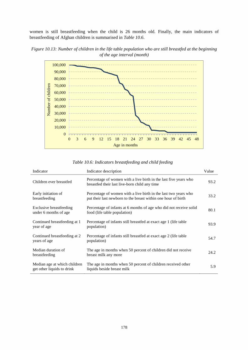
178
women is still breastfeeding when the child is 26 months old. Finally, the main indicators of
breastfeeding of Afghan children is summarised in Table 10.6.
Figure 10.13: Number of children in the life table population who are still breastfed at the beginning
of the age interval (month)
Table 10.6: Indicators breastfeeding and child feeding
Indicator Indicator description Value
Children ever breastfed Percentage of women with a live birth in the last five years who
breastfed their last live-born child any time 93.2
Early initiation of
breastfeeding
Percentage of women with a live birth in the last two years who
put their last newborn to the breast within one hour of birth 33.2
Exclusive breastfeeding
under 6 months of age
Percentage of infants at 6 months of age who did not receive solid
food (life table population) 80.1
Continued breastfeeding at 1
year of age
Percentage of infants still breastfed at exact age 1 (life table
population) 93.9
Continued breastfeeding at 2
years of age
Percentage of infants still breastfed at exact age 2 (life table
population) 54.7
Median duration of
breastfeeding
The age in months when 50 percent of children did not receive
breast milk any more 24.2
Median age at which children
get other liquids to drink
The age in months when 50 percent of children received other
liquids beside breast milk 5.9
0
10,000
20,000
30,000
40,000
50,000
60,000
70,000
80,000
90,000
100,000
0 3 6 9 12 15 18 21 24 27 30 33 36 39 42 45 48
Num
ber
of
chil
dre
n
Age in months
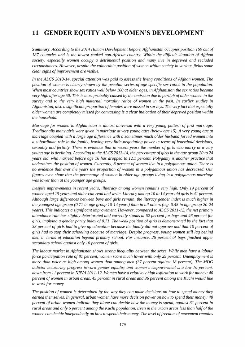
179
11 GENDER EQUITY AND WOMEN’S DEVELOPMENT
Summary. According to the 2014 Human Development Report, Afghanistan occupies position 169 out of
187 countries and is the lowest ranked non-African country. Within the difficult situation of Afghan
society, especially women occupy a detrimental position and many live in deprived and secluded
circumstances. However, despite the vulnerable position of women within society in various fields some
clear signs of improvement are visible.
In the ALCS 2013-14, special attention was paid to assess the living conditions of Afghan women. The
position of women is clearly shown by the peculiar series of age-specific sex ratios in the population.
When most countries show sex ratios well below 100 at older ages, in Afghanistan the sex ratios become
very high after age 50. This is most probably caused by the omission due to purdah of older women in the
survey and to the very high maternal mortality ratios of women in the past. In earlier studies in
Afghanistan, also a significant proportion of females were missed in surveys. The very fact that especially
older women are completely missed for canvassing is a clear indication of their deprived position within
the household.
Marriage for women in Afghanistan is almost universal with a very young pattern of first marriage.
Traditionally many girls were given in marriage at very young ages (below age 15). A very young age at
marriage coupled with a large age difference with a sometimes much older husband forced women into
a subordinate role in the family, leaving very little negotiating power in terms of household decisions,
sexuality and fertility. There is evidence that in recent years the number of girls who marry at a very
young age is declining. According to the ALCS 2013-14, the percentage of girls in the age group 20 to 24
years old, who married before age 16 has dropped to 12.1 percent. Polygamy is another practice that
undermines the position of women. Currently, 8 percent of women live in a polygamous union. There is
no evidence that over the years the proportion of women in a polygamous union has decreased. Our
figures even show that the percentage of women in older age groups living in a polygamous marriage
was lower than at the younger age groups.
Despite improvements in recent years, illiteracy among women remains very high. Only 19 percent of
women aged 15 years and older can read and write. Literacy among 10 to 14 year old girls is 41 percent.
Although large differences between boys and girls remain, the literacy gender index is much higher in
the youngest age group (0.71 in age group 10-14 years) than in all others (e.g. 0.45 in age group 20-24
years). This indicates a significant improvement. However, compared to ALCS 2011-12, the net primary
attendance rate has slightly deteriorated and currently stands at 62 percent for boys and 46 percent for
girls, implying a gender parity index of 0.71. The weak position of girls is demonstrated by the fact that
33 percent of girls had to give up education because the family did not approve and that 10 percent of
girls had to stop their schooling because of marriage. Despite progress, young women still lag behind
men in terms of education beyond primary school. For instance, 26 percent of boys finished upper
secondary school against only 10 percent of girls.
The labour market in Afghanistan shows strong inequality between the sexes. While men have a labour
force participation rate of 81 percent, women score much lower with only 29 percent. Unemployment is
more than twice as high among women than among men (37 percent against 18 percent). The MDG
indictor measuring progress toward gender equality and women’s empowerment is a low 10 percent,
down from 11 percent in NRVA 2011-12. Women have a relatively high aspiration to work for money: 40
percent of women in urban areas, 45 percent in rural areas and 36 percent among the Kuchi would like
to work for money.
The position of women is determined by the way they can make decisions on how to spend money they
earned themselves. In general, urban women have more decision power on how to spend their money: 48
percent of urban women indicate they alone can decide how the money is spend, against 31 percent in
rural areas and only 6 percent among the Kuchi population. Even in the urban areas less than half of the
women can decide independently on how to spend their money. The level of freedom of movement remains
180
very restricted with three quarters of women not leaving the dwelling without the company of another
person. Levels of seclusion remain high: about 50 percent of women leave the house four times or less
per month, while 12 percent of women indicate they never left the house in a whole month.
The health position of women is not discussed in this chapter but in chapter 11 on health. However, some
health aspects are closely related to the position of women and deserve some attention here. In the 2013-
14 ALCS a question was asked about women's use of the health system and why they would not seek
medical attention when needed. The most important reason why women did not seek medical attention
was that it was too expensive to get medical attention; 40 percent of women indicated this as the first
reason. Pre-coded reasons that are closely connected to deprivation of women are ‘no female medical
staff’, ‘no one to accompany’, ‘husband or family did not allow’ and ‘traditional constraints’. Of these
categories, ‘no one to accompany’ is the most important with 2 percent as the first reason and 6 percent
as the second reason. Our results clearly show that poverty and geographical isolation are much more
important reasons than gender deprivation to explain why women often do not get the medical attention
they need when they are sick or injured. These results confirm the findings of the NRVA 2007-08 when
expenses and distance were also found to be the major constraints for women to use health services.
It is interesting that despite the huge differences in social position and status, the priorities for
development activities for men and women come very close together. Both indicate that the most
important way in which the government can assist their community is by the construction or repair of
local roads. Also other priorities score quite similar for men and women alike. This is a clear indication
that despite the detrimental position of women vis à vis men both sexes continue to suffer from high levels
of poverty and deprivation and need similar actions to improve their condition.
11.1 Introduction
Afghanistan is faced with many challenges to improve the position of women and to tap their potential
for the economic and social development of the country. Every year, UNDP ranks countries according
to their Gender Inequality Index (GII) in the Human Development Report. The GII is a composite
measure which uses three dimensions to quantify gender-based inequalities: a) reproductive health
(indicators: maternal mortality ratio and adolescent fertility rates), b) Empowerment (indicators:
percentage of parliamentary seats held by women and secondary and higher educational attainment),
and c) economic activity (indicators: participation rate of women). According to the 2014 Human
Development Report (UNDP 2014, p.174), Afghanistan occupies the 150th position, out of 151
countries for which data were available, in terms of the Gender Inequality Index. The only country with
a lower GII-score than Afghanistan is Chad.
During the last ten years, the Afghan government has taken important steps to ameliorate the position
of women in society and to improve their overall living conditions. Gender equality and women’s
empowerment were made a key dimension in the national development framework. A series of policies
and strategies were developed to protect women and to promote their empowerment. Among others the
following legal actions were taken:
the National Action Plan for the Women of Afghanistan (2008-2018)
the Law on Elimination of Violence Against Women (2009)
the National Reproductive Health Strategy (2006-2009)
the National Gender Strategy, MoPH 2012-2016
The ALCS 2013-14 provides information to monitor progress in the field of gender equality and
women’s empowerment. The situation should be seen against the background of the country’s general
poverty reduction strategy and (in)security situation. In the ALCS 2013-14 questionnaire, a special
module was dedicated to gender issues. In this module a total of 45 questions were asked to each woman
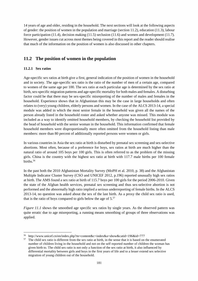
181
14 years of age and older, residing in the household. The next sections will look at the following aspects
of gender: the position of women in the population and marriage (section 11.2), education (11.3), labour
force participation (11.4), decision making (11.5) seclusion (11.6) and women and development (11.7).
However, gender issues cut across most themes being covered in this report and the reader should realise
that much of the information on the position of women is also discussed in other chapters.
11.2 The position of women in the population
11.2.1 Sex ratios
Age-specific sex ratios at birth give a first, general indication of the position of women in the household
and in society. The age-specific sex ratio is the ratio of the number of men of a certain age, compared
to women of the same age per 100. The sex ratio at each particular age is determined by the sex ratio at
birth, sex-specific migration patterns and age-specific mortality for both males and females. A disturbing
factor could be that there may be sex-specific misreporting of the number of males and females in the
household. Experience shows that in Afghanistan this may be the case in large households and often
relates to (very) young children, elderly persons and women. In the case of the ALCS 2013-14, a special
module was added in which the most senior female in the household was given all the names of the
person already listed in the household roster and asked whether anyone was missed. This module was
included as a way to identify omitted household members, by checking the household list provided by
the head of household with the senior woman in the household. This information confirmed that female
household members were disproportionally more often omitted from the household listing than male
members: more than 80 percent of additionally reported persons were women or girls.
In various countries in Asia the sex ratio at birth is disturbed by prenatal sex screening and sex-selective
abortions. Most often, because of a preference for boys, sex ratios at birth are much higher than the
natural ratio of around 105 boys per 100 girls. This is often referred to as the problem of the missing
girls. China is the country with the highest sex ratio at birth with 117.7 male births per 100 female
births.56
In the past both the 2010 Afghanistan Mortality Survey (MoPH et al. 2010, p. 38) and the Afghanistan
Multiple Indicator Cluster Survey (CSO and UNICEF 2012, p.196) reported unusually high sex ratios
at birth. The AMS found a sex ratio at birth of 115.7 boys per 100 girls for the period 2006-2010. Given
the state of the Afghan health services, prenatal sex screening and thus sex-selective abortion is not
performed and the abnormally high ratio implied a serious underreporting of female births. In the ALCS
2013-14, no question was asked about the sex of the last birth. As a proxy the child sex ratio is used,
that is the ratio of boys compared to girls below the age of 5.57
Figure 11.1 shows the smoothed age specific sex ratios by single years. As the observed pattern was
quite erratic due to age misreporting, a running means smoothing of groups of three observations was
applied.
56 http://www.unicef.cn/en/index.php?m=content&c=index&a=show&catid=196&id=777 57 The child sex ratio is different from the sex ratio at birth, in the sense that it is based on the enumerated
number of children living in the household and not on the self reported number of children the woman has
given birth to. The child sex ratio is not only a function of the sex ratio at birth, it also influenced by
differential mortality between girls and boys in the first years of life and to a lesser extend sex selective
migration of young children out of the household.
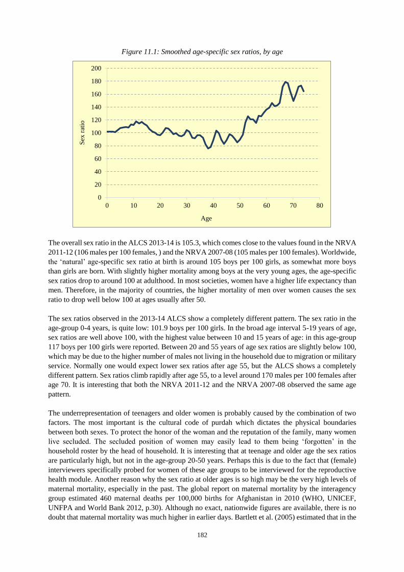
182
Figure 11.1: Smoothed age-specific sex ratios, by age
The overall sex ratio in the ALCS 2013-14 is 105.3, which comes close to the values found in the NRVA
2011-12 (106 males per 100 females, ) and the NRVA 2007-08 (105 males per 100 females). Worldwide,
the ‘natural’ age-specific sex ratio at birth is around 105 boys per 100 girls, as somewhat more boys
than girls are born. With slightly higher mortality among boys at the very young ages, the age-specific
sex ratios drop to around 100 at adulthood. In most societies, women have a higher life expectancy than
men. Therefore, in the majority of countries, the higher mortality of men over women causes the sex
ratio to drop well below 100 at ages usually after 50.
The sex ratios observed in the 2013-14 ALCS show a completely different pattern. The sex ratio in the
age-group 0-4 years, is quite low: 101.9 boys per 100 girls. In the broad age interval 5-19 years of age,
sex ratios are well above 100, with the highest value between 10 and 15 years of age: in this age-group
117 boys per 100 girls were reported. Between 20 and 55 years of age sex ratios are slightly below 100,
which may be due to the higher number of males not living in the household due to migration or military
service. Normally one would expect lower sex ratios after age 55, but the ALCS shows a completely
different pattern. Sex ratios climb rapidly after age 55, to a level around 170 males per 100 females after
age 70. It is interesting that both the NRVA 2011-12 and the NRVA 2007-08 observed the same age
pattern.
The underrepresentation of teenagers and older women is probably caused by the combination of two
factors. The most important is the cultural code of purdah which dictates the physical boundaries
between both sexes. To protect the honor of the woman and the reputation of the family, many women
live secluded. The secluded position of women may easily lead to them being ‘forgotten’ in the
household roster by the head of household. It is interesting that at teenage and older age the sex ratios
are particularly high, but not in the age-group 20-50 years. Perhaps this is due to the fact that (female)
interviewers specifically probed for women of these age groups to be interviewed for the reproductive
health module. Another reason why the sex ratio at older ages is so high may be the very high levels of
maternal mortality, especially in the past. The global report on maternal mortality by the interagency
group estimated 460 maternal deaths per 100,000 births for Afghanistan in 2010 (WHO, UNICEF,
UNFPA and World Bank 2012, p.30). Although no exact, nationwide figures are available, there is no
doubt that maternal mortality was much higher in earlier days. Bartlett et al. (2005) estimated that in the
0
20
40
60
80
100
120
140
160
180
200
0 10 20 30 40 50 60 70 80
Sex
rat
io
Age
183
period 1999-2002 the maternal mortality ratio (MMR) was between 1,600 and 2,200. If we assume for
a moment that in the period 1970-2000 the MMR was 2,000 and the Total Fertility Rate58 was around
7, then the lifetime risk of maternal mortality can be approximated to be 14,000 per 100,000 women;
which means that in those days almost one in seven women would have died during pregnancy and
childbirth. Obviously, this would have had a direct effect on the number of women who survive beyond
age 50 and would seriously distort the current sex ratios at older ages.
Unfortunately, data are not available to unravel the effect of seclusion and maternal mortality on the sex
ratios. Fact is that both factors are closely connected to the situation of women in society and are proof
of the difficult position of women.
11.2.2 Head of household
In the ALCS 2013-14 the head of household was defined as ‘the person commonly regarded by the
household members as their head. The head would usually be the main income earner and decision
maker for the household, but you should accept the decision of the household members as to who they
consider their head’ (ALCS 1392-1393, Interviewer Manual, p.8).
According to the ALCS 2013-14 only one percent of all households are headed by a female. Little
variation exist between age groups. The age group with the highest percentage of female heads is 60-64
years with 1.7 percent of households being led by a woman.
11.2.3 Child marriage
Girls who are given in marriage at a very young age are denied their youth and being cut off from their
families, they frequently suffer from social isolation, lack of education and limited chances on the labour
market. Because of the often large age differences with the husband (see also section 3.4.3), these girls
are forced into a subordinate role in the family, with little negotiating power in terms of sexuality and
fertility decisions. Early fertility is a major cause of childbirth complications, poor health of both mother
and child and maternal mortality. Forced marriage of girls at a very young age is a clear manifestation
of gender discrimination having an important impact on the emotional and physical wellbeing of young
women.
Afghanistan has a tradition of very early marriage for girls with a significant proportion of women being
given in marriage by the family as child brides. Currently, legal age at marriage in Afghanistan is set at
16 for women and at 18 for men. However, an exception is made if the woman has not reached age
sixteen, in which case permission can be granted by her father or through a competent court (LandInfo
2011, p.8). However, marriage of girls below the age of fifteen is strictly forbidden.
As discussed earlier, marriage for women in Afghanistan is almost universal with a very young pattern
of first marriage. At age 50, only 9 per thousand of all women have never been married.59 The proportion
of never-married men is even smaller: only 3 per thousand of all men had never been married at exact
age 50. Figure 11.2 depicts the percentage of women 20 to 59 years, who married respectively before
ages 16, 18 and 20. Age 16 was selected because this is the legal minimum age at marriage. According
to the UNICEF definition, child marriage occurs when a person, male or female, enters a formal
58 The Population Reference Bureau estimates that the TFR for Afghanistan was around 7.5 in 1970
(http://www.prb.org/DataFinder) 59 To calculate the proportion at exact age 50, we took the average of the proportion never married between the age groups
45-49 and 50 - 54 years of age.
184
marriage or informal union before the age of consent of 18 years60. To measure the level of child
marriage in Afghanistan the cut-off age of 18 years was included in Figure 11.2 as one of the categories.
Figure 11.2: Percentage of women 20-59 years of age who married before ages 16, 18 and 20, by age
five-year age group
There is evidence that the number of girls who marry before the age of 16 is declining. The age group
with the highest percentage of very young brides is between 35-39 years of age; 29.4 percent of women
who were in this age group at the time of the survey were married before age 16. These women were at
a very young age during the time when the Taliban were establishing their power over the country. One
can clearly see the reduction in the marriages before age 16 in the three consecutive five year age groups
between 20 and 35. In these age groups the proportion of girls who were given in marriage below the
age of 16 were respectively 21.4 (30-34 years) and 19.4 percent (25-29 years). Important progress seems
to be made in recent years. The percentage of 20 to 24 year olds who married before age 16 has dropped
to 12.1 percent.
A similar trend can be observed with the percentage of child marriages before age 18. Among women
currently aged 35 to 39, 61.9 percent married before their 18th birthday. For women who were between
20 and 24 years of age at the time of the ALCS 2013-14, this percentage was 32.8 percent. This means
that during a period of about fifteen years, the proportion of women who entered marriage as a child
bride has almost been cut in half. Also the proportion of women who marry before the age of 20 has
come down significantly in recent years.
11.2.4 Polygamy
In its International Convenant on Civil and Political Rights, the United Nations take a clear stand on the
issue of polygamy and women’s rights: ‘States should provide information on these laws and practices
and on the measures taken to abolish the laws and eradicate the practices which undermine the right of
women to marry only when they have given free and full consent. It should also be noted that equality
of treatment with regard to the right to marry implies that polygamy is incompatible with this principle.
60 http://www.unicef.org/protection/57929_58008.html
0
10
20
30
40
50
60
70
80
90
100
20-24 25-29 30-34 35-39 40-44 45-49 50-54 55-59
Beforeage 16 Before age 18 Before age 20
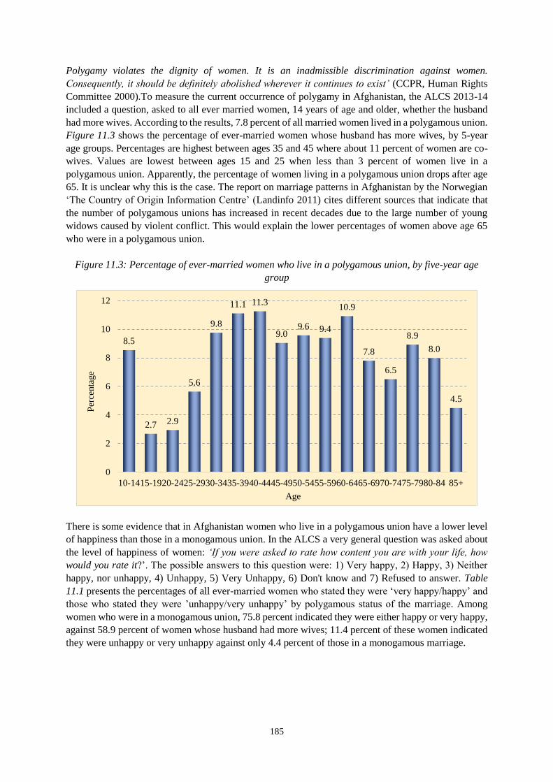
185
Polygamy violates the dignity of women. It is an inadmissible discrimination against women.
Consequently, it should be definitely abolished wherever it continues to exist’ (CCPR, Human Rights
Committee 2000).To measure the current occurrence of polygamy in Afghanistan, the ALCS 2013-14
included a question, asked to all ever married women, 14 years of age and older, whether the husband
had more wives. According to the results, 7.8 percent of all married women lived in a polygamous union.
Figure 11.3 shows the percentage of ever-married women whose husband has more wives, by 5-year
age groups. Percentages are highest between ages 35 and 45 where about 11 percent of women are co-
wives. Values are lowest between ages 15 and 25 when less than 3 percent of women live in a
polygamous union. Apparently, the percentage of women living in a polygamous union drops after age
65. It is unclear why this is the case. The report on marriage patterns in Afghanistan by the Norwegian
‘The Country of Origin Information Centre’ (Landinfo 2011) cites different sources that indicate that
the number of polygamous unions has increased in recent decades due to the large number of young
widows caused by violent conflict. This would explain the lower percentages of women above age 65
who were in a polygamous union.
Figure 11.3: Percentage of ever-married women who live in a polygamous union, by five-year age
group
There is some evidence that in Afghanistan women who live in a polygamous union have a lower level
of happiness than those in a monogamous union. In the ALCS a very general question was asked about
the level of happiness of women: ‘If you were asked to rate how content you are with your life, how
would you rate it?’. The possible answers to this question were: 1) Very happy, 2) Happy, 3) Neither
happy, nor unhappy, 4) Unhappy, 5) Very Unhappy, 6) Don't know and 7) Refused to answer. Table
11.1 presents the percentages of all ever-married women who stated they were ‘very happy/happy’ and
those who stated they were ’unhappy/very unhappy’ by polygamous status of the marriage. Among
women who were in a monogamous union, 75.8 percent indicated they were either happy or very happy,
against 58.9 percent of women whose husband had more wives; 11.4 percent of these women indicated
they were unhappy or very unhappy against only 4.4 percent of those in a monogamous marriage.
8.5
2.7 2.9
5.6
9.8
11.1 11.3
9.09.6 9.4
10.9
7.8
6.5
8.9
8.0
4.5
0
2
4
6
8
10
12
10-1415-1920-2425-2930-3435-3940-4445-4950-5455-5960-6465-6970-7475-7980-84 85+
Per
centa
ge
Age
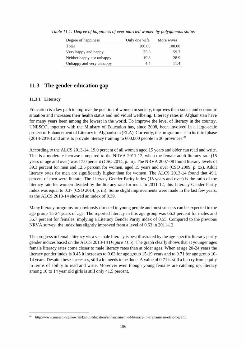
186
Table 11.1: Degree of happiness of ever married women by polygamous status
Degree of happiness Only one wife More wives
Total 100.00 100.00
Very happy and happy 75.8 59.7
Neither happy nor unhappy 19.8 28.9
Unhappy and very unhappy 4.4 11.4
11.3 The gender education gap
11.3.1 Literacy
Education is a key path to improve the position of women in society, improves their social and economic
situation and increases their health status and individual wellbeing. Literacy rates in Afghanistan have
for many years been among the lowest in the world. To improve the level of literacy in the country,
UNESCO, together with the Ministry of Education has, since 2008, been involved in a large-scale
project of Enhancement of Literacy in Afghanistan (ELA). Currently, the programme is in its third phase
(2014-2016) and aims to provide literacy training to 600,000 people in 30 provinces.61
According to the ALCS 2013-14, 19.0 percent of all women aged 15 years and older can read and write.
This is a moderate increase compared to the NRVA 2011-12, when the female adult literacy rate (15
years of age and over) was 17.0 percent (CSO 2014, p. iii). The NRVA 2007-08 found literacy levels of
39.3 percent for men and 12.5 percent for women, aged 15 years and over (CSO 2009, p. xx). Adult
literacy rates for men are significantly higher than for women. The ALCS 2013-14 found that 49.1
percent of men were literate. The Literacy Gender Parity index (15 years and over) is the ratio of the
literacy rate for women divided by the literacy rate for men. In 2011-12, this Literacy Gender Parity
index was equal to 0.37 (CSO 2014, p. iii). Some slight improvements were made in the last few years,
as the ALCS 2013-14 showed an index of 0.39.
Many literacy programs are obviously directed to young people and most success can be expected in the
age group 15-24 years of age. The reported literacy in this age group was 66.3 percent for males and
36.7 percent for females, implying a Literacy Gender Parity index of 0.55. Compared to the previous
NRVA survey, the index has slightly improved from a level of 0.53 in 2011-12.
The progress in female literacy vis à vis male literacy is best illustrated by the age-specific literacy parity
gender indices based on the ALCS 2013-14 (Figure 11.5). The graph clearly shows that at younger ages
female literacy rates come closer to male literacy rates than at older ages. When at age 20-24 years the
literacy gender index is 0.45 it increases to 0.63 for age group 15-19 years and to 0.71 for age group 10-
14 years. Despite these successes, still a lot needs to be done. A value of 0.71 is still a far cry from equity
in terms of ability to read and write. Moreover even though young females are catching up, literacy
among 10 to 14 year old girls is still only 41.5 percent.
61 http://www.unesco.org/new/en/kabul/education/enhancement-of-literacy-in-afghanistan-ela-program/
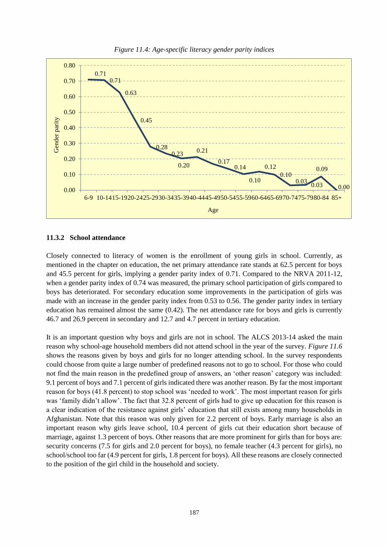
187
Figure 11.4: Age-specific literacy gender parity indices
11.3.2 School attendance
Closely connected to literacy of women is the enrollment of young girls in school. Currently, as
mentioned in the chapter on education, the net primary attendance rate stands at 62.5 percent for boys
and 45.5 percent for girls, implying a gender parity index of 0.71. Compared to the NRVA 2011-12,
when a gender parity index of 0.74 was measured, the primary school participation of girls compared to
boys has deteriorated. For secondary education some improvements in the participation of girls was
made with an increase in the gender parity index from 0.53 to 0.56. The gender parity index in tertiary
education has remained almost the same (0.42). The net attendance rate for boys and girls is currently
46.7 and 26.9 percent in secondary and 12.7 and 4.7 percent in tertiary education.
It is an important question why boys and girls are not in school. The ALCS 2013-14 asked the main
reason why school-age household members did not attend school in the year of the survey. Figure 11.6
shows the reasons given by boys and girls for no longer attending school. In the survey respondents
could choose from quite a large number of predefined reasons not to go to school. For those who could
not find the main reason in the predefined group of answers, an ‘other reason’ category was included:
9.1 percent of boys and 7.1 percent of girls indicated there was another reason. By far the most important
reason for boys (41.8 percent) to stop school was ‘needed to work’. The most important reason for girls
was ‘family didn’t allow’. The fact that 32.8 percent of girls had to give up education for this reason is
a clear indication of the resistance against girls’ education that still exists among many households in
Afghanistan. Note that this reason was only given for 2.2 percent of boys. Early marriage is also an
important reason why girls leave school, 10.4 percent of girls cut their education short because of
marriage, against 1.3 percent of boys. Other reasons that are more prominent for girls than for boys are:
security concerns (7.5 for girls and 2.0 percent for boys), no female teacher (4.3 percent for girls), no
school/school too far (4.9 percent for girls, 1.8 percent for boys). All these reasons are closely connected
to the position of the girl child in the household and society.
0.710.71
0.63
0.45
0.280.23
0.20
0.21
0.170.14
0.10
0.12
0.100.03
0.03
0.09
0.000.00
0.10
0.20
0.30
0.40
0.50
0.60
0.70
0.80
6-9 10-1415-1920-2425-2930-3435-3940-4445-4950-5455-5960-6465-6970-7475-7980-84 85+
Gen
der
par
ity
Age
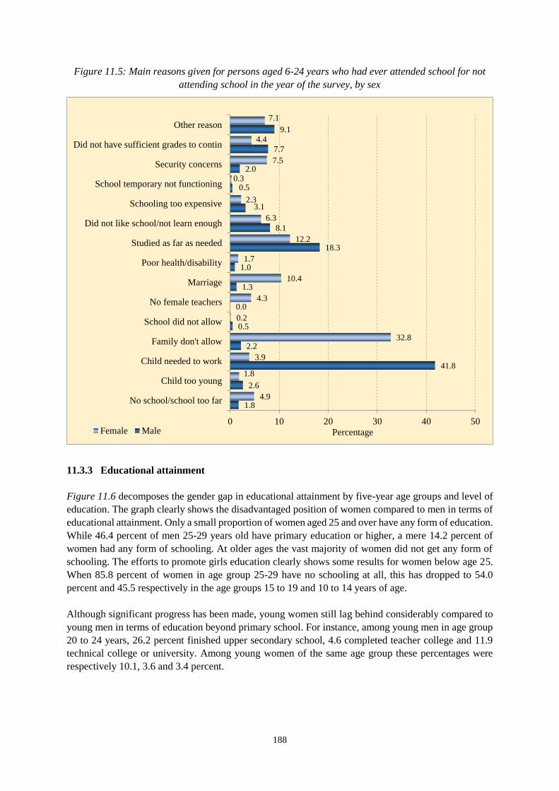
188
Figure 11.5: Main reasons given for persons aged 6-24 years who had ever attended school for not
attending school in the year of the survey, by sex
11.3.3 Educational attainment
Figure 11.6 decomposes the gender gap in educational attainment by five-year age groups and level of
education. The graph clearly shows the disadvantaged position of women compared to men in terms of
educational attainment. Only a small proportion of women aged 25 and over have any form of education.
While 46.4 percent of men 25-29 years old have primary education or higher, a mere 14.2 percent of
women had any form of schooling. At older ages the vast majority of women did not get any form of
schooling. The efforts to promote girls education clearly shows some results for women below age 25.
When 85.8 percent of women in age group 25-29 have no schooling at all, this has dropped to 54.0
percent and 45.5 respectively in the age groups 15 to 19 and 10 to 14 years of age.
Although significant progress has been made, young women still lag behind considerably compared to
young men in terms of education beyond primary school. For instance, among young men in age group
20 to 24 years, 26.2 percent finished upper secondary school, 4.6 completed teacher college and 11.9
technical college or university. Among young women of the same age group these percentages were
respectively 10.1, 3.6 and 3.4 percent.
1.8
2.6
41.8
2.2
0.5
0.0
1.3
1.0
18.3
8.1
3.1
0.5
2.0
7.7
9.1
4.9
1.8
3.9
32.8
0.2
4.3
10.4
1.7
12.2
6.3
2.3
0.3
7.5
4.4
7.1
0 10 20 30 40 50
No school/school too far
Child too young
Child needed to work
Family don't allow
School did not allow
No female teachers
Marriage
Poor health/disability
Studied as far as needed
Did not like school/not learn enough
Schooling too expensive
School temporary not functioning
Security concerns
Did not have sufficient grades to contin
Other reason
PercentageFemale Male
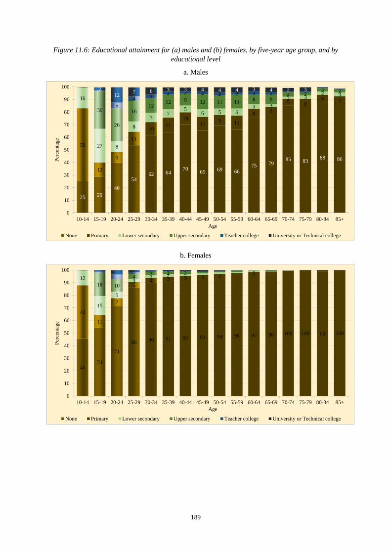
189
Figure 11.6: Educational attainment for (a) males and (b) females, by five-year age group, and by
educational level
a. Males
b. Females
25 29
40
5462 64
7065
69 6675 79
85 8388 86
58
12
9
11
1011
1011
9 11
85
5 86 7
16
27 8
8
77
56 5 6
3 3
2 32 3
30
26
1612
12 9 12 11 11 8 84 2
3 2
5
4 32 2 2 2 2 3 2
212
7 6 3 3 4 4 4 3 4 2 3
0
10
20
30
40
50
60
70
80
90
100
10-14 15-19 20-24 25-29 30-34 35-39 40-44 45-49 50-54 55-59 60-64 65-69 70-74 75-79 80-84 85+
Per
centa
ge
Age
None Primary Lower secondary Upper secondary Teacher college University or Technical college
4554
71
8690 91 92 93 94 96 97 98 100 100 99 100
42
11
7
54 3 3 3 2 2
12
15
5
32 2
18 10
43 2 2
0
10
20
30
40
50
60
70
80
90
100
10-14 15-19 20-24 25-29 30-34 35-39 40-44 45-49 50-54 55-59 60-64 65-69 70-74 75-79 80-84 85+
Per
centa
ge
Age
None Primary Lower secondary Upper secondary Teacher college University or Technical college
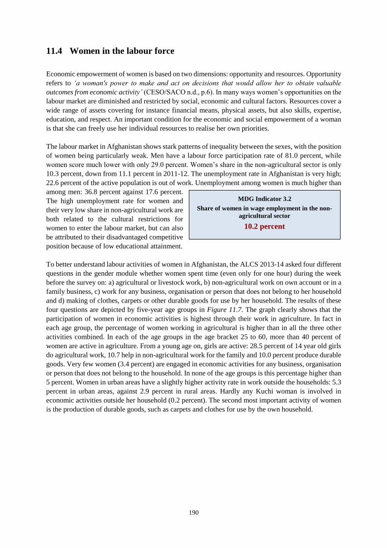
190
11.4 Women in the labour force
Economic empowerment of women is based on two dimensions: opportunity and resources. Opportunity
refers to ‘a woman's power to make and act on decisions that would allow her to obtain valuable
outcomes from economic activity’ (CESO/SACO n.d., p.6). In many ways women’s opportunities on the
labour market are diminished and restricted by social, economic and cultural factors. Resources cover a
wide range of assets covering for instance financial means, physical assets, but also skills, expertise,
education, and respect. An important condition for the economic and social empowerment of a woman
is that she can freely use her individual resources to realise her own priorities.
The labour market in Afghanistan shows stark patterns of inequality between the sexes, with the position
of women being particularly weak. Men have a labour force participation rate of 81.0 percent, while
women score much lower with only 29.0 percent. Women’s share in the non-agricultural sector is only
10.3 percent, down from 11.1 percent in 2011-12. The unemployment rate in Afghanistan is very high;
22.6 percent of the active population is out of work. Unemployment among women is much higher than
among men: 36.8 percent against 17.6 percent.
The high unemployment rate for women and
their very low share in non-agricultural work are
both related to the cultural restrictions for
women to enter the labour market, but can also
be attributed to their disadvantaged competitive
position because of low educational attainment.
To better understand labour activities of women in Afghanistan, the ALCS 2013-14 asked four different
questions in the gender module whether women spent time (even only for one hour) during the week
before the survey on: a) agricultural or livestock work, b) non-agricultural work on own account or in a
family business, c) work for any business, organisation or person that does not belong to her household
and d) making of clothes, carpets or other durable goods for use by her household. The results of these
four questions are depicted by five-year age groups in Figure 11.7. The graph clearly shows that the
participation of women in economic activities is highest through their work in agriculture. In fact in
each age group, the percentage of women working in agricultural is higher than in all the three other
activities combined. In each of the age groups in the age bracket 25 to 60, more than 40 percent of
women are active in agriculture. From a young age on, girls are active: 28.5 percent of 14 year old girls
do agricultural work, 10.7 help in non-agricultural work for the family and 10.0 percent produce durable
goods. Very few women (3.4 percent) are engaged in economic activities for any business, organisation
or person that does not belong to the household. In none of the age groups is this percentage higher than
5 percent. Women in urban areas have a slightly higher activity rate in work outside the households: 5.3
percent in urban areas, against 2.9 percent in rural areas. Hardly any Kuchi woman is involved in
economic activities outside her household (0.2 percent). The second most important activity of women
is the production of durable goods, such as carpets and clothes for use by the own household.
MDG Indicator 3.2
Share of women in wage employment in the non-
agricultural sector
10.2 percent
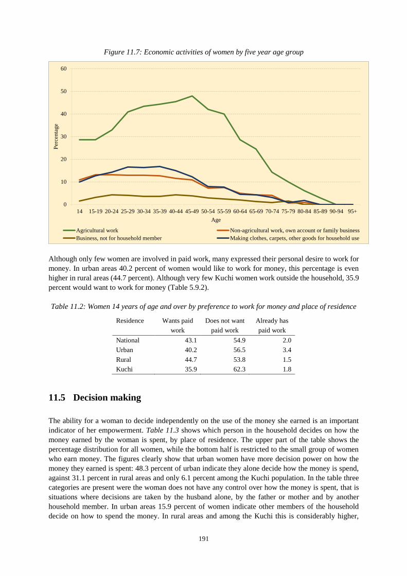
191
Figure 11.7: Economic activities of women by five year age group
Although only few women are involved in paid work, many expressed their personal desire to work for
money. In urban areas 40.2 percent of women would like to work for money, this percentage is even
higher in rural areas (44.7 percent). Although very few Kuchi women work outside the household, 35.9
percent would want to work for money (Table 5.9.2).
Table 11.2: Women 14 years of age and over by preference to work for money and place of residence
Residence Wants paid Does not want Already has
work paid work paid work
National 43.1 54.9 2.0
Urban 40.2 56.5 3.4
Rural 44.7 53.8 1.5
Kuchi 35.9 62.3 1.8
11.5 Decision making
The ability for a woman to decide independently on the use of the money she earned is an important
indicator of her empowerment. Table 11.3 shows which person in the household decides on how the
money earned by the woman is spent, by place of residence. The upper part of the table shows the
percentage distribution for all women, while the bottom half is restricted to the small group of women
who earn money. The figures clearly show that urban women have more decision power on how the
money they earned is spent: 48.3 percent of urban indicate they alone decide how the money is spend,
against 31.1 percent in rural areas and only 6.1 percent among the Kuchi population. In the table three
categories are present were the woman does not have any control over how the money is spent, that is
situations where decisions are taken by the husband alone, by the father or mother and by another
household member. In urban areas 15.9 percent of women indicate other members of the household
decide on how to spend the money. In rural areas and among the Kuchi this is considerably higher,
0
10
20
30
40
50
60
14 15-19 20-24 25-29 30-34 35-39 40-44 45-49 50-54 55-59 60-64 65-69 70-74 75-79 80-84 85-89 90-94 95+
Per
centa
ge
Age
Agricultural work Non-agricultural work, own account or family business
Business, not for household member Making clothes, carpets, other goods for household use
192
respectively 32.0 percent and 30.3 percent. In many cases women have some decision power but share
it with either their husband or other household members. Although only 6.1 percent of Kuchi women
could decide independently how to spend the money, 63.6 percent have some influence, in consultation
with the husband or other household members.
Table 11.3: Women 14 years of age and over, by person who decides how money earned by the woman
is spent, and by residence (in percentages)
Residence Total Don't Woman Husband Father Other Herself Herself
earn any alone alone or household and and other
money mother member husband household
member
National 100.0 83.6 5.5 1.8 2.2 0.7 3.0 3.2
Urban 100.0 87.2 6.2 0.5 1.1 0.4 1.8 2.8
Rural 100.0 82.1 5.6 2.2 2.7 0.9 3.4 3.2
Kuchi 100.0 85.5 0.9 2.9 0.9 0.6 3.3 5.9
For women who earn money
National 100.0 n.a. 33.7 10.9 13.3 4.5 18.3 19.3
Urban 100.0 n.a. 48.3 4.0 8.4 3.5 14.3 21.6
Rural 100.0 n.a. 31.1 12.3 15.0 4.7 19.2 17.6
Kuchi 100.0 n.a. 6.1 20.1 6.4 3.8 22.9 40.7
One would expect that younger women could decide more independently on how to spend their self-
earned money, but the ALCS 2013-14 does not support this supposition (data not shown here).
Percentages for all age groups 14 to 70 years of age hovering between 30 and 40 percent, without any
clear age pattern.
Many women in Afghanistan possess livestock. It should not come as a surprise that more women in
rural areas and among the Kuchi have their own animals; 32.5 percent in rural, 6.6 percent in urban areas
and 35 percent among Kuchi women. Figure 11.8 shows the percentage of women who have one or
more animals of a particular type. The possession of livestock by women rises with age, reaches a peak
in the age group 45-49, and then drops again. Chickens are the livestock most often possessed by women,
but more than just a few women have their own cows, goats and sheep.
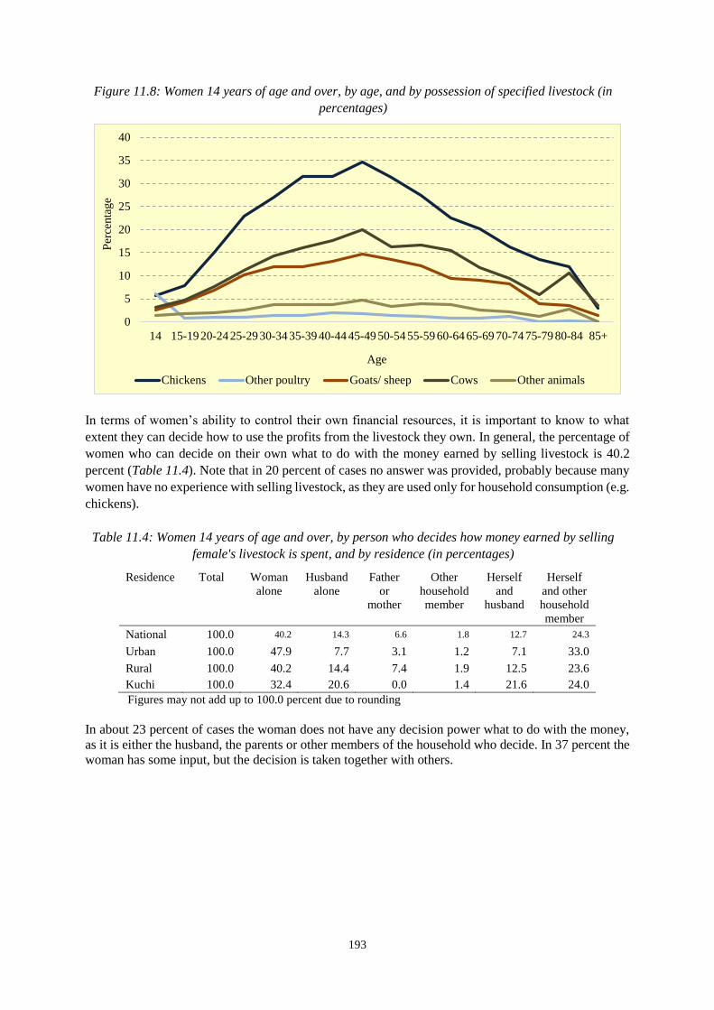
193
Figure 11.8: Women 14 years of age and over, by age, and by possession of specified livestock (in
percentages)
In terms of women’s ability to control their own financial resources, it is important to know to what
extent they can decide how to use the profits from the livestock they own. In general, the percentage of
women who can decide on their own what to do with the money earned by selling livestock is 40.2
percent (Table 11.4). Note that in 20 percent of cases no answer was provided, probably because many
women have no experience with selling livestock, as they are used only for household consumption (e.g.
chickens).
Table 11.4: Women 14 years of age and over, by person who decides how money earned by selling
female's livestock is spent, and by residence (in percentages)
Residence Total Woman Husband Father Other Herself Herself
alone alone or household and and other
mother member husband household
member
National 100.0 40.2 14.3 6.6 1.8 12.7 24.3
Urban 100.0 47.9 7.7 3.1 1.2 7.1 33.0
Rural 100.0 40.2 14.4 7.4 1.9 12.5 23.6
Kuchi 100.0 32.4 20.6 0.0 1.4 21.6 24.0
Figures may not add up to 100.0 percent due to rounding
In about 23 percent of cases the woman does not have any decision power what to do with the money,
as it is either the husband, the parents or other members of the household who decide. In 37 percent the
woman has some input, but the decision is taken together with others.
0
5
10
15
20
25
30
35
40
14 15-19 20-24 25-29 30-34 35-39 40-44 45-49 50-54 55-59 60-64 65-69 70-74 75-79 80-84 85+
Per
centa
ge
Age
Chickens Other poultry Goats/ sheep Cows Other animals
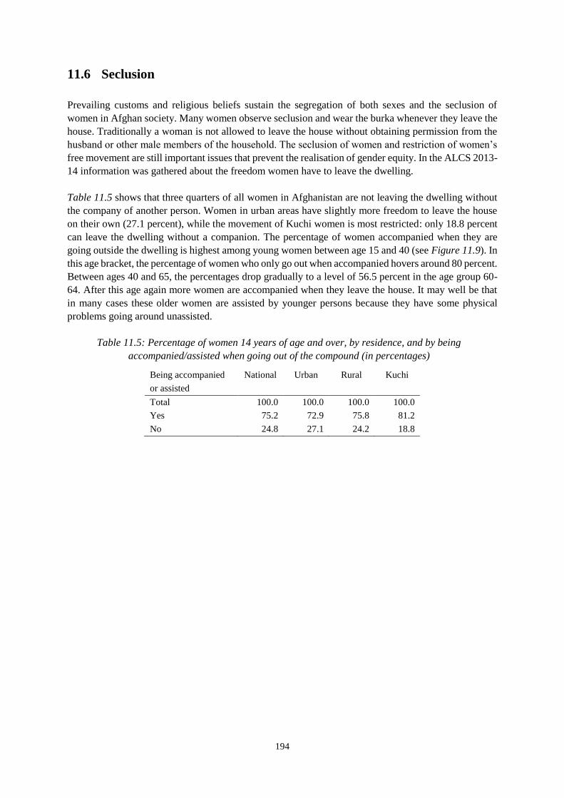
194
11.6 Seclusion
Prevailing customs and religious beliefs sustain the segregation of both sexes and the seclusion of
women in Afghan society. Many women observe seclusion and wear the burka whenever they leave the
house. Traditionally a woman is not allowed to leave the house without obtaining permission from the
husband or other male members of the household. The seclusion of women and restriction of women’s
free movement are still important issues that prevent the realisation of gender equity. In the ALCS 2013-
14 information was gathered about the freedom women have to leave the dwelling.
Table 11.5 shows that three quarters of all women in Afghanistan are not leaving the dwelling without
the company of another person. Women in urban areas have slightly more freedom to leave the house
on their own (27.1 percent), while the movement of Kuchi women is most restricted: only 18.8 percent
can leave the dwelling without a companion. The percentage of women accompanied when they are
going outside the dwelling is highest among young women between age 15 and 40 (see Figure 11.9). In
this age bracket, the percentage of women who only go out when accompanied hovers around 80 percent.
Between ages 40 and 65, the percentages drop gradually to a level of 56.5 percent in the age group 60-
64. After this age again more women are accompanied when they leave the house. It may well be that
in many cases these older women are assisted by younger persons because they have some physical
problems going around unassisted.
Table 11.5: Percentage of women 14 years of age and over, by residence, and by being
accompanied/assisted when going out of the compound (in percentages)
Being accompanied National Urban Rural Kuchi
or assisted
Total 100.0 100.0 100.0 100.0
Yes 75.2 72.9 75.8 81.2
No 24.8 27.1 24.2 18.8
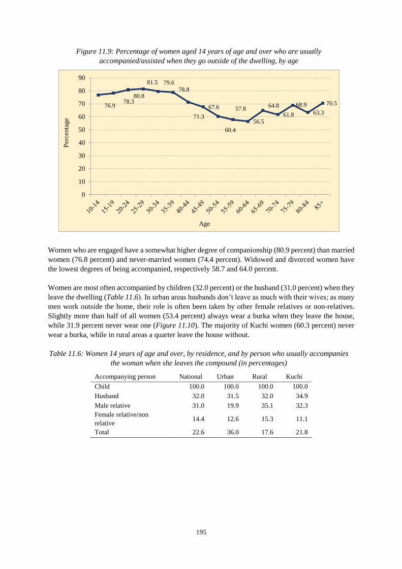
195
Figure 11.9: Percentage of women aged 14 years of age and over who are usually
accompanied/assisted when they go outside of the dwelling, by age
Women who are engaged have a somewhat higher degree of companionship (80.9 percent) than married
women (76.8 percent) and never-married women (74.4 percent). Widowed and divorced women have
the lowest degrees of being accompanied, respectively 58.7 and 64.0 percent.
Women are most often accompanied by children (32.0 percent) or the husband (31.0 percent) when they
leave the dwelling (Table 11.6). In urban areas husbands don’t leave as much with their wives; as many
men work outside the home, their role is often been taken by other female relatives or non-relatives.
Slightly more than half of all women (53.4 percent) always wear a burka when they leave the house,
while 31.9 percent never wear one (Figure 11.10). The majority of Kuchi women (60.3 percent) never
wear a burka, while in rural areas a quarter leave the house without.
Table 11.6: Women 14 years of age and over, by residence, and by person who usually accompanies
the woman when she leaves the compound (in percentages)
Accompanying person National Urban Rural Kuchi
Child 100.0 100.0 100.0 100.0
Husband 32.0 31.5 32.0 34.9
Male relative 31.0 19.9 35.1 32.3
Female relative/non
relative 14.4 12.6 15.3 11.1
Total 22.6 36.0 17.6 21.8
76.978.3
80.8
81.5 79.678.8
71.3
67.6
60.4
57.8
56.5
64.8
61.8
68.9
63.3
70.5
0
10
20
30
40
50
60
70
80
90
Per
centa
ge
Age
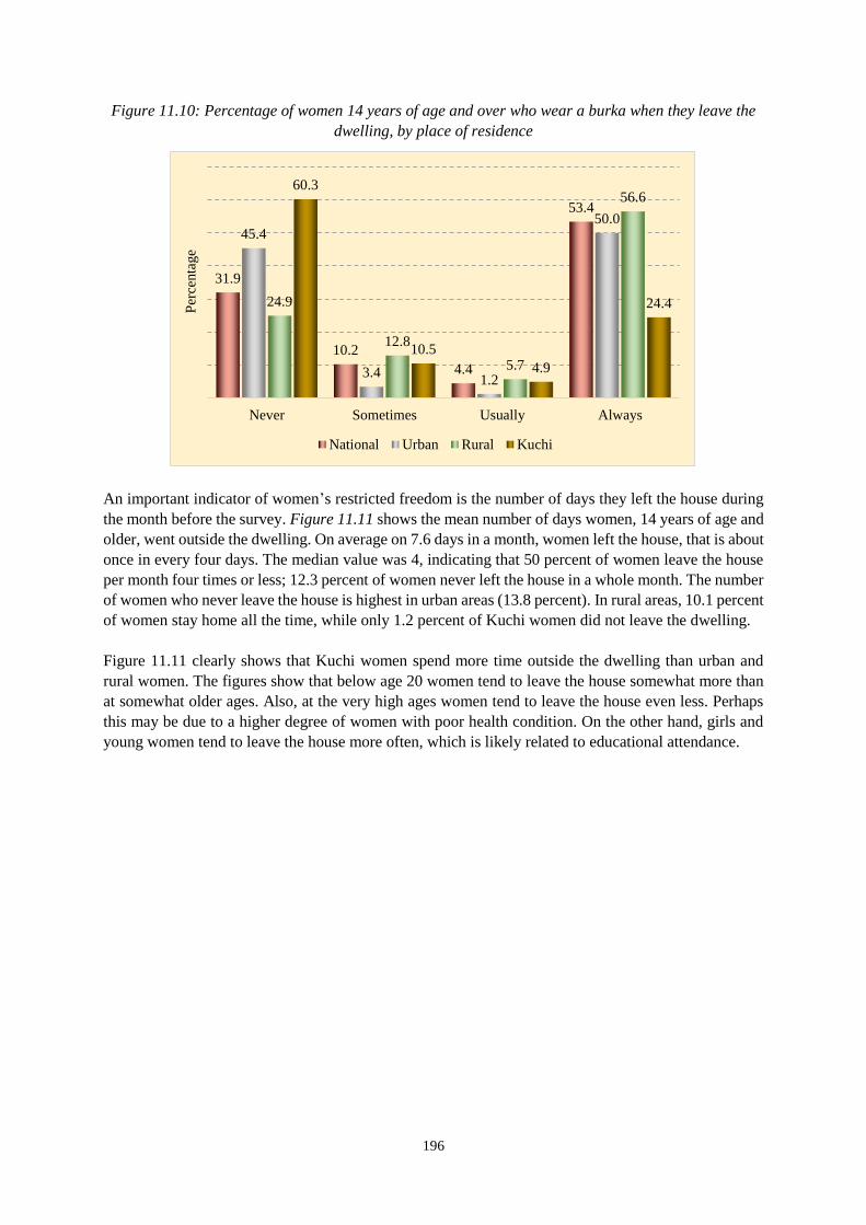
196
Figure 11.10: Percentage of women 14 years of age and over who wear a burka when they leave the
dwelling, by place of residence
An important indicator of women’s restricted freedom is the number of days they left the house during
the month before the survey. Figure 11.11 shows the mean number of days women, 14 years of age and
older, went outside the dwelling. On average on 7.6 days in a month, women left the house, that is about
once in every four days. The median value was 4, indicating that 50 percent of women leave the house
per month four times or less; 12.3 percent of women never left the house in a whole month. The number
of women who never leave the house is highest in urban areas (13.8 percent). In rural areas, 10.1 percent
of women stay home all the time, while only 1.2 percent of Kuchi women did not leave the dwelling.
Figure 11.11 clearly shows that Kuchi women spend more time outside the dwelling than urban and
rural women. The figures show that below age 20 women tend to leave the house somewhat more than
at somewhat older ages. Also, at the very high ages women tend to leave the house even less. Perhaps
this may be due to a higher degree of women with poor health condition. On the other hand, girls and
young women tend to leave the house more often, which is likely related to educational attendance.
31.9
10.2
4.4
53.4
45.4
3.41.2
50.0
24.9
12.8
5.7
56.660.3
10.5
4.9
24.4
Never Sometimes Usually Always
Per
centa
ge
National Urban Rural Kuchi
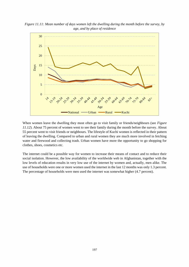
197
Figure 11.11: Mean number of days women left the dwelling during the month before the survey, by
age, and by place of residence
When women leave the dwelling they most often go to visit family or friends/neighbours (see Figure
11.12). About 75 percent of women went to see their family during the month before the survey. About
55 percent went to visit friends or neighbours. The lifestyle of Kuchi women is reflected in their pattern
of leaving the dwelling. Compared to urban and rural women they are much more involved in fetching
water and firewood and collecting trash. Urban women have more the opportunity to go shopping for
clothes, shoes, cosmetics etc.
The internet could be a possible way for women to increase their means of contact and to reduce their
social isolation. However, the low availability of the worldwide web in Afghanistan, together with the
low levels of education results in very low use of the internet by women and, actually, men alike. The
use of households were one or more women used the internet in the last 12 months was only 1.3 percent.
The percentage of households were men used the internet was somewhat higher (4.7 percent).
0
5
10
15
20
25
30D
ays
Age
National Urban Rural Kuchi
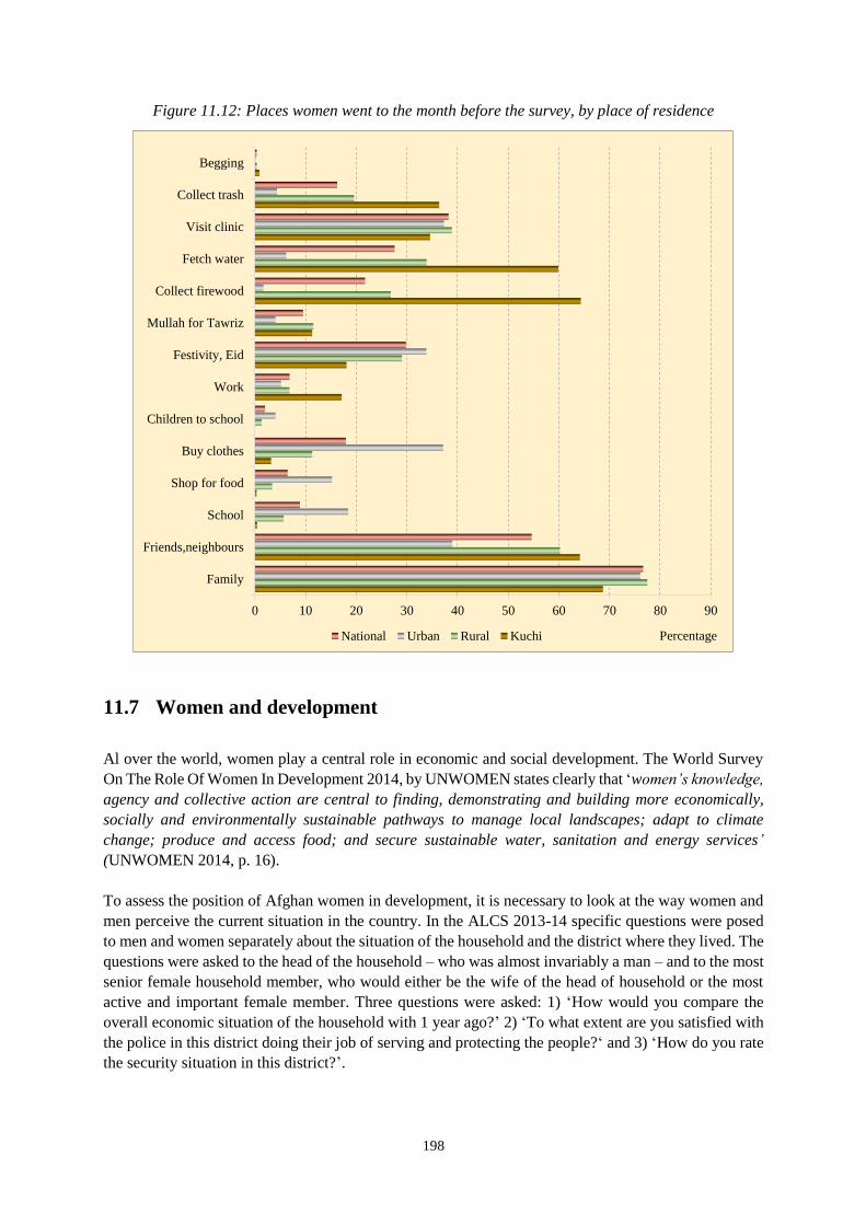
198
Figure 11.12: Places women went to the month before the survey, by place of residence
11.7 Women and development
Al over the world, women play a central role in economic and social development. The World Survey
On The Role Of Women In Development 2014, by UNWOMEN states clearly that ‘women’s knowledge,
agency and collective action are central to finding, demonstrating and building more economically,
socially and environmentally sustainable pathways to manage local landscapes; adapt to climate
change; produce and access food; and secure sustainable water, sanitation and energy services’
(UNWOMEN 2014, p. 16).
To assess the position of Afghan women in development, it is necessary to look at the way women and
men perceive the current situation in the country. In the ALCS 2013-14 specific questions were posed
to men and women separately about the situation of the household and the district where they lived. The
questions were asked to the head of the household – who was almost invariably a man – and to the most
senior female household member, who would either be the wife of the head of household or the most
active and important female member. Three questions were asked: 1) ‘How would you compare the
overall economic situation of the household with 1 year ago?’ 2) ‘To what extent are you satisfied with
the police in this district doing their job of serving and protecting the people?‘ and 3) ‘How do you rate
the security situation in this district?’.
0 10 20 30 40 50 60 70 80 90
Family
Friends,neighbours
School
Shop for food
Buy clothes
Children to school
Work
Festivity, Eid
Mullah for Tawriz
Collect firewood
Fetch water
Visit clinic
Collect trash
Begging
PercentageNational Urban Rural Kuchi
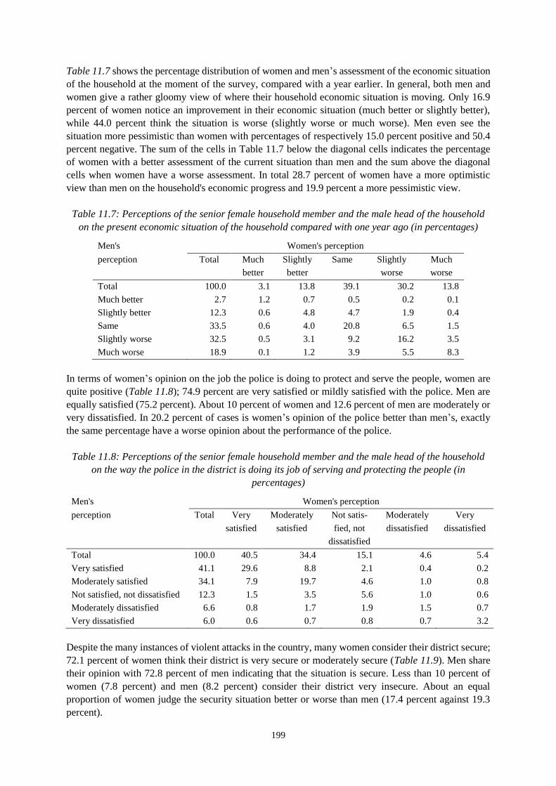
199
Table 11.7 shows the percentage distribution of women and men’s assessment of the economic situation
of the household at the moment of the survey, compared with a year earlier. In general, both men and
women give a rather gloomy view of where their household economic situation is moving. Only 16.9
percent of women notice an improvement in their economic situation (much better or slightly better),
while 44.0 percent think the situation is worse (slightly worse or much worse). Men even see the
situation more pessimistic than women with percentages of respectively 15.0 percent positive and 50.4
percent negative. The sum of the cells in Table 11.7 below the diagonal cells indicates the percentage
of women with a better assessment of the current situation than men and the sum above the diagonal
cells when women have a worse assessment. In total 28.7 percent of women have a more optimistic
view than men on the household's economic progress and 19.9 percent a more pessimistic view.
Table 11.7: Perceptions of the senior female household member and the male head of the household
on the present economic situation of the household compared with one year ago (in percentages)
Men's Women's perception
perception Total Much Slightly Same Slightly Much
better better worse worse
Total 100.0 3.1 13.8 39.1 30.2 13.8
Much better 2.7 1.2 0.7 0.5 0.2 0.1
Slightly better 12.3 0.6 4.8 4.7 1.9 0.4
Same 33.5 0.6 4.0 20.8 6.5 1.5
Slightly worse 32.5 0.5 3.1 9.2 16.2 3.5
Much worse 18.9 0.1 1.2 3.9 5.5 8.3
In terms of women’s opinion on the job the police is doing to protect and serve the people, women are
quite positive (Table 11.8); 74.9 percent are very satisfied or mildly satisfied with the police. Men are
equally satisfied (75.2 percent). About 10 percent of women and 12.6 percent of men are moderately or
very dissatisfied. In 20.2 percent of cases is women’s opinion of the police better than men’s, exactly
the same percentage have a worse opinion about the performance of the police.
Table 11.8: Perceptions of the senior female household member and the male head of the household
on the way the police in the district is doing its job of serving and protecting the people (in
percentages)
Men's Women's perception
perception Total Very Moderately Not satis- Moderately Very
satisfied satisfied fied, not dissatisfied dissatisfied
dissatisfied
Total 100.0 40.5 34.4 15.1 4.6 5.4
Very satisfied 41.1 29.6 8.8 2.1 0.4 0.2
Moderately satisfied 34.1 7.9 19.7 4.6 1.0 0.8
Not satisfied, not dissatisfied 12.3 1.5 3.5 5.6 1.0 0.6
Moderately dissatisfied 6.6 0.8 1.7 1.9 1.5 0.7
Very dissatisfied 6.0 0.6 0.7 0.8 0.7 3.2
Despite the many instances of violent attacks in the country, many women consider their district secure;
72.1 percent of women think their district is very secure or moderately secure (Table 11.9). Men share
their opinion with 72.8 percent of men indicating that the situation is secure. Less than 10 percent of
women (7.8 percent) and men (8.2 percent) consider their district very insecure. About an equal
proportion of women judge the security situation better or worse than men (17.4 percent against 19.3
percent).
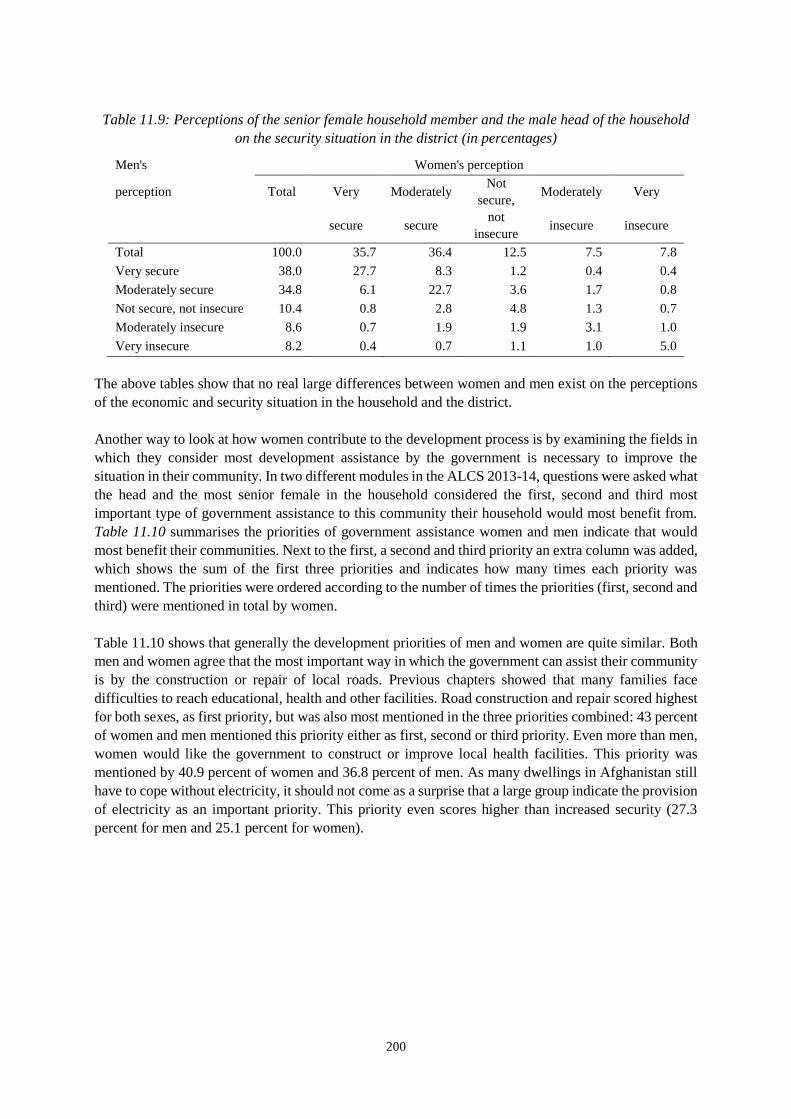
200
Table 11.9: Perceptions of the senior female household member and the male head of the household
on the security situation in the district (in percentages)
Men's Women's perception
perception Total Very Moderately Not
secure, Moderately Very
secure secure not
insecure insecure insecure
Total 100.0 35.7 36.4 12.5 7.5 7.8
Very secure 38.0 27.7 8.3 1.2 0.4 0.4
Moderately secure 34.8 6.1 22.7 3.6 1.7 0.8
Not secure, not insecure 10.4 0.8 2.8 4.8 1.3 0.7
Moderately insecure 8.6 0.7 1.9 1.9 3.1 1.0
Very insecure 8.2 0.4 0.7 1.1 1.0 5.0
The above tables show that no real large differences between women and men exist on the perceptions
of the economic and security situation in the household and the district.
Another way to look at how women contribute to the development process is by examining the fields in
which they consider most development assistance by the government is necessary to improve the
situation in their community. In two different modules in the ALCS 2013-14, questions were asked what
the head and the most senior female in the household considered the first, second and third most
important type of government assistance to this community their household would most benefit from.
Table 11.10 summarises the priorities of government assistance women and men indicate that would
most benefit their communities. Next to the first, a second and third priority an extra column was added,
which shows the sum of the first three priorities and indicates how many times each priority was
mentioned. The priorities were ordered according to the number of times the priorities (first, second and
third) were mentioned in total by women.
Table 11.10 shows that generally the development priorities of men and women are quite similar. Both
men and women agree that the most important way in which the government can assist their community
is by the construction or repair of local roads. Previous chapters showed that many families face
difficulties to reach educational, health and other facilities. Road construction and repair scored highest
for both sexes, as first priority, but was also most mentioned in the three priorities combined: 43 percent
of women and men mentioned this priority either as first, second or third priority. Even more than men,
women would like the government to construct or improve local health facilities. This priority was
mentioned by 40.9 percent of women and 36.8 percent of men. As many dwellings in Afghanistan still
have to cope without electricity, it should not come as a surprise that a large group indicate the provision
of electricity as an important priority. This priority even scores higher than increased security (27.3
percent for men and 25.1 percent for women).
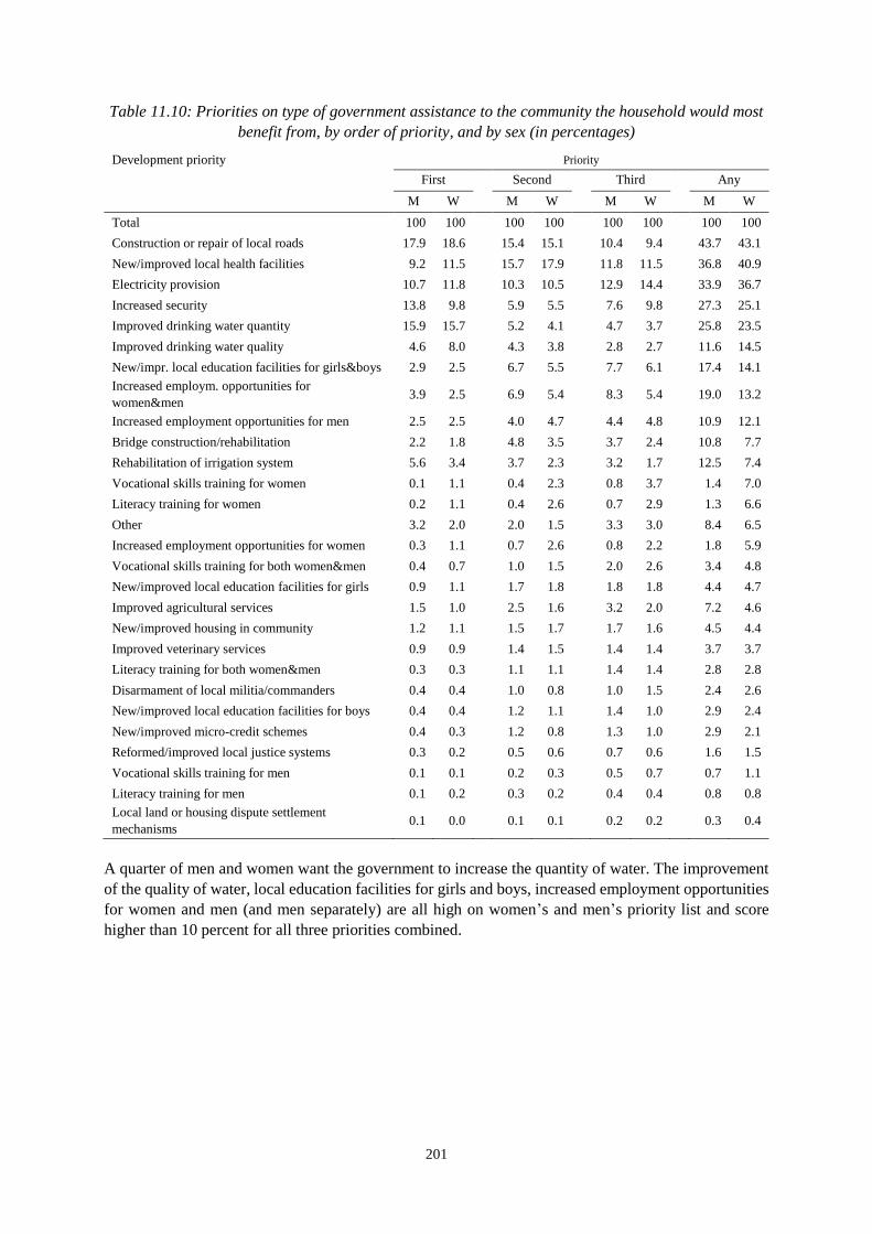
201
Table 11.10: Priorities on type of government assistance to the community the household would most
benefit from, by order of priority, and by sex (in percentages)
Development priority Priority
First Second Third Any
M W M W M W M W
Total 100 100 100 100 100 100 100 100
Construction or repair of local roads 17.9 18.6 15.4 15.1 10.4 9.4 43.7 43.1
New/improved local health facilities 9.2 11.5 15.7 17.9 11.8 11.5 36.8 40.9
Electricity provision 10.7 11.8 10.3 10.5 12.9 14.4 33.9 36.7
Increased security 13.8 9.8 5.9 5.5 7.6 9.8 27.3 25.1
Improved drinking water quantity 15.9 15.7 5.2 4.1 4.7 3.7 25.8 23.5
Improved drinking water quality 4.6 8.0 4.3 3.8 2.8 2.7 11.6 14.5
New/impr. local education facilities for girls&boys 2.9 2.5 6.7 5.5 7.7 6.1 17.4 14.1
Increased employm. opportunities for
women&men 3.9 2.5 6.9 5.4 8.3 5.4 19.0 13.2
Increased employment opportunities for men 2.5 2.5 4.0 4.7 4.4 4.8 10.9 12.1
Bridge construction/rehabilitation 2.2 1.8 4.8 3.5 3.7 2.4 10.8 7.7
Rehabilitation of irrigation system 5.6 3.4 3.7 2.3 3.2 1.7 12.5 7.4
Vocational skills training for women 0.1 1.1 0.4 2.3 0.8 3.7 1.4 7.0
Literacy training for women 0.2 1.1 0.4 2.6 0.7 2.9 1.3 6.6
Other 3.2 2.0 2.0 1.5 3.3 3.0 8.4 6.5
Increased employment opportunities for women 0.3 1.1 0.7 2.6 0.8 2.2 1.8 5.9
Vocational skills training for both women&men 0.4 0.7 1.0 1.5 2.0 2.6 3.4 4.8
New/improved local education facilities for girls 0.9 1.1 1.7 1.8 1.8 1.8 4.4 4.7
Improved agricultural services 1.5 1.0 2.5 1.6 3.2 2.0 7.2 4.6
New/improved housing in community 1.2 1.1 1.5 1.7 1.7 1.6 4.5 4.4
Improved veterinary services 0.9 0.9 1.4 1.5 1.4 1.4 3.7 3.7
Literacy training for both women&men 0.3 0.3 1.1 1.1 1.4 1.4 2.8 2.8
Disarmament of local militia/commanders 0.4 0.4 1.0 0.8 1.0 1.5 2.4 2.6
New/improved local education facilities for boys 0.4 0.4 1.2 1.1 1.4 1.0 2.9 2.4
New/improved micro-credit schemes 0.4 0.3 1.2 0.8 1.3 1.0 2.9 2.1
Reformed/improved local justice systems 0.3 0.2 0.5 0.6 0.7 0.6 1.6 1.5
Vocational skills training for men 0.1 0.1 0.2 0.3 0.5 0.7 0.7 1.1
Literacy training for men 0.1 0.2 0.3 0.2 0.4 0.4 0.8 0.8
Local land or housing dispute settlement
mechanisms 0.1 0.0 0.1 0.1 0.2 0.2 0.3 0.4
A quarter of men and women want the government to increase the quantity of water. The improvement
of the quality of water, local education facilities for girls and boys, increased employment opportunities
for women and men (and men separately) are all high on women’s and men’s priority list and score
higher than 10 percent for all three priorities combined.
202
12 HOUSING AND HOUSEHOLD AMENITIES
Summary. Housing conditions of the Afghan population are overall poor, but improving, with large
differences between urban and rural communities and among provinces. The most impressive
improvement has been observed in the percentage on people having access to safe water, which increased
at national level from 46 to 65 percent in only three years, reaching the MDGS target of 61.5 percent for
2020 more than five years in advance. In addition, the proportion of households with access to any source
of electricity has increased significantly, from 69 to 89 percent. Other improvements are registered in a
slight decrease of the urban slum population, use of solid fuels, and in a slight increase of improved
sanitation, access to roads and use of communication means.
Housing tenure, which can be seen as a useful proxy for income or wealth of people, is characterized by
high-levels of owner-occupied dwellings, with almost 90 percent of households – more in rural than in
urban areas - owning dwellings. The majority of the Afghan households live in single-family houses –
more in rural than in urban areas. About 60 percent of the entire number of permanent dwellings in the
country have been constructed after 1995, but only less than 3 percent in the last three years. Traditional
mud houses continue to form the majority of housing in Afghanistan, with external walls made of mud
bricks (68 percent) and roofs constructed with wood and mud (74 percent). Dwellings have
approximately the same number of rooms in urban and rural areas. Around one-third of the dwellings
have two rooms and close to another 40 percent has three or four rooms. Kuchi households lives in the
majority in one tent, and in about 30 percent in two tents.
The percentage of urban population living in slums is almost 74 percent of the total urban population in
Afghanistan (almost 5 million people). Slum dwellers, as defined by the MDG indicator 7.10, are still a
very significant number, even if their number and proportion have slight decreased in comparison to the
2011-12 NRVA. This indicator is affected by the high level of overcrowding, high number of dwellings
made of non-durable material, lack of access to improved sanitation and lack of access to improved
water supply.
The figure for safe drinking water (65 percent of the population uses improved drinking water sources –
MDG Indicator 7.8) showed, however, a very significant improvement compared to 2007-08, when it was
only 27 percent. The situation improved in rural areas in particular, where the percentage using
improved sources increased from 20 (2007-08) to 58, but relevant disparities remain at geographic level:
in seven provinces, the percentage is below 30 percent. The situation with regard to sanitation improved
slightly (4.5 percent more compared to 2011-12 NRVA data), but continues to be poor, with only 39
percent of the population having access to improved sanitation (13 percent if using the old definition,
which did not include the category of covered pit latrines as improved sanitation facilities). The still
widespread lack of basic infrastructure for water and sanitation implies high risks of potentially fatal
diseases, and is especially detrimental for the health and survival chances of infants and young children.
Physical access to rural communities is often problematic in terms of access to drivable roads. However,
almost 93 percent of households reported to have access to their dwellings by an unpaved or paved road
that is in a distance of less than 1 kilometer, showing a remarkable progress compared to 2011-12 NRVA
data.
Health conditions in the household are further impaired by the use of solid fuels for cooking (76 percent)
and heating (95 percent), with minor improvements in the last three years. Solid fuels are largely used
over the country for heating purposes, but only by the 27 percent of the population in urban areas. The
most widespread source of electricity at national level is solar and wind energy, which account for 48
percent, more than the double of the 22 percent registered in the 2011-12 NRVA data. It is the most
frequently reported source of electricity in rural areas and among the Kuchi population. Internet is used
only by 2 percent of the population, while the use of mobile telephones is rapidly increasing among the
Afghan population.
203
12.1 Introduction
The housing situation of a population is often a direct reflection of their living conditions and socio-
economic development. Insufficient income force people to live in dwellings with low conditions.
Inappropriate housing may have consequences towards promiscuity, lesser protection against diseases,
difficulty to sleep and rest, difficulty for children to do school homework, fire hazards, family conflicts,
lesser social interaction, etc. Poverty may also entail inability to afford heating, cooking and cooling,
and basic household amenities.
Often, sanitation systems are insufficient, drinking water unavailable or remote, evacuation and rescue
difficult in emergencies. In some poor neighbourhoods, waste is not removed, thus creating sources of
epidemics and other health problems. Poor neighbourhoods also often lack schools, playing grounds,
sports and entertainment facilities, and may sometimes be unsafe. Lack of access to transport and
telephone makes it more difficult to find work or to exert an independent economic activity. Difficulties
in road access limits both access to work and to recreation. Poverty of the household makes it impossible
sometimes to pay for electricity or to be connected to the power network, thus depriving low-income
households of commodities as well as of the possibility to improve their living standards through
productive activities that require electrical energy.
Despite different initiative taken by the Government and the International Community, an important
proportion of the Afghan population continues to suffer from shortages of housing, clean water, adequate
sanitation, electricity, means of communication, access to transportation, both in rural and urban areas
with sometimes big differences between provinces. In addition, an important number of internally
displaced people and former refugees now live in informal settlements located in or around the major
cities of the country, like Kabul, Herat, Mazar-e-Sharif, Jalalabad and Kandahar. Indeed, rapid urban
growth has been fuelled by the repatriation of refugees, the arrival of IDPs and by the economic
migration from rural areas. Therefore, in specific areas of the country, housing conditions are
particularly poor and slum dwellers are particularly numerous.
This chapter describes different housing characteristics, including the tenancy status (section 12.2.1),
dwelling characteristics (12.2.2) and various facilities usually related to the housing situation, such as
water supply and sanitation, sources of electricity, but also available communication and information
means. Consequently, the chapter also covers several related MDG indicators, including the access to
safe drinking water and adequate sanitation.
12.2 Tenancy and dwelling characteristics
12.2.1 Tenancy
The types of arrangements based on which Afghan households occupy dwellings confirm that most of
the Afghan households own the units where they live (around 89 percent in 2013-2014 and in 2011-12).
The majority of households who own a dwelling is considerably higher in rural areas (95 percent) than
in urban areas (73). Table 12.1 shows the distribution of households by tenancy status in urban and rural
areas and among Kuchis. The owned dwellings include inherited units or units provided by the family,
purchased dwellings, and dwellings constructed by the household.
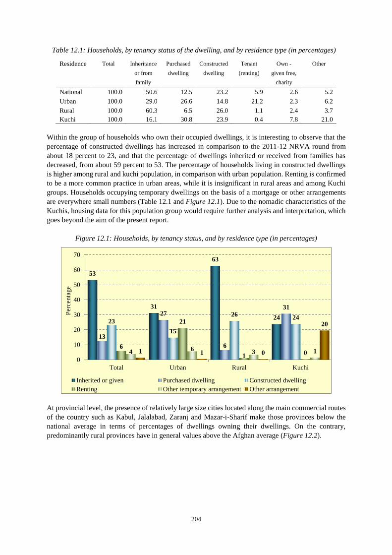
204
Table 12.1: Households, by tenancy status of the dwelling, and by residence type (in percentages)
Residence Total Inheritance Purchased Constructed Tenant Own - Other
or from dwelling dwelling (renting) given free,
family charity
National 100.0 50.6 12.5 23.2 5.9 2.6 5.2
Urban 100.0 29.0 26.6 14.8 21.2 2.3 6.2
Rural 100.0 60.3 6.5 26.0 1.1 2.4 3.7
Kuchi 100.0 16.1 30.8 23.9 0.4 7.8 21.0
Within the group of households who own their occupied dwellings, it is interesting to observe that the
percentage of constructed dwellings has increased in comparison to the 2011-12 NRVA round from
about 18 percent to 23, and that the percentage of dwellings inherited or received from families has
decreased, from about 59 percent to 53. The percentage of households living in constructed dwellings
is higher among rural and kuchi population, in comparison with urban population. Renting is confirmed
to be a more common practice in urban areas, while it is insignificant in rural areas and among Kuchi
groups. Households occupying temporary dwellings on the basis of a mortgage or other arrangements
are everywhere small numbers (Table 12.1 and Figure 12.1). Due to the nomadic characteristics of the
Kuchis, housing data for this population group would require further analysis and interpretation, which
goes beyond the aim of the present report.
Figure 12.1: Households, by tenancy status, and by residence type (in percentages)
At provincial level, the presence of relatively large size cities located along the main commercial routes
of the country such as Kabul, Jalalabad, Zaranj and Mazar-i-Sharif make those provinces below the
national average in terms of percentages of dwellings owning their dwellings. On the contrary,
predominantly rural provinces have in general values above the Afghan average (Figure 12.2).
53
31
63
24
13
27
6
31
23
15
2624
6
21
104 6 3 11 1 0
20
0
10
20
30
40
50
60
70
Total Urban Rural Kuchi
Per
centa
ge
Inherited or given Purchased dwelling Constructed dwelling
Renting Other temporary arrangement Other arrangement

205
Figure 12.2: Percentage of households owning their dwelling, by province
12.2.2 Dwelling characteristics
About 67 percent of Afghan households live in single-family houses, and one-fourth in shared houses.
While the majority of single-family houses are located in rural areas, most of the shared houses are in
urban areas, where also almost all the apartments are located. As expected, the percentages of tents and
temporary shelters are significant only for the Kuchi population (Table 12.2).
Table 12.2: Households, by type of dwelling, and by residence type (in percentages)
Residence Total Single Part of a Apartment Tent Temporary Other
family shared shelter /
house house shack
National 100.0 66.9 25.6 0.5 4.5 2.4 0.2
Urban 100.0 52.1 42.8 1.6 0.2 3.1 0.2
Rural 100.0 76.2 21.5 0.1 0.2 1.9 0.1
Kuchi 100.0 5.3 1.2 0.0 86.4 6.4 0.7
The majority of the dwellings inhabited by Afghan households have been constructed after 1995 (60.1
percent), of which 20.8 between 2005 and 2009, 12.2 between 2012 and 2012, and 2.6 between 2013
and 2014. These percentages do not include the 85 percent of Kuchi dwellings identified as tents. At
provincial level, 28 provinces out of 34 have similar percentages of relatively recent dwellings, close to
the national average (between 40 to 80 percent). On the contrary, in Kapisa, Paktya, Zabul and Nimroz
almost all the dwellings have been constructed in the last 20 years, while in Herat and Khost the majority
of households are living in old dwellings (Figure 12.3).
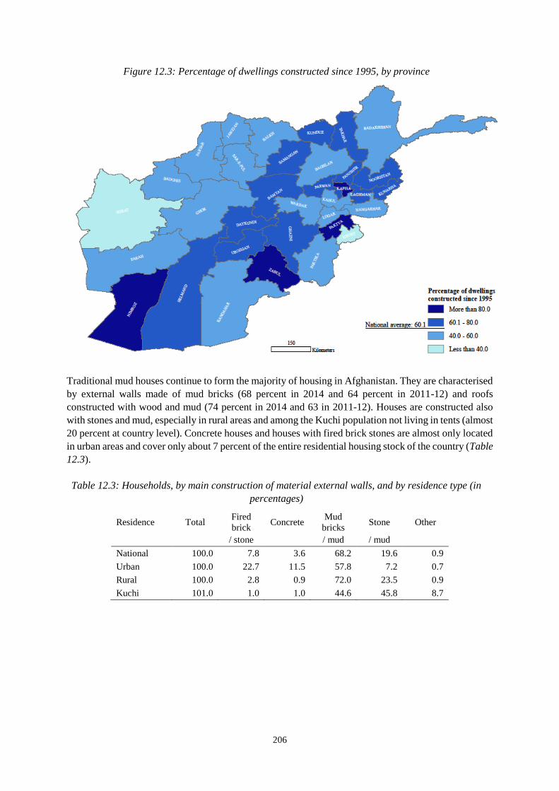
206
Figure 12.3: Percentage of dwellings constructed since 1995, by province
Traditional mud houses continue to form the majority of housing in Afghanistan. They are characterised
by external walls made of mud bricks (68 percent in 2014 and 64 percent in 2011-12) and roofs
constructed with wood and mud (74 percent in 2014 and 63 in 2011-12). Houses are constructed also
with stones and mud, especially in rural areas and among the Kuchi population not living in tents (almost
20 percent at country level). Concrete houses and houses with fired brick stones are almost only located
in urban areas and cover only about 7 percent of the entire residential housing stock of the country (Table
12.3).
Table 12.3: Households, by main construction of material external walls, and by residence type (in
percentages)
Residence Total Fired
brick Concrete
Mud
bricks Stone Other
/ stone / mud / mud
National 100.0 7.8 3.6 68.2 19.6 0.9
Urban 100.0 22.7 11.5 57.8 7.2 0.7
Rural 100.0 2.8 0.9 72.0 23.5 0.9
Kuchi 101.0 1.0 1.0 44.6 45.8 8.7
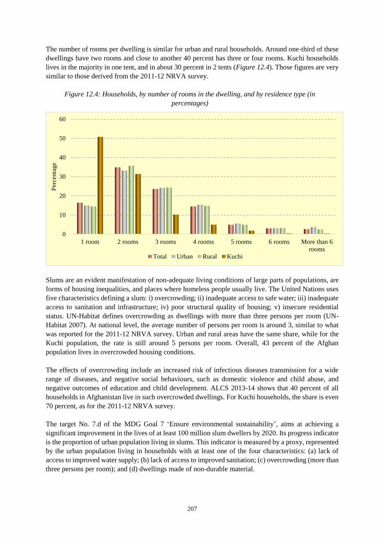
207
The number of rooms per dwelling is similar for urban and rural households. Around one-third of these
dwellings have two rooms and close to another 40 percent has three or four rooms. Kuchi households
lives in the majority in one tent, and in about 30 percent in 2 tents (Figure 12.4). Those figures are very
similar to those derived from the 2011-12 NRVA survey.
Figure 12.4: Households, by number of rooms in the dwelling, and by residence type (in
percentages)
Slums are an evident manifestation of non-adequate living conditions of large parts of populations, are
forms of housing inequalities, and places where homeless people usually live. The United Nations uses
five characteristics defining a slum: i) overcrowding; ii) inadequate access to safe water; iii) inadequate
access to sanitation and infrastructure; iv) poor structural quality of housing; v) insecure residential
status. UN-Habitat defines overcrowding as dwellings with more than three persons per room (UN-
Habitat 2007). At national level, the average number of persons per room is around 3, similar to what
was reported for the 2011-12 NRVA survey. Urban and rural areas have the same share, while for the
Kuchi population, the rate is still around 5 persons per room. Overall, 43 percent of the Afghan
population lives in overcrowded housing conditions.
The effects of overcrowding include an increased risk of infectious diseases transmission for a wide
range of diseases, and negative social behaviours, such as domestic violence and child abuse, and
negative outcomes of education and child development. ALCS 2013-14 shows that 40 percent of all
households in Afghanistan live in such overcrowded dwellings. For Kuchi households, the share is even
70 percent, as for the 2011-12 NRVA survey.
The target No. 7.d of the MDG Goal 7 ‘Ensure environmental sustainability’, aims at achieving a
significant improvement in the lives of at least 100 million slum dwellers by 2020. Its progress indicator
is the proportion of urban population living in slums. This indicator is measured by a proxy, represented
by the urban population living in households with at least one of the four characteristics: (a) lack of
access to improved water supply; (b) lack of access to improved sanitation; (c) overcrowding (more than
three persons per room); and (d) dwellings made of non-durable material.
0
10
20
30
40
50
60
1 room 2 rooms 3 rooms 4 rooms 5 rooms 6 rooms More than 6
rooms
Per
centa
ge
Total Urban Rural Kuchi
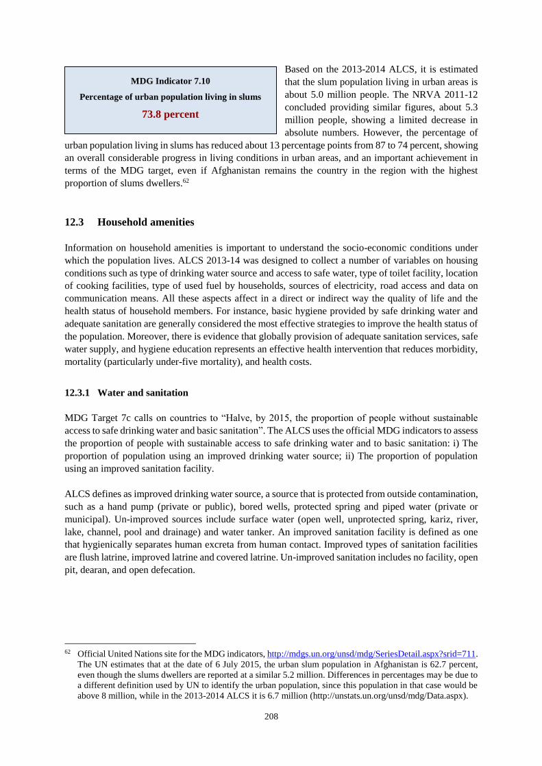
208
Based on the 2013-2014 ALCS, it is estimated
that the slum population living in urban areas is
about 5.0 million people. The NRVA 2011-12
concluded providing similar figures, about 5.3
million people, showing a limited decrease in
absolute numbers. However, the percentage of
urban population living in slums has reduced about 13 percentage points from 87 to 74 percent, showing
an overall considerable progress in living conditions in urban areas, and an important achievement in
terms of the MDG target, even if Afghanistan remains the country in the region with the highest
proportion of slums dwellers.62
12.3 Household amenities
Information on household amenities is important to understand the socio-economic conditions under
which the population lives. ALCS 2013-14 was designed to collect a number of variables on housing
conditions such as type of drinking water source and access to safe water, type of toilet facility, location
of cooking facilities, type of used fuel by households, sources of electricity, road access and data on
communication means. All these aspects affect in a direct or indirect way the quality of life and the
health status of household members. For instance, basic hygiene provided by safe drinking water and
adequate sanitation are generally considered the most effective strategies to improve the health status of
the population. Moreover, there is evidence that globally provision of adequate sanitation services, safe
water supply, and hygiene education represents an effective health intervention that reduces morbidity,
mortality (particularly under-five mortality), and health costs.
12.3.1 Water and sanitation
MDG Target 7c calls on countries to “Halve, by 2015, the proportion of people without sustainable
access to safe drinking water and basic sanitation”. The ALCS uses the official MDG indicators to assess
the proportion of people with sustainable access to safe drinking water and to basic sanitation: i) The
proportion of population using an improved drinking water source; ii) The proportion of population
using an improved sanitation facility.
ALCS defines as improved drinking water source, a source that is protected from outside contamination,
such as a hand pump (private or public), bored wells, protected spring and piped water (private or
municipal). Un-improved sources include surface water (open well, unprotected spring, kariz, river,
lake, channel, pool and drainage) and water tanker. An improved sanitation facility is defined as one
that hygienically separates human excreta from human contact. Improved types of sanitation facilities
are flush latrine, improved latrine and covered latrine. Un-improved sanitation includes no facility, open
pit, dearan, and open defecation.
62 Official United Nations site for the MDG indicators, http://mdgs.un.org/unsd/mdg/SeriesDetail.aspx?srid=711.
The UN estimates that at the date of 6 July 2015, the urban slum population in Afghanistan is 62.7 percent,
even though the slums dwellers are reported at a similar 5.2 million. Differences in percentages may be due to
a different definition used by UN to identify the urban population, since this population in that case would be
above 8 million, while in the 2013-2014 ALCS it is 6.7 million (http://unstats.un.org/unsd/mdg/Data.aspx).
MDG Indicator 7.10
Percentage of urban population living in slums
73.8 percent
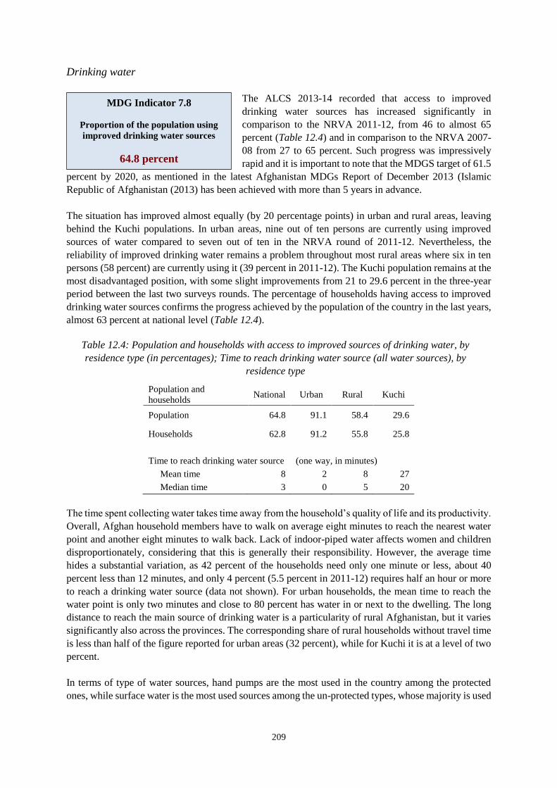
209
Drinking water
The ALCS 2013-14 recorded that access to improved
drinking water sources has increased significantly in
comparison to the NRVA 2011-12, from 46 to almost 65
percent (Table 12.4) and in comparison to the NRVA 2007-
08 from 27 to 65 percent. Such progress was impressively
rapid and it is important to note that the MDGS target of 61.5
percent by 2020, as mentioned in the latest Afghanistan MDGs Report of December 2013 (Islamic
Republic of Afghanistan (2013) has been achieved with more than 5 years in advance.
The situation has improved almost equally (by 20 percentage points) in urban and rural areas, leaving
behind the Kuchi populations. In urban areas, nine out of ten persons are currently using improved
sources of water compared to seven out of ten in the NRVA round of 2011-12. Nevertheless, the
reliability of improved drinking water remains a problem throughout most rural areas where six in ten
persons (58 percent) are currently using it (39 percent in 2011-12). The Kuchi population remains at the
most disadvantaged position, with some slight improvements from 21 to 29.6 percent in the three-year
period between the last two surveys rounds. The percentage of households having access to improved
drinking water sources confirms the progress achieved by the population of the country in the last years,
almost 63 percent at national level (Table 12.4).
Table 12.4: Population and households with access to improved sources of drinking water, by
residence type (in percentages); Time to reach drinking water source (all water sources), by
residence type
Population and
households National Urban Rural Kuchi
Population 64.8 91.1 58.4 29.6
Households 62.8 91.2 55.8 25.8
Time to reach drinking water source (one way, in minutes)
Mean time 8 2 8 27
Median time 3 0 5 20
The time spent collecting water takes time away from the household’s quality of life and its productivity.
Overall, Afghan household members have to walk on average eight minutes to reach the nearest water
point and another eight minutes to walk back. Lack of indoor-piped water affects women and children
disproportionately, considering that this is generally their responsibility. However, the average time
hides a substantial variation, as 42 percent of the households need only one minute or less, about 40
percent less than 12 minutes, and only 4 percent (5.5 percent in 2011-12) requires half an hour or more
to reach a drinking water source (data not shown). For urban households, the mean time to reach the
water point is only two minutes and close to 80 percent has water in or next to the dwelling. The long
distance to reach the main source of drinking water is a particularity of rural Afghanistan, but it varies
significantly also across the provinces. The corresponding share of rural households without travel time
is less than half of the figure reported for urban areas (32 percent), while for Kuchi it is at a level of two
percent.
In terms of type of water sources, hand pumps are the most used in the country among the protected
ones, while surface water is the most used sources among the un-protected types, whose majority is used
MDG Indicator 7.8
Proportion of the population using
improved drinking water sources
64.8 percent
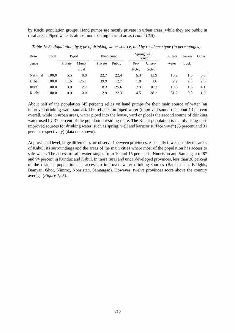
210
by Kuchi population groups. Hand pumps are mostly private in urban areas, while they are public in
rural areas. Piped water is almost non existing in rural areas (Table 12.5).
Table 12.5: Population, by type of drinking water source, and by residence type (in percentages)
Resi- Total Piped Hand pump Spring, well,
kariz Surface Tanker Other
dence Private Muni- Private Public Pro- Unpro- water truck
cipal tected tected
National 100.0 5.5 8.0 22.7 22.4 6.3 13.9 16.2 1.6 3.5
Urban 100.0 11.6 25.1 39.9 12.7 1.8 1.6 2.2 2.8 2.3
Rural 100.0 3.8 2.7 18.3 25.6 7.9 16.3 19.8 1.3 4.1
Kuchi 100.0 0.0 0.0 2.9 22.3 4.5 38.2 31.2 0.0 1.0
About half of the population (45 percent) relies on hand pumps for their main source of water (an
improved drinking water source). The reliance on piped water (improved source) is about 13 percent
overall, while in urban areas, water piped into the house, yard or plot is the second source of drinking
water used by 37 percent of the population residing there. The Kuchi population is mainly using non-
improved sources for drinking water, such as spring, well and kariz or surface water (38 percent and 31
percent respectively) (data not shown).
At provincial level, large differences are observed between provinces, especially if we consider the areas
of Kabul, its surroundings and the areas of the main cities where most of the population has access to
safe water. The access to safe water ranges from 10 and 15 percent in Nooristan and Samangan to 87
and 94 percent in Kunduz and Kabul. In more rural and underdeveloped provinces, less than 30 percent
of the resident population has access to improved water drinking sources (Badakhshan, Badghis,
Bamyan, Ghor, Nimroz, Nooristan, Samangan). However, twelve provinces score above the country
average (Figure 12.5).
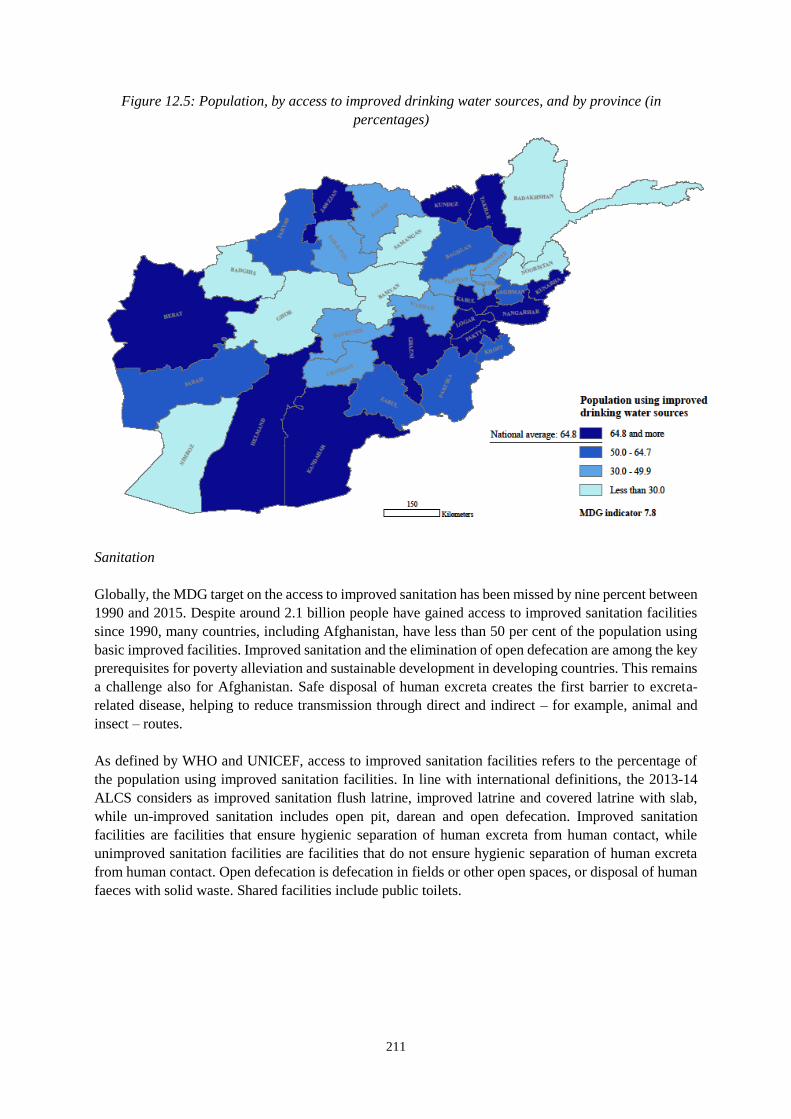
211
Figure 12.5: Population, by access to improved drinking water sources, and by province (in
percentages)
Sanitation
Globally, the MDG target on the access to improved sanitation has been missed by nine percent between
1990 and 2015. Despite around 2.1 billion people have gained access to improved sanitation facilities
since 1990, many countries, including Afghanistan, have less than 50 per cent of the population using
basic improved facilities. Improved sanitation and the elimination of open defecation are among the key
prerequisites for poverty alleviation and sustainable development in developing countries. This remains
a challenge also for Afghanistan. Safe disposal of human excreta creates the first barrier to excreta-
related disease, helping to reduce transmission through direct and indirect – for example, animal and
insect – routes.
As defined by WHO and UNICEF, access to improved sanitation facilities refers to the percentage of
the population using improved sanitation facilities. In line with international definitions, the 2013-14
ALCS considers as improved sanitation flush latrine, improved latrine and covered latrine with slab,
while un-improved sanitation includes open pit, darean and open defecation. Improved sanitation
facilities are facilities that ensure hygienic separation of human excreta from human contact, while
unimproved sanitation facilities are facilities that do not ensure hygienic separation of human excreta
from human contact. Open defecation is defecation in fields or other open spaces, or disposal of human
faeces with solid waste. Shared facilities include public toilets.
212
The 2013-14 ALCS – using a revised definition – shows that
39 percent of the population and households use improved
sanitation facilities (Table 12.6). According to the definition
used in previous NRVAs (not including covered pit latrines
with slab), only 12.8 percent of the population has access to
an improved sanitation facility. This shows an improvement
of 4.5 percentage points in comparison to the NRVA 2011-
12, which detected a percentage of 8.3 of population.
However, despite a moderate progress and even considering the new definition of improved sanitation
facilities, this indicator is in Afghanistan still much below the MDG target of 66 percent set in the
Afghanistan National Development Strategy.
Table 12.6: Population and households, by access to improved sanitation, and by residence type (in
percentages)
Population and National Urban Rural Kuchi
households
Population 39.0 76.5 29.0 1.3
Households 38.8 76.7 28.5 1.7
Overall, up to 76.5 percent of the urban population has access to improved sanitation compared to about
one third of the population that live in rural areas. The most commonly used sanitation facilities in
Afghanistan are open pit latrines (almost 42 percent) and covered pit latrines (26 percent), while flush
toilets are used only by 9.5 percent of the population (data not shown). There are pronounced differences
between urban and rural areas. In rural areas for instance, 50 percent of the population use open pit
latrines. Almost none of the Kuchi population has access to any sanitation facility.
Using the latest criterion applied by WHO and UNICEF that defines the quality of sanitation by
distinguishing private and shared facilities, the data report that, among the 39 percent of people with
access to improved sanitation, 71 percent – 63 percent in urban areas and 79 percent in rural areas – use
a private toilet/latrine facility, while, 29 percent use a shared latrine (Table 12.7). Irrespective of whether
an improved or a non-improved facility is used, 62 percent of the Afghan population uses a private
facility and 38 percent a shared one.
Table 12.7: Population, by use of improved sanitation, access privacy, and by residence type (in
percentages)
Resi- Total With access to Without access to
dence improved facility improved facility
Total Private Shared Total Private Shared Total Private Shared
National 100.0 61.8 38.2 39.0 71.3 28.7 61.0 55.8 44.2
Urban 100.0 65.9 34.1 76.5 63.0 37.0 23.5 75.1 24.9
Rural 100.0 64.1 35.9 29.0 78.6 21.4 71.0 58.1 41.9
Kuchi 100.0 12.8 87.2 1.3 84.0 16.0 98.7 11.8 88.2
At sub-national level, disparities among provinces are very large. In 17 provinces, less than 20 percent
of the population have access to improved sanitation, and in 9 provinces this proportion is higher but
still below the national average of 39 percent. Only in the provinces of Kabul, Parwan, Takhar, Nimroz
and Herat, the percentage of people using improved sanitation facilities is more than 50 percent (Figure
12.6). The best situation – above 70 percent – is in Kabul, Nimroz and Parwan provinces.
MDG Indicator 7.9
Proportion of population using an
improved sanitation facility
39.0 percent
(Old definition: 12.8 percent)
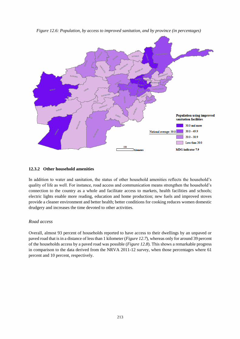
213
Figure 12.6: Population, by access to improved sanitation, and by province (in percentages)
12.3.2 Other household amenities
In addition to water and sanitation, the status of other household amenities reflects the household’s
quality of life as well. For instance, road access and communication means strengthen the household’s
connection to the country as a whole and facilitate access to markets, health facilities and schools;
electric lights enable more reading, education and home production; new fuels and improved stoves
provide a cleaner environment and better health; better conditions for cooking reduces women domestic
drudgery and increases the time devoted to other activities.
Road access
Overall, almost 93 percent of households reported to have access to their dwellings by an unpaved or
paved road that is in a distance of less than 1 kilometer (Figure 12.7), whereas only for around 39 percent
of the households access by a paved road was possible (Figure 12.8). This shows a remarkable progress
in comparison to the data derived from the NRVA 2011-12 survey, when those percentages where 61
percent and 10 percent, respectively.
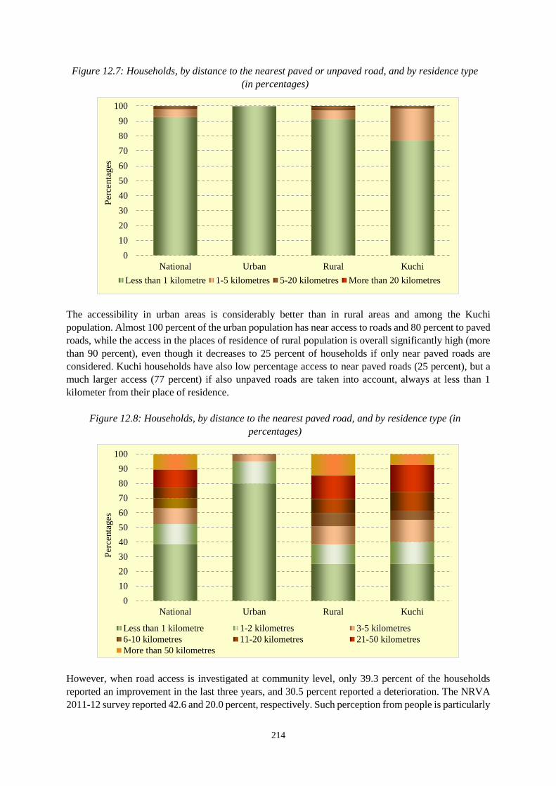
214
Figure 12.7: Households, by distance to the nearest paved or unpaved road, and by residence type
(in percentages)
The accessibility in urban areas is considerably better than in rural areas and among the Kuchi
population. Almost 100 percent of the urban population has near access to roads and 80 percent to paved
roads, while the access in the places of residence of rural population is overall significantly high (more
than 90 percent), even though it decreases to 25 percent of households if only near paved roads are
considered. Kuchi households have also low percentage access to near paved roads (25 percent), but a
much larger access (77 percent) if also unpaved roads are taken into account, always at less than 1
kilometer from their place of residence.
Figure 12.8: Households, by distance to the nearest paved road, and by residence type (in
percentages)
However, when road access is investigated at community level, only 39.3 percent of the households
reported an improvement in the last three years, and 30.5 percent reported a deterioration. The NRVA
2011-12 survey reported 42.6 and 20.0 percent, respectively. Such perception from people is particularly
0
10
20
30
40
50
60
70
80
90
100
National Urban Rural Kuchi
Per
centa
ges
Less than 1 kilometre 1-5 kilometres 5-20 kilometres More than 20 kilometres
0
10
20
30
40
50
60
70
80
90
100
National Urban Rural Kuchi
Per
centa
ges
Less than 1 kilometre 1-2 kilometres 3-5 kilometres
6-10 kilometres 11-20 kilometres 21-50 kilometres
More than 50 kilometres
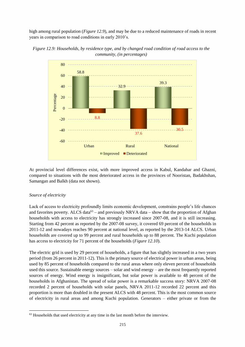
215
high among rural population (Figure 12.9), and may be due to a reduced maintenance of roads in recent
years in comparison to road conditions in early 2010’s.
Figure 12.9: Households, by residence type, and by changed road condition of road access to the
community, (in percentages)
At provincial level differences exist, with more improved access in Kabul, Kandahar and Ghazni,
compared to situations with the most deteriorated access in the provinces of Nooristan, Badakhshan,
Samangan and Balkh (data not shown).
Source of electricity
Lack of access to electricity profoundly limits economic development, constrains people’s life chances
and favorites poverty. ALCS data63 – and previously NRVA data – show that the proportion of Afghan
households with access to electricity has strongly increased since 2007-08, and it is still increasing.
Starting from 42 percent as reported by the 2007-08 survey, it covered 69 percent of the households in
2011-12 and nowadays reaches 90 percent at national level, as reported by the 2013-14 ALCS. Urban
households are covered up to 99 percent and rural households up to 88 percent. The Kuchi population
has access to electricity for 71 percent of the households (Figure 12.10).
The electric grid is used by 29 percent of households, a figure that has slightly increased in a two years
period (from 26 percent in 2011-12). This is the primary source of electrical power in urban areas, being
used by 85 percent of households compared to the rural areas where only eleven percent of households
used this source. Sustainable energy sources – solar and wind energy – are the most frequently reported
sources of energy. Wind energy is insignificant, but solar power is available to 48 percent of the
households in Afghanistan. The spread of solar power is a remarkable success story: NRVA 2007-08
recorded 2 percent of households with solar panels, NRVA 2011-12 recorded 22 percent and this
proportion is more than doubled in the present ALCS with 48 percent. This is the most common source
of electricity in rural areas and among Kuchi population. Generators – either private or from the
63 Households that used electricity at any time in the last month before the interview.
58.8
32.939.3
8.8
37.630.5
-60
-40
-20
0
20
40
60
80
Urban Rural National
Per
centa
ge
Improved Deteriorated
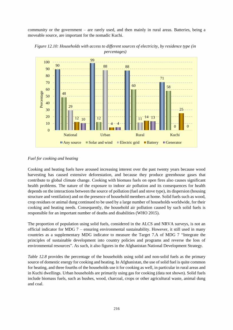
216
community or the government – are rarely used, and then mainly in rural areas. Batteries, being a
moveable source, are important for the nomadic Kuchi.
Figure 12.10: Households with access to different sources of electricity, by residence type (in
percentages)
Fuel for cooking and heating
Cooking and heating fuels have aroused increasing interest over the past twenty years because wood
harvesting has caused extensive deforestation, and because they produce greenhouse gases that
contribute to global climate change. Cooking with biomass fuels on open fires also causes significant
health problems. The nature of the exposure to indoor air pollution and its consequences for health
depends on the interactions between the source of pollution (fuel and stove type), its dispersion (housing
structure and ventilation) and on the presence of household members at home. Solid fuels such as wood,
crop residues or animal dung continued to be used by a large number of households worldwide, for their
cooking and heating needs. Consequently, the household air pollution caused by such solid fuels is
responsible for an important number of deaths and disabilities (WHO 2015).
The proportion of population using solid fuels, considered in the ALCS and NRVA surveys, is not an
official indicator for MDG 7 – ensuring environmental sustainability. However, it still used in many
countries as a supplementary MDG indicator to measure the Target 7.A of MDG 7 “Integrate the
principles of sustainable development into country policies and programs and reverse the loss of
environmental resources”. As such, it also figures in the Afghanistan National Development Strategy.
Table 12.8 provides the percentage of the households using solid and non-solid fuels as the primary
source of domestic energy for cooking and heating. In Afghanistan, the use of solid fuel is quite common
for heating, and three fourths of the households use it for cooking as well, in particular in rural areas and
in Kuchi dwellings. Urban households are primarily using gas for cooking (data not shown). Solid fuels
include biomass fuels, such as bushes, wood, charcoal, crops or other agricultural waste, animal dung
and coal.
90
99
88
71
48
12
60 58
29
88
11
0
12
4
14
25
104
13
00
10
20
30
40
50
60
70
80
90
100
National Urban Rural Kuchi
Per
centa
ge
Any source Solar and wind Electric grid Battery Generator
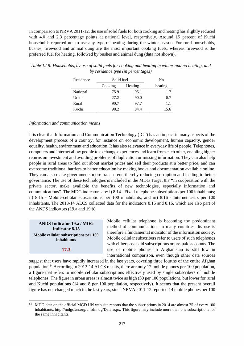
217
In comparison to NRVA 2011-12, the use of solid fuels for both cooking and heating has slightly reduced
with 4.0 and 2.3 percentage points at national level, respectively. Around 15 percent of Kuchi
households reported not to use any type of heating during the winter season. For rural households,
bushes, firewood and animal dung are the most important cooking fuels, whereas firewood is the
preferred fuel for heating, followed by bushes and animal dung (data not shown).
Table 12.8: Households, by use of solid fuels for cooking and heating in winter and no heating, and
by residence type (in percentages)
Residence Solid fuel No
Cooking Heating heating
National 75.9 95.1 1.7
Urban 27.2 90.0 0.7
Rural 90.7 97.7 1.1
Kuchi 98.2 84.4 15.6
Information and communication means
It is clear that Information and Communication Technology (ICT) has an impact in many aspects of the
development process of a country, for instance on economic development, human capacity, gender
equality, health, environment and education. It has also relevance in everyday life of people. Telephones,
computers and internet allow people to exchange experiences and learn from each other, enabling higher
returns on investment and avoiding problems of duplication or missing information. They can also help
people in rural areas to find out about market prices and sell their products at a better price, and can
overcome traditional barriers to better education by making books and documentation available online.
They can also make governments more transparent, thereby reducing corruption and leading to better
governance. The use of these technologies is included in the MDG Target 8.F “In cooperation with the
private sector, make available the benefits of new technologies, especially information and
communications”. The MDG indicators are: i) 8.14 - Fixed-telephone subscriptions per 100 inhabitants;
ii) 8.15 - Mobile-cellular subscriptions per 100 inhabitants; and iii) 8.16 - Internet users per 100
inhabitants. The 2013-14 ALCS collected data for the indicators 8.15 and 8.16, which are also part of
the ANDS indicators (19.a and 19.b).
Mobile cellular telephone is becoming the predominant
method of communications in many countries. Its use is
therefore a fundamental indicator of the information society.
Mobile cellular subscribers refer to users of such telephones
with either post-paid subscriptions or pre-paid accounts. The
use of mobile phones in Afghanistan is still low in
international comparison, even though other data sources
suggest that users have rapidly increased in the last years, covering three fourths of the entire Afghan
population.64 According to 2013-14 ALCS results, there are only 17 mobile phones per 100 population,
a figure that refers to mobile cellular subscriptions effectively used by single subscribers of mobile
telephones. The figure in urban areas is almost twice as high (30 per 100 population), but lower for rural
and Kuchi populations (14 and 8 per 100 population, respectively). It seems that the present overall
figure has not changed much in the last years, since NRVA 2011-12 reported 14 mobile phones per 100
64 MDG data on the official MGD UN web site reports that the subscriptions in 2014 are almost 75 of every 100
inhabitants, http://mdgs.un.org/unsd/mdg/Data.aspx. This figure may include more than one subscriptions for
the same inhabitants.
ANDS Indicator 19.a / MDG
Indicator 8.15
Mobile cellular subscriptions per 100
inhabitants
17.3
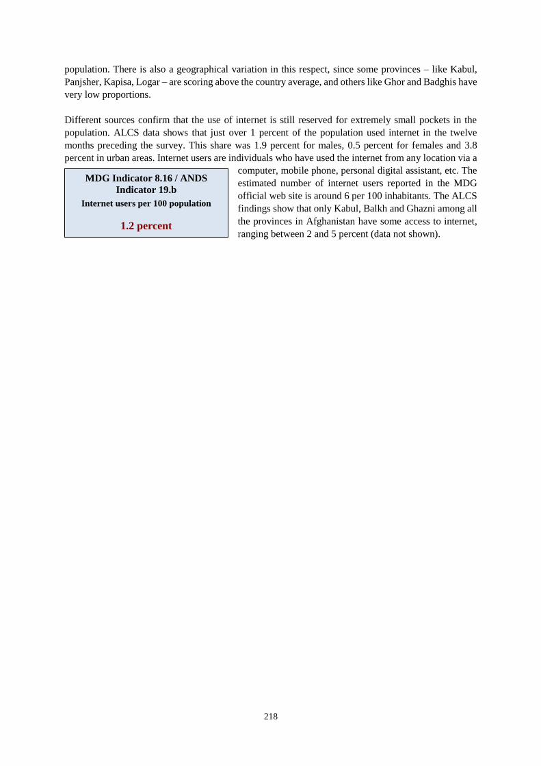
218
population. There is also a geographical variation in this respect, since some provinces – like Kabul,
Panjsher, Kapisa, Logar – are scoring above the country average, and others like Ghor and Badghis have
very low proportions.
Different sources confirm that the use of internet is still reserved for extremely small pockets in the
population. ALCS data shows that just over 1 percent of the population used internet in the twelve
months preceding the survey. This share was 1.9 percent for males, 0.5 percent for females and 3.8
percent in urban areas. Internet users are individuals who have used the internet from any location via a
computer, mobile phone, personal digital assistant, etc. The
estimated number of internet users reported in the MDG
official web site is around 6 per 100 inhabitants. The ALCS
findings show that only Kabul, Balkh and Ghazni among all
the provinces in Afghanistan have some access to internet,
ranging between 2 and 5 percent (data not shown).
MDG Indicator 8.16 / ANDS
Indicator 19.b
Internet users per 100 population
1.2 percent
219
ANNEX I PERSONS INVOLVED IN ALCS 2013-14
I.1 CSO staff
Mohammad Sami Nabi - Project Leader / Head of Field Operation
Esmatullah "Hakimi" - Project National Coordinator
Ahmad Khalid "Amarkhel" - Lead Statistician
Tamim Ahmad "Shakeb" - Survey Administration Officer
Mohammad Muneer "Jamshidi" - Assistant of Survey Administration Officer
Ahmad Sameer "Samadi" - Data Checking Supervisor
Mohammad Sadeq "Sediqi" - Data Quality Checker
Mohammad Aman "Rahimi" - Data Quality Checker
Nargiss "Akbar" - Data Quality Checker
Farah Diba "Yousufzai" - Coder
Sediqa "Merzai" - Coder
Sofia "Rahimi" - Coder
Abdul Ahmad "Sherzai" - Support Staff
Mohammad Waheed Ibrahimi - Database Director
Ahmad Zubair “Sarwary” - Data Entry Director
Shakeeba “Rahimi” - GIS Director
Mohammad Naiam - Driver
I.2 ICON
Roberto Bianchini - Team Leader (Key Expert 1)
Bart de Bruijn - Chief Analyst / Editor (Key Expert 2)
Christophe Dietrich - Project Manager / Deputy Team Leader
Frank Eelens - Data Processing Expert
Tarana Feroz - Financial Manager
Samiullah Zazai - Driver
220
I.3 Steering Committee
H.E. Sheer Mohammad Jami zada, Acting President General CSO
Prof. Hasibullah Mowahed, Deputy President General CSO
Mr. Wali Mohammed Farhodi, Programme Manager - Rural Development, EU Delegation to
Afghanistan
Ms. Thi Van Huang, Head WFP-VAM Unit
Mr. Amanullah Assil, Programme Officer, WFP-VAM
Mr. Haji Qudratullah H.R.P, Ministry of Rural Rehabilitation Development
Mr. Abdul Rehman Shekib, AIRD Executive Director, MRRD
Ms. Siping Wang, Chief PME, UNICEF
Mr. Chandra Sekhar Cherla, P&M Specialist, UNICEF
Mr. Gulam Rabani Haqiqat Pal, Head Statistical Departement, MAIL
Mr. Esmatullah Ramzi, Advisor to the President General, CSO
Mr. Mohammad Sami Nabi, Head of Field and Sampling Department, CSO
And non-disclosed others
I.4 Technical Advisory Committee
H.E. Sheer Mohammad Jami zada, Acting President General CSO
Prof. Hasibullah Mowahed, Deputy President General CSO
Mr. Esmatullah Ramzi, Advisor to the President General, CSO
Mr. Mohammad Sami Nabi, Head of Field and Sampling Department, CSO
Ms. Thi Van Huang, Head WFP-VAM Unit
Mr. Amanullah Assil, Programme Officer, WFP-VAM
Dr. Silvia Redaelli, Economist, Economic Policy and Poverty Team, World Bank
Dr. Bart de Bruijn, Chief Analyst/Editor ALCS 2013-14, ICON
And non-disclosed others
221
I.5 Chapter authors
2. Survey methodology and operations – Bart de Bruijn (ICON), Esmatullah "Hakimi" and Ahmad
Khalid "Amarkhel" (CSO)
3. Population and households – Bart de Bruijn and Frank Eelens (ICON)
4. Migration – Bart de Bruijn (ICON)
5. Labour market outcomes – Ramani Gunatilaka (ILO Consultant) and Bart de Bruijn (ICON)
6. Farming and livestock – Bart de Bruijn (ICON) and Ahmad Khalid "Amarkhel" (CSO)
7. Poverty – Silvia Radaelli (World Bank) and Maya Sherpa (World Bank Consultant)
8. Food security – Thi Van Hoang, Amanullah Assil and Siemon Hollema (WFP)
9. Education – Bart de Bruijn (ICON)
10. Health – Frank Eelens and Bart de Bruijn (ICON)
11. Gender equity and women’s development – Frank Eelens (ICON)
12. Housing and household amenities – Roberto Bianchini (ICON)
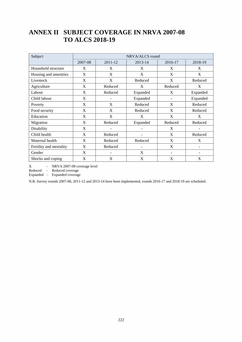
222
ANNEX II SUBJECT COVERAGE IN NRVA 2007-08
TO ALCS 2018-19
X – NRVA 2007-08 coverage level
Reduced – Reduced coverage
Expanded – Expanded coverage
N.B. Survey rounds 2007-08, 2011-12 and 2013-14 have been implemented, rounds 2016-17 and 2018-19 are scheduled.
Subject NRVA/ALCS round
2007-08 2011-12 2013-14 2016-17 2018-19
Household structure X X X X X
Housing and amenities X X X X X
Livestock X X Reduced X Reduced
Agriculture X Reduced X Reduced X
Labour X Reduced Expanded X Expanded
Child labour X - Expanded - Expanded
Poverty X X Reduced X Reduced
Food security X X Reduced X Reduced
Education X X X X X
Migration X Reduced Expanded Reduced Reduced
Disability X - - X -
Child health X Reduced - X Reduced
Maternal health X Reduced Reduced X X
Fertility and mortality X Reduced - X -
Gender X - X - -
Shocks and coping X X X X X
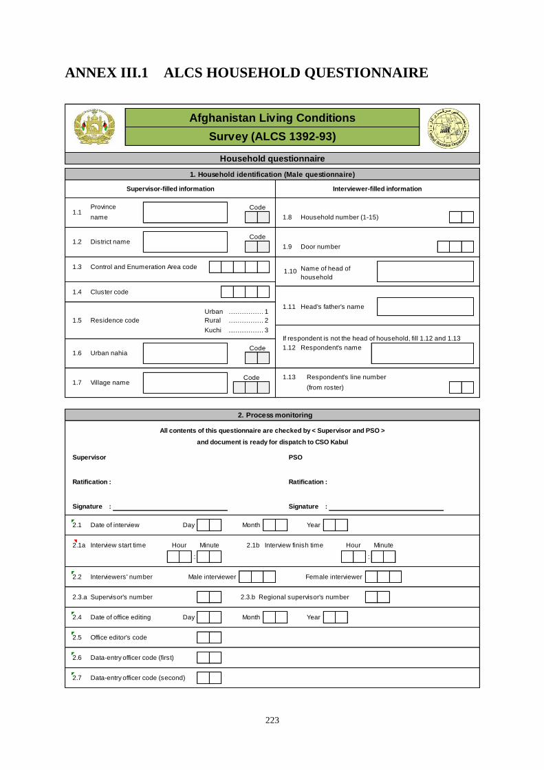
223
ANNEX III.1 ALCS HOUSEHOLD QUESTIONNAIRE
Household questionnaire
1. Household identification (Male questionnaire)
Supervisor-filled information Interviewer-filled information
Province Code
name 1.8 Household number (1-15)
Code
Door number
Control and Enumeration Area code Name of head of
household
Cluster code
Urban …………………………1
Rural …………………………2
Kuchi …………………………3
Code 1.12 Respondent's name
Code Respondent's line number
(from roster)
2. Process monitoring
All contents of this questionnaire are checked by < Supervisor and PSO >
and document is ready for dispatch to CSO Kabul
Supervisor PSO
Ratification : Ratification :
Signature : Signature :
Date of interview Day Month Year
2.1a Interview start time Hour Minute 2.1b Interview finish time Hour Minute
: :
Interviewers' number Male interviewer Female interviewer
Supervisor's number Regional supervisor's number
Date of office editing Day Month Year
Office editor's code
Data-entry officer code (first)
Data-entry officer code (second)
2.3.a 2.3.b
2.7
2.6
2.5
2.1
2.2
2.4
1.13
1.31.10
1.7 Village name
If respondent is not the head of household, fill 1.12 and 1.13
1.6
District name
Urban nahia
1.5 Residence code
1.11 Head's father's name
1.1
1.2
Afghanistan Living Conditions
Survey (ALCS 1392-93)
1.4
1.9
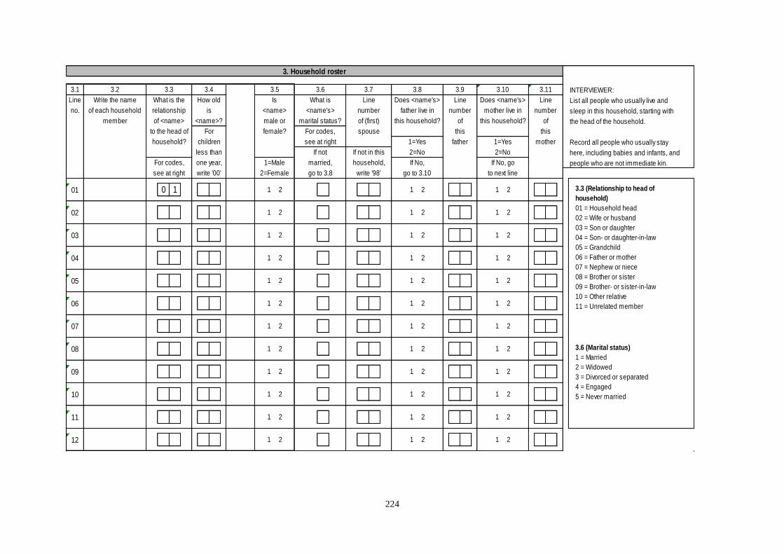
224
3. Household roster
3.1 3.2 3.3 3.4 3.5 3.6 3.7 3.8 3.9 3.10 3.11 INTERVIEWER:
Line Write the name What is the How old Is What is Line Does <name's> Line Does <name's> Line List all people who usually live and
no. of each household relationship is <name> <name's> number father live in number mother live in number sleep in this household, starting with
member of <name> <name>? male or marital status? of (first) this household? of this household? of the head of the household.
to the head of For female? For codes, spouse this this
household? children see at right 1=Yes father 1=Yes mother Record all people who usually stay
less than If not If not in this 2=No 2=No here, including babies and infants, and
For codes, one year, 1=Male married, household, If No, If No, go people who are not immediate kin.
see at right write '00' 2=Female go to 3.8 write '98' go to 3.10 to next line
01 1 2 1 2 1 2
02 1 2 1 2 1 2
03 1 2 1 2 1 2
04 1 2 1 2 1 2
05 1 2 1 2 1 2
06 1 2 1 2 1 2
07 1 2 1 2 1 2
08 1 2 1 2 1 2
09 1 2 1 2 1 2
10 1 2 1 2 1 2
11 1 2 1 2 1 2
12 1 2 1 2 1 2
3.3 (Relationship to head of
household)
01 = Household head
02 = Wife or husband
03 = Son or daughter
04 = Son- or daughter-in-law
05 = Grandchild
06 = Father or mother
07 = Nephew or niece
08 = Brother or sister
09 = Brother- or sister-in-law
10 = Other relative
11 = Unrelated member
3.6 (Marital status)
1 = Married
2 = Widowed
3 = Divorced or separated
4 = Engaged
5 = Never married
10
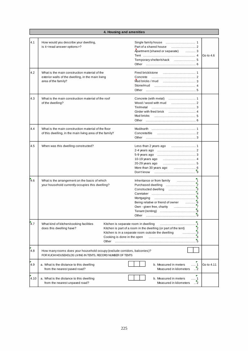
225
4. Housing and amenities
4.1 How would you describe your dwelling, Single family house ……………………………………………………………1
is it <read answer options>? Part of a shared house ……………………………………………………………2
Apartment (shared or separate) ……………………………………………………………3
Tent ……………………………………………………………4 Go to 4.6
Temporary shelter/shack ……………………………………………………………5
Other ……………………………………………………………6
4.2 What is the main construction material of the Fired brick/stone ……………………………………………………………1
exterior walls of the dwelling, in the main living Concrete ……………………………………………………………2
area of the family? Mud bricks / mud ……………………………………………………………3
Stone/mud ……………………………………………………………4
Other ……………………………………………………………5
4.3 What is the main construction material of the roof Concrete (with metal) ……………………………………………………………1
of the dwelling? Wood / wood with mud ……………………………………………………………2
Tin/metal ……………………………………………………………3
Girder with fired brick ……………………………………………………………4
Mud bricks ……………………………………………………………5
Other ……………………………………………………………6
4.4 What is the main construction material of the floor Mud/earth ……………………………………………………………1
of this dwelling, in the main living area of the family? Concrete/tile ……………………………………………………………2
Other ……………………………………………………………3
4.5 When was this dwelling constructed? Less than 2 years ago ……………………………………………………………1
2-4 years ago ……………………………………………………………2
5-9 years ago ……………………………………………………………3
10-19 years ago ……………………………………………………………4
20-29 years ago ……………………………………………………………5
More than 30 years ago ……………………………………………………………6
Don't know ……………………………………………………………9
4.6 What is the arrangement on the basis of which Inheritance or from family ……………………………………………………………1
your household currently occupies this dwelling? Purchased dwelling ……………………………………………………………2
Constructed dwelling ……………………………………………………………3
Caretaker ……………………………………………………………4
Mortgaging ……………………………………………………………5
Being relative or friend of owner ……………………………………………………………6
Own - given free, charity ……………………………………………………………7
Tenant (renting) ……………………………………………………………8
Other ……………………………………………………………9
4.7 What kind of kitchen/cooking facilities Kitchen is separate room in dwelling ……………………………………………………………1
does this dwelling have? Kitchen is part of a room in the dwelling (or part of the tent) 2
Kitchen is in a separate room outside the dwelling ……………………………………………………………3
Cooking is done in the open ……………………………………………………………4
Other ……………………………………………………………………..5
4.8 How many rooms does your household occupy (exclude corridors, balconies)?
FOR KUCHI HOUSEHOLDS LIVING IN TENTS, RECORD NUMBER OF TENTS
4.9 a. What is the distance to this dwelling b. Measured in meters …….1 Go to 4.11
from the nearest paved road? Measured in kilometers …….2
4.10 a. What is the distance to this dwelling b. Measured in meters …….1
from the nearest unpaved road? Measured in kilometers …….2
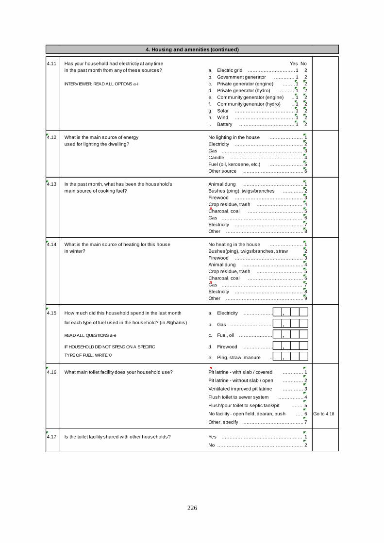
226
4. Housing and amenities (continued)
4.11 Has your household had electrictiy at any time Yes No
in the past month from any of these sources? a. Electric grid ……………………………………………………………1 2
b. Government generator ……………………………………………………………1 2
INTERVIEWER: READ ALL OPTIONS a-i c. Private generator (engine) ……………………………………………………………1 2
d. Private generator (hydro) ……………………………………………………………1 2
e. Community generator (engine) ……………………………………………………………1 2
f. Community generator (hydro) ……………………………………………………………1 2
g. Solar ……………………………………………………………1 2
h. Wind ……………………………………………………………1 2
i. Battery ……………………………………………………………1 2
4.12 What is the main source of energy No lighting in the house ……………………………………………………………1
used for lighting the dwelling? Electricity ……………………………………………………………2
Gas ……………………………………………………………3
Candle ……………………………………………………………4
Fuel (oil, kerosene, etc.) ……………………………………………………………5
Other source ……………………………………………………………6
4.13 In the past month, what has been the household's Animal dung ……………………………………………………………1
main source of cooking fuel? Bushes (ping), twigs/branches ……………………………………………………………2
Firewood ……………………………………………………………3
Crop residue, trash ……………………………………………………………4
Charcoal, coal ……………………………………………………………5
Gas ……………………………………………………………6
Electricity ……………………………………………………………7
Other ……………………………………………………………8
4.14 What is the main source of heating for this house No heating in the house ……………………………………………………………1
in winter? Bushes(ping), twigs/branches, straw 2
Firewood ……………………………………………………………3
Animal dung ……………………………………………………………4
Crop residue, trash ……………………………………………………………5
Charcoal, coal ……………………………………………………………6
Gas ……………………………………………………………7
Electricity ……………………………………………………………8
Other ……………………………………………………………9
4.15 How much did this household spend in the last month a. Electricity ……………………………………………………………
for each type of fuel used in the household? (in Afghanis) b. Gas ……………………………………………………………
READ ALL QUESTIONS a-e c. Fuel, oil ……………………………………………………………
IF HOUSEHOLD DID NOT SPEND ON A SPECIFIC d. Firewood ……………………………………………………………
TYPE OF FUEL, WRITE '0'e. Ping, straw, manure ……………………………………………………………
4.16 What main toilet facility does your household use? Pit latrine - with slab / covered ……………………………………………………………1
Pit latrine - without slab / open ……………………………………………………………2
Ventilated improved pit latrine ……………………………………………………………3
Flush toilet to sewer system ……………………………………………………………4
Flush/pour toilet to septic tank/pit ……………………………………………………………5
No facility - open field, dearan, bush ……………………………………………………………6 Go to 4.18
Other, specify ……………………………………………………………7
4.17 Is the toilet facility shared with other households? Yes ……………………………………………………………1
No ……………………………………………………………2
,
,
,
,
,
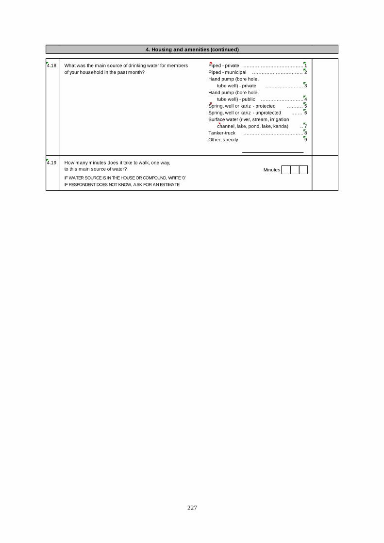
227
4. Housing and amenities (continued)
4.18 What was the main source of drinking water for members Piped - private ……………………………………………………………1
of your household in the past month? Piped - municipal ……………………………………………………………2
Hand pump (bore hole,
tube well) - private ……………………………………………………………3
Hand pump (bore hole,
tube well) - public ……………………………………………………………4
Spring, well or kariz - protected ……………………………………………………………5
Spring, well or kariz - unprotected ……………………………………………………………6
Surface water (river, stream, irrigation
channel, lake, pond, lake, kanda) ……………………………………………………………7
Tanker-truck ……………………………………………………………8
Other, specify 9
4.19 How many minutes does it take to walk, one way,
to this main source of water? Minutes
IF WATER SOURCE IS IN THE HOUSE OR COMPOUND, WRITE '0'
IF RESPONDENT DOES NOT KNOW, ASK FOR AN ESTIMATE
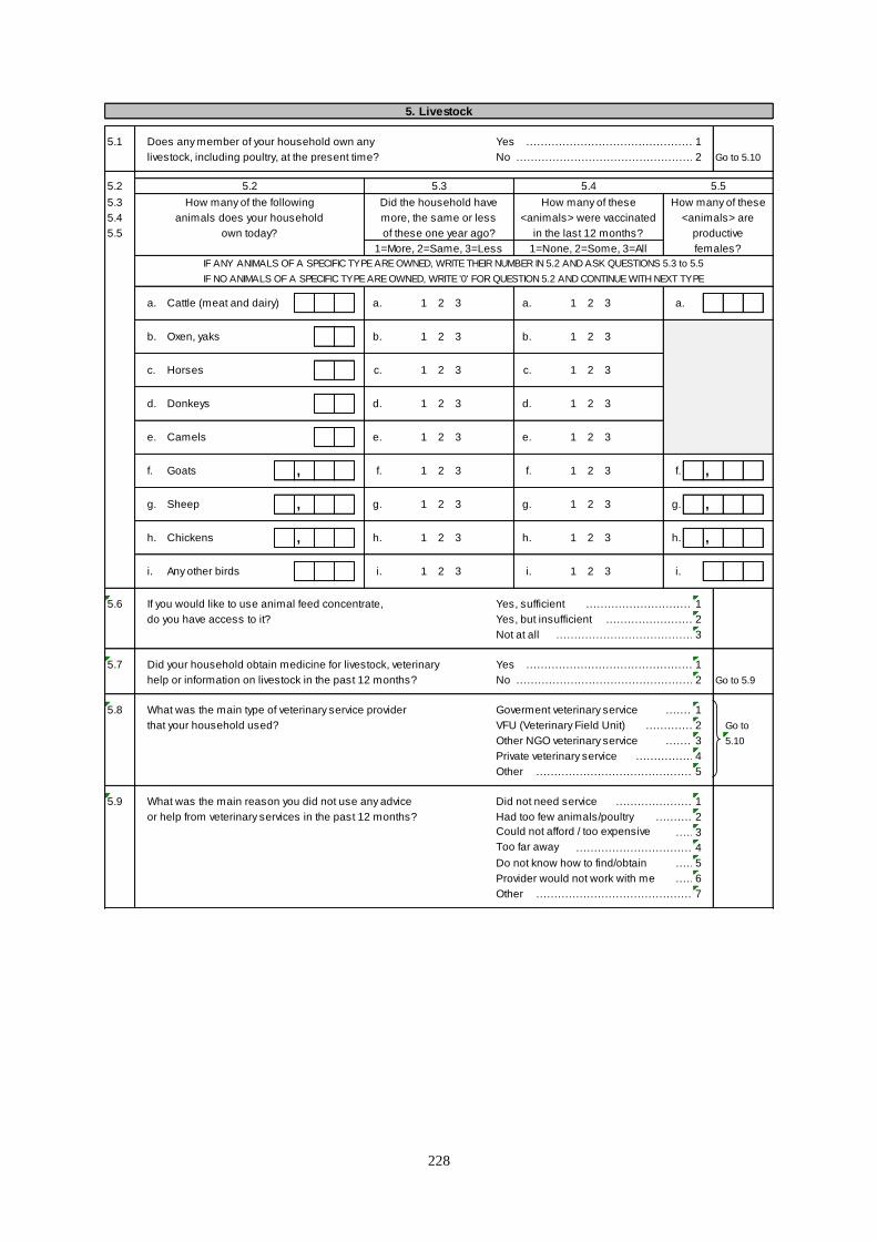
228
5. Livestock
5.1 Does any member of your household own any Yes ……………………………………………………………1
livestock, including poultry, at the present time? No ……………………………………………………………2 Go to 5.10
5.2 5.2 5.3 5.4 5.5
5.3 How many of the following Did the household have How many of these How many of these
5.4 animals does your household more, the same or less <animals> were vaccinated <animals> are
5.5 own today? of these one year ago? in the last 12 months? productive
1=More, 2=Same, 3=Less 1=None, 2=Some, 3=All females?
IF ANY ANIMALS OF A SPECIFIC TYPE ARE OWNED, WRITE THEIR NUMBER IN 5.2 AND ASK QUESTIONS 5.3 to 5.5
IF NO ANIMALS OF A SPECIFIC TYPE ARE OWNED, WRITE '0' FOR QUESTION 5.2 AND CONTINUE WITH NEXT TYPE
a. Cattle (meat and dairy) a. 1 2 3 a. 1 2 3 a.
b. Oxen, yaks b. 1 2 3 b. 1 2 3
c. Horses c. 1 2 3 c. 1 2 3
d. Donkeys d. 1 2 3 d. 1 2 3
e. Camels e. 1 2 3 e. 1 2 3
f. Goats f. 1 2 3 f. 1 2 3 f.
g. Sheep g. 1 2 3 g. 1 2 3 g.
h. Chickens h. 1 2 3 h. 1 2 3 h.
i. Any other birds i. 1 2 3 i. 1 2 3 i.
5.6 If you would like to use animal feed concentrate, Yes, sufficient ……………………………………………………………1
do you have access to it? Yes, but insufficient ……………………………………………………………2
Not at all ……………………………………………………………3
5.7 Did your household obtain medicine for livestock, veterinary Yes ……………………………………………………………1
help or information on livestock in the past 12 months? No ……………………………………………………………2 Go to 5.9
5.8 What was the main type of veterinary service provider Goverment veterinary service ……………………………………………………………1
that your household used? VFU (Veterinary Field Unit) ……………………………………………………………2 Go to
Other NGO veterinary service ……………………………………………………………3 5.10
Private veterinary service ……………………………………………………………4
Other ……………………………………………………………5
5.9 What was the main reason you did not use any advice Did not need service ……………………………………………………………1
or help from veterinary services in the past 12 months? Had too few animals/poultry ……………………………………………………………2
Could not afford / too expensive ……………………………………………………………3
Too far away ……………………………………………………………4
Do not know how to find/obtain ……………………………………………………………5
Provider would not work with me ……………………………………………………………6
Other ……………………………………………………………7
,,
,
, ,
,
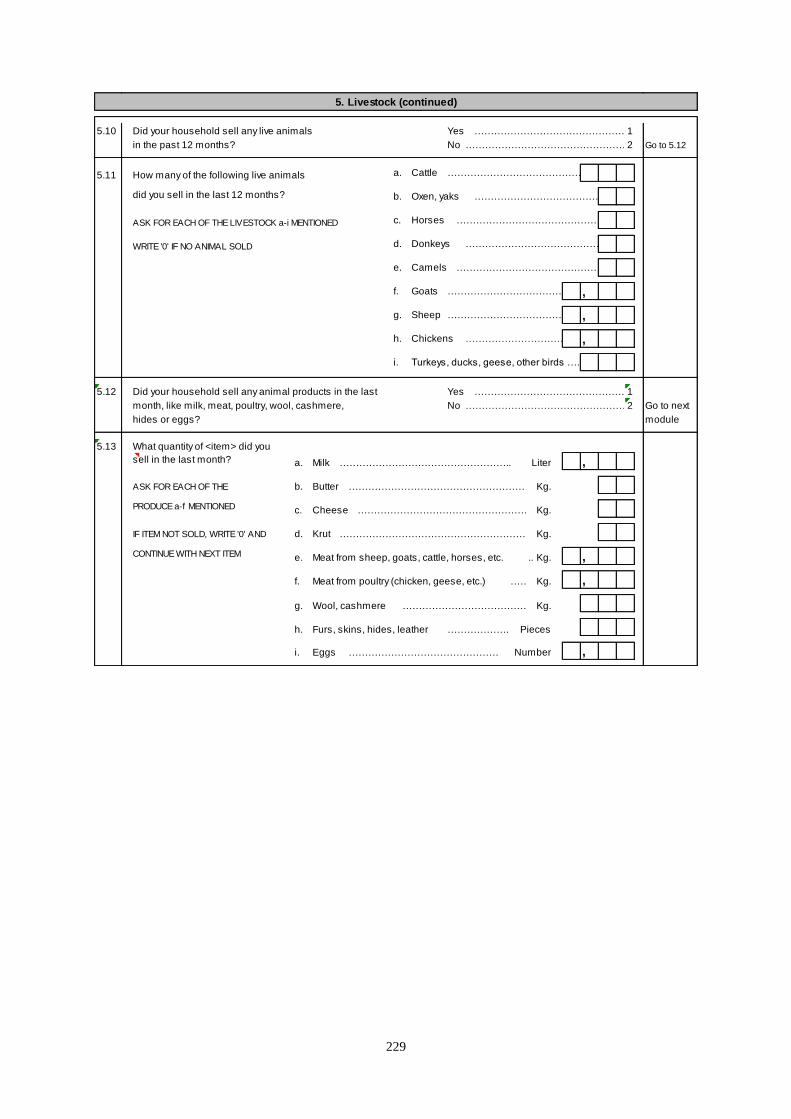
229
5. Livestock (continued)
5.10 Did your household sell any live animals Yes ……………………………………………………………1
in the past 12 months? No ……………………………………………………………2 Go to 5.12
5.11 How many of the following live animals a. Cattle ……………………………………………………………
did you sell in the last 12 months? b. Oxen, yaks ……………………………………………………………
ASK FOR EACH OF THE LIVESTOCK a-i MENTIONED c. Horses ……………………………………………………………
WRITE '0' IF NO ANIMAL SOLD d. Donkeys ……………………………………………………………
e. Camels ……………………………………………………………
f. Goats ……………………………………………………………
g. Sheep ……………………………………………………………
h. Chickens ……………………………………………………………
i. Turkeys, ducks, geese, other birds ….
5.12 Did your household sell any animal products in the last Yes ……………………………………………………………1
month, like milk, meat, poultry, wool, cashmere, No ……………………………………………………………2 Go to next
hides or eggs? module
5.13 What quantity of <item> did you
sell in the last month? a. Milk …………………………………………….. Liter
ASK FOR EACH OF THE b. Butter …………………………………………………………………..Kg.
PRODUCE a-f MENTIONED c. Cheese …………………………………………………………………..Kg.
IF ITEM NOT SOLD, WRITE '0' AND d. Krut …………………………………………………………………..Kg.
CONTINUE WITH NEXT ITEM e. Meat from sheep, goats, cattle, horses, etc. .. Kg.
f. Meat from poultry (chicken, geese, etc.) ……. Kg.
g. Wool, cashmere ……………………………………..Kg.
h. Furs, skins, hides, leather ………………. Pieces
i. Eggs …………………………………………….Number
,
,
,
,
,
,
,
230
6. Agriculture
6.1 Did anyone in your household own any irrigated land - Yes ……………………………………………………………1 Go to 6.3 6.2 Did anyone in your household have access to any Yes ……………………………………………………………1
not including a garden plot - in the spring harvesting No ……………………………………………………………2 irrigated land - not including a garden plot - in the No ……………………………………………………………2 Go to 6.27
season in 1392? spring harvesting season in 1392, without owning it?
Since your household owned irrigated land or had access to irrigated land in the spring harvesting season of 1392, please answer the following questions
about land tenure and land use.
6.3 6.3 6.4 6.5 6.6 6.7
6.4 How many jeribs of irrigated land did How many jeribs of this How many jeribs of this What was the main What was the share of
6.5 did members of your household together land did members of land did your household reason for not cultiva- produce given to the land
6.6 Ask a for 6.3-6.4-6.5-6.6(-6.7), then b, etc. your household cultivate? leave fallow? ting this land? owner from the land that was
6.7 If no land of specific category (a-g), write '0.0' and go to the next category (b-g) For codes, see below <rented>/<sharecropped> in?
a. own . a. . a. . If '0'0, go to 6.3.b a. Go to 6.3.b
b. lease/rent in . b. . b. . If '0'0, go to 6.7.b b. Go to 6.7.b b.
c. sharecrop in . c. . c. . If '0'0, go to 6.7.c c. Go to 6.7.c c.
d. mortgage in . d. . d. . If '0'0, go to 6.3.e d. Go to 6.3.e
e. lease/rent out .
f. share crop out . SUM 6.4.a to 6.4.d
g. mortgage out .
6.8 So, the total of irrigated land that members . 6.9 Altogether, did your household in the spring harvesting More ……………………………………………………………1
of your household cultivated was: season in 1392 cultivate more, the same or less Same ……………………………………………………………2
IF INCORRECT, REVIEW QUESTIONS 6.4.a TO 6.4.d irrigated land area compared to 1391? Less ……………………………………………………………3
IF 6.8=0 go to 6.18
6.10 What was the main source of irrigation Irrigated river, canal, dam ……………………………………………………………1 6.11 For the spring harvesting season in 1392, did you Yes ……………………………………………………………1
for most of the irrigated land you Irrigated deep-well pump ……………………………………………………………2 have sufficient irrigation for your irrigated crops? No ……………………………………………………………2
cultivated during for the spring Spring ……………………………………………………………3
harvesting season in 1392? Kariz ……………………………………………………………4
Nawara ……………………………………………………………5
Absialab, snow melt, flood ……………………………………………………………6
Other ……………………………………………………………7
,
5. Land not fertile / shifting
cultivation
6. No manpower to help
7. Other reason
,
,
, Codes for 6.6
1. Lack of water
2. No money for cultivation
3. Conflict over water or land
4. Security concerns
, ,,
,
, ,
, ,
,
, ,,
231
6. Agriculture (continued)
6.12 In terms of total value, what was the most important crop your household 6.13 How much of this <most important crop> Kgs.
harvested in the spring harvesting season in 1392 on irrigated land? did your household harvest then?
FOR CODES, SEE AT BOTTOM OF PAGE
6.14 What was the second most important crop (in total value) your household If '00' 6.15 How much of this <second-most Kgs.
harvested in the spring harvesting season in 1392 on irrigated land? go to 6.18 important crop> did your household
FOR CODES, SEE AT BOTTOM OF PAGE IF NO SECOND CROP, WRITE '00' harvest then?
6.16 What was the third most important crop (in total value) your household If '00' 6.17 How much of this <third-most Kgs.
harvested in the spring harvesting season in 1392 on irrigated land? go to 6.18 important crop> did your household
FOR CODES, SEE AT BOTTOM OF PAGE IF NO THIRD CROP, WRITE '00' harvest then?
6.18 How many jeribs of irrigated land did your household Jeribs . If '0.0'
cultivate in the winter harvesting season in 1392 IF NONE, WRITE '0.0' go to 6.27
6.19 In terms of total value, what was the most important crop your household 6.20 How much of this <most important crop> Kgs.
harvested in the winter harvesting season in 1392 on irrigated land? did your household harvest then?
FOR CODES, SEE AT BOTTOM OF PAGE
6.21 What was the second most important crop (in total value) your household If '00' 6.22 How much of this <second-most Kgs.
harvested in the winter harvesting season in 1392 on irrigated land? go to 6.25 important crop> did your household
FOR CODES, SEE AT BOTTOM OF PAGE IF NO SECOND CROP, WRITE '00' harvest then?
6.23 What was the third most important crop (in total value) your household If '00' 6.24 How much of this <third-most Kgs.
harvested in the winter harvesting season in 1392 on irrigated land? go to 6.25 important crop> did your household
FOR CODES, SEE AT BOTTOM OF PAGE IF NO THIRD CROP, WRITE '00' harvest then?
6.25 What was the main source of irrigation Irrigated river, canal, dam ……………………………………………………………1 6.26 For the winter harvesting season in 1392, Yes ……………………………………………………………1
for most of the irrigated land your Irrigated deep-well pump ……………………………………………………………2 did your household have sufficient No ……………………………………………………………2
household cultivated during for the Spring ……………………………………………………………3 irrigation for your irrigated crops?
winter harvesting season in 1392? Kariz ……………………………………………………………4
Nawara ……………………………………………………………5
Absialab, snow melt, flood ……………………………………………………………6
Other ……………………………………………………………7
Codes for 6.12 0=No second or 1=Wheat 5=Flax 8=Millet 12=Kourgit 16=Tomato 20=Fruit from trees
6.14/16/19/21/23 third crop 2=Maize/sorghum 6=Sugar cane/beet 9=Cotton 13=Potatoes 17=Onions 21=Melon/watermelon
(Harvested crops (only for 6.21 3=Barley 7=Alfalfa/clover/ 10=Opium 14=Beans 18=Okra 22=Other fruits
irrigated land) and 6.23) 4=Rice other fodder 11=Cumin 15=Eggplant 19=Other vegetables 23=Nuts
,
,
,
,
,
,
,
232
6. Agriculture (continued)
6.27 Did anyone in your household own any rain-fed land - Yes ……………………………………………………………1 Go to 6.29 6.28 Did anyone in your household have Yes ……………………………………………………………1
not including a garden plot - in the spring harvesting No ……………………………………………………………2 access to any rain-fed land - not including No ……………………………………………………………2 Go to 6.42
season in 1392? a garden plot - in the spring harvesting
season in 1392, without owning it?
Since your household owned or had access to rain-fed land in the spring of 1392, please answer the following questions about land tenure and land use.
6.29 6.29 6.30 6.31 6.32 6.33
6.30 How many jeribs of rain-fed land did How many jeribs of this How many jeribs of this What was the main What was the share of
6.31 members of your household together land did members of land did your household reason for not cultiva- produce given to the land
6.32 Ask a for 6.29.a to 6.33.a, then b, etc. your household cultivate? leave fallow? ting this land? owner from the land that was
6.33 If no land of specific category (a-g), write '0.0' and go to the next category (b-g) For codes, see below <rented>/<sharecropped> in?
a. own . a. . a. . If '0'0, go to 6.29.b a. Go to 6.29.b
b. lease/rent in . b. . b. . If '0'0, go to 6.33.b b. Go to 6.33.b b.
c. sharecrop in . c. . c. . If '0'0, go to 6.33.c c. Go to 6.33.c c.
d. mortgage in . d. . d. . If '0'0, go to 6.29.e d. Go to 6.29.e
e. lease/rent out .
f. share crop out . SUM 6.30.a to 6.30.d
g. mortgage out .
6.34 So, the total of rain-fed land that members . 6.35 Altogether, did your household in the spring More ……………………………………………………………1
of your household cultivated was: season in 1392 cultivate more, the same or Same ……………………………………………………………2
IF INCORRECT, REVIEW QUESTIONS 6.4.a TO 6.4.d less rain-fed land area compared to 1391? Less ……………………………………………………………3
IF 6.34=0 go to 6.42
6.36 In terms of total value, what was the most important crop your household 6.37 How much of this <most important crop> Kgs.
harvested in the spring harvesting season in 1392 on rain-fed land? CODES AT BOTTOM did your household harvest then?
6.38 What was the second most important crop (in total value) harvested in If '0' 6.39 How much of this <second-most Kgs.
the spring harvesting season in 1392 on rain-fed land? IF NO SECOND CROP, WRITE '0' go to 6.42 important crop> was harvested then?
6.40 What was the third most important crop (in total value) harvested in If '0' 6.41 How much of this <third-most Kgs.
the spring harvesting season in 1392 on rain-fed land? IF NO THIRD CROP, WRITE '0' go to 6.42 important crop> was harvested then?
Codes for 6.36, 6.38 and 6.40 (Harvested crops rain-fed land)
0 = No second or third crop 1 = Wheat 3 = Maize / sorghum 5 = Flax 7 = Melon / watermelon
(only for 6.38 and 6.40) 2 = Barley 4 = Cotton 6 = Cumin 8 = Other crop
,
,
,
5. Land not fertile / shifting
cultivation
6. No manpower to help
7. Other reason:____________
,
,
,
,
Codes for 6.32
1. Lack of water
2. No money for cultivation
3. Conflict over water or land
4. Security concerns
,
,,
,
, , ,
, , ,
,
,
233
6. Agriculture (continued)
6.42 INTERVIEWER: DID THE HOUSEHOLD CULTIVATE ANY Yes ……………………………………………………………1 6.43 What was the main traction power your Tractor / other machine 1
FARM LAND IN THE SPRING HARVESTING PERIOD IN 1392, No ……………………………………………………………2 go to 6.48 household used for ploughing in the Ox or other animal ……………………………………………………………2
EITHER IRRIGATED OR RAIN-FED LAND? CHECK 6.8 AND 6.34 1392 spring harvesting season? Human power ……………………………………………………………3
6.44 For the 1392 harvesting season, how many kilo Kgs.
of fertiliser was your household able to afford?
6.45 Did your household obtain any information or products for the Yes ……………………………………………………………1 go to 6.47 6.46 What was the main reason Did not need service ……………………………………………………………1
1392 harvesting season from agriculture extension services? No ……………………………………………………………2 the household did not use Could not afford / too expensive ……………………………………………………………2
any information or products Too far away ……………………………………………………………3
from extension services Do not know how to find/obtain ……………………………………………………………4
for the 1392 harvesting Service would not work with me ……………………………………………………………5
season? Do not trust service ……………………………………………………………6
Not safe to go / security ……………………………………………………………7
Other ……………………………………………………………8
6.47 For the total 1392 harvesting, how much did your Afghanis Afghanis
household spend on the following farming inputs? WRITE '00' IF NO SPENDING WRITE '00' IF NO SPENDING
a. Land rent …………………………………………………………………………………………… e. Pesticides and herbicides ……………………………………………………………………………………………
b. Seeds …………………………………………………………………………………………… f. Labour costs (e.g. for weeding) ……………………………………………………………………………………………
c. Irrigation water …………………………………………………………………………………………… g. Machine/tractor rent ……………………………………………………………………………………………
d. Fertilisers (UREA/DAP) ……………………………………………………………………………………………h. Other costs for land preparation, ……………………………………………………………………………………………
tillage and harvesting
,
,
,
,
, ,
,
,
,
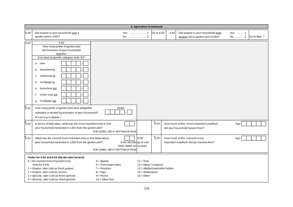
234
6. Agriculture (continued)
6.48 Did anyone in your household own a Yes ……………………………………………………………1 Go to 6.50 6.49 Did anyone in your household have Yes ……………………………………………………………1
garden plot in 1392? No ……………………………………………………………2 access any a garden plot in1392? No ……………………………………………………………2 Go to Mod. 7
6.50 6.50
How many jeribs of garden plot
did members of your household
together:
If no land of specific category, write '0.0'
a. own .
b. lease/rent in .
c. sharecrop in .
d. mortgage in .
e. lease/rent out .
f. share crop out .
g. mortgage out .
6.51 How many jeribs of garden plot were altogether Jeribs
cultivated or tended by members of your household? .
IF 6.51=0 go to Module 7
6.52 In terms of total value, what was the most important crop or fruit 6.53 How much of this <most important crop/fruit> Kgs.
your household harvested in 1392 from the garden plot? did your household harvest then?
FOR CODES, SEE AT BOTTOM OF PAGE
6.54 What was the second most important crop or fruit (total value) If '00' 6.55 How much of this <second-most Kgs.
your household harvested in 1392 from the garden plot? IF NO SECOND go to next important crop/fruit> did you harvest then?
CROP, WRITE '00' module
FOR CODES, SEE AT BOTTOM OF PAGE
Codes for 6.52 and 6.54 (Garden plot harvest)
0 = No second-most important crop 5 = Apples 11 = Nuts
(only for 6.53) 6 = Pommegrenates 12 = Maize / sorghum
1 = Grapes, later sold as fresh grapes 7 = Peaches 13 = Alfalfa/clover/other fodder
2 = Grapes, later sold as raisins 8 = Figs 14 = Shakarpara
3 = Apricots, later sold as fresh apricots 9 = Plums 15 = Other
4 = Apricots, later sold as dried apricots 10 = Other fruit
,
,
,
,
,
,
,
,
,
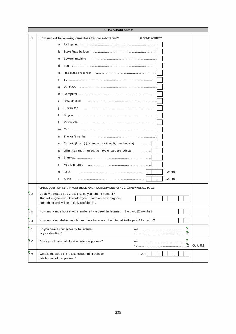
235
7. Household assets
7.1 How many of the following items does this household own? IF NONE, WRITE '0'
a Refrigerator …………………………………………………………………………..
b Stove / gas balloon …………………………………………………………………………..
c Sewing machine …………………………………………………………………………..
d Iron …………………………………………………………………………..
e Radio, tape recorder …………………………………………………………………………..
f TV …………………………………………………………………………..
g VCR/DVD …………………………………………………………………………..
h Computer …………………………………………………………………………..
i Satellite dish …………………………………………………………………………..
j Electric fan …………………………………………………………………………..
k Bicycle …………………………………………………………………………..
l Motorcycle …………………………………………………………………………..
m Car …………………………………………………………………………..
n Tractor / thresher …………………………………………………………………………..
o Carpets (khalin) (expensive best quality hand-woven) …………………………………………………………………………..
p Gilim, satrangi, namad, fash (other carpet-products) …………………………………………………………………………..
q Blankets …………………………………………………………………………..
r Mobile phones …………………………………………………………………………..
s Gold ………………………………………………………………………….. Grams
t Silver ………………………………………………………………………….. Grams
CHECK QUESTION 7.1-r; IF HOUSEHOLD HAS A MOBILE PHONE, ASK 7.2, OTHERWISE GO TO 7.3
7.2 Could we please ask you to give us your phone number?
This will only be used to contact you in case we have forgotten
something and will be entirely confidential.
7.3 How many male household members have used the Internet in the past 12 months?
7.4 How many female household members have used the Internet in the past 12 months?
7.5 Do you have a connection to the Internet Yes ……………………………………………………………1
in your dwelling? No ……………………………………………………………2
7.6 Does your household have any debt at present? Yes ……………………………………………………………1
No ……………………………………………………………2 Go to 8.1
7.7 What is the value of the total outstanding debt for Afs.
this household at present?
, ,
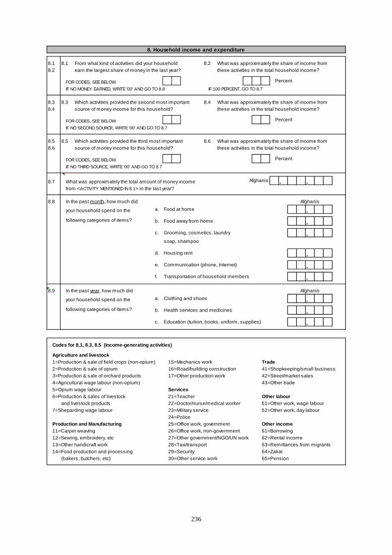
236
8. Household income and expenditure
8.1 8.1 From what kind of activities did your household 8.2 What was approximately the share of income from
8.2 earn the largest share of money in the last year? these activities in the total household income?
FOR CODES, SEE BELOW Percent
IF NO MONEY EARNED, WRITE '00' AND GO TO 8.8 IF 100 PERCENT, GO TO 8.7
8.3 8.3 Which activities provided the second most important 8.4 What was approximately the share of income from
8.4 source of money income for this household? these activities in the total household income?
FOR CODES, SEE BELOW Percent
IF NO SECOND SOURCE, WRITE '00' AND GO TO 8.7
8.5 8.5 Which activities provided the third most important 8.6 What was approximately the share of income from
8.6 source of money income for this household? these activities in the total household income?
FOR CODES, SEE BELOW Percent
IF NO THIRD SOURCE, WRITE '00' AND GO TO 8.7
8.7 What was approximately the total amount of money income Afghanis
from <ACTIVITY MENTIONED IN 8.1> in the last year?
8.8 In the past month, how much did Afghanis
your household spend on the a. Food at home
following categories of items? b. Food away from home
c. Grooming, cosmetics, laundry
soap, shampoo
d. Housing rent
e. Communication (phone, internet)
f. Transportation of household members
8.9 In the past year, how much did Afghanis
your household spend on the a. Clothing and shoes
following categories of items? b. Health services and medicines
c. Education (tuition, books, uniform, supplies)
Codes for 8.1, 8.3, 8.5 (Income-generating activities)
Agriculture and livestock
1=Production & sale of field crops (non-opium) 15=Mechanics work Trade
2=Production & sale of opium 16=Road/building construction 41=Shopkeeping/small business
3=Production & sale of orchard products 17=Other production work 42=Street/market sales
4=Agricultural wage labour (non-opium) 43=Other trade
5=Opium wage labour Services
6=Production & sales of livestock 21=Teacher Other labour
and livestock products 22=Doctor/nurse/medical worker 51=Other work, wage labour
7=Sheparding wage labour 23=Military service 52=Other work, day labour
24=Police
Production and Manufacturing 25=Office work, government Other income
11=Carpet weaving 26=Office work, non-government 61=Borrowing
12=Sewing, embroidery, etc 27=Other government/NGO/UN work 62=Rental income
13=Other handicraft work 28=Taxi/transport 63=Remittances from migrants
14=Food production and processing 29=Security 64=Zakat
(bakers, butchers, etc) 30=Other service work 65=Pension
,
,
,
,
,
,
, ,
,
,
,
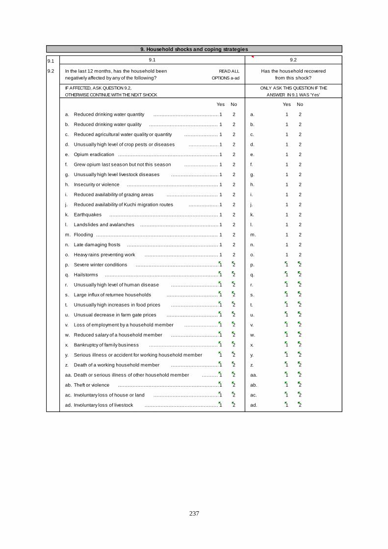
237
9. Household shocks and coping strategies
9.1 9.1 9.2
9.2 In the last 12 months, has the household been READ ALL Has the household recovered
negatively affected by any of the following? OPTIONS a-ad from this shock?
IF AFFECTED, ASK QUESTION 9.2, ONLY ASK THIS QUESTION IF THE
OTHERWISE CONTINUE WITH THE NEXT SHOCK ANSWER IN 9.1 WAS 'Yes'
Yes No Yes No
a. Reduced drinking water quantity ……………………………………………………………………………………………………..1 2 a. 1 2
b. Reduced drinking water quality ……………………………………………………………………………………………………..1 2 b. 1 2
c. Reduced agricultural water quality or quantity ……………………………………………………………………………………………………..1 2 c. 1 2
d. Unusually high level of crop pests or diseases ……………………………………………………………………………………………………..1 2 d. 1 2
e. Opium eradication ……………………………………………………………………………………………………..1 2 e. 1 2
f. Grew opium last season but not this season ……………………………………………………………………………………………………..1 2 f. 1 2
g. Unusually high level livestock diseases ……………………………………………………………………………………………………..1 2 g. 1 2
h. Insecurity or violence ……………………………………………………………………………………………………..1 2 h. 1 2
i. Reduced availability of grazing areas ……………………………………………………………………………………………………..1 2 i. 1 2
j. Reduced availability of Kuchi migration routes ……………………………………………………………………………………………………..1 2 j. 1 2
k. Earthquakes ……………………………………………………………………………………………………..1 2 k. 1 2
l. Landslides and avalanches ……………………………………………………………………………………………………..1 2 l. 1 2
m. Flooding ……………………………………………………………………………………………………..1 2 m. 1 2
n. Late damaging frosts ……………………………………………………………………………………………………..1 2 n. 1 2
o. Heavy rains preventing work ……………………………………………………………………………………………………..1 2 o. 1 2
p. Severe winter conditions ……………………………………………………………………………………………………..1 2 p. 1 2
q. Hailstorms ……………………………………………………………………………………………………..1 2 q. 1 2
r. Unusually high level of human disease ……………………………………………………………………………………………………..1 2 r. 1 2
s. Large influx of returnee households ……………………………………………………………………………………………………..1 2 s. 1 2
t. Unusually high increases in food prices ……………………………………………………………………………………………………..1 2 t. 1 2
u. Unusual decrease in farm gate prices ……………………………………………………………………………………………………..1 2 u. 1 2
v. Loss of employment by a household member ……………………………………………………………………………………………………..1 2 v. 1 2
w. Reduced salary of a household member ……………………………………………………………………………………………………..1 2 w. 1 2
x. Bankruptcy of family business ……………………………………………………………………………………………………..1 2 x. 1 2
y. Serious illness or accident for working household member 1 2 y. 1 2
z. Death of a working household member ……………………………………………………………………………………………………..1 2 z. 1 2
aa. Death or serious illness of other household member ……………………………………………………………………………………………………..1 2 aa. 1 2
ab. Theft or violence ……………………………………………………………………………………………………..1 2 ab. 1 2
ac. Involuntary loss of house or land ……………………………………………………………………………………………………..1 2 ac. 1 2
ad. Involuntary loss of livestock ……………………………………………………………………………………………………..1 2 ad. 1 2
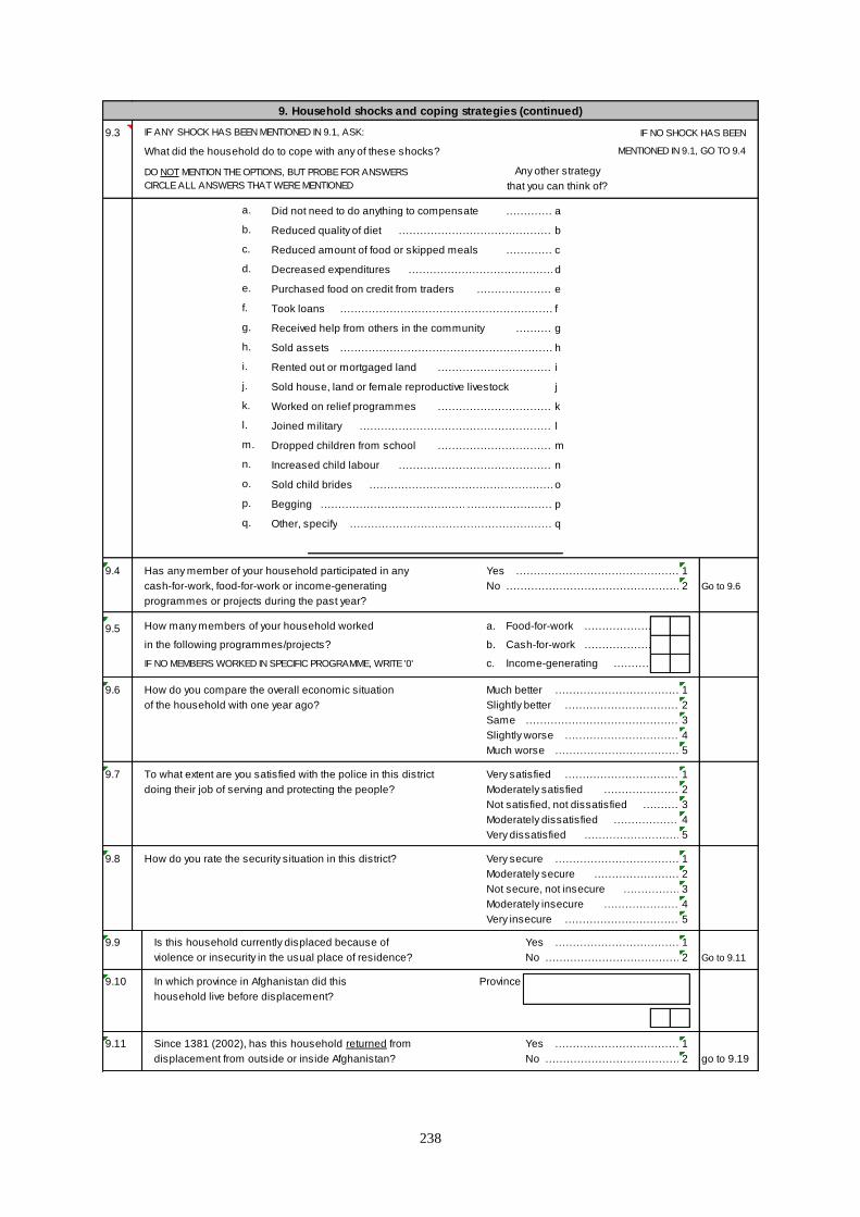
238
9. Household shocks and coping strategies (continued)
9.3 IF ANY SHOCK HAS BEEN MENTIONED IN 9.1, ASK: IF NO SHOCK HAS BEEN
What did the household do to cope with any of these shocks? MENTIONED IN 9.1, GO TO 9.4
DO NOT MENTION THE OPTIONS, BUT PROBE FOR ANSWERS Any other strategy
CIRCLE ALL ANSWERS THAT WERE MENTIONED that you can think of?
a. Did not need to do anything to compensate ……………………………………………………………………………………………………..a
b. Reduced quality of diet ……………………………………………………………………………………………………..b
c. Reduced amount of food or skipped meals ……………………………………………………………………………………………………..c
d. Decreased expenditures ……………………………………………………………………………………………………..d
e. Purchased food on credit from traders ……………………………………………………………………………………………………..e
f. Took loans ……………………………………………………………………………………………………..f
g. Received help from others in the community ……………………………………………………………………………………………………..g
h. Sold assets ……………………………………………………………………………………………………..h
i. Rented out or mortgaged land ……………………………………………………………………………………………………..i
j. Sold house, land or female reproductive livestock j
k. Worked on relief programmes ……………………………………………………………………………………………………..k
l. Joined military ……………………………………………………………………………………………………..l
m. Dropped children from school ……………………………………………………………………………………………………..m
n. Increased child labour ……………………………………………………………………………………………………..n
o. Sold child brides ……………………………………………………………………………………………………..o
p. Begging ……………………………………………………………………………………………………..……………………………………………………………………………………………………..p
q. Other, specify ……………………………………………………………………………………………………..q
9.4 Has any member of your household participated in any Yes ……………………………………………………………1
cash-for-work, food-for-work or income-generating No ……………………………………………………………2 Go to 9.6
programmes or projects during the past year?
9.5 How many members of your household worked a. Food-for-work ……………………………………………………………
in the following programmes/projects? b. Cash-for-work ……………………………………………………………
IF NO MEMBERS WORKED IN SPECIFIC PROGRAMME, WRITE '0' c. Income-generating ……………………………………………………………
9.6 How do you compare the overall economic situation Much better ……………………………………………………………1
of the household with one year ago? Slightly better ……………………………………………………………2
Same ……………………………………………………………3
Slightly worse ……………………………………………………………4
Much worse ……………………………………………………………5
9.7 To what extent are you satisfied with the police in this district Very satisfied ……………………………………………………………1
doing their job of serving and protecting the people? Moderately satisfied ……………………………………………………………2
Not satisfied, not dissatisfied ……………………………………………………………3
Moderately dissatisfied ……………………………………………………………4
Very dissatisfied ……………………………………………………………5
9.8 How do you rate the security situation in this district? Very secure ……………………………………………………………1
Moderately secure ……………………………………………………………2
Not secure, not insecure ……………………………………………………………3
Moderately insecure ……………………………………………………………4
Very insecure ……………………………………………………………5
9.9 Is this household currently displaced because of Yes ……………………………………………………………1
violence or insecurity in the usual place of residence? No ……………………………………………………………2 Go to 9.11
9.10 In which province in Afghanistan did this Province
household live before displacement?
9.11 Since 1381 (2002), has this household returned from Yes ……………………………………………………………1
displacement from outside or inside Afghanistan? No ……………………………………………………………2 go to 9.19
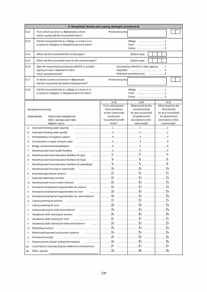
239
9. Household shocks and coping strategies (continued)
9.12 From which province in Afghanistan or from Province/country
which country did this household return?
9.13 Did the household live in a village, in a town or in Village ……………………………………………………………1
a camp for refugees or displaced persons there? Town ……………………………………………………………2
Camp ……………………………………………………………3
9.14 When did the household flee to that place? Shamsi year
9.15 When did the household come to this present place? Shamsi year
9.16 Was the household assisted by UNHCR or another Assisted by UNHCR or other agency ……………………………………………………………1
agency or was it deported or did it Deported ……………………………………………………………2
return spontaneously? Returned spontaneously ……………………………………………………………3
9.17 In which country or province in Afghanistan Province/country
did this household live before displacement?
9.18 Did the household live in a village or a town or in Village ……………………………………………………………1
a camp for refugees or displaced persons then? Town ……………………………………………………………2
Camp ……………………………………………………………3
9.19 9.20 9.21
From what govern- What would be the What would be the
Development priority ment assitance second priority third priority
to this community for your household for your household
INTERVIEWER: CIRCLE ONE ANSWER FOR would your for government for government
FIRST, SECOND AND THIRD household benefit assistance to this assistance to this
PRIORITY EACH most? community? community?
a Improved drinking water quantity …………………………………………………………………………..1 ……………..……………..1 ……………..……………..1
b Improved drinking water quality …………………………………………………………………………..2 ……………..……………..2 ……………..……………..2
c Rehabilitation of irrigation system …………………………………………………………………………..3 ……………..……………..3 ……………..……………..3
d Construction or repair of local roads …………………………………………………………………………..4 ……………..……………..4 ……………..……………..4
e Bridge construction/rehabilitation …………………………………………………………………………..5 ……………..……………..5 ……………..……………..5
f New/improved local health facilities …………………………………………………………………………..6 ……………..……………..6 ……………..……………..6
g New/improved local education facilities for girls …………………………………………………………………………..7 ……………..……………..7 ……………..……………..7
h New/improved local education facilities for boys …………………………………………………………………………..8 ……………..……………..8 ……………..……………..8
i New/improved local education facilities for girls&boys …………………………………………………………………………..9 ……………..……………..9 ……………..……………..9
j New/improved housing in community …………………………………………………………………………..10 ……………..……………..10 ……………..……………..10
k Improved agricultural services …………………………………………………………………………..11 ……………..……………..11 ……………..……………..11
l Improved veterinary services …………………………………………………………………………..12 ……………..……………..12 ……………..……………..12
m New/improved micro-credit schemes …………………………………………………………………………..13 ……………..……………..13 ……………..……………..13
n Increased employment opportunities for women …………………………………………………………………………..14 ……………..……………..14 ……………..……………..14
o Increased employment opportunities for men …………………………………………………………………………..15 ……………..……………..15 ……………..……………..15
p Increased employment opportunities for women&men ……………..16 ……………..……………..16 ……………..……………..16
q Literacy training for women …………………………………………………………………………..17 ……………..……………..17 ……………..……………..17
r Literacy training for men …………………………………………………………………………..18 ……………..……………..18 ……………..……………..18
s Literacy training for both women&men …………………………………………………………………………..19 ……………..……………..19 ……………..……………..19
t Vocational skills training for women …………………………………………………………………………..20 ……………..……………..20 ……………..……………..20
u Vocational skills training for men …………………………………………………………………………..21 ……………..……………..21 ……………..……………..21
v Vocational skills training for both women&men …………………………………………………………………………..22 ……………..……………..22 ……………..……………..22
w Electricity provision …………………………………………………………………………..23 ……………..……………..23 ……………..……………..23
x Reformed/improved local justice systems …………………………………………………………………………..24 ……………..……………..24 ……………..……………..24
y Increased security …………………………………………………………………………..25 ……………..……………..25 ……………..……………..25
z Disarmament of local militia/commanders …………………………………………………………………………..26 ……………..……………..26 ……………..……………..26
aa Local land or housing dispute settlement mechanisms ……………..27 ……………..……………..27 ……………..……………..27
ab Other, specify ……………..28 ……………..……………..28 ……………..……………..28____________________________
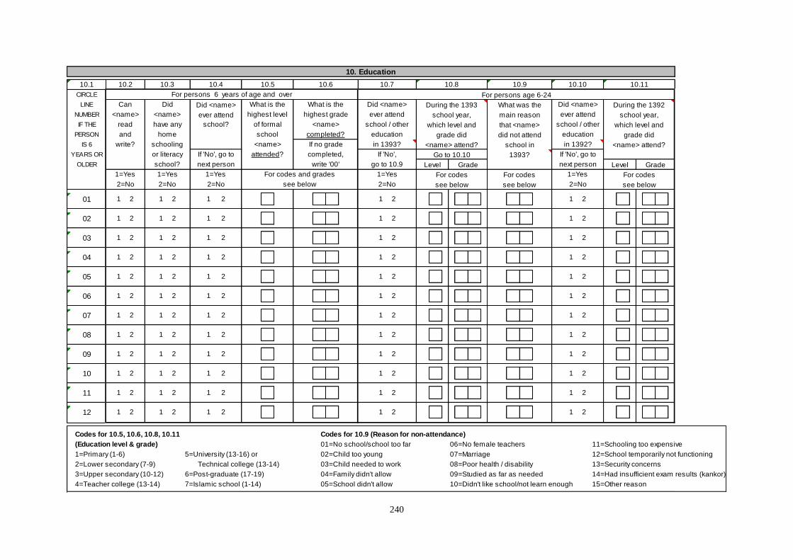
240
10. Education
10.1 10.2 10.3 10.4 10.5 10.6 10.7 10.8 10.9 10.10 10.11
CIRCLE For persons 6 years of age and over For persons age 6-24
LINE Can Did Did <name> What is the What is the Did <name> During the 1393 What was the Did <name> During the 1392
NUMBER <name> <name> ever attend highest level highest grade ever attend school year, main reason ever attend school year,
IF THE read have any school? of formal <name> school / other which level and that <name> school / other which level and
PERSON and home school completed? education grade did did not attend education grade did
IS 6 write? schooling <name> If no grade in 1393? <name> attend? school in in 1392? <name> attend?
YEARS OR or literacy If 'No', go to attended? completed, If 'No', Go to 10.10 1393? If 'No', go to
OLDER school? next person write '00' go to 10.9 Level Grade next person Level Grade
1=Yes 1=Yes 1=Yes For codes and grades 1=Yes For codes For codes 1=Yes For codes
2=No 2=No 2=No see below 2=No see below see below 2=No see below
01 1 2 1 2 1 2 1 2 1 2
02 1 2 1 2 1 2 1 2 1 2
03 1 2 1 2 1 2 1 2 1 2
04 1 2 1 2 1 2 1 2 1 2
05 1 2 1 2 1 2 1 2 1 2
06 1 2 1 2 1 2 1 2 1 2
07 1 2 1 2 1 2 1 2 1 2
08 1 2 1 2 1 2 1 2 1 2
09 1 2 1 2 1 2 1 2 1 2
10 1 2 1 2 1 2 1 2 1 2
11 1 2 1 2 1 2 1 2 1 2
12 1 2 1 2 1 2 1 2 1 2
Codes for 10.5, 10.6, 10.8, 10.11 Codes for 10.9 (Reason for non-attendance)
(Education level & grade) 01=No school/school too far 06=No female teachers 11=Schooling too expensive
1=Primary (1-6) 5=University (13-16) or 02=Child too young 07=Marriage 12=School temporarily not functioning
2=Lower secondary (7-9) Technical college (13-14) 03=Child needed to work 08=Poor health / disability 13=Security concerns
3=Upper secondary (10-12) 6=Post-graduate (17-19) 04=Family didn't allow 09=Studied as far as needed 14=Had insufficient exam results (kankor)
4=Teacher college (13-14) 7=Islamic school (1-14) 05=School didn't allow 10=Didn't like school/not learn enough 15=Other reason
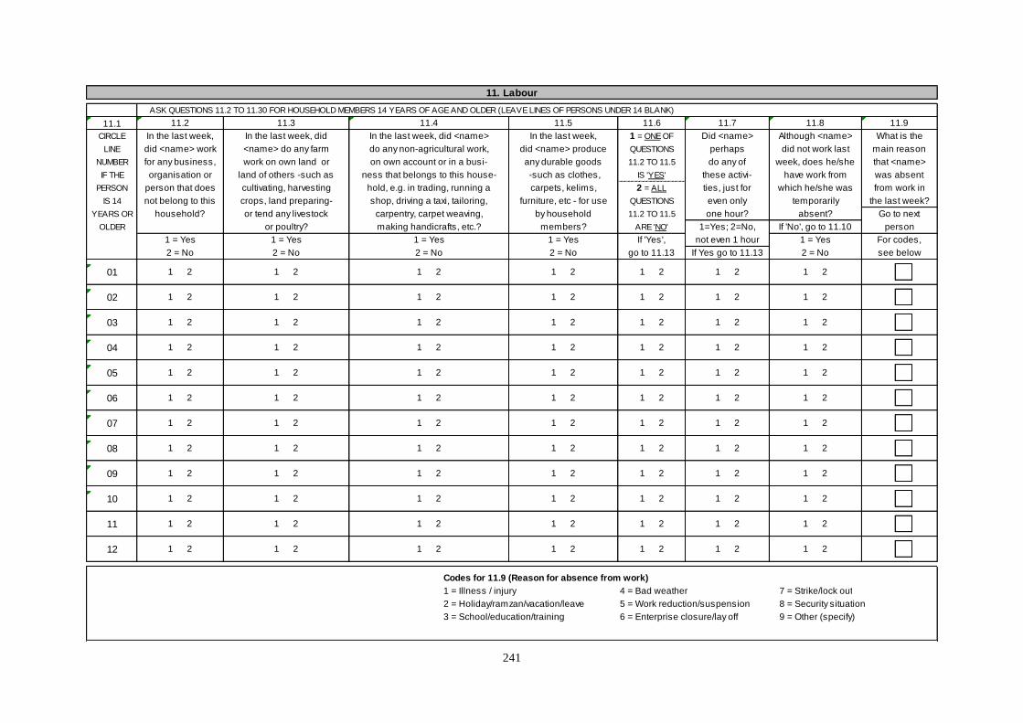
241
11. Labour 11. Labour (continued)
ASK QUESTIONS 11.2 TO 11.30 FOR HOUSEHOLD MEMBERS 14 YEARS OF AGE AND OLDER (LEAVE LINES OF PERSONS UNDER 14 BLANK) All
11.1 11.2 11.3 11.4 11.5 11.6 11.7 11.8 11.9 11.1
CIRCLE In the last week, In the last week, did In the last week, did <name> In the last week, 1 = ONE OF Did <name> Although <name> What is the Line
LINE did <name> work <name> do any farm do any non-agricultural work, did <name> produce QUESTIONS perhaps did not work last main reason no.
NUMBER for any business, work on own land or on own account or in a busi- any durable goods 11.2 TO 11.5 do any of week, does he/she that <name> available
IF THE organisation or land of others -such as ness that belongs to this house- -such as clothes, IS 'YES' these activi- have work from was absent for work in
PERSON person that does cultivating, harvesting hold, e.g. in trading, running a carpets, kelims, 2 = ALL ties, just for which he/she was from work in the last week
IS 14 not belong to this crops, land preparing- shop, driving a taxi, tailoring, furniture, etc - for use QUESTIONS even only temporarily the last week? if it had been
YEARS OR household? or tend any livestock carpentry, carpet weaving, by household 11.2 TO 11.5 one hour? absent? Go to next offered?
OLDER or poultry? making handicrafts, etc.? members? ARE 'NO' 1=Yes; 2=No, If 'No', go to 11.10 person
1 = Yes 1 = Yes 1 = Yes 1 = Yes If 'Yes', not even 1 hour 1 = Yes For codes,
2 = No 2 = No 2 = No 2 = No go to 11.13 If Yes go to 11.13 2 = No see below
01 1 2 1 2 1 2 1 2 1 2 1 2 1 2
02 1 2 1 2 1 2 1 2 1 2 1 2 1 2
03 1 2 1 2 1 2 1 2 1 2 1 2 1 2
04 1 2 1 2 1 2 1 2 1 2 1 2 1 2
05 1 2 1 2 1 2 1 2 1 2 1 2 1 2
06 1 2 1 2 1 2 1 2 1 2 1 2 1 2
07 1 2 1 2 1 2 1 2 1 2 1 2 1 2
08 1 2 1 2 1 2 1 2 1 2 1 2 1 2
09 1 2 1 2 1 2 1 2 1 2 1 2 1 2
10 1 2 1 2 1 2 1 2 1 2 1 2 1 2
11 1 2 1 2 1 2 1 2 1 2 1 2 1 2
12 1 2 1 2 1 2 1 2 1 2 1 2 1 2
Codes for 11.9 (Reason for absence from work)
1 = Illness / injury 4 = Bad weather 7 = Strike/lock out
2 = Holiday/ramzan/vacation/leave 5 = Work reduction/suspension 8 = Security situation
3 = School/education/training 6 = Enterprise closure/lay off 9 = Other (specify)
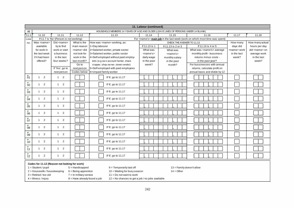
242
11. Labour (continued) 11. Labour (continued)
All HOUSEHOLD MEMBERS 14 YEARS OF AGE AND OLDER (LEAVE LINES OF PERSONS UNDER 14 BLANK) All
11.1 11.10 11.11 11.12 11.13 11.14 11.15 11.16 11.17 11.18 11.1
Line If 11.7 is 'No' (Person is not working) For <name's> main job in the last week (work on which most time was spent) Line
no. Was <name> Did <name> What is the How was <name> working, as: CHECK THE ANSWER TO 11.13 How many How many actual no.
available try to find main reason 1=Day labourer If 11.13 is 1 If 11.13 is 2 or 3 If 11.13 is 4 or 5 days did hours per day or services delivered by the
for work in work or start <name> did 2=Salaried worker, private sector What was What was What was <name's> average <name> work did <name> on bussiness or organisation in which
the last week a business not look for 3=Salaried worker, public sector <name's> <name's> monthly profit - bussiness in the last average work <name> worked the last week?
if it had been in the last work in the 4=Self-employed without paid employ- daily wage monthly salary returns minus costs - week? in the last E.g producing w heat, raising livestock,
offered? four weeks? last month? ees (e.g ow n-account farmer, share in the past in the past in the past year? week? retail sale of bread, primary school
Go to cropper, shop ow ner, street vendor) week? month? For bussinesses with annual education, providing health care, police
If 'Yes', go to next person 5=Self-employed with paid employees returns, calculate profit on services, construction of buildings,
next person Codes below 6=Unpaid family worker annual basis and divide by 12 transportation, local government
01 1 2 1 2 If '6', go to 11.17 , , ,
02 1 2 1 2 If '6', go to 11.17 , , ,
03 1 2 1 2 If '6', go to 11.17 , , ,
04 1 2 1 2 If '6', go to 11.17 , , ,
05 1 2 1 2 If '6', go to 11.17 , , ,
06 1 2 1 2 If '6', go to 11.17 , , ,
07 1 2 1 2 If '6', go to 11.17 , , ,
08 1 2 1 2 If '6', go to 11.17 , , ,
09 1 2 1 2 If '6', go to 11.17 , , ,
10 1 2 1 2 If '6', go to 11.17 , , ,
11 1 2 1 2 If '6', go to 11.17 , , ,
12 1 2 1 2 If '6', go to 11.17 , , ,
Codes for 11.12 (Reason not looking for work)
1 = Student / pupil 5 = Handicapped 9 = Temporarily laid off 13 = Family doesn't allow
2 = Housewife / housekeeping 6 = Being apprentice 10 = Waiting for busy season 14 = Other
3 = Retired / too old 7 = In military service 11 = Do not want to work
4 = Illness / injury 8 = Have already found a job 12 = No chances to get a job / no jobs available
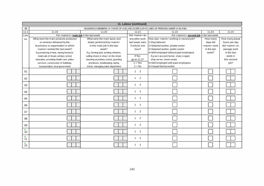
243
11. Labour (continued) 11. Labour (continued)
All HOUSEHOLD MEMBERS 14 YEARS OF AGE AND OLDER (LEAVE LINES OF PERSONS UNDER 14 BLANK) All
11.1 11.19 11.20 11.21 11.22 11.23 11.24 11.1
Line For <name's> main job in the last week Did <name> do For <name's> second job in the last week Line
no. What were the main products produced What were the main tasks and any other work How was <name> working in second job? How many How many actual no.
or services delivered by the duties performed by <name> last week, even 1=Day labourer days did hours per day or services delivered by the
bussiness or organisation in which in this main job in the last if only for one 2=Salaried worker, private sector <name> work did <name> on bussiness or organisation in which
<name> worked the last week? week? hour? 3=Salaried worker, public sector in the last average work <name> worked the last week?
E.g producing w heat, raising livestock, E.g. farming land, tending chickens, 4=Self-employed without paid employees week? in the last E.g producing w heat, raising livestock,
retail sale of bread, primary school selling shoes in shop / on the street, If 'No', E.g ow n-account farmer, share cropper week in retail sale of bread, primary school
education, providing health care, police teaching at primary school, guarding go to 11.27 shop ow ner, street vendor this second education, providing health care, police
services, construction of buildings, premisses, bookkeeping, laying 1 = Yes 5=Self-employed with paid employees job? services, construction of buildings,
transportation, local government bricks, managing sales department 2 = No 6=Unpaid family worker transportation, local government
01 1 2
02 1 2
03 1 2
04 1 2
05 1 2
06 1 2
07 1 2
08 1 2
09 1 2
10 1 2
11 1 2
12 1 2
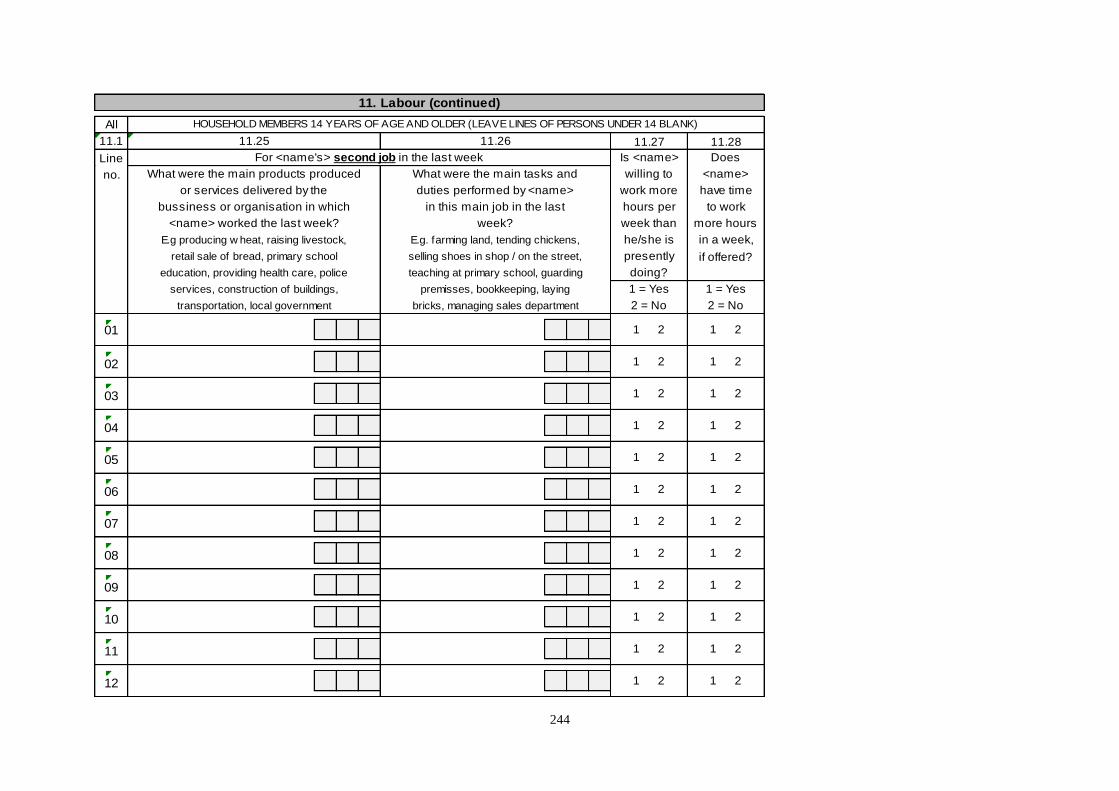
244
11. Labour (continued)
All HOUSEHOLD MEMBERS 14 YEARS OF AGE AND OLDER (LEAVE LINES OF PERSONS UNDER 14 BLANK)
11.1 11.25 11.26 11.27 11.28
Line For <name's> second job in the last week Is <name> Does
no. What were the main products produced What were the main tasks and willing to <name>
or services delivered by the duties performed by <name> work more have time
bussiness or organisation in which in this main job in the last hours per to work
<name> worked the last week? week? week than more hours
E.g producing w heat, raising livestock, E.g. farming land, tending chickens, he/she is in a week,
retail sale of bread, primary school selling shoes in shop / on the street, presently if offered?
education, providing health care, police teaching at primary school, guarding doing?
services, construction of buildings, premisses, bookkeeping, laying 1 = Yes 1 = Yes
transportation, local government bricks, managing sales department 2 = No 2 = No
01 1 2 1 2
02 1 2 1 2
03 1 2 1 2
04 1 2 1 2
05 1 2 1 2
06 1 2 1 2
07 1 2 1 2
08 1 2 1 2
09 1 2 1 2
10 1 2 1 2
11 1 2 1 2
12 1 2 1 2
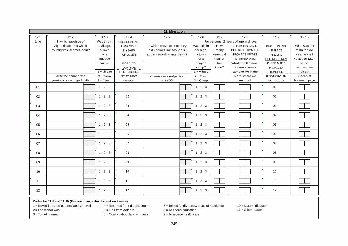
245
12. Migration 12. Migration (continued)
12.1 12.2 12.3 12.4 12.5 12.6 12.7 12.8 12.9 12.10 12.11
Line In which province of Was this in CIRCLE LINE NO. For persons 2 years of age and over CIRCLE LINE NO.
no. Afghanistan or in which a village, IF <NAME> IS In which province or country Was this in How IF PLACE IN 12.5 IS CIRCLE LINE NO. What was the IF <NAME> IS
country was <name> born? a town 2 YEARS did <name> live two years a village, many DIFFERENT FROM THE IF PLACE main reason 12 YEARS
or a OR OLDER ago in <month of interview>? a town years did PROVINCE OF THIS IN 12.2 IS <name> left OR OLDER
refugee or a <name> INTERVIEW ASK: DIFFERENT FROM <place of 12.2> the Taliban in 1380?
camp? IF CIRCLED, refugee live What was the main PLACE IN 12.5 to live IF CIRCLED,
CONTINUE camp? there? reason <name> IF CIRCLED, somewhere CONTINUE
1 = Village IF NOT CIRCLED, 1 = Village came to live in the CONTINUE else? IF NOT CIRCLED,
Write the name of the 2 = Town GO TO NEXT If <name> was not yet born, 2 = Town place where we IF NOT CIRCLED, Codes at GO TO NEXT
province or country of birth 3 = Camp PERSON write '00' 3 = Camp are now? GO TO 12.11 bottom of page PERSON
01 1 2 3 01 1 2 3 01 01
02 1 2 3 02 1 2 3 02 02
03 1 2 3 03 1 2 3 03 03
04 1 2 3 04 1 2 3 04 04
05 1 2 3 05 1 2 3 05 05
06 1 2 3 06 1 2 3 06 06
07 1 2 3 07 1 2 3 07 07
08 1 2 3 08 1 2 3 08 08
09 1 2 3 09 1 2 3 09 09
10 1 2 3 10 1 2 3 10 10
11 1 2 3 11 1 2 3 11 11
12 1 2 3 12 1 2 3 12 12
Codes for 12.8 and 12.10 (Reason change the place of residence)
1 = Moved because parents/family moved 4 = Returned from displacement 7 = Joined family at new place of residence 10 = Natural disaster
2 = Looked for work 5 = Fled from violence 8 = To attend education 11 = Other reason
3 = To get married 6 = Conflict about land or house 9 = To receive health care
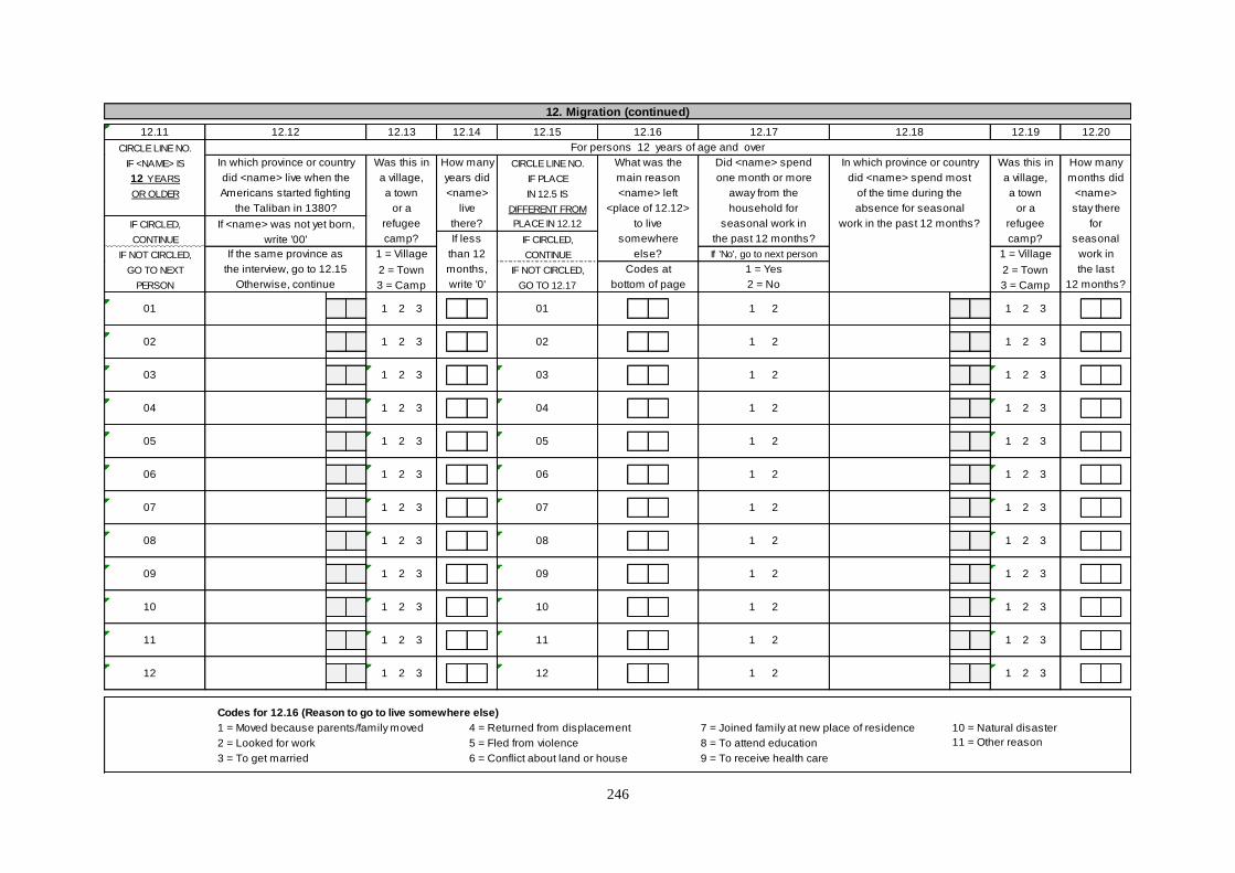
246
12. Migration (continued)
12.11 12.12 12.13 12.14 12.15 12.16 12.17 12.18 12.19 12.20
CIRCLE LINE NO. For persons 12 years of age and over
IF <NAME> IS In which province or country Was this in How many CIRCLE LINE NO. What was the Did <name> spend In which province or country Was this in How many
12 YEARS did <name> live when the a village, years did IF PLACE main reason one month or more did <name> spend most a village, months did
OR OLDER Americans started fighting a town <name> IN 12.5 IS <name> left away from the of the time during the a town <name>
the Taliban in 1380? or a live DIFFERENT FROM <place of 12.12> household for absence for seasonal or a stay there
IF CIRCLED, If <name> was not yet born, refugee there? PLACE IN 12.12 to live seasonal work in work in the past 12 months? refugee for
CONTINUE write '00' camp? If less IF CIRCLED, somewhere the past 12 months? camp? seasonal
IF NOT CIRCLED, If the same province as 1 = Village than 12 CONTINUE else? If 'No', go to next person 1 = Village work in
GO TO NEXT the interview, go to 12.15 2 = Town months, IF NOT CIRCLED, Codes at 1 = Yes 2 = Town the last
PERSON Otherwise, continue 3 = Camp write '0' GO TO 12.17 bottom of page 2 = No 3 = Camp 12 months?
01 1 2 3 01 1 2 1 2 3
02 1 2 3 02 1 2 1 2 3
03 1 2 3 03 1 2 1 2 3
04 1 2 3 04 1 2 1 2 3
05 1 2 3 05 1 2 1 2 3
06 1 2 3 06 1 2 1 2 3
07 1 2 3 07 1 2 1 2 3
08 1 2 3 08 1 2 1 2 3
09 1 2 3 09 1 2 1 2 3
10 1 2 3 10 1 2 1 2 3
11 1 2 3 11 1 2 1 2 3
12 1 2 3 12 1 2 1 2 3
Codes for 12.16 (Reason to go to live somewhere else)
1 = Moved because parents/family moved 4 = Returned from displacement 7 = Joined family at new place of residence 10 = Natural disaster
2 = Looked for work 5 = Fled from violence 8 = To attend education 11 = Other reason
3 = To get married 6 = Conflict about land or house 9 = To receive health care
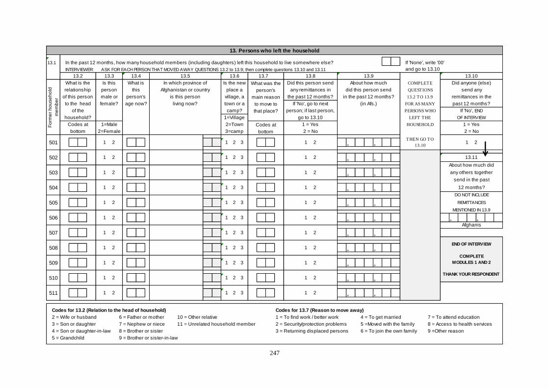
247
13. Persons who left the household
13.1 In the past 12 months, how many household members (including daughters) left this household to live somewhere else? If 'None', write '00'
INTERVIEWER: ASK FOR EACH PERSON THAT MOVED AWAY QUESTIONS 13.2 to 13.9; then complete questions 13.10 and 13.11 and go to 13.10
13.2 13.3 13.4 13.5 13.6 13.7 13.8 13.9 13.10
What is the Is this What is In which province of Is the new What was the Did this person send About how much COMPLETE Did anyone (else)
relationship person this Afghanistan or country place a person's any remittances in did this person send QUESTIONS send any
of this person male or person's is this person village, a main reason the past 12 months? in the past 12 months? 13.2 TO 13.9 remittances in the
to the head female? age now? living now? town or a to move to If 'No', go to next (in Afs.) FOR AS MANY past 12 months?
of the camp? that place? person; if last person, PERSONS WHO If 'No', END
household? 1=Village go to 13.10 LEFT THE OF INTERVIEW
Codes at 1=Male 2=Town Codes at 1 = Yes HOUSEHOLD 1 = Yes
bottom 2=Female 3=camp bottom 2 = No 2 = No
501 1 2 1 2 3 1 2 1 2
502 1 2 1 2 3 1 2 13.11
503 1 2 1 2 3 1 2 any others together
504 1 2 1 2 3 1 2 12 months?
505 1 2 1 2 3 1 2 REMITTANCES
506 1 2 1 2 3 1 2
507 1 2 1 2 3 1 2
508 1 2 1 2 3 1 2
509 1 2 1 2 3 1 2
510 1 2 1 2 3 1 2
511 1 2 1 2 3 1 2
2 = Wife or husband 6 = Father or mother 10 = Other relative 1 = To find work / better work 4 = To get married 7 = To attend education
3 = Son or daughter 7 = Nephew or niece 11 = Unrelated household member 2 = Security/protection problems 5 =Moved with the family 8 = Access to health services
4 = Son or daughter-in-law 8 = Brother or sister 3 = Returning displaced persons 6 = To join the own family 9 =Other reason
5 = Grandchild 9 = Brother or sister-in-law
Afghanis
,
Codes for 13.2 (Relation to the head of household) Codes for 13.7 (Reason to move away)
,,
THANK YOUR RESPONDENT
, ,
,
COMPLETE
MODULES 1 AND 2
, ,END OF INTERVIEW
,,
, ,,,
,
MENTIONED IN 13.9
,
send in the past
,
DO NOT INCLUDE
, ,
,
,
About how much did
,
THEN GO TO
13.10
Fo
rme
r h
ou
se
ho
ld
me
mb
er
,,
248
20. Household identification (Female questionnaire)
INTERVIEWER: COPY INFORMATION FROM MODULE 1 (HOUSEHOLD IDENTIFICATION, MALE QUESTIONNAIRE)
Province Code
name 20.8 Household number (1-15)
Code
Door number
Control and Enumeration Area code Name of head of
household
Cluster code
Urban …………………………1
Rural …………………………2
Kuchi …………………………3
Code
20.11 Line number of senior female respondent
Code 20.12 Line number of male respondent in case
of absence of female household members
20.13 Interview start time Hour Minute 20.14 Interview finish time Hour Minute
: :
MODULES 21 TO 24 SHOULD BE ADMINISTERED TO THE SENIOR FEMALE HOUSEHOLD MEMBER, WHO IS EITHER
THE WIFE OF THE HEAD OF HOUSEHOLD, THE MOST ACTIVE AND IMPORTANT FEMALE MEMBER OF THE
HOUSEHOLD OR, IN CASE OF FEMALE-HEADED HOUSEHOLDS, THE HEAD OF HOUSEHOLD
IN CASE OF ABSENCE OF ANY RESPONSIBLE FEMALE HOUSEHOLD MEMBER, A MALE HOUSEHOLD MEMBER
SHOULD BE ASKED TO ANSWER QUESTIONS OF MODULES 23 AND 24 ONLY.
IN THESE CASES, THE LINE NUMBER OF THE MALE RESPONDENT SHOULD BE FILLED IN QUESTION 20.12 ABOVE
MODULES 25 AND 26 SHOULD BE ADMINISTERED TO ELIGIBLE WOMEN INDIVIDUALLY
Afghanistan Living Conditions
Survey (ALCS 1392-93)
20.1
20.9
20.320.10
20.2 District name
20.4
20.5
20.6 Urban nahia
20.7 Village name
Residence code
249
21. Missing household members
We listed all the members of this household, but I would like check with you to see whether really
everyone who usually lives here is included. We are especially eager to see that no children, newborns,
girls and women - especially older women - are omitted from the list
GO THROUGH THE HOUSEHOLD LISTING WITH THE RESPONDENT AND ADD MISSING PERSONS
WITH ADDITIONAL INFORMATION BELOW
21.1 21.2 21.3 21.4 21.5 21.6 21.7 21.8 21.9 21.10 21.11
Line Write the name What is the How old Is What is Line Does Line Does Line
no. of each missed relationship is <name> <name's> number <name's> number <name's> number
household member of <name> <name>? male or marital of (first) father live of mother of
to the head female? status? spouse in this this live in this this
CON- of house- house- father house- mother
TINUE hold? For For codes, hold? hold?
FROM children see below 1=Yes 1=Yes
LAST less than If not If not in this 2=No 2=No
NUM - For codes, one year, 1=Male married, household, If No, go If No, go
BER see below write '00' 2=Female go to 21.8 write '98' to 21.10 to next line
1 2 1 2 1 2
1 2 1 2 1 2
1 2 1 2 1 2
1 2 1 2 1 2
Codes for 21.3 (Relationship to head of household) Codes for 21.6 (Marital status)
02 = Wife or husband 06 = Father or mother 10 = Other relative 1 = Married 4 = Engaged
03 = Son or daughter 07 = Nephew or niece 11 = Unrelated member 2 = Widowed 5 = Never married
04 = Son-/daughter-in-law 08 = Brother or sister 3 = Divorced or
05 = Grandchild 09 = Brother-/sister-in-law separated
INTERVIEWER,
SAY:
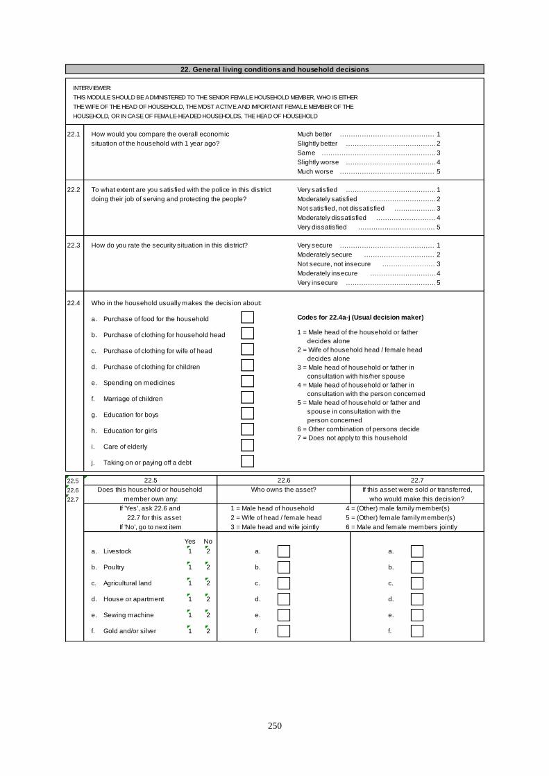
250
22. General living conditions and household decisions
INTERVIEWER:
THIS MODULE SHOULD BE ADMINISTERED TO THE SENIOR FEMALE HOUSEHOLD MEMBER, WHO IS EITHER
THE WIFE OF THE HEAD OF HOUSEHOLD, THE MOST ACTIVE AND IMPORTANT FEMALE MEMBER OF THE
HOUSEHOLD, OR IN CASE OF FEMALE-HEADED HOUSEHOLDS, THE HEAD OF HOUSEHOLD
22.1 How would you compare the overall economic Much better ……………………………………………………………1
situation of the household with 1 year ago? Slightly better ……………………………………………………………2
Same ……………………………………………………………3
Slightly worse ……………………………………………………………4
Much worse ……………………………………………………………5
22.2 To what extent are you satisfied with the police in this district Very satisfied ……………………………………………………………1
doing their job of serving and protecting the people? Moderately satisfied ……………………………………………………………2
Not satisfied, not dissatisfied ……………………………………………………………3
Moderately dissatisfied ……………………………………………………………4
Very dissatisfied ……………………………………………………………5
22.3 How do you rate the security situation in this district? Very secure ……………………………………………………………1
Moderately secure ……………………………………………………………2
Not secure, not insecure ……………………………………………………………3
Moderately insecure ……………………………………………………………4
Very insecure ……………………………………………………………5
22.4 Who in the household usually makes the decision about:
a. Purchase of food for the household Codes for 22.4a-j (Usual decision maker)
b. Purchase of clothing for household head
c. Purchase of clothing for wife of head
d. Purchase of clothing for children
e. Spending on medicines
f. Marriage of children
g. Education for boys
h. Education for girls
i. Care of elderly
j. Taking on or paying off a debt
22.5 22.5 22.6 22.7
22.6 Does this household or household Who owns the asset? If this asset were sold or transferred,
22.7 member own any: who would make this decision?
If 'Yes', ask 22.6 and 1 = Male head of household 4 = (Other) male family member(s)
22.7 for this asset 2 = Wife of head / female head 5 = (Other) female family member(s)
If 'No', go to next item 3 = Male head and wife jointly 6 = Male and female members jointly
Yes No
a. Livestock 1 2 a. a.
b. Poultry 1 2 b. b.
c. Agricultural land 1 2 c. c.
d. House or apartment 1 2 d. d.
e. Sewing machine 1 2 e. e.
f. Gold and/or silver 1 2 f. f.
1 = Male head of the household or father
decides alone
2 = Wife of household head / female head
decides alone
3 = Male head of household or father in
consultation with his/her spouse
4 = Male head of household or father in
consultation with the person concerned
5 = Male head of household or father and
spouse in consultation with the
person concerned
6 = Other combination of persons decide
7 = Does not apply to this household
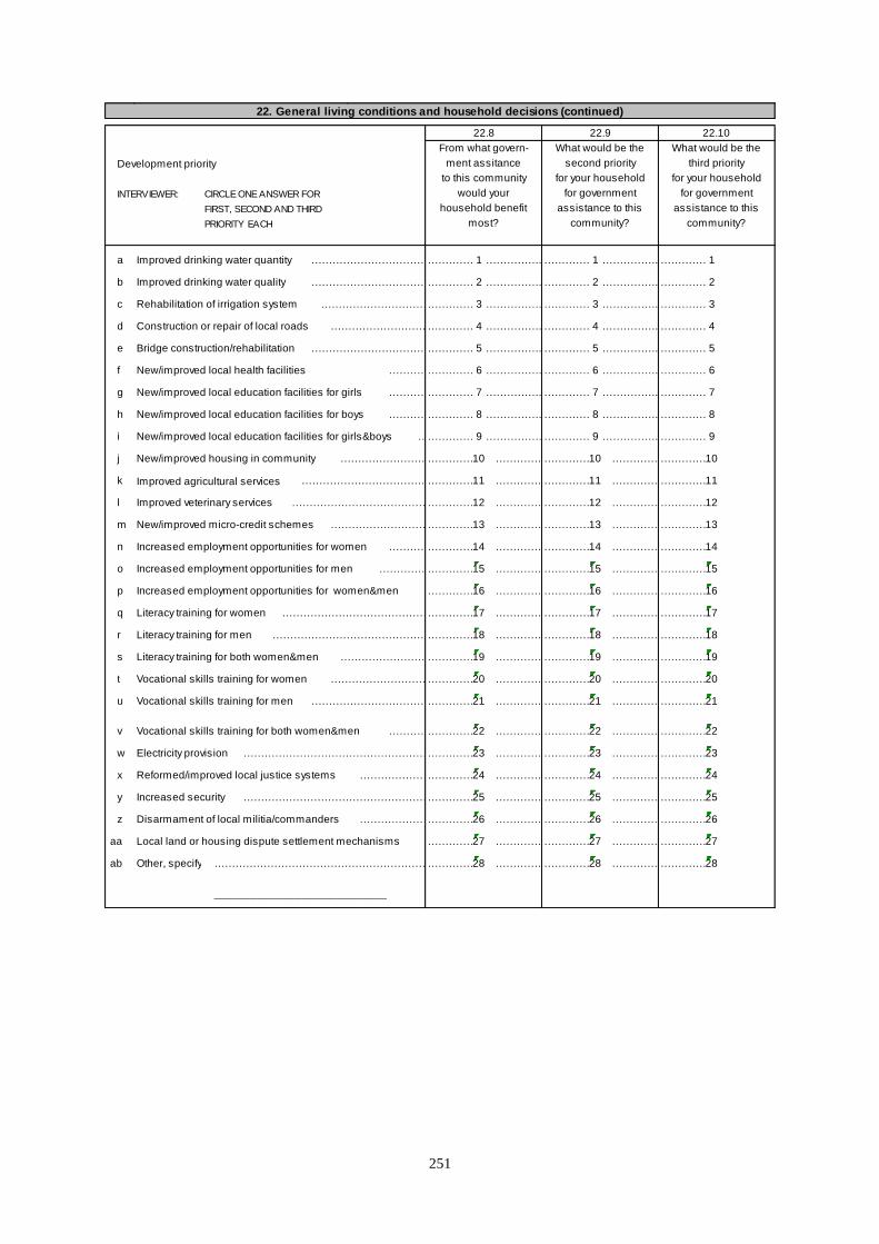
251
22. General living conditions and household decisions (continued)
22.8 22.9 22.10
From what govern- What would be the What would be the
Development priority ment assitance second priority third priority
to this community for your household for your household
INTERVIEWER: CIRCLE ONE ANSWER FOR would your for government for government
FIRST, SECOND AND THIRD household benefit assistance to this assistance to this
PRIORITY EACH most? community? community?
a Improved drinking water quantity …………………………………………………………………………..1 ……………..……………..1 ……………..……………..1
b Improved drinking water quality …………………………………………………………………………..2 ……………..……………..2 ……………..……………..2
c Rehabilitation of irrigation system …………………………………………………………………………..3 ……………..……………..3 ……………..……………..3
d Construction or repair of local roads …………………………………………………………………………..4 ……………..……………..4 ……………..……………..4
e Bridge construction/rehabilitation …………………………………………………………………………..5 ……………..……………..5 ……………..……………..5
f New/improved local health facilities …………………………………………………………………………..6 ……………..……………..6 ……………..……………..6
g New/improved local education facilities for girls …………………………………………………………………………..7 ……………..……………..7 ……………..……………..7
h New/improved local education facilities for boys …………………………………………………………………………..8 ……………..……………..8 ……………..……………..8
i New/improved local education facilities for girls&boys …………………………………………………………………………..9 ……………..……………..9 ……………..……………..9
j New/improved housing in community …………………………………………………………………………..10 ……………..……………..10 ……………..……………..10
k Improved agricultural services …………………………………………………………………………..11 ……………..……………..11 ……………..……………..11
l Improved veterinary services …………………………………………………………………………..12 ……………..……………..12 ……………..……………..12
m New/improved micro-credit schemes …………………………………………………………………………..13 ……………..……………..13 ……………..……………..13
n Increased employment opportunities for women …………………………………………………………………………..14 ……………..……………..14 ……………..……………..14
o Increased employment opportunities for men …………………………………………………………………………..15 ……………..……………..15 ……………..……………..15
p Increased employment opportunities for women&men ……………..16 ……………..……………..16 ……………..……………..16
q Literacy training for women …………………………………………………………………………..17 ……………..……………..17 ……………..……………..17
r Literacy training for men …………………………………………………………………………..18 ……………..……………..18 ……………..……………..18
s Literacy training for both women&men …………………………………………………………………………..19 ……………..……………..19 ……………..……………..19
t Vocational skills training for women …………………………………………………………………………..20 ……………..……………..20 ……………..……………..20
u Vocational skills training for men …………………………………………………………………………..21 ……………..……………..21 ……………..……………..21
v Vocational skills training for both women&men …………………………………………………………………………..22 ……………..……………..22 ……………..……………..22
w Electricity provision …………………………………………………………………………..23 ……………..……………..23 ……………..……………..23
x Reformed/improved local justice systems …………………………………………………………………………..24 ……………..……………..24 ……………..……………..24
y Increased security …………………………………………………………………………..25 ……………..……………..25 ……………..……………..25
z Disarmament of local militia/commanders …………………………………………………………………………..26 ……………..……………..26 ……………..……………..26
aa Local land or housing dispute settlement mechanisms ……………..27 ……………..……………..27 ……………..……………..27
ab Other, specify …………………………………………………………………………..28 ……………..……………..28 ……………..……………..28
____________________________
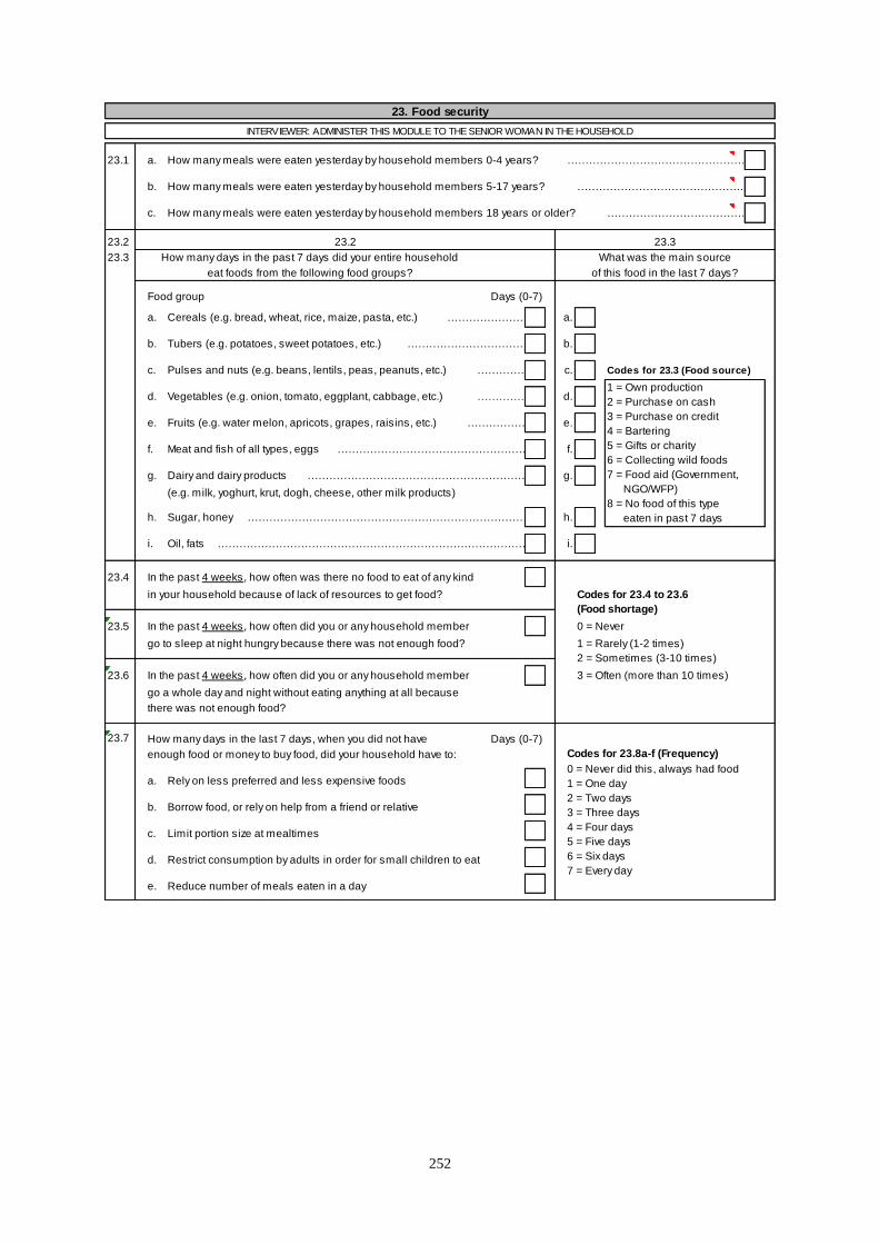
252
23. Food security
INTERVIEWER: ADMINISTER THIS MODULE TO THE SENIOR WOMAN IN THE HOUSEHOLD
23.1 a. How many meals were eaten yesterday by household members 0-4 years? …………………………………………..
b. How many meals were eaten yesterday by household members 5-17 years? ………………………………………..
c. How many meals were eaten yesterday by household members 18 years or older? ………………………………………
23.2 23.2 23.3
23.3 How many days in the past 7 days did your entire household What was the main source
eat foods from the following food groups? of this food in the last 7 days?
Food group Days (0-7)
a. Cereals (e.g. bread, wheat, rice, maize, pasta, etc.) ………………………………………………………….a.
b. Tubers (e.g. potatoes, sweet potatoes, etc.) ………………………………………………………….b.
c. Pulses and nuts (e.g. beans, lentils, peas, peanuts, etc.) ………………………………………………………….c. Codes for 23.3 (Food source)
d. Vegetables (e.g. onion, tomato, eggplant, cabbage, etc.) ………………………………………………………………………..d.
e. Fruits (e.g. water melon, apricots, grapes, raisins, etc.) …………………………………………………………………………………e.
f. Meat and fish of all types, eggs ………………………………………………………….f.
g. Dairy and dairy products …………………………………………………………. g.
(e.g. milk, yoghurt, krut, dogh, cheese, other milk products)
h. Sugar, honey …………………………………………………………………………….h.
i. Oil, fats ……………………………………………………………………………. i.
23.4 In the past 4 weeks, how often was there no food to eat of any kind
in your household because of lack of resources to get food? Codes for 23.4 to 23.6
23.5 In the past 4 weeks, how often did you or any household member 0 = Never
go to sleep at night hungry because there was not enough food? 1 = Rarely (1-2 times)
23.6 In the past 4 weeks, how often did you or any household member 3 = Often (more than 10 times)
go a whole day and night without eating anything at all because
there was not enough food?
23.7 How many days in the last 7 days, when you did not have Days (0-7)
enough food or money to buy food, did your household have to: Codes for 23.8a-f (Frequency)
a. Rely on less preferred and less expensive foods
b. Borrow food, or rely on help from a friend or relative
c. Limit portion size at mealtimes
d. Restrict consumption by adults in order for small children to eat
e. Reduce number of meals eaten in a day
0 = Never did this, always had food
1 = One day
2 = Two days
3 = Three days
4 = Four days
5 = Five days
6 = Six days
7 = Every day
1 = Own production
2 = Purchase on cash
3 = Purchase on credit
4 = Bartering
5 = Gifts or charity
6 = Collecting wild foods
7 = Food aid (Government,
NGO/WFP)
8 = No food of this type
eaten in past 7 days
(Food shortage)
2 = Sometimes (3-10 times)
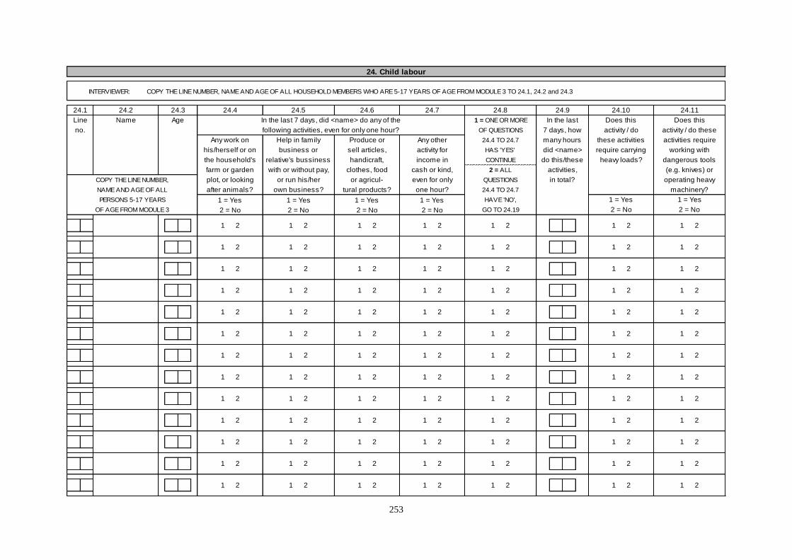
253
24. Child labour 24. Child labour (continued)
INTERVIEWER: COPY THE LINE NUMBER, NAME AND AGE OF ALL HOUSEHOLD MEMBERS WHO ARE 5-17 YEARS OF AGE FROM MODULE 3 TO 24.1, 24.2 and 24.3
24.1 24.2 24.3 24.4 24.5 24.6 24.7 24.8 24.9 24.10 24.11 24.1
Line Name Age In the last 7 days, did <name> do any of the 1 = ONE OR MORE In the last Does this Does this COPY
no. following activities, even for only one hour? OF QUESTIONS 7 days, how activity / do activity / do these LINE
Any work on Help in family Produce or Any other 24.4 TO 24.7 many hours these activities activities require NUMBER
his/herself or on business or sell articles, activity for HAS 'YES' did <name> require carrying working with fumes
the household's relative's bussiness handicraft, income in CONTINUE do this/these heavy loads? dangerous tools or gas?
farm or garden with or without pay, clothes, food cash or kind, 2 = ALL activities, (e.g. knives) or
COPY THE LINE NUMBER, plot, or looking or run his/her or agricul- even for only QUESTIONS in total? operating heavy
NAME AND AGE OF ALL after animals? own business? tural products? one hour? 24.4 TO 24.7 machinery?
PERSONS 5-17 YEARS 1 = Yes 1 = Yes 1 = Yes 1 = Yes HAVE 'NO', 1 = Yes 1 = Yes Line
OF AGE FROM MODULE 3 2 = No 2 = No 2 = No 2 = No GO TO 24.19 2 = No 2 = No no.
1 2 1 2 1 2 1 2 1 2 1 2 1 2
1 2 1 2 1 2 1 2 1 2 1 2 1 2
1 2 1 2 1 2 1 2 1 2 1 2 1 2
1 2 1 2 1 2 1 2 1 2 1 2 1 2
1 2 1 2 1 2 1 2 1 2 1 2 1 2
1 2 1 2 1 2 1 2 1 2 1 2 1 2
1 2 1 2 1 2 1 2 1 2 1 2 1 2
1 2 1 2 1 2 1 2 1 2 1 2 1 2
1 2 1 2 1 2 1 2 1 2 1 2 1 2 1 2
1 2 1 2 1 2 1 2 1 2 1 2 1 2 1 2
1 2 1 2 1 2 1 2 1 2 1 2 1 2 1 2
1 2 1 2 1 2 1 2 1 2 1 2 1 2 1 2
1 2 1 2 1 2 1 2 1 2 1 2 1 2 1 2
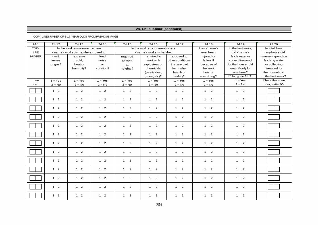
254
24. Child labour (continued) 24. Child labour (continued)
COPY LINE NUMBER OF 5-17 YEAR OLDS FROM PREVIOUS PAGE
24.1 24.12 24.13 24.14 24.15 24.16 24.17 24.18 24.19 24.20 24.1
COPY In the work environment where In the work environment where Has <name> In the last week, In total, how COPY
LINE <name> works, is he/she exposed to: <name> works is he/she: ever been did <name> many hours did LINE
NUMBER dust, extreme loud required required to exposed to injured or fetch water or <name> spend on NUMBER
fumes cold, noise to work work with other conditions fallen ill collect firewood fetching water household?
or gas? heat or or at explosives or that are bad because of for the household or collecting
humidity? vibration? heights? chemicals for his/her the work even if only for firewood for
(pesticides, health or he/she one hour? the household
glues, etc)? safety? was doing? If 'No', go to 24.21 in the last week?
Line 1 = Yes 1 = Yes 1 = Yes 1 = Yes 1 = Yes 1 = Yes 1 = Yes 1 = Yes If less than one Line
no. 2 = No 2 = No 2 = No 2 = No 2 = No 2 = No 2 = No 2 = No hour, write '00' no.
1 2 1 2 1 2 1 2 1 2 1 2 1 2 1 2
1 2 1 2 1 2 1 2 1 2 1 2 1 2 1 2
1 2 1 2 1 2 1 2 1 2 1 2 1 2 1 2
1 2 1 2 1 2 1 2 1 2 1 2 1 2 1 2
1 2 1 2 1 2 1 2 1 2 1 2 1 2 1 2
1 2 1 2 1 2 1 2 1 2 1 2 1 2 1 2
1 2 1 2 1 2 1 2 1 2 1 2 1 2 1 2
1 2 1 2 1 2 1 2 1 2 1 2 1 2 1 2
1 2 1 2 1 2 1 2 1 2 1 2 1 2 1 2 1 2
1 2 1 2 1 2 1 2 1 2 1 2 1 2 1 2 1 2
1 2 1 2 1 2 1 2 1 2 1 2 1 2 1 2 1 2
1 2 1 2 1 2 1 2 1 2 1 2 1 2 1 2 1 2
1 2 1 2 1 2 1 2 1 2 1 2 1 2 1 2 1 2
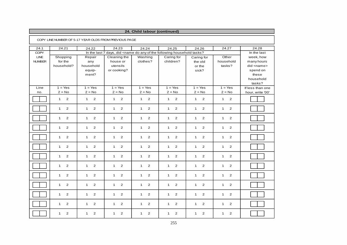
255
24. Child labour (continued)
COPY LINE NUMBER OF 5-17 YEAR OLDS FROM PREVIOUS PAGE
24.1 24.21 24.22 24.23 24.24 24.25 24.26 24.27 24.28
COPY In the last 7 days, did <name do any of the following household tasks? In the last
LINE Shopping Repair Cleaning the Washing Caring for Caring for Other week, how
NUMBER for the any house or clothes? children? the old household many hours
household? household utensils or the tasks? did <name>
equip- or cooking? sick? spend on
ment? these
household
tasks?
Line 1 = Yes 1 = Yes 1 = Yes 1 = Yes 1 = Yes 1 = Yes 1 = Yes If less than one
no. 2 = No 2 = No 2 = No 2 = No 2 = No 2 = No 2 = No hour, write '00'
1 2 1 2 1 2 1 2 1 2 1 2 1 2
1 2 1 2 1 2 1 2 1 2 1 2 1 2
1 2 1 2 1 2 1 2 1 2 1 2 1 2
1 2 1 2 1 2 1 2 1 2 1 2 1 2
1 2 1 2 1 2 1 2 1 2 1 2 1 2
1 2 1 2 1 2 1 2 1 2 1 2 1 2
1 2 1 2 1 2 1 2 1 2 1 2 1 2
1 2 1 2 1 2 1 2 1 2 1 2 1 2
1 2 1 2 1 2 1 2 1 2 1 2 1 2
1 2 1 2 1 2 1 2 1 2 1 2 1 2
1 2 1 2 1 2 1 2 1 2 1 2 1 2
1 2 1 2 1 2 1 2 1 2 1 2 1 2
1 2 1 2 1 2 1 2 1 2 1 2 1 2
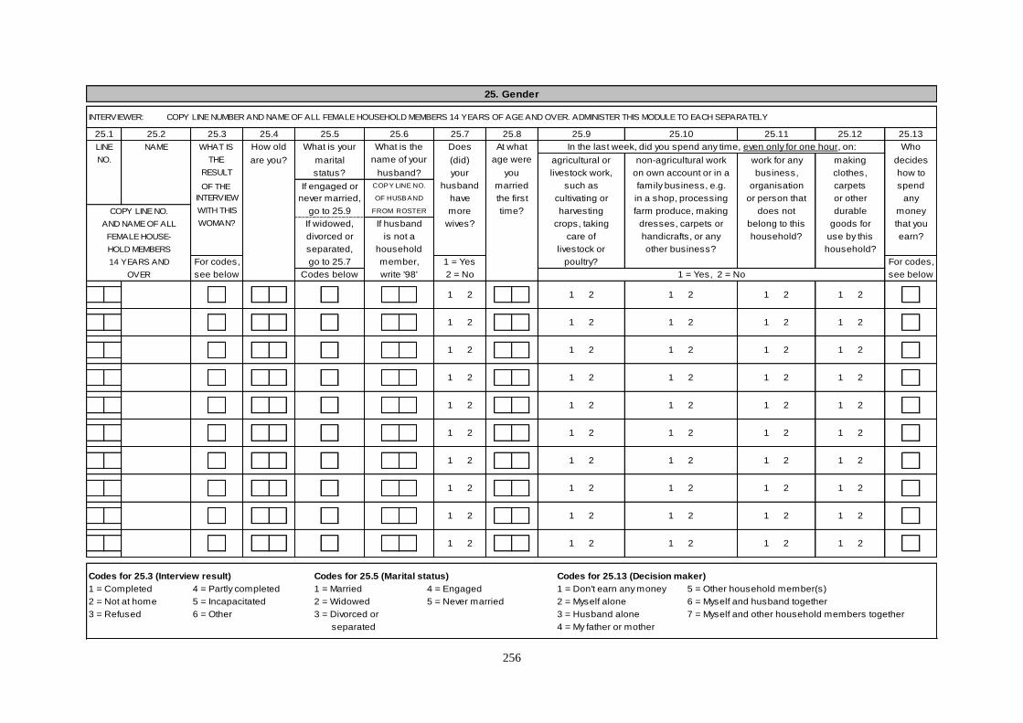
256
25. Gender
INTERVIEWER: COPY LINE NUMBER AND NAME OF ALL FEMALE HOUSEHOLD MEMBERS 14 YEARS OF AGE AND OVER. ADMINISTER THIS MODULE TO EACH SEPARATELY
25.1 25.2 25.4 25.5 25.7 25.9 25.10 25.11 25.12 25.13
LINE NAME WHAT IS How old What is your Does In the last week, did you spend any time, even only for one hour, on: Who
NO. THE are you? marital (did) agricultural or non-agricultural work work for any making decides
status? your livestock work, on own account or in a business, clothes, how to
OF THE If engaged or husband such as family business, e.g. organisation carpets spend
never married, have cultivating or in a shop, processing or person that or other any
COPY LINE NO. go to 25.9 more harvesting farm produce, making does not durable money
AND NAME OF ALL If widowed, wives? crops, taking dresses, carpets or belong to this goods for that you
FEMALE HOUSE- divorced or care of handicrafts, or any household? use by this earn?
HOLD MEMBERS separated, livestock or other business? household?
14 YEARS AND go to 25.7 1 = Yes poultry? For codes,
OVER Codes below 2 = No 1 = Yes, 2 = No see below
1 2 1 2 1 2 1 2 1 2
1 2 1 2 1 2 1 2 1 2
1 2 1 2 1 2 1 2 1 2
1 2 1 2 1 2 1 2 1 2
1 2 1 2 1 2 1 2 1 2
1 2 1 2 1 2 1 2 1 2
1 2 1 2 1 2 1 2 1 2
1 2 1 2 1 2 1 2 1 2
1 2 1 2 1 2 1 2 1 2
1 2 1 2 1 2 1 2 1 2
Codes for 25.3 (Interview result) Codes for 25.5 (Marital status) Codes for 25.13 (Decision maker)
1 = Completed 4 = Partly completed 1 = Married 4 = Engaged 1 = Don't earn any money 5 = Other household member(s)
2 = Not at home 5 = Incapacitated 2 = Widowed 5 = Never married 2 = Myself alone 6 = Myself and husband together
3 = Refused 6 = Other 3 = Divorced or 3 = Husband alone 7 = Myself and other household members together
separated 4 = My father or mother
RESULT husband? you
COPY LINE NO. married
INTERVIEW OF HUSBAND the first
25.3 25.6 25.8
What is the At what
name of your age were
For codes,
WOMAN?
WITH THIS
household
member,
FROM ROSTER time?
If husband
is not a
see below write '98'
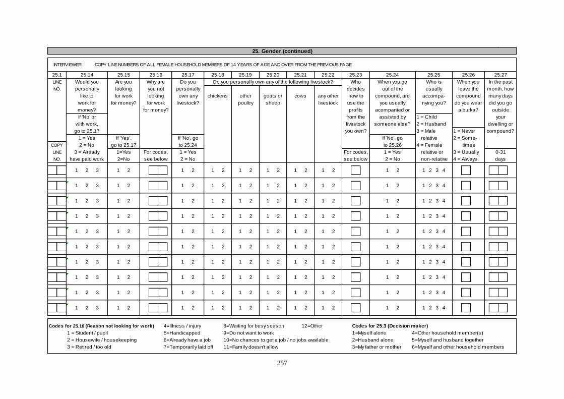
257
25. Gender (continued)
INTERVIEWER: COPY LINE NUMBERS OF ALL FEMALE HOUSEHOLD MEMBERS OF 14 YEARS OF AGE AND OVER FROM THE PREVIOUS PAGE
25.1 25.14 25.15 25.16 25.17 25.18 25.19 25.20 25.21 25.22 25.23 25.24 25.25 25.26 25.27
LINE Would you Are you Why are Do you Do you personally own any of the following livestock? Who When you go Who is When you In the past
NO. personally looking you not personally decides out of the usually leave the month, how
like to for work looking own any chickens other goats or cows any other how to compound, are accompa- compound many days
work for for money? for work livestock? poultry sheep livestock use the you usually nying you? do you wear did you go
money? for money? profits acompanied or a burka? outside
If 'No' or from the assisted by 1 = Child your
with work, livestock someone else? 2 = Husband dwelling or
go to 25.17 you own? 3 = Male 1 = Never compound?
1 = Yes If 'Yes', If 'No', go If 'No', go relative 2 = Some-
COPY 2 = No go to 25.17 to 25.24 to 25.26 4 = Female times
LINE 3 = Already 1=Yes For codes, 1 = Yes For codes, 1 = Yes relative or 3 = Usually 0-31
NO. have paid work 2=No see below 2 = No see below 2 = No non-relative 4 = Always days
1 2 3 1 2 1 2 1 2 1 2 1 2 1 2 1 2 1 2 1 2 3 4
1 2 3 1 2 1 2 1 2 1 2 1 2 1 2 1 2 1 2 1 2 3 4
1 2 3 1 2 1 2 1 2 1 2 1 2 1 2 1 2 1 2 1 2 3 4
1 2 3 1 2 1 2 1 2 1 2 1 2 1 2 1 2 1 2 1 2 3 4
1 2 3 1 2 1 2 1 2 1 2 1 2 1 2 1 2 1 2 1 2 3 4
1 2 3 1 2 1 2 1 2 1 2 1 2 1 2 1 2 1 2 1 2 3 4
1 2 3 1 2 1 2 1 2 1 2 1 2 1 2 1 2 1 2 1 2 3 4
1 2 3 1 2 1 2 1 2 1 2 1 2 1 2 1 2 1 2 1 2 3 4
1 2 3 1 2 1 2 1 2 1 2 1 2 1 2 1 2 1 2 1 2 3 4
1 2 3 1 2 1 2 1 2 1 2 1 2 1 2 1 2 1 2 1 2 3 4
Codes for 25.16 (Reason not looking for work) 4=Illness / injury 8=Waiting for busy season 12=Other Codes for 25.3 (Decision maker)
1 = Student / pupil 5=Handicapped 9=Do not want to work 1=Myself alone 4=Other household member(s)
2 = Housewife / housekeeping 6=Already have a job 10=No chances to get a job / no jobs available 2=Husband alone 5=Myself and husband together
3 = Retired / too old 7=Temporarily laid off 11=Family doesn't allow 3=My father or mother 6=Myself and other household members
258
25. Gender (continued)
INTERVIEWER: COPY LINE NUMBERS OF ALL FEMALE HOUSEHOLD MEMBERS OF 14 YEARS OF AGE AND OVER FROM THE PREVIOUS PAGE.
25.1 25.28 25.29 25.30 25.31 25.32 25.33 25.34 25.35 25.36 25.37 25.38 25.39 25.40 25.41
In the past month, did you leave the dwelling compound to
visit visit attend go to go to buy to go to work go to see collect fetch visit a collect collect
COPY family friends or school or shops to clothes, accompany outside the celebrations a mullah firewood, water clinic or trash money
LINE neighbours literacy buy food shoes, children compound (wedding, for tawriz brush, a health (begging)
NO. classes or bread cosmetics, to school Eid, etc.) ping worker
etc.
1 2 1 2 1 2 1 2 1 2 1 2 1 2 1 2 1 2 1 2 1 2 1 2 1 2 1 2
1 2 1 2 1 2 1 2 1 2 1 2 1 2 1 2 1 2 1 2 1 2 1 2 1 2 1 2
1 2 1 2 1 2 1 2 1 2 1 2 1 2 1 2 1 2 1 2 1 2 1 2 1 2 1 2
1 2 1 2 1 2 1 2 1 2 1 2 1 2 1 2 1 2 1 2 1 2 1 2 1 2 1 2
1 2 1 2 1 2 1 2 1 2 1 2 1 2 1 2 1 2 1 2 1 2 1 2 1 2 1 2
1 2 1 2 1 2 1 2 1 2 1 2 1 2 1 2 1 2 1 2 1 2 1 2 1 2 1 2
1 2 1 2 1 2 1 2 1 2 1 2 1 2 1 2 1 2 1 2 1 2 1 2 1 2 1 2
1 2 1 2 1 2 1 2 1 2 1 2 1 2 1 2 1 2 1 2 1 2 1 2 1 2 1 2
1 2 1 2 1 2 1 2 1 2 1 2 1 2 1 2 1 2 1 2 1 2 1 2 1 2 1 2
1 2 1 2 1 2 1 2 1 2 1 2 1 2 1 2 1 2 1 2 1 2 1 2 1 2 1 2
Codes for 25.28 to 25.29 (Leaving compound) 1 = Yes, 2 = No
259
25. Gender (continued)
INTERVIEWER: COPY LINE NUMBERS OF ALL FEMALE HOUSEHOLD MEMBERS OF 14 YEARS OF AGE AND OVER FROM THE PREVIOUS PAGE.
25.1 25.42 25.43 25.44 25.45 25.46 25.47
In the last Did you What was the What was the If you were asked CHECK ELIGIBILITY OF
30 days, seek main reason you second reason to rate how content THIS WOMAN FOR FOR EACH ELIGIBLE (25.47=1) WOMAN,
have you medical did not seek you did not seek you are with your MODULE 26 IN QUESTIONS CONTINUE WITH MODULE 26
been care? medical care? medical care? life, how would you 25.4 AND 25.5 (MATERNAL AND CHILD HEALTH)
sick or rate it?
injured? A WOMAN IS ELIGIBLE IF SHE IS: IF THE WOMAN IS NOT ELIGIBLE (25.47=2),
• 14-49 YEARS OLD END THE INTERVIEW WITH HER
AND BY COMPLETING QUESTION 25.3 FOR HER
• EVER MARRIED (MARRIED, THEN CONTINUE WITH 25.1 FOR A
If 'No', go If 'Yes', go WIDOWED OR DIVORCED / NEXT WOMAN IF PRESENT
COPY to 25.46 to 25.46 SEPARATED)
LINE 1 = Yes 1 = Yes For codes, For codes, For codes, 1 = Eligible
NO. 2 = No 2 = No see bottom of page see bottom of page see bottom of page 2 = Not eligible
1 2 1 2 1 2
1 2 1 2 1 2
1 2 1 2 1 2
1 2 1 2 1 2
1 2 1 2 1 2
1 2 1 2 1 2
1 2 1 2 1 2
1 2 1 2 1 2
1 2 1 2 1 2
1 2 1 2 1 2
Code for 25.44 and 25.45 (Reasons for not seeking health care) Code for 25.46 (Life rating)
1 = No need/ not serious 5 = No one to accompany 9 = Other 1 = Very happy 5 = Very unhappy
2 = Too far 6 = Security concerns 10 = No second reason 2 = Happy 6 = Don't know
3 = Too expensive 7 = Husband or family did not allow 3 = Neither happy, nor'unhappy 7 = Refused to answer
4 = No female medical personnel 8 = Traditional constraints 4 = Unhappy
IF THE WOMAN IS NOT ELIGIBLE (25.47=2),
AND SHE IS THE LAST WOMAN 14 YEARS
OR OLDER, COMPLETE QUESTION 25.3 FOR HER
AND THANK YOUR RESPONDENTS
THEN, CONTACT YOUR SUPERVISOR
260
26. Maternal and child health
INTERVIEWER: ASK THESE QUESTIONS SEPARATELY TO EVERY WOMAN FOUND ELIGIBLE IN MODULE 25.47 (EVER MARRIED AND 49 YEARS OR LESS)
26.1 26.2 26.3 26.4 26.5 26.6 26.7 26.8 26.9 26.10 26.11 26.12 26.13 26.14
Have you ever Did you give What was the month Did you How many Did you see any of the following persons for Who Where
no. given birth? birth in the last and year of the last see anyone times did ante-natal care care during your last pregnancy? assisted did this
5 years? birth you had? for you receive A A A A Someone with the delivery
I mean, even a child (even if the child died)? ante-natal ante-natal doctor midwife traditional Commu- else delivery take
that ever cried or CHECK MODULE 3 care during care during or nurse birth nity of your place?
breathed or showed FOR ANY your last your last attendant Health last
COPY LINE NO. any signs of life, CHILDREN pregnancy? pregnancy? Worker child?
AND NAME FOR but lived only hours UNDER-5 FOR
ELIGIBLE WOMEN or minutes? THIS WOMAN
(EVER-MARRIED If 26.3=2 or 26.4=2, end the interview
WOMEN, AGED 49 with this woman by completing 25.3 and RECORD MONTH AND If 'No'
OR LESS) continue with 25.1 for the next woman YEAR IN SHAMSI go to 26.13
FROM MODULE 25 1 = Yes 1 = Yes CALENDAR 1 = Yes 98 = For codes For codes
(SEE 25.47) 2 = No 2 = No M M Y Y Y Y 2 = No Don't know see below see below
1 2 1 2 1 2 1 2 1 2 1 2 1 2 1 2
1 2 1 2 1 2 1 2 1 2 1 2 1 2 1 2
1 2 1 2 1 2 1 2 1 2 1 2 1 2 1 2
1 2 1 2 1 2 1 2 1 2 1 2 1 2 1 2
1 2 1 2 1 2 1 2 1 2 1 2 1 2 1 2
1 2 1 2 1 2 1 2 1 2 1 2 1 2 1 2
1 2 1 2 1 2 1 2 1 2 1 2 1 2 1 2
1 2 1 2 1 2 1 2 1 2 1 2 1 2 1 2
Codes for 26.13 (Delivery assistance) Codes for 26.14 (Place of delivery)
1 = Doctor 4 = Community Health Worker 1 = At home or relative's/neighbour's home 4 = Private health facility
2 = Midwife or nurse 5 = Someone else 2 = Public hospital 5 = Other
3 = Traditional birth attendant 6 = No one 3 = Other public health facility
Line Name
261
26. Maternal and child health (continued)
26.1 26.15 26.16 26.17 26.18 26.19 26.20 26.21 26.22 26.23
Did you Why did How long after birth did In the first How many days did Have you How old was Are you still How old
no. ever you not you first put your last-born three days you feed the baby only started feeding the child when breastfeeding was the
breastfed breastfeed to the breast? after breastmilk before solid foods you started this child? baby when
your the child? delivery, giving other liquids? to the child? solid foods? you
last-born Complete was the If baby still drinks only If 'Yes' or 'Child died', completely
child? 25.3 for this IF LESS THAN 1 HOUR, child given breastmilk, write '997' complete 25.3 for stopped
woman and RECORD ‘00' HOURS. anything to If baby died before beginning this woman breast-
go to 25.1 IF LESS THAN 24 HOURS, drink other other liquids, write '998' and go to 25.1 for feeding?
If 'Yes' for next RECORD HOURS. than In these cases, complete If 'No'' the next woman
COPY go to 26.17 woman OTHERWISE, RECORD breastmilk? 25.3 for this woman go to 26.22 1 = Yes
LINE 1 = Yes For codes, DAYS 1 = Yes and go to 25.1 for 1 = Yes RECORD IN 2 = No RECORD IN
NO. 2 = No see below 2 = No the next woman 2 = No MONTHS 3 = Child died MONTHS
1 2 Hours Days 1 2 Days ………………… 1 2 1 2 3
1 2 Hours Days 1 2 Days ………………… 1 2 1 2 3
1 2 Hours Days 1 2 Days ………………… 1 2 1 2 3
1 2 Hours Days 1 2 Days ………………… 1 2 1 2 3
1 2 Hours Days 1 2 Days ………………… 1 2 1 2 3
1 2 Hours Days 1 2 Days ………………… 1 2 1 2 3
1 2 Hours Days 1 2 Days ………………… 1 2 1 2 3
1 2 Hours Days 1 2 Days ………………… 1 2 1 2 3
Codes for 26.16 (Reason for not breastfeeding) WHEN YOU FINISHED MODULE 26 FOR A WOMAN, GO TO QUESTION 25.3 AND FILL IN THE
1 = Baby died 5 = Did not want to RESULT OF THE INTERVIEW WITH HER AND CONTINUE WITH QUESTION 25.1 FOR
2 = Baby too sick 6 = Had to work THE NEXT WOMAN 14 YEARS OR OLDER.
3 = Did not have milk 7 = Other reason IF THIS WOMAN IS THE LAST WOMAN 14 YEARS OR OLDER IN THE HOUSEHOLD, FILL IN
4 = Mother too sick QUESTION 25.3 FOR HER, THANK YOUR RESPONDENT(S) AND CONTACT YOUR SUPERVISOR.
Line
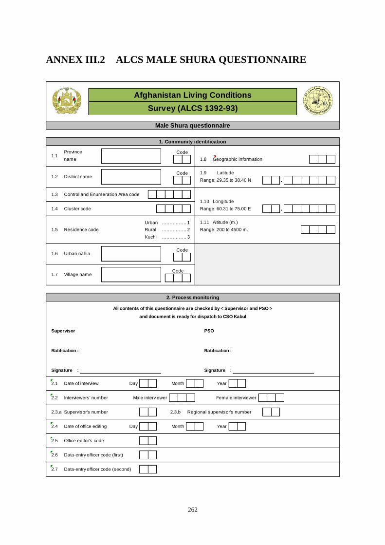
262
ANNEX III.2 ALCS MALE SHURA QUESTIONNAIRE
Male Shura questionnaire
1. Community identification
Province Code
name 1.8 Geographic information
Code 1.9 Latitude
Range: 29.35 to 38.40 N .
Control and Enumeration Area code
Cluster code Range: 60.31 to 75.00 E .
Urban …………………………1 1.11 Altitude (m.)
Rural …………………………2 Range: 200 to 4500 m.
Kuchi …………………………3
Code
Code
2. Process monitoring
All contents of this questionnaire are checked by < Supervisor and PSO >
and document is ready for dispatch to CSO Kabul
Supervisor PSO
Ratification : Ratification :
Signature : Signature :
Date of interview Day Month Year
Interviewers' number Male interviewer Female interviewer
Supervisor's number Regional supervisor's number
Date of office editing Day Month Year
Office editor's code
Data-entry officer code (first)
Data-entry officer code (second)
Afghanistan Living Conditions
Survey (ALCS 1392-93)
2.1
2.2
1.1
1.2 District name
1.4
2.4
2.5
2.6
2.7
1.3
2.3.a 2.3.b
1.10 Longitude
1.7 Village name
1.5 Residence code
1.6 Urban nahia
263
3a. Access
3.1 What is the landscape characteristic of the largest part Open plain …………………………………………………………………………………….1
of the cropland used by the community? Valley …………………………………………………………………………………….2
Valley and hills …………………………………………………………………………………….3
Hills (no valley cultivation) …………………………………………………………………………………….4
3.2 How far is the nearest drivable road to this community? km.
IF A DRIVABLE ROAD IS IN THE COMMUNITY, WRITE ‘0’
3.3 Is the closest road to your community usable by vehicles all year? Yes ……………………………………………………………1 Go to 3.5
No ……………………………………………………………2
3.4 During which months is the road impassable in a normal year? INTERVIEWER:
CIRCLE ALL MONTHS THAT ARE MENTIONED
Hamal Sawr Jawza Saratan Asad Sunbula Mizan Aqrab Qaws Jady Dalwa Hoot
1 2 3 4 5 6 7 8 9 10 11 12
3.5 Has there been any program for road repair or/and bridge Own community work ……………………………………………………………a
construction in last 3 years? Government road project ……………………………………………………………b
WFP food-for-work road improvement c
INTERVIEWER: CIRCLE ALL ANSWERS THAT ARE MENTIONED Other food-for-work road project ……………………………………………………………d
NSP road constuction programme ……………………………………………………………e
NGO road construction project ……………………………………………………………f
Military road construction ……………………………………………………………g
Other ……………………………………………………………h
None ……………………………………………………………i
3.6 Has there been a change in road access in the last 3 years? No change in road access ……………………………………………………………1
Road access improved ……………………………………………………………2
Road access has deteriorated ……………………………………………………………3
3.7 What is the name of the place where this community
bought their foodstuffs in the last month?
3.8 Where is this place located? Local community market ……………………………………………………………1 Go to 3.10
District market in the same province ……………………………………………………………2
District market in other province ……………………………………………………………3
Provincial market ……………………………………………………………4 Go to 3.10
3.9 What is the name of that district a. District name
and province? b. Province name
Transport type: a. Foot/animal b. Bicycle c. Car / taxi
3.10 How long did it take to reach the nearest permanent If '1' or '7',
food market - one way travel - by <transport type> SKIP 3.11 AND
in the past month? FOR CODES, SEE BELOW 3.12
3.11 What was the cost of return transport to the Afghanis
permanent food market, including overnight
accommodation if needed, in the past month?
3.12 What is the cost of transporting 50 kg of wheat Afghanis
from the permanent food market to the
community in the past month?
Codes for 3.10a-c 1 = Less than 1 hour - market in 4 = 4 hours or more, but less than 6 hours
(Time to reach or near community 5 = 6 hours or more, but less than 12 hours
food market) 2 = 1 hour or more, but less than 2 hours 6 = 12 hours or more
3 = 2 hours or more, but less than 4 hours 7 = Cannot reach market (e.g. no road)
,
,
264
3b. Access
3.13 3.14 3.15 3.16 Codes 3.13 and 3.14 (Time to reach health facilities)
Type of health How long did it take How long did it take What was the cost of Are the following types 1 = Less than 1 hour - health facility in or near
facility to reach the nearest to reach the nearest one-way transport by car of staff present in the community
<facility> on foot or <facility> by car from this community to nearest <health facility>? 2 = 1 hour or more, but less than 2 hours
animal in the in the last month? this <facility> in the 3 = 2 hours or more, but less than 4 hours
last month? (one-way travel) last month? 4 = 4 hours or more, but less than 6 hours
(one-way travel) (cost for one person) 5 = 6 hours or more, but less than 12 hours
1=Yes 6 = 12 hours or more
For codes, 2=No 7 = Cars cannot reach health facility (e.g. no road
see at right If '7', go to 3.16 3=Don't know to health facility
Health post (house of Afghanis
community health Female CHW ………..1 2 3 CHW is Community Health Worker
worker, CHW) Male CHW ………..1 2 3
Female doctor ………..1 2 3
Public clinic Afghanis Female nurse ………..1 2 3
(Basic or Female midwife ………..1 2 3
Comprehensive Male doctor ………..1 2 3
health centre) Male nurse ………..1 2 3
Female doctor ………..1 2 3
District or Afghanis Female nurse ………..1 2 3
Provincial Female midwife ………..1 2 3
hospital Male doctor ………..1 2 3
Male nurse ………..1 2 3
Female doctor ………..1 2 3
Private doctor's Afghanis Female nurse ………..1 2 3
office or private Female midwife ………..1 2 3
hospital Male doctor ………..1 2 3
Male nurse ………..1 2 3
Afghanis
Private pharmacy Female CHW ………..1 2 3
Male CHW ………..1 2 3
,
,
,
,
,
265
3b. Access (continued)
3.17 3.18 3.19 3.20
Type of Is a <education type> present How many of these <education How many of these <education What is the one-way distance in km.
education in or near the community? type> facilities are public or type> facilities are private or to the nearest <education type> facility
If 'No', go to 3.20 government schools? NGO schools? either in or outside the community?
1=Yes IF NOT REACHABLE, WRITE '98'
2=No AND GO TO NEXT SCHOOL TYPE
Primary education, 1 2
mixed / shift boys-girls
Primary education, 1 2
girls only
Primary education, 1 2
boys only
Lower secondary education, 1 2
mixed / shift boys-girls
Lower secondary education, 1 2
girls only
Lower secondary education, 1 2
boys only
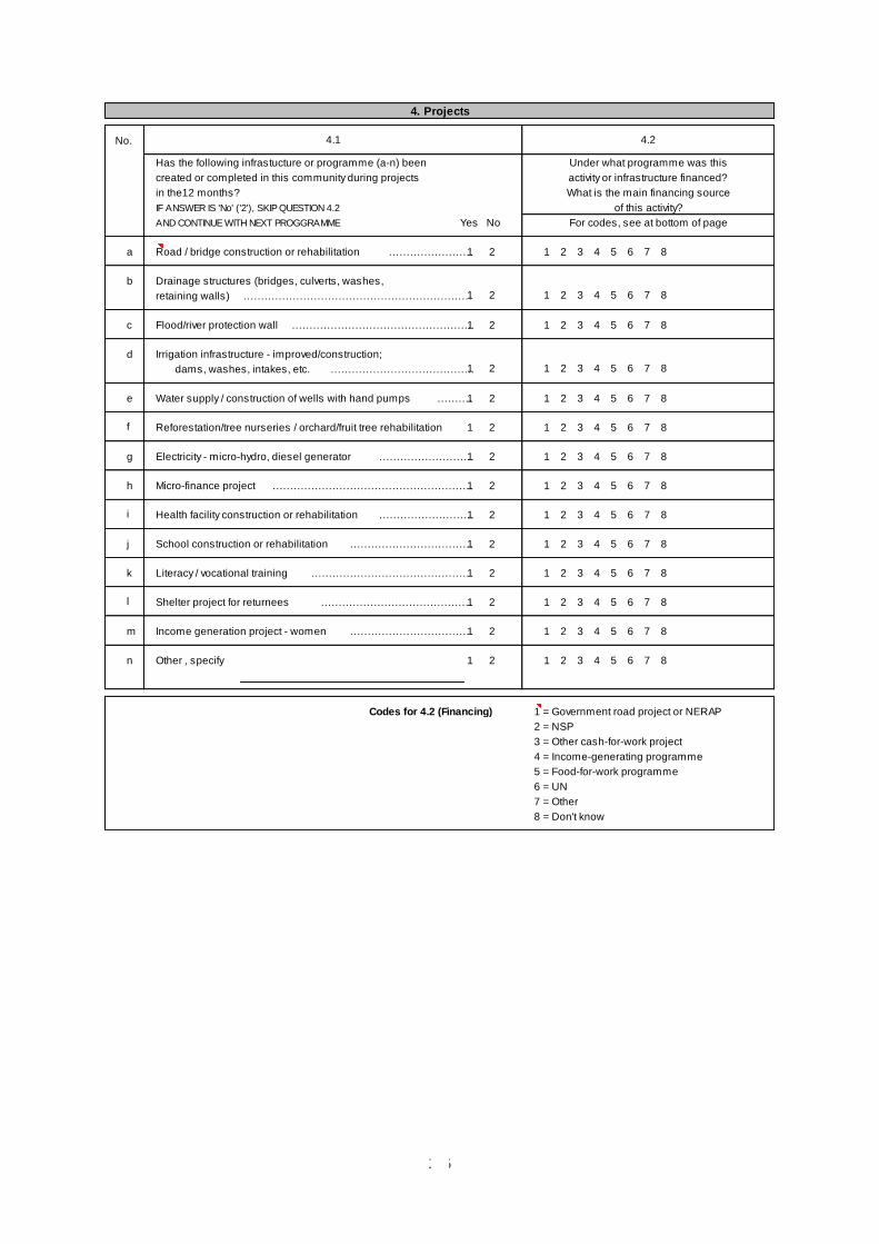
266
4. Projects
No. 4.1 4.2
Has the following infrastucture or programme (a-n) been Under what programme was this
created or completed in this community during projects activity or infrastructure financed?
in the12 months? What is the main financing source
IF ANSWER IS 'No' ('2'), SKIP QUESTION 4.2 of this activity?
AND CONTINUE WITH NEXT PROGGRAMME Yes No For codes, see at bottom of page
a Road / bridge construction or rehabilitation …………………………………………………………… 1 2 1 2 3 4 5 6 7 8
b Drainage structures (bridges, culverts, washes,
retaining walls) …………………………………………………………… 1 2 1 2 3 4 5 6 7 8
c Flood/river protection wall …………………………………………………………… 1 2 1 2 3 4 5 6 7 8
d Irrigation infrastructure - improved/construction;
dams, washes, intakes, etc. …………………………………………………………… 1 2 1 2 3 4 5 6 7 8
e Water supply / construction of wells with hand pumps …………………………………………………………… 1 2 1 2 3 4 5 6 7 8
f Reforestation/tree nurseries / orchard/fruit tree rehabilitation 1 2 1 2 3 4 5 6 7 8
g Electricity - micro-hydro, diesel generator …………………………………………………………… 1 2 1 2 3 4 5 6 7 8
h Micro-finance project …………………………………………………………… 1 2 1 2 3 4 5 6 7 8
i Health facility construction or rehabilitation …………………………………………………………… 1 2 1 2 3 4 5 6 7 8
j School construction or rehabilitation …………………………………………………………… 1 2 1 2 3 4 5 6 7 8
k Literacy / vocational training …………………………………………………………… 1 2 1 2 3 4 5 6 7 8
l Shelter project for returnees …………………………………………………………… 1 2 1 2 3 4 5 6 7 8
m Income generation project - women …………………………………………………………… 1 2 1 2 3 4 5 6 7 8
n Other , specify 1 2 1 2 3 4 5 6 7 8
Codes for 4.2 (Financing) 1 = Government road project or NERAP
2 = NSP
3 = Other cash-for-work project
4 = Income-generating programme
5 = Food-for-work programme
6 = UN
7 = Other
8 = Don't know
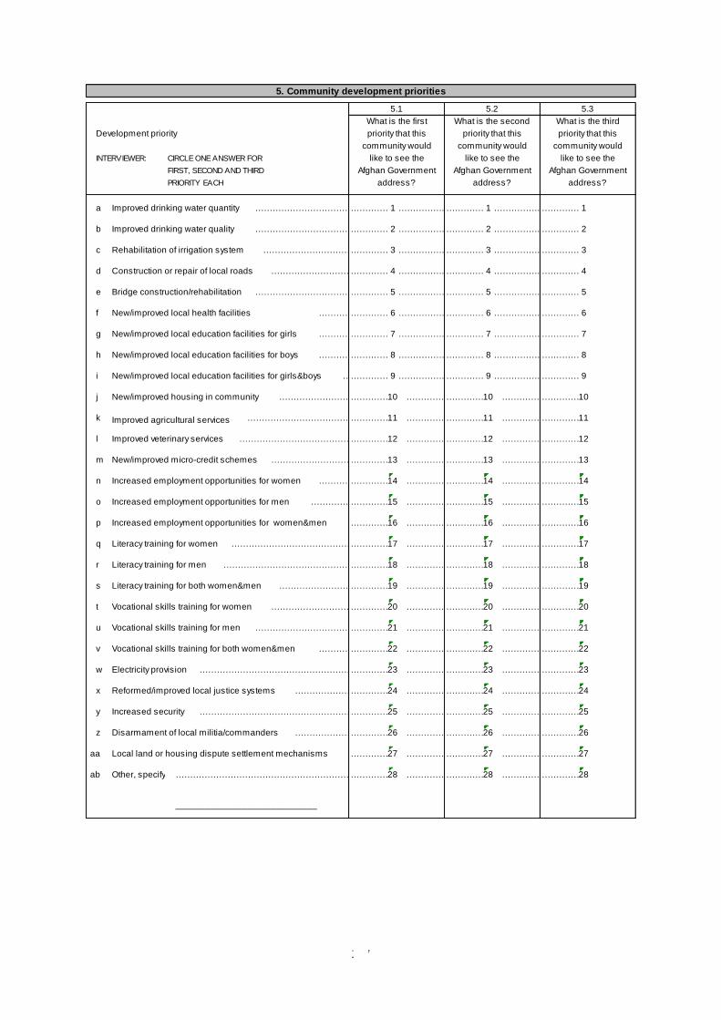
267
5. Community development priorities
5.1 5.2 5.3
What is the first What is the second What is the third
Development priority priority that this priority that this priority that this
community would community would community would
INTERVIEWER: CIRCLE ONE ANSWER FOR like to see the like to see the like to see the
FIRST, SECOND AND THIRD Afghan Government Afghan Government Afghan Government
PRIORITY EACH address? address? address?
a Improved drinking water quantity …………………………………………………………………………..1 ……………..……………..1 ……………..……………..1
b Improved drinking water quality …………………………………………………………………………..2 ……………..……………..2 ……………..……………..2
c Rehabilitation of irrigation system …………………………………………………………………………..3 ……………..……………..3 ……………..……………..3
d Construction or repair of local roads …………………………………………………………………………..4 ……………..……………..4 ……………..……………..4
e Bridge construction/rehabilitation …………………………………………………………………………..5 ……………..……………..5 ……………..……………..5
f New/improved local health facilities …………………………………………………………………………..6 ……………..……………..6 ……………..……………..6
g New/improved local education facilities for girls …………………………………………………………………………..7 ……………..……………..7 ……………..……………..7
h New/improved local education facilities for boys …………………………………………………………………………..8 ……………..……………..8 ……………..……………..8
i New/improved local education facilities for girls&boys …………………………………………………………………………..9 ……………..……………..9 ……………..……………..9
j New/improved housing in community …………………………………………………………………………..10 ……………..……………..10 ……………..……………..10
k Improved agricultural services …………………………………………………………………………..11 ……………..……………..11 ……………..……………..11
l Improved veterinary services …………………………………………………………………………..12 ……………..……………..12 ……………..……………..12
m New/improved micro-credit schemes …………………………………………………………………………..13 ……………..……………..13 ……………..……………..13
n Increased employment opportunities for women …………………………………………………………………………..14 ……………..……………..14 ……………..……………..14
o Increased employment opportunities for men …………………………………………………………………………..15 ……………..……………..15 ……………..……………..15
p Increased employment opportunities for women&men ……………..16 ……………..……………..16 ……………..……………..16
q Literacy training for women …………………………………………………………………………..17 ……………..……………..17 ……………..……………..17
r Literacy training for men …………………………………………………………………………..18 ……………..……………..18 ……………..……………..18
s Literacy training for both women&men …………………………………………………………………………..19 ……………..……………..19 ……………..……………..19
t Vocational skills training for women …………………………………………………………………………..20 ……………..……………..20 ……………..……………..20
u Vocational skills training for men …………………………………………………………………………..21 ……………..……………..21 ……………..……………..21
v Vocational skills training for both women&men …………………………………………………………………………..22 ……………..……………..22 ……………..……………..22
w Electricity provision …………………………………………………………………………..23 ……………..……………..23 ……………..……………..23
x Reformed/improved local justice systems …………………………………………………………………………..24 ……………..……………..24 ……………..……………..24
y Increased security …………………………………………………………………………..25 ……………..……………..25 ……………..……………..25
z Disarmament of local militia/commanders …………………………………………………………………………..26 ……………..……………..26 ……………..……………..26
aa Local land or housing dispute settlement mechanisms ……………..27 ……………..……………..27 ……………..……………..27
ab Other, specify …………………………………………………………………………..28 ……………..……………..28 ……………..……………..28
____________________________
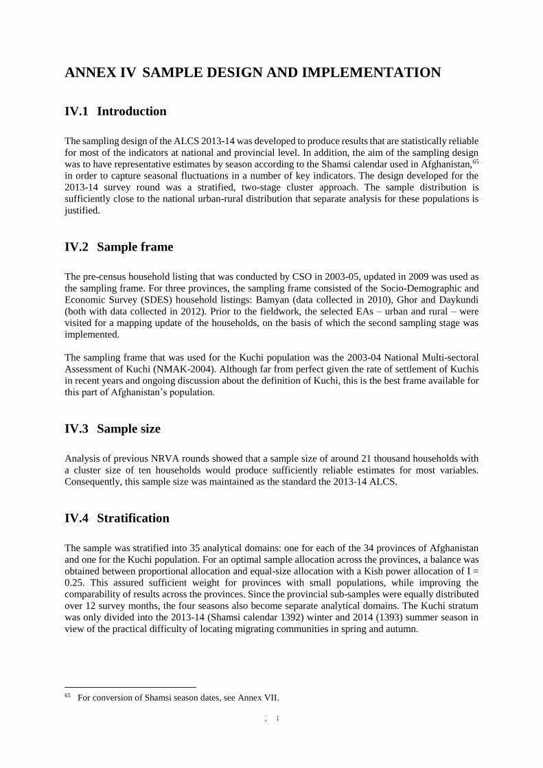
268
ANNEX IV SAMPLE DESIGN AND IMPLEMENTATION
IV.1 Introduction
The sampling design of the ALCS 2013-14 was developed to produce results that are statistically reliable
for most of the indicators at national and provincial level. In addition, the aim of the sampling design
was to have representative estimates by season according to the Shamsi calendar used in Afghanistan,65
in order to capture seasonal fluctuations in a number of key indicators. The design developed for the
2013-14 survey round was a stratified, two-stage cluster approach. The sample distribution is
sufficiently close to the national urban-rural distribution that separate analysis for these populations is
justified.
IV.2 Sample frame
The pre-census household listing that was conducted by CSO in 2003-05, updated in 2009 was used as
the sampling frame. For three provinces, the sampling frame consisted of the Socio-Demographic and
Economic Survey (SDES) household listings: Bamyan (data collected in 2010), Ghor and Daykundi
(both with data collected in 2012). Prior to the fieldwork, the selected EAs – urban and rural – were
visited for a mapping update of the households, on the basis of which the second sampling stage was
implemented.
The sampling frame that was used for the Kuchi population was the 2003-04 National Multi-sectoral
Assessment of Kuchi (NMAK-2004). Although far from perfect given the rate of settlement of Kuchis
in recent years and ongoing discussion about the definition of Kuchi, this is the best frame available for
this part of Afghanistan’s population.
IV.3 Sample size
Analysis of previous NRVA rounds showed that a sample size of around 21 thousand households with
a cluster size of ten households would produce sufficiently reliable estimates for most variables.
Consequently, this sample size was maintained as the standard the 2013-14 ALCS.
IV.4 Stratification
The sample was stratified into 35 analytical domains: one for each of the 34 provinces of Afghanistan
and one for the Kuchi population. For an optimal sample allocation across the provinces, a balance was
obtained between proportional allocation and equal-size allocation with a Kish power allocation of I =
0.25. This assured sufficient weight for provinces with small populations, while improving the
comparability of results across the provinces. Since the provincial sub-samples were equally distributed
over 12 survey months, the four seasons also become separate analytical domains. The Kuchi stratum
was only divided into the 2013-14 (Shamsi calendar 1392) winter and 2014 (1393) summer season in
view of the practical difficulty of locating migrating communities in spring and autumn.
65 For conversion of Shamsi season dates, see Annex VII.
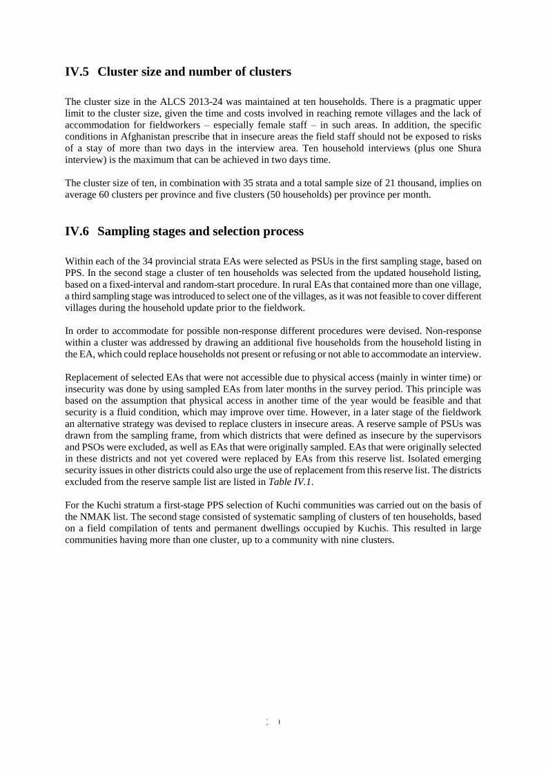
269
IV.5 Cluster size and number of clusters
The cluster size in the ALCS 2013-24 was maintained at ten households. There is a pragmatic upper
limit to the cluster size, given the time and costs involved in reaching remote villages and the lack of
accommodation for fieldworkers – especially female staff – in such areas. In addition, the specific
conditions in Afghanistan prescribe that in insecure areas the field staff should not be exposed to risks
of a stay of more than two days in the interview area. Ten household interviews (plus one Shura
interview) is the maximum that can be achieved in two days time.
The cluster size of ten, in combination with 35 strata and a total sample size of 21 thousand, implies on
average 60 clusters per province and five clusters (50 households) per province per month.
IV.6 Sampling stages and selection process
Within each of the 34 provincial strata EAs were selected as PSUs in the first sampling stage, based on
PPS. In the second stage a cluster of ten households was selected from the updated household listing,
based on a fixed-interval and random-start procedure. In rural EAs that contained more than one village,
a third sampling stage was introduced to select one of the villages, as it was not feasible to cover different
villages during the household update prior to the fieldwork.
In order to accommodate for possible non-response different procedures were devised. Non-response
within a cluster was addressed by drawing an additional five households from the household listing in
the EA, which could replace households not present or refusing or not able to accommodate an interview.
Replacement of selected EAs that were not accessible due to physical access (mainly in winter time) or
insecurity was done by using sampled EAs from later months in the survey period. This principle was
based on the assumption that physical access in another time of the year would be feasible and that
security is a fluid condition, which may improve over time. However, in a later stage of the fieldwork
an alternative strategy was devised to replace clusters in insecure areas. A reserve sample of PSUs was
drawn from the sampling frame, from which districts that were defined as insecure by the supervisors
and PSOs were excluded, as well as EAs that were originally sampled. EAs that were originally selected
in these districts and not yet covered were replaced by EAs from this reserve list. Isolated emerging
security issues in other districts could also urge the use of replacement from this reserve list. The districts
excluded from the reserve sample list are listed in Table IV.1.
For the Kuchi stratum a first-stage PPS selection of Kuchi communities was carried out on the basis of
the NMAK list. The second stage consisted of systematic sampling of clusters of ten households, based
on a field compilation of tents and permanent dwellings occupied by Kuchis. This resulted in large
communities having more than one cluster, up to a community with nine clusters.
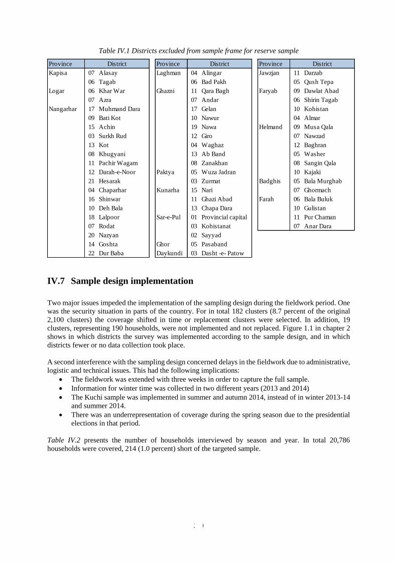
270
Table IV.1 Districts excluded from sample frame for reserve sample
IV.7 Sample design implementation
Two major issues impeded the implementation of the sampling design during the fieldwork period. One
was the security situation in parts of the country. For in total 182 clusters (8.7 percent of the original
2,100 clusters) the coverage shifted in time or replacement clusters were selected. In addition, 19
clusters, representing 190 households, were not implemented and not replaced. Figure 1.1 in chapter 2
shows in which districts the survey was implemented according to the sample design, and in which
districts fewer or no data collection took place.
A second interference with the sampling design concerned delays in the fieldwork due to administrative,
logistic and technical issues. This had the following implications:
The fieldwork was extended with three weeks in order to capture the full sample.
Information for winter time was collected in two different years (2013 and 2014)
The Kuchi sample was implemented in summer and autumn 2014, instead of in winter 2013-14
and summer 2014.
There was an underrepresentation of coverage during the spring season due to the presidential
elections in that period.
Table IV.2 presents the number of households interviewed by season and year. In total 20,786
households were covered, 214 (1.0 percent) short of the targeted sample.
Province District Province District Province District
Kapisa 07 Alasay Laghman 04 Alingar Jawzjan 11 Darzab
06 Tagab 06 Bad Pakh 05 Qush Tepa
Logar 06 Khar War Ghazni 11 Qara Bagh Faryab 09 Dawlat Abad
07 Azra 07 Andar 06 Shirin Tagab
Nangarhar 17 Muhmand Dara 17 Gelan 10 Kohistan
09 Bati Kot 10 Nawur 04 Almar
15 Achin 19 Nawa Helmand 09 Musa Qala
03 Surkh Rud 12 Giro 07 Nawzad
13 Kot 04 Waghaz 12 Baghran
08 Khugyani 13 Ab Band 05 Washer
11 Pachir Wagam 08 Zanakhan 08 Sangin Qala
12 Darah-e-Noor Paktya 05 Wuza Jadran 10 Kajaki
21 Hesarak 03 Zurmat Badghis 05 Bala Murghab
04 Chaparhar Kunarha 15 Nari 07 Ghormach
16 Shinwar 11 Ghazi Abad Farah 06 Bala Buluk
10 Deh Bala 13 Chapa Dara 10 Gulistan
18 Lalpoor Sar-e-Pul 01 Provincial capital 11 Pur Chaman
07 Rodat 03 Kohistanat 07 Anar Dara
20 Nazyan 02 Sayyad
14 Goshta Ghor 05 Pasaband
22 Dur Baba Daykundi 03 Dasht -e- Patow
271
Table IV.2 Interviewed households, by year, and by season (Shamsi calendar)
Season Year Total
1392 1393
Winter 5,067 - 5,067
Spring 4,449 4,449
Summer 4,880 4,880
Autumn 6,390 6,390
Total 5,067 15,719 20,786
Non-response within clusters was very limited. Only 845 (4.1 percent) of the households in the visited
clusters were not available or refused or were unable to participate. In 841 of these cases households
were replaced by reserve households listed in the cluster reserve list, leaving 4 households unaccounted
for (0.02 percent).
IV.8 Calculation of sampling weights and post-stratification
Sample weights are the scaling factors that are required to inflate the sampled households to the number
of households that they represent in the survey. The use of stratification in the ALCS 2014 sample design
requires that sample weights are separately calculated for each stratum. Due to imperfections in the
survey implementation, the design weights are adjusted in order to achieve optimal representation of the
survey results. This section separately addresses the calculation of the sampling weights for the resident
population and that for the Kuchi population.
IV.8.1 Resident population
Calculation of the design weight
The first step in calculating the sample weights is calculating the weights that would inflate the sampled
households to the number of households in the sampling frame. This calculation follows from the
selection probability of the households as defined in the sampling design.
In the two-stage sampling design of ALCS 2013-14, the PSUs were the EAs as defined in the sample
frame, made up of the 2009 household listing and the available household listings from the SDS. The
selection of PSUs in the first sampling stage was implemented in accordance with:
stratification by province
an optimum allocation distribution for provinces, which minimises the standard error
selection with probability proportional to the number of households (PPS).
The probability of selecting a PSU in stage 1 is
p1 = cs * hps / Hs09
where p1 is the probability of selecting PSU (or EA) p in stratum s, cs is the number of clusters selected
in stratum s, hps is the number of households in EA p from stratum s and Hs09 is the number of households
in stratum s as reported in the sampling frame.
For EAs encompassing two or more villages, a second sampling stage was introduced in order to reduce
travel time and costs. The selection of the village to be included was done with probability proportional
to the number of households, with
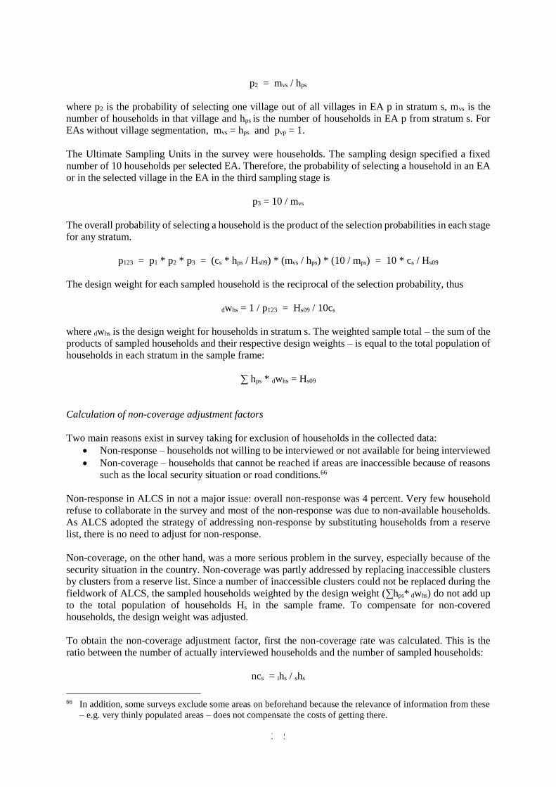
272
p2 = mvs / hps
where p2 is the probability of selecting one village out of all villages in EA p in stratum s, mvs is the
number of households in that village and hps is the number of households in EA p from stratum s. For
EAs without village segmentation, mvs = hps and pvp = 1.
The Ultimate Sampling Units in the survey were households. The sampling design specified a fixed
number of 10 households per selected EA. Therefore, the probability of selecting a household in an EA
or in the selected village in the EA in the third sampling stage is
p3 = 10 / mvs
The overall probability of selecting a household is the product of the selection probabilities in each stage
for any stratum.
p123 = p1 * p2 * p3 = (cs * hps / Hs09) * (mvs / hps) * (10 / mps) = 10 * cs / Hs09
The design weight for each sampled household is the reciprocal of the selection probability, thus
dwhs = 1 / p123 = Hs09 / 10cs
where dwhs is the design weight for households in stratum s. The weighted sample total – the sum of the
products of sampled households and their respective design weights – is equal to the total population of
households in each stratum in the sample frame:
∑ hps * dwhs = Hs09
Calculation of non-coverage adjustment factors
Two main reasons exist in survey taking for exclusion of households in the collected data:
Non-response – households not willing to be interviewed or not available for being interviewed
Non-coverage – households that cannot be reached if areas are inaccessible because of reasons
such as the local security situation or road conditions.66
Non-response in ALCS in not a major issue: overall non-response was 4 percent. Very few household
refuse to collaborate in the survey and most of the non-response was due to non-available households.
As ALCS adopted the strategy of addressing non-response by substituting households from a reserve
list, there is no need to adjust for non-response.
Non-coverage, on the other hand, was a more serious problem in the survey, especially because of the
security situation in the country. Non-coverage was partly addressed by replacing inaccessible clusters
by clusters from a reserve list. Since a number of inaccessible clusters could not be replaced during the
fieldwork of ALCS, the sampled households weighted by the design weight (∑hps* dwhs) do not add up
to the total population of households Hs in the sample frame. To compensate for non-covered
households, the design weight was adjusted.
To obtain the non-coverage adjustment factor, first the non-coverage rate was calculated. This is the
ratio between the number of actually interviewed households and the number of sampled households:
ncs = ihs / shs
66 In addition, some surveys exclude some areas on beforehand because the relevance of information from these
– e.g. very thinly populated areas – does not compensate the costs of getting there.
273
where ncs is the non-coverage rate in stratum s, ihs is the number of interviewed households in stratum
s and shs is the number of sampled households in stratum s. The adjustment factor for non-coverage in
stratum s (nwhs) is the reciprocal of the non-coverage rate nc:
nwhs = 1 / ncs
The sample weight that is required to scale-up the sampled households to the total population of
households in the sample frame (dnwhs) now becomes the product of the design weight and the non-
coverage factor. For each stratum s this is:
dnwhs = dwhs * nwhs
The newly weighted sample total ∑ hps * dnwhs is again equal to the sample frame population Hs09.
Calculation of post-stratification factors
Additional expansion factors are required to re-scale the number of households in the sample frame to
the number in the period in which the survey was conducted. As in the previous survey round, the
estimated number of households was derived from the CSO population projections by province (Ps14).67
For the settled households, the provincial population was divided by the average household size for that
province, which was obtained in the current survey by applying dnws (the combined design weight and
non-coverage factor) in order to reduce distortion by sampling and coverage effects.
Since the re-scaling of the number of households is done at province level, this normalisation exercise
implies post-stratification of the sample. The re-scaling factors are calculated as the ratio between the
CSO estimate of the number of households in 2014 in a stratum and the number of households in the
sampling frame:
rwhs = Hs14 / Hs09
and the combined sampling weight becomes
dnrwhs = dnwhs * rwhs
Seasonal distribution
Because the interview implementation was not entirely uniform across seasons (quarters), uncorrected
annual estimates would place relatively larger weights on those seasons which had a large sample
(winter and autumn), thereby distorting the representativeness of national results. Because the sample
was stratified by season, and imposing the assumption that the level of seasonal, international migration
is negligible, the weighted distribution can be smoothed out to ensure that the estimated population size
by quarter is the same. This adjustment is implemented as:
whsq = (1 / dnrwhs) * 0.25 * Ps14 / dnrpsq
where whsq is the factor that standardises across seasons (quarters) and dnrpsq is the sampled population
in stratum s and season q, weighted by the weights for the sampling design, non-coverage and re-scaling.
The denominator gives the total number of sampled, settled individuals in each stratum by quarter. The
adjustment term in the numerator gives the population of individuals for each stratum by quarter
according to the CSO 2014 population estimate.
67 The 1393 population projections are considered a sufficient approximation for the mid-survey population.
274
The final household sampling weight hwhsq is the product of all weighting factors:
hwsq = dnrwhs * whsq
Individual weights
In order to obtain the expansion factor for individuals the following calculation was made:
iwhsq = hwhsq * hshsq
the term hshsq being the household size of household h in stratum s and quarter q.
IV.8.2 Kuchi population
The Kuchi sample was designed on basis of the 2003-04 National Multi-sectoral Assessment of Kuchi
(NMAK-2004). For this separate Kuchi stratum a community selection was implemented with PPS and
a second stage selection with again a constant cluster size of ten households. The 66 clusters (660
households) for this stratum were divided between the summer (30 clusters) and winter (36 clusters)
periods in 1393 (2014).
In the absence of up-to-date information about the actual number of Kuchis and the poltical sensitivity
of addressing this issue, the present position taken by CSO is that the Kuchi pupolation is stable at a
number close to 1.5 million people.
Apart from the sampling frame, the restriction to two seasons and the absence of the need to
accommodate population growth, the procedures for the calculation of the sampling weights for the
Kuchi stratum are the same as those for the resident population
IV.8.3 Weights variables
The values of the final household sample weight hwhsq and individual sample weight iwhsq are included
in the ALCS 2013-14 dataset as weight variables hh_weight and ind_weight, respectively. The weight
variable hh_weight expands household-level data to the total population of households and individual-
level data to the total population of individuals. The weight variable ind_weight expands household-
level data to the total population individuals.
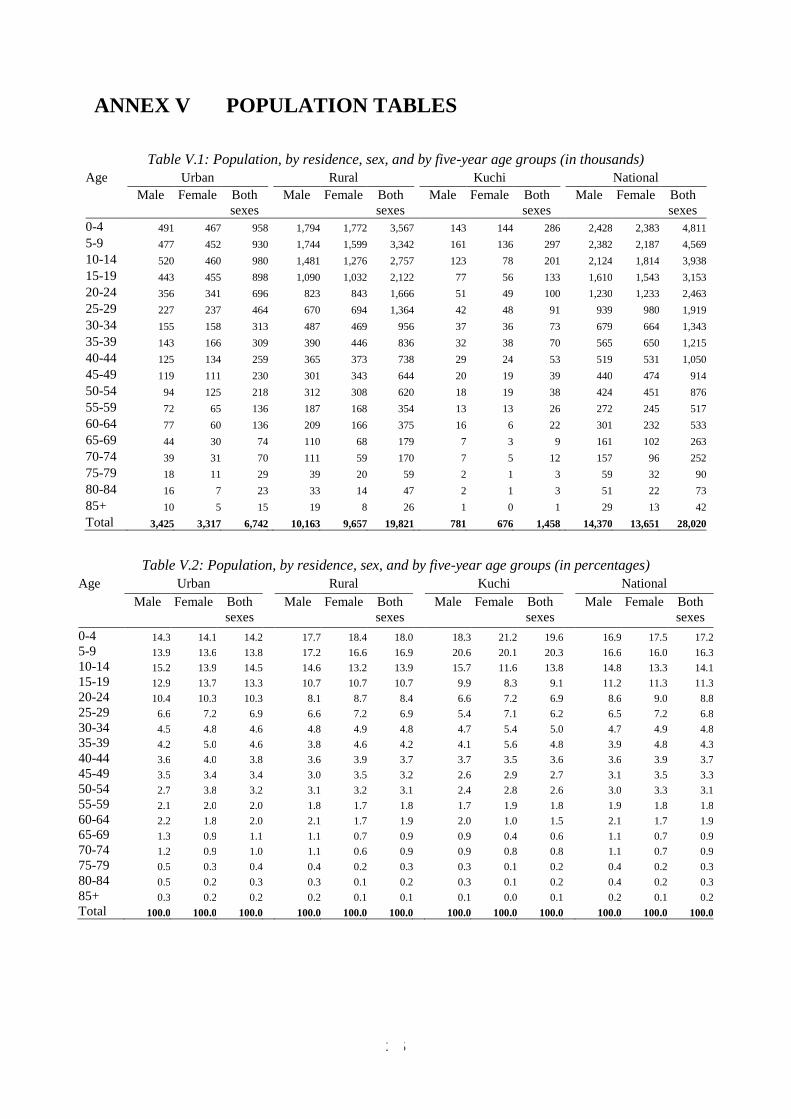
275
ANNEX V POPULATION TABLES
Table V.1: Population, by residence, sex, and by five-year age groups (in thousands)
Age Urban Rural Kuchi National
Male Female Both
sexes
Male Female Both
sexes
Male Female Both
sexes
Male Female Both
sexes
0-4 491 467 958 1,794 1,772 3,567 143 144 286 2,428 2,383 4,811
5-9 477 452 930 1,744 1,599 3,342 161 136 297 2,382 2,187 4,569
10-14 520 460 980 1,481 1,276 2,757 123 78 201 2,124 1,814 3,938
15-19 443 455 898 1,090 1,032 2,122 77 56 133 1,610 1,543 3,153
20-24 356 341 696 823 843 1,666 51 49 100 1,230 1,233 2,463
25-29 227 237 464 670 694 1,364 42 48 91 939 980 1,919
30-34 155 158 313 487 469 956 37 36 73 679 664 1,343
35-39 143 166 309 390 446 836 32 38 70 565 650 1,215
40-44 125 134 259 365 373 738 29 24 53 519 531 1,050
45-49 119 111 230 301 343 644 20 19 39 440 474 914
50-54 94 125 218 312 308 620 18 19 38 424 451 876
55-59 72 65 136 187 168 354 13 13 26 272 245 517
60-64 77 60 136 209 166 375 16 6 22 301 232 533
65-69 44 30 74 110 68 179 7 3 9 161 102 263
70-74 39 31 70 111 59 170 7 5 12 157 96 252
75-79 18 11 29 39 20 59 2 1 3 59 32 90
80-84 16 7 23 33 14 47 2 1 3 51 22 73
85+ 10 5 15 19 8 26 1 0 1 29 13 42
Total 3,425 3,317 6,742 10,163 9,657 19,821 781 676 1,458 14,370 13,651 28,020
Table V.2: Population, by residence, sex, and by five-year age groups (in percentages)
Age Urban Rural Kuchi National
Male Female Both
sexes
Male Female Both
sexes
Male Female Both
sexes
Male Female Both
sexes
0-4 14.3 14.1 14.2 17.7 18.4 18.0 18.3 21.2 19.6 16.9 17.5 17.2
5-9 13.9 13.6 13.8 17.2 16.6 16.9 20.6 20.1 20.3 16.6 16.0 16.3
10-14 15.2 13.9 14.5 14.6 13.2 13.9 15.7 11.6 13.8 14.8 13.3 14.1
15-19 12.9 13.7 13.3 10.7 10.7 10.7 9.9 8.3 9.1 11.2 11.3 11.3
20-24 10.4 10.3 10.3 8.1 8.7 8.4 6.6 7.2 6.9 8.6 9.0 8.8
25-29 6.6 7.2 6.9 6.6 7.2 6.9 5.4 7.1 6.2 6.5 7.2 6.8
30-34 4.5 4.8 4.6 4.8 4.9 4.8 4.7 5.4 5.0 4.7 4.9 4.8
35-39 4.2 5.0 4.6 3.8 4.6 4.2 4.1 5.6 4.8 3.9 4.8 4.3
40-44 3.6 4.0 3.8 3.6 3.9 3.7 3.7 3.5 3.6 3.6 3.9 3.7
45-49 3.5 3.4 3.4 3.0 3.5 3.2 2.6 2.9 2.7 3.1 3.5 3.3
50-54 2.7 3.8 3.2 3.1 3.2 3.1 2.4 2.8 2.6 3.0 3.3 3.1
55-59 2.1 2.0 2.0 1.8 1.7 1.8 1.7 1.9 1.8 1.9 1.8 1.8
60-64 2.2 1.8 2.0 2.1 1.7 1.9 2.0 1.0 1.5 2.1 1.7 1.9
65-69 1.3 0.9 1.1 1.1 0.7 0.9 0.9 0.4 0.6 1.1 0.7 0.9
70-74 1.2 0.9 1.0 1.1 0.6 0.9 0.9 0.8 0.8 1.1 0.7 0.9
75-79 0.5 0.3 0.4 0.4 0.2 0.3 0.3 0.1 0.2 0.4 0.2 0.3
80-84 0.5 0.2 0.3 0.3 0.1 0.2 0.3 0.1 0.2 0.4 0.2 0.3
85+ 0.3 0.2 0.2 0.2 0.1 0.1 0.1 0.0 0.1 0.2 0.1 0.2
Total 100.0 100.0 100.0 100.0 100.0 100.0 100.0 100.0 100.0 100.0 100.0 100.0
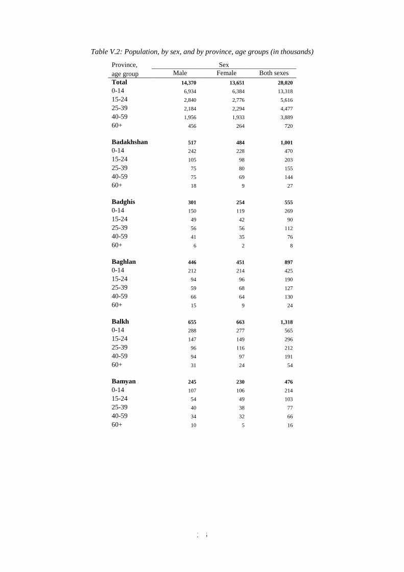
276
Table V.2: Population, by sex, and by province, age groups (in thousands)
Province, Sex
age group Male Female Both sexes
Total 14,370 13,651 28,020
0-14 6,934 6,384 13,318
15-24 2,840 2,776 5,616
25-39 2,184 2,294 4,477
40-59 1,956 1,933 3,889
60+ 456 264 720
Badakhshan 517 484 1,001
0-14 242 228 470
15-24 105 98 203
25-39 75 80 155
40-59 75 69 144
60+ 18 9 27
Badghis 301 254 555
0-14 150 119 269
15-24 49 42 90
25-39 56 56 112
40-59 41 35 76
60+ 6 2 8
Baghlan 446 451 897
0-14 212 214 425
15-24 94 96 190
25-39 59 68 127
40-59 66 64 130
60+ 15 9 24
Balkh 655 663 1,318
0-14 288 277 565
15-24 147 149 296
25-39 96 116 212
40-59 94 97 191
60+ 31 24 54
Bamyan 245 230 476
0-14 107 106 214
15-24 54 49 103
25-39 40 38 77
40-59 34 32 66
60+ 10 5 16
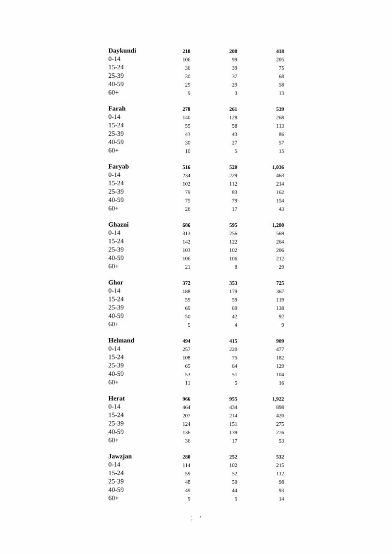
277
Daykundi 210 208 418
0-14 106 99 205
15-24 36 39 75
25-39 30 37 68
40-59 29 29 58
60+ 9 3 13
Farah 278 261 539
0-14 140 128 268
15-24 55 58 113
25-39 43 43 86
40-59 30 27 57
60+ 10 5 15
Faryab 516 520 1,036
0-14 234 229 463
15-24 102 112 214
25-39 79 83 162
40-59 75 79 154
60+ 26 17 43
Ghazni 686 595 1,280
0-14 313 256 569
15-24 142 122 264
25-39 103 102 206
40-59 106 106 212
60+ 21 8 29
Ghor 372 353 725
0-14 188 179 367
15-24 59 59 119
25-39 69 69 138
40-59 50 42 92
60+ 5 4 9
Helmand 494 415 909
0-14 257 220 477
15-24 108 75 182
25-39 65 64 129
40-59 53 51 104
60+ 11 5 16
Herat 966 955 1,922
0-14 464 434 898
15-24 207 214 420
25-39 124 151 275
40-59 136 139 276
60+ 36 17 53
Jawzjan 280 252 532
0-14 114 102 215
15-24 59 52 112
25-39 48 50 98
40-59 49 44 93
60+ 9 5 14
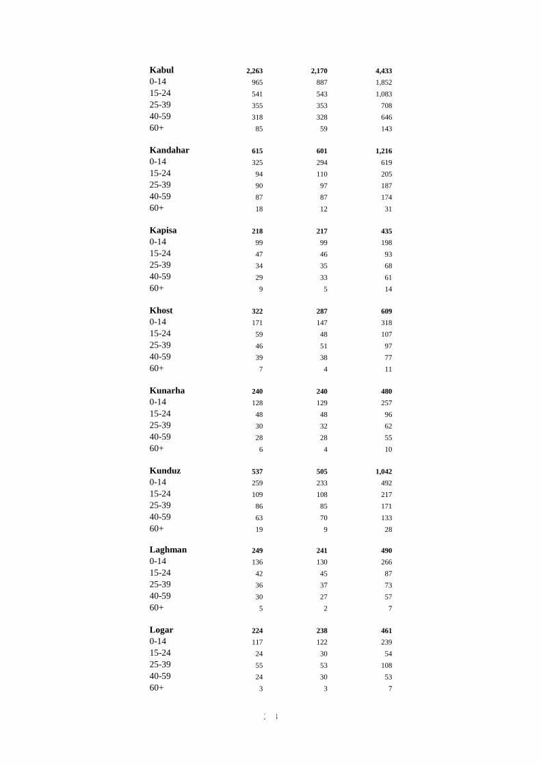
278
Kabul 2,263 2,170 4,433
0-14 965 887 1,852
15-24 541 543 1,083
25-39 355 353 708
40-59 318 328 646
60+ 85 59 143
Kandahar 615 601 1,216
0-14 325 294 619
15-24 94 110 205
25-39 90 97 187
40-59 87 87 174
60+ 18 12 31
Kapisa 218 217 435
0-14 99 99 198
15-24 47 46 93
25-39 34 35 68
40-59 29 33 61
60+ 9 5 14
Khost 322 287 609
0-14 171 147 318
15-24 59 48 107
25-39 46 51 97
40-59 39 38 77
60+ 7 4 11
Kunarha 240 240 480
0-14 128 129 257
15-24 48 48 96
25-39 30 32 62
40-59 28 28 55
60+ 6 4 10
Kunduz 537 505 1,042
0-14 259 233 492
15-24 109 108 217
25-39 86 85 171
40-59 63 70 133
60+ 19 9 28
Laghman 249 241 490
0-14 136 130 266
15-24 42 45 87
25-39 36 37 73
40-59 30 27 57
60+ 5 2 7
Logar 224 238 461
0-14 117 122 239
15-24 24 30 54
25-39 55 53 108
40-59 24 30 53
60+ 3 3 7
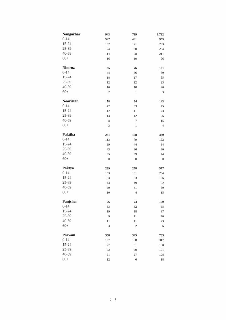
279
Nangarhar 943 789 1,732
0-14 527 431 959
15-24 162 121 283
25-39 124 130 254
40-59 114 98 211
60+ 16 10 26
Nimroz 85 76 161
0-14 44 36 80
15-24 18 17 35
25-39 12 12 23
40-59 10 10 20
60+ 2 1 3
Nooristan 78 64 143
0-14 42 33 75
15-24 12 11 23
25-39 13 12 26
40-59 8 7 15
60+ 3 1 4
Paktika 231 198 430
0-14 113 79 192
15-24 39 44 84
25-39 43 36 80
40-59 35 39 74
60+ 0 0 0
Paktya 299 278 577
0-14 153 131 284
15-24 53 53 106
25-39 43 49 92
40-59 39 41 80
60+ 10 4 15
Panjsher 76 74 150
0-14 33 32 65
15-24 19 18 37
25-39 9 11 20
40-59 11 11 23
60+ 3 2 6
Parwan 358 345 703
0-14 167 150 317
15-24 77 81 158
25-39 52 50 101
40-59 51 57 108
60+ 12 6 18
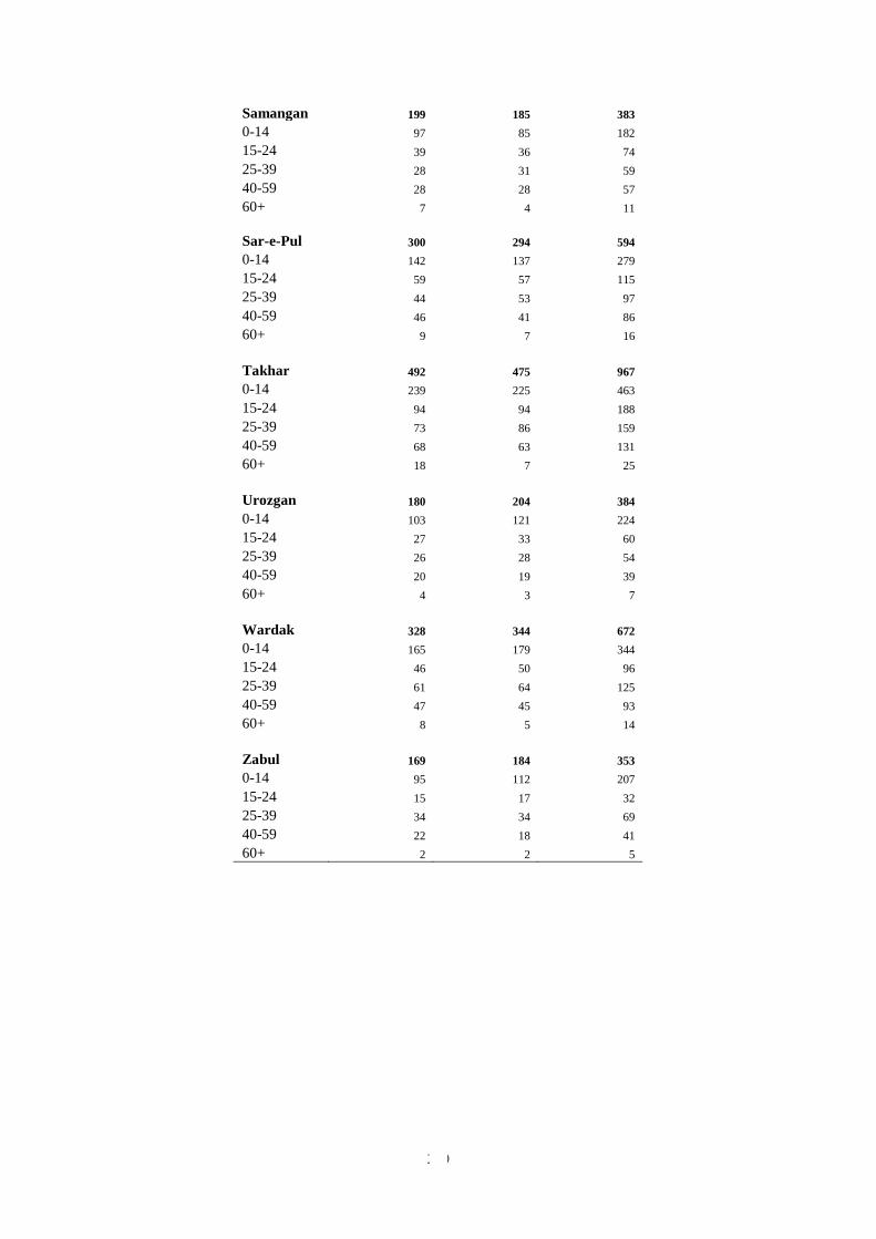
280
Samangan 199 185 383
0-14 97 85 182
15-24 39 36 74
25-39 28 31 59
40-59 28 28 57
60+ 7 4 11
Sar-e-Pul 300 294 594
0-14 142 137 279
15-24 59 57 115
25-39 44 53 97
40-59 46 41 86
60+ 9 7 16
Takhar 492 475 967
0-14 239 225 463
15-24 94 94 188
25-39 73 86 159
40-59 68 63 131
60+ 18 7 25
Urozgan 180 204 384
0-14 103 121 224
15-24 27 33 60
25-39 26 28 54
40-59 20 19 39
60+ 4 3 7
Wardak 328 344 672
0-14 165 179 344
15-24 46 50 96
25-39 61 64 125
40-59 47 45 93
60+ 8 5 14
Zabul 169 184 353
0-14 95 112 207
15-24 15 17 32
25-39 34 34 69
40-59 22 18 41
60+ 2 2 5
281
ANNEX VI TECHNICAL NOTE ON SURVEY TO SURVEY
IMPUTATION: POVERTY PROJECTION FOR
AFGHANISTAN
The ‘survey-to-survey imputation’ technique uses a model built from existing data from one survey to
estimate missing data in another survey. Using the NRVA 2011-12 survey, which has consumption data,
we used the survey-to-survey imputation method to estimate household consumption expenditure and
poverty rates for the ALCS 2013-14, which does not have consumption data. This annex describes in
detail the survey-to-survey imputation methodology.68
VI.1 Data
Data used for the survey-to-survey exercise come from three rounds of national household surveys,
NRVA 2007-08, NRVA 2011-12, and the 2013-14 ALCS survey. All three surveys are multi-topic
surveys that collected a wide range of individual, household, and community-level socio-economic
information, each over a one-year period (to capture seasonal variations).
The NRVA surveys’ sampling frame (from the CSO’s 2003-05 pre-census household listing) are
representative at the national and the province level. For the ALCS 2013-14 the sampling frame stems
from the 2003-05 household listing, subsequently updated in 2009. Comparability between surveys are
maintained as much as possible by using similar questionnaires, training and data collection. ALCS
2013-14 collects many of the same variables as the 2007-08 and 2011-12 NRVA surveys, except for the
food consumption.
Besides the household surveys, we included conflict data from the UN Security Information and
Operation Center (SIOC). UN SIOC collects district-level daily conflict data. Total number of casualties
in each district represents a proxy for level of conflict and insecurity. For each household, we calculated
the total casualties for the district where the household resides for 1 month, 2 months, and 3 months
prior to the household surveys.
We used NRVA 2011-12 data and NRVA 2007-08 and ALCS 2013-14 data to create, validate, and
‘impute’ our final household consumption estimates. The final data used for survey-to-survey
imputation excludes households from Helmand and Khost provinces from all three surveys because
consumption aggregates for these two provinces for NRVA 2011-12, the base year for the consumption
model, are not reliable.
68 We applied the survey-to-survey imputation method in Yoshida et al. (2015), the basis for a new household
survey instrument called SWIFT (Survey of Well-being via Instant, Frequent Tracking). The SWIFT approach
used recent innovations in survey-to-survey imputation techniques developed by Harvard University, Stanford
University and the World Bank’s research department.
282
VI.2 Model development
The exercise proceeds in three steps.
First, we identified common non-consumption variables across surveys, including variables that
correlate well with household consumption data. Obviously, the model’s ability to estimate
changes in household consumption and poverty depends on changes in the explanatory variables
over the same time. If the final model includes only variables that do not change – things such
as type of dwelling and construction material of walls and floor – the model will predict a
poverty rate the same as the poverty rate for the base year. The model therefore must include
variables that change more over time, such as household head’s employment status and level of
conflict.
We reviewed each question across the three surveys to ensure that the common variables used
remained comparable across surveys.69 For instance, although the question ‘type of toilet
facility used by household’ is in all three surveys, the list of the categories of toilet changed in
ALCS 2013-14. Therefore, we selected only categories within the question that are comparable.
Similarly, the labour module covers a different length of time in the different surveys, altering
female labour participation rates across surveys; as such, we restrict labour outcome variables
such as employment status and employment type to ‘head of household’ and ‘adult male
members between the ages of 25 and 50’, categories not affected by the time range used. Table
VI.1 summarises the variables.
Secondly, we developed a model following the Yoshida et al. (2015) SWIFT approach. The
model assumes a linear relationship between household consumption and its correlates, and the
model assumes a projection error.70 The equation representing the consumption model is:
ln 𝑦ℎ𝑡 = 𝑥ℎ𝑡′𝛽 + 𝑢ℎ𝑡 (1)
Where, 𝑙𝑛𝑌ℎ𝑡 is the log of per capita consumption of household h, 𝑥ℎ𝑡 is a (k×1) vector of
poverty correlates of household h, β is a (k×1) vector of coefficients of poverty correlates, k is
a number of variables and 𝑢ℎ𝑡 is the projection. The explanatory variables in the right-hand side
of the model capture variation in household consumption, thus differentiating poor from non-
poor households. For the equation (1) we use NRVA 2011-12 survey, which has the
consumption data. We then impose the estimated variables of the model onto the ALCS 2013-
14 dataset to predict household consumption and the poverty rate.
The SWIFT modelling process includes multiple steps to improve the ability of the formula to
project household income or expenditures by adjusting the coefficients (β) and estimating the
distributions of both the coefficients and the projection errors. 71 No formula is perfect; so
inclusion of the projection error is essential and estimating the distribution of the projection
error is key for estimating poverty rates and their standard errors.
69 Beegle et al. (2011) show empirical evidence of how responses of households to questions can change based on the
questionnaire designs. 70 This does not mean SWIFT does not use a non-linear model. However, SWIFT’s formula is linear in variables created in
the dataset. Since some variables can be squares of other variables, SWIFT’s formula can be non-linear. One of typical
examples is that SWIFT uses household size and household size squared in a formula. 71 The approach adopted by the SWIFT team is rather conservative in that the team did not adopt some approaches discussed
at the frontier of research on modelling because the team thought evidence for these approaches is not yet strong enough.
However, the team has been exploring such new techniques and may update the SWIFT modelling process once enough
supportive evidence for these methodologies is provided.
283
VI.3 Model selection: cross-validation
We selected carefully from the long list of possible variables because creating a model including all
available variables can lead to ‘overfitting’ of the model, where data ‘noise’ impairs the ability to
understand causal relationships between dependent and independent variables.72 The variables we
selected across surveys include demographic information (household size, dependency ratio, proportion
of females in the household), household head’s characteristics (age, education, employment), household
assets (including land, livestock and dwelling) and household access to basic services (water, sanitation
and electricity). We also included some subjective measures of well-being and UN proxy measures for
district-level conflict and insecurity.
We used a 10-fold validation approach to check for over-fitting bias; that is, we randomly divided
household survey data into 10 folds (parts), using nine folds as ‘training data’ and using the remaining
fold as ‘testing data’. The consumption model is estimated on the nine folds ‘training data’ using a
stepwise Ordinary Least Square [stepwise] regression (OLS), an iterative process that selects variables
based on their correlation with household consumption and their predictive power. We repeated this
analysis 10 times,73 each time using a different nine folds as ‘training data’ and the remaining fold for
‘testing data’, and each time testing the model’s performance against the actual – surveyed – poverty
rates and on mean squared errors (MSEs).74 Figure VI.1 illustrates the validation approach.
72 While a model may perform well within the sample data used to create the model, ‘over-fitting’ may cause the model to
perform poorly on new data. 73 SWIFT method creates 10 folds. However, a test may indicate any number of folds. 74 We assume that the error and regression coefficients will follow normal distributions in projecting (simulating) household
expenditure. The simulation process is repeated for all households, typically twenty times (using STATA’s ‘mi impute
regress’ command). A poverty headcount rate is calculated by comparing the simulated household expenditure or income
with a poverty line for each of the twenty simulation rounds. The average poverty rate of the simulations is used as a poverty
estimate.
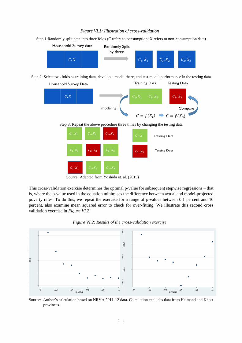
284
Figure VI.1: Illustration of cross-validation
Step 1:Randomly split data into three folds (C refers to consumption; X refers to non-consumption data)
Step 2: Select two folds as training data, develop a model there, and test model performance in the testing data
Step 3: Repeat the above procedure three times by changing the testing data
Source: Adapted from Yoshida et. al. (2015)
This cross-validation exercise determines the optimal p-value for subsequent stepwise regressions – that
is, where the p-value used in the equation minimises the difference between actual and model-projected
poverty rates. To do this, we repeat the exercise for a range of p-values between 0.1 percent and 10
percent, also examine mean squared error to check for over-fitting. We illustrate this second cross
validation exercise in Figure VI.2.
Figure VI.2: Results of the cross-validation exercise
Source: Author’s calculation based on NRVA 2011-12 data. Calculation excludes data from Helmand and Khost
provinces.
Randomly Split
by three
Household Survey data
Household Survey Data Training Data Testing Data
modeling
)
Compare
Training Data
Testing Data
.135
6.1
35
8.1
36
.136
2.1
36
4
mea
n s
qu
are
err
or
0 .02 .04 .06 .08 .1p-value
.010
5.0
11
.011
5.0
12
.012
5
Abso
luate
diffe
rence
0 .02 .04 .06 .08 .1p-value
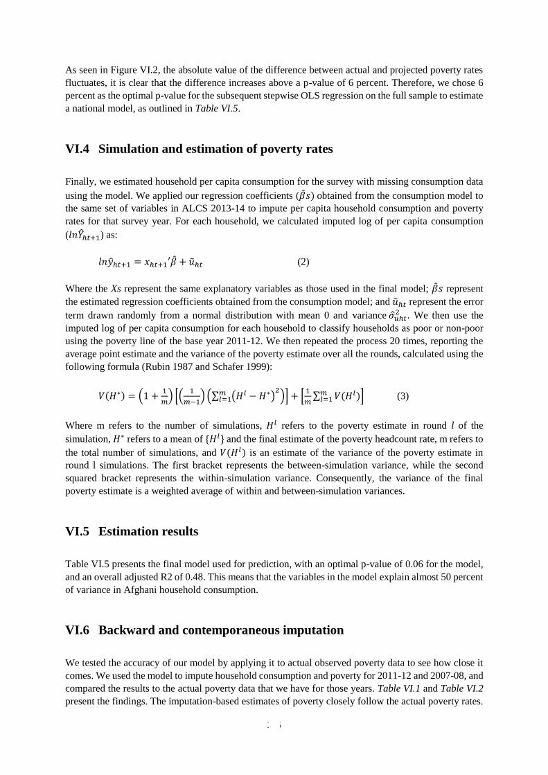
285
As seen in Figure VI.2, the absolute value of the difference between actual and projected poverty rates
fluctuates, it is clear that the difference increases above a p-value of 6 percent. Therefore, we chose 6
percent as the optimal p-value for the subsequent stepwise OLS regression on the full sample to estimate
a national model, as outlined in Table VI.5.
VI.4 Simulation and estimation of poverty rates
Finally, we estimated household per capita consumption for the survey with missing consumption data
using the model. We applied our regression coefficients (�̂�𝑠) obtained from the consumption model to
the same set of variables in ALCS 2013-14 to impute per capita household consumption and poverty
rates for that survey year. For each household, we calculated imputed log of per capita consumption
(𝑙𝑛�̂�ℎ𝑡+1) as:
𝑙𝑛�̂�ℎ𝑡+1 = 𝑥ℎ𝑡+1′�̂� + �̃�ℎ𝑡 (2)
Where the Xs represent the same explanatory variables as those used in the final model; �̂�𝑠 represent
the estimated regression coefficients obtained from the consumption model; and �̃�ℎ𝑡 represent the error
term drawn randomly from a normal distribution with mean 0 and variance �̂�𝑢ℎ𝑡2 . We then use the
imputed log of per capita consumption for each household to classify households as poor or non-poor
using the poverty line of the base year 2011-12. We then repeated the process 20 times, reporting the
average point estimate and the variance of the poverty estimate over all the rounds, calculated using the
following formula (Rubin 1987 and Schafer 1999):
𝑉(𝐻∗) = (1 +1
𝑚) [(
1
𝑚−1) (∑ (𝐻𝑙 − 𝐻∗)
2𝑚𝑙=1 )] + [
1
𝑚∑ 𝑉(𝐻𝑙)𝑚
𝑙=1 ] (3)
Where m refers to the number of simulations, 𝐻𝑙 refers to the poverty estimate in round l of the
simulation, 𝐻∗ refers to a mean of {𝐻𝑙} and the final estimate of the poverty headcount rate, m refers to
the total number of simulations, and 𝑉(𝐻𝑙) is an estimate of the variance of the poverty estimate in
round l simulations. The first bracket represents the between-simulation variance, while the second
squared bracket represents the within-simulation variance. Consequently, the variance of the final
poverty estimate is a weighted average of within and between-simulation variances.
VI.5 Estimation results
Table VI.5 presents the final model used for prediction, with an optimal p-value of 0.06 for the model,
and an overall adjusted R2 of 0.48. This means that the variables in the model explain almost 50 percent
of variance in Afghani household consumption.
VI.6 Backward and contemporaneous imputation
We tested the accuracy of our model by applying it to actual observed poverty data to see how close it
comes. We used the model to impute household consumption and poverty for 2011-12 and 2007-08, and
compared the results to the actual poverty data that we have for those years. Table VI.1 and Table VI.2
present the findings. The imputation-based estimates of poverty closely follow the actual poverty rates.
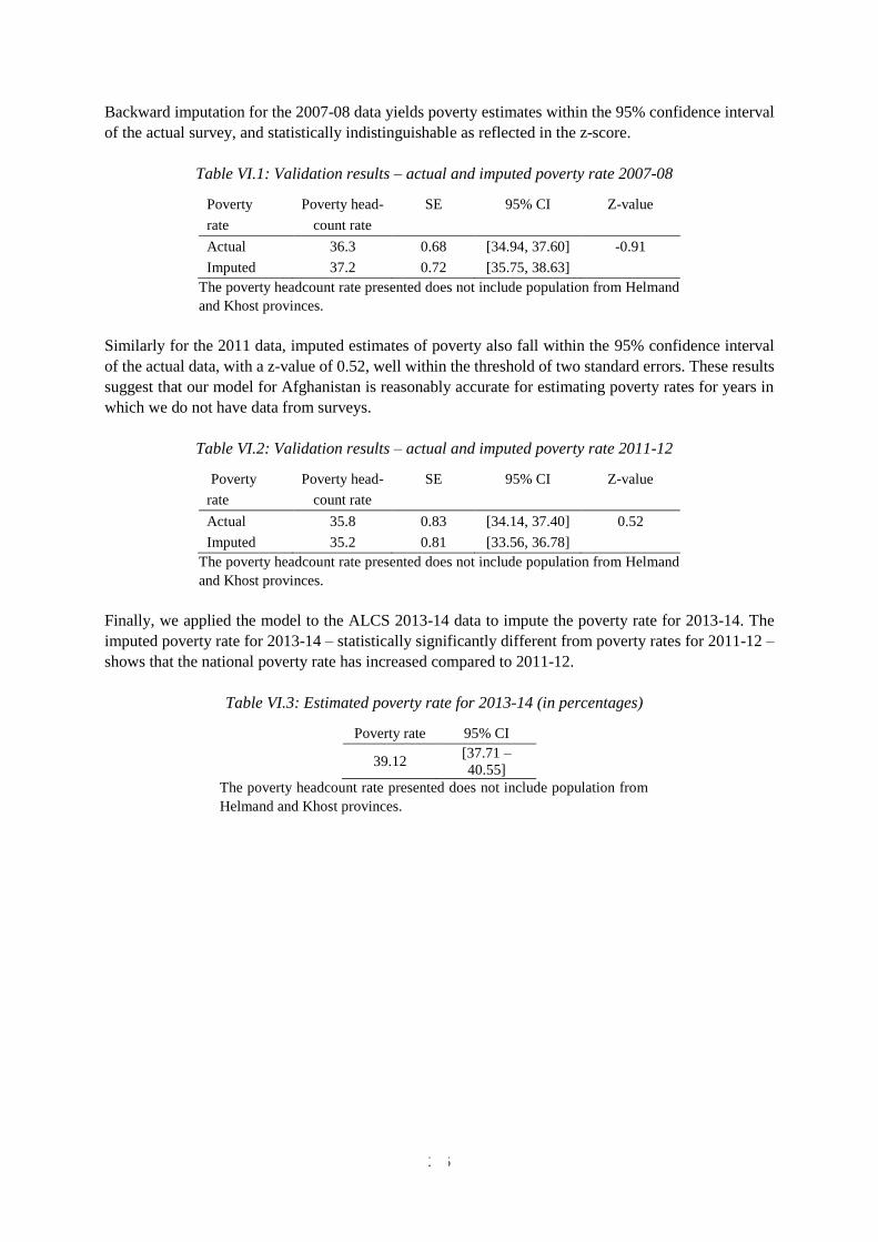
286
Backward imputation for the 2007-08 data yields poverty estimates within the 95% confidence interval
of the actual survey, and statistically indistinguishable as reflected in the z-score.
Table VI.1: Validation results – actual and imputed poverty rate 2007-08
Poverty Poverty head- SE 95% CI Z-value
rate count rate
Actual 36.3 0.68 [34.94, 37.60] -0.91
Imputed 37.2 0.72 [35.75, 38.63]
The poverty headcount rate presented does not include population from Helmand
and Khost provinces.
Similarly for the 2011 data, imputed estimates of poverty also fall within the 95% confidence interval
of the actual data, with a z-value of 0.52, well within the threshold of two standard errors. These results
suggest that our model for Afghanistan is reasonably accurate for estimating poverty rates for years in
which we do not have data from surveys.
Table VI.2: Validation results – actual and imputed poverty rate 2011-12
Poverty Poverty head- SE 95% CI Z-value
rate count rate
Actual 35.8 0.83 [34.14, 37.40] 0.52
Imputed 35.2 0.81 [33.56, 36.78]
The poverty headcount rate presented does not include population from Helmand
and Khost provinces.
Finally, we applied the model to the ALCS 2013-14 data to impute the poverty rate for 2013-14. The
imputed poverty rate for 2013-14 – statistically significantly different from poverty rates for 2011-12 –
shows that the national poverty rate has increased compared to 2011-12.
Table VI.3: Estimated poverty rate for 2013-14 (in percentages)
Poverty rate 95% CI
39.12 [37.71 –
40.55]
The poverty headcount rate presented does not include population from
Helmand and Khost provinces.
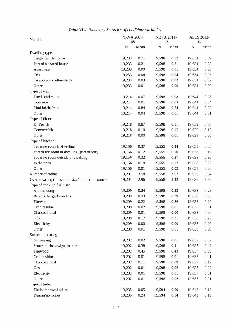
287
Table VI.4: Summary Statistics of candidate variables
Variable NRVA 2007-
08
NRVA 2011-
12
ALCS 2013-
14
N Mean N Mean N Mean
Dwelling type
Single family house 19,233 0.71 19,598 0.72 19,634 0.69
Part of a shared house 19,233 0.21 19,598 0.21 19,634 0.23
Apartment 19,233 0.00 19,598 0.01 19,634 0.00
Tent 19,233 0.04 19,598 0.04 19,634 0.05
Temporary shelter/shack 19,233 0.03 19,598 0.02 19,634 0.02
Other 19,233 0.01 19,598 0.00 19,634 0.00
Type of wall
Fired brick/stone 19,214 0.07 19,598 0.08 19,644 0.08
Concrete 19,214 0.01 19,598 0.03 19,644 0.04
Mud bricks/mud 19,214 0.84 19,598 0.84 19,644 0.83
Other 19,214 0.04 19,598 0.01 19,644 0.01
Type of Floor
Dirt/earth 19,218 0.87 19,598 0.81 19,639 0.80
Concrete/tile 19,218 0.10 19,598 0.15 19,639 0.15
Other 19,218 0.00 19,598 0.01 19,639 0.00
Type of kitchen
Separate room in dwelling 19,156 0.37 19,555 0.44 19,638 0.33
Part of the room in dwelling (part of tent) 19,156 0.12 19,555 0.10 19,638 0.16
Separate room outside of dwelling 19,156 0.32 19,555 0.27 19,638 0.30
In the open 19,156 0.18 19,555 0.17 19,638 0.22
Other 19,156 0.01 19,555 0.02 19,638 0.00
Number of rooms 19,201 3.58 19,558 3.07 19,636 3.04
Overcrowding (household size/number of rooms) 19,201 2.96 19,558 3.42 19,636 3.37
Type of cooking fuel used
Animal dung 19,209 0.24 19,598 0.23 19,638 0.23
Bushes, twigs, branches 19,209 0.33 19,598 0.29 19,638 0.30
Firewood 19,209 0.22 19,598 0.26 19,638 0.20
Crop residue 19,209 0.02 19,598 0.01 19,638 0.01
Charcoal, coal 19,209 0.01 19,598 0.00 19,638 0.00
Gas 19,209 0.17 19,598 0.21 19,638 0.25
Electricity 19,209 0.00 19,598 0.00 19,638 0.00
Other 19,209 0.01 19,598 0.01 19,638 0.00
Source of heating
No heating 19,202 0.02 19,598 0.01 19,637 0.02
Straw, bushes/twigs, manure 19,202 0.38 19,598 0.41 19,637 0.42
Firewood 19,202 0.45 19,598 0.43 19,637 0.39
Crop residue 19,202 0.01 19,598 0.01 19,637 0.01
Charcoal, coal 19,202 0.11 19,598 0.09 19,637 0.12
Gas 19,202 0.01 19,598 0.02 19,637 0.02
Electricity 19,202 0.01 19,598 0.01 19,637 0.01
Other 19,202 0.01 19,598 0.02 19,637 0.01
Type of toilet
Flush/improved toilet 19,235 0.05 19,594 0.09 19,642 0.12
Dearan/no Toilet 19,235 0.24 19,594 0.14 19,642 0.19
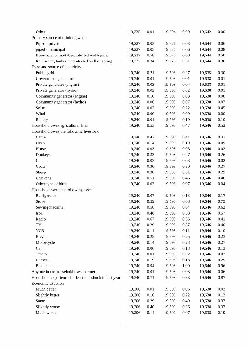
288
Other 19,235 0.01 19,594 0.00 19,642 0.00
Primary source of drinking water
Piped - private 19,227 0.03 19,576 0.03 19,644 0.06
piped - municipal 19,227 0.05 19,576 0.06 19,644 0.08
Bore-hole, pump/tube/protected well/spring 19,227 0.58 19,576 0.60 19,644 0.50
Rain water, tanker, unprotected well or spring 19,227 0.34 19,576 0.31 19,644 0.36
Type and source of electricity
Public grid 19,240 0.21 19,598 0.27 19,635 0.30
Government generator 19,240 0.01 19,598 0.01 19,638 0.01
Private generator (engine) 19,240 0.03 19,598 0.04 19,638 0.01
Private generator (hydro) 19,240 0.02 19,598 0.02 19,638 0.01
Community generator (engine) 19,240 0.10 19,598 0.03 19,638 0.00
Community generator (hydro) 19,240 0.06 19,598 0.07 19,638 0.07
Solar 19,240 0.02 19,598 0.22 19,638 0.45
Wind 19,240 0.00 19,598 0.00 19,638 0.00
Battery 19,240 0.01 19,598 0.10 19,638 0.10
Household owns agricultural land 19,240 0.53 19,598 0.47 19,646 0.52
Household owns the following livestock
Cattle 19,240 0.42 19,598 0.41 19,646 0.41
Oxen 19,240 0.14 19,598 0.10 19,646 0.09
Horses 19,240 0.03 19,598 0.03 19,646 0.02
Donkeys 19,240 0.33 19,598 0.27 19,646 0.26
Camels 19,240 0.03 19,598 0.03 19,646 0.02
Goats 19,240 0.30 19,598 0.30 19,646 0.27
Sheep 19,240 0.30 19,598 0.31 19,646 0.29
Chickens 19,240 0.51 19,598 0.46 19,646 0.46
Other type of birds 19,240 0.03 19,598 0.07 19,646 0.04
Household owns the following assets
Refrigerator 19,240 0.07 19,598 0.13 19,646 0.17
Stove 19,240 0.59 19,598 0.68 19,646 0.75
Sewing machine 19,240 0.58 19,598 0.64 19,646 0.62
Iron 19,240 0.46 19,598 0.58 19,646 0.57
Radio 19,240 0.67 19,598 0.55 19,646 0.41
TV 19,240 0.29 19,598 0.37 19,646 0.40
VCR 19,240 0.11 19,598 0.11 19,646 0.10
Bicycle 19,240 0.25 19,598 0.25 19,646 0.23
Motorcycle 19,240 0.14 19,598 0.23 19,646 0.27
Car 19,240 0.06 19,598 0.13 19,646 0.13
Tractor 19,240 0.01 19,598 0.02 19,646 0.03
Carpets 19,240 0.19 19,598 0.18 19,646 0.29
Blankets 19,240 0.94 19,598 1.00 19,646 0.96
Anyone in the household uses internet 19,240 0.01 19,598 0.03 19,646 0.06
Household experienced at least one shock in last year 19,240 0.71 19,598 0.83 19,646 0.87
Economic situation
Much better 19,206 0.01 19,500 0.06 19,638 0.03
Slightly better 19,206 0.16 19,500 0.22 19,638 0.13
Same 19,206 0.29 19,500 0.40 19,638 0.33
Slightly worse 19,206 0.40 19,500 0.26 19,638 0.32
Much worse 19,206 0.14 19,500 0.07 19,638 0.19
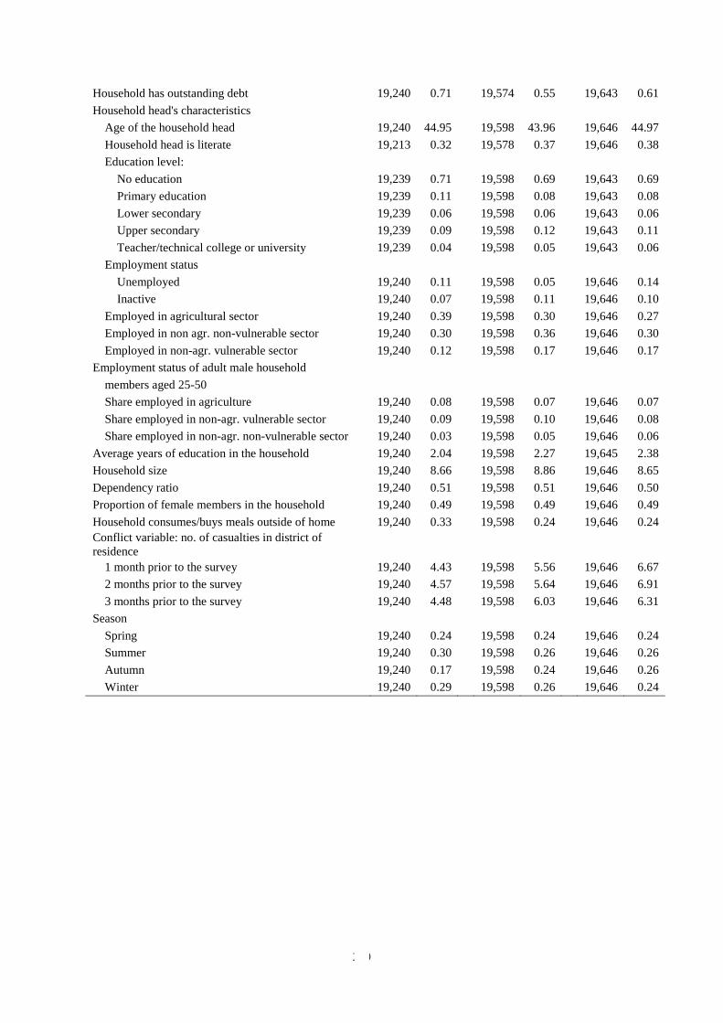
289
Household has outstanding debt 19,240 0.71 19,574 0.55 19,643 0.61
Household head's characteristics
Age of the household head 19,240 44.95 19,598 43.96 19,646 44.97
Household head is literate 19,213 0.32 19,578 0.37 19,646 0.38
Education level:
No education 19,239 0.71 19,598 0.69 19,643 0.69
Primary education 19,239 0.11 19,598 0.08 19,643 0.08
Lower secondary 19,239 0.06 19,598 0.06 19,643 0.06
Upper secondary 19,239 0.09 19,598 0.12 19,643 0.11
Teacher/technical college or university 19,239 0.04 19,598 0.05 19,643 0.06
Employment status
Unemployed 19,240 0.11 19,598 0.05 19,646 0.14
Inactive 19,240 0.07 19,598 0.11 19,646 0.10
Employed in agricultural sector 19,240 0.39 19,598 0.30 19,646 0.27
Employed in non agr. non-vulnerable sector 19,240 0.30 19,598 0.36 19,646 0.30
Employed in non-agr. vulnerable sector 19,240 0.12 19,598 0.17 19,646 0.17
Employment status of adult male household
members aged 25-50
Share employed in agriculture 19,240 0.08 19,598 0.07 19,646 0.07
Share employed in non-agr. vulnerable sector 19,240 0.09 19,598 0.10 19,646 0.08
Share employed in non-agr. non-vulnerable sector 19,240 0.03 19,598 0.05 19,646 0.06
Average years of education in the household 19,240 2.04 19,598 2.27 19,645 2.38
Household size 19,240 8.66 19,598 8.86 19,646 8.65
Dependency ratio 19,240 0.51 19,598 0.51 19,646 0.50
Proportion of female members in the household 19,240 0.49 19,598 0.49 19,646 0.49
Household consumes/buys meals outside of home 19,240 0.33 19,598 0.24 19,646 0.24
Conflict variable: no. of casualties in district of
residence
1 month prior to the survey 19,240 4.43 19,598 5.56 19,646 6.67
2 months prior to the survey 19,240 4.57 19,598 5.64 19,646 6.91
3 months prior to the survey 19,240 4.48 19,598 6.03 19,646 6.31
Season
Spring 19,240 0.24 19,598 0.24 19,646 0.24
Summer 19,240 0.30 19,598 0.26 19,646 0.26
Autumn 19,240 0.17 19,598 0.24 19,646 0.26
Winter 19,240 0.29 19,598 0.26 19,646 0.24
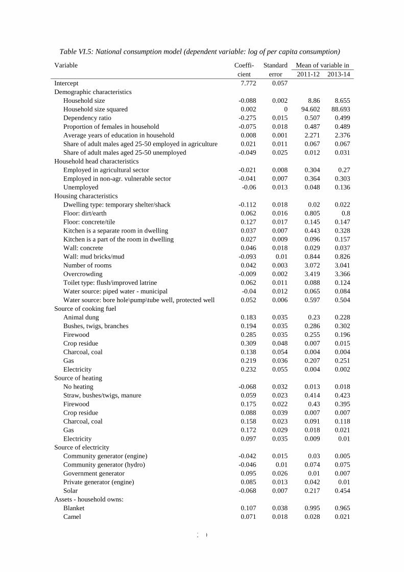
290
Table VI.5: National consumption model (dependent variable: log of per capita consumption)
Variable Coeffi- Standard Mean of variable in
cient error 2011-12 2013-14
Intercept 7.772 0.057
Demographic characteristics
Household size -0.088 0.002 8.86 8.655
Household size squared 0.002 0 94.602 88.693
Dependency ratio -0.275 0.015 0.507 0.499
Proportion of females in household -0.075 0.018 0.487 0.489
Average years of education in household 0.008 0.001 2.271 2.376
Share of adult males aged 25-50 employed in agriculture 0.021 0.011 0.067 0.067
Share of adult males aged 25-50 unemployed -0.049 0.025 0.012 0.031
Household head characteristics
Employed in agricultural sector -0.021 0.008 0.304 0.27
Employed in non-agr. vulnerable sector -0.041 0.007 0.364 0.303
Unemployed -0.06 0.013 0.048 0.136
Housing characteristics
Dwelling type: temporary shelter/shack -0.112 0.018 0.02 0.022
Floor: dirt/earth 0.062 0.016 0.805 0.8
Floor: concrete/tile 0.127 0.017 0.145 0.147
Kitchen is a separate room in dwelling 0.037 0.007 0.443 0.328
Kitchen is a part of the room in dwelling 0.027 0.009 0.096 0.157
Wall: concrete 0.046 0.018 0.029 0.037
Wall: mud bricks/mud -0.093 0.01 0.844 0.826
Number of rooms 0.042 0.003 3.072 3.041
Overcrowding -0.009 0.002 3.419 3.366
Toilet type: flush/improved latrine 0.062 0.011 0.088 0.124
Water source: piped water - municipal -0.04 0.012 0.065 0.084
Water source: bore hole\pump\tube well, protected well 0.052 0.006 0.597 0.504
Source of cooking fuel
Animal dung 0.183 0.035 0.23 0.228
Bushes, twigs, branches 0.194 0.035 0.286 0.302
Firewood 0.285 0.035 0.255 0.196
Crop residue 0.309 0.048 0.007 0.015
Charcoal, coal 0.138 0.054 0.004 0.004
Gas 0.219 0.036 0.207 0.251
Electricity 0.232 0.055 0.004 0.002
Source of heating
No heating -0.068 0.032 0.013 0.018
Straw, bushes/twigs, manure 0.059 0.023 0.414 0.423
Firewood 0.175 0.022 0.43 0.395
Crop residue 0.088 0.039 0.007 0.007
Charcoal, coal 0.158 0.023 0.091 0.118
Gas 0.172 0.029 0.018 0.021
Electricity 0.097 0.035 0.009 0.01
Source of electricity
Community generator (engine) -0.042 0.015 0.03 0.005
Community generator (hydro) -0.046 0.01 0.074 0.075
Government generator 0.095 0.026 0.01 0.007
Private generator (engine) 0.085 0.013 0.042 0.01
Solar -0.068 0.007 0.217 0.454
Assets - household owns:
Blanket 0.107 0.038 0.995 0.965
Camel 0.071 0.018 0.028 0.021
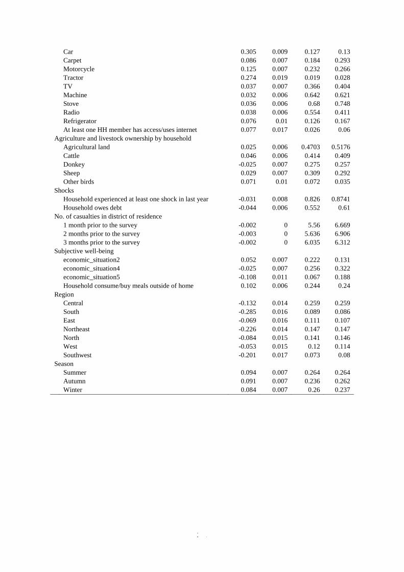
291
Car 0.305 0.009 0.127 0.13
Carpet 0.086 0.007 0.184 0.293
Motorcycle 0.125 0.007 0.232 0.266
Tractor 0.274 0.019 0.019 0.028
TV 0.037 0.007 0.366 0.404
Machine 0.032 0.006 0.642 0.621
Stove 0.036 0.006 0.68 0.748
Radio 0.038 0.006 0.554 0.411
Refrigerator 0.076 0.01 0.126 0.167
At least one HH member has access/uses internet 0.077 0.017 0.026 0.06
Agriculture and livestock ownership by household
Agricultural land 0.025 0.006 0.4703 0.5176
Cattle 0.046 0.006 0.414 0.409
Donkey -0.025 0.007 0.275 0.257
Sheep 0.029 0.007 0.309 0.292
Other birds 0.071 0.01 0.072 0.035
Shocks
Household experienced at least one shock in last year -0.031 0.008 0.826 0.8741
Household owes debt -0.044 0.006 0.552 0.61
No. of casualties in district of residence
1 month prior to the survey -0.002 0 5.56 6.669
2 months prior to the survey -0.003 0 5.636 6.906
3 months prior to the survey -0.002 0 6.035 6.312
Subjective well-being
economic_situation2 0.052 0.007 0.222 0.131
economic_situation4 -0.025 0.007 0.256 0.322
economic_situation5 -0.108 0.011 0.067 0.188
Household consume/buy meals outside of home 0.102 0.006 0.244 0.24
Region
Central -0.132 0.014 0.259 0.259
South -0.285 0.016 0.089 0.086
East -0.069 0.016 0.111 0.107
Northeast -0.226 0.014 0.147 0.147
North -0.084 0.015 0.141 0.146
West -0.053 0.015 0.12 0.114
Southwest -0.201 0.017 0.073 0.08
Season
Summer 0.094 0.007 0.264 0.264
Autumn 0.091 0.007 0.236 0.262
Winter 0.084 0.007 0.26 0.237
292
ANNEX VII QUALITY ASSURANCE AND QUALITY
ASSESSMENT
VII.1 Introduction
Quality assurance is relevant for each activity and each operations stage of statistical operations. It
should be understood as a multi-dimensional concept, including the following dimensions:75
a. Relevance
b. Completeness
c. Accuracy
d. Comparability
e. Coherence
f. Timeliness
g. Accessibility.
This understanding implies that data accuracy is only one – albeit important – dimension of overall data
quality. Section 2 of this annex gives brief overviews of measures to assess the quality of the ALCS
2013-14 data according to these dimensions, and of actions and procedures implemented to assure data
quality.
Subsequent sections VII.3 and VII.4 further elaborate on two main types of data errors that affect
sampling surveys: sampling errors and non-sampling errors. Sampling errors relate to the fact that
selected households are one of many possible samples that could have been selected from the sampling
frame. Each of these would produce results that are somewhat different from one another and likely
somewhat different from the total population. Non-sampling errors refer to a wide variety of other data
errors that arise during the course of all survey activities other than sampling. Whereas estimates of
sampling errors can be quantified by calculating standard errors, non-sampling errors are difficult to
evaluate statistically.
VII.2 Quality assurance
No survey is able to achieve a perfect score on each of the dimensions of data quality, as many tend to
improve at the expenses of the others. For example, very high quality data require training of the staff
involved in the survey at each level for such extensive periods, field monitoring and supervision at such
intensity, and data editing at such comprehensive detail, that the project will exceed any acceptable time
and budget limit. Thus, any survey will have to find a practical and acceptable balance within the bounds
of existing resources and constraints. Table VII.1 gives an overview of the measures relevant to ALCS
2013-14 with respect to the specified dimensions of quality assurance. The remainder of this section
lists the key activities and procedures implemented in the survey to assure data quality.
a. Management of relevance
Extensive stakeholder consultation was organised to discuss and define the information to be
collected in 2011-12 and subsequent rounds of the survey (January-March 2010). Ad-hoc
consultations were organised to accommodate emerging information needs.
75 See e.g. UNECE 2006, United Nations 2008.
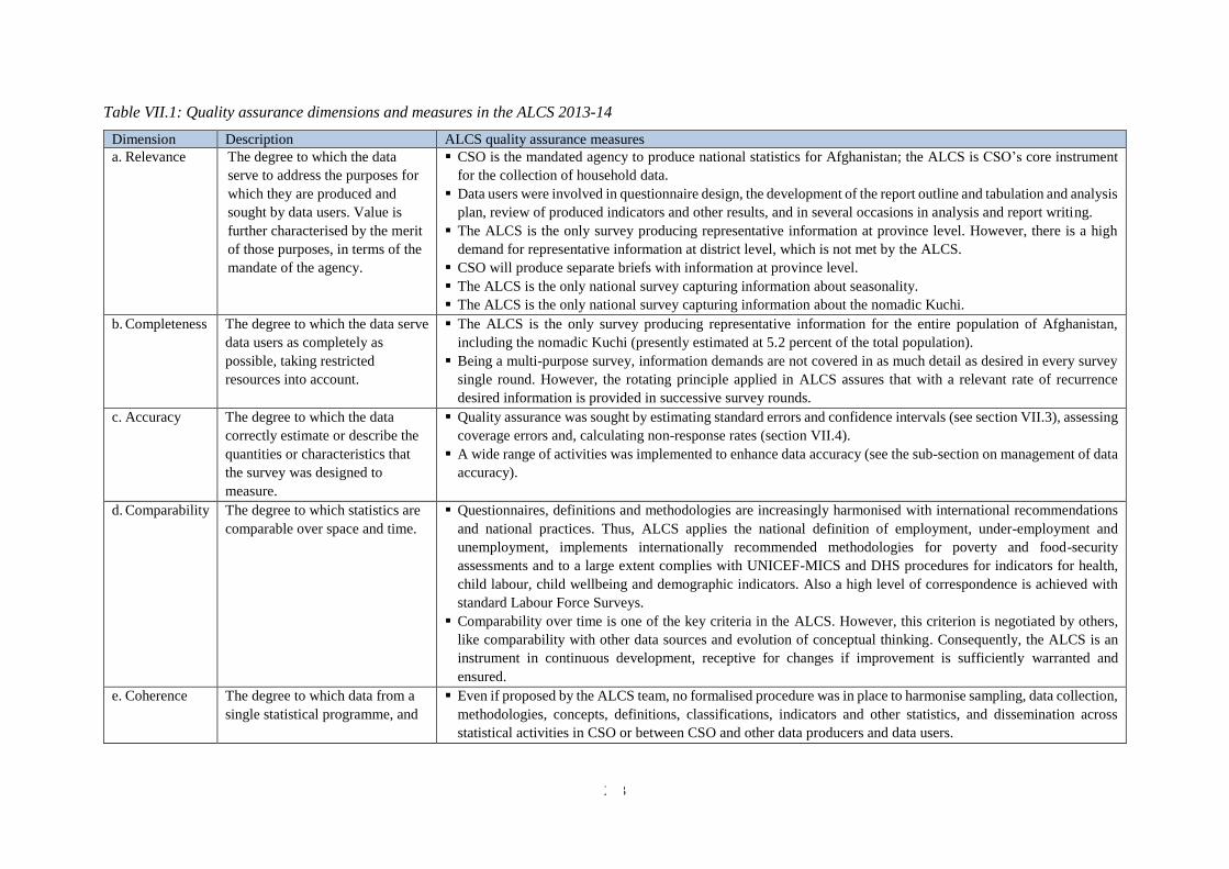
293
Table VII.1: Quality assurance dimensions and measures in the ALCS 2013-14
Dimension Description ALCS quality assurance measures
a. Relevance The degree to which the data
serve to address the purposes for
which they are produced and
sought by data users. Value is
further characterised by the merit
of those purposes, in terms of the
mandate of the agency.
CSO is the mandated agency to produce national statistics for Afghanistan; the ALCS is CSO’s core instrument
for the collection of household data.
Data users were involved in questionnaire design, the development of the report outline and tabulation and analysis
plan, review of produced indicators and other results, and in several occasions in analysis and report writing.
The ALCS is the only survey producing representative information at province level. However, there is a high
demand for representative information at district level, which is not met by the ALCS.
CSO will produce separate briefs with information at province level.
The ALCS is the only national survey capturing information about seasonality.
The ALCS is the only national survey capturing information about the nomadic Kuchi.
b. Completeness The degree to which the data serve
data users as completely as
possible, taking restricted
resources into account.
The ALCS is the only survey producing representative information for the entire population of Afghanistan,
including the nomadic Kuchi (presently estimated at 5.2 percent of the total population).
Being a multi-purpose survey, information demands are not covered in as much detail as desired in every survey
single round. However, the rotating principle applied in ALCS assures that with a relevant rate of recurrence
desired information is provided in successive survey rounds.
c. Accuracy The degree to which the data
correctly estimate or describe the
quantities or characteristics that
the survey was designed to
measure.
Quality assurance was sought by estimating standard errors and confidence intervals (see section VII.3), assessing
coverage errors and, calculating non-response rates (section VII.4).
A wide range of activities was implemented to enhance data accuracy (see the sub-section on management of data
accuracy).
d. Comparability The degree to which statistics are
comparable over space and time.
Questionnaires, definitions and methodologies are increasingly harmonised with international recommendations
and national practices. Thus, ALCS applies the national definition of employment, under-employment and
unemployment, implements internationally recommended methodologies for poverty and food-security
assessments and to a large extent complies with UNICEF-MICS and DHS procedures for indicators for health,
child labour, child wellbeing and demographic indicators. Also a high level of correspondence is achieved with
standard Labour Force Surveys.
Comparability over time is one of the key criteria in the ALCS. However, this criterion is negotiated by others,
like comparability with other data sources and evolution of conceptual thinking. Consequently, the ALCS is an
instrument in continuous development, receptive for changes if improvement is sufficiently warranted and
ensured.
e. Coherence The degree to which data from a
single statistical programme, and
Even if proposed by the ALCS team, no formalised procedure was in place to harmonise sampling, data collection,
methodologies, concepts, definitions, classifications, indicators and other statistics, and dissemination across
statistical activities in CSO or between CSO and other data producers and data users.
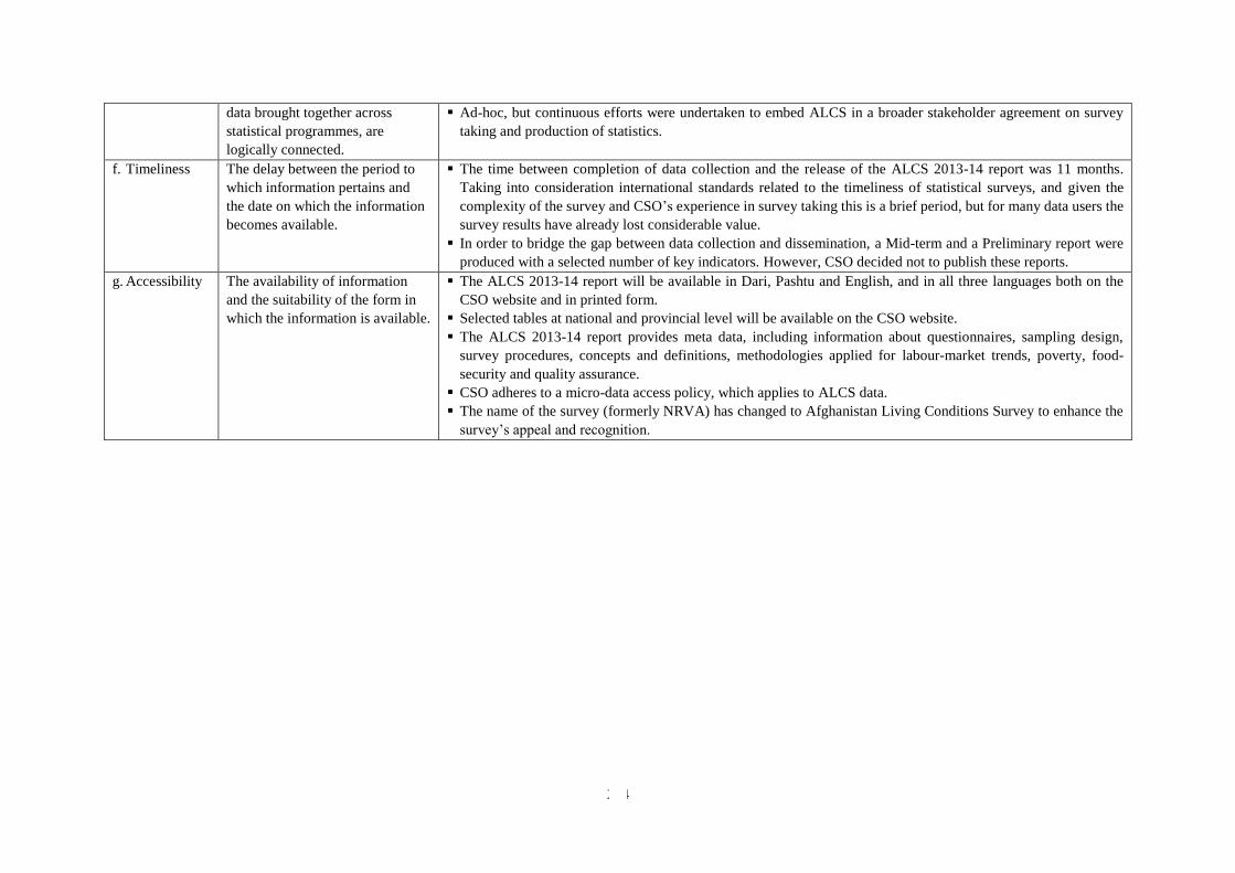
294
data brought together across
statistical programmes, are
logically connected.
Ad-hoc, but continuous efforts were undertaken to embed ALCS in a broader stakeholder agreement on survey
taking and production of statistics.
f. Timeliness The delay between the period to
which information pertains and
the date on which the information
becomes available.
The time between completion of data collection and the release of the ALCS 2013-14 report was 11 months.
Taking into consideration international standards related to the timeliness of statistical surveys, and given the
complexity of the survey and CSO’s experience in survey taking this is a brief period, but for many data users the
survey results have already lost considerable value.
In order to bridge the gap between data collection and dissemination, a Mid-term and a Preliminary report were
produced with a selected number of key indicators. However, CSO decided not to publish these reports.
g. Accessibility The availability of information
and the suitability of the form in
which the information is available.
The ALCS 2013-14 report will be available in Dari, Pashtu and English, and in all three languages both on the
CSO website and in printed form.
Selected tables at national and provincial level will be available on the CSO website.
The ALCS 2013-14 report provides meta data, including information about questionnaires, sampling design,
survey procedures, concepts and definitions, methodologies applied for labour-market trends, poverty, food-
security and quality assurance.
CSO adheres to a micro-data access policy, which applies to ALCS data.
The name of the survey (formerly NRVA) has changed to Afghanistan Living Conditions Survey to enhance the
survey’s appeal and recognition.
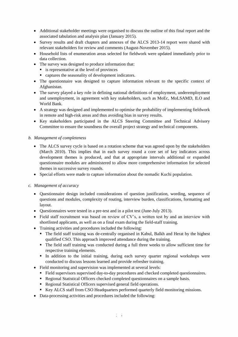
295
Additional stakeholder meetings were organised to discuss the outline of this final report and the
associated tabulation and analysis plan (January 2015).
Survey results and draft chapters and annexes of the ALCS 2013-14 report were shared with
relevant stakeholders for review and comments (August-November 2015).
Household lists of enumeration areas selected for fieldwork were updated immediately prior to
data collection.
The survey was designed to produce information that:
is representative at the level of provinces
captures the seasonality of development indicators.
The questionnaire was designed to capture information relevant to the specific context of
Afghanistan.
The survey played a key role in defining national definitions of employment, underemployment
and unemployment, in agreement with key stakeholders, such as MoEc, MoLSAMD, ILO and
World Bank.
A strategy was designed and implemented to optimise the probability of implementing fieldwork
in remote and high-risk areas and thus avoiding bias in survey results.
Key stakeholders participated in the ALCS Steering Committee and Technical Advisory
Committee to ensure the soundness the overall project strategy and technical components.
b. Management of completeness
The ALCS survey cycle is based on a rotation scheme that was agreed upon by the stakeholders
(March 2010). This implies that in each survey round a core set of key indicators across
development themes is produced, and that at appropriate intervals additional or expanded
questionnaire modules are administered to allow more comprehensive information for selected
themes in successive survey rounds.
Special efforts were made to capture information about the nomadic Kuchi population.
c. Management of accuracy
Questionnaire design included considerations of question justification, wording, sequence of
questions and modules, complexity of routing, interview burden, classifications, formatting and
layout.
Questionnaires were tested in a pre-test and in a pilot test (June-July 2013).
Field staff recruitment was based on review of CV’s, a written test by and an interview with
shortlisted applicants, as well as on a final exam during the field-staff training.
Training activities and procedures included the following:
The field staff training was de-centrally organised in Kabul, Balkh and Herat by the highest
qualified CSO. This approach improved attendance during the training.
The field staff training was conducted during a full three weeks to allow sufficient time for
respective training elements.
In addition to the initial training, during each survey quarter regional workshops were
conducted to discuss lessons learned and provide refresher training.
Field monitoring and supervision was implemented at several levels:
Field supervisors supervised day-to-day procedures and checked completed questionnaires.
Regional Statistical Officers checked completed questionnaires on a sample basis.
Regional Statistical Officers supervised general field operations.
Key ALCS staff from CSO Headquarters performed quarterly field monitoring missions.
Data-processing activities and procedures included the following:
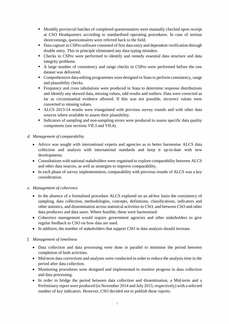
296
Monthly provincial batches of completed questionnaires were manually checked upon receipt
at CSO Headquarters according to standardised operating procedures. In case of serious
shortcomings, questionnaires were referred back to the field.
Data capture in CSPro software consisted of first data entry and dependent verification through
double entry. This in principle eliminated any data typing mistakes.
Checks in CSPro were performed to identify and remedy essential data structure and data
integrity problems.
A large number of consistency and range checks in CSPro were performed before the raw
dataset was delivered.
Comprehensive data-editing programmes were designed in Stata to perform consistency, range
and plausibility checks.
Frequency and cross tabulations were produced in Stata to determine response distributions
and identify any skewed data, missing values, odd results and outliers. Data were corrected as
far as circumstantial evidence allowed. If this was not possible, incorrect values were
converted to missing values.
ALCS 2013-14 results were triangulated with previous survey rounds and with other data
sources where available to assess their plausibility.
Indicators of sampling and non-sampling errors were produced to assess specific data quality
components (see sections VII.3 and VII.4).
d. Management of comparability
Advice was sought with international experts and agencies as to better harmonise ALCS data
collection and analysis with international standards and keep it up-to-date with new
developments.
Consultations with national stakeholders were organised to explore comparability between ALCS
and other data sources, as well as strategies to improve comparability.
In each phase of survey implementation, comparability with previous rounds of ALCS was a key
consideration.
e. Management of coherence
In the absence of a formalised procedure ALCS explored on an ad-hoc basis the consistency of
sampling, data collection, methodologies, concepts, definitions, classifications, indicators and
other statistics, and dissemination across statistical activities in CSO, and between CSO and other
data producers and data users. Where feasible, these were harmonised.
Coherence management would require government agencies and other stakeholders to give
regular feedback to CSO on how data are used.
In addition, the number of stakeholders that support CSO in data analysis should increase.
f. Management of timeliness
Data collection and data processing were done in parallel to minimise the period between
completion of both activities.
Mid-term data corrections and analyses were conducted in order to reduce the analysis time in the
period after data collection.
Monitoring procedures were designed and implemented to monitor progress in data collection
and data processing.
In order to bridge the period between data collection and dissemination, a Mid-term and a
Preliminary report were produced (in November 2014 and July 2015, respectively) with a selected
number of key indicators. However, CSO decided not to publish these reports.
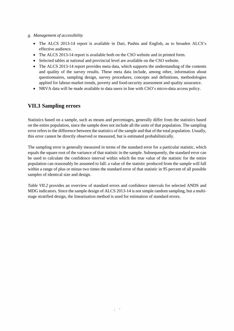
297
g. Management of accessibility
The ALCS 2013-14 report is available in Dari, Pashtu and English, as to broaden ALCS’s
effective audience.
The ALCS 2013-14 report is available both on the CSO website and in printed form.
Selected tables at national and provincial level are available on the CSO website.
The ALCS 2013-14 report provides meta data, which supports the understanding of the contents
and quality of the survey results. These meta data include, among other, information about
questionnaires, sampling design, survey procedures, concepts and definitions, methodologies
applied for labour-market trends, poverty and food-security assessment and quality assurance.
NRVA data will be made available to data users in line with CSO’s micro-data access policy.
VII.3 Sampling errors
Statistics based on a sample, such as means and percentages, generally differ from the statistics based
on the entire population, since the sample does not include all the units of that population. The sampling
error refers to the difference between the statistics of the sample and that of the total population. Usually,
this error cannot be directly observed or measured, but is estimated probabilistically.
The sampling error is generally measured in terms of the standard error for a particular statistic, which
equals the square root of the variance of that statistic in the sample. Subsequently, the standard error can
be used to calculate the confidence interval within which the true value of the statistic for the entire
population can reasonably be assumed to fall: a value of the statistic produced from the sample will fall
within a range of plus or minus two times the standard error of that statistic in 95 percent of all possible
samples of identical size and design.
Table VII.2 provides an overview of standard errors and confidence intervals for selected ANDS and
MDG indicators. Since the sample design of ALCS 2013-14 is not simple random sampling, but a multi-
stage stratified design, the linearisation method is used for estimation of standard errors.
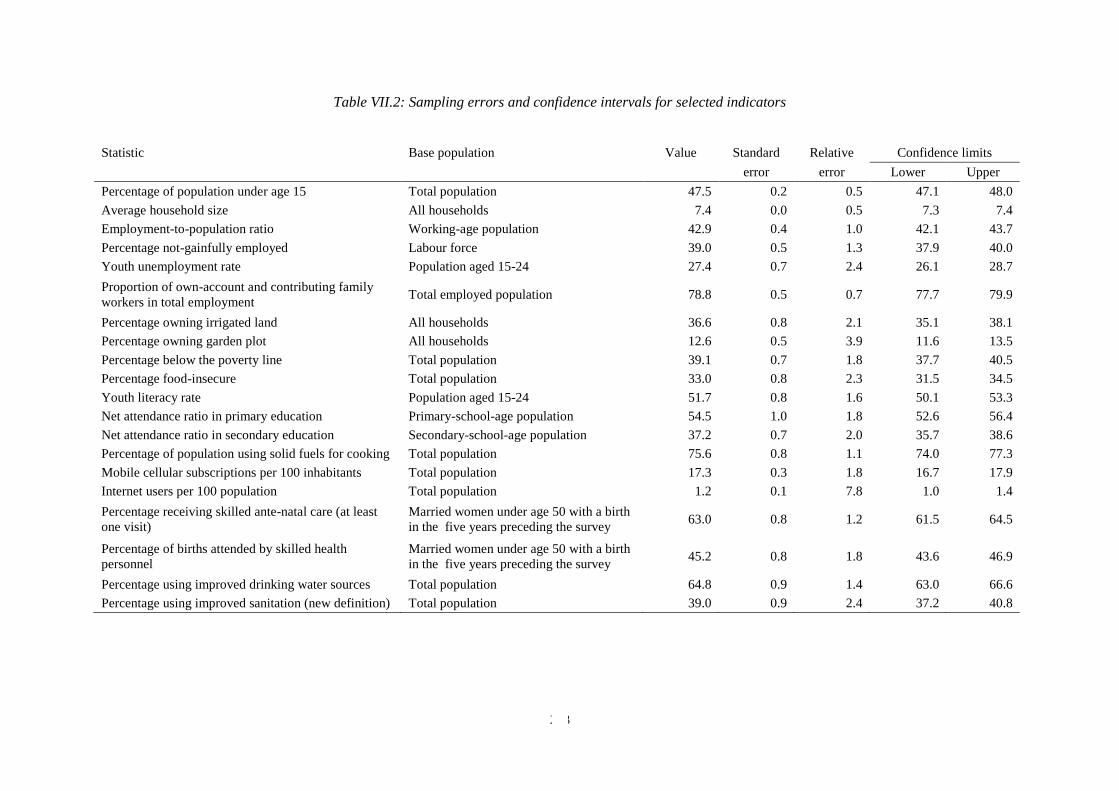
298
Table VII.2: Sampling errors and confidence intervals for selected indicators
Statistic Base population Value Standard Relative Confidence limits
error error Lower Upper
Percentage of population under age 15 Total population 47.5 0.2 0.5 47.1 48.0
Average household size All households 7.4 0.0 0.5 7.3 7.4
Employment-to-population ratio Working-age population 42.9 0.4 1.0 42.1 43.7
Percentage not-gainfully employed Labour force 39.0 0.5 1.3 37.9 40.0
Youth unemployment rate Population aged 15-24 27.4 0.7 2.4 26.1 28.7
Proportion of own-account and contributing family
workers in total employment Total employed population 78.8 0.5 0.7 77.7 79.9
Percentage owning irrigated land All households 36.6 0.8 2.1 35.1 38.1
Percentage owning garden plot All households 12.6 0.5 3.9 11.6 13.5
Percentage below the poverty line Total population 39.1 0.7 1.8 37.7 40.5
Percentage food-insecure Total population 33.0 0.8 2.3 31.5 34.5
Youth literacy rate Population aged 15-24 51.7 0.8 1.6 50.1 53.3
Net attendance ratio in primary education Primary-school-age population 54.5 1.0 1.8 52.6 56.4
Net attendance ratio in secondary education Secondary-school-age population 37.2 0.7 2.0 35.7 38.6
Percentage of population using solid fuels for cooking Total population 75.6 0.8 1.1 74.0 77.3
Mobile cellular subscriptions per 100 inhabitants Total population 17.3 0.3 1.8 16.7 17.9
Internet users per 100 population Total population 1.2 0.1 7.8 1.0 1.4
Percentage receiving skilled ante-natal care (at least
one visit)
Married women under age 50 with a birth
in the five years preceding the survey 63.0 0.8 1.2 61.5 64.5
Percentage of births attended by skilled health
personnel
Married women under age 50 with a birth
in the five years preceding the survey 45.2 0.8 1.8 43.6 46.9
Percentage using improved drinking water sources Total population 64.8 0.9 1.4 63.0 66.6
Percentage using improved sanitation (new definition) Total population 39.0 0.9 2.4 37.2 40.8
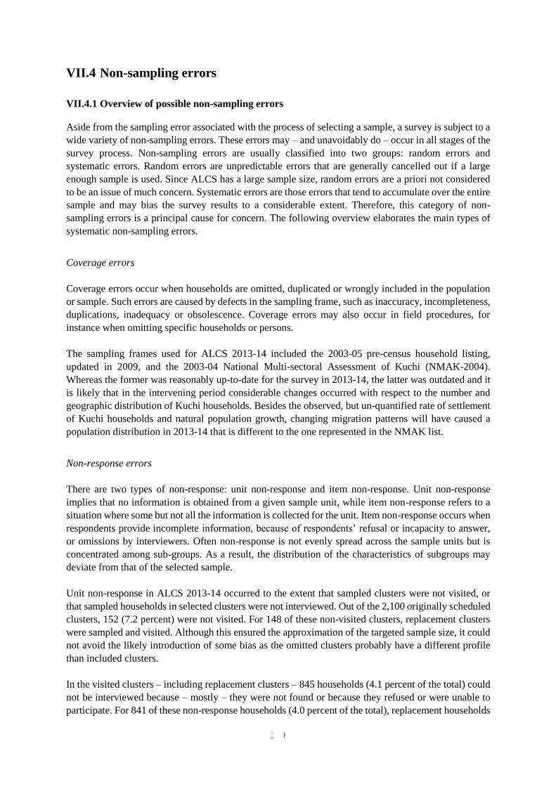
299
VII.4 Non-sampling errors
VII.4.1 Overview of possible non-sampling errors
Aside from the sampling error associated with the process of selecting a sample, a survey is subject to a
wide variety of non-sampling errors. These errors may – and unavoidably do – occur in all stages of the
survey process. Non-sampling errors are usually classified into two groups: random errors and
systematic errors. Random errors are unpredictable errors that are generally cancelled out if a large
enough sample is used. Since ALCS has a large sample size, random errors are a priori not considered
to be an issue of much concern. Systematic errors are those errors that tend to accumulate over the entire
sample and may bias the survey results to a considerable extent. Therefore, this category of non-
sampling errors is a principal cause for concern. The following overview elaborates the main types of
systematic non-sampling errors.
Coverage errors
Coverage errors occur when households are omitted, duplicated or wrongly included in the population
or sample. Such errors are caused by defects in the sampling frame, such as inaccuracy, incompleteness,
duplications, inadequacy or obsolescence. Coverage errors may also occur in field procedures, for
instance when omitting specific households or persons.
The sampling frames used for ALCS 2013-14 included the 2003-05 pre-census household listing,
updated in 2009, and the 2003-04 National Multi-sectoral Assessment of Kuchi (NMAK-2004).
Whereas the former was reasonably up-to-date for the survey in 2013-14, the latter was outdated and it
is likely that in the intervening period considerable changes occurred with respect to the number and
geographic distribution of Kuchi households. Besides the observed, but un-quantified rate of settlement
of Kuchi households and natural population growth, changing migration patterns will have caused a
population distribution in 2013-14 that is different to the one represented in the NMAK list.
Non-response errors
There are two types of non-response: unit non-response and item non-response. Unit non-response
implies that no information is obtained from a given sample unit, while item non-response refers to a
situation where some but not all the information is collected for the unit. Item non-response occurs when
respondents provide incomplete information, because of respondents’ refusal or incapacity to answer,
or omissions by interviewers. Often non-response is not evenly spread across the sample units but is
concentrated among sub-groups. As a result, the distribution of the characteristics of subgroups may
deviate from that of the selected sample.
Unit non-response in ALCS 2013-14 occurred to the extent that sampled clusters were not visited, or
that sampled households in selected clusters were not interviewed. Out of the 2,100 originally scheduled
clusters, 152 (7.2 percent) were not visited. For 148 of these non-visited clusters, replacement clusters
were sampled and visited. Although this ensured the approximation of the targeted sample size, it could
not avoid the likely introduction of some bias as the omitted clusters probably have a different profile
than included clusters.
In the visited clusters – including replacement clusters – 845 households (4.1 percent of the total) could
not be interviewed because – mostly – they were not found or because they refused or were unable to
participate. For 841 of these non-response households (4.0 percent of the total), replacement households
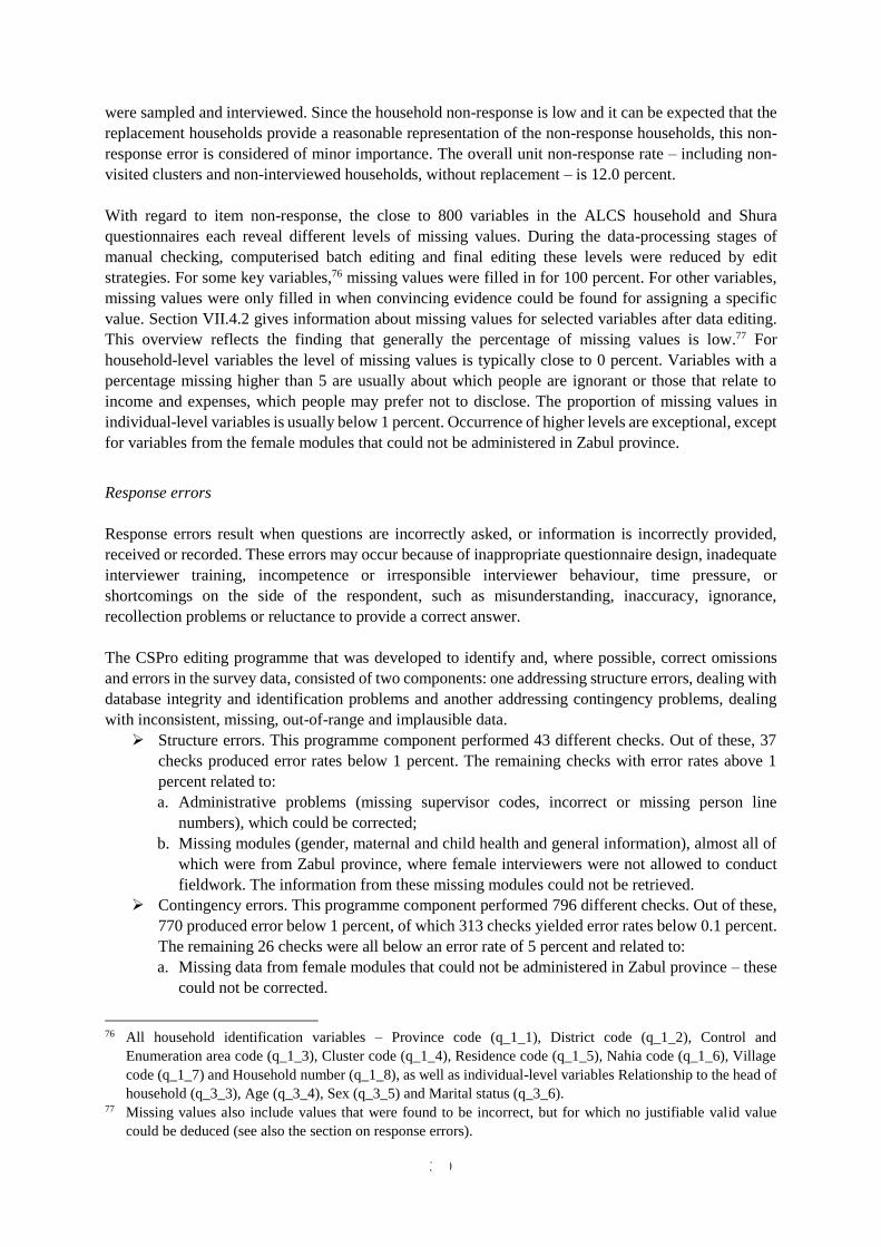
300
were sampled and interviewed. Since the household non-response is low and it can be expected that the
replacement households provide a reasonable representation of the non-response households, this non-
response error is considered of minor importance. The overall unit non-response rate – including non-
visited clusters and non-interviewed households, without replacement – is 12.0 percent.
With regard to item non-response, the close to 800 variables in the ALCS household and Shura
questionnaires each reveal different levels of missing values. During the data-processing stages of
manual checking, computerised batch editing and final editing these levels were reduced by edit
strategies. For some key variables,76 missing values were filled in for 100 percent. For other variables,
missing values were only filled in when convincing evidence could be found for assigning a specific
value. Section VII.4.2 gives information about missing values for selected variables after data editing.
This overview reflects the finding that generally the percentage of missing values is low.77 For
household-level variables the level of missing values is typically close to 0 percent. Variables with a
percentage missing higher than 5 are usually about which people are ignorant or those that relate to
income and expenses, which people may prefer not to disclose. The proportion of missing values in
individual-level variables is usually below 1 percent. Occurrence of higher levels are exceptional, except
for variables from the female modules that could not be administered in Zabul province.
Response errors
Response errors result when questions are incorrectly asked, or information is incorrectly provided,
received or recorded. These errors may occur because of inappropriate questionnaire design, inadequate
interviewer training, incompetence or irresponsible interviewer behaviour, time pressure, or
shortcomings on the side of the respondent, such as misunderstanding, inaccuracy, ignorance,
recollection problems or reluctance to provide a correct answer.
The CSPro editing programme that was developed to identify and, where possible, correct omissions
and errors in the survey data, consisted of two components: one addressing structure errors, dealing with
database integrity and identification problems and another addressing contingency problems, dealing
with inconsistent, missing, out-of-range and implausible data.
Structure errors. This programme component performed 43 different checks. Out of these, 37
checks produced error rates below 1 percent. The remaining checks with error rates above 1
percent related to:
a. Administrative problems (missing supervisor codes, incorrect or missing person line
numbers), which could be corrected;
b. Missing modules (gender, maternal and child health and general information), almost all of
which were from Zabul province, where female interviewers were not allowed to conduct
fieldwork. The information from these missing modules could not be retrieved.
Contingency errors. This programme component performed 796 different checks. Out of these,
770 produced error below 1 percent, of which 313 checks yielded error rates below 0.1 percent.
The remaining 26 checks were all below an error rate of 5 percent and related to:
a. Missing data from female modules that could not be administered in Zabul province – these
could not be corrected.
76 All household identification variables – Province code (q_1_1), District code (q_1_2), Control and
Enumeration area code (q_1_3), Cluster code (q_1_4), Residence code (q_1_5), Nahia code (q_1_6), Village
code (q_1_7) and Household number (q_1_8), as well as individual-level variables Relationship to the head of
household (q_3_3), Age (q_3_4), Sex (q_3_5) and Marital status (q_3_6). 77 Missing values also include values that were found to be incorrect, but for which no justifiable valid value
could be deduced (see also the section on response errors).
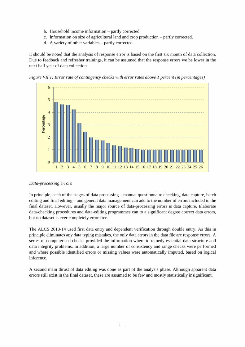
301
b. Household income information – partly corrected.
c. Information on size of agricultural land and crop production – partly corrected.
d. A variety of other variables – partly corrected.
It should be noted that the analysis of response error is based on the first six month of data collection.
Due to feedback and refresher trainings, it can be assumed that the response errors we be lower in the
next half year of data collection.
Figure VII.1: Error rate of contingency checks with error rates above 1 percent (in percentages)
Data-processing errors
In principle, each of the stages of data processing – manual questionnaire checking, data capture, batch
editing and final editing – and general data management can add to the number of errors included in the
final dataset. However, usually the major source of data-processing errors is data capture. Elaborate
data-checking procedures and data-editing programmes can to a significant degree correct data errors,
but no dataset is ever completely error-free.
The ALCS 2013-14 used first data entry and dependent verification through double entry. As this in
principle eliminates any data typing mistakes, the only data errors in the data file are response errors. A
series of computerised checks provided the information where to remedy essential data structure and
data integrity problems. In addition, a large number of consistency and range checks were performed
and where possible identified errors or missing values were automatically imputed, based on logical
inference.
A second main thrust of data editing was done as part of the analysis phase. Although apparent data
errors still exist in the final dataset, these are assumed to be few and mostly statistically insignificant.
0
1
2
3
4
5
6
1 2 3 4 5 6 7 8 9 10 11 12 13 14 15 16 17 18 19 20 21 22 23 24 25 26
Per
centa
ge
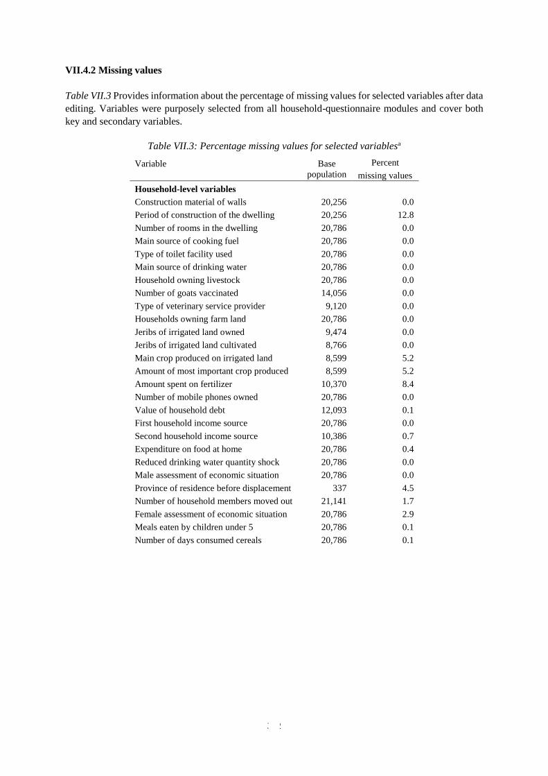
302
VII.4.2 Missing values
Table VII.3 Provides information about the percentage of missing values for selected variables after data
editing. Variables were purposely selected from all household-questionnaire modules and cover both
key and secondary variables.
Table VII.3: Percentage missing values for selected variablesa
Variable Base Percent
population missing values
Household-level variables
Construction material of walls 20,256 0.0
Period of construction of the dwelling 20,256 12.8
Number of rooms in the dwelling 20,786 0.0
Main source of cooking fuel 20,786 0.0
Type of toilet facility used 20,786 0.0
Main source of drinking water 20,786 0.0
Household owning livestock 20,786 0.0
Number of goats vaccinated 14,056 0.0
Type of veterinary service provider 9,120 0.0
Households owning farm land 20,786 0.0
Jeribs of irrigated land owned 9,474 0.0
Jeribs of irrigated land cultivated 8,766 0.0
Main crop produced on irrigated land 8,599 5.2
Amount of most important crop produced 8,599 5.2
Amount spent on fertilizer 10,370 8.4
Number of mobile phones owned 20,786 0.0
Value of household debt 12,093 0.1
First household income source 20,786 0.0
Second household income source 10,386 0.7
Expenditure on food at home 20,786 0.4
Reduced drinking water quantity shock 20,786 0.0
Male assessment of economic situation 20,786 0.0
Province of residence before displacement 337 4.5
Number of household members moved out 21,141 1.7
Female assessment of economic situation 20,786 2.9
Meals eaten by children under 5 20,786 0.1
Number of days consumed cereals 20,786 0.1
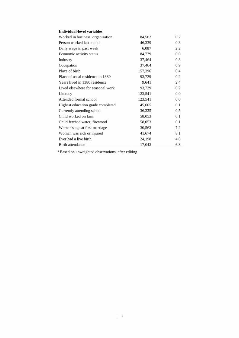
303
Individual-level variables
Worked in business, organisation 84,562 0.2
Person worked last month 46,339 0.3
Daily wage in past week 6,087 2.2
Economic activity status 84,739 0.0
Industry 37,464 0.8
Occupation 37,464 0.9
Place of birth 157,396 0.4
Place of usual residence in 1380 93,729 0.2
Years lived in 1380 residence 9,641 2.4
Lived elsewhere for seasonal work 93,729 0.2
Literacy 123,541 0.0
Attended formal school 123,541 0.0
Highest education grade completed 45,605 0.1
Currently attending school 36,325 0.5
Child worked on farm 58,053 0.1
Child fetched water, firewood 58,053 0.1
Woman's age at first marriage 30,563 7.2
Woman was sick or injured 41,674 8.1
Ever had a live birth 24,198 4.8
Birth attendance 17,043 6.8
a Based on unweighted observations, after editing
304
ANNEX VIII CONCEPTS AND DEFINITIONS
Adult. Person age 18 or over.
Adult literacy rate. The percentage of literate persons aged 15 years and over.
Age at first marriage. The weighted average of the different ages (limited at age 50), using as weights
the age-specific marriage rates of first marriage only.
Aged dependency ratio. The ratio of the number of elderly aged 65 and over to the number of persons
in the most productive ages of 15-64, expressed as a percentage.
Ante-natal care. Workers/attendants which are accredited health professionals - such as a midwife,
doctor or nurse - who have been educated and trained to proficiency in the skills needed to manage
normal (uncomplicated) pregnancies, childbirth and the immediate postnatal period, and in the
identification, management and referral of complications in women and newborns. Both trained
and untrained traditional birth attendants (TBA) are excluded.
Calorie deficiency. A daily caloric intake of less than 2,100 Kcal per person.
Child. Person below age 18.
Child labour. Work that is (i) mentally, physically, socially and/or morally dangerous and harmful to
children, and (ii) hazardous work which by its nature or the circumstances under which it is
performed, jeopardises the health, safety and morals of a child.
ILO: The term ‘child labour’ is often defined as work that deprives children of their childhood,
their potential and their dignity, and that is harmful to physical and mental development. It refers
to work that:
is mentally, physically, socially or morally dangerous and harmful to children; and
interferes with their schooling by:
depriving them of the opportunity to attend school;
obliging them to leave school prematurely; or
requiring them to attempt to combine school attendance with excessively long and heavy work.
UNICEF: (a) children 5 to 11 years of age that during the week preceding the survey did at least
one hour of economic activity or at least 28 hours of domestic work, and (b) children 12 to 14
years of age that during the week preceding the survey did at least 14 hours of economic activity
or at least 42 hours of economic activity and domestic work combined.
Child dependency ratio. The ratio of the number of children aged 0-14 to the number of persons in the
most productive ages of 15-64, expressed as a percentage.
Child sex ratio. Number of male children per 100 female children, under 1 year of age.
Contributing family workers. Those workers who hold a ‘self-employment’ job in a market-oriented
establishment operated by a related person living in the same household, who cannot be regarded
as partners, because their degree of commitment to the operation of the establishment, in terms of
working time or other factors to be determined by national circumstances, is not at a level
comparable to that of the head of the establishment.
Coping strategy. Household strategies to adjust the livelihood situation in response to household shocks.
Dependency ratio. The ratio of the number of persons in the unproductive ages of 0-14 and 65 and over
to the number of persons in the most productive ages of 15-64, expressed as a percentage.
Durable housing. Housing of which the outer walls, roof and floor are made of durable materials that
protect its inhabitants from the extremes of climatic conditions, such as rain, heat, cold and
humidity. Fired brick, concrete, mud bricks and stone are considered durable materials. For roofs
also wood is regarded durable.
305
Early initiation of breastfeeding. Putting a newborn baby to the breast within one hour of birth.
Economic sector. A group of establishments engaged on the same, or similar, kinds of production
activity.
Educational attainment. The highest level of education an individual has successfully completed.
Elderly. Person age 65 or over.
Emigrant. A person who left a country and took up residence abroad for at least one year.
Emigration. The act of crossing an international border and taking up residence abroad for at least one
year.
Emigration rate. The number of emigrants as percentage of the resident population.
Employed. All persons age 14 and over who, during the reference period of one week, were in paid
employment or self-employed and who worked at least eight hours. The employed include
military and apprentices, as well as persons who were temporarily absent from work because of
holidays or leave, temporary lay-off, or who had a job attachment defined by having access to
irrigated farm land.
Employers. Those workers who, working on their own account or with one or a few partners, hold the
type of job defined as a self-employed job, and in this capacity, on a continuous basis have
engaged one or more persons to work for them in their business as employees.
Employees. Persons who enter an agreement, which may be formal or informal, with an enterprise to
work for the enterprise in return for remuneration in cash or in kind.
Employment-to-population ratio. The proportion of the working-age population that is employed.
Enumeration Area. Areas into which a country is divided that covers a number of households that can
be enumerated in a census by one enumerator.
Exclusive breastfeeding. Breastfeeding whereby the infant only receives breast milk without any
additional food or drink, not even water (with the exception of oral rehydration solutions,
vitamins, minerals and medicines).
Food security. Food security exists when all people, at all times have physical, social and economic access
to sufficient, safe and nutritious food for a healthy and active life. Here, households that meet a
minimum of 2,100 calories per person per day are considered as food secure.
Gender parity index (for educational attendance). The ratio of the number of female students attending
primary, secondary and tertiary levels of education to the number of male students in each level
(based on the gross attendance ratio).
Gross attendance ratio. The number of pupils attending a given level of education, regardless of age,
expressed as a percentage of the population in the official age group for the same level of
education.
Gross intake ratio. The total number of new entrants in the first grade of primary education, regardless
of age, expressed as a percentage of the total number of children of school-entry age.
Gini Index. An index measuring the extent to which the distribution of consumption expenditure among
individuals or households within an economy deviates from a perfectly equal distribution.
Hazardous work. Refers to work which, by its nature or the circumstances in which it is performed, is
likely to harm the health, safety or morals of children (ILO 2008).
Head of household. The person commonly regarded by the household members as their head. Usually
it is the main income earner and decision maker for the household.
Headcount index. The percentage of the population whose monthly per capita consumption expenditure
are below the poverty line.
306
Health post. A community health service provided by community health workers from their home,
delivering basic health care services.
Household. A group of people, either related or unrelated, who live together as a single unit in the sense
that they have common housekeeping arrangements, that is, they share or are supported by a
common budget. They live together, pool their money, and eat at least one meal together each
day.
Immigrant. A person who has entered a country and took up residence there for at least one year.
Inactive population or persons not in the labour force. All persons age 14 and over who were not
employed or unemployed during reference period of one week because of (a) attendance at
educational institutions, (b) engagement in household duties, (c) retirement or old age, (d)
infirmity or disablement or (e) other reasons, which may be specified.
In-migrant. A person who has entered an administrative area from within a country and took up
residence there for at least one year.
Immigration. The act of crossing an international border into a country and taking up residence in the
country for at least one year.
Immigration ratio. The number of immigrants as percentage of the resident population.
Improved water source. Includes hand pump (private or public), bored wells, protected spring, piped
water (private or municipal); does not include surface water (open well, unprotected spring, kariz,
river, lake, channel, pool, drainage), water tanker, bottled water.
Improved sanitation facility: Includes flush latrine, improved latrine and covered latrine; does not
include open pit, darean and open defecation.
Infant mortality rate. The number of deaths of infants under 1 year age per 1,000 live births.
In-migration. The act of crossing an administrative area border within a country and taking up residence
in the area for at least one year.
In-migration ratio. The number of in-migrants as percentage of the resident population.
Internal migration. The act of crossing a border between two administrative areas within a country and
taking up residence in another area for at least one year.
International migration. The act of crossing a border between two countries and taking up residence
abroad for at least one year.
Internally displaced person (IDP). A persons who has been forced or obliged to flee or to leave his/her
home or place of habitual residence, in particular as a result of or in order to avoid the effects of
armed conflict, situations of generalized violence, violations of human rights or natural or human-
made disasters, and who have not crossed an internationally recognized State border.
Islamic education. Encompasses Madrassa (grades 1-12), Dar-ul-ulum (grades 13-14) and Dar-ul-hefaz
(grades 1-12).
Kuchi. Nomadic pastoralists living in Afghanistan as nomads or semi-nomads.
Life-time migrant. A person who changed residence across an administrative border – either national or
international – since birth.
Literacy Gender Parity Index. The ratio of the literacy rate for women divided by the literacy rate for
men.
Labour force. The economically active population – encompassing the (under)employed and
unemployed – in the working-age (14 and over).
Labour force participation rate. The ratio of the labour force to the working-age population (14 and
over), expressed as a percentage.
Life-time migration. Migration – either internal or international – since birth.
307
Light work. Work that is a) not likely to be harmful to children’s health or development; and b) not such
as to prejudice their attendance at school, their participation in vocational orientation or training
programmes approved by the competent authority or their capacity to benefit from the instruction
received (ILO 2008)
Maternal mortality ratio. The number of pregnancy-related deaths during a given time period per
100,000 live births during the same time period.
Migration. The act of crossing an administrative border and taking up residence elsewhere for at least a
year.
Net attendance ratio. The number of pupils of the theoretical school-age group for a given level of
education, expressed as a percentage of the total population in that age group.
Net intake rate in primary education. The number of children of school-entry age who enter the first
grade of primary school as a percentage of the total number of children of school-entry age.
Occupation. A set of jobs whose main tasks and duties are characterised by a high degree of similarity.
Persons are classified by occupation through their relationship to a past, present or future job.
Out-migrant. A person who left an administrative area and took up residence elsewhere in the same
country country for at least one year.
Out-migration. The act of crossing an administrative area border within a country and taking up
residence elsewhere in the same country for at least one year.
Out-migration rate. The number of out-migrants as percentage of the resident population of the area of
departure.
Overcrowded dwelling. Dwelling in which more than three persons live per room.
Own-account workers. Those workers who, working on their own account or with one or more partners,
hold the type of job defined as a self-employed job, and have not engaged on a continuous basis
any employees to work for them during the reference period.
Poverty gap. The average distance between the consumption levels of the poor and the poverty line.
Primary completion rate. The total number of new entrants in the last grade of primary education (grade
six), regardless of age, expressed as a percentage of the number of children of the theoretical
entrance age to the last grade (age 12).
Primary education. Encompasses education at grades 1-6. Primary school age is the age at which
children receive primary education.
Pyramid (population‒ or ‒age). Graphical illustration showing the distribution of population by age
group. The shape of the illustration is similar to a pyramid when the population is growing.
Quality assurance. Any method or procedure for planning, collecting, processing or analysing survey
data that is aimed at maintaining or enhancing their reliability or validity.
Recent migrant. A person who changed residence across an administrative border – either national or
international – a specific point in recent time, here defined as migration in the last two years
before the interview.
Recent migration. Migration – either internal or international – since a specific point in recent time, here
defined as migration in the last two years before the interview.
Returnee. A person who has returned from displacement either within the country (former IDP) or to
another country (former refugee or asylum seeker).
Repetition rate. The number of repeaters in a given grade in the current school year as a percentage of
the number of pupils attending the same grade in the previous school year.
Reproductive age. Women in age 15-49 years.
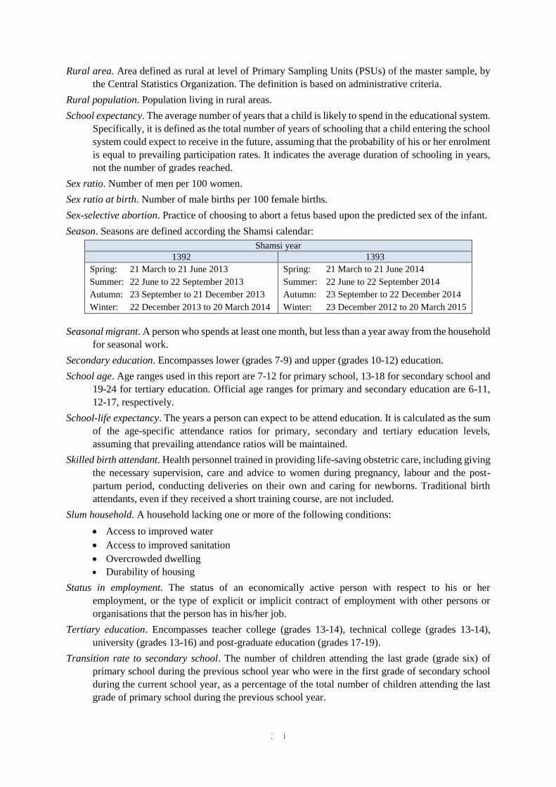
308
Rural area. Area defined as rural at level of Primary Sampling Units (PSUs) of the master sample, by
the Central Statistics Organization. The definition is based on administrative criteria.
Rural population. Population living in rural areas.
School expectancy. The average number of years that a child is likely to spend in the educational system.
Specifically, it is defined as the total number of years of schooling that a child entering the school
system could expect to receive in the future, assuming that the probability of his or her enrolment
is equal to prevailing participation rates. It indicates the average duration of schooling in years,
not the number of grades reached.
Sex ratio. Number of men per 100 women.
Sex ratio at birth. Number of male births per 100 female births.
Sex-selective abortion. Practice of choosing to abort a fetus based upon the predicted sex of the infant.
Season. Seasons are defined according the Shamsi calendar:
Shamsi year
1392 1393
Spring: 21 March to 21 June 2013 Spring: 21 March to 21 June 2014
Summer: 22 June to 22 September 2013 Summer: 22 June to 22 September 2014
Autumn: 23 September to 21 December 2013 Autumn: 23 September to 22 December 2014
Winter: 22 December 2013 to 20 March 2014 Winter: 23 December 2012 to 20 March 2015
Seasonal migrant. A person who spends at least one month, but less than a year away from the household
for seasonal work.
Secondary education. Encompasses lower (grades 7-9) and upper (grades 10-12) education.
School age. Age ranges used in this report are 7-12 for primary school, 13-18 for secondary school and
19-24 for tertiary education. Official age ranges for primary and secondary education are 6-11,
12-17, respectively.
School-life expectancy. The years a person can expect to be attend education. It is calculated as the sum
of the age-specific attendance ratios for primary, secondary and tertiary education levels,
assuming that prevailing attendance ratios will be maintained.
Skilled birth attendant. Health personnel trained in providing life-saving obstetric care, including giving
the necessary supervision, care and advice to women during pregnancy, labour and the post-
partum period, conducting deliveries on their own and caring for newborns. Traditional birth
attendants, even if they received a short training course, are not included.
Slum household. A household lacking one or more of the following conditions:
Access to improved water
Access to improved sanitation
Overcrowded dwelling
Durability of housing
Status in employment. The status of an economically active person with respect to his or her
employment, or the type of explicit or implicit contract of employment with other persons or
organisations that the person has in his/her job.
Tertiary education. Encompasses teacher college (grades 13-14), technical college (grades 13-14),
university (grades 13-16) and post-graduate education (grades 17-19).
Transition rate to secondary school. The number of children attending the last grade (grade six) of
primary school during the previous school year who were in the first grade of secondary school
during the current school year, as a percentage of the total number of children attending the last
grade of primary school during the previous school year.
309
Transition rate to tertiary school. The number of children attending the last grade (grade twelve) of
secondary school during the previous school year who were in the first grade of tertiary school
during the current school year, as a percentage of the total number of children attending the last
grade of secondary school during the previous school year.
Underemployed. Persons working hours of work that are insufficient in relation to an alternative
employment situation in which the person is willing and available to engage (time-related
underemployment). The Afghanistan national time-criterion is working less than 40 hours.
Unemployed. All persons age 14 and over who during the reference period of one week were:
a. without any work or working less than eight hours, and
b. seeking work.
The unemployed include persons not working who are not seeking work because of being
discouraged in finding any (the ‘relaxed unemployment’ definition).
Unemployment rate. The number of unemployed as a percentage of the labour force.
Urban area. Area defined as urban at level of Primary Sampling Units (PSUs) of the master sample, by
the Central Statistics Organization. The definition is based on administrative criteria.
Urban population. Population living in urban areas.
Vulnerable employment. Employment characterised by relatively precarious circumstances such as a
lack of formal work arrangements and access to benefits or social protection programmes, as well
as low remuneration. Own-account workers and contributing family workers are the statuses in
employment that are considered vulnerable employment. In ALCS, day labourers are included as
well.
Working age. Age 14 and over.
Working child. Children who participate in work that does not affect their health and personal
development or interfere with their schooling.
Youth literacy rate. The percentage of literate persons aged 15–24 years.
310
REFERENCES
APHI/MoPH, CSO, ICF Macro, IIHMR and WHO/EMRO (2011), Afghanistan Mortality Survey 2010.
Calverton, Maryland, USA, ICF Macro.
Aturupane, H., R. Gunatilaka, R. Ebenezer, and M. Shojo (2013), Education, Economic Welfare and
Subjective well-being in Afghanistan. Washington D.C., World Bank.
Bartlett, L.A., S. Mawji, S. Whitehead, C. Crouse, S. Dalil, D. Ionete, P.Salama, Afghan Maternal
Mortality Study Team (2005), Where giving birth is a forecast of death: Maternal mortality in
four districts of Afghanistan, 1999-2002. The Lancet, Vol. 365, pp. 864-870.
Beegle, K., De Weerdt, J., Friedman, J. and Gibson, J. (2011), Methods of household consumption
measurement through surveys: Experimental results from Tanzania. Journal of Development
Economics, Vol. 98, No. 1, pp. 3-18.
CESO/SACO (n.d.), Women’s Economic Empowerment. A CESO perspective. Toronto.
CSO (2007), The National Risk and Vulnerability Assessment 2005. Kabul, Central Statistics
Organisation.
CSO (2009), National Risk and Vulnerability Assessment 2007/8. A profile of Afghanistan. Kabul,
Central Statistics Organisation.
CSO (2010), Afghanistan National Statistical Plan. Kabul, Central Statistics Organisation.
CSO (2014), National Risk and Vulnerability Assessment 2011-12. Afghanistan Living Conditions
Survey. Kabul, Central Statistics Organisation.
CSO and UNICEF (2003), Multiple Indicator Cluster Survey Afghanistan. Kabul, Central Statistics
Organisation and UNICEF.
CSO and UNICEF (2012), Afghanistan Multiple Indicator Cluster Survey 2010-11: Final report. Kabul,
Central Statistics Organisation and UNICEF.
Eurostat (2015), Immigration in the EU.
http://ec.europa.eu/dgs/home-affairs/e-library/docs/infographics/immigration/migration-in-eu-
infographic_en.pdf.
FAO (2008), Afghanistan national livestock census 2002-2003. Final report 2006. Rome, Food and
Agriculture Organization.
Government of Afghanistan (1999), Labor Code.
http://www.ilo.org/dyn/natlex/docs/MONOGRAPH/78309/83636/F774573068/AFG78309.pdf
Goverment of Afghanistan. (2008), Afghanistan National Development Strategy 2008-2013. Phoenix
Design Aid A/S.
ILO (2008), Child labour statistics. Report III. 18th International Conference of Labour Statisticians
Geneva, 24 November–5 December 2008. ILO Geneva.
Islamic Republic of Afghanistan (2009), Millennium Development Goals Islamic Republic of
Afghanistan. Vision 2020. Annual progress report 2008. Kabul, Islamic Republic of Afghanistan.
Islamic Republic of Afghanistan (2010), Afghanistan Millennium Development Goals Report 2010.
Kabul, Islamic Republic of Afghanistan.
Islamic Republic of Afghanistan (2013), Afghanistan Millennium Development Goals Report 2012.
Kabul, Islamic Republic of Afghanistan.
Kronenfeld, D. (2008), Afghan Refugees in Pakistan: Not All Refugees, Not Always in Pakistan, Not
Necessarily Afghan? Journal of Refugee Studies, Vol. 21, No. 1, pp. 43-63.
311
Landinfo (2011), Report Afghanistan: Marriage. LANDINFO – 19 MAY 2011. Country of Origin
Information Centre.
MAIL (2004-2014), Agricultural Prospect Reports. Kabul, MAIL
Ministry of Education (2014), National Education Strategic Plan (2015-2020) (Draft). Kabul, Ministry
of Education.
Ministry of Health (2002), Afghanistan National Health Resources Assessment. Kabul, Ministry of
Health.
Ministry of Health (2003), The Basic Package of Health Services for Afghanistan. Kabul, Ministry of
Health.
Monsutti, A. (2008), Afghan Migratory Strategies and the Three Solutions to the Refugee Problem.
Refugee Survey Quarterly, Vol. 27, No. 1, pp. 58-73.
MoPH (2005), A Basic Package of Health Services for Afghanistan 2005/1384. Kabul, Ministry of
Public Health.
MoPH (2007), Afghanistan Health Survey 2006. Estimates of Priority Health Indicators. Kabul,
Ministry of Public Health, General Directorate of Policy and Planning Monitoring & Evaluation
Department.
MoPH (n.d.), National reproductive health strategy 2011-2015. Kabul, Reproductive Health Task
Force, MoPH.
MoPH, CSO, ICF Macro, IIHMR and WHO/EMRO (2011), Afghanistan Mortality Survey 2010. Kabul,
Ministry of Public Health, Afghan Public Health Institute.
NUFFIC 2015 - The Afghan education system. NUFFIC. https://www.nuffic.nl/en/library/education-
system-afghanistan.pdf
Preston, S. H., P. Heuveline and M. Guillot (2001), Demography: Measuring and Modeling Population
Processes. Oxford, Blackwell Publishing Ltd.
Rubin, D. B. (1987), Multiple Imputation for Nonresponse in Surveys. Wiley. New York.
Schafer, J. (1999), Multiple Imputation: a Primer. Statistical Methods in Medical Research, Vol. 8, pp.
3-15.
SIGAR (2015), Quarterly report to the United States Congress. Special Inspector General for
Afghanistan Reconstruction, January.
UNDESA (2015), World population prospects. New York, United Nations.
UNDP (2014), Human Development Report 2014. Sustaining human progress: reducing vulnerabilities
and building resilience. New York, UNDP.
UN-HABITAT (2007), The state of the world's cities 2006-7. London, Earthscan.
UNHCR (2015), The 2015 Afghanistan refugee and returnee overview.
https://docs.unocha.org/sites/dms/Afghanistan/2015%20Afghanistan%20Refugee%20and%20R
eturnee%20Overview.pdf
UNICEF (2012), The State of the World’s Children 2009. Children in an urban World. New York,
UNICEF.
UNICEF (2014), Water, Sanitation and Hygiene. New York, UNICEF and Water, Sanitation and
Hygiene (WASH).
UNICEF (2007), Fact Sheet. The remarkable first hour of life.
http://www.unicef.org/malaysia/Breastfeeding_First_Hour_of_Life.pdf
United Nations (2000), CCPR Human Rights Committee (2000), General Comments Adopted By The
Human Rights Committee Under Article 40, Paragraph 4,Of The International Covenant On Civil
And Political Rights. Addendum, GENERAL COMMENT No. 28 (68), Equality of rights between
312
men and women. General Comment No. 28: Equality of rights between men and women (article
3) : . 03/29/2000. CCPR/C/21/Rev.1/Add.10, General Comment No. 28. (General Comments)
Villar, J. and P. Bergsjø (2002), WHO Ante-natal Care Randomized Trial: Manual for the
Implementation of the New Model. WHO Programme to Map Best Reproductive Health Practices
(WHO/RHR/01.30).
WHO (2002), Report of the Expert Consultation on the Optimal Duration of Exclusive Breastfeeding.
Geneva, WHO Department of Nutrition for Health and Development, Department of Child and
Adolescent Health and Development.
WHO/UNICEF (2015), Joint Monitoring Programme. Retrieved from http://www.wssinfo.org.
Bulletin of the World Health Organization 2015;93:507-508. doi:
http://dx.doi.org/10.2471/BLT.14.144923
WHO, UNICEF, UNFPA and World Bank (2012), Trends in Maternal Mortality: 1990 to 2010. WHO,
UNICEF, UNFPA and The World Bank estimates.
Yoshida, N., R. Munoz, A., Skinner, C. Kyung-eun Lee, M. Brataj, W. Durbin, D. Sharma, and C.
Wieser (2015), SWIFT Data Collection Guidelines version 2. Washington, World Bank.

0