Advanced methods of speech processing and noise reduction ...
169
THÈSE / IMT Atlantique sous le sceau de l’Université Bretagne Loire pour obtenir le grade de DOCTEUR DE IMT Atlantique Mention : Sciences et Technologies de l’Information et de la Communication École Doctorale Sicma Présentée par Van-Khanh Mai Préparée au département Signal & communication Laboratoire Labsticc Méthodes avancées de traitement de la parole et de réduction du bruit pour les terminaux mobiles Advanced Methods of speech processing and noise reduction for mobile devices Thèse soutenue le 09 mars 2017 devant le jury composé de : Régine Le Bouquin Jeannes Professeur, Ecole supérieure d’Ingénieur de Rennes / Présidente Jérôme Boudy Professeur, Telecom SudParis / Rapporteur Abdourrahmane Mahamane Atto Maître de conférences (HDR), Polytech Annecy-Chambéry / Rapporteur Laurent Navarro Maître de conférences, Ecole des mines de Saint-Etienne / Examinateur Raphaël Le Bidan Maître de conférences, IMT-Atlantique / Examinateur Abdeldjalil Aïssa El Bey Professeur, IMT-Atlantique / Co-directeur de thèse Dominique Pastor Professeur, IMT-Atlantique / Directeur de thèse
-
Upload
khangminh22 -
Category
Documents
-
view
4 -
download
0
Transcript of Advanced methods of speech processing and noise reduction ...

THÈSE / IMT Atlantique
sous le sceau de l’Université Bretagne Loire
pour obtenir le grade de
DOCTEUR DE IMT Atlantique
Mention : Sciences et Technologies de l’Information et de la Communication
École Doctorale Sicma
Présentée par
Van-Khanh Mai Préparée au département Signal & communication
Laboratoire Labsticc
Méthodes avancées
de traitement de la parole
et de réduction du bruit
pour les terminaux mobiles
Advanced Methods of
speech processing and noise
reduction for mobile devices
Thèse soutenue le 09 mars 2017
devant le jury composé de :
Régine Le Bouquin Jeannes Professeur, Ecole supérieure d’Ingénieur de Rennes / Présidente Jérôme Boudy Professeur, Telecom SudParis / Rapporteur
Abdourrahmane Mahamane Atto Maître de conférences (HDR), Polytech Annecy-Chambéry / Rapporteur
Laurent Navarro Maître de conférences, Ecole des mines de Saint-Etienne / Examinateur
Raphaël Le Bidan Maître de conférences, IMT-Atlantique / Examinateur
Abdeldjalil Aïssa El Bey Professeur, IMT-Atlantique / Co-directeur de thèse Dominique Pastor Professeur, IMT-Atlantique / Directeur de thèse


RemerciementsCes travaux de thèse ont été réalisés au sein du département Signal & Communications de IMT-Atlantique. La thèse est financée par la bourse régionale et le PRACOM (Pôle de RechercheAvancée en Communications).
Je tiens tout d’abord à exprimer toute ma gratitude et mes plus vifs remerciements à mesdirecteurs de thèse, Monsieur Dominique Pastor et Monsieur Abdeldjallil Aïssa-El-Bey, Pro-fesseurs à IMT-Atlantique, pour m’avoir donné la possibilité d’entreprendre mes travaux dedoctorant, ainsi que pour de leur disponibilité, leur enthousiasme et leur patience malgré leursnombreuses charges.
Mes remerciements vont également à mon encadrant, Monsieur Raphaël Le Bidan, Maîtrede Conférence à IMT-Atlantique, pour la confiance qu’il m’a accordée en acceptant d’encadrerce travail doctoral et pour ses multiples conseils.
Je tiens aussi à remercier l’ensemble des membres de mon jury : Madame Régine Le BouquinJeannes et Messieurs Jerome Boudy, Abdourahmane Atto et Laurent Navarro, pour accepterde participer mon jury de thèse, pour leur lecture de ce manuscrit ainsi que pour les remarquespertinentes sur mes travaux de thèse.
De plus, je remercie tous les membres et ex-membres des équipes COM et TOM du dépar-tement Signal & Communications de IMT-Atlantique, pour le climat sympathique dans lequelils m’ont permis de faire de la recherche. Je voudrais exprimer particulièrement toute mon ami-tié à Thomas Guilment, Budhi Guanadharma et Nicolas Alibert pour leur gentillesse, leurscompétences, leurs conseils, leur amitié et leur humour.
Un grand merci va à mes amis vietnamiens qui m’ont soutenu et avec qui j’ai pu partagerdes moments inoubliables.
Pour finir, les mots les plus simples étant les plus forts, je tiens à adresser toute mon affectionà ma famille et en particulier à ma femme Quynh Trang et ma fille Vivi. Leur confiance, leuramour, leur soutient ont toujours su me porter dans la réussite de ma thèse et continuent de meguider dans la vie.
Merci à vous !
i

ii

Table des matières
Remerciement i
Résumé en Français vii
Abstract xix
Résumé xxi
Acronyms xxiii
List of Figures xxix
List of Tables xxxi
I Introduction 1
1 Introduction 31.1 Context of the thesis . . . . . . . . . . . . . . . . . . . . . . . . . . . . . . . . . . 41.2 A brief history of speech enhancement . . . . . . . . . . . . . . . . . . . . . . . . 5
1.2.1 Unsupervised methods . . . . . . . . . . . . . . . . . . . . . . . . . . . . . 51.2.2 Supervised methods . . . . . . . . . . . . . . . . . . . . . . . . . . . . . . 6
1.3 Thesis motivation and outline . . . . . . . . . . . . . . . . . . . . . . . . . . . . . 7
2 Single microphone speech enhancement techniques 92.1 Introduction . . . . . . . . . . . . . . . . . . . . . . . . . . . . . . . . . . . . . . . 102.2 Overview of single microphone speech enhancement system . . . . . . . . . . . . 10
2.2.1 Decomposition block . . . . . . . . . . . . . . . . . . . . . . . . . . . . . . 102.2.2 Noise estimation block . . . . . . . . . . . . . . . . . . . . . . . . . . . . . 132.2.3 Noise reduction block . . . . . . . . . . . . . . . . . . . . . . . . . . . . . 142.2.4 Reconstruction block . . . . . . . . . . . . . . . . . . . . . . . . . . . . . . 16
2.3 Performance evaluation of speech enhancement algorithms . . . . . . . . . . . . . 172.3.1 Objective tests . . . . . . . . . . . . . . . . . . . . . . . . . . . . . . . . . 192.3.2 Mean opinion scores subjective listening test . . . . . . . . . . . . . . . . 23
2.4 Conclusion . . . . . . . . . . . . . . . . . . . . . . . . . . . . . . . . . . . . . . . 23
II Noise: Understanding the Enemy 25
3 Noise estimation block 273.1 Introduction . . . . . . . . . . . . . . . . . . . . . . . . . . . . . . . . . . . . . . . 28
iii

Table des matières
3.2 DATE algorithm . . . . . . . . . . . . . . . . . . . . . . . . . . . . . . . . . . . . 293.3 Weak-sparseness model for noisy speech . . . . . . . . . . . . . . . . . . . . . . . 333.4 Noise power spectrum estimation by E-DATE . . . . . . . . . . . . . . . . . . . . 34
3.4.1 Stationary WGN . . . . . . . . . . . . . . . . . . . . . . . . . . . . . . . . 353.4.2 Colored stationary noise . . . . . . . . . . . . . . . . . . . . . . . . . . . . 353.4.3 Extension to non-stationary noise: The E-DATE algorithm . . . . . . . . 363.4.4 Practical implementation of the E-DATE algorithm . . . . . . . . . . . . 37
3.5 Performance evaluation . . . . . . . . . . . . . . . . . . . . . . . . . . . . . . . . 393.5.1 Number of parameters . . . . . . . . . . . . . . . . . . . . . . . . . . . . . 393.5.2 Noise estimation quality . . . . . . . . . . . . . . . . . . . . . . . . . . . . 403.5.3 Performance evaluation in speech enhancement . . . . . . . . . . . . . . . 433.5.4 Complexity analysis . . . . . . . . . . . . . . . . . . . . . . . . . . . . . . 44
3.6 Conclusion . . . . . . . . . . . . . . . . . . . . . . . . . . . . . . . . . . . . . . . 49
III Speech: Improving you 51
4 Spectral amplitude estimator based on joint detection and estimation 53
4.1 Introduction . . . . . . . . . . . . . . . . . . . . . . . . . . . . . . . . . . . . . . . 544.2 Signal model in the DFT domain . . . . . . . . . . . . . . . . . . . . . . . . . . . 554.3 Strict presence/absence estimators . . . . . . . . . . . . . . . . . . . . . . . . . . 56
4.3.1 Strict joint STSA estimator . . . . . . . . . . . . . . . . . . . . . . . . . 584.3.2 Strict joint LSA estimator . . . . . . . . . . . . . . . . . . . . . . . . . . 60
4.4 Uncertain presence/absence estimators . . . . . . . . . . . . . . . . . . . . . . . . 624.4.1 Uncertain joint STSA detector/estimator . . . . . . . . . . . . . . . . . . 654.4.2 Uncertain joint LSA estimator . . . . . . . . . . . . . . . . . . . . . . . . 67
4.5 Experimental results . . . . . . . . . . . . . . . . . . . . . . . . . . . . . . . . . . 694.5.1 Database and Criteria . . . . . . . . . . . . . . . . . . . . . . . . . . . . . 694.5.2 STSA-based results . . . . . . . . . . . . . . . . . . . . . . . . . . . . . . . 704.5.3 LSA-based results . . . . . . . . . . . . . . . . . . . . . . . . . . . . . . . 75
4.6 Conclusion . . . . . . . . . . . . . . . . . . . . . . . . . . . . . . . . . . . . . . . 80
5 Non-diagonal smoothed shrinkage for robust audio denoising 83
5.1 Introduction . . . . . . . . . . . . . . . . . . . . . . . . . . . . . . . . . . . . . . . 845.1.1 Motivation and organization . . . . . . . . . . . . . . . . . . . . . . . . . 845.1.2 Signal model and notation in the DCT domain . . . . . . . . . . . . . . . 855.1.3 Sparse thresholding and shrinkage for detection and estimation . . . . . . 86
5.2 Non-diagonal audio estimation of Discrete Cosine Coefficients . . . . . . . . . . . 885.2.1 Non-parametric estimation by Block-SSBS . . . . . . . . . . . . . . . . . . 885.2.2 MMSE STSA in the DCT domain . . . . . . . . . . . . . . . . . . . . . . 935.2.3 Combination method . . . . . . . . . . . . . . . . . . . . . . . . . . . . . . 95
5.3 Experimental Results . . . . . . . . . . . . . . . . . . . . . . . . . . . . . . . . . . 975.3.1 Parameter adjustment . . . . . . . . . . . . . . . . . . . . . . . . . . . . . 975.3.2 Speech data set . . . . . . . . . . . . . . . . . . . . . . . . . . . . . . . . . 975.3.3 Music data set . . . . . . . . . . . . . . . . . . . . . . . . . . . . . . . . . 104
5.4 Conclusion . . . . . . . . . . . . . . . . . . . . . . . . . . . . . . . . . . . . . . . 104
iv

Table des matières
IV Conclusion 107
6 Conclusions and Perspectives 1096.1 Conclusion . . . . . . . . . . . . . . . . . . . . . . . . . . . . . . . . . . . . . . . 1106.2 Perspectives . . . . . . . . . . . . . . . . . . . . . . . . . . . . . . . . . . . . . . . 111
A Lemma of the integral optimization problem 117
B Detection threshold under joint detection and estimation 119B.1 Strict model . . . . . . . . . . . . . . . . . . . . . . . . . . . . . . . . . . . . . . . 119B.2 Uncertain model . . . . . . . . . . . . . . . . . . . . . . . . . . . . . . . . . . . . 120
B.2.1 Independent estimators . . . . . . . . . . . . . . . . . . . . . . . . . . . . 120B.2.2 Joint estimator . . . . . . . . . . . . . . . . . . . . . . . . . . . . . . . . . 120
C Semi-parametric approach 123C.1 The unbiased estimate risk of block for Block-SSBS . . . . . . . . . . . . . . . . 123C.2 The MMSE gain function in the DCT domain . . . . . . . . . . . . . . . . . . . . 124
D Author Publications 125
Bibliography 134
v

vi

Résumé en Français
Introduction
En traitement du signal une des tâches les plus importantes et fondamentales est l’éliminationou la réduction du bruit de fond. Cette thématique est connue sous le nom de débruitage,suppression du bruit ou rehaussement de la parole dans le cas particulier du traitement de laparole. Cette thèse est consacrée au traitement de la parole, et plus particulièrement à sondébruitage. Ces dernières années, l’exploitation du traitement du signal dans les applicationsmobiles tel que les systèmes de commandes vocales ou les applications dans les smartphones,a connu un intérêt croissant. Dans le cadre de ces applications mobile le rehaussement de laparole a une place centrale. Dans les systèmes de télécommunication, les transmissions ontgénéralement lieu dans un environnement bruité non-stationnaire ; à l’intérieur d’une voiture,dans la rue ou à l’intérieur d’un aéroport. Le traitement de la parole joue alors un rôle importantaux récepteurs pour améliorer la qualité de la parole. Les méthodes du réhaussement de la parolesont également utilisées comme pré-traitement dans les systèmes de codage et de reconnaissancede la parole [1]. Aussi, les algorithmes de rehaussement de la parole peuvent également êtreappliqués aux prothèses auditives ou aux implants cochléaires pour réduire le bruit ambiant.
Le rehaussement de la parole a pour objectif, d’augmenter le confort auditif d’une part etde diminuer la fatigue de l’auditeur d’autre part . Dans ce contexte, ce rehaussement de laparole vise idéalement à améliorer, non seulement la qualité, mais aussi l’intelligibilité de laparole. Dans la littérature actuelle, les solutions proposées consistent en général à réduire lebruit de font afin d’améliorer la qualité de la parole. Cependant, ces méthodes peuvent générerune distorsion de la parole. C’est la raison pour laquelle, le défi principal du rehaussement deparole est de trouver le meilleur compromis entre la réduction du bruit de fond et la conservationde la qualité de la parole d’origine. De plus, la conception des techniques de rehaussement dela parole dépend aussi de l’application visée, de la bases de données, du type de bruit, dela relation entre le bruit et le signal intérêt et du nombre de capteurs utilisés. En fonctiondu nombre de capteurs disponibles, les techniques de rehaussement de la parole peuvent êtreclassées en deux catégories : i) les techniques mono-capteur et ii) multi-capteurs. Théoriquement,une amélioration des performances est possible par l’utilisation d’un système multi-capteur aulieu d’un système mono-capteur. Par exemple, un capteur placé près de la source du bruitnous permet d’estimer au mieux ce bruit. Cependant, la complexité de la mise en œuvre, laconsommation d’énergie et la taille de l’appareil peuvent être un frein important à la réalisationdu rehaussement de la parole dans des applications réelles. De plus, les méthodes utilisant unsystème mono-capteur peuvent directement être exploitées après un beamforming sur le signalreçu par un système multi-capteur. Par conséquent, nous avons décidé de restreindre notreattention aux méthodes mono-capteur qui sont, non seulement un véritable défi, mais aussijouent un rôle essentiel dans le traitement de la parole.
De nombreuses méthodes mono-capteur ont été proposées dans la littérature pour le re-haussement de la parole. En général, ces méthodes peuvent être classées en deux catégories :
vii

Résumé en Français
les méthodes supervisées et non-supervisées. Malgré les bonnes performances obtenues par lesméthodes supervisées, les méthodes non-supervisées sont toujours nécessaires. En effet, les mé-thodes non-supervisée permettent de compenser les lacunes des bases de données qui ne sontpas toujours suffisamment représentatives de l’ensemble des cas d’applications réelles. Dans cesapplications, les techniques non-supervisées doivent répondre à tous les critères suivants sansdevoir recourir à la aucun apprentissage (training en anglais), ni du bruit ni du signal d’intérêt :
• avoir une bonne performance pour les signaux audio (parole, musique ou autres),
• garantir un bon compromis entre la qualité et l’intelligibilité de la parole
• être robuste aux différents types de bruit stationnaire et non-stationnaire.
Ainsi, la motivation principale de cette thèse est de construire un système complet de dé-bruitage avec des techniques innovantes pour le problème de débruitage de la parole et du signalaudio corrompus par un bruit additif. Tout d’abord, une vue d’ensemble de l’architecture gé-nérale du système de débruitage mono-capteur en bloc est attentivement étudiée. Cette étudenous permet d’extraire les point clés de chaque bloc et d’identifier les améliorations possibles.Cette thèse est donc divisée en deux parties. Dans la première partie, notre travail consiste àdévelopper une méthode robuste d’estimation du bruit ce qui est un des problème principal dansles systèmes de débruitage monocapteur. Pour ce faire, nous présentons une vue d’ensemble desprincipales méthodes d’estimation du bruit avec leurs avantages et leurs inconvénients. On nousbasant sur cette analyse, nous proposons ensuite une méthode robuste d’estimation du bruitpour les environnements non-stationnaires. Cette méthode repose sur le fait que la transforméede Fourier à courte terme des signaux bruités est parcimonieux dans le sens où les signaux deparole transformés peuvent être représentés par un nombre relativement petit de coefficients avecde grandes amplitudes dans le domaine temps-fréquence. Cette méthode est robuste car elle nenécessite pas d’information à priori sur la distribution de probabilité du signal intérêt. Ainsi,cette méthode peut améliorer les performances du rehaussement de la parole dans n’importequel scénario où les signaux bruités peuvent avoir une représentation parcimonieuse faible.
Dans la deuxième partie de cette thèse, nous considérons le cas où nous disposons d’une esti-mation précise de la densité spectrale de puissance du bruit. Dans ce contexte, nous avons pro-posé des méthodes de débruitage paramétrique et aussi non-paramétrique. La première famillede méthodes sont des approches paramétriques qui nous permettent d’améliorer non seulementla qualité mais aussi de réduire l’impact négatif sur l’intelligibilité de la parole. Les méthodesproposées sont basées sur la combinaison de la détection et de l’estimation ce qui améliore lesperformances par rapport aux algorithmes d’estimations paramétriques uniques. Ainsi, deuxmodèles de la parole bruitées sont pris en compte. Dans le premier modèle, la parole est soitprésente, soit absente, alors que dans le deuxième modèle, la parole est toujours présente maisavec différents niveaux d’énergies. La deuxième famille de méthodes sont des approches non-paramétriques. Ces méthodes sont basées sur la fonction SSBS (pour smoothed sigmoid-basedshrinkage) dans le domaine de la transformée discrète en cosinus (DCT). Aussi, nous propo-sons une méthode hybride capable de capter des avantages des méthodes paramétriques etnon-paramétriques.
Architecture générale
Comme nous l’avons introduit précédemment, l’objectif principal de ce travail de thèse est l’étudeet le développement d’approches non-supervisées de rehaussement de la parole dans le contextemono-capteur. Les challenges principaux dans ce contexte pour l’amélioration de la qualité de la
viii

parole sont le manque de ressources (un microphone disponible) et l’absence de bases de données(seul le signal bruité est disponible). Dans ce qui suit (Chapitre 2) nous présentons un aperçude l’architecture générale des systèmes de débruitage mono-capteur.
Un système de débruitage mono-capteur se compose de quatre blocs principaux : décompo-sition du signal, estimation du bruit, débruitage et reconstruction du signal (voir Figure 2.1). Lesignal bruité observé est segmenté, fenêtré et transformé par une transformée harmonique à courtterme dans le bloc de décomposition. En effet, la plupart, des algorithmes de rehaussement de laparole sont appliqués dans un domaine transformé (Discrete Fourier Transform (DFT), DiscreteCosinus Transform (DCT),...) où la séparation entre le signal propre et le bruit est accentuée.La sortie du bloc de décomposition sont donc les coefficients de la transformée à court termedu signal bruité. Ces coefficients sont mis à l’entrée du bloc d’estimation du bruit et du bloc deréduction du bruit. Le bloc d’estimation du bruit à pour objectif d’estimer la densité spectralede puissance du bruit. L’estimation du bruit est le bloc principal où diverses techniques ont étéproposées. Après avoir obtenu une estimation de la densité spectrale de puissance du bruit, unalgorithme de réduction du bruit est utilisé pour estimer les coefficients du signal débruités dansle domaine transformé en appliquant une fonction de gain. Cette fonction de gain est généra-lement calculée à partir de l’amplitude du signal bruité à la sortie du bloc de décompositionet de la densité spectrale de puissance du bruit estimé au bloc d’estimation du bruit. Enfin, lebloc de reconstruction permet de transformer les coefficients estimés dans le domaine temporel.Notez qu’il est possible de récupérer exactement le signal dans le domaine temporel à partir deses coefficients de la transformée à courte terme (transformations réversibles).
Afin d’évaluer les performances du système de débruitage, un bloc d’évaluation supplémen-taire est ajouté (voir Figure 2.7). Dans cette partie, nous présentons certains critères qui sontfréquemment utilisés pour évaluer les performances des méthodes de rehaussement de la parole.Ces critères seront également utilisés dans cette thèse. Ces critères peuvent être divisés en deuxcatégories ; tests objectifs (SSNR– pour Segmental Signal to noise ratio, SNRI – pour SNR im-provement, MARSovrl – pour Multivariate adaptive resgression splines overall speech quality,STOI – pour Short Time Objective Intelligibility) et tests subjectifs (MOS-Mean opinion score).Les tests d’écoute subjectifs sont les critères les plus fiables, mais ils nécessitent plus de tempspour l’évaluation. Certains tests objectifs ont été fortement corrélés avec des tests subjectifs. Parconséquent, ces tests objectifs sont fréquemment utilisés pour évaluer la qualité et l’intelligibilitéde la parole.
Comme mentionné précédemment, l’architecture générique des systèmes de rehaussementde la parole est composée de quatre blocs principaux. Par conséquent, une amélioration ouune modification de l’un de ces blocs peut se traduire par une amélioration des performancespour l’ensemble du système. C’est l’objectif des chapitres suivants. Dans le chapitre 3 le blocd’estimation du bruit sera revisité. Dans le chapitre 4 nous développerons une nouvelle approchepour le bloc de réduction de bruit alors que dans le chapitre 5 nous présenterons une méthodebasée sur l’optimisation conjointe des blocs de décomposition du signal et de réduction du bruit.
Estimation du bruit
Comme nous l’avons présenté précédemment, nous avons motivé l’intérêt d’une approche non-supervisée pour les systèmes de débruitage mono-capteur. Un aperçu général des systèmes aensuite été présenté. Dans ces systèmes, l’estimation de la densité spectrale de puissance dubruit est une question clé dans la conception des méthodes robustes de réduction du bruit pourle rehaussement de la parole. La question est de savoir comment estimer la densité spectralede puissance du bruit à partir du signal bruité capturé par un seul capteur. Dans les systèmes
ix

Résumé en Français
mono-capteur de rehaussement de la parole le principal défi consiste à traiter le cas d’un bruitnon-stationnaire. En notant que le signal d’intérêt a une parcimonie faible dans un domainetransformé, une nouvelle méthode d’estimation de la densité spectrale de puissance de bruit non-paramétrique est introduite dans le chapitre 3. Cet algorithme est capable d’estimer efficacementla densité spectrale de puissance du bruit non-stationnaire.
Cette nouvelle méthode ne nécessite pas de modèle ou de connaissances a priori des distri-butions de probabilité des signaux de parole. Fondamentalement, nous ne prenons même pas enconsidération le fait que le signal d’intérêt ici est la parole. L’approche est appelée extended-DATE (E-DATE) puisqu’elle étend essentiellement le DATE (d-dimensional amplitude trimmedestimator) pour le bruit blanc Gaussien, le bruit stationnaire et le bruit non-stationnaire coloré.Le principe général de l’algorithme E-DATE est la propriété de parcimonie faible de la STFT(pour Short Time Fourier Transform) des signaux bruités. Aussi, la séquence de valeur complexerenvoyée par le STFT dans le domaine temps-fréquence peut être modélisée comme un signalaléatoire complexe avec une distribution inconnue et dont la probabilité inconnue d’occurrencedans le bruit de fond ne dépasse pas la 1
2 . Ainsi, l’estimation du bruit à pour objectif l’estimationde la variance du bruit dans chaque bande fréquentielle ce qui est fourni par le DATE.
L’algorithme E-DATE consiste à réaliser l’estimation de la densité spectrale de puissancedu bruit en exécutant l’algorithme DATE pour chaque bande de fréquence sur des périodesde D trames consécutives sans chevauchements, où D est choisi de sorte que le bruit peutêtre considéré comme approximativement stationnaire dans cet intervalle de temps. Une foisl’estimation de la densité spectrale de puissance du bruit obtenue, elle peut être utilisée pourle débruitage par exemple. Bien que l’algorithme E-DATE ait été spécifiquement conçu pourl’estimation de la densité spectrale de puissance du bruit non-stationnaire, il peut être utilisésans modification pour l’estimation de la densité spectrale de puissance du bruit blanc ou dubruit stationnaire coloré, ainsi il offre un estimateur de la densité spectrale de puissance du bruitrobuste et universel dont les paramètres sont fixés une fois pour tous les types de bruit.
Deux implémentations différentes de l’algorithme E-DATE sont mises en œuvre dans ce cha-pitre. La première approche est une implémentation simple par blocs de l’algorithme présentéedans Figure 3.3. Il s’agit d’estimer la densité spectrale de puissance du bruit sur chaque périodede D trames successives et sans chevauchement. Cela nécessite d’enregistrer D trames, de cal-culer la densité spectrale de puissance du bruit en utilisant les observations dans ces D trames,puis d’attendre D nouvelles trames sans chevauchement. Cet algorithme s’appelle Bloc-E-DATE(B-E-DATE). L’estimation de la densité spectrale de puissance du bruit sur des périodes sépa-rées de D trames réduit la complexité globale de l’algorithme. Cependant, cela implique unelatence de D trames, qui doit être considéré dans les applications à temps réelles. Cette latencepeut être contournée comme suit. Tout d’abord, une méthode standard d’estimation est utiliséepour estimer la densité spectrale de puissance du bruit pendant les D− 1 premières trames. Parla suite, en commençant par la trame Dème et en faisant glisser une fenêtre d’observation, uneversion de l’algorithme E-DATE est utilisée pour estimer la densité spectrale de puissance dubruit trame par trame. Cette implémentation alternative s’appelle SW-E-DATE (pour Sliding-Window-E-DATE) montrée dans Figure 3.4.
Les algorithmes B-E-DATE et SW-E-DATE peuvent être considérés comme deux exemplesparticuliers d’un algorithme général utilisant une fenêtre d’observation. Plus précisément, l’al-gorithme B-E-DATE correspond au cas extrême où la fenêtre d’observation est totalement vidéeet mise à jour une fois toutes les D trames. En revanche, l’algorithme SW-E-DATE correspondà l’autre cas extrême où seul la trame la plus ancienne est enlevée pour stocker la nouvelle,en mode First-In First-Out (FIFO). De toute évidence, une approche plus générale entre ces
x

deux extrêmes consiste à une mise à jour partielle de la fenêtre d’observation en renouvelantseulement L trames parmi D.
Ces algorithmes ont été évaluer en utilisant la base de donnée NOIZEUS. Les résultat sontrapportés dans le tableau 3.1 (pour le nombre de paramètres), dans les figure 3.5, 3.6 (pourl’erreur de l’estimation la densité spectrale de puissance du bruit), la figure 3.7 (pour SNRI),les figures 3.8, 3.9 (pour SSNR), les figures 3.10 et 3.11 (pour MARSovrl). Les résultats expé-rimentaux montrent que l’algorithme E-DATE fournit généralement l’estimation de la densitéspectrale de puissance du bruit la plus précise et qu’il surpasse d’autres méthodes en étant utilisédans des système de débruitage de la parole en présence de différents types et niveaux de bruit.En raison de ses bonnes performances et sa faible complexité, l’algorithme B-E-DATE devraitêtre préféré dans la pratique lorsque les fréquences de traitement des données sont suffisammentélevées pour induire des délais acceptables ou même négligeables.
Débruitage
Dans cette partie, nous proposons deux approches pour estimer l’amplitude spectrale à courtterme (STSA). L’objectif principal de cette partie est de prendre en compte les résultats récentsde la théorie statistique paramétrique et non paramétrique pour améliorer les performances dessystèmes mono-capteur de débruitage de la parole. Le Chapitre 4 prend en considération lathéorie statistique en combinant l’estimation et la détection basée sur l’approche paramétrique.Chapitre 5 les performances du rehaussement de la parole sont améliorées en utilisant uneapproche semi-paramétrique.
Approche paramétriqueL’objectif de cette partie (chapitre 4) est de de suivre une approche bayésienne visant à
optimiser conjointement la détection et l’estimation des signaux de la parole afin d’améliorerl’intelligibilité de la parole. Pour ce faire, nous nous concentrons sur l’estimateur de l’amplitudespectrale basé sur la combinaison de la détection et de l’estimation. En définissant la fonctionde coût sur l’erreur d’amplitude spectrale, notre stratégie est de déterminer une fonction de gainsous la forme d’un masque binaire généralisé.
Ainsi, deux modèles d’hypothèse binaire sont utilisés pour déterminer la fonction de gaindiscontinue. Tout d’abord, on considère les hypothèses binaires où l’absence de la parole eststricte (Strict Model - SM). Dans ce modèle, nous supposons que le signal observé contientdu bruit et du signal de parole dans certains atomes temps-fréquence, alors que dans d’autresatomes, l’observation contient uniquement du bruit. La présence de la parole est détectée encontraignant la probabilité de fausse d’alarme comme dans l’approche Neyman-Pearson.
En résumé, pour chaque atome temps-fréquence, la méthode conjointe proposée estimed’abord la STSA de la parole en utilisant l’estimateur bayésien (STSA-MMSE), ainsi le dé-tecteur se base sur cette estimation pour détecter la présence ou l’absence de parole à chaqueatome. Si la parole est absent, cette méthode fixe la STSA de la parole à 0. En se concentrantuniquement sur l’estimateur, l’estimation STSA peut être écrite comme un masque binaire.Cette méthode s’appelle SM-STSA. Dans cette méthode, le détecteur dépend de l’estimateur. Àson tour, l’estimateur dépend du détecteurs. Cette double dépendance est censée améliorer lesperformances du détecteur et de l’estimateur.
Deuxièmement, nous supposons que la parole est toujours présente avec différents niveauxd’énergie (Uncertain Model - UM). Plus précisément, sous l’hypothèse nulle, le signal observéest composé du bruit et d’une part négligeable du signal de parole alors que, dans l’hypothèse
xi

Résumé en Français
alternative, le signal observé est la somme du bruit et de la parole d’intérêt. Comme dans lepremier modèle, le détecteur est déterminé par la stratégie de Neyman-Pearson. La différenceprincipale entre les deux modèles est que le premier ne fournit aucune amplitude estimée sousl’hypothèse nulle (la parole est absente) tandis que le dernier introduit une estimation même sousl’hypothèse nulle (le signal de la parole de peu d’intérêt est présent). Ce modèle nous permet deréduire le bruit musical. En effet, les méthodes basées sur le modèle strict de présence/absencede la parole peuvent introduire un bruit musical puisque ces estimateurs peuvent générer auhasard des pics isolés dans le domaine temps-fréquence. Ainsi, sous l’hypothèse nulle, l’estimateurproposé devrait permettre de réduire l’impact de l’erreur des détections manquées. Pour cemodèle, on considère la même fonction de coût pour toutes les situation, nous obtenons ainsi lemême estimateur STSA sous les deux hypothèse. C’est la raison pour la quelle nous l’appelonsestimateur STSA indépendant (IUM-STSA). Le détecteur influe uniquement sur l’estimateurvia un paramètre pondéré (cf. Eq. 4.84).
Pour prendre en compte le rôle de la présence et de l’absence de la parole, nous considéronsensuite la fonction de coût qui nous permet de mettre davantage l’accent sur les détectionsmaquées. L’erreur de détection dépend alors uniquement de la vraie amplitude au lieu de ladifférence entre la vraie amplitude son estimation. En particulier, lorsque une détection estmanquée, le fonction de coût pénalise implicitement non seulement l’erreur estimée mais aussil’erreur détectée. L’estimation JUM-STSA (c’est-à-dire Joint estimation in the Uncertain Model)peut être écrite comme un masquage binaire généralisé (cf. Eq. 4.93).
Nous avons aussi évalué les performances de nos méthodes proposées sur la base de donnéesNOIZEUS et 11 types de bruit provenant de la base de données AURORA. Les performances detoutes les méthodes proposées et les méthode de référence ont été évaluées dans deux scénarios.Dans le premier scénario, le débruitage est effectué en utilisant la densité spectrale de puissancedu bruit de référence. Dans le deuxième scénario, la densité spectrale de puissance du bruit estestimée par la méthode B-E-DATE. Les résultats expérimentaux sont présentés dans les figures4.2 (pour SSNR), 4.3 (pour SNRI), 4.4 (pour MARSovrl) et 4.5 (pour STOI). Les résultatsexpérimentaux ont montré la pertinence de l’approche proposée. En d’autre termes, ces résultatsexpérimentaux confirme l’intérêt de combiner la détection et l’estimation pour l’améliorationde la parole. En effet ces résultats expérimentaux de l’estimateur basé sur la combinaison dela détection et de l’estimation sont généralement meilleurs que ceux de la méthode STSA-MMSE, qui est reconnue comme une approche de référence. Par conséquent, en pratique, nousrecommandons l’utilisation de tels détecteurs/estimateurs. Le choix entre eux peut être régi parle type de critère que nous souhaitons optimiser.
Extension semi-paramétriqueDans la partie précédente (Chapitre 4) nous nous sommes concentrés uniquement sur les
méthodes paramétriques. Il s’avère que de nombreux résultats dans l’estimation statistique non-paramétrique et robuste établis au cours des deux dernières décennies et basés sur les techniquesde seuillage sont suffisamment prometteurs pour suggérer leur utilisation dans le traitementde signal audio non-supervisé afin d’améliorer la robustesse des méthodes de débruitage. Demanière générale et comme rappelé ci-dessous, l’intérêt du débruitgae non-paramétrique estdouble. Tout d’abord, le débruitgae non-paramétrique ne nécessite pas de connaissance a prioride la distribution du signal. Deuxièmement, il permet d’avoir un gain d’intelligibilité de la parole.Étant donné que les approches bayésiennes sont connues pour améliorer la qualité de la parole,l’idée est de combiner ces deux approches. Néanmoins, cette combinaison nécessite d’être mise enplace avec soin. En effet, la plupart des estimateurs non-paramétriques forcent à 0 des coefficientsde petite amplitude obtenus après une transformation dans un certain domaine. Bien que de
xii

nombreux bruits de fond soient annulés, en éliminant les petits coefficients cela génère du bruitmusical et réduit la qualité du signal audio an général et du signal de parole en particulier. Ceproblème est bien connu dans le traitement d’image où le forçage à zéro des petits coefficientsinduit des artefacts.
Par conséquent, si nous voulons améliorer la qualité de la parole en éliminant le bruit musicalrésiduel, le débruitage non-paramétrique devrait être une bonne alternative dont le principe estd’atténuer les petits coefficients. Un estimateur bayésien peut ensuite être utilisé en aval dudébruitage non-paramétrique pour récupérer les informations dans les petits coefficients et ainsiaméliorer la qualité globale du signal audio. Une façon de procéder est d’estimer les amplitudesspectrale des coefficients du signal propre dans le domaine temps-fréquence. L’estimation estbasée sur le critère MMSE. Cependant, au lieu d’utiliser une DFT, nous nous proposons d’utiliserune transformée en cosinus discrète (DCT), qui évite d’estimer la phase du coefficients et peutréduire la complexité.
Nous commençons par l’amélioration de l’intelligibilité de la parole et de l’audio par uneapproche non-paramétrique basée sur le SSBS [2], initialement introduit pour le débruitage del’image. Deux caractéristiques principales de l’approche sont : 1) elle atténue les coefficientsDCT qui sont très susceptibles de concerner uniquement le bruit ou la parole avec une faibleamplitude dans le bruit ; 2) il tend à maintenir des coefficients DCT de grande amplitude.Cependant, une telle approche non-paramétrique peut être considérée comme un filtrage deWiener et, en tant que telle, introduit du bruit musical. Nous modifions ensuite l’approcheSSBS initiale et proposons l’estimateur de bloc SSBS, ci-après nommé Bloc-SSBS. Bloc-SSBSest pertinent pour éliminer les points isolés dans le domaine temps-fréquence qui peuvent générerdu bruit musical. Fondamentalement, Bloc-SSBS applique la même fonction de gain SSBS auxblocs temps-fréquence. La taille de ces blocs est déterminée par le théorème SURE (pour Stein’sUnbiased Risk Estimate) [3] afin de minimiser l’estimation impartialle de l’erreur quadratiquemoyenne sur une régions temps-fréquence. En outre, d’autres paramètres de Bloc-SSBS peuventêtre optimisés en se basant sur des résultats récents de traitement du signal statistique non-paramétrique [4] (méthode RDT). Une bonne caractéristique de la procédure d’optimisationdes paramètres proposée est le niveau de contrôle offert sur les performances de débruitage quipermet de faire un compromis entre la qualité et l’intelligibilité de la parole. Ceci est rendupossible en distinguant les composants de la parole (ou audio) significatifs et les composants dela parole (resp. audio) avec un intérêt faible.
Les coefficients en sorti de Bloc-SSBS sont supposés satisfaire les mêmes hypothèses quecelles généralement utilisées pour l’estimation bayésienne. Par conséquent, dans une deuxièmeétape, afin de réduire le bruit musical et, surtout, pour améliorer la qualité de la parole, unestimateur statistique bayésien est proposé dans le domaine DCT pour une application à laSTSA lissée après Bloc-SSBS. Cette stratégie est nommée BSSBS-MMSE et présentée dans lafigure 5.4.
L’évaluation des performances des méthodes proposées ont été effectuées sur la base dedonnées NOIZEUS, avec et sans connaissance de la densité spectrale de puissance du bruit deréférence. Différents types de bruits stationnaires et non-stationnaires ont été considérés. Dans lecas où la densité spectrale de puissance du bruit est inconnue, elle est estimés par l’algorithme E-DATE. En outre, des tests objectifs et subjectifs ont été utilisés pour évaluer les performances desestimateurs de la parole. Les tests subjectifs impliquaient un nombre statistiquement significatifd’évaluateurs. Les résultats expérimentaux montrent que BSSBS-MMSE donne de meilleuresrésultats que les autres méthodes dans la plupart des situations. Ces expériences confirmentégalement la pertinence du choix de la transformée dans le domaine DCT.
xiii

Résumé en Français
Conclusions
L’objectif de cette thèse était de proposer un système mono-capteur complet d’amélioration dela parole avec des techniques innovantes de traitement du signal pour des applications tellesque l’écoute assistée pour les prothèses auditives, les implants cochléaires et les applications decommunication vocale avec manque de ressources. Dans ces domaines d’applications, le systèmecomplet d’amélioration de la parole devrait non seulement améliorer la qualité de la parole, maisaussi son intelligibilité. En outre, ce système devrait avoir un faible coût de calcul, une faibleconsommation d’énergie et fonctionner sans aide des bases de données. Afin de surmonter cescontraintes, l’objectif de ce travail est d’évaluer possibilité d’utiliser uniquement des méthodesstatistiques non-supervisées, sans recourir à une approche psycho-acoustique ou à de l’appren-tissage (supervisé). À cet égard et en tenant compte de la grande quantité de résultats fournisdans la littérature sur le sujet, cette recherche impliquait à la fois des statistiques paramétriqueset non paramétriques pour le débruitage audio, lorsque le signal d’intérêt est dégradé par unbruit additif non corrélé et indépendant.
Dans la première partie, l’estimation de la densité spectrale de puissance du bruit a été consi-dérée. Nous avons proposé une nouvelle méthode pour l’estimation de la densité spectrale depuissance du bruit, appelée Étendu-DATE (E-DATE). Cette méthode étend l’algorithme DATE(pour D-dimensional Amplitude Trimmed Estimator), initialement introduit pour l’estimationde la densité spectrale de puissance de bruit Gaussien blanc additif, au cas plus difficile dubruit non-stationnaire. L’idée clé est que, dans chaque bande de fréquence et dans une périodede temps suffisamment court, la densité spectrale de puissance instantanée du bruit peut êtreconsidérée comme approximativement constante et ainsi estimée comme la variance du bruitgaussien complexe observé en présence du signal d’intérêt. La méthode proposée repose sur lefait que la transformée de Fourier à courte terme des signaux de la parole bruitée est parcimo-nieuse dans le sens où les coefficients transformés des signaux du signal de parole peuvent êtrereprésentés par un nombre relativement petit de coefficients avec de grandes amplitudes dans ledomaine temps-fréquence.
L’estimateur E-DATE est robuste car il ne nécessite pas d’informations a priori sur la dis-tribution de la probabilité du signal d’intérêt, à l’exception de la propriété de parcimonie faible.Par rapport à d’autres méthodes de l’état de l’art, on constate que l’E-DATE nécessite le pluspetit nombre de paramètres (seulement deux). Deux implémentations pratiques de l’algorithmeE-DATE ; B-E-DATE et SW-E-DATE, permettent d’obtenir de bonnes performances. En géné-ral, l’algorithme E-DATE nous permet d’estimer la densité spectrale de puissance de bruit laplus précise pour différents types et niveaux de bruit. Cet estimateur a également montré sapertinence pour améliorer la qualité et l’intelligibilité de la parole lorsqu’il est intégré dans unsystème complet basé sur la méthode STSA-MMSE. Bien que l’algorithme B-E-DATE soit uneversion simple par blocs de l’algorithme E-DATE, mais il implique un délai d’estimation dû à lalatence du traitement. Ceci peut être contourné en recourant à la version SW-E-DATE, baséesur une méthode de fenêtre glissante.
Après l’estimation de la densité spectrale de puissance du bruit par la méthode E-DATE,nous nous sommes concentrés dans la deuxième partie sur les techniques de réduction du bruit.Nous avons considéré deux approches différentes pour récupérer le signal d’intérêt : l’approchesparamétrique et non-paramétrique. Dans les deux approches, nous avons exploité une stratégiede combinaison de la détection et de l’estimation pour supprimer ou réduire le bruit de fond,sans augmenter la distorsion du signal. Cette stratégie a été motivée par le fait que, le signald’intérêt dans le bruit a une représentation parcimonieuse faible qui peut souvent être trouvée
xiv

sur une base orthogonale appropriée. Ainsi, nous pouvons supposé raisonnablement que le signald’intérêt n’est pas être toujours présent dans le domaine temps-fréquence.
Plus précisément, nous avons proposé de nouvelles méthodes pour estimer la STSA de laparole. Ces méthodes sont basées sur la combinaison paramétrique de la détection et de l’esti-mation. L’idée principale est de prendre en compte la présence et l’absence de la parole danschaque atome temps-fréquence afin d’améliorer les performances des estimateurs. Les détecteursoptimaux ont été dérivés où ils nous permettent de déterminer l’absence ou la présence du signalde parole dans chaque atome temps-fréquence en fonction de ces estimateurs. Les estimateursprennent en compte les informations issues de ces détecteurs pour améliorer leurs performances.Deux modèles de signaux incluant une présence et une absence de la parole strictes et incertainesont été pris en considération. Selon le modèle de signal, la STSA a été forcée à zéro ou remplacépar un petite plancher spectral pour réduire le bruit musical lorsque l’absence de parole a étédétectée. Ces méthodes ont été évaluées dans deux scénarios, c’est-à-dire avec et sans connais-sance de la densité spectrale de puissance du bruit de référence. Les tests objectifs ont confirméla pertinence de ces approches en termes de qualité et d’intelligibilité de la parole.
La combinaison de la détection et de l’estimation peuvent être considérées comme une fonc-tion de SSBS. Afin d’améliorer les performances et la robustesse des méthodes de débruitageaudio précédemment présentées, une approche semi-paramétrique a été proposée. Il est bienconnu que la transformée de Fourier à court terme possède une bonne résolution fréquentielle.Ainsi, la plupart des algorithmes de rehaussement de la parole se base sur cette transforméepour représenter le signal observé dans le domaine temps-fréquence. Cependant, les coefficientsde Fourier sont complexes ce qui nécessite une estimation ou une connaissance de la phase deces coefficients. Pour contourner ce problème, nous avons présenté une nouvelle méthode pourestimer l’amplitude des coefficients du signal de parole dans le domaine temps-fréquence utili-sant la transformée cosinus discrète (DCT). Cet estimateur vise à minimiser l’erreur quadratiquemoyenne de la valeur absolue des coefficients DCT du signal de parole. Afin de tirer des avan-tages des approches paramétriques et non-paramétriques, on étudie également la combinaisondu shrinkage par blocs et de l’estimation bayésienne statistique. Ainsi, la valeur absolue descoefficients du signal d’intérêt est d’abord estimée par Bloc-SSBS. La taille du bloc requise parBloc-SSBS est obtenue par l’optimisation statistique via l’application du théorème SURE. Cetteétape nous permet d’améliorer l’intelligibilité de la parole grâce à un masque binaire lissé. Afind’évaluer les performances des méthodes proposées, nous avons utilisé des tests subjectif et sub-jectif informel. Les expériences réalisées démontrent que les méthodes proposées présentent desrésultats prometteurs, en termes de qualité et d’intelligibilité de la parole.
En résumé, nous avons proposé plusieurs algorithmes de rehaussement de la parole qui sonttous basés sur une stratégie de combinaison de la détection et de l’estimation. Ceux-ci nouspermettent d’améliorer la qualité et l’intelligibilité des signaux vocaux et audio, par rapport auxestimateurs standard. Il est à noter que les approches paramétriques et semi-paramétriques ontété exploitées et que chacune d’entre elles ont montré leur propre pertinence. Par conséquent,selon l’application considérée, un estimateur approprié devrait être choisi. Les estimateurs pa-ramétriques proposés ci-dessus sont plus efficaces pour réduire le bruit musical dans le rehaus-sement de la parole, alors que les estimateurs non-paramétriques se sont révélés plus pertinentspour le débruitage d’autres types de signaux audio, comme la musique.
Perspectives
Suite aux travaux réalisés dans le cadre de cette thèse, nous proposons les perspectives suivantes :
xv

Résumé en Français
1. Bien que notre travail ait porté sur la réduction du bruit dans les systèmes de rehaussementde la parole utilisant la DFT, il faut souligner que l’estimateur E-DATE n’est restreint niau domaine DFT ni aux signaux de parole. Par conséquent, il pourrait trouver d’autresapplications dans n’importe quel scénario où les signaux bruités ont une représentation deparcimonie faible. Par exemple, nous avons réussi à considérer l’utilisation de l’E-DATEdans le domaine DCT. Pour de nombreux signaux d’intérêt, non limités à la parole, une tellereprésentation de parcimonie faible peut être fournie par une transformation d’ondelettesappropriée. A cet égard, l’application de l’algorithme E-DATE à la séparation de sourceaudio pourrait être considérée. L’estimateur E-DATE repose fondamentalement sur l’esti-mateur DATE qui peut être considéré comme un détecteur d’anomalie. Par conséquent,l’E-DATE peut également être utilisé comme détecteur d’anomalie dans chaque bande defréquence. Cela ouvre des perspectives intéressantes dans la détection d’activité vocalebasée sur l’analyse de fréquence ainsi que dans la détection et l’estimation de signaux dechirp dans différents types de bruit.
2. Pour tenir compte de la présence ou de l’absence de parole, de nouveaux estimateursparamétriques ont été proposés en s’appuyant sur la combinaison de la détection et del’estimation. Ces estimateurs sont basés sur la STSA et la LSA où les hypothèses gaus-siennes pour les coefficients DFT sont considérées. Cependant, d’autres distributions pourles coefficients DFT pourraient être étudiées. En outre, plusieurs stratégies qui combinentla détection et l’estimation pour améliorer la performance des estimateurs bayésiens durehaussement de la parole ont été proposées. L’efficacité de toutes ces approches dépendfortement de la qualité du détecteur. En outre, tous les détecteurs sont basés sur l’hypo-thèse gaussienne pour les signaux de parole. Étant donné que cette hypothèse peut ne pasêtre satisfaite, d’autres types de détecteurs de parole dans chaque atome temps-fréquencepourraient être considérés. Une approche prometteuse à cet égard est le détecteur basé surl’algorithme RDT qui pourra fournir de bonnes performances sans connaissance a prioride la distribution du signal d’intérêt.
3. On a aussi étudié les méthodes de débruitage en utilisant le DCT. Étant donné qu’il neprend aucune hypothèse sur le signal d’intérêt, Bloc-SSBS peut être appliqué à d’autresapplications comme le débruitage de l’image. Nous avons également dérivé un STSA-MMSE dans le domaine DCT en faisant une hypothèse gaussienne sur les coefficients DCT.Il est donc naturel de se demander si d’autres distributions pourraient être plus pertinentespour la modélisation des coefficients DCT. En outre, il a été observé que bien que la DCTait une représentation réelle et plus compacte que la DFT, l’application du Bloc-SSBS etdu STSA-MMSE dans le domaine DCT sont plus sensibles aux erreurs d’estimation de ladensité spectral de puissance du bruit que dans le domaine DFT. Ce point nécessite uneétude approfondie.
4. Pour conclure, il convient de noter que toutes les méthodes de rehaussement de la paroleexposées dans cette thèse ont été proposées dans le cadre d’un seul microphone disponibleet étaient basées uniquement sur des approches statistiques. En tant que tel, quelquesperspectives prometteuses apparaissent comme une généralisation naturelle de nos résul-tats. Tout d’abord et comme discuté dans l’introduction, les systèmes d’amélioration dela parole de multi-microphones peuvent immédiatement s’appliquer et bénéficier des mé-thodes proposées à la sortie d’une formation de voies. Deuxièmement, les performances denos algorithmes de rehaussement de la parole peuvent être améliorées en incorporant desinformations perceptuelles. Enfin, bien que nous ayons limité l’attention aux approches
xvi

non-supervisées, les méthodes proposées peuvent être utilisées comme un post-traitementdans des approches supervisées.
xvii

xviii

AbstractAbstract: This PhD thesis deals with one of the most challenging problem in speech enhance-ment for assisted listening where only one micro is available with the low computational cost, thelow power usage and the lack out of the database. Based on the novel and recent results both innon-parametric and parametric statistical estimation and sparse representation, this thesis workproposes several techniques for not only improving speech quality and intelligibility and but alsotackling the denoising problem of the other audio signal. In the first major part, our work ad-dresses the problem of the noise power spectrum estimation, especially for non-stationary noise,that is the key part in the single channel speech enhancement. The proposed approach takesinto account the weak-sparseness model of speech in the transformed model. Once the noisepower spectrum has been estimated, a semantic road is exploited to take into consideration thepresence or absence of speech in the second major part. By applying the joint of the Bayesianestimator and the Neyman-Pearson detection, some parametric estimators were developed andtested in the discrete Fourier transform domain. For further improve performance and robustnessin audio denoising, a semi-parametric approach is considered. The joint detection and estima-tion can be interpreted by Smoothed Sigmoid-Based Shrinkage (SSBS). Thus, Block-SSBS isproposed to take into additionally account the neighborhood bins in the time-frequency domain.Moreover, in order to enhance fruitfully speech and audio, a Bayesian estimator is also derivedand combined with Block-SSBS. The effectiveness and relevance of this strategy in the discreteCosine transform for both speech and audio denoising are confirmed by experimental results.
Keywords: speech and audio enhancement, noise reduction, spare representation, parametricestimator, joint detection and estimation, sparse thresholding, non-parametric estimator.
xix

xx

RésuméCette thèse traite d’un des plus problème stimulant dans traitement de la parole pour la prothèseauditive où un seul capteur est disponible avec les faibles coûts de calcul, la faible l’utilisationd’énergie et l’absence de bases de données. Basée sur les récents nouveaux résultats dans les deuxestimation statistiques paramétrique et non-paramétrique et la représentation parcimonieuse,cette étude propose quelques techniques pour non seulement améliorer la qualité et l’intelligibilitéde la parole, mais aussi s’attaquer au débruitage du signal audio en général. La thèse est diviséen deux parties. Dans la première partie, on aborde la problème d’estimation de la densitéspectrale de puissance du bruit, particulièrement pour le bruit non-stationnaire. Ce problèmeest un des parties principales du traitement de la parole du mono-capteur. La méthode proposéeprend en compte le modèle parcimonieux de la parole dans le domaine transféré. Lors quela densité spectrale de puissance du bruit est estimée, une approche sémantique est exploitéepour tenir en compte la présence ou absence de la parole dans la deuxième partie. En combinantl’estimation Bayésienne et la détection Neyman-Pearson, quelques estimateur paramétriques sontdéveloppés et testés dans le domaine Fourier. Pour approfondir la performance et la robustessede débruitage du signal audio, une approche semi-paramétrique est considérée. La conjointedétection et estimation peut être interprétée par Smoothed Sigmoid-Based Shrinkage (SSBS).Donc, la méthode Bloc-SSBS est proposée pour prendre en compte les atomes voisinages dans ledomaine temporel-fréquentiel. De plus, pour améliorer fructueusement la qualité de la parole etdu signal audio, un estimateur Bayésien est aussi dérivé et combiné avec la méthode Bloc-SSBS.La efficacité et la pertinence de la stratégie dans le domaine de transformée cosinus pour lesdébruitages de la parole et de l’audio sont confirmées par les résultats expérimentaux.
Mots clés : enrichissement de la parole et de l’audio, débruitage statistique, représentationparcimonieuse, estimation paramétrique, combinaison de détection et estimation, seuillage par-cimonieux, estimation non-paramétrique
xxi

xxii

AcronymsAI Articulation Index
ANC Active Noise Cancellation
AR Auto-regressive
B-E-DATE Block Extend-d-Dimensional Amplitude Trimmed Estimator
BSSBS Block Smoothed Sigmoid-Based Shrinkage
DCT Discrete Cosine Transform
DATE d-Dimensional Amplitude Trimmed Estimator
DFT Discrete Fourier Transform
DNN Deep Neutral Network
DTFT Discrete Time Fourier Transform
E-DATE Extended d-Dimensional Amplitude Trimmed Estimator
FA False Alarm
HMM Hidden Markov Model
IDCT Inverse Discrete Cosine Transform
IMCRA Improved Minima-Controlled Recursive-Averaging
IS Itakura-Saito distance
ISTCT Inverse Short Time Cosine Transform
ISTFT Inverse Short Time Fourier Transform
ISTT Inverse Short Time Transform
IUM Independent Uncertain Model
JUM Joint Uncertain Model
KLT Karhumen-Loève Transform
LSA Log-Spectral Amplitude
MAP Maximum A Posteriori
xxiii

Résumé en Français
MARS Multivariate Adaptive Regression Spline
MCRA Minima-Controlled Recursive-Averaging
ML Maximum Likelihood
MMSE Minimum Mean Square Error
MOS Mean Opinion Score
MS Minimum-Statistic
NMF Non-negative Matrix Factorization
NR Noise Reduction
OSM Optimal Strict Model
PESQ Perceptual Evaluation of Speech Quality
PDF Probability Density Function
RDT Random Distortion Threshold
SII Speech Intelligibility Index
SM Strict Model
SNR Signal to Noise Ratio
SNRI Signal to Noise Ratio Improvement
SSBS Smoothed Sigmoid-Based Shrinkage
SSNR Segmental Signal to Noise Ratio
SSM Sub-optimal Strict Model
STCT Short Time Cosine Transform
STFT Short Time Fourier Transform
STHT Short Time Harmonic Transform
STI Speech Transmission Index
STOI Short-Time Objective Intelligibility
STSA Short-Time Spectral Amplitude
STT Short Time Transform
SURE Stein’s Unbiased Risk Estimate
SVD Singular Value Decomposition
SW-E-DATE Sliding-Window Extended d-Dimensional Amplitude TrimmedEstimator
xxiv

UM Uncertain Model
UMP Uniform Most Powerful
WGN White Gaussian Noise
xxv

xxvi

List of Figures
1.1 Single channel block function 1.1a and post-processor single channel in blockdiagram of multi-channel denoising system 1.1b after [6]. . . . . . . . . . . . . . . 4
2.1 General principle of the classical audio enhancement system [1]. . . . . . . . . . . 10
2.2 Two window functions are frequently used in speech enhancement system: theHanning window shown in Figure 2.2a and the Hamming window shown in Figure2.2b. . . . . . . . . . . . . . . . . . . . . . . . . . . . . . . . . . . . . . . . . . . . 12
2.3 Example of the minimum statistic tracking for the noise power spectrum esti-mation [71]. Above sub-figure shows the smoothed periodogram P [m, k] (orangeline) and its minimum Pmin[m, k] (blue line). Below sub-figure displays the peri-odogram of the car noisy signal at 5 dB SNR (black line) and the noise powerestimation (red line). . . . . . . . . . . . . . . . . . . . . . . . . . . . . . . . . . . 15
2.4 The gain function of the power spectral subtraction for over subtraction factorsα = 1, 3, 5. . . . . . . . . . . . . . . . . . . . . . . . . . . . . . . . . . . . . . . 16
2.5 Schema to synthesize the enhanced signal s[n] by 75% (left side) or 50% (rightside) overlap-add method. Note that the percent of the overlapped part is thesame for decomposition and reconstruction blocks. . . . . . . . . . . . . . . . . . 18
2.6 Example of reconstructing a sinusoidal signal using 50% overlap-add method. . . 18
2.7 Full audio enhancement system under consideration in the present work. . . . . . 19
2.8 Principle of STOI evaluation [87]. . . . . . . . . . . . . . . . . . . . . . . . . . . . 22
3.1 Spectrograms of clean and noisy speech signals from the NOIZEUS database. Thenoise source is car noise. No weighting function was used to calculate the STFT. 33
3.2 Principle of noise power spectrum estimation based on the DATE in colored sta-tionary noise . . . . . . . . . . . . . . . . . . . . . . . . . . . . . . . . . . . . . . 36
3.3 Block E-DATE (B-E-DATE) combined with noise reduction (NR). A single noisepower spectrum estimate is calculated every D non-overlapping frames and usedto denoise each of these D frames. . . . . . . . . . . . . . . . . . . . . . . . . . . 38
3.4 Sliding-Window E-DATE (SW-E-DATE) combined with noise reduction. For thefirst D − 1 frames, a surrogate method for noise power spectrum estimation isused in combination with noise reduction. Once D frames are available and uponreception of frame D + ℓ, ℓ ≥ 0, the SW-E-DATE algorithm provides the NRsystem with a new estimate of the noise power spectrum computed using the lastD frames Fℓ+1, . . . , Fℓ+D for denoising of the current frame. . . . . . . . . . . . . 39
3.5 Noise estimation quality comparison of several noise power spectrum estimatorsat different SNR levels and with different kinds of stationary synthetic noise andslowly varying non-stationary noise. Legend is displayed in Figure 3.5a. . . . . . 41
xxvii

List of Figures
3.6 Noise estimation quality comparison of several noise power spectrum estimatorsat different SNR levels and with different kinds of non-stationary noise wherenoise power spectra are changing fast. The same legend as in Figure 3.5a is used. 42
3.7 SNRI with various noise types . . . . . . . . . . . . . . . . . . . . . . . . . . . . . 43
3.8 Speech quality evaluation after speech denoising (SSNR) for the stationary andlow-varying non-stationary noise. Legend of all sub-figure is illustrated in Figure3.8a. . . . . . . . . . . . . . . . . . . . . . . . . . . . . . . . . . . . . . . . . . . . 45
3.9 Speech quality evaluation after speech denoising (SSNR)for the fast-changing orspeech-like non-stationary noise. Legend is the same as in Figure 3.8a. . . . . . . 46
3.10 Speech quality evaluation after speech denoising (MARSovrl composite criterion)for stationary or low-varying non-stationary noise. Legend is the same as in Figure3.10a. . . . . . . . . . . . . . . . . . . . . . . . . . . . . . . . . . . . . . . . . . . 47
3.11 Speech quality evaluation after speech denoising (MARSovrl composite criterion)for fast-changing or speech-like non-stationary noise. Legend is also pointed outin Figure 3.10a. . . . . . . . . . . . . . . . . . . . . . . . . . . . . . . . . . . . . . 48
4.1 Attenuation curves of all joint detection/estimations in comparison with the stan-dard STSA and LSA methods at a piori SNR level ξ = 5dB . The detectorthresholds were calculated with α = 0.05 and β = −25 dB. . . . . . . . . . . . . . 70
4.2 Speech quality evaluation by SSNR improvement after speech denoising usingSTSA-based methods for stationary, slowly-changing,speech-like and fast-changingnon-stationary noise. The common legend to all the sub-figures is that of Figure4.2a. . . . . . . . . . . . . . . . . . . . . . . . . . . . . . . . . . . . . . . . . . . . 71
4.3 SNRI with various noise types for all STSA-based methods with and without thereference noise power spectrum . . . . . . . . . . . . . . . . . . . . . . . . . . . . 72
4.4 Speech quality evaluation by MARSovrl improvement after speech denoising us-ing STSA-based methods for stationary, slowly-changing,speech-like and fast-changing non-stationary noise. Legend is also pointed out in Figure 4.4a. . . . . . 73
4.5 Speech intelligibility evaluation by STOI after speech denoising using STSA-based methods for stationary, slowly-changing,speech-like and fast-changing non-stationary noise. Legend of all sub-figure is also illustrated in Figure 4.5a. . . . . 74
4.6 Speech quality evaluation by SSNR improvement after speech denoising usingLSA-based methods for stationary, slowly-changing,speech-like and fast-changingnon-stationary noise. Legend of all sub-figure is also given in Figure 4.6a. . . . . 76
4.7 SNRI with various noise types for all LSA-based methods in two scenarios wherethe reference noise power spectrum is used or not. . . . . . . . . . . . . . . . . . 77
4.8 Speech quality evaluation by MARSovrl improvement after speech denoising usingLSA-based methods for stationary, slowly-changing,speech-like and fast-changingnon-stationary noise. Legend of all sub-figure is also illustrated in Figure 4.8a. . . 78
4.9 Speech intelligibility evaluation by STOI after speech denoising using LSA-basedmethods for stationary, slowly-changing,speech-like and fast-changing non-stationarynoise. Legend is also pointed out in Figure 4.9a. . . . . . . . . . . . . . . . . . . . 79
xxviii

List of Figures
5.1 A typical division of the time-frequency domain into boxes and blocks insideboxes shown in sub-figure above. This division is obtained by risk minimizationfor noisy white speech at SNR = 5dB. The time-frequency domain is first dividedinto non-overlapping rectangular boxes of size 23 × 24. Then, each box is splitinto blocks whose size is determined by minimizing the overall risk (5.18) via theSURE approach. We can see that this division matches rather well to the DCTspectrogram displayed by sub-figure below. . . . . . . . . . . . . . . . . . . . . . 91
5.2 Spectrogram of clean speech (a), corresponding noisy car speech (b) and denoisedspeech by SSBS with two different levels: level = 0.01 (c) and level = 0.15 (d) . . 94
5.3 Gain functions of the STSA-MMSE estimators in the DCT and DFT domains asfunctions of ξ and γ. In Fig. 5.3 (a) the gain functions vary with γ at fixed valuesof ξ whereas, in Fig. 5.3 (b), the gain functions vary with ξ at fixed values of γ. . 96
5.4 Block overview of combination method where y[n] is the input and ∆T , ∆F , δand α are the parameters of the proposed combination method. . . . . . . . . . . 97
5.5 Speech quality evaluation after speech denoising: improvement of segmental SNRcriterion. The result is displayed from stationary noise (White,AR) to quasi-stationary noise (train, car and station) and up to non-stationary noise (restau-rant, exhibition, babble, street, modulated and airport). The legend is shown byFigure 5.5a. . . . . . . . . . . . . . . . . . . . . . . . . . . . . . . . . . . . . . . . 99
5.6 SNRI with various noise types for all methods in two scenarios where the referencenoise power spectrum is used or not. The legend is the same than in Fig. 5.5b. . 100
5.7 Speech quality evaluation after speech denoising: improvement of MARSovrl com-posite criterion. The legend is shown in Figure 5.7a. . . . . . . . . . . . . . . . . 101
5.8 Speech intelligibility evaluation after speech denoising: Intelligibility score bymapping STOI criterion. . . . . . . . . . . . . . . . . . . . . . . . . . . . . . . . 103
5.9 The SSNR improve for audio signal with the reference noise for 6 kinds of noisefrom stationary noise (white) to slow-changing non-stationary noise (car and trainnoise) and up to speech-like and fast-changing non-stationary noise (street, airportand babble noise). . . . . . . . . . . . . . . . . . . . . . . . . . . . . . . . . . . . 105
6.1 A general view of all noise reduction methods based on STSA-MMSE consideredin this thesis. . . . . . . . . . . . . . . . . . . . . . . . . . . . . . . . . . . . . . . 112
xxix

xxx

List of Tables
2.1 MOS rating score . . . . . . . . . . . . . . . . . . . . . . . . . . . . . . . . . . . . 23
3.1 Number of parameters (NP) required by different noise power spectrum estimationalgorithms . . . . . . . . . . . . . . . . . . . . . . . . . . . . . . . . . . . . . . . . 40
3.2 Computational cost of MMSE2 per new frame and per frequency bin . . . . . . . 493.3 Computational cost of B-E-DATE per group of D frames and per frequency bin . 493.4 Computational cost of SW-E-DATE per new frame and per frequency bin . . . . 49
4.1 All jointed STSA methods have been implemented in the simulation . . . . . . . 704.2 All jointed LSA methods have been implemented in the simulation . . . . . . . . 77
5.1 MOS obtained with BSSBS-MMSE and STSA-MMSE(DFT) in the two scenarios 1025.2 MOS for music signal obtained with BSSBS-MMSE and STSA-MMSE(DFT) . . 104
xxxi

xxxii

Part I
Introduction
1


1
Chapte
r
Introduction
The important thing is to not stop questioning. Curiosity has itsown reason for existence.
Albert Einstein
1.1 Context of the thesis . . . . . . . . . . . . . . . . . . . . . . . . . . . . . . . . . . 41.2 A brief history of speech enhancement . . . . . . . . . . . . . . . . . . . . . . . . 5
1.2.1 Unsupervised methods . . . . . . . . . . . . . . . . . . . . . . . . . . . . . 51.2.2 Supervised methods . . . . . . . . . . . . . . . . . . . . . . . . . . . . . . 6
1.3 Thesis motivation and outline . . . . . . . . . . . . . . . . . . . . . . . . . . . . . 7
3

Chapter 1. Introduction
1.1 Context of the thesis
One of the most fundamental, long-studied and important task in signal processing is the removalor reduction of background noise from a noisy signal, known as denoising, noise suppression orspeech enhancement in the particular case of speech signal. This thesis is dedicated to speechenhancement, especially to signal processing techniques for assisted listening. With an increasinginterest in mobile speech processing applications such as voice control devices, smart phoneapplication, assisted listening, etc, improving speech quality is a basic requirement in manysituations. Communication electronic support, telephone communication, in particular oftentake place in noisy and non-stationary environments such as the inside of a car, in the streetor inside an airport. Speech enhancement methods thus play an important role at the receivingend to improve speech quality. Speech enhancement techniques are also used as pre-processingin speech coding or speech recognition systems, which can be employed in telephone [1]. Speechenhancement algorithms can be also applied to hearing aids like hearing impaired listener orcochlear implant devices for reducing noise before amplification.
Speech enhancement is expected to increase the comfort and also to reduce listener’s fatigue.In this respect, speech enhancement ideally aims at improving not only the quality but also theintelligibility of noisy speech. Various solutions make it possible to remove the background noiseso as to enhance speech quality. However, they introduce speech distortion. Thus, the main chal-lenge of speech enhancement algorithms is to reduce residual noise without distorting too muchthe speech signal. Moreover, the design of a speech enhancement technique depends also on theapplication, the database resource, the nature of noise, the relationship between noise and cleanspeech, and the number of microphones in the device. Considering the number of microphonesor sensors available, speech enhancement technique can be classified into single-microphone andmulti-microphones techniques. Technically, the larger the number of microphones, the better thespeech quality. For instance, a microphone placed close to the noise source provides a better noiseestimate. However, the computational complexity, power consumption, size demands of devices,and etc may impede their usability in real application, for example the invisible in the ear canalhearing aid. Moreover, a technique designed in the single channel case can always be used afterbeamforming on a microphones array. Indeed, for Gaussian noise model, an optimal method formulti-channel noise reduction is a combination of a minimum-variance distortion-less responsemulti-microphone beamformer with a single-channel noise reduction algorithm [5]. Figure 1.1displays the role of single channel technique in the two situations. Therefore, we restrict ourattention to single microphone, which is not only the most challenging problem but also play acentral role in speech enhancement.
Single-microphone
system
[] []
(a) Single channel
Single-microphone
systems
[] [] Spatial filter/
Beamformer [] []
(b) Multi-channel
Figure 1.1 – Single channel block function 1.1a and post-processor single channel in block diagram ofmulti-channel denoising system 1.1b after [6].
4

1.2. A brief history of speech enhancement
The next section will provide a brief review of single channel denoising methods, includingsupervised and non-supervised approaches, from which we find motivation for taking a closerlook at unsupervised techniques. Then, an advanced strategy is going to be proposed by takinginto account the constraint of the application. Finally, the main objective, motivation and outlineof this thesis will be introduced in Section 1.3.
1.2 A brief history of speech enhancement
Many methods have been proposed in the literature for single channel speech enhancement.In general, these methods can be categorized into two broad classes including supervised andunsupervised approaches. Thus, these two types of approaches will be reviewed here by dividingthem into some basic sub-classes.
1.2.1 Unsupervised methods
Many algorithms have been proposed for speech enhancement with the primary objective toimprove speech quality and intelligibility. A detailed review can be found in [1, 7], most ofthem operating in the Discrete Fourier Transform (DFT) domain in [6]. These methods canbe divided into two principal approaches including parametric and non-parametric approaches.In parametric approach, the signal distribution is known. Therefore, possibly up to a certainvector parameter, that makes it possible to resort to standard Bayesian and likelihood theory.In non-parametric approach, the signal distribution is unknown.
Non-parametric approach: In this framework, the simplest speech enhancement methodsto implement are power spectral subtractions. The methods can be carried out with low compu-tation and without much prior information [8–12]. They are based only on the basic signal modelwhere noise is additive. Another technique is the optimal Wiener algorithm, which assumes alinear relationship between the noisy coefficients and the clean signal coefficients [13–17]. Othernon-parametric estimators are based on subspace decomposition. The main idea is that the noisyspace can be decomposed into a clean signal space and a noise-only space [18–22]. Recently, somebinary masking methods have been proposed in order to improve speech intelligibility [23–25].In the time-frequency domain, the techniques consist in keeping only some frequency bins fromthe noisy spectra while forcing to zeros the remaining ones.
Parametric approach: By taking the distribution of the clean speech and noise into account,this approach estimates clean speech by formulating denoising as an estimation problem usingeither maximum likelihood (ML) [26], minimum mean square error (MMSE) [27,28] or maximuma posteriori (MAP) [29, 30] estimators. In order to derive MAP and MMSE estimators, theprobability density function (PDF) of speech can be assumed to be Gaussian [27], super-Gaussian[31,32], Laplacian [33] or generalized gamma [34]. For MMSE estimators, the cost functions arethe mean-square error of magnitude or log-magnitude spectra or the distortion measures, forinstance, Itakura-Saito or Cosh measures [35]. In most parametric techniques mentioned above,noise is assumed to be Gaussian. In fact, noise is also supposed to have Laplacian distribution[36]. Some techniques incorporate also the knowledge of speech presence or absence to furtherimprove speech quality [37–39].
5

Chapter 1. Introduction
1.2.2 Supervised methods
For the supervised approach, both the speech and noise model parameters are estimated bylearning from the corresponding training samples. Based on these model parameters, a strategyis proposed to combine the signal of interest and the noise models. Then, the denoising problemsare tackled with the noisy signal. This broad approach can be divided into four main classes:codebooks-based Wiener approach, Hidden Markov Model (HMM) based approach, dictionary-based approach and Deep Neural Network (DNN) based approach.
Codebooks-based Wiener approach: Based on the Wiener filter, this approach uses code-books of auto-regressive (AR) parameters for linear prediction synthesis of the speech and noisesignals. In fact, the Wiener filter is the ratio of the clean signal and the noisy power spectrum.Moreover, the noisy power spectrum is reasonably assumed to be the sum of the clean signal andnoise power spectra. These spectra can be determined from the AR parameters. Therefore, thisapproach first builds codebooks for speech and noise spectra via training the clean signal andnoise database. This training can perform offline for both the clean and noise signals [40–42]or offline only for signal and online for noise [43]. The AR parameters (AR coefficients andgain) of the observed signal are then estimated by ML or Bayesian MMSE criteria based on thecode-books.
HMM-based approach: Here, instead of linear prediction synthesis, the clean speech andnoise AR or the other parameters are modeled by HMM. In [44–46], the speech and noise ARparameters are assumed to be Gaussian. More recently, the authors of [47] and [48] work directlywith the coefficients in the transformed domain where these signal coefficients are assumed tohave complex Gaussian or super Gaussian distribution. The model parameters have been trainedfrom the speech and noise databases via the Expectation Maximization (EM) algorithm. Finally,for estimation of the clean speech, a maximum a posteriori (MAP) or a Bayesian MMSE havebeen proposed to process the noisy signal based on the model parameters. These processes can bedone in the discrete Fourier transform (DFT) domain or in the reduced-resolution mel frequencydomain.
DNN-based approach: DNN has a long history, but was only applied to speech enhancementat the end of year 2013 [49]. Like other supervised approaches, DNN-based approach has twostages: the training and the enhancement stage. The logarithm of clean and noisy amplitude andphase in DFT domain are the parameters of interest here [49–51]. A regression DNN model isused to train these parameters from the signal and noise database. The trained DNN is then fedwith the noisy speech to estimate the amplitude of clean speech. In addition, a post-processorcan be incorporated to further improve speech quality [50,51].
Dictionary-based approach: This approach can be separated into K-SVD-based meth-ods [52–55] and non-negative matrix factorization (NMF)-based methods [56–59]. The mainidea is that, a dictionary or a non-negative matrix for clean speech and/or for noise is trainedoffline from the database based on K-SVD [60] or on NMF [61]. An over-complete matrix isfrequently constructed by concatenating the trained matrix of clean speech with one of noise.In the enhancement stage, a Wiener filter-type, or MMSE estimators are derived from the noisysignal and the over-complete matrix.
6

1.3. Thesis motivation and outline
1.3 Thesis motivation and outline
Despite good results obtained by machine learning (supervised) based approach, there is stillroom for unsupervised techniques, especially in applications where large enough databases arehardly available for all the types of noise, speech and audio signals that can actually be en-countered. This is the case in assisted listening for hearing aids, cochlear implants and voicecommunication applications with lack of resources. That is the reason why we decided to fur-ther investigate unsupervised approach.
In such applications, unsupervised techniques are then expected to fulfill the following crite-ria, without resorting to any prior training, either for noise or for the signal of interest. Any suchmethod is asked to perform well on both speech and audio signals in noise. It should achieve agood trade-off between intelligibility and quality, for both audio and speech. It must be robustto various stationary and non-stationary types of noise. Its complexity must be low so as to limitcomputational cost in real-time applications.
Therefore, the main motivation in this thesis work is to construct a complete denoising systemwith innovative techniques for audio denoising problem where the signal of interest is degradedby uncorrelated and independent additive noise. This system should have low computationalcost and low power usage without the help of any database. We also assume that a single noisyobservation is available at the system input. It now turns out that many results both in non-parametric and parametric statistical estimation established in the last two decades [4, 62–68]and based on sparse thresholding and shrinkage, are general enough to suggest their use in un-supervised speech and audio denoising. It is worth noting that the parametric approach providessome statistical optimality in terms of MMSE or MAP criteria whereas the non-parametric leadsto robustness. Therefore, this work investigates both parametric and non-parametric statisticalapproaches for single channel speech enhancement. This suggests the use of a semi-parametricmethod to take advantage of both approaches.
With respect to the content of our research and for the sake of clarity, the thesis will beorganized in four main parts : "Introduction", "Noise", "Speech" and "Conclusion and FutureWork".
Part I consists of Chapter 1 and 2. A general introduction of the thesis is already pre-sented in this chapter. Then, Chapter 2 provides a brief overview of the main single channelspeech enhancement methods, which allows us to clearly identify the main foundations of speechenhancement systems and to point out areas for potential improvement.
The next two parts are the main contribution of this PhD research work.Part II reduces to Chapters 3. The main problem of all supervised approach is noise estima-
tion accuracy. Hence, this part focuses on the problem of noise estimation. Our work looks firstfor a robust noise estimation solution. Many noise estimation methods have been proposed inthe literature. Is there still room for further improvement? To answer this question, we presenta review of the major noise estimation methods with their advantages and drawbacks. We thenpropose a robust noise power spectra estimator for non-stationary environments that relies onthe fact that the Short-Time Fourier Transform (STFT) of noisy speech signals is sparse in thesense that transformed speech signals can be represented by a relatively small number of coef-ficients with large amplitudes in the time-frequency domain. The proposed estimation methodis robust in that it does not require prior information about the signal probability distribution.Thus, this method can improve performance of speech enhancement in any scenario where noisysignal have weak-sparseness representations.
Part III is the core of this research work and consists of Chapter 4 and Chapter 5. Allproposed speech enhancement algorithms are developed in this part.
7

Chapter 1. Introduction
• Chapter 4 proposes a parametric approach for enhancing not only speech quality but alsoreducing the negative impact on speech intelligibility. The proposed methods are basedon joint detection and estimation that improve upon previous parametric algorithms. Tothis end, two models of noisy speech are taken into account. In the first model, speech iseither present, or absent, whereas in the second model the speech is always present butwith various levels of energy. The later is also called uncertain speech absence/presence.
• Chapter 5 describes a non-parametric algorithm for audio enhancement. The new non-parametric approach is based on sparse coding and smoothed sigmoid-based shrinkage(SSBS) in the discrete cosine transform (DCT) domain for dealing with speech and otheraudio signal like music. Moreover, we propose a combined method that captures the ad-vantages of both parametric and non-parametric solution.
Part IV is Chapter 6 concludes the PhD thesis and provides some perspectives for furtherwork.
8

2
Chapte
r
Single microphone speech
enhancement techniques
What we know is a drop, what we don’t know is an ocean.
Isaac Newton
2.1 Introduction . . . . . . . . . . . . . . . . . . . . . . . . . . . . . . . . . . . . . . . 102.2 Overview of single microphone speech enhancement system . . . . . . . . . . . . 10
2.2.1 Decomposition block . . . . . . . . . . . . . . . . . . . . . . . . . . . . . . 102.2.2 Noise estimation block . . . . . . . . . . . . . . . . . . . . . . . . . . . . . 132.2.3 Noise reduction block . . . . . . . . . . . . . . . . . . . . . . . . . . . . . 142.2.4 Reconstruction block . . . . . . . . . . . . . . . . . . . . . . . . . . . . . . 16
2.3 Performance evaluation of speech enhancement algorithms . . . . . . . . . . . . . 172.3.1 Objective tests . . . . . . . . . . . . . . . . . . . . . . . . . . . . . . . . . 192.3.2 Mean opinion scores subjective listening test . . . . . . . . . . . . . . . . 23
2.4 Conclusion . . . . . . . . . . . . . . . . . . . . . . . . . . . . . . . . . . . . . . . 23
9

Chapter 2. Single microphone speech enhancement techniques
2.1 Introduction
As introduced in the first chapter, our primary goal in this thesis work is to pursue and im-prove upon the unsupervised approach in the single microphone situation. The problem in thissituation is one of the most difficult problems in speech enhancement because of low resource(one microphone available), lack of database (only noisy signal is presented). This chapter willpresent an overview of single microphone systems for speech enhancement. In Section 2.2, wefirst describe the general structure of single microphone system and detail each block in this sys-tem. Section 2.3 then introduces several metrics which will be used to evaluate and validate theperformance of speech enhancement algorithms in this thesis. Section 2.4 concludes the chapter.
2.2 Overview of single microphone speech enhancement system
In audio and speech enhancement, one of the most important tasks is the removal or reductionof background noise from a noisy signal. The observed signal is frequently segmented, windowedand transformed into a representation domain. Then, the clean signal coefficients are usuallyretrieved by applying an enhancement algorithm to the noisy observations in this domain. Figure2.1 shows a basic single channel speech enhancement system block diagram. A single microphonesystem consists of four blocks: Decomposition, Noise Estimation, Noise Reduction Algorithm andReconstruction Blocks, respectively. In short, the process is performed as follows. First, the noisysignal y[n] is decomposed using a short time harmonic transform (STHT) in the decompositionblock. Second, the time-frequency noisy coefficient Y [m, k] is modified to obtain the enhancedcoefficient S[m, k] in the noise reduction block. Note that the noise estimation block providesthe noise power spectrum σ2
X [m, k], which is an important input of the noise reduction block.Finally, the enhanced signal s[n] is synthesized from the enhanced time-frequency coefficientS[m, k] in the reconstruction block. Specially, we used the Hamming window and 50% overlap-add method in implementation for all the algorithms in this thesis. We now describe the role ofeach block in detail in the following sub-sections.
Decomposition Noise
Reduction Reconstruction
Noisy signal/ Observation
Additive Noise Enhanced Signal
Clean Signal
Noise Estimation ,
, ,
Figure 2.1 – General principle of the classical audio enhancement system [1].
2.2.1 Decomposition block
The noisy observed signal is segmented, windowed and transformed by a computational harmonictransform in the decomposition block. In fact, most but not all of speech enhancement algorithms
10

2.2. Overview of single microphone speech enhancement system
proceed in the time-domain but rather in a transformed domain where the separate between cleansignal and noise is made easier. As mentioned above, we concentrate on speech enhancementscenario where noise is uncorrelated and additive. Therefore, the noisy signal is modeled byy[n] = s[n] + x[n], where s and x are respectively the clean signal and independent noise in thetime domain and n = 0, 1, . . . , N − 1 is the sampling time index. Most enhancement algorithmsoperate on frame-by-frame where only a finite collection of observation y[n] is available. Atime-domain window w[n] is usually applied to the noisy signal, yielding the windowed signalas:
yW [n] = y[n]w[n]. (2.1)
In frame-based signal processing, the shape of window is obtained by trading-off between smear-ing and leakage effects [69]. The second parameter is the window length, which allows to trade-offbetween spectral resolution and statistical variance. In speech enhancement, if the length of win-dow is too large, can no longer speech be considered stationary within a frame. On the otherhand, if the length is too small, the spectral solution may not be accurate enough. Based onprevious consideration, Hanning and Hamming window functions are often chosen to truncatethe signal of interest in the considered frame. The shape of these windows is illustrated in Figure2.2. In this thesis, we prefer the Hamming window function, which does not vanish to zero atthe end. The Hamming window function is defined as follow:
w[n] =
0.54 − 0.46 cos(
2πnK − 1
)0 ≤ n ≤ K − 1,
0 Otherwise(2.2)
where K is the length of the window.Once the truncated signal yW [n] has been obtained, a short time transform is applied.
Common short time transforms include wavelet, Fourier and cosines transform. Let us denotethe noisy signal in the transformed domain by:
Y [m, k] = S[m, k] +X[m, k], (2.3)
where m and k ∈ 0, 1, . . . ,K − 1 are the time and frequency-bin indices, respectively. Thetransformed coefficients can be obtained as:
Y [m, k] =K−1∑
n=0
αk[n]w[n]y[mK∗ + n], (2.4)
where K∗ is the number of shifted samples of the two consecutive frames and αk[n] is a scalingcoefficient dependent on the transform. For instance, in the short time Fourier transform (STFT),the value αDFT
k [n] is defined following:
αDFTk [n] = exp
(−j 2π
Kkn
), (2.5)
whereas, for the short time cosines transform (STCT):
αDCTk [n] =
√1 + (0,∞)(n)
Kcos
(π
2Kk(2n+ 1)
), (2.6)
where (0,∞)(θ) is the indicator function (0,∞)(θ) = 1 if θ > 0 and (0,∞)(θ) = 0 otherwise.The output of the decomposition block, the noisy signal in the transformed domain Y [m, k],
can be written in polar form as:
Y [m, k] = AY [m, k] exp (jφY [m, k]) , (2.7)
11

Chapter 2. Single microphone speech enhancement techniques
50 100 150 200 2500
0.2
0.4
0.6
0.8
1
Samples
Am
plit
ud
e
Time domain
0 0.2 0.4 0.6 0.8−200
−150
−100
−50
0
50
Normalized Frequency (×π rad/sample)
Ma
gn
itu
de
(d
B)
Frequency domain
(a) Hanning window
50 100 150 200 2500
0.2
0.4
0.6
0.8
1
Samples
Am
plit
ud
e
Time domain
0 0.2 0.4 0.6 0.8−140
−120
−100
−80
−60
−40
−20
0
20
40
60
Normalized Frequency (×π rad/sample)
Ma
gn
itu
de
(d
B)
Frequency domain
(b) Hamming window
Figure 2.2 – Two window functions are frequently used in speech enhancement system: the Hanningwindow shown in Figure 2.2a and the Hamming window shown in Figure 2.2b.
12

2.2. Overview of single microphone speech enhancement system
where AY [m, k] and φY [m, k] denote the amplitude and the phase of the noisy signal in the[m, k] time frequency-bin, respectively. Therefore, the signal model is now given by:
AY [m, k] exp (jφY [m, k]) = AS [m, k] exp (jφS [m, k]) +AX [m, k] exp (jφX [m, k]) , (2.8)
where AS [m, k], AX [m, k] are also the amplitudes and φS [m, k], φX [m, k] are the phases ofthe clean speech, and the noise signal, at the frame m and frequency bin k. The well-knownquantity periodogram, handled the spectrographic analysis of speech signal, is specified as:
‖S[m, k]‖2 = A2S [m, k], (2.9)
where ‖ · ‖ denotes the ℓ2 norm. Moreover, the same definitions ‖Y [m, k]‖2 and ‖X[m, k]‖2 areused for the periodogram of the noisy speech and the noise signal, respectively.
To summarize, the output Y [m, k] of the decomposition block is the short time transformcoefficient of the truncated noisy signal frame y[n] where n ∈ mK∗,mK∗ + 1, . . . ,mK∗ +K − 1. This coefficient is the input of the noise estimation and noise reduction blocks. Thenoise estimation block often solely uses the noisy signal periodograms ‖Y [m, k]‖2 whereas noisereduction block takes into consideration both the noisy amplitude AY [m, k] and the noisy phaseφY [m, k].
2.2.2 Noise estimation block
The noise estimation block aims at estimating the power spectrum σ2X [m, k] = E[‖X[m, k]‖2].
Therefore, the noise estimation is the main block where various techniques have been proposed.In this section, we discuss only some general points for completeness. For further detail aboutnoise estimation, readers are invited to consult Chapter 3 in Part II. Most noise estimationalgorithms are based on the following assumptions [1, Chapter 9]:
(A1) As mentioned above, the speech signal is degraded by a statistically independent additivenoise.
(A2) Speech is not always present. Thus, we can always find an analysis segment, formed bysome consecutive frames, that contains speech-pause or noise-only.
(A3) Noise is more stationary than clean speech so that we can assume that noise remainsstationary within a given analysis segment.
As an example, we will detail one of the first noise power spectrum estimation based on minimum-statistic (MS) [70]. This algorithm tracks the minimum value of the noisy speech power spectrumwithin an analysis segment. For the reason that noise and speech are statistically independent(A1), the periodogram of noisy speech is approximated as:
‖Y [m, k]‖2 ≈ ‖X[m, k]‖2 + ‖S[m, k]‖2 . (2.10)
Based on this approximation and the assumption (A2), when speech is paused or absent, theperiodogram ‖S[m, k]‖2 = 0 then ‖Y [m, k]‖2 ≈ ‖X[m, k]‖2. Moreover ‖S[m, k]‖2 ≥ 0 so that‖Y [m, k]‖2 ≥ ‖X[m, k]‖2. Therefore, the minimum of the periodogram ‖Y [m, k]‖2 over a givenanalysis segment is the estimated noise power spectrum. The periodogram ‖Y [m, k]‖2 variesquickly over time. Thus, in order to estimate the noise power spectrum σ2
X , instead of theperiodogram, a recursive smoothed periodogram is used:
P [m, k] = αP [m− 1, k] + (1 − α) ‖Y [m, k]‖2 , (2.11)
13

Chapter 2. Single microphone speech enhancement techniques
where P [m, k] is a first-order recursive version of the periodogram, or smoothed periodogram andα is the smoothing constant, which was recommended be equal to 0.95 in [70]. The noise powerspectrum is now estimated by tracking the minimum of the smoothed periodogram P [m, k] overan analysis segment. The length of the analysis segment should be long enough to include speechpause but should remain small enough at the same time to track accurately and to adapt tonon-stationary noise. Let us denote the minimum of the smoothed periodogram at the frame mand the frequency bin k by Pmin[m, k], determined over an analysis segment of D consecutiveframes. The minimum Pmin[m, k] is updated only after a given analysis segment as show byAlgorithm 1 [1]. In this algorithm, Ptmp[m, k] is the temporary minimum periodogram wherePtmp[0, k] = P [0, k] and mod( · ) is the modulus operator. Effectively, the temporary minimumperiodogram makes it possible to update the minimum of the smoothed periodogram over everyD consecutive frames. Once Pmin[m, k] is tracked, the estimated noise power spectrum σ2
X [m, k]is given as:
σ2X [m, k] = BminPmin[m, k], (2.12)
where Bmin is a factor, which enables to compensate for the bias of the minimum estimate. Thisfactor was found to depend only on the D parameter [71]. Figure 2.3 illustrates an example ofminimum tracking at frequency of 500 Hz. We used in this example the parameters recommendedin [71], namely Bmin = 1.5, α = 0.95 and D = 50.
Algorithm 1: Simple MS algorithm for tracking the minimum of the smoothed peri-odogram and updating it.
for m = 1 to the end of signal doif mod(m/D) = 0Pmin[m, k] = min Ptmp[m− 1, k], P [m, k]Ptmp[m, k] = P [m, k]
elsePmin[m, k] = min Pmin[m− 1, k], P [m, k]Ptmp[m, k] = min Ptmp[m, k], P [m, k]
end ifend for
2.2.3 Noise reduction block
Once the noise power spectrum estimation is obtained, in single microphone system, a noisereduction algorithm is used for retrieving the enhanced signal S[m, k]. Like the noise estimationblock, in this section, for the sake of self-completeness, we chose to present one of the firstnoise reduction method, which is computationally efficient [9] and called the power spectralsubtraction algorithm. Further details will be given in the following chapters.
For most noise reduction algorithms, we can define a gain function G[m, k] for which theenhanced amplitude of the signal of interest AS [m, k] is obtained as follows:
AS [m, k] = G[m, k]AY [m, k] (2.13)
whereas the enhanced phase φS [m, k] is made equal to the noisy phase φY [m, k]. Therefore, theestimated coefficient in the transformed domain S[m, k] is :
S[m, k] = AS [m, k] exp(jφS [m, k]
)= G[m, k]Y [m, k]. (2.14)
14

2.2. Overview of single microphone speech enhancement system
0 2 4 6 8 10 12 14 160
2
4
6
8
10
Time(s)
Ma
gn
itu
de
(d
B)
0 2 4 6 8 10 12 14 160
5
10
15
20
Time(s)
Ma
gn
itu
de
(d
B)
Figure 2.3 – Example of the minimum statistic tracking for the noise power spectrum estimation [71].Above sub-figure shows the smoothed periodogram P [m, k] (orange line) and its minimum Pmin[m, k](blue line). Below sub-figure displays the periodogram of the car noisy signal at 5 dB SNR (black line)and the noise power estimation (red line).
The gain function of the power spectral subtraction method is given by [9]:
G(γ[m, k]) =
√(γ[m, k] − α)/γ[m, k] γ[m, k] > α+ β,√β/γ[m, k] Otherwise
(2.15)
where α ≥ 1 and β (0 < β << 1) are the over subtraction factor and the spectral floor parameter,respectively. The a posteriori signal to noise ratio (SNR) γ[m, k] is defined as follows:
γ[m, k] =‖Y [m, k]‖2
σ2X [m, k]
. (2.16)
The gain function of the power spectral subtraction method is a function of the a posteriori SNRonly with two parameters α and β. In general, for other methods, this gain can be dependenton other variables, which can be estimated from the noisy signal. Going back to the powerspectral subtraction, parameter α controls the trade-off between the speech distortion and theresidual noise whereas β is determined by trading-off between musical noise and the remainingresidual noise. Note that musical noise is the noise generated by the isolated point or peak in the
15

Chapter 2. Single microphone speech enhancement techniques
transformed domain or in the spectrum. In [9], β is in the range of [0.005, 0.1] and α is obtainedfrom the estimated SNR γ in each frame as:
α = α0 − (3γ)/20, (2.17)
where α0 is the over subtraction factor at 0 dB. In addition, for γ ≥ 20, α = 1. Figure 2.4 showsthe gain function of the power spectral subtraction algorithm as a function of γ for fixed floorparameter β = 0.1 and with various values α. At low SNR, these gain functions are the samesince they depend only on the floor parameter β. At high SNR, these gain functions tend to 1.Clearly, the choice of the two parameters α and β dictates the performance of this algorithm.
−20 −15 −10 −5 0 5 10 15 20−20
−15
−10
−5
0
5
10
SNR(dB)
20
log
(G
[m,k
])(d
B)
α = 1
α = 3
α = 5
Figure 2.4 – The gain function of the power spectral subtraction for over subtraction factors α = 1, 3, 5.
In summary, the noise reduction block estimates the enhanced coefficient S[m, k] in thetransformed domain by applying a gain function G[m, k] to the noisy coefficient Y [m, k]. Thisgain function is usually calculated from the noisy amplitude AY [m, k] at the output of thedecomposition block and from the estimated noise power spectrum σ2
X [m, k] at the downstreamof the noise estimation block.
2.2.4 Reconstruction block
This block dedicates to transform the estimated clean speech back into the time-domain. Notethat it is possible to recover the signal in time domain exactly from its short time transform
16

2.3. Performance evaluation of speech enhancement algorithms
coefficients. Several methods have been proposed in the literature [72–77]. In this section, weonly present the implementation of the overlap-add method, which is frequently used in speechenhancement. The mathematical framework is detailed in [1, Chap. 2] and [73]. The inverse shorttime transform is applied to each frame of enhanced coefficients S[m, 0], S[m, 1], . . . , S[m,K −1]. The time enhanced signal sm[n] in the given frame m is written as:
sm[n] =K−1∑
k=0
βn[k]S[m, k], (2.18)
where βn[k] depends on the used transform in the decomposition block. For example, whenSTFT is used, the value βDFT
n [k] is:
βDFTn [k] = exp
(j
2πKnk
)(2.19)
while for STCT the value βDFTn [k] is:
βDCTn [k] =
√1 + (0,∞)(k)
Kcos
(π
2K(2n+ 1)k
). (2.20)
Once we have obtained the time enhanced signal sm[n] in the relevant overlapped frames, theenhanced signal is calculated as:
s[n] =∑
m,k
sm[k], (2.21)
where 1 ≤ m and 0 ≤ k ≤ K − 1 are chosen to satisfy n = (m − 1)K∗ + k. Figure 2.5 showsthe reconstruction of the enhanced signal s[n] from the time enhanced sm[n] by using 75% and50% overlap-add methods. For the 75% overlap-add method, to recover the enhanced signal, weneed to know the three consecutive previous frames whereas, for the 50% overlap-add method,only the previous frame m− 1 is required.
Figure 2.6 displays an example of reconstruction of a single sinusoidal signal s[n] using50% overlap-add method, where the sampling rate of the sinusoidal signal is equal to 8 kHz.The sinusoidal signal was Hamming-windowed into 32-ms frames with 50% overlap, and thentransformed by DFT. The obtained coefficients S[m, k] is then synthesized by 50% overlap-addto obtain s[n]. In Figure 2.6, the original and reconstructed signals are shown respectively bythe red and blue lines. A slight difference is appeared in maximal amplitude between the twosignals.
2.3 Performance evaluation of speech enhancement algorithms
Practical audio enhancement systems include the four main blocks of Figure 2.1. In research,for evaluating the performance, an additional evaluation block is added as illustrated in Figure2.7. In this section, we will present some criteria that are frequently selected to evaluate theperformance of speech enhancement methods. These criteria will also be used in this thesis. Allthe criteria can be divided into objective and subjective tests. The subjective listening tests arethe most reliable criteria but they require more time for evaluation. Certain objective tests wereshown to be highly correlated with subjective tests. Therefore, these objective tests can be oftenselected to assess the quality and intelligibility of speech. Let us first introduce the objectivecriteria used in this thesis.
17

Chapter 2. Single microphone speech enhancement techniques
%
Overlap-add %
Overlap-add
Add
Add
A frame
Overlapped part [ ]
[ ]
[ ]
[ ]
Figure 2.5 – Schema to synthesize the enhanced signal s[n] by 75% (left side) or 50% (right side)overlap-add method. Note that the percent of the overlapped part is the same for decomposition andreconstruction blocks.
1000 1050 1100 1150 1200 1250 1300−1.5
−1
−0.5
0
0.5
1
1.5
Time(sample)
Recontructed signal
Original signal
Figure 2.6 – Example of reconstructing a sinusoidal signal using 50% overlap-add method.
18

2.3. Performance evaluation of speech enhancement algorithms
Decomposition Noise
Reduction Reconstruction
Noisy signal/ Observation
Additive Noise Enhanced Signal
Clean Signal
Noise Estimation ,
, ,
Evaluation
2 ,
Figure 2.7 – Full audio enhancement system under consideration in the present work.
2.3.1 Objective tests
2.3.1.1 Segmental signal to noise ratio measure
The segmental signal to noise ratio (SSNR) measure is one of the simplest and well-knowncriteria. This measure is the geometric mean of the SNR over all frames of the speech signal [1]:
SSNR =10M
M−1∑
m=0
log10
∑Km+K−1n=Km s2[n]
∑Km+K−1n=Km (s[n] − s[n])2
, (2.22)
where K is the frame length in samples and M is the total frames number. The evaluated signals[n] and the clean signal s[n] have the same length and must be synchronized in time. Note thatthe frames, with SNRs above 35 dB, do not provide a large perceptual difference so that theseSNRs are clipped to 35 dB. Moreover, in the noise-only frames, the speech energies are small inthat the frame-based SNRs are very low. These frames do not also contribute to the perceptionof the signal. Therefore, the frame-based SNRs values were trimmed so as to remain within therange [−10,35 dB] instead of using a silence/speech detector [78].
2.3.1.2 Spectral distance measure
The SSNR criterion was based on the frame-based SNRs across all frames of the speech signal inthe time domain. We introduce now the second measure called Itakura-Saito (IS) distance basedon the dissemblance between all-pole model of the clean signal and the evaluated signal [79].This distance is defined as:
dIS(as,as) =σ2
s
σ2s
(aT
sRsas
aTs Rsas
)+ log
(σ2
s
σ2s
)− 1, (2.23)
where Rs is the auto correlation matrix of the clean signal, σ2s and σ2
sdenote the LPC gains of
the clean speech and evaluated or enhanced speech, respectively. as and as are the LPC vectorsof the clean signal frame and the evaluated signal frame. RT is the transpose operator of thematrix R. The LPC vectors of the clean and evaluated signal frame are estimated by assumingthat the speech signal over an interval can be modeled as:
s[n] =p∑
i=1
as(i)s[n− i] + σsu[n]T (2.24)
19

Chapter 2. Single microphone speech enhancement techniques
where p is the order of the all-pole model, as(i) denotes the coefficient of the all-pole filter andu[n] is the white Gaussian noise with unit variance. Thus, the LPC vector of the clean signalas are formed as as = [1,−as(1),−as(2), . . . ,−as(p)] where as(i) can be estimated by linearprediction method. A similar way is used for determining the LPC vector as of the evaluatedsignal.
2.3.1.3 SNR improvement measure
The SNR improvement (SNRI) measure is an objective criterion standardized in the ITU-TG.160 recommendation for evaluating noise reduction algorithms in transmission systems [80].This measure requires various types of noises and at different SNR levels. The clean speechutterance si is degraded by noise xj , yielding the noisy speech yij :
yij = si + βijxj , (2.25)
where βij depends on the SNR levels. The output of the speech enhancement system is thecorresponding enhanced signal sij . Like SSNR above, for evaluating the frame-based SNR, thenoisy and enhanced signals are segmented into 10-ms frame. We denote the noisy and enhancedframed signal as yij [m,n] and sij [m,n], where m is the frame indice and n is the sample in-dice within a given frame m. These frames are then divided into the four frame-energy classesincluding: three speech classes (high, medium and low power of the speech presence) and onenoise-only class (the speech absence). For the three speech classes, the output and input speechSNRs are determined in the same way. For instance, the output SNRs and the input SNRs ofhigh power speech class are calculated as follows:
SNRout_hij = 10 log
max
ǫ,
10
1Msph
∑Msphm=1 logmax[ξ,
∑n
s2ij [m,n]]
10
1Mnse
∑Mnsem=1
logmax[ξ,∑
ns2
ij [m,n]]− 1
(2.26)
SNRin_hij = 10 log
max
ǫ,
10
1Msph
∑Msphm=1 logmax[ξ,
∑n
y2ij [m,n]]
10
1Mnse
∑Mnsem=1
logmax[ξ,∑
ny2
ij [m,n]]− 1
, (2.27)
where Msph and Mnse are the total number of high power speech classes and speech absenceclasses in the considered signal, respectively. ǫ and ξ are constants that are set equal to −12 dBand −71 dB. The SNRI_hij of the high power speech frames is defined as:
SNRI_hij = SNRout_hij − SNRin_hij . (2.28)
Therefore, the SNRI of the signal sij is given by:
SNRIij =1
Msph +Mspm +Mspl(MsphSNRI_hij +MspmSNRI_mij +MsplSNRI_lij) , (2.29)
where Mspm and Mspm are the total numbers of the medium power and the low power speechframes and SNRI_mij and SNRI_lij denote the SNRI of the medium power and the low powerspeech frames. Finally, the SNRI is obtained by the mean measure over all types and levels ofnoise:
SNRI =1J
J∑
j=1
(1I
I∑
i=1
SNRIij
), (2.30)
20

2.3. Performance evaluation of speech enhancement algorithms
where I is the total number of clean speech utterances and J is the number of different back-ground noises.
2.3.1.4 Perceptual motivated Measure
The perceptual evaluation of speech quality (PESQ) criterion is widely used for evaluatingthe performance of the noise reduction algorithms in telephone handset application, which wasrecommended by IUT-T P.862 [81]. A semantic description of the PESQ measure is presentedin [1, Chap 11. Sec 11.1.3.3].
In brief, the structure of the PESQ measure contains five main blocks, namely, pre-processing,time alignment, auditory transforming, disturbance processing and time and frequency averagingblocks. The clean and the enhanced speech are firstly passed through the pre-processing blockto have the same listening level and to adapt to a standard telephone handset. Then, the timealignment block determines the time delay value between the clean and the enhanced signals.This block provides also a delay confidence. Next, the auditory transforming block codifies theclean and the enhanced signal into a perceptual representation of the perceived loudness, wherewe can point out the loudness spectra of the two signals. Latter, the disturbance processing blockmeasures the dissimilarity between the enhanced and the clean speech representations. Finally,the time and frequency averaging block evaluates the PESQ measure from the dissimilaritydetermined in the previous block.
2.3.1.5 Composite measures
For capturing different dissimilarities between original and enhanced signals, several compositemeasures formed by combining multiple objective measures have been proposed. These combi-nations, either linear or non-linear, make it possible to achieve high correlation with subjectivelistening tests [78,82–84]. In this thesis, we use the composite measures that are based on multi-variate adaptive regression splines (MARS) and have been found to yield a good correlation withlistening tests [83]. The MARSovrl, predicting overall speech quality (OVRL) is the combinationof the IS and PESQ criteria and is defined as:
MARSovrl = 1.757 + 1.740BF1 + 0.047BF2 − 0.049BF3 − 2.593BF4 + 11.549BF5, (2.31)
where
BF1 = max(0,PESQ − 1.696) BF2 = max(0, IS − 11.708) (2.32)
BF3 = max(0, IS − 3.559) BF4 = max(0,PESQ − 2.431) (2.33)
BF5 = max(0,PESQ − 2.564). (2.34)
This measure is found to have a high correlation with the mean opinion score (MOS) of subjectivelistening test [83]. In this paper, two other metrics are introduced, MARSsig and MARSbak,that are designed to provide a high correlation with the two usual corresponding subjectivemeasures that are the signal distortion (SIG) and the background intrusiveness (BAK).
2.3.1.6 Short-time objective intelligibility measure
All criteria mentioned above enable us to estimate speech quality. In this section, we brieflypresent a widely used criterion for predicting speech intelligibility. Many intelligibility measureshave been proposed in the literature. Most of them are based on the articulation index (AI)
21

Chapter 2. Single microphone speech enhancement techniques
with the speech intelligibility index (SII) standardized as S3. 5-1997 [85] or on the speech trans-mission index (STI) [86]. Recently, a short-time objective intelligibility (STOI) measure hasbeen presented in [87]. This criterion has a high correlation with subjective speech intelligibilitytest. Therefore, we use it for evaluating all the algorithms considered in this thesis. Figure 2.8illustrates the structure for evaluating STOI in block.
1/3 octave-band
Decomposition
Short-Time Segmentation
Evaluated signal
Clean Signal
1/3 octave-band
Decomposition
Short-Time Segmentation
Correlation
Normalization
STOI
Figure 2.8 – Principle of STOI evaluation [87].
In the one-third octave band decomposition block, both the clean and the enhanced signalare first Hanning-windowed into 256-sample frames with 50% overlap, and then transformed byDFT to obtain S[m, k] and S[m, k], respectively. Then, the norm of the clean speech Sj [m] atthe jth one-third octave band is computed as:
Sj [m] =√∑
k
‖S[m, k]‖2, (2.35)
where k is the frequency index pertaining to the jth one-third octave band. In the same way, wealso obtain the norm of the evaluated speech Sj [m] at the one-third octave band jth.
In the short-time segmentation block, the short-time temporal envelope vector Sj [m] of theclean speech at the jth one-third octave band is formed from the N consecutive norms Sj [m] as:
Sjm = [Sjm(1),Sjm(2), . . . ,Sjm(N)]T = [Sj [m−N + 1], Sj [m−N + 2], . . . , Sj [m]]T , (2.36)
where N is recommended to be equal to 30 frames. Similarly, the same N is used for groupingSj [m] in Sjm. The short-time temporal vector Sjm of the evaluated signal are then normalizedand trimmed in the normalization block via:
Sjm(n) = min
(‖Sjm‖‖Sjm‖
Sjm(n), (1 + 10−β/20)Sjm(n)
), (2.37)
where β = −15 dB is the signal to distortion ratio lower bound, Sjm is the normalized andtrimmed vector of Sjm and n ∈ 1, 2, . . . , N.
The intelligibility in the jth one-third octave band is the sample correlation between Sjmand Sjm:
STOIjm =
(Sjm − µSjm
)T (Sjm − µ
Sjm
)
‖Sjm − µSjm‖ ‖Sjm − µSjm
‖, (2.38)
where µX denotes the empirical mean of vector X. The final STOI measure is obtained byaveraging over all bands and time-segmentation:
STOI =1JM
∑
j,m
STOIjm, (2.39)
22

2.4. Conclusion
where M and J refer to the total numbers of the frames and bands in the considered signal,respectively. In addition, a logistic function is applied to map the STOI measure to a meaningfulintelligibility score. This function is defined by:
f(STOI) =100
1 + exp(a× STOI + b), (2.40)
where a = −17.4906 and b = 9.6921 for fitting with the IEEE sentences in the NOIZEUSdatabase [1].
2.3.2 Mean opinion scores subjective listening test
All the criteria mentioned above are objective measures which enable us to save time-consumingtests. For further reliable evaluation, we can not avoid the subjective listening test. In thissection, we describe the widely used directed method called mean opinion scores (MOS). Thismethod was selected by the IEEE Subcommittee on Subjective Methods [88]. Raters evaluatethe speech quality of the test signal using five numerical scores shown by Table 2.1. Overallspeech quality is then determined by averaging all the scores obtained by all raters so that thissubjective listening test, hence the name of the test. For further detail, the interested readersare invited to consult paper [88].
Table 2.1 – MOS rating score
Score Speech quality Level distortion5 Excellent Imperceptible4 Good Just perceptible, but not annoying3 Fair Perceptible and slightly annoying2 Poor Annoying, but not objectionable1 Bad Very annoying and objectionable
In brief, the MOS listening test consists of two steps: training and evaluation. In the trainingstep, the raters listen to a group of reference sentences that are clear representative of each ofthe five point rates. In the evaluation step, listeners are invited to rate the test signal accordingto the MOS score table (see Table 2.1). Note that some constraints must be respected in theMOS listening test. First, there must be at least 10 listeners. Second, the test duration of eachrater should not exceed 20 minutes because of listening fatigue. Third, headphones should beused for listening to avoid external distortions due to the use of loudspeakers.
2.4 Conclusion
In this chapter, we have described the general structure of speech enhancement system whereonly a single microphone is available to capture or record noisy speech. Objective and subjectivecriteria for evaluating the performance of speech enhancement algorithms have also been intro-duced and discussed. From a high-level perspective, the generic structure of speech enhancementsystems was shown to include four main signal processing blocks. An improvement or modifica-tion in any of these blocks may translate into better performance for the whole systems. This isthe purpose of the following chapters. Chapter 3 will revisit the noise estimation block. Chapter4 will investigate a new approach for noise reduction block whereas Chapter 5 will take a broadperspective and jointly optimize the signal decomposition and noise reduction blocks.
23


Part II
Noise: Understanding the Enemy
25

In the first chapter, we have motivated the need to carry out an unsupervised approach for singlemicrophone speech enhancement. A general overview of the speech enhancement systems wasthen given in the second chapter. In these systems, noise power spectrum estimation is a key is-sue in designing robust noise reduction methods for speech enhancement. The question is how toestimate the noise power spectrum from only the noisy signal captured by only one microphone.In the single speech enhancement, this is the main challenge, especially when background noiseis non-stationary. By noting that the signal of interest is weak-sparse in a transformed domain,a novel non-parametric noise power spectrum estimation algorithm is introduced in this chap-ter. This algorithm can deal efficiently with non-stationary noise. The results described in thischapter have been published in [89].
26

3
Chapte
r
Noise estimation block
Problems are not stop signs, they are guidelines.
Robert H. Schuller
3.1 Introduction . . . . . . . . . . . . . . . . . . . . . . . . . . . . . . . . . . . . . . . 283.2 DATE algorithm . . . . . . . . . . . . . . . . . . . . . . . . . . . . . . . . . . . . 293.3 Weak-sparseness model for noisy speech . . . . . . . . . . . . . . . . . . . . . . . 333.4 Noise power spectrum estimation by E-DATE . . . . . . . . . . . . . . . . . . . . 34
3.4.1 Stationary WGN . . . . . . . . . . . . . . . . . . . . . . . . . . . . . . . . 353.4.2 Colored stationary noise . . . . . . . . . . . . . . . . . . . . . . . . . . . . 353.4.3 Extension to non-stationary noise: The E-DATE algorithm . . . . . . . . 363.4.4 Practical implementation of the E-DATE algorithm . . . . . . . . . . . . 37
3.5 Performance evaluation . . . . . . . . . . . . . . . . . . . . . . . . . . . . . . . . 393.5.1 Number of parameters . . . . . . . . . . . . . . . . . . . . . . . . . . . . . 393.5.2 Noise estimation quality . . . . . . . . . . . . . . . . . . . . . . . . . . . . 403.5.3 Performance evaluation in speech enhancement . . . . . . . . . . . . . . . 433.5.4 Complexity analysis . . . . . . . . . . . . . . . . . . . . . . . . . . . . . . 44
3.6 Conclusion . . . . . . . . . . . . . . . . . . . . . . . . . . . . . . . . . . . . . . . 49
Decomposition Noise
Reduction Reconstruction
Noisy signal/ Observation
Additive Noise Enhanced Signal
Clean Signal
Noise Estimation ,
, ,
27

Chapter 3. Noise estimation block
3.1 Introduction
Most noise power spectrum estimation algorithms found in the literature can be classified intofour main categories [1], namely histogram-based methods, minimal-tracking algorithms, time-recursive averaging algorithms, and other techniques derived from Maximum-Likelihood (ML)or Bayesian estimation principles, e.g. minimum mean square error (MMSE) methods.
In the first category of algorithms, the noise power spectrum is estimated from the maximumof the histogram in the time-frequency domain of the observed signal power spectrum, the latterbeing determined by using a first-order smoothing recursion [90]. An improvement of this methodinvolves updating the noise power spectrum solely on the frames detected as noise-only by achi-square test [91]. However, most of the histogram-based algorithms have the drawback ofbeing relatively complex in terms of computational cost and memory resources [92].
In the second family of methods, the noise power spectrum is tracked via minimum statistics,according to the reasonable hypothesis that the noise power spectrum level is below that of noisyspeech [71, 93]. First, the smoothed noisy speech power spectrum is evaluated by a first-orderrecursive operation. Then, the noise variance is computed as the statistical minimum of thesmoothed power spectrum with a factor of correction. The main difference between the twomethods in [71] and [93] lies in the computation of the smoothing parameter used in the firstorder recursion. In [71], the smoothing parameter is chosen empirically, whereas this parameteris derived by minimizing the mean square error between the noise and the smoothed noisyspeech power spectrum in [93]. Minimum-statistics methods require observing the noisy signalson a sufficiently long time interval so as to track speech power instead of noise power. Onthe other hand, a long time interval is detrimental to the quality of the estimate in case of nonstationary noise. A trade-off is thus necessary, leading to a typical time-delay of 1 to 3 seconds inpractice. This causes underestimation which decreases in turn the performance of noise reductionalgorithms.
Famous methods in the third category include the Minima-Controlled Recursive-Averaging(MCRA) algorithm [94] and its many modifications such as the Improved-MCRA (IMCRA) [92]or the MCRA2 [95] methods. In this class of algorithms, the noise power spectrum in a givenfrequency bin is estimated by first-order recursive operations where smoothing parameters de-pend on the conditional speech presence probability inside the bin. The main difference betweenMCRA, MCRA2 and IMCRA lies in the way the speech-presence probability is estimated.MCRA and MCRA2 directly estimate the speech-presence probability frame-by-frame via asmoothing operation whereby, for a given frame, the probability of speech presence is increasedwhen this frame is detected as noisy speech and decreased otherwise. A frame is detected asnoisy speech if the ratio of the smoothed noisy speech power spectrum to its local minimum isabove a certain threshold, the local minimum being computed by using the minimum-statisticstechnique proposed in [93]. Fixed and frequency-dependent thresholds are used in MCRA andMCRA2, respectively. On the other hand, IMCRA derives the speech-presence probability ineach bin by a two-step estimation of the speech-absence probability. The first iteration aims atdetecting the absence of speech in a given frame, while the second iteration actually estimatesthe speech-absence probability from the power spectral components in the speech-absence frame.The main disadvantage of these methods is the estimation delay in case of sudden rising noise,this delay being mainly due to the use of the minimum-statistics methods of [93].
Techniques derived from ML or Bayesian estimation principles overcome the problem ofsudden rising noise by estimating the noise power spectrum from the noise periodogram via astatistical criterion. In [96], [97] called MMSE1 and MMSE2, respectively, the noise instantaneouspower is evaluated by MMSE and then incorporated in a recursive noise power spectrum estima-
28

3.2. DATE algorithm
tion technique. [96] proposes a simple bias compensation of the noise instantaneous power beforeestimating the noise power spectrum via the same recursive smoothing and under the same hy-potheses as in [97]. However, the noise instantaneous power estimate in [96] remains biased. Incontrast, an unbiased estimator for the noise instantaneous spectrum is obtained in [97] by soft-weighting the noisy speech instantaneous power and the previous noise power spectrum estimateby the conditional probabilities of speech-absence and speech-presence, respectively. The noisepower spectrum estimation can also be carried out by recursive ML-Expectation-Maximization(ML-EM) [98], similar to MCRA and IMCRA. This approach allows for rapid noise power spec-trum estimation and tracking by avoiding the use of minimum-statistics methods.
In this chapter, we propose a new approach for noise power spectrum estimation, withoutrequiring any model or any prior knowledge for the probability distributions of the speech signals.Fundamentally, we do not even take into consideration the fact that the signal of interest here isspeech. The approach is henceforth called extended-DATE (E-DATE) since it basically extendsthe d-dimensional amplitude trimmed estimator (DATE), initially proposed in [65] for whiteGaussian noise (WGN), to colored stationary and non-stationary noise. The main principleat the heart of the E-DATE algorithm is the weak-sparseness property of the STFT of noisysignals, according to which the sequence of complex values returned by the STFT in a giventime-frequency bin can be modeled as a complex random signal with unknown distribution andwhose unknown probability of occurrence in noise does not exceed one half. Noise in each binis assumed to follow a zero-mean complex gaussian distribution [1, p. 210], so that estimatingthe noise power spectrum amounts to estimating the noise variance in each bin, the latterbeing provided by the DATE. The DATE trims the amplitudes in each given bin, after havingsorted them by increasing norm. Noise power spectrum estimation by E-DATE is thus similarto and actually extends the quantile-based approach of [99], which relies on assumptions thatthe weak-sparseness model embraces. More generally, the reader will notice similarities betweenthe proposed method and the state-of-the-art techniques mentioned above. A main differencebetween the E-DATE approach and standard ones is actually the mathematical justification ofthe former via the weak-sparseness model, which formalizes more or less standard heuristics inspeech processing and yields a reduced number of parameters for more robustness. Althoughthe E-DATE does not rely on minimum-statistics principles or methods, it does however requirea time buffer having the same length — typically 80 frames for a sampling rate frequency of 8kHz — as other popular algorithms.
The chapter is organized as follows. In Section 3.2, the main features of the DATE arereviewed. Section 3.3 develops the weak-sparseness model for noisy speech. The E-DATE isthen introduced in Section 3.4, following a step-by-step methodology where we successively dealwith WGN, stationary noise and non-stationary noise. Two practical implementations of theE-DATE algorithm are then described. The performance of the E-DATE algorithm is evaluatedin Section 3.5 and compared to state-of-the-art methods in terms of number of parametersand estimation errors. Speech enhancement experimental comparisons using objective as well aspseudo-subjective criteria are also conducted by combining the noise power spectrum estimationmethods with a noise reduction system. Conclusions are finally given in Section 3.6.
3.2 DATE algorithm
For the sake of self-completeness, this section presents the DATE in its full generality. Givend-dimensional observations of random signals that are themselves randomly absent or presentin independent and additive WGN, the purpose of the DATE is to estimate the noise standarddeviation. Such an estimation may serve to detect the signals or to estimate them as in speech
29

Chapter 3. Noise estimation block
denoising. As in [100], the DATE addresses the frequently-encountered case where 1) most ob-servations follow the same zero-mean normal distribution with unknown variance, 2) signals ofinterest have unknown distributions and occurrences in noise. Standard robust scale estimatorssuch as the very popular median absolute deviation (MAD) estimator and the trimmed estima-tor (T-estimator) have performance that degrades significantly when the proportion of signalincreases. In contrast, the DATE can still estimate the noise standard deviation when the sig-nals of interest occur with a probability too large for usual scale estimators to perform well. Asindicated by its name, the DATE basically trims the norms of the d-dimensional observations.However, in contrast to the conventional T-estimator, which applies to one-dimensional dataand fixes the number of outliers to remove, the DATE applies to any dimension and choosesadaptively the number of outliers to discard. It performs the trimming by assuming that thesignal norms are above some known lower-bound and that the signal probabilities of occurrenceare less than one half. These assumptions bound our lack of prior knowledge about the signalsand make it possible to separate signals from noise. Moreover, these assumptions are suitablefor signal processing applications where noisy signals are considered as outliers with respectto the noise distribution. They are particularly suitable for observations obtained after sparsetransforms capable of representing signals by coefficients that are small for the most part excepta few ones whose norms are relatively big. In particular, the sequel will exhaustively use the factthat the Fourier transform of speech signals is sparse in a weak sense detailed hereafter.
The DATE basically relies on [65, Theorem 1], which is asymptotic and can be viewed asa method of moments. A detailed presentation of the theoretical background of the DATE isbeyond the scope of this chapter and the reader is referred to [65] for details. However, thefollowing brief heuristic presentation may be convenient for the reader. This heuristic exposuredeparts from that proposed in [65, Theorem 1], so as to shed different light on the theory behindthe DATE.
Notation: In what follows, ‖ · ‖ is the usual euclidean norm in the space of all d-dimensionalreal vectors, Id stands for the d × d identity matrix, N (0, σ2
0Id) designates the d-dimensionalGaussian distribution with zero-mean and covariance matrix σ2Id and [X ∈ B] stands for theindicator function of the event [U ∈ B], where U is any random variable and B is any borelset of the real line: [U ∈ B] = 1 if U ∈ B and [U ∈ B] = 0, otherwise. In addition, Γ is thestandard Gamma function and 0F1 is the generalized hyper-geometric function [101, p. 275]. Allthe random vectors and variables are henceforth assumed to be defined on the same probabilityspace (Ω,P,E).
Let (Yn)n∈N be a sequence of d-dimensional random observations such that:
(A0) The observations Y1, Y2, . . . , Yn, . . . are mutually independent, Yn = εnΛn + Xn whereXn ∼ N (0, σ2
0Id) and εn is Bernoulli distributed with values in 0, 1 for each n ∈ N.
In this model, each observation is either noise alone or the sum of some signal and noise. Theprobability distributions of the signals Λn are supposed to be unknown. Our purpose is then toestimate σ0.
If all the ratios ‖Λn‖/σ0 are known to be above some sufficiently large signal to noise ratio(SNR) ρ, it can be expected that some threshold height σ0ξ(ρ) can suitably be chosen to decidewith small error probability that Λn is present (resp. absent) whenever ‖Yn‖ is above (resp.less) σ0ξ(ρ). Therefore, most of the non-zero terms in the sum
∑Nn=1 ‖Yn‖[‖Yn‖ 6 σ0ξ(ρ)]
should pertain to noise alone. If the number∑Nn=1 [‖Yn‖ 6 σ0ξ(ρ)] of these non-zero terms is
itself large enough, we should have an approximation of the form∑N
n=1‖Yn‖[‖Yn‖6σ0ξ(ρ)]∑N
n=1[‖Yn‖6σ0ξ(ρ)]
≈ λσ0.
30

3.2. DATE algorithm
Such an approximation can actually be proved asymptotically with the help of some additionalassumptions. More precisely, suppose that:
(A1) Λn, Xn and εn are independent for every n ∈ N;
(A2) the set of priorsP[εn = 1] : n ∈ N
is upper-bounded by 1/2 and the random variables
εn, n ∈ N, are independent;
(A3) supn∈N
E[‖Λn‖2
]< ∞.
These assumptions including (A0) deserve some comments. To begin with, the independenceassumption in (A0) is mainly technical to prove the results stated in [65]. In fact, our exper-imental results below suggest that this assumption is not so constraining in speech processing,where we deal with non-overlapping but not necessarily independent time frames. Assumption(A1) simply means that the two hypotheses for the observation occur independently and thatthe noise and signal are independent. The model thus assumes prior probabilities of presenceand absence through the random variables εn. However, the impact of these priors is reducedby assuming that the probabilities of presence and absence are actually unknown. The role ofAssumption (A2) is then to bound this lack of prior knowledge about the occurrences of thetwo possible hypotheses that any Yn is supposed to satisfy. Assumption (A3) simply means thatthe signals Λn have finite power.
Under assumptions (A0)-(A3) and with the help of [102, Theorem 1], [65, Theorem 1] thenguarantees that σ0 is the unique positive real number σ such that:
limρ→∞
∥∥∥∥∥ lim supN→∞
∣∣∣∣∣
∑Nn=1 ‖Yn‖[‖Yn‖ 6 σξ(ρ)]∑Nn=1 [‖Yn‖ 6 σξ(ρ)]
− λσ
∣∣∣∣∣
∥∥∥∥∥∞
= 0 (3.1)
where λ =√
2 Γ(d+1
2
)/Γ(d2
)and ξ(ρ) is the unique positive solution in x to the equality
0F1(d/2; ρ2x2/4) = e ρ2/2. It is thus natural to estimate the noise standard deviation σ0 by
seeking for a possibly local minimum with respect to N of:∣∣∣∣∣
∑Nn=1 ‖Yn‖[‖Yn‖ 6 σξ(ρ)]∑Nn=1 [‖Yn‖ 6 σξ(ρ)]
− λσ
∣∣∣∣∣ , (3.2)
where σ ranges over some search interval [σmin, σmax]. Given a lower bound ρ for the ratios‖Λn‖/σ0, the DATE computes the solution in σ to the equality:
∑Nn=1 ‖Yn‖[‖Yn‖ 6 σξ(ρ)]∑Nn=1 [‖Yn‖ 6 σξ(ρ)]
= λσ. (3.3)
Indeed, such a solution trivially minimizes (3.2).In addition, an application of Bienaymé-Chebyshev’s inequality makes it possible to deter-
mine the value nmin ∈ 1, 2, . . . , N such that the probability that the number of observationsdue to noise alone be above nmin is larger than or equal to some given probability value Q.The main steps of the DATE are summarized in Algorithm 2, where Y(1), Y(2), . . . , Y(N) is thesequence Y1, Y2, . . . , YN sorted by increasing norm so that ‖Y(1)‖ 6 ‖Y(2)‖ 6 . . . ‖Y(N)‖, andwhere we have defined
M∗‖Y1‖,‖Y2‖,...,‖YN ‖(n) =
1n
n∑
k=1
‖Y(k)‖ if n 6= 0
0 if n = 0,(3.4)
31

Chapter 3. Noise estimation block
Algorithm 2: DATE algorithm for estimation of noise standard deviation
Input:
• A finite subsequence Y1, Y2, . . . , YN of a sequence Y = (Yn)n∈N of d-dimensional realrandom vectors satisfying assumptions (A0-A3) above
• A lower bound ρ for the SNRs ‖Λn‖/σ0, n ∈ N
• A probability value Q 6 1 − N4(N/2−1)2
Constants: nmin = N/2 −√N/4(1 −Q), ξ(ρ), λ
Output: The estimate σ∗Y1,Y2,...,YN of σ0
Computation of σ∗Y1,Y2,...,YN :
Sort Y1, Y2, . . . , YN by increasing norm so that ‖Y(1)‖ 6 ‖Y(2)‖ 6 . . . 6 ‖Y(N)‖if there exists a smallest integer n in nmin, . . . , N such that:‖Y(n)‖ 6
(M∗
‖Y1‖,‖Y2‖,...,‖YN ‖(n)/λ)ξ(ρ) < ‖Y(n+1)‖
n∗ = nelse
n∗ = nmin
end ifσ∗
Y1,Y2,...,YN = M∗‖Y1‖,‖Y2‖,...,‖YN ‖(n∗)/λ
The parameters on which the DATE relies are thus: the dimension d of the observations, thenumber N of observations and the lower bound ρ for the possible SNRs. The two parametersthat directly influence the DATE performance are N and ρ. As recommended in [65, Remark4], we can use ρ = 4 in practice. Theoretically, N should be large since the theoretical result onwhich the DATE relies is asymptotic by nature. However, experimental results show that theDATE performance is acceptable when N is above 200. This will be confirmed by the applicationto speech processing in Sections 3.4 and 3.5.
Another means to choose the minimal SNR required by the DATE is to resort to the notion ofuniversal threshold [103], as proposed in [104]. Indeed, the coordinates of all the N observationsY1, Y2, . . . , YN form a set of N × d random variables. If no signals were present, these N × drandom variables would be i.i.d (independent and identically distributed) Gaussian with zero-mean and variance equal to σ2
0. According to [105, Equations (9.2.1), (9.2.2), Section 9.2, p.187] [106, p. 454] [107, Section 2.4.4, p. 91], the universal threshold λu(N×d) = σ0
√2 ln(N × d)
could then be regarded as the maximum absolute value of these Gaussian random variableswhen N × d is large. Instead of proceeding as in wavelet shrinkage [103] where the universalthreshold is utilized to discriminate noisy signal wavelet coefficients from wavelet coefficientsof noise alone, the trick proposed in [108] and [104] is to consider λu(N × d) as the minimumamplitude that a signal must have to be distinguishable from noise. The minimal SNR can thenbe defined as ρ = ρ(N × d) = λu(N × d)/σ0 =
√2 ln(N × d). It is an interesting fact that the
value of ρ(N × d) grows rapidly to 4 with N × d.In the sequel, we will consider values returned by STFT. The DATE will therefore be applied
to sequences of real and complex values, that is, one- and two-dimensional data since complexvalues can be regarded as 2-dimensional real vectors. It is thus worth recalling the specific valuesof ξ(ρ) and λ for d = 1 and d = 2. If d = 1, ξ(ρ) = cosh−1(eρ
2/2) = 12ρ + 1
ρ log(1 +√
1 − e−ρ2)
32

3.3. Weak-sparseness model for noisy speech
Fre
qu
ency
Time
(a) Clean speech
Fre
qu
ency
Time
(b) Noisy speech
Figure 3.1 – Spectrograms of clean and noisy speech signals from the NOIZEUS database. The noisesource is car noise. No weighting function was used to calculate the STFT.
and λ = 0.7979. If d = 2, ξ(ρ) = I−10 (e ρ
2/2)/ρ where I0 is the zeroth order modified Besselfunction of the first kind and λ = 1.2533. Note that 1/λ can be regarded as a bias correctionfactor, similar to those employed by minimum-statistics approaches.
3.3 Weak-sparseness model for noisy speech
The main motivation for utilizing the DATE is that noisy speech signals in the time-frequencydomain after STFT reasonably satisfy the same type of weak-sparseness model as used to es-tablish [65, Theorem 1]. This weak-sparseness model essentially assumes that the noisy speechsignal can be represented by a relatively small number of coefficients with large amplitudes.Indeed, let us consider the spectrograms of Figure 3.1 obtained by STFT of typical examplesof clean and noisy speech signals. In the time-frequency domain, speech is composed of a setof time-frequency components or atoms. Most atoms with small amplitudes are masked in thepresence of noise. Only the few atoms whose amplitudes are above some minimum value remainvisible in noise. Clearly, the proportion of these significant atoms does not exceed one half. Theseremarks lead to the following model for noisy speech STFTs. In the time domain, as mentionedin Chapter 2, the observed signal is given by
y[n] = s[n] + x[n], (3.5)
where s[n] and x[n] denotes clean speech and independent additive noise. Note that both arereal-valued signals. The signal in the time domain is transformed into the time-frequency domainby STFT since most noise reduction systems operate in this particular transform domain. Hence,all processing is frame-based. Let K be the frame length, or equivalently, the STFT length. Thecorresponding system model in the time-frequency domain then reads:
Y [m, k] = S[m, k] +X[m, k], (3.6)
in which m denotes the frame index, k is the frequency-bin index, and S[m, k] (resp. X[m, k])stands for the STFT component of the speech signal (resp. noise) at time-frequency point [m, k].Following [1, page 210], we model each X[m, k] as a complex Gaussian random variable. Complexvalues Y [m, k] are manipulated as 2-dimensional real vectors. According to the empirical remarksabove, the weak-sparseness model first assumes that an atomic speech audio source is eitherpresent or absent at any given time-frequency point [m, k]. The presence or the absence of this
33
Chapter 3. Noise estimation block
source is modeled by a Bernoulli random variable ε[m, k]. This Bernoulli model is tantamountto and justified by the concept of ideal binary masking in the time-frequency domain, as usedin audio source separation [104, 109]. The probability of presence is assumed to be less than orequal to 1/2. Thus P
[ε[m, k] = 1
] ≤ 1/2. Second, the atomic audio source must have significantamplitude so as to contribute effectively to the mixture that composes the speech signal. Theminimum amplitude that such a source must have will hereafter be denoted by ρ. Let us furtherdenote by Θ[m, k] the underlying atomic audio source. Then, under the previous assumptions,the noisy speech signal at time-frequency point [m, k] can be modeled as:
Y [m, k] = ε[m, k]Θ[m, k] +X[m, k] (3.7)
We recognize here the weak-sparseness model [110] applied to speech processing, in the contin-uation of [104].
In summary, our model essentially assumes that the STFT of noisy speech signals satisfiesthe following three key properties in each time-frequency bin [m, k]:(A’1): the presence/absence of speech ε[m, k] and the atomic speech audio source Θ[m, k] areindependent,(A’2): the speech-presence probability does not exceed 1/2,(A’3): the instantaneous power of the random clean speech signal is upper-bounded by a finitevalue.
Assumptions (A’1-A’3) are adaptations of (A1-A3) to the particular case of noisy speechsignals. Regarding (A0), its equivalent form for noisy speech signals is simply Equation (3.7).
Our purpose is then to estimate the noise power spectrum σ2X [m, k] = E
[‖X[m, k]‖2]
at anygiven time-frequency point [m, k]. This problem is similar to that addressed in [104], where thesignal of interest was a mixture of audio signals, possibly including speech signals, and whereadditive noise was stationary, Gaussian and white. The DATE was used to estimate the noisepower spectrum in [104] because this estimator does not make prior assumption on the statisticalnature of the signals of interest. In the present chapter and in contrast to [104], we do not restrictour attention to WGN and generalize the approach of [104] to the estimation of colored andpossibly non-stationary noise in the presence of speech. The corresponding extension will becalled E-DATE in the following.
3.4 Noise power spectrum estimation by E-DATE
In this section, we derive the E-DATE algorithm that will be used for noise power spectrum es-timation in all the experiments conducted in Section 3.5. The derivation follows a three-stepprocess, which aims at gradually introducing the modifications required to evolve from the aca-demic WGN model to the much more realistic, but also more challenging, practical case ofnon-stationary noise. More precisely, we first describe the application of the DATE algorithm tonoise power spectrum estimation of noisy speech signals in the time-frequency domain. We ex-tend the DATE to the case of colored stationary Gaussian noise, and then discuss the estimationof non-stationary noise. This leads to the E-DATE algorithm, which is specifically designed fornoise power spectrum estimation in non-stationary noisy environments, but can be used withstationary noise as well.
In the following, we suppose to be given M noisy speech frames of K samples. The framesare assumed to be non-overlapping so as to satisfy assumption (A0). The STFTs are normalizedby 1/
√K.
34

3.4. Noise power spectrum estimation by E-DATE
3.4.1 Stationary WGN
In this case, the noise power spectrum is constant and equals σ2X over the whole time-frequency
plane. Accordingly, and by properties of the (normalized) STFT, each noise sample X[m, k]in the time-frequency domain is a zero-mean circularly-symmetric Gaussian complex randomvariable with variance σ2
X :X[m, k] ∼ Nc(0, σ2
X).
Equivalently, X[m, k] may be viewed as a zero-mean two-dimensional real Gaussian randomvector with covariance matrix (σ2
X/2)I2:
X[m, k] ∼ N(0, (σ2
X/2)I2
).
Since the STFT of noisy speech signals is weakly-sparse in the sense of Section 3.3, the M ×(K/2 − 1) values Y [m, k] for m ∈ 1, 2, . . . ,M and k ∈ 1, 2, . . . ,K/2 − 1 can be used asinputs of the two-dimensional (d = 2) version of the DATE to provide an estimate σ2
X ofσ2X . Note that, due to the Hermitian property of the STFT of real input signals, ‖Y [m, k]‖ =
‖Y (m,K−k)‖. Therefore, the frequency bins K/2+1 to K are not used in the estimation processas they do not bring additional information. Note also that, in principle, another estimate ofσ2X could be obtained by applying a one-dimensional (d = 1) DATE on the 2 × M real data-
set Y [1, 0], Y [2, 0], . . . , Y [M, 0], Y [1,K/2], Y [2,K/2], . . . , Y [M,K/2]. However, the size of thissecond dataset is usually much smaller than that of the first one. Thus only the first option isused in practice as it leads to a more reliable estimate.
3.4.2 Colored stationary noise
For colored stationary noise, the noise power spectrum is no longer constant over the wholetime-frequency plane but may vary as a function of frequency. Consequently, each noise sampleX[m, k] in a given frequency bin k will now be modeled as a zero-mean complex Gaussianrandom variable with variance σ2
X(k):
X[m, k] ∼ Nc(0, σ2
X(k)).
Here again, the STFT output sequence Y [m, k] for m = 1, 2, . . . ,M is assumed to be weakly-sparse in the sense of Section 3.3 so that in each frequency bin k, only a few of these values willhave an SNR above ρ and in a proportion that does not exceed 1/2. As a result and as illustratedin Figure 3.2, the extension to colored stationary noise involves running concurrently K/2 + 1independent instances of the DATE to estimate σ2
X(k) in each frequency bin k = 0, 1, 2, . . . ,K/2.As discussed earlier, we do not use the DATE to estimate σ2
X(k) for k > K/2 because of theHermitian symmetry. For k ∈ 1, 2,K/2 − 1, the estimate of σ2
X(k) is computed by the two-dimensional (d = 2) DATE whereas the one dimensional (d = 1) DATE is used for bins 0 andK/2. For colored noise, assumption (A’1) may not always rigorously hold, especially at lowfrequencies. However, as supported by the experimental results of Section 3.5, this deviationwith respect to the underlying theoretical model turns out to be no real issue in practice, thanksto the robust behavior of the DATE, even when the signal presence probability may exceed 1/2(see [65, Figure 2]).
In contrast to WGN for which the whole time-frequency plane (≈ MK/2 observations) isused to estimate the noise variance σ2
X , M frames only are available here to estimate σ2X(k)
in each frequency bin. Clearly a more reliable estimate can be obtained by increasing M , butthis increases in return the overall computational cost and may also entail some time-delay. A
35

Chapter 3. Noise estimation block
Y[1, K/2-1] Y[2, K/2-1] Y[M, K/2-1] …
Y[1, K/2] Y[2, K/2] Y[M, K/2] …
Y[1, 0] Y[2, 0] Y[M,0] …
Y[1, 1] Y[2, 1] Y[M,1] …
DATE (1, ρ)
DATE (2, ρ)
DATE (2, ρ)
DATE (1, ρ)
… K/ −− − K/
Figure 3.2 – Principle of noise power spectrum estimation based on the DATE in colored stationarynoise
possible solution is to begin with a first estimate σ2X(k) computed over the first M frames, and
then to periodically update this estimate as new frames are acquired. For stationary noise, theinitial number of frames M does not need to be very high. Even if the first estimate is not veryaccurate, it is expected to improve rapidly as new frames enter the estimation process.
3.4.3 Extension to non-stationary noise: The E-DATE algorithm
Most practical applications including speech denoising usually face a mix of stationary as wellas non-stationary noise. Unlike white or colored stationary noise, the power spectrum of non-stationary noise varies over time and frequency, and, as such, proves to be much more challengingto estimate. Interestingly, non-stationary noise models including car noise, babble noise, exhi-bition noise and others, usually exhibit some form of local stationarity in time and frequency.In such cases, non-stationary noise can be considered as approximately stationary within shorttime periods of D consecutive frames, where parameter D has to be defined appropriately foreach noise model. This amounts to assuming the existence of a noise power spectrum in thistime interval, which is a function of frequency only. The DATE algorithm for colored stationarynoise introduced in Section 3.4.2 can then be used to estimate the noise power spectrum withinthis time window of D frames. This is the basis of the E-DATE algorithm.
Parameter D can be preset once for all or could be optimized for applications where priorknowledge about noise is available. The choice for duration D results from a trade-off betweenestimation accuracy, stationarity and practical constraints such as computational cost and time-delay. A large value for D may violate the local stationary property. On the other hand, thenumber of frames D should be large enough to produce reliable estimates σ2
X(k). In case Dis too small to provide the DATE with a sufficient number of input data, a possible solutionconsists in grouping several consecutive frequency bins. This is tantamount to assuming thatthe noise power spectrum is approximately constant over those frequencies. Such a procedurehowever requires prior knowledge on the noise spectrum properties, which can be irrelevant inpractical applications where noise has often unknown type and may evolve across time. For thisreason, this solution will not be further studied below.
In summary, the E-DATE algorithm consists in carrying noise power spectrum estimationby running a per-bin instance of the DATE (see Figure 3.2) on periods of D consecutive non-overlapping frames, where D is chosen so that noise can be considered as approximately station-ary within this time interval. Once an estimate of the noise power spectrum has been obtained,
36

3.4. Noise power spectrum estimation by E-DATE
it can be used for denoising purpose for instance, but will not be taken into account in the com-putation of future estimates, as the local power spectrum of non-stationary noise may changesignificantly from one period of D frames to the next.
Although the E-DATE algorithm was specifically designed for power spectrum estimationof non-stationary noise, it can be used without modification for power spectrum estimation ofWGN or colored stationary noise, thereby offering a robust and universal noise power spec-trum estimator whose parameters are fixed once for all types of noise considered above. Let usnow discuss the practical implementation of the E-DATE algorithm.
3.4.4 Practical implementation of the E-DATE algorithm
Two different implementations of the E-DATE algorithm are proposed here. The first approachis a straightforward block-based implementation of the algorithm described in Section 3.4.3. Itinvolves estimating the noise power spectrum on each period of D successive non-overlappingframes. This requires storing D frames, calculating the K/2 + 1 estimates σ2
X(k) using theobservations in these D frames, and then waiting for D new non-overlapping frames. The result-ing algorithm is called Block-E-DATE (B-E-DATE) and summarized in Algorithm 3, whereσ = DATEd,ρ
(y1, y2, . . . , yn
)denotes the standard deviation estimate σ returned by the d-
dimensional DATE with minimal SNR ρ and n real d-dimensional inputs y1, y2, . . . , yn.Estimation of the noise power spectrum over separate periods of D non-overlapping frames
reduces the overall algorithm complexity. However, this entails a time-delay of D frames, whichmust be considered in applications. Consider the particular example of speech denoising illus-trated in Figure 3.3. Noise reduction is performed on a frame-by-frame basis. A new noise powerspectrum estimate is provided to the noise reduction system by the B-E-DATE algorithm onceevery D non-overlapping frames, and then used to denoise each of those D frames. Clearly, de-noising cannot start before the first D non-overlapping frames have been recorded. This resultsin an overall latency of about 1 or 2 seconds for typical sampling rates of 8 and 16 kHz. Thisdelay can then have some impact for speech applications embedded in current mobile devices. Itwill naturally be lesser in applications such as Active Noise Cancellation (ANC) where frequencyrates are much higher.
Algorithm 3: Block-Extended-DATE (B-E-DATE) algorithm for noise power spectrum es-timation
for m ≥ D doif mod (m,D) = 0m∗ = mσX [m∗, 0] = DATE1,ρ
(Y [m−D + 1, 0], Y [m−D + 2, 0], . . . , Y [m, 0]
)
σX [m∗,K/2] = DATE1,ρ(Y [m−D + 1,K/2], Y [m−D + 2,K/2], . . . , Y [m,K/2]
)
for k := 1 to K2 − 1 do
σX [m∗, k] = DATE2,ρ(Y [m−D + 1, k], Y [m−D + 2, k], . . . , Y [m, k]
)
σX [m∗,K − k] = σX [m∗, k]end for
elsefor k := 0 to K − 1 doσX [m−D, k] = σ∗
X [m∗, k]end for
end ifend for
37

Chapter 3. Noise estimation block
F#1 … F#D
E-DATE
NR
(F#1)
NR
(F#2)
…
…
F#2D
NR
(F#D+1)
E-DATE
NR
(F#D+2)
…
E-DATE
…
Frame indices
Noise Estimation
Noise
Reduction (NR)
Time
NR
(F#2D+1)
NR
(F#2D+2)
…
Time delay
F#3D
Figure 3.3 – Block E-DATE (B-E-DATE) combined with noise reduction (NR). A single noise powerspectrum estimate is calculated every D non-overlapping frames and used to denoise each of these Dframes.
The delay limitation can be bypassed as follows. First, a standard noise power spectrum track-ing method is used to estimate the noise power spectrum during the first D− 1 non-overlappingframes. Any of the methods mentioned in the introduction can be used for this purpose. Af-terwards, starting from the Dth frame onwards, a sliding-window version of the E-DATE algo-rithm is used to estimate the noise spectrum on a per-frame basis, using the latest recorded Dnon-overlapping frames. This alternative implementation called Sliding-Window E-DATE (SW-E-DATE) is summarized in Algorithm 4. Its application to speech denoising is illustrated inFigure 3.4.
Algorithm 4: Sliding-Window Extended-DATE (SW-E-DATE) algorithm for noise powerspectrum estimation
for m = 1 to the end of signal doif m < D
Calculate σX by an alternative methodelseσX [m, 0] = DATE1,ρ
(Y [m−D + 1, 0], Y [m−D + 2, 0], . . . , Y [m, 0]
)
σX [m,K/2] = DATE1,ρ(Y [m−D + 1,K/2], Y [m−D + 2,K/2], . . . , Y [m,K/2]
)
for k := 1 to K2 + 1 do
σX [m, k] = DATE2,ρ(Y [m−D + 1, k], Y [m−D + 2, k], . . . , Y [m, k]
)
σX [m,K − k] = σX [m, k]end for
end ifend for
The B-E-DATE and the SW-E-DATE algorithms may be viewed as two particular instancesof a more general buffer-based algorithm. More precisely, the B-E-DATE algorithm correspondsto the extreme case where the buffer is totally flushed and updated once every D non-overlappingframes. In contrast, the SW-E-DATE algorithm corresponds to the other extreme case where
38

3.5. Performance evaluation
F#1 F# 2 F#D+1 … F#D+2 F#D … Frame indices
Noise Estimation
Noise Reduction
(NR)
NR
(F#1)
NR
(F#D+2)
NR
(F#2)
… NR
(F#D)
NR
(F#D+1)
Time
…
E-DATE E-DATE E-DATE
Figure 3.4 – Sliding-Window E-DATE (SW-E-DATE) combined with noise reduction. For the firstD− 1 frames, a surrogate method for noise power spectrum estimation is used in combination with noisereduction. Once D frames are available and upon reception of frame D + ℓ, ℓ ≥ 0, the SW-E-DATEalgorithm provides the NR system with a new estimate of the noise power spectrum computed using thelast D frames Fℓ+1, . . . , Fℓ+D for denoising of the current frame.
only the oldest frame is discarded in order to store the current one, in a First-In First-Out(FIFO) mode. Clearly, a more general approach between these two extremes consists in partiallyupdating the buffer by renewing only L frames among D. This point has not been furtherinvestigated in the present work.
Note finally that the proposed implementations of the E-DATE algorithm are not limited tospeech denoising but could find use in any application involving signals corrupted by additiveand independent non-stationary noise, and to which the weak-sparseness model locally applies.
3.5 Performance evaluation
Several comparisons and experiments were conducted in order to assess the performance andbenefits of the E-DATE noise power spectrum estimator in comparison with other state-of-the-artalgorithms. Both the B-E-DATE and the SW-E-DATE implementations were considered in twodifferent benchmarks. In subsection 3.5.1, we first compare the number of parameters requiredby the E-DATE and several classical or more recent noise power spectrum estimators. Then, wecompare in subsection 3.5.2 the estimation quality of the different algorithms in several distinctnoise environments. The combination of the noise power spectrum estimation algorithms with anoise reduction system based on the STSA-MMSE algorithm is investigated using the NOIZEUSspeech corpus in subsection 3.5.3. Finally, the time-complexity of the E-DATE algorithm isanalyzed in subsection 3.5.4.
3.5.1 Number of parameters
Table 3.1 gives the number of parameters required by the E-DATE as well as by the state-of-the-art noise power spectrum estimation algorithms mentioned in the introduction. Derivedfrom robust statistical signal processing concepts, the E-DATE is the simplest algorithm toconfigure, with only two parameters to specify, namely the SNR lower bound ρ and the number
39

Chapter 3. Noise estimation block
Table 3.1 – Number of parameters (NP) required by different noise power spectrum estimation algorithms
Method MS IMCRA MCRA2 MMSE1 MMSE2 E-DATENP 7 10 7 3 5 2
of frames D. This stands in sharp contrast with other popular approaches such as MinimumStatistics (MS) [93], which involves 7 parameters. In practice, the minimal SNR ρ can be setas explained at the end of Section 3.2 so that the only crucial parameter is D. Working withD = 80 non-overlapping frames of K = 256 samples was found to yield good performance in allthe experiments reported here.
3.5.2 Noise estimation quality
The estimation quality of the noise power spectrum estimation algorithms listed in Table 3.1 wasevaluated on several noise models using the symmetric segmental logarithmic estimation errormeasure defined in [111]. The difference between the estimated noise power spectrum σ2
X [m, k]and reference noise power spectrum σ2
X [m, k] is evaluated by
LogErr =1
MK
M−1∑
m=0
K−1∑
k=0
∣∣∣∣∣10 log10
σ2X [m, k]σ2X [m, k]
∣∣∣∣∣ (3.8)
where M denotes the total number of the available frames. For WGN, the theoretical referencenoise power spectrum is known and can be substituted to σ2
X [m, k] in (3.8). This is no longerthe case for non-stationary noise involved in the NOIZEUS database. For non stationary noise,the reference noise power spectrum σ2
X [m, k] is estimated as follows [111]:
σ2X [m, k] = ασ2
X [m− 1, k] + (1 − α)|X[m, k]|2,with α = 0.9. (3.9)
Both the B-E-DATE and the SW-E-DATE implementations of the E-DATE algorithm wereevaluated and compared. The SW-E-DATE uses the recently-introduced MMSE2 method [97]as a surrogate algorithm to provide an estimate for the first D− 1 frames since, as shown below,this algorithm turns out to offer excellent performance among state-of-the-art noise estimators.
The LogErr measures obtained with the different noise power spectrum estimators are givenin Figures 3.5 and 3.6. All algorithms have been benchmarked at four SNR levels and against var-ious noise models, namely three synthetic noises (WGN, auto-regressive (AR) colored stationarynoise and modulated WGN), and 8 typical real non-stationary noise environments.
The results for white and colored stationary noise are given in Figures 3.5b and 3.5c, re-spectively. The B-E-DATE and SW-E-DATE methods yield the lowest LogErr error, the bestperformance being achieved by the B-E-DATE algorithm in WGN. This is no surprise since theunderlying DATE algorithm was originally developed for estimating the standard deviation ofadditive WGN.
For non-stationary noise with slowly-varying noise spectrum like car, station, train and withspeech-like noise including exhibition, restaurant and babble, depending on the noise level, theB-E-DATE algorithm uniformly obtains either the best score, or comes very close to the bestscore, as shown in Figures 3.5d- 3.5e and 3.6a-3.6c respectively.
Figures 3.6e-3.6f present the results obtained with the least favorable types of non-stationarynoise. In the case of modulated WGN (resp. babble noise), the SW-E-DATE algorithm yields thesmallest LogErr error. As illustrated in Figures 3.6e and 3.6f, the two proposed algorithms areamong the best in estimating the very challenging airport noise environment. Their performanceclosely match those obtained with the state-of-the-art MMSE2 estimator.
40

3.5. Performance evaluation
MSIMCRAMCRA2MMSE1MMSE2B−E−DATESW−E−DATE
(a) Legend
0 5 10 150
1
2
3
4
5
6
7
8
SNR (dB)
LogE
rr (
dB
)
(b) WGN
0 5 10 150
1
2
3
4
5
6
7
8
SNR (dB)
LogE
rr (
dB
)
(c) AR noise
0 5 10 150
1
2
3
4
5
6
7
8
9
SNR (dB)
LogE
rr (
dB
)
(d) car noise
0 5 10 150
2
4
6
8
10
12
SNR (dB)
LogE
rr (
dB
)
(e) train noise
0 5 10 150
1
2
3
4
5
6
7
8
9
10
SNR (dB)
LogE
rr (
dB
)
(f) station noise
Figure 3.5 – Noise estimation quality comparison of several noise power spectrum estimators at differentSNR levels and with different kinds of stationary synthetic noise and slowly varying non-stationary noise.Legend is displayed in Figure 3.5a.
41

Chapter 3. Noise estimation block
SNR(dB)
0 5 10 15
LogE
rr(d
B)
0
2
4
6
8
10
12MS
IMCRA
MCRA2
MMSE1
MMSE2
B-E-DATE
SW-E-DATE
(a) exhibition noise
0 5 10 150
2
4
6
8
10
12
SNR (dB)
LogE
rr (
dB
)
(b) restaurant noise
0 5 10 150
2
4
6
8
10
12
SNR (dB)
LogE
rr (
dB
)
(c) babble noise
0 5 10 150
1
2
3
4
5
6
7
8
9
10
SNR (dB)
LogE
rr (
dB
)
(d) modulated WGN
0 5 10 150
1
2
3
4
5
6
7
8
9
10
SNR (dB)
LogE
rr (
dB
)
(e) street noise
0 5 10 150
2
4
6
8
10
12
SNR (dB)
LogE
rr (
dB
)
(f) airport noise
Figure 3.6 – Noise estimation quality comparison of several noise power spectrum estimators at differentSNR levels and with different kinds of non-stationary noise where noise power spectra are changing fast.The same legend as in Figure 3.5a is used.
42

3.5. Performance evaluation
3.5.3 Performance evaluation in speech enhancement
White AR Car Train Station Exhibition Restaurant Babble Modulate Street Airport Total1
2
3
4
5
6
7
8
9
10
11
Noise Type
SN
RI(
dB
)
MSIMCRAIMCRA2MMSE1MMSE2B−E−DATESW−E−DATE
Figure 3.7 – SNRI with various noise types
In complement to the previous study, the performance of the noise power spectrum estimationalgorithms listed in Table 3.1 have also been evaluated and compared in combination with a noisereduction system. The speech denoising experiments are based on the NOIZEUS database [1],which contains IEEE sentences corrupted by eight types of noise coming from the AURORAnoise database, at four SNR levels, namely 0, 5, 10 and 15 dB. The noise reduction algorithmretained for our experiments is the STSA-MMSE estimator [27]. This method is a standardreference in speech denoising. It can easily be implemented and is known to reduce residualnoise without introducing musical noise [1, p. 215, Sec. 7.3].
Three different criteria have been used to compare the different algorithms as mentioned inSection 2.3.1 in Chapter 2. The first one is the SSNR objective criterion. For illustrating theperformance of speech enhancement, we evaluated the SSNR improvement (SSNRI) defined asthe difference between SSNR of the enhanced signal and SSNR of the noisy signal. Figures 3.8and 3.9 provide the SSNRI performance for various noise types and SNR levels. B-E-DATE andSW-E-DATE yield good performance in the case of stationary and low-varying non-stationarynoise like WGN, AR noise, car noise, train noise and station noise (see Figure 3.8). Even betterperformances are obtained in Figures 3.9a-3.9c for the exhibition, restaurant and babble speech-like non-stationary noises, respectively. For the fast-changing non-stationary noise shown inFigures 3.9d-3.9f, the two proposed methods are also the best algorithms. Their SSNRI areclosed to those achieved with MMSE2 estimator.
The second performance metric is the Signal-to-Noise Ratio Improvement (SNRI) objectivecriterion standardized in the ITU-T G.160 recommendation for evaluating noise reduction sys-tems [80]. The SNRI performance obtained with the STSA-MMSE combined with the noisepower spectrum estimators of Table 3.1 are shown in Figure 3.7 for various noise environments.Note that 4 noise levels were used for each noise type, the final SNRI score being computed asthe average score over these 4 levels. We observe that the B-E-DATE and SW-E-DATE yield
43

Chapter 3. Noise estimation block
similar performance measurements and that they outperform all other methods for each type ofnoise. The average SNRI score computed over the 11 noise types and labeled Total at the rightof Figure 3.7 clearly emphasizes the SNRI gain brought by the E-DATE in comparison to othermethods.
The third criterion used to assess noise power spectrum estimation in speech enhancementis the composite objective measures proposed in [83]. As mentioned in Chapter 2, the threemeasures MARSsig, MARSbak and MARSovrl are designed so as to provide a high correla-tion with the three widely used corresponding subjective measures that are signal distortion(SIG), background intrusiveness (BAK) and Mean Opinion Score (OVRL). We focus here onthe MARSovrl criterion since it has the highest correlation with the real subjective tests. Figures3.10 and 3.11 show the MARSovrl improvement scores, defined as SSNRI scores, obtained withthe different noise power spectrum estimators and noise environments. The good performance ofthe B-E-DATE and SW-E-DATE are confirmed by the MARSovrl measures obtained in the caseof WGN, AR noise, car noise, station noise and train noise. These results allow us to concludethat the E-DATE approach is well-suited for stationary or slowly varying non-stationary noise.Although not shown here for space limitation, we hasten to mention that very similar trendswere observed for the other two criteria MARSsig and MARSbak. In the challenging case offast-changing noise, all the methods in this chapter yield the same result at 0dB. At higherSNR levels, depending on the kind of noise, the E-DATE MARSovrl scores are similar to thatobtained by the best method or are the highest scores (see Figure 3.11).
Two final remarks are in order here. First, the B-E-DATE algorithm generally performs bet-ter than the SW-E-DATE algorithm. This is particularly evident in Figures 3.9 and 3.9 and canalso be noticed in the other experimental results. This is mainly due to the fact that our imple-mentation of the SW-E-DATE initially resorts to a surrogate algorithm to estimate noise powerspectrum during the first D = 80 frames, which has inferior performance to the B-E-DATE.Since these D frames represent a significant part of the total duration of many of the testedutterances, the performance loss incurred by the use of a worse estimator significantly impactsthe overall score. Second, in the previous section was evoked the possibility to partially updatethe buffer by renewing only L frames among D instead of flushing it completely (B-E-DATE), orrenewing it only one frame at a time in a FIFO manner (SW-E-DATE). The difference in perfor-mance between these two E-DATE implementations suggests that such a partial renewal shouldnot dramatically modify the results. This means that buffer optimization can be performed inpractice whenever required by practical constraints, and without significantly impacting the de-noising performance. For instance, additional experimental results with airport, babble, station,car and train noises suggest that D can be chosen in the range [50, 80] without really affectingMARSovrl for SNR > 0dB.
3.5.4 Complexity analysis
Tables 3.3 and 3.4 compare the computational costs of the B-E-DATE and SW-E-DATE imple-mentations, respectively. Each table gives the number of real additions, multiplications, divisionsand square roots required to perform the estimate. Both the B-E-DATE and the SW-E-DATEuse D frames to compute the noise power spectrum estimate. However computation is performedonly once every D frames for the B-E-DATE algorithm, whereas it is performed once per framein the SW-E-DATE implementation. Hence the number of operations in Table 3.3 should bedivided by D to allow for a fair per-frame computational cost comparison between the twoimplementations. For reference purpose, Table 3.2 lists the number of operations required bythe MMSE2 estimator of [97]. Inspection of Tables 3.3 and 3.2 shows that the B-E-DATE and
44

3.5. Performance evaluation
MSIMCRAMCRA2MMSE1MMSE2B−E−DATESW−E−DATE
(a) Legend
0 5 10 150
1
2
3
4
5
SNR (dB)
SegS
NR
Im
pro
vem
ent
(b) WGN
0 5 10 150
1
2
3
4
SNR (dB)
SegS
NR
Im
pro
vem
ent
(c) AR noise
0 5 10 15−1
0
1
2
3
4
SNR (dB)
SegS
NR
Im
pro
vem
ent
(d) car noise
0 5 10 15−0.5
0
0.5
1
1.5
2
2.5
3
SNR (dB)
SegS
NR
Im
pro
vem
ent
(e) train noise
0 5 10 15−0.5
0
0.5
1
1.5
2
2.5
3
SNR (dB)
SegS
NR
Im
pro
vem
ent
(f) station noise
Figure 3.8 – Speech quality evaluation after speech denoising (SSNR) for the stationary and low-varyingnon-stationary noise. Legend of all sub-figure is illustrated in Figure 3.8a.
45

Chapter 3. Noise estimation block
SNR(dB)
0 5 10 15
SegS
NR
Im
pro
vem
ent
-0.5
0
0.5
1
1.5
2
2.5
3MS
IMCRA
MCRA2
MMSE1
MMSE2
B-E-DATE
SW-E-DATE
(a) exhibition noise
0 5 10 15−1
−0.5
0
0.5
1
1.5
2
SNR (dB)
SegS
NR
Im
pro
vem
ent
(b) restaurant noise
0 5 10 15−0.5
0
0.5
1
1.5
2
2.5
SNR (dB)
SegS
NR
Im
pro
vem
ent
(c) babble noise
0 5 10 15−1
0
1
2
3
4
SNR (dB)
SegS
NR
Im
pro
vem
ent
(d) modulated WGN
0 5 10 15−1
−0.5
0
0.5
1
1.5
2
2.5
SNR (dB)
SegS
NR
Im
pro
vem
ent
(e) street noise
0 5 10 15−0.5
0
0.5
1
1.5
2
SNR (dB)
SegS
NR
Im
pro
vem
ent
(f) airport noise
Figure 3.9 – Speech quality evaluation after speech denoising (SSNR)for the fast-changing or speech-likenon-stationary noise. Legend is the same as in Figure 3.8a.
46

3.5. Performance evaluation
MSIMCRAMCRA2MMSE1MMSE2B−E−DATESW−E−DATE
(a) Legend
0 5 10 150
0.5
1
1.5
2
2.5
3
3.5
SNR (dB)
MA
RS
ovrl Im
pro
vem
ent
(b) WGN
0 5 10 150
0.5
1
1.5
2
2.5
3
3.5
SNR (dB)
MA
RS
ovrl Im
pro
vem
ent
(c) AR noise
0 5 10 150
0.5
1
1.5
2
2.5
3
SNR (dB)
MA
RS
ovrl Im
pro
vem
ent
(d) car noise
0 5 10 150
0.5
1
1.5
2
2.5
SNR (dB)
MA
RS
ovrl Im
pro
vem
ent
(e) train noise
0 5 10 150
0.5
1
1.5
2
2.5
3
SNR (dB)
MA
RS
ovrl Im
pro
vem
ent
(f) station noise
Figure 3.10 – Speech quality evaluation after speech denoising (MARSovrl composite criterion) for sta-tionary or low-varying non-stationary noise. Legend is the same as in Figure 3.10a.
47

Chapter 3. Noise estimation block
SNR(dB)
0 5 10 15
MA
RS
ovrl Im
pro
vem
ent
0
0.5
1
1.5
2
2.5MS
IMCRA
MCRA2
MMSE1
MMSE2
B-E-DATE
SW-E-DATE
(a) exhibition noise
0 5 10 15−0.5
0
0.5
1
1.5
2
SNR (dB)
MA
RS
ovrl Im
pro
vem
ent
(b) restaurant noise
0 5 10 150
0.5
1
1.5
2
2.5
SNR (dB)
MA
RS
ovrl Im
pro
vem
ent
(c) babble noise
0 5 10 150
0.5
1
1.5
2
2.5
SNR (dB)
MA
RS
ovrl Im
pro
vem
ent
(d) modulated WGN
0 5 10 150
0.5
1
1.5
2
2.5
SNR (dB)
MA
RS
ovrl Im
pro
vem
ent
(e) street noise
0 5 10 150
0.5
1
1.5
2
2.5
SNR (dB)
MA
RS
ovrl Im
pro
vem
ent
(f) airport noise
Figure 3.11 – Speech quality evaluation after speech denoising (MARSovrl composite criterion) for fast-changing or speech-like non-stationary noise. Legend is also pointed out in Figure 3.10a.
48

3.6. Conclusion
Table 3.2 – Computational cost of MMSE2 per new frame and per frequency bin
Addition Multiplication Division Exponent12 10 2 1
Table 3.3 – Computational cost of B-E-DATE per group of D frames and per frequency bin
Addition Multiplication Division Square rootNorm D 2D 0 D
Sorting D logD 0 0 0Search n∗(worst case) D(D − 1)/2 D D 0
Total D (logD + (D + 1)/2) 3D D D
MMSE2 estimators have similar computational complexity. This is confirmed by execution timesof Matlab implementations of these algorithms where the B-E-DATE algorithm is found to havea processing time about 1.53 times that of the MMSE2 algorithm. We also note from Tables 3.3and 3.4 that SW-E-DATE requires approximately D/3 times more operations that B-E-DATE.Indeed, B-E-DATE requires 3D multiplications to process D frames at once, whereas SW-E-DATE requires D+ 2 multiplications per frame. Execution times of Matlab implementations ofthese algorithms also confirm this ratio.
3.6 Conclusion
In this chapter, we have proposed a novel method to estimate the power spectrum of some non-stationary noise, in applications where a weak-sparse transform makes it possible to represent thesignal of interest by a relatively small number of coefficients with significantly large amplitude.The resulting estimator called Extended-DATE (E-DATE) is robust in that it does not use priorknowledge about the signal or the noise except for the weak-sparseness property. Comparedto other methods in the literature, the E-DATE algorithm has the remarkable advantage ofrequiring only two parameters to specify. A straightforward block-based implementation of theE-DATE, called B-E-DATE, has first been introduced. This implementation entails an estimationdelay, which diminishes as the frequency rate increases. This delay could be reduced by groupingfrequency bins. Another solution to shorten this delay involves resorting to a sliding-windowimplementation called SW-E-DATE, but at the price of a higher computational cost. The B-E-DATE and SW-E-DATE have been benchmarked against various classical and recent noisepower spectrum estimation methods in two situations: with and without noise reduction. Theexperimental results show that the E-DATE estimator generally provides the most accurate
Table 3.4 – Computational cost of SW-E-DATE per new frame and per frequency bin
Addition Multiplication Division Square rootNorm 1 2 0 1
Sorting logD 0 0 0Search n∗(worst case) D(D − 1)/2 D D 0
Total 1 + logD +D(D − 1)/2 D + 2 D 1
49

Chapter 3. Noise estimation block
noise estimate, and that it outperforms other methods for speech denoising in the presence ofvarious noise types and levels. For its good performance and low complexity, the B-E-DATEshould be preferred in practice when frequency rates are high enough to induce acceptable oreven negligible time-delay.
50

Part III
Speech: Improving you
51

In this part, we propose two approaches for estimating speech short-time spectral amplitude(STSA). The main objective of this part is to take into account the recent result in parametricand non-parametric statistical theory to improve the performance of speech enhancement system.Chapter 4 takes into consideration the joint estimation and detection theory based on the para-metric approach. Chapter 5 further improves speech quality by resorting to a semi-parametricapproach.
Decomposition Noise
Reduction Reconstruction
Noisy signal/ Observation
Additive Noise Enhanced Signal
Clean Signal
Noise Estimation ,
, ,
Evaluation
52

4
Chapte
r
Spectral amplitude estimator based
on joint detection and estimation
It does not matter how slowly you go as long as you do not stop.
Confucius
4.1 Introduction . . . . . . . . . . . . . . . . . . . . . . . . . . . . . . . . . . . . . . . 544.2 Signal model in the DFT domain . . . . . . . . . . . . . . . . . . . . . . . . . . . 554.3 Strict presence/absence estimators . . . . . . . . . . . . . . . . . . . . . . . . . . 56
4.3.1 Strict joint STSA estimator . . . . . . . . . . . . . . . . . . . . . . . . . 584.3.2 Strict joint LSA estimator . . . . . . . . . . . . . . . . . . . . . . . . . . 60
4.4 Uncertain presence/absence estimators . . . . . . . . . . . . . . . . . . . . . . . . 624.4.1 Uncertain joint STSA detector/estimator . . . . . . . . . . . . . . . . . . 654.4.2 Uncertain joint LSA estimator . . . . . . . . . . . . . . . . . . . . . . . . 67
4.5 Experimental results . . . . . . . . . . . . . . . . . . . . . . . . . . . . . . . . . . 694.5.1 Database and Criteria . . . . . . . . . . . . . . . . . . . . . . . . . . . . . 694.5.2 STSA-based results . . . . . . . . . . . . . . . . . . . . . . . . . . . . . . . 704.5.3 LSA-based results . . . . . . . . . . . . . . . . . . . . . . . . . . . . . . . 75
4.6 Conclusion . . . . . . . . . . . . . . . . . . . . . . . . . . . . . . . . . . . . . . . 80
Decomposition Noise
Reduction Reconstruction
Noisy signal/ Observation
Additive Noise Enhanced Signal
Clean Signal
Noise Estimation ,
, ,
Evaluation
53

Chapter 4. Spectral amplitude estimator based on joint detection and estimation
4.1 Introduction
Optimal Bayesian estimator algorithms aimed to remove or to reduce background noise arefrequently used in speech enhancement. By assuming a statistical distribution for the signalof interest and the observation in the STFT domain, the estimator of the short-time spectralamplitude (STSA) is obtained by minimizing the statistical expectation of a cost function thatmeasures the difference between the true amplitude and its estimate. These optimal estimatorsperform better than most unsupervised methods including the spectral-subtractive algorithms,the Wiener filtering and subspace approach [1].
The first original optimal Bayesian STSA estimator was proposed in [27], where the costfunction is the square error between the clean signal and its STSA estimate. A general STSAestimator was developed in [112], where the cost function of this method is defined by thesquare error of the β power amplitude. Based on the properties of auditory systems, a numberof STSA Bayesian estimators are also derived by defining the cost function as the perceptualdistortion metric [28, 35]. Taking advantage of the β-power and the auditory approaches, aweighted estimator is proposed in [113]. Similarly, instead of the Gaussian assumption as inthe above methods, some Bayesian estimators are calculated or approximated by supposing thesuper-Gaussian or generalized Gamma distribution for the STSA [34,114,115].
Nevertheless, these algorithms implicitly suppose that speech is present in all time-frequencybins, which may degrade their performance. Hence, some studies take into account speechpresence uncertainty to estimate STSA for improving speech quality [27, 116, 117]. In thoseapproaches, the gain function is simply multiplied by the speech presence probability, whichprovides much more attenuation. The speech presence probability is calculated by using the apriori probability of speech presence, which is assumed to be fixed or to vary with time andfrequency [37,118]. An optimal approach applied to log-short-time spectral amplitude (LSA) isalso proposed in [37] but this method does not yield better performance than the original LSAestimator [119]. In addition, most algorithms do not improve speech intelligibility [120].
Recently, some researches try to combine detection and estimation as in the binary maskingapproach where spectral amplitudes in some time-frequency bins are retained, whereas the otheramplitudes are discarded for improving performance [121]. The gain function of these methods isdefined as a generalized binary mask function, which enables to recover speech intelligibility [122].This is the reason why we decided to pursue these approaches.
In this respect, the purpose of this chapter is to follow a Bayesian approach aimed at jointlyoptimizing detection and estimation of speech signals so as to improve speech intelligibility. Tothe best of our knowledge, this approach is the first attempt of that kind in speech processing. Tothis end, we focus on the spectral amplitude estimator based on joint detection and estimationtheory. By defining the cost function on the spectral amplitude error, our strategy tries todetermine a gain function in the form of a generalized binary masking. Furthermore, two binaryhypothesis state-models are used to figure out the discontinuous gain function. First, the well-known strict binary speech and absence hypotheses are considered. In this model, we assumethat the observed presence signal contains noise and speech signal in some given time-frequencybins, whereas in other time-frequency bins, the observation is noise-only. The presence of speechis detected by constraining the false alarm probability as in the Neyman-Pearson approach.Second, we assume that speech is always present with variable energies. Specifically, we assumethat, under the null hypothesis, the observed signal is composed of noise and negligible speechwhile, in the alternative hypothesis, the observed signal is the sum of noise and speech of actualinterest. As in the first model, the detector is determined by the Neyman-Pearson strategy. Themain difference between the two models is that the former provides no estimated amplitude
54

4.2. Signal model in the DFT domain
under the null hypothesis (i.e speech is absent) whereas the later introduces a rough estimateeven under the null hypothesis (i.e some speech of little interest is present).
The remainder of this chapter is organized as follows. Section 4.2 presents notation andassumptions about noise and the signal of interest. In Section 4.3, the combination strategyof detection and estimation for speech enhancement is presented in the strict speech presenceand absence model. Based on this, we derive the generalized binary STSA combined estimatorby defining different cost functions under each hypothesis. Similarly, Section 4.4 introduces theuncertainty of speech presence/absence and the derivation of the discontinuous STSA estimatorsare also proposed. Then, in Section 4.5, experimental results conducted on both synthetic andreal-word noise emphasizes the gain brought by our methods. Finally, Section 4.6 concludes thischapter.
4.2 Signal model in the DFT domain
As mentioned in the second chapter, one most important problem in speech enhancement appli-cations is to estimate the clean speech from noisy speech y[n] = s[n] + x[n], where s[n] and x[n]are respectively the clean signal and independent noise in the time domain. The observed signalis frequently segmented, windowed and transformed by a computational harmonic transform asthe short-time Fourier, wavelet or discrete cosine transforms. As most methods in the literature,this chapter considers the STFT.
The corrupted speech in the time-frequency domain is denoted by Y [m, k] = S[m, k] +X[m, k], where m and k denote the time frame and frequency-bin indices, respectively andS[m, k] and X[m, k] also denote the STFT coefficients of the clean speech signal and noise,correspondingly. These STFT coefficients are assumed to have complex Gaussian distributionswith zero-mean and to be uncorrelated [27]. For convenience, the m and k indices will be omittedin the sequel unless for clarification, and estimates are pointed by a wide hat symbol: e.g. ψis an estimate of ψ. The complex noisy coefficients in polar form are also given as AY eΦY =ASe
ΦS + AXeΦX , where AY , AS , AX and ΦY , ΦS , ΦX are the amplitudes and phases of
the observed signal, clean speech and noise respectively. Clean speech and noise are furthermoresupposed to be independent and centered so that E(A2
Y ) = E(A2S) + E(A2
X) = σ2S + σ2
X , withE(A2
S) = σ2S , E(A2
X) = σ2X , where E is the expectation. The a priori signal-to-noise ratio (SNR)
ξ and the a posteriori SNR γ are defined as follows ξ = σ2S/σ
2X , γ = A2
Y /σ2X . For the sake of
simplicity, we then denote also A for the clean speech amplitude AS .Concerning the two-state model, the true hypothesis H is valued in H0, H1. The decision
D takes its value in 0, 1 and thus returns the index of the so-called accepted hypothesis. Forsimplicity sake, let PHj (D = i) denote the probability that D = i under the true hypothesis Hj
and P(D = i|Y = y) denote the probability that D = i given Y = y, where i, j ∈ 1, 0.Generally, for determining the decision rule D, the Neyman-Pearson test maximizes the de-
tection probability PD(D) = PH1(D = 1) or minimizes the miss probability PM (D) = PH1(D =0) subject to PF (D) = PH0(D = 1) ≤ α, where α is the so-called level of the test [123]. Onthe other hand, for estimating the signal of interest, Bayesian estimators minimize Bayes risksR that are constructed via a cost function c(A, A), where A is the clean signal amplitude andA is its estimate [1, p.241]. Usually, R(A) = E[c(A, A)]. The two optimization problems aresummarized as:
Detection: minD
PM (D) subject to PF (D) ≤ α
Estimation: minA
E[c(A, A)
] (4.1)
55

Chapter 4. Spectral amplitude estimator based on joint detection and estimation
In the sequel, we focus our attention on decisions D for which exists some test δ such thatD = δ(Y ). We recall that a test δ is a function defined on C and valued in 0, 1. By takinginto account two well-known approaches, we now present several joint detection/estimation ofspeech.
4.3 Strict presence/absence estimators
In the certain two-state modeled by binary hypothesis, the noisy speech signal is given by
H0 : speech is absent: Y = XH1 : speech is present: Y = S +X,
(4.2)
where H0 and H1 are the null and alternative hypotheses denoting speech presence and speechabsence in the given time-frequency bin, respectively. Using the assumptions of the above section,we have the probability density function of Y under each hypothesis Hi, i ∈ 0, 1 as follows
fY (y;H0) =1
πσ2X
exp
(−|y|2σ2X
), (4.3)
fY (y;H1) =1
πσ2X(1 + ξ)
exp
(− |y|2σ2X(1 + ξ)
), (4.4)
for any complex value y. In order to improve performance of optimal Bayesian estimators, adetector is applied to each time-frequency bin for detecting the presence of speech. Then, anestimator allows us to retrieve the signal of interest. Furthermore, the estimator and the detectorare obtained by defining a Bayesian/Neyman-Pearson based risk.
Following [67], in order to combine detection and estimation, we aim to find the couple (A, δ),where A is the estimate of A and δ denotes a test valued in 0, 1. The decision made by thetest when the observation is Y is thus D = δ(Y ) and is the index of the accepted hypothesis.Basically, when the decision is 0, the absence of speech is accepted and thus, the estimate ofA must be A = 0 and the cost is then c(A) := c(0, A). Otherwise, the presence of speech isaccepted and the estimation cost must then be c(A, A). Therefore, given the observation Y , theestimated cost is defined by
C(A, A) = c(A, A)δ(Y ) + c(A)(1 − δ(Y )). (4.5)
Thus, the average Bayes risk R under H1 is defined by:
R(A,D
)= E1
[C(A, A)
], (4.6)
where E1 stands for the expectation under H1 with respect to Y and A.By taking the constraint on the Neyman-Pearson detector and the generalized cost of the
Bayesian estimator, the joint detection and estimation problem becomes the following con-strained minimization problem:
minA,D
R(A,D
)
subject to: PH0(D = 1) ≤ α.(4.7)
This problem is investigated and solved in [67, Theorem 1] for randomized tests. The proof ofthis result can be simplified for non-randomized tests, which are sufficient for application to
56

4.3. Strict presence/absence estimators
speech. In fact, the result follows by minimizing the Lagrange multipliers:
L(A,D) = R(A,D
)+ τ (PH0(D = 1) − α)
= τ(1 − α) +(E1
[C(A, A)
]− τPH0(D = 0)
).
(4.8)
Therefore, the problem amounts to minimizing the second term in the right hand side (rhs)term of the second equality in Equation (4.8). This term is henceforth named L1(A,D). Let uscompute it. We have first
E1
[C(A, A)
]=∫C(ψ(y), a)fA,Y (a, y;H1)dady, (4.9)
where ψ is a map of C into [0,∞) and given an observation Y , the estimate A of A provided bythis map is:
A = ψ(Y ). (4.10)
Using the cost function defined by Equation (4.5) and Bayes’s theorem, we obtain
E1
[C(A, A)
]=∫
[c(ψ(y), a)δ(y) + c(a)(1 − δ(y))] fA|Y=y(a)fY (y;H1)dady
=∫ [
δ(y)∫c(ψ(y), a)fA|Y=y(a)da+ (1 − δ(y))
∫c(a)fA|Y=y(a)da
]fY (y;H1)dy.
(4.11)
Moreover, let us recall that the conditional expectation E [g(X,Y )|Y = y] of a measurable func-tion g(X,Y ) is given by:
E [g(Y,X)|Y = y] .=∫g(x, y)fX|Y=y(x)dx, (4.12)
so that, the Bayesian risk is :
E1
[C(A, A)
]=∫
[E [c(ψ(Y ), A)|Y = y] δ(y) + E [c(A)|Y = y] (1 − δ(y))] fY (y;H1)dy. (4.13)
For the sake of simplicity, we denote E [c(ψ(Y ), A)|Y = y] and E [c(A)|Y = y] by r(y; A) andr(y), respectively. Therefore, L1(A,D) rewrites:
L1(A,D) =∫ [
r(y; A)δ(y) + r(y)(1 − δ(y))]fY (y;H1)dy + τ
∫(1 − δ(y))fY (y;H0)dy
=∫ [
r(y; A)fY (y;H1)δ(y) + (r(y)fY (y;H1) − τfY (y;H0)) (1 − δ(y))]dy
(4.14)
Since we consider non-randomized tests, δ is completely specified by its critical region A so that:
δ = A and δ(Y ) = A(Y ) (4.15)
where A is the indicator function of A. It follows that:
L1(A,D) =∫
A
[r(y; A)fY (y;H1) − (r(y)fY (y;H1) − τfY (y;H0))
]dy
+∫
[r(y)fY (y;H1) − τfY (y;H0)] dy.(4.16)
57

Chapter 4. Spectral amplitude estimator based on joint detection and estimation
The second term in the right-hand side term in Equation (4.16) depends neither on A nor on thedecision D. Therefore, minimizing L1(A,D) with respect to A and D amounts to minimizingthe first integral to the right-hand side of Equation (4.16). Using Lemma 1 (see Appendix A),the optimal critical region that minimizes L1(A,D) is:
A =[(r(y; A)fY (y;H1) − r(y)fY (y;H1) + τfY (y;H0)
)< 0
], (4.17)
where [f < 0] = x ∈ C : f(x) < 0. Furthermore, over this set, we must also minimize r(y; A)with respect to A, which is the standard Bayesian estimator. Thus, the obtained result is simplygiven by
A = ψ(Y ) where ψ(y) = argmina
r(y; a)
Test H0 vs. H1:fY (y;H1)fY (y;H0)
[r(y) − r(y; A)
] D=1
RD=0
τ,
if D = 0, force A = 0
(4.18)
In addition, τ is calculated by imposing PH0(D = 1) = α. Moreover, using Equations (4.3)and (4.4), the likelihood ratio is given by:
fY (y;H1)fY (y;H0)
=exp
(γξ
1 + ξ
)
1 + ξ=
exp(ν)1 + ξ
, (4.19)
where
ν =γξ
1 + ξ
This approach is similar to ideal binary masking [122]. When the decision is that noiseonly is present, the amplitude is set to 0. The difference is that, when the decision is thatspeech is present, the binary masking keeps simply the noisy amplitude, whereas joint detec-tion/estimation provides a Bayesian estimator. Additionally, in speech enhancement, the squareerror between the clean STSA (or the clean LSA) and its estimate is widely used as the costfunction. Therefore, we propose the following detectors derived from the the STSA and LSAcost functions.
4.3.1 Strict joint STSA estimator
The STSA cost function is:
c(A) = A2 (4.20)
c(A, A) =(A−A
)2(4.21)
Under hypothesis H1, the Bayesian estimator of the speech STSA when deciding D = 1 is amap ψSM
STSA1 of C into [0,∞) aimed at minimizing r(y; A). It is known to be derived from the
conditional mean and is given for every y ∈ C by [124]:
ψSMSTSA(y) =
∫ ∞
0afA|Y=y(a;H1)da =
∫ ∞
0afY |A=a(y;H1)fA(a)da
∫ ∞
0fY |A=a(y; , H1)fA(a)da
. (4.22)
1SM: Strict Model
58

4.3. Strict presence/absence estimators
Thus, given the DFT coefficient Y , the estimate A of A provided by this estimator is:
A = ψSMSTSA(Y ). (4.23)
In order to determine ψSMSTSA via Equation (4.22), the DFT coefficients of the clean speech
and noise are assumed to be statistically independent and to have complex centered Gaussiandistributions. According to this assumption, the probability density function (pdf) of the STSAA and the phase ΦS are Rayleigh and uniform in the range (0, 2π) [125, Example 6-22, p. 202],respectively. We have:
fY |A=a(y;H1)fA(a) =∫ 2π
0fY |A=a,ΦS=φ(y;H1)fA,ΦS
(a, φ)dφ, (4.24)
where
fA,φS(a, φ) =
a
πσ2S
exp
− a2
σ2S
, (4.25)
and
fY |A=a,ΦS=φ(y;H1) =1
πσ2X
exp
−|y − a exp(−iφ)|2
σ2X
. (4.26)
The map ψSMSTSA is given by [27]:
ψSMSTSA(y) = GSTSA(ξ, γ)|y|, (4.27)
where
GSTSA(ξ, γ) =√πν
2γexp
(−ν2
)[(1 + ν)I0
(ν
2
)+ νI1
(ν
2
)], (4.28)
where I0( · ) and I1( · ) are the modified Bessel functions of zero and first order, respectively. Thisgain is a function of two variables: the a priori SNR ξ and the a posteriori SNR γ. As mentionedin [27], for high a posteriori SNR, this gain function is close to the Wiener gain function. Thea posteriori SNR is directly given by the observed amplitude AY . In contrast, the a priori SNRis unknown. This variable ξ can be estimated via the decision directed approach [27]:
ξ[m, k] = βA2[m− 1, k]σ2X [m− 1, k]
+ (1 − β) max ((γ[m, k] − 1), 0) , (4.29)
where 0 < β < 1 is the smoothing parameter and A[m − 1, k] is the estimated STSA at theprevious frame. Thus, the STSA estimate under hypothesis H1 is obtained as :
A = GSTSA(ξ, γ)AY . (4.30)
The joint detector is determined via two risks r(y) and r(A, y). They are respectively themiss detection risk and the standard Bayesian risk under H1. In this case, the miss detectionrisk is calculated by:
r(y) =∫ ∞
0c(a)fA|Y=y(a;H1)da =
∫ ∞
0a2fA|Y=y(a;H1)da. (4.31)
Similarly, the cost for the Bayesian estimating error is also provided by:
r(y; A) =∫ ∞
0c(ψ(y), a)fA|Y=y(a;H1)da =
∫ ∞
0(ψSM
STSA(y) − a)2fA|Y=y(a;H1)da. (4.32)
59

Chapter 4. Spectral amplitude estimator based on joint detection and estimation
Expanding the square in the rhs of Equation (4.32), the Bayesian risk can be written as thefunction of the miss detection risk by using Equation (4.22):
r(y; A)=∫ ∞
0
((ψSM
STSA(y))2
−2aψSMSTSA(y)+a2
)fA|Y=y(a;H1)da=r(y) −
(ψSM
STSA(y))2. (4.33)
So, in the strict present/absent model considered in this section for STSA estimation, the decisionin Equation (4.18) is
DSMSTSA(y)
D=1
RD=0
τ, (4.34)
where:
DSMSTSA(y) =
exp(ν)1 + ξ
(r(y) − r(y; A)
)=
exp(ν)1 + ξ
(ψSM
STSA(y))2. (4.35)
In short, for each time-frequency bin, the proposed joint method estimates first the speechSTSA by using the Bayesian estimator, then the detector is based on this estimate to detect thepresence or absence of speech at each bin. If speech is absent, this method sets the speech STSAto 0. Focusing only on the estimator, the STSA estimate can be written as a binary masking:
A = GSMSTSA(ξ, γ)AY , (4.36)
where the gain function GSMSTSA(ξ, γ) is:
GSMSTSA(ξ, γ) =
GSTSA(ξ, γ) if DSM
STSA(y) ≥ τSMSTSA
0 otherwise,(4.37)
where the threshold τSMSTSA is determined by seeking a solution to PH0(D = 1) = α (see Appendix
B).
4.3.2 Strict joint LSA estimator
4.3.2.1 Optimal joint LSA estimator
We now consider that the cost function is the square of the error between the clean LSA andits estimate:
c(A) = (log(A) − log(ε))2 (4.38)
c(A, A) =(log(A) − log(A)
)2(4.39)
where ε satisfies (0 < ε ≤ A) and is a fixed constant that enables us to ensure a monotoniccost function under hypothesis H0. Therefore, similarly to above, the Bayesian estimator underhypothesis H1 of the speech LSA is also a map ψOSM
LSA2 of C into (−∞,∞):
ψOSMLSA (y) =
∫ ∞
0log(a)fA|Y (a|y,H1)da =
∫ ∞
0log(a)fY |A(y|a,H1)fA(a)da∫ ∞
0fY |A(y|a,H1)fA(a)da
. (4.40)
Using the moment-generating function of A, this estimator is calculated in [28]:
A = exp(ψOSM
LSA (Y ))
= GLSA(ξ, γ)AY , (4.41)
2OSM means Optimal estimator in the "Strict Model".
60

4.3. Strict presence/absence estimators
where GLSA(ξ, γ) is the LSA gain function given by :
GLSA(ξ, γ) =ξ
1 + ξexp
12
∫ ∞
ν
e−t
tdt
. (4.42)
Note that the a priori SNR ξ is estimated by decision-directed approach again. The integral inEquation (4.42) can be numerically approximated.
For determining the detector, the two Bayesian risks r(y), r(A, y) need to be evaluated. Thevalue of r(y) is calculated by
r(y) =∫ ∞
0(log(a) − log(ǫ))2fA|Y=y(a;H1)da (4.43)
and then, the cost value with the optimal estimate A is
r(y; A) =∫ ∞
0
(log(a) − ψOSM
LSA (y))2fA|Y=y(a;H1)da. (4.44)
Based on Equation(4.43), Equation (4.44) simplifies to
r(y; A) = r(y) −(ψOSM
LSA (y) − log(ε))2. (4.45)
Thus, with the results of Eqs. (4.41) and (4.45), the joint optimal LSA estimator under strictspeech absence/presence model (OSM) turns into a binary masking function as well:
A = GOSMLSA (ξ, γ)AY , (4.46)
where the spectral gain function GOSMLSA (ξ, γ) is
GOSMLSA (ξ, γ) =
GLSA(ξ, γ) if DOSM
LSA (Y ) ≥ τOSMLSA ,
0 otherwise.(4.47)
where:
DOSMLSA (y) =
exp(ν)1 + ξ
(ψLSA(y) − log(ε))2 . (4.48)
Note that A is a function of three parameters: the a priori SNR ξ, the a posteriori SNR γ andthe spectral amplitude AY . The calculation of the threshold τOSM
LSA is presented in Appendix B.
4.3.2.2 Sub-optimal joint LSA estimator
In the above subsection, because of the logarithmic-based non-decreasing cost function, we hadto introduce a fixed constant ε, which cannot be chosen theoretically since A is unknown andwhich can be fixed in practice after some preliminary experiments. For eliminating this undesiredconstant ε and taking advantage from the performance of the LSA approach, an alternative costfunction can be defined as:
c(A) = (log(A+ 1))2 (4.49)
c(A, A) =(log(A+ 1) − log(A+ 1)
)2(4.50)
The choice of c(A) defined by (4.49) is suitable for penalizing the decision in terms of LSA. Thiscost function is monotonically increasing and equals zero when the true amplitude is zero. In the
61

Chapter 4. Spectral amplitude estimator based on joint detection and estimation
same way, the choice of c(A, A) under hypothesis H1 is adapted to the same kind of constraints:this cost function increases with A and equal to 0 when A = A.
Following the same process as in the above subsection, the corresponding Bayesian estimatorunder hypothesis H1 is given by a map ψSSM
LSA3 of C into [0,∞):
ψSSMLSA (y) =
∫ ∞
0log(a+ 1)fA|Y=y(a;H1)da. (4.51)
Thus, the STSA estimated is obtained as:
A = exp(ψSSM
LSA (Y ))
− 1. (4.52)
Then, the Bayesian risk for the miss detection r(y) is written as
r(y) =∫ ∞
0(log(a+ 1))2 fA|Y=y(a;H1)da. (4.53)
and so that the standard Bayesian risk under hypothesis H1, r(A, y) is
r(y; A) = r(y) −(ψSSM
LSA (y))2. (4.54)
Even if we use the moment-generating function of A+1, the integral in Equation(4.51) is hardlytractable. In addition, the estimator of Equation (4.51) is similar to that of Equation (4.40). Thelatter will thus be used to approximate the former. We thus propose the sub-optimal spectralgain function in the strict presence/absence model (SSM) as follows:
GSSMLSA (ξ, γ) =
GLSA(ξ, γ) if DSSM
LSA (y) ≥ τSSMLSA ,
0 otherwise,(4.55)
where DSSMLSA (y) is given by:
DSSMLSA (y) =
exp(ν)1 + ξ
log
[exp
(ψOSM
LSA (y))
+ 1]2
(4.56)
and the calculation of the threshold τSSMLSA is detailed in Appendix B.
The detectors DOSMLSA (Equation (4.48)) and DSSM
LSA (Equation (4.56)) are slightly different.Both are monotonic increasing and depend on the LSA estimator. In turn, the OSM-LSA andSSM-LSA estimators depend on the detectors. This twofold dependency is expected to improvethe performance of the two detectors and estimators. However, in contrast to the optimal esti-mator (DOSM
LSA ) , the sub-optimal (DSSMLSA ) does not introduce any auxiliary parameter ε, which
should be beneficial.
4.4 Uncertain presence/absence estimators
The proposed above methods based on strict presence/absence hypotheses may introduce musicalnoise since these estimators can randomly generate some isolated peaks in the time frequencydomain. Thus, under H0, it should be proposed an estimator that allows us to reduce the impactof miss detection error, since such error may introduce musical noise [1, pp.132]. Normally,under H0, this estimate should be A0 =
√βAX where β (0 < β ≪ 1) is a constant spectral floor
3SSM means "Sub-optimal" estimator in the "Strict Model"
62

4.4. Uncertain presence/absence estimators
parameter [9], which is empirically chosen. In favor of this suggestion, as in [126], we now assumethat, under hypothesis H0, the signal of little interest S0 is present but with small amplitude.Under the alternative hypothesis H1, the noisy signal remains the sum of the signal of actualinterest S1 and noise. Therefore, with these hypotheses, the two-state model is
H0 : Y = S0 +X,
H1 : Y = S1 +X,(4.57)
where S0 is key to distinguish between the two models summarized by Equations (4.2) and(4.57). Furthermore, supposing that S0 =
√βX, we similarly get the conditional pdf of the
observed signal, so that :
fY (y;H0) =1
πσ2X(1 + β)
exp
(− |y|2σ2X(1 + β)
)(4.58)
fY (y;H1) =1
πσ2X(1 + ξ)
exp
(− |y|2σ2X(1 + ξ)
)(4.59)
The main difference between the conditional pdfs above is that, under hypothesis H0, the apriori SNR β is identical for all frequency bins since β is fixed once for all, whereas, underhypothesis H1, the a priori SNR ξ = ξ[m, k] varies in time and frequency.
The true signal S is either S0 or S1, depending on the true hypothesis. Set Ai = |Si| fori ∈ 0, 1 and denote the clean speech amplitude by A. Under hypothesis Hi, we have A = Ai.Let Aj be the estimate of A when the decision is Hj , that is, when D = j. As in Section 4.3and in Bayesian detection, we then define a priori cost function cji for deciding D = j underthe true hypothesis Hi. When deciding D = j, the cost of providing the estimate Aj of A underthe true hypothesis Hi is thus cji(Aj , Ai). By involving the decision made by the test δ, theweighted cost function under true hypothesis Hi becomes:
Ci(A1, A0, Ai) = c1i(A1, Ai)δ(Y ) + c0i(A0, Ai)(1 − δ(Y )). (4.60)
Thus, the Bayesian risk under hypothesis Hi can now be computed as :
Ri
(A1, A0,D
)= Ei
[Ci(A1, A0, Ai)
], (4.61)
where Ei denotes the statistical expectation under hypothesis Hi with respect to Y and Aiand where i ∈ 0, 1. Since a non-null estimate of the clean speech amplitude is provided whenthe decision is 0, which entails an estimation cost, we follow [127] by tackling the followingconstrained optimization problem:
minA1,A0,D
R1
(A1, A0,D
)
subject to R0
(A1, A0,D
)≤ α,
(4.62)
where the false alarm probability of Equation (4.7) is replaced by the cost under H0. In thisstrategy, we control the cost of erroneously estimating the signal amplitude under H0, that is,when the signal is of little interest and there is no real need to estimate it accurately. So, wecan be satisfied by upper-bounding the estimation cost under H0. Of course, the upper-boundmust be fixed to a small value. In contrast, under H1, the speech signal must be estimated aswell as possible and thus, we want to minimize the estimation cost.
63
Chapter 4. Spectral amplitude estimator based on joint detection and estimation
It is worth noticing that this optimization problem (4.62) is a general case of the problemtreated in the section above. Indeed, if under H0, we assume that A = A0 = 0 and thus forcethe estimate under H0 to A0 = 0, we choose c00(A0, A0) = 0 and the upper-bounding of thecost under H0 amounts to upper-bounding the false alarm probability. Furthermore, if we focusonly on the detection cost and set cii(Ai, Ai) = 0, cji(Aj , Ai) = 1 with j 6= i, the optimizationproblem of Equation 4.62 becomes the testing problem solved by the Neyman-Pearson lemma.
The problem (4.62) is considered and solved by using [127, theorem 2.1]. As above, analternative and much simpler proof of [127] is given in Appendix B by using Lagrange multiplierand seeking estimators and a non-randomized test that solves:
minA1,A0,D
L(A1, A0,D) (4.63)
with:L(A1, A0,D) = R1(A1, A0,D) + τ
(R0(A1, A0,D) − α
). (4.64)
For i = 0, 1, we have:
Ri(A1, A0,D) = Ei
[Ci(A1, A0, Ai)
]
=∫
Ei
[Ci(A1, A0, Ai)|Y = y
]fY (y;Hi)dy,
(4.65)
by definition of a conditional. Properties of a conditional now induce that:
Ei
[Ci(A1, A0, Ai)|Y = y
]= Ei
[c1i(A1, Ai)δ(Y ) + c0i(A0, Ai)(1 − δ(Y ))|Y = y
]
= Ei
[c1i(A1, Ai)δ(Y )|Y = y
]+ Ei
[c0i(A0, Ai)(1 − δ(Y ))|Y = y
]
= Ei
[c(A1, Ai)|Y = y
]δ(y) + Ei
[c(A0, Ai)|Y = y
](1 − δ(y))
= Ei [c1i(ψ1(Y ), Ai)|Y = y] δ(y) + Ei [c0i(ψ0(Y ), Ai)|Y = y] (1 − δ(y))
For any ψ : C → [0,∞), we set
rji(y;ψ) = Ei [cji(ψ(Y ), Ai)|Y = y] (4.66)
Therefore,Ei
[Ci(A1, A0, Ai)|Y = y
]= r1i(y;ψ1)δ(y) + r0i(y;ψ0)(1 − δ(y)) (4.67)
It follows that:
Ri(A1, A0,D) =∫r1i(y;ψ1)δ(y)fY (y;Hi)dy +
∫r0i(y;ψ0)(1 − δ(y))fY (y;Hi)dy (4.68)
Injecting Equation (4.68) into Equation (4.64), the optimization problem of the latter is simpli-fied into the minimization of the function L1
(A1, A0,D
)given by
L1
(A1, A0,D
)= R1(A1, A0,D) + τR0(A1, A0,D)
=∫
[D1(y;ψ1)δ(y) + D0(y;ψ0)(1 − δ(y))] dy,(4.69)
whereDi(y;ψi) = fY (y;H1)ri1(y;ψi) + τfY (y;H0)ri0(y;ψi), (i = 0, 1) (4.70)
64

4.4. Uncertain presence/absence estimators
As in Section 4.3, we are looking for a test defined by Equation (4.15). Equation (4.69)rewrites
L1
(A1, A0,D
)=∫
A[D1(y;ψ1) − D0(y, ψ0)] dy +
∫D0(y;ψ0)dy. (4.71)
Using Lemma 1 again, we obtain:
A = y ∈ C : (D1(y;ψ1) − D0(y;ψ0)) ≤ 0 . (4.72)
This specifies δ and D. In particular,
∀y ∈ C, δ(y) =
1 if y ∈ A0 otherwise
(4.73)
It remains to calculate optimal ψ0 and ψ1. To this end, with our choice for δ, it follows fromEquation (4.69) that:
L1
(A1, A0,D
)=∫
AD1(y;ψ1)dy +
∫
AcD0(y;ψ0)dy, (4.74)
where Ac is the complementary set of A. Provided they exist, it suffices to choose
ψi = argminψ
Di(y;ψ) = argminψ
[fY (y;H1)ri1(y;ψ) + τfY (y;H0)ri0(y;ψ)] (4.75)
Summarizing the foregoing, the estimator and detector are respectively given by
Ai = ψi(Y ) withψi = argminψ
[fY (y;H1)ri1(y;ψ) + τfY (y;H0)ri0(y;ψ)] , i = 0, 1 (4.76)
fY (y;H1)fY (y;H0)
[r01(y;ψ0) − r11(y;ψ1)
] D=1
RD=0
τ [r10(y;ψ1) − r00(y;ψ0)] , (4.77)
where τ is determined by using the constraint with equality (see Appendix B). Moreover, thestandard likelihood ratio Λ(ξ, γ) is directly computed by using Equations (4.58) and (4.59)
Λ(ξ, γ) =fY (y;H1)fY (y;H0)
=1 + β
1 + ξexp
(γ(ξ − β)
(1 + β)(1 + ξ)
). (4.78)
In the next sections, we consider different cost functions, we propose some approaches to deriveseveral joint detector/estimator with the structure of Equations (4.76) and (4.77).
4.4.1 Uncertain joint STSA detector/estimator
4.4.1.1 Independent STSA estimator
In this section, we consider the same cost function for the four different situations where D = junder true hypothesis Hi with (j, i) ∈ 0, 12. This cost is defined as:
cji(a, b) = c(a, b) = (a− b)2 (4.79)
It follows from Equations (4.12) and (4.66) that:
rji(y;ψ) =∫c(ψ(y), ai)fAi|Y=y(ai)dai (4.80)
65

Chapter 4. Spectral amplitude estimator based on joint detection and estimation
which does not depend on j any more. Given ψ : C → [0,∞) and y ∈ C, set t = ψ(y) and rewriteDi(y;ψ) as:
Di(y;ψ) = fY (y;H1)∫c(t, a1)fA1|Y=y(a1)da1 + τfY (y;H0)
∫c(t, a0)fA0|Y=y(a0)da0
= fY (y;H1)∫
(t− a1)2fA1|Y=y(a1)da1 + τfY (y;H0)∫
(t− a0)2fA0|Y=y(a0)da0
We have a convex function of t and by derivation with respect to t, some routine algebra showsthat the value of t = ψ(y) that minimizes Di(y;ψ) is 4
ψIUMSTSA(y) =
fY (y;H1)GSTSA(ξ, γ) + τ IUMSTSAfY (y;H0)GSTSA(β, γ)
fY (y;H1) + τ IUMSTSAfY (y;H0)
|y|, (4.81)
where GSTSA(ξ, γ) is defined by Equation (4.28) and τ IUMSTSA is given in Appendix B. This function
can be simplified by using the likelihood ratio Λ(ξ, γ):
ψIUMSTSA(y) =
Λ(ξ, γ)GSTSA(ξ, γ) + τ IUMSTSAGSTSA(β, γ)
Λ(ξ, γ) + τ IUMSTSA
|y|. (4.82)
It is important to note that ψIUMSTSA(y) of Equation (4.82) does not depend on i. Therefore, the
estimated STSA A1 and A0 are given as:
A1 = A0 = ψIUMSTSA(Y ) = GIUM
STSA(ξ, γ)AY , (4.83)
where the gain function GIUMSTSA(ξ, γ) is given by:
GIUMSTSA(ξ, γ) =
Λ(ξ, γ)GSTSA(ξ, γ) + τ IUMSTSAGSTSA(β, γ)
Λ(ξ, γ) + τ IUMSTSA
. (4.84)
Because under any hypothesis, we get the same STSA estimator, we call it as independentSTSA estimator. The detector influences the estimator only via the threshold τ IUM
STSA in the gainfunction GIUM
STSA(ξ, γ).
4.4.1.2 Joint STSA estimator
For further taking into account the role of the presence and absence of speech, we consider thecost function as follows:
cji(Aj , Ai) =
A2i , i 6= j,
(Aj −Ai)2, i = j,(4.85)
where i, j ∈ 0, 1. The cost function enables us to put more emphasis on the miss detection.Thus, the error miss detection depends only on the true amplitude instead of the differencebetween the true amplitude under true hypothesis and its estimate under deciding the otherhypothesis. Particularly, when we make the false-alarm and miss detection, unlike Subsection4.4.1.1, the cost functions now not only implicitly penalize the estimated error but also thedetected error.
Similar to the above subsection, given ψ : C → [0,∞) and y ∈ C, set t = ψ(y), Di(y;ψ) canbe now rewritten as:
D1(y;ψ) = fY (y;H1)∫
(t− a1)2fA1|Y=y(a1)da1 + τfY (y;H0)∫a2
0fA0|Y=y(a0)da0 (4.86)
D0(y;ψ) = fY (y;H1)∫a2
1fA1|Y=y(a1)da1 + τfY (y;H0)∫
(t− a0)2fA0|Y=y(a0)da0 (4.87)
4IUM means "Independent" estimator in the "Uncertain Model"
66

4.4. Uncertain presence/absence estimators
By derivation with respect to t of each Di(y;ψ), the value of t = ψ(y) that minimizes Di(y;ψ)defines the function ψ
JUM(i)STSA
5 evaluated as:
ψJUM(i)STSA (y) =
∫ ∞
0aifAi|Y=y(ai;Hi)dai = GSTSA(ξi, γ)|y|. (4.88)
where ξ1 = ξ as in the standard gain function GSTSA(ξ, γ) whereas ξ0 = β. Therefore, theestimated Ai is given as
Ai = ψJUM(i)STSA (Y ) = GSTSA(ξi, γ)AY , (4.89)
According to Equation (4.66), the Bayesian risk rji for j 6= i is given by:
rji(y;ψj) =∫ ∞
0a2i fAi|Y=y(ai;Hi)dai (j 6= i) (4.90)
Moreover, under correct detection, the Bayesian risk rii is computed by using Equations (4.66)and (4.88) and equals:
rii(y;ψi) =∫ ∞
0
(ψ
JUM(i)STSA (y) − ai
)2fAi|Y=y(ai;Hi)dai = rji(y;ψj) −
(ψ
JUM(i)STSA (y)
)2, (4.91)
with j 6= i. Injecting Equations 4.91 and 4.78 into Equation (4.77), we obtain the decision ruleas:
Λ(ξ, γ)(ψ
JUM(1)STSA (y)
)2 D=1
RD=0
τJUMSTSA
(ψ
JUM(0)STSA (y)
)2(4.92)
where τJUMSTSA is given in Appendix B. Finally, the gain function in this situation is written as
GJUMSTSA(ξ, γ) =
GSTSA(ξ, γ) if DJUM
STSA(y) ≥ τJUMSTSA,
GSTSA(β, γ) otherwise,(4.93)
where DJUMSTSA is given by:
DJUMSTSA(y) = Λ(ξ, γ)
(ψ
JUM(1)STSA (y)
ψJUM(0)STSA (y)
)2
. (4.94)
4.4.2 Uncertain joint LSA estimator
4.4.2.1 Independent LSA estimator
The first method is derived by defining the cost function as follows
cji(Aj , Ai) =(log(Aj) − log(Ai)
)2, (4.95)
The estimators are sequentially evaluated following Equation (4.76). We have fist:
Di(y;ψ) = fY (y;H1)∫
(t− log(a1))2fA1|Y=y(a1)da1 +τfY (y;H0)∫
(t− log(a0))2fA0|Y=y(a0)da0,
where, given y ∈ C, t = log(ψ(y)) with ψ : C → (0,∞). Therefore, the value of t = log(ψ(y))that minimize Di(y;ψ) is :
tIUMLSA =
f(y;H1)∫
log(a1))fA1|Y=y(a1)da1 + τ IUMLSA fY (y;H0)
∫log(a0))fA0|Y=y(a0)da0
fY (y;H1) + τ IUMLSA fY (y;H0)
, (4.96)
5JUM mean "Joint" estimation in the "Uncertain Model".
67

Chapter 4. Spectral amplitude estimator based on joint detection and estimation
where τ IUMLSA is calculated in Appendix B. This value can be evaluated by using the standard
LSA gain function as follows:
tIUMLSA =
Λ(ξ, γ) log(GLSA(ξ, γ)|y|) + τ IUMLSA log(GLSA(β, γ)|y|)
Λ(ξ, γ) + τ IUMLSA
, (4.97)
The corresponding map function ψIUMLSA from C to (0,+∞) under the two hypotheses are the
same and equal to
ψIUMLSA (y) = exp
(tIUMLSA
)= exp
(Λ(ξ, γ) log(GLSA(ξ, γ)) + τ IUM
LSA log(GLSA(β, γ))Λ(ξ, γ) + τ IUM
LSA
)|y|. (4.98)
Thus, the amplitude estimators under two hypotheses are identical A, which is determined asfollows:
A = ψIUMLSA (Y ) = GIUM
LSA (ξ, γ)AY , (4.99)
where the gain function GIUMLSA (ξ, γ), independent on the decided hypothesis, is a combination of
GLSA(β, γ) and GLSA(ξ, γ).
GIUMLSA (ξ, γ) = exp
(tIUMLSA
)= exp
(Λ(ξ, γ) log(GLSA(ξ, γ)) + τ IUM
LSA log(GLSA(β, γ))Λ(ξ, γ) + τ IUM
LSA
). (4.100)
Note that the gain function GIUMLSA (ξ, γ) in Equation (4.100) and GIUM
STSA(ξ, γ) in Equation (4.84)clearly become GLSA(ξ, γ) and respectively (res.) GSTSA(ξ, γ) when the threshold τ IUM
LSA = 0 andres. τ IUM
STSA = 0.
4.4.2.2 Sub-optimum joint LSA estimator
As Subsection 4.4.1.2, for more emphasizing the role of the detector, the second LSA estimatorin the uncertain model is built by basing on the cost function succeeding
cji(Aj , Ai) =
(log(Ai + 1))2 , i 6= j,(log(Aj + 1) − log(Ai + 1)
)2, i = j.
(4.101)
In the same way, as for the above cost function, we firstly calculate the risk Di(y;ψ) whereψ : C → [0,∞). Then, we set the derivative of this risk with respect to t = log(ψ(y)+1) to equalzero for seeking the ψi. First, the risk Di(y;ψ) following the cost defined in Equation (4.101) isgiven by:
D1(y;ψ) =fY (y;H1)∫
(t− log(a1 + 1))2fA1|Y=y(a1)da1
+ τfY (y;H0)∫
(log(a0 + 1))2fA0|Y=y(a0)da0,
D0(y;ψ) =fY (y;H1)∫
(log(a1 + 1))2fA1|Y=y(a1)da1
+ τfY (y;H0)∫
(t− log(a0 + 1))2fA0|Y=y(a0)da0,
Thus, the value of tJUM(i)LSA that minimizes Di(y;ψ) is
tJUM(i)LSA =
∫log(ai + 1)fAi|Y=y(ai)dai. (4.102)
68

4.5. Experimental results
As discussed in Subsection 4.4.1.2, tJUM(i)LSA can be approximated by :
tJUM(i)LSA = log [GLSA(ξi, γ)|y| + 1] , (4.103)
where ξ1 = ξ and ξ0 = β. The corresponding map ψJUM(i)LSA from C to [0,+∞) writes:
ψJUM(i)LSA (y) = exp
(tJUM(i)LSA
)− 1 = GLSA(ξi, γ)|y|. (4.104)
In order to determine the decision rule, as in Section 4.4.1.2, with j 6= i, we have:
rji(y;ψj) =∫
(log(ai + 1))2fAi|Y=y(ai)dai, (4.105)
rii(y;ψi) =∫
(tJUM(i)LSA − log(ai + 1))2fAi|Y=y(ai)dai = rji − (tJUM(i)
LSA )2,
Thus, we obtain the decision rule as follows:
DJUMLSA (y)
D=1
RD=0
τJUMLSA , (4.106)
where τJUMLSA is given in Appendix B and the lhs of the decision rule is
DJUMLSA (y) = Λ(ξ, γ)
log(ψ
JUM(1)LSA (y) + 1
)
log(ψ
JUM(0)LSA (y) + 1
)
2
. (4.107)
The detector DJUMLSA can be simply expressed as a function of two variables A0 and A1 to point
out the relation between the detector and the estimator. Additionally, the detector depends onthe a priori SNR ξ and the a posteriori SNR γ. Finally, the estimator is summarized as
A = GJUMLSA (ξ, γ)AY , (4.108)
where
GJUMLSA (ξ, γ) =
GLSA(ξ, γ) if DJUM
LSA (y) ≥ τJUMLSA ,
GLSA(β, γ) otherwise.(4.109)
The gain functions of all the methods in this chapter are displayed by Figure 4.1. Compared tothe standard STSA and LSA methods (Figures 4.1a and 4.1b, respectively), these joint methodsprovide more impact at low instantaneous SNR. We recall that the instantaneous SNR is definedby γ − 1 [1].
4.5 Experimental results
4.5.1 Database and Criteria
We assessed our proposed methods on the NOIZEUS database [1] and 11 types of noise fromthe AURORA database. We also involved synthetic white noise and auto-regressive noise (AR).These tests were conducted at four SNR levels, namely 0, 5, 10 and 15 dB, as in Chapter 3. In ourexperiments, speech signals are sampled at 8 kHz, segmented into frames of 256 samples each,transformed by STFT with 50% overlapped Hamming windows. All thresholds are calculated byfixing the false alarm probability α to 0.05 for all noise levels (see Appendix B). The parameterβ is chosen as β = 0.002.
69

Chapter 4. Spectral amplitude estimator based on joint detection and estimation
−15 −10 −5 0 5 10 150
0.5
1
1.5
2
2.5
3
3.5
Instantaneous SNR γ −1 (dB)
10
lo
g1
0(G
+1
) (d
B)
GSTSA
GSM
STSA
GIUM
STSA
GJUM
STSA
(a) STSA
−15 −10 −5 0 5 10 150
0.5
1
1.5
2
2.5
3
Instantaneous SNR γ −1 (dB)
10
lo
g1
0(G
+1
) (d
B)
GLSA
GIUM
LSA
GJUM
LSA
GSSM
LSA
(b) LSA
Figure 4.1 – Attenuation curves of all joint detection/estimations in comparison with the standard STSAand LSA methods at a piori SNR level ξ = 5dB . The detector thresholds were calculated with α = 0.05and β = −25 dB.
The performance of all the methods were evaluated in two scenarios. In the first scenario,denoising is performed by using the reference noise power spectrum. This one is simply thetheoretical power spectrum if noise is stationary. Otherwise, the reference noise power spectrumof the frame m in a given bin k is estimated as in [111] by:
σ2X [m, k] = µσ2
X [m− 1, k] + (1 − µ)A2X [m, k], (4.110)
where µ = 0.9. This iterative estimation is initialized by setting σ2X [0, k] = A2
X [0, k]. The purposeof this scenario is to assess the performance of the denoising in itself, as much as possible. Inthe second scenario, for all the methods, the noise power spectrum was estimated using theB-E-DATE algorithm introduced in the chapter above [89]. This scenario makes it possible toestimate the performance loss in denoising incurred by integrating an up-to-date noise estimator.
For assessing speech quality and preliminary speech intelligibility after denoising, objectivequality and intelligibility criteria have been used. Speech quality is firstly measured by SSNRimprovement and then by SNRI. The overall quality of speech was also predicted by MARSovrlmeasure as in Chapter 3. Secondly, intelligibility of speech was initially evaluated by the short-time objective intelligibility measure (STOI), which highly correlates with intelligibility mea-sured by listening tests.
4.5.2 STSA-based results
Methods STSA SM-STSA IUM-STSA JUM-STSAGain Eq. (4.28) Eq. (4.37) Eq. (4.84) Eq. (4.93)
Table 4.1 – All jointed STSA methods have been implemented in the simulation
In this section, we consider all methods given by Table 4.1. All algorithms have been bench-marked at four SNR levels and against various noise models, namely white Gaussian noise(White), 2nd-order auto-regressive (AR) noise, 3 usual types of quasi-stationary noise (car,train and station) and 6 kinds of non-stationary noise (airport, exhibition, restaurant, street,modulated WGN and babble). The experimental results of all the methods based on the STSA
70

4.5. Experimental results
STSASM−STSAIUM−STSAJUM−STSA
(a) Legend
0 5 10 151
2
3
4
5
6
SNR (dB)S
eg
SN
R Im
pro
ve
me
nt
(b) WGN
0 5 10 151
2
3
4
5
6
SNR (dB)
Se
gS
NR
Im
pro
ve
me
nt
(c) AR noise
0 5 10 151
2
3
4
5
6
SNR (dB)
SegS
NR
Im
pro
ve
me
nt
(d) car noise
0 5 10 150
1
2
3
4
5
6
SNR (dB)
SegS
NR
Im
pro
ve
me
nt
(e) train noise
0 5 10 150
1
2
3
4
5
SNR (dB)S
egS
NR
Im
pro
ve
me
nt
(f) station noise
0 5 10 150
1
2
3
4
5
6
SNR (dB)
SegS
NR
Im
pro
vem
ent
(g) exhibition noise
0 5 10 15−1
0
1
2
3
4
5
SNR (dB)
SegS
NR
Im
pro
vem
ent
(h) restaurant noise
0 5 10 150
1
2
3
4
5
SNR (dB)
SegS
NR
Im
pro
vem
ent
(i) babble noise
0 5 10 151
2
3
4
5
6
SNR (dB)
SegS
NR
Im
pro
vem
ent
(j) modulated WGN
0 5 10 150
1
2
3
4
5
SNR (dB)
SegS
NR
Im
pro
vem
ent
(k) street noise
0 5 10 150
1
2
3
4
5
SNR (dB)
SegS
NR
Im
pro
vem
ent
(l) airport noise
Figure 4.2 – Speech quality evaluation by SSNR improvement after speech denoising using STSA-basedmethods for stationary, slowly-changing,speech-like and fast-changing non-stationary noise. The commonlegend to all the sub-figures is that of Figure 4.2a.
71

Chapter 4. Spectral amplitude estimator based on joint detection and estimation
Figure 4.3 – SNRI with various noise types for all STSA-based methods with and without the referencenoise power spectrum
cost function are shown by Figures 4.2-4.5. Our methods are compared to the standard short-time spectral amplitude estimator (STSA) proposed in [27]. This STSA-based method is simpleto implement and generally considered as a good reference method.
All measures of the STSA, SM-STSA, IUM-STSA and JUM-STSA methods are designatedby the blue, red, green and black lines with the circle, x-mark, plus and star makers, respectively,as displayed in Figure 4.2a. Moreover, all of the measures obtained with the reference noise powerspectrum and with B-E-DATE methods are drawn by dashed and solid lines, correspondingly.
Figure 4.2 displays the average results of the objective criterion SSNR improvement fordifferent noise types and SNR levels and with two noise estimators. In the ideal situation wherenoise is Gaussian and known, IUM-STSA yields the best score at all SNR levels shown byFigure 4.2b. More specifically, in the same situation, between two strict and uncertain models,SM-STSA and JUM-STSA provide almost the same measures, whereas IUM-STSA derivedfrom the uncertain model perform better than SM-STSA derived from the strict model. Thegain is about 0.5 dB. Compared to STSA, the gain of the joint estimators is around 1 − 1.8dB. In the more realistic case where noise power spectrum is estimated by B-E-DATE, SSNRimprovement measures obtained by the joint estimators are not so much different. The gain ofthe joint estimators regarding to STSA is now around 1 dB. The loss due to the use of noiseestimator. The error of noise estimator can generate undesirable effect both in the estimatorand the detector of the joint detection and estimation.
For stationary (AR) and slowly-change non-stationary (car, train and station) noise as inFigures 4.2c-4.2f, all joint estimators lead the same measure and outperform STSA with a gainaround 1.5 dB in the first scenario where the reference noise power spectrum is used and witha gain around 1 dB in the second scenario.
For fast-changing and speech-like non-stationary (modulated, street, airport, exhibition,restaurant and babble) noise, the SSNR improvement score of IUM-STSA achieves also the bestmeasure (see Figures 4.2g- 4.2l). The gain is also equal around to 1.5 dB in the first scenarioand to 1 dB in the second scenario in comparison to standard STSA.
72

4.5. Experimental results
STSASM−STSAIUM−STSAJUM−STSA
(a) Legend
0 5 10 150
2
4
6
8
SNR (dB)
MA
RS
ovrl Im
pro
ve
me
nt
(b) WGN
0 5 10 150
1
2
3
4
5
6
SNR (dB)
MA
RS
ovrl Im
pro
vem
ent
(c) AR noise
0 5 10 15−2
0
2
4
6
8
SNR (dB)
MA
RS
ovrl Im
pro
vem
ent
(d) car noise
0 5 10 15−1
0
1
2
3
4
5
6
SNR (dB)
MA
RS
ovrl Im
pro
vem
ent
(e) train noise
0 5 10 15−2
0
2
4
6
8
SNR (dB)M
AR
Sovrl Im
pro
vem
ent
(f) station noise
0 5 10 15−2
0
2
4
6
SNR (dB)
MA
RS
ovrl I
mpro
vem
ent
(g) exhibition noise
0 5 10 15−1
0
1
2
3
4
5
6
SNR (dB)
MA
RS
ovrl Im
pro
vem
ent
(h) restaurant noise
0 5 10 15−1
0
1
2
3
4
5
6
SNR (dB)
MA
RS
ovrl Im
pro
vem
ent
(i) babble noise
0 5 10 15−1
0
1
2
3
4
5
6
SNR (dB)
MA
RS
ovrl Im
pro
vem
ent
(j) modulated WGN
0 5 10 15−2
0
2
4
6
8
SNR (dB)
MA
RS
ovrl Im
pro
vem
ent
(k) street noise
0 5 10 15−2
0
2
4
6
8
SNR (dB)
MA
RS
ovrl Im
pro
vem
ent
(l) airport noise
Figure 4.4 – Speech quality evaluation by MARSovrl improvement after speech denoising using STSA-based methods for stationary, slowly-changing,speech-like and fast-changing non-stationary noise. Legendis also pointed out in Figure 4.4a.
73

Chapter 4. Spectral amplitude estimator based on joint detection and estimation
STSASM−STSAIUM−STSAJUM−STSA
(a) Legend
0 5 10 1575
80
85
90
95
100
SNR (dB)IS
(b) WGN
0 5 10 1550
60
70
80
90
100
SNR (dB)
IS
(c) AR noise
0 5 10 1570
75
80
85
90
95
100
SNR (dB)
IS
(d) car noise
0 5 10 1565
70
75
80
85
90
95
100
SNR (dB)
IS
(e) train noise
0 5 10 1565
70
75
80
85
90
95
100
SNR (dB)IS
(f) station noise
0 5 10 1580
85
90
95
100
SNR (dB)
IS
(g) exhibition noise
0 5 10 1550
60
70
80
90
100
SNR (dB)
IS
(h) restaurant noise
0 5 10 1550
60
70
80
90
100
SNR (dB)
IS
(i) babble noise
0 5 10 1565
70
75
80
85
90
95
100
SNR (dB)
IS
(j) modulated WGN
0 5 10 1570
75
80
85
90
95
100
SNR (dB)
IS
(k) street noise
0 5 10 1560
70
80
90
100
SNR (dB)
IS
(l) airport noise
Figure 4.5 – Speech intelligibility evaluation by STOI after speech denoising using STSA-based methodsfor stationary, slowly-changing,speech-like and fast-changing non-stationary noise. Legend of all sub-figureis also illustrated in Figure 4.5a.
74

4.5. Experimental results
The second criterion SNRI measure is displayed in Figure 4.3. The legend is that in Figure4.2a. This criterion confirms that IUM-STSA gives the best overall SNR improvement in thetwo scenarios. The gain is around 6 dB when using B-E-DATE and 8 dB when using the ref-erence noise power for fast-changing non-stationary noise). For stationary and slowly-changingnon-stationary noise, the gain is around 10 dB (res. 11.5 dB) when using noise power spectrumestimated by B-E-DATE (res. when using the reference noise power spectrum). We can summa-rize the foregoing by saying that joint estimators generally outperform standard STSA [27] interms of SSNR improvement and SNRI in all situations. The overall gain is around 6 to 10 dB,which is emphasized by label "Total" in Figure 4.3.
The composite speech quality overall MARSovrl improvement measure results are illustratedby Figure 4.4. The legend is given by Figure 4.4a. For stationary (white and AR) noise, in the twoscenarios, at low SNR levels, SM-STSA and JUM-STSA yield the same score and outperformIUM-STSA and STSA (see Figures 4.4b-4.4c). However, the gain is not significant. At high SNRlevels, joint estimators outperform STSA as well. For slowly-changing non-stationary noise, inthe two scenarios, at low SNR levels, JUM-STSA and STSA lead the same measure and slightlyperform better than SM-STSA and IUM-STSA. At high SNR levels, joint estimators performoutperform standard STSA, except at 10 dB, for train noise, where SM-STSA and STSA yieldthe same score for using the noise power spectrum estimated by B-E-DATE (see Figures 4.4d-4.4f).
In the case of fast-changing and speech-like non-stationary noise, when all estimators arecombined with the B-E-DATE noise power spectrum estimator, all methods provide similarscores at low SNR levels, even at 10 dB except for modulated WGN. The relevance of jointdetection/estimation is only confirmed at higher SNR levels (see Figures 4.4g-4.4l). However,when using the reference noise power spectrum, a significant gain is yielded by joint detec-tor/estimators in comparison to STSA at high SNR levels. This emphasizes the impact of noiseestimation which seemingly provide undesirable effects in the detection quality. The good per-formance of the detector is obtained with the reference noise power spectrum and at high SNRlevels.
With respect to the foregoing three criteria, we can say that, in a nutshell, in terms ofSSNR and SNRI, SM-STSA leads better scores than JUM-STSA but performs lesser than IUM-STSA. In terms of overall speech quality, providing an estimation of the speech signal under H0
hypothesis (JUM-STSA) makes it possible to obtain a better score than forcing the estimatedamplitude to 0 under the null hypothesis (SM-STSA).
Finally, the intelligibility score (IS) obtained by mapping the STOI measure is shown byFigure 4.5. At high SNR levels, the methods yield the same results. Therefore, we focus at 0dB. For stationary (white and AR) and slowly-changing non-stationary (car, train and station)noises, the proposed SM-STSA and JUM-STSA obtain the best score. The IS measure of thesemethods improves 5 to 10% in comparison to STSA and in the two scenarios. However, for thefast-changing airport and speech-like non-stationary noises, SM-STSA, JUM-STSA and STSAgive the same score and are better than IUM-STSA. For modulated WGN and street noises, thegain in IS is around 4−7% when using SM-STSA and JUM-STSA instead of STSA (see Figures4.5g-4.5l).
4.5.3 LSA-based results
We now consider the joint detection and estimation methods mentioned in Table 4.2 and basedon the log-spectral amplitude error function. We compare these methods to the standard log-spectral amplitude estimator (LSA) presented in [28]. In order to perform a significant analysis,
75

Chapter 4. Spectral amplitude estimator based on joint detection and estimation
LSASSM−LSAIUM−LSAJUM−LSA
(a) Legend
0 5 10 152
3
4
5
6
7
SNR (dB)
Se
gS
NR
Im
pro
ve
me
nt
(b) WGN
0 5 10 151
2
3
4
5
6
7
SNR (dB)
SegS
NR
Im
pro
vem
ent
(c) AR noise
0 5 10 151
2
3
4
5
6
SNR (dB)
SegS
NR
Im
pro
vem
ent
(d) car noise
0 5 10 151
2
3
4
5
6
SNR (dB)
SegS
NR
Im
pro
vem
ent
(e) train noise
0 5 10 151
2
3
4
5
6
SNR (dB)S
egS
NR
Im
pro
vem
ent
(f) station noise
0 5 10 151
2
3
4
5
6
7
SNR (dB)
SegS
NR
Im
pro
vem
ent
(g) exhibition noise
0 5 10 150
1
2
3
4
5
6
SNR (dB)
SegS
NR
Im
pro
vem
ent
(h) restaurant noise
0 5 10 150
1
2
3
4
5
6
SNR (dB)
SegS
NR
Im
pro
vem
ent
(i) babble noise
0 5 10 151
2
3
4
5
6
7
SNR (dB)
SegS
NR
Im
pro
vem
ent
(j) modulated WGN
0 5 10 150
1
2
3
4
5
6
SNR (dB)
SegS
NR
Im
pro
vem
ent
(k) street noise
0 5 10 150
1
2
3
4
5
6
SNR (dB)
SegS
NR
Im
pro
vem
ent
(l) airport noise
Figure 4.6 – Speech quality evaluation by SSNR improvement after speech denoising using LSA-basedmethods for stationary, slowly-changing,speech-like and fast-changing non-stationary noise. Legend of allsub-figure is also given in Figure 4.6a.
76

4.5. Experimental results
Table 4.2 – All jointed LSA methods have been implemented in the simulation
Methods LSA SSM-LSA IUM-LSA JUM-LSAGain Eq. (4.42) Eq. (4.55) Eq. (4.100) Eq. (4.109)
Figure 4.7 – SNRI with various noise types for all LSA-based methods in two scenarios where thereference noise power spectrum is used or not.
all the methods have also been tested at four SNR levels and against 11 kinds of noise, fromstationary to slowly-changing non-stationary and fast-changing or speech-like non-stationarynoises. All the scores obtained with these methods at all SNR levels and for all types of noiseare displayed in Figures 4.6-4.9.
The scores of the LSA, SSM-LSA, IUM-LSA and JUM-LSA are plotted in pink, yellow, darkgreen, light blue lines with square, diamond, pentagram and hexagram markers, respectively (seelegend of Figure 4.6a). As in the above section, the scores obtained when using the referencenoise power spectrum are designed by dashed lines with same colors as that used to representresults obtained when the noise power spectrum is estimated by B-E-DATE.
The objective criterion SSNR improvement is shown in Figure 4.6 for all kinds of noiseand in the two possible scenarios. We can see that IUM-LSA achieves the best score under allsituations, from stationary noise (see Figures 4.6b-4.6c) to slowly-changing non-stationary noise(see Figures 4.6d-4.6f), and up to speech-like and fast-changing non-stationary noise (see Figures4.6g-4.6l). At 15 dB SNR level, combining with the noise power spectrum estimated by B-E-DATE, the three joint detector/estimators (SSM-LSA, IUM-LSA, JUM-LSA) lead to the samescore. By forcing the estimated amplitude A0 under decision H0 to 0, SSM-LSA yields slightlybetter results than JUM-LSA when the reference noise power spectrum is given. Moreover, thethree joint detector/estimators outperform the standard LSA for all noise types and in the twoscenarios in terms of SSNR improvement. This gain is more significant at low SNR levels. Inthis case, the gain is around 0.5 − 1.5 dB.
Figure 4.7 displays the average ITU criterion SNRI for various noise types, levels, and also inthe two scenarios. The legend is the same as in Figure 4.6a. SSNR improvement demonstrates thegain of the joint detector/estimators at each noise SNR levels, SNRI confirms the performance ofjoint detector/estimators at all SNR levels for each noise and for all considered noise. IUM-LSA
77

Chapter 4. Spectral amplitude estimator based on joint detection and estimation
LSASSM−LSAIUM−LSAJUM−LSA
(a) Legend
0 5 10 15−2
0
2
4
6
8
SNR (dB)M
AR
So
vrl Im
pro
ve
me
nt
(b) WGN
0 5 10 15−2
0
2
4
6
SNR (dB)
MA
RS
ovrl I
mp
rove
me
nt
(c) AR noise
0 5 10 15−4
−2
0
2
4
6
SNR (dB)
MA
RS
ovrl Im
pro
vem
ent
(d) car noise
0 5 10 15−2
0
2
4
6
SNR (dB)
MA
RS
ovrl Im
pro
vem
ent
(e) train noise
0 5 10 15−4
−2
0
2
4
6
8
SNR (dB)M
AR
Sovrl Im
pro
vem
ent
(f) station noise
0 5 10 15−2
0
2
4
6
SNR (dB)
MA
RS
ovrl I
mpro
vem
ent
(g) exhibition noise
0 5 10 15−4
−2
0
2
4
6
SNR (dB)
MA
RS
ovrl Im
pro
vem
ent
(h) restaurant noise
0 5 10 15−4
−2
0
2
4
6
SNR (dB)
MA
RS
ovrl Im
pro
vem
ent
(i) babble noise
0 5 10 15−2
0
2
4
6
SNR (dB)
MA
RS
ovrl Im
pro
vem
ent
(j) modulated WGN
0 5 10 15−2
0
2
4
6
8
SNR (dB)
MA
RS
ovrl Im
pro
vem
ent
(k) street noise
0 5 10 15−2
0
2
4
6
8
SNR (dB)
MA
RS
ovrl Im
pro
vem
ent
(l) airport noise
Figure 4.8 – Speech quality evaluation by MARSovrl improvement after speech denoising using LSA-based methods for stationary, slowly-changing,speech-like and fast-changing non-stationary noise. Legendof all sub-figure is also illustrated in Figure 4.8a.
78

4.5. Experimental results
LSASSM−LSAIUM−LSAJUM−LSA
(a) Legend
0 5 10 1560
70
80
90
100
SNR (dB)IS
(b) WGN
0 5 10 1540
50
60
70
80
90
100
SNR (dB)
IS
(c) AR noise
0 5 10 1560
70
80
90
100
SNR (dB)
IS
(d) car noise
0 5 10 1550
60
70
80
90
100
SNR (dB)
IS
(e) train noise
0 5 10 1550
60
70
80
90
100
SNR (dB)IS
(f) station noise
0 5 10 1570
75
80
85
90
95
100
SNR (dB)
IS
(g) exhibition noise
0 5 10 1530
40
50
60
70
80
90
100
SNR (dB)
IS
(h) restaurant noise
0 5 10 1530
40
50
60
70
80
90
100
SNR (dB)
IS
(i) babble noise
0 5 10 1550
60
70
80
90
100
SNR (dB)
IS
(j) modulated WGN
0 5 10 1550
60
70
80
90
100
SNR (dB)
IS
(k) street noise
0 5 10 1550
60
70
80
90
100
SNR (dB)
IS
(l) airport noise
Figure 4.9 – Speech intelligibility evaluation by STOI after speech denoising using LSA-based methodsfor stationary, slowly-changing,speech-like and fast-changing non-stationary noise. Legend is also pointedout in Figure 4.9a.
79

Chapter 4. Spectral amplitude estimator based on joint detection and estimation
remains better than the other methods. Compared to LSA, the gain is in the range of [10 − 17]dB. This gain is higher in the situation where the noise reference is used. Generally, all of thejoint detector/estimators give better scores than standard LSA. The gain is at least 3 dB.
In terms of MARSovrl improvement, the averaged scores are illustrated in Figure 4.8. Notethat IUM-LSA, which achieves the best SSNR improvement and SNRI scores, gives the smallestMARSovrl score in all situations. IUM-LSA as IUM-STSA removes more the background noise sothat they may suppress the signal of interest. Therefore, IUM-LSA leads the smallest MARSovrlmeasure. An informal listening confirms that IUM-LSA provides a large noise distortion and alsoa signal distortion.
Considering the other methods, at low SNR levels in the two scenarios, for stationary noise,LSA, SSM-LSA and JUM-LSA obtain similar results (see Figure 4.8b and 4.8c). In the samesituation, for non-stationary noise, LSA and JUM-LSA yield better scores than SSM-LSA (seeFigures 4.8d-4.8l). At high SNR levels, in the first scenario (i.e. using the reference noise powerspectrum) JUM-LSA and SSM-LSA achieve better scores than LSA for all noise types. For thesecond scenario (i.e. using the noise power spectrum estimated by B-E-DATE), only at 15 dBJUM-LSA yields a significantly better score than LSA and SSM-LSA, except for white noiseand its modulation (see Figures 4.8b and 4.8j ). The fact that JUM-LSA outperforms SSM-LSAin the realistic situation where noise is unknown strengthens the motivation to provide a smallestimate under hypothesis H0,
In terms of speech intelligibility, the IS scores are shown by Figure 4.9. In general, we focusalso on low SNR levels. JUM-LSA presents the best measure, whereas IUM-LSA returns thesmallest measure in all the situations under consideration. In the first scenario, SSM-LSA hasthe same score than JUM. Compared to LSA the gain is around 1−2%. For the second scenario,for stationary and slowly-changing non-stationary noise, the gain is equal to 1 − 2%. It caneven reach 5% for train noise (see Figure 4.9e). For speech-like and fast-changing noise, LSA,SSM-LSA and JUM-LSA yield same scores, except for modulated WGN.
4.6 Conclusion
In this chapter, for speech enhancement, we have proposed joint detection and estimation meth-ods based on STSA and LSA estimation. The key idea is to take into account the presence andabsence of speech in each time-frequency bin. Thus, optimal detectors are derived to improvequality of speech in noisy environments. When the absence of speech is detected, our methodshave set the STSA to zero or to a small spectral floor for avoiding musical noise. The perfor-mance evaluation was conducted in two scenarios, one where the reference noise power spectrumis used and one where noise is estimated by an up-to-date method. The experimental resultshave shown the relevance of the approach. In a nutshell, these experimental results enhancethe interest to combine speech detection and estimation. Actually, joint detection/estimationgenerally outperforms the standard STSA, which is still recognized as a reference approach. So,in practice, we would recommend the use of such detector/estimators. the choice between themcan be ruled by the type of criterion the practitioner wishes to optimize.
We proposed a unified framework based on the combination of detection and estimationfor improving the performance of Bayesian estimators in speech enhancement. The efficiency ofthe approaches deriving from this framework is totally dependent on the quality of the speechdetection on which the estimation is based. Indeed, miss detection induces degradation of theestimation, whereas false alarms may generate musical noise. In addition, all detector/estimatorsare based on the Gaussian assumption, which may not be respected. Therefore, another typeof detector could be considered in each time-frequency bin. Prospects in this respect will be
80

4.6. Conclusion
discussed in the final chapter. In the next chapter, we will introduce a semi-parametric approach,where the Gaussianity of the speech is not required.
81

82

5
Chapte
r
Non-diagonal smoothed shrinkage for
robust audio denoising
Believe you can and you’re halfway there.
Theodore Roosevelt
5.1 Introduction . . . . . . . . . . . . . . . . . . . . . . . . . . . . . . . . . . . . . . . 845.1.1 Motivation and organization . . . . . . . . . . . . . . . . . . . . . . . . . 845.1.2 Signal model and notation in the DCT domain . . . . . . . . . . . . . . . 855.1.3 Sparse thresholding and shrinkage for detection and estimation . . . . . . 86
5.2 Non-diagonal audio estimation of Discrete Cosine Coefficients . . . . . . . . . . . 885.2.1 Non-parametric estimation by Block-SSBS . . . . . . . . . . . . . . . . . . 885.2.2 MMSE STSA in the DCT domain . . . . . . . . . . . . . . . . . . . . . . 935.2.3 Combination method . . . . . . . . . . . . . . . . . . . . . . . . . . . . . . 95
5.3 Experimental Results . . . . . . . . . . . . . . . . . . . . . . . . . . . . . . . . . . 975.3.1 Parameter adjustment . . . . . . . . . . . . . . . . . . . . . . . . . . . . . 975.3.2 Speech data set . . . . . . . . . . . . . . . . . . . . . . . . . . . . . . . . . 975.3.3 Music data set . . . . . . . . . . . . . . . . . . . . . . . . . . . . . . . . . 104
5.4 Conclusion . . . . . . . . . . . . . . . . . . . . . . . . . . . . . . . . . . . . . . . 104
Decomposition Noise
Reduction Reconstruction
Noisy signal/ Observation
Additive Noise Enhanced Signal
Clean Signal
Noise Estimation ,
, ,
Evaluation
83

Chapter 5. Non-diagonal smoothed shrinkage for robust audio denoising
5.1 Introduction
5.1.1 Motivation and organization
The previous chapter focused solely on the parametric methods. But it turns out that manyresults in non-parametric and robust statistical estimation established in the last two decades[2,62–64,66,103] and based on sparse thresholding and shrinkage, are generally enough to suggesttheir use in unsupervised speech and audio denoising for improving the robustness of the de-noising methods. Generally speaking and as recalled below, the interest in non-parametric audioand speech denoising is twofold. First, it performs regardless of the signal distribution. Second,it achieves gain in intelligibility [120]. Since Bayesian approaches are known to improve qual-ity [82], the idea is to combine the two approaches. Nonetheless, this combination requires somecare. Indeed, most non-parametric estimators force to 0 small amplitude coefficients obtainedafter transformation into a certain domain. Although much background noise is canceled bydoing so, removing small noisy coefficients pertaining to the signal of interest generates musicalnoise and reduces speech and audio quality [1]. This problem is well known in image processingwhere zero-forcing of small coefficients induces artifacts [63].
Therefore, if we want to improve quality by eliminating residual musical noise, the non-parametric denoising should be a smooth shrinkage merely aimed at attenuating small coeffi-cients. A Bayesian estimator can then be used downstream the non-parametric one to retrievespeech and audio information in small coefficients and thus improving the overall quality. Notethat if the Bayesian estimator were used before the non-parametric one, the latter would tendto shrink small coefficients estimated by the former, which is not desirable because even smallcoefficients after Bayesian estimation may pertain to relevant speech or audio contents for overallquality.
With respect to the foregoing, the problem addressed in this chapter is the design andcombination of non-parametric and Bayesian estimation for speech and audio denoising. In thischapter, as the other methods mentioned above, we estimate the amplitudes of the clean signalcoefficients in the time-frequency domain. The estimation is based on the MMSE criterion.However, instead of the DFT, we focus on the discrete cosine transform (DCT), which avoidsestimating the phase spectrum and may reduce complexity [128, 129]. To this end, we willconsider the following strategy.
We begin by improving speech and audio intelligibility by a non-parametric approach basedon smoothed sigmoid-based shrinkage (SSBS) [2], originally introduced for image denoising.Two main features of the approach are: 1) it attenuates DCT coefficients that are very likely topertain to noise only or to speech with small amplitude in noise; 2) it tends to keep unalteredlarge-magnitude DCT coefficients. However, such a non-parametric approach can be regardedas an approximated Wiener filtering and, as such, introduces musical noise. We then modifythe original SSBS approach and propose the SSBS block estimator, hereafter named Block-SSBS. Block-SSBS is relevant to eliminate isolated points in the time-frequency domain thatmay induce musical noise. Basically, Block-SSBS applies the same SSBS gain function to time-frequency blocks. The sizes of these blocks are determined by adaptive Stein’s Unbiased RiskEstimate (SURE) [3] so as to minimize the unbiased estimate of the mean square error overregularly distributed time-frequency regions. In addition, other parameters of Block-SSBS canbe optimized by resorting to recent results in non-parametric statistical signal processing [4]. Anice feature of the proposed parameter optimization procedure is the level of control offered onthe denoising performance that allows trading-off speech quality and intelligibility. This is made
84

5.1. Introduction
possible by discriminating speech (or audio) components with significant contents from speech(resp. audio) components with lesser interest.
For reasons detailed below, the outcome of Block-SSBS is assumed to satisfy the same hy-potheses as those generally used for Bayesian estimation. Therefore, in a second step, to furtherreduce musical noise and, above all, to improve speech quality, a Bayesian statistical estimatoris devised for application to smoothed short-time spectral amplitude (STSA) after Block-SSBS.This Bayesian estimator is hereafter called STSA-MMSE.
In a nutshell, the main contributions of this chapter are as follows. To begin with, the wholemethod is carried out in the DCT domain, so as to get rid of the phase estimation problem.It introduces Block-SSBS in the DCT domain for speech and audio denoising in presence ofstationary or non-stationary noise. Block-SSBS is then optimized via automatic and adaptivestatistical methods tailored to speech and audio enhancement. The derivation of STSA-MMSEin the DCT domain is another contribution. The chapter also propounds and studies the com-bination of Block-SSBS and STSA-MMSE and shows that this combination is very promisingfor speech and audio denoising in presence of various types of noise, via objective and subjectivetests. It must also be pointed out that these tests include situations where the noise spectrumis known, as well as cases where this spectrum is estimated via an up-to-date estimator.
The rest of this chapter is organized as follows. Sub-Section 5.1.2 introduces the signal model,the notation and makes some general recalls on the DCT. Sub-Section 5.1.3 reviews the non-parametric thresholding methods originally developed for image denoising, with a particularemphasis on SSBS. In Section 5.2, we present semi-parametric audio and speech enhancementby Block-SSBS, derive the Bayesian STSA-MMSE in the DCT domain and then combine thetwo. Experimental results, both objective and subjective, are reported and analyzed in Section5.3. Finally, Section 5.4 concludes this chapter.
5.1.2 Signal model and notation in the DCT domain
As announced above, the DCT will hereafter be used for denoising. Therefore, this sectionreviews the principle of the DCT and the reasons why the DCT can be applied to speech andaudio enhancement.
The DCT is analyzed from a general point of view in [130]. Originally developed for pat-tern recognition and Wiener filtering in image processing, its interest in speech and audio en-hancement is more specifically studied in [128, 129]. Basically, given a sequence y[n] with0 ≤ n ≤ K − 1, the DCT coefficients are calculated as:
Y [k] = αk
K−1∑
n=0
y[n] cos(2n+ 1)kπ
2K, (5.1)
with α0 =√
1/K and αk =√
2/K for 1 ≤ k ≤ K − 1 [131]. The inverse DCT is then given by:
y[n] =K−1∑
k=0
αk Y [k] cos(2n+ 1)kπ
2K. (5.2)
The DCT defined by (5.1) and (5.2) can be effectively used in speech and audio enhancementor noise reduction for the subsequent reasons. As discussed in [128, 130, 131], DCT has higherenergy compaction than DFT. The signal of interest can thus have a sparse representation in theDCT domain. That is why the DCT is widely used in image compression [130] and dictionarylearning [132]. Second, the DCT coefficients are real whereas DFT coefficients are complex. TheDCT coefficients have binary phase, whereas phases of the DFT coefficients are often assumed
85

Chapter 5. Non-diagonal smoothed shrinkage for robust audio denoising
to follow the uniform distribution in the range [−π, π]. Therefore, the DCT phase [128] doesnot need to be estimated because error in the DCT phase has no important role for estimatingthe signal of interest. Third, DCT is known to be better than DFT for approximating theKarhumen-Lovève transform (KLT), which is optimal in terms of variance distribution, ratedistortion function and mean-square estimation error. Moreover, DCT and inverse DCT (IDCT)can be also calculated by fast computation algorithms.
For estimating a clean audio signal from its noisy observation, the latter is often segmented,windowed and transformed by computational harmonic analysis. In the present framework, thisharmonic analysis will be performed by DCT.
Let us denote the noisy signal in the DCT domain by:
Y [m, k] = S[m, k] +X[m, k], (5.3)
where m and k ∈ 0, 1, . . . ,K − 1 are the time and frequency-bin indices, respectively. As anextension of (5.1) and similarly to the expressions of DFT coefficients, the DCT coefficients areobtained as [1]:
Y [m, k] =K−1∑
n=0
αnw[n]y[mK∗ + n] cos(2n+ 1)kπ
2K, (5.4)
where K is the frame length, K∗ is the number of shifted samples between two consecutiveframes and w[n] is a window such as the Hamming or the Hanning windows with length K.For the sake of simplicity, the indices m and k will be omitted unless for clarification. Wide hatsymbols are henceforth used to denote estimates. Moreover, lower case letters denote realizationsof random variable. The absolute value (resp. sign) of the DCT coefficients of the noisy signal,signal of interest and noise are denoted by AY , AS , AX (resp. φY , φS , φX), correspondingly.
The signal of interest and noise are assumed to be independent and zero mean, so thatE(Y 2) = E(S2) + E(X2) = σ2
S + σ2X , where the spectra of the clean signal and noise are
denoted by E(S2) = σ2S , E(X2) = σ2
X , respectively, and where E(.) is the expectation. We alsodefine the a priori signal-to-noise ratio (SNR) ξ and the a posteriori SNR γ as ξ = σ2
S/σ2X ,
γ = |Y |2/σ2X . As usual [28], the DCT coefficients Y [m, k] with k ∈ 0, 1, . . . ,K−1 are assumed
to be uncorrelated. The notation introduced above is used throughout with always the samemeaning.
5.1.3 Sparse thresholding and shrinkage for detection and estimation
Because we want to study to what extent sparse thresholding and, more precisely, smooth shrink-age can contribute to speech and audio denoising, this section provides recalls on such methods,originally devised for retrieving the transformed coefficients of a clean image observed in noise.These methods perform estimation regardless of the signal distribution. Their implementationis quite simple.
Image denoising can be typically achieved via shrinkage functions, whereby an estimate ofthe signal of interest is obtained by thresholding the coefficients obtained by projection of thenoisy observation onto an orthogonal basis. Given an observation coefficient Y in the wavelet,DCT or DFT domain with Y = S+X, the estimate S of the clean signal coefficient is obtainedby S = GY , where G is a gain or shrinkage function. Such a shrinkage function depends on Y .In the sequel, G will be expressed as a function of γ or an estimate of γ. In this respect, hardthresholding is the first shrinkage function introduced in [103] and further developed in [62].Hard thresholding estimates S by keeping or discarding Y according to:
S =
Y if ‖Y ‖ ≥ λσX ,0 otherwise,
(5.5)
86

5.1. Introduction
where λ is an appropriate threshold. The hard thresholding gain function is thus:
Gλ(γ) =
1 if γ ≥ λ2,0 otherwise.
(5.6)
Smooth shrinkage performs estimation of the clean transformed coefficient by the soft thresh-olding gain function proposed in [62]:
Gλ(γ) =
1 − λ√
γ if γ ≥ λ2,
0 otherwise.(5.7)
It is illuminating to interpret shrinkage by soft thresholding as a combined detection and esti-mation process. By comparing the a posteriori SNR γ to a suitable threshold and setting S tozero if the a posteriori SNR γ falls below the threshold, a kind of speech and audio detectionis indeed realized. In addition, soft thresholding provides a transformed coefficient estimate ofthe desired signal by subtracting the threshold from the noisy coefficients. A similar approachoperating in the time domain was proposed in [133].
Another form of smoothed shrinkage is provided by the SSBS approach proposed and an-alyzed in [2, 63]. The SSBS gain function relies on the sigmoid function, also called logisticfunction, widely used in machine learning. Based on three desirable properties for any shrink-age function, that is, smoothness, penalized shrinkage and vanishing attenuation at infinity, theSSBS method allows for a trade-off between hard and soft thresholding. The original SSBS gainfunction in [2] reads:
Gτ,λ(γ) =1
1 + e−τ(√γ−λ)
, (5.8)
where parameter λ influences the detection performance, whereas τ controls the attenuation pro-vided by the SSBS function. The hard thresholding gain function is a limiting case of SSBS gainfunction. Furthermore, SSBS functions make it possible to attenuate
√γ below λ in a continuous
manner, instead of setting it to zero as conventionally done in hard and soft thresholding. SSBSmethods are simple to implement since they only require multiplying the noisy coefficients bythe logistic function to obtain the enhanced transformed coefficients.
In the DFT or DCT domain, the attenuation factors or gain functions Gλ(γ) , Gτ,λ(γ) ofthe above methods are independently and singly evaluated for each [m, k] atom. Therefore, inorder to incorporate the impact of neighboring time-frequency atoms, the block thresholdingapproach, originally proposed in [134] for wavelet transform, can be applied to the DFT [135].In both cases, the method is based on the so-called subtraction gain function or soft thresholdingso that the gain function for block Bi with size Li is:
Gλ(γi) =(
1 − λ
γi
)
+
, (5.9)
where
γi =
∑[m,k]∈Bi
|Y [m, k]|2Liσ2
X
, (5.10)
and (θ)+ = θ if θ ≥ 0 and (θ)+ = 0 otherwise.
87

Chapter 5. Non-diagonal smoothed shrinkage for robust audio denoising
5.2 Non-diagonal audio estimation of Discrete Cosine Coeffi-
cients
Non-parametric and parametric estimations are very different. Non-parametric methods cancope with lack of prior knowledge about the signal of interest and its distribution. Thus, theycan deal with various signals.
However, because non-parametric methods perform estimation regardless of the signal distri-bution, the quality of denoised speech can be reduced. Moreover, such methods tend to introducemusical noise. To the contrary, parametric methods take a model for the distribution of the signalof interest into account. Therefore, if the model is reasonably good, they can achieve good per-formance in speech enhancement applications by noticeably improving speech quality. However,they can fail to improve speech intelligibility [120].
Therefore, our objective is to design a method that takes advantage of both the parametricand non-parametric approaches so as to achieve a good trade-off between intelligibility andquality. To this end, we combine an SSBS-based method with a Bayesian statistical estimator.The rationale for this combination is the following. Bayesian statistical estimators of STSAin the DCT domain can be expected to provide good performance in speech enhancement,especially to improve quality without introducing musical noise. Since an SSBS-based approachmerely attenuates small coefficients, the idea is to enhance speech quality thanks to a Bayesianestimator. This one, placed downstream an SSBS-based estimator aimed at canceling most ofthe background noise, should retrieve information on clean speech.
In this respect, the next subsection introduces the Block-SSBS approach. Based on theSSBS estimator, it is designed for audio denoising. Section 5.2.2 then presents STSA-MMSE, aBayesian estimation of STSA in the DCT domain. The combination of Block-SSBS and STSA-MMSE is described in Section 5.2.3.
5.2.1 Non-parametric estimation by Block-SSBS
The original SSBS estimation is a diagonal method which may yield isolated spectral amplitudesand, thus, musical noise in speech enhancement. We can eliminate these isolated points byperforming SSBS on blocks of time-frequency neighboring atoms. Such an approach is verysimilar to that proposed in [134] for denoising signals in the wavelet domain. However, themethod we propose has some specific features.
First, it is carried out in the DCT domain for reasons evoked before. Second, speech oraudio is not stationary but can be considered stationary on relatively small time-frequencyzones. The same may hold for non-stationary noise as well. It follows that we must choosetime-frequency zones in which speech and noise can reasonably be expected to be stationary.Such zones are unknown and highly dependent on the signal and noise of interest. The designof algorithms dedicated to the detection of such zones is beyond the scope of this thesis. In thiswork, we restrict attention to a regular splitting of the time-frequency domain in rectangulartime-frequency boxes with the same size (∆T,∆F ), where ∆T is the number of time frames and∆F is the number of frequency bins in each box. Values for ∆T and ∆F will hereafter be chosenso that audio signal and noise can acceptably be regarded as stationary in the resulting time-frequency boxes. If the audio and speech distribution in a given box is assumed to be unknown,the general methodology exposed in [134] can be adapted as follows for noisy speech and audioestimation in the DCT domain.
Since the signal distribution in a given box is unknown, the idea is to divide the box into non-overlapping rectangular blocks so that the signal can reasonably be considered to be deterministic
88

5.2. Non-diagonal audio estimation of Discrete Cosine Coefficients
and unknown in each block. To reduce computational cost, we look for blocks with the samesize inside a given box. The issue is then to find the optimal blocks size such that the overallestimation error in the box containing these blocks is minimal. On the one hand, when the boxis filled with noise only, it makes seem to divide this box into small blocks. In this case, theoptimal block size should be the minimum possible block size. On the other hand, when the boxcontains the signal of interest, it is expected that the deterministic assumption should lead thealgorithm to find a relatively big optimal block size. Based on the aforementioned, the followingestimation algorithm arises.
5.2.1.1 Block-SSBS gain function
Consider a given box B and a block B within this box. As mentioned above, speech is assumed tobe deterministic unknown in B. For noise estimation by various noise power spectrum estimators,noise is assumed to be centered and Gaussian distributed in the box under consideration, so thatthe noise variance is supposed to be the same in all blocks within this box. Let σ2
X(B) stand forthe noise power spectrum in B. Under these assumptions, in block B, the estimated a posterioriSNR γ can be calculated by averaging the instantaneous noisy signal energies Y 2[m, k] dividedby the noise variance, so that:
γ = Y 2/σ2X(B), (5.11)
withY 2 =
1|B|
∑
(m,k)∈BY 2[m, k], (5.12)
where |B| is the number of time-frequency points (m, k) within B. Since we want to removeisolated time-frequency points, we proceed similarly to Equations. (5.9) and (5.10) for blockthresholding, by choosing the SSBS gain function in block B equal to:
GBτ,λ(γ) =1
1 + e−τ(√γ−λ)
. (5.13)
To implement the above SSBS gain function, we must choose the sizes of the boxes and blocksas well as parameters τ and λ.
5.2.1.2 Size of the time-frequency boxes
With the notation introduced above, the larger ∆T , the greater the time delay. Therefore, for realtime processing applications, the length ∆T should be small enough. We have chosen ∆T = 8(i.e 128 ms in the our implementation) as a good trade-off between performance and time-delay.Furthermore, for taking into consideration that non-stationary noise impacts differently distinctfrequency bands, we follow [10], which recommends to choose more than 6 bands, linearly spacedwithin the 8kHz bandwidth, to get good speech quality. Accordingly, and as a good trade-offbetween performance and computational load, we set ∆F = 16, which corresponds to 8 bandslinearly spaced.
5.2.1.3 Time-frequency splitting by SURE
We now address the computation of the optimal block size within a given box B. The commonsize of the blocks is a pair henceforth denoted by (L,W ). The number of DCT coefficientspertaining to any block is thus N = L × W . The computation of the optimal size (L∗,W ∗)for the blocks within a given box B can be performed as in [134, 135], by resorting to the
89

Chapter 5. Non-diagonal smoothed shrinkage for robust audio denoising
SURE approach derived from Stein’s Theorem [3]. However, in contrast to [134,135], the SUREapproach is hereafter limited to the estimation of the optimal block size (L∗,W ∗) and will notbe used to estimate λ or τ . Indeed, these two parameters can be evaluated via other means aswe shall explain later.
For a given τ and λ, consider a box B. Split this box in J non-overlapping rectangular blocksB1, . . . , BJ . The overall estimation risk for B and its partition in J boxes is thus:
R =J∑
j=1
Rj , (5.14)
whereRj =
∑
(m,k)∈Bj
E[|S[m, k] − S[m, k]|2
]
andS[m, k] = G
Bj
τ,λ(γ)Y [m, k]
for (m, k) ∈ Bj . Since the SSBS gain function is constant in each block and the blocks areconstrained to have the same size, the overall risk depends on the block size (L,W ). The SURETheorem now provides us with an unbiased estimate of Rj . Therefore, we can calculate anunbiased estimate of the overall risk R. It is then possible to look for the block size (L∗,W ∗)that minimizes this unbiased estimate of R.
Specifically, we proceed as follows. Let Y [m, k] with (m, k) ∈ Bj be the N available DCTvalues in block Bj . We can re-arrange these DCT values so as to form the N -dimensional randomvector Y = (Y1, Y2, . . . , YN ). Since the signal of interest is supposed to be deterministic unknownand noise to be Gaussian in Bj with variance σ2
X , we assume that
Y ∼ N (S, σ2XIN ) (5.15)
where S models the unknown clean signal in Bj and IN is the N ×N identity matrix.Now, define S : RN → R
N for any y ∈ RN by
S(y) = G(y)y
and use Equations (5.11), (5.12) so that:
G(y) = GBj
τ,λ
(‖y‖2
2
Nσ2X(B)
)
where ‖ · ‖2 stands for the usual Euclidean norm in RN . Readily, S is differentiable. Therefore,
[136, Section 2] applies and the Stein’s unbiased risk estimate of Rj is given by:
Rj(y) = −Nσ2X + ‖y − S(y)‖2
2 + 2σ2N∑
n=1
∂Snyn
(y) (5.16)
with S = (S1, . . . , SN ). Some easy algebra leads to (see Appendix C.1):
Rj(y) = Nσ2X(B)
(2GBj
τ,λ(γ) − 1)
+(1 −G
Bj
τ,λ(γ))
×(1 + τG
Bj
τ,λ(γ)/(N√γ) −G
Bj
τ,λ(γ))
‖y‖22,
(5.17)We can then estimate R by:
R =J∑
j=1
Rj (5.18)
90

5.2. Non-diagonal audio estimation of Discrete Cosine Coefficients
Time index
Fre
quency index
10 20 30 40 50 60 70 80 90
50
100
150
20
40
60
80
100
120
Time index
Fre
quency index
10 20 30 40 50 60 70 80 90
50
100
150
0
0.05
0.1
0.15
0.2
0.25
Figure 5.1 – A typical division of the time-frequency domain into boxes and blocks inside boxes shownin sub-figure above. This division is obtained by risk minimization for noisy white speech at SNR = 5dB.The time-frequency domain is first divided into non-overlapping rectangular boxes of size 23 × 24. Then,each box is split into blocks whose size is determined by minimizing the overall risk (5.18) via the SUREapproach. We can see that this division matches rather well to the DCT spectrogram displayed by sub-figure below.
It then suffices to carry out an exhaustive search among all possible pairs (L,W ) so as to findthe pair (L∗,W ∗) that minimizes R. Note that the value of Rj does not only depend on N butalso on L and W through y. With respect to the values ∆T and ∆F chosen above for the boxesB, it turns out that the set of all possible sizes (L,W ) contains 20 values only, which is easilytractable in practice. In addition, the noise variance σ2
X(B) within a given box B was estimatedaccording to:
σ2X(B) =
1|B|
∑
(m,k)∈B
σ2X [m, k], (5.19)
where |B| is the number of the time-frequency bin [m, k] in B and the values σ2[m, k] are thetrue spectrum if it is known, or estimated values of the spectrum otherwise.
Fig. 5.1 shows an example of box and block tiling obtained by minimization of the overallrisk (5.18) on some noisy speech. In this figure, boxes have size 8 × 16 and the color of eachbox corresponds to the size determined by the SURE approach for the blocks within this box.For example, the rectangular box that spans from frames 41 to 48 and from frequency bins 16to 32 is divided into blocks with size 128. Note that, as expected, the SURE approach yields ablock size equal to the box size in time-frequency zones occupied by speech and noise. This isnormal since, within a noisy box, speech is homogeneous. In contrast, in boxes where noise isonly present, the SURE approach returns smaller block sizes because variations of speech insidethese boxes require a finer analysis. This was expected as well.
91

Chapter 5. Non-diagonal smoothed shrinkage for robust audio denoising
5.2.1.4 RDT-based selection of Block-SSBS parameters τ and λ
For speech enhancement applications, the two parameters τ and λ in (5.8) are also key elementsfor controlling the performance of the proposed method and reaching the desired trade-off be-tween signal distortion and noise reduction. As mentioned above, it is possible to estimate τ andλ via the SURE approach. Such a possibility has not been tested in this work for the followingreasons.
On the one hand, the SURE approach is particularly relevant to estimate local parameters,whereas the authors’ feeling and experience with speech and images [137] suggests that τ canbe adjusted as a global parameter. Indeed, τ is basically a slope which may vary from one signalto another but a global or average value for this parameter is not really detrimental. Basically,τ controls the level of attenuation applied by the SSBS gain function to the noisy signal. For afixed λ and when τ tends to infinity, the SSBS gain function behaves like hard thresholding gainfunction or binary masking. Binary masking or channel selection improves successfully speechintelligibility [1, pp.615]. Thus, shrinkage by the SSBS gain function can also be expected tobring some gain in speech intelligibility. Moreover, a large τ will affect speech quality. Someinformal tests then led to choose
τ ≈ 4/λ, (5.20)
as recommended in [2] for images, without resorting to any statistical approach.As far as λ is concerned, the question is a bit more intricate because λ plays the role of a
threshold that can be used to make a decision on speech presence or absence. This threshold maytherefore vary significantly in the time-frequency domain with respect to the type of speech signalunder observation. Thus the idea to estimate this threshold in each block, once (L∗,W ∗) hasbeen calculated. Additionally, it is desirable to keep some control on the estimation performance,which is not actually feasible via the SURE approach. Thence, the interest of the non-parametricapproach introduced below has the advantage of ensuring that the proposed choice for λ isoptimal in the particular sense of guaranteeing the false alarm probability of erroneously decidingthat significant speech is present.
The method we propose below is based on the following rationale. Parameter λ influencesshrinkage performance by SSBS gain function because it affects the level of noise reductionapplied to the noisy DCT coefficients. Although the SSBS gain function is smoother than hardthresholding, parameter λ must however be carefully chosen to enhance speech quality. Indeed,suppressing too many speech components for reducing noise will necessary induce loss of speechquality. Otherwise said, when one aims at improving not only speech quality but also speechintelligibility, missing some important speech-carrying time-frequency channels may be moredetrimental to speech enhancement than conserving more noise-only channels than strictly re-quired. This favors the choice of small values for λ. On the other hand, the smaller λ, the smallerthe signal distortion and musical noise, but the larger the background noise. Therefore, we can-not choose a too small value for λ. Hence, the necessity to achieve a trade-off between speechquality and denoising. A mean to achieve such a trade-off is to control the denoising by takingthe outcome of some speech detector into account.
We follow a similar strategy by choosing λ such that DCT coefficients with amplitudes aboveλ with high probability pertain to relevant speech signal components, whereas DCT coefficientsbelow λ are more likely to be components of noise only or noisy speech coefficients that canbe safely discarded. Since we accept that observations with amplitudes below λ may containinformation merely attenuated by the SSBS function, the choice of λ is not derived hereafterfrom a detection problem as in [63, 137] for denoising images by wavelet shrinkage. Instead, weresort to the random distortion testing (RDT) approach [4].
92

5.2. Non-diagonal audio estimation of Discrete Cosine Coefficients
Basically, with the notation and hypotheses of (5.15), the RDT approach amounts to testingwhether ‖S‖2 6 δ or not when we observe Y, where δ is a tolerance that is specified by theapplication. For better understanding the sequel, it must be noticed that this binary hypothesistest is invariant by orthogonal transform, in the sense that it remains identical if Y is transformedby any orthogonal transform of RN . This basically derives from the properties of the Gaussiandistribution.
Let us decide that ‖S‖2 6 δ if ‖Y‖2 6 ηα(δ) and that ‖S‖2 > δ otherwise, where ηα(δ)is the unique solution in x to the equation QN/2(δ, x) = α 1, where QN/2( · , · ) stands for theGeneralized Marcum function [4] . According to [4, Proposition 2], the thresholding test satisfiesseveral optimality properties with respect to the inherent invariant features of the problem. Inparticular, it is Uniformly Most Powerful Invariant (UMPI) with size α among all of the testswith level α that are invariant by orthogonal transforms. The reader is asked to refer to [4] forfurther details.
According to these properties, the threshold ηα(δ) makes it possible to control the falsealarm probability via α and guarantees optimal power or correct decision probability, withoutprior knowledge on the signal of interest, an appealing feature for speech enhancement. Forhomogeneity of the physical quantities in Equations (5.11) (5.12) and (5.13), we choose
λ = ηα(δ)/√N. (5.21)
To clarify the use of RDT theory in speech denoising, Fig. 5.2 shows spectrograms when de-noising is performed by SSBS on blocks and two different levels α are tested. The smaller theα, the smaller the background noise. However, with α = 0.05, some important frequency-timeatoms are ignored (for instance, see the rectangle in Fig.5.2 (c)).
5.2.2 MMSE STSA in the DCT domain
Similarly to standard MMSE-based methods in the DFT domain [27], we compute the MMSEBayesian estimator of the absolute value of the DCT clean signal coefficients. To this end, weneed a model for the clean speech distribution. Motivated by the central limit theorem when theframe length is large enough, we assume that DCT coefficients of the clean signal have Gaussianprior density. Based on this assumption, the probability of each event φS = 1 or φS = −1 isequal to 1/2. Thus, the probability density function of the amplitude of a given clean speechDCT coefficient AS has half-normal distribution:
fAS(a) =
√2
σS√π
exp
(− a2
2σ2S
)[0,∞)(a), (5.22)
where [0,∞) is the indicator function [0,∞)(x) = 1 if x ≥ 0 and [0,∞)(x) = 0 otherwise.Moreover, noise is assumed to be Gaussian. Thus,
fY |AS(y|a) = P (φS = 1)fY |AS=a,φS=1(y) + P (φS = −1)fY |AS=a,φS=−1(y) (5.23)
so that fY |AScan be rewritten as:
fY |AS=a(y) =1
2σX√
2π×(
exp
(−(y − a)2
2σ2X
)+ exp
(−(y + a)2
2σ2X
)). (5.24)
1For any x ∈ [0, ∞), QN/2(δ, x) = 1 −Fχ2
N(δ2)(x
2) is the cumulative distribution function of the square root of
non-central chi-square distribution with N degrees of freedom and non-central parameter δ2.
93

Chapter 5. Non-diagonal smoothed shrinkage for robust audio denoising
(a) Clean signal (b) Noisy signal at 5dB
(c) α = 0.01 (d) α = 0.15
Figure 5.2 – Spectrogram of clean speech (a), corresponding noisy car speech (b) and denoised speechby SSBS with two different levels: level = 0.01 (c) and level = 0.15 (d)
The Bayesian estimator of the speech short-time spectral amplitude (STSA) is a map ψ of R
into [0,∞) aimed at minimizing the mean-square error between the estimated and the trueamplitude. It is known to be the conditional mean and is given for every y ∈ R by [124]:
ψ(y) =
∫ ∞
0afY |AS=a(y)fAS
(a)da∫ ∞
0fY |AS=a(y)fAS
(a)da. (5.25)
Given the DCT coefficient Y , the estimate AS of AS provided by this estimator is:
AS = ψ(Y ), (5.26)
Injecting (5.22) and (5.24) into (5.25) yields:
ψ(y)=
∫∞0 a
[exp
(ayσ2
X− a2
2σ2
)+ exp
(− yaσ2
X− a2
2σ2
)]da
∫∞0
[exp
(ayσ2
X− a2
2σ2
)+ exp
(− yaσ2
X− a2
2σ2
)]da
, (5.27)
94

5.2. Non-diagonal audio estimation of Discrete Cosine Coefficients
whereσ =
σSσX√σ2X + σ2
S
. (5.28)
As in [27], we can compute the gain function. By a direct computation from (5.27) (see AppendixC.2) or by using [138, Equations 3.462.1, 9.254.1, 9.254.2] successively, we get:
ψ(Y ) = G(ξ, γ)AY , (5.29)
where the gain function G(ξ, γ) is given by:
G(ξ, γ) =√ν
γ
√2 +
√πν erf(
√ν/2) exp(ν/2)√
π exp(ν/2), (5.30)
where
ν =ξ
1 + ξγ =
σ2A2Y
σ4X
. (5.31)
and erf( · ) is the error function. This gain function depends on the a priori SNR ξ and thea posteriori SNR γ. The a posteriori SNR is directly given by the observed amplitude AY . Incontrast, the a priori SNR is unknown. This variable ξ can be estimated via the decision directedapproach [27]:
ξ[m, k] = βA2S [m− 1, k]
σ2X [m− 1, k]
+ (1 − β)(γ[m, k] − 1)+, (5.32)
where 0 < β < 1 is the smoothing parameter and AS [m − 1, k] is the estimated STSA at theprevious frame.
Figure 5.3 (a) displays G(ξ, γ) as a function of the a posteriori SNR γ for fixed values ofξ = 5,−5,−10 dB. Alternatively, this gain function G(ξ, γ) is plotted as a function of ξ forfixed values of γ = 5,−5,−10 dB in Fig 5.3 (b). The gain function of the STSA MMSE in theDFT domain [27] is also a function of the same a priori and a posteriori SNRs. Therefore, forcomparative purpose, Fig. 5.3 (a) and (b) also display the gain functions in the DFT domain withdashed lines in the same settings. In the two cases, the gain function of the STSA estimatorin the DCT domain is shifted down by 2 dB with respect to the gain function of the STSAestimator in the DFT domain. This suggests that denoising in the DCT domain tends to reducemore the background noise.
5.2.3 Combination method
After Block-SSBS, the transformed signal and noise are assumed to be Gaussian distributed.We then apply Bayesian STSA-MMSE. By doing so, prior knowledge on speech is incorporatedto improve speech quality beyond speech intelligibility improvement achieved by Block-SSBS.Whence the following suggested combination of these parametric and non-parametric methods,which is summarized by Figure 5.4.
(i) Signal decomposition: The observed signal is segmented and transformed using DCT.
(ii) Noise reduction: The transformed coefficients are shrunk by the block SSBS gain functionGBτ,λ(γ) in each block B. Given a DCT coefficient Y in this block, the estimate A∗
S of theamplitude AS of the clean signal is calculated by:
A∗S = GBτ,λ(γ)AY (5.33)
95

Chapter 5. Non-diagonal smoothed shrinkage for robust audio denoising
−15 −10 −5 0 5 10 15−50
−40
−30
−20
−10
0
10
20
30
a posteriori SNR γ (dB)
20lo
g(g
ain
)
DCT
DFT
5 dB
−10 dB
−5 dB
(a) Fixed ξ
−15 −10 −5 0 5 10 15−50
−40
−30
−20
−10
0
10
20
30
a priori SNR ξ (dB)
20lo
g(g
ain
)
DCTDFT
5 dB
−5 dB
−10 dB
(b) Fixed γ
Figure 5.3 – Gain functions of the STSA-MMSE estimators in the DCT and DFT domains as functionsof ξ and γ. In Fig. 5.3 (a) the gain functions vary with γ at fixed values of ξ whereas, in Fig. 5.3 (b), thegain functions vary with ξ at fixed values of γ.
96

5.3. Experimental Results
(iii) Refined Estimation: The Bayesian MMSE statistical estimator is applied to the coeffi-cients shrunk by Block-SSBS so that the final estimate of the clean signal amplitude is:
AS = G(ξ, |A∗S |2/σ2
X)A∗S , (5.34)
where G is the gain function of the STSA-MMSE Bayes estimator given by (5.30) and ξ iscalculated by the decision-directed approach (5.32).
(iv) Signal reconstruction: The enhanced signal is finally obtained from the estimated STSAAS and the noisy phase φY by the overlap-add method [1].
Short-time DCT
Time Frequency Block
Segmentation
Overlap-add
Noise Estimation
,
Block-SSBS STSA-MMSE
Signal
Decomposition Noise Reduction
Refined
Estimation
Signal
Reconstruction
RDT , δ
,
SURE ,
∗,∗ ɸ
,
∗
Figure 5.4 – Block overview of combination method where y[n] is the input and ∆T , ∆F , δ and α arethe parameters of the proposed combination method.
5.3 Experimental Results
5.3.1 Parameter adjustment
For Block-SSBS, the tolerance δ and the level α were chosen by maximizing the segmental SNR(SSNR) on sentences randomly chosen and corrupted by car noise at SNR level of 5 dB. Thesepreliminary tests led us to choose α = 0.05 and δ = 4 dB for Block-SSBS.
5.3.2 Speech data set
The performance of all the methods were evaluated in two scenarios. In the first scenario,denoising is performed by using the reference noise power spectrum. This one is simply thetheoretical power spectrum if noise is stationary. Otherwise, the reference noise power spectrumin a given bin m is estimated as in [111] by:
σ2X [m, k] = µσ2
X [m− 1, k] + (1 − µ)A2X [m, k], (5.35)
97

Chapter 5. Non-diagonal smoothed shrinkage for robust audio denoising
where µ = 0.9. In the second scenario, for all the methods, the noise power spectrum wasestimated using the E-DATE algorithm introduced in [89].
Experiments have been first conducted on the NOIZEUS database to evaluate the per-formance of the proposed methods in speech enhancement. The NOIZEUS database containsspeech sentences degraded by noise environments from the AURORA database at various levels,namely 0, 5, 10 and 15 dB. The speech signals are sampled at 8 kHz. The noisy signals weresegmented and windowed into 32-ms duration frames, and then transformed using STCT forSTSA-MMSE(DCT), Block-SSBS, and BSSBS-MMSE and using STFT for STSA-MMSE(DFT)with 50% overlapped Hamming windows. STSA-MMSE(DFT) proposed in [27] is the referentmethod. This MMSE-based method is simple to implement and generally considered as a goodreference method. As for STSA-MMSE(DCT) and Block-SSBS, this method is based on theMMSE criterion
5.3.2.1 Speech objective Test
Speech quality and intelligibility were evaluated using objective quality as well as intelligibilitycriteria. Speech quality was assessed using the standard SSNR, SNRI, and the overall quality ofspeech criteria MARSovrl criterion. Speech intelligibility was first estimated by STOI criterion.A logistic function is applied to map the STOI measure to a meaningful intelligibility score [87].
The results are displayed in Figs. 5.5-5.8. Each figure has the same legend where STSA-MMSE(DFT), STSA-MMSE(DCT), Block-SSBS, and BSSBS-MMSE denote the STSA-MMSEin the DFT domain, the STSA-MMSE, the Block-SSBS and the combination of Block-SSBS andSTSA-MMSE(DCT) methods in the DCT domain and designed by the red, green, black andblue lines with the circle, x-mark, plus and star makers, respectively as displayed in Fig. 5.5b.Moreover, the all measures obtained with the reference noise power spectrum and with B-E-DATE methods are drawn by dashed and solid lines, correspondingly. All algorithms have beenbenchmarked at four SNR levels and against various noise models, namely white Gaussian noise(White), 2nd-order auto-regressive (AR) noise, 4 usual types of quasi-stationary noise (car,train, station and street) and 4 kinds of non-stationary noise (airport, exhibition, restaurantand babble). AR noise was obtained by filtering white Gaussian noise by the discrete filter withtransfer function 1/(1 + az−1) and a = 0.5. Fig. 5.5 shows the segmental SNR improvementobtained with the different denoising methods employing the reference noise power spectrum(dashed lines) and the noise power spectrum estimated by E-DATE (solid lines). We firstlyconsider the scenario where the reference noise power spectrum is used. The result for white andAR noises are given in Fig. 5.5b and 5.5c, respectively. The proposed BSSBS-MMSE methodyields the highest segmental SNR improvement at three levels including 0, 5 and 10 dB, whereasthe non-parametric Block-SSBS method achieves the best SSNR at 15dB. For non-stationarywith slowly-varying noise spectrum like car, train, station and street noises, similar results areobtained: BSSBS-MMSE provides the largest SSNR improvement at the low and medium SNRs,while Block-SSBS performs better than BSSBS-MMSE at 15 dB. But the difference is small, asshown by Figs. 5.5d-5.5k. Figs. 5.5g- 5.5i present SSNR improvement for non-stationary noises.In this case, BSSBS-MMSE yields the best score at low and medium SNRs. At high SNR level,Block-SSBS and BSSBS-MMSE both lead to the same best measure. Remarkably, in comparisonto STSA-MMSE in the DFT domain, the BSSBS-MMSE method has a gain of around 2.5−3dBin this case.
The SSNR improvement, obtained in the more realistic case where the noise power spectrumis estimated by E-DATE, is also shown in Fig. 5.5 by solid lines. In this case, the BSSBS-MMSE method still yields the best score for all noise types from 0 dB to 10 dB, whereasBlock-SSBS achieves the highest score at 15 dB. The gain now is about 0.5 − 1 dB. Such results
98

5.3. Experimental Results
STSA−MMSE(DFT)STSA−MMSE(DCT)Block−SSBSBSSBS−MMSE
(a) Legend
0 5 10 150
2
4
6
8
SNR (dB)
Se
gS
NR
Im
pro
ve
me
nt
(b) White
0 5 10 150
2
4
6
8
SNR (dB)
Se
gS
NR
Im
pro
ve
me
nt
(c) AR
0 5 10 150
1
2
3
4
5
6
7
SNR (dB)
SegS
NR
Im
pro
vem
ent
(d) Car
0 5 10 150
1
2
3
4
5
6
SNR (dB)
SegS
NR
Im
pro
vem
ent
(e) Train
0 5 10 150
1
2
3
4
5
6
SNR (dB)
SegS
NR
Im
pro
vem
ent
(f) Station
0 5 10 150
1
2
3
4
5
6
7
SNR (dB)
SegS
NR
Im
pro
vem
ent
(g) Exhibtion
0 5 10 15−1
0
1
2
3
4
5
6
SNR (dB)
SegS
NR
Im
pro
vem
ent
(h) Restaurant
0 5 10 150
1
2
3
4
5
6
SNR (dB)
SegS
NR
Im
pro
vem
ent
(i) Babble
0 5 10 150
2
4
6
8
SNR (dB)
SegS
NR
Im
pro
vem
ent
(j) Modulated white
0 5 10 150
1
2
3
4
5
6
SNR (dB)
SegS
NR
Im
pro
vem
ent
(k) Street
0 5 10 150
1
2
3
4
5
6
SNR (dB)
SegS
NR
Im
pro
vem
ent
(l) Airport
Figure 5.5 – Speech quality evaluation after speech denoising: improvement of segmental SNR criterion.The result is displayed from stationary noise (White,AR) to quasi-stationary noise (train, car and station)and up to non-stationary noise (restaurant, exhibition, babble, street, modulated and airport). The legendis shown by Figure 5.5a.
99
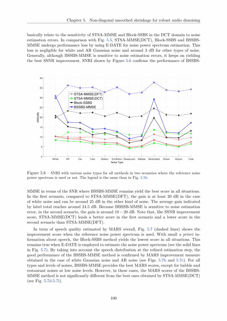
Chapter 5. Non-diagonal smoothed shrinkage for robust audio denoising
basically relate to the sensitivity of STSA-MMSE and Block-SSBS in the DCT domain to noiseestimation errors. In comparison with Fig. 5.5, STSA-MMSE(DCT), Block-SSBS and BSSBS-MMSE undergo performance loss by using E-DATE for noise power spectrum estimation. Thisloss is negligible for white and AR Gaussian noise and around 3 dB for other types of noise.Generally, although BSSBS-MMSE is sensitive to noise estimation errors, it keeps on yieldingthe best SSNR improvement. SNRI shown by Figure 5.6 confirms the performance of BSSBS-
Noise Type
White AR Car Train Station Exhibition Restaurant Babble Modulated Street Airport Total
SN
RI(
dB
)
0
5
10
15
20
25
30
35
40
STSA-MMSE(DFT)
STSA-MMSE(DCT)
Block-SSBS
BSSBS-MMSE
Figure 5.6 – SNRI with various noise types for all methods in two scenarios where the reference noisepower spectrum is used or not. The legend is the same than in Fig. 5.5b.
MMSE in terms of the SNR where BSSBS-MMSE remains yield the best score in all situations.In the first scenario, compared to STSA-MMSE(DFT), the gain is at least 20 dB in the caseof white noise and can be around 25 dB in the other kind of noise. The average gain indicatedby label total reaches around 24.5 dB. Because BBSSB-MMSE is sensitive to noise estimationerror, in the second scenario, the gain is around 10 − 20 dB. Note that, like SSNR improvementscore, STSA-MMSE(DCT) leads a better score in the first scenario and a lower score in thesecond scenario than STSA-MMSE(DFT).
In term of speech quality estimated by MARS overall, Fig. 5.7 (dashed lines) shows theimprovement score when the reference noise power spectrum is used. With small a priori in-formation about speech, the Block-SSBS method yields the lowest score in all situations. Thisremains true when E-DATE is employed to estimate the noise power spectrum (see the solid linesin Fig. 5.7). By taking into account the speech distribution at the refined estimation step, thegood performance of the BSSBS-MMSE method is confirmed by MARS improvement measureobtained in the case of white Gaussian noise and AR noise (see Figs. 5.7b and 5.7c). For alltypes and levels of noises, BSSBS-MMSE provides the best MARS scores, except for babble andrestaurant noises at low noise levels. However, in these cases, the MARS scores of the BSSBS-MMSE method is not significantly different from the best ones obtained by STSA-MMSE(DCT)(see Fig. 5.7d-5.7i).
100

5.3. Experimental Results
STSA−MMSE(DFT)STSA−MMSE(DCT)Block−SSBSBSSBS−MMSE
(a) Legend
0 5 10 150
2
4
6
8
SNR (dB)M
AR
So
vl Im
pro
ve
me
nt
(b) White
0 5 10 150
2
4
6
8
SNR (dB)
MA
RS
ovl Im
pro
ve
me
nt
(c) AR
0 5 10 150
1
2
3
4
5
6
7
SNR (dB)
MA
RS
ovl Im
pro
vem
ent
(d) Car
0 5 10 150
1
2
3
4
5
6
7
SNR (dB)
MA
RS
ovl Im
pro
vem
ent
(e) Train
0 5 10 150
1
2
3
4
5
6
7
SNR (dB)M
AR
Sovl Im
pro
vem
ent
(f) Station
0 5 10 150
1
2
3
4
5
6
7
SNR (dB)
MA
RS
ovl Im
pro
vem
ent
(g) Exhibition
0 5 10 15−1
0
1
2
3
4
5
6
7
SNR (dB)
MA
RS
ovl Im
pro
vem
ent
(h) Restaurant
0 5 10 150
1
2
3
4
5
6
7
SNR (dB)
MA
RS
ovl Im
pro
vem
ent
(i) Babble
0 5 10 150
2
4
6
8
SNR (dB)
MA
RS
ovl Im
pro
ve
ment
(j) Modulated white
0 5 10 150
1
2
3
4
5
6
7
SNR (dB)
MA
RS
ovl Im
pro
vem
ent
(k) Street
0 5 10 150
2
4
6
8
SNR (dB)
MA
RS
ovl Im
pro
ve
ment
(l) Airport
Figure 5.7 – Speech quality evaluation after speech denoising: improvement of MARSovrl compositecriterion. The legend is shown in Figure 5.7a.
101

Chapter 5. Non-diagonal smoothed shrinkage for robust audio denoising
When combining denoising with E-DATE noise estimation, the MARS overall improvementis presented in Fig. 5.7 by solid lines. It turns out that the speech quality obtained by STSA-MMSE(DFT) is not really affected by errors in the noise spectrum estimation (compare thedashed lines to solid line in Fig. 5.7). In contrast, for non-stationary noise, the sensitivity tonoise estimation errors mentioned above for methods carried out in the DCT domain is greater.Thereby, BSSBS-MMSE, STSA-MMSE(DCT) and STSA-MMSE(DFT) yield very similar re-sults for this type of noise, especially at low and medium SNR levels (see Figs. 5.7e-5.7i). Forstationary noise, Figs. 5.7b and 5.7c show that the BSSBS-MMSE method remains better thanthe other methods, without real performance loss due to noise spectrum estimation by E-DATE.
In terms of speech intelligibility, the intelligibility score (IS) obtained by mapping the STOImeasure is shown in Figs. 5.8. At high SNR, the scores obtained by all the methods are notsignificantly different. At low SNR and in presence of AR and white Gaussian noise, Block-SSBS and BSSSBS-MMSE behave similarly in the two scenarios (with and without referencenoise power spectrum). For non-stationary noises and when using the reference noise spectrum,BSSBS-MMSE yields the highest scores. In comparison with the worst results, the gain is around10 − 15%. When noise spectrum is estimated by E-date, the best performance is attained byBlock-SSBS. In comparison to the STSA-MMSE(DFT) method, BSSBS-MMSE provides oftenbetter score in the case of non-stationary noise with a gain 5−15%, whereas Block-SSBS methodleads to the improvement 10 − 20% (see Figs. 5.8h, 5.8l and 5.8i).
Summarily, the BSSBS-MMSE method achieves a better trade-off between speechquality and intelligibility than the other methods.
5.3.2.2 Subjective Test
We have also conducted a subjective test for comparing two methods namely BSSBS-MMSE andSTSA-MMSE(DFT). This test was performed with ten listeners using the mean opinion score(MOS) method recommended by the IEEE Subcommittee [88]. Two SNR noise levels namely5dB and 10 dB and three different kinds of noise from stationary white noise to speech-likenon-stationary babble noise up to fast-changing non-stationary street noise are used.
The results obtained with different noise types and SNR values are compiled in Table 5.1. Foreach scenario, noise types and considered noise level, the best results are shown in boldface. In
Table 5.1 – MOS obtained with BSSBS-MMSE and STSA-MMSE(DFT) in the two scenarios
Reference noise E-DATESTSA-MMSE SBSSB-MMSE STSA-MMSE SBSSB-MMSE
White5 dB 2.35 2.4 2.15 2.3110 dB 2.80 3.00 2.78 2.78
Street5 dB 2.1 2.68 1.73 2.3510 dB 3.08 3.2 2.73 2.85
Babble5 dB 2.53 2.88 2.05 1.7510 dB 3.23 3.25 2.28 2.98
the first scenario, BSSBS-MMSE yields a better score than STSA-MMSE(DFT) in all situations.In the second scenario, at 5 dB SNR level, for babble noise, MMSE-STSA leads to better scores,whereas, for the other case, BSSBS-MMSE provides similar or better results than the STSA-MMSE(DFT).
102

5.3. Experimental Results
STSA−MMSE(DFT)STSA−MMSE(DCT)Block−SSBSBSSBS−MMSE
(a) Legend
0 5 10 1575
80
85
90
95
100
SNR (dB)IS
(b) White
0 5 10 1560
70
80
90
100
SNR (dB)
IS
(c) AR
0 5 10 1570
75
80
85
90
95
100
SNR (dB)
IS
(d) Car
0 5 10 1565
70
75
80
85
90
95
100
SNR (dB)
IS
(e) Train
0 5 10 1565
70
75
80
85
90
95
100
SNR (dB)IS
(f) Station
0 5 10 1580
85
90
95
100
SNR (dB)
IS
(g) Exhibition
0 5 10 1565
70
75
80
85
90
95
100
SNR (dB)
IS
(h) Restaurant
0 5 10 1550
60
70
80
90
100
SNR (dB)
IS
(i) Babble
0 5 10 1560
70
80
90
100
SNR (dB)
IS
(j) Modulated White
0 5 10 1570
75
80
85
90
95
100
SNR (dB)
IS
(k) Street
0 5 10 1570
75
80
85
90
95
100
SNR (dB)
IS
(l) Airport
Figure 5.8 – Speech intelligibility evaluation after speech denoising: Intelligibility score by mappingSTOI criterion.
103

Chapter 5. Non-diagonal smoothed shrinkage for robust audio denoising
5.3.3 Music data set
For demonstrating the robustness and universality of our algorithms, we also assessed our pro-posed method on music audio signal recorded from the solo wind instrument (oboe). Experimentshave been realized with 6 types of noise (White, car, train, babble, street and airport noise) andat 4 levels (0, 5, 10 and 15 dB). The music signal is sampled at 11kHz and transformed intotime-frequency domain by using 50ms frames with 50% overlapped Hamming windows. Thereference noise power spectrum as given in section above is also used.
5.3.3.1 Objective criterion
In order to evaluate the algorithm performance, we used the SSNR criterion for the objectivetest. The results are shown in the Figure 5.9. For white noise displayed by Figure 5.9a, atlow SNR levels, Block-SSBS and BSSBS-MMSE yield similar and better measures than STSA-MMSE(DFT) and STSA-MMSE(DCT) with gains of 3 dB. At high SNR levels, Block-SSBSleads to the best score with a gain of 4.5 dB in comparison to STSA-MMSE(DFT). The samebehavior for car, train and airport noise is seen in Figures 5.9b, 5.9c and 5.9e. For street andbabble noise, in all situations, Block-SSBS achieves the best score (see Figures 5.9d and 5.9f),albeit with lower gain compared to BSSBS-MMSE. Note that as for speech data set, when usingthe reference noise, STSA-MMSE(DCT) outperforms slightly the STSA-MMSE(DCT).
In conclusion, Block-SSBS gives the best score in terms of SSNR for most sit-uations, with a gain in range 0.5 − 6 dB in comparison to the reference method.Although BSSBS-MMSE provides a lower score than Block-SSBS, which is a non-parametric method, there is not much difference.
5.3.3.2 Subjective criterion
For further analyzing the robustness of the semi-parametric approach, we have also performedsubjective test on the same music database with 15 raters some of them being music players.We consider only the white noise (5 and 10 dB) where its power spectral can be theoreticallydetermined at two SNR levels. Moreover, this subjective test has been conducted for comparingBSSBS-MMSE to STSA-MMSE(DFT).
The MOS score obtained is given by Table 5.2. In each element, the first number is theaverage score and the second couple numbers is the 95% confidence interval (CI). In two SNRlevels, SSBS-MMSE provides a higher average score and also the CI than STSA-MMSE(DFT).This result confirms the relevance of BSSBS-MMSE for audio signal denoising.
Table 5.2 – MOS for music signal obtained with BSSBS-MMSE and STSA-MMSE(DFT)
STSA-MMSE(DFT)(CI) SBSSB-MMSE (CI)
5 dB 2.78 ([2.65 2.91]) 3.82 ([3.67 3.97])
10 dB 3.21 ([3.09 3.34]) 4.02 ([3.89 4.16])
5.4 Conclusion
In this chapter, we have introduced several speech denoising methods in the DCT domain,which makes it possible to get rid of the phase estimation problem. These methods are Block-SSBS, STSA-MMSE(DCT) and BSSBS-MMSE. Block-SSBS is non-parametric and can be seenas a smooth shrinkage of DCT coefficients. Its parameters are optimized by SURE and RDT
104

5.4. Conclusion
htp0 5 10 15
4
6
8
10
12
14
SNR (dB)
Se
gS
NR
Im
pro
ve
me
nt
STSA−MMSE(DFT)STSA−MMSE(DCT)Block−SSBSBSSBS−MMSE
(a) White
0 5 10 154
6
8
10
12
14
16
SNR (dB)
Se
gS
NR
Im
pro
ve
me
nt
(b) Car
0 5 10 153
4
5
6
7
8
9
10
11
SNR (dB)
SegS
NR
Im
pro
vem
ent
(c) Train
0 5 10 154
5
6
7
8
9
10
11
SNR (dB)
SegS
NR
Im
pro
vem
ent
(d) Street
0 5 10 154
5
6
7
8
9
10
11
12
SNR (dB)
SegS
NR
Im
pro
vem
ent
(e) Airport
0 5 10 153
4
5
6
7
8
9
10
SNR (dB)
SegS
NR
Im
pro
vem
ent
(f) Babble
Figure 5.9 – The SSNR improve for audio signal with the reference noise for 6 kinds of noise fromstationary noise (white) to slow-changing non-stationary noise (car and train noise) and up to speech-likeand fast-changing non-stationary noise (street, airport and babble noise).
105

Chapter 5. Non-diagonal smoothed shrinkage for robust audio denoising
approaches, which are also non-parametric methods for statistical inference. STSA-MMSE(DCT)is a Bayesian estimator. BSSBS-MMSE combines Block-SSBS and STSA-MMSE(DCT) so as tobenefit from the advantages of each method. Namely, Block-SSBS achieves good performancein terms of speech intelligibility by background noise reduction; STSA-MMSE improves speechquality by enhancing speech contained in small coefficients returned by the shrinkage.
The performance evaluation was conducted on the NOIZEUS database, with and withoutnoise power spectrum reference. Various types of stationary and non-stationary noises wereconsidered. When the noise spectrum is unknown, it is estimated by an up-to-date method. Inaddition, objective and subjective tests were used to assess the speech estimators, in comparisonto a reference approach. Subjective tests involved a statistically significant number of raters.The experimental results show that BSSBS-MMSE performs better than the other methods inmost situations. These experiments also confirm the relevance of working in the DCT domain.
The STSA-MMSE is devised under the Gaussian assumption for the Block-SSBS outcome.Asymptotic statistics could perhaps help justifying this assumption. However, the task seemsrather difficult and, in any case, the experimental results provide evidence that such a Gaussianassumption leads to an STSA-MMSE good enough to retrieve relevant speech contents in smallDCT coefficients.
All these results have proved the relevance of the proposed methods for speech signals. Notinghowever that the theoretical framework is based on very general assumptions, it can be wonderedwhether the proposed methods could be used to denoise other kinds of signals. As a proof ofconcept, these methods were applied here to denoise music signals. Subjective tests involvingseveral raters confirm these very good and promising results. They demonstrate the robustnessof the approaches independently of the nature of the signal of interest.
106

Part IV
Conclusion
107

108

6
Chapte
r
Conclusions and Perspectives
Good, better, best. Never let it rest. ’Til your good is better andyour better is best.
St. Jerome
6.1 Conclusion . . . . . . . . . . . . . . . . . . . . . . . . . . . . . . . . . . . . . . . 1106.2 Perspectives . . . . . . . . . . . . . . . . . . . . . . . . . . . . . . . . . . . . . . . 111
109

Chapter 6. Conclusions and Perspectives
6.1 Conclusion
The objective of this thesis work was to propose a complete speech enhancement system withinnovative techniques in signal processing for applications such as assisted listening for hearingaids, cochlear implants and voice communication applications with lack of resources. In suchareas of applications, the complete speech enhancement system should not only further enhancespeech quality but also speech intelligibility. Moreover, this system is expected to have lowcomputational cost, low power usage and operate without help of any database. In order toovercome these constraints, this research intended to investigate how far we can get in speechdenoising by using unsupervised statistical methods only, without resorting to psycho-acousticsor machine learning (supervised) based approach. In this respect and taking into account thelarge amount of results provided by the literature on the topic, this research involved bothparametric and non-parametric statistics for audio denoising, when the signal of interest isdegraded by uncorrelated and independent additive noise.
In the first part, noise power spectrum estimation, the main block of most single microspeech enhancement system, has been considered. We have proposed a novel method for noisepower spectrum estimation, called Extended-DATE (E-DATE). This method extends the d-dimensional amplitude trimmed estimator (DATE), originally introduced for additive whiteGaussian noise power spectrum estimation to the more challenging scenario of non-stationarynoise. The key idea is that, in each frequency bin and within a sufficiently short time period, thenoise instantaneous power spectrum can be considered as approximately constant and estimatedas the variance of a complex Gaussian noise process possibly observed in the presence of thesignal of interest. The proposed method relies on the fact that the Short-Time Fourier Transformof noisy speech signals is sparse in the sense that transformed speech signals can be representedby a relatively small number of coefficients with large amplitudes in the time-frequency domain.The E-DATE estimator is robust in that it does not require prior information about the signalprobability distribution except for the weak-sparseness property. In comparison to other state-of-the-art methods, the E-DATE is found to require the smallest number of parameters (onlytwo). Two practical implementations of E-DATE algorithm, namely the B-E-DATE and SW-E-DATE, achieve good performance with and without noise reduction. In general, the E-DATEestimator yields the most accurate noise power spectrum estimate for speech enhancement inpresence of various noise types and levels. This estimator has also shown its relevance for bothspeech quality and intelligibility improvement when incorporated into a complete system basedSTSA, a standard noise reduction algorithm. Although B-E-DATE is the straightforward block-based implementation of the E-DATE, but it entails an estimation delay. This can however becircumvented by resorting to the sliding window implementation SW-E-DATE.
After noise power spectrum estimation by E-DATE, Part III focused on noise reductiontechniques. We have considered two different approaches for recovering the signal of interest: aparametric one and a non-parametric one. In the two approaches, we exploited a joint detectionand estimation strategy to further remove or reduce background noise, without increasing thesignal distortion. This strategy was motivated by the fact that for the signal of interest in noisehas a sparse representation that can often be found on an appropriate orthogonal basis. Thus,the signal of interest can be reasonably assumed to be not always present in the time-frequencydomain. These two joint strategies have been applied to speech enhancement in a parametricand a semi-parametric approaches presented in Chapters 4 and 5, respectively. In Chapter 4,the approach is purely parametric, whereas Chapter 5 focuses on non-parametric approaches aswell as their combination with parametric statistics.
110

6.2. Perspectives
More specifically, in Chapter 4, we proposed some novel methods for estimating the STSAand LSA of speech. These methods are based on the combination of parametric detection andestimation theories. The main idea is to take into consideration speech presence and absencein each time-frequency bin for improving performance of minimum mean square error basedestimators. Optimal detectors have been derived where they enable to figure out the absence orpresence of speech in each time-frequency bin based on the estimators. Conversely, the estima-tors take into account the feedback from these detectors to improve them. Two signal modelsincluding strict and uncertain presence/absence of speech have been considered. Depending onthe signal model, the STSA was either forced to zero or replaced by a small spectral floor for re-ducing musical noise when speech absence has been detected. These methods have been assessedin two scenarios, that is, with and without reference noise power spectrum. The objective testsconfirmed the relevance of these approaches both in terms of speech quality and intelligibility.
Joint detection and estimation can be viewed as a form of Smoothed Sigmoid-Based Shrink-age (SSBS). For further improvement of performance and robustness in audio denoising, a semi-parametric approach was proposed in Chapter 5. As is well known, the narrowband Fouriertransform has good frequency resolution. Thus, most speech enhancement algorithms use it totransform the observed signal into the time-frequency domain. However, the Fourier coefficientsare complex so that these algorithms require phase spectrum estimation. To bypass this issue,Chapter 5 presents a novel estimator for estimating the amplitude of the speech coefficients inthe cosine time-frequency domain after discrete cosine transform (DCT). This estimator aimsat minimizing the mean square error of the absolute value of speech DCT coefficients. In orderto take advantage of both parametric and non-parametric approaches, Chapter 5 studies alsothe combination of block shrinkage and Bayesian statistical estimation. In such a combination,the absolute value of the clean coefficient is firstly estimated by block smoothed sigmoid-basedshrinkage (Block-SSBS). The block size required by Block-SSBS is obtained by statistical opti-mization via application of the SURE theorem. This step enables us to improve speech intelli-gibility as achieved by smoothed binary masking. In addition, it makes it possible to deal withvarious types of signals. Secondly, for refining the estimation, an optimal statistical estimatoris added to handle musical noise. For evaluating the performance of the proposed method, ob-jective as well as informal subjective test were used. The experiments described in this chapteryield promising results, both in terms of speech quality and intelligibility.
In summary, we have proposed several speech enhancement algorithms that are all based ona joint detection/estimation strategy. These enable us to improve quality and intelligibility, forspeech as well as audio signals, in comparison to standard estimators. Figure 6.1 displays allmethods in the plan of quality and intelligibility. Parametric methods (STSA-MMSE) provide ahigher score in terms of quality and a lower score of intelligibility than non-parametric approach(Block-SSBS). Semi-parametric approach allow us to take advantage of two methods. It is worthnoticing that, both parametric and semi-parametric approaches were exploited and that eachof them has been shown to have its own relevance. Therefore, depending on the consideredapplication, a suitable estimator should be chosen. The parametric estimators proposed above aremore efficient to reduce musical noise in speech enhancement, whereas non-parametric estimatorshave been shown to be more relevant to denoise other types of audio signal, like music forinstance.
6.2 Perspectives
Although the present work focused on noise reduction in speech enhancement systems using theDFT, it must be emphasized that the E-DATE estimator introduced in Chapter 3 is neither
111

Chapter 6. Conclusions and Perspectives
Intelligibility
Quality
BLOCK-
SSBS BSSBS-MMSE
JUM-STSA
STSA-MMSE DFT
IUM-STSA
SM-STSA
STSA-MMSE DCT
Figure 6.1 – A general view of all noise reduction methods based on STSA-MMSE considered in thisthesis.
restricted to the DFT domain nor to speech signals. Therefore, it could find other applicationsin any scenario where noisy signals have a weakly-sparse representation. For instance, we havesuccessfully considered the use of the E-DATE in the DCT in Chapter 5. For many signalsof interest, not limited to speech, such a weakly-sparse representation can be provided by anappropriate wavelet transform. In this respect, the application of the E-DATE algorithm toaudio source separation could be considered in continuation of [104]. The E-DATE estimatorfundamentally relies on the DATE estimator which, as emphasized in [65], can be regarded asan outlier detector. Consequently the E-DATE can also be used as an outlier detector in eachfrequency bin. This opens interesting perspectives in voice activity detection based on frequencyanalysis as well as in the detection and estimation of chirp signals in various types of noise.
In Chapter 4, to take into account the presence or absence of speech, a novel estimatorhas been proposed relying on joint detection and estimation. This estimator is based on STSAand LSA where a Gaussian distribution of DFT coefficients is assumed. But other distributionsfor the DFT coefficients could be investigated. In addition, in this chapter, several strategiesthat combine detection and estimation for improving the performance of Bayesian estimatorsin speech enhancement have been proposed. The efficiency of all these approaches is highlydependent on the quality of the detector. In addition, all detectors are based on the Gaussianassumption for speech signals. Because this assumption may not be satisfied, other types ofspeech detectors in each time-frequency bin could be considered. A promising approach in thisrespect is proposed in [4]. This detector is based on the RDT algorithm and can provide goodperformance without knowledge about the distribution of signal of interest as already discussedin Chapter 5. Therefore, the semi-parametric estimators could be paired with the RDT detectorin each time-frequency bin.
Chapter 5 investigated denoising methods using the DCT. Since it does not make any as-sumption on the signal of interest, Block-SSBS can be applied to other applications like imagedenoising. In this chapter, we also derived an STSA-MMSE in the DCT domain by making aGaussian assumption on the DCT coefficients. It is thus natural to wonder again whether otherdistributions could be more relevant for modeling DCT coefficients. In addition, it has been ob-served that although DCT has a real and more compact representation than DFT, Block-SSBS,
112

6.2. Perspectives
STSA-MMSE in the DCT domain and BSSBS-MMSE are more sensitive to noise estimationerrors than STSA-MMSE in the DFT domain. This point requires further investigation.
As a final note, it is worth noticing that all the speech enhancement methods exposed inthis thesis were proposed in the context of a single microphone and were based on statisticalapproaches only. As such, a few promising perspectives arise as a natural generalization ofour results. First and as discussed in the introduction, multi-microphone speech enhancementsystems can immediately apply and benefit from the proposed methods at the output of the beamformer. Second, the performance of our speech enhancement algorithms may be further improvedby incorporating perceptual information, in continuation of researches such as [139,140]. Finally,although we have restricted attention to unsupervised approaches, the proposed methods canbe used to post-process supervised approaches like the Wiener filter or the MMSE estimator.
113


Appendices
115

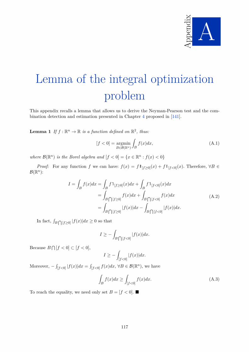
A
Appen
dix
Lemma of the integral optimization
problemThis appendix recalls a lemma that allows us to derive the Neyman-Pearson test and the com-bination detection and estimation presented in Chapter 4 proposed in [141].
Lemma 1 If f : Rn → R is a function defined on R2, thus:
[f < 0] = argminB∈B(Rn)
∫
Bf(x)dx, (A.1)
where B(Rn) is the Borel algebra and [f < 0] = x ∈ Rn : f(x) < 0
Proof: For any function f we can have: f(x) = f[f≥0](x) + f[f<0](x). Therefore, ∀B ∈B(Rn):
I =∫
Bf(x)dx =
∫
Bf[f≥0](x)dx+
∫
Bf[f<0](x)dx
=∫
B⋂
[f≥0]f(x)dx+
∫
B⋂
[f<0]f(x)dx
=∫
B⋂
[f≥0]|f(x)|dx−
∫
B⋂
[f<0]|f(x)|dx.
(A.2)
In fact,∫B⋂
[f≥0] |f(x)|dx ≥ 0 so that
I ≥ −∫
B⋂
[f<0]|f(x)|dx.
Because B⋂
[f < 0] ⊂ [f < 0],
I ≥ −∫
[f<0]|f(x)|dx.
Moreover, − ∫[f<0] |f(x)|dx =∫
[f<0] f(x)dx, ∀B ∈ B(Rn), we have
∫
Bf(x)dx ≥
∫
[f<0]f(x)dx. (A.3)
To reach the equality, we need only set B = [f < 0].
117


B
Appen
dix
Detection threshold under joint
detection and estimation
B.1 Strict model . . . . . . . . . . . . . . . . . . . . . . . . . . . . . . . . . . . . . . . 119B.2 Uncertain model . . . . . . . . . . . . . . . . . . . . . . . . . . . . . . . . . . . . 120
B.2.1 Independent estimators . . . . . . . . . . . . . . . . . . . . . . . . . . . . 120B.2.2 Joint estimator . . . . . . . . . . . . . . . . . . . . . . . . . . . . . . . . . 120
This appendix provides the computation of detection threshold in Chapter 4 based on Gaus-sian assumption.
B.1 Strict model
In the strict presence/absence model, the threshold τ can be chosen by fixing the false alarmprobability to a specified value. Thanks to the Gaussian assumption, the pdf of AY under H0 isRayleigh [1, p.212] and given by:
fAY(a;H0) =
2aσ2X
exp
(− a2
σ2X
). (B.1)
Consider the decision
|Y |D=1
RD=0
τ, (B.2)
The false alarm probability is:
PH0(D = 1) =∫ ∞
τ
2rσ2X
exp
(− r2
σ2X
)dr = exp
(− τ2
σ2X
). (B.3)
Therefore the threshold to guarantee a false alarm probability equal to α is
τSM(α) = σX
√− log(α) (B.4)
Therefore, the detection thresholds in the strict speech presence/absence model are determinedas follows:
τSMSTSA(α) = DSM
STSA(τSM(α)), (B.5)
τSSMLSA (α) = DSSM
LSA (τSM(α)). (B.6)
119

Appendix B. Detection threshold under joint detection and estimation
B.2 Uncertain model
Generally, in the uncertain model, the detection threshold τ is obtained by imposing R0(A1, A0,D) =α. In addition, in the uncertain model, the distribution of AY under hypothesis H0 is given by
fAY(a;H0) =
2aσ2X(1 + β)
exp
(− a2
σ2X(1 + β)
). (B.7)
However, for the sake of simplicity, we propose the different choices of the threshold for thecorresponding situations.
B.2.1 Independent estimators
In this situation, because D1(y;ψ1) = D0(y;ψ0), the choice of threshold τ does not affect A.Thus, focusing on the estimation problem and with regard to Equations (4.84) and (4.100), itseems coherent to choose τ IUM
STSA in the form of a likelihood ratio. In this respect, we propose tochoose:
τ IUMSTSA = τ IUM
LSA = Λ(ξ, γ0), (B.8)
where γ0 is the smallest a posteriori SNR above which we have a false alarm. Since the probabilitydensity function under H0 is given by Equation (B.7), Equation (B.2) can be rewritten as
γD=1
RD=0
−(1 + β) log(α), (B.9)
where α is the false probability. It follows that γ0 = −(1 + β) log(α).
B.2.2 Joint estimator
B.2.2.1 STSA-based estimator
In this section, the Bayesian risk under H0 is given by:
R0(A1, A0,D) =∫r10(y;ψ1)δ(y)fY (y;H0)dy +
∫r00(y;ψ0)(1 − δ(y))fY (y;H0)dy, (B.10)
where
r10(y;ψ1) =∫c10(ψ1, a0)fA0|Y=y(a0)da0 =
∫a2
0fA0|Y=y(a0)da0,
r00(y;ψ0) =∫c00(ψ0, a0)fA0|Y=y(a0)da0 = r10(y;ψ1) −
(ψ
JUM(0)STSA (y)
)2.
According to [1, Equation (7.94)], we have:
r10(y;ψ1) = E0[A20|Y = y] =
β
1 + β
(1 + νβγ
)|y|2 = G0|y|2, (B.11)
where νβ = γβ/(1 + β) and G0 =β
1 + β
(1 + νβγ
). Moreover (see Equation (4.88):
ψJUM(0)STSA (y) = GSTSA(β, γ)|y|. (B.12)
120

B.2. Uncertain model
The Bayesian risk under H0 is now
R0(A1, A0,D) =∫
AG0|y|2fY (y;H0)dy +
∫
Ac(G0 −G2
STSA(β, γ))|y|2fY (y;H0)dy (B.13)
where A is the critical region given by Equation (4.72). Theoretically, G0 and GSTSA(β, γ) aredependent on y. However, 0 ≤ β ≪ 1 so that G0 and GSTSA(β, γ) are smaller than 1. Wecan reasonably assume that G0 and GSTSA(β, γ) are independent on y. By taking into accountthat β is less than ξ, it follows from Equations (4.93) and (4.94) that the decision amounts tocomparing the absolute value of the observation to a threshold τ∗. Therefore, the Bayesian riskis approximated by:
R0(A1, A0,D) =G0
∫ ∞
τ∗
2r3
σ2X(1 + β)
exp
(− r2
σ2X(1 + β)
)dr
+ (G0 −G2STSA(β, γ))
∫ τ∗
0
2r3
σ2X(1 + β)
exp
(− r2
σ2X(1 + β)
)dr,
(B.14)
After a change of variable and an integration by parts, some routine algebra leads to:
R0(A1, A0,D) = σ2X(1+β)(G0−G2
STSA(β, γ))+(G2
STSA(β, γ)τ2∗ + σ2
X(1 + β))
exp
(− τ2
∗σ2X(1 + β)
).
By solving equality R0(A1, A0,D) = α, we can find τ∗(α). Therefore the detection thresholdτJUM
STSA(α) is given by:τJUM
STSA(α) = DJUMSTSA(τ∗(α)) (B.15)
B.2.2.2 LSA-based estimator
With the same methodology as above, we have first:
r10(y;ψ1) =∫
(log(a0 + 1))2fA0|Y=y(a0)da0,
r00(y;ψ0) =∫c00(ψ0, a0)fA0|Y=y(a0)da0 = r10(y;ψ1) −
(tJUM(0)LSA (y)
)2,
where tJUM(0)STSA (y) = log[GLSA(β, γ)|y| + 1]. The r10(y;ψ1) is hardly tractable in theory. In order
to evaluate R0(A1, A0,D), we can reasonably assume that A0 = β0AY where 0 ≤ β0 ≪ 1.Moreover, log(x+ 1) ≈ x with x ≪ 1. Therefore, according to Equation (B.11):
r10(y;ψ1) = G0|y|2
r00(y;ψ0) =(G0 −G2
LSA(β, γ))
|y|2,
In the similar way as section above,
R0(A1, A0,D) = σ2X(1+β)(G0−G2
LSA(β, γ))+(G2
LSA(β, γ)τ2∗ + σ2
X(1 + β))
exp
(− τ2
∗σ2X(1 + β)
).
where τ∗(α) is found by solving R0(A1, A0,D) = α. Thus, the detection threshold is given by:
τJUMLSA (α) = DJUM
LSA (τ∗(α)). (B.16)
121


C
Appen
dix
Semi-parametric approach
C.1 The unbiased estimate risk of block for Block-SSBS . . . . . . . . . . . . . . . . 123C.2 The MMSE gain function in the DCT domain . . . . . . . . . . . . . . . . . . . . 124
C.1 The unbiased estimate risk of block for Block-SSBS
In the block Bj , the estimate risk Rj in Equation 5.17 is calculated by SURE theorem given byEquation 5.16. We derive now this result. We consider first that the estimated risk is the sumof the three part following:
Rj1 = −Nσ2X(B), (C.1)
Rj2 = ‖y − S(y)‖22, (C.2)
Rj3 = 2σ2X(B)
N∑
n=1
∂Snyn
(y). (C.3)
The second part Rj2 is the difference between the estimated S and the observation Y. Readily,G(y) is a scalar gain so that this difference can be written as:
Rj2 = (1 −G(y))2 ‖y‖22. (C.4)
In the fact that Sn(y) = G(y)yn. Therefore the partial derivative∂Snyn
(y) can be calculated as:
∂Snyn
(y) =∂G(y)yn
yn +G(y). (C.5)
Moreover, the gain function in the Bj block can be explicitly expressed as a function of ynwhereas other are considered as the parameter. Thus, using the chain rule for computing thederivative, we have
∂G(y)yn
= τe−τ(
√γ−λ)
(1 + e−τ(
√γ−λ)
)2
12√γ
2ynNσ2
X(B)= τG(y) (1 −G(y))
yn√γNσ2
X(B), (C.6)
where the estimated a posteriori SNR γ = ‖y‖22
Nσ2X(B)
. The third part of the estimated block risk
is leaded to:
Rj3 = 2Nσ2X(B)G(y) + 2τG(y) (1 −G(y))
‖y‖22
N√γ. (C.7)
123

Appendix C. Semi-parametric approach
Taking the sum of the three part Rj1, Rj2 and Rj1, we obtain the estimated risk of the blockBj as Equation (5.17).
C.2 The MMSE gain function in the DCT domain
The gain function G(ξ, γ) for STSA-MMSE in the DCT domain is derived from Equation (5.27)by two ways and shown by Equation (5.30). This appendix section provides the computationaldetail of the direct method for calculating this gain function. Without the loss of generality, wesuppose that y ≥ 0 so that y = |y|. Let us denote,
I1± =∫ ∞
0a exp
(− a2
2σ2± ay
σ2X
)da, (C.8)
I2± =∫ ∞
0exp
(− a2
2σ2± ay
σ2X
)da, (C.9)
the nominator I1 and the denominator I2 of Equation (5.27) are respectively given by:
I1 = I1+ + I1−, (C.10)
I2 = I2+ + I2−. (C.11)
Moreover, we have
I1± =∫ ∞
0(−σ2)
(−aσ2
± y
σ2X
)exp
(− a2
2σ2± ay
σ2X
)da±
(yσ2
σ2X
)I2±. (C.12)
Therefore, the nominator can be written as I1 = I1+ + I1− = 2σ2 +
(yσ2
σ2X
)(I2+ − I2−). In
addition,
I2± =∫ ∞
0exp
−
(a√2σ2
∓ y√σ2
√2σ2
X
)2 exp
(σ2y2
2σ4X
)da. (C.13)
Thus, the denominator and the nominator can be evaluated as:
I2 = I2+ + I2− = 2√
2σ2 exp
(σ2y2
2σ4X
)∫ ∞
0exp(−t2)dt, (C.14)
I1 = 2σ2 +
(yσ2
σ2X
)(I2+ − I2−) = 2σ2 +
yσ2
σ2X
2√
2σ2 exp
(σ2y2
2σ4X
)∫ +y∗
−y∗
exp(−t2)dt, (C.15)
Considering the zero-mean Gaussian distribution with its variance equal to 1/2, its prob-
ability density function is φ(t) = e−t2
√π
. It makes possible that∫∞
0 exp(−t2)dt =√π/2 and
∫+y∗
−y∗ exp(−t2)dt =√π/2 erf(y∗). Replacing these results to Equations (C.14) and (C.15), we
can compute ψ(y) and G(ξ, γ) = ψ(y)/ |y|, Equation (5.30) is proved.
124

D
Appen
dix
Author Publications
(J-5) V.K. Mai, D. Pastor, A. Aissa-El-Bey, R. Le-Bidan, “MMSE-based Speech Enhancement:From Parametric to Non-Parametric Approaches”, in preparation.
(J-4) V.K. Mai, D. Pastor, A. Aissa-El-Bey, R. Le-Bidan, “Speech Enhancement with SpectralAmplitude and Log-Spectral amplitude Estimators Based on Joint Detection and Estima-tion”, IEEE/ACM Trans. Audio, Speech, Language Processing, in preparation.
(J-3) V.K. Mai, D. Pastor, A. Aissa-El-Bey, R. Le-Bidan, “Semi-Parametric Block Shrinkageand Application to Musical Audio Denoising”, IEEE Signal Processing Letters, submitted.
(J-2) V.K. Mai, D. Pastor, A. Aissa-El-Bey, R. Le-Bidan, “Robust Speech Denoising by Non-diagonal Smoothed Sigmoid-Based Shrinkage in the DCT Domain”, IEEE/ACM Trans.Audio, Speech, Language Processing, submitted.
(J-1) V.K. Mai, D. Pastor, A. Aissa-El-Bey, R. Le-Bidan, “Robust Estimation of Non-StationaryNoise Power Spectrum for Speech Enhancement.”, IEEE/ACM Trans. Audio, Speech, Lan-guage Processing, n. 23(4), pp. 670-682, 2015.
125

Bibliography[1] P. C. Loizou. Speech enhancement: theory and practice. CRC press, 2013.
[2] A. M. Atto, D. Pastor, and G. Mercier. Smooth sigmoid wavelet shrinkage for non-parametric estimation. In Proc. IEEE Int. Conf. Acoust. Speech, Signal Process., pages3265–3268, 2008.
[3] C. M. Stein. Estimation of the mean of a multivariate normal distribution. The annals ofStatistics, pages 1135–1151, 1981.
[4] D. Pastor and Q. T. Nguyen. Random distortion testing and optimality of thresholdingtests. IEEE Trans. Signal Process., 61(16):4161–4171, 2013.
[5] R. C. Hendriks, R. Heusdens, U. Kjems, and J. Jensen. On optimal multichannel mean-squared error estimators for speech enhancement. IEEE Signal Process. Lett., 16(10):885–888, 2009.
[6] R. C. Hendriks, T. Gerkmann, and J. Jensen. DFT-domain based single-microphone noisereduction for speech enhancement: A survey of the state of the art. Synthesis Lectures onSpeech and Audio Processing, 9(1):1–80, 2013.
[7] R. Le Bouquin-Jeannès, P. Scalart, G. Faucon, and C. Beaugeant. Combined noise andecho reduction in hands-free systems: A survey. IEEE Trans., Speech, Audio, Process.,9(8):808–820, 2001.
[8] M. R. Weiss, E. Aschkenasy, and T. W. Parsons. Study and development of the INTELtechnique for improving speech intelligibility. Technical report, DTIC Document, 1975.
[9] M Berouti, R Schwartz, and John Makhoul. Enhancement of speech corrupted by acousticnoise. In IEEE Int. Conf. Acoustics, Speech, Signal Process.(ICASSP), volume 4, pages208–211. IEEE, 1979.
[10] S. Kamath and P. C. Loizou. A multi-band spectral subtraction method for enhancingspeech corrupted by colored noise. In Proc. IEEE Int. Conf. Acoust. Speech, Signal Process.(ICASSP), volume 4, pages IV–4164. IEEE, 2002.
[11] M. T. Sadiq, N. Shabbir, and W. J. Kulesza. Spectral subtraction for speech enhancementin modulation domain. IJCSI Int. Journal, Computer, Science, 10(2), 2013.
[12] N. Upadhyay and A. Karmakar. Speech enhancement using spectral subtraction-typealgorithms: A comparison and simulation study. Procedia Computer Science, 54:574–584,2015.
[13] N. Wiener. Extrapolation, interpolation, and smoothing of stationary time series, volume 2.MIT press Cambridge, 1949.
126
Bibliography
[14] P. Scalart and J. VIEIRA FILH0. Speech enhancement based on a priori signal to noiseestimation. In Proc. IEEE Int. Conf. Acoust. Speech, Signal, Process. (ICASSP), volume 2,pages 629–632. IEEE, 1996.
[15] J. Chen, J. Benesty, Y. Huang, and S. Doclo. New insights into the noise reduction wienerfilter. IEEE Trans. audio, speech, and lang. process., 14(4):1218–1234, 2006.
[16] B. Xia and C. Bao. Wiener filtering based speech enhancement with weighted denoisingauto-encoder and noise classification. Speech Communication, 60:13–29, 2014.
[17] N. Upadhyay and R. Jaiswal. Single channel speech enhancement: Using wiener filteringwith recursive noise estimation. Procedia Computer Science, 84:22–30, 2016.
[18] M. Dendrinos, S. Bakamidis, and G. Carayannis. Speech enhancement from noise: Aregenerative approach. Speech Commun., 10(1):45–57, 1991.
[19] Y. Ephraim and H. L. Van Trees. A signal subspace approach for speech enhancement.IEEE Trans. Speech, Audio, Process., 3(4):251–266, 1995.
[20] J. Huang and Y. Zhao. A DCT-based fast signal subspace technique for robust speechrecognition. IEEE Trans. Speech, Audio, Process., 8(6):747–751, 2000.
[21] Y. Hu and P. C. Loizou. A generalized subspace approach for enhancing speech corruptedby colored noise. IEEE Trans. Speech, Audio, Process., 11(4):334–341, 2003.
[22] J. Sun, C.and Xie and Y. Leng. A signal subspace speech enhancement approach basedon joint low-rank and sparse matrix decomposition. Archives of Acoustics, 41(2):245–254,2016.
[23] U. Kjems, M. S. Pedersen, J. B. Boldt, T. Lunner, and D. Wang. Speech intelligibilityof ideal binary masked mixtures. In 18th Europ. Signal Process. Conf., pages 1909–1913.IEEE, 2010.
[24] N. Madhu, A. Spriet, S. Jansen, R. Koning, and J. Wouters. The potential for speechintelligibility improvement using the ideal binary mask and the ideal wiener filter in singlechannel noise reduction systems: Application to auditory prostheses. IEEE Trans. Audio,Speech, and Lang. Process., 21(1):63–72, 2013.
[25] R. Koning, N. Madhu, and J. Wouters. Ideal time–frequency masking algorithms lead todifferent speech intelligibility and quality in normal-hearing and cochlear implant listeners.IEEE Trans. Biomed. Eng., 62(1):331–341, 2015.
[26] R. McAulay and M. Malpass. Speech enhancement using a soft-decision noise suppressionfilter. IEEE Trans. Acoust. Speech, Signal Process., 28(2):137–145, 1980.
[27] Y. Ephraim and D. Malah. Speech enhancement using a minimum-mean square errorshort-time spectral amplitude estimator. IEEE Trans. Acoust. Speech, Signal Process.,32(6):1109–1121, 1984.
[28] Y. Ephraim and D. Malah. Speech enhancement using a minimum mean-square errorlog-spectral amplitude estimator. IEEE Trans. Acoust., Speech, Signal, Process., ASSP-33(2):443–445, Apr. 1985.
127

Bibliography
[29] T. Lotter and P. Vary. Speech enhancement by map spectral amplitude estimation usinga super-gaussian speech model. EURASIP J. applied, signal, process., 2005:1110–1126,2005.
[30] P. J. Wolfe and S. J. Godsill. Simple alternatives to the ephraim and malah suppressionrule for speech enhancement. In 2001. Proc. IEEE Signal Process. Workshop, Stat. SignalProcess.,, pages 496–499. IEEE, 2001.
[31] C. Breithaupt and R. Martin. MMSE estimation of magnitude-squared DFT coeffi-cients with supergaussian priors. In Proc. IEEE Int. Conf. Acoust. Speech, Signal Pro-cess.(ICASSP), volume 1, pages I–896. IEEE, 2003.
[32] I. Cohen. Speech enhancement using super-gaussian speech models and noncausal a priorisnr estimation. Speech commun., 47(3):336–350, 2005.
[33] B. Chen and P. C. Loizou. A laplacian-based MMSE estimator for speech enhancement.Speech commun., 49(2):134–143, 2007.
[34] J. S. Erkelens, R. C. Hendriks, R. Heusdens, and J. Jensen. Minimum mean-square errorestimation of discrete fourier coefficients with generalized gamma priors. IEEE Trans.Audio, Speech, Lang. Process., 15(6):1741–1752, 2007.
[35] P. C. Loizou. Speech enhancement based on perceptually motivated bayesian estimatorsof the magnitude spectrum. IEEE Trans. Speech, Audio, Process., 13(5):857–869, 2005.
[36] R. Martin. Speech enhancement based on minimum mean-square error estimation andsupergaussian priors. IEEE Trans. Speech, Audio, Process., 13(5):845–856, 2005.
[37] I. Cohen. Optimal speech enhancement under signal presence uncertainty using log-spectral amplitude estimator. IEEE Signal Process. Lett., 9(4):113–116, 2002.
[38] Y. Soon, S. N. Koh, and C. K. Yeo. Improved noise suppression filter using self-adaptiveestimator of probability of speech absence. Signal Process., 75(2):151–159, 1999.
[39] A. Abramson and I. Cohen. Simultaneous detection and estimation approach for speechenhancement. IEEE Trans. Audio, Speech, Lang. Process., 15(8):2348–2359, 2007.
[40] T. Sreenivas and P. Kirnapure. Codebook constrained wiener filtering for speech enhance-ment. IEEE Trans. Speech, Audio, Process., 4(5):383–389, 1996.
[41] S. Srinivasan, J. Samuelsson, and W. B. Kleijn. Codebook driven short-term predictorparameter estimation for speech enhancement. IEEE Trans. Audio, Speech, Lang. Process.,14(1):163–176, 2006.
[42] S. Srinivasan, J. Samuelsson, and W. B. Kleijn. Codebook-based bayesian speech en-hancement for nonstationary environments. IEEE Trans. Audio, Speech, Lang. Process.,15(2):441–452, 2007.
[43] Q. He, C. Bao, and F. Bao. Multiplicative update of ar gains in codebook-driven speechenhancement. In Proc. IEEE Int. Conf. Acoust. Speech, Signal Process. (ICASSP), pages5230–5234. IEEE, 2016.
[44] Y. Ephraim. A bayesian estimation approach for speech enhancement using hidden markovmodels. IEEE Trans. Signal, Process., 40(4):725–735, 1992.
128

Bibliography
[45] D. Y. Zhao and W. B. Kleijn. HMM-based gain modeling for enhancement of speech innoise. IEEE Trans. Audio, Speech, and Lang. Process., 15(3):882–892, 2007.
[46] H. Veisi and H. Sameti. Speech enhancement using hidden markov models in mel-frequencydomain. Speech Communication, 55(2):205–220, 2013.
[47] N. Mohammadiha, R. Martin, and A. Leijon. Spectral domain speech enhancement usingHMM state-dependent super-gaussian priors. IEEE Signal, Process. Lett., 20(3):253–256,2013.
[48] N. Mohammadiha and A. Leijon. Nonnegative HMM for babble noise derived from speechHMM: Application to speech enhancement. IEEE Trans. Audio, Speech, Lang. Process.,21(5):998–1011, 2013.
[49] J. Xu, Y.and Du, L. R. Dai, and C. H. Lee. An experimental study on speech enhancementbased on deep neural networks. IEEE Signal Process. Lett., 21(1):65–68, 2014.
[50] J. Xu, Y.and Du, L. R. Dai, and C. H. Lee. A regression approach to speech enhancementbased on deep neural networks. IEEE/ACM Trans. Audio, Speech,Lang. Process., 23(1):7–19, 2015.
[51] T. T. Vu, B. Bigot, and E. S. Chng. Combining non-negative matrix factorization anddeep neural networks for speech enhancement and automatic speech recognition. In Proc.IEEE Int. Conf. Acoust. Speech, Signal, Process., pages 499–503. IEEE, 2016.
[52] C. D. Sigg, T. Dikk, and J. M. Buhmann. Speech enhancement with sparse coding inlearned dictionaries. In Proc. IEEE Int. Conf. Acoust. Speech, Signal, Process., pages4758–4761. IEEE, 2010.
[53] C. D. Sigg, T. Dikk, and J. M. Buhmann. Speech enhancement using generative dictionarylearning. IEEE Trans. Audio, Speech, and Lang. Process., 20(6):1698–1712, 2012.
[54] Y. Zhou, H. Zhao, and T. Shang, L.and Liu. Immune K-SVD algorithm for dictionarylearning in speech denoising. Neurocomputing, 137:223–233, 2014.
[55] S. Mavaddaty, S. M. Ahadi, and S. Seyedin. Modified coherence-based dictionary learningmethod for speech enhancement. IET Signal Process., 9(7):537–545, 2015.
[56] K. W. Wilson, B. Raj, P. Smaragdis, and A. Divakaran. Speech denoising using nonneg-ative matrix factorization with priors. In Proc. IEEE Int. Conf. Acoust. Speech, Signal,Process. (ICASSP), pages 4029–4032, 2008.
[57] N. Mohammadiha, T. Gerkmann, and A. Leijon. A new linear MMSE filter for single chan-nel speech enhancement based on nonnegative matrix factorization. In IEEE WorkshopAppli. Signal Process. Audio, Acoust. (WASPAA), pages 45–48. IEEE, 2011.
[58] N. Mohammadiha, W. B. Kleijn, and A. Leijon. Gamma hidden markov model as aprobabilistic nonnegative matrix factorization. In 21st European Signal, Process. Conf.(EUSIPCO), pages 1–5. IEEE, 2013.
[59] K. Kwon, J. W. Shin, and N. S. Kim. Nmf-based speech enhancement using bases update.IEEE Signal, Process. Lett., 22(4):450–454, 2015.
129

Bibliography
[60] M. Aharon, M. Elad, and A. Bruckstein. K-SVD: An algorithm for designing overcompletedictionaries for sparse representation. IEEE Trans. signal, process., 54(11):4311–4322,2006.
[61] D. D. Lee and H. S. Seung. Algorithms for non-negative matrix factorization. In NIPS,pages 556–562, 2001.
[62] D. L. Donoho. De-noising by soft-thresholding. IEEE Trans. Inf. Theory, 41(3):613–627,1995.
[63] A. M. Atto, D. Pastor, and G. Mercier. Detection threshold for non-parametric estimation.Signal, Image and Video processing, 2(3):207–223, 2008.
[64] A. M Zoubir, V. Koivunen, Y. Chakhchoukh, and M. Muma. Robust estimation in signalprocessing: A tutorial-style treatment of fundamental concepts. IEEE Signal ProcessingMagazine, 29(4):61–80, 2012.
[65] D. Pastor and F. Socheleau. Robust estimation of noise standard deviation in presenceof signals with unknown distributions and occurrences. IEEE Trans. Signal, Process.,60(4):1545–1555, Apr. 2012.
[66] B. P. Rao. Nonparametric functional estimation. Academic press, 2014.
[67] G. V. Moustakides. Optimum joint detection and estimation. In Proc. IEEE Int. Inf.Theory, pages 2984–2988, 2011.
[68] G. V. Moustakides, G. H. Jajamovich, A. Tajer, and X. Wang. Joint detection and es-timation: Optimum tests and applications. IEEE Trans. Inf. Theory, 58(7):4215–4229,2012.
[69] P. Stoica and R. L. Moses. Introduction to spectral analysis, volume 1. Prentice hall UpperSaddle River, 1997.
[70] R. Martin. An efficient algorithm to estimate the instantaneous snr of speech signals. InProceeding of the Eurospeech, volume 93, pages 1093–1096, 1993.
[71] R. Martin. Spectral subtraction based on minimum statistics. In Proc. European, Signal,Process. Conf. (EUSIPCO), pages 1182–1185, 1994.
[72] M. Portnoff. Time-frequency representation of digital signals and systems based on short-time fourier analysis. IEEE Trans., Acoust., Speech, Signal Process., 28(1):55–69, 1980.
[73] R. Crochiere. A weighted overlap-add method of short-time fourier analysis/synthesis.IEEE Trans., Acoust., Speech, Signal Process., 28(1):99–102, 1980.
[74] S. Nawab, T. Quatieri, and J. Lim. Signal reconstruction from short-time fourier transformmagnitude. IEEE Trans., Acoust. , Speech, Signal Process., 31(4):986–998, 1983.
[75] D. Griffin and J. Lim. Signal reconstruction from short-time fourier transform magnitude.IEEE Trans., Acoust. , Speech, Signal Process., 32(2):236–243, 1984.
[76] G. T. Beauregard, X. Zhu, and L. Wyse. An efficient algorithm for real-time spectrograminversion. In Int. conf. digital audio eff. (DAFx), pages 116–118, 2005.
130

Bibliography
[77] N. Sturmel and L. Daudet. Signal reconstruction from stft magnitude: a state of the art.In Int. conf. digital audio eff. (DAFx), pages 375–386, 2011.
[78] J. H. L. Hansen and B. L. Pellom. An effective quality evaluation protocol for speechenhancement algorithms. In Proc. Int. Conf. Spoken Language (ICSLP), volume 7, pages2819–2822, 1998.
[79] S. R. Quackenbush, T. P. Barnwell, and M. A. Clements. Objective measures of speechquality. Prentice Hall, 1988.
[80] IUT. ITU recommendation, G. 160. Voice Enhancement Devices for Mobile Networks,2005.
[81] A. W. Rix, John G. Beerends, M. P. Hollier, and A. P. Hekstra. Perceptual evaluation ofspeech quality (PESQ)-a new method for speech quality assessment of telephone networksand codecs. In Proc. IEEE Int. Conf. Acoust. Speech, Signal Process., volume 2, pages749–752. IEEE, 2001.
[82] Y. Hu and P. C. Loizou. Evaluation of objective measures for speech enhancement. InProc. Interspeech, pages 1447–1450, 2006.
[83] Y. Hu and P. C. Loizou. Evaluation of objective quality measures for speech enhancement.IEEE Trans. Audio, Speech, Lang. Process., 16(1):229–238, 2008.
[84] M. Guéguin, R. Le Bouquin-Jeannès, V. Gautier-Turbin, G. Faucon, and V. Barriac. Onthe evaluation of the conversational speech quality in telecommunications. EURASIPJournal, Advances, Signal Process., 2008:93, 2008.
[85] ANSI. S3. 5-1997, methods for the calculation of the speech intelligibility index. NewYork: American National Standards Institute, 19:90–119, 1997.
[86] Ray L Goldsworthy and Julie E Greenberg. Analysis of speech-based speech transmis-sion index methods with implications for nonlinear operations. J. Acoust. Soc. Amer.,116(6):3679–3689, 2004.
[87] C. H. Taal, R. C. Hendriks, R. Heusdens, and J. Jensen. An algorithm for intelligibilityprediction of time–frequency weighted noisy speech. IEEE Trans. Audio, Speech, Lang.Process., 19(7):2125–2136, 2011.
[88] E. H. Rothauser, W. D. Chapman, N. Guttman, K. S. Nordby, H. R. Silbiger, G. E.Urbanek, and M. Weinstock. Ieee recommended practice for speech quality measurements.IEEE Trans. Audio Electroacoust., 17(3):225–246, 1969.
[89] V. K. Mai, D. Pastor, A. Aïssa-El-Bey, and R. Le-Bidan. Robust estimation of non-stationary noise power spectrum for speech enhancement. IEEE/ACM Trans. Audio,Speech, Lang. Process., 23(4):670–682, 2015.
[90] H. G. Hirsch and C. Ehrlicher. Noise estimation techniques for robust speech recognition.In Proc. IEEE Int. Conf. Acoust. Speech, Signal, Process. (ICASSP), volume 1, pages153–156, Detroit, Michigan, USA, May 1995.
[91] B. Ahmed and W. H. Holmes. A voice activity detector using the chi-square test. In IEEEInt. Conf. Acoust., Speech, Signal Process., volume 1, pages I–625, Montreal, Quebec,Canada, 2004.
131

Bibliography
[92] I. Cohen. Noise spectrum estimation in adverse environments: Improved minima controlledrecursive averaging. IEEE Trans. Speech, Audio, Process., 11(5):466–475, Sep. 2003.
[93] R. Martin. Noise power spectral density estimation based on optimal smoothing andminimum statistics. IEEE Trans. Speech, Audio Process., 9(5):504–512, Jul. 2001.
[94] I. Cohen and B. Berdugo. Noise estimation by minima controlled recursive averaging forrobust speech enhancement. IEEE Signal, Process. Lett., 9(1):12–15, Jan. 2002.
[95] S. Rangachari and P. C. Loizou. A noise-estimation algorithm for highly non-stationaryenvironments. Speech communications, 48(2):220–231, Feb. 2006.
[96] R. Yu. A low-complexity noise estimation algorithm based on smoothing of noise powerestimation and estimation bias correction. In Proc. IEEE Int. Conf. Acoust. Speech, Signal,Process. (ICASSP), pages 4421–4424, Taipei, Taiwan, Apr. 2009.
[97] T. Gerkmann and R. C. Hendriks. Unbiased MMSE-based noise power estimation with lowcomplexity and low tracking delay. IEEE Trans. Audio, Speech, Lang. Process., 20(4):1383–1393, May 2012.
[98] M. Souden, M. Delcroix, K. Kinoshita, T. Yoshioka, and T. Nakatani. Noise power spec-tral density tracking: A maximum likelihood perspective. IEEE Signal, Process. Lett.,19(8):495–498, Aug. 2012.
[99] V. Stahl, A. Fischer, and R. Bippus. Quantile based noise estimation for spectral sub-traction and wiener filtering. In Proc. IEEE Inter. Conf. Acoust., Speech, Signal Process.(ICASSP), volume 3, pages 1875–1878 vol.3, 2000.
[100] P.L. Davies and U. Gather. The identification of multiple outliers (with discussion). J.Amer. Statist. Assoc., (423):782 – 801, 1993.
[101] N. N. Lebedev. Special Functions and their Applications. Prentice-Hall, Englewood Cliffs,1965.
[102] D. Pastor. A theoretical result for processing signals that have unknown distributionsand priors in white gaussian noise. Computational Statistics & Data Analysis, CSDA,52(6):3167 – 3186, 2008.
[103] D. L. Donoho and J. M. Johnstone. Ideal spatial adaptation by wavelet shrinkage.Biometrika, 81(3):425–455, 1994.
[104] S. M. Aziz Sbai, A. Aïssa-El-Bey, and D. Pastor. Contribution of statistical tests tosparseness-based blind source separation. EURASIP journal, applied, signal, process., Jul.2012.
[105] S. M. Berman. Sojourns and extremes of stochastic processes. Wadsworth, Reading, MA,January 1992.
[106] S. Mallat. A wavelet tour of signal processing, second edition. Academic Press, 1999.
[107] R. J. Serfling. Approximations theorems of mathematical statistics. Wiley, 1980.
[108] A. M. Atto, D. Pastor, and G. Mercier. Detection thresholds for non-parametric estimation.Signal, Image, Video process., 2(3):207–223, February 2008.
132

Bibliography
[109] O. Yilmaz and Scott Rickard. Blind separation of speech mixtures via time-frequencymasking. IEEE Trans. Signal Process., 52(7):1830–1847, July 2004.
[110] D. Pastor and A. M. Atto. Wavelet shrinkage: from sparsity and robust testing to smoothadaptation; In Fractals and Related Fields, Eds: J. Barral & S. Seuret. Birkhaüser, 2010.
[111] R. C. Hendriks, J. Jensen, and R. Heusdens. Noise tracking using DFT domain subspacedecompositions. IEEE Trans. Audio, Speech, Lang. Process., 16(3):541–553, Mar. 2008.
[112] C. H. You, S. N. Koh, and S. Rahardja. β-order MMSE spectral amplitude estimation forspeech enhancement. IEEE Trans. Speech, Audio, Process., 13(4):475–486, 2005.
[113] E. Plourde and B. Champagne. Auditory-based spectral amplitude estimators for speechenhancement. IEEE Trans. Audio, Speech, Lang. Process., 16(8):1614–1623, 2008.
[114] B. J. Borgström and A. Alwan. Log-spectral amplitude estimation with generalized gammadistributions for speech enhancement. In Proc. IEEE Int. Conf. Acoust. Speech, Signal,Process., pages 4756–4759. IEEE, 2011.
[115] Ioannis Andrianakis and Paul R White. MMSE speech spectral amplitude estimators withchi and gamma speech priors. In Proc. IEEE Int. Conf. Acoust. Speech, Signal, Process.,volume 3, pages 1068–1071. IEEE, 2006.
[116] D. Malah, R. V. Cox, and A. J. Accardi. Tracking speech-presence uncertainty to improvespeech enhancement in non-stationary noise environments. In Proc. IEEE Int. Conf.Acoust. Speech, Signal, Process., volume 2, pages 789–792. IEEE, 1999.
[117] N. S. Kim and J. H. Chang. Spectral enhancement based on global soft decision. IEEESignal Process. Lett., 7(5):108–110, 2000.
[118] T. Gerkmann, C. Breithaupt, and R. Martin. Improved a posteriori speech presenceprobability estimation based on a likelihood ratio with fixed priors. IEEE Trans. Audio,Speech, Lang. Process., 16(5):910–919, 2008.
[119] Y. Hu and P. C. Loizou. Subjective comparison of speech enhancement algorithms. InProc. IEEE Int. Conf. Acoust. Speech, Signal Process., volume 1, pages I–1523–I–156.IEEE, 2006.
[120] P. C. Loizou and G. Kim. Reasons why current speech-enhancement algorithms do notimprove speech intelligibility and suggested solutions. IEEE Trans. Audio, Speech, Lang.Process., 19(1):47–56, 2011.
[121] J. Jensen and R. C. Hendriks. Spectral magnitude minimum mean-square error estimationusing binary and continuous gain functions. IEEE Trans. Audio, Speech, Lang. Process.,20(1):92–102, 2012.
[122] Y. Hu and P. C. Loizou. Techniques for estimating the ideal binary mask. In Proc. 11thInt. Workshop Acoust. Echo Noise Control, pages 154–157, 2008.
[123] H. V. Poor. An introduction to signal detection and estimation. Springer Science &Business Media, 2013.
[124] S. M Kay. Fundamentals of statistical signal processing, volume i: estimation theory. 1993.
133

Bibliography
[125] A. Papoulis and U. Pillai, S. Probability, random variables, and stochastic processes. TataMcGraw-Hill Education, 2002.
[126] A. Aziz-Sbaï, S. M.and Aïssa-El-Bey and D. Pastor. Contribution of statistical tests tosparseness-based blind source separation. EURASIP J. Adv. Signal, Process., 2012(1):1–15, 2012.
[127] G.V. Moustakides. Optimum joint detection and estimation. Technical Report SSP-2010-1, Department of Electrical and Computer Engineering University of Patras, GREEC,2010.
[128] Y. Soon, S. N. Koh, and C. K. Yeo. Noisy speech enhancement using discrete cosinetransform. Speech communication, 24(3):249–257, 1998.
[129] Saeed Gazor and Wei Zhang. Speech enhancement employing laplacian-gaussian mixture.IEEE Trans. Speech, Audio, Process., 13(5):896–904, 2005.
[130] K. R. Rao and P. Yip. Discrete cosine transform: algorithms, advantages, applications.Academic press, 2014.
[131] N. Ahmed, T. Natarajan, and K. R Rao. Discrete cosine transfom. IEEE trans., Comput.,(1):90–93, 1974.
[132] M. Elad. Sparse and redundant representations. Springer, 2010.
[133] R. Tavares and R. Coelho. Speech enhancement with nonstationary acoustic noise detec-tion in time domain. IEEE Signal Process. Lett., 23(1):6–10, 2016.
[134] T. T. Cai. Adaptive wavelet estimation: a block thresholding and oracle inequality ap-proach. Annals of statistics, pages 898–924, 1999.
[135] G. Yu, S. Mallat, and E. Bacry. Audio denoising by time-frequency block thresholding.IEEE Trans. Signal Process., 56(5):1830–1839, 2008.
[136] R. Tibshirani and L. Wasserman. Stein’s unbiased risk estimate. Course notes from“Statistical Machine Learning, Spring 2015”, pages 1–12, 2015.
[137] D. Pastor and A. M. Atto. Wavelet shrinkage: from sparsity and robust testing to smoothadaptation; In Fractals and Related Fields, Eds: J. Barral & S. Seuret. Birkhaüser, 2010.
[138] A. Jeffrey and D. Zwillinger. Table of integrals, series, and products. Academic Press,2007.
[139] A. Amehraye. Débruitage perceptuel de la parole. Ecole Nationale Supérieure des Télé-communications de Bretagne, Thèse de Doctorat, 2009.
[140] A. Amehraye, D. Pastor, A. Tamtaoui, and D. Aboutajdine. From maskee to audible noisein perceptual speech enhancement. Int., Journal, Signal, Process.,, 5(2):93–96, 2009.
[141] D. Pastor. Lecture notes on decesion theory. Ecole Nationale Supérieure des Télécommu-nications de Bretagne, Poly, 2016.
134

N° d’ordre : 2017IMTA0008
Résumé
Cette thèse traite d'un des problèmes les plus stimulants dans le
traitement de la parole concernant la prothèse auditive, où seulement
un capteur est disponible avec de faibles coûts de calcul, de faible
utilisation d'énergie et l'absence de bases de données. Basée sur les
récents résultats dans les deux estimations statistiques paramétriques
et non-paramétriques, ainsi que la représentation parcimonieuse. Cette
étude propose quelques techniques non seulement pour améliorer la
qualité et l'intelligibilité de la parole, mais aussi pour s'attaquer au
débruitage du signal audio en général.
La thèse est divisée en deux parties ; Dans la première partie, on
aborde le problème d'estimation de la densité spectrale de puissance
du bruit, particulièrement pour le bruit non-stationnaire. Ce problème
est une des parties principales du traitement de la parole du mono-
capteur. La méthode proposée prend en compte le modèle
parcimonieux de la parole dans le domaine transféré. Lorsque la
densité spectrale de puissance du bruit est estimée, une approche
sémantique est exploitée pour tenir compte de la présence ou de
l’absence de la parole dans la deuxième partie.
En combinant l'estimation Bayésienne et la détection Neyman-
Pearson, quelques estimateurs paramétriques sont développés et
testés dans le domaine Fourier. Pour approfondir la performance et la
robustesse de débruitage du signal audio, une approche semi-
paramétrique est considérée. La conjointe détection et estimation peut
être interprétée par Smoothed Sigmoid-Based Shrinkage (SSBS).
Ainsi, la méthode Bloc-SSBS est proposée afin de prendre en compte
les atomes voisinages dans le domaine temporel-fréquentiel. De plus,
pour améliorer fructueusement la qualité de la parole et du signal
audio, un estimateur Bayésien est aussi dérivé et combiné avec la
méthode Bloc-SSBS. L’efficacité et la pertinence de la stratégie dans le
domaine transformée cosinus pour les débruitages de la parole et de
l'audio sont confirmées par les résultats expérimentaux.
Mots clés: Enrichissement de la parole et de l'audio, Débruitage
statistique, Représentation parcimonieuse, Estimation paramétrique,
Combinaison de détection et estimation, Seuillage parcimonieux,
Estimation non-paramétrique
Abstract
This PhD thesis deals with one of the most challenging problem in
speech enhancement for assisted listening where only one micro is
available with the low computational cost, the low power usage and the
lack out of the database. Based on the novel and recent results both in
non-parametric and parametric statistical estimation and sparse
representation, this thesis work proposes several techniques for not
only improving speech quality and intelligibility and but also tackling the
denoising problem of the other audio signal.
In the first major part, our work addresses the problem of the noise
power spectrum estimation, especially for non-stationary noise, that is
the key part in the single channel speech enhancement. The proposed
approach takes into account the weak-sparseness model of speech in
the transformed model. Once the noise power spectrum has been
estimated, a semantic road is exploited to take into consideration the
presence or absence of speech in the second major part.
By applying the joint of the Bayesian estimator and the Neyman-
Pearson detection, some parametric estimators were developed and
tested in the discrete Fourier transform domain. For further improve
performance and robustness in audio denoising, a semi-parametric
approach is considered. The joint detection and estimation can be
interpreted by Smoothed Sigmoid-Based Shrinkage (SSBS). Thus,
Block-SSBS is proposed to take into additionally account the
neighborhood bins in the time-frequency domain. Moreover, in order to
enhance fruitfully speech and audio, a Bayesian estimator is also
derived and combined with Block-SSBS. The effectiveness and
relevance of this strategy in the discrete Cosine transform for both
speech and audio denoising are confirmed by experimental results.
Keywords: Speech and audio enhancement, Noise reduction, Spare
representation, Parametric estimator, Joint detection and estimation,
Sparse thresholding, Non-parametric estimator.