Available online at www.sciencedirect.com

ScienceDirect

Computer Speech and Language 28 (2014) 858–872

Speech energy redistribution for intelligibility improvement in noisebased on a perceptual distortion measure�

Cees H. Taal a,∗, Richard C. Hendriks b, Richard Heusdens b

a Leiden University Medical Center, ENT-Department, 2300 RC Leiden, The Netherlandsb Delft University of Technology, Signal Information & Processing Lab, Mekelweg 4, 2628 CD Delft, The Netherlands

Received 29 November 2012; received in revised form 24 September 2013; accepted 13 November 2013

Available online 7 December 2013

Abstract

A speech pre-processing algorithm is presented that improves the speech intelligibility in noise for the near-end listener. The

algorithm improves intelligibility by optimally redistributing the speech energy over time and frequency according to a perceptual

distortion measure, which is based on a spectro-temporal auditory model. Since this auditory model takes into account short-

time information, transients will receive more amplification than stationary vowels, which has been shown to be beneficial for

intelligibility of speech in noise. The proposed method is compared to unprocessed speech and two reference methods using an

intelligibility listening test. Results show that the proposed method leads to significant intelligibility gains while still preserving

quality. Although one of the methods used as a reference obtained higher intelligibility gains, this happened at the cost of decreased

quality. Matlab code is provided.

Crown Copyright © 2013 Published by Elsevier Ltd. All rights reserved.

Keywords: Near-end speech enhancement; Intelligibility improvement; Transients

1. Introduction

Speech intelligibility for the near-end listener can be affected by background noise from both sides of the commu-

nication channel (see Fig. 1). That is, the noise can come from both the far-end and the near-end. In order to eliminate

the negative impact of the far-end noise, one would typically apply a single-channel noise-reduction algorithm (see, for

example, Hendriks et al., 2013; Loizou, 2007 for an overview). However, the speech can also be pre-processed before

playback in order to become more intelligible in presence of the near-end background noise, which is the focus of this

work. Here we assume that a clean recording of the speech is available and that the far-end noise is successfully removed

with noise-reduction. A relevant application would be a train-station where the intelligibility of an announcement is

degraded by a passing train. To improve the speech intelligibility in a noisy environment, one obvious solution would

be to increase the level of the speech. However, at a certain point increasing the playback level may not be possible

anymore due to loudspeaker limitations. Moreover, unpleasant playback levels may be reached which are close to the

� This paper has been recommended for acceptance by Prof. R.K. Moore.∗ Corresponding author. Tel.: +31 715262408.

E-mail address: chtaal@gmail.com (C.H. Taal).

0885-2308/$ – see front matter. Crown Copyright © 2013 Published by Elsevier Ltd. All rights reserved.

http://dx.doi.org/10.1016/j.csl.2013.11.003

C.H. Taal et al. / Computer Speech and Language 28 (2014) 858–872 859

Speech

Background

Noise

Background

Noise

Listener

Near en dFar end

Noise

reductionPre-process

Fig. 1. The pre-process algorithm improves speech intelligibility for the near-end listener as a function of the near-end noise statistics. It is assumed

that a clean speech signal is available with far-end noise successfully removed by noise-reduction.

threshold of pain. An alternative approach would be to fix the speech energy and redistribute energy within the speech

signal over time and/or frequency.

One straightforward and effective approach for improving intelligibility of speech in noise is by boosting high

frequencies at a cost of lower frequencies. For example, Griffiths (1968) concluded already in 1968 that the long-term

average speech spectrum should be ‘whitened’, which effectively results in a strong amplification of high frequencies.

Positive effects of high-pass-filtering were also found in Griffiths (1968), Niederjohn and Grotelueschen (1976), Hall

and Flanagan (2010), Skowronski and Harris (2006). To further gain intelligibility improvements, linear filtering was

combined with dynamic range compression by Niederjohn and Grotelueschen (1976). Also dynamic range compression

without any form of high-pass filtering was found to improve speech intelligibility in noise (Rhebergen et al., 2009).

Other approaches are based on the fact that transient-like parts of speech signals, e.g., consonants, play an important

role in speech intelligibility. For example, Strange et al. (1983) showed that the center vowel in CVC words is almost

fully understandable based on the preceding and succeeding consonant only. Unfortunately, the energy of consonants

is relatively low compared to vowels and therefore, despite their importance, more vulnerable to noise. In line with

these findings are the experiments from Gordon-Salant (1986) and Hazan and Simpson (1998), which found significant

intelligibility improvements in noise for normal-hearing listeners by amplifying hand-annotated consonants. Similar

results were found with hearing-impaired listeners (Kennedy et al., 1998). To use these principles in a practical applica-

tion several methods are also available that automatically modify the vowel-consonant energy ratio, e.g., (Skowronski

and Harris, 2006; Huang et al., 2009; Jayan et al., 2008; Yoo et al., 2007).

Most of the high-frequency boosting and transient-detection methods are noise-independent, while noise-statistics

maybe available in an application scenario as illustrated in Fig. 1. Sauert and Vary therefore proposed several algorithms,

which do take into account the noise statistics (e.g. Sauert et al., 2006; Sauert and Vary, 2010a), to further improve

intelligibility. These methods improve objective speech intelligibility as predicted by the speech intelligibility index

(SII) (ANSI, 1997). Similar work based on the SII has been done more recently by Taal et al. (2013). Other methods

exploiting noise statistics are, for example, based on the masking effects of the auditory system (Brouckxon et al.,

2008) or a loudness perception model (Shin and Kim, 2007). Tang and Cooke investigated several strategies where

energy is relocated based on local SNRs (Tang and Cooke, 2010, 2011). Best results were obtained with a strategy

where only the high frequency regions (1800–7500) were amplified, when a local SNR <5 dB was observed.

In this work we propose a new method where speech energy is redistributed over time and/or frequency as a

function of the near-end noise statistics, based on a perceptual distortion measure. The time-span over which energy

is redistributed is flexible, such that the method can be used in both low-delay applications and applications where a

higher delay is tolerated. As we will show, speech intelligibility can be further improved when more delay is allowed

in the system. The results we present in this article extend existing work due to several reasons: (1) the considered

perceptual distortion measure (Taal and Heusdens, 2009; Taal et al., 2012) (see Section 2.1) takes into account short-time

information, which results in a higher sensitivity to transient regions compared to spectral-only models as in Brouckxon

et al. (2008), Shin and Kim (2007), Sauert et al. (2006), Sauert and Vary (2010a). When a delay is tolerated in the

system, the proposed method will therefore automatically distribute energy from vowels to transients as a function

of the noise statistics. (2) An analytic solution is provided to optimally redistribute speech energy relevant for the

perceptual distortion measure subject to a power constraint. This is different from the majority of algorithms (with the

exception of Griffiths, 1968; Sauert and Vary, 2010b), which instead normalize the speech signal heuristically after

860 C.H. Taal et al. / Computer Speech and Language 28 (2014) 858–872

processing which may result in suboptimal solutions. (3) Some algorithms are very effective in improving intelligibility

of speech in noise, while they may have poor speech quality (pleasantness or naturalness of speech). For example,

aggressive amplitude compression (Niederjohn and Grotelueschen, 1976) results in very unnatural speech but the SNR

can be lowered down to 15 dB while preserving intelligibility. The proposed method improves speech intelligibility

while preserving speech quality.

The remainder of this article is organized as follows. First, we will explain the proposed algorithm and the used

perceptual distortion measure in Section 2, followed by an evaluation and comparison of other reference methods in

Section 3. Finally, in Section 4, a discussion is provided followed by conclusions.

2. Proposed speech pre-processing algorithm

Let x denote a time-domain speech signal and x + ε a noisy version, where ε represents the far-end background

noise. We assume that in isolation, x is fully intelligible and that far-end noise is either absent or successfully removed

by a single-channel noise reduction algorithm. The distortion measure considered in this work, denoted by D (x, ε),

will inform us about the audibility of ε in the presence of x. Hence, a lower D value implies less audible noise and

therefore more audible speech. Our goal is to adjust the speech signal x such that D (x, ε) is minimized subject to

the constraint that the energy of the modified speech remains unchanged. First, in Section 2.1, more details will be

given about the considered distortion measure, after which in Section 2.2 we will formalize and solve the constrained

optimization problem. Section 2.3 will describe several implementation details, where in Section 2.4 some properties

of the algorithm are revealed.

2.1. Perceptual distortion measure

The perceptual distortion measure is based on the work from Taal and Heusdens (2009), Taal et al. (2012). There are

three important motivations why this particular distortion measure is used. (1) The measure takes into account a spectro-

temporal auditory model and therefore also considers the temporal envelope within a short-time frame (20–40 ms). As

a consequence, the distortion measure is more sensitive to transients than spectral-only models, e.g., as used in (Sauert

et al., 2006; Sauert and Vary, 2010a). (2) The measure fulfills certain mathematical properties, which makes it possible

to derive an analytic solution in the eventual constrained optimization problem (see Section 2.2) and (3) the measure

correlates well with the intelligibility of speech in noise (Taal et al., 2009).

To guide the reader, we give a brief summary of the perceptual distortion measure presented in Taal et al. (2012). The

basic structure for the distortion measure is shown in Fig. 2. First, a time–frequency (TF) decomposition is performed

on the speech and noise by segmentation into short-time (32 ms), 50% overlapping square-root Hann-windowed frames.

Then, a simple auditory model is applied to each short-time frame, which consists of an auditory filter bank followed

by the absolute squared and low-pass filtering per band, in order to extract a temporal envelope. Here, the filter bank

resembles the properties of the basilar membrane in the cochlea, while the envelope extraction stage is used as a crude

model of the hair-cell transduction in the auditory system.

Let hi denote the impulse response of the ith auditory filter and xm the mth short-time frame of the clean speech.

The output of their linear convolution at time sample n is denoted by xi,m(n) = (xm * hi)(n). Subsequently, the temporal

Fig. 2. Basic structure of the proposed perceptual distortion measure based on the work from Taal et al. (2012).

C.H. Taal et al. / Computer Speech and Language 28 (2014) 858–872 861

envelope is defined by (|xm,i|2 * hs)(n), where hs represents the smoothing low-pass filter. Similar definitions hold for

(|εm,i|2 * hs)(n). The audibility of the noise in presence of the speech, within one TF-unit, is determined by a per-sample

noise-to-signal ratio (Taal and Heusdens, 2009). By summing these ratios over time, an intermediate distortion measure

for one TF-unit is obtained denoted by lower-case d. That is,

d(xm,i, εm,i) =∑

n

(|εm,i|2 ∗ hs)(n)

(|xm,i|2 ∗ hs)(n)

, (1)

where n denotes the time index running over all samples within one short-time frame. To prevent divisions by very

small numbers only speech-active regions are considered in the eventual algorithm (see Section 2.2 for more details).

As an example, internal representations within one auditory filter are shown in Fig. 2 for a windowed noise realization

εm and a speech transient xm. Also, the point-wise division in Eq. (1) of the internal representations before summation

over n is shown in the figure. Due to the fact that the measure uses a per-sample (16 kHz) rather than a frame-based

noise-to-signal ratio, the measure is sensitive to the short-temporal structure. Note that the cutoff frequency of the

low-pass filter hs determines the sensitivity of the model toward temporal fluctuations within a short-time frame.

The distortion measure for the complete signal is then obtained by summing all the individual distortion outcomes

over time and frequency, which gives,

D(x, ε) =∑

m,i

d(xm,i, εm,i). (2)

2.2. Power-constrained speech-audibility optimization

To improve the speech audibility in noise, we minimize Eq. (2) by applying a TF-dependent gain function α which

redistributes the speech energy by scaling of the individual (perceptually) filtered frames, i.e., αm,ixm,i, where αm,i ≥ 0.

Only TF-units are modified where speech is present. This is done in order to prevent that a large amount of energy

would be redistributed to speech-absent regions. We consider a TF-unit to be speech-active when its energy is within

a 25 dB range of the TF-unit with maximum energy within that particular frequency band. Note that with the near-end

speech enhancement application the clean speech is available and voice activity detection is a relatively easy process

(in contrast to the detection of speech already corrupted by noise). The TF-description of the noise is assumed to be a

stochastic process denoted by Em,i and the speech deterministic (recall that the speech signal is known in the near-end

enhancement application). Hence, we minimize for the expected value of the distortion measure. Let L denote the set

of speech-active TF-units and ‖ · ‖ the ℓ2-norm, the problem can then be formalized as follows, which has to be solved

for ∀αm,i, {m, i} ∈ L,

αm,i = argminαm,i,{m,i}∈L

∑

{m,i}∈L

E[

d(αm,ixm,i, εm,i)]

s.t.∑

{m,i}∈L

∥

∥αm,ixm,i

∥

∥

2= r

, (3)

where r =∑

{m,i}∈L

∥

∥xm,i

∥

∥

2is the total power measured at the output of the auditory filters and E denotes the expected

value. Two important reasons exist for fixing the speech energy r rather than any other constraint, for example, based

on loudness: (1) typically, algorithms are compared with a listening test by fixing the SNR for which the used global

energy constraint is optimal.1 (2) The used constraint is mathematical tractable in contrast to complex loudness models

for which closed-form solutions may not exist, resulting in suboptimal and computational demanding methods, e.g.,

as in Shin and Kim (2007).

1 Since the gammatone filters are not perfectly orthogonal (e.g., as in a Fourier transform), the energy of the signal waveform is not mathematically

equal to the energy measured at the output of the auditory filters. However, these differences due to the non-orthogonal gammatone filters are relatively

small and are a good approximation of the actual energies used in determining the SNR at the waveform level.

862 C.H. Taal et al. / Computer Speech and Language 28 (2014) 858–872

Let λ denote a Lagrangian multiplier such that we can introduce the following cost function,

J =∑

{m,i}∈L

E[

d(αm,ixm,i, Em,i)]

+ λ

⎛

⎝

∑

{m,i}∈L

∥

∥αm,ixm,i

∥

∥

2− r

⎞

⎠ . (4)

Due to the linearity of the convolution in Eq. (1) and the assumption that α ≥ 0 we have that d (αx, y) = d (x, y) /α2.

Therefore, in order to minimize Eq. (4), we have to solve the following set of equations for α,

∂J

∂αm,i

= −2E[d(xm,i, Em,i)]

α3m,i

+ λ2αm,i

∥

∥xm,i

∥

∥

2= 0

∂J

∂λ=

∑

{m,i}∈L

α2m,i

∥

∥xm,i

∥

∥

2− r = 0

(5)

The solution is given by,

α2m,i =

rβ2m,i

∑

{m′,i′}∈Lβ2m′,i′

∥

∥xm′,i′∥

∥

2, (6)

where,

βm,i =

(

E[d(xm,i, Em,i)]∥

∥xm,i

∥

∥

2

)1/4

. (7)

In order to determine α, we have to compute the expected value E[d(xm,i, Em,i)], which can be expressed as follows,

E[d(xm,i, Em,i)] =∑

n

(E[|Em,i|2] ∗ hs)(n)

(|xm,i|2 ∗ hs)(n)

, (8)

Here we used the linearity of the convolution and the summation in order to move the expected value operator inside

the distortion measure. To simplify, we assume that the power-spectral density of the noise within the frequency range

of an (relatively narrow) auditory band is constant, i.e., has a ‘flat’ spectrum. As a consequence, the noise within an

auditory band can be modeled by Em,i = (wmNm,i) ∗ hi, where wm denotes the window function and Nm,i represents a

zero mean, i.i.d. stochastic process with variance E[N2m,i(n)] = σ2

m,i, ∀n. By combining this statistical model and the

numerator of Eq. (8) we have,

E[|Em,i|2(n)] = E

[

|∑

k

hi(k)wm(n − k)Nm,i(n − k)|2

]

=∑

k

h2i (k)w2

m(n − k)E[N2m,i(n − k)] = (h2

i ∗ w2m)(n)σ2

m,i. (9)

where h2i ∗ w2

m can be calculated offline and reused, and σ2m,i can be estimated with any noise power spectral density

(PSD) estimator from the field of single-channel speech enhancement (Loizou, 2007) (see next section for more details).

Here we use the method from Hendriks et al. (2010).

2.3. Implementation details

2.3.1. Optimization control

An exponential smoother is applied to αm,i in order to reduce variations which may negatively effect the speech

quality, that is,

α̂m,i = (1 − γ) αm,i + γα̂m−1,i, (10)

where good results were obtained with γ = 0.9. Note that the applied smoothing in Eq. (10) will also prevent that too

much energy is distributed to specific TF-units. Hence, large energy differences between TF-units, which may violate

C.H. Taal et al. / Computer Speech and Language 28 (2014) 858–872 863

some of the motivations for including the power constraint (loudspeaker limitations, unpleasant playback level), are

reduced significantly. In rare cases where specific TF-units receive too much amplification, the processed signal is

clipped within the available dynamic range.

2.3.2. Filterbank properties

The filter bank and the low-pass filter are applied by means of a point-wise multiplication in the DFT-domain with

real-valued, even-symmetric frequency responses. For the filter bank the approach as presented in van de Par et al.

(2005) is used and for the low-pass filter the magnitude response of a one-pole low-pass filter is used. A total amount

of 40 filters are considered spaced according the equivalent rectangular bandwidth (ERB) (Glasberg and Moore, 1990)

between 150 and 8000 Hz. Furthermore, the speech signal is reconstructed by addition of the scaled TF-units where a

square-root Hann-window is used for analysis/synthesis.

2.3.3. Estimation of noise statistics

As mentioned, a noise-tracker from the field of single-channel speech enhancement (i.e., estimating the underlying

clean speech given a noisy observation) is used for estimation of the noise PSD. However, three important differences

apply when using such a traditional noise-tracker in the field of near-end enhancement:

1. The noise realization which degrades the TF-units in the set L is a future event. Therefore only the noise PSD from

the last known time-frame can be used, which is estimated from previous time-frames. We assume that the noise is

stationary during the duration of L.

2. From Fig. 1 it is clear that the noise PSD tracker is applied on the processed speech plus noise rather than on the

clean unprocessed speech plus noise, where the latter equals the situation in single-channel noise reduction.

3. The transfer function from microphone to loudspeaker should be known in order to compensate for any introduced

delay and coloration of the signal. In our experiments this is ignored, however, this transfer function can be easily

measured offline and included in the algorithm.

Finally it is important to add that noise PSD estimation is significantly easier in the field of near-end enhancement

than in single-channel noise reduction, since we have access to the clean speech. Hence, a perfect voice activity detector

could also be used where noise statistics are estimated during speech pauses.

2.3.4. Algorithmic delay

The performance of the method depends on the amount of TF-units available in the set L. When this set contains

a larger span over time and/or frequency, a better redistribution of energy is possible and a lower final distortion as

defined in Eq. (2) can be expected. The delay of the proposed algorithm is directly related to the amount of future

time-frames in the set L with respect to the current time-frame. Increasing the lookahead in the set L will result in

a larger delay. Although the delay of the proposed method can be adjusted, depending on the application, we will

analyze the following two extreme situations in the remaining of the article: (1) L contains all speech-active TF-units

in one entire sentence (say approximately 3 s) (PROP1) and (2) L only contains the set of TF-units in one short-time

frame (32 ms) (PROP2). PROP1 is relevant in situations where the speech is pre-recorded and the noise is stationary.

Think of safety announcements in an airplane, traffic information in a train or navigation instructions in a car. Note

that the noise here is assumed to be stationary for the considered time-span, as would be the typically the case, e.g.,

on board of a plane. For real-time applications and situations where the noise is non-stationary the PROP2 algorithm

can be used, for example, as in mobile telephony, or public address systems. For PROP1 the noise PSD is based on

averaging estimated noise PSDs over several frames and sentences offline. The delay can be adjusted to anything in

between these extreme cases, for example, for mobile telephony where a limited amount of delay is not necessarily an

issue (ITU, 2003).

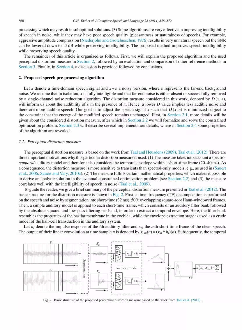
2.4. Effect of short-time information and algorithmic delay

The cutoff frequency of the auditory model low-pass filter hs (see Section 2.1) determines the temporal sensitivity

of the distortion measure. A higher cutoff frequency will result in a larger intermediate distortion value for transient

signals, and therefore the algorithm will distribute more energy to these regions. We investigated the amount of

864 C.H. Taal et al. / Computer Speech and Language 28 (2014) 858–872

−1

−0.5

0

0.5

1Unprocessed

−1

−0.5

0

0.5

1Processed (0 Hz)

−1

−0.5

0

0.5

1Processed (125 Hz)

−1

−0.5

0

0.5

1Processed (250 Hz)

0.2 0.3 0.4 0.5 0.6 0.7 0.8 0.9 1

0

5

10

Time Energy Redistribution

Time(s)

Am

plif

ica

tio

n(d

B) 0 Hz

125 Hz

250 Hz

Fig. 3. Unprocessed and processed (PROP1) speech signal for three different auditory model cutoff frequencies. The bottom plot indicates how the

energy is redistributed over time. Notice that transient parts are more amplified when the cutoff frequency is increased.

amplification received by transients as a function of the cutoff frequency. One example is shown in Fig. 3 for PROP1

with speech shaped (SSN) noise at −5 dB SNR, where processed clean speech signals are shown for three different cutoff

frequencies (0, 125 and 250 Hz). Here, a cutoff frequency of 0 Hz means that the short-time envelope is constant and

equals its average value. The bottom plot indicates how the energy is redistributed over time where energy differences

are calculated within individual short-time frames independently of frequency. Note that only 0.8 s of the entire 2.5 s

long speech signal is shown. Although transients are also amplified with a cutoff frequency of 0 Hz, (i.e., when using

no short-time information), this only results in small amplifications in the range of 3–6 dBs. In contrast, when we use a

cutoff frequency of 125 Hz, transients are amplified in the order of 6–12 dB. This is more in line with results based on

earlier research which found better results in this range (Gordon-Salant, 1986; Hazan and Simpson, 1998; Kennedy et al.,

1998; Skowronski and Harris, 2006). In the remainder of this article 125 Hz is therefore used for the cutoff frequency.

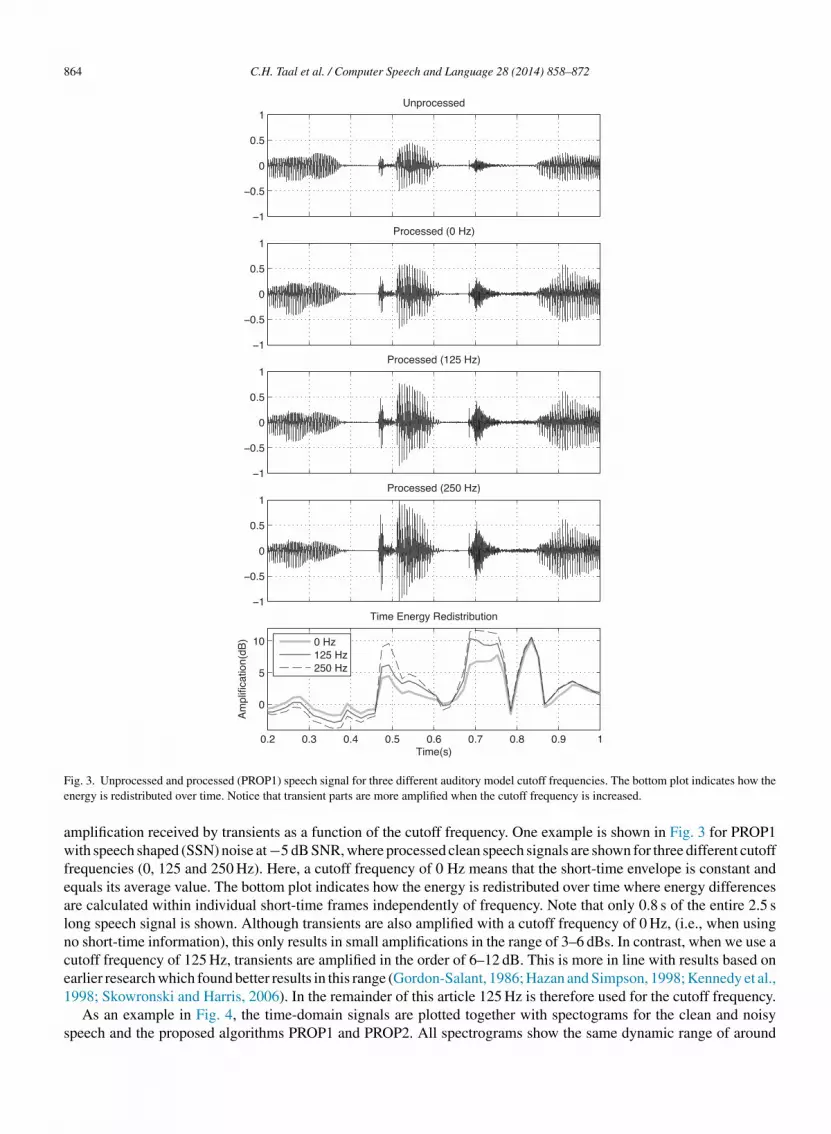
As an example in Fig. 4, the time-domain signals are plotted together with spectograms for the clean and noisy

speech and the proposed algorithms PROP1 and PROP2. All spectrograms show the same dynamic range of around

C.H. Taal et al. / Computer Speech and Language 28 (2014) 858–872 865

Fig. 4. Spectograms and time-domain plots for the clean speech, noisy speech, and noise with added processed speech (PROP1, PROP2). Here,

PROP1 redistributes energy over all TF-units and PROP2 only over frequency within one short-time frame.

45 dB where the energy of all speech signals (before noise addition) is equal. For this particular example one sentence

of speech is used with a length of around 2.5 s which is degraded with white noise at 5 dB SNR. From the noisy

speech spectrograms we can conclude that the high frequencies are almost fully masked by the noise. For example,

the transients at approximately 0.7 and 1.8 s are hardly visible anymore and can be expected to be inaudible due to

the negative effects of the noise. For PROP1 it can be observed that the transients are almost fully recovered, both in

the time domain and spectogram plots. Beside transient regions, the plots also reveal that PROP1 increases the high

frequencies of the vowel sounds at, e.g., 0.2 and 1 s. For PROP2, this amplification of high frequency vowel sounds is

also observed. However, the amplification of transient regions is not present with PROP2, since only energy could be

redistributed within one short-time frame. For both PROP1 and PROP2 low frequency regions (around 100–250 Hz)

are attenuated in order to accomplish the amplification of high frequencies.

3. Experimental evaluation

The proposed methods PROP1 and PROP2 are compared with two reference methods in terms of speech intelligibility

and speech quality. This includes the method as proposed by (Skowronski and Harris, 2006) based on changing the

vowel-consonant ratio referred to as energy redistribution voiced/unvoiced (ERVU). This particular method detects

transients based on the spectral flatness measure where the transient part is amplified by 7.4 dB. After transient

amplification the signal is normalized such that it has the same energy as the original speech signal. This method is

independent of the noise statistics.

Secondly, the ‘maximal power transfer’ method is included as proposed by Sauert et al. (2006) (SAU). This method

is based on the assumption that the human brain acts at least as intelligent as a Wiener filter. Let x̂m,k denote the kth

DFT-bin of the mth short-time frame for the clean speech and σ2n (m, k) the noise PSD. The gain function applied to

each DFT-bin is then given as follows,

α2m,k =

K1|x̂m,k|2

K1|x̂m,k|2 + σ2

n (m, k), (11)

866 C.H. Taal et al. / Computer Speech and Language 28 (2014) 858–872

−12.5 −10 −7.5 −50

10

20

30

40

50

60

70

80

90

100

SNR (dB)

Word

s c

orr

ect (%

)

UN

ERVU

PROP2

PROP1

SAU

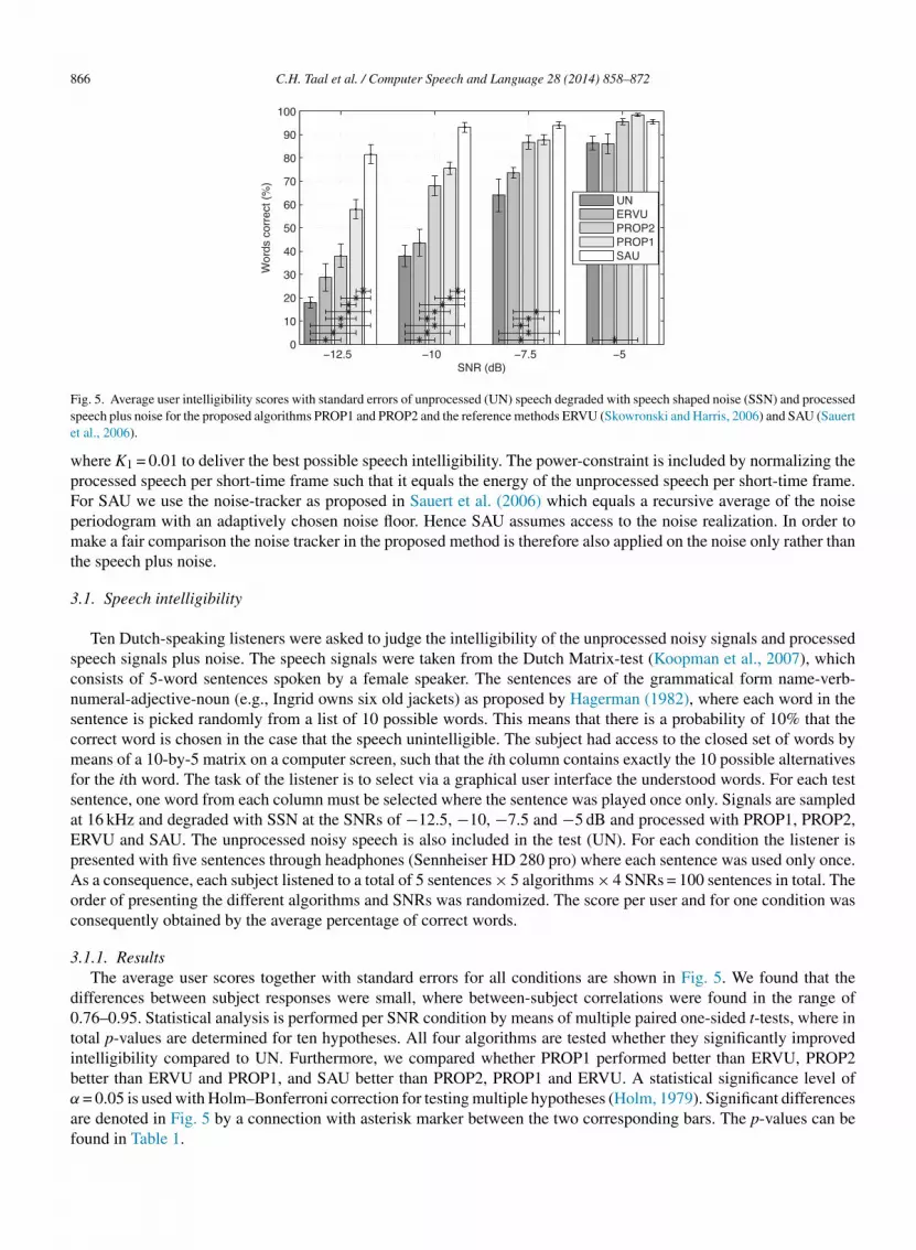
Fig. 5. Average user intelligibility scores with standard errors of unprocessed (UN) speech degraded with speech shaped noise (SSN) and processed

speech plus noise for the proposed algorithms PROP1 and PROP2 and the reference methods ERVU (Skowronski and Harris, 2006) and SAU (Sauert

et al., 2006).

where K1 = 0.01 to deliver the best possible speech intelligibility. The power-constraint is included by normalizing the

processed speech per short-time frame such that it equals the energy of the unprocessed speech per short-time frame.

For SAU we use the noise-tracker as proposed in Sauert et al. (2006) which equals a recursive average of the noise

periodogram with an adaptively chosen noise floor. Hence SAU assumes access to the noise realization. In order to

make a fair comparison the noise tracker in the proposed method is therefore also applied on the noise only rather than

the speech plus noise.

3.1. Speech intelligibility

Ten Dutch-speaking listeners were asked to judge the intelligibility of the unprocessed noisy signals and processed

speech signals plus noise. The speech signals were taken from the Dutch Matrix-test (Koopman et al., 2007), which

consists of 5-word sentences spoken by a female speaker. The sentences are of the grammatical form name-verb-

numeral-adjective-noun (e.g., Ingrid owns six old jackets) as proposed by Hagerman (1982), where each word in the

sentence is picked randomly from a list of 10 possible words. This means that there is a probability of 10% that the

correct word is chosen in the case that the speech unintelligible. The subject had access to the closed set of words by

means of a 10-by-5 matrix on a computer screen, such that the ith column contains exactly the 10 possible alternatives

for the ith word. The task of the listener is to select via a graphical user interface the understood words. For each test

sentence, one word from each column must be selected where the sentence was played once only. Signals are sampled

at 16 kHz and degraded with SSN at the SNRs of −12.5, −10, −7.5 and −5 dB and processed with PROP1, PROP2,

ERVU and SAU. The unprocessed noisy speech is also included in the test (UN). For each condition the listener is

presented with five sentences through headphones (Sennheiser HD 280 pro) where each sentence was used only once.

As a consequence, each subject listened to a total of 5 sentences × 5 algorithms × 4 SNRs = 100 sentences in total. The

order of presenting the different algorithms and SNRs was randomized. The score per user and for one condition was

consequently obtained by the average percentage of correct words.

3.1.1. Results

The average user scores together with standard errors for all conditions are shown in Fig. 5. We found that the

differences between subject responses were small, where between-subject correlations were found in the range of

0.76–0.95. Statistical analysis is performed per SNR condition by means of multiple paired one-sided t-tests, where in

total p-values are determined for ten hypotheses. All four algorithms are tested whether they significantly improved

intelligibility compared to UN. Furthermore, we compared whether PROP1 performed better than ERVU, PROP2

better than ERVU and PROP1, and SAU better than PROP2, PROP1 and ERVU. A statistical significance level of

α = 0.05 is used with Holm–Bonferroni correction for testing multiple hypotheses (Holm, 1979). Significant differences

are denoted in Fig. 5 by a connection with asterisk marker between the two corresponding bars. The p-values can be

found in Table 1.

C.H. Taal et al. / Computer Speech and Language 28 (2014) 858–872 867

Table 1

p-values for comparing intelligibility scores between algorithms.

SNR Method >UN >ERVU >PROP2 >PROP1

−12.5 ERVU 0.035 – – –

PROP1 0.002 0.062 – –

PROP2 0 0 0 –

SAU 0 0 0 0.001

−10 ERVU 0.217 – – –

PROP1 0 0.007 – –

PROP2 0 0 0.086 –

SAU 0 0 0 0

−7.5 ERVU 0.094 – – –

PROP1 0.01 0.001 – –

PROP2 0.005 0 0.346 –

SAU 0.001 0 0.037 0.046

−5 ERVU 0.549 – – –

PROP1 0.01 0.021 – –

PROP2 0.002 0.007 0.022 –

SAU 0.015 0.038 0.5 0.967

From the results we can conclude that for the lowest three SNRs, the algorithms have the same ranking in perfor-

mance. That is, all algorithms improve speech intelligibility compared to UN where SAU showed the best performance

followed by PROP1, PROP2 and ERVU. For the highest SNR of −5 dB results were slightly different, which is proba-

bly due to ceiling effects, i.e., most of the listeners had scores close to 100 percent. For the SNRs of −12.5 and −10 dB

all algorithms significantly improve speech intelligibility compared to UN, except for ERVU where the improvements

where not statistically significant. The fact that ERVU has a smaller effect on intelligibility compared to the other three

methods is expected, since it is only limited to changing the consonant-vowel ratio and not the spectrum of the speech

as a function of the noise, which is case with the other methods. Furthermore, as hypothesized in Section 2.2, we found

that in general PROP1 performs better than PROP2, where a significant improvement was found for −12.5 dB SNR.

This is a direct consequence of the fact that the energy can be distributed over the complete signal in PROP1 rather

than only within one short-time frame as with PROP2. Best performance was obtained with SAU which showed better

performance than all methods for the lowest three SNRs.

3.2. Speech quality

From the listening test results we can conclude that the proposed methods PROP1 and PROP2 both lead to intelligi-

bility improvements of the speech, when corrupted by SSN. However, we also found that one of the reference methods

(SAU) performed better than the proposed methods in terms of speech intelligibility. This result is remarkable since

SAU includes a power constraint within one short-time frame which implies a much lower algorithmic delay than

PROP1, which distributes energy over a complete sentence. One would expect better results with PROP1 since the

energy could be redistributed more efficiently over the complete signal rather than only one short-time frame.

Some of the subjects reported that specific conditions in the listening test contained speech which sounded very

unnatural. Motivated by this we also performed an initial evaluation in terms of subjective and objective predictions of

speech quality. It was hypothesized that the aggressive filtering of the SAU algorithm may come with a cost in terms

of speech quality.

3.2.1. Objective PESQ scores

Additional tests are performed to investigate the speech quality of the different methods. Speech quality is predicted

by PESQ (ITU, 2001; Rix et al., 2002) at SNRS within the range of −15 and 25 dB. The wideband version of

PESQ is used, which is standardized as ITU-T recommendation P.862.2 (ITU, 2005) and is suitable many different

degradations as typically encountered in telephony applications. This includes (non-)linear degradations which share

similar properties as the proposed algorithm, e.g., the addition of background noise, filtering (Beerends et al., 2002) and

applying TF-varying gain functions as used in noise reduction (Hu and Loizou, 2008) and source separation algorithms

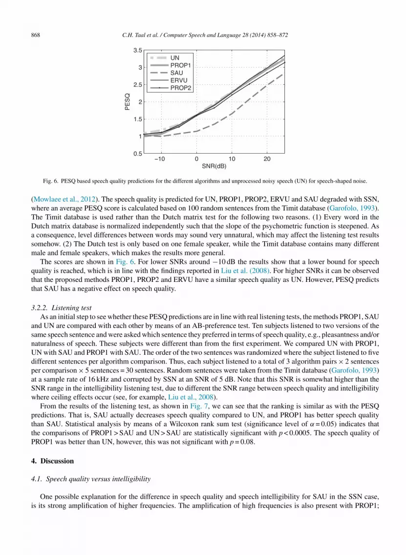
868 C.H. Taal et al. / Computer Speech and Language 28 (2014) 858–872

−10 0 10 200.5

1

1.5

2

2.5

3

3.5

SNR(dB)

PE

SQ

UN

PROP1

SAU

ERVU

PROP2

Fig. 6. PESQ based speech quality predictions for the different algorithms and unprocessed noisy speech (UN) for speech-shaped noise.

(Mowlaee et al., 2012). The speech quality is predicted for UN, PROP1, PROP2, ERVU and SAU degraded with SSN,

where an average PESQ score is calculated based on 100 random sentences from the Timit database (Garofolo, 1993).

The Timit database is used rather than the Dutch matrix test for the following two reasons. (1) Every word in the

Dutch matrix database is normalized independently such that the slope of the psychometric function is steepened. As

a consequence, level differences between words may sound very unnatural, which may affect the listening test results

somehow. (2) The Dutch test is only based on one female speaker, while the Timit database contains many different

male and female speakers, which makes the results more general.

The scores are shown in Fig. 6. For lower SNRs around −10 dB the results show that a lower bound for speech

quality is reached, which is in line with the findings reported in Liu et al. (2008). For higher SNRs it can be observed

that the proposed methods PROP1, PROP2 and ERVU have a similar speech quality as UN. However, PESQ predicts

that SAU has a negative effect on speech quality.

3.2.2. Listening test

As an initial step to see whether these PESQ predictions are in line with real listening tests, the methods PROP1, SAU

and UN are compared with each other by means of an AB-preference test. Ten subjects listened to two versions of the

same speech sentence and were asked which sentence they preferred in terms of speech quality, e.g., pleasantness and/or

naturalness of speech. These subjects were different than from the first experiment. We compared UN with PROP1,

UN with SAU and PROP1 with SAU. The order of the two sentences was randomized where the subject listened to five

different sentences per algorithm comparison. Thus, each subject listened to a total of 3 algorithm pairs × 2 sentences

per comparison × 5 sentences = 30 sentences. Random sentences were taken from the Timit database (Garofolo, 1993)

at a sample rate of 16 kHz and corrupted by SSN at an SNR of 5 dB. Note that this SNR is somewhat higher than the

SNR range in the intelligibility listening test, due to different the SNR range between speech quality and intelligibility

where ceiling effects occur (see, for example, Liu et al., 2008).

From the results of the listening test, as shown in Fig. 7, we can see that the ranking is similar as with the PESQ

predictions. That is, SAU actually decreases speech quality compared to UN, and PROP1 has better speech quality

than SAU. Statistical analysis by means of a Wilcoxon rank sum test (significance level of α = 0.05) indicates that

the comparisons of PROP1 > SAU and UN > SAU are statistically significant with p < 0.0005. The speech quality of

PROP1 was better than UN, however, this was not significant with p = 0.08.

4. Discussion

4.1. Speech quality versus intelligibility

One possible explanation for the difference in speech quality and speech intelligibility for SAU in the SSN case,

is its strong amplification of higher frequencies. The amplification of high frequencies is also present with PROP1;

C.H. Taal et al. / Computer Speech and Language 28 (2014) 858–872 869

SAU UN SAU0

20

40

60

80

100

Pre

fere

nce (

%)

PROP1 PROP1 UN

Fig. 7. Average users score of AB-preference listening test between the unprocessed noisy speech UN and the algorithms PROP1, SAU for speech

shaped noise degraded at 5 dB SNR. The error bars denote the standard error of the average user preference.

however, to a less extent. To get a better insight in these properties, the average spectra are plotted in Fig. 8 for the

unprocessed speech, the processed speech for SAU and PROP1 and the noise. The noise types consist of SSN (as used

in the experiments), white noise and noise from a bottling factory hall. Signals are mixed at −10 dB where 50 sentences

are used for estimating the spectrum.

For SSN it is indeed observed that the average spectrum of PROP1 is closer to the original speech and therefore may

sound more natural. However, these high frequencies with SAU are probably responsible for the good performance

in terms of intelligibility. From the remaining two spectra (white noise and bottling factory hall noise) we can clearly

see that SAU tends to give the speech spectrum the shape of the inverse noise spectrum. This is indeed in line with

−30

−20

−10

0

10

20

Le

ve

l (d

B)

Speech Shaped

−30

−20

−10

0

10

20

Le

ve

l (d

B)

White Noise

102

10 3

−30

−20

−10

0

10

20

Le

ve

l (d

B)

Frequency (kHz)

Bottling Factory

Noise

Speech

PROP1

SAU

Fig. 8. Average processed speech spectra for SAU and PROP1 plus unprocessed speech and noise spectra for different noise types.

870 C.H. Taal et al. / Computer Speech and Language 28 (2014) 858–872

0.4 0.5 0.6 0.7 0.80

20

40

60

80

100

STOI

Inte

llig

iblit

y(%

)

UN

PROP2

PROP1

30

40

50

60

70

80

Pre

dic

ted

In

telli

gib

lity (

ST

OI)

Delay (ms)PR

OP2

250

500

750

1000

PROP1

Fig. 9. STOI predictions versus listening test results (left) and predicted intelligibility by STOI for SSN, −12.5 dB SNR as a function of algorithmic

delay (right).

Eq. (11) where for low SNRs the gain function will be dominated by the inverse of the noise PSD. This is most visible

for the bottling factory noise where the strong high frequencies present in the noise (1000–2000 Hz) are attenuated in

the speech. From the spectra we also observe that SAU does not change the spectrum for the white noise, since the

inverse of this noise spectrum results in a flat gain function. Therefore, the benefits of SAU with SSN are not expected

with white noise. With PROP1 we observe a different effect for white noise, where the high frequencies of speech are

amplified instead. We know that amplifying high frequencies in the case of white noise improves speech intelligibility

(Griffiths, 1968; Niederjohn and Grotelueschen, 1976; Skowronski and Harris, 2006), therefore it is expected that

PROP1 will also improve intelligibility and therefore will show better performance than SAU for this particular noise

type. In the future, additional tests will be performed to test the algorithms for other noise types.

The PESQ scores in Fig. 6 show a lower-bound convergence around −10 dB. Here, the speech quality is probably

dominated by the low SNRs and the added noise, rather than the applied speech pre-processing algorithms. Moreover,

a ceiling effect can be observed with respect to speech intelligibility in Fig. 5 around −5 dB, where most of the

conditions result in almost fully intelligible speech. We would like to add that this SNR is relatively low because

the speech material is based on a closed set of words and is therefore more easy to understand. In the case of more

realistic sentence-based material the intelligibility can still be harmed at 5 dB (Hu and Loizou, 2007) and in the case

of non-native talkers this could even go up to 15 dB (van Wijngaarden et al., 2002) when perceived by native listeners.

Note that announcements by non-native talkers are very likely to happen at (international) airports and train stations.

In many applications a large range of SNRs can be expected. In a train station, for example, speech can become

unintelligible due to a passing train, while little far-end noise will be present outside rush hour. As a consequence,

the algorithm should have good performance in both quality and intelligibility over a wide range of SNRs like the

proposed method. For applications where speech is only presented at lower SNRs, or where speech quality is of

minor importance like military applications, one could argue that SAU should be preferred over the proposed methods.

However, as previously explained, this argument may not be valid for all noise types since it is expected that the

proposed method will result in higher intelligibility than SAU in the case of white noise.

4.2. Predicted intelligibility versus algorithmic delay

In the experiments performed in this article we included two extreme cases of the algorithm that is PROP1 and

PROP2, referring to a low and high algorithmic delay, respectively. As hypothesized, we found that increasing the

lookahead, and therefore the delay, leads to more intelligible speech in noise. An interesting question is how much

lookahead is needed in order to reach maximum intelligibility. To answer this question, an initial experiment is

performed where the speech intelligibility is predicted with STOI (Taal et al., 2011) as a function of algorithmic delay.

STOI is used for prediction since it gave high correlation for the conditions PROP1, PROP2 and UN in isolation

(ρ = 0.96) as shown in the left plot in Fig. 9. Here a scatter plot is shown between the STOI predictions and the actual

intelligibility scores of the listening test. A logistic function is fitted which will be used to map the STOI predictions

to intelligibility scores for other algorithmic delays.

C.H. Taal et al. / Computer Speech and Language 28 (2014) 858–872 871

In total 50 sentences of the Dutch matrix test (Koopman et al., 2007) are used, which are degraded with SSN at an

SNR of −12.5 dB, where we found the largest difference in intelligibility between PROP1 and PROP2 in the listening

test. We considered the following block lengths in which energy could be redistributed by the proposed method: 125,

250, 500, 750, and 1000 ms. Furthermore, the versions PROP1 (32 ms) and PROP2 (approximately 2–3 s) were also

included in the experiment. To prevent fast changing fluctuations between consecutive blocks, a 50% block overlap

together with a Hann window is used. The results are shown in the right plot in Fig. 9, from which we can conclude

that from around 500 ms the predicted intelligibility tends to converge to the performance of PROP1. These predictions

indicate that almost maximum intelligibility can be achieved for certain voice applications, e.g., international telephone

connection, when taking into account the maximum tolerated network delay of around 400 ms (ITU, 2003).

5. Conclusions

A speech pre-processing algorithm is presented to improve the speech intelligibility in noise for the near-end listener

without modifying the speech energy. This was accomplished by optimally redistributing the speech energy over time

and frequency based on a perceptual distortion measure. Due to the fact that the distortion measure takes into account

short-time information, transient signals, which are more important for speech intelligibility than vowels, receive more

amplification. The lookahead of the algorithm can be adjusted to the specific application. To verify the effect of this, two

extreme versions of the proposed method were considered: one with maximum lookahead, where energy is distributed

over time and frequency jointly for a complete sentence (PROP1), and one with minimum lookahead where energy is

redistributed over frequency within a short-time frame (PROP2). From the results we can conclude that the proposed

methods result in a large intelligibility improvement compared to the noisy unprocessed speech. PROP1 performed

better than PROP2 due to the fact that PROP1 contains a larger time-span, where a better redistribution of energy is

possible. However, this results in a larger algorithmic delay. The proposed methods were compared with a method

where transients were amplified (ERVU) and a method that redistributes energy over frequency within one short-time

frame (SAU). PROP1 and PROP2 resulted in higher intelligibility scores than ERVU. Best performance in terms of

speech intelligibility was obtained with SAU. However, additional tests reveal that the good performance of SAU comes

with a decrease in speech quality. PROP1 did not have a negative effect on speech quality. Matlab code of PROP1 and

PROP2 is provided at http://www.ceestaal.nl/.

Acknowledgements

The research is supported by the Oticon foundation, the Dutch Technology Foundation STW and the European

Commission within the Marie Curie ITN AUDIS, grant PITNGA-2008-214699.

References

ANSI, 1997. Methods for Calculation of the Speech Intelligibility Index, S3. 5-1997. American National Standards Institute, New York.

Beerends, J.G., Hekstra, A.P., Rix, A.W., Hollier, M.P., 2002. Perceptual evaluation of speech quality (PESQ): the new ITU standard for end-to-end

speech quality assessment. Part II. Psychoacoustic model. Journal of the Audio Engineering Society 50 (10), 765–778.

Brouckxon, H., Verhelst, W., Schuymer, B., 2008. Time and frequency dependent amplification for speech intelligibility enhancement in noisy

environments. In: Proc. Interspeech, pp. 557–560.

Garofolo, J., 1993. Timit: Acoustic–Phonetic Continuous Speech Corpus. National Institute of Standards and Technology (NIST).

Glasberg, B.R., Moore, B.C., 1990. Derivation of auditory filter shapes from notched-noise data. Hearing Research 47 (1), 103–138.

Gordon-Salant, S., 1986. Recognition of natural and time/intensity altered CVs by young and elderly subjects with normal hearing. Journal of the

Acoustical Society of America 80 (6), 1599–1607.

Griffiths, J.D., 1968. Optimum linear filter for speech transmission. Journal of the Acoustical Society of America 43 (1), 81–86.

Hagerman, B., 1982. Sentences for testing speech intelligibility in noise. Scandinavian Audiology 11 (2), 79–87.

Hall, J.L., Flanagan, J.L., 2010. Intelligibility and listener preference of telephone speech in the presence of babble noise. Journal of the Acoustical

Society of America 127 (1), 280–285.

Hazan, V., Simpson, A., 1998. The effect of cue-enhancement on the intelligibility of nonsense word and sentence materials presented in noise.

Speech Communication 24 (3), 211–226.

Hendriks, R.C., Gerkmann, T., Jensen, J., 2013. DFT-domain based single-microphone noise reduction for speech enhancement: a survey of the

state of the art. Synthesis Lectures on Speech and Audio Processing 9 (1), 1–80.

Hendriks, R.C., Heusdens, R., Jensen, J., 2010. MMSE based noise PSD tracking with low complexity. In: IEEE International Conference on

Acoustics, Speech and Signal Processing, pp. 4266–4269.

872 C.H. Taal et al. / Computer Speech and Language 28 (2014) 858–872

Holm, S., 1979. A simple sequentially rejective multiple test procedure. Scandinavian Journal of Statistics 6 (2), 65–70.

Hu, Y., Loizou, P.C., 2007. A comparative intelligibility study of single-microphone noise reduction algorithms. Journal of the Acoustical Society

of America 122 (3), 1777–1786.

Hu, Y., Loizou, P.C., 2008. Evaluation of objective quality measures for speech enhancement. IEEE Transactions on Audio Speech and Language

Processing 16 (1), 229–238.

Huang, D.-Y., Rahardja, S., Ong, E.P., 2009. Biologically inspired algorithm for enhancement of speech intelligibility over telephone channel. In:

IEEE International Workshop on Multimedia Signal Processing, pp. 1–6.

ITU, 2001. Perceptual evaluation of speech quality (pesq): an objective method for end-to-end speech quality assessment of narrow-band telephone

networks and speech codecs. ITU-T Recommendation P. 862.

ITU, 2003. One-way transmission time. ITU-T Recommendation G.114.

ITU, 2005. Wideband extension to recommendation P.862 for the assessment of wideband telephone networks and speech codecs. ITU-T Recom-

mendation P.862.2.

Jayan, A., Pandey, P., Lehana, P., 2008. Automated detection of transition segments for intensity and time-scale modification for speech intelligibility

enhancement. In: IEEE International Conference on Signal Processing, Communications and Networking, pp. 63–68.

Kennedy, E., Levitt, H., Neuman, A.C., Weiss, M., 1998. Consonant-vowel intensity ratios for maximizing consonant recognition by hearing-impaired

listeners. Journal of the Acoustical Society of America 103 (2), 1098–1114.

Koopman, J., Houben, R., Dreschler, W.A., Verschuure, J., 2007 June. Development of a speech in noise test (matrix). In: 8th EFAS Congress, 10th

DGA Congress, Heidelberg, Germany.

Liu, W.M., Jellyman, K.A., Evans, N.W.D., Mason, J.S.D., 2008. Assessment of objective quality measures for speech intelligibility. In: Proc.

Interspeech, pp. 699–702.

Loizou, P.C., 2007. Speech Enhancement: Theory and Practice. CRC, Boca Raton, FL.

Mowlaee, P., Saeidi, R., Christensen, M.G., Martin, R., 2012. Subjective and objective quality assessment of single-channel speech separation

algorithms. In: IEEE International Conference on Acoustics, Speech and Signal Processing, pp. 69–72.

Niederjohn, R., Grotelueschen, J., 1976. The enhancement of speech intelligibility in high noise levels by high-pass filtering followed by rapid

amplitude compression. IEEE Transactions on Audio Speech and Language Processing 24 (4), 277–282.

Rhebergen, K.S., Versfeld, N.J., Dreschler, W.A., 2009. The dynamic range of speech, compression, and its effect on the speech reception threshold

in stationary and interrupted noise. Journal of the Acoustical Society of America 126 (6), 3236–3245.

Rix, A.W., Hollier, M.P., Hekstra, A.P., Beerends, J.G., 2002. Perceptual evaluation of speech quality (PESQ): the new ITU standard for end-to-end

speech quality assessment. Part I. Time-delay compensation. Journal of the Audio Engineering Society 50 (10), 755–764.

Sauert, B., Enzner, G., Vary, P., 2006. Near end listening enhancement with strict loudspeaker output power constraining. In: Proceedings of

International Workshop on Acoustic Echo and Noise Control (IWAENC).

Sauert, B., Vary, P., 2010a. Near end listening enhancement optimized with respect to speech intelligibility index and audio power limitations. In:

Proceedings of European Signal Processing Conference (EUSIPCO).

Sauert, B., Vary, P., 2010b. Recursive closed-form optimization of spectral audio power allocation for near end listening enhancement. In: ITG-

Fachbericht-Sprachkommunikation.

Shin, J., Kim, N., 2007. Perceptual reinforcement of speech signal based on partial specific loudness. IEEE Signal Processing Letters 14 (11),

887–890.

Skowronski, M., Harris, J., 2006. Applied principles of clear and Lombard speech for automated intelligibility enhancement in noisy environments.

Speech Communication 48 (5), 549–558.

Strange, W., Jenkins, J., Johnson, T., 1983. Dynamic specification of coarticulated vowels. Journal of the Acoustical Society of America 74 (3),

695–705.

Taal, C.H., Hendriks, R.C., Heusdens, R., 2012. A low-complexity spectro-temporal distortion measure for audio processing applications. IEEE

Transactions on Audio Speech and Language Processing 20 (5), 1553–1564.

Taal, C.H., Hendriks, R.C., Heusdens, R., Jensen, J., 2011. An algorithm for intelligibility prediction of time–frequency weighted noisy speech.

IEEE Transactions on Audio Speech and Language Processing 19 (7), 2125–2136.

Taal, C.H., Hendriks, R.C., Heusdens, R., Jensen, J., Kjems, U., 2009. An evaluation of objective quality measures for speech intelligibility prediction.

In: Proc. Interspeech, pp. 1947–1950.

Taal, C.H., Heusdens, R., 2009. A low-complexity spectro-temporal based perceptual model. In: IEEE International Conference on Acoustics,

Speech and Signal Processing, pp. 153–156.

Taal, C.H., Jensen, J., Leijon, A., 2013. On optimal linear filtering of speech for near-end listening enhancement. IEEE Signal Processing Letters

20 (3), 225–228.

Tang, Y., Cooke, M., 2010. Energy reallocation strategies for speech enhancement in known noise conditions. In: Proc. Interspeech, pp. 1636–1639.

Tang, Y., Cooke, M., 2011. Subjective and objective evaluation of speech intelligibility enhancement under constant energy and duration constraints.

In: Proc. Interspeech, pp. 345–348.

van de Par, S., Kohlrausch, A., Heusdens, R., Jensen, J., Jensen, S., 2005. A perceptual model for sinusoidal audio coding based on spectral

integration. EURASIP Journal on Advances in Signal Processing 2005 (9), 1292–1304.

van Wijngaarden, S., Steeneken, H., Houtgast, T., 2002. Quantifying the intelligibility of speech in noise for non-native talkers. Journal of the

Acoustical Society of America 112, 3004–3013.

Yoo, S.D., Boston, J.R., El-Jaroudi, A., Li, C.-C., Durrant, J.D., Kovacyk, K., Shaiman, S., 2007. Speech signal modification to increase intelligibility

in noisy environments. Journal of the Acoustical Society of America 122 (2), 1138–1149.