Mechanical and Physical Properties of Edmonton Stiff Clay Treated with Cement and Fly Ash

by

Adriana E. Luis Goncalves

A thesis submitted in partial fulfillment of the requirements for the degree of

Master of Science

in GEOTECHNICAL ENGINEERING

Department of Civil and Environmental Engineering University of Alberta

© Adriana E. Luis Goncalves, 2017

ii

Abstract

Cementitious binders have been widely used to improve the mechanical, hydraulic, and physical

properties of soft soils by deep soil mixing and jet grouting in the past 50 years. However, the

majority of previous investigations are limited to the stabilization of very soft clays in marine

environments or sandy soils, which are often mixed with cement contents lower than 15%. This

research considers a context where the soil-cement mix (soilcrete) would be produced with stiff

clays as a deep foundation to support heavy loads that require cement contents higher than 20%

to meet the design requirements for strength. The objective of the present research is to

determine the mechanical properties of Edmonton stiff clay mixed with binders composed by

cementitious additives. Two binders were used for the investigation, which contained 100%

Portland cement and a mix of 90% Portland cement and 10% fly ash.

In the first phase of this research, unconfined compressive strength tests were carried out

at different curing ages on soilcrete specimens produced with different cement contents. The

results demonstrate that soilcrete with cement contents near 22% continue developing strength at

a faster rate after 28 days, when compared to soilcrete with greater cement content. Soilcrete

behaves similar to an overconsolidated clay, and reaches peak strength at strains lower than 1%

at mature age (>56 days). Scanning electron microscope images show the main differences in the

microstructure of soilcrete between the binders.

In the second phase of this research, mechanical properties of specimens produced in the

laboratory were investigated through isotropically consolidated–undrained triaxial tests, confined

to a pressure ranging from 100 kPa to 3 MPa. Effects of consolidation and shear failure on the

soilcrete permeability were quantified. The microstructures of soilcrete failure surface and outer

surface were inspected with scanning electron microscope. Computed tomography (CT) scanned

iii

images of the soilcrete were analyzed and a method was proposed to estimate the porosity of the

specimen and porosity distribution. The results show strain softening behaviour on all the

specimens, and suggest the breakage of cement bonds with confining pressure over 1 MPa. The

peak friction angle is the same for both soilcrete, with greater cohesion in specimens with cement

only. Significant cohesion remained at the fully-softened state. The new method of analyzing CT

scanned images predicted the soilcrete porosities that match the lab-estimated porosity very well.

Key words: soilcrete, cemented clay, unconfined compression, triaxial test, mechanical

properties, porosity, SEM, CT scan.

iv

Acknowledgments

Almost two years ago, I started my postgraduate studies in the University of Alberta and it has

been an incredible and rewarding journey. I wish to dedicate the following lines to express my

sincere gratitude to everyone that contributed to this journey, and especially this project.

In the first place, I want to express my appreciation to my supervisor Dr. Lijun Deng, who has

been always helpful, patient and understanding from the beginning, and to Dr. Rick Chalaturnyk,

who believed in me and accepted me into the program. Thanks to you both for your helpful

insight, and for granting me this opportunity.

I would like to express my gratitude to the Natural Sciences and Engineering Research

Council of Canada (NSERC) who funded this research project under the Collaborative R&D

program (CRDPJ 493088). My gratitude is extended to Keller Canada Ltd (Edmonton), who

provided financial and technical support for the project. I would like to thank especially Claude

Berard from Keller, Dr. Lisheng Shao and Dr. Allen Sehn from Hayward Baker Inc. for

designing the lab tests, and Dr. Andy Li from the University of Alberta for his thoughtful advice

since the beginning of this research project. I also acknowledge Gilbert Wong and Keivan

Khalegui from the GeoRef lab at the University of Alberta for providing support for triaxial

testing, and Chunhui Liu, Wanying Pang and Allen Gao, graduate students at the University of

Alberta, for assisting in preparing the laboratory specimens.

To my friends Ed, JJ and Mau. We have sticked together since day 1, and I am truly grateful

for all the laughter, the coffee breaks, our poutine dinners, and most specially for your friendship

and support through these months. Now I have three brothers in Canada that will always remind

me of my roots and my beloved Venezuela. Los quiero mucho mis poutines.

Last but not least, I want to thank my Parents and my brother Carlos for their constant support

since I came to Canada, and their valuable words of advice on difficult times. Mom, Dad, you

always believed in me and taught me I could dream big and work hard to get where I wanted. I

am here today because of you.

v

Table of Contents

Abstract ........................................................................................................................................... ii

Acknowledgments .......................................................................................................................... iv

List of Figures .............................................................................................................................. viiiList of Tables ................................................................................................................................. xi

1. Introduction ............................................................................................................................. 1

1.1. Background ...................................................................................................................... 1

1.2. Objectives ......................................................................................................................... 21.3. Test program .................................................................................................................... 3

1.4. Thesis organization .......................................................................................................... 3

2. Literature Review .................................................................................................................... 5

2.1. Ground improvement and use in engineering practice ..................................................... 52.2. Deep soil mixing technique .............................................................................................. 5

2.2.1. Use of dry method versus wet method ...................................................................... 6

2.2.2. Application of DSM .................................................................................................. 7

2.3. Hardening reactions on soilcrete ...................................................................................... 8

2.3.1. Influence of stabilizing binders on the mechanical properties of soilcrete ............... 92.3.1.2. Ordinary Portland cement ................................................................................... 10

2.3.1.3. Fly ash ................................................................................................................. 10

2.3.1.4. Combination of additives .................................................................................... 11

2.3.2. Influence of pore water on the mechanical properties of soilcrete. ........................ 112.3.3. Effect of soil properties on mechanical properties of soilcrete. .............................. 13

2.4. Previous research in DSM in cohesive soils .................................................................. 14

2.5. Use of images on analysis of physical properties in soilcrete ........................................ 18

2.5.1. Scanning electron microscopy (SEM) .................................................................... 182.5.2. Computed tomography scan ................................................................................... 18

3. Development of Mechanical Properties of Edmonton Stiff Clay Treated with Cement and Fly Ash .......................................................................................................................................... 20

Abstract ..................................................................................................................................... 20

3.1. Introduction .................................................................................................................... 20

3.2. Materials and methodology ............................................................................................ 223.2.1. Soil samples ............................................................................................................ 22

vi

3.2.2. Binder materials ...................................................................................................... 24

3.2.3. Soilcrete mix plan ................................................................................................... 24

3.2.4. Soilcrete preparation ............................................................................................... 253.2.5. Unconfined compression strength test procedure ................................................... 26

3.3. Results, analysis and discussion ..................................................................................... 26

3.3.1. Axial stress-strain behaviour ................................................................................... 26

3.3.2. Peak strength developed with curing age ................................................................ 273.3.3. Young’s modulus E0 and secant modulus E50 ......................................................... 28

3.3.4. Strain at peak strength ............................................................................................. 29

3.3.5. Residual strength ..................................................................................................... 29

3.4. SEM image analysis ....................................................................................................... 303.5. Conclusions .................................................................................................................... 31

4. Mechanical and Physical Properties of Cement Treated Edmonton Stiff Clay Using Triaxial Tests and Image Analysis ............................................................................................ 48

Abstract ..................................................................................................................................... 48

4.1. Introduction .................................................................................................................... 48

4.2. Materials and Methodology ........................................................................................... 504.2.1. Soils and cementitious binders ................................................................................ 50

4.2.2. Soilcrete preparation and properties ....................................................................... 51

4.2.3. Triaxial test procedure ............................................................................................ 53

4.2.4. SEM and CT scan ................................................................................................... 544.3. Results of triaxial compression tests .............................................................................. 55

4.3.1. Volumetric strain during consolidation and yield strength ..................................... 55

4.3.2. Stress-strain behaviour in ICU triaxial tests ........................................................... 56

4.3.3. Axial strain at peak stress ....................................................................................... 574.3.4. Peak stress versus confining stress ......................................................................... 57

4.3.5. Young’s modulus E0 and secant modulus E50 ......................................................... 58

4.3.6. Effective strength parameters ................................................................................. 58

4.3.7. Hydraulic conductivity versus confining stress ...................................................... 604.4. Image Analysis ............................................................................................................... 60

4.4.1. Scanning electron microscopy ................................................................................ 61

4.4.2. CT scan image analysis ........................................................................................... 61

4.5. Conclusions .................................................................................................................... 63

vii

5. Conclusions and Recommendations ...................................................................................... 81

References ..................................................................................................................................... 84

Appendix A. Soilcrete mixing plan, soil characterization, and raw data of UCS tests. ............... 89Appendix B. Raw data of isotropically-consolidated undrained triaxial tests. ........................... 111

Appendix C. SEM images of failure surface and outer surface of soilcrete specimens. ............ 139

Appendix D. Results of CT scan and report of mercury intrusion porosimetry (MIP) tests. ..... 157

Appendix E. Soilcrete mixing procedure. ................................................................................... 178

Appendix F. Laboratory standard operation procedure for triaxial testing of soilcrete specimens. ..................................................................................................................................................... 183

viii

List of Figures

Figure 2- 1. Mechanism of cement stabilization (Kitazume and Terashi 2012). ............................ 8

Figure 2- 2. Improvement of unconfined strength in cement improved clays with respect to wc/CT

(Ma et al. 2014). ............................................................................................................................ 12

Figure 2- 3. Identification of clay minerals with index properties on Casagrande’s plasticity chart

(Holtz et al. 2011). ........................................................................................................................ 14

Figure 2- 4. Consolidated triaxial test results for laboratory soilcrete specimens by Porbaha et al.

(2000): (a) drained test and (b) undrained test. ............................................................................. 17

Figure 3- 1. Particle size distribution of the natural soil sample. ................................................. 35

Figure 3- 2. X-Ray Diffraction (XRD) spectrum on soil sample minerals. .................................. 35

Figure 3- 3. SEM image of clay minerals of natural soil sample. ................................................ 36

Figure 3- 4. Soilcrete before performing UCS test. Detail of gypsum cap on soilcrete being

leveled. .......................................................................................................................................... 36

Figure 3- 5. Typical axial deviator stress versus axial strain curves for soilcrete at several curing

ages compared to an undisturbed stiff clay sample: (a) C-1 soilcrete and (b) CF-2 soilcrete. ..... 37

Figure 3- 6. Peak strength (qpeak) versus wc/CT ratio for curing ages between 14 and 56 days. ... 38

Figure 3- 7. Average peak strength (qpeak) development versus curing age for all tested binders. 38

Figure 3- 8. Failure plane in C-1 soilcrete specimens with different curing ages: (a) specimen

cured for 7 days failed on loading frame, (b) specimens failed at 7 days of curing and (c)

specimens failed at 28 days of curing. .......................................................................................... 39

Figure 3- 9. Young’s modulus E0 versus secant modulus E50 for all soilcrete specimens. Shaded

area shows the range of results at the mature age (>56 days). Dash line illustrates linear trend of

results where E50 = 0.94 E0. ........................................................................................................... 39

Figure 3- 10. Elastic modulus versus wc/CT ratio at several curing ages: (a) Young’s modulus E0

and (b) secant modulus E50. .......................................................................................................... 40

Figure 3- 11. Maximum deviator stress versus axial strain at peak for each binder mix. ............ 41

Figure 3- 12. Axial strain at peak strength (εpeak) versus wc/CT ratio at early and mature curing

ages. .............................................................................................................................................. 41

Figure 3- 13. Residual strength (qr) versus wc/CT ratio compared to natural soil residual strength.

....................................................................................................................................................... 42

Figure 3- 14. qpeak versus qr at early and mature age. .................................................................... 42

ix

Figure 3- 15. SEM images for microstructural analysis: (a) dry remolded Edmonton stiff clay; (b)

C-1 mature specimen (>56 days) and (c) CF-2 mature specimen (>56 days). Sample taken from

the outer surface of the soilcrete specimen. .................................................................................. 43

Figure 3- 16. SEM images for samples taken from the outer surface of the soilcrete specimen at

mature age (>56 days): (a) C-1 specimen and (b) CF-2 specimen. .............................................. 44

Figure 3- 17. SEM images of the failure surface for soilcrete mature specimens (>56 days) with

different binder: (a) C-1 specimen; and (b) CF-2 specimen. Images were taken on the failure

surface after a UCS test. ................................................................................................................ 45

Figure 3- 18. SEM images for C-1 soilcrete mature specimens (>56 days): (a) image taken from

the failure surface and (b) image from the external surface of the specimen. .............................. 46

Figure 3- 19. SEM images for CF-2 soilcrete mature specimens (>56 days): (a) image taken from

the failure surface and (b) image from the external surface of the specimen. .............................. 47

Figure 4- 1. Particle size distribution of natural soil sample. ....................................................... 68

Figure 4- 2. SEM images of binders used for soilcrete production: (a) C binder: ordinary Portland

cement and (b) CF binder: 90% ordinary Portland cement and 10% fly ash by weight. .............. 68

Figure 4- 3. Testing procedure flowchart. .................................................................................... 69

Figure 4- 4. Volumetric strain versus effective confining stress during the consolidation stage: a)

C soilcrete and b) CF soilcrete. ..................................................................................................... 69

Figure 4- 5. Deviator stress versus strain and pore pressure versus strain relationships: (a) and (c)

for C soilcrete, and (b) and (d) for CF soilcrete. ........................................................................... 70

Figure 4- 6. Fully-softened deviator stress (qs) versus the peak deviator stress (qpeak) for soilcrete

specimens tested under undrained conditions with σc' between 100 and 3000 kPa. .................... 71

Figure 4- 7. Typical failure modes of soilcrete samples during ICU tests: (a) shear failure plane

developed in the C soilcrete at σc' of 1 MPa, and (b) shear failure with crushing in the CF

soilcrete at σc' of 200 kPa. ............................................................................................................ 71

Figure 4- 8. Axial strain at peak strength versus confining stress for C and CF soilcrete. ........... 72

Figure 4- 9. Peak strength versus confining stress for: (a) C soilcrete and (b) CF soilcrete. ....... 72

Figure 4- 10. Young’s modulus E0 and secant modulus E50 with respect to the confining stress

for: (a) C soilcrete and (b) CF soilcrete. ....................................................................................... 73

Figure 4- 11. Young’s modulus E0 versus secant modulus E50 for C and CF soilcrete. ............... 73

x

Figure 4- 12. Stress path during ICU tests: (a) C soilcrete, and (b) CF soilcrete. Dash line is the

peak strength envelope and solid straight line is the fully-softened strength envelope. ............... 74

Figure 4- 13. Hydraulic conductivity (k) of soilcrete specimens after consolidation and after

shear. ............................................................................................................................................. 75

Figure 4- 14. SEM images on failure plane surface of soilcrete at σc' of 0, 500, and 3000 kPa. (a),

(b), (c): C soilcrete failure plane with increasing σc', and (d), (e), (f): CF soilcrete failure plane

with increasing σc'. ........................................................................................................................ 76

Figure 4- 15. Comparison between samples taken at different locations of a CF specimen at σc' of

3000 kPa after shear failure: (a) sample taken from end of specimen, and (b) sample taken from

failure plane. ................................................................................................................................. 77

Figure 4- 16. SEM images of a sample taken from the failure plane of a CF specimen at σc' of

500 kPa: (a) image of failure surface with broken bonds and (b) closer image to show broken

fibers. ............................................................................................................................................ 78

Figure 4- 17. CT scan images of a CF soilcrete specimen at σc' of 500 kPa: (a) transverse slice

located near the bottom of the specimen, and (b) longitudinal slice along the central axis

generated by the combination of 480 transverse slices. ................................................................ 78

Figure 4- 18. A histogram of the total pixel number for each color in a stack of 480 images of the

C soilcrete at σc' of 500 kPa. ......................................................................................................... 79

Figure 4- 19. Comparison between porosity estimated from CT scanned images and laboratory

calculated porosity. ....................................................................................................................... 79

Figure 4- 20. Porosity profiles for soilcrete specimens consolidated at σc' of 0, 500, and 3000

kPa. (a), (b), and (c): C specimens, and (d), (e), and (f): CF specimens. .................................... 80

xi

List of Tables

Table 2- 1. Summary of research conducted for DSM on Cohesive soils .................................... 15

Table 3- 1. Natural soil characteristics determined in the laboratory. .......................................... 33

Table 3- 2. Oxide composition of soil and binders. ...................................................................... 33

Table 3- 3. Component quantities in each soilcrete. ..................................................................... 34

Table 4- 1. Natural soil characteristics determined in the laboratory ........................................... 65

Table 4- 2. Oxide composition of binders and soil ....................................................................... 65

Table 4- 3. Binder characteristics ................................................................................................. 66

Table 4- 4. Summary of results of ICU tests ................................................................................ 66

Table 4- 5. Summary of estimated Young’s modulus E0 and secant modulus E50 ....................... 66

Table 4- 6. Summary of strength parameters for C and CF soilcrete specimens .......................... 67

1

1. Introduction

This chapter includes the background on the use of the deep soil mixing technique for ground

improvement of cohesive soils, the objectives of the present research, a brief description of

research scope, and the thesis organization.

1.1. Background

The development of infrastructure in areas with problematic soils is a common challenge for the

current civil engineering practice. The need of extending populated centers and industrial

developments to areas with non-suitable soils leads to the use of mechanical or chemical

techniques to improve the mechanical and physical properties of the native soil. One of these

techniques, known as the deep soil mixing (DSM), has been developed to improve the

mechanical properties of soils through the inclusion and in-situ mixing of solidifying/stabilizing

additives.

The use of DSM has been investigated for cohesive soils in marine environments with

inclusions of cement and lime (Porbaha et al. 1998, Ahnberg et al. 2007). For onshore

developments, the use of DSM is more focused on the improvement of sandy soils for

embankments that usually require cement contents less than 15% by weight. However, the

current need of developing areas inland for the construction of heavy oil tanks requires the

inclusion of greater cement contents (>20%) to achieve the design strength requirements with the

use of DSM.

The use of Portland cement as the stabilizing additive (i.e., binder) for DSM in cohesive soils

has been well investigated in the literature for the production of cement-stabilized materials,

termed as “soilcrete”. Recent publications (e.g., Horpibulsuk et al 2005, Bushra and Robbinson

2013) investigated the effect of the inclusion of alternative cementing products, such as fly ash,

on the strength of soilcrete. Their findings suggest that the strength developed by these mixtures

with time is similar to the strength achieved when using cement only, but the addition of fly ash

modifies the physical properties of the soilcrete in a way that may affect the mechanical

performance under the action of stresses.

2

Research on soilcrete specimens produced with cement-only binders have shown that the

development of strength with axial strain changes with increasing confining stress. These

changes occur because of the breakage of the cementing bonds after yielding and have been

investigated at microscopic scale (Horpibulsuk et al. 2004). Even though there is publication on

the development of strength on soilcrete produced with combined binders under unconfined

conditions, the microstructure produced in soilcrete with fly ash inclusions may affect the

strength development when soilcrete is subject to confining stress.

A literature review reveals a lack of knowledge on the mechanical behavior of soilcrete with

fly ash inclusion, and the effect of the microstructural changes cause by fly ash on the

mechanical behaviour under the action of confining stresses is not very clear. Most of the related

research has been focused on the use of DSM for improving the mechanical properties of soft

marine clays. The soils considered for the present investigation are Edmonton stiff clay, more

representative of onshore sites, where cohesive soils are naturally stiff but still require ground

improvement for the support of heavy loads. Furthermore, the previous research on soilcrete with

cohesive soils is usually limited to confining pressures less than 1 MPa; Horpibulsuk et al.

(2004) show that a greater confining stress is required in order to exceed the yielding strength of

the soilcrete specimens and observe changes in the mechanical behaviour due to breakage of the

cementation.

1.2. Objectives

Due to the lack of knowledge on the use of DSM on stiff clays with high cement contents and the

effects of inclusion of alternative cementing agents on the performance of the soilcrete under

confining stress, the present research project was conducted.

The objectives of this research are the following:

• Design a laboratory mixing plan to produce soilcrete specimens with Edmonton stiff clay

and high cement content, using ordinary Portland cement and fly ash.

• Investigate the development of the mechanical properties with curing age of soilcrete

specimens subject to unconfined compression.

• Investigate the mechanical and physical properties of mature soilcrete specimens subject

to undrained triaxial compression.

3

• Investigate the microstructure of the failure surface and outer surface of soilcrete

specimens.

• Develop a methodology to estimate the porosity of soilcrete specimens using images

taken with a computed tomography scanner.

1.3. Test program

To fulfil the research objectives, a series of tests on laboratory produced soilcrete specimens

were carried out as follows.

The first phase of the research designed five types of soilcrete. The specimens were produced

with an ordinary Portland cement binder and a compound binder of 90% Portland cement and

10% fly ash by weight. Unconfined compression strength tests were carried out on the specimens

at curing ages between 3 to 56 days. Scanning electron microscope images of the shear failure

surface were inspected. The mechanical properties of each soilcrete type were processed and

compared.

The second phase of the research produced specimens of soilcrete with two binder types. The

specimens were subjected to a confining stress ranging from 100 to 3000 kPa, and sheared with

axial loading under undrained conditions. Consolidated undrained triaxial tests were combined

with permeability measurement, scanning electron microscope images, and computed

tomography scanner image analysis. The mechanical and physical properties of the soilcrete

were calculated and compared to investigate the effect of the microstructural differences of the

soilcrete specimens on the strength development with confining pressure, at mature age (>56

days).

1.4. Thesis organization

This thesis consists of five chapters. Chapter 1 is an introduction to the present research. Chapter

2 constitutes a literature review on the history of deep soil mixing technique, the main chemical

reactions occurring on the deep soil mixing procedure, and the research development on the use

of this technique for improving cohesive soil with cement and other alternative cementing

products. Chapter 3 investigates the development of the mechanical properties with curing age of

Edmonton stiff clay treated with cement and fly ash using unconfined compression tests. Chapter

4 investigates the development of the mechanical and physical properties with confining stress of

4

Edmonton stiff clay treated with cement and fly ash. Chapter 5 summarizes the conclusions of

this research.

Chapters 3 and 4 have been submitted to the journal Construction and Building Materials for

possible publication. Although the papers have multiple authors, the thesis author carried out

most of the work, and therefore these papers are included as chapters of this thesis.

Appendix A contains the soil characterization, the soilcrete mix design, and the raw data of

unconfined compression strength tests. Appendix B contains the raw data of isotropically-

consolidation undrained triaxial tests. Appendix C compiles the images taken with the scanning

electron microscope on soilcrete samples. Appendix D compiles the images for the CT scan

analysis and a report of mercury intrusion porosimetry tests. The mixing procedure for laboratory

production of soilcrete and the standard test procedure for triaxial testing on soilcrete specimens

are attached in Appendix E and F, respectively.

5

2. Literature Review

2.1. Ground improvement and use in engineering practice

As cities and populated areas continue to expand, land with favorable geotechnical properties for

development of roads and civil structures tend to become scarce leading to the use of less

suitable areas with problematic soils. This challenge is common nowadays, and is an important

part of the current civil and geotechnical engineering practice. Usually, one or several ground

improvement techniques need to be applied in order to improve the mechanical properties and

other geotechnical conditions of the local soils.

Ground improvement techniques are designed to improve deficiencies in local soils, which

may require remediation due to conditions that are induced naturally or by human activity.

Naturally induced conditions may be due to the local geology, hydrology, temperature, and

seismicity, which are proper of each location. Human induced conditions are related to the

human activities that had taken place previously at the site or nearby locations, such as the

presence of fill or dredged material not suitable for construction, or the existence of solid waste

that might require remediation for future development of the land.

Ground improvement techniques are classified depending on their basic work principles,

which can be replacement, densification, consolidation or dewatering, grouting, admixture

stabilization, thermal stabilization, reinforcement, and miscellaneous (Kitazume and Terashi

2012). Most of these techniques are limited because of the environmental restrictions for civil

engineering activities that require excavation and replacement of soil, or activities that produce

noise and vibration.

2.2. Deep soil mixing technique

The deep soil mixing (DSM) is part of the admixture stabilization techniques used to improve the

mechanical, hydraulic, and physical properties of soils. This is possible by adding a chemical

additive (i.e. binder) into the natural soil and forming stabilized soil columns with diverse radius

and disposition, by using an auger. Although DSM might be perceived as a costly ground

improvement technique, there are several advantages when compared with other traditional

methods, since the strength of the stabilized material can be improved greatly, with reduction of

6

settlement and hydraulic conductivity. Principally, DSM provides a low construction related

noise and vibration while improving large extensions of land not suitable for infrastructure.

The use of DSM as a ground improvement technique was first developed in 1954 in the

United States (Bruce et al. 2013). However, most of the research after the invention of the

method took place mainly in Japan and Scandinavia between 1960 and early 1970’s, due to the

need of developing infrastructure on soft cohesive soils and marine or port environments. The

use of lime, cement, and other additives became popular in Southeast Asia and Scandinavia, with

most of the research published in their own languages. In 1996, an international conference on

grouting and deep mixing was hosted in Tokyo, Japan; this conference allowed a widespread

divulgation of the advances in this technique. Since then, many studies have been conducted on

the use of the DSM technique with different additives and in the applications of the technique for

development of infrastructure in other locations around the world.

2.2.1. Use of dry method versus wet method

The basic principle of the DSM technique is to combine the soil in situ with a stabilizing additive

or a combination of additives (i.e., binder), in order to enhance the mechanical, hydraulic, and

physical properties of the native soil by producing a stabilized mix, termed as “soilcrete”. During

this process, the goal is to achieve a uniform distribution of the binder in the volume being

treated, usually by employing a cutting tool that rotates in a vertical and/or horizontal direction

along the cutting arm. The addition of the binder into the soil can occur through the dry or wet

method.

The dry method in DSM adds the binder into the soil as a dry powder. To use this method,

the soil needs to be soft to allow the tools to penetrate, cut, and properly mix all the elements,

meaning that the soil should be saturated or nearly saturated. A mixing tool with blades cuts the

soil to reach the specified depth, where the binder is delivered with compressed air and injected

into the soil upon retrieval of the mixing tool (Kirsch and Bell 2012).

When the wet method is applied, the binder is added by mixing the dry binder powder with

water to form a slurry. In this case, the soil does not need to be saturated prior to the addition of

the slurry, since additional moisture is added to the soil through the slurry during the mixing

process. The equipment used for this method may have maximum eight rotary hollow shafts,

7

similar to an auger, with cutting tools and mixing blades above the nozzle that injects the slurry

(Han 2015). Several configurations exist for these machines, which depend mainly on the depth

to achieve during improvement and the configuration of the final improved section, as individual

columns or cut-off walls.

2.2.2. Application of DSM

The DSM is mostly used to improve strength and reduce the compressibility of cohesive soils. In

granular soils, it can be used for applications such as liquefaction mitigation and seepage cut-off.

The extension of DSM could go as deep as 70 m for marine sites, or 30 m for inland operations

(Han 2015). Favorable soil conditions for the use of DSM are usually: water content less than

200% (for dry method) and less than 60% (for wet method), loss on ignition less than 10%, and

pH greater than 5. The use of DSM might be limited or restricted in locations with abundance of

boulders into the soil and in locations with limited access for large equipment.

The application of DSM on inland sites has been largely used in the pavement industry for

embankment improvement and stability on cohesive soils. For instance, Horpibulsuk et al. (2006,

2009, 2010) conducted research on soft clays improved with cement and fly ash, and studied the

effects of binder dosage on the mechanical properties and microstructure of the soilcrete. Lo and

Wardani (2002) investigated the mechanical properties of compacted silts stabilized with cement

and fly ash. Jamshidi and Lake (2014) investigated the reduction of seepage and the strength

development with curing time for sandy soils stabilized with cement. These investigations

conducted for applications on the pavement industry are usually limited to the use of maximum

10% cement content by weight. However, when using DSM to enhance the bearing capacity of

cohesive soils under large superstructures (such as oil storage tanks) greater cement contents are

required to meet the design strength.

The application of DSM for foundation of heavy structures has been investigated outside

Canada. Investigations conducted by Rampello and Callisto (2003) on stiff silty clays in Italy

found that the addition on the site of several DSM columns with cement content in a range of 18

to 21% allowed reductions of a maximum of 30% on the settlement below the center of the tank.

Pakbaz and Alipour (2012) and Eskisar (2015) conducted research on soft lean clays from Iran

and Turkey in order to assess the strength improvement of the soil and investigate the changes in

8

the mechanical properties with cement stabilization. Their results show important improvement

of strength on the native soils, but were limited to a cement content of 10%. The published

resources related to cement stabilization through the DSM when using more than 20% cement

content to improve the strength have been mostly conducted on soft cohesive soils (e.g., Uddin et

al. 1997, Miura et al. 2001, Sassanian and Newson 2014), which are representative of marine

environments. The research on stiff cohesive soils has shown to be very limited in the literature.

2.3. Hardening reactions on soilcrete

The hardening process of a cementing binder occurs in four phases: hydration of the binder, ion

exchange, formation of cement hydration products, and formation of pozzolanic reaction

products. These reactions allow for hardening to occur in the short term, and to develop for long

term when the proper curing conditions are provided, as shown in Figure 2-1 (Kitazume and

Terashi 2012).

Figure 2- 1. Mechanism of cement stabilization (Kitazume and Terashi 2012).

In the first two phases, the reaction occurs when the binder enters in contact with water. The

water content in the mix is decreased due to the hydroxide ion (OH-) exchange between water

and the cement components. Hydration occurs shortly after the first 3 hours in which this

reaction takes place, producing the following cementitious products (Lorenzo and Bergado

2006):

9

Hydrated calcium silicates (C2SHx, C3S2Hx)

Hydrated calcium aluminates (C3AHx, C4AHx)

Hydrated lime or calcium hydroxide Ca(OH)2

where: C, S, A, and H are symbols for calcium oxide (CaO), silicate (SiO2), aluminate (Al2O3),

and water (H2O), respectively.

In the third phase, cement clusters of gels start forming and hardening the mix, causing a

loss in the workability. If the conditions of humidity and temperature are maintained, the cement

silica or alumina gels (CSH or CAH) expand and stretch out filling the voids and attaching to the

aggregate or soil particles. After the first month of curing, the hydration reactions tend to be

complete. As a result, the cement clusters are bonded with the aggregates and the pH of the mix

has increased due to the ion exchange and the production of calcium hydroxides (Ca(OH)2).

In the fourth phase, the increased alkalinity of the soil after hydration and continuum curing

conditions allow for pozzolanic reactions to take place and generate stronger bonds due to the

crystallization of the gels, which continue developing with time (Kosmatka et al. 2002). The

reactions in this phase are mainly the production of silica and alumina gels as follows (Das and

Sivakugan 2016):

Ca(OH)2 + SiO2 CSH

Ca(OH)2 + Al2O3 CAH

2.3.1. Influence of stabilizing binders on the mechanical properties of soilcrete

The most commonly used additives in DSM are lime, ordinary Portland cement, and other

cementitious additives such fly ash, gypsum, and slag.

2.3.1.1. Lime

Lime based stabilization is common in soils with very high water content and it has been shown

to provide stabilization in soft cohesive soils (Ahnberg et al. 2003). The pore water chemical

composition is especially important in this case, since the addition of lime to the soil generates

10

pozzolanic hardening and not hydration products. Therefore, the reaction of lime with water is

what causes the increase in soil alkalinity to trigger the pozzolanic reactions.

2.3.1.2. Ordinary Portland cement

Ordinary Portland cement is being increasingly used as a stabilizing material for ground

improvement. Cement based stabilization can be used for granular or cohesive soils alike, being

more effective in granular soils and low plasticity clays (Das and Sivakugan 2016). Similar as in

lime stabilization, cement decreases the workability of the stabilized soil due to hardening

reactions. However, the strength improvement in cement stabilization tends to be greater than in

lime-stabilized soils, mainly because the calcium hydroxides produced during hydration of

cement are more reactive than the free lime present in lime binders (Sassanian and Newson

2014).

2.3.1.3. Fly ash

Fly ash is a by-product of the pulverized coal combustion process in electrical power plants, and

is mainly composed by silica, alumina and various oxides (Kosmatka et al. 2002), causing fly ash

to be pozzolanic in nature. Therefore, fly ash reacts with calcium hydroxides to generate

cementitious products. It is often used as a supplementary cementitious material (SCM) due to

the technical benefits that it can add to the hardening in lime or cement stabilization, such as

resistance to alkali-aggregate reactivity.

There are two main classes of fly ash. Class C fly ash contains free lime in its composition,

allowing the fly ash itself to be a cementing product without being combined with lime or

cement. Class F fly ash on the other hand, contains no calcium hydroxides by itself, and need to

be combined with lime or cement to allow for the pH in the mix to increase and trigger the

pozzolanic reactions for hardening to occur.

Fly ash can be used as a partial replacement of ordinary Portland cement, since the reactivity

is similar to cement and the cost is significantly less (Das and Sivakugan 2016). However,

laboratory investigations are usually recommended to select the proper dosage of the components

into the stabilizing binder to achieve the design purpose (e.g., increase bearing capacity, reduce

settlement, decrease hydraulic conductivity, etc.).

11

2.3.1.4. Combination of additives

In DSM the additive used for stabilization, known as the “binder”, can be composed by one or

more additives. Binders that include the combination of several cementitious additives such as

ordinary Portland cement, gypsum, and fly ash are commonly used in practice to maintain a

balance between the economy and mechanical or physical properties of the soilcrete.

Horpibulsuk et al. (2009) conducted research on cohesive soils stabilized with different

dosages of cement and fly ash. Their results show that fly ash generates dispersion of the cement

cluster present in the soilcrete allowing for more surface of the cement particles to take part in

the hardening reactions. The dispersion effects of fly ash on the soilcrete were inspected by using

scanning electron microscope (SEM) images on samples with different contents of fly ash.

Horpibulsuk et al. (2011) and Bushra and Robinson (2013) conducted research on similar

soils to gather more information on the effects of dosages of fly ash on the improvement of

strength in soilcrete. Their investigations found that by replacing 10 to 20% of the Portland

cement in the binder with fly ash, the strength of soilcrete is nearly the same as that of cement-

only soilcrete. Therefore, additions of fly ash in a range of 10 to 20% per binder weight reduces

the cement use in the binder, and in consequence reduces the costs.

Horpibulsuk et al. (2011) and Ma et al. (2014) showed that the dispersion effect of fly ash in

a soilcrete mixture can be accounted as a cement content, since it enhances the strength of the

soilcrete mix. The total cement content CT is calculated with Equation [1] (Horpibulsuk et al.

2011):

𝐶T = 𝐶c(1 + 0.75𝐶f ) [1]

where Cc and Cf are the mass of cement and mass of fly ash by mass of soil solids, respectively.

2.3.2. Influence of pore water on the mechanical properties of soilcrete.

The chemistry of the pore water might influence as well the improvement of strength in soilcrete

materials. Ahnberg et al. (2003) suggested that in cement base soilcrete the pore water alkalinity

is more important for the hardening reactions than the alkalinity of the soil, since the cement

reacts mainly with the pore water. The pH of the pore water increases during hydration reactions

12

and continues developing hardening reactions as long as the water content present in the mix is

adequate. Therefore, the water content with respect to the cement content by weight in a binder is

crucial for the improvement of strength.

Miura (2001), Lorenzo and Bergado (2004), and Horpibulsuk et al. (2005) defined the clay

water content in the soil (wc) as the total water mass per mass of soil solids in the soilcrete. wc is

defined in Equation [2]:

𝑤c = 𝑚w + 𝑚ws𝑚s

∙ (100%) [2]

where: mw is the mass of water in the clay, mws is the mass of water in the water/binder slurry,

and ms the mass of soil solids. Their research showed that the hardening of soilcrete relies on the

water content available with respect to the cement content, following the principle of Abraham’s

law for hardening of concrete (Miura et al. 2001, Horpibulsuk et al. 2003). This relationship is

better known as the clay water to cement ratio wc/CT.

Lee et al. (2005), Bruce et al. (2013) and Ma et al. (2014) compared the wc/CT ratio to the

achieved strength; they found that the strength improvement is greater as the wc/CT ratio

decreases, and the greater strength development is achieved in a range of wc/CT from 2.5 to 1.5

(Figure 2-2).

Figure 2- 2. Improvement of unconfined strength in cement improved clays with respect to wc/CT (Ma et al. 2014).

13

2.3.3. Effect of soil properties on mechanical properties of soilcrete.

The soil type can also influence the strength development of a soilcrete material. Previous

research suggests that granular soils are more suitable for strength development than cohesive

soils, such as clays. The principal reason for this behaviour is that sandy soils possess lesser

specific surface than clayey soils, and the later would require greater amounts of stabilizing

binder to bond the particles together.

Several factors may affect the suitability of a clayey soil for cement stabilization, mainly the

texture and mineralogy composition. Clay minerals tend to consume the calcium hydroxides

(lime) produced during hydration of cementitious products. The affinity of montmorillonite clay

minerals (expansive clays) to lime reduces the pH of the pore water in a greater extent than less

active clay minerals, such as kaolinite or illite. Therefore, in presence of active clay minerals, the

requirement of lime to promote hardening through pozzolanic reactions is not fulfilled unless

greater amounts of cement are added, and the developed strength is usually lower than in

soilcrete with less active clays (Bell 1993).

Due to the size of the clay minerals, their identification cannot be done with optical

mineralogical techniques, but with the application of X-ray diffraction (XRD) tests. Clay

minerals have crystalline structures, conformed by colloidal silica or alumina crystal sheets

arranged in groups (Holtz et al. 2011). In the analysis of the clay mineral, it is possible to

compare the intensity of the peaks given in the diffraction spectrum of a specific soil and the

spectrum of known minerals, to define the type of clay minerals. Microscopic analysis and

chemical analysis can be used to define the constituents of the non-clay fraction and the organic

content, respectively (Mitchell and Soga 2005).

Some clay minerals are easily recognizable through the XRD spectrums on the crystals, or

by inspection of images taken with SEM. However, many soils might be composed by

combinations of several clay minerals. In such case, a detailed qualitative analysis may not be

assessed. In order to approximate to the clay mineral in a specific soil, Holtz et al. (2011)

developed a guide to identify the clay minerals (Figure 2-3) based on Casagrande’s plasticity

chart and clay mineralogy data from Mitchell and Soga (2005).

14

Figure 2- 3. Identification of clay minerals with index properties on Casagrande’s plasticity chart (Holtz et al. 2011).

Illite clay minerals are very common in clayey soils, especially in glacio-lacustrine clay

deposits in central and North America. According to the chart (Figure 2-3), glacial lake clays

from the great lakes in U.S. and Canada would most probably plot above the A-line, due to their

illitic nature (Holtz 2011).

2.4. Previous research in DSM in cohesive soils

Previous research in DSM has focused on the application of the technique for improvement of

the mechanical properties of soft cohesive soils in marine sites, for improvement of

embankments, or for pavement. Table 2-1 summarizes the recent research in this area, describes

the characteristics of the soil and stabilizing binders used, and explained the type of testing.

Most of these investigations (Table 2-1) were conducted in soft marine clays stabilized with

cement contents in the order of 2 to 18%. The research conducted on soilcrete produced with

high cement contents (>20%) is usually limited to applications in soft cohesive soils (Miura et al.

2001, Kamruzzaman et al. 2009). Therefore, there is a knowledge gap in the use of cement

contents greater than 20% by weight on stiff cohesive soils for applications of the DSM on

inland sites that require great strength improvement.

15

Table 2- 1. Summary of research conducted for DSM on Cohesive soils

Reference Type of soil Type of binder Cement content by weight Tests conducted

Ahnberg (2007) Soft clay Cement, slag, lime and fly ash 5 to 20% CU and CD

Banks (2001) Kaolin clay Cement 2 to 10% UC, CU and CD Bushra and Robinson (2013) Marine clay Cement and fly ash 10 to 20% cement and

10 to 30% Fly ash UC and oedometer

Chew et al. (2004) Marine clay Cement 5 to 50% UC and SEM

Eskisar (2015) Lean clay Cement 5 to 10% UC and oedometer Horpibulsuk et al. (2003) Soft clay Cement 5 to 20% UC

Horpibulsuk et al. (2004) Soft clay Cement 6 to 18% CU

Horpibulsuk et al. (2005) Soft clay Cement 8 to 33% UC and CD

Horpibulsuk et al. (2009) Silty clay Cement and fly ash

10% cement with 10 to 40% fly ash replacement per binder weight

UC and SEM

Horpibulsuk et al. (2010) Silty clay Cement 0 to 10% UC and SEM

Horpibulsuk et al. (2011) Soft clay Cement and ash

0 to 30% cement content with 0 to 60% ash replacement per binder weight

UC

Jamshidi and Lake (2014) Silty sand Cement 10% UC and permeability

Kamruzzaman et al. (2009) Marine clay Cement 10 to 60% UC, SEM, oedometer

and CU Kasama et al. (2006) Soft clay Cement 5 to 10% CU

Lee et al. (2005) Marine clay Cement soil/cement ratio 1 to 4 UC Lo and Wardani (2002) Sandy silt Cement and fly ash 2% cement and 4% fly

ash UC, CU and CD

Lorenzo and Bergado (2006) Soft clay Cement 5 to 20% UC and CU

Ma et al. (2014) Soft clay Cement, sodium silicate and sodium hydroxide

10 to 80% cement and 10% cement with 2 to 6% other additives

UC and SEM

Miura et al. (2001) Soft clay Cement 8 to 33% UC and CD

Pakbaz and Alipour (2012) Lean clay Cement 4 to 10% UC and oedometer

Uddin et al. (1997) Soft clay Cement 5 to 40% UC, oedometer and CU

UC: unconfined compression test. CU: consolidated undrained triaxial test. CD: consolidated drained triaxial test.

16

Laboratory investigations are usually implemented for research on cement-stabilized soils.

The soilcrete specimens are mixed in the laboratory and later subject to different types of tests.

The test results are used to compare the effectivity of several dosages of binder, and to assess the

mechanical properties of the stabilized material to determine if the improvement of these

properties is suitable for the design purpose.

The unconfined compressive strength (UCS) of soilcrete specimens produced in the

laboratory has been used in investigations on soilcrete due to its simplicity and rapid

reproduction in the laboratory. Although the UCS can be an indicator of the actual strength

achieved in the field (Han 2015), other investigations subject the soilcrete specimens to

confining pressure and controlled drainage conditions through triaxial tests. These advanced tests

account for the presence of surrounding stresses and estimate an approximation to the actual

strength developed in the field.

The effect of confining stress on soilcrete specimens has been investigated in several studies

listed in Table 2-1. The use of consolidated drained (CD) or undrained tests (CU) is intended for

assessing the strength development and deformability of soilcrete specimens under confining

stress, which may resemble better the field conditions of deep soilcrete columns.

Porbaha et al. (2000), Banks (2001), Lo and Wardani (2002), and Ahnberg (2007) show that

specimens of soilcrete tested under short-term undrained condition allow very little deformation

to occur before reaching the peak strength, when compared to specimens under drained

conditions. The tendency of soilcrete to reach peak strength and later fail with low axial strain

under undrained tests makes the undrained condition more critical. The comparison of drained

and undrained tests by Porbaha (2000) is shown in Figure 2-4.

Uddin et al. (1997), Banks (2001), Chew et al. (2004), Horpibulsuk et al. (2004), and

Kasama et al. (2006) conducted isotropically consolidated-undrained (ICU) triaxial tests of

soilcrete specimens produced with very soft clays or sand-clay mixed with cement contents

between 2 and 18% by mass of soil solids. The results show that the soilcrete behaved

overconsolidated when subject to confining pressure ranging from 50 kPa to 1 MPa.

17

Figure 2- 4. Consolidated triaxial test results for laboratory soilcrete specimens by Porbaha et al. (2000): (a) drained test and (b) undrained test.

Horpibulsuk et al. (2004) conducted research on soilcrete produced with cement subjected to

confining stress in a range of 50 kPa to 3 MPa. Their results show that the soilcrete tends to

allow for greater volumetric deformation when reaching the yield strength Py'. When the

soilcrete is subject to a broad range of confining stress it tends to develop a strain softening

behaviour similar to an overconsolidated (OC) soil before reaching Py' and transition to normally

consolidated (NC) behaviour with confining stress beyond Py'. The transition from OC to NC

behavior occurs between 1 and 2 MPa for soilcrete with cement inclusion of 18%, and the peak

strength shows to increase greatly with confining stresses beyond Py'.

These results suggest a change in fabric of the soilcrete due to the breakage of cement bonds

when confining pressure increases beyond Py'. When producing soilcrete specimens with greater

cement content the confining stresses should be selected accordingly to be able to assess results

in both the OC and NC range. The results presented in the literature are typical for soilcrete

produced with cement-only binders, but there is a lack of knowledge on the behaviour developed

by soilcrete specimens produced with inclusion of fly ash in the binder. Since previous research

18

acknowledge changes in the microstructure of the soilcrete with inclusion of fly ash, and the

changes in physical properties, such as porosity (e.g, Horpibulsuk et al. 2009, and Kamruzzaman

et al. 2009), the mechanical properties might change as well. Therefore, further investigation in

this topic is recommended.

2.5. Use of images on analysis of physical properties in soilcrete

2.5.1. Scanning electron microscopy (SEM)

The use of SEM images on investigations with clayey materials is usually focused on

determining the clay mineral type of the soil. The SEM method has been recently used for

soilcrete specimens. For example, Tomac et al. (2005) studied in detail the binder and soil

interaction, and the changes on microstructure of the material, which in consequence affects the

mechanical behaviour.

Kamruzzaman et al. (2009) used SEM images to investigate the effect of confining stress on

the destructuration of the cementing bonds on a soilcrete produced with marine clays and

variable cement contents subject to UCS and ICU triaxial tests. The results show a

destructuration of the bonding mainly in the failure surface, and little to no effect of the stresses

on other sections of the specimen.

Horpibulsuk et al. (2009) made a similar analysis on compacted soilcrete samples produced

with combinations of cement and fly ash, to investigate the effects of fly ash on the mechanical

properties and porosity of soilcrete. Their findings show a dispersive effect of the fly ash on

cement clusters, which results in an enhancement of the strength and a decrease in the porosity of

the specimen, with respect to soilcrete produced with cement only.

2.5.2. Computed tomography scan

Non-destructive tests such as SEM and computed tomography (CT) scanned images have

become popular to determine physical characteristics of rock, minerals and soils, in combination

with destructive tests like UCS. For instance, Peyton et al. (1992) used CT scanned images to

estimate porosity and pore size distribution on rock samples, by inspecting the macropores

(diameter > 0.5 mm).

19

Further investigations on clays and rocks focused on the use of the grayscale colors given

through the CT scan to determine indirectly the porosity of the specimen. Research conducted by

Saadat et al. (2011) on bentonite samples and by Mao et al. (2012) on coal inspected the

specimens with CT scanned images, to analyze the color given by saturated and dry specimens.

The shades in the CT scanned images were used to determine the density of the samples through

a CT number, which is determined when comparing the shade of the material with the shade of

water or air.

Investigations on concrete-like geomaterials, such as Waller (2011), estimated the porosity

variation on the specimen with a qualitative approach. For specimens in Waller (2011), the

porosity is determined in sections that develop a specific color in the CT scanned images, and the

results are used to establish the upper and lower bound for the porosity of the specimen. This

approach could be used in soilcrete specimens. However, the determination of the porosity is

subjective and might lead to errors and high variability among interpretation of the reader.

Therefore, a different approach might be used with the high resolution of CT scanned images

available nowadays.

20

3. Development of Mechanical Properties of Edmonton Stiff Clay Treated with Cement

and Fly Ash1

Abstract

Cohesive soils are often mixed in situ with cementitious binders to serve as a deep foundation.

However, there is limited research on cemented stiff clay in applications where high soil strength

is required. The present research is aimed to determine the mechanical properties of soilcrete

produced with Edmonton stiff clay. The equivalent cement content is high, between 18 and 30%.

Two cementitious binders were used: 100% ordinary Portland cement and a mix of 90% cement

and 10% fly ash. Unconfined compressive strength tests were carried out at different curing ages.

Scanning electron microscopy images were taken to inspect soilcrete texture and examine the

effects of fly ash. Results showed that soilcrete behaves similar to an overconsolidated clay; the

specimens reach peak strength at strain lower than 1% at mature age (>56 days). The peak

strength decreases with increasing water to cement ratio. The measured moduli range widely

from 30 to 270 MPa; the initial and secant moduli have a linear relation. The residual strength is

nearly linearly related to the peak strength. SEM images show that addition of 10% fly ash helps

disperse the cement and reduce cement clusters; the damage on soilcrete occurs along the failure

plane due to crushing of cement clusters.

Key words: soilcrete, stiff clay, unconfined compression, strength, Young’s modulus, SEM

3.1. Introduction

Ground improvement techniques such as the deep soil mixing (DSM) have been used broadly for

stabilization of large areas required for pavement embankments, marine structures, contaminant

remediation, and so on (Bruce et al. 2013, Han 2015) by producing cement-treated soils, termed

as “soilcrete”. In such applications, the techniques are commonly used to modify the hydraulic

properties of soils, decrease the compressibility, or enhance the bearing capacity of cohesive

soils depending on the type of application. Ground improvement techniques using a mixture of

cement, lime, and other additives have been exercised in practice and investigated extensively

1 A version of this chapter has been submitted as Luis and Deng (2017) to the journal Construction and Building Materials for possible publication

21

(e.g. Porbaha et al. 2000, Ahnberg et al. 2003, Lorenzo and Bergado 2004). Notably, many

preceding studies were focused on characterizing the physical and mechanical properties of very

soft soils in the coastal areas, where the soils have been admixed with solidifying/stabilizing

binders (e.g., Portland cement, lime, fly ash) to study the influence of binder content, water

content, curing conditions, temperature, and other parameters on the hardening of soft soils. In

addition, the mechanical and hydraulic behaviour of soils with cement-based

solidification/stabilization was investigated for the pavement subgrade (e.g., Horpibulsuk et al.

2006, 2010) or conducted on granular soils (Lo and Wardani, 2002, Jamshidi and Lake 2014).

The DSM technique may also be used to increase the bearing capacity and reduce the

settlement of heavy structures such as oil storage tanks built upon cohesive soils. In such a

context, Rampello and Callisto (2003) investigated the settlement of stiff silty clays in Italy

treated with cement content in a range of 18 to 21% of the dry soil mass. Pakbaz and Alipour

(2012) and Eskisar (2015) studied the soft lean clays from Iran and Turkey and showed an

improvement of strength by adding a maximum of 10% cement content by weight. It is noted

that much of the published literature in soilcrete research was directed towards very soft cohesive

soils with about 20% or less cement content in coastal areas (e.g., Uddin et al. 1997, Miura et al.

2001, Sasanian and Newson 2014); it appears that research toward stiff clay treated with very

high cement content for onshore heavy foundation support is very limited.

The growing demand for construction of large, heavy structures increases the use of DSM

technique that is desired to greatly improve the soil strength when the in-situ stiff soils are

incompetent in supporting the structures. A literature review suggests that there is a lack of

research in the mechanical properties of stiff cohesive soils stabilized with cement content near

or greater than 20%, where the cemented stiff soil is required as a foundation support.

The additive (also known as the “binder”) used in the DSM technique can be composed of

one or more materials. Binders that include the combination of several cementitious additives

such as ordinary Portland cement, gypsum, and fly ash are commonly used in practice to

maintain a balance between the economy and properties of the soilcrete. For instance,

Horpibulsuk et al. (2009) found that fly ash generates dispersion in the soilcrete by separating the

cement clusters and allow for more surface of cement particles to generate hardening.

Horpibulsuk et al. (2011) and Bushra and Robinson (2013) found that by replacing 10% to 20%

22

of the Portland cement with fly ash, the strength of soilcrete is nearly the same as that of cement-

only soilcrete. Therefore, Horpibulsuk et al. (2011) proposed to consider a fraction of the fly ash

content in the binder as a cement content when designing soilcrete mixes.

The strength development in soilcrete has been shown to be dependent not on the total

cement content of the binder, but on the ratio of the water content to the cement content (Miura

et al. 2001, Ma et al. 2014). For the selection of the water content to use in the soilcrete previous

investigations have acknowledged that the natural characteristics of clay play a fundamental role,

especially the liquid limit of the clay (Horpibulsuk et al. 2005, Liu et al. 2013). The proper

characterization of the native soil allows to design the soilcrete with an effective water content,

which will provide workability to the mix. Since the natural conditions of the soil vary in each

location, a laboratory investigation is recommended to be conducted on the native soil, and later

the binder performance can be tested by using two or more binders with additives that work the

best for the intended application.

The present research investigates the development of mechanical properties of soilcrete at

various curing days. The soilcrete was produced with Edmonton stiff clay of glaciolacustrial

origin and a high cement content in a range of 20 to 30% to achieve a great strength

enhancement. Two binders were considered: ordinary Portland cement (OPC) and a mix of 90%

OPC and 10% fly ash by weight. The mineralogy and oxide composition of the soil was

characterized using X-Ray diffraction (XRD) and X-Ray fluorescence (XRF) techniques. The

axial stress-strain behavior of soilcrete and post-peak behavior at various curing ages were

investigated through unconfined compression strength (UCS) tests. The mechanical parameters

such as the peak strength qpeak, strain at peak εpeak, Young’s modulus E0, secant modulus E50, and

residual strength qr were obtained from the UCS test results and analyzed in detail. The surface

texture of soilcrete specimens at the failure and outer surfaces was inspected via scanning

electron microscope (SEM) images; effects of fly ash on the texture were qualitatively examined.

3.2. Materials and methodology

3.2.1. Soil samples

Natural soil samples in disturbed and undisturbed states were collected from a site located in

eastern Edmonton, where the DSM is to be performed to support oil storage tanks. Soils at this

23

site were formed as the glaciolacustrine deposit of Great Edmonton Lake that existed after the

last glacial period in the Holocene (Godfrey 1993). Edmonton stiff clay is usually an interbedded

combination of cohesive soils with sand or silt.

Undisturbed soils were recovered from Shelby tubes at a depth of 5 m or greater below

ground surface (BGS) to determine the mechanical and physical properties of the natural soil.

The undrained shear strength su of intact soil samples ranges from 63 to 72 kPa, which was

determined from laboratory vane shear tests, meaning that the soil is considered as a “stiff” soil

in term of consistency (Holtz et al. 2011). Disturbed soil samples were recovered with an auger

from depths ranging from 5 to 9.5 m BGS and would be used as the base material to produce the

soilcrete specimens.

Physical properties of soils were characterized in the laboratory, as listed in Table 3-1. The

particle size distribution, shown in Figure 3-1, shows that the soil contains 24% clay size, 43%

silt size, and 33% sand size particles by weight. Based on the Atterberg limit tests, the natural

soil was classified as low plasticity clay with sand (i.e., sandy CL) according to Unified Soil

Classification System (USCS, Holtz et al. 2011). The organic content of soil was 3.6% obtained

from the loss-on-ignition tests at 440 °C in an oven. Natural water content of the soil was 21.8%

and the liquidity index was 32.7% prone to the dry side, making the wet mixing method more

appropriate for this soil type.

Figure 3-2 shows the X-Ray diffraction (XRD) spectrum of Edmonton clay sample. The soil

contains minerals such as quartz, dolomite, albite, muscovite, calcite, and pyrite. The XRD

profile suggests the presence of muscovite (or illite) in the soil, which is a mica-like mineral. The

major oxide compounds by weight in the soil are listed in Table 3-2, as obtained with an X-Ray

fluorescence (XRF) spectrometer. The XRF test shows that the amount of potassium oxide K2O

is 3.71% of the oxide composition of the entire soil sample (including sand); this infers that illite

is the major mineral constituent of this soil, as only illite contains less than 10% potassium

oxides in the mica-like clay group (Mitchell and Soga 2005). As noted in Holtz et al. (2011),

illites are particularly common in the glaciolacustrine clay deposits in the central North America.

Figure 3-3 shows the clay minerals of the natural soil inspected with SEM; the clay particles

show to be similar to the illite clay particles exhibited in Holtz et al. (2011).

24

3.2.2. Binder materials

Two types of binders were adopted for present investigation. The first binder contains 100%

ordinary Portland cement (OPC) and the second contains a mix of 90% OPC and 10% fly ash by

weight. The binder types are named C and CF, respectively, throughout the study. The chemical

composition of binder type C and CF was provided by the manufacturers and are listed in Table

3-2. The cement is known to be mainly composed of calcium silicates, whereas the fly ash is a

by-product of the combustion of coal and contains primarily silicate glass composed of silica,

alumina, iron, calcium, and other minor constituents like sodium and potassium. Due to the

addition of fly ash, a small amount of sodium oxide Na2O and potassium oxide K2O are present

in the CF binder, as shown in Table 3-2.

Since the natural clay is stiff and the natural water content is low, additional tap water was

introduced to the clay through a water/binder slurry to generate a manageable material for

mixing. Each binder was first mixed with the required amount of water to form a slurry and then

mixed into the soil. This technique resembles the in-situ wet mixing method for which the slurry

of tap water and binder is mixed with naturally moist soils in order to achieve proper mixing

conditions (Kirsch and Bell 2012).

3.2.3. Soilcrete mix plan

The soil should be in moist conditions for the production of soilcrete according to studies by Lee

et al. (2005), and the optimal water content of soilcrete should be around 1 to 3 times the liquid

limit to ensure enough water for the hydration of cement to occur (Horpibulsuk et al. 2005, Liu

et al. 2013). In the present research, the amount of water in the slurry (a mix of water and binder)

was designed to achieve a water content (wc) in the soilcrete of 1.25 to 1.35 times the liquid limit

of the natural soil. Miura et al. (2001), Lorenzo and Bergado (2004), and Horpibulsuk et al.

(2005) introduced the water content of a soilcrete mixture as in Equation [1]:

𝑤c = 𝑚w + 𝑚ws𝑚s

∙ (100%) [1]

where mw is the mass of water in the natural clay, mws is the mass of water in the water/binder

slurry, and ms is the mass of soil solids.

25

The cement content (Cc) and fly ash content (Cf) are defined in Equations [2] and [3]:

𝐶c = 𝑚c 𝑚s

∙ (100%) [2]

𝐶f = 𝑚f 𝑚𝑠

∙ (100%) [3]

where mc and mf are the mass of cement and fly ash, respectively.

The total cement content CT is calculated using Equation [4] (Horpibulsuk et al. 2011):

𝐶T = 𝐶c(1 + 0.75𝐶f ) [4]

where the coefficient 0.75 considers the dispersion caused by fly ash on the cement clusters. The

fly ash content Cf is introduced into Equation [4] in a decimal form.

The in-place binder content used for this investigation ranges from 190 to 300 kg/m3, where

the binder content is defined as the ratio of binder mass to the volume of soilcrete (composed of

moist soil and slurry) as mentioned in Filz et al. (2005). Five binder contents were used for this

investigation as shown in Table 3-3 and each binder content is assigned with a unique binder ID.

The selected binder contents covered the range typically used in the DSM practice.

Miura et al. (2001) and Ma et al. (2014) showed that the wc/CT ratio dominates the strength

development in soilcrete produced with cohesive soils and the best strength improvement is

achieved with wc/CT between 1.5 and 3. The as-built component quantities used in each binder

ID are listed in Table 3-3. The amount of each component in the mix was selected in order to

achieve a wc/CT range between 1.8 and 3.1 for the specimens tested during this investigation.

3.2.4. Soilcrete preparation

The binder and tap water were mixed with an electrical blender (model: Waring Commercial

WSB60) to obtain a uniform slurry and immediately incorporated to the natural soil required for

the soilcrete. The soil and slurry were mixed in an automatic dough mixer (model: Hobart

Legacy HL200 18.9 L volume) with a dough blender hook for 2 min. The soilcrete paste was

introduced into greased plastic cylinders with 75 mm diameter and 150 mm height by

introducing the soilcrete paste in layers. The plastic cylinder was tapped at the bottom end

26

against a hard surface to extract air bubbles from the mix, until the surface was even. The

cylinders were covered with plastic film and plastic lids to avoid loss of moisture during curing

time. Finally, the specimens were stored at room temperature and left to cure for the duration

required for each test, which ranges from 3 days to 56 days.

These procedures are similar to the methodology proposed by Bruce et al. (2013) for

applications in the USA, which ensures that the soilcrete is not over-mixed in the laboratory and

may resemble the conditions of in-situ soil mixing.

3.2.5. Unconfined compression strength test procedure

The plastic molds were cut on one side to extract the soilcrete specimens. Before each test, the

specimens were capped at both ends with a gypsum layer, as standardized in ASTM (2015).

During this process, the bottom and top of the specimen were leveled to ensure the even

distribution of the compressive pressure during the test. Figure 3-4 shows a soilcrete specimen

prepared for UCS test.

The UCS tests were performed on duplicated samples with the same binder ID (see Table 3-

3) and curing age at an axial loading rate of 0.5 mm/min. The load and displacement were

recorded until 10% axial strain, although specimens may collapse before reaching the 10% axial

strain due to the brittleness of the soilcrete material. After failure, the shear plane and failure

mode were inspected and recorded.

3.3. Results, analysis and discussion

UCS tests were performed on duplicated soilcrete specimens produced with the 5 binders

designed for this investigation. The specimens were tested after curing for a period of 3 to 56

days to determine the development of the mechanical behaviour of soilcrete.

3.3.1. Axial stress-strain behaviour

Figure 3-5 exhibits the typical deviator stress q versus axial strain ε behaviour of soilcrete

produced with C-1 and CF-2 binders. The q–ε behaviour of soilcrete specimens is compared with

the behaviour of natural undisturbed soil sample recovered from a depth of 9.5 m BGS. The

development of strength in the soilcrete is presented at different curing ages in a range from 3 to

27

56 days. Soilcrete specimens tend to be similar to a heavily overconsolidated clay with

significant strain softening, while the natural stiff clay behaved as a normally-consolidated soil

without any post-peak softening.

Figure 3-5 shows that the peak strength (qpeak) for soilcrete increases with curing age and the

curves show a shifting of the axial strain at peak (εpeak), because the material becomes more

brittle with the curing age due to the hardening. The post-peak curves suggest that the residual

strength (qr) of all soilcrete specimens seemed independent of the curing age; all residual

strengths approached a constant value that is near the residual strength of the stiff clay, which

suggests that at the residual state the soilcrete behaviour is govern by the residual strength of soil

since the cementation bonds are broken. After reaching the peak, the specimens tended to

collapse at axial strains less than 4 to 5% due to their brittle nature, while the natural soil

specimen continued to maintain the natural cohesion bonding even after being compressed

beyond 10% axial strain.

3.3.2. Peak strength developed with curing age

Duplicated soilcrete specimens for 5 binder ID were tested at various curing ages. The results of

peak strength (qpeak) were compiled. Figure 3-6 shows the development of qpeak versus wc/CT

ratio of the soilcrete at curing ages of 14, 28, and 56 days. The results show that qpeak decreases

with the increasing wc/CT ratio and increases with longer curing ages; this observation agrees

with the findings for many other soilcrete types in the literature (e.g., Porbaha et al. 2000). The

results also suggest that 50% of qpeak at mature age (>56 days) was developed within the first 14

days of curing, for all the specimens tested.

After the first 28 days of curing, the soilcrete with the lowest wc/CT ratio achieved the

highest qpeak. However, the results in Figure 3-6 show that soilcrete with wc/CT between 2.4 and

2.6 improved more strength than the soilcrete mixes with more cement during the second month

of curing.

Figure 3-7 shows the average peak strength development with curing ages for all binder

ID’s. It suggests that the soilcrete with wc/CT between 2.4 and 2.6 (C-1 and CF-2) develop

strength continuously at a faster rate than other soilcrete, especially after 28 days. Specimens

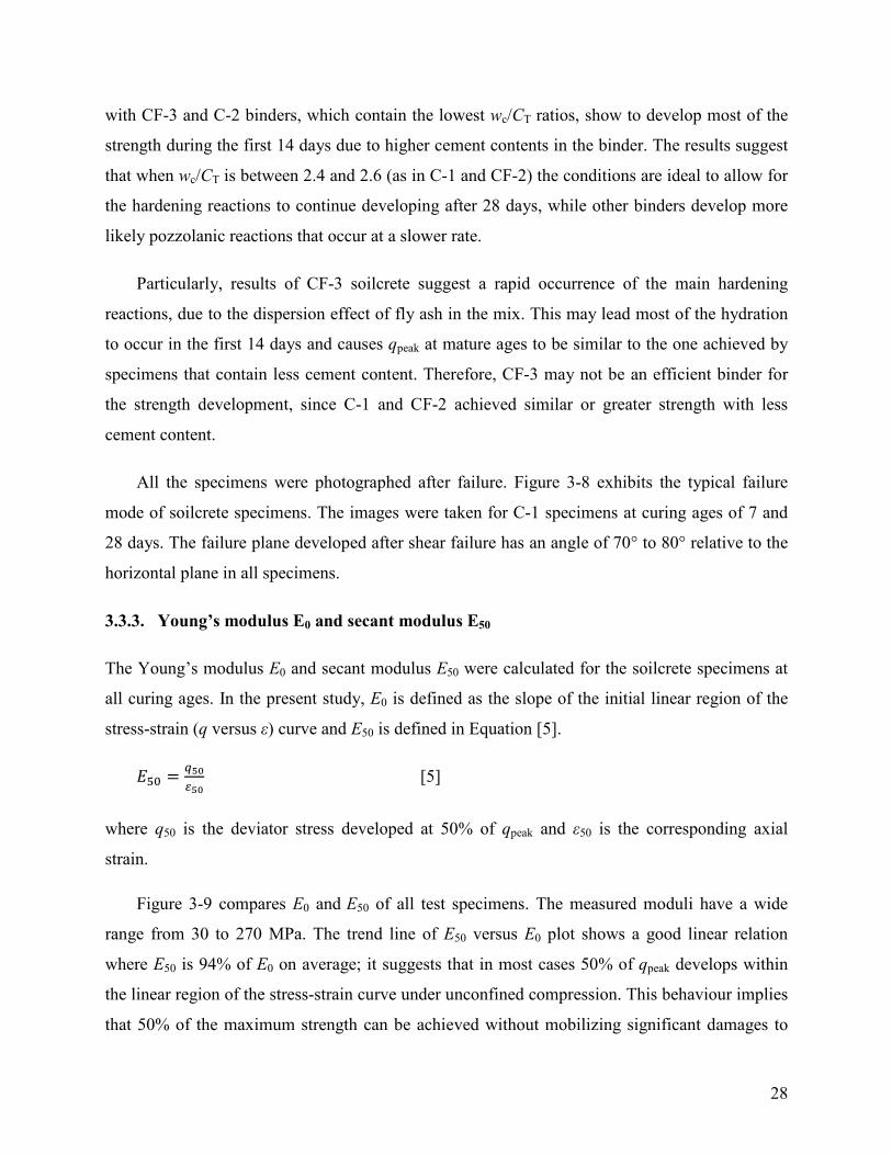
28

with CF-3 and C-2 binders, which contain the lowest wc/CT ratios, show to develop most of the

strength during the first 14 days due to higher cement contents in the binder. The results suggest

that when wc/CT is between 2.4 and 2.6 (as in C-1 and CF-2) the conditions are ideal to allow for

the hardening reactions to continue developing after 28 days, while other binders develop more

likely pozzolanic reactions that occur at a slower rate.

Particularly, results of CF-3 soilcrete suggest a rapid occurrence of the main hardening

reactions, due to the dispersion effect of fly ash in the mix. This may lead most of the hydration

to occur in the first 14 days and causes qpeak at mature ages to be similar to the one achieved by

specimens that contain less cement content. Therefore, CF-3 may not be an efficient binder for

the strength development, since C-1 and CF-2 achieved similar or greater strength with less

cement content.

All the specimens were photographed after failure. Figure 3-8 exhibits the typical failure

mode of soilcrete specimens. The images were taken for C-1 specimens at curing ages of 7 and

28 days. The failure plane developed after shear failure has an angle of 70° to 80° relative to the

horizontal plane in all specimens.

3.3.3. Young’s modulus E0 and secant modulus E50

The Young’s modulus E0 and secant modulus E50 were calculated for the soilcrete specimens at

all curing ages. In the present study, E0 is defined as the slope of the initial linear region of the

stress-strain (q versus ε) curve and E50 is defined in Equation [5].

𝐸50 = 𝑞50𝜀50

[5]

where q50 is the deviator stress developed at 50% of qpeak and ε50 is the corresponding axial

strain.

Figure 3-9 compares E0 and E50 of all test specimens. The measured moduli have a wide

range from 30 to 270 MPa. The trend line of E50 versus E0 plot shows a good linear relation

where E50 is 94% of E0 on average; it suggests that in most cases 50% of qpeak develops within

the linear region of the stress-strain curve under unconfined compression. This behaviour implies

that 50% of the maximum strength can be achieved without mobilizing significant damages to

29

the cementation. Figure 3-9 also shows a shaded zone where the moduli of soilcrete at mature

age (> 56 days) are located. It is observed that the largest moduli were achieved on the

specimens tested at mature age, when the soilcrete became stiffer.

Figure 3-10 shows the development of E0 and E50 with the wc/CT ratio at curing ages of 14,

28 and 56 days. The trend is similar to the one observed for qpeak in Figure 3-6; in general, the

moduli decreased as the wc/CT ratio increased. The moduli in the first month of curing was

greater with less wc/CT ratio. After the mature age is reached, the moduli values are very similar

among the soilcrete specimens with different wc/CT. This occurs because there is less

improvement of moduli in the second month of curing in specimens with low wc/CT, when

compared to the results for specimens with higher with wc/CT.

3.3.4. Strain at peak strength

Figure 3-11 shows the qpeak versus εpeak correlation. It is observed that qpeak at different curing

ages is reached at a very low axial strain between 0.42 and 1.25%. The εpeak decreased with

increasing peak strength, implying a softer response as the strength decreases.

Figure 3-12 illustrates that when soilcrete specimens are subject to compression in the first

28 days of curing, the dispersion of the axial strain values obtained at peak strength is greater

than the dispersion at mature age. This may happen because the development of strength in each

type of soilcrete occurs at different rates in the first stages of curing, when hydration processes

are triggered. Moreover, the changes in the microstructure of the soilcrete tend to be more stable

when mature curing age is reached, because pozzolanic reactions occur very slowly and the

microstructure is stiff, resulting in similar axial deformations for different soilcrete after 56 days

of curing.

3.3.5. Residual strength

For the soilcrete specimens in this investigation, Figure 3-5 suggests a tendency of stabilization

of the strength after 3.5% strain. Therefore, qr in the present research was taken as the post-peak

stress developed at the axial strain of 3.5%.

30

Figure 3-13 summarizes the results of qr versus wc/CT ratio for all soilcrete specimens. It

suggests that qr is insensitive to the curing age due to the dispersion of the points. For instance,

the mature specimens at 56 days developed qr similar to early-aged specimens (<28 days). The

loss of strength occurs rapidly in soilcrete specimens (Figure 3-5) and qr tends to be near the soil

residual deviator stress measured from UCS tests of undisturbed soils.

Figure 3-14 shows the correlation of qpeak versus qr for soilcrete specimens at early curing

ages (<28 days) and mature ages (>56 days). The results exhibit nearly-linear trend lines; the

specimens that have been curing for less than 28 days achieved a qpeak 3.7 times qr. In mature

samples, the change was more noticeable and qpeak is 7.3 times qr, meaning that soilcrete after 56

days curing would lose 86% of the peak strength on average when loaded to the residual state.

3.4. SEM image analysis

Figure 3-15 shows the texture of the mature soilcrete specimens produced with binders C-1 and

CF-2. The soilcrete images were taken on samples from the surface of mature specimens, after

being dried in an oven. The images of the soilcrete show tightly-bonded texture due to the action

of the cementitious binder. The image of C-1 soilcrete (Figure 3-15a) shows a cement cluster that

bonds the cement and soil particles together through fibers expanding in all directions. This

bonded structure is the result of the hydration and pozzolanic reactions that took place during

curing of the soilcrete (Horpibulsuk et al. 2009). The image of CF-2 soilcrete (Figure 3-15b)

shows several spherical particles of fly ash embedded in the bonded structure of the soilcrete.

The addition of fly ash into the binder helped disperse the cement clusters.

Figures 3-16a and 3-16b compare the bonded texture of specimens C-1 and CF-2 with less

magnification, for a visualization of the effect of fly ash dispersion on the cement clusters. In

Figures 3-16 to 3-19, the inset drawing shows the location of samples for SEM imaging. The

presence of cement clusters in Figure 3-16a gives the surface a wavy (or coarse) appearance,

which is diminished in Figure 3-16b due to the dispersive action of fly ash.

Figure 3-17 shows the bonded texture of samples obtained from the failure surface of each

soilcrete specimen after UCS test. The texture of the failure surfaces in these SEM images does

not show a significant difference. Therefore, the texture of the failure surface under unconfined

31

conditions is not significantly affected by the addition of fly ash, perhaps because the surfaces

had been smoothed during shear failure.

Figure 3-18 shows the texture of one sample taken from the failure surface and another from

the outer surface of a mature C-1 specimen. The sample taken from the failure surface (Figure 3-

18a) seems to contain less accumulation of cement clusters and have a flatter texture than the

image taken from the outer surface (Figure 3-18b), where the clusters give the image a bulky

texture. This suggests that the cement clusters were crushed and minimized during the shear

caused by axial compression on the specimen. In consequence, the bonding of the particles was

minimized and the failure plane is generated where the bonding was most affected.

Figure 3-19 compares the images of a sample from the failure plane and a sample from the

outer surface of a mature CF-2 specimen. The images for these samples show the presence of fly

ash embedded in the soilcrete structure and the fibers generated through hydration processes.

Many fibers in Figure 3-19a, taken from the failure surface, were shown to be broken due to the

action of shearing. On the contrary, the cementing fibers in Figure 3-19b, which was taken on the

outer section of the specimen, are still bonded to the particles around them.

3.5. Conclusions

Five types of soilcrete were produced in the laboratory with Edmonton stiff clays and binders

containing OPC or a mix of 90% OPC and 10% fly ash. The specimens were subject to UCS

tests at different curing ages and images were taken on the specimens with SEM. The following

conclusion may be drawn:

1 The q–ε behaviour of soilcrete specimens suggests that soilcrete behaved similar to a heavily

overconsolidated clay with significant strain softening, while the natural stiff clay was

normally-consolidated without any post-peak softening.

2 The results show that qpeak decreases with the increasing wc/CT ratio and increases with

longer curing ages. After 28-day curing, the soilcrete with the lowest wc/CT ratio achieved the

highest qpeak. However, the results show that soilcrete with wc/CT between 2.4 and 2.6

improved more strength than the soilcrete mixes with more cement during the second month

of curing.

32

3 The qpeak versus εpeak correlation shows that qpeak at different curing ages is reached at a very

low axial strain from 0.42 to 1.25%. The εpeak decreases with increasing qpeak, implying a

stiffer stress-strain response as qpeak increases.

4 The measured moduli have a wide range from 30 to 270 MPa. E50 versus E0 plot shows a

good linear relation where E50 is 94% of E0 on average; it suggests that in most cases 50% of

qpeak develops within the linear region of the stress-strain curve under unconfined

compression. Therefore, 50% of the maximum strength can be achieved without mobilizing

significant damages to the cementation.

5 The development of the moduli on the first 28 days of curing is greater in specimens with

lower wc/CT ratio; however, after 56 days of curing the increase of moduli in specimens with

lower wc/CT is less significant, and the moduli values are similar for the different soilcrete

mixes. A similar trend was shown for qpeak versus wc/CT.

6 For all specimens, the residual strength qr ranges from 100 and 200 kPa. The relation of qr

versus qpeak exhibits nearly-linear trend lines; the specimens that have been curing for less

than 28 days achieved a qpeak 3.7 times qr. For mature samples qpeak is 7.3 times qr.

7 SEM images taken from soilcrete samples show that soilcrete have a bonded and compact

text, due to the action of hydration and pozzolanic reactions that develop cementation bonds.

The dispersive action of fly ash on the soilcrete generates a more uniform appearance, with

less concentrated cement clusters.

8 Samples taken from the failure surface have less cement clusters and cement bonding than

samples from the outer surface of the soilcrete specimens, suggesting that the damage in a

specimen of soilcrete subject to UCS occurs mainly along the failure plane, due to crushing

of the cement clusters. The texture in the rest of the specimen presents less disturbance

induced by crushing.

33

Table 3- 1. Natural soil characteristics determined in the laboratory.

Property Value USCS classification Sandy CL Liquid Limit 40.9 Plastic Limit 12.5 Plasticity Index 28.4 Natural water content (%) 21.8 pH 8.1 su of undisturbed soil samples (kPa)

63-72 (Vane shear), 50 (UCS)

Specific gravity 2.54

Table 3- 2. Oxide composition of soil and binders.

Oxide Composition (% by weight)

Soil C 1 CF 1 SiO2 65.66 20.80 19.87 Al2O3 10.56 4.20 4.75 Fe2O3 8.13 2.40 3.58 CaO 5.21 63.50 62.76 MgO - 2.00 2.54 SO3 1.96 3.50 2.67 Na2O - - 0.24 TiO2 1.18 - 0.44 K2O 3.71 - 0.18 P2O5 - - 0.04 SrO - - 0.08 Mn2O3 - - 0.11 LOI2 3.6 2.37 2.32 Total 100 98.77 99.58 1. C: 100% ordinary Portland cement; CF: 90% ordinary Portland cement and 10% class F fly ash. 2.

LOI: loss on ignition at 440°C for soil and 1000°C for binder C and CF.

34

Table 3- 3. Component quantities in each soilcrete.

Property Binder ID

C-1 C-2 CF -1 CF-2 CF-3 wc (%) 54.1 55.1 59.7 53.4 51.9 Cc (%) 22.5 30.0 18.0 20.2 24.8 Cf (%) 0 0 2.0 2.2 2.8 CT (%) 22.5 30.0 18.2 20.6 25.3 wc/CT 2.4 1.8 3.3 2.6 2.1 Binder content (kg/m3) 225 290 190 225 275

35

Figure 3- 1. Particle size distribution of the natural soil sample.

Figure 3- 2. X-Ray Diffraction (XRD) spectrum on soil sample minerals.

0.0010.010.11100

20

40

60

80

100Pe

rcen

t fin

er b

y w

eigh

t (%

)

Particle diameter (mm)

ClaySand Silt

0 10 20 30 40 50 60 70 80 900

20

40

60

80

x103

654 73

2

81

Inte

nsity

(Cou

nts)

2θ (°)

2. Quartz SiO2

4. Albite NaAlSi3O8

3. Microcline K(AlSi3O8)

6. Dolomite CaMg(CO3)2

5. Calcite CaCO3

7. Pyrite FeS28. Muscovite KAl2((AlSi3)O10)(OH)2

1. Clinochlore Mg2.5Fe1.65Al1.5Si2.2Al1.8O10(OH)8

36

Figure 3- 3. SEM image of clay minerals of natural soil sample.

Figure 3- 4. Soilcrete before performing UCS test. Detail of gypsum cap on soilcrete being leveled.

37

Figure 3- 5. Typical axial deviator stress versus axial strain curves for soilcrete at several curing ages compared to an undisturbed stiff clay sample: (a) C-1 soilcrete and (b) CF-2 soilcrete.

0

200

400

600

800

1000

0 1 2 3 4 5 10 110

200

400

600

800

1000

(a) Curing Age(days)

3 7 14 28 56Undisturbed clay

(b) Curing Age(days)

3 7 14 56

Dev

iato

r str

ess,

q (k

Pa)

Axial strain, ε (%)

Undisturbed clay

38

Figure 3- 6. Peak strength (qpeak) versus wc/CT ratio for curing ages between 14 and 56 days.

Figure 3- 7. Average peak strength (qpeak) development versus curing age for all tested binders.

1 2 3 4

400

600

800

1000

1200

wc/CT

Curing age(Days)

14 28 56

q peak

(kPa

)

CF-

1

CF-

2C

-1CF-

3C

-2

0 20 40 600

200

400

600

800

1000

1200

C-1 C-2 CF-1 CF-2 CF-3

q peak

(kPa

)

Curing Age (days)

39

Figure 3- 8. Failure plane in C-1 soilcrete specimens with different curing ages: (a) specimen cured for 7 days failed on loading frame, (b) specimens failed at 7 days of curing and (c) specimens failed at 28 days of curing.

Figure 3- 9. Young’s modulus E0 versus secant modulus E50 for all soilcrete specimens. Shaded area shows the range of results at the mature age (>56 days). Dash line illustrates linear trend of results where E50 = 0.94 E0.

0 50 100 150 200 250 3000

50

100

150

200

250

300

E50 = 0.94 E0

R2 = 0.99

1Early age (< 28 days)

Mature age (> 56 days)

E 50 (M

Pa)

E0 (MPa)

E0, E50 range at mature age

1

(a) (b)

(c)

40

Figure 3- 10. Elastic modulus versus wc/CT ratio at several curing ages: (a) Young’s modulus E0 and (b) secant modulus E50.

0

50

100

150

200

250

300

1 2 3 40

50

100

150

200

250

300

(a) Mature >56 Days

28 Days

Curing age(Days)

14 28 56

E 0 (M

Pa)

14 Days

(b)Mature >56 Days

28 Days

wc/CT

Curing age(Days)

14 28 56

E 50 (M

Pa)

14 Days

41

Figure 3- 11. Maximum deviator stress versus axial strain at peak for each binder mix.

Figure 3- 12. Axial strain at peak strength (εpeak) versus wc/CT ratio at early and mature curing ages.

0.4 0.6 0.8 1.0 1.20

500

1000

1500

CF-1 CF-2 CF-3 C-1 C-2

q peak

(kPa

)

εpeak (%)

1 2 3 4

0.4

0.6

0.8

1.0

1.2

1.4

wc/CT

Early age (< 28 days)

Mature Age (< 56 days)

ε peak

(%)

CF-

1

CF-

2C

-1CF-

3C

-2

42

Figure 3- 13. Residual strength (qr) versus wc/CT ratio compared to natural soil residual strength.

Figure 3- 14. qpeak versus qr at early and mature age.

1 2 3 40

100

200

300 Early Age

(< 28 days) Mature Age

(> 56 days)

wc/CT

Res

idua

l str

engt

h, q

r (kP

a)

Residual strengthof undisturbed soil

CF-

1

CF-

2C

-1CF-

3C

-2

0 50 100 150 200 2500

500

1000

1500

Early age(< 28 days)

Early ageqpeak /qr = 3.7

Mature age qpeak /qr = 7.3

q peak

(kPa

)

qr (kPa)

Mature age(> 56 days)

43

Figure 3- 15. SEM images for microstructural analysis: (a) dry remolded Edmonton stiff clay; (b) C-1 mature specimen (>56 days) and (c) CF-2 mature specimen (>56 days). Sample taken from the outer surface of the soilcrete specimen.

44

Figure 3- 16. SEM images for samples taken from the outer surface of the soilcrete specimen at mature age (>56 days): (a) C-1 specimen and (b) CF-2 specimen.

45

Figure 3- 17. SEM images of the failure surface for soilcrete mature specimens (>56 days) with different binder: (a) C-1 specimen; and (b) CF-2 specimen. Images were taken on the failure surface after a UCS test.

46

Figure 3- 18. SEM images for C-1 soilcrete mature specimens (>56 days): (a) image taken from the failure surface and (b) image from the external surface of the specimen.

47

Figure 3- 19. SEM images for CF-2 soilcrete mature specimens (>56 days): (a) image taken from the failure surface and (b) image from the external surface of the specimen.

48

4. Mechanical and Physical Properties of Cement Treated Edmonton Stiff Clay Using

Triaxial Tests and Image Analysis2

Abstract

Cementitious binders have been widely used to improve the strength of soft soils by deep soil

mixing. Most of past research has been directed toward soft soils stabilized with a small cement

content. This research investigates the mechanical and physical properties of Edmonton stiff clay

treated with ordinary Portland cement and a compound binder of 90% cement and 10% fly ash

by weight. The cement contents were greater than 20%. Laboratory-prepared soilcrete specimens

were compressed in isotropically-consolidated undrained triaxial tests at a confining pressure

ranging from 100 kPa to 3000 kPa. Effects of consolidation and shear failure on the permeability

of soilcrete were quantified. The microstructure of soilcrete samples was inspected with scanning

electron microscope. Several full-scale soilcrete specimens were scanned by computed

tomographer and a new method of analyzing the images was developed to obtain the porosity

and its distribution. This research determined the yield strength, peak and fully-softened

strengths, moduli, and effective strength parameters of soilcrete. The results show that all

specimens exhibited strain-softening behaviour. Specimens exhibited an effective peak friction

angle of 38.3°, with an effective cohesion of 145.6 kPa and 107.9 kPa in C and CF soilcrete,

respectively. Porosities estimated with the developed method matched the lab-estimated

porosities very well.

Key words: soilcrete, stiff clay, triaxial test, mechanical properties, porosity, SEM, CT scan.

4.1. Introduction

The increasing use of ground improvement techniques such as deep soil mixing (DSM) and jet

grouting arose with the need of installing urban and industrial developments in locations where

in situ soils have an unsatisfactory bearing capacity and are susceptible to large settlement. A

cementitious additive (i.e. a binder) or a combination of additives can be added to the soils as a

2 A version of this chapter has been submitted as Luis et al. (2017) to the Canadian Geotechnical Journal for possible publication

49

powder or a slurry in order to enhance certain engineering properties of the soil. The resulting

binder-soil mix is termed as “soilcrete”.

A binder such as Portland cement is effective in improving the mechanical properties of soft

soils through the DSM. Miura et al. (2001), Åhnberg et al. (2003), and Lorenzo and Bergado

(2004) showed that the chemical reaction efficiency that hardens the soil through hydration and

pozzolanic reactions depends principally on the amount of cement used and the water available

for the reactions, following the concept of Abrams’ law for hardening of concrete mixtures

(Horpibulsuk et al. 2003). Factors such as the soil type, temperature, and curing conditions may

also influence the properties of resulted materials (Porbaha et al. 2000, Liu and Starcher 2012).

Therefore, laboratory strength tests of soilcrete are often recommended to guide the in situ DSM

The unconfined compressive strength (UCS) of soilcrete specimens produced in the

laboratory may be an indicator of the actual strength achieved in the field (Porbaha et al. 2000,

Han 2015). However, when large superstructures are supported by soilcrete columns, the

soilcrete may be subjected to considerably high confining pressure, and the presence of

groundwater and the drainage condition make the UCS unrepresentative of the actual in-situ

behaviour. Porbaha et al. (2000), Banks (2001), and Lo and Wardani (2002) showed that

specimens of soilcrete under undrained load condition developed very little deformation before

reaching the peak strength when compared to drained test specimens, which makes the undrained

condition more critical.

The growing need for the DSM to support large superstructures such as oil storage tanks in

urban areas may lead to the use of cement mass greater than 20% of the mass of soil solids in

order to meet the design specifications for strength. However, published literature related to

applications of the DSM using high cement content has been very limited (Miura et al. 2001,

Kamruzzaman et al. 2009). Further, there is a lack of research on the effects of confining stress

on soilcrete made of stiff clays, because most of the previous research was conducted on cement-

treated soft soils, typically in marine environment, pavement subgrade, or contaminant

confinement (e.g., Uddin et al. 1997, Banks 2001, Chew et al. 2004, Horpibulsuk et al. 2004, and

Kasama et al. 2006). The range of confining stress used in previous research was usually limited

to 1 MPa. For an improved understanding of the effects of confinement on properties of soilcrete

with high cement content, a greater confining stress should be used.

50

In addition to the use of destructive loading tests, researchers (e.g., Horpibulsuk et al. 2009,

Kamruzzaman et al. 2009) used images taken with a scanning electron microscope (SEM) to

investigate the soil–cement interaction and to quantify the effects of fly ash on the mechanical

properties and porosity of soilcrete. Peyton et al. (1992), Waller (2011), and Mao et al. (2012)

used computed tomography (CT) scanned images to estimate the porosity and pore size

distribution of coal, rocks, and concrete. These studies qualitatively estimated the ranges of

porosity through density measurement based on the grayscale color detected on the images.

Therefore, the present research investigated the effects of confining pressure on the

mechanical and physical properties of mature soilcrete made of Edmonton stiff clay treated with

cementitious binders, using triaxial tests and images analysis. Results of the present research

may be used to support the binder design for DSM when the improvement of engineering

properties of stiff clays is needed. This research adopted two types of binders: ordinary Portland

cement and a mix of ordinary Portland cement and fly ash. A series of triaxial compression tests

on laboratory-prepared soilcrete specimens were carried out for confining pressures ranging from

100 kPa to 3000 kPa. The mechanical and hydraulic properties of the soilcrete were assessed.

The parameters analyzed in the present study include the peak strength qpeak, Young’s modulus

E0, secant modulus E50, fully-softened strength qs, hydraulic conductivity k, porosity n, and

effective strength parameters. SEM images were taken to investigate the effects of confining

pressure and fly ash on the microstructure of soilcrete at the failure plane and outer surfaces. CT

scan was performed on selected full-scale soilcrete specimens; a new method of post-processing

the CT scanned images was developed to evaluate the porosity and its distribution along the

specimens.

4.2. Materials and Methodology

4.2.1. Soils and cementitious binders

Natural disturbed soils were collected from a site in eastern Edmonton, where the DSM would be

performed to support oil storage tanks that load the soils with overburden stresses between 50 to

250 kPa. The soil is a glaciolacustrine deposit formed in Glacial Lake Edmonton. Engineering

properties of this soil type has been extensively investigated in the literature (e.g. Thomson

1970). The soil at the site is a low plasticity clay with a sand content of 33% and a natural water

51

content of 22%. The soil is classified as “sandy CL” according to Unified Soil Classification

System (USCS). The soil characteristics are summarized in Table 4-1 and the particle size

distribution is illustrated in Figure 4-1. With an undrained shear strength (su) of 63 to 72 kPa

determined from laboratory vane shear tests, the soil is classified as a “stiff clay”. However, the

soil may be still incapable of providing sufficient bearing resistance to the tanks. The soil

contains minerals such as quartz, illite (muscovite), dolomite, albite, calcite and pyrite, according

to the X-Ray Diffraction (XRD) tests performed on a representative soil sample. The oxide

composition of the soil was assessed with X-Ray fluorescence tests and the oxide distribution is

listed in Table 4-2. From the gathered information, the primary clay mineral was from the mica

group, particularly illite (muscovite), due to the presence of potassium ions (Holtz et al. 2011).

The binders used in the present study were composed of ordinary Portland cement or a mix

of 90% ordinary Portland cement and 10% fly ash by weight. The binder types are named C and

CF, respectively. The chemical composition of the binders is listed in Table 4-2, which shows

about 63% calcium oxide (CaO) in both binders, typical for cement. The addition of small

amount of sodium and potassium oxides in the CF binder is due to the presence of fly ash. The

grains of each binder were inspected using SEM images, as shown in Figure 4-2. It is seen that

the cement particles are flaky and the fly ash is mainly spherical.

4.2.2. Soilcrete preparation and properties

To prepare soilcrete specimens, the dry binder powder and tap water were mixed with an

electrical blender (Warring Commercial model WSB60) to obtain a uniform slurry, and then

combined with the natural soil by mixing the components for 2 min in an automatic dough mixer

(Hobart model Legacy HL200 18.9 Litre). The final product was cast into plastic cylinders of 75

mm diameter and 150 mm length. The mixture was scooped to the cylinders in layers, and then

the cylinder was tapped against a hard surface to extract air bubbles. The cylinders were capped

with plastic lids and stored in a container at room temperature during curing time. The

procedures are similar to the methodology proposed by Bruce et al. (2013) to resemble the

conditions of the mixing performed in situ and to avoid over-mixing of the paste in the

laboratory.

52

The as-built component quantities used in the mix of C and CF type soilcrete are

summarized in Table 4-3. In the present study, the in-place binder content (Bc) used for all

soilcrete was 225 kg/m3, where Bc is defined in Equation [1] (e.g., Filz et al. 2005, Timoney et al.

2012):

𝐵𝑐 = 𝑚𝑐 + 𝑚𝑓

𝑉𝑠𝑜𝑖𝑙+𝑉𝑠𝑙𝑢𝑟𝑟𝑦 [1]

where: mc and mf are the masses of cement and fly ash, respectively, and Vsoil and Vslurry are the

volumes of the natural soil and the slurry, respectively. The in-place binder content Bc is a

critical parameter used in the design of soilcrete for DSM. A Bc of 225 kg/m3 is commonly used

in the practice and was kept constant for comparison purpose.

The water content (wc) introduced by Miura et al. (2001), Lorenzo and Bergado (2004) and

Horpibulsuk et al. (2005) is defined in Equation [2]:

𝑤c = 𝑚w + 𝑚ws𝑚s

∙ (100%) [2]

where: mw is the mass of water in the clay, mws is the mass of water in the water/binder slurry,

and ms the mass of soil solids. In the present study, wc was 1.20 times the liquid limit of the

natural soil to ensure adequate mixing.

The cement content (Cc) and fly ash content (Cf) used in the binders are defined in Equations

[3] and [4]:

𝐶c = 𝑚c 𝑚s

∙ (100%) [3]

𝐶f = 𝑚f 𝑚𝑠

∙ (100%) [4]

The total cement content CT is calculated with Equation [5] (Horpibulsuk et al. 2011):

𝐶T = 𝐶c(1 + 0.75𝐶f ) [5]

where the coefficient 0.75 considers the dispersion caused by the fly ash on the cement clusters.

In Equation [5], Cf is in a decimal form.

53

The Cc and Cf for this study (Table 4-3) were selected in order to achieve CT in a range of

20.6 to 22.5%. The water content wc was selected in a range of 53.4 to 54.1% for CF and C

soilcrete, respectively. Bruce et al. (2013) and Ma et al. (2014) show that the best strength

development is achieved for wc/CT from 1.5 to 3.

4.2.3. Triaxial test procedure

The specimens were allowed to cure for at least 56 days in order to develop most of the strength

expected at the mature age, since the UCS results presented by Luis and Deng (2017) show less

development of strength after 28 days. The specimen was dissembled from the plastic cylinder

and the weight and volume were measured for the initial void ratio estimation. The specimens

were placed into a cylindrical confining cell with a maximum pressure capacity of 4 MPa. The

pumps used to exert the confining and back pressures were purged prior to the test to ensure no

air was entrapped in the system. The cell fluid was tap water and the pore fluid was deionized

water. The specimen was placed in the confining cell following procedures listed in ASTM

(2011).

A summary flowchart of the test procedure is shown in Figure 4-3. Based on the dry weight

measured at end of consolidation tests, the degree of saturation of specimens after curing was

estimated to be 0.8 to 0.98. To ensure full saturation during the triaxial test, the specimen was

subject to 500 kPa back pressure, which was maintained constant through all stages of the test.

The soilcrete was saturated for 24 to 36 hours by applying a confining pressure of 525 kPa. After

the saturation period, the specimen was subjected to a B-test to confirm the level of saturation.

The B parameter is defined in Equation [6]:

𝐵 = 𝛥𝑢𝛥𝜎𝑐′

[6]

where: Δu is the resultant pore pressure increment due to the confining pressure increment Δσc'

around the specimen. For geomaterials with a stiff skeleton, a B parameter of near 0.8 instead of

1.0 implies the saturation (Banks 2001, Quiroga et al. 2015). Specimens in present study had B

values in a range of 0.7 to 0.9; therefore, they were considered fully saturated.

The soilcrete was isotropically consolidated in 3 or 4 stages until reaching the target

effective confining pressure (σc') of 100, 200, 500, 800, 1000, 2000, and 3000 kPa, where each

54

stage took about 8 to 12 hours to complete. The σc' is the cell pressure minus the back pressure.

Once the consolidation was finalized, the specimen was subject to a permeability test, by forcing

upward flow within the soilcrete matrix. The differential pressure used in the permeability tests

was about 10% of σc', which resulted in a hydraulic gradient in a range of 6 to 200. The

permeability test was conducted according to the procedure of the constant head test with

flexible wall permeameter (ASTM 2010). The results were used to assess the change in in

hydraulic conductivity due to changes in the microstructure during the consolidation stage.

After consolidation, the specimen was subject to axial displacement under the undrained

condition at a rate of 0.0125 mm / min (or 0.5% strain / hour). The specimen was subject to axial

load until reaching approximately 15% axial strain. During the shearing, the pore pressure and

deviator stress were recorded at every 120 sec.

The permeability test was conducted again after the shear failure was reached, before the

specimen was dismounted for visual inspection. As shown in Figure 4-3, selected soilcrete

specimens were also tested for the permeability after the saturation, consolidated, and then tested

under the CT scan.

4.2.4. SEM and CT scan

For each binder type, three specimens that were sheared under σc' of 0, 500, and 3000 kPa,

respectively, were selected for the SEM image analysis. The specimens were dismounted

carefully after the triaxial test, and then dried in an oven for 24 hours. Three samples for each

specimen were selected from the top, the bottom, and the failure plane, respectively. The samples

were sputtered with a thin layer of gold (about 1.6×10-5 mm) before placing them into the SEM

device. Several images were taken from each sample at various magnifications using the SEM

device (ZEISS EVO MA10).

As shown in Figure 4-3, selected full-scale specimens were scanned in a computed

tomographer, which provided transversal images of specimens at 0.3 mm interval with a

resolution of 512 by 512 pixels. Two specimens for each binder type were consolidated at σc' of

500 and 3000 kPa and then subject to CT scanning. An intact specimen of each binder type

55

without consolidation was also scanned. The images from the scanner were later analyzed to

determine the effects of confinement on the porosity of specimens.

4.3. Results of triaxial compression tests

Fourteen soilcrete specimens produced with C and CF binders were compressed in isotropically-

consolidated undrained (ICU) condition after being subject to σc' ranging from 100 to 3000 kPa.

All specimens for the ICU triaxial tests had been cured for 56 days or longer because the present

study is aimed at studying the behaviour of mature soilcrete that is more critical to the DSM

application.

4.3.1. Volumetric strain during consolidation and yield strength

Horpibulsuk et al. (2004) showed that the peak strength (qpeak) increased substantially after

applying a σc' greater than the yield strength (Py') due to the breakage of the bonding produced

by hydration and pozzolanic reactions of cement. This makes Py' an important parameter in

addressing the change in mechanical behaviour of soilcrete.

Figure 4-4 shows the semi-log curves of the volumetric strain (Δεv) versus σc' of all

specimens during the consolidation stage. The curves show that the slope increased as σc' passed

through a certain point, similar to a consolidation curve of a natural soil. Py' was estimated at the

intersection of the tangents to the initial and final portions of the Δεv versus σc' curves. It appears

that Py' were 1400 kPa for C specimens and 1200 kPa for CF specimens. These values are in

accordance with previous findings by Miura et al. (2001) and Horpibulsuk et al. (2004) on soft

clay with Cc between 16 and 33%, which developed a Py' between 800 and 2500 kPa.

The different behaviour before and after yield (Figure 4-4) suggests two phases of straining

in the soilcrete specimens. Prior to yield, the soilcrete experienced little strain due to the

cementation bond, which enabled the soilcrete to show apparent overconsolidated behaviour.

With σc' beyond the yield strength, the strain was much greater due to the partial loss of the

cementation bond during yielding of the soilcrete (Horpibulsuk et al. 2004). In Figure 4-4, C

soilcrete exhibited a greater Δεv than CF soilcrete given the same σc', especially after yield.

56

4.3.2. Stress-strain behaviour in ICU triaxial tests

Figures 4-5a and 4-5b show the deviator stress (q) versus axial strain (ε) curves of C and CF

soilcrete specimens. The results show that specimens at low σc' developed more strain before

reaching the peak stress than those under high σc'. As anticipated, the peak deviator stress (qpeak)

increased with increasing σc'. All specimens developed a strain-softening response, which was

more pronounced at a low confining stress (σc' < 1 MPa); the specimens were more similar to a

perfectly-plastic material once σc' was at the highest values (3 MPa).

Figures 4-5c and 4-5d show the pore pressure (u) versus axial strain curves, where u is the

measured pore pressure subtracting the constant back pressure in the specimens. Specimens

tested at σc' of 100 and 200 kPa developed positive u at small strain and then negative u after

exceeding qpeak suggesting a high dilation potential, similar to heavily overconsolidated clays.

When σc' was less than Py', the maximum pore pressure (umax) was reached at strains much less

than the strains for qpeak. When σc' was greater than Py', umax was reached with a larger strain.

Uddin et al. (1997) found similar behaviour in soilcrete produced with soft clays, and attributed

the dilative response under low σc' to the heavily overconsolidated structure of the soilcrete. As

σc' increased, the positive umax increased; because the cementing bonds had been weakened by

the effect of confinement, u was stabilized more rapidly at a large σc'. In this study, u was

stabilized after axial strain around 10%, when the post-peak strength had been stabilized.

The fully-softened state (also known as critical state; see Fell et al. 2014) strength qs is

adopted as the stabilized deviator stress achieved after the peak stress. In the present research,

the deviator stresses exhibited in Figures 4-5a and 4-5b seemed to stabilize at an axial strain of

about 12%. qs of all test specimens were obtained and compared with qpeak as shown in Figure 4-

6. A linear relation between qs and qpeak was observed; qs in specimens of C and CF soilcrete

were 90 and 87% of their respective qpeak on average. Therefore, there is a slightly greater loss of

strength after peak in CF specimens. The peak deviator stress, initial void ratio, strain at the peak

stress, and upeak of all test specimens are summarized in Table 4-4.

Figure 4-7 shows the typical failure modes of specimens. All specimens developed an

inclined shear failure plane (Figure 4-7a). In addition to the shear plane, a few specimens (e.g.

57

the one at σc' of 200 kPa shown in Figure 4-7b) exhibited deformation around the failure surface,

which can be attributed to crushing or bulging deformation of the specimen (Figure 4-7b). Closer

inspection revealed that the failure surface was rougher in specimens confined with σc' less than

1 MPa. For specimens confined at σc' of 2 and 3 MPa, the surface of the failure plane became

much smoother. The difference suggests a change in the texture of the soilcrete in the failure

surface due to the effect of σc'.

4.3.3. Axial strain at peak stress

The axial strain at peak strength (εpeak) versus σc' is shown in Figure 4-8. For C specimens, εpeak

ranged from 1 to 8%. Specimens at σc' less than Py' tended to develop the greatest εpeak, and εpeak

decreased with increasing σc'. CF specimens also developed a decreasing εpeak as σc' increased.

Figure 4-8 shows that CF specimens generally exhibited greater εpeak than C specimens at the

same σc', implying that CF specimens had a softer initial response than C specimens.

4.3.4. Peak stress versus confining stress

Figure 4-9 shows the relation of qpeak and σc'. For C specimens (Figure 4-9a), qpeak appeared to

remain almost constant when σc' was between 100 to 800 kPa. qpeak increased more significantly

with σc' after Py' was exceeded; the trend was in accordance with the findings of Horpibulsuk et

al. (2004) for soilcrete produced with cement-only binders. The breakpoint where the transition

from overconsolidated to normally consolidated behaviour occurred was near Py'. This suggests

that the increase in strength was derived from a change in the cementation bond of the soilcrete

when the confining stress was greater than Py'.

Specimens of CF soilcrete (Figure 4-9b) achieved qpeak usually less than C soilcrete due to a

slight difference in the cement content. In CF specimens, qpeak increased progressively with

increasing σc', in contrast to the results for C specimens, where qpeak remained constant with σc'

less than Py'. The presence of fly ash in CF specimen enabled the dispersion of the cement

clusters during curing and hardening of the soilcrete. Therefore, the cementation was weaker in

CF specimens, but the cementation bonds were spread more uniformly, leading to a more stable

structure.

58

4.3.5. Young’s modulus E0 and secant modulus E50

The initial Young’s modulus E0 and secant modulus E50 (defined at 50% of the peak strength)

were obtained from the q versus ε curves for all specimens. The results are summarized in Table

4-5. Figure 4-10 shows the results of moduli versus σc'. It is observed that the moduli (E0, E50)

generally increased with increasing σc' for both soilcrete types, except for several anomalies. The

results also show that the C soilcrete had greater moduli than the CF soilcrete at the same σc'.

Figure 4-11 compares E50 to E0. A linear regression shows that E50 was 0.91 and 0.93 times

E0 for C and CF soilcrete, respectively. This suggests that 50% of the strength was mobilized

before the cementation bonds were damaged since E50 were very close to results of E0, especially

for CF soilcrete.

4.3.6. Effective strength parameters

Figure 4-12 shows the deviator stress (q) versus mean effective confining stress (p') curves

during the ICU tests developed by the C and CF soilcrete. The results were used to estimate the

effective strength parameters. The dash lines in Figure 4-12 represent the peak strength envelope

with a slope M, whereas the solid straight lines represent the envelope of the fully-softened

strength with a slope Ms.

The curves in Figure 4-12 are comparable to the typical stress path of clays during undrained

triaxial tests. The p'-q stress path developed by the soilcrete specimens suggest heavily

overconsolidated to lightly overconsolidated behaviour, which was dependent on σc'. For

specimens at p' from 100 to 200 kPa, p' tended to decrease slightly and then grow, suggesting the

dilative potential and the development of negative u. As σc' increased, the development of

positive u decreased p', and the specimens exhibited normally consolidated behaviour with

further increase of σc'. For C soilcrete, the transition from overconsolidated to normally

consolidated behaviour appears to take place approximately when the initial p' exceeds Py'. For

CF soilcrete, the curve at σc' of 2000 kPa continued to show lightly overconsolidated behaviour.

59

The slope M of the peak strength envelope was determined for both binder types to estimate

the effective strength parameters. The peak friction angle φpk' was estimated through a

correlation with the parameter M as expressed in Equation [7] (Parry 2004):

𝑀 = 6𝑠𝑖𝑛𝜙pk′3−𝑠𝑖𝑛𝜙pk′

[7]

The effective cohesion (c') was determined using Equation [8] (Parry 2004):

𝑐′ = 𝑐𝑀

[8]

where c is the intercept with the q axis of the plot in Figure 4-12.

The parameters φs' and cs' at the fully-softened state were calculated in a similar method,

using the slope of the fully-softened envelop Ms and the intercept. The calculated effective

strength parameters for C and CF soilcrete are listed in Table 4-6.

The strength envelopes shown in Figure 4-12 at the peak had the same slope, and the

cohesion of C soilcrete was slightly greater than that of CF soilcrete (145.6 kPa and 107.9 kPa,

respectively). This suggests that the two soilcrete types had the same peak friction angle (38.3°)

but the C soilcrete had a stronger cohesion due to stronger cementation than CF soilcrete. The

addition of binders into the soil substantially improved the effective strength parameters of the

natural soil. Thomson (1970) showed that a glaciolascustrine soil from Glacial Lake Edmonton

would typically have φpk' from 14° to 24° and c' from 20 to 55 kPa.

The φs' of C and CF soilcrete were 4.1° and 1.6° less than the respective φpk'. At the fully-

softened state, a significant cs' was still maintained. For CF specimens, cs' is less than c' due to

the breakage in cementation bonds. φs' ranged from 34.2 to 36.7° in this investigation, which is

less than the results in previous research conducted on very soft soils treated with cement (e.g.,

Chen et al. 2015) where φs' ranged from 48 to 57° for cracked specimens subject to ICU tests.

Moreover, the change in the strength parameters for CF specimens was less significant,

suggesting that the structure of CF soilcrete was more stable under the effects of confining

pressure, when compared to the C soilcrete.

60

4.3.7. Hydraulic conductivity versus confining stress

The hydraulic conductivity (k) was measured after saturation for two specimens of each binder

type (Figure 4-3) that were later used for the CT scan test. The saturated samples were subject to

upward permeability tests with two differential heads of 20 and 40 kPa resulting in a hydraulic

gradient of 13.6 and 27.2; k was calculated for each test and the average was taken as the initial k

(2×10-9 and 1×10-9 m/s for C and CF soilcrete, respectively).

For the specimens selected for the ICU test, k was measured at two stages: end of the

consolidation and after shear (see Figure 4-3). Variations of k for both C and CF soilcrete are

shown in Figure 4-13. Results show that k decreased after consolidation and were from 3 to 25%

of the initial k. The decrease of k upon consolidation was associated with the volumetric strain

due to the action of σc', which led to a decrease in pore volume. Specimens of CF soilcrete had

an initial porosity in a range from 0.45 to 0.48, and specimens of C soilcrete had a slightly

greater porosity from 0.48 to 0.51. After consolidation, the CF specimens developed k values 30

to 60% less than k of C soilcrete, due to a greater porosity of C soilcrete.

Figure 4-13 shows that k increased significantly after shear. In C specimens, the post-shear k

were 3 to 400 times of the post-consolidation k. In CF specimens, the post-shear k were 30 to 700

times of the post-consolidation k. This confirms the presence of cracks and fractures in the

soilcrete due to the effects of axial strain. The amplification in k between consolidation and shear

stages is much larger in CF than that in C soilcrete. It is possibly because the CF soilcrete had

rougher cracks and apertures and therefore was able to develop wider flow channels than C

soilcrete at high confining pressure. The surface roughness will be further inspected using SEM

images in the subsequent section. Figure 4-13 also shows that the amplification in k at high σc'

was less pronounced than at low σc', due to the closure of the cracks at high σc'.

4.4. Image Analysis

SEM images were used to inspect the microstructure of soilcrete samples and to investigate the

changes in the texture of specimens with confining stresses. CT scanned images were used to

estimate the porosity and its distribution in the soilcrete specimens

61

4.4.1. Scanning electron microscopy

After ICU tests, samples located along the failure plane and other locations of specimens were

inspected at several magnifications with SEM. Figure 4-14 compares the failure planes in

samples of C and CF soilcrete confined at 0, 500, and 3000 kPa. It is shown that the roughness of

the failure surface decreased with increasing σc', especially in samples taken from C soilcrete.

This suggests that the reorientation of particles due to the action of high σc' leads to a smooth

shear failure plane. By comparing images of C and CF soilcrete, it appears that a greater

confining pressure was required to reach the same level of smoothness in CF soilcrete.

Figure 4-15 compares the images of a sample taken from the surface with a sample taken

from the failure plane of the CF specimen at σc' of 3000 kPa. The sample taken from the failure

plane (Figure 4-15b) was much smoother than the sample from the top surface (Figure 4-15a),

perhaps because the action of axial load had smoothed the failure surface due to crushing. The

results show resemblance with observations by Kamruzzaman et al. (2009) on cement-stabilized

clay, where the sample taken from the outer section of the specimen showed little disturbance.

Figure 4-16 shows the images of a sample taken from the failure plane of CF soilcrete at σc'

of 500 kPa. It is seen that the failure plane was still rough when confined at 500 kPa, in contrary

to C specimens (Figure 4-14b) that had a smoother texture. Furthermore, Figure 4-16 shows that

clearly a bonding net was generated by the hardening reactions in a CF specimen sample taken

from the failure surface. These fibers were broken by the action of shearing.

4.4.2. CT scan image analysis

The image-processing software ImageJ (Rasband 1997) was used to analyze CT scan images of

specimens, which were scanned on 480 transverse slices at an equal interval of 0.3 mm. The

image of each slice is given in grayscale colored pixels, and the color of the pixel varies with the

density of the physical element. A darker-colored pixel means less density, which implies a more

porous element. The size of the element (0.35 mm squared) gives a reasonably good resolution to

visualize the voids through the specimen, because it is much less than the specimen diameter (75

mm). Figures 4-17a and 4-17b show example images of a specimen of soilcrete CF confined to

500 kPa along a transverse and a longitudinal section plane, respectively. The color is

62

heterogeneous across the images. The 100% black patches in the images represent the least

density (i.e., cavities) in the soilcrete, whereas the 100% white patches likely represent the zones

with more concentrated cement clusters.

For a scanned specimen, the total number of pixels for each grayscale color was summed

and displayed in a histogram, as shown in Figure 4-18. The modal color representing the most

frequent color was then determined from the histogram. In this study, the modal color is adopted

to separate the porous and filled fractions of the specimen (Figure 4-18). The pixels on the darker

side (left of the modal color) are considered as the voids, which includes the pores, cracks, and

the most porous materials. The porosity n is then calculated using the pixel color histogram:

𝑛 = 𝑉𝑣𝑉𝑇

[9]

where: Vv is the voids volume calculated as the total number of pixels in the porous fraction, and

VT is the total volume of the specimen calculated as the total number of pixels in the 480-image

sequence.

The porosity n could also be estimated from the laboratory-measured mass and volume of

specimen using Equation [10]:

𝑛 = 𝑉𝑇− 𝑚𝑠

𝐺𝑠𝑒𝑞 ∙ 𝜌𝑤

𝑉𝑇 [10]

where: VT is the total volume of the specimen measured after curing and modified by the

volumetric strain due to consolidation, Gseq is the equivalent specific gravity of the soilcrete, ρw is

the density of water, and ms is the mass of the soilcrete solids. Gseq was taken as 2.64 for the CF

soilcrete and 2.65 for the C soilcrete, according to the specific gravity of clay (2.54), cement

(3.15), and fly ash (2.40), and their relative mass contents.

Figure 4-19 shows the porosity of six soilcrete specimens after consolidation estimated

using Equations [9] and [10]. Apparently, the porosity based on Equation [10] is very consistent

with the porosity from the CT scan image analysis. The greatest difference in porosity was 0.04

for a C specimen at σc' of 3000 kPa. The simplicity of the proposed method and closeness of

results with the laboratory values makes it useful in estimating the porosity, when compared to

other qualitative methods (e.g., Waller 2011).

63

To estimate the porosity distribution, images of 25 equally-spaced slices in each specimen

were extracted from the image sequence. The modal color was estimated from the color

frequency histogram corresponding to the whole specimen, and the same modal color was used

to define the porous fraction of each of the 25 slices. After defining the porous fraction and total

pixel count of each slice, the porosity of each slice was estimated using Equation [9]. The results

of all specimens are shown in Figure 4-20.

The porosity profiles in Figure 4-20 show that concentrations of greater porosity occur near

one end of the mold. These results suggest that the mixture may be unevenly cast near mold

ends, and the top of the specimen accumulated more voids than other locations. The specimen

slice with lower porosity may be caused by the accumulation of denser materials such as cement

clusters.

The profiles show that the CF soilcrete had more homogeneously distributed porosity than

the C soilcrete. The standard deviation (s) of the porosity distribution shown in Figure 4-20

ranged from 0.083 to 0.155 for C specimens. In contrast, s of CF specimens ranged from 0.075 to

0.099, suggesting a more homogeneous distribution due to the dispersing effect of fly ash on the

cement clusters.

4.5. Conclusions

Fourteen mature specimens of soilcrete produced with two binder types were subject to ICU

triaxial compression at confining stresses from 100 to 3000 kPa; hydraulic conductivity was

measured at various stages of ICU tests. The specimens were inspected with SEM and CT

scanned images. The following conclusions may be drawn:

1. The Δεv versus σc' curves shows that the slope increased significantly as σc' exceeded the

yield strength Py', similar to the consolidation curve of a clay. Py' was 1400 kPa for C

specimens and 1200 kPa for CF specimens, respectively.

2. Stress-strain relationships show slight strain-softening behaviour in all the specimens. When

σc' was much less than Py', the specimens were heavily overconsolidated; when σc' was

greater than Py', the specimens developed normally consolidated behaviour.

64

3. qpeak of CF specimens was less than that of C specimens due to the difference in the cement

content. For C specimens, qpeak remained constant at σc' less than Py'. For CF specimens,

however, qpeak increased progressively with increasing σc'.

4. Soilcrete specimens exhibited the dilation potential at p' from 100 to 200 kPa. For C

specimens, the transition from overconsolidated to normally consolidated behaviour occurred

when the initial p' exceeded Py'. The two types of soilcrete had the same peak friction angle

(38.3°), but the C soilcrete had a stronger cohesion than CF soilcrete. At the fully-softened

state, a significant cs' was maintained and φs' ranged from 34.2 to 36.7°.

5. The post-consolidation k decreased with increasing σc'; k of CF specimens was less than k of

C specimens due to a smaller porosity in CF specimens. After shear failure, k increased

significantly from 3 to 700 times the post-consolidation k due to post-shear cracks; k

amplification at high σc' was less pronounced because of crack closure.

6. SEM images showed rough failure surfaces when σc' was less than 1 MPa and smooth failure

planes with greater σc'. CF specimens had rougher failure surfaces than C specimens at the

same σc'.

7. For CT scanned images, the modal color was adopted to differentiate the voids from the solid

volume and estimate the porosity. The porosity based on the developed method exhibited a

good agreement with porosity estimated from laboratory data. Porosity was more

homogenously distributed in CF specimens than in C specimens, and there were more voids

near ends of specimens.

65

Table 4- 1. Natural soil characteristics determined in the laboratory

Property Value USCS classification Sandy CL

Liquid Limit 40.9 Plastic Limit 12.5 Plasticity Index 28.4 Natural water content (%) 21.8 pH 8.1 Undisturbed soil su (kPa) 63-72 Specific gravity 2.54

Table 4- 2. Oxide composition of binders and soil

Oxide Composition (% by weight) Soil C 1 CF 1

SiO2 65.66 20.80 19.87 Al2O3 10.56 4.20 4.75 Fe2O3 8.13 2.40 3.58 CaO 5.21 63.50 62.76 MgO 0 2.00 2.54 SO3 1.96 3.50 2.67 Na2O 0 0 0.24 TiO2 1.18 0 0.44 K2O 3.71 0 0.18 P2O5 0 0 0.04 SrO 0 0 0.08 Mn2O3 0 0 0.11 LOI 2 3.6 2.37 2.32 Total 100 98.77 99.58 1. C: 100% ordinary Portland cement; CF: 90% ordinary Portland cement and 10% class F fly ash. The specific gravity of cement and fly ash is 3.15 and 2.40, respectively. 2. LOI: loss on ignition at 440°C for soil and 1000°C for binder C and CF.

66

Table 4- 3. Binder characteristics

Property Binder types

C CF

Bc (kg/m3) 225 225

wc (%) 54.1 53.4

Cc (%) 22.5 20.2

Cf (%) 0 2.2

CT (%) 22.5 20.6

wc/CT 2.4 2.6

Table 4- 4. Summary of results of ICU tests

Binder type: C Binder type: CF σc'

(kPa) e0

1 qpeak (kPa)

εpeak (%)

upeak (kPa)

σc' (kPa) e0 1 qpeak

(kPa) εpeak (%)

upeak (kPa)

100 1.02 1470.1 3.56 -153.4 100 0.85 1211.1 8.14 -221.6 200 0.94 1491.2 5.12 -120.8 200 0.88 1475.2 6.91 -124.8 500 0.94 1519.7 6.37 106.7 500 0.95 1339.4 3.18 55.3 800 0.97 1531.9 3.27 497.6 800 0.86 1453.4 5.46 460.8 1000 1.02 1749.8 4.26 622.4 1000 0.94 1919.3 6.86 529.9 2000 1.06 1845.4 2.17 1559.3 2000 0.86 1928.2 4.46 1458.2 3000 0.94 2742.6 1.26 2321.7 3000 0.88 2424.4 1.57 2323.8

Note: 1. e0 = initial void ratio of specimens after curing.

Table 4- 5. Summary of estimated Young’s modulus E0 and secant modulus E50

Binder type: C Binder type: CF σc'

(kPa) E0

(MPa) E50

(MPa) E0/qpeak E50/qpeak σc' (kPa)

E0 (MPa)

E50 (MPa) E0/qpeak E50/qpeak

100 229.5 180.4 156 123 100 179.8 110.3 149 91 200 294.8 291.1 198 195 200 172.9 172.5 117 117 500 236.5 205.4 156 135 500 319.1 307.4 238 230 800 320.8 280.3 209 183 800 211.5 210.8 146 145 1000 385.0 383.4 220 219 1000 304.7 274.3 159 143 2000 371.9 342.9 202 186 2000 238.8 229.4 124 119 3000 495.7 446.5 181 163 3000 438.6 417.5 181 172

67

Table 4- 6. Summary of strength parameters for C and CF soilcrete specimens

Binder type

φpk' (°)

c' (kPa)

φs' (°)

cs' (kPa)

C 38.3 145.6 34.2 187.5 CF 38.3 107.9 36.7 43.3

68

Figure 4- 1. Particle size distribution of natural soil sample.

Figure 4- 2. SEM images of binders used for soilcrete production: (a) C binder: ordinary Portland

cement and (b) CF binder: 90% ordinary Portland cement and 10% fly ash by weight.

69

Figure 4- 3. Testing procedure flowchart.

Figure 4- 4. Volumetric strain versus effective confining stress during the consolidation stage: a)

C soilcrete and b) CF soilcrete.

100 1000

0.00

0.01

0.02

0.03

0.04100 1000

(a)

Py' = 1400 kPa

Effective confining stress, σc' (kPa)

Volu

met

ric s

trai

n, ∆

ε v

Py'

Py' = 1200 kPa

(b)

Py'

70

Figure 4- 5. Deviator stress versus strain and pore pressure versus strain relationships: (a) and (c)

for C soilcrete, and (b) and (d) for CF soilcrete.

0 5 100

500

1000

1500

2000

2500

3000

0 5 10

0 5 10-500

0

500

1000

1500

2000

2500

0 5 10

σc' [kPa] 100 200 500 800 1000 2000 3000

Dev

iato

r str

ess,

q (k

Pa)

(a)

σc' [kPa] 100 200 500 800 1000 2000 3000

(b)

(d)(c)

Pore

pre

ssur

e, u

(kPa

)

Axial strain, ε (%)

71

Figure 4- 6. Fully-softened deviator stress (qs) versus the peak deviator stress (qpeak) for soilcrete

specimens tested under undrained conditions with σc' between 100 and 3000 kPa.

Figure 4- 7. Typical failure modes of soilcrete samples during ICU tests: (a) shear failure plane

developed in the C soilcrete at σc' of 1 MPa, and (b) shear failure with crushing in the CF

soilcrete at σc' of 200 kPa.

1000 1500 2000 2500 30001000

1500

2000

2500

3000

qs = 0.90 qPeak

R2 = 0.99

1CCF

q s (kP

a)

qpeak (kPa)

qs = 0.87 qPeak

R2 = 0.99

1C

CF

72

Figure 4- 8. Axial strain at peak strength versus confining stress for C and CF soilcrete.

Figure 4- 9. Peak strength versus confining stress for: (a) C soilcrete and (b) CF soilcrete.

0 1000 2000 30000

2

4

6

8

10

C CF

ε Peak

(%)

σc' (kPa)

0 1000 2000 30001000

1500

2000

2500

3000

0 1000 2000 3000

q peak

(kPa

)

σc' (kPa)

(a) (b)

73

Figure 4- 10. Young’s modulus E0 and secant modulus E50 with respect to the confining stress

for: (a) C soilcrete and (b) CF soilcrete.

Figure 4- 11. Young’s modulus E0 versus secant modulus E50 for C and CF soilcrete.

0 1000 2000 30000

100

200

300

400

500

600

0 1000 2000 3000

E0

E50

E 0 , E

50 (M

Pa)

(a)

E0

E50

σc' (kPa)

(b)

0 100 200 300 400 500 6000

100

200

300

400

500

600

E50 = 0.93 E0

R 2 = 0.99

E0 (MPa)

C

CF

E 50 (M

Pa)

CF

C

11

E50 = 0.91 E0

R 2 = 0.99

74

Figure 4- 12. Stress path during ICU tests: (a) C soilcrete, and (b) CF soilcrete. Dash line is the

peak strength envelope and solid straight line is the fully-softened strength envelope.

0

1000

2000

3000

0 1000 2000 30000

1000

2000

3000

q = 1.38 p' + 258.99 R 2 = 0.99

(a)q = 1.56 p' + 227.53 R 2 = 0.98

M

q = 1.49 p' + 64.64 R 2 = 0.95

q = 1.56 p' + 107.93 R 2 = 0.96

Dev

iato

r str

ess,

q (k

Pa)

Mean effective stress, p' (kPa)

(b)M

75

Figure 4- 13. Hydraulic conductivity (k) of soilcrete specimens after consolidation and after

shear.

100 1000

1E-10

1E-9

1E-8

1E-7 CF C CF C

After shear failure

Hyd

raul

ic c

ondu

ctiv

ity, k

(m/s

)

Effective confining stress, σc' (kPa)

After consolidation

76

Figure 4- 14. SEM images on failure plane surface of soilcrete at σc' of 0, 500, and 3000 kPa. (a),

(b), (c): C soilcrete failure plane with increasing σc', and (d), (e), (f): CF soilcrete failure plane

with increasing σc'.

77

Figure 4- 15. Comparison between samples taken at different locations of a CF specimen at σc' of

3000 kPa after shear failure: (a) sample taken from end of specimen, and (b) sample taken from

failure plane.

78

Figure 4- 16. SEM images of a sample taken from the failure plane of a CF specimen at σc' of

500 kPa: (a) image of failure surface with broken bonds and (b) closer image to show broken

fibers.

Figure 4- 17. CT scan images of a CF soilcrete specimen at σc' of 500 kPa: (a) transverse slice

located near the bottom of the specimen, and (b) longitudinal slice along the central axis

generated by the combination of 480 transverse slices.

79

Figure 4- 18. A histogram of the total pixel number for each color in a stack of 480 images of the

C soilcrete at σc' of 500 kPa.

Figure 4- 19. Comparison between porosity estimated from CT scanned images and laboratory

calculated porosity.

0

50

100

150

200

250

300

x103

Porousfraction

Pixel Color

Frec

uenc

y (c

ount

s)

Modal color

C-0C-50

0

C-3000

CF-0

CF-500

CF-3000

0.0

0.2

0.4

0.6

0.8

1.0

CT Scan

Laboratory

Poro

sity

, n

80

Figure 4- 20. Porosity profiles for soilcrete specimens consolidated at σc' of 0, 500, and 3000

kPa. (a), (b), and (c): C specimens, and (d), (e), and (f): CF specimens.

81

5. Conclusions and Recommendations

Edmonton stiff clays were mixed with cementitious binders containing OPC or a mix of 90%

OPC and 10% fly ash. A mixing plan was designed to produce soilcrete specimens. The

specimens were subject to destructive tests and image analysis in two phases of testing.

For the first testing phase, five types of soilcrete were produced in the laboratory with the two

binders. The specimens were subject to UCS tests at different curing ages and images were taken

on the specimens with SEM. The following conclusion may be drawn:

1. The q–ε behaviour of soilcrete specimens suggests that soilcrete behaved similar to a

heavily overconsolidated clay with significant strain softening, while the natural stiff

clay was normally-consolidated without any post-peak softening.

2. The results show that qpeak decreases with the increasing wc/CT ratio and increases with

longer curing ages. After 28-day curing, the soilcrete with the lowest wc/CT ratio

achieved the highest qpeak. However, the results show that soilcrete with wc/CT between

2.4 and 2.6 improved more strength than the soilcrete mixes with more cement during

the second month of curing.

3. The qpeak versus εpeak correlation shows that qpeak at different curing ages is reached at a

very low axial strain from 0.42 to 1.25%. The εpeak decreases with increasing qpeak,

implying a stiffer stress-strain response as qpeak increases.

4. The measured moduli have a wide range from 30 to 270 MPa. E50 versus E0 plot shows a

good linear relation where E50 is 94% of E0 on average; it suggests that in most cases

50% of qpeak develops within the linear region of the stress-strain curve under

unconfined compression. Therefore, 50% of the maximum strength can be achieved

without mobilizing significant damages to the cementation.

5. The development of the moduli on the first 28 days of curing is greater in specimens

with lower wc/CT ratio; however, after 56 days of curing the increase of moduli in

specimens with lower wc/CT is less significant, and the moduli values are similar for the

different soilcrete mixes. A similar trend was shown for qpeak versus wc/CT.

82

6. For all specimens, the residual strength qr ranges from 100 and 200 kPa. The relation of

qr versus qpeak exhibits nearly-linear trend lines; the specimens that have been curing for

less than 28 days achieved a qpeak 3.7 times qr. For mature samples qpeak is 7.3 times qr.

7. SEM images taken from soilcrete samples show that soilcrete have a bonded and

compact text, due to the action of hydration and pozzolanic reactions that develop

cementation bonds. The dispersive action of fly ash on the soilcrete generates a more

uniform appearance, with less concentrated cement clusters.

8. Samples taken from the failure surface have less cement clusters and cement bonding

than samples from the outer surface of the soilcrete specimens, suggesting that the

damage in a specimen of soilcrete subject to UCS occurs mainly along the failure plane,

due to crushing of the cement clusters. The texture in the rest of the specimen presents

less disturbance induced by crushing.

For the second phase of testing, 14 mature specimens produced with two binders were subject

to ICU triaxial tests under confining stresses from 100 to 3000 kPa; hydraulic conductivity was

measured during the triaxial test. The specimens were inspected with SEM and CT scanned

images to estimate the physical properties, such as porosity and microstructure. The following

conclusions may be drawn:

1. The Δεv versus σc' curves shows that the slope increased significantly as σc' exceeded the

yield strength Py', similar to the consolidation curve of a clay. Py' was 1400 kPa for C

specimens and 1200 kPa for CF specimens, respectively.

2. Stress-strain relationships show slight strain-softening behaviour in all the specimens.

When σc' was much less than Py', the specimens were heavily overconsolidated; when

σc' was greater than Py', the specimens developed normally consolidated behaviour.

3. qpeak of CF specimens was less than that of C specimens due to the difference in the

cement content. For C specimens, qpeak remained constant at σc' less than Py'. For CF

specimens, however, qpeak increased progressively with increasing σc'.

4. Soilcrete specimens exhibited the dilation potential at p' from 100 to 200 kPa. For C

specimens, the transition from overconsolidated to normally consolidated behaviour

occurred when the initial p' exceeded Py'. For CF specimens, normally consolidated

behaviour was exhibited when the initial p' exceeded 2 MPa. The two types of soilcrete

83

had the same peak friction angle (38.3°), but the C soilcrete had a stronger cohesion than

CF soilcrete. At the fully-softened state, a significant cs' was maintained and φs' ranged

from 34.2 to 36.7°.

5. The post-consolidation k decreased with increasing σc'; k of CF specimens was less than

k of C specimens due to a smaller porosity in CF specimens. After shear failure, k

increased significantly from 3 to 700 times the post-consolidation k due to post-shear

cracks; k amplification at high σc' was less pronounced because of crack closure.

6. SEM images showed rough failure surfaces when σc' was less than 1 MPa and smooth

failure planes with greater σc'. CF specimens had rougher failure surfaces than C

specimens at the same σc'.

7. For CT scanned images, the modal color was adopted to differentiate the voids from the

solid volume and estimate the porosity. The porosity based on the developed method

exhibited a good agreement with porosity estimated from laboratory data. Porosity was

more homogenously distributed in CF specimens than in C specimens, and there were

more voids near ends of specimens.

The results from this research may be valuable for the design of soilcrete mixes on stiff clays

similar to the natural soils from Glacial Lake Edmonton. However, there is still lack of

knowledge on the effective strength parameters of these cement-stabilized materials when

reaching residual state. More research is recommended regarding the residual strength and

effective strength parameters at residual state of laboratory-produced soilcrete, and also on the

effects of other stresses that may affect the durability of the specimens, such as freeze-thaw

cycles. Furthermore, the method proposed in this investigation for estimating the porosity

variability along the soilcrete specimens may be valuable for inspecting the quality of the

laboratory-mixing, and could be used on specimens taken from the in-situ mixed columns as

well.

84

References

ASTM. (2010). Standard Test Methods for Measurement of Hydraulic Conductivity of Saturated

Porous Materials Using a Flexible Wall Permeameter, D5084-10 American Society for

Testing and Materials, West Conshohocken, PA.

ASTM. (2011). Standard Test Method for Consolidated Undrained Triaxial Compression Test

for Cohesive Soils, D4767-11 American Society for Testing and Materials, West

Conshohocken, PA.

ASTM (2015). Standard Practice for Capping Cylindrical Concrete Specimens, C617/C617M15

American Society for Testing and Materials ASTM International, West Conshohocken, PA.

Åhnberg, H., Johansson, S. E., Pihl, H., and Carlsson, T. (2003). Stabilizing effects of different

binders in some Swedish soils. Proceedings of the Institution of Civil Engineers–Ground

Improvement, 7(1), 9-23.

Åhnberg, H. (2007). On yield stresses and the influence of curing stresses on stress paths and

strength measured in triaxial testing of stabilized soils. Canadian Geotechnical Journal, 44(1),

54-66.

Banks, S. (2001). Mechanical characteristics of kaolin-cement mixture, M.Sc. thesis, Civil and

Environmental Engineering Department, University of Alberta, Edmonton, AB, Canada.

Bell, F. G. (1993). Engineering Treatment of Soils. London, England: E & FN Spon.

Bruce, M. E. C., Berg, R. R., Collin, J. G., Filz, G. M., Terashi, M., and Yang, D. S.

(2013). Federal Highway Administration Design Manual: Deep Mixing for Embankment and

Foundation Support. Report No. FHWA-HRT-13-046. US Department of Transportation.

Federal Highway Administration. McLean, VA, USA.

Bushra, I., and Robinson, R. G. (2013). Effect of fly ash on cement admixture for a low plasticity

marine soil. Advances in Civil Engineering Materials, 2(1), 608-621.

Chen, W. Y., Friesen, S. J., and Driller, M. W. (2015). Seismic remediation of Perris dam.

Proceedings of the Deep Mixing 2015 Conference, San Francisco, CA. 21-34.

Chew, S., Kamruzzaman, A., and Lee, F. (2004). Physicochemical and engineering behavior of

cement treated clays. Journal of Geotechnical and Geoenvironmental Engineering,

130:7(696), 696-706.

Das, B. M., and Sivakugan, N. (2016). Fundamentals of Geotechnical Engineering, Fifth Edition.

Boston, MA: Cengage Learning.

85

Eskisar, T. (2015). Influence of cement treatment on unconfined compressive strength and

compressibility of lean clay with medium plasticity. Arabian Journal for Science and

Engineering, 40(3), 763-772.

Fell, R., MacGregor, P., Stapledon, D., Bell, G., and Foster, M. 2014. Chapter 6, Geotechnical

Engineering of Dams, Boca Raton, FL.: CRC Press.

Filz, G. M., Hodges, D. K., Weatherby, D. E., and Marr, W. A. (2005). Standardized definitions

and laboratory procedures for soil-cement specimens applicable to the wet method of deep

mixing. Innovations in Grouting and Soil Improvement, ASCE, Reston, VA. 1-13.

Godfrey, J. D. (1993). Edmonton beneath Our Feet: A Guide to the Geology of the Edmonton

Region. Edmonton, Alta: Edmonton Geological Survey.

Han, J. (2015). Principles and Practice of Ground Improvement. Hoboken, N.J.: John Wiley &

Sons.

Holtz, R. D., Kovacs, W. D., and Sheahan, T. C. (2011). An Introduction to Geotechnical

Engineering. Upper Saddle River, N.J.: Prentice-Hall.

Horpibulsuk, S., Miura, N., and Nagaraj, T. S. (2003). Assessment of strength development in

cement-admixed high water content clays with Abrams' law as a basis. Geotechnique, 53(4),

439-444.

Horpibulsuk, S., Miura, N., and Bergado, D. T. (2004). Undrained shear behavior of cement

admixed clay at high water content. Journal of Geotechnical and Geoenvironmental

Engineering, 130(10), 1096-1105.

Horpibulsuk, S., Miura, N., and Nagaraj, T. (2005). Clay–water∕cement ratio identity for cement

admixed soft clays. Journal of Geotechnical and Geoenvironmental Engineering, 131(2), 187-

192.

Horpibulsuk, S., Katkan, W., Sirilerdwattana, W., and Rachan, R. (2006). Strength development

in cement stabilized low plasticity and coarse grained soils: laboratory and field study. Soils

and Foundations, 46(3), 351-366.

Horpibulsuk, S., Rachan, R., and Raksachon, Y. (2009). Role of fly ash on strength and

microstructure development in blended cement stabilized silty clay. Soils and Foundations,

49(1), 85-98.

86

Horpibulsuk, S., Rachan, R., Chinkulkijniwat, A., Raksachon, Y., and Suddeepong, A. (2010).

Analysis of strength development in cement-stabilized silty clay from microstructural

considerations. Construction and Building Materials, 24(10), 2011-2021.

Horpibulsuk, S., Rachan, R., and Suddeepong, A. (2011). Assessment of strength development in

blended cement admixed Bangkok clay. Construction and Building Materials, 25(4), 1521-

1531.

Jamshidi, R. J., and Lake, C. B. (2014). Hydraulic and strength properties of unexposed and

freeze–thaw exposed cement-stabilized soils. Canadian Geotechnical Journal, 52(3), 283-294.

Kamruzzaman, A. H., Chew, S. H., and Lee, F. H. (2009). Structuration and destructuration

behavior of cement-treated Singapore marine clay. Journal of Geotechnical and

Geoenvironmental Engineering, 135(4), 573-589.

Kasama, K., Zen, K., and Iwataki, K. (2006). Undrained shear strength of cement-treated

soils. Soils and Foundations, 46(2), 221-232.

Kirsch, K., and Bell, A. (2012). Ground Improvement. Boca Raton, FL: CRC Press.

Kitazume, M., and Terashi, M. (2013). The Deep Mixing Method. Leiden, The Netherlands:

CRC Press.

Kosmatka, S. H., Panarese, W. C., and Kerkhoff, B. (2002). Design and control of concrete

mixtures (Vol. 5420, pp. 60077-1083). Skokie, IL: Portland Cement Association.

Lee, F., Lee, Y., Chew, S., and Yong, K. (2005). Strength and modulus of marine clay-cement

mixes. Journal of Geotechnical and Geoenvironmental Engineering, 131(2): 178-186.

Liu, C., and Starcher, R. D. (2012). Effects of curing conditions on unconfined compressive

strength of cement-and cement-fiber-improved soft soils. Journal of Materials in Civil

Engineering, 25(8), 1134-1141.

Lo, S. R., and Wardani, S. P. (2002). Strength and dilatancy of a silt stabilized by a cement and

fly ash mixture. Canadian Geotechnical Journal, 39(1), 77-89.

Lorenzo, G., and Bergado, D. (2004). Fundamental parameters of cement-admixed clay—new

approach. Journal of Geotechnical and Geoenvironmental Engineering, 130(10), 1042-1050.

Lorenzo, G. A., & Bergado, D. T. (2006). Fundamental characteristics of cement-admixed clay

in deep mixing. Journal of Materials in Civil Engineering, 18(2), 161-174.

Luis, A., and Deng, L. (2017). Development of mechanical properties of Edmonton stiff clay

treated with cement and fly ash. Construction and Building Materials, Elsevier (submitted).

87

Luis, A., Deng, L., Shao, L., and Li, H.A. (2017). Mechanical and physical properties of

Edmonton stiff clay treated with cement and fly ash using triaxial tests and image analysis.

Canadian Geotechnical Journal, NRC Research Press (submitted).

Ma, C., Chen, L., and Chen, B. (2014). Analysis of strength development in soft clay stabilized

with cement-based stabilizer. Construction and Building Materials, 71, 354-362.

Mao, L., Shi, P., Tu, H., An, L., Ju, Y., and Hao, N. (2012). Porosity analysis based on CT

images of coal under uniaxial loading. Advances in Computed Tomography, 1, 5-10.

Mitchell, J. K., and Soga, K. (2005). Fundamentals of Soil Behavior. 3rd Edition. Hoboken, NJ:

John Wiley & Sons.

Miura, N., Horpibulsuk, S., and Nagaraj, T. S. (2001). Engineering behavior of cement stabilized

clay at high water content. Soils and Foundations, 41(5), 33-45.

Pakbaz, M. S., and Alipour, R. (2012). Influence of cement addition on the geotechnical

properties of an Iranian clay. Applied Clay Science, 67, 1-4.

Parry, R. H. G. (2004). Mohr Circles, Stress Paths and Geotechnics. London: Taylor and Francis.

Porbaha, A., Tanaka, H., and Kobayashi, M. (1998). State of the art in deep mixing technology:

Part II. Applications. Proceedings of the Institution of Civil Engineers-Ground

Improvement, 2(3), 125-139.

Porbaha, A., Shibuya, S., and Kishida, T. (2000). State of the art in deep mixing technology. Part

III: geomaterial characterization. Proceedings of the Institution of Civil Engineers–Ground

Improvement, 4(3), 91-110.

Peyton, R. L., Haeffner, B. A., Anderson, S. H., and Gantzer, C. J. (1992). Applying X-ray CT to

measure macropore diameters in undisturbed soil cores. Geoderma, 53(3-4), 329-340.

Quiroga, A. J., Muraleetharan, K. K., Cerato, A. B., and Miller, G. A. (2015). Stress-strain

behavior of cement-improved clays. In Proceedings of the International Foundations Congress

and Equipment Expo, 2328-2338.

Rampello, S., and Callisto, L. (2003). Predicted and observed performance of an oil tank founded

on soil-cement columns in clayey soils. Soils and Foundations, 43(4): 229-241.

Rasband, W. S. (1997). ImageJ [Computer software for image analysis]. US National Institutes

of Health, Bethesda, MD.

Saadat, K., Rahimpour-Bonab, H., and Esfahani, M. R. (2011). Empirical correlation for porosity

deduction from X-ray computed tomography (CT). Geopersia, 1(2), 47-54.

88

Sasanian, S., and Newson, T. A. (2014). Basic parameters governing the behaviour of cement-

treated clays. Soils and Foundations, 54(2), 209-224.

Thomson, S. (1970). Riverbank stability study at the University of Alberta, Edmonton. Canadian

Geotechnical Journal, 7(2), 157-168.

Timoney, M. J., McCabe, B. A., and Bell, A. L. (2012). Experiences of dry soil mixing in highly

organic soils. Proceedings of the Institution of Civil Engineers–Ground Improvement,

165(GI1), 3-14.

Tomac, I., Van Impe, W., Verastegui Flores, R., and Mengé, P. (2005). Binder-soil interaction in

Cement Deep Mixing through SEM analysis. In Proceedings of the 16th International

Conference on Soil Mechanics and Geotechnical Engineering, Osaka, Japan, September 12-

15, 2005. (pp. 1149-1936). Millpress.

Uddin, K., Balasubramaniam, A. S., and Bergado, D. T. (1997). Engineering behavior of cement-

treated Bangkok soft clay. Geotechnical Engineering, 28, 89-119.

Waller, J. T. (2011). Influence of bio-cementation on shearing behavior in sand using x-ray

computed tomography. MSc thesis, Department of Civil and Environmental Engineering,

University of California, Davis, California.

89

Appendix A. Soilcrete mixing plan, soil characterization, and raw data of UCS tests.

90

91

92

93

94

95

96

97

98

99

100

101

102

103

104

105

106

107

108

109

110

111

Appendix B. Raw data of isotropically-consolidated undrained triaxial tests.

C-100 ICU test results (>56-days)

112

113

C-200 ICU test results (>56-days)

114

115

C-500 ICU test results (>56-days)

116

117

C-800 ICU test results (>56-days)

118

119

C-1000 ICU test results (>56-days)

120

121

C-2000 ICU test results (>56-days)

122

123

C-3000 ICU test results (>56-days)

124

125

CF-100 ICU test results (>56-days)

126

127

CF-200 ICU test results (>56-days)

128

129

CF-500 ICU test results (>56-days)

130

131

CF-800 ICU test results (>56-days)

132

133

CF-1000 ICU test results (>56-days)

134

135

CF-2000 ICU test results (>56-days)

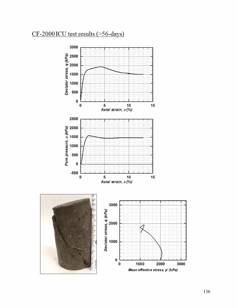
136

137

CF-3000 ICU test results (>56-days)

138

139

Appendix C. SEM images of failure surface and outer surface of soilcrete specimens.

140

141

142

143

144

145

146

147

148

149

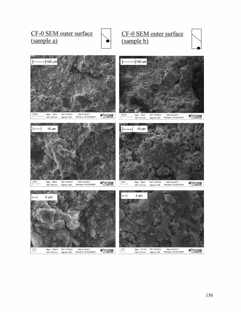
150

151

152

153

154

155

156

157

Appendix D. Results of CT scan and report of mercury intrusion porosimetry (MIP) tests.

C-0 CT scan specimen consolidation

Sample ID CT C-225-0 Type of test Iso ConsolidationConfining stress 0 kPa

Height (mm) Diameter (mm) Specific gravity Gs 2.65149.99 76.03 Density 1737.89 kg/m3

149.69 77.02 Unit weight 17.05 kN/m3

149.87 76.6276.65

Average Height Average Diameter Initial mass BT 1199.5 g149.85 76.58 mm Final mass AT - g14.99 7.66 cm Dry mass 874.62 g

Solids volume 330.05 cm3

Water content 37.15 %Volume 690.20 cm3

Void ratio 1.091Porosity 0.522Saturation degree 0.902

Notes:

Image of sample after test

Intact specimen used for CT scan

158

159

C-500 CT scan specimen consolidation

Sample ID CT C-225-500 Type of test Iso ConsolidationConfining stress 500 kPa

Height (mm) Diameter (mm) Specific gravity Gs 2.65149.83 76.4 Density 1862.32 kg/m3

149.8 76.43 Unit weight 18.27 kN/m3

149.79 77.0677.06

Average Height Average Diameter Initial mass BT 1290.3 g149.81 76.74 mm Final mass AT 1298.8 g14.98 7.67 cm Dry mass 1057.9 g

Solids volume 399.21 cm3

B-value 0.70Volume change 1.896 cm3

Trial 1 Trial 2Pressure head 20.22 49.11 kPaHydraulic gradient 13.76 33.42 m/mk 2.12E-10 4.31E-10 m/s

Before test After testWater content 21.97 22.77 %Volume 692.85 690.95 cm3

Void ratio 0.736 0.731Porosity 0.424 0.422Saturation degree 0.791 0.826

Notes:

Image of sample after test

Specimen used for CT scan. It was only consolidated to the required pressure. Not sheared with axial

displacement. Permeability test was done after saturation and prior to consolidation with different pressure head

160

161

C-3000 CT scan specimen consolidation

Sample ID CT C-225-3000 Type of test Iso ConsolidationConfining stress 3000 kPa

Height (mm) Diameter (mm) Specific gravity Gs 2.65150.14 76.49 Density 1886.64 kg/m3

150.31 76.63 Unit weight 18.51 kN/m3

150.31 76.4976.42

Average Height Average Diameter Initial mass BT 1303.2 g150.25 76.51 mm Final mass AT 1304.4 g15.03 7.65 cm Dry mass 1065.56 g

Solids volume 402.10 cm3

B-value 0.78Volume change 13.168 cm3

Trial 1 Trial 2Pressure head 19.60 49.13 kPaHydraulic gradient 13.30 33.33 m/mk 2.47E-10 1.61E-09 m/s

Before test After testWater content 22.30 22.41 %Volume 690.75 677.58 cm3

Void ratio 0.718 0.685Porosity 0.418 0.407Saturation degree 0.823 0.867

Notes:

Image of sample after test

Specimen used for CT scan. It was only consolidated to the required pressure. Not sheared with axial

displacement. Permeability test was done after saturation and prior to consolidation with different pressure head

162

163

CF-0 CT scan specimen consolidation

Sample ID CT CF-225-0 Type of test Iso ConsolidationConfining stress 0 kPa

Height (mm) Diameter (mm) Specific gravity Gs 2.64150.48 76.68 Density 1809.70 kg/m3

150.69 76.78 Unit weight 17.75 kN/m3

150.3 76.6176.58

Average Height Average Diameter Initial mass BT 1257.1 g150.49 76.66 mm Final mass AT - g15.05 7.67 cm Dry mass 964.6 g

Solids volume 365.38 cm3

Water content 30.32 %Volume 694.65 cm3

Void ratio 0.901Porosity 0.474Saturation degree 0.888

Notes:

Image of sample after test

Intact specimen used for CT scan

164

165

CF-500 CT scan specimen consolidation

Sample ID CT CF-225-500 Type of test Iso ConsolidationConfining stress 500 kPa

Height (mm) Diameter (mm) Specific gravity Gs 2.64150.63 75.92 Density 1825.23 kg/m3

150.59 75.01 Unit weight 17.91 kN/m3

150.41 76.3176.38

Average Height Average Diameter Initial mass BT 1243.4 g150.54 75.91 mm Final mass AT 1254.8 g15.05 7.59 cm Dry mass 1017.14 g

Solids volume 385.28 cm3

B-value 0.70Volume change 2.46 cm3

Trial 1 Trial 2Pressure head 19.88 48.37 kPaHydraulic gradient 13.48 32.79 m/mk 1.80E-10 3.50E-08 m/s

Before test After testWater content 22.24 23.37 %Volume 681.23 678.77 cm3

Void ratio 0.768 0.762Porosity 0.434 0.432Saturation degree 0.765 0.810

Notes:

Image of sample after test

Specimen used for CT scan. It was only consolidated to the required pressure. Not sheared with axial

displacement. Permeability test was done after saturation and prior to consolidation with different pressure head

166

167

CF-3000 CT scan specimen consolidation

Sample ID CT CF-225-3000 Type of test Iso ConsolidationConfining stress 3000 kPa

Height (mm) Diameter (mm) Specific gravity Gs 2.64149.99 76.19 Density 1776.18 kg/m3

150.31 76.87 Unit weight 17.42 kN/m3

150.13 76.4876.54

Average Height Average Diameter Initial mass BT 1226.4 g150.14 76.52 mm Final mass AT 1224 g15.01 7.65 cm Dry mass 985.6 g

Solids volume 373.33 cm3

B-value 0.70Volume change 21.252 cm3

Trial 1 Trial 2Pressure head 19.23 49.23 kPaHydraulic gradient 13.05 33.42 m/mk 9.76E-10 8.31E-10 m/s

Before test After testWater content 24.43 24.19 %Volume 690.47 669.22 cm3

Void ratio 0.849 0.793Porosity 0.459 0.442Saturation degree 0.759 0.806

Notes:

Image of sample after test

Specimen used for CT scan. It was only consolidated to the required pressure. Not sheared with axial

displacement. Permeability test was done after saturation and prior to consolidation with different pressure head

168

169

Mercury intrusion porosimetry summary report for soilcrete specimen samples

1. Objective

The following document summarizes the procedure and results for MIP tests conducted at the

Energy Systems Design Laboratory at the University of Alberta. The soilcrete specimen C-0 was

used for the CT scan analysis and samples from the top and bottom sections of the specimens

were selected to conduct the MIP test.

2. Parameters

The following constants are needed for calculations:

• ρHg, the density of mercury at room temperature and pressure: 13:5 g/cm3

•γ, the surface tension of mercury on the sample material at room temperature and pressure: 480

dyne/cm-1

• θ, the contact angle of mercury on the sample material at room temperature and pressure: 140°

3. Procedure and Theory

Porosimetry tests were performed using a PoreMaster 33 Mercury Porosimeter manufactured by

Quantachrome Instruments.

The soilcrete specimen was dried in an oven overnight after performing the CT scan. Two

samples were carved directly from the top and bottom section of the soilcrete specimen. The

samples were carved with a square section, at least 1 cm long on each side, and approximately

0.5 to 1 cm thickness.

To perform the mercury intrusion tests, the sample was placed inside the bulb of a glass

penetrometer cell with 0.5 cc stem volume. The penetrometer cell was evacuated to an absolute

pressure of 0.004 psi and then further evacuated for 30 min. The cell was filed with mercury and

the mercury was then pressurized, up to a maximum pressure of 33000 psi. The change in

volume of mercury was measured as the pressure was raised. A plot of the cumulative amount of

volume intruded at each step, plotted against the pressure at each step, given the cumulative

170

intruded volume curve. The volume is normalized with respect to the total intruded volume to

allow comparison between multiple samples of differing volume.

3.1 Pore Size Distribution

The pressure at which intrusion occurs can be related to the presence of pores within the sample

using the Washburn equation:

[1]

where P is the applied pressure, r is the pore radius,γ is the surface tension of mercury and θ is

the contact angle between the mercury and the sample material.

The logarithmic pore size distribution, for a given pressure Pi normalized with respect to total

sample volume, is calculated using the following equation:

[2]

where Vi is the absolute intruded volume measured up to pressure Pi, and Vpore is the total

measured intruded volume.

DX is the volume of the pores ∆V intruded at radius r divided by the total pore volume of the

entire sample Vpore. In this way, X represents the pore volume of each pore size normalized with

respect to the total pore volume. The value X is used rather than ∆V so that when multiple tests

are done with different sample volumes, the tests can be directly compared.

Note that, because smaller pores contain significantly less volume than larger ones, we need to

adjust the pore size distribution graph to make the smaller pores in the sample more visible. To

do this, we use ln(r) instead of r for the above graph, and we use a log scale for the x axis. This

allows us to see more clearly the areas we are most interested in (i.e. those pores of 10 um or

smaller).

3.2 Density and Porosity Calculations

171

There are three distinct values for density and porosity that can be found for a given sample:

bulk, particle and true. The following section will explain the difference between each type and

the calculations used to find it. Before discussion of the calculations of density and porosity,

some terms must be defined:

• Interparticle Void Space: Void space formed between individual particles of a bulk material.

This value may vary signi_cantly depending on the handling of the material. For instance,

interparticle void space can be reduced by manually compressing the material.

• Intraparticle Void Space or Intraparticle Pores: The volume of the pores existing within each

individual particle. This value will not vary significantly between samples of the same material,

assuming the measured material is homogeneous.

For these calculations, the cumulative intruded volume curve as described above is needed. Also

needed is the value Vatm, which is defined as the volume of mercury displaced by the sample

when the mercury is pressurized to atmospheric pressure. To measure this value, another test

procedure known as pycnometry is performed. The procedure for a pycnometry test is as

follows:

1. The porosimeter cell is evacuated and filled with mercury while no sample is in the cell.

2. The mass of the cell filled with mercury, mcell+Hg, is recorded with the mercury under

atmospheric pressure.

3. The same cell is emptied, the sample is added, and the cell is again evacuated and filled with

mercury.

4. The mass of the cell with both mercury and sample, mcell+Hg+sample, is recorded, again at

atmospheric pressure.

The difference in mass between these two measurements plus the mass of the sample itself,

msample, corresponds to the mass of mercury displaced by the sample at atmospheric conditions.

The equation used to find Vatm is:

172

[3]

Note that since the pycnometry and porosimetry tests are done with two separate samples of the

same material, they will likely have different masses. For calculation purposes, we must

normalize our volumes with respect to the sample mass. Thus our normalized volume, V*atm is

found using the equation:

[4]

where mpycno is the mass of sample used for the pycnometry experiment. V*atm has units of

cm3/g.

Once the value of V*atm is found, it can be used to find more significant volume values. The first

of these is bulk volume, Vbulk, which is defined as the volume taken up by the solid sample

material, as well as the volume of both interparticle void space and intraparticle void space. This

volume cannot be directly measured by the porosimeter, but we can estimate this volume to be

the volume of mercury displaced by the sample when the mercury is under extremely low

pressure (0.004 psi of absolute pressure). The normalized bulk volume, V*bulk, is calculated as

follows:

[5]

where V*atm is defined as above and V*int,atm is defined as the normalized volume intruded from

0.004 psi to 14.7 psi (atmospheric pressure). V*int,atm can be obtained from the porosimetry test,

specifically the normalized cumulative intruded volume curve.

The second useful is true volume, Vtrue, which is defined as the volume taken up by only the

solid material of the sample. The normalized true volume, Vtrue, is calculated as follows:

173

[6]

Vbulk is defined as above and V*int,33000psi is defined as the normalized volume intruded from

0.004 psi to 33000 psi (the maximum pressure attainable by the porosimeter). V*int,33000psi can be

obtained from the porosimetry test, specifically the normalized cumulative intruded volume

curve.

The third volume needed is the particle volume, Vparticle, which is defined as the volume taken up

by the solid material of the sample plus the volume taken up by intraparticle void space. The

normalized particle volume, V*particle, is calculated as follows:

[7]

where Vint;particle is defined as the normalized volume intruded from 0.004 psi up to a certain

pressure, Pparticle. V*int,particle is harder to define compared to V*int,atm and V*int,33000psi, as it

depends on the size of the intraparticle pores present in the sample. Pparticle should be determined

based on the appearance of the pore size distribution (PSD) curve. Commonly, the PSD curve

will have a bimodal distribution with two distinct peaks. The peak in the region of larger pore

sizes will correspond to interparticle void, while the other peak will correspond to intraparticle

void. A Pparticle is picked by taking a pore size in the region of little or no intrusion between these

two peaks and applying equation [1]. To ensure that a proper threshold radius is found, the pore

radii of the peaks should be compared to the average particle size (if known). The size of pores

in the smaller peak should be well below the average particle size (as the pores must fit within

the particles). The size of the pores in the larger peak should be larger than the average particle

size (otherwise intraparticle pores may be mistaken for intraparticle void).

Now, with these volumes determined, we can calculate porosity and density.

3.2.1 Density Calculations

True density, ρtrue, is defined as the ratio of sample mass to true volume. True density

represents the density of the material disregarding all void space, both interparticle and

174

intraparticle. Given that the normalized true volume was just found above, the true density is

simply found using the equation:

[8]

Particle density, ρparticle, is defined as the ratio of sample mass to particle volume. Particle

density represents the density of the material when including intraparticle void space, but

excluding interparticle void space. The equation for particle density is:

[9]

Bulk density, ρbulk, is defined as the ratio of sample mass to particle volume. Bulk density

represents the density of the material when including both intraparticle void space and

interparticle void space. Again, as stated above, the bulk properties of the material will change

based on handling of the bulk material. The equation for bulk density is:

[10]

Note that true density will always be greater than particle density, which will always be greater

than bulk density.

3.2.2 Porosity Calculations

Porosity, in general, is given as a ratio of void volume to the total volume, Vtotal, of a material.

In general, porosity, ϵ is calculated as:

175

[11]

True, particle and bulk porosities are distinguished by where the control volume of the material

is drawn. For bulk porosity the total volume of the material includes both interparticle and

intraparticle void. For particle porosity only intraparticle void is included. Neither types of void

are included for true porosity. By definition, true porosity is always 0%, as no void space is

included in the total volume. Bulk porosity, ϵbulk, is calculated as follows:

[12]

Particle porosity, ϵparticle is calculated similarly:

[13]

Note that bulk porosity will always be greater than particle porosity.

4. Results

4.1 Porosity and density of the samples

The particle porosity and density are calculated using a Pparticle value of 209 PSI, i.e., the pore

size is smaller than 1µm.

Table D-1. Summary of porosity and density values for tested samples.

176

The resulting porosity was compared to the porosity obtained from the CT scan analysis for the

same specimen (C-0) and the results show a good agreement. The sample labeled as “top”

showed a porosity of 38.59, which is similar to the one obtained for the section at 20 mm in the

porosity distribution for the specimen C-0 (Figure 4-20a). The sample labeled as “bottom”

showed a porosity of 31.23, which is similar to the one obtained on the other end of the soilcrete

specimen C-0, specifically in a section tested at approximately 115 mm from the bottom end of

the specimen (refer to Figure 4-20a).

4.2 Pore size distribution

Figure D-1 shows pore size distribution of the measured two samples. It can be seen from the

Figure D-1 that the pore size distribution between the two samples are pretty similar.

177

Figure D-1. Pore size distribution for samples at top and bottom of C-0 soilcrete specimen

178

Appendix E. Soilcrete mixing procedure.

1. General

Mixing methodology for laboratory production of soilcrete specimens

This document describes the mixing procedure used in the laboratory to produce cement-clay specimens (termed as soilcrete) in the context of a research project on ground improvement techniques applied to stiff Edmonton clay.

2. General Safety Precautions During Laboratory Procedure

2.1. There are inherent risks when working with electrical equipment and heavy objects, such as the mixing tools. The main concerns when working with the mixing equipment is the risk of malfunction or improper handling of the equipment.

2.2. Do NOT attempt to undertake these tests unless you have been trained in the safe use of the equipment, and have familiarized yourself in the correct use.

2.3. Proper PPE is required to be used during the mixing procedure according to the Laboratory safety rules. This includes but is not limited to: long pants, closed shoes, laboratory coat, safety glasses and nitrile gloves.

3. Apparatus 3.1. Electric blender (Warring Commercial model WSB60)

The electric blender is employed to mix the cement and water slurry. Prior to using the blender, it should be tested with clean water in a bucket to ensure proper functioning.

3.2. Automatic dough mixer (Hobart model Legacy HL200 18.9 Litre) 3.2.1. Hobart mixer base. Should be placed over a stable and flat surface for

the mixing procedure. A plastic sheet can be placed underneath to facilitate cleaning after mixing.

3.2.2. Mixing cup. Has a capacity of 18.9 Litre, which is suitable for mixing around 10 kg of dry soil mass and the slurry volume. The cup must be placed correctly on the based and secured on the sides to avoid sliding during the mixing procedure.

3.2.3. Dough mixer hook (Figure E-1a). The shape of this hook provides adequate mixing considering that the soil used for this investigation is a stiff clay. When softer soils are used a palette-shaped hook may be more appropriate (Figure E-1b).

179

Figure E-1. Dough mixer tools: (a) dough mixer hook used for stiff soil in the

present research, and (b) dough mixer palette for soft soil (not used in the present research)

4. Sampling

4.1. The soil used in the mixing for this research project is representative of a location in Eastern Edmonton where the soil is more likely a stiff low plastic clay with some sands. A total of six buckets of soil were collected at the site and stored in a moisture room to avoid the loss of natural water content.

4.2. To ensure a uniform water content among the sampling buckets the whole sample of soil was mixed thoroughly, and then stored in the same buckets until the time of the mixing.

5. Pre-Test Calculations 5.1. Prior to the mixing the soil natural water content needs to be measured, since the

natural water content is taken into account to select the water content for the mixing slurry.

5.2. Atterberg limits test should be performed on the soil sample to identify the liquid and plastic limits.

5.3. Determine the water content in the mix. The water content in the natural soil in addition to the water used in the slurry should range from 1.2 to 1.3 of the liquid limit of the soil, to ensure proper mixing.

6. Procedure 6.1. Preparation

6.1.1. All the devices must be placed in an appropriate and safe location for performing the mixing and tested to ensure proper functioning.

6.2. Setup 6.2.1. Soil content, binder content (additive) and water content need to be

selected and properly measured in this stage.

180

6.2.2. Soil is weighted in humid state with the natural water content, and is broken to small pieces for the mixing. The soil is placed directly in the cup of the mixer. The cup is later set correctly on the mixer base and the dough mixer hook must be placed.

Figure E-2. (a) soil being weighted in dough mixer cup, and (b) cup with soil

placed on dough mixer.

6.2.3. Cement and water are placed in independent containers for weighting. Cement content depends on the binder content selected by mass of dry soil for the mix. The water mass weighted is the water required for the slurry, as stated in 5.3.

6.2.4. The molds used for the production of the specimens are cylindrical plastic molds 75 mm diameter by 150 mm height. The molds must be greased inside before the mixing takes place

6.3. Slurry preparation 6.3.1. The water for the slurry is placed in a clean bucket and the blender is

introduced in the bucket and turned-on to medium speed. 6.3.2. The cement or the binder weighted on 6.2.3. is introduced by parts into

the bucket, and mixed in a rotary motion to avoid sticking of the cement to the walls of the bucket.

6.3.3. The mixing motion should be kept for at least 1 to 2 minutes.

181

Figure E-3. (a) blender with bucket containing water-cement slurry, and (b) dough mixer

with soil and slurry.

6.4. Mixing of the soilcrete 6.4.1. The slurry mixed in 6.3 is incorporated immediately to the soil in the

blender cup. 6.4.2. The component will be mixed at medium speed in stages of 30 seconds

each. After each stage the mix will be inspected and the portions of soil sticking to the sides of the cup will be separated with a spatula.

6.4.3. The total mixing time should not exceed 2 min, to avoid over-mixing.

6.5. Casting of the mix into the molds 6.5.1. The cup of the blender is removed and the mix is inspected. Hand

mixing may be required for the portions of the mix sticked to the sides to fully blend with the rest of the paste.

6.5.2. The mix is cast into the molds by holding a ball size of the paste and pressing it against the inside wall of the mold. The mold is later tapped on a hard surface to make the paste fall by gravity to the bottom and release air. Once the surface of the paste is even and no air is released the procedure is repeated with a new portion of paste.

6.5.3. Once the mold is filled to the top, the surface is leveled with a spatula and plastic film or a plastic lid is placed to cover the open end of the cylinder.

6.5.4. The specimens are stored in a closed container at room temperature, ensuring to have a 2-inch level of water into the container to provide the humid conditions for curing of the specimens.

6.5.5. The specimens remain in the closed container until completing the curing time for the following tests.

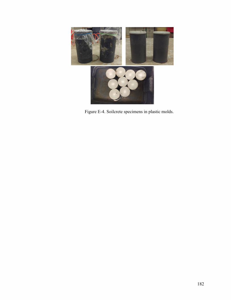
182

Figure E-4. Soilcrete specimens in plastic molds.

183

Appendix F. Laboratory standard operation procedure for triaxial testing of soilcrete specimens.

1. General

Standard Operation Procedure for Consolidated-Undrained Triaxial Test with permeability measurement Using GDS System

This SOP details the requirements for conducting consolidated-undrained triaxial tests on cement-stabilized clay specimens using GDS triaxial test system measuring the mechanical properties of specimens, including Young’s Modulus, friction angle, and cohesion. The SOP includes the measurement of permeability at different stages of the test and could further be adapted for other testing materials and consolidated-drained triaxial tests. This test method specifies the apparatus, instrumentation and procedures.

2. Referenced Documents

2.1. GeoREF Equipment Manuals 2.1.1. ISCO D-Series Pump, Installation and Operation Guide 2.1.2. GDS Pumps 2.1.3. ELE Tritest 50 Load Frame Operation Manual

3. General Safety Precautions and Corresponding SWP

3.1. There are inherent risks in working with high pressures, such as those required for consolidation. Programmable controllers are used for the pressure pumps, which require that the operator be familiar with the operation of the complete system.

3.2. Do NOT attempt to undertake these tests unless you have been trained in the safe use of the equipment, have familiarized yourself with the software and equipment manuals, as identified in Clause 2.1 above, and have read and understood the corresponding Safe Work Practices.

3.3. The corresponding Safe Work Practices include: 3.3.1. SWP – Pressure Safety 3.3.2. SWP – Mobile Crane 3.3.3. SWP – Hand Tools

184

4. Pre-test Safety Procedures 4.1. Adjust the ELE Load frame to ensure that it is levelled and firmly sitting on the

work station. 4.2. Run the ISCO and GDS pressure pumps at 3MPa to check if there is any leakage

in the pump and the pressure lines before assembling the setup.

5. Summary of Test Method 5.1. A cement-stabilized clay specimen, shape of a cylinder is placed inside the

triaxial cell. Tap water surrounding the specimen exerts confining pressure while ELE Tritest 50 load frame to apply axial load on the specimen.

5.2. Two GDS pressure pumps and one ISCO D-Series pump are used in the GDS system. One of the GDS pressure pumps is used to apply top back pressure, and another is used to apply cell pressure. The ISCO pump is used to apply bottom back pressure.

5.3. After a 25kPa back saturation overnight (back pressure at 500kPa and cell pressure at 525kPa), B-test is conducted on the specimen to ensure that the specimen has been fully saturated. Then the specimen could be consolidated to the targeted effective stress level.

5.4. Permeability test is conducted after finalizing the consolidation stage by closing the by-pass valve for GDS and ISCO back pressure pumps and running a higher pressure at the bottom of the specimen using ISCO back pressure pump.

5.5. When the targeted effective stress level is reached, shearing could be started using the ELE load frame at a certain shearing rate. The top crossbar of the load frame is fixed while the triaxial cell is moved up driven by a motor. The specimen volume change is directly measured by the GDS back pressure pump readings.

6. Mid-test Safety Procedures 6.1. It is essential to make sure that the LVDT has enough travel during the whole

process especially during shearing stage. 6.2. It is of great importance to make sure that all three pumps have enough volume to

accommodate the volume change during consolidation, permeability test and shearing.

6.3. Before shearing, it has to be ensured that the top crossbar of the ELE load frame is fixed and the loading rod is in center with the load frame.

6.4. When entering the shearing rate, it has to be ensured that the rate is correctively entered and really enforced by the system. Stay and monitor the LVDT and load cell readings in the initial stage of shearing.

6.5. When operating the GDS and ISCO pressure pumps, it is important to distinguish between volume/flow rate control and pressure control. It is safer to operate in the

185

pressure control mode. Great caution has to be paid when operating these pressure pumps.

7. Significance and Use

7.1. The consolidated-undrained triaxial tests are commonly used to get the mechanical properties of soil/rock specimens like Young’s Modulus, Poisson’s ratio, friction angle, and cohesion. Also consolidation and permeability tests could be conducted to get the compressibility parameters and permeability of the specimen.

8. Apparatus 8.1. Compression Apparatus

The ELE Tritest 50 load frame is employed to apply axial load on the specimen. The axial load is exerted on the specimen by moving the triaxial cell up using a motor at the base of the load frame while the top crossbar of the load frame is fixed.

8.2. Confining System 8.2.1. Triaxial Cell. Prior to using, ensure that the selected cell has the

required capacity to meet the confining pressure and axial load requirements for the diameter and depth (confining pressure) of the specimen to be tested.

8.2.2. Latex Rubber Membranes. Tap water is used as confining fluid in the GDS system and thus latex rubber membranes are suitable.

8.2.3. GDS Pressure Pump. A GDS pressure pump is used to apply cell pressure. The GDS pressure pump measures pressure and volume.

8.2.4. Confining pressure fluid. Tap water is used for applying confining pressure in this system.

8.2.5. Air pressure system. An air pressure system is connected to the three-way valve for confining pressure control. When the valve is opened to the air pressure system, this system could pressurize the triaxial cell to the target pressure first and then the GDS cell pressure pump could take over the control of confining pressure.

8.3. Flow Lines 8.3.1. GDS Pressure Pump. The GDS back pressure pump is connected to the

top of the specimen to apply top back pressure. 8.3.2. ISCO Pressure Pump. The ISCO back pressure pump is connected to

the bottom of the specimen to apply bottom back pressure. The ISCO pressure pump measures pressure, flow rate and volume.

186

8.3.3. Pore pressure transducer. The pore pressure transducer is connected to the bottom of the specimen to measure the pore pressure within the specimen.

8.4. Deformation 8.4.1. Axial deformation, if required, is determined through the use of a

LVDT.

9. Calibrations 9.1. Pore pressure transducer, LVDT, and load cell should be re-calibrated annually. 9.2. GDS and ISCO pressure pumps should be re-calibrated regularly.

10. Sampling

10.1. The samples are all representative of a same mixing batch, where a natural low plasticity clay was mixed with a binder of 22.5% of cement and mixing water content of 55 to 60%. At the time the test is conducted the samples would have at least 28 days of curing age and would be demolded and inspected for any visible imperfections on the surface.

10.2. Specimen should have a diameter of 3”. The average-height-to-average-diameter ratio shall be between 2 and 2.5 (ASTM D4767-11).

11. Test Specimens 11.1. Test specimens will be circular cylinders with a diameter of 3’’.

12. Pre-Test Calculations

12.1. Determine the required confining pressure for the consolidation phase of the test based on the depth of the specimen. This is equal to the overburden unit weight/m2 multiplied by depth.

12.2. Determine the average pore pressure according to the desired effective stress and the in-situ hydrostatic pressure.

13. Procedure 13.1. Preparation

13.1.1. Check if the right pump fluid is used. If not, both the ISCO pressure pump and GDS pressure pumps should be emptied and then refilled with the right fluid for a couple of times to make sure all the lines are both clean and saturated. Generally, brine and deionized water will be used in the testing system. The bottles for different fluid should be marked as it is hard to tell between brine and deionized water.

187

13.1.2. Saturate the base where the specimen will be seated. Inject deionized water from one side of the bottom back pressure channel and make sure the fluid comes out from another side. Then inject high-speed air into the channel for a while and finally refill the channel with the test fluid and close the valve. Repeat this procedure for cell pressure channel, and top back pressure channel.

13.1.3. Get two 3” porous stones ready by using ultrasonic cleaner and boiling in deionized water. Also cut two pieces of filter paper for the porous stones.

13.1.4. Check if the GDSLAB software is communicating well with the GDS system and getting reasonable readings from each instrument (LVDT, Load Cell, pore pressure transducer, GDS pumps and ISCO pump). Connect the ISCO and GDS pumps to atmosphere to check if the pressure reading is zero. If not, the pressure reading has to be zeroed.

13.2. Setup 13.2.1. Put a porous stone and then a filter paper on top of the specimen

pedestal, and saturate them with test fluid. Carefully place the specimen on top of the pedestal.

13.2.2. Use the membrane holder to place two layers of Latex rubber membranes over the specimen.

13.2.3. Put a filter paper and then a porous stone on top of the specimen. Flood the top of the specimen test fluid, and then carefully put on the loading cap. Place the port of the loading cap at the comfortable position for connecting to the top back pressure line.

13.2.4. Use the membrane holder to place three O-rings in the pedestal area to fix the bottom part of latex rubber membrane. Then flip over the membranes to cover the O-rings. In a similar way, put another three O-rings in the loading cap area to fix the top part of the membrane and flip the membranes over to cover the O-rings.

13.2.5. Attach the top back pressure line and saturate the line. 13.2.6. Connect the top back pressure line to the loading cap. Hand tight first

and then use wrenches to turn 1/8 circle to make sure the connection is tight.

13.2.7. The end of the loading rod is screwed into the main shaft and may be loose. Before putting on the triaxial cell, make sure that the end of loading rod is firmly fixed to the main shaft. Otherwise during shearing, the loading rod will be wobbling.

13.2.8. Put on the triaxial cell and transfer it to the ELE load frame using a mobile crane.

188

13.2.9. Connect the cell pressure port at the base of the triaxial cell to tap water and fill it up. The outlet at the top of the triaxial cell should be connected to atmosphere using a tube. When water comes out from the tube, the tap water should be stopped and let some time for the air inside the triaxial cell to escape. Then close the outlet.

189

13.2.10. Close the cell pressure valve, detach the tap water line, saturate the port and then connect the GDS cell pressure pump line to the cell pressure port.

13.2.11. Turn the three-way valve to the air pressure system. Open the cell pressure valve and use the air pressure to pressurize the triaxial cell to 525kPa. Watch out the water level indicator in the water tank of the air pressure system and make sure no air is injected into the triaxial cell. Make sure at this time, the GDS cell pressure pump is stopped.

13.2.12. Turn the three-way valve to the GDS cell pressure pump, and the readings on the pump control panel should indicate a pressure close to 525kPa. Then start running GDS cell pressure pump at 525kPa.

13.2.13. Saturate the ports for top (GDS) and bottom (ISCO) back pressure pump lines. Then connect the ISCO pump to bottom back pressure port 1. Connect the GDS back pressure pump to top back pressure port 1 and connect the pore pressure transducer to bottom back pressure port 2. At this time, make sure all ports are closed.

13.2.14. Open the valve for the pore pressure transducer. 13.2.15. Keep the by-pass valve for ISCO and GDS back pressure pumps open.

Open the valves for back pressure pumps. Run the GDS back pressure pump and gradually increase the pressure to 500kPa. Make sure the pressure does not exceed the cell pressure.

13.2.16. Setup the GDS data logging system. At this time, the computer will take over the control of GDS system. Remember to reset the targeted pressure values each time the data logging is reset and also note that the volume reading for GDS back pressure pump will be automatically zeroed.

13.3. B-Test 13.3.1. Keep the back pressure at 500kPa and cell pressure at 525kPa

overnight for back saturation. 13.3.2. Set the GDS back pressure pump in ‘HOLD’ mode using GDSLAB

software. Increase the cell pressure by 50kPa each step and wait until the GDS back pressure pump readings stabilize. Repeat this step for at least 5 times.

13.3.3. If the B-value is more than 90% ~ 95% (depends on the material), then it means the specimen has been saturated.

13.4. Consolidation

190

13.4.1. Decrease the cell pressure gradually to 525 kPa and then run the GDS back pressure pump to restore the 500kPa back pressure. Let the system stabilize for a while.

13.4.2. For consolidation, effective consolidation pressure for each step should not exceed 2 times of that for the previous step. So consolidation pressure could be increased in such a way as 50kPa, 100kPa, 200kPa, 400kPa, 800kPa and etc. until the targeted effective stress level is reached.

13.4.3. To capture the full process of consolidation, for each consolidation step, the GDS back pressure pump should be set to ‘HOLD’ mode and then increase the cell pressure. When the GDS back pressure pump readings become stable, then restore the back pressure to 500kPa, which will start the consolidation.

13.4.4. During consolidation, the by-pass valve is kept open and ISCO back pressure pump is stopped.

13.5. Permeability test

13.5.1. Run the ISCO back pressure pump at 500kPa. 13.5.2. Close the by-pass valve for GDS and ISCO back pressure pumps. 13.5.3. The ISCO bottom back pressure pump will be used to exert higher

pressure. And the pressure head for the permeability test should not exceed 10% of the effective consolidation pressure.

13.5.4. To make sure the overall back pressure within the specimen is maintained at 500kPa, the ISCO bottom back pressure pump should be running at (500+ permeability test pressure head/2) kPa and the GDS top back pressure pump should be running at (500- permeability test pressure head/2) kPa.

13.5.5. Monitor the ISCO and GDS back pressure pumps volume change for the initial one hour to ensure that the ISCO back pressure pump has enough volume remaining to pump out fluid and the GDS back pressure pump has enough capacity to receive fluid.

13.5.6. After the perm test, run both the GDS and ISCO back pressure pumps at 500kPa for a while. Then open the by-pass valve and stop the ISCO back pressure pump. Let the system stabilize.

13.5.7. Do the same for the permeability test after shearing.

13.6. Shearing 13.6.1. Setup the LVDT and ensure that there would be enough travel of

LVDT for the shearing.

191

13.6.2. Set the shearing rate based on the consolidation data and the equation recommended at ASTM D4767-11.

13.6.3. For some specimens, it would take long time for the loading rod to touch the specimen. Thus, in the beginning, a higher velocity could be used to shorten the waiting time for the rod to touch the specimen. However, during this period, someone has to be monitoring the load cell readings. Once significant increase of load cell reading (~50N) is observed, the movement of loading rod should be stopped. Then use the shearing rate to move the loading rod.

13.7. Disassemble the triaxial cell 13.7.1. Decrease cell pressure to 600kPa. 13.7.2. Decrease back pressure to 100 ~ 200kPa and then stop the GDS back

pressure pump. 13.7.3. Disconnect both ISCO and GDS back pressure pump lines and open

both the top and bottom back pressure valves to atmosphere for a while. Then close the valves.

13.7.4. Decrease the cell pressure to 200kPa, during which suction will be developing in the specimen. The suction will help maintain the shape of specimen.

13.7.5. Disconnect GDS cell pressure pump line and then connect the cell pressure port to a tube for chamber fluid drainage. Open the outlet on top of the triaxial cell and let the fluid drainage by gravity for a while.

13.7.6. Connect the outlet on the top of triaxial cell to air pressure which will fasten cell fluid drainage.