ARTICLE IN PRESS

Mechanical Systemsand

Signal Processing

0888-3270/$ - se

doi:10.1016/j.ym

�CorrespondE-mail addr

Mechanical Systems and Signal Processing 20 (2006) 2305–2320

www.elsevier.com/locate/jnlabr/ymssp

Adaptive-randomised self-calibration of electro-mechanicalshutters for space imaging

Mariolino De Ceccoa, Stefano Debeib, Mirco Zaccariottob,�, Marco Pertileb

aDIMS, Department of Mechanical and Structural Engineering, via Mesiano 77, 38050 Trento, ItalybCISAS, Centre of Studies and Activities for Space, University of Padova, Via Venezia 15, 35131 Padova, Italy

Received 25 November 2004; received in revised form 29 March 2006; accepted 30 March 2006

Available online 19 June 2006

Abstract

This work describes the self-calibration of a high-precision open-loop mechanism. The self-calibration method is applied

to a mechanical shutter for space applications, which was launched onboard the ESA-ROSETTA mission (launch: 2

March 2004). It is based on an adaptive ‘model reference’ and a ‘randomised’ search method which may be generalised to

applications in which high performance and functionality are strongly interconnected. The method makes use of an

adaptive ‘model-reference’ control approach [K.J. Astrom, B. Wittenmark, On self-tuning regulators Automatica 9 (1973)

185–199 [16]; K.J. Astrom, Theory and application of adaptive control, in: Proceedings of the Eighth IFAC World

Conference, Kyoto, Japan, 1981 [17]; D.E. Seborg, S.L. Shah, T.F. Edgar, Adaptive control strategies for process control,

AIChE Journal 6(32) (1986) 881–895 [18]] to guarantee mechanism performance. The proposed control system comprises

both a deterministic adaptive part and a random-search one [K.L. Clarkson, Applications of random sampling in

computational geometry, II, in: Proceedings of the Fourth Annual ACM Symposium on Computational Geometry, 1998,

pp. 1–11 [19]; P.K. Agarwal, M. Sharir, Efficient randomised algorithms for some geometric optimisation problems,

Discrete Computational Geometry 16 (1996) 317–337 [15]] to guarantee shutter mechanism functionality and performance

over testing lifetime (5� 104 cycles).

r 2006 Elsevier Ltd. All rights reserved.

Keywords: Self-calibration; Optical encoders; Adaptive control; Randomised optimisation

1. Introduction

Electromechanical shutters for imaging are specifically required when high contrast is mandatory. Theinfluence of shutter effects on the signal-to-noise ratio in an image is related not only to its performance but isalso closely dependant on the contents of the observed object. In particular, the OSIRIS imaging system, onboard the Rosetta spacecraft (ESA Cornerstone Mission, launched on March 2004 from Kourou, FrenchGuiana), was required to detect and map the nucleus of the Churyumov–Gerasimenko comet, and to studystructural evolution in the coma, part of the tail of the comet, and monitor-related dynamics. The OSIRISimaging system consists of two CCD (2048� 2048 pixels, pixel size 13.5 mm) cameras: a narrow angle camera

e front matter r 2006 Elsevier Ltd. All rights reserved.

ssp.2006.03.014

ing author. Tel.: +390498276801; fax: +39 0498276788.

ess: mirco.zaccariotto@unipd.it (M. Zaccariotto).

ARTICLE IN PRESSM. De Cecco et al. / Mechanical Systems and Signal Processing 20 (2006) 2305–23202306

(NAC) and a wide angle camera (WAC) with identical CCD and electro-mechanical shutters. Located in frontof the detector, each shutter consists of two independent four-bar linkages, each driving a thin blade.

As a comet is composed of extremely bright and dark parts, high contrast near the limb is obtained with a16-bit ADC converter and, thanks to short exposure times (minimum value 10ms), with an electromechanicalshutter instead of an electronic one, higher signal-to-noise ratios are obtained. As the imaging system canobserve the surface of the comet as close as 2 km, and as the comet nucleus rapidly rotates (period ¼ 0.2 day),the requirement of exposure repeatability and uniformity of the two camera shutters becomes 0.2%.

Deviation from uniformity of exposure is defined as the percentage of maximum difference in exposure timebetween two pixels of the CCD to the nominal exposure time. As the shutter is composed of two independentblades, driven by two four-bar linkages, the previous requirement implies an extremely constant velocity of theblades themselves in front of the CCD: 1.370.0026m/s [20].

In addition, performance (extremely constant velocity in front of the CCD) and functionality (reliablelocking and unlocking of shutter blades, light tightness) are closely interconnected: when SHM performancedecreases, the blade trajectories differ from the reference trajectories and thus SHM actuation fails. For thisreason, performance and functionality must be simultaneously controlled. High-speed and high-precisionmechanisms usually employ feedback control schemes, as described for instance in [1]. Feedback controlssatisfy precision requirements and at the same time cope with disturbances and unpredicted dynamics.Unfortunately, due to lack of resources for the OSIRIS project, the closed-loop control system was notimplemented, thus greatly complicating the control scheme. In a previous paper [2], it was shown thatmechanism performance could be achieved by means of an identification-based adaptive algorithm togetherwith closed-loop control. Other control methods were considered, particularly stochastic ones such as geneticalgorithms [3–5]. They were employed to find an optimal model of the mechanism but were discarded, becausetheir unconstrained random search could lead to dangerous solutions for mechanism integrity. One ofthe stochastic methods studied is reported in Section 3 and the preferred adaptive solution is described inSection 4.

The adaptive control was chosen and implemented to compensate for variations in parameters. A ‘model-reference’ scheme instead of an identification one was chosen, because of the poor accuracy achievable inparameter identification due to low friction and low damping. A search method, comprising a deterministicadaptive part and a random part, was chosen in order to achieve the lowest impact velocity of blades near theirtravel end. The target was to achieve reliability in locking and unlocking while ensuring light tightness. Duringtests, it was found that an increase in impact velocity leads to an increase in locking and unlocking reliabilityand to a decrease in light tightness. The random-search method adds stochastic capability to the system. Itmeans that the control system can cope with unmodelled phenomena. Indeed, the optimal solution depends onphenomena difficult to model and to take into account in a deterministic and explicit manner, such astribology and impact phenomena.

2. Mechanism and measurement unit

As shown in Figs. 1 and 2, the shutter comprises two four-bar linkages, driven by corresponding limited-angle torque (LAT) motors.

Each four-bar linkage consists of two parallel links having pivoted extremities on a common plate and theother extremities pivoted on a blade. In particular, links 1, 2 are connected to blade 1, and links 3, 4 to blade 2.All links have the same length and can rotate around four different parallel axes, which are normal to thecommon plate. Since links 1, 2 are parallel and have the same length, a rotation of link 1 yields a rotation ofthe same amplitude of link 2 and a pure translation of blade 1. The same behavior applies to links 3, 4 andblade 2. Both four-bar linkages have 1 degree of freedom (d.o.f.) and are moved by corresponding LATmotors, mounted on the rotation axis of links 2 and 4. One rotation of a motor makes the corresponding bladetranslate.

Referring to Fig. 1, the CCD which the shutter is due to cover selectively is placed behind blade 1. Whenblade 1 remains in the rest position, the CCD is completely covered and no light can reach it. Instead, whenblade 1 is moved by its motor (Fig. 2b), the CCD is gradually uncovered until blade 1 reaches the end of itslinear travel (Fig. 2c). The SHM comprises a latch mechanism (Fig. 2), which blocks blade 1 when it reaches

ARTICLE IN PRESS

Fig. 1. Perspective view of shutter mechanism (SHM).

Fig. 2. (a) Top view of shutter mechanism (SHM) and (b)–(d) back section of SHM.

M. De Cecco et al. / Mechanical Systems and Signal Processing 20 (2006) 2305–2320 2307

the end of its travel. The latch mechanism is a pivoted balance, comprising a blocking lever interacting withlink 1 and a release lever interacting with link 3. When blade 1 reaches the end of its travel, link 1 raises theblocking lever, whose U-shaped extremity blocks link 1 and blade 1 (Fig. 2d). In this position, the CCD iscompletely uncovered. After a suitable delay time, calculated according to a predetermined exposure time,blade 2 is also moved and gradually covers the CCD. When blade 2 reaches the end of its travel, link 3 pushesthe release lever (Fig. 2d) so that the blocking lever is raised, its U-shaped extremity frees link 1, and bothblades 1 and 2 can come back to their initial positions. The blades return by means of an elastic spring.

A complete SHM actuation cycle thus comprises: forward travel of blade 1, moved according to atrapezoidal velocity profile; blocking of blade 1 at the end of its travel, in order to leave the CCD completelyuncovered; forward travel of blade 2 according to a trapezoidal velocity profile; interaction of blade 2 with the

ARTICLE IN PRESSM. De Cecco et al. / Mechanical Systems and Signal Processing 20 (2006) 2305–23202308

latch mechanism and consequent release of blade 1; joint back travel of both blades 1 and 2, while the CCDremains covered. Total travel is about 42–45mm for both blades, whose trapezoidal velocity profile comprisesan acceleration from 0 to 1.3m/s in about 5mm, constant velocity in front of the 28-mm wide CCD,deceleration in about 3–4mm, in order to impact with the latch mechanism (blade 1 against the blocking leverand blade 2 against the release lever) at suitable velocity and to ensure reliable functioning (less than 0.1%failures); during back travel, blades 1 and 2 remain in contact, in order to ensure light tightness. In this phase,no power is available and the motors remain idle, since otherwise they may disturb CCD reading. The backtravel of each blade is driven by a corresponding spring acting on link 1 for blade 1 and link 3 for blade 2.

A pair of space-qualified optical encoders are directly coupled to each motor shaft and measure linkrotations, allowing the position and velocity profiles of both blades to be calculated. Position and velocityprofiles may be employed to post-process CCD-acquired images and to add self-calibration capability to theSHM. Taking into account a minimum exposure time of 10ms, the requirement of 1/500 exposure timeuniformity limits the maximum relative error in displacement estimation between the two blades to 0.02mm.The optical encoders have 3600 ppr with an edge accuracy of 72%, which means a displacement accuracy in(100mm link length) of about70.0035mm, i.e., one order of magnitude less. From a dynamical point of view,the maximum frequency of speed disturbance over the part (at ideal constant velocity travel, leading to anamplitude comparable to 0.02mm) is about 1 kHz [6,7]. The two 3600-ppr quadrature channels give anacquisition frequency of about 15 kHz, which therefore ensures that no aliasing affects measurements.

A Hall-effect sensor (called position sensor in Fig. 1) is mounted near the point of end-travel of blade 1 anddetermines whether blade 1 is in its locked position. A temperature sensor is embedded in each motor toprevent mechanism activation outside the set range of temperatures. A fail-safe mechanism is added to moveblade 1 and to allow CCD operation, even in the case of motor failure.

As stated above, each four-bar linkage is a 1-d.o.f. mechanism and may be modeled as follows:

J

kt

€yþc

kt

_yþk

kt

ðyþ y0Þ ¼ I3€yþc

J_yþ

k

Jðyþ y0Þ ¼

kt

JI , (1)

where J is the reduced moment of inertia of the four-bar linkage, which takes into account the inertia of twolinks and one blade; k is the elastic constant of a spring acting on link 1 (for blade 1) or link 3 (for blade 2); c isan overall damping factor, to take into account all possible friction sources acting on the four-bar linkage; yois a preload angle, which is set to keep both blades from leaving their initial resting positions when the motorsare idle; kt is the motor torque constant, which relates motor-applied torque to motor supply current I.

As noted in the Introduction, the mechanism exhibits constant velocity within 1.370.0026m/s for bothblades. This demanding requirement can be satisfied, providing that:

1.

the system has no feedback (open-loop mechanism), as imposed by low resources in terms of power andmass of the electronics unit [8,9];

2.

energy to drive the motors is available only for 53.3ms, so that the latching and unlatching of blade 2 arepartially uncontrolled. This was imposed by: (a) the need to ensure electromagnetic compatibility (EMC)during CCD reading, which starts immediately after mechanism movement in order to achieve a maximumsignal-to-noise ratio [10]; (b) the need to save electrical energy for long exposure times;

3.

the two independent four-bar linkages are not damped: their linear models are equivalent to a second-ordersystem with a very low damping ratio of the order of 0.01, which implies very low accuracy of mechanicalparameter identification [11,12]. By adding other effects such as friction, variations in actuating forces, andstatic and dynamic irregularities (as may be ascertained in [13,14]), the accuracy of a mechanism andparticularly of a focal plane shutter may be compromised. The need to lower damping was imposed by thehigh levels of cleanness required inside the telescope (which contains many optical components) and inorder to ensure maximum stability of mechanism performance;

4.

the system must guarantee performance over an extended range of temperatures (�30 to +60 1C) and greatvariations in parameters may be expected. This requirement is due to lack of thermal control of the NACtelescope;

5.

the system must guarantee performance for more than 50,000 cycles (predicted mechanism life, 105 cyclesduring lifetime testing) in about 10 years onboard a deep-space mission.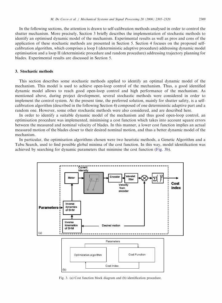

ARTICLE IN PRESSM. De Cecco et al. / Mechanical Systems and Signal Processing 20 (2006) 2305–2320 2309

In the following sections, the attention is drawn to self-calibration methods analysed in order to control theshutter mechanism. More precisely, Section 3 briefly describes the implementation of stochastic methods toidentify an optimised dynamic model of the mechanism. Experimental results as well as pros and cons of theapplication of these stochastic methods are presented in Section 5. Section 4 focuses on the proposed self-calibration algorithm, which comprises a loop I (deterministic adaptive procedure) addressing dynamic modeloptimisation and a loop II (deterministic procedure and random procedure) addressing trajectory planning forblades. Experimental results are discussed in Section 5.

3. Stochastic methods

This section describes some stochastic methods applied to identify an optimal dynamic model of themechanism. This model is used to achieve open-loop control of the mechanism. Thus, a good identifieddynamic model allows to reach good open-loop control and high performance of the mechanism. Asmentioned above, during project development, several stochastic methods were considered in order toimplement the control system. At the present time, the preferred solution, mainly for shutter safety, is a self-calibration algorithm (described in the following Section 4) composed of one deterministic adaptive part and arandom one. However, some other stochastic methods were also considered, and are described here.

In order to identify a suitable dynamic model of the mechanism and thus good open-loop control, anoptimisation procedure was implemented, minimising a cost function which takes into account square errorsbetween the measured and nominal velocity of blades. In this manner, a lower cost function implies an actualmeasured motion of the blades closer to their desired nominal motion, and thus a better dynamic model of themechanism.

In particular, the optimisation algorithms chosen were two heuristic methods, a Genetic Algorithm and aTabu Search, used to find possible global minima of the cost function. In this way, model identification wasachieved by searching for dynamic parameters that minimise the cost function (Fig. 3b).

Fig. 3. (a) Cost function block diagram and (b) identification procedure.

ARTICLE IN PRESSM. De Cecco et al. / Mechanical Systems and Signal Processing 20 (2006) 2305–23202310

The cost function is shown in Fig. 3a: the independent cost function variables are the parametersk=J; c=J; yo; kt=J of the dynamic model (1), (see preceding section), and the cost function output is the costindex. The higher the cost index, the worse the updated model, and vice versa. So Genetic Algorithms andTabu Search seek an overall cost index minimum.

As a cost function relates only to one four-bar linkage and its corresponding blade, the optimisationprocedure must be applied twice, once for blade 1 and once for blade 2. The cost function and optimisationmethods are the same for both blades.

The first time the cost function is evaluated, the desired displacement, and velocity and acceleration profilesof the blades are used to generate the desired value of motor rotation, which is computed only once and alwaysremains the same, stored in a local memory. An inverse kinematics model of the shutter is used to calculate thedesired motor rotation value.

Every time the function is evaluated, the following procedure is carried out:

�

the parameter values, in which the function must be evaluated, are chosen according to the selectedoptimisation algorithm (Genetic Algorithm or Tabu Search) and the inverse dynamic model, obtained frommodel (1), is updated using these values; � the intensity current waveform to be sent to the motors is calculated by the updated inverse dynamic model

and the desired motor rotation value;

� the current waveform is converted into an analog signal, is amplified by the current driver, and then

supplies the motor;

� blade motion is measured by encoders; � acquired motion profiles are pre-processed by a wavelet filter, selected so as not to introduce undesirable

time delays;

� the following error index is computed, and is the cumulative squared error between nominal and measured

velocities:

�

X

i

ðvi � vmiÞ2 (2)

where vi is the desired velocity at time i; vmi the measured velocity at time i.This solution presents the following advantages:

� some non-linear effects can be included in the model relatively easily; � there is no need to supply the shutter motors with special purpose signals: during optimisation, the motors

are fed by nominal current intensities. In this way, blade velocities have substantially the same trapezoidalwaveform during calibration and normal working.

4. Self-calibration algorithm

The architecture of the self-calibration algorithm, which compensates for parameter variation, is a ‘modelreference’ (see Fig. 4), in order to preserve performance and functionality on a photo-to-photo basis.

The control algorithm is of open-loop type, i.e., there is no real-time processing of the encoder feedback tomodify the input current during blade motion. However, when the SHM is actuated to acquire a new imagefrom CCD, the encoders measure link rotations and thus blade motion. In this way encoder output can beanalysed to improve SHM performance. This control method is not a real-time feedback control, and comprisestwo simultaneous loops, described below. Each loop uses the analysed encoder output in a different way:

1.

Loop I modifies the dynamic model (1) of each blade, changing the following parameters: elastic constant k,preload angle yo, and motor torque constant kt. This action is shown in Fig. 4 as an oriented connectionfrom ‘Error’ block to ‘Dynamic inversion’ block.

2.

Loop II modifies the trajectory of each blade, changing the desired trapezoidal motion profile of the blades.The target of loop II is to ensure reliable locking and unlocking and to minimise blade bouncing duringlocking and unlocking. When blade 1 reaches the blocking lever and link 1 engages in the U-shaped

ARTICLE IN PRESS

Fig. 4. Diagram of control system.

Fig. 5. Bouncing of blades 1 and 2.

M. De Cecco et al. / Mechanical Systems and Signal Processing 20 (2006) 2305–2320 2311

extremity, may bounce slightly inside it. Similarly, when blade 2 reaches its travel end and link 3 interactswith the release lever, the motor may keep pushing link 3 against the lever, causing impacts and rebounds.These oscillations and bounces must be avoided, since they accelerate wear of impacting surfaces, degradeSHM reliability, and increase the possibility of light entering between the blades during their back travel(Fig. 5). The action of loop II is shown in Fig. 4 as an oriented loop from ‘Error’ block to ‘Trajectoryplanning’ block, and vice versa.

4.1. Loop I: adaptive part

Referring to Fig. 6, the desired reference trajectories of blades 1 and 2 have a trapezoidal shape. Inparticular, the trajectory of each blade has a constant velocity portion as the CCD is uncovered or covered(respectively, blades 1 or 2): an initial acceleration portion, to drive the blade from its initial rest position toconstant velocity, and a deceleration portion to drive the blade from constant velocity to a proper impactvelocity of interaction with the locking mechanism. Both acceleration and deceleration portions are outsidethe optical field of view of the CCD.

Referring to Fig. 4, the dynamic inversion block receives the parameters of the dynamic model (1) from the‘Adaptive strategy’ block and computes the current to feed the motors. With this current profile, the motorsshould make the corresponding four-bar linkage follow the desired trajectory as closely as possible. Theoutput of the mechanism is the vector of encoder pulses, which is processed by the ‘Encoder pulse processing’block to generate a measured blade trajectory (a vector). This measured trajectory is then compared with thenominal trajectory in the ‘Error’ block. The difference between nominal and measured trajectories causes achange in the parameters of the ‘Dynamic inversion’ block.

If friction is neglected, Eq. (1) may be rewritten as follows:

€yþ ðk=Jðyþ yoÞÞ

kt=Jffi I . (3)

Clearly, the controlled parameters are k=J; yo; kt=J. The ‘Adaptive strategy’ block calculates a new set ofdynamic parameters, taking into account the previous values and any error between desired and measured

ARTICLE IN PRESS

Fig. 6. An experimental example of reference and measured velocities (top); error and linear interpolation (bottom).

M. De Cecco et al. / Mechanical Systems and Signal Processing 20 (2006) 2305–23202312

trajectories. In particular, a mean error Err is calculated, employing only those values of the reference andmeasured trajectory vectors corresponding to the constant velocity portion, and a mean error Err0.2 iscalculated considering only 1/5 (from the first value) of the previously employed values (i.e., referring to Fig. 6,the mean error calculated between 0.03 and 0.035 s). A linear regression of the difference between referenceand measured trajectory vectors is also performed (see interpolation line of bottom part of Fig. 6) and slopepp(1) of the linear fitting is calculated.

For the dynamic parameters, the algorithm computes a set of updated values as follows:

kt

J!

kt

Jþ 1100Err,

yo ! yo þ 50Err0:2,

k

J!

k

Jþ 5 ppð1Þ. ð4Þ

Numerical coefficients (1100, 50, 5) are obtained by trial-and-error empirical procedure. Eq. (4) updatedynamic parameters k=J; yo; kt=J basing on different error indexes pp(1), Err0.2, Err, correspondingly. Thisparticular updating rule is due to the fact that each error index is more sensitive to the correspondingparameter than to the others, i.e., Err is more sensitive to a change of kt/J than to a change of the otherparameters yo and k/J. However, it does not mean that a change in yo or k/J does not modify Err. A variationof kt/J makes change all three error indexes, but it mostly affects the error index Err. This preferred connectionbetween one dynamic parameter and one error index derives from experimental observations.

4.2. Loop II: randomised part

The desired acceleration and velocity profiles of blades 1 and 2 are shown in detail in Fig. 7. After theacceleration, constant velocity and deceleration portions described above, blade 1 reaches the blocking leverand blade 2 reaches the release lever at velocity Vi. During experimental testing, it was found that imposing asecond acceleration portion on the blade after deceleration reduces the number of failures of the latchmechanism. This second acceleration portion is characterised by two acceleration values, a1 and a2 (Fig. 7).

The algorithm of loop II modifies the deceleration and second acceleration portion of both bladetrajectories, in order to ensure reliable locking and unlocking and to minimise blade bouncing. The algorithm

ARTICLE IN PRESS

Fig. 7. Trajectory planning.

M. De Cecco et al. / Mechanical Systems and Signal Processing 20 (2006) 2305–2320 2313

can modify three kinematic parameters independently for each blade: impact velocity Vi and the twoacceleration values a1, a2.

When derivatives are not known, and the cost function may have multiple minima, randomised searchmethods have greater efficiency compared with deterministic techniques [15].

The control of blade kinematics by means of trajectory planning (see Fig. 4) is different for blades 1 and 2,since the two blades have different tasks: blade 1 must uncover the CCD and be properly locked, minimisingoscillations, blade 2 must cover the CCD again, unlock blade 1 and induce blade back travel maintaining lighttightness. As regards blade 1, impact velocity Vi should be minimised and the extra accelerations a1, a2 shouldbe set to reduce blade 1 bouncing inside the U-shaped extremity of the blocking lever, while keeping thelocking rate reliable. In the following, only the self-calibration algorithm for blade 1 is described in detail,since the reasoning for blade 2 is almost the same.

In order to satisfy SHM performance requirements, the optimal kinematic parameter search is implementedjointly by a deterministic procedure and a random procedure. After each SHM actuation, the algorithmcomputes an index F, which is proportional to the oscillations of blade 1 inside the U-shaped extremity of theblocking lever, and an index G, which takes into account the reliability of the latching mechanism—the higherG, the more reliable the latching mechanism. Then the algorithm adjusts kinematic parameters Vi and a1,a2.This adjustment may be performed by either a deterministic calculating procedure or a random process. Themanner and degree of adjustment depend on the calculated values of indexes F and G and aim at minimisingindex F and keeping index G sufficiently high. The search for optimal kinematics takes place in an iterativefashion, performing SHM actuation and then kinematic parameter adjustment.

In more detail, with reference to Fig. 8, the proposed mixed deterministic and randomised algorithm may besummarised in the following steps:

1.

Initialisation steps:(a) Initialisation of kinematic parameters Vi, a1, a2, and of three reference values Vi_memo, a1_memo,

a2_memo;(b) Initial setting of two integer indexes: nx is the number of iterations between two subsequent parameter

adjustments performed by a random process (random adjustment); n0 (onx) generates a checking

ARTICLE IN PRESS

Fig. 8. Flow chart of first blade control of impact velocity and extra accelerations in order to maintain reliable locking and minimise first

blade oscillations inside U-shape extremity.

M. De Cecco et al. / Mechanical Systems and Signal Processing 20 (2006) 2305–23202314

iteration which verifies if index F is decreasing or not. This check is performed after n0 iterations fromthe random adjustment;

(c) Initialisation of iterations counter n ¼ 1;(d) Initialisation of index G ¼ 1 and a reference value F_memo ¼+N;(e) Initial setting of a series of optimisation parameters which is employed during kinematic parameter

adjustment: three increments DVi, Da1, Da2 of Vi, a1, a2, respectively, and three corresponding signedintegers Visd, a1sd, a2sdA[�1, 1] which define the direction of the adjustments;

(f) Initial SHM actuation: if blade 1 has been properly locked by the latch mechanism, a variable Lock isset to 1 (Lock ¼ 1), otherwise Lock ¼ 0;

ARTICLE IN PRESSM. De Cecco et al. / Mechanical Systems and Signal Processing 20 (2006) 2305–2320 2315

(g) The algorithm analyzes the encoder output (encoder pulses) in order to quantify the amount of bladeoscillation inside the U-shaped extremity, and uses this amount and the Lock value to calculate aninitial index F; the greater the oscillation, the higher the index F;

(h) Index G is updated by: G ¼ 0:9G+0.1 Lock;

2. Parameter adjustment: the remainder of the division n/nx is computed and, depending on its value, one of

the following three alternative subroutines is performed:(a) Random adjustment: If the remainder ¼ 0, which means that the number of iterations after the

preceding random adjustment is equal to fixed number nx, then the following updating and adjustmentsare made: G ¼ 1, F_memo ¼ F, Vi_memo ¼ Vi, a1_memo ¼ a1, a2_memo ¼ a2, Vi ¼ Vi+(Ran-dom1–0.5) DVi, a1 ¼ a1+(Random2–0.5) Da1, a2 ¼ a2+(Random3–0.5) Da2, where Random1,Random2, Random3 are randomly generated numbers between 0 and 1;

(b) Optimisation adjustment: if the remainder is 6¼0 and 6¼n0, then the algorithm tries to optimise kinematicparameters Vi, a1, a2 according to the selected optimisation parameters (DVi, Da1, Da2, Visd, a1sd,a2sd). The three parameters are adjusted one at a time, i.e., only one is adjusted during every iteration.So the remainder of the division n/3 is computed and, depending on its value, one of the following threealternative adjustments is performed:(i) If the remainder ¼ 0, then a1 ¼ a1+a1sd Da1;(ii) If the remainder ¼ 1, then Vi ¼ Vi+Visd DVi;(iii) If the remainder ¼ 2, then a2 ¼ a2+a2sd Da2;

(c) Iteration check: If the remainder ¼ n0, which means that the algorithm has performed n0 iterations afterthe latest random adjustment, then variable F is compared with the current F_memo. The task of thissubroutine is to verify if the iterations performed from the latest random adjustment have actually beenable to reduce value F; if FpF_memo, then the preceding optimisation subroutine (b) is performed,otherwise the following adjustments are made: G ¼ 1, Vi ¼ Vi_memo, a1 ¼ a1_memo, a2 ¼ a2_memo—that is, the values of Vi_memo, a1_memo, a2_memo (which were stored just before the latest randomadjustment) are restored;

3.

SHM actuation:(a) the SHM is actuated and encoder output is acquired;(b) if blade 1 has been properly locked by the latch mechanism, then Lock ¼ 1, otherwise Lock ¼ 0;(c) a backup Fprec of the current F variable is created: Fprec ¼ F;(d) variable F is updated by analyzing the latest acquired encoder pulses and taking into account latest

updated Lock variable, as performed in point 1(g).

4. variable G check:

(a) The G variable is updated: G ¼ 0:9G þ 0:1 Lock;(b) The G variable is compared with a reference value (0.89) and, depending on the result, two different

actions are performed:(i) If GX0:89, which means that the reliability of the latch mechanism is high, then the algorithm goes

on to point 5;(ii) If Go0:89, which means that the reliability of the latch mechanism was decreased by the

optimisation adjustments (phase 2(b)), then impact velocity Vi is increased, V i ¼ Vi þ 5DVi,G ¼ 0:9, and the algorithm goes back to point 3;

5.

variable F check: variable F is compared with the backup value stored in 3(c) (Fprec) and, depending on theresult, two different actions are performed:(a) If FpFprec, which means that the oscillations of blade 1 were not increased by phases 2 or 4, then the

algorithm goes on to point 6;(b) If F4Fprec, which means that the oscillations of blade 1 were increased by phases 2 or 4, then one

kinematic parameter is adjusted and the corresponding search direction of phase 2(b) is reversed (bychanging the sign of Visd, a1sd or a2sd). For this, the remainder of the division n/3 is computed and,depending on its value, one of the following three alternative adjustments is performed:(i) If the remainder ¼ 0, then a1 ¼ a1�a1sd Da1, a1sd ¼ �a1sd;(ii) If the remainder ¼ 1, then Vi ¼ Vi�Visd DVi, Visd ¼ �Visd;(iii) If the remainder ¼ 2, then a2 ¼ a2�a2sd Da2; a2sd ¼ �a2sd;

ARTICLE IN PRESSM. De Cecco et al. / Mechanical Systems and Signal Processing 20 (2006) 2305–23202316

6.

Ta

Lis

Sym

F

G

Vi

DV

Vis

Ai

Da

Ais

n

Lo

Un

Ra

nx

no

Iteration return:(a) The iteration counter is increased: n ¼ nþ 1;(b) Execution of the algorithm goes back to phase 2.

ble 1

t of

bol

i

d

i

d

ck

lock

ndom

Fig. 8 shows the flow chart of the search method (see Table 1 for meaning of symbols).

5. Experimental results

5.1. Stochastic methods

The optimisation procedure does allow the required performance to be achieved, particularly when a geneticalgorithm is used. Fig. 9(a) and (b) shows the very accurate velocity profile obtained at the end of a geneticalgorithm optimisation procedure. However, as the shutter is actuated every time the cost function isevaluated, the number of shutter actuations may be considerable. Worse, during the optimisation procedure,the algorithm may select parameters of the dynamical model (1) which make the blades move too fast and/orimpact with violence at their travel end, as shown in Fig. 9(c). This behaviour does not guarantee shuttermechanism integrity and thus this optimisation procedure cannot be employed.

5.2. Self-calibration algorithm

This section describes tests performed at room temperature and in a thermal vacuum (TV) environment.The results of loop I (adaptive part, which adapts dynamic model (1)) and loop II (randomised part, whichmodifies the kinematic parameters) are shown separately.

Fig. 10 shows three cycles of the dynamic calibration (loop I), held at constant (clean room) temperature. Itclearly highlights the fast convergence of the algorithm: from 7.7% of mean error at the first attempt, a 4%error is obtained at the second attempt, and the third cycle has a 0.5% error. During all tests at constanttemperature, the dynamic optimisation algorithm proved to converge within the required performance in lessthan five cycles.

Moreover, dynamic calibration (loop I) was qualified to be compliant with the space environment by meansof TV tests conducted at the CISAS laboratories (see Fig. 11). Dynamic calibration was performed with theSHM subjected to temperature step functions, in order to test the capacity of the algorithm to cope withsudden temperature changes. Fig. 12 shows the behavior of the dynamic self-calibration algorithm facing astepped temperature change. As the temperature changes, the mean blade velocity over the CCD (which

symbols

Description

Cost function proportional to the first blade bouncing inside U-shaped extremity

Locking-failure/unlocking-failure indicator inversely proportional to blade reliability

Impact velocity

Step variation in impact velocity

Direction of search for velocity

First (i ¼ 1) or second (i ¼ 2) extra accelerations

Step variation in extra accelerations (i ¼ 1 or 2)

Direction of search for extra accelerations

Iteration counter

1 if blade was successfully locked in previous shutter cycle, 0 otherwise

1 if blade was successfully unlocked in previous shutter cycle, 0 otherwise

i Random number between 0 and 1

Number of iterations between random adjustments

Number of cycles to allow optimization after random adjustment

ARTICLE IN PRESS

Fig. 9. Measured blade velocities: (a, b) after genetic algorithm optimisation procedure and (c) intermediate step during optimisation, with

impact at end of travel.

Fig. 10. Three cycles of dynamic calibration.

M. De Cecco et al. / Mechanical Systems and Signal Processing 20 (2006) 2305–2320 2317

should be constant at 1.3m/s) veers from the desired value, and the adaptive algorithm modifies the dynamicparameters of model (1) to restore good performance (blade velocity close to 1.3m/s).

Loop II was applied at constant temperature. It was found that best SHM performance was achieved whendynamic calibration was performed before kinematic optimisation.

Fig. 13 shows an example of the kinematic optimisation test, which starts from an impact velocity Vi of0.3m/s and end with a final impact velocity Vi of about 0.08m/s, corresponding to the lowest F index. Thisalgorithm takes about 90 cycles to find good kinematic parameters and about 300 cycles to reach the lowestF index (i.e., the lowest number of blade 1 oscillations inside the U-shaped extremity of the blocking lever,and the most effective light tightness). Initial impact velocity Vi ¼ 0:3m=s gives reliable locking performance(G index is always max 1) but yields poor light tightness (high F index), whereas final impact velocityV i � 0:08m=s ensures both good locking (G index remains at 1) and light tightness (low F index). The loop IIalgorithm decreases impact velocity Vi by attempting to minimise the F index until the locking mechanism isno longer able to block blade 1 properly. In this state, blade 1 does not have sufficient kinetic energy to raisethe blocking lever, and the algorithm again has to increase impact velocity Vi.

If the loop II algorithm continues, as shown in Fig. 13, it may find subsequent optimal sets of parameters.However, if a proper cycling end condition is not set, it may keep on oscillating between suboptimal stateswithout converging. In order to cope with problem, it must save the best parameters set during cycling, andreload them at the end of optimisation.

ARTICLE IN PRESS

Fig. 11. TV chamber used for development and qualification of mechanism and self-calibration algorithm.

Fig. 12. Dynamic calibration (loop I) during a TV step test.

M. De Cecco et al. / Mechanical Systems and Signal Processing 20 (2006) 2305–23202318

ARTICLE IN PRESS

Fig. 13. Results of kinematic search (loop II).

M. De Cecco et al. / Mechanical Systems and Signal Processing 20 (2006) 2305–2320 2319

6. Conclusions

The self-calibration technique described here was applied to a mechanical shutter for space applications.The dynamic optimisation algorithm (loop I) was verified both at constant temperature and when subjected toa temperature step function at the CISAS Thermo Vacuum facility. The dynamic optimisation algorithmproved to converge at constant temperature within the required performance values of 1.3m/s70.2% in lessthan five cycles. These values were also achieved during temperature step changes, due to continual adjustmentof dynamic parameters. A kinematic optimisation algorithm (loop II) was implemented to ensure reliablefunction during the long-lasting Rosetta mission. The kinematic optimisation algorithm combines adeterministic adaptive part with a randomised method, and allowed a good performance to be achieved interms of locking and light tightness in about 90 cycles, starting from a wrong configuration.

Acknowledgements

Work done in the frame of the OSIRIS/ROSETTA programme partly supported by the Italian SpaceAgency (ASI) through a contract to CISAS/UPd. The OSIRIS imaging system (PI Dr. U. Keller) on boardROSETTA is managed by the Max-Planck Institute for Solar System Research (MPS) in Katlenburg-Lindau,thanks to an International collaboration between Germany, France, Italy, Spain and Sweden.

References

[1] US Patent No. 5,822,629, Electronically controlled variable slit width focal plane shutter, 1998.

[2] M. De Cecco, F. Angrilli, R. Da Forno, S. Debei, Uniformity error reduction by adaptive control of an electro-mechanical shutter for

space imaging, in: Proceedings of the 48th International Astronautical Congress, Torino, Italy, October 1997.

ARTICLE IN PRESSM. De Cecco et al. / Mechanical Systems and Signal Processing 20 (2006) 2305–23202320

[3] G. Acosta, E. Todorovich, Genetic algorithms and fuzzy control: a practical synergism for industrial applications, Computers in

Industry 52 (2003) 183–195.

[4] K.T. Kalveram, U. Natke, Motor control and movement optimization learned by combining auto-imitative and genetic algorithms,

in: ESANN 2001 Proceedings—European Symposium on Artificial Neural Networks, Bruges, Belgium, D-Facto public, ISBN:

2-930307-01-3, April 2001, pp. 165–170.

[5] D.K. Liu, Y.L. Yang, Q.S. Li, Optimum positioning of actuators in tall buildings using genetic algorithm, Computers and Structures

81 (2003) 2823–2827.

[6] M. Zaccariotto, M. De Cecco, S. Debei, M. Pertile, Calibration of an electro-mechanical shutter: dynamical effects, Congress on

Mechanical Measurement, Montegrotto, Italy, September 2002.

[7] S. Debei, M. De Cecco, M. Pertile, M. Zaccariotto, High performance shutter for space applications, in: Proceedings of the

International Symposium on Optical Science and Technology, SPIE 47th Annual Meeting, Seattle, WA, USA, July 2002.

[8] H.U. Keller, et al., ROSETTA Comet Rendezvous Mission, ESA Publication Science 7 (1993).

[9] S. Debei, F. Angrilli, G. Bianchini, M. De Cecco, G. Guizzo, G. Parzianello, M. Pertile, B. Saggin, P. Ramous, M. Zaccariotto, The

wide angle camera for OSIRIS experiment of the ROSETTA Mission: design validation and qualification, XVI congresso nazionale

AIDAA, Palermo, Italy, September 2001.

[10] N. Thomas, The Influence of an Electronic Shutter on OSIRIS CCD Images, Draft 1, November 1995.

[11] Prakah-Asante, O. Kwaku, Single-axis servomechanism for control experiments involving Coulomb friction, backlash and joint

compliance, American Society of Mechanical Engineers, Applied Mechanics Division, 1992.

[12] T. Soderstrom, P. Stoica, System Identification, Prentice-Hall International, UK, 1989.

[13] M. Gautier, Identification of the inertial and drive gain parameters of robots, in: Proceedings of the 33rd IEEE Conference on

Decision and Control, 1994.

[14] A.I. Katkov, Analysis of the accuracy and operating stability of focal-plane camera shutters with independent movement of the

curtains, Soviet Journal of Optical Technology (1977).

[15] P.K. Agarwal, M. Sharir, Efficient randomized algorithms for some geometric optimization problems, Discrete & Computational

Geometry 16 (1996) 317–337.

[16] K.J. Astrom, B. Wittenmark, On self-tuning regulators, Automatica 9 (1973) 185–199.

[17] K.J. Astrom, Theory and application of adaptive control, in: Proceedings of the Eighth IFAC World Conference, Kyoto, Japan,

1981.

[18] D.E. Seborg, S.L. Shah, T.F. Edgar, Adaptive control strategies for process control, AIChE Journal 6 (32) (1986) 881–895.

[19] K.L. Clarkson, Applications of random sampling in computational geometry, in: II Proceedings of the Fourth Annual ACM

Symposium on Computational Geometry, 1998, pp. 1–11.

[20] Guide to Expression of Uncertainty in Measurements ISO, 1993.