J Comput NeurosciDOI 10.1007/s10827-014-0508-6

Adaptation and shunting inhibition leadsto pyramidal/interneuron gamma with sparsefiring of pyramidal cells

Martin Krupa · Stan Gielen · Boris Gutkin

Received: 15 April 2012 / Revised: 29 May 2014 / Accepted: 2 June 2014© Springer Science+Business Media New York 2014

Abstract Gamma oscillations are a prominent phe-nomenon related to a number of brain functions. Data showthat individual pyramidal neurons can fire at rate belowgamma with the population showing clear gamma oscilla-tions and synchrony. In one kind of idealized model of suchweak gamma, pyramidal neurons fire in clusters. Here weprovide a theory for clustered gamma PING rhythms withstrong inhibition and weaker excitation. Our simulations ofbiophysical models show that the adaptation of pyramidalneurons coupled with their low firing rate leads to clusterformation. A partially analytic study of a canonical modelshows that the phase response curves with a near zero flatregion, caused by the presence of the slow adaptive current,are the key to the formation of clusters. Furthermore weexamine shunting inhibition and show that clusters becomerobust and generic

Action Editor: N. Kopell

M. Krupa (�)Project Team MYCENAE, INRIA Paris-RocquencourtResearch Centre, Domaine de Voluceau BP 105,78153 Le Chesnay cedex, Francee-mail: maciej.p.krupa@gmail.com

S. GielenHuygens Gebouw, Radboud University Nijmegen,Heyendaalseweg 135, 6525 AJ Nijmegen, The Netherlands

B. GutkinGroup for Neural Theory, Ecole Normale Superieure,29, rue d’Ulm, 75005 Paris, France

B. GutkinNational Research University Higher School of Economics,Center for Cognition and Decision Making, Moscow, Russia

Keywords Gamma oscillations · Spike frequencyadaptation · Clustered oscillations · Multiple timer scales ·Shunting inhibition

1 Introduction

The gamma rhythm is ubiquitous in the cortex. It appearsduring sensory and cognitive tasks and has been associatedwith increased attention (Engel et al. 2001), with sensoryprocessing and feature binding, (Gray 1999; Fries et al.2001), with short memory formation (Tallon-Baudry et al.1998) as well as with a range of other forms of neuronalinformation processing, see Wang (2010) for a review. Thisgamma band activity appears to be spatially organized withlocal coherence (von Stein and Sarnthein 2000; Jia et al.2011).

Two regimes of gamma have been observed: stronggamma, where the pyramidal cells and fast-spiking,parvalbumin-positive basket cells fire on every cycle, andweak gamma, where interneurons fire on every cycle andpyramidal cells skip cycles (randomly), so that the individ-ual pyramidal cell firing is sparse and yet the populationshows clear gamma oscillations (Borgers et al. 2005). In anidealized and simplified model of weak gamma the pyrami-dal cells fire in clusters, with synchrony within each cluster(Kilpatrick and Ermentrout 2011).

One of the prevalent mechanisms of gamma is Pyra-midal Interneuron Gamma (PING), based on the idea thatexcitatory input from the pyramidal cells to the interneu-rons plays an important role in the formation of the rhythm(Whittington et al. 1997; Cunningham et al. 2004). Theoverall scheme for PING (weak or strong) is as follows: thepyramidal cells fire a volley of spikes, strongly exciting theinhibitory interneurons, whose firing, in turn, suppresses the

J Comput Neurosci

pyramidal cell activity. When the inhibition wears off, thepyramidal cells are free to fire a volley again. Theoreticalanalyses have shown (Borgers and Kopell 2003, 2005) thatsuch ping-pong of excitation and inhibition should lead tosynchronization. The difference between weak and strongPING is that, in strong PING, the pyramidal cells fire in syn-chrony (all approximately at the same time), while in weakPING only a subset of the pyramidal cells fire at a time.Thus the mechanisms that lead to PING synchronizationare a combination of intrinsic cellular properties and synap-tic properties. The focus of earlier work on strong gamma(Borgers and Kopell 2003, 2005) has been on the synapticproperties, specifically on the role of inhibition in timing thegamma oscillations. While gamma synchrony is genericallyglobal, several works have shown that the firing of individ-ual pyramidal cells can have much lower frequency thangamma (Cunningham et al. 2004). Some of the time tracesof experimental data indicate that the pyramidal cells couldbe firing regularly, in particular this is suggested by Fig. 1 inCunningham et al. (2004).

The spatial organization of weak gamma remains a ques-tion of interest. An important advance in understandingweak gamma came through the work of Kilpatrick andErmentrout (2011) who showed using methods of singu-lar perturbation theory that a combination of inhibitionand spike frequency adaptation can lead to clustered fir-ing of pyramidal cells. These authors derived an asymp-totic formula for the number of clusters depending onthe strength and the duration of the adaptation current.Formally speaking, the mechanism of the formation of clus-ters depends on the skewed shape of the Phase ResponseCurve (PRC). The strength and the duration of adaptioninfluence the shape of the PRC and thus play an impor-tant role in the formation of clusters (weak gamma). Wealso mention earlier work on clustered solutions in net-works with inhibitory connections (Golomb and Rinzel1994).

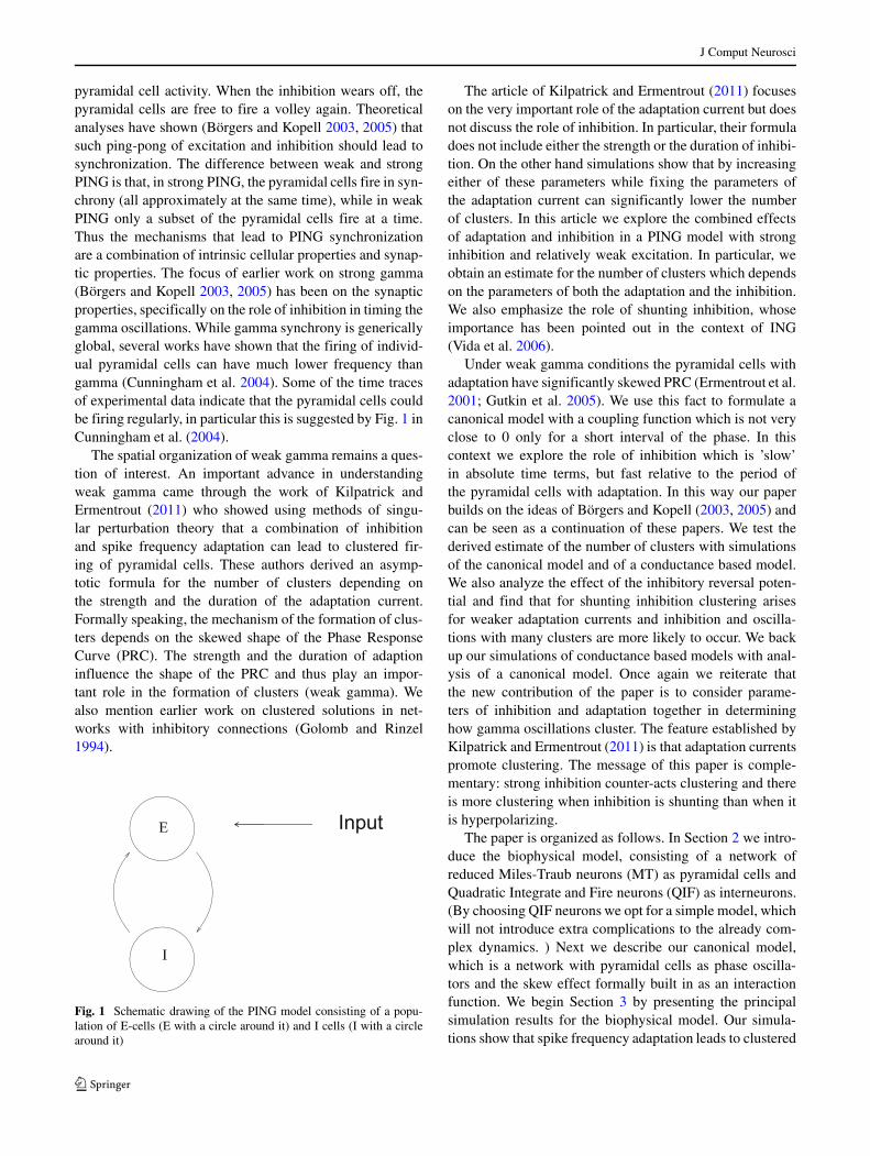
Fig. 1 Schematic drawing of the PING model consisting of a popu-lation of E-cells (E with a circle around it) and I cells (I with a circlearound it)

The article of Kilpatrick and Ermentrout (2011) focuseson the very important role of the adaptation current but doesnot discuss the role of inhibition. In particular, their formuladoes not include either the strength or the duration of inhibi-tion. On the other hand simulations show that by increasingeither of these parameters while fixing the parameters ofthe adaptation current can significantly lower the numberof clusters. In this article we explore the combined effectsof adaptation and inhibition in a PING model with stronginhibition and relatively weak excitation. In particular, weobtain an estimate for the number of clusters which dependson the parameters of both the adaptation and the inhibition.We also emphasize the role of shunting inhibition, whoseimportance has been pointed out in the context of ING(Vida et al. 2006).

Under weak gamma conditions the pyramidal cells withadaptation have significantly skewed PRC (Ermentrout et al.2001; Gutkin et al. 2005). We use this fact to formulate acanonical model with a coupling function which is not veryclose to 0 only for a short interval of the phase. In thiscontext we explore the role of inhibition which is ’slow’in absolute time terms, but fast relative to the period ofthe pyramidal cells with adaptation. In this way our paperbuilds on the ideas of Borgers and Kopell (2003, 2005) andcan be seen as a continuation of these papers. We test thederived estimate of the number of clusters with simulationsof the canonical model and of a conductance based model.We also analyze the effect of the inhibitory reversal poten-tial and find that for shunting inhibition clustering arisesfor weaker adaptation currents and inhibition and oscilla-tions with many clusters are more likely to occur. We backup our simulations of conductance based models with anal-ysis of a canonical model. Once again we reiterate thatthe new contribution of the paper is to consider parame-ters of inhibition and adaptation together in determininghow gamma oscillations cluster. The feature established byKilpatrick and Ermentrout (2011) is that adaptation currentspromote clustering. The message of this paper is comple-mentary: strong inhibition counter-acts clustering and thereis more clustering when inhibition is shunting than when itis hyperpolarizing.

The paper is organized as follows. In Section 2 we intro-duce the biophysical model, consisting of a network ofreduced Miles-Traub neurons (MT) as pyramidal cells andQuadratic Integrate and Fire neurons (QIF) as interneurons.(By choosing QIF neurons we opt for a simple model, whichwill not introduce extra complications to the already com-plex dynamics. ) Next we describe our canonical model,which is a network with pyramidal cells as phase oscilla-tors and the skew effect formally built in as an interactionfunction. We begin Section 3 by presenting the principalsimulation results for the biophysical model. Our simula-tions show that spike frequency adaptation leads to clustered

J Comput Neurosci

gamma under strong coupling and that the number of clus-ters and the sparsity of firing increase when the adaptationcurrent becomes stronger. We give a heuristic argumentexplaining how adaptation and low firing rate for the indi-vidual pyramidal cells lead to the clustering. Subsequently,in the context of the canonical model, we derive an estimatefor the maximal number of clusters and the maximal firingperiod of the pyramidal cells, depending on the parame-ters of the canonical model. Finally we discuss shuntinginhibition. Simulations for the biophysical model and forthe canonical model show the clustering arises for a muchlarger range of adaptation currents when inhibition is shunt-ing. Hence shunting makes out of cluster gamma a genericphenomenon. We end the paper with a discussion section.

2 Materials and methods

In this computational study we consider networks consist-ing of a population of excitatory (E) cells and inhibitory (I)cells, known as PING networks, see Fig. 1.

The E-cells are meant to represent pyramidal cells andthe I-cells are meant to represent interneurons. The acronymPING stands for Pyramidal Interneuron Gamma. Gammaoscillations can arise in a PING model as a result of theinterplay between the excitation from the E-cells to the I-cells and the inhibition from the I-cells to the E-cells. Werefer to the work of Borgers and Kopell (2003) for an expla-nation of this phenomenon. In the present work we usePING models with two kinds of E-cells, reduced Miles-Traub (MT) cell with adaptation (AHP current) and a phasemodel with a specially designed coupling function (PRC).In both cases the I-cells are represented by QIF neurons.

2.1 The MT cells

The MT cell model used in this work is given by thefollowing system:

dv

dt= Iapp − IL − IK − INa − ICa − IAHP

dn

dt= αn(v)(1 − n)− βn(v)n

dCa2

dt= −εCaICa − Ca2/τCa. (1)

with Iapp representing the external drive, IL the leak cur-rent and INa , IK are the usual spike generating sodium andpotassium currents and IAHP is a hyperpolarization acti-vated, calcium dependent potassium current. Without theAHP current the equation is as in Borgers et al. (2005). TheAHP current is as introduced in Jeong and Gutkin (2007).

The currents appearing in the RHS of Eq. (1) weredefined as follows: IL = gL(v − EL), IK = gKn

4(v −EK), INa = gNaminf(v)

3Fh(n)(v − ENa) and IAHP =gAHP (Ca2/(Ca2 + 1))(v − EK). The functions weredefined as follows: m∞(v) = αm(v)/(αm(v) + βm(v)),αm(v) = 0.32(v+54)/(1− e−(v+54)/4), βm(v) = 0.28(v+27)/(e(v+27)/5 − 1) and Fh = max{1 − 1.25n, 0}. Thevariable n measures the activation of the potassium cur-rent IK , with αn(v) = 0.032(v + 52)/(1 − e−(v+52)/5)

and βn(v) = 0.5e−(v+57)/40. The variable Ca2 correspondsto the calcium concentration and the calcium current isgiven by ICa = gCaminf,1(v)(v − ECa), with m∞,1(v) =1/(1 + e−(v+25)/2.5). The following parameters were fixedthroughout the computation gNa = 100, gK = 80, gCa =1, gL = 0.1 (in mS/cm2), EL = −67, ENa = 50,EK = −100 ECa = 120 (in mV), and τCa = 80 ms,εCa = 0.002 (in μM (ms μA)−1cm2 ). In our simulationswe omitted the ICa current in the current balance equa-tion as its presence seemed to have no qualitative effecton the presence of clustering. The maximal conductanceof the adaptation current, gAHP and the external drive Iapp

were varied, as reported in the article. The AHP currenthas the effect of extending the relative refractory period.This means that the neuron does not respond to input inthe early stage of the cycle. This feature is reflected in thePRC, which is almost 0 in the first part of the cycle, seeFig. 2, panel A, showing the PRC with three different valuesof gAHP .

2.2 The MT PING model

The MT PING model is a network consisting of a populationof MT cells (E-cells) and a population of QIF neurons (Icells), given by the following system of equations:

dve,j

dt= Iapp − IL(ve,j )− IK(ve,j , nj )− INa(ve,j , nj )

−ICa(ve,j )− IAHP (ve,j , Ca2,j )

−gee

(1

Ne

Ne∑k=1

se,k

)(ve,j −Eei

rev)

−gie

⎛⎝ 1

Ni

Ni∑k=1

si,k

⎞⎠ (ve,j −Eei

rev)

dvi,l

dt= 2vi,l(vi,l − 1)+ Iint

−gei

(1

Ne

Ne∑k=1

se,k

)(vi,l −Eie

rev)

−gii

⎛⎝ 1

Ni

Ni∑k=1

si,k

⎞⎠ (ve,j −Eii

rev)

(2)

J Comput Neurosci

Fig. 2 A PRC of the Miles-Traub model with I = 0.8 and with differ-ent strengths of the AHP current, gAHP = 0.5 (blue curve), gAHP = 1(black curve) and gAHP = 1.5 (red curve), respectively. The MT cellhas an inactive phase, at the beginning of the cycle (after the spike),and an active phase, at the end of the cycle. This is reflected in the PRCwhich is almost 0 in the early stage of the cycle and is bell shaped at

the end of the cycle. As gAHP increases the flat part is longer, whilethe bell-shaped part remains almost unchanged. B The graph of thecoupling function f ((θ − 1)/ω+T0) of Eq. (3) plotted along the solu-tion θ(t) = ωt , which exists in the absence of inhibition.The values ofω corresponding to different colors are ω = 0.0125 (blue), ω = 0.01(black) and ω = 1/120 (red)

with j = 1, . . . Ne and l = 1, . . . Ni . The variables vi,j(dimensionless) varied between 0 and 1 and were reset to0 when they reached 1 (this corresponds to a spike). Thesynaptic variables se,k (respectively si,k) vary between 0 and1. They were set to 1 after each spike of the correspondingE-cell (respectively I-cell) after a delay δE (respectively δI )and decayed exponentially with time constant τE (respec-tively τI ). The values of the delays were δE = δI = 1ms

and the values of the time constants were τE = 1ms andτI = 9ms. The maximal conductances of the synaptic cur-rents varied; gii and gie between 1 and 2, gei between 0.1and 0.2 and gee between 0 and 0.05. The reversal poten-tial Eei

rev was either −80 mV (hyperpolarizing inhibition)or −65 mV (shunting inhibition). The values of the otherreversal potentials were: Eee

rev = 50 mV, Eierev = 6.5,

Eiirev = −0.25. N.B. The latter two reversal potentials

are for synapses onto the QIF model of the inhibitoryinter-neuron, where the voltage is a non-dimensionalizedvariable. Hence the reversal values are also non-dimensionaland are scaled with respect to the corresponding biophysicalvalues. The value of the drive to the I-cells was Iint = 0.5(corresponding to the saddle-node bifurcation). Since therole of interneurons in our model is intended to be very sim-ple, and a QIF neuron is one of the the simplest models ofexcitable cells, we decided to use a network of QIF neurons.

2.3 PING with phase oscillators as E-cells (phase PING)

As a toy model we used a PING network with E-cells givenby phase oscillators, defined by the following equations:

dθl

dt= ω − gief ((θl − θleft)/ω)

⎛⎝ 1

Ni

Ni∑j=1

sl,j

⎞⎠

dvj

dt= 2vj (vj − 1)+ I0 − gei

(1

Ne

Ne∑i=1

se,i

)(vj − Eie

rev)

−gii

⎛⎝ 1

Ni

NI∑l=1

si,l

⎞⎠ (vj −Eii

rev), (3)

with θl and vj reset to 0 after reaching 1 (correspondingto a spike), l = 1, . . . Ne, j = 1, . . .Ni The treatment ofthe synaptic variables was the same as for MT PING. Themaximal synaptic conductances had the following values:gii = 0.5, gei = 0.2, with gie used as a parameter. Theconstant θleft is defined as

θleft = 1 − ωT0, (4)

where T0 is set to 20 ms. The meaning of θleft and T0 willbe discussed in Section 3.2.

J Comput Neurosci

In the absence of the coupling term θl is a phase oscilla-tor, with frequencyω. As we will argue later changing ω hasthe same effect as changing gAHP . We assume that f (t) ispositive on an interval (0, T0) and equal to 0 elsewhere. Inaddition we assume that f ′(t) is monotonically decreasingfor t ∈ (0, T0); these assumptions imply the existence of aunique maximum at some tM ∈ (0, T0). In a rigorous phasereduction the coupling function is the PRC of the oscilla-tor to which the reduction is applied. Here we choose anidealized coupling function whose form is motivated by thePRCs of the Miles-Traub model; more specifically, if gAHP

is increased the period of the oscillation increases, but thelength of the time interval in which the PRC is significantlydifferent from 0 remains approximately constant, see Fig. 2,panel A. Similarly, if we change ω in Eq. (3), the period ofthe solution existing in the absence of inhibition increasesbut the time interval when the coupling function is activestays constant, see Fig. 2, panel B.

The first component of Eq. (3) is similar to the phasemodel of oscillator death used by Ermentrout and Kopell(1990) to model a transition from oscillation to equilib-rium behavior. In our model this transition is transient andcorresponds to the action of inhibition; after inhibition hassufficiently worn off the system returns to the oscillatorystate.

We have also considered the modified phase PING modelto mimic the effect of shunting inhibition. This modificationconsisted of multiplying the coupling term in the RHS ofthe θl equation by the following sigmoidal function:

σ(θ) = 1

1 + exp(20(0.9 − θ)). (5)

Note that σ(θ) close to 0 in the initial part of the cycle andnear 1 for θ near 1. This idea of modeling shunting inhi-bition was already introduced in Jeong and Gutkin (2007)and is based on the following observation. The voltage vari-able of the Miles-Traub cell with adaptation increases veryslowly in the initial part of the cycle but becomes muchfaster as it passes near the value of the inhibition reversalpotential, so that inhibition grows very quickly from 0 to toa near maximum value in the last stage of the cycle.

3 Results

3.1 MT PING

3.1.1 Simulations with hyperpolarizing inhibition

Borgers and Kopell (2003) describe gamma oscillationsin PING models for which both the E-cells and theI-cells oscillate in synchrony at gamma frequency. The

fundamental assumption of PING is that the rhythm isdriven by external input coming into the E-cells and thatthe I cells do not receive enough drive to fire at gammafrequency. The mechanism of the oscillation can be brieflydescribed as follows. The E-cells fire first and excite theI-cells. Excitation from the E-cells causes spikes of the I-cells, releasing a volley of inhibition. As a result no cellsin the network can fire until the inhibition has sufficientlydecayed. Inhibition not only delays the next spike but alsosynchronizes the population of the E-cells and leads to atighter synchrony in the I-cells.

On the other hand it is known from some experimentsthat pyramidal cells can fire at a much lower frequency thanthe frequency of the rhythm (Cunningham et al. 2004). Thesimplest way that this can occur is if the pyramidal cellsfire in clusters. Here we identify one mechanism how suchfiring in clusters can come about, namely a long refractoryperiod of the E- cells (inactive phase). In our MT model thisis caused by the AHP current. The main idea behind ourwork is that E-cells spike very slowly, so that their periodis much larger than the time constant of inhibition, and thatthe cells are not sensitive to input in the early phase of ofthe cycle, so that the synchronization effect is present for apart of the phase only.

In Fig. 3 we show some simulations of clustered MTPING. The first of the two raster plots shows a solution withtwo clusters, with I = 7, gie = 1.5 and gAHP = 1.2. Thesolution is obtained from an initial condition of the MT cellsdistributed evenly in the phase of their uncoupled oscilla-tion with I = 7 and gAHP = 1.2. The panel on the rightshows a similarly obtained solution, now with three clus-ters, for gAHP = 2.3. This example supports the results ofKilpatrick and Ermentrout (2011) that increasing gAHP

leads to the occurrence of more clusters.The effect of varying inhibition is the main focus of

this work. In Section 3.2, in the context of phase PINGwe give some analytic results illustrating this effect. Inthe context of MT PING our evidence consists of sim-ulations, see Fig. 4, where we show that the number ofclusters can significantly decrease if gie is decreased. Inorder to better explain this effect, based on heuristic con-siderations, we design an expression which approximatesthe the maximal number of clusters (see Eq. (6)), and dis-cuss its dependance on gie. Our numerical computations(see Figs. 7 and 8), give a comparison of the predictions (6)and the changes in the number of clusters obtained by directsimulation.

The effect of changing gAHP is illustrated in Fig. 3 as wellas in Fig. 5, panels A and B.

Another parameter strongly influencing the number ofclusters is Iapp (the drive to the E-cells). Our simulations

J Comput Neurosci

Fig. 3 Clustered gamma oscillations of the PING model with hyper-polarizing inhibition for the maximal conductance of inhibition gie =1.5 and the drive to the E-cells I = 7. A A solution with two

clusters, corresponding gAHP = 1.2 (maximal conductance ofthe AHP current). B A solution with three clusters, correspondinggAHP = 2.3

Fig. 4 Increased inhibition leads to the reduction of the number of clusters. A Five clusters with I = 4, gAHP = 2.3, gie = 0.5. B Four clusterswith I = 4, gAHP = 2.3, gie = 1.8 . C Three clusters with I = 4, gAHP = 2.3, gie = 1.8

J Comput Neurosci

Fig. 5 The effect of changing gAHP, I and gei . All solutions are com-puted starting from the same initial condition. A A five cluster solutionfor gAHP = 2, IAHP = 4 and gei = 0.3. B A four cluster solution

for gAHP = 1.5, IAHP = 4 and gei = 0.3. C A four cluster solutionfor gAHP = 2, IAHP = 5 and gei = 0.3. D A five cluster solution forgAHP = 2, IAHP = 4 and gei = 0.2

show that raising Iapp decreases the number of clusters seeFig. 5, panels A and C. Our heuristic argument in support ofthis point is as follows: if Iapp is increased then T decreasesas well as the refractory period introduced by the AHP cur-rent. Hence inhibition has a simultaneous effect on a largerportion of the cells, leading to fewer clusters (see below foran explanation of this point using the ‘river picture’).

Finally, the number of clusters is also controlled bygei , i.e. the strength of the projection from the E-cellsto the I-cells. If gei is small then many E-cells have tospike approximately at the same time to produce a spike ofthe I-cells. This rules out the possibility of small clusters.Figure 5, panels A and D, shows that decreasing gei can leadto the occurrence of fewer clusters.

The main goal of this paper is to study the combinedeffect of inhibition (controlled by gie) and adaptation (con-trolled by gAHP) on the existence and stability of clusteredsolutions. To understand the role of gAHP and gie we have

computed the time-to-spike function T T S, which is definedas follows. Let t∗ ∈ [0, T ] be the time elapsed from the lastspike of the spiking solution of the MT cell, with T corre-sponding to the period. Then T T S(t∗) is the time it takes tothe next spike given that a pulse of slowly decaying inhibi-tion was applied at t∗. In Fig. 6 we show the graphs of T T Scorresponding to the parameter values of Fig. 4.

Some properties of the T T S function in relation to theparameter gie can be easily deduced. If gie = 0 thenT T S(t) = T − t , i.e. the graph of T T S is a straight linewith slope −1. For gie > 0 the slope is strictly between−1 and 0 and becomes close to 0 in the final stage of thecycle, where the PRC is positive and therefore the ’riverargument’ of Borgers and Kopell (2003) implies that thetime of spike is almost constant, equal to some constant Tmin

(the river argument will be reviewed in Section 3.2). At thevery end of the cycle, due to the finite width of the spike,the T T S function drops sharply to 0. The T T S function is

J Comput Neurosci

Fig. 6 Time-to-spike (TTS) function for the MT cell with adaptation.The TTS function (blue curve) assigns to the phase of the cell (wrt thenatural period) the time to the next spike given that a pulse of inhibi-tion arrives at the given value of the phase. For larger values of gAHP

the TTS function is close to the function h(t) = T − t (black line with

slope −1) at the earlier stage but its slope becomes much closer to 0at the later stage, indicating contraction.This feature leads to a higherlevel of clustering, see Fig. 3. A TTS function with gAHP = 1.2,gie = 1.5 and I = 7. B TTS function with gAHP = 2.3, gie = 1.5 andI = 7. C TTS function with gAHP = 2.3, gie = 1.5 and I = 4

decreasing, hence its maximal value Tmax corresponds tot∗ = 0. Our heuristic picture of the clustering is as fol-lows. Different E-cells can be identified with the differenttime instances along the oscillation of the MT cell with-out inhibition. Suppose we divide the interval [0, Tmax] intointervals of length Tmin, starting from the right. All the cellsthat are in the last interval of length Tmin at the momentof the arrival of inhibition will be synchronized, due to the’river picture’, and will spike after approximately Tmin, giv-ing rise to the first cluster. During this period, the cells inthe second last interval of length Tmin will continue to thelast interval of length Tmin, without feeling much inhibition.When the second volley of inhibition arrives, these cellsform a cluster, etc. Now suppose that the interval [0, Tmax]can be covered by k − 1 copies of interval of length Tmin

plus a remaining interval of length smaller than Tmin (exceptfor special cases). By the argument above, the number ofclusters should be given by k.

Expressing this by a formula, we have the followingestimate for the existence of a solutions with k clusters:

(k − 1)Tmin + k(δE + δI ) < Tmax. (6)

(recall that δE (resp. δI ) are the delay of the arrival of excita-tion (inhibition)). Note that the maximal number of clusterscorresponds to the largest k satisfying (6), but solutions withfewer clusters are not excluded. We define:

kmax = Tmax − δE − δI

Tmin + (δE + δI )+ 1. (7)

Inequality (6) is now equivalent to k < kmax.We have done a number of simulations and compared

them with the predictions of Eq. (6). In most simulations theestimate is too low, but we have found some situations whenit is too high. We found that for many parameter valuesthere exist multiple clustered states. We can obtain some ofthem by using nearby initial conditions for which a similar

J Comput Neurosci

cluster state exists. Other solutions are obtained froma phase distributed initial condition, obtained by takinga solution of a single MT cell, with the natural timeparametrization (which we often refer to as phase), andtranslating the time variable by small intervals to obtaininitial conditions for different cells in Eq. (2).

As mentioned, for solutions obtained from nearby initialconditions (6) typically underestimates the maximal number

of clusters. A possible explanation for this is that the slopeof the T T S function is very close to 0 only for a very smallrange of the natural time variable of the MT cell, whichincreases the possibility of small clusters. To see this imag-ine a group of E-cells loosely arranged in a cluster. Supposethe leading cells spike, causing a volley of inhibition. Ifinhibition arrives soon enough then the cells that werebehind are stopped from spiking– this leads to two or more

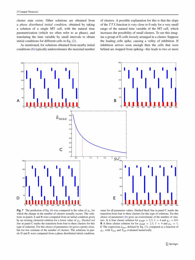
Fig. 7 The prediction of Eq. (6) was compared to the value of gie forwhich the change in the number of clusters actually occurs. The solu-tions in panels A and B were computed from an initial condition givenby an existing clustered solution for a lower value of gie. Dashed redline in panel C marks the transition from four to three clusters for thistype of solutions. For this choice of parameters (6) gives a pretty close,but too low estimate of the number of clusters. The solutions in pan-els D and E were computed from a phase distributed initial condition,

same for all parameter values. Dashed black line in panel C marks thetransition from four to three clusters for this type of solutions. For thischoice of parameters (6) gives an overestimate of the number of clus-ters. A A four cluster solution for gAHP = 2.3, I = 4 and gie = 0.9.B A three cluster solution for for gAHP = 2.3, I = 4 and gie = 1.C The expression kmax, defined by Eq. (7), computed as a function ofgie, with Tmax and Tmin evaluated numerically

J Comput Neurosci

separate clusters. If inhibition comes later then all the cellsin the loosely organized cluster can spike before it arrives –in this case just one cluster is formed. By varying parame-ters to increase the delay between the spikes of the E cellsand the arrival of inhibition (e.g. increasing δI ) one canimprove the accuracy of Eq. (6). In Fig. 7 we show a plotof kmax (panel C). This plot predicts a change from fourto three clusters at gie ≈ 0.8, however simulations showthat for solutions obtained from nearby initial conditions thechange actually occurs for gie ≈ 1. The estimate given (6)

is close, but too low. To obtain Fig. 8 we decreased δI . Thenumber of clusters is now significantly larger than predictedby Eq. (6). For this simulation the effect of varying gie ismore pronounced, i.e. as gie is varied there are more possi-bilities for clustered solutions. Summarizing, the larger thedelay of the arrival of inhibition after a spike of E-cells, themore accurate the formula. On the other hand the effect ofchanging gie on the maximal number of clusters becomesstronger when the delay of the arrival of inhibition issmaller.

Fig. 8 In this simulation we decreased the value δE + δI as well thedrive to the I cells Ii . We used δE = δI = 0.1 and Ii = 0.5 asopposed to δE = 0.1, δI = 0.2 and Ii = 0.52, used in the sim-ulations shown in Fig. 7. All solutions were computed from initialconditions given by a clustered solution existing for a nearby parame-ter setting. Changing the parameters resulted in the occurrence of moreclusters and in the reduction of the accuracy of Eq. (6). A A five cluster

solution for gAHP = 2.3, I = 4 and gie = 0.8. B A four cluster solu-tion for gAHP = 2.3, I = 4 and gie = 0.9. C The expression kmaxcomputed as a function of gie, with Tmax and Tmin evaluated numeri-cally. The changes from a five cluster to four cluster and from a fourcluster to three clusters are marked by red lines. D A four cluster solu-tion for gAHP = 2.3, I = 4 and gie = 1.7. E A three cluster solutionfor gAHP = 2.3, I = 4 and gie = 1.8

J Comput Neurosci

For solutions obtained from phase distributed initial con-ditions (6) typically overestimates the maximal number ofclusters, see Fig. 7, panels D and E. One possible explana-tion is that the assumption of a rapid change of the slope ofthe T T S function from near 0 to near −1 is not accurate.In fact the slope of the T T S function increases fairly grad-ually (see Fig. 6), so that even cells that are far away fromspiking are still affected by inhibition. This is due to the factthat inhibition, no matter in which stage of the cycle, addsto the leakiness of the cell, and hence increases the value ofthe T T S function. Hence inhibition is effective over a largerrange of the phase variable (natural time variable of the MTcell) than given by Tmin.

The arguments presented in this section are heuristic aswe are not able to obtain rigorous results in the context ofEq. (2). In Section 3.2, where we study phase PING, i.e.system (3), we obtain more rigorous results. In particularwe derive asymptotic estimates for Tmin and Tmax, which,in combination with Eq. (6) gives an estimate of the num-ber of clusters as a function of the key parameters of themodel. This estimate depends not just on the parametersof the adaptation current, but also on inhibition. Using alimit obtained by letting adaptation and inhibition simulta-neously increase towards ∞ in such a way that the numberof clusters predicted by Eq. (6) is constant, we prove thatEq. (6) gives a sharp estimate, see Theorem 1 for a precisestatement.

3.2 Phase PING

Phase PING (see Section 2.3, system (3)) is a toy model inwhich we have replaced the MT cells with phase oscillatorsand introduced the coupling function θ �→ f ((θ−θleft)/ω),where θleft is given by Eq. (4), T0 is a fixed constant, f (t) =0 for t ∈ (0, T0) and is quadratic on (0, T0) (with valueT0 = 20). An accurate computation of the PRC was carriedout in Kilpatrick and Ermentrout (2011). The choice of thecoupling function (PRC) which we made here is motivatedby the wish to simplify the arguments. Our results could,however, be extendend to the case of a more accurate PRC.Finally, note that the parameter ω in Eq. (3) plays a similarrole as gAHP for Eq. (2).

For this model it is possible to get good analytic esti-mates for Tmax and Tmin. We will also determine whenand with what rate the phases representing different cellsapproach each other. Finally, in a limit consisting of simul-taneously letting ω → 0 and g → ∞ in such a waythat the number of clusters predicted by Eq. (6) remainsconstant, we prove that Eq. (6) is an optimal estimate,i.e. there exists a stable periodic solution with k clus-ters, with k maximal given by Eq. (6) and there is nosuch solution with more than k clusters. In this section wehave focused on the two parameters ω and g, and on the

dependence of the two derived quantities Tmin and Tmax onthese parameters.

As our arguments are based on the ’river picture’ ofBorgers and Kopell (2003), we begin by reviewing thisapproach in the context of Eq. (3).

3.2.1 Review of the ’river picture’ of Borgers and Kopell(2003)

Borgers and Kopell (2003) consider a PING model withboth E-cells and I-cells given by theta neurons. They studythe existence of oscillations in which all the E-cells aswell as all the I-cells fire in synchrony (with slight delaybetween the E-cells and the I-cells). In the simplest casethey assume that the E-cells are not coupled to each other,so that each E-cell can be considered independently, i.e. asa single cell receiving a volley of inhibition. Before we goon let us point out two differences between our approach.First, we use phase oscillators, rather than theta neurons,which, we feel, simplifies the presentation, although, asshown by Kilpatrick and Ermentrout (2011), theta neuronscan also be used, leading to analytic solutions. Reductionto phase oscillators can be made in a rather general con-text (Ermentrout and Kopell 1991), which means that theapplicability of our approach is quite general. The sec-ond difference is that, rather than using the concept of’river’, we use Fenichel slow manifold (Fenichel 1979).These two concepts have a similar meaning, however ’river’was introduced using non-standard analysis, so that itsprecise meaning is not accessible to the authors of thispaper.

For ω = 1/T0 system (3) has properties analogous tothose of the model studied by Borgers and Kopell (2003).In this case θleft = 0, so that the coupling function (PRC)is non-zero on the entire interval [0, 1]. Following the foot-steps of Borgers and Kopell (2003) we study the dynamicsof a single E-cell in the presence of inhibition. In the con-text of Eq. (3) with ω = 1/T0 this equation is givenby

dθ

dt= ω − gsf (θ/ω)

ds

dt= −εs; s(0) = 1. (8)

Recall that f has a parabolic shape with maximal value fM .We will assume that inhibition is sufficiently strong, i.e. thecondition

ω < gfM (9)

is satisfied. System (8) is slow/fast and all solutions startingwith s = 1 and arbitrary θ are exponentially attracted to aFenichel slow manifold, which is one dimensional, locally

J Comput Neurosci

invariant, and, in this case, parametrized by a solution. Thephase portrait of Eq. (8) is given in Fig. 9. The idea isnow that all solutions, with initial conditions correspondingto the states of different E-cells at the time of the arrivalof inhibition, are strongly attracted to each other, i.e. theirθ components quickly approach each other (the s compo-nents are already equal). The Fenichel slow manifold canbe thought of as a river attracting all the nearby solutions.Any two solutions are extremely close to each other at thetime when they reach the vicinity of the critical point off , thus the cells they represent spike almost at the sametime.

We end this section on few remarks concerning the use ofsingular perturbation theory. The fact that ε is the inverse ofthe time constant of inhibition, which equals approximately9 ms, may cast a doubt on the relevance of singular pertur-bation theory. Another point is that the inverse of the timeconstant of adaptation is a much smaller parameter (usedby Kilpatrick and Ermentrout (2011) in their perturbationanalysis). We feel that our approach is an interesting alter-native, for the following reasons. First, the hallmark featureof singular perturbation theory is the presence of strong con-traction and the synchronization brought about by inhibition(river picture) is precisely that. Second, even though sin-gular perturbation only works, mathematically, in the limitof ε → 0, its predictions often extend to ε not so close to0. The reason for this is that strong contraction/expansioncan be present even when ε is not so small. For example,ε = 0.1 may give (positive or negative) eigenvalues of theorder of e10. Simulations of the toy model with ε = 0.1 (seeFigs. 11 and 10) were in reasonable agreement with thesingular perturbation estimates.

Fig. 9 The ’river effect’. The curve of quasi stationary points (blue)and two solutions (black and red)

3.2.2 Extension of the ’river picture’

We now consider the general case of ω 1/T0. The systemcorresponding to an E-cell subjected to a spike of inhibition(generalization of Eq. (8) now has the form:

dθ

dt= ω − gsf ((θ − θleft)/ω)

ds

dt= −εs; s(0) = 1, (10)

where f is as defined in Section 2.3, i.e. f is quadratic onthe interval (0, T0), and 0 otherwise. For Eq. (10) the pictureis more complicated than for Eq. (8). We distinguish threecases:

θleft < θ < 1 Here the ’river picture’ fully applies, sothat any two cells with initial condition satisfying thiscondition are attracted to each other and fire almostinstantenously.

1 − ωTmin < θ As mentioned earlier, due to inhibition,there exists a minimal time needed for any initialcondition (10) to reach a spike. We denote this time byTmin. Solutions satisfying 1 − ωTmin < θ experience adelay to spike and there is some contraction between anytwo solutions starting in this region. In the sequel we willshow that, in the aforementioned limit of ω approaching 0with g adjusted simultaneously so thatω(Tmin+ωδ) staysfixed, trajectories starting in this region can be attractedto each other to form a a cluster.

θ < 1 − ωTmin Solutions starting at θ are not affectedby inhibition and therefore spike at approximately thesame time as they would have if inhibition had not beenpresent. Given solutions with initial conditions θ1 and θ2,with θ1 or θ2 satisfying θ < 1−ωTmin, the correspondingsolutions are not attracted to each other.

The T T S function is determined by the solutions of Eq. (10)and assigns to every θ0 the time needed for the solution ofEq. (10) with θ(0) = θ0 to reach the firing threshold θ = 1.

3.2.3 Computation of Tmin and the contraction rate

Let

sM = ω

gfM. (11)

By Eq. (9) sM < 1.To fix ideas we use a specific definition for f , namely:

f (t) = 4t (t − T0)

T 20

. (12)

We will argue that the approximate value of Tmin is:

Tmin ≈ −1

εln(sM)−0

(T 2

0

4ε

)1/3

(13)

J Comput Neurosci

Fig. 10 The TTS function for phase PING shows the validity of the approximation of Tmin by Eq. (13) for ω = 0.0075 and ε = 0.1. The redhorizontal line corresponds to the value of Tmin as predicted by Eq. (13) with gie = 0.3 in panel A and gie = 0.5 in panel B

where 0 ≈ −2.34 is a universal constant whose meaningwill be explained in the Appendix.

Figure 10 shows examples of the application of Eq. (13).We will now show how Eq. (10) can be transformed to

a slow/fast system for which estimate (13) can be obtainedfrom existing results. We first rewrite Eq. (13) as a sum oftwo terms

Tmin = TSN + Tesc TSN = −1

εln(sM),

Tesc = −0

(T 2

0

4ε

)1/3

The time TSN is defined as the time needed for s to decreasefrom 1 to sM . If s is treated as a constant (ε = 0 limitin Eq. (10)) then sM is a point of saddle-node bifurcation.For ε > 0, while s > sM , there is an attracting Fenichelslow manifold close to the curve (s, θ(s)), where θ(s) is asolution of

0 = ω − gsf ((θ − θleft)/ω),

and every other solution has to follow the slow manifold.This implies that the time it needs to reach the vicinity offM is approximately log(1/sM).

To get the estimate of Tesc we begin by a transformation:

x = θ − θleft

ω, s = sM s.

In the new coordinates Eq. (10) becomes

dx

dt= 1 − sf (x)

ds

dt= −εs; s(0) = 1. (14)

Note that the term gsfM/ω is less than 1 for s > sM . Wereplacing x by x + 1 and Taylor expand at (x, s) = (0, 1),which, at lowest order, gives the followng system:

dx

dt= (1 − s)− Bx2

ds

dt= −ε, (15)

where B = 4/T 20 . Based on a result of Krupa and Szmolyan

(2001) (a review of this result with precise references willbe given in the Appendix) we can give an estimate

Tesc = −0(Bε)1/3 = −0

(T 2

0

4ε

)1/3

(16)

3.2.4 Estimate of Tmax

The value of Tmax equals the time it takes for a solution ofEq. (10) with θ(0) = 0 to reach θ = 1. Note that Tmax >

1/ω, but when ω is sufficiently small then the followingholds. If the inhibition comes at the beginning of the cycle itdecays to negligible size by the time the phase advances tothe regime where inhibition could have an effect. Hence, inthis case

Tmax ≈ 1

ω. (17)

For ω larger Tmax can be significantly larger than 1/ω, butthe maximal value it can reach is

Tmax ≈ 1

ω+ Tmin. (18)

Also, a rise in gie could lead to a loss of accuracy ofEq. (18).

J Comput Neurosci

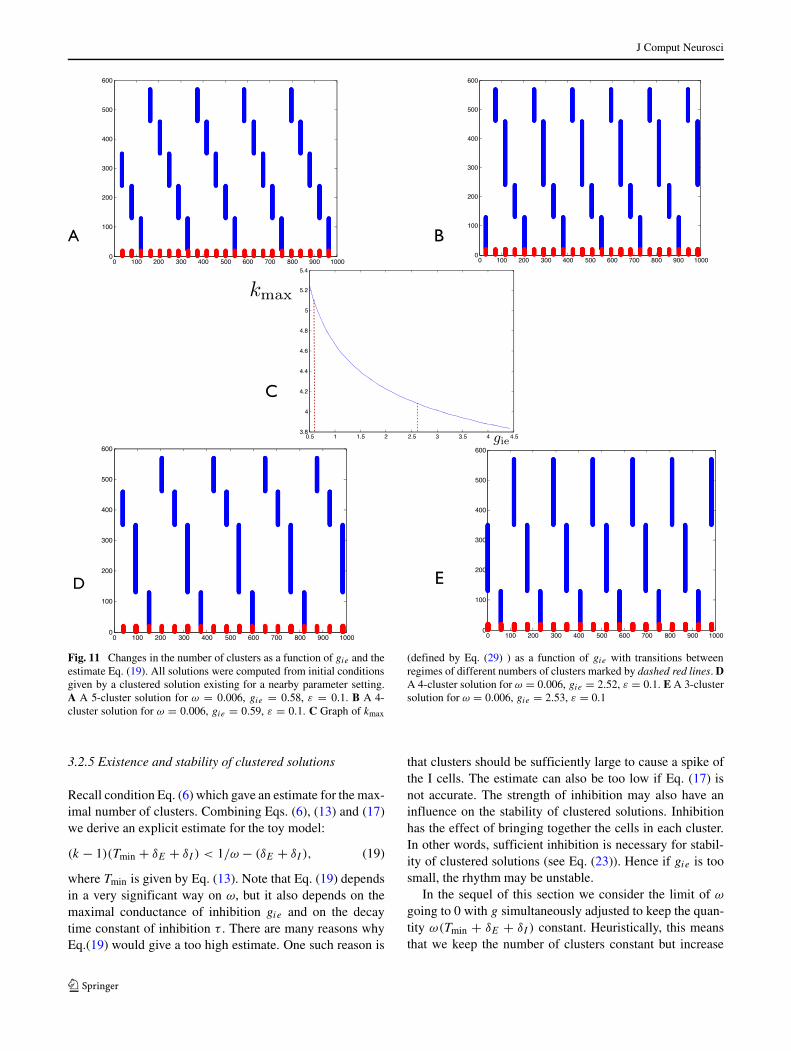
Fig. 11 Changes in the number of clusters as a function of gie and theestimate Eq. (19). All solutions were computed from initial conditionsgiven by a clustered solution existing for a nearby parameter setting.A A 5-cluster solution for ω = 0.006, gie = 0.58, ε = 0.1. B A 4-cluster solution for ω = 0.006, gie = 0.59, ε = 0.1. C Graph of kmax

(defined by Eq. (29) ) as a function of gie with transitions betweenregimes of different numbers of clusters marked by dashed red lines. DA 4-cluster solution for ω = 0.006, gie = 2.52, ε = 0.1. E A 3-clustersolution for ω = 0.006, gie = 2.53, ε = 0.1

3.2.5 Existence and stability of clustered solutions

Recall condition Eq. (6) which gave an estimate for the max-imal number of clusters. Combining Eqs. (6), (13) and (17)we derive an explicit estimate for the toy model:

(k − 1)(Tmin + δE + δI ) < 1/ω − (δE + δI ), (19)

where Tmin is given by Eq. (13). Note that Eq. (19) dependsin a very significant way on ω, but it also depends on themaximal conductance of inhibition gie and on the decaytime constant of inhibition τ . There are many reasons whyEq.(19) would give a too high estimate. One such reason is

that clusters should be sufficiently large to cause a spike ofthe I cells. The estimate can also be too low if Eq. (17) isnot accurate. The strength of inhibition may also have aninfluence on the stability of clustered solutions. Inhibitionhas the effect of bringing together the cells in each cluster.In other words, sufficient inhibition is necessary for stabil-ity of clustered solutions (see Eq. (23)). Hence if gie is toosmall, the rhythm may be unstable.

In the sequel of this section we consider the limit of ωgoing to 0 with g simultaneously adjusted to keep the quan-tity ω(Tmin + δE + δI ) constant. Heuristically, this meansthat we keep the number of clusters constant but increase

J Comput Neurosci

the strength of inhibition and thus the strength of the ‘rivereffect’.

The phase space of Eq. (3) is given by points of the form(θ1, . . . , θN, w1, . . . , wM), where N is the number of E-cells and M the number of I-cells (for simplicity of notationwe suppress the dependence of phase points on synapticvariables). In this work we assume that the I-cells are in theexcitable regime but very close to the firing threshold so thatthey fire as soon as the spike from the E-cells arrives. Wewill also assume that there is no delay of the arrival of theinhibition to the E-cells (δI = 0). On the other hand we willkeep the delay of the arrival of excitation as positive. Thisis necessary to ensure that the E-cells that are very closecan form clusters (the cell slightly behind can spike withoutbeing stopped by inhibition). To simplify the notation wewill write δ = δE > 0. We also only consider the value of kwhich is maximal to satisfy Eq. (19). With these conventionwe re-write Eq. (19) to obtain

ωδ < 1 − (k − 1)ω(Tmin + δ)) < ω(Tmin + δ)+ ωδ. (20)

We define θmin = ω(Tmin + δ) and re-write Eq. (20) inthe form:

ωδ < 1 − (k − 1)θmin < θmin + ωδ. (21)

Note that for fixed θmin and ω estimate (21) defines a uniquek, except for the cases when one of the inequalities becomesan equality for some integer k.

We now introduce the subset Ck of the phase space cor-responding to k-cluster states. Elements of Ck are definedas follows: for each p = (θ1, θ2, . . . θN , w1, . . .wM) ∈ Ck

there exist θc1 , . . . θck , and indices 1 = j1 < j2 < . . . <

jk < jk+1 = N such that θj = θcl for jl ≤ l < jl+1. Notethat jl+1 − jl gives the number of elements in cluster j andθl is the common value of θ corresponding to each cluster.Thus defined clusters are ordered but for non-ordered clus-tered one could apply the same arguments by re-numberingthe equations.

Theorem 1 Let k be an integer satisfying (21). Then, pro-vided that ω is sufficiently small and g is adjusted so thatθmin stays constant, system (2) has a stable k-cluster peri-odic solution and does not have a periodic solution withmore than k clusters.

Proof We define sections �j by the condition θj = ωδ

(the j th neuron is at time δ after its reset value, which cor-responds to the moment of the arrival of inhibition). We willsearch for cluster states as fixed points of the return mapfrom �1 to itself. By definition, points in �1 have the form(ωδ, θ2, . . . θN, w1, . . . , wM), points in �2 have the form(θ1, ωδ, . . . θN, w1, . . . , wM), etc. We consider firing mapsπfj,l mapping �j to �l ; these maps are defined for states

in �j for which cell l will be the first one to fire, with the

image given by the solution at t = δ after the spike of the l-th cell. We look for cluster states obtained by application ofcomposition of firing maps corresponding to different clus-ters. For an initial condition in �1 ∩ Ck we assume thatthe k-th cluster fires first, then cluster k − 1, and so on,in decreasing order. An argument for firing events occur-ring in in a different order is similar and will be omitted.We identify elements of Ck with the sequences (θc1 , ..., θ

ck )

and (j1, . . . , jk+1). We define firing maps πfl as π

fjl+1,jl

(N + 1 ≡ 1 and k + 1 ≡ 1), i.e. cluster l − 1 fires aftercluster l.

Let pl = (θc,l1 , . . . , θ

c,lm ), m ≥ k be a sequence of cluster

states corresponding to a fixed point of the return map, i.e.p2 = π

f

k (p1), p3 = πf

k−1(p2), . . ., pm = πf

2 (pm−1) and

p1 = πf

2 (pm). Note that θc,j1 ≥ ωδ + jω(Tmin + δ), sincethe time between consecutive firings is at least Tmin + δ.By Eq. (20) cluster 1 must be the one to fire next, seeProposition 1. Hence a cluster with more than k statescannot exist.

We now prove that Eq. (20) is sufficient for the existenceof k clusters. We consider the sequence (θc1 , . . . , θ

ck ) satisfy-

ing θcj = ωδ+ (j−1)θmin, j = 1, . . . , k−1, and consider astate p with k clusters (approximately the same size) definedby this sequence, with w1 = w2 = . . . wM = we, where we

is the excitable equilibrium of the QIF model governing thedynamics of the I-cells. By Eq. (21), θck is the only one ofthe θcj ’s to satisfy 1 − θmin < θck < 1, hence the kth clusterwill be the first one to fire. By Proposition 1 the spike willhappen approximately at t ≈ Tmin and the time cluster k

reaches section �k will be t ≈ Tmin + δ. Let p2 = πf

k (p) =(θ

c,21 , . . . , θ

c,2k−1, ωδ). Clearly θ

c,2k−1 ≈ ωδ + (k − 1)θmin. By

the same argument cluster k − 1 fires next and we can con-struct the point p3 = π

f

k−1(p2), etc., until we obtain pk

equal to the image of p by πf

1 πf

2 . . . πf

k and very close top. Let V be a small neighborhood of p in the phase space. IfV is small enough than the return map restricted to V equalsπf

1 πf

2 . . . πfk , and is a contraction, by Proposition 2. Hence,

by the contraction mapping theorem, a stable k-cluster stateexists.

Proposition 1 Fix θ∗ satisfying

1 − ωTmin < θ∗ < 1.

Suppose that ω converges to 0 with g increased simultane-ously so that ωTmin stays fixed. Let T∗ be the time needed forthe solution of Eq. (10) with θ(0) = θ∗ to reach the firingthreshold. Then T∗ converges to Tmin as ω approaches 0.

Proof Let θ(t) denote the solution of Eq. (10) withθ(0) = θ∗. Let

T1 = 1 − θ∗ω

.

J Comput Neurosci

If T1 < TSN then s(T1) > sM . In this case, by Proposi-tion 2, the solution θ(t) will be attracted to the solution ofEq. (10) with initial condition θl = (1−ωT0) and will spikeat T ≈ Tmin. By definition of θ∗ we have (1− θ∗) < ωTmin.Since Tesc does not depend on ω and g, ω(TSN −Tmin) → 0as ω approaches 0 with g adjusted so that ωTmin stays fixed.It follows that, for ω sufficiently small (1 − θ∗) < ωTSN.The result follows.

Proposition 2 Let θ1(t) and θ2(t) be two trajectories ofEq. (10) and suppose that there exists 0 < t1 < TSN withθl < θj (t1) < θM , j = 1, 2, where θl = 1 − ωT0. Supposethat s1 = s(t1) > sM .The following estimate holds at thetime of the spike:

|θ1(t)− θ2(t)| ≈ C|θ1(0)− θ2(0)| (22)

where

C = e− 1

ε

∫ s1sM

f ′((θ0(σ ))/ω−1+T0)dσ , (23)

and θ0(s) is the parametrization of the curve ω−sf (θ) = 0.

Proof By Fenichel theory (Fenichel 1979) there exists aslow manifold of Eq. (10) which is O(ε) close to the curveω − sf (θ) = 0. Such a slow manifold is sometimes calledriver, see Borgers and Kopell (2003). Let θε,0 be such that(θε,0, 1) is on the slow manifold and let (θε(t), s(t)) be thesolution of Eq. (10) satisfying (θ(t), s(t)) = (θε, 1). Notethat (θε(t), s(t)) parametrizes the Fenichel slow manifold.The linearization of Eq. (10) is given as follows:

dv

ds= −sf ′(θ0(s))v

ds

dt= −εs; s(0) = 1; (24)

or

dv

ds= 1

εf ′(θε(s))v (25)

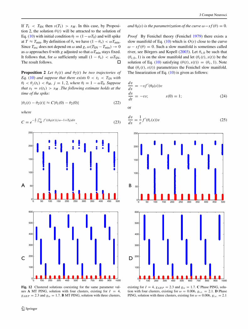
Fig. 12 Clustered solutions coexisting for the same parameter val-ues A MT PING, solution with four clusters, existing for I = 4,gAHP = 2.3 and gie = 1.7. B MT PING, solution with three clusters,

existing for I = 4, gAHP = 2.3 and gie = 1.7. C Phase PING, solu-tion with four clusters, existing for ω = 0.006, gi.e. = 2.1. D PhasePING, solution with three clusters, existing for ω = 0.006, gi.e. = 2.1

J Comput Neurosci

We replace θε(s) by θ0(s), which is the the curve obtainedby solving the equation ω− sf (θ) = 0 for θ as a function ofs. We replace θε(s) by θ0(s) in Eq. (25), this incurs an errorof O(ε). We obtain

dv

ds= 1

εf ′(θ0(s))v (26)

A solution to Eq. (26) on an interval [s1, s2] is given by

v(s) = v0e− 1

ε

∫ s2s1

f ′(θ0(σ ))dσ (27)

In other words the vector v(s) contracts with the rate

C(s1, s2) = e− 1

ε

∫ s2s1

f ′(θ0(σ ))dσ . (28)

Now note that all the solutions of Eq. (10) starting in theinterval [θl, 1], with s < smax are attracted to the Fenichelslow manifold, hence any two such solutions have to attracteach other with the rate given approximately by Eq. (28).

In Fig. 11 we show a transition between the regimes of5-cluster, 4-cluster and 3-cluster oscillations. Let

kmax = 1/ω − (δE + δI )

Tmin + δE + δI+ 1. (29)

Clearly, the condition (19) is equivalent to k < kmax.For the example shown in Fig. 11 the transition from fiveto four clusters occurs for kmax ≈ 5.09 and the transi-tion from four to three clusters occurs for kmax ≈ 4.09.

Hence, for these parameter values, the condition (19) givesa quite precise approximation of the maximal number ofclusters.

3.2.6 Co-existence of cluster solutions and the effectof E → E connections

Estimate Eq. (6) does not exclude the existence of multi-ple stable cluster solutions. In fact there can exist solutionswhich have fewer clusters than given by the maximal k sat-isfying Eq. (6). Solutions with different number of clusters,co-existing for the same parameter values, are shown inFig. 12 for both MT PING and phase PING.

The situation is even more complicated if E → E con-nections are included in the model (gee > 0). Figure 13,panel A shows a solution of the MT PING model in thepresence of E → E connections and in the absence ofinhibition (gie = 0) resulting from a simulation starting ata phase distributed initial condition. Clearly the E cells allspike at approximately the same time. If inhibition is ’turnedon’, i.e. the simulation is restarted with gie > 0, this solu-tion remains stable, as inhibition arriving after the spike ofthe E-cells will have decayed before the E-cells return tothe region where they can be affected by inhibition. How-ever, if we perturb the synchronous state by adding a randomperturbation then the resulting solution converges to a clus-tered state arising due to the action of the river mechanismas described at the end of Section 3.1.1 and in the proofof Theorem 1. Such a cluster solution is shown in Fig. 13,panel B.

Fig. 13 E → E connections (gee > 0) provide a synchronizationmechanism complementary to the river picture, enabling coexistenceof stable solutions with full synchronization of E-cells and cluster solu-tions. A Solution of the MT PING model obtained for gee = 0.3and gie = 0. The simulation was started at phase-distributed initial

condition. B Four cluster solution of the MT PING model obtained forgee = 0.3 and gie = 0.5. The initial condition was obtained by a (suf-ficiently large) random perturbation of the solution shown in panel A.A synchronized solution still exists, (not shown) but has a small basinof attraction

J Comput Neurosci

Fig. 14 Clustered solutions of the MT PING model with shuntinginhibition, with vrev = −65, gie = 1.5 and the drive to the E-cells I = 1.1. The left panel shows a solution with three clusters,

corresponding gAHP = 0.35 (maximal conductance of the AHPcurrent) and the right panel shows a solution with four clusters,corresponding gAHP = 0.45

3.3 Effects of shunting inhibition, MT PING

Since GABA-ergic inhibition can be shunting or partiallydepolarizing, with the reversal potential possibly close toor above the resting voltage of the cell, we have carriedout simulations with EGABA = −65mV . We expected thatintroducing shunting inhibition would reduce the intervalof voltage values for which inhibition is effective, adding

robustness to to the clustering effect, but the extent to whichthis was true was a surprise. Clustered solutions could befound at much lower values of gAHP than for the hyper-polarizing case, see captions of Figs. 3 and 14. Moreover,oscillations with many clusters (four or five) could easily befound; thus the firing rate of individual pyramidal cells wasless than 10 Hz for relatively small values of gAHP. Raster-grams for rhythms with three and four clusters are shown in

Fig. 15 Clustered solutions of the phase PING model with ω = 0.0075, gie = 0.3, ε = 0.1. A Shunting inhibition. B Hyperpolarizing inhibition

J Comput Neurosci

Fig. 14. We note that the same strength of adaptation for thehyperpolarizing inhibition case leads to 0 clusters (globalsynchrony).

3.4 Effects of shunting inhibition, phase PING

Recall that to introduce the effect of shunting inhibitionwe modify the phase PING model by replacing the termf ((θl−θleft)/ω) in the first equation of Eq. (3) with f ((θl−θleft)/ω)σ(θ), where σ is given by Eq. (5) (see end ofSection 2.3 for the explanation of our modeling approach).

In Fig. 15 we show two oscillations, one for the phasemodel with shunting inhibition, as introduced above, andone for the original model. Note that ω is very low, yet in thecase of shunting inhibition, an oscillation with fairly largegamma frequency is obtained.

4 Discussion

In this paper we have studied a PING model of gammarhythm allowing for the existence of a rhythm with the exci-tatory (pyramidal) cells firing in clusters. We have shownhow biophysical parameters, like the strength of the adap-tation current, the strength of inhibition and the amount ofexternal input can facilitate a transition between a rhythmwhere the pyramidal cells are synchronized and a clus-tered gamma, which we associate with weak gamma. Ourwork concerns the case of strong inhibition, as presented inBorgers and Kopell (2003). We have also shown that clus-tered gamma is more likely to arise if inhibition is shuntingrather than hyperpolarizing.

In a recent study, Kilpatrick and Ermentrout (2011) alsoconsidered the clustered gamma oscillations, but concen-trated mainly on the effect of the adaptation current. In ourpaper we obtain complementary results, exploring the effectthat inhibition has on the formation on clusters and sta-bility of clustered oscillations. We follow the approach ofBorgers and Kopell (2003, 2005), using the fact that the timeconstant of inhibition is large as compared to the excita-tion. In addition, we rely on the assumption that the periodof the pyramidal cell is very large, much larger than thetime constant of inhibition. Thus there are three timescalesin the system, with the ratio, approximately, 2:10:50.These assumptions form the basis of our perturbationanalysis.

We focus on describing how the parameters of the sys-tem mediate the transitions between synchronous and clus-tered states. These parameters correspond to biophysicalfactors: the strength and the reversal potential of inhibi-tion, the strength of the external input and the strengthof the adaptation current. Various neuromodulators (as, forexample acetylcholine, (Stiefel et al. 2009)) influence these

parameters and could influence the type of gamma oscil-lation occurring at a particular moment. We know thatadaptation currents are decreased by increasing the lev-els of acetylcholine (Stiefel et al. 2009). During bouts ofincreased cholinergic modulation one could expect seeinggamma with decreased number of clusters (increased syn-chronization). Other factors, like the cortical area where theoscillation is taking place, could also be a factor, since thecellular properties of pyramidal cells and interneurons aswell as the synaptic properties could differ.

In this paper we considered a PING model with pyrami-dal cells being oscillators and interneurons being excitable.Complementary model of gamma oscillations is called ING,where the interneurons are oscillators. In the context ofING it is assumed that the drive feeds into the interneu-ron network and the projections from the pyramidal cellsare negligible. Therefore an ING model consists only ofinterneurons. Bartos et al. (2007) showed that shunting inhi-bition plays an important role in stabilizing the synchronousoscillation, whereas Jeong and Gutkin (2007) suggested thatfor weak coupling shunting inhibition can promote cluster-ing. It is an interesting question what happens to clusteringin a population of pyramidal cells which receive input fromsuch an interneuron network. As a follow-up of this work weintend to investigate clustered oscillations in such pyramidalcell networks.

Acknowledgments The research of MK was supported in part by agrant from the city of Paris (Bourse de la ville de Paris) and by CLSNWO grant to Stan Gielen. The research of BG was supported bythe CNRS, INSERM, ANR, ENP, by Ville de Paris and by the BasicResearch Program of the National Research University Higher Schoolof Economics, Moscow, Russia. The research of SG was supported inpart by the CLS program of NWO.

Conflict of interest The authors declare that they have no conflictof interest.

Appendix: Review of the result of Krupaand Szmolyan (2001) and the estimate of Tesc

Considerdx

dt= f (x, y) = −y + x2 +O(xy, x2)

dy

dt= −ε(1 +O(x, y)). (30)

Note that system (30) has the same form as system (2.5)in Krupa and Szmolyan (2001). The following estimate isa consequence of Theorem 2.1 and Remark 2.11 in Krupaand Szmolyan (2001). Let 0 be the smallest positive zeroof the function

J−1/3

(2z2/3

3

)+ J1/3

(2z2/3

3

),

J Comput Neurosci

where J−1/3 (resp. J1/3) are Bessel functions of the firstkind.

Proposition 3 Let y0 ≥ 0 and x0 < 0 satisfy f (x0, y0) = 0.Also fix δ > 0. Consider a family of solutions of Eq. (30)with initial conditions x(0) = x0 + O(ε) and y(0) = y0.Let (δ, h(ε)) be the intersection point of this trajectory withthe line x = δ. Then, for sufficiently small δ,

h(ε) = 0ε2/3 +O(ε ln ε). (31)

Now let T be the time needed for a trajectory with initialcondition x0 < 0, y0 = 0. It follows from Eq. (31) and theform of Eq. (30) that εT ≈ −0ε

2/3. It follows that

T ≈ −0ε−1/3. (32)

By scaling the variables and time (30) can be brought to theform Eq. (15) and estimate Eq. (16) can be obtained.

References

Bartos, M., Vida, I., Jonas, P. (2007). Synaptic mechanisms of syn-chronized gamma oscillations in inhibitory interneuron networks.Nature Reviews Neuroscience, 8, 45–56.

Borgers, C., & Kopell, N. (2003). Synchronization in networks of exci-tatory and inhibitory neurons with sparse, random connectivity.Neural Computation, 15(3), 509–539.

Borgers, C., & Kopell, N. (2005). Effects of noisy drive on rhythms innetworks of excitatory and inhibitory neurons. Neural Computa-tion, 17(3), 557–608.

Borgers, C., Epstein, S., Kopell, N. (2005). Background gamma rhyth-micity and attention in cortical local circuits: a computationalstudy. Proceedings of the National Academy of Science USA,102(19), 7002–7007.

Cunningham, M.O., Whittington, M.A., Bibbig, A., Roopun, A.,LeBeau, F.E.N., Vogt, A., Monyer, H., Buhl, E.H., Traub, R.(2004). A role for fast rhythmic bursting neurons in corticalgamma oscillations in vitro. Proceedings of the Natural Academyof Sciences USA, 101, 7152–7157.

Engel, A., Fries, P., Singer, W. (2001). Dynamic predictions: oscil-lations and synchrony in top-down processing. Nature ReviewsNeuroscience, 2, 704–716.

Ermentrout, G.B., Pascal, M., Gutkin, B.S. (2001). The effects ofspike frequency adaptation and negative feedback on the syn-chronization of neural oscillators. Neural Computation, 13, 1285–1310.

Ermentrout, G.B., & Kopell, N. (1991). Journal of MathematicalBiology, 29, 195–217.

Ermentrout, G.B., & Kopell, N. (1990). Oscillator death in systems ofcoupled neural oscillators. SIAM Journal on Applied Mathematics,50(1), 125–146.

Fenichel, N. (1979). Geometric singular perturbation theory for ordi-nary differential equations. Journal Differential Equations, 31,53–98.

Fries, P., Reynolds, J., Rorie, A., Desimone, R. (2001). Modulation ofoscillatory neuronal synchronization by selective visual attention.Science, 291, 1560–1563.

Golomb, D., & Rinzel, J. (1994). Clustering in globally coupledinhibitory neurons. Physica D, 72, 259–282.

Gray, C.M. (1999). The temporal correlation hypothesis of visualfeature integration: still alive and well. Neuron, 24, 31–47.

Jeong, H.Y., & Gutkin, B.S. (2007). Synchrony of neuronal oscillationscontrolled by GABAergic reversal potentials. Neural Computa-tion, 19(3), 706–729.

Gutkin, B.S., Ermentrout, G.B., Reyes, A. (2005). Phase-responsecurves give the responses of neurons to transient inputs. Journalof Neurophysiology, 94, 1623–1635.

Jia, X., Smith, M.A., Kohn, A. (2011). Stimulus selectivity and spa-tial coherence of gamma components of the local field potential.Journal of Neuroscience, 31(25), 9390–9403.

Kilpatrick, Z., & Ermentrout, B.E. (2011). Sparse gamma rhythmsarising through clustering in adapting neuronal networks. PLOSComputational Biology, to appear.

Krupa, M., & Szmolyan, P. (2001). Extending singular perturbationtheory to nonhyperbolic points – fold and canard points in twodimensions. SIAM Journal on Mathematical Analysis, 33, 286–314.

von Stein, A., & Sarnthein, J. (2000). Different frequencies for differ-ent scales of cortical integration: from local gamma to long rangealpha/theta synchronization. International Journal of Psychophys-iology, 38(3), 301–13.

Stiefel, K.M., Gutkin, B.S., Sejnowski, T.E. (2009). The effects ofcholinergic neuromodulation on neuronal phase-response curvesof modeled cortical neurons. Journal of Computational Neuro-science, 29, 289–301.

Tallon-Baudry, C., Bertrand, O., Peronnet, F., Pernier, J. (1998).Induced gamma- band activity during the delay of a visual short-term memory task in humans. Journal of Neuroscience, 18,4244–4254.

Vida, I., Bartos, M., Jonas, P. (2006). Shunting inhibition improvesrobustness of gamma oscillations in hippocampal interneuronnetworks by homogenizing firing rates. Neuron, 49, 107–117.

Wang, X.J. (2010). Neurophysiological and computational princi-ples of cortical rhythms in cognition. Physiology Review, 90,1195–1268.

Whittington, M.A., Stanford, I.M., Colling, S.B., Jefferys, J.R.G.,Traub, R.D. (1997). Spatiotemporal patterns of gamma frequencyoscillations tetanically induced in the rat hippocampal slice.Journal Physiology, 502, 591–607.