Rotation–vibration motion of pyramidal XY 3 molecules described in the Eckart frame: Theory and...

Rotation–vibration motion of pyramidal XY3 molecules describedin the Eckart frame: Theory and application to NH3

SERGEI N. YURCHENKOyk, MIGUEL CARVAJALz, PER JENSEN}*, HAI LIN�?,JINGJING ZHENG� and WALTER THIEL�*

ySteacie Institute for Molecular Sciences, National Research Council of Canada,Ottawa, Ontario, Canada K1A 0R6

zDepartamento de Fisica Aplicada, Facultad de Ciencias Experimentales, Avda. de las FF.AA. s/n,Universidad de Huelva, 21071, Huelva, Spain

}FB C-Theoretische Chemie, Bergische Universitat, D–42097 Wuppertal, Germany�Max-Planck-Institut fur Kohlenforschung, Kaiser-Wilhelm-Platz 1, D–45470 Mulheim an der Ruhr, Germany

(Received 7 June 2004; in final form 31 July 2004)

We present a new model for the rotation-vibration motion of pyramidal XY3 molecules, basedon the Hougen–Bunker–Johns approach. Inversion is treated as a large-amplitude motion,while the small-amplitude vibrations are described by linearized stretching and bendingcoordinates. The rotation–vibration Schrodinger equation is solved variationally. We reportthree applications of the model to 14NH3 using an analytic potential function derived fromhigh-level ab initio calculations. These applications address the J ¼ 0 vibrational energies upto 6100 cm, the J 4 2 energies for the vibrational ground state and the �2, �4, and 2�2 excitedvibrational states, and the J 4 7 energies for the 4�þ2 vibrational state. We demonstrate thatalso for four-atomic molecules, theoretical calculations of rotation–vibration energies canbe helpful in the interpretation and assignment of experimental, high-resolution rotation–vibration spectra. Our approach incorporates an optimum inherent separation of differenttypes of nuclear motion and thus remains applicable for rotation–vibration states with higherJ values where alternative variational treatments are no longer feasible.

1. Introduction

In a recent publication [1] we have reported high-levelab initio potential energy surfaces for the NH3 electronicground state together with variational calculations ofthe associated vibrational energies. The correspondingnuclear-motion computer program has also beenemployed to compute vibrational energies of PH3 [2].We have now made some technical improvements of themodel used in [1, 2] and extended the theoreticaltreatment to include rotation. The main purpose of thepresent paper is to provide a complete description of thenuclear-motion model, which has previously been out-lined only very briefly in [1, 2]. We also report calculated

vibrational and rotational energies for NH3 andcompare them to experimentally derived term valuesand to other recent theoretical results [3, 4].

In constructing a quantum mechanical model for therotation and vibration of a molecule, we are first facedwith the problem of choosing suitable coordinates fordescribing the system. The starting point is a quantummechanical (or classical) Hamiltonian expressed interms of the Cartesian coordinates of the nuclei; thisHamiltonian has a simple form but is not very useful formost practical purposes. Generally one has to transformfrom the Cartesian coordinates to a set of coordinatesthat facilitate the solution of the rotation–vibrationSchrodinger equation. In the present work, we adopt theconcept of Hougen, Bunker, and Johns (HBJ) [5] forthis coordinate transformation. In the HBJ approach,the molecular coordinates are defined so as to providemaximum separation of the different types of molecularmotion: rotation, large-amplitude vibration (i.e. theinversion, ‘umbrella-flipping’ motion of the NH3 mole-cule), and small-amplitude vibration. The extension ofthe HBJ-formalism to tetra-atomic, ammonia-typemolecules was first made by Papousek et al. [6] and

Dedicated to Professor Nicholas C. Handy.*Corresponding authors. Email: [email protected](PJ); [email protected] (WT)kPresent address: Max-Planck-Institut fur Kohlenforschung,Kaiser-Wilhelm-Platz 1, D-45470 Mulheim an der Ruhr,Germany.?Present address: Department of Chemistry, University ofMinnesota, 334 Smith Hall, 207 Pleasent St. SE. Minneapolis,MN 55455, USA.

Molecular Physics, Vol. 103, No. 2–3, 20 January–10 February 2005, 359–378

Molecular PhysicsISSN 0026–8976 print/ISSN 1362–3028 online # 2005

Taylor & Francis Group Ltdhttp://www.tandf.co.uk/journals

DOI: 10.1080/002689705412331517255

culminated in the nonrigid invertor model by Spirko [7],in which the rotation–vibration Schrodinger equation issolved by means of perturbation theory.The basic idea of HBJ is to introduce a flexible

reference configuration replacing the rigid equilibriumstructure of customary rotation–vibration theory (see,for example, [8]). The reference configuration followsthe large-amplitude vibration (which, for NH3, is theinversion) and the remaining small-amplitude vibrationsare described as displacements from it. One importantaim of our work is to treat highly excited rotationalstates, and to calculate the energies and wavefunctionsof these states accurately we require a model thatprovides a large degree of separation between rotationand vibration. The HBJ approach is ideally suited in thisrespect. However, its implementation requires a trun-cated power series expansion of the rotation–vibrationkinetic energy operator in the small-amplitude vibra-tional coordinates. This approximation can be avoidedby expressing the kinetic energy operator entirely interms of geometrically defined, internal coordinates(typically bond lengths, bond angles, and dihedralangles). With these coordinates, it is possible to derivea kinetic energy operator that is exact within the Born-Oppenheimer approximation. In this latter approach, nomeasures are taken to minimize rotation–vibrationcoupling, and therefore the accurate variational calcula-tion of highly excited rotational energies requires anextreme computational effort.The HBJ approach has been successfully applied

to triatomic molecules in the form of the nonrigidbender model [9–11] (which is analogous to thenonrigid invertor model in that the Schrodingerequation is solved by perturbation methods) and, morerecently, in the form of the MORBID approach [12]which is purely variational. For XH2 molecules with arelatively heavy central atom, the MORBID treatmenthas proved to be an efficient tool for studyinglocal mode effects, in particular the formation of near-degenerate clusters of rotation–vibration energies athigh rotational excitation [13], and we aim at investigat-ing analogous phenomena in XH3 molecules.The present theoretical approach for XY3 moleculeshas considerable similarity with the MORBID approachfor XY2 molecules, but the two methods differ in oneimportant aspect: Whereas MORBID describes thesmall-amplitude vibrations by geometrically defined,internal coordinates (e.g. the two bond lengths ofa triatomic molecule), the present approach employslinearized coordinates (i.e. selected linear combinationsof Cartesian displacement coordinates) for this purpose.

During the last decade, ab initio electronic-structuremethods have come to play an increasingly importantrole in the theoretical description of molecularrovibronic spectra. Variational calculations on ab initiopotential energy surfaces now provide rovibronicenergies with accuracies comparable to, and sometimesbetter than, the accuracy obtained in the traditionalspectroscopic approach of refining the parameter valuesof a parameterized, analytical representation of thepotential energy surface in least-squares fittings toexperimental data. This development is exemplified byrecent work on the water molecule (see [14, 15] and thereferences therein). For the electronic ground state ofNH3, several highly accurate six-dimensional potentialenergy surfaces have been computed recently [1, 4,16–18] and variational calculations have been performedon these and other surfaces to describe the vibrationalmotion in NH3 [1, 3, 4, 16–27].

The recent work by Colwell et al. [3] is similar to oursin that it introduces a variational treatment of rotationand vibration for NH3, considering all vibrationalmodes explicitly. Their theoretical approach differsfrom ours in that it employs a kinetic energy operatorexpressed entirely in terms of geometrically defined,internal coordinates; this operator is exact within theBorn-Oppenheimer approximation. We compare ourresults to the reported [3] theoretical J ¼ 0, 1, 2 energiesfor low-lying vibrational states. In addition, we calcu-late the rotational structure in the 4�þ2 vibrational state1

of NH3 up to J¼ 7, which allows us to make a criticalevaluation of the tentative assignments of 55 weaktransitions to the lower inversion component of the 4�2state of NH3; these transitions were observed in a recentexperimental study of the �1, �3, and 2�4 bands [28].

The article is structured as follows. In section 2 wediscuss the symmetry properties of pyramidal XY3

molecules. In section 3 we construct the coordinatetransformation to the non-rigid reference coordinatesystem and introduce the linearized coordinates. Insection 4 we derive the kinetic energy operator andpseudo-potential function. We introduce the MORBID-type representation for the potential energy surfaces ofammonia in section 5, where the numerical procedurefor calculating the expansion coefficients is also dis-cussed. The basis set for the variational calculationsis given in section 6. In section 7 we return to thesymmetry properties of ammonia concerning the matrixelement calculations. In section 8 we discuss technicaldetails of the variational calculations, such as compu-tation of the Hamiltonian matrix elements, size of thebasis set, and convergence. Finally, in section 9 we apply

1The superscript þ indicates the lower (symmetric) inversion component; the upper (antisymmetric) component is indicated bya superscript –.

360 S. N. Yurchenko et al.

the developed theory to NH3: We calculate vibrationalenergies to high excitation as well as low-J rotationalenergies in selected vibrational states, and as mentionedabove, we investigate the energies of the states involvedin experimentally observed [28] transitions to the 4�þ2vibrational state.

2. Coordinates and symmetry

The potential energy surface for the electronic groundstate of NH3 has two different, equivalent minimaseparated by a relatively small energy barrier ofapproximately 1800 cm�1 [1, 17, 24, 26, 29, 30]. Thetunneling through the barrier by ‘umbrella-flipping’inversion motion takes place on the time scale of atypical spectroscopic experiment so that the resultingenergy splittings (0.79 cm�1 for the rovibrational groundstate [7]) are easily observable. Consequently, theappropriate molecular symmetry (MS) group [31] isD3h(M). The two equilibrium structures are mirrorimages of each other; we can call them the ‘clockwisestructure’ and the ‘anti-clockwise structure’. The pro-tons are labeled 1, 2, 3, and in the clockwise (anti-clockwise) structure a rotation from proton 1 to proton2 and on to proton 3 is a clockwise (an anti-clockwise)rotation for an observer sitting on the nitrogen nucleus(labeled as nucleus 4). For phosphine PH3, the inversionbarrier is so high (about 12000 cm�1 [32]) that notunneling takes place on the time scale of a typicalspectroscopic experiment, and hence the appropriateMS group is C3v(M) [31].To describe the symmetries in D3h(M) of the

vibrational and rotational coordinates for NH3, we usethe same conventions for the permutation–inversionoperations as in section 15.4.1 of [31]. Our choice ofthe vibrational coordinates is based on geomet-rically defined coordinates, i.e. on the bond lengths

and interbond angles. The instantaneous internucleardistance N–Hi (i ¼ 1, 2, 3) between the N nucleusand proton i is denoted ri. The bond lengths ri alongwith corresponding Morse-type variables are usedto characterize the stretching motion in the molecule.The interbond angle �ij is defined as the angle betweenthe N–Hi and N–Hj bonds. We introduce symmetrizedcombinations of the bond angles below (section 3).

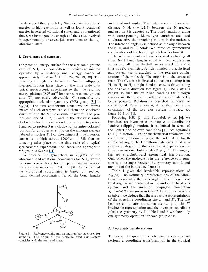
The reference configuration is defined as having allthree N–H bond lengths equal to their equilibriumvalues and all three H–N–H angles equal [6], and itthus has C3v symmetry. A right handed molecule fixedaxis system xyz is attached to the reference config-uration of the molecule. The origin is at the centre ofmass. The C3 axis z is directed so that on rotating fromH1 to H2 to H3 a right handed screw is driven alongthe positive z direction (see figure 1). The x axis ischosen so that the xz plane contains the nitrogennucleus and the proton H1 with the x coordinate of H1

being positive. Rotation is described in terms ofconventional Euler angles �, �, � that define theorientation of the xyz axis system in space; seefigure 10–1 of [31].

Following HBJ [5] and Papousek et al. [6], weintroduce an inversion coordinate � to describe the‘umbrella-flipping’ motion. It is defined in terms ofthe Eckart and Sayvetz conditions [31], see equations(8–10) in section 3. In the mathematical treatment, thecoordinate � formally plays the role of a fourthrotational angle; the Hamiltonian depends on it in amanner analogous to the way that it depends on thethree conventional Euler angles �, �, � [5]. The angle �has no straightforward geometrical interpretation.Only when the molecule is in the reference configura-tion is � the angle between the symmetry axis C3 andany one of the bonds (see figure 1).

Table 1 gives the irreducible representations ofD3h(M). The symmetry transformations of the vibra-tional coordinates, the Euler angles, the components oftotal angular momentum J in the molecular fixed axissystem, and the inversion conjugate momentumJ� ¼ �i �h@=@� are given in table 2. From the charactersin table 1 we deduce that the irreducible representationsof the stretching coordinates are A0

1 and E 0. The twobending coordinates transform according to the E 0

irreducible representation and the inversion coordinate� has the symmetry A00

2. In table 1 and 2, we show onlyone symmetry operation for each group class.

3. Coordinate transformations

To derive the quantum kinetic energy operator weperform a coordinate transformation in the classical

Figure 1. Reference configuration and numbering chosen forammonia. The origin of the molecule fixed axis systemcoincides with the centre of mass.

Rotation–vibration motion of pyramidal XY3 molecules 361

https://www.researchgate.net/publication/224812829_Molecular_Symmetry_and_Spectroscopy?el=1_x_8&enrichId=rgreq-d34e6153f4ce1922f353328fd8356d2f-XXX&enrichSource=Y292ZXJQYWdlOzIyNDg4OTc4MjtBUzoyNjUwMDMzODMxMjgwNjRAMTQ0MDE5MzEzODMxMA==





Hamiltonian, which is then quantized by applyingstandard procedures [31, 33–35] as explained insection 4. The Cartesian coordinates in the space fixedaxis system are transformed to the internal coordinatesin the non-rigid reference configuration system [5],where the large-amplitude motions (rotation and inver-sion) are treated explicitly, while other vibrationalmodes are considered as small displacements from thereference geometry.The coordinate transformation between the space

fixed axis system XYZ and the molecule fixed axissystem xyz is given by [5]:

Ri ¼ RCM þ S�1ð�,�,�Þ aið�Þ þ di½ �, ð1Þ

which is subject to seven constraints (the Eckart [36]and Sayvetz [37] conditions) given as equations (8–10)below. Owing to the constraints, the numbers ofindependent variables on both sides of the equationbecome equal. In equation (1) the vector Ri pointsto the position of nucleus i, and RCM points to the

position of the nuclear centre of mass in the spacefixed system. A 3� 3 orthogonal transformation matrixS�1ð�,�,�Þ, expressed in terms of the Euler anglesf�,�,�g [8], rotates XYZ to xyz; the vector di [withcomponents ðdix, diy, dizÞ] gives the displacement,due to small-amplitude vibration, of nucleus i fromits reference position aið�Þ in the molecular fixedsystem. The coordinates of the reference-configurationvectors aið�Þ are defined in [6] for NH3:

a1, x ¼ re sin �, ð2Þ

a2, x ¼ a3,x ¼ �1

2re sin �, ð3Þ

a4, x ¼ a1, y ¼ a4, y ¼ 0, ð4Þ

a2, y ¼ �a3, y ¼

ffiffiffi3

p

2re sin �, ð5Þ

a1, z ¼ a2, z ¼ a3, z ¼mNre cos �

3mH þmN, ð6Þ

a4, z ¼ �3mHre cos �

3mH þmN, ð7Þ

Table 1. The character table of the D3hðMÞ group [31].

G E (123) (23) E* (123)* (23)*

A01 1 1 1 1 1 1

1ffiffiffi3

p ðr1 þ r2 þ r3Þ, sin �A00

1 1 1 1 �1 �1 �1

A02 1 1 �1 1 1 �1 Jz

A002 1 1 �1 �1 �1 1 cos �, J�

E 0 2 �1 0 2 �1 0

�1ffiffiffi6

p ð2�23 � �13 � �12Þ,1ffiffiffi2

p ð�13 � �12Þ

�E 00 2 �1 0 �2 1 0 fJx, Jyg

Table 2. Transformation of the internal coordinates, the Euler angles and the components of themolecule fixed angular momentum and the inversion conjugate momentum by the symmetry operations

of the permutation–inversion group D3hðMÞ.

Variables fEg fð23Þg fð123Þg fE�g fð23Þ�g fð123Þ�g

r1 r1 r1 r3 r1 r1 r3r2 r2 r3 r1 r2 r3 r1r3 r3 r2 r2 r3 r2 r2�23 �23 �23 �12 �23 �23 �12�13 �13 �12 �23 �13 �12 �23�12 �12 �13 �13 �12 �13 �13� � p� � � p� � � p� �� p� � � � p� � �� þ p � � �þ p �� 2p� � �� 2p=3 �þ p p� � �þ p=3

Jx Jx Jx �1

2Jx �

ffiffiffi3

p

2Jy �Jx �Jx

1

2Jx þ

ffiffiffi3

p

2Jy

Jy Jy �Jy

ffiffiffi3

p

2Jx �

1

2Jy �Jy Jy �

ffiffiffi3

p

2Jx þ

1

2Jy

Jz Jz �Jz Jz Jz �Jz JzJ� J� �J� J� �J� J� �J�



where mH and mN are the nuclear masses of hydrogenand nitrogen, respectively, and re is the equilibriumbond length.In terms of the aið�Þ vectors, the Eckart [36] and

Sayvetz [37] conditions are given by:

XNi¼1

mi di ¼ 0, ð8Þ

XNi¼1

mi aið�Þ � dið Þ ¼ 0, ð9Þ

XNi¼1

midaið�Þ

d�� di ¼ 0, ð10Þ

where the sums run over all the nuclei of the moleculeand mi is the mass of the nucleus i. The condi-tions (8–10) have the following physical meanings:The first Eckart condition in equation (8) keeps thenuclear centre of mass at the origin of the xyz fixedsystem. The second Eckart condition in equation (9)and the Sayvetz condition in equation (10) reduce therotation–vibration and the inversion-vibration inter-actions, respectively [31]. For a given instantaneousnuclear geometry, the values of � and the rotationalcoordinates �, �, � can be determined by solvingequations (8–10).We must define five small-amplitude vibrational

coordinates in addition to the rotation-inversioncoordinates �, �, �, and �. An obvious choicewould be the geometrically defined coordinates r1,r2, r3, combined with suitable linear combinations ofthe interbond angles �12, �23, and �13, but we havedecided to use linearized internal coordinates [38]since they provide a simpler coordinate transfor-mation. The linearized internal coordinates Sl

n aregiven as linear combinations of the Cartesiandisplacements as

S‘n ¼XNi¼1

X�¼x, y, z

Bn, i�ð�Þ di�; n ¼ 1, 2, 3, 4a, 4b, ð11Þ

where the subscript � is used to denote the axes(x, y, z), Bn, i�ð�Þ is an element of a �-dependenttransformation matrix [39], and N is the number ofnuclei. To obtain the matrix elements Bn, i�ð�Þ wefirst introduce a set of geometrically defined coordi-nates ð�r1,�r2,�r3,S4a,S4bÞ, where �ri are bondlength displacements from the equilibrium value re,

and the symmetrized combinations of the instantaneousinterbond angles �ij are given by:

S4a ¼1ffiffiffi6

p ð2�23 � �13 � �12Þ, ð12Þ

S4b ¼1ffiffiffi2

p ð�13 � �12Þ: ð13Þ

The geometrically defined, internal coordinates Sn

(¼ �r1,�r2,�r3,S4a, or S4b) can be represented exactlyas infinite-order, power-series expansions in theCartesian displacements di�. When we truncate thesepower-series expansions after the first order termsand define

Bn, i�ð�Þ ¼@Sn

@di�

� �ðrefÞ

, ð14Þ

where the derivative is calculated in the referenceconfiguration, we obtain equation (11). The linearizedcoordinates S‘n thus coincide with curvilinear ones Sn

in the linear approximation Sn � S‘n þOðd2i�Þ. The

quantities S‘4a, S‘4b are the first and second components,

respectively, of the E 0 degenerate bending coordinates

S‘4a ¼1ffiffiffi6

p ð2��‘23 ��‘13 ��‘12Þ, ð15Þ

S‘4b ¼1ffiffiffi2

p ð��‘13 ��‘12Þ: ð16Þ

The linearized bond length displacements �r‘k and thelinearized interbond-angle displacements ��‘kl are givenby [31]:

�r‘k ¼X

�¼x, y, z

ak� � a4�

reðdk� � d4�Þ, ð17Þ

��‘kl ¼ �1

r2e sin�e

X�¼x,y, z

�

"�ðal� � a4�Þ � cos�eðak� � a4�Þ

�ðdk� � d4�Þ

þ ðak� � a4�Þ � cos�eðal� � a4�Þ� �

ðdl� � d4�Þ

#, ð18Þ

where re and �e are the equilibrium values of the bondlength and the interbond angle, respectively. Equations(17–18) are derived from the first-order expansion in di�




of the following geometrical expressions:

re þ�rk ¼

ffiffiffiffiffiffiffiffiffiffiffiffiffiffiffiffiffiffiffiffiffiffiffiffiffiffiffiffiffiffiffiffiffiffiffiffiffiffiffiffiffiffiffiffiffiffiffiffiffiffiffiffiffiffiffiffiffiffiffiffiffiffiffiffiffiffiffiffiX�¼x, y, z

ðak� � a4�Þ þ ðdk� � d4�Þ� �2s

, ð19Þ

cosð�e þ��klÞ

¼ðak � a4Þ þ ðdk � d4Þ½ � � ðal � a4Þ þ ðdl � d4Þ½ �

ðre þ�rkÞðre þ�rlÞ: ð20Þ

The nonzero matrix elements Bk, i� are given by:

Bk, i� ¼ai� � a4�

re�k, i ¼ �Bk, 4�, k ¼ 1, 2, 3, ð21Þ

B4a, i� ¼1ffiffiffi6

p 2 �BB23, i� � �BB13, i� � �BB12, i�

� , ð22Þ

B4b, i� ¼1ffiffiffi2

p �BB13, i� � �BB12, i�

� . ð23Þ

where � ¼ x, y, z and

�BBkl, i�¼�1

r2e sin�eðal��a4�Þ� cos�eðak��a4�Þ� �

�k, i

�1

r2e sin�eðak��a4�Þ� cos�eðal��a4�Þ� �

�l, i, ð24Þ

�BBkl,4�¼� �BBkl,k�� BBkl, l�, k, l¼ 1,2,3 and k 6¼ l: ð25Þ

The coordinate transformation inverse to equation (11)can be written as:

di� ¼X3N�7

n¼1

Ai�, nS‘n, ð26Þ

where the coefficients Ai�, n are obtained by solvinga system of 3N � ð3N � 7Þ linear equations

XNi¼1

mi Ai�, n ¼ 0, ð27Þ

XNi¼1

X�, ¼x, y, z

mi �� ai� Ai, n ¼ 0, ð28Þ

XNi¼1

X�¼x, y, z

midai�ð�Þ

d�Ai�, n ¼ 0, ð29Þ

XNi¼1

X�¼x, y, z

Bm, i� Ai�, n ¼ �m, n, ð30Þ

where �� is the fully antisymmetric tensor, � assumesthe values x, y, or z, and n,m ¼ 1, 2, 3, . . . ,3N � 7. Equations (27–29) follow from the Eckart(8,9) and the Sayvetz condition (10), while weobtain equation (30) by inserting equation (26) inequation (11).

The coordinate transformation implemented here[equations (1,26)] is fully determined by the quantitiesai� and Ai�, n. The vector components ai� are defined byequations (2–7), while the matrix elements Ai�, n arederived analytically by solving equations (27–30).The matrix elements ai� and Ai�, n are simple functionsof the inversion coordinate �, the masses mi, and theequilibrium parameter re.

Equations (1) and (26) define the transformationbetween the Cartesian coordinates ðRi,X ,Ri,Y ,Ri,ZÞ

of each nucleus in the space-fixed system and thegeneralized coordinates contained in the vector

q ¼ ðRCMX ,RCM

Y ,RCMZ , �,�,�,�r‘1,�r‘2,�r‘3,S

‘4a,S

‘4b, �Þ:

ð31Þ

We use q� (� ¼ 1, . . . , 12) to denote a general element ofq. The q� coordinates define three types of motions: (a)the translational motion described by ðRCM

X ,RCMY ,RCM

Z Þ

coordinates, (b) the overall rotation described byð�,�,�Þ coordinates, and (c) the relative motions ofthe nuclei described by the internal coordinatesð�r‘1,�r‘2,�r‘3,S

‘4a,S

‘4b, �Þ. The associated, generalized

momenta are given by:

� ¼ ðPX , PY , PZ, Jx, Jy, Jz, p‘1, p

‘2, p

‘3, p

‘4a, p

‘4b, J�Þ,

ð32Þ

where PF (F ¼ X ,Y ,Z) is the momentum conjugate tothe translational coordinate RCM

F (these translationalmomenta are of no spectroscopic interest in the absenceof external fields), ðJx, Jy, JzÞ are xyz components of thetotal angular momentum [8, 31], p‘n (n ¼ 1, 2, 3, 4a, 4b)is the momentum conjugate to the linearized vibrationalcoordinate S‘n, and J� is the momentum conjugate to �,i.e. quantum mechanically

JJ� ¼ �i �h@

@�: ð33Þ

We use �� (� ¼ 1, . . . , 12) to denote a generalelement of �.

The vector Ri (i ¼ 1 . . .N) in equation (1) has thespace fixed coordinates ðRiX ,RiY ,RiZÞ and the momen-tum conjugate to RiF , F ¼ X ,Y ,Z, is denoted PiF .The transformation from generalized momenta �� to



the Cartesian conjugate momenta PiF (i ¼ 1 . . .N,F ¼ X,Y ,Z),

PiF ¼X3N�¼1

s�, iF ��, ð34Þ

is defined by a Jacobian matrix with elements

s�, iF ¼@q�@RiF

: ð35Þ

We assume that the 3N-dimensional square matrixwith elements s�, iF is non-singular so that it can beinverted by means of the chain rule:

XNi¼1

XF¼X ,Y ,Z

@q�@RiF

@RiF

q�¼ ��,�, ð36Þ

or

XNi¼1

s�, i � ti,� ¼ ��,�: ð37Þ

We have introduced here the elements tiF , � of the matrixeffecting the transformation between Cartesian andgeneralized classical velocities:

dRiF

dt¼X3N�¼1

tiF , �dq�dt

ð38Þ

where t is time and

tiF , � ¼@RiF

@q�, ð39Þ

i ¼ 1 . . .N, F ¼ X ,Y ,Z and � ¼ 1, 2, . . . , 3N.Following [33], we establish the correspondence betweenthe XYZ and xyz representations of the vectors ti, �and s�, i as

s�, i ¼X

F¼X ,Y ,Z

eF s�, iF ¼X

�¼x, y, z

e� s�, i�, ð40Þ

ti, � ¼X

F¼X ,Y ,Z

eF tiF , � ¼X

�¼x, y, z

e� ti�, �, ð41Þ

where eF and ea are the orthogonal, normalized basisvectors. The index � runs over x, y, z, and F runs overX ,Y ,Z.

The classical rovibrational kinetic energy can bewritten as [33, 34]:

T ¼1

2

XNi¼1

XF¼X,Y ,Z

m�1i PiFPiF ¼

1

2

X3N�¼1

X3N�¼1

�� G�,��,

ð42Þ

where

G�,� ¼X

�¼x, y, z

XNi¼1

s�, i�s�, i�

mi: ð43Þ

That is, the expression for the classical kinetic energyin terms of the momenta conjugate to the generalizedcoordinates q� is defined by the matrix elements s�, i�.

The coefficients ti�, � associated with translation,rotation, inversion and vibration have simple analyticalrepresentations [33]:

tiF ,F 0 ¼ �F ,F 0 translation

ti�, � ¼X

��Ri rotation

ti�, � ¼ @Ri�=@� inversion

ti�, n ¼ @Ri�=@S‘n vibration: ð44Þ

It follows from the straightforward coordinate trans-formation Ri� ¼ Ri�ðqÞ in equation (1) that thematrix elements ti�,� are simple analytical functionsof the generalized coordinates q : ti�,� ¼ ti�,�ðqÞ.Thus, the matrix elements s�, i� in equation (35) canreadily be determined by inverting the matrix withelements ti�,� or, equivalently, by solving the systemof linear equations (37). The choice of linearizedvibrational coordinates provides a simple form forti�,�. Had we chosen geometrically defined, internalvibrational coordinates (i.e., bond lengths and interbondangles) as generalized coordinates, the elements of ti�,�would be more complicated, but the approach forobtaining s�, i�, which we describe below, would stillbe applicable.

At this point we choose to introduce linearizedMorse variables y‘k ¼ 1� exp ð�a�r‘kÞ (k ¼ 1, 2, 3),where a is the range parameter of the Morse potential.These variables simplify the computation of thematrix elements required for the variational calcula-tion. Morse oscillator basis functions are used insetting up the Hamiltonian matrix; these functionsprovide a rather good description of stretching motion[13] and allow us to express the potential energyfunction as a low-order power series expansion.All analytical functions in the rotational–vibrational


Hamiltonian are expanded as power series in thevibrational variables

‘n ¼ y‘1, y‘2, y

‘3,S4a,S4b

� , ð45Þ

i.e. linearized Morse variables and linearized symme-trized bending coordinates. These coordinates are alsoemployed for solving equation (37).Generally, it is not a trivial problem to invert the

matrix with elements ti�,�. We cannot, in practice,determine an analytical solution of equation (37) andso we solve it numerically. The system of equations (37)consists of ð3NÞ

2¼ 144 equations involving 144 vari-

ables ti�,�, which can easily be reduced by taking intoaccount the properties of the coordinate transfor-mation. The translational, vibrational and rotationalparts of equation (37) are separable, and there is nointermode interaction in the matrix with elements ti�,�.Consequently, equation (37) can be solved for eachmode � independently. This leaves us with 12 sets,labeled by � ¼ 1 . . . 12, each set with 3N ¼ 12 inde-pendent equations which define 3N ¼ 12 matrixelements si�, �, i ¼ 1, 2, 3, 4 and � ¼ x, y, z. Howeverthis is still a complicated problem to solve analytically.In order to solve it numerically, we expand the ti�,�and s�; i�, matrix elements as power series in the ‘ncoordinates defined above:

ti�,�ð ‘nÞ ¼

XL�0

XL½l�

ti�,�L½l � ð ‘Þ

L½l�, ð46Þ

s�, i�ð ‘nÞ ¼

XL�0

XL½l�

s�, i�L½l � ð ‘Þ

L½l�, ð47Þ

where we introduced the notation

XL½l�

fL½l�ðxÞL½l�

�XLl1¼0

XðL�l1Þ

l2¼0

XðL�l1�l2Þ

l3¼0

XðL�l1�l2�l3Þ

l4a¼0

f Ll1l2l3l4al4b

� xl11 xl22 x

l33 x

l4a4a x

l4b4b , ð48Þ

with l4b ¼ L� l1 � l2 � l3 � l4a. We end up with a systemof linear equations of the type Tx ¼ b:X

i�

ti�,�0½0� s�, i�0½0� ¼ ��,�, ð49Þ

Xi�

ti�,�0½0� s�, i�L½l� ¼ b�,�L½l� , L > 0, ð50Þ

where

b�, �L½l� ¼ �XL�1

K¼0

XK½k�

Xi�

ti�,�ðL�KÞ½l�k� s

�, i�K½k�: ð51Þ

Each set of equations given in (49) and (50) isrepresented by the 12� 12 coefficient matrix T withelements ti�,�0½0� , which is common for all orders ofmagnitude L, and by the 12-dimensional ‘right-hand-side’ vector b

�L½�� with elements b�, lL½l�; this vector is

recursively determined at each order. Thus, for everymode � at each iteration step L, there are 12� ðLþ 4ÞðLþ 3ÞðLþ 2ÞðLþ 1Þ=24 independent sets of 12 equa-tions for 12 independent variables xi� ¼ s�, i�L½l� . If weknow the solution of equation (50) up to and includingorder L we can derive recursively the matrix elementss�, i�Lþ1½l� for order (L þ 1). We should bear in mind that allquantities ti�,�

ðL�KÞ½l�k� and s�, i�K½k� are functions of �.Therefore, we construct a discrete grid of equidistantlyspaced �-values �k and solve the system of linearequations (49–50) at each �k point. The matrix elementss�, i� are obtained as expansions in the ‘n coordinatesat the non-rigid reference configuration.

The expansion coefficients G�,� in the kinetic energyoperator [equation (42)] are expressed as power seriesin the n coordinates:

G�,�ð ‘n, �Þ ¼

XL�0

XL½l�

G�,�L½l� ð�Þ ð ‘nÞ

L½l�ð52Þ

and, from equation (43) and the known expansions ofthe s�, i� matrix elements, the expansion coefficients areobtained as

G�,�L½l� ð�Þ ¼Xi�

1

mi

XLK¼0

XK ½k�

s�, i�ðL�KÞ½l�k�ð�Þ s

�, i�K ½k� ð�Þ: ð53Þ

It should be emphasized that we do not derive anyanalytical expressions for the �-dependent functionsconsidered here except in rather trivial cases, such asthe vector components ai�ð�Þ and the matrix elementsAi�, nð�Þ. The two-line recursion relations (49) and (50)replace thousands of lines with the correspondinganalytical expressions. No additional analytical deriva-tions or tiresome expressions are required. The kineticenergy operator is entirely defined by the recursionprocedure in equations (49, 50) so that it is a trivialtask to implement it as computer code. In our currentrealization of the procedure given in equations(49, 50), the expansions in equations (46, 47) can havea maximum order of eight.

The strategy chosen for solving the rotational-vibrational Schrodinger equation (i.e. to obtain a matrixrepresentation of the rotation–vibration Hamiltonianthat we can diagonalize) is the logical consequence ofthe procedure developed in the present section. All�–dependent functions in the Hamiltonian are repre-sented as power series expansions in the ‘n coordinates


around the reference configuration. The expansioncoefficients depend on � and are represented as a tableof numerical values determined at a grid of equidistantlyspaced �-values �k. All matrix element integration over� is done numerically by means of Simpson’s rule.

4. Quantum-mechanical kinetic operator

We quantize the classical kinetic energy in equation(42) by the methods described in [33, 34]. The momen-tum transformation (34) in symmetrized form isgiven by:

Pi ¼1

2

X3N�¼1

ðs�, i �� þ�� s�, iÞ ð54Þ

where Pi has the components ðPiX ,PiY ,PiZÞ and s�, ihas the components ðs�, iX , s�, iY , s�, iZÞ. Equation (54) isthe quantum mechanical replacement for the classicalequation (34). By inserting equation (54) in equation (42)and taking into account relations (40), we obtain thequantum-mechanical kinetic energy operator [33, 34]:

TT ¼1

2

X3N�¼1

X3N�¼1

�� G�,�� þUð ‘n, �Þ; ð55Þ

where G�,� are determined by equation (43) and

U ¼X3N�¼1

X3N�0¼1

XNi¼1

1

8m�1

i ��, s�, i� �

� ��0 , s�0, i� ��

þ1

4m�1

i s�, i ��, ½��0 , s�0, i�

��:

ð56Þ

The pseudopotential term U is expressed in terms ofcommutators between the conjugate momenta andthe transformation vectors. It can be included in thepotential energy function.Employing the recursion procedure in equations (49,

50), the pseudopotential function U is expressed in termsof the five linearized vibrational coordinates ‘n and thecurvilinear � coordinate analogous to expansion (52),and truncated at the same order as the G�,� terms.

5. Potential energy function

We distinguish two types of potential energysurface representations here. Type A is defined interms of geometrically defined, internal coordinates.It is designed with the sole purpose of representingthe potential energy surface in the best possible way; its

form has no direct relation to the variational problemand can, at least in principle, be chosen freely. Usuallyit is taken to be isotope independent. A Type Brepresentation defines the potential energy surfacein terms of our non-rigid reference configuration[see equation (1)] and is not isotope independent. It isexpanded as a power series in the linearized coordinates ‘n for a particular value of �. The expansion coefficientsare �-dependent and we express them as a table ofnumerical values determined at a grid of equidistantlyspaced �-values �k, exactly as done for the �-dependentfunctions in the kinetic energy operator. The Type Bexpansion is designed to simplify the calculationof Hamiltonian matrix elements in the subsequentvariational calculations.

In the present work, we initially employ a Type Aexpansion of the potential energy surface for theelectronic ground state of NH3

Vð 1, 2, 3, 4a, 4b; sin ��Þ

¼ V0ðsin ��Þ þXj

Fjðsin ��Þ j þXjk

Fjkðsin ��Þ j k

þXjkl

Fjklðsin ��Þ j k l þX

jklm

Fjklmðsin ��Þ

� j k l m . . . . ð57Þ

This analytical function [1] is expressed in terms of thevariables

k ¼ 1� exp ð�aðrk � reÞÞ, k ¼ 1, 2, 3, ð58Þ

4a ¼1ffiffiffi6

p 2�23 � �13 � �12ð Þ, ð59Þ

4b ¼1ffiffiffi2

p �13 � �12ð Þ, ð60Þ

sin �� ¼2ffiffiffi3

p sin ð ��=2Þ, ð61Þ

where �� ¼ ð�12 þ �23 þ �13Þ=3 is the average of theinterbond angles. The variable sin �� is of A1 symmetryin D3h(M), by definition, and coincides with sin � atthe reference configuration. We use sin �� only for therepresentation of the potential energy surface, and hencewe never require the value of ��.

The pure inversion potential energy function inequation (57) is

V0ðsin ��Þ ¼Xs

fðsÞ

0 ðsin �e � sin ��Þs, ð62Þ


and the functions Fjk...ðsin ��Þ are defined as

Fjk...ðsin ��Þ ¼Xs

fðsÞjk... ðsin �e � sin ��Þs, ð63Þ

where �e is the equilibrium value2 of �, a is a molecularparameter, and the quantities f

ðsÞ0 and f

ðsÞjk... in equations

(62) and (63) are expansion coefficients. The analyticalfunction in equation (57) is similar to the expansionintroduced for triatomic molecules in [12].By expressing V as an expansion in sin ��, we ensure

that, as required by symmetry, the potential energyfunction always has a maximum or a minimum at planarconfigurations. Further, V is totally symmetric under theoperations in the MS group D3h(M), and this imposesrelations between the f

ðsÞjk... parameters in equation (63).

The kinetic energy operator described in section 4is expressed in terms of the generalized coordinatesfrom equation (31) and the quantum mechanical formof the momenta from equation (32). In order to obtaina useful Hamiltonian with this kinetic energy operator,we must transform the Type A representation of thepotential energy function in equation (57) to a Type Brepresentation that depends on the generalized coordi-nates from equation (31). The corresponding coordinatetransformation is done in three steps:

f n, sin ��g!ðaÞfr1, r2, r3,�23,�13,�12g!

ðbÞfRi, �g!

ðcÞf ‘n, �g:

ð64Þ

In transformation (a) the geometrically defined coordi-nates from equations (58–60) are expanded in terms ofthe bond lengths and interbond angles; in transforma-tion (b) these latter coordinates are expanded in terms ofthe xyz Cartesian displacement coordinates by usingequations (19, 20), and finally in transformation (c) thelinearized coordinates are introduced by means ofequations (1, 26). The resulting Type B representationof the potential energy surface is expressed in a formsimilar to equation (57), where the expansion coeffi-cients parameters F‘jk...ð�Þ are given as tables ofnumerical values determined at the grid of equidistantlyspaced �-values �k. Our current code allows a 6th orderexpansion in the ‘n variables for the Type B potentialfunction.We generally follow a strategy of avoiding compli-

cated analytical derivations and, for the transforma-tion Vð n, sin ��Þ ! Vð ‘n, �Þ, this means that we calculatethe coefficients F‘ijk...ð�Þ numerically by a 4-point

finite-difference expression. This is a universal proce-dure, independent of the form of the Type A representa-tion for the potential energy function employed. As longas the particular choice of the geometrically defined,internal coordinates can be related to the Cartesiancoordinates, we can always expand Vð ‘n, �Þ by means ofthe finite-difference method. The disadvantage of thenumerical procedure is the error introduced by the finitedifferences. Alternatively, the parameters F‘ijk...ð�Þ couldbe obtained in least-squares fittings, either to potentialenergy values generated from a Type A representa-tion, or directly to the ab initio data. Such fittingswould have to be carried out for each isotopomerseparately.

6. Basis set

Aiming at solving the rotational-vibrationalSchrodinger equation variationally, we construct therovibrational basis functions as symmetrized linearcombinations of primitive-basis-function products:

jJ,m,NvirGviri

¼ jJ,K ,m, �roti½

� jni, J,K , �invijnb, lb, �bendijn1ijn2ijn3i�Gvir , ð65Þ

where jn1i, jn2i, and jn3i are one-dimensional Morse-oscillator eigenfunctions [40], jnb, lb, �bendi are 2Disotropic-harmonic-oscillator functions, jni, J,K , �inviare Numerov-Cooley eigenfunctions of the one-dimensional inversion Schrodinger equation (seebelow), and jJ,K ,m, �roti are rigid symmetric rotorwavefunctions. The symbol Gvir represents one ofthe irreducible representations of D3h(M) containedin the representation spanned by the functionproduct in equation (65) (see [31]), and the quantumnumber Nvir enumerates basis functions with the sameJ and Gvir.

6.1. Rotational basis functions

The rotational basis set is represented by usual rigidsymmetric rotor wavefunctions jJ, k,mi (see, forexample, [31]). The quantum numbers J, k ¼ �J . . . Jand m ¼ �J . . . J are associated with the total angularmomentum, its projection onto the z axis and itsprojection onto the Z axis, respectively. The symme-trized linear combinations jJ,K ,m, �roti are identicalto those used in [40]. They provide a real matrix

2 Since the equilibrium geometry is a reference configuration, sin �� and sin � have the same equilibrium value sin �e.



representation of the kinetic energy operator inequation (55) and are given by

jJ, 0,m, �roti ¼ i�rot jJ, 0,mi, �rot ¼ J mod 2, ð66Þ

jJ,K ,m, �roti ¼i�rot ð�1Þ�rotffiffiffi

2p jJ,K ,mi þ ð�1ÞJþKþ�rot

�J, � K ,mij Þ, ð67Þ

where �rot ¼ 0, 1 indicates the rotational parity ð�1Þ�rot ,�rot ¼ K mod 3 for �rot ¼ 1, and �rot ¼ 0 for �rot ¼ 0,and K ¼ 0 . . . J. The phases in equations (66, 67) arechosen as in [8]. The symmetry Grot of the rotationalfunction jJ,K ,m, �roti is given as

jJ,K ¼ 3t,m, �rot ¼ 0i ! Ay

1

jJ,K ¼ 3t,m, �rot ¼ 1i ! Ay

2

jJ,K 6¼ 3t,m, �rot ¼ 0i ! E ya

jJ,K 6¼ 3t,m, �rot ¼ 1i ! Ey

b

ð68Þ

where t is a positive integer number, y ¼ 0 if K is even,and y ¼00 when K is odd.

6.2. Inversion basis functions

The inversion wavefunctions jni, J,K , �invi are obtainedas numerical solution of the pure inversion one-dimensional Schrodinger equation:

H0ðinvÞ ¼ �

1

2

@

@�G0�, �ð�Þ

@

@�þ1

4G0

x, xð�Þ þ G0y, yð�Þ

h i� JðJ þ 1Þ � K2� �

þ1

2G0

z, zK2

þ V0ð�Þ þUð ‘n ¼ 0, �Þ, ð69Þ

obtained by neglecting, in the complete rovibrationalHamiltonian, the small-amplitude displacements fromthe reference configuration (see [6]). In equation (69)we introduced the notation G0

�, �ð�Þ � G�, �ð ‘n ¼ 0, �Þ.

The one-dimensional Schrodinger equation obtainedfrom equation (69) is solved by the numerical Numerov-Cooley integration method [41, 42] as detailed in [11].The Hamiltonian H0

ðinvÞ depends parametrically on therotational quantum numbers J and K, i.e. the effectiveinversion potential is different for each rotational state.The eigenfunctions of equation (69), being stationarysolutions, are labeled by the inversion quantum numberni and by the parity parameter �inv. The parity is ð�1Þ�inv

so that for �inv ¼ 0(1) the primitive inversion basisfunction is unchanged (changed in sign) by the inversionoperation E* which takes � into p��. Positive parity

is associated with A01 symmetry in D3h(M), negative

parity with A002 symmetry.

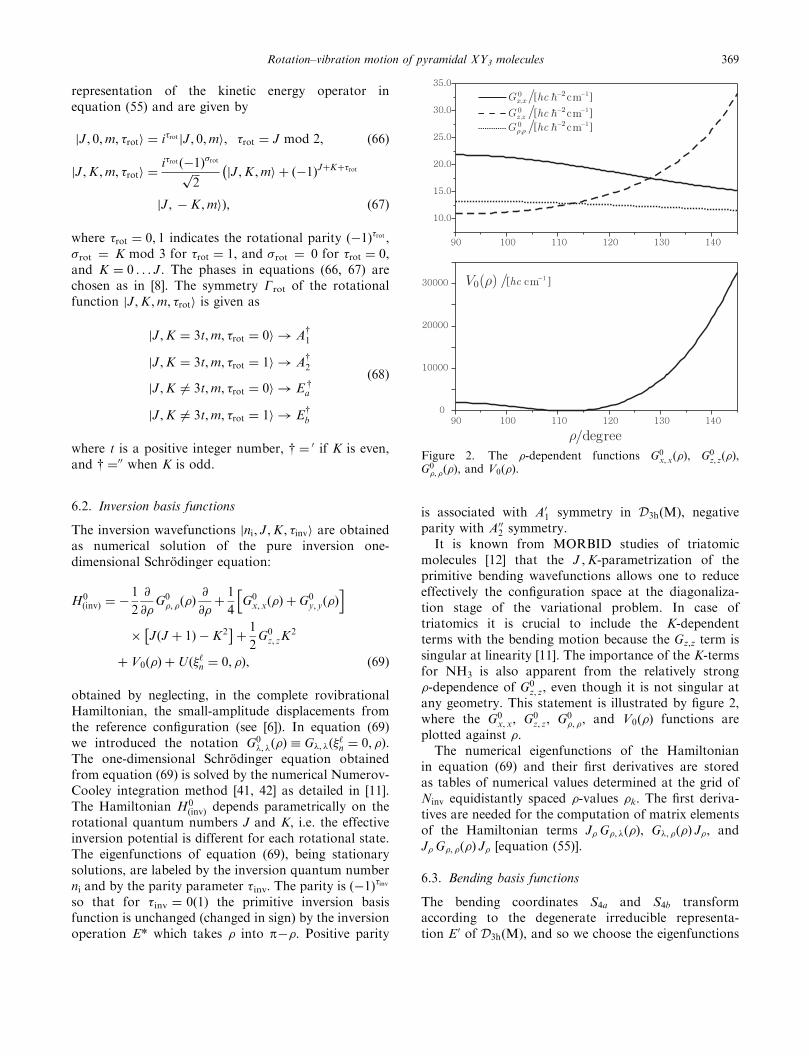
It is known from MORBID studies of triatomicmolecules [12] that the J ,K-parametrization of theprimitive bending wavefunctions allows one to reduceeffectively the configuration space at the diagonaliza-tion stage of the variational problem. In case oftriatomics it is crucial to include the K-dependentterms with the bending motion because the Gz,z term issingular at linearity [11]. The importance of the K-termsfor NH3 is also apparent from the relatively strong�-dependence of G0

z, z, even though it is not singular atany geometry. This statement is illustrated by figure 2,where the G0

x, x, G0z, z, G0

�, �, and V0ð�Þ functions areplotted against �.

The numerical eigenfunctions of the Hamiltonianin equation (69) and their first derivatives are storedas tables of numerical values determined at the grid ofNinv equidistantly spaced �-values �k. The first deriva-tives are needed for the computation of matrix elementsof the Hamiltonian terms J� G�, �ð�Þ, G�, �ð�Þ J�, andJ� G�, �ð�Þ J� [equation (55)].

6.3. Bending basis functions

The bending coordinates S4a and S4b transformaccording to the degenerate irreducible representa-tion E0 of D3h(M), and so we choose the eigenfunctions

Figure 2. The �-dependent functions G0x,xð�Þ, G0

z, zð�Þ,G0�, �ð�Þ, and V0ð�Þ.


of a two-dimensional, isotropic harmonic oscillator asthe basis functions associated with them. Since theHamiltonian is Hermitian, we can obtain a real matrixrepresentation by using real harmonic-oscillator eigen-functions involving cos ðlb ’Þ and sin ðlb ’Þ, rather thanthe usual complex form involving exp ðilb ’Þ [43].The positive-parity functions (�bend ¼ 0), expressed interms of polar coordinates fr4, ’g, are given by:

jnb, lb, 0i ¼ Nnb, lb exp ð�r24=2Þ rlb4 Llb

ðnb�lbÞ=2ðr24Þ cosðlb ’Þ

ð70Þ

and the negative-parity functions (�bend ¼ 1) are:

jnb, lb, 1i ¼ ð�1Þ�b Nnb, lb

� exp ð�r24=2Þ rlb4 Llb

ðnb�lbÞ=2ðr24Þ sinðlb ’Þ,

ð71Þ

where Llbk is a generalized Laguerre polynomial [44],

nb is the principal vibrational quantum number, lb isthe vibrational angular momentum quantum number,and �b ¼ lb mod 3 . The normalization constant is

Nnb, lb ¼ffiffiffiffiffiffiffiffiffiffiffiffiffiffiffiffiffi2� �lb, 0

p ffiffiffiffiffiffiffiffiffiffiffiffiffiffiffiffiffiffiffiffiffiffiffiffiffiffiffiffiffi½ðnb � lbÞ=2�!

p½ðnb þ lbÞ=2�!

sð72Þ

and the dimensionless normal coordinates are given by:

Q4a ¼ r4 cos ð’Þ ¼2f 0

4a4a

G04a, 4að�eÞ

!1=4

� S4a ð73Þ

Q4b ¼ r4 sin ð’Þ ¼2f 0

4a4a

G04a, 4að�eÞ

!1=4

� S4b, ð74Þ

where !b ¼ ½2f 04a4aG

04a, 4að�eÞ�

1=2is the vibrational fre-

quency of the two-dimensional isotropic harmonicoscillator and G0

4a, 4að�eÞ ¼ G4a, 4að ‘n ¼ 0, � ¼ �eÞ. The

vibrational angular momentum lb can only take posi-tive values nb, nb � 2, . . . , 1 or 0. The eigenvalues areindependent of lb so that an energy level with a givenvalue of nb is ðnb þ 1Þ-fold degenerate. The constructedbending basis functions have the following symmetryproperties:

jnb, lb ¼ 0, �bend ¼ 0i ! A01

jnb, lb ¼ 3t, �bend ¼ 0i ! A01

jnb, lb ¼ 3t, �bend ¼ 1i ! A02

jnb, lb 6¼ 3t, �bend ¼ 0i ! E0a

jnb, lb 6¼ 3t, �bend ¼ 1i ! E0b:

ð75Þ

where the two components of E0 (see table 1) are labeledE0a and E0

b, respectively.

6.4. Stretching basis set

The Morse potential

VMorseðrÞ ¼ Dy2 ¼ D 1� expð�a�rÞ½ �2

ð76Þ

models the potential energy curves of many diatomicmolecules very well [45], and therefore it is also usedto describe stretching motion in polyatomic systems(see, for example, [13]). In equation (76), r is theinternuclear distance describing the stretching motionand�r ¼ r� re is the displacement from the equilibriumvalue re, D is the dissociation energy, a is a parameterdetermining the curvature of the potential at r ¼ re,and y ¼ 1� expð�a�rÞ. A stretching potential energysurface represented in terms of Morse variables yhas obvious mathematical advantages, such as goodconvergence properties and simple analytical expres-sions for matrix elements between Morse oscillatoreigenfunctions.

The Morse oscillator eigenfunctions jni are solutionsof the one-dimensional Schrodinger equation with theMorse potential:

��h2

2�

@2

@r2þDy2

�jni ¼ Enjni, ð77Þ

where � is the reduced mass of the system and jniis expressed in terms of generalized Laguerre poly-nomials (see [44]). The stretching basis functions areconstructed as the products jn1ijn2ijn3i. It should benoted that the Morse oscillator eigenfunctions used asbasis functions here depend on the linearized stretchingcoordinates �r‘1, �r‘2, �r‘3, rather than on the usual,geometrically defined bond length displacements.

7. Symmetry factorization of the Hamiltonian matrix

The variational solution of the fully-dimensionalrotation-vibration Schrodinger equation for a four-atomic molecule is a formidable numerical problem,involving the diagonalization of huge matrices.Therefore it is essential to take advantage of the highintrinsic symmetry of pyramidal XY3 molecules. TheHamiltonian matrix is diagonal in the total angularmomentum quantum number J, and when we employbasis functions symmetrized in D3h(M), each J-blockbecomes block diagonal with a sub-block for eachirreducible representation of D3h(M) [31]. The sub-blocks can be diagonalized separately and so we caneffectively reduce the sizes of the matrices that needto be diagonalized. In addition, each of the degenerateirreducible representations E0 and E00 gives rise to two


sub-blocks with identical eigenvalues so that it issufficient to diagonalize only one of these.The eigenvalue problem is solved as follows. The

matrix elements Hk,l of the total rotation–vibrationHamiltonian are first calculated in terms of primitivebasis functions

’½r� ¼ jJ,K ,m, �roti|fflfflfflfflfflfflfflfflffl{zfflfflfflfflfflfflfflfflffl}rotation

jni, J,K , �invi|fflfflfflfflfflfflfflfflffl{zfflfflfflfflfflfflfflfflffl}inversion

jnb, lb, �bendi|fflfflfflfflfflfflfflfflffl{zfflfflfflfflfflfflfflfflffl}bending

jn1ijn2ijn3i|fflfflfflfflfflfflffl{zfflfflfflfflfflfflffl}stretching

ð78Þ

that transform according to reducible representations ofD3h(M). Then the matrix with elements Hk,l is trans-formed to the block-diagonal form associated with thesymmetrized basis functions ½irr�,G

� (where ‘irr’ standsfor ‘irreducible representation,’ G is the MS groupsymmetry of the basis function, and � labels functionswith the same G). Towards this end, we perform anorthogonal transformation to the symmetrized basisfunctions by means of projection operators PPG [31]:

½irr�,G� ¼ PPG’½r�: ð79Þ

It is not necessary to calculate and transform thewhole primitive matrix of elements Hk,l in one fellswoop. The primitive basis functions can be sortedinto relatively small sets, each of which spans a reduciblerepresentation of D3h(M). For example, the primitivestretching basis functions jnij0ij0i, j0ijnij0i and j0ij0ijnispan the three-dimensional reducible representationA0

1 E0 of D3h(M) [31]. From these three primitivebasis functions, we obtain the symmetrized functions

A01 ¼ ðj0ij0ijni þ jnij0ij0i þ j0ijnij0iÞ=

ffiffiffi3

p, ð80Þ

E 0a ¼ ð2j0ij0ijni � jnij0ij0i � j0ijnij0iÞ=

ffiffiffi6

p, ð81Þ

E 0b ¼ ðjnij0ij0i � j0ijnij0iÞ=

ffiffiffi2

p: ð82Þ

In general, any combination of indexes fJK ; n1 �n2 � n3; nblb; nig is associated with a set of primitivebasis functions

jJ, K, m, 0i

jJ, K, m, 1i

" #�

jni, J;K; 0i

jni, J;K; 1i

" #�

jnb, lb, 0i

jnb, lb, 1i

" #

�

jn1ijn2ijn3i

jn2ijn3ijn1i

jn3ijn1ijn2i

jn1ijn3ijn2i

jn2ijn1ijn3i

jn3ijn2ijn1i

2666666666664

3777777777775ð83Þ

which span an Nr-dimensional reducible representationof D3h(M). There are at most (when n1, n2, n3 are alldifferent) 48 basis functions in the set defined byequation (83). However, these can be separated into24 functions with positive parity (�rot þ �inv þ �bend even)and 24 functions with negative parity (�rot þ �inv þ �bendodd). Thus, in constructing symmetrized basis functions,we must consider at most 24 primitive basis functionssimultaneously.

The elements of the representation matrices generatedby the set of functions in equation (83) are obtained as

Driv½R�ijk, i0j0k0 ¼ DðrotÞii0 ½R� D

ðinvÞjj0 ½R� D

ðvibÞkk0 ½R�, ð84Þ

where R is a group operation and DðrotÞii0 ½R�, D

ðinvÞjj0 ½R�,

and Dvibkk0 ½R� are elements of the representation matrices

generated by the primitive basis functions describingrotation, inversion, and small-amplitude vibration(bending and stretching), respectively. These matricesare determined as described in [31]. The indices i and i0

label the primitive rotational basis functions, j and j0

label the primitive inversion basis functions, and kand k0 label the primitive small-amplitude vibrationbasis functions. The quantity Driv½R�ijk, i0j0k0 in equation(84) is, in this labeling, an element of a representationmatrix generated by the function products defined inequation (83). The corresponding representation has thecharacters

�ðrivÞ½R� ¼ �ðrotÞ½R��ðinvÞ½R��ðvibÞ½R� ð85Þ

and can be reduced in terms of irreducible represen-tations by means of equation (5–45) of [31].

We obtain a symmetrized basis function ½irr�,G� by

applying [equation (79)] the projection operator PPG tothe primitive basis function ’½r� which, in an obviousnotation, can be written as

’½r� ¼ FðrivÞijk ¼ FðrotÞ

i FðinvÞj FðvibÞ

k : ð86Þ

We express ½irr�,G� in terms of the primitive basis

functions as

½irr�,G� ¼ PPG FðrivÞ

ijk ¼Xi0j0k0

PG�, i0j0k0 F

ðrivÞi0j0k0 : ð87Þ

For the non-degenerate irreducible representations ofD3h(M),G ¼ A0

1,A02,A

001, or A00

2, it follows fromequation (6–67) of [31] that

PG�, i0j0k0 ¼

1

12

XR

�G½R�� Driv½R�ijk, i0j0k0 . ð88Þ


Projecting to the doubly degenerate representations E0

and E00 is more tricky. We use equation (6–64) of [31]to obtain

~PPEa

�, i0j0k0 ¼2

12

XR

DðEÞ½R��

11 Driv½R�ijk, i0j0k0 , ð89Þ

~PPEb

�, i0j0k0 ¼2

12

XR

DE ½R��

22 Driv½R�ijk, i0j0k0 , ð90Þ

where DðEÞ½R�11 and DE ½R�22 are the diagonal elementsof representation matrices associated with the Eirreducible representation in question. If the twosymmetrized basis functions obtained in this way arenot orthogonal, they can be orthogonalized by standardSchmidt orthogonalization [31].The elements HG

�0, �00 of the block diagonal, ‘symme-trized’ matrix are given in terms of the elementsHi0j0k0, i00j00k00 of the original, ‘primitive’ matrix:

HG�0,�00 ¼

Xi0j0k0

Xi00j00k00

PG�0, i0j0k0

��Hi0j0k0, i00j00k00 P

G�00, i00j00k00 : ð91Þ

8. Computational details

As described in sections 4 and 5, we expand therotation–inversion–vibration Hamiltonian bHHriv in thevariables given in equations (45) and so we can write itsymbolically as

bHHriv ¼Xp

bOOðpÞ

rbOOðpÞ

ibOOðpÞ

bbOOðpÞ

s ð92Þ

where the rotational operator bOOðpÞ

r depends on theEuler angles �, �, � through the components of the total

angular momentum, the inversion operator bOOðpÞ

i depends

on � and JJ�, the bending operator bOOðpÞ

b depends onðS‘4a,S

‘4bÞ and their conjugate momenta, and finally the

stretching operator bOOðpÞ

s depends on ð�r‘1,�r‘2,�r‘3Þ andtheir conjugate momenta. The summation index p labelsthe different terms in the Hamiltonian.A matrix element of one term in equation (92)

between two of the primitive basis functions givenin equation (65) is obviously a product of fourdistinct integrals involving different coordinates:

hJ,K 00,m, �00rotjbOOðpÞ

rjJ,K 0,m, �0roti, hn00i , J,K

00, �00invjbOOðpÞ

i jn0i,

J,K 0, �0invi, hn00b, l00b, �

00bendj

bOOðpÞ

b jn0b, l0b, �

0bendi, and hn001jhn

002j

hn003jbOOðpÞ

s jn01ijn02ijn

03i.

The matrix elements hJ,K 00,m, �00rotjbOOðpÞ

r jJ,K 0,m, �0rotiinvolving symmetrized rotational wavefunctions can

be obtained by making suitable transformations of thematrix elements calculated in terms of unsymmetrizedrigid rotor functions jJ, k,mi; these latter matrixelements are given, for example, in [8]. The rotationalmatrix elements are diagonal in J and m, and they donot depend on m.

The inversion matrix elements hn00i , J,K00, �00invj

bOOðpÞ

i jn0i,J,K 0, �0invi are integrals over �; they are calcu-lated numerically by means of Simpson’s rule. Becauseof the symmetry, the functions integrated, F(�)say, are always even or odd under the coordinatechange �! p� � caused by the inversion operation E*.Consequently we haveZ p

0

Fð�Þ d� ¼2R pp=2 Fð�Þ d�, Fð�Þ even,

0, Fð�Þ odd,

�ð93Þ

so that we only have to integrate the non-vanishingintegrals over the interval ½p=2, p�, i.e. the upper half ofthe definition interval ½0, p�.

Matrix elements hn00b, l00b, �

00bendj

bOOðpÞ

b jn0b, l0b, �

0bendi involv-

ing ðS‘4a,S‘4bÞ, p‘4a, and p‘4b are obtained from Nielsen

[43]. The matrix elements for their products can beobtained numerically by the recursive procedure:

hnlj ‘j Fð ‘nÞjn

0l0i ¼Xn00l00

hnlj ‘j jn00l00ihn00l00jFð ‘nÞjn

0l0i, ð94Þ

hnljp‘j Fð ‘nÞjn

0l0i ¼Xn00l00

hnljp‘j jn00l00ihn00l00jFð ‘nÞjn

0l0i. ð95Þ

We have used Efremov’s approach [46] to deriverecursive numerical routines generating the one-dimensional integrals hnþ jjy�jni, hnþ jjy� d=drjni,and hnþ jjy� d2=dr2jni involving Morse-oscillator eigen-functions and the Morse variable y. The stretchingintegrals hn001jhn

002jhn

003jbOOðpÞ

s jn01ijn02ijn

03i are obtained from

the one-dimensional integrals in a straightforwardmanner.

In the calculations presented in the following section,the basis set was truncated according to

2ðn1 þ n2 þ n3Þ þ nb þ ni 14 ð96Þ

These limits correspond to the following matrix dimen-sions: NA1

¼ 1455, NA2¼ 1125, NE ¼ 2571. With this

basis set, we obtain convergence to about 0.5 cm�1

for energy values below 6100 cm�1. The �k numericalgrid, used to represent �-dependent functions, containedNinv ¼ 1000 points.

In the variational calculations we employed sixthorder expansions in the ‘n variables both for the kineticenergy part (G�,� and U) and for the potential energyfunction (Type B). Although in our current realizationof the recursive procedure in equation (50), the


expansions in equations (46, 47) can be taken up toeighth order, truncation after the sixth-order termsturned out to be sufficient in the present case; itproduces convergence to about 0.02 cm�1 for thevibrational energy values below 6100 cm�1.

9. Calculations

We report here three sets of results obtained for 14NH3

with the theoretical model described above: J¼ 0vibrational energies up to 6100 cm�1, J 4 2 energiesfor the vibrational ground state and the �2, �4, and 2�2excited vibrational states, and J 4 7 energies for the4�þ2 vibrational state. The calculated energies are labeledby the quantum numbers of the basis state with thelargest contribution to the eigenstate.The calculations are based on an accurate

ab initio potential energy surface, which is denoted asCBS**�45 760 [18] and may be viewed as an extensionof our published CBS* surface [1]. Briefly, a regulargrid with 45760 points was constructed that coveredgeometries with 0.85 A r1 r2 r3 1.20 A and808 �12, �23, �31 1208. Energies (ATZfc) werecomputed at all grid points using the CCSD(T) method(coupled cluster theory with all single and doublesubstitutions [47] and a perturbative treatment ofconnected triple excitations [48, 49]) with the aug-mented correlation-consistent triple-zeta basis aug-cc-pVTZ [50, 51]. At 1460 selected points, more accurateenergies (CBSþ ) were determined by extrapolating theCCSD(T) results to the complete basis set limit andincluding corrections for relativistic effects and core-valence correlation [1]. The differences between theATZfc and CBSþ energies were fitted by a quinticpolynomial in geometrically defined, internal coordi-nates, and the corrections were added to the ATZfcenergies at all 45 760 grid points to generate the CBS**-45760 surface (which is close to CBSþ quality).An analytical representation of this surface wasobtained by fitting a fifth-order expansion (57), throughall CBS**-45760 data points. The resulting 130 potentialparameters will be given elsewhere [18] and are alsoavailable from the authors on request.In table 3, we compare calculated vibrational (J¼ 0)

term values with available, experimentally derivedvalues and with theoretical results [3] for the 33lowest vibrational levels (up to 6100 cm�1). The root-mean-square (rms) deviation between the theoreticaland experimental values is 4.7 cm�1 in our case and7.6 cm�1 in the case of Colwell et al. [3].Table 4 presents a comparison of our theoretical

values of the J ¼ 1 and 2 energies in the vibrationalground state and the �2, �4, and 2�2 excited vibrational

states with experimentally derived values [52, 53] andthe theoretical results of Colwell et al. [3]. Here the rmsdeviations between theory and experiment, calculatedfor the 44 states listed in table 4, are 1.2 cm�1 for ourcalculated energies and 6.0 cm�1 for those of Colwellet al. [3]. For the vibrational ground state our theoreticalterm values are consistently slightly above the experi-mentally derived values, whereas those from [3] aresignificantly above the experimental values for highK and below them for low K, and thus show a lessuniform behaviour. The largest contribution to theerrors in the computed rovibrational term values comesfrom the vibrational term values. Adjusting the valuesof the �2, �4, and 2�2 band centres to coincide withexperiment, our rms deviation for the rovibrationallevels drops to 0.07 cm�1, compared with 1.47 cm�1 inthe case of Colwell et al. [3].

In a recent experimental study of the 2�4=�1=�3vibrational band system of 14NH3, Kleiner et al. [28]observed weak absorption transitions to 23rotational levels of a vibrational state which theyassigned as the ðv1, v

p2, v

l33 , v

l44 Þ ¼ ð0, 4þ, 00, 00Þ state. A

complete analysis of these transitions was not possiblebecause of strong resonances not included in the modelused for analysis [28]. We can now check the proposedassignment [28] by calculating theoretically the rota-tional structure in the v

p2 ¼ 4þ state up to J¼ 7 (i.e. the

highest rotational levels involved in the 4�þ2 transitionsassigned). Such variational calculations for high J valuesare taxing: for example, in the case of J¼ 7, we have tohandle matrices of dimension 38 610 for E symmetry.This was not feasible with the available computationalresources, and so we reduced the basis set to

ni 8, 2ðn1 þ n2 þ n3Þ þ nb 8,

which leads to matrices of dimension 6516 (A01,A

002), 6714

(A001,A

02), and 13230 (E0,E 00). The term values obtained

for the vp2 ¼ 4þ state are listed in table 5, relative to the

calculated zero point energy of 7446.279 cm�1. To betterappreciate the consistence, within the vibrational state,of the calculated rotational structure, the calculatedenergies for J > 0 are shifted by the deviation foundfor the v

p2 ¼ 4þ, J ¼ 1, K ¼ 0 term value (5.825 cm�1).

Table 5 also contains the experimentally derived termvalues taken from table 10 of [28].

The calculated energies are mostly in good agree-ment with the experimentally derived values, withone striking exception: The experimental term valueof 3730.442 cm�1, assigned to ðJ,K ,GÞ ¼ ð5, 1,E00Þ,differs by 7.538 cm�1 from the theoretical value. Ithas been obtained [28] as the upper level of twoobserved transitions, starting in levels with ðv1, v

p2, v

l33 ,

vl44 , J,K ,GÞ ¼ ð0, 0�, 00, 00, 6, 1,E0Þ [3317.204 cm�1] and


ð0, 0�, 00, 00, 4, 1,E0Þ [3534.830 cm�1], respectively, wherethe respective observed wavenumbers are given insquare brackets. However, Appendix 1 of [28] alsolists two transitions with wavenumbers at 3317.20623and 3534.83109 cm�1, that are assigned to the �1and �3 bands, respectively. The wavenumbers of thesetransitions are very close (within 0.002 cm�1) to thoseof the two transitions assigned to end in the level at3730.442 cm�1. Apparently, the proposed assignment[28] assumes that two weak transitions to the

4�þ2 ðJ,K,GÞ ¼ ð5, 1,E00Þ level are hidden under therelatively strong lines at 3317.20623 cm�1(�1) and3534.83109 cm�1(�3), respectively, whereas our calcula-tions predict these 4�2 transitions to be shifted about7.5 cm�1 away from the positions of these lines.

Closer inspection of table 5 shows that there aretwo further rovibrational levels with smaller, but ratherunsystematic deviations from the experimentallyderived term values [28]: ðJ,K,GÞ ¼ ð5, 2,E00Þ predictedat 3715.255 cm�1 (obs�calc is �0.987 cm�1), and

Table 3. Vibrational term valuesa for 14NH3 (in cm�1).

G v1vp2v

l33 v

l44 Obs.b Calc. Obs.-Calc. Ref. [3]c

A0 01þ0000 932.43 933.75 �1.32 942.88

A0 02þ0000 1597.47 1598.67 �1.20 1613.10

A0 03þ0000 2384.15 2387.66 �3.51 2382.66

A0 00þ0020 3216.02 3213.77 2.25 3215.08

A0 10þ0000 3336.02 3341.58 �5.56 3321.26

A0 04þ0000 3462.00 3468.35 �6.35 3456.59

A0 01þ0020 4115.62 4099.92 15.70 4124.44

A0 11þ0000 4294.51 4301.40 �6.89 4289.83

E0 00þ0011 1626.28 1626.00 0.28 1626.79

E0 01þ0011 2540.53 2537.13 3.40 2549.78

E0 00þ0022 3240.18 3238.62 1.56 3240.97

E0 00þ1100 3443.68 3446.23 �2.55 3440.79

E0 01þ1100 4416.91 4420.95 �4.04 4426.04

E0 10þ0011 4955.85 4960.23 �4.38 4941.33

E0 00þ1111 5052.60 5054.77 �2.17 5054.32

E0 01þ1111 6012.90 6012.59 0.31 6023.87

A0 0 00�0000 0.79 0.80 �0.01 0.60

A0 0 01�0000 968.12 969.80 �1.68 973.30

A00 02�0000 1882.18 1885.04 �2.86 1883.57

A0 0 03�0000 2895.51 2900.27 �4.76 2889.79

A0 0 00�0020 3217.59 3215.61 1.98 3216.69

A00 10�0000 3337.08 3342.62 �5.54 3322.76

A0 0 04�0000 4055.00d 4068.65 �13.65d 4054.53

A0 0 01�0020 4173.25 4164.34 8.91 4175.72

A0 0 11�0000 4320.06 4327.16 �7.10 4313.71

E0 0 00�0011 1627.37 1627.16 0.21 1627.64

E0 0 01�0011 2586.13 2584.75 1.38 2589.20e

E0 0 00�0022 3241.61 3240.17 1.44 3242.03

E0 0 00�1100 3443.99 3446.60 �2.61 3441.07

E0 0 01�1100 4435.4 4439.69 �4.29 4441.49

E00 10�0011 4956.79 4961.51 �4.72 4942.76

E0 0 00�1111 5052.97 5055.41 �2.44 5054.77

E0 0 01�1111 6037.12 6037.40 �0.28 6043.99

rms 4.7

aLabeled by ðv1, vp2, v

l33 , v

l44 Þ, where the vr and lr are usual harmonic oscillator quantum numbers and p ¼ þ (�) indicates the lower,

symmetric (upper, antisymmetric) inversion component.bExperimentally derived values taken from [1], which also contains the references to the experimental work.cTheoretical values from Colwell et al. [3], Table 7.dThe original experimental value [55] for the 4�a2 band centre is 4055� 5 cm�1. A misprinted value of 4045 cm�1 appeared later [56]and was used in many compilations. We use the original value [55] but do not include it when calculating rms deviations becauseof its high uncertainty.eOriginally [3] given as 1589.20 cm�1. We have corrected this obvious misprint and use 2589.20 cm�1 , which is also consistent withthe quoted inversion splitting [3].


ðJ,K ,GÞ ¼ ð5, 5,E00Þ predicted at 3665.142 cm�1

(obs�calc is �2.206 cm�1).For the remaining 20 rotational term values in

table 5, our calculations confirm the suggestedassignments [28] because the deviations between experi-

mentally derived and computed values are small(0.35 cm�1 or less) and systematic. In the other threecases (see above) the original assignment shouldbe reconsidered, especially for 4�þ2 ð5, 1,E 00Þ, wherethe deviation of 7.5 cm�1 is exceedingly large. It should

Table 4. Rotation–vibration term valuesa of 14NH3 for J ¼ 1 and 2 ðin cm�1Þ:

v1 vp2 vl33 vl44 G J K Obs.b Calc. Obs.-Calc Ref. [3]c

0 0þ 00 00 E 00 1 1 16.13 16.22 �0.09 16.27

A02 1 0 19.89 19.91 �0.02 19.71

E0 2 2 44.84 44.85 �0.01 45.37

E 00 2 1 55.91 56.00 �0.09 55.69

A01 2 0 59.60 59.73 �0.13 59.10

0 0� 00 00 E0 1 1 16.93 16.99 �0.06 16.87

A001 1 0 20.67 20.70 �0.03 20.31

E 00 2 2 45.51 45.64 �0.13 45.97

E0 2 1 56.67 56.78 �0.11 56.27

A002 2 0 60.39 60.49 �0.10 59.68

0 1þ 00 00 E 00 1 1 948.57 949.93 �1.36 959.10

A02 1 0 952.56 953.92 �1.36 962.85

E0 2 2 976.78 978.29 �1.51 987.84

E 00 2 1 988.81 990.24 �1.43 990.04

A01 2 0 992.82 994.24 �1.42 1002.78

0 1� 00 00 E0 1 1 984.13 985.86 �1.73 989.44

A001 1 0 987.86 989.60 �1.74 993.05

E 00 2 2 1012.43 1014.25 �1.82 1018.30

E0 2 1 1023.67 1025.45 �1.78 1028.85

A002 2 0 1027.42 1029.18 �1.76 1032.53

0 0þ 00 11 E 00 1 1 1639.47 1639.34 0.13 1640.14

A002 1 1 1645.39 1645.11 0.28 1646.11

E0 1 0 1646.59 1646.40 0.19 1647.01

A02 2 2 1664.97 1665.00 �0.03 1666.23

E0 2 2 1677.27 1677.10 0.17 1678.49

E 00 2 1 1680.17 1680.09 0.08 1680.61

A002 2 1 1687.24 1687.08 0.16 1687.39

E0 2 0 1687.33 1687.20 0.13 1687.46

0 0� 00 11 E0 1 1 1640.45 1640.47 �0.02 1640.97

A02 1 1 1647.30 1647.11 0.19 1647.89

E 00 1 0 1647.79 1647.63 0.16 1648.04

A002 2 2 1665.98 1666.12 �0.14 1667.03

E 00 2 2 1678.61 1678.43 0.18 1679.79

E0 2 1 1681.36 1681.36 0.00 1681.66

A02 2 1 1686.54 1686.40 0.14 1686.89

E 00 2 0 1688.71 1688.65 0.06 1688.96

0 2þ 00 00 E 00 1 1 1613.57 1614.82 �1.25 1629.20

A02 1 0 1617.84 1619.06 �1.22 1633.18

E0 2 2 1641.52 1642.88 �1.36 1657.54

E 00 2 1 1654.29 1655.56 �1.27 1669.33

0 2� 00 00 E0 1 1 1898.02 1900.90 �2.88 1899.55

E 00 2 2 1926.12 1929.13 �3.01 1928.36

E0 2 1 1936.87 1939.69 �2.82 1938.44

A002 2 0 1940.29 1943.22 �2.93 1942.22

aLabeled by ðv1, vp2, v

l33 , v

l44 Þ, where the vr and lr are usual harmonic oscillator quantum numbers and p ¼ þ (�) indicates the lower,

symmetric (upper, antisymmetric) inversion component.bExperimentally derived values from [52] and [53].cTheoretical values from Colwell et al. [3].


be noted that a later experimental investigation ofthe 4�2–�2 hot band [54] confirmed most of theoriginal assignments [28] but did not address the threecritical cases discussed above.

10. Summary and conclusion

In the preceding sections we have presented, inconsiderable detail, a new variational model fordescribing the rotation–vibration motion of pyramidalXY3 molecules, which is based on the Hougen-Bunker-Johns approach [5]. We introduce a flexiblereference configuration that follows the large-amplitude vibration (i.e. the inversion motion in NH3)and the remaining small-amplitude vibrations aredescribed as displacements from this configuration.In this way, we obtain a model with maximum

separation between the different types of molecularmotion. The price paid for this advantage is thatwe need to approximate the kinetic energy operator bya finite power-series expansion in the small-amplitudevibrational parameters.

We report three applications, all for 14NH3, of themodel developed addressing the J¼ 0 vibrationalenergies to high excitation, the J 4 2 energies for thevibrational ground state and the �2, �4, and 2�2 excitedvibrational states, and the J 4 7 energies for the4�þ2 vibrational state. The calculations are based onthe CBS**-45760 potential energy surface describedelsewhere [1, 18].

We have compared our calculated energies to experi-mental data and to recent theoretical results by Colwellet al. [3]. We achieve very satisfactory agreementwith experiment for both the purely vibrational term

Table 5. Rotational term values for the 4�þ2 vibrational state of 14NH3 (in cm�1).

J K G Obs.a Calc.-5.825 Obs.-Calc.

1 0 A02 3479.614 3479.614 0.000

1 1 E00 3477.113 3477.460 �0.347

2 2 E 0 3505.184 3505.237 �0.053

2 1 E00 3511.913 3511.865 0.048

3 0 A02 3566.580 3566.508 0.072

3 2 E 0 3557.040 3556.978 0.062

3 3 A001 3545.710 3545.795 �0.085

3 3 A002 3545.710 3545.795 �0.085

3 1 E00 3564.175 3564.100 0.075

4 4 E 0 3598.973 3599.106 �0.133

4 2 E 0 3627.017 3626.970 0.047

4 3 A001 3614.926 3614.861 0.065

4 3 A002 3614.927 3614.860 0.067

4 1 E00 3634.403 3634.402 0.001

5 4 E 0 3685.472 3685.398 0.074

5 2 E 0 3714.268 3715.255 �0.987

5 3 A001 3702.653 3702.650 0.003

5 3 A002 3702.653 3702.652 0.001

5 5 E00 3662.936 3665.142 �2.206

5 1 E00 3730.442 3722.904 7.538

6 6 A01 3743.604 3743.879 �0.275

6 6 A02 3743.604 3743.879 �0.275

6 4 E 0 3790.983 3791.033 �0.050

6 3 A001 3808.781 3808.931 �0.150

6 3 A002 3808.781 3808.927 �0.146

6 5 E00 3768.609 3768.508 0.101

6 1 E00 3829.337 3829.565 �0.228

7 6 A01 3864.252 3864.080 0.169

aExperimentally derived values from [28].


values and the rotational spacings. This demonstratesthe high accuracy of the CBS**-45760 potential energysurface and the soundness of our approach to thesolution of the rotation–vibration problem.Our theoretical calculation largely verifies the

tentative assignments made by Kleiner et al. [28] oftransitions in the 4�þ2 band of 14NH3. The proposedquantum number labels for 23 experimentally derived,rotational term values in the v

p2 ¼ 4þ �ibrational

state are confirmed in 20 cases, and theoreticalpredictions are made for the remaining three cases,particularly for 4�2 ð5, 1,E00Þ where a misassignment ismost likely.This last example shows that theoretical

calculations of rotation–vibration energies can nowbe carried out also for four-atomic moleculeswith sufficient accuracy to be helpful in the interpreta-tion and assignment of experimental, high-resolutionrotation–vibration spectra. It also demonstrates thatour approach can be applied to rotation–vibrationstates with higher J values (here up to J¼ 7) whereexact variational treatments of nuclear motion are nolonger feasible. This advantage arises from the max-imum separation of different types of motion that isinherently built into our approach.

Acknowledgements

This work was supported by the EuropeanCommission through contract no. HPRN-CT-2000-00022 ‘Spectroscopy of Highly Excited RovibrationalStates’. S. Yu. acknowledges financial support fromNSERC (Canada) and thanks P. Bunker andS. Patchkovskii for helpful discussions.

References

[1] H. Lin, W. Thiel, S.N. Yurchenko, M. Carvajal,P. Jensen, J. Chem. Phys., 117, 11265–11276 (2002).

[2] S.N. Yurchenko, M. Carvajal, P. Jensen,F. Herregodts, T.R. Huet, Chem. Phys., 290, 59–67(2003).

[3] S.M. Colwell, S. Carter, N.C. Handy, Mol. Phys., 101,523–544 (2003).

[4] C. Leonard, N.C. Handy, S. Carter, J.M. Bowman,Spectrochim. Acta A, 58, 825–838 (2002).

[5] J.T. Hougen, P.R. Bunker, J.W.C. Johns, J. Mol.Spectrosc., 34, 136-172 (1970).

[6] D. Papousek, J.M.R. Stone, V. Spirko, J. Mol. Spectrosc.,48, 17–37 (1973).

[7] V. Spirko, J. Mol. Spectrosc., 101, 30–47 (1983).[8] D. Papousek, M.R. Aliev, Molecular Vibrational-

Rotational Spectra, Elsevier, Amsterdam (1982).[9] A.R. Hoy, P.R. Bunker, J. Mol. Spectrosc., 52, 439–456

(1974).

[10] A.R. Hoy, P.R. Bunker, J. Mol. Spectrosc., 74,

1–8 (1979).[11] P. Jensen, Comp. Phys. Rep., 1, 1–55 (1983).[12] P. Jensen, J. Mol. Spectrosc., 128, 478–501 (1988).[13] P. Jensen, Mol. Phys., 98, 1253–1285 (2000).[14] S.V. Shirin, O.L. Polyansky, N.F. Zobov, P. Barletta,

J. Tennyson, J. Chem. Phys., 118, 2124–2129 (2003).[15] O.L. Polyansky, A. G. Csaszar, S.V. Shirin, N.F. Zobov,

P. Barletta, J. Tennyson, D.W. Schwenke, P.J. Knowles,Science, 299, 539–542 (2003).

[16] T. Rajamaki, A. Miani, L. Halonen, J. Chem. Phys., 118,6358–6369 (2003).

[17] T. Rajamaki, A. Miani, L. Halonen, J. Chem. Phys.,118, 10929–10938 (2003).

[18] H. Lin, J.J. Zheng, S.N. Yurchenko, P. Jensen, W. Thiel,to be published.

[19] E. Kauppi, L. Halonen, J. Chem. Phys., 103, 6861–6872(1995).

[20] F. Gatti, J. Chem. Phys., 111, 7225–7235 (1999).[21] F. Gatti, C. Iung, C. Leforestier, X. Chapuisat, J. Chem.

Phys., 111, 7236–7243 (1999).[22] N.C. Handy, S. Carter, S.M. Colwell, Mol. Phys., 96,

477–491 (1999).[23] D. Luckhaus, J. Chem. Phys., 113, 1329–1347 (2000).[24] J. Pesonen, A. Miani, L. Halonen, J. Chem. Phys., 115,

1243–1250 (2001).[25] T. Rajamaki, A. Miani, J. Pesonen, L. Halonen, Chem.

Phys. Lett., 363, 226–232 (2002).[26] C. Leonard, S. Carter, N.C. Handy, Chem. Phys. Lett.,

370, 360–365 (2003).[27] H.-G. Yu, T. Muckerman, J. Molec. Spectrosc., 214,

11–20 (2002).[28] I. Kleiner, L.R. Brown, G. Tarrago, Q.-L. Kou,

N. Picque, G. Guelachvili, V. Dana, J.-Y. Mandin,J. Mol. Spectrosc., 193, 46–71 (1999).

[29] A.G. Csaszar, W.D. Allen, H.F. Schaefer, J. Chem. Phys.,108, 9751–9764 (1998).

[30] W. Klopper, C.C.M. Samson, G. Tarczay, A.G.Csaszar, J. Comput. Chem., 22, 1306–1314 (2001).

[31] P.R. Bunker, P. Jensen, Molecular Symmetry and Spec-troscopy, 2nd ed., NRC Research Press, Ottawa (1998).

[32] P. Schwerdtfeger, L.J. Laakkonen, P. Pyykko, J. Chem.Phys., 96, 6807–6819 (1992).

[33] G.O. Sørensen, Topics in Current Chemistry, M.J.S.Dewar et al. (Eds.), Vol. 82, p. 97–175. Springer-Verlag,Heidelberg (1979).

[34] A. Nauts, X. Chapuisat, Mol. Phys., 55, 1287–1318(1985).

[35] B. Podolsky, Phys. Rev., 32, 812–816 (1928).[36] C. Eckart, Phys. Rev., 47, 552–558 (1935).[37] A. Sayvetz, J. Chem. Phys., 7, 383–389 (1939).[38] A.R. Hoy, I.M. Mills, G. Strey, Mol. Phys., 24,

1265–1290 (1972).[39] E.B. Wilson Jr, J.C. Decius, P.C. Cross,

Molecular Vibrations, Dover Publications, Inc.,New York (1995).

[40] V. Spirko, P. Jensen, P.R. Bunker, A. Cejchan, J. Mol.Spectrosc. 112, 183–202 (1985).

[41] B. Numerov, Publ. of the Central Astrophys. Observatory(Rus), 2, 188–259 (1923).

[42] J.W. Cooley, Math. Comp., 15, 363–374 (1961).[43] H.H. Nielsen, Rev. Mod. Phys., 23, 90–136 (1951).[44] M. Abramowitz, I. Stegun, Handbook of Mathematical

Functions, Dover Pub., New York (1972).




[45] P.M. Morse, Phys. Rev., 34, 57–64 (1929).[46] Yu. S. Efremov, Opt. Spectrosc., 43, 693–694

(1977).[47] G.D. Purvis, R.J. Bartlett, J. Chem. Phys., 76, 1910–1918

(1982).[48] M. Urban, J. Noga, S.J. Cole, R.J. Bartlett, J. Chem.

Phys., 83, 4041–4046 (1985).[49] K. Raghavachari, G.W. Trucks, J.A. Pople, M. Head-

Gordon, Chem. Phys. Lett., 157, 479–483 (1989).[50] T.H. Dunning, J. Chem. Phys., 90, 1007–1023 (1989).[51] D.E. Woon, T.H. Dunning, J. Chem. Phys., 98,

1358–1371 (1993).

[52] S. Urban, V. Spirko, D. Papousek, J. Kauppinen, S.P.Belov, L.I. Gershtein, A.F. Krupnov, J. Mol. Spectrosc.,88, 274–292 (1981).

[53] J.S. Garing, H.H. Nielsen, K. Narahari Rao, J. Mol.Spectrosc., 3, 496–527 (1959).

[54] C. Cottaz, G. Tarrago, I. Kleiner, L.R. Brown, J. Mol.Spectrosc., 209, 30–49 (2001).

[55] L.D. Ziegler, B. Hudson, J. Phys. Chem., 88, 1110–1116(1984).

[56] P. Rosmus, P. Botschwina, H.-J. Werner, V. Vaida,P.C. Engelking, M.I. McCarthy, J. Chem. Phys., 86,

6677–6692 (1987).


Rotation–vibration motion of pyramidal XY 3 molecules described in the Eckart frame: Theory and...

Documents

Transcript of Rotation–vibration motion of pyramidal XY 3 molecules described in the Eckart frame: Theory and...