Ad hoc & Sensor Networks IV year II sem - IARE
272
Ad hoc & Sensor Networks IV year II sem INSTITUTE OF AERONAUTICAL ENGINEERING (Autonomous) Dundigal, Hyderabad - 500 043 COMPUTER SCIENCE AND ENGINEERING
-
Upload
khangminh22 -
Category
Documents
-
view
1 -
download
0
Transcript of Ad hoc & Sensor Networks IV year II sem - IARE

Ad hoc & Sensor Networks
IV year II sem
INSTITUTE OF AERONAUTICAL ENGINEERING (Autonomous)
Dundigal, Hyderabad - 500 043
COMPUTER SCIENCE AND ENGINEERING

UNIT –I

Introduction to Ad Hoc Wireless Networks
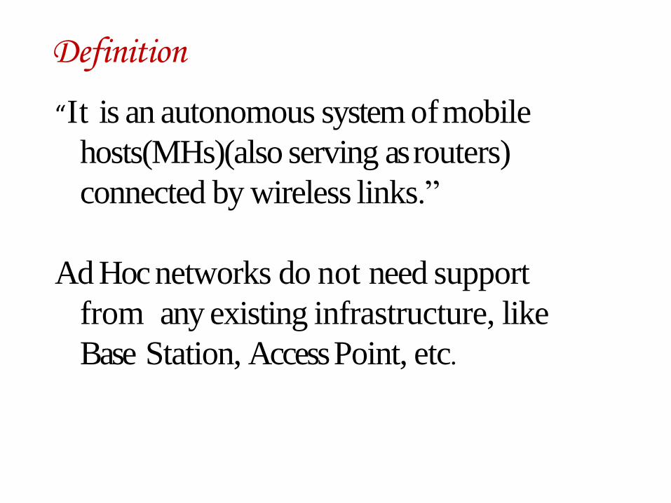
Definition
“It is an autonomous system of mobile
hosts(MHs)(also serving as routers)
connected by wireless links.”
Ad Hoc networks do not need support
from any existing infrastructure, like
Base Station, Access Point, etc.

Ad Hoc Model

Infrastructure Vs Ad Hoc Network Infrastructure networks Ad-hoc wireless networks
Fixed infrastructure No infrastructure
Single-hop wireless links Multi-hop wireless links
High cost and time of deployment Very quick and cost-effective
Reuse of frequency via channel reuse Dynamic frequency sharing
Nowadays applications: civilian, commercial Nowadays applications: military, rescue
High cost of network maintenance Maintenance operations are built-in
Low complexity of mobile devices Intelligent mobile devices are required
Widely deployed, evolves Still under development in commercial sector
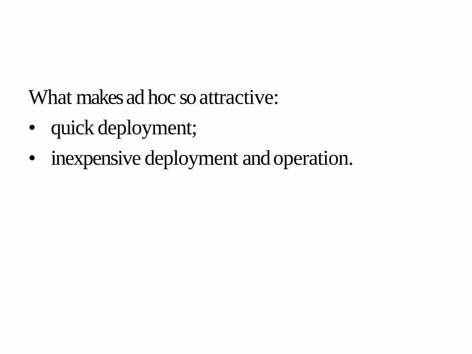
What makes ad hoc so attractive:
• quick deployment;
• inexpensive deployment and operation.

Technical challenges
There are many challenges in design, deployment, and performance of ad hoc:
1. Medium access scheme;
2. Routing and multicasting;
3. Transport layer protocol;
4. Quality of service provisioning;
5. Self Organizing
6. Security;
7. Energy management;
8. Addressing and service discovery;
9. Scalability;
10. Deployment considerations.
Note! no good solutions for these challenges.
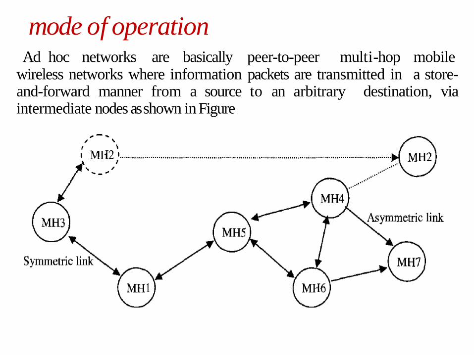
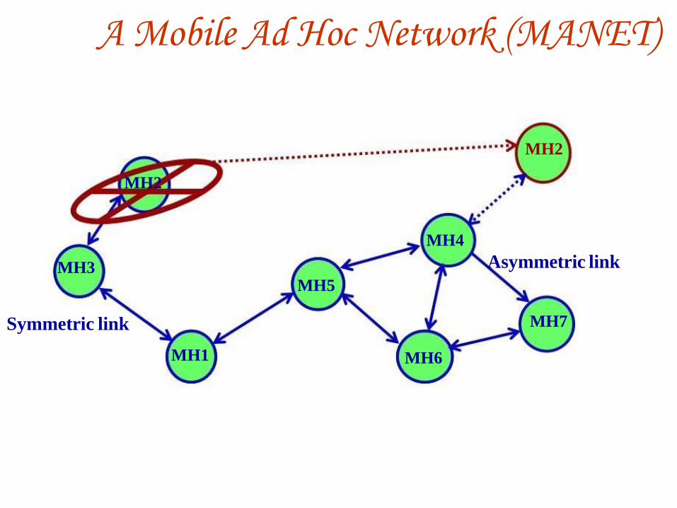
mode of operation Ad hoc networks are basically peer-to-peer multi-hop mobile
wireless networks where information packets are transmitted in a store-and-forward manner from a source to an arbitrary destination, via intermediate nodes as shown in Figure

As the MHs move, the resulting change in network topology must be
made known to the other nodes so that outdated topology information
can be updated or removed.
For example, as the MH2 in the above Figure changes its point of
attachment from MH3 to MH4 other nodes part of the network should
use this new route to forward packets to MH2.

Important characteristics of a MANET
• Dynamic Topologies : nodes move randomly with different speeds, network topology changes
• Energy-constrained Operation: nodes also involve in network management, system and applications be designed to save the energy
• Limited Bandwidth: Transmission rate is low
• Security Threats: Mobile wireless networks are generally more prone to physical security threats than fixed-cable nets. Security services be designed carefully

The Communication Puzzle
• There are different types of wireless networks with
different transmission speeds and ranges
• Personal Area Network (PAN) personal objects
• Local Area Network(LAN) single building or campus
• Metropolitan Area Networks (MAN) towns and cities
• Wide Area Network (WAN) states, countries, continents
• Regional Area Network (RAN) to provide coverage ranges in the order of tens of kilometers with applications in rural and remote areas
All these are differed by the physical distance that the
network spans
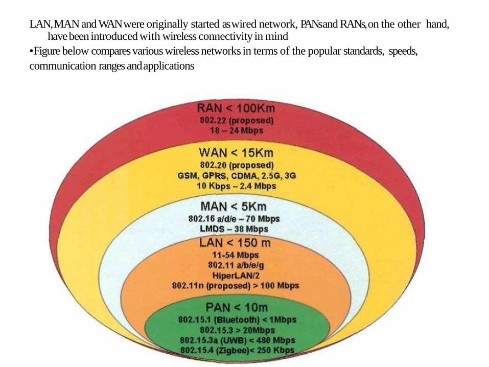
LAN, MAN and WAN were originally started as wired network, PANs and RANs, on the other hand, have been introduced with wireless connectivity in mind
•Figure below compares various wireless networks in terms of the popular standards, speeds,
communication ranges and applications

• Ad hoc networks are mostly within the framework of Wireless
LANs and Wireless PANs, a lot of movement is currently
undergoing as to integrate ad hoc networks with MANs and
WWANs
• With this it would be easy to connect the ad hoc network with
the outside world (e.g., Internet)
• While the mobile devices are equipped with dual mode and dual
band radio frequencies , heterogeneous networks will become
more and more common and the need to integrate them will be
of paramount importance

Challenges:
• Active research is going on in Adhoc, several aspects have been
explored, many problems have been arisen, still some issues to be
addressed.
• Major challenges are:
1.Scalability;
2.Quality of service;
3.Client server model shift;
4.Security;
5.Interoperation with the Internet;
6.Energy conservation;
7.Node cooperation;
8.Interoperation.
Scalability • Ad hoc networks suffer, by nature, from the scalability
problems in capacity.
• In a non-cooperative network, where omni-directional antennas are
being used, the through put per node decreases at a rate
1/(sqrt(N)),where N is the number of nodes.
• That is, in a network with100 nodes, a single device gets, at most,
approximately one tenth of the theoretical network data rate.
The problem fixed with bi directional antennas
• As the network size increases the problems like Route
acquisition, service location and encryption key exchanges need
to be solved.
Quality of Service
• There are many applications for transfer of Voice, live video, and
file transfer.
• QoS parameters such as delay, jitter, bandwidth, Packet loss
probability, and so on need to be addressed carefully.
• Issues of QoS robustness, QoS routing policies, algorithms and
protocols with multiple, including preemptive, priorities remain
to be addressed.
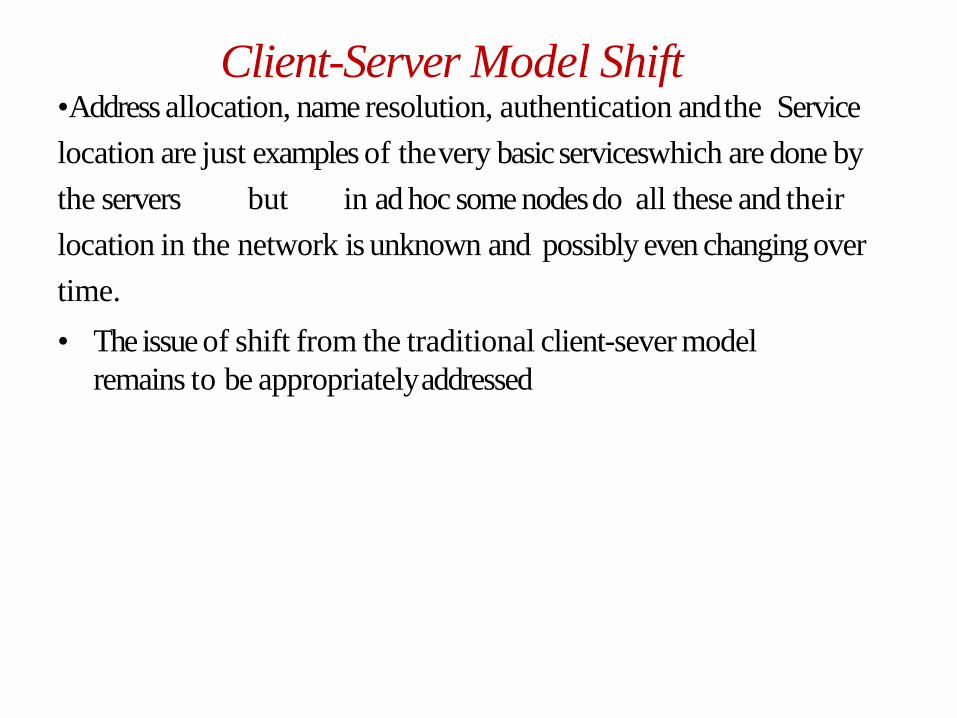
Client-Server Model Shift •Address allocation, name resolution, authentication and the Service
location are just examples of the very basic serviceswhich are done by
the servers but in ad hoc some nodes do all these and their
location in the network is unknown and possibly even changing over
time.
• The issue of shift from the traditional client-sever model
remains to be appropriately addressed
Security
•Lack of any centralized network management or certification
authority makes these dynamically changing wireless structures
leads security threats like infiltration, eavesdropping,
interference, and so on.
• Security is indeed one of the most difficult problems to be
solved, but it has received only modest attention so far
Energy Conservation
• There are two primary research topics: maximization of life time of a
single node and maximization of the life time of the whole network.
• These goals can be achieved either by developing better
batteries, or by making the network terminals‘ operation more
energy efficient.
• The first approach is likely to give a 40% increase in battery life,
remaining 60% can be achieved though the design of energy efficient
protocols design
A Mobile Ad Hoc Network (MANET)
MH2
MH2
MH4
MH3
Symmetric link
MH5
MH1
Asymmetric link
MH7
MH6
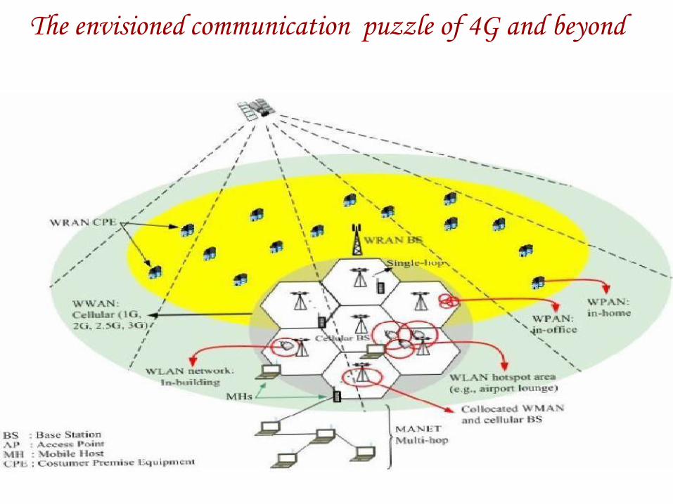
The envisioned communication puzzle of 4G and beyond

The scope of various wireless technologies

UNIT –II

Data Transmission In MANETS
MAC PROTOCOLS FOR AD HOC WIRELESS
NETWORKS
Issues in designing a MAC Protocol- Classification of MAC
Protocols- Contention based protocols- Contention based
protocols with Reservation Mechanisms- Contention
based protocols with Scheduling Mechanisms – Multi
channel MAC-IEEE 802.11
2

Issues
The main issues need to be addressed while designing a
MAC protocol for ad hoc wireless networks:
Bandwidth efficiency is defined at the ratio of the
bandwidth used for actual data transmission to the total
available bandwidth. The MAC protocol for ad-hoc
networks should maximize it.
Quality of service support is essential for time-
critical applications. The MAC protocol for ad-hoc
networks should consider the constraint of ad-hoc
networks.
Synchronization can be achieved by exchange of
control packets. 27
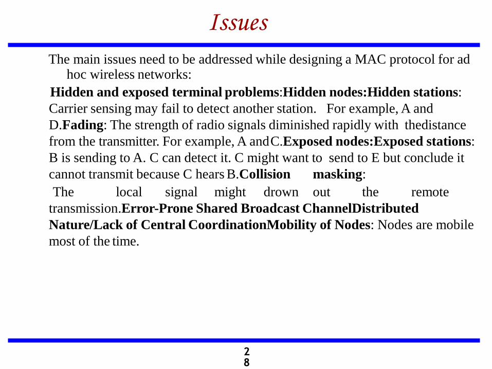
Issues
The main issues need to be addressed while designing a MAC protocol for ad hoc wireless networks:
Hidden and exposed terminal problems:Hidden nodes:Hidden stations:
Carrier sensing may fail to detect another station. For example, A and
D.Fading: The strength of radio signals diminished rapidly with thedistance
from the transmitter. For example, A and C.Exposed nodes:Exposed stations:
B is sending to A. C can detect it. C might want to send to E but conclude it
cannot transmit because C hears B.Collision masking:
The local signal might drown out the remote
transmission.Error-Prone Shared Broadcast ChannelDistributed
Nature/Lack of Central CoordinationMobility of Nodes: Nodes are mobile
most of the time.
28
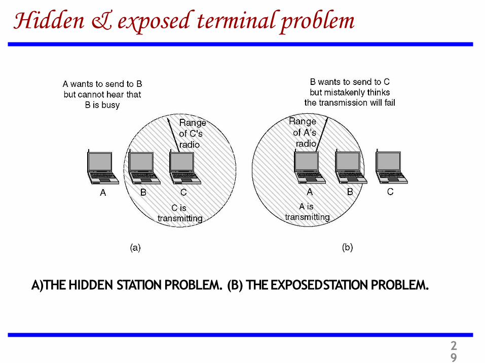
A)THE HIDDEN STATION PROBLEM. (B) THE EXPOSED STATION PROBLEM.
Hidden & exposed terminal problem
29
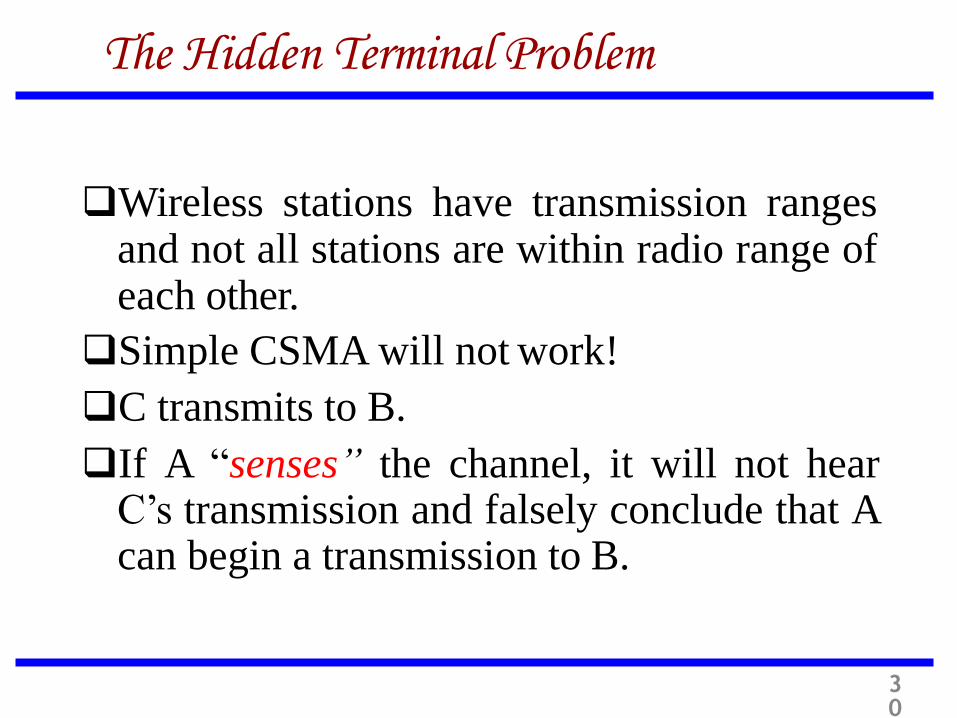
The Hidden Terminal Problem
Wireless stations have transmission ranges and not all stations are within radio range of each other.
Simple CSMA will not work!
C transmits to B.
If A “senses” the channel, it will not hear C’s transmission and falsely conclude that A can begin a transmission to B.
30
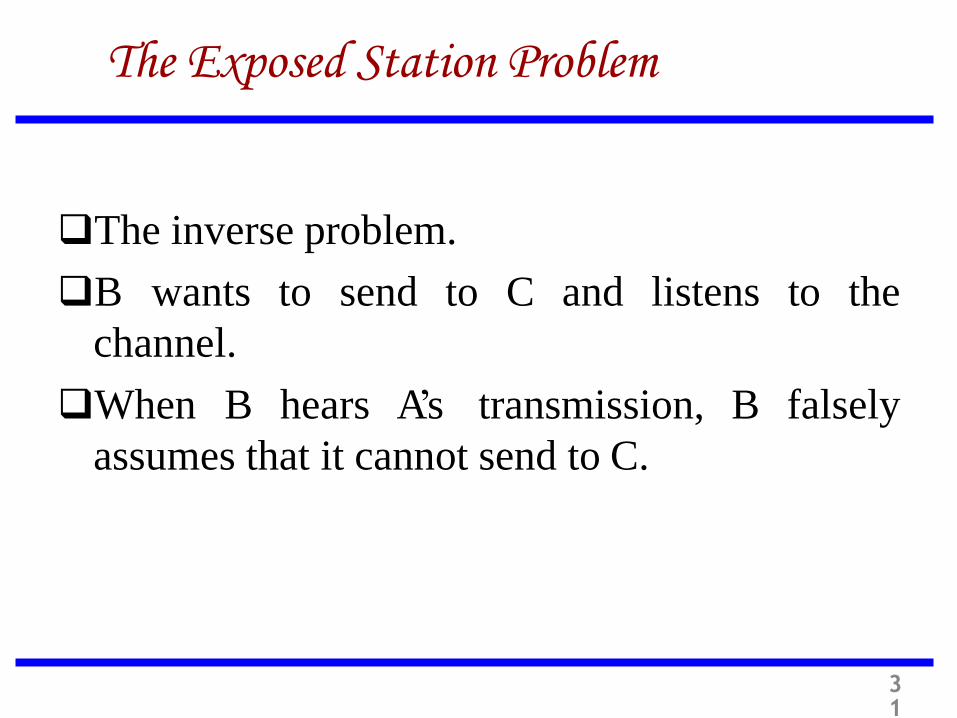
The Exposed Station Problem
The inverse problem.
B wants to send to C and listens to the
channel.
When B hears A’s transmission, B falsely
assumes that it cannot send to C.
31

Wireless LAN configuration
LAN
Server
Wireles s LAN
Base st ation/ ac cess point
Palmt op
Lapt ops
radio obs truc tion
A B C
D E
32
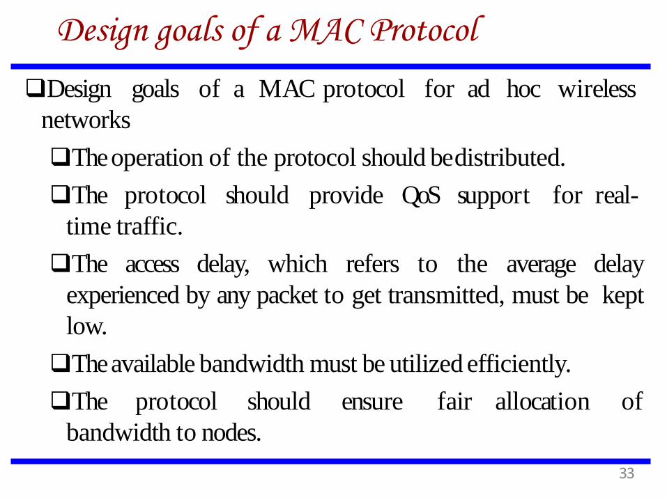
Design goals of a MAC Protocol
Design goals of a MAC protocol for ad hoc wireless
networks
The operation of the protocol should be distributed.
The protocol should provide QoS support for real-
time traffic.
The access delay, which refers to the average delay
experienced by any packet to get transmitted, must be kept
low.
The available bandwidth must be utilized efficiently.
The protocol should ensure fair allocation of
bandwidth to nodes.
33

Design goals of a MAC Protocol
Control overhead must be kept as low as possible.
The protocol should minimize the effects of hidden
and exposed terminal problems.
The protocol must be scalable to large networks.
It should have power control mechanisms.
The protocol should have mechanisms for adaptive
data rate control.
It should try to use directional antennas.
The protocol should provide synchronization among
nodes.
34

Classifications of MAC protocols
Ad hoc network MAC protocols can be classified into three types:
Contention-based protocols
protocols with reservation
protocols with scheduling
Contention-based mechanisms
Contention-based mechanisms
Other MAC protocols
35
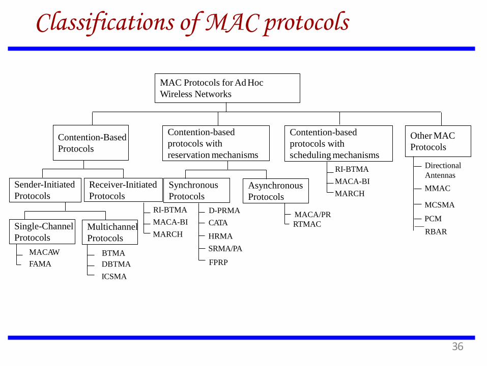
Classifications of MAC protocols
MAC Protocols for Ad Hoc
Wireless Networks
Contention-Based
Protocols
Contention-based
protocols with
reservation mechanisms
Other MAC
Protocols
Contention-based
protocols with
scheduling mechanisms
Sender-Initiated
Protocols
Receiver-Initiated
Protocols
Synchronous
Protocols
Asynchronous
Protocols
Single-Channel
Protocols
Multichannel
Protocols
MACAW
FAMA
BTMA
DBTMA
ICSMA
RI-BTMA
MACA-BI
MARCH
D-PRMA
CATA
RI-BTMA
MACA-BI
MARCH
HRMA
SRMA/PA
FPRP
MACA/PR
RTMAC
Directional
Antennas
MMAC
MCSMA
PCM
RBAR
36
Classifications of MAC Protocols
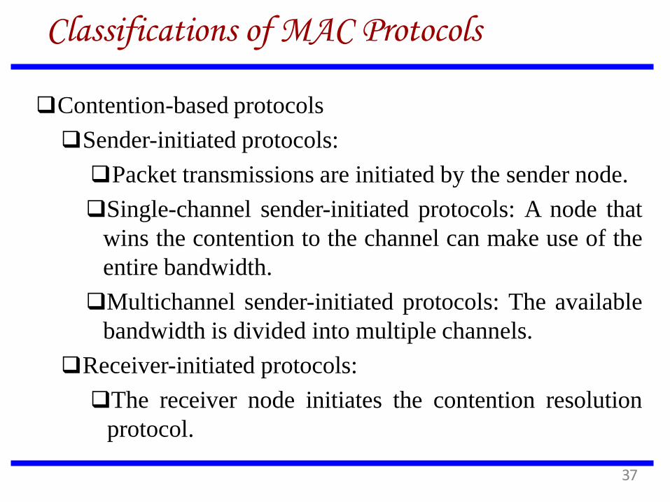
Contention-based protocols
Sender-initiated protocols:
Packet transmissions are initiated by the sender node.
Single-channel sender-initiated protocols: A node that
wins the contention to the channel can make use of the
entire bandwidth.
Multichannel sender-initiated protocols: The available
bandwidth is divided into multiple channels.
Receiver-initiated protocols:
The receiver node initiates the contention resolution
protocol.
37

Classifications of MAC Protocols
Contention-based protocols with reservation
mechanisms
Synchronous protocols
All nodes need to be synchronized. Global
time synchronization is difficult to achieve.
Asynchronous protocols
These protocols use relative time
information for effecting reservations.
38
Classifications of MAC Protocols
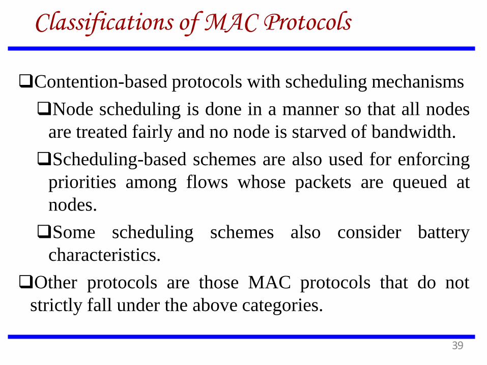
Contention-based protocols with scheduling mechanisms
Node scheduling is done in a manner so that all nodes
are treated fairly and no node is starved of bandwidth.
Scheduling-based schemes are also used for enforcing
priorities among flows whose packets are queued at
nodes.
Some scheduling schemes also consider battery
characteristics.
Other protocols are those MAC protocols that do not
strictly fall under the above categories.
39
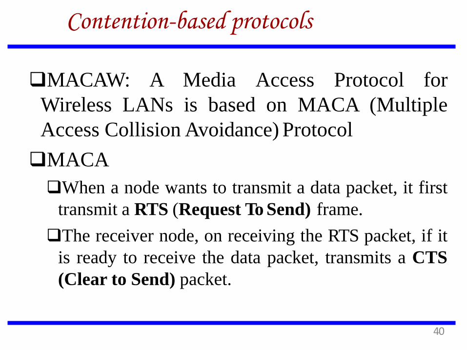
Contention-based protocols
MACAW: A Media Access Protocol for
Wireless LANs is based on MACA (Multiple
Access Collision Avoidance) Protocol
MACA
When a node wants to transmit a data packet, it first
transmit a RTS (Request To Send) frame.
The receiver node, on receiving the RTS packet, if it
is ready to receive the data packet, transmits a CTS
(Clear to Send) packet.
40
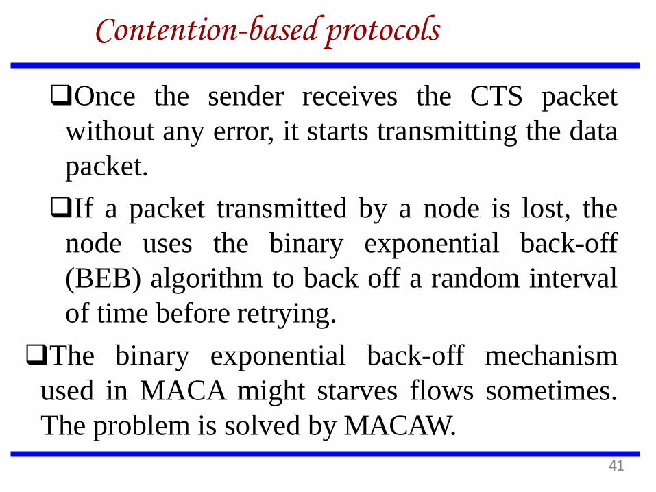
Contention-based protocols
Once the sender receives the CTS packet
without any error, it starts transmitting the data
packet.
If a packet transmitted by a node is lost, the
node uses the binary exponential back-off
(BEB) algorithm to back off a random interval
of time before retrying.
The binary exponential back-off mechanism
used in MACA might starves flows sometimes.
The problem is solved by MACAW.
41
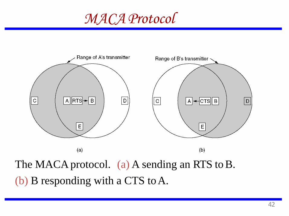
MACA Protocol
The MACA protocol. (a) A sending an RTS to B.
(b) B responding with a CTS to A.
42

MACA avoids the problem of hidden terminals
A and C want to send to B
A sends RTS first
C waits after receiving CTS from B
MACA examples
A B C
RTS
CTS CTS
43
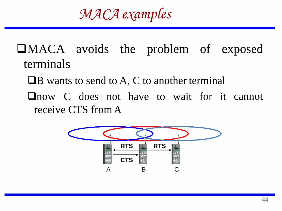
exposed MACA avoids the problem of
terminals
cannot
B wants to send to A, C to another terminal
now C does not have to wait for it
receive CTS from A
MACA examples
A B C
RTS
CTS
RTS
44
Contention-based protocols
Floor acquisition Multiple Access Protocols
(FAMA)
Based on a channel access discipline which consists
of a carrier-sensing operation and a collision-
avoidance dialog between the sender and the intended
receiver of a packet.
Floor acquisition refers to the process of gaining
control of the channel.
At any time only one node is assigned to use the
channel.
45
Contention-based protocols
Carrier-sensing by the sender, followed by the RTS-
CTS control packet exchange, enables the protocol to
perform as efficiently as MACA.
Two variations of FAMA
RTS-CTS exchange with no carrier-sensing uses the
ALOHA protocol for transmitting RTS packets.
RTS-CTS exchange with non-persistent carrier-
sensing uses non-persistent CSMA for the same
purpose.
46
Contention-based protocols
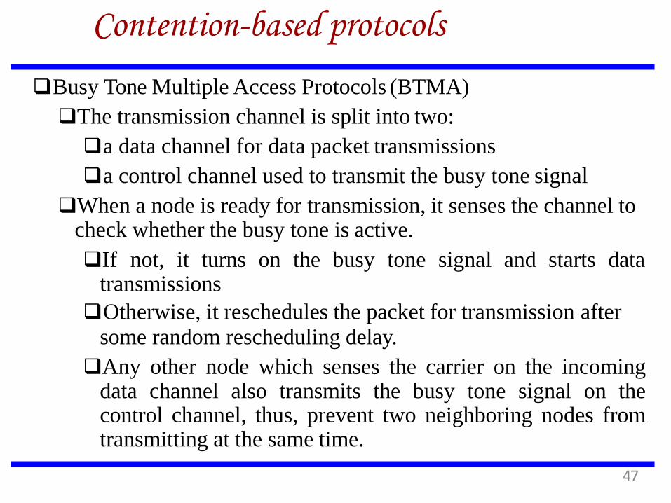
Busy Tone Multiple Access Protocols (BTMA)
The transmission channel is split into two:
a data channel for data packet transmissions
a control channel used to transmit the busy tone signal
When a node is ready for transmission, it senses the channel to check whether the busy tone is active.
If not, it turns on the busy tone signal and starts data transmissions
Otherwise, it reschedules the packet for transmission after some random rescheduling delay.
Any other node which senses the carrier on the incoming data channel also transmits the busy tone signal on the control channel, thus, prevent two neighboring nodes from transmitting at the same time.
47

Contention-based protocols
Dual Busy Tone Multiple Access Protocol (DBTMAP) is an extension of the BTMA scheme.
a data channel for data packet transmissions
a control channel used for control packet transmissions (RTS and CTS packets) and also for transmitting the busy tones.
48

Contention-based protocols
Receiver-Initiated Busy Tone Multiple Access Protocol
(RI-BTMA)
The transmission channel is split into two:
a data channel for data packet transmissions
a control channel used for transmitting the busy
tone signal
A node can transmit on the data channel only if it
finds the busy tone to be absent on the control
channel.
The data packet is divided into two portions: a
preamble and the actual data packet.
49
Contention-based protocols
MACA-By Invitation (MACA-BI) is a receiver-
initiated MAC protocol.
By eliminating the need for the RTS packet it
reduces the number of control packets used in
the MACA protocol which uses the three-way
handshake mechanism.
Media Access with Reduced Handshake
(MARCH) is a receiver-initiated protocol.
50

Contention-based Protocols with
Reservation Mechanisms
Contention-based Protocols with Reservation Mechanisms
Contention occurs during the resource (bandwidth) reservation phase.
Once the bandwidth is reserved, the node gets exclusive access to the reserved bandwidth.
QoS support can be provided for real-time traffic.
51
Contention-based Protocols with
Reservation Mechanisms
Distributed packet reservation multiple access protocol (D-PRMA)
It extends the centralized packet reservation multiple access (PRMA) scheme into a distributed scheme that can be used in ad hoc wireless networks.
PRMA was designed in a wireless LAN with a base station.
D-PRMA extends PRMA protocol in a wireless LAN.
D-PRMA is a TDMA-based scheme. The channel is divided into fixed- and equal-sized frames along the time axis.
52
Access method DAMA: Reservation- TDMA
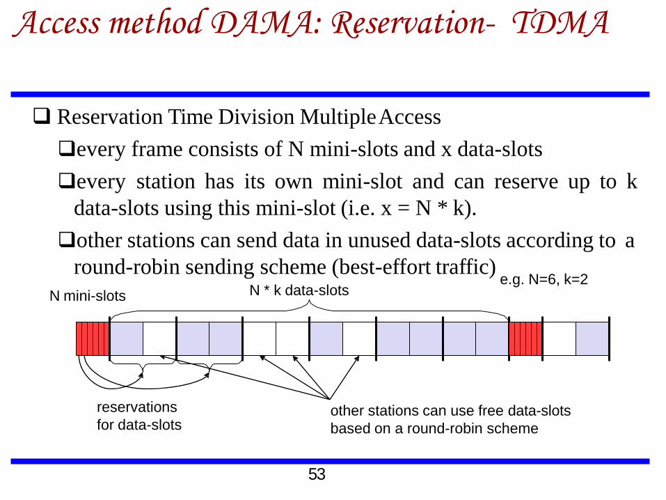
Reservation Time Division Multiple Access
every frame consists of N mini-slots and x data-slots
every station has its own mini-slot and can reserve up to k
data-slots using this mini-slot (i.e. x = N * k).
other stations can send data in unused data-slots according to a
round-robin sending scheme (best-effort traffic)
N mini-slots N * k data-slots
reservations
for data-slots other stations can use free data-slots
based on a round-robin scheme
e.g. N=6, k=2
53

33
Distributed Packet Reservation Multiple
Access Protocol (D-PRMA)
Implicitreservation(PRMA-Packet Reservation Multiple Access)
collision at
reservation
attempts
1 2 3 4 5 6 7 8 time-slot
A C D A B A F
A C A B A
A B A F
A B A F D
A C E E B A F D t
reservation
ACDABA-F frame1
ACDABA-F frame2
AC-ABAF- frame3
A---BAFD frame4
ACEEBAFD frame5
54
Distributed Packet Reservation Multiple
Access Protocol (D-PRMA)
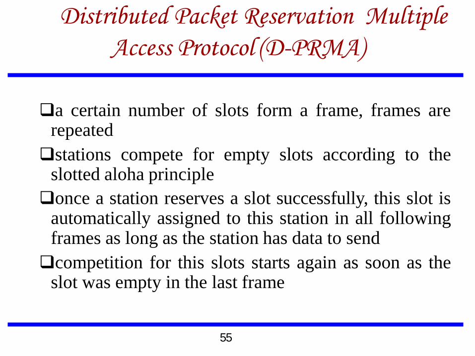
a certain number of slots form a frame, frames are repeated
stations compete for empty slots according to the slotted aloha principle
once a station reserves a slot successfully, this slot is automatically assigned to this station in all following frames as long as the station has data to send
competition for this slots starts again as soon as the slot was empty in the last frame
55

Contention-based protocols with
Reservation Mechanisms
Collision avoidance time allocation protocol (CATA)
based on dynamic topology-dependent transmission
scheduling
Nodes contend for and reserve time slots by means
of a distributed reservation and handshake
mechanism.
Support broadcast, unicast, and multicast
transmissions.
56
Contention-based protocols with
Reservation Mechanisms
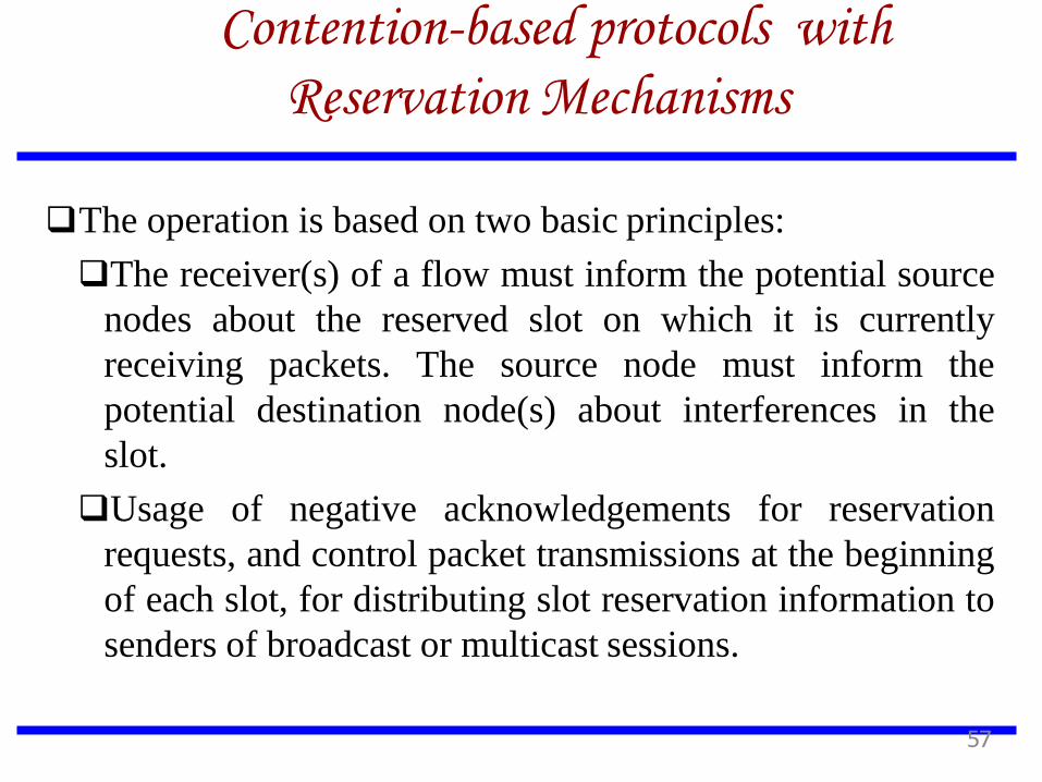
The operation is based on two basic principles:
The receiver(s) of a flow must inform the potential source
nodes about the reserved slot on which it is currently
receiving packets. The source node must inform the
potential destination node(s) about interferences in the
slot.
Usage of negative acknowledgements for reservation
requests, and control packet transmissions at the beginning
of each slot, for distributing slot reservation information to
senders of broadcast or multicast sessions.
57
Contention-based protocols with
Reservation Mechanisms
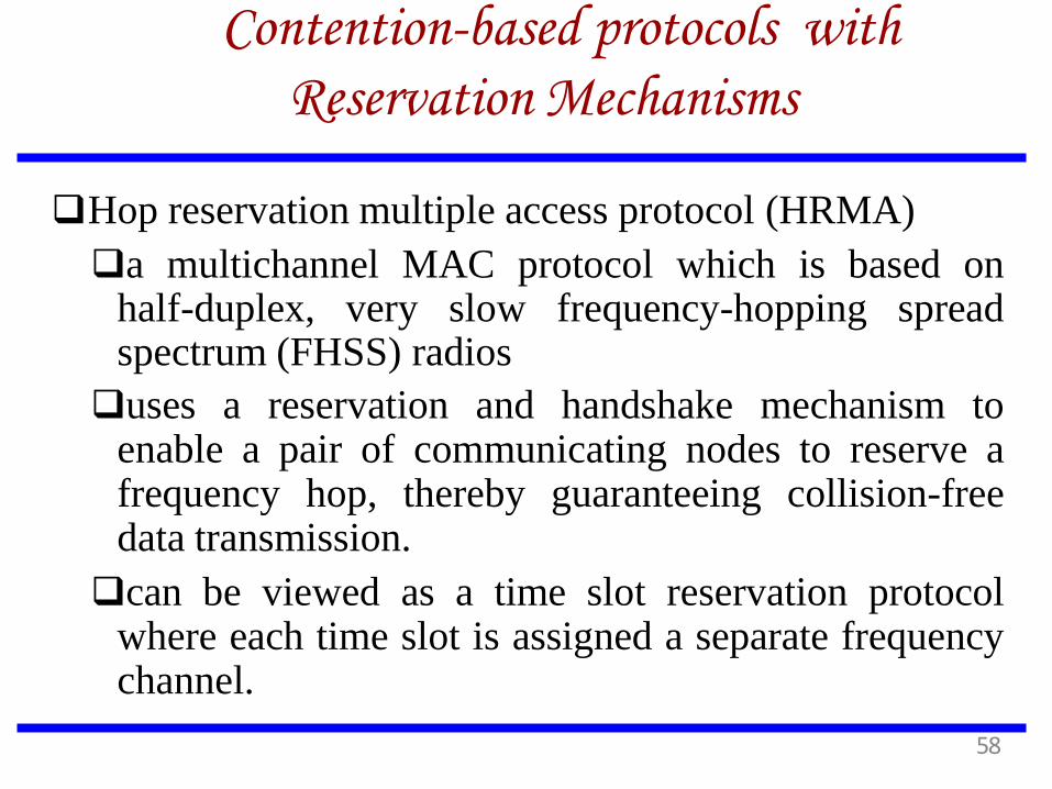
Hop reservation multiple access protocol (HRMA)
a multichannel MAC protocol which is based on half-duplex, very slow frequency-hopping spread spectrum (FHSS) radios
uses a reservation and handshake mechanism to enable a pair of communicating nodes to reserve a frequency hop, thereby guaranteeing collision-free data transmission.
can be viewed as a time slot reservation protocol where each time slot is assigned a separate frequency channel.
58
Contention-based protocols with
Reservation Mechanisms
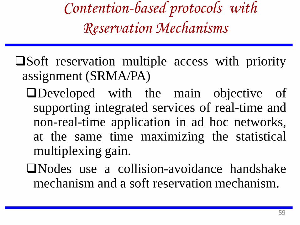
Soft reservation multiple access with priority assignment (SRMA/PA)
Developed with the main objective of supporting integrated services of real-time and non-real-time application in ad hoc networks, at the same time maximizing the statistical multiplexing gain.
Nodes use a collision-avoidance handshake mechanism and a soft reservation mechanism.
59
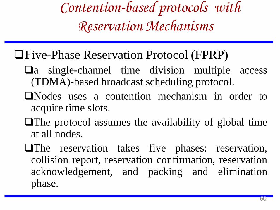
Five-Phase Reservation Protocol (FPRP)
a single-channel time division multiple access (TDMA)-based broadcast scheduling protocol.
Nodes uses a contention mechanism in order to acquire time slots.
The protocol assumes the availability of global time at all nodes.
The reservation takes five phases: reservation, collision report, reservation confirmation, reservation acknowledgement, and packing and elimination phase.
Contention-based protocols with
Reservation Mechanisms
60

MACA with Piggy-Backed Reservation (MACA/PR)
Provide real-time traffic support in multi-hop wireless networks
Based on the MACAW protocol with non-persistent CSMA
The main components of MACA/PR are:
A MAC protocol
A reservation protocol
A QoS routing protocol
Contention-based protocols with
Reservation Mechanisms
61

Real-Time Medium Access Control Protocol (RTMAC)
Provides a bandwidth reservation mechanism for
supporting real-time traffic in ad hoc wireless networks
RTMAC has two components
A MAC layer protocol is a real-time extension of the
IEEE 802.11 DCF.
A medium-access protocol for best-effort traffic
A reservation protocol for real-time traffic
A QoS routing protocol is responsible for end-to-end
reservation and release of bandwidth resources.
Contention-based protocols with
Reservation Mechanisms
62
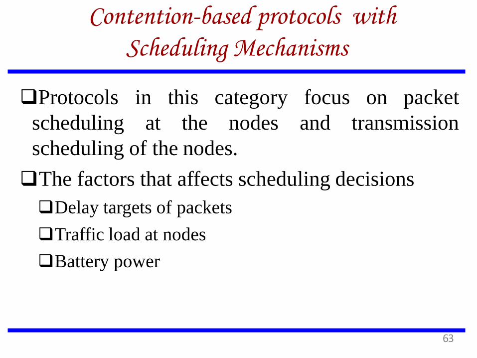
Protocols in this category
scheduling at the nodes
focus on packet
and transmission
scheduling of the nodes.
The factors that affects scheduling decisions
Delay targets of packets
Traffic load at nodes
Battery power
Contention-based protocols with
Scheduling Mechanisms
63

Distributed priority
access in
scheduling and medium
Networks present two Ad Hoc
for providing quality of service mechanisms
(QoS)
Distributed priority scheduling (DPS) – piggy-backs
the priority tag of a node’s current and head-of-line
packets o the control and data packets
Multi-hop coordination – extends the DPS scheme to
carry out scheduling over multi-hop paths.
Contention-based protocols with
Scheduling Mechanisms
64
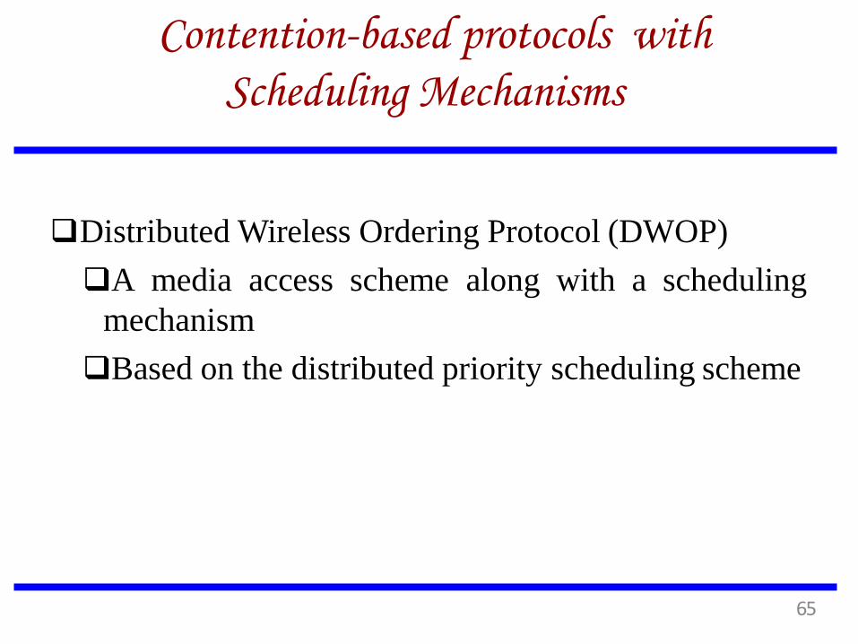
Distributed Wireless Ordering Protocol (DWOP)
A media access scheme along with a scheduling
mechanism
Based on the distributed priority scheduling scheme
Contention-based protocols with
Scheduling Mechanisms
65
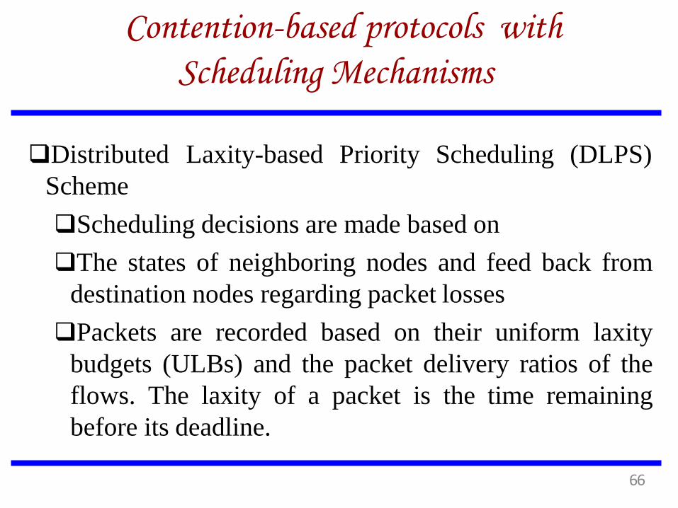
Distributed Laxity-based Priority Scheduling (DLPS)
Scheme
Scheduling decisions are made based on
The states of neighboring nodes and feed back from
destination nodes regarding packet losses
Packets are recorded based on their uniform laxity
budgets (ULBs) and the packet delivery ratios of the
flows. The laxity of a packet is the time remaining
before its deadline.
Contention-based protocols with
Scheduling Mechanisms
66
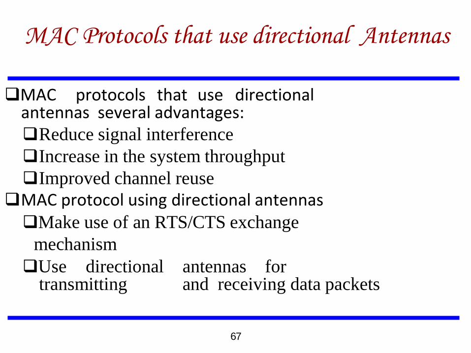
MAC protocols that use directional antennas several advantages: Reduce signal interference
Increase in the system throughput
Improved channel reuse
MAC protocol using directional antennas Make use of an RTS/CTS exchange
mechanism
Use directional antennas for transmitting and receiving data packets
MAC Protocols that use directional Antennas
67

Directional Busy Tone-based MAC Protocol (DBTMA)
It uses directional antennas for transmitting the RTS, CTS, data frames, and the busy tones.
Directional MAC Protocols for Ad Hoc Wireless Networks
DMAC-1, a directional antenna is used for transmitting RTS packets and omni-directional antenna for CTS packets.
DMAC-1, both directional RTS and omni-directional RTS transmission are used.
MAC Protocols that use directional Antennas
68
Other MAC Protocols
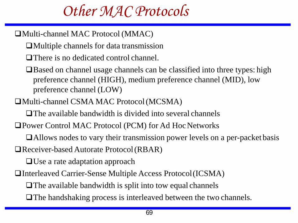
Multi-channel MAC Protocol (MMAC)
Multiple channels for data transmission
There is no dedicated control channel.
Based on channel usage channels can be classified into three types: high
preference channel (HIGH), medium preference channel (MID), low
preference channel (LOW)
Multi-channel CSMA MAC Protocol (MCSMA)
The available bandwidth is divided into several channels
Power Control MAC Protocol (PCM) for Ad Hoc Networks
Allows nodes to vary their transmission power levels on a per-packet basis
Receiver-based Autorate Protocol (RBAR)
Use a rate adaptation approach
Interleaved Carrier-Sense Multiple Access Protocol (ICSMA)
The available bandwidth is split into tow equal channels
The handshaking process is interleaved between the two channels.
69

Network Setup
Ethernet
MT
AP AP AP
MT MT
Basic Network Setup is Cellular
Mobile Terminals (MT) connect with Access Points (AP)
Standard also supports ad-hoc networking where MT’s talk directly to MT’s
70
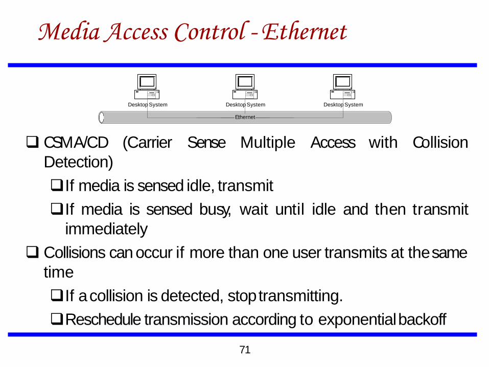
Media Access Control - Ethernet
CSMA/CD (Carrier Sense Multiple Access with Collision
Detection)
If media is sensed idle, transmit
If media is sensed busy, wait until idle and then transmit
immediately
Collisions can occur if more than one user transmits at the same
time
If a collision is detected, stop transmitting.
Reschedule transmission according to exponential backoff
Desktop System Desktop System Desktop System
Ethernet
71
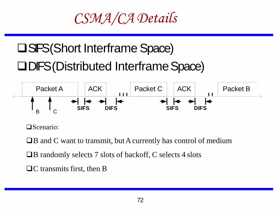
CSMA/CA Details
SIFS (Short Interframe Space)
DIFS (Distributed Interframe Space)
Packet A ACK
B C
Packet C ACK
SIFS DIFS SIFS DIFS
Packet B
Scenario:
B and C want to transmit, but A currently has control of medium
B randomly selects 7 slots of backoff, C selects 4 slots
C transmits first, then B
72
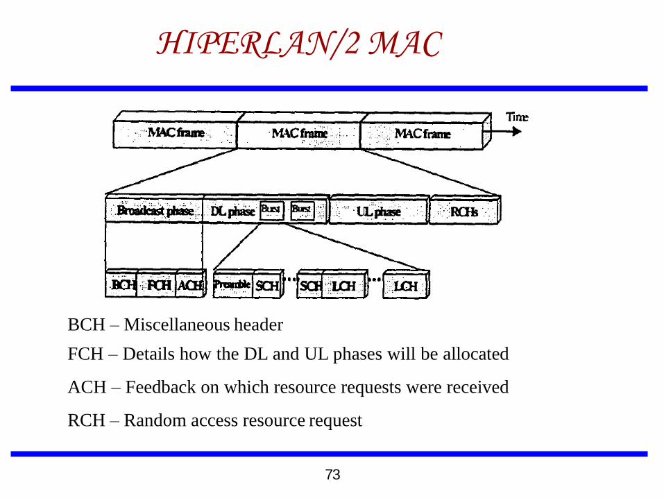
HIPERLAN/2 MAC
BCH – Miscellaneous header
FCH – Details how the DL and UL phases will be allocated
ACH – Feedback on which resource requests were received
RCH – Random access resource request
73
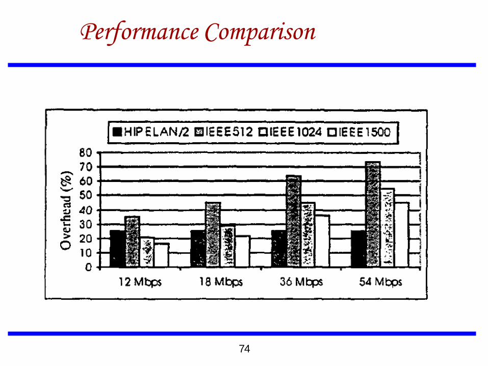
Performance Comparison
74
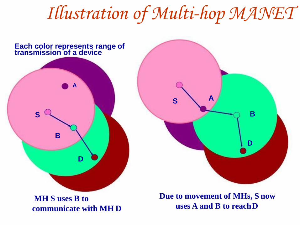
Illustration of Multi-hop MANET
Each color represents range of transmission of a device
A
S
S
B
D
A
B
D
MH S uses B to
communicate with MH D
Due to movement of MHs, S now
uses A and B to reach D
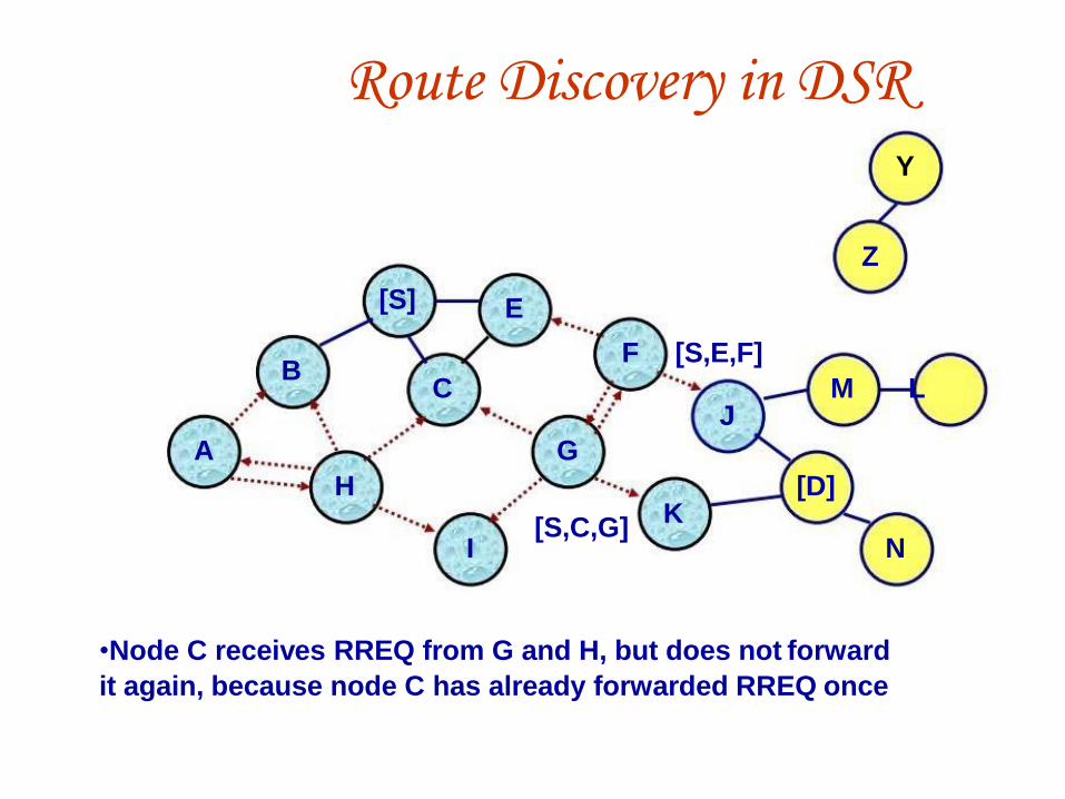
Route Discovery in DSR Y
Z
B
A
H
[S]
C
I
E
G
[S,C,G]
F [S,E,F]
M L J
[D] K
N
•Node C receives RREQ from G and H, but does not forward
it again, because node C has already forwarded RREQ once

Route Discovery in DSR Y
Z
B
A
H
[S]
C
I
E
F
G
K
[S,E,F,J]
M L J
[D]
[S,C,G,K] N
•Nodes J and K both broadcast RREQ to node D
•Since nodes J and K are hidden from each other, their
transmissions may collide

Route Discovery in DSR Y
Z
B
A
H
[S]
C
I
E
F
G
K
[S,E,F,J,M]
M L J
[D]
N
•Node D does not forward RREQ, because node D
is the intended target of the route discovery

An Overview of Protocol Characteristics
Routing Protocol
Route Acquisition
Multipath Capability
Flood for Route Discovery
Delay for Route Discovery
DSDV Computed a priori No No No
Upon Route Failure
Flood route updates throughout the network
Ultimately, updates the routing tables of
WRP Computed a
priori No No No all nodes by
Yes, aggressive use of caching
DSR
On-demand, only when needed may reduce Yes
On-demand, Yes AODV only when
exchanging MRL between neighbors
Route error propagated up to the source to erase invalid path
Route error broadcasted to erase multipath
needed
Not explicitly, as the technique of salvaging may quickly restore a route
Not directly, however, multipath AODV (MAODV) protocol includes this support
On-demand, TORA only when
Yes, once the DAG is constructed, Yes
needed
flood
Yes, conservative use of cache to reduce route discovery delay
Usually only one flood for initial DAG construction multiple paths
are found
Only if the ZRP Hybrid
Only outside a source's zone destination is
No outside the source's zone
Error is recovered locally and only when alternative routes are not available
Hybrid of updating nodes' tables within a zone and propagating route error to the source

Position Based Routing
Three main packet forwarding schemes:
„Greedy forwarding
„Restricted directional flooding
„Hierarchical approaches
For the first two, a MH forwards a given packet to one (greedy forwarding) or more (restricted
directional flooding) one-hop neighbors The selection of the neighbor depends on the
optimization criteria of the algorithm The third forwarding strategy forms a hierarchy in
order to scale to a large number of MHs
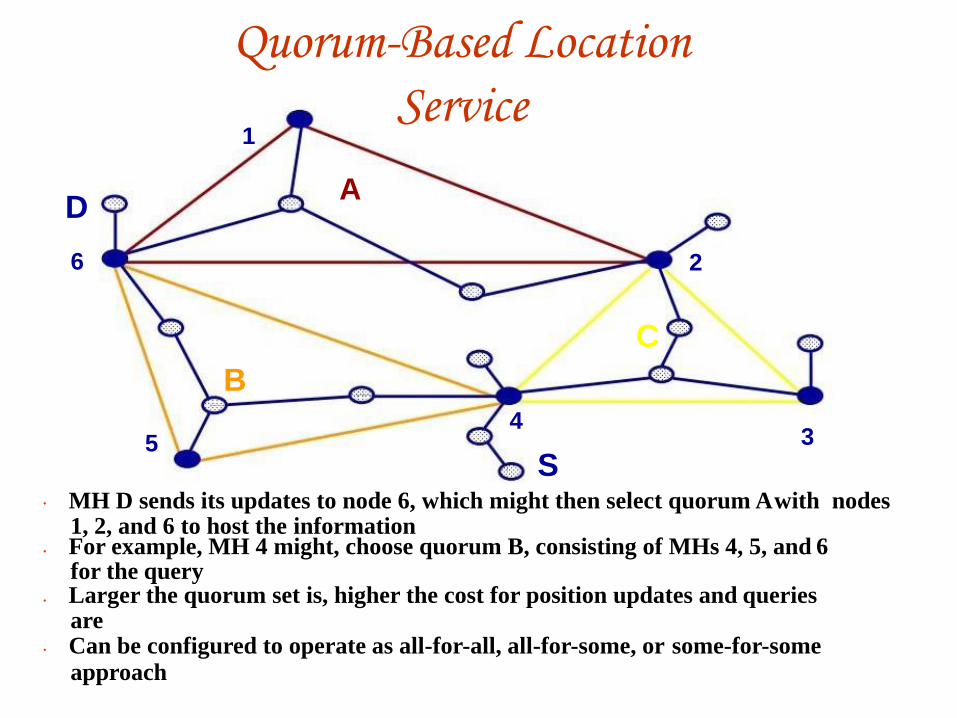
Quorum-Based Location
1
D
6
B
Service
A
2
C
5 3 4
S MH D sends its updates to node 6, which might then select quorum A with nodes 1, 2, and 6 to host the information For example, MH 4 might, choose quorum B, consisting of MHs 4, 5, and 6 for the query Larger the quorum set is, higher the cost for position updates and queries are Can be configured to operate as all-for-all, all-for-some, or some-for-some approach
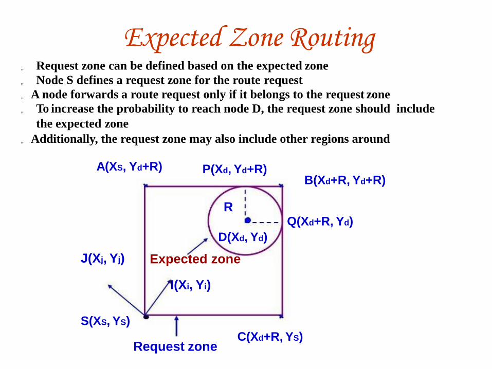
Expected Zone Routing „ Request zone can be defined based on the expected zone
„ Node S defines a request zone for the route request
„ A node forwards a route request only if it belongs to the request zone
„ To increase the probability to reach node D, the request zone should include
the expected zone
„ Additionally, the request zone may also include other regions around
A(XS, Yd+R) P(Xd, Yd+R) B(Xd+R, Yd+R)
R Q(Xd+R, Yd)
J(Xj, Yj)
D(Xd, Yd)
Expected zone
I(Xi, Yi)
S(XS, YS)
C(Xd+R, YS) Request zone

UNIT –III
Basics Of Wireless Sensors And Applications:

Introduction
Wireless Sensor Networks can be considered as a special case of ad hoc
networks with reduced or no mobility
WSNs enable reliable monitoring and analysis of unknown and untested
environments
These networks are “data centric”, i.e., unlike traditional ad hoc networks
where data is requested from a specific node, data is requested based on
certain attributes such as, “which area has temperature over 35ºC or
95ºF”
A sensor has many functional components as shown in Figure 8.1
A typical sensor consists of a transducer to sense a given physical quantity,
an embedded processor, small memory and a wireless transceiver to
transmit or receive data and an attached battery

Functional Components: A Sensor
Transceiver
10Kbps-1Mbps 50-125m range
Memory
(3K-1Mb)
Sensor
Transducer
Embedded
Processor
(8 bit 4-8Mhz)
Battery

The Mica Mote
• The Mica Mote is a comprehensive sensor node developed by University
of California at Berkeley and marketed by Crossbow
• It uses an Atmel Atmega 103 microcontroller running at 4 MHz, with a
radio operating at the 916 MHz frequency band with bidirectional
communication at 40 kbps when energized with a pair of AA batteries
• Mica Board is stacked to the processor board via the 51 pin extension
connector to provide temperature, photo resistor, barometer, humidity,
and thermopile sensors
• To conserve energy, later designs include an A/D Converter and an 8x8
power switch on the sensor board
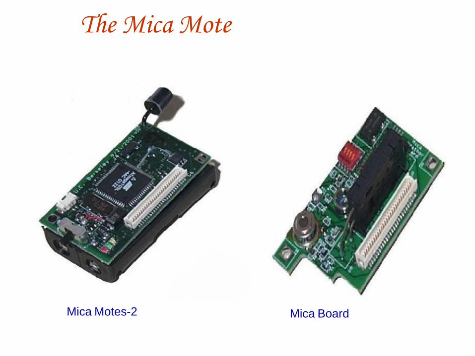
The Mica Mote
Mica Motes-2 Mica Board

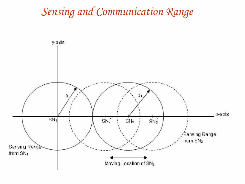
Sensing and Communication Range
A wireless sensor network (WSN) consists of a large number of sensor nodes (SNs)
Adequate density of sensors is required so as to void any unsensed area
rs
Sensing Area
Desired
Coverage
Area
Sensing and Communication Range
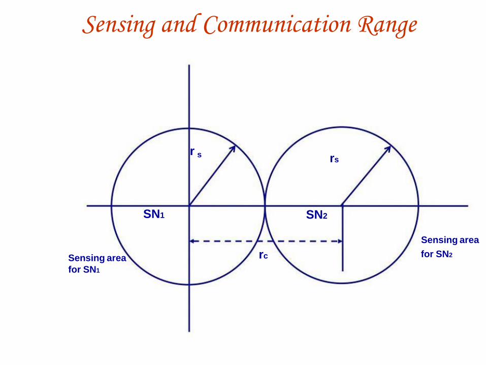
Sensing and Communication Range
r s rs
SN1
Sensing area
for SN1
SN2
rc
Sensing area
for SN2
Sensing and Communication Range
Transmission between adjacent SNs is feasible if there is at
least one SN within the communication range of each SN
Not just the sensing coverage, but the communication
connectivity is equally important
The wireless communication coverage of a sensor must be at
least twice the sensing distance
Data from a single SN is not adequate to make any useful
decision and need to be collected from a set of SNs
Design Issues: Advantages of WSNs
Ease of deployment - Can be dropped from a plane or placed in a factory,
without any prior organization, thus reducing the installation cost and time, and
increasing the flexibility of deployment
Extended range - One huge wired sensor (macro-sensor) can be replaced by
many smaller wireless sensors for the same cost
Fault tolerant - With wireless sensors, failure of one node does not affect the
network operation
Mobility - Since these wireless sensors are equipped with battery, they can
possess limited mobility (e.g., if placed on robots)
Disadvatage: The wireless medium has a few inherent limitations such as
low bandwidth, error prone transmissions, and potential collisions in channel
access, etc.

Design Issues
Traditional routing protocols defined for MANETs are not well suited
for wireless sensor networks due to the following reasons:
Wireless sensor networks are “data centric”, where data is requested
based on particular criteria such as “which area has temperature
35ºC”
In traditional wired and wireless networks, each node is given a unique
identification and cannot be effectively used in sensor networks
Adjacent nodes may have similar data and rather than sending data
separately from each sensor node, it is desirable to aggregate similar
data before sending it
The requirements of the network change with the application and
hence, it is application-specific
Desirable Features
Attribute-based addressing: This is typically employed in
sensor networks where addresses are composed of a group of
attribute-value pairs
Location awareness: Since most data collection is based on
location, it is desirable that the nodes know their position
The sensors should react immediately to drastic changes in
their environment
Query Handling: Users should be able to request data from the
network through some base station (also known as a sink) or
through any of the nodes, whichever is closer

Design Issues : Challenges
Routing protocol design is heavily influenced by many challenging
factors
These challenges can be summarized as follows:
Ad hoc deployment - Sensor nodes are randomly deployed so
that they form connections between the nodes
Computational capabilities - Sensor nodes have limited
computing power and therefore may run simple versions of
routing protocols
Energy consumption without losing accuracy - Sensor nodes
can use up their limited energy supply carrying out
computations and transmitting information
Design Issues : Challenges
• Scalability - The number of sensor nodes deployed in the sensing area may be
in the order of hundreds, thousands, or more and routing scheme must be
scalable enough to respond to events
• Communication range - The bandwidth of the wireless links connecting
sensor nodes is often limited, hence constraining inter- sensor communication
• Fault tolerance - Some sensor nodes may fail or be blocked due to
• lack of power, physical damage, or environmental interference
• Connectivity - High node density in sensor networks precludes
them from being completely isolated from each other
Design Issues : Challenges Transmission media -Communicating nodes are linked by a
wireless medium and traditional problems associated with a wireless channel
(e.g., fading, high error rate) also affect the operation
QoS - In some applications (e.g., some military applications), the
data should be delivered within a certain period of time from the
moment it
is sensed
Control Overhead - When the number of retransmissions in
wireless medium increases due to collisions, the latency and energy consumption also increases
Security -Besides physical security, both authentication and
encryption should be feasible while complex algorithm needs to be avoided
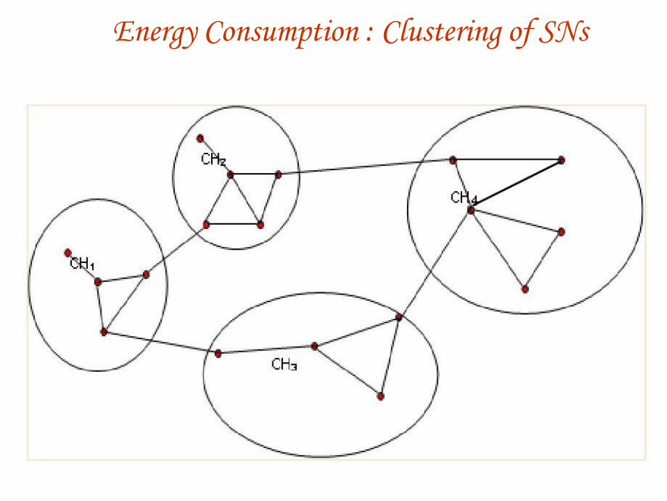
Energy Consumption : Clustering of SNs
Clustering of SNs not only allows aggregation of sensed data, but limits data
transmission primarily within the cluster
The sequence starts with discovery of neighboring SNs by sending periodic
Beacon Signals, determining close by SNs with some intermediate SNs, forming
clusters and selecting cluster head (CH) for each cluster
So, the real question is how to group adjacent SNs, and how many groups
should be there that could optimize some performance parameter
One approach is to partition the WSN into clusters such that all members of the
clusters are directly connected to the CH
One such example for randomly deployed SNs
SNs in a WSN in a cluster, can transmit directly to the CH without any
intermediate SN
Energy Consumption : Clustering of SNs
Clustering of Sensors
Data from SNs belonging to a single cluster can be combined together in an
intelligent way (aggregation) using local transmissions
This can not only reduce the global data to be transferred and localized most
traffic to within each individual cluster
A lot of research gone into testing coverage of areas by k-sensors clustering
adjacent SNs and defining the size of the cluster so that the cluster heads (CHs) can
communicate and get data from their own cluster members
If each cluster is covered by more than one subset of SNs all the time, then some of
the SNs can be put into sleep mode so as to conserve energy while keeping full
coverage
The use of a second smaller radio has been suggested for waking up the sleeping
sensor, thereby conserving the power of main wireless transmitter

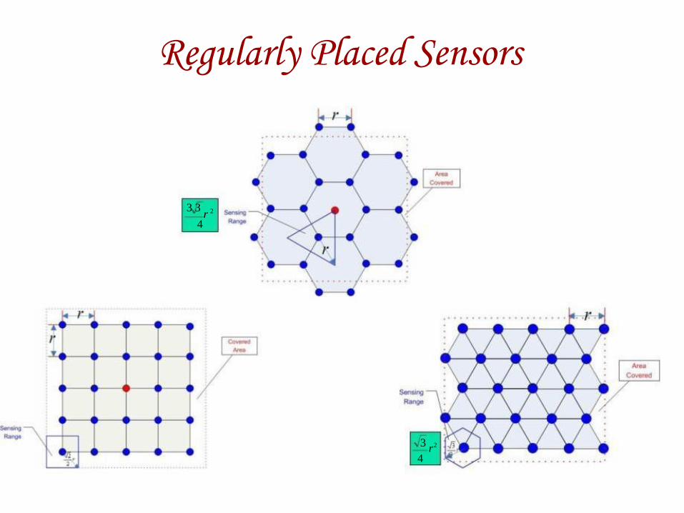
Clustering of Sensors: Predetermined Grid v/s Random Placement
Regularly placed sensors
A simple strategy is to place the sensors in the form of two-
dimensional grid as such cross-point and such configuration
may be very useful for uniform coverage
Such symmetric placement allows best possible regular
coverage and easy clustering of the close-by SNs
Three such examples of SNs in rectangular, triangular and
hexagonal tiles of clusters are shown

Regularly Placed Sensors
Useful for deploying in a controlled environment
Clusters of size 5x5, with a SN located at each intersection of lines Square, triangle, or hexagonal placement of the SNs also dictates the
minimum sensing area that need to be covered by each sensor
Regularly placed sensors
Detailed views of three different configurations, are shown in next three slides
For simplicity of calculation, the sensing area covered by rectangular placement is taken
rectangular, while sensing are by the two configurations are assumed hexagonal and
triangular respectively
The required number of SNs in each scheme, is given in Table 8.2
Radio transmission distance between adjacent SNs need to be such that the sensors can
receive data from adjacent sensors using wireless radio
Clustering can be done for these configurations and the size of each cluster can be fixed as per
application requirements
If the sensing and radio transmission ranges are set to the minimum value, then all the SNs
need to be active all the time to cover the area and function properly
If these ranges are increased, then each sub-region can be covered by more than one
sensor node and selected SNs can be allowed to go to sleep mode
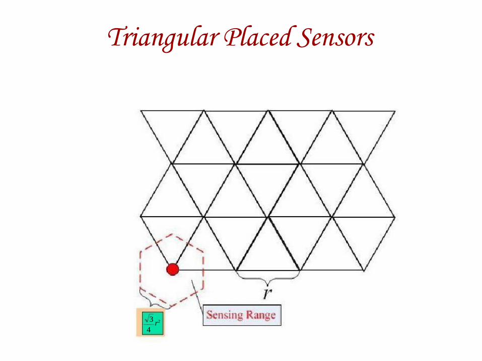
Triangular Placed Sensors
3 r2
4

Hexagonal Placed Sensors
3 3
r2
4
Regularly Placed Sensors
3 3 r 2
4
3 r 2
4
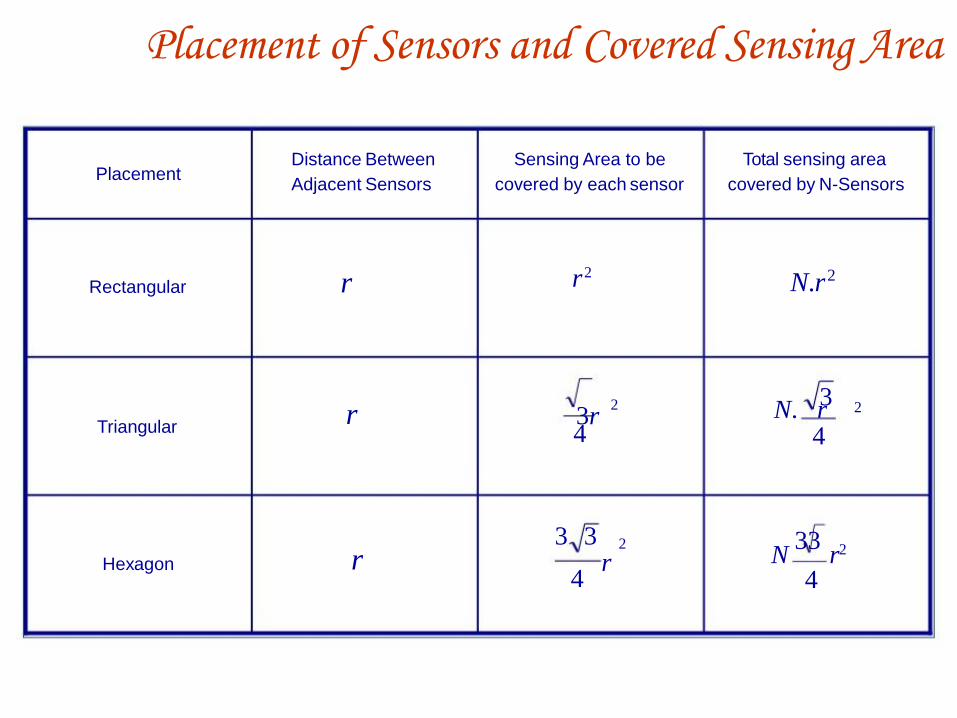
Placement of Sensors and Covered Sensing Area
Placement Distance Between
Adjacent Sensors
Sensing Area to be
covered by each sensor
Total sensing area
covered by N-Sensors
Rectangular r r 2 N.r2
Triangular r 3r
4
2 3 N. r
4
2
Hexagon r 4
3 3 2
r N 33
r2
4
Randomly distributed sensors
The sensors could also be used in an unknown territory or inaccessible area by
deploying them from a low flying airplane or unmanned ground/aerial vehicle
SNs have to find themselves who their communicating neighbors are and how
many of them are present
The adjacency among SNs can be initially determined by sending bacon
signals as is done in a typical ad hoc network (MANET)
The communication range of associated wireless radio should be such that the
SNs could be connected together to form a WSN
Distribution of the SNs and their sensing range would also determine if the
physical parameter in the complete deployed area can be sensed by at least one SN
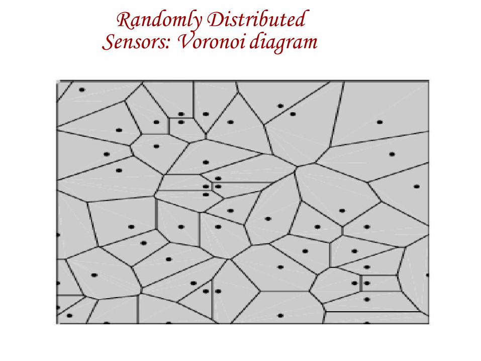
Randomly Distributed Sensors: Voronoi diagram
Heterogeneous WSNs
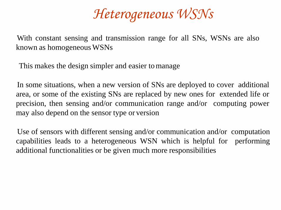
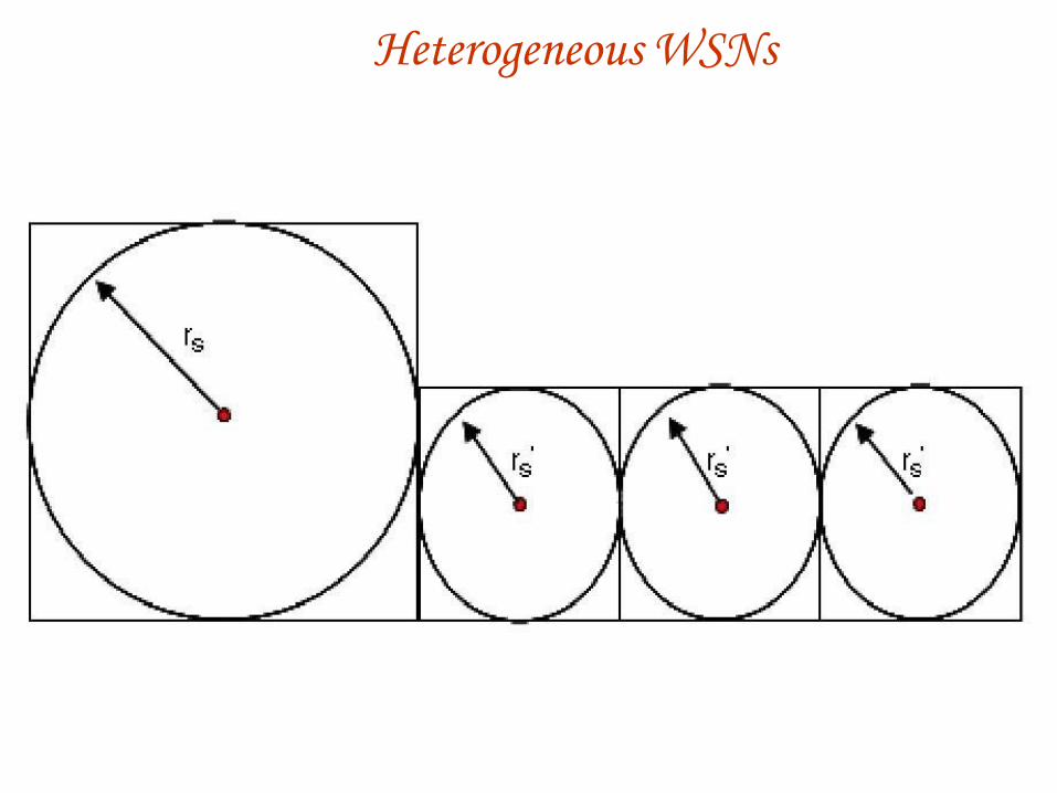
With constant sensing and transmission range for all SNs, WSNs are also
known as homogeneous WSNs
This makes the design simpler and easier to manage
In some situations, when a new version of SNs are deployed to cover additional
area, or some of the existing SNs are replaced by new ones for extended life or
precision, then sensing and/or communication range and/or computing power
may also depend on the sensor type or version
Use of sensors with different sensing and/or communication and/or computation
capabilities leads to a heterogeneous WSN which is helpful for performing
additional functionalities or be given much more responsibilities
Heterogeneous WSNs
Mobile Sensors
The enhancements in the field of robotics are paving the way for industrial
robots to be applied to a wider range of tasks
However, harnessing their full efficiency also depends on how accurately
they understand their environment
Thus, as sensor networks are the primary choice for environmental sensing,
combining sensor networks with mobile robots is a natural and very
promising application
Robots could play a major role of high-speed resource carriers in defense and
military applications where human time and life is very precious
Other applications include fire fighting, autonomous waste disposal
Thus, we see that there are a number of future applications where sensors and
robots could work together through some form of cooperation

Mobile Sensors
Sensors detect events autonomously and the mobile robots could take appropriate actions based on the nature of the event
Coordination between the mobile robots is obviously critical in achieving better resource distribution and information retrieval
Mobile sensor Networks have been suggested to cover the area not reachable by static sensors
Coordination between multiple robots for resource transportation has been explored for quite some time now
Transporting various types of resources for different applications like defense, manufacturing process, and so on, has been suggested
In these schemes, time taken to detect an event depends entirely on the trail followed by the robots
Though the path progressively gets better with the use of an ant-like type of algorithm, the whole process has to be started anew when the position of the event changes
Mobile Sensors
In terrains where human ingress is difficult, mobile robots can be used to imitate
the human’s chore
Typical resource-carrying robots are depicted in Figure 8.12 which depicts a possible
means of a robot transferring its resources to anothers
Once depleted of their resource, they may get themselves refilled from the sink
The resource in demand could be water or sand (to extinguish fire), oxygen supply,
medicines, bullets, clothes or chemicals to neutralize hazardous wastes, and so on
The target region that is in need of these resources is sometimes called an event location
Whether it is a sensor or another robot within collision distance, it is considered an obstacle
and the robot proceeds in a direction away from it

Mobile Sensors
Applications
Thousands of sensors over strategic locations are used in a structure such as an automobile or an
airplane, so that conditions can be constantly monitored
both from the inside and the outside and a real-time warning can be issued whenever a major
problem is forthcoming in the monitored entity
These wired sensors are large (and expensive) to cover as much area is desirable
Each of these need a continuous power supply and communicates their data to the end-user using a
wired network
The organization of such a network should be pre-planned to find strategic position to place
these nodes and then should be installed appropriately
The failure of a single node might bring down the whole network or leave that region completely
un-monitored
Applications
Under the civil category, envisioned applications can be classified into
environment observation and forecast system, habitat monitoring equipment
and human health, large structures and other commercial applications
Habitat Monitoring
A prototype test bed consisting of iPAQs (i.e., a type of handheld device) has
been built to evaluate the performance of these target classification and
localization methods
As expected, energy efficiency is one of the design goals at every level: hardware, local
processing (compressing, filtering, etc.), MAC and topology control, data aggregation,
data-centric routing and storage
Preprocessing is proposed in for habitat monitoring applications, where it is argued that
the tiered network in GDI is solely used for communication
The proposed 2-tier network architecture consists of micro nodes and macro nodes,
wherein the micro nodes perform local filtering and data to significantly
reduce the amount of data transmitted to macro nodes
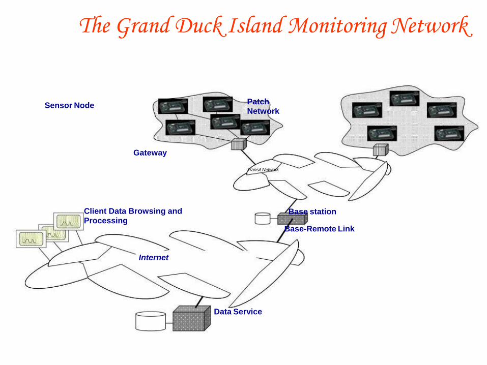
The Grand Duck Island Monitoring Network
Sensor Node
Gateway
Client Data Browsing and Processing
Internet
Patch Network
Transit Network
Base station
Base-Remote Link
Data Service

Environmental Monitoring Application
Sensors to monitor landfill and the air quality
Household solid waste and non-hazardous industrial waste such as construction
debris and sewer sludge are being disposed off by using over 6000 landfills in USA and
associated organic components undergo biological and chemical reaction such as
fermentation, biodegradation and oxidation-reduction
This causes harmful gases like methane, carbon dioxide, nitrogen, sulfide compounds and
ammonia to be produced and migration of gases in the landfill causes physical reactions
which eventually lead to ozone gases, a primary air pollutant and an irritant to our
respiratory systems
The current method of monitoring landfill employs periodic drilling of collection
well, collecting gas samples in airtight bags and analyze off-site, making the process
very time consuming
Environmental Monitoring Application
The idea is to interface gas sensors with custom-made devices and wireless radio and
transmit sensed data for further analysis
Deployment of a large number of sensors allows real-time monitoring of gases
being emitted by the waste material or from industrial spills
Place a large number of sensors throughout the area of interest and appropriate type
of sensors can be placed according to the type of pollutant anticipated in a given area
A large volume of raw data from sensors, can be collected, processed and
efficiently retrieval
A generic set up of a WSN, has been covered and various associated issues have
been clearly pointed out
Drinking Water Quality
A sensor based monitoring system with emphasis on placement and utilization of
in situ sensing technologies and doing spatial-temporal data mining for
water-quality monitoring and modeling
The main objective is to develop data-mining techniques to water-quality
databases and use them for interpreting and using environmental data
This also helps in controlling addition of chlorine to the treated water before
releasing to the distribution system
Detailed implementation of a bio-sensor for incoming wastewater treatment has
been discussed
A pilot-scale and full scale system has also been described
Conclusions and Future Directions
Sensor networks are perhaps one of the fastest growing areas in the broad
wireless ad hoc networking field
As we could see throughout this chapter, the research in sensor networks is
flourishing at a rapid pace and still there are many challenges to be addressed such
as:
Energy Conservation - Nodes are battery powered with limited resources
while still having to perform basic functions such as sensing, transmission
and routing
Sensing - Many new sensor transducers are being developed to convert physical
quantity to equivalent electrical signal and many new development is
anticipated
Communication - Sensor networks are very bandwidth-limited and how to
optimize the use of the scarce resources and how can sensor nodes minimize
the amount of communication
Computation - Here, there are many open issues in what regards signal
processing algorithms and network protocols
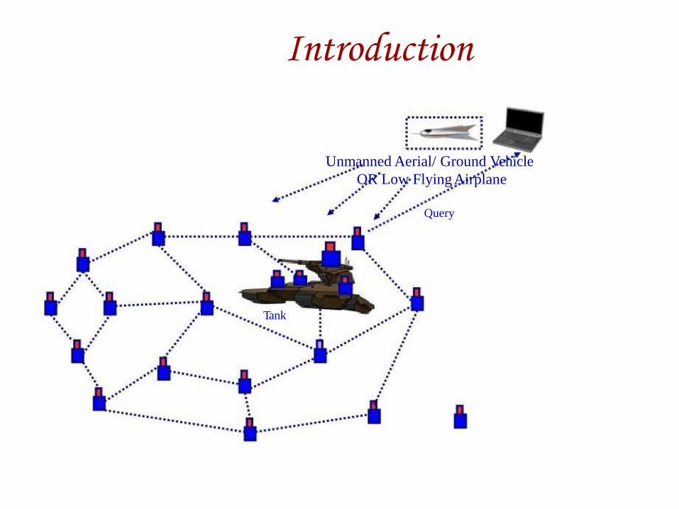
Introduction
Unmanned Aerial/ Ground Vehicle
OR Low Flying Airplane
Query
Tank

Introduction

What is a Sensor Network?
BS or Sink (far away)
Event
Query from BS to Sensors

Application of Wireless Sensor Networks in Defense Applications
Data Collection
Center (BS or Sink)
Path between SNs
Path of the Query
The Path of the Response
Query Response
Sensor Node (SN)
A typical Sensor Node (SN) of the network contains several
transducers to measure many different physical parameters and any one
could be selected under the program control at a given time
The sensed values need to be routed by each SN to the BS either directly
or via its CH in a multihop fashion due to power limitations In a WSN, the overall objective can be defined by the BS and this
process is usually known as injection of the query by the BS
In real-life, a low-flying airplane, an unmanned aerial or ground vehicle
or a powerful laptop can act as a BS or a sink and usually have adequate
source of power
This enables the BS to transmit a query message at a very high power
level so as to reach all SNs in a given area simultaneously Such
broadcasting is to enable all SNs to start working on the request and the
query could also include information about some necessary
characteristics of the query
Architecture of Sensor Networks
The typical hardware platform of a wireless sensor node will consist of:
A simple embedded microcontrollers, such as the Atmel or the Texas Instruments
MSP 430
Currently used radio transceivers include the RFM TR1001 or Infineon or
Chipcon devices
Typically, ASK or FSK is used, while the Berkeley PicoNodes employ OOK
modulation
Radio concepts like ultra-wideband are in an advanced stage
Batteries provide the required energy as an important concern is battery
management and whether and how energy scavenging can be done to recharge
batteries in the field
The operating system and the run-time environment is a hotly debated issue in
the literature
On one hand, minimal memory footprint and execution overhead are required
while on the other, flexible means of combining protocol building blocks are
necessary, as meta information has to be used in many places in a protocol stack
Network Architecture
WSN architecture need to cover a desired area both for sensing coverage
and communication connectivity point of view
Therefore, density of the WSN network is critical for the effective use of
the WSN
There is no well-defined measure of life-time of a WSN and some
assume either the failure of a single sensor running out of battery power as
life-time of the network
Perhaps a better definition is if certain percentage of sensors stops
working, may define the life-time as the network continues to operate
The percentage failure may depend on the nature of application and as
long as the area is adequately covered by the operating sensors, a WSN
may be considered operational
The SNs are yet to become inexpensive to be deploying with some degree
of redundancy
Network Architecture
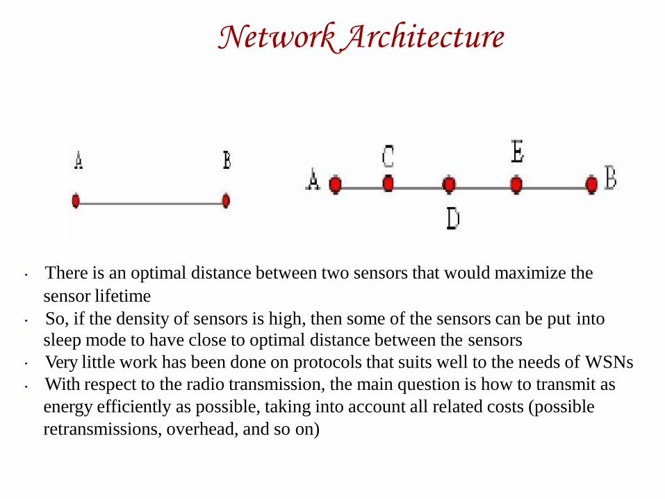
There is an optimal distance between two sensors that would maximize the
sensor lifetime
So, if the density of sensors is high, then some of the sensors can be put into
sleep mode to have close to optimal distance between the sensors
Very little work has been done on protocols that suits well to the needs of WSNs
With respect to the radio transmission, the main question is how to transmit as
energy efficiently as possible, taking into account all related costs (possible
retransmissions, overhead, and so on)
MAC Protocols
WSNs are designed to operate for long time as it is rather impractical to replenish the batteries However, nodes are in idle state for most time when no sensing occurs Measurements have shown that a typical radio consumes the similar level of energy in idle mode as in receiving mode
Therefore, it is important that nodes are able to operate in low duty cycles
The Sensor-MAC
The Sensor-MAC (S-MAC) protocol explores design trade-offs for energy- conservation in the MAC layer It reduces the radio energy consumption from the following sources: collision, control overhead, overhearing unnecessary traffic, and idle listening
The basic scheme of S-MAC is to put all SNs into a low-duty-cycle mode -listen and sleep periodically
When SNs are listening, they follow a contention rule to access the medium, which is similar to the IEEE 802.11 DCF
Sensor-MAC
In S-MAC, SNs exchange and coordinate on their sleep schedules rather than randomly sleep on their own
Before each SN starts the periodic sleep, it needs to choose a schedule and broadcast it to its neighbors
To prevent long-term clock drift, each SN periodically broadcasts its schedule as the SYNC packet
To reduce control overhead and simplify broadcasting, S-MAC encourages neighboring SNs to choose the same schedule, but it is
not a requirement A SN first listens for a fixed amount of time, which is at least the
period for sending a SYNC packet If it receives a SYNC packet from any neighbor, it will follow that
schedule by setting its own schedule to be the same
Otherwise, the SN will choose an independent schedule after the initial listening period

Sensor-MAC
Listen Sleep Listen Sleep
Time
for SYNC for RTS for CTS
Figure depicts the low-duty-cycle operation of each SN
The listen interval is divided into two parts for both SYNC and
data packets
There is a contention window for randomized carrier sense time
before sending each SYNC or data (RTS or broadcast) packet

SMACS The SMACS is an infrastructure-building protocol that forms a flat topology (as
opposed to a cluster hierarchy) for sensor networks
SMACS is a distributed protocol which enables a collection of SNs to discover
their neighbors and establish transmission/reception schedules for
communicating with them without the need for any local or global master nodes
In order to achieve this ease of formation, SMACS combines the neighbor
discovery and channel assignment phases
SMACS assigns a channel to a link immediately after the link’s existence is
discovered
This way, links begin to form concurrently throughout the network
By the time all nodes hear all their neighbors, they would have formed a
connected network
In a connected network, there exists at least one multihop path between any two
distinct nodes
SMACS
Since only partial information about radio connectivity in the vicinity of a
SN is used to assign time intervals to links, there is a potential for time
collisions with slots assigned to adjacent links whose existence is not
known at the time of channel assignment
To reduce the likelihood of collisions, each link is required to operate on a
different frequency
This frequency band is chosen at random from a large pool of possible
choices when the links are formed
This idea is described in Figure 9.6(a) for the topology of Figure 9.5
Here, nodes A and D wake up at times Ta and Td
After they find each other, they agree to transmit and receive during a pair
of fixed time slots
This transmission/reception pattern is repeated periodically every Tframe
Nodes B and C, in turn, wake up later at times Tb and Tc, respectively

Network Topology
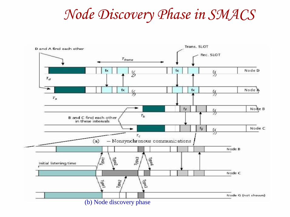
Node Discovery Phase in SMACS
(b) Node discovery phase
SMACS
The method by which SNs find each other and the scheme by which time
slots and operating frequencies are determined constitute an important
part of SMACS
To illustrate this scheme, consider nodes B, C, and D shown in Figure
9.6(b)
These nodes are engaged in the process of finding neighbors and wake up
at random times
Upon waking up, each node listens to the channel on a fixed frequency
band for some random time duration
A node decides to transmit an invitation by the end of this initial listening
time if it has not heard any invitations from other nodes
This is what happens to node C, which broadcasts an invitation or TYPE1
message
Nodes B and D hear this TYPE1 message and broadcasts a response, or
TYPE2, message addressed to node C during a random time following
reception of TYPE1
EAR (Eaves-drop-And-Register)
Mobility can be introduced into a WSN as extensions to the stationary sensor
network
Mobile connections are very useful to a WSN and can arise in many scenarios
where either energy or bandwidth is a major concern
Where there is the constraint of limited power consumption, small, low bit rate
data packets can be exchanged to relay data to and from the network whenever
necessary
At the same time, it cannot be assumed that each mobile node is aware of the
global network state and/or node positions
Similarly, a mobile node may not be able to complete its task (data collection,
network instruction, information extraction) while remaining motionless
Thus, the EAR protocol attempts to offer continuous service to these mobile
nodes under both mobile and stationary constraints
EAR is a low-power protocol that allows for operations to continue within the
stationary network while intervening at desired moments for information
exchange
EAR
The EAR algorithm employs the following four primary messages:
1. Broadcast Invite (BI) - This is used by the stationary node to invite other nodes to join and if multiple BIs are received, the mobile node continues to register every stationary node encountered, until its registry becomes full
2. Mobile Invite (MI) - This message is sent by the mobile node in response to
the BI message from the stationary node for establishing connection
3. Mobile Response (MR) - This is sent by the stationary node in response to a MI
message, and indicates the acceptance of the MI request which causes the stationary node to select slots along the TDMA frame for communication and the stationary node will enter the mobile node in its own registry
4. Mobile Disconnect (MD) - With this message, the mobile node informs the stationary node of a disconnection and for energy saving purposes, no response is needed from the stationary node
The STEM
The idea behind STEM is to turn on only a node’s sensors and some preprocessing circuitry during monitoring states Whenever a possible event is detected, the main processor is woken up
to analyze the sensed data in detail and forward it to the data sink However, the radio of the next hop in the path to the data sink is still turned off, if it did not detect the same event STEM solves this problem by having each node to periodically turn on
its radio for a short time to listen if someone else wants to communicate with it The node that wants to communicate, i.e. , the initiator SN, sends out a
beacon with the ID of the node it is trying to wake up, i.e. , the target SN This can be viewed as a procedure by which the initiator SN attempts to activate the link between itself and the target SN As soon as the target SN receives this beacon, it responds back to the initiator node and both keep their radio on at this point
The STEM
If the packet needs to be relayed further, the target SN will become the
initiator node for the next hop and the process is repeated
Once both the nodes that make up a link have their radio on, the link is
active and can be used for subsequent packets
However, the actual data transmissions may still interfere with the
wakeup protocol
To overcome this problem, STEM proposes the wakeup protocol and the
data transfer to employ different frequency bands as depicted in
In addition, separate radios would be needed in each of these bands
In Figure 9.7 we see that the wakeup messages are transmitted by the
radio operating in frequency band f1
STEM refers to these communications as occurring in the wakeup plane
Once the initiator SN has successfully notified the target SN, both SNs
turn on their radio that operates in frequency band f2
The actual data packets are transmitted in this band, called the data plane
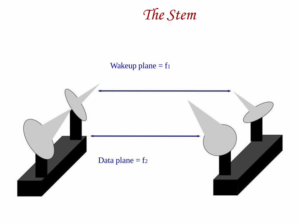
The Stem
Wakeup plane = f1
Data plane = f2

Routing Layer
Routing in sensor networks is usually multi-hop
The goal is to send the data from source node(s) to a known destination node
The destination node or the sink node is known and addressed by means of its
location
A BS may be fixed or mobile, and is capable of connecting the sensor network to an
existing infrastructure where the user can have access to the collected data
The task of finding and maintaining routes in WSNs is nontrivial since energy
restrictions and sudden changes in node status (e.g., failure) cause frequent
unpredictable topological changes
Thus, the main objective of routing techniques is to minimize the energy
consumption in order to prolong WSN lifetime To achieve this objective, routing protocols proposed in the literature employ some
well-known routing techniques as well as tactics special to WSNs
To preserve energy, strategies like data aggregation and in-network processing,
clustering, different node role assignment, and data-centric methods are employed
Routing Layer
In sensor networks, conservation of energy is considered relatively more
important than quality of data sent
Therefore, energy-aware routing protocols need to satisfy this requirement
Routing protocols for WSNs have been extensively studied in the last few
years
Routing protocols for WSNs can be broadly classified into flat-based,
hierarchical-based, and adaptive, depending on the network structure
In flat-based routing, all nodes are assigned equal role
In hierarchical-based routing, however, nodes play different roles and certain
nodes, called cluster heads (CHs), are given more responsibility
In adaptive routing, certain system parameters are controlled in order to adapt
to the current network conditions and available energy levels
Furthermore, these protocols can be classified into multipath-based, query-
based, negotiation-based, or location-based routing techniques

Routing Layer
Network Structure Based
In this class of routing protocols, the network structure is one of the determinant factors
In addition, the network structure can be further subdivided into flat, hierarchical and adaptive
depending upon its organization
Flat Routing
and we present the most In flat routing based protocols, all nodes play the same role
prominent protocols falling in this category
Directed Diffusion
Directed Diffusion is a data aggregation and dissemination paradigm for sensor networks
It is a data-centric (DC) and application-aware approach in the sense that all data generated by
sensor nodes is named by attribute-value pairs
Directed Diffusion is very useful for applications requiring dissemination and processing of
queries
The main idea of the DC paradigm is to combine the data coming from different sources en- route(in-network aggregation) by eliminating redundancy, minimizing the number of transmissions; thus saving network energy and prolonging its lifetime
Data Centric Routing and Directed Diffusion
Unlike traditional end-to-end routing, DC routing finds routes from multiple
sources to a single destination (BS) that allows in-network consolidation of
redundant data
In Directed Diffusion, sensors measure events and create gradients of
information in their respective neighborhoods
The BS requests data by broadcasting interests, which describes a task to be
done by the network
Interest diffuses through the network hop-by-hop, and is broadcast by each
node to its neighbors
As the interest is propagated throughout the network, gradients are setup to
draw data satisfying the query towards the requesting node
Each SN that receives the interest setup a gradient toward the SNs from
which it receives the interest
This process continues until gradients are setup from the sources back to the

Data Centric Routing and Directed Diffusion
Sensor nodes in a directed diffusion-based network are application-aware, which
enables diffusion to achieve energy savings by choosing empirically good paths
and by caching and processing data in the network
An application of directed diffusion is to spontaneously propagate an important
event to regions of the sensor network
Such type of information retrieval is well suited for persistent queries where
requesting nodes expect data that satisfy a query for a period of time
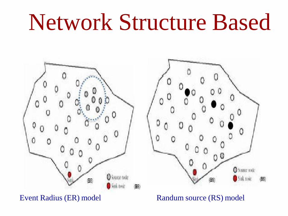
Network Structure Based
Event Radius (ER) model Randum source (RS) model

Sequential Assignment Routing (SAR) The routing scheme in SAR depends on three factors: energy resources, QoS on each path, and the
priority level of each packet
To avoid single route failure, a multi-path approach coupled with a localized path restoration
scheme is employed
To create multiple paths from a source node, a tree rooted at the source node
to the destination nodes (i.e. , the set of BSs) is constructed
The paths of the tree are defined by avoiding nodes with low energy or QoS guarantees
At the end of this process, each sensor node is a part of multi-path tree
For each SN, two metrics are associated with each path: delay (which is an
additive QoS metric); and energy usage for routing on that path
The energy is measured with respect to how many packets will traverse that path
SAR calculates a weighted QoS metric as the product of the additive QoS
metric and a weight coefficient associated with the priority level of the
packet
The goal of SAR is to minimize the average weighted QoS metric for the
network
Minimum Cost Forwarding Algorithm
The minimum cost forwarding algorithm (MCFA) exploits the
fact that the direction of routing is always known, that is, towards
fixed and predetermined external BS
Therefore, a SN need not have a unique ID nor maintain a
routing table
Instead, each node maintains the least cost estimate from itself to
the BS
Each message forwarded by the SN is broadcast to its neighbors
When a node receives the message, it checks if it is on the least
cost path between the source SN and the BS
If so, it re-broadcasts the message to its neighbors
This process repeats until the BS is reached
In MCFA, each sensor node should know the least cost path
estimate from itself to the BS
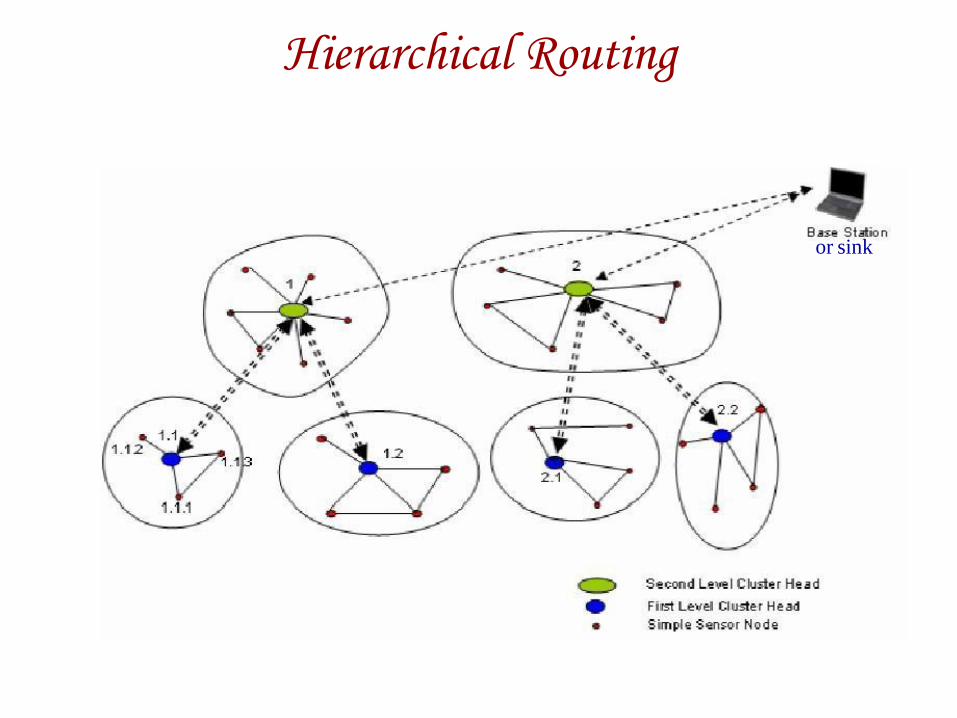
Hierarchical Routing
or sink

Cluster Based Routing Protocol (CBRP)
A simple cluster based routing protocol (CBRP) divides the network nodes into
a number of overlapping or disjoint two-hop-diameter clusters in a distributed
manner The cluster members just send the data to the CH, and the CH is responsible for
routing the data to the destination
The major drawback with CBRP is that it requires a lot of hello messages to
form and maintain the clusters, and thus may not be suitable for WSN
Given that sensor nodes are stationary in most of the applications this is a
considerable and unnecessary overhead
Scalable Coordination
In hierarchical clustering method, the cluster formation appears to require
considerable amount of energy as periodic advertisements are needed to form
the hierarchy Also, any changes in the network conditions or sensor energy level result in re-
clustering which may be not quite acceptable as some parameters tend to change
dynamically
Small Minimum Energy Communication Network (MECN)
The minimum energy communication network (MECN) protocol has been
designed to compute an energy-efficient subnetwork for a given sensor network
On top of MECN, a new algorithm called Small MECN (SMECN) has been
proposed to construct such a subnetwork
The subnetwork (i.e. , subgraph G') constructed by SMECN is smaller than the one
constructed by MECN if the broadcast region around the broadcasting node is
circular for a given power assignment
The subgraph G' of graph G, which represents the sensor network, minimizes the
energy consumption satisfying the following conditions:
The number of edges in G' is less than in G, while containing all nodes in G
The energy required to transmit data from a node to all its neighbors in
subgraph G' is less than the energy required to transmit to all its neighbors in
graph G
The resulting subnetwork computed by SMECN helps in the task of sending
messages on minimum-energy paths
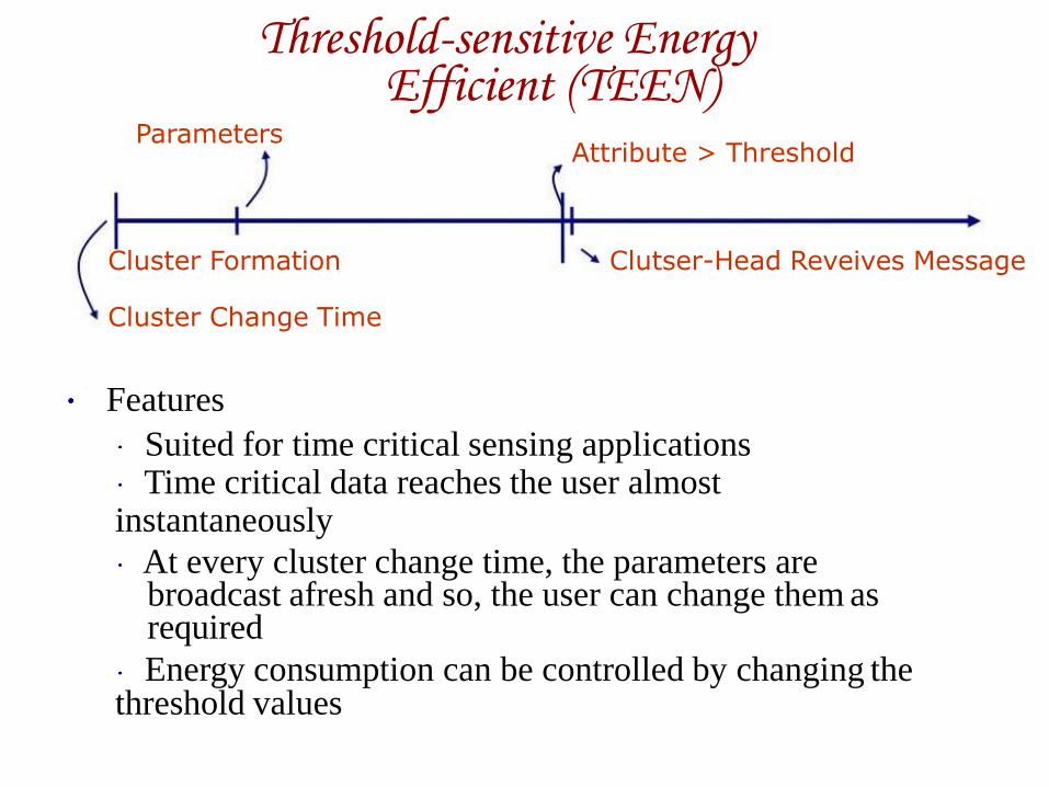
Threshold-sensitive Energy Efficient (TEEN)
Parameters Attribute > Threshold
Clutser-Head Reveives Message Cluster Formation
Cluster Change Time
Features
Suited for time critical sensing applications Time critical data reaches the user almost
instantaneously
At every cluster change time, the parameters are broadcast afresh and so, the user can change them as required
Energy consumption can be controlled by changing the threshold values
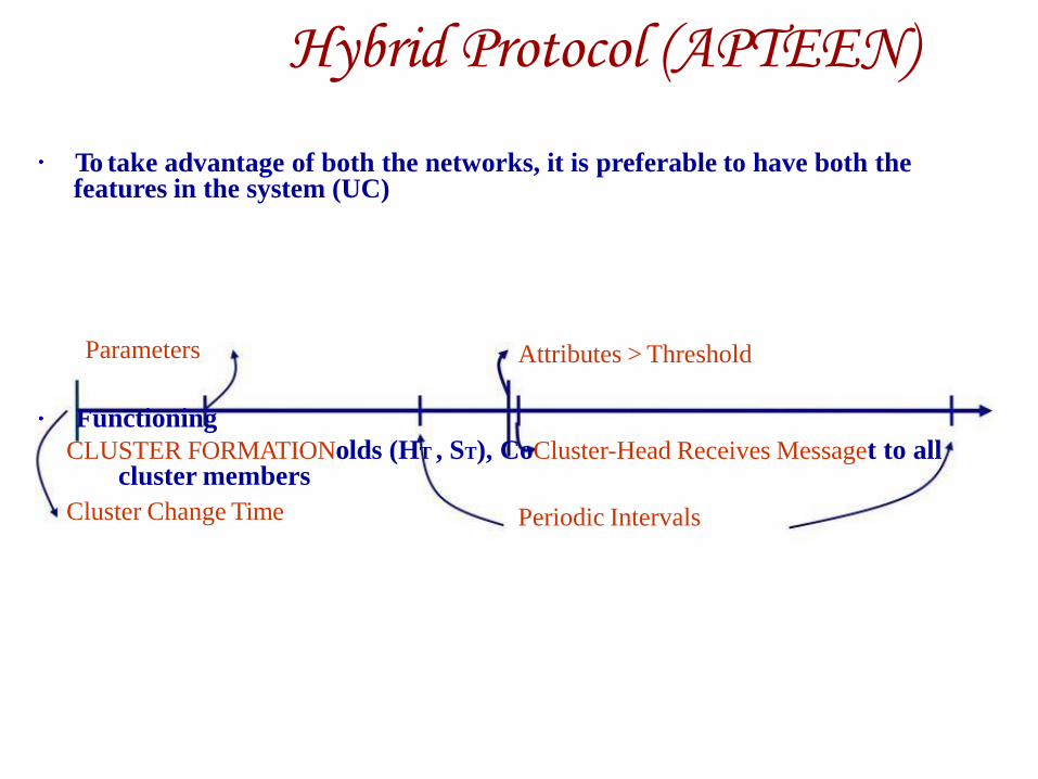
Hybrid Protocol (APTEEN)
To take advantage of both the networks, it is preferable to have both the features in the system (UC)
Parameters Attributes > Threshold
Functioning
CLUSTER FORMATIONolds (HT , ST), CoCluster-Head Receives Messaget to all cluster members
Cluster Change Time Periodic Intervals

Modified TDMA for APTEEN
Time-critical queries and historical queries are answered by the BS
Based on the assumption that adjacent nodes sense similar data, we can make only one of them handle the query
This might reduces the accuracy of data for non-critical queries
This is acceptable since it almost doubles the life of the network
Original TDMA
a
Sleep
nodes
Modified TDMA
Idle nodes
Routing in Fixed-size Clusters
Routing in sensor networks can also take advantage of geography-
awareness
One such routing protocol is called Geography Adaptive Fidelity (GAF)
where the network is firstly divided into fixed zones
Within each zone, nodes collaborate with each other to play different roles
For example, nodes elect one SN to stay awake for a certain period of time
while the others sleep
This particular elected SN is responsible for monitoring and reporting data
to the BS on behalf of all nodes within the zone
Here, each SN is positioned randomly in a two dimensional plane
When a sensor transmits a packet for a total distance r, the signal is strong
enough for other sensors to hear it within the Euclidean distance r from
the sensor that originates the packet
Figure 9.14 depicts an example of fixed zoning that can be applied to
WSN

Routing in Fixed-size Clusters
r is the distance of
packet transmission
by each sensor
A fixed cluster of each side a can be selected and is connected if:
If the signal travels a distance of a = r/( 5) v/n adjacent vertical or horizontal
directions, two sensors can communicate directly
For a diagonal communication to take place, the signal has to span a distance of a =
r/(2 2) v/
Sensor Aggregates Routing
A sensor aggregate includes those SNs in a network that satisfy a grouping
predicate for a collaborative processing task
The parameters of the predicate depend on the task and its resource requirements
Here, the formation of appropriate sensor aggregate is considered in terms of
resource allocation for communication and sensing
Sensors in the network are divided into clusters according to their sensed signal
strength
After that, local cluster leaders (CH) are elected by exchanging information
between neighboring sensors
Once a sensor node has exchanged packets with all its one-hop neighbors, if it
finds that its signal strength is higher than all its one-hop neighbors, it declares
itself as a leader
This leader-based tracking algorithm assumes a unique leader to know
surrounding geographical region for collaboration
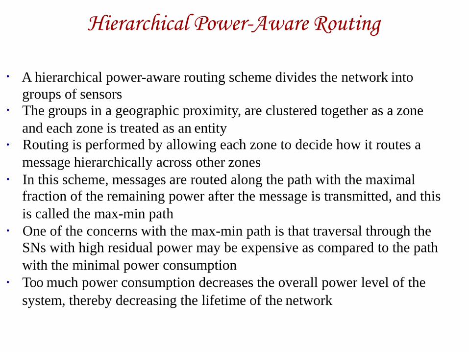
Hierarchical Power-Aware Routing
A hierarchical power-aware routing scheme divides the network into
groups of sensors
The groups in a geographic proximity, are clustered together as a zone
and each zone is treated as an entity
Routing is performed by allowing each zone to decide how it routes a
message hierarchically across other zones
In this scheme, messages are routed along the path with the maximal
fraction of the remaining power after the message is transmitted, and this
is called the max-min path
One of the concerns with the max-min path is that traversal through the
SNs with high residual power may be expensive as compared to the path
with the minimal power consumption
Too much power consumption decreases the overall power level of the
system, thereby decreasing the lifetime of the network

Sensor Protocols for Information via Negotiation (SPIN)
„Disseminates all the information of each SN to every other SN in the network
„All SNs in the network are potential BS
„A user is able to query any SN and get the required information immediately
„These protocols make use of the property that SNs in close proximity have similar data and thus transmit only the data that the other SNs do not have
„SPIN assigns a high-level name to appropriately describe their collected data, called meta-data, and perform meta-data negotiations before any data is transmitted
„This ensures that no redundant data is transmitted throughout the network
„The format of the meta-data is application-specific and is not specified in SPIN
„SPIN works in a time-driven manner wherein it distributes the information all over the network, even when a user does not request any data
„The SPIN family of protocols includes two protocols, namely, SPIN-1 and SPIN-2, which incorporate negotiation before transmitting data so as to ensure that only useful information is transferred
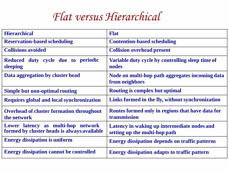
Flat versus Hierarchical
periodic
Hierarchical
Reservation-based scheduling
Collisions avoided
Reduced duty cycle due to
sleeping
Data aggregation by cluster head
Simple but non-optimal routing
Requires global and local synchronization
Overhead of cluster formation throughout
the network
Lower latency as multi-hop network formed by cluster heads is always available
Energy dissipation is uniform
Energy dissipation cannot be controlled
Flat
Contention-based scheduling
Collision overhead present
Variable duty cycle by controlling sleep time of
nodes
Node on multi-hop path aggregates incoming data
from neighbors
Routing is complex but optimal
Links formed in the fly, without synchronization
Routes formed only in regions that have data for
transmission
Latency in waking up intermediate nodes and
setting up the multi-hop path
Energy dissipation depends on traffic patterns
Energy dissipation adapts to traffic pattern
Negotiation-based Routing
Negotiation-based routing protocols use high level data descriptors in
order to eliminate redundant data transmissions
Communication decisions are also made based on the available resources
The motivation here is that the use of flooding to disseminate data
produces implosion and data overlap, leading to scenarios where nodes
receive duplicate copies of the same data
If the same data is transmitted by several sensors, considerable energy is
consumed
The main idea behind negotiation-based routing in WSNs is to suppress
duplicate information and prevent redundant data from being sent to the
next sensor or the BS
This is done by conducting a series of negotiation messages before the
actual data transmission begins

Query-based Routing
In query-based routing, the destination nodes propagate a query for data (sensing
task) from a node throughout the network
A node having the data matching the query sends it back to the node which
requested it
Usually, these queries are described in natural language or in high-level query
languages
For example, a BS B1 may submit a query to node N1 inquiring: “Are there moving
vehicles in battlefield region 1?”
In query-based routing, all the nodes have tables consisting of the sensing tasks
queries that they received, and send back data matching these tasks whenever they
receive it
Directed diffusion (discussed earlier in this chapter) is an example of this type of
routing
Here, the sink node sends out messages of interest to SNs
As the interest is propagated throughout the WSN, the gradients from the source
back to the sink (BS) are set up
Location-based Routing
In location-based routing, SNs are addressed by means of their locations
Here, the distance between neighboring SNs can be estimated on the basis
of incoming signal strengths, and relative coordinates of neighboring SNs
can be obtained by exchanging such information
Alternatively, the location of nodes may be available directly through GPS
if we consider nodes are equipped with a small low power GPS receiver
In order to conserve energy, some location-based schemes demand that
SNs should go to sleep if there is no activity
Clearly, the more sleeping SNs in the network the more energy can be
saved
However, the active SNs should be connected, should cover the entire
sensing region, and should provide basic routing and broadcasting
functionalities

High-Level Application Layer Support
The protocols we have presented so far are also found, albeit in some different
form in traditional wired, cellular, or ad hoc networks
For specific applications, a higher level of abstraction specifically tailored to
WSN appears to be useful
Distributed Query Processing
The number of messages generated in distributed query processing is several
magnitudes less than in centralized scheme
There are two approaches for processing sensor queries: warehousing and
distributed
In the warehousing approach, data is extracted in a pre-defined manner and stored
in a central database
In the distributed approach, only relevant data is extracted from the sensor
network, when and where it is needed
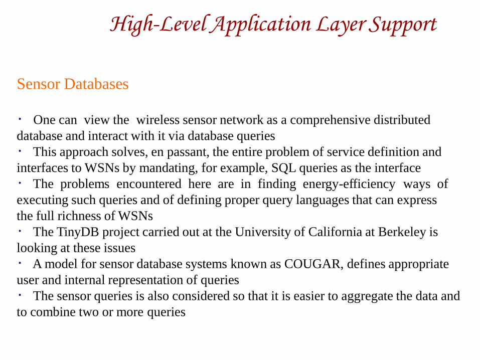
High-Level Application Layer Support
Sensor Databases
One can view the wireless sensor network as a comprehensive distributed
database and interact with it via database queries
This approach solves, en passant, the entire problem of service definition and
interfaces to WSNs by mandating, for example, SQL queries as the interface
The problems encountered here are in finding energy-efficiency ways of
executing such queries and of defining proper query languages that can express
the full richness of WSNs
The TinyDB project carried out at the University of California at Berkeley is
looking at these issues
A model for sensor database systems known as COUGAR, defines appropriate
user and internal representation of queries
The sensor queries is also considered so that it is easier to aggregate the data and
to combine two or more queries
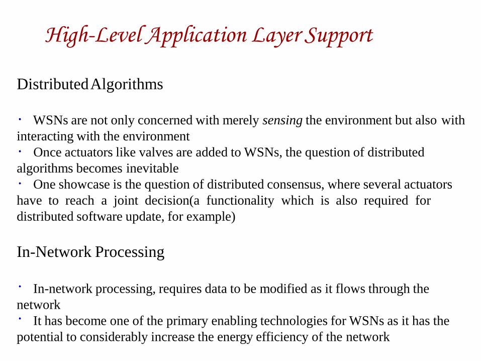
High-Level Application Layer Support
Distributed Algorithms
WSNs are not only concerned with merely sensing the environment but also with
interacting with the environment
Once actuators like valves are added to WSNs, the question of distributed
algorithms becomes inevitable
One showcase is the question of distributed consensus, where several actuators
have to reach a joint decision(a functionality which is also required for
distributed software update, for example)
In-Network Processing
In-network processing, requires data to be modified as it flows through the
network
It has become one of the primary enabling technologies for WSNs as it has the
potential to considerably increase the energy efficiency of the network
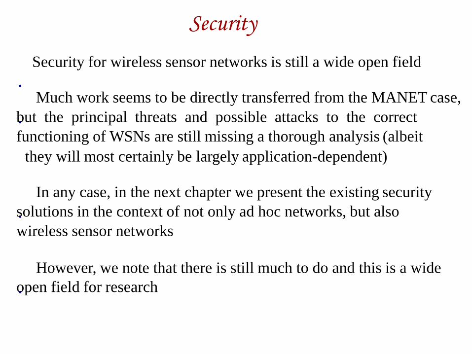
Security
Security for wireless sensor networks is still a wide open field
Much work seems to be directly transferred from the MANET case,
but the principal threats and possible attacks to the correct
functioning of WSNs are still missing a thorough analysis (albeit
they will most certainly be largely application-dependent)
In any case, in the next chapter we present the existing security
solutions in the context of not only ad hoc networks, but also
wireless sensor networks
However, we note that there is still much to do and this is a wide
open field for research

Adapting to the Inherent Dynamic Nature of WSNs
Some important goals that current research in this area is aiming to achieve
are as follows:
Exploit spatial diversity and density of sensor/actuator nodes to build
an adaptive node sleep schedule
Spontaneously create and assemble network, dynamically adapt to
device failure and degradation, manage mobility of sensor nodes and
react to changes in task and sensor requirements
Adaptability to drastic changes in the traffic
Having finer control over the precision and coverage
The Scalable Coordination Architectures for Deeply Distributed Systems
(SCADDS) project, also a part of DARPA SensIT program, focuses on
adaptive fidelity, dynamically adjusting the overall fidelity of sensing in
response to task dynamics (turn on more sensors when a threat is
perceived)
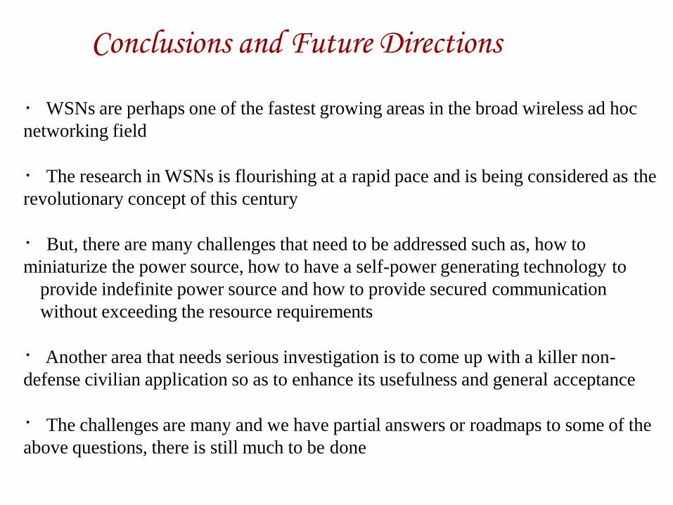
Conclusions and Future Directions
WSNs are perhaps one of the fastest growing areas in the broad wireless ad hoc
networking field
The research in WSNs is flourishing at a rapid pace and is being considered as the
revolutionary concept of this century
But, there are many challenges that need to be addressed such as, how to
miniaturize the power source, how to have a self-power generating technology to
provide indefinite power source and how to provide secured communication
without exceeding the resource requirements
Another area that needs serious investigation is to come up with a killer non-
defense civilian application so as to enhance its usefulness and general acceptance
The challenges are many and we have partial answers or roadmaps to some of the
above questions, there is still much to be done

UNIT –IV

Security in Ad Hoc Wireless Networks
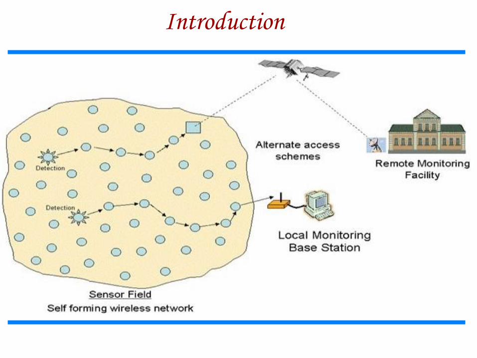
Introduction
Wireless Sensor Network?
It’s a collection of devices “ sensor nodes”
They are small, inexpensive, with constrained power
They are organized in a cooperative network
They communicate wirelessly
in multi hop routing
Heavily deployment
Changing network topology

Introduction
Component and Schematic of Node
Processor.
Memory.
RF Radio.
Power Source.
Sensor.
GPS
178
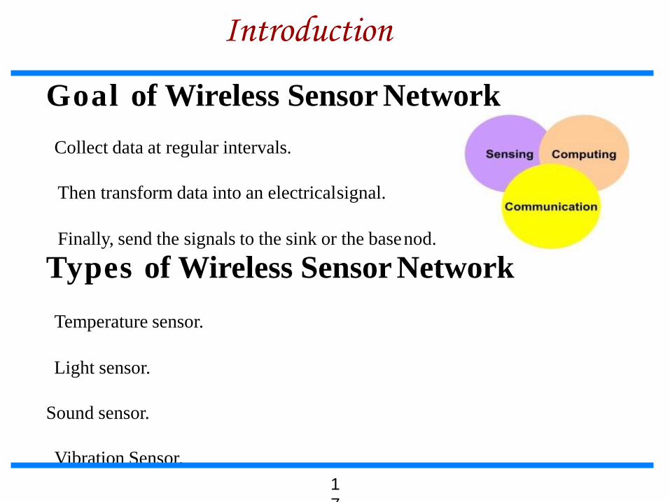
Introduction
Goal of Wireless Sensor Network
Collect data at regular intervals.
Then transform data into an electrical signal.
Finally, send the signals to the sink or the base nod.
Types of Wireless Sensor Network
Temperature sensor.
Light sensor.
Sound sensor.
Vibration Sensor.
1
7

Introduction
Communication pattern
Broadcast : Base station transmits message to all its immediate
neighbors.
Converge cast : a group of sensors communicates to a specific
sensor
Local gossip: a sensor node sends a message to its neighboring
nodes within a range.
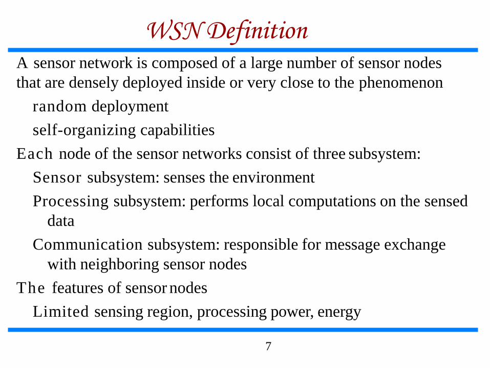
WSN Definition A sensor network is composed of a large number of sensor nodes
that are densely deployed inside or very close to the phenomenon
random deployment
self-organizing capabilities
Each node of the sensor networks consist of three subsystem:
Sensor subsystem: senses the environment
Processing subsystem: performs local computations on the sensed
data
Communication subsystem: responsible for message exchange
with neighboring sensor nodes
The features of sensor nodes
Limited sensing region, processing power, energy
7
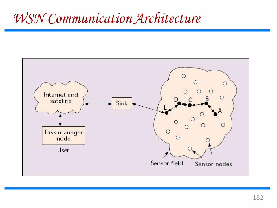
WSN Communication Architecture
182
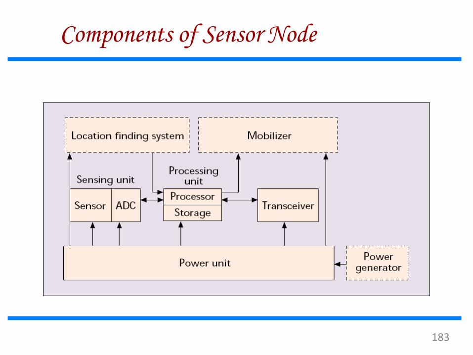
Components of Sensor Node
183
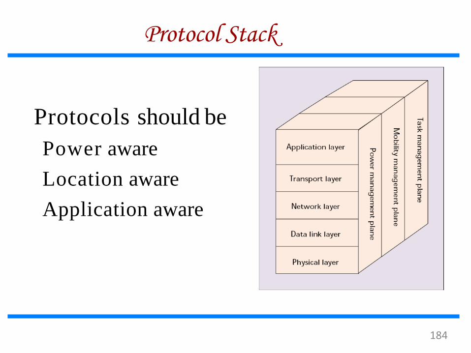
Protocol Stack
Protocols should be
Power aware
Location aware
Application aware
184
WSN Characteristics
Major differences between sensor and ad-hoc network
Number of nodes is higher
Densely deployment
Sensor nodes are prone to failure.
Frequent topology changes
Broadcast communication paradigm
Limited processing and power capabilities.
Possible absence of unique global ID
185

WSN Design Factors
Fault Tolerance
Scalability
Production Costs
Hardware Constraints
Sensor Network Topology
Environment
Transmission Media
Power Consumption
186
Design Factors : Fault Tolerance
Each Nodes are prone to unexpected
failure (more than other network)
Fault tolerance is the ability to sustain
sensor network functionalities without
any interruption due to sensor node
failures.
187

Design Factors:Production Costs
The cost of a single node must be low
given the amount of functionalities
Much less than $1
188

Design Factors:Hardware Constraint
All these units combined together must
Extremely low power
Extremely small volume
189

Design Factors : Topology
Must be maintained specially in very high
densities
Pre-deployment and deployment phase
Post-deployment phase
Re-deployment of additional nodes phase
190
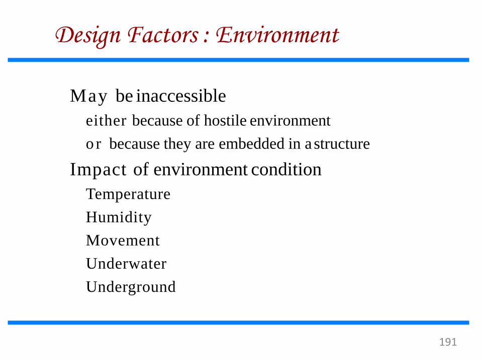
Design Factors : Environment
May be inaccessible
either because of hostile environment
o r because they are embedded in a structure
Impact of environment condition
Temperature
Humidity
Movement
Underwater
Underground
191
Design Factors: Environment
Busy intersections
Interior of a large machinery
Bottom of an ocean
Surface of an ocean during a tornado
Biologically or chemically contaminated field
Battlefield beyond the enemy lines
Home or a large building
Large warehouse
Animals
Fast moving vehicles
Drain or river moving with current
192
Design Factors : Transmission Media
R F
Infrared
Optical
Acoustic
193

Design Factors: Power Consumption
Power conservation
Sensing
Communication
Data processing
194
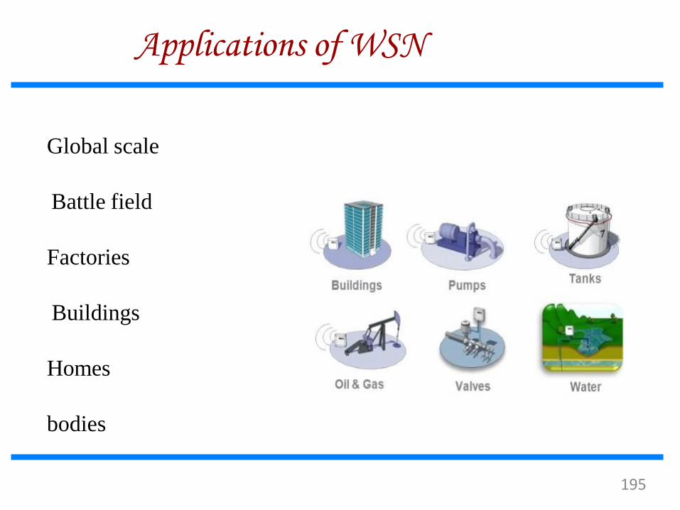
Applications of WSN
Global scale
Battle field
Factories
Buildings
Homes
bodies
195

Applications of Sensor Networks
Using in military
and monitoring, guidance systems of Battlefield surveillance
intelligent missiles, detection of attack by weapons of mass
destruction such as chemical, biological, or nuclear
Using in nature
Forest fire, flood detection, habitat exploration of animals
Using in health
Monitor the patient’s heart rate or blood pressure, and sent regularly
to alert the concerned doctor, provide patients a greater freedom of
movement
196
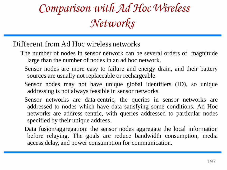
Comparison with Ad Hoc Wireless
Networks
Different from Ad Hoc wireless networks
The number of nodes in sensor network can be several orders of magnitude large than the number of nodes in an ad hoc network.
Sensor nodes are more easy to failure and energy drain, and their battery sources are usually not replaceable or rechargeable.
Sensor nodes may not have unique global identifiers (ID), so unique addressing is not always feasible in sensor networks.
Sensor networks are data-centric, the queries in sensor networks are addressed to nodes which have data satisfying some conditions. Ad Hoc networks are address-centric, with queries addressed to particular nodes specified by their unique address.
Data fusion/aggregation: the sensor nodes aggregate the local information before relaying. The goals are reduce bandwidth consumption, media access delay, and power consumption for communication.
197

Classification ofsensor network protocol
198

Layered Architecture
A layered architecture has a single
powerful base station, and the layers of
sensor nodes around it correspond to
the nodes that have the same hop-count
to the BS.
In the in-building scenario, the BS acts
an access point to a wired network, and
small nodes form a wireless backbone
to provide wireless connectivity.
The advantage of a layered architecture
is that each node is involved only in
short-distance, low-power
transmissions to nodes of the
neighboring layers.
199
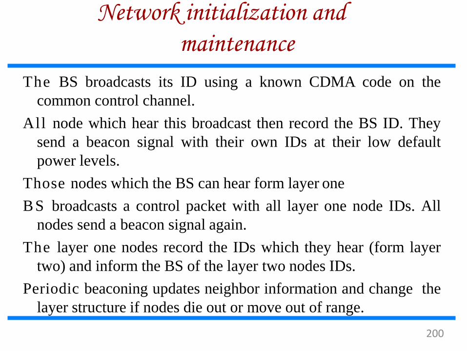
Network initialization and
maintenance
The BS broadcasts its ID using a known CDMA code on the
common control channel.
All node which hear this broadcast then record the BS ID. They
send a beacon signal with their own IDs at their low default
power levels.
Those nodes which the BS can hear form layer one
BS broadcasts a control packet with all layer one node IDs. All
nodes send a beacon signal again.
The layer one nodes record the IDs which they hear (form layer
two) and inform the BS of the layer two nodes IDs.
Periodic beaconing updates neighbor information and change the
layer structure if nodes die out or move out of range.
200

Routing protocol
Downlink from the BS is by direct broadcast on the
control channel. Uplink from the sensor nodes to BS is
by multi-hop data forwarding.
The node to which a packet is to be forwarded is
selected considering the remaining energy of the nodes.
This achieves a higher network lifetime.
201

UNPF-R
Optimize the network performance by make the sensor nodes adaptively vary their
transmission range.
Because while a very small transmission range cause network partitioning, a very
large transmission range reduce the spatial reuse of frequencies.
The optimal range (R) is determined by simulated annealing
Objective function :
N : the total number of sensors
n : the number of nodes in layer on
202
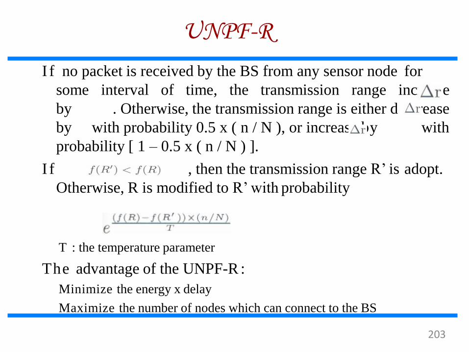
UNPF-R
I f no packet is received by the BS from any sensor node for
reas
. Otherwise, the transmission range is either d ec
some interval of time, the transmission range inc e
by
by with probability 0.5 x ( n / N ), or increas y e b
rease
with
probability [ 1 – 0.5 x ( n / N ) ].
I f , then the transmission range R’ is adopt.
Otherwise, R is modified to R’ with probability
T : the temperature parameter
The advantage of the UNPF-R :
Minimize the energy x delay
Maximize the number of nodes which can connect to the BS
203

Clustered Architecture
clustered architecture organizes the
sensor nodes into clusters, each governed
by a cluster-head. The nodes in each
cluster are involved in message exchanges
with their cluster-heads, and these heads
send message to a BS.
Clustered architecture is useful for sensor
networks because of its inherent suitability
for data fusion. The data gathered by all
member of the cluster can be fused at the
cluster-head, and only the resulting
information needs to be communicated to
the BS.
The cluster formation and election of
cluster-heads must be an autonomous,
distributed process.
204
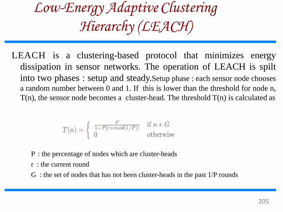
Low-Energy Adaptive Clustering
Hierarchy (LEACH)
LEACH is a clustering-based protocol that minimizes energy
dissipation in sensor networks. The operation of LEACH is spilt
into two phases : setup and steady.Setup phase : each sensor node chooses
a random number between 0 and 1. If this is lower than the threshold for node n,
T(n), the sensor node becomes a cluster-head. The threshold T(n) is calculated as
P : the percentage of nodes which are cluster-heads
r : the current round
G : the set of nodes that has not been cluster-heads in the past 1/P rounds
205

After selection, the cluster-heads advertise their selection to
all nodes. All nodes choose their nearest cluster-head by
signal strength (RSSI). The cluster-heads then assign a
TDMA schedule for their cluster members
Steady phase : data transmission takes place based on the
TDMA schedule, and the cluster-heads perform data
aggregation/fusion.
After a certain period of time in the steady phase, cluster-
heads are selected again through the setup phase.
Low-Energy Adaptive Clustering
Hierarchy (LEACH)
206
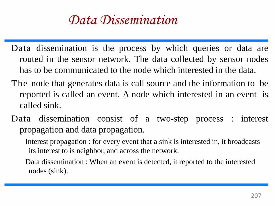
Data Dissemination
Data dissemination is the process by which queries or data are
routed in the sensor network. The data collected by sensor nodes
has to be communicated to the node which interested in the data.
The node that generates data is call source and the information to be
reported is called an event. A node which interested in an event is
called sink.
Data dissemination consist of a two-step process : interest
propagation and data propagation.
Interest propagation : for every event that a sink is interested in, it broadcasts
its interest to is neighbor, and across the network.
Data dissemination : When an event is detected, it reported to the interested
nodes (sink).
207
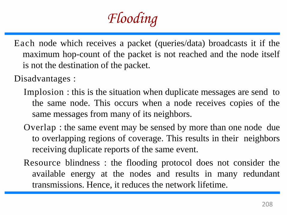
Flooding
Each node which receives a packet (queries/data) broadcasts it if the
maximum hop-count of the packet is not reached and the node itself
is not the destination of the packet.
Disadvantages :
Implosion : this is the situation when duplicate messages are send to
the same node. This occurs when a node receives copies of the
same messages from many of its neighbors.
Overlap : the same event may be sensed by more than one node due
to overlapping regions of coverage. This results in their neighbors
receiving duplicate reports of the same event.
Resource blindness : the flooding protocol does not consider the
available energy at the nodes and results in many redundant
transmissions. Hence, it reduces the network lifetime.
208
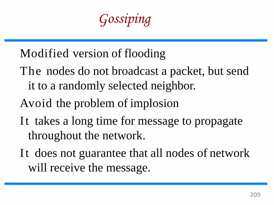
Gossiping
Modified version of flooding
The nodes do not broadcast a packet, but send
it to a randomly selected neighbor.
Avoid the problem of implosion
I t takes a long time for message to propagate
throughout the network.
I t does not guarantee that all nodes of network
will receive the message.
209
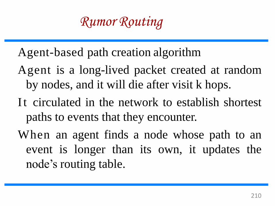
Rumor Routing
Agent-based path creation algorithm
Agent is a long-lived packet created at random
by nodes, and it will die after visit k hops.
I t circulated in the network to establish shortest
paths to events that they encounter.
When an agent finds a node whose path to an
event is longer than its own, it updates the
node’s routing table.
210
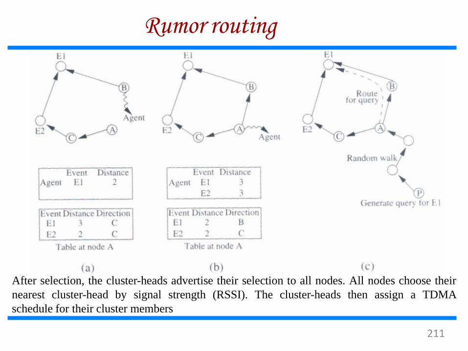
Rumor routing
After selection, the cluster-heads advertise their selection to all nodes. All nodes choose their
nearest cluster-head by signal strength (RSSI). The cluster-heads then assign a TDMA
schedule for their cluster members
211
Sequential Assignment Routing
(SAR) The sequential assignment routing (SAR) algorithm creates
multiple trees, where the root of each tree is a one-hop neighbor
of the sink.
To avoid nodes with low throughput or high delay.
Each sensor node records two parameters about each path though
it : available energy resources on the path and an additive QoS
metric such as delay
SAR minimizes the average weighted QoS metric over the
lifetime of the network.
212
Directed Diffusion
The directed diffusion protocol is useful in scenarios where the sensor
nodes themselves generate requests/queries for data sensed by other
nodes.
Each sensor node names its data with one or more attributes.
Each sensor node express their interest depending on these attributes.
Each path is associated with a interest gradient, while positive gradient
make the data flow along the path, negative gradient inhibit the
distribution data along a particular path.
Example : two path formed with gradient 0.4 and 0.8, the source may
twice as much data along the higher one
Suppose the sink wants more frequent update from the sensor which have
detected an event => send a higher data-rate requirement for increasing
the gradient of that path.
213
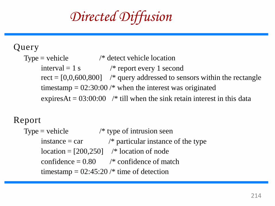
Query Type = vehicle
interval = 1 s
/* detect vehicle location
/* report every 1 second
rect = [0,0,600,800] /* query addressed to sensors within the rectangle
timestamp = 02:30:00 /* when the interest was originated
expiresAt = 03:00:00 /* till when the sink retain interest in this data
Report Type = vehicle
instance = car
/* type of intrusion seen
/* particular instance of the type
location = [200,250]
confidence = 0.80
/* location of node
/* confidence of match
timestamp = 02:45:20 /* time of detection
Directed Diffusion
214

Sensor Protocols for Information via
Negotiation
SPIN use negotiation and resource
adaptation to address the
disadvantage of flooding.
Reduce overlap and implosion, and
prolong network lifetime.
Use meta-data instead of raw data.
SPIN has three types of
messages:ADV, REQ, and DATA.
SPIN-2 using an energy threshold to
reduce participation. A node may join
in the ADV-REQ-DATA handshake
only if it has sufficient resource
above a threshold.
215
Cost-Field Approach
The cost-field approach considers the problem of setting up paths to a
sink. The first phase being to set up the cost field, based on metrics
such as delay. The second phase being data dissemination using the
costs.
A sink broadcasts an ADV packet with its own cost as 0.
When a node N hears an ADV message from node M, it sets its own
path cost to min (LN,LM+CNM), where LN is the total path cost from node
N to the sink, LM is the cost of node M to the sink, CNM is the cost from
N to M.
I f LN updated, the new cost is broadcast though another ADV.
The back-off time make a node defer its ADV instead of immediately
broadcast it. The back-off time is r x CMN, where r is a parameter of
algorithm.
216
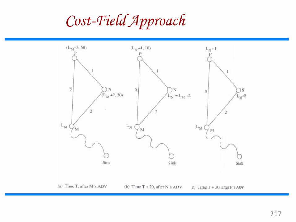
Cost-Field Approach
217

Geographic Hash Table (GHT)
GHT hashes keys into geographic
coordinates and stores a (key, value)
pair at the sensor node nearest to the
hash value.
Stored data is replicated to ensure
redundancy in case of node failures.
The data is distributed among nodes such that it is scalable
and the storage load is balanced. The routing protocol used is greedy perimeter stateless routing
(GPSR), which again uses geographic information to route the
data and queries.
218
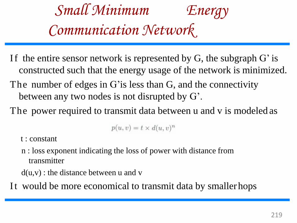
Small Minimum Energy
Communication Network
I f the entire sensor network is represented by G, the subgraph G’ is
constructed such that the energy usage of the network is minimized.
The number of edges in G’ is less than G, and the connectivity
between any two nodes is not disrupted by G’.
The power required to transmit data between u and v is modeled as
t : constant
n : loss exponent indicating the loss of power with distance from
transmitter
d(u,v) : the distance between u and v
I t would be more economical to transmit data by smaller hops
219
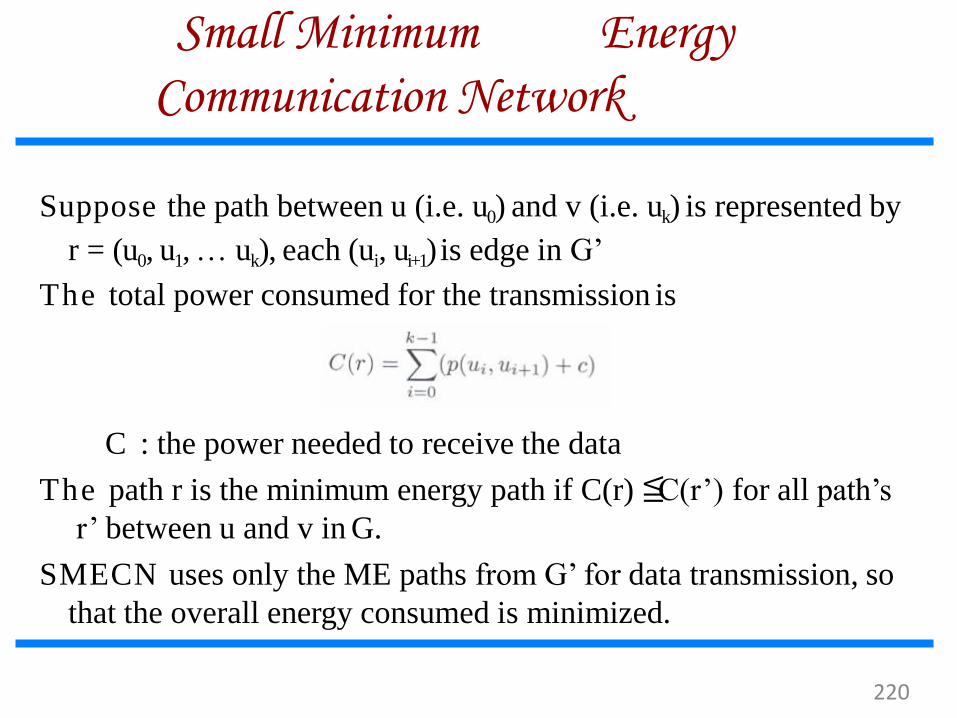
Suppose the path between u (i.e. u0) and v (i.e. uk) is represented by
r = (u0, u1, … uk), each (ui, ui+1) is edge in G’
The total power consumed for the transmission is
C : the power needed to receive the data
The path r is the minimum energy path if C(r) ≦ C(r’) for all path’s
r’ between u and v in G.
SMECN uses only the ME paths from G’ for data transmission, so
that the overall energy consumed is minimized.
Small Minimum Energy
Communication Network
220
Data Gathering
The objective of the data gathering problem is to
transmit the sensed data from each sensor node to a
BS.
The goal of algorithm which implement data gathering
is
maximize the lifetime of network
Minimum energy should be consumed
The transmission occur with minimum delay
The energy x delay metric is used to compare
algorithm
221
Direct Transmission
All sensor nodes transmit their data directly to
the BS.
I t cost expensive when the sensor nodes are
very far from the BS.
Nodes must take turns while transmitting to the
BS to avoid collision, so the media access delay
is also large. Hence, this scheme performs
poorly with respect to the energy x delay
metric.
222
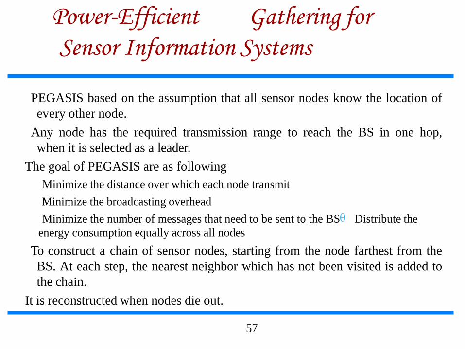
Power-Efficient Gathering for
Sensor Information Systems
PEGASIS based on the assumption that all sensor nodes know the location of
every other node.
Any node has the required transmission range to reach the BS in one hop,
when it is selected as a leader.
The goal of PEGASIS are as following
Minimize the distance over which each node transmit
Minimize the broadcasting overhead
Minimize the number of messages that need to be sent to the BS Distribute the
energy consumption equally across all nodes
To construct a chain of sensor nodes, starting from the node farthest from the
BS. At each step, the nearest neighbor which has not been visited is added to
the chain.
It is reconstructed when nodes die out.
57
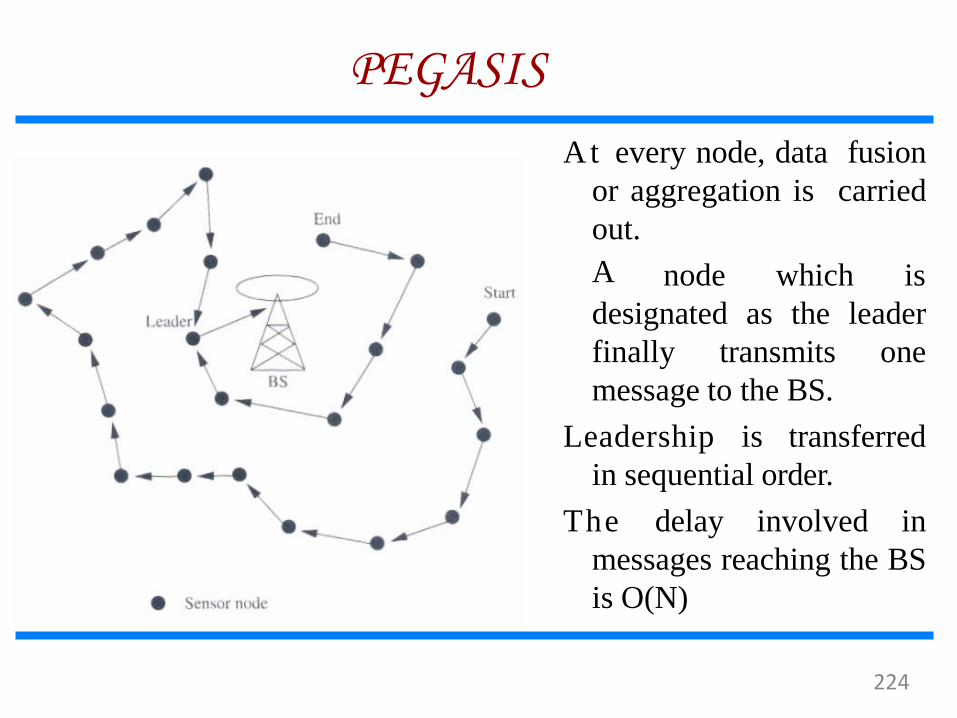
At every node, data fusion
or aggregation is carried
out.
A node which is
designated as the leader
finally transmits one
message to the BS.
Leadership is transferred
in sequential order.
The delay involved in
messages reaching the BS
is O(N)
PEGASIS
224
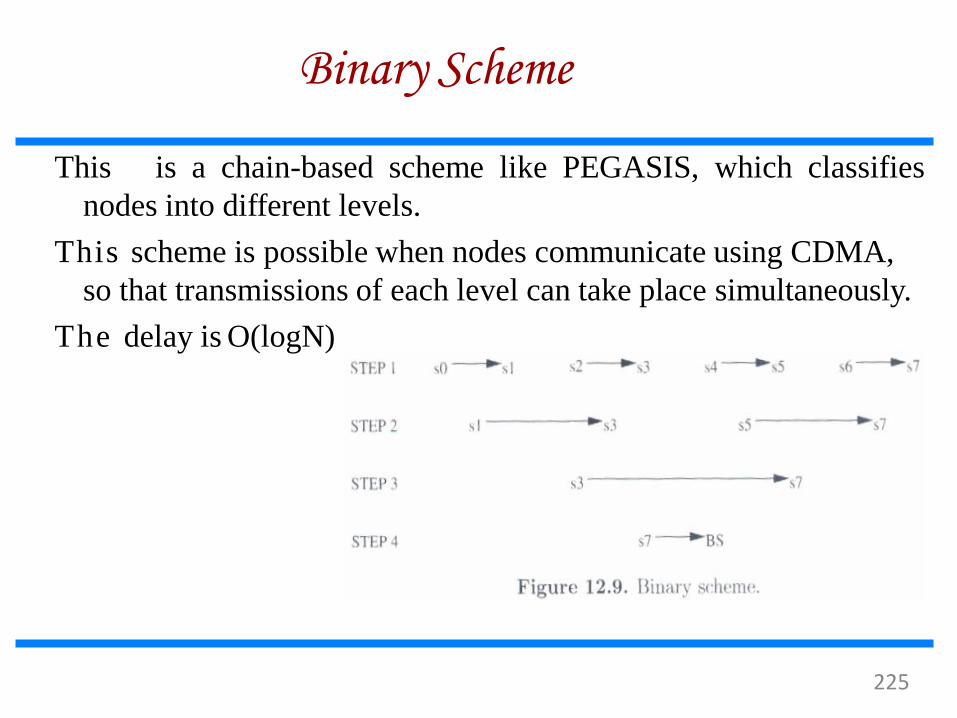
Binary Scheme
This is a chain-based scheme like PEGASIS, which classifies
nodes into different levels.
This scheme is possible when nodes communicate using CDMA,
so that transmissions of each level can take place simultaneously.
The delay is O(logN)
225
Chain-Based Three-Level Scheme
For non-CDMA sensor nodes
The chain is divided into a number of groups to space out
simultaneous transmissions in order to minimize
interference.
Within a group, nodes transmit data to the group leader,
and the leader fusion the data, and become the member
to the next level.
I n the second level, all nodes are divided into two groups.
I n the third level, consists of a message exchange
between one node from each group of the second level.
Finally, the leader transmit a single message to the BS.
226
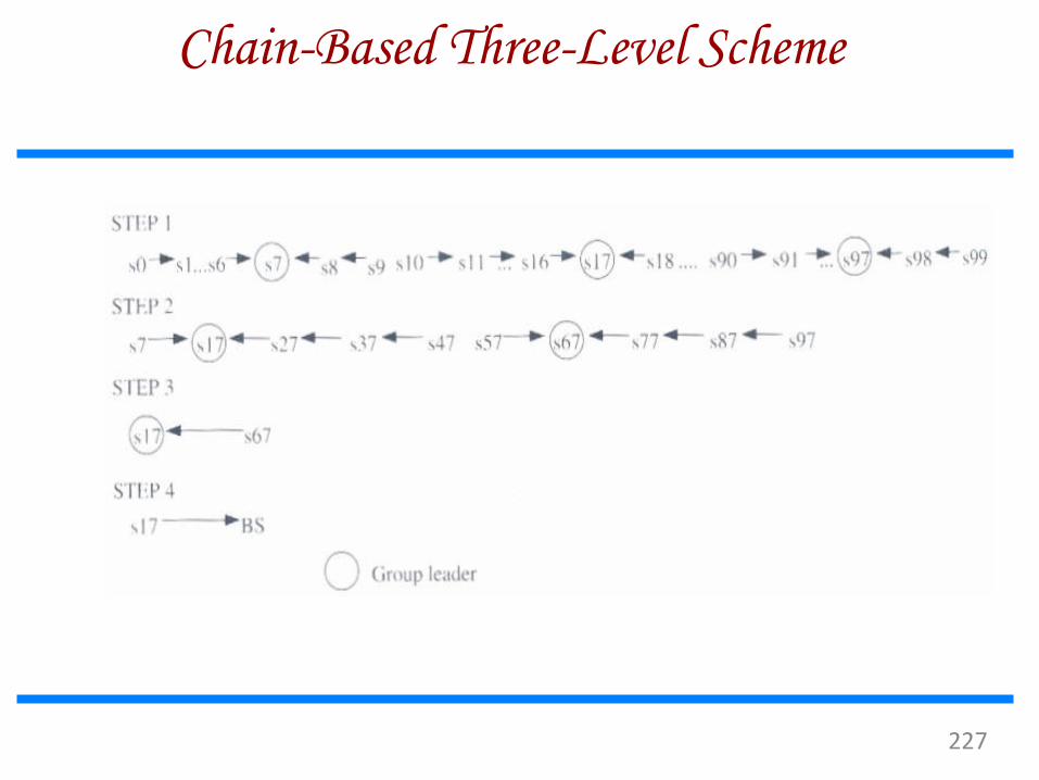
Chain-Based Three-Level Scheme
227

MAC Protocols for Sensor Networks
The challenges posed by sensor network MAC
protocol
No single controlling authority, so global synchronization is
difficult
Power efficiency issue
Frequent topology changes due to mobility and failure
There are three kinds of MAC protocols used in sensor
network:
Fixed-allocation
228
Fixed-allocation MAC protocol
Share the common medium through a predetermined
assignment.
I t is suitable for sensor network that continuously monitor and
generate deterministic data traffic
Provide a bounded delay for each node
However, in the case of bursty traffic, where the channel
requirements of each node may vary over time, it may lead to
inefficient usage of the channel.
MAC Protocols for Sensor Networks
229
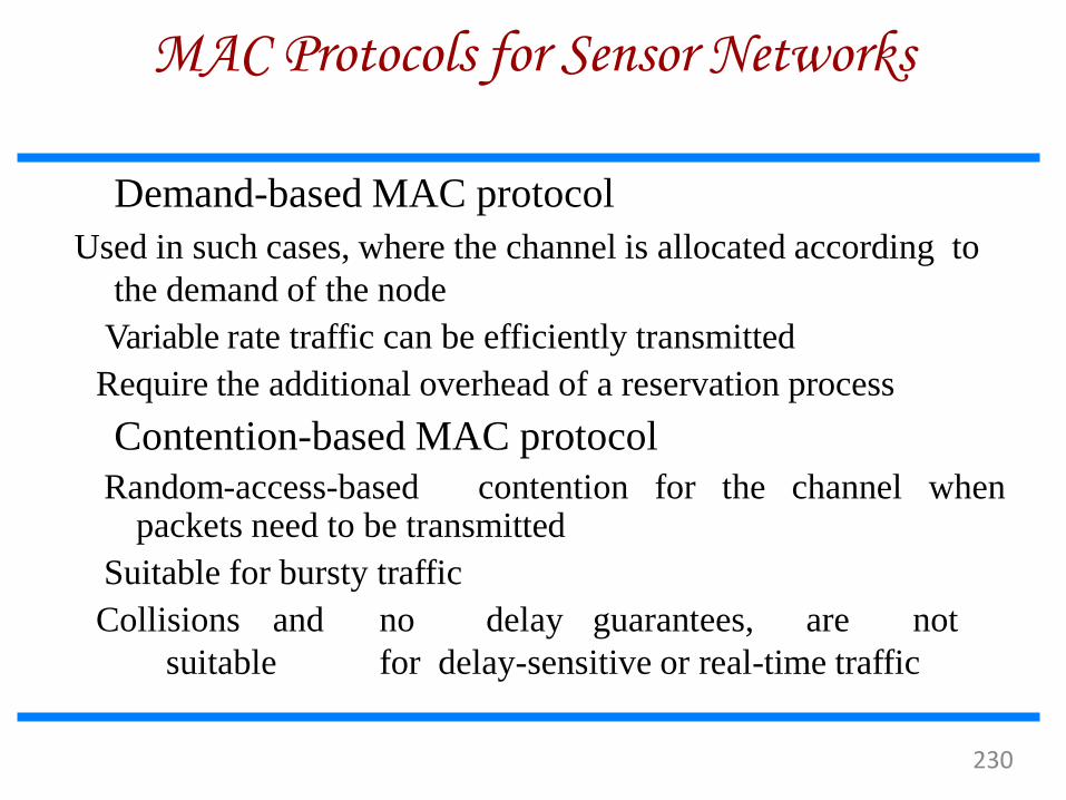
Demand-based MAC protocol
Used in such cases, where the channel is allocated according to
the demand of the node
Variable rate traffic can be efficiently transmitted
Require the additional overhead of a reservation process
Contention-based MAC protocol Random-access-based contention for the channel when
packets need to be transmitted
Suitable for bursty traffic
Collisions and no delay guarantees, are not
suitable for delay-sensitive or real-time traffic
MAC Protocols for Sensor Networks
230
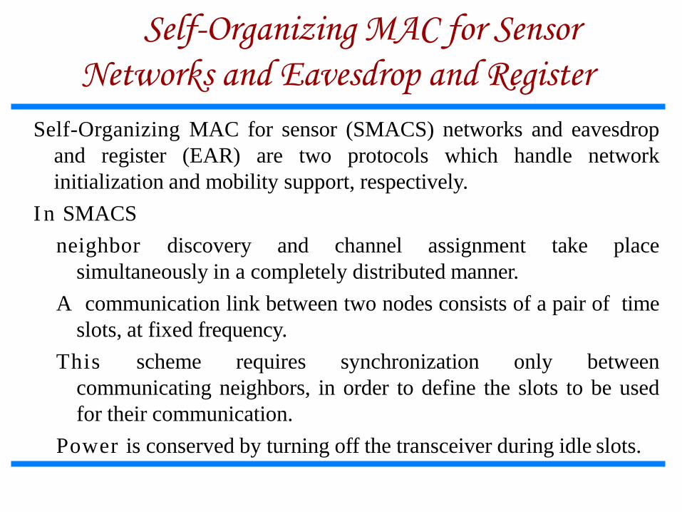
Self-Organizing MAC for Sensor
Networks and Eavesdrop and Register
Self-Organizing MAC for sensor (SMACS) networks and eavesdrop
and register (EAR) are two protocols which handle network
initialization and mobility support, respectively.
I n SMACS
neighbor discovery and channel assignment take place
simultaneously in a completely distributed manner.
A communication link between two nodes consists of a pair of time
slots, at fixed frequency.
This scheme requires synchronization only between
communicating neighbors, in order to define the slots to be used
for their communication.
Power is conserved by turning off the transceiver during idle slots.

Hybrid TDMA/FDMA
TDMA scheme minimize the time for which a node has to
be kept on, but the associated time synchronization cost
are very high.
A pure FDMA scheme allots the minimum required
bandwidth for each connection
I f the transmitter consumes more power, a TDMA
scheme is favored, since it can be switch off in idle slots
to save power.
I f the receiver consumes greater power, a FDMA scheme
is favored, because the receiver need not expend power
for time synchronization.
232
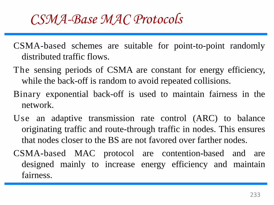
CSMA-Base MAC Protocols
CSMA-based schemes are suitable for point-to-point randomly
distributed traffic flows.
The sensing periods of CSMA are constant for energy efficiency,
while the back-off is random to avoid repeated collisions.
Binary exponential back-off is used to maintain fairness in the
network.
Use an adaptive transmission rate control (ARC) to balance
originating traffic and route-through traffic in nodes. This ensures
that nodes closer to the BS are not favored over farther nodes.
CSMA-based MAC protocol are contention-based and are
designed mainly to increase energy efficiency and maintain
fairness.
233

IEEE 802.15.4 MAC
Architecture
IEEE 802.15.4 MAC
Applications
ZigBee Network
IEEE 802.15.4
PHY
Channel acquisition Contention Window
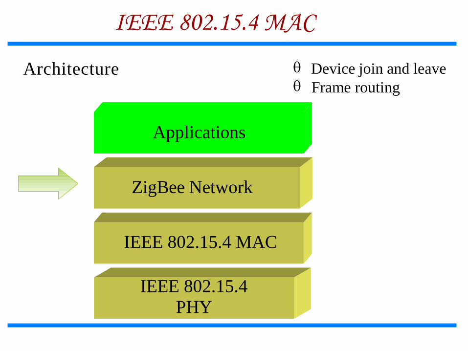
Architecture
IEEE 802.15.4 MAC
IEEE 802.15.4 MAC
Applications
ZigBee Network
IEEE 802.15.4
PHY
Device join and leave Frame routing

General characteristics
Approaches for low power
In order to achieve the low power and low cost goals
established by IEEE 802.15.4 the following approaches
are taken
Reduce the amount of data transmitted
Reduce the transceiver duty cycle and frequency of data
transmissions
Reduce the frame overhead
Reduce complexity
Reduce range
Implement strict power management mechanisms (power-
down and sleep modes)

Network layer
The services which network layer provides are more
challenging to implement because of low power
consumption requirement.
Network layer over this standard are expected to be self
configuring and self maintaining to minimize total cost of
user.
IEEE 802.15.4 draft standard supports multiple network
topologies including star and peer to peer topology.
topology selection is application dependent. PC peripherals
may require low latency connection of star topology while
perimeter security which needs large coverage area may
require peer to peer networking.
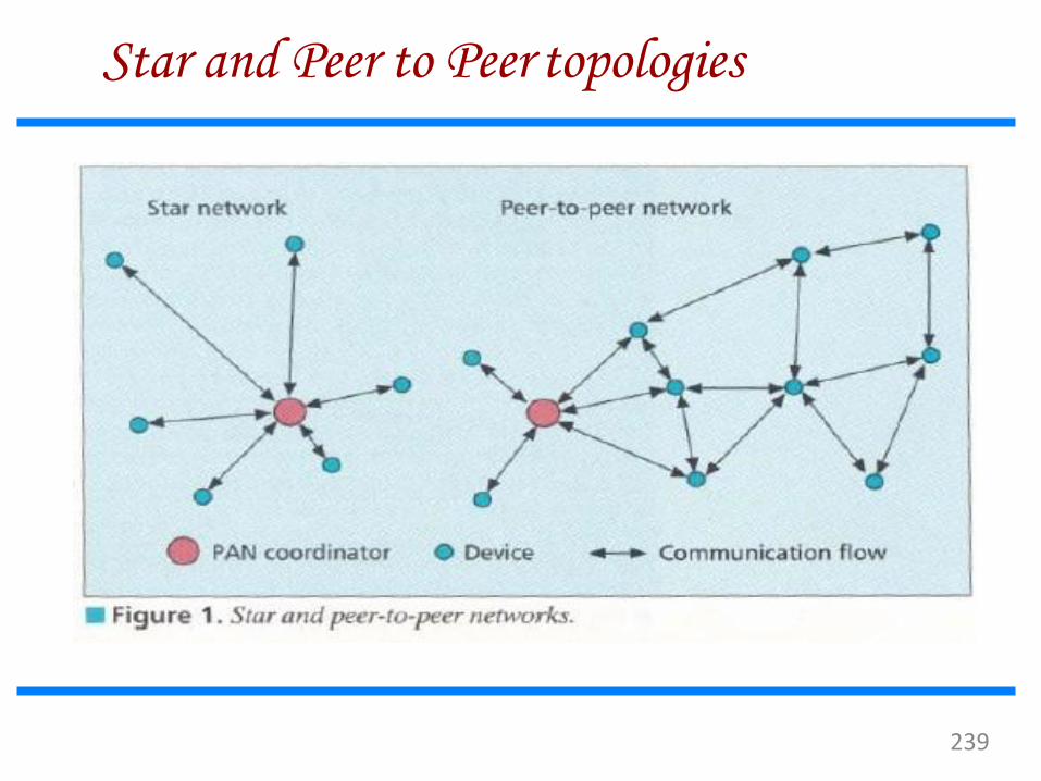
Star and Peer to Peer topologies
239
MAC
MAC provides data and management services to upper
layers
The MAC management service has 26 primitives
whereas 802.15.1 has about 131 primitives and 32
events,
802.15.4 MAC is of very low complexity, making it very
suitable for its intended low-end applications, albeit at
the cost of a smaller feature set than 802.15.1 (e.g.,
802.15.4 does not support synchronous voice links).
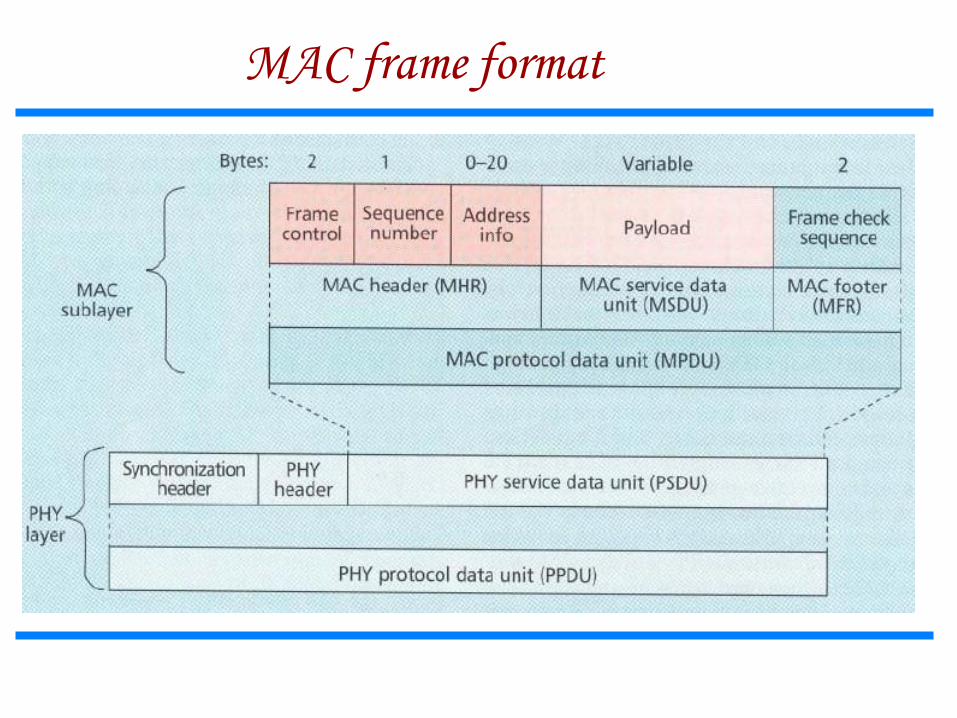
MAC frame format
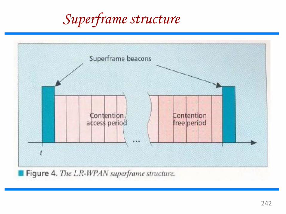
Superframe structure
242
Other MAC features
I n a beacon-enabled network with superframes, a slotted carrier
sense multiple access with collision avoidance (CSMA- CA)
mechanism is used.
I n others standard CSMA-CA is used I.e it first checks if
another device is transmitting in the same channel if so backs
off for certain time.
MAC confirms successful reception of data with an
acknowledgement.
The IEEE 802.15.4 draft standard provides for three levels of
security: no security of any type ,access control lists (non
cryptographic security) and symmetric key security, employing
AES-128.
PHY layer
This standard provides 2 PHY options with
frequency band as fundamental difference.
2.4 GHz band has worldwide availability and
provides a transmission rate of 250 kb/s.
The 868/915 MHz PHY specifies operation in the 868
MHz band in Europe and 915 MHz ISM band in the
United States and offer data rates 20 kb/s and 40 kb/s
respectively.
Different transmission rates can be exploited to
achieve a variety of different goals.

Channel structure
245

Channelization
2 7 frequency channels are available across all the 3 bands.
This standard includes the necessary things to implement
dynamic channel selection to avoid interference.
The PHY layers contain several lower-level functions, such
as receiver energy detection, link quality indication, and
channel switching, which enable channel assessment.
These functions are used by the network to establish its
initial operating channel and to change channels in
response to a prolonged outage.

PHY layer packet structure
247
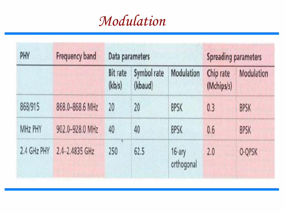
Modulation

Interference
Interference is common in 2.4 GHz band because of
other services operating in that band
IEEE 802.15.4 applications have low QOS
requirements and may need to perform multiple
retries for packet transmissions on interference.
Since IEEE 802.15.4 devices may be sleeping as
much as 99.9 percent of the time they are
operational, and employ low-power spread spectrum
transmissions, they should be among the best of
neighbors in the 2.4 GHz band.
249
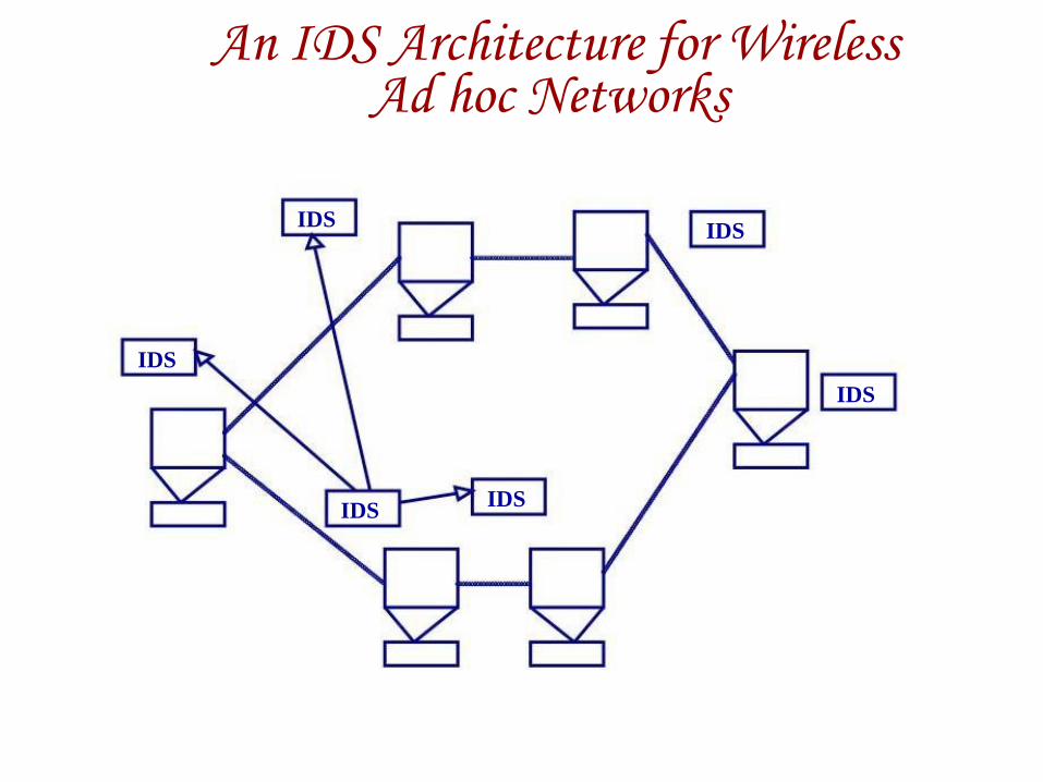
An IDS Architecture for Wireless Ad hoc Networks
IDS
IDS
IDS
IDS
IDS
IDS

Summing up Wireless & Mobile
Technology……
ANY ONE ANY DEVICE
ANY TIME
ANY WHERE
No limit. It ‘s
beyond
the sky?
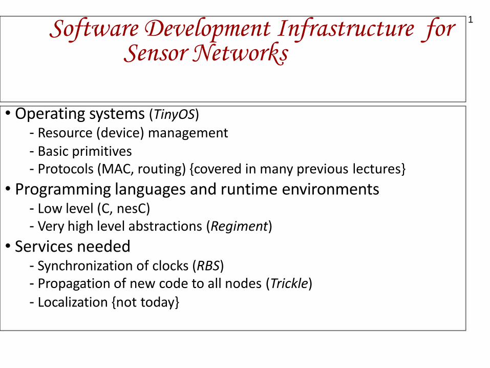
1
Software Development Infrastructure for Sensor Networks
• Operating systems (TinyOS) - Resource (device) management - Basic primitives - Protocols (MAC, routing) {covered in many previous lectures}
• Programming languages and runtime environments - Low level (C, nesC) - Very high level abstractions (Regiment)
• Services needed - Synchronization of clocks (RBS) - Propagation of new code to all nodes (Trickle)
- Localization {not today}
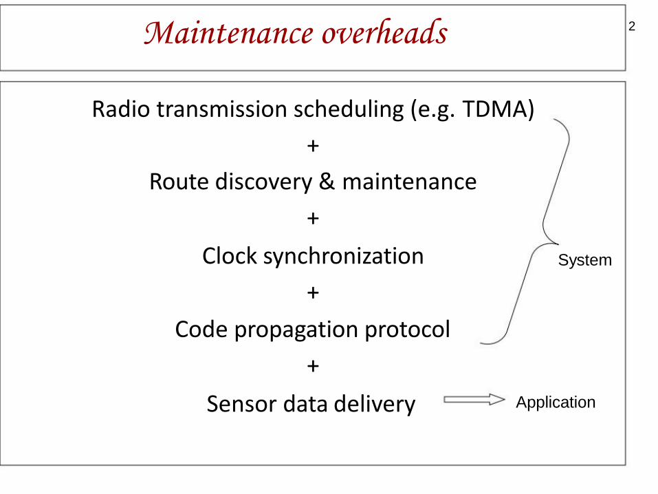
Maintenance overheads
System
Radio transmission scheduling (e.g. TDMA)
+
Route discovery & maintenance
+
Clock synchronization
+
Code propagation protocol
+
Application
2
Sensor data delivery
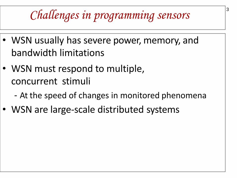
Challenges in programming sensors
• WSN usually has severe power, memory, and bandwidth limitations
• WSN must respond to multiple, concurrent stimuli
- At the speed of changes in monitored phenomena
• WSN are large-scale distributed systems
3
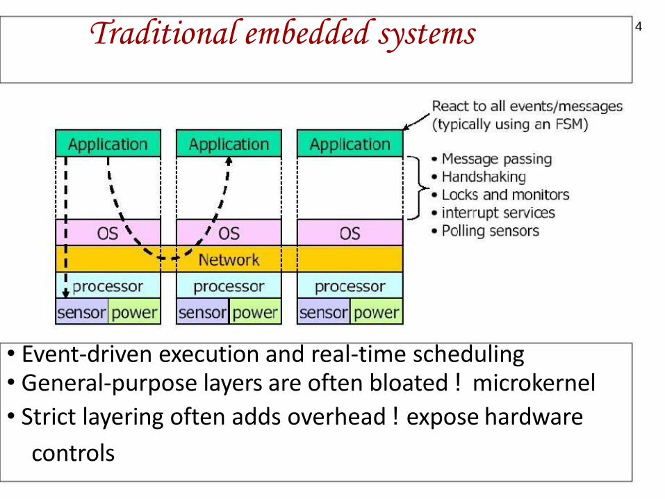
Traditional embedded systems
• Event-driven execution and real-time scheduling • General-purpose layers are often bloated ! microkernel
• Strict layering often adds overhead ! expose hardware
controls
4

UNIT -V

Operating System-Tiny OS

Operating System-Tiny OS •Started out as a research project at Berkeley
•Now probably the de facto platform
•Overarching goal: conserving resources
•No file system
•No dynamic memory allocation
•No memory protection
•Very simple task model
•Minimal device and networking abstractions
•Application and OS are coupled—composed into one image

Tiny OS components
• Components: reusable building blocks
• Each component is specified by a set of interfaces
- Provide “hooks” for wiring components together
• A component C can provide an interface
- C must implement all commands available through
- Commands are methods exposed to an upper layer
• An upper layer can call a command
• A component C can use an interface - C must implement all events that can be signaled by
- These are methods available to a lower layer

Component specification
module TimerModule {
provides {
interface StdControl;
interface Timer01;
}
interface StdControl {
command result_t init();
command result_t start();
command result_t stop();
}
uses interface Clock as Clk; } …
TimerModule
interface Timer01 {
command result_t start(char type, uint32_t interv
command result_t stop();
event result_t timer0Fire();
event result_t timer1Fire(); }
interface Clock { command result_t setRate(char interval, charsca
event result_t fire();
}
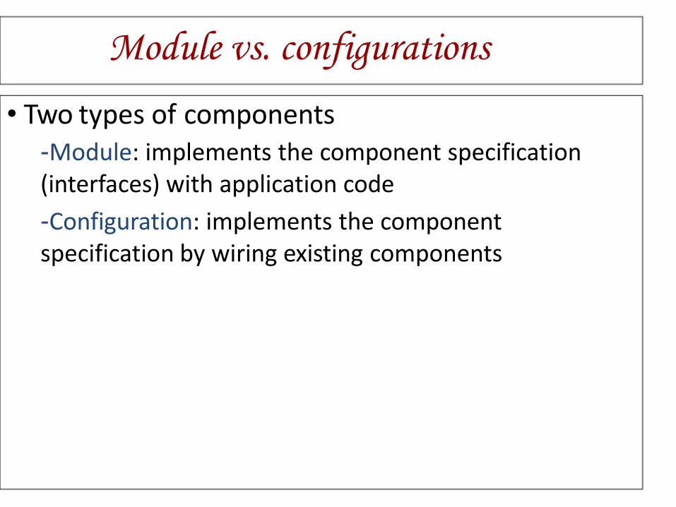
Module vs. configurations
• Two types of components -Module: implements the component specification (interfaces) with application code
-Configuration: implements the component specification by wiring existing components
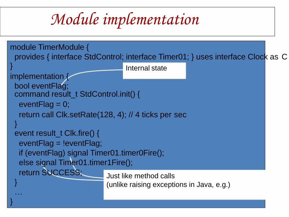
Module implementation
module TimerModule {
provides { interface StdControl; interface Timer01; } uses interface Clock as C
Internal state }
implementation {
bool eventFlag; command result_t StdControl.init() {
eventFlag = 0;
return call Clk.setRate(128, 4); // 4 ticks per sec } event result_t Clk.fire() {
eventFlag = !eventFlag;
if (eventFlag) signal Timer01.timer0Fire();
else signal Timer01.timer1Fire();
return SUCCESS;
}
…
}
Just like method calls
(unlike raising exceptions in Java, e.g.)
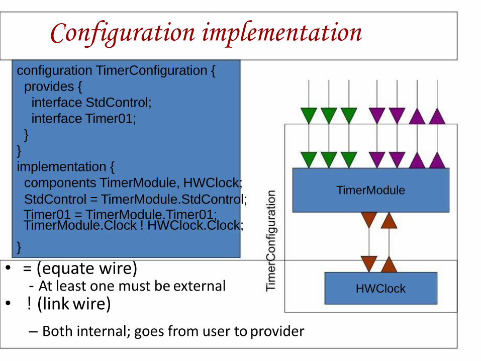
Configuration implementation configuration TimerConfiguration {
provides {
interface StdControl;
interface Timer01;
}
}
implementation {
components TimerModule, HWClock;
StdControl = TimerModule.StdControl; Timer01 = TimerModule.Timer01; TimerModule.Clock ! HWClock.Clock;
}
• = (equate wire) - At least one must be external
• ! (link wire)
– Both internal; goes from user to provider
TimerModule
HWClock

FieldMonitor example
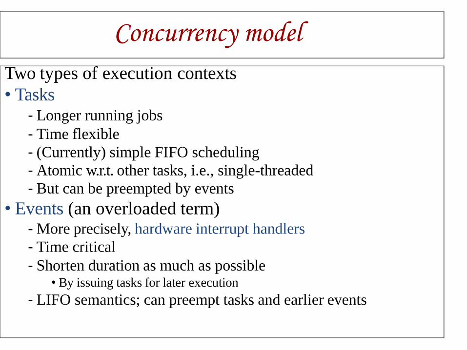
Concurrency model
Two types of execution contexts
• Tasks - Longer running jobs
- Time flexible
- (Currently) simple FIFO scheduling
- Atomic w.r.t. other tasks, i.e., single-threaded
- But can be preempted by events
• Events (an overloaded term) - More precisely, hardware interrupt handlers
- Time critical
- Shorten duration as much as possible • By issuing tasks for later execution
- LIFO semantics; can preempt tasks and earlier events

Tasks
implementation { task void TaskName() { …
}
… … { … post TaskName(); …
}
}
• A task is always posted for later execution; control returns to poster immediately
• Scheduler supports a bounded queue of pending tasks
- Node sleeps when the queue is empty
• For simplicity, tasks don’t take args and don’t return values
• Typical use
- Event necessitates further processing
• Wrap it up in a task
- Event handler simply posts the task and can return immediately

Execution example
Task queue
Task B
Event 1
Task A
Event 3
Event 2
Task B …
Task C
Hardware interrupts
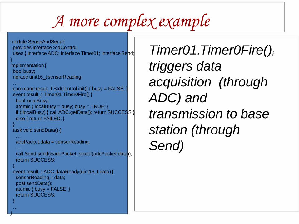
A more complex example module SenseAndSend { provides interface StdControl; uses { interface ADC; interface Timer01; interface Send;
} implementation { bool busy; norace unit16_t sensorReading; … command result_t StdControl.init() { busy = FALSE; } event result_t Timer01.Timer0Fire() {
bool localBusy; atomic { localBusy = busy; busy = TRUE; } if (!localBusy) { call ADC.getData(); return SUCCESS;}
else { return FAILED; } } task void sendData() { … adcPacket.data = sensorReading; …
call Send.send(&adcPacket, sizeof(adcPacket.data));
return SUCCESS; } event result_t ADC.dataReady(uint16_t data) {
sensorReading = data; post sendData(); atomic { busy = FALSE; } return SUCCESS;
}
… }
Timer01.Timer0Fire()}
triggers data
acquisition (through
ADC) and
transmission to base
station (through
Send)
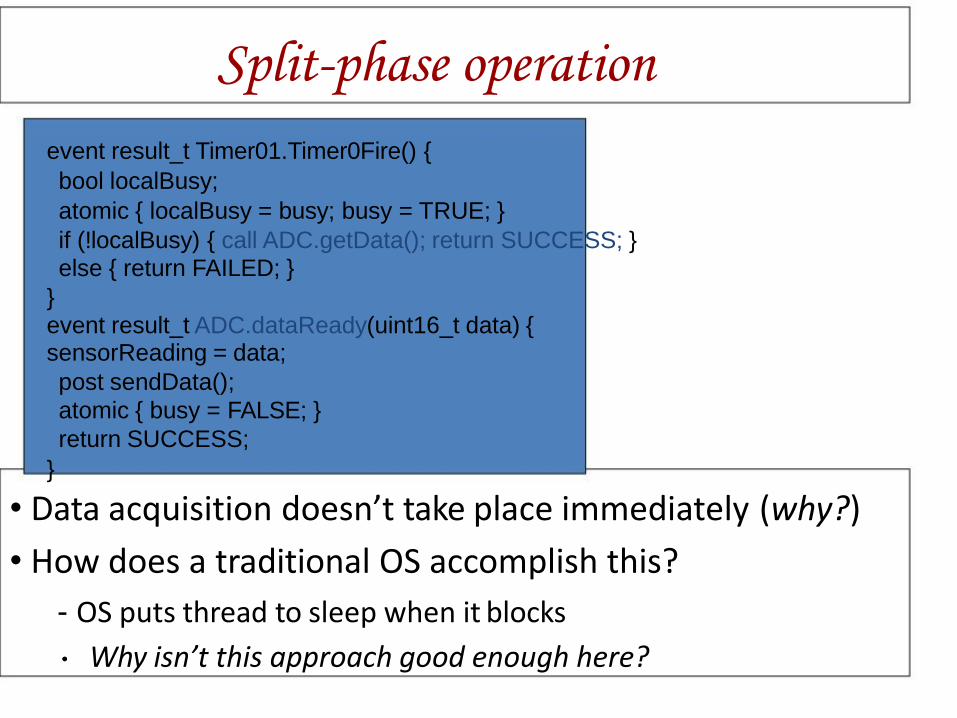
Split-phase operation
event result_t Timer01.Timer0Fire() {
bool localBusy;
atomic { localBusy = busy; busy = TRUE; }
if (!localBusy) { call ADC.getData(); return SUCCESS; } else { return FAILED; }
} event result_t ADC.dataReady(uint16_t data) { sensorReading = data;
post sendData();
atomic { busy = FALSE; }
return SUCCESS;
}
• Data acquisition doesn’t take place immediately (why?)
• How does a traditional OS accomplish this?
- OS puts thread to sleep when it blocks
Why isn’t this approach good enough here?
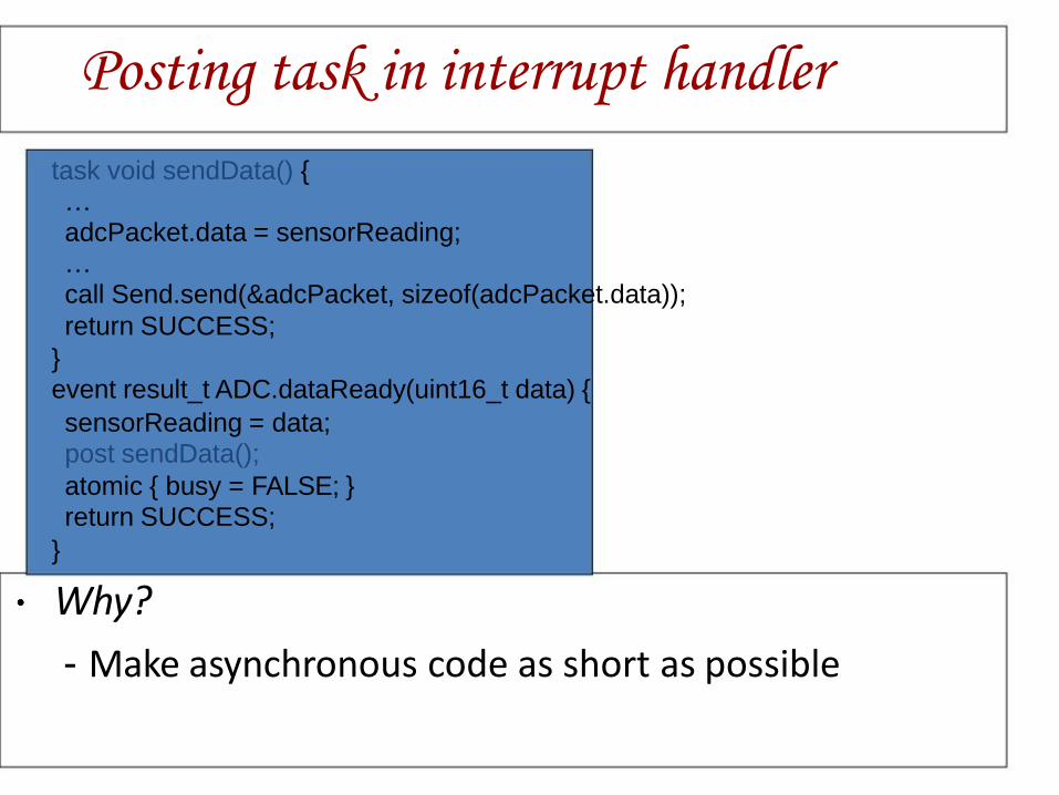
Posting task in interrupt handler
task void sendData() { … adcPacket.data = sensorReading; … call Send.send(&adcPacket, sizeof(adcPacket.data));
return SUCCESS;
} event result_t ADC.dataReady(uint16_t data) {
sensorReading = data; post sendData();
atomic { busy = FALSE; } return SUCCESS;
}
Why?
- Make asynchronous code as short as possible

Race conditions
• Because of preemption, race conditions may arise on shared data
- nesC compiler can detect them, but with false positives
• In case of false positive, declare shared variable with norace keyword
• In case of real race conditions, use atomic to make code blocks non-preemptible
bool busy;
norace unit16_t sensorReading;
…
event result_t Timer01.Timer0Fire() {
bool localBusy;
atomic { localBusy = busy; busy = TRUE; }
if (!localBusy) { call ADC.getData(); return SUCCES
else { return FAILED; } }
task void sendData() {
…
adcPacket.data = sensorReading;
…
call Send.send(&adcPacket, sizeof(adcPacket.data
return SUCCESS;
}
event result_t ADC.dataReady(uint16_t data) {
sensorReading = data;
post sendData();
atomic { busy = FALSE; }
return SUCCESS;
}
Discussion
•Provides framework for concurrency and
modularity
•Interleaves flows, events, energy management
•Never poll, never block
•Trade off flexibility for more optimization
opportunities
Still a node-level platform