500043, Hyderabad - IARE
436
LINEAR ALGEBRA AND CALCULUS(LAC) B.TECH ISEM FRESHMAN ENGINEERING Ms. L Indira Associate Professor 1 INSTITUTE OF AERONAUTICAL ENGINEERING (Autonomous) Dundigal – 500043, Hyderabad
-
Upload
khangminh22 -
Category
Documents
-
view
3 -
download
0
Transcript of 500043, Hyderabad - IARE

LINEAR ALGEBRA AND CALCULUS(LAC)
B.TECH ISEM
FRESHMAN ENGINEERING
Ms. L IndiraAssociate Professor
1
INSTITUTE OF AERONAUTICAL ENGINEERING
(Autonomous)Dundigal – 500043, Hyderabad

CONTENTS
2
THEORY OF MATRICES
FUNCTIONS OF SINGLE AND SEVERAL VARIABLES
HIGHER ORDER DIFFERENTIAL EQUATIONS
MULTIPLE INTEGRALS
VECTOR CALCULUS

TEXT BOOKS
3
1. B.S. Grewal, Higher Engineering Mathematics, Khanna Publishers, 36th
Edition, 2010.
2. N.P. Bali and Manish Goyal, A text book of Engineering Mathematics, Laxmi
Publications, Reprint, 2008.
3. Ramana B.V., Higher Engineering Mathematics, Tata McGraw Hill New Delhi,
11th Reprint, 2010.

REFERENCE BOOKS
1. Erwin Kreyszig, Advanced Engineering Mathematics, 9thEdition, John Wiley & Sons, 2006.
2. Veerarajan T., Engineering Mathematics for first year, TataMcGraw-Hill, New Delhi, 2008.
3. D. Poole, Linear Algebra: A Modern Introduction, 2ndEdition, Brooks/Cole, 2005.
4. Dr. M Anita, Engineering Mathematics-I, Everest PublishingHouse, Pune, First Edition, 2016.
4
MODULE -ITHEORY OF MATRICES
5

THEORY OF MATRICES
6

THEORY OF MATRICES
7

THEORY OF MATRICES
8

THEORY OF MATRICES
9

THEORY OF MATRICES
10

THEORY OF MATRICES
11

THEORY OF MATRICES
12

THEORY OF MATRICES
13

THEORY OF MATRICES
14

THEORY OF MATRICES
15

THEORY OF MATRICES
16

THEORY OF MATRICES
17

THEORY OF MATRICES
18

THEORY OF MATRICES
19

THEORY OF MATRICES
20
THEORY OF MATRICES
21
THEORY OF MATRICES
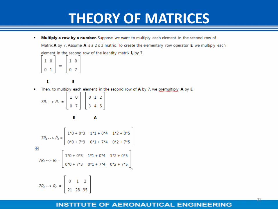
22

THEORY OF MATRICES
23

THEORY OF MATRICES
24

THEORY OF MATRICES
25

THEORY OF MATRICES
26

THEORY OF MATRICES
27

THEORY OF MATRICES
28

THEORY OF MATRICES
29

THEORY OF MATRICES
30

THEORY OF MATRICES
31

THEORY OF MATRICES
32

THEORY OF MATRICES
33

THEORY OF MATRICES
34

THEORY OF MATRICES
35

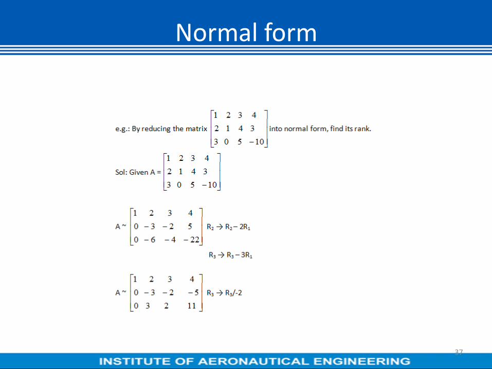
Normal form
36
Normal form
37

Normal form
38

Inverse of a matrix by Gauss-Jordhan method
Normal form
39
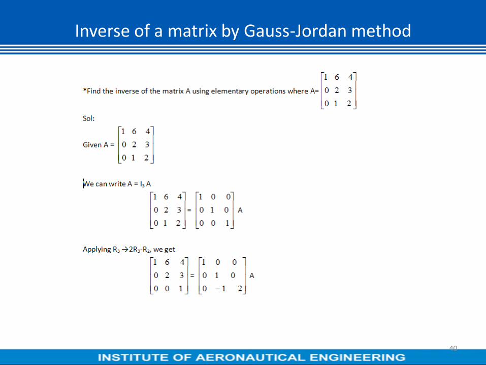
Inverse of a matrix by Gauss-Jordan method
40

Inverse of a matrix by Gauss-Jordan method
41

Inverse of a matrix by Gauss-Jordan method
42

Inverse of a matrix by Gauss-Jordan method
43
Inverse of a matrix by Gauss-Jordan method
44

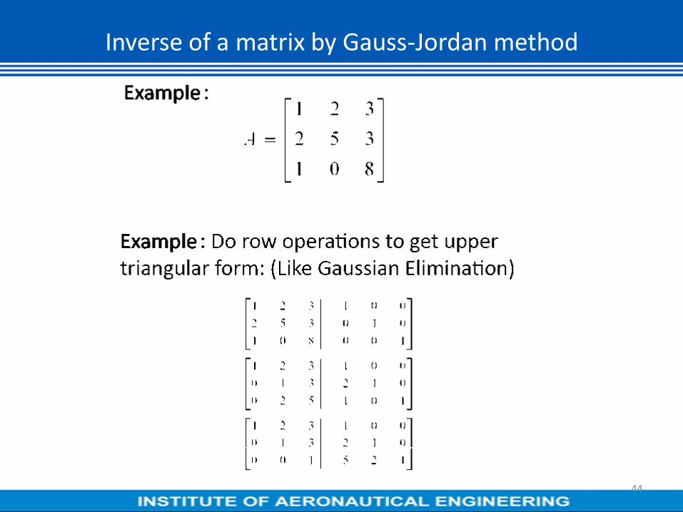
Inverse of a matrix by Gauss-Jordan method
45
Inverse of a matrix by Gauss-Jordan method
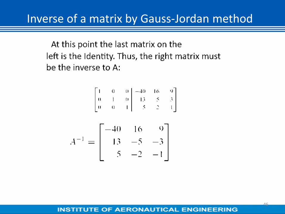
46
Inverse of a matrix by Gauss-Jordan method
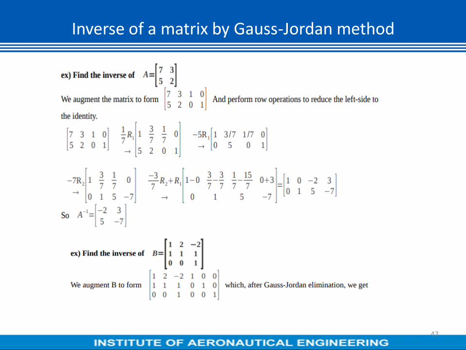
47

THEORY OF MATRICES
Inverse of a matrix by Gauss-Jordan method
48

Eigen values and Eigen vectors of a matrix
49

Eigen values and Eigen vectors of a matrix
50

Eigen values and Eigen vectors of a matrix
51

Eigen values and Eigen vectors of a matrix
52

Eigen values and Eigen vectors of a matrix
53

Eigen values and Eigen vectors of a matrix
54

Eigen values and Eigen vectors of a matrix
55

Eigen values and Eigen vectors of a matrix
56

Eigen values and Eigen vectors of a matrix
57

Eigen values and Eigen vectors of a matrix
58

Eigen values and Eigen vectors of a matrix
59

Properties of Eigen values and Eigen vectors of real and complex matrices
60

Properties of Eigen values and Eigen vectors of real and complex
matrices
61

Properties of Eigen values and Eigen vectors of real and complex matrices
62

Properties of Eigen values and Eigen vectors of real and complex matrices
63

Properties of Eigen values and Eigen vectors of real and complex matrices
64

Properties of Eigen values and Eigen vectors of real and complex matrices
65

Properties of Eigen values and Eigen vectors of real and complex matrices
66

Properties of Eigen values and Eigen vectors of real and complex matrices
67

Properties of Eigen values and Eigen vectors of real and complex matrices
68

Properties of Eigen values and Eigen vectors of real and complex matrices
0
0
0
000
510
432
,3
3
2
1
x
x
x
becomesFor
X =
2
10
19
X is the Eigen vector corresponding to 3
Eigen values of A –1are
1 1 11, ,
2 3E ig en va lu es o f A a re
We know Eigen vectors of A –1 are same as Eigen vectors of A.
69

Cayley-Hamilton theorem
70

Cayley-Hamilton theorem
71

Cayley-Hamilton theorem
72

Cayley-Hamilton theorem
73

Cayley-Hamilton theorem
74

Cayley-Hamilton theorem
75
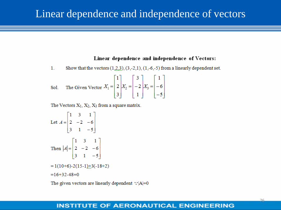
Linear dependence and independence of vectors
76

Linear dependence and independence of vectors
77

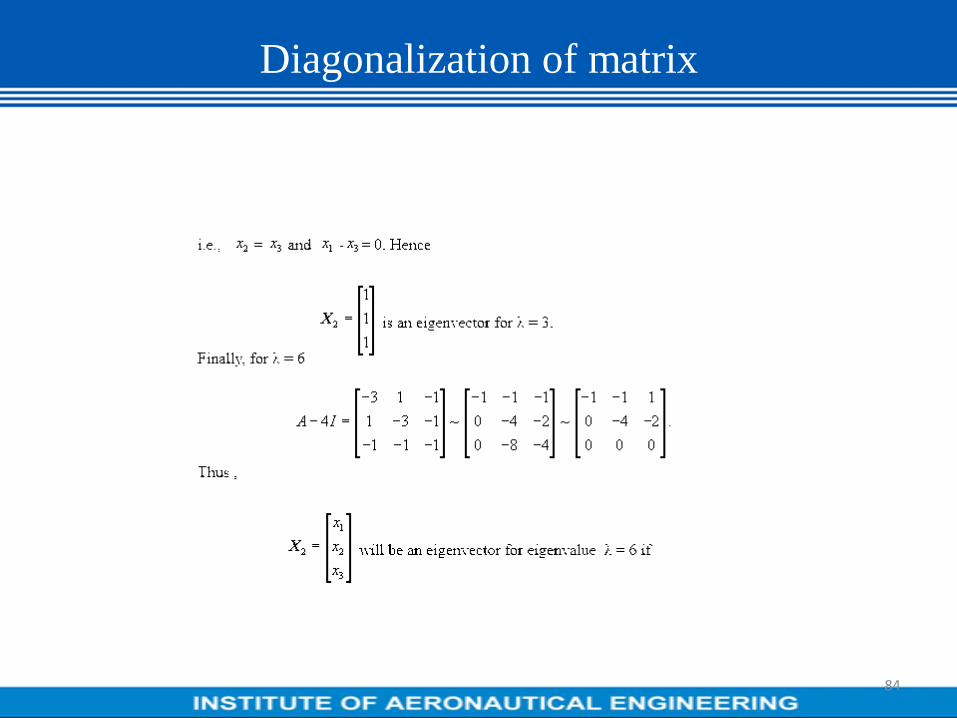
Diagonalization of matrix
78

Diagonalization of matrix
79

Diagonalization of matrix
80

Diagonalization of matrix
81

Diagonalization of matrix
82

Diagonalization of matrix
83
Diagonalization of matrix
84

Diagonalization of matrix
85

Diagonalization of matrix
86

MODULE-IIFUNCTIONS OF SINGLE AND SEVERAL
VARIABLES
87

CONTENTS
• Rolle’s mean value theorem
• Geometric representation of Rolle’s mean value theorem
• Applications of Rolle’s mean value theorem
88

OBJECTIVE AND OUTCOME
OBJECTIVE:
Rolle’s mean value theorem.
OUTCOME:Student get to understand the concept of Rolle’s mean value theorem and its
applications.
89

Statement of Rolle ’s Mean Value Theorem
Let f(x) be a function defined in [a,b] such that
(i) f(x) It is continuous in closed interval [a,b]
(ii) f(x) is differentiable in open interval (a,b) and
(iii) f(a) = f(b).
Then there exists at least one point ‘c’ in (a,b) such that f1(c) = 0.
90

Geometrical Representation of Rolle ’s Mean Value Theorem
Let Rbaf ],[:
be a function satisfying the three conditions of Rolle’s theorem.
Then the graph drawn is as follows
Geometrically Rolles mean value theorem means the following
1. y=f(x) in a continuous curve in [a,b].
2. There exist a unique tangent line at every point x=c, where a<c<b
3. The ordinates f(a), f(b) at the end points A,B are equal so that the points A and B are
equidistant from the X-axis.
By Rolle’s Theorem, There is at least one point x=c between A and B on the curve at which
the tangent line is parallel to the x-axis and also it is parallel to chord of the curve.
91

Applications of Rolle ’s Mean Value Theorem
Example 1. Verify Rolle‟s theorem for the function f(x) = sinx/ex or e
-x sinx in [0,π]
Sol: i) Since sinx and ex are both continuous functions in [0, π].
Therefore, sinx/ex is also continuous in [0,π].
ii) Since sinx and ex be derivable in (0,π), then f is also derivable in (0,π).
iii) f(0) = sin0/e0 = 0 and f(π)= sin π/e
π =0
f(0) = f(π)
Thus all three conditions of Rolle’s theorem are satisfied.
There exists c є(0, π) such that f1(c)=0
Now xx
xx
e
xx
e
exxexf
sincos
)(
sincos)(
2
1
f1(c)= 0 => 0
sincos
ce
cc
cos c = sin c => tan c = 1
c = π/4 є(0,π)
Hence Rolle’s theorem is verified.
92

Applications of Rolle ’s Mean Value Theorem Contd.,
Example 2. Verify Rolle‟s theorem for the functions 2
lo g
x a b
x ( a b ) in[a,b] , a>0, b>0,
Sol: Let f(x)= 2
lo g
x a b
x ( a b )
= log(x2+ab) – log x –log(a+b)
(i). Since f(x) is a composite function of continuous functions in [a,b], it is continuous in [a,b].
(ii). f1(x) =
)(
12.
1
2
2
2abxx
abx
xx
abx
f1(x) exists for all xє (a,b)
(iii). f(a) = 01loglog2
2
aba
aba
f(b) = 01loglog2
2
abb
abb
f(a) = f(b)
Thus f(x) satisfies all the three conditions of Rolle’s theorem.
So, c (a, b) f1(c) = 0,
f1(c) = 0,
2
2
c a b
c( c a b )
= 0 c2 = ab
),( baabc
Hence Rolle’s theorem verified.
93

Applications of Rolle ’s Mean Value Theorem Contd.,
Example 3. Verify whether Rolle ‟s Theorem can be applied to the following functions in the
intervals.
i) f(x) = tan x in[0 , π] and ii) f(x) = 1/x2 in [-1,1]
(i) f(x) is discontinuous at x = π/2 as it is not defined there. Thus condition (i) of Rolle ’s
Theorem is not satisfied. Hence we cannot apply Rolle ’s Theorem here.
Rolle’s theorem cannot be applicable to f(x) = tan x in [0,π].
(ii). f(x) = 1/x2 in [-1,1]
f(x) is discontinuous at x= 0.
Hence Rolle ’s Theorem cannot be applied.
94

Applications of Rolle ’s Mean Value Theorem Contd.,
Example 4. Using Rolle ‟s Theorem, show that g(x) = 8x3-6x
2-2x+1 has a zero between
0 and 1.
Sol: g(x) = 8x3-6x
2-2x+1 being a polynomial, it is continuous on [0,1] and differentiable on (0,1)
Now g(0) = 1 and g(1)= 8-6-2+1 = 1
Also g(0)=g(1)
Hence, all the conditions of Rolle’s theorem are satisfied on [0,1].
Therefore, there exists a number cє(0,1) such that g1(c)=0.
Now g1(x) = 24x
2-12x-2
g1(c)= 0 => 24c
2-12c-2 =0
c= ie12
213 c= 0.63 or -0.132
only the value c = 0.63 lies in (0,1)
Thus there exists at least one root between 0 and 1.
95

Applications of Rolle ’s Mean Value Theorem Contd.,
Example 5. Verify Rolle‟s theorem for f(x) = x 2/3
-2x 1/3
in the interval (0,8).
Sol: Given f(x) = x 2/3
-2x 1/3
f(x) is continuous in [0,8]
f1(x) = 2/3 . 1/x
1/3 -2/3 . 1/x
2/3 = 2/3(1/x
1/3 – 1/x
2/3)
Which exists for all x in the interval (0,8)
f is derivable (0,8).
Now f(0) = 0 and f(8) = (8)2/3
-2(8)1/3
= 4-4 =0
i.e., f(0) = f(8)
Thus all the three conditions of Rolle’s Theorem are satisfied.
There exists at least one value of c in(0,8) such that f1(c)=0
ie. 011
3
2
3
1
cc
=> c = 1 є (0,8)
Hence Rolle’s Theorem is verified.
96

Applications of Rolle ’s Mean Value Theorem Contd.,
Example 6. Verify Rolle‟s theorem for f(x) = x(x+3)e-x/2
in [-3,0].
Sol: - (i). Since x(x+3) being a polynomial is continuous for all values of x and e-x/2
is also
continuous for all x, their product x(x+3)e-x/2
= f(x) is also continuous for every value of x and in
particular f(x) is continuous in the [-3,0].
(ii). we have f1(x) = x(x+3)( -1/2 e
-x/2)+(2x+3)e
-x/2
= e-x/2
[2x+3-2
32
xx ]
=e-x/2
[6+x-x2/2]
Since f1(x) does not become infinite or indeterminate at any point of the interval(-3,0).
f(x) is derivable in (-3,0)
97

Applications of Rolle ’s Mean Value Theorem Contd.,
(i) Also we have f(-3) = 0 and f(0) =0
f (-3)=f(0)
Thus f(x) satisfies all the three conditions of Rolle’s theorem in the interval [-3,0].
Hence there exist at least one value c of x in the interval (-3,0) such that f1(c)=0
i.e., ½ e-c/2
(6+c-c2)=0 =>6+c-c
2=0 (e
-c/2≠0 for any c)
=> c2+c-6 = 0 => (c-3)(c+2)=0
c=3,-2
Clearly, the value c= -2 lies within the (-3,0) which verifies Rolle’s theorem.
98

Applications of Rolle ’s Mean Value Theorem Contd.,Example 7.
99

CONTENTS
• Lagrange’s mean value theorem
• Geometric Representation of Lagrange’s mean value theorem
• Applications of Lagrange’s mean value theorem
100

OBJECTIVE AND OUTCOME
OBJECTIVE:
Lagrange’s mean value theorem.
OUTCOME:Student get to understand the concept of Lagrange’s mean value theorem
and its applications.
101

Statement of Lagrange ’s Mean Value Theorem
Let f(x) be a function defined in [a,b] such that
(i) f(x) is continuous in closed interval [a,b] &
(ii) f(x) is differentiable in (a,b).
Then there exists at least one point c in (a,b) such that f1(c) =
ab
afbf
)()(
102

Geometrical Representation of Lagrange ’s Mean Value Theorem
Let Rbaf ],[:
be a function satisfying the two conditions of Lagrange’s theorem.
Then the graph is as follows
Geometrically Lagrange’s mean value theorem means the following
1. y=f(x) is continuous curve in [a,b]
2. At every point x=c, when a<c<b, on the curve y=f(x), there is unique tangent to the curve. By
Lagrange’s theorem there exists at least one point ab
afbfcfbac
)()()(),(
1
Geometrically there exist at least one point c on the curve between A and B such that the tangent
line is parallel to the chord
AB
103

Applications of Lagrange ’s Mean Value Theorem
Example 1. Verify Lagrange‟s Mean value theorem for f(x) = x3-x
2-5x+3 in [0,4]
Sol: Let f(x)= x3-x
2-5x+3 is a polynomial in x.
It is continuous & derivable for every value of x.
In particular, f(x) is continuous [0,4] & derivable in (0,4)
Hence by Lagrange’s Mean value theorem c (0,4)
f1(c)=
04
)0()4(
ff
i.e., 3c2-2c-5 =
4
)0()4( ff …………………….(1)
Now f(4) = 43-4
2-5.4+3 =64-16-20-3=67-36= 31 & f(0)=3
4
)0()4( ff = 7
4
)331(
From equation (1), we have
3c2-2c-5 =7 => 3c
2-2c-12 =0
c =3
371
6
1482
6
14442
We see that 3
371 lies in open interval (0,4) & thus Lagrange’s Mean value theorem
is verified.
104

Example 2. Verify Lagrange‟s Mean value theorem for f(x) = xe
log in [1,e]
Sol: - f(x) = xe
log
This function is continuous in closed interval [1,e] & derivable in (1,e). Hence L.M.V.T is
applicable here. By this theorem, a point c in open interval (1,e) such that
f1(c) =
1
1
1
01
1
)1()(
eee
fef
But f1(c)=
1
11
1
1
ece
c = e - 1
Note that (e-1) is in the interval (1,e).
Hence Lagrange’s mean value theorem is verified.
Applications of Lagrange ’s Mean Value Theorem Contd.,
105

Example 3. Give an example of a function that is continuous on [-1, 1] and for which mean
value theorem does not hold with explanations.
Sol:- The function f(x) = x is continuous on [-1,1]
But Lagrange Mean value theorem is not applicable for the function f(x) as its derivative
does not exist in (-1,1) at x=0.
Applications of Lagrange ’s Mean Value Theorem Contd.,
106

Example 4. If a<b, P.T 2
11
211 a
abaTanbTan
b
ab
using Lagrange‟s Mean
value theorem. Deduce the following.
i). 6
1
43
4
25
3
4
1
Tan
ii). 4
22
20
45 1
Tan
Sol: consider f(x) = Tan-1
x in [a,b] for 0<a<b<1
Since f(x) is continuous in closed interval [a,b] & derivable in open interval
(a,b).
We can apply Lagrange’s Mean value theorem here.
Applications of Lagrange ’s Mean Value Theorem Contd.,
107

Hence there exists a point c in (a,b)
f1(c) =
ab
afbf
)()(
Here f1(x) =
2
1
21
1)(&
1
1
ccfhence
x
Thus c, a<c<b
ab
aTanbTan
c
11
21
1 ------- (1)
We have 1+a2<1+c
2<1+b
2
2221
1
1
1
1
1
bca
……….. (2)
From (1) and (2), we have
2
11
21
1
1
1
bab
aTanbTan
a
or
2
11
211 b
abaTanbTan
a
ab
………………(3)
Hence the result
Applications of Lagrange ’s Mean Value Theorem Contd.,
108

Deductions: -
(i) We have 2
11
211 a
abaTanbTan
b
ab
Take
3
4b & a=1, we
get
6
1
4)
3
4(
425
3 1
Tan
(ii) Taking b=2 and a=1, we get
1 1 1
2 2
2 1 2 1 1 12 1 2
1 2 1 1 5 4 2
T a n T a n T a n
4
22
45
1 1
Tan
14 5 22
2 0 4
T a n
2
3
34
4)
3
4(
9
25
3
34
11
13
4
)1()3
4(
9
161
13
4
1
2
11
TanTanTan
Applications of Lagrange ’s Mean Value Theorem Contd.,
109

Example 5. Show that for any x > 0, 1 + x < ex
< 1 + xex.
Sol: - Let f(x) = ex defined on [0,x]. Then f(x) is continuous on [0,x] & derivable on (0,x).
By Lagrange’s Mean value theorem a real number c є(0,x) such that
)(0
)0()( 1cf
x
fxf
x 0 x
c ce -e e -1= e = e
x -0 x ………….(1)
Note that 0<c<x => e0<e
c<e
x ( e
x is an increasing function)
=> x
x
ex
e
11 From (1)
=> x<ex-1<xe
x
=> 1+x<ex<1+xe
x.
Applications of Lagrange ’s Mean Value Theorem Contd.,
110

Example 6. Calculate approximately 5
2 4 5 by using L.M.V.T.
Sol:- Let f(x) = 5x =x
1/5 & a=243 , b=245
Then f1(x) = 1/5 x
- 4/5 & f
1(c) = 1/5c
- 4/5
By L.M.V.T, we have
)()()( 1
cfab
afbf
=> 5
4
5
1
243245
)243()245(
c
ff
=> f (245) =f(243)+2/5c-4/5
=> c lies b/w 243 & 245 take c= 243
=> 5245 = (243)
1/5 +2/5(243)
-4/5 = 5
4
55
1
5)3(
5
2)3(
= 3+ (2/5)(1/81) = 3+2/405 = 3.0049
Applications of Lagrange ’s Mean Value Theorem Contd.,
111

Example 7. Find the region in which f(x) = 1-4x-x2 is increasing & the region in which
it is decreasing using M.V.T.
Sol: - Given f(x) = 1-4x-x2
f(x) being a polynomial function is continuous on [a,b] & differentiable on (a,b) a,b
R
f satisfies the conditions of L.M.V.T on every interval on the real line.
f1(x)= - 4-2x= -2(2+x) xR
f1(x)= 0 if x = -2
for x<-2, f1(x) >0 & for x>-2 , f
1(x)<0
Hence f(x) is strictly increasing on (-∞, -2) & strictly decreasing on (-2,∞)
Applications of Lagrange ’s Mean Value Theorem Contd.,
112

Example 8. Using Mean value theorem prove that Tan x > x in 0<x</2
Sol:- Consider f(x) = Tan x in x, where 0< <x</2
Apply L.M.V.T to f(x)
a points c such that 0< <c<x</2 such that
c
x
TanxTan 2sec
c )sec -(x =Tan -Tan x
2
xxxTanthenTake
2sec00
But sec2c>1.
Hence Tan x > x
Applications of Lagrange ’s Mean Value Theorem Contd.,
113

Example 9. If f1(x) = 0 Through out an interval [a,b], prove using M.V.T f(x) is a
constant in that interval.
Sol:- Let f(x) be function defined in [a,b] & let f1(x) = 0 x in [a,b].
Then f1(t) is defined & continuous in [a,x] where axb.
& f(t) exist in open interval (a,x).
By L.M.V.T a point c in open interval (a,x)
)(
)()( 1cf
ax
afxf
But it is given that f1(c) = 0
0 = f(a)-f(x)
x f(a)=f(x)
Hence f(x) is constant.
Applications of Lagrange ’s Mean Value Theorem Contd.,
114

CONTENTS
• Cauchy’ s Mean value theorem
• Applications of Cauchy’ s Mean value theorem
115

OBJECTIVE AND OUTCOME
OBJECTIVE:Cauchy’ s Mean value theorem.
OUTCOME:Student get to understand the concept of Cauchy’ s Mean value theorem
and its applications.
116

Statement of Cauchy ’s Mean Value Theorem
If f: [a,b] R, g:[a,b] R are any two functions such that
(i) f,g are continuous on [a,b]
(ii) (ii) f,g are differentiable on (a,b)
thenbaxxgiii ),,(0)()(1
)()(
)()(
)(
)(),(int
1
1
agbg
afbf
cg
cfbacpoa
117

Applications of Cauchy ’s Mean Value Theorem
Example 1.Find c of Cauchy‟s mean value theorem for
xxgxxf
1)(&)(
in [a,b] where 0<a<b
Sol: - Clearly f, g are continuous on [a,b] R+
We have xxxgnd
xxf
2
1)(
2
1)(
11 a
which exits on (a,b)
+R b)(a,on abledifferenti are g f,
Also g1 (x)0, x (a,b) R
+
Conditions of Cauchy’s Mean value theorem are satisfied on (a,b) so c(a,b)
)(
)(
)()(
)()(
1
1
cg
cf
agbg
afbf
cabc
cc
ab
ba
ab
cc
c
ab
ab
2
2
2
1
2
1
11
Since a,b >0 , ab is their geometric mean and we have a<ab <b
c(a,b) which verifies Cauchy’s mean value theorem.
118

Applications of Cauchy ’s Mean Value Theorem Contd.,
Example 2. Verify Cauchy‟s Mean value theorem for f(x) = ex & g(x) = e
-x in [3,7] &
find the value of c.
Sol: We are given f(x) = ex & g(x) = e
-x
f(x) & g(x) are continuous and derivable for all values of x.
=>f & g are continuous in [3,7]
=> f & g are derivable on (3,7)
Also g1(x) = e
-x 0 x (3,7)
Thus f & g satisfies the conditions of Cauchy’s mean value theorem.
Consequently, a point c (3,7) such that
c
c
c
e
ee
ee
e
e
ee
ee
cg
cf
gg
ff 2
37
37
37
37
1
1
11)(
)(
)3()7(
)3()7(
=> -e7+3
= -e2c
=> 2c = 10
=> c = 5(3,7)
Hence C.M.T. is verified
119

Applications of Cauchy ’s Mean Value Theorem Contd.,
Example 3.
120

Applications of Cauchy ’s Mean Value Theorem Contd.,
121

Applications of Cauchy ’s Mean Value Theorem Contd.,
122
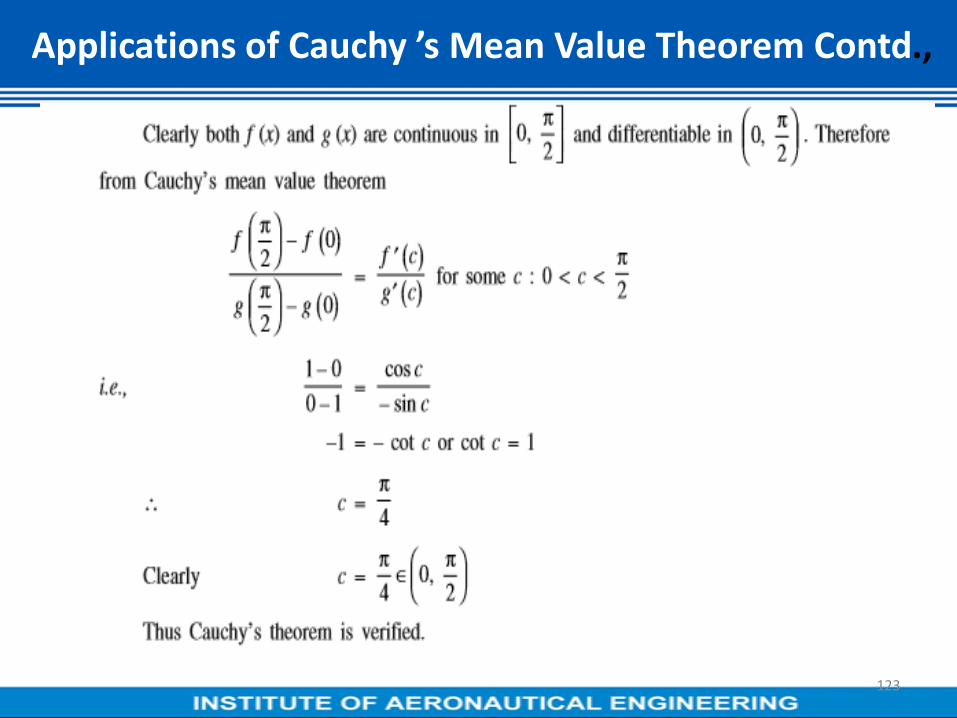
Applications of Cauchy ’s Mean Value Theorem Contd.,
123

Applications of Cauchy ’s Mean Value Theorem Contd.,
124

Applications of Cauchy ’s Mean Value Theorem Contd.,
125

CONTENTS
• Partial Differentiation
• Chain rule of Partial Differentiation
126

OBJECTIVE AND OUTCOME
OBJECTIVE:
Partial Differentiation and Chain rule of Partial Differentiation.
OUTCOME:Student get to understand the concept of Partial Differentiation and
Chain rule of Partial Differentiation.
127

Partial Differentiation
128

Applications on Partial Differentiation
129

Applications on Partial Differentiation Contd.,
130

Applications on Partial Differentiation Contd.,
131

Applications on Partial Differentiation Contd.,
132

Applications on Partial Differentiation Contd.,
133

Applications on Partial Differentiation Contd.,
134

Applications on Partial Differentiation Contd.,
135

Applications on Partial Differentiation Contd.,
136

Applications on Partial Differentiation Contd.,
137

Chain rule of Partial Differentiation
This is called as Chain rule of Partial Differentiation.
138

Applications of Chain rule of Partial Differentiation
Example 1:
139

Applications of Chain rule of Partial Differentiation contd.,
140

Applications of Chain rule of Partial Differentiation contd.,
141

Applications of Chain rule of Partial Differentiation contd.,
Example 2:
142

Applications of Chain rule of Partial Differentiation contd.,
143

Applications of Chain rule of Partial Differentiation contd.,
Example 3: ,
144

Applications of Chain rule of Partial Differentiation contd.,
Example 4:
145

Applications of Chain rule of Partial Differentiation contd.,
146

Applications of Chain rule of Partial Differentiation contd.,
147

CONTENTS
• Total derivatives of partial differentiation
• Euler’s homogeneous function
• Euler’s theorem of homogeneous function
148

OBJECTIVE AND OUTCOME
OBJECTIVE:
Total derivatives of partial differentiation, Euler’s theorem of homogeneous
function.
OUTCOME:Student get to understand the concept of Total derivatives of partial
differentiation and Euler’s theorem of homogeneous function.
149

Total derivatives of Partial Differentiation
150

Total derivatives of Partial Differentiation
151

Total derivatives of Partial Differentiation
152

Applications of Total derivatives
Example 1:
153

Applications of Total derivatives Contd.,
Example 2:
154

Applications of Total derivatives Contd.,
Example 3:
155

Applications of Total derivatives Contd.,
Example 4:
156

Euler’s Theorem of Homogeneous functions
157

Euler’s Theorem of Homogeneous functions Contd.,
158

Applications of Euler’s Theorem of Homogeneous functions
Example 1:
159

Applications of Euler’s Theorem of Homogeneous functions
Example 2:
160

Applications of Euler’s Theorem of Homogeneous functions
Example 3:
161

Applications of Euler’s Theorem of Homogeneous functions
Example 4:
162

Applications of Euler’s Theorem of Homogeneous functions
163

Applications of Euler’s Theorem of Homogeneous functions
Example 5:
164

CONTENTS
• Jacobian’s of two and three variables
• Functional dependence and Independence
165

OBJECTIVE AND OUTCOME
OBJECTIVE:
Jacobian’s of two and three variables , Functional Dependence and
Independence.
OUTCOME:Student get to understand the concept of Jacobian’s of two and three
variables , Functional Dependence and Independence.
166

Jacobian (J) of two and three variables
Let u = u (x , y) , v = v(x , y) are two functions of the independent variables x , y.
The jacobian of ( u , v ) w.r.t (x , y ) is given by
J ( ) = =
Note: 1),(
),(
),(
),( 11
JJthen
vu
yxJand
yx
vuJ
Similarly of u = u(x, y, z ) , v = v (x, y , z) , w = w(x, y , z)
Then the Jacobian of u , v , w w.r.to x , y , z is given by
J ( ) = =
167

Applications of Jacobian’s
Example 1.
If x + y2 = u , y + z
2 = v , z + x
2 = w find
),,(
),,(
wvu
zyx
Sol : Given x + y2 = u , y + z
2 = v , z + x
2 = w
We have = =
= 1(1-0) – 2y(0 – 4xz) + 0
= 1 – 2y(-4xz)
= 1 + 8xyz
= =
168

Applications of Jacobian’s Contd.,Example 2.
S.T the functions u = x + y + z , v = x2 + y
2 + z
2 -2xy – 2yz -2xz and
w = x3 + y
3 + z
3 -3xyz are functionally related.
Sol: Given u = x + y + z
v = x2 + y
2 + z
2 -2xy – 2yz -2xz
w = x3 + y
3 + z
3 -3xyz
we have
=
=
=6
322
211
ccc
ccc
xyzxyzxzyxzyyzx
xyzzyyx
22222
2222
100
6
=6[2(x - y) (y2
+ xy – xz -z2 )-2(y - z)(x
2 + xz – yz - y
2)]
=6[2(x - y)( y – z)(x + y + z) – 2(y – z)(x – y)(x + y + z)]
=0
Hence there is a relation between u,v,w.
169

Applications of Jacobian’s Contd.,Example 3.
If x + y + z = u , y + z = uv , z = uvw then evaluate
Sol: x + y + z = u
y + z = uv
z = uvw
y = uv – uvw = uv (1 – w)
x = u – uv = u (1 – v)
=
=
322RRR
=
= uv [ u –uv +uv]
= u2v
170

Applications of Jacobian’s Contd.,Example 4.
If u = x2 – y
2 , v =2xy where x = r cos , y = r sin S.T = 4r
3
Sol: Given u = x2 – y
2 , v = 2xy
=r2cos
2 – r
2sin
2 = 2rcos r sin
= r2 (cos
2 – sin
2 = r
2 sin2
= r2 cos2
= =
= (2r)(2r)
= 4r2 [rcos
22 + r sin
22 ]
=4r2(r)[ cos
22 + sin
22 ]
=4r3
171

Applications of Jacobian’s Contd.,Example 5.
If u = , v = , w = find
Sol: Given u = , v = , w =
We have
=
ux = yz(-1/x2) = , uy = , uz =
= , xz(-1/y2) = ,
= , = , = xy (-1/z2) =
=
= . .
=
= 1[-1(1-1) -1(-1-1) + (1+1) ]
= 0 -1(-2) + (2)
=2 + 2
=4
172

Applications of Jacobian’s Contd.,
Example 6.
If x = er sec , y = e
r tan P.T . = 1
Sol: Given x = er sec , y = e
r tan
= , =
= er sec = x , = e
rsec tan
= er tan = y , = e
r sec
2
x2 – y
2 = e
2r (sec
2 - tan
2 )
2r = log (x2 – y
2 )
r = ½ log (x2 – y
2 )
173

Applications of Jacobian’s Contd.,)(
)2(1
2
1
2222yx
xx
yxr
x
)()2(
1
2
1
2222yx
yy
yxr
y
= = =
= , = sin-1
( )
222
2
2
1
1
1
yxx
y
xy
x
yx
= (1/x) =
= = e2r
sec2
- y er sec tan
= e2r
sec [sec2
- tan2
] = e2r
sec
2222
2222
1
)()(
),(
,
yxyxx
y
yx
y
yx
x
yx
r
=[ - ]
= = =
. = 1
174

Functional Dependence and Independence
175

Functional Dependence and Independence Contd.,
Example 1.
176

Functional Dependence and Independence Contd.,
177

Functional Dependence and Independence Contd.,
Example 2.
178

CONTENTS
• Maxima and Minima of two variables with constraints
• Working Rule of Maxima and Minima of two variables with constraints
• Applications of Maxima and Minima of two variables with constraints
179

OBJECTIVE AND OUTCOME
OBJECTIVE:
Maxima and Minima of two variables with constraints.
OUTCOME:Student get to understand the concept of Maxima and Minima of two
variables with constraints.
180

Maximum & Minimum for function of a single Variable
To find the Maxima & Minima of f(x) we use the following procedure.
(i) Find f1(x) and equate it to zero
(ii) Solve the above equation we get x0,x1 as roots.
(iii) Then find f11
(x).
If f11
(x)(x = x0) > 0, then f(x) is minimum at x0
If f11
(x)(x = x0) , < 0, f(x) is maximum at x0 . Similarly we do this for other
stationary
points.
181

Maximum & Minimum for function of a single Variable
Example. Find the max & min of the function f(x) = x5 -3x
4 + 5
Sol: Given f(x) = x5 -3x
4 + 5
f1(x) = 5x
4 – 12x
3
for maxima or minima f1(x) =0
5x4 – 12x
3 = 0
x =0, x= 12/5
f11
(x) = 20 x3 – 36 x
2
At x = 0 => f11
(x) = 0. So f is neither maximum nor minimum at x
= 0
At x = (12/5) => f11
(x) =20 (12/5)3 – 36(12/5)
=144(48-36) /25 =1728/25 > 0
So f(x) is minimum at x = 12/5
The minimum value is f (12/5) = (12/5)5 -3(12/5)
4 + 5
182

Definitions
*Extremum : A function which have a maximum or minimum or both is called
‘extremum’
*Extreme value :- The maximum value or minimum value or both of a function is
Extreme value.
*Stationary points: - To get stationary points we solve the equations = 0 and
= 0 i.e the pairs (a1, b1), (a2, b2) ………….. are called
Stationary.
183

Maximum & Minimum for function of two Variables
Necessary and Sufficient Conditions for Maxima and Minima:
The necessary conditions for a function f (x, y) to have either a
maximum or a minimum at a point (a, b) are fx (a, b) = 0
and fy (a, b) = 0.
The points (x, y) where x and y satisfy fx (x, y) = 0 and fy (x, y) = 0 are called the stationary or the critical values of the function.
Suppose (a, b) is a critical value of the function f (x, y). Then fx (a, b) = 0, fy
(a, b) = 0.
Now denote
fxx (a, b) = A, fxy (a, b) = B, fyy (a, b) = C
1. Then, the function f (x, y) has a maximum at (a, b) if AC – B2 > 0 and A
< 0.
2. The function f (x, y) has a minimum at (a, b) if AC – B2 > 0 and A > 0.
Maximum and minimum values of a function are called the “extreme values
of the function”.
184

Maximum & Minimum for function of two Variables
Working procedure:
1. Find and Equate each to zero. Solve these equations for x & y we get
the pair of values (a1, b1) (a2,b2) (a3 ,b3) ………………
2. Find l =2 2
2
f f,m
x x y
, n = 2
2
f
y
3. i. If l n –m2 > 0 and l < 0 at (a1,b1) then f(x ,y) is maximum at (a1,b1)
and maximum value is f(a1,b1)
ii. If l n –m2 > 0 and l > 0 at (a1,b1) then f(x ,y) is minimum at (a1,b1) and
minimum value is f(a1,b1) .
iii. If l n –m2 < 0 and at (a1, b1) then f(x, y) is neither maximum nor minimum
at (a1, b1). In this case (a1, b1) is saddle point.
iv. If l n –m2 = 0 and at (a1, b1) , no conclusion can be drawn about maximum
or minimum and needs further investigation. Similarly we do this for other
stationary points.
185

Applications of Maximum & Minimum for function of two Variables
Example 1. Locate the stationary points & examine their nature of the following
functions.
u =x4 + y
4 -2x
2 +4xy -2y
2, (x > 0, y > 0)
Sol: Given u(x ,y) = x4 + y
4 -2x
2 +4xy -2y
2
For maxima & minima u
x
= 0,
u
y
= 0
= 4x3 -4x + 4y = 0 x
3 – x + y = 0 -------------------> (1)
= 4y3 +4x - 4y = 0 y
3 + x – y = 0 -------------------> (2)
Adding (1) & (2),
x3 + y
3 = 0
x = – y -------------------> (3)
186

Applications of Maximum & Minimum for function of two Variables
(1) x3 – 2x x = 0 , 2 , 2
Hence (3) y = 0, - 2 , 2
l = 2
2
x
u
= 12x
2 – 4, m =
yx
u
2
= ( ) = 4 & n = 2
2
y
u
= 12y
2 – 4
ln – m2 = (12x
2 – 4 )( 12y
2 – 4 ) -16
At ( , ), ln – m2 = (24 – 4)(24 -4) -16 = (20) (20) – 16 > 0 and l=20>0
The function has minimum value at ( , )
At (0,0) , ln – m2 = (0– 4)(0 -4) -16 = 0
(0,0) is not a extreme value.
187

Applications of Maximum & Minimum for function of two Variables
Example 2. Investigate the maxima & minima, if any, of the function
f(x) = x3y
2 (1-x-y).
Sol: Given f(x) = x3y
2 (1-x-y) = x
3y
2- x
4y
2 – x
3y
3
= 3x2y
2 – 4x
3y
2 -3x
2y
3 = 2x
3y – 2x
4y -3x
3y
2
For maxima & minima = 0 and = 0
3x2y
2 – 4x
3y
2 -3x
2y
3 = 0 => x
2y
2(3 – 4x -3y) = 0 --------------->
(1)
2x3y – 2x
4y -3x
3y
2 = 0 => x
3y(2 – 2x -3y) = 0 ---------------->
(2)
From (1) & (2) 4x + 3y – 3 = 0
2x + 3y - 2 = 0
2x = 1 => x = ½
4 ( ½) + 3y – 3 = 0 => 3y = 3 -2 , y = (1/3)
188

Applications of Maximum & Minimum for function of two Variables
l = 2
2
x
f
= 6xy
2-12x
2y
2 -6xy
3
2
2
x
f(1/2,1/3) = 6(1/2)(1/3)
2 -12 (1/2)
2(1/3)
2 -6(1/2)(1/3)
3 = 1/3 – 1/3 -1/9
= -1/9
m =yx
f
2
=
y
f
x = 6x
2y -8 x
3y – 9x
2y
2
yx
f2
(1/2 ,1/3) = 6(1/2)2(1/3) -8 (1/2)
3(1/3) -9(1/2)
2(1/3)
3 = =
n =2
2
y
f
= 2x
3 -2x
4 -6x
3y
2
2
y
f (1/2,1/3) = 2(1/2)
3 -2(1/2)
4 -6(1/2)
3(1/3) = - - = -
ln- m2 =(-1/9)(-1/8) –(-1/12)
2 = - = = > 0
and l = 09
1
The function has a maximum value at (1/2 , 1/3)
Maximum value is 432
1
3
1
2
1
72
1
3
1
2
11
9
1
8
1
3
1,
2
1
f
189

Applications of Maximum & Minimum for function of two Variables
Example 3. Find the maxima & minima of the function f(x) = 2(x2 –y
2) –x
4 +y
4
Sol: Given f(x) = 2(x2 –y
2) –x
4 +y
4 = 2x
2 –2y
2 –x
4 +y
4
For maxima & minima = 0 and = 0
= 4x - 4x3 = 0 => 4x(1-x
2) = 0 => x = 0 , x = ± 1
= -4y + 4y3 = 0 => -4y (1-y
2) = 0 =>y = 0, y = ± 1
l =
2
2
x
f = 4-12x
2
m =
yx
f2
=
f
x y
= 0
n =
2
2
y
f= -4 +12y
2
190

Applications of Maximum & Minimum for function of two Variables
we have ln – m2 = (4-12x
2)( -4 +12y
2 ) – 0
= -16 +48x2 +48y
2 -144x
2y
2
= 48x2 +48y
2 -144x
2y
2 -16
i) At ( 0 , ± 1 )
ln – m2 = 0 + 48 - 0 -16 =32 > 0
l = 4-0 = 4 > 0
f has minimum value at ( 0 , ± 1 )
f (x ,y ) = 2(x2 –y
2) –x
4 +y
4
f ( 0 , ± 1 ) = 0 – 2 – 0 + 1 = -1
The minimum value is ‘-1 ‘.
ii) At ( ± 1 ,0 )
ln – m2 = 48 + 0 - 0 -16 =32 > 0
l = 4-12 = - 8 < 0
f has maximum value at ( ± 1 ,0 )
f (x ,y ) = 2(x2 –y
2) –x
4 +y
4
f ( ± 1 , 0 ) =2 -0 -1 + 0 = 1
The maximum value is ‘1 ‘.
iii) At (0,0) , (± 1 , ± 1)
ln – m2 < 0
l = 4 -12x2
(0 , 0) & (± 1 , ± 1) are saddle points.
f has no max & min values at (0 , 0) , (± 1 , ± 1).
191

Applications of Maximum & Minimum for function of two Variables
Example 4.
192

Applications of Maximum & Minimum for function of two Variables
193

Applications of Maximum & Minimum for function of two Variables
Example 5.
194

Applications of Maximum & Minimum for function of two Variables
195

Applications of Maximum & Minimum for function of two Variables
Example 6. Find three positive numbers whose sum is 100 and whose
product is
maximum.
Sol: Let x ,y ,z be three +ve numbers.
Then x + y + z = 100
z = 100 – x – y
Let f (x,y) = xyz =xy(100 – x – y) =100xy –x2y-xy
2
For maxima or minima = 0 and = 0
=100y –2xy-y2 = 0 => y(100- 2x –y) = 0 ----------------> (1)
= 100x –x2 -2xy = 0 => x(100 –x -2y) = 0 ------------------> (2)
100 -2x –y = 0
200 -2x -4y =0
-----------------------------
-100 + 3y = 0 => 3y =100 => y =100/3
100 – x –(200/3) = 0 => x = 100/3
196

Applications of Maximum & Minimum for function of two Variables
l = 2
2
x
f
=- 2y
2
2
x
f (100/3 , 100/3 ) = - 200/3
m = yx
f
2
=
y
f
x = 100 -2x -2y
yx
f2
(100/3 , 100/3 ) = 100 –(200/3) –(200/3) = -(100/3)
n = 2
2
y
f
= -2x
2
2
y
f (100/3 , 100/3 ) = - 200/3
ln -m2 = (-200/3) (-200/3) - (-100/3)
2 = (100)
2 /3
The function has a maximum value at (100/3 , 100/3)
i.e. at x = 100/3, y = 100/3 z = 1 0 0 1 0 0 1 0 0
1 0 03 3 3
The required numbers are x = 100/3, y = 100/3, z = 100/3
197

CONTENTS
• Maxima and Minima of two variables without constraints
• Applications of Maxima and Minima of two variables without constraints
198

OBJECTIVE AND OUTCOME
OBJECTIVE:
Maxima and Minima of two variables without constraints.
OUTCOME:Student get to understand the concept of Maxima and Minima of two
variables without constraints.
199

Definitions
*Extremum : A function which have a maximum or minimum or both is called
‘extremum’
*Extreme value :- The maximum value or minimum value or both of a function is
Extreme value.
*Stationary points: - To get stationary points we solve the equations = 0 and
= 0 i.e the pairs (a1, b1), (a2, b2) ………….. are called
Stationary.
200

Applications of Maximum & Minimum for function of two Variables
Example 1.
201

Applications of Maximum & Minimum for function of two Variables
202
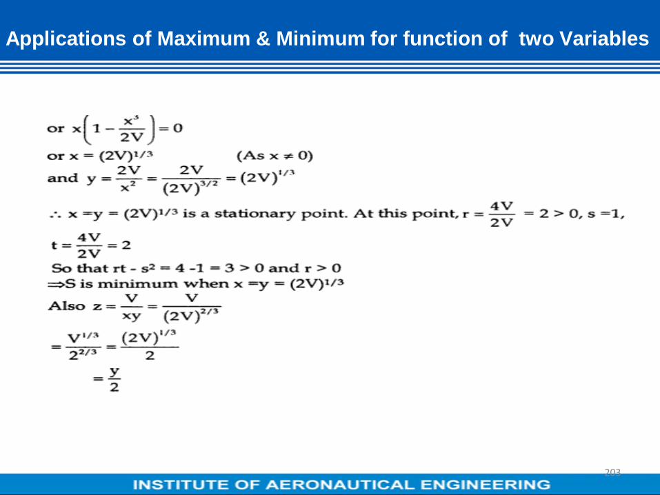
Applications of Maximum & Minimum for function of two Variables
203

Applications of Maximum & Minimum for function of two Variables
Example 2.
204

Applications of Maximum & Minimum for function of two Variables
205

Applications of Maximum & Minimum for function of two Variables
206

CONTENT
• Maxima and Minima of two variable function by method of
Lagrange multipliers
207

OBJECTIVE AND OUTCOME
OBJECTIVE:• Maxima and Minima of two variable function by method of Lagrange
multipliers.
OUTCOME:• Student get to understand the concept of Maxima and Minima of two
variable function by method of Lagrange multipliers.
208

Method of Lagrange Multipliers
209

Method of Lagrange Multipliers
210

Method of Lagrange Multipliers Summary:
Suppose f(x , y , z) = 0 ------------(1)
( x , y , z) = 0 ------------- (2)
F(x , y , z) = f(x , y , z) + ( x , y , z) where is called Lagrange’s
constant.
1.
F
x= 0 => + = 0 --------------- (3)
F
y= 0 => + = 0 --------------- (4)
F
z = 0 => + = 0 --------------- (5)
2. Solving the equations (2) (3) (4) & (5) we get the stationary point (x,
y, z).
3. Substitute the value of x , y , z in equation (1) we get the extremum.
211

Applications of Method of Lagrange Multipliers
Example 1. Find the minimum value of x2 +y
2 +z
2, given x + y + z =3a
Sol: u = x2 +y
2 +z
2
= x + y + z - 3a = 0
Using Lagrange’s function
F(x , y , z) = u(x , y , z) + ( x , y , z)
For maxima or minima
F
x = + = 2x + = 0 ------------ (1)
F
y = + = 2y + = 0 ------------ (2)
F
z = + = 2z + = 0 ------------ (3)
(1) , (2) & (3)
= -2x = -2y = -2z
= x + x + x - 3a = 0
= a
= y =z = a
Minimum value of u = a2 + a
2 + a
2 =3 a
2
212

Example 2.
Applications of Method of Lagrange Multipliers
213

Example
Applications of Method of Lagrange Multipliers
214

Applications of Method of Lagrange Multipliers
215

Example
4.
Applications of Method of Lagrange Multipliers
216

Applications of Method of Lagrange Multipliers
217

Applications of Method of Lagrange Multipliers
218

Applications of Method of Lagrange Multipliers
219
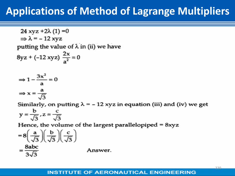
Applications of Method of Lagrange Multipliers
220

MODULE-III
HIGHER ORDER DIFFERENTIAL EQUATIONS AND ITS APPLICATIONS
221

LINEAR DIFFERENTIAL EQUATIONS OF SECOND AND HIGHER ORDER
222

Note:
1. Operator D = ; D2 = ; …………………… D
n =
Dy = ; D2 y= ; …………………… D
n y=
2. Operator Q = i e D-1
Q is called the integral of Q.
223

To find the general solution of f(D).y = 0 :
Where f(D) = Dn + P1 D
n-1 + P2 D
n-2 +-----------+Pn is a polynomial in D.
Now consider the auxiliary equation : f(m) = 0
i.e f(m) = mn + P1 m
n-1 + P2 m
n-2 +-----------+Pn = 0
where p1,p2,p3 ……………pn are real constants.
Let the roots of f(m) =0 be m1, m2, m3,…..mn.
Depending on the nature of the roots we write the complementary function
as follows:
224

Consider the following table
S.No Roots of A.E f(m) =0 Complementary function(C.F)
1. m1, m2, ..mn are real and distinct. yc = c1em
1x+ c2e
m2x +…+ cne
mnx
2. m1, m2, ..mn are and two roots are
equal i.e., m1, m2 are equal and
real(i.e repeated twice) &the rest
are real and different.
yc = (c1+c2x)em
1x+ c3e
m3x +…+ cne
mnx
3. m1, m2, ..mn are real and three
roots are equal i.e., m1, m2 , m3 are
equal and real(i.e repeated thrice)
&the rest are real and different.
yc = (c1+c2x+c3x2)e
m1x + c4e
m4x+…+ cne
mnx
4. Two roots of A.E are complex say
+i -i and rest are real and
distinct.
yc = (c1 cos x + c2sin x)+ c3em
3x +…+ cne
mn
x
5. If ±i are repeated twice & rest
are real and distinct
yc = [(c1+c2x)cos x + (c3+c4x) sin x)]+ c5em
5x
+…+ cnem
nx
6. If ±i are repeated thrice & rest
are real and distinct
yc = [(c1+c2x+ c3x2)cos x + (c4+c5x+ c6x
2) sin
x)]+ c7em
7x +……… + cne
mnx
7. If roots of A.E. irrational say
and rest are real and
distinct.
xm
n
xmx
c
nececxcxcey .......sinhcosh 3
321
225

1. Solve - 3 + 2y = 0
: Given equation is of the form f(D).y = 0
Where f(D) = (D3 -3D +2) y = 0
Now consider the auxiliary equation f(m) = 0
f(m) = m3 -3m +2 = 0 (m-1)(m-1)(m+2) = 0
m = 1 , 1 ,-2
Since m1 and m2 are equal and m3 is -2
We have yc = (c1+c2x)ex + c3e
-2x
2. Solve (D4 -2 D
3 - 3 D
2 + 4D +4)y = 0
Sol: Given f(D) = (D4 -2 D
3 - 3 D
2 + 4D +4) y = 0
A.equation f(m) = (m4 -2 m
3 - 3 m
2 + 4m +4) = 0
(m + 1)2 (m – 2)
2 = 0
m= -1 , -1 , 2 , 2
yc = (c1+c2x)e-x
+(c3+c4x)e2x
226

3. Solve (D4 +8D
2 + 16) y = 0
Sol: Given f(D) = (D4 +8D
2 + 16) y = 0
Auxiliary equation f(m) = (m4 +8 m
2 + 16) = 0
(m2 + 4)
2 = 0
(m+2i)2 (m+2i)
2 = 0
m= 2i ,2i , -2i , -2i
Yc = [(c1+c2x)cos x + (c3+c4x) sin x)]
227

4. Solve y11
+6y1+9y = 0 ; y(0) = -4 , y
1(0) = 14
Sol: Given equation is y11
+6y1+9y = 0
Auxiliary equationf(D) y = 0 (D2 +6D +9) y = 0
A.equation f(m) = 0 (m2 +6m +9) = 0
m = -3 ,-3
yc = (c1+c2x)e-3x
-------------------> (1)
Differentiate of (1) w.r.to x y1 =(c1+c2x)(-3e
-3x ) + c2(e
-3x )
Given y1 (0) =14 c1 = -4 & c2 =2
Hence we get y =(-4 + 2x) (e-3x
)
5. Solve 4y111
+ 4y11
+y1 = 0
Sol: Given equation is 4y111
+ 4y11
+y1 = 0
That is (4D3+4D
2+D)y=0
Auxiliary equation f(m) = 0
4m3 +4m
2 + m = 0
m(4m2 +4m + 1) = 0
m( = 0
m = 0 , -1/2 ,-1/2
y =c1+ (c2+ c3x) e-x/2
228

General solution of f(D) y = Q(x)
Is given by y = yc + yp
i.e. y = C.F+P.I
Where the P.I consists of no arbitrary constants and P.I of f (D) y = Q(x)
Is evaluated as P.I = . Q(x)
Depending on the type of function of Q(x).
P.I is evaluated as follows:
229

1. P.I of f (D) y = Q(x) where Q(x) =eax
for (a) ≠ 0
Case1: P.I = . Q(x) = eax
= eax
Provided f(a) ≠ 0
Case 2: If f(a) = 0 then the above method fails. Then
if f(D) = (D-a)k
(D)
(i.e ‘ a’ is a repeated root k times).
Then P.I = eax
. xk provided (a) ≠ 0
Express = = [1± ] -1
Hence P.I = Q(x).
= [1± ] -1
.xk
230

1) Particular integral of f(D) y = when f(a) ≠0
Working rule:
Case (i):
In f(D), put D=a and Particular integral will be calculated.
Particular integral= = provided f(a) ≠0
Case (ii) :
If f(a)= 0 , then above method fails. Now proceed as below.
If f(D)= (D-a)K (D)
i.e. ‘a’ is a repeated root k times, then
Particular integral= . provided (a) ≠0
231

Solve the Differential equation(D2+5D+6)y=e
x
Sol : Given equation is (D2+5D+6)y=e
x
Here Q( x) =e x
Auxiliary equation is f(m) = m2+5m+6=0
m2+3m+2m+6=0
m(m+3)+2(m+3)=0
m=-2 or m=-3
The roots are real and distinct
C.F = yc= c1e-2x
+c2 e-3x
232

Particular Integral = yp= . Q(x)
= ex = ex
Put D = 1 in f(D)
P.I. = ex
Particular Integral = yp= . ex
General solution is y=yc+yp
y=c1e-2x+c2 e
-3x +
233

Solve y11
-4y1+3y=4e
3x, y(0) = -1, y
1(0) = 3
Sol : Given equation is y11-4y1+3y=4e3x
i.e. - 4 +3y=4e3x
it can be expressed as
D2y-4Dy+3y=4e
3x
(D2-4D+3)y=4e
3x
Here Q(x)=4e3x
; f(D)= D2-4D+3
Auxiliary equation is f(m)=m2-4m+3 = 0
m2-3m-m+3 = 0
m(m-3) -1(m-3)=0 => m=3 or 1
The roots are real and distinct.
C.F= yc=c1e3x
+c2ex ---- (2)
234

P.I.= yp= . Q(x)
= yp= . 4e3x
= yp= . 4e3x
Put D=3
xx
xx
pxee
x
D
e
D
ey
33
133
2!1
232
4
313
4
General solution is y=yc+yp
y=c1e3x
+c2 ex+2xe
3x ------------------- (3)
Equation (3) differentiating with respect to ‘x’
y1=3c1e
3x+c2e
x+2e
3x+6xe
3x ----------- (4)
By data, y(0) = -1 , y1(0)=3
From (3), -1=c1+c2 ------------------- (5)
From (4), 3=3c1+c2+2
3c1+c2=1 ------------------- (6)
Solving (5) and (6) we get c1=1 and c2 = -2
y=-2e x +(1+2x)e
3x
235
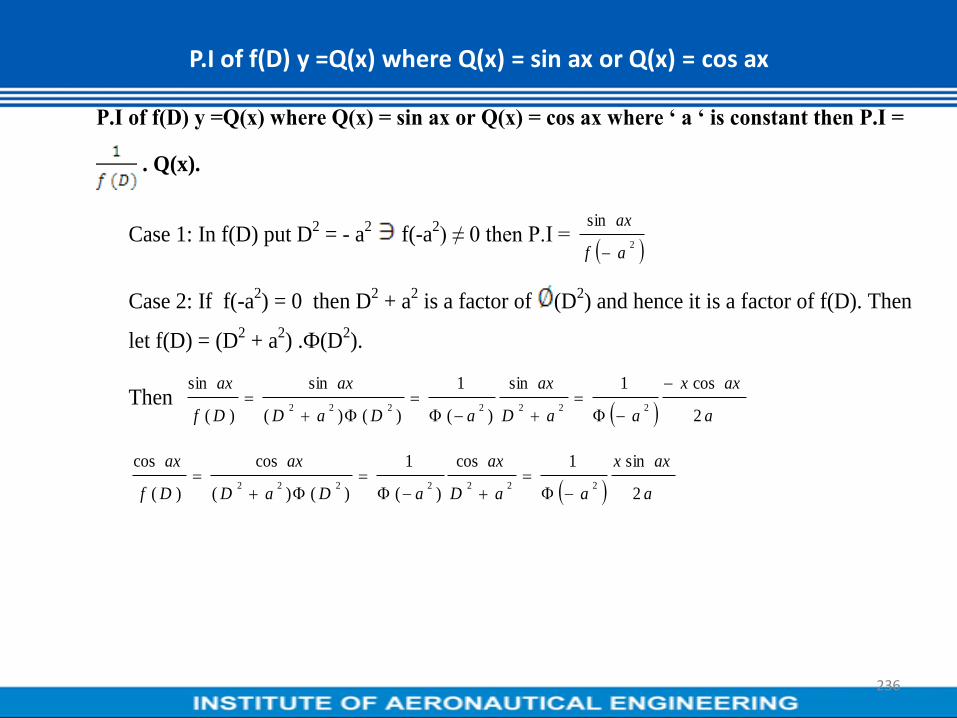
P.I of f(D) y =Q(x) where Q(x) = sin ax or Q(x) = cos ax
P.I of f(D) y =Q(x) where Q(x) = sin ax or Q(x) = cos ax where „ a „ is constant then P.I =
. Q(x).
Case 1: In f(D) put D2 = - a
2 f(-a
2) ≠ 0 then P.I =
2
sin
af
ax
Case 2: If f(-a2) = 0 then D
2 + a
2 is a factor of (D
2) and hence it is a factor of f(D). Then
let f(D) = (D2 + a
2) .Ф(D
2).
Then a
axx
aaD
ax
aDaD
ax
Df
ax
2
cos1sin
)(
1
)()(
sin
)(
sin
2222222
a
axx
aaD
ax
aDaD
ax
Df
ax
2
sin1cos
)(
1
)()(
cos
)(
cos
2222222
236

Solve y11+4y1+4y= 4cosx + 3sinx, y(0) = 0, y1(0) = 0
Sol: Given differential equation in operator form
( )y= 4cosx +3sinx
A.E is m2+4m+4 = 0
(m+2)2=0 then m=-2, -2
C.F is yc= (c1 + c2x)
P.I is = yp= put = -1
yp= =
=
237

Put = -1
yp=
= = = sinx
General equation is y = yc+ yp
y = (c1 + c2x) + sinx ------------ (1)
By given data, y(0) = 0 c1 = 0 and
Diff (1) w.r.. t. y1 = (c1 + c2x) + (c2) +cosx ------------ (2)
given y1(0) = 0
(2) -2c1 + c2+1=0 c2 = -1
Required solution is y = +sinx
238

Solve (D2+9)y = cos3x
Sol:Given equation is (D2+9)y = cos3x
A.E is m2+9 = 0
m = 3i
yc = C.F = c1 cos3x+ c2sin3x
yc =P.I = =
= sin3x = sin3x
General equation is y = yc+ yp
y = c1cos3x + c2cos3x + sin3x
239
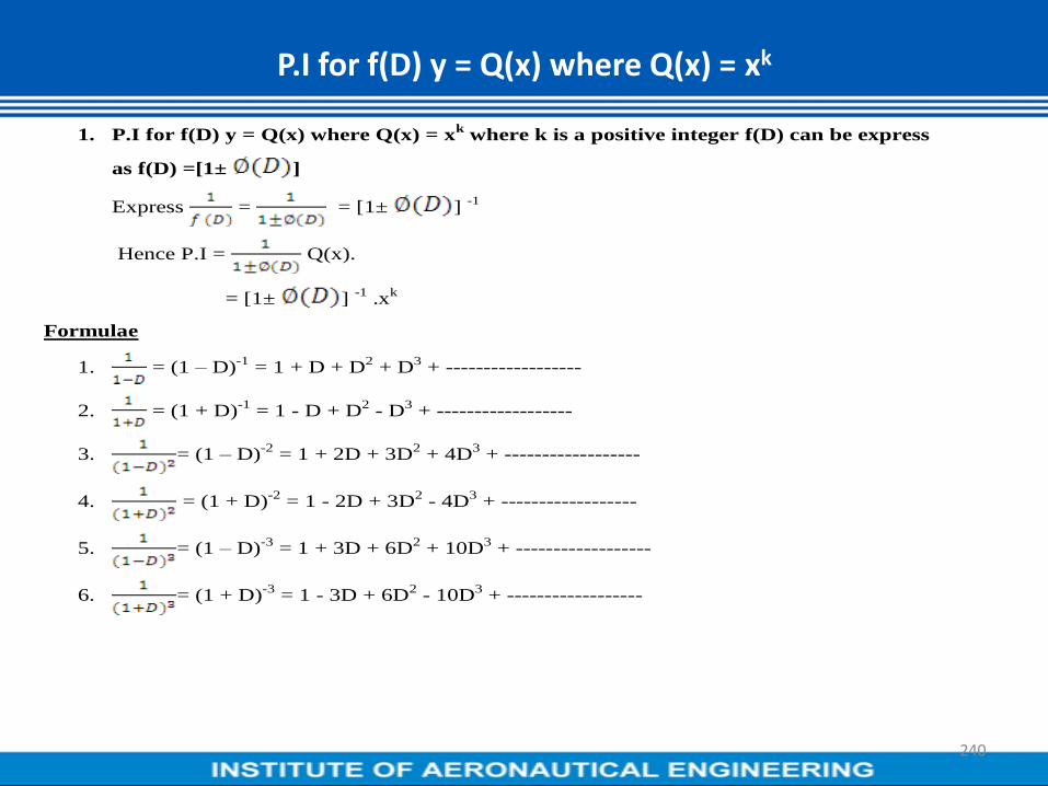
P.I for f(D) y = Q(x) where Q(x) = xk
1. P.I for f(D) y = Q(x) where Q(x) = xk where k is a positive integer f(D) can be express
as f(D) =[1± ]
Express = = [1± ] -1
Hence P.I = Q(x).
= [1± ] -1
.xk
Formulae
1. = (1 – D)-1
= 1 + D + D2 + D
3 + ------------------
2. = (1 + D)-1
= 1 - D + D2 - D
3 + ------------------
3. = (1 – D)-2
= 1 + 2D + 3D2 + 4D
3 + ------------------
4. = (1 + D)-2
= 1 - 2D + 3D2 - 4D
3 + ------------------
5. = (1 – D)-3
= 1 + 3D + 6D2 + 10D
3 + ------------------
6. = (1 + D)-3
= 1 - 3D + 6D2 - 10D
3 + ------------------
240

Solve y111+2y11 - y1-2y= 1-4x3
Sol:Given equation can be written as
= 1-4x3
A.E is = 0
( (m+2) = 0
m=- 2
m = 1, -1, -2
C.F =c1 + c2 + c3
241

P.I = 341 x
= )413
x
= )413
x
= [ 1 + + + + …..] 341 x
33322341
8
14
4
12
2
11
2
1xDDDDDD
= [ 1 - + - D] 1-4 )
= [(1-4 ) - + - (-12
= [-4x3+6x2 -30x +16] =
= [2x3-3x2 +15x -8]
242

The general solution is
y= C.F + P.I
y= c1 + c2 + c3 + [2x3-3x2 +15x -8]
243

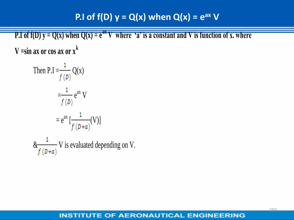
P.I of f(D) y = Q(x) when Q(x) = eax V
P.I of f(D) y = Q(x) when Q(x) = eax
V where „a‟ is a constant and V is function of x. where
V =sin ax or cos ax or xk
Then P.I = Q(x)
= eax
V
= eax
[ (V)]
& V is evaluated depending on V.
244
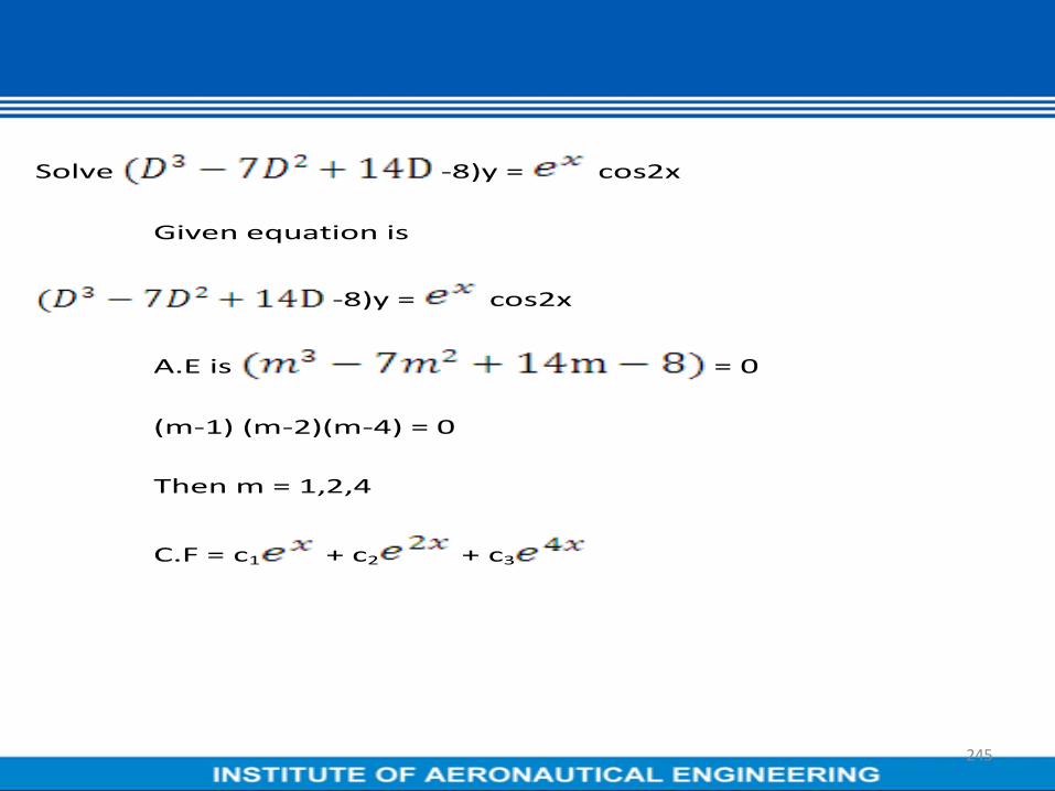
Solve -8)y = cos2x
Given equation is
-8)y = cos2x
A.E is = 0
(m-1) (m-2)(m-4) = 0
Then m = 1,2,4
C.F = c1 + c2 + c3
245

P.I =
= . . Cos2x
v
aDfeve
DfIP
axax 1
)(
1.
= . .cos2x
= . .cos2x (Replacing D2 with -22)
246

= . .cos2x
= . .cos2x
= . .cos2x
= . .cos2x
= (16cos2x – 2sin2x)
xxe
x
2sin2cos8260
2
xxe
x
2sin2cos8130
General solution is y = yc + yp
xxe
ecececy
x
xxx2sin2cos8
130
4
3
2
21
247

Solve +4)y = +3
Sol:Given +4)y = +3
A.E is = 0
( = 0 then m=2,2
C.F. = (c1 + c2x)
P.I = = + (3)
Now ) = ) (I.P of )
= I.P of ) )
248

= I.P of . )
On simplification, we get
= [(220x+244)cosx+(40x+33)sinx]
and ) = ),
) =
P.I = [(220x+244)cosx+(40x+33)sinx] + ) +
y = yc+ yp
y= (c1 + c2x) + [(220x+244)cosx+(40x+33)sinx] + ) +
249
P.I of f(D) y = Q(x) when Q(x) = eax V
P.I of f(D) y = Q(x) when Q(x) = eax
V where „a‟ is a constant and V is function of x. where
V =sin ax or cos ax or xk
Then P.I = Q(x)
= eax
V
= eax
[ (V)]
& V is evaluated depending on V.
250

Solve -8)y = cos2x
Given equation is
-8)y = cos2x
A.E is = 0
(m-1) (m-2)(m-4) = 0
Then m = 1,2,4
C.F = c1 + c2 + c3
251

252

MODULE-IV
Multiple Integrals
253

254

255

256

257

258

259

260

261
262

263

264

265

266

267

268

269

270

Three Dimensional Space
271

In Two-Dimensional Space, you have a circleIn Three-Dimensional space, you have a _____________!!!!!!!!!!!
272

More 3-D graphs
273

The Iterated Integral
2
1
2
y
xyd x2
2 2
1 1
2 2
x
x y yd yd x
274

Setting up the Double Integral
275

Finding Area using Double Integrals
276

Compute the integral on the pictured region
2
R
x y d A
277

Compute the integral on the pictured region
2
R
x y d A
278

Finding Volume using the Double Integral
279

Evaluate the volume using the region
2 21 11
2 2R
x y d A
0 1x
0 1y
280

Volume using the Triple Integral
4 4 4
0 0 0
d V
The cubes density is proportional to its distance away from theXy-plane. Find its mass.
281

12
0 0 0
x yx
d V
282

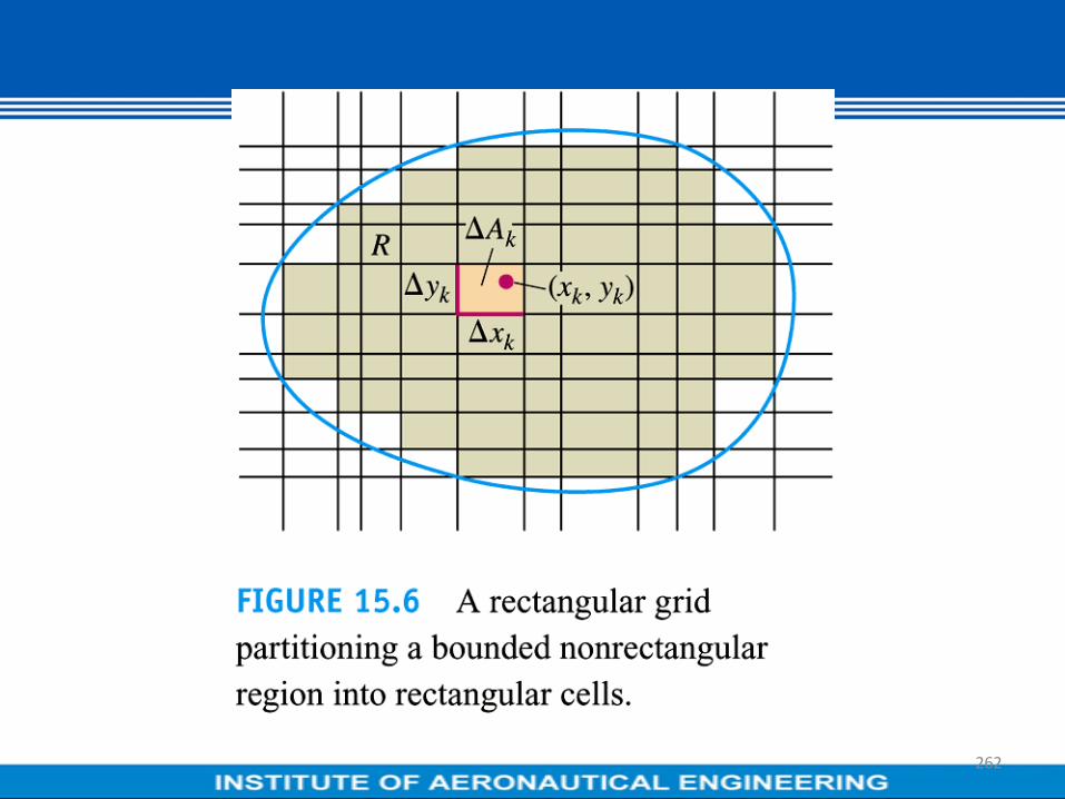
Double integrals
283

Definition of Double Integral
The expression:
is called a double integral and indicates that f (x, y) is first integrated with respect to
x and the result is then integrated with respect to y
If the four limits on the integral are all constant the order in which the integrations
are performed does not matter.
If the limits on one of the integrals involve the other variable then the order in
which the integrations are performed is crucial.
2 2
1 1
( , ) .y x
y y x x
f x y d x d y
284

Double integrals
Multiple Integrals
Double Integral :
I. When y1,y2 are functions of x and 1
x and x2 are constants. f(x,y)is first integrated w.r.t y
keeping ‘x’ fixed between limits y1,y2 and then the resulting expression is integrated w.r.t ‘x’ with
in the limits x1,x2 i.e.,
,
R
f x y d x d y
2 2
1 1
( )
( )
( , )
x x y x
x x y x
f x y d y d x
II. When x1,x2 are functions of y and y1 ,y2 are constants, f(x,y)is first integrated w.r.t ‘x’
keeping ‘y’ fixed, with in the limits x1,x2 and then resulting expression is integrated w.r.t ‘y’
between the limits y1,y2 i.e.,
,
R
f x y d x d y
22
1 1
,
x yy y
y y x y
f x y d x d y
III. When x1,x2, y1,y2 are all constants. Then
,
R
f x y d x d y
2 2 2 2
1 1 1 1
, ,
y x x y
y x x y
f x y d x d y f x y d y d x
285

Double integrals ,
R
f x y d x d y
2 2 2 2
1 1 1 1
, ,
y x x y
y x x y
f x y d x d y f x y d y d x
Problems
1. Evaluate 2 3
2
1 1
xy d x d y
Sol. 2 3
2
1 1
x y d x d y
32 22 2
2
1 11
. 9 12 2
x yy d y d y
2 2
2 2
1 1
84 .
2y d y y d y
23
1
4 4 .7 2 84 . 8 1
3 3 3 3
y
2. Evaluate 2
0 0
x
y d y d x
Sol. 2 2
0 0 0 0
x x
x y x y
y d y d x y d y d x
22 2 22 3
2 2
0 0 00 0
1 1 1 1 8 40 8 0
2 2 2 2 3 6 6 3
x
x x x
y xd x x d x x d x
286

Double integrals
2. Evaluate 2
0 0
x
y d y d x
Sol. 2 2
0 0 0 0
x x
x y x y
y d y d x y d y d x
22 2 22 3
2 2
0 0 00 0
1 1 1 1 8 40 8 0
2 2 2 2 3 6 6 3
x
x x x
y xd x x d x x d x
3. Evaluate
25
2 2
0 0
x
x x y d x d y
Sol.
22
5 5 3
2 2 3
0 0 0 03
xx
x y x y
xyx x y d y d x x y d x
565 52 3 7 6 8 8
3 2 5
0 0 0
( ) 1 5 5. .
3 3 6 3 8 6 2 4x x
x x x x xx x d x x d x
287

Double integrals
4. Evaluate
21 1
2 2
0 01
x
d y d x
x y
Sol:
2 21 1 1 1
2 2 2 2
0 0 0 0
1
1 1
x x
x y
d y d xd y d x
x y x y
2
2
1
1 1 1
1
22 2
2 20 0 0
0
1 1
1 11
x
x
x y x
y
yd y d x T a n d x
x xx y
1
2 2
1 1[ tan ( )]xd x
ax a a
1
1 1
2
0
11 0
1x
T a n T a n d x
x
o r
1 1 1
0(s in h x ) (s in h 1)
4 4
11
2
2 00
1lo g ( 1)
4 41 xx
d x x x
x
lo g (1 2 )4
288

Double integrals
5. Evaluate
24
/
0 0
x
y xe d y d x
Ans: 3e4-7
6. Evaluate
1
2 2
0
( )
x
x
x y d x d y
Ans: 3/35
7. Evaluate 2
( )
0 0
x
x ye d yd x
Ans: 4 2
2
e e
8. Evaluate 12
2 2
0 1
x y d x d y
Ans: 3
3 6
9. Evaluate 2 2
( )
0 0
x ye d xd y
Sol: 2 2 2 2
( )
0 0 0 0
x y y xe d xd y e e d x d y
2
02
ye d y
2
02
xe d x
2
0
.2 2 2 4
ye d y
289

Double integrals
10. Evaluate ( )xy x y d xd y
over the region R bounded by y=x2 and y=x
Sol: y= 2x is a parabola through (0,0) symmetric about y-axis y=x is a straight line through (0,0) with
slope1.
Let us find their points of intersection solving y= 2x , y=x we get 2
x =x x=0,1Hence y=0,1
The point of intersection of the curves are (0,0), (1,1)
Consider ( )
R
xy x y d xd y
For the evaluation of the integral, we first integrate w.r.t ‘y’ from y=x2 to y=x and then w.r.t. ‘x’ from x=0 to
x=1
2 2
1 12 2
0 0
x x
x y x x y x
xy x y d y d x x y xy d y d x
2
321
2
0 2 3
x
x
y x
y xyx d x
4 4 6 71
0 2 3 2 3x
x x x xd x
4 6 71
0
5
6 2 3x
x x xd x
15 7 8
0
5.
6 5 1 4 2 4
x x x
1 1 1 2 8 1 2 7 2 8 1 9 9 3
6 1 4 2 4 1 6 8 1 6 8 1 6 8 5 6
290

Double integrals11. Evaluate
R
xyd xd y where R is the region bounded by x-axis and x=2a and the curve x2=4ay.
Sol. The line x=2a and the parabola x2=4ay intersect at B(2a,a)
The given integral =
R
xy d x d y
Let us fix ‘y’
For a fixed ‘y’, x varies from 2 a y
to 2a. Then y varies from 0 to a.
Hence the given integral can also be written as
2 2
0 2 0 2
a x a a x a
y x a y y x a y
xy d x d y xd x yd y
22
0
22
a
a
y
x a y
xy d y
2
0
2 2a
y
a a y y d y
2 2 3
0
2 2
2 3
a
a y a y
4 4 4 4
4 2 3 2
3 3 3
a a a aa
12. Evaluate 2
1
0
0
s inr d d r
Sol. 1
2
0 0
s inr
r d d r
1
2
00
c o sr
r d r
1
0
c o s c o s 02r
r d r
291

Double integrals
292

Definition of Double Integral
293

Double integrals
294

Double integrals
295

2 1
1
12
1
2
1
0
2
0
2
1
. .
.2
1.
2
r
r
r
A r d r d
rd
r d
Double integrals
296

Evaluate .
1. 3π-12
2. 3π5π
3. 3π+12
4. Don’t know
drdI
4
1 0
cos21
297

Change of order of integration
298

Change of order of integration
299

Change of order of integration
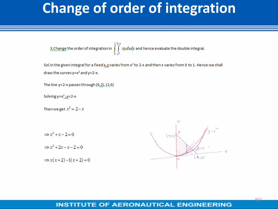
300

Change of order of integration
301
Change of order of integration
302

Change of order of integration
303

Change of order of integration
304

Change of order of integration
305

Change of order of integrals
306

Change of order of integrals
307

Change of order of integrals
308

Change of order of integrals
309

Change of order of integrals
310

Change of order of integrals
311

312

313

Change of Variables
314

Change of Variables
315

Change of Variables
316

Inverse of a matrix by Gauss-Jordan method
317

Inverse of a matrix by Gauss-Jordan method
318

Change of Variables
319

Inverse of a matrix by Gauss-Jordan method
320

Change of Variables
321

Change of Variables
322

Change of Variables
323

Inverse of a matrix by Gauss-Jordan method
324

Inverse of a matrix by Gauss-Jordan method
325

Change of Variables
326

Inverse of a matrix by Gauss-Jordan method
327

Transformation of coordinate systems
328

Transformation of coordinate systems
329

Transformation of coordinate systems
Example1
Evaluate
0 0
)(22
dxdyeyx
by changing to polar coordinates.
Hence show that
dxex
0
𝜋
2
Solution: Since both x and y vary from 0 to ∞
The region of integration is the 1st quadrant of the xy plane.
Change into polar coordinates, by putting sin,cos ryrx ,
we have dxdy = rdrd𝜃
330

Transformation of coordinate systems
331

Eigen values and Eigen vectors of a matrix
332
Transformation of coordinate systems
333

Transformation of coordinate systems
334

Transformation of coordinate systems
335

Transformation of coordinate systems
336

Transformation of coordinate systems
337

Transformation of coordinate systems
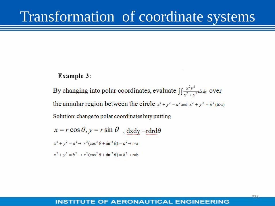
Example1
Evaluate
0 0
)(22
dxdyeyx
by changing to polar coordinates.
Hence show that
dxex
0
𝜋
2
Solution: Since both x and y vary from 0 to ∞
The region of integration is the 1st quadrant of the xy plane.
Change into polar coordinates, by putting sin,cos ryrx ,
we have dxdy = rdrd𝜃
338

Transformation of coordinate systems
339

Eigen values and Eigen vectors of a matrix
340

Transformation of coordinate systems
341

Transformation of coordinate systems
342

Transformation of coordinate systems
343

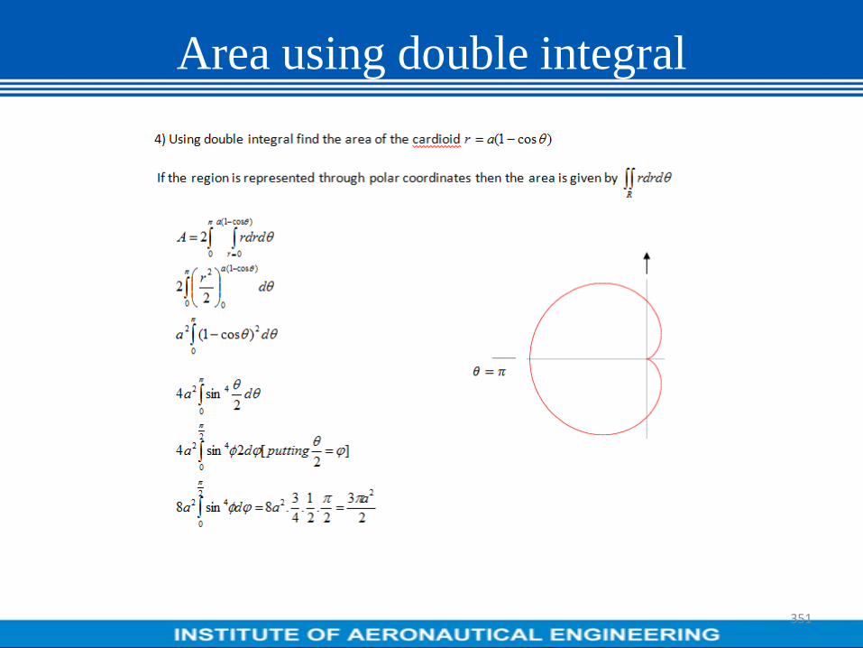
Area using double integral
344

Areas using double integrals
345

Area of a Region in the Plane, Figure 14.2 and Figure 14.3
346

Determination of areas by multiple integrals polar regions
2 1
1
12
1
2
1
0
2
0
2
1
. .
.2
1.
2
r
r
r
A r d r d
rd
r d
347

Example 2: To find the area enclosed by the curves
and
29y x
2
9
xy
A @ d yy=x2 /9
y=3x1/2
åx=0
x=9
å .d x so A = dy
y=x2 /9
3x1/2
òx=0
9
ò dx
= 3x12 -
x2
9
æ
èç
ö
ø÷x=0
9
ò dx
= 2x32 -
x3
27
é
ëê
ù
ûú
x=0
9
= 27 units2
348

Example 3: To find the area bounded by the x-axis and the
ordinate at x = 5.
4
5
xy
5 4 / 54 / 55
0 0 0 0
5
0
52
0
. s o
4 / 5
2
5
1 0 u n i
xy xx
x y x y
x
x
A y x A d yd x
x d x
x
2ts
349

Area using double integral
350
Area using double integral
351
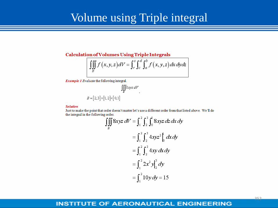
Volume using Triple integral
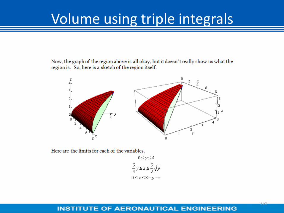
352

Volume using Triple integral
353

Volume using Triple integral
354

Volume using Triple integral
355

Volume using Triple integral
356

Volume using triple integrals
357

Volume using triple integrals
358

Volume using triple integrals
359

Volume using triple integrals
360
Volume using triple integrals
361

MODULE-V
VECTOR CALCULUS
362

CONTENT
INTRODUCTION OF SCALAR AND VECTOR POINT FUNCTIONS
363

OBJECTIVE:
Definitions of Gradient, divergent and curl
OUTCOME:
Students get to understand the concept of
Vector functions and its application on solving
Problems.
364

SCALAR AND VECTOR POINT FUNCTIONS
DIFFERENTIATION OF A VECTOR FUNCTION
Let S be a set of real numbers. Corresponding to each scalar t ε S,
let there be associated a unique vector . Then is said to be a vector
(vector valued) function. S is called the domain of . We write =
(t).
Let be three mutually perpendicular unit vectors in three
dimensional space. We can write = (t)= , where
f1(t), f2(t), f3(t) are real valued functions (which are called components
of ). (we shall assume that are constant vectors).
f f
f f f
kji ,,
f f ktfjtfitf )()()(321
f kji ,,
365

PROPERTIES
1)
2). If λ is a constant, then
3). If is a constant vector, then
4).
5).
6).
7). Let = , where f1, f2, f3are differential scalar functions
of more than one variable, Then (treating as
fixed directions)
t
aa
ta
t
)(
t
aa
t
)(
ct
cct
)(
t
b
t
aba
t
)(
t
bab
t
aba
t
..).(
t
bab
t
aba
t
)(
f kfjfif321
t
fk
t
fj
t
fi
t
f
321
kji ,,
366

VECTOR DIFFERENTIAL OPERATOR
Def. The vector differential operator (read as del) is defined as
. This operator possesses properties analogous to those
of ordinary vectors as well as differentiation operator. We will define
now some quantities known as “gradient”, “divergence” and “curl”
involving this operator .
zk
yj
xi
367

GRADIENT OF A SCALAR POINT FUNCTION
Let (x,y,z) be a scalar point function of position defined in some region
of space. Then the vector function is known as the
gradient of or
= ( ) =
zk
yj
xi
zk
yj
xi
zk
yj
xi
368
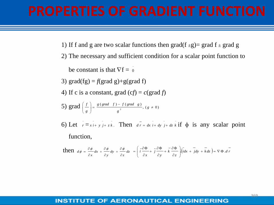
PROPERTIES OF GRADIENT FUNCTION
1) If f and g are two scalar functions then grad(f g)= grad f grad g
2) The necessary and sufficient condition for a scalar point function to
be constant is that f =
3) grad(fg) = f(grad g)+g(grad f)
4) If c is a constant, grad (cf) = c(grad f)
5) grad
6) Let = Then if is any scalar point
function,
then
0
)0(,)()(
2
g
g
ggradffgradg
g
f
r .
kzjyix
kdzjdyidxrd
dzz
dyy
dxx
d
rddzkdyjdxi
zk
yj
xi ..
369

DIRECTIONAL DERIVATIVE
Let (x,y,z) be a scalar function defined throughout some region of space. Let this
function have a value at a point P whose position vector referred to the origin O is
OP = r . Let +Δ be the value of the function at neighboring point Q. If Δ r .
Let Δr be the length of Δ
gives a measure of the rate at which change when we move from P to Q. The
limiting value of is called the derivative of in the direction of PQ or
simply directional derivative of at P and is denoted by d/dr.
370

CONTENT
SCALAR AND VECTOR POINT FUNCTIONS
GRADIENT AND DIVERGENCE
CURL OF A VECTOR
DIRECTIONAL DERIVATIVE
SOLENOIDAL VECTOR
IRROTATIONAL VECTOR
371

Scalar and vector point functions: Consider a region
in three dimensional space. To each point p(x,y,z),
suppose we associate a unique real number (called
scalar) say . This (x,y,z) is called a scalar point
function on the region. Similarly if to each point
p(x,y,z) we associate a unique vector ),,( zyxf then f is
called a vector point function.
SCALAR AND VECTOR POINT FUNCTIONS
372

For example take a heated solid. At each point p(x,y,z)of the solid, there
will be temperature T(x,y,z). This T is a scalar point function. Suppose
a particle (or a very small insect) is tracing a path in space. When it
occupies a position p(x,y,z) in space, it will be having some speed, say, v.
This speed v is a scalar point function.
Consider a particle moving in space. At each point P on its path, the
particle will be having a velocity v which is vector point function.
Similarly, the acceleration of the particle is also a vector point function.
In a magnetic field, at any point P(x,y,z) there will be a magnetic
force ),,( zyxf This is called magnetic force field. This is also an example
of a vector point function.
SCALAR AND VECTOR POINT FUNCTIONS
373

VECTOR DIFFERENTIAL OPERATOR
Def. The vector differential operator (read as del) is
defined as z
ky
jx
i
GRADIENT OF A SCALAR POINT FUNCTION
Let (x,y,z) be a scalar point function of position defined
in some region of space. Then the vector function
is known as the gradient of or
zk
yj
xi
374

Find the directional derivative of xyz2+xz at (1, 1 ,1)
in a direction of the normal to the surface 3xy2+y= z
at (0,1,1).
Sol:- Let f(x, y, z) 3xy2+y- z = 0
Let us find the unit normal e to this surface at (0,1,1).
Then
f = 3y2i+(6xy+1)j-k
(f)(0,1,1) = nkji 3
=
.1,16,32
z
fxy
y
fy
x
f
e11
3
119
3 kjikji
n
n
DIRECTIONAL DERIVATIVE
375

DIVERGENCE OF A VECTOR
Let f be any continuously differentiable vector
point function. Then is called the
divergence of f and is written as div f .
i.e., div f = =
Hence we can write div f as div f = f. This is a scalar point function. Theorem 1: If the vector = , then div =
Prof: Given =
Also . Similarly and
We have div =
Note : If is a constant vector then are zeros.
div =0 for a constant vector .
z
fk
y
fj
x
fi
...
z
fk
y
fj
x
fi
... f
zk
yj
xi .
f kfjfif321
f
z
f
y
f
x
f
321
f kfjfif321
x
fk
x
fj
x
fi
x
f
321
x
f
x
fi
1
.y
f
y
fj
2
.z
f
z
fk
3
.
f
x
fi .
z
f
y
f
x
f
321
fz
f
y
f
x
f
321
,,
f f
DIVERGENCE OF A VECTOR
376

Depending upon f in a physical problem, we can
interpret ffdiv .
Suppose (x,y,z,t) is the velocity of a fluid at a
point(x,y,z) and time ‘t’. Though time has no role in
computing divergence, it is considered here because
velocity vector depends on time.
Imagine a small rectangular box within the fluid
as shown in the figure. We would like to measure the
rate per unit volume at which the fluid flows out at
any given time. The divergence of measures the
outward flow or expansions of the fluid from their
point at any time. This gives a physical interpretation
of the divergence.
F
F
PHYSICAL INTERPRETATION OF DIVERGENCE
377

SOLENOIDAL VECTOR
A vector point function is said to be solenoidal if div f =0. Find div f = rnr Find n if it is solenoidal? Sol: Given = where
We have r2 = x2+y2+z2 Differentiating partially w.r.t. x , we get
Similarly
=rn ( div =
=
= +3rn = nrn+3rn= (n+3)rn
Let = be solenoidal. Then div = 0
(n+3)rn = 0 n= -3
f
f .rrn
rrandkzjyixr
,22r
x
x
rx
x
rr
r
z
z
rand
r
y
y
r
f )kzjyix
f )()()( zrz
yry
xrx
nnn
nnnnnnrz
z
rnrry
y
rnrrx
x
rnr
111
r
rnrr
r
z
r
y
r
xnr
nnn
2
1
222
13
f rrn
f
SOLENOIDAL VECTOR
378

SOLENOIDAL VECTOR A vector point function is said to be solenoidal if div =0. Find div = Find n if it is solenoidal? Sol: Given = where
We have r2 = x2+y2+z2 Differentiating partially w.r.t. x , we get
Similarly
=rn ( div =
=
= +3rn = nrn+3rn= (n+3)rn
Let = be solenoidal. Then div = 0
(n+3)rn = 0 n= -3
f
f
f .rrn
f .rrn
rrandkzjyixr
,22r
x
x
rx
x
rr
r
z
z
rand
r
y
y
r
f )kzjyix
f )()()( zrz
yry
xrx
nnn
nnnnnnrz
z
rnrry
y
rnrrx
x
rnr
111
r
rnrr
r
z
r
y
r
xnr
nnn
2
1
222
13
f rrn
f
379

CURL OF A VECTOR Def: Let be any continuously differentiable vector
point function. Then the vector function defined by
is called curl of and is denoted by curl
or (x ).
Curl =
Theorem 1: If is differentiable vector point function
given by = then curl =
f
z
fk
y
fj
x
fi
f
f f
f
x
fi
z
fk
y
fj
x
fi
f
f kfjfif321
f
ky
f
x
fj
x
f
z
fi
z
f
y
f
123123
CURL OF A VECTOR
380

Theorem 1: If is differentiable vector point function given by = then curl
=
Proof : curl =
=
=
Note : (1) The above expression for curl can be remembered easily through the representation.
curl = =x
Note (2) : If is a constant vector then curl = .
f f kfjfif321
f
ky
f
x
fj
x
f
z
fi
z
f
y
f
123123
f
j
x
fk
x
fkfjfif
xif
xi
32
321)()(
i
z
fj
z
fk
y
fi
y
fj
x
fk
x
f211332
y
f
x
fk
x
f
z
fj
z
f
y
fi
123123
f
f
321fff
zyx
kji
f
f f o
CURL OF A VECTOR
381

CURL OF A VECTOR
Def: Let be any continuously differentiable vector
point function. Then the vector function defined by
is called curl of and is
denoted by curl or (x ).
Curl =
Theorem 1: If is differentiable vector point function
given by = then curl =
Proof : curl =
=
=
Note : (1) The above expression for curl can be remembered
easily through the representation.
curl = =x
Note (2) : If is a constant vector then
curl = .
f
z
fk
y
fj
x
fi
f
f f
f
x
fi
z
fk
y
fj
x
fi
f
f kfjfif321
f
ky
f
x
fj
x
f
z
fi
z
f
y
f
123123
f
j
x
fk
x
fkfjfif
xif
xi
32
321)()(
i
z
fj
z
fk
y
fi
y
fj
x
fk
x
f211332
y
f
x
fk
x
f
z
fj
z
f
y
fi
123123
f
f
321fff
zyx
kji
f
f
f o
CURL OF A VECTOR
382

Physical Interpretation of curl
If is the angular velocity of a rigid body
rotating about a fixed axis and is the velocity of any
point P(x,y,z) on the body, then = ½ curl . Thus
the angular velocity of rotation at any point is equal
to half the curl of velocity vector. This justifies the
use of the word “curl of a vector”.
2. Irrotational Motion, Irrotational Vector
Any motion in which curl of the velocity vector
is a null vector i.e curl = is said to be Irrotational.
Def: A vector is said to be Irrotational if curl = .
w
v
w v
v 0
f f 0
PHYSICAL INTERPRETATION OF CURL
383

If is Irrotational, there will always exist a scalar
function (x,y,z) such that =grad . This is called
scalar potential of .
It is easy to prove that, if = grad , then curl = 0.
Hence x = 0 there exists a scalar function
such that = .
This idea is useful when we study the “work done by
a force” later.
f
f
f
f f
f
f
SCALAR POTENTIAL
384

If = find curl at the point (1,-1,1).
Sol:- Let = . Then
curl = x =
=
=
= curl at (1,-1,1) =
f kyzjyzxixy222
32 f
f kyzjyzxixy222
32
f f
22232 yzyzxxy
zyx
kji
)()2()3()()2()3(
222222xy
yyzx
xkyz
xxy
zjyzx
zyz
yi
kxyxyziyxzxyxyzkjzxzi 24232400232222
f .2 ki
PROBLEM
385

Prove that div
Note : Since we have is always solenoidal.
0c u r l f
kfjfiffLetoof321
:Pr
1 2 3
i j k
c u r l f fx y z
f f f
3 32 1 2 1f ff f f f
i j ky z x z x y
3 32 1 2 1.( )
f ff f f fd iv cu r l f f
x y z y x z z x y
01
2
2
2
1
2
3
2
2
2
3
2
yz
f
xz
f
zy
f
xy
f
zx
f
yx
f
( ) 0 ,d iv c u r l f c u r l f
VECTOR IDENTITY
386

Find constants a,b,c so that the vector = is Irrotational.
Also find such that = . Sol: Given vector is
=
Vector is Irrotational curl =
=
Comparing both sides,
c+1=0, a-4=0, b-2=0
c= -1, a=4,b=2
Now = , on
substituting the values of a,b,c
A kzcyxjzybxiazyx )24()3()2(
A
A kzcyxjzybxiazyx )24()3()2(
A A 0
0
2432
zcyxzybxazyx
zyx
kji
0)2()4()1( kbjaic
kbjaic )2()4()1( kji 000
A kzyxjzyxizyx )24()32()42(
PROBLEM
387

we have = .
= =
Comparing both sides, we have
x+2y+4z = x2/2+2xy+4zx+f1(y,z)
2x-3y-z = 2xy-3y2/2-yz+f2(z,x)
4x-y+2z = 4xz-yz+z2+f3(x,y)
Hence = x2/2 -3y2/2+z2+2xy+4zx-yz+c
A
A kzyxjzyxizyx )24()32()42( z
ky
jx
i
x
y
z
PROBLEM
388

Laplacian Operator 2
.=
Thus the operator 2 is called Laplacian
operator.
Note : (i). 2= .() = div(grad )
(ii). If 2=0 then is said to satisfy Laplacian
equation. This is called a harmonic function Find div , where = grad (x3+y3+z3-3xyz)
Sol: Let = x3+y3+z3-3xyz. Then
= grad
= =
div = = 6x+6y+6z= 6(x+y+z)
i.e div[grad(x3+y3+z3-3xyz)]= 2(x3+y3+z3-3xyz)=
6(x+y+z).
2
2
2
2
2
2
2
2
2
.zyxxz
ky
jx
ix
i
2
2
2
2
2
2
zyx
F F
F
xi
kxyxjzxyiyzx )(3)(3)(3
222 )(
321saykFjFiF
Fz
F
y
F
x
F
321
LAPLACIAN OPERATOR
389

Prove that div
Note : Since we have is always solenoidal.
0c u r l f
kfjfiffLetoof321
:Pr
1 2 3
i j k
c u r l f fx y z
f f f
3 32 1 2 1f ff f f f
i j ky z x z x y
3 32 1 2 1.( )
f ff f f fd iv cu r l f f
x y z y x z z x y
01
2
2
2
1
2
3
2
2
2
3
2
yz
f
xz
f
zy
f
xy
f
zx
f
yx
f
( ) 0 ,d iv c u r l f c u r l f
VECTOR IDENTITY
390

If =(x2-27) -6yz +8xz2 , evaluate rdF
C
from the
point (0,0,0) to the point (1,1,1) along the Straight
line from (0,0,0) to (1,0,0), (1,0,0) to (1,1,0) and
(1,1,0) to (1,1,1).
Solution : Given = (x2-27) -6yz +8xz2
Now = + + + +
. = (x2-27)dx – (6yz)dy +8xz2dz
(i) Along the straight line from O = (0,0,0) to A =
(1,0,0)
Here y =0 =z and dy=dz=0. Also x changes
from 0 to 1.
. = (x2-27)dx = =
F
i
j
k
F
i
j
k
r ix jy kz rd d x i jyd kdz
F rd
O A
F rd
1
o
1
0
3
273
x
x
3
8027
3
1
PROBLEM
391

(i) Along the straight line from A = (1,0,0) to B = (1,1,0)
Here x =1, z=0 dx=0, dz=0. y changes from 0 to 1.
. =
(ii)Along the straight line from B = (1,1,0) to C = (1,1,1)
x =1 =y dx=dy=0 and z changes from 0 to 1.
. =
. =
A B
F rd
1
0
0)6(
y
dyyz
B C
F rd
1
0
28
z
dzxz
1
0
28
z
dzxz
3 1
0
8 8
3 3
z
C
iiiiii )()()(
F rd3
88
PROBLEM
392

If =(5xy-6x2) +(2y-4x) , evaluate rdFC
along the curve C in xy-plane y=x3from
(1,1) to (2,8).
Solution : Given =(5xy-6x2) +(2y-4x) ,-------(1)
Along the curve y=x3, dy =3x2 dx
=(5x4-6x2) +(2x3-4x) , [Putting y=x3 in (1)]
d = + = +3x2dx
d = [(5x4-6x2) +(2x3-4x) ].
F
i
j
F
i
j
F
i
j
r idx jdy idx
j
.
F r
i
j2 dx 3x dx ji
PROBLEM
393

= (5x4 – 6x2) dx+(2x3 – 4x)3x3dx
= (6x5+5x4-12x3 -6x2)dx
Hence . =
=
= 16(4+2-3-1) – (1+1-3-2) = 32+3 = 35
3xy
F rd
2
1
2345)61256( dxxxxx
6 5 4 3
26 5 4 3
1
6 . 5 . 1 2 . 6 . 3 26 5 4 4
x x x xx x x x
PROBLEM
394
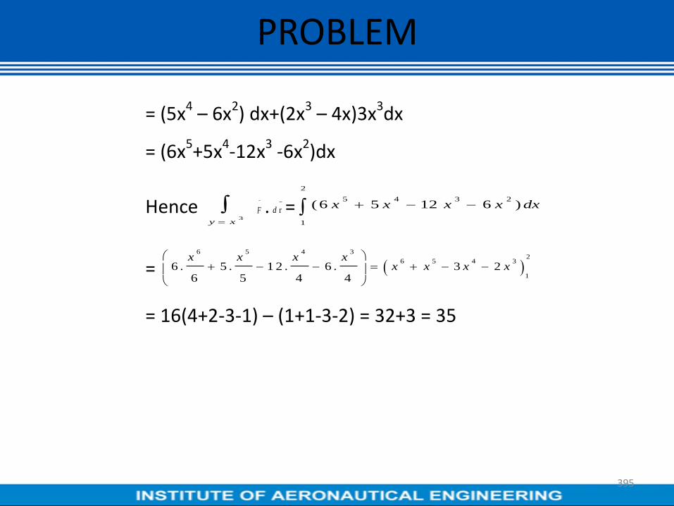
= (5x4 – 6x2) dx+(2x3 – 4x)3x3dx
= (6x5+5x4-12x3 -6x2)dx
Hence . =
=
= 16(4+2-3-1) – (1+1-3-2) = 32+3 = 35
3xy
F rd
2
1
2345)61256( dxxxxx
6 5 4 3
26 5 4 3
1
6 . 5 . 1 2 . 6 . 3 26 5 4 4
x x x xx x x x
PROBLEM
395

Hence work done = d = (t sin t + cos2 t – sin t ) dt
dt
=
=
2
0
.
F r
2
0
2 2 2
2
0
0 0 0
1 co s 2( co s ) ( s in ) s in
2
tt t t d t d t t
2
0
2
0
2
0cos
2
2sin
2
1)(cos2 t
ttt
2)11()2(2
1)11(2
PROBLEM
396

Surface integral
is called surface integral
.
S
F n d s
SURFACE INTEGRAL
397

Evaluate where = zi + xj 3y2zk and S is the
surface x2 + y2 = 16 included in the first octant
between z = 0 and z = 5.
Sol. The surface S is x2 + y2 = 16 included in the
first octant between z = 0 and z = 5.
Let x2 + y2 = 16
Then =
unit normal
Let R be the projection of S on yz-plane
Then = ……………. *
F.n d S F
i j k 2 x i 2 y jx y z
2 2x i y j
n ( x + y = 1 6 )4
S
F.n d SR
d yd zF.n
n . i
PROBLEM
398

Given = zi + xj 3y2zk
and
In yz-plane, x = 0, y = 4
In first octant, y varies from 0 to 4 and z varies from 0 to 5.
=
=
= 90.
F
1F . n ( x z x y )
4
xn . i
4
S
F.n d S
4 5
z 0y 0
x z x y d yd z
x4
4
4 5
z 0y 0
( y z ) d z d y
PROBLEM
399

If = zi + xj 3y2zk, evaluate where S is the surface of the cube bounded by x = 0, x
= a, y = 0, y= a, z = 0, z = a.
Sol. Given that S is the surface of the x = 0, x = a, y = 0, y = a, z = 0, z = a, and = zi + xj
3y2zk we need to evaluate .
F
S
F.nd S
F
S
F.nd S
O A
S R
Q
y
C
P
B
X
PROBLEM
400
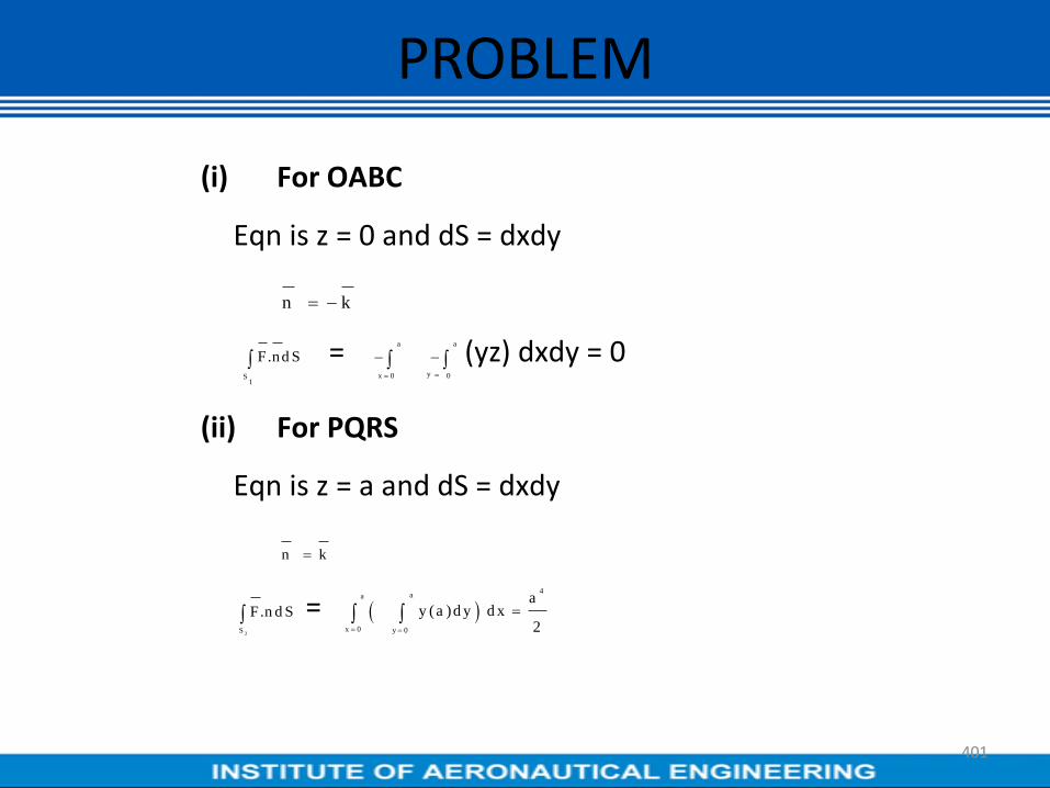
(i) For OABC
Eqn is z = 0 and dS = dxdy
= (yz) dxdy = 0
(ii) For PQRS
Eqn is z = a and dS = dxdy
=
n k
S1
F.nd Sa
x 0
a
y 0
n k
2S
F.n d S 4
aa
x 0 y 0
ay (a )d y d x
2
PROBLEM
401

(i) For OCQR
Eqn is x = 0, and , dS = dydz
=
(ii) For ABPS
Eqn is x = a, and , dS = dydz
=
(iii) For OASR
Eqn is y = 0, and , dS = dxdz
=
n i
3S
F.n d S
aa
z 0y 0
4 x z d yd z 0
n i
3S
F.nd S aa
4
z 0y 0
4 a z d z d y 2 a
n j
5S
F.n d S
aa2
z 0y 0
y d z d x 0
PROBLEM
402
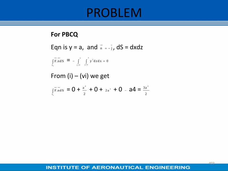
For PBCQ
Eqn is y = a, and , dS = dxdz
=
From (i) – (vi) we get
= 0 + + 0 + + 0 a4 =
n j
6S
F.nd S aa
2
z 0y 0
y d z d x 0
6S
F.nd S
4
a
2
4
2 a
4
3a
2
PROBLEM
403

GAUSS’S DIVERGENCE THEOREM (Transformation between surface integral and volume integral) Let S be a closed surface enclosing a volume V. If
is a continuously differentiable vector point function, then
dS
When is the outward drawn normal vector at any point of S.
F
.
V s
d iv F d v F n
n
GAUSS DIVERGENCE THEOREM
404

Verify Gauss Divergence theorem for
taken over the surface of the cube
bounded by the planes x = y = z = a and coordinate
planes.
Sol: By Gauss Divergence theorem we have
.
S V
F nd S d iv F d v
3 3 3 3 5
2 3
0
0 0 0 0
( )3 3 3 3 3
a a a a
aa a a a aa d yd z a y d z a a d z a a a
……(1)
PROBLEM
405

Verification: We will calculate the value of .
S
F nd S over the six faces of the cube.
(i) For S1 = PQAS; unit outward drawn normal
x=a; ds=dy dz; 0≤y≤a, 0≤z≤a
3 3. s inF n x y z a y z c e x a
1
3
0 0
. (a )
a a
S z y
F nd S y z d y d z
PROBLEM
406

For S2 = OCRB; unit outward drawn normal
x=0; ds=dy dz; 0≤y≤a, y≤z≤a
PROBLEM
407

For S3 = RBQP; Z = a; ds = dxdy;
0≤x≤a, 0≤y≤a
3
3
0 0
. . . . .( 4 )
a a
S y x
F nd S a d x d y a
PROBLEM
408
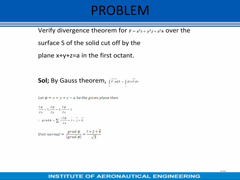
Verify divergence theorem for over the
surface S of the solid cut off by the
plane x+y+z=a in the first octant.
Sol; By Gauss theorem, .
s v
F nd S d iv F d v
1, 1, 1x y z
g r a d i i j kx
PROBLEM
409
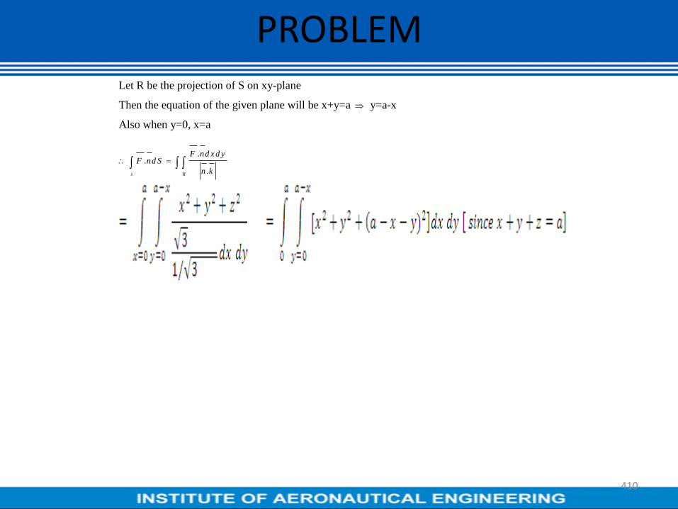
Let R be the projection of S on xy-plane
Then the equation of the given plane will be x+y=a y=a-x
Also when y=0, x=a
..
.s R
F nd x d yF nd S
n k
PROBLEM
410

=
4
3 2 2 3
0
5 2. 3 2 ,
3 3 4
a
s
aF nd S x a x a x a d x
on simplification…(1)
PROBLEM
411

Given 2 2 2F x i y j z k
d iv2 2 2
( ) ( ) ( ) 2 ( )F x y z x y zx y z
N ow
0 0 0
. 2 ( )
a x ya a x
x y z
d iv F d v x y z d x d y d z
PROBLEM
412
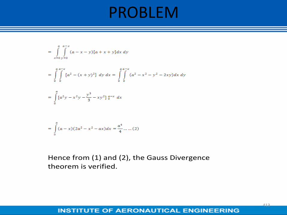
Hence from (1) and (2), the Gauss Divergence theorem is verified.
PROBLEM
413

II. GREEN’S THEOREM IN A PLANE
(Transformation Between Line Integral and Surface
Integral )
If S is Closed region in xy plane bounded by a simple
closed curve C and if M and N are continuous
functions of x and y having continuous derivatives in
R, then
.
C R
N MM d x N d y d xd y
x y
Where C is traversed in the positive(anti clock-wise)
direction
GREENS THEOREM IN A PLANE
414

GREENS THEOREM IN A PLANE
415

Verify Green’s theorem in plane for
where C is the region bounded
by y= and y= .
Solution: Let M=3 - and N=4y-6xy. Then
,
PROBLEM
416

We have by Green’s theorem,
.
C R
N MM d x N d y d xd y
x y
Now 1 6 6
R R
N Md xd y y y d xd y
x y
=1 0
R
yd xd y =102
2
1 1 2
0 0
1 02
xx
x xy x x
yyd yd x d x
PROBLEM
417

Verification:
We can write the line integral along c
=[line integral along y= (from O to A) + [line
integral along =x(from A to O)]
= + (say)
Now =
PROBLEM
418

=
And
0 0
32 22
2
1 1
1 53 8 4 6 3 1 1 2
22
l x x d x x x d x x x d x
x
From(1) and (2), we have
.
C R
N MM d x N d y d xd y
x y
Hence the verification of the Green’s theorem.
PROBLEM
419

Verify Green’s theorem for where C is
bounded by y=x and
y=
Solution:By Green’s theorem, we have
C R
N MM d x N d y d xd y
x y
Here M=xy + and N=
PROBLEM
420

The line y=x and the parabola y= intersect at O
and A
Now 1 2
......(1)
c c c
M d x N d y M d x N d y M d x N d y …..(1)
Along the line integral is
1 1
1
2 4 2 2 3 4 3 3 4
0
[ ( ) ] ( ) ( 2 ) (3 )
c c c
M d x N d y x x x d x x d x x x x d x x x d x
=
= …….(2)
PROBLEM
421

Along from to the line integral is
2 2
2 2( . )
c c
M d x N d y x x x d x x d x
= = 0-1 = -1 ….(3)
PROBLEM
422

From (1), (2) and (3), we have
…(4)
Now
R
N Md xd y
x y
= ( 2 2 )
R
x x y d xd y
=
= =
….(5)
Fromc
M d x N d y =R
N M
x y
dxdy
Hence the verification of the Green’s theorem.
PROBLEM
423

Verify Green’s theorem for where C is
bounded by y=x and
y=
Solution:By Green’s theorem, we have
C R
N MM d x N d y d xd y
x y
Here M=xy + and N=
PROBLEM
424

The line y=x and the parabola y= intersect at O
and A
Now 1 2
......(1)
c c c
M d x N d y M d x N d y M d x N d y …..(1)
Along the line integral is
1 1
1
2 4 2 2 3 4 3 3 4
0
[ ( ) ] ( ) ( 2 ) (3 )
c c c
M d x N d y x x x d x x d x x x x d x x x d x
=
= …….(2)
PROBLEM
425

Along from to the line integral is
2 2
2 2( . )
c c
M d x N d y x x x d x x d x
= = 0-1 = -1 ….(3)
PROBLEM
426

From (1), (2) and (3), we have
…(4)
Now
R
N Md xd y
x y
= ( 2 2 )
R
x x y d xd y
=
= =
….(5)
Fromc
M d x N d y =R
N M
x y
dxdy
Hence the verification of the Green’s theorem.
PROBLEM
427

III. STOKE’S THEOREM
(Transformation between Line
Integral and Surface Integral)
Let S be a open surface bounded
by a closed, non intersecting curve C.
If is any
differentieable vector point function
then
=
direction
and
STOKES THEOREM
428

Verify Stokes theorem for ,
Where S is the circular disc
Solution: Given that . The
boundary of C of S is a circle in xy
plane.
We use the parametric co-
ordinates x=cos
dx=-sin and dy =cos
=
=
=
=
=2 =2
PROBLEM
429

Now
We have ( . )k n d s d x d y and R is the region on xy-plane
.
Put x=r cos
r is varying from 0 to 1 and 0
. .rdr d
L.H.S=R.H.S.Hence the theorem is verified.
PROBLEM
430

Verify Stokes theorem for over the
upper half surface of the sphere bounded
by the projection of the xy-plane.
Solution: The boundary C of S is a circle in xy plane
i.e =1, z=0
The parametric equations are x=
2 2
1 2 3. ( 2 )
c c c
F d r F d x F d y F d z x y d x yz d y y zd z
= 2 2 2
2
0 0 0
( 2 co s s in ) s in s in s in 2d d d
=
=
PROBLEM
431

Again =
. =
Where R is the projection of S on xy plane and
Now
= 2 =
Stokes theorem is verified.
PROBLEM
432

PROBLEM
433
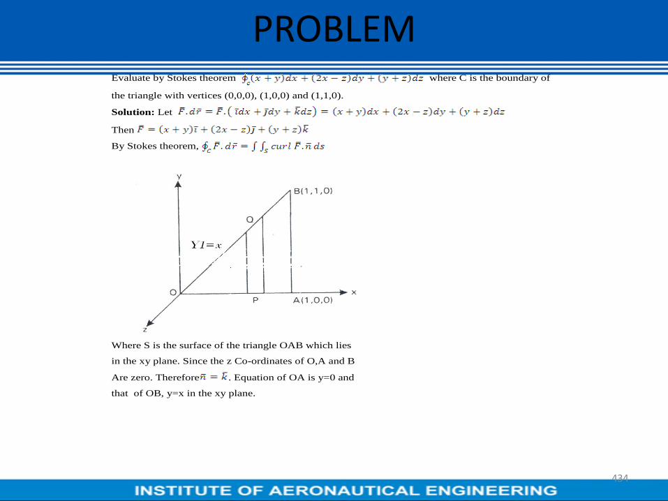
Evaluate by Stokes theorem where C is the boundary of
the triangle with vertices (0,0,0), (1,0,0) and (1,1,0).
Solution: Let
Then
By Stokes theorem,
Where S is the surface of the triangle OAB which lies
in the xy plane. Since the z Co-ordinates of O,A and B
Are zero. Therefore . Equation of OA is y=0 and
that of OB, y=x in the xy plane.
PROBLEM
434

Now
We have ( . )k n d s d x d y and R is the region on xy-plane
.
Put x=r cos
r is varying from 0 to 1 and 0
. .rdr d
L.H.S=R.H.S.Hence the theorem is verified.
PROBLEM
435

= 2
ds=curl
the
= OA AB=1 1
1 12 2
PROBLEM
436