Active Shape Model Segmentation with Optimal Features

924 IEEE TRANSACTIONS ON MEDICAL IMAGING, VOL. 21, NO. 8, AUGUST 2002

Active Shape Model Segmentation WithOptimal Features

Bram van Ginneken*, Alejandro F. Frangi, Joes J. Staal, Bart M. ter Haar Romeny, and Max A. Viergever

Abstract—An active shape model segmentation scheme is pre-sented that is steered by optimal local features, contrary to normal-ized first order derivative profiles, as in the original formulation[Cootes and Taylor, 1995, 1999, and 2001]. A nonlinearNN-clas-sifier is used, instead of the linear Mahalanobis distance, to findoptimal displacements for landmarks. For each of the landmarksthat describe the shape, at each resolution level taken into accountduring the segmentation optimization procedure, a distinct set ofoptimal features is determined. The selection of features is auto-matic, using the training images and sequential feature forwardand backward selection. The new approach is tested on syntheticdata and in four medical segmentation tasks: segmenting the rightand left lung fields in a database of 230 chest radiographs, and seg-menting the cerebellum and corpus callosum in a database of 90slices from MRI brain images. In all cases, the new method pro-duces significantly better results in terms of an overlap error mea-sure ( 0 001 using a paired T-test) than the original activeshape model scheme.

Index Terms—Active shape models, medical image segmenta-tion, model-based segmentation.

I. INTRODUCTION

SEGMENTATION is one of the key areas in computer vi-sion. During the 1970s and 1980s, many researchers ap-

proached the segmentation problem in abottom-upfashion: em-phasis was on the analysis and design of filters for the detectionof local structures such as edges, ridges, corners and T-junc-tions. The structure of an image can be described as a collectionof such syntactical elements and their (spatial) relations, andsuch descriptions can be used as input for generic segmentationschemes. Unfortunately, these segmentations are often not verymeaningful. On the other hand,top-downstrategies (also re-ferred to asmodel-basedoractiveapproaches) for segmentationwere used successfully in highly constrained environments, e.g.,in industrial inspection tasks. Often these methods are based

Manuscript received August 10, 2001; revised May 21, 2002. This work wassupported by the Ministry of Economic Affairs, The Netherlands through theIOP Image Processing program. The Associate Editor responsible for coordi-nating the review of this paper was M. Sonka.Asterisk indicates correspondingauthor.

*B. van Ginneken is with the Image Sciences Institute, University MedicalCenter Utrecht, Heidelberglaan 100, 3584 CX Utrecht, The Netherlands (e-mail:[email protected]).

A. F. Frangi is with the Grupo de Tecnología de las Comunicaciones, Depar-tamento de Ingeniería Electrónica y Comunicaciones, Universidad de Zaragoza,50015 Zaragoza, Spain.

J. J. Staal and M. A. Viergever are with the Image Sciences Institute, Univer-sity Medical Center Utrecht, 3584 CX Utrecht, The Netherlands.

B. M. ter Haar Romeny is with the Faculty of Biomedical Engineering, Med-ical and Biomedical Imaging, Eindhoven University of Technology, 5600 MBEindhoven, The Netherlands.

Digital Object Identifier 10.1109/TMI.2002.803121

on template matching. Templates incorporate knowledge aboutboth the shape of the object to be segmented and its gray-levelappearance in the image, and are matched for instance by cor-relation or with generalized Hough transform techniques. Buttemplate matching, or related techniques, are likely to fail if theobject and/or background exhibit a large variability in shape orgray-level appearance, as is often the case in real-life imagesand medical data.

Active contours or snakes [4], [5] and wave propagationmethods such as level sets [6], have been heralded as a newparadigms for segmentation. It was their ability to deform freelyinstead of rigidly that spurred this enthusiasm. Nevertheless,such methods have two inherent limitations which make themunsuited for many medical segmentation tasks. First, littlea priori knowledge about the shape to be segmented can beincorporated, except for adjusting certain parameters. Second,the image structure at object boundaries is prescribed by lettingthe snakes attract to edges or ridges in the image, or by termi-nation conditions for propagating waves. In practice, objectboundaries do not necessarily coincide with edges or ridges.

To overcome these limitations, researchers experimented withhand-crafted parametric models. An illustrative example is thework of Yuille et al. [7] where a deformable model of an eye isconstructed from circles and parabolic patches and a heuristiccost function is proposed for the gray-level appearance of theimage inside and on the border of these patches. There are twoproblems with parametric models. First of all they arededicated,that is, limited to a single application. Second, there is no proofthat the shape model and cost function proposed by the designerof the model are the optimal choice for the given application.

Consequently, there is a need for generic segmentationschemes that can be trained with examples as to acquire a modelof the shape of the object to be segmented (with its variability)and the gray-level appearance of the object in the image (withits variability). Such methods are prototype-based which makesit easy to adapt them to new applications by replacing theprototypes; they use statistical techniques to extract the majorvariations from the prototypes in a principled manner.

Several of such schemes have been proposed. For an overviewsee the book of Blake and Isard [8] and the review by Jainet al.[9]. In this paper, we focus on active shape models (ASMs) putforward by Cootes and Taylor [1], [3]. We have implementedthe method based on the description of the ASM segmentationmethod detailed in [10]. The shape model in ASMs is given bythe principal components of vectors of landmark points. Thegray-level appearance model is limited to the border of the ob-ject and consists of the normalized first derivative of profiles

0278-0062/02$17.00 © 2002 IEEE

VAN GINNEKEN et al.: ACTIVE SHAPE MODEL SEGMENTATION WITH OPTIMAL FEATURES 925

centered at each landmark that run perpendicular to the objectcontour. The cost (or energy) function to be minimized is theMahalanobis distance of these first derivative profiles. The fit-ting procedure is an alternation of landmark displacements andmodel fitting in a multiresolution framework.

Several comparable approaches are found in the literature.Shapes and objects have been modeled by landmarks, finite-el-ement methods, Fourier descriptors and by expansion in spher-ical harmonics (especially for surfaces in three dimensions[11], [12]). Jainet al. [13] have presented a Bayesian frame-work in which templates are deformed and more probable de-formations are more likely to occur. They use a coarse-to-finesearch algorithm. Ronfard [14] has used statistics of objectand background appearance in the energy function of a snake.Brejl and Sonka [15] have described a scheme similar to ASMsbut with a nonlinear shape and appearance model that is op-timized with an energy function after an exhaustive search tofind a suitable initialization. Pizeret al. [16] describe an objectmodel that consists of linked primitives which can be fittedto images using methods similar to ASMs. Cootes and Taylorhave explored active appearance models (AAMs) [2], [17], [18]as an alternative to ASMs. In AAMs, a combined principalcomponent analysis of the landmarks and pixel values insidethe object is made which allows one to generate plausible in-stances of both geometry and texture. The iterative steps in theoptimization of the segmentation are steered by the differencebetween the true pixel values and the modeled pixel valueswithin the object. Sclaroff and co-workers [19], [20] have pro-posed a comparable method in which the object is modeled asa finite-element model.

While there are differences, the general layout of theseschemes is similar in that there are: 1) a shape model thatensures that the segmentation can only produce plausibleshapes; 2) a gray-level appearance model that ensures that thesegmentation places the object at a location where the imagestructure around the border or within the object is similar towhat is expected from the training images; and 3) an algorithmfor fitting the model by minimizing some cost function. Usu-ally, the algorithm is implemented in a multiresolution fashionto provide long-range capture capabilities.

ASMs have been used for several segmentation tasks in med-ical images [21]–[27]. Our contribution in this paper consistsof a new type of appearance model for the gray-level varia-tions around the border of the object. Instead of using the nor-malized first derivative profile, we consider a general set oflocal image structure descriptors,viz. the moments of local his-tograms extracted from filtered versions of the images using afilter bank of Gaussian derivatives. Subsequently a statisticalanalysis is performed to learn which descriptors are the most in-formative at each resolution, and at each landmark. This analysisamounts to feature selection with a-nearest neighbors (NN)classifier and sequential feature forward and backward selec-tion. The NN classifier with the selected set of features is usedto compute the displacements of landmarks during optimiza-tion, instead of the Mahalanobis distance for the normalized firstderivative profile. In this paper, we refer to this new segmenta-tion method as “ASMs with optimal features,” where the termoptimal must be understood as described above.

TABLE IPARAMETERS FORACTIVE SHAPE MODELS (ORIGINAL SCHEME AND NEW

METHOD WITH OPTIMAL FEATURES). VALUES USED IN THE EXPERIMENTS

ARE GIVEN BETWEEN PARENTHESES

This paper is organized as follows. In Section II, there is astep-by-step description of the original ASM scheme. In Sec-tion III, some observations regarding ASMs are made and pos-sible modifications to the method are discussed. In Section IV,the new method is explained. In Section V, the experiments onsynthetic images, chest radiographs, and brain MR data withboth the original ASM scheme and the new method with op-timal features are described and the results are presented inSection VI. Discussion and conclusions are given in the Sec-tion VII.

II. A CTIVE SHAPE MODELS

This section briefly reviews the ASM segmentation scheme.We follow the description and notation of [2]. The parameters ofthe scheme are listed in Table I. In principle, the scheme can beused in D, but in this paper we give a two-dimensional (2-D)formulation.


A. Shape Model

An object is described by points, referred to as landmarkpoints. The landmark points are (manually) determined in aset of training images. From these collections of landmarkpoints, a point distribution model [28] is constructed as follows.The landmark points are stacked in shapevectors

(1)

Principal component analysis (PCA) is applied to the shapevectors by computing the mean shape

(2)

the covariance

(3)

and the eigensystem of the covariance matrix. The eigenvectorscorresponding to the largest eigenvalues are retained in amatrix . A shape can now be approximatedby

(4)

where is a vector of elements containing the model param-eters, computed by

(5)

When fitting the model to a set of points, the values ofareconstrained to lie within the range , where usuallyhas a value between two and three.

The number of eigenvalues to retain is chosen so as toexplain a certain proportion of the variance in the trainingshapes, usually ranging from 90% to 99.5%. The desirednumber of modes is given by the smallestfor which

(6)

Before PCA is applied to the shapes, the shapes can be alignedby translating, rotating and scaling them so as to minimize thesum of squared distances between the landmark points. An iter-ative scheme known as Procrustes analysis [29] is used to alignthe shapes. This transformation and its inverse are also appliedbefore and after the projection of the shape model in (5). Thisalignment procedure makes the shape model independent of thesize, position, and orientation of the objects. Alignment can alsohelp to better fulfill the requirement that the family of point dis-tributions is Gaussian, which is an underlying assumption of thePCA model. To this end, a projection into tangent space of eachshape may be useful; see [2] for details.

However, the alignment can also be omitted. In that case, theresult is a shape model that can generate only shapes with asize, position, and orientation that is consistent with the suppliedexamples. If, for a certain application, the objects occur only

within a specific range of sizes, positions and orientations, sucha model might lead to higher segmentation performance. In anunaligned shape model, the first few modes of variation are usu-ally associated with variations in size and position and the vari-ation seen in the first few modes had the shape model been con-structed from aligned shapes, is usually shifted toward modeswith lower eigenvalues. Therefore, the parametershould belarger than in the case of aligned shapes in which no variationis present with respect to size and position. In our experience,building an unaligned shape model can improve segmentationperformance provided that enough training data is available.

B. Gray-Level Appearance Model

The gray-level appearance model that describes the typicalimage structure around each landmark is obtained from pixelprofiles, sampled (using linear interpolation) around each land-mark, perpendicular to the contour.

Note that this requires a notion of connectivity between thelandmark points from which the perpendicular direction can becomputed. The direction perpendicular to a landmarkis computed by rotating the vector that runs fromto over 90 . In the applications presented in thispaper, all objects are closed contours, so for the first landmark,the last landmark and the second landmark are the points fromwhich a perpendicular direction is computed; for the last land-mark, the second to last landmark and the first landmark areused.

On either side pixels are sampled using a fixed step size,which gives profiles of length . Cootes and Taylor [2]propose to use the normalized first derivatives of these profilesto build the gray-level appearance model. The derivatives arecomputed using finite differences between the th andthe th point. The normalization is such that the sum ofabsolute values of the elements in the derivative profile is 1.

Denoting these normalized derivative profiles as ,the mean profile and the covariance matrix are computedfor each landmark. This allows for the computation of the Ma-halanobis distance [30] between a new profileand the profilemodel

(7)

Minimizing is equivalent to maximizing the probabilitythat originates from a multidimensional Gaussian distribu-tion.

C. Multiresolution Framework

These profile models, given byand , are constructed formultiple resolutions. The number of resolutions is denoted by

. The finest resolution uses the original image and a stepsize of one pixel when sampling the profiles. The next resolutionis the image observed at scale and a step size of twopixels. Subsequent levels are constructed by doubling the imagescale and the step size.1

The doubling of the step size means that landmarks are dis-placed over larger distances at coarser resolutions. The blurringcauses small structures to disappear. The result is that the fitting

1Note that we do not subsample the images, as proposed by Cootes and Taylor.


at coarse resolution allows the model to find a good approxi-mate location based on global images structures, while the laterstages at fine resolutions allow for refinement of the segmenta-tion result.

D. Optimization Algorithm

Shapes are fitted in an iterative manner, starting from themean shape. Each landmark is moved along the direction per-pendicular to the contour to positions on either side, evalu-ating a total of positions. The step size is, again,pixels for the th resolution level. The landmark is put at theposition with the lowest Mahalanobis distance. After movingall landmarks, the shape model is fitted to the displaced points,yielding an updated segmentation. This is repeated timesat each resolution, in a coarse-to-fine fashion.

There is no guarantee that the procedure will converge. It isour experience, however, that in practice the scheme almost al-ways converges. The gray-level model fit improves steadily andreaches a constant level within a few iterations at each resolu-tion level. Therefore, we, conservatively, take a large value (10)for .2

III. I MPROVING ASMS

There are several ways to modify, refine and improve ASMs.In this section, we mention some possibilities.

Bounds for the Shape Model. The shape model is fitted byprojecting a shape in the -dimensional space (the number oflandmarks, the factor two is because we consider 2-D images)upon the subspace spanned by thelargest eigenvectors and bytruncating the model parametersso that the point is inside thebox bounded by . Thus there is no smooth transition;all shapes in the box are allowed, outside the box no shape is al-lowed. Clearly this can be refined in many ways, using a penaltyterm or an ellipsoid instead of a box, and so on [2], [16].

Nonlinear Shape Models. The shape model uses PCAand, therefore, assumes that the distribution of shapesin the

-dimensional space is normal. If this is not true, nonlinearmodels, such as mixture models, could be more suitable (seefor example [31]).

Projecting the Shape Model. By projecting a shapeaccording to (5), i.e., fitting the shape model, the resultingmodel parameters minimize the sum of squared distancesbetween true positions and modeled positions. In practice, itcan be desirable to minimize only the distance between trueand model positions in the direction perpendicular to the objectcontour because deviation along the contour does not changewhether pixels are inside or outside the object. In [32], it isdemonstrated how to perform this projection on the contour.

Landmark Displacements. After the Mahalanobis distanceat each new possible position has been computed, Behielset al.[25] propose to use dynamic programming to find new positionsfor the landmarks, instead of moving each point to the positionwith the lowest distance. This avoids the possibility that neigh-boring landmarks jump to new positions in different directions

2We always performN iterations, contrary to Cootes and Taylor whomove to a finer resolution if a convergence criterion is reached before theN th iteration.

and thus leads to a “smoother” set of displacements. This canlead to quicker convergence [25].

Confidence in Landmark Displacements. If information isavailable about the confidence of the proposed landmark dis-placement, weighted fitting of the shape model can be used, asexplained in [21].

Initialization. Because of the multiresolution implementa-tion, the initial position of the object (the mean shape, i.e., themean location of each landmark) does not have to be very pre-cise, as long as the distance between true and initial landmarkpositions is well within pixels. But if the objectcan be located anywhere within the input image, an (exhaustive)search to find a suitable initialization, e.g., as described in [15],can be necessary.

Optimization Algorithm. Standard nonlinear optimizationalgorithms, such as hill climbing, Levenberg–Marquardt, or ge-netic algorithms can be used to find the optimal model param-eters instead of using the algorithm of alternating displace-ment of landmarks and model fitting. A minimization criterioncould be the sum of the Mahalanobis distances, possibly com-plemented by a regularization term constructed from the shapemodel parameters. Note that a multiresolution approach can stillbe used with standard nonlinear optimization methods. Alterna-tively, a snake algorithm can be used in which the shape modelprovides an internal energy term and the gray-level appearancemodel fit is used as external energy term.

This list is not complete, but it is beyond the scope of this ar-ticle to present a complete discussion of the strengths and weak-nesses of the ASM segmentation method. The issues describedabove are not considered in this work. Instead, we focus on thefollowing points:

Normalized First Derivative Profiles. The original versionof the gray-level appearance model is always based on normal-ized first derivative profiles. There is noa priori reason why thisshould be an optimal choice. In this paper, we propose an alter-native.

Mahalanobis Distance. The Mahalanobis distance in (7) as-sumes a normal distribution of profiles. In practice, the distribu-tions of profiles will often be nonnormal, for example in caseswhere the background of the object may be one of several pos-sible choices. The ASM scheme proposed here uses a nonlinearclassifier in the gray-level appearance model and can, therefore,deal with nonnormal distributions.

IV. ASMS WITH OPTIMAL FEATURES

In this section, a new gray-level appearance model is de-scribed that is an alternative to the construction of normalizedfirst derivative profiles and the Mahalanobis distance cost func-tion of the original ASMs.

The aim is to be able to move the landmark points to better lo-cations during optimization, along a profile perpendicular to theobject contour. The best location is the one for which everythingon one side of the profile is outside the object, and everythingon the other side is inside of it.3 Therefore, the probability that

3This assumes that the thickness of the object, in the direction perpendicularto a landmark, is larger than half the length of the profile. We will return to thispoint later.


a location is inside/outside the object is estimated, for the areaaround each landmark separately. We base this classification onoptimal local image features obtained by feature selection anda nonlinear NN-classifier, instead of using the fixed choice ofthe normalized first derivative profiles and the Mahalanobis dis-tance.

A. Image Features

We are looking for general image structure descriptors. ATaylor expansion approximates a functionaround a point ofinterest by a polynomial of (some) order . The coefficientsin front of each term are given by the derivatives at

(8)

Derivatives of images are computed by convolution withderivatives of Gaussians at a particular scale. This motivatesthe use of a filter bank of multiscale Gaussian derivatives todescribe local image structure. The Taylor expansion of imagesis known as the local jet, or multiscale local jet in the case ofthe Taylor expansion of the scale-space of the image [33], [34].

Given a set of filtered images, we will extract features for eachlocation by taking the first few moments of the local distribu-tion of image intensities (the histogram) around each location.The most suitable choice for a window function to compute thishistogram, is a Gaussian, since every other choice induces spu-rious resolution [35]. The size of this window function is char-acterized by a second scale parameter. The construction oflocal histograms, extracted from a Gaussian aperture function,is called alocally orderless imageand discussed in [36]. Theidea of using moments of histograms of responses of an imageto a bank of filters is a standard technique in texture analysis;see, e.g., [37].

Notice that there are quite some parameters to vary: the orderof the Taylor expansion (i.e., the number of filters in the filterbank), the number of scalesto consider, the number of scales

to use for the local window, and the number of momentstoextract from the local histograms. It remains an open questionwhich combinations are optimal for a given application and evena given location in the images. Our strategy is to compute anextensive set of features and use feature selection techniques inthe subsequent classification stage to determine the optimal fea-tures. However, we must have , otherwise the histogramwill be computed over a homogeneous region and will, there-fore, be uninteresting.

In this paper, we use only first and second moments (), all derivatives up to second-order (, , , , ,), five inner scales ( pixels), and a fixed

relation between the inner scaleand the histogram extentof. For the first moments this yields an effective scale of

1.12, 2.23, 4.47, 8.94, and 17.89 pixels, respectively (becausethe image is first blurred with a kernel of scaleand subse-quently with a kernel ). The total number of featureimages is 2 6 5 60.

Obviously the method can be extended by using more scalesand higher-order derivatives, higher-order moments, or by re-leasing the fixed relation betweenand .

B. Training and Classification

The next step is to specify how to construct a training set fromthe training images, which classifier to use, and how to performfeature selection.

Consider again the optimization procedure. At each iteration,each landmark is positioned at locations along a pro-file perpendicular to the current object location. Obviously theimage structure is different for each landmark, but the positionsthat are evaluated are also different for each resolution. There-fore, we will select a distinct optimal set of features for eachlandmarkand for each resolution, amounting to featuresets. Note that in the original ASMs the same strategy is fol-lowed: mean profiles and the covariance matricesasthey appear in (7) are computed: for each landmark, at each res-olution.

From each training image and for each landmark a square gridof points is defined with an odd integer andthe landmark point at the center of the grid. The spacing ispixels for the th resolution level.

is fixed to 5, which means that for each landmark andfor each resolution level, a feature vector with 60 elements issampled at 25 points. The output of each feature vector is eitherinside (1) or outside (0) the object. The landmark points them-selves are considered to be inside the objects (this is an arbitrarychoice). The set of training images is divided in two equal parts.This leads to two sets of samples, a training and a validation set.A NN classifier [38] with weighted voting is used.was used and the weight of each vote is , where isthe Euclidean distance to each neighbor in the feature space.

Sequential feature forward selection (also known asWhitney’s method [39]–[41]) is used to find a feature setof at most features. This set is subsequently trimmedby sequential feature backward selection, that is, featuresare removed if that improves performance. This procedureof forward selection followed by backward selection is asor almost as effective as optimal “floating” feature selectionschemes [40], [41]. The resulting set is the “optimal” set offeatures that will be used during segmentation. After featureselection, the samples from the training and the validation setare merged and a list of the selected features for each landmarkand each resolution is stored.

When the model is fitted to an input image, the scheme startsby computing the 60 feature images. Instead of sampling thenormalized derivative profiles, the optimal feature set at eachposition along the profile is fed into aNN classifier to de-termine the probability that this pixel is inside the object. Theobjective function to be minimized is the sum of abso-lute differences between the expected probability (0 or one forpoints outside or inside the object, respectively) and the pre-dicted probability, for each point along the profile

(9)

where the index along the profile, that is oriented from theoutside to the inside of the object, runs from , to . Thismetric replaces the Mahalanobis distance from (7).


C. Summary of Training and Segmentation Algorithm

Training the shape model.

1) Construct shape model [(2) and (3)].Training the gray-level appearance model.

1) Compute the 60 feature images for each training image.2) For each landmark, at each resolution, construct a set

of training samples with as input the 60 features and asoutput zero or one depending on whether the sample is inor outside the object. Samples are taken from angrid around the landmark in each training image (so eachtraining set contains samples).

3) For each training set, construct aNN classifier with se-lected optimal features. So the final result of the trainingphase is a set of classifiers.

Segmentation.

1) Initialize with the mean shape.2) Start the coarsest resolution level.3) For each landmark, put it at new locations, eval-

uate (9) with the NN classifier, move landmark to bestnew position.

4) Fit the shape model to displaced landmarks; cf. (5).5) Iterate steps 3 and 4 times.6) If the current resolution is not yet the finest resolution,

move to a finer resolution and go to Step 3.

D. Computational Considerations

One of the advantages of the original ASM scheme comparedto other segmentation methods is its speed. The new methodis considerably more computationally expensive. However, allthe feature selection is to be done off-line (during training).An optimized NN classifier [42] was used, available on theweb at http://www.cs.umd.edu/~mount/ANN. We provide somebenchmark figures, obtained with a 600-MHz Pentium III PC, a256 256 image, and the same parameter settings that are usedin all experiments in this study. The feature images have to becomputed on-line (during segmentation), which required 8.0 s.For the original ASM method, a number of blurred images haveto be computed, which required 0.35 s.

During optimization feature vectors must be classified byNN classifiers and this requires more time than computing

Mahalanobis distances. The total time for segmentation was0.17 s for the original ASM scheme and 4.1 s for the methodwith optimal features.

Using a smaller feature set would reduce the computationalcost of the method (almost linearly). An alternative would be toselect a subset of the 60 features for all operations (each land-mark, each resolution) so that it is no longer necessary to com-pute all 60 images for each input image. However, this speedimprovement would probably come at the price of a decrease inperformance.

V. EXPERIMENTS

A. Materials

Five different segmentation experiments have been per-formed with three types of data. The images and objects used in

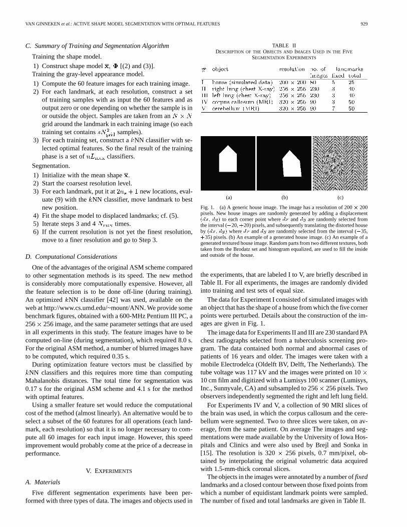
TABLE IIDESCRIPTION OF THEOBJECTS ANDIMAGES USED IN THE FIVE

SEGMENTATION EXPERIMENTS

(a) (b) (c)

Fig. 1. (a) A generic house image. The image has a resolution of 200� 200pixels. New house images are randomly generated by adding a displacement(dx; dy) to each corner point wheredx anddy are randomly selected fromthe interval (�20,+20) pixels, and subsequently translating the distorted houseby (dx; dy) wheredx anddy are randomly selected from the interval (�35,+35) pixels. (b) An example of a generated house image. (c) An example of agenerated textured house image. Random parts from two different textures, bothtaken from the Brodatz set and histogram equalized, are used to fill the insideand outside of the house.

the experiments, that are labeled I to V, are briefly described inTable II. For all experiments, the images are randomly dividedinto training and test sets of equal size.

The data for Experiment I consisted of simulated images withan object that has the shape of a house from which the five cornerpoints were perturbed. Details about the construction of the im-ages are given in Fig. 1.

The image data for Experiments II and III are 230 standard PAchest radiographs selected from a tuberculosis screening pro-gram. The data contained both normal and abnormal cases ofpatients of 16 years and older. The images were taken with amobile Electrodelca (Oldelft BV, Delft, The Netherlands). Thetube voltage was 117 kV and the images were printed on 1010 cm film and digitized with a Lumisys 100 scanner (Lumisys,Inc., Sunnyvale, CA) and subsampled to 256256 pixels. Twoobservers independently segmented the right and left lung field.

For Experiments IV and V, a collection of 90 MRI slices ofthe brain was used, in which the corpus callosum and the cere-bellum were segmented. Two to three slices were taken, on av-erage, from the same patient. On average The images and seg-mentations were made available by the University of Iowa Hos-pitals and Clinics and were also used by Brejl and Sonka in[15]. The resolution is 320 256 pixels, 0.7 mm/pixel, ob-tained by interpolating the original volumetric data acquiredwith 1.5-mm-thick coronal slices.

The objects in the images were annotated by a number offixedlandmarks and a closed contour between those fixed points fromwhich a number of equidistant landmark points were sampled.The number of fixed and total landmarks are given in Table II.


B. Methods

For each parameter of ASMs, a fixed setting was selected thatyielded good performance, after initial pilot experiments. For thehouse and lung shapes, no shape alignment was performed anda shape model was constructed with . For these ex-periments, omitting alignment led to better segmentation perfor-mance. The number of modes in the shape models was six for thehouse images and ten and 11 for the right and left lung, respec-tively. For the brain structures, shape alignment was used (in thiscase better segmentation performance was obtained with the useof alignment) and a shape model explaining 98% of the variance( ) was constructed. The number of modes in the shapemodel was six for the cerebellum and 20 for the corpus callosum.

The other settings were four levels of resolution ( ),ten iterations/level ( ), profiles of length five ( )and evaluation of nine positions/iteration ( ). When fittingthe shape model to the displaced landmarks, each mode wasconstrained within two times the standard deviation ( ).For the extended ASMs, at most ten features were selected foreach landmark and each resolution ( ). Training datawere selected from 5 5 neighborhoods around each landmark( ). In the NN classifier, five neighbors were used( ). All parameter settings are listed in Table I.

To compare different segmentations, the following “overlap”measure was used

(10)

where TP stands for true positive (the area correctly classifiedas object), FP for false positive (area incorrectly classified asobject), and FN for false negative (area incorrectly classified asbackground). for a perfect result and if there is nooverlap at all between the detected and true object. This measuremore closely reflects the idea of a good segmentation than theaverage distance between the true and detected landmark loca-tion, because the latter is not sensitive to shifts of the landmarksalong the contour.

In all experiments, the performance when fitting the shapedirectly to the true landmarks [cf. (5)] was also computed. ForExperiments II and III manual segmentations by a second ob-server were available. Therefore,for the second observer canbe compared with for the automatic methods.

VI. RESULTS

The results of all experiments are given in Table III. The re-sult of directly fitting the shape model to the landmark pointscf. (5) is included because it indicates an upper bound for boththe original method and the method with optimal features. Notethat fitting the shape model minimizes the distance between thepredicted landmark position and the true landmark position; itdoes not necessarily optimize. Therefore, it is possible that anASM scheme produces a set of model parametersfor which

is higher than for fitting the shape model directly. This oc-curred in a few cases. Another practical measure of the optimalperformance any automatic segmentation method that is trainedwith examples can achieve, is the variation between observers.This measure is given for Experiments II and III, where the me-

TABLE IIIEXPERIMENTAL RESULTS OFORIGINAL ASM, ASM WITH OPTIMAL

FEATURES, DIRECTLY FITTING THE SHAPE MODEL AND A COMPARISON

WITH A SECOND OBSERVER(EXP. II AND III)

dian of the ASM method with optimal features is close tomedian of a second human observer.

Experiment I was included to demonstrate the limitations ofthe original ASM method. In the case of texture boundaries, apixel profile or a normalized first derivative of such a profile,will not produce a clear distinction between the inside and out-side of the object. The optimal features are derived from localimage structure measures and usually some of these will be dif-ferent for two different textures. Consequently the method basedon optimal features can deal with many different types of textureboundaries. For the other experiments the differences betweenthe methods are smaller, but in all cases ASMs with optimalfeatures produced significantly highervalues than the orig-inal scheme ( in a paired t-Test for all experiments).This is also clear from Fig. 2 which shows scatter plots for eachsegmentation task. In these plots, points which are above the di-agonal line indicate images for which the segmentation with op-timal features is better than the result of the original scheme. It isapparent that a substantial improvement is achieved for Exper-iment I and evident improvements for Experiments II, IV, andV. Only for Experiment III, the left lung fields, there is a con-siderable number of cases where the original method has betterperformance.

Example results are shown in Figs. 3–7. There were no signif-icant differences between the results for normal and abnormalchest radiographs.


(a) (b)

(c) (d)

(e)

Fig. 2. Scatter plots of each segmentation experiment. The overlap measure for the original ASM scheme is plotted against for the ASM methodwith optimal features for each segmented image. (a) Houses,p = 1:6410 ;(b) right lung fields,p = 7:9210 ; (c) left lung fields,p = 8:6310 ;(d) corpus callosum,6:4810 ; and (e) cerebellum,p = 1:7910 .

VII. D ISCUSSION

In this section, we discuss some properties and possible re-finements of the proposed ASM method.

The largest improvement in performance is obtained for sim-ulated data in which the textural appearance of the image in-side and outside the object is different. This indicates that theproposed method may be especially useful to segment texturedobjects from textured backgrounds. An example could be seg-mentation in ultrasound images.

An important aspect is that an optimal set of features is se-lected for each landmark and each resolution separately. Alter-natively, a single set of optimal features could be used, whichwould be equivalent to designing a pixel classifier that assignseach image location to one of two classes: outside or inside theobject of interest. The segmentation method could be run onthese “potential images” instead of on the real data. We have

(a) (b) (c)

Fig. 3. Example result for the segmentation of the generated textured imageswith a house shape. Segmentations are given by the thick white line. (a) Trueshape. (b) ASMs ( = 0:219). (c) Optimal ASMs ( = 0:861).

conducted pilot experiments which indicated that the perfor-mance of such an approach is worse than that of the methodpresented here, ASMs with optimal features. The set of selectedfeatures varies considerably/landmark and resolution and is dif-ferent for different applications. Had we used a standard feed-forward neural network to for the classification of locations inthe image as inside or outside the object, instead of aNN-clas-sifier and feature selection, the particular combination of inputfeatures constructed by the network could be considered as theoptimal filter for that particular landmark and resolution. In ourcase, the selected features cannot directly be interpreted as asingle optimal filter, but the idea is similar. Note that the methoddoes not require the use of aNN classifier; any classifier couldbe used instead. Similarly, the method does not rely on the spe-cific set of features used here. More feature images can be used,by using higher moments, more (higher-order) derivatives andby relaxing the fixed relation betweenand .

The results of the improved ASM method approaches the me-dian result of a second observer, which was available for Exper-iments II and III. However, the second observer performed stillsignificantly better.

Both the original and improved ASM method contain a rangeof free parameters (Table I). Although we have found that seg-mentation results are not very dependent on the choice for theseparameters, as long as they are within a sensible range, it couldbe desirable to use a straightforward iterative procedure to se-lect optimal settings using the training set.

A more elaborate criterion for evaluating new landmark po-sitions could be as follows. Currently landmarks are moved tothose locations where the profile values are closest to zero forpoints outside the object and closest to one for points inside theobject. In practice, the optimal profiles may be different. Espe-cially if the object is very thin and the fitting occurs at a coarseresolution level, the innermost points of the profile may crossthe border on the other side of the object! The actual profilescan be extracted from the training set and used to construct amodel based on their mean and covariance matrices, that cansteer the landmark displacement, in the same way as the originalASM scheme. Another enhancement would be to take into ac-count the structure along the profile, instead of using local pixelclassification for each position along the profile independently.This may improve performance. Consider a set of images, halfshow a black object on a white background, and the other half awhite object on a black background. With local image features,it is impossible to classify locations as inside or outside the ob-ject. But a set of features measured along the profile can easily


(a) (b) (c) (d)

Fig. 4. Example result for the right lung field segmentation. Segmentations are given by the thick white line. (a) True shape. (b) ASMs, = 0:884. (c) ASMs, = 0:945. (d) ASMs, = 0:952.

(a) (b) (c) (d)

Fig. 5. Example result for the left lung field segmentation. Segmentations are given by the thick white line. (a) True shape. (b) ASMs, = 0:873. (c) ASMs, = 0:935. (d) ASMs, = 0:961.

(a) (b) (c)

Fig. 6. Example result of segmenting the corpus callosum. Segmentations aregiven by the thick white line. (a) True shape. (b) ASMs, = 0:474. (c) ASMs, = 0:828.

(a) (b) (c)

Fig. 7. Example result of segmenting the cerebellum. Segmentations are givenby the thick white line. (a) True shape. (b) ASMs, = 0:679. (c) ASMs, = 0:909.

distinguish correct profiles, with an intensity jump at exactlythe landmark location, from incorrect profiles, with no intensityjump or an intensity jump at a different location.

The computational complexity of the improved ASM methodis roughly 20-fold that of the original scheme. The computa-tional burden can be reduced if the feature images are computedonly at those points where their value is required during seg-

mentation. Using a faster classifier will also reduce computa-tion time. Nevertheless, the algorithm still requires only a fewseconds on standard PC hardware.

We conclude by stating that active shape models provide afast, effective, automatic, model-based method for segmentationproblems in medical imaging. The new ASM method introducedin this paper significantly improves the original method throughthe use of an adaptive gray-level appearance model based onlocal image features.

ACKNOWLEDGMENT

M. Brejl from Vital Images, and J. Haller and L. Bolingerfrom the University of Iowa are gratefully acknowledged for al-lowing the use of their MR brain data and manual segmentationsin this study.

REFERENCES

[1] T. F. Cootes, C. J. Taylor, D. Cooper, and J. Graham, “Active shapemodels—Their training and application,”Comput. Vis. Image Under-standing, vol. 61, no. 1, pp. 38–59, 1995.

[2] T. F. Cootes and C. J. Taylor, “Statistical models of appearance forcomputer vision,” Wolfson Image Anal. Unit, Univ. Manchester,Manchester, U.K., Tech. Rep., 1999.

[3] , “Statistical models of appearance for medical image analysis andcomputer vision,”Proc. SPIE, vol. 4322, pp. 236–248, 2001.

[4] M. Kass, A. Witkin, and D. Terzopoulos, “Snakes: Active contourmodels,”Int. J. Comput. Vis., vol. 1, no. 4, pp. 321–331, 1988.

[5] T. McInerney and D. Terzopoulos, “Deformable models in medicalimage analysis: A survey,”Med. Image Anal., vol. 1, no. 2, pp. 91–108,1996.


[6] J. A. Sethian,Level Set Methods and Fast Marching Methods, 2ed. Cambridge, U.K.: Cambridge Univ. Press, 1999.

[7] A. L. Yuille, P. W. Hallinan, and D. S. Cohen, “Feature extraction fromfaces using deformable templates,”Int. J. Comput. Vis., vol. 8, no. 2, pp.99–112, 1992.

[8] A. Blake and M Isard,Active Contours. Berlin, Germany: Springer-Verlag, 1998.

[9] A. K. Jain, Y. Zhong, and M. P. Dubuisson-Jolly, “Deformable templatemodels: A review,”Signal Processing, vol. 71, no. 2, pp. 109–129, 1998.

[10] T. F. Cootes and C. J. Taylor, “A mixture model for representing shapevariation,” Image Vis. Computing, vol. 17, no. 8, pp. 567–574, 1999.

[11] A. Kelemen, G. Székely, and G. Gerig, “Elastic model-based segmenta-tion of 3-D neuroradiological data sets,”IEEE Trans. Med. Imag., vol.18, pp. 828–839, Oct. 1999.

[12] B. M. ter Haar Romeny, B. Titulaer, S. Kalitzin, G. Scheffer, F. Broek-mans, E. te Velde, and J. J. Staal, “Computer assisted human follicleanalysis for fertility prospects with 3D ultrasound,” inLecture Notesin Computer Science. Berlin, Germany: Springer-Verlag, 1999, vol.1613, IPMI ’99, pp. 56–69.

[13] A. K. Jain, Y. Zhong, and S. Lakshaman, “Object matching using de-formable templates,”IEEE Trans. Pattern Anal. Machine Intell., vol. 18,pp. 267–278, Mar. 1996.

[14] R. Ronfard, “Region-based strategies for active contour models,”Int. J.Comput. Vis., vol. 13, no. 2, pp. 229–251, 1994.

[15] M. Brejl and M. Sonka, “Object localization and border detection criteriadesign in edge-based image segmentation: Automated learning from ex-amples,”IEEE Trans. Med. Imag., vol. 19, pp. 973–985, Oct. 2000.

[16] S. M. Pizer, D. S. Fritsch, P. A. Yushkevich, V. E. Johnson, and E. L.Chaney, “Segmentation, registration, and measurement of shape vari-ation via image object shape,”IEEE Trans. Med. Imag., vol. 18, pp.851–865, Oct. 1999.

[17] T. F. Cootes, G. J. Edwards, and C. J. Taylor, “Active appearancemodels,” inProc. Eur. Conf. Computer Vision, vol. 2, H. Burkhardt andB. Neumann, Eds., 1998, pp. 484–498.

[18] , “Active appearance models,”IEEE Trans. Pattern Anal. MachineIntell., vol. 23, pp. 681–685, June 2001.

[19] S. Sclaroff and A. P. Pentland, “Modal matching for correspondenceand recognition,”IEEE Trans. Pattern Anal. Machine Intell., vol. 17,pp. 545–561, July 1995.

[20] S. Sclaroff and J. Isodor, “Active blobs,” inProc. IEEE ICCV, 1998, pp.1146–1153.

[21] T. F. Cootes, A. Hill, C. J. Taylor, and J. Haslam, “The use of activeshape models for locating structures in medical images,”Image Vis.Computing, vol. 12, no. 6, pp. 355–366, 1994.

[22] P. P. Smyth, C. J. Taylor, and J. E. Adams, “Automatic measurement ofvertebral shape using active shape models,” inProc. Br. Machine VisionConf., 1996, pp. 705–714.

[23] S. Solloway, C. J. Taylor, C. E. Hutchinson, and J. C. Waterton, “The useof active shape models for making thickness measurements from MRimages,” inProc. 4th Eur. Conf. Computer Vision, 1996, pp. 400–412.

[24] N. Duta and M. Sonka, “Segmentation and interpretation of MR brainimages: An improved active shape model,”IEEE Trans. Med. Imag., vol.17, pp. 1049–1067, June 1998.

[25] G. Behiels, D. Vandermeulen, F. Maes, P. Suetens, and P. Dewaele, “Ac-tive shape model-based segmentation of digital X-ray images,” inLec-ture Notes in Computer Science. Berlin, Germany: Springer-Verlag,1999, MICCAI ’99, pp. 128–137.

[26] F. Vogelsang, M. Kohnen, J. Mahlke, F. Weiler, M. W. Kilbinger, B.Wein, and R. W. Günther, “Model based analysis of chest radiographs,”Proc. SPIE, vol. 3979, pp. 1040–1052, 2000.

[27] G. Hamarneh and T. Gustavsson, “Combining snakes and active shapemodels for segmenting the human left ventricle in echocardiographicimages,” inComputers in Cardiology. Piscataway, NJ: IEEE, 2000,vol. 27, pp. 115–118.

[28] I. Dryden and K. V. Mardia,The Statistical Analysis of Shape. London,U.K.: Wiley, 1998.

[29] C. Goodall, “Procrustes methods in the statistical analysis of shapes,”J.Roy. Statist. Soc. B, vol. 53, no. 2, pp. 285–339, 1991.

[30] C. Rao,Linear Statistical Inference and Its Applications. New York:Wiley, 1973.

[31] P. Sozou, T. F. Cootes, C. J. Taylor, and E. DiMauro, “A nonlinear gen-eralization of point distribution models using polynomial regression,”Image Vis. Computing, vol. 13, no. 5, pp. 451–457, 1995.

[32] A. Hill, T. F. Cootes, and C. J. Taylor, “Active shape models and theshape approximation problem,”Image Vis. Computing, vol. 14, no. 8,pp. 601–607, 1996.

[33] J. J. Koenderink and A. J. van Doorn, “Representation of local geometryin the visual system,”Biological Cybern., vol. 55, pp. 367–375, 1987.

[34] L. M. J. Florack, B. M. ter Haar Romeny, J. J. Koenderink, and M. A.Viergever, “The Gaussian scale-space paradigm and the multiscale localjet,” Int. J. Comput. Vis., vol. 18, no. 1, pp. 61–75, 1996.

[35] J. J. Koenderink, “The structure of images,”Biological Cybern., vol. 50,pp. 363–370, 1984.

[36] J. J. Koenderink and A. J. van Doorn, “The structure of locally orderlessimages,”Int. J. Comput. Vis., vol. 31, no. 2/3, pp. 159–168, 1999.

[37] M. Unser, “Local linear transforms for texture measurements,”SignalProcessing, vol. 11, pp. 61–79, 1986.

[38] R. Duda and P. Hart,Pattern Classification and Scene Analysis. NewYork: Wiley, 1973.

[39] A. Whitney, “A direct method of non parametric measurement selec-tion,” IEEE Trans. Computing, vol. C-20, pp. 1100–1103, 1971.

[40] P. Pudil, J. Novovicova, and J. Kittler, “Floating search methods in fea-ture selection,”Pattern Recogn. Lett., vol. 15, no. 11, pp. 1119–1125,1994.

[41] P. Somol, P. Pudil, J. Novovicova, and P. Paclik, “Adaptive floatingsearch methods in feature selection,”Pattern Recogn. Lett., vol. 20, no.11–13, pp. 1157–1163, 1999.

[42] S. Arya, D. M. Mount, N. S. Netanyahu, R. Silverman, and A. Y. Wu,“An optimal algorithm for approximate nearest neighbor searching infixed dimensions,”J. ACM, vol. 45, no. 6, pp. 891–923, 1998.

Active Shape Model Segmentation with Optimal Features

Documents

Transcript of Active Shape Model Segmentation with Optimal Features