IMAGE SEGMENTATION AND SHAPE ANALYSIS OFBLOOD VESSELS WITH APPLICATIONS TO

CORONARY ATHEROSCLEROSIS

A ThesisPresented to

The Academic Faculty

by

Yan Yang

In Partial Fulfillmentof the Requirements for the Degree

Doctor of Philosophy in theSchool of Biomedical Engineering

Georgia Institute of TechnologyMay 2007

IMAGE SEGMENTATION AND SHAPE ANALYSIS OFBLOOD VESSELS WITH APPLICATIONS TO

CORONARY ATHEROSCLEROSIS

Approved by:

Professor Don P. Giddens, AdvisorSchool of Biomedical EngineeringGeorgia Institute of Technology

Professor Anthony J. YezziSchool of Electrical and ComputerEngineeringGeorgia Institute of Technology

Professor Allen R. Tannenbaum,AdvisorSchool of Electrical and ComputerEngineeringGeorgia Institute of Technology

Professor John N. OshinskiDepartment of RadiologyEmory University

Professor Raymond P. VitoDepartment of MechanicalEngineeringGeorgia Institute of Technology

Date Approved: March, 2007

To my parents Chen, Kaixuan and Yang, Jisheng,

and my husband Tinghao.

iii

ACKNOWLEDGEMENTS

I would like to thank those who have been supporting me and helping me throughout

my doctorate years.

First, I would like to thank my PhD advisors, Professor Don Giddens and Professor

Allen Tannenbaum for your invaluable guidance throughout my study and research at

Georgia Tech. It has been a privilege to be a student of yours, to learn from you and to

be inspired by you. I am so grateful to have had such great advisors who not only have

incredible foresight and view of the big picture, but also guided me through numerous

technical details. I would like to thank my thesis reading committee, Professor Ray

Vito, Professor Anthony Yezzi and Professor John Oshinski for your helpful comments

and suggestions, which improved my thesis in many aspects. Thanks to Dr. Arthur

Stillman for teaching me useful knowledge in medicine, sending me many real-world

clinical data sets, and helping me with the validation of the algorithms.

Thank you to everyone who is currently in the Biomedical Imaging Lab and who

have been here: Lei, Cecilia, Delphine, Eric, Marc, Yi, Yogesh, Patricio, John, Sam,

Xavier, Ponnappan, Shawn, Jimi, Gallagher, Tauseef, Vandana, Eli, and Oleg; and

everyone from the Cardiovascular Lab: Amanda, Suo Jin, Binjian, Stephanie, Mas-

similiano, Sungho and Annica. I have learned much from each and everyone of you,

and it’s always been a pleasure to spend time in the lab, attend group meetings, and

share the knowledge and happiness with you.

I would also like to thank my intern supervisors, Gozde Unal at Siemens Corporate

Research and Zhujiang Cao at Vital Images, for being great mentors to me and guiding

me through two wonderful internship experiences. I have learned so much from you

which I couldn’t have learned at school.

iv

To my dear husband Tinghao, your love and support have been keeping me warm

at heart for so many years. I cherish all the memories we have had together, and I

look forward to creating and sharing many more new memories with you.

Thanks to my parents and every family member in China, for supporting me

unconditionally all the time. The distance across half of the earth will never separate

you and me.

The last but not least, thanks to every Chinese friend I have met in the US, it’s

you who have made this place another home away from home.

v

TABLE OF CONTENTS

DEDICATION . . . . . . . . . . . . . . . . . . . . . . . . . . . . . . . . . . . iii

ACKNOWLEDGEMENTS . . . . . . . . . . . . . . . . . . . . . . . . . . . . iv

LIST OF TABLES . . . . . . . . . . . . . . . . . . . . . . . . . . . . . . . . . viii

LIST OF FIGURES . . . . . . . . . . . . . . . . . . . . . . . . . . . . . . . . ix

SUMMARY . . . . . . . . . . . . . . . . . . . . . . . . . . . . . . . . . . . . . xiii

I INTRODUCTION . . . . . . . . . . . . . . . . . . . . . . . . . . . . . . 1

1.1 Atherosclerosis and Coronary Artery Diseases . . . . . . . . . . . . 1

1.2 Medical Imaging in Assisting the Diagnosis of Coronary Artery Dis-eases . . . . . . . . . . . . . . . . . . . . . . . . . . . . . . . . . . . 5

1.3 Organization of the Thesis . . . . . . . . . . . . . . . . . . . . . . . 13

II BACKGROUND: MEDICAL IMAGE SEGMENTATION AND 3D VES-SEL IMAGE ANALYSIS . . . . . . . . . . . . . . . . . . . . . . . . . . 14

2.1 Medical Image Segmentation Methods – A Brief Review . . . . . . 14

2.1.1 Definition of Image Segmentation . . . . . . . . . . . . . . . 14

2.1.2 Thresholding and Region Growing . . . . . . . . . . . . . . 15

2.1.3 Classifiers and Clustering Methods . . . . . . . . . . . . . . 16

2.1.4 Active Contour Models . . . . . . . . . . . . . . . . . . . . 17

2.1.5 Combination of Image Segmentation Methods . . . . . . . . 18

2.2 Previous Work on 3D Vessel Image Analysis . . . . . . . . . . . . . 19

2.2.1 Enhancement of Curvilinear Structures . . . . . . . . . . . . 20

2.2.2 General Vessel Extraction and Analysis Approaches . . . . . 22

2.2.3 CTA Image Analysis . . . . . . . . . . . . . . . . . . . . . . 28

2.2.4 Coronary Artery Image Analysis . . . . . . . . . . . . . . . 30

III SEGMENTATION USING BAYESIAN DRIVEN IMPLICIT SURFACES(BDIS) . . . . . . . . . . . . . . . . . . . . . . . . . . . . . . . . . . . . 33

3.1 Geodesic Active Contour Models and Limitations . . . . . . . . . . 33

vi

3.2 An Improved Geodesic Active Contour Model . . . . . . . . . . . . 38

3.2.1 A New Conformal Factor Based on Bayesian Probabilities . 38

3.2.2 An Adaptive Inflation Term . . . . . . . . . . . . . . . . . . 40

3.2.3 Estimation of Probability Density Functions . . . . . . . . . 40

3.2.4 Numerical Implementation Using Level Sets . . . . . . . . . 42

3.3 2D Experimental Results . . . . . . . . . . . . . . . . . . . . . . . 43

IV FULLY AUTOMATIC DETECTION AND SEGMENTATION OF CORO-NARY ARTERIES IN 3D . . . . . . . . . . . . . . . . . . . . . . . . . . 49

4.1 Lung and Heart Segmentation . . . . . . . . . . . . . . . . . . . . . 50

4.2 Multi-Scale Vessel Filtering . . . . . . . . . . . . . . . . . . . . . . 51

4.3 3D Segmentation of Coronary Arteries Using BDIS . . . . . . . . . 54

4.3.1 Numerical Details and Optimization . . . . . . . . . . . . . 55

4.3.2 Removing Calcified Plaques . . . . . . . . . . . . . . . . . . 58

4.4 Results and Validation . . . . . . . . . . . . . . . . . . . . . . . . . 58

V CENTERLINE EXTRACTION AND STENOSIS EVALUATION FOR CORO-NARY ARTERIES . . . . . . . . . . . . . . . . . . . . . . . . . . . . . . 82

5.1 Harmonic Skeletonization . . . . . . . . . . . . . . . . . . . . . . . 82

5.2 Cross-sectional Area Measurement and Stenosis Detection . . . . . 86

5.3 Results and Validation . . . . . . . . . . . . . . . . . . . . . . . . . 89

5.3.1 Digital Phantoms . . . . . . . . . . . . . . . . . . . . . . . . 89

5.3.2 Clinical Data . . . . . . . . . . . . . . . . . . . . . . . . . . 90

5.3.3 Generation of Harmonic Skeletons . . . . . . . . . . . . . . 90

5.3.4 Stenosis Evaluation . . . . . . . . . . . . . . . . . . . . . . . 92

VI CONCLUSIONS AND FUTURE RESEARCH . . . . . . . . . . . . . . 100

REFERENCES . . . . . . . . . . . . . . . . . . . . . . . . . . . . . . . . . . . 104

VITA . . . . . . . . . . . . . . . . . . . . . . . . . . . . . . . . . . . . . . . . 113

vii

LIST OF TABLES

1 Possible patterns in 3D based on Hessian eigenvalues. Adapted from[28]. . . . . . . . . . . . . . . . . . . . . . . . . . . . . . . . . . . . . 52

2 Segmentation results and validation for 18 datasets. Part I - Dataproperties. . . . . . . . . . . . . . . . . . . . . . . . . . . . . . . . . . 59

3 Segmentation results and validation for 18 datasets. Part II - Quantita-tive comparison between automatic and manual segmentation. (1MDE- Mean Distance Error, 2MMDE - Mean Maximum Distance Error) . 62

4 Segmentation results and validation for 18 datasets. Part III - Com-putation time and number of branches segmented. Tested using Pen-tium(R) 4 CPU 3.60 GHz, 2.00 GB of RAM, in Matlab. (1 Heart &VF: Heart segmentation and Vessel Filtering) . . . . . . . . . . . . . 63

viii

LIST OF FIGURES

1 Schematic representation of the major components of a normal vascularwall [47]. . . . . . . . . . . . . . . . . . . . . . . . . . . . . . . . . . . 2

2 Schematic representation of the major components of a well-developedatherosclerotic plaque [47]. . . . . . . . . . . . . . . . . . . . . . . . . 2

3 Histological features of an atherosclerotic plaque in a coronary artery[47]. L - lumen, F - fibrous cap, C - central lipid core, arrow - plaque-free segment of the vessel wall. . . . . . . . . . . . . . . . . . . . . . . 3

4 Illustrated anatomy of human coronary arteries and cardiac veins [62]. 4

5 Cast of human coronary arteries viewed from top [59]. 1. Ascendingaorta, 2. Left coronary artery, 3. Circumflex branch, 4. Anteriorinterventricular branch (anterior descending artery), 5. Right coronaryartery, 6. Sinuatrial nodal artery, 7. Marginal branch, 8. Posteriorinterventricular branch. . . . . . . . . . . . . . . . . . . . . . . . . . . 5

6 A typical X-ray angiography of the right coronary artery, arrow show-ing a severe narrowing of the distal segment [88]. . . . . . . . . . . . 7

7 OCT (A) and IVUS (B) images of a coronary artery cross-section.Single arrow in both images indicates a calcified plaque with low in-tensities in OCT and high intensities in IVUS. Two arrowheads in theOCT image indicate a high intensity region showing a fibrous bandoverlying the calcification, which is obscured in the IVUS image. Theborders of the guide wire artifact (∗) are marked by dotted lines in (A)[40]. . . . . . . . . . . . . . . . . . . . . . . . . . . . . . . . . . . . . 8

8 Same RCA as in Figure 6 imaged with a 64 multi-slice CT scanner [88].The arrow points to the distal end stenosis which was also detected byX-ray angiography. Arrowhead points to an additional high intensityregion parallel to the lumen, which could represent an ulcerated cavity.Several calcium deposits in the proximal side are also shown in thisimage which were not detected by X-ray angiography. . . . . . . . . . 10

9 Extraction of the inner boundary of a CT cardiac image. (a) Initialcontour. (b) Final contour that segments the heart chamber. . . . . . 17

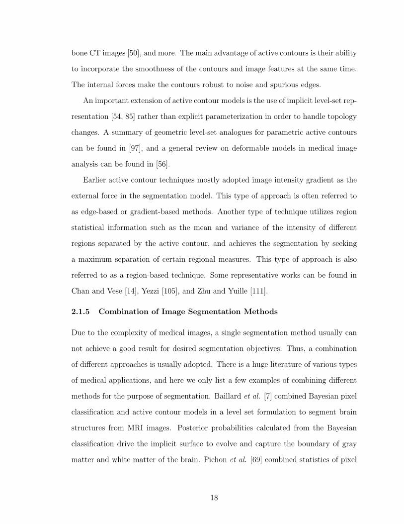
10 Enhancement of CT liver images using anisotropic diffusion. Upper:MIP views of the liver before (left) and after (right) diffusion; Lower:Iso-surfaces of the vessels before (left) and after (right) diffusion [44]. 21

ix

11 Hessian-based enhancement of brain MRI images. (a) A slice of theinput original image (left) and filtered image (right). (b) Volume-rendered images of the input original (left), and filtered images (right).The filter gave high responses to the vessel structures [77]. . . . . . . 22

12 Reconstruction of the vessel surface using a tubular deformable modelfrom contrast enhanced MRA images [106]. (a) Original image of acarotid artery. (b) Reconstructed branch of the external carotid artery(ECA). (c) Reconstructed branch of the internal carotid artery (ICA).(d) The ECA and ICA are merged into a complete carotid model. . 23

13 Level set reconstruction of a carotid artery [4]. (A) Iso-surface of theoriginal CTA images with computed centerlines for level sets initial-ization. (B) Level sets evolving under inflation in the common carotidartery. (C) Level sets approaching the vessel wall. (D) Zero-level setconverged to the boundary. (E) Level sets reconstruction of ECA. (F)Reconstruction of ICA. (G) Merging of the three branches in (D)-(F). 25

14 Centerline extraction and vessel wall segmentation of coronary arteriesusing a minimal cost path approach [5]. Left: volume-rendered CTAimages and three seed points. Center: Segmented region. Right: Axesobtained from the minimal path search. . . . . . . . . . . . . . . . . 27

15 Conventional geodesic active contours fail to segment thin blood ves-sels. (a) Initial contour; (b) after 1300 iterations leakage appears andthe segmented vessel is thinner than the real size. . . . . . . . . . . . 37

16 Comparing edge maps between the conventional conformal factor andthe proposed function. (a) Original image; (b) Gaussian smoothed gra-dient image; (c) conventional conformal factor edge map; (d) proposedconformal factor edge map. . . . . . . . . . . . . . . . . . . . . . . . 39

17 An example of using EM to approximate an image histogram. In blue:the original histogram; in black: the estimated Gaussian mixture pro-file; in red: each individual component in the Gaussian mixture. . . 42

18 Segmentation of a synthetic vessel image using the proposed method.(a) Initial contour; (b) after 120 iterations; (c) after 500 iterations; (d)after 1000 iterations, final segmentation. . . . . . . . . . . . . . . . . 46

19 Segmentation of a real coronary artery image (MPR image), the sameas in Figure 15, where the conventional geodesic active contours failto segment. (a) Initial contour; (b) after 150 iterations (c) after 600iterations; (d) after 1600 iterations, final segmentation. . . . . . . . . 47

x

20 Segmentation of a heart chamber. a1. the original image; a2. theinitial contour; b1 and b2. evolution contours and final segmentationusing the conventional gradient-based method; c1 and c2. results of aregion-based method; d1 and d2. results of the proposed method. Seetext for details. . . . . . . . . . . . . . . . . . . . . . . . . . . . . . . 48

21 Original coronary artery CTA images, Dataset #1, Part I. . . . . . . 65

22 Original coronary artery CTA images, Dataset #1, Part II. . . . . . . 66

23 Lung and heart segmentation, Dataset #1, Part I. (a)→(b) thresh-olding, (b)→(c) dilation, (c)→(d) hole filling, (d)→(e) tipping pointdetection, (e)→(f) Bresenham lines. See text for details. . . . . . . . 67

24 Lung and heart segmentation, Dataset #1, Part II. (f)→(g) dilation,(g)→(h) hole filling, (g)&(h)→(i) subtraction, (i)→(j) dilation, (k)Original image, (l) masked image. See text for details. . . . . . . . . . 68

25 Volume rendering of the images before (a) and after (b) heart segmen-tation. Dataset #1. . . . . . . . . . . . . . . . . . . . . . . . . . . . 69

26 Volume rendering of the images before (a) and after (b) vessel filtering.Dataset #2. . . . . . . . . . . . . . . . . . . . . . . . . . . . . . . . 70

27 The output of vessel filtering as iso-surfaces. Dataset #2. . . . . . . 71

28 Comparing vessel filter response with and without heart segmentation.Dataset #1. Left: original image, Middle: result of applying the filteron the original image, Right: result on pixels within the heart mask. . 71

29 Comparing segmentation contours before and after BDIS. Dataset #2.(a) Initial contour on slice #6, (b) BDIS result on slice #6; (c) Initialcontour on slice #23, (d) BDIS result on slice #23. . . . . . . . . . . 72

30 Segmentation results shown in 2D as contours. Dataset #2, Part I. . 73

31 Segmentation results shown in 2D as contours. Dataset #2, Part II. . 74

32 Segmentation results shown in 2D as contours. Dataset #2, Part III. 75

33 Segmentation results shown in 2D as contours. Dataset #2, Part IV. 76

34 3D results. Left and right coronary arteries rendered as surfaces. Up-per: Automatic BDIS segmentation; Lower: Manual delineated con-tours rendered as surfaces. . . . . . . . . . . . . . . . . . . . . . . . . 77

35 Removing calcified plaques from the segmentation. (a1) and (a2):before and after removing the calcium on Slice #34 of Dataset #8;(b1) and (b2): Slice #8 of Dataset #15; (c1) and (c2): Slice #6 ofDataset #16. . . . . . . . . . . . . . . . . . . . . . . . . . . . . . . . 78

xi

36 BDIS segmentation results shown as surfaces. Part I. Datasets #1 - #6. 79

37 BDIS segmentation results shown as surfaces. Part II. Datasets #7 -#12. . . . . . . . . . . . . . . . . . . . . . . . . . . . . . . . . . . . . 80

38 BDIS segmentation results shown as surfaces. Part III. Datasets #13- #18. . . . . . . . . . . . . . . . . . . . . . . . . . . . . . . . . . . . 81

39 The segmented surface of left coronary arteries with boundary contoursshown in blue at each end. Dataset #7. . . . . . . . . . . . . . . . . 84

40 The coronary artery surface is color-painted with solved harmonic func-tion u, where dark color means lower u, and light color means higheru. Dataset #7. . . . . . . . . . . . . . . . . . . . . . . . . . . . . . . 85

41 In blue: level contours of the harmonic function u. In red: vesselcenterline formed by a series of centroids of the level contours. Dataset#7. . . . . . . . . . . . . . . . . . . . . . . . . . . . . . . . . . . . . 87

42 Digital phantom of a stenosed vessel. Left: volume rendering of thephantom; Middle: solved harmonic function u colored-painted on thesurface; Right: selected level contours of u (in blue) and harmonicskeleton (in red). . . . . . . . . . . . . . . . . . . . . . . . . . . . . . 91

43 Skeletonization results. Part I. Datasets #1 - #6. . . . . . . . . . . . 95

44 Skeletonization results. Part II. Datasets #7 - #12. . . . . . . . . . . 96

45 Skeletonization results. Part III. Datasets #13 - #16. . . . . . . . . . 97

46 Skeletonization results. Part IV. Datasets #17 - #18. . . . . . . . . . 98

47 Cross-sectional area visualization #1. The cross-sectional area of eachbranch of the coronaries for a certain u. Dataset #7. . . . . . . . . . 98

48 Cross-sectional area visualization #2. Color-painted LAD indicates anobvious stenosis site in the vessel. Dataset #1. . . . . . . . . . . . . . 99

49 Cross-sectional area along the LAD shown in Figure 48. The left y-axisshows the cross-sectional area in mm2, and the right y-axis shows thestenosis percentage. . . . . . . . . . . . . . . . . . . . . . . . . . . . . 99

xii

SUMMARY

Atherosclerosis is a systemic disease of the vessel wall that occurs in the aorta,

carotid, coronary and peripheral arteries. Atherosclerotic plaques in coronary arteries

may cause the narrowing (stenosis) or complete occlusion of the arteries and lead to

serious results such as heart attacks and strokes. Medical imaging techniques such

as X-ray angiography and computed tomography angiography (CTA) have greatly

assisted the diagnosis of atherosclerosis in living patients. Analyzing and quantifying

vessels in these images, however, is an extremely laborious and time consuming task

if done manually. A novel image segmentation approach and a quantitative shape

analysis approach are proposed to automatically isolate the coronary arteries and

measure important parameters along the vessels.

The segmentation method is based on the active contour model using the level

set formulation. Regional statistical information is incorporated in the framework

through Bayesian pixel classification. A new conformal factor and an adaptive speed

term are proposed to counter the problems of contour leakage and narrowed vessels

resulting from the conventional geometric active contours. The proposed segmenta-

tion framework is tested and evaluated on a large amount of 2D and 3D, including

synthetic and real 2D vessels, 2D non-vessel objects, and eighteen 3D clinical CTA

datasets of coronary arteries.

The centerlines of the vessels are proposed to be extracted using harmonic skele-

tonization technique based on the level contour sets of the harmonic function, which

is the solution of the Laplace equation on the triangulated surface of the segmented

xiii

vessels. The cross-sectional areas along the vessels can be measured while the center-

line is being extracted. Local cross-sectional areas can be used as a direct indicator

of stenosis for diagnosis. A comprehensive validation is performed by using digital

phantoms and real CTA datasets.

This study provides the possibility of fully automatic analysis of coronary atheroscle-

rosis from CTA images, and has the potential to be used in a real clinical setting along

with a friendly user interface. Comparing to the manual segmentation which takes

approximately an hour for a single dataset, the automatic approach on average takes

less than five minutes to complete, and gives more consistent results across datasets.

xiv

CHAPTER I

INTRODUCTION

1.1 Atherosclerosis and Coronary Artery Diseases

Cardiovascular disease (CVD) is the most prevalent cause of death in the United

States. Approximately 64,400,000 Americans have one or more types of CVD, and

these account for approximately 40 percent of all deaths in the United States per

year [1]. CVD includes high blood pressure, coronary heart disease (CHD), conges-

tive heart failure, stroke, and congenital cardiovascular defects. Among these, CHD

accounts for approximately 54 percent of deaths of CVD in the United States.

Atherosclerosis is a systemic disease of the vessel wall that occurs in the aorta,

carotid, coronary and peripheral arteries [29]. Major consequences of atheroscle-

rosis are myocardial infarction (heart attack), cerebral infarction (stroke), aortic

aneurysms, and peripheral vascular disease (gangrene of the legs). Figure 1 and Fig-

ure 2 compare the main components of the vascular wall of a normal vessel and vessel

with well-developed atheromatous plaque [47]. The most clearly defined layers of a

vessel wall are: intima, media, and adventitia. In normal arteries, the intima consists

of a single layer of endothelial cells, with minimal underlying sub-endothelial connec-

tive tissue. The intima and media are separated by a dense elastic membrane called

the internal elastic lamina. The media layer consists mainly of smooth muscle cells,

and is separated from the adventitia by the external elastic lamina. Atherosclerosis

is characterized by intimal lesions called atheromas, or atheromatous or fibrofatty

plaques, that protrude into and obstruct vascular lumina, weaken the underlying me-

dia, and may undergo serious complications. The key processes in atherosclerosis are

intimal thickening and lipid accumulation. An atherosclerotic plaque consists of a

1

raised focal lesion initiating within the intima, having a lipid core and covered by a

firm fibrous cap, as shown in Figure 2.

Figure 1: Schematic representation of the major components of a normal vascularwall [47].

Figure 2: Schematic representation of the major components of a well-developedatherosclerotic plaque [47].

Atherosclerotic lesions usually involve the arterial wall only partially around its

circumference and are patchy and variable along the vessel length. Plaques generally

continue to change and enlarge; focal and sparsely distributed lesions may become

more and more numerous and diffuse as the disease advances. Moreover, atheroscle-

rotic plaques often undergo calcification. Figure 3 illustrates the histology of a vessel

cross section showing the typical features of an advanced plaque in the coronary

artery. The advanced lesion of atherosclerosis may lead to further pathologic changes

2

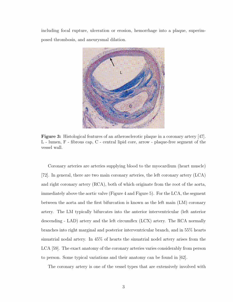
including focal rupture, ulceration or erosion, hemorrhage into a plaque, superim-

posed thrombosis, and aneurysmal dilation.

Figure 3: Histological features of an atherosclerotic plaque in a coronary artery [47].L - lumen, F - fibrous cap, C - central lipid core, arrow - plaque-free segment of thevessel wall.

Coronary arteries are arteries supplying blood to the myocardium (heart muscle)

[72]. In general, there are two main coronary arteries, the left coronary artery (LCA)

and right coronary artery (RCA), both of which originate from the root of the aorta,

immediately above the aortic valve (Figure 4 and Figure 5). For the LCA, the segment

between the aorta and the first bifurcation is known as the left main (LM) coronary

artery. The LM typically bifurcates into the anterior interventricular (left anterior

descending - LAD) artery and the left circumflex (LCX) artery. The RCA normally

branches into right marginal and posterior interventricular branch, and in 55% hearts

sinuatrial nodal artery. In 45% of hearts the sinuatrial nodel artery arises from the

LCA [59]. The exact anatomy of the coronary arteries varies considerably from person

to person. Some typical variations and their anatomy can be found in [62].

The coronary artery is one of the vessel types that are extensively involved with

3

Figure 4: Illustrated anatomy of human coronary arteries and cardiac veins [62].

atherosclerosis. Hence, atherosclerosis is one of the main causes of CHD. Atheroscle-

rotic plaques in coronary arteries may cause stenosis or complete occlusion of the

arteries and lead to serious results such as angina pectoris and myocardial infarction.

As reported by the American Heart Association [1], in 2006 an estimated 1,200,000

Americans will have a new or recurrent coronary attack, of which 700,000 will have a

new coronary attack. It is estimated that an additional 175,000 silent first heart at-

tacks occur each year. It is essential to be able to detect and diagnose atherosclerosis

in coronary arteries at its early stage of development, and to apply according treat-

ments using medications or surgical procedures such as diagnostic cardiac catheteri-

zation, angioplasty procedures, stent implantation and bypass procedures in order to

prevent or delay the serious consequences listed above.

4

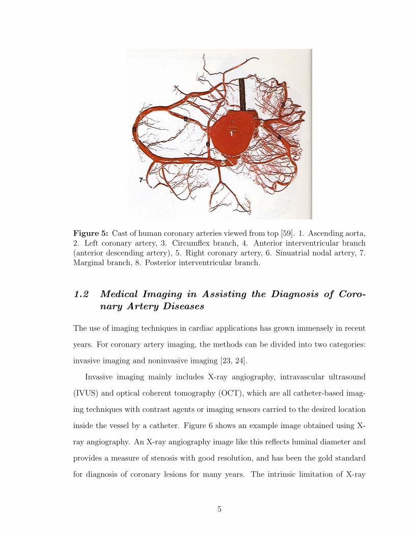
Figure 5: Cast of human coronary arteries viewed from top [59]. 1. Ascending aorta,2. Left coronary artery, 3. Circumflex branch, 4. Anterior interventricular branch(anterior descending artery), 5. Right coronary artery, 6. Sinuatrial nodal artery, 7.Marginal branch, 8. Posterior interventricular branch.

1.2 Medical Imaging in Assisting the Diagnosis of Coro-nary Artery Diseases

The use of imaging techniques in cardiac applications has grown immensely in recent

years. For coronary artery imaging, the methods can be divided into two categories:

invasive imaging and noninvasive imaging [23, 24].

Invasive imaging mainly includes X-ray angiography, intravascular ultrasound

(IVUS) and optical coherent tomography (OCT), which are all catheter-based imag-

ing techniques with contrast agents or imaging sensors carried to the desired location

inside the vessel by a catheter. Figure 6 shows an example image obtained using X-

ray angiography. An X-ray angiography image like this reflects luminal diameter and

provides a measure of stenosis with good resolution, and has been the gold standard

for diagnosis of coronary lesions for many years. The intrinsic limitation of X-ray

5

angiography, however, is the ability to acquire only two-dimensional (2D) projections

of the vessels, which are indeed three-dimensional (3D) anatomical structures. As a

result, the stenosis or lesion may be underestimated by the 2D X-ray angiography

images, and the exact 3D geometry of the coronaries can not be recovered from a

single 2D image. To overcome the limitations and enable 3D reconstruction of the

vessels, several variations of X-ray angiography have been developed. Cineangiograms

can be generated from different angles of X-ray projection as well as different time

points, so 3D dynamic structures of the coronaries can be reconstructed from these

series of 2D images using projective reconstruction techniques. A rotational X-ray

angiography system can acquire angiograms at all angles by performing a continuous

rotation of a C-arm X-ray emission and detection system. In this way, a complete se-

ries of images is obtained in a range of projections, and the images can be re-sampled

and reconstructed to create a 3D volume to emulate a computed tomography (CT)

scan. However, due to the rotational nature of this imaging technique, the spacial

resolution varies from the center of the image volume to the outer field, sometimes

bringing trouble for the reconstruction of larger field of views (FOV), and the image

quality is usually inferior to a real CT scan.

Catheter-based IVUS and OCT are relatively new techniques to arterial vascular

wall imaging. These invasive imaging modalities allow direct and real-time imaging of

atherosclerotic plaques and provide a cross-sectional view of the lumen and vessel wall.

They both acquire images by carrying an imaging sensor at the tip of the catheter

to the desired location and collecting signals from reflected ultrasound beams (for

IVUS) or laser beams (for OCT). Figure 7 compares images of the same vessel at

the same location, imaged by both OCT (A) and IVUS (B). It can be seen that

a calcified plaque at 8-9 o’clock is revealed in both OCT and IVUS images. OCT

sometimes is capable of revealing more structures in the vessel wall than IVUS, since

some structures are echo-lucent in the ultrasound field. It is also evident that OCT

6

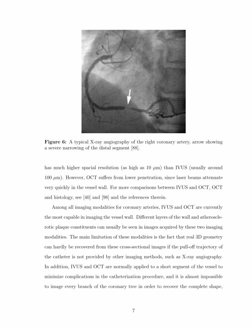
Figure 6: A typical X-ray angiography of the right coronary artery, arrow showinga severe narrowing of the distal segment [88].

has much higher spacial resolution (as high as 10 µm) than IVUS (usually around

100 µm). However, OCT suffers from lower penetration, since laser beams attenuate

very quickly in the vessel wall. For more comparisons between IVUS and OCT, OCT

and histology, see [40] and [98] and the references therein.

Among all imaging modalities for coronary arteries, IVUS and OCT are currently

the most capable in imaging the vessel wall. Different layers of the wall and atheroscle-

rotic plaque constituents can usually be seen in images acquired by these two imaging

modalities. The main limitation of these modalities is the fact that real 3D geometry

can hardly be recovered from these cross-sectional images if the pull-off trajectory of

the catheter is not provided by other imaging methods, such as X-ray angiography.

In addition, IVUS and OCT are normally applied to a short segment of the vessel to

minimize complications in the catheterization procedure, and it is almost impossible

to image every branch of the coronary tree in order to recover the complete shape,

7

Figure 7: OCT (A) and IVUS (B) images of a coronary artery cross-section. Singlearrow in both images indicates a calcified plaque with low intensities in OCT andhigh intensities in IVUS. Two arrowheads in the OCT image indicate a high intensityregion showing a fibrous band overlying the calcification, which is obscured in theIVUS image. The borders of the guide wire artifact (∗) are marked by dotted linesin (A) [40].

even when the pull-off trajectories are available.

Although catheter-based imaging approaches can acquire coronary images with

quite good image quality and imaging speed, the main drawback of the above tech-

niques is bringing complicated clinical procedures and risks to the patient because of

their invasiveness. It is acceptable if the imaging procedure takes place at the same

time with a catheter-based treatment procedure, however the invasive imaging tech-

niques are not suitable for observational or routine follow up examinations performed

in the same patient on a regular basis.

With the development of engineering technology, noninvasive imaging modali-

ties have become more and more attractive, and more frequently used in clinical

settings. Among the noninvasive imaging modalities, computed tomography angiog-

raphy (CTA) is the most widely used for patients at present, and magnetic resonance

imaging (MRI) is currently more preferable for conducting advanced research and

8

studies. Other than the apparent advantage of being noninvasive, these techniques

also provide information of the whole 3D volume rather than 2D projections in the

conventional X-ray angiography, or 2D vessel cross-sections in IVUS and OCT.

CTA has been used in various clinical applications including cardiac, head and

neck, abdomen, and extremities with a spacial resolution of under 0.5 mm in all three

dimensions. The imaging contrast agent is delivered intravenously instead of carried

by a catheter to the desired imaging location, which makes the imaging procedure

much less invasive. For coronary imaging, CTA is especially good at revealing the

blood pool and calcified plaques, which both have high intensities in the images,

calcium being higher. Soft plaques can sometimes be observed as well, if the image

quality is sufficiently high. Figure 8 shows the same RCA as in Figure 6, imaged using

CTA. The 3D volumetric image is re-sampled using the multi-planar reformatting

(MPR) technique in order to show the entire vessel on a 2D image. It can be seen

that the stenosis at the distal end of this RCA is clearly shown with similar image

quality as in the X-ray angiography.

In addition, CTA revealed more information about the plaque as shown in the high

intensity region right below the stenosis in Figure 8, which is possibly a ulcerated

cavity in the vessel wall [88]. The CTA image also shows calcium deposits in the

proximal region which can not be seen in the X-ray angiography. This case indicates

that CTA has the ability of non-invasively imaging not only the lumen in vivo as well

as X-ray angiography, but sometimes with even more information of the vascular wall.

Another advantage of CTA is the ability to show cross-sections of the vessel as in IVUS

and OCT. Given the center point of the vessel at a certain location and the tangential

direction of the centerline (either specified manually or extracted automatically), the

3D CTA data can be re-sampled on the plane defined by the center point and the

direction vector. The resolution is usually not as high as intravascular OCT or IVUS,

however CTA is still superior to X-ray angiography in this respect.

9

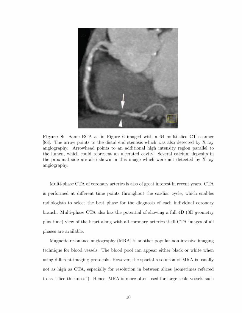
Figure 8: Same RCA as in Figure 6 imaged with a 64 multi-slice CT scanner[88]. The arrow points to the distal end stenosis which was also detected by X-rayangiography. Arrowhead points to an additional high intensity region parallel tothe lumen, which could represent an ulcerated cavity. Several calcium deposits inthe proximal side are also shown in this image which were not detected by X-rayangiography.

Multi-phase CTA of coronary arteries is also of great interest in recent years. CTA

is performed at different time points throughout the cardiac cycle, which enables

radiologists to select the best phase for the diagnosis of each individual coronary

branch. Multi-phase CTA also has the potential of showing a full 4D (3D geometry

plus time) view of the heart along with all coronary arteries if all CTA images of all

phases are available.

Magnetic resonance angiography (MRA) is another popular non-invasive imaging

technique for blood vessels. The blood pool can appear either black or white when

using different imaging protocols. However, the spacial resolution of MRA is usually

not as high as CTA, especially for resolution in between slices (sometimes referred

to as “slice thickness”). Hence, MRA is more often used for large scale vessels such

10

as the aorta or large vessels in the brain. In vivo imaging of coronary arteries using

MRA is still being investigated and is not widely used clinically for the time being.

Digital subtraction angiography (DSA) is a computational technique to better

visualize blood vessels by subtracting a non-contrast image (either an MRI or a CT)

from a contrast-enhanced image. This technique suppresses the surrounding bones

and tissues significantly and the resulting image is usually nice and clean. However

DSA normally can not be easily applied to coronary artery imaging for the following

reasons. First, DSA requires two sets of images: non-contrast and contrast, which

means doubling the radiation dose for CT imaging. Second, DSA requires perfect

alignment of the two sets of images in order to subtract one from another. Coronaries

are moving structures and it is very hard to acquire perfectly aligned data even if the

coronaries are imaged at the same time point during the cardiac cycle. Hence, DSA

is most widely used in head and neck MRA imaging, where motion is minimal and

there is no X-ray radiation. DSA is not used commonly in CTA, although it is a very

attractive technique that can reduce much of the image post processing work.

CTA is the imaging modality of interest in this thesis for its various advantages

listed above, and also for the reason that with the 3D volumetric data at hand,

image processing and analysis have become more important as compared to the 2D

case. The growing number of the images in a single dataset has made viewing images

slice by slice an extremely time consuming task for radiologists. It is also desirable

that different body organs be visualized and studied separately, instead of displayed

with many irrelevant surrounding organs. This is where image segmentation and

3D visualization come into play to provide more possibilities to explore the data

extensively so that physicians can perform diagnoses and treatments more accurately

and more efficiently.

There are many image segmentation algorithms proposed in the literature, as will

be reviewed in more detail in Chapter 2, and some have become standard and have

11

been described in textbooks [30, 81]. The algorithms vary from the simplest thresh-

olding and edge detection techniques, to more complicated region-based models and

active contour models. The problem of image segmentation, however, continues to be

an active research field because there is no single framework that fits all applications

and meets all requirements. In medical applications, segmentation algorithms need

to be accurate to avoid mistakes as much as possible; they need to be reasonably

fast; and they also need to be able to effectively separate the interested organs from

the other parts of the images. To meet these requirements, an efficient and accurate

segmentation algorithm is needed for the task of coronary artery segmentation, which

becomes one of the major topics of this thesis.

After the image segmentation is done, several useful tasks can be conducted in

addition. The most straightforward would be the surface rendering [33] of the 3D

object that has been segmented. By using computer visualization techniques, a 3D

surface can be generated and displayed on the 2D computer screen. This also allows

users to zoom and rotate in order to observe the object from different perspectives.

Shape analysis is an equally important task, especially for complicated structures

such as blood vessels. In this thesis, a centerline extraction (also referred to as

skeletonization process) approach is proposed to trace the center axis of the segmented

and triangulated surface of the vessel, and a method to measure local cross-sectional

areas is also proposed for the purpose of quantitative analysis and stenosis detection.

Other applications of 3D segmentation of coronary arteries include generating pa-

tient specific geometric boundary conditions for computational fluid dynamic (CFD)

simulation of blood flow and study of the relation between the flow patterns and

atherosclerotic plaque distribution along the vessel wall [83]. Some cases studied in

the thesis have been used to conduct CFD simulations and compared to clinical ob-

servations [84]. The detailed formulation of CFD, however, is beyond the scope of

this thesis.

12

1.3 Organization of the Thesis

In the next chapters, we will fully explore the problem of CTA coronary image anal-

ysis. In Chapter 2, we start by reviewing the existing image segmentation and vessel

analysis methods in the literature followed by the discussion of their advantages and

limitations. In Chapter 3 we propose a general image segmentation framework which

has the potential to be used for segmenting blood vessels, and in Chapter 4 we apply

the proposed algorithm to extract coronary arteries from CTA images. The seg-

mentation process is made fully automatic with the assistance of a automatic heart

segmentation method and a Hessian-based vessel filtering technique. We also look

at the problem of identifying and segmenting calcified plaques from the images. In

Chapter 5 we will present a centerline extraction approach based on the segmented

surface of tubular structures, which we call the harmonic skeletonization approach.

As we search for the centerlines, we also measure cross-sectional areas of the coronary

arteries, which provide a good reference for stenosis detection and evaluation. The

final chapter (Chapter 6) concludes the thesis and discusses several possible future

directions.

13

CHAPTER II

BACKGROUND: MEDICAL IMAGE SEGMENTATION

AND 3D VESSEL IMAGE ANALYSIS

2.1 Medical Image Segmentation Methods – A Brief Re-view

Image segmentation algorithms for the delineation of anatomical structures and other

regions of interest are becoming increasingly important in assisting and automating

specific radiological tasks. These algorithms play a vital role in numerous biomed-

ical imaging applications, such as quantification of tissue volumes, diagnosis and

localization of pathology, study of anatomical structures, treatment planning, and

computer-guided surgery [70].

2.1.1 Definition of Image Segmentation

Classically, image segmentation is defined as the partitioning of an image into non-

overlapping, constituent regions that are homogeneous with respect to some charac-

teristic such as intensity or texture [30, 34, 68]. If the domain of the image is given

by Ω, then the segmentation problem is to determine the sets Sk ⊂ Ω, whose union

is the entire domain Ω. Thus, the sets that make up a segmentation must satisfy:

Ω =K⋃

k=1

Sk (1)

where Sk ∩ Sj = φ (a null set) for k 6= j, and each Sk is connected. Ideally, a seg-

mentation method finds those sets that correspond to distinct anatomical structures

or regions of interest in the image.

Pixel segmentation, rather than classical segmentation, is often a desirable goal

14

in medical images, particularly when disconnected regions belong to the same tis-

sue class. When the constraint that regions must be connected is removed from the

classical segmentation, determining the sets Sk is called pixel classification, and the

sets themselves are called classes. Determining the total number of classes K can

be a difficult problem [48]. Usually, the value of K is assumed to be known based

on prior knowledge of the anatomy being considered. For example, in the segmenta-

tion of cardiac images, we assume that K = 3, corresponding to blood-filled region,

myocardium region, and lung region [100].

The commonly used image segmentation methods include: thresholding, region

growing, classifiers, clustering, Markov random field (MRF) models, artificial neural

networks, deformable models and atlas-guided approaches. Several of these techniques

are often used in conjunction for solving different segmentation problems. Here we

only review those which are closely related to this thesis. Other methods can be found

in the surveys of image segmentation in literature [6, 17, 70].

2.1.2 Thresholding and Region Growing

Thresholding approaches segment scalar images by creating a binary partitioning of

the image intensities. It is a simple yet often effective method for obtaining a segmen-

tation of images in which different structures have contrasting intensities. Threshold-

ing is usually used as an initial step in a sequence of image processing operations. Its

main limitation is that typically it does not take into account the spatial characteris-

tics of an image. This causes it to be sensitive to noise and intensity inhomogeneities,

which often occur in medical images. Variations on classical thresholding have been

proposed to incorporate information based on local intensities and connectivity. A

survey of thresholding techniques can be found in [76].

Region growing is a technique that extracts connected regions based on certain

criteria such as image intensity and/or edges. A seed is needed to be placed inside

15

the desired region to extract all the connected pixels according to the criteria. Like

thresholding, the simplest form of region growing can be sensitive to noise, and it

requires the manual placement of seeds in every region to be segmented. Region

growing is seldom used alone but usually combined with other segmentation tech-

niques to delineate small, simple structures such as tumors and lesions [70].

2.1.3 Classifiers and Clustering Methods

Classifiers and clustering methods are pattern recognition techniques that apply to

image segmentation problems. Classifiers are known as supervised methods because

they require training data, and clustering algorithms are termed unsupervised because

they perform classification of the data without the use of training data.

Classifier methods seek to partition a feature space (usually image intensities) by

using training data. There are a number of ways in which the training data can

be applied. The commonly used nonparametric classifiers include k-nearest neighbor

(kNN) and Parzen window; a parametric classifier is usually the maximum-likelihood

or Bayes classifier [21]. It is assumed that the pixel intensities are independent samples

from a mixture of probability distributions, usually Gaussian for CT and MRI images.

The estimation of the means, covariances, and mixing coefficients of the K classes is

also needed. Being non-iterative, classifiers are relatively computationally efficient,

and they can be applied to multichannel images. The disadvantage is the requirement

of manual interaction to obtain training data, which can be laborious. If a same set of

training data were used for a large number of images, biased results could be obtained.

Clustering algorithms, on the other hand, do not need training data. But to

compensate for this, they iteratively alternate between segmenting the image and

characterizing the properties of each class. Three commonly used clustering algo-

rithms are the K-means algorithm, the fuzzy c-means algorithm, and the expectation-

maximization (EM) algorithm.

16

Classifiers and clustering methods do not directly incorporate spatial modeling

and can be sensitive to noise. This lack of spatial modeling, however, can provide

advantages for fast computation. The use of MRF models [73] can improve the

robustness to noise of these algorithms.

2.1.4 Active Contour Models

Active contour models, also called deformable models [92] or “snakes” [41], are phys-

ically motivated techniques for segmenting objects using closed parametric curves or

surfaces that deform under the influence of internal and external forces. The internal

forces serve to impose a smoothing constraint. The external or image forces push the

active contour to move toward salient image features like lines and edges. A closed

curve or surface is needed to be placed near the desired boundary and then allowed

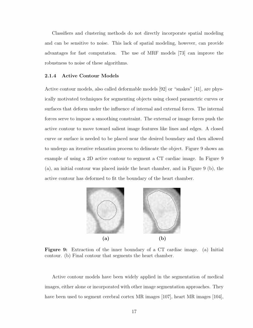
to undergo an iterative relaxation process to delineate the object. Figure 9 shows an

example of using a 2D active contour to segment a CT cardiac image. In Figure 9

(a), an initial contour was placed inside the heart chamber, and in Figure 9 (b), the

active contour has deformed to fit the boundary of the heart chamber.

(a) (b)

Figure 9: Extraction of the inner boundary of a CT cardiac image. (a) Initialcontour. (b) Final contour that segments the heart chamber.

Active contour models have been widely applied in the segmentation of medical

images, either alone or incorporated with other image segmentation approaches. They

have been used to segment cerebral cortex MR images [107], heart MR images [104],

17

bone CT images [50], and more. The main advantage of active contours is their ability

to incorporate the smoothness of the contours and image features at the same time.

The internal forces make the contours robust to noise and spurious edges.

An important extension of active contour models is the use of implicit level-set rep-

resentation [54, 85] rather than explicit parameterization in order to handle topology

changes. A summary of geometric level-set analogues for parametric active contours

can be found in [97], and a general review on deformable models in medical image

analysis can be found in [56].

Earlier active contour techniques mostly adopted image intensity gradient as the

external force in the segmentation model. This type of approach is often referred to

as edge-based or gradient-based methods. Another type of technique utilizes region

statistical information such as the mean and variance of the intensity of different

regions separated by the active contour, and achieves the segmentation by seeking

a maximum separation of certain regional measures. This type of approach is also

referred to as a region-based technique. Some representative works can be found in

Chan and Vese [14], Yezzi [105], and Zhu and Yuille [111].

2.1.5 Combination of Image Segmentation Methods

Due to the complexity of medical images, a single segmentation method usually can

not achieve a good result for desired segmentation objectives. Thus, a combination

of different approaches is usually adopted. There is a huge literature of various types

of medical applications, and here we only list a few examples of combining different

methods for the purpose of segmentation. Baillard et al. [7] combined Bayesian pixel

classification and active contour models in a level set formulation to segment brain

structures from MRI images. Posterior probabilities calculated from the Bayesian

classification drive the implicit surface to evolve and capture the boundary of gray

matter and white matter of the brain. Pichon et al. [69] combined statistics of pixel

18

intensity and a region growing method, and a employed fast marching method [80] to

calculate the arrival time of the growing front. The user determines a time t0 to pick

the best region that represents the desired object. Leventon et al. [50] incorporate

shape prior information to the level set segmentation framework based on a set of

previously segmented data. The shape constraint was defined based on dimensionality

reduction techniques on the distance transform of pre-segmented shapes. This method

is especially efficient for medical structures that do not vary too much from patient

to patient.

The above methods are all general segmentation frameworks which are not specif-

ically designed for blood vessels. In the next section, we will review segmentation

methods proposed for blood vessel segmentation and examine some of the specific

considerations for this application.

2.2 Previous Work on 3D Vessel Image Analysis

Segmentation makes up a great portion of the 3D vessel image analysis problem, how-

ever it is not the sole topic of interest. In fact, the segmentation problem for vessels

is largely blended with other problems, such as automatic enhancement and detec-

tion, centerline extraction and advanced visualization. Several of these problems are

often investigated together to explore the original image fully and perform automatic

extraction of significant information as much as possible.

From the perspective of specific applications, many excellent works have been

focused on vessel analysis in MRA images, especially cerebral MRA. There is also a

special interest recently in analyzing retinal images to extract vessels in the eye [60,

82], where the input images are typically 2D images generated using optical imaging

methods. For coronary artery image analysis, most works have been performed on

X-ray angiography images due to the availability of this imaging modality for many

years. CTA is relatively new for coronary imaging and not much previous work has

19

been seen in the literature. We will explore this problem extensively in the following

chapters of this thesis.

In this section, we first review some methods for enhancing vessel images to better

present and visualize the original image. These techniques can also serve as pre-

processing steps for further analysis such as automatic segmentation. We then review

some general vessel extraction and analysis approaches, with a special focus on 3D

applications. After that, we specifically look at vessel analysis studies which have been

done on CTA data. Finally, we review important works on coronary artery image

processing, which are mainly performed on X-ray angiography. For a comprehensive

review of vessel extraction techniques presented in the literature before the year of

2003, see [43] and the references therein. It can also be seen from the tables comparing

the performance of different approaches listed in [43] that the use of CTA as an input

type is far less than the use of X-ray angiography, MRA and DSA.

2.2.1 Enhancement of Curvilinear Structures

Anisotropic diffusion has been used to smooth and enhance blood vessels in 3D images

[44, 45]. The multi-directional diffusion flux is decomposed in an orthogonal basis,

which enhances the iso-level contours of the image as well as diffuses along the con-

tours. The method was tested on CT liver images in both MIP (maximum intensity

projection) view and iso-surfaces (Figure 10). The noise in the image was significantly

suppressed after the diffusion, and details of small vessels are better preserved than

using a Gaussian isotropic smoothing filter.

Another type of vessel enhancement technique is based on the Hessian analysis of

the Gaussian smoothed image, specifically the eigenvalues of the Hessian matrix. Sato

et al. [77] identified blood vessels as 3D curvilinear structures that can be enhanced by

a 3D multi-scale Hessian-based filter. The filter response can be used to visualize the

vessels through isosurface extraction. The multi-scale property enables the filter to

20

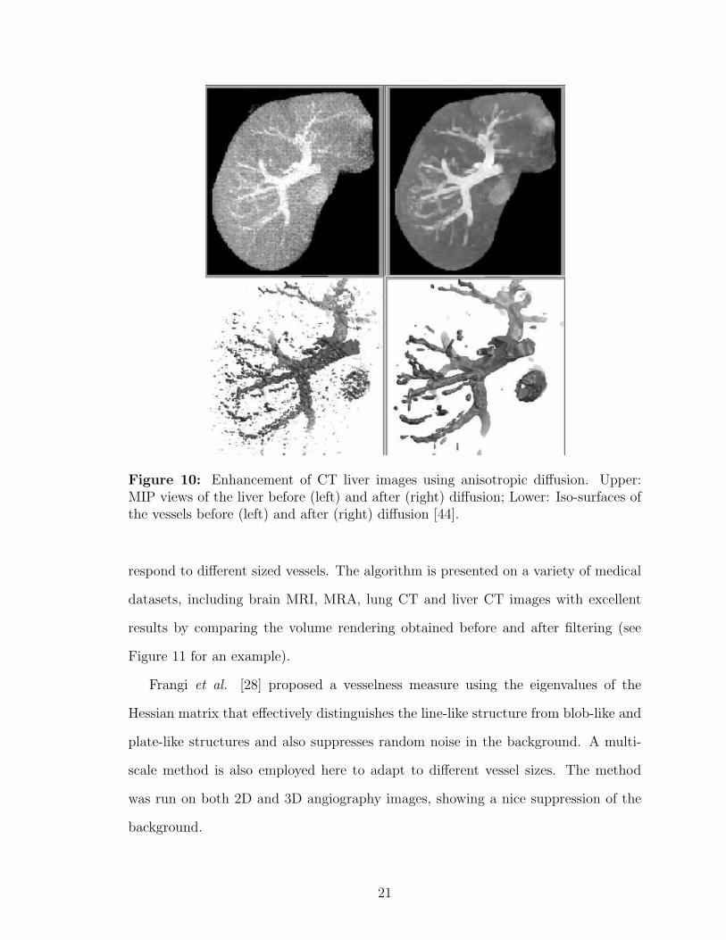
Figure 10: Enhancement of CT liver images using anisotropic diffusion. Upper:MIP views of the liver before (left) and after (right) diffusion; Lower: Iso-surfaces ofthe vessels before (left) and after (right) diffusion [44].

respond to different sized vessels. The algorithm is presented on a variety of medical

datasets, including brain MRI, MRA, lung CT and liver CT images with excellent

results by comparing the volume rendering obtained before and after filtering (see

Figure 11 for an example).

Frangi et al. [28] proposed a vesselness measure using the eigenvalues of the

Hessian matrix that effectively distinguishes the line-like structure from blob-like and

plate-like structures and also suppresses random noise in the background. A multi-

scale method is also employed here to adapt to different vessel sizes. The method

was run on both 2D and 3D angiography images, showing a nice suppression of the

background.

21

Figure 11: Hessian-based enhancement of brain MRI images. (a) A slice of theinput original image (left) and filtered image (right). (b) Volume-rendered images ofthe input original (left), and filtered images (right). The filter gave high responses tothe vessel structures [77].

Vessel enhancement techniques can be useful and helpful not only for better MIP

and iso-surface visualization, but for initiating and assisting segmentation as well. In

Chapter 4, we will employ the Hessian-based vessel filtering technique to initiate our

coronary segmentation process.

2.2.2 General Vessel Extraction and Analysis Approaches

Earlier work by Verdonck et al. [93] and Wink et al. [94] used an iterative method to

find the center axis and vessel boundaries alternately. The 3D data were re-sampled

perpendicularly to the the axis and within the re-sampled 2D slices, vessel boundaries

were located by detecting high gradients of the image intensity. The segmentation,

however, is not accurate enough since it is only based on local gradients, which are

sensitive to noise and the threshold chosen.

22

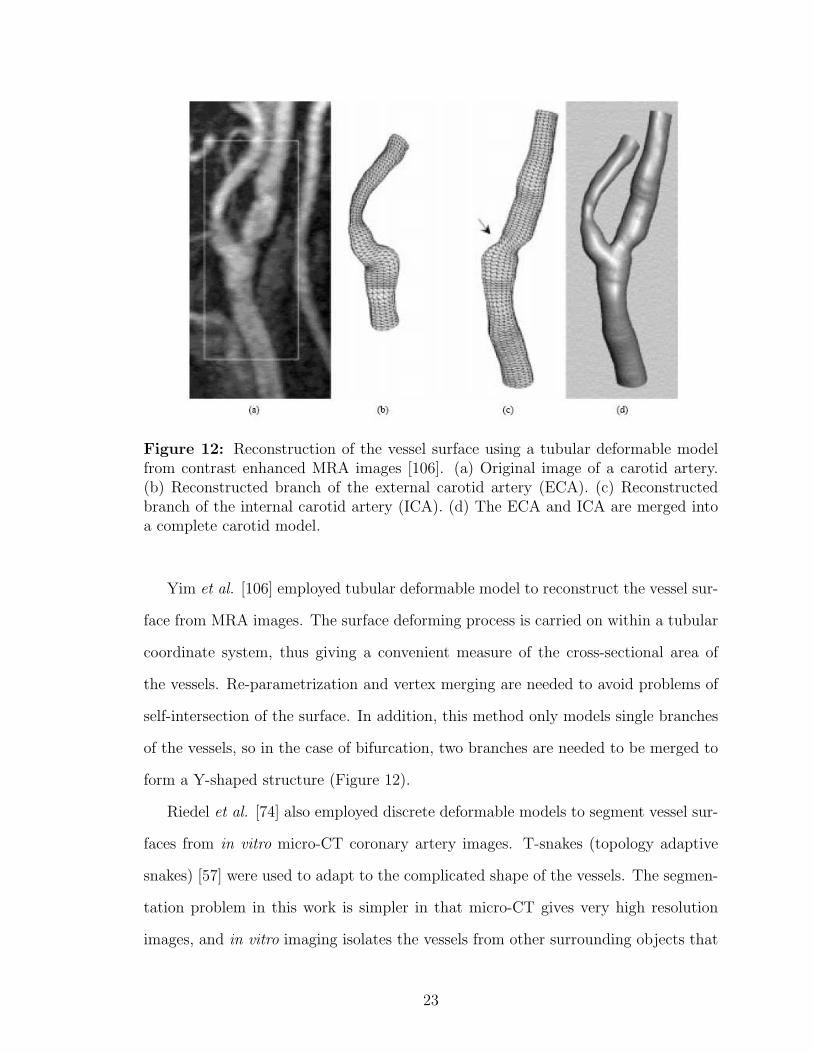
Figure 12: Reconstruction of the vessel surface using a tubular deformable modelfrom contrast enhanced MRA images [106]. (a) Original image of a carotid artery.(b) Reconstructed branch of the external carotid artery (ECA). (c) Reconstructedbranch of the internal carotid artery (ICA). (d) The ECA and ICA are merged intoa complete carotid model.

Yim et al. [106] employed tubular deformable model to reconstruct the vessel sur-

face from MRA images. The surface deforming process is carried on within a tubular

coordinate system, thus giving a convenient measure of the cross-sectional area of

the vessels. Re-parametrization and vertex merging are needed to avoid problems of

self-intersection of the surface. In addition, this method only models single branches

of the vessels, so in the case of bifurcation, two branches are needed to be merged to

form a Y-shaped structure (Figure 12).

Riedel et al. [74] also employed discrete deformable models to segment vessel sur-

faces from in vitro micro-CT coronary artery images. T-snakes (topology adaptive

snakes) [57] were used to adapt to the complicated shape of the vessels. The segmen-

tation problem in this work is simpler in that micro-CT gives very high resolution

images, and in vitro imaging isolates the vessels from other surrounding objects that

23

usually bring difficulties to the segmentation.

The generalized cylinder model is also adopted by Worz et al. [96], where a

parametric intensity model is proposed to deal with scale variance in vessel sizes.

This work models the cross-sections of the vessels as circles, which sometimes is not

true for diseased vessels. Also, there is no constraint between different levels of circles,

leading to non-smoothness in the longitudinal direction.

Other model-based methods include [27, 46], where the Hessian enhancement tech-

nique is employed in both works. In [46], the vessel is modeled as a cylindrical shape

with a series of center points and elliptical cross-sections. In [27], a linear vessel

segment defined by two user-defined end points is modeled with a central axis curve

coupled with a vessel wall surface. Model-based methods simplify the vessel extraction

and representation problem by fitting the shape of the vessel to a certain geometric

model, and can be fast and intuitive. However, the model usually has limitations

in representing all possible shapes, such as bifurcations and irregular cross-sections,

which is often the case for diseased vessels.

The level set formalism has been adopted in several studies of vessel segmentation.

Antiga et al. [3, 4] used geodesic active surfaces to segment carotid arteries from CTA

images. A sparse field approach [95] is used for efficient implementation. The active

surface grows like a balloon to capture the vessel boundary with initial seeds placed

near the center axis of the vessel (Figure 13). A local smoothing filter is applied on

the segmented surface to eliminate protrusion artifacts due to collateral vessels of the

carotid artery.

Shape priors were also incorporated in the level set segmentation framework for

blood vessels. Lorigo et al. [52] proposed the use of co-dimension 2 active contours

to incorporate directionality to the mean curvature flow. The vessels are modeled as

tubes with varying width. The center axis evolves in the 3D space and an estimation

of the local radius is made along the vessel. The method was applied to brain MRA

24

Figure 13: Level set reconstruction of a carotid artery [4]. (A) Iso-surface of theoriginal CTA images with computed centerlines for level sets initialization. (B) Levelsets evolving under inflation in the common carotid artery. (C) Level sets approachingthe vessel wall. (D) Zero-level set converged to the boundary. (E) Level sets recon-struction of ECA. (F) Reconstruction of ICA. (G) Merging of the three branches in(D)-(F).

images and is effective in extracting small scale vessels. The vessel radii, however,

are observed to be smaller than in MIP projections. Nain et al. [61] proposed a soft

shape prior that incorporates a local ball filter to restrain the shape to be segmented

to a long and thin structure. This method prevents leaks effectively, and the level set

formulation allows the vessels and adjacent leaked-through regions to be separated

automatically after certain times of iterations.

Chen and Amini [15] combined several vessel analysis techniques and proposed

a hybrid approach to quantify 3D vascular structures. The MRA image was first

enhanced using a Hessian-based method, and then a level set method is applied to

the filtered image to segment the vessels. To further refine the result, the vessel

surface is triangulated using 3D Delaunay triangulation and used as a parametric

deformable model. This hybrid approach was tested on a phantom and three MRA

abdomen datasets with encouraging results. No CTA data were tested.

In both parametric deformable models and level sets, the initial placement of the

vessel surface is important. If the process is initialized with a single seed point, the

25

surface tends to over-evolve around the seed, and may leak out of the vessel boundary

before the propagating front even reaches the far-end of the vessel. Deschamps and

Cohen [20] proposed a freezing-front approach that stops the evolution near the seed

based on the distance, and only allows the actual moving front to continue to propa-

gate. This idea is successfully demonstrated on MRA images, however it is a heuristic

approach and the stopping criteria must be chosen carefully. It is more desirable that

the segmentation process is initialized with a surface near the centerline of the vessel,

which must be extracted beforehand either manually or automatically. This leads to

the gray-scale centerline extraction problem.

Several studies based on a minimal cost path have been applied to extract vessels

in gray-scale 2D and 3D images [5, 18, 51, 63]. This type of approach is essentially

searching a path between two user-specified points in order to minimize a total cost

along the path. The cost can be defined based on image intensity, gradients or other

smoothness constraints. Using wave front propagation and backtracking techniques,

the resulting centerline usually lies within the boundary of the vessel. It may not

be very well centered, however, and normally needs to be refined. Li and Yezzi

[51] addressed this problem by proposing a method to search the vessel path in an

augmented space as 4D curves, the fourth dimension being the vessel size. This

additional parameter adds more constraint to the model and leads to a better centered

vessel axis. The intrinsic nature of the minimal path type technique makes it non-

automatic, for the fact that at least two input points are needed for the generation of

a single path. For coronary arteries, especially left coronary arteries, more end points

are required as input to deal with multiple branches (see Figure 14 for an example).

Many methods have also been proposed to extract skeletons of tubular structures

given a segmentation. Most methods in the literature fall into the following two

classes [109]: boundary peeling (also called thinning or erosion) [38], and distance

coding (distance transform) [9, 53]. Although both classes of methods have yielded

26

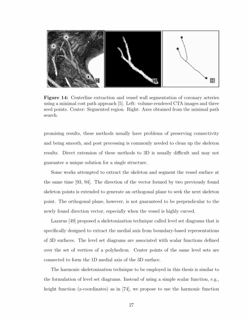
Figure 14: Centerline extraction and vessel wall segmentation of coronary arteriesusing a minimal cost path approach [5]. Left: volume-rendered CTA images and threeseed points. Center: Segmented region. Right: Axes obtained from the minimal pathsearch.

promising results, these methods usually have problems of preserving connectivity

and being smooth, and post processing is commonly needed to clean up the skeleton

results. Direct extension of these methods to 3D is usually difficult and may not

guarantee a unique solution for a single structure.

Some works attempted to extract the skeleton and segment the vessel surface at

the same time [93, 94]. The direction of the vector formed by two previously found

skeleton points is extended to generate an orthogonal plane to seek the next skeleton

point. The orthogonal plane, however, is not guaranteed to be perpendicular to the

newly found direction vector, especially when the vessel is highly curved.

Lazarus [49] proposed a skeletonization technique called level set diagrams that is

specifically designed to extract the medial axis from boundary-based representations

of 3D surfaces. The level set diagrams are associated with scalar functions defined

over the set of vertices of a polyhedron. Center points of the same level sets are

connected to form the 1D medial axis of the 3D surface.

The harmonic skeletonization technique to be employed in this thesis is similar to

the formulation of level set diagrams. Instead of using a simple scalar function, e.g.,

height function (z-coordinates) as in [74], we propose to use the harmonic function

27

which is the solution of the Laplace equation to achieve better centeredness of the

skeleton and the convenience to measure local cross-sectional areas accurately. The

details will be described and discussed in Section 5.

For a more comprehensive survey on geometric methods for vessel visualization

and quantification, see Buhler [11] and the references therein.

2.2.3 CTA Image Analysis

CTA image analysis has begun to draw much more interest and attention in recent

years as the imaging technique rapidly develops and improves. As we have introduced

in Chapter 1, CTA for vessel imaging is fast and non-invasive, with a very high and

isotropic in vivo resolution.

There are many challenges in CTA image analysis, due to the nature of intensity

distribution of different anatomical structures in CTA. In MRA and DSA, blood

vessels present either very low or very high intensities and the intensity range is

normally distinctive in the histogram. Other structures are well-suppressed in the

imaging or post subtraction process, thus the MRA and DSA image can be directly

visualized by a MIP or a 3D surface/volume rendering, although the direct rendering

may not be as clean as further processed images. CTA, on the other hand, is difficult

to be directly visualized by MIP on a full dataset. Vessels in CTA have an intensity

value in the middle range of the histogram, between the intensity of bones and other

soft tissues. In a MIP of CTA, bones or large areas of blood-filled regions (such as

a heart ventricle) may occlude thin vessels completely, which makes the full MIP

almost impossible to use. Local MIP may assist the visualization of a short segment

of the vessel, but it is quite limited by the small FOV. Thus image processing is

more important for efficient CTA viewing and analyzing, and also more challenging

as compared to MRA/DSA processing.

Here we first look at some interesting CTA investigations on applications other

28

than coronary arteries. In the next section (2.2.4) we will focus more on coronary

artery image analysis studies.

Carotid artery CTA is probably the most studied among all CTA applications.

Carotids are larger vessels than coronaries, are more stationary, thus presenting better

image quality, and are relatively easier to be processed. In Section 2.2.2 we reviewed

the work by Antiga et al. [4] (Figure 13) using level set methods to segment each

branch of the carotids. Andel et al. [2] developed a center lumen line extraction

method for carotid arteries using first and second order derivatives of the image,

called VAMPIRE (Vascular Analysis using Multiscale Paths Inferred from Ridges

and Edges). This method falls in the category of minimal cost path search, where

they incorporate the Hessian filter and Canny edge filter into the cost.

In a very recent work by Scherl et al. [78], the authors proposed a semi-automatic

segmetation method improved from the Chan and Vese [14] model, with special efforts

taken to exclude plaques from the lumen segmentation in order to achieve an accu-

rate stenosis evaluation. The algorithm was tested on four phantoms and the MPR

cross-sectional images of 10 CTA datasets. By comparing their results with stenosis

percentage evaluated by radiologists, a mean error of about 8% was achieved.

Hernandez et al. [36] and Holtzman-Gazit and Kimmel [37] analyzed CTA images

of patients with brain aneurysms. A challenge in brain CTA vessel segmentation

is to distinguish the vessel from the bone, which also has high intensity values. In

[36] the authors combined a pixel classifications method with geodesic active regions,

where the kNN rule was applied to estimate probability density functions for pixel

classification to achieve a different labeling for vessel and bone structures. In [37]

a hierarchical approach was adopted to handle the segmentation of multiple objects

(bone and vessel). The segmentation algorithm was first applied on the entire image

to obtain both the bone and vessel, and then the algorithm was applied again only

in the segmented region to separate the two objects.

29

Another work by Olabarriaga et al. [64] focused on the segmentation of thrombus

in abdominal aortic aneurysms from CTA images. In this study, the authors used

a double-layered deformable model to fit with both the inner and outer vessel wall

of the abdominal aorta. The inner boundary was relatively easy to obtain since the

contrast was better between the blood-pool and the vessel wall in a such a large

scale vessel, and the points on the outer boundary were driven by the probablity of

their belonging to the inside, outside or on the boundary, calculated using a nearest

neighbor approach.

It can be seen that in CTA image analysis, many of the general vessel analysis

methods are employed, such as level sets, deformable models, minimal cost path,

Hessian analysis and so on. Due to the specific properties of CTA images, additional

efforts were taken into dealing with problems such as bone and vessel separation,

plaque and lumen separation, and inner and outer boundary separation. In chapter

4 we will address these problems for CTA coronary segmentation in great detail.

2.2.4 Coronary Artery Image Analysis

A major portion of work on coronary image analysis has been dedicated to X-ray

angiography due to its long existence for clinical use. Since X-ray angiography will

not be the focus of this thesis, we briefly review a recent work by Blondel et al. [8]

here and direct interested readers to the references of this paper for other previous

works. In [8] a reconstruction technique of coronary arteries from a rotational X-ray

projection sequence is presented. This represents a common goal of image post-

processing on X-ray angiography, which is to recover the true 3D shape of coronaries

from 2D X-ray projections. Three steps were taken in [8] to achieve this goal: 3D

centerline reconstruction, 4D motion estimation, and 3D tomographic reconstruction

to emulate a CT scan. In fact, most of these laborious processing tasks can be

eliminated if a CTA scan is directly performed.

30

There are a very limited number of works dedicated to coronary CTA analysis in

the literature, and the existing methods vary in their performance and the amount

of required user interaction. Chen and Molloi [16] proposed a vascular tree recon-

struction method in coronary CTA, which inolves 3D thinning and skeleton pruning

techniques. The method was tested on a cast of the coronary arteries of a pig heart,

which does not fully emulate in vivo CTA images, since all non-coronary structures

in their testing images are well suppressed. Florin et al. [26] employed a Particle

Filter-based approach for the segmentation of coronary arteries. Successive planes of

the vessel are modeled as unknown states of a sequential process, which consist of the

orientation, position, shape and appearance of the vessel that are recovered using a

particle filter. This interesting probabilistic approach has shown its potential in the

segmentation problem, but it would be useful to see more quantitative results than

what is presented in the paper in order to evaluate the accuracy of this method. An-

other interesting work by Szymczak et al. [87] used a topological approach to extract

coronary vessel cores from CTA images. The method is robust to image artifacts from

implanted pacemakers, and shows very good tracking of coronaries in the distal end.

Several topological techniques are employed in order to generate a clean result, such

as trimming, pruning and gap filling, and the user needs to maually select a tree from

the forest to identify the coronary arteries in the later stage of centerline cleaning.

This method also needs to be further validated, as mentioned by the authors in the

paper, and the segmentation of the vessel is not addressed in this study.

In this chapter, we have reviewed several general image segmentation methods,

followed by a comprehensive literature review on previous works which have been per-

formed on blood vessel image analysis. A number of techniques are discussed, includ-

ing vessel enhancement methods, centerline extraction and skeletonization methods,

3D vessel wall segmentation and reconstruction methods and more. Since this thesis

will be focused on coronary CTA analysis, we also looked at some interesting research

31

on CTA image analysis for differet kind of vessels, and finally we reviewed some ex-

isting investigations of coronary CTA and discussed their values and limitations. It

can be seen that the problem of coronary CTA analysis is far from fully explored. In

the next chapter (Chapter 3) we will develop an image segmentation framework with

its applicability to CTA coronary segmentaion in mind, and compare the proposed

method to other well-known segmentation techniques.

32

CHAPTER III

SEGMENTATION USING BAYESIAN DRIVEN

IMPLICIT SURFACES (BDIS)

In this chapter, we present an image segmentation framework based on the geodesic

active contour model with a significant improvement on the segmentation perfor-

mance, which is especially beneficial for CTA blood vessel segmentation. We will

start the chapter by reviewing the conventional geodesic active contour model and its

limitations, and then move to the proposed algorithm, for which we employ Bayesian

probability theory and level set techniques. In 3D, this algorithm yields a segmen-

tation of an object as a surface, implicitly embedded in the level set function and

evolved to the boundary of the object driven by Bayesian posterior probabilities.

Hence, we call this method Bayesian driven implicit surfaces (BDIS).

3.1 Geodesic Active Contour Models and Limitations

As we have mentioned in the previous chapter, there are two key factors dominating

the segmentation using an active contour model. The first is the physical property

of the contour itself, such as its smoothness and elasticity; the second is the driving

force from the image, which will attract and lead the contour to move toward edges

or other salient features in the image, that finally separates the image into different

regions according to certain homogeneity criteria.

We begin by discussing the contour itself, and we will add the image term later as

we move forward. Let C = C(p, t) be a family of closed curves where t parameterizes

the family and p the given curve, where 0 ≤ p ≤ 1. We assume that C(0, t) = C(1, t)

and similarly for the first derivatives for closed curves. The curve length functional

33

is defined as:

L(t) :=

∫ 1

0

‖∂C

∂p‖dp (2)

By taking the first variation of the length functional, we obtain a curve shortening

flow, in the sense that the Euclidean curve length shrinks as quickly as possible when

the curve evolves:

∂C

∂t= κ ~N , (3)

where κ is the local curvature of the contour, and ~N is the inward unit normal. The

detailed derivation can be found in [89].

For the intrinsic property of being closed, the curve under the evolution of the

curve shortening flow (3) will continue to shrink until it vanishes. By adding a

constant ν, which we will refer to as the “inflation term”, the curve tends to grow

and counteracts the effect of the curvature term when ν is negative [42]:

∂C

∂t= (κ + ν) ~N . (4)

The image influence can be introduced to the above framework by changing the

ordinary Euclidean arc-length function along the curve C given by:

ds = ‖∂C

∂p‖dp

to a geodesic arc length

dsφ = φds = φ‖∂C

∂p‖dp

by multiplying a conformal factor φ, where φ = φ(x, y) is a positive differentiable

function that is defined based on the given image I(x, y).

We now take the first variation of the following geodesic curve length function:

Lφ(t) =

∫ 1

0

φ‖∂C

∂p‖dp, (5)

34

and reach a new evolution equation combining both the internal property of the

contour and the external image force:

∂C

∂t= φκN −∇φ (6)

As in equation (4), we also add an inflation term to this curve evolution model:

∂C

∂t= φ(κ + ν)N −∇φ (7)

More details of the geodesic active contours can be found in the work of Caselles

et al. [12], Kichenassamy et al. [42], and Yezzi et al. [104].

The level set formulation [66, 80] of Equation 7 is:

∂Ψ

∂t= φ(div

( ∇Ψ

‖∇Ψ‖)

+ ν)‖∇Ψ‖+∇φ · ∇Ψ, (8)

where Ψ is the level set function (usually initialized to be a signed distance function)

to be updated in each time step, and div(

∇Ψ‖∇Ψ‖

)is essentially the curvature κ of the

level sets of Ψ, and in 2D:

κ =ΨyyΨ

2x − 2ΨxΨyΨxy + ΨxxΨ

2y

(Ψ2x + Ψ2

y)3/2

. (9)

As mentioned above, φ is usually associated with the image intensity or intensity

gradients to stop the implicit active contour from evolving at image boundaries or

salient features. A usual choice of φ is:

φ(x, y) =1

1 + ‖∇Gσ ∗ I(x, y)‖2, (10)

where Gσ is a Gaussian smoothing filter with variance σ, and I(x, y) is the image

intensity of the pixel located at (x, y).

The two different representations of the deformable models, namely the parametric

active contours (“snakes”) and geometric level-set representations, have both drawn

great interest in recent years. They each have their advantages and disadvantages.

The snakes model is a fast, intuitive and powerful technique in both 2D and 3D, for

35

the fact that it directly controls the evolution of points or grids of the actual interface

(a contour in 2D or a surface in 3D) of interest. The two main limitations of the

snakes are: first, it lacks the ability to naturally handle topology changes without

sophisticated re-parameterization schemes; second, re-sampling is needed to keep the

points equally spaced and not crossing each other, when the initial and final contours

differ greatly. These problems can be solved relatively easily for the 2D case; however

the 2D solution usually can not be extended to 3D directly, and it is much more

complex to handle the 3D case.

Vessels are objects with complex shape and topology, which has a 3D form in CTA

data. The snakes model is thus not an ideal choice for this application. The level set

representation, on the other hand, has a number of advantages. The contours and

surfaces can naturally split or merge in this formulation, and it is straightforward

to extend the 2D implementation to 3D. The only issue with level sets is its com-

putational cost, since the actual interface is embedded in a higher dimensional level

set function, which need to be updated iteratively to evolve the interface. We will

address the implementation efficiency issue in Chapter 4 as we apply our proposed

method to 3D coronary artery segmentation.

The geodesic active contour model reviewed above has been successfully applied

to many medical applications. This model, however, has some inherent limitations. It

preforms better on images that have roundish objects of interest (e.g., Figure 9), with

relatively strong intensity gradients at the boundaries. For objects with complicated

shapes such as blood vessels, however, the model fails to achieve satisfying results,

see Figure 15 for an example. The problems mainly come from the following reasons:

1. The conformal factor φ does not provide a stopping force that is good enough to

attract the active contour and restrain it from leaking once it reaches the bound-

aries. Because φ is usually designed based on intensity gradients, it ignores the

pixel intensity information, which can provide important regional properties of

36

the image. Also, because the intensity gradients are sensitive to noise, it is

necessary that the image convolves with a Gaussian smoothing filter for the

calculation of the conformal factor. The Gaussian smoothing, however, blurs

and widens the boundary of the desired object, (e.g., Figure 16 (b) (c)), and the

segmentation may stop too early before reaching the true boundary and give a

smaller segmentation than the real object. For example, thinner vessels were

obtained in [52] compared to MIP projections because of using only image gradi-

ents to attract the active contour. This may in turn cause the underestimation

of cross-sectional areas of the vessels.

2. The constant inflation term ν only drives the active contour in a certain direction

without adaptability. This means the initialization of the active contour must be

completely inside or outside the desired object, which requires precise manual

placement of the initial contour. Also, once the contour leaks through the

boundary, there is no additional force to pull it back, thus it will continue to

leak without any restraints.

initial contour dt=0.005, after 1300 iterations

(a) (b)

Figure 15: Conventional geodesic active contours fail to segment thin blood vessels.(a) Initial contour; (b) after 1300 iterations leakage appears and the segmented vesselis thinner than the real size.

37

3.2 An Improved Geodesic Active Contour Model

To address these problems, an adaptive active contour model is proposed. This

method incorporates Bayesian pixel classification to the conventional geodesic active

contour model and drives the segmentation using posteriors from the Bayesian and

pixel labellings from the maximum a posterior (MAP) classification.

3.2.1 A New Conformal Factor Based on Bayesian Probabilities

Bayesian classifiers have been used in a number of image segmentation applications

[32, 90]. Given the probability density function p(I(x)|ck) of each image class ck

along with the prior probability Pr(x ∈ ck) of each class, posterior probabilities can

be calculated via the Bayes’ rule to give the probabilities of a single pixel at position

x = (x, y) with intensity value v belonging to different classes:

Pr(x ∈ ck|I(x) = v) =Pr(I(x) = v|x ∈ ck)Pr(x ∈ ck)∑n

γ=1 Pr(I(x) = v|x ∈ cγ)Pr(x ∈ cγ). (11)

There will be n posteriors for a single pixel if there are n classes presented in the

image. The classification of the pixels can be obtained using the MAP rule:

C(x) = arg maxc∈c1,c2,...,cn

Pr∗(x ∈ c|I(x) = v), (12)

where C(x) is the class that pixel x belongs to, and Pr∗ is a smoothed version of

the posterior probability obtained using anisotropic smoothing [65] described by the

following affine invariant flow in 2D:

∂Pr

∂t= κ1/3

pr~N (13)

In 3D, the affine invariant flow becomes:

∂Pr

∂t= sign(H)κ

1/4pr+

~N , (14)

where H and κpr are the mean curvature and Gaussian curvature of Pr, and κpr+ :=

maxκpr, 0. ~N is the inward unit normal. This approach may be rigorously justified

by the theory of MRF with a non-interacting, analog discontinuity field [91].

38

(a) (b)

(c) (d)

Figure 16: Comparing edge maps between the conventional conformal factor andthe proposed function. (a) Original image; (b) Gaussian smoothed gradient image;(c) conventional conformal factor edge map; (d) proposed conformal factor edge map.

The proposed method redefines the conformal factor using the smoothed posterior

probabilities. Suppose we have a bimodal image with class cin representing the object

to be segmented, and class cout representing the background, we define the conformal

factor as the squared difference between the posteriors that pixel x belongs to cin and

cout:

φ(x) = (Pr∗(x ∈ cin)− Pr∗(x ∈ cout))2 (15)

This can be extended to n classes (n > 2) by using the squared difference between

the largest two posterior probabilities for a single pixel.

Figure 16 shows the comparison between the commonly used conformal factor

based on gradient and the proposed conformal factor based on posterior probabilities.

The proposed factor is smoother and has a much better defined dark valley at the

boundaries than the conformal factor that only uses the gradient information.

39

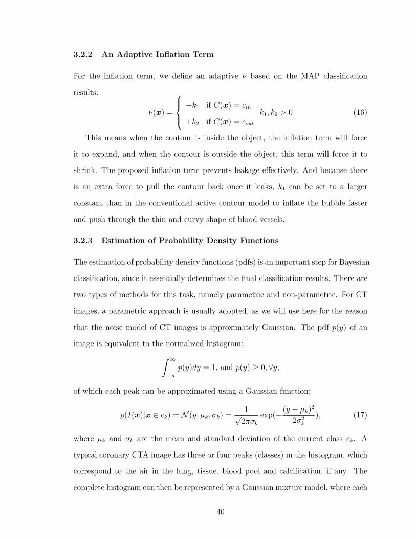
3.2.2 An Adaptive Inflation Term

For the inflation term, we define an adaptive ν based on the MAP classification

results:

ν(x) =

−k1 if C(x) = cin

+k2 if C(x) = cout

k1, k2 > 0 (16)

This means when the contour is inside the object, the inflation term will force

it to expand, and when the contour is outside the object, this term will force it to

shrink. The proposed inflation term prevents leakage effectively. And because there

is an extra force to pull the contour back once it leaks, k1 can be set to a larger

constant than in the conventional active contour model to inflate the bubble faster

and push through the thin and curvy shape of blood vessels.

3.2.3 Estimation of Probability Density Functions

The estimation of probability density functions (pdfs) is an important step for Bayesian

classification, since it essentially determines the final classification results. There are

two types of methods for this task, namely parametric and non-parametric. For CT

images, a parametric approach is usually adopted, as we will use here for the reason

that the noise model of CT images is approximately Gaussian. The pdf p(y) of an

image is equivalent to the normalized histogram:

∫ ∞

−∞p(y)dy = 1, and p(y) ≥ 0,∀y,

of which each peak can be approximated using a Gaussian function:

p(I(x)|x ∈ ck) = N (y; µk, σk) =1√

2πσk

exp(−(y − µk)2

2σ2k

), (17)

where µk and σk are the mean and standard deviation of the current class ck. A

typical coronary CTA image has three or four peaks (classes) in the histogram, which

correspond to the air in the lung, tissue, blood pool and calcification, if any. The

complete histogram can then be represented by a Gaussian mixture model, where each

40

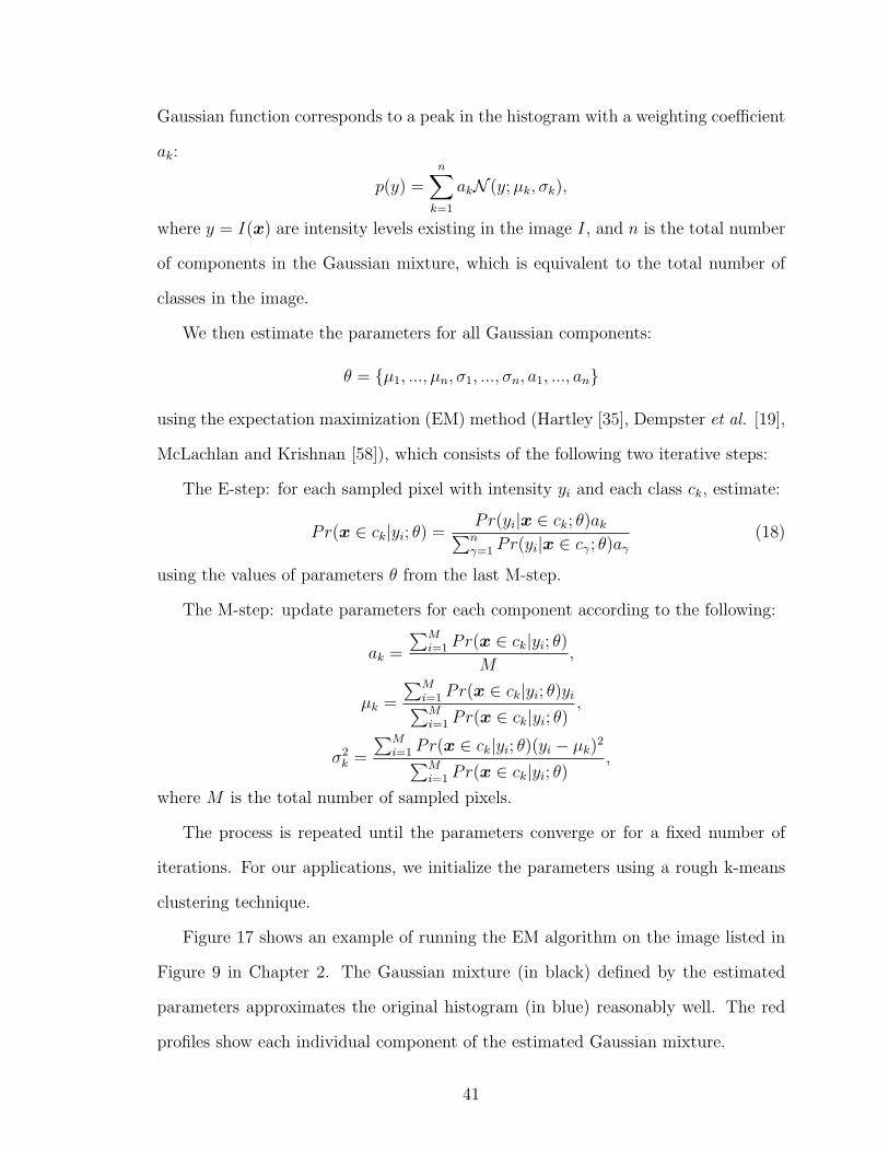
Gaussian function corresponds to a peak in the histogram with a weighting coefficient

ak:

p(y) =n∑

k=1

akN (y; µk, σk),

where y = I(x) are intensity levels existing in the image I, and n is the total number

of components in the Gaussian mixture, which is equivalent to the total number of

classes in the image.

We then estimate the parameters for all Gaussian components:

θ = µ1, ..., µn, σ1, ..., σn, a1, ..., an

using the expectation maximization (EM) method (Hartley [35], Dempster et al. [19],

McLachlan and Krishnan [58]), which consists of the following two iterative steps:

The E-step: for each sampled pixel with intensity yi and each class ck, estimate:

Pr(x ∈ ck|yi; θ) =Pr(yi|x ∈ ck; θ)ak∑n

γ=1 Pr(yi|x ∈ cγ; θ)aγ

(18)

using the values of parameters θ from the last M-step.

The M-step: update parameters for each component according to the following:

ak =

∑Mi=1 Pr(x ∈ ck|yi; θ)

M,

µk =

∑Mi=1 Pr(x ∈ ck|yi; θ)yi∑Mi=1 Pr(x ∈ ck|yi; θ)

,

σ2k =

∑Mi=1 Pr(x ∈ ck|yi; θ)(yi − µk)

2

∑Mi=1 Pr(x ∈ ck|yi; θ)

,

where M is the total number of sampled pixels.

The process is repeated until the parameters converge or for a fixed number of

iterations. For our applications, we initialize the parameters using a rough k-means

clustering technique.

Figure 17 shows an example of running the EM algorithm on the image listed in

Figure 9 in Chapter 2. The Gaussian mixture (in black) defined by the estimated

parameters approximates the original histogram (in blue) reasonably well. The red

profiles show each individual component of the estimated Gaussian mixture.

41

Figure 17: An example of using EM to approximate an image histogram. In blue:the original histogram; in black: the estimated Gaussian mixture profile; in red: eachindividual component in the Gaussian mixture.

3.2.4 Numerical Implementation Using Level Sets

To first test the effectiveness of the algorithm on 2D images, the proposed model

was implemented through a standard finite difference scheme. Equation (8) can be

re-written as:

Ψt = φκ‖∇Ψ‖+ (νφ +∇Ψ

‖∇Ψ‖ · ∇φ)‖∇Ψ‖, (19)

where central differences are used for the first term, and an upwind scheme is used for

the second term for stability. More specifically, the numerical scheme can be written

as [80]:

Ψn+1ij = Ψn

ij + ∆t((φijκnij((D

0xij )2 + (D0y

ij )2)1/2)

+(max(νφij, 0)∇+ + min(νφij, 0)∇−)

+(max((φx)ij, 0)D−xij + min((φx)ij, 0)D+x

ij

+max((φy)ij, 0)D−yij + min((φy)ij, 0)D+y

ij )) (20)

42

where κnij can be calculated by Equation (9) using central differences of Ψ, which are:

Ψx = D0xij =

Ψi+1,j −Ψi−1,j

2∆x,

Ψy = D0yij =

Ψi,j+1 −Ψi,j−1

2∆y, (21)

Ψxx = D0xxij =

Ψi+1,j − 2Ψi,j + Ψi−1,j

∆x2,

Ψyy = D0yyij =

Ψi,j+1 − 2Ψi,j + Ψi,j−1

∆y2, (22)

Ψxy = D0xyij =

Ψi+1,j+1 + Ψi−1,j−1 −Ψi+1,j−1 −Ψi−1,j+1

∆x∆y. (23)

D0xij , D0y

ij are central differences of Ψ along x and y directions (Equation (21)),

D−xij =

Ψi,j−Ψi−1,j

∆x, D−y

ij =Ψi,j−Ψi,j−1

∆yare one sided backward differences, D+x

ij =

Ψi+1,j−Ψi,j

∆x, D+y

ij =Ψi,j+1−Ψi,j

∆yare one sided forward differences, and ∇+, ∇− are:

∇+ = (max(D−xij , 0)2 + min(D+x

ij , 0)2 + max(D−yij , 0)2 + min(D+y

ij , 0)2)1/2

∇− = (max(D+xij , 0)2 + min(D−x

ij , 0)2 + max(D+yij , 0)2 + min(D−y

ij , 0)2)1/2

The conformal factor φ has been calculated ahead of time, and φx, φy are calcu-

lated using central differences. Reinitialization of the level set function is performed

after a fixed number of iterations for stability purposes.

3.3 2D Experimental Results

The proposed method was tested on 2D synthetic images and real CT images of both

vessels and non-vessels.

Figure 18 shows an example of running the algorithm on a synthetic image of

branched vessels. The vessels are hand-drawn with additive Gaussian noise. The

initial contour crosses the boundary of the vessels and differs largely from the actual

vessel boundary. Due to the adaptive inflation term, the contour shrinks or expands

locally according to the local image characteristics. This emulates the property of

region-based deformable models [14, 104].

43

Figure 19 shows an example of a coronary artery CT image. The image was

generated through curved multi-planar reformatting (MPR) from a 3D dataset. It

is the same image as in Figure 15, where the conventional geodesic active contour

fails to segment the vessel. In this new result, also by starting with an initial contour

crossing the boundary of the vessel, the proposed method successfully segments the

image as shown in Figure 19 (d).

In Figure 20 we compare the segmentation of a heart chamber using three different

methods. The original image is shown in (a1), and the initial contour is placed inside

the object of interest as in (a2). On each row of two images that follows, we show

the evolution contours and the final segmentation as a binary mask. The figures in

(b1) and (b2) are the results of using the conventional gradient-based method with

a uni-directional inflation term. It can be seen that the contour moves toward the

boundary initially; however it fails to stay at the boundary and start to leak after

more iterations, due to the fact that the gradient-based conformal factor defined by

(10) never becomes zero at the boundary, although it may be very small. Also, once

it leaks, the uni-directional inflation term keeps pushing the contour to grow, without

the ability to remedy the leakage. The final result is certainly not satisfying.

Figures 20 (c1) and (c2) show the results obtained using a region-based segmen-

tation method proposed by Chan and Vese [14]. This method is essentially seeking a

maximum global separation of the average intensity inside and outside the object by

minimizing the following functional:

F (m1m2, C) = µ · Length(C) + λ1

∫

inside(C)

|I(x, y)−m1|2dxdy

+λ2

∫

outside(C)

|I(x, y)−m2|2dxdy, (24)

where µ ≥ 0, λ1, λ2 > 0 are fixed parameters, C is the curve, I(x, y) is the original

image, and m1 and m2 are the mean values of the image intensity inside and outside

of contour C, which are updated dynamically as C evolves. This model has the nice

44

property of utilizing the region intensity information of the image and being able to

segment images without strong edges. However, it is a fully global method which

segments all regions in the image with similar intensity no matter where the initial

contour is placed. This may be a good property for certain applications, but for

segmenting coronary arteries from CTA, this method will lead to the segmentation of

not only the vessels, but other unwanted blood-filled regions, such as the aorta and

ventricles of the heart. As shown in (c1) and (c2), although our goal is to segment

only the heart chamber in the image and the initial contour was placed fully inside

the chamber, the segmentation result contains all regions in the image with similar

intensity level.

Finally we show in Figures 20 (d1) and (d2) the results of the proposed method us-

ing BDIS. The final segmentation shows the desired heart chamber, and the evolution

process shows a very good convergence at the boundary without any leakage. The

curves also evolve faster and smoother as comparing to the gradient-based approach

in (b1), due to the smooth high value of φ in homogeneous regions in the image.

With these 2D testing results, we conclude this chapter where we proposed a new

segmentation method with great potential and proven abilities in segmenting coro-

nary CTA imagery. The method addressed the commonly seen problems of leakage

and under-segmentation in the conventional geodesic active contour models, by us-

ing Bayesian probability estimation with pdf parameters calculated through EM and

level set methods.

In the next chapter, we will propose a complete framework for the fully automatic

segmentation of coronary arteries from 3D CTA images.

45

(a) (b)

(c) (d)

Figure 18: Segmentation of a synthetic vessel image using the proposed method.(a) Initial contour; (b) after 120 iterations; (c) after 500 iterations; (d) after 1000iterations, final segmentation.

46

(a) (b)

(c) (d)

Figure 19: Segmentation of a real coronary artery image (MPR image), the sameas in Figure 15, where the conventional geodesic active contours fail to segment.(a) Initial contour; (b) after 150 iterations (c) after 600 iterations; (d) after 1600iterations, final segmentation.

47

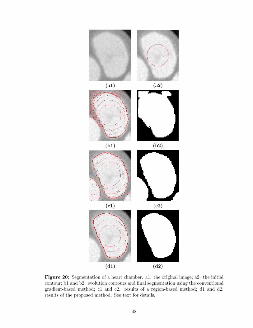
(a1) (a2)

(b1) (b2)

(c1) (c2)

(d1) (d2)

Figure 20: Segmentation of a heart chamber. a1. the original image; a2. the initialcontour; b1 and b2. evolution contours and final segmentation using the conventionalgradient-based method; c1 and c2. results of a region-based method; d1 and d2.results of the proposed method. See text for details.

48

CHAPTER IV

FULLY AUTOMATIC DETECTION AND

SEGMENTATION OF CORONARY ARTERIES IN 3D

In this chapter, we present a fully automatic segmentation framework for coronary

arteries in 3D CTA images. We start by a simple lung and heart segmentation using

mathematical morphological approaches to eliminate vessels in the lung and define

the region of interest (ROI) for further processing. We then use a Hessian-based

vessel filtering technique to enhance vessels within the ROI. An isosurface from the

Hessian filtering response serves as the initial surface for a further segmentation step

using the Bayesian driven implicit surfaces (BDIS) method proposed in the previous

chapter. We also examine implementation and optimization details as we apply BDIS

to 3D datasets.

In the final section, we present the segmentation results on 18 real clinical datasets

and compare them quantitatively with manual segmentation by evaluating the sensi-

tivity, specificity, and accuracy of the proposed method.

Figure 21 and Figure 22 show a series of coronary CTA images as they are in

their original form. It can be seen that the LM appears first in the image and as

we go forward, the LM bifurcates into two branches, LAD and LCX, which further

bifurcate into smaller branches. The RCA starts to appear in the last three slices in

Figure 21. At first the slices cut through the RCA in its longitudinal direction, and

then gradually change into orthogonal direction. RCA presents less variations than

the left coronary tree.

We number the datasets used in this thesis in a sequential manner as they appear

in the following sections. Shown in Figure 21 and Figure 22 are images from Dataset

49

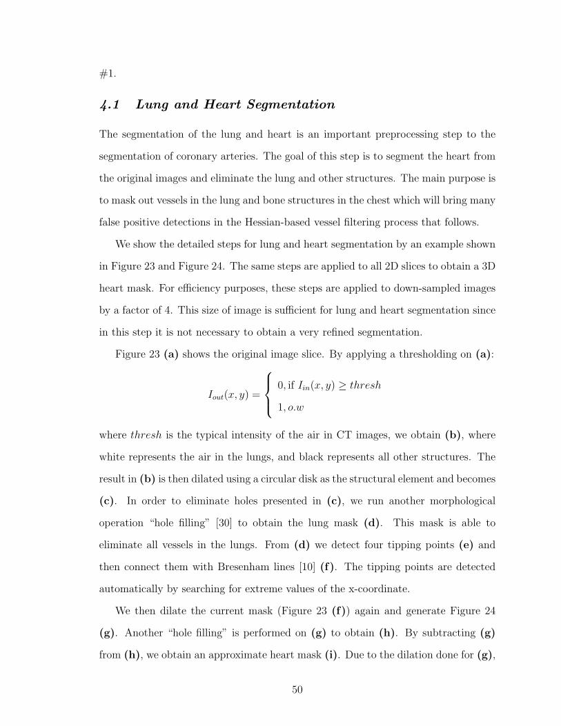
#1.

4.1 Lung and Heart Segmentation

The segmentation of the lung and heart is an important preprocessing step to the

segmentation of coronary arteries. The goal of this step is to segment the heart from

the original images and eliminate the lung and other structures. The main purpose is

to mask out vessels in the lung and bone structures in the chest which will bring many

false positive detections in the Hessian-based vessel filtering process that follows.

We show the detailed steps for lung and heart segmentation by an example shown

in Figure 23 and Figure 24. The same steps are applied to all 2D slices to obtain a 3D

heart mask. For efficiency purposes, these steps are applied to down-sampled images

by a factor of 4. This size of image is sufficient for lung and heart segmentation since

in this step it is not necessary to obtain a very refined segmentation.

Figure 23 (a) shows the original image slice. By applying a thresholding on (a):

Iout(x, y) =

0, if Iin(x, y) ≥ thresh

1, o.w

where thresh is the typical intensity of the air in CT images, we obtain (b), where

white represents the air in the lungs, and black represents all other structures. The

result in (b) is then dilated using a circular disk as the structural element and becomes

(c). In order to eliminate holes presented in (c), we run another morphological

operation “hole filling” [30] to obtain the lung mask (d). This mask is able to

eliminate all vessels in the lungs. From (d) we detect four tipping points (e) and

then connect them with Bresenham lines [10] (f). The tipping points are detected

automatically by searching for extreme values of the x-coordinate.

We then dilate the current mask (Figure 23 (f)) again and generate Figure 24

(g). Another “hole filling” is performed on (g) to obtain (h). By subtracting (g)

from (h), we obtain an approximate heart mask (i). Due to the dilation done for (g),

50

we need to dilate (i) using the same sized structural element to recover the shape, as

in (j), which is the final heart mask. The last row compares the original image (k)

with the masked image (l). It can be seen that the heart has been kept and other

structures have been eliminated completely.

Figure 25 compares the 3D volume rendering of the original (a) and masked (b)

images. It is apparent that the vessels in the lung and bones in the chest have been

eliminated effectively in (b) by applying the mask, and the masked image is much

cleaner than the original one. The masked image now solely represents the heart and

some segments of the left coronary arteries can already be seen on the surface of the

heart.

4.2 Multi-Scale Vessel Filtering

In this section, we apply a 3D Hessian-based filter [28, 102] to enhance the coronary

arteries in CTA images and generate an initial surface for further refined BDIS seg-

mentation. The filter is performed in a multi-scaled fashion in order to respond to

vessels of different sizes. Only voxels within the heart mask are calculated for a filter

response; voxels outside the mask are ignored. Notice that we still do the filtering on

the original image rather than the masked image, since the sharp edges between the

heart and the masking background will bring strong false filter responses.

This Hessian-based filter is a voxel-based filter, meaning that each voxel is calcu-

lated for a filter response. We start by calculating the second order derivatives of the

intensity values to form a Hessian matrix for each voxel:

∇2I(x) =

Ixx(x) Ixy(x) Ixz(x)

Iyx(x) Iyy(x) Iyz(x)

Izx(x) Izy(x) Izz(x)

, (25)

where x = (x, y, z) represents a voxel location in 3D, and each element in the Hessian

matrix can be calculated by convolving the image with the second order derivatives

51

Table 1: Possible patterns in 3D based on Hessian eigenvalues. Adapted from [28].

λ1 λ2 λ3 orientation patternN N N noisy, no preferred directionL L H- plate-like structure (bright)L L H+ plate-like structure (dark)L H- H- tubular structure (bright)L H+ H+ tubular structure (dark)H- H- H- blob-like structure (bright)H+ H+ H+ blob-like structure (dark)

of a 3D Gaussian function with a standard deviation of σ:

Iuv(x; σ) =

(∂2

∂u∂vG(x; σ)

)∗ I(x). (26)

By adjusting σ we adjust the width of the Gaussian function to adapt to different

vessel sizes. In CTA, the variation in the size of coronary arteries is not large. In

general, two scales (two values of σ) are sufficient to extract all coronary artery

branches.

We then compute the eigenvalues (λ1, λ2 and λ3) of the Hessian matrix (25).

Frangi et al. [28] summarized the relationship between different combinations of the

eigenvalues and their corresponding possible 3D patterns (Table 1). The shape of

coronary arteries in CTA images are bright tubular structures, listed as the fourth

row of Table 1, where λ1 is approximately zero, and λ2 and λ3 are negative numbers

with high absolute values:

0 ≈ |λ1| ¿ |λ2| ≤ |λ3|,λ2 < 0, λ3 < 0.

(27)

To discriminate the tubular structure from other types of structures, a vesselness

measure is defined:

M(x, σ) =

0, if λ2 > 0 or λ3 > 0(1− exp

(−R2

A

2α2

))exp

(−R2

B

2β2

)(1− exp

(− S2

2c2

)), otherwise,

(28)

52

where

RA =|λ2||λ3| , RB =

λ1√|λ2λ3|

, S =

√ ∑1≤i≤3

λ2i .

In measure (28), RA is able to discriminate tubular structures from plate-like

structures, RB mainly differentiates blob-like structures from other structures and

also favors tubular structures, and S penalizes random background noise. α, β and

c are constants that control the balance between the three terms. We have used

α = 0.5, β = 0.5, c = 10 for all cases.

Finally, to incorporate contributions from every scale, the maximum value of all

scales at each voxel is selected to be the final filter response:

Mmulti(x) = maxσ

M(x; σ). (29)

Figure 26 demonstrates the effectiveness of the above multi-scale vessel filter. In

(a) we show the volume rendering of the images after the lung and heart segmentation,

where all tissues in the heart present in the rendering, and in (b) we show the

rendering of the vessel filter response as a volume of images. Since for each voxel

there exists a vesselness measure, the filter response is essentially another volume of

images with the same size as the original images which can also be rendered in the

same fashion. It can be seen that most tissues in the heart other than the vessels

have been effectively suppressed, and the shape of both LCA and RCA can be clearly

seen in the filter response.

The next step is to extract a surface of the vessels from the filter response in

order to generate an initial surface for BDIS segmentation. The iso-surface at 30% of

the maximum filter response is extracted. This iso-surface threshold is heuristically

selected and worked well for all our testing cases. The iso-surface contains some

small fragments which do not belong to the coronary arteries. In order to remove

these fragments, a size filter is applied to all connected regions in the thresholded

image volume. The isolated regions which are too small in size are thus eliminated.

53

Figure 27 shows the final surface which represents the coronary arteries of both sides.

It can be seen that the structures of the vessels are very well extracted, however the

boundaries are quite ragged and in some locations the vessels are disconnected. In

the next section (4.3), we will use this surface as the initial surface for a much more

refined BDIS segmentation.

Before we conclude this section, we show another example to demonstrate the

importance of the heart segmentation step. In Figure 28, we compare the vessel filter

responses performed on the whole image (middle) and image within the heart mask

(right). It is apparent that the vessels in the lung brought a tremendous amount

of false filter responses in the original image, while in the masked image, the filter

response focuses only on the coronary arteries.

Another benefit of performing the heart segmentation is to improve the speed for

vessel filtering. Since this is a voxel-based approach, the computation will be signifi-

cantly faster if the number of voxels is reduced. The heart segmentation eliminated

all voxels outside the heart, which reduces approximately 1/3 amount of voxels to be

processed and hence improves the speed by about 30%. Also, for the sake of computa-

tion efficiency, the vessel filtering step is performed on a down-sampled image volume

by a factor of 2, which contains 1/8 of the original voxels. The resolution is sufficient

for vessel filtering, while the computation speed is maximized. The computational

time for each dataset will be reported in section 4.4, Table 4.

4.3 3D Segmentation of Coronary Arteries Using BDIS

In this section, we apply the proposed BDIS algorithm to coronary artery segmenta-

tion using the initial surface obtained from the Hessian-based vessel filtering in the

previous section. We first show the detailed numerical implementation in 3D, along

with some optimization considerations, and then show an example to demonstrate the

54

segmentation on a healthy volunteer (Dataset #2). In the BDIS segmentation pro-

cess, we have considered three classes (blood, tissue and background) for all datasets,

and calcified plaques are initially classified and segmented as the blood. An additional

step is taken to remove calcium from the segmented blood region in diseased vessels

to finally offer a true lumen segmentation. The difference between the initial blood

mask and the final lumen mask represents the calcified plaques.

4.3.1 Numerical Details and Optimization

We rewrite Equation (19) in Chapter 3 here, which is the updating equation for the

level set function:

Ψt = φκ‖∇Ψ‖+ (νφ +∇Ψ

‖∇Ψ‖ · ∇φ)‖∇Ψ‖.

The 3D implementation can be extended straightforwardly from the 2D case,

which is essentially the same as in 3D except for the addition of a third dimension.

We still show the details here since the 3D implementation is rarely seen in the

literature:

Ψn+1ijk = Ψn

ijk + ∆t((φijkκnijk((D

0xijk)

2 + (D0yijk)

2 + (D0zijk)

2)1/2)

+(max(νijkφijk, 0)∇+ + min(νijkφijk, 0)∇−)

+(max((φx)ijk, 0)D−xijk + min((φx)ijk, 0)D+x

ijk

+max((φy)ijk, 0)D−yijk + min((φy)ijk, 0)D+y

ijk

+max((φz)ijk, 0)D−zijk + min((φz)ijk, 0)D+z

ijk)), (30)

where in 3D

κnijk = [(D0xx

ijk + D0yyijk )(D0z

ijk)2 − 2D0x

ijkD0yijkD

0xyijk

(D0yyijk + D0zz

ijk )(D0xijk)

2 − 2D0yijkD

0zijkD

0yzijk

(D0xxijk + D0zz

ijk )(D0yijk)

2 − 2D0xijkD

0zijkD

0xzijk ]

55

/((D0xijk)

2 + (D0yijk)

2 + (D0zijk)

2)3/2, (31)

D0xijk, D0y

ijk and D0zijk are central differences for the first derivatives which can be cal-

culated using Equation (21) in Chapter 3, D0xxijk , D0yy

ijk , D0zzijk , D0xy

ijk , D0xzijk and D0yz

ijk are

second order derivatives (Equations (22) and (23)), and ∇+, ∇− are:

∇+ = (max(D−xijk , 0)2 + min(D+x

ijk , 0)2 + max(D−yijk, 0)2 + min(D+y

ijk, 0)2

+max(D−zijk, 0)2 + min(D+z

ijk, 0)2)1/2,

∇− = (max(D+xijk , 0)2 + min(D−x

ijk , 0)2 + max(D+yijk, 0)2 + min(D−y

ijk, 0)2

+max(D+zijk, 0)2 + min(D−z

ijk, 0)2)1/2.

Ψ(x, y, z, t) is essentially a scalar field defined on the 3D space being updated by

Equation (30). A full computation for all grid points in 3D is very computational

expensive. Here we adopt a well-known “narrow band” approach to reduce the com-

putation cost. Only a narrow band of grid points around the zero level set is being

updated for each iteration and other grid points are ignored. Since vessels are long

and thin structures that stretch in long distances in the 3D space but with very lim-

ited surface areas which correspond to small number of grid points on the zero level

set, the narrow band approach is especially efficient for this application.

Another concern is the initialization of the level set function. Ψ is usually ini-

tialized to be a signed distance function with negative values inside the surface and

positive values outside [80]. However, in a large 3D volume the computation of such a

distance function takes a extremely long time. Also for numerical stability, the signed

distance function is needed to be re-initialized after a certain number of iterations.

This is often referred to as “re-distancing” in the literature. The need for re-distancing

adds more computation cost since this is usually necessary to be performed several

times before reaching the final solution. To address this issue, we divide the 3D vol-

ume into sub-volumes, and perform the computation on smaller volumes, since the

56

calculation of 3D distance function on small volumes takes significantly less time than

large volumes. We also notice that the initial surfaces of the vessels only occupy some

of the sub-volumes, so we perform the computation only within these volumes and

ignore the others. This will further reduce the computation cost. The size of the

sub-volume is heuristically selected to be 30× 30× 30 for the coronary segmentation.

Here we show the segmentation results on a healthy case (Dataset #2) to demon-

strate the algorithm. More results on diseased vessels and more datasets will be tested

and validated in the next few sections.

Figure 29 compares the 2D contours on two example slices of the initial shape

obtained using the Hessian-based vessel filtering and the final shape obtained by

BDIS. These are slice #6 and #23 from Dataset #2. It can be seen that the final

contours exhibit much smoother appearance than the initial contours, although the

initial contours already lie within the vessels. The final contours define the vessel

boundaries precisely (as we will also quantitatively show in Section 4.4) with sub-

voxel accuracy due to the property of level set segmentation. We should mention

that we show the results here in 2D only for demonstration, however the algorithm is

performed in a true 3D manner.

In Figure 30 and Figure 31 we show a series of segmentation results as 2D contours

from Dataset #2. Both LCA and RCA are successfully tracked and delineated with

a reasonable distal-end sensitivity. Figure 34 (Upper) shows the final segmentation

as a 3D surface. Comparing to the vessel filtering result (initial surface) in Figure 27,

the final surface is much smoother and some broken branches in the initial surface

are connected automatically, thanks to the ability of level sets in handling topological

changes.

57

4.3.2 Removing Calcified Plaques

We have assumed that there are three classes in the image volume, being the blood-

filled region, tissue, and lungs. In diseased vessels with calcified plaques, the calcium

deposits are initially classified as the blood-filled region due to their high values in

image intensity. An additional step is performed to remove the calcium from the

segmentation mask, thus the remainder is a volume mask which solely represents the

lumen.

Figure 35 demonstrates the calcium removing task using three examples. Starting

from the segmentation that includes both the lumen and calcium, we calculate an

Otsu threshold [67] using all pixels within the “lumen + calcium” mask, and use this

threshold to separate the calcium from the lumen. The Otsu threshold is calculated

based on the minimization of the intraclass variance of the background (lumen) and

the foreground (calcium) regions.

The left column of Figure 35 shows three slices of images showing the initial

segmentation result from Dataset #8, Dataset #15, and Dataset #16, respectively.

The right column shows the result after removing the calcified plaques. It can be seen

that the red contours now delineate the true boundary of the lumen itself.

4.4 Results and Validation

In this section, we show the segmentation results on 18 real clinical datasets, including

the two datasets we have used in the previous sections as examples. Most datasets

were acquired at Emory clinic using a Siemens Sensation 64 slice CT scanner, except

that Dataset #2 was acquired using a GE LightSpeed Pro 16 scanner. The image

acquisition process is not performed as part of this thesis, but by CT specialists

at Emory, under an IRB-approved protocol. The acquisition date, volume size and

spacial resolution are listed in Table 2. The average volume size is 313×362×210,

and the average pixel resolution is 0.3703mm × 0.3703mm × 0.7361mm over all 18

58

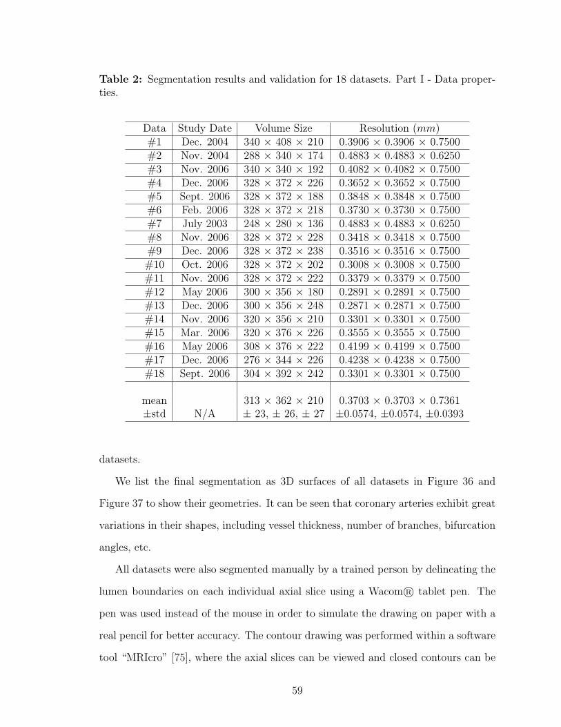
Table 2: Segmentation results and validation for 18 datasets. Part I - Data proper-ties.

Data Study Date Volume Size Resolution (mm)#1 Dec. 2004 340 × 408 × 210 0.3906 × 0.3906 × 0.7500#2 Nov. 2004 288 × 340 × 174 0.4883 × 0.4883 × 0.6250#3 Nov. 2006 340 × 340 × 192 0.4082 × 0.4082 × 0.7500#4 Dec. 2006 328 × 372 × 226 0.3652 × 0.3652 × 0.7500#5 Sept. 2006 328 × 372 × 188 0.3848 × 0.3848 × 0.7500#6 Feb. 2006 328 × 372 × 218 0.3730 × 0.3730 × 0.7500#7 July 2003 248 × 280 × 136 0.4883 × 0.4883 × 0.6250#8 Nov. 2006 328 × 372 × 228 0.3418 × 0.3418 × 0.7500#9 Dec. 2006 328 × 372 × 238 0.3516 × 0.3516 × 0.7500#10 Oct. 2006 328 × 372 × 202 0.3008 × 0.3008 × 0.7500#11 Nov. 2006 328 × 372 × 222 0.3379 × 0.3379 × 0.7500#12 May 2006 300 × 356 × 180 0.2891 × 0.2891 × 0.7500#13 Dec. 2006 300 × 356 × 248 0.2871 × 0.2871 × 0.7500#14 Nov. 2006 320 × 356 × 210 0.3301 × 0.3301 × 0.7500#15 Mar. 2006 320 × 376 × 226 0.3555 × 0.3555 × 0.7500#16 May 2006 308 × 376 × 222 0.4199 × 0.4199 × 0.7500#17 Dec. 2006 276 × 344 × 226 0.4238 × 0.4238 × 0.7500#18 Sept. 2006 304 × 392 × 242 0.3301 × 0.3301 × 0.7500

mean 313 × 362 × 210 0.3703 × 0.3703 × 0.7361±std N/A ± 23, ± 26, ± 27 ±0.0574, ±0.0574, ±0.0393

datasets.

We list the final segmentation as 3D surfaces of all datasets in Figure 36 and

Figure 37 to show their geometries. It can be seen that coronary arteries exhibit great

variations in their shapes, including vessel thickness, number of branches, bifurcation

angles, etc.

All datasets were also segmented manually by a trained person by delineating the

lumen boundaries on each individual axial slice using a Wacom R© tablet pen. The

pen was used instead of the mouse in order to simulate the drawing on paper with a

real pencil for better accuracy. The contour drawing was performed within a software

tool “MRIcro” [75], where the axial slices can be viewed and closed contours can be

59

drawn on the slices by the tablet pen. A surface rendering of manually segmented

Dataset #2 is shown in Figure 34 (Lower). Since there are no constraints enforced on

the third dimension when doing manual segmentations, the surface is not as smooth

as the automatic segmentation result as shown in Figure 34 (Upper).

We compare the results of our proposed automatic segmentation with the manual

segmentation using four measures to quantify their differences. The comparison is

performed in terms of contours on the 2D axial slices since manual segmentation were

all done in this manner. We first evaluate the sensitivity of the proposed method by

looking at the percentage of overlapped contours between the automatic segmentation

and manual segmentation (true positives) among the total number of contours in the

manual segmentation:

Sensitivity =number of overlapped contours

total number of contours in manual seg.× 100%. (32)

The sensitivity gives an evaluation on the ability of the proposed approach to

detect as many vessels as presented in the image. A higher sensitivity normally

implies a better distal end detection of the coronary arteries. The sensitivity of every

dataset is reported in the first column of Table 3 and the average sensitivity over all

18 datasets is 89.63% with a standard deviation of 4.42%.

We then evaluate the specificity by calculating 100% minus the percentage of con-

tours which exist in the automatic segmentation, but not in the manual segmentation

(false positives), among the total number of contours in the automatic segmentation:

Specificity =

(1− number of contours in auto, but not in manual

total number of contours in auto seg.

)× 100%. (33)

The specificity evaluates the occurrence of false positive detections, usually due

to a contour leakage or the pick-up of bright noise. In rare occasions the false posi-

tive detection is due to the better sensitivity of the automatic segmentation than the

manual segmentation, where a true vessel contour is missed by the manual segmenta-

tion, but was detected by the automatic approach. The specificity of every dataset is

60

reported in the second column of Table 3. The average specificity over all 18 datasets

is 94.51% with a standard deviation of 3.33%.

The third and fourth measures focus on the detailed comparison between each

contour pairs in the automatic and manual segmentation. For these two measures we

compare all true positive vessel contours (overlapped contours) in every dataset by

calculating their mean distance error and maximum distance error.

To calculate the distance between two contours, a set of discrete points are first

generated using Matlab function contourc to represent the zero-level set contour on

each slice, and then a distance map is calculated using function bwdist from the

manual segmentation mask. Each zero-level set contour point corresponds to a point

in the manual segmentation distance map, which gives a distance from this point to

the manual segmentation contour. All distances from the zero-level set contour points

to the manual segmentation contour are calculated, and the mean and maximum

distances are recorded. For each dataset a mean distance error (MDE) and a mean

maximum distance error (MMDE) are then calculated over all true positive contours

in this dataset. The results are shown in the last four columns of Table 3 in terms

of pixel and mm. The mean MDE over all 18 datasets is about 0.7 pixels, which

is 0.2676mm and the MMDE is about 3 pixels, which is equivalent to 1.1225mm in

distance.

We also recorded the computation time for each datasets in Table 4. The time

for computing the heart mask and performing the vessel filtering are recorded as a

whole, and the BDIS segmentation is recorded separately. It is observed that the

heart segmentation and vessel filtering, which on average takes 4.0754 minutes, takes

significantly longer time than the BDIS segmentation, which on average only takes

0.7372 minutes. The average total computation time is 4.8126 minutes. The last

two columns of Table 4 recorded the number of branches extracted by the proposed

method. On average, about four branches are extracted for LCA and 2 for RCA,

61

Table 3: Segmentation results and validation for 18 datasets. Part II - Quantitativecomparison between automatic and manual segmentation. (1MDE - Mean DistanceError, 2MMDE - Mean Maximum Distance Error)

Data Sensitivity Specificity MDE1 MDE MMDE2 MMDE(%) (%) (pix) (mm) (pix) (mm)

#1 88.38 94.62 1.3714 0.5357 4.0953 1.5997#2 91.37 97.94 1.2229 0.5971 3.3384 1.6301#3 85.51 92.52 1.0612 0.4332 5.2635 2.1486#4 86.65 90.89 0.8824 0.3223 3.6074 1.3175#5 92.28 87.77 0.8904 0.3426 3.6258 1.3951#6 80.69 94.74 1.0266 0.3830 3.7691 1.4060#7 91.16 99.22 0.2639 0.1289 1.5152 0.7398#8 91.09 95.64 0.8040 0.2748 4.1167 1.4071#9 94.77 98.53 0.7405 0.2603 2.9240 1.0280#10 86.55 98.95 0.2586 0.0778 2.2053 0.6633#11 90.32 91.71 0.3004 0.1015 2.1607 0.7301#12 95.51 93.06 0.6657 0.1924 2.5847 0.7472#13 92.80 97.18 0.3641 0.1045 2.2855 0.6562#14 90.29 96.77 0.1955 0.0645 1.6957 0.5597#15 97.88 93.75 0.2864 0.1018 2.1420 0.7614#16 89.84 94.35 0.7392 0.3104 3.5282 1.4816#17 81.04 95.55 0.8302 0.3519 2.6422 1.1198#18 87.24 88.02 0.7079 0.2337 2.4631 0.8130

mean 89.63 94.51 0.7006 0.2676 2.9979 1.1225±std ±4.42 ±3.33 ±0.3453 ±0.1535 ±0.9545 ±0.4322

62

Table 4: Segmentation results and validation for 18 datasets. Part III - Computationtime and number of branches segmented. Tested using Pentium(R) 4 CPU 3.60 GHz,2.00 GB of RAM, in Matlab. (1 Heart & VF: Heart segmentation and Vessel Filtering)

Data Time (min) Time (min) Total # LCA # RCAHeart & VF1 3D BDIS time (min) branches branches

#1 4.4748 0.7775 5.2523 4 1#2 2.5555 0.4960 3.0515 5 2#3 4.0234 0.7958 4.8192 5 2#4 4.9977 0.9435 5.9412 5 2#5 4.0139 0.7597 4.7736 5 2#6 4.2829 0.7540 5.0369 4 3#7 1.7246 0.2770 2.0016 3 1#8 4.2718 0.7826 5.0544 4 2#9 4.5916 0.8981 5.4897 6 2#10 4.3990 0.7193 5.1183 4 3#11 4.5176 0.7417 5.2593 4 3#12 3.1602 0.6573 3.8175 4 3#13 3.9819 0.8621 4.8440 5 2#14 4.3337 0.7182 5.0519 4 1#15 4.9690 0.8442 5.8132 5 2#16 4.8225 0.7320 5.5545 5 2#17 3.7319 0.6462 4.3781 4 2#18 4.5058 0.8646 5.3704 3 3

mean 4.0754 0.7372 4.8126 4.3889 2.0556±std ±0.8190 ±0.1500 ±0.9832 ±0.7556 ±0.7049

which represent the typical number of large branches on both sides.

With the above validation and evaluation results, we conclude this chapter where

we presented a fully automatic approach for the segmentation of coronary arteries

from contrast CTA images. The algorithm is mainly composed of three consecutive

steps: lung and heart segmentation, vessel filtering, and BDIS segmentation. An

additional effort was taken to deal with cases where calcified plaques present in the

images. The proposed method is validated using 18 clinical datasets with a large

variety of geometries. The result is quite encouraging, with the mean distance error

63

of well under one pixel, comparing to the manual segmentation result. The whole

process for an image volume with an average size of 313 × 362 × 210, which con-

tains approximately 24 million voxels, takes well under 5 minutes to complete on a

Pentium(R) 4 3.60GHz CPU with 2GB of RAM in Matlab.

The fully automatic segmentation can greatly assist clinicians in making diagnosis

of coronary artery disease, by isolating the vessels from other irrelevant anatomical

structures and visualizing the complete coronary tree from the proximal to distal end.

The algorithm is developed in order to achieve an optimal performance, with current

average sensitivity of 89.63 %, specificity of 94.51 % and pixel-wise accuracy of MDE

= 0.7 pix. These quantitative results indicate that with minimal user adjusting and

editing, the clinicians can obtain a 100 % satisfying result for diagnosis. Depending on

the locations the discrepancies occur, some cases may not need to be further adjusted,

since the discrepancy may not directly relate to any clinical significant segment of

the vessels. For example, the sensitivity of the algorithm tends to decrease when

approaching the distal end of the vessel; however, many critical lesions normally

occur in the more proximal end instead of the very distal end of the vessels. Hence,

this algorithm provides reasonably good results, which at least can serve as a good

starting point for clinicians to efficiently explore the datasets, and make additional

adjustments accordingly if necessary. The segmentation result also has the potential

of being used for further measurement of significant parameters, as will be presented

in the next chapter.

64

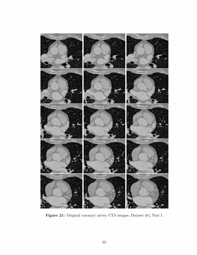
Figure 21: Original coronary artery CTA images, Dataset #1, Part I.

65

Figure 22: Original coronary artery CTA images, Dataset #1, Part II.

66

(a) (b)

(c) (d)

(e) (f)

Figure 23: Lung and heart segmentation, Dataset #1, Part I. (a)→(b) threshold-ing, (b)→(c) dilation, (c)→(d) hole filling, (d)→(e) tipping point detection, (e)→(f)Bresenham lines. See text for details.

67

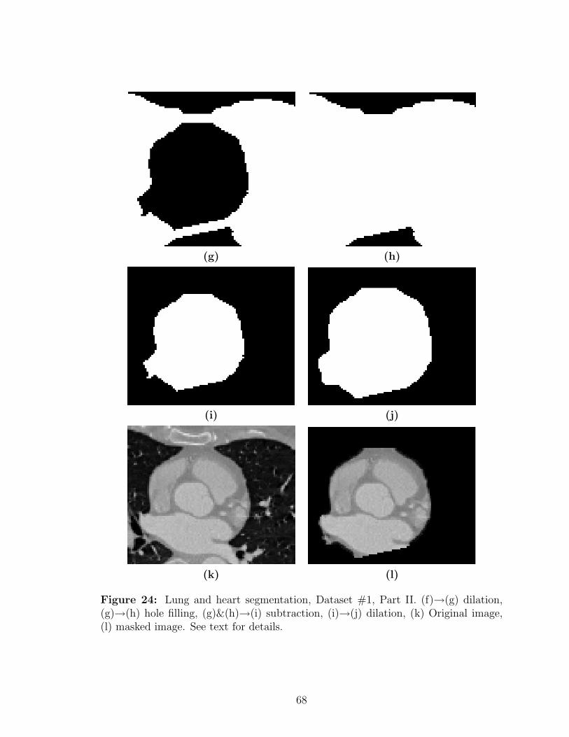
(g) (h)

(i) (j)

(k) (l)

Figure 24: Lung and heart segmentation, Dataset #1, Part II. (f)→(g) dilation,(g)→(h) hole filling, (g)&(h)→(i) subtraction, (i)→(j) dilation, (k) Original image,(l) masked image. See text for details.

68

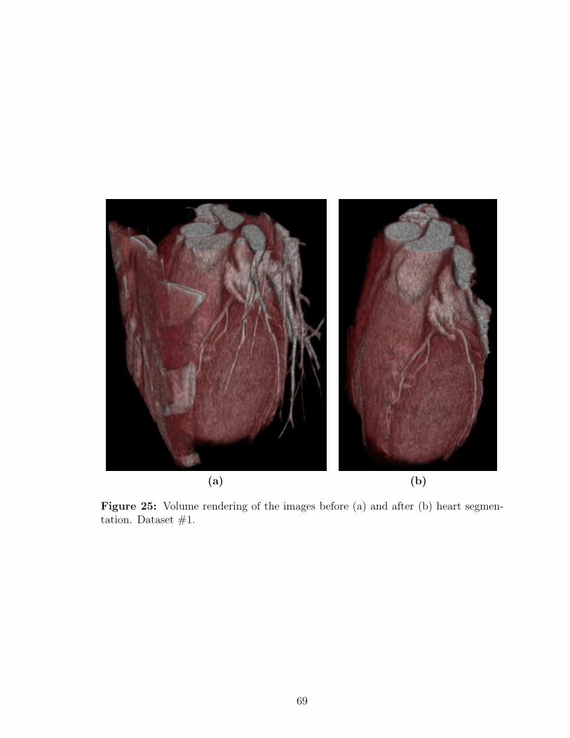
(a) (b)

Figure 25: Volume rendering of the images before (a) and after (b) heart segmen-tation. Dataset #1.

69

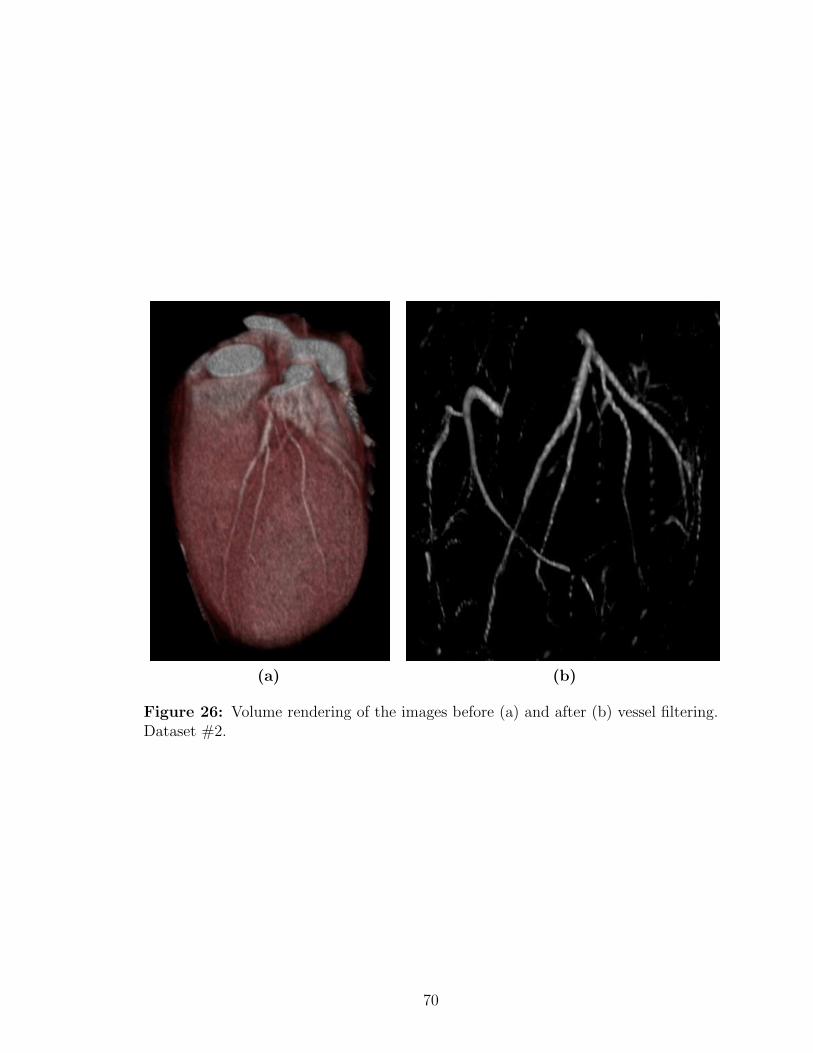
(a) (b)

Figure 26: Volume rendering of the images before (a) and after (b) vessel filtering.Dataset #2.

70

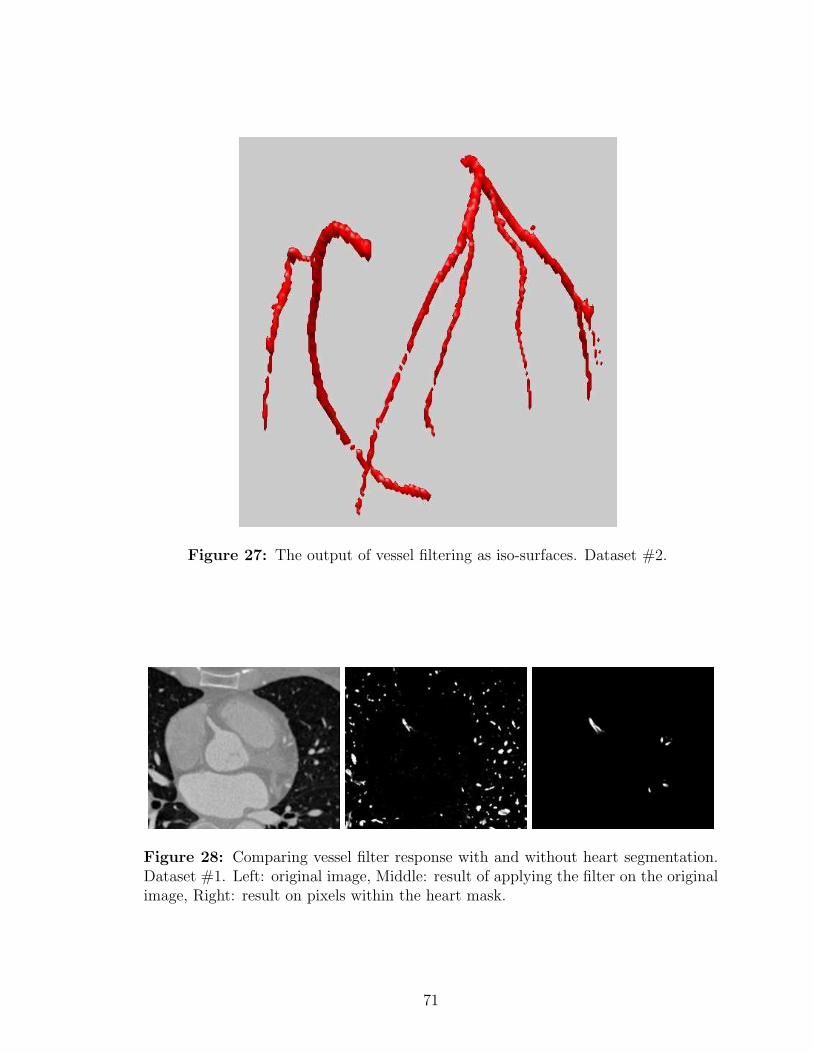
Figure 27: The output of vessel filtering as iso-surfaces. Dataset #2.

Figure 28: Comparing vessel filter response with and without heart segmentation.Dataset #1. Left: original image, Middle: result of applying the filter on the originalimage, Right: result on pixels within the heart mask.

71

(a) (b)

(c) (d)

Figure 29: Comparing segmentation contours before and after BDIS. Dataset #2.(a) Initial contour on slice #6, (b) BDIS result on slice #6; (c) Initial contour onslice #23, (d) BDIS result on slice #23.

72

Figure 30: Segmentation results shown in 2D as contours. Dataset #2, Part I.

73

Figure 31: Segmentation results shown in 2D as contours. Dataset #2, Part II.

74

Figure 32: Segmentation results shown in 2D as contours. Dataset #2, Part III.

75

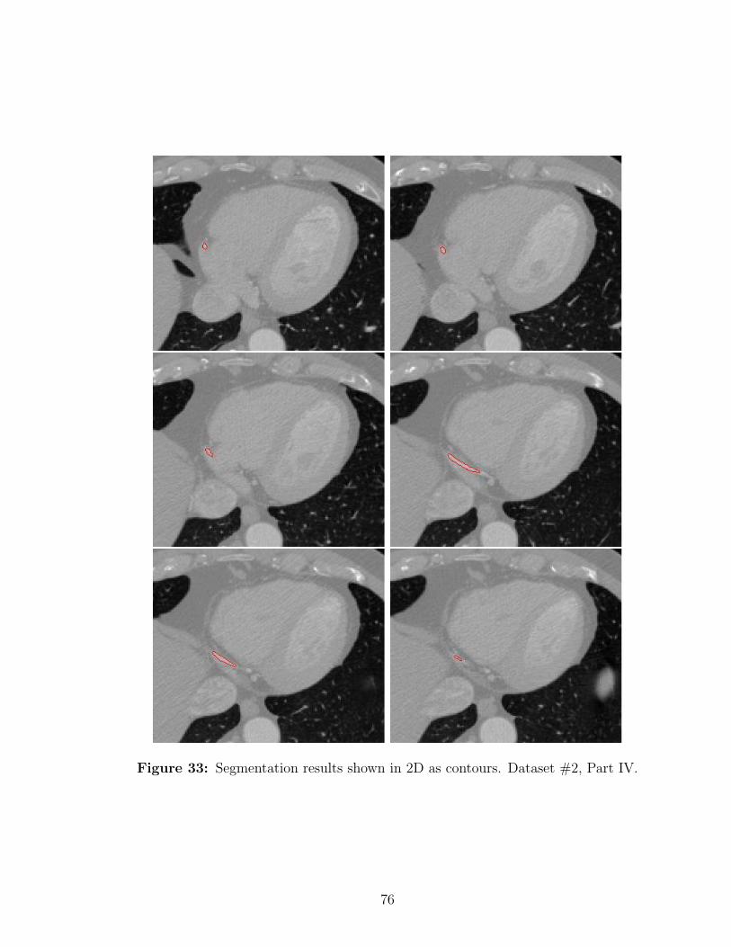
Figure 33: Segmentation results shown in 2D as contours. Dataset #2, Part IV.

76

Figure 34: 3D results. Left and right coronary arteries rendered as surfaces. Up-per: Automatic BDIS segmentation; Lower: Manual delineated contours rendered assurfaces.

77

(a1) (a2)

(b1) (b2)

(c1) (c2)

Figure 35: Removing calcified plaques from the segmentation. (a1) and (a2):before and after removing the calcium on Slice #34 of Dataset #8; (b1) and (b2):Slice #8 of Dataset #15; (c1) and (c2): Slice #6 of Dataset #16.

78

Figure 36: BDIS segmentation results shown as surfaces. Part I. Datasets #1 - #6.

79

Figure 37: BDIS segmentation results shown as surfaces. Part II. Datasets #7 -#12.

80

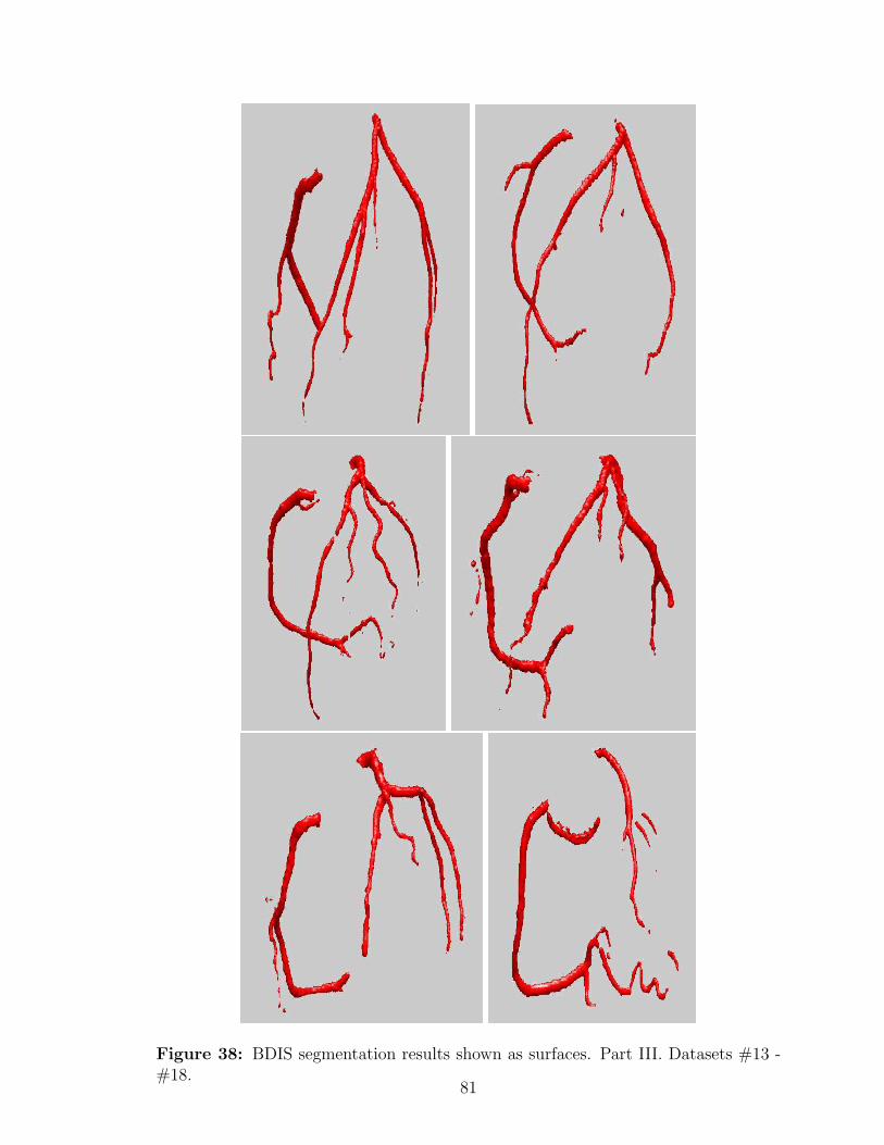
Figure 38: BDIS segmentation results shown as surfaces. Part III. Datasets #13 -#18.

81

CHAPTER V

CENTERLINE EXTRACTION AND STENOSIS

EVALUATION FOR CORONARY ARTERIES

In this chapter, we present a centerline extraction (skeletonization) approach for tri-

angulated surfaces of 3D tubular structures. In our application of coronary artery

analysis, we use the segmented surfaces obtained in the previous chapter as the input

to the skeletonization method presented in this chapter. These two chapters bind

naturally to provide a complete tool set for coronary CTA analysis. In addition, the

“harmonic skeletonization” approach proposed here also provides orthogonal cutting

planes located at each centerline point, and thus offers a convenient way to mea-

sure cross-sectional areas of the vessels, which is an important indicator of coronary

stenosis.

We first describe and explain the algorithms in Sections 5.1 and 5.2, and then

further test and validate the method using a digital phantom and real clinical datasets

in Section 5.3.

5.1 Harmonic Skeletonization

The harmonic skeletonization is a centerline extraction method based on the solution

of the Laplace equation with boundary conditions of the first kind (Dirichlet problem)

on the surface of a tubular structure. Since the solution of the Laplace equation is a

harmonic function, the skeleton extracted using this method is called the harmonic

skeleton [110]. The harmonic skeleton is easy to compute, is guaranteed to be smooth,

and can automatically give a viewing vector when used as a guidance for fly-throughs

for virtual endoscopy. Moreover, the space of harmonic functions is linear (as opposed

82

to that of the distance transform on which the ordinary skeleton is founded).

An effective way to determine the boundary conditions for solving the appropriate

Laplace equation is proposed here, so that the points that form the final skeleton are

evenly distributed, without being too dense or too sparse, thus guaranteeing the

connectivity of the skeleton. Then, the cross-sectional area at a certain location on

the artery can be conveniently measured using the least squares plane that fits all

the points on the iso-value contour of the solution of the Laplace equation. This

means that we can acquire the cross-sectional areas throughout the artery in order

to identify stenoses.

The harmonic skeleton can be obtained by solving the Laplace equation on the

surface of the artery. Let Σ denote the surface, which is topologically a branched tube.

Each branch has a boundary σi (i = 0, . . . , N−1), which is a closed contour, as shown

in Figure 39 in blue. Here N denotes the total number of boundaries including the root

σ0, which can be selected arbitrarily or selected based on physiological considerations.

We have chosen the root σ0 to be at the proximal section of the left main (LM)

coronary artery. Note that the initial segmented surface is normally a closed surface

and here we use these boundary contours to cut the branches in order to create

open-ended tubes for our computation.

Next we can calculate the harmonic function u by solving the Laplace equation

on Σ\σi(i = 0, . . . , N − 1):

∆u = 0, (34)

with proper boundary conditions. To find these boundary conditions, we assign the

values at the boundaries in the following manner:

1. Set the boundary value of u at the root σ0 to be zero, and set StepNumber =

0;

2. Label all the points on σ0 as “visited”;

3. Label all the neighbors of the “visited” points as “visited”;

83

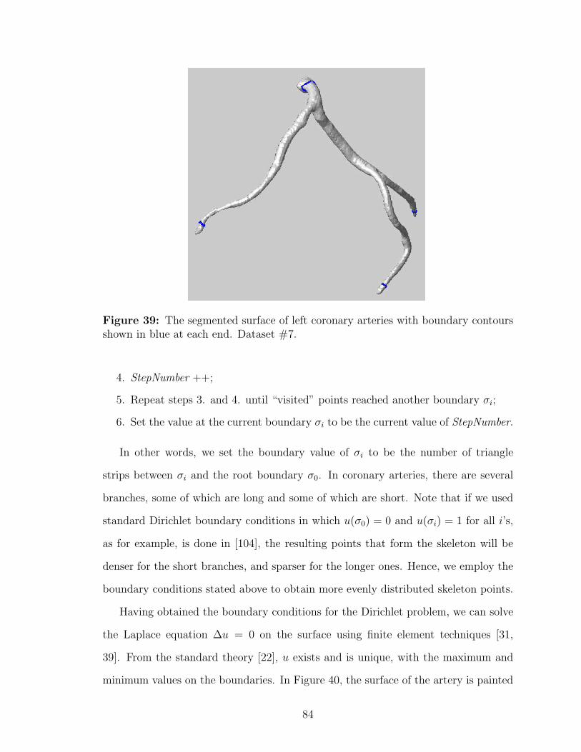
Figure 39: The segmented surface of left coronary arteries with boundary contoursshown in blue at each end. Dataset #7.

4. StepNumber ++;

5. Repeat steps 3. and 4. until “visited” points reached another boundary σi;

6. Set the value at the current boundary σi to be the current value of StepNumber.

In other words, we set the boundary value of σi to be the number of triangle

strips between σi and the root boundary σ0. In coronary arteries, there are several

branches, some of which are long and some of which are short. Note that if we used

standard Dirichlet boundary conditions in which u(σ0) = 0 and u(σi) = 1 for all i’s,

as for example, is done in [104], the resulting points that form the skeleton will be

denser for the short branches, and sparser for the longer ones. Hence, we employ the

boundary conditions stated above to obtain more evenly distributed skeleton points.

Having obtained the boundary conditions for the Dirichlet problem, we can solve

the Laplace equation ∆u = 0 on the surface using finite element techniques [31,

39]. From the standard theory [22], u exists and is unique, with the maximum and

minimum values on the boundaries. In Figure 40, the surface of the artery is painted

84

Figure 40: The coronary artery surface is color-painted with solved harmonic func-tion u, where dark color means lower u, and light color means higher u. Dataset #7.

with the solved u, where brighter color indicates higher u, and darker color indicates

lower u.

Using the harmonic function u, we can now build the harmonic skeleton. We first

find the level sets of u on the surface, i.e., sets x|u(x) = ν for values of ν ranging

from 0 to max(u). Each level set corresponds to a group of points on the surface

which have the value of a certain ν. These points are not necessarily located on the

vertices of our original triangulation of the surface, so we obtain these level points by

linearly interpolating the coordinates of the vertices according to the values of u.

We also check the change in the topology of the level contours as we proceed, and

further partition these contours into sub-contours if not all the points are connected

to form a single contour. This means there is a bifurcation and one contour splits

into two at the current level of u. We assume one contour cannot split into more than

85

two contours, which is true for coronary arteries in most cases. The centroid of each

contour or sub-contour is then calculated:

1

M

M∑i=1

xi,

where xi = (xi, yi, zi)′ is a point on the contour, and M is the total number of points

on the current contour. Each centroid contributes a point to the final harmonic

skeleton. By increasing ν from 0 to the maximum value of u, we can find a series

of centroids that can finally be connected to build a structured tree, which is the

harmonic skeleton.

Figure 41 demonstrates the above procedure by showing a series of level contours

(in blue) on the surface and the centerline (in red) achieved from the centroids of these

level contours. As the algorithm runs, the contours and center points are generated

from a lower level of u to a higher level, which is equivalent to the situation from top

to bottom in this example. Notice that only a portion of the level contours are shown

here for visualization. In fact, if all the contours are visualized, the surface with be

covered completely with these contours.

5.2 Cross-sectional Area Measurement and Stenosis Detec-tion

The harmonic skeleton obtained using the above method can be used as a guide in

calculating cross-sectional areas at specific locations along the vessels, and the cross-

sectional areas can in turn be used to precisely evaluate stenoses in the coronaries.

Cross-sectional areas are better than diameters because atherosclerotic plaques are

usually eccentric and asymmetric as we have introduced in Chapter 1, and the cross-

sections of the narrowed vessel lumen may not be circular. The stenosis may be

underestimated if one uses only diameters for stenosis evaluation. Cross-sectional

areas, on the other hand, provide more information about the stenosis, and are directly

related to the flow rate of blood through the cross-section.

86

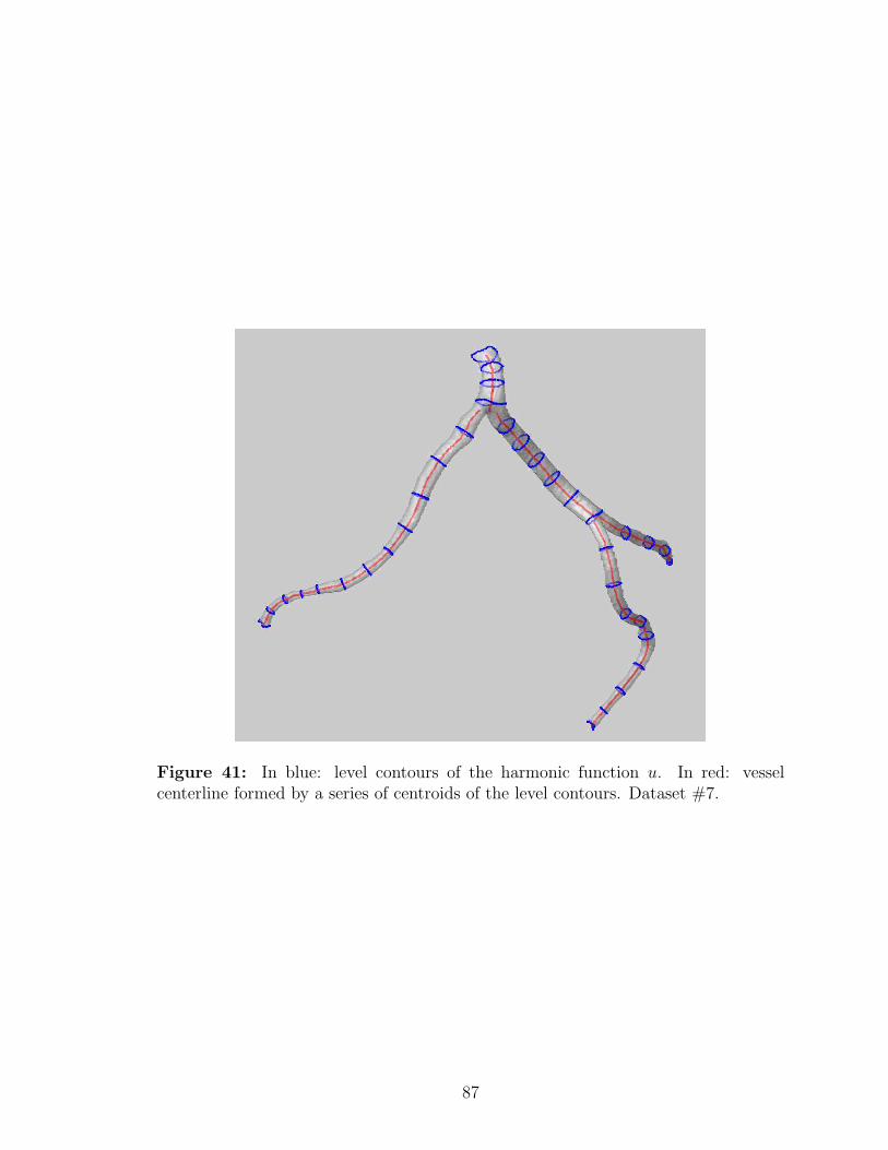
Figure 41: In blue: level contours of the harmonic function u. In red: vesselcenterline formed by a series of centroids of the level contours. Dataset #7.

87

One straightforward way of obtaining the cross-sections of the artery is by looking

for a plane that is perpendicular to the skeleton to cut the tube at a certain location.

But this strongly depends on the local properties of the skeleton, and a plane that

is perpendicular to the skeleton locally may not be perpendicular to the vessel itself.

What we do here is to start with the contours or sub-contours obtained in the above

section, and measure the cross-sectional area at the same time as we calculate the

centroid. It can be seen from Figure 41 that the level contours already exhibit an

orthogonal appearance to the vessels.

The first step is to find the cross-sectional plane. We have many more points

(about 50 points, somewhat more for wider contours and somewhat less for narrower

contours) on a level contour than are necessary (3 points) for determining a plane.

Hence we need to use least squares to solve this over-determined problem. Suppose

we have a set of points X = (x1,x2, ...xN)′, where xi = (xi, yi, zi)′, i = 1, . . . ,M is a

point on the level contour, and we build a matrix A = X−x0, where x0 = (x0, y0, z0)′

is the centroid of all the points on the contour. Calculating the Singular Value

Decomposition (SVD) [71] of matrix A, we get A = USV T , where U and V are

orthogonal matrices and S is a diagonal matrix with non-negative diagonal entries in

decreasing order. The singular vector in V that corresponds to the smallest singular

value in S is the cosine of the direction of the normal to the best-fit plane. The

centroid and the normal vector can now be used to uniquely determine the least

squares plane.

We now use this plane to cut the surface of the vessel and obtain a series of points

on the surface which also belong to the least squares plane. Again, these points may

not coincide with the vertices of the triangulated surface, so we find the points on the

triangle edges, and connect them to form a polygon. We then calculate the area of

the polygon, and the result is the desired cross-sectional area at the current location

on the vessel.

88

5.3 Results and Validation

In this section we present the results of applying the proposed method to a digital

phantom and all clinical datasets which have been presented in the previous chapter.

The results are validated quantitatively on the digital phantom to show the accuracy

of our approach. On real clinical datasets, we first show the skeletonization results on

the 18 clinical datasets, and then present two methods to visualize the cross-sectional

area measuring results.

5.3.1 Digital Phantoms

We first test and validate our skeletonization and area measuring algorithm using a

digital phantom simulating a stenosed vessel. The phantom is constructed from a

series of images with a circle located at the center of each image. The radius of the

circles is composed of five segments of 40 slices, first being a larger value (10 in pixel

space), then gradually changing to a smaller value (5 in the pixel space) according to

a sinusoid function, keeping the smaller value for 40 slices, gradually changing back

to the larger value, and finally keeping the larger value for another 40 slices.

Each individual slice is added with Gaussian noise, and further blurred with a

Gaussian kernel of size 7×7 with a standard deviation of 2. The volume rendering of

the phantom images is shown in Figure 42 (Left).

Using Matlab function isosurface we generate a triangulated surface of the phan-

tom, and the Laplace equation is then solved on this open-ended surface. Figure 42

(Middle) shows the solution u by representing different u values with different colors.

The harmonic skeleton is then obtained and the cross-sectional areas are measured

at the same time. Figure 42 (Right) is a similar figure to Figure 41 showing selected

level contours of u (in blue) and the skeleton (in red).

We compared both the skeleton and the cross-sectional areas to the ground truth

parameters, with which we have constructed the phantom. To compare the skeleton,

89

we calculate the distance from each skeleton point to the ground truth skeleton. The

average distance error is 0.0788 pixel, which is 0.788% of the larger radius and 1.58%

of the smaller radius.

We also compared the cross-sectional areas measured with our approach against

the ground truth. The mean error over the whole phantom is 6.1842 pixel2, which

is 1.97% of the normal area, and 7.87% of the stenosed area. To further detail the

quantification, we compared the difference at the normal area, which is 3.36%, and

the stenosed area, which is 6.46%. In terms of vessel radius, the error is 0.1665 pixel

at the normal site (with a true radius of 10 pixel) and 0.1643 pixel at the stenosed site

(with a true radius of 5 pixel). Interestingly, we have observed that the automatic

algorithm tends to overestimate the area of the normal segment of the vessel, but

underestimate the area of the stenosed segment, which in turn will overestimate the

degree of stenosis. This error is mostly due to the Gaussian smoothing of the original

images and the isosurface step that follows.

5.3.2 Clinical Data

The proposed harmonic skeletonization and cross-sectional area measuring method

is applied to all clinical datasets used in Chapter 4. The input is the triangulated

surfaces obtained from the results of BDIS segmentation of the vessels. For the

attributes of all datasets, see Table 2.

5.3.3 Generation of Harmonic Skeletons

We first present the results of harmonic skeletons of all 18 datasets. Figure 43, 44

and 45 show both semi-transparent surfaces of the vessels and the skeletons. The

results are visually satisfying except for a few tiny isolated branches whose skeletons

are missing in the results. This is due to the fact that our method is based on a

singly connected genus zero triangulated surface, and these tiny branches are not

topologically connected to the major vessels.

90

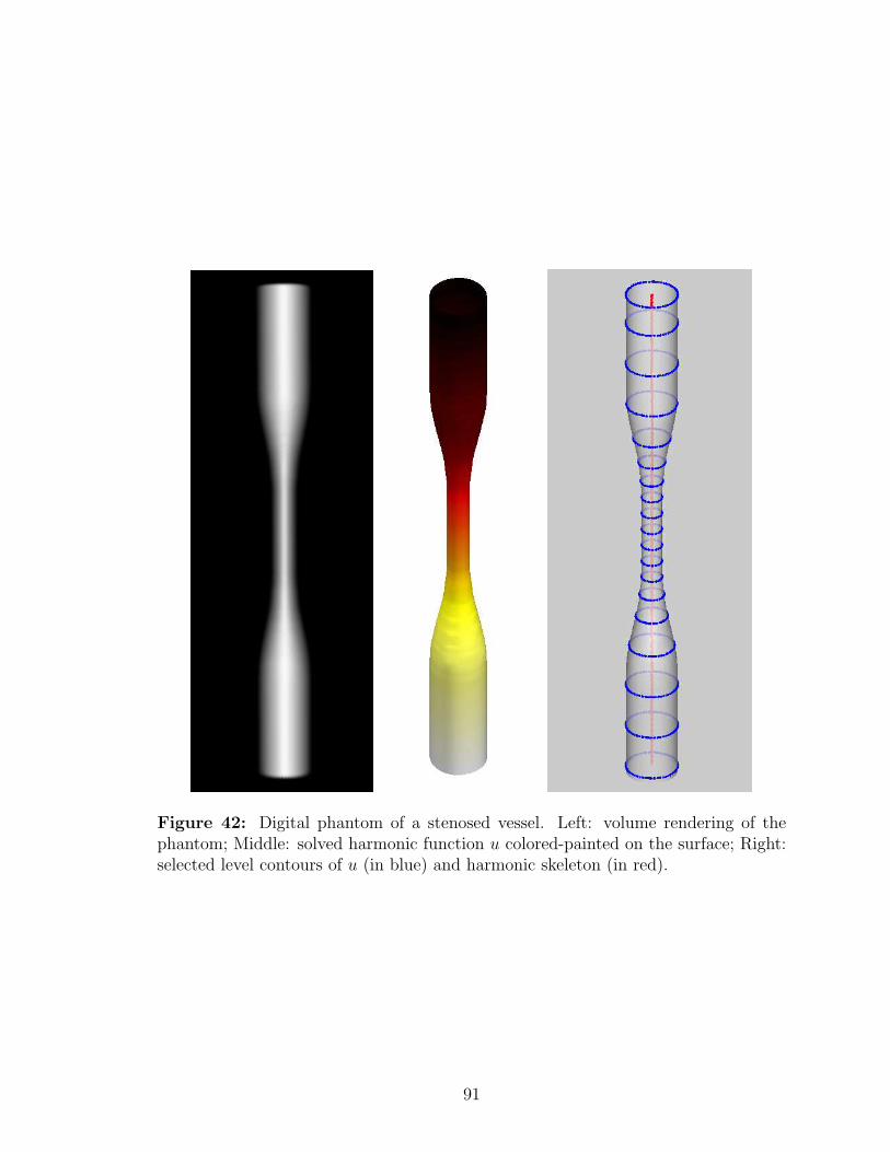
Figure 42: Digital phantom of a stenosed vessel. Left: volume rendering of thephantom; Middle: solved harmonic function u colored-painted on the surface; Right:selected level contours of u (in blue) and harmonic skeleton (in red).

91

At the bifurcation sites, some post-processing was performed to keep the skeleton

smooth and natural. Increasing the value of u and tracking the topology change of

the level contours, one contour will split into two at a certain u level, and there will be

a jump between the centroid of the single parent contour and the centroids of the two

daughter contours. If we connect the centroids directly, the resulting skeleton may

not be smooth where it bifurcates. To solve this problem, we start from the daughter

branches, and trace back until they reach the bifurcation site, and then extend the

branches further until they meet the parent branch. After the post-processing, the

skeleton is visually more natural at the bifurcation sites.

5.3.4 Stenosis Evaluation

The cross-sectional areas were calculated along the vessel with a resolution of δu = 0.5,

which means we measure the cross-sectional area once we increase the harmonic func-

tion u by 0.5. For each coronary artery, there are roughly 400 levels of cross-sectional

areas, and at each level, there are one or several cross-sectional areas measured ac-

cording to the number of branches at this level.

We propose two methods to visualize the quantitative measurements and illus-

trate using two examples. The first is to specify a u value, which is equivalent to

specifying a location on the vessel, and show the cross-sectional areas at this u level,

as demonstrated in Figure 47, where three sub-contours at the same u level are shown

along with the cross-sectional areas at these locations.

The second way is to create a color map of the cross-sectional area values, and

paint the surface with the color of these values. This provides an intuitive way to

localize the stenosis, by showing different colors where the cross-sectional area has

an apparent change along the vessels, as demonstrated in Figure 48. In this figure,

lighter color indicates normal sized vessel lumen, and darker color means the lumen

is narrowed, thus implying stenosis.

92

Figure 49 is a plot of u versus cross-sectional area along the LAD of Figure 48.

The left y-axis shows the cross-sectional areas in mm2, and the right y-axis shows

the stenosis percentage, which is an important measure for the evaluation of stenosis.

We can see from this plot that this LAD has two stenosis sites, one mild (a little less

than 40% blockage) and another more severe (60% blockage). This is in consistent

with what is shown in Figure 48.

With these results we conclude this chapter, in which we proposed a skeletoniza-

tion approach for the segmented surface of branched vessels. This approach gives

a straightforward way to measure cross-sectional areas of the vessels, thus provides

useful references for stenosis detection and evaluation. We should mention that since

the cross-sectional area measuring process is performed on the segmented surface, the

result is essentially determined by the segmentation result. The algorithms proposed

in this chapter were applied to the segmented vessel surfaces obtained from the previ-

ous chapter using the BDIS method, which has been validated in the previous chapter

as well. In this chapter, we quantitatively validated our skeletonization method using

a digital phantom.

The skeletons provide an abstract yet informative representation of the vessel tree,

which leads to many possibilities of visualizing the vessels, such as MPRs and fly-

throughs. These visualization methods are very often used clinically nowadays for

3D tubular structure, including airways, colons and vessels. The essential step is to

acquire a reliable and accurate skeleton of these tubular structures with minimal user

input. The skeletonization method proposed in this chapter is an automatic approach

given a segmented surface, and the phantom study also shows a good centeredness of

the skeleton. The stenosis estimation presented here is based on local cross-sectional

areas, which is theoretically better than the ones based on the diameter. However,

there are clinicians who prefer to use minimum/maximum diameter in the stenosis

93

evaluation or surgical planning procedures for stent implantation, and these param-

eters can also be acquired following the harmonic skeletonization method, since we

essentially extract the cross-sectional boundary of the vessels, which is a closed con-

tour in 2D. For further visualization, these 2D contours can be overlaid onto the

original image data that are re-sampled in the corresponding location and direction.

Hence, there are many ways to use the skeletons in a clinical setting, according to

the preference of clinicians who actually use them. The algorithm would show more

value if it is integrated to a friendly graphical user interface (GUI), which allows

more flexibility in visualizing and exploring the datasets; however, the design and

implementation of GUI is beyond the scope of this thesis.

94

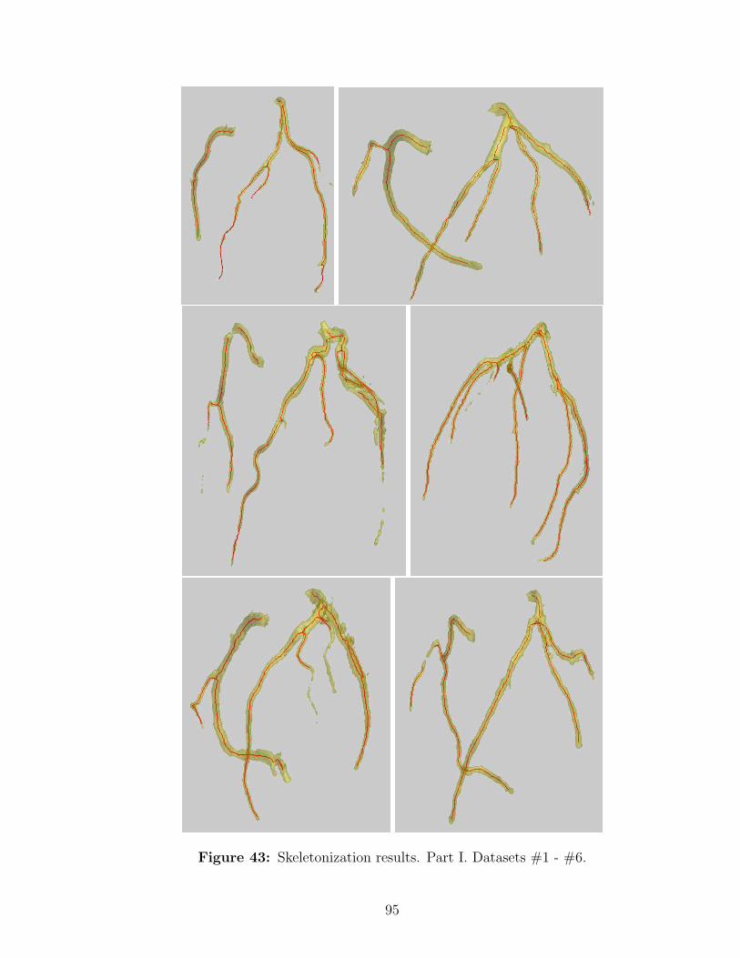
Figure 43: Skeletonization results. Part I. Datasets #1 - #6.

95

Figure 44: Skeletonization results. Part II. Datasets #7 - #12.

96

Figure 45: Skeletonization results. Part III. Datasets #13 - #16.

97

Figure 46: Skeletonization results. Part IV. Datasets #17 - #18.

Figure 47: Cross-sectional area visualization #1. The cross-sectional area of eachbranch of the coronaries for a certain u. Dataset #7.

98

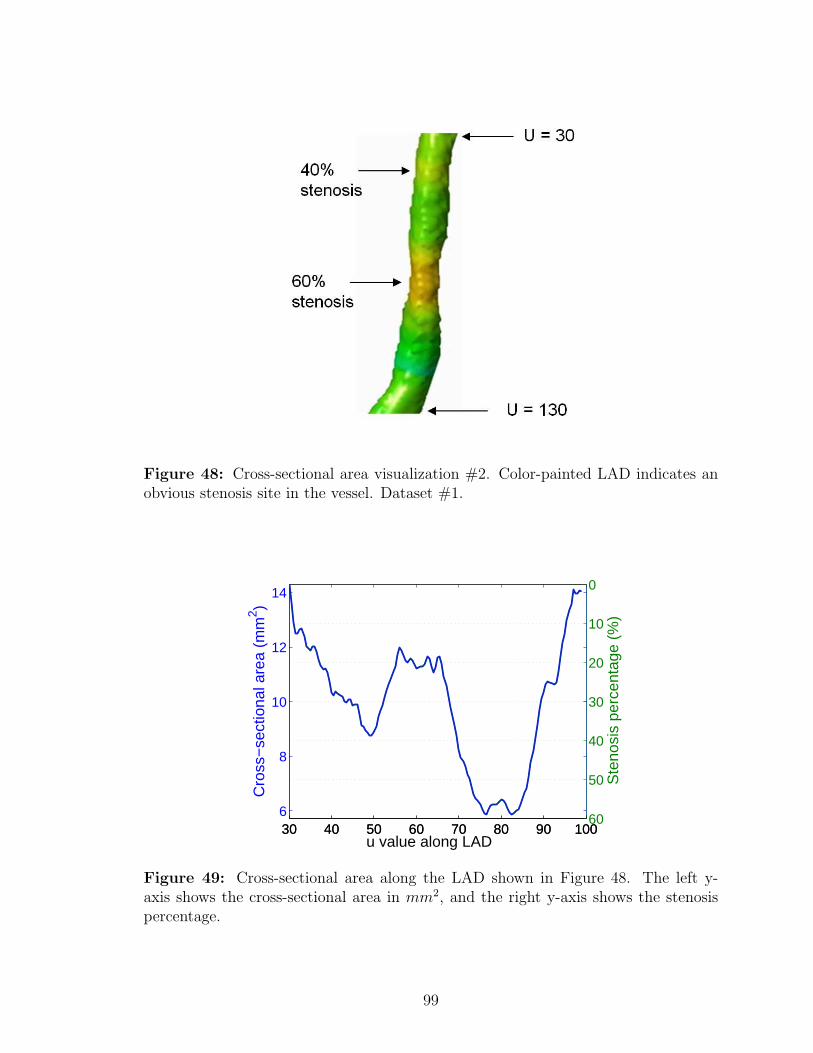
Figure 48: Cross-sectional area visualization #2. Color-painted LAD indicates anobvious stenosis site in the vessel. Dataset #1.

30 40 50 60 70 80 90 1006

8

10

12

14

Cro

ss−

sect

iona

l are

a (m

m2 )

u value along LAD30 40 50 60 70 80 90 100

0

10

20

30

40

50

60

Ste

nosi

s pe

rcen

tage

(%

)

Figure 49: Cross-sectional area along the LAD shown in Figure 48. The left y-axis shows the cross-sectional area in mm2, and the right y-axis shows the stenosispercentage.

99

CHAPTER VI

CONCLUSIONS AND FUTURE RESEARCH

In this final chapter, we conclude the thesis and mention some possible extensions

and future directions. This thesis has focused on the 3D image analysis of coronary

arteries using CTA images. We first proposed a general image segmentation approach

called BDIS in Chapter 3, which is based on Bayesian pixel processing and the level

set image segmentation framework. The algorithm can be easily extended to 3D,

with which we segmented coronary arteries from CTA images in Chapter 4. In order

to generate an initial segmentation to start the BDIS process, we adopted a multi-

scale Hessian based 3D line filtering technique to isolate the vessels and eliminate

other structures in the images. The algorithm was applied to 18 real clinical datasets

and was validated using manual segmentation of the same datasets. In Chapter

5 we further proposed shape analysis methods based on the segmented surface of

the vessels. First, a skeletonization algorithm is explored using the solution of the

Laplace equation on the surface in order to extract the centerlines of the branched

vessels. Then a convenient way to measure cross-sectional areas of the vessel lumen

is proposed to assist the detection and evaluation of stenosis.

The automatic image processing techniques have the potential to change the rou-

tinely clinical work-flow of a radiologist fundamentally. In stead of viewing the 2D

axial image slice by slice to look for interested structures such as coronary arteries

which only occupy a small number of voxels, the automatic approach proposed in

this thesis takes the 3D dataset as a whole and output the structure of interest with

minimal user input or interaction, with clinical significant parameters measured in

100

addition. Commercial software systems are now incorporating more and more auto-

matic techniques to assist the clinical work-flow; however, higher level of automation

and better accuracy are always desirable and critical. To our knowledge, so far there

is no commercial systems which provide algorithms with the level of automation pre-

sented in this thesis. Normally the user still needs a great amount of manual work

such as mouse clicking or parameter tuning to achieve a result similar to the results

presented here. In order for the algorithms to be used clinically in a more efficient

manner, a friendly GUI is desirable to visualize the results in multiple intuitive ways,

as we have discussed at the end of the previous chapter. This needs more software

engineering work including interface design, usability testing, speed optimization and

more.

The validation of the proposed methods is performed quantitatively by comparing

with the manual segmentation in this thesis. However, this is not a clinical valida-

tion, since the datasets are anonymous and the diagnoses were not available with

the datasets. To strictly validate the proposed methods for clinical use, one should

compare the results acquired here with the real diagnosis on each patient, especially

for calcium identification and stenosis evaluation, to see how much difference there is

between the automatic approach and the real diagnosis.

Also notice that the vessel analysis discussed in this thesis is essentially “lumen”

analysis, since we have been aiming at segmenting regions filled with the contrast

agent which is the blood-filled region. However, more information of atherosclerotic

plaques is, in fact, hidden in the vessel wall, which can be composed of stable cores or

vulnerable ones. Vulnerable plaques are prone to rupture, thus are more dangerous to

patients. However, they are usually the ones which are more difficult to image. CTA

is capable of revealing calcified plaques which may or may not be vulnerable plaques,

and we have proposed a method to analyze this (see Chapter 4, Section 4.3.2). More

challenges lie in the image post-processing and analysis of the vessel wall, which

101

normally do not have a good contrast with other tissues, but may contain valuable

information about the plaques themselves. In order to reveal more information, one

can explore texture analysis approaches (e.g., based on wavelets) which have been used

to analyze the image of myocardium, cartilage and bones, and apply these methods

on the vessel walls. With the hope that certain measures developed from the texture

features of the vessel wall may differentiate stable and vulnerable plaques, texture

analysis of the plaques can be an interesting future direction of this line of research.

The segmentation of the lumen presented here can provide an ideal starting point

for the texture analysis, which can be applied along the inner boundary of the vessel

wall.

In the automatic segmentation work (Chapter 4), we have observed that the

Hessian-based vessel filtering offers a slightly better sensitivity in the distal end of

the vessels than the final BDIS segmentation results. This might be due to the poor

diffusion of contrast agent at the distal end, which makes the image intensity lower

than the proximal end. One alternative process would be to generate a centerline

from the Hessian-based filter response to preserve the better sensitivity. This center-

line, however, can hardly be smooth or well connected, since the filter response gives

quite ragged isosurface and in many places are disjointed. Hence, the harmonic skele-

tonization is still essential in generating a smooth centerline which also has better

connectivity.

In this thesis, the harmonic skeletonization work (Chapter 5) is based on the

surface of a 3D tubular structure, which is a quite general model. This method hence

has the potential to be applied to other structures such as airways, colons, elongated

bones, and even other non-medical structures, generated either from tomography

images such as the one used in this thesis, or any other imaging or modeling methods.

Since the harmonic skeletonization method is completely surface-based, we have not

used the original images in this step once we have obtained the surface from image

102

segmentation. However, one interesting extension would be to go back to the original

CTA images, and use the generated centerline to guide a fly-through of the gray

scale images, where the vessels can be viewed in either longitudinal or orthogonal

directions, by re-sampling the 3D CTA images using oblique or curved planes following

the centerline. In this way, the vessels and their segmentation can be examined in a

more intuitive manner, and stenoses can be detected more straightforwardly.

Some works (e.g. Chalopin et al. [13]) have considered the problem of automatic

labeling of different branches in a vessel tree by fitting the geometry of the vessels to

a pre-defined model. The harmonic skeletons generated in this thesis can certainly

serve as a good representation of the vessel tree for labeling purposes.

In the past few decades, medical imaging has grown rapidly and made tremendous

contributions to the diagnosis and treatment to different diseases, such as atheroscle-

rosis studied in this thesis. We hope the automatic image processing techniques

explored here can provide a convenient way for radiologist and physicians to extract

useful information from the large amount of images acquired by modern scanners more

efficiently and accurately. The image segmentation technique also provides patient-

specific models of coronary arteries, which can in turn be used to simulate blood

flow patterns specifically for these patients, with the hope that the flow patterns and

other bio-fluid mechanical properties of the blood may reveal more information about

disease formation and development.

103

REFERENCES

[1] American Heart Association, “A.H.A. Heart Disease and Stroke Statistics - 2006Update”, (2006).

[2] Andel, H.A.F.G., Meijering, E., Lugt, A., Vrooman, H.A., Stokking, R., “VAM-PIRE: Improved Method for Automated Center Lumen Line Definition inAtherosclerotic Carotid Arteries in CTA Data”, MICCAI’04, LNCS 3216,(2004) pp. 525-532

[3] Antiga, L., Ene-Iordache, B., Caverni, L., Cornalba, G.P., and Remuzzi, A.,“Geometric Reconstruction for Computational Mesh Generation of Arterial Bi-furcations from CT angiography”, Computerized Medical Imaging and Graphics,26 (2002) pp. 227-235.

[4] Antiga, L., Ene-Iordache, B., and Remuzzi, A., “Computational Geometry forPatient-Specific Reconstruction and Meshing of Blood Vessels From MR andCT Angiography”, IEEE Trans. Med. Imag., 22 (2003) pp. 674-684

[5] Avants, B.B, Williams, J.P., “An Adaptive Minimal Path Generation Tech-niques for Vessel Tracking in CTA/CE-MRA Volume Images”, MICCAI’00LNCS 1935, (2000), pp. 707-716

[6] Bezdek, J.C., Hall, L.O., and Clarke, L.P., “Review of MR Image SegmentationTechniques Using Pattern Recognition” Med. Phys. 20 (1993) pp.1033-1048.

[7] Baillard, C., Barillot, C., and Boutherny, P., “Robust Adaptive Segmentationof 3D Medical Images with Level Sets” INRIA, Rennes Cedex, France, Res.Rep. 1369, Nov. 2000

[8] Blondel, C., Malandain, G., Vaillant, R., and Anyche, N., “Reconstruction ofCoronary Arteries From a Single Rotational X-Ray Projection Sequence”, IEEETrans. Med. Imag., Vol. 25, No. 5 (2006), pp. 653-663

[9] Bouix, S., Siddiqi, K., and Tannenbaum, A., “Flux Driven Automatic Center-line Extraction,” Medical Image Analysis 9, 2005, pp. 209-221.

[10] http://en.wikipedia.org/wiki/Bresenham%27s line algorithm, last visited Jan.15th, 2007

[11] Buhler, K., Felkel, P., and Cruz, A.L., “Geometric Methods for Vessel Visual-ization and Quantification - A Survey”, technical report TR VRVis 2002 035,VRVis Research Center, Vienna, Austria, (2002)

104

[12] Caselles, V., Kimmel, R., and Sapiro, G., “Geodesic Active Contours,” Int.Journal Computer Vision, 22(1) (1997) pp. 61-79.

[13] Chalopin, C., Finet, G., Magnin, I.E., “Modeling the 3D Coronary Tree forLabeling Purposes”, Medical Image Analysis, 5, (2001), pp. 301-315

[14] Chan, T.F. and Vese, L.A., “Active Contours Without Edges”, IEEE Trans.Imag. Proc., Vol. 10, No. 2, (2001) pp.266-277

[15] Chen, J. and Amini, A. A., “Quantifying 3-D Vascular Structures in MRAImages Using Hybrid PDE and Geometric Deformable Models”, IEEE Trans.Med. Imag., Vol. 23, No. 10, (2004) pp. 1251-1262

[16] Chen, Z., Molloi, S., “Automatic 3D Vascular Tree Construction in CT Angiog-raphy”, Computerized Medical Imaging and Graphics, 27, (2003) pp. 469-479

[17] Clarke, L. P., Velthuizen, R. P., Camacho, M. A., Heine, J. J., Vaidyanathan,M., et al. “MRI Segmentation: Methods and Applications” Magn. Reson. Imag-ing 13 (1995) pp. 343-368.

[18] Cohen, L. D., “Global Minimum for Active Contour Models: A Minimal PathApproach”, International Journal of Computer Vision, 24(1), (1997) pp. 57-78

[19] Dempster, A., Laird, N., and Rubin, D., “Maximum Likelihood From Incom-plete Data Via the EM Algorithm”, Journal of the Royal Statistical Society,Series B, 39(1), (1977) pp. 1-38

[20] Deschamps, T. and Cohen, L. D., “Fast Extraction of Tubular and Tree 3DTurfaces With Front Propagation Methods”, Intl. Conf. Pattern Recognition,(2002)

[21] Duda, R. O., Hart, P. E., and Stork, D. G., “Pattern Classification”, SecondEdition, Wiley-Interscience, John Wiley & Sons, Inc. (2000)

[22] Farlow, S. J., “Partial Differential Equations for Scientists and Engineers”,Dover Publications, Inc. New York (1993).

[23] Fayad, Z. A., Fuster, V., “Clinical Imaging of the High-Risk or VulnerableAtherosclerotic Plaque”, Circulation Research, August17 (2001) pp. 305-316.

[24] Fayad, Z. A., Fuster, V., Nikolaou, K., and Becker, C., “Computed Tomographyand Magnetic Resonance Imaging for Noninvasive Coronary Angiography andPlaque Imaging”, Circulation, 106 (2002) pp. 2026-2034.

[25] Felkel, P., Wegenkittl, R., Kanitsar, A., “Vessel Tracking in Peripheral CTADatasets - An Overview”, Spring Conference on Computer Graphics - SC-CCG’01, (2001) pp. 232-239.

105

[26] Florin, C., Paragios, N., Williams, J., “Particle Filters, a Quasi-Monte-Carlo-Solution for Segmentation of Coronaries”, MICCAI’05, LNCS 3749, (2005) pp.246-253

[27] Frangi, A. F., Niessen, W. J., Hoogeveen, R. M., Walsum, T. V., and Viergever,M. A., “Model-Based Quantization of 3-D Magnetic Resonance AngiographicImages”, IEEE Tran. on Med. Imag., 18 (1999), pp. 946-956

[28] Frangi, A. F., Niessen, W. J., Vincken, K. L. and Viergever, M. A., “Multi-scaleVessel Enhancement Filtering”, MICCAI’98, LNCS 1496, (1998) pp. 130-137

[29] Fuster, V., Fayad, A. and Badimon, J. J., “Acute Coronary Syndromes: Biol-ogy”, Lancet, (1999) 353 (suppl 2): SII5-SII9

[30] Gonzalez, R. C., Woods, R. E., “Digital Image Processing”, Second Edition,Prentice Hall.

[31] Haker, S., Angenent, S., Tannenbaum, A., and Kikinis, R., “Non-distortingFlattening Maps and the 3D Visualization of Colon CT Images”, IEEE Trans-actions on Medical Imaging, 19, (2000) pp 665-670.

[32] Haker, S., Sapiro, G., Tannenbaum, A., “Knowledge-Based Segmentation ofSAR Data with Learned Priors”, IEEE Tran. on Image Processing, 9 (2000)pp. 298-302.

[33] Halin, N. J., “True 3D Moves into Practice - Computerized Processes Take Overand Improve a Task Once Performed Mentally by Radiologists”, DiagnosticImaging, Feb (2004), cover story.

[34] Haralick, R. M., Shapiro, L. G., “Image Segmentation Techniques”, Comput.Vis. Graph. Image Proc. 29 (1985) pp. 100-132.

[35] Hartley, H., “Maximum Likelihood Estimation From Incomplete Data”, Bio-metrics, 14, (1958) pp. 174-194

[36] Hernandez, M., Frangi, A. F., Sapiro, G., “Three-Dimensional Segmentation ofBrain Aneurysms in CTA Using Non-parametric Region-Based Information andImplicit Deformable Models: Method and Evaluation”, MICCAI 2003, LNCS2879 pp. 594-602.

[37] Holtzman-Gazit, M., and Kimmel, R., “Segmentation of Thin Structures inVolumetric Medical Images”, IEEE Trans. Imag. Proc., Vol. 15 (2006), pp.354-363

[38] Hong, L., Kaufman, A., Wei, Y., Viswambharan, A., Wax, M. and Liang, Z.,“3D Virtual Colonoscopy”, Proc. of IEEE Biomedical Visualization, (1995), pp.26-32.

106

[39] Hughes, T., “The Finite Element Method”, Upper Saddle River, NJ: Prentice-Hall, 1987

[40] Jang, I-K, Bouma, B. E., Kang, D-H., Park, S-J., Park, S-W., Seung, K-B.,Choi, K-B., Shishkov, M., Schlendorf, K., Pomerantsev, E., Houser, S. L., Aretz,H. T., Tearney, G. J., “Visualization of Coronary Atherosclerotic Plaques in Pa-tients Using Optical Coherence Tomography: Comparison With IntravascularUltrasound”, Journal of American College of Cardiology, Vol. 39, No. 4, (2002)pp. 604-609

[41] Kass, M., Witkin, A., and Terzopoulos, D., “Snakes: Active Contour Models”,International Journal of Computer Vision, (1988), pp. 321-331.

[42] Kichenassamy, S., Kumar, A., Olver, P., Tannenbaum, A., and Yezzi, A., “Con-formal Curvature Flows: From Phase Transitions to Active Vision,” Archive ofRational Mechanics and Analysis, 134 (1996) pp. 275-301.

[43] Kirbas, C. and Quek, F., “A Review of Vessel Extraction Techniques and Al-gorithms”, ACM Comput. Surv. 36 (2) (2004), pp. 81-121

[44] Krissian, K., “Flux-Based Anisotropic Diffusion Applied to Enhancement of3-D Angiogram”, IEEE Trans. Med. Imag., 21, (2002) pp.1440-1442

[45] Krissian, K., Malandain, G., Ayache, N., “Directional Anisotropic DiffusionApplied to Segmentation of Vessels in 3D Images”, Scale-Space Theory in Com-puter Vision, LNCS 1252, (1997) pp. 345-348

[46] Krissian, K., Malandain, G., Ayache, N., “Model-Based Detection of TubularStructures in 3D Images”, Computer Vision and Image Understanding, 80(2),(2000) pp. 130-171

[47] Kumar, V., Cotran, R. S., Robbins, S., “Robins Basic Pathology”, 7th Edition,Saunders, an imprint of Elsevier Science.

[48] Langan, D. A., Modestino, J. W., and Zhang, J., “Cluster Validation for Un-supervised Stochastic Model-Based Image Segmentation”, IEEE Trans. ImageProcess. 7 (1998) pp. 180-195.

[49] Lazarus, F. and Verroust, A., “Level Set Diagrams of Polyhedral Objects”,Proc. of the 5th Symposium on Solid Modeling and Applications, (1999), pp.130-140.

[50] Leventon, M. E., Grimson, W. E. L. and Faugeras, O., “Statistical Shape In-fluence in Geodesic Active Contours” Proc. Conf. Computer Vis. and PatternRecog, (2000).

[51] Li, H., Yezzi, A., “Vessels as 4D Curves: Global Minimal 4D Paths to 3D Tubu-lar Structure Extraction”, IEEE Computer Society Workshop on MathematicalMethods in Biomedical Image Analysis (MMBIA’06), (2006)

107

[52] Lorigo, L. M., Faugeras, O., Grimson, W. E. L., Keriven, R., Kikinis Ron andWestin C F, “Co-Dimension 2 Geodesic Active Contours for MRA Segmenta-tion”, in Proc. 16th Int. Conf. Inform. Processing Medical Imaging, LectureNotes in Computer Science, Visegrad, Hungary, June/July (1999), 1613, pp.126-139.

[53] Maddah, M., Soltanian-Zadeh, H., and Afzali-Kusha, A., “Snake Modeling andDistance Transform Approach to Vascular Centerline Extraction and Quantifi-cation”, Computerized Medical Imaging and Graphics, 27, (2003) pp. 503-512.

[54] Malladi, R., Sethian, J. A., Vemuri, B. C., “Shape Modeling with Front Prop-agation: A Level Set Approach”, IEEE Trans. Pattern Analysis and MachineIntelligence 17 (1995) pp. 158-174.

[55] Manniesing, R., Viergever, M. A., Niessen, W. J., “Vessel Enhancing Diffusion:A Scale Space Representation of Vessel Structures”, Medical Image Analysis,10, (2006), pp. 815-825

[56] McInerney, T. and Terzopoulos, D., “Deformable Models in Medical ImageAnalysis: A Survey” Medical Image Analysis 1 pp. 91-108.

[57] McInerney, T. and Terzopoulos, D., “T-snakes: Topology Adaptive Snakes,‘Medical Image Analysis”, 4, (2000) pp. 73-91.

[58] McLachlan, G. and Krishnan, T., The EM Algorithm and Extensions, Wileyseries in probability and statistics, John Wiley & Sons.

[59] McMinn, R. M. H., Hutchings, R. T., Color Atlats of Human Anatomy, YearBook Medical Publishers, Inc. 35E. Wacker Drive Chicago, (1977)

[60] Mendonca, A. M., Campilho, A., “Segmentation of Retinal Blood Vessels byCombining the Detection of Centerlines and Morphological Reconstruction”,IEEE Trans. Med. Imag., 25, (2006) pp. 1200-1213

[61] Nain, D., Yezzi, A., and Turk, G., “Vessel Segmentation Using a Shape DrivenFlow”, MICCAI 2004, LNCS 3216, (2004) pp. 51-59.

[62] Netter, F. H., Atlas of Human Anatomy, Second Edition, Novartis, EastHanover, New Jersey (1999)

[63] Olabarriaga, S. D., Breeuwer, M., Niessen, W. J., “Minimum Cost Path Al-gorithm for Coronary Artery Central Axis Tracking in CT Images,” MICCAI2003, LNCS 2879 pp. 687-694.

[64] Olabarriaga, S. D., Rouet, J-M., Fradkin, M., Breeuwer, M., Niessen, W. J.,“Segmentation of Thrombus in Abdominal Aortic Aneurysms From CTA WithNonparametric Statistical Grey Level Appearance Modeling”, IEEE Trans.Med. Imag., Vol. 24, No. 4, (2005), pp. 477-485

108

[65] Olver, P., Sapiro, G. and Tannenbaum, A., “Invariant Geometric Evolutions ofSurfaces and Volumetric Smoothing”, SIAM J. Applied Math., 57 (1997) pp.176-194.

[66] Osher, S. and Fedkiw, R., Level Set Methods and Dynamic Implicit Surfaces,Springer-Verlag, 2003.

[67] Otsu, N., “A Threshold Selection Method from Gray-Level Histograms”, IEEETrans. Systems, Man and Cybernetics, Vol. 9, (1979), pp. 62-66

[68] Pal, N. R., Pal, S. K., “A Review on Image Segmentation Techniques”, PatternRecognition 26 (1993) pp. 716.

[69] Pichon, E., Tannenbaum, A. and Kikinis, R., “A Statistically Based Flow forImage Segmentation”, Medical Image Analysis, 8 (2004) pp. 267-274

[70] Pham, D. L., Xu, C., and Prince, J. L., “Current Methods in Medical ImageSegmentation”, Annu. Rev. Biomed. Eng. 2 (2000) pp. 315-337.

[71] Press, W., Teukolsky, S., Vetterling, W., and Flannery, B., Numerical Recipesin C, 2nd ed. Cambridge: Cambridge Univ. Press, (1992).

[72] Silverthorn, D. U., “Human Physiology, An Integrated Approach”, second edi-tion, (2001), Prentice Hall

[73] Rajapakse, J. C., Giedd, J. N., Rapoport, J. L., “Statistical Approach to Seg-mentation of Single-Channel Cerebral MR Images”, IEEE Trans. Med. Imaging16 (1997) pp. 176-186.

[74] Riedel, C. H., Chuah, S. C., Zamir, M. and Ritman, E. L., “Accurate Segmen-tation for Quantitative Analysis of Vascular Trees in 3D Micro-CT Images”,Proc. SPIE Medical Imaging: Physiology and Function from MultidimensionalImages (2002), pp. 256-265.

[75] Rorden, C., http://www.sph.sc.edu/comd/rorden/mricro.html, last visited Jan22, 2007

[76] Sahoo, P. K., Soltani, S., Wong, A. K. C., “A Survey of Thresholding Tech-niques”, Comput. Vis. Graph. Image Proc. 41 pp. 233-260.

[77] Sato, Y., Nakajima, S., Shiraga, N., Atsumi, H., Yoshida, S., Koller, T., Gerig,G., and Kikinis, R., “Three Dimensional Multi-Scale Line Filter for Segmen-tation and Visualization of Curvilinear Structures in Medical Images”, MedicalImage Analysis, (1998), 2, pp. 143-168

[78] Scherl, H., Hornegger, J., Prummer, M., Lell, M., “Semi-Automatic Level-setBased Segmentation and Stenosis Quantification of the Internal Carotid Arteryin 3D CTA Data Sets”, Medical Image Analysis, In Press, (2006)

109

[79] Schroeder, W., Martin, K., and Lorensen, B., “The Visualization Toolkit- An Object-Oriented Approach to 3D Graphics”, Third Edition, Kitware,http://www.vtk.org

[80] Sethian, J., “Level Set Methods and Fast Marching Methods”, Cambridge Uni-versity Press (1999)

[81] Smith, M. J. T., Docef, A., “A Study Guide for Digital Image Processing”,Second Edition, Scientific Publishers, Inc. (1999).

[82] Sofka, M., Steward, C. V., “Retinal Vessel Centerline Extraction Using Mul-tiscale Matched Filters, Confidence and Edge Measures”, IEEE Trans. Med.Imag., 25, (2006) pp. 1531-1546

[83] Steinman, D. A., “Image-Based Computational Fluid Dynamics Modeling inRealistic Arterial Geometries”, Annals of Biomedical Engineering, 30 (2002)pp. 483-497.

[84] Suo, J., Yang, Y., Oshinski, J., Tannenbaum, A., Gruden, J., Giddens, D. P.,“Flow Patterns and Wall Shear Stress Distributions at Atherosclerotic-ProneSites in a Human Left Coronary Artery - An Exploration Using CombinedMethods of CT and Computational Fluid Dynamics”, In Proceedings of the26th Annual International Conference of the IEEE EMBS, (2004) pp. 3789-3791.

[85] Suri, J. S., Liu, K., Singh, S., Swamy, N. L., Zeng, X. and Reden, L., “ShapeRecovery Algorithms Using Level Sets in 2-D/3-D Medical Imagery: A State-of-the-are Review” IEEE Trans. Information Technology in Biomedicine 6 (2002)pp. 8-28.

[86] Suri, J., Liu, K., Reden, L., Laxminarayan, S., “A Review on MR VascularImage Processing: Skeleton Versus Nonskeleton Approaches, Part II”, IEEETrans. Info. Tech. in Biom., 6, (2002) pp. 338-350

[87] Szymczak, A., Stillman, A., Tannenbaum, A., Mischaikow, K., “Coronary Ves-sel Trees From 3D Imagery: A Topological Approach”, Medical Image Analysis,10 (2006) pp. 548-559

[88] Tanaka, N., Ehara, M., Surmely, J-F., Matsubara, T., Terashima, M.,Tsuchikane, E., Katoh, O., and Suzuki, T., “Sixty-Four-Multislice ComputedTomography Image of a Ruptured Coronary Plaque”, Circulation, (2006) 114,pp. 519-520

[89] Tannenbaum, A., “Three Snippets of Curve Evolution Theory in ComputerVision”, Mathematical and computer modelling, 24, (1996), pp. 103-119

[90] Teo, P. C., Sapiro, G., “Creating Connected Representations of Cortical GrayMatter for Functional MRI Visualization,” IEEE Trans. on Medical Imaging,16 (1997) pp.852-863.

110

[91] Teo, P. C., Sapiro, G. and Wandell, B. A., “Anisotropic Smoothing of PosteriorProbabilities”, Intl. Conf. on Image Processing (1997) pp. 675-678

[92] Terzopoulos, D., http://deformable.com, Last visited: March 01, 2007

[93] Verdonck, B., Block, I., Maitre, H., Vandermeulen, D., Suetens, P., and Mar-chal, G., “Accurate Segmentation of Blood Vessels From 3D Medical Images”,IEEE ICIP (1996), pp. 311-314.

[94] Wink, O., Niessen, W. J., and Viergever, M. A., “Fast Delineation and Visu-alization of Vessels in 3-D Angiographic Image”, IEEE Trans. Med. Imag, 19,(2000) pp. 337-346

[95] Whitaker, R. T. and Breen, D. E., “Level-set Models For the Deformation ofSolid Objects”, Proc. 3rd Intl. workshop on Implicit Surfaces, EurographicsAssociation, (1998), pp. 19-35.

[96] Worz, S., and Rohr, K., “A New 3D Parametric Intensity Model for AccurateSegmentation and Quantification of Human Vessels”, MICCAI 2004, LNCS3216, (2004) pp. 491-499.

[97] Xu, C., Yezzi, A. and Prince, J. L., “A Summary of Geometric Level-Set Ana-logues for a General Class of Parametric Active Contour and Surface Models”,In Proc. of 1st IEEE Workshop on Variational and Level Set Methods in Com-puter Vision, (2001) pp. 104-111.

[98] Yabushita, H., Buma, B. E., Houser, S. L., Aretz, H. T., Jang, I-K. J., Schlen-dorf, K. H., Kauffman, C. R., Shishkov, M., Kang, D-H., Halpern, E. F., Tear-ney, G. J., “Characterization of Human Atherosclerosis by Optical CoherenceTomography”, Circulation, Sept. 24 (2002), pp. 1640-1645

[99] Yan, P., Kassim, A. A., “Segmentation of Volumetric MRA Images by UsingCapillary Active Contour”, Medical Image Analysis, 10, (2006), pp. 317-329

[100] Yang, Y., Tannenbaum, A., and Giddens, D., “Knowledge-Based 3D Segmen-tation and Reconstruction of Coronary Arteries Using CT Images”, In Proceed-ings of the 26th Annual International Conference of the IEEE EMBS, (2004)pp. 1664-1666.

[101] Yang, Y., Zhu, L., Haker, S., Tannenbaum, A., and Giddens, D. P., “HarmonicSkeleton Guided Evaluation of Stenoses in Human Coronary Arteries”, MICCAI2005, LNCS 3749, (2005) pp. 490-497.

[102] Yang, Y., Tannenbaum, A., Giddens, D., “Multiscale Vessel Filtering in Assist-ing the Generation of Patient-Specific CFD Models for Coronary Arteries”, InProceedings of ASME BIO2006, Summer Bioengineering Conference, (2006)

111

[103] Yang, Y., Stillman, A., Tannenbaum, A., Giddens, D., “Automatic Segmenta-tion of Coronary Arteries Using Bayesian Driven Implicit Surfaces”, In Proceed-ings of Intl. Sym. Biomed. Img. (ISBI’07), (2007)

[104] Yezzi, A., Kichenassamy, S., Kumar, A., Olver, P., and Tannenbaum, A., “Ageometric Snake Model For Segmentation of Medical Imagery,” IEEE Trans.on Medical Imaging, 16 (1997) pp. 199-209.

[105] Yezzi, A., “A Fully Global Approach to Image Segmentation via Coupled CurveEvolution Equations”, Journal of Visual Communication an Image Represen-tation, 13, (2002) pp. 195-216

[106] Yim, P. J., Cebral, J. J., Mullick, R. M., Marcos, H. B., and Choyke, P. L., “Ves-sel Surface Reconstruction With a Tubular Deformable Model”, IEEE Trans.Med. Imag. 20, (2001) pp. 1411-1421

[107] Zeng, X., Staib, L. H., Schultz, R. T., and Duncan, J. S., “Segmentation andMeasurement of the Cortex from 3-D MR Images Using Coupled-Surfaces Prop-agation”, IEEE Trans. Med. Imag. 18 (1999) pp. 927-937.

[108] Zhang, Y., “A Survey on Evaluation Methods For Image Segmentation”, Pat-tern Recognition, 29(8) (1996) pp. 1335-1346.

[109] Zhou, Y., and Toga, A. W., “Efficient Skeletonization of Volumetric Objects”,IEEE Trans. Visualization and Computer Graphics, 5, (1999), pp. 196-209.

[110] Zhu, L., Haker, S., and Tannenbaum, A., “Flattening Maps for the Visualizationof Multi-Branched Vessels”, IEEE Transactions on Medical Imaging, 24(2)(2005) pp. 191-198.

[111] Zhu, S. C. and Yuille, A., “Region Competition: Unifying Snakes, Region Grow-ing, and Bayes/MDL for Multi-band Image Segmentation”, IEEE Trans. Pat-tern Analysis and Machine Intelligence, Vol. 18, No. 9, (1996) pp. 884-900

112

VITA

Yan Yang was born in Harbin, Heilongjiang Province in China on June 16th, 1980.

She received a Bachelor of Science in Biomedical Engineering in 2002 from Tsinghua

University, Beijing, China. Her doctorate research at Georgia Institute of Technology

has focused on medical imaging and image processing with applications to coronary

atherosclerosis. She has been a graduate research assistant in the Cardiovascular lab

and the Minerva research lab at Georgia Tech since 2002, and was also involved in

projects of liver image analysis and computational modeling of 3D geometries using

imaging techniques.

113