Computing Teichmller Shape Space

SUBMITTED TO IEEE TVCG 1

Computing Teichmuller Shape SpaceMiao Jin1, Wei Zeng2, Feng Luo3, and Xianfeng Gu2

1University of Louisiana at Lafayette 2Stony Brook University 3Rutgers University

Abstract— Shape indexing, classification, and retrieval are fun-damental problems in computer graphics. This work introducesa novel method for surface indexing and classification basedon Teichmuller theory. Two surfaces are conformal equivalent,if there exists a bijective angle-preserving map between them.The Teichmuller space for surfaces with the same topology isa finite dimensional manifold, where each point represents aconformal equivalence class, and the conformal map is homotopicto Identity. A curve in the Teichmuller space represents adeformation process from one class to the other.

In this work, we apply Teichmuller space coordinates as shapedescriptors, which are succinct, discriminating and intrinsic,invariant under the rigid motions and scalings, insensitive toresolutions. Furthermore, the method has solid theoretic founda-tion, and the computation of Teichmuller coordinates is practical,stable and efficient.

The algorithms for the Teichmuller coordinates of surfaceswith positive or zero Euler numbers have been studied before.This work focuses on the surfaces with negative Euler numbers,which have a unique conformal Riemannian metric with −1Gaussian curvature. The coordinates which we will compute arethe lengths of a special set of geodesics under this special metric.The metric can be obtained by the curvature flow algorithm, thegeodesics can be calculated using algebraic topological method.

We tested our method extensively for indexing and comparisonof about one hundred of surfaces with various topologies,geometries and resolutions. The experimental results show theefficacy and efficiency of the length coordinate of the Teichmullerspace.

Index Terms— Surface Classification, Surface Comparison,Shape Retrieval, Teichmuller Space, Hyperbolic Structure, Fuch-sian Group, Ricci Flow, Riemann Uniformization

I. INTRODUCTION

A. Motivation

Effective index and classification for shapes are very demand-ing with the dramatically increasing of 3D geometric modelsin online repositories, while also challenging. For a geometricalgorithm, all the information that can be utilized is only thetopology and geometry of the shape. But for human beings,shape classification and comparison involves the expectationsof the functionalities of the objects. For example, for a humanobserver, the slatted chairs can still be quite similar even if theyhave a different number of slats; but for a computer, the objectsare quite different because they have different topologies. Lowlevel algorithms based on the geometric information need to bedeveloped first to lay down the foundation for high level methods,which are closer to the human intelligence. The algorithms inboth levels have fundamental importance. This work focuses onthe algorithms solely based on the geometric information.

Shape descriptors can be constructed using different levels ofgeometric information. For example, surfaces can be classified by

their topological properties, such as the number of the handles andthe boundaries. Shapes can be differentiated more precisely bydifferential geometric properties, such as principle curvatures andfundamental forms. Topological descriptors are global, succinctand intuitive, but less discriminating; whereas differential geomet-ric descriptors are local, redundant, but much more discriminating.The huge storage requirements prevent differential geometricdescriptors from practical applications. This work introducesa novel approach for shape indexing and classification, withdescriptors based on conformal geometry. In practice, it is hardto find two different types of shapes with handles sharing thesame conformal descriptors, so descriptors based on conformalgeometry are discriminating enough. What’s more, conformalshape descriptors are intrinsic, independent of rotation, translationand scaling, and are also invariant to tessellation and isometricdeformation. They are stable for deformations with small areastretching, like the posture change of a human skin surface,which changes slightly. They are efficient, easy to compute andcompare. Therefore, we believe conformal geometric approachfor shape classification and comparison has the potential for realapplications.

B. Conformal Equivalence

A conformal map, also called an angle-preserving map, pre-serves local angles between two surfaces. while given two arbi-trary surfaces with same topology, there may not exist conformalmap between them, which is demonstrated as the angle distortedtexture transferring from kitten model to rocker-arm model infigure 1 base on a map between them. They both are genus onesurfaces, while no conformal map between them. For surfaceswith same topology, We say they are conformally equivalent orbelong to the same conformal class if there exists a bijectiveconformal map between them. Therefore, surfaces can be easilydifferentiated by conformal equivalence. All conformal classesform a space called Teichmuller space, which can be modeled as afinite dimensional manifold. Each surface has a unique coordinatein the space, and the dimension of the coordinates is determinedby the topology of the surface. Two surfaces share the samecoordinates in Teichmuller space if and only if they belong tothe same conformal class.

An intuitive example is given by two planar annuli: we canscale them such that both of their outer radii are 1, while theinner radii are r1 and r2 respectively. There is no conformal mapbetween them as long as r1 6= r2. Therefore, the dimension of theconformal descriptors for all planar annuli is one, and the value isthe inner radius after normalization. Another example is given byhumans faces with three boundaries in Figure 2 (a), (b), (c). Theirconformal descriptors are the geodesic lengths of their boundariesunder hyperbolic uniformization metric, after we conformally mapeach face to two congruent right-angled hyperbolic polygons in


Fig. 1. A semi-conformal Map between genus one kitten model (a) androcker-arm model (a) where the right corner angles on the kitten surface aredistorted on the rocker-arm surface, which demonstrates that the map is notconformal.

Fig. 2. Three human faces sharing the same topology (two holes annulus) arenot conformally equivalent, which is verified by conformally mapping them tohyperbolic space and comparing their conformal descriptors: the edge lengthsof the hyperbolic hexagon under hyperbolic uniformization metric.

Poincare disk as shown in Figure 2 (d), (e), and (f). The dimensionof their coordinates in Teichmuller space is three, the number ofboundaries. Since those edge lengths are not equal, they do notbelong to the same conformal class.

Conformal descriptors are invariant under conformal deforma-tions, which include isometric deformations, rigid motions, andscaling. Figure 3 gives an example of a toy face (with differentview points in Fig. 3 (a) and (b)) and its conformal descriptors(visualized as the three inner circles radii in Fig. 3 (c)). Afterisometric deformation of the toy face (with different view pointsin Fig. 3 (d) and (e)), the values of its conformal descriptors(visualized as the three inner circles radii in Fig. 3 (f)) do notchange, which can be verified by the comparison of the threecircles radii (between Fig. 3 (c) and (f)), and the difference erroris under 0.0177.

This work proposes to classify surfaces based on Teichmullerspace theory. In this work, we only consider oriented surfaces.We use (g,r) to represent the topological type of the surface,where g means the number of handles (genus), r the number ofboundaries. After fixing the topology of the surfaces, all con-formally equivalent classes form a finite dimensional manifold,

Fig. 3. Conformal descriptors are invariant under isometric deformations. Thefirst row shows two views of the original surface and its conformal image; thesecond row shows two views of the deformed surface and its conformal image.Their conformal descriptors are visualized as the inner circles radii. Underisometric deformation, their conformal images are identical, which meanstheir conformal descriptors are same.

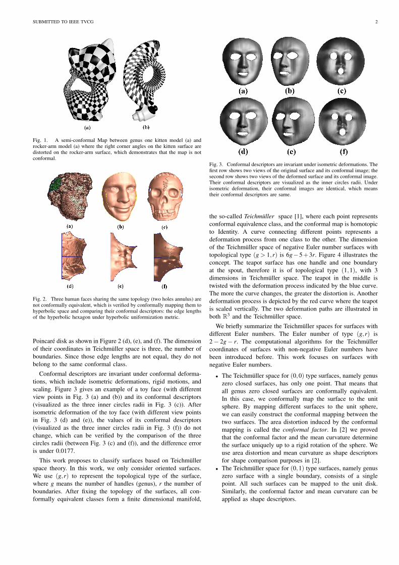
the so-called Teichmuller space [1], where each point representsconformal equivalence class, and the conformal map is homotopicto Identity. A curve connecting different points represents adeformation process from one class to the other. The dimensionof the Teichmuller space of negative Euler number surfaces withtopological type (g > 1,r) is 6g−5+3r. Figure 4 illustrates theconcept. The teapot surface has one handle and one boundaryat the spout, therefore it is of topological type (1,1), with 3dimensions in Teichmuller space. The teapot in the middle istwisted with the deformation process indicated by the blue curve.The more the curve changes, the greater the distortion is. Anotherdeformation process is depicted by the red curve where the teapotis scaled vertically. The two deformation paths are illustrated inboth R3 and the Teichmuller space.

We briefly summarize the Teichmuller spaces for surfaces withdifferent Euler numbers. The Euler number of type (g,r) is2− 2g− r. The computational algorithms for the Teichmullercoordinates of surfaces with non-negative Euler numbers havebeen introduced before. This work focuses on surfaces withnegative Euler numbers.

• The Teichmuller space for (0,0) type surfaces, namely genuszero closed surfaces, has only one point. That means thatall genus zero closed surfaces are conformally equivalent.In this case, we conformally map the surface to the unitsphere. By mapping different surfaces to the unit sphere,we can easily construct the conformal mapping between thetwo surfaces. The area distortion induced by the conformalmapping is called the conformal factor. In [2] we provedthat the conformal factor and the mean curvature determinethe surface uniquely up to a rigid rotation of the sphere. Weuse area distortion and mean curvature as shape descriptorsfor shape comparison purposes in [2].

• The Teichmuller space for (0,1) type surfaces, namely genuszero surface with a single boundary, consists of a singlepoint. All such surfaces can be mapped to the unit disk.Similarly, the conformal factor and mean curvature can beapplied as shape descriptors.


• The Teichmuller space for (1,0) type surfaces, namelytori, is two dimensional. The Teichmuller coordinates ofa torus can be computed using global surface conformalparameterization method [3]. Basically, we can compute aholomorphic 1-form. By integrating the 1-form, we can mapthe universal covering space of the surface to the plane R2.Each fundamental domain is mapped to a parallelogram. TheTeichmuller coordinates of the torus are the angle and thelength ratio between two adjacent edges of the parallelogram.We refer readers to [3] for details.

• For all the other surfaces, the Euler numbers are negative.The coordinates in Teichmuller space can be computed in thefollowing method. First, there exists a unique Riemannianmetric, called the hyperbolic uniformization metric, which isconformal to the original metric of the surface and induces−1 constant Gaussian curvature everywhere. Furthermore, allthe boundaries become geodesics under the uniformizationmetric. Two closed curves are homotopic, if one can deformto the other without leaving the surface. Under the hyperbolicuniformization metric, each homotopy class has a uniquegeodesic. We choose a special set of homotopy classes on thesurface, then compute the unique geodesic in each class. Thelengths of these geodesics are Luo’s coordinates [4], whichform the length coordinates of the surface in Teichmullerspace. This work focuses on the computation of the lengthcoordinates of surfaces with negative Euler numbers.

The major goal of this paper is to develop rigorous andpractical algorithms to compute length coordinates of surfaceswith negative Euler numbers in Teichmuller space. The majorcontributions of this work are:

1) it proposes a theoretical framework to model all negativeEuler number surfaces in a shape space, Teichmuller space.The framework has deep roots in modern geometry and ispractical for computation. It offers novel views and toolsfor tackling engineering problems.

2) it introduces a series of practical algorithms for computinglength coordinates of negative Euler number surfaces inTeichmuller space. Those coordinates are with finite di-mension, independent of scaling and rigid motion, and arealso invariant to different tessellations. They can be appliedfor shape indexing to classify surfaces according to theirconformal class.

The remainder of the paper is organized as follows. SectionII contains a summary of related work, and the challenges inthis area. Section III briefly introduces the theoretical backgroundof Teichmuller space. Section IV describes our algorithms forcomputing the coordinates for general surfaces with negativeEuler numbers in Teichmuller space. Section V presents resultsof our experiments on surface indexing and shape comparison,which evaluate the robustness, discriminability, and efficiency ofour algorithms. We summarize the paper and point out futuredirections in the final section VI.

II. RELATED WORK

Our work proposes to compute Teichmuller space coordinatesas shape descriptors based on surface hyperbolic uniformizationmetric, which classify surfaces according to their conformalstructures. Surfaces having the same descriptors share the sameconformal structure, invariant to conformal deformations.

The research literature on shape descriptors is vast. A thoroughreview of shape descriptors is beyond the scope of current work.We will focus here only on recent shape descriptors which aremost relevant to our work using conformal geometry, and methodsfor designing metrics by prescribed curvatures.

A. Shape Descriptors

For the application of 3D shape classification and matching,shape descriptors are to extract meaningful and simplified rep-resentations from the 3D model based on the geometric andtopological characteristics of the object. As the name suggests,shape descriptors should be descriptive enough to be able todiscriminate similar and dissimilar shapes. The interested reader isreferred to [5], [6] and [7] for comprehensive surveys of differentshape descriptors and evaluations of their performance.

Shape descriptors can be classified by the corresponding trans-formation groups, to which they are invariant. The followingtransformation groups are considered: rigid motion, isometrictransformation and conformal deformation. The former groupsare the subgroups of the latter ones. In the discussion, we focuson shape descriptors based on conformal geometry. There aremany other shape descriptors invariant to the above transformationgroups based on other methods. We only brief some of them.

1) Shape Descriptors Invariant to Conformal Deformations:Conformal structure is invariant to conformal deformations, whichinclude isometric deformations and rigid motions. To the best ofour knowledge, the first work proposed to use conformal structurefor shape classification is [8], where the conformal structureis represented as period matrices. Later, geodesic spectrum ofsurfaces under their uniformization metrics are applied as theconformal structure descriptors in [9], which can be computedsymbolically. A general framework for 3D surface matching isproposed in [10] and [11]. By conformally parameterizing the3D surfaces to canonical 2D domains, the matching problem isgreatly simplified. If the surfaces are conformally equivalent, then2D mapping is an identity with appropriate boundary conditions.

2) Shape Descriptors Invariant to Isometric Transformations:Pose changes are a quasi-isometric transformation of the 3Dmesh, in the sense that edge lengths do not change much as aresult of the transformation. Pose-invariant Shape Descriptors areinvariant under non-rigid isometric transformations, and tolerantquasi-isometric transformations. Pose-invariant shape descriptorsbased on conformal geometry is introduced in [12], where thehistogram of the conformal factor computed from surface uni-formization metric is applied as shape descriptor. This descriptoris intrinsic and pose-invariant.

Laplace-Beltrami operator is determined by the Riemannianmetric. Therefore, most descriptors related to discrete laplace-Beltrami operators are also invariant to isometric deformations,and tolerant quasi-isometric deformations. For examples, Reuteret al. in [13] use the eigenvalues of Laplace-Beltrami operator;Rustamov in [14] uses the eigenvectors; Xiang et al. in [15] usethe histogram of the solution to the volumetric Poisson equationwhich involves the Laplace-Beltrami operator.

3) Shape Descriptors Invariant to Rigid Motions: Shape de-scriptors invariant to rigid motions and based on conformalgeometry are used in [2] and [16] for medical application purpose,where both conformal factor and mean curvature are considered.


0.740.76

0.780.8

0.82

3.2

3.3

3.4

3.53.4

3.45

3.5

3.55

3.6

3.65

Coordinate 1Coordinate 2

Coo

rdin

ate

3

Deformation 2Deformation 1

(a) Teapots deformed in Euclidean Space (b) Deformation paths in Teichmuller space

Fig. 4. The teapot surface with one handle and one boundary at the spout as shown in (a) has 3 dimensions in Teichmuller space, where each point representsone conformal equivalent class, and a curve connecting different points represents a deformation process from one class to the other as shown in (b).

Conformal factor itself fully determines the Riemannian metric ofsurfaces. After adding mean curvature, they two can determinethe embedding of surfaces unique up to rigid motions withappropriate boundary conditions.

4) Other Shape Descriptors: There are many other shape de-scriptors invariant to isometric deformations based on Riemanniangeometry. For example, those methods in [17]–[19] compute fromsurface geodesic distances. The method in [20] computes thediameter of the 3D shape at each point, and the average geodesicdistance from each point to all other points. The histograms ofthe two functions are applied as the shape descriptors.

Many global or local features based, or graph based shapedescriptors are invariant to rigid motions, while extra algorithmsfor feature and graph matching are necessary. We refer readers to[7] for more details.

B. Computing Metric from Prescribed Curvature

There are many algorithms for conformal surface parameteri-zation in the literature. Comprehensive reviews can be found in[21] and [22]. Here we focus on approaches to compute conformalmetrics from prescribed curvatures.

Richard Hamilton introduced Ricci flow for general Rieman-nian manifold in [23]. Later, Hamilton introduced surface Ricciflow in [24]. Perelman applied Ricci flow for the proof of Poincareconjecture and Thurston’s geometrization conjecture in [25]–[27].A thorough introduction to Ricci flow can be found in [28] and[29].

A circle packing algorithm was introduced by Thurston in [30].Bowers et al. and Stephenson et.al. improved the algorithm andbuilt the software system, which are explained in [31], [32]. Chowand Luo discovered the intrinsic relation between Ricci flow andcircle packing and laid down the theoretic foundation for discreteRicci flow in [33], where the existence and convergence of thediscrete Ricci flow were established. The variational approachto find constant curvature metrics on triangulated surfaces waspioneered in the works [34], [35], [36]. More recently, it appearsin [37], [38] and [39]. Combinatorial Yamabe flow is introducedin [40].

The algorithm of discrete surface Ricci flow was given in[41], where the Ricci flows on meshes with spherical, Euclideanand hyperbolic background geometries are explained in details.Furthermore, Newton’s method is directly applied to optimizethe discrete Ricci energy. Optimal surface parameterization isformulated as a variational problem with respect to the targetboundary curvatures in [42], and solved by constrained optimiza-tion algorithm.

Circle pattern method was proposed by Bobenko-Springbornin [43], [44], which used the notion of angle structures firstintroduced by Colin de Verdiere [45]. Based on [43], circle patternalgorithm was introduced in [46].

Metric scaling method is introduced in [47], which solvedthe discretized Poisson equation with the cot-Laplace operatorinduced by the original metric, then use harmonic maps tocompute the embedding from the result metric. The method islinear and efficient.

Similar to the formulation of combinatorial Yamabe flowintroduced in [39], [48] computes conformal equivalent metricsaccording to prescribed curvatures. The Yamabe energy in [39] isrepresented as an integration of a differential form, and formulatedto an explicit form using Milnor’s Lobachevsky function in [48].The explicit formula of the Hessian matrix in [39] and [48] areequivalent, which is the cot-Laplace operator.

III. TEICHMULLER SPACE THEORY

In this section, we briefly introduce the theoretical backgroundof Teichmuller space theory, and the most directly related back-ground knowledge in topology and hyperbolic geometry. Fordetails, we refer readers to [49] for information on Algebraictopology, [50] for hyperbolic geometry, and [1] for Teichmullerspace theory.

A. Topological Background

Let Σ be a surface, the closed curves in the surface arehomotopic to each other if they can be deformed to each otherwithout leaving the surface. Closed curves are classified by this


(a) (b) (c)

(d)

(e) (f)

Fig. 5. (a) Building block I (b) Building block II (c) Building block III. For all of the three basic building blocks, the lengths of geodesics homotopic to thelabeled curves determine the building block’s metric. (d) Using building blocks I, II and III to build all surfaces: from left to right, using building block I andII to build genus one surface with two boundaries. Then adding building block III to build genus two surface with one boundary. Then adding building blockII to build genus two surface with two boundaries. Repeating to get all surfaces. Note that marked curves on surface indicate the boundaries of overlappingpart where two building blocks are glued together, and red and blue colors are used to distinguish boundaries coming from different building blocks. (e) Theconstruction of genus two surface. (f) The geodesic lengths of the set of color labeled curves determine the metric of a genus two surface. Blue curves andgreen curves come from the first and the second Building blocks with type I; red curves come from building block with type II. Note that two of the curvesfor building block with type II and one for the second building block with type I are redundant and have been canceled off.

homotopic relation. The homotopy classes with the same basepoint form a group, which is called the fundamental group.Suppose Σ is of genus g, then there exists a set of canonicalfundamental group generators {a1,b1,a2,b2, · · · ,ag,bg}, such thaton each handle, there are two loops ai,bi. One loop ai circlesthe hole and the other loop bi loops around the tube. Figure 6(a)shows a set of canonical fundamental group generators of a genustwo surface.

Suppose Σ is another surface, then (Σ,π) is said to be acovering space of Σ if locally, π is a homeomorphism. If Σ issimply connected, then (Σ,π) is the universal covering space ofΣ.

For surface with negative Euler number, its universal coveringspace Σ is the hyperbolic space H2, which will be introduced inSection III-C. Its Fuchsian transformations, the transformationsof the universal covering space to itself, φ : Σ → Σ, are hy-perbolic rigid motions (Mobius transformations). Each Fuchsiantransformation associates a homotopy class in the fundamentalgroup in the following manner: giving a point p on Σ andp0, p1 ∈ π−1(p) on the universal covering space Σ. If φ is aFuchsian transformation, such that φ(p0) = p1, then any pathγ ⊂ Σ connecting p0 and p1 will be projected to a closed curve

γ = π(γ). Then we associate φ with the homotopy class of γ .Therefore, the Fuchsian transformation group is isotopic to thefundamental group of the surface.

B. Hyperbolic Uniformization Metric

A surface Σ in R3 has an induced Euclidean metric, denoted asg. Suppose u is a function defined on Σ, u : Σ→ R, then e2ug isanother metric conformal to the original one. If Σ has a negativeEuler number, then it has a unique metric g = e2ug, which isconformal to g and induces −1 Gaussian curvature at all interiorpoints and 0 geodesic curvature at boundary points. The metricg is called the hyperbolic uniformization metric of Σ.

In order to compute the hyperbolic uniformization metric, weneed to find the function u : Σ → R, which can be solved usingRicci flow method:

du(t)dt

=−2K(t),u(0) = 0,

where K(t) is induced by the metric of e2u(t)g. It has been proventhat Ricci flow will converge u(0) = 0 to u(∞) = u which inducesthe hyperbolic uniformization metric [24], .


C. Hyperbolic Geometry

If Σ has a negative Euler number, then with uniformizationmetric, the universal covering space Σ can be isometricallyembedded in the hyperbolic space H2.

There are two commonly used models for hyperbolic space, thePoincare disk and the upper half plane model. The Poincare diskis the unit disk in the complex plane, |z| < 1, with Riemannianmetric ds2 = dzdz

(1−zz)2 . The rigid motions are the so-called Mobius

transformations with the form w = eiθ z−z01−z0z . The hyperbolic lines

are circular arcs perpendicular to the unit circle. The secondmodel is the upper half plane model y > 0 with the metricds2 = dzdz

y2 . The Mobius motions are of the form:

w =az+bcz+d

,a,b,c,d ∈ R,ad−bc = 1.

A Mobius transformation in the upper half plane model isrepresented by its coefficients matrix. The coefficients matrix ofthe product of two Mobius transformations is equal to the productof their coefficients matrices.

The conformal transformation that maps the upper half planeto the Poincare disk is T = i−z

i+z . Any Mobius transformation onthe Poincare disk φ can be converted to a Mobius transformationon the upper half plane as

T−1 ◦φ ◦T. (1)

The deck transformations of Σ on the hyperbolic disk areMobius transformations, which form the Fuchsian group of Σ.Corresponding to the canonical fundamental group generators{a1,b1,a2,b2, · · · ,ag,bg}, the canonical Fuchsian group genera-tors are referred as {α1,β1,α2,β2, · · · ,αg,βg}. Suppose a loophas homotopy class aib j, then its corresponding Fuchsian trans-formation is αi ◦β j.

Suppose γ is a closed curve on a surface Σ with the hyper-bolic uniformization metric, then there is a unique geodesic γhomotopic to γ . Also, there is a unique Fuchsian transformationφ associated with the homotopy class of γ . The length of γ , l(γ),satisfies the following equation:

|trace(φ)|= 2cosh(l(γ)

2).

In our implementation, we use this relation to compute the lengthsof geodesics which are homotopic to a set of special closed loopson surfaces.

D. Teichmuller Space Coordinates

There are several coordinates defined in Teichmuller space.Here we adopt Luo’s coordinates in [4] to avoid complicatedcomputation of the twisting angles of Fenchel-Nielsen coordinatesin [1].

In the following discussion, we use Σg,r to represent a surfaceΣ with topological type (g,r), where g represents the genus, rmeans the number of boundaries.

Given a surface Σg,r with negative Euler number, we candecompose the surface into three types of building blocks, asshown in Fig. 5 (a), (b) and (c). The procedure to build Σ fromthe building blocks is illustrated by Fig. 5 (d). We use I

⋂II to

denote the process of gluing the block I to the block II. The gluing

does not mean combining two blocks along their correspondingboundary curves, but by merging their overlapping regions. Forexample, in the first gluing step in the figure, the overlappingregion of I and II is a two-holed annulus. From left to right, weuse basic building blocks I and II so that I

⋂II is homeomorphic

to Σ1,2, a genus one surface with two boundaries; smoothly joiningbuilding block III, so that Σ1,2

⋂III is homeomorphic to Σ2,1,

a genus two surface with one boundary; then joining buildingblock II, so that Σ2,1

⋂II is homeomorphic to Σ2,2, a genus two

surface with two boundaries; repeating this procedure, we cangenerate all types of surfaces with negative Euler surfaces. Bythis construction, a simple method is provided to define Luo’scoordinates in Techmuller space for general surfaces.

For each building block, its conformal structure is determinedby the lengths of geodesics homotopic to those red loops underthe hyperbolic uniformization metric.

Although on general surfaces, in each homotopy class, theremay be multiple geodesics, which are the locally shortest curveson surfaces. For surfaces with hyperbolic uniformization metric,the geodesic is unique in each homotopy class, which can beproved by Gauss-Bonnet theorem. We refer readers to [51] fordetails.

When two building blocks are glued together to form a newsurface, non-homotopic loops on the original blocks may becomehomotopic on the resulting surface. After canceling off theredundant loops, the lengths of geodesics homotopic to remainingloops determine the conformal structure of the resulting surface,which are the coordinates of this surface in Techmuller space. Forexample, for a closed genus two surface, constructed from twobuilding blocks of type I and one building block of type II asshown in Fig. 5 (e), its Techmuller coordinates are the lengthsof geodesics homotopic to those loops marked with differentcolors as shown in Fig. 5 (f). Loops with the same color indicatethat they come from the same building block. In general, for asurface Σg>1,r with a negative Euler number, their Teichmullercoordinates are determined by the lengths of 6g + 3r− 5 closedgeodesics.

IV. ALGORITHMS TO COMPUTE LENGTH COORDINATES IN

TEICHMULLER SPACE

This section explains the algorithms for computing the Te-ichmuller space coordinates for surfaces with negative Eulernumbers in details, represented as the lengths of a special setof geodesics under hyperbolic uniformization metric. The lengthsof those geodesics can be symbolically computed from Fuchsiantransformations, which require the generators of Fuchsian group,and Fuchsian group generators are calculated using the systemof loops: canonical fundamental group generators. All of thesecomputations are based on hyperbolic geometry.

The whole algorithms pipeline is as follows:

1) Compute hyperbolic uniformization metric of the surface,discussed in Sec. IV-A;

2) Compute Fuchsian group generators, discussed in Sec. IV-B;

3) Compute the coordinates in Teichmuller space, discussed inSec. IV-C.

Following this pipeline, we discuss each step in detail.


(a) (b)

Fig. 6. (a) Vase model with a set of canonical fundamental group generatorsmarked with red. (b) Fundamental domain of vase model embedded in thePoincare disk with the Hyperbolic Uniformization metric

A. Step 1. Compute Hyperbolic Uniformization Metric

In engineering fields, smooth surfaces are often approximatedby discrete surfaces with triangulations. Since conformal deforma-tion transforms infinitesimal circles to other infinitesimal circlesand preserves the intersection angles among the circles, we canapproximate discrete conformal deformation using circle packingmetric introduced by Thurston in [30] by associating each vertexvi with a cone of radius γi, each edge with edge weight Phii jwhich is the intersection angle of the two cones centered withthe ending vertices vi and v j of that edge ei j.

The discrete hyperbolic surface Ricci Flow on a discrete nega-tive Euler number surface with circle packing metric is a processthat the scaling of cone radius of Vertex vi is proportionallyevolving according to the discrete Gaussian curvature Ki of thatvertex:

dγi

dt=−Ki sinhγi, (2)

while the intersection angles Φi j keeping unchanged. The finalcircle packing metric induces new metric of original surfaceapproximated by edge lengths, which is conformal to originalone but induces constantly negative Gaussian curvature, calledhyperbolic uniformization metric. The discrete hyperbolic Ricciflow will converge exponentially. We refer the readers to [33] fortheoretical proofs for the convergence of the discrete hyperbolicRicci flow.

to compute discrete hyperbolic Ricci flow, we need to set theinitial circle packing metric for a giving discrete surface, whichapproximates its original Euclidean metric as much as possible.Then we can use gradient descent method to solve Eqn. 2. Thedetailed algorithm can be found in Appendix Alg. 1.

We can further improve the convergence speed of comutingdiscrete hyperbolic Ricci flow with Newton’s method. Letting ui =ln tanh γi

2 , we can define an energy form

f (u) =∫ u

u0

n

∑i=1

Kidui,

where u = (u1,u2, · · · ,un), u0 = (0,0, · · · ,0) and ∂ f∂ ui

= Ki. Thenthe discrete hyperbolic surface Ricci Flow in Eqn. 2 is the negativegradient flow of this convex energy f (u), and the solution of anenergy optimization problem. So in practice we can use Newton’smethod to compute hyperbolic uniform metric with even fasterconvergence speed.

B. Step 2. Compute Fuchsian Group Generators in the PoincareDisk Model

This step aims to compute the canonical Fuchsian groupgenerators used for computing the geodesic lengths in the futurestep. There are several major steps to compute Fuchsian groupgenerators:

1) Compute fundamental group generators, discussed in Sec.IV-B.1;

2) Isometric embed the mesh in the Poincare disk, discussedin Sec. IV-B.2;

3) Compute the Fuchsian group generators, discussed in Sec.IV-B.3.

1) Compute Fundamental Group Generators: On a ’marked’surface, which means we have enumerated surface handles withh1, h2, h3 etc., we pick a point on the surface as the basepoint (which can be any vertex on the surface), then for eachhandle hi, we can uniquely decide a tunnel loop ai which goesaround the circle, a handle loop bi which goes around thehandle, and both of them go through the base point. By thisway, We get a set of canonical fundamental group generators{a1,b1,a2,b2, · · · ,ag,bg}. Figure 6(a) shows a set of canonicalfundamental group generators marked with different colors onvase model. The way to compute the canonical fundamentalgroup generators has been studied in computational topologyand computer graphics literature. We adopted the methods in-troduced in [52]. The surface S is then sliced open along thefundamental group generators to form a topological disk D,called fundamental domain. The boundary of D takes the form∂D = a1b1a−1

1 b−11 a2b2a−1

2 b−12 · · ·agbga−1

g b−1g .

2) Isometric Embedding in Hyperbolic Disk: Now we isomet-rically embed D onto the Poincare disk using the uniformizationmetric computed from the first step. Let τ : D → H2 denote theisometric embedding.

First, we select an arbitrary face f012 from D as a starting face.Suppose the three edge lengths of the face are {l01, l12, l20}, andthe corner angles are {θ 12

0 ,θ 201 ,θ 01

2 } under the uniform hyperbolicmetric. We can simply embed the triangle as

τ(v0) = 0,τ(v1) =el01 −1el01 +1

,τ(v2) =el02 −1el02 +1

eiθ 120 .

Second, we can embed all the faces which share an edge withthe starting face. Suppose a face fi jk is adjacent to the startingface, and vertices vi,v j have been embedded. A hyperbolic circleis denoted as (c,r), where c is the center, r is the radius. Thenτ(vk) should be one of the two intersection points of (τ(vi), lik)and (τ(v j), l jk). Also, the orientation of τ(vi),τ(v j),τ(vk) shouldbe counter-clock-wise. In the Poincare model, a hyperbolic circle(c,r) coincides with an Euclidean circle (C,R),

C =2−2µ2

1−µ2|c|2 c,R2 = |C|2− |c|2−µ2

1−µ2|c|2 ,

where µ = er−1er+1 . The intersection points between two hyperbolic

circles can be found by intersecting the corresponding Euclideancircles. The orientation of triangles can also be determined usingEuclidean geometry on the Poincare disk.

Then, we can continue to embed faces which share edges withembedded faces in the same manner, until we embed the wholeD onto the Poincare disk.


Figure 6(b) shows the embedding of fundamental domain ofvase model onto the Poincare disk with its Hyperbolic Uni-formization metric.

Fig. 7. (a) One Deck transformation maps the left period to the right one.(b) Two closed loops homotopic to the red one on the vase model lift as twoblue Paths in the universal covering space.

Fig. 8. (a) 2g Fuchsian group generators act on vase model, which are rigidmotions in the hyperbolic space. Different color indicates different periods(fundamental domains). The generators maps the central period to the coloredones respectively. (b) A finite portion of the universal covering space of vasemodel, generated by the actions of Fuchsian group elements with boundariesmarked with geodesics in hyperbolic space.

3) Fuchsian Group Generators: The embedding of a canonicalfundamental domain for a closed genus g surface has 4g differentsides, which induce 4g rigid transformations. These 4g rigidmotions are the Fuchsian group generators.

Figures 6, 7, and 8 illustrate the process to computeFuchsian group generators for a mesh with a negative Eu-ler number. Let {a1,b1, · · · ,ag,bg} be a set of canonicalfundamental group generators as marked with red in Fig.6(a), where g is the genus. The embedding of the vase’scanonical fundamental domain in hyperbolic space has 4gsides, τ(a1),τ(b1),τ(a−1

1 ),τ(b−11 ), ...,τ(ag),τ(bg),τ(a−1

g ),τ(b−1g )

(see Fig. 6(b) in Poincare disk). There exists unique Mobiustransformations αk,βk, which map the τ(ak) and τ(bk) to τ(a−1

k )and τ(b−1

k ) respectively. Figure 7(a) shows one Fuchsian groupgenerator acting on one copy of the fundamental domain ofthe vase model, which maps the τ(bk) to τ(b−1

k ). The two redpoints are the pre-images of a same point on the vase model.Paths connecting them are projected to closed loops homotopicto the red one on vase model, see Figure 7(b). And we willsee the computation of the length of the geodesic homotopyto the loop in Fig. 7(b) only involves the Mobius transforma-tion which maps τ(bk) to τ(b−1

k ). The Mobius transformations{α1,β1,α2,β2, · · · ,αg,βg} form a set of generators of Fuchsiangroup. Figure 8(a) shows eight copies of the fundamental domainof vase model tesselated coherently along boundaries by a set

of Fuchsian group generators, and Fig. 8(b) shows more copiestesselated by Fuchsian transformations.

The following explains the details for computing β1. Let thestarting and ending vertices of the two sides be: ∂τ(b1) = q0− p0and ∂τ(b−1

1 ) = p1− q1. Then the geodesic distance from p0 toq0 equals to the geodesic distance from p1 to q1 in the Poincaredisk. To align them, we first construct a Mobius transformationτ0, which maps p0 to the origin, and q0 to a positive real number,with

τ0 = e−iθ0z− p0

1− p0z,θ0 = arg

q0− p0

1− p0q0.

Similarly, we can construct another Mobius transformation τ1,which maps p1 to the origin, and q1 to a real number, with τ1(q1)equals to τ0(q0). By composing the two, we get the final Mobiustransformation β1 = τ−1

1 ◦τ0, which satisfies p1 = β1(p0) and q1 =β1(q0), and aligns the two sides together.

Then we convert the Fuchsian group generators from thePoincare disk model to the upper half plane model using formula1.

C. Compute Teichmuller Coordinates

Teichmuller coordinates are obtained by measuring the lengthsof geodesics homotopic to a group of loops on surfaces underhyperbolic uniformization metric, and the geodesics are unique ineach homotopy class since Gauss curvature is constantly negativeeverywhere. The major steps are as follows:

1) Decompose the surface to building blocks;2) Determine the homotopy classes of the geodesics;3) Compute the lengths of the geodesics in each homotopy

class.

Surface with enumerated handles has fixed decomposition tobuilding blocks with one handle by one handle as illustratedinversely in Figure 4(d) since the decomposition is purely basedon topology. After redundant loops with the same homotopic classwhile belonging to different building blocks have been removed,our goal is to compute the lengths of geodesics homotopic tothe remaining loops. For example, for a genus two surface, theremaining loops can be seen in Fig. 5 (f).

Since in the above steps, the canonical homology basis{a1,b1,a2,b2, · · · ,ag,bg} and the corresponding Fuchsian groupgenerator {α1,β1,α2,β2, · · · ,αg,βg} have been calculated al-ready. To compute the length of geodesic homotopic to a loopγ on surface, we first use the algorithm in [49] to determineits homotopy class, which can be symbolically represented, forexample: γ = a1b1a−1

1 b−11 . Then by mapping each ai to αi and

b j to β j, we get its representation using corresponding Fuchsiantransformations, still the previous example: φγ = α1β1α−1

1 β−11 .

Let the length of γ denoted as lγ , and we use the matrixrepresentation of φγ on the upper half plane. lγ can be easilycomputed from the following relation: |tr(φγ)|= 2cosh( lγ

2 ).

V. IMPLEMENTATION AND RESULTS

We have implemented the algorithms for computing the Te-ichmuller coordinates using C++ on the Windows platform. Weverify our method by computing the shape coordinates on a largenumber of surface models with various topologies. The trianglescount for the model ranging from thousands to tens of thousands.Due to the page limit, we only list part of our experimental results.


0 5 10 15 20 25 30 35 40 45 500

0.5

1

1.5

2

2.5

3

3.5

4

4.5

time: second

Dec

reas

ing

of c

urva

ture

err

orr

Hyperbolic Ricci Flow on Amphora Model (#Face:20K)

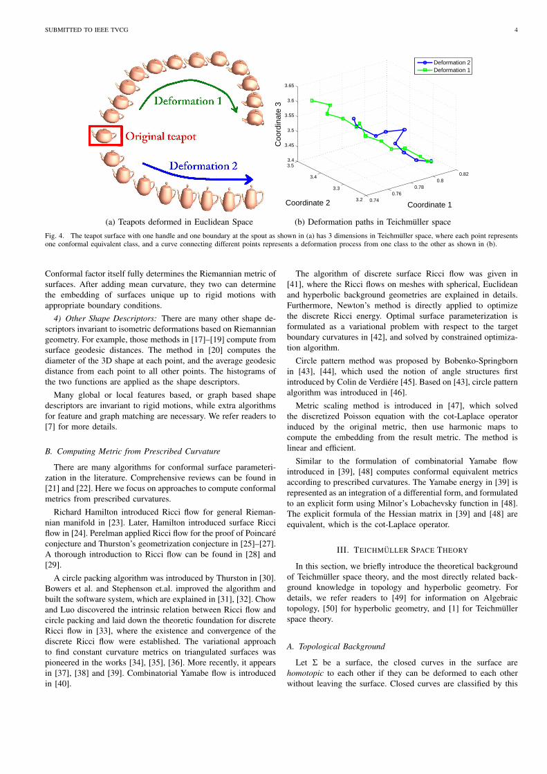
Fig. 9. Performance of curvature flow to compute hyperbolic uniformizationmetric for closed genus two amphora model with 20k faces. The horizontalaxis represents time, and the vertical axis represents the maximal curvatureerror. The blue curves are for the Newton’s method; the green curves arefor the gradient descent method. The tests were carried out on a laptop with1.7GHz CPU and 1G RAM. All the algorithms are written in C++ on aWindows platform without using any other numerical library.

A. Time Complexity

In the whole algorithm pipeline, the most time consuming iscomputing the hyperbolic uniformization metric. Figure 9 showsthe statistics for the computation of hyperbolic uniformizationmetric for a closed genus two amphora model with 20k faces.The x-axis indicates the time, and the y-axis indicates the maximalcurvature error. The green curve shows the steepest descendantmethod, and the blue curves show the Newton’s method. For mostmodels listed in the work, the time to compute their hyperbolicuniformization metrics is less than one minute.

B. Robustness

Teichmuller space coordinates are intrinsic properties of sur-faces, independent of translation , rotation, scaling, and alsoinsensitive to local noises, and the resolutions of the surface.We tested the robustness of our algorithm by computing for amodel with different resolutions. Figure 10 illustrates one such anexample. The vase model is tessellated using different resolutions,with the number of faces 5k, 10k, 20k and 40k respectively. Wetested our Teichmuller coordinates algorithm on them. The resultsare listed in table I, including the mean average and standarddeviation. As we can see, the relative error is less than 0.3%.

C. Surface Indexing and Classification

Teichmuller coordinates can be directly applied for indexingand classification of surfaces with the same topology. The distanceamong shapes in the Teichmuller space can be approximateddirectly using the Euclidean distances among their Teichmullercoordinates. In our experiments, we tested genus two closedsurfaces and genus three closed surfaces.

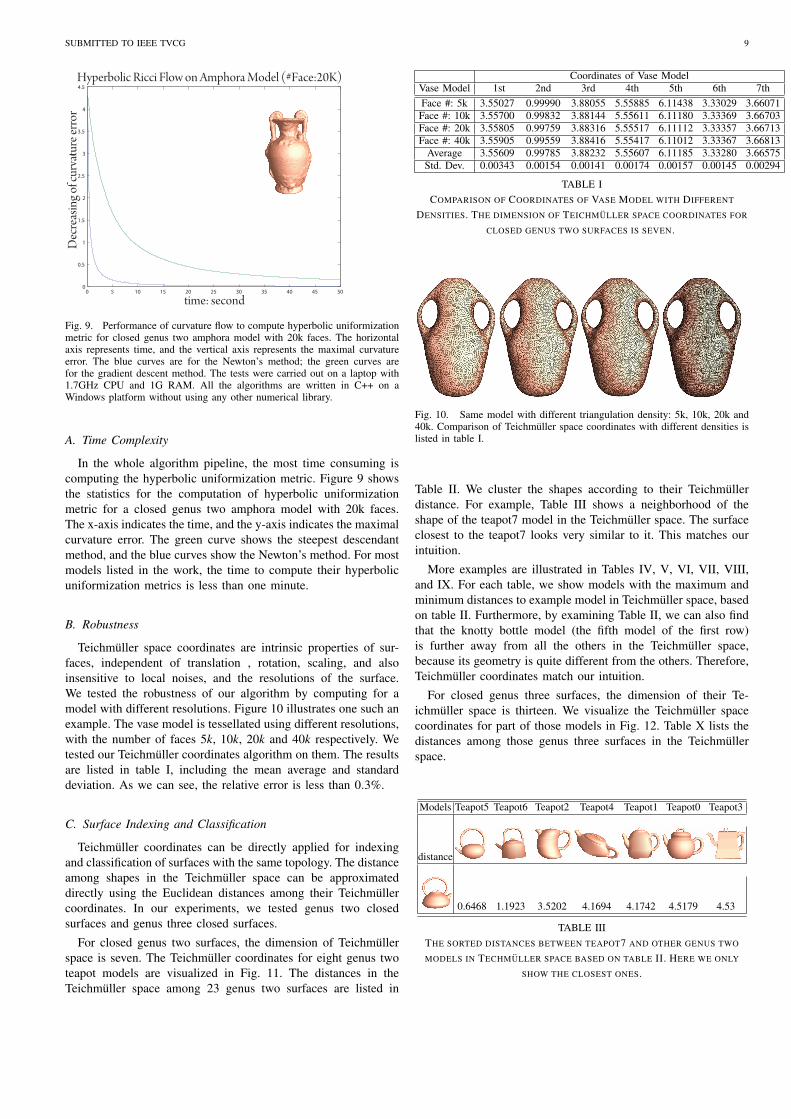
For closed genus two surfaces, the dimension of Teichmullerspace is seven. The Teichmuller coordinates for eight genus twoteapot models are visualized in Fig. 11. The distances in theTeichmuller space among 23 genus two surfaces are listed in

Coordinates of Vase ModelVase Model 1st 2nd 3rd 4th 5th 6th 7thFace #: 5k 3.55027 0.99990 3.88055 5.55885 6.11438 3.33029 3.66071Face #: 10k 3.55700 0.99832 3.88144 5.55611 6.11180 3.33369 3.66703Face #: 20k 3.55805 0.99759 3.88316 5.55517 6.11112 3.33357 3.66713Face #: 40k 3.55905 0.99559 3.88416 5.55417 6.11012 3.33367 3.66813

Average 3.55609 0.99785 3.88232 5.55607 6.11185 3.33280 3.66575Std. Dev. 0.00343 0.00154 0.00141 0.00174 0.00157 0.00145 0.00294

TABLE ICOMPARISON OF COORDINATES OF VASE MODEL WITH DIFFERENT

DENSITIES. THE DIMENSION OF TEICHMULLER SPACE COORDINATES FOR

CLOSED GENUS TWO SURFACES IS SEVEN.

Fig. 10. Same model with different triangulation density: 5k, 10k, 20k and40k. Comparison of Teichmuller space coordinates with different densities islisted in table I.

Table II. We cluster the shapes according to their Teichmullerdistance. For example, Table III shows a neighborhood of theshape of the teapot7 model in the Teichmuller space. The surfaceclosest to the teapot7 looks very similar to it. This matches ourintuition.

More examples are illustrated in Tables IV, V, VI, VII, VIII,and IX. For each table, we show models with the maximum andminimum distances to example model in Teichmuller space, basedon table II. Furthermore, by examining Table II, we can also findthat the knotty bottle model (the fifth model of the first row)is further away from all the others in the Teichmuller space,because its geometry is quite different from the others. Therefore,Teichmuller coordinates match our intuition.

For closed genus three surfaces, the dimension of their Te-ichmuller space is thirteen. We visualize the Teichmuller spacecoordinates for part of those models in Fig. 12. Table X lists thedistances among those genus three surfaces in the Teichmullerspace.

Models Teapot5 Teapot6 Teapot2 Teapot4 Teapot1 Teapot0 Teapot3

distance

0.6468 1.1923 3.5202 4.1694 4.1742 4.5179 4.53

TABLE IIITHE SORTED DISTANCES BETWEEN TEAPOT7 AND OTHER GENUS TWO

MODELS IN TECHMULLER SPACE BASED ON TABLE II. HERE WE ONLY

SHOW THE CLOSEST ONES.


distance

4.09 5.39 3.22 4.49 6.69 2.22 2.16 2.21 2.39 2.32 4.38 3.87 4.88 3.51 3.52 3.42 3.25 4.02 3.293.20 3.44 3.26 3.41

7.75 3.06 6.74 9.98 2.11 2.37 2.82 2.05 2.14 4.59 3.68 4.97 2.76 2.84 3.01 3.59 2.81 2.993.64 4.78 3.73 4.30

4. 95 1.04 7.92 6.62 5.95 5.62 6.17 6.17 7.27 7.89 7. 34 7.46 6.56 6.48 5.61 6.97 6.325.63 4.72 5.56 5. 23

3.94 8.99 2.47 1.73 1.64 1.85 1.83 4.27 4.27 4.56 3.08 3.43 3.22 2.37 3.84 3.022.52 2.75 2.43 2.64

7.79 5.61 4.92 4.59 5.16 5.14 6.35 6.91 6.45 5.44 5.56 5.48 4.57 6.00 5.304.60 3.71 4.53 4.21

8.48 8.48 8.35 8.61 8.62 9.27 9.13 9.57 8.75 8 .65 8.68 8.48 8.95 8.578.40 8.08 8.43 8.31

0.83 1.51 0.73 0.71 4.05 3.15 4.51 2.09 1.92 1.51 2.27 2.42 1.512.36 3.59 2.43 3.12

0.79 0.65 0.25 3.72 3.15 4.17 1.79 2.30 1.8 6 1.44 2.88 1.481.60 2.83 1.63 2.37

1.40 0.92 3.10 2.83 3.52 2.51 3.02 2.64 1.54 3.62 2.141.26 2.13 1.28 1.61

0.59 4.28 3.60 4.53 2.36 2.76 2.40 2.95 2.28 2.512.18 3.38 2.21 2.96

3.71 3.07 4.16 1.63 2.20 1.76 1.62 2. 761.301.74 3.01 1.79 2.52

1.62 0.64 5.21 5.71 5.40 4.61 6.26 4.834.30 4.03 4.35 3.88

1.19 4.43 4.86 4.58 4.24 5.33 4.103.97 4.30 4.06 3.94

5.67 6.19 5.88 5.02 6.73 5.314.92 4.82 4.86 4.63

0.37 0.62 1.14 1.14 0.961.30 2.55 1.36 1.61

0.63 1.63 0.63 0.961.802.9 7 1.87 2.58

1.25 1.09 0.601.45 2.68 1.49 2.23

2.20 0.870.34 1.47 0.29 1.03

0.531.39 3.57 2.45 3. 18

0.90 2.22 1.04 1.75

1.28 0.18 0.80

1.24 0.57

0.76

TABLE IIDISTANCES BETWEEN GENUS TWO SURFACES IN TECHMULLER SPACE.


Fig. 11. The dimension of Teichmuller space coordinates for closedgenus two surfaces is seven. Here we visualize the Teichmuller spacecoordinates for teapots listed in table III.

Distance

0.60 0.62 0.63 1.09 5.48 5.88 6.48 8.68

TABLE IVTHE SORTED DISTANCES BETWEEN POT AND OTHER GENUS TWO MODELS

IN TECHMULLER SPACE BASED ON TABLE II. HERE WE ONLY SHOW

MODELS WITH MAXIMUM AND MINIMUM DISTANCES TO POT MODEL.

Distance

0.53 0.60 0.87 0.90 5.30 5.31 6.32 8.57

TABLE VTHE SORTED DISTANCES BETWEEN VASE AND OTHER GENUS TWO


SHOW MODELS WITH MAXIMUM AND MINIMUM DISTANCES TO POT

MODEL.

Distance

1.04 4.72 4.95 5.23 7.46 7.75 7.89 7.92

TABLE VITHE SORTED DISTANCES BETWEEN CUP AND OTHER GENUS TWO MODELS

IN TECHMULLER SPACE BASED ON TABLE II. HERE WE ONLY SHOW

MODELS WITH MAXIMUM AND MINIMUM DISTANCES TO POT MODEL.

Distance

0.57 0.76 0.80 1.03 4.30 4.63 5.23 8.31

TABLE VIITHE SORTED DISTANCES BETWEEN WORLD CUP AND OTHER GENUS TWO



MODEL.

Distance

0.59 0.65 0.73 1.40 4.53 5.16 6.17 8.61

TABLE VIIITHE SORTED DISTANCES BETWEEN TEAPOT3 AND OTHER GENUS TWO



MODEL.

Distance

0.37 0.62 0.96 1.14 5.44 5.67 7.46 8.75

TABLE IXTHE SORTED DISTANCES BETWEEN EIGHT AND OTHER GENUS TWO



MODEL.

2 4 6 8 10 120

2

4

6

8

10

12

Leng

ths

Coordinates

Coordinates of Genus Three ModelsDavidsculpturevasepotpantetrahedronthree−torus1

Fig. 12. The dimension of Techmuller space coordinates for closedgenus three surfaces is thirteen. Here we visualize the length coordinatesof Techmuller space for part of genus 3 surfaces listed in table X.


Models three- tetra- vase David sculp- puppet pot pan cliptorus hedron ture

Distance

6.43 5.56 13.19 8.16 7.60 8.21 9.19 9.16 5.95

7 .07 8.36 3.89 5.11 2.16 3.02 3.27 8.50

10.80 8.28 8.82 8.76 9.53 8.73 4.84

7.29 12.17 7.50 7.03 5.83 12.02

8.61 3.35 4.45 3.87 9.81

6.52 6.66 7.49 10.56

1.47 1.97 9.85

1.79 10.50

9.97

TABLE XDISTANCES BETWEEN GENUS THREE SURFACES IN TECHMULLER SPACE.

VI. CONCLUSION AND FUTURE WORK

In this work, we propose a novel approach for surface indexingand classification based on Teichmuller space theory. Teichmullerspace is a finite dimensional manifold, where each point rep-resents a conformally equivalent class of surfaces, and a curverepresents a deformation process from one shape to another.

As shape descriptors, Teichmuller coordinates are succinct,discriminating and intrinsic; invariant under the rigid motions andscalings, insensitive to resolutions. Furthermore, the method hassolid theoretic foundation, and the computation of Teichmullercoordinates are practical, stable and efficient.

This work introduces a series of algorithms for computing theTeichmuller coordinates of surfaces with negative Euler numbers.The computational algorithms are theoretically sound and prac-tically simple. The coordinates are algebraically deduced fromlengths of geodesics homotopic to a set of special curves underthe hyperbolic uniformization metric, which is obtained by usingcurvature flow method.

We verified our method on a large number of surfaces withnegative Euler number and with various geometries, topologiesand resolutions. We apply for surface indexing and classificationapplications. The extensive experiments demonstrate the efficacy,efficiency and robustness of our method.

Current work focuses on the computation of Teichmuller co-ordinates and approximates the geodesic distance between twopoints in the space by Euclidean distance. In theory, Teichmullerspace has well-defined Riemannian metrics, and the geodesicsbetween two shapes can be accurately computed. In the future,we will devise practical algorithms to compute the geodesics in

Teichmuller spaces, and use geodesic distance to measure thedifference between two shapes, to apply for surface deformationand surface morphing.

REFERENCES

[1] P. Buser, Geometry and spectra of compact Riemann surfaces.Birkhauser, 1992.

[2] X. Gu and B. C. Vemuri, “Matching 3d shapes using 2d conformal rep-resentations,” in MICCAI (1) (C. Barillot, D. R. Haynor, and P. Hellier,eds.), vol. 3216 of Lecture Notes in Computer Science, pp. 771–780,Springer, 2004.

[3] X. Gu and S.-T. Yau, “Global conformal parameterization,” in Sympo-sium on Geometry Processing (L. Kobbelt, P. Schroder, and H. Hoppe,eds.), vol. 43 of ACM International Conference Proceeding Series,pp. 127–137, Eurographics Association, 2003.

[4] F. Luo, “Geodesic length functions and teichmuller spaces,”J.DIFFERENTIAL GEOMETRY, vol. 48, p. 275, 1998.

[5] P. Shilane, P. Min, M. Kazhdan, and T. Funkhouser, “The princetonshape benchmark,” pp. 167–178, 2004.

[6] N. Iyer, S. Jayanti, K. Lou, Y. Kalyanaraman, and K. Ramani, “Three-dimensional shape searching: state-of-the-art review and future trends.,”Computer-Aided Design, vol. 37, no. 5, pp. 509–530, 2005.

[7] J. W. Tangelder and R. C. Veltkamp, “A survey of content based 3d shaperetrieval methods,” in Multimedia Tools and Applications, in press, 2008.

[8] X. Gu and S.-T. Yau, “Surface classification using conformal structures,”in ICCV, pp. 701–708, 2003.

[9] M. JIN, F. LUO, S. YAU, and X. GU, “Computing geodesic spectra ofsurfaces,” in Proc. ACM Symposium on Solid and Physical Modeling(2007), pp. 387–393.

[10] S. WANG, Y. WANG, M. JIN, X. GU, and D. SAMARAS, “3dsurface matching and recognition using conformal geometry,” in Proc.IEEE Conference on Computer Vision and Pattern Recognition, no. 2,pp. 2453–2460, 2006.

[11] X. Gu, S. Wang, J. Kim, Y. Zeng, Y. Wang, H. Qin, and D. Samaras,“Ricci flow for 3d shape analysis,” in ICCV ’07: IEEE InternationalConference on Computer Vision (ICCV’07), pp. 1–8, 2007.

[12] M. Ben-Chen and C. Gotsman, “Characterizing shape using conformalfactors,” in Proceedings of Eurographics Workshop on Shape Retrieval,(Crete), April 2008.

[13] M. Reuter, F.-E. Wolter, and N. Petnecke, “Laplacespectra as fingerprintsfor shape matching,” in Solid and Physical Modeling, p. 101C106, 2005.

[14] R.-M. Rustamov, “Laplace-beltrami eigenfunctions for deformation in-variant shape representation,” in Proc. Symposium on Geometry Pro-cessing, 2007.

[15] P. Xiang, C.-O. Hua, F.-X. Gang, and Z.-B. Chuan, “Pose insensitive3d retrieval by poisson shape histogram,” in Lecture Notes in ComputerScience, vol. 4488, pp. 25–32, 2007.

[16] Y. Wang, M.-C. Chiang, and P. M. Thompson, “Mutual information-based 3d surface matching with applications to face recognition andbrain mapping,” in ICCV ’05: Proceedings of the Tenth IEEE Interna-tional Conference on Computer Vision (ICCV’05) Volume 1, pp. 527–534, 2005.

[17] V. Jain and H. Zhang, “A spectral approach to shape-based retrieval ofarticulated 3d models,” Computer Aided Design, vol. 39, pp. 398–407,2007.

[18] A. Elad and R. Kimmel, “On bending invariant signatures for sur-faces,” IEEE Transactions on Pattern Analysis and Machine Intelligence,vol. 25, no. 10, pp. 1285–1295, 2003.

[19] T. Tung and F. Schmitt, “The augmented multiresolution reeb graphapproach for content-based retrieval of 3d shapes,” International Journalof Shape Modeling, vol. 11, no. 1, pp. 91–120, 2005.

[20] R. Gal, A. Shamir, and D. Cohen-or, “Pose oblivious shape signature,”IEEE Transactions on Visualization and Computer Graphics, vol. 13,no. 2, p. 261C271, 2007.

[21] M. S. Floater and K. Hormann, “Surface parameterization: a tutorialand survey,” in Advances in Multiresolution for Geometric Modelling,pp. 157–186, Springer, 2005.

[22] A. Sheffer, E. Praun, and K. Rose, “Mesh parameterization methods andtheir applications,” Foundations and Trendsr in Computer Graphics andVision, vol. 2, no. 2, 2006.

[23] R. S. Hamilton, “Three manifolds with positive Ricci curvature,” Journalof Differential Geometry., vol. 17, pp. 255–306, 1982.

[24] R. S. Hamilton, “The ricci flow on surfaces,” Mathematics and generalrelativity, vol. 71, pp. 237–262, 1988.


[25] G. Perelman, “The entropy formula for the Ricci flow and its geometricapplications,” Tech. Rep. arXiv.org, November 11 2002.

[26] G. Perelman, “Ricci flow with surgery on three-manifolds,” Tech. Rep.arXiv.org, March 10 2003.

[27] G. Perelman, “Finite extinction time for the solutions to the Ricci flowon certain three-manifolds,” Tech. Rep. arXiv.org, July 17 2003.

[28] B. Chow, P. Lu, and L. Ni, Hamilton’s Ricci Flow, vol. 77 of GraduateStudies in Mathematics. AMS, 2006.

[29] B. Chow, S.-C. Chu, D. Glickenstein, C. Guenther, J. Isenberg, F. Luo,T. Ivey, D. Knopf, P. Lu, and L. Ni, The Ricci flow: techniques andapplications. Part I. Mathematical Surveys and Monographs, vol. 135.Providence, RI: American Mathematical Society, 2007.

[30] W. P. Thurston, Geometry and Topology of Three-Manifolds. Princetonlecture notes, 1976.

[31] P. L. Bowers and M. K. Hurdal, “Planar conformal mappings ofpiecewise flat surfaces,” In Vis. and Math. III. Springer, pp. 3–34, 2003.

[32] K. Stephenson, Introduction To Circle Packing. Cambridge UniversityPress, 2005.

[33] B. Chow and F. Luo, “Combinatorial ricci flows on surfaces,” JournalDifferential Geometry, vol. 63, no. 1, pp. 97–129, 2003.

[34] C. de Verdiere Yves, “Un principe variationnel pour les empilements decercles,” Invent. Math., vol. 104, no. 3, pp. 655–669, 1991.

[35] Braegger and Walter, “Kreispackungen und triangulierungen,” Enseign.Math., vol. (2) 38, no. 3-4, pp. 201–217, 1992.

[36] I. Rivin, “Euclidean structures on simplicial surfaces and hyperbolicvolume,” Ann. of Math., vol. 2, no. 3, pp. 553–580, 1994.

[37] A. I. Bobenko and B. A. Springborn, “Variational principles for circlepatterns and koebe’s theorem,” Trans. Amer. Math. Soc., vol. 256, no. 2,pp. 659–689, 2004.

[38] G. Leibon, “Characterizing the delaunay decompositions of compacthyperbolic surfaces,” Geom. Topol., vol. 6, pp. 361–391, 2002.

[39] F. Luo, “Combinatorial yamabe flow on surfaces,” Commun. Contemp.Math., vol. 6, no. 5, pp. 765–780, 2004.

[40] F. Luo, “On teichmuller space of surface with boundary,” preprint, 2005.[41] M. Jin, J. Kim, F. Luo, and X. Gu, “Discrete surface ricci flow,” IEEE

Transaction on Visualization and Computer Graphics, 2008.[42] Y.-L. Yang, J. Kim, F. Luo, and X. Gu, “Optimal surface parameteri-

zation using inverse curvature map,” IEEE Transaction on Visualizationand Computer Graphics, 2008.

[43] A. I. Bobenko and B. A. Springborn, “Variational principles for circlepatterns and koebe’s theorem,” Transactions of the American Mathemat-ical Society, vol. 356, pp. 659–689, 2004.

[44] A. Bobenko and P. Schrooder, “Discrete willmore flow,” in Symposiumon Geometry Processing, pp. 101–110, 2005.

[45] Y. C. de Verdiere, “Un principe variationnel pour les empilements decercles. (french) [a variational principle for circle packings],” Invent.Math., vol. 104, no. 3, pp. 655–669, 1991.

[46] L. Kharevych, B. Springborn, and P. Schroder, “Discrete conformalmappings via circle patterns,” ACM Trans. Graph., vol. 25, no. 2,pp. 412–438, 2006.

[47] M. Ben-Chen, C. Gotsman, and G. Bunin, “Conformal flattening bycurvature prescription and metric scaling,” Computer Graphics Forum(Proc. Eurographics 2008), vol. 27, no. 2, p. to appear, 2008.

[48] B. Springborn, P. Schroder, and U. Pinkall, “Conformal equivalence oftriangle meshes,” SIGGRAPH 2008, 2008.

[49] J.R.Munkres, Elements of Algebraic Topology. Addison-Wesley Co.,1984.

[50] W. P. Thurston, Three-Dimensional Geometry and Topology. PrincetonUniversity Presss, 1997.

[51] T. S. Mika Seppala, Geometry of Riemann surfaces and Teichmullerspaces. North-Holland Math Stud, 1992.

[52] C. Carner, M. Jin, X. Gu, and H. Qin, “Topology-driven surface map-pings with robust feature alignment,” in IEEE Visualization, pp. 543–550, 2005.

APPENDIX

Algorithm 1 Compute Hyperbolic Uniformization Metricfor each vertex vi do

for each face fi jk adjacent to vertex vi docompute a radius for vi:

γ jki =

lki + li j− l jk

2,

{li j, l jk, lki: lengths of the edges ei j,e jk,eki on fi jk}end foraverage the radii from the faces adjacent to vi:

γi =1m ∑

fi jk∈Fγ jk

i ,

{m: the number of the adjacent faces to vi}end for{Associating each vertex with a cone of radius which approx-imates the original Euclidean metric.}for each edge ei j do

compute edge weight Φi j(ei j) from γi,γ j using hyperboliccosine law:

cosh li j = coshγi coshγ j + sinhγi sinhγ j cosΦi j

end for{Assigning an edge weight to each edge based on the inter-section angle of the two cones centered with the two endingvertices of the edge.}repeat

for each edge ei j docompute edge length li j from the current vertices radii γiand γ j, and the fixed edge weight Φi j using the inverse ofhyperbolic cosine law.

end for{Computing edge length from current circle packing metric.}for each face fi jk do

for all face fi jk doCompute the corner angles θ jk

i from the current edgelengths using hyperbolic cosine law.

end forend forfor each vertex vi do

Compute the discrete Gaussian curvature Ki on vi.if vi is interior vertex then

Ki = 2π− ∑fi jk∈F

α jki , (3)

{α jki : corner angle attached to vertex vi in the face fi jk}

else if vi is boundary vertex then

Ki = π− ∑fi jk∈F

α jki , (4)

end ifend forfor each vertex vi do

Update γi of each vertex vi,

γi = γi + ε(Ki−Ki),

{Ki: target Gaussian curvature}end for

until max |Ki−Ki|< δ{Optimizing discrete hyperbolic Ricci energy with steepestdescent method.}

Computing Teichmller Shape Space

Documents

Transcript of Computing Teichmller Shape Space