962 Biophysical Journal Volume 105 August 2013 962–974

Accurate SAXS Profile Computation and its Assessment by ContrastVariation Experiments

Dina Schneidman-Duhovny,†* Michal Hammel,‡ John A. Tainer,§{ and Andrej Sali†*†Department of Bioengineering and Therapeutic Sciences, Department of Pharmaceutical Chemistry, and California Institute for QuantitativeBiosciences (QB3), University of California at San Francisco; ‡Physical Biosciences Division, Lawrence Berkeley National Laboratory,Berkeley, California; §Department of Molecular Biology, Skaggs Institute of Chemical Biology, The Scripps Research Institute, La Jolla,California; and {Life Sciences Division, Department of Molecular Biology, Lawrence Berkeley National Laboratory, Berkeley, California

ABSTRACT A major challenge in structural biology is to characterize structures of proteins and their assemblies in solution. Atlow resolution, such a characterization may be achieved by small angle x-ray scattering (SAXS). Because SAXS analyses oftenrequire comparing profiles calculated from many atomic models against those determined by experiment, rapid and accurateprofile computation from molecular structures is needed. We developed fast open-source x-ray scattering (FoXS) for profilecomputation. Tomatch the experimental profile within the experimental noise, FoXS explicitly computes all interatomic distancesand implicitly models the first hydration layer of the molecule. For assessing the accuracy of the modeled hydration layer, weperformed contrast variation experiments for glucose isomerase and lysozyme, and found that FoXS can accurately representdensity changes of this layer. The hydration layer model was also compared with a SAXS profile calculated for the explicit watermolecules in the high-resolution structures of glucose isomerase and lysozyme. We tested FoXS on eleven protein, one DNA,and two RNA structures, revealing superior accuracy and speed versus CRYSOL, AquaSAXS, the Zernike polynomials-basedmethod, and Fast-SAXS-pro. In addition, we demonstrated a significant correlation of the SAXS score with the accuracy of astructural model. Moreover, FoXS utility for analyzing heterogeneous samples was demonstrated for intrinsically flexibleXLF-XRCC4 filaments and Ligase III-DNA complex. FoXS is extensively used as a standalone web server as a componentof integrative structure determination by programs IMP, Chimera, and BILBOMD, as well as in other applications that requirerapidly and accurately calculated SAXS profiles.

INTRODUCTION

Atomic resolution modeling and validation of macromolec-ular assemblies in solution by small-angle x-ray scattering(SAXS) has become a key tool in structural biology (1–4).Combining data from solution scattering with atomic reso-lution structures holds great promise for addressing howspecific complexes and conformational changes drivebiological processes. High-accuracy and precision SAXSexperiments with advanced instrumentation (5) lead tomore confident assignment of the conformational state(s)of a given sample. Notwithstanding instrumentation devel-opments, the accurate and rapid calculation of a modelSAXS profile is in turn essential for accurate and rapiddevelopment of a structural hypothesis. Applications ofSAXS profile calculation from atomic models includemodeling of perturbed conformations relative to availablecrystal structures (6,7), determination of biologically rele-vant states from the crystal (8), binding of small molecules(9), structural characterization of protein flexibility (10,11),assembly of complexes from subunit structures (12–14),fold recognition (15), and comparative modeling (16,17).

Several methods are available to calculate SAXS profilesfrom atomic models. They differ in the calculation of theinteratomic distances, in the treatment of the hydrationlayer, and in background adjustment (1,18,19). Interatomic

Submitted September 10, 2012, and accepted for publication July 11, 2013.

*Correspondence: sali@salilab.org or dina@salilab.org

Editor: Lois Pollack.

� 2013 by the Biophysical Society

0006-3495/13/08/0962/13 $2.00

distances can be computed explicitly (20) by applying theDebye formula (21), using spherical harmonics for rapidcalculation (18,22,23) or based on a hierarchical spatialdecomposition (24). Another approach to speed up thecalculation is Monte Carlo sampling of the distances inthe model (25). Coarse graining that combines several atomsin a single scattering center is also used to speed up profilecalculation (26–28). However, with experimental data ofhigher accuracy, precision, and range, there is a greaterneed for high-accuracy rapid computations of SAXS pro-files to interpret experimental data for informative results.By using explicit atom distances (20) and water models toaccount for the effect of solvent (18), superior fits betweenexperimental high-resolution structures and SAXS data areobtained (3). The explicit representation of the molecule isparticularly useful for multidomain flexible assemblies,which frequently adopt highly anisometric shapes (18).

A SAXS experiment involves determining both the scat-tering profile of a solute in a buffer and a buffer on its own; ascattering profile is an intensity of a sample as a function ofspatial frequency. The experimental scattering profile of asolute with its ordered hydration layer is that obtained asthe difference between these two profiles. The theoreticalSAXS profile is also computed as the difference betweenthe scattering of a single solute molecule with its orderedhydration layer and the scattering of the excluded volume(i.e., the scattering of the bulk solvent in the excludedvolume of the solute with its ordered hydration layer)

http://dx.doi.org/10.1016/j.bpj.2013.07.020

SAXS Profile Computation 963

(22,29,30). However, accurate approximation of the ex-cluded volume is a challenging task, because the volumevaries significantly depending on the atomic radii. Addition-ally, the protein crystal packing and cryo-cooling used inx-ray crystallography may reduce the protein volume inthe crystal compared to that in solution (31). Thus, adjust-ment of the excluded volume is required for optimal match-ing of the experimental SAXS profile.

Although solute atoms dominate the scattering signal athigh angles, the scattering from the ordered solvent atomsin the hydration layer must also be considered (32). Stronglybound water molecules are known to fill surface grooves andchannels, stabilizing their structures and smoothing theexcluded volume (33). The first hydration layer with anaverage density ~10% larger than that of the bulk solventwas observed using x-ray and neutron scattering (34).Computationally, the hydration shell has been modeledby explicitly placing water molecules on the surface(18,26,28,35–37). Alternatively, implicit models surroundthe solute particle by a continuous envelope representingthe hydration shell of 3 A with a density that can differfrom the free solute (22) or use voxelized representationof the protein and the hydration layer (23,38–40). In implicitmodels, the density of the hydration layer can be adjustedfor optimal fitting to the experimental SAXS profile.Modeling the hydration layer improves the accuracy of thecalculated scattering profiles, although the contributionfrom the ordered hydration layer is several orders of magni-tude lower than the scattering from the solute or theexcluded volume (40).

Here, we developed fast open-source x-ray scattering(FoXS) to take advantage of high-quality data and enableus to better distinguish between proposed atomic models.FoXS provides an efficient method with explicit computa-tion of interatomic distances, accurate estimation of theexcluded volume, and an implicit model of the first hydra-tion layer. FoXS was tested on 14 cases with availablehigh-quality experimental SAXS profiles and crystallo-graphic atomic structures. We also compared FoXS tofour state-of-the-art programs, including CRYSOL (22),AquaSAXS (39), the Zernike polynomials-based method(23), and Fast-SAXS-pro (28) for accuracy and runningtimes. In addition, we performed an in-depth comparisonof the excluded volume and hydration layer modeling tothe most commonly used program CRYSOL. To assess therelevance of adjusting the hydration layer density parameter,we performed contrast variation experiments and found thatFoXS can accurately represent the changes in the density ofthe hydration layer.

METHODS

Profile computation

The Debye formula (21) is used for accurate computation of SAXS profiles,

IðqÞ ¼XNi¼ 1

XNj¼ 1

fiðqÞfjðqÞsin

�qdij

�qdij

; (1)

where the intensity, I(q), is a function of the momentum transfer q ¼ (4p

sin q)/l, in which 2q is the scattering angle and l is the wavelength of

the incident x-ray beam. The value fi(q) is the atomic form factor, dijis the distance between atoms i and j, and N is the number of atoms in

the molecule.

Form factors

In FoXS, the form factor fi(q) takes into account the displaced solvent as

well as the hydration layer,

fiðqÞ ¼ f vi ðqÞ � C1ðqÞf si ðqÞ þ c2sifwðqÞ; (2)

where fv(q) is the atomic form factor in vacuo, fs(q) is the form factor of the

dummy atom that represents the displaced solvent represented by the

Gaussian function (29), si is the fraction of solvent-accessible surface of

the atom i (41), and fw(q) is the water form factor. The surface is calculated

using a probe with radius of 1.8 A. The third term in Eq. 2 implicitly

accounts for the first hydration layer by placing a water molecule with

the same coordinates as the solvent-exposed solute atom. The function

C1(q) is used to adjust the total excluded volume of the atoms and is

equivalent to the G(s) function in CRYSOL (22) (Eq. 13),

C1ðqÞ ¼ c31 exp

264�

�4p3

�3=2

q2r2m�c21 � 1

�4p

375; (3)

where c1 is the scaling of the atomic radius (default value ¼ 1.0) and rmis the average atomic radius of the molecule. During fitting, we allow

5% variance of the radius 0.95 % c1 % 1.05. For comparison, CRYSOL

allows ~11% variance in the atomic radius (1.4 % rm % 1.8, rm value

is ~1.62 for proteins). The parameter c2 is used to adjust the difference

between the densities of the hydration layer and the bulk water (default

value ¼ 0.0). During fitting, the value of c2 can vary from 0 to 4.0, reflect-

ing an estimate of up to four water molecule neighbors for an exposed

solute atom. This threshold is comparable to the average number of water

molecules within 3 A of each other in the TIP3P water box. The hydration

shell density for c2 ¼ 4.0 is 0.388e/A3. The density of the hydration layer

around the protein can, in principle, be lower than that of bulk water,

depending on the amount of surface charge. Therefore, we also allow

c2 to be negative (�2.0 % c2 % 4.0). The hydration shell density for

c2 ¼ �2.0 is 0.307e/A3.

Profile fitting

The computed profile is fitted to a given experimental SAXS profile by

minimizing the c-function with respect to c, c1, and c2,

c ¼ffiffiffiffiffiffiffiffiffiffiffiffiffiffiffiffiffiffiffiffiffiffiffiffiffiffiffiffiffiffiffiffiffiffiffiffiffiffiffiffiffiffiffiffiffiffiffiffiffiffiffiffiffiffi1

M

XMi¼ 1

�IexpðqiÞ � cIðqiÞ

sðqiÞ�2

;

vuut (4)

where Iexp(q) is the experimental profile, s(q) is the experimental error of

the measured profile, M is the number of points in the profile, and c is

the scale factor. The minimal value of c is found by enumerating c1 and

c2 (0.95 % c1 % 1.05 and �2.0 % c2 % 4.0), in steps of 0.005 and 0.05,

respectively, and performing the linear least-squares minimization to find

the value of c that minimizes c for each c1, c2 combination. To avoid profile

computation for each combination of c1 and c2, the multiplication of two

Biophysical Journal 105(4) 962–974

964 Schneidman-Duhovny et al.

form factors from Eq. 1, fi(q)fj(q), is divided into six parts independent of

the c1 and c2 values:

fiðqÞfjðqÞ ¼ f vi ðqÞf vj ðqÞ1

þC21ðqÞ f si ðqÞf sj ðqÞ

2

� C1ðqÞ ðf vi ðqÞf sj ðqÞ þ f si ðqÞf vj ðqÞÞ3

þ c2 fwðqÞðsjf vi ðqÞ þ sif

vj ðqÞÞ

4

� C1ðqÞc2 f wðqÞðsjf si ðqÞ þ sifsj ðqÞÞ

5

þ c22ðf wðqÞÞ2sisj6

:

(5)

Profiles are computed separately using Debye formula for each of the six

parts and summed up during parameter enumeration.

Form factors and distances approximation

The computational time for the Debye formula is proportional to N2jqj,where N is the number of atoms and jqj is the number of points in the

computed profile (typically jqj > 100). To allow for rapid calculation of

many profiles, form factors and distances are approximated as follows.

A form factor fi(q) is approximated by fi(0)E(q), where fi(0) is the form

factor at q¼ 0 and E(q) is an approximation function (13). The atomic form

factor in vacuo is simply the number of electrons in the atom. The form fac-

tor of the dummy atom is rVi, where r is the electron density of the solvent

and Vi is the solvent volume displaced by the atom. The form factors of

hydrogen atoms are added to the covalently bound heavy atom. E(q) is

approximated by a Gaussian function e�bq2, where b is obtained from the

full form factor calculation (13).

The distances between atoms are binned into a distance histogram,

where each bin specifies the number of atom pairs with distance r5D.

However, instead of counting atom pairs at distance r5D, their zero

form factors are summed up into six form factor histograms, F(r), indepen-

dent of c1 and c2 values (Eq. 5). The bin size of 0.5 A is much smaller than

the highest resolution of the data (at the maximal q of 1 A�1, the resolution

is 2pA).

These approximations allow for a rapid evaluation of the Debye formula,

without sacrificing accuracy. Once the distance histogram F(r) is computed,

it is converted into reciprocal space:

IðqÞ ¼ E2ðqÞXr

FðrÞ sinðqrÞqr

: (6)

For additional speed-up, a squared-distance histogram is used in practice;

squared interatomic distance is computed first and the square root is com-

puted for r during conversion to reciprocal space in Eq. 7. These approxi-

mations reduce the computational complexity from N2jqj to N2 only.

Additional program options

The program has additional options that may be useful in different

applications:

c2free for assessing model data agreement

Analogous to Rfree in x-ray crystallography, c2free uses a cross-validation

scheme, where only a fraction of randomly selected data points are used

for calculating the c-score. The value c2free is taken as a median over mul-

tiple rounds of selections of data points (42).

Biophysical Journal 105(4) 962–974

Profile offset

A constant can be added to the experimental data to minimize c:

c ¼ffiffiffiffiffiffiffiffiffiffiffiffiffiffiffiffiffiffiffiffiffiffiffiffiffiffiffiffiffiffiffiffiffiffiffiffiffiffiffiffiffiffiffiffiffiffiffiffiffiffiffiffiffiffiffiffiffiffiffiffiffiffiffi1

M

XMi¼ 1

�IexpðqiÞ � cIðqiÞ þ a

sðqiÞ�2

:

vuut (7)

This offset accounts for possible systematic errors in the experimental data

due to mismatched buffers. The optimal value of the constant is found using

the linear least-squares minimization.

Background correction for high-resolution datasets

FoXS provides optional background correction for high-resolution SAXS

data (qmax > 0.3 A�1) with small noise (43). Briefly, the profile is trans-

formed into

IcorrectedðqÞ ¼ IðqÞ½1þ G1q2 þ ðG1=4þ G2=12Þq4�; (8)

where G1 ¼ B/C and G2 ¼ 3(4AC-B2)/C2. To determine the values of A, B,

and C, the SAXS profile is transformed to

Xq>0:2

q2IðqÞ

as a function q2; A, B, and C are the coefficients of the parabola that fits this

function.

Residue-level coarse-graining

The profile is computed using one point per residue, resulting in signifi-

cantly faster but less accurate calculation. The option can be used for initial

filtering of unlikely models, followed by more accurate atomic resolution

profile calculation.

Log-scale fitting

This option allows the user to fit the profiles using logarithms of intensity

values and their standard deviations.

Single form factor profile computation

This option allows estimating the profile of shapes represented by a bead

model.

Benchmark

FoXS was tested on 14 experimental datasets and corresponding high-

resolution structures (Table 1). The cases vary in size (from 424 to

12,833 atoms), in shape (globular versus elongated), and in molecule

type (11 proteins and three nucleic acids). Atomic structures fit the profiles

well in all cases (Fig. 1), including three cases with high-resolution profiles

(qmax ¼ 0.5 A�1) of glycosyl hydrolase (44), glucose isomerase, and super-

oxide dismutase (45). The application of FoXS in combination with mini-

mal ensemble search (MES) (11) was tested on the XLF-XRCC4 complex

(46) and flexible human ligase III-DNA assembly (47).

Data collection

All SAXS data was collected at the Advanced Light Source SIBYLS beam-

line (BL12.3.1) (5) at Lawrence Berkeley National Laboratory (Berkeley,

CA), except for glycosyl hydrolase data that was collected at the European

Synchrotron Radiation Facility (Grenoble, France) beamline ID02 (48).

The datasets are available from BIOISIS.net (Table 1). The SAXS data

for contrast variation experiments have been collected using two standard

proteins, lysozyme (14 kDa) and glucose isomerase (174 kDa). Proteins

at the concentration 5 mg/mL were first dialyzed in buffer containing

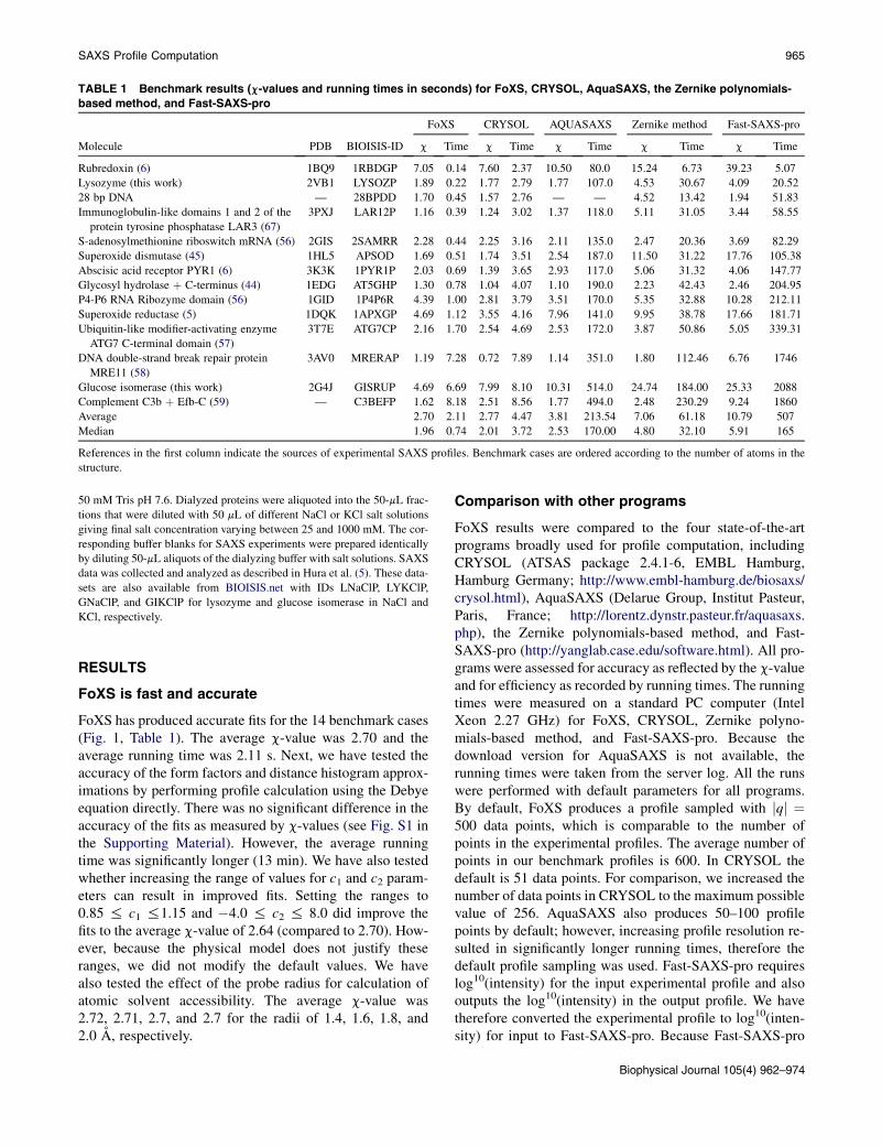
TABLE 1 Benchmark results (c-values and running times in seconds) for FoXS, CRYSOL, AquaSAXS, the Zernike polynomials-

based method, and Fast-SAXS-pro

Molecule PDB BIOISIS-ID

FoXS CRYSOL AQUASAXS Zernike method Fast-SAXS-pro

c Time c Time c Time c Time c Time

Rubredoxin (6) 1BQ9 1RBDGP 7.05 0.14 7.60 2.37 10.50 80.0 15.24 6.73 39.23 5.07

Lysozyme (this work) 2VB1 LYSOZP 1.89 0.22 1.77 2.79 1.77 107.0 4.53 30.67 4.09 20.52

28 bp DNA — 28BPDD 1.70 0.45 1.57 2.76 — — 4.52 13.42 1.94 51.83

Immunoglobulin-like domains 1 and 2 of the

protein tyrosine phosphatase LAR3 (67)

3PXJ LAR12P 1.16 0.39 1.24 3.02 1.37 118.0 5.11 31.05 3.44 58.55

S-adenosylmethionine riboswitch mRNA (56) 2GIS 2SAMRR 2.28 0.44 2.25 3.16 2.11 135.0 2.47 20.36 3.69 82.29

Superoxide dismutase (45) 1HL5 APSOD 1.69 0.51 1.74 3.51 2.54 187.0 11.50 31.22 17.76 105.38

Abscisic acid receptor PYR1 (6) 3K3K 1PYR1P 2.03 0.69 1.39 3.65 2.93 117.0 5.06 31.32 4.06 147.77

Glycosyl hydrolase þ C-terminus (44) 1EDG AT5GHP 1.30 0.78 1.04 4.07 1.10 190.0 2.23 42.43 2.46 204.95

P4-P6 RNA Ribozyme domain (56) 1GID 1P4P6R 4.39 1.00 2.81 3.79 3.51 170.0 5.35 32.88 10.28 212.11

Superoxide reductase (5) 1DQK 1APXGP 4.69 1.12 3.55 4.16 7.96 141.0 9.95 38.78 17.66 181.71

Ubiquitin-like modifier-activating enzyme

ATG7 C-terminal domain (57)

3T7E ATG7CP 2.16 1.70 2.54 4.69 2.53 172.0 3.87 50.86 5.05 339.31

DNA double-strand break repair protein

MRE11 (58)

3AV0 MRERAP 1.19 7.28 0.72 7.89 1.14 351.0 1.80 112.46 6.76 1746

Glucose isomerase (this work) 2G4J GISRUP 4.69 6.69 7.99 8.10 10.31 514.0 24.74 184.00 25.33 2088

Complement C3b þ Efb-C (59) — C3BEFP 1.62 8.18 2.51 8.56 1.77 494.0 2.48 230.29 9.24 1860

Average 2.70 2.11 2.77 4.47 3.81 213.54 7.06 61.18 10.79 507

Median 1.96 0.74 2.01 3.72 2.53 170.00 4.80 32.10 5.91 165

References in the first column indicate the sources of experimental SAXS profiles. Benchmark cases are ordered according to the number of atoms in the

structure.

SAXS Profile Computation 965

50 mM Tris pH 7.6. Dialyzed proteins were aliquoted into the 50-mL frac-

tions that were diluted with 50 mL of different NaCl or KCl salt solutions

giving final salt concentration varying between 25 and 1000 mM. The cor-

responding buffer blanks for SAXS experiments were prepared identically

by diluting 50-mL aliquots of the dialyzing buffer with salt solutions. SAXS

data was collected and analyzed as described in Hura et al. (5). These data-

sets are also available from BIOISIS.net with IDs LNaClP, LYKClP,

GNaClP, and GIKClP for lysozyme and glucose isomerase in NaCl and

KCl, respectively.

RESULTS

FoXS is fast and accurate

FoXS has produced accurate fits for the 14 benchmark cases(Fig. 1, Table 1). The average c-value was 2.70 and theaverage running time was 2.11 s. Next, we have tested theaccuracy of the form factors and distance histogram approx-imations by performing profile calculation using the Debyeequation directly. There was no significant difference in theaccuracy of the fits as measured by c-values (see Fig. S1 inthe Supporting Material). However, the average runningtime was significantly longer (13 min). We have also testedwhether increasing the range of values for c1 and c2 param-eters can result in improved fits. Setting the ranges to0.85 % c1 %1.15 and �4.0 % c2 % 8.0 did improve thefits to the average c-value of 2.64 (compared to 2.70). How-ever, because the physical model does not justify theseranges, we did not modify the default values. We havealso tested the effect of the probe radius for calculation ofatomic solvent accessibility. The average c-value was2.72, 2.71, 2.7, and 2.7 for the radii of 1.4, 1.6, 1.8, and2.0 A, respectively.

Comparison with other programs

FoXS results were compared to the four state-of-the-artprograms broadly used for profile computation, includingCRYSOL (ATSAS package 2.4.1-6, EMBL Hamburg,Hamburg Germany; http://www.embl-hamburg.de/biosaxs/crysol.html), AquaSAXS (Delarue Group, Institut Pasteur,Paris, France; http://lorentz.dynstr.pasteur.fr/aquasaxs.php), the Zernike polynomials-based method, and Fast-SAXS-pro (http://yanglab.case.edu/software.html). All pro-grams were assessed for accuracy as reflected by the c-valueand for efficiency as recorded by running times. The runningtimes were measured on a standard PC computer (IntelXeon 2.27 GHz) for FoXS, CRYSOL, Zernike polyno-mials-based method, and Fast-SAXS-pro. Because thedownload version for AquaSAXS is not available, therunning times were taken from the server log. All the runswere performed with default parameters for all programs.By default, FoXS produces a profile sampled with jqj ¼500 data points, which is comparable to the number ofpoints in the experimental profiles. The average number ofpoints in our benchmark profiles is 600. In CRYSOL thedefault is 51 data points. For comparison, we increased thenumber of data points in CRYSOL to the maximum possiblevalue of 256. AquaSAXS also produces 50–100 profilepoints by default; however, increasing profile resolution re-sulted in significantly longer running times, therefore thedefault profile sampling was used. Fast-SAXS-pro requireslog10(intensity) for the input experimental profile and alsooutputs the log10(intensity) in the output profile. We havetherefore converted the experimental profile to log10(inten-sity) for input to Fast-SAXS-pro. Because Fast-SAXS-pro

Biophysical Journal 105(4) 962–974

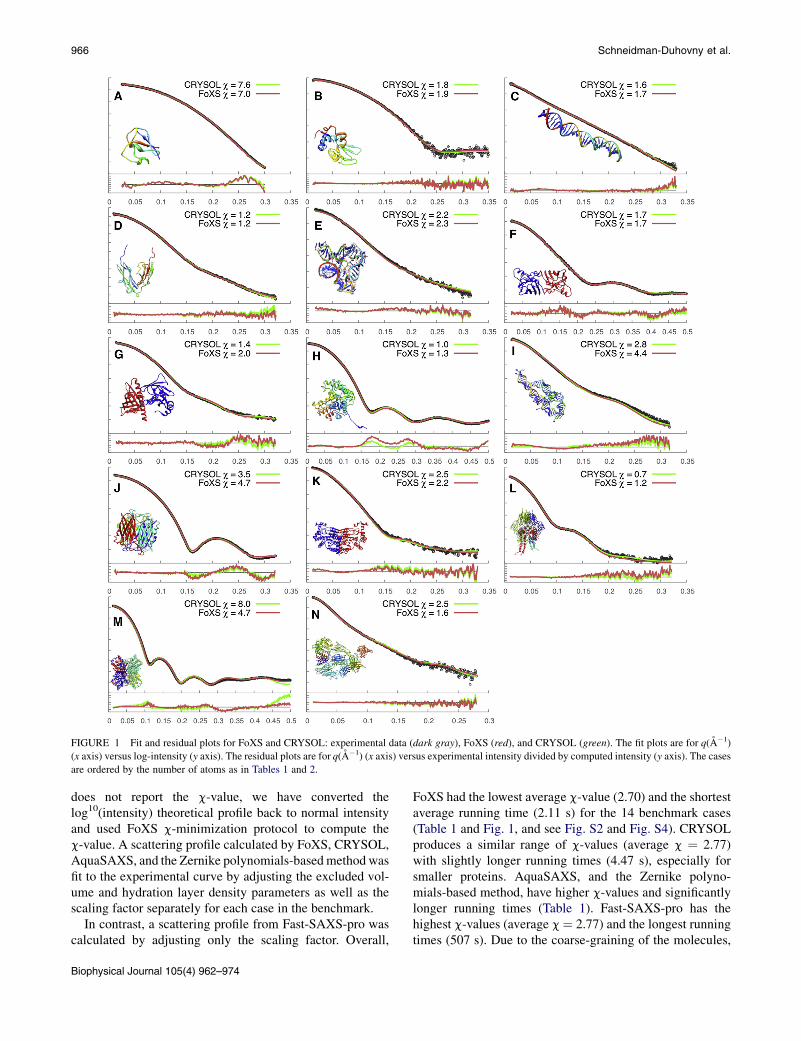
FIGURE 1 Fit and residual plots for FoXS and CRYSOL: experimental data (dark gray), FoXS (red), and CRYSOL (green). The fit plots are for q(A�1)

(x axis) versus log-intensity (y axis). The residual plots are for q(A�1) (x axis) versus experimental intensity divided by computed intensity (y axis). The cases

are ordered by the number of atoms as in Tables 1 and 2.

966 Schneidman-Duhovny et al.

does not report the c-value, we have converted thelog10(intensity) theoretical profile back to normal intensityand used FoXS c-minimization protocol to compute thec-value. A scattering profile calculated by FoXS, CRYSOL,AquaSAXS, and the Zernike polynomials-basedmethod wasfit to the experimental curve by adjusting the excluded vol-ume and hydration layer density parameters as well as thescaling factor separately for each case in the benchmark.

In contrast, a scattering profile from Fast-SAXS-pro wascalculated by adjusting only the scaling factor. Overall,

Biophysical Journal 105(4) 962–974

FoXS had the lowest average c-value (2.70) and the shortestaverage running time (2.11 s) for the 14 benchmark cases(Table 1 and Fig. 1, and see Fig. S2 and Fig. S4). CRYSOLproduces a similar range of c-values (average c ¼ 2.77)with slightly longer running times (4.47 s), especially forsmaller proteins. AquaSAXS, and the Zernike polyno-mials-based method, have higher c-values and significantlylonger running times (Table 1). Fast-SAXS-pro has thehighest c-values (average c¼ 2.77) and the longest runningtimes (507 s). Due to the coarse-graining of the molecules,

SAXS Profile Computation 967

the profiles computed by Fast-SAXS-pro often do not fit thedata at high q values (q > 0.25) (see Fig. S4, A, D, F–I, andM). Moreover, there is often a significant deviation from theexperimental profile at low q values (see Fig. S4, F, and K–N). These results indicate that obtaining a good fit to the datarequires a full atom model as well as fitting excluded vol-ume and hydration layer density parameters, in addition tothe scaling factor. Because c-values may vary due to profileexperimental noise and are not directly comparable betweendifferent experimental datasets, we have also compared themedian c-value for the 14 benchmark cases among the fiveprograms. FoXS had the lowest median c-value (1.96), fol-lowed by CRYSOL (2.01) and AquaSAXS (2.53).

FoXS accurately accounts for the excludedvolume contribution

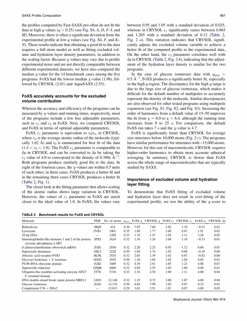
Whereas the accuracy and efficiency of the programs can bemeasured by c-values and running times, respectively, mostof the programs include a few free adjustable parameters,such as c1 and c2 in FoXS. Next, we compared CRYSOLand FoXS in terms of optimal adjustable parameters.

FoXS c1 parameter is equivalent to r0/rm in CRYSOL,where rm is the average atomic radius of the molecule (typi-cally 1.62 A) and r0 is enumerated for best fit of the data(1.4 < r0 < 1.8). The FoXS c2 parameter is comparable todr in CRYSOL and can be converted to dr by taking thec2 value of 4.0 to correspond to the density of 0.388e A�3.Both programs produce similarly good fits to the data. Ineight of the fourteen cases, the c-values are within 0.5 unitsof each other; in three cases, FoXS produces a better fit andin the remaining three cases CRYSOL produces a better fit(Table 2, Fig. 1).

The closer look at the fitting parameter that allows scalingof the atomic radius shows large variation in CRYSOL.However, the values of c1 parameter in FoXS are muchcloser to the ideal value of 1.0. In FoXS, the values vary

TABLE 2 Benchmark results for FoXS and CRYSOL

Molecule PDB No. of atoms qm

Rubredoxin 1BQ9 424 0.3

Lysozyme 2VB1 1001 0.3

28 bp DNA — 1209 0.3

Immunoglobulin-like domains 1 and 2 of the protein

tyrosine phosphatase LAR3

3PXJ 1624 0.3

S-adenosylmethionine riboswitch mRNA 2GIS 2058 0.3

Superoxide dismutase 1HL5 2220 0.5

Abscisic acid receptor PYR1 3K3K 2924 0.3

Glycosyl hydrolase þ C terminus 1EDG 3035 0.5

P4-P6 RNA ribozyme domain 1GID 3409 0.3

Superoxide reductase 1DQK 4060 0.3

Ubiquitin-like modifier-activating enzyme ATG7

C-terminal domain

3T7E 5318 0.3

DNA double-strand break repair protein MRE11 3AV0 12,148 0.3

Glucose isomerase 2G4J 12,176 0.5

Complement C3b þ Efb-C — 12,833 0.2

between 0.95 and 1.05 with a standard deviation of 0.025,whereas in CRYSOL c1 significantly varies between 0.865and 1.265 with a standard deviation of 0.12 (Table 2,Fig. 2 a). This variation indicates that CRYSOL signifi-cantly adjusts the excluded volume variable to achieve abetter fit of the computed profile to the experimental data.On the other hand, the c2 parameter correlates well withdr in CRYSOL (Table 2, Fig. 2 b), indicating that the adjust-ment of the hydration layer density is similar for the twoprograms.

In the case of glucose isomerase data with qmax ¼0.5 A�1, FoXS produces a significantly better fit, especiallyin the high q region. The discrepancy for the high q range isdue to the large size of glucose isomerase, which makes itdifficult for the default number of multipoles to accuratelyrepresent the density of the molecule. Similar discrepanciesare also observed for other tested programs using multipoleexpansion (see Fig. S1, Fig. S2, and Fig. S3). Increasing theorder of harmonics from a default value of 15–50 improvesthe fit from c ¼ 8.0 to c ¼ 6.4, although the running timeincreases from 8 to 25 s. For comparison, the defaultFoXS run takes 7 s and the c-value is 4.7.

FoXS is significantly faster than CRYSOL for averagesize structures below 10,000 atoms (Fig. 2 c). The programshave similar performance for structures with ~15,000 atoms.However, for this size of macromolecule, CRYSOL requireshigher-order harmonics to obtain more accurate sphericalaveraging. In summary, CRYSOL is slower than FoXSacross the whole range of macromolecules that are typicallystudied by SAXS.

Importance of excluded volume and hydrationlayer fitting

To demonstrate that FoXS fitting of excluded volumeand hydration layer does not result in over-fitting of theexperimental profile, we test the ability of the c-score to

ax FoXS c CRYSOL c FoXS c1 CRYSOL c1 FoXS c2 CRYSOL dr

0 7.05 7.60 1.02 1.10 �0.15 0.01

5 1.89 1.77 1.00 0.87 1.91 0.02

3 1.70 1.57 1.05 1.11 3.28 0.05

2 1.16 1.24 1.04 1.10 �0.33 0.01

2 2.28 2.25 0.95 1.12 0.88 0.01

0 1.69 1.74 1.02 0.88 �0.18 0.00

2 2.03 1.39 1.02 0.87 �0.82 0.00

0 1.30 1.04 1.02 1.04 0.05 0.01

2 4.39 2.81 1.05 1.21 4.00 0.07

2 4.69 3.55 1.03 1.00 0.68 0.01

3 2.16 2.54 1.00 1.11 4.00 0.04

2 1.19 0.72 1.00 1.07 4.00 0.04

0 4.69 7.99 1.02 0.87 0.23 0.01

8 1.62 2.51 1.01 0.87 4.00 0.05

Biophysical Journal 105(4) 962–974

A B C

FIGURE 2 Comparison of FoXS and CRYSOL adjustable parameters and running times. (A) CRYSOL r0 versus c1. (B) CRYSOL dr versus FOXS c2. (C)

Running times of FoXS (red) versus CRYSOL (green) and CRYSOL L50 (dark green, order of harmonics ¼ 50).

968 Schneidman-Duhovny et al.

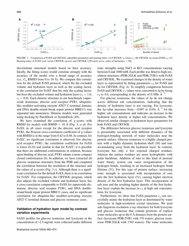
discriminate structural models based on their accuracy.Ideally, the fitting scores would correlate strongly with theaccuracy of the model over a broad range of accuracy(i.e., Ca RMSD from 0 to 10 A). We compare this correla-tion for the default FoXS protocol, which fits the excludedvolume and hydration layer as well as the scaling factor,to the correlation for FoXS0 that fits only the scaling factor,but fixes the excluded volume and hydration layer (c1 ¼ 1.0,c2 ¼ 0.0). Each dimeric structure in our benchmark (super-oxide dismutase, abscisic acid receptor PYR1, ubiquitin-like modifier-activating enzyme ATG7 C-terminal domain,and DNA double-strand break repair protein MRE11) wasseparated into monomers. Dimeric models were generatedusing docking by PatchDock or SymmDock (49).

We have examined the correlation of c-scores withRMSD for models with RMSD < 10 A (Fig. 3, a–d). ForFoXS, in all cases except for the abscisic acid receptorPYR1, the Pearson cross-correlation coefficient of c-valueswith RMSD is in the range from 0.42 to 0.48. In contrast, forFoXS0, no significant correlation is observed. For abscisicacid receptor PYR1, the correlation coefficient for FoXSis lower (0.24) and similar to that for FoXS0; it is possiblethat there are additional conformations in solution, becauseupon binding of abscisic acid, PYR1 adopts a more compactclosed conformation (6). In addition, we have extracted allglucose isomerase structures from the PDB and computedthe correlation between the resolution of the structure andthe values of c-scores (Fig. 3 e). Although there is a signif-icant correlation for the default FoXS, there is no correlationfor FoXS0. For comparison, the CRYSOL program, whichalso adjusts the excluded volume and hydration layer, hasa cross-correlation comparable to FoXS for superoxide dis-mutase, abscisic acid receptor PYR1, and DNA double-strand break repair protein MRE11 cases, and no significantcorrelation for ubiquitin-like modifier-activating enzymeATG7 C-terminal domain and glucose isomerase cases.

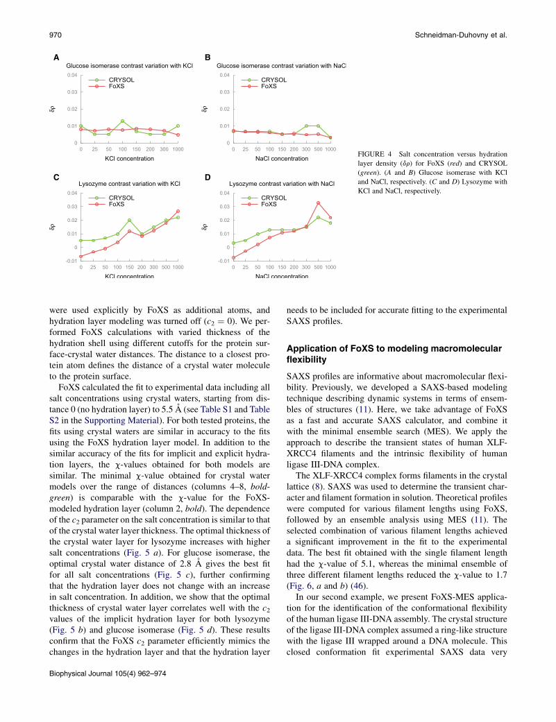
Validation of hydration layer model by contrastvariation experiments

SAXS profiles for glucose isomerase and lysozyme at theconcentration of ~2.5 mg/mL were collected under different

Biophysical Journal 105(4) 962–974

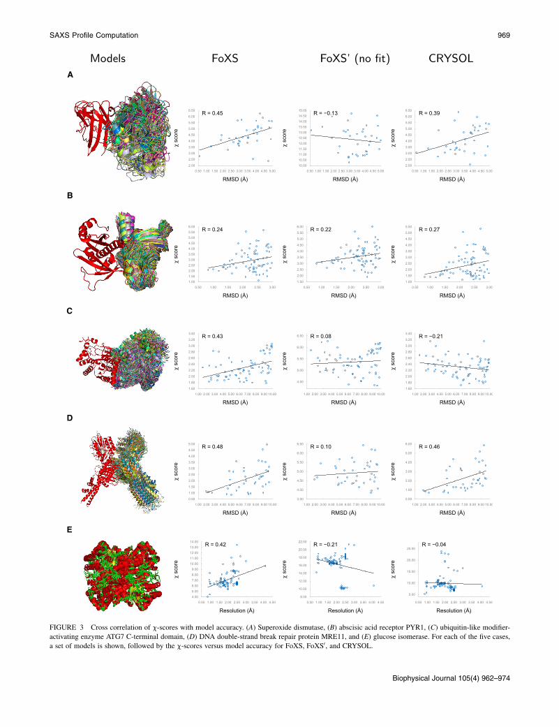
ionic strengths using NaCl or KCl concentrations varyingbetween 0 and 1000 mM. Each profile was fitted to high-res-olution structures (PDB:2GLK and PDB:2VB1) with FoXSand CRYSOL. We examined changes in the density of waterlayer as represented by fitting parameters c2 for FoXS anddr for CRYSOL (Fig. 4). To simplify comparison betweenFoXS and CRYSOL c2 values were converted to dr by fixingc2 to 4.0, corresponding to the density of 0.388e A�3.

For glucose isomerase, the values of dr do not changeacross different salt concentrations, indicating that thedensity of hydration layer is not varying. For lysozyme,the dr-value increases from �0.007 to 0.03e A�3 for thehigher salt concentrations and indicates an increase in thehydration layer density at higher salt concentrations. Weobserved similar changes in hydration layer parameters forboth FoXS and CRYSOL.

The difference between glucose isomerase and lysozymeis presumably associated with different dynamics of thehydrogen-bonding network of water molecules near theprotein surface. Glucose isomerase is a highly charged pro-tein with a highly dynamic hydration shell (50) and ionsaccumulating away from the hydration layer. In contrast,lysozyme has only a few exposed charged residues,whereas the surface residues are more hydrophobic withpolar backbone. Addition of ions to this kind of protein/water binary system can cause reorganization of thehydrogen bonds, resulting in an increased hydrogen bondlifetime (51). For this type of protein surface, increasingionic strength is associated with incorporation of ionsinto the first hydration layer (51), causing higher electrondensity of the first hydration layer. This incorporation ofsalt ions and the resulting higher density of the first hydra-tion layer explain the increase in c2 at high salt concentra-tions for lysozyme.

Furthermore, we show that FoXS parameter c2 can suc-cessfully mimic the hydration layer as determined by watermolecules in high-resolution crystal structures. We usedsub-Angstrom resolution x-ray structures for both lysozymeand glucose isomerase that contain positions of explicitwater molecules up to the 6 A distance from the protein sur-face (lysozyme PDB:2VB1 with 170 waters; glucose isom-erase PDB:2GLK with 1705 waters). The water molecules

A

B

C

D

E

FIGURE 3 Cross correlation of c-scores with model accuracy. (A) Superoxide dismutase, (B) abscisic acid receptor PYR1, (C) ubiquitin-like modifier-

activating enzyme ATG7 C-terminal domain, (D) DNA double-strand break repair protein MRE11, and (E) glucose isomerase. For each of the five cases,

a set of models is shown, followed by the c-scores versus model accuracy for FoXS, FoXS0, and CRYSOL.

Biophysical Journal 105(4) 962–974

SAXS Profile Computation 969

A B

C D

FIGURE 4 Salt concentration versus hydration

layer density (dr) for FoXS (red) and CRYSOL

(green). (A and B) Glucose isomerase with KCl

and NaCl, respectively. (C and D) Lysozyme with

KCl and NaCl, respectively.

970 Schneidman-Duhovny et al.

were used explicitly by FoXS as additional atoms, andhydration layer modeling was turned off (c2 ¼ 0). We per-formed FoXS calculations with varied thickness of thehydration shell using different cutoffs for the protein sur-face-crystal water distances. The distance to a closest pro-tein atom defines the distance of a crystal water moleculeto the protein surface.

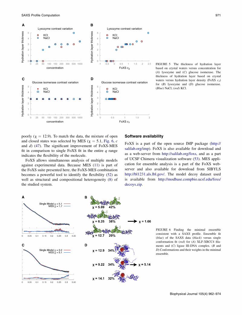
FoXS calculated the fit to experimental data including allsalt concentrations using crystal waters, starting from dis-tance 0 (no hydration layer) to 5.5 A (see Table S1 and TableS2 in the Supporting Material). For both tested proteins, thefits using crystal waters are similar in accuracy to the fitsusing the FoXS hydration layer model. In addition to thesimilar accuracy of the fits for implicit and explicit hydra-tion layers, the c-values obtained for both models aresimilar. The minimal c-value obtained for crystal watermodels over the range of distances (columns 4–8, bold-green) is comparable with the c-value for the FoXS-modeled hydration layer (column 2, bold). The dependenceof the c2 parameter on the salt concentration is similar to thatof the crystal water layer thickness. The optimal thickness ofthe crystal water layer for lysozyme increases with highersalt concentrations (Fig. 5 a). For glucose isomerase, theoptimal crystal water distance of 2.8 A gives the best fitfor all salt concentrations (Fig. 5 c), further confirmingthat the hydration layer does not change with an increasein salt concentration. In addition, we show that the optimalthickness of crystal water layer correlates well with the c2values of the implicit hydration layer for both lysozyme(Fig. 5 b) and glucose isomerase (Fig. 5 d). These resultsconfirm that the FoXS c2 parameter efficiently mimics thechanges in the hydration layer and that the hydration layer

Biophysical Journal 105(4) 962–974

needs to be included for accurate fitting to the experimentalSAXS profiles.

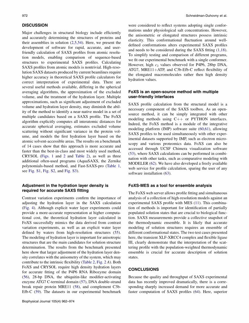
Application of FoXS to modeling macromolecularflexibility

SAXS profiles are informative about macromolecular flexi-bility. Previously, we developed a SAXS-based modelingtechnique describing dynamic systems in terms of ensem-bles of structures (11). Here, we take advantage of FoXSas a fast and accurate SAXS calculator, and combine itwith the minimal ensemble search (MES). We apply theapproach to describe the transient states of human XLF-XRCC4 filaments and the intrinsic flexibility of humanligase III-DNA complex.

The XLF-XRCC4 complex forms filaments in the crystallattice (8). SAXS was used to determine the transient char-acter and filament formation in solution. Theoretical profileswere computed for various filament lengths using FoXS,followed by an ensemble analysis using MES (11). Theselected combination of various filament lengths achieveda significant improvement in the fit to the experimentaldata. The best fit obtained with the single filament lengthhad the c-value of 5.1, whereas the minimal ensemble ofthree different filament lengths reduced the c-value to 1.7(Fig. 6, a and b) (46).

In our second example, we present FoXS-MES applica-tion for the identification of the conformational flexibilityof the human ligase III-DNA assembly. The crystal structureof the ligase III-DNA complex assumed a ring-like structurewith the ligase III wrapped around a DNA molecule. Thisclosed conformation fit experimental SAXS data very

A B

C D

FIGURE 5 The thickness of hydration layer

based on crystal waters versus concentration for

(A) lysozyme and (C) glucose isomerase. The

thickness of hydration layer based on crystal

waters versus hydration layer density (FoXS c2)

for (B) lysozyme and (D) glucose isomerase.

(Blue) NaCl; (red) KCl.

SAXS Profile Computation 971

poorly (c ¼ 12.9). To match the data, the mixture of openand closed states was selected by MES (c ¼ 5.1, Fig. 6, cand d) (47). The significant improvement of FoXS-MESfit in comparison to single FoXS fit in the entire q rangeindicates the flexibility of the molecule.

FoXS allows simultaneous analysis of multiple modelsagainst experimental data. Because MES (11) is part ofthe FoXS suite presented here, the FoXS-MES combinationbecomes a powerful tool to identify the flexibility (52) aswell as structural and compositional heterogeneity (8) ofthe studied system.

Software availability

FoXS is a part of the open source IMP package (http://

salilab.org/imp). FoXS is also available for download and

as a web-server from http://salilab.org/foxs, and as a part

of UCSF Chimera visualization software (53). MES appli-

cation for ensemble analysis is a part of the FoXS web-

server and also available for download from SIBYLS

http://bl1231.als.lbl.gov/. The model decoy dataset used

is available from http://modbase.compbio.ucsf.edu/foxs/

decoys.zip.

FIGURE 6 Finding the minimal ensemble

consistent with a SAXS profile. Ensemble fit

(blue) of the SAXS data (black) versus single

conformation fit (red) for (A) XLF-XRCC4 fila-

ments and (C) ligase III-DNA complex. (B and

D) Conformations and their weights in the minimal

ensemble.

Biophysical Journal 105(4) 962–974

972 Schneidman-Duhovny et al.

DISCUSSION

Major challenges in structural biology include efficientlyand accurately determining the structures of proteins andtheir assemblies in solution (2,5,54). Here, we present thedevelopment of software for rapid, accurate, and user-friendly calculation of SAXS profiles from atomic resolu-tion models, enabling comparison of sequence-basedstructures to experimental SAXS profiles. CalculatingSAXS profiles from atomic models is nontrivial. High-reso-lution SAXS datasets produced by current beamlines requirehigher accuracy in theoretical SAXS profile calculators forcorrect interpretation of experimental data. There areseveral useful methods available, differing in the sphericalaveraging algorithms, the approximation of the excludedvolume, and the treatment of the hydration layer. Multipleapproximations, such as significant adjustment of excludedvolume and hydration layer density, may diminish the abil-ity of the method to identify a near-native model in a set ofmultiple candidates based on a SAXS profile. The FoXSalgorithm explicitly computes all interatomic distances foraccurate spherical averaging, estimates excluded volumescattering without significant variance in the protein vol-ume, and models the first hydration layer based on theatomic solvent-accessible areas. The results on a benchmarkof 14 cases show that this approach is more accurate andfaster than the best-in-class and most widely used method,CRYSOL (Figs. 1 and 2 and Table 2), as well as threeadditional often-used programs (AquaSAXS, the Zernikepolynomials-based method, and Fast-SAXS-pro (Table 1,see Fig. S1, Fig. S2, and Fig. S3).

Adjustment in the hydration layer density isrequired for accurate SAXS fitting

Contrast variation experiments confirm the importance ofadjusting the hydration layer in the SAXS calculation(Fig. 4). Although explicit water layer experiments couldprovide a more-accurate representation at higher computa-tional cost, the theoretical hydration layer calculated inFoXS successfully mimics the data derived from contrastvariation experiments, as well as an explicit water layerdefined by waters from high-resolution structures (55).The modeling of hydration layer is important for anisotropicstructures that are the main candidates for solution structuredetermination. The results from the benchmark presentedhere show that larger adjustment of the hydration layer den-sity correlates with the anisometry of the system, which maycontribute to the intrinsic flexibility (Table 2, Fig. 2 A). BothFoXS and CRYSOL require high density hydration layersfor accurate fitting of the P4P6 RNA Ribozyme domain(56), 28-bp DNA, the ubiquitin-like modifier-activatingenzyme ATG7 C-terminal domain (57), DNA double-strandbreak repair protein MRE11 (58), and complement C3b-Efb-C (59). The datasets in our experimental benchmark

Biophysical Journal 105(4) 962–974

were considered to reflect systems adopting single confor-mations under physiological salt concentrations. However,the anisometric or elongated structures possess intrinsicelasticity. This conformational fluctuation around well-defined conformations alters experimental SAXS profilesand needs to be considered during the SAXS fitting (1,18).To simplify testing and comparison of different programs,we fit our experimental benchmark with a single conformer.However, high c2 values observed for P4P6, 28bp DNA,ATG7, MRE11þATP, and C3b-Efb-C reflect flexibility ofthe elongated macromolecules rather then high densityhydration values.

FoXS is an open-source method with multipleuser-friendly interfaces

SAXS profile calculation from the structural model is anecessary component of the SAXS toolbox. As an open-source method, it can be simply integrated with othermodeling methods using Cþþ or PYTHON interfaces.Indeed, the FoXS method is a module of the integrativemodeling platform (IMP) software suite (60,61), allowingSAXS profiles to be used simultaneously with other exper-imental datasets supported by IMP, such as electron micro-scopy and various proteomics data. FoXS can also beaccessed through UCSF Chimera visualization software(53), where SAXS calculations can be performed in combi-nation with other tasks, such as comparative modeling withMODELER (62). We have also developed a freely availableweb service for profile calculation, sparing the user of anysoftware installation (63).

FoXS-MES as a tool for ensemble analysis

The FoXS web server allows profile fitting and simultaneousanalysis of a collection of high-resolution models against anexperimental SAXS profile with MES (11). This combina-tion of methods is important for identification of partiallypopulated solution states that are crucial to biological func-tion. SAXS measurements provide a collective snapshot ofthe thermodynamic ensemble. It is likely that accuratemodeling of solution structures requires an ensemble ofdifferent conformational states. The two test cases presentedhere, the transient XLF-XRCC4 complex and flexible ligaseIII, clearly demonstrate that the interpretation of the scat-tering profile with the population-weighted thermodynamicensemble is crucial for accurate description of solutionstates.

CONCLUSIONS

Because the quality and throughput of SAXS experimentaldata has recently improved dramatically, there is a corre-sponding sharply increased demand for more accurate andfaster computation of SAXS profiles (64). Here, superior

SAXS Profile Computation 973

fits between experimental high-resolution structures andSAXS data are obtained by using explicit all-atom distancesand a hydration layer model to account for the effect ofsolvent. The explicit representation of the hydrated macro-molecule is particularly useful for multidomain-flexibleassemblies, which frequently adopt highly anisometricshapes. The FoXS algorithm explicitly computes all inter-atomic distances that include the first solvation layer basedon the atomic solvent-accessible areas. In addition to accu-racy, rapid calculation speed is critical for SAXS-basedstructural modeling tools, which often perform multipleSAXS calculations for large pools of conformers or assem-blies (5). FoXS capabilities have proven valuable fordefining the archaeal motor mechanism (65), for validatingmodel-data resolution limits (42), and for comprehensiveSAXS structural comparison maps revealing structural sim-ilarities (66), suggesting FoXS will prove important foremerging biology plus advanced SAXS metrics and analysistechniques. In fact, we show here that FoXS is faster thanother best-in-class programs. Because FoXS is availablethrough a web server, it enables uploading and simultaneousanalysis of a collection of atomic coordinate input filesagainst experimental data. In combination with the MES(11), the user is provided with tools to identify the flexibilityas well as the conformational and compositional heteroge-neity of the studied system.

SUPPORTING MATERIAL

Two tables and four figures are available at http://www.biophysj.org/

biophysj/supplemental/S0006-3495(13)00805-9.

D.S.-D. has been funded by the Weizmann Institute’s Advancing Women in

Science Postdoctoral Fellowship. We also acknowledge support from Na-

tional Institutes of Health grant Nos. R01 GM083960, U54 RR022220,

and PN2 EY016525, and Rinat (Pfizer) Inc. (to A.S.) as well as the Law-

rence Berkeley National Lab IDAT program and National Institutes of

Health grant No. MINOS R01GM105404 (to J.A.T.).

REFERENCES

1. Putnam, C. D., M. Hammel,., J. A. Tainer. 2007. X-ray solution scat-tering (SAXS) combined with crystallography and computation:defining accurate macromolecular structures, conformations andassemblies in solution. Q. Rev. Biophys. 40:191–285.

2. Rambo, R. P., and J. A. Tainer. 2010. Bridging the solution divide:comprehensive structural analyses of dynamic RNA, DNA, and proteinassemblies by small-angle x-ray scattering. Curr. Opin. Struct. Biol.20:128–137.

3. Hammel, M. 2012. Validation of macromolecular flexibility insolution by small-angle x-ray scattering (SAXS). Eur. Biophys. J.41:789–799.

4. Jacques, D. A., and J. Trewhella. 2010. Small-angle scattering forstructural biology—expanding the frontier while avoiding the pitfalls.Protein Sci. 19:642–657.

5. Hura, G. L., A. L. Menon, ., J. A. Tainer. 2009. Robust, high-throughput solution structural analyses by small angle x-ray scattering(SAXS). Nat. Methods. 6:606–612.

6. Nishimura, N., K. Hitomi, ., E. D. Getzoff. 2009. Structural mecha-nism of abscisic acid binding and signaling by dimeric PYR1. Science.326:1373–1379.

7. Lamb, J. S., B. D. Zoltowski, ., L. Pollack. 2009. Illuminating solu-tion responses of a LOV domain protein with photocoupled small-anglex-ray scattering. J. Mol. Biol. 393:909–919.

8. Hammel, M., M. Rey, ., J. A. Tainer. 2011. XRCC4 protein interac-tions with XRCC4-like factor (XLF) create an extended grooved scaf-fold for DNA ligation and double strand break repair. J. Biol. Chem.286:32638–32650.

9. Fenton, A. W., R. Williams, and J. Trewhella. 2010. Changes in small-angle x-ray scattering parameters observed upon binding of ligand torabbit muscle pyruvate kinase are not correlated with allosteric transi-tions. Biochemistry. 49:7202–7209.

10. Bernado, P., E. Mylonas, ., D. I. Svergun. 2007. Structural character-ization of flexible proteins using small-angle x-ray scattering. J. Am.Chem. Soc. 129:5656–5664.

11. Pelikan, M., G. L. Hura, and M. Hammel. 2009. Structure and flexi-bility within proteins as identified through small angle x-ray scattering.Gen. Physiol. Biophys. 28:174–189.

12. Petoukhov, M. V., and D. I. Svergun. 2005. Global rigid body modelingof macromolecular complexes against small-angle scattering data.Biophys. J. 89:1237–1250.

13. Forster, F., B. Webb,., A. Sali. 2008. Integration of small-angle x-rayscattering data into structural modeling of proteins and their assem-blies. J. Mol. Biol. 382:1089–1106.

14. Perkins, S. J., and A. Bonner. 2008. Structure determinations of humanand chimeric antibodies by solution scattering and constrained molec-ular modeling. Biochem. Soc. Trans. 36:37–42.

15. Zheng, W., and S. Doniach. 2002. Protein structure prediction con-strained by solution x-ray scattering data and structural homology iden-tification. J. Mol. Biol. 316:173–187.

16. Zheng, W., and S. Doniach. 2005. Fold recognition aided by constraintsfrom small angle x-ray scattering data. Protein Eng. Des. Sel.18:209–219.

17. dos Reis, M. A., R. Aparicio, and Y. Zhang. 2011. Improving proteintemplate recognition by using small-angle x-ray scattering profiles.Biophys. J. 101:2770–2781.

18. Grishaev, A., L. Guo, ., A. Bax. 2010. Improved fitting of solutionx-ray scattering data to macromolecular structures and structural en-sembles by explicit water modeling. J. Am. Chem. Soc. 132:15484–15486.

19. Schneidman-Duhovny, D., S. J. Kim, and A. Sali. 2012. Integrativestructural modeling with small angle x-ray scattering profiles. BMCStruct. Biol. 12:17.

20. Zuo, X., G. Cui, ., D. M. Tiede. 2006. X-ray diffraction ‘‘finger-printing’’ of DNA structure in solution for quantitative evaluationof molecular dynamics simulation. Proc. Natl. Acad. Sci. USA.103:3534–3539.

21. Debye, P. 1915. Scattering of x-rays [Zerstreuung von Rontgenstrah-len]. Annalen der Physik. 351:809–823.

22. Svergun, D., C. Barberato, and M. H. J. Koch. 1995. CRYSOL—a pro-gram to evaluate x-ray solution scattering of biological macromole-cules from atomic coordinates. j. Appl. Cryst. 28:768–773.

23. Liu, H., R. J. Morris, ., P. H. Zwart. 2012. Computation of small-angle scattering profiles with three-dimensional Zernike polynomials.Acta Crystallogr. A. 68:278–285.

24. Gumerov, N. A., K. Berlin, ., R. Duraiswami. 2012. A hierarchicalalgorithm for fast Debye summation with applications to small anglescattering. J. Comput. Chem. 33:1981–1996.

25. Tjioe, E., andW. T. Heller. 2007. ORNL_SAS: software for calculationof small-angle scattering intensities of proteins and protein complexes.J. Appl. Cryst. 40:782–785.

26. Yang, S., S. Park, ., B. Roux. 2009. A rapid coarse residue-basedcomputational method for x-ray solution scattering characterization

Biophysical Journal 105(4) 962–974

974 Schneidman-Duhovny et al.

of protein folds and multiple conformational states of large proteincomplexes. Biophys. J. 96:4449–4463.

27. Stovgaard, K., C. Andreetta, ., T. Hamelryck. 2010. Calculation ofaccurate small angle x-ray scattering curves from coarse-grained pro-tein models. BMC Bioinformatics. 11:429.

28. Ravikumar, K. M., W. Huang, and S. Yang. 2013. Fast-SAXS-pro: aunified approach to computing SAXS profiles of DNA, RNA, protein,and their complexes. J. Chem. Phys. 138:024112.

29. Fraser, R. D. B., T. P. MacRae, and E. Suzuki. 1978. An improvedmethod for calculating the contribution of solvent to the x-ray diffrac-tion pattern of biological molecules. J. Appl. Cryst. 11:693–694.

30. Lattman, E. E. 1989. Rapid calculation of the solution scattering profilefrom a macromolecule of known structure. Proteins. 5:149–155.

31. Fraser, J. S., H. van den Bedem, ., T. Alber. 2011. Accessing proteinconformational ensembles using room-temperature x-ray crystallog-raphy. Proc. Natl. Acad. Sci. USA. 108:16247–16252.

32. Perkins, S. J. 2001. X-ray and neutron scattering analyses of hydrationshells: a molecular interpretation based on sequence predictions andmodeling fits. Biophys. Chem. 93:129–139.

33. Kuhn, L. A., M. A. Siani, ., J. A. Tainer. 1992. The interdependenceof protein surface topography and bound water molecules revealed bysurface accessibility and fractal density measures. J. Mol. Biol.228:13–22.

34. Svergun, D. I., S. Richard, ., G. Zaccai. 1998. Protein hydration insolution: experimental observation by x-ray and neutron scattering.Proc. Natl. Acad. Sci. USA. 95:2267–2272.

35. Hubbard, S. R., K. O. Hodgson, and S. Doniach. 1988. Small-anglex-ray scattering investigation of the solution structure of troponin C.J. Biol. Chem. 263:4151–4158.

36. Grossmann, J. G., Z. H. Abraham,., S. S. Hasnain. 1993. X-ray scat-tering using synchrotron radiation shows nitrite reductase from Achro-mobacter xylosoxidans to be a trimer in solution. Biochemistry.32:7360–7366.

37. Fujisawa, T., T. Uruga, ., T. Ueki. 1994. The hydration of Ras p21 insolution during GTP hydrolysis based on solution x-ray scattering pro-file. J. Biochem. 115:875–880.

38. Bardhan, J., S. Park, and L. Makowski. 2009. SoftWAXS: a computa-tional tool for modeling wide-angle x-ray solution scattering from bio-molecules. J. Appl. Cryst. 42:932–943.

39. Poitevin, F., H. Orland, ., M. Delarue. 2011. AquaSAXS: a webserver for computation and fitting of SAXS profiles with non-unifor-mally hydrated atomic models. Nucleic Acids Res. 39(Web Serverissue):W184–W189.

40. Virtanen, J. J., L. Makowski, ., K. F. Freed. 2011. Modeling thehydration layer around proteins: applications to small- and wide-anglex-ray scattering. Biophys. J. 101:2061–2069.

41. Connolly, M. L. 1983. Solvent-accessible surfaces of proteins andnucleic acids. Science. 221:709–713.

42. Rambo, R. P., and J. A. Tainer. 2013. Accurate assessment of mass,models and resolution by small-angle scattering. Nature. 496:477–481.

43. Ciccariello, S., J. Goodisman, and H. Brumberger. 1988. On the Porodlaw. J. Appl. Cryst. 21:117–128.

44. Hammel, M., H. P. Fierobe, ., V. Receveur-Brechot. 2005. Structuralbasis of cellulosome efficiency explored by small angle x-ray scat-tering. J. Biol. Chem. 280:38562–38568.

45. Shin, D. S., M. Didonato,., J. A. Tainer. 2009. Superoxide dismutasefrom the eukaryotic thermophile Alvinella pompejana: structures, sta-bility, mechanism, and insights into amyotrophic lateral sclerosis. J.Mol. Biol. 385:1534–1555.

46. Hammel, M., Y. Yu, ., J. A. Tainer. 2010. XLF regulates filament ar-chitecture of the XRCC4$ligase IV complex. Structure. 18:1431–1442.

Biophysical Journal 105(4) 962–974

47. Cotner-Gohara, E., I. K. Kim, ., T. Ellenberger. 2010. Human DNAligase III recognizes DNA ends by dynamic switching between twoDNA-bound states. Biochemistry. 49:6165–6176.

48. Hammel, M., H. P. Fierobe, ., V. Receveur-Brechot. 2004. Structuralinsights into the mechanism of formation of cellulosomes probed bysmall angle x-ray scattering. J. Biol. Chem. 279:55985–55994.

49. Schneidman-Duhovny, D., Y. Inbar, ., H. J. Wolfson. 2005. Patch-Dock and SymmDock: servers for rigid and symmetric docking.Nucleic Acids Res. 33(Web Server issue):W363–W367.

50. Russo, D., G. Hura, and T. Head-Gordon. 2004. Hydration dynamicsnear a model protein surface. Biophys. J. 86:1852–1862.

51. Russo, D. 2008. The impact of kosmotropes and chaotropes on bulkand hydration shell water dynamics in a model peptide solution.Chem. Phys. 345:200–211.

52. Burke, J. R., G. L. Hura, and S. M. Rubin. 2012. Structures of inactiveretinoblastoma protein reveal multiple mechanisms for cell cycle con-trol. Genes Dev. 26:1156–1166.

53. Yang, Z., K. Lasker, ., T. E. Ferrin. 2012. UCSF Chimera,MODELER, and IMP: an integrated modeling system. J. Struct.Biol. 179:269–278.

54. Perry, J. J., E. Cotner-Gohara, ., J. A. Tainer. 2010. Structural dy-namics in DNA damage signaling and repair. Curr. Opin. Struct.Biol. 20:283–294.

55. Kuhn, L. A., C. A. Swanson, ., E. D. Getzoff. 1995. Atomic and res-idue hydrophilicity in the context of folded protein structures. Proteins.23:536–547.

56. Rambo, R. P., and J. A. Tainer. 2010. Improving small-angle x-ray scat-tering data for structural analyses of the RNAworld. RNA. 16:638–646.

57. Taherbhoy, A. M., S. W. Tait, ., B. A. Schulman. 2011. Atg8 transferfrom Atg7 to Atg3: a distinctive E1-E2 architecture and mechanism inthe autophagy pathway. Mol. Cell. 44:451–461.

58. Williams, G. J., R. S. Williams, ., J. A. Tainer. 2011. ABC ATPasesignature helices in Rad50 link nucleotide state to Mre11 interfacefor DNA repair. Nat. Struct. Mol. Biol. 18:423–431.

59. Chen, H., D. Ricklin, ., J. D. Lambris. 2010. Allosteric inhibition ofcomplement function by a staphylococcal immune evasion protein.Proc. Natl. Acad. Sci. USA. 107:17621–17626.

60. Webb, B., K. Lasker, ., A. Sali. 2011. Modeling of proteins and theirassemblies with the integrative modeling platform.Methods Mol. Biol.781:377–397.

61. Russel, D., K. Lasker, ., A. Sali. 2012. Putting the pieces together:integrative modeling platform software for structure determination ofmacromolecular assemblies. PLoS Biol. 10:e1001244.

62. Sali, A., and T. L. Blundell. 1993. Comparative protein modeling bysatisfaction of spatial restraints. J. Mol. Biol. 234:779–815.

63. Schneidman-Duhovny, D., M. Hammel, and A. Sali. 2010. FoXS: aweb server for rapid computation and fitting of SAXS profiles. NucleicAcids Res. 38(Web Server issue, Suppl):W540–W544.

64. Rambo, R. P., and J. A. Tainer. 2013. Super-resolution in solution x-rayscattering and its applications to structural systems biology. Annu. Rev.Biophys. 42:415–441.

65. Reindl, S., A. Ghosh,., J. A. Tainer. 2013. Insights into FlaI functionsin archaeal motor assembly and motility from structures, conforma-tions, and genetics. Mol. Cell. 49:1069–1082.

66. Hura, G. L., H. Budworth, ., J. A. Tainer. 2013. Comprehensivemacromolecular conformations mapped by quantitative SAXS ana-lyses. Nat. Methods. 10:453–454.

67. Biersmith, B. H., M. Hammel,., S. Bouyain. 2011. The immunoglob-ulin-like domains 1 and 2 of the protein tyrosine phosphataseLAR adopt an unusual horseshoe-like conformation. J. Mol. Biol.408:616–627.