accuracy and monotonicity of spectral element method on ...

ACCURACY AND MONOTONICITY OF SPECTRALELEMENT METHOD ON STRUCTURED MESHES

by

Hao Li

A Dissertation

Submitted to the Faculty of Purdue University

In Partial Fulfillment of the Requirements for the degree of

Doctor of Philosophy

Department of Mathematics

West Lafayette, Indiana

May 2021

THE PURDUE UNIVERSITY GRADUATE SCHOOLSTATEMENT OF COMMITTEE APPROVAL

Dr. Xiangxiong Zhang, Chair


Dr. Daniel Appelö

Department of Computational Mathematics, Science, and Engineering,

Michigan State University

Dr. Jingwei Hu


Dr. Jie Shen


Approved by:

Dr. Plamen D. Stefanov

2

To my parents

3

ACKNOWLEDGMENTS

My deepest gratitude is to my advisor Prof. Xiangxiong Zhang, who supported me for

five years not only academically, but also mentally. Prof. Zhang provided inspired research

advice when I was confused, taught me how to analyze questions, express ideas and think

critically. I learned how valuable ideas come out by looking ways he works in. I am grateful

to him for holding me to a high research standard and telling me how to embrace bigger

challenges. His support and patience have been helping me overcome many frustrating

situations. Beyond my research, he has been a role model and a tremendous influence on

my life. I am very fortunate to have him as my Ph.D advisor.

I would like to thank Prof. Daniel Appelö, Prof. Jingwei Hu and Prof. Jie Shen who have

graciously agreed to serve on my dissertation committee, spent time and provided invaluable

feedback.

Parts of this dissertation are based on two publications, [1 ] and [2 ]. My coauthors Dr. Shusen

Xie and Dr. Daniel Appelö have contributed considerably through their intelligent work.

I am grateful to the Department of Mathematics and graduate school of Purdue University

for generous financial support in the past five years.

4

TABLE OF CONTENTS

LIST OF TABLES . . . . . . . . . . . . . . . . . . . . . . . . . . . . . . . . . . . . . 11

LIST OF FIGURES . . . . . . . . . . . . . . . . . . . . . . . . . . . . . . . . . . . . 13

ABSTRACT . . . . . . . . . . . . . . . . . . . . . . . . . . . . . . . . . . . . . . . . 15

1 INTRODUCTION . . . . . . . . . . . . . . . . . . . . . . . . . . . . . . . . . . . 16

1.1 Superconvergence Of Spectral Element Method And Its Finite Difference

Type Implementation . . . . . . . . . . . . . . . . . . . . . . . . . . . . . . . 16

1.2 Monotonicity And Discrete Maximum Principle . . . . . . . . . . . . . . . . 19

1.3 Organization Of The Dissertation . . . . . . . . . . . . . . . . . . . . . . . . 20

2 SUPERCONVERGENCE OF SPECTRAL ELEMENT METHOD FOR ELLIP-

TIC EQUATIONS . . . . . . . . . . . . . . . . . . . . . . . . . . . . . . . . . . . 22

2.1 Introduction . . . . . . . . . . . . . . . . . . . . . . . . . . . . . . . . . . . . 22

2.1.1 Motivation . . . . . . . . . . . . . . . . . . . . . . . . . . . . . . . . 22

2.1.2 Superconvergence Of C0-Qk Finite Element Method . . . . . . . . . . 23

2.1.3 Related Work And Difficulty In Using Standard Tools . . . . . . . . 25

2.2 Notations And Assumptions . . . . . . . . . . . . . . . . . . . . . . . . . . . 26

2.2.1 Notations and basic tools . . . . . . . . . . . . . . . . . . . . . . . . 26

2.2.2 Coercivity and elliptic regularity . . . . . . . . . . . . . . . . . . . . 31

2.3 Quadrature Error Estimates . . . . . . . . . . . . . . . . . . . . . . . . . . . 32

2.3.1 Standard estimates . . . . . . . . . . . . . . . . . . . . . . . . . . . . 32

2.3.2 A refined consistency error . . . . . . . . . . . . . . . . . . . . . . . . 39

2.4 The M-type Projection . . . . . . . . . . . . . . . . . . . . . . . . . . . . . . 44

2.4.1 One dimensional case . . . . . . . . . . . . . . . . . . . . . . . . . . . 45

2.4.2 Two dimensional case . . . . . . . . . . . . . . . . . . . . . . . . . . 46

2.4.3 The C0-Qk projection . . . . . . . . . . . . . . . . . . . . . . . . . . 50

2.5 Superconvergence Of The Bilinear Form . . . . . . . . . . . . . . . . . . . . 51

2.6 Homogeneous Dirichlet Boundary Conditions . . . . . . . . . . . . . . . . . 65

5

2.6.1 V h-ellipticity . . . . . . . . . . . . . . . . . . . . . . . . . . . . . . . 65

2.6.2 Standard estimates for the dual problem . . . . . . . . . . . . . . . . 66

2.6.3 Superconvergence of function values . . . . . . . . . . . . . . . . . . 68

2.7 Nonhomogeneous Dirichlet Boundary Conditions . . . . . . . . . . . . . . . 70

2.7.1 An auxiliary scheme . . . . . . . . . . . . . . . . . . . . . . . . . . . 71

2.7.2 The main result . . . . . . . . . . . . . . . . . . . . . . . . . . . . . . 72

2.8 Neumann Boundary Conditions . . . . . . . . . . . . . . . . . . . . . . . . . 75

2.8.1 Quadrature error estimates . . . . . . . . . . . . . . . . . . . . . . . 76

2.8.2 Superconvergence of function values . . . . . . . . . . . . . . . . . . 78

2.9 Finite Difference Implementation . . . . . . . . . . . . . . . . . . . . . . . . 80

2.9.1 One-dimensional case . . . . . . . . . . . . . . . . . . . . . . . . . . . 81

2.9.2 Notations and tools for the two-dimensional case . . . . . . . . . . . 84

2.9.3 Two-dimensional case . . . . . . . . . . . . . . . . . . . . . . . . . . 87

2.9.4 The Laplacian case . . . . . . . . . . . . . . . . . . . . . . . . . . . . 89

2.10 Numerical Results . . . . . . . . . . . . . . . . . . . . . . . . . . . . . . . . 91

2.11 Concluding Remarks . . . . . . . . . . . . . . . . . . . . . . . . . . . . . . . 93

3 ACCURACY OF SPECTRAL ELEMENT METHOD FOR WAVE, PARABOLIC

AND SCHRÖDINGER EQUATIONS . . . . . . . . . . . . . . . . . . . . . . . . . 94

3.1 Introduction . . . . . . . . . . . . . . . . . . . . . . . . . . . . . . . . . . . . 94

3.2 Equations, Notation, And Assumptions . . . . . . . . . . . . . . . . . . . . . 97

3.2.1 Problem Setup . . . . . . . . . . . . . . . . . . . . . . . . . . . . . . 97

3.2.2 Notation and basic tools . . . . . . . . . . . . . . . . . . . . . . . . . 98

3.2.3 Assumption on the coercivity and the elliptic regularity . . . . . . . . 99

3.3 Quadrature Error Estimates . . . . . . . . . . . . . . . . . . . . . . . . . . . 100

3.4 Error Estimates For The Elliptic Projection . . . . . . . . . . . . . . . . . . 101

3.5 Accuracy Of The Semi-discrete Schemes . . . . . . . . . . . . . . . . . . . . 105

3.5.1 The hyperbolic problem . . . . . . . . . . . . . . . . . . . . . . . . . 106

3.5.2 The parabolic problem . . . . . . . . . . . . . . . . . . . . . . . . . . 108

3.5.3 The linear Schrödinger equation . . . . . . . . . . . . . . . . . . . . . 110

6

3.5.4 Neumann boundary conditions and `∞-norm estimate . . . . . . . . . 113

3.6 Implementation For Nonhomogeneous Dirichlet Boundary Conditions . . . . 113

3.7 Numerical Examples . . . . . . . . . . . . . . . . . . . . . . . . . . . . . . . 114

3.7.1 Numerical examples for the wave equation . . . . . . . . . . . . . . . 115

Timestepping . . . . . . . . . . . . . . . . . . . . . . . . . . . . . . . 115

Standing mode with Dirichlet conditions . . . . . . . . . . . . . . . . 115

Standing mode in a sector of an annulus with Dirichlet conditions . . 118

Standing mode with Neumann conditions . . . . . . . . . . . . . . . 120

Standing mode in a sector of an annulus with Neumann conditions . 121

3.7.2 Numerical tests for the parabolic equation . . . . . . . . . . . . . . . 122

3.7.3 Numerical tests for the linear Schrödinger equation . . . . . . . . . . 122


4 SUPERCONVERGENCE OF C0-Qk FINITE ELEMENT METHOD FOR ELLIP-

TIC EQUATIONS WITH APPROXIMATED COEFFICIENTS . . . . . . . . . . 125

4.1 Introduction . . . . . . . . . . . . . . . . . . . . . . . . . . . . . . . . . . . . 125

4.1.1 Motivations . . . . . . . . . . . . . . . . . . . . . . . . . . . . . . . . 125

4.2 Notations And Preliminaries . . . . . . . . . . . . . . . . . . . . . . . . . . . 127

4.3 Superconvergence Of The Bilinear Form . . . . . . . . . . . . . . . . . . . . 128

4.4 The Main Result . . . . . . . . . . . . . . . . . . . . . . . . . . . . . . . . . 132

4.4.1 Superconvergence of bilinear forms with approximated coefficients . . 132

4.4.2 The variable coefficient Poisson equation . . . . . . . . . . . . . . . . 134

4.4.3 General elliptic problems . . . . . . . . . . . . . . . . . . . . . . . . . 138

4.5 Numerical Results . . . . . . . . . . . . . . . . . . . . . . . . . . . . . . . . 141

4.5.1 Accuracy . . . . . . . . . . . . . . . . . . . . . . . . . . . . . . . . . 141

4.5.2 Robustness . . . . . . . . . . . . . . . . . . . . . . . . . . . . . . . . 147


5 ON THE MONOTONICITY AND DISCRETE MAXIMUM PRINCIPLE OF THE

FINITE DIFFERENCE IMPLEMENTATION OF C0-Q2 FINITE ELEMENT METHOD 149

5.1 Introduction . . . . . . . . . . . . . . . . . . . . . . . . . . . . . . . . . . . . 149

7

5.1.1 Monotonicity and discrete maximum principle . . . . . . . . . . . . . 149

5.1.2 Second order schemes and M -Matrices . . . . . . . . . . . . . . . . . 150

5.1.3 Existing high order accurate monotone methods for two-dimensional

Laplacian . . . . . . . . . . . . . . . . . . . . . . . . . . . . . . . . . 150

5.1.4 Other known results regarding discrete maximum principle . . . . . . 151

5.1.5 Existing inverse-positive approaches when Lh is not an M -Matrix . . 152

5.1.6 Extensions to the discrete maximum principle for parabolic equations 152

5.2 Finite Difference Implementation Of C0-Q2 Finite Element Method . . . . . 154

5.2.1 One-dimensional case . . . . . . . . . . . . . . . . . . . . . . . . . . . 155

5.2.2 Two-dimensional case . . . . . . . . . . . . . . . . . . . . . . . . . . 157

Two-dimensional Laplacian . . . . . . . . . . . . . . . . . . . . . . . 157

5.2.3 Two-dimensional variable coefficient case . . . . . . . . . . . . . . . . 159

5.3 Sufficient Conditions For Monotonicity And Discrete Maximum Principle . . 160

5.3.1 Discrete maximum principle . . . . . . . . . . . . . . . . . . . . . . . 160

5.3.2 Characterizations of nonsingular M -Matrices . . . . . . . . . . . . . 162

5.3.3 Lorenz’s sufficient condition for monotonicity . . . . . . . . . . . . . 163

5.4 The Main Result . . . . . . . . . . . . . . . . . . . . . . . . . . . . . . . . . 166

5.4.1 A simplified sufficient condition for monotonicity . . . . . . . . . . . 166

5.4.2 One-dimensional Laplacian case . . . . . . . . . . . . . . . . . . . . . 169

5.4.3 One-dimensional variable coefficient case . . . . . . . . . . . . . . . . 171

5.4.4 Two-dimensional variable coefficient case . . . . . . . . . . . . . . . . 174

5.5 Numerical Tests . . . . . . . . . . . . . . . . . . . . . . . . . . . . . . . . . . 181


6 A HIGH ORDER ACCURATE BOUND-PRESERVING COMPACT FINITE DIF-

FERENCE SCHEME FOR SCALAR CONVECTION DIFFUSION EQUATIONS 193

6.1 Introduction . . . . . . . . . . . . . . . . . . . . . . . . . . . . . . . . . . . . 193

6.1.1 The bound-preserving property . . . . . . . . . . . . . . . . . . . . . 193

6.1.2 Popular methods for convection problems . . . . . . . . . . . . . . . 194

6.1.3 The weak monotonicity in compact finite difference schemes . . . . . 195

8

6.1.4 The weak monotonicity for diffusion problems . . . . . . . . . . . . . 197

6.2 A Fourth Order Accurate Scheme For One-dimensional Problems . . . . . . 199

6.2.1 One-dimensional convection problems . . . . . . . . . . . . . . . . . . 199

6.2.2 A three-point stencil bound-preserving limiter . . . . . . . . . . . . . 200

6.2.3 A TVB limiter . . . . . . . . . . . . . . . . . . . . . . . . . . . . . . 209

6.2.4 One-dimensional convection diffusion problems . . . . . . . . . . . . 212

6.2.5 High order time discretizations . . . . . . . . . . . . . . . . . . . . . 214

6.3 Extensions To Two-dimensional Problems . . . . . . . . . . . . . . . . . . . 215

6.3.1 Two-dimensional convection equations . . . . . . . . . . . . . . . . . 216

6.3.2 Two-dimensional convection diffusion equations . . . . . . . . . . . . 218

6.4 Two-dimensional Incompressible Navier-Stokes Equation . . . . . . . . . . . 220

6.4.1 Incompressible Euler equations . . . . . . . . . . . . . . . . . . . . . 221

6.4.2 A discrete divergence free velocity field . . . . . . . . . . . . . . . . . 223

6.4.3 A fourth order accurate bound-preserving scheme . . . . . . . . . . . 223

6.5 Higher Order Extensions . . . . . . . . . . . . . . . . . . . . . . . . . . . . . 225

6.5.1 Higher order compact finite difference operators . . . . . . . . . . . . 225

6.5.2 Convection problems . . . . . . . . . . . . . . . . . . . . . . . . . . . 226

6.5.3 Diffusion problems . . . . . . . . . . . . . . . . . . . . . . . . . . . . 229

6.6 Extensions To General Boundary Conditions . . . . . . . . . . . . . . . . . . 231

6.6.1 Inflow-outflow boundary conditions for convection problems . . . . . 231

6.6.2 Dirichlet boundary conditions for one-dimensional convection diffu-

sion equations . . . . . . . . . . . . . . . . . . . . . . . . . . . . . . . 233

6.7 Numerical Tests . . . . . . . . . . . . . . . . . . . . . . . . . . . . . . . . . . 241

6.7.1 One-dimensional problems with periodic boundary conditions . . . . 241

6.7.2 One-dimensional problems with non-periodic boundary conditions . . 247

6.7.3 Two-dimensional problems with periodic boundary conditions . . . . 249

6.7.4 Two-dimensional incompressible Navier-Stokes equation . . . . . . . 253


6.9 Appendix A: Comparison With The Nine-point Discrete Laplacian . . . . . . 258

6.10 Appendix B: M -matrices And A Discrete Maximum Principle . . . . . . . . 260

9

6.11 Appendix C: Fast Poisson Solvers . . . . . . . . . . . . . . . . . . . . . . . . 262

6.11.1 Dirichlet boundary conditions . . . . . . . . . . . . . . . . . . . . . . 262

6.11.2 Periodic boundary conditions . . . . . . . . . . . . . . . . . . . . . . 265

6.11.3 Neumann boundary conditions . . . . . . . . . . . . . . . . . . . . . 266

REFERENCES . . . . . . . . . . . . . . . . . . . . . . . . . . . . . . . . . . . . . . . 271

PUBLICATIONS . . . . . . . . . . . . . . . . . . . . . . . . . . . . . . . . . . . . . . 281

10

LIST OF TABLES

2.1 A 2D elliptic equation with Dirichlet boundary conditions. The first column isthe number of regular cells in a finite element mesh. The second column is thenumber of grid points in a finite difference implementation, i.e., number of degreeof freedoms. . . . . . . . . . . . . . . . . . . . . . . . . . . . . . . . . . . . . . 91

2.2 A 2D elliptic equation with Neumann boundary conditions. . . . . . . . . . . . 92

2.3 −∆u = f in 3D with homogeneous Dirichlet boundary condition. . . . . . . . . 92

2.4 A 2D elliptic equation with convection term and Dirichlet boundary conditions. 93

3.1 A two-dimensional parabolic equation with Dirichlet boundary conditions. . . . 124

3.2 A two-dimensional linear Schrödinger equation with Dirichlet boundary conditions. 124

4.1 The errors of C0-Q2 for a Poisson equation with Dirichlet boundary conditionsat Lobatto points. . . . . . . . . . . . . . . . . . . . . . . . . . . . . . . . . . . 142

4.2 The errors of C0-Q2 for a Poisson equation with Neumann boundary conditionsat Lobatto points. . . . . . . . . . . . . . . . . . . . . . . . . . . . . . . . . . . 143

4.3 An elliptic equation with mixed second order derivatives and Neumann boundaryconditions. . . . . . . . . . . . . . . . . . . . . . . . . . . . . . . . . . . . . . . . 144

4.4 An elliptic equation with mixed second order derivatives and Dirichlet boundaryconditions. . . . . . . . . . . . . . . . . . . . . . . . . . . . . . . . . . . . . . . . 145

4.5 A Poisson equation with coefficient min(x,y)

a(x, y) ≈ 0.001. . . . . . . . . . . . . . . 146

5.1 Minimum of entries in L−1h and L−1

h for Poisson equation ( 5.29 ) with smoothcoefficients. . . . . . . . . . . . . . . . . . . . . . . . . . . . . . . . . . . . . . . 182

5.2 Minimum of all entries of L−1h and L−1

h for a(x, y) being random coefficients. . . 183


h for solving heat equation with backwardEuler. . . . . . . . . . . . . . . . . . . . . . . . . . . . . . . . . . . . . . . . . . 183

6.1 Fourth order scheme accuracy test. . . . . . . . . . . . . . . . . . . . . . . . . . 242

6.2 Eighth order scheme accuracy test. . . . . . . . . . . . . . . . . . . . . . . . . . 242

6.3 The fourth order scheme with limiter for the Burgers’ equation. Smooth solutions. 245

6.4 Burgers’ equation. The errors are measured in the smooth region away from theshock. . . . . . . . . . . . . . . . . . . . . . . . . . . . . . . . . . . . . . . . . . 245

6.5 The fourth order compact finite difference with limiter for linear convection dif-fusion. . . . . . . . . . . . . . . . . . . . . . . . . . . . . . . . . . . . . . . . . 246

6.6 The eighth order compact finite difference with limiter for linear convection dif-fusion. . . . . . . . . . . . . . . . . . . . . . . . . . . . . . . . . . . . . . . . . . 247

11

6.7 Burgers’ equation. The fourth order scheme. Inflow and outflow boundary con-ditions. . . . . . . . . . . . . . . . . . . . . . . . . . . . . . . . . . . . . . . . . 248

6.8 A linear convection diffusion equation with Dirichlet boundary conditions. . . . 249

6.9 Fourth order accurate compact finite difference with limiter for the 2D linearequation. . . . . . . . . . . . . . . . . . . . . . . . . . . . . . . . . . . . . . . . 249

6.10 Fourth order compact finite difference scheme with the bound-preserving limiterfor the 2D Burgers’ equation. . . . . . . . . . . . . . . . . . . . . . . . . . . . . 251

6.11 Fourth order compact finite difference with limiter for the 2D convection diffusionequation. . . . . . . . . . . . . . . . . . . . . . . . . . . . . . . . . . . . . . . . 252

6.12 Fourth order compact finite difference scheme with the bound-preserving limiterfor the incompressible Navier-Stokes equation. . . . . . . . . . . . . . . . . . . . 253

12

LIST OF FIGURES

1.1 An illustration of Lagrangian Q2 element and the 3× 3 Gauss-Lobatto quadrature. 18

3.1 Two typical grids used in the numerical examples in Section 3.7.1 and 3.7.1 . . . 116

3.2 Dirichlet problem in a square. Errors measured in the l2 and the l∞ norms forthe three different sequences of grids. The top row is for k = 2 and the bottomrow is for k = 4. . . . . . . . . . . . . . . . . . . . . . . . . . . . . . . . . . . . 117

3.3 Dirichlet problem in an annular sector. Errors measured in the l2 and the l∞norms for the three different sequences of grids. The top row is for k = 2 andthe bottom row is for k = 4. These results are for the annular problem withhomogenous Dirichlet boundary conditions. . . . . . . . . . . . . . . . . . . . . 118

3.4 Neumann square problem. Errors measured in the l2 and the l∞ norms for thethree different sequences of grids. The top row is for k = 2 and the bottom rowis for k = 4. . . . . . . . . . . . . . . . . . . . . . . . . . . . . . . . . . . . . . 120

3.5 Neumann annular sector problem. Errors measured in the l2 and the l∞ normsfor the three different sequences of grids. The top row is for k = 2 and the bottomrow is for k = 4. These results are for the annular problem with homogenousNeumann conditions. . . . . . . . . . . . . . . . . . . . . . . . . . . . . . . . . 123

4.1 An illustration of meshes. . . . . . . . . . . . . . . . . . . . . . . . . . . . . . . 126

5.1 An illustration of Q2 element and the 3× 3 Gauss-Lobatto quadrature. . . . . 154

5.2 Three types of interior grid points: red cell center, blue knots and black edgecenters for a finite element cell. . . . . . . . . . . . . . . . . . . . . . . . . . . . 158

5.3 An illustration of the directed graph described by off-diagonal entries of thematrix in ( 5.22 ): the domain [0, 1] is discretized by a uniform 5-point grid; theblack points are interior grid points and the blue ones are the boundary gridpoints. There is a directed path from any interior grid point to at least one ofthe boundary points. . . . . . . . . . . . . . . . . . . . . . . . . . . . . . . . . 167

5.4 An illustration of the directed graph described by off-diagonal entries in the 5-point discrete Laplacian matrix: the domain [0, 1] × [0, 1] is discretized by auniform 5× 5 grid; the black points are interior grid points and the blue ones arethe boundary grid points. There is a directed path from any interior grid pointto at least one of the boundary grid points. . . . . . . . . . . . . . . . . . . . . 168


h on 16× 32 mesh with different time steps. 184

6.1 Fourth order scheme for linear convection with discontinuous initial data. . . . . 243

6.2 Eighth order scheme for linear convection with discontinuous initial data. . . . . 244

6.3 Burgers’ equation at T = 2. . . . . . . . . . . . . . . . . . . . . . . . . . . . . . 246

13

6.4 The fourth order compact finite difference with limiter for the porous mediumequation. . . . . . . . . . . . . . . . . . . . . . . . . . . . . . . . . . . . . . . . 247

6.5 Burgers’ equation. The fourth order scheme. Inflow and outflow boundary con-ditions. . . . . . . . . . . . . . . . . . . . . . . . . . . . . . . . . . . . . . . . . 248

6.6 Fourth order compact finite difference for the 2D linear convection. . . . . . . . 250

6.7 The fourth order scheme for 2D Burgers’ equation. . . . . . . . . . . . . . . . . 251

6.8 The fourth order scheme with limiter for 2D porous medium equations ut =∆(um). . . . . . . . . . . . . . . . . . . . . . . . . . . . . . . . . . . . . . . . . 252

6.9 Double shear layer problem. . . . . . . . . . . . . . . . . . . . . . . . . . . . . . 254

6.10 Vortex patch for incompressible Naiver-Stokes equation on the 120× 120 mesh. 256

6.11 Vortex patch for incompressible Naiver-Stokes equation on the 60× 60 mesh. . . 257

6.12 Vortex patch for Naiver-Stokes equation on the 120× 120 mesh. . . . . . . . . . 258

6.13 Error comparison. . . . . . . . . . . . . . . . . . . . . . . . . . . . . . . . . . . 260

6.14 Accuracy test for Neumann boundary condition. . . . . . . . . . . . . . . . . . . 270

14

ABSTRACT

On rectangular meshes, the simplest spectral element method for elliptic equations is the

classical Lagrangian Qk finite element method with only (k+1)-point Gauss-Lobatto quadra-

ture, which can also be regarded as a finite difference scheme on all Gauss-Lobatto points.

We prove that this finite difference scheme is (k + 2)-th order accurate for k ≥ 2, whereas

Qk spectral element method is usually considered as a (k + 1)-th order accurate scheme

in L2-norm. This result can be extended to linear wave, parabolic and linear Schrödinger

equations.

Additionally, the Qk finite element method for elliptic problems can also be viewed as a

finite difference scheme on all Gauss-Lobatto points if the variable coefficients are replaced

by their piecewise Qk Lagrange interpolants at the Gauss Lobatto points in each rectangular

cell, which is also proven to be (k + 2)-th order accurate.

Moreover, the monotonicity and discrete maximum principle can be proven for the fourth

order accurate Q2 scheme for solving a variable coefficient Poisson equation, which is the

first monotone and high order accurate scheme for a variable coefficient elliptic operator.

Last but not the least, we proved that certain high order accurate compact finite difference

methods for convection diffusion problems satisfy weak monotonicity. Then a simple limiter

can be designed to enforce the bound-preserving property when solving convection diffusion

equations without losing conservation and high order accuracy.

15

1. INTRODUCTION

Accurate and efficient approximations of solutions to partial differential equations are im-

portant to numerous applications arising in engineering and the sciences. For the numerical

methods solving the partial differential equations, we are interested in three practical per-

spectives: accuracy, efficiency and stability. The methods that are based on a variational

formulation, such as spectral methods and finite element methods, are usually with accu-

racy guaranteed. High order numerical methods will help achieve the desired accuracy with

low computation cost. For numerical stability, it is desired to have numerical solutions to

preserve some discrete analogues of the key properties of the exact solution. The First three

chapters are dedicated for accuracy analysis and the last two chapters will deal with stability

issues.

1.1 Superconvergence Of Spectral Element Method And Its Finite DifferenceType Implementation

Consider solving a two-dimensional elliptic equation with smooth coefficients on a rect-

angular domain (or some geometry that can be mapped to a rectangular smoothly) with

homogeneous Dirichlet boundary condition by the classical spectral element method on a

rectangular mesh. The variational problem from the elliptic equation is to find u ∈ H10 (Ω) =

v ∈ H1(Ω) : v|∂Ω = 0 satisfying

A(u, v) :=∫∫

Ω(∇vT a∇u+ b∇uv + cuv) dxdy = (f, v), ∀v ∈ H1

0 (Ω), (1.1)

where a =

a11 a12

a21 a22

is real symmetric positive definite and b = (b1 b2).

Let h be the mesh size and V h0 ⊆ H1

0 (Ω) be the piecewise polynomial space consisting of

piecewise Qk polynomials (i.e., tensor product of piecewise polynomials of degree k), then

the continuous finite element solution is defined as uh ∈ V h0 satisfying

A(uh, vh) = (f, vh), ∀vh ∈ V h0 . (1.2)

16

It is well-known that standard error estimates of (1.2 ) are ‖u − uh‖1 ≤ Chk‖u‖k+1 and

‖u − uh‖0 ≤ Chk+1‖u‖k+1 where ‖ · ‖k denotes Hk(Ω)-norm, see [3 ]. For k ≥ 2, O(hk+1)

superconvergence for the gradient at Gauss quadrature points and O(hk+2) superconvergence

for functions values at Gauss-Lobatto quadrature points were proven for one-dimensional case

in [4 ]–[6 ] and for two-dimensional case in [7 ]–[10 ].

The spectral element method in the literature usually refers to implementing the scheme

(1.2 ) with tensor product of m-point Gauss-Lobatto quadrature with m ≥ k+ 1. For the Qk

spectral element method, the previous standard finite element error estimates still hold [11 ],

i.e., the error in H1-norm is k-th order and the error in L2-norm is (k+1)-th order. It is also

well known that the Lagrangian Qk (k ≥ 2) continuous finite element method is (k + 2)-th

order accurate in the discrete 2-norm over all (k+1)-point Gauss-Lobatto quadrature points

[8 ]–[10 ]. If using a very accurate quadrature in the finite element method for a variable

coefficient operator ∇ · (a(x)∇u), then (k + 2)-th order superconvergence at Gauss-Lobatto

points holds trivially. In practice users might use over-integration m > k + 1 for problems

with variable coefficients, which will deteriorate the efficiency. In this dissertation, we prove

that even the superconvergence of function values still hold for the simplest choice m = k+1

i.e. (k + 1)-points Gauss-Lobatto quadrature, which is desired for the efficiency of having a

diagonal mass matrix and for the convenience of implementation. In particular in the seismic

community, where highly efficient simulation of the elastic wave equation is of important,

the spectral method has become the method of choice, [12 ], [13 ].

It may not seem surprising that the (k + 2)-th order superconvergence of (1.2 ) would be

affected by the (k + 1)-point Gauss-Lobatto quadrature, but it is actually quite difficult to

prove by standard superconvergence techniques and never proved in the literature.

The spectral element scheme can be denoted as finding uh ∈ V h0 satisfying

Ah(uh, vh) = 〈f, vh〉h, ∀vh ∈ V h0 , (1.3)

where Ah(uh, vh) and 〈f, vh〉h denote using tensor product of (k + 1)-point Gauss-Lobatto

quadrature for integrals A(uh, vh) and (f, vh) respectively. Such a scheme can be regarded

as a finite difference type scheme on all Gauss-Lobatto points, see Figure 1.1 .

17

(a) The quadrature points and the spectral ele-ment mesh. (b) The corresponding finite difference grid

Figure 1.1. An illustration of Lagrangian Q2 element and the 3 × 3 Gauss-Lobatto quadrature.

So the coincidence of the superconvergence points and degrees of freedom actually pro-

vides us a (k + 2)-th order accurate finite difference type scheme. To be more specific, for

homogeneous and non-homogeneous Dirichlet type boundary conditions, we can show that

(1.3 ) with k ≥ 2 is a (k+ 2)-th order accurate finite difference scheme in the discrete 2-norm

under suitable smoothness assumptions on the exact solution and the coefficients.

We emphasize that such a superconvergence result cannot be proven by the standard

quadrature estimate, i.e., the Bramble-Hilbert Lemma. In order to obtain desired estimate,

we used a novel and very tight Gauss-Lobatto quadrature error estimate by counting all

possible cancellations of quadrature errors across element boundaries. The (k + 2)-th order

accuracy over all Gauss-Lobatto points explains why people observe higher order accuracy

in spectral element method than the L2-estimate when the errors are only measured at the

quadrature points.

The above superconvergence results to spectral element method can also be extended to

the case for solving parabolic, hyperbolic equations and linear Schrödinger equation. Thus

for the time-dependent problem, we can gain more from the superconvergence i.e. we get

a (k + 2)-th order accurate finite difference method, which is one more order accurate than

the traditional spectral element method.

Based on the same idea as above, to have the coincidence of the superconvergence points

and degrees of freedom and compute the bilinear form in the scheme (1.2 ), another convenient

implementation is to replace the smooth coefficient a(x, y) by a piecewise Q2 polynomial

aI(x, y) obtained by interpolating a(x, y) at the quadrature points in each cell shown in

18

Figure 1.1 . Then one can compute the integrals in the bilinear form exactly since the

integrand is a polynomial. The same (k + 2)-th order superconvergence of function values

for such an approximated coefficient scheme will be proven in Chapter 4 .

1.2 Monotonicity And Discrete Maximum Principle

Consider solving a two-dimensional Poisson equation with variable coefficient and Dirich-

let boundary condition on a rectangular domain Ω = [0, 1]2:

Lu ≡ −∇ · (a∇u) + cu = 0 on Ω,

u = g on ∂Ω,(1.4)

where a(x, y) ∈ C1(Ω), c(x, y) ∈ C0(Ω) with 0 < amin ≤ a(x, y) ≤ amax and c(x, y) ≥ 0.

For a smooth enough solution u, maximum principle holds [14 ]: Lu ≤ 0 in Ω =⇒ maxΩ u ≤

max 0,max∂Ω u , and in particular,

Lu = 0 in Ω =⇒ |u(x, y)| ≤ max∂Ω|u|, ∀(x, y) ∈ Ω. (1.5)

A linear approximation to L can be represented as a matrix Lh. The matrix Lh is

called monotone if its inverse has nonnegative entries, i.e., L−1h ≥ 0. All matrix inequal-

ities in the following are entrywise inequalities. One sufficient condition for the discrete

maximum principle is the monotonicity of the scheme [15 ], which was also used to prove

convergence of numerical schemes, e.g., [16 ]–[19 ]. Monotonicity is a sufficient condition to

achieve bound-preserving property. For various purposes, it is desired to have numerical

schemes to satisfy (1.5 ) in the discrete sense or a monotone approximation of elliptic oper-

ators, e.g., constructing bound-preserving and positivity-preserving schemes for convection

dominated convection-diffusion problems.

For discrete maximum principle to hold in P 2 FEM on a generic triangular mesh, it was

proven in [20 ] that it is necessary and sufficient to require a very strong mesh constraint,

which essentially gives either regular triangulation or equilateral triangulation. Thus usually

discrete maximum principle is regarded as not true for high order accurate schemes on

19

unstructured meshes. On structured meshes, there are a few fourth order accurate finite

difference schemes that is monotone for discrete Laplacian. For instance, the classical fourth

order accurate 9-point discrete Laplacian, which is a fourth order accurate compact finite

difference scheme, forms an M-matrix thus is monotone. However, for a variable coefficient

elliptic operator, even on structured meshes, no high order accurate schemes have been

proven monotone before.

For proving monotonicity, the main viable tool in the literature is to use M-matrices

which are inverse positive. All off-diagonal entries of M-matrices must be non-positive.

Except the fourth order compact finite difference, all high order accurate schemes induce

positive off-diagonal entries, destroying M-matrix structure, which is a major challenge of

proving monotonicity. M-matrix factorization of the form Lh = M1M2 were shown for special

high order schemes for Laplacian but these M-matrix factorization seem ad hoc and do not

apply to complicated variable coefficient problems. In [21 ], Lorenz proposed some matrix

entry-wise inequality for ensuring a matrix to be a product of two M-matrices and applied it

to Lagrangian P 2 finite element method on uniform regular triangular meshes for Laplacian.

We were able to extend Lorenz’s condition to the Q2 spectral element method for a scalar

variable coefficient problem −∇ · (a∇u) + cu = f on uniform meshes. This is the first time

a high order accurate is proven monotone for a variable coefficient problem. Following this

approach, the fifth order accurate Q3 scheme was proven monotone for Laplacian in [22 ].

For convection dominated convection-diffusion problems, we also proved that certain high

order accurate compact finite difference methods with high order strong stability preserving

time discretizations for convection diffusion problems satisfies weak monotonicity as in [23 ].

Then a simple limiter can be designed to enforce the bound-preserving property in compact

finite difference schemes solving convection diffusion equations without losing conservation

and high order accuracy.

1.3 Organization Of The Dissertation

In this dissertation, in Chapter 2 , we analyze the accuracy of spectral element method

for elliptic equation measured on the (k + 1) Gauss-Lobatto points, on which the method

20

can be viewed as a (k + 2)-th order finite difference method. In Chapter 3 , we extend this

result to second order linear parabolic, wave and Schrödinger equations. Then in Chapter

4 , following the same idea, we describe how to construct high-order finite difference method

for elliptic equations by replacing the coefficients with their piecewise Qk interpolant and

analyze its accuracy. In Chapter 5 , we show that the discrete maximum principle can be

proven for the method constructed in Chapter 2 in the case k = 2 under some mesh constraint

when solving the variable coefficient Poisson equations. In Chapter 6 , we present a class of

high-order bound-preserving compact finite difference methods.

21

2. SUPERCONVERGENCE OF SPECTRAL ELEMENT

METHOD FOR ELLIPTIC EQUATIONS

In this chapter, we analyze the accuracy of spectral element method for the elliptic equations

with Dirichlet boundary conditions. The classical spectral element method with Lagrangian

Qk basis reduces to a finite difference scheme when all the integrals are approximated by

the (k+ 1)× (k+ 1) Gauss-Lobatto quadrature. We prove that this finite difference scheme

is (k + 2)-th order accurate in the discrete 2-norm for the elliptic equations with Dirichlet

boundary conditions, which is a superconvergence result of function values. We also give a

convenient implementation for the case k = 2, which is a simple fourth order accurate elliptic

solver on a rectangular domain.

2.1 Introduction

2.1.1 Motivation

In this chapter we consider solving a two-dimensional elliptic equation with smooth coeffi-

cients on a rectangular domain by high order finite difference schemes, which are constructed

via using suitable quadrature in the classical continuous finite element method on a rect-

angular mesh. Consider the following model problem as an example: a variable coefficient

Poisson equation −∇ · (a(x)∇u) = f, a(x) > 0 on a square domain Ω = (0, 1) × (0, 1) with

homogeneous Dirichlet boundary conditions. The variational form is to find u ∈ H10 (Ω) =

v ∈ H1(Ω) : v|∂Ω = 0 satisfying

A(u, v) = (f, v), ∀v ∈ H10 (Ω),

where A(u, v) =∫∫

Ω a∇u ·∇vdxdy, (f, v) =∫∫

Ω fvdxdy. Let h be the mesh size of an uniform

rectangular mesh and V h0 ⊆ H1

0 (Ω) be the continuous finite element space consisting of

piecewise Qk polynomials (i.e., tensor product of piecewise polynomials of degree k), then

the C0-Qk finite element solution is defined as uh ∈ V h0 satisfying

A(uh, vh) = (f, vh), ∀vh ∈ V h0 . (2.1)

22

Standard error estimates of (2.1 ) are ‖u−uh‖1 ≤ Chk‖u‖k+1 and ‖u−uh‖0 ≤ Chk+1‖u‖k+1

where ‖ · ‖k denotes Hk(Ω)-norm, see [3 ]. For k ≥ 2, O(hk+1) superconvergence for the gra-

dient at Gauss quadrature points and O(hk+2) superconvergence for functions values at

Gauss-Lobatto quadrature points were proven for one-dimensional case in [4 ]–[6 ] and for

two-dimensional case in [7 ]–[10 ].

When implementing the scheme (2.1 ), integrals are usually approximated by quadrature.

The most convenient implementation is to use (k + 1)× (k + 1) Gauss-Lobatto quadrature

because they not only are superconvergence points but also can define all the degree of

freedoms of Lagrangian Qk basis. See Figure 1.1 for the case k = 2. Such a quadrature

scheme can be denoted as finding uh ∈ V h0 satisfying

Ah(uh, vh) = 〈f, vh〉h, ∀vh ∈ V h0 , (2.2)

where Ah(uh, vh) and 〈f, vh〉h denote using tensor product of (k + 1)-point Gauss-Lobatto

quadrature for integrals A(uh, vh) and (f, vh) respectively.

It is well known that many classical finite difference schemes are exactly finite element

methods with specific quadrature scheme, see [3 ]. We will write scheme (2.2 ) as an exact

finite difference type scheme in Section 2.9 for k = 2. Such a finite difference scheme

not only provides an efficient and also convenient way for assembling the stiffness matrix

especially for a variable coefficient problem, but also with has advantages inherited from

the variational formulation, such as symmetry of stiffness matrix and easiness of handling

boundary conditions in high order schemes. This is the variational approach to construct a

high order accurate finite difference scheme .

2.1.2 Superconvergence Of C0-Qk Finite Element Method

Standard error estimates of (2.1 ) are ‖u−uh‖1 ≤ Chk‖u‖k+1 and ‖u−uh‖0 ≤ Chk+1‖u‖k+1

[3 ]. At certain quadrature or symmetry points the finite element solution or its derivatives

have higher order accuracy, which is called superconvergence. Douglas and Dupont first

proved that continuous finite element method using piecewise polynomial of degree k has

O(h2k) convergence at the knots in an one dimensional mesh [24 ], [25 ]. In [25 ], O(h2k) was

23

proven to be the best possible convergence rate. For k ≥ 2, O(hk+1) for the derivatives

at Gauss quadrature points and O(hk+2) for functions values at Gauss-Lobatto quadrature

points were proven in [4 ]–[6 ].

For two dimensional cases, it was first showed in [26 ] that the (k + 2)-th order super-

convergence for k ≥ 2 at vertices of all rectangular cells in a two dimensional rectangular

mesh. Namely, the convergence rate at the knots is as least one order higher than the rate

globally. Later on, the 2k-th order (for k ≥ 2) convergence rate at the knots was proven for

Qk elements solving −∆u = f , see [27 ], [28 ].

For the multi-dimensional variable coefficient case, when discussing the superconvergence

of derivatives, it can be reduced to the Laplacian case. Superconvergence of tensor product

elements for the Laplacian case can be established by extending one-dimensional results

[8 ], [26 ]. See also [29 ] for the superconvergence of the gradient. The superconvergence of

function values in rectangular elements for the variable coefficient case were studied in [9 ]

by Chen with M-type projection polynomials and in [10 ] by Lin and Yan with the point-

line-plane interpolation polynomials. In particular, let Z0 denote the set of tensor product

of (k+ 1)-point Gauss-Lobatto quadrature points for all rectangular cells, then the following

superconvergence of function values for Qk elements was shown in [9 ]:

h2 ∑(x,y)∈Z0

|u(x, y)− uh(x, y)|21/2

≤ Chk+2‖u‖k+2, k ≥ 2, (2.3)

max(x,y)∈Z0

|u(x, y)− uh(x, y)| ≤ Chk+2| ln h|‖u‖k+2,∞,Ω, k ≥ 2. (2.4)

Classical quadrature error estimates imply that standard finite element error estimates

still hold for (2.2 ), see [3 ], [30 ]. The focus of this chapter is to prove that the superconvergence

of function values at Gauss-Lobatto points still holds with the Gauss-Lobatto quadrature.

To be more specific, for Dirichlet type boundary conditions, we will show that (2.2 ) with

k ≥ 2 is a (k + 2)-th order accurate finite difference scheme in the discrete 2-norm under

suitable smoothness assumptions on the exact solution and the coefficients.

In this chapter, the main motivation to study superconvergence is to use it for construct-

ing (k + 2)-th order accurate finite difference schemes. For such a task, superconvergence

24

points should define all degree of freedoms over the whole computational domain including

boundary points. For high order finite element methods, this seems possible only on quite

structured meshes such as rectangular meshes for a rectangular domain and equilateral tri-

angles for a hexagonal domain, even though there are numerous superconvergence results for

interior cells in unstructured meshes.

2.1.3 Related Work And Difficulty In Using Standard Tools

To illustrate our perspectives and difficulties, we focus on the case k = 2 in the following.

For computing the bilinear form in the scheme (2.1 ), another convenient implementation is

to replace the smooth coefficient a(x, y) by a piecewise Q2 polynomial aI(x, y) obtained by

interpolating a(x, y) at the quadrature points in each cell shown in Figure 1.1 . Then one

can compute the integrals in the bilinear form exactly since the integrand is a polynomial.

Superconvergence of function values for such an approximated coefficient scheme was proven

in Chapter 5 and the proof can be easily extended to higher order polynomials and three-

dimensional cases. This result might seem surprising since interpolation error a(x, y) −

aI(x, y) is of third order. On the other hand, all the tools used in Chapter 4 are standard in

the literature.

From a practical point of view, (2.2 ) is interesting and practical since it gives a genuine

finite difference scheme. It is straightforward to use standard tools in the literature for

showing superconvergence still holds for accurate enough quadrature. Even though the 3×3

Gauss-Lobatto quadrature is fourth order accurate, the standard quadrature error estimates

cannot be used directly to establish the fourth order accuracy of (2.2 ), as will be explained

in detail in Remark 2.3.10 in Section 2.3.2 .

We can also rewrite (2.2 ) for k = 2 as a finite difference scheme but its local truncation

error is only second order as will be shown in Section 2.9.4 . The phenomenon that trun-

cation errors have lower orders was named supraconvergence in the literature. The second

order truncation error makes it difficult to establish the fourth order accuracy following any

traditional finite difference analysis approaches.

25

To construct high order finite difference schemes from variational formulation, we can

also consider finite element method with P 2 basis on a regular triangular mesh in which

two adjacent triangles form a rectangle [31 ]. Superconvergence of function values in C0-P 2

finite element method at the three vertices and three edge centers can be proven [8 ], [9 ]. See

also [32 ]. Even though the quadrature using only three edge centers is third order accurate,

error cancellations happen on two adjacent triangles forming a rectangle, thus fourth order

accuracy of the corresponding finite difference scheme is still possible. However, extensions

to construct higher order finite difference schemes are much more difficult.

The main contribution is to give the proof of the (k + 2)-th order accuracy of (2.2 ) with

k ≥ 2, which is an easy construction of high order finite difference schemes for variable

coefficient problems. An important step is to obtain desired sharp quadrature estimate

for the bilinear form, for which it is necessary to count in quadrature error cancellations

between neighboring cells. Conventional quadrature estimating tools such as the Bramble-

Hilbert Lemma only give the sharp estimate on each cell thus cannot be used directly. A

key technique in this chapter is to apply the Bramble-Hilbert Lemma after integration by

parts on proper interpolation polynomials to allow error cancellations.

In Section 2.2 , we introduce our notations and assumptions. In Section 2.3 , standard

quadrature estimates are reviewed. Superconvergence of bilinear forms with quadrature is

shown in Section 2.5 . Then we prove the main result for homogeneous Dirichlet boundary

conditions in Section 2.6 and for nonhomogeneous Dirichlet boundary conditions in Section

2.7 . The Neumann boundary condition case is in Section 2.8 . Section 2.9 provides a simple

finite difference implementation of (2.2 ). Section 2.10 contains numerical tests. Concluding

remarks are given in Section 2.11 .

2.2 Notations And Assumptions

2.2.1 Notations and basic tools

Except the notations in the introduction, we have the following notations and common

tools.

26

• We only consider a rectangular domain Ω = (0, 1)× (0, 1) with its boundary denoted

as ∂Ω.

• Only for convenience, we assume Ωh is an uniform rectangular mesh for Ω and e =

[xe − h, xe + h]× [ye − h, ye + h] denotes any cell in Ωh with cell center (xe, ye). The

assumption of an uniform mesh is not essential to the discussion of superconvergence.

All superconvergence results in this chapter can be easily extended to continuous finite

element method with Qk element on a quasi-uniform rectangular mesh, but not on a

generic quadrilateral mesh or any curved mesh.

• Qk(e) =p(x, y) =

k∑i=0

k∑j=0

pijxiyj, (x, y) ∈ e

is the set of tensor product of polynomi-

als of degree k on a cell e.

• V h = p(x, y) ∈ C0(Ωh) : p|e ∈ Qk(e), ∀e ∈ Ωh denotes the continuous piecewise

Qk finite element space on Ωh.

• V h0 = vh ∈ V h : vh|∂Ω = 0.

• The norm and seminorms for W k,p(Ω) and 1 ≤ p < +∞, with standard modification

for p = +∞:

‖u‖k,p,Ω = ∑

i+j≤k

∫∫Ω|∂i

x∂jyu(x, y)|pdxdy

1/p

,

|u|k,p,Ω = ∑

i+j=k

∫∫Ω|∂i

x∂jyu(x, y)|pdxdy

1/p

,

[u]k,p,Ω =(∫∫

Ω|∂k

xu(x, y)|pdxdy +∫∫

Ω|∂k

yu(x, y)|pdxdy)1/p

.

Notice that [u]k+1,p,Ω = 0 if u is a Qk polynomial.

• For simplicity, sometimes we may use ‖u‖k,Ω, |u|k,Ω and [u]k,Ω denote norm and semi-

norms for Hk(Ω) = W k,2(Ω).

• When there is no confusion, Ω may be dropped in the norm and seminorms, e.g.,

‖u‖k = ‖u‖k,2,Ω.

27

• For any vh ∈ V h, 1 ≤ p < +∞ and k ≥ 1, we will abuse the notation to denote the

broken Sobolev norm and seminorms by the following symbols

‖vh‖k,p,Ω :=(∑

e

‖vh‖pk,p,e

) 1p

, |vh|k,p,Ω :=(∑

e

|vh|pk,p,e

) 1p

, [vh]k,p,Ω :=(∑

e

[vh]pk,p,e

) 1p

.

• Let Z0,e denote the set of (k + 1)× (k + 1) Gauss-Lobatto points on a cell e.

• Z0 = ⋃e Z0,e denotes all Gauss-Lobatto points in the mesh Ωh.

• Let ‖u‖l2(Ω) and ‖u‖l∞(Ω) denote the discrete 2-norm and the maximum norm over Z0

respectively:

‖u‖l2(Ω) =h2 ∑

(x,y)∈Z0

|u(x, y)|2 1

2

, ‖u‖l∞(Ω) = max(x,y)∈Z0

|u(x, y)|.

• When there is no confusion, for simplicity, sometimes we may use ‖u‖l2 and |u|l∞ to

denote ‖u‖l2(Ω) and ‖u‖l∞(Ω) respectively.

• For a continuous function f(x, y), let fI(x, y) denote its piecewise Qk Lagrange inter-

polant at Z0,e on each cell e, i.e., fI ∈ V h satisfies:

f(x, y) = fI(x, y), ∀(x, y) ∈ Z0.

• P k(t) denotes the set of polynomial of degree k of variable t.

• (f, v)e denotes the inner product in L2(e) and (f, v) denotes the inner product in L2(Ω):

(f, v)e =∫∫

efv dxdy, (f, v) =

∫∫Ωfv dxdy =

∑e

(f, v)e.

• 〈f, v〉e,h denotes the approximation to (f, v)e by using (k + 1) × (k + 1)-point Gauss

Lobatto quadrature with k ≥ 2 for integration over cell e.

• 〈f, v〉h denotes the approximation to (f, v) by using (k + 1) × (k + 1)-point Gauss

Lobatto quadrature with k ≥ 2 for integration over each cell e.

28

• K = [−1, 1]× [−1, 1] denotes a reference cell.

• For f(x, y) defined on e, consider f(s, t) = f(sh + xe, th + ye) defined on K. Let fI

denote the Qk Lagrange interpolation of f at the (k + 1) × (k + 1) Gauss Lobatto

quadrature points on K.

• (f , v)K =∫∫

K f v dsdt.

• 〈f , v〉K denotes the approximation to (f , v)K by using (k + 1)× (k + 1)-point Gauss-

Lobatto quadrature.

• On the reference cell K, for convenience we use the superscript h over the ds or dt to

denote we use (k+ 1)-point Gauss-Lobatto quadrature for the corresponding variable.

For example,

∫∫Kfdhsdt =

∫ 1

−1[w1f(−1, t) + wk+1f(1, t) +

k∑i=2

wif(xi, t)]dt.

Since (f v)I coincides with f v at the quadrature points, we have

∫∫K

(f v)Idxdy =∫∫

K(f v)Id

hxdhy =∫∫

Kf vdhxdhy = 〈f , v〉K .

• On the domain Ω, for convenience we use the superscript h over the dx or dy to denote

we use (k+ 1)-point Gauss-Lobatto quadrature for the corresponding variable on each

cell. For example, we have

∫∫Ω(fv)Idxdy =

∫∫Ω(fv)Id

hxdhy =∫∫

Ωfvdhxdhy = 〈f, v〉h.

The following are commonly used tools and facts:

• For n-dimensional problems, the following scaling argument will be used:

hk−n/p|v|k,p,e = |v|k,p,K , hk−n/p[v]k,p,e = [v]k,p,K , 1 ≤ p ≤ ∞. (2.5)

29

• There exist constants Ci (i = 1, 2, 3, 4) independent of h such that l2-norm and L2-norm

are equivalent for V h:

C1‖vh‖l2(Ω) ≤ ‖vh‖0 ≤ C2‖vh‖l2(Ω), ∀v ∈ V h,

C3〈vh, vh〉h ≤ ‖vh‖20 ≤ C4〈vh, vh〉h, ∀v ∈ V h.

(2.6)

• Inverse estimates for polynomials:

‖vh‖k+1,e ≤ Ch−1‖vh‖k,e, ∀vh ∈ V h, k ≥ 0. (2.7)

• Sobolev’s embedding in two and three dimensions: H2(K) → C0(K).

• The embedding implies

‖f‖0,∞,K ≤ C‖f‖k,2,K , ∀f ∈ Hk(K), k ≥ 2,

‖f‖1,∞,K ≤ C‖f‖k+1,2,K , ∀f ∈ Hk+1(K), k ≥ 2.

• Cauchy-Schwarz inequalities in two dimensions:

∑e

‖u‖k,e‖v‖k,e ≤(∑

e

‖u‖2k,e

) 12(∑

e

‖v‖2k,e

) 12

, ‖u‖k,1,e = O(h)‖u‖k,2,e.

• Poincaré inequality: let u be the average of u ∈ H1(Ω) on Ω, then

|u− u|0,p,Ω ≤ C|∇u|0,p,Ω, p ≥ 1.

If u is the average of u ∈ H1(e) on a cell e, we have

|u− u|0,p,e ≤ Ch|∇u|0,p,e, p ≥ 1.

• For k ≥ 2, the (k + 1)× (k + 1) Gauss-Lobatto quadrature is exact for integration of

polynomials of degree 2k − 1 ≥ k + 1 on K.

30

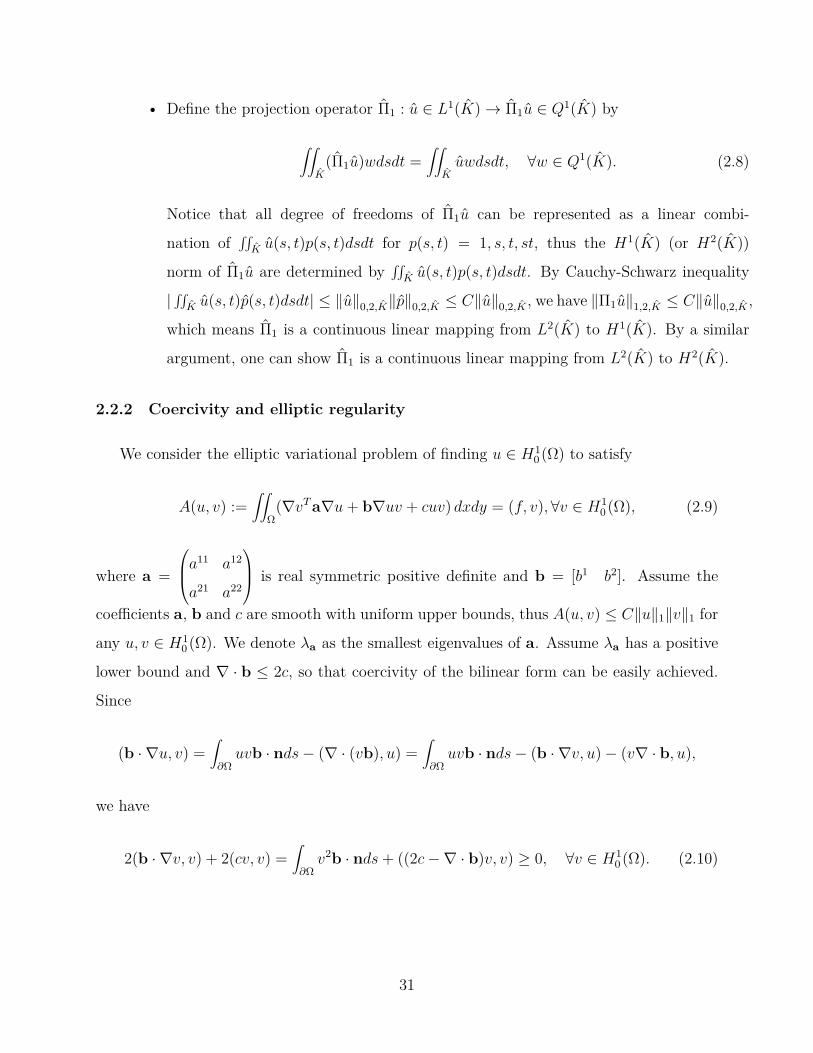
• Define the projection operator Π1 : u ∈ L1(K)→ Π1u ∈ Q1(K) by

∫∫K

(Π1u)wdsdt =∫∫

Kuwdsdt, ∀w ∈ Q1(K). (2.8)

Notice that all degree of freedoms of Π1u can be represented as a linear combi-

nation of∫∫

K u(s, t)p(s, t)dsdt for p(s, t) = 1, s, t, st, thus the H1(K) (or H2(K))

norm of Π1u are determined by∫∫

K u(s, t)p(s, t)dsdt. By Cauchy-Schwarz inequality

|∫∫

K u(s, t)p(s, t)dsdt| ≤ ‖u‖0,2,K‖p‖0,2,K ≤ C‖u‖0,2,K , we have ‖Π1u‖1,2,K ≤ C‖u‖0,2,K ,

which means Π1 is a continuous linear mapping from L2(K) to H1(K). By a similar

argument, one can show Π1 is a continuous linear mapping from L2(K) to H2(K).

2.2.2 Coercivity and elliptic regularity

We consider the elliptic variational problem of finding u ∈ H10 (Ω) to satisfy

A(u, v) :=∫∫

Ω(∇vT a∇u+ b∇uv + cuv) dxdy = (f, v),∀v ∈ H1

0 (Ω), (2.9)

where a =

a11 a12

a21 a22

is real symmetric positive definite and b = [b1 b2]. Assume the

coefficients a, b and c are smooth with uniform upper bounds, thus A(u, v) ≤ C‖u‖1‖v‖1 for

any u, v ∈ H10 (Ω). We denote λa as the smallest eigenvalues of a. Assume λa has a positive

lower bound and ∇ · b ≤ 2c, so that coercivity of the bilinear form can be easily achieved.

Since

(b · ∇u, v) =∫

∂Ωuvb · nds− (∇ · (vb), u) =

∫∂Ωuvb · nds− (b · ∇v, u)− (v∇ · b, u),

we have

2(b · ∇v, v) + 2(cv, v) =∫

∂Ωv2b · nds+ ((2c−∇ · b)v, v) ≥ 0, ∀v ∈ H1

0 (Ω). (2.10)

31

By the equivalence of two norms | · |1 and ‖·‖1 for the space H10 (Ω) (see [3 ]), we conclude that

the bilinear form A(u, v) = (a∇u,∇v) + (b · ∇u, v) + (cu, v) satisfies coercivity A(v, v) ≥

C‖v‖1 for any v ∈ H10 (Ω).

The coercivity can also be achieved if we assume |b| < 4λac. By Young’s inequality

|(b · ∇v, v)| ≤∫∫

Ω

|b · ∇v|2

4c + c|v|2dxdy ≤(|b|2

4c ∇v,∇v)

+ (cv, v),

we have

A(v, v) ≥ (a∇v,∇v) + (cv, v)− |(b · ∇v, v)| ≥(

(λa −|b|2

4c )∇v,∇v)> 0, ∀v ∈ H1

0 (Ω).

(2.11)

Let A∗ be the dual operator of A, i.e., A∗(u, v) = A(v, u). We need to assume the elliptic

regularity holds for the dual problem of (2.9 ) :

w ∈ H10 (Ω), A∗(w, v) = (f, v), ∀v ∈ H1

0 (Ω) =⇒ ‖w‖2 ≤ C‖f‖0, (2.12)

where C is independent of w and f . See [33 ], [34 ] for the elliptic regularity with Lipschitz

continuous coefficients on a Lipschitz domain.

2.3 Quadrature Error Estimates

In the following, we will use ˆ for a function to emphasize the function is defined on or

transformed to the reference cell K = [−1, 1]× [−1, 1] from a mesh cell.

2.3.1 Standard estimates

By the abstract Bramble-Hilbert Lemma in [35 ], with the result ‖v‖m,p,Ω ≤ C(|v|0,p,Ω +

[v]m,p,Ω) for any v ∈ Wm,p(Ω) [36 ], [37 ], the Bramble-Hilbert Lemma for Qk polynomials can

be stated as (see Exercise 3.1.1 and Theorem 4.1.3 in [38 ]):

32

Theorem 2.3.1. If a continuous linear mapping Π : Hk+1(K)→ Hk+1(K) satisfies Πv = v

for any v ∈ Qk(K), then

‖u− Πu‖k+1,K ≤ C[u]k+1,K , ∀u ∈ Hk+1(K). (2.13)

Thus if l(·) is a continuous linear form on the space Hk+1(K) satisfying l(v) = 0,∀v ∈ Qk(K),

then

|l(u)| ≤ C‖l‖k+1,K [u]k+1,K , ∀u ∈ Hk+1(K),

where ‖l‖k+1,K is the norm in the dual space of Hk+1(K).

For Qk element (k ≥ 2), consider (k + 1) × (k + 1) Gauss-Lobatto quadrature, which is

exact for integration of Q2k−1 polynomials.

It is straightforward to establish the interpolation error:

Theorem 2.3.2. For a smooth function a, |a− aI |0,∞,Ω = O(hk+1)|a|k+1,∞,Ω.

Let sj, tj and wj (j = 1, · · · , k + 1) be the Gauss-Lobatto quadrature points and weight

for the interval [−1, 1]. Notice f coincides with its Qk interpolant fI at the quadrature points

and the quadrature is exact for integration of fI , the quadrature can be expressed on K as

k+1∑i=1

k+1∑j=1

f(si, tj)wiwj =∫∫

KfI(x, y)dxdy,

thus the quadrature error is related to interpolation error:

∫∫Kf(x, y)dxdy −

k+1∑i=1

k+1∑j=1

f(si, tj)wiwj =∫∫

Kf(x, y)dxdy −

∫∫KfI(x, y)dxdy.

We have the following estimates on the quadrature error:

Theorem 2.3.3. For n = 2 and a sufficiently smooth function a(x, y), if k ≥ 2 and m is an

integer satisfying k ≤ m ≤ 2k, we have

∫∫ea(x, y)dxdy −

∫∫eaI(x, y)dxdy = O(hm+ n

2 )[a]m,e = O(hm+n)[a]m,∞,e.

33

Proof. Let E(a) denote the quadrature error for function a(x, y) on e. Let E(a) denote the

quadrature error for the function a(s, t) = a(sh+ xe, th+ ye) on the reference cell K. Then

for any f ∈ Hm(K) (m ≥ k ≥ 2), since quadrature are represented by point values, with the

Sobolev’s embedding we have

|E(f)| ≤ C|f |0,∞,K ≤ C‖f‖m,2,K .

Thus E(·) is a continuous linear form on Hm(K) and E(f) = 0 if f ∈ Qm−1(K). With (2.5 ),

the Bramble-Hilbert lemma implies

|E(a)| = hn|E(a)| ≤ Chn[a]m,2,K = O(hm+ n2 )[a]m,2,e = O(hm+n)[a]m,∞,e.

Theorem 2.3.4. If k ≥ 2, (f, vh)− 〈f, vh〉h = O(hk+2)‖f‖k+2‖vh‖2, ∀vh ∈ V h.

Proof. This result is a special case of Theorem 5 in [30 ]. For completeness, we include a

proof. Let E(·) denote the quadrature error term on the reference cell K. Consider the

projection (2.8 ). Let Π1 denote the same projection on e. Since Π1 leaves Q0(K) invariant,

by the Bramble-Hilbert lemma on Π1, we get [vh − Π1vh]1,K ≤ ‖vh − Π1vh‖1,K ≤ C[vh]1,K

thus [Π1vh]1,K ≤ [vh]1,K + [vh − Π1vh]1,K ≤ C[vh]1,K . By setting w = Π1vh in (2.8 ), we get

|Π1vh|0,K ≤ |vh|0,K . For k ≥ 2, repeat the proof of Theorem 2.3.3 , we can get

|E(fΠ1vh)| ≤ C[fΠ1vh]k+2,K ≤ C([f ]k+2,K |Π1vh|0,∞,K + [f ]k+1,K |Π1vh|1,∞,K),

where the fact [Π1vh]l,∞,K = 0 for l ≥ 2 is used. The equivalence of norms over Q1(K)

implies

|E(fΠ1vh)| ≤ C([f ]k+2,K |Π1vh|0,K + [f ]k+1,K |Π1vh|1,K)

≤ C([f ]k+2,K |vh|0,K + [f ]k+1,K |vh|1,K).

34

Next consider the linear form f ∈ Hk(K) → E(f(vh − Π1vh)). Due to the embedding

Hk(K) → C0(K), it is continuous with operator norm ≤ C‖vh − Π1vh‖0,K since

|E(f(vh − Π1vh))| ≤ C|f(vh − Π1vh)|0,∞,K ≤ C|f |0,∞,K |vh − Π1vh|0,∞,K

≤ C‖f‖k,K‖vh − Π1vh‖0,K .

For any f ∈ Qk−1(K), E(f vh) = 0. By the Bramble-Hilbert lemma, we get

|E(f(vh − Π1vh))| ≤ C[f ]k,K‖vh − Π1vh‖0,K ≤ C[f ]k,K [vh]2,K .

So on a cell e, with (2.5 ), we get

E(fvh) = hnE(f vh) = Chk+2([f ]k+2,e|vh|0,e + [f ]k+1,e|vh|1,e + [f ]k,e[vh]2,e).

Summing over e and use Cauchy-Schwarz inequality, we get the desired result.

Remark 2.3.5. By the Theorem 2.3.1 , on the reference cell K, for a(x, y) ∈ Hk+2(e) and

k ≥ 2, we have

∫∫Ka(s, t)− aI(s, t)dsdt ≤ C[a]k+2,K ≤ C[a]k+2,∞,K , (2.14)

and

‖a− aI‖k+1,K ≤ C[a]k+1,K . (2.15)

Lemma 2.3.6. If g ∈ Hk+3(∂Ω) and vh ∈ V h, then for k ≥ 3, we have

∫∂Ω

(g − gI)vhdµ = O(hk+2.5)‖g‖k+3,∂Ω‖vh‖2.

Proof. Note

∫∂Ω

(g − gI)vhdµ =∫

∂Ω(g − gI)(vh − Π1vh)dµ+

∫∂Ω

(g − gI)Π1vhdµ = I + II.

35

In the following, we will focus on the left boundary L2 instead of ∂Ω since the same estimate

can be applied to the top boundary L1, bottom boundary L3 and right boundary L4 as well.

Assume the left boundary of cell e is denoted as le2.

For part I, by the Bramble-Hilbert Lemma, we have

∫L2

(g − gI)(vh − Π1vh)(−1, y)dy

=h∑

e∩L2 6=∅

∫ 1

−1(g − gI)(vh − Π1vh)(−1, t)dt

≤h∑

e∩L2 6=∅

(∫ 1

−1|g − gI |2(−1, t)dt

) 12(∫ 1

−1|vh − Π1vh|2(−1, t)dt

) 12

≤h∑

e∩L2 6=∅

(∫ 1

−1|∂k+1

t g|2(−1, t)dt) 1

2(∫ 1

−1|∂2

t vh|2(−1, t)dt) 1

2= O(hk+3)

∑e∩L2 6=∅

|g|k+1,le2|vh|2,le2

.

For part II, let E1(·) denote the quadrature error term on the reference cell K1 = [−1, 1],

then

∫L2

(g−gI)Π1vhdy =∫

L2(g−gI)Π1vhdµ−

∫L2

(g−gI)Π1vhdhy = h

∑e∩L2 6=∅

E1 ((g − gI)Π1vh(−1, t)) .

Following the proof of Theorem 2.3.4 , we have

E1((g − gI)Π1vh(−1, t)

)≤ C[(g − gI)Π1vh(−1, t)]k+3,K1

≤C[g(−1, t)]k+3,K1

|vh|0,K1+ [g(−1, t)]k+2,K1

|vh|1,K1

)= O(hk+2)‖g‖k+3,le2

‖vh‖1,le2.

Thus ∫L2

(g − gI)Π1vhdy = O(hk+3)∑

e∩L2 6=∅‖g‖k+3,le2

‖vh‖1,le2.

For polynomial q(s, t) ∈ Q2k(K), let sα and ωα (α = 1, 2, · · · , k+2) denote the quadrature

points and weights in (k + 2)-point Gauss-Lobatto quadrature rule for s ∈ [−1, 1]. Since

q2(s, t) ∈ Q2k(K), (k + 2)-point Gauss-Lobatto quadrature is exact for s-integration thus

∫ 1

−1

∫ 1

−1q2(s, t)dsdt =

k+2∑α=1

ωα

∫ 1

−1q2(sα, t)dt,

36

which implies ∫ 1

−1q2(±1, t)dt ≤ C

∫ 1

−1

∫ 1

−1q2(s, t)dsdt, (2.16)

thus

h12 |q|0,le2

≤ C|q|0,e. (2.17)

Above all, we have

∫L2

(g − gI)vh(−1, y)dy

=O(hk+3)∑

e∩L2 6=∅‖g‖k+3,le2

‖vh‖2,le2= O(hk+2.5)

∑e∩L2 6=∅

‖g‖k+3,le2‖vh‖2,e = O(hk+2.5)‖g‖k+3,L2‖vh‖2,Ω,

which implies the theorem.

The following two results are also standard estimates obtained by applying the Bramble-

Hilbert Lemma.

Lemma 2.3.7. If f ∈ H2(Ω) or f ∈ V h, we have (f, vh)−〈f, vh〉h = O(h2)|f |2‖vh‖0, ∀vh ∈

V h.

Proof. For simplicity, we ignore the subscript in vh. Let E(f) denote the quadrature error

for integrating f(x, y) on e. Let E(f) denote the quadrature error for integrating f(s, t) =

f(xe +sh, ye + th) on the reference cell K. Due to the embedding H2(K) → C0(K), we have

|E(f v)| ≤ C|f v|0,∞,K ≤ C|f |0,∞,K |v|0,∞,K ≤ C‖f‖2,K‖v‖0,K .

Thus the mapping f → E(f v) is a continuous linear form on H2(K) and its norm is bounded

by C‖v‖0,K . If f ∈ Q1(K), then we have E(f v) = 0. By the Bramble-Hilbert Lemma

Theorem 2.3.1 on this continuous linear form, we get

|E(f v)| ≤ C[f ]2,K‖v‖0,K .

37

So on a cell e, we get

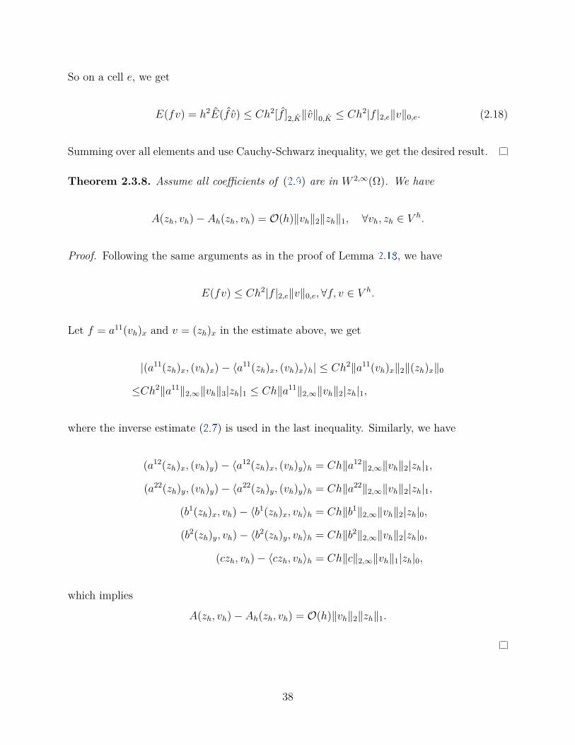
E(fv) = h2E(f v) ≤ Ch2[f ]2,K‖v‖0,K ≤ Ch2|f |2,e‖v‖0,e. (2.18)

Summing over all elements and use Cauchy-Schwarz inequality, we get the desired result.

Theorem 2.3.8. Assume all coefficients of (2.9 ) are in W 2,∞(Ω). We have

A(zh, vh)− Ah(zh, vh) = O(h)‖vh‖2‖zh‖1, ∀vh, zh ∈ V h.

Proof. Following the same arguments as in the proof of Lemma 2.18 , we have

E(fv) ≤ Ch2|f |2,e‖v‖0,e,∀f, v ∈ V h.

Let f = a11(vh)x and v = (zh)x in the estimate above, we get

|(a11(zh)x, (vh)x)− 〈a11(zh)x, (vh)x〉h| ≤ Ch2‖a11(vh)x‖2‖(zh)x‖0

≤Ch2‖a11‖2,∞‖vh‖3|zh|1 ≤ Ch‖a11‖2,∞‖vh‖2|zh|1,

where the inverse estimate (2.7 ) is used in the last inequality. Similarly, we have

(a12(zh)x, (vh)y)− 〈a12(zh)x, (vh)y〉h = Ch‖a12‖2,∞‖vh‖2|zh|1,

(a22(zh)y, (vh)y)− 〈a22(zh)y, (vh)y〉h = Ch‖a22‖2,∞‖vh‖2|zh|1,

(b1(zh)x, vh)− 〈b1(zh)x, vh〉h = Ch‖b1‖2,∞‖vh‖2|zh|0,

(b2(zh)y, vh)− 〈b2(zh)y, vh〉h = Ch‖b2‖2,∞‖vh‖2|zh|0,

(czh, vh)− 〈czh, vh〉h = Ch‖c‖2,∞‖vh‖1|zh|0,

which implies

A(zh, vh)− Ah(zh, vh) = O(h)‖vh‖2‖zh‖1.

38

2.3.2 A refined consistency error

In this subsection, we will show how to establish the desired consistency error estimate

for smooth enough coefficients:

A(u, vh)− Ah(u, vh) =

O(hk+2)‖u‖k+3‖vh‖2, ∀vh ∈ V h

0

O(hk+ 32 )‖u‖k+3‖vh‖2, ∀vh ∈ V h

.

Theorem 2.3.9. Assume a(x, y) ∈ W k+2,∞(Ω), u ∈ Hk+3(Ω), k ≥ 2, then

(a∂xu, ∂xvh)− 〈a∂xu, ∂xvh〉h =

O(hk+2)‖a‖k+2,∞‖u‖k+3‖vh‖2, ∀vh ∈ V h0 , (2.19a)

O(hk+ 32 )‖a‖k+2,∞‖u‖k+3‖vh‖2, ∀vh ∈ V h, (2.19b)

(a∂xu, ∂yvh)− 〈a∂xu, ∂yvh〉h =

O(hk+2)‖a‖k+2,∞‖u‖k+3‖vh‖2, ∀vh ∈ V h0 , (2.20a)

O(hk+ 32 )‖a‖k+2,∞‖u‖k+3‖vh‖2, ∀vh ∈ V h, (2.20b)

(a∂xu, vh)− 〈a∂xu, vh〉h = O(hk+2)‖a‖k+2,∞‖u‖k+3‖vh‖2, ∀vh ∈ V h0 , (2.21)

(au, vh)− 〈au, vh〉h = O(hk+2)‖a‖k+2,∞‖u‖k+2‖vh‖2, ∀vh ∈ V h0 . (2.22)

Remark 2.3.10. We emphasize that Theorem 2.3.9 cannot be proven by applying the Bramble-

Hilbert Lemma directly. Consider the constant coefficient case a(x, y) ≡ 1 and k = 2 as an

example,

(∂xu, ∂xvh)− 〈∂xu, ∂xvh〉h =∑

e

(∫∫eux(vh)xdxdy −

∫∫eux(vh)xd

hxdhy).

Since the 3×3 Gauss-Lobatto quadrature is exact for integratingQ3 polynomials, by Theorem

2.3.1 we have

∣∣∣∣∫∫eux(vh)xdxdy −

∫∫eux(vh)xd

hxdhy

∣∣∣∣ =∣∣∣∣∫∫

Kus(vh)sdsdt−

∫∫Kus(vh)sd

hsdht

∣∣∣∣ ≤ C[us(vh)s]4,K .

39

Notice that vh is Q2 thus (vh)stt does not vanish and [(vh)s]4,K ≤ C|vh|3,K . So by Bramble-

Hilbert Lemma for Qk polynomials, we can only get

∫∫eux(vh)xdxdy −

∫∫eux(vh)xd

hxdhy = O(h4)‖u‖5,e‖vh‖3,e.

Thus by Cauchy-Schwarz inequality after summing over e, we only have

(∂xu, ∂xvh)− 〈∂xu, ∂xvh〉h = O(h4)‖u‖5‖vh‖3.

In order to get the desired estimate involving only the broken H2-norm of vh, we will

take advantage of error cancellations between neighboring cells through integration by parts.

Proof. For simplicity, we ignore the subscript h of vh in this proof and all the following v

are in V h which are Qk polynomials in each cell. First, by Theorem 2.3.4 , we easily obtain

(2.21 ) and (2.22 ):

(aux, v)− 〈aux, v〉h = O(hk+2)‖aux‖k+2‖v‖2 = O(hk+2)‖a‖k+2,∞‖u‖k+3‖v‖2,

(au, v)− 〈au, v〉h = O(hk+2)‖au‖k+2‖v‖2 = O(hk+2)‖a‖k+2,∞‖u‖k+2‖v‖2.

We will only discuss (aux, vx) − 〈aux, vx〉h and the same discussion also applies to derive

(2.20a ) and (2.20b ).

Since we have

(aux, vx)− 〈aux, vx〉h =∑

e

(∫∫eauxvxdxdy −

∫∫eauxvxd

hxdhy)

=∑

e

(∫∫Kausvsdsdt−

∫∫Kausvsd

hsdht)

=∑

e

(∫∫Kausvsdsdt−

∫∫K

(aus)I vsdhsdht

),

where we use the fact ausvs = (aus)I vs on the Gauss-Lobatto quadrature points. For fixed

t, (aus)I vs is a polynomial of degree 2k − 1 w.r.t. variable s, thus the (k + 1)-point Gauss-

Lobatto quadrature is exact for its s-integration, i.e.,

∫∫K

(aus)I vsdhsdht =

∫∫K

(aus)I vsdsdht.

40

To estimate the quadrature error we introduce some intermediate values then do interpreta-

tion by parts,

∫∫Kausvsdsdt−

∫∫K

(aus)I vsdhsdht (2.23)

=∫∫

Kausvsdsdt−

∫∫K

(aus)I vsdsdt+∫∫

K(aus)I vsdsdt−

∫∫K

(aus)I vsdsdht (2.24)

=∫∫

K[aus − (aus)I ] vsdsdt+

(∫∫K

[(aus)I ]s vdsdht−

∫∫K

[(aus)I ]s vdsdt)

(2.25)

+(∫ 1

−1(aus)I vdt

∣∣∣∣s=1

s=−1−∫ 1

−1(aus)I vd

ht∣∣∣∣s=1

s=−1

)= I + II + III. (2.26)

For the first term in (2.26 ), let vs be the cell average of vs on K, then

I =∫∫

K(aus − (aus)I) vsdsdt+

∫∫K

(aus − (aus)I) (vs − vs)dsdt.

By (2.14 ) we have

∣∣∣∣∫∫K

(aus − (aus)I) vsdsdt∣∣∣∣ ≤ C[aus]k+2,K

∣∣∣vs

∣∣∣ = O(hk+2)‖a‖k+2,∞,e‖u‖k+3,e‖v‖1,e.

By Cauchy-Schwarz inequality, the Bramble-Hilbert Lemma on interpolation error and Poincaré

inequality, we have

∣∣∣∣∫∫K

(aus − (aus)I) (vs − vs)dsdt∣∣∣∣ ≤ |aus − (aus)I |0,K |vs − vs|0,K

≤C[aus]k+1,K |v|2,K = O(hk+2)‖a‖k+1,∞,e‖u‖k+2,e‖v‖2,e.

Thus we have

I = O(hk+2)‖a‖k+2,∞,e‖u‖k+3,e‖v‖2,e.

For the second term in (2.26 ), we can estimate it the same way as in the proof of Theorem

2.4. in [39 ]. For each v ∈ Qk(K) we can define a linear form on Hk(K) as

Ev(f) =∫∫

K(FI)svdsdt−

∫∫K

(FI)svdsdht,

41

where F is an antiderivative of f w.r.t. variable s. Due to the linearity of interpolation

operator and differentiating operation, Ev is well defined. By the embedding H2(K) →

C0(K), we have

Ev(f) ≤ C‖F‖0,∞,K‖v‖0,∞,K ≤ C‖f‖0,∞,K‖v‖0,∞,K ≤ C‖f‖2,K‖v‖0,K ≤ C‖f‖k,K‖v‖0,K ,

where we use the fact that all the norms on Qk(K) are equivalent to derive the first inequality.

The above inequalities imply that the mapping Ev is a continuous linear form on Hk(K).

With projection Π1 defined in (2.8 ), we have

Ev(f) = Ev−Π1v(f) + EΠ1v(f), ∀v ∈ Qk(K).

Notice that F by definition is an antiderivative of f w.r.t. only variable s. If f ∈ Qk−1(K),

then FI is a polynomial of degree only k − 1 w.r.t. to variable t thus (FI)s ∈ Qk−1(K). The

quadrature is exact for polynomials of degree 2k− 1, thus Qk−1(K) ⊂ ker Ev−Π1v. So by the

Bramble-Hilbert Lemma, we get

Ev−Π1v(f) ≤ C[f ]k,K‖v − Π1v‖0,K ≤ C[f ]k,K |v|2,K ,

and we also have

EΠ1v(f) =∫∫

K(FI)sΠ1vdsdt−

∫∫K

(FI)sΠ1vdsdht = 0.

Thus we have

∫∫K

[(aus)I ]s vdsdht−

∫∫K

[(aus)I ]s vdsdt = −Ev((aus)s) = −Ev−Π1v((aus)s)

≤C[(aus)s]k,K |vh|2,K ≤ C|aus|k+1,K |v|2,K = O(hk+2)‖a‖k+1,∞,e‖u‖k+2,e|v|2,e

Now we only need to discuss the line integral term. Let L2 and L4 denote the left and

right boundary of Ω and let le2 and le4 denote the left and right edge of element e or lK2 and

lK4 for K. Since (aus)I v mapped back to e will be 1h(aux)Iv which is continuous across le2 and

42

le4, after summing over all elements e, the line integrals along the inner edges are canceled

out and only the line integrals on L2 and L4 remain.

For a cell e adjacent to L2, consider its reference cell K, and define a linear form E(f) =∫ 1−1 f(−1, t)dt−

∫ 1−1 f(−1, t)dht, then we have

E(f v) ≤ C|f |0,∞,lK2|v|0,∞,lK2

≤ C‖f‖2,lK2‖v‖0,lK2

,

which means that the mapping f → E(f v) is continuous with operator norm less than

C‖v‖0,lK2for some C. Clearly we have

E(f v) = E(fΠ1v) + E(f(v − Π1v)).

By the Theorem 2.3.1 we get

E((aus)I(v − Π1v)) ≤ C[(aus)I ]k,lK2

[v]2,lK2≤ C(|aus − (aus)I |k,lK2

+ |aus|k,lK2)[v]2,lK2

≤(|aus|k+1,lK2+ |aus|k,lK2

)[v]2,lK2= O(hk+2)‖a‖k+1,∞,le2

‖u‖k+2,le2[v]2,le2

,

where the first inequality comes from the accuracy of the (k+1)-point Gauss-Lobatto quadra-

ture rule, i.e. E(f) = 0, ∀f ∈ P 2k−1(K). The (k + 1)-point Gauss-Lobatto quadrature rule

also gives

E((aus)IΠ1v) = 0.

For the third term in (2.26 ), we sum them up over all the elements. Then for the line

integral along L2

∑e∩L2 6=∅

∫ 1

−1(aus)I(−1, t)v(−1, t)dt−

∑e∩L2 6=∅

∫ 1

−1(aus)I(−1, t)v(−1, t)dht

=∑

e∩L2 6=∅E((aus)I v) =

∑e∩L2 6=∅

O(hk+2)‖a‖k+1,∞,le2‖u‖k+2,le2

|v|2,le2.

43

Let sα and ωα (α = 1, 2, · · · , k+ 2) denote the quadrature points and weights in (k+ 2)-

point Gauss-Lobatto quadrature rule for s ∈ [−1, 1]. Since v2tt(s, t) ∈ Q2k(K), (k + 2)-point

Gauss-Lobatto quadrature is exact for s-integration thus

∫ 1

−1

∫ 1

−1v2

tt(s, t)dsdt =k+2∑α=1

ωα

∫ 1

−1v2

tt(sα, t)dt,

which implies ∫ 1

−1v2

tt(±1, t)dt ≤ C∫ 1

−1

∫ 1

−1v2

tt(s, t)dsdt, (2.27)

thus

h12 |v|2,le2

≤ C[v]2,e.

By Cauchy-Schwarz inequality and trace inequality, we have

∑e∩L2 6=∅

(∫ 1

−1(aus)I vdt

∣∣∣∣s=1

s=−1−∫ 1

−1(aus)I vd

ht∣∣∣∣s=1

s=−1

)

=∑

e∩L2 6=∅O(hk+2)‖a‖k+1,∞,le2

‖u‖k+2,le2|v|2,le2

=∑

e∩L2 6=∅O(hk+ 3

2 )‖a‖k+1,∞,le2‖u‖k+2,le2

|v|2,e = O(hk+ 32 )‖a‖k+1,∞,Ω‖u‖k+2,L2 |v|2,Ω

=O(hk+ 32 )‖a‖k+1,∞,Ω‖u‖k+3,Ω|v|2,Ω.

Combine all the estimates above, we get (2.19b ). Since the 12 order loss is only due to the

line integral along the boundary ∂Ω. If v ∈ V h0 , vyy = 0 on L2 and L4 so we have (2.19a ).

2.4 The M-type Projection

To establish the superconvergence of C0-Qk finite element method for multi-dimensional

variable coefficient equations, it is necessary to use a special polynomial projection of the

exact solution, which has two equivalent definitions. One is the M-type projection used in

[9 ], [40 ]. The other one is the point-line-plane interpolation used in [10 ], [41 ].

44

For the sake of completeness, we review the relevant results regarding M-type projection,

which is a more convenient tool. Most results in this section were considered and established

for more general rectangular elements in [9 ]. For simplicity, we use some simplified proof

and arguments for Qk element in this section. We only discuss the two dimensional case and

the extension to three dimensions is straightforward.

2.4.1 One dimensional case

The L2-orthogonal Legendre polynomials on the reference interval K = [−1, 1] are given

as

lk(t) = 12kk!

dk

dtk(t2 − 1)k : l0(t) = 1, l1(t) = t, l2(t) = 1

2(3t2 − 1), · · ·

Define their antiderivatives as M-type polynomials:

Mk+1(t) = 12kk!

dk−1

dtk−1 (t2−1)k : M0(t) = 1,M1(t) = t,M2(t) = 12(t2−1),M3(t) = 1

2(t3−t), · · ·

which satisfy the following properties:

• Mk(±1) = 0,∀k ≥ 2.

• If j − i 6= 0,±2, then Mi(t) ⊥Mj(t), i.e.,∫ 1

−1 Mi(t)Mj(t)dt = 0.

• Roots of Mk(t) are the k-point Gauss-Lobatto quadrature points for [−1, 1].

Since Legendre polynomials form a complete orthogonal basis for L2([−1, 1]), for any f(t) ∈

H1([−1, 1]), its derivative f(t) can be expressed as Fourier-Legendre series

f ′(t) =∞∑

j=0bj+1lj(t), bj+1 = (j + 1

2)∫ 1

−1f(t)lj(t)dt.

Define the M-type projection

fk(t) =k∑

j=0bjMj(t),

45

where b0 = f(1)+f(−1)2 is determined by b1 = f(1)−f(−1)

2 to make fk(±1) = f(±1). Since the

Fourier-Legendre series converges in L2, by Cauchy Schwarz inequality,

limk→∞

fk(t)− f(t) = limk→∞

∫ t

−1[fk(x)− f(x)] dx ≤ lim

k→∞

√2‖fk(t)− f(t)‖L2([−1,1]) = 0.

We get the M-type expansion of f(t): f(t) = limk→∞

fk(t) =∞∑

j=0bjMj(t). The remainder Rk(t)

of M-type projection is

R[f ]k(t) = f(t)− fk(t) =∞∑

j=k+1bjMj(t).

The following properties are straightforward to verify:

• fk(±1) = f(±1) thus Rk(±1) = 0 for k ≥ 1.

• R[f ]k(t) ⊥ v(t) for any v(t) ∈ P k−2(t) on [−1, 1], i.e.,∫ 1

−1 R[f ]kvdt = 0.

• R[f ]k(t) ⊥ v(t) for any v(t) ∈ P k−1(t) on [−1, 1].

• For j ≥ 2, bj = (j − 12)[f(t)lj−1(t)|1−1]−

∫ 1−1 f(t)l(j − 1)(t)dt.

• For j ≤ k, |bj| ≤ Ck‖f‖0,∞,K .

• ‖R[f ]k(t)‖0,∞,K ≤ Ck‖f‖0,∞,K .

2.4.2 Two dimensional case

Consider a function f(s, t) ∈ H2(K) on the reference cell K = [−1, 1] × [−1, 1], it has

the expansion

f(s, t) =∞∑

i=0

∞∑j=0

bi,jMi(s)Mj(t),

46

where

b0,0 = 14[f(−1,−1) + f(−1, 1) + f(1,−1) + f(1, 1)],

b0,j, b1,j = 2j − 14

∫ 1

−1[ft(1, t)± ft(−1, t)]lj−1(t)dt, j ≥ 1,

bi,0, bi,1 = 2i− 14

∫ 1

−1[fs(s, 1)± fs(s,−1)]li−1(s)ds, i ≥ 1,

bi,j = (2i− 1)(2j − 1)4

∫∫Kfst(s, t)li−1(s)lj−1(t)dsdt, i, j ≥ 1.

Define the Qk M-type projection of f on K and its remainder as

fk,k(s, t) =k∑

i=0

k∑j=0

bi,jMi(s)Mj(t), R[f ]k,k(s, t) = f(s, t)− fk,k(s, t).

For f(x, y) on e = [xe− h, xe + h]× [ye− h, ye + h], let f(s, t) = f(sh+ xe, th+ ye) then the

Qk M-type projection of f on e and its remainder are defined as

fk,k(x, y) = fk,k(x− xe

h,y − ye

h), R[f ]k,k(x, y) = f(x, y)− fk,k(x, y).

Theorem 2.4.1. The Qk M-type projection is equivalent to the Qk point-line-plane projection

Π defined as follows:

1. Πu = u at four corners of K = [−1, 1]× [−1, 1].

2. Πu− u is orthogonal to polynomials of degree k − 2 on each edge of K.

3. Πu− u is orthogonal to any v ∈ Qk−2(K) on K.

Proof. We only need to show that M-type projection fk,k(s, t) satisfies the same three prop-

erties. By Mj(±1) = 0 for j ≥ 2, we can derive that fk,k = f at (±1,±1). For instance,

fk,k(1, 1) = b0,0 + b1,0 + b0,1 + b1,1 = f(1, 1).

The second property is implied by Mj(±1) = 0 for j ≥ 2 and Mj(t) ⊥ P k−2(t) for

j ≥ k + 1. For instance, at s = 1, fk,k(1, t) − f(1, t) =∞∑

j=k+1(b0,j + b1,j)Mj(t) ⊥ P k−2(t) on

[−1, 1].

The third property is implied by Mj(t) ⊥ P k−2(t) for j ≥ k + 1.

47

Lemma 2.4.2. Assume f ∈ Hk+1(K) with k ≥ 2, then

1. |bi,j| ≤ Ck‖f‖0,∞,K , ∀i, j ≤ k.

2. |bi,j| ≤ Ck|f |i+j,2,K , ∀i, j ≥ 1, i+ j ≤ k + 1.

3. |bi,k+1| ≤ Ck|f |k+1,2,K , 0 ≤ i ≤ k + 1.

4. If f ∈ Hk+2(K), then |bi,k+1| ≤ Ck|f |k+2,2,K , 1 ≤ i ≤ k + 1.

Proof. First of all, similar to the one-dimensional case, through integration by parts, bi,j can

be represented as integrals of f thus |bi,j| ≤ Ck‖f‖0,∞,K for i, j ≤ k.

By the fact that the antiderivatives (and higher order ones) of Legendre polynomials

vanish at ±1, after integration by parts for both variables, we have

|bi,j| ≤ Ck

∫∫K|∂i

s∂jt f |dsdt ≤ Ck|f |i+j,2,K , ∀i, j ≥ 1, i+ j ≤ k + 1.

For the third estimate, by integration by parts only for the variable t, we get

∀i ≥ 1, |bi,k+1| ≤ Ck

∫∫K|∂s∂

kt f |dsdt ≤ Ck|f |k+1,2,K .

For b0,k+1, from the first estimate, we have |b0,k+1| ≤ Ck‖f‖0,∞,K ≤ Ck‖f‖k+1,2,K thus b0,k+1

can be regarded as a continuous linear form on Hk+1(K) and it vanishes if f ∈ Qk(K). So

by the Bramble-Hilbert Lemma, |b0,k+1| ≤ Ck[f ]k+1,2,K .

Finally, by integration by parts only for the variable t, we get

|bi,k+1| ≤ Ck

∫∫K|∂s∂

k+1t f |dsdt ≤ Ck|f |k+2,2,K , 1 ≤ i ≤ k + 1.

Lemma 2.4.3. For k ≥ 2, we have

1. |R[f ]k,k|0,∞,K ≤ Ck[f ]k+1,K, |R[f ]k,k|0,2,K ≤ Ck[f ]k+1,K.

2. |∂sR[f ]k,k|0,∞,K ≤ Ck[f ]k+1,K, |∂sR[f ]k,k|0,2,K ≤ Ck[f ]k+1,K.

48

3.∫∫

K ∂sR[f ]k,kdsdt = 0

Proof. Lemma 2.4.2 implies ‖fk,k‖0,∞,K ≤ Ck‖f‖0,∞,K and ‖∂sfk,k‖0,∞,K ≤ Ck‖f‖0,∞,K .

Thus

∀(s, t) ∈ K, |R[f ]k,k(s, t)| ≤ |fk,k(s, t)|+ |f(s, t)| ≤ Ck‖f‖0,∞,K ≤ Ck‖f‖k+1,K .

Notice that here Ck does not depend on (s, t). So R[f ]k,k(s, t) is a continuous linear form

on Hk+1(K) and its operator norm is bounded by a constant independent of (s, t). Since

it vanishes for any f ∈ Qk(K), by the Bramble-Hilbert Lemma, we get |R[f ]k,k(s, t)| ≤

Ck[f ]k+1,K where Ck does not depend on (s, t). So the L∞ estimate holds and it implies the

L2 estimate.

The second estimate can be established similarly since we have

|∂sR[f ]k,k(s, t)| ≤ |∂sfk,k(s, t)|+ |∂sf(s, t)| ≤ Ck‖f‖1,∞,K ≤ Ck‖f‖k+1,K .

The third equation is implied by the fact that Mj(t) ⊥ 1 for j ≥ 3 and Mj(t) ⊥ 1 for

j ≥ 2. Another way to prove the third equation is to use integration by parts

∫∫K∂sR[f ]k+1,k+1dsdt =

∫ 1

−1

(R[f ]k+1,k+1(1, t)− R[f ]k+1,k+1(−1, t)

)dt,

which is zero the second property in Theorem 2.4.1 .

For the discussion in the next few subsections, it is useful to consider the lower order

part of the remainder of R[f ]k,k:

Lemma 2.4.4. For f ∈ Hk+2(K) with k ≥ 2, define R[f ]k+1,k+1 − R[f ]k,k = R1 + R2 with

R1 =k∑

i=0bi,k+1Mi(s)Mk+1(t),

R2 =k+1∑j=0

bk+1,jMk+1(s)Mj(t) = Mk+1(s)bk+1(t), bk+1(t) =k+1∑j=0

bk+1,jMj(t).(2.28)

They have the following properties:

49

1.∫∫

K ∂sR1dsdt = 0.

2. |∂sR1|0,∞,K ≤ Ck|f |k+2,2,K, |∂sR1|0,2,K ≤ Ck|f |k+2,2,K .

3. |bk+1(t)| ≤ Ck|f |k+1,K, |bk+1(t)| ≤ Ck|f |k+2,K, ∀t ∈ [−1, 1].

Proof. The first equation is due to the fact that Mk+1(t) ⊥ 1 since k ≥ 2.

Notice that M0(s) = 0, by Lemma 2.4.2 , we have

|∂sR1(s, t)| =∣∣∣∣∣

k∑i=1

bi,k+1Mi(s)Mk+1(t)∣∣∣∣∣ ≤ Ck|f |k+2,K .

So we get the L∞ estimate for |∂sR1(s, t)| thus the L2 estimate.

Similar to the estimates in Lemma 2.4.2 , we can show |bk+1,j| ≤ Ck|f |k+1,K for j ≤ k+ 1,

thus |bk+1(t)| ≤ Ck|f |k+1,K . Since bk+1(t) =k+1∑j=1

bk+1,jMj(t), by the last estimate in Lemma

2.4.2 , we get |bk+1(t)| ≤ Ck|f |k+2,K .

2.4.3 The C0-Qk projection

Now consider a function u(x, y) ∈ Hk+2(Ω), let up(x, y) denote its piecewise Qk M-type

projection on each element e in the mesh Ωh. The first two properties in Theorem 2.4.1

imply that up(x, y) on each edge is uniquely determined by u(x, y) along that edge. Thus

up(x, y) is continuous on Ωh. The approximation error u − up is one order higher at all

Gauss-Lobatto points Z0:

Theorem 2.4.5.

‖u− up‖l2(Ω) = O(hk+2)‖u‖k+2, ∀u ∈ Hk+2(Ω).

‖u− up‖l∞(Ω) = O(hk+2)‖u‖k+2,∞, ∀u ∈ W k+2,∞(Ω).

Proof. Consider any e with cell center (xe, ye), define u(s, t) = u(xe + sh, ye + th). Since

the (k + 1) Gauss-Lobatto points are roots of Mk+1(t), Rk+1,k+1[u] − Rk,k[u] vanishes at

(k+ 1)× (k+ 1) Gauss-Lobatto points on K. By Lemma 2.4.3 , we have |Rk+1,k+1[u](s, t)| ≤

C[u]k+2,K .

50

Mapping back to the cell e, with (2.5 ), at the (k + 1)× (k + 1) Gauss-Lobatto points on

e, |u− up| ≤ Chk+2− n2 [u]k+2,e. Summing over all elements e, we get

‖u− up‖l2(Ω) ≤ C

[hn∑

e

h2k+4−n[u]2k+2,e

] 12

= O(hk+2)[u]k+2,Ω.

If further assuming u ∈ W k+2,∞(Ω), then at the (k + 1)× (k + 1) Gauss-Lobatto points

on e, |u− up| ≤ Chk+2− n2 [u]k+2,e ≤ Chk+2[u]k+2,∞,Ω, which implies the second estimate.

2.5 Superconvergence Of The Bilinear Form

The M-type projection in [9 ], [40 ] is a very convenient tool for discussing the superconver-

gence of function values. Let up be the M-type Qk projection of the smooth exact solution u

and its definition will be given in the following subsection. To establish the superconvergence

of the original finite element method (2.1 ) for a generic elliptic problem (2.9 ) with smooth

coefficients, one can show the following superconvergence of bilinear forms, see [9 ], [10 ] (see

also 4 for a detailed proof):

A(u− up, vh) =

O(hk+2)‖u‖k+3‖vh‖2, ∀vh ∈ V h

0 ,

O(hk+ 32 )‖u‖k+3‖vh‖2, ∀vh ∈ V h.

In this section we will show the superconvergence of the bilinear form Ah:

Ah(u− up, vh) =

O(hk+2)‖u‖k+3‖vh‖2, ∀vh ∈ V h0 , (2.29a)

O(hk+ 32 )‖u‖k+3‖vh‖2, ∀vh ∈ V h. (2.29b)

Lemma 2.5.1. Assume f(s, t) ∈ Hk+3(K), k ≥ 2,

〈R[f ]k+1,k+1 − R[f ]k,k, 1〉K = 0, |〈∂sR[f ]k+1,k+1, 1〉K | ≤ C|f |k+3,K .

51

Proof. First, we have

〈R[f ]k+1,k+1 − R[f ]k,k, 1〉K = 〈Mk+1(t)k∑

i=0bi,k+1Mi(s) +Mk+1(s)

k+1∑j=0

bk+1,jMj(t), 1〉K = 0

due to the fact that roots of Mk+1(t) are the (k+ 1)-point Gauss-Lobatto quadrature points

for [−1, 1].

We have

〈∂sR[f ]k+1,k+1, 1〉K

=〈∂sR[f ]k+2,k+2, 1〉K − 〈∂s(R[f ]k+2,k+2 − R[f ]k+1,k+1), 1〉K

=〈∂sR[f ]k+2,k+2, 1〉K − 〈Mk+2(t)k+1∑i=0

bi,k+2Mi(s) +Mk+2(s)k+2∑j=0

bk+2,jMj(t), 1〉K

=〈∂sR[f ]k+2,k+2, 1〉K − 〈Mk+2(t)k∑

i=0bi+1,k+2li(s), 1〉K + 〈lk+1(s)

k+2∑j=0

bk+2,jMj(t), 1〉K .

Then by Lemma 2.4.3 ,

|〈∂sR[f ]k+2,k+2, 1〉K | ≤ C|f |k+3,K .

Notice that we have 〈lk+1(s)∑k+2

j=0 bk+2,jMj(t), 1〉K = 0 since the (k+1)-point Gauss-Lobatto

quadrature for s-integration is exact and lk+1(s) is orthogonal to 1. Lemma 2.4.2 implies

|bi+1,k+2| ≤ C[f ]k+3,K for i ≥ 0, thus we have

|〈Mk+2(t)k∑

i=0bi+1,k+2li(s), 1〉K | ≤ C[f ]k+3,K .

Lemma 2.5.2. Assume a(x, y) ∈ W k,∞(Ω), u(x, y) ∈ Hk+3(Ω) and k ≥ 2. Then

〈a(u− up)x, (vh)x〉h = O(hk+2)‖a‖2,∞‖u‖k+3‖vh‖2, ∀vh ∈ V h.

52

Proof. As before, we ignore the subscript of vh for simplicity. We have

〈a(u− up)x, vx〉h =∑

e

〈a(u− up)x, vx〉e,h,

and on each cell e,

〈a(u− up)x, vx〉e,h = 〈(R[u]k,k)x, avx〉e,h = 〈(R[u]k,k)s, avs〉K

=〈(R[u]k+1,k+1)s, avs〉K + 〈(R[u]k,k − R[u]k+1,k+1)s, avs〉K . (2.30)

For the first term in (2.30 ), we have

〈(R[u]k+1,k+1)s, avs〉K = 〈(R[u]k+1,k+1)s, avs〉K + 〈(R[u]k+1,k+1)s, a(vs − vs)〉K .

By Lemma 2.5.1 ,

〈(R[u]k+1,k+1)s, a vs〉K ≤ C|a|0,∞|u|k+3,K |v|1,K .

By Lemma 2.4.3 ,

|(R[u]k+1,k+1)s|0,∞,K ≤ C[u]k+2,K .

By Bramble-Hilbert Lemma Theorem 2.3.1 we have

〈(R[u]k+1,k+1)s, avs〉K = 〈(R[u]k+1,k+1)s, a vs〉K + 〈(R[u]k+1,k+1)s, (a− a)vs〉K

≤C(|a|0,∞|u|k+3,K |v|1,K + |a− a|0,∞|u|k+2,K |v|1,K)

≤C(|a|0,∞|u|k+3,K |v|1,K + |a|1,∞|u|k+2,K |v|1,K) = O(hk+2)‖a‖1,∞,e‖u‖k+3,e‖v‖1,e,

and

〈(R[u]k+1,k+1)s, a(vs − vs)〉K ≤ C[u]k+2,2,K |a|0,∞,K |vs − vs|0,∞,K

≤C[u]k+2,2,K |a|0,∞,K |vs − vs|0,2,K = O(hk+2)[u]k+2,2,e|a|0,∞,e|v|2,2,e.

Thus,

〈(R[u]k+1,k+1)s, avs〉K = O(hk+2)‖a‖1,∞,e|u|k+3,2,e‖v‖2,e. (2.31)

53

For the second term in (2.30 ), we have

〈(R[u]k,k − R[u]k+1,k+1)s, avs〉K

=− 〈(Mk+1(t)k∑


k+1∑j=0

bk+1,jMj(t))s, avs〉K

=− 〈Mk+1(t)k−1∑i=0

bi+1,k+1li(s) + lk(s)k+1∑j=0

bk+1,jMj(t), avs〉K

=− 〈Mk+1(t)k−1∑i=0

bi+1,k+1li(s), avs〉K − 〈lk(s)k+1∑j=0

bk+1,jMj(t), avs〉K . (2.32)

Since Mk+1(t) vanishes at (k + 1) Gauss-Lobatto points, we have

〈Mk+1(t)k−1∑i=0

bi+1,3li(s), avs〉K = 0.

For the second term in (2.32 ),

〈lk(s)k+1∑j=0

bk+1,jMj(t), avs〉K = 〈lk(s)k+1∑j=0

bk+1,jMj(t), avs〉K + 〈lk(s)k+1∑j=0

bk+1,jMj(t), a(vs − vs)〉K

=〈lk(s)k+1∑j=0

bk+1,jMj(t), (a− Π1a)vs〉K + 〈lk(s)k+1∑j=0

bk+1,jMj(t), (Π1a)vs〉K

+ 〈lk(s)k+1∑j=0

bk+1,jMj(t), (a− a)(vs − vs)〉K + 〈lk(s)k+1∑j=0

bk+1,jMj(t), a(vs − vs)〉K

=〈lk(s)k+1∑j=0

bk+1,jMj(t), (a− Π1a)vs〉K + 〈lk(s)k+1∑j=0

bk+1,jMj(t), (a− a)(vs − vs)〉K ,

where the last step is due to the facts that (Π1a)vs and a(vs− vs) are polynomials of degree

at most k − 1 with respect to variable s, the (k + 1)-point Gauss-Lobatto quadrature on

s-integration is exact for polynomial of degree 2k− 1, and lk(s) is orthogonal to polynomials

of lower degree. With Lemma 2.4.2 , we have

〈lk(s)k+1∑j=0

bk+1,jMj(t), avs〉K ≤ C|u|k+1,2,K(|a|2,∞|v|1,K + |a|1,∞|v|2,K) = O(hk+2)‖a‖2,∞‖u‖k+1,e‖v‖2,e.

(2.33)

54

Combined with (2.31 ), we have proved the estimate.

Lemma 2.5.3. Assume a(x, y) ∈ W 2,∞(Ω), u(x, y) ∈ Hk+2(Ω) and k ≥ 2. Then

〈a(u− up), vh〉h = O(hk+2)‖a‖2,∞‖u‖k+2‖vh‖2, ∀vh ∈ V h.

Proof. As before, we ignore the subscript of vh for simplicity and

〈a(u− up), v〉h =∑

e

〈a(u− up), v〉e,h.

On each cell e we have

〈a(u− up), v〉e,h = 〈R[u]k,k, av〉e,h = h2〈R[u]k,k, av〉K = h2〈R[u]k,k, av − av〉K + h2〈R[u]k,k, av〉K .

(2.34)

For the first term in (2.34 ), due to the embedding H2(K) → C0(K), Bramble-Hilbert Lemma

Theorem 2.3.1 and Lemma 2.4.3 , we have

h2〈R[u]k,k, av − av〉K ≤ Ch2|R[u]k,k|∞|av − av|∞ ≤ Ch2|u|k+1,K‖av − av‖2,K

≤ Ch2|u|k+1,K(‖av − av‖L2(K) + |av|1,K + |av|2,K)

≤ Ch2|u|k+1,K(|av|1,K + |av|2,K) = O(hk+2)‖a‖2,∞,e‖u‖k+1,e‖v‖2,e.


h2〈R[u]k+1,k+1, av〉K = h2〈R[u]k+1,k+1, av〉K − h2〈R[u]k+1,k+1 − R[u]k,k, av〉K .

By Lemma 2.4.3 and Lemma 2.5.1 we have

h2〈R[u]k+1,k+1, av〉K ≤ Ch2|u|k+2,K |av|0,K = O(hk+2)‖a‖0,∞,e‖u‖k+2,e‖v‖0,e,

and

h2〈R[u]k+1,k+1 − R[u]k,k, av〉K = 0.

55

Thus, we have 〈a(u− up), vh〉h = O(hk+2)‖a‖2,∞‖u‖k+2‖vh‖2.

Lemma 2.5.4. Assume a ∈ W 2,∞(Ω), u ∈ Hk+3(Ω) and k ≥ 2. Then

〈a(u− up)x, vh〉h = O(hk+2)‖a‖2,∞‖u‖k+3‖vh‖2, ∀vh ∈ V h.

Proof. As before, we ignore the subscript in vh and we have

〈a(u− up)x, v〉h =∑

e

〈a(u− up)x, v〉e,h.

On each cell e, we have

〈a(u− up)x, v〉e,h = 〈(R[u]k,k)x, av〉e,h = h〈(R[u]k,k)s, av〉K

=h〈(R[u]k+1,k+1)s, av〉K − h〈(R[u]k+1,k+1 − R[u]k,k)s, av〉K . (2.35)

For the first term in (2.35 ), we have

〈(R[u]k+1,k+1)s, av〉K ≤ 〈(R[u]k+1,k+1)s, av〉K + 〈(R[u]k+1,k+1)s, av − av〉K

Due to Lemma 2.5.1 ,

h〈(R[u]k+1,k+1)s, av〉K ≤ Ch‖a‖0,∞|u|k+3,K‖v‖0,K = O(hk+2)‖a‖0,∞‖u‖k+3,e‖v‖0,e,

and by the same arguments as in the proof of Lemma 2.5.3 we have

h〈(R[u]k+1,k+1)s, av − av〉K ≤ Ch|(R[u]k+1,k+1)s|∞|av − av|∞ ≤ Ch|u|k+2,K‖av − av‖2,K

≤Ch|u|k+2,K(‖av − av‖L2(K) + |av|1,K + |av|2,K) ≤ Ch|u|k+2,K(|av|1,K + |av|2,K) = O(hk+2)‖a‖2,∞‖u‖k+2,e‖v‖2,e.

Thus

h〈(R[u]k+1,k+1)s, av〉K = O(hk+2)‖a‖2,∞‖u‖k+3,e‖v‖2,e. (2.36)

56


〈(R[u]k+1,k+1 − R[u]k,k)s, av〉K

=〈(Mk+1(t)k∑


k+1∑j=0

bk+1,jMj(t))s, av〉K

=〈Mk+1(t)k−1∑i=0

bi+1,k+1li(s) + lk(s)k+1∑j=0

bk+1,jMj(t), av〉K

=〈Mk+1(t)k−1∑i=0

bi+1,k+1li(s), av〉K + 〈lk(s)k+1∑j=0

bk+1,jMj(t), av〉K

=〈lk(s)k+1∑j=0

bk+1,jMj(t), av〉K ,

where the last step is due to that Mk+1(t) vanishes at (k + 1) Gauss-Lobatto points. Then

〈(R[u]k,k − R[u]k+1,k+1)s, av〉K = 〈lk(s)k+1∑j=0

bk+1,jMj(t), av〉K

=〈lk(s)k+1∑j=0

bk+1,jMj(t), av − Π1(av)〉K + 〈lk(s)k+1∑j=0

bk+1,jMj(t), Π1(av)〉K

=〈lk(s)k+1∑j=0

bk+1,jMj(t), av − Π1(av)〉K ,

where the last step is due to the facts that Π1(av) is a linear function in s thus the (k + 1)-

point Gauss-Lobatto quadrature on s-variable is exact, and lk(s) is orthogonal to linear

functions.

By Lemma 2.4.4 , Lemma 2.4.2 , and Theorem 2.3.1 , we have

〈(R[u]k,k − R[u]k+1,k+1)s, av〉K = 〈lk(s)k+1∑j=0

bk+1,jMj(t), av − Π1(av)〉K

≤C|u|k+1,K |av|2,K ≤ C|u|k+1,K(|a|2,∞,K |v|0,K + |a|1,∞,K |v|1,K + |a|0,∞|v|2,K)

Thus

h〈(R[u]k,k − R[u]k+1,k+1)s, av〉K = O(hk+2)‖a‖2,∞‖u‖k+1,e‖v‖2,e. (2.37)

By (2.36 ) and (2.37 ) and sum up over all the cells, we get the desired estimate.

57

Lemma 2.5.5. Assume a(x, y) ∈ W 4,∞(Ω), u(x, y) ∈ Hk+3(Ω) and k ≥ 2. Then

〈a(u− up)x, (vh)y〉h =

O(hk+ 3

2 )‖a‖k+2,∞‖u‖k+3‖vh‖2, ∀vh ∈ V h, (2.38a)

O(hk+2)‖a‖k+2,∞‖u‖k+3‖vh‖2, ∀vh ∈ V h0 . (2.38b)

Proof. We ignore the subscript in vh and we have

〈a(u− up)x, vy〉h =∑

e

〈a(u− up)x, vy〉e,h,

and on each cell e

〈a(u− up)x, vy〉e,h = 〈(R[u]k,k)x, avy〉e,h = 〈(R[u]k,k)s, avt〉K

=〈(R[u]k+1,k+1)s, avt〉K + 〈(R[u]k,k − R[u]k+1,k+1)s, avt〉K . (2.39)

By the same arguments as in the proof of Lemma 2.5.2 , we have

〈(R[u]k+1,k+1)s, avt〉K = O(hk+2)‖a‖1,∞|u|k+3,2,e‖v‖2,e, (2.40)

and

〈(R[u]k,k − R[u]k+1,k+1)s, avt〉K = −〈lk(s)k+1∑j=0

bk+1,jMj(t), avt〉K .

For simplicity, we define

bk+1(t) :=k+1∑j=0

bk+1,jMj(t).

then by the third and fourth estimates in Lemma 2.4.4 , we have

|bk+1(t)| ≤ Ck+1∑j=0|bk+1,j| ≤ C|u|k+1,K ,

|b(m)k+1(t)| ≤ C

k+1∑j=m

|bk+1,j| ≤ C|u|k+2,K , 1 ≤ m,

58

where b(m)k+1(t) is the m-th derivative of bk+1(t). We use the same technique in the proof of

Theorem 2.3.9 and we let lk = lk(s), bk+1 = bk+1(t) in the following,

〈(R[u]k,k − R[u]k+1,k+1)s, avt〉K = −〈lk(s)bk+1(t), avt〉K

=−∫∫

Klk(s)bk+1(t)avtd

hsdht = −∫∫

K(lkbk+1a)I vtd

hsdht

=−∫∫

K(lkbk+1a)I vtd

hsdht+∫∫

Klkbk+1avtdsdt−

∫∫Klkbk+1avtdsdt,

and

−∫∫

K(lkbk+1a)I vtd

hsdht+∫∫

Klkbk+1avtdsdt

=∫∫

K

[lkbk+1a− (lkbk+1a)I

]vtdsdt+

∫∫K

(lkbk+1a)I vtdsdt−∫∫

K(lkbk+1a)I vtd

hsdt

=∫∫

K


]vtdsdt+

∫∫K∂t(lkbk+1a)I vd

hsdt−∫∫

K∂t(lkbk+1a)I vdsdt

+(∫ 1

−1(lkbk+1a)I vds

∣∣∣∣t=1

t=−1−∫ 1

−1(lkbk+1a)I vd

hs∣∣∣∣t=1

t=−1

)= I + II + III.

After integration by parts with respect to the variable s, we have

∫∫Klk(s)bk+1(t)avtdsdt = −

∫∫KMk+1(s)bk+1(t)(asvt + avst)dsdt. (2.41)

Let N(s) be the antiderivative of Mk+1(s). After integration by parts, we have

−∫∫

KMk+1(s)bk+1(t)(asvt + avst) =

∫∫Kbk+1(t)N(s)(assvt + 2asvst) +

∫∫Kbk+1(t)N(s)avsst.

After integration by parts on the t-variable,

−∫∫

Kbk+1(t)N(s)avsst =

∫∫K∂t[bk+1(t)N(s)a]vss −

∫ 1

−1bk+1(t)N(s)avssds

∣∣∣∣t=1

t=−1,

∫∫K∂t[bk+1(t)N(s)a]vss =

∫∫K

[bk+1(t)N(s)a+ bk+1(t)N(s)at]vss.

59

By Lemma 2.4.4 , we have the estimate for the two double integral terms

∣∣∣∣∫∫Kbk+1(t)N(s)(assvt + 2asvst)

∣∣∣∣ ≤ C|u|k+1,2,K(|a|2,∞,K |v|1,2,K + |a|1,∞,K |v|2,2,K),

∣∣∣∣∫∫K

[bk+1(t)N(s)a+ bk+1(t)N(s)at]vss

∣∣∣∣≤C(|u|k+2,2,K |a|0,∞,K |v|2,2,K + |u|k+1,2,K |a|1,∞,K |v|2,2,K),

which gives the estimate Chk+2‖a‖2,∞,Ω‖u‖k+2,e‖v‖k+2,e after mapping back to e.

After mapping back to e, we have

∫ 1

−1bk+1(t)Mk+1(s)avssds

∣∣∣∣t=1

t=−1= h

∫ xe+h

xe−hbk+1(y)Mk+1(

x− xe

h)avxxdx

∣∣∣∣∣y=ye+h

y=ye−h

.

Notice that we have

bk+1(ye + h) = bk+1(1) =k+1∑j=0

bk+1,jMj(1) = bk+1,0 + bk+1,1

= (k + 12)∫ 1

−1∂su(s, 1)lk(s)ds = (k + 1

2)∫ xe+h

xe−h∂xu(x, ye + h)lk(x− xe

h)dx,

and similarly we get bk+1(ye− h) = bk+1(−1) = (k+ 12)∫ xe+h

xe−h ∂xu(x, ye− h)lk(x−xe

h)dx. Thus

the term bk+1(y)Mk+1(x−xe

h)avxx is continuous across the top/bottom edge of cells. Therefore,

if summing over all elements e, the line integral on the inner edges are cancelled out. Let

L1 and L3 denote the top and bottom boundary of Ω. Then the line integral after summing

over e consists of two line integrals along L1 and L3. We only need to discuss one of them.

Let l1 and l3 denote the top and bottom edge of e. First, after integration by parts k

times, we get

bk+1(1) = (k + 12)∫ 1

−1∂su(s, 1)lk(s)ds = (−1)k(k + 1

2)∫ 1

−1

∂k+1

∂sk+1 u(s, 1) 12kk! (s

2 − 1)kds,

60

thus by Cauchy Schwarz inequality we get

|bk+1(1)| ≤ Ck

√√√√∫ 1

−1

[∂k+1

∂sk+1 u(s, 1)]2

ds ≤ Ckhk+ 1

2 |u|k+1,2,l1 .

Second, since v2xx is a polynomial of degree 2k w.r.t. y variable, by using (k+2)-point Gauss

Lobatto quadrature for integration w.r.t. y-variable in∫∫

e v2xxdxdy, we get

∫ xe+h

xe−hv2

xx(x, ye + h)dx ≤ Ch−1∫∫

ev2

xx(x, y)dxdy.

So by Cauchy Schwarz inequality, we have

∫ xe+h

xe−h|vxx(x, ye + h)|dx ≤

√2h√∫ xe+h

xe−hv2

xx(x, ye + h)dx ≤ C|v|2,2,e.

Thus the line integral along L1 can be estimated by considering each e adjacent to L1 in

the reference cell:

∑e∩L1 6=∅

∣∣∣∣∫ 1

−1bk+1(1)Mk+1(s)a(s, 1)vss(s, 1)ds

∣∣∣∣≤

∑e∩L1 6=∅

C|a|0,∞,K |bk+1(1)|∫ 1

−1|vss(s, 1)|ds

=O(hk+ 32 )

∑e∩L1 6=∅

|u|k+1,2,l1

∫ xe+h

xe−h|vxx(x, ye + h)|dx

=O(hk+ 32 )

∑e∩L1 6=∅

|u|k+1,2,l1|v|2,2,e

=O(hk+ 32 )‖u‖k+1,L1‖v‖2,Ω = O(hk+ 3

2 )‖u‖k+2,Ω‖v‖2,Ω,

where the trace inequality ‖u‖k+1,∂Ω ≤ C‖u‖k+2,Ω is used.

Combine all the estimates above and sum over all elements, we have the estimate for the

term∫∫

K lk(s)bk+1(t)avtdsdt:

∑e

∫∫Klk(s)bk+1(t)avtdsdt =

O(hk+ 3

2 )‖a‖k+2,∞‖u‖k+3‖v‖2, ∀v ∈ V h, (2.42a)

O(hk+2)‖a‖k+2,∞‖u‖k+3‖v‖2, ∀v ∈ V h0 . (2.42b)

61

We get (k + 32)-th order for the above estimation. Since the 1

2 order loss is only due to

the line integral along L1 and L3, on which vxx = 0 if v ∈ V h0 , we get (k + 2)-th order.

Then we can do similar estimation as in Theorem 2.3.9 for I, II, III separately.

For term I, by Theorem 2.3.1 and the estimate (2.14 ), we have

∫∫K


]vtdsdt

=∫∫

K


]vtdsdt+

∫∫K


](vt − vt)dsdt

≤C[lkbk+1a

]k+2,K

|v|1,K + C[lkbk+1a

]k+1,K

|v|2,K

≤C(

k+2∑m=2|a|m,∞,K max

t∈[−1,1]|bk+1(t)|

)|v|1,K + C

(k+2∑m=0|a|m,∞,K max

t∈[−1,1]|b(k+2−m)

k+1 (t)|)|v|1,K

+C(

k+1∑m=1|a|m,∞,K max

t∈[−1,1]|bk+1(t)|

)|v|2,K + C

(k+1∑m=0|a|m,∞,K max

t∈[−1,1]|b(k+1−m)

k+1 (t)|)|v|2,K

=O(hk+2)‖a‖k+2,∞‖u‖k+2,e‖v‖2,e.

For term II, as in the proof of Theorem 2.3.9 , we define the linear form as

Ev(f) =∫∫

K(FI)tvdsdt−

∫∫K

(FI)tvdhsdt,

for each v ∈ Qk(K) and F is an antiderivative of f w.r.t. variable t. We can easily see that

Ev is well defined and Ev is a continuous linear form on Hk(K). With projection Π1 defined

in (2.8 ), we have

Ev(f) = Ev−Π1v(f) + EΠ1v(f), ∀v ∈ Qk(K).

Since Qk−1(K) ⊂ ker Ev−Π1v thus

Ev−Π1v(f) ≤ C[f ]k,K‖v − Π1v‖0,K ≤ C[f ]k,K |v|2,K

and

EΠ1v(f) =∫∫

K(FI)tΠ1vdsdt−

∫∫K

(FI)tΠ1vdhsdt = 0.

62

Thus we have

∫∫K∂t(lkbk+1a)I vd

hsdt−∫∫

K∂t(lkbk+1a)I vdsdt = −Ev((lkbk+1a)t)

=− Ev−Π1v((lkbk+1a)t) ≤ C[(lkbk+1a)t]k,K |vh|2,K = O(hk+2)‖a‖k+1,∞,e‖u‖k+2,e|v|2,e.

Now we only need to discuss term III. Let L1 and L3 denote the top and bottom

boundaries of Ω and let le1, le3 denote the top and bottom edges of element e (and lK1 and lK3for K). Notice that after mapping back to the cell e we have

bk+1(ye + h) = bk+1(1) =k+1∑j=0

bk+1,jMj(1) = bk+1,0 + bk+1,1

= (k + 12)∫ 1

−1∂su(s, 1)lk(s)ds = (k + 1

2)∫ xe+h

xe−h∂xu(x, ye + h)lk(x− xe

h)dx,

and similarly we get bk+1(ye− h) = bk+1(−1) = (k+ 12)∫ xe+h

xe−h ∂xu(x, ye− h)lk(x−xe

h)dx. Thus

the term l(x−xe

h)bk+1(y)av is continuous across the top and bottom edges of cells. Therefore,

if summing over all elements e, the line integral on the inner edges are cancelled out. So

after summing over all elements, the line integral reduces to two line integrals along L1 and

L3. We only need to discuss one of them. For a cell e adjacent to L1, consider its reference

cell K and define linear form E(f) =∫ 1

−1 f(s, 1)ds−∫ 1

−1 f(s, 1)dhs, then we have

E(f v) ≤ C|f |0,∞,lK1|v|0,∞,lK1

≤ C‖f‖2,lK1‖v‖0,lK1

,

63

thus the mapping f → E(f v) is continuous with operator norm less than C‖v‖0,lK1for some

C. Since E((aus)IΠ1v) = 0 we have

∑e∩L1 6=∅

∫ 1

−1(lkbk+1a)I vds−

∫ 1

−1(lkbk+1a)I vd

hs

=∑

e∩L1 6=∅E((lkbk+1a)I v) =

∑e∩L1 6=∅

E((lkbk+1a)I(v − Π1v)) ≤∑

e∩L1 6=∅C[(lkbk+1a)I ]

k,lK1[v]2,lK1

≤∑

e∩L1 6=∅C(|lkbk+1a− (lkbk+1a)I |k,lK1

+ |lkbk+1a|k,lK1)[v]2,lK1

≤∑

e∩L1 6=∅(|lkbk+1a|k+1,lK1

+ |lkbk+1a|k,lK1)[v]2,lK1

≤∑

e∩L1 6=∅C‖a‖k,∞,K |bk+1(1)|[v]2,lK1

,

where the first inequality is derived from E(f(v − Π1v)) = 0,∀f ∈ Qk−1(K) and Theorem

2.3.1 .

Since lk(t) = 12kk!

dk

dtk (t2 − 1)k, after integration by parts k times,

bk+1(1) = (k + 12)∫ 1

−1∂su(s, 1)lk(s)dx = (−1)k(k + 1

2)∫ 1

−1∂k+1

s u(s, 1)L(s)ds,

where L(s) is a polynomial of degree 2k by taking antiderivatives of lk(s) k times. Then by

Cauchy-Schwarz inequality we have

bk+1(1) ≤ C(∫ 1

−1|∂k+1

s u(s, 1)|2ds) 1

2≤ Chk+ 1

2 |u|k+1,le1.

By (2.27 ), we get |v|2,lK1= h

32 |v|2,le1

≤ Ch|v|2,e. Thus we have

∑e∩L1 6=∅

∫ 1

−1(lkbk+1a)I vds−

∫ 1

−1(lkbk+1a)I vd

hs ≤∑

e∩L1 6=∅C‖a‖k,∞,K |bk+1(1)||v|2,lK1

=O(hk+ 32 )

∑e∩L1 6=∅

‖a‖k,∞|u|k+1,le1|v|2,e = O(hk+ 3

2 )‖a‖k,∞|u|k+1,L1‖v‖2,Ω = O(hk+ 32 )‖a‖k,∞‖u‖k+2,Ω‖v‖2,Ω,

where the trace inequality ‖u‖k+1,∂Ω ≤ C‖u‖k+2,Ω is used.

Combine all the estimates above, we get (2.38a ). Since the 12 order loss is only due to

the line integral along L1 and L3, on which vxx = 0 if v ∈ V h0 , we get (2.38b ).

By all the discussions in this subsection, we have proven (2.29a ) and (2.29b ).

64

2.6 Homogeneous Dirichlet Boundary Conditions

2.6.1 V h-ellipticity

In order to discuss the scheme (2.2 ), we need to show Ah satisfies V h-ellipticity

∀vh ∈ V h0 , C‖vh‖2

1 ≤ Ah(vh, vh). (2.43)

We first consider the Vh-ellipticity for the case b ≡ 0.

Lemma 2.6.1. Assume the coefficients in (2.9 ) satisfy that b ≡ 0, both c(x, y) and the

eigenvalues of a(x, y) have a uniform upper bound and a uniform positive lower bound, then

there exist two constants C1, C2 > 0 independent of mesh size h such that

∀vh ∈ V h0 , C1‖vh‖2

1 ≤ Ah(vh, vh) ≤ C2‖vh‖21.

Proof. Let Z0,K denote the set of (k+1)× (k+1) Gauss-Lobatto points on the reference cell

K. First we notice that the set Z0,K is a Qk(K)-unisolvent subset. Since the Gauss-Lobatto

quadrature weights are strictly positive, we have

∀p ∈ Qk(K),2∑

i=1〈∂ip, ∂ip〉K = 0 =⇒ ∂ip = 0 at quadrature points,

where i = 1, 2 represents the spatial derivative on variable xi respectively. Since ∂ip ∈

Qk(K) and it vanishes on a Qk(K)-unisolvent subset, we have ∂ip ≡ 0. As a consequence,√∑ni=1〈∂ip, ∂ip〉h defines a norm over the quotient space Qk(K)/Q0(K). Since that | · |1,K

is also a norm over the same quotient space, by the equivalence of norms over a finite

dimensional space, we have

∀p ∈ Qk(K), C1|p|21,K≤

n∑i=1〈∂ip, ∂ip〉K ≤ C2|p|21,K

.

On the reference cell K, by the assumption on the coefficients, we have

C1|vh|21,K≤ C1

n∑i

〈∂ivh, ∂ivh〉K ≤n∑

i,j=1(〈aij∂ivh, ∂j vh〉K + 〈cvh, vh〉K) ≤ C2‖vh‖2

1,K

65

Mapping these back to the original cell e and summing over all elements, by the equiva-

lence of two norms |·|1 and ‖·‖1 for the space H10 (Ω) ⊃ V h

0 [3 ], we get C1‖vh‖21 ≤ Ah(vh, vh) ≤

C2‖vh‖21.

For discussing Vh-ellipticity when b is nonzero, by Young’s inequality we have

|〈b · ∇vh, vh〉h| ≤∑

e

∫∫e

(b · ∇vh)2

4c + c|vh|2dhxdhy ≤ 〈|b|2

4c ∇vh,∇vh〉h + 〈cvh, vh〉h.

Thus we have

〈a∇vh,∇vh〉h + 〈b · ∇vh, vh〉h + 〈cvh, vh〉h ≥ 〈λa∇vh,∇vh〉h − 〈|b|2

4c ∇vh,∇vh〉h,

where λa is smallest eigenvalue of a. Then we have the following Lemma

Lemma 2.6.2. Assume 4λac > |b|2, then there exists a constant C > 0 independent of mesh

size h such that

∀vh ∈ V h0 , Ah(vh, vh) ≥ C‖vh‖2

1.

2.6.2 Standard estimates for the dual problem

In order to apply the Aubin-Nitsche duality argument for establishing superconvergence

of function values, we need certain estimates on a proper dual problem. Define θh := uh−up.

Then we consider the dual problem: find w ∈ H10 (Ω) satisfying

A∗(w, v) = (θh, v), ∀v ∈ H10 (Ω), (2.44)

where A∗(·, ·) is the adjoint bilinear form of A(·, ·) such that

A∗(u, v) = A(v, u) = (a∇v,∇u) + (b · ∇v, u) + (cv, u).

Let wh ∈ V h0 be the solution to

A∗h(wh, vh) = (θh, vh), ∀vh ∈ V h

0 . (2.45)

66

Notice that the right hand side of (2.45 ) is different from the right hand side of the scheme

(2.2 ).

We need the following standard estimates on wh for the dual problem.

Theorem 2.6.3. Assume all coefficients in (2.9 ) are in W 2,∞(Ω). Let w be defined in (2.44 ),

wh be defined in (2.45 ), and θh = uh−up. Assume elliptic regularity (2.12 ) and V h ellipticity

holds, we have

‖w − wh‖1 ≤ Ch‖w‖2,

‖wh‖2 ≤ C‖θh‖0.

Proof. By V h ellipticity, we have C1‖wh− vh‖21 ≤ A∗

h(wh− vh, wh− vh). By the definition of

the dual problem, we have

A∗h(wh, wh − vh) = (θh, wh − vh) = A∗(w,wh − vh), ∀vh ∈ V h

0 .

Thus for any vh ∈ V h0 , by Theorem 2.3.8 , we have

C1‖wh − vh‖21 ≤ A∗

h(wh − vh, wh − vh)

=A∗(w − vh, wh − vh) + [A∗h(wh, wh − vh)− A∗(w,wh − vh)] + [A∗(vh, wh − vh)− A∗

h(vh, wh − vh)]

=A∗(w − vh, wh − vh) + [A(wh − vh, vh)− Ah(wh − vh, vh)]

≤C‖w − vh‖1‖wh − vh‖1 + Ch‖vh‖2‖wh − vh‖1.

Thus

‖w − wh‖1 ≤ ‖w − vh‖1 + ‖wh − vh‖1 ≤ C‖w − vh‖1 + Ch‖vh‖2. (2.46)

Now consider Π1w ∈ V h0 where Π1 is the piecewise Q1 projection and its definition on each

cell is defined through (2.8 ) on the reference cell. By the Bramble Hilbert Lemma Theorem

2.3.1 on the projection error, we have

‖w − Π1w‖1 ≤ Ch‖w‖2, ‖w − Π1w‖2 ≤ C‖w‖2, (2.47)

67

thus ‖Π1w‖2 ≤ ‖w‖2 + ‖w − Π1w‖2 ≤ C‖w‖2. By setting vh = Π1w, from (2.46 ) we have

‖w − wh‖1 ≤ C‖w − Π1w‖1 + Ch‖Π1w‖2 ≤ Ch‖w‖2. (2.48)

By the inverse estimate on the piecewise polynomial wh − Π1w, we get

‖wh‖2 ≤ ‖wh − Π1w‖2 + ‖Π1w − w‖2 + ‖w‖2 ≤ Ch−1‖wh − Π1w‖1 + C‖w‖2. (2.49)

By (2.47 ) and (2.48 ), we also have

‖wh − Π1w‖1 ≤ ‖w − Π1w‖1 + ‖w − wh‖1 ≤ Ch‖w‖2. (2.50)

With (2.49 ), (2.50 ) and the elliptic regularity ‖w‖2 ≤ C‖θh‖0, we get

‖wh‖2 ≤ C‖w‖2 ≤ C‖θh‖0.

2.6.3 Superconvergence of function values

Theorem 2.6.4. Assume aij, bi, c ∈ W k+2,∞(Ω) and u(x, y) ∈ Hk+3(Ω), f(x, y) ∈ Hk+2(Ω)

with k ≥ 2. Assume elliptic regularity (2.12 ) and V h ellipticity holds. Then uh, the numerical

solution from scheme (2.2 ), is a (k+2)-th order accurate approximation to the exact solution

u in the discrete 2-norm over all the (k + 1)× (k + 1) Gauss-Lobatto points:

‖uh − u‖l2(Ω) = O(hk+2)(‖u‖k+3,Ω + ‖f‖k+2,Ω).

Proof. By Theorem 2.3.9 and Theorem 2.3.4 , for any vh ∈ V h0 ,

Ah(u− uh, vh) = [A(u, vh)− Ah(uh, vh)] + [Ah(u, vh)− A(u, vh)]

= A(u, vh)− Ah(uh, vh) +O(hk+2)‖a‖k+2,∞‖u‖k+3‖vh‖2

= [(f, vh)− 〈f, vh〉h] +O(hk+2)‖u‖k+3‖vh‖2 = O(hk+2)(‖u‖k+3 + ‖f‖k+2)‖vh‖2.

68

Let θh = uh−up, then θh ∈ V h0 due to the properties of the M-type projection. So by (2.29a )

and Theorem 2.6.3 , we get

‖θh‖20 = (θh, θh) = Ah(θh, wh) = Ah(uh − u,wh) + Ah(u− up, wh)

=Ah(u− up, wh) +O(hk+2)(‖u‖k+3 + ‖f‖k+2)‖wh‖2

=O(hk+2)(‖u‖k+3 + ‖f‖k+2)‖wh‖2 = O(hk+2)(‖u‖k+3 + ‖f‖k+2)‖θh‖0,

thus

‖uh − up‖0 = ‖θh‖0 = O(hk+2)(‖u‖k+3 + ‖f‖k+2).

Finally, by the equivalence of the discrete 2-norm on Z0 and the L2(Ω) norm in finite-

dimensional space V h and Theorem 2.4.5 , we obtain

‖uh − u‖l2(Ω) ≤ ‖uh − up‖l2(Ω) + ‖up − u‖l2(Ω) ≤ C‖uh − up‖0 + ‖up − u‖l2(Ω)

= O(hk+2)(‖u‖k+3 + ‖f‖k+2).

Remark 2.6.5. To extend the discussions to Neumann type boundary conditions, due to

(2.29b ) and Theorem 2.3.9 , one can only prove (k + 32)-th order accuracy:

‖uh − u‖l2(Ω) = O(hk+ 32 )(‖u‖k+3 + ‖f‖k+2).

On the other hand, for solving a general elliptic equation, only O(hk+ 32 ) superconvergence

at all Lobatto point can be proven for Neumann boundary conditions even for the full finite

element scheme (2.1 ), see [9 ].

Remark 2.6.6. All key discussions can be extended to three-dimensional cases. For instance,

M-type expansion has been used for discussing superconvergence for the three-dimensional

case [9 ]. The most useful technique in Section 2.3.2 to obtain desired consistency error

estimate is to derive error cancellations between neighboring cells through integration by

69

parts on suitable interpolation polynomials, which still seems possible on rectangular meshes

in three dimensions.

2.7 Nonhomogeneous Dirichlet Boundary Conditions

We consider a two-dimensional elliptic problem on Ω = (0, 1)2 with nonhomogeneous

Dirichlet boundary condition,

−∇ · (a∇u) + b · ∇u+ cu = f on Ω

u = g on ∂Ω.(2.51)

Assume there is a function g ∈ H1(Ω) as a smooth extension of g so that g|∂Ω = g. The

variational form is to find u = u− g ∈ H10 (Ω) satisfying

A(u, v) = (f, v)− A(g, v), ∀v ∈ H10 (Ω). (2.52)

In practice, g is not used explicitly. By abusing notations, the most convenient imple-

mentation is to consider

g(x, y) =

0, if (x, y) ∈ (0, 1)× (0, 1),

g(x, y), if (x, y) ∈ ∂Ω,

and gI ∈ V h which is defined as the Qk Lagrange interpolation at (k + 1)× (k + 1) Gauss-

Lobatto points for each cell on Ω of g(x, y). Namely, gI ∈ V h is the piecewise P k interpolation

of g along the boundary grid points and gI = 0 at the interior grid points. The numerical

scheme is to find uh ∈ V h0 , s.t.

Ah(uh, vh) = 〈f, vh〉h − Ah(gI , vh), ∀vh ∈ V h0 . (2.53)

Then uh = uh + gI will be our numerical solution for (2.51 ). Notice that (2.53 ) is not a

straightforward approximation to (2.52 ) since g is never used. Assuming elliptic regularity

70

and V h ellipticity hold, we will show that uh−u is of (k+ 2)-th order in the discrete 2-norm

over all (k + 1)× (k + 1) Gauss-Lobatto points.

2.7.1 An auxiliary scheme

In order to discuss the superconvergence of (2.53 ), we need to prove the superconvergence

of an auxiliary scheme. Notice that we discuss the auxiliary scheme only for proving the

accuracy of (2.53 ). In practice one should not implement the auxiliary scheme since (2.53 )

is a much more convenient implementation with the same accuracy.

Let gp ∈ V h be the piecewise M-type Qk projection of the smooth extension function g,

and define gp ∈ V h as gp = gp on ∂Ω and gp = 0 at all the inner grids. The auxiliary scheme

is to find u∗h ∈ V h

0 satisfying

Ah(u∗h, vh) = 〈f, vh〉h − Ah(gp, vh), ∀vh ∈ V h

0 , (2.54)

Then u∗h = u∗

h + gp is the numerical solution for problem (2.52 ). Define θh = u∗h − up,

then by Theorem 2.4.1 we have θh ∈ V h0 . Following Section 2.6.2 , define the following dual

problem: find w ∈ H10 (Ω) satisfying

A∗(w, v) = (θh, v), ∀v ∈ H10 (Ω). (2.55)



0 . (2.56)

Notice that the dual problem has homogeneous Dirichlet boundary conditions. By Theorem

2.3.9 , Theorem 2.3.4 , for any vh ∈ V h0 ,

Ah(u− u∗h, vh) = [A(u, vh)− Ah(u∗

h, vh)] + [Ah(u, vh)− A(u, vh)]

= A(u, vh)− Ah(u∗h, vh) +O(hk+2)‖a‖k+2,∞‖u‖k+3‖vh‖2

= [(f, vh)− 〈f, vh〉h] +O(hk+2)‖u‖k+3‖vh‖2 = O(hk+2)(‖u‖k+3 + ‖f‖k+2)‖vh‖2.

71

By (2.29a ) and Theorem 2.6.3 , we get

‖θh‖20 = (θh, θh) = Ah(θh, wh) = Ah(u∗

h − u,wh) + Ah(u− up, wh)



thus ‖u∗h − up‖0 = ‖θh‖0 = O(hk+2)(‖u‖k+3 + ‖f‖k+2). So Theorem 2.6.4 still holds for the

auxiliary scheme (2.54 ):

‖u∗h − u‖l2(Ω) = O(hk+2)(‖u‖k+3 + ‖f‖k+2). (2.57)

2.7.2 The main result

In order to extend Theorem 2.6.4 to (2.53 ), we only need to prove

‖uh − u∗h‖0 = O(hk+2).

The difference between (2.54 ) and (2.53 ) is

Ah(u∗h − uh, vh) = Ah(gI − gp, vh), ∀vh ∈ V h

0 . (2.58)

We need the following Lemma.

Lemma 2.7.1. Assuming u ∈ Hk+4(Ω) for k ≥ 2, with gI and gp being defined as in this

Section, then we have

Ah(gI − gp, vh) = O(hk+2)‖u‖k+4,Ω‖vh‖2,Ω, ∀vh ∈ V h0 . (2.59)

Proof. For simplicity, we ignore the subscript h of vh in this proof and all the following v are

in V h.

Notice that gI − gp ≡ 0 in interior cells. Thus we only consider cells adjacent to ∂Ω. Let

L1, L2, L3 and L4 denote the top, left, bottom and right boundary edges of Ω = [0, 1]× [0, 1]

72

respectively. Without loss of generality, we consider cell e = [xe−h, xe +h]× [ye−h, ye +h]

adjacent to the left boundary L2, i.e., xe − h = 0. Let le1, le2, le3 and le4 denote the top, left,

bottom and right boundary edges of e respectively.

On l2 ⊂ L2, Let φij(x, y), i, j = 0, 1, . . . , k, be Lagrange basis functions on edge le2 for

the (k + 1)× (k + 1) Gauss-Lobatto points in cell e. Then gI − gp = ∑ki,j=0 λijφij(x, y) and

|λij| ≤ ‖gI − gp‖l∞(Ω). Due to Sobolev’s embedding, we have u ∈ W k+2,∞(Ω). By Theorem

2.4.5 , we have

‖gI − gp‖l∞(Ω) ≤ ‖u− up‖l∞(Ω) = O(hk+2)‖u‖k+2,∞,Ω = O(hk+2)‖u‖k+4,Ω.

Thus we get ∀v ∈ V h0 ,

〈a(gI − gp)x, vx〉e = 〈ak∑

i,j=0λijφij(x, y)x, vx〉e ≤ C‖a‖∞,Ω max

i,j|λij||〈

k∑i,j=0

φij(x, y)x, vx〉e|.

Since for polynomials on K all the norm are equivalent, we have

|〈k∑

i,j=0φij(x, y)x, vx〉e| = |〈

k∑i,j=0

φij(s, t)s, vs〉K | ≤ C|vs|∞,K ≤ C|v|1,K = C|v|1,e,

which implies

〈a(gI − gp)x, vx〉h ≤ C‖a‖∞,Ω∑

e

maxi,j|λij||v|1,e = O(hk+2)‖a‖∞,Ω‖u‖k+4,Ω‖v‖2,Ω

Similarly, for any v ∈ V h0 , we have

〈a(gI − gp)y, vy〉h = O(hk+2)‖a‖∞‖u‖k+4‖v‖2,

〈a(gI − gp)x, vy〉h = O(hk+2)‖a‖∞‖u‖k+4‖v‖2,

〈b · ∇(gI − gp), v〉h = O(hk+2)‖b‖∞‖u‖k+4‖v‖2,

〈c(gI − gp), v〉h = O(hk+2)‖c‖∞‖u‖k+4‖v‖2.

73

Thus we conclude that

Ah(gI − gp, vh) = O(hk+2)‖u‖k+4‖vh‖2, ∀vh ∈ V h0 .

By (2.58 ) and Lemma 2.7.1 , we have

Ah(u∗h − uh, vh) = O(hk+2)‖u‖k+4‖vh‖2, ∀vh ∈ V h

0 . (2.60)

Let θh = u∗h − uh ∈ V h

0 . Following Section 2.6.2 , define the following dual problem: find

w ∈ H10 (Ω) satisfying

A∗(w, v) = (θh, v), ∀v ∈ H10 (Ω). (2.61)



0 . (2.62)

By (2.60 ) and Theorem 2.6.3 , we get

‖θh‖20 = (θh, θh) = A∗

h(wh, θh) = Ah(u∗h−uh, wh) = O(hk+2)‖u‖k+4‖wh‖2 = O(hk+2)‖u‖k+4‖θh‖0,

thus ‖u∗h − uh‖0 = ‖θh‖0 = O(hk+2)‖u‖k+4. By equivalence of norms for polynomials, we

have

‖u∗h − uh‖l2(Ω) ≤ C‖u∗

h − uh‖0 = O(hk+2)‖u‖k+4,Ω. (2.63)

Notice that both uh and u∗h are constant zero along ∂Ω, and uh|∂Ω = gI is the Lagrangian

interpolation of g along ∂Ω. With (2.57 ), we have proven the following main result.

Theorem 2.7.2. Assume elliptic regularity (2.12 ) and V h ellipticity holds. For a non-

homogeneous Dirichlet boundary problem (2.51 ), with suitable smoothness assumptions for

k ≥ 2, aij, bi, c ∈ W k+2,∞(Ω), the exact solution of (2.52 ) u(x, y) = u + g ∈ Hk+4(Ω) and

74

f(x, y) ∈ Hk+2(Ω), the numerical solution uh by scheme (2.53 ) is a (k+ 2)-th order accurate

approximation to u in the discrete 2-norm over all the (k+1)× (k+1) Gauss-Lobatto points:

‖uh − u‖l2(Ω) = O(hk+2)(‖u‖k+4 + ‖f‖k+2).

2.8 Neumann Boundary Conditions

Consider the elliptic problem with Neumann boundary condition:

−∇ · (a∇u) + b · ∇u+ cu =f in Ω

(a∇u) · n =g on ∂Ω.(2.64)

The corresponding variational form is to find u ∈ H1(Ω) to satisfy

A(u, v) = (f, v) +∫

∂Ωgvdµ, ∀v ∈ H1(Ω). (2.65)

In this section we consider the problem:

−∇ · (a∇u) + b · ∇u+ cu =f in Ω

(a∇u) · n =gI on ∂Ω.(2.66)

The corresponding variational form is to find u ∈ H1(Ω) to satisfy

A(u, v) = (f, v) +∫

∂ΩgIvdµ, ∀v ∈ H1(Ω). (2.67)

The numerical scheme is to find uh ∈ V h(Ω) to satisfy

Ah(uh, vh) = 〈f, vh〉h +∫

∂Ωgvhd

hµ, ∀v ∈ H1(Ω). (2.68)

75

2.8.1 Quadrature error estimates

Theorem 2.8.1. For the equation (2.64 ), assume the coefficients a(x, y),b(x, y), c ∈ W k+2,∞(Ω)

and u ∈ Hk+3(Ω) is the solution of (2.64 ), k ≥ 2, then we have

A(u, vh)−Ah(u, vh) =∫

∂Ωgvdµ−

∫∂Ωgvhd

hµ+∫

∂Ω(gI−g)vhdµ+O(hk+2)‖u‖k+3‖vh‖2, ∀vh ∈ V h.

Proof. By the proof for (2.19a ) and (2.19b ), we have

(a11∂xu, ∂xvh)− 〈a11∂xu, ∂xvh〉h

=∑

e∩L4 6=∅

∫ 1

−1(a11us)I(1, t)vh(1, t)dt−

∑e∩L4 6=∅

∫ 1

−1(a11us)I(1, t)vh(1, t)dht

−∑

e∩L2 6=∅

∫ 1

−1(a11us)I(−1, t)vh(−1, t)dt+

∑e∩L2 6=∅

∫ 1

−1(a11us)I(−1, t)vh(−1, t)dht

+O(hk+2)‖a11‖k+2,∞‖u‖k+3‖vh‖2

=∫

L4(a11ux)I(1, y)vh(1, y)dy −

∫L4

(a11ux)I(1, y)vh(1, y)dhy

−∫

L2(a11ux)I(−1, y)vh(−1, y)dy +

∫L2

(a11ux)I(−1, y)vh(−1, y)dhy

+O(hk+2)‖a11‖k+2,∞‖u‖k+3‖vh‖2.

(2.69)

Follow the same procedure we have

(a12∂yu, ∂xvh)− 〈a12∂yu, ∂xvh〉h

=∑

e∩L4 6=∅

∫ 1

−1(a12ut)I(1, t)vh(1, t)dt−

∑e∩L4 6=∅

∫ 1

−1(a12ut)I(1, t)vh(1, t)dht

−∑

e∩L2 6=∅

∫ 1

−1(a12ut)I(−1, t)vh(−1, t)dt+

∑e∩L2 6=∅

∫ 1

−1(a12ut)I(−1, t)vh(−1, t)dht

+O(hk+2)‖a12‖k+2,∞‖u‖k+3‖vh‖2.

=∫

L4(a12uy)I(1, y)vh(1, y)dy −

∫L4

(a12uy)I(1, y)vh(1, y)dhy

−∫

L2(a12uy)I(−1, y)vh(−1, y)dy +

∫L2

(a12uy)I(−1, y)vh(−1, y)dhy

+O(hk+2)‖a11‖k+2,∞‖u‖k+3‖vh‖2.

(2.70)

76

Add (2.69 ) and (2.70 ) on both sides then we have

(a11∂xu+ a12∂yu, ∂xvh)− 〈a11∂xu+ a12∂yu, ∂xvh〉h

=∫

L4(a11ux + a12uy)I(1, y)vh(1, y)dy −

∫L4

(a11ux + a12uy)I(1, y)vh(1, y)dhy

−∫

L2(a11ux + a12uy)I(−1, y)vh(−1, y)dy +

∫L2

(a11ux + a12uy)I(−1, y)vh(−1, y)dhy

+O(hk+2)(‖a11‖k+2,∞ + ‖a12‖k+2,∞

)‖u‖k+3‖vh‖2.

(2.71)

Note on the boundary L2 and L4, by the Neumann boundary condition, we have

a11∂xu+ a12∂yu =g, on L4

a11∂xu+ a12∂yu =− g on L2,

thus with Lemma 2.3.4 ,

(a11∂xu+ a12∂yu, ∂xvh)− 〈a11∂xu+ a12∂yu, ∂xvh〉h

=∫

L4gI(1, y)vh(1, y)dy −

∫L4g(1, y)vh(1, y)dhy +

∫L2gI(−1, y)vh(−1, y)dy −

∫L2g(−1, y)vh(−1, y)dhy

+O(hk+2)(‖a11‖k+2,∞ + ‖a12‖k+2,∞

)‖u‖k+3‖vh‖2

(2.72)

By the same argument and denoting the upper boundary and lower boundary with L1

and L3 respectively, we have

(a12∂xu+ a22∂yu, ∂yvh)− 〈a12∂xu+ a22∂yu, ∂yvh〉h

=∫

L1gI(x, 1)vh(x, 1)dx−

∫L1g(x, 1)vh(x, 1)dhx+

∫L3gI(x,−1)vh(x,−1)dx−

∫L3g(x,−1)vh(x,−1)dhx

+O(hk+2)(‖a12‖k+2,∞ + ‖a22‖k+2,∞

)‖u‖k+3‖vh‖2.

(2.73)

77

By (2.21 ), (2.22 ), (2.72 ) and (2.73 ), we have

A(u, vh)−∫

∂Ωgvdµ− Ah(u, vh) +

∫∂Ωgvhd

hµ

=∫

∂ΩgIvdµ−

∫∂Ωgvhd

hµ−∫

∂Ωgvdµ+

∫∂Ωgvhd

hµ+O(hk+2)‖u‖k+3‖vh‖2

=∫

∂Ω(gI − g)vhdµ+O(hk+2)‖u‖k+3‖vh‖2.

(2.74)

By the same argument, we immediately have the following theorem.

Theorem 2.8.2. For the equation (2.66 ), assume the coefficients a(x, y),b(x, y), c ∈ W k+2,∞(Ω)

and u ∈ Hk+3(Ω) is the solution of (2.66 ), k ≥ 2, then we have

A(u, vh)− Ah(u, vh) =∫

∂Ωgvhdµ−

∫∂Ωgvhd

hµ+O(hk+2)‖u‖k+3‖vh‖2, ∀vh ∈ V h.

Remark 2.8.3. For the homogeneous Neumann boundary case(2.64 ) and (2.66 ) are the same.

To analyze the accuracy of scheme (2.68 ) to problem (2.64 ), one only need to estimate the

extra error by∫

∂Ω(gI − g)vdµ. For simplicity, we only analyze the accuracy of scheme (2.68 )

to problem (2.66 ) for the case k ≥ 2 and to problem (2.64 ) for the case k ≥ 3.

2.8.2 Superconvergence of function values

The V h-elliptic and standard estimates for the dual problem are stated as Lemma 2.6.1

Theorem 2.6.3 , then we have the superconvergence of function values.

Theorem 2.8.4. For problem (2.66 ), assume aij, bi, c ∈ W k+2,∞(Ω) and u(x, y) ∈ Hk+3(Ω),

f(x, y) ∈ Hk+2(Ω) with k ≥ 2. Assume elliptic regularity (2.12 ) and V h ellipticity holds.

Then the numerical solution uh from scheme (2.68 ), in the discrete 2-norm over all the

(k + 1)× (k + 1) Gauss-Lobatto points, is a (k + 2)-th order accurate approximation to the

78

exact solution u if the coefficient matrix a is diagonal and is at least a (k + 32)-th order

accurate approximation for general coefficient matrix a:

‖uh − u‖l2(Ω) =

O(hk+2) (‖u‖k+3 + ‖f‖k+2) ‖vh‖2, if a is diagonal

O(hk+ 32 ) (‖u‖k+3 + ‖f‖k+2) ‖vh‖2, otherwise.

.

Proof. By Theorem 2.8.2 and Theorem 2.3.4 , for any vh ∈ V h0 ,

Ah(u− uh, vh) = [A(u, vh)− Ah(uh, vh)] + [Ah(u, vh)− A(u, vh)]

= A(u, vh)− Ah(uh, vh)−∫

∂Ω gvdµ+∫

∂Ω gvhdhµ+O(hk+2)‖a‖k+2,∞‖u‖k+3‖vh‖2

= [(f, vh)− 〈f, vh〉h] +O(hk+2)‖u‖k+3‖vh‖2

= O(hk+2)(‖u‖k+3 + ‖f‖k+2)‖vh‖2.

Let θh = uh−up, then θh ∈ V h0 due to the properties of the M-type projection. So by (2.29a )

and Theorem 2.6.3 , we get

‖θh‖20 = (θh, θh) = Ah(θh, wh) = Ah(uh − u,wh) + Ah(u− up, wh)



thus

‖uh − up‖0 = ‖θh‖0 = O(hk+2)(‖u‖k+3 + ‖f‖k+2).

Finally, by the equivalence of the discrete 2-norm on Z0 and the L2(Ω) norm in finite-

dimensional space V h and Theorem 2.4.5 , we obtain

‖uh − u‖l2(Ω) ≤ ‖uh − up‖l2(Ω) + ‖up − u‖l2(Ω) ≤ C‖uh − up‖0 + ‖up − u‖l2(Ω)

= O(hk+2)(‖u‖k+3 + ‖f‖k+2).

79

Theorem 2.8.5. For problem (2.64 ), assume aij, bi, c ∈ W k+2,∞(Ω) and u(x, y) ∈ Hk+3(Ω),

f(x, y) ∈ Hk+2(Ω) with k ≥ 3. Assume elliptic regularity (2.12 ) and V h ellipticity holds.

Then the numerical solution uh from scheme (2.68 ), in the discrete 2-norm over all the

(k + 1)× (k + 1) Gauss-Lobatto points, is a (k + 2)-th order accurate approximation to the

exact solution u if the coefficient matrix a is diagonal and is at least a (k + 32)-th order

accurate approximation for general coefficient matrix a:

‖uh − u‖l2(Ω) =

O(hk+2) (‖u‖k+3 + ‖f‖k+2 + ‖g‖k+3,∂Ω) ‖vh‖2, if a is diagonal

O(hk+ 32 ) (‖u‖k+3 + ‖f‖k+2 + ‖g‖k+3,∂Ω) ‖vh‖2, otherwise.

.

Proof. By Theorem 2.8.1 and Lemma 2.3.6 , we have, ∀vh ∈ V h

A(u, vh)− Ah(u, vh) =∫

∂Ωgvdµ−

∫∂Ωgvhd

hµ+O(hk+2) (‖u‖k+3 + ‖g‖k+3,∂Ω) ‖vh‖2.

Then the rest will be the same as the proof of Theorem 2.8.4 .

Remark 2.8.6. All key discussions can be extended to three-dimensional cases.

2.9 Finite Difference Implementation

In this section we present the finite difference implementation of the scheme (2.53 ) for the

case k = 2 on a uniform mesh. The finite difference implementation of the nonhomogeneous

Dirichlet boundary value problem is based on a homogeneous Neumann boundary value prob-

lem, which will be discussed first. We demonstrate how it is derived for the one-dimensional

case then give the two-dimensional implementation. It provides efficient assembling of the

stiffness matrix and one can easily implement it in MATLAB. Implementations for higher

order elements or quasi-uniform meshes can be similarly derived, even though it will no

longer be a conventional finite difference scheme on a uniform grid.

80

2.9.1 One-dimensional case

Consider a homogeneous Neumann boundary value problem −(au) = f on [0, 1], u(0) =

0, u(1) = 0, and its variational form is to seek u ∈ H1([0, 1]) satisfying

(au, v) = (f, v), ∀v ∈ H1([0, 1]). (2.75)

Consider a uniform mesh xi = ih, i = 0, 1, . . . , n + 1, h = 1n+1 . Assume n is odd and let

N = n+12 . Define intervals Ik = [x2k, x2k+2] for k = 0, . . . , N − 1 as a finite element mesh for

P 2 basis. Define

V h = v ∈ C0([0, 1]) : v|Ik∈ P 2(Ik), k = 0, . . . , N − 1.

Let vin+1i=0 ⊂ V h be a basis of V h such that vi(xj) = δij, i, j = 0, 1, . . . , n+ 1. With 3-point

Gauss-Lobatto quadrature, the C0-P 2 finite element method for (2.75 ) is to seek uh ∈ V h

satisfying

〈auh, vi〉h = 〈f, vi〉h, i = 0, 1, . . . , n+ 1. (2.76)

Let uj = uh(xj), aj = a(xj) and fj = f(xj) then uh(x) =n+1∑j=0

ujvj(x). We have

n+1∑j=0

uj〈avj, vi〉h = 〈auh, vj〉h = 〈f, vi〉h =n+1∑j=0

fj〈vj, vi〉h, i = 0, 1, . . . , n+ 1.

The matrix form of this scheme is Su = M f , where

u =[u0, u1, . . . , un, un+1

]T

, f =[f0, f1, . . . , fn, fn+1

]T

,

the stiffness matrix S is has size (n + 2) × (n + 2) with (i, j)-th entry as 〈avi, vj〉h, and

the lumped mass matrix M is a (n + 2) × (n + 2) diagonal matrix with diagonal entries

h(

13 ,

43 ,

23 ,

43 ,

23 , . . . ,

23 ,

43 ,

13

).

81

Next we derive an explicit representation of the matrix S. Since basis functions vi ∈ V h

and uh(x) are not C1 at the knots x2k (k = 1, 2, . . . , N − 1), their derivatives at the knots

are double valued. We will use superscripts + and − to denote derivatives obtained from

the right and from the left respectively, e.g., v+2k and v−

2k+2 denote the derivatives of v2k and

v2k+2 respectively in the interval Ik = [x2k, x2k+2]. Then in the interval Ik = [x2k, x2k+2] we

have the following representation of derivatives

v+

2k(x)

v2k+1(x)

v−2k+2(x)

= 12h

−3 4 −1

−1 0 1

1 −4 3

v2k(x)

v2k+1(x)

v2k+2(x)

. (2.77)

By abusing notations, we use (vi)2k to denote the average of two derivatives of vi at the

knots x2k:

(vi)2k = 12[(vi)−

2k + (vi)+2k].

Let [vi] denote the difference between the right derivative and left derivative:

[vi]0 = [vi]n+2 = 0, [vi]2k := (vi)+2k − (vi)−

2k, k = 1, 2, . . . , N − 1.

Then at the knots, we have

(vi)−2k(vj)−

2k + (vi)+2k(vj)+

2k = 2(vi)2k(vj)2k + 12[vi]2k[vj]2k. (2.78)

We also have

〈avj, vi〉I2k= h

[13a2k(vj)+

2k(vi)+2k + 4

3a2k+1(vj)2k+1(vi)2k+1 + 13a2k+2(vj)−

2k+2(vi)−2k+2

]. (2.79)

Let vi denote a column vector of size n+ 2 consisting of grid point values of vi(x). Plugging

(2.78 ) into (2.79 ), with (2.77 ), we get

〈avj, vi〉h =N−1∑k=0〈avj, vi〉I2k

= 1h

vTi (DTWAD + ETWAE)vj,

82

where A is a diagonal matrix with diagonal entries a0, a1, . . . , an, an+1, and

W =diag(

13 ,

43 ,

23 ,

43 ,

23 , . . . ,

23 ,

43 ,

13

)(n+2)×(n+2)

,

D =12

−3 4 −1−1 0 1

12 −2 0 2 − 1

2−1 0 1

12 −2 0 2 − 1

2−1 0 1

... ... ...−1 0 1

12 −2 0 2 − 1

2−1 0 11 −4 3

(n+2)×(n+2)

, E = 12

0 0 00 0 0

− 12 2 −3 2 − 1

20 0 0

− 12 2 −3 2 − 1

20 0 0

... ... ...0 0 0

− 12 2 −3 2 − 1

20 0 00 0 0

(n+2)×(n+2)

.

Since vini=0 are the Lagrangian basis for V h, we have

S = 1h

(DTWAD + ETWAE). (2.80)

Now consider the one-dimensional Dirichlet boundary value problem:

−(au) =f on [0, 1],

u(0) = σ1, u(1) = σ2.

Consider the same mesh as above and define

V h0 = v ∈ C0([0, 1]) : v|Ik

∈ P 2(Ik), k = 0, . . . , N − 1; v(0) = v(1) = 0.

Then vini=1 ⊂ V h is a basis of V h

0 for vin+1i=0 defined above. The one-dimensional version

of (2.53 ) is to seek uh ∈ V h0 satisfying

〈auh, vi〉h = 〈f, vi〉h − 〈agI , vi〉h, i = 1, 2, . . . , n,

gI(x) = σ0v0(x) + σ1vn+1(x).(2.81)

Notice that we can obtain (2.81 ) by simply setting uh(0) = σ0 and uh(1) = σ1 in (2.76 ). So

the finite difference implementation of (2.81 ) is given as follows:

83

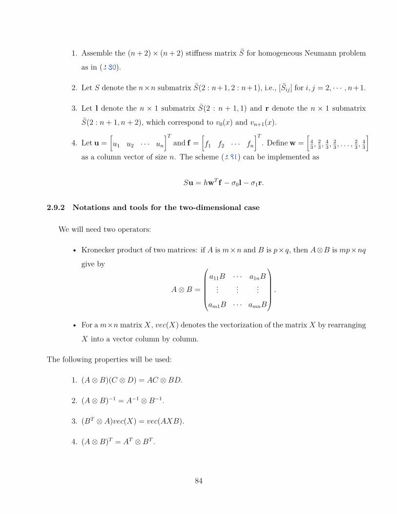
1. Assemble the (n+ 2)× (n+ 2) stiffness matrix S for homogeneous Neumann problem

as in (2.80 ).

2. Let S denote the n×n submatrix S(2 : n+1, 2 : n+1), i.e., [Sij] for i, j = 2, · · · , n+1.

3. Let l denote the n × 1 submatrix S(2 : n + 1, 1) and r denote the n × 1 submatrix

S(2 : n+ 1, n+ 2), which correspond to v0(x) and vn+1(x).

4. Let u =[u1 u2 · · · un

]T

and f =[f1 f2 · · · fn

]T

. Define w =[

43 ,

23 ,

43 ,

23 , . . . ,

23 ,

43

]as a column vector of size n. The scheme (2.81 ) can be implemented as

Su = hwT f − σ0l− σ1r.

2.9.2 Notations and tools for the two-dimensional case

We will need two operators:

• Kronecker product of two matrices: if A is m×n and B is p×q, then A⊗B is mp×nq

give by

A⊗B =

a11B · · · a1nB

... ... ...

am1B · · · amnB

.

• For a m×n matrix X, vec(X) denotes the vectorization of the matrix X by rearranging

X into a vector column by column.

The following properties will be used:

1. (A⊗B)(C ⊗D) = AC ⊗BD.

2. (A⊗B)−1 = A−1 ⊗B−1.

3. (BT ⊗ A)vec(X) = vec(AXB).

4. (A⊗B)T = AT ⊗BT .

84

Consider a uniform grid (xi, yj) for a rectangular domain Ω = [0, 1]×[0, 1] where xi = ihx,

i = 0, 1, . . . , nx + 1, hx = 1nx+1 and yj = jhy, j = 0, 1, . . . , ny + 1, hy = 1

ny+1 .

Assume nx and ny are odd and let Nx = nx+12 and Ny = ny+1

2 . We consider rectangular

cells ekl = [x2k, x2k+2] × [y2l, y2l+2] for k = 0, . . . , Nx − 1 and l = 0, . . . , Ny − 1 as a finite

element mesh for Q2 basis. Define

V h = v ∈ C0(Ω) : v|ekl∈ Q2(ekl), k = 0, . . . , Nx − 1, l = 0, . . . , Ny − 1,

V h0 = v ∈ C0(Ω) : v|ekl

∈ Q2(ekl), k = 0, . . . , Nx − 1, l = 0, . . . , Ny − 1; v|∂Ω ≡ 0.

For the coefficients a(x, y) =

a11 a12

a21 a22

, b = [b1 b2] and c in the elliptic operator (2.9 ),

consider their grid point values in the following form:

Akl =

a00 a01 . . . a0,nx+1

a10 a11 . . . a1,nx+1... ... ...

any+1,0 any+1,1 . . . any+1,,nx+1

(ny+2)×(nx+2)

, aij = akl(xj, yi), k, l = 1, 2,

Bm =

b00 b01 . . . b0,nx+1

b10 b11 . . . b1,nx+1... ... ...

bny+1,0 bny+1,1 . . . bny+1,nx+1

(ny+2)×(nx+2)

, bij = bm(xj, yi), m = 1, 2,

C =

c00 c01 . . . c0,nx+1

c10 c11 . . . c1,nx+1... ... ...

cny+1,0 cny+1,1 . . . cny+1,nx+1

(ny+2)×(nx+2)

, cij = c(xj, yi).

85

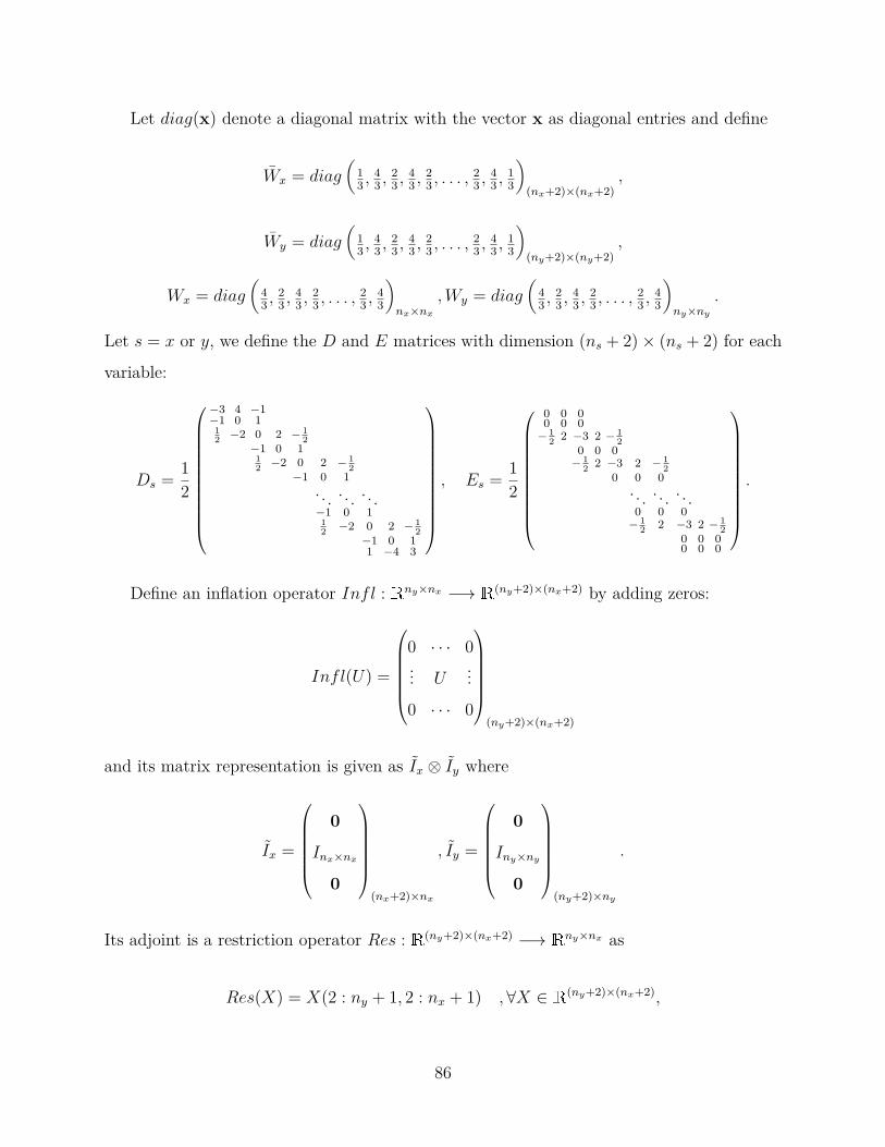
Let diag(x) denote a diagonal matrix with the vector x as diagonal entries and define

Wx = diag(

13 ,

43 ,

23 ,

43 ,

23 , . . . ,

23 ,

43 ,

13

)(nx+2)×(nx+2)

,

Wy = diag(

13 ,

43 ,

23 ,

43 ,

23 , . . . ,

23 ,

43 ,

13

)(ny+2)×(ny+2)

,

Wx = diag(

43 ,

23 ,

43 ,

23 , . . . ,

23 ,

43

)nx×nx

,Wy = diag(

43 ,

23 ,

43 ,

23 , . . . ,

23 ,

43

)ny×ny

.

Let s = x or y, we define the D and E matrices with dimension (ns + 2)× (ns + 2) for each

variable:

Ds = 12

−3 4 −1−1 0 1

12 −2 0 2 − 1

2−1 0 1

12 −2 0 2 − 1

2−1 0 1

... ... ...−1 0 1

12 −2 0 2 − 1

2−1 0 11 −4 3

, Es = 1

2

0 0 00 0 0

− 12 2 −3 2 − 1

20 0 0

− 12 2 −3 2 − 1

20 0 0

... ... ...0 0 0

− 12 2 −3 2 − 1

20 0 00 0 0

.

Define an inflation operator Infl : Rny×nx −→ R(ny+2)×(nx+2) by adding zeros:

Infl(U) =

0 · · · 0... U

...

0 · · · 0

(ny+2)×(nx+2)

and its matrix representation is given as Ix ⊗ Iy where

Ix =

0

Inx×nx

0

(nx+2)×nx

, Iy =

0

Iny×ny

0

(ny+2)×ny

.

Its adjoint is a restriction operator Res : R(ny+2)×(nx+2) −→ Rny×nx as

Res(X) = X(2 : ny + 1, 2 : nx + 1) ,∀X ∈ R(ny+2)×(nx+2),

86

and its matrix representation is ITx ⊗ IT

y .

2.9.3 Two-dimensional case

For Ω = [0, 1]2 we first consider an elliptic equation with homogeneous Neumann bound-

ary condition:

−∇ · (a∇u) + b∇u+ cu =f on Ω, (2.82)

a∇u · n =0 on ∂Ω. (2.83)

The variational form is to find u ∈ H1(Ω) satisfying

A(u, v) = (f, v), ∀v ∈ H1(Ω). (2.84)

The C0-Q2 finite element method with 3 × 3 Gauss-Lobatto quadrature is to find uh ∈ V h

satisfying

〈a∇uh,∇vh〉h + 〈b∇uh, vh〉h + 〈cuh, vh〉h = 〈f, vh〉h, ∀vh ∈ V h, (2.85)

Let U be a (ny +2)×(nx+2) matrix such that its (j, i)-th entry is U(j, i) = uh(xi−1, yj−1),

i = 1, . . . , nx + 2, j = 1, . . . , ny + 2. Let F be a (ny + 2) × (nx + 2) matrix such that its

(j, i)-th entry is F (j, i) = f(xi−1, yj−1). Then the matrix form of (2.85 ) is

Svec(U) = Mvec(F ), M = hxhyWx ⊗ Wy, S =2∑

k,l=1Skl

a +2∑

m=1Sm

b + Sc, (2.86)

87

where

S11a = hy

hx

(DTx ⊗ Iy)diag(vec(WyA

11Wx))(Dx ⊗ Iy) + hy

hx

(ETx ⊗ Iy)diag(vec(WyA

11Wx))(Ex ⊗ Iy),

S12a = (DT

x ⊗ Iy)diag(vec(WyA12Wx))(Ix ⊗Dy) + (ET

x ⊗ Iy)diag(vec(WyA12Wx))(Ix ⊗ Ey),

S21a = (Ix ⊗DT

y )diag(vec(WyA21Wx))(Dx ⊗ Iy) + (Ix ⊗ ET

y )diag(vec(WyA21Wx))(Ex ⊗ Iy),

S22a = hx

hy

(Ix ⊗DTy )diag(vec(WyA

22Wx))(Ix ⊗Dy) + hx

hy

(Ix ⊗ ETy )diag(vec(WyA

22Wx))(Ix ⊗ Ey),

S1b = hydiag(vec(WyB

1Wx))(Dx ⊗ Iy), S2b = hxdiag(vec(WyB

2Wx))(Ix ⊗Dy),

Sc = hxhydiag(vec(WyCWx).

Now consider the scheme (2.53 ) for nonhomogeneous Dirichlet boundary conditions. Its

numerical solution can be represented as a matrix U of size ny×nx with (j, i)-entry U(j, i) =

uh(xi, yj) for i = 1, · · · , nx; j = 1, · · · , ny. Similar to the one-dimensional case, its stiffness

matrix can be obtained as the submatrix of S in (2.86 ). Let G be a (ny + 2) by (nx + 2)

matrix with (j, i)-th entry as G(j, i) = g(xi−1, yj−1), where

g(x, y) =

0, if (x, y) ∈ (0, 1)× (0, 1),

g(x, y), if (x, y) ∈ ∂Ω.

In particular, G(j + 1, i + 1) = 0 for j = 1, . . . , ny, i = 1, . . . , nx. Let F be a matrix of size

ny × nx with (j, i)-entry as F (j, i) = f(xi, yj) for i = 1, · · · , nx; j = 1, · · · , ny. Then the

scheme (2.53 ) becomes

(ITx ⊗ IT

y )S(Ix ⊗ Iy)vec(U) = (Wx ⊗Wy)vec(F )− (ITx ⊗ IT

y )Svec(G). (2.87)

Even though the stiffness matrix is given as S = (ITx ⊗ IT

y )S(Ix ⊗ Iy), S should be imple-

mented as a linear operator in iterative linear system solvers. For example, the matrix vector

88

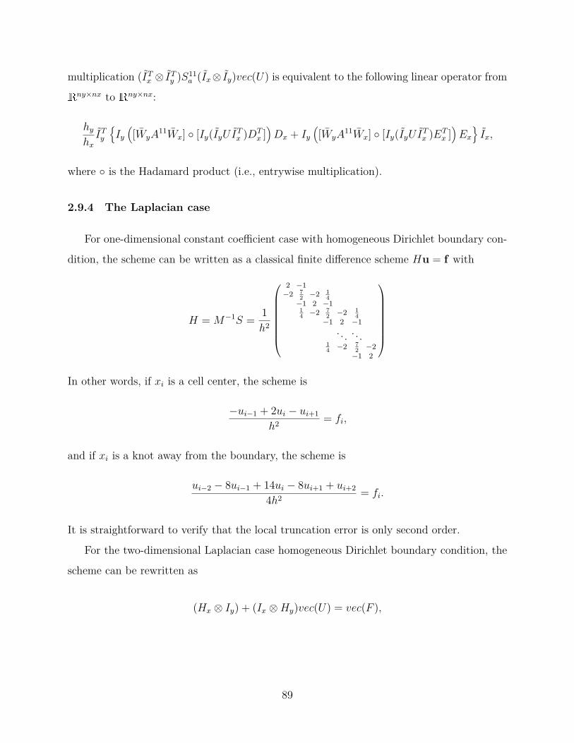
multiplication (ITx ⊗ IT

y )S11a (Ix⊗ Iy)vec(U) is equivalent to the following linear operator from

Rny×nx to Rny×nx:

hy

hx

ITy

Iy

([WyA

11Wx] [Iy(IyUITx )DT

x ])Dx + Iy

([WyA

11Wx] [Iy(IyUITx )ET

x ])Ex

Ix,

where is the Hadamard product (i.e., entrywise multiplication).

2.9.4 The Laplacian case

For one-dimensional constant coefficient case with homogeneous Dirichlet boundary con-

dition, the scheme can be written as a classical finite difference scheme Hu = f with

H = M−1S = 1h2

2 −1−2 7

2 −2 14

−1 2 −114 −2 7

2 −2 14

−1 2 −1... ...

14 −2 7

2 −2−1 2

In other words, if xi is a cell center, the scheme is

−ui−1 + 2ui − ui+1

h2 = fi,

and if xi is a knot away from the boundary, the scheme is

ui−2 − 8ui−1 + 14ui − 8ui+1 + ui+2

4h2 = fi.

It is straightforward to verify that the local truncation error is only second order.

For the two-dimensional Laplacian case homogeneous Dirichlet boundary condition, the

scheme can be rewritten as

(Hx ⊗ Iy) + (Ix ⊗Hy)vec(U) = vec(F ),

89

where Hx and Hy are the same H matrix above with size nx × nx and ny × ny respectively.

The inverse of (Hx⊗Iy)+(Ix⊗Hy) can be efficiently constructed via the eigen-decomposition

of small matrices Hx and Hy:

1. Compute eigen-decomposition of Hx = TxΛxT−1x and Hy = TyΛyT

−1y .

2. The properties of Kronecker product imply that

(Hx ⊗ Iy) + (Ix ⊗Hy) = (Tx ⊗ Ty)(Λx ⊗ Iy + Ix ⊗ Λy)(T−1x ⊗ T−1

y ),

thus

[(Hx ⊗ Iy) + (Ix ⊗Hy)]−1 = (Tx ⊗ Ty)(Λx ⊗ Iy + Ix ⊗ Λy)−1(T−1x ⊗ T−1

y ).

3. It is nontrivial to determine whether H is diagonalizable. In all our numerical tests,

H has no repeated eigenvalues. So if assuming Λx and Λy are diagonal matrices, the

matrix vector multiplication [(Hx⊗ Iy) + (Ix⊗Hy)]−1vec(F ) can be implemented as a

linear operator on F :

Ty([T−1y F (T−1

x )T ]./Λ)T Tx , (2.88)

where Λ is a ny × nx matrix with (i, j)-th entry as Λ(i, j) = Λy(i, i) + Λx(j, j) and ./

denotes entry-wise division for two matrices of the same size.

For the 3D Laplacian, the matrix can be represented as Hx ⊗ Iy ⊗ Iz + Ix ⊗ Hy ⊗ Iz +

Ix ⊗ Iy ⊗Hz thus can be efficiently inverted through eigen-decomposition of small matrices

Hx, Hy and Hz as well.

Since the eigen-decomposition of small matrices Hx and Hy can be precomputed, and

(2.88 ) costs only O(n3) for a 2D problem on a mesh size n × n, in practice (2.88 ) can be

used as a simple preconditioner in conjugate gradient solvers for the following linear system

equivalent to (2.87 ):

(W−1x ⊗W−1

y )(ITx ⊗ IT

y )S(Ix ⊗ Iy)vec(U) = vec(F )− (W−1x ⊗W−1

y )(ITx ⊗ IT

y )Svec(G),

90

even though the multigrid method as reviewed in [42 ] is the optimal solver in terms of

computational complexity.

2.10 Numerical Results

In this section we show a few numerical tests verifying the accuracy of the scheme (2.53 )

for k = 2 implemented as a finite difference scheme on a uniform grid. We first consider the

following two dimensional elliptic equation:

−∇ · (a∇u) + b · ∇u+ cu = f on [0, 1]× [0, 2] (2.89)

where a =

a11 a12

a21 a22

, a11 = 10 + 30y5 + x cos y + y, a12 = a21 = 2 + 0.5(sin(πx) +

x3)(sin(πy) + y3) + cos(x4 + y3), a22 = 10 + x5, b = 0, c = 1 + x4y3, with an exact solution

u(x, y) = 0.1(sin(πx) + x3)(sin(πy) + y3) + cos(x4 + y3).

Table 2.1. A 2D elliptic equation with Dirichlet boundary conditions. Thefirst column is the number of regular cells in a finite element mesh. The secondcolumn is the number of grid points in a finite difference implementation, i.e.,number of degree of freedoms.

FEM Mesh FD Grid l2 error order l∞ error order2× 4 3× 7 3.94E-2 - 7.15E-2 -4× 8 7× 15 1.23E-2 1.67 3.28E-2 1.128× 16 15× 31 1.46E-3 3.08 5.42E-3 2.6016× 32 31× 63 1.14E-4 3.68 3.96E-4 3.7832× 64 63× 127 7.75E-6 3.88 2.62E-5 3.9264× 128 127× 255 5.02E-7 3.95 1.73E-6 3.92128× 256 255× 511 3.23E-8 3.96 1.13E-7 3.94

The errors at grid points are listed in Table 2.1 for purely Dirichlet boundary condition

and Table 2.2 for purely Neumann boundary condition. We observe fourth order accuracy

in the discrete 2-norm for both tests, even though only O(h3.5) can be proven for Neu-

mann boundary condition as discussed in Remark 2.6.5 . Regarding the maximum norm of

91

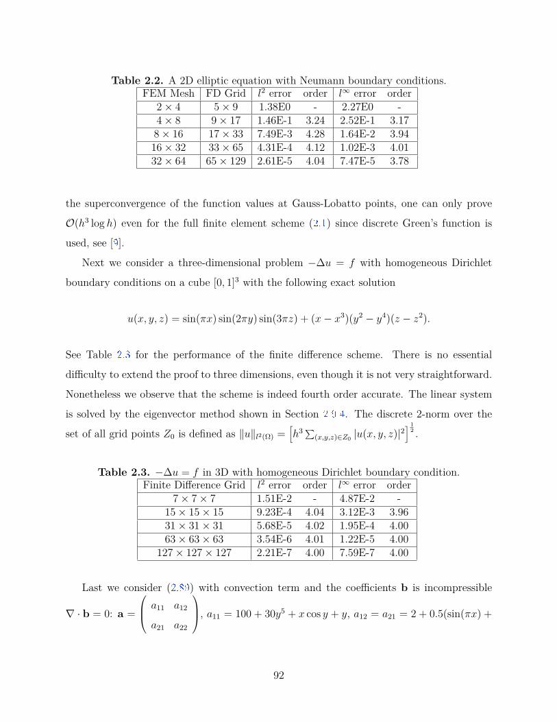
Table 2.2. A 2D elliptic equation with Neumann boundary conditions.FEM Mesh FD Grid l2 error order l∞ error order

2× 4 5× 9 1.38E0 - 2.27E0 -4× 8 9× 17 1.46E-1 3.24 2.52E-1 3.178× 16 17× 33 7.49E-3 4.28 1.64E-2 3.9416× 32 33× 65 4.31E-4 4.12 1.02E-3 4.0132× 64 65× 129 2.61E-5 4.04 7.47E-5 3.78

the superconvergence of the function values at Gauss-Lobatto points, one can only prove

O(h3 log h) even for the full finite element scheme (2.1 ) since discrete Green’s function is

used, see [9 ].

Next we consider a three-dimensional problem −∆u = f with homogeneous Dirichlet

boundary conditions on a cube [0, 1]3 with the following exact solution

u(x, y, z) = sin(πx) sin(2πy) sin(3πz) + (x− x3)(y2 − y4)(z − z2).

See Table 2.3 for the performance of the finite difference scheme. There is no essential

difficulty to extend the proof to three dimensions, even though it is not very straightforward.

Nonetheless we observe that the scheme is indeed fourth order accurate. The linear system

is solved by the eigenvector method shown in Section 2.9.4 . The discrete 2-norm over the

set of all grid points Z0 is defined as ‖u‖l2(Ω) =[h3∑

(x,y,z)∈Z0 |u(x, y, z)|2] 1

2 .

Table 2.3. −∆u = f in 3D with homogeneous Dirichlet boundary condition.Finite Difference Grid l2 error order l∞ error order

7× 7× 7 1.51E-2 - 4.87E-2 -15× 15× 15 9.23E-4 4.04 3.12E-3 3.9631× 31× 31 5.68E-5 4.02 1.95E-4 4.0063× 63× 63 3.54E-6 4.01 1.22E-5 4.00

127× 127× 127 2.21E-7 4.00 7.59E-7 4.00

Last we consider (2.89 ) with convection term and the coefficients b is incompressible

∇ · b = 0: a =

a11 a12

a21 a22


92

x3)(sin(πy) + y3) + cos(x4 + y3), a22 = 100 + x5, b =

b1

b2

, b1 = ψy, b2 = −ψx, ψ =

x exp(x2 + y), c = 1 + x4y3, with an exact solution

u(x, y) = 0.1(sin(πx) + x3)(sin(πy) + y3) + cos(x4 + y3).

The errors at grid points are listed in Table 2.4 for Dirichlet boundary conditions.

Table 2.4. A 2D elliptic equation with convection term and Dirichlet bound-ary conditions.

FEM Mesh FD Grid l2 error order l∞ error order2× 4 3× 7 1.26E-1 - 2.71E-1 -4× 8 7× 15 2.85E-2 2.15 9.70E-2 1.488× 16 15× 31 1.89E-3 3.92 7.25E-3 3.7416× 32 31× 63 1.17E-4 4.01 4.01E-4 4.1732× 64 63× 127 7.41E-6 3.98 2.54E-5 3.98

2.11 Concluding Remarks

In this chapter we have proven the superconvergence of function values in the simplest

finite difference implementation of Qk spectral element method for elliptic equations. In

particular, for the case k = 2 the scheme (2.53 ) can be easily implemented as a fourth order

accurate finite difference scheme as shown in Section 2.9 . It provides only only an convenient

approach for constructing fourth order accurate finite difference schemes but also the most

efficient implementation of C0-Qk finite element method without losing superconvergence of

function values. In the last section, we will show that discrete maximum principle can be

proven for the scheme (2.53 ) in the case k = 2 when solving a variable coefficient Poisson

equation.

93

3. ACCURACY OF SPECTRAL ELEMENT METHOD FOR

WAVE, PARABOLIC AND SCHRÖDINGER EQUATIONS

3.1 Introduction

In this Chapter, we are actually extending the results in Chapter 2 to wave, parabolic

and Schrödinger equations.

In recent years many such stable and high order accurate methods for wave equations have

been developed. These include discontinuous Galerkin methods for first order hyperbolic

systems [43 ]–[49 ] and wave equations in second order form [50 ]–[53 ], and finite differences

with summation by parts operators [54 ]–[60 ], as well as spectral elements for wave equations

[12 ], [13 ].

In this chapeter we study the rates of convergence of the error, as measured in norms

over nodes for all degree of freedoms, for the spectral element method applied to linear wave

and parabolic, and Schrödinger equations.

To be precise, we consider the Lagrangian Qk (k ≥ 2) continuous finite element method

for solving linear evolution PDEs with a second order operator ∇ · (a(x)∇u) on rectangular

meshes implemented by (k + 1)-point Gauss-Lobatto quadrature for all integrals. This is

often referred to as the spectral element method in the literature and this is the notation we

will use here.

For the Qk spectral element method, it is well known that the standard finite element

error estimates still hold [11 ], i.e., the error in H1-norm is k-th order and the error in L2-

norm is (k + 1)-th order. It is also well known that the Lagrangian Qk (k ≥ 2) continuous

finite element method is (k + 2)-th order accurate in the discrete 2-norm over all (k + 1)-

point Gauss-Lobatto quadrature points [8 ]–[10 ]. If using a very accurate quadrature in the

finite element method for a variable coefficient operator ∇ · (a(x)∇u), then (k+ 2)-th order

superconvergence at Gauss-Lobatto points holds trivially. However, for the efficiency of

having a diagonal mass matrix and for the convenience of implementation, the most popular

method for wave equations is the simplest choice of quadrature, i.e. using (k+1)-point Gauss-

Lobatto quadrature for Qk elements in all integrals for both mass and stiffness matrices. In

94

particular in the seismic community, where highly efficient simulation of the elastic wave

equation is of important, the spectral method has become the method of choice, [12 ], [13 ].

When using this (k+1)-point Gauss-Lobatto quadrature for Lagrangian Qk finite element

method, the quadrature nodes coincide with the nodes defining the degrees of freedom, and

the resulting method becomes the so-called spectral element method. Thus the spectral

element method can also be regarded as a finite difference scheme at all Gauss-Lobatto points.

For instance, consider solving utt = uxx on the interval [0, 1] with homogeneous Dirichlet

boundary conditions. Introduce the uniform grid 0 = x0 < x1 < · · · < xN < xN+1 = 1 with

spacing h = 1/(N + 1) and N being odd. This grid gives a uniform partition of the interval

[0, 1] into uniform intervals Ik = [x2k, x2k+2] (k = 0, · · · , N−12 ). Then all 3-point Gauss-

Lobatto quadrature points for intervals Ik = [x2k, x2k+2] coincide with the grid points xi.

The Q2 spectral element method on intervals Ik = [x2k, x2k+2] (k = 0, · · · , N−12 ) is equivalent

to the following semi-discrete finite difference scheme [61 ], [62 ]:

d2

dt2ui = ui−1 − 2ui + ui+1

h2 , if i is odd; (3.1a)

d2

dt2ui = −ui−2 + 8ui−1 − 14ui + 8ui+1 − ui+2

4h2 , if i is even. (3.1b)

The truncation error of (3.1 ) is only second order yet the dispersion error is fourth order,

see Section 11 in [61 ]. Although the dispersion error results can in principle be extended

to any order, the derivation and expressions become increasingly cumbersome. Further the

dispersion error results are limited to unbounded or periodic domains and do not produce

error estimates in the form of a norm of the error. In fact, as we have shown in [62 ], it is

nontrivial and requires new analysis tools to establish the (k+ 2)-th order superconvergence

when (k + 1)-point Gauss-Lobatto quadrature is used. In [62 ], (k + 2)-th order accuracy at

all Gauss-Lobatto points of Qk spectral element method was proven for elliptic equations

with Dirichlet boundary conditions. In this chapter, we extend those results and will prove

that the Qk spectral element method is a (k + 2)-th order accurate scheme for linear wave,

parabolic and Schrödinger equations with Dirichlet boundary conditions. For Neumann

boundary conditions, if a(x) is diagonal, i.e., there are no mixed second order derivatives

95

in ∇ · (a(x)∇u), (k + 2)-th order accuracy in discrete 2-norm can be proven. When mixed

second order derivatives are involved, only (k + 32)-th order can be proven for Neumann

boundary conditions, and we indeed observe some order loss in numerical tests.

This chapter explains the order of accuracy of Qk spectral element method, when the

errors are measured only at nodes of degree of freedoms. As mentioned above we consider

the case of rectangular elements and a smooth coefficient a(x) in the term ∇ · (a(x)∇u).

We note that this does include discretizations on regular meshes of curvilinear domains that

can be smoothly mapped to rectangular meshes for the unit cube, e.g., the spectral element

method for ∆u on such a mesh for a curvilinear domain is equivalent to the spectral element

method for ∇·(a(x)∇u)+b(x) ·∇u on a reference uniform rectangular mesh where a(x) and

b(x) emerge from the mapping between the curvilinear domain and the unit cube. It does

however not include problems on unstructured quadrilateral meshes where the metric terms

typically are non-smooth at element interfaces but we note that the numerical examples that

we present indicate that such meshes may still exhibit larger rates than k + 1.

This chapter is organized as follows. In Section 3.2 , we introduce notation and as-

sumptions. In Section 3.3 , we review a few standard quadrature estimates. In Section 3.4 ,

the superconvergence of elliptic projection is analyzed, which is parallel to the classic error

estimation for hyperbolic and parabolic equations by involving elliptic projection of the cor-

responding elliptic operator, see [63 ]–[65 ]. We then prove the main result for homogeneous

Dirichlet boundary conditions in Section 3.5 , for the second-order wave equation in Section

3.5.1 , parabolic equations in Section 3.5.2 and linear Schrödinger equation in Section 3.5.3 .

Neumann boundary conditions can be discussed similarly as summarized in Section 3.5.4 .

For problems with nonhomogeneous Dirichlet boundary conditions, a convenient implemen-

tation which maintains the (k + 2)-th order of accuracy is given in Section 3.6 . Numerical

tests verifying the estimates are given in Section 3.7 . Concluding remarks are given in Section

3.8

96

3.2 Equations, Notation, And Assumptions

3.2.1 Problem Setup

Let L be a linear second order differential operator with time dependent coefficients:

Lu = −∇ · (a(x, t)∇u) + b(x, t) · ∇u+ c(x, t)u,

where a(x, t) = (aij(x, t)) is a positive symmetric definite operator for t ∈ [0, T ], i.e. there ex-

ists a constant α, β > 0 such that α|ξ|2 ≤ ξT a(x, t)ξ ≤ β|ξ|2, for all (x, t) ∈ Ω×[0, T ], ξ ∈ Rn.

Consider the following two initial-boundary value problems with smooth enough coefficients

on a rectangular domain Ω = (0, 1)× (0, 1) with its boundary ∂Ω:

Given 0 < T <∞, find u(x, t) on Ω× [0, T ] satisfying

ut =− Lu+ f(x, t) in Ω× (0, T ],

u(x, t) =0 on ∂Ω× [0, T ],

u(x, 0) =u0(x) on Ω.

(3.2)

Given 0 < T <∞, find u(x, t) on Ω× [0, T ] satisfying

utt =− Lu+ f(x, t) in Ω× (0, T ],

u(x, t) =0 on ∂Ω× [0, T ],

u(x, 0) =u0(x), ut(x, 0) = u1(x) on Ω× t = 0.

(3.3)

We use A(·) to denote the bilinear form: for u, v ∈ H1(Ω),

A(u, v) =∫

Ω∇uT a(x, t)∇v + b(x, t) · ∇u+ c(x, t)uvdx. (3.4)

For convenience, we assume Ωh is an uniform rectangular mesh for Ω and e = [xe−h, xe +

h]× [ye − h, ye + h] denotes any cell in Ωh with cell center (xe, ye). Though we only discuss

uniform meshes, the main result can be easily extended to nonuniform rectangular meshes

with smoothly varying cells. Let Qk(e) =p(x, y) =

k∑i=0

k∑j=0

pijxiyj, (x, y) ∈ e

, denote the

97

set of tensor product of polynomials of degree k on an element e. Then we use V h =

p(x, y) ∈ C0(Ωh) : p|e ∈ Qk(e), ∀e ∈ Ωh to denote the continuous piecewise Qk finite

element space on Ωh and V h0 = vh ∈ V h : vh|∂Ω = 0. Further let (u, v) =

∫Ω uvdx and

let 〈·, ·〉h and Ah(·, ·) denote approximation of the integrals by (k + 1)-point Gauss-Lobatto

quadrature for each spatial variable in each cell. Also, u(i) will denote the i-th time derivative

of the function u(x, t).

For the equations that we are interested in, assume the exact solution u(x, t) ∈ H10 (Ω)∩

H2(Ω) for any t, and define its discrete elliptic projection Rhu ∈ V h0 as

Ah(Rhu, vh) = 〈−Lu, vh〉h, ∀vh ∈ V h0 , 0 ≤ t ≤ T. (3.5)

Also, let uI ∈ V h denote the piecewise Lagrangian Qk interpolation polynomial of function

u at (k + 1)× (k + 1) Gauss-Lobatto points in each rectangular cell.

We consider semi-discrete spectral element schemes whose initial conditions are defined

by the elliptic projection and the Lagrange interpolant of the continuous initial data.

For problem (3.2 ) the scheme is to find uh(x, t) ∈ V h0 satisfying

〈u(1)h , vh〉h + Ah(uh, vh) =〈f, vh〉h, ∀vh ∈ V h

0 ,

uh(0) =Rhu0.(3.6)

We consider the semi-discrete spectral element scheme for problem (3.3 ) with special

initial conditions: solve for uh(t) ∈ V h0 satisfying

〈u(2)h , vh〉h + Ah(uh, vh) =〈f, vh〉h, ∀vh ∈ V h

0 ,

uh(0) = Rhu0, u(1)h (0) =(u1)I .

(3.7)

3.2.2 Notation and basic tools

We will use the same notation as in Chapter 2 , we may also need:

98

• Let superscript (i) denote i-th time derivatives for coefficients a,b, and c. For the

time dependent operators L and A, the symbols L(i) and A(i) are defined as taking

time derivatives only for coefficients:

L(i)u = −∇ · (a(i)∇u) + b(i) · ∇u+ c(i)u,

and

A(i)(u, v) =∫

Ω∇uT a(i)∇v + b(i) · ∇u+ c(i)uvdx.

The symbol A(i)h is similarly defined as taking time derivatives only for coefficients in

Ah. With this notation, for u(x, t) and time independent test function v(x), we have

Leibniz rule

(Lu)(m) =m∑

j=0

(m

j

)L(m−j)u(j), [A(u, v)](m) =

m∑j=0

(m

j

)A(m−j)(u(j), v).

• By integration by parts, it is straightforward to verify

(L(m−j)u(j), v) = A(m−j)(u(j), v), ∀v ∈ H10 (Ω). (3.8)

3.2.3 Assumption on the coercivity and the elliptic regularity

For the operator A(u, v) :=∫

Ω[∇uT a∇v + (b · ∇u)v + cuv] dx where a =

a11 a12

a21 a22

is

positive definite and b = (b1 b2), assume the coefficients aij, bj, c ∈ Cm1 ([0, T ];Wm2,∞(Ω))

for m1, m2 large enough. Thus for t ∈ [0, T ], A(u, v) ≤ C‖u‖1‖v‖1 for any u, v ∈ H10 (Ω).

As discussed in Chapter 2 , if we assume λa has a positive lower bound and ∇ · b ≤ 2c,

where λa as the smallest eigenvalues of a, the coercivity of the bilinear form can be easily

achieved. For the V h-ellipticity, as pointed out in Lemma 2.6.2 of Chapter 2 , if 4λac > |b|2,

for t ∈ [0, T ],

C‖vh‖21 ≤ Ah(vh, vh), ∀vh ∈ V h, (3.9)

99

can be proven. In the rest of this chapter, we assume coercivity for the bilinear forms A, A∗,

and Ah. We assume the elliptic regularity ‖w‖2 ≤ C‖f‖0 holds for the exact dual problem of

finding w ∈ H10 (Ω) satisfying A∗(w, v) = (f, v), ∀v ∈ H1

0 (Ω). See [33 ], [34 ] for the elliptic

regularity with Lipschitz continuous coefficients on a Lipschitz domain.

We remark that in the case of the wave equation we also assume finite speed of propa-

gation i.e. that there is an upper bound on the eigenvalues of a.

3.3 Quadrature Error Estimates

For any continuous function u(x, t0) with fixed time t0, its M-type projection (defined

in Section 2.4 of Chapter 2 ) on spatial variables is a continuous piecewise Qk polynomial of

x, denoted as up(x, t0) ∈ V h. The M-type projection was used to analyze superconvergence

[9 ]. For m ≥ 0, (up)(m) =(u(m)

)p, thus there is no ambiguity to use the notation u(m)

p . The

M-type projection has the following properties.

For convenience, we write (2.29a ) and (2.29b ) and Theorem 2.3.9 as the follows respec-

tively.

Lemma 3.3.1. For i, j ≥ 0 and any fixed t ∈ [0, T ], assuming sufficiently smooth coefficients

a,b, c and function u(x, t) ∈ Hk+3(Ω), we have

A(i)h ((u− up)(j), vh) =

O(hk+2)‖u(j)(t)‖k+3‖vh‖2, if vh ∈ V h

0 or a is diagonal;

O(hk+ 32 )‖u(j)(t)‖k+3‖vh‖2, otherwise.

(3.10)

Lemma 3.3.2. For the differential operator L and any fixed t ∈ [0, T ], assume aij(x, t),

bi(x, t), c(x, t) ∈ L∞([0, T ];W k+2,∞(Ω)

)and u(x, t) ∈ Hk+3(Ω). For k ≥ 2, we have

A(u, vh)− Ah(u, vh) =

O(hk+2)‖u(t)‖k+3‖vh‖2, if vh ∈ V h

0 or a is diagonal;

O(hk+ 32 )‖u(t)‖k+3‖vh‖2, otherwise.

(3.11)

100

Remark 3.3.3. There is half order loss in (3.10 ) and (3.11 ), only when using v ∈ V h for

non-diagonal a, i.e., when solving second order equations containing mixed second order

derivatives with Neumann boundary conditions.

We have the Gronwall’s inequality in integral form as follows:

Lemma 3.3.4. Let ξ(t) be continuous on [0, T ] and

ξ(t) ≤ C1

∫ t

0ξ(s)ds+ α(t)

for constant C1 ≥ 0 and α(t) ≥ 0 nondescreasing in t. Then ξ(t) ≤ α(t)eC1t thus ξ(t) ≤

α(t)eC1T = Cα(t) for all 0 ≤ t ≤ T .

3.4 Error Estimates For The Elliptic Projection

Let uh(x, t) denote the solution of the semi-discrete numerical scheme. Let e(x, t) =

uh(x, t)− up(x, t), then we can write

e = θh + ρh,

where θh := uh −Rhu ∈ V h0 and ρh := Rhu− up ∈ V h

0 .

We have the following superconvergence result for ‖ρ(m)h (t)‖, m ≥ 0, t ∈ [0, T ].

Lemma 3.4.1. If aij, bj, c ∈ Cm([0, T ];W k+2,∞(Ω)

), u ∈ Cm

([0, T ];Hk+4(Ω)

), then we

have

‖ρ(m)h (t)‖1 ≤Chk+1

m∑j=0

(‖u(j)(t)‖k+3 + ‖(Lu)(j)(t)‖k+2), (3.12)

‖ρ(m)h ‖L2([0,T ];L2(Ω)) ≤Chk+2

m∑j=0

(‖u(j)‖L2([0,T ];Hk+3(Ω)) + ‖(Lu)(j)‖L2([0,T ];Hk+2(Ω))), (3.13)

‖ρ(m)h ‖L∞([0,T ];L2(Ω)) ≤Chk+2

m∑j=0

(‖u(j)‖L∞([0,T ];Hk+3(Ω)) + ‖(Lu)(j)‖L∞([0,T ];Hk+2(Ω))), (3.14)

where C is independent of h, u, f , and time t.

101

Proof. First we prove (3.12 ), with which we then prove (3.13 ) and (3.14 ) by the dual argu-

ment.

From the definition of the discrete elliptic projection (3.5 ) we have

Ah(ρh, vh) = ε(vh), ∀vh ∈ V h0 . (3.15)

where

ε(vh) = 〈Lu, vh〉h − Ah(up, vh).

Note that vh is time independent. Taking m time derivatives of (3.15 ) yields

(Ah(ρh, vh))(m) =m∑

j=0

(m

j

)A

(m−j)h (ρ(j)

h , vh) = ε(m)(vh). (3.16)

The term ε(m)(vh) can be rewritten as follows:

ε(m)(vh) = 〈(Lu)(m), vh〉h − (Ah(up, vh))(m)

=[((Lu)(m), vh)− (A(u, vh))(m)

]−[((Lu)(m), vh)− 〈(Lu)(m), vh〉h

]+[(A(u, vh))(m) − (Ah(u, vh))(m)

]+ (Ah(u− up, vh))(m) .

By Leibniz rule and (3.8 ), we have

((Lu)(m), vh)− (A(u, vh))(m) =m∑

j=0

(m

j

) [(L(m−j)u(j), vh)− A(m−j)(u(j), vh)

]= 0.

By Lemma 2.3.4 ,

((Lu)(m), vh)− 〈(Lu)(m), vh〉h = O(hk+2)‖(Lu)(m)(t)‖k+2‖vh‖2.

102

By Leibniz rule and Lemma 3.3.2 ,

(A(u, vh))(m) − (Ah(u, vh))(m) =m∑

j=0

(m

j

) [A(m−j)(u(j), vh)− A(m−j)

h (u(j), vh)]

= O(hk+2)m∑

j=0

(m

j

)‖u(j)(t)‖k+3‖vh‖2.

Now, Lemma 3.3.1 implies

(Ah(u− up, vh))(m) =m∑

j=0

(m

j

)A

(m−j)h

((u− up)(j), vh

)= O(hk+2)

m∑j=0

(m

j

)‖u(j)(t)‖k+3‖vh‖2.

Thus we have

ε(m)(vh) = O(hk+2) m∑

j=0‖u(j)(t)‖k+3 + ‖(Lu)(m)(t)‖k+2

‖vh‖2. (3.17)

For i ≥ 0, by the Vh-ellipticity (3.9 ), (3.16 ), and (3.17 ) we have

C‖ρ(i)h (t)‖2

1 ≤ Ah(ρ(i)h , ρ

(i)h )

=i∑

j=0

(i

j

)A

(i−j)h (ρ(j)

h , ρ(i)h )−

i−1∑j=0

(i

j

)A

(i−j)h (ρ(j)

h , ρ(i)h )

=ε(i)(ρ(i)h )−

i−1∑j=0

(i

j

)A

(i−j)h (ρ(j)

h , ρ(i)h )

≤O(hk+1) i∑

j=0‖u(j)‖k+3 + ‖(Lu)(i)‖k+2

h‖ρ(i)h ‖2 + C

i−1∑j=0‖ρ(j)

h (t)‖1‖ρ(i)h (t)‖1

≤

O(hk+1) i∑

j=0‖u(j)‖k+3 + ‖(Lu)(i)‖k+2

+ Ci−1∑j=0‖ρ(j)

h (t)‖1

‖ρ(i)h (t)‖1,

the last inequality follows from an application of an inverse estimate. Thus

‖ρ(i)h (t)‖1 ≤ O(hk+1)

i∑j=0‖u(j)‖k+3 + ‖(Lu)(i)‖k+2

+ Ci−1∑j=0‖ρ(j)

h (t)‖1. (3.18)

103

Now (3.12 ) can be proven by induction as follows. First, set i = 0 in (3.18 ) to obtain

(3.12 ) with m = 0. Second, assume (3.18 ) holds for m = i − 1, then (3.18 ) implies that

(3.12 ) also holds for m = i.

For fixed t ∈ [0, T ], to estimate ρ(m)h in L2-norm, we consider the dual problem: find

φh ∈ V h0 satisfying: for i ≥ 0,

A∗(φh, vh) = (ρ(i)h (t), vh), ∀vh ∈ V h

0 . (3.19)

Based on Theorem 5.3 in [62 ], by assuming the elliptic regularity and V h ellipticity, problem

(3.19 ) has a unique solution satisfying

‖φh‖2 ≤ C‖ρ(i)h (t)‖0. (3.20)

Take vh = ρ(i)h in (3.19 ) then we have

‖ρ(i)h (t)‖2

0

=A∗(φh, ρ(i)h ) = A(ρ(i)

h , φh)

=i∑

j=0

(i

j

)A(i−j)(ρ(j)

h , φh)−i−1∑j=0

(i

j

)A(i−j)(ρ(j)

h , φh)

=i∑

j=0

(i

j

)(A

(i−j)h (ρ(j)

h , φh) + E(A(i−j)(ρ(j)

h , φh)))−

i−1∑j=0

(i

j

)(ρ

(j)h , (L∗)(i−j)φh

).

Note that ∀χ ∈ V h0 , with (3.16 ) and (3.17 ),

i∑j=0

(i

j

)A

(i−j)h (ρ(j)

h , φh)

=i∑

j=0

(i

j

)A

(i−j)h (ρ(j)

h , φh − χ) +i∑

j=0

(i

j

)A

(i−j)h (ρ(j)

h , χ)

=i∑

j=0

(i

j

)A

(i−j)h (ρ(j)

h , φh − χ) + ε(i)(χ)

≤Ci∑

j=0‖ρ(j)

h (t)‖1‖φh − χ‖1 +O(hk+2) i∑

j=0‖u(j)(t)‖k+3 + ‖(Lu)(i)(t)‖k+2

‖χ‖2.

(3.21)

104

Let χ = Π1φh where Π1 is the L2 projection to functions in the continuous piecewise

Q1 polynomial space, see [62 ]. Then we have ‖φh − χ‖1 ≤ Ch‖φh‖2 and ‖χ‖2 ≤ C‖φh‖2.

Inserting (3.12 ) and (3.20 ) into (3.21 ), we have

i∑j=0

(i

j

)A

(i−j)h (ρ(j)

h , φh) = O(hk+2) i∑

j=0(‖u(j)t)‖k+3 + ‖(Lu)(i)(t)‖k+2

‖φh‖2. (3.22)

Thus with (3.22 ), Lemma 3.3.2 , and inverse inequality we have

‖ρ(i)h (t)‖2

0

≤O(hk+2) i∑

j=0‖u(j)(t)‖k+3 + ‖(Lu)(i)(t)‖k+2

‖φh‖2

+O(hk+2)i∑

j=0‖ρ(j)

h (t)‖k+2‖φh‖2 + Ci−1∑j=0‖ρ(j)

h (t)‖0‖φh‖2

=O(hk+2)

i∑j=0‖u(j)‖k+3 + ‖(Lu)(i)‖k+2

+ Ci−1∑j=0‖ρ(j)

h (t)‖0

‖φh‖2

≤

O(hk+2) i∑

j=0‖u(j)‖k+3 + ‖(Lu)(i)‖k+2

+ Ci−1∑j=0‖ρ(j)

h (t)‖0

‖ρ(i)h (t)‖0,

(3.23)

where (3.20 ) is applied in the last inequality.

With similar induction arguments as above, (3.23 ) implies

‖ρ(i)h (t)‖0 ≤ O(hk+2)

i∑j=0

(‖u(j)(t)‖k+3 + ‖(Lu)(j)(t)‖k+2). (3.24)

Take square for both sides of (3.24 ) then integrate from 0 to T and take square root for

both sides, we can get (3.13 ). Take the maximum of the right hand side then the left hand

side of (3.24 ) for t ∈ [0, T ], we can get (3.14 ).

3.5 Accuracy Of The Semi-discrete Schemes

Throughout this section the generic constant C is independent of h. Although in principle

it may depend on t though the coefficients aij(t), bj(t), c(t), we also treat it as independent of

time since its time dependent version can always be replaced by a time independent constant

105

after taking maximum over the ime interval [0, T ]. In what follows we will state and prove

the main theorems for wave, parabolic and the Schrödinger equations.

3.5.1 The hyperbolic problem

The main result for the wave equation can be stated as the following theorem.

Theorem 3.5.1. If aij, bj, c ∈ C2([0, T ];W k+2,∞(Ω)

), u ∈ C2

([0, T ];Hk+4(Ω)

), then for

the semi-discrete scheme (3.7 ) we have

‖uh − u‖L2([0,T ];l2(Ω)) ≤Chk+2

2∑j=0

(‖u(j)‖L2([0,T ];Hk+3(Ω)) + ‖(Lu)(j)‖L2([0,T ];Hk+2(Ω)))

+1∑

j=0(‖u(j)(0)‖k+3 + ‖(Lu)(j)(0)‖k+2)

,‖uh − u‖L∞([0,T ];l2(Ω)) ≤Chk+2

2∑j=0

(‖u(j)‖L∞([0,T ];Hk+3(Ω)) + ‖(Lu)(j)‖L∞([0,T ];Hk+2(Ω))),

where C is independent of t, h, u, and f .

Proof. Note that for the numerical solution uh we have

〈u(2)h , vh〉h + Ah(uh, vh) = 〈f, vh〉h, ∀vh ∈ V h

0 . (3.25)

The exact solution u satisfies utt = −Lu+ f thus the elliptic projection (3.5 ) satisfies

Ah(Rhu, vh) = 〈u(2) − f, vh〉h, ∀vh ∈ V h0 .

Subtracting the two equations above, we get θh = uh −Rhu, which satisfies

〈θ(2)h , vh〉h + Ah(θh, vh) = −〈ρ(2)

h , vh〉h + 〈u(2) − u(2)p , vh〉, ∀vh ∈ V h

0 . (3.26)

Note that

d

dtAh(θh, θh) = A

(1)h (θh, θh) + 2Ah(θh, θ

(1)h )− 〈b · ∇θh, θ

(1)h 〉h + 〈b · ∇θ(1)

h , θh〉h. (3.27)

106

Thus by Lemma 2.3.7 and (2.6 ), we have

〈b · ∇θ(1)h , θh〉h =(b · ∇θ(1)

h , θh) +O(h2)|bθh|2‖∇θ(1)h ‖0

≤(b · ∇θ(1)h , θh) + C‖θ(1)

h ‖0‖θh‖1

=(∇ · (bθh), θ(1)h ) + C‖θ(1)

h ‖0‖θh‖1

≤C‖θ(1)h ‖0‖θh‖1 ≤ C‖θ(1)

h ‖l2‖θh‖1,

(3.28)

where an inverse inequality was applied to the first inequality and integration by parts in

θh ∈ V h0 yields the last equation.

Next we estimate ‖θ(1)h (s)‖2

0+‖θh(s)‖21. Take vh = θ

(1)h in (3.26 ) and integrate with respect

to t from 0 to s. With (3.27 ), we have

∫ s

0

d

dt

(12〈θ

(1)h , θ

(1)h 〉h + 1

2Ah(θh, θh))dt

=12

∫ s

0A

(1)h (θh, θh)− 〈b · ∇θh, θ

(1)h 〉h + 〈b · ∇θ(1)

h , θh〉h − 2〈ρ(2)h , θ

(1)h 〉h + 2〈u(2) − u(2)

p , θ(1)h 〉hdt.

(3.29)

With θh(0) = 0 and (3.28 ), this implies

12(‖θ(1)

h (s)‖2l2 + Ah(θh(s), θh(s)))− 1

2‖θ(1)h (0)‖2

l2

≤C∫ s

0(‖θh‖2

1 + ‖θ(1)h ‖0‖θh‖1)dt+ C

∫ s

0‖ρ(2)

h ‖0‖θ(1)h ‖0dt

+ C∫ s

0‖u(2) − u(2)

p ‖l2‖θ(1)h ‖0dt

≤C∫ s

0(‖θ(1)

h ‖20 + ‖θh‖2

1)dt+ C∫ s

0(‖ρ(2)

h ‖20 + ‖u(2) − u(2)

p ‖2l2)dt,

(3.30)

where Cauchy-Schwarz inequality was used in the last inequality.

Thus with (2.6 ), (3.9 ), and (3.30 ) we have

‖θ(1)h (s)‖2

0 + ‖θh(s)‖21 ≤ C‖θ(1)

h (s)‖2l2 + CAh(θh(s), θh(s))

≤C‖θ(1)h (0)‖2

l2 + C∫ s

0(‖θ(1)

h ‖20 + ‖θh‖2

1)dt+ C∫ s

0(‖ρ(2)

h ‖20 + ‖u(2) − u(2)

p ‖2l2)dt.

(3.31)

107

With the Gronwall inequality (3.3.4 ) we can eliminate the second term to find

‖θ(1)h (s)‖2

0 + ‖θh(s)‖21 ≤ C‖θ(1)

h (0)‖2l2 + C

∫ s

0‖ρ(2)

h ‖20 + ‖u(2) − u(2)

p ‖2l2dt.

With (3.14 ) and Theorem 2.4.5 we have

‖θ(1)h (s)‖2

0 + ‖θh(s)‖21 ≤ C‖θ(1)

h (0)‖2l2 +O(h2k+4)

∫ s

0

2∑j=0

(‖u(j)‖k+3 + ‖(Lu)(j)‖k+2)2dt,

i.e.

‖θ(1)h (s)‖0 + ‖θh(s)‖1 ≤ C‖θ(1)

h (0)‖l2 +O(hk+2)∫ s

0

2∑j=0

(‖u(j)‖k+3 + ‖(Lu)(j)‖k+2)dt. (3.32)

To estimate ‖θ(1)h (0)‖l2 we use Theorem 2.4.5 , (3.14 ), and (2.6 ),

‖θ(1)h (0)‖l2 =‖(u1)I − (Rhu)(1)(0)‖l2

=‖(u1)I − (u1)p + (u1)p − (Rhu)(1)(0)‖l2

≤‖(u1)I − (u1)p‖l2 + ‖(u1)p − (Rhu)(1)(0)‖l2

=‖u1 − (u1)p‖l2 + ‖(u1)p −Rh(u(1)(0))‖l2

=‖u1 − (u1)p‖l2 + ‖(u1)p −Rh(u1)‖l2

=O(hk+2)(‖u1‖k+3 + ‖Lu1‖k+2).

Then we have

‖θ(1)h ‖0 + ‖θh‖1

≤O(hk+2)‖u1‖k+3 + ‖Lu1‖k+2 +

∫ s

0

2∑j=0

(‖u(j)‖k+3 + ‖(Lu)(j)‖k+2)dt . (3.33)

Now with (3.13 ), (3.14 ), and Theorem 2.4.5 , the proof is concluded.

3.5.2 The parabolic problem

We now present the main result for the parabolic problem.

108

Theorem 3.5.2. If aij, bj, c ∈ C1([0, T ];W k+1,∞(Ω)), u ∈ C1([0, T ];Hk+4(Ω)), then for the

semi-discrete scheme (3.6 ) we have

‖uh − u‖L2([0,T ];l2(Ω)) ≤Chk+21∑

j=0(‖u(j)‖L2([0,T ];Hk+3(Ω)) + ‖(Lu)(j)‖L2([0,T ];Hk+2(Ω))),

‖uh − u‖L∞([0,T ];l2(Ω)) ≤Chk+21∑

j=0(‖u(j)‖L∞([0,T ];Hk+3(Ω)) + ‖(Lu)(j)‖L∞([0,T ];Hk+2(Ω))),


Proof. By our semi-discrete numerical scheme (3.6 ) and the definition of the elliptic projec-

tion (3.5 ), we have

〈θ(1)h , vh〉h + Ah(θh, vh) = −〈ρ(1)

h , vh〉h + 〈u(1) − u(1)p , vh〉, ∀vh ∈ V h

0 . (3.34)

Take vh = θ(1)h in (3.34 ) and integrate with respect to t from 0 to s,

∫ s

0〈θ(1)

h , θ(1)h 〉h + 1

2d

dtAh(θh, θh)dt

=12

∫ s

0A

(1)h (θh, θh)− 〈b · ∇θh, θ

(1)h 〉h + 〈b · ∇θ(1)

h , θh〉h − 2〈ρ(1)h , θ

(1)h 〉h + 2〈u(1) − u(1)

p , θ(1)h 〉hdt.

(3.35)

Note that θh(0) = 0, then with (2.6 ), (3.28 ), and (3.35 ) we have

∫ s

0〈θ(1)

h , θ(1)h 〉hdt+ ‖θh(s)‖2

1 ≤∫ s

0〈θ(1)

h , θ(1)h 〉hdt+ CAh(θh(s), θh(s))

≤C∫ s

0‖θh‖2

1dt+ C∫ s

0‖θ(1)

h ‖l2‖θh‖1dt+ C∫ s

0‖ρ(1)

h ‖l2‖θ(1)h ‖l2dt

+ C∫ s

0‖u(1) − u(1)

p ‖l2‖θ(1)h ‖l2dt

≤C∫ s

0‖θh‖2

1dt+∫ s

0ε〈θ(1)

h , θ(1)h 〉h + C

4ε‖θh‖21dt+

∫ s

0ε〈θ(1)

h , θ(1)h 〉h + C

4ε‖ρ(1)h ‖2

0dt

+∫ s

0ε〈θ(1)

h , θ(1)h 〉h + C

4ε‖u(1) − u(1)

p ‖2l2dt,

where Cauchy-Schwartz inequality was applied in the last inequality. Thus we have

(1− 3ε)∫ s

0〈θ(1)

h , θ(1)h 〉hdt+ ‖θh(s)‖2

1 ≤ C(1 + 14ε)

∫ s

0‖θh‖2

1dt+ C

4ε

∫ s

0‖ρ(1)

h ‖20dt+ C

4ε

∫ s

0‖u(1) − u(1)

p ‖2l2dt.

109

Now take ε small enough to make 1− 3ε ≥ 12 then

12

∫ s

0〈θ(1)

h (s), θ(1)h 〉h(s)dt+ ‖θh(s)‖2

1 ≤ C∫ s

0‖ρ(1)

h ‖20dt+ C

∫ s

0‖u(1) − u(1)

p ‖2l2dt

+C∫ s

0

(‖θh(t)‖2

1 + 12

∫ t

0〈θ(1)

h (η), θ(1)h (η)〉hdη

)dt.

(3.36)

Next, apply Gronwall’s inequality to eliminate the last term of the right hand side of (3.36 )

to find12

∫ s

0〈θ(1)

h , θ(1)h 〉hdt+ ‖θh‖2

1 ≤ C∫ s

0‖ρ(1)

h ‖20dt+ C

∫ s

0‖u(1) − u(1)

p ‖2l2dt.

Using (3.13 ), (3.14 ), and Theorem 2.4.5 we have

12

∫ s

0〈θ(1)

h , θ(1)h 〉hdt+ ‖θh‖2

1 ≤ O(hk+2)∫ s

0

1∑j=0

(‖u(j)‖k+3 + ‖(Lu)(j)‖k+2)dt,

concluding the proof.

3.5.3 The linear Schrödinger equation

Consider the problem

iut = −∆u+ V u+ f, in Ω× [0, T ],

u(x, t) = 0, on ∂Ω× [0, T ],

u(x, 0) = u0(x), in Ω,

(3.37)

where Ω ∈ R2 is a rectangular domain, the functions u0(x), f(x, t), and the solution u(x, t)

are complex-valued while the potential function V (x, t) is real-valued, non-negative, and

bounded for all (x, t) ∈ Ω× [0, T ].

In this subsection we work with complex-valued functions and the definition of inner

product and the induced norms are modified accordingly. For instance, for complex-valued

v, w ∈ L2(Ω), the inner product is defined as

(v, w) :=∫

Ωvwdx.

110

We assume all the functions of the function spaces defined previously are complex-valued for

this subsection, such as Hk(Ω), Hk0 (Ω), V h

0 , etc.

The variational form of (3.37 ) is: for t ∈ [0, T ], find u(t) ∈ H10 (Ω) satisfying:

i (ut, v)− (∇u,∇v)− (V u, v) = (f, v), ∀v ∈ H10 (Ω),

u(0) = u0, ∀v ∈ H10 (Ω).

(3.38)

The semi-discrete numerical scheme discretizing (3.38 ) is to find uh ∈ V h0 satisfying

i〈(uh)t, vh〉h − 〈∇uh,∇vh〉h − 〈V uh, vh〉h = 〈f, vh〉h, ∀vh ∈ V h0 ,

uh(0) = (u0)I ,(3.39)

and the elliptic projection Rhu ∈ V h0 is defined as

〈∇Rhu,∇vh〉h + 〈V Rhu, vh〉h = 〈−∆u+ V u, vh〉h, ∀vh ∈ V h0 . (3.40)

As in Section 3.4 , we split the error into two parts

e = θh + ρh,

where θh = uh − Rhu ∈ V h0 and ρh = Rhu − up ∈ V h

0 . The estimates for ρ(m)h , m ≥ 0 from

Lemma 3.4.1 are still valid.

Theorem 3.5.3. If u ∈ C1([0, T ];Hk+4(Ω)), then for the semi-discrete scheme (3.39 ) we

have

‖uh − u‖L2([0,T ];l2(Ω)) ≤Chk+21∑

j=0(‖u(j)‖L2([0,T ];Hk+3(Ω)) + ‖(Lu)(j)‖L2([0,T ];Hk+2(Ω))),

‖uh − u‖L∞([0,T ];l2(Ω)) ≤Chk+21∑

j=0(‖u(j)‖L∞([0,T ];Hk+3(Ω)) + ‖(Lu)(j)‖L∞([0,T ];Hk+2(Ω))),


111

Proof. As in the parabolic case we start by estimating θh.

〈θ(1)h , vh〉h + i〈∇θh,∇vh〉h + i〈V θh, vh〉h = −〈ρ(1)

h , vh〉h + 〈u(1)−u(1)p , vh〉h, ∀vh ∈ V h

0 . (3.41)

Taking vh = θh in (3.41 ) and taking real part,

d

dt‖θh‖2

l2(Ω) = d

dt〈θh, θh〉h =2Re

(−〈ρ(1)

h , θh〉h + 〈u(1) − u(1)p , θh〉h

)≤2

(‖ρ(1)

h ‖l2(Ω) + ‖u(1) − u(1)p ‖l2(Ω)

)‖θh‖l2(Ω).

Since ddt‖θh‖2

l2(Ω) = 2‖θh‖l2(Ω)ddt‖θh‖l2(Ω), it impilies

d

dt‖θh‖l2(Ω) ≤ ‖ρ(1)

h ‖l2(Ω) + ‖u(1) − u(1)p ‖l2(Ω).

Upon integrating this inequality with respect to t from 0 to s we have

‖θh(s)‖l2(Ω) ≤ ‖θh(0)‖l2(Ω) +∫ s

0(‖ρ(1)

h ‖l2(Ω) + ‖u(1) − u(1)p ‖l2(Ω))dt.

Now, using Theorem 2.4.5 , (3.14 ), and (2.6 ) we have

‖θh(0)‖l2 =‖(u0)I − (Rhu)(0)‖l2

=‖(u0)I − (u0)p + (u0)p − (Rhu)(0)‖l2

≤‖(u0)I − (u0)p‖l2 + ‖(u0)p − (Rhu)(0)‖l2

=‖u0 − (u0)p‖l2 + ‖(u0)p −Rhu0‖l2

=O(hk+2)(‖u0‖k+3 + ‖Lu0‖k+2).

With this result in concert with (3.13 ), (3.14 ), and Theorem 2.4.5 we note

‖θh(s)‖l2(Ω) ≤ O(hk+2)‖u0‖k+3 + ‖Lu0‖k+2 +

∫ s

0

1∑j=0

(‖u(j)‖k+3 + ‖(Lu)(j)‖k+2)dt .

Together with (3.13 ), (3.14 ), and Theorem 2.4.5 , proof is concluded.

112

3.5.4 Neumann boundary conditions and `∞-norm estimate

For Neumann type boundary conditions, due to Lemma 3.3.1 and Lemma 3.3.2 , in general

we can only prove (k+ 32)-th order accuracy for the hyperbolic equation, parabolic equation,

and linear Schrödinger equation. As explained in Remark 3.3.3 , the half order loss happens

for Neumann boundary condition only when the second order operator coefficient a is not

diagonal, e.g., when the PDE contains second order mixed derivatives. If a is diagonal,

then all results of (k + 2)-th order in `2 norm in this Section can be easily extended to the

Neumann boundary conditions.

For Lagrangian Qk finite element method without any quadrature solving the elliptic

equation with Dirichlet boundary conditions, the best superconvergence order in max norm

of function values at Gauss-Lobatto that one can prove is O(| log h|hk+2) in two dimensions,

see [62 ] and references therein. Thus we do not expect better results can be proven in the

Qk spectral element method in `∞ norm over all nodes of degree of freedoms.

3.6 Implementation For Nonhomogeneous Dirichlet Boundary Conditions

Consider the hyperbolic problem on Ω = (0, 1)2 with compatible nonhomogeneous Dirich-

let boundary condition and initial value

utt =− Lu+ f(x, t) in Ω× (0, T ],

u(x, t) =g on ∂Ω× [0, T ],

u(x, 0) =u0(x), ut(x, 0) = u1(x) on Ω× t = 0.

(3.42)

As in [62 ], [66 ], by abusing notation, we define

g(x, y, t) =

0, if (x, y) ∈ (0, 1)× (0, 1),

g(x, y, t), if (x, y) ∈ ∂Ω,

and define gI ∈ V h as the Qk Lagrange interpolation at (k + 1) × (k + 1) Gauss-Lobatto

points for each cell on Ω of g(x, y, t). Namely, gI ∈ V h is the piecewise Qk interpolant of

113

g along ∂Ω at the boundary grid points and gI = 0 at the interior grid points. Then the

semi-discrete scheme for problem (3.42 ) is as follows: for t ∈ [0, T ], find uh ∈ V h0 such that

〈u(2)h , vh〉h + Ah(uh, vh) =〈f, vh〉h − Ah(gI , vh), ∀vh ∈ V h

0 ,

uh(0) = Rhu0, u(1)h (0) =(u1)I .

(3.43)

Then

uh := uh + gI , (3.44)

is the desired numerical solution. Notice that uh and uh are the same at all interior grid

points.

For the initial value of numerical solution, instead of using discrete elliptic projection,

we can also use uh(0) = u(x, y, 0)I in (3.43 ) where u(x, y, 0)I is the piecewise Lagrangian Qk

interpolation of u(x, y, 0). In all numerical tests in Section 3.7 , (k + 2)-th order accuracy is

still observed for the initial condition uh(0) = u(x, y, 0)I .

The treatment for nonhomogeneous Dirichlet boundary condition above can be extended

naturally to the parabolic equation and linear Schrödinger equation,

Remark 3.6.1. For the (k+ 2)-th order accuracy of the scheme (3.43 ), it can be shown anal-

ogously as in [62 ], and in Section 3.4 and Section 3.5 by defining discrete elliptic projection

as

Rhu := Rhu+ gI , (3.45)

where Rhu ∈ V h0 satisfying

Ah(Rhu, vh) = 〈−Lu, vh〉h − Ah(gI , vh), ∀vh ∈ V h0 , 0 ≤ t ≤ T.

3.7 Numerical Examples

In this section we present numerical examples for the wave equation, a parabolic equation

and the Schrödinger equation.

114

3.7.1 Numerical examples for the wave equation

Timestepping

After semidiscretization the method (3.7 ) can be written as

d2uh

dt2= Quh,

where uh is a vector containing all the degrees of freedom and Q is a matrix. To evolve in

time we expand the approximate solution around t+ ∆ and t−∆t

uh(t+ ∆t) + uh(t−∆t) = 2uh(t) + ∆t2d2uh(t)dt2

+ ∆t412

d4uh(t)dt4

+ ∆t6360

d6uh(t)dt4

+O(∆t8).

Replacing the even time derivatives with applications of the matrix Q we obtain, for example,

a 6th order accurate explicit temporal approximation

uh(t+ ∆t) + uh(t−∆t) = 2uh(t) + ∆t2Q2uh(t) + ∆t412 Q4uh(t) + ∆t6

360Q6uh(t).

Standing mode with Dirichlet conditions

In this experiment we solve the the wave equation utt = uxx + uyy with homogenous

Dirichlet boundary conditions in the square domain (x, y) ∈ [−π, π]2. We take the initial

data to be

u(x, y, 0) = sin(x) sin(y), ut(x, y, 0) = 0,

which results in the exact standing mode solution

u(x, y, 0) = sin(x) sin(y) cos(√

2t).

We consider the two cases k = 2 and k = 4 and discretize on three different sequences of

grids. The first sequence contains only plain Cartesian of increasing refinement. The second

sequence consists of the same grids as in the Cartesian sequence but with all the interior

115

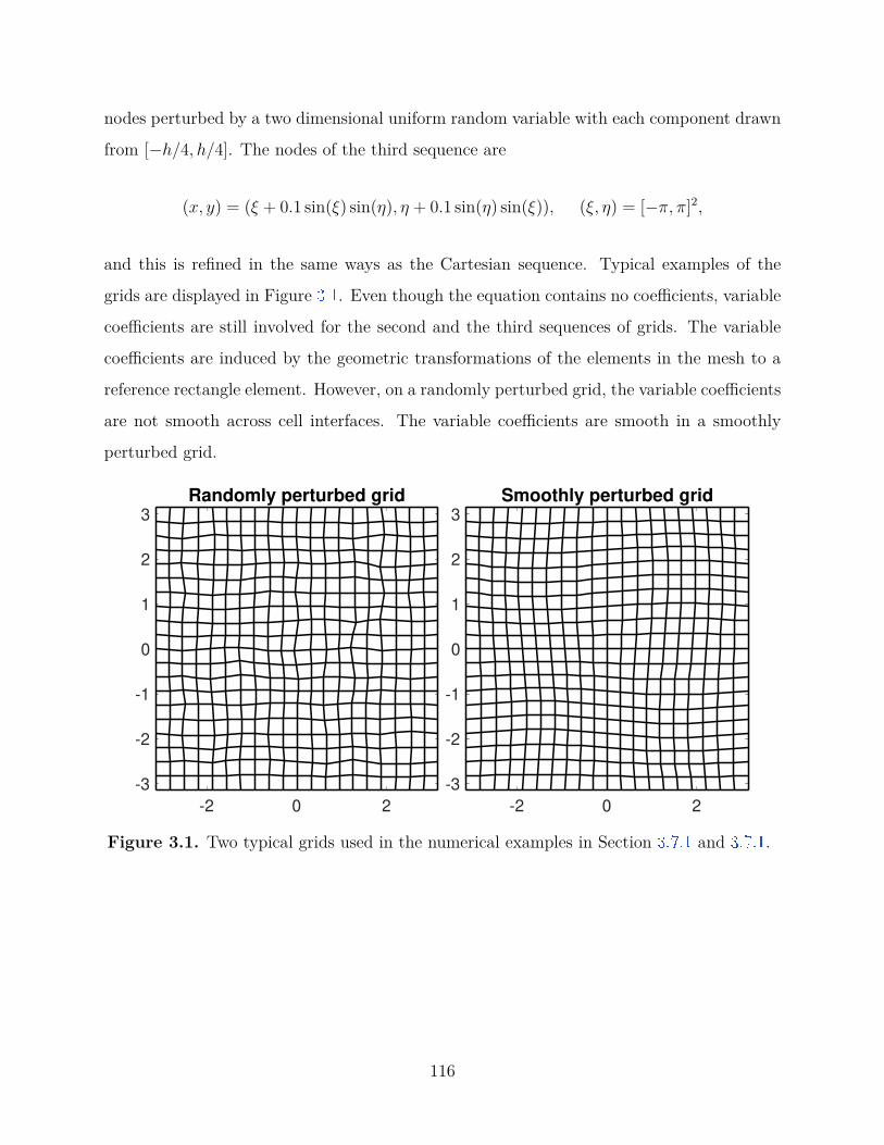
nodes perturbed by a two dimensional uniform random variable with each component drawn

from [−h/4, h/4]. The nodes of the third sequence are

(x, y) = (ξ + 0.1 sin(ξ) sin(η), η + 0.1 sin(η) sin(ξ)), (ξ, η) = [−π, π]2,

and this is refined in the same ways as the Cartesian sequence. Typical examples of the

grids are displayed in Figure 3.1 . Even though the equation contains no coefficients, variable

coefficients are still involved for the second and the third sequences of grids. The variable

coefficients are induced by the geometric transformations of the elements in the mesh to a

reference rectangle element. However, on a randomly perturbed grid, the variable coefficients

are not smooth across cell interfaces. The variable coefficients are smooth in a smoothly

perturbed grid.

-2 0 2

-3

-2

-1

0

1

2

3

Randomly perturbed grid

-2 0 2

-3

-2

-1

0

1

2

3

Smoothly perturbed grid

Figure 3.1. Two typical grids used in the numerical examples in Section 3.7.1 and 3.7.1 .

116

10-1

100

Gridsize

10-6

10-4

10-2

100

L2

-err

or

rate = 3

rate = 4

Cartesian

rand. pert.

smooth pert.

10-1

100

Gridsize

10-6

10-4

10-2

100

Ma

x-e

rro

r

rate = 3

rate = 4

Cartesian

rand. pert.

smooth pert.

10-1

100

Gridsize

10-10

10-5

L2

-err

or

rate = 5

rate = 6

Cartesian

rand. pert.

smooth pert.

10-1

100

Gridsize

10-10

10-5

Ma

x-e

rro

r

rate = 5

rate = 6

Cartesian

rand. pert.

smooth pert.

Figure 3.2. Dirichlet problem in a square. Errors measured in the l2 and thel∞ norms for the three different sequences of grids. The top row is for k = 2and the bottom row is for k = 4.

We evolve the numerical solution until time 5 by the time stepping discussed in Section

3.7.1 of order of accuracy 4 when k = 2 and 6 when k = 4. To get clean measurements of

the error we report the time integrated errors

(∫ 5

0‖u(·, t)− uh(·, t)‖2

l2 dt) 1

2,

∫ 5

0‖u(·, t)− uh(·, t)‖l∞ dt,

for the spatial l2 and l∞ errors respectively.

The results are displayed in Figure 3.2 . Note that here and in the rest of this section the

solid lines in the figures are the computed errors, using many different grid sizes, and the

symbols are indicating the slopes or rates of convergence of the curves. The Cartesian grids

117

and smoothly perturbed grids satisfy the assumptions of the theory developed in this chapter

while the second sequence of randomly perturbed grids does not. The results confirm the

theoretical predictions for smooth variable coefficients as the rate of convergence is k + 2

for the l2-norm in the cases of the Cartesian meshes and the smoothly perturbed meshes.

We also observe the rate k + 2 in the l∞-norm for these cases. For the non-smooth variable

coefficients resulting from the randomly perturbed grid, which not covered by our theory,

we see a rate of convergence of k + 1 in the l2-norm.

Standing mode in a sector of an annulus with Dirichlet conditions

10-1

100

Gridsize

10-10

10-5

L2

-err

or

rate = 4

rate = 2

Straight

True curvi.

Bdry. curvi.

10-1

100

Gridsize

10-10

10-5

Ma

x-e

rro

r

rate = 4

rate = 2

Straight

True curvi.

Bdry. curvi.

10-1

100

Gridsize

10-10

10-5

L2

-err

or

rate = 6

rate = 2

Straight

True curvi.

Bdry. curvi.

10-1

100

Gridsize

10-10

10-5

Ma

x-e

rro

r

rate = 6

rate = 2

Straight

True curvi.

Bdry. curvi.

Figure 3.3. Dirichlet problem in an annular sector. Errors measured in thel2 and the l∞ norms for the three different sequences of grids. The top row isfor k = 2 and the bottom row is for k = 4. These results are for the annularproblem with homogenous Dirichlet boundary conditions.

118

In this experiment we solve the wave equation utt = uxx + uyy and and with ho-

mogenous Dirichlet boundary conditions. The computational domain is the first quad-

rant of the annular region between two circles with radii ri = 7.58834243450380438 and

ro = 14.37253667161758967, i.e. the domain is described by (x, y) = (r cos θ, r sin θ) where

ri ≤ r ≤ ro, 0 ≤ θ ≤ π/2.

On this domain the standing mode

u(r, θ, t) = J4(r) sin(4θ) cos(t),

is an exact solution and we use this solution to specify the initial conditions and to compute

errors.

We consider the two cases k = 2 and k = 4 and discretize on three different sequences

of grids. The first sequence uses a straight sided approximation of the annulus and all

internal elements are quadrilaterals with straight sides. The second sequence uses curvilinear

elements throughout the domain and all internal element boundaries conform with the polar

coordinate transformation. After the smooth mapping to the unit square, smooth variable

coefficients emerge due to the geometric terms. The metric terms are approximated with

numerical differentiation using the values at the quadrature points. The third sequence is

the same as the second sequence but all the internal element edges are straight. The meshes

in the last sequence are likely close to those that would be provided by most grid generators.

We evolve the numerical solution until time 1 by the time stepping discussed in Section

3.7.1 of order of accuracy 4 when k = 2 and 6 when k = 4. Again, to get clean measurements

of the error we report the time integrated errors

(∫ 1

0‖u(·, t)− uh(·, t)‖2

l2 dt) 1

2,

∫ 1

0‖u(·, t)− uh(·, t)‖l∞ dt,

for the spatial l2 and l∞ errors respectively.

119

The results are displayed in Figure 3.3 . Here, as expected, we only observe second

order accuracy independent of k for the non-geometry-conforming meshes. We observe a

convergence at the rate of k+2 in both the l2-norm and l∞-norm for the geometry-conforming

meshes. The true curvilinear grids are covered by our theory since the variable coefficients

due to the geometric transformation are smooth. For the third sequence of grids, since

internal edges are straightsided, the variable coefficients from the geometric transformation

are not smooth across edges thus this configuration is not covered by our theory. Nonetheless,

its convergence rate is still k + 2.

Standing mode with Neumann conditions

10-2

10-1

100

Gridsize

10-10

10-8

10-6

10-4

10-2

100

L2

-err

or

rate = 3

rate = 4

rate = 3.666

Cartesian

rand. pert.

smooth pert.

10-2

10-1

100

Gridsize

10-10

10-8

10-6

10-4

10-2

100

Ma

x-e

rro

rrate = 3

rate = 4

rate = 3

Cartesian

rand. pert.

smooth pert.

10-1

100

Gridsize

10-10

10-8

10-6

10-4

10-2

L2

-err

or

rate = 5

rate = 6

rate = 5.666

Cartesian

rand. pert.

smooth pert.

10-1

100

Gridsize

10-10

10-8

10-6

10-4

10-2

Ma

x-e

rro

r

rate = 5

rate = 6

rate = 5

Cartesian

rand. pert.

smooth pert.

Figure 3.4. Neumann square problem. Errors measured in the l2 and the l∞norms for the three different sequences of grids. The top row is for k = 2 andthe bottom row is for k = 4.

120

In this experiment we approximate the solution to the wave equation utt = uxx + uyy in

the square domain (x, y) ∈ [−π, π]2. Then with homogenous Neumann boundary conditions

and initial data

u(x, y, 0) = cos(x) cos(y), ut(x, y, 0) = 0,

the exact standing mode solution is

u(x, y, 0) = cos(x) cos(y) cos(√

2t).

We consider the two cases k = 2 and k = 4 and discretize on the same three sequences

of grids as those used in §3.7.1 . We evolve the numerical solution until time 5 as above and

we report the time integrated errors as above.

The results are displayed in Figure 3.4 . For the Cartesian mesh we observe a rate of

convergence k + 2 in the `2-norm, confirming our theory. For the smoothly perturbed grids,

which corresponds to smooth variable coefficients resulting in mixed second order derivatives

on the reference rectangular mesh, the rate in the l2-norm appears to be k + 5/3. As

explained in Section 3.5.4 , only (k + 32)-th order can be proven when both mixed second

order derivatives and Neumann boundary conditions are involved. As in the Dirichlet case,

the randomly perturbed grid yields rates of convergence k + 1 in both norms.

Standing mode in a sector of an annulus with Neumann conditions

In this experiment we solve the the wave equation utt = uxx + uyy with homogenous

Neumann boundary conditions. The computational domain is again the first quadrant of

the annular region between two circles, now with radii ri = 5.31755312608399 and ro =

9.28239628524161, to satisfy the boundary conditions. On this domain the standing mode

u(r, θ, t) = J4(r) cos(4θ) cos(t),

is an exact solution and we use this solution to specify the initial conditions and to compute

errors.

121

As in the previous examples we consider the two cases k = 2 and k = 4 and discretize

on the same three different sequences of grids as was used in the Dirichlet example above.

We evolve the numerical solution until time 1 in the same way as above and we report the

time integrated errors.

The results are displayed in Figure 3.5 . Here, the only grid satisfying our assumptions

is the true curvilinear grid. For this case, the problem is equivalent to solving a variable

coefficient problem utt = urr + 1r2uθθ + 1

rur on rectangular meshes for polar coordinates

(r, θ) ∈ [ri, ro] × [0, π2 ]. Since there are no mixed second order derivatives, by our theory as

explained in Section 3.5.4 , (k + 2)-th order in the `2-norm can still be proven. We can see

that the rate for the true curvilinear grid is indeed k + 2 in `2-norm, confirming our theory

for Neumann boundary conditions.

3.7.2 Numerical tests for the parabolic equation

For problem (3.2 ) on the domain Ω = (0, π)2, we set a =

a11 a12

a21 a22

with a11 =(

34 + 1

4 sin(t))

(1 + y + y2 + x cos y), a12 = a21 =(

34 + 1

4 sin(t)) (

1 + 12(sin(πx) + x3)(sin(πy) + y3) + cos(x4 + y3)

),

a22 =(

34 + 1

4 sin(t))

(1 + x2), b =

b1

b2

with b1 =(

34 + 1

4 sin(t)) (

15 + x

), b2 =

(34 + 1

4 sin(t)) (

15 − y

),

and c =(

34 + 1

4 sin(t))

(10 + x4y3). For time discretization in (3.6 ), we use the third order

backward differentiation formula (BDF) method. Let u(x, y, t) = (34+1

4 sin(t))(− sin(y) cos(y) sin(x)2)

and we use a potential function f so that u is the exact solution. The time step is set as

∆t = min(∆x10 ,

∆x10bM

, fM

10 ), where bM = maxx∈Ω,i=1,2 |bi(0,x)| and fM = maxx∈Ω |f(0,x)|. The

errors at time T = 0.1 are listed in Table 3.1 , in which we observe order around k + 2 for

the `2-norm.

3.7.3 Numerical tests for the linear Schrödinger equation

For problem (3.37 ) on the domain (0, 2)2, a fourth-order explicit Adams-Bashforth as

time discretization for (3.39 ). The solution and potential functions are as follows: u(x, y, t) =

122

10-1

100

Gridsize

10-10

10-5

L2

-err

or

rate = 4

rate = 2

rate = 3.666

Straight

True curvi.

Bdry. curvi.

10-1

100

Gridsize

10-10

10-5

Ma

x-e

rro

r

rate = 4

rate = 2

rate = 3

Straight

True curvi.

Bdry. curvi.

10-1

100

Gridsize

10-10

10-5

L2

-err

or

rate = 6

rate = 2

rate = 5.666

Straight

True curvi.

Bdry. curvi.

10-1

100

Gridsize

10-10

10-5

Ma

x-e

rro

rrate = 6

rate = 2

rate = 5

Straight

True curvi.

Bdry. curvi.

Figure 3.5. Neumann annular sector problem. Errors measured in the l2and the l∞ norms for the three different sequences of grids. The top row isfor k = 2 and the bottom row is for k = 4. These results are for the annularproblem with homogenous Neumann conditions.

e−ite− x2+y22 , V (x, y) = x2+y2

2 , and f(x, y, t) = 0. The time step is set as ∆t = ∆x2

500 . Errors at

time T = 0.5 are listed in Table 3.2 , in which we observe order near k + 2 for the `2-norm.


We have proven that the Qk (k ≥ 2) spectral element method, when regarded as a finite

difference scheme, is a (k + 2)-th order accurate scheme in the discrete 2-norm for linear

hyperbolic, parabolic and Schrödinger equations with Dirichlet boundary conditions, under

smoothness assumptions of the exact solution and the differential operator coefficients. The

same result holds for Neumann boundary conditions when there are no mixed second order

123

Table 3.1. A two-dimensional parabolic equation with Dirichlet boundary conditions.Qk polynomial SEM Mesh l2 error order l∞ error order

k = 2

4× 4 8.34E-3 - 4.57E-3 -8× 8 6.59E-4 3.66 3.16E-4 3.85

16× 16 4.52E-5 3.86 2.36E-5 3.7432× 32 2.91E-6 3.96 1.53E-6 3.94

k = 3

4× 4 5.88E-4 - 1.71E-4 -8× 8 2.24E-5 4.71 7.56E-6 4.50

16× 16 7.49E-7 4.90 2.52E-7 4.9132× 32 2.38E-8 4.97 8.06E-9 4.96

k = 4

4× 4 4.26E-5 - 1.16E-5 -8× 8 7.62E-7 5.81 2.34E-7 5.63

16× 16 1.26E-8 5.92 4.12E-9 5.8332× 32 2.00E-10 5.98 6.68E-11 5.95

Table 3.2. A two-dimensional linear Schrödinger equation with Dirichletboundary conditions.

Qk polynomial SEM Mesh l2 error order l∞ error order

k = 2

4× 4 9.98E-4 - 6.36E-4 -8× 8 6.65E-5 3.91 4.01E-5 3.99

16× 16 4.10E-6 4.02 2.77E-6 3.8532× 32 2.53E-7 4.02 1.79E-7 3.89

k = 3

4× 4 4.06E-5 - 2.12E-5 -8× 8 1.12E-6 5.18 5.56E-7 5.26

16× 16 3.22E-8 5.12 1.75E-8 4.9932× 32 1.05E-9 4.94 5.33E-10 5.04

k = 4

4× 4 1.61E-6 - 5.86E-7 -8× 8 2.65E-8 5.92 9.93E-9 5.88

16× 16 3.95E-10 6.07 1.66E-10 5.9032× 32 5.30E-12 6.22 2.66E-12 5.97

derivatives. This explains the observed order of accuracy when the errors of the spectral

element method are only measured at nodes of degree of freedoms.

124

4. SUPERCONVERGENCE OF C0-Qk FINITE ELEMENT

METHOD FOR ELLIPTIC EQUATIONS WITH

APPROXIMATED COEFFICIENTS

4.1 Introduction

In this chapter, we prove that the superconvergence of C0-Qk finite element method at

the Gauss Lobatto quadrature points still holds if variable coefficients in an elliptic problem

are replaced by their piecewise Qk Lagrange interpolants at the Gauss Lobatto points in

each rectangular cell.

4.1.1 Motivations

Consider solving a variable coefficient Poisson equation

−∇ · (a∇u) = f, a(x, y) > 0 (4.1)

with homogeneous Dirichlet boundary conditions on a rectangular domain Ω as in Chapter

2 . The variational form is to find u ∈ H10 (Ω) = v ∈ H1(Ω) : v|∂Ω = 0 satisfying

A(u, v) = (f, v), ∀v ∈ H10 (Ω), (4.2)


Ω a∇u · ∇vdxdy, (f, v) =∫∫

Ω fvdxdy. Consider a rectangular mesh with

mesh size h, the C0-Qk finite element solution of (4.2 ) is defined as uh ∈ V h0 satisfying

A(uh, vh) = (f, vh), ∀vh ∈ V h0 . (4.3)

For implementing finite element method (4.3 ), either some quadrature is used or the

coefficient a(x, y) is approximated by polynomials for computing∫∫

Ω auhvh dxdy. In this

chapter, we consider the implementation to approximate the smooth coefficient a(x, y) by

its Qk Lagrangian interpolation polynomial in each cell. For instance, consider Q2 element in

two dimensions, tensor product of 3-point Lobatto quadrature form nine uniform points on

125

each cell, see Figure 4.1 . By point values of a(x, y) at these nine points, we can obtain a Q2

Lagrange interpolation polynomial on each cell. Let aI(x, y) and fI(x, y) denote the piecewise

Qk interpolation of a(x, y) and f(x, y) respectively. For a smooth functions a ≥ C > 0, the

interpolation error on each cell e is maxx∈e |aI(x)−a(x)| = O(hk+1) thus aI > 0 if h is small

enough. So if assuming the mesh is fine enough so that aI(x, y) ≥ C > 0, we consider the

following scheme using the approximated coefficients aI(x, y): find uh ∈ V h0 satisfying

AI(uh, vh) :=∫∫

ΩaI∇u · ∇vdxdy = 〈f, vh〉h, ∀vh ∈ V h

0 , (4.4)

where 〈f, vh〉h denotes using tensor product of (k + 1)-point Gauss Lobatto quadrature for

the integral (f, vh). One can also simplify the computation of the right hand side by using

fI(x, y), so we also consider the scheme to find uh satisfying

AI(uh, vh) = (fI , vh), ∀vh ∈ V h0 . (4.5)

(a) A nx × ny finite difference grid (b) The corresponding nx−12 × ny−1

2 mesh Ωh forQ2 element

Figure 4.1. An illustration of meshes.

The schemes (4.4 ) and (4.5 ) correspond to the equation

−∇ · (aI(x, y)∇u(x, y)) = f(x, y). (4.6)

At first glance, one might expect (k+ 1)-th order accuracy for a numerical method applying

to (4.6 ) due to the interpolation error a(x, y)− aI(x, y) = O(hk+1). But as we will show in

Section 4.4.1 , the difference between exact solutions u and u to the two elliptic equations

126

(4.1 ) and (4.6 ) is O(hk+2) in L2(Ω)-norm under suitable assumptions. The main focus of this

chapter is to show (4.4 ) and (4.5 ) are (k+2)-th order accurate finite difference type schemes

via the superconvergence of finite element method. Such a result is very interesting from the

perspective that a fourth order accurate scheme can be constructed even if the coefficients

in the equation are approximated by quadratic polynomials, which does not seem to be

considered before in the literature.

Since only grid point values of a(x, y) and f(x, y) are needed in scheme (4.4 ) or (4.5 ),

they can be regarded as finite difference type schemes. Consider a uniform nx × ny grid for

a rectangle Ω with grid points (xi, yj) and grid spacing h, where nx and ny are both odd

numbers as shown in Figure 4.1 (a). Then there is a mesh Ωh of (nx − 1)/2× (ny − 1)/2 Q2

elements so that Gauss-Lobatto points for all cells in Ωh are exactly the finite difference grid

points. By using the scheme (4.4 ) or (4.5 ) on the finite element mesh Ωh shown in Figure

4.1 (b), we obtain a fourth order finite difference scheme in the sense that uh is fourth order

accurate in the discrete 2-norm at all grid points.

In practice the most convenient implementation is to use tensor product of (k+ 1)-point

Gauss Lobatto quadrature for integrals in (4.2 ) i.e. scheme (2.2 ) as described in Chapter 2 .

Numerical tests suggest that the approximated coefficient scheme (4.5 ) is more accurate and

robust than the quadrature scheme (2.2 ) in some cases.

4.2 Notations And Preliminaries

We will continue to use the notations in Section 3.2 of Chapter 2 . Besides the error

estimate in Section 2.3 , we also need the following estimate.

Theorem 4.2.1. For k ≥ 2, (f, vh)− (fI , vh) = O(hk+2)‖f‖k+2‖vh‖2, ∀vh ∈ V h.

Proof. Repeat the proof of Theorem 2.3.4 for the function f − fI on a cell e, with the fact

[fI ]k+1,p,e = [fI ]k+2,p,e = 0, we get

E[(f − fI)vh] = Chk+2([f ]k+2,e|vh|0,e + [f ]k+1,e|vh|1,e + [f − fI ]k,e|vh|2,e).

127

By (2.13 ) on the Lagrange interpolation operator and the fact [f − fI ]k,e ≤ ‖f − fI‖k+1,e, we

get [f − fI ]k,e ≤ Ch[f ]k+1,e. Notice that 〈f − fI , vh〉h = 0, with (2.5 ), we get

(f, vh)− (fI , vh) = (f − fI , vh)− 〈f − fI , vh〉h = O(hk+2)‖f‖k+2‖vh‖2,∀vh ∈ V h.

4.3 Superconvergence Of The Bilinear Form

For convenience, in this subsection, we drop the subscript h in a test function vh ∈ V h.

When there is no confusion, we may also drop dxdy or dsdt in a double integral.

Lemma 4.3.1. Assume a(x, y) ∈ W 2,∞(Ω). For k ≥ 2,

∫∫Ωa(u− up)xvx dxdy = O(hk+2)‖u‖k+2‖v‖2, ∀v ∈ V h.

Proof. For each cell e, we consider∫∫

e a(u − up)xvx dxdy. Let R[u]k,k = u − up denote

the M-type projection remainder on e. Then R[u]k,k can be splitted into lower order part

R[u]k,k −R[u]k+1,k+1 and high order part R[u]k+1,k+1.

∫∫ea(u− up)xvx dxdy =

∫∫ea(R[u]k+1,k+1)xvx +

∫∫ea(R[u]k,k −R[u]k+1,k+1)xvx.

We first consider the high order part. Mapping everything to the reference cell K and let

avs denote the average of avs on K. By the last property in Lemma 2.4.3 , we get

h2−n

∣∣∣∣∫∫ea(R[u]k+1,k+1)xvx dxdy

∣∣∣∣ =∣∣∣∣∫∫

K∂s(R[u]k+1,k+1)avsdsdt

∣∣∣∣=∣∣∣∣∫∫

K∂s(R[u]k+1,k+1)(avs − avs)dsdt

∣∣∣∣ ≤ |∂s(R[u]k+1,k+1)|0,2,K |avs − avs|0,2,K .

By Poincaré inequality and Cauchy-Schwarz inequality, we have

|avs − avs|0,2,K ≤ C|∇(avs)|0,2,K ≤ C|a|1,∞,K |v|1,2,K + C|a|0,∞,K |v|2,2,K .

128

Mapping back to the cell e, with (2.5 ), by Lemma 2.4.3 , the higher order part is bounded

by Chk+2[u]k+2,2,e(|a|1,∞,e|v|1,2,e + |a|0,∞,e|v|2,2,e) thus

∑e

∫∫ea(R[u]k+1,k+1)xvx dxdy = O(hk+2)‖a‖1,∞,Ω

∑e

‖u‖k+2,e‖v‖2,e

= O(hk+2)‖a‖1,∞,Ω‖u‖k+2,Ω‖v‖2,Ω.

Now we only need to discuss the lower order part of the remainder. Let R[u]k,k −

R[u]k+1,k+1 = R1 +R2 which is defined similarly as in (2.28 ). For R1, by the first two results

in Lemma 2.4.4 , we have

∫∫K

(∂sR1)avs =∫∫

K(∂sR1)(avs − avs) ≤ |∂sR1|0,2,K |avs − avs|0,2,K

≤ C|u|k+2,2,K |avs − avs|0,2,K .

By similar discussions above, we get

∑e

∫∫ea(R1)xvx dxdy = O(hk+2)‖a‖1,∞,Ω‖u‖k+2,Ω‖v‖2,Ω.

For R2, let N(s) be the antiderivative of Mk+1(s) then N(±1) = 0. Let ¯a be the

average of ¯a on K then |a − ¯a|0,∞,K ≤ C|a|1,∞,K . Since Mk+1(s) ⊥ P k−2(s), we have∫∫K bk+1(t)Mk+1(s)vss = 0. After integration by parts, by Lemma 2.4.4 we have

∫∫K

(∂sR2)avs = −∫∫

Kbk+1(t)Mk+1(s)(asvs + avss)

=∫∫

Kbk+1(t)N(s)(assvs + asvss)−

∫∫Kbk+1(t)Mk+1(s)(a− ¯a)vss

≤C|u|k+1,K(|a|2,∞,K |v|1,2,K + |a|1,∞,K |v|2,2,K).

Thus we can get

∑e

∫∫e(∂xR2)avxdxdy = O(hk+2)‖a‖2,∞,Ω‖u‖k+1,Ω‖v‖2,Ω.

So we have∫∫

Ω a(u− up)xvx dxdy = O(hk+2)‖a‖2,∞,Ω‖u‖k+2‖v‖2, ∀v ∈ V h.

129

Lemma 4.3.2. Assume c(x, y) ∈ W 1,∞(Ω). For k ≥ 2,

∫∫Ωc(u− up)v dxdy = O(hk+2)‖u‖k+1‖v‖1, ∀v ∈ V h.

Proof. Let cv be the average of cv on K. Following similar arguments as in the proof Lemma

4.3.1 ,

∣∣∣∣∫∫KR[u]k,kcv

∣∣∣∣ =∣∣∣∣∫∫

KR[u]k,k(cv − cv)

∣∣∣∣ ≤ |R[u]k,k|0,2,K |cv − cv|0,2,K

≤ C[u]k+1,2,K [cv]1,2,K ≤ C[u]k+1,2,K(|c|0,∞,K |v|1,2,K + |c|1,∞,K |v|0,2,K).

So with (2.5 ) we have

∫∫ecR[u]k,kvdxdy = hn

∫∫K

(R[u]k,k)cvdsdt = O(hk+2)‖c‖1,∞,Ω‖u‖k+1,e‖v‖1,e,

which implies the estimate.

Lemma 4.3.3. Assume b(x, y) ∈ W 2,∞(Ω). For k ≥ 2,

∫∫Ωb(u− up)xv dxdy = O(hk+2)‖u‖k+2‖v‖2, ∀v ∈ V h.

Proof. Let bv be the average of bv on K. Following similar arguments as in the proof Lemma

4.3.1 , we have

∣∣∣∣∫∫K∂s(R[u]k+1,k+1)bv

∣∣∣∣ =∣∣∣∣∫∫

K∂s(R[u]k+1,k+1)(bv − bv)

∣∣∣∣≤ |∂s(R[u]k+1,k+1)|0,2,K |bv − bv|0,2,K ≤ C[u]k+2,2,K(|b|1,∞,K |v|0,2,K + |b|0,∞,K |v|1,2,K).

∫∫K

(∂sR1)bv =∫∫

K(∂sR1)(bv − bv) ≤ |∂sR1|0,2,K |bv − bv|0,2,K

≤ C|u|k+2,2,K(|b|1,∞,K |v|0,2,K + |b|0,∞,K |v|1,2,K).

130

Let N(s) be the antiderivative of Mk+1(s). After integration by parts, we have

∫∫K

(∂sR2)bv = −∫∫

Kbk+1(t)Mk+1(s)(bsv + bvs)

=∫∫

Kbk+1(t)N(s)(bssv + bsvs + bvss)

≤C|u|k+1,2,K(|b|2,∞,K |v|0,2,K + |b|1,∞,K |v|1,2,K + |b|0,∞,K |v|2,2,K).

After combining all the estimates, with (2.5 ), we have

∫∫eb(u− up)xv = hn−1

∫∫Kb(R[u]k,k)sv = O(hk+2)‖b‖2,∞,Ω‖u‖k+2,e‖v‖2,e.

Lemma 4.3.4. Assume a(x, y) ∈ W 2,∞(Ω). For k ≥ 2,

∫∫Ωa(u− up)x(vh)y dxdy =

O(hk+ 3

2 )‖a‖k+2,∞‖u‖k+2‖vh‖2, ∀vh ∈ V h, (4.7a)

O(hk+2)‖a‖k+2,∞‖u‖k+2‖vh‖2, ∀vh ∈ V h0 . (4.7b)

Proof. Similar to the proof of Lemma 4.3.1 , we have

∣∣∣∣∫∫ea(R[u]k+1,k+1)xvy dxdy

∣∣∣∣ = hn−2∣∣∣∣∫∫

K∂s(R[u]k+1,k+1)avtdsdt

∣∣∣∣=hn−2

∣∣∣∣∫∫K∂s(R[u]k+1,k+1)(avt − avt)dsdt

∣∣∣∣ ≤ hn−2|∂s(R[u]k+1,k+1)|0,2,K |avt − avt|0,2,K

≤Chk+2‖a‖1,∞,Ω‖u‖k+2,e‖v‖2,e,

and ∫∫K

(∂sR1)avt =∫∫

K(∂sR1)(avt − avt) ≤ |∂sR1|0,2,K |avt − avt|0,2,K .

Following the proof of Lemma 4.3.1 , with (2.5 ), we get

∑e

∫∫ea(R1)xvy dxdy = O(hk+2)‖a‖1,∞,Ω‖u‖k+2,Ω‖v‖2,Ω.

131

After integration by parts, we have

∫∫K

(∂sR2)avt = −∫∫

Kbk+1(t)Mk+1(s)(asvt + avst),

which is exactly the same integral estimates (2.41 ) in the proof of Lemma 2.5.5 in Chapter

2 . By the same proof as (2.41 ), after combining all the estimates above and summing over

all elements, we have the estimate for the term∫∫

K lk(s)bk+1(t)avtdsdt:

∑e

|∫∫

K(∂sR2)avt| =

O(hk+ 3

2 )‖a‖k+2,∞‖u‖k+3‖v‖2, ∀v ∈ V h,

O(hk+2)‖a‖k+2,∞‖u‖k+3‖v‖2, ∀v ∈ V h0 .

Combine all the estimates above, we get (4.7a ). Since the 12 order loss is only due to the

line integral along L1 and L3, on which vxx = 0 if v ∈ V h0 , we get (4.7b ).

4.4 The Main Result

4.4.1 Superconvergence of bilinear forms with approximated coefficients

Even though standard interpolation error is a− aI = O(hk+1), as shown in the following

discussion, the error in the bilinear forms is related to∫∫

e(a−aI) dxdy on each cell e, which is

the quadrature error thus the order is higher. We have the following estimate on the bilinear

forms with approximated coefficients:

Lemma 4.4.1. Assume a(x, y) ∈ W k+2,∞(Ω) and u(x, y) ∈ H2(Ω), then ∀v ∈ V h or ∀v ∈

H2(Ω),

∫∫Ωauxvx dxdy −

∫∫ΩaIuxvx dxdy = O(hk+2)‖a‖k+2,∞,Ω‖u‖2‖v‖2,∫∫

Ωauxvy dxdy −

∫∫ΩaIuxvy dxdy = O(hk+2)‖a‖k+2,∞,Ω‖u‖2‖v‖2,∫∫

Ωauxv dxdy −

∫∫ΩaIuxv dxdy = O(hk+2)‖a‖k+2,∞,Ω‖u‖2‖v‖1,∫∫

Ωauv dxdy −

∫∫ΩaIuv dxdy = O(hk+2)‖a‖k+2,∞,Ω‖u‖1‖v‖1.

132

Proof. For every cell e in the mesh Ωh, let uxvx be the cell average of uxvx. By Theorem

2.3.2 and Theorem 2.3.3 , we have

∫∫e(aI − a)uxvx

=∫∫

e(aI − a)uxvx +

∫∫e(aI − a)(uxvx − uxvx)

= 14h2

∫∫e(aI − a)

∫∫euxvx +

∫∫e(aI − a)(uxvx − uxvx)

=O(hk+2)‖a‖k+2,∞,Ω‖u‖1,e‖v‖1,e +O(hk+1)‖a‖k+1,∞,Ω

∫∫e|uxvx − uxvx|.

By Poincaré inequality and Cauchy-Schwarz inequality, we have

∫∫e|uxvx − uxvx| = O(h)‖∇(uxvx)‖0,1,e = O(h)‖u‖2,e‖v‖2,e

thus∫∫

e(aI−a)uxvx = O(hk+2)‖a‖k+2,∞,Ω‖u‖2,e‖v‖2,e. Summing over all elements e, we have∫∫Ω(aI − a)uxvx = O(hk+2)‖a‖k+2,∞,Ω‖u‖2‖v‖2. Similarly we can establish the other three

estimates.

Lemma 4.4.1 implies that the difference in the solutions to (4.6 ) and (4.1 ) is O(hk+2) in

the L2(Ω)-norm:

Theorem 4.4.2. Assume a(x, y) ∈ W k+2,∞(Ω) and aI(x, y) ≥ C > 0. Let u, u ∈ H10 (Ω) be

the solutions to

A(u, v) :=∫∫

a∇u · ∇v dxdy = (f, v), ∀v ∈ H10 (Ω)

and

AI(u, v) :=∫∫

aI∇u · ∇v dxdy = (f, v), ∀v ∈ H10 (Ω)

respectively, where f ∈ L2(Ω). Then ‖u− u‖0 = O(hk+2)‖a‖k+2,∞,Ω‖f‖0.

133

Proof. By Lemma 4.4.1 , for any v ∈ H2(Ω) we have

AI(u− u, v) = AI(u, v)− AI(u, v) = [AI(u, v)− A(u, v)] + [A(u, v)− AI(u, v)]

= AI(u, v)− A(u, v) = O(hk+2)‖a‖k+2,∞,Ω‖u‖2‖v‖2.

Let w ∈ H10 (Ω) be the solution to the dual problem

AI(v, w) = (u− u, v) ∀v ∈ H10 (Ω).

Since aI ≥ C > 0 and |aI(x, y)| ≤ C|a(x, y)|, the coercivity and boundedness of the bilinear

form AI hold [3 ]. Moreover, aI is Lipschitz continuous because a(x, y) ∈ W k+2,∞(Ω). Thus

the solution w exists and the elliptic regularity ‖w‖2 ≤ C‖u− u‖0 holds on a convex domain,

e.g., a rectangular domain Ω, see [34 ]. Thus,

‖u− u‖20 = (u− u, u− u) = AI(u− u, w) = O(hk+2)‖a‖k+2,∞,Ω‖u‖2‖w‖2.

With elliptic regularity ‖w‖2 ≤ C‖u− u‖0 and ‖u‖2 ≤ C‖f‖0, we get

‖u− u‖0 = O(hk+2)‖a‖k+2,∞,Ω‖f‖0.

Remark 4.4.3. For even number k ≥ 4, (k + 1)-point Newton-Cotes quadrature rule has the

same error order as the (k + 1)-point Gauss-Lobatto quadrature rule. Thus Theorem 4.4.2

still holds if we redefine aI(x, y) as the Qk interpolant of a(x, y) at the uniform (k+1)×(k+1)

Newton-Cotes points in each cell if k ≥ 4 is even.

4.4.2 The variable coefficient Poisson equation

Let u(x, y) ∈ H10 (Ω) be the exact solution to

A(u, v) :=∫∫

Ωa∇u · ∇v dxdy = (f, v), ∀v ∈ H1

0 (Ω).

134

Let uh ∈ V h0 (Ω) be the solution to

AI(uh, vh) :=∫∫

ΩaI∇uh · ∇vh dxdy = 〈f, vh〉h, ∀vh ∈ V h

0 (Ω).

Theorem 4.4.4. For k ≥ 2, let up be the piecewise Qk M-type projection of u(x, y) on each

cell e in the mesh Ωh. Assume a ∈ W k+2,∞(Ω) and u, f ∈ Hk+2(Ω), then

AI(uh − up, vh) = O(hk+2)(‖a‖k+2,∞‖u‖k+2 + ‖f‖k+2)‖vh‖2, ∀vh ∈ V h0 .

Proof. For any vh ∈ V h, we have

AI(uh, vh)− AI(up, vh)

=(f, vh)− AI(up, vh) + 〈f, vh〉h − (f, vh)

=A(u, vh)− AI(up, vh) + 〈f, vh〉h − (f, vh)

=[A(u, vh)− AI(u, vh)] + [AI(u− up, vh)− A(u− up, vh)] + A(u− up, vh) + 〈f, vh〉h − (f, vh).

Lemma 4.4.1 implies A(u, vh) − AI(u, vh) = O(hk+2)‖a‖k+2,∞‖u‖2‖vh‖2. Theorem 2.3.4

gives 〈f, vh〉h−(f, vh) = O(hk+2)‖f‖k+2‖vh‖2. By Lemma 4.3.1 , A(u−up, vh) = O(hk+2)‖a‖2,∞‖u‖k+2‖vh‖2.

For the second term AI(u−up, vh)−A(u−up, vh) =∫∫

Ω(a−aI)∇(u−up)∇vh, by Theorem

2.3.2 and Lemma 2.4.3 , we have

∣∣∣∣∫∫Ω(a− aI)(u− up)x∂xvh

∣∣∣∣ ≤ |a− aI |0,∞,Ω∑

e

∫∫e|(u− up)x∂xvh|

≤ |a− aI |0,∞,Ω∑

e

|(u− up)x|0,2,e|vh|1,2,e

= O(h2k+1)‖a‖k+1,∞,Ω∑

e

‖u‖k+1,e‖vh‖1,e

= O(h2k+1)‖a‖k+1,∞,Ω‖u‖k+1‖vh‖1.

Theorem 4.4.5. Assume a(x, y) ∈ W k+2,∞(Ω) is positive and u(x, y), f(x, y) ∈ Hk+2(Ω).

Assume the mesh is fine enough so that the piecewise Qk interpolant satisfies aI(x, y) ≥ C >

135

0. Then uh is a (k+ 2)-th order accurate approximation to u in the discrete 2-norm over all

the (k + 1)× (k + 1) Gauss-Lobatto points:

‖uh − u‖2,Z0 = O(hk+2)(‖a‖k+2,∞‖u‖k+2 + ‖f‖k+2).

Proof. Let θh = uh − up. By the definition of up and Theorem 2.4.1 , it is straightforward to

show θh = 0 on ∂Ω. By the Aubin-Nitsche duality method, let w ∈ H10 (Ω) be the solution

to the dual problem

AI(v, w) = (θh, v) ∀v ∈ H10 (Ω).

By the same discussion as in the proof of Theorem 4.4.2 , the solution w exists and the

regularity ‖w‖2 ≤ C‖θh‖0 holds.

Let wh be the finite element projection of w, i.e., wh ∈ V h0 satisfies

AI(vh, wh) = (θh, vh) ∀vh ∈ V h0 .

Since wh ∈ V h0 , by Theorem 4.4.4 , we have

‖θh‖20 = (θh, θh) = AI(θh, wh) = O(h4)(‖a‖k+2,∞‖u‖k+2 + ‖f‖k+2)‖wh‖2. (4.8)

Let wI = Π1w be the piecewise Q1 projection of w on Ωh as defined in (2.8 ). By the

Bramble-Hilbert Lemma, we get ‖w − wI‖2,e ≤ C[w]2,e ≤ C‖w‖2,e thus

‖w − wI‖2 ≤ C‖w‖2.

By the inverse estimate on the piecewise polynomial wh − wI , we have

‖wh‖2 ≤ ‖wh − wI‖2 + ‖wI − w‖2 + ‖w‖2 ≤ Ch−1‖wh − wI‖1 + C‖w‖2. (4.9)

136

With coercivity, Galerkin orthogonality and Cauchy Schwarz inequality, we get

C‖wh − wI‖21 ≤ AI(wh − wI , wh − wI) = AI(wh − wI , w − wI) ≤ C‖w − wI‖1‖wh − wI‖1,

which implies

‖wh − wI‖1 ≤ C‖w − wI‖1 ≤ Ch‖w‖2. (4.10)

With (4.9 ), (4.10 ) and the elliptic regularity ‖w‖2 ≤ C‖θh‖0, we get

‖wh‖2 ≤ C‖w‖2 ≤ C‖θh‖0. (4.11)

By (4.8 ) and (4.11 ) we have

‖θh‖20 ≤ O(hk+2)(‖a‖k+2,∞‖u‖k+2 + ‖f‖k+2)‖θh‖0,

i.e.,

‖uh − up‖0 = ‖θh‖0 = O(hk+2)(‖a‖k+2,∞‖u‖k+2 + ‖f‖k+2).

Finally, by the equivalency between the discrete 2-norm on Z0 and the L2(Ω) norm in the

space V h, with Theorem 2.4.5 , we obtain

‖uh − u‖2,Z0 = O(hk+2)(‖a‖k+2,∞‖u‖k+2 + ‖f‖k+2).

Remark 4.4.6. To extend Theorem 4.4.5 to homogeneous Neumann boundary conditions or

mixed homogeneous Dirichlet and Neumann boundary conditions, dual problems with the

same homogeneous boundary conditions as in primal problems should be used. Then all the

estimates such as Theorem 4.4.4 hold not only for v ∈ V h0 but also for any v in V h.

Remark 4.4.7. With Theorem 4.2.1 , all the results hold for the scheme (4.5 ).

137

Remark 4.4.8. It is straightforward to verify that all results hold in three dimensions. Notice

that the in three dimensions the discrete 2-norm is

‖u‖2,Z0 =h3 ∑

x∈Z0

|u(x)|2 1

2

.

Remark 4.4.9. For discussing superconvergence of the scheme (2.2 ), we have to consider

the dual problem of the bilinear form A instead and the exact Galerkin orthogonality in

(2.2 ) no longer holds. In order for the proof above holds, we need to show the Galerkin

orthogonality in (2.2 ) holds up to O(hk+2)‖vh‖2 for a test function vh ∈ Vh, which is very

difficult to establish. This is the main difficulty to extend the proof of Theorem 4.4.5 to the

Gauss Lobatto quadrature scheme (2.2 ), which will be analyzed in next section by different

techniques.

4.4.3 General elliptic problems

In this section, we discuss extensions to more general elliptic problems. Consider an

elliptic variational problem of finding u ∈ H10 (Ω) to satisfy

A(u, v) :=∫∫

Ω(∇vT a∇u+ b∇uv + cuv) dxdy = (f, v),∀v ∈ H1

0 (Ω),

where a(x, y) =

a11 a12

a21 a22

is positive definite and b = [b1 b2]. Assume the coefficients

a, b and c are smooth, and A(u, v) satisfies coercivity A(v, v) ≥ C‖v‖1 and boundedness

|A(u, v)| ≤ C‖u‖1‖v‖1 for any u, v ∈ H10 (Ω).

By the estimates in Section 4.3 , we first have the following estimate on the Qk M-type

projection up:

Lemma 4.4.10. Assume aij(x, y), bi(x, y) ∈ W 2,∞(Ω) and bi(x, y) ∈ W 2,∞(Ω), then

A(u− up, vh) =

O(hk+2)‖u‖k+2‖vh‖2, ∀vh ∈ V h0 ,

O(hk+1.5)‖u‖k+2‖vh‖2, ∀vh ∈ V h.

138

If a12 = a21 ≡ 0, then

A(u− up, vh) = O(hk+2)‖u‖k+2‖vh‖2, ∀vh ∈ V h.

Let aI , bI and cI denote the corresponding piecewise Qk Lagrange interpolation at Gauss-

Lobatto points. We are interested in the solution uh ∈ V h0 to

AI(uh, vh) :=∫∫

Ω(∇vT

h aI∇uh + bI∇uhvh + cI uhvh) dxdy = 〈f, vh〉h,∀vh ∈ V h0 .

We need to assume that AI still satisfies coercivity AI(v, v) ≥ C‖v‖1 and boundedness

|AI(u, v)| ≤ C‖u‖1‖v‖1 for any u, v ∈ H10 (Ω), so that the solution u ∈ H1

0 (Ω) of the following

problem exists and is unique:

AI(u, v) = (f, v), ∀v ∈ H10 (Ω).

We also need the elliptic regularity to hold for the dual problem:

AI(v, w) = (f, v), ∀v ∈ H10 (Ω).

For instance, if b ≡ 0, it suffices to require that eigenvalues of aI+cI

1 0

0 1

has a uniform

positive lower bound on Ω, which is achievable on fine enough meshes if a + c

1 0

0 1

are

positive definite. This implies the coercivity of AI . The boundedness of AI follows from the

smoothness of coefficients. Since aI and cI are Lipschitz continuous, the elliptic regularity

for AI holds on a convex domain [34 ].

By Lemma 4.4.1 and Lemma 4.4.10 , it is straightforward to extend Theorem 4.4.4 to the

general elliptic case:

139

Theorem 4.4.11. For k ≥ 2, assume aij, bi, c ∈ W k+2,∞(Ω) and u, f ∈ Hk+2(Ω), then

AI(uh − up, vh) =

O(hk+2)(‖u‖k+2 + ‖f‖k+2)‖vh‖2, ∀vh ∈ V h0 ,

O(hk+1.5)(‖u‖k+2 + ‖f‖k+2)‖vh‖2, ∀vh ∈ V h,.

And if a12 = a21 ≡ 0, then

AI(uh − up, vh) = O(hk+2)(‖u‖k+2 + ‖f‖k+2)‖vh‖2, ∀vh ∈ V h.

With suitable assumptions, it is straightforward to extend the proof of Theorem 4.4.5 to

the general case:

Theorem 4.4.12. For k ≥ 2, assume aij, bi, c ∈ W k+2,∞(Ω) and u, f ∈ Hk+2(Ω), Assume the

approximated bilinear form AI satisfies coercivity and boundedness and the elliptic regularity

still holds for the dual problem of AI . Then uh is a (k + 2)-th order accurate approximation

to u in the discrete 2-norm over all the (k + 1)× (k + 1) Gauss-Lobatto points:

‖uh − u‖2,Z0 = O(hk+2)(‖u‖k+2 + ‖f‖k+2).

Remark 4.4.13. With Neumann type boundary conditions, due to Lemma 4.3.4 , we can only

prove (k + 1.5)-th order accuracy

‖uh − u‖2,Z0 = O(hk+1.5)(‖u‖k+2 + ‖f‖k+2),

unless there are no mixed second order derivatives in the elliptic equation, i.e., a12 = a21 ≡ 0.

We emphasize that even for the full finite element scheme (4.3 ), only (k + 1.5)-th order

accuracy at all Lobatto points can be proven for a general elliptic equation with Neumann

type boundary conditions.

140

4.5 Numerical Results

In this section we show some numerical tests of C0-Q2 finite element method on an

uniform rectangular mesh and verify the order of accuracy at Z0, i.e., all Gauss-Lobatto

points. The following four schemes will be considered:

1. Full Q2 finite element scheme (4.3 ) where integrals in the bilinear form are approxi-

mated by 5 × 5 Gauss quadrature rule, which is exact for Q9 polynomials thus exact

for A(uh, vh) if the variable coefficient is a Q5 polynomial.

2. The Gauss Lobatto quadrature scheme (2.2 ): all integrals are approximated by 3× 3

Gauss Lobatto quadrature.

3. The schemes (4.4 ) and (4.5 ).

The last three schemes are finite difference type since only grid point values of the coeffi-

cients are needed. In (4.4 ) and (4.5 ), AI(uh, vh) can be exactly computed by 4 × 4 Gauss

quadrature rule since coefficients are Q2 polynomials. An alternative finite difference type

implementation of (4.4 ) and (4.5 ) is to precompute integrals of Lagrange basis functions and

their derivatives to form a sparse tensor, then multiply the tensor to the vector consisting

of point values of the coefficient to form the stiffness matrix. With either implementation,

computational cost to assemble stiffness matrices in schemes (4.4 ) and (4.5 ) is higher than

the stiffness matrix assembling in the simpler scheme (2.2 ) since the Lagrangian Qk basis

are delta functions at Gauss-Lobatto points.

4.5.1 Accuracy

We consider the following example with either purely Dirichlet or purely Neumann bound-

ary conditions:

∇ · (a∇u) = f on [0, 1]× [0, 2]

where a(x, y) = 1 + 0.1x3y5 + cos(x3y2 + 1) and u(x, y) = 0.1(sin(πx) + x3)(sin(πy) +

y3) + cos(x4 + y3). The nonhomogeneous boundary condition should be computed in a way

consistent with the computation of integrals in the bilinear form.

141

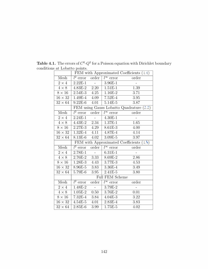
Table 4.1. The errors of C0-Q2 for a Poisson equation with Dirichlet boundaryconditions at Lobatto points.

FEM with Approximated Coefficients (4.4 )Mesh l2 error order l∞ error order2× 4 2.22E-1 - 3.96E-1 -4× 8 4.83E-2 2.20 1.51E-1 1.398× 16 2.54E-3 4.25 1.16E-2 3.7116× 32 1.49E-4 4.09 7.52E-4 3.9532× 64 9.22E-6 4.01 5.14E-5 3.87

FEM using Gauss Lobatto Quadrature (2.2 )Mesh l2 error order l∞ error order2× 4 2.24E-1 - 4.30E-1 -4× 8 4.43E-2 2.34 1.37E-1 1.658× 16 2.27E-3 4.29 8.61E-3 4.0016× 32 1.32E-4 4.11 4.87E-4 4.1432× 64 8.13E-6 4.02 3.09E-5 3.97


Full FEM SchemeMesh l2 error order l∞ error order2× 4 1.48E-2 - 3.79E-2 -4× 8 1.05E-2 0.50 3.76E-2 0.018× 16 7.32E-4 3.84 4.04E-3 3.2216× 32 4.54E-5 4.01 2.83E-4 3.8332× 64 2.85E-6 3.99 1.75E-5 4.02

142

Table 4.2. The errors of C0-Q2 for a Poisson equation with Neumann bound-ary conditions at Lobatto points.

FEM with Approximated Coefficients (4.4 )Mesh l2 error order l∞ error order2× 4 3.44E0 - 5.39E0 -4× 8 1.83E-1 4.23 3.51E-1 3.938× 16 1.38E-2 3.73 3.43E-2 3.3616× 32 8.37E-4 4.04 2.21E-3 3.9632× 64 5.13E-5 4.03 1.41E-4 3.96

FEM using Gauss Lobatto Quadrature (2.2 )Mesh l2 error order l∞ error order2× 4 3.43E0 - 4.95E0 -4× 8 1.81E-1 4.25 3.11E-1 3.998× 16 1.37E-2 3.72 2.81E-2 3.4716× 32 8.33E-4 4.04 1.76E-3 4.0032× 64 5.11E-5 4.03 1.12E-4 3.97



143

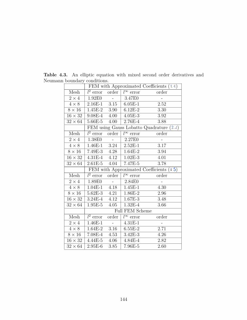
Table 4.3. An elliptic equation with mixed second order derivatives andNeumann boundary conditions.


FEM using Gauss Lobatto Quadrature (2.2 )Mesh l2 error order l∞ error order2× 4 1.38E0 - 2.27E0 -4× 8 1.46E-1 3.24 2.52E-1 3.178× 16 7.49E-3 4.28 1.64E-2 3.9416× 32 4.31E-4 4.12 1.02E-3 4.0132× 64 2.61E-5 4.04 7.47E-5 3.78



144

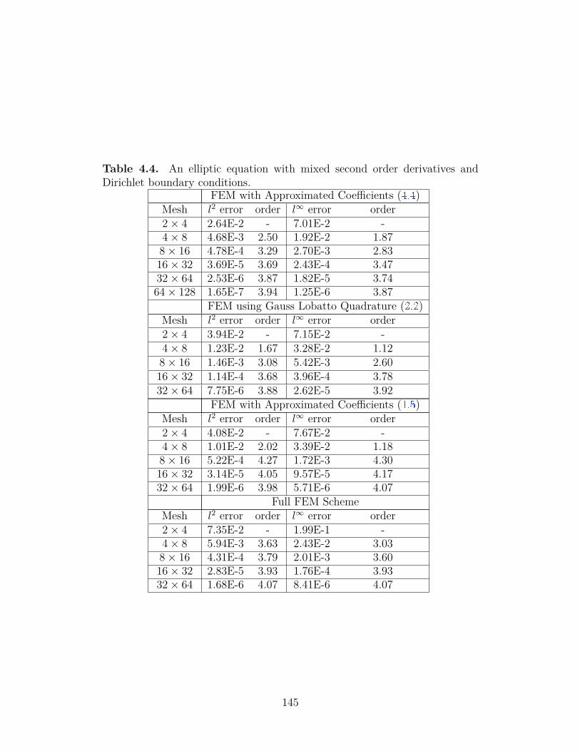
Table 4.4. An elliptic equation with mixed second order derivatives andDirichlet boundary conditions.

FEM with Approximated Coefficients (4.4 )Mesh l2 error order l∞ error order2× 4 2.64E-2 - 7.01E-2 -4× 8 4.68E-3 2.50 1.92E-2 1.878× 16 4.78E-4 3.29 2.70E-3 2.8316× 32 3.69E-5 3.69 2.43E-4 3.4732× 64 2.53E-6 3.87 1.82E-5 3.7464× 128 1.65E-7 3.94 1.25E-6 3.87

FEM using Gauss Lobatto Quadrature (2.2 )Mesh l2 error order l∞ error order2× 4 3.94E-2 - 7.15E-2 -4× 8 1.23E-2 1.67 3.28E-2 1.128× 16 1.46E-3 3.08 5.42E-3 2.6016× 32 1.14E-4 3.68 3.96E-4 3.7832× 64 7.75E-6 3.88 2.62E-5 3.92



145

Table 4.5. A Poisson equation with coefficient min(x,y)

a(x, y) ≈ 0.001.


FEM using Gauss Lobatto Quadrature (2.2 )Mesh l2 error order l∞ error order2× 4 2.81E-1 - 4.59E-1 -4× 8 4.69E-2 2.58 1.37E-1 1.748× 16 5.06E-3 3.21 3.75E-2 1.8716× 32 7.04E-4 2.85 7.86E-3 2.2532× 64 6.74E-5 3.39 1.21E-3 2.7064× 128 4.94E-6 3.77 1.17E-4 3.37


146

The errors at Z0 are shown in Table 4.1 and Table 4.2 . We can see that the four schemes

are all fourth order in the discrete 2-norm on Z0. Even though we did not discuss the max

norm error on Z0, we should expect a | ln h| factor in the order of l∞ error over Z0 due to

(2.4 ), which was proven upon the discrete Green’s function.

Next we consider an elliptic equation with purely Dirichlet or purely Neumann boundary

conditions:

∇ · (a∇u) + cu = f on [0, 1]× [0, 2]

where a =

a11 a12

a21 a22


x3)(sin(πy) + y3) + cos(x4 + y3), a22 = 10 + x5, c = 1 + x4y3 and u(x, y) = 0.1(sin(πx) +

x3)(sin(πy)+y3)+cos(x4 +y3). The errors at Z0 are listed in Table 4.3 and Table 4.4 . Recall

that only O(h3.5) can be proven due to the mixed second order derivatives for the Neumann

boundary conditions as discussed in Remark 4.4.13 , we observe around fourth order accuracy

for (4.4 ) and (4.5 ) for Neumann boundary conditions in this particular example.

4.5.2 Robustness

In Table 4.1 and Table 4.2 , the errors of approximated coefficient schemes (4.4 ), (4.5 )

and the Gauss Lobatto quadrature scheme (2.2 ) are close to one another. We observe that

the scheme (4.5 ) tends to be more accurate than (4.4 ) and (2.2 ) when the coefficient a(x, y)

is closer to zero in the Poisson equation. See Table 4.5 for errors of solving ∇ · (a∇u) =

f on [0, 1]× [0, 2] with Dirichlet boundary conditions, a(x, y) = 1 + εx3y5 + cos(x3y2 + 1)

and u(x, y) = 0.1(sin(πx) + x3)(sin(πy) + y3) + cos(x4 + y3) where ε = 0.001. Here the

smallest value of a(x, y) is around ε = 0.001. We remark that the difference among three

schemes is much smaller for larger ε such as ε = 0.1 as in Table 4.1 .


We have shown that the classical superconvergence of functions values at Gauss Lobatto

points in C0-Qk finite element method for an elliptic problem still holds if replacing the

coefficients by their piecewise Qk Lagrange interpolants at the Gauss Lobatto points. Such a

147

superconvergence result can be used for constructing a fourth order accurate finite difference

type scheme by usingQ2 approximated variable coefficients. Numerical tests suggest that this

is an efficient and robust implementation of C0-Q2 finite element method without affecting

the superconvergence of function values.

148

5. ON THE MONOTONICITY AND DISCRETE MAXIMUM

PRINCIPLE OF THE FINITE DIFFERENCE

IMPLEMENTATION OF C0-Q2 FINITE ELEMENT METHOD

5.1 Introduction

5.1.1 Monotonicity and discrete maximum principle

Consider a Poisson equation with variable coefficients and Dirichlet boundary conditions

on a two dimensional rectangular domain Ω = (0, 1)× (0, 1):

Lu ≡ −∇ · (a∇u) + cu = 0 on Ω,

u = g on ∂Ω,(5.1)

where a(x, y) ∈ C1(Ω), c(x, y) ∈ C0(Ω) with 0 < amin ≤ a(x, y) ≤ amax and c(x, y) ≥ 0.

For a smooth function u ∈ C2(Ω) ∩ C(Ω), maximum principle holds [14 ]: Lu ≤ 0 in Ω =⇒

maxΩ u ≤ max 0,max∂Ω u , and in particular,

Lu = 0 in Ω =⇒ |u(x, y)| ≤ max∂Ω|u|, ∀(x, y) ∈ Ω. (5.2)

For various purposes, it is desired to have numerical schemes to satisfy (5.2 ) in the discrete

sense. A linear approximation to L can be represented as a matrix Lh. The matrix Lh is

called monotone if its inverse has nonnegative entries, i.e., L−1h ≥ 0. All matrix inequalities

in this chapter are entrywise inequalities. One sufficient condition for the discrete maximum

principle is the monotonicity of the scheme, which was also used to prove convergence of

numerical schemes, e.g., [16 ]–[19 ].

In this chapter, we will discuss the monotonicity and discrete maximum principle of the

simplest finite difference implementation of the continuous finite element method with Q2

basis (i.e., tensor product of quadratic polynomial) for (5.1 ), which is a fourth order accurate

scheme.

149

5.1.2 Second order schemes and M-Matrices

The second order centered difference u ≈ ui−1−2ui+ui+1∆x2 for solving −u(x) = f(x), u(0) =

u(1) = 0 results in a tridiagonal (−1, 2,−1) matrix, which is an M -Matrix. Nonsingular

M -Matrices are inverse-positive matrices and it is the most convenient tool for construct-

ing inverse-positive matrices. There are many equivalent definitions or characterizations of

M -Matrices, see [67 ]. One convenient characterization of nonsingular M -Matrices are non-

singular matrices with nonpositive off-diagonal entries and positive diagonal entries, and all

row sums are non-negative with at least one row sum is positive.

The continuous finite element method with piecewise linear basis forms an M -Matrix for

the variable coefficient problem (5.1 ) on triangular meshes under reasonable mesh constraints

[68 ]. The M -Matrix structure in linear finite element method also holds for a nonlinear

elliptic equation [69 ]. For solving −∆u = f on regular triangular meshes, linear finite

element method reduces to the 5-point discrete Laplacian. Linear finite element method or

the 5-point discrete Laplacian is the most popular method in the literature for constructing

schemes satisfying a discrete maximum principle and bound-preserving properties.

Almost all high order accurate schemes result in positive off-diagonal entries in Lh for

solving −∆u = f thus Lh is no longer an M -Matrix. The only known exceptions are the

fourth order accurate 9-point discrete Laplacian and the fourth order accurate compact finite

difference scheme.

5.1.3 Existing high order accurate monotone methods for two-dimensional Lapla-cian

There are at least three kinds of high order accurate schemes which have been proven to

satisfy L−1h ≥ 0 for the Laplacian operator Lu = −∆u:

1. Both the fourth order accurate 9-point discrete Laplacian scheme [16 ], [70 ] and the

fourth order accurate compact finite difference scheme [1 ], [71 ] for −∆u = f can be

written as Su = W f with S being an M -Matrix and W ≥ 0, thus L−1h = S−1M ≥ 0.

150

2. In [72 ], [73 ], Bramble and Hubbard constructed a fourth order accurate finite difference

discrete Laplacian operator for which Lh is not an M -Matrix but monotonicity L−1h ≥ 0

is ensured through an M -Matrix factorization Lh = M1M2, i.e., Lh is a product of two

M -Matrices.

3. Finite element method with quadratic polynomial (P2 FEM) basis on a regular trian-

gular mesh can be implemented as a finite difference scheme defined at vertices and

edge centers of triangles [31 ]. The error estimate of P2 FEM is third order in L2-norm.

The error at at vertices and edge centers are fourth order accurate in l2-norm due to

superconvergence. The stiffness matrix is not an M -Matrix but its monotonicity was

proven in [21 ].

For discrete maximum principle to hold in P2 FEM on a generic triangular mesh, it was

proven in [20 ] that it is necessary and sufficient to require a very strong mesh constraint,

which essentially gives either regular triangulation or equilateral triangulation. Thus, the

discrete maximum principle holds in P2 FEM on a regular triangulation or an equilateral

triangulation. For finite element method with cubic and higher order polynomials on regular

triangular meshes, it was shown that the discrete maximum principle fails in [74 ].

5.1.4 Other known results regarding discrete maximum principle

For one-dimensional Laplacian, discrete maximum principle was proven for arbitrarily

high order finite element method using discrete Green’s function in [75 ]. The discrete Green’s

function was also used to analyze P1 FEM in two dimensions [76 ]. Discontinuous coefficients

were considered and a nonlinear scheme was constructed in [77 ]. Piecewise constant co-

efficient in one dimension was considered in [78 ]. A numerical study for high order FEM

with very accurate Gauss quadrature in two dimensions showed that DMP was violated on

non-uniform unstructured meshes for variable coefficients in [79 ]. A more general operator

∇(a∇u) with matrix coefficients a was considered for linear FEM in [80 ]. See [81 ] for an

anisotropic computational example.

151

5.1.5 Existing inverse-positive approaches when Lh is not an M-Matrix

In this chapter, we will focus on the finite difference implementation of continuous finite

element method with Q2 basis (Q2 FEM), which will be reviewed in Section 5.2 . The matrix

Lh in such a scheme is not an M -Matrix due to its off-diagonal positive entries. There are

at least three methods to study whether L−1h ≥ 0 holds when M -Matrix structure is lost:

1. An M -Matrix factorization of the form Lh = M1M2 was shown in [73 ] and [82 ]. In

Appendix 5.6 , we will demonstrate an M -Matrix factorization for the finite difference

implementation of Q2 FEM solving −∆u = f .

2. Perturbation of M -Matrices by positive off-diagonal entries without losing monotonic-

ity was discussed in [83 ].

3. In [21 ], Lorenz proposed a sufficient condition for ensuring Lh = M1M2. Lorenz’s

condition will be reviewed in Section 5.3.3 .

The main result of this chapter is to prove that L−1h ≥ 0 and a discrete maximum principle

holds under some mesh constraint in the fourth order accurate finite difference implementa-

tion of Q2 FEM solving (5.1 ) by verifying the Lorenz’s condition.

5.1.6 Extensions to the discrete maximum principle for parabolic equations

Classical solutions to the parabolic equation ut = ∇· (a∇u) satisfy a maximum principle

[14 ]. With suitable boundary conditions and initial value u(x, y, 0) such as periodic or

homogeneous Dirichlet boundary conditions and initial minimum minΩu(x, y, 0) = 0, the

solution to the initial value problem satisfies the following maximum principle:

min(x,y)

u(x, y, 0) ≤ u(x, y, t) ≤ max(x,y)

u(x, y, 0). (5.3)

Now consider solving ut = ∇· (a∇u) with backward Euler time discretization, then Un+1

satisfies an elliptic equation of the form (5.1 ):

−∇ · (a∇Un+1) + 1∆tU

n+1 = 1∆tU

n. (5.4)

152

If Sh denotes spatial discretization for −∇·(a∇u), then the numerical scheme can be written

as Un+1 = (I+∆tSh)−1Un. Let 1 =[1 1 · · · 1

]T

. Then for suitable boundary conditions

usually we have Sh1 = 0 since Sh approximates a differential operator. So we have (I +

∆tSh)1 = 1 thus (I + ∆tSh)−11 = 1. If we further have the monotonicity (I + ∆tSh)−1 ≥ 0,

then each row of the (I+∆tSh)−1 has nonnegative entries and sums to one, thus the discrete

maximum principle holds minj Unj ≤ Un+1

j ≤ maxj Unj , which is a desired and useful property

in many applications. For instance, second order centered difference or P1 finite element

method has been used to construct schemes satisfying the discrete maximum principle in

solving phase field equations [84 ]–[86 ]. In the rest of the chapter, we will only focus on

discussing the equation (5.1 ), even though all discussions can be extended to solving the

parabolic equation with backward Euler time discretization.

To the best of our knowledge, this is the first time that a high order accurate scheme

under suitable mesh constraints is proven to be monotone in the sense L−1h ≥ 0 for solving a

variable coefficient a(x) in (5.1 ) in two dimensions. For simplicity, we only discuss an uniform

mesh in this chapter, even though the main results can be extended to non-uniform meshes.

However, an additional mesh constraint is expected for the discrete maximum principle to

hold. See such a mesh constraint of non-uniform meshes for Q1 FEM in [87 ] and P2 FEM

for one-dimensional problem in [75 ].

This chapter is organized as follows. In Section 5.2 , we describe the fourth order accurate

finite difference implementation of C0-Q2 finite element method. In Section 5.3 , we review

the sufficient conditions to ensure monotonicity and discrete maximum principle. In Section

5.4 , we prove that the fourth order accurate finite difference implementation of C0-Q2 finite

element method is monotone under some mesh constraints. Numerical tests are given in

Section 5.5 . Concluding remarks are given in Section 5.6 .

153

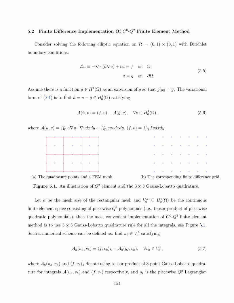
5.2 Finite Difference Implementation Of C0-Q2 Finite Element Method

Consider solving the following elliptic equation on Ω = (0, 1) × (0, 1) with Dirichlet

boundary conditions:

Lu ≡ −∇ · (a∇u) + cu = f on Ω,

u = g on ∂Ω.(5.5)

Assume there is a function g ∈ H1(Ω) as an extension of g so that g|∂Ω = g. The variational

form of (5.1 ) is to find u = u− g ∈ H10 (Ω) satisfying

A(u, v) = (f, v)−A(g, v), ∀v ∈ H10 (Ω), (5.6)


Ω a∇u · ∇vdxdy +∫∫

Ω cuvdxdy, (f, v) =∫∫

Ω fvdxdy.

(a) The quadrature points and a FEM mesh. (b) The corresponding finite difference grid.

Figure 5.1. An illustration of Q2 element and the 3× 3 Gauss-Lobatto quadrature.

Let h be the mesh size of the rectangular mesh and V h0 ⊆ H1

0 (Ω) be the continuous

finite element space consisting of piecewise Q2 polynomials (i.e., tensor product of piecewise

quadratic polynomials), then the most convenient implementation of C0-Q2 finite element

method is to use 3 × 3 Gauss-Lobatto quadrature rule for all the integrals, see Figure 5.1 .

Such a numerical scheme can be defined as: find uh ∈ V h0 satisfying

Ah(uh, vh) = 〈f, vh〉h −Ah(gI , vh), ∀vh ∈ V h0 , (5.7)

where Ah(uh, vh) and 〈f, vh〉h denote using tensor product of 3-point Gauss-Lobatto quadra-

ture for integrals A(uh, vh) and (f, vh) respectively, and gI is the piecewise Q2 Lagrangian

154

interpolation polynomial at the 3× 3 quadrature points shown in Figure 5.1 of the following

function:

g(x, y) =

0, if (x, y) ∈ (0, 1)× (0, 1),

g(x, y), if (x, y) ∈ ∂Ω.

Then uh = uh + gI is the numerical solution for the problem (5.5 ). We emphasize that

(5.7 ) is not a straightforward approximation to (5.6 ) since g is never used. It was proven in

chapter 2 that the scheme (5.7 ) is fourth order accurate if coefficients and exact solutions

are smooth. Notice that uh satisfies:

Ah(uh, vh) = 〈f, vh〉h, ∀vh ∈ V h0 . (5.8)

See chapter 2 for the detailed finite difference implementation and proof of fourth order

accuracy for the scheme (5.7 ).

5.2.1 One-dimensional case

Now consider the one-dimensional Dirichlet boundary value problem:

−(au) + cu =f on (0, 1),

u(0) = σ0, u(1) = σ1.

Consider a uniform mesh xi = ih, i = 0, 1, . . . , n+ 1, h = 1n+1 . Assume n is odd and let

M = n+12 . Define intervals Ik = [x2k, x2k+2] for k = 0, . . . ,M − 1 as a finite element mesh for

P 2 basis. Define

V h = v ∈ C0([0, 1]) : v ∈ P 2(Ik), k = 0, . . . ,M − 1.

Let φin+1i=0 ⊂ V h be a basis for V h so that φi(xj) = δij, i, j = 0, 1, . . . , n + 1. Let u0 = σ0,

ui = uh(xi) and un+1 = σ1, then uh, uh ∈ V h can be represented as

uh(x) =n∑

i=1uiφi(x), uh(x) =

n+1∑i=0

uiφi(x).

155

Let fj = f(xj), then (5.8 ) becomes

〈auh, φi〉h + 〈cuh, φi〉h = 〈f, φi〉h, i = 1, . . . , n;u0 = σ0, un+1 = σ1,

which are

n+1∑j=0

uj (〈aφj, φi〉h + 〈cφj, φi〉h) =n+1∑j=0

fj〈φj, φi〉h, i = 1, . . . , n;

u0 = σ0, un+1 = σ1.

The matrix form is Su = M f where

u =[u0 u1 u2 · · · un un+1

]T

, f =[σ0 f1 f2 · · · fn σ1

]T

.

The scheme can be written as Lh(u) = f . The linear operator Lh has the matrix represen-

tation Lh = M−1S.

For the Laplacian Lu = −u, we have

Lh(u)0 = u0 = σ0, Lh(u)n+1 = un+1 = σ1, (5.9a)

if i is odd, i.e., xi is a cell center, (5.9b)

Lh(u)i = −ui−1 + 2ui − ui+1

h2 = fi, (5.9c)

if i is even, i.e., xi is a cell end, (5.9d)

Lh(u)i = ui−2 − 8ui−1 + 14ui − 8ui+1 + ui+2

4h2 = fi. (5.9e)

For the variable coefficient operator Lu = −(au) + cu, we have

Lh(u)0 = u0 = σ0, Lh(u)n+1 = un+1 = σ1, (5.10a)

and if xi is a cell center, we have

Lh(u)i = −(3ai−1 + ai+1)ui−1 + 4(ai−1 + ai+1)ui − (ai−1 + 3ai+1)ui+1

4h2 + ciui = fi; (5.10b)

156

and if xi is a cell end, then

Lh(u)i = (3ai−2 − 4ai−1 + 3ai)ui−2 − (4ai−2 + 12ai)ui−1

8h2

+(ai−2 + 4ai−1 + 18ai + 4ai+1 + ai+2)ui

8h2

+−(12ai + 4ai+2)ui+1 + (3ai+2 − 4ai+1 + 3ai)ui+2

8h2 + ciui = fi. (5.10c)

5.2.2 Two-dimensional case

Consider a uniform grid (xi, yj) for a rectangular domain [0, 1] × [0, 1] where xi = ih,

i = 0, 1, . . . , n + 1 and yj = jh, j = 0, 1, . . . , n + 1, h = 1n+1 , where n must be odd. Let

uij denote the numerical solution at (xi, yj). Let u denote an abstract vector consisting

of uij for i, j = 1, 2, · · · , n. Let u denote an abstract vector consisting of uij for i, j =

0, 1, 2, · · · , n, n + 1. Let f denote an abstract vector consisting of fij for i, j = 1, 2, · · · , n

and the boundary condition g at the boundary grid points.

The scheme (5.8 ) for solving (5.5 ) can still be written as Lh(u) = f .

Two-dimensional Laplacian

For the Laplacian Lu = −∆u, Lh(u) can be expressed as the following. If (xi, yj) ∈ ∂Ω,

then

Lh(u)i,j = ui,j = gi,j.

If (xi, yj) is an interior grid point and a cell center , Lh(u)i,j is equal to

−ui−1,j − ui+1,j + 4ui,j − ui,j+1 − ui+1,j

h2 = fi,j. (5.11a)

For interior grid points, there are three types: cell center, edge center and knots. See Figure

5.2 . If (xi, yj) is an interior grid point and an edge center for an edge parallel to x-axis,

Lh(u)i,j is equal to

−ui−1,j + 2ui,j − ui+1,j

h2 + ui,j−2 − 8ui,j−1 + 14ui,j − 8ui,j+1 + ui,j+2

4h2 = fi,j. (5.11b)

157

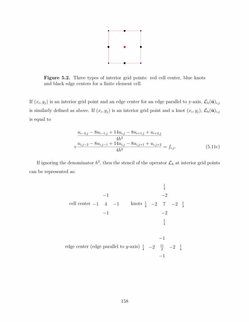
Figure 5.2. Three types of interior grid points: red cell center, blue knotsand black edge centers for a finite element cell.

If (xi, yj) is an interior grid point and an edge center for an edge parallel to y-axis, Lh(u)i,j

is similarly defined as above. If (xi, yj) is an interior grid point and a knot (xi, yj), Lh(u)i,j

is equal to

ui−2,j − 8ui−1,j + 14ui,j − 8ui+1,j + ui+2,j

4h2

+ui,j−2 − 8ui,j−1 + 14ui,j − 8ui,j+1 + ui,j+2

4h2 = fi,j. (5.11c)

If ignoring the denominator h2, then the stencil of the operator Lh at interior grid points

can be represented as:

cell center−1

−1 4 −1

−1

knots

14

−214 −2 7 −2 1

4

−214

edge center (edge parallel to y-axis)−1

14 −2 11

2 −2 14

−1

158

edge center (edge parallel to x-axis)

14

−2

−1 112 −1

−214

5.2.3 Two-dimensional variable coefficient case

For Lu = −∇· (a∇u)+ cu, Lh(u) will have exactly the same stencil size as the Laplacian

case. At boundary points (xi, yj) ∈ ∂Ω, Lh(u) = f becomes

Lh(u)i,j = ui,j = gi,j. (5.12a)

If (xi, yj) is an interior grid point and a cell center, Lh(u)i,j is equal to

−(3ai−1,j + ai+1,j)ui−1,j + 4(ai−1,j + ai+1,j)ui,j − (ai−1,j + 3ai+1,j)ui+1,j

4h2 (5.12b)

+−(3ai,j−1 + ai,j+1)ui,j−1 + 4(ai,j−1 + ai,j+1)ui,j − (ai,j−1 + 3ai,j+1)ui,j+1

4h2 + cijuij.

If (xi, yj) is an interior grid point and a knot, Lh(u)i,j is equal to

(3ai−2,j − 4ai−1,j + 3ai,j)ui−2,j − (4ai−2,j + 12ai,j)ui−1,j

8h2

+(ai−2,j + 4ai−1,j + 18ai,j + 4ai+1,j + ai+2,j)ui,j

8h2

+−(12ai,j + 4ai+2,j)ui+1,j + (3ai+2,j − 4ai+1,j + 3ai,j)ui+2,j

8h2

+(3ai,j−2 − 4ai,j−1 + 3ai,j)ui,j−2 − (4ai,j−2 + 12ai,j)ui,j−1

8h2

+(ai,j−2 + 4ai,j−1 + 18ai,j + 4ai,j+1 + ai,j+2)ui,j

8h2 (5.12c)

+−(12ai,j + 4ai,j+2)ui,j+1 + (3ai,j+2 − 4ai,j+1 + 3ai,j)ui,j+2

8h2 + cijuij.

159

If (xi, yj) is an interior grid point and an edge center for an edge parallel to y-axis,

Lh(u)i,j is equal to

(3ai−2,j − 4ai−1,j + 3ai,j)ui−2,j − (4ai−2,j + 12ai,j)ui−1,j

8h2

+(ai−2,j + 4ai−1,j + 18ai,j + 4ai+1,j + ai+2,j)ui,j

8h2

+−(12ai,j + 4ai+2,j)ui+1,j + (3ai+2,j − 4ai+1,j + 3ai,j)ui+2,j

8h2 (5.12d)

+−(3ai,j−1 + ai,j+1)ui,j−1 + 4(ai,j−1 + ai,j+1)ui,j − (ai,j−1 + 3ai,j+1)ui,j+1

4h2 + cijuij.

If (xi, yj) is an interior grid point and an edge center for an edge parallel to x-axis, Lh(u)i,j

is equal to

(3ai,j−2 − 4ai,j−1 + 3ai,j)ui,j−2 − (4ai,j−2 + 12ai,j)ui,j−1

8h2

+(ai,j−2 + 4ai,j−1 + 18ai,j + 4ai,j+1 + ai,j+2)ui,j

8h2

+−(12ai,j + 4ai,j+2)ui,j+1 + (3ai,j+2 − 4ai,j+1 + 3ai,j)ui,j+2

8h2 (5.12e)

+−(3ai−1,j + ai+1,j)ui−1,j + 4(ai−1,j + ai+1,j)ui,j − (ai−1,j + 3ai+1,j)ui+1,j

4h2 + cijuij.

5.3 Sufficient Conditions For Monotonicity And Discrete Maximum Principle

5.3.1 Discrete maximum principle

Assume there are N grid points in the domain Ω and N∂ grid points on ∂Ω. Define

u =(u1 u2 · · · uN

)T

, u∂ =(u∂

1 u∂2 · · · u∂

N∂

)T

,

u =(u1 u2 · · · uN u∂

1 u∂2 · · · u∂

N∂

)T

.

160

A finite difference scheme can be written as

Lh(u)i =N∑

j=1bijuj +

N∂∑j=1

b∂iju

∂j =fi, 1 ≤ i ≤ N,

u∂i =gi, 1 ≤ i ≤ N∂.

The matrix form is

Lhu = f , Lh =

Lh B∂

0 I

, u =

u

u∂

, f =

f

g

.The discrete maximum principle is

Lh(u)i ≤ 0, 1 ≤ i ≤ N =⇒ maxiui ≤ max0,max

iu∂

i (5.13)

which implies

Lh(u)i = 0, 1 ≤ i ≤ N =⇒ |ui| ≤ maxi|u∂

i |.

The following result was proven in [15 ]:

Theorem 5.3.1. A finite difference operator Lh satisfies the discrete maximum principle

(5.13 ) if L−1h ≥ 0 and all row sums of Lh are non-negative.

Let u and f be the same vectors as defined in Section 5.2 . For the same finite difference

scheme, the matrix form can also be written as

Lhu = f .

Notice that there exist two permutation matrices P1 and P2 such that u = P1u and f = P2f .

Since the matrix vector form of the same scheme is also Lhu = f , we obtain P−12 LhP1 = Lh.

Notice that a permutation matrix P is inverse-positive and the signs of row sums will not

be altered after multiplying P to Lh. Thus we have

Theorem 5.3.2. If Lh is inverse-positive and row sums of Lh are non-negative, then Lh

satisfies the discrete maximum principle (5.13 ).

161

Notice that L−1h =

L−1h −L−1

h B∂

0 I

, thus we have

Theorem 5.3.3. If L−1h ≥ 0, then L−1

h ≥ 0 and thus L−1h ≥ 0.

Let 1 denote a vector of suitable size with 1 as entries, then for all schemes in Section

5.2 , Lh(1) ≥ 0, which implies the row sums of Lh are non-negative. Thus from now on, we

only need to discuss the monotonicity of the matrix Lh.

5.3.2 Characterizations of nonsingular M-Matrices

M -Matrices belong to the set of Z-matrices which are matrices with nonpositive off-

diagonal entries. Nonsingular M -Matrices are always inverse-positive. See [67 ] for the defi-

nition and various characterization of nonsingular M -Matrices. The following is a convenient

sufficient condition to characterize nonsingular M -Matrices:

Theorem 5.3.4. For a real square matrix A with positive diagonal entries and non-positive

off-diagonal entries, A is a nonsingular M-Matrix if all the row sums of A are non-negative

and at least one row sum is positive.

Proof. By condition C10 in [67 ], A is a nonsingular M -Matrix if and only if A + aI is

nonsingular for any a ≥ 0. Since all the row sums of A are non-negative and at least one

row sum is positive, the matrix A is irreducibly diagonally dominant thus nonsingular, and

A+ aI is strictly diagonally dominant thus nonsingular for any a > 0.

Definition 1. Let N = 1, 2, . . . , n. For N1,N2 ⊂ N , we say a matrix A of size n × n

connects N1 with N2 if

∀i0 ∈ N1, ∃ir ∈ N2,∃i1, . . . , ir−1 ∈ N s.t. aik−1ik6= 0, k = 1, · · · , r. (5.14)

If perceiving A as a directed graph adjacency matrix of vertices labeled by N , then (5.14 )

simply means that there exists a directed path from any vertex in N1 to at least one vertex

in N2. In particular, if N1 = ∅, then any matrix A connects N1 with N2.

162

Given a square matrix A and a column vector x, we define

N 0(Ax) = i : (Ax)i = 0, N+(Ax) = i : (Ax)i > 0.

By condition L36 in [67 ], we have the following characterization of nonsingular M -

Matrices:

Theorem 5.3.5. For a real square matrix A with non-positive off-diagonal entries, if there is

a vector x > 0 with Ax ≥ 0 s.t. A connects N 0(Ax) with N+(Ax), then A is a nonsingular

M-Matrix thus A−1 ≥ 0.

5.3.3 Lorenz’s sufficient condition for monotonicity

All results in this subsection were first shown in [21 ]. For completeness, we include a

detailed proof.

Given a matrix A = [aij] ∈ Rn×n, define its diagonal, positive and negative off-diagonal

parts as n× n matrices Ad, Aa, A+a , A−

a :

(Ad)ij =

aii, if i = j

0, if i 6= j

, Aa = A− Ad,

(A+a )ij =

aij, if aij > 0, i 6= j

0, otherwise., A−

a = Aa − A+a .

Lemma 5.3.6. If A is monotone, then for any two matrices B ≥ C, A−1B ≥ A−1C.

Proof. For any two column vectors b ≥ c, we have

b− c ≥ 0⇒ A−1(b− c) ≥ 0⇒ A−1b ≥ Ac.

By considering b and c as column vectors of B and C, we get A−1B ≥ A−1C.

Lemma 5.3.7. If A is an M-Matrix, then Ad ≥ A and A−1 ≥ A−1d .

163

Proof. Ad ≥ A is trivial. A is monotone, thus

Ad ≥ A⇒ A−1Ad ≥ A−1A = I.

And A−1d ≥ 0 implies

A−1Ad ≥ I ⇒ A−1AdA−1d ≥ IA−1

d ⇒ A−1 ≥ A−1d .

Theorem 5.3.8. If Aa ≤ 0 and there exists a nonzero vector e ∈ Rn such that e ≥ 0 and

Ae ≥ 0. Moreover, A connects N 0(Ae) with N+(Ae). Then the following hold:

• e > 0.

• aii > 0, ∀i ∈ N .

• A is a M-Matrix and A−1 ≥ 0.

Proof. Assume there is one index i such that ei = 0, then

0 ≤ (Ae)i =∑j 6=i

aijej ≤ 0⇒ (Ae)i = 0⇒∑j 6=i

aijej = 0⇒ aijej = 0,∀j.

Thus if aij < 0, then ej = 0, which implies (Ae)j = 0 by the same argument as above.

Therefore, A has no off-diagonal nonzero entry akl such that k ∈ N 0(Ae) and l ∈ N+(Ae).

In other words, if A represents the graph adjacency matrix for a directed graph of vertices

indexed by 1, 2, · · · , n, then any edge starting from a vertex i ∈ N 0(Ae) points to vertices

in N 0(Ae), thus there is no directed path from i ∈ N 0(Ae) to any vertex in N+(Ae), which

contradicts to the assumption that A connects N 0(Ae) with N+(Ae). With e > 0, the rest

is proven by following Theorem 5.3.5 .

corollary 5.3.9. If A is a nonsingular M-Matrix, f ∈ Rn is a nonzero vector with f ≥ 0

and A connects N 0(f) with N+(f), then A−1f > 0.

Proof. By using e = A−1f ≥ 0 in Theorem 5.3.8 , we get A−1f > 0.

164

Theorem 5.3.10. If A ≤ M1M2 · · ·MkL where M1, · · · ,Mk are nonsingular M-Matrices

and La ≤ 0, and there exists a nonzero vector e ≥ 0 such that one of the matrices

M1, · · · ,Mk, L connects N 0(Ae) with N+(Ae). Then A is a product of k + 1 nonsingu-

lar M-Matrices thus A−1 ≥ 0.

Proof. Let M = M1M2 · · ·Mk, then M is monotone. By Lemma 5.3.6 , we get

M−1A ≤ L, (5.15)

thus

(M−1A)a ≤ 0. (5.16)

For each Mi, i = 1, . . . , k, by Lemma 5.3.7 , we have

(Mi)−1 ≥ ((Mi)d)−1 ⇒M−1 ≥ (Mk)−1d · · · (M1)−1

d , (5.17)

which implies

M−1Ae ≥ cAe, (5.18)

for some positive number c.

If L connects N 0(Ae) with N+(Ae), then M−1A also connects N 0(Ae) with N+(Ae) be-

cause (5.15 ) implies that (M−1A)ij 6= 0 whenever Lij 6= 0 for any i 6= j. By (5.18 ), N+(Ae) ⊂

N+(M−1Ae) and N 0(M−1Ae) ⊂ N 0(Ae), thus M−1A also connects N 0(M−1Ae) with

N+(M−1Ae). With (5.16 ), by Theorem 5.3.8 , M−1A is a nonsingular M -Matrix thus A

is a product of k + 1 M -Matrices which implies A is monotone.

If Mi connects N 0(Ae) with N+(Ae) for some 1 ≤ i ≤ k. Let M = M1 . . .Mi−1. Similar

to (5.17 ) and (5.18 ), we get

(M)−1Ae ≥ c2Ae, c2 > 0, (5.19)

which implies that Mi connects N 0((M)−1Ae) with N+((M)−1Ae). By Corollary 5.3.9 ,

we know M−1i (M)−1Ae > 0, thus M−1Ae > 0. With (5.16 ), through Theorem 5.3.8 we

165

find M−1A is a M -Matrix thus A is a product of k + 1 M -Matrices which implies A is

monotone.

Theorem 5.3.11. If A−a has a decomposition: A−

a = Az + As = (azij) + (as

ij) with As ≤ 0

and Az ≤ 0, such that

Ad + Az is a nonsingular M-Matrix, (5.20a)

A+a ≤ AzA−1

d As or equivalently ∀aij > 0 with i 6= j, aij ≤n∑

k=1az

ika−1kk a

skj, (5.20b)

∃e ∈ Rn \ 0, e ≥ 0 with Ae ≥ 0 s.t. Az or As connects N 0(Ae) with N+(Ae). (5.20c)

Then A is a product of two nonsingular M-Matrices thus A−1 ≥ 0.

Proof. By (5.20b ), we have

A = Ad + Az + As + A+a ≤ (Ad + Az)(I + A−1

d As). (5.21)

By (5.20c ), either Ad + Az or I + A−1d As connects N 0(Ae) with N+(Ae). By applying

Theorem 5.3.10 for the case k = 1, M1 = Ad +Az and L = I +A−1d As, we get A−1 ≥ 0.

5.4 The Main Result

For a general matrix, conditions (5.20 ) in Theorem 5.3.11 can be difficult to verify. We

will first derive a simplified version of Theorem 5.3.11 then verify it for the schemes in Section

5.2 .

5.4.1 A simplified sufficient condition for monotonicity

We will take advantage of the directed graph described by the 5-point discrete Laplacian,

i.e., the second order centered difference scheme, which has similar off-diagonal negative entry

patterns as the schemes in Section 5.2 .

166

(a) Grid points. (b) The directed graph.

Figure 5.3. An illustration of the directed graph described by off-diagonalentries of the matrix in (5.22 ): the domain [0, 1] is discretized by a uniform5-point grid; the black points are interior grid points and the blue ones are theboundary grid points. There is a directed path from any interior grid point toat least one of the boundary points.

For the one-dimensional problem −u = f, x ∈ (0, 1) with u(0) = u(1), the scheme can

be written as u0 = σ0, un+1 = σ1,−ui−1+2ui−ui+1

h2 = fi, i = 1, · · · , n. The matrix vector form

is Ku = f where

K = 1h2

h2−1 2 −1

−1 2 −1... ... ...

−1 2 −1h2

, (5.22)

which described the directed graph illustrated in Figure 5.3 . Let 1 denote a vector of suitable

size with each entry as 1, then (K1)i =

0, i = 1, · · · , n

1, i = 0, n+ 1. By Figure 5.3 , it is easy to see

that K connects N 0(K1) with N+(K1).

Next we consider the second order accurate 5-point discrete Laplacian scheme for solving

−∆u = f on Ω = (0, 1)× (0, 1) with homogeneous Dirichlet boundary conditions:

ui,j = 0, (xi, yj) ∈ ∂Ω;−ui−1,j − ui+1,j + 4ui,j − ui,j+1 − ui+1,j

h2 = fij, (xi, yj) ∈ Ω.

See Figure 5.4 for the directed graph described by its matrix representation. Let K be the

matrix representation of the 5-point discrete Laplacian scheme, then

(K1)i,j =

1, if (xi, yj) ∈ ∂Ω,

0, if (xi, yj) ∈ Ω.

By Figure 5.4 , it is easy to see that K connects N 0(K1) with N+(K1).

167

(a) Grid points. (b) The directed graph.

Figure 5.4. An illustration of the directed graph described by off-diagonalentries in the 5-point discrete Laplacian matrix: the domain [0, 1] × [0, 1] isdiscretized by a uniform 5 × 5 grid; the black points are interior grid pointsand the blue ones are the boundary grid points. There is a directed path fromany interior grid point to at least one of the boundary grid points.

168

Let A := Lh denote the matrix representation of any scheme in Section 5.2 . Then

(A1)i,j =

1, if (xi, yj) ∈ ∂Ω,

cij ≥ 0, if (xi, yj) ∈ Ω.

Therefore, N+(K1) ⊂ N+(A1) implies N 0(A1) ⊂ N 0(K1), thus K also connects N 0(A1)

with N+(A1). Notice that indices of nonzero off-diagonal entries in K is a subset of indices

of nonzero entries in A−a , thus A−

a also connects N 0(A1) with N+(A1). So the vector e can

be set as 1 in (5.20c ). If assuming c(x, y) > 0, then A1 > 0 thus the condition (5.20c ) is

trivially satisfied.

By Theorem 5.3.4 , for any decomposition of off-diagonal negative entries A−a = Az +As,

Ad + Az is an M -Matrix if (Ad + Az)1 6= 0 and (Ad + Az)1 ≥ 0. So Theorem 5.3.11 for the

schemes (5.10 ) and (5.12 ) can be simplified as

Theorem 5.4.1. Let A denote the matrix representation of the schemes solving −∇·(a∇)u+

cu = f in Section 5.2 . Assume A−a has a decomposition A−

a = Az + As with As ≤ 0 and

Az ≤ 0. Then A−1 ≥ 0 if the following are satisfied:

1. (Ad + Az)1 6= 0 and (Ad + Az)1 ≥ 0;

2. A+a ≤ AzA−1

d As;

3. For c(x, y) ≥ 0, either Az or As has the same sparsity pattern as A−a . If c(x, y) > 0,

then this condition can be removed.

5.4.2 One-dimensional Laplacian case

As a demonstration of how to apply Theorem 5.4.1 , we first consider the scheme (5.9 ).

Let A be the matrix representation of the linear operator Lh in the scheme (5.9 ). Let Ad

and A±a be linear operators corresponding to the matrices Ad and A±

a respectively.

169

Consider the following decomposition of A−a = Az +As with Az = As = 1

2A−a :

Az(u)0 = As(u)0 = 0, Az(u)n+1 = As(u)n+1 = 0,

Az(u)i = As(u)i = −ui−1 − ui+1

2h2 , if xi is a cell center,

Az(u)i = As(u)i = −8ui−1 − 8ui+1

8h2 , if xi is an interior cell end.

The operator Ad and A+a are given as:

Ad(u)0 = u0, Ad(u)n+1 = un+1,

Ad(u)i = 2ui

h2 , if xi is a cell center,

Ad(u)i = 14ui


A+a (u)0 = 0, A+

a (u)n+1 = 0,

A+a (u)i = 0, if xi is a cell center,

A+a (u)i = ui−2 + ui+2


Obviously, Az and As both have have the same sparsity pattern as A−a . It is straightforward to

verify [Ad+Az](1) is a non-negative nonzero vector. So we only need to verify A+a ≤ AzA−1

d As

to apply Theorem 5.4.1 . Since AzA−1d As ≥ 0, we only need to compare nonzero coefficients

in A+a (u)i and Az

(A−1

d [As(u)])

i.

When xi is an interior cell end, xi±1 are cell centers, and we have

As(u)i−1 = −ui−2 − ui

2h2 , A−1d [As(u)]i−1 = h2As(u)i−2

2 ,

Az(A−1d [As(u)])i = −A

−1d [−As(u)]i−1 −A−1

d [As(u)]i+1

h2 = ui−2 + 2ui + ui+2

4h2 .

We can verify A+a ≤ AzA−1

d As by comparing only the coefficients of ui±2 in A+a (u)i and

Az(A−1

d [As(u)])

ibecause AzA−1

d As ≥ 0. By Theorem 5.4.1 , we get A−1 ≥ 0.

170

5.4.3 One-dimensional variable coefficient case

As we have seen in the previous discussion, all the operators are either zero or identity

at the boundary points thus do not affect the discussion verifying the condition (5.20b ). For

the sake of simplicity, we only consider the interior grid points for the linear operators. With

the positive and negative parts for a number f defined as:

f+ = |f |+ f

2 , f− = |f | − f2 ,

the linear operators Ad, A±a are

if xi is a cell center, Ad(u)i =(ai−1 + ai+1

h2 + ci

)ui;

if xi is an interior cell end,

Ad(u)i =(ai−2 + 4ai−1 + 18ai + 4ai+1 + ai+2

8h2 + ci

)ui.

if xi is a cell center, A+a (u)i = 0;

if xi is an interior cell end,

A+a (u)i = (3ai−2 − 4ai−1 + 3ai)+ui−2 + (3ai+2 − 4ai+1 + 3ai)+ui+2

8h2 .

If xi is a cell center, A−a (u)i = −(3ai−1 + ai+1)ui−1 − (ai−1 + 3ai+1)ui+1

4h2 ;

If xi is an interior cell end, A−a (u)i = −(3ai−2 − 4ai−1 + 3ai)−ui−2

8h2

+ −(4ai−2 + 12ai)ui−1 − (12ai + 4ai+2)ui+1 − (3ai − 4ai+1 + 3ai+2)−ui+2

8h2 .

We can easily verify that (Ad + Az)1 ≥ 0 for the following Az:

if xi is a cell center, Az(u)i = ε−(3ai−1 + ai+1)ui−1 − (ai−1 + 3ai+1)ui+1

4h2 ,

if xi is an interior cell end, Az(u)i =−(3ai−2 − 4ai−1 + 3ai)−ui−2 − [4ai−2 + 12ai − (3ai−2 − 4ai−1 + 3ai)+]ui−1

8h2

+ −[12ai + 4ai+2 − (3ai − 4ai+1 + 3ai+2)+]ui+1 − (3ai − 4ai+1 + 3ai+2)−ui+2

8h2 ,

171

where ε > 0 is a small number. Moreover, Az has the same sparsity pattern as A−a for any

ε > 0. For ε < 1 we can verify that As = A−a − Az ≤ 0:

If xi is a cell center, As(u)i = (1− ε)−(3ai−1 + ai+1)ui−1 − (ai−1 + 3ai+1)ui+1

4h2 ,

If xi is an interior cell end,

As(u)i = −(3ai−2 − 4ai−1 + 3ai)+ui−1 − (3ai − 4ai+1 + 3ai+2)+ui+1

8h2 .

Now we only need to compare nonzero coefficients in A+a (u)i and Az

(A−1

d [As(u)])

ifor xi

being an interior cell end. When xi is an interior cell end, xi±1 are cell centers, and we have

As(u)i−1 = (1− ε)−(3ai−2 + ai)ui−2 − (ai−2 + 3ai)ui

4h2 ,

As(u)i−2 = −(3ai−4 − 4ai−3 + 3ai−2)+ui−3 − (3ai−2 − 4ai−1 + 3ai)+ui−1

8h2 ,

A−1d [As(u)]i−1 = h2As(u)i−1

(ai−2 + ai + h2ci−1)= (1− ε)−(3ai−2 + ai)ui−2 − (ai−2 + 3ai)ui

4(ai−2 + ai + h2ci−1).

It suffices to focus on the coefficient of ui−2 in Az(A−1d [As(u)])i and the discussion for the co-

efficient of ui+2 is similar. Notice that A−1d [As(u)]i−2 will contribute nothing to the coefficient

of ui−2. So the coefficient of ui−2 in Az(A−1d [As(u)])i is

(1− ε)(3ai−2 + ai)(4ai−2 + 12ai − (3ai−2 − 4ai−1 + 3ai)+)32h2(ai−2 + ai + h2ci−1)

.

Thus to ensure A+a ≤ AzA−

d As, it suffices to have the following holds for any interior cell end

xi:

(1− ε)(3ai−2 + ai)(4ai−2 + 12ai − (3ai−2 − 4ai−1 + 3ai)+)32h2(ai−2 + ai + h2ci−1)

≥ (3ai−2 − 4ai−1 + 3ai)+

8h2 .

Equivalently, we need the following inequality holds for any cell center xi:

(1− ε)(3ai−1 + ai+1)(4ai−1 + 12ai+1 − (3ai−1 − 4ai + 3ai+1)+)32h2(ai−1 + ai+1 + h2ci)

≥ (3ai−1 − 4ai + 3ai+1)+

8h2 .

(5.23)

172

Notice that ε can be any fixed number in [0, 1) so that Ad + Az is an M -Matrix and

As ≤ 0. And ε must be strictly positive so that Az has the same sparsity pattern as A−a .

Thus if there is one fixed ε ∈ (0, 1) so that (5.23 ) holds for any cell center xi, then by

Theorem 5.4.1 , A−1 ≥ 0. A sufficient condition for (5.23 ) to hold for any cell center xi with

some fixed ε ∈ (0, 1) is to have the following inequality for any cell center xi:

(3ai−1 + ai+1)(4ai−1 + 12ai+1 − (3ai−1 − 4ai + 3ai+1)+)32h2(ai−1 + ai+1 + h2ci)

>(3ai−1 − 4ai + 3ai+1)+

8h2 . (5.24)

If 3ai−1 − 4ai + 3ai+1 ≤ 0, then (5.24 ) holds trivially. We only need to discuss the case

3ai−1 − 4ai + 3ai+1 > 0, for which (5.24 ) becomes

(3ai−1 + ai+1)(ai−1 + 4ai + 9ai+1) > 4(ai−1 + ai+1 + h2ci)(3ai−1 − 4ai + 3ai+1). (5.25)

So we have proven the first result for the variable coefficient case:

Theorem 5.4.2. For the scheme (5.10 ) solving −(au) + cu = f with a(x) > 0 and c(x) ≥ 0,

its matrix representation A = Lh satisfies A−1 ≥ 0 if (5.25 ) holds for any cell center xi.

The constraint (5.25 ) will be satisfied for small enough h. The proof of the following two

theorems are included in the Appendix 5.6 .

Theorem 5.4.3. For the scheme (5.10 ) solving −(au) + cu = f with a(x) > 0 and c(x) ≥ 0

on a uniform mesh, its matrix representation A = Lh satisfies A−1 ≥ 0 if any of the following

constraints is satisfied for each finite element cell Ii = [xi−1, xi+1]:

• There exists some λ ∈ ( 313 , 1) such that

h2ci <13(1− λ) min

Ii

a2(x)

6 maxIi

a(x)− 4 minIi

a(x) , hmaxx∈Ii

|a(x)|

minx∈Ii

a(x) <

√39λ− 3

6 .

• 2hmaxIi

|a(x)|+ h2ci

(1− 2

3

minIi

a(x)

maxIi

a(x)

)< 5

3

minIi

a2(x)

maxIi

a(x) .

• If c(x) ≡ 0, then we only need hmaxx∈Ii

|a(x)|

minx∈Ii

a(x) <√

39−36 .

173

• If a(x) ≡ a > 0, then we only need h2ci < 5a.

Theorem 5.4.4. For the scheme (5.10 ) solving −(au) + cu = f with a(x) > 0 and c(x) ≥ 0,

its matrix representation A = Lh satisfies A−1 ≥ 0 if the following mesh constraint is achieved

for all cell centers xi:

h2(

32ci + max

x∈(xi−1,xi+1)a(x)

)<

7445 minai−1, ai, ai+1. (5.26a)

If a(x) is a concave function, then (5.26a ) can be replaced by

h2ci < 3 minai−1, ai, ai+1. (5.26b)

Remark 5.4.5. For solving heat equation with backward Euler time discretization (5.4 ), the

mesh constraints in Theorem 5.4.3 and Theorem 5.4.4 imply that a lower bound for ∆th2 is a

sufficient condition for ensuring monotonicity. Numerical tests suggest that a lower bound

on ∆th2 is also a necessary condition, see Section 5.5 . A lower bound constraint on the time

step is common for high order accurate spatial discretizations with backward Euler to satisfy

monotonicity, e.g., [88 ].

5.4.4 Two-dimensional variable coefficient case

Next we apply Theorem 5.4.1 to the scheme (5.12 ). The splitting A−a = Az +As is quite

similar to one-dimensional case due to its stencil pattern.

174

Let A := Lh be the matrix representation of the linear operator Lh in the scheme (5.12 ).

We only consider interior grid points since Lh is identity operator on boundary points which

do not affect applying Theorem 5.4.1 . We first have

if xij is a cell center, Ad(u)ij =(ai−1,j + ai+1,j + ai,j−1 + ai,j+1

h2 + cij

)uij;

if xij is an edge center for an edge parallel to y-axis,

Ad(u)ij =(

(ai−2,j + 4ai−1,j + 18aij + 4ai+1,j + ai+2,j) + 8(ai,j−1 + ai,j+1)8h2 + cij

)uij;

if xij is an edge center for an edge parallel to x-axis,

Ad(u)ij =(

(ai,j−2 + 4ai,j−1 + 18aij + 4ai,j+1 + ai,j+2) + 8(ai−1,j + ai+1,j)8h2 + cij

)uij;

if xij is a knot,

Ad(u)ij =(ai−2,j + 4ai−1,j + 18aij + 4ai+1,j + ai+2,j

8h2

+(ai,j−2 + 4ai,j−1 + 18aij + 4ai,j+1 + ai,j+2)8h2 + cij

)uij.

For the operator A+a , it is given as

if xij is a cell center, A+a (u)ij = 0;

if xij is an edge center for an edge parallel to y-axis,

A+a (u)ij = (3ai−2,j − 4ai−1,j + 3ai,j)+ui−2,j + (3ai+2,j − 4ai+1,j + 3ai,j)+ui+2,j

8h2 ;

if xij is an edge center for an edge parallel to x-axis,

A+a (u)ij = (3ai,j−2 − 4ai,j−1 + 3ai,j)+ui,j−2 + (3ai,j+2 − 4ai,j+1 + 3ai,j)+ui,j+2

8h2 ;

if xij is a knot, A+a (u)ij =

(3ai−2,j − 4ai−1,j + 3ai,j)+ui−2,j + (3ai+2,j − 4ai+1,j + 3ai,j)+ui+2,j

8h2

+ (3ai,j−2 − 4ai,j−1 + 3ai,j)+ui,j−2 + (3ai,j+2 − 4ai,j+1 + 3ai,j)+ui,j+2

8h2 .

175

Let ε ∈ (0, 1) be a fixed number. We consider the following Az ≤ 0 so that (Ad+Az)1 ≥ 0:

if xij is a cell center, Az(u)ij = −ε(3ai−1,j + ai+1,j)ui−1,j

4h2

− ε(ai−1,j + 3ai+1,j)ui+1,j + (3ai,j−1 + ai,j+1)ui,j−1 + (ai,j−1 + 3ai,j+1)ui,j+1

4h2 ;

if xij is an edge center for an edge parallel to y-axis, Az(u)ij =−(3ai−2,j − 4ai−1,j + 3ai,j)−ui−2,j − [4ai−2,j + 12ai,j − (3ai−2,j − 4ai−1,j + 3ai,j)+]ui−1,j

8h2

+ −[12ai,j + 4ai+2,j − (3ai+2,j − 4ai+1,j + 3ai,j)+]ui+1,j − (3ai+2,j − 4ai+1,j + 3ai,j)−ui+2,j

8h2

+ ε−(3ai,j−1 + ai,j+1)ui,j−1 − (ai,j−1 + 3ai,j+1)ui,j+1

4h2 ;

if xij is an edge center for an edge parallel to x-axis, Az(u)ij =−(3ai,j−2 − 4ai,j−1 + 3ai,j)−ui,j−2 − [4ai,j−2 + 12ai,j − (3ai,j−2 − 4ai,j−1 + 3ai,j)+]ui,j−1

8h2

+ −[12ai,j + 4ai,j+2 − (3ai,j+2 − 4ai,j+1 + 3ai,j)+]ui,j+1 − (3ai,j+2 − 4ai,j+1 + 3ai,j)−ui,j+2

8h2

+ ε−(3ai−1,j + ai+1,j)ui−1,j − (ai−1,j + 3ai+1,j)ui+1,j

4h2 ;

if xij is a knot, Az(u)ij =

frac−(3ai−2,j − 4ai−1,j + 3ai,j)−ui−2,j − [4ai−2,j + 12ai,j − (3ai−2,j − 4ai−1,j + 3ai,j)+]ui−1,j8h2

+ −[12ai,j + 4ai+2,j − (3ai+2,j − 4ai+1,j + 3ai,j)+]ui+1,j − (3ai+2,j − 4ai+1,j + 3ai,j)−ui+2,j

8h2

+ −(3ai,j−2 − 4ai,j−1 + 3ai,j)−ui,j−2 − [4ai,j−2 + 12ai,j − (3ai,j−2 − 4ai,j−1 + 3ai,j)+]ui,j−1

8h2

+ −[12ai,j + 4ai,j+2 − (3ai,j+2 − 4ai,j+1 + 3ai,j)+]ui,j+1 − (3ai,j+2 − 4ai,j+1 + 3ai,j)−ui,j+2

8h2 ;

176

Then As = A−a − Az is given as:

if xi is a cell center, As(u)ij =

− (1− ε)(3ai−1,j + ai+1,j)ui−1,j + (ai−1,j + 3ai+1,j)ui+1,j

4h2

− (1− ε)(3ai,j−1 + ai,j+1)ui,j−1 + (ai,j−1 + 3ai,j+1)ui,j+1

4h2 ;

if xij is an edge center for an edge parallel to y-axis, As(u)ij =−(3ai−2,j − 4ai−1,j + 3ai,j)+ui−1,j − (3ai+2,j − 4ai+1,j + 3ai,j)+ui+1,j

8h2

+ (1− ε)−(3ai,j−1 + ai,j+1)ui,j−1 − (ai,j−1 + 3ai,j+1)ui,j+1

4h2 ;

if xij is an edge center for an edge parallel to x-axis, As(u)ij =−(3ai,j−2 − 4ai,j−1 + 3ai,j)+ui,j−1 − (3ai,j+2 − 4ai,j+1 + 3ai,j)+ui,j+1

8h2

+ (1− ε)−(3ai−1,j + ai+1,j)ui−1,j − (ai−1,j + 3ai+1,j)ui+1,j

4h2 ;

if xij is a knot, As(u)ij =−(3ai−2,j − 4ai−1,j + 3ai,j)+ui−1,j − (3ai+2,j − 4ai+1,j + 3ai,j)+ui+1,j

8h2

+ −(3ai,j−2 − 4ai,j−1 + 3ai,j)+ui,j−1 − (3ai,j+2 − 4ai,j+1 + 3ai,j)+ui,j+1

8h2 ;

For the positive off-diagonal entries, A+a (u)ij is nonzero only for xij being an edge center

or a cell center. Thus to verify A+a ≤ AzA−1

d As, it suffices to compare Az[A−1

d (As(u))]

ij

with A+a (u)ij for xij being an edge center or a cell center.

If xij is an edge center for an edge parallel to y-axis, then xi±1,j are cell centers. Since

everything here has a symmetric structure, we only need to compare the coefficients of ui−2,j

177

in Az[A−1

d (As(u))]

ijand A+

a (u)ij, and the comparison for the coefficients of ui+2,j will be

similar.

As(u)i−1,j = −(1− ε)(3ai−2,j + aij)ui−2,j + (ai−2,j + 3ai,j)ui,j

4h2

−(1− ε)(3ai−1,j−1 + ai−1,j+1)ui−1,j−1 + (ai−1,j−1 + 3ai−1,j+1)ui−1,j+1

4h2 ,

A−1d [As(u)]i−1,j = −(1− ε) (3ai−2,j + aij)ui−2,j + (ai−2,j + 3aij)ui,j

4(ai−2,j + aij + ai−1,j+1 + ai−1,j−1 + h2ci−1,j)

− (1− ε)(3ai−1,j−1 + ai−1,j+1)ui−1,j−1 + (ai−1,j−1 + 3ai−1,j+1)ui−1,j+1

4(ai−2,j + aij + ai−1,j+1 + ai−1,j−1 + h2ci−1,j).

Since the coefficient of ui−2,j in A+a (u)ij is (3ai−2,j − 4ai−1,j + 3aij)+/(8h2), we only

need to discuss the case 3ai−2,j − 4ai−1,j + 3aij > 0, for which the coefficient of ui−2,j in

Az[A−1

d (As(u))]

ijbecomes

ai−2,j + 4ai−1,j + 9aij

8h2(1− ε)(3ai−2,j + aij)

4(ai−2,j + aij + ai−1,j+1 + ai−1,j−1 + h2ci−1,j).

To ensure the coefficient of ui−2,j in Az[A−1

d (As(u))]

ijis no less than the coefficient of ui−2,j

in A+a (u)ij, we need

(1− ε)(ai−2,j + 4ai−1,j + 9aij)(3ai−2,j + aij)32h2(ai−2,j + aij + ai−1,j+1 + ai−1,j−1 + h2ci−1,j)

≥ 3ai−2,j − 4ai−1,j + 3aij

8h2 .

Similar to the one-dimensional case, it suffices to require

(ai−2,j + 4ai−1,j + 9aij)(3ai−2,j + aij)4(ai−2,j + aij + ai−1,j+1 + ai−1,j−1 + h2ci−1,j)

> 3ai−2,j − 4ai−1,j + 3aij.

Equivalently, we need the following inequality holds for any cell center xij:

(ai−1,j + 4ai,j + 9ai+1,j)(3ai−1,j + ai+1,j)4(ai−1,j + ai+1,j + ai,j+1 + ai,j−1 + h2ci,j)

> 3ai−1,j − 4ai,j + 3ai+1,j. (5.27a)

178

Notice that (5.27a ) was derived for comparing Az[A−1

d (As(u))]

ijand A+

a (u)ij for xij being

an edge center of an edge parallel to y-axis. If xij is an edge center of an edge parallel to

x-axis, then we can derive a similar constraint:

(ai,j−1 + 4ai,j + 9ai,j+1)(3ai,j−1 + ai,j+1)4(ai,j−1 + ai,j+1 + ai+1,j + ai−1,j + h2ci,j)

> 3ai,j−1 − 4ai,j + 3ai,j+1. (5.27b)

If xij is a knot, then xi±1,j are edge centers for an edge parallel to x-axis. Since every-

thing here has a symmetric structure, we only need to compare the coefficients of ui−2,j in

Az[A−1

d (As(u))]

ijand A+

a (u)ij, and the comparison for the coefficients of ui+2,j, ui,j−2 and

ui,j+2 will be similar.

As(u)i−1,j = (1− ε)−(3ai−2,j + ai,j)ui−2,j − (ai−2,j + 3ai,j)ui,j

4h2

+ −(3ai−1,j−2 − 4ai−1,j−1 + 3ai−1,j)+ui−1,j−1 − (3ai−1,j+2 − 4ai−1,j+1 + 3ai−1,j)+ui−1,j+1

8h2

A−1d [As(u)]i−1,j =

(1− ε) −(3ai−2,j + ai,j)ui−2,j − (ai−2,j + 3ai,j)ui,j12(ai−1,j−2 + 4ai−1,j−1 + 18ai−1,j + 4ai−1,j+1 + ai−1,j+2) + 4(ai−2,j + ai,j) + 4h2ci−1,j

+ −(3ai−1,j−2 − 4ai−1,j−1 + 3ai−1,j)+ui−1,j−1 − (3ai−1,j+2 − 4ai−1,j+1 + 3ai−1,j)+ui−1,j+1

(ai−1,j−2 + 4ai−1,j−1 + 18ai−1,j + 4ai−1,j+1 + ai−1,j+2) + 8(ai−2,j + ai,j) + 8h2ci−1,j

.

For the same reason as above we still only consider the case where 3ai−2,j−4ai−1,j +3aij > 0.

So the coefficient of ui−2,j in Az[A−1

d (As(u))]

ijis

14h2

(1− ε)(ai−2,j + 4ai−1,j + 9aij)(3ai−2,j + ai,j)(ai−1,j−2 + 4ai−1,j−1 + 18ai−1,j + 4ai−1,j+1 + ai−1,j+2) + 8(ai−2,j + ai,j) + 8ci−1,jh2 .

To ensure the coefficient of ui−2,j in Az[A−1

d (As(u))]

ijis no less than the coefficient of ui−2,j

in A+a (u)ij, we only need

2(ai−2,j + 4ai−1,j + 9aij)(3ai−2,j + ai,j)(ai−1,j−2 + 4ai−1,j−1 + 18ai−1,j + 4ai−1,j+1 + ai−1,j+2) + 8(ai−2,j + ai,j) + 8ci−1,jh2

> 3ai−2,j − 4ai−1,j + 3aij.

179

Equivalently, we need the following inequality holds for any edge center xij for an edge

parallel to x-axis:

2(ai−1,j + 4ai,j + 9ai+1,j)(3ai−1,j + ai+1,j)(ai,j−2 + 4ai,j−1 + 18ai,j + 4ai,j+1 + ai,j+2) + 8(ai−1,j + ai+1,j) + 8ci,jh2

> 3ai−1,j − 4ai,j + 3ai+1,j. (5.28a)

We also need the following inequality holds for any edge center xij for an edge parallel to

y-axis:

2(ai,j−1 + 4ai,j + 9ai,j+1)(3ai,j−1 + ai,j−1)(ai−2,j + 4ai−1,j + 18ai,j + 4ai+1,j + ai+2,j) + 8(ai,j−1 + ai,j+1) + 8ci,jh2

> 3ai,j−1 − 4ai,j + 3ai,j+1. (5.28b)

We have similar result to the one-dimensional case as following:

Theorem 5.4.6. For the scheme (5.12 ) solving −∇ · (a∇u) + cu = f with a(x) > 0 and

c(x) ≥ 0, its matrix representation A = Lh satisfies A−1 ≥ 0 if (5.27 ) holds for any cell

center xij, (5.28a ) holds for xij being any edge center of an edge parallel to x-axis and (5.28b )

holds for xij being any edge center of an edge parallel to y-axis.

The constraints (5.27 ), (5.28a ) and (5.28b ) can be satisfied for small h.

Theorem 5.4.7. For the scheme (5.12 ) solving −∇(a(x)∇u) + cu = f with a(x) > 0 and

c(x) ≥ 0, its matrix representation A = Lh satisfies A−1 ≥ 0 if the following mesh constraint

is achieved for all edge centers xij:

minJij

a(x)2 >4961 max

Jij

a(x)2 + 861

(3 max

Jij

a(x)− 2 minJij

a(x))h2cij,

where Jij is the union of two finite element cells: if xij is an edge center of an edge parallel

to x-axis, then Jij = [xi−1, xi+1]× [yj−2, yj+2]; if xij is an edge center of an edge parallel to

y-axis, then Jij = [xi−2, xi+2]× [yj−1, yj+1].

180

Theorem 5.4.8. For the scheme (5.12 ) solving −∇ · (a∇u) + cu = f with a(x) > 0 and

c(x) ≥ 0 on a uniform mesh, its matrix representation A = Lh satisfies A−1 ≥ 0 if any of

the following mesh constraints is satisfied for any edge center xij:

• There exists some λ ∈ (4961 , 1) such that

h2cij <61(1− λ) min

Jij

a2(x)

8(

3 maxJij

a(x)− 2 minJij

a(x)) , h

maxx∈Jij

|∇a(x)|

minx∈Jij

a(x) <

√122λ− 7

√2

28 .

• 49√

23 hmax

Jij

|∇a(x)|+ 2h2cij

1− 23

minJij

a(x)

maxJij

a(x)

<minJij

a2(x)

maxJij

a(x) .

• If c(x) ≡ 0, then we only need hmax

x∈Jij

|∇a(x)|

minx∈Jij

a(x) <√

122−7√

228 .

• If a(x) ≡ a > 0, then we only need h2cij <32a.

Here the definition of Jij is the same as in Theorem 5.4.7 .

The proof of Theorem 5.4.7 is included in the Appendix 5.6 . The proof of Theorem 5.4.8

is very similar to the proof of Theorem 5.4.3 thus omitted. Since the two-dimensional case

is more complicated, it does not seem possible to derive a similar mesh constraint involving

second order derivatives of a(x, y) as in Theorem 5.4.4 . For instance, by Theorem 5.4.4 , if

a(x) > 0 is concave and c(x) ≡ 0, then the one-dimensional scheme (5.10 ) satisfies L−1h ≥ 0

without any mesh constraint. For the two-dimensional scheme (5.12 ), even if assuming

a(x, y) > 0 is concave and c(x, y) ≡ 0, constraints (5.27 ), (5.28a ) and (5.28b ) are not all

satisfied for any h.

5.5 Numerical Tests

In this section we show some numerical tests of scheme (5.12 ) on an uniform rectangular

mesh and verify the inverse non-negativity of Lh. See chapter 2 for numerical tests on the

fourth order accuracy of this scheme. In order to minimize round-off errors, we redefine

(5.12a ) to its equivalent expression Lh(u)i,j = 1h2ui,j = 1

h2 gi,j so that all nonzero entries in

181

Lh have similar magnitudes. By Theorem 5.3.3 , we have L−1h ≥ 0 whenever L−1

h ≥ 0. Even

though L−1h ≥ 0 is not sufficient to ensure the discrete maximum principle, in practice only

L−1h is used directly thus its positivity is also important.

We first consider the following equation with purely Dirichlet conditions:

−∇ · (a∇u) + cu = f on [0, 1]× [0, 2] (5.29)

where c(x) ≡ 10 and a(x, y) = 1+d cos(πx) cos(πy) with d = 0.5, 0.9, and 0.99. The smallest

entries in L−1h and L−1

h are listed in Table 5.1 , in which −10−18 should be regarded as the

numerical zero. As we can see, L−1h ≥ 0 and L−1

h ≥ 0 are achieved when h is small enough.

Table 5.1. Minimum of entries in L−1h and L−1

h for Poisson equation (5.29 )with smooth coefficients.

Finite Element Mesh d = 0.5 d = 0.9 d = 0.99L−1

h L−1h L−1

h L−1h L−1

h L−1h

2× 4 −7.32E − 18 7.48E − 06 −3.90E − 04 6.37E − 06 −7.41E − 04 6.14E − 064× 8 −1.31E − 18 1.23E − 07 −4.02E − 19 9.95E − 08 −1.65E − 04 9.44E − 088× 16 −3.96E − 19 1.91E − 09 −4.91E − 19 1.52E − 09 −1.77E − 05 1.44E − 0916× 32 −1.92E − 19 2.98E − 11 −7.60E − 19 2.35E − 11 −1.06E − 18 2.22E − 11

Next we consider (5.12 ) solving (5.29 ) with c(x, y) ≡ 0 and aij being random uniformly

distributed random numbers in the interval (d, d+1). Notice that the larger d is, the smallermax

ijaij

minij

aij is. When d = 10, we havemax

ijaij

minij

aij <√

6149 , thus L−1

h ≥ 0 and L−1h ≥ 0 are guaranteed

by Theorem 5.4.7 . In Table 5.2 we can see that the upper bound onmax

ijaij

minij

aij is indeed a

necessary condition to have L−1h ≥ 0, even though constraints in Theorem 5.4.7 may not be

sharp since we still have the positivity when d = 1. We have tested d = 0.3 many times and

never observed negative entries in L−1h and L−1

h .

Last we consider solving the heat equation ut = ∆u on [0, 1]× [0, 2] with backward Euler

time discretization −∆un+1 + 1∆tun+1 = un

∆t, corresponding to (5.29 ) with a(x, y) ≡ 1 and

c = 1∆t

. By Theorem 5.4.8 , ∆th2 >

23 , is a sufficient condition to ensure L−1

h ≥ 0 and L−1h ≥ 0.

In Table 5.3 , we can see that it is necessary to have a lower bound constraint on ∆th2 but

∆th2 >

23 is not sharp at all. In Figure 5.5 , we can see the minimum of entries in L−1

h and L−1h

182

Table 5.2. Minimum of all entries of L−1h and L−1

h for a(x, y) being random coefficients.

Finite Element Mesh d = 0.1 d = 1 d = 10L−1

h L−1h L−1

h L−1h L−1

h L−1h

2× 4 −1.00E − 03 6.60E − 05 −8.15E − 18 4.73E − 05 −1.98E − 16 6.74E − 064× 8 −2.14E − 04 3.22E − 06 −3.46E − 18 9.95E − 07 −5.10E − 17 1.35E − 078× 16 −6.73E − 05 2.88E − 08 −5.24E − 19 1.65E − 08 −1.81E − 17 2.21E − 0916× 32 −2.34E − 05 3.61E − 10 −9.01E − 19 2.02E − 10 −8.37E − 18 3.56E − 11

decreases for smaller ∆th2 . The lower bound to ensure the inverse non-negativity of L−1

h and

L−1h seems to be near ∆t

h2 = 13.6 .

Table 5.3. Minimum of all entries of L−1h and L−1

h for solving heat equationwith backward Euler.

Finite Element Mesh ∆t = 3h2

2 ∆t = h2

2 ∆t = h2

4L−1

h L−1h L−1

h L−1h L−1

h L−1h

2× 4 0 7.95E − 06 0 3.21E − 07 −9.14E − 05 −5.34E − 074× 8 0 1.01E − 09 0 1.93E − 13 −2.28E − 05 −1.00E − 078× 16 0 7.74E − 17 0 2.58E − 25 −5.71E − 06 −2.51E − 0816× 32 0 2.63E − 30 0 2.73E − 48 −1.43E − 06 −6.27E − 09


In this paper we have proven that the simplest fourth order accurate finite difference im-

plementation of C0-Q2 finite element method is monotone thus satisfies a discrete maximum

principle for solving a variable coefficient problem −∇·(a(x, y)∇u)+c(x, y)u = f under some

suitable mesh constraints. The main results in this paper can be used to construct high order

spatial discretization preserving positivity or maximum principle for solving time-dependent

diffusion problems implicitly by backward Euler time discretization.

183

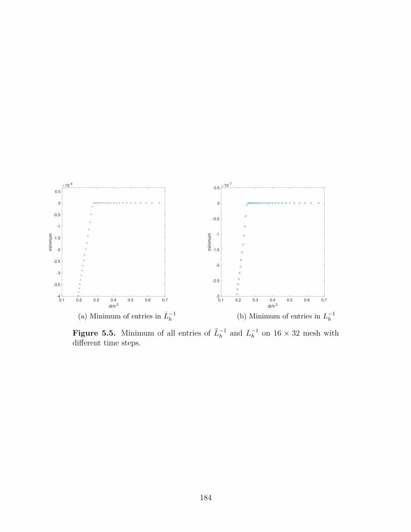
0.1 0.2 0.3 0.4 0.5 0.6 0.7

dt/h2

-4

-3.5

-3

-2.5

-2

-1.5

-1

-0.5

0

0.5

min

imum

×10-6

(a) Minimum of entries in L−1h

0.1 0.2 0.3 0.4 0.5 0.6 0.7

dt/h2

-3

-2.5

-2

-1.5

-1

-0.5

0

0.5

min

imum

×10-7

(b) Minimum of entries in L−1h

Figure 5.5. Minimum of all entries of L−1h and L−1

h on 16 × 32 mesh withdifferent time steps.

184

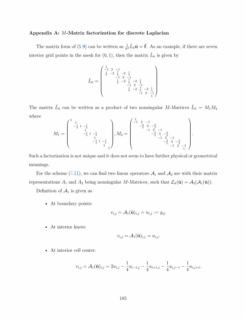
Appendix A: M-Matrix factorization for discrete Laplacian

The matrix form of (5.9 ) can be written as 1h2 Lhu = f . As an example, if there are seven

interior grid points in the mesh for (0, 1), then the matrix Lh is given by

Lh =

1−1 2 −1

14 −2 7

2 −2 14

−1 2 −114 −2 7

2 −2 14

−1 2 −114 −2 7

2 −2 14

−1 2 −11

The matrix Lh can be written as a product of two nonsingular M -Matrices Lh = M1M2

where

M1 =

11

− 14 1 − 1

41

− 14 1 − 1

41

− 14 1 − 1

41

1

,M2 =

1−1 2 −1

− 32 3 − 3

2−1 2 −1

− 32 3 − 3

2−1 2 −1

− 32 3 − 3

2−1 2 −1

1

.

Such a factorization is not unique and it does not seem to have further physical or geometrical

meanings.

For the scheme (5.11 ), we can find two linear operators A1 and A2 are with their matrix

representations A1 and A2 being nonsingular M -Matrices, such that Lh(u) = A2(A1(u)).

Definition of A1 is given as

• At boundary points:

vi,j = A1(u)i,j = ui,j := gij.

• At interior knots:

vi,j = A1(u)i,j = ui,j.

• At interior cell center:

vi,j = A1(u)i,j = 2ui,j −14ui−1,j −

14ui+1,j −

14ui,j−1 −

14ui,j+1.

185

• At interior edge center (an edge parallel to x-axis):

vi,j = A1(u)i,j = −16ui−1,j + 4

3ui,j −16ui+1,j.

• At interior edge center (an edge parallel to y-axis):

vi,j = A1(u)i,j = −16ui,j−1 + 4

3ui,j −16ui,j+1.

Definition of A2 is given as:

• At boundary points:

A2(v)i,j = vi,j.

• At an interior knot:

A2(v)i,j = −32vi−1,j + 3vi,j −

32vi+1,j −

32vi,j−1 + 3vi,j −

32vi,j+1

• At an interior cell center:

A2(v)i,j =2vi,j −38vi−1,j −

38vi+1,j −

38vi,j−1 −

38vi,j+1

−18vi−1,j+1 −

18vi+1,j+1 −

18vi−1,j−1 −

18vi+1,j+1.

• At an interior edge center (an edge parallel to x-axis):

A2(v)i,j = − 716vi−1,j + 15

4 vi,j −716vi+1,j − vi,j+1 − vi,j−1 −

316vi−1,j−1 −

316vi+1,j−1

− 316vi−1,j+1 −

316vi+1,j+1 −

132vi−1,j+2 −

132vi+1,j+2 −

132vi−1,j−2 −

132vi+1,j−2.

186

• At an interior edge center (an edge parallel to y-axis):

A2(v)i,j = − 716vi,j−1 + 15

4 vi,j −716vi,j+1 − vi+1,j − vi−1,j −

316vi−1,j−1 −

316vi−1,j+1

− 316vi+1,j−1 −

316vi+1,j+1 −

132vi+2,j−1 −

132vi+2,j+1 −

132vi−2,j−1 −

132vi−2,j+1.

It is straightforward to verify that Lh(u) = A2(v) where v = A1(u). Obviously, matrices

of A1 and A2 have positive diagonal entries and nonpositive off-diagonal entries. Moreover,

A1(1) ≥ 0 and A2(1) ≥ 0 thus A1 and A2 satisfy the row sum conditions in Theorem 5.3.4 .

So A1 and A2 are both nonsingular M -matrices and the matrix representation of Lh is A2A1.

However, this kind of M -Matrix factorization cannot be extended to the variable coefficient

case.

Appendix B

Proof of Theorem 5.4.3 . If c(x) ≡ 0, then (5.25 ) reduces to

(28ai−1 + 20ai+1)ai + 4ai+1ai−1 > 9a2i−1 + 3a2

i+1.

A convenient sufficient condition is to require

52 mina2i−1, a

2i , a

2i+1 > 12 maxa2

i−1, a2i , a

2i+1,

which is equivalent tomaxai−1, ai, ai+1minai−1, ai, ai+1

<

√133 .

Let a(x1) = maxai−1, ai, ai+1 and a(x2) = minai−1, ai, ai+1. Then the inequality above

is equivalent toa(x1)− a(x2)

a(x2) <

√39− 3

3 .

187

By the Mean Value Theorem, there is some ξ ∈ (xi−1, xi+1) such that a(x1) − a(x2) =

a(ξ)(x2 − x1). Since |x2 − x1| ≤ 2h, we have

|a(x1)− a(x2)| ≤ maxx∈(xi−1,xi+1)

|a(x)| 2h.

Thus a sufficient condition is to require

h

maxx∈(xi−1,xi+1)

|a(x)|

minx∈(xi−1,xi+1)

a(x) <

√39− 3

6 .

For c(x) ≥ 0, (5.25 ) reduces to

(28ai−1 + 20ai+1)ai + 4ai+1ai−1 > 9a2i−1 + 3a2

i+1 + 4h2ci(3ai−1 − 4ai + 3ai+1),

for which a sufficient condition is

13 minIi

a2(x) > 3 maxIi

a2(x) + h2ci(6 maxIi

a(x)− 4 minIi

a(x)). (5.30)

One sufficient condition for (5.30 ) is to have

∃λ ∈ (0, 1), h2ci(6 maxIi

a(x)− 4 minIi

a(x)) <13(1− λ) minIi

a2(x),

3 maxIi

a2(x) <13λminIi

a2(x).

By similar discussions above, a sufficient condition for 3 maxIi

a2(x) < 13λminIi

a2(x) is to have

λ > 313 and

hmaxx∈Ii

|a(x)|

minx∈Ii

a(x) <

√39λ− 3

6 .

The inequality (5.30 ) is also equivalent to

10 minIi

a2(x) > 3(maxIi

a2(x)−minIi

a2(x)) + h2ci(6 maxIi

a(x)− 4 minIi

a(x)).

188

Let a2(x1) = maxIi

a2(x) and a2(x2) = minIi

a2(x), then by the Mean Value Theorem on the

function a2(x), there is some ξ ∈ (xi−1, xi+1) such that

a2(x1)− a2(x1) = 2a(ξ)a(ξ)(x1 − x2) ≤ 4hmaxIi

a(x) maxIi

|a(x)|.

So it suffices to have

10 minIi

a2(x) > 12hmaxIi

a(x) maxIi

|a(x)|+ h2ci(6 maxIi

a(x)− 4 minIi

a(x)),

which can be simplified to

2hmaxIi

|a(x)|+ h2ci(1−23

minIi

a(x)

maxIi

a(x)) < 53

minIi

a2(x)

maxIi

a(x) .

If a(x) ≡ a > 0, it is straightforward to verify that (5.25 ) is equivalent to hci < 5a.

of Theorem 5.4.4 . For a smooth coefficient a(x), by Taylor’s Theorem,

a(x+ h) = a(x) + ha(x) + 12h

2a(ξ1), ξ1 ∈ [x, x+ h],

a(x− h) = a(x)− ha(x) + 12h

2a(ξ2), ξ2 ∈ [x− h, x].

With the Intermediate Value Theorem for a(x), we get

a(x) = 12[a(x+ h) + a(x− h)− h2a(ξ)], ξ ∈ (ξ2, ξ1) ⊂ [x− h, x+ h].

Thus we can rewrite ai as ai = 12(ai−1 + ai+1 − dih

2) where

di := ai−1 + ai+1 − 2ai

h2 = a(ξ), for some ξ ∈ (xi−1, xi+1).

189

If c(x) ≡ 0, then (5.25 ) reduces to (28ai−1+20ai+1)ai+4ai+1ai−1 > 9a2i−1+3a2

i+1. Introducing

an arbitrary number λ ∈ (0, 2], it is equivalent to

4ai+1ai−1 + (4− 2λ)ai(7ai−1 + 5ai+1) + 2λai(7ai−1 + 5ai+1) > 9a2i−1 + 3a2

i+1,

(12λ+ 4)ai+1ai−1 + (4− 2λ)ai(7ai−1 + 5ai+1) + (7λ− 9)a2i−1 + (5λ− 3)a2

i+1

> λh2di(7ai−1 + 5ai+1),

( 4λ− 2)ai + ai−1

(5λ− 3)θ2 + (12λ+ 4)θ + (7λ− 9)λ(5θ + 7) > h2di, θ = ai+1

ai−1,

(4λ− 2

)ai +

( 415 θ − 9

λ(5θ + 7) + 1)ai−1 +

(1− 3

5λ

)ai+1 > h2di.

Notice that415 θ−95θ+7 > −9

7 . By taking 97 ≤ λ ≤ 2, it suffices to require

(1− 97λ)ai−1 + ( 4

λ− 2)ai + (1− 3

5λ)ai+1 > h2di, (5.31)

as a sufficient condition of the above inequalities. If a(x) is a concave function, then it

satisfies a(xi) = a(xi−1+xi−12 ) ≥ 1

2a(xi−1) + 12a(xi+1), which implies ai−1 +ai+1− 2ai ≤ 0, thus

(5.31 ) holds trivially. Otherwise, (5.31 ) holds for λ = 97 if the following mesh constraint is

satisfied:

h2 maxx∈(xi−1,xi+1)

a(x) < 7445 minai−1, ai, ai+1.

If c(x) ≥ 0, for any λ ∈ (0, 2], (5.25 ) is equivalent to


i+1

> λh2di(7ai−1 + 5ai+1) + 4h2ci(ai−1 + ai+1 + 2dih2). (5.32)

If assuming dih2 ≤ 74

45 minai−1, ai, ai+1, then dih2 ≤ λ1ai−1 + λ2ai+1 for any two positive

numbers λ1, λ2 satisfying λ1 + λ2 = 7445 . In particular, for λ1 = 563

540 , we get dih2 ≤ 563

540ai−1 +65108ai+1, which implies

ai−1 + ai+1 + 2dih2 ≤ 119

270(7ai−1 + 5ai+1).

190

By replacing ai−1+ai+1+2dih2 by the inequality above in (5.32 ), we get a sufficient condition

for (5.32 ) as following:


i+1

> λh2di(7ai−1 + 5ai+1) + 4h2ci119270(7ai−1 + 5ai+1). (5.33)

Similar to the derivation of (5.31 ), we can derive a sufficient condition of (5.33 ) as

h2(

1.5ci + maxx∈(xi−1,xi+1)

a(x))<

7445 minai−1, ai, ai+1.

If di ≤ 0, then a sufficient condition for (5.32 ) is


i+1ai−1 + ai+1

> 4h2ci,

from which we can derive a sufficient condition as

4h2ci < (7λ− 9)ai−1 + (5− 52λ)ai + (5λ− 3)ai+1,

for which a sufficient condition by setting λ = 2 is h2ci < 3 minai−1, ai, ai+1.

of Theorem 5.4.7 . Since (5.27a ) and (5.28a ) are equivalent to

4(7ai−1,j + 5ai+1,j)aij + 4ai−1,jai+1,j + 16aij(ai,j−1 + ai,j+1)

> 9a2i−1,j + 3a2

i+1,j + 12(ai−1,j + ai+1,j)(ai,j−1 + ai,j+1) + 4(3ai−1,j − 4aij + 3ai+1,j)h2cij

and

ai−1,jai+1,j + 2aijai−1,j + 4aij(ai,j−2 + 4ai,j−1 + 18ai,j + 4ai,j+1 + ai,j+2) > 18a2i−1,j + 6a2

i+1,j

+14aijai+1,j + 3(ai−1,j + ai+1,j)(ai,j−2 + 4ai,j−1 + 4ai,j+1 + ai,j+2) + 8(3ai−1,j − 4aij + 3ai+1,j)h2cij.

191

A sufficient condition is to require

7 minIij

a(x)2 > 5 maxIij

a(x)2 + 23(3 max

Iij

a(x)− 2 minIij

a(x))h2cij (5.34)

for all cell centers xij of cell Iij = [xi−1, xi+1]× [yi−1, yi+1], and the following mesh constraints

for all edge centers xij:

61 minJij

a(x)2 > 49 maxJij

a(x)2 + 8(3 maxJij

a(x)− 2 minJij

a(x))h2cij, (5.35)

where we Jij is the union of two cells: if xij is an edge center of an edge parallel to x-

axis, then Jij = Ii,j−1 ∪ Ii,j+1; if xij is an edge center of an edge parallel to y-axis, then

Jij = Ii−1,j ∪ Ii+1,j. Notice that (5.35 ) implies (5.34 ), thus it suffices to have (5.35 ) only.

192

6. A HIGH ORDER ACCURATE BOUND-PRESERVING

COMPACT FINITE DIFFERENCE SCHEME FOR SCALAR

CONVECTION DIFFUSION EQUATIONS

In this chapter, we show that the classical fourth order accurate compact finite difference

scheme with high order strong stability preserving time discretizations for convection diffu-

sion problems satisfies a weak monotonicity property, which implies that a simple limiter can

enforce the bound-preserving property without losing conservation and high order accuracy.

Higher order accurate compact finite difference schemes satisfying the weak monotonicity

will also be discussed.

6.1 Introduction

6.1.1 The bound-preserving property

Consider the initial value problem for a scalar convection diffusion equation ut +f(u)x =

a(u)xx, u(x, 0) = u0(x), where a(u) ≥ 0. Assume f(u) and a(u) are well-defined smooth

functions for any u ∈ [m,M ] where m = minx u0(x) and M = maxx u0(x). Its exact solution

satisfies:

minxu0(x) = m ≤ u(x, t) ≤M = max

xu0(x), ∀t ≥ 0. (6.1)

In this chapter, we are interested in constructing a high order accurate finite difference

scheme satisfying the bound-preserving property (6.1 ).

For a scalar problem, it is desired to achieve (6.1 ) in numerical solutions mainly for the

physical meaning. For instance, if u denotes density and m = 0, then negative numerical

solutions are meaningless. In practice, in addition to enforcing (6.1 ), it is also critical to

strictly enforce the global conservation of numerical solutions for a time-dependent convec-

tion dominated problem. Moreover, the computational cost for enforcing (6.1 ) should not

be significant if it is needed for each time step.

193

6.1.2 Popular methods for convection problems

For the convection problems, i.e., a(u) ≡ 0, a straightforward way to achieve the above

goals is to require a scheme to be monotone, total-variational-diminishing (TVD), or satisfy-

ing a discrete maximum principle, which all imply the bound-preserving property. But most

schemes satisfying these stronger properties are at most second order accurate. For instance,

a monotone scheme and traditional TVD finite difference and finite volume schemes are at

most first order accurate [89 ]. Even though it is possible to have high order TVD finite

volume schemes in the sense of measuring the total variation of reconstruction polynomials

[90 ], [91 ], such schemes can be constructed only for the one-dimensional problems. The sec-

ond order central scheme satisfies a discrete maximum principle minj unj ≤ un+1

j ≤ maxj unj

where unj denotes the numerical solution at n-th time step and j-th grid point [92 ]. Any finite

difference scheme satisfying such a maximum principle can be at most second order accu-

rate, see Harten’s example in [93 ]. By measuring the extrema of reconstruction polynomials,

third order maximum-principle-satisfying schemes can be constructed [94 ] but extensions to

multi-dimensional nonlinear problems are very difficult.

For constructing high order accurate schemes, one can enforce only the bound-preserving

property for fixed known bounds, e.g., m = 0 and M = 1 if u denotes the density ratio. Even

though high order linear schemes cannot be monotone, high order finite volume type spatial

discretizations including the discontinuous Galerkin (DG) method satisfy a weak monotonic-

ity property [23 ], [93 ], [95 ]. Namely, in a scheme consisting of any high order finite volume

spatial discretization and forward Euler time discretization, the cell average is a monotone

function of the point values of the reconstruction or approximation polynomial at Gauss-

Lobatto quadrature points. Thus if these point values are in the desired range [m,M ], so

are the cell averages in the next time step. A simple and efficient local bound-preserving

limiter can be designed to control these point values without destroying conservation. More-

over, this simple limiter is high order accurate, see [23 ] and the appendix in [96 ]. With

strong stability preserving (SSP) Runge-Kutta or multistep methods [97 ], which are convex

combinations of several formal forward Euler steps, a high order accurate finite volume or

DG scheme can be rendered bound-preserving with this limiter. These results can be easily

194

extended to multiple dimensions on cells of general shapes. However, for a general finite

difference scheme, the weak monotonicity does not hold.

For enforcing only the bound-preserving property in high order schemes, efficient alter-

natives include a flux limiter [98 ], [99 ] and a sweeping limiter in [100 ]. These methods are

designed to directly enforce the bounds without destroying conservation thus can be used

on any conservative schemes. Even though they work well in practice, it is nontrivial to an-

alyze and rigorously justify the accuracy of these methods especially for multi-dimensional

nonlinear problems.

6.1.3 The weak monotonicity in compact finite difference schemes

Even though the weak monotonicity does not hold for a general finite difference scheme,

in this paper we will show that some high order compact finite difference schemes satisfy

such a property, which implies a simple limiting procedure can be used to enforce bounds

without destroying accuracy and conservation.

To demonstrate the main idea, we first consider a fourth order accurate compact finite

difference approximation to the first derivative on the interval [0, 1]:

16(fi+1 + 4fi + fi−1) = fi+1 − fi−1

2∆x +O(∆x4),

where fi and fi are point values of a function f(x) and its derivative f(x) at uniform

grid points xi (i = 1, · · · , N) respectively. For periodic boundary conditions, the following

tridiagonal linear system needs to be solved to obtain the implicitly defined approximation

to the first order derivative:

16

4 1 1

1 4 1. . . . . . . . .

1 4 1

1 1 4

f1

f2...

fN−1

fN

= 1

2∆x

0 1 −1

−1 0 1. . . . . . . . .

−1 0 1

1 −1 0

f1

f2...

fN−1

fN

. (6.2)

195

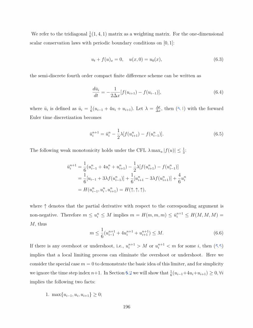
We refer to the tridiagonal 16(1, 4, 1) matrix as a weighting matrix. For the one-dimensional

scalar conservation laws with periodic boundary conditions on [0, 1]:

ut + f(u)x = 0, u(x, 0) = u0(x), (6.3)

the semi-discrete fourth order compact finite difference scheme can be written as

dui

dt= − 1

2∆x [f(ui+1)− f(ui−1)], (6.4)

where ui is defined as ui = 16(ui−1 + 4ui + ui+1). Let λ = ∆t

∆x, then (6.4 ) with the forward

Euler time discretization becomes

un+1i = un

i −12λ[f(un

i+1)− f(uni−1)]. (6.5)

The following weak monotonicity holds under the CFL λmaxu |f(u)| ≤ 13 :

un+1i = 1

6(uni−1 + 4un

i + uni+1)−

12λ[f(un

i+1)− f(uni−1)]

= 16[ui−1 + 3λf(un

i−1)] + 16[un

i+1 − 3λf(uni+1)] + 4

6uni

= H(uni−1, u

ni , u

ni+1) = H(↑, ↑, ↑),

where ↑ denotes that the partial derivative with respect to the corresponding argument is

non-negative. Therefore m ≤ uni ≤ M implies m = H(m,m,m) ≤ un+1

i ≤ H(M,M,M) =

M, thus

m ≤ 16(un+1

i−1 + 4un+1i + un+1

i+1 ) ≤M. (6.6)

If there is any overshoot or undershoot, i.e., un+1i > M or un+1

i < m for some i, then (6.6 )

implies that a local limiting process can eliminate the overshoot or undershoot. Here we

consider the special casem = 0 to demonstrate the basic idea of this limiter, and for simplicity

we ignore the time step index n+1. In Section 6.2 we will show that 16(ui−1+4ui+ui+1) ≥ 0,∀i

implies the following two facts:

1. maxui−1, ui, ui+1 ≥ 0;

196

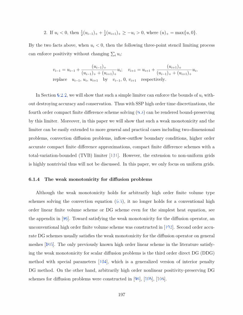
2. If ui < 0, then 12(ui−1)+ + 1

2(ui+1)+ ≥ −ui > 0, where (u)+ = maxu, 0.

By the two facts above, when ui < 0, then the following three-point stencil limiting process

can enforce positivity without changing ∑i ui:

vi−1 = ui−1 + (ui−1)+

(ui−1)+ + (ui+1)+ui; vi+1 = ui+1 + (ui+1)+

(ui−1)+ + (ui+1)+ui,

replace ui−1, ui, ui+1 by vi−1, 0, vi+1 respectively.

In Section 6.2.2 , we will show that such a simple limiter can enforce the bounds of ui with-

out destroying accuracy and conservation. Thus with SSP high order time discretizations, the

fourth order compact finite difference scheme solving (6.3 ) can be rendered bound-preserving

by this limiter. Moreover, in this paper we will show that such a weak monotonicity and the

limiter can be easily extended to more general and practical cases including two-dimensional

problems, convection diffusion problems, inflow-outflow boundary conditions, higher order

accurate compact finite difference approximations, compact finite difference schemes with a

total-variation-bounded (TVB) limiter [101 ]. However, the extension to non-uniform grids

is highly nontrivial thus will not be discussed. In this paper, we only focus on uniform grids.

6.1.4 The weak monotonicity for diffusion problems

Although the weak monotonicity holds for arbitrarily high order finite volume type

schemes solving the convection equation (6.3 ), it no longer holds for a conventional high

order linear finite volume scheme or DG scheme even for the simplest heat equation, see

the appendix in [96 ]. Toward satisfying the weak monotonicity for the diffusion operator, an

unconventional high order finite volume scheme was constructed in [102 ]. Second order accu-

rate DG schemes usually satisfies the weak monotonicity for the diffusion operator on general

meshes [103 ]. The only previously known high order linear scheme in the literature satisfy-

ing the weak monotonicity for scalar diffusion problems is the third order direct DG (DDG)

method with special parameters [104 ], which is a generalized version of interior penalty

DG method. On the other hand, arbitrarily high order nonlinear positivity-preserving DG

schemes for diffusion problems were constructed in [96 ], [105 ], [106 ].

197

In this paper we will show that the fourth order accurate compact finite difference and

a few higher order accurate ones are also weakly monotone, which is another class of linear

high order schemes satisfying the weak monotonicity for diffusion problems.

It is straightforward to verify that the backward Euler or Crank-Nicolson method with

the fourth order compact finite difference methods satisfies a maximum principle for the heat

equation but it can be used be as a bound-preserving scheme only for linear problems. The

method is this chapter is explicit thus can be easily applied to nonlinear problems. It is

difficult to generalize the maximum principle to an implicit scheme. Regarding positivity-

preserving implicit schemes, see [107 ] for a study on weak monotonicity in implicit schemes

solving convection equations. See also [108 ] for a second order accurate implicit and explicit

time discretization for the BGK equation.

Although high order compact finite difference methods have been extensively studied in

the literature, e.g., [71 ], [101 ], [109 ]–[112 ], this is the first time that the weak monotonicity

in compact finite difference approximations is discussed. This is also the first time a weak

monotonicity property is established for a high order accurate finite difference type scheme.

The weak monotonicity property suggests it is possible to post process the numerical solu-

tion without losing conservation by a simple limiter to enforce global bounds. Moreover,

this approach allows an easy justification of high order accuracy of the constructed bound-

preserving scheme.

For extensions to two-dimensional problems, convection diffusion problems, and sixth

order and eighth order accurate schemes, the discussion about the weak monotonicity in

general becomes more complicated since the weighting matrix may become a five-diagonal

matrix instead of the tridiagonal 16(1, 4, 1) matrix in (6.2 ). Nonetheless, we demonstrate

that the same simple three-point stencil limiter can still be used to enforce bounds because

we can factor the more complicated weighting matrix as a product of a few of tridiagonal1

c+2(1, c, 1) matrices with c ≥ 2.

The chapter is organized as follows: in Section 6.2 we demonstrate the main idea for

the fourth order accurate scheme solving one-dimensional problems with periodic boundary

conditions. Two-dimensional extensions are discussed in in Section 6.3 . Section 6.5 is the

extension to higher order accurate schemes. Inflow-outflow boundary conditions and Dirich-

198

let boundary conditions are considered in Section 6.6 . Numerical tests are given in Section

6.7 . Section 6.8 consists of concluding remarks.

6.2 A Fourth Order Accurate Scheme For One-dimensional Problems

In this section we first show the fourth order compact finite difference with forward Euler

time discretization satisfies the weak monotonicity. Then we discuss how to design a simple

limiter to enforce the bounds of point values. To eliminate the oscillations, a total variation

bounded (TVB) limiter can be used. We also show that the TVB limiter does not affect the

bound-preserving property of ui, thus it can be combined with the bound-preserving limiter

to ensure the bound-preserving and non-oscillatory solutions for shocks. High order time

discretizations will be discussed in Section 6.2.5 .

6.2.1 One-dimensional convection problems

Consider a periodic function f(x) on the interval [0, 1]. Let xi = iN

(i = 1, · · · , N)

be the uniform grid points on the interval [0, 1]. Let f be a column vector with numbers

f1, f2, · · · , fN as entries, where fi = f(xi). Let W1, W2, Dx and Dxx denote four linear

operators as follows:

W1f = 16

4 1 1

1 4 1. . . . . . . . .

1 4 1

1 1 4

f1

f2...

fN−1

fN

, Dxf = 1

2

0 1 −1

−1 0 1. . . . . . . . .

−1 0 1

1 −1 0

f1

f2...

fN−1

fN

,

199

W2f = 112

10 1 1

1 10 1. . . . . . . . .

1 10 1

1 1 10

f1

f2...

fN−1

fN

, Dxxf =

−2 1 1

1 −2 1. . . . . . . . .

1 −2 1

1 1 −2

f1

f2...

fN−1

fN

.

The fourth order compact finite difference approximation to the first order derivative (6.2 )

with periodic assumption for f(x) can be denoted as W1f = 1∆xDxf . The fourth order

compact finite difference approximation to f(x) is W2f = 1∆x2Dxxf . The fourth compact

finite difference approximations can be explicitly written as

f = 1∆xW

−11 Dxf , f = 1

∆x2W−12 Dxxf ,

where W−11 and W−1

2 are the inverse operators. For convenience, by abusing notations we

let W−11 fi denote the i-th entry of the vector W−1

1 f .

Then the scheme (6.4 ) solving the scalar conservation laws (6.3 ) with periodic boundary

conditions on the interval [0, 1] can be written as W1ddtui = − 1

2∆x[f(ui+1)−f(ui−1)], and the

scheme (6.5 ) is equivalent to W1un+1i = W1u

ni − 1

2λ[f(uni+1)− f(un

i−1)]. As shown in Section

6.1.3 , the scheme (6.5 ) satisfies the weak monotonicity.

Theorem 6.2.1. Under the CFL constraint ∆t∆x

maxu |f(u)| ≤ 13 ,if u

ni ∈ [m,M ], then un+1

computed by the scheme (6.5 ) satisfies (6.6 ).

6.2.2 A three-point stencil bound-preserving limiter

In this subsection, we consider a more general constraint than (6.6 ) and we will design a

simple limiter to enforce bounds of point values based on it. Assume we are given a sequence

of periodic point values ui (i = 1, · · · , N) satisfying

m ≤ 1c+ 2(ui−1 + cui + ui+1) ≤M, i = 1, · · · , N, c ≥ 2, (6.7)

200

where u0 := uN , uN+1 := u1 and c ≥ 2 is a constant. We have the following results:

Lemma 6.2.2. The constraint (6.7 ) implies the following for stencil i− 1, i, i+ 1:

(1) minui−1, ui, ui+1 ≤M, maxui−1, ui, ui+1 ≥ m.

(2) If ui > M , then (ui−M)+(M−ui−1)++(M−ui+1)+

≤ 1c.

If ui < m, then (m−ui)+(ui−1−m)++(ui+1−m)+

≤ 1c.

Here the subscript + denotes the positive part, i.e., (a)+ = maxa, 0.

Remark 6.2.3. The first statement in Lemma 6.2.2 states that there do not exist three con-

secutive overshoot points or three consecutive undershoot points. But it does not necessarily

imply that at least one of three consecutive point values is in the bounds [m,M ]. For in-

stance, consider the case for c = 4 and N is even, define ui ≡ 1.1 for all odd i and ui ≡ −0.1

for all even i, then 1c+2(ui−1 + cui + ui+1) ∈ [0, 1] for all i but none of the point values ui is

in [0, 1].

Remark 6.2.4. Lemma 6.2.2 implies that if ui is out of the range [m,M ], then we can

set ui ← m for undershoot (or ui ← M for overshoot) without changing the local sum

ui−1 + ui + ui+1 by decreasing (or increasing) its neighbors ui±1.

Proof. We only discuss the upper bound. The inequalities for the lower bound can be

similarly proved. First, if ui−1, ui, ui+1 > M then 1c+2(ui−1 + cui + ui+1) > M which is a

contradiction to (6.7 ). Second, (6.7 ) implies ui−1 + cui + ui+1 ≤ (c+ 2)M , thus c(ui−M) ≤

(M − ui−1) + (M − ui+1) ≤ (M − ui−1)+ + (M − ui+1)+. If ui > M , we get (M − ui−1)+ +

(M − ui+1)+ > 0. Moreover, (ui−M)+(M−ui−1)++(M−ui+1)+

= ui−M(M−ui−1)++(M−ui+1)+

≤ 1c.

For simplicity, we first consider a limiter to enforce only the lower bound without de-

stroying global conservation. For m = 0, this is a positivity-preserving limiter.

Remark 6.2.5. Even though a for loop is used, Algorithm 1 is a local operation to an under-

shoot point since only information of two immediate neighboring points of the undershoot

point are needed. Thus it is not a sweeping limiter.

Theorem 6.2.6. The output of Algorithm 1 satisfiesN∑

i=1vi =

N∑i=1

ui and vi ≥ m.

201

Algorithm 1 A limiter for periodic data ui to enforce the lower bound.Require: The input ui satisfies ui = 1

c+2(ui−1 + cui + ui+1) ≥ m, i = 1, · · · , N , with c ≥ 2.Let u0, uN+1 denote uN , u1 respectively.

Ensure: The output satisfies vi ≥ m, i = 1, · · · , n and ∑Ni=1 vi = ∑N

i=1 ui.First set vi = ui, i = 1, · · · , N . Let v0, vN+1 denote vN , v1 respectively.for i = 1, · · · , N do

if ui < m thenvi−1 ← vi−1 − (ui−1−m)+

(ui−1−m)++(ui+1−m)+(m− ui)+

vi+1 ← vi+1 − (ui+1−m)+(ui−1−m)++(ui+1−m)+

(m− ui)+vi ← m

end ifend for

202

Proof. First of all, notice that the algorithm only modifies the undershoot points and their

immediate neighbors.

Next we will show the output satisfies vi ≥ m case by case:

• If ui < m, the i-th step in for loops sets vi = m. After the (i+ 1)-th step in for loops,

we still have vi = m because (ui −m)+ = 0.

• If ui = m, then vi = m in the final output because (ui −m)+ = 0.

• If ui > m, then limiter may decrease it if at least one of its neighbors ui−1 and ui+1 is

below m:

vi = ui −(ui −m)+(m− ui−1)+

(ui−2 −m)+ + (ui −m)+− (ui −m)+(m− ui+1)+

(ui −m)+ + (ui+2 −m)+

≥ ui −1c(ui −m)+ −

1c(ui −m)+ > m,

where the inequalities are implied by Lemma 6.2.2 and the fact c ≥ 2.

Finally, we need to show the local sum vi−1 +vi +vi+1 is not changed during the i-th step

if ui < m. If ui < m, then after (i− 1)-th step we still have vi = ui because (ui −m)+ = 0.

Thus in the i-th step of for loops, the point value at xi is increased by the amount m− ui,

and the point values at xi−1 and xi+1 are decreased by (ui−1−m)+(ui−1−m)++(ui+1−m)+

(m − ui)+ +(ui+1−m)+

(ui−1−m)++(ui+1−m)+(m − ui)+ = m − ui. So vi−1 + vi + vi+1 is not changed during the i-th

step. Therefore the limiter ensures the output vi ≥ m without changing the global sum.

The limiter described by Algorithm 1 is a local three-point stencil limiter in the sense

that only undershoots and their neighbors will be modified, which means the limiter has

no influence on point values that are neither undershoots nor neighbors to undershoots.

Obviously a similar procedure can be used to enforce only the upper bound. However, to

enforce both the lower bound and the upper bound, the discussion for this three-point stencil

limiter is complicated for a saw-tooth profile in which both neighbors of an overshoot point

are undershoot points. Instead, we will use a different limiter for the saw-tooth profile. To

this end, we need to separate the point values ui, i = 1, · · · , N into two classes of subsets

consisting of consecutive point values.

203

In the following discussion, a set refers to a set of consecutive point values ul, ul+1, ul+2, · · · , um−1, um.

For any set S = ul, ul+1, · · · , um−1, um, we call the first point value ul and the last point

value um as boundary points, and call the other point values ul+1, · · · , um−1 as interior points.

A set of class I is defined as a set satisfying the following:

1. It contains at least four point values.

2. Both boundary points are in [m,M ] and all interior points are out of range.

3. It contains both undershoot and overshoot points.

Notice that in a set of class I, at least one undershoot point is next to an overshoot

point. For given point values ui, i = 1, · · · , N , suppose all the sets of class I are S1 =

um1 , um1+1, · · · , un1, S2 = um2 , · · · , un2, · · · , SK = umK, · · · , unK

, where m1 < m2 <

· · · < umK.

A set of class II consists of point values between Si and Si+1 and two boundary points

uniand umi+1 . Namely they are T0 = u1, u2, · · · , um1, T1 = un1 , · · · , um2, T2 =

un2 , · · · , um3, · · · , TK = unK, · · · , uN. For periodic data ui, we can combine TK and T0

to define TK = unK, · · · , uN , u1, · · · , um1.

In the sets of class I, the undershoot and the overshoot are neighbors. In the sets of

class II, the undershoot and the overshoot are separated, i.e., an overshoot is not next to

any undershoot. We remark that the sets of class I are hardly encountered in the numerical

tests but we include them in the discussion for the sake of completeness. When there are no

sets of class I, all point values form a single set of class II. We will use the same procedure

as in Algorithm 1 for Ti and a different limiter for Si to enforce both the lower bound and

the upper bound.

Theorem 6.2.7. Assume periodic data ui(i = 1, · · · , N) satisfies ui = 1c+2(ui−1+cui+ui+1) ∈

[m,M ], c ≥ 2 for all i = 1, · · · , N with u0 := uN and uN+1 := u1, then the output of Algorithm

2 satisfies ∑Ni=1 vi = ∑N

i=1 ui and vi ∈ [m,M ], ∀i.

Proof. First we show the output vi ∈ [m,M ]. Consider Step II, which only modifies the

undershoot and overshoot points and their immediate neighbors. Notice that the operation

204

Algorithm 2 A bound-preserving limiter for periodic data ui satisfying ui ∈ [m,M ]Require: the input ui satisfies ui = 1

c+2(ui−1 + cui + ui+1) ∈ [m,M ], c ≥ 2. Let u0, uN+1denote uN , u1 respectively.

Ensure: the output satisfies vi ∈ [m,M ], i = 1, · · · , N and ∑Ni=1 vi = ∑N

i=1 ui.1: Step 0: First set vi = ui, i = 1, · · · , N . Let v0, vN+1 denote vN , v1 respectively.2: Step I: Find all the sets of class I S1, · · · , SK (all local saw-tooth profiles) and all the

sets of class II T1, · · · , TK .3: Step II: For each Tj (j = 1, · · · , K), the same limiter as in Algorithm 1 (but for both

upper bound and lower bound) is used:4: for all index i in Tj do5: if ui < m then6: vi−1 ← vi−1 − (ui−1−m)+

(ui−1−m)++(ui+1−m)+(m− ui)+

7: vi+1 ← vi+1 − (ui+1−m)+(ui−1−m)++(ui+1−m)+

(m− ui)+8: vi ← m9: end if

10: if ui > M then11: vi−1 ← vi−1 + (M−ui−1)+

(M−ui−1)++(M−ui+1)+(ui −M)+

12: vi+1 ← vi+1 + (M−ui+1)+(M−ui−1)++(M−ui+1)+

(ui −M)+13: vi ←M14: end if15: end for16: Step III: for each saw-tooth profile Sj = umj

, · · · , unj (j = 1, · · · , K), let N0 and N1

be the numbers of undershoot and overshoot points in Sj respectively.17: Set Uj = ∑nj

i=mjvi.

18: for i = mj + 1, · · · , nj − 1 do19: if ui > M then20: vi ←M .21: end if22: if ui < m then23: vi ← m.24: end if25: end for26: Set Vj = N1M +N0m+ vmj

+ vnj.

27: Set Aj = vmj+ vnj

+N1M − (N1 + 2)m, Bj = (N0 + 2)M − vmj− vnj

−N0m.28: if Vj − Uj > 0 then29: for i = mj, · · · , nj do30: vi ← vi − vi−m

Aj(Vj − Uj)

31: end for32: else33: for i = mj, · · · , nj do34: vi ← vi + M−vi

Bj(Uj − Vj)

35: end for36: end if

205

described by lines 6-8 will not increase the point value of neighbors to an undershoot point

thus it will not create new overshoots. Similarly, the operation described by lines 11-13 will

not create new undershoots. In other words, no new undershoots (or overshoots) will be

created when eliminating overshoots (or undershoots) in Step II.

Each interior point ui in any Tj belongs to one of the following four cases:

1. ui ≤ m or ui ≥M .

2. m < ui < M and ui−1, ui+1 ≤M .

3. m < ui < M and ui−1, ui+1 ≥ m.

4. m < ui < M and ui−1 > M,ui+1 < m (or ui+1 > M,ui−1 < m).

We want to show vi ∈ [m,M ] after Step II. For the first three cases, by the same arguments

as in the proof of Theorem 6.2.6 , we can easily show that the output point values are in the

range [m,M ]. For case (1), after Step II, if ui ≤ m then vi = m; if ui ≥ M then vi = M .

For case (2), vi 6= ui only if at least one of ui−1 and ui+1 is an undershoot. If so, then

vi = ui −(ui −m)+(m− ui−1)+

(ui−2 −m)+ + (ui −m)+− (ui −m)+(m− ui+1)+

(ui −m)+ + (ui+2 −m)+

≥ ui −1c(ui −m)+ −

1c(ui −m)+ > m.

Similarly, for case (3), vi 6= ui only if at least one of ui−1 and ui+1 is an overshoot, and we

can show vi < M .

Notice that case (2) and case (3) are not exclusive to each other, which however does not

affect the discussion here. When case (2) and case (3) overlap, we have ui, ui−1, ui+1 ∈ [m,M ]

thus vi = ui ∈ [m,M ] after Step II.

For case (4), without loss of generality, we consider the case when ui+1 > M,ui ∈

[m,M ], ui−1 < m, and we need to show that the output vi ∈ [m,M ]. By Lemma 6.2.2 , we

know that Algorithm 2 will decrease the value at xi by at most 1c(ui −m) to eliminate the

206

undershoot at xi−1 then increase the point value at xi by at most 1c(M − ui) to eliminate

the overshoot at xi+1. So after Step II,

vi ≤ ui + 1c(M − ui) ≤M (because c ≥ 2, ui < M);

vi ≥ ui −1c(ui −m) ≥ m (because c ≥ 2, ui > m).

Thus we have vi ∈ [m,M ] after Step II. By the same arguments as in the proof of Theorem

6.2.6 , we can also easily show the boundary points are in the range [m,M ] after Step II.

It is straightforward to verify that ∑Ni=1 vi = ∑N

i=1 ui after Step II because the operations

described by lines 6-8 and lines 11-13 do not change the local sum vi−1 + vi + vi+1.

Next we discuss Step III in Algorithm 2 . Let N = 2 + N0 + N1 = nj −mj + 1 be the

cardinality of Sj = umj, · · · , unj

.

We need to show that the average value in each saw-tooth profile Sj is in the range [m,M ]

after Step II before Step III. Otherwise it is impossible to enforce the bounds in Sj without

changing the sum in Sj. In other words, we need to show Nm ≤ Uj = ∑vi∈Sj

vi ≤ NM . We

will prove the claim by conceptually applying the upper or lower bound limiter Algorithm

1 to Sj. Consider a boundary point of Sj, e.g., umj∈ [m,M ], then during Step II the

point value at xmjcan be unchanged, moved down at most 1

c(umj

−m) or moved up at most1c(M − umj

). We first show the average value in Sj after Step II is not below m:

(a) Assume both boundary point values of Sj are unchanged during Step II. If applying

Algorithm 1 to Sj after Step II, by the proof of Theorem 6.2.6 , we know that the

output values would be greater than or equal to m with the same sum, which implies

that ∑vi∈Sjvi ≥ Nm.

(b) If a boundary point value of Sj is increased during Step II, the same discussion as in

(a) still holds because an increased boundary value does not affect the discussion for

the lower bound.

(c) If a boundary point value vmjof Sj is decreased during Step II, then with the fact

that it is decreased by at most the amount 1c(umj

−m), the same discussion as in (a)

still holds.

207

Similarly if applying the upper bound limiter similar to Algorithm 1 to Sj after Step II,

then by the similar arguments as above, the output values would be less than or equal to M

with the same sum, which implies ∑vi∈Sjvi ≤ NM .

Now we can show the output vi ∈ [m,M ] for each Sj after Step III:

1. Assume Vj = N1M + N0m + vmj+ vnj

> Uj before the for loops in Step III. Then

after Step III: if ui < m we get vi = m; if ui ≥ m we have

M ≥ vi −vi −mAj

(Vj − Uj)

= vi −vi −m

vmj+ vnj

+N1M − (N1 + 2)m(vmj+ vnj

+N1M +N0m− Uj)

≥ vi −vi −m

vmj+ vnj

+N1M − (N1 + 2)m(vmj+ vnj

+N1M +N0m− Nm)

= vi −(vi −m) = m.

2. Assume Vj = N1M + N0m + vmj+ vnj

≤ Uj before the for loops in Step III. Then

after Step III: if ui > M we get vi = M ; if ui ≥M we have

m ≤ vi +M − vi

Bj

(Uj − Vj)

= vi + M − vi

(N0 + 2)M − vmj− vnj

−N0m(Uj − vmj

− vnj−N1M −N0m)

≤ vi + M − vi

(N0 + 2)M − vmj− vnj

−N0m(NM − vmj

− vnj−N1M −N0m)

= vi +(M − vi) = M.

Thus we have shown all the final output values are in the range [m,M ].

Finally it is straightforward to verify that ∑Ni=1 vi = ∑N

i=1 ui.

The limiters described in Algorithm 1 and Algorithm 2 are high order accurate limiters

in the following sense. Assume ui(i = 1, · · · , N) are high order accurate approximations

to point values of a very smooth function u(x) ∈ [m,M ], i.e., ui − u(xi) = O(∆xk). For

fine enough uniform mesh, the global maximum points are well separated from the global

minimum points in ui, i = 1, · · · , N. In other words, there is no saw-tooth profile in ui, i =

208

1, · · · , N. Thus Algorithm 2 reduces to the three-point stencil limiter for smooth profiles on

fine resolved meshes. Under these assumptions, the amount which limiter increases/decreases

each point value is at most (ui − M)+ and (m − ui)+. If (ui − M)+ > 0, which means

ui > M ≥ u(xi), we have (ui −M)+ = O(∆xk) because (ui −M)+ < ui − u(xi) = O(∆xk).

Similarly, we get (m − ui)+ = O(∆xk). Therefore, for point values ui approximating a

smooth function, the limiter changes ui by O(∆xk).

6.2.3 A TVB limiter

The scheme (6.5 ) can be written into a conservation form:

un+1i = un

i −∆t∆x(fi+ 1

2− fi− 1

2), (6.8)

which is suitable for shock calculations and involves a numerical flux

fi+ 12

= 12(f(un

i+1) + f(uni )). (6.9)

To achieve nonlinear stability and eliminate oscillations for shocks, a TVB (total variation

bounded in the means) limiter was introduced for the scheme (6.8 ) in [101 ]. In this subsection

we will show that the bound-preserving property of ui (6.6 ) still holds for the scheme (6.8 )

with the TVB limiter in [101 ]. Thus we can use both the TVB limiter and the bound-

preserving limiter in Algorithm (2 ) at the same time.

The compact finite difference scheme with the limiter in [101 ] is

un+1i = un

i −∆t∆x(f (m)

i+ 12− f (m)

i− 12), (6.10)

where the numerical flux f (m)i+ 1

2is the modified flux approximating (6.9 ).

First we write f(u) = f+(u) + f−(u) with the requirement that ∂f+(u)∂u≥ 0, and ∂f−(u)

∂u≤

0. The simplest such splitting is the Lax-Friedrichs splitting f±(u) = 12(f(u) ± αu), α =

209

maxu∈[m,M ]

|f(u)|. Then we write the flux fi+ 12

as fi+ 12

= f+i+ 1

2+ f−

i+ 12, where f±

i+ 12

are obtained

by adding superscripts ± in (6.9 ). Next we define

df+i+ 1

2= f+

i+ 12− f+(ui), df−

i+ 12

= f−(ui+1)− f−i+ 1

2.

Here df±i+ 1

2are the differences between the numerical fluxes f±

i+ 12

and the first-order, upwind

fluxes f+(ui) and f−(ui+1). The limiting is defined by

df+(m)i+ 1

2= m(df+

i+ 12,∆+f+(ui),∆+f+(ui−1)), df

−(m)i+ 1

2= m(df−

i+ 12,∆+f−(ui),∆+f−(ui+1)),

where ∆+vi ≡ vi+1 − vi is the usual forward difference operator, and the modified minmod

function m is defined by

m(a1, . . . , ak) =

a1, if |a1| ≤ p∆x2,

m(a1, . . . , ak), otherwise,(6.11)

where p is a positive constant independent of ∆x and m is the minmod function

m(a1, . . . , ak) =

smin1≤i≤k |ai|, if sign(a1) = · · · = sign(ak) = s,

0, otherwise.

The limited numerical flux is then defined by f+(m)i+ 1

2= f+(ui)+df+(m)

i+ 12, f

−(m)i+ 1

2= f−(ui+1)−

df−(m)i+ 1

2,and f

(m)i+ 1

2= f

+(m)i+ 1

2+ f

−(m)i+ 1

2. The following result was proved in [101 ]:

Lemma 6.2.8. For any n and ∆t such that 0 ≤ n∆t ≤ T , scheme (6.10 ) is TVBM (total

variation bounded in the means): TV (un) = ∑i |un

i+1 − uni | ≤ C, where C is independent of

∆t, under the CFL condition maxu( ∂∂uf+(u)− ∂

∂uf−(u)) ∆t

∆x≤ 1

2 .

Next we show that the TVB scheme still satisfies (6.6 ).

Theorem 6.2.9. If uni ∈ [m,M ], then under a suitable CFL condition, the TVB scheme

(6.10 ) satisfies m ≤ 16(un+1

i−1 + 4un+1i + un+1

i+1 ) ≤M.

210

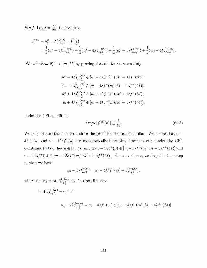
Proof. Let λ = ∆t∆x

, then we have

un+1i = un

i − λ(f (m)i+ 1

2− f (m)

i− 12)

= 14(un

i − 4λf+(m)i+ 1

2) + 1

4(uni − 4λf−(m)

i+ 12

) + 14(un

i + 4λf+(m)i− 1

2) + 1

4(uni + 4λf−(m)

i− 12

).

We will show un+1i ∈ [m,M ] by proving that the four terms satisfy

uni − 4λf+(m)

i+ 12∈ [m− 4λf+(m),M − 4λf+(M)],

ui − 4λf−(m)i+ 1

2∈ [m− 4λf−(m),M − 4λf−(M)],

uni + 4λf+(m)

i− 12∈ [m+ 4λf+(m),M + 4λf+(M)],

ui + 4λf−(m)i− 1

2∈ [m+ 4λf−(m),M + 4λf−(M)],

under the CFL condition

λmaxu|f (±)(u)| ≤ 1

12 . (6.12)

We only discuss the first term since the proof for the rest is similar. We notice that u −

4λf+(u) and u − 12λf+(u) are monotonically increasing functions of u under the CFL

constraint (6.12 ), thus u ∈ [m,M ] implies u−4λf+(u) ∈ [m−4λf+(m),M −4λf+(M)] and

u − 12λf+(u) ∈ [m − 12λf+(m),M − 12λf+(M)]. For convenience, we drop the time step

n, then we have

ui − 4λf+(m)i+ 1

2= ui − 4λ(f+(ui) + df

+(m)i+ 1

2),

where the value of df+(m)i+ 1

2has four possibilities:

1. If df+(m)i+ 1

2= 0, then

ui − 4λf+(m)i+ 1

2= ui − 4λf+(ui) ∈ [m− 4λf+(m),M − 4λf+(M)].

211

2. If df+(m)i+ 1

2= df+

i+ 12, then we get

ui − 4λf+(m)i+ 1

2= 1

6(ui−1 + 4ui + ui+1)− 4λf+(ui) + f+(ui+1)

2= 1

6ui−1 + 23(ui − 3λf+(ui)) + 1

6(ui+1 − 12λf+(ui+1)).

By the monotonicity of the function u− 12λf+(u) and u− 3λf+(u), we have

ui − 3λf+(ui) ∈ [m− 3λf+(m),M − 3λf+(M)],

ui+1 − 12λf+(ui+1) ∈ [m− 12λf+(m),M − 12λf+(M)],

which imply ui − 4λf+(m)i+ 1

2∈ [m− 4λf+(m),M − 4λf+(M)].

3. If df+(m)i+ 1

2= ∆+f+(ui), ui − 4λf+(m)

i+ 12

= ui − 4λf+(ui+1). If ∆+f+(ui) > 0, ui −

4λf+(ui+1) < ui − 4λf+(ui) ≤ M − 4λf+(M), which implies the upper bound holds.

Due to the definition of the minmod function, we can get 0 < ∆+f+(ui) < df+i+ 1

2.

Thus, f+i+ 1

2= f+(ui)+f+(ui+1)

2 = f+(ui)+df+i+ 1

2> f+(ui)+∆+f+(ui) = f+(ui+1). Then,

ui−4λf+(ui+1) > ui−4λf+(ui)+f+(ui+1)2 ≥ m−4λf+(m), which gives the lower bound.

For the case ∆+f+(ui) < 0, the proof is similar.

4. If df+(m)i+ 1

2= ∆+f+(ui−1), the proof is the same as the previous case.

6.2.4 One-dimensional convection diffusion problems

We consider the one-dimensional convection diffusion problems with periodic boundary

conditions: ut + f(u)x = a(u)xx, u(x, 0) = u0(x), where a(u) ≥ 0. Let fn denote the

column vector with entries f(un1 ), · · · , f(un

N). By notations introduced in Section 6.2.1 , the

fourth-order compact finite difference with forward Euler can be denoted as:

un+1 = un − ∆t∆xW

−11 Dxfn + ∆t

∆x2W−12 Dxxan. (6.13)

212

Recall that we have abused the notation by using W1fni to denote the i-th entry of the vector

W1fn and we have defined ui = W1ui. We now define

ui = W2ui.

Notice that W1 and W2 are both circulant thus they both can be diagonalized by the discrete

Fourier matrix, so W1 and W2 commute. Thus we have

˜ui = (W2W1u)i = (W1W2u)i = ¯ui.

Let fni = f(un

i ) and ani = a(un

i ), then the scheme (6.13 ) can be written as

¯un+1i = ¯un

i −∆t∆xW2Dxf

ni + ∆t

∆x2W1Dxxani .


maxu |f(u)| ≤ 16 ,

∆t∆x2 maxu a(u) ≤ 5

24 , if

uni ∈ [m,M ], then the scheme (6.13 ) satisfies that m ≤ ¯un+1

i ≤M.

Proof. Let λ = ∆t∆x

and µ = ∆t∆x2 . We can rewrite the scheme (6.13 ) as

un+1 = 12(un − 2λW−1

1 Dxfn) + 12(un + 2µW−1

2 Dxxan),

W2W1un+1 = 12W2(W1un − 2λDxfn) + 1

2W1(W2un + 2µDxxan),

¯un+1i = 1

2W2(uni − 2λDxf

ni ) + 1

2W1(uni + 2µDxxa

ni ).

By Theorem 6.2.1 , we have uni − 2λDxf

ni ∈ [m,M ]. We also have

uni + 2µDxxa

ni = 1

12(un−1 + 10un

i + uni+1) + 2µ(an

i−1 − 2ani + an

i+1)

=(5

6uni − 4µan

i

)+( 1

12uni−1 + 2µan

i−1

)+( 1

12uni+1 + 2µan

i+1

).

Due to monotonicity under the CFL constraint and the assumption a(u) ≥ 0, we get uni +

2µDxxani ∈ [m,M ]. Thus we get ¯un+1

i ∈ [m,M ] since it is a convex combination of uni −

2λDxfni and un

i + 2µDxxani .

213

Given point values ui satisfying ¯ui ∈ [m,M ] for any i, Lemma 6.2.2 no longer holds since¯ui has a five-point stencil. However, the same three-point stencil limiter in Algorithm 2 can

still be used to enforce the lower and upper bounds. Given ¯ui = W2W1ui i = 1, · · · , N , con-

ceptually we can obtain the point values ui by first computing ui = W−12 ¯ui then computing

ui = W−11 ui. Thus we can apply the limiter in Algorithm 2 twice to enforce ui ∈ [m,M ]:

1. Given ¯ui ∈ [m,M ], compute ui = W−12 ¯ui which are not necessarily in the range [m,M ].

Then apply the limiter in Algorithm 2 to ui, i = 1, · · · , N . Let vi denote the output

of the limiter. Since we have

¯ui = ˜ui = 1c+ 2(ui−1 + cui + ui+1), c = 10,

all discussions in Section 6.2.2 are still valid, thus we have vi ∈ [m,M ].

2. Compute ui = W−11 vi. Apply the limiter in Algorithm 2 to ui, i = 1, · · · , N . Let vi

denote the output of the limiter. Then we have vi ∈ [m,M ].

6.2.5 High order time discretizations

For high order time discretizations, we can use strong stability preserving (SSP) Runge-

Kutta and multistep methods, which are convex combinations of formal forward Euler steps.

Thus if using the limiter in Algorithm 2 for fourth order compact finite difference schemes

considered in this section on each stage in a SSP Runge-Kutta method or each time step in

a SSP multistep method, the bound-preserving property still holds.

In the numerical tests, we will use a fourth order SSP multistep method and a fourth

order SSP Runge-Kutta method [97 ]. Now consider solving ut = F (u). The SSP coefficient

C for a SSP time discretization is a constant so that the high order SSP time discretization

is stable in a norm or a semi-norm under the time step restriction ∆t ≤ C∆t0, if under

the time step restriction ∆t ≤ ∆t0 the forward Euler is stable in the same norm or semi-

norm. The fourth order SSP Multistep method (with SSP coefficient Cms = 0.1648) and the

fourth order SSP Runge-Kutta method (with SSP coefficient Crk = 1.508) will be used in

the numerical tests. See [97 ] for their definitions.

214

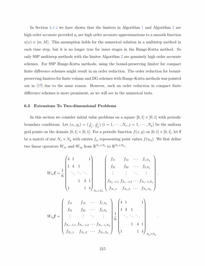
In Section 6.2.2 we have shown that the limiters in Algorithm 1 and Algorithm 2 are

high order accurate provided ui are high order accurate approximations to a smooth function

u(x) ∈ [m,M ]. This assumption holds for the numerical solution in a multistep method in

each time step, but it is no longer true for inner stages in the Runge-Kutta method. So

only SSP multistep methods with the limiter Algorithm 2 are genuinely high order accurate

schemes. For SSP Runge-Kutta methods, using the bound-preserving limiter for compact

finite difference schemes might result in an order reduction. The order reduction for bound-

preserving limiters for finite volume and DG schemes with Runge-Kutta methods was pointed

out in [23 ] due to the same reason. However, such an order reduction in compact finite

difference schemes is more prominent, as we will see in the numerical tests.

6.3 Extensions To Two-dimensional Problems

In this section we consider initial value problems on a square [0, 1]× [0, 1] with periodic

boundary conditions. Let (xi, yj) = ( iNx, j

Ny) (i = 1, · · · , Nx, j = 1, · · · , Ny) be the uniform

grid points on the domain [0, 1]× [0, 1]. For a periodic function f(x, y) on [0, 1]× [0, 1], let f

be a matrix of size Nx×Ny with entries fij representing point values f(uij). We first define

two linear operators W1x and W1y from RNx×Ny to RNx×Ny :

W1xf = 16

4 1 1

1 4 1. . . . . . . . .

1 4 1

1 1 4

Nx×Nx

f11 f12 · · · f1,Ny

f21 f22 · · · f2,Ny

... ... . . . ...

fNx−1,1 fNx−1,2 · · · fNx−1,Ny

fNx,1 fNx,2 · · · fNx,Ny

,

W1yf =

f11 f12 · · · f1,Ny

f21 f22 · · · f2,Ny

... ... . . . ...

fNx−1,1 fNx−1,2 · · · fNx−1,Ny

fNx,1 fNx,2 · · · fNx,Ny

16

4 1 1

1 4 1. . . . . . . . .

1 4 1

1 1 4

Ny×Ny

.

215

We can define W2x, W2y, Dx, Dy, W2x and W2y similarly such that the subscript x denotes

the multiplication of the corresponding matrix from the left for the x-index and the subscript

y denotes the multiplication of the corresponding matrix from the right for the y-index. We

abuse the notations by using W1xfij to denote the (i, j) entry of W1xf . We only discuss the

forward Euler from now on since the discussion for high order SSP time discretizations are

the same as in Section 6.2.5 .

6.3.1 Two-dimensional convection equations

Consider solving the two-dimensional convection equation: ut+f(u)x+g(u)y = 0, u(x, y, 0) =

u0(x, y). By the our notations, the fourth order compact scheme with the forward Euler time

discretization can be denoted as:

un+1ij = un

ij −∆t∆xW

−11x Dxf

nij −

∆t∆yW

−11y Dyg

nij. (6.14)

We define un = W1xW1yun, then by applying W1yW1x to both sides, (6.14 ) becomes

un+1ij = un

ij −∆t∆xW1yDxf

nij −

∆t∆yW1xDyg

nij. (6.15)

Theorem 6.3.1. Under the CFL constraint

∆t∆x max

u|f(u)|+ ∆t

∆y maxu|g(u)| ≤ 1

3 , (6.16)

if unij ∈ [m,M ], then the scheme (6.15 ) satisfies un+1

ij ∈ [m,M ].

Proof. For convenience, we drop the time step n in unij, fn

ij, and introduce:

U =

ui−1,j+1 ui,j+1 ui+1,j+1

ui−1,j ui,j ui+1,j

ui−1,j−1 ui,j−1 ui+1,j−1

, F =

fi−1,j+1 fi,j+1 fi+1,j+1

fi−1,j fi,j fi+1,j

fi−1,j−1 fi,j−1 fi+1,j−1

.

216

Let λ1 = ∆t∆x

and λ2 = ∆t∆y

, then the scheme (6.15 ) can be written as

un+1ij = W1yW1xu

nij − λ1W1yDxf

nij − λ2W1xDyg

nij,

= 136

1 4 1

4 16 4

1 4 1

: U − λ1

12

−1 0 1

−4 0 4

−1 0 1

: F − λ2

12

1 4 1

0 0 0

−1 −4 −1

: G,

where : denotes the sum of all entrywise products in two matrices of the same size. Obviously

the right hand side above is a monotonically increasing function with respect to ulm for

i − 1 ≤ l ≤ i + 1, j − 1 ≤ m ≤ j + 1 under the CFL constraint (6.16 ). The monotonicity

implies the bound-preserving result of un+1ij .

Given uij, we can recover point values uij by obtaining first vij = W−11x uij then uij =

W−11y vij. Thus similar to the discussions in Section 6.2.4 , given point values uij satisfying

uij ∈ [m,M ] for any i and j, we can use the limiter in Algorithm 2 in a dimension by

dimension fashion to enforce uij ∈ [m,M ]:

1. Given uij ∈ [m,M ], compute vij = W−11x uij which are not necessarily in the range

[m,M ]. Then apply the limiter in Algorithm 2 to vij (i = 1, · · · , Nx) for each fixed j.

Since we have

uij = 1c+ 2(vi−1,j + cvi,j + vi+1,j), c = 4,

all discussions in Section 6.2.2 are still valid. Let vij denote the output of the limiter,

thus we have vij ∈ [m,M ].

2. Compute uij = W−11y vij. Then we have

vij = 1c+ 2(ui,j−1 + cui,j + ui,j+1), c = 4.

Apply the limiter in Algorithm 2 to uij (j = 1, · · · , Ny) for each fixed i. Then the

output values are in the range [m,M ].

217

6.3.2 Two-dimensional convection diffusion equations

Consider the two-dimensional convection diffusion problem:

ut + f(u)x + g(u)y = a(u)xx + b(u)xx, u(x, y, 0) = u0(x, y),

where a(u) ≥ 0 and b(u) ≥ 0. A fourth-order accurate compact finite difference scheme can

be written as

dudt

= − 1∆xW

−11x Dxf − 1

∆yW−11y Dyg + 1

∆x2W−12x Dxxa + 1

∆y2W−12y Dyyb.

Let λ1 = ∆t∆x

, λ2 = ∆t∆y

, µ1 = ∆t∆x2 and µ2 = ∆t

∆y2 . With the forward Euler time discretization,

the scheme becomes

un+1ij = un

ij − λ1W−11x Dxf

nij − λ2W

−11y Dyg

nij + µ1W

−12x Dxxa

nij + µ2W

−12y Dyyb

nij. (6.17)

We first define u = W1xW1yu and u = W2xW2yu, where W1 = W1xW1y and W2 =

W2xW2y. Due to the fact W1W2 = W2W1, we have

˜u = W2xW2y(W1xW1yu) = W1xW1y(W2xW2yu) = ¯u.

The scheme (6.17 ) is equivalent to the following form:

˜un+1ij = ˜un

ij − λ1W1yW2xW2yDxfnij − λ2W1xW2xW2yDyg

nij

+µ1W1xW1yW2yDxxanij + µ2W1xW1yW2xDyyb

nij.

Theorem 6.3.2. Under the CFL constraint

∆t∆x max

u|f(u)|+ ∆t

∆y maxu|g(u)| ≤ 1

6 ,∆t

∆x2 maxu

a(u) + ∆t∆y2 max

ub(u) ≤ 5

24 , (6.18)

if unij ∈ [m,M ], then the scheme (6.17 ) satisfies ˜un+1

ij ∈ [m,M ].

218

Proof. By using ˜unij = 1

2˜un

ij + 12¯un

ij, we obtain

˜un+1ij = 1

2W2xW2y[unij − 2λ1W1yDxf

nij − 2λ2W1xDyg

nij]

+12W1xW1y[un

ij + 2µ1W2yDxxanij + 2µ2W2xDyyb

nij].

Let vij = unij−2λ1W1yDxf

nij−2λ2W1xDyg

nij, wij = un

ij +2µ1W2yDxxanij +2µ2W2xDyyb

nij. Then

by the same discussion as in the proof of Theorem 6.3.1 , we can show vij ∈ [m,M ]. For wij,

it can be written as

wij = 1144

1 10 1

10 100 10

1 10 1

: U + µ1

6

1 −2 1

10 −20 10

1 −2 1

: A+ µ2

6

1 10 1

−2 −20 −2

1 10 1

: B,

A =

ai−1,j+1 ai,j+1 ai+1,j+1

ai−1,j ai,j ai+1,j

ai−1,j−1 ai,j−1 ai+1,j−1

, B =

bi−1,j+1 bi,j+1 bi+1,j+1

bi−1,j bi,j bi+1,j

bi−1,j−1 bi,j−1 bi+1,j−1

.

Under the CFL constraint (6.18 ), wij is a monotonically increasing function of unij involved

thus wij ∈ [m,M ]. Therefore, ˜un+1ij ∈ [m,M ].

Given ˜uij, we can recover point values uij by obtaining first uij = W−11x W

−11y

˜uij then

uij = W−12x W

−12y uij. Thus similar to the discussions in the previous subsection, given point

values uij satisfying ˜uij ∈ [m,M ] for any i and j, we can use the limiter in Algorithm 2

dimension by dimension several times to enforce uij ∈ [m,M ]:

1. Given ˜uij ∈ [m,M ], compute uij = W−11x W

−11y

˜uij and apply the limiting algorithm in

the previous subsection to ensure uij ∈ [m,M ].

2. Compute vij = W−12x uij which are not necessarily in the range [m,M ]. Then apply the

limiter in Algorithm 2 to vij for each fixed j. Since we have

uij = 1c+ 2(vi−1,j + cvi,j + vi+1,j), c = 10,

219

all discussions in Section 6.2.2 are still valid. Let vij denote the output of the limiter,

thus we have vij ∈ [m,M ].

3. Compute uij = W−12y vij. Then we have vij = 1

c+2(ui,j−1 +cui,j +ui,j+1), c = 10. Apply

the limiter in Algorithm 2 to uij for each fixed i. Then the output values are in the

range [m,M ].

6.4 Two-dimensional Incompressible Navier-Stokes Equation

In this section we consider the two-dimensional incompressible Navier-Stokes equation in

the vorticity stream-function form:

ωt + (uω)x + (vω)y = 1Re

∆ω, (6.19a)

ψ = ∆ω, (6.19b)

〈u, v〉 = 〈−ψy, ψx〉, (6.19c)

where ω is the vorticity, ψ is the stream function, 〈u, v〉 is the velocity and Re is the Reynolds

number. The equation (6.19c ) implies the incompressiblility condition

ux + vy = 0. (6.20)

Due to (6.20 ), (6.19a ) is equivalent to

ωt + uωx + vωy = 1Re

∆ω, (6.21)

for which the initial value problem satisfies the same bound-preserving property as discussed

before:

minx,y

ω(x, y, 0) = m ≤ ω(x, y, t) ≤M = maxx,y

ω(x, y, 0).

If solving (6.21 ) directly, it is usually easier to achieve a bound-preserving scheme. But

for the sake of conservation, it is desired to solve the conservative form equation (6.19a ).

In order to enforce the bound-preserving property for (6.19a ) without losing accuracy, the

220

divergence free constraint (6.20 ) must be properly used since the bound-preserving property

may not hold for (6.19a ) without (6.20 ), see [23 ], [102 ], [103 ].

For simplicity, we only consider a periodic boundary condition on a square [0, 1]× [0, 1].

Let (xi, yj) = ( iNx, j

Ny) (i = 1, · · · , Nx, j = 1, · · · , Ny) be the uniform grid points on the

domain [0, 1]× [0, 1]. All notations are the same as in the previous section.

Standard fourth order compact finite difference schemes can be used to solve the Poisson

equation (6.19b ). Efficient Fourier-based Poisson solvers can be constructed.

6.4.1 Incompressible Euler equations

For simplicity, we first consider how to achieve the weak monotonicity for the incom-

pressible Euler equations

ωt + (uω)x + (vω)y = 0. (6.22)

A fourth order compact finite difference scheme with the forward Euler method for (6.22 )

can be given as

ωn+1ij = ωn

ij − λ1[W−11x Dx(un ωn)]ij − λ2[W−1

1y Dy(un ωn)]ij, (6.23)

and it is equivalent to

ωn+1ij = ωn

ij − λ1[W1yDx(un ωn)]ij − λ2[W1xDy(vn ωn)]ij

= 136

1 4 1

4 16 4

1 4 1

: Ωn − λ1

12

−1 0 1

−4 0 4

−1 0 1

: (Un Ωn)− λ2

12

1 4 1

0 0 0

−1 −4 −1

: (V n Ωn),

(6.24)

where denotes the matrix Hadamard product, and

U =

ui−1,j+1 ui,j+1 ui+1,j+1


ui−1,j−1 ui,j−1 ui+1,j−1

, V =

vi−1,j+1 vi,j+1 vi+1,j+1

vi−1,j vi,j vi+1,j

vi−1,j−1 vi,j−1 vi+1,j−1

,Ω =

ωi−1,j+1 ωi,j+1 ωi+1,j+1

ωi−1,j ωi,j ωi+1,j

ωi−1,j−1 ωi,j−1 ωi+1,j−1

.

221

By the discussions in the Section 6.3.1 , we can easily conclude that ωn+1ij is a monotonically

increasing function with respect to all ωnij involved in (6.24 ) under the CFL condition

∆t∆x max

ij|un

ij|+∆t∆y max

ij|vn

ij| ≤13 .

However, to obtain ωn+1ij ∈ [m,M ], the monotonicity is sufficient only if the following con-

sistency condition holds:

ωnij ≡ m⇒ ωn+1

ij = m, ωnij ≡M ⇒ ωn+1

ij = M. (6.25)

Plugging ωnij ≡ m in (6.24 ), we get

ωn+1ij =m+ ∆t

6∆x

(un

i+1,j−1 − uni−1,j−1

2 +4(un

i+1,j − uni−1,j)

2 +un

i+1,j+1 − uni−1,j+1

2

)

+ ∆t6∆y

(vn

i−1,j+1 − vni−1,j−1

2 +4(vn

i,j+1 − vni,j−1)

2 +vn

i+1,j+1 − vni+1,j−1

2

).

Thus the consistency (6.25 ) holds only if the velocity 〈un, vn〉 satisfies:

16∆x

(un

i+1,j−1 − uni−1,j−1

2 +4(un

i+1,j − uni−1,j)

2 +un

i+1,j+1 − uni−1,j+1

2

)

+ 16∆y

(vn

i−1,j+1 − vni−1,j−1

2 +4(vn

i,j+1 − vni,j−1)

2 +vn

i+1,j+1 − vni+1,j−1

2

)= 0.

(6.26)

Thus we get the following bound-preserving result:

Theorem 6.4.1. If the velocity 〈un, vn〉 satisfies the constraint (6.26 ) and ωnij ∈ [m,M ],

then under the CFL constraint

∆t∆x max

ij|un

ij|+∆t∆y max

ij|vn

ij| ≤13 ,

the scheme (6.24 ) satisfies ωn+1ij ∈ [m,M ].

222

6.4.2 A discrete divergence free velocity field

Note that (6.26 ) is a discrete divergence free constraint and we can reconstruct a fourth

order accurate velocity field satisfying (6.26 ) by direct difference.

In the following discussion, we may discard the superscript n sometimes for convenience

since everything discussed is at time step n. Given ωij, we first compute ψij by a fourth

order compact finite difference scheme (i.e., the nine-point discrete Laplacian) for the Poisson

equation (6.19b ). Then by the fourth order compact finite difference we have

−DyΨ = W1yure, DxΨ = W1xvre, (6.27)

where

Ψ =

ψ11 ψ12 · · · ψ1,Ny

ψ21 ψ22 · · · ψ2,Ny

... ... . . . ...

ψNx−1,1 ψNx−1,2 · · · ψNx−1,Ny

ψNx,1 ψNx,2 · · · ψNx,Ny

Nx×Ny

.

Write (6.26 ) in matrix form, then we have

DxW1yu +DyW1xv = 0.

We can clearly see that ure and vre constructed in (6.27 ) satisfy (6.26 ) immediately.

Now we let

u = ure, v = vre.

6.4.3 A fourth order accurate bound-preserving scheme

For the Euler equations (6.22 ), the following implementation of the fourth order compact

finite difference with forward Euler time discretization scheme can preserve the bounds:

1. Given ωnij ∈ [m,M ], solve the Poisson equation by the fourth order accurate nine-point

discrete Laplacian scheme to obtain point values of the stream function ψij.

223

2. Reconstruct u and v by (6.27 ).

3. Obtain ωn+1ij ∈ [m,M ] by scheme (6.24 ).

4. Apply the limiting procedure in Section 6.3.1 to obtain ωn+1ij ∈ [m,M ].

For high order SSP time discretizations, we should use the same implementation above for

each time stage or time step.

For the Navier-Stokes equations (6.19a ), the scheme can be written as

ωn+1ij =ωn

ij − λ1[W−11x Dx(un ωn)]ij − λ2[W−1

1y Dy(vn ωn)]ij

+ µ1

ReW−1

2x Dxxωnij + µ2

ReW−1

2y Dyyωnij,

which is equivalent to

˜ωn+1ij = ˜ωn

ij−W2xW2y

136

1 4 1

4 16 4

1 4 1

: Ωn − λ1

12

−1 0 1

−4 0 4

−1 0 1

: (Un Ωn)

−λ2

12

1 4 1

0 0 0

−1 −4 −1

: (V n Ωn)

ij

+ µ1

ReW1xW1yW2yDxxω

nij + µ2

ReW1xW1yW2xDyyω

nij.

(6.28)

Following the discussions in Section 6.4.1 and Section 6.3.2 , we obtain the following

result:

Theorem 6.4.2. If the velocity 〈un, vn〉 satisfies the constraint (6.26 ) and ωnij ∈ [m,M ],

then under the CFL constraint

∆t∆x max

ij|un

ij|+∆t∆y max

ij|vn

ij| ≤16 ,

∆tRe∆x2 + ∆t

Re∆y2 ≤524 ,

the scheme (6.28 ) satisfies ˜ωn+1ij ∈ [m,M ].

224

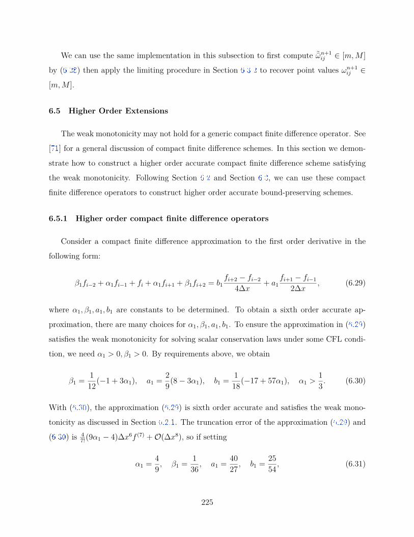
We can use the same implementation in this subsection to first compute ˜ωn+1ij ∈ [m,M ]

by (6.28 ) then apply the limiting procedure in Section 6.3.2 to recover point values ωn+1ij ∈

[m,M ].

6.5 Higher Order Extensions

The weak monotonicity may not hold for a generic compact finite difference operator. See

[71 ] for a general discussion of compact finite difference schemes. In this section we demon-

strate how to construct a higher order accurate compact finite difference scheme satisfying

the weak monotonicity. Following Section 6.2 and Section 6.3 , we can use these compact

finite difference operators to construct higher order accurate bound-preserving schemes.

6.5.1 Higher order compact finite difference operators

Consider a compact finite difference approximation to the first order derivative in the

following form:

β1fi−2 + α1fi−1 + fi + α1fi+1 + β1fi+2 = b1fi+2 − fi−2

4∆x + a1fi+1 − fi−1

2∆x , (6.29)

where α1, β1, a1, b1 are constants to be determined. To obtain a sixth order accurate ap-

proximation, there are many choices for α1, β1, a1, b1. To ensure the approximation in (6.29 )

satisfies the weak monotonicity for solving scalar conservation laws under some CFL condi-

tion, we need α1 > 0, β1 > 0. By requirements above, we obtain

β1 = 112(−1 + 3α1), a1 = 2

9(8− 3α1), b1 = 118(−17 + 57α1), α1 >

13 . (6.30)

With (6.30 ), the approximation (6.29 ) is sixth order accurate and satisfies the weak mono-

tonicity as discussed in Section 6.2.1 . The truncation error of the approximation (6.29 ) and

(6.30 ) is 47!(9α1 − 4)∆x6f (7) +O(∆x8), so if setting

α1 = 49 , β1 = 1

36 , a1 = 4027 , b1 = 25

54 , (6.31)

225

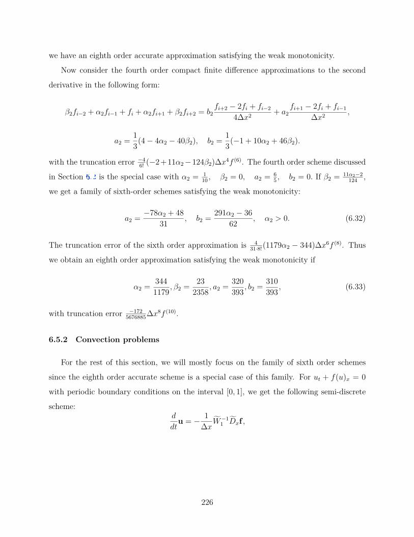
we have an eighth order accurate approximation satisfying the weak monotonicity.

Now consider the fourth order compact finite difference approximations to the second

derivative in the following form:

β2fi−2 + α2fi−1 + fi + α2fi+1 + β2fi+2 = b2fi+2 − 2fi + fi−2

4∆x2 + a2fi+1 − 2fi + fi−1

∆x2 ,

a2 = 13(4− 4α2 − 40β2), b2 = 1

3(−1 + 10α2 + 46β2).

with the truncation error −46! (−2+11α2−124β2)∆x4f (6). The fourth order scheme discussed

in Section 6.2 is the special case with α2 = 110 , β2 = 0, a2 = 6

5 , b2 = 0. If β2 = 11α2−2124 ,

we get a family of sixth-order schemes satisfying the weak monotonicity:

a2 = −78α2 + 4831 , b2 = 291α2 − 36

62 , α2 > 0. (6.32)

The truncation error of the sixth order approximation is 431·8!(1179α2 − 344)∆x6f (8). Thus

we obtain an eighth order approximation satisfying the weak monotonicity if

α2 = 3441179 , β2 = 23

2358 , a2 = 320393 , b2 = 310

393 , (6.33)

with truncation error −1725676885∆x8f (10).

6.5.2 Convection problems

For the rest of this section, we will mostly focus on the family of sixth order schemes

since the eighth order accurate scheme is a special case of this family. For ut + f(u)x = 0

with periodic boundary conditions on the interval [0, 1], we get the following semi-discrete

scheme:d

dtu = − 1

∆xW−11 Dxf ,

226

W1u = β1

1 + 2α1 + 2β1

1β1

α1β1

1 1 α1β1

α1β1

1β1

α1β1

1 1

1 α1β1

1β1

α1β1

1. . . . . . . . . . . . . . .

1 α1β1

1β1

α1β1

1

1 1 α1β1

1β1

α1β1

α1β1

1 1 α1β1

1β1

u1

u2

u3...

uN−2

uN−1

uN

,

Dxf = 14(1 + 2α1 + 2β1)

0 2a1 b1 −b1 −2a1

−2a1 0 2a1 b1 −b1

−b1 −2a1 0 2a1 b1. . . . . . . . . . . . . . .

−b1 −2a1 0 2a1 b1

b1 −b1 −2a1 0 2a1

2a1 b1 −b1 −2a1 0

f1

f2

f3...

fN−2

fN−1

fN

,

where fi and ui are point values of functions f(u(x)) and u(x) at uniform grid points xi

(i = 1, · · · , N) respectively. We have a family of sixth-order compact schemes with forward

Euler time discretization:

un+1 = un − ∆t∆xW

−11 Dxf . (6.34)

Define u = W1u and λ = ∆t∆x

, then scheme (6.34 ) can be written as

un+1i = un

i −λ

4(1 + 2α1 + 2β1)(b1f

ni+2 + 2a1f

ni+1 − 2a1f

ni−1 − b1f

ni−2).

Following the lines in Section 6.2.1 , we can easily conclude that the scheme (6.34 ) satisfies

un+1i ∈ [m,M ] if un

i ∈ [m,M ], under the CFL constraint

∆t∆x |f(u)| ≤ min 9

8− 3α1,6(3α1 − 1)57α1 − 17 .

Given ui ∈ [m,M ], we also need a limiter to enforce ui ∈ [m,M ]. Notice that ui has

a five-point stencil instead of a three-point stencil in Section 6.2.2 . Thus in general the

227

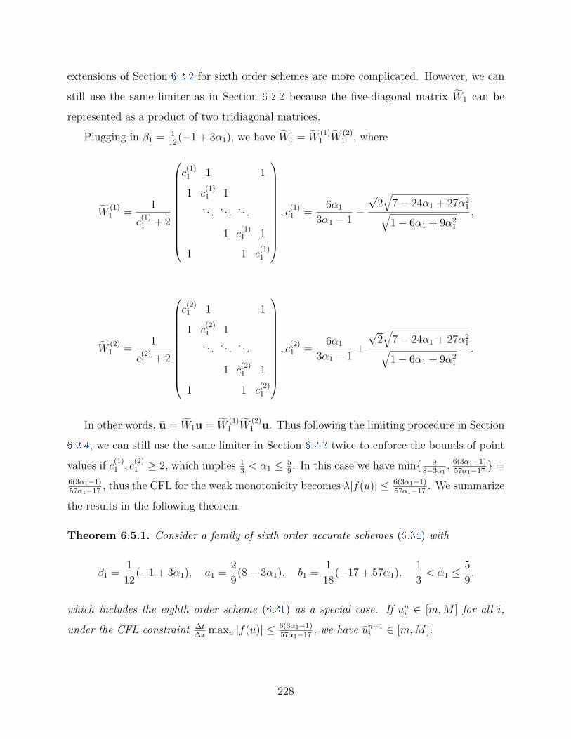
extensions of Section 6.2.2 for sixth order schemes are more complicated. However, we can

still use the same limiter as in Section 6.2.2 because the five-diagonal matrix W1 can be

represented as a product of two tridiagonal matrices.

Plugging in β1 = 112(−1 + 3α1), we have W1 = W

(1)1 W

(2)1 , where

W(1)1 = 1

c(1)1 + 2

c(1)1 1 1

1 c(1)1 1. . . . . . . . .

1 c(1)1 1

1 1 c(1)1

, c

(1)1 = 6α1

3α1 − 1 −√

2√

7− 24α1 + 27α21√

1− 6α1 + 9α21

,

W(2)1 = 1

c(2)1 + 2

c(2)1 1 1

1 c(2)1 1. . . . . . . . .

1 c(2)1 1

1 1 c(2)1

, c

(2)1 = 6α1

3α1 − 1 +√

2√

7− 24α1 + 27α21√

1− 6α1 + 9α21

.

In other words, u = W1u = W(1)1 W

(2)1 u. Thus following the limiting procedure in Section

6.2.4 , we can still use the same limiter in Section 6.2.2 twice to enforce the bounds of point

values if c(1)1 , c

(2)1 ≥ 2, which implies 1

3 < α1 ≤ 59 . In this case we have min 9

8−3α1, 6(3α1−1)

57α1−17 =6(3α1−1)57α1−17 , thus the CFL for the weak monotonicity becomes λ|f(u)| ≤ 6(3α1−1)

57α1−17 . We summarize

the results in the following theorem.

Theorem 6.5.1. Consider a family of sixth order accurate schemes (6.34 ) with

β1 = 112(−1 + 3α1), a1 = 2

9(8− 3α1), b1 = 118(−17 + 57α1),

13 < α1 ≤

59 ,

which includes the eighth order scheme (6.31 ) as a special case. If uni ∈ [m,M ] for all i,

under the CFL constraint ∆t∆x

maxu |f(u)| ≤ 6(3α1−1)57α1−17 , we have un+1

i ∈ [m,M ].

228

Given point values ui satisfying W(1)1 W

(2)1 ui = W1ui = ui ∈ [m,M ] for any i, we can

apply the limiter in Algorithm 2 twice to enforce ui ∈ [m,M ]:

1. Given ui ∈ [m,M ], compute vi = [W (1)1 ]−1ui which are not necessarily in the range

[m,M ]. Then apply the limiter in Algorithm 2 to vi, i = 1, · · · , N . Let vi denote

the output of the limiter. Since we have ui = 1c

(1)1 +2

(vi−1 + c(1)1 vi + vi+1), c(1)

1 > 2, all

discussions in Section 6.2.2 are still valid, thus we have vi ∈ [m,M ].

2. Compute ui = [W (2)1 ]−1vi. Apply the limiter in Algorithm 2 to ui, i = 1, · · · , N . Since

we have vi = 1c

(2)1 +2

(ui−1 + c(2)1 ui + ui+1), c(2)

1 > 2, all discussions in Section 6.2.2 are

still valid, thus the output are in [m,M ].

6.5.3 Diffusion problems

For simplicity we only consider the diffusion problems and the extension to convection

diffusion problems can be easily discussed following Section 6.2.4 . For the one-dimensional

scalar diffusion equation ut = g(u)xx with g(u) ≥ 0 and periodic boundary conditions on an

interval [0, 1], we get the sixth order semi-discrete scheme: ddt

u = 1∆x2 W

−12 Dxxg, where

W2u = β2

1 + 2α2 + 2β2

1β2

α2β2

1 1 α2β2

α2β2

1β2

α2β2

1 1

1 α2β2

1β2

α2β2

1. . . . . . . . . . . . . . .

1 α2β2

1β2

α2β2

1

1 1 α2β2

1β2

α2β2

α2β2

1 1 α2β2

1β2

u1

u2

u3...

uN−2

uN−1

uN

,

229

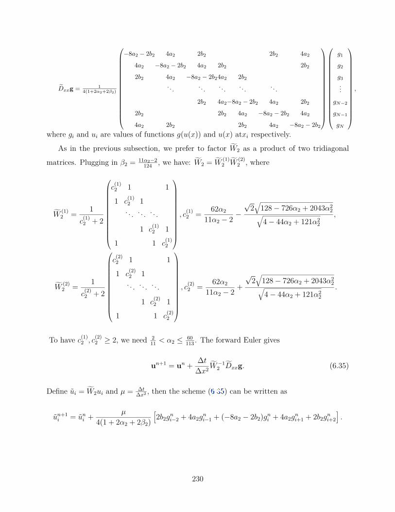
Dxxg = 14(1+2α2+2β2)

−8a2 − 2b2 4a2 2b2 2b2 4a2

4a2 −8a2 − 2b2 4a2 2b2 2b2

2b2 4a2 −8a2 − 2b24a2 2b2. . . . . . . . . . . . . . .

2b2 4a2−8a2 − 2b2 4a2 2b2

2b2 2b2 4a2 −8a2 − 2b2 4a2

4a2 2b2 2b2 4a2 −8a2 − 2b2

g1

g2

g3...

gN−2

gN−1

gN

,

where gi and ui are values of functions g(u(x)) and u(x) atxi respectively.

As in the previous subsection, we prefer to factor W2 as a product of two tridiagonal

matrices. Plugging in β2 = 11α2−2124 , we have: W2 = W

(1)2 W

(2)2 , where

W(1)2 = 1

c(1)2 + 2

c(1)2 1 1

1 c(1)2 1. . . . . . . . .

1 c(1)2 1

1 1 c(1)2

, c

(1)2 = 62α2

11α2 − 2 −√

2√

128− 726α2 + 2043α22√

4− 44α2 + 121α22

,

W(2)2 = 1

c(2)2 + 2

c(2)2 1 1

1 c(2)2 1. . . . . . . . .

1 c(2)2 1

1 1 c(2)2

, c

(2)2 = 62α2

11α2 − 2 +√

2√

128− 726α2 + 2043α22√

4− 44α2 + 121α22

.

To have c(1)2 , c

(2)2 ≥ 2, we need 2

11 < α2 ≤ 60113 . The forward Euler gives

un+1 = un + ∆t∆x2 W

−12 Dxxg. (6.35)

Define ui = W2ui and µ = ∆t∆x2 , then the scheme (6.35 ) can be written as

un+1i = un

i + µ

4(1 + 2α2 + 2β2)[2b2g

ni−2 + 4a2g

ni−1 + (−8a2 − 2b2)gn

i + 4a2gni+1 + 2b2g

ni+2

].

230

Theorem 6.5.2. Consider a family of sixth order accurate schemes (6.35 ) with

β2 = 11α2 − 2124 , a2 = −78α2 + 48

31 , b2 = 291α2 − 3662 ,

211 < α2 ≤

60113 ,

which includes the eighth order scheme (6.33 ) as a special case. If uni ∈ [m,M ] for all i,

under the CFL ∆t∆x2 g(u) < 124

3(116−111α2) , the scheme satisfies un+1 ∈ [m,M ].

As in the previous subsection, given point values ui satisfying W (1)2 W

(2)2 ui = W2ui = ui ∈

[m,M ] for any i, we can apply the limiter in Algorithm 2 twice to enforce ui ∈ [m,M ]. The

matrices W1 and W2 commute because they are both circulant matrices thus diagonalizable

by the discrete Fourier matrix. The discussion for the sixth order scheme solving convection

diffusion problems is also straightforward.

6.6 Extensions To General Boundary Conditions

Since the compact finite difference operator is implicitly defined thus any extension to

other type boundary conditions is not straightforward. In order to maintain the weak mono-

tonicity, the boundary conditions must be properly treated. In this section we demonstrate

a high order accurate boundary treatment preserving the weak monotonicity for inflow and

outflow boundary conditions. For convection problems, we can easily construct a fourth

order accurate boundary scheme. For convection diffusion problems, it is much more com-

plicated to achieve weak monotonicity near the boundary thus a straightforward discussion

gives us a third order accurate boundary scheme.

6.6.1 Inflow-outflow boundary conditions for convection problems

For simplicity, we consider the following initial boundary value problem on the interval

[0, 1] as an example: ut + f(u)x = 0, u(x, 0) = u0(x), u(0, t) = L(t), where we assume

f(u) > 0 so that the inflow boundary condition at the left cell end is a well-posed boundary

condition. The boundary condition at x = 1 is not specified thus understood as an outflow

boundary condition. We further assume u0(x) ∈ [m,M ] and L(t) ∈ [m,M ] so that the exact

solution is in [m,M ].

231

Consider a uniform grid with xi = i∆x for i = 0, 1, · · · , N,N + 1 and ∆x = 1N+1 . Then

a fourth order semi-discrete compact finite difference scheme is given by

d

dt

16

1 4 1

. . . . . . . . .

1 4 1

u0...

uN+1

= 12∆x

−1 0 1

. . . . . . . . .

−1 0 1

f0...

fN+1

.

With forward Euler time discretization, the scheme is equivalent to

un+1i = un

i −12λ(fn

i+1 − fni−1), i = 1, · · · , N. (6.36)

Here un0 = L(tn) is given as boundary condition for any n. Given un

i for i = 0, 1, · · · , N + 1,

the scheme (6.36 ) gives un+1i for i = 1, · · · , N , from which we still need un+1

N+1 to recover

interior point values un+1i for i = 1, · · · , N .

Since the boundary condition at xN+1 = 1 can be implemented as outflow, we can

use un+1i for i = 1, · · · , N to obtain a reconstructed un+1

N+1. If there is a cubic polynomial

pi(x) so that ui−1, ui, ui+1 are its point values at xi−1, xi, xi+1, then 12∆x

∫ xi+1xi−1

pi(x) dx =16ui−1 + 4

6ui + 16ui+1 = ui, due to the exactness of the Simpson’s quadrature rule for cubic

polynomials. To this end, we can consider a unique cubic polynomial p(x) satisfying four

equations: 12∆x

∫ xj+1xj−1

p(x) dx = un+1j , j = N − 3, N − 2, N − 1, N. If un+1

j are fourth order

accurate approximations to 16u(xj−1, t

n+1)+ 46u(xj, t

n+1)+ 16u(xj+1, t

n+1), then p(x) is a fourth

order accurate approximation to u(x, tn+1) on the interval [xN−4, xN+1]. So we get a fourth

order accurate un+1N+1 by

p(xN+1) = −23 uN−3 + 17

6 uN−2 −143 uN−1 + 7

2 uN . (6.37)

Since (6.37 ) is not a convex linear combination, p(xN+1) may not lie in the bound [m,M ].

Thus to ensure un+1N+1 ∈ [m,M ] we can define

un+1N+1 := maxminp(xN+1),M,m. (6.38)

232

Obviously Theorem 6.2.1 still holds for the scheme (6.36 ). For the forward Euler time

discretization, we can implement the bound-preserving scheme as follows:

1. Given uni for all i, compute un+1

i for i = 1, · · · , N by (6.36 ).

2. Obtain boundary values un+10 = L(tn+1) and un+1

N+1 by (6.37 ) and (6.38 ).

3. Given un+1i for i = 1, · · · , N and two boundary values un+1

0 and un+1N+1, recover point

values un+1i for i = 1, · · · , N by solving the tridiagonal linear system (the superscript

n+ 1 is omitted):

16

4 1

1 4 1. . . . . . . . .

1 4 1

1 4

u1

u2...

uN−1

uN

=

u1 − 16u0

u2...

uN−1

uN − 16uN+1

.

4. Apply the limiter in Algorithm 2 to the point values un+1i for i = 1, · · · , N .

6.6.2 Dirichlet boundary conditions for one-dimensional convection diffusionequations

Consider the initial boundary value problem for a one-dimensional scalar convection

diffusion equation on the interval [0, 1]:

ut + f(u)x = g(u)xx, u(x, t) = u0(x), u(0, t) = L(t), u(1, t) = R(t), (6.39)

where g(u) ≥ 0. We further assume u0(x) ∈ [m,M ] and L(t), R(t) ∈ [m,M ] so that the

exact solution is in [m,M ].

We demonstrate how to treat the boundary approximations so that the scheme still

satisfies some weak monotonicity such that a certain convex combination of point values

is in the range [m,M ] at the next time step. Consider a uniform grid with xi = i∆x

233

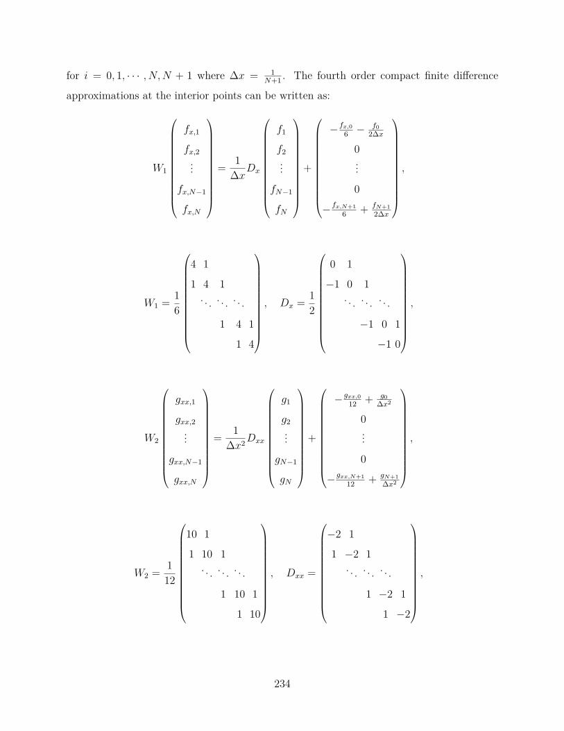
for i = 0, 1, · · · , N,N + 1 where ∆x = 1N+1 . The fourth order compact finite difference

approximations at the interior points can be written as:

W1

fx,1

fx,2...

fx,N−1

fx,N

= 1

∆xDx

f1

f2...

fN−1

fN

+

−fx,06 −

f02∆x

0...

0

−fx,N+16 + fN+1

2∆x

,

W1 = 16

4 1

1 4 1. . . . . . . . .

1 4 1

1 4

, Dx = 1

2

0 1

−1 0 1. . . . . . . . .

−1 0 1

−1 0

,

W2

gxx,1

gxx,2...

gxx,N−1

gxx,N

= 1

∆x2Dxx

g1

g2...

gN−1

gN

+

−gxx,012 + g0

∆x2

0...

0

−gxx,N+112 + gN+1

∆x2

,

W2 = 112

10 1

1 10 1. . . . . . . . .

1 10 1

1 10

, Dxx =

−2 1

1 −2 1. . . . . . . . .

1 −2 1

1 −2

,

234

where fx,i and gxx,i denotes the values of f(u)x and g(u)xx at xi respectively. Let

F =

−fx,06 −

f02∆x

0...

0

−fx,N+16 + fN+1

2∆x

, G =

−gxx,012 + g0

∆x2

0...

0

−gxx,N+112 + gN+1

∆x2

.

Define W := W1W2 = W2W1. Here W2 and W1 commute because they have the same

eigenvectors, which is due to the fact that 2W2 − W1 is the identity matrix. Let u =(u1 u2 · · · uN

)T

, f =(f(u1) f(u2) · · · f(uN)

)T

and g =(g(u1) g(u2) · · · g(uN)

)T

. Then

a fourth order compact finite difference approximation to (6.39 ) at the interior grid points

is ddt

u +W−11 ( 1

∆xDxf + F ) = W−1

2 ( 1∆x2Dxxg +G) which is equivalent to

d

dt(Wu) + 1

∆xW2Dxf − 1∆x2W1Dxxg = −W2F +W1G.

If ui(t) = u(xi, t) where u(x, t) is the exact solution to the problem, then it satisfies

ut,i + fx,i = gxx,i, (6.40)

where ut,i = ddtui(t), fx,i = f(ui)x and gxx,i = g(ui)xx. If we use (6.40 ) to simplify −W2F +

W1G, then the scheme is still fourth order accurate. In other words, setting −fx,i+gxx,i = ut,i

235

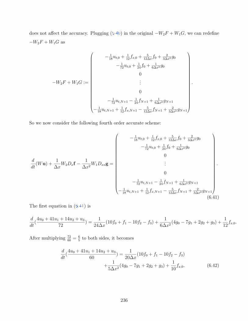
does not affect the accuracy. Plugging (6.40 ) in the original −W2F +W1G, we can redefine

−W2F +W1G as

−W2F +W1G :=

− 118ut,0 + 1

12fx,0 + 512∆x

f0 + 23∆x2 g0

− 172ut,0 + 1

24f0 + 16∆x2 g0

0...

0

− 172ut,N+1 − 1

24fN+1 + 16∆x2 gN+1

− 118ut,N+1 + 1

12fx,N+1 − 512∆x

fN+1 + 23∆x2 gN+1

.

So we now consider the following fourth order accurate scheme:

d

dt(Wu) + 1

∆xW2Dxf − 1∆x2W1Dxxg =

− 118ut,0 + 1

12fx,0 + 512∆x

f0 + 23∆x2 g0

− 172ut,0 + 1

24f0 + 16∆x2 g0

0...

0

− 172ut,N+1 − 1

24fN+1 + 16∆x2 gN+1

− 118ut,N+1 + 1

12fx,N+1 − 512∆x

fN+1 + 23∆x2 gN+1

.

(6.41)

The first equation in (6.41 ) is

d

dt(4u0 + 41u1 + 14u2 + u3

72 ) = 124∆x(10f0 + f1 − 10f2 − f3) + 1

6∆x2 (4g0 − 7g1 + 2g2 + g3) + 112fx,0.

After multiplying 7260 = 6

5 to both sides, it becomes

d

dt(4u0 + 41u1 + 14u2 + u3

60 ) = 120∆x(10f0 + f1 − 10f2 − f3)

+ 15∆x2 (4g0 − 7g1 + 2g2 + g3) + 1

10fx,0. (6.42)

236

In order for the scheme (6.42 ) to satisfy a weak monotonicity in the sense that 4un+10 +41un+1

1 +14un+12 +un+1

360

in (6.42 ) with forward Euler can be written as a monotonically increasing function of uni

under some CFL constraint, we still need to find an approximation to f(u)x,0 using only

u0, u1, u2, u3, with which we have a straightforward third order approximation to f(u)x,0:

fx,0 = 1∆x(−11

6 f0 + 3f1 −32f2 + 1

3f3) +O(∆x3). (6.43)

Then (6.42 ) becomes

d

dt(4u0 + 41u1 + 14u2 + u3

60 ) = 160∆x(19f0 + 21f1 − 39f2 − f3)

+ 15∆x2 (4g0 − 7g1 + 2g2 + g3). (6.44)

The second to second last equations of (6.41 ) can be written as

d

dt(ui−2 + 14ui−1 + 42ui + 14ui+1 + ui+2

72 ) = 124∆x(fi−2 + 10fi−1 (6.45)

−10fi+1 − fi+2) + 16∆x2 (gi−2 + 2gi−1 − 6gi + 2gi+1 + gi+2), 2 ≤ i ≤ N − 1,

which satisfies a straightforward weak monotonicity under some CFL constraint.

The last equation in (6.41 ) is

d

dt(4uN+1 + 41uN + 14uN−1 + uN−2

72 ) = 124∆x(fN−2 + 10fN−1 − fN

−10fN+1) + 16∆x2 (gN−2 + 2gN−1 − 7gN + 4gN+1) + 1

12fx,N+1.

After multiplying 7260 = 6

5 to both sides, it becomes

d

dt(uN−2 + 14uN−1 + 41uN + 4uN+1

60 ) = 120∆x(fN−2 + 10fN−1 − fN

−10fN+1) + 15∆x2 (gN−2 + 2gN−1 − 7gN + 4gN+1) + 1

10fx,N+1.

237

Similar to the boundary scheme at x0, we should use a third-order approximation:

fx,N+1 = 1∆x(−1

3fN−2 + 32fN−1 − 3fN + 11

6 fN+1) +O(∆x3). (6.46)

Then the boundary scheme at xN+1 becomes

d

dt(uN−2 + 14uN−1 + 41uN + 4uN+1

60 ) = 160∆x(fN−2 + 39fN−1 − 21fN

−19fN+1) + 15∆x2 (gN−2 + 2gN−1 − 7gN + 4gN+1). (6.47)

To summarize the full semi-discrete scheme, we can represent the third order scheme

(6.44 ), (6.45 ) and (6.47 ), for the Dirichlet boundary conditions as:

d

dtW u = − 1

∆xDxf(u) + 1∆x2 Dxxg(u),

where

W = 172

245

2465

845

65

1 14 42 14 1. . . . . . . . . . . . . . .

1 14 42 14 165

845

2465

245

N×(N+2)

, u =

u0

u1...

uN

uN+1

(N+2)×1

,

Dx = 124

−385 −

425

785

25

−1 −10 0 10 1. . . . . . . . . . . . . . .

−1 −10 0 10 1

−25 −

785

425

385

N×(N+2)

, Dxx = 16

245 −

425

125

65

1 2 −6 2 1. . . . . . . . . . . . . . .

1 2 −6 2 165

125 −

425

245

N×(N+2)

.

238

Let u = W u, λ = ∆t∆x

and µ = ∆t∆x2 . With forward Euler, it becomes

un+1i = un

i −12λDxfi + µDxxgi, i = 1, · · · , N. (6.48)

We state the weak monotonicity without proof.


maxu |f(u)| ≤ 419 ,

∆t∆x2 maxu g(u) ≤ 695

1596 , if

uni ∈ [m,M ], then the scheme (6.48 ) satisfies un+1

i ∈ [m,M ].

We notice that

un+11 = 1

60(4un+10 + 41un+1

1 + 14un+12 + un+1

3 )

= un+10 +4un+1

1 +un+12

6 + 110

un+11 +4un+1

2 +un+13

6 − 110u

n+10 ,

un+1N = 1

60(un+1N−2 + 14un+1

N−1 + 41un+1N + 4un+1

N+1)

= 110

un+1N−2+4un+1

N−1+un+1N

6 + un+1N−1+4un+1

N +un+1N+1

6 − 110u

n+1N+1.

Recall that the boundary values are given: un+10 = L(tn+1) ∈ [m,M ] and un+1

N+1 = R(tn+1) ∈

[m,M ], so we have

1011un+1

0 + 4un+11 + un+1

26 + 1

11un+1

1 + 4un+12 + un+1

36 ≤ 10

11M + 111M = M,

1011un+1

0 + 4un+11 + un+1

26 + 1

11un+1

1 + 4un+12 + un+1

36 ≥ 10

11m+ 111m = m,

111un+1

N−2 + 4un+1N−1 + un+1

N

6 + 1011un+1

N−1 + 4un+1N + un+1

N+16 ≤ 10

11M + 111M = M,

111un+1

N−2 + 4un+1N−1 + un+1

N

6 + 1011un+1

N−1 + 4un+1N + un+1

N+16 ≥ 10

11m+ 111m = m.

Thus define wn+1 =(wn+1

1 , wn+12 , wn+1

3 , . . . , wn+1N−1, w

n+1N

)T

as follows and we have:

m ≤ wn+1i : = un+1

i ≤M, i = 2, · · · , N − 1,

m ≤ wn+11 : = 10

11un+1

0 + 4un+11 + un+1

26 + 1

11un+1

1 + 4un+12 + un+1

36 ≤M,

m ≤ wn+1N : = 1

11un+1

N−3 + 4un+1N−2 + un+1

N−16 + 10

11un+1

N−2 + 4un+1N−1 + un+1

N

6 ≤M.

239

By the notations above, we get

wn+1 = Kun+1 + un+1bc = ˜

W u, (6.49)

K =

1011

1. . .

11011

N×N

,ubc = 111

u0

0...

0

uN+1

N×1

,˜W = 1

72

12011

49211

16811

1211

1 14 42 14 1. . . . . . . . . . . . . . .

1 14 42 14 11211

16811

49211

12011

N×(N+2)

.

We notice that ˜W can be factored as a product of two tridiagonal matrices:

172

12011

49211

16811

1211

1 14 42 14 1. . . . . . . . . . . . . . .

1 14 42 14 11211

16811

49211

12011

= 1

12

12011

1211

1 10 1. . . . . . . . .

1 10 11211

12011

N×N

16

1 4 1

1 4 1. . . . . . . . .

1 4 1

1 4 1

N×(N+2)

,

which can be denoted as ˜W = W2W1. Fortunately, all the diagonal entries of W1 and W2

are in the form of cc+2 , c > 2. So given ui = Wui ∈ [m,M ], we construct wn+1

i ∈ [m,M ]. We

can apply the limiter in Algorithm 2 twice to enforce ui ∈ [m,M ]:

1. Given uni for all i, use the scheme (6.48 ) to obtain un+1

i ∈ [m,M ] for i = 1, · · · , N .

Then construct wn+1i ∈ [m,M ] for i = 1, · · · , N by (6.49 ).

240

2. Notice that W2 is a matrix of size N ×N . Compute v = W−12 wn+1. Apply the limiter

in Algorithm 2 to vi and let vi denote the output values. Since we have W2vi ∈ [m,M ],

i.e.,

m ≤ 1011v1 + 1

11v2 ≤M,

m ≤ 112v1 + 10

12v2 + 112v3 ≤M,

...

m ≤ 112vN−2 + 10

12vN−1 + 112vN ≤M,

m ≤ 111vN−1 + 10

11vN ≤M.

Following the discussions in Section 6.2.2 , it implies vi ∈ [m,M ].

3. Obtain values of un+1i , i = 1, · · · , N by solving a N ×N system:

16

4 1

1 4 1. . . . . . . . .

1 4 1

1 4

un+11

un+12...

un+1N−1

un+1N

=

v1

v2...

vN−1

vN

− 1

6un+1bc .

4. Apply the limiter in Algorithm 2 to un+1i to ensure un+1

i ∈ [m,M ].

6.7 Numerical Tests

6.7.1 One-dimensional problems with periodic boundary conditions

In this subsection, we test the fourth order and eighth order accurate compact finite

difference schemes with the bound-preserving limiter. The time step is taken to satisfy both

the CFL condition required for weak monotonicity in Theorem 6.2.1 and Theorem 6.2.10

and the SSP coefficient for high order SSP time discretizations.

Example 1. One-dimensional linear convection equation. Consider ut + ux = 0 with and

initial condition u0(x) = 12 + sin4(x) and periodic boundary conditions on the interval [0, 2π]

241

with a uniform N -point grid. The L1 and L∞ errors for the fourth order scheme with a

smooth initial condition at time T = 10 are listed in Table 6.1 where ∆x = 2πN

, the time

step is taken as ∆t = Cms13∆x for the multistep method, and ∆t = 5Cms

13∆x for the Runge-

Kutta method so that the number of spatial discretization operators computed is the same

as in the one for the multistep method. We can observe the fourth order accuracy for the

multistep method and obvious order reductions for the Runge-Kutta method.

The errors for smooth initial conditions u0(x) = 12 + 1

2 sin4(x) at time T = 10 for the

eighth order accurate scheme are listed in Table 6.2 . For the eighth order accurate scheme,

the time step to achieve the weak monotonicity is ∆t = Cms625∆x for the fourth-order SSP

multistep method. On the other hand, we need to set ∆t = ∆x2 in fourth order accurate

time discretizations to verify the eighth order spatial accuracy. To this end, the time step

is taken as ∆t = Cms625∆x2 for the multistep method, and ∆t = 5Cms

625∆x2 for the Runge-

Kutta method. We can observe the eighth order accuracy for the multistep method and the

order reduction for N = 160 is due to the roundoff errors. We can also see an obvious order

reduction for the Runge-Kutta method.

Table 6.1. Fourth order scheme accuracy test.Fourth order SSP multistep Fourth order SSP Runge-Kutta

N L1 error order L∞ error order L1 error order L∞ error order20 3.44E-2 - 6.49E-2 - 3.41E-2 - 6.26E-2 -40 3.12E-3 3.47 6.19E-3 3.39 3.14E-3 3.44 6.62E-3 3.2480 1.82E-4 4.10 2.95E-4 4.39 1.86E-4 4.08 3.82E-4 4.11160 1.10E-5 4.05 1.85E-5 4.00 1.29E-5 3.85 4.48E-5 3.09320 6.81E-7 4.02 1.15E-6 4.01 1.42E-6 3.18 1.03E-5 2.13

Table 6.2. Eighth order scheme accuracy test.Fourth order SSP multistep Fourth order SSP Runge-Kutta

N L1 error order L∞ error order L1 error order L∞ error order10 6.31E-2 - 1.01E-1 - 6.44E-2 - 9.58E-2 -20 3.35E-5 7.55 5.59E-4 7.49 3.39E-4 7.57 5.79E-4 7.3740 9.58E-7 8.45 1.49E-6 8.55 1.52E-6 7.80 4.32E-6 7.0680 3.50E-9 8.10 5.51E-9 8.08 5.34E-8 4.83 2.31E-7 4.23160 6.57E-11 5.74 1.01E-10 5.77 2.40E-9 4.48 1.45E-8 3.99

242

Next, we consider the following discontinuous initial data:

u0(x) =

1, if 0 < x ≤ π,

0, if π < x ≤ 2π.(6.50)

See Figure 6.1 for the performance of the bound-preserving limiter and the TVB limiter on

the fourth order scheme at T = 10. Fourth order compact finite difference and fourth order

SSP multistep with ∆t = 13Cms∆x and 100 grid points are used. The TVB parameter in

(6.11 ) is p = 5. We observe that the TVB limiter can reduce oscillations but cannot remove

the overshoot/undershoot. When both limiters are used, we can obtain a non-oscillatory

bound-preserving numerical solution. See Figure 6.2 for the performance of the bound-

preserving limiter on the eighth order scheme at T = 10 with ∆t = Cms625∆x and 100 grid

points.

0 1 2 3 4 5 6

-0.2

0

0.2

0.4

0.6

0.8

1

1.2 Numerical

Exact

(a) Without any limiter.0 1 2 3 4 5 6

-0.2

0

0.2

0.4

0.6

0.8

1

1.2 Numerical

Exact

(b) With only the bound-preserving limiter.

0 1 2 3 4 5 6

-0.2

0

0.2

0.4

0.6

0.8

1

1.2 Numerical

Exact

(c) With only the TVB limiter.0 1 2 3 4 5 6

-0.2

0

0.2

0.4

0.6

0.8

1

1.2 Numerical

Exact

(d) With both limiters.

Figure 6.1. Fourth order scheme for linear convection with discontinuous initial data.

Example 2. One dimensional Burgers’ equation. Consider the Burgers’ equation ut +(u2

2 )x =

0 with a periodic boundary condition on [−π, π]. For the initial data u0(x) = sin(x) + 0.5,

243

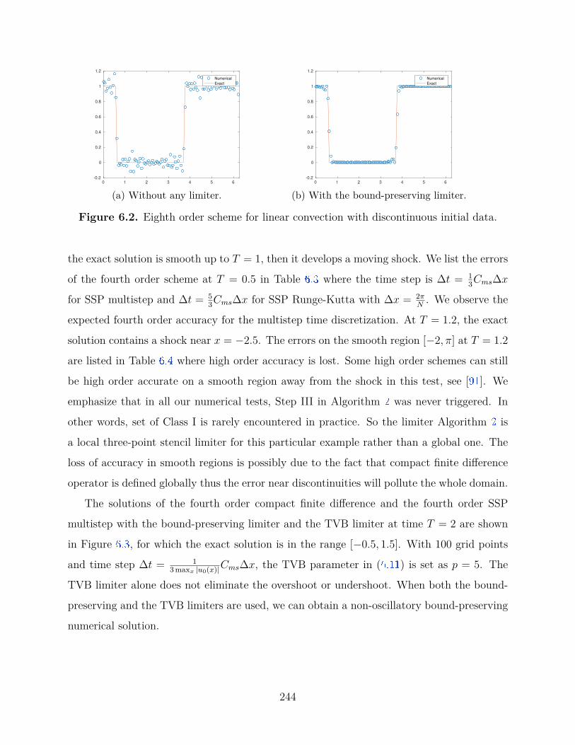
0 1 2 3 4 5 6

-0.2

0

0.2

0.4

0.6

0.8

1

1.2

Numerical

Exact


-0.2

0

0.2

0.4

0.6

0.8

1

1.2

Numerical

Exact

(b) With the bound-preserving limiter.

Figure 6.2. Eighth order scheme for linear convection with discontinuous initial data.

the exact solution is smooth up to T = 1, then it develops a moving shock. We list the errors

of the fourth order scheme at T = 0.5 in Table 6.3 where the time step is ∆t = 13Cms∆x

for SSP multistep and ∆t = 53Cms∆x for SSP Runge-Kutta with ∆x = 2π

N. We observe the

expected fourth order accuracy for the multistep time discretization. At T = 1.2, the exact

solution contains a shock near x = −2.5. The errors on the smooth region [−2, π] at T = 1.2

are listed in Table 6.4 where high order accuracy is lost. Some high order schemes can still

be high order accurate on a smooth region away from the shock in this test, see [91 ]. We

emphasize that in all our numerical tests, Step III in Algorithm 2 was never triggered. In

other words, set of Class I is rarely encountered in practice. So the limiter Algorithm 2 is

a local three-point stencil limiter for this particular example rather than a global one. The

loss of accuracy in smooth regions is possibly due to the fact that compact finite difference

operator is defined globally thus the error near discontinuities will pollute the whole domain.

The solutions of the fourth order compact finite difference and the fourth order SSP

multistep with the bound-preserving limiter and the TVB limiter at time T = 2 are shown

in Figure 6.3 , for which the exact solution is in the range [−0.5, 1.5]. With 100 grid points

and time step ∆t = 13 maxx |u0(x)|Cms∆x, the TVB parameter in (6.11 ) is set as p = 5. The

TVB limiter alone does not eliminate the overshoot or undershoot. When both the bound-

preserving and the TVB limiters are used, we can obtain a non-oscillatory bound-preserving

numerical solution.

244

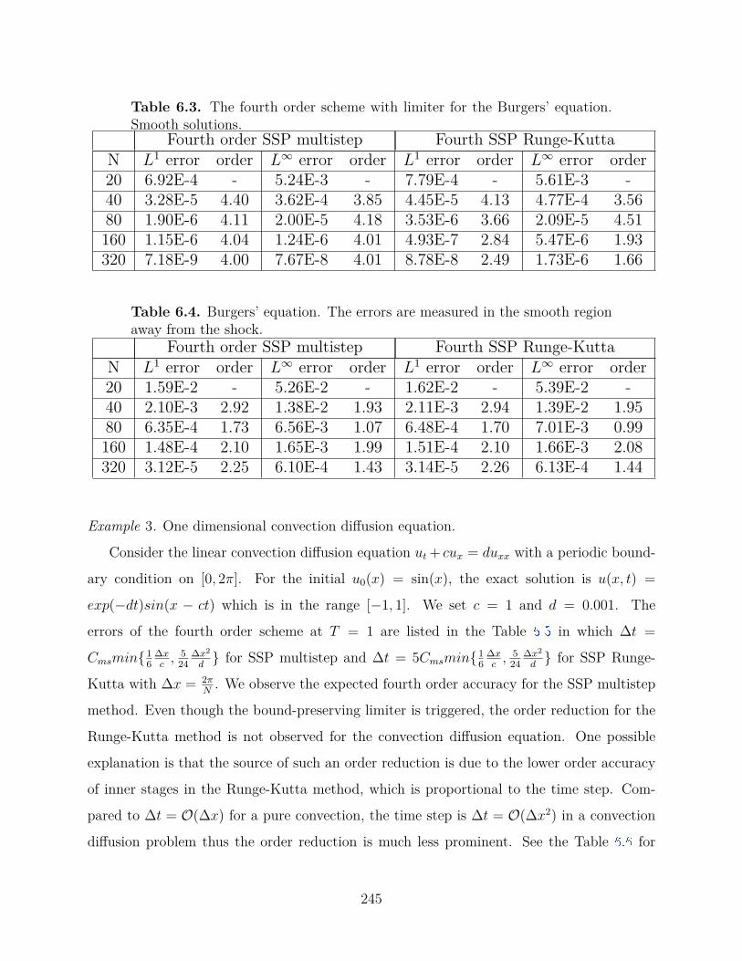
Table 6.3. The fourth order scheme with limiter for the Burgers’ equation.Smooth solutions.

Fourth order SSP multistep Fourth SSP Runge-KuttaN L1 error order L∞ error order L1 error order L∞ error order20 6.92E-4 - 5.24E-3 - 7.79E-4 - 5.61E-3 -40 3.28E-5 4.40 3.62E-4 3.85 4.45E-5 4.13 4.77E-4 3.5680 1.90E-6 4.11 2.00E-5 4.18 3.53E-6 3.66 2.09E-5 4.51160 1.15E-6 4.04 1.24E-6 4.01 4.93E-7 2.84 5.47E-6 1.93320 7.18E-9 4.00 7.67E-8 4.01 8.78E-8 2.49 1.73E-6 1.66

Table 6.4. Burgers’ equation. The errors are measured in the smooth regionaway from the shock.

Fourth order SSP multistep Fourth SSP Runge-KuttaN L1 error order L∞ error order L1 error order L∞ error order20 1.59E-2 - 5.26E-2 - 1.62E-2 - 5.39E-2 -40 2.10E-3 2.92 1.38E-2 1.93 2.11E-3 2.94 1.39E-2 1.9580 6.35E-4 1.73 6.56E-3 1.07 6.48E-4 1.70 7.01E-3 0.99160 1.48E-4 2.10 1.65E-3 1.99 1.51E-4 2.10 1.66E-3 2.08320 3.12E-5 2.25 6.10E-4 1.43 3.14E-5 2.26 6.13E-4 1.44

Example 3. One dimensional convection diffusion equation.

Consider the linear convection diffusion equation ut + cux = duxx with a periodic bound-

ary condition on [0, 2π]. For the initial u0(x) = sin(x), the exact solution is u(x, t) =

exp(−dt)sin(x − ct) which is in the range [−1, 1]. We set c = 1 and d = 0.001. The

errors of the fourth order scheme at T = 1 are listed in the Table 6.5 in which ∆t =

Cmsmin16

∆xc, 5

24∆x2

d for SSP multistep and ∆t = 5Cmsmin1

6∆xc, 5

24∆x2

d for SSP Runge-

Kutta with ∆x = 2πN

. We observe the expected fourth order accuracy for the SSP multistep

method. Even though the bound-preserving limiter is triggered, the order reduction for the

Runge-Kutta method is not observed for the convection diffusion equation. One possible

explanation is that the source of such an order reduction is due to the lower order accuracy

of inner stages in the Runge-Kutta method, which is proportional to the time step. Com-

pared to ∆t = O(∆x) for a pure convection, the time step is ∆t = O(∆x2) in a convection

diffusion problem thus the order reduction is much less prominent. See the Table 6.6 for

245

-3 -2 -1 0 1 2 3

-1

-0.5

0

0.5

1

1.5

2

Numerical

Exact

(a) Without any limiter.-3 -2 -1 0 1 2 3

-1

-0.5

0

0.5

1

1.5

2

Numerical

Exact

(b) With both limiters.

Figure 6.3. Burgers’ equation at T = 2.

the errors at T = 1 of the eighth order scheme with ∆t = Cms min 325

∆x2

c, 131

530∆x2

d for SSP

multistep and ∆t = 5Cms min 325

∆x2

c, 131

530∆x2

d for SSP Runge-Kutta where ∆x = 2π

N.

Table 6.5. The fourth order compact finite difference with limiter for linearconvection diffusion.

Fourth order SSP multistep Fourth order SSP Runge-KuttaN L1 error order L∞ error order L1 error order L∞ error order20 3.30E-5 - 5.19E-5 - 3.60E-5 - 6.09E-5 -40 2.11E-6 3.97 3.30E-6 3.97 2.44E-6 4.00 3.52E-6 4.1280 1.33E-7 3.99 2.09E-7 3.98 1.37E-7 4.04 2.15E-7 4.03160 8.36E-9 3.99 1.31E-8 3.99 8.46E-9 4.02 1.33E-8 4.02320 5.24E-10 4.00 8.23E-10 4.00 5.29E-10 4.00 8.31E-10 4.00

Example 4. Nonlinear degenerate diffusion equations.

A representative test for validating the positivity-preserving property of a scheme solving

nonlinear diffusion equations is the porous medium equation, ut = (um)xx,m > 1. We

consider the Barenblatt analytical solution given by

Bm(x, t) = t−k[(1− k(m− 1)2m

|x|2

t2k)+]1/(m−1),

where u+ = maxu, 0 and k = (m + 1)−1. The initial data is the Barenblatt solution

at T = 1 with periodic boundary conditions on [6, 6]. The solution is computed till time

T = 2. High order schemes without any particular positivity treatment will generate negative

solutions [102 ], [103 ], [106 ]. See Figure 6.4 for solutions of the fourth order scheme and the

246

Table 6.6. The eighth order compact finite difference with limiter for linearconvection diffusion.

SSP multistep SSP Runge-KuttaN L1 error order L∞ error order L1 error order L∞ error order10 3.85E-7 - 5.96E-7 - 3.85E-7 - 5.95E-7 -20 1.40E-9 8.10 2.20E-9 8.08 1.42E-9 8.08 2.23E-9 8.0640 5.46E-12 8.01 8.60E-12 8.00 5.48E-12 8.02 8.69E-12 8.0180 3.53E-12 0.63 6.46E-12 0.41 1.06E-12 2.37 3.29E-12 1.40

SSP multistep method with ∆t = 13mCms∆x and 100 grid points. Numerical solutions are

strictly nonnegative. Without the bound-preserving limiter, negative values emerge near the

sharp gradients.

-6 -4 -2 0 2 4 6

0

0.2

0.4

0.6

0.8

1

1.2 4th order Compact FD with limiter

Exact solution of ut=(u 5)

xx

(a) m = 5.

-6 -4 -2 0 2 4 6

0

0.2

0.4

0.6

0.8

1

1.2 4th order Compact FD with limiter

Exact solution of ut=(u 8)

xx

(b) m = 8.

Figure 6.4. The fourth order compact finite difference with limiter for theporous medium equation.

6.7.2 One-dimensional problems with non-periodic boundary conditions

Example 5. One-dimensional Burgers’ equation with inflow-outflow boundary condition.

Consider ut + (u2

2 )x = 0 on interval [0, 2π] with inflow-outflow boundary condition and

smooth initial condition u(x, 0) = u0(x). Let u0(x) = 12 sin(x) + 1

2 ≥ 0, we can set the left

boundary condition as inflow u(0, t) = L(t) and right boundary as outflow, where L(t) is

obtained from the exact solution of initial-boundary value problem for the same initial data

and a periodic boundary condition. We test the fourth order compact finite difference and

fourth order SSP multistep method with the bound-preserving limiter. The errors at T = 0.5

247

are listed in Table 6.7 where ∆t = Cms∆x and ∆x = 2πN

. See Figure 6.5 for the shock at

T = 3 on a 120-point grid with ∆t = Cms∆x.

Table 6.7. Burgers’ equation. The fourth order scheme. Inflow and outflowboundary conditions.

N L∞ error order L1 error order20 1.15E-4 - 7.80E-4 -40 4.10E-6 4.81 2.00E-5 5.2980 2.17E-7 4.24 9.43E-7 4.40160 1.22E-8 4.15 4.87E-8 4.28320 7.41E-10 4.05 2.87E-9 4.09

0 1 2 3 4 5 6

-0.2

0

0.2

0.4

0.6

0.8

1

1.2

1.4


-0.2

0

0.2

0.4

0.6

0.8

1

1.2

1.4


Figure 6.5. Burgers’ equation. The fourth order scheme. Inflow and outflowboundary conditions.

Example 6. One-dimensional convection diffusion equation with Dirichlet boundary condi-

tions. We consider equation ut + cux = duxx on [0, 2π] with boundary conditions u(0, t) =

cos(−ct)e−dt and u(2π, t) = cos(2π−ct)e−dt. The exact solution is u(x, y, t) = cos(x−ct)e−dt.

We set c = 1 and d = 0.01. We test the third order boundary scheme proposed in

Section 6.6.2 and the fourth order interior compact finite difference with the fourth or-

der SSP multistep time discretization. The errors at T = 1 are listed in Table 6.8 where

∆t = Cms min 419

∆xc, 695

1596∆x2

d, ∆x = 2π

N.

248

Table 6.8. A linear convection diffusion equation with Dirichlet boundary conditions.N L∞ error order L1 error order10 1.68E-3 - 8.76E-3 -20 1.47E-4 3.51 7.12E-4 3.6240 8.35E-6 4.14 4.27E-5 4.0680 4.44E-7 4.23 2.28E-6 4.23160 2.30E-8 4.27 1.10E-7 4.37

6.7.3 Two-dimensional problems with periodic boundary conditions

In this subsection we test the fourth order compact finite difference scheme solving two-

dimensional problems with periodic boundary conditions.

Example 7. Two-dimensional linear convection equation. Consider ut + ux + uy = 0 on the

domain [0, 2π] × [0, 2π] with a periodic boundary condition. The scheme is tested with a

smooth initial condition u0(x, y) = 12 + 1

2 sin4(x + y) to verify the accuracy. The errors at

time T = 1 are listed in Table 6.9 where ∆t = Cms16∆x for the SSP multistep method and

∆t = 5Cms16∆x for the SSP Runge-Kutta method with ∆x = ∆y = 2π

N. We can observe

the fourth order accuracy for the multistep method on resolved meshes and obvious order

reductions for the Runge-Kutta method.

Table 6.9. Fourth order accurate compact finite difference with limiter forthe 2D linear equation.

Fourth order SSP multistep Fourth order SSP Runge-KuttaN ×N Mesh L1 error order L∞ error order L1 error order L∞ error order

10× 10 4.70E-2 - 1.17E-1 - 8.45E-2 - 1.07E-1 -20× 20 5.47E-3 3.10 8.97E-3 3.71 5.56E-3 3.93 9.09E-3 3.5640× 40 3.04E-4 4.17 5.09E-4 4.13 2.88E-4 4.27 6.13E-4 3.8980× 80 1.78E-5 4.09 2.99E-5 4.09 1.95E-5 3.89 6.77E-5 3.18

160× 160 1.09E-6 4.03 1.85E-6 4.01 2.65E-6 2.88 1.26E-5 2.43

We also test the following discontinuous initial data:

u0(x, y) =

1, if (x, y) ∈ [−0.2, 0.2]× [−0.2, 0.2],

0, otherwise.

249

-3 -2 -1 0 1 2 3

-3

-2

-1

0

1

2

3

-0.2

0

0.2

0.4

0.6

0.8

1

1.2

1.4

(a) Without any limiter.-3 -2 -1 0 1 2 3

-3

-2

-1

0

1

2

3

0.1

0.2

0.3

0.4

0.5

0.6

0.7

0.8

0.9


Figure 6.6. Fourth order compact finite difference for the 2D linear convection.

250

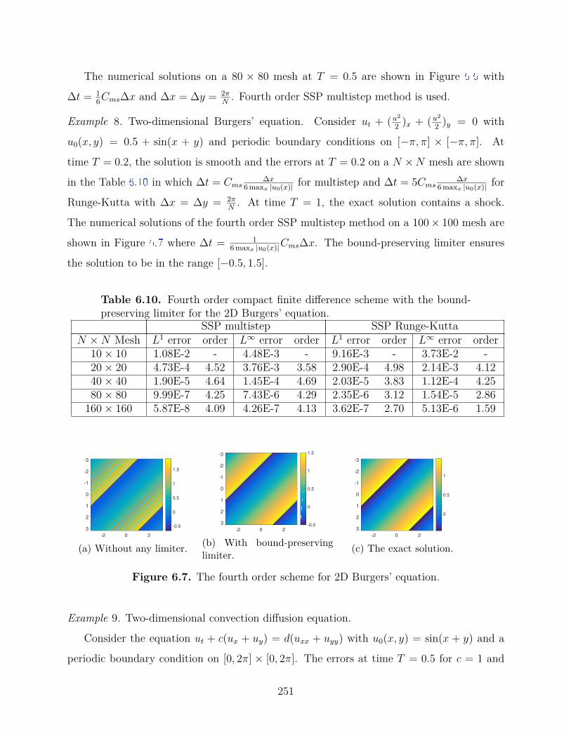
The numerical solutions on a 80 × 80 mesh at T = 0.5 are shown in Figure 6.6 with

∆t = 16Cms∆x and ∆x = ∆y = 2π

N. Fourth order SSP multistep method is used.

Example 8. Two-dimensional Burgers’ equation. Consider ut + (u2

2 )x + (u2

2 )y = 0 with

u0(x, y) = 0.5 + sin(x + y) and periodic boundary conditions on [−π, π] × [−π, π]. At

time T = 0.2, the solution is smooth and the errors at T = 0.2 on a N ×N mesh are shown

in the Table 6.10 in which ∆t = Cms∆x

6 maxx |u0(x)| for multistep and ∆t = 5Cms∆x

6 maxx |u0(x)| for

Runge-Kutta with ∆x = ∆y = 2πN

. At time T = 1, the exact solution contains a shock.

The numerical solutions of the fourth order SSP multistep method on a 100× 100 mesh are

shown in Figure 6.7 where ∆t = 16 maxx |u0(x)|Cms∆x. The bound-preserving limiter ensures

the solution to be in the range [−0.5, 1.5].

Table 6.10. Fourth order compact finite difference scheme with the bound-preserving limiter for the 2D Burgers’ equation.

SSP multistep SSP Runge-KuttaN ×N Mesh L1 error order L∞ error order L1 error order L∞ error order


160× 160 5.87E-8 4.09 4.26E-7 4.13 3.62E-7 2.70 5.13E-6 1.59

-2 0 2

-3

-2

-1

0

1

2

3-0.5

0

0.5

1

1.5

(a) Without any limiter.

-2 0 2

-3

-2

-1

0

1

2

3-0.5

0

0.5

1

1.5

(b) With bound-preservinglimiter.

-2 0 2

-3

-2

-1

0

1

2

3

0

0.5

1

(c) The exact solution.

Figure 6.7. The fourth order scheme for 2D Burgers’ equation.

Example 9. Two-dimensional convection diffusion equation.

Consider the equation ut + c(ux + uy) = d(uxx + uyy) with u0(x, y) = sin(x + y) and a

periodic boundary condition on [0, 2π] × [0, 2π]. The errors at time T = 0.5 for c = 1 and

251

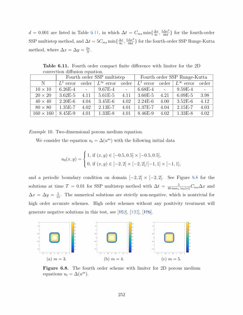
d = 0.001 are listed in Table 6.11 , in which ∆t = Cms min∆x6c, 5∆x2

48d for the fourth-order

SSP multistep method, and ∆t = 5Cms min∆x6c, 5∆x2

48d for the fourth-order SSP Runge-Kutta

method, where ∆x = ∆y = 2πN

.

Table 6.11. Fourth order compact finite difference with limiter for the 2Dconvection diffusion equation.

Fourth order SSP multistep Fourth order SSP Runge-KuttaN L1 error order L∞ error order L1 error order L∞ error order


160× 160 8.45E-9 4.01 1.33E-8 4.01 8.46E-9 4.02 1.33E-8 4.02

Example 10. Two-dimensional porous medium equation.

We consider the equation ut = ∆(um) with the following initial data

u0(x, y) =

1, if (x, y) ∈ [−0.5, 0.5]× [−0.5, 0.5],

0, if (x, y) ∈ [−2, 2]× [−2, 2]/[−1, 1]× [−1, 1],

and a periodic boundary condition on domain [−2, 2] × [−2, 2]. See Figure 6.8 for the

solutions at time T = 0.01 for SSP multistep method with ∆t = 548 maxx |u0(x)|Cms∆x and

∆x = ∆y = 115 . The numerical solutions are strictly non-negative, which is nontrivial for

high order accurate schemes. High order schemes without any positivity treatment will

generate negative solutions in this test, see [102 ], [103 ], [106 ].

-1.5 -1 -0.5 0 0.5 1 1.5 2

-1.5

-1

-0.5

0

0.5

1

1.5

2

0.1

0.2

0.3

0.4

0.5

0.6

0.7

0.8

0.9

(a) m = 3.-1.5 -1 -0.5 0 0.5 1 1.5 2

-1.5

-1

-0.5

0

0.5

1

1.5

2

0.1

0.2

0.3

0.4

0.5

0.6

0.7

0.8

0.9

(b) m = 4.-1.5 -1 -0.5 0 0.5 1 1.5 2

-1.5

-1

-0.5

0

0.5

1

1.5

2

0.1

0.2

0.3

0.4

0.5

0.6

0.7

0.8

0.9

(c) m = 5.

Figure 6.8. The fourth order scheme with limiter for 2D porous mediumequations ut = ∆(um).

252

6.7.4 Two-dimensional incompressible Navier-Stokes equation

In this subsection, we test the bound-preserving fourth order compact finite difference

scheme for the two-dimensional incompressible flow.

Example 11. Consider solving (6.19 ) on the domain [0, 2π]× [0, 2π] with a periodic boundary

condition. We use a smooth solution ω(x, y, t) = sin(2x) sin(2y) exp(−8Ret) to test the accuracy

of the proposed scheme. The errors for Re = 1000 at T = 1 are listed in Table 6.12 . The

time step is taken as ∆t = Cms min 112 maxx |u0|∆x,

5Re48 ∆x2 for the SSP multistep method

and ∆t = 5Cms min 112 maxx |u0|∆x,

5Re48 ∆x2 for the SSP Runge-Kutta method.

Table 6.12. Fourth order compact finite difference scheme with the bound-preserving limiter for the incompressible Navier-Stokes equation.

SSP multistep SSP Runge-KuttaN ×N L1 error order L∞ error order L1 error order L∞ error order10× 10 2.76E-5 - 6.58E-5 - 3.67E-5 - 8.76E-5 -20× 20 1.80E-6 3.94 4.29E-6 3.94 2.16E-6 4.09 5.16E-6 4.0940× 40 1.22E-7 3.88 3.07E-7 3.80 1.33E-7 4.02 3.35E-7 3.9480× 80 7.93E-9 3.95 1.97E-8 3.97 8.42E-9 3.99 2.09E-8 4.00

160× 160 5.03E-10 3.98 1.24E-9 3.98 5.17E-10 4.03 1.28E-9 4.03

Example 12. Double Shear Layer Problem. We test the double shear layer problem on the

domain [0, 2π]× [0, 2π] with a periodic boundary condition. The initial condition is

ω(x, y, 0) =

δcos(x)− 1ρsech2((y − π

2 )/ρ), y ≤ π

δcos(x) + 1ρsech2((3π

2 − y)/ρ), y > π

with δ = 0.05 and ρ = π/15. The vorticity ω for Re = 5000 at time T = 6 and T = 8 are

shown in Figure 6.9 . We use the fourth order compact finite difference with SSP multistep

method on a 120 × 120 mesh solving the Navier-Stokes equation (6.19 ) with Re = 5000.

The time step is ∆t = Cms min 112 maxx |u0|∆x,

5Re48 ∆x2. Although one can barely see any

difference between the results with the limiter and without the limiter from the contour,

we point out that the numerical solutions of the scheme with the bound-preserving limiter

are ensured to be in the range [−δ − 1ρ, δ + 1

ρ]. In the numerical solutions, we observe some

253

obvious oscillations, which would be reduced if the TVB limiter is also used. On the other

hand, if the physical diffusion in the Navier-Stokes equation is resolved on a fine enough

mesh, the physical diffusion can also smooth out the oscillations, as we will see in the next

example.

2 4 6

X

2

4

6

Y

-4

-2

0

2

4

(a) T = 6, without limiter.

2 4 6

X

2

4

6

Y

-4

-2

0

2

4

(b) T = 6, with limiter.

2 4 6

X

2

4

6

Y

-4

-2

0

2

4

(c) T = 8, with limiter.

2 4 6

X

2

4

6

Y

-4

-2

0

2

4

(d) T = 8, with limiter.

Figure 6.9. Double shear layer problem.

Example 13. Vortex Patch Problem. We test the vortex patch problem in the domain [0, 2π]×

[0, 2π] with a periodic boundary condition. The initial condition is

ω(x, y, 0) =

−1, (x, y) ∈ [π

2 ,3π2 ]× [π

4 ,3π4 ];

1, (x, y) ∈ [π2 ,

3π2 ]× [5π

4 ,7π4 ];

0, otherwise.

Numerical solutions for incompressible Euler and Navier-Stokes equations are shown in

Figure 6.10 , Figure 6.11 and Figure 6.12 . In Figure 6.10 , we use fourth order accurate

254

compact finite difference scheme to solve the incompressible Euler equation at T = 5 on a

120 × 120 mesh. The time step is ∆t = Cms1

6 max |u0|∆x. The second row is the cut along

the diagonal of the two-dimensional array. We can observe that the solutions generated by

the compact finite difference scheme with only the bound-preserving limiter are still highly

oscillatory for the Euler equation, thus in principle other limiters should be used to eliminate

the oscillations, e.g., the TVB limiter. On the other hand, we solve the incompressible

Navier-Stokes equation with Re = 1000, at time T = 5 on a 60 × 60 mesh with the time

step ∆t = Cms min 112 max |u0|∆x,

5Re48 ∆x2. The second row is the cut along the diagonal of

the two-dimensional array. We observe that the numerical solution is non-oscillatory on a

fine enough mesh. Notice that the oscillations in Figure 6.10 and Figure 6.11 suggest that

the artificial viscosity induced by the bound-preserving limiter is quite low, thus it is the

physical diffusion in the Navier-Stokes equation that starts to smooth out the numerical

oscillations in Figure 6.12 . For Figure 6.12 , on a 120 × 120 mesh we use time step is

∆t = Cms min 112 max |u0|∆x,

5Re48 ∆x2.

The same phenomenon was also observed for the high order positivity-preserving discon-

tinuous Galerkin scheme for the compressible Navier-Stokes system in [96 ]. In other words,

for solving convection diffusion problems on resolved meshes, the bound-preserving limiter

is enough for high order schemes producing satisfying results and there is no need to use the

TVB limiter.


In this chapter we have demonstrated that fourth order accurate compact finite difference

schemes for convection diffusion problems with periodic boundary conditions satisfy a weak

monotonicity property, and a simple three-point stencil limiter can enforce bounds without

destroying the global conservation. Since the limiter is designed based on an intrinsic prop-

erty in the high order finite difference schemes, the accuracy of the limiter can be easily

justified. This is the first time that the weak monotonicity is established for a high order

accurate finite difference scheme, complementary to results regarding the weak monotonicity

property of high order finite volume and discontinuous Galerkin schemes in [23 ], [93 ], [95 ].

255

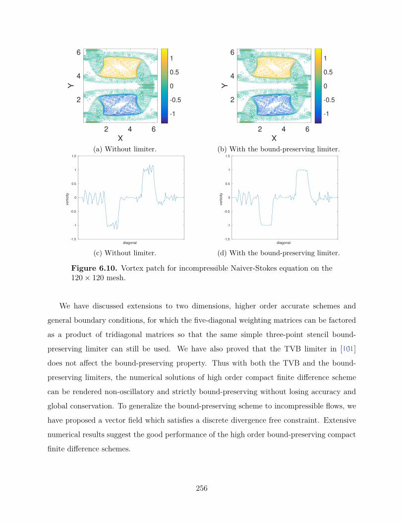
2 4 6

X

2

4

6

Y

-1

-0.5

0

0.5

1

(a) Without limiter.

2 4 6

X

2

4

6

Y

-1

-0.5

0

0.5

1


diagonal-1.5

-1

-0.5

0

0.5

1

1.5

vo

rtic

ity

(c) Without limiter.diagonal

-1.5

-1

-0.5

0

0.5

1

1.5

vo

rtic

ity

(d) With the bound-preserving limiter.

Figure 6.10. Vortex patch for incompressible Naiver-Stokes equation on the120× 120 mesh.

We have discussed extensions to two dimensions, higher order accurate schemes and

general boundary conditions, for which the five-diagonal weighting matrices can be factored

as a product of tridiagonal matrices so that the same simple three-point stencil bound-

preserving limiter can still be used. We have also proved that the TVB limiter in [101 ]

does not affect the bound-preserving property. Thus with both the TVB and the bound-

preserving limiters, the numerical solutions of high order compact finite difference scheme

can be rendered non-oscillatory and strictly bound-preserving without losing accuracy and

global conservation. To generalize the bound-preserving scheme to incompressible flows, we

have proposed a vector field which satisfies a discrete divergence free constraint. Extensive

numerical results suggest the good performance of the high order bound-preserving compact

finite difference schemes.

256

2 4 6

X

2

4

6

Y

-1

-0.5

0

0.5

1

(a) Without limiter. The maximum of the numer-ical solution is around 1.07.

2 4 6

X

2

4

6

Y

-0.5

0

0.5


diagonal-1.5

-1

-0.5

0

0.5

1

1.5

vo

rtic

ity

(c) Without limiter. The maximum of the numer-ical solution is around 1.07.

diagonal-1.5

-1

-0.5

0

0.5

1

1.5

vo

rtic

ity


Figure 6.11. Vortex patch for incompressible Naiver-Stokes equation on the60× 60 mesh.

For more generalizations and applications, there are certain complications. For using

compact finite difference schemes on non-uniform meshes, one popular approach is to intro-

duce a mapping to a uniform grid but such a mapping results in an extra variable coefficient

which may affect the weak monotonicity. Thus any extension to non-uniform grids is much

less straightforward. For applications to systems, e.g., preserving positivity of density and

pressure in compressible Euler equations, the weak monotonicity can be easily extended to

a weak positivity property. However, the same three-point stencil limiter cannot enforce the

positivity for pressure. One has to construct a new limiter for systems.

257

2 4 6

X

1

2

3

4

5

6

Y

-0.5

0

0.5

(a) Without limiter. The maximum of the numer-ical solution is around 1.04.

2 4 6

X

2

4

6

Y

-0.5

0

0.5


diagonal-1.5

-1

-0.5

0

0.5

1

1.5

vo

rtic

ity

(c) Without limiter. The maximum of the numer-ical solution is around 1.04.

diagonal-1.5

-1

-0.5

0

0.5

1

1.5

vo

rtic

ity


Figure 6.12. Vortex patch for Naiver-Stokes equation on the 120× 120 mesh.

6.9 Appendix A: Comparison With The Nine-point Discrete Laplacian

Consider solving the two-dimensional Poisson equations uxx + uyy = f with either ho-

mogeneous Dirichlet boundary conditions or periodic boundary conditions on a rectangular

domain. Let u be a Nx × Ny matrix with entries ui,j denoting the numerical solutions at

a uniform grid (xi, yj) = ( iNx, j

Ny). Let f be a Nx × Ny matrix with entries fi,j = f(xi, yj).

The fourth order compact finite difference method in Section 6.3.2 for uxx + uyy = f can be

written as:1

∆x2W−12x Dxxu + 1

∆y2W−12y Dyyu = f(u). (6.1)

258

For convenience, we introduce two matrices,

U =

ui−1,j+1 ui,j+1 ui+1,j+1


ui−1,j−1 ui,j−1 ui+1,j−1

, F =

fi−1,j+1 fi,j+1 fi+1,j+1

fi−1,j fi,j fi+1,j

fi−1,j−1 fi,j−1 fi+1,j−1

.

Notice that the scheme (6.1 ) is equivalent to

1∆x2W2yDxxu + 1

∆y2W2xDyyu = W2xW2yf(u),

which can be written as

112∆x2

1 −2 1

10 −20 10

1 −2 1

: U + 112∆y2

1 10 1

−2 −20 −2

1 10 1

: U = 1144

1 10 1

10 100 10

1 10 1

: F, (6.2)

where : denotes the sum of all entrywise products in two matrices of the same size.

In particular, if ∆x = ∆y = h, the scheme above reduces to

16h2

1 4 1

4 −20 4

1 4 1

: U = 1144

1 10 1

10 100 10

1 10 1

: F.

Recall that the classical nine-point discrete Laplacian [113 ] for the Poisson equation can be

written as

112∆x2

1 −2 1

10 −20 10

1 −2 1

: U + 112∆y2

1 10 1

−2 −20 −2

1 10 1

: U = 112

0 1 0

1 8 1

0 1 0

: F, (6.3)

259

which reduces to the following under the assumption ∆x = ∆y = h,

16h2

1 4 1

4 −20 4

1 4 1

: U = 112

0 1 0

1 8 1

0 1 0

: F.

Both schemes (6.2 ) and (6.3 ) are fourth order accurate and they have the same stencil in the

left hand side. As to which scheme produces smaller errors, it seems to be problem dependent,

see Figure 6.13 . Figure 6.13 shows the errors of two schemes (6.2 ) and (6.3 ) using uniform

grids with ∆x = 23∆y for solving the Poisson equation uxx+uyy = f on a rectangle [0, 1]×[0, 2]

with Dirichlet boundary conditions. For solution 1, we have u(x, y) = sin(πx) sin(πy) + 2x,

for solution 2, we have u(x, y) = sin(πx) sin(πy) + 4x4y4.

100

101

102

Number of grid points in x-direction

10-8

10-7

10-6

10-5

10-4

Err

or

in m

ax-n

orm

9-point scheme

compact FD

fourth order slope

(a) Solution 1.

100

101

102


10-8

10-7

10-6

10-5

10-4

Err

or

in m

ax-n

orm

9-point scheme

compact FD

fourth order slope

(b) Solution 2.

Figure 6.13. Error comparison.

6.10 Appendix B: M-matrices And A Discrete Maximum Principle

Consider solving the heat equation ut = uxx + uyy with a periodic boundary condition.

It is well known that a discrete maximum principle is satisfied under certain time step

constraints if the spatial discretization is the nine-point discrete Laplacian or the compact

260

scheme (6.1 ) with backward Euler and Crank-Nicolson time discretizations. For simplicity,

we only consider the compact scheme (6.1 ) and the discussion for the nine-point discrete

Laplacian is similar. Assume ∆x = ∆y = h. For backward Euler, the scheme can be written

as

1144

1 10 1

10 100 10

1 10 1

: (Un+1 − Un) = ∆t6h2

1 4 1

4 −20 4

1 4 1

: Un+1,

thus

1144

1 10 1

10 100 10

1 10 1

: Un+1 − ∆t6h2

1 4 1

4 −20 4

1 4 1

: Un+1 = 1144

1 10 1

10 100 10

1 10 1

: Un.

Let A and B denote the matrices corresponding to the operator in the left hand side and

right hand side above respectively, then the scheme can be written as

Aun+1 = Bun,

and A is a M -Matrix (diagonally dominant, positive diagonal entries and non-positive off

diagonal entries) under the following constraint which allows very large time steps:

∆th2 ≥

548 .

The inverses of M -Matrices have non-negative entries, e.g., see [107 ]. Thus A−1 has non-

negative entries. Moreover, it is straightforward to check thatAe = e where e =(

1 1 · · · 1)T

.

Thus A−1e = e, which implies the sum of each row of A−1 is 1 thus each row of A−1 mul-

tiplying any vector V is a convex combination of entries of V . It is also obvious that each

entry of B is non-negative and the sum of each row of B is 1. Therefore, un+1 = A−1Bun

satisfies a discrete maximum principle:

mini,j

uni,j ≤ un+1

i,j ≤ maxi,j

uni,j.

261

For the second order accurate Crank-Nicolson time discretization, the scheme can be

written as

1144

1 10 1

10 100 10

1 10 1

: (Un+1 − Un) = ∆t6h2

1 4 1

4 −20 4

1 4 1

: Un+1 + Un

2 ,

thus 1

144

1 10 1

10 100 10

1 10 1

−∆t

12h2

1 4 1

4 −20 4

1 4 1

: Un+1 =

1

144

1 10 1

10 100 10

1 10 1

+ ∆t12h2

1 4 1

4 −20 4

1 4 1

: Un.

Let the matrix-vector form of the scheme above be Aun+1 = Bun. Then for A to be an

M -Matrix, we only need ∆th2 ≥ 5

24 . However, for B to have non-negative entries, we need∆th2 ≤ 5

12 . Thus the Crank-Nicolson method can ensure a discrete maximum principle if the

time step satisfies,524h

2 ≤ ∆t ≤ 512h

2.

6.11 Appendix C: Fast Poisson Solvers

6.11.1 Dirichlet boundary conditions

Consider solving the Poisson equation uxx + uyy = f(x, y) on a rectangular domain

[0, Lx] × [0, Ly] with homogeneous Dirichlet boundary conditions. Assume we use the grid

xi = i∆x, i = 0, · · · , Nx + 1 with uniform spacing ∆x = Lx

Nx+1 for the x-variable and

yj = j∆y, j = 0, · · · , Ny + 1 with uniform spacing ∆y = Ly

Ny+1 for y-variable. Let u be a

Nx×Ny matrix such that its (i, j) entry ui,j is the numerical solution at interior grid points

(xi, yj). Let F be a (Nx + 2) × (Ny + 2) matrix with entries f(xi, yj) for i = 0, · · · , Nx + 1

and j = 0, · · · , Ny + 1.

262

To obtain the matrix representation of the operator in (6.2 ) and (6.3 ), we consider two

operators:

• Kronecker product of two matrices: if A is m×n and B is p×q, then A⊗B is mp×nq

give by

A⊗B =

a11B · · · a1nB

... ... ...

am1B · · · amnB

.

• For a m×n matrix X, vec(X) denotes a column vector of size mn made of the columns

of X stacked atop one another from left to right.

The following properties will be used:

1. (A⊗B)(C ⊗D) = AC ⊗BD.

2. (A⊗B)−1 = A−1 ⊗B−1.

3. (BT ⊗ A) vec(X) = vec(AXB).

We define two tridiagonal square matrices of size Nx ×Nx:

Dxx =

−2 1

1 −2 1

1 −2 1. . . . . . . . .

1 −2 1

1 −2

,W2x = 1

12

10 1

1 10 1

1 10 1. . . . . . . . .

1 10 1

1 10

.

Let W 2x denote a Nx × (Nx + 2) tridiagonal matrix of the following form:

W 2x = 112

1 10 1

1 10 1. . . . . . . . .

1 10 1

. (6.4)

263

The matrices Dyy, W2y and W 2y are similarly defined.

Then the scheme (6.2 ) can be written in a matrix-vector form:

1∆x2DxxuW T

2y + 1∆y2W2xuDT

yy = W 2xFW T

2y,

or equivalently,

(W2y ⊗

1∆x2Dxx + 1

∆y2Dyy ⊗W2x

)vec(u) = (W 2x ⊗W 2y) vec(F). (6.5)

Let hx = [h1, h2, · · · , hNx ]T with hi = iNx+1 , and sin(mπhx) denote a column vector of size

Nx with its i-th entry being sin(mπhi). Then sin(mπhx) are the eigenvectors of Dxx and

W2x with the associated eigenvalues being 2 cos( mπNx+1)− 2 and 5

6 + 16 cos( mπ

Nx+1) respectively

for m = 1, · · · , Nx. Let

Sx = [sin(πhx), sin(2πhx), · · · , sin(Nxπhx)]

be the Nx×Nx eigenvector matrix, then Sx is a symmetric matrix. Let Λ1x denote a diagonal

matrix with diagonal entries 2 cos( mπNx+1)−2 and Λ2x denote a diagonal matrix with diagonal

entries 56 + 1

6 cos( mπNx+1), then we have Dxx = SxΛ1xS

−1x and W2x = SxΛ2xS

−1x , thus

W2y ⊗Dxx = (SyΛ2yS−1y )⊗ (SxΛ1xS

−1x ) = (Sy ⊗ Sx)(Λ2y ⊗ Λ1x)(S−1

y ⊗ S−1x ).

The scheme can be written as

(Sy ⊗ Sx)( 1∆x2 Λ2y ⊗ Λ1x + 1

∆y2 Λ1y ⊗ Λ2x)(S−1y ⊗ S−1

x ) vec(u) = (W 2y ⊗W 2x) vec(F).

Let Λ be a Nx ×Ny matrix with Λi,j being equal to

13∆x2

(cos( iπ

Nx + 1)− 1)(

cos( mπ

Ny + 1) + 5)

+ 13∆y2

(cos( mπ

Nx + 1) + 5)(

cos( jπ

Ny + 1)− 1),

264

then vec(Λ) are precisely the diagonal entries of the diagonal matrix 1∆x2 Λ2y⊗Λ1x + 1

∆y2 Λ1y⊗

Λ2x, then the scheme above is equivalent to

Sx(Λ (S−1x uS−1

y ))Sy = W 2xFW T

2y,

where the symmetry of S matrices is used. The solution is given by

u = Sx[S−1x (W 2xFW T

2y)S−1y ]./ΛSy, (6.6)

where ./ denotes the entrywise division for two matrices of the same size.

Since the multiplication of the matrices S and S−1 can be implemented by the Discrete

Sine Transform, (6.6 ) gives a fast Poisson solver.

For nonhomogeneous Dirichlet boundary conditions, the fourth order accurate compact

finite difference scheme can also be written in the form of (6.5 ):

(W2y ⊗

1∆x2Dxx + 1

∆y2Dyy ⊗W2x

)vec(u) = vec(F), (6.7)

where F consists of both F and the Dirichlet boundary conditions. Thus the scheme can

still be efficiently implemented by the Discrete Sine Transform.

6.11.2 Periodic boundary conditions

For periodic boundary conditions on a rectangular domain, we should consider the uni-

form grid xi = i∆x, i = 1, · · · , Nx with ∆x = Lx

Nxand yj = j∆y, j = 1, · · · , Ny with uniform

spacing ∆y = Ly

Ny, then the fourth order accurate compact finite difference scheme can still

265

be written in the form of (6.5 ) with the Dxx, Dyy, W2x and W2y matrices being redefined as

circulant matrices:

Dxx =

−2 1 1

1 −2 1

1 −2 1. . . . . . . . .

1 −2 1

1 1 −2

,W2x = 1

12

10 1 1

1 10 1

1 10 1. . . . . . . . .

1 10 1

1 1 10

.

The Discrete Fourier Matrix is the eigenvector matrix for any circulant matrices, and the

corresponding eigenvalues are for Dxx and W2x are 2 cos(m2πNx

) − 2 and 16 cos(m2π

Nx) + 5

6 for

m = 0, 1, 2, · · · , Nx− 1. The matrix W2y ⊗ 1∆x2Dxx + 1

∆y2Dyy ⊗W2x is singular because its

first eigenvalue Λ1,1 is zero. Nonetheless, the scheme can still be implemented by solving

(6.6 ) with Fast Fourier Transform. For the zero eigenvalue, we can simply reset the division

by eigenvalue zero to zero. Since the eigenvector for eigenvalue zero is e =(

1 1 · · · 1)T

,

and the columns of the Discrete Fourier Matrix are orthogonal to one another, resetting

the division by eigenvalue zero to zero simply means that we obtain a numerical solution

satisfying ∑i

∑j ui,j = 0. And this is also the least square solution to the singular linear

system.

6.11.3 Neumann boundary conditions

For Dirichlet and periodic boundary conditions, we can invert the matrix coefficient

matrix in (6.5 ) using eigenvectors of much smaller matrices W2x and Dxx due to the fact that

W2x− 112Dxx is the identity matrix Id. Here we discuss how to achieve a fourth order accurate

boundary approximation for Neumann boundary conditions by keeping W2x − 112Dxx =

266

Id. We first consider a one-dimensional problem with homogeneous Neumann boundary

conditions:

u(x) = f(x), x ∈ [0, Lx],

u(0) = u(Lx) = 0.

Assume we use the uniform grid xi = i∆x, i = 0, · · · , Nx + 1 with ∆x = Lx

Nx+1 . The

two boundary point values u0 and uNx+1 can be expressed in terms of interior point values

through boundary conditions. For approximating the boundary conditions, we can apply

the fourth order one-sided difference at x = 0:

u(0) ≈ −25u(0) + 48u(∆x)− 36u(2∆x) + 16u(3∆x)− 3u(4∆x)12∆x

which implies the finite difference approximation:

u0 = 48u1 − 36u2 + 16u3 − 3u4

25 .

Define two column vectors:

u = [u1, u2, · · · , uNx ]T , f = [f(x0), f(x1), · · · , f(xNx), f(xNx+1)]T ,

then a fourth order accurate compact finite difference scheme can be written as

1∆x2DxxIxu = W 2xf ,

267

where W 2x is the same as in (6.4 ), and Dxx is a matrix of size Nx × (Nx + 2) and Ix is a

matrix of size (Nx + 2)×Nx:

Dxx =

1 −2 1

1 −2 1. . . . . . . . .

1 −2 1

, Ix =

4825 −

3625

1625 −

325

1

1. . .

1

− 325

1625 −

3625

4825

.

Now consider solving the Poisson equation uxx + uyy = f(x, y) on a rectangular domain

[0, Lx]× [0, Ly] with homogeneous Neumann boundary conditions. Assume we use the grid

xi = i∆x, i = 0, · · · , Nx + 1 with ∆x = Lx

Nx+1 and yj = j∆y, j = 0, · · · , Ny + 1 with uniform

spacing ∆y = Ly

Ny+1 . Let u be a Nx × Ny matrix such that ui,j is the numerical solution at

(xi, yj) and F be a (Nx + 2) × (Ny + 2) matrix with entries f(xi, yj) (i = 0, · · · , Nx + 1,

j = 0, · · · , Ny + 1). Then a fourth order accurate compact finite difference scheme can be

written as1

∆x2DxxIxuITy W

T2y + 1

∆y2W 2xIxuITy D

Tyy = W 2xFW T

2y.

Let Dxx = DxxIx and W2x = W 2xIx, then the scheme can be written as (6.5 ).

Notice that W2x − 112Dxx = (W 2x − 1

12Dxx)Ix is still the identity matrix thus W2x and

Dxx still have the same eigenvectors. Let S be the eigenvector matrix and Λ1 and Λ2 be

diagonal matrices with eigenvalues, then the scheme can still be implemented as (6.6 ). The

eigenvectors S and the eigenvalues can be obtained by computing eigenvalue problems for two

small matrices Dxx of size Nx×Nx and Dyy of size Ny×Ny. If such a Poisson problem needs

to be solved in each time step in a time-dependent problem such as the incompressible flow

equations, then this is an efficient Poisson solver because S and Λ can be computed before

time evolution without considering eigenvalue problems for any matrix of size NxNy×NxNy.

For nonhomogeneous Neumann boundary conditions, the point values of u along the

boundary should be expressed in terms of interior ones as follows:

268

1. First obtain the point values except the two cell ends (i.e., corner points of the rect-

angular domain) for each of the four boundary line segments. For instance, if the left

boundary condition is ∂u∂x

(0, y) = g(y), then we obtain

u0,j = 48u1,j − 36u2,j + 16u3,j − 3u4,j + 12∆xg(yj)25 , j = 1, · · · , Ny.

2. Second, obtain the approximation at four corners using the point values along the

boundary. For instance, if the bottom boundary condition is ∂u∂y

(x, 0) = h(x), then

u0,0 = 48u1,0 − 36u2,0 + 16u3,0 − 3u4,0 + 12∆yh(0)25

The scheme can still be written as (6.7 ) with F consisting of F and the nonhomogeneous

boundary conditions. Notice that the matrix in (6.7 ) is singular thus we need to reset

the division by eigenvalue zero to zero, which however no longer means that the obtained

solution satisfies ∑i

∑j ui,j = 0 since the eigenvectors are not necessarily orthogonal to one

another. See Figure 6.14 for the accuracy test of the fourth order compact finite difference

scheme using uniform grids with ∆x = 32∆y for solving the Poisson equation uxx + uyy = f

on a rectangle [0, 1] × [0, 2] with nonhomogeneous Neumann boundary conditions. The

exact solution is u(x, y) = cos(πx) cos(3πy) + sin(πy) + x4. Since the solutions to Neumann

boundary conditions are unique up to any constant, when computing errors, we need to add

a constant 1Nx

1Ny

∑i,j[u(xi, yj)− ui,j] to each entry of u.

269

100

101

102


10-9

10-8

10-7

10-6

10-5

10-4

Err

or

in m

ax-n

orm

compact FD

fourth order slope

(a) Convergence rate.

0.2 0.4 0.6 0.8

X

0.2

0.4

0.6

0.8

1

1.2

1.4

1.6

1.8

Y

-1.5

-1

-0.5

0

0.5

1

1.5

2

2.5

(b) The contour of the solution.

Figure 6.14. Accuracy test for Neumann boundary condition.

270

REFERENCES

[1] H. Li, S. Xie, and X. Zhang, “A high order accurate bound-preserving compact fi-nite difference scheme for scalar convection diffusion equations,” SIAM Journal onNumerical Analysis, vol. 56, no. 6, pp. 3308–3345, 2018.

[2] H. Li, D. Appelö, and X. Zhang, Accuracy of spectral element method for wave,parabolic and schrödinger equations, 2021. arXiv: 2103.00400 [math.NA] .

[3] P. G. Ciarlet, “Basic error estimates for elliptic problems,” Handbook of NumericalAnalysis, vol. 2, pp. 17–351, 1991.

[4] P. Lesaint and M. Zlamal, “Superconvergence of the gradient of finite element solu-tions,” RAIRO. Analyse numérique, vol. 13, no. 2, pp. 139–166, 1979.

[5] C. Chen, “Superconvergent points of Galerkin’s method for two point boundary valueproblems,” Numerical Mathematics A Journal of Chinese Universities, vol. 1, pp. 73–79, 1979.

[6] M. Bakker, “A note on C0 Galerkin methods for two-point boundary problems,”Numer. Math., vol. 38, no. 3, pp. 447–453, 1982.

[7] J. Douglas Jr, T. Dupont, and M. F. Wheeler, “An L∞ estimate and a superconver-gence result for a Galerkin method for elliptic equations based on tensor products ofpiecewise polynomials,” 1974.

[8] L. Wahlbin, Superconvergence in Galerkin finite element methods. Springer, 2006.

[9] C. Chen, Structure theory of superconvergence of finite elements (In Chinese). HunanScience and Technology Press, Changsha, 2001.

[10] Q. Lin and N. Yan, Construction and Analysis for Efficient Finite Element Method(In Chinese). Hebei University Press, 1996.

[11] Y. Maday and E. M. Rønquist, “Optimal error analysis of spectral methods withemphasis on non-constant coefficients and deformed geometries,” Computer Methodsin Applied Mechanics and Engineering, vol. 80, no. 1-3, pp. 91–115, 1990.

[12] D. Komatitsch, J.-P. Vilotte, R. Vai, J. M. Castillo-Covarrubias, and F. J. Sánchez-Sesma, “The spectral element method for elastic wave equations: Application to 2-Dand 3-D seismic problems,” International Journal for numerical methods in engineer-ing, vol. 45, no. 9, pp. 1139–1164, 1999.

271

https://arxiv.org/abs/2103.00400

[13] D. Komatitsch and J. Tromp, “Introduction to the spectral element method for three-dimensional seismic wave propagation,” Geophysical journal international, vol. 139,no. 3, pp. 806–822, 1999.

[14] L. C. Evans, Partial Differential Equations, 2nd ed., ser. Graduate Studies in Math-ematics. American Mathematical Society, 2010, vol. 019.

[15] P. G. Ciarlet, “Discrete maximum principle for finite-difference operators,” Aequa-tiones Math., vol. 4, no. 3, pp. 338–352, 1970.

[16] J. Bramble and B. Hubbard, “On the formulation of finite difference analogues of theDirichlet problem for Poisson’s equation,” Numer. Math., vol. 4, no. 1, pp. 313–327,1962.

[17] P. G. Ciarlet and P.-A. Raviart, “Maximum principle and uniform convergence for thefinite element method,” Comput. Methods Appl. Mech. Engrg., vol. 2, no. 1, pp. 17–31,1973.

[18] O. Axelsson and L. Kolotilina, “Monotonicity and discretization error estimates,”SIAM J. Numer. Anal., vol. 27, no. 6, pp. 1591–1611, 1990.

[19] P. J. Ferket and A. A. Reusken, “A finite difference discretization method for ellipticproblems on composite grids,” Computing, vol. 56, no. 4, pp. 343–369, 1996.

[20] W. Höhn and H. D. Mittelmann, “Some remarks on the discrete maximum-principlefor finite elements of higher order,” Computing, vol. 27, no. 2, pp. 145–154, 1981.

[21] J. Lorenz, “Zur inversmonotonie diskreter probleme,” Numer. Math., vol. 27, no. 2,pp. 227–238, 1977.

[22] L. J. Cross and X. Zhang, “On the monotonicity of high order discrete laplacian,”arXiv preprint arXiv:2010.07282, 2020.

[23] X. Zhang and C.-W. Shu, “On maximum-principle-satisfying high order schemes forscalar conservation laws,” Journal of Computational Physics, vol. 229, no. 9, pp. 3091–3120, 2010.

[24] J. Douglas, “Some superconvergence results for Galerkin methods for the approximatesolution of two-point boundary problems,” Topics in numerical analysis, pp. 89–92,1973.

[25] J. Douglas and T. Dupont, “Galerkin approximations for the two point boundaryproblem using continuous, piecewise polynomial spaces,” Numer. Math., vol. 22, no. 2,pp. 99–109, 1974.

272

[26] J. Douglas Jr, T. Dupont, and M. F. Wheeler, “An l∞ estimate and a superconver-gence result for a galerkin method for elliptic equations based on tensor products ofpiecewise polynomials,” ESAIM: Mathematical Modelling and Numerical Analysis-Modélisation Mathématique et Analyse Numérique, vol. 8, no. R2, pp. 61–66, 1974.

[27] C. Chen and S. Hu, “The highest order superconvergence for bi-k degree rectangularelements at nodes: A proof of 2k-conjecture,” Math. Comp., vol. 82, no. 283, pp. 1337–1355, 2013.

[28] W. He and Z. Zhang, “2k superconvergence of Qk finite elements by anisotropic meshapproximation in weighted Sobolev spaces,” Mathematics of Computation, vol. 86,no. 306, pp. 1693–1718, 2017.

[29] W. He, Z. Zhang, and Q. Zou, “Ultraconvergence of high order fems for elliptic prob-lems with variable coefficients,” Numerische Mathematik, vol. 136, no. 1, pp. 215–248,May 2017.

[30] P. G. Ciarlet and P.-A. Raviart, “The combined effect of curved boundaries andnumerical integration in isoparametric finite element methods,” in The mathemati-cal foundations of the finite element method with applications to partial differentialequations, Elsevier, 1972, pp. 409–474.

[31] J. Whiteman, “Lagrangian finite element and finite difference methods for poissonproblems,” in Numerische Behandlung von Differentialgleichungen, Springer, 1975,pp. 331–355.

[32] Y. Huang and J. Xu, “Superconvergence of quadratic finite elements on mildly struc-tured grids,” Math. Comp., vol. 77, no. 263, pp. 1253–1268, 2008.

[33] G. Savaré, “Regularity results for elliptic equations in Lipschitz domains,” Journal ofFunctional Analysis, vol. 152, no. 1, pp. 176–201, 1998.

[34] P. Grisvard, Elliptic problems in nonsmooth domains. SIAM, 2011, vol. 69.

[35] F. Brezzi and L. Marini, “On the numerical solution of plate bending problemsby hybrid methods,” Revue française d’automatique, informatique, recherche opéra-tionnelle. Analyse numérique, vol. 9, no. R3, pp. 5–50, 1975.

[36] K. Smith, “Inequalities for formally positive integro-differential forms,” Bulletin ofthe American Mathematical Society, vol. 67, no. 4, pp. 368–370, 1961.

[37] S. Agmon, Lectures on elliptic boundary value problems. American Mathematical Soc.,2010, vol. 369.

273

[38] P. G. Ciarlet, The Finite Element Method for Elliptic Problems. Society for Industrialand Applied Mathematics, 2002.

[39] H. Li and X. Zhang, “Superconvergence of c0-qk finite element method for ellipticequations with approximated coefficients,” Journal of Scientific Computing, vol. 82,no. 1, pp. 1–28, 2020.

[40] C. Chen, “Superconvergence of finite element solutions and their derivatives,” Nu-merical Mathematics A Journal of Chinese Universities, vol. 3, no. 2, pp. 118–125,1981.

[41] Q. Lin, N. Yan, and A. Zhou, “A rectangle test for interpolated finite elements,”in Proc. Sys. Sci. and Sys. Eng.(Hong Kong), Great Wall Culture Publ. Co, 1991,pp. 217–229.

[42] J. Xu and L. Zikatanov, “Algebraic multigrid methods,” Acta Numerica, vol. 26,pp. 591–721, 2017.

[43] J. Hesthaven and T. Warburton, “Nodal high-order methods on unstructured grids:I. time-domain solution of Maxwell’s equations,” J. Comput. Phys., vol. 181, pp. 186–221, 2002.

[44] P. Monk and G. Richter, “A discontinuous Galerkin method for linear symmetric hy-perbolic systems in inhomogeneous media,” Journal of Scientific Computing, vol. 22-23, no. 1-3, pp. 443–477, 2005, issn: 0885-7474.

[45] E. T. Chung and B. Engquist, “Optimal discontinuous Galerkin methods for wavepropagation,” SIAM Journal on Numerical Analysis, vol. 44, no. 5, pp. 2131–2158,2006.

[46] E. T. Chung and B. Engquist, “Optimal discontinuous Galerkin methods for theacoustic wave equation in higher dimensions,” SIAM Journal on Numerical Analysis,vol. 47, no. 5, pp. 3820–3848, 2009.

[47] J. Hesthaven and T. Warburton, Nodal Discontinuous Galerkin Methods, ser. Textsin Applied Mathematics 54. New York: Springer-Verlag, 2008.

[48] T. Warburton, “A low-storage curvilinear discontinuous Galerkin method for waveproblems,” SIAM Journal on Scientific Computing, vol. 35, no. 4, A1987–A2012,2013.

[49] X. Meng, C.-W. Shu, and B. Wu, “Optimal error estimates for discontinuous Galerkinmethods based on upwind-biased fluxes for linear hyperbolic equations,” Mathematicsof Computation, vol. 85, no. 299, pp. 1225–1261, 2016.

274

[50] B. Riviere and M. Wheeler, “Discontinuous finite element methods for acoustic andelastic wave problems. part i: Semidiscrete error estimates,” Contemporary Mathe-matics, vol. 329, pp. 271–282, 2003.

[51] M. J. Grote, A. Schneebeli, and D. Schötzau, “Discontinuous Galerkin finite elementmethod for the wave equation,” SIAM Journal on Numerical Analysis, vol. 44, no. 6,pp. 2408–2431, 2006, issn: 00361429.

[52] C.-S. Chou, C.-W. Shu, and Y. Xing, “Optimal energy conserving local discontinuousGalerkin methods for second-order wave equation in heterogeneous media,” Journalof Computational Physics, vol. 272, pp. 88–107, 2014, issn: 0021-9991.

[53] D. Appelö and T. Hagstrom, “A new discontinuous Galerkin formulation for waveequations in second order form,” SIAM Journal On Numerical Analysis, vol. 53,no. 6, pp. 2705–2726, 2015.

[54] K. Mattsson, “Summation by parts operators for finite difference approximations ofsecond-derivatives with variable coefficients,” Journal of Scientific Computing, vol. 51,no. 3, pp. 650–682, Jun. 2012.

[55] K. Mattsson and J. Nordström, “Summation by parts operators for finite differenceapproximations of second derivatives,” J. Comput. Phys., vol. 199, pp. 503–540, 2004.

[56] K. Mattsson, F. Ham, and G. Iaccarino, “Stable and accurate wave–propagation indiscontinuous media,” J. Comput. Phys., vol. 227, pp. 8753–8767, 2008.

[57] K. Virta and K. Mattsson, “Acoustic wave propagation in complicated geometries andheterogeneous media,” Journal of Scientific Computing, vol. 61, no. 1, pp. 90–118,2014.

[58] M. Almquist, S. Wang, and J. Werpers, “Order-preserving interpolation for summation-by-parts operators at nonconforming grid interfaces,” SIAM J. Sci. Comput., vol. 41,A1201–A1227, 2019.

[59] S. Wang, “An improved high order finite difference method for non–conforming gridinterfaces for the wave equation,” J. Sci. Comput., vol. 77, pp. 775–792, 2018.

[60] S. Wang, K. Virta, and G. Kreiss, “High order finite difference methods for thewave equation with non-conforming grid interfaces,” Journal of Scientific Computing,vol. 68, no. 3, pp. 1002–1028, 2016.

[61] G. Cohen, Higher-order numerical methods for transient wave equations. SpringerScience & Business Media, 2001.

275

[62] H. Li and X. Zhang, “Superconvergence of high order finite difference schemes basedon variational formulation for elliptic equations,” Journal of Scientific Computing,vol. 82, no. 2, pp. 1–39, 2020.

[63] M. F. Wheeler, “A priori L_2 error estimates for Galerkin approximations to parabolicpartial differential equations,” SIAM Journal on Numerical Analysis, vol. 10, no. 4,pp. 723–759, 1973.

[64] P. H. Sammon, “Convergence estimates for semidiscrete parabolic equation approxi-mations,” SIAM Journal on Numerical Analysis, vol. 19, no. 1, pp. 68–92, 1982.

[65] T. Dupont, “L2-estimates for Galerkin methods for second order hyperbolic equa-tions,” SIAM journal on numerical analysis, vol. 10, no. 5, pp. 880–889, 1973.

[66] M. S. Gockenbach, Understanding and implementing the finite element method. Siam,2006, vol. 97.

[67] R. J. Plemmons, “M-matrix characterizations. I-nonsingular M-matrices,” Numer.Anal. Appl., vol. 18, no. 2, pp. 175–188, 1977.

[68] J. Xu and L. Zikatanov, “A monotone finite element scheme for convection-diffusionequations,” Math. Comp., vol. 68, no. 228, pp. 1429–1446, 1999.

[69] J. Karátson and S. Korotov, “Discrete maximum principles for fem solutions of somenonlinear elliptic interface problems,” Int. J. Numer. Anal. Model, vol. 6, no. 1, pp. 1–16, 2009.

[70] J. H. Bramble, “Fourth-order finite difference analogues of the Dirichlet problemfor Poisson’s equation in three and four dimensions,” Math. Comp., vol. 17, no. 83,pp. 217–222, 1963.

[71] S. K. Lele, “Compact finite difference schemes with spectral-like resolution,” Journalof Computational Physics, vol. 103, no. 1, pp. 16–42, 1992.

[72] J. Bramble and B. Hubbard, “On a finite difference analogue of an elliptic boundaryproblem which is neither diagonally dominant nor of non-negative type,” J. Math.and Phys., vol. 43, no. 1-4, pp. 117–132, 1964.

[73] J. H. Bramble and B. E. Hubbard, “New monotone type approximations for ellipticproblems,” Math. Comp., vol. 18, no. 87, pp. 349–367, 1964.

[74] T. Vejchodskỳ, “Angle conditions for discrete maximum principles in higher-orderFEM,” in Numerical Mathematics and Advanced Applications 2009, Springer, 2010,pp. 901–909.

276

[75] T. Vejchodskỳ and P. Šolın, “Discrete maximum principle for higher-order finite ele-ments in 1D,” Math. Comp., vol. 76, no. 260, pp. 1833–1846, 2007.

[76] A. Drăgănescu, T. Dupont, and L. Scott, “Failure of the discrete maximum principlefor an elliptic finite element problem,” Math. Comp., vol. 74, no. 249, pp. 1–23, 2005.

[77] Z. Li and K. Ito, “Maximum principle preserving schemes for interface problems withdiscontinuous coefficients,” SIAM J. Sci. Comput., vol. 23, no. 1, pp. 339–361, 2001.

[78] T. Vejchodskỳ and P. Šolın, “Discrete maximum principle for a 1D problem withpiecewise-constant coefficients solved by hp-FEM,” J. Numer. Math., vol. 15, no. 3,pp. 233–243, 2007.

[79] G. Payette, K. Nakshatrala, and J. Reddy, “On the performance of high-order finiteelements with respect to maximum principles and the nonnegative constraint fordiffusion-type equations,” Internat. J. Numer. Methods Engrg., vol. 91, no. 7, pp. 742–771, 2012.

[80] S. Korotov, M. Křıžek, and J. Šolc, “On a discrete maximum principle for linear fesolutions of elliptic problems with a nondiagonal coefficient matrix,” in InternationalConference on Numerical Analysis and Its Applications, Springer, 2008, pp. 384–391.

[81] D. Kuzmin, M. J. Shashkov, and D. Svyatskiy, “A constrained finite element methodsatisfying the discrete maximum principle for anisotropic diffusion problems,” J. Com-put. Phys., vol. 228, no. 9, pp. 3448–3463, 2009.

[82] E. Bohl and J. Lorenz, “Inverse monotonicity and difference schemes of higher order. asummary for two-point boundary value problems,” Aequationes Math., vol. 19, no. 1,pp. 1–36, 1979.

[83] F. Bouchon, “Monotonicity of some perturbations of irreducibly diagonally dominantm-matrices,” Numer. Math., vol. 105, no. 4, pp. 591–601, 2007.

[84] T. Tang and J. Yang, “Implicit-explicit scheme for the Allen-Cahn equation preservesthe maximum principle,” J. Comput. Math, vol. 34, no. 5, pp. 471–481, 2016.

[85] J. Shen, T. Tang, and J. Yang, “On the maximum principle preserving schemes forthe generalized Allen–Cahn equation,” Commun. Math. Sci, vol. 14, no. 6, pp. 1517–1534, 2016.

[86] J. Xu, Y. Li, S. Wu, and A. Bousquet, “On the stability and accuracy of partiallyand fully implicit schemes for phase field modeling,” Comput. Methods Appl. Mech.Engrg., vol. 345, pp. 826–853, 2019.

277

[87] I. Christie and C. Hall, “The maximum principle for bilinear elements,” Internat. J.Numer. Methods Engrg., vol. 20, no. 3, pp. 549–553, 1984.

[88] T. Qin and C.-W. Shu, “Implicit positivity-preserving high-order discontinuous galerkinmethods for conservation laws,” SIAM Journal on Scientific Computing, vol. 40, no. 1,A81–A107, 2018.

[89] R. J. LeVeque, Numerical Methods for Conservation Laws. Birkhauser Basel, 1992.

[90] R. Sanders, “A third-order accurate variation nonexpansive difference scheme forsingle nonlinear conservation laws,” Mathematics of Computation, vol. 51, no. 184,pp. 535–558, 1988.

[91] X. Zhang and C.-W. Shu, “A genuinely high order total variation diminishing schemefor one-dimensional scalar conservation laws,” SIAM Journal on Numerical Analysis,vol. 48, no. 2, pp. 772–795, 2010.

[92] D. Levy and E. Tadmor, “Non-oscillatory central schemes for the incompressible 2-DEuler equations,” Mathematical Research Letters, vol. 4, pp. 321–340, 1997.

[93] X. Zhang and C.-W. Shu, “Maximum-principle-satisfying and positivity-preservinghigh-order schemes for conservation laws: Survey and new developments,” Proceedingsof the Royal Society A: Mathematical, Physical and Engineering Sciences, vol. 467,no. 2134, pp. 2752–2776, 2011.

[94] X.-D. Liu and S. Osher, “Nonoscillatory high order accurate self-similar maximumprinciple satisfying shock capturing schemes I,” SIAM Journal on Numerical Analysis,vol. 33, no. 2, pp. 760–779, 1996.

[95] X. Zhang, Y. Xia, and C.-W. Shu, “Maximum-principle-satisfying and positivity-preserving high order discontinuous Galerkin schemes for conservation laws on trian-gular meshes,” Journal of Scientific Computing, vol. 50, no. 1, pp. 29–62, 2012.

[96] X. Zhang, “On positivity-preserving high order discontinuous galerkin schemes forcompressible navier–stokes equations,” Journal of Computational Physics, vol. 328,pp. 301–343, 2017.

[97] S. Gottlieb, D. I. Ketcheson, and C.-W. Shu, Strong stability preserving Runge-Kuttaand multistep time discretizations. World Scientific, 2011.

[98] Z. Xu, “Parametrized maximum principle preserving flux limiters for high orderschemes solving hyperbolic conservation laws: One-dimensional scalar problem,” Math-ematics of Computation, vol. 83, no. 289, pp. 2213–2238, 2014.

278

[99] T. Xiong, J.-M. Qiu, and Z. Xu, “High order maximum-principle-preserving discontin-uous Galerkin method for convection-diffusion equations,” SIAM Journal on ScientificComputing, vol. 37, no. 2, A583–A608, 2015.

[100] Y. Liu, Y. Cheng, and C.-W. Shu, “A simple bound-preserving sweeping techniquefor conservative numerical approximations,” Journal of Scientific Computing, vol. 73,no. 2-3, pp. 1028–1071, 2017.

[101] B. Cockburn and C.-W. Shu, “Nonlinearly stable compact schemes for shock calcu-lations,” SIAM Journal on Numerical Analysis, vol. 31, no. 3, pp. 607–627, 1994.

[102] X. Zhang, Y. Liu, and C.-W. Shu, “Maximum-principle-satisfying high order finite vol-ume weighted essentially nonoscillatory schemes for convection-diffusion equations,”SIAM Journal on Scientific Computing, vol. 34, no. 2, A627–A658, 2012.

[103] Y. Zhang, X. Zhang, and C.-W. Shu, “Maximum-principle-satisfying second order dis-continuous Galerkin schemes for convection–diffusion equations on triangular meshes,”Journal of Computational Physics, vol. 234, pp. 295–316, 2013.

[104] Z. Chen, H. Huang, and J. Yan, “Third order maximum-principle-satisfying directdiscontinuous Galerkin methods for time dependent convection diffusion equations onunstructured triangular meshes,” Journal of Computational Physics, vol. 308, pp. 198–217, 2016.

[105] Z. Sun, J. A. Carrillo, and C.-W. Shu, “A discontinuous Galerkin method for nonlinearparabolic equations and gradient flow problems with interaction potentials,” Journalof Computational Physics, vol. 352, pp. 76–104, 2018.

[106] S. Srinivasan, J. Poggie, and X. Zhang, “A positivity-preserving high order discontin-uous galerkin scheme for convection–diffusion equations,” Journal of ComputationalPhysics, vol. 366, pp. 120–143, 2018.

[107] T. Qin and C.-W. Shu, “Implicit positivity-preserving high order discontinuous Galerkinmethods for conservation laws,” to appear in SIAM Journal on Scientific Computing,

[108] J. Hu, R. Shu, and X. Zhang, “Asymptotic-preserving and positivity-preserving implicit-explicit schemes for the stiff BGK equation,” to appear in SIAM Journal on NumericalAnalysis, 2017.

[109] M. H. Carpenter, D. Gottlieb, and S. Abarbanel, “The stability of numerical bound-ary treatments for compact high-order finite-difference schemes,” Journal of Compu-tational Physics, vol. 108, no. 2, pp. 272–295, 1993.

279

[110] A. I. Tolstykh, High accuracy non-centered compact difference schemes for fluid dy-namics applications. World Scientific, 1994, vol. 21.

[111] W. Spotz and G. Carey, “High-order compact finite difference methods,” in Prelim-inary Proceedings International Conference on Spectral and High Order Methods,Houston, TX, 1995, pp. 397–408.

[112] A. I. Tolstykh and M. V. Lipavskii, “On performance of methods with third-andfifth-order compact upwind differencing,” Journal of Computational Physics, vol. 140,no. 2, pp. 205–232, 1998.

[113] R. J. LeVeque, Finite difference methods for ordinary and partial differential equations:steady-state and time-dependent problems. SIAM, 2007.

280

PUBLICATIONS

• Hao Li, Shusen Xie and Xiangxiong Zhang. A high order accurate bound-preserving

compact finite difference scheme for scalar convection diffusion equations, SIAM Jour-

nal on Numerical Analysis, 56(6), 3308-3345.

• Hao Li and Xiangxiong Zhang. Superconvergence of C0-Qk finite element method for

elliptic equations with approximated coefficients, Journal of Scientific Computing 82,

1 (2020).

• Hao Li and Xiangxiong Zhang. Superconvergence of high order finite difference

schemes based on variation formulation for elliptic equations, Journal of Scientific

Computing 82, 36 (2020).

• Hao Li and Xiangxiong Zhang. On the monotonicity and discrete maximum principle

of the finite difference implementation of C0-Q2 finite element method, Numerische

Mathematik 145, 437-472 (2020).

• Hao Li, Daniel Appelö, and Xiangxiong Zhang. Accuracy of spectral element method

for wave, parabolic and Schrödinger equations, arXiv:2103.00400 .

281

https://epubs.siam.org/doi/abs/10.1137/18M1208551

https://epubs.siam.org/doi/abs/10.1137/18M1208551

https://link.springer.com/article/10.1007/s10915-019-01102-1


https://link.springer.com/article/10.1007/s10915-020-01144-w

https://link.springer.com/article/10.1007/s10915-020-01144-w



https://arxiv.org/abs/2103.00400

accuracy and monotonicity of spectral element method on ...

Documents

Transcript of accuracy and monotonicity of spectral element method on ...