Dynamic evaluation of spatial CNC contouring accuracy

Dynamic evaluation of spatial CNC contouring accuracy

Tony Schmitza,†, John Ziegertb,*aAutomated Production Technology Division, Manufacturing Engineering Laboratory, National Institute of Standards and Technology,

Gaithersburg, MarylandbDepartment of Mechanical Engineering, University of Florida, Gainesville, Florida

Received 3 June 1999; received in revised form 10 September 1999; accepted 10 September 1999

Abstract

An instrument capable of measuring arbitrary, dynamic CNC tool paths through three-dimensional space with micrometer-level accuracyis developed and tested. The instrument uses three Laser Ball Bars simultaneously (i.e., simultaneous trilateration) to allow for dynamic pathmeasurements. The design of the instrument is described. The performance is verified by static repeatability testing, comparison with anindependent measurement system, and comparison with the dimensions of machined parts. The instrument is demonstrated to be capableof measurement of arbitrary three dimensional tool paths with near micron level accuracy. Published by Elsevier Science Inc.

Keywords:Spatial metrology; Dynamic path measurement; Contouring errors; Laser ball bar

1. Introduction

In computer numerical control (CNC) machining, thedesired spatial trajectory of the cutting tool is ideally de-fined by the part program. The purpose of the part programis to place the tool tip at particular coordinates relative to thepart at every instant in time, leaving behind newly createdsurfaces that form a workpiece of the proper dimensions.Errors in the final dimensions of the machined part aredetermined by the accuracy with which the commanded tooltrajectory is followed, combined with any deflections of thetool, part, or machine caused by the cutting forces. Theaccuracy of the tool trajectory is dependent on the staticmachine geometry, the thermal state of the machine, anddynamic errors of the machine/control system. Using cur-rent technology, it is possible to measure the quasistaticgeometric errors of a machine tool and their thermallyinduced deviations. With these data, we can construct athermal/geometric error model of the machine that predictsthe static tool point positioning error anywhere in the work-space and at any thermal state [1]. This machine error modelcan be used to predict tool position errors at discrete pointsalong arbitrary CNC paths and predict the dimensional

errors of a machined part that are caused by the imperfectmachine geometry. It is also possible to machine parts usingthe same CNC part paths and then measure the actualdimensions of the resulting parts. Comparisons of the pre-dicted and actual part dimensions show that the thermal/geometric error model obtained from static measurements iscapable of predicting some, but not all, of the resulting partdimensional errors [1–3]. To improve the accuracy of mod-els seeking to predict part dimensions, it is necessary toextend these models to include trajectory following errorsrelated to the controller, as well as errors induced by theforces generated in the cutting process.

The purpose of this text is to describe and demonstratethe use of an instrument capable of measuring arbitrary,dynamic tool paths through three-dimensional (3-D) spacewith micrometer-level accuracy. The results of these dy-namic path measurements can ultimately be used in twoways. First, differences between the measured dynamic pathand the path predicted by the static thermal/geometric errormodel must be attributable to dynamic effects inherent inthe control system of the machine. The dynamic errors canthen be separated from the thermal/geometric errors andused to evaluate, model, and optimize the contouring per-formance of NC systems. Second, differences between themeasured dynamic path of the tool (with no cutting) and thefinal part dimensions must be caused by forces generated inthe cutting process. These discrepancies between part di-

* Corresponding author. Tel.:1352-392-0828; fax:1352-392-1071.E-mail address:[email protected] (J. Ziegert).† Research completed at the University of Florida.

Precision Engineering 24 (2000) 99–118

0141-6359/00/$ – see front matter Published by Elsevier Science Inc.PII: S0141-6359(99)00034-3

mensions and dynamic path errors may then be used tounderstand and model the cutting process dynamics. There-fore, we believe that the ability to perform dynamic spatialCNC tool path measurements is a vital step toward theability to understand and correctly model all sources thatlead to part dimensional errors, and eventually the ability topredict final part dimensions (for a given CNC part pro-gram) based on a set of preprocess measurements performedon the machine.

The instrument described here for the measurement ofdynamic spatial paths is based on the laser ball bar (LBB),developed by Ziegert and Mize [4,5]. The laser ball bar usessequential trilateration to measure the static spatial coordi-nates of the tool at arbitrary points throughout the workvolume of a CNC machine tool. The instrument describedhere uses three LBBs simultaneously (i.e., simultaneoustrilateration) to allow for dynamic path measurements. Thedesign and testing of this instrument have been describedpreviously [6]. However, as a convenience to the reader, weinclude a brief description here, along with some typical testresults.

2. Simultaneous trilateration

In this research, simultaneous trilateration was imple-mented to calculate the spatial coordinates of points alongarbitrary CNC contours. In trilateration, a tetrahedron isformed by placing four sockets in a machine tool’s workvolume. Three of the sockets are rigidly fixed to the ma-chine table. These sockets are referred to as the base sock-ets. The fourth socket (the tool socket) is mounted in themachine spindle at the tool point and traces the path fol-

lowed by the cutting tool during the machine tool’s dynamiccontouring motions. If the lengths of the six edges of thetetrahedron are known, the spatial coordinates of the toolsocket (in the local trilateration coordinate system) may becalculated (see Fig. 1).

The lengths between the three base sockets (LB1, LB2,LB3) shown in Fig. 1 are measured once and are assumed toremain constant during the motion of the tool socket. Thethree base-to-tool socket lengths (denoted L1, L2, L3 in Fig.1) are measured simultaneously at regular time intervals bythree separate measurement transducers during the execu-tion of a given CNC part program. Because all three base-to-tool socket lengths are obtained at (ideally) the sameinstant in time for each measurement point, this method isreferred to as simultaneous trilateration.

Previous research has focused on sequential trilateration[2,5,7]. In sequential trilateration, only one transducer isrequired, and the part program is executed three times withone base-to-tool socket length obtained during each run. Inpractical applications, this method is limited to static (geo-metric) measurements; whereas, simultaneous trilaterationis well suited to dynamic measurements.

Simultaneous trilateration requires that each of the threetransducer axes meet at a single point (at the tetrahedronvertex in Fig. 1). Fig. 2 shows a closer view of the sphericaljoint (located at the tool socket) that supports the threemeasurement transducers during simultaneous trilateration.As the tool socket follows the machine contours, the spatialcoordinates of the tool point vary. Because the base socketsare fixed in space, the tool point motion causes the lengthsof the individual transducers to change as well as the rela-tive angles between them. This motion requires a joint thatprovides three independent angular degrees of freedom for

Fig. 1. Simultaneous trilateration.

100 T. Schmitz, J. Ziegert / Precision Engineering 24 (2000) 99–118

each transducer, while prohibiting relative axial translationsbetween the endpoints of each of the three transducer (e.g.,a spherical joint).

For this research, the tool socket joint was attached to amachine spindle at a typical tool offset by a stiff bracketmounted on a standard 50-taper tool holder. The spindle wasthen locked against possible rotation during the measure-ments. One of the transducers was attached to a Grade 5,38.1-mm diameter precision tool sphere by a removablethreaded stud and three-point contact, and the other twowere held in place by neodymium magnets mounted inthree-point contact sockets, with additional support pro-vided by spring aid assemblies. The three-point kinematicmounts were necessary to ensure that the location of theintersection of the three transducer axes (ideally at the

sphere geometric center) did not change as the angularorientation varied during path motion. The spring aid as-semblies were developed to make sure that the correspond-ing sockets slid smoothly over the surface of the sphere,rather than tip off it, under high accelerations.

As noted, the transducer used to measure the six sides of thetrilateration tetrahedron in this research is the laser ball bar(LBB). The LBB is a precision linear displacement measuringdevice. It consists of a two-stage telescoping tube with aprecision sphere mounted at each end (see Fig. 3). A hetero-dyne displacement measuring interferometer is aligned insidethe tubes and measures the relative displacement between thetwo sphere centers. The heterodyne (two frequency) laser lightis carried from a remote He–Ne, frequency-stabilized laserhead to the Michelson-type interferometer by a single-mode,

Fig. 2. Spherical joint.

Fig. 3. Laser ball bar.

101T. Schmitz, J. Ziegert / Precision Engineering 24 (2000) 99–118

polarization-maintaining (SMPM) fiber. The initial orthogonalpolarization of the two light frequencies (leaving the laserhead) are essentially maintained as they pass through the fiberby an internal birefringence (index of refraction dependent ondirection of propagation).

At the LBB, a local phase reference is generated toeliminate the inherent cable-induced phase shifts betweenthe two light frequencies (in the fiber optic cable) attribut-able to mechanical or thermal deformations of the SMPMfiber. The local phase reference signal and the measurementsignal from the interferometer are carried to the phase-measuring electronics via two multimode (MM) opticalfibers. The final linear displacement is calculated from thephase difference between the measurement signal (repre-senting the actual LBB displacement combined with theSMPM errors) and local phase reference signal (containingonly the SMPM fiber-induced displacement errors). TheLBB has been shown to be accurate to submicrometer levelsduring static measurements [8].

Fig. 4 shows the optics package located in each LBB.The 4-mm diameter input laser beam is shown at the lowerright-hand side of the top view. This beam is first split intotwo components by the nonpolarization beam splitter(NPBS). The transmitted portion (approximately 15%) isrouted via prisms 1 and 2 to a polarizer (i.e., polarizingfilter) oriented at 45° to the two orthogonal polarizations inthe heterodyne signal, causing the two frequency compo-nents to interfere. The interference signal is carried to aphotodetector by a MM fiber where the electronic localphase reference signal is generated. Any variation of the

phase (i.e., measured displacement) in this reference signalattributable to fiber optic-induced phase shifts will bepresent in both the measurement and reference signals andwill, therefore, be removed from the final displacementmeasurement.

The portion of the light initially reflected at the NPBStravels to a Michelson-type interferometer (composed of apolarization beam splitter, two retroreflectors, and two quar-ter wave plates) and is directed along the centerline of thetelescoping tubes. The phase of the interfered measurementsignal from the interferometer is compared to the phase ofthe local reference signal to obtain the final measurementsignal, which represents the actual displacement of the mov-ing retroreflector.

Because the linear displacement interferometer is onlyable to measure changes in displacement and not absolutedistance, each LBB must be initialized before use todetermine the sphere-center to sphere-center length. Theinitialization procedure is composed of three steps (seeFig. 5). First, the LBB is placed between sockets 1 and 2of the initialization fixture, and the displacement counteris zeroed. Next, the LBB is extended from socket 2 to 3,and the displacement is recorded. This displacement isthe distance between sockets 2 and 3. Finally, the LBB isplaced between sockets 2 and 3, and the length of theLBB is initialized to the previously recorded displace-ment. The entire procedure takes less than 1 minute, thusminimizing any length changes in the initialization fix-ture caused by temperature fluctuations. Because the ini-tialization length is measured directly during the initial-

Fig. 4. Optics package.


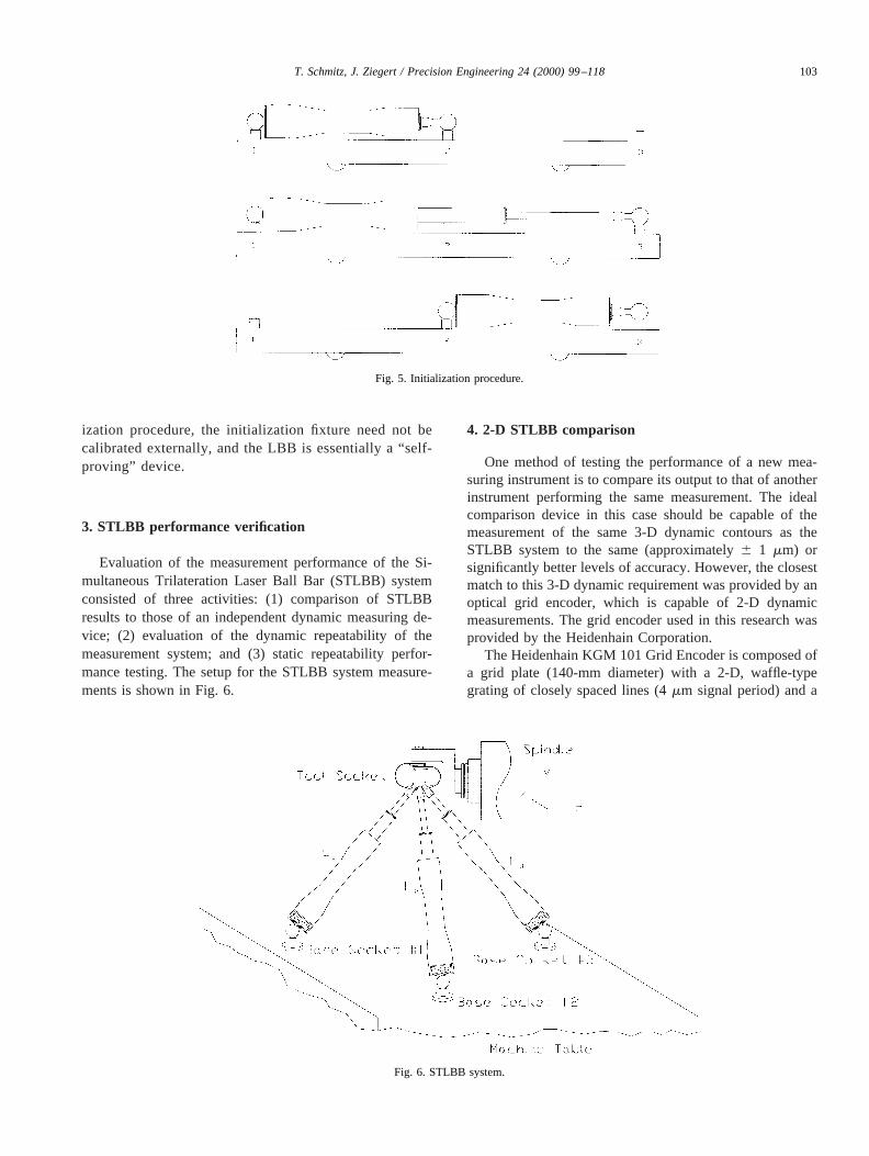
ization procedure, the initialization fixture need not becalibrated externally, and the LBB is essentially a “self-proving” device.

3. STLBB performance verification

Evaluation of the measurement performance of the Si-multaneous Trilateration Laser Ball Bar (STLBB) systemconsisted of three activities: (1) comparison of STLBBresults to those of an independent dynamic measuring de-vice; (2) evaluation of the dynamic repeatability of themeasurement system; and (3) static repeatability perfor-mance testing. The setup for the STLBB system measure-ments is shown in Fig. 6.

4. 2-D STLBB comparison

One method of testing the performance of a new mea-suring instrument is to compare its output to that of anotherinstrument performing the same measurement. The idealcomparison device in this case should be capable of themeasurement of the same 3-D dynamic contours as theSTLBB system to the same (approximately6 1 mm) orsignificantly better levels of accuracy. However, the closestmatch to this 3-D dynamic requirement was provided by anoptical grid encoder, which is capable of 2-D dynamicmeasurements. The grid encoder used in this research wasprovided by the Heidenhain Corporation.

The Heidenhain KGM 101 Grid Encoder is composed ofa grid plate (140-mm diameter) with a 2-D, waffle-typegrating of closely spaced lines (4mm signal period) and a

Fig. 5. Initialization procedure.

Fig. 6. STLBB system.


noncontact scanning head that can measure translations intwo directions. The optical grid plate is attached to analuminum mounting base. This base is mounted in the planeto be measured (on an X–Y table, for example), and thescanning head is fixed perpendicular to the plate (e.g., on theZ-axis attached to the spindle). This system measures therelative planar motion between the grid and read head forany curvilinear path in the plane of the mounting base witha resolution of 4 nm and accuracy of62 mm. The recordedmotions allow the user to observe the dynamic effects of themachine tool’s performance on 2-D CNC paths.

For this comparison, both instruments were configured tomeasure the same planar CNC paths. Fig. 7 shows theHeidenhain setup used for the 2-D measurements. Note thatthe measurement point is on the spindle centerline with thesame Z-direction offset for both experimental setups. There-fore, geometric error variations within the work volume willnot introduce a relative difference between the measure-ments (attributable to an Abbe offset). In addition, the CNCprograms for both the STLBB and Heidenhain tests wereexecuted from the same starting coordinates, so, again, anygeometric variations within the machine tool’s work volumewould be minimized. Finally, the part programs were run inthe same order from a cold machine state to minimizethermal deviations in the machine tool between the two setsof tests.

Several planar contours were selected to be measuredwith both measurement systems. These contours and theirdimensions are summarized in Fig. 8. Although the mea-sured paths were all confined to a single plane, the resultswere adequate to verify the spatial measurement perfor-mance of the STLBB based on the following argument.

1. The STLBB system requires no special alignment ofits axes (by base socket placement) with the machine

tool’s coordinate system, and, in general, they are notaligned.

2. Although the commanded path is in two dimensionswith respect to the machine tool, the spatial coordi-nates of this path lie in three dimensions in theSTLBB system. (The trilateration coordinates arethen transformed in the machine’s coordinate systemusing a rotation matrix obtained by an independentLBB measurement to give the final 2-D results inmachine coordinates.)

3. All of the measured contours require extension and/orcontraction in length of all three individual LBBs,rotations of the LBBs within their respective sockets(change in angular orientation), or both.

Therefore, although all points on the commanded pathslie in a single plane, this plane is oriented arbitrarily to theSTLBB system, and the coordinates of the measured pointsvary in all three coordinates in the STLBB system. For thesepaths, the types and ranges of required motions of theindividual LBBs are identical to those required for a general3-D path.

Comparisons between the Heidenhain and STLBB mea-surements are now presented. Three of the six verificationcontours (angle, step, sultan, square, triangle, and circle) areconsidered separately in the following paragraphs. All pathswere executed at constant commanded accelerations (i.e.,trapezoidal velocity profiles) of 0.98 to 4.91 m/s2, withfeedrates ranging from 889 to 1778 mm/min (35 to 70inches per minute). In addition, a small motion in the pos-itive X- and Y-directions was commanded before the exe-cution of each CNC contour to minimize the effects ofpossible reversal errors in each axis. Both instruments weresampled at a nominal frequency of 1 kHz, which provided(minimum) spatial sampling rates of roughly 15 to 30mm/sample at maximum steady-state velocity.

Fig. 7. Heidenhain setup.


4.1. Angle path

The angle path includes motions in the X–Y plane thatrequire linear interpolation in the two axes simultaneously.Fig. 9 shows a comparison between the Heidenhain gridplate and STLBB measurements for a feed of 889 mm/minand an acceleration of 0.98 m/s2. Only the cornering portionof the path is shownto enhance the viewing resolution. Fig.

10 exhibits the two measurements for a feed of 1778 mm/min and an acceleration of 4.91 m/s2.

This path aids in the tuning of the servomotors on ma-chine tools. The measured response can be used to set theindividual axis gains. If both axes have the same servo loopgain, then the steady-state servo lag for each axis (which isproportional to the axis velocity) will combine to create anactual tool path that lies along the same line as the com-manded path, but lags the commanded position. For the

Fig. 8. Verification contours.

Fig. 9. Angle path comparison (889 mm/min, 0.98 m/s2). Fig. 10. Angle path comparison (1778 mm/min, 4.91 m/s2).


machine tool used in this research, however, a difference inthe gain between the X- and Y-axes caused two differentsteady-state lag errors. Therefore, the actual contour is spa-tially offset from the commanded contour during constantvelocity motion. Because this error is proportional to thecommanded feed rate, the offset is seen to be approximatelytwice as large in Fig. 10 as in Fig. 9.

4.2. Step path

The step path includes linear interpolation in the X- andY-axes individually and sharp corners with both positiveand negative Y-direction motions. Consequently, this pathcan also be used to set the individual axis gains duringtuning. Fig. 11 shows a comparison between the Heidenhainand STLBB measurements for the first cornering motion(1X to 1Y) at a feed rate of 1778 mm/min and an accel-eration of 0.98 m/s2. Fig. 12 displays the same contoursection at a feed of 1778 mm/min and 4.91 m/s2 accelera-tion. Because of the low axis gain settings in this machinetool and the inherent velocity lag (i.e., commands are exe-cuted with some delay), there is a large undershoot seen inthe cornering motion of both paths. In addition, an over-shoot/corrective action controller effect is identified withboth measurement systems in Fig. 12.

4.3. Circle path

Both counterclockwise and clockwise circle paths were alsomeasured using the two measurement systems. The circle pathis a historically popular dynamic evaluation contour, becauseits measurement can also be completed with the telescopingmagnetic ball bar and/or disk check [9–12]. Figs. 13 and 14display measurement results for clockwise and counterclock-wise motions, respectively, with a commanded velocity of

1778 mm/min. The radial deviations of the measured pathfrom the commanded have been amplified by a factor of five inboth cases. Fig. 13 shows an elliptical distortion of the pathwith the major axis of the ellipse rotated 45° counterclockwisefrom the positive Y-axis. Fig. 14 exhibits the same ellipticaldistortion, but the major axis is now oriented at 135°. Thisdirectional-dependent, elliptical distortion of the circular pathswas caused by the previously mentioned gain mismatch be-tween the X- and Y-axes.

5. Dynamic repeatability

The good agreement between the optical grid plate andSTLBB results at all feeds and accelerations served to verify

Fig. 11. Step path comparison (1778 mm/min, 0.98 m/s2). Fig. 12. Step path comparison (1778 mm/min, 4.91 m/s2).

Fig. 13. Clockwise circle path comparison (1778 mm/min).


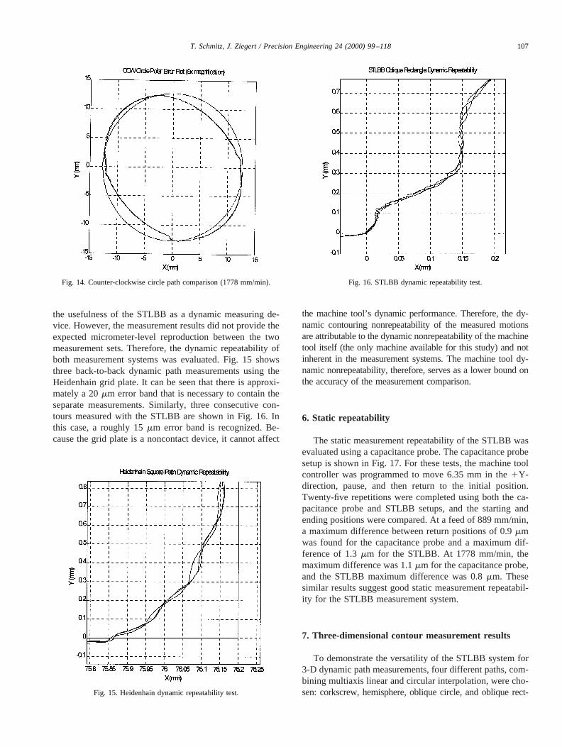
the usefulness of the STLBB as a dynamic measuring de-vice. However, the measurement results did not provide theexpected micrometer-level reproduction between the twomeasurement sets. Therefore, the dynamic repeatability ofboth measurement systems was evaluated. Fig. 15 showsthree back-to-back dynamic path measurements using theHeidenhain grid plate. It can be seen that there is approxi-mately a 20mm error band that is necessary to contain theseparate measurements. Similarly, three consecutive con-tours measured with the STLBB are shown in Fig. 16. Inthis case, a roughly 15mm error band is recognized. Be-cause the grid plate is a noncontact device, it cannot affect

the machine tool’s dynamic performance. Therefore, the dy-namic contouring nonrepeatability of the measured motionsare attributable to the dynamic nonrepeatability of the machinetool itself (the only machine available for this study) and notinherent in the measurement systems. The machine tool dy-namic nonrepeatability, therefore, serves as a lower bound onthe accuracy of the measurement comparison.

6. Static repeatability

The static measurement repeatability of the STLBB wasevaluated using a capacitance probe. The capacitance probesetup is shown in Fig. 17. For these tests, the machine toolcontroller was programmed to move 6.35 mm in the1Y-direction, pause, and then return to the initial position.Twenty-five repetitions were completed using both the ca-pacitance probe and STLBB setups, and the starting andending positions were compared. At a feed of 889 mm/min,a maximum difference between return positions of 0.9mmwas found for the capacitance probe and a maximum dif-ference of 1.3mm for the STLBB. At 1778 mm/min, themaximum difference was 1.1mm for the capacitance probe,and the STLBB maximum difference was 0.8mm. Thesesimilar results suggest good static measurement repeatabil-ity for the STLBB measurement system.

7. Three-dimensional contour measurement results

To demonstrate the versatility of the STLBB system for3-D dynamic path measurements, four different paths, com-bining multiaxis linear and circular interpolation, were cho-sen: corkscrew, hemisphere, oblique circle, and oblique rect-

Fig. 14. Counter-clockwise circle path comparison (1778 mm/min).

Fig. 15. Heidenhain dynamic repeatability test.

Fig. 16. STLBB dynamic repeatability test.


angle. For all measurements shown, the commanded path isrepresented by a dashed line, and the actual tool motion isshown as a (datapoint-to-datapoint) continuous line.

7.1. Corkscrew path

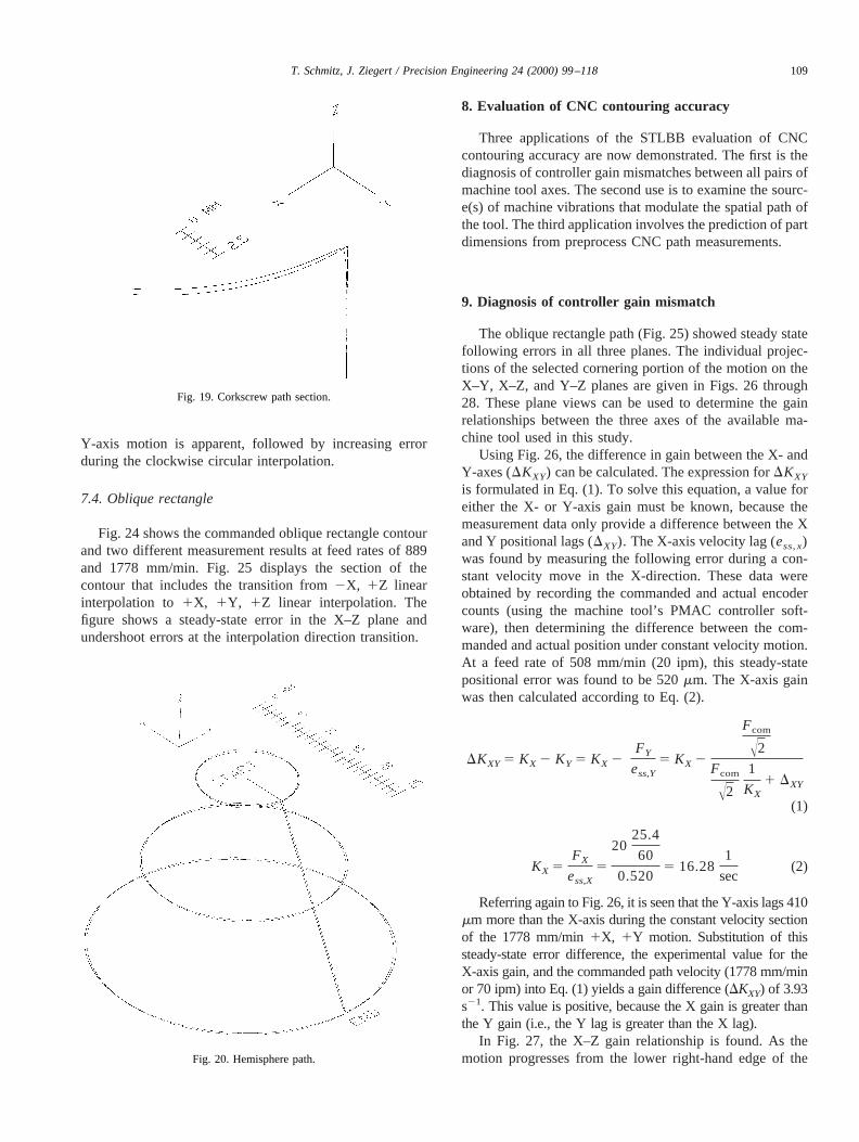
The results of the STLBB measurement of the corkscrewpath are shown in Fig. 18. For this path, a counterclockwisehalf-circle was commanded in the X–Y plane, followed bya step in the2Z-direction. Next, the half-circle was com-pleted and followed by another step in the2Z-direction,and so forth. In Fig. 19, the transition from the first half-circle to the first2Z motion in the corkscrew path is shown.The elliptical distortion of the half-circle in the X–Y planeis evident as well as undershoot in both the X- and Y-directions for the start of the2Z motion. The integral gainin the controller then begins to correct the steady-state errorin the X- and Y-directions as the Z motion progresses.

7.2. Hemisphere path

The second CNC program roughly simulated a hemi-spherical cutting path. First, a small circle was executed inthe X–Y plane. Next, a Y–Z linear interpolation was com-manded, followed by a larger circle with the same centercoordinates from this new starting point. The completion ofthis circle was followed by another linear motion, and so on.This path and a corresponding STLBB measurement isshown in Fig. 20. Fig. 21 shows the smallest circle in thispath. It is immediately apparent that the circular path doesnot close and also exhibits an elliptical distortion due to theunequal X–Y controller gains. An X-axis reversal error canalso be seen as the short Y-direction straight line motionduring the circular interpolation.

7.3. Oblique circle

This path was executed in a plane oblique to each of themachine tool’s coordinate axes. Fig. 22 shows the obliquecircle path. Fig. 23 shows a selected portion of the projec-tion of this path on the Y–Z plane. A modulation of the

Fig. 17. Capacitance probe setup.

Fig. 18. Corkscrew path.


Y-axis motion is apparent, followed by increasing errorduring the clockwise circular interpolation.

7.4. Oblique rectangle

Fig. 24 shows the commanded oblique rectangle contourand two different measurement results at feed rates of 889and 1778 mm/min. Fig. 25 displays the section of thecontour that includes the transition from2X, 1Z linearinterpolation to 1X, 1Y, 1Z linear interpolation. Thefigure shows a steady-state error in the X–Z plane andundershoot errors at the interpolation direction transition.

8. Evaluation of CNC contouring accuracy

Three applications of the STLBB evaluation of CNCcontouring accuracy are now demonstrated. The first is thediagnosis of controller gain mismatches between all pairs ofmachine tool axes. The second use is to examine the sourc-e(s) of machine vibrations that modulate the spatial path ofthe tool. The third application involves the prediction of partdimensions from preprocess CNC path measurements.

9. Diagnosis of controller gain mismatch

The oblique rectangle path (Fig. 25) showed steady statefollowing errors in all three planes. The individual projec-tions of the selected cornering portion of the motion on theX–Y, X–Z, and Y–Z planes are given in Figs. 26 through28. These plane views can be used to determine the gainrelationships between the three axes of the available ma-chine tool used in this study.

Using Fig. 26, the difference in gain between the X- andY-axes (DKXY) can be calculated. The expression forDKXY

is formulated in Eq. (1). To solve this equation, a value foreither the X- or Y-axis gain must be known, because themeasurement data only provide a difference between the Xand Y positional lags (DXY). The X-axis velocity lag (ess,x)was found by measuring the following error during a con-stant velocity move in the X-direction. These data wereobtained by recording the commanded and actual encodercounts (using the machine tool’s PMAC controller soft-ware), then determining the difference between the com-manded and actual position under constant velocity motion.At a feed rate of 508 mm/min (20 ipm), this steady-statepositional error was found to be 520mm. The X-axis gainwas then calculated according to Eq. (2).

DKXY5 KX 2 KY 5 KX 2FY

ess,Y5 KX 2

Fcom

Î2

Fcom

Î2

1

KX1 DXY

(1)

KX 5FX

ess,X5

2025.4

60

0.5205 16.28

1

sec(2)

Referring again to Fig. 26, it is seen that the Y-axis lags 410mm more than the X-axis during the constant velocity sectionof the 1778 mm/min1X, 1Y motion. Substitution of thissteady-state error difference, the experimental value for theX-axis gain, and the commanded path velocity (1778 mm/minor 70 ipm) into Eq. (1) yields a gain difference (DKXY) of 3.93s21. This value is positive, because the X gain is greater thanthe Y gain (i.e., the Y lag is greater than the X lag).

In Fig. 27, the X–Z gain relationship is found. As themotion progresses from the lower right-hand edge of the

Fig. 19. Corkscrew path section.

Fig. 20. Hemisphere path.


figure to the upper right, the X motion lags more than the Zby 138 mm (at a commanded feed rate of 1778 mm/min).Therefore, the Z controller gain is larger than the X. Sub-stitution into Eq. (3) yields aDKXZ value of 25.13 s21.Note that in Eq. (3),bXZ is the angle between the X–Z planeand the commanded direction of motion.

DKXZ 5 KX 2 KZ 5 KX 2

F

Î2cosbXZ

F

Î2

cosbXZ

KX2 DXZ

(3)

Fig. 28 displays motion in the1Z-direction followed bya 1Y, 1Z linear interpolation. In this case, the Z controllergain is greater than the Y gain, because the Y lag is approx-imately 700mm larger than the Z lag (at a feed rate of 1778mm/min). The difference in gain,DKYZ, may be calculatedusing Eq. (4). The calculated gain difference,28.84 s21, isnegative, because the Y gain is smaller than the Z.

DKYZ5 KY 2 KZ 5 ~KX 2 DKXY! 2 ~KX 2 DKXZ!

5 2 8.84s21 (4)

Fig. 21. Hemisphere path section.

Fig. 22. Oblique circle path.


10. Path modulation by machine noise

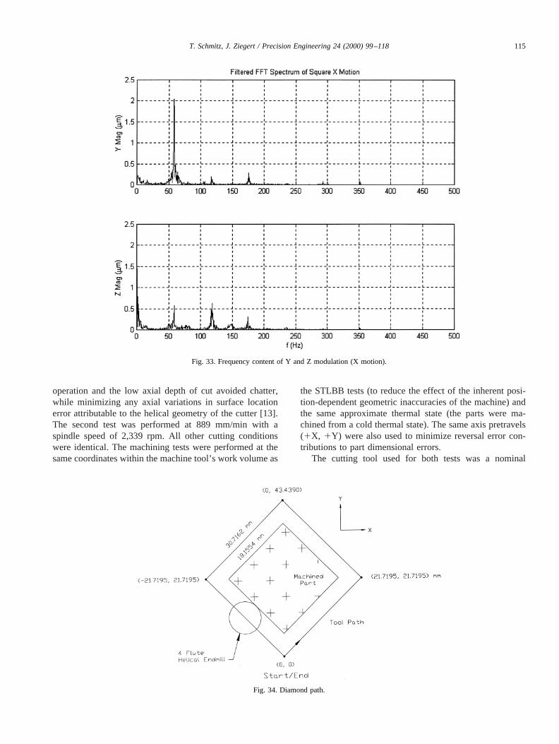
As shown in Fig. 23, single axis motions on the machinetool used in this study were modulated by some high-frequency disturbance. To determine the source of this dis-turbance, the 3-D motions of the tool point were measuredwith the machine on (no commanded feed) and with themachine off (1 kHz sampling rate in both cases). The time-domain results of the “machine on” measurements areshown in Fig. 29 (with digital 4th order lowpass Butter-

worth filters applied). The frequency content of the “ma-chine on”/“machine off” measurements is shown in Fig. 30and 31. It can be seen in the measurements with the machineon that there is significant frequency content at 60, 120, and180 Hz in the X-axis, 60 Hz in the Y-axis, and 60 and 120Hz in the Z-axis. With the machine off, however, the fre-quency content drops to the noise floor threshold. The 60,120, and 180 Hz frequency components in the machinenoise were, therefore, attributed to the three-phase power ofthe axis motor amplifiers.

The single axis path modulation and corresponding fre-quency content is demonstrated in the Y and Z error mo-

Fig. 23. Oblique circle section.

Fig. 24. Oblique rectangle path.

Fig. 25. Oblique rectangle path section.

Fig. 26. Oblique rectangle path section (X–Y plane).


tions during a commanded X-axis travel shown in Figs. 32and 33. It can be seen in Fig. 32 that the Y and Z motions(which are nominally zero) are modulated and cause arapidly varying dynamic nonstraightness of motion. In Fig.33, the expected frequency components are identified ineach axis (60 Hz in Y and 60 and 120 in Z).

11. Comparison of measured trajectory to machinedpart dimensions

Perhaps the most traditional method for assessing the ac-curacy of CNC machine tools is to machine a test part and

compare its actual dimensions to the dimensions commandedin the part program. See, for example, the Part Check (or PartTrace Test) in [11]. Because the purpose of the STLBB is tomeasure dynamic CNC tool paths, comparison of its measure-ments to machined part dimensions can also be used to eval-uate the performance of the STLBB system. Although theSTLBB system can measure 3-D dynamic contouring accuracyduring the execution of arbitrary CNC contours, it cannotperform these measurements during the machining process(i.e., the CNC part path must be measured before cutting).Therefore, to verify the STLBB system by the manufacture ofa test part, it is necessary to measure a given CNC contour,machine a part using the same part program, and then comparethe results. However, the final part dimensions are also signif-icantly affected by cutter/workpiece deflections attributable tothe cutting forces [13], as well as by differences between thenominal and actual cutter diameter. Therefore, it is necessary todefine the test part and measurement comparisons carefully, soas to eliminate these effects.

To this end, we have chosen a diamond path (Fig. 34) tobe executed in the X–Y plane of the machine at variousfeedrates. The X–Y gain mismatch observed during theangle path tests (Figs. 9 and 10) is expected to cause anoffset, which is dependent on the commanded velocity, ofthe actual path from the commanded path. The total effect ofthe gain mismatch on the experimental diamond path is tolengthen the distance across one face (d1, in Fig. 35) bytwice the servo gain mismatch error and shorten the distanceacross the other (d2 in Fig. 35), again by twice the gainmismatch error. The absolute magnitudes ofd1 and d2

depend on the dynamic contouring errors, errors in theassumed cutter diameter, and also on deflections of the toolattributable to cutting forces. However, because the cuttingforce deflections and tool diameter errors affect all foursides of the diamond path equally, the difference betweenthese dimensions,Dd 5 d1 2 d2, is independent of theseeffects. Therefore, we use the metric,Dd, to compare theSTLBB measurement results to the machined test part mea-surements. These results, as well as the experimental meth-odology, are presented in the following paragraphs.

11.1. STLBB results

By importing the STLBB measurements into AutoCAD®

(version 14.0) via a script file, the distances (d1 and d2)were computed at nine different locations for each recordedpath. Fig. 36 shows an example of thed1 and d2 experi-mental values for an 889 mm/min STLBB test. In Fig. 36,it can be seen that the previously discussed controller errorsexert a sizable influence on the path straightness (i.e., largevariation ind values) as the integral gain attempts to correctthe steady-state error. Therefore, points very near the dia-mond edge were avoided. The final values ford1 and d2

were obtained by averaging the nine measurements acrosseach face. The value forDd was then calculated by sub-tracting the averaged2 value from the averaged1 value.

Fig. 27. Oblique rectangle path section (X–Z plane).

Fig. 28. Oblique rectangle path section (Y–Z plane).


This method was chosen, because it most closely corre-sponds to the CMM probing method used to measure themachined parts (i.e., 13 points were probed and a line bestfit to the data in the CMM software). STLBB results for the

two different feed rates are listed in Table 1. Also listed isthe commanded value and the difference (Dd) betweend1

andd2. It should be noted that these values reflect measure-ments of the actual tool path followed by the cutter.

Fig. 29. Tool point motions (machine on).

Fig. 30. Frequency content of X, Y and Z motions (machine on).


11.2. Diamond path machining results

The machining verification for the diamond path partwas performed at the same two linear feed rates as theSTLBB measurements, as well as the same commanded

acceleration. The first test was executed under the followingup-milling cutting conditions: 508 mm/min linear feed, 0.1mm feed per tooth, 1337 rpm spindle speed, 1% radialimmersion, and axial depth of cut equal to 0.254 mm. Thelow radial immersion was chosen to simulate a finishing

Fig. 31. Frequency content of X, Y and Z motions (machine off).

Fig. 32. Y and Z path modulation during X motion.


operation and the low axial depth of cut avoided chatter,while minimizing any axial variations in surface locationerror attributable to the helical geometry of the cutter [13].The second test was performed at 889 mm/min with aspindle speed of 2,339 rpm. All other cutting conditionswere identical. The machining tests were performed at thesame coordinates within the machine tool’s work volume as

the STLBB tests (to reduce the effect of the inherent posi-tion-dependent geometric inaccuracies of the machine) andthe same approximate thermal state (the parts were ma-chined from a cold thermal state). The same axis pretravels(1X, 1Y) were also used to minimize reversal error con-tributions to part dimensional errors.

The cutting tool used for both tests was a nominal

Fig. 33. Frequency content of Y and Z modulation (X motion).

Fig. 34. Diamond path.


12.7-mm diameter, 4-flute, high-speed steel (HSS) helicalend mill extending 38 mm from the tool holder face. Thefrequency response function for the tool was obtained usingan impact test. A curve fit to this data yielded modal valuesof 0.01 kg mass, 3.5e6 N/m stiffness, and a damping ratio of0.03 for the most flexible mode at a natural frequency of2950 Hz.

Once the diamond test parts were machined, they wereallowed to soak overnight in a temperature-controlled en-vironment (686 0.2°F) and then measured on a Brown &

Sharpe Micro Val PFx coordinate measuring machine.These measurements were completed under “Direct Com-puter Control” to improve the measurement accuracy. Inthis method, the part is first probed manually by the user (13points were probed on each face of the diamond parts). Thecomputer records the location in the CMM work volume ofthe measured features (four 2-D lines in this case) and thencalculates the surface normal to each probed point. A cor-responding part program is automatically written that in-cludes the user-defined measurements and the appropriateapproach directions. When this part program is executed,and the features are probed under computer control, themeasurement accuracy (roughly61 mm for the portion ofthe work volume used in these measurements) is maximizedbecause of the normal approach directions and constant(computer-controlled) approach speed. The measurementresults for two machining verification parts are given inTable 2.

Comparing these results with the STLBB dynamic con-tour measurements provides the final verification for theSTLBB system. At 889 mm/min, the difference between theface dimensions of the diamond path,Dd, was measured as0.5837 mm using the STLBB. The difference between theface dimensions for a machined part was then measured as0.5839 mm using the CMM. These measurements agree to

Fig. 35. STLBB diamond path (1778 mm/min).

Fig. 36. Determination ofDd (889 mm/min).

Table 1STLBB diamond path results

Feed rate Commanded,d

Measured,d1

Measured,d2

Difference,Dd

508 mm/min 30.7162 mm 30.8891 30.5453 0.3438 mm889 mm/min 30.7162 31.0099 30.4262 0.5837


within 0.2 mm. The 508 mm/min tests provided a largerdiscrepancy of 9.4mm. Table 3 shows a comparison of themachining and STLBB tests in tabular form.

To understand better the small measurement differencesobserved, several consecutive STLBB measurements andmachining tests were completed to attempt to quantify therepeatability ofDd, the metric used to evaluate the STLBBperformance in these tests. At 889 mm/min, the maximumdifference between calculatedDd values for successiveSTLBB measurements was 3.5mm. The maximum differ-ence forDd between sequential machined part measure-ments, again at a feed rate of 889 mm/min, was 5.2mm.These repeatability errors are on the same order of magni-tude as the differences seen between the STLBB and ma-chined part measurements. This close agreement betweenthe STLBB and machined part measurements further vali-dates the STLBB system as a preprocess tool for CNC partprogram validation.

It should be noted that the diamond path used in thisresearch represents a special case. Because the path is sym-metric about both the X- and Y-axes, common path varia-tions (such as surface location errors attributable to cutterdeflections during machining, runout of the cutter, spindleerror motions, or quasistatic spindle thermal growth errors)will not affect the metric (Dd) used to verify the STLBBsystem. Runout of the cutter teeth, for example, will affectboth dimensions (d1 and d2) by the same amount and,therefore, have no effect onDd. In addition, the path waskept small to minimize the introduction of the machinetool’s parametric errors into the machined part geometry. Infact, this path was expressly chosen for the combination ofthe large X–Y gain mismatch errors and the absence ofthese other error sources.

In general, these special considerations cannot be met, andthe cutting force and runout errors, as well as the machinetool’s inherent parametric and thermal errors, can have a sig-nificant effect on the final dimensions of a machined part. Forexample, if an improper tool offset (tool diameter) is used inthe CAD/CAM generation of complicated CNC part paths,significant part errors can be obtained as the cutter follows both

inside and outside contours. Perhaps more insidious is theeffect of forced vibrations during stable machining on the finalpart dimensions. In another publication [13], we have shownthat machined part dimensions are dependent on the selectedspindle speed, cutter dynamics, and chip load. Furthermore,significant variations in part dimensions may be obtained byrelatively small variations of the spindle speed. These differ-ences between the commanded and actual part dimensionsattributable to cutting force effects have been termedSurfaceLocation Errors[14]. To the uninformed observer, these sur-face location errors could be attributed to other common errorsources (e.g., parametric, thermal, programming) and a signif-icant amount of time wasted in attempting to diagnose andcorrect the problem.

12. Conclusions

We have developed an instrument capable of measuringarbitrary, dynamic CNC tool paths through 3-D space withmicrometer-level accuracy. The measurement accuracy ofthe STLBB system was verified by comparison to a Hei-denhain KGM 101 Grid Encoder using a number of differ-ent 2-D paths. The results of the two instruments were foundto agree within the dynamic path repeatability of the ma-chine tool used to produce the motions.

The STLBB measurement accuracy was also verified bymeasuring a diamond-shaped path and then machining apart using the same NC code. The dimensions of the ma-chined part were measured on a CMM and compared to theSTLBB results. The part shape and comparison metricswere specifically chosen to eliminate any contributionscaused by imperfect knowledge of the cutter diameter, andany cutter deflections caused by the cutting forces. TheSTLBB path measurements were found to agree with themachined part measurements to within the repeatability ofthe machine tool.

Finally, the spatial dynamic path measurement capabilityof the STLBB was demonstrated for several 3-D paths. Theutility of these measurements in identifying controller gainmismatch errors and servo switching frequency errors wasshown.

Acknowledgment

This work was partially supported by the National Sci-ence Foundation under Grants DDM-935138 and GER-9354980 and the Department of Energy under the 1999Integrated Manufacturing Predoctoral Fellowship.

References

[1] Donmez MA. A general methodology for machine tool accuracyenhancement: Theory application, and implementation. Ph.D. Disser-tation, Purdue University, West Lafayette, IN, 1985.

Table 2Machining verification results

Feed rate Commanded,d

Measured,d1

Measured,d2

Difference,Dd

508 mm/min 18.1554 mm 18.3056 17.9712 0.3344 mm889 mm/min 18.1554 18.4278 17.8439 0.5839

Table 3STLBB vs. machining verification results

Feed rate Dd, STLBB Dd, machining Error

508 mm/min 0.3438 mm 0.3344 9.4mm889 mm/min 0.5837 0.5839 0.2mm


[2] Srinivasa N. Modeling and prediction of thermally induced errors inmachine tools using a laser ball bar and a neural network. Ph.D.Dissertation, University of Florida, Gainesville, FL, 1994.

[3] Chen JS, Ling C. Improving the machine accuracy through machinetool metrology and error correction.Int J Manufact Technol1996;11(3):198–205.

[4] Ziegert JC, Mize CD. Laser ball bar: A new instrument for machinetool metrology.Prec Eng1994;16(4):259–67.

[5] Mize CD. Design and implementation of a laser ball bar basedmeasurement technique for machine tool calibration. M.S. Thesis,University of Florida, Gainesville, FL, 1993.

[6] Schmitz T, Ziegert JC. A new sensor for the micrometre-level mea-surement of three-dimensional, dynamic contours.Measure Sci Tech-nol 1999;10(2):51–62.

[7] Kulkarni RB. Design and evaluation of a technique to find theparametric errors of a numerically controlled machine tool using alaser ball bar. M.S. Thesis, University of Florida, Gainesville, FL,1996.

[8] Mize CD, Ziegert JC, Pardue R, Zurcher N. Spatial measurementaccuracy tests of the laser ball bar. Final Report for CRADA No.Y-1293-02244 between Martin Marietta Energy Systems and TetraPrecision, Inc., August 1994.

[9] Bryan JB. A simple method for testing measuring machines andmachine tools Part 1: Principles and applications.Prec Eng1982;4(2):61–9.

[10] Bryan JB. A simple method for testing measuring machines and machinetools Part 2: Construction details.Prec Eng1982;4(3):125–138.

[11] Bryan JB, Bowerbank JE, Holland ED, Mohl O. Updating tracer lathemachining operations.ASTME1960;61(1):1–45.

[12] Bryan JB, Pearson JW. Machine tool metrology. Western Metal andTool and ASTME Exposition and Golden Gate Conference, SanFrancisco, CA, September 24, 1968.

[13] Schmitz T, Ziegert JC. Examination of surface location error due tophasing of cutter vibrations.Prec Eng1999;23(1):51–62.

[14] Tlusty J. EML 6934 Class Notes: Fundamentals of Production Engineer-ing Part 2. University of Florida, Gainesville, FL, Fall Semester, 1994.


Dynamic evaluation of spatial CNC contouring accuracy

Documents

Transcript of Dynamic evaluation of spatial CNC contouring accuracy